IEEE TRANSACTIONS ON SOFTWARE ENGINEERING 1

On Fault Representativeness of

Software Fault Injection Roberto Natella, Student Member, IEEE, Domenico Cotroneo, Joao A. Duraes, and Henrique S.

Madeira, Member, IEEE

Abstract—The injection of software faults in software components to assess the impact of these faults on other components or

on the system as a whole, allowing the evaluation of fault tolerance, is relatively new compared to decades of research on

hardware fault injection. This paper presents an extensive experimental study (more than 3.8 millions of individual experiments

in three real systems) to evaluate the representativeness of faults injected by a state-of-the-art approach (G-SWFIT). Results

show that a significant share (up to 72%) of injected faults cannot be considered representative of residual software faults, as

they are consistently detected by regression tests, and that representativeness of injected faults is affected by the fault location

within the system, resulting in different distributions of representative/non-representative faults across files and functions.

Therefore, we propose a new approach to refine the faultload by removing faults that are not representative of residual software

faults. This filtering is essential to assure meaningful results and to reduce the cost (in terms of number of faults) of software

fault injection campaigns in complex software. The proposed approach is based on classification algorithms, is fully automatic,

and can be used for improving fault representativeness of existing software fault injection approaches.

Index Terms—Software Fault Injection, Experimental Dependability Evaluation, Software Reliability, Fault-Tolerant Systems.

—————————— ——————————

1 INTRODUCTION

LTHOUGH society is increasingly dependent on software, it is a fact that it is practically impossible to guarantee that software is perfect, due to the

many complex functions that software has to perform and due to budget and time constraints of the software devel-opment process. As a result, complex software will even-tually execute under faulty conditions that have not been foreseen during testing [1][2][3][4]. To face this problem, it is well known, even recommended by some safety standards [6][7], that software developers adopt software fault tolerance mechanisms. Examples are masking soft-ware faults through diversity (e.g., N-version program-ming, recovery blocks, N self-checking programming) [8][9], and detecting a wrong state of the system, in order to provide a fail-stop behavior or a degraded mode of service (e.g., concurrent error detection, checkpointing and recovery, exception handling) [1][10]. In order to as-sess the effectiveness of fault tolerance mechanisms, it be-comes important to evaluate the system behavior under unforeseen faulty conditions. This can be done by delibe-rately injecting a fault condition into the system.

The process of introducing faults in a system in order to assess its behavior and to measure the efficiency (cov-erage, latency, etc.) of fault tolerance mechanisms is re-ferred to as fault injection [11][12][13]. It is recommended

by most of safety standards, such as the ISO/DIS 26262 standard for automotive safety [7], which prescribes the use of error detection and handling mechanisms in soft-ware and their verification through fault injection, and the NASA standard 8719.13B for software safety [6], which recommends fault injection to assess system beha-vior in the presence of faulty off-the-shelf software.

Many fault injection approaches have been proposed in the last four decades. As it is generally well accepted that simple hardware fault models such as bit-flip or bit stuck-at do represent real hardware faults, the first fault injection approaches consisted of injecting physical faults into the target system hardware (e.g., using radiation, pin-level, power supply disturbances, etc). The growing complexity of the hardware turned the use of these physi-cal approaches quite difficult or even impossible, and a new family of fault injection approaches based on the runtime emulation of hardware faults through software (Software Implemented Fault Injection - SWIFI) become quite popular. Some examples of SWIFI tools are NFTAPE [34], Xception [38], and GOOFI [35]. However, all these tools have been proposed for the emulation of hardware faults and their potential to emulate more com-plex faults such as software faults is very limited.

The use of fault injection to emulate the effects of real software faults (i.e., bugs) is relatively recent when com-pared to the first fault injection proposals. These tech-niques are referred to as Software Fault Injection (SFI). In practice, the injection of software faults consists of the in-troduction of small changes in the target program code, creating different versions of a program (each version has one injected software fault). The way faults are injected resembles the well-known mutation testing technique [14][15][16] but the injection of software faults has com-

————————————————

R. Natella and D. Cotroneo are with the Department of Computer and Control Engineering, Federico II University of Naples, Via Claudio 21, 80125, Naples, Italy. E-mail: roberto.natella@unina.it, cotro-neo@unina.it.

J.A. Duraes is with the Institute of Engineering of Coimbra, Rua Pedro Nunes--Quinta da Nora, 3030-199 Coimbra, Portugal. E-mail: jdu-raes@isec.pt.

H.S. Madeira is with the Centre of Informatics and Systems of the Uni-versity of Coimbra, Polo II--Pinhal de Marrocos, 3030-290 Coimbra, Portugal. E-mail: henrique@dei.uc.pt.

A

2 IEEE TRANSACTIONS ON SOFTWARE ENGINEERING

pletely different goals. While mutation testing uses pro-gram mutations to identify an adequate test suite, Soft-ware Fault Injection is meant to validate fault-handling mechanisms at runtime and to evaluate the way a system behaves in the presence of the injected faults [12][13][19][20]. This difference of goals reflects on the approaches and fault models adopted by SFI.

A key property of SFI is the representativeness of in-jected faults. That is, the faultload (i.e., the set of faults to be injected in a given software component/system) should reproduce the faults that are actually experienced in the field (i.e., residual faults), in order to obtain a realis-tic evaluation of fault tolerance in face of runtime faulty conditions. Residual faults are those faults that are over-looked by rigorous design and testing, and that actually affect the mission of the system, as evidenced by recent accidents occurred in space missions [4][5]. If the injected software faults are not representative of residual faults, then it is risky to assert the effectiveness of software fault tolerance. This means to carefully selecting fault types (“what to inject”) and fault locations (“where to inject”) in order to achieve the representativeness of injected faults.

Unfortunately, in spite of decades of fault injection re-search, including the more recent advances on the injec-tion of software faults, the fact is that the accurate emula-tion of residual software faults through fault injection re-mains largely unknown. Most recent techniques, such as G-SWFIT (Generic Software Fault Injection Technique) [17], use a set of fault operators derived from the most frequent types of software faults found in field failure studies. These proposals focused only on fault types and they completely neglected fault locations, in terms of modules and/or routines. Given a fault type, existing techniques inject it in every module and routine, without accounting for the complexity of code in the mod-ule/routine and testing efforts that have been spent on that part of code [3][18]. This is a strong limitation espe-cially when dealing with complex software systems, for the two following reasons. First, injecting defects in every location of complex software leads to a dramatic increase of the cost of the campaign. For example, the software systems considered in this study have tenths of thousands of potential fault locations, and injecting faults in all of them could make impractical the fault injection campaign. Second, even if we want to take on the entire campaign, the most important issue is that results could be mislead-ing. For example, if we aim to measure the fault coverage, we should be able to select the subset of experiments that represents residual faults, since this measure is related to the likelihood of faults to exist in the field [19][20]. Repre-sentativeness in terms of fault types and fault locations is thus a paramount of importance to achieve effective fault injection campaigns, in terms of costs and accuracy of results.

This work proposes a new SFI strategy able to careful-ly select fault locations to achieve representative fault-loads. The study is based on an extensive experimental campaign (more than 3.8 million individual experiments) to evaluate and improve the representativeness, as a func-tion of fault types and locations, of a state-of-the-art SFI technique (G-SWFIT).

The definition of representative faultloads is accom-plished performing the following steps. First, we choose three real world software systems, including two Data Base Management Systems (MySQL and PostgreSQL) and a Real-Time Operating System (RTEMS) largely adopted in business and safety-critical applications. Second, we conduct extensive SFI campaigns using as workload the actual test cases adopted by developers, in order to assess whether injected faults are representative of residual faults or not. The driving idea is that faults disclosed by the test cases do not represent residual faults, as they would be easily detected and fixed by developers. Third, from the results of SFI campaigns we identify the faults that are difficult to find by testing and thus worth consi-dering for SFI, as they are representative of residual faults. Fourth, we conduct a statistical analysis on repre-sentative faults to understand how to define a representa-tive faultload for a given software. To this aim, we pro-pose an approach based on classification algorithms and software complexity metrics to identify suitable fault lo-cations for emulating residual software faults.

This study provides the following key contributions: 1. It shows that the issue of non-representative faults

can significantly affect SFI, even using state-of-the-art techniques, such as G-SWFIT [17]. Considering the experiments done in the RTEMS operating sys-tem, it was observed that non-representative faults are the majority of injected faults (72.23%) using the G-SWFIT technique. Even if we consider less-tested and large systems in which the chance of faults to escape testing is higher, such as MySQL and PostgreSQL, the percentage of non-representative faults is still noticeable (respective-ly, 14.57% and 23.13%).

2. The distribution of faults across components (files and functions) reveals that fault representativeness is significantly affected by fault locations, thus confirming that the careful selection of fault loca-tions is needed to define realistic faultloads.

3. It shows that representativeness can be improved by using classification algorithms and software metrics. This is a novel approach compared to ex-isting ones that focus on fault types [17][44][29]. We evaluated both a supervised (i.e., trained using examples) algorithm, namely decision trees, and an unsupervised one, namely k-means clustering. In particular, we found that the faultload can be improved using either the supervised algorithm (4.10%-26.08%) or the unsupervised one (2.16%-16.24%). At the same time, the approach can signif-icantly reduce the faultload size (filtering out up to 69.43% of faults), thus reducing the cost and the time of SFI campaigns in complex software.

This work is organized as follows. Section 2 surveys fault injection techniques and its relationship with muta-tion testing. Section 3 presents the experimental evalua-tion of the representativeness of faults injected by G-SWFIT on three systems. Section 4 discusses how repre-sentativeness can be improved and shows that there is a clear difference in the distribution of representative/non-

NATELLA ET AL.: ON FAULT REPRESENTATIVENESS OF SOFTWARE FAULT INJECTION 3

representative faults across files and functions. This con-clusion leads to the proposal, in Section 5, of a new fault selection approach that improves fault representative-ness. Sections 6 and 7 summarize and discuss the main results of the paper.

2 RELATED WORK

This section overviews the works that use the insertion of software faults in programs such as mutation testing, and those that specifically address SFI, including an overview of existing approaches and tools and typical scenarios where it has been used. Finally, we describe the G-SWFIT technique, which is used as reference of a state-of-the-art SFI technique in this paper.

The usefulness of inserting software faults to improve software reliability is recognized in many works. There are several approaches on how to use software faults dur-ing or after software development to improve quality of software. One approach, mutation testing, focuses on the systematic improvement of the test cases to assure that most bugs will be detected with the least effort. To this effect, programs are modified to include an artificial fault to assess the efficacy of the test case to detect it. Another approach intercepts the interfaces of modules to change the data being passed. This approach, robustness testing, is based on the idea that these wrong data values might be the result of an internal fault in the calling module and the goal is to evaluate the ability of the called module to handle this unexpected input. A third approach, fault in-jection, modifies programs by inserting an artificial fault to observe the behavior of the target programs in pres-ence of faults, to validate fault tolerance mechanisms and to perform dependability benchmarking. In the following we review the fundamentals of these three approaches.

2.1 Mutation testing

Mutation testing is a well-known technique for software quality improvement used during the software develop-ment phase. The main goal is to improve the ability of test cases to detect faults while maintaining testing time as low as possible [14][15][16]. This approach evaluates the effectiveness of test cases (namely, the mutation adequacy score) by executing tests with versions of the program in which a small “faulty” change has been introduced. These faulty changes can be manually inserted (hand-seeded faults) or can be automatically generated (mutants) using a set of mutation operators (i.e., rules followed for introduc-ing changes in the code). Test cases are then defined such that they detect as many of the injected faults as possible. The adequacy of test cases is evaluated by measuring the ratio of faulty versions that have been “killed” (i.e., the output differs from the original program for at least one test case). The effectiveness of mutation testing to find real faults is based on the observation (referred to as the “coupling hypothesis” [15]) that test cases able to detect simple faults (such as the faults typically injected in muta-tion testing) are sensitive enough to detect more complex faults. Empirical studies confirmed that mutants are suit-able for estimating the fault detection ability of test cases,

and that automatically-generated mutants are an accurate and more practical support compared to hand-seeded faults [21][22]. Moreover, mutation testing can significant-ly improve software reliability [23].

There are issues that make this approach costly, and that have been investigated since its birth (a thorough survey is presented in [24]). The foremost issue is the large number of experiments required to run each test case on each mutant. This is due to the large number of mutants that can be generated from a program, since mu-tation operators encompass many language constructs that can be potentially affected by defects (e.g., “constant replacement” [16]).

It has been found that mutants can be reduced while preserving testing effectiveness. The state-of-the-art of this problem is the selection of a sufficient set of mutation operators. This can be achieved by omitting the mutation operators that generate most of the mutants [25][26], or by only including operators that are considered the most ef-fective [27]. A Bayesian selection approach has been re-cently proposed, that iteratively prioritizes mutation op-erators with respect to their ability to produce “hard-to-kill” mutants, which make necessary to extend the test suite and thus can improve testing effectiveness [28]. Other approaches randomly select a subset of mutants (mutation sampling), or remove mutants that are detected by similar inputs (mutation clustering) [24]. “Hard-to-kill” mutants do not aim to emulate residual faults such as the ones studied in our work: while mutants are concerned with the improvement of test suites, SFI aims to emulate faults that escape the actual test suites adopted in real sys-tems, which are the result of the testing techniques actual-ly adopted by developers and of the amount of efforts devoted to software verification. Representative faults are not meant to enhance test suites by including more test cases able to detect them, but to reproduce the faults that are missed by testing in real projects.

2.2 Software fault injection

Software Fault Injection is a kind of what-if experimenta-tion. The target is exercised with a given workload (ideal-ly, one representative of the operation scenario of the target) and faults are inserted into specific software com-ponents of the target system. The main goal is to observe how the system behaves in the presence of the injected faults, considering that these faults reproduce plausible faults that may affect a given software component of the system during operation. SFI is used in several (typically post-development) scenarios: to validate the effectiveness and to quantify the coverage of software fault tolerance, to assess risk, to perform dependability evaluation [11][12][13]. The application scenario constitutes the first difference from mutation testing and software fault injec-tion: the former is used mainly during software develop-ment and is focused on test cases, while the latter is most-ly used in post-development scenarios and has a strong requirement of fault representativeness. Since SFI is con-cerned with the analysis of the system behavior during operation, the conduction of experiments closely emu-lates the real operational scenario of the target system. In-

4 IEEE TRANSACTIONS ON SOFTWARE ENGINEERING

stead of a test set, a workload representative of opera-tional usage is used. Moreover, fault representativeness is a chief concern, in the sense that faults should emulate the residual faults that go with the deployed system.

The relevance of fault representativeness can be at-tested by looking at how SFI has been used in past stud-ies. In [29], a write-back file cache is designed to be as reli-able as a write-through file cache. In order to validate this requirement, several kinds of software fault are injected in the OS. In [30], SFI has been adopted to evaluate whether the PostgreSQL DBMS exhibits a fail-stop behav-iour in the presence of software faults. The study found that the transaction mechanism is effective at preventing fail-stop violations (they are reduced from 7% to 2%). These claims, and therefore the trust on fault tolerance, are based on the assumption that the injected faults emulate real faults, which is a best effort assumption in the ab-sence of any guarantee. SFI was adopted in [31] to charac-terize four different fault tolerance techniques (N-version programming, recovery blocks, concurrent error-detection, and algorithmic fault-tolerance) and to com-pare them by populating stochastic reliability models. Again, the accuracy of the comparison is intimately related to the representativeness of the injected faults. In [31], a de-pendability benchmark is proposed to evaluate different DBMS configurations with respect to operator and soft-ware faults, in order to aid system administrators; in this case, a representative faultload is required to identify the best configuration and to make systems comparable.

2.3 Software fault injection approaches

Fault injection was initially developed in the context of hardware faults (e.g., to emulate faults caused by heavy ion radiation). Traditional fault injection techniques can emulate transient and permanent hardware faults using simple bit-flip or stuck-at models. The need for SFI arose with the emergence of software faults as a major cause of system failures [1], leading to the development of several SFI approaches. The realistic emulation of residual soft-ware faults by fault injection is difficult and it still represents an open issue. In fact, the problem of emulat-ing residual software faults is intrinsically difficult and even sophisticated fault injection tools (e.g., NFTAPE [34] and GOOFI [35], or commercial tools such as Xception [38]) only emulate accurately hardware faults [45][46]. Software faults are more complex than the simple models used to emulate hardware faults, and the applications scenarios of fault injection requires the use of faults repre-sentative of the residual ones existing in the field.

The injection of software faults has been addressed us-ing different methods. Most of them are based on indi-rect approaches, that is, they emulate the possible effects of software faults instead of injecting actual software faults. These approaches can be classified according to what is actually injected, namely data errors or interface errors.

Data errors are erroneous data injected in the running program causing deviations from the correct system state [11]. This is in fact an indirect form of fault injection, as what is being injected is not the fault itself but only a pos-sible effect of the fault (i.e., errors [33]). Fault injection

tools based on data error injection are FIAT [36], FER-RARI [37], NFTAPE [34], GOOFI [35], and Xception [38].

The injection of interface errors is another form of error injection where the error is specifically injected at the in-terface between modules (e.g., system components, or functional units of a program). This usually translates to parameter corruption in functions and API, and it is con-sidered a form of robustness testing. The errors injected can take many forms: from simple data corruption to syn-tactically valid but semantically incorrect information. The following fault injection tools use parameter corrup-tion: BALLISTA [40], RIDDLE [41], MAFALDA [42], Jaca [43], and commercial versions of Xception.

The representativeness of injected errors (in data or at the interfaces) is difficult to assert, as the relationship be-tween faults and possible corruptions is difficult to estab-lish. There is some empirical evidence supporting the idea that injecting errors and actual faults in the code produce different effects in the system [39]. Although the relationship between real software faults and errors is not clear or direct, error injection has proven to be quite valu-able for robustness testing. Actually, the representative-ness of the errors injected is not really an issue in robust-ness testing, as the goal is to find weaknesses in compo-nents and this technique has been successfully used to uncover weaknesses in several software systems [40].

Concerning the accuracy of the effects and behavior in the target, the best approach to inject software faults is then the insertion of the actual faults in target code, in a similar way as mutation testing. However, contrary to mutation testing, and because fault injection is meant for the post-development operations scenario, we are not in-terested in all faults that are syntactically correct; instead we are interested only in those that are representative of faults that elude testing and do exist in the field.

Following this notion, more recent SFI approaches change the code of the target component to introduce a fault, which is naturally the closest form of having the fault there in the first place. However, this is not easily achieved as it requires to know exactly where in the tar-get code one might apply such change, and knowing ex-actly what instructions should be placed in the target code, especially if this is done at the binary-code level (which makes sense given that in post-development sce-narios source code may not be available). Several works followed this notion, although with some limitations: Ng and Chen [29] used code changes in OS code, based on a fault model that does not necessarily apply to other soft-ware. The tools FINE and DEFINE [44] also use code changes, although the fault model is very simple and its representativeness is not clear. The problem of represen-tativeness in SFI was explicitly addressed for the first time in [13]. It proposed a set of rules for the injection of errors that emulate software faults, based on field data. However, the procedure relies on the availability of field data on residual faults of the target system, which is nor-mally not the case. This makes the technique very difficult to apply in practice, if not totally impossible. This limita-tion has been addressed by G-SWFIT, which is analyzed in this work and described in the following subsection.

NATELLA ET AL.: ON FAULT REPRESENTATIVENESS OF SOFTWARE FAULT INJECTION 5

2.4 G-SWFIT

G-SWFIT [17] is a technique for injecting code changes based on field data statistics about the frequency of fault types. That work used as starting point the fault classifi-cation proposed by the Orthogonal Defect Classification (ODC) [1]. The field data study [17], encompassing 668 software faults found in 12 widely deployed software sys-tems, was the basis of a more refined classification scheme that fulfilled the requirements of being precise enough for automated fault emulation (e.g., for the ODC Assignment class of faults, G-SWFIT specifies if the as-signment is an initialization, and if an expression or con-stant is involved). G-SWFIT proposes a set of fault emula-tion operators that allow the injection of realistic software faults even when the target source code is not available. These fault operators were defined based on the findings of the field data study and the knowledge on how source code is translated to binary code [17].

The first important finding was that the systems used in [17] (along with an IBM commercial OS [13]) follow a similar distribution of ODC fault types. This result makes SFI feasible when field data is not available for the target system (as in the case of third-party software), since a ge-neric fault distribution can be adopted. Moreover, the field study pointed out that most of the software faults found in the field belong to the small set of fault types shown in Table 1, and that other fault types are rarely found in the field. These fault types have to be taken into account to avoid non-representative faults and to reduce the experiment time and to obtain accurate results.

TABLE 1.

MOST FREQUENT FAULT TYPES OCCURRING IN THE FIELD [17].

Type Description

MFC Missing Function Call

MVIV Missing Variable Initialization using a Value

MVAV Missing Variable Assignment using a Value

MVAE Missing Variable Assignment using an Expression

MIA Missing IF construct Around Statements

MIFS Missing IF construct plus Statements

MIEB Missing IF construct plus Statements plus ELSE Before

Statements

MLC Missing AND/OR clause in branch condition

MLPA Missing small and localized part of the algorithm

WVAV Wrong Value Assigned to Variable

WPFV Wrong Variable used in Parameter of Function call

WAEP Wrong Arithmetic Expression in Parameter of Function

Call

G-SWFIT consists in a set of fault emulation operators

that define code patterns in which faults can be injected, and code changes to be introduced, based on the most frequent fault types. The proposed fault operators inject valid faults in terms of programming language (i.e., changed code is syntactically correct). Compared to muta-tion operators proposed in the literature for the C lan-guage, the fault emulation operators in G-SWFIT are more selective and only encompass faults found in the field (12 fault types against 71 mutation operators pro-

posed in [47]). This reflects the fact that mutation opera-tors inject many kinds of fault that can occur before and during coding and are used to assess the thoroughness of test cases, while fault operators represent faults that es-cape the whole development process (including testing) and are not designed for improving test suites but assess-ing fault tolerance. Another difference relies in how fault operators are defined, since they provide additional rules (“constraints”) for selecting fault locations in order to bet-ter reproduce the fault types observed in the field [17]. For instance, compared to the “statement deletion” muta-tion operator for the C language, the MLPA fault removes between 2 and 5 consecutives statements that are assign-ments or function calls (e.g., control and loop statement are not valid fault locations). Another example is represented by the MFC fault type, which only affects function calls that do not return any value or do not make use of the return value. The proposal of fault operators that reflect the relative occurrence of software faults is in-strumental for obtaining a trustworthy evaluation of fault tolerance, and for defining standard and widely agreed procedures for the comparison of software components, such as dependability benchmarks [30][31].

3 EVALUATION OF FAULT REPRESENTATIVENESS

This section presents an evaluation of representativeness of the faults injected by G-SWFIT in complex software. We analyze the ability of injected faults to escape testing, as they should emulate residual faults that escaped test-ing and that manifest themselves during the operational phase. It consists of the following steps:

1. We apply G-SWFIT to generate faulty versions of the systems under study. The targets are mature programs that are already well tested and for which real test suites are available.

2. For each injected fault, we evaluate its ability to escape testing (since residual faults, which we aim at emulating, escape testing by their own nature) by running the target with the provided tests cases. Each injected fault will cause a number of the test cases to fail (i.e., the fault is detected). A key aspect here is the fact that we are using the same test cases as the development team of the target system, in order to gain insights about how difficult to detect is a fault.

3. We evaluate if each injected fault can be consid-ered representative or not. If the fault is detected by many test cases, we can assume that the fault is not representative as it is easily discovered by test-ing. If the fault is not detected by most of the test cases, then we can assume that the fault is hard to discover and representative of residual faults.

In the remainder of this section we discuss the details and the results of this analysis on three case studies.

3.1 Systems used in the Case Studies

The case studies are the MySQL and PostgreSQL DBMSs, and the RTEMS Real-Time Operating System. MySQL is one of the most used DBMSs, accounting for a large share

6 IEEE TRANSACTIONS ON SOFTWARE ENGINEERING

of installations among IT organizations [48]. PostgreSQL is also widely used, including many commercial database applications [49]. RTEMS is an open-source RTOS tar-geted at embedded systems, and it is also adopted in safety-critical systems [50]. The three software systems considered in our analysis are adopted in real business- and safety-critical contexts, and are a potential target for fault injection (see also past works on fault injection in OSs and DBMSs discussed in Subsections 2.2 and 2.3 [29][30][31][32][40][41][42][44]).

TABLE 2.

THE CASE STUDIES USED IN THIS WORK.

LoC Files Functions Test

Cases

Statement

coverage

MySQL 231,851 223 10,426 469 76.30%

PostgreSQL 366,844 585 9,863 122 66.39%

RTEMS 5,863 555 828 151 96.41%

Software characteristics are depicted in Table 2. State-ment coverage of test suites was measured using the GCC 3.4.4 compiler and the GCOV tool [51]. MySQL (5.1.34) is made up of more than 230K Lines of Code (LoC) distrib-uted among 223 files and a little over than 10K functions. PostgreSQL (9.0.1) has more than 360K LoC distributed among 585 files and nearly 10K functions. RTEMS (4.9.4) is not as large as the two DBMSs; however, it is still com-plex software, and, most important, it is supplied with test cases covering more than 96% of the code (running in the QEMU x86 emulator [52]). For the DBMSs, we focus on the DBMS engine, which is the largest and most im-portant part of the DBMS (it is in charge of managing threads and connections, SQL query parsing and optimi-zation); other parts are not considered (e.g., client code, additional plug-ins). Regarding RTEMS, we strictly focus on the kernel code (including task scheduling, time and synchronization, memory management), and do not con-sider library code (e.g., C library, networking).

All these systems are provided with source code and test cases. Test cases are actually adopted by developers for automating functional and regression testing, and they are augmented as new functionalities are added or unknown faults are found. Test cases are grouped based on the specific part of the system or functionality under test, and we consider only the test cases targeted at the part of the systems we focus on. Since many experiments are conducted for each test case (one experiment per faulty version and test case, see Table 3), we selected a sample of 50 test cases for each case study. This sampling reduces the time required for experiments, and can still provide insights about how difficult is to detect faults. Test cases were randomly sampled, and we checked that selected test cases were not too similar. Moreover, test cases achieve at least 50% of statement coverage for all systems. In the case of DBMSs, test cases populate a data-base and perform several SQL commands with different variants; they also test specific functionalities of the DBMSs such as triggers and stored procedures. In the RTEMS case study, test cases define a set of tasks to exer-cise real-time scheduling and system calls. All test cases provided with the case studies are correctly executed (i.e., the system passes the test in no fault is injected).

TABLE 3.

INJECTED FAULTS AND EXPERIMENTS FOR EACH CASE STUDY.

Faults (faul-

ty versions)

Number of

test cases

Statement

coverage

Total expe-

riments

MySQL 39,539 50 51.12% 1,976,950

PostgreSQL 32,915 50 57.91% 1,645,750

RTEMS 3,962 50 71.52% 198,100

3.2 Experimental Software Fault Injection Setup

We used an automated fault injection tool to handle the experiments of this study [53]. The tool injects software faults in a program according to the most common fault types (Table 1) found in the field [17]. The tool adopts the same fault operators of G-SWFIT, although faults are in-troduced in the source code instead of the binary code (Fig. 1). First, a C pre-processor translates all the C macros in a source code file (e.g., “include” directives), producing a self-contained compilation unit. A C/C++ front-end then analyzes the file and builds an Abstract Syntax Tree representation of the code. This representation guides the identification of locations where a fault type can be intro-duced in a syntactically correct manner, and that comply to fault type constraints (see Subsection 2.4). The tool produces a set of faulty source code files, each containing a different software fault (faulty versions). Each faulty ver-sion is then compiled.

Fig. 1. Process for generating faulty versions of the target system.

Among the faults generated by the tool, we consider faults in the parts of the system exercised by at least one test case (i.e., source files that are covered during execu-tion). This choice reduces the bias of test case selection, since we draw conclusions about representativeness of faults in the modules that are targeted by the selected test cases. Table 3 reports the number of injected faults and experiments for each case study. More than 76 thousands faults were injected, and a total of 3.8 million experiments were performed, which is a very large number when compared to experiments typically found in the literature, and which brings confidence on the validity of results.

The experimental setup is shown in Fig. 2. In each ex-periment, the Test Manager executes a test case on a faulty version and collects the test result. Since we are in-terested in whether the test case is able to detect a given fault (i.e., to cause a failure), we only need a simple fail-ure model (i.e., a pass/fail outcome). DBMS failures are the crash of the DBMS, an incorrect answer to an SQL query, and the timeout of the test. RTEMS failures are the crash of the system or task running, an incorrect output, and the timeout of the test case. Experiments were per-formed on 4 workstations equipped with an Intel Core 2 Duo 2.4GHz CPU, 4 Gb RAM, and a SATA 3 Gb/s disk.

NATELLA ET AL.: ON FAULT REPRESENTATIVENESS OF SOFTWARE FAULT INJECTION 7

Fig. 2. Overview of experimental campaigns.

3.3 Result Discussion

We analyzed the number of test cases that were able to detect the existence of each fault, in order to identify which injected faults can be considered representative. We also analyze whether the fault location has been exe-cuted during a test, by collecting data about statement coverage produced by testing tools. Fig. 3 shows exam-ples of outcomes occurred in our analysis (not related to a specific system). The horizontal axis represents injected faults (F1, F2, and F3); the vertical axis provides:

1. the percentage of test cases that activated the fault and caused a failure (dark gray);

2. the percentage of test cases that did not detect the fault (i.e., no failure observed), and executed the fault location at least one time (light gray);

3. the percentage of test cases that did not detect the fault and never executed the fault location (white).

Since a faulty version is run against all the 50 test cases selected for that system, it can cause a number of failures from 0 to 50. For instance, from the figure it can be noted that fault F1 is detected by 1 out of 50 test cases, fault F2 is detected by 3 out of 50 test cases and its fault location is covered by 40 out of 50 test cases, and fault F3 is detected by almost all test cases (45 out of 50).

Fig. 3. Examples of analysis of injected faults with respect to the percentage of failed and correctly executed test cases.

The results are shown in Fig. 4 (DBMSs) and Fig. 5 (RTEMS). Faults are ordered by percentage of failures; due to the high number of faults, bars are displayed as lines. A significant part of the faults is detected by most of the test cases (i.e., by more than 50% test cases): 14.57% and 23.13% for the DBMSs, and 72.23% for RTEMS (faults on the right side of the axis). These faults should be con-sidered as non-representative; given that the test suites are adopted by developers for detecting faults before a release, we can say that faults that easily cause the system to fail should not be considered as representative. This behavior does not resemble residual faults, which are not caught by testing and remain in the released product.

Conversely, faults that hardly cause any failure are much more difficult to detect. Part of these faults (the ones under the gray areas) tends to remain undetected even if their location is executed many times. They cause a failure only when the faulty location is executed under specific conditions, which could be easily missed during testing. For instance, the failure condition can be related to specific values took by input and state variables. The remaining faults (the ones under the white areas) are de-tected only by few test cases since the fault location is not executed in most cases. The locations where they reside are hard to cover, therefore faults injected there are prone not to be detected by testing. These faults can be consi-dered as representative of residual faults escaping tests.

Fig. 4. Analysis of injected faults in MySQL and PostgreSQL. Key: 1) Faults detected by few tests; 2) Faults detected by most tests.

8 IEEE TRANSACTIONS ON SOFTWARE ENGINEERING

Fig. 5. Analysis of injected faults in RTEMS.

In order to identify more precisely which faults are “detected by few test cases” and those “detected by many test cases”, we analyzed how the percentage of represent-ative faults varies with the threshold, i.e., with the percen-tage of test cases used to discriminate between these two cases. The resulting chart is presented in Fig. 6. The hori-zontal axis represents the threshold value. The vertical axis represents the percentage of representative faults de-tected by a percentage of test cases below the threshold.

Fig. 6. Percentage of representative faults across threshold values.

It can be noted that the curves sharply increase when the threshold is below 20%, and then stabilize around a fixed value. The curves sharply increase again when the threshold is over than 90%. This behavior means that in the majority of faults is detected by less than 20% of tests (these faults can be regarded as representative), or by more than 90% of tests. This can be noticed in Fig. 5 and Fig. 4. Conversely, only a minority of faults is detected by a percentage of tests between 20% and 90%. Therefore, faults detected by “few” and “many” test cases can be easily identified, that is, the identification of “representa-tive faults” is negligibly affected by the choice of the thre-shold. Since there is no further evidence that could sup-port the choice of a specific threshold, we opted for the simplest choice of considering half the number of test case sets that we used in our study. Using this threshold, we

can see that 85.43% of the injected faults in MySQL are representative as they are detected by less than 50% of the test cases. We can also observe that 76.87% of the faults injected in PostgreSQL are representative, and that only 27.77% of the fault injected in RTEMS are representative. The difference between the DBMSs (which have similar values) and the RTOS is reasonable: MySQL and Post-greSQL are similar systems, and their test coverage is also similar and not as high as a much smaller system such as RTEMS. In fact, RTEMS has a high test coverage, making harder to inject representative faults into it.

3.4 Validation of Fault Representativeness

The results previously presented are based on the as-sumption that faults escaping the set of test cases are able to represent residual faults that are shipped with the software. However, the faults could still be easily de-tected before release by using other kind of workloads not necessarily included in the test cases, since test cases tend to assess a specific functionality and not the system as a whole. If this were true, the faults that we consider as representative would be easily detected by using a more complex and comprehensive workload. In order to vali-date our results, we performed an additional SFI cam-paign using an implementation of the TPC-C benchmark [54] as a workload for the MySQL case study. TPC-C is an Online Transaction Processing (OLTP) workload that in-cludes a mixture of read-only and update intensive trans-actions that emulate the activities found in OLTP applica-tion environments. With TPC-C the DBMS is now being exercised with a long-running and more demanding workload in terms of resources and data manipulation.

We selected one third of the faults that in the previous experiments were detected by at most three test cases. They are the faults that are most difficult to detect (they seldom cause a failure), therefore we expected that most of them will not be detected in this test. We randomly se-lected 4 samples of injected faults, shown in Table 4. For instance, Sample 2 includes a third of the faults that caused exactly 2 failed test cases. Each faulty version is exercised by the TPC-C workload for 30 minutes. Table 4 provides the percentage of faults that caused a failure. Results show that faults that were difficult to find using test suites were also difficult to find using a more stressful workload. This result supports the assumption that faults avoiding test cases are difficult to find, and the use of test cases to decide if faults are representative.

TABLE 4.

FAULTS AND FAILURES USING TPC-C.

Faults in the sample % TPC-C Failures

Sample 0 (0 failed tests) 3,960 0.96 %

Sample 1 (1 failed test) 3,775 3.31 %

Sample 2 (2 failed tests) 993 4.03 %

Sample 3 (3 failed tests) 480 4.58 %

All samples 9,280 2.44 %

NATELLA ET AL.: ON FAULT REPRESENTATIVENESS OF SOFTWARE FAULT INJECTION 9

4 IMPROVEMENT OF FAULT REPRESENTATIVENESS

Results of the previous section gave evidence that SFI campaigns can be affected by a significant amount of faults that are not representative. However, it is not feasi-ble for practitioners to conduct an analysis as the ones in Section 3 to identify which faults are representative for a given system. Therefore, we devise a method to identify representative faults with no need to perform a prelimi-nary experimental analysis. In this way, we would be able to keep SFI campaigns both feasible and accurate. Since a fault being injected is characterized by its type (“what to inject”) and by its location (“where to inject”), we assess the relationships between these characteristics and fault representativeness. These relationships can be exploited to identify beforehand which faults are representative. In order to understand if representative faults can be identi-fied by looking at fault types or locations, we analyze i) the distribution of representative/non-representative faults across fault types, and ii) the distribution of repre-sentative/non-representative faults across code locations.

4.1 Representativeness across Fault Types

Fig. 7 depicts the distribution of representative and non-representative faults across fault types. If fault representa-tiveness were influenced by fault types, a difference be-tween these distributions would be observed. In order to quantitatively evaluate if differences are statistically sig-nificant, we perform a statistical test to assess the null hy-pothesis H0 that faults follow the same distribution. To this

aim, we adopt two non-parametric test procedures1 [55], namely the Kolmogorov-Smirnov (KS) test, which evalu-ates if two samples are drawn from the same underlying probability distribution, and the Wilcoxon rank sum (WRS) test, which evaluates if one of two samples tends to have larger values than the other. Table 5 shows the p-values of the tests, which are the probability that observed differences could occur, given that H0 is true. The tests confirm that for all systems the distributions are the same (i.e., H0 cannot be rejected) with a reasonable degree of confidence (e.g., to reject the null hypothesis with a 90% significance level, p-values should be lower than 0.1). There is no statistically significant difference in the distri-butions of representative/non-representative faults across fault types, therefore fault types do not affect fault re-presentativeness. This observation can be noticed in Fig. 9, which shows the percentage of representative faults generated for each fault type and case study: there is no fault type that, for all three case studies, generates more representative faults than every other fault type.

TABLE 5.

HYPOTHESIS TESTS ON DISTRIBUTIONS ACROSS FAULT TYPES.

Null Hypothesis MySQL PostgreSQL RTEMS

Same distribution across

fault types (KS)

0.4333

(accept)

0.4889

(accept)

0.9950

(accept)

Same distribution across

fault types (WRS)

0.2602

(accept)

0.4025

(accept)

0.9310

(accept)

1 They were preferred over parametric procedures to not rely on assump-tions about distributions (e.g., normal distributions with same variance).

(a) MySQL (b) PostgreSQL (c) RTEMS

Fig. 7. Fault distributions across fault types.

(a) MySQL (b) PostgreSQL (c) RTEMS

Fig. 8. Fault distributions across files.

10 IEEE TRANSACTIONS ON SOFTWARE ENGINEERING

4.2 Representativeness across Components

As in the case of fault types, we test if there is a statistical-ly significant difference in the distribution of representa-tive/non-representative faults across locations. In particu-lar, we consider fault distributions across source code files and functions of the target systems. Fig. 8 presents the fault distributions for each case study. We test the null hypothesis H0 that the distributions are the same. Table 6 presents the resulting p-values.

TABLE 6.

HYPOTHESIS TESTS ON DISTRIBUTIONS ACROSS COMPONENTS.

Null Hypothesis MySQL PostgreSQL RTEMS

Same distribution across

files (KS)

7.2862e-07

(reject)

1.1742e-20

(reject)

5.1124e-04

(reject)

Same distribution across

functions (KS)

< smallest

float (reject)

< smallest

float (reject)

4.0775e-06

(reject)

Same distribution across

files (WRS)

0.0021

(reject)

2.0000e-06

(reject)

0.0160

(reject)

Same distribution across

functions (WRS)

5.7566e-254

(reject)

3.8765e-160

(reject)

0.0867

(reject)

All the p-values obtained for MySQL and PostgreSQL are extremely small, and in the case of RTEMS they are less than 0.1. Therefore, we can reject the null hypothesis with a high confidence degree and conclude that there is a significant difference in the distribution of represent-ative/non-representative faults across components (both files and functions). The focus of the next section will be the identification of locations more likely to have repre-sentative faults, in order to focus fault injection on them.

5 THE PROPOSED FAULT SELECTION APPROACH

We found in the previous section that there is a relation-ship between fault representativeness and fault locations, and that in some components the percentage of repre-sentative faults tends to be higher than the percentage of non-representative faults. This result is due to complexity of the software and its architecture, since fault activation and propagation through the system are affected by the code surrounding the fault.

In order to define more representative faultloads and, at the same time, to reduce the cost of fault injection cam-paigns (in terms of number of injected faults), we propose

an approach for identifying components in which to per-form the injection campaign, among the set of all compo-nents belonging to the target system. The approach ana-lyzes software metrics to decide whether a component is appropriate or not for injecting representative faults. It is based on binary classification algorithms, where software metrics (e.g., size and degree of connection of a compo-nent) [56] are the classification features. Classification al-gorithms are useful for making decisions based on com-plex data (in this case, software metrics), and have also been adopted in other software engineering problems, such as defect predictors [60] or estimation of software development effort [61]. The approach works as follows:

1. Software metrics are collected for every compo-nent (files or functions).

2. A classification algorithm is trained with examples (i.e., components for which the percentage of rep-resentative faults is known); this step is unneces-sary when using an unsupervised classification al-gorithm (this aspect is discussed in Subsection 5.4).

3. The classification algorithm is used to identify components where most of the injected faults are representative, that will be selected for SFI.

In the following, we first describe how to characterize components, by detailing which components should be selected and which metrics can be analyzed for compo-nent selection (Subsection 5.1). We then define criteria to evaluate the effectiveness of the approach, in terms of faultload representativeness and size (Subsection 5.2). Fi-nally, we evaluate two classification algorithms for com-ponent selection (Subsections 5.3 and 5.4).

5.1 Characterization of Software Components

In the context of this study, the objects to classify are represented by components. We introduce two classes:

1. Class "Most Representative" (MR): components with high percentage of representative faults. These components are thus suitable to be injected.

2. Class "Least Representative" (LR): the components with low percentage of representative faults. Injec-tions on these components should be avoided.

There are two possible criteria for dividing compo-nents between MR and LR. The first criterion is to assign to the MR class those components where the percentage of representative faults is higher than a fixed threshold; the remaining components are assigned to the LR class. The second criterion is to divide the components such that the MR class includes the components with a percen-tage of representative faults above the average, and the remaining are assigned to the LR class. Fig. 10 shows the division according to the latter criterion: it shows the per-centage of representative faults in each component (com-ponents are sorted by increasing percentage of represent-ative faults), and the vertical line separates the MR class (components “above the average”, on the right) from the LR class (components “below the average”, on the left).

The latter criterion is adopted in this study to assign a class to components rather than using a fixed threshold on the percentage of representative faults, which would lead to an unbalanced division of the components (in the

Fig. 9. Percentage of representative faults per fault type.

NATELLA ET AL.: ON FAULT REPRESENTATIVENESS OF SOFTWARE FAULT INJECTION 11

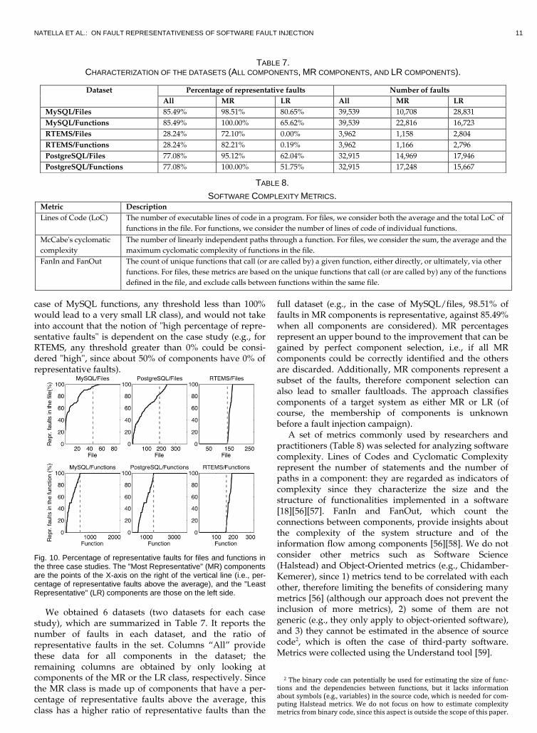
case of MySQL functions, any threshold less than 100% would lead to a very small LR class), and would not take into account that the notion of "high percentage of repre-sentative faults" is dependent on the case study (e.g., for RTEMS, any threshold greater than 0% could be consi-dered "high", since about 50% of components have 0% of representative faults).

Fig. 10. Percentage of representative faults for files and functions in the three case studies. The "Most Representative" (MR) components are the points of the X-axis on the right of the vertical line (i.e., per-centage of representative faults above the average), and the "Least Representative" (LR) components are those on the left side.

We obtained 6 datasets (two datasets for each case study), which are summarized in Table 7. It reports the number of faults in each dataset, and the ratio of representative faults in the set. Columns “All” provide these data for all components in the dataset; the remaining columns are obtained by only looking at components of the MR or the LR class, respectively. Since the MR class is made up of components that have a per-centage of representative faults above the average, this class has a higher ratio of representative faults than the

full dataset (e.g., in the case of MySQL/files, 98.51% of faults in MR components is representative, against 85.49% when all components are considered). MR percentages represent an upper bound to the improvement that can be gained by perfect component selection, i.e., if all MR components could be correctly identified and the others are discarded. Additionally, MR components represent a subset of the faults, therefore component selection can also lead to smaller faultloads. The approach classifies components of a target system as either MR or LR (of course, the membership of components is unknown before a fault injection campaign).

A set of metrics commonly used by researchers and practitioners (Table 8) was selected for analyzing software complexity. Lines of Codes and Cyclomatic Complexity represent the number of statements and the number of paths in a component: they are regarded as indicators of complexity since they characterize the size and the structure of functionalities implemented in a software [18][56][57]. FanIn and FanOut, which count the connections between components, provide insights about the complexity of the system structure and of the information flow among components [56][58]. We do not consider other metrics such as Software Science (Halstead) and Object-Oriented metrics (e.g., Chidamber-Kemerer), since 1) metrics tend to be correlated with each other, therefore limiting the benefits of considering many metrics [56] (although our approach does not prevent the inclusion of more metrics), 2) some of them are not generic (e.g., they only apply to object-oriented software), and 3) they cannot be estimated in the absence of source code2, which is often the case of third-party software. Metrics were collected using the Understand tool [59].

2 The binary code can potentially be used for estimating the size of func-tions and the dependencies between functions, but it lacks information about symbols (e.g., variables) in the source code, which is needed for com-puting Halstead metrics. We do not focus on how to estimate complexity metrics from binary code, since this aspect is outside the scope of this paper.

Metric Description

Lines of Code (LoC) The number of executable lines of code in a program. For files, we consider both the average and the total LoC of

functions in the file. For functions, we consider the number of lines of code of individual functions.

McCabe's cyclomatic

complexity

The number of linearly independent paths through a function. For files, we consider the sum, the average and the

maximum cyclomatic complexity of functions in the file.

FanIn and FanOut The count of unique functions that call (or are called by) a given function, either directly, or ultimately, via other

functions. For files, these metrics are based on the unique functions that call (or are called by) any of the functions

defined in the file, and exclude calls between functions within the same file.

TABLE 8.

SOFTWARE COMPLEXITY METRICS.

Dataset Percentage of representative faults Number of faults

All MR LR All MR LR

MySQL/Files 85.49% 98.51% 80.65% 39,539 10,708 28,831

MySQL/Functions 85.49% 100.00% 65.62% 39,539 22,816 16,723

RTEMS/Files 28.24% 72.10% 0.00% 3,962 1,158 2,804

RTEMS/Functions 28.24% 82.21% 0.19% 3,962 1,166 2,796

PostgreSQL/Files 77.08% 95.12% 62.04% 32,915 14,969 17,946

PostgreSQL/Functions 77.08% 100.00% 51.75% 32,915 17,248 15,667

TABLE 7. CHARACTERIZATION OF THE DATASETS (ALL COMPONENTS, MR COMPONENTS, AND LR COMPONENTS).

12 IEEE TRANSACTIONS ON SOFTWARE ENGINEERING

5.2 Evaluation Measures

We introduce a set of measures for assessing the ability of the proposed approach to correctly classify components and, ultimately, to improve faultload representativeness. Since the purpose of our approach is to avoid injecting non-representative faults, the primary measure is the per-centage of representative faults within the faultload:

in particular, we denote with the percentage of representative faults in the faultload using the proposed approach, and with and

the percentage computed for the MR and LR classes, respectively (see Table 7). In a similar way, we evaluate the number of faults in the faultload, namely , , and .

Additionally, we consider measures specifically aimed at evaluating classification algorithms, namely precision and recall [62]. These measures compare the set of objects that should be selected (i.e., the MR class) with the set of objects actually selected by the classifier (see Fig. 11). The measures are based on the following quantities, that is, the number of objects correctly or wrongly classified:

1. True Positives (TP): Number of MR components correctly identified as MR.

2. False Positives (FP): Number of LR components wrongly classified as MR.

3. False Negatives (FN): Number of MR components wrongly classified as LR.

In turn, precision and recall are computed as follows: 1. Precision = : Percentage of True

Positives with respect to the whole set of selected components (which includes both TPs and FPs).

2. Recall = : Percentage of True Posi-tives with respect to the set of MR components (which includes both TPs and FNs).

Fig. 11. Measures adopted for assessing classification algorithms.

Ideally, a classifier should have high precision (as close as possible to 1), to keep low the number of non-representative faults in the faultload (due to False Positives), and it should also have high recall (as close as possible to 1), to keep low the number of representative faults missed (due to False Negatives). Both precision and recall are related to the percentage of representative faults that can be obtained by filtering components through a classifier. The expected percentage of representative faults after selection is

which is the weighted average between the densities of representative faults in MR and LR classes: the higher the precision, the closer the average to the MR class. The expected number of faults in the faultload after filtering is

It should be noted that is inflated with

False Positives when Precision is low. When Recall is low, is low due to False Negatives (i.e., some MR

components are not recognized by the classifier).

5.3 Fault Selection by using Decision Trees

The first algorithm that we adopt for component classification is a technique commonly used in data mining problems, namely decision trees [62]. A decision tree is a hierarchical set of questions that are used to classify an element. In our study, questions are based on software metrics (for instance "Is LoC greater than 340?"), and the components are the elements to be classified. This algorithm is a supervised classifier, since it requires to be trained with examples in order to classify unknown elements. Decision trees have been preferred over other supervised classifiers because they are simple to interpret, therefore they can provide insights on the relationship between complexity metrics and component classes. This classifier is provided by most machine learning tools, such as the WEKA tool used in this work [62].

A decision tree is obtained from a training dataset using the C4.5 algorithm [62]. The C4.5 algorithm iteratively splits the dataset in two parts, by choosing the individual attribute (i.e., complexity metric) and a threshold that best separates the training data into the classes; this operation is then repeated on the subsets, until the classification error (estimated on the training set) cannot be reduced anymore. The root and inner nodes represent questions about complexity metrics, and leafs represent class labels. To classify a component, a metric of the component is first compared to the threshold specified in the root node, to choose one of the two children nodes; this operation is repeated for each selected node, until a leaf is reached.

The performance of decision trees was evaluated on the 6 datasets (Subsection 5.1) through cross-validation. Each dataset is divided in a training set (one third of the data) and a test set (two thirds of the data); evaluation metrics (Subsection 5.2) are then computed by classifying the components of the test set. Since the dataset split can affect the performance of the classifier, we considered 10 random splits for each dataset. The results of cross-validation are provided in Table 9. It is worth noting that the average precision is higher than 0.6 for every dataset (i.e., TPs are more than FPs), therefore we expect that the percentage of representative faults is increased in the filtered faultload. Moreover, since the recall ranges between 0.63 and 0.93, the filtered faultload includes most of the MR components (i.e., TPs are more than FNs) and therefore most of the representative faults. It should be observed that decision trees provide better performance on the "functions" datasets than on the "files" datasets (with respect to all metrics and case studies), since a

(3)

(2)

(1)

NATELLA ET AL.: ON FAULT REPRESENTATIVENESS OF SOFTWARE FAULT INJECTION 13

smaller granularity can enable a more precise filtering (e.g., if most of the non-representative faults in a file are in a few functions, only these functions can be removed).

Table 10 provides the faultload size and percentage of representative faults when using decision trees. The first two columns describe the original datasets (they report data from Table 7 for the sake of readability). The last two columns describe the expected number of faults and ratio of representative faults when a subset of components is selected using a decision tree with precision/recall as estimated through cross-validation (see Table 9 and Eq. (2) and (3)). Faultload representativeness increases in all cases (see the column on the right side). The improvement is more significant for RTEMS (up to 26.08%), since the difference between and (Table 7) is more significant in this case study (e.g., there are several components with 0% of representative faults), therefore the benefit of faultload filtering is greater in this case. After filtering, a large share of faults is removed from the faultload (between 30.30% and 69.43%); at the same time, due to the high recall, we are confident that most of the representative faults in the initial faultload are still present in the filtered faultload.

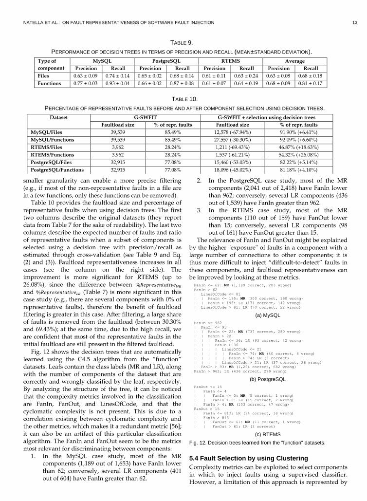
Fig. 12 shows the decision trees that are automatically learned using the C4.5 algorithm from the “function” datasets. Leafs contain the class labels (MR and LR), along with the number of components of the dataset that are correctly and wrongly classified by the leaf, respectively. By analyzing the structure of the tree, it can be noticed that the complexity metrics involved in the classification are FanIn, FanOut, and LinesOfCode, and that the cyclomatic complexity is not present. This is due to a correlation existing between cyclomatic complexity and the other metrics, which makes it a redundant metric [56]; it can also be an artifact of this particular classification algorithm. The FanIn and FanOut seem to be the metrics most relevant for discriminating between components:

1. In the MySQL case study, most of the MR components (1,189 out of 1,653) have FanIn lower than 62; conversely, several LR components (401 out of 604) have FanIn greater than 62.

2. In the PostgreSQL case study, most of the MR components (2,041 out of 2,418) have FanIn lower than 962; conversely, several LR components (436 out of 1,539) have FanIn greater than 962.

3. In the RTEMS case study, most of the MR components (110 out of 159) have FanOut lower than 15; conversely, several LR components (98 out of 161) have FanOut greater than 15.

The relevance of FanIn and FanOut might be explained by the higher "exposure" of faults in a component with a large number of connections to other components; it is thus more difficult to inject “difficult-to-detect” faults in these components, and faultload representativeness can be improved by looking at these metrics.

5.4 Fault Selection by using Clustering

Complexity metrics can be exploited to select components in which to inject faults using a supervised classifier. However, a limitation of this approach is represented by

Fig. 12. Decision trees learned from the "function" datasets.

FanIn <= 62: MR (1,189 correct, 203 wrong)

FanIn > 62

| LinesOfCode <= 81

| | FanIn <= 195: MR (300 correct, 160 wrong)

| | FanIn > 195: LR (171 correct, 142 wrong)

| LinesOfCode > 81: LR (70 correct, 22 wrong)

(a) MySQL

FanIn <= 962

| FanIn <= 93

| | FanIn <= 22: MR (737 correct, 280 wrong)

| | FanIn > 22

| | | FanIn <= 36: LR (93 correct, 42 wrong)

| | | FanIn > 36

| | | | LinesOfCode <= 21

| | | | | FanIn <= 74: MR (40 correct, 8 wrong)

| | | | | FanIn > 74: LR (3 correct)

| | | | LinesOfCode > 21: LR (37 correct, 26 wrong)

| FanIn > 93: MR (1,294 correct, 682 wrong)

FanIn > 962: LR (436 correct, 279 wrong)

(b) PostgreSQL

FanOut <= 15

| FanIn <= 4

| | FanIn <= 0: MR (5 correct, 1 wrong)

| | FanIn > 0: LR (15 correct, 2 wrong)

| FanIn > 4: MR (103 correct, 47 wrong)

FanOut > 15

| FanIn <= 813: LR (94 correct, 38 wrong)

| FanIn > 813

| | FanOut <= 61: MR (11 correct, 1 wrong)

| | FanOut > 61: LR (3 correct)

(c) RTEMS

TABLE 9.

PERFORMANCE OF DECISION TREES IN TERMS OF PRECISION AND RECALL (MEAN±STANDARD DEVIATION).

Type of

component

MySQL PostgreSQL RTEMS Average

Precision Recall Precision Recall Precision Recall Precision Recall

Files 0.63 ± 0.09 0.74 ± 0.14 0.65 ± 0.02 0.68 ± 0.14 0.61 ± 0.11 0.63 ± 0.24 0.63 ± 0.08 0.68 ± 0.18

Functions 0.77 ± 0.03 0.93 ± 0.04 0.66 ± 0.02 0.87 ± 0.08 0.61 ± 0.07 0.64 ± 0.19 0.68 ± 0.08 0.81 ± 0.17

TABLE 10.

PERCENTAGE OF REPRESENTATIVE FAULTS BEFORE AND AFTER COMPONENT SELECTION USING DECISION TREES.

Dataset G-SWFIT G-SWFIT + selection using decision trees

Faultload size % of repr. faults Faultload size % of repr. faults

MySQL/Files 39,539 85.49% 12,578 (-67.94%) 91.90% (+6.41%)

MySQL/Functions 39,539 85.49% 27,557 (-30.30%) 92.09% (+6.60%)

RTEMS/Files 3,962 28.24% 1,211 (-69.43%) 46.87% (+18.63%)

RTEMS/Functions 3,962 28.24% 1,537 (-61.21%) 54.32% (+26.08%)

PostgreSQL/Files 32,915 77.08% 15,460 (-53.03%) 82.22% (+5.14%)

PostgreSQL/Functions 32,915 77.08% 18,096 (-45.02%) 81.18% (+4.10%)

14 IEEE TRANSACTIONS ON SOFTWARE ENGINEERING

the need for a training set, since getting a training set would require an experimental analysis similar to the one in Section 3. Therefore, a practitioner would need to identify representative faults for a subset of components, to train the algorithm, and to classify the remaining components. To overcome this limitation, we consider an unsupervised classifier (i.e., not requiring a training phase), namely a clustering algorithm. This approach is based on the finding that MR components have low FanIn or FanOut and tend to be aggregated below a threshold.

A clustering algorithm partitions a dataset into subsets (clusters) such that data in each subset are similar (according to some distance measure). Therefore, it can be used to partition the components into two sets, and then to select only one subset for fault injection. Two aspects need to be defined to adopt this strategy: a distance measure, and a criterion for selecting the target cluster.

Define a distance measure: we define the distance measure as the euclidean distance in the space of software complexity metrics, in order to discriminate between “low” and “high” values of software metrics. In the following, we evaluate several combinations of software complexity metrics for this purpose; we focus on LinesOfCode, FanIn, and FanOut, since they turned out to be the most relevant metrics in the previous analysis.

Define a criterion for selecting the target cluster: a clustering algorithm can split the data set in two subsets; however, only one subset has to be selected for fault injection. Since the MR components are characterized by the lowest FanIn and FanOut, we select the cluster in which to inject faults by computing the mean value of FanIn and FanOut of components in each cluster. We then select the cluster with the lowest average FanOut or the lowest average FanIn (both criteria were evaluated).

Among the clustering algorithms proposed in the literature, we adopt the Lloyd k-means clustering algorithm, which is well known and simple to understand [62]. K-means clustering identifies k clusters that minimize the variance of distance of elements within the same cluster. In our approach, we adopt the fixed value k=2 when applying clustering (even if the samples could be divided in more clusters), since we aim at discriminating between only two classes. The algorithm is an iterative procedure. It randomly selects k elements (namely centroids), each representing the “mean” of a cluster, and assigns the remaining elements to the cluster of the nearest centroid. The procedure is repeated by computing the means of the clusters obtained in the previous iteration, that are used as new centroids. It stops when clusters do not change between iterations or after a maximum number of iterations. The clustering algorithm is executed 10 times, by varying the random selection of the initial k elements. Data were normalized in the range [0,1] before clustering.

Table 11 and Table 12 show the performance of k-means clustering with respect to the three case studies with respect to "function" components. We evaluated the effectiveness of different sets of metrics and cluster selection criteria. The best results (in terms of high average and low standard deviation of both precision and recall) are obtained when (i) the cluster with the lowest FanOut is selected, and (ii) the distance measure is based on LoC and FanOut (highlighted in Table 11). It can be observed that clustering is close to decision trees in terms of precision (respectively, 0.63 and 0.68 in average) and recall (0.81 for both decision trees and clustering using FanOut and LinesOfCode). Although cluster selection using the lowest FanIn still gives good results for MySQL and PostgreSQL, FanIn is not effective in the case of

TABLE 12 PERFORMANCE OF CLUSTERING (MEAN±STANDARD DEVIATION), USING FANIN FOR SELECTING THE TARGET CLUSTER.

Metrics MySQL PostgreSQL RTEMS Average

Precision Recall Precision Recall Precision Recall Precision Recall

LoC, FanIn, FanOut 0.70 ± 0.06 0.36 ± 0.42 0.62 ± 0.01 0.45 ± 0.23 0.44 ± 0.00 0.72 ± 0.00 0.59 ± 0.11 0.51 ± 0.31

FanIn, FanOut 0.68 ± 0.05 0.23 ± 0.35 0.63 ± 0.01 0.46 ± 0.22 0.44 ± 0.00 0.72 ± 0.00 0.58 ± 0.11 0.47 ± 0.31

LoC, FanOut 0.65 ± 0.00 0.06 ± 0.00 0.62 ± 0.00 0.35 ± 0.07 0.35 ± 0.00 0.14 ± 0.00 0.54 ± 0.14 0.18 ± 0.13

FanOut 0.65 ± 0.00 0.06 ± 0.00 0.62 ± 0.00 0.34 ± 0.08 0.33 ± 0.00 0.14 ± 0.01 0.54 ± 0.14 0.18 ± 0.13

LoC, FanIn 0.78 ± 0.00 0.92 ± 0.00 0.66 ± 0.01 0.78 ± 0.07 0.44 ± 0.00 0.72 ± 0.00 0.63 ± 0.14 0.81 ± 0.09

FanIn 0.78 ± 0.00 0.92 ± 0.00 0.66 ± 0.02 0.80 ± 0.09 0.44 ± 0.00 0.72 ± 0.00 0.62 ± 0.14 0.81 ± 0.10

LoC 0.74 ± 0.00 0.99 ± 0.00 0.44 ± 0.01 0.05 ± 0.00 0.51 ± 0.00 0.87 ± 0.01 0.57 ± 0.13 0.64 ± 0.43

Average 0.58 ± 0.13 0.51 ± 0.34

TABLE 11 PERFORMANCE OF CLUSTERING (MEAN±STANDARD DEVIATION), USING FANOUT FOR SELECTING THE TARGET CLUSTER.

Metrics MySQL PostgreSQL RTEMS Average

Precision Recall Precision Recall Precision Recall Precision Recall

LoC, FanIn, FanOut 0.68 ± 0.12 0.77 ± 0.35 0.56 ± 0.10 0.52 ± 0.27 0.71 ± 0.00 0.28 ± 0.00 0.65 ± 0.11 0.52 ± 0.32

FanIn, FanOut 0.68 ± 0.12 0.76 ± 0.36 0.57 ± 0.08 0.55 ± 0.23 0.71 ± 0.00 0.28 ± 0.00 0.65 ± 0.10 0.53 ± 0.31

LoC, FanOut 0.74 ± 0.00 0.94 ± 0.00 0.61 ± 0.00 0.63 ± 0.04 0.54 ± 0.00 0.86 ± 0.00 0.63 ± 0.08 0.81 ± 0.13

FanOut 0.74 ± 0.00 0.94 ± 0.00 0.61 ± 0.00 0.66 ± 0.08 0.54 ± 0.00 0.86 ± 0.01 0.63 ± 0.08 0.82 ± 0.13

LoC, FanIn 0.46 ± 0.07 0.13 ± 0.20 0.47 ± 0.03 0.23 ± 0.06 0.71 ± 0.00 0.28 ± 0.00 0.54 ± 0.13 0.21 ± 0.14

FanIn 0.44 ± 0.00 0.08 ± 0.00 0.46 ± 0.04 0.22 ± 0.07 0.71 ± 0.00 0.28 ± 0.00 0.54 ± 0.13 0.19 ± 0.09

LoC 0.74 ± 0.00 0.99 ± 0.00 0.62 ± 0.00 0.95 ± 0.00 0.51 ± 0.00 0.87 ± 0.01 0.63 ± 0.09 0.94 ± 0.05

Average 0.61 ± 0.11 0.57 ± 0.34

NATELLA ET AL.: ON FAULT REPRESENTATIVENESS OF SOFTWARE FAULT INJECTION 15

RTEMS (precision is less than 0.50). Instead, FanOut turned out to be more useful than FanIn to provide a common selection criteria among all the systems. This result is due to a correlation existing between FanIn and FanOut (i.e., high FanIn and high FanOut tend to occur at the same time). Therefore, both FanIn and FanOut are effective for the MySQL and PostgreSQL systems, but the FanOut metric should be preferred as a generic criterion.

Fig. 13 shows the distribution of components with respect to FanOut and LinesOfCode metrics. The cross marks represent the centroids of the clusters. The cluster to be selected is the one on the bottom-left corner of the plots (lowest FanOut). The high precision and recall of the clustering algorithm is due to the density of MR functions being higher than the density of LR functions in that cluster. In other words, when only the target cluster is selected, a high amount of MR functions is retained, while several LR functions are avoided at the same time.

Table 13 summarizes the results of clustering in terms of percentage of representative faults and faultload size. The clustering algorithm is able to improve the faultload representativeness, and the best results are achieved when clustering at the "function" granularity (the improvement ranges between 4.10% and 16.24%). Clustering is almost as effective as decision trees, and it does not need to be trained using examples (which can be costly to obtain) as it exploits the relationship between the FanOut metric and fault representativeness (see Fig. 12). Thus, clustering is a valuable approach for improving representativeness and reducing experimental effort.

6 LIMITATIONS

The approach and the results reported in this study are based on empirical data, which limit the generality of the conclusions. We considered open-source systems, and results could not apply to software developed under other paradigms. Nevertheless, they are supported by commercial organizations, and they were tested using best practices also adopted in commercial software, such as request/bug tracking for introducing test cases related to new features or faults that should be avoided in future development. Moreover, the RTEMS system has been designed and tested to fulfill the requirements of industrial safety standards, for its adoption in space applications by the European Space Agency [50]. Due to similarities between these systems and industrial ones, the results can potentially be extended to other systems, which is a direction for future research.

7 CONCLUSION

In this paper, we analyzed the representativeness of injected faults in three complex, real-world software systems, and proposed an approach for improving fault representativeness. This aspect is important for obtaining a realistic assessment of fault tolerance. The SFI technique considered in this work, G-SWFIT, aims to achieve fault representativeness by emulating the most frequent fault types found in operational systems. In this work, we study fault representativeness with respect to an

Fig. 13 Scatter plot of MR (non-filled circles) and LR (filled circles) functions in the LoC/FanOut space. Cross marks identify cluster centroids.

TABLE 13. PERCENTAGE OF REPRESENTATIVE FAULTS BEFORE AND AFTER COMPONENT SELECTION USING CLUSTERING.

Dataset G-SWFIT G-SWFIT + selection using clustering

Faultload size % of repr. faults Faultload size % of repr. faults

MySQL/Files 39,539 85.49% 16,159 (-59.13%) 90.47% (+4.98%)

MySQL/Functions 39,539 85.49% 28,982 (-26.70%) 91.06% (+5.57%)

RTEMS/Files 3,962 28.24% 1,816 (-54.16%) 36.77% (+8.53%)

RTEMS/Functions 3,962 28.24% 1,857 (-53.13%) 44.48% (+16.24%)

PostgreSQL/Files 32,915 77.08% 25,620 (-22.16%) 79.24% (+2.16%)

PostgreSQL/Functions 32,915 77.08% 17,813 (-45.88%) 81.18% (+4.10%)

16 IEEE TRANSACTIONS ON SOFTWARE ENGINEERING

additional criterion, that is, the ability of faults to escape real test suites, which characterizes residual faults that affect operational systems and that should be tolerated.

After analyzing a large set of injected faults and real test cases (up to 3.8 million experiments), we concluded that the percentage of representative faults ranges from a minor share in the case of DBMSs (14.57% and 23.13%) to a significant share in the case of a RTOS (72.23%). The proposed approach selects a subset of components suitable for injecting representative faults, by analyzing their complexity and relationships using classification algorithms and software metrics. The first considered algorithm, decision trees, is a supervised classifier, which is trained by providing examples of components to be selected. The second algorithm, k-means clustering, is an unsupervised classifier, which does not require to be trained with examples but relies on the observation that suitable components have the lowest FanIn and FanOut, as they are less exposed to testing. We found that both these algorithms can accurately classify components for all the case studies (ranging from small and well-tested to large and less-tested software), and that it is possible to improve fault representativeness and reduce faultload size at the same time. In the light of these results, the proposed approach can be regarded as an effective and practical means for improving the realism of SFI.

ACKNOWLEDGMENT

This work was supported by the CRITICAL-STEP FP7 European project (http://www.critical-step.eu).

REFERENCES

[1] J. Gray, “Why do computers stop and what can be done about it?,” Tandem TR85.7, June 1985

[2] R. Chillarege, I.S. Bhandari, J.K. Chaar, M.J. Halliday, D.S. Moebus, B.K. Ray, and M.-Y. Wong, “Orthogonal Defect Classi- fication—A Concept for In-Process Measurements,” IEEE Trans. Software Eng., vol. 18, no. 11, pp. 943-956, Nov. 1992

[3] J. Musa, Software Reliability Engineering. McGraw-Hill, 1996 [4] E.J. Weyuker, "Testing component-based software: a cautionary

tale," IEEE Software, vol.15, no.5, pp.54-59, Sep.-Oct. 1998 [5] J.C. Knight, “Safety critical systems: challenges and directions”,

Proc. 24th Intl. Conf. on Software Eng., pp. 547-550, 2002 [6] NASA Software Safety Guidebook, NASA-GB-8719.13, 2004. [7] International Organization for Standardization, “Product de-

velopment: software level”, ISO/DIS 26262-6, 2009. [8] A. Avizienis, "The N-Version Approach to Fault-Tolerant Soft-

ware," IEEE Trans. Software Eng., vol. SE-11, no.12, pp. 1491- 1501, Dec. 1985

[9] M.R. Lyu, Software Fault Tolerance. John Wiley & Sons, 1995 [10] F. Cristian, "Exception Handling and Software Fault Tolerance,"

IEEE Trans. Computers, vol.C-31, no.6, pp.531-540, June 1982 [11] J. Arlat, M. Aguera, L. Amat, Y. Crouzet, J.C. Fabre, J.C. Laprie,

E. Martin, and D. Powell, “Fault Injection for Dependability Va-lidation: A Methodology and Some Applications,” IEEE Trans. Software Eng., vol. 16, no. 2, pp. 166-182, Feb. 1990

[12] J. Voas, F. Charron, G. McGraw, K. Miller, and M. Friedman, “Predicting How Badly ―Good‖ Software can Behave,” IEEE Software, vol. 14, no. 4, 1997

[13] J. Christmansson and R. Chillarege, "Generation of an Error Set that Emulates Software Faults based on Field Data," Proc. 26th IEEE Fault Tolerant Computing Symp., pp.304-313, 1996

[14] R. G. Hamlet, “Testing Programs with the Aid of a Compiler,” IEEE Trans. Software Eng., vol. 3, no. 4, pp. 279-290, July 1977

[15] R. A. DeMillo, R. J. Lipton, and F. G. Sayward, “Hints on Test Data Selection: Help for the Practicing Programmer,” Computer, vol. 11, no. 4, pp. 34-41, Apr. 1978

[16] K.N. King and A.J. Offutt, “A Fortran Language System for Mu-tation-based Software Testing,” Software: Practice and Experience, vol. 21, no. 7, pp. 685-718, July 1991

[17] J.A. Duraes and H. Madeira, "Emulation of Software Faults: A Field Data Study and a Practical Approach," IEEE Trans. Soft-ware Eng., vol.32, no.11, pp.849-867, Nov. 2006

[18] N.E. Fenton and N. Ohlsson, "Quantitative Analysis of Faults and Failures in a Complex Software System," IEEE Trans. Soft-ware Eng., vol.26, no.8, pp.797-814, Aug. 2000

[19] D. Powell, E. Martins, J. Arlat, and Y. Crouzet, “Estimators for Fault Tolerance Coverage Evaluation,” IEEE Trans. Computers, vol.44, no.2, pp.261-274, Feb. 1995

[20] M. Cukier, D. Powell, and J. Arlat, “Coverage Estimation Me-thods for Stratified Fault-Injection,” IEEE Trans. on Computers, vol.48, no.7, pp.707-723, July 1999

[21] J.H. Andrews, L.C. Briand, and Y. Labiche, “Is Mutation an Appropriate Tool for Testing Experiments?,” Proc. 27th Intl. Conf. on Software Eng., pp. 402-411, 2005

[22] H. Do and G. Rothermel, “On the Use of Mutation Faults in Empirical Assessments of Test Case Prioritization Techniques,” IEEE Trans. Software Eng., vol.32, no.9, pp.733-752, Sep. 2006

[23] R. Geist, A.J. Offutt, and F.C. Harris Jr, “Estimation and En-hancement of Real-Time Software Reliability through Mutation Analysis,” IEEE Trans. Computers, pp. 550-558, vol. 41, no. 5, May 1992

[24] Y. Jia and M. Harman, “An Analysis and Survey of the Devel-opment of Mutation Testing,” IEEE Trans. Software Eng., vol. 37, no. 5, pp. 649-678, Sep. 2011

[25] A.J. Offutt, G. Rothermel, and C. Zapf, “An Experimental Eval-uation of Selective Mutation,” Proc. 15th Intl. Conf. on Software Eng., pp.100-107, 1993

[26] A.J. Offutt, A. Lee, G. Rothermel, R.H. Untch, and C. Zapf, “An Experimental Determination of Sufficient Mutant Operators,” ACM Trans. Software Engineering and Methodology, vol. 5, no. 2, pp. 99-118, Apr. 1996

[27] W.E. Wong and A.P. Mathur, “Reducing the Cost of Mutation Testing: An Empirical Study,” J. of Systems and Software, vol. 31, no. 3, pp. 185-196, Dec. 1995

[28] M. Sridharan and A.S. Namin, “Prioritizing Mutation Opera-tors Based on Importance Sampling,” Proc. 21st Intl. Symp. of Software Reliability Engineering, pp. 378-387, 2010

[29] W.T. Ng and P.M. Chen, “The design and verification of the Rio file cache,” IEEE Trans. Computers, vol.50, no.4, pp.322-337, Apr. 2001

[30] S. Chandra and P.M. Chen, “How Fail-Stop are Faulty Pro-grams?” Proc. 28th IEEE Fault Tolerant Computing Symp., 1998

[31] J.J. Hudak, B.H. Suh, D.P. Siewiorek, and Z. Segall, "Evaluation and Comparison of Fault-Tolerant Software Techniques," IEEE Trans. Reliability, vol. 42, no. 2, pp.190-204, June 1993

[32] M. Vieira and H. Madeira, "A Dependability Benchmark for OLTP Application Environments," Proc. 29th Int'l Conf. on Very Large Data Bases, pp. 742-753, 2003

[33] A. Avizienis, J.-C. Laprie, B. Randell, and C. Landwehr, "Basic Concepts and Taxonomy of Dependable and Secure Compu-ting," IEEE Trans. Dependable and Secure Computing, vol.1, no.1, pp. 11- 33, Jan.-March 2004

[34] D. Stott, B. Floering, D. Burke, Z. Kalbarczyk, and R. Iyer, “NFTAPE: A Framework for Assessing Dependability in Dis-tributed Systems with Lightweight Fault Injectors,” Proc. Int’l Computer Performance and Dependability Symp., pp. 91-100, 2000

[35] J. Aidemark, J. Vinter, P. Folkesson, and J. Karlsson, “GOOFI: Generic Object-Oriented Fault Injection Tool,” Proc. Int’l Conf. on Dependable Systems and Networks, pp. 83–88, 2001

[36] Z. Segall, D. Vrsalovic, D. Siewiorek, J. Kownacki, J. Barton, R. Dancey, A. Robinson, and T. Lin, "FIAT - Fault Injection Based Automated Testing Environment", Proc. 18th IEEE Fault Tolerant Computing Symp., pp. 102-107, 1988

NATELLA ET AL.: ON FAULT REPRESENTATIVENESS OF SOFTWARE FAULT INJECTION 17

[37] M.-C. Hsueh, T.K. Tsai, and R.K. Iyer, "Fault Injection Tech-niques and Tools," IEEE Computer, vol.30, no.4, pp.75-82, 1997

[38] J. Carreira, H. Madeira, and J.G. Silva, "Xception: A Technique for the Experimental Evaluation of Dependability in Modern Computers," IEEE Trans. Software Eng., vol. 24, no. 2, pp.125-136, Feb. 1998

[39] R. Moraes, R. Barbosa, J.A. Duraes, N. Mendes, E. Martins, H. Madeira, "Injection of Faults at Component Interfaces and In-side the Component Code: Are They Equivalent?" Proc. 6th Eu-ropean Dependable Computing Conf., pp.53-64, 2006

[40] P. Koopman and J. DeVale, "The Exception Handling Effective-ness of POSIX Operating Systems," IEEE Trans. Software Eng., vol. 26, no. 9, pp. 837-848, Sep. 2000

[41] A. K. Ghosh, M. Schmid, and V. Shah, "Testing the Robustness of Windows NT Software", Proc. 9th IEEE Int'l Symp. Software Reliability Engineering, pp. 231-236, 1998

[42] J. Arlat, J.-C. Fabre, M. Rodriguez, and F. Salles, "Dependability of COTS microkernel-based systems," IEEE Trans. Computers, vol.51, no.2, pp.138-163, Feb. 2002

[43] E. Martins, C.M.F. Rubira, and N.G.M. Leme, "Jaca: A Reflective Fault Injection Tool based on Patterns", Proc. IEEE Int'l Depen-dable Systems and Networks, pp. 483-487, 2002

[44] W.-L. Kao, R.K. Iyer, and D. Tang, "FINE: A Fault Injection and Monitoring Environment for Tracing the UNIX System Beha-vior under Faults," IEEE Trans. Software Eng., vol.19, no.11, pp.1105-1118, Nov. 1993

[45] H. Madeira, D. Costa, and M. Vieira, "On the Emulation of Software Faults by Software Fault Injection," Proc. IEEE Int'l Conf. Dependable Systems and Networks, pp. 417-426, 2000

[46] T. Jarboui, J. Arlat, Y. Crouzet, K. Kanoun, and T. Marteau, "Analysis of the Effects of Real and Injected Software Faults: Linux as a Case Study," Proc. Pacific Rim Int'l Symp. Dependable Computing, pp. 51- 58, 2002

[47] M.E. Delamaro and J.C. Maldonado, “Proteum-A Tool for the Assessment of Test Adequacy for C Programs,” Proc. Conf. Per-formability in Computer Systems, pp. 79-95, 1996

[48] MySQL Market Share, http://www.mysql.com/why-mysql/marketshare/, accessed on March 2011

[49] EnterpriseDB's Postgres Plus users by Application Type, http://www.enterprisedb.com/customer-success/customers-by-application-workload, accessed on March 2011

[50] J. Rufino, S. Filipe, M. Coutinho, S. Santos, and J. Windsor, "ARINC 653 Interface in RTEMS," Data Systems in Aerospace Conf., 2007

[51] GCC documentation, http://gcc.gnu.org/onlinedocs/gcc/ [52] QEMU virtualization software, http://qemu.org [53] SAFE Software Fault Emulation Tool,

http://www.mobilab.unina.it/SFI.htm [54] TPC-C OLTP Benchmark, http://www.tpc.org/tpcc/ [55] D. Sheskin. Handbook of Parametric and Nonparametric Statistical

Procedures. Chapman and Hall/CRC, 2004 [56] N.E. Fenton and S.L. Pfleeger. Software Metrics: A Rigorous and

Practical Approach. PWS Publishing Co., 1998 [57] V.R. Basili and B.T. Perricone, “Software Errors and Complexi-

ty: An Empirical Investigation,” Communications of the ACM, vol.27, no.1, pp.42-52, Jan. 1984

[58] S. Henry and D. Kafura, “Software Structure Metrics Based on Information Flow,” IEEE Trans. Software Eng., vol. SE-7, no.5, pp.510-518, Sep. 1981

[59] SciTools Understand tool, http://www.scitools.com [60] T. Menzies, J. Greenwald, and A. Frank, "Data mining static

code attributes to learn defect predictors," IEEE Trans. Software Eng., vol.33, no.1, pp. 2-13, Apr. 2007

[61] K. Srinivasan and D. Fisher, "Machine Learning Approaches to Estimating Software Development Effort," IEEE Trans. Software Eng., vol.21, no.2, pp.126-137, Feb. 1995

[62] I. Witten and E. Frank. Data Mining: Practical Machine Learning Tools and Techniques. Morgan Kaufmann, 2005

Roberto Natella received the BS and MSc degrees cum laude (2005 and 2007) and the PhD degree (2011) in Computer Engineering from the Federico II University of Naples. He is currently a researcher at the Consorzio

Interuniversitario Nazionale per l’Informatica (CINI). His research interests include depen-dability assessment and certification of sa-fety-critical software, and software aging and rejuvenation. He authored about 20 interna-

tional publications on these topics. He is student member of the IE-EE and ACM.

Domenico Cotroneo received his Ph.D. in 2001 from the Department of Computer Science and System Engineering at the University of Naples, Italy. He is currently Associate Professor at the University of Na-ples. His main interests include software fault injection, dependability assessment techni-ques, and field-based measurements techni-ques. Domenico Cotroneo has served as Program Committee member in a number of scientific conferences on dependability to-

pics, including DSN, EDCC, ISSRE, SRDS, and LADC, and he is involved in several national/european projects in the context of de-pendable systems.

Joao A. Duraes received the BS, MSc, and PhD degrees in informatics engineering from the University of Coimbra in 1994, 1999, and 2006, respectively. He has been with the Centre for Informatics and Systems of the University of Coimbra as a researcher since 1994. He teaches computer-related courses at the Institute of Engineering of Coimbra sin-ce 1995. He was the recipient of the IEE-E/IFIP William C. Carter award for the best paper at the Dependable Systems and Ne-

tworks Symposium (DSN 2003).

Henrique S. Madeira is a professor at the University of Coimbra, where he has been involved in research on dependable computing since 1987. He has authored or coauthored more than 100 papers in refereed conferences and journals and has coordina-ted or participated in tens of projects funded by the Portuguese government and by the European Union. He was the vice-chair of the IFIP Working Group 10.4 Special Interest Group (SIG) on Dependability Benchmarking

from the establishment of the SIG from the summer of 1999 until 2002. He was the program cochair of the International Performance and Dependability Symposium track of the IEEE/IFIP International Conference on Dependable Systems and Networks (DSN-PDS ’04) and was appointed Conference Coordinator of IEEE/IFIP DSN ’08. He is currently the president of the Centre for Informatics and Systems of the University of Coimbra Research Centre and the head of the Department of Informatics Engineering at the University of Coimbra. He is a member of the IEEE.