PNNL-16071

Regional Atmospheric Transport Code for Hanford Emission Tracking, Version 2 (RATCHET2) RATCHET2: Modification and Implementation of RATCHET for Use in SAC J. V. Ramsdell, Jr. J. P. Rishel  July 2006 Prepared for the U.S. Department of Energy under Contract DE-AC05-76RL01830

DISCLAIMER

This report was prepared as an account of work sponsored by an agency of the United States Government. Neither the United States Government nor any agency thereof, nor Battelle Memorial Institute, nor any of their employees, makes any warranty, express or implied, or assumes any legal liability or responsibility for the accuracy, completeness, or usefulness of any information, apparatus, product, or process disclosed, or represents that its use would not infringe privately owned rights. Reference herein to any specific commercial product, process, or service by trade name, trademark, manufacturer, or otherwise does not necessarily constitute or imply its endorsement, recommendation, or favoring by the United States Government or any agency thereof, or Battelle Memorial Institute. The views and opinions of authors expressed herein do not necessarily state or reflect those of the United States Government or any agency thereof.

PACIFIC NORTHWEST NATIONAL LABORATORY operated by BATTELLE

for the UNITED STATES DEPARTMENT OF ENERGY

under Contract DE-AC05-76RL01830

Printed in the United States of America

Available to DOE and DOE contractors from the Office of Scientific and Technical Information,

P.O. Box 62, Oak Ridge, TN 37831-0062; ph: (865) 576-8401 fax: (865) 576-5728

email: reports@adonis.osti.gov

Available to the public from the National Technical Information Service, U.S. Department of Commerce, 5285 Port Royal Rd., Springfield, VA 22161

ph: (800) 553-6847 fax: (703) 605-6900

email: orders@ntis.fedworld.gov online ordering: http://www.ntis.gov/ordering.htm

This document was printed on recycled paper.

PNNL-16071

Regional Atmospheric Transport Code for Hanford Emission Tracking, Version 2 (RATCHET2) RATCHET2: Modification and Implementation of RATCHET for Use in SAC J. V. Ramsdell, Jr. J. P. Rishel July 2006 Prepared for the U.S. Department of Energy under Contract DE-AC05-76RL01830 Pacific Northwest National Laboratory Richland, Washington 99352

iii

Summary

In 1999, the U.S. Department of Energy initiated the development of an assessment tool that enables users to model the movement of contaminants from all waste sites at Hanford through the vadose zone, groundwater, and Columbia River and estimate the impact of contaminants on human health, ecology, and the local cultures and economy. This tool was named the System Assessment Capability (SAC) and is an integrated system of computer models and databases used to assess the impact of waste remaining on the Hanford Site.

This manual describes the atmospheric model and computer code for the Atmospheric Transport Module within SAC. The Atmospheric Transport Module, called RATCHET2, calculates the time-integrated air concentration and surface deposition of airborne contaminants to the soil. The RATCHET2 code is an adaptation of the Regional Atmospheric Transport Code for Hanford Emissions Tracking (RATCHET), as described by Ramsdell et al. (1994). The original RATCHET code was developed to perform the atmospheric transport for the Hanford Environmental Dose Reconstruction Project.

Fundamentally, the two sets of codes are identical; no capabilities have been deleted from the original version of RATCHET. Most modifications are generally limited to revision of the run-specification file to streamline the simulation process for SAC. In this regard, many model parameters that were set within the RATCHET run-specification file are now set internally to the RATCHET2 code. New variables have also been added to the RATCHET2 run-specification file to allow for flexibility in implementing the code into SAC. For example, the center of the model domain is now specified in the run-specification file rather than set internally within the RATCHET code.

Other notable changes from RATCHET to the RATCHET2 code include:

• Meteorological data input has been changed from direct access files to sequential files, and the file format has been modified to accommodate the meteorological data available from the current meteorological data acquisition system at Hanford.

• The format of the meteorological station file has been modified so that station locations are specified in latitude and longitude.

• The portions of RATCHET that dealt with determining mixing-layer thickness have been changed in RATCHET2. The mixing-layer thickness is determined for each station and then interpolated to nodes following the procedure described for RASCAL Version 3.

• For SAC, the RATCHET code has been revised to estimate annual, time-integrated concentrations normalized to the annual release rate for each analyte class (noble gas, iodine, and particle).

• The code is run for a single-source with a unit release; SAC scales the results from RATCHET2 to the appropriate emission rate.

• Decay calculations have been disabled within RATCHET2; SAC calculates radionuclide decay where appropriate.

iv

This manual has three major sections: a description of the model, a user’s guide, and a programmer's guide. These sections discuss RATCHET2 from three different perspectives. The first section provides a technical description of the code with emphasis on details such as the representation of the model domain, the data required by the model, and the equations used to make the model calculations. The second section is the user’s guide to the model and provides information on the model input, output, and instruction for running the code. The third and final section is a programmer’s guide to the code. It discusses the hardware and software required to run the code and discusses the program’s code structure and code elements.

v

Contents

Summary ...................................................................................................................................................... iii 1.0 Introduction ....................................................................................................................................... 1.1

1.1 Relationship to Other Atmospheric Dispersion Models......................................................... 1.2 1.2 Quality Assurance .................................................................................................................. 1.2 1.3 Manual Organization.............................................................................................................. 1.3

2.0 Technical Description........................................................................................................................ 2.1 2.1 Model Domain........................................................................................................................ 2.1

2.1.1 Cartesian Representation........................................................................................... 2.1 2.1.2 Coordinate Transformations...................................................................................... 2.3

2.2 Topography ............................................................................................................................ 2.4 2.2.1 Surface Roughness .................................................................................................... 2.6

2.3 Meteorology ........................................................................................................................... 2.6 2.3.1 Meteorological Stations............................................................................................. 2.7 2.3.2 Meteorological Data Input......................................................................................... 2.7 2.3.3 Calculated Meteorological Parameters.................................................................... 2.11 2.3.4 Spatial Representation of Meteorological Conditions............................................. 2.15

2.4 Source Term ......................................................................................................................... 2.16 2.4.1 Release Times and Rates......................................................................................... 2.16 2.4.2 Plume Rise and Effective Release Height ............................................................... 2.16

2.5 Transport .............................................................................................................................. 2.19 2.6 Diffusion............................................................................................................................... 2.21

2.6.1 Calculation of Time-Integrated Air Concentrations................................................ 2.22 2.6.2 Estimation of Diffusion Coefficients ...................................................................... 2.24 2.6.3 Estimation of Turbulence Parameters ..................................................................... 2.27

2.7 Transformation, Deposition, and Depletion ......................................................................... 2.28 2.7.1 Chemical and Physical Transformation................................................................... 2.28 2.7.2 Dry Deposition ........................................................................................................ 2.29 2.7.3 Wet Deposition........................................................................................................ 2.32 2.7.4 Surface Contamination ............................................................................................ 2.33 2.7.5 Depletion ................................................................................................................. 2.34

2.8 RATCHET2 Model Evaluation............................................................................................ 2.35 2.8.1 Krypton-85 Monitoring Data................................................................................... 2.36 2.8.2 RATCHET Comparison to Other Dispersion Models............................................. 2.37

3.0 RATCHET2 User’s Guide................................................................................................................. 3.1 3.1 Run-Specification File............................................................................................................ 3.1

3.1.1 Run Description......................................................................................................... 3.2 3.1.2 Model Parameters...................................................................................................... 3.3 3.1.3 Environmental Data Files.......................................................................................... 3.3 3.1.4 Output File Names .................................................................................................... 3.4 3.1.5 Source Characterization ............................................................................................ 3.4

3.2 Selection of Internal Values for RATCHET2 Model Control Parameters ............................. 3.4 3.2.1 Number of Puffs per Hour......................................................................................... 3.4 3.2.2 Minimum Time Step for Calculations....................................................................... 3.5 3.2.3 Puff Consolidation..................................................................................................... 3.5

vi

3.2.4 Puff Radius................................................................................................................ 3.6 3.2.5 De Minimis Concentration ........................................................................................ 3.6 3.2.6 Horizontal Diffusion Coefficient Proportionality Constant ...................................... 3.7

3.3 Input Files............................................................................................................................... 3.8 3.3.1 Surface Roughness Length File................................................................................. 3.8 3.3.2 Default Mixing-Layer Depth File.............................................................................. 3.8 3.3.3 Meteorological Station File ....................................................................................... 3.9 3.3.4 Meteorological Data File......................................................................................... 3.10

3.4 Output Files .......................................................................................................................... 3.11 3.4.1 Time-Integrated Air Concentrations and Deposition .............................................. 3.12 3.4.2 Run-Log File ........................................................................................................... 3.13 3.4.3 Run Indicator Files .................................................................................................. 3.13

3.5 Program Control ................................................................................................................... 3.13 4.0 Programmer’s Guide.......................................................................................................................... 4.1

4.1 Program Development............................................................................................................ 4.1 4.1.1 Language and Style ................................................................................................... 4.1 4.1.2 Target Computer ....................................................................................................... 4.2 4.1.3 Program Size ............................................................................................................. 4.2

4.2 Program Organization ............................................................................................................ 4.2 4.2.1 Main Program............................................................................................................ 4.2 4.2.2 Relationships Between Program Units...................................................................... 4.4

4.3 Program Element Descriptions............................................................................................... 4.6 4.3.1 Initialization Subroutines .......................................................................................... 4.6 4.3.2 Hourly Update Subroutines ....................................................................................... 4.9 4.3.3 Transport and Diffusion Subroutines ...................................................................... 4.11 4.3.4 Housekeeping Subroutines ...................................................................................... 4.13 4.3.5 Segment-End Output Subroutines ........................................................................... 4.13 4.3.6 RATCHET2 Functions............................................................................................ 4.14

5.0 References ......................................................................................................................................... 5.1

vii

Figures

Figure 1.1. Relationship of RATCHET2 to Other SAC Modules ........................................................ 1.1 Figure 2.1. The SAC Environmental Grid and Concentration Grid. .................................................... 2.2 Figure 2.2. Wind Rose Plots 30 Feet Above Ground Level for the Year 2003 at the Hanford

Meteorological Observation Stations ................................................................................. 2.5 Figure 2.3. Meteorological Station Locations used in SAC ................................................................. 2.9 Figure 2.4. Relationship between Stability Class and Monin-Obukhov Length as a Function of Surface

Roughness Length ............................................................................................................ 2.12 Figure 2.5. Wind Speed Variations at Heights between 10 and 100 m in the Diabatic Wind Speed

Profile Model.................................................................................................................... 2.14 Figure 2.6. Error Band for the Numerical Procedure Used to Estimate Time-Integrated Values ...... 2.25 Figure 2.7. Variation of Dry Deposition Velocities for Reactive Gases as a Function of Wind Speed

and Stability Class ............................................................................................................ 2.30 Figure 2.8. Variation of Dry Deposition Velocities for Small Particles as a Function of Wind Speed

and Stability Class ............................................................................................................ 2.31 Figure 2.9. Comparison of Predicted and Measured Dry Deposition Velocities for Ozone............... 2.32 Figure 2.10. RATCHET2 Predicted vs. Observed Krypton-85 Annual Concentrations in and Around the

Hanford Site for 1984-1987.............................................................................................. 2.37 Figure 3.1. Comparison of Time-Integrated Concentrations for 50 Locations Computed with NPH=4

and NPH=15 ....................................................................................................................... 3.5 Figure 3.2. Comparison of Time-Integrated Concentrations for 50 Locations Computed with 1-Minute

and 5-Minute Time Steps ................................................................................................... 3.6 Figure 3.3. Comparison of Calculated Surface Contamination Values for Puff Radius of 3.7 σr and

5.3 σr ................................................................................................................................... 3.7 Figure 3.4. Default Mixing-Layer Depths at the Hanford Site for January through March ................. 3.9 Figure 3.5. Sample Meteorological Station File for the Year 2002 .................................................... 3.10 Figure 4.1. RATCHET2 Code Organization and Processing ............................................................... 4.3 Figure 4.2. The RATCHET2 Subroutine Call Sequence ...................................................................... 4.6

Tables

Table 2.1. Typical Surface Roughness Lengths .................................................................................. 2.6 Table 2.2. Details of Meteorological Station Supplied to the Station File .......................................... 2.8 Table 2.3. Typical Wet Deposition Velocities for Gases and Particle-Washout Coefficients .......... 2.33 Table 2.4. Non-Depositing Species Average Exposure Relative Comparison to LODI ................... 2.37 Table 2.5. Depositing Species Average Exposure Relative Comparison to LODI ........................... 2.38 Table 2.6. Average Deposition Relative Comparison to LODI......................................................... 2.38 Table 3.1. Sample RATCHET2 Run-Specification File used in SAC. ............................................. 3.2 Table 3.2. Distribution of Horizontal Diffusion Coefficient, SY_CNST............................................ 3.8 Table 3.3. Summary of RATCHET2 Input Files................................................................................. 3.8 Table 3.4. Units and Ranges for Meteorological Variables............................................................... 3.12 Table 4.4. Units and Ranges for Meteorological Variables................................................................. 4.4

viii

1.1

1.0 Introduction

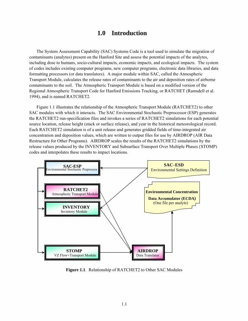
The System Assessment Capability (SAC) Systems Code is a tool used to simulate the migration of contaminants (analytes) present on the Hanford Site and assess the potential impacts of the analytes, including dose to humans, socio-cultural impacts, economic impacts, and ecological impacts. The system of codes includes existing computer programs, new computer programs, electronic data libraries, and data formatting processors (or data translators). A major module within SAC, called the Atmospheric Transport Module, calculates the release rates of contaminants to the air and deposition rates of airborne contaminants to the soil. The Atmospheric Transport Module is based on a modified version of the Regional Atmospheric Transport Code for Hanford Emissions Tracking, or RATCHET (Ramsdell et al. 1994), and is named RATCHET2.

Figure 1.1 illustrates the relationship of the Atmospheric Transport Module (RATCHET2) to other SAC modules with which it interacts. The SAC Environmental Stochastic Preprocessor (ESP) generates the RATCHET2 run-specification files and invokes a series of RATCHET2 simulations for each potential source location, release height (stack or surface release), and year in the historical meteorological record. Each RATCHET2 simulation is of a unit release and generates gridded fields of time-integrated air concentration and deposition values, which are written to output files for use by AIRDROP (AIR Data Restructure for Other Programs). AIRDROP scales the results of the RATCHET2 simulations by the release values produced by the INVENTORY and Subsurface Transport Over Multiple Phases (STOMP) codes and interpolates these results to impact locations.

Figure 1.1. Relationship of RATCHET2 to Other SAC Modules

INVENTORY Inventory Module

STOMP VZ Flow+Transport Module

SAC - ESP Environmental Stochastic Preprocess

SAC- ESD Environmental Settings Definition

Environmental Concentration

Data Accumulator (ECDA)(One file per analyte)

RATCHET2Atmospheric Transport Module

AIRDROPData Translator

1.2

1.1 Relationship to Other Atmospheric Dispersion Models

RATCHET2 is a Lagrangian trajectory, Gaussian-puff atmospheric dispersion model that includes deposition and depletion. Gaussian models are used to describe the atmospheric dispersion of radioactive and chemical effluents from nuclear facilities. These models have frequently been used in licensing and emergency response calculations (e.g., PAVAN [Bander 1982], XOQDOQ [Sagendorf et al. 1982], MESORAD [Scherpelz et al. 1986; Ramsdell et al. 1988], and RASCAL Version 2.0 [Athey et al. 1993; McGuire et al. 2003]) because they quickly provide reasonable estimates of atmospheric concentrations, deposition, and doses given relatively limited information on topography and meteorology. A Lagrangian trajectory, Gaussian puff model is used where temporal or spatial variations in meteorological conditions or depletion of the plume due to dry deposition may be significant.

The RATCHET2 code was originally developed for the Hanford Environmental Dose Reconstruction (HEDR) Project. For HEDR, it used hourly meteorological and iodine-131 release data to estimate daily exposures (time-integrated concentrations) and surface contamination over an area of approximately 195,000 km2 (75,000 mi2) in eastern Washington, eastern Oregon, and northern Idaho. For SAC, RATCHET2 has been modified to estimate normalized annual exposures and surface contamination over an area of approximately 9,100 km2 (3,500 mi2) that includes the Hanford Site and adjacent land. Meteorological data for the SAC calculations consist of hourly observations made at 28 stations from 1983 through 2002. These data, which include wind direction and speed, temperature, precipitation, and an indicator of atmospheric stability, are used to derive the spatially and temporally varying meteoro-logical fields needed by RATCHET2. Ground-level and elevated release points can be placed at appro-priate locations on the Hanford Site, and exposures and surface contamination are estimated at more than 2,100 locations on a 41 x 53 node Cartesian grid that has 2-km (1.2-mi) spacing.

1.2 Quality Assurance

The original RATCHET codes, on which the RATCHET2 code is based, were developed in accor-dance with the requirements of ANSI/ASME NQA-1, 1989 edition (ASME 1989), Quality Assurance Program Requirements for Nuclear Facilities, as interpreted by the Battelle Quality Assurance Program. The following steps were taken to ensure quality.

• An external workshop/peer review established the appropriate phenomena and suggested mathematical equations for use in RATCHET (Ramsdell 1992).

• The RATCHET codes were subjected to an extensive external peer review process.1 Peer reviewers included internationally recognized atmospheric scientists.

• The RATCHET codes have had extensive testing, and the results have undergone independent review.

• The RATCHET codes were placed under configuration control.

1Letter (HEDR Project Office Document No. 09930289), “Review of the Regional Atmospheric Transport Code for Hanford Emission Tracking (RATCHET),” from JE Till (TSP) to DB Shipler (BNW), July 12, 1993.

1.3

• RATCHET2 was placed under SAC configuration control when transferred to the Hanford Remediation Assessment Project.

The objective in the development of RATCHET was to address atmospheric phenomena that are included in nationally accepted applied dispersion models to the extent that available data permit. Experts assisted in identification and evaluation of alternative methods for estimating transport, diffusion, and deposition to ensure completeness, representativeness, and comparability of the models implemented in RATCHET. The results of an independent review of RATCHET conducted for the Centers for Disease Control and Prevention in early 1993 indicate that this objective has been met.

1.3 Manual Organization

The remaining sections of this manual consist of a technical description of the code, a user’s guide, and a programmer’s guide. These sections provide the following functions:

Technical description− illustrates the model domain, discusses the data required by the model, and presents the equations used to make the model calculations.

User’s guide− gives detailed information about the model input and output. It describes the content and format of the run-specification file that is used to provide input to RATCHET2 and contains rationale for the selection of certain model control parameters that are intrinsic to the RATCHET2 code.

Programmer’s guide− provides the programming details of the code. It discusses the hardware and software required to run the code, the program structure, and each of the program elements.

2.1

2.0 Technical Description

The RATCHET2 computer code implements a Lagrangian-trajectory, Gaussian-puff dispersion model. In the model, sequences of Gaussian puffs represent plumes from ground-level and elevated sources. As the puffs move through the model domain, time-integrated air concentrations and surface contamination are calculated at node locations by summing the contributions from puffs moving past the nodes. Transport, diffusion, and deposition of material in the puffs are controlled by wind, atmospheric stability, precipitation, and mixing-layer depth fields that describe the spatial and temporal variations of meteorological conditions throughout the domain.

RATCHET2 is diagnostic in the sense that it calculates puff movement and diffusion based on observed meteorological data. The model does not have the capability to predict changes in meteorological conditions.

This section describes the technical aspects of the atmospheric dispersion model. It first describes the model domain and coordinate systems followed by descriptions of the topographic and meteorological data used by the model. It then describes the source term, transport, diffusion, deposition, and depletion.

2.1 Model Domain

The atmospheric model domain in RATCHET2 is a rectangular area. It is fixed in space and is referenced to a particular location on the earth’s surface by specifying a latitude and longitude for the center of the domain in the run-specification file. For SAC, these coordinates are 46.3333º N, 119.4167º W, and the domain extends approximately 106 km (65.9 mi) from north-to-south and 82 km (51.0 mi) from east-to-west.

2.1.1 Cartesian Representation

Two collocated Cartesian grid systems describe horizontal positions in the domain. The first grid, called the environmental grid, is used to specify environmental conditions, such as wind direction and wind speed. The second grid, called the concentration grid, is where time-integrated air concentration and surface contamination calculations are performed. Vertical positions in the domain are represented by height above the ground in meters.

The size of the domain is controlled by the number of nodes along the x and y axes and the spacing between nodes in the environmental grid. The concentration grid system overlies the environmental grid but has spacing between nodes that is half that of the environmental grid. Thus, a coordinate, N, in the environmental grid system has a corresponding coordinate, n, in the concentration grid system. The transformation between the coordinates is n=2N-1.

Figure 2.1 illustrates how the two grid systems are used in RATCHET2. Hourly meteorological records are used to estimate the wind, stability, and precipitation at nodes on the environmental grid. These gridded values are used in the calculation of transport, diffusion, and deposition of material. As the puffs move through the model domain, the time-integrated air concentrations are calculated at nodes of

2.2

Figure 2.1. The SAC Environmental Grid (red dots) and Concentration Grid (cross marks). The Hanford facility boundary is shaded in gray. Note that the environmental and concentration grids are co-located, with the concentration grid having twice the resolution.

2.3

the concentration grid. Finally, at the end of each simulated period (normally a year), the time-integrated air concentration and surface contamination grid data are written to files for use in subsequent calcula-tions by other SAC components.

The number of nodes along each axis is specified in PARAMETER statements in the RATCHET2 code. The parameters IMaxWG and JMaxWG set the number of nodes in the environmental grid; the parameters IMaxCG and JMaxCG set the number of nodes in the concentration grid. For a given grid, the number of nodes in the north-south and east-west directions do not have to be the same. However, the node spacing is the same and it is set via the run-specification file and applies to the environmental grid. The environmental grid for SAC has 21 nodes along the x axis, 27 nodes along the y axis (set via a PARAMETER statement), and a node spacing of 4 km (2.5 mi) (set in the run-specification file). Therefore, given the coordinate transformation above, the concentration grid has 41 nodes along the x axis, 53 nodes along the y axis, and a node spacing of 2 km (1.2 mi). The coordinates of the reference point are also set in PARAMETER statements within the code. The coordinates of the reference point in the environmental grid system are XRefl,YRefl, and in the concentration grid system are IRef2,JRef2. The center of the model domain is used as the reference point for SAC.

2.1.2 Coordinate Transformations

To facilitate association of geographic positions with model coordinates, the earth is assumed to be spherical, and a line passing through the domain reference point, parallel to the y axis, is assumed to run north and south. With these assumptions, the standard spherical-to-Cartesian coordinate transformation can be used for converting between latitude and longitude and grid coordinates.

Expressed in finite difference form, the transformation is

λΔϕ=Δ )cos(rx e (2.1)

and

ϕΔ=Δ ery (2.2)

where Δx = east-west component of the distance between two points (km) Δy = north-south component of the distance between two points (km) re = radius of the earth (≈6370 km; ≈3960 mi) φ = latitude (degrees) Δλ = difference in longitude between two points (radians) Δφ = difference in latitude between two points (radians).

Note that Δx is a function of latitude. The latitude of the center of the domain can be used to determine Δx for the entire domain. Although this assumption is probably adequate, a more accurate transformation was used in which all positions are referenced to the center of the grid.

2.4

Given the position of the center of the grid (x0,y0), and any other point (xl,yl) with latitude φ1 and longitude λl, then the x component of distance to the point is

))(cos(r)xx(x 101e011 λ−λϕ=−=Δ (2.3)

The order of the longitudes has been reversed from the usual sense so a positive Δx indicates points that are east of the center of the domain.

The center of the SAC grid (in decimal degrees) is 46.3333º N, 119.4167º W. The nodes on the RATCHET2 output grids are 2 km (1.2 mi) apart, and node 21,27 is the center of the SAC concentration grid. With this information and Equations 2.2 and 2.3, the Cartesian coordinates (I,J) on the concentration grid of a position originally given in latitude and longitude are

0.2/x21I Δ+= (2.4)

and

0.2/y27J Δ+= (2.5)

Similarly, the latitude, φn, and longitude, λn, of any node N(I,J) in the domain can be determined by

)27J(01799.03333.46n −+=ϕ (2.6)

and

)cos(/)I21(01799.04167.119 nn ϕ−+=λ (2.7)

where φn = latitude λn = longitude 0.01799 = number of degrees of latitude between nodes

Meteorological station locations are entered in latitude and longitude locations in the meteorological station file. Release points are entered using environmental grid coordinates in the run-specification file, with the position 1,1 representing the southwest corner of the model domain.

The vertical extent of the model domain is unspecified. However, the atmosphere has been divided into two regions. The atmospheric boundary layer is the lower region. Its thickness is equal to the depth of the mixing layer, which varies as a function of time and location. The other region is above the mixing layer. Its depth is undefined. Within the mixing layer, the wind speed and diffusion are functions of height above ground, surface roughness, and atmospheric stability. Above the mixing layer, wind speed and diffusion are independent of height.

2.2 Topography

Differences in terrain elevation are not treated explicitly in RATCHET2. Instead, terrain effects on transport and diffusion are handled implicitly through the use of observed wind data for multiple station locations. Figure 2.2 is a sample annual (2003) wind rose plot for meteorological stations located

2.5

throughout the Hanford Site. The effects of major topographic features in the model domain are reflected in the wind variability that exists from station to station, as is evidenced by the differences in the wind rose plots.

Figure 2.2. Wind Rose Plots 30 Feet Above Ground Level for the Year 2003 at the Hanford Meteorological Observation Stations (adapted from Hoitink et al. 2003)

2.6

2.2.1 Surface Roughness

The RATCHET2 Cartesian environmental grid is too coarse to attempt to explicitly model the effects of small-scale topographic features on puff movement. The effects of small-scale features could not be represented accurately even if the resolution were finer because the existing meteorological data are inadequate to define these effects. RATCHET2 does use estimates of surface roughness (z0), which is associated with small-scale topographic features, in modeling various aspects of the atmosphere that are directly related to transport and diffusion. These aspects include atmospheric stability, wind profiles, diffusion coefficients, and the mixing-layer depth.

A surface roughness length estimate (in meters) must be entered for each node on the environmental grid. The surface roughness length is a characteristic length associated with surface roughness elements. It arises as a constant of integration in derivation of the wind profile equations and is used in several other boundary-layer relationships. Texts on atmospheric diffusion and air pollution and boundary-layer meteorology (Panofsky and Dutton 1984; Stull 1988) contain tables that give approximate relationships between z0 and land use, vegetation type, and topographic roughness. Table 2.1 gives typical roughness length ranges based on data in Stull 1988 (Figure 9.6).

Table 2.1. Typical Surface Roughness Lengths (Stull 1988, Figure 9.6)

Land Use/Characteristics z0 (m)

Level grass plains 0.007 – 0.02Farmland 0.02 – 0.1 Uncut grass, airport runways 0.02 Many trees/hedges, a few buildings 0.1 – 0.5 Average North America 0.15 Average U.S. plains 0.5 Dense forest 0.2 – 0.6 Small towns/cities without tall buildings 0.6 – 2.5 Very hilly/mountainous regions 1.5+

Data on land use, vegetation types, and topographic roughness are readily available for the SAC model domain. The roughness length near the 200 Areas at the Hanford Site has been determined to be in the 0.03- to 0.05-m range (Horst and Elderkin 1970; Powell 1974). Based on these results, and the previous work from HEDR, a surface roughness length file has been prepared for the SAC model domain. The details of this file are discussed in Section 3.3.1.

2.3 Meteorology

Atmospheric transport, diffusion, and deposition calculations in RATCHET2 are based on observed meteorological data. This section discusses the input data required by the model, adjustments to the data, and calculation of meteorological variables that are not directly measured.

2.7

2.3.1 Meteorological Stations

RATCHET2 calculations require hourly meteorological data for one or more observation locations. The maximum number of stations for which data can be entered is established in a parameter file (parm.inc) within the RATCHET2 code. For the purposes of SAC, 28 observation stations are available in and near the atmospheric model domain.

A station file is used to specify information about each of the 28 station locations. Specifically, the station file contains the

• station name • station location (latitude and longitude) • wind instrument height • surface roughness length • wind direction reporting convention • wind speed reporting units • station status.

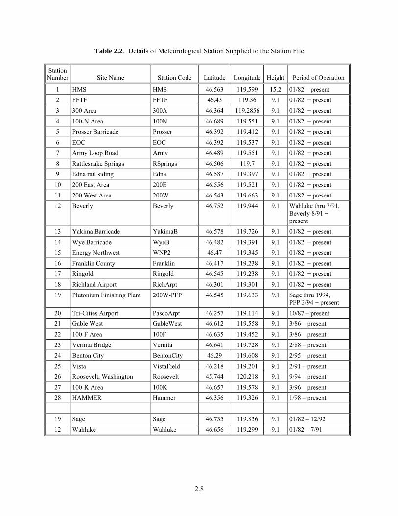
Table 2.2 provides a list of stations that are used in SAC for the 1983-2002 modeling period. The information in this table is used to construct the station files, the format of which is detailed in Section 3.3.3. Figure 2.3 is a plot showing the location of the meteorological observation stations. The shaded region is the boundary of the SAC model domain. Note that meteorological stations that are outside of the domain are used to extrapolate data to the domain.

In general, information about meteorological stations does not change during a model run. However, over the course of the SAC study period, some station locations did change (see stations 12 and 19 in Table 2.2). To ensure accurate station information, a separate station file is prepared and used for each simulation year.

2.3.2 Meteorological Data Input

RATCHET2 requires the following meteorological data:

• wind direction and speed at release height • ambient temperature at release height • precipitation type (i.e., none, liquid, or frozen).

These data are for the first station listed in the station file, which is the Hanford Meteorology Station (HMS) for SAC. In addition, for each subsequent station listed in the station file, surface values of the following parameters must be specified:

• wind direction and speed • atmospheric stability class • temperature • precipitation rate.

2.8

Table 2.2. Details of Meteorological Station Supplied to the Station File

Station Number Site Name Station Code Latitude Longitude Height Period of Operation

1 HMS HMS 46.563 119.599 15.2 01/82 – present 2 FFTF FFTF 46.43 119.36 9.1 01/82 − present 3 300 Area 300A 46.364 119.2856 9.1 01/82 − present 4 100-N Area 100N 46.689 119.551 9.1 01/82 − present 5 Prosser Barricade Prosser 46.392 119.412 9.1 01/82 − present 6 EOC EOC 46.392 119.537 9.1 01/82 − present 7 Army Loop Road Army 46.489 119.551 9.1 01/82 − present 8 Rattlesnake Springs RSprings 46.506 119.7 9.1 01/82 − present 9 Edna rail siding Edna 46.587 119.397 9.1 01/82 − present

10 200 East Area 200E 46.556 119.521 9.1 01/82 − present 11 200 West Area 200W 46.543 119.663 9.1 01/82 − present 12 Beverly Beverly 46.752 119.944 9.1 Wahluke thru 7/91,

Beverly 8/91 − present

13 Yakima Barricade YakimaB 46.578 119.726 9.1 01/82 − present 14 Wye Barricade WyeB 46.482 119.391 9.1 01/82 − present 15 Energy Northwest WNP2 46.47 119.345 9.1 01/82 − present 16 Franklin County Franklin 46.417 119.238 9.1 01/82 − present 17 Ringold Ringold 46.545 119.238 9.1 01/82 − present 18 Richland Airport RichArpt 46.301 119.301 9.1 01/82 − present 19 Plutonium Finishing Plant 200W-PFP 46.545 119.633 9.1 Sage thru 1994,

PFP 3/94 − present 20 Tri-Cities Airport PascoArpt 46.257 119.114 9.1 10/87 – present 21 Gable West GableWest 46.612 119.558 9.1 3/86 – present 22 100-F Area 100F 46.635 119.452 9.1 3/86 – present 23 Vernita Bridge Vernita 46.641 119.728 9.1 2/88 – present 24 Benton City BentonCity 46.29 119.608 9.1 2/95 – present 25 Vista VistaField 46.218 119.201 9.1 2/91 – present 26 Roosevelt, Washington Roosevelt 45.744 120.218 9.1 9/94 – present 27 100-K Area 100K 46.657 119.578 9.1 3/96 – present 28 HAMMER Hammer 46.356 119.326 9.1 1/98 – present

19 Sage Sage 46.735 119.836 9.1 01/82 – 12/92 12 Wahluke Wahluke 46.656 119.299 9.1 01/82 – 7/91

2.9

Figure 2.3. Meteorological Station Locations (red dots) used in SAC

All data are hourly values, and each hour’s data is entered as a single record in a meteorological data file. Each record is checked for missing data. When missing data are encountered for a station, the data for that station are not used in the preparation of meteorological data fields.

The parameters listed above are discussed in the following sections. The format of the meteoro-logical data file is described in detail in Section 3.3.4.

2.10

2.3.2.1 Surface Wind

Wind directions and speeds are entered as two-digit integer values. The interpretation of the numerical values for each station is controlled by the codes for wind direction reporting and wind speed units entered for the station in the meteorological station file. RATCHET2 has provisions for entering wind directions in compass points or 10-degree increments. Wind speeds may be entered as m/sec, mph, or knots.

Missing direction data may be indicated by entering a wind direction greater than 16 if directions are in compass points, or 36 if directions are in 10-degree increments. Missing wind speeds are indicated by values greater than 80. Wind speeds should be entered even if the direction is missing because they can be used in calculations of the friction velocity and mixing depth at the station.

2.3.2.2 Atmospheric Stability Class

RATCHET2 requires an estimate of the atmospheric stability class at each meteorological station. The stability class is entered as an integer ranging from 1 for extremely unstable atmospheric conditions to 7 for extremely stable conditions. A stability code less than 1 or greater than 7 is interpreted as missing or erroneous data.

Atmospheric stability is not observed directly. Therefore, a preprocessor program is used to estimate stability classes from meteorological data available in standard meteorological records. The preprocessor program implements a general classification scheme discussed by Pasquill (1961), Gifford (1983), and Turner (1964) for estimating atmospheric stability classes from routine meteorological measurements, including wind speed, time of day, sky cover, and ceiling height. Sky cover and ceiling height data are obtained from the hourly meteorological records.

The specific algorithm used in the preprocessor program to estimate stability class is a modified version of the National Weather Service implementation of Turner's classification scheme. The modified algorithm estimates stability if the time of day (solar altitude) and wind speed are available. Nighttime stability classes range from 6 to 4 as a function of wind speed, assuming a net radiation index of -1 in Table A-1 of Turner (1964). Daytime stability classes are determined as a function of wind speed using the unmodified insolation class number from Turner (1964, Table A-2) as the net radiation index. Additional information on sky cover, ceiling, and precipitation, as available, is used to refine stability class estimates following the complete procedure described in Turner (1964).

2.3.2.3 Current Weather

The RATCHET2 meteorological data record includes a code for the current weather at each meteorological station. These codes determine the precipitation type and rate used in wet deposition calculations.

The current weather code ranges from 0 to 6. A zero is used when there is no precipitation. Codes 1, 2, and 3 indicate light, moderate, and heavy liquid precipitation, respectively. Liquid precipitation includes rain, drizzle, freezing rain, and freezing drizzle. All drizzle intensities are coded as 1. Codes 4, 5, and 6 indicate light, moderate, and heavy frozen precipitation, respectively. Frozen precipitation includes snow, snow grains, snow pellets, ice pellets, ice crystals, and hail.

2.11

2.3.2.4 Release Height Wind

RATCHET2 uses the release height wind in plume-rise calculations. If a measurement for release height wind is available, it may be entered using the meteorological data file. Release height wind is entered in the same manner as surface winds. The wind direction convention and wind speed conversion factor specified for the fist meteorological station are assumed to apply to the release height wind.

A release height wind speed greater than 80 indicates that the release height wind is not available. In this case, RATCHET2 uses a diabatic wind profile to estimate the release height wind using the surface wind speed, stability, and surface roughness for the first meteorological station.

2.3.2.5 Temperature

RATCHET2 uses the ambient air temperature at the release height in plume-rise calculations. This temperature, in degrees Fahrenheit, is entered hourly using the meteorological data file. The code does not include a default temperature. Therefore, an ambient air temperature must be supplied in the meteorological data file, even if it is a default value. The effluent temperature, which is also used in plume-rise calculations, is input as a source-term variable in the run-specification file.

In addition to its use in plume-rise calculations, the release height temperature is used to control washout of gases by frozen precipitation. In this application, the release height temperature is assumed to apply over the entire model domain.

2.3.3 Calculated Meteorological Parameters

In addition to the input for meteorological data supplied by the user, RATCHET2 uses several meteorological parameters that are computed hourly from the input data. This section describes the calculated parameters.

2.3.3.1 Monin-Obukhov Length (L)

Atmospheric stability classes are routinely used in dispersion modeling as a basis for choosing among alternative algorithms. However, in atmospheric boundary layer theory, a scaling length for vertical motions called the Monin-Obukhov length (L) is used as the measure of atmospheric stability. This length is needed for wind profile, turbulence, and mixing-layer depth calculations.

The Monin-Obukhov length varies from a small negative value (a few meters) in extremely unstable atmospheric conditions to negative infinity as the atmospheric stability approaches neutral from unstable. In extremely stable conditions, the Monin-Obukhov length is small and positive. As neutral conditions are approached from stable conditions, the Monin-Obukhov length approaches infinity. Thus, there is a discontinuity in the Monin-Obukhov length at neutral. However, this discontinuity is not a problem because the Monin-Obukhov length is found in the denominator of expressions.

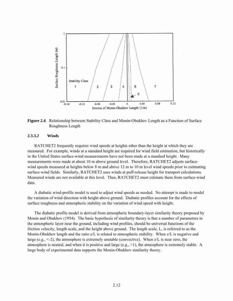
Golder (1972) provides a means for converting from stability-class estimates to Monin-Obukhov lengths. Figure 2.4, derived from Golder (1972, Figure 5), shows ranges for 1/L as a function of Turner stability class and surface roughness length. Mid-range values for 1/L from this figure are used by RATCHET2 when a single estimate of 1/L is needed by the model.

2.12

Figure 2.4. Relationship between Stability Class and Monin-Obukhov Length as a Function of Surface Roughness Length

2.3.3.2 Winds

RATCHET2 frequently requires wind speeds at heights other than the height at which they are measured. For example, winds at a standard height are required for wind field estimation, but historically in the United States surface-wind measurements have not been made at a standard height. Many measurements were made at about 10 m above ground level. Therefore, RATCHET2 adjusts surface-wind speeds measured at heights below 8 m and above 12 m to 10 m level wind speeds prior to estimating surface-wind fields. Similarly, RATCHET2 uses winds at puff-release height for transport calculations. Measured winds are not available at this level. Thus, RATCHET2 must estimate them from surface-wind data.

A diabatic wind-profile model is used to adjust wind speeds as needed. No attempt is made to model the variation of wind direction with height above ground. Diabatic profiles account for the effects of surface roughness and atmospheric stability on the variation of wind speed with height.

The diabatic profile model is derived from atmospheric boundary-layer similarity theory proposed by Monin and Obukhov (1954). The basic hypothesis of similarity theory is that a number of parameters in the atmospheric layer near the ground, including wind profiles, should be universal functions of the friction velocity, length scale, and the height above ground. The length scale, L, is referred to as the Monin-Obukhov length and the ratio z/L is related to atmospheric stability. When z/L is negative and large (e.g., <-2), the atmosphere is extremely unstable (convective). When z/L is near zero, the atmosphere is neutral, and when it is positive and large (e.g., >1), the atmosphere is extremely stable. A large body of experimental data supports the Monin-Obukhov similarity theory.

2.13

The diabatic wind profile is

)]L/z()z/z[ln(ku

)z(U 0* ψ−= (2.8)

where U(z) = wind speed at height z (m/s) u* = friction velocity (boundary-layer turbulence scaling velocity) (m/s) k = von Karman constant, which has a value of about 0.4 (dimensionless) z = wind speed measurement height (m) zo = measure of local surface roughness (roughness length) (m) Ψ = stability correction factor L = Monin-Obukhov length (m).

The term Ψ (z/L) accounts for the effects of stability on the wind profile. In stable atmospheric conditions, Ψ (z/L) has the form –αz/L, where α has a value between 4.7 and 5.2. In neutral conditions it is zero, and the diabatic profile simplifies to a logarithmic profile.

In unstable air, Ψ (z/L) is more complicated. According to Panofsky and Dutton (1984), the most common form of Ψ (z/L) for unstable conditions is based in work by Businger et al. (1971) and Paulson (1970). It is

2/xtan2}]2/)x1][(2/)x1ln{[()L/z( 122 π+−++=ψ − (2.9)

where x = (1-16z/L)1/4. Equation 2.8 is used to estimate the friction velocity (u*) from wind speed, surface roughness, and Monin-Obukhov length. In unstable and neutral conditions, the use of Equation 2.8 is limited to the lowest 100 m of the atmosphere. In stable conditions, the upper limit for application of Equation 2.8 is the smaller of 100 m or three times the Monin-Obukhov length. Skibin and Businger (1985) provide rationale for limiting application of Equation 2.8 to three times the Monin-Obukhov length in stable conditions.

Figure 2.5 shows the variation in wind speed with height between 10 and 100 m. For unstable atmospheric conditions, the wind speed increases slowly with height, while in extremely stable conditions the increase in speed with height is relatively large. The wind speed profile for stability class 7 is only shown to a height of 70 m because that is about the upper limit for application of Equation 2.8.

2.3.3.3 Mixing-Layer Depth

In the layer of the atmosphere next to the earth’s surface, friction caused by surface roughness and heating of the surface combine to generate turbulence that efficiently mixes material released at or near the surface through the layer. This layer is referred to as the mixing layer. The top of the mixing layer is marked by a decrease in turbulence brought about by stable atmospheric conditions above. The depth of the mixing layer, also referred to as the thickness of the mixing layer, changes with atmospheric conditions. The mixing layer is generally thickest during the day and during periods with high wind speeds, and it is thinnest at night during periods with low wind speeds. In either case, the mixing-layer depth tends to increase with increasing surface roughness.

2.14

Figure 2.5. Wind Speed Variations at Heights between 10 and 100 m in the Diabatic Wind Speed Profile Model

RATCHET2 estimates the atmospheric mixing-layer depth hourly at each meteorological station. The estimates are based on a combination of reported meteorological conditions and default values provided by the user. The choice between calculated and default values is made on the basis of the relative magnitudes of the calculated and default values, stability, season, and time of day.

Mixing depths are calculated using relationships derived by Zilitinkevich (1972) for stable and neutral conditions. For stable atmospheric conditions, this relationship is

2/1* )f/Lu(kH = (2.10)

where H = mixing-layer depth (m) k = von Karman constant (dimensionless, ~0.4) u* = friction velocity (m/s) L = Monin-Obukhov length (m) f = Coriolis parameter (s-1).

Pasquill and Smith (1983) indicate that constant values in the range 0.2 to 0.7 have been suggested in place of the von Karman constant in Equation 2.10, and authors referenced by Weil (1985) suggest constant values in the range 0.4 to 0.7. RATCHET2 includes provisions to use either the von Karman constant or a random value selected from a uniform distribution between 0.2 to 0.7.

2.15

For neutral and unstable conditions, the mixing-layer depth is estimated using

f/uH *β= (2.11)

where H = mixing-layer depth (m) β = constant (dimensionless) u* = friction velocity (m/s) f = Coriolis parameter (s-1).

Zilitinkevich (1972) assumes that β is equal to k; Pasquill and Smith (1983) suggest β has a value in the range 0.2 to 0.3; and Panofsky and Dutton (1984) suggest its range is 0.15 to 0.25. In RATCHET2, β is assigned a value of 0.2.

In addition to computing the mixing-layer depth, RATCHET2 obtains a default mixing-layer depth from a file supplied by the user. The default mixing-layer depth file is described in Section 3.3.2. It contains an array that has three dimensions with indices based on time of day, atmospheric stability class, and month. In the default mixing-height file used for SAC, the day is divided into eight 3-hour incre-ments and the stability class index ranges from one to five (the two most unstable and the two most stable classes are combined). The data in the file are based on the hourly mixing heights estimated by the Hanford forecasters in the 5-year period from 1983 through 1987.

After a mixing-layer depth has been calculated and a default value has been obtained, the calculated and default values are compared. The larger of the two values is selected as the mixing-layer depth for the station for the hour. Ultimately, the mixing-layer height is constrained to be within the range of 10 to 2,000 m.

One additional option has been retained in RATCHET2. That option permits users to bypass the calculated and default mixing-layer depth and use a constant depth. This option is particularly useful when testing the code.

2.3.4 Spatial Representation of Meteorological Conditions

The RATCHET2 code accounts for spatial and temporal variations in atmospheric conditions between the time material is released to the atmosphere and the time it leaves the model domain. The spatial variations in the atmosphere are modeled by interpolating/extrapolating data collected at meteorological stations to nodes on the environmental Cartesian grid. The following paragraphs describe the interpolation/extrapolation methods.

2.3.4.1 Wind

Wind fields used to estimate Lagrangian trajectories for puffs are based on hourly wind speed and direction data reported for meteorological stations in and near the model domain. The wind fields are estimated by weighted averages of the reported data. Weights used are inversely proportional to the square of the distance between the station and the node. This weighting is common in spatial interpolation of wind fields (Hanna et al. 1982).

2.16

The wind fields are computed for a standard reference height of 10 m. However, puff advection is based on the winds at the effective release height. This wind is estimated by first computing the 10-m speed beneath the puff center, then adjusting the wind speed using the diabatic wind profile model. The wind direction is not adjusted.

Ramsdell and Skyllingstad (1993) provide a detailed description and discussion of the alternatives for treating winds. Experimental evidence discussed in that report indicates that neither adjusting the wind fields to obtain mass consistency nor estimating upper-level winds from surface data would improve the ability of RATCHET2 to estimate the transport of radionuclides released to the atmosphere from Hanford operations.

2.3.4.2 Stability and Precipitation

The stability and precipitation fields are created by identifying the meteorological station with valid data closest to each node. The reported stability class and precipitation class for the station are then assigned to the node. This procedure avoids averaging that would minimize the effects of extreme stability or instability. It also permits maximum detail in treating isolated precipitation events.

2.3.4.3 Mixing-Layer Depth

The mixing-layer depth grid is created by first taking the meteorological station closest to a given node and assigning that node with the stations’ calculated or default mixing-layer depth. The final mixing-layer depth grid is then smoothed, such that neighboring mixing heights within a box defined by a two-node radius about a given node are summed and averaged to produce the final mixing-layer depth at that node. This process provides a spatially smooth variation of mixing-layer depth across the model domain.

2.4 Source Term

RATCHET2 allows for the input of a single point source with a unit emission rate. The release point must be described by a grid point location (referenced by the environmental grid), stack release height, stack-exit radius, nominal stack flow, and nominal effluent temperature. The point source information is entered in the run-specification file (see Section 3.1).

2.4.1 Release Times and Rates

In RATCHET2, the point source that is specified in the run-specification file has a constant, unit emission rate for the duration of the release. The unit emission rate is set within the RATCHET2 code.

2.4.2 Plume Rise and Effective Release Height

When appropriate, plume rise is computed. Although several methods exist for estimating plume rise, the equations proposed by Briggs (1969, 1975, 1984) have gained a general acceptance unequaled by the other methods. The equations that follow in this section are from the INPUFF model (Petersen and Lavdas 1986). They are implementations of Briggs’ equations. Unless otherwise noted, the numerical constants in the equations are dimensionless.

2.17

Plume rise is caused by two factors: vertical momentum of the exhaust gases in a stack and buoyancy due to the density difference between the stack gases and the atmosphere. In general, one factor or the other will be dominant and the other will not contribute significantly to plume rise. RATCHET2 includes equations for both momentum- and buoyancy-dominated plume rise. For a given set of stack and atmospheric conditions, the temperature difference between the stack effluent and the air determines which of the factors is dominant. A critical temperature difference that separates the two regimes can be determined from the plume-rise equations. When the actual temperature difference (stack effluent temperature minus air temperature) is less than the critical temperature, momentum is the dominant factor in determining plume rise. Otherwise, plume rise is due primarily to buoyancy forces.

All plume-rise calculations in RATCHET2 estimate the final height of the plume. In all cases, rise is corrected for stack downwash if the stack-exit velocity is less than 1.5 times the wind speed at the release height. The downwash correction is

]5.1)h(U/w[r4h spsd −=Δ (2.12)

where Δhd = downwash correction (m) rs = inside stack radius (m) wp = stack exit vertical velocity (m/s) U(hs) = wind speed at stack height (m/s).

A minimum stack height wind speed of 1.37 m/sec is assumed when the wind is near calm (<1.37 m/sec).

If the release height is greater than the mixing-layer height, the atmospheric stability is assumed to be extremely stable (class 7) for plume-rise calculations. Otherwise, the stability class used in plume-rise calculations is the stability-class estimate for the closest meteorological station.

2.4.2.1 Unstable and Neutral Conditions

In unstable and neutral atmospheric conditions, plume rise is dominated by momentum as long as the temperature difference between the plume and the air is less than a critical temperature difference. The critical temperature difference is calculated using

3/2sp

3/1pc )r2(Tw0297.0t −=Δ (2.13)

where Δtc = critical temperature difference (°K) wp = stack exit vertical velocity (m/s) Tp = initial plume temperature (°K) rs = inside stack radius (m).

Note that 0.0297 is a dimensional constant, which arises from the combination of constants (and near constants) when Equations 2.14, 2.15, 2.16, and 2.17 are solved for Δtc. The specific value of the constant depends on the units used for variables in the equations. Assuming the use of metric units, the dimensions of the constant are (m-s)-1/3.

2.18

When Tp -Ta is less than Δtc, plume rise is estimated using

dsps h)]h(U/w[r6h Δ+=Δ (2.14)

where Δh is the final plume rise in meters and the other symbols remain as previously defined.

If Tp -Ta is greater than Δtc, the plume rise is estimated using the equation for buoyancy- dominated rise. This equation is

d1

s3/2

f3/1

b h)h(UxF6.1h Δ+=Δ − (2.15)

where Fb is a buoyancy flux parameter, xf is the distance to final plume rise (m), and the other symbols remain as previously defined. The buoyancy flux parameter, Fb, is defined by

2sppapb rw]T/)TT[(gF −= (2.16)

where Fb = buoyancy flux parameter (m4/s3) g = gravitational acceleration (9.8 m/s2) Tp = initial plume temperature (°K) Ta = air temperature at release height (°K) wp = stack exit vertical velocity (m/s) rs = inside stack radius (m).

According to Peterson and Lavdas (1986), the distance to final plume rise, xf, for relatively low-temperature emissions, such as those from the fuel-processing plants at the Hanford Site, is given by

8/5bf F49x = (2.17)

The leading constant (49) in this equation has dimensions of s15/8/m3/2.

2.4.2.2 Stable Conditions

In stable atmospheric conditions, the critical temperature difference at which buoyancy-dominated plume rise exceeds momentum-dominated plume rise is

2/1apc STw0196.0t =Δ (2.18)

where S is a stability parameter. The dimensions of the constant in this equation are m/s2.

The parameter S is computed from the stability class and air temperature from

z

TgS 1a ∂

θ∂= − (2.19)

where δθ/δz is the potential temperature lapse rate. Potential temperature lapse rates of 0.02°K/m, 0.035°K/m, and 0.05°K/m are assumed for stability classes 5, 6, and 7, respectively.

2.19

When Tp -Ta is less than Δtc, momentum-dominated plume rise is estimated using Equation 2.14. It is also estimated using

d3/1

psap06/1 h)]T)h(U/()TwF[(S5.1h Δ+π=Δ − (2.20)

where F0 is the stack flow in m3/s. The final estimate for plume rise is the smaller of these two values.

When Tp -Ta is greater than Δtc, one of two equations is used to estimate plume rise. If the wind speed is greater than a critical wind speed, Uc, defined by

8/14/1bc SF275.0U = (2.21)

then the plume rise is calculated using

d3/1

s3/1

b h)]h(US[F6.2h Δ+=Δ − (2.22)

If the wind speed is less than Uc during stable conditions, the plume rise is computed using

d8/34/1

b hSF4h Δ+=Δ − (2.23)

2.4.2.3 Effective Release Height

The effective release height used for puff transport is the sum of the actual stack height and the plume rise. This height is computed in subroutine PUFFR at the time each puff is released.

2.5 Transport

There are two fundamental assumptions in all puff models. The first is that plumes can be represented by a sequence of puffs, and the second is that puff movement may be separated from puff diffusion. This section discusses how RATCHET2 moves puffs. The following sections discuss the calculation of diffusion and deposition.

Energy spectra computed from Eulerian wind turbulence data described by Panofsky and Dutton (1984) indicate that there is a local maximum in the energy associated with eddies with periods on the order of a few (~10 to 20) minutes. The spectra also indicate a minimum associated with eddies with periods on the order of an hour. Thus, there tends to be a natural division of eddy sizes in the atmosphere that roughly coincides with the observation frequency for meteorological data.

Large eddies associated with the weather systems and the diurnal variations of meteorological condi-tions are characterized in the hourly meteorological data. These eddies, which are treated in atmospheric transport, are large compared to the crosswind or vertical dimensions of puffs. They tend to move puffs from place to place rather than changing their size or shape.

Hourly wind fields, based on the observed winds, are used to compute puff movement in RATCHET2. However, the number of time steps used in computing puff movement is equal to the number of puffs released per hour (NPH) and is set within the SPECIN code module within RATCHET2.

2.20

The time step used in puff movement is then 1/NPH. This interval is referred to as the puff advection period. An even shorter interval, called the sampling period, is used in computing time-integrated concentrations and surface contamination. In SAC, NPH = 4. The rationale behind this choice is discussed in Section 3.2.1.

Puff movement is computed in a five-step process. In sequence, the steps in the process are:

1. estimate the wind at puff transport height at the current puff position

2. make an initial estimate of puff position at the end of the advection period using the transport-height wind for the current puff position

3. estimate the transport-height wind at this initial estimate of the puff’s position at the end of the advection period

4. using the winds estimated in step one and the puff’s current position, make a second estimate of the puff’s position at the end of the advection period

5. average the positions estimated in steps two and four.

This average position will be the position of the puff at the end of the advection period. These steps are described mathematically below.

The puff movement calculation begins by calculating the wind at the puff’s current position. Bilinear interpolation is used to calculate the wind vector components at a height of 10 m directly beneath the center of the puff from the wind vector components at the closest nodes of the environmental grid. Bilinear interpolation, which is described by Press et al. (1989), results in wind vectors that vary continuously throughout the model domain.

When the 10-m wind vector components beneath the puff center have been determined, the diabatic profile is used to adjust the wind speed to puff-transport height, if necessary. In general, the transport height for puffs will be their effective release height. The distance moved will be calculated using wind speed for the effective release height of puffs, when the effective release height is ≥10 m and ≤100 m. The 10-m wind speed will be used in computing movement for puffs with release heights <10 m, and the wind speed at 100 m will be used to compute movement of puffs with effective release heights >100 m. Extrapolation of wind speeds from a height of 10 m to heights in excess of 100 m is not considered appropriate. The 10-m wind direction will be used in puff movement calculations.

Next, an initial estimate of the movement is made using the components of the transport vector at the puff’s starting position. For a puff initially at x,y,z, the change in position is given by

t)z,y,x(vyt)z,y,x(ux

Δ=ΔΔ=Δ

(2.24)

2.21

where u and v are the east-west and north-south components of the wind vector, respectively, and Δt is the advection period (60 min/NPH). The initial estimate of the puff’s position at the end of the advection period is

yy'yxx'x

Δ+=Δ+=

(2.25)

The transport winds at this location at the current time are then determined following the same procedure used to obtain the initial transport wind estimates. Bilinear interpolation is used to estimate the 10-m wind components at x', y', and the diabatic profile is used to adjust the wind speed to the transport height.

The second set of estimates of the transport wind components is used to obtain a second estimate of the puff movement

t)z,'y,'x(v'yt)z,'y,'x(u'x

Δ=ΔΔ=Δ

(2.26)

Finally, the puff’s position at the end of the advection period x", y" is determined from the current position and the average of the two movement estimates

2/)'yy(y''y2/)'xx(x''x

Δ+Δ+=Δ+Δ+=

(2.27)

Material in a puff continues to contribute to the time-integrated air concentrations and surface contamination at grid nodes near the edge of the model domain for a period of time after the center of the puff leaves the interior of the domain. During this period, puff movement is determined by the winds at the nearest nodes of the environmental grid. Movement is based on linear interpolation between the winds at the closest two nodes when the puff is off one of the sides of the domain, and the wind at the corner node is used when the puff is off a corner.

Movement of puffs occurs in subroutine DIFDEP and takes place in one or more steps. The number of steps is controlled by the size of the puff and the transport speed to ensure an acceptable level of precision in the calculation of time-integrated concentrations and surface contamination. The maximum number of steps that the model will take during an advection period is controlled by a parameter called IOPDTA, which is in the code module SPECIN. Model sensitivity to this parameter is discussed in Section 3.2.2.

2.6 Diffusion

Once material is released to the atmosphere, it acts as a passive tracer. Large-scale motions move plumes about, and small-scale atmospheric motions distribute material within plumes. The preceding discussion of transport described how RATCHET2 accounts for the effects of large-scale motions. This section describes how RATCHET2 accounts for the effects of the small-scale motions. Section 2.7 describes the deposition of material on surfaces and depletion of the puffs to account for material lost due to deposition.

2.22

2.6.1 Calculation of Time-Integrated Air Concentrations

The second basic assumption in puff models is that a continuous plume can be approximated by a finite number of puffs released in succession. The concentration at a receptor is assumed to be equal to the sum of the concentrations from all of the puffs, that is

∑=

χ=χN

1ii )t,z,y,x()t,z,y,x( (2.28)

where χ = concentration x,y,z = position of the receptor in Cartesian coordinates t = time of the concentration estimate i = puff number N = total number of puffs in the model domain.

In practice, computational rules based on puff dimensions have been established to limit the number of terms included in the summation. These rules include assigning a finite radius to each puff and combining puffs that overlap. The rules and RATCHET2 sensitivity to the rules are discussed in Section 3.2.

In the absence of external influences such as the ground, the concentration distribution in each of the puffs in RATCHET2 is assumed to be Gaussian. Diffusion in the direction of the wind and cross-wind diffusion are assumed to be equal; that is, horizontal cross sections through puffs are circular. A corollary of this assumption is that concentrations in a horizontal plane decrease as a function of increasing distance from the puff center and are independent of the direction in which the distance is increased. It is, therefore, possible to revise the definition of the coordinate system without changing the relationship in Equation 2.28. The x axis of the coordinate system now may be assumed to point toward the east, with the y axis pointing north and the vertical axis pointing upward.

Because the concentration in puffs is horizontally symmetrical, it is only necessary to know the height of the center of a puff and the distance between the center of a puff and a node to compute the puff’s contribution to the concentration at the node. Therefore, the concentration distribution in puffs is defined in terms of the radial distance, r, from the puff center rather than x and y. With these assumptions, the concentration at x,y,z at time t due to puff i is given by

])2/[()z(G)r(F)t(Q)t,z,r( z2r

2/3i σσπ=χ (2.29)

where Q(t) = mass of material (radionuclide) in the puff at time t F(r) = exponential function that describes the horizontal concentration distribution G(z) = set of terms describing the vertical concentration distribution σr = diffusion coefficient that describes the spread of the puff in the horizontal σz = diffusion coefficient that describes the spread of the puff in the vertical

2.23

F(r) is defined by

)]2/(rexp[)r(F 2r

2 σ−= (2.30)

where r2 = (x-x0)2 + (y-y0)2, with x,y representing the position of the node and x0,y0 representing the horizontal position of the puff center. The diffusion coefficient σr is assumed to be the same as the crosswind diffusion coefficient σy used in Gaussian plume models.

Definition of G(z) requires further description of the modeling assumptions. The height of the puff center above ground, which is assumed to be constant, is referred to as the effective release height. If the release is from a stack or elevated vent, the effective release height is the actual stack or vent height plus plume rise.

The ground and the top of the mixing layer are assumed to be totally reflecting surfaces for material within the mixing layer. The top of the mixing layer is not a reflecting surface for material above the mixing layer. Consequently, the top of the mixing layer is similar to a semipermeable membrane.

G(z) describes both the vertical diffusion of material and the effects of the reflection. It is an infinite sum that involves superposition of contributions from virtual sources located below the ground and above the top of the mixing layer. This approach follows from the discussion in Csanady (1973) and is described in detail in Ramsdell et al. (1983). When receptors are at ground level, as they are in RATCHET2, G(z) is given by

∑∞

−∞=

σ−−=n

2z

2e ]/)hnH2(5.0exp[2)z(G (2.31)

where H is the mixing-layer depth and he is the effective release height.

The infinite sum of exponential terms rapidly converges to a limit. Only the terms with n = -1, 0, and 1 are used in RATCHET2. When the vertical diffusion coefficient becomes sufficiently large (σz ≈ H or σz ≈ 0.8 he, whichever is larger), material may be assumed to be uniformly distributed in the vertical. In this case, G(z) is given by

G(z) = Hhifh2/)2(

HhifH2/)2(

eez2/1

ez2/1

>σπ

≤σπ (2.32)

and the concentration in the puff is given by

]H2/[)r(F)t(Q)t,z,r( 2ri πσ=χ (2.33)

or

]h2/[)r(F)t(Q)t,z,r( e2ri πσ=χ (2.34)

Equation 2.33 is used when the effective release height is within the mixing layer, and Equation 2.34 is used when the release height is above the mixing layer.

2.24

Dose calculations in subsequent codes in SAC require two products from RATCHET2. These products are time-integrated air concentration, which is occasionally referred to as exposure, and surface contamination. Both products are output for the period specified in the run-specification file, which for SAC is normally one year. Time-integrated air concentrations, which have units of Ci-s/m3, and the surface contamination, which has units of Ci/m2, are computed at each node on the concentration grid covering the model domain. The spacing between nodes in this grid is half the spacing of the environ-mental grid node spacing set in the run-specification file. SAC uses an environmental-grid spacing of 4 km (2.5 mi); therefore, the concentration-grid node spacing is 2 km (1.2 mi).

Time-integrated air concentrations are computed from puff concentrations using the approximation

∑∑δ

= =

δχ=t/T

1j

N

1iij

j

t)r()m,1(TIC (2.35)

where TIC(l,m) = time-integrated concentration at node 1,m (Ci-s/m3) j = model interval within T T = total time period being modeled (s) δt = duration of the time interval (60 min/NPH or less, expressed in seconds) i = puff number Nj = number of puffs at time interval j χij = concentration at 1,m due to puff i at time interval j r = distance between 1,m and the center of puff i.

The accuracy of this approximation depends upon the ratio of puff dimensions to the distance moved by the puff during the time step. Decreasing the length of the time step used in the calculation increases the accuracy of the approximation. However, it also increases computational time. Figure 2.6 shows the range of potential errors in time-integrated concentrations for an isolated plume as a function of the ratio between distance moved and σr. When the distance moved is less than 2σr, the maximum error in time-integrated concentrations and average deposition rates is less than 10 percent. The dashed lines show that the ratio between distance moved and σr could be relaxed to almost four before the range of potential errors in the integrated values would increase to plus or minus a factor of two. Section 3.2.2 discusses the sensitivity of RATCHET2 output to changes in the size of the minimum time step.

2.6.2 Estimation of Diffusion Coefficients

Numerous methods for estimating diffusion coefficients are described in the literature. They have been compared and evaluated by several researchers (Gifford 1976; Hanna et al. 1977; Randerson 1979; Irwin 1983; Weil 1985; Gryning et al. 1987). The general consensus is that diffusion coefficients should be estimated directly from statistics for atmospheric turbulence. Measured turbulence statistics are not available for use in the SAC study. However, turbulence statistics may be estimated from atmospheric conditions, such as wind speed, atmospheric stability, and surface roughness. The estimation of turbulence statistics is discussed in Section 2.6.3.

2.25

Figure 2.6. Error Band for the Numerical Procedure Used to Estimate Time-Integrated Values

2.6.2.1 Horizontal Diffusion Coefficients

The equation generally recommended for estimating horizontal diffusion coefficients near the source is

)t(ft yvr σ=σ (2.36)

where σr = horizontal diffusion coefficient (m) σv = standard deviation of the component of the wind perpendicular to the mean direction (m/s) t = travel time (s) fy(t) = non-dimensional function related to the travel time and turbulence time scale.

Irwin (1983) recommends that the function fy(t) be computed using

12/1iy ])T/t(9.01[)t(f −+= (2.37)

where t is the travel time and Ti is the turbulence time scale, which has a value of about 1,000 s.

In Equation 2.36, with fy(t) defined by Equation 2.37, σr increases as a function of time to the first power near the source and as a function of time to the one-half power at long times. This behavior is consistent with Taylor’s (1921) theoretical result and diffusion data collected near the release point. However, Gifford (1977, 1982) presents a strong case based on both theory and observed plumes that horizontal diffusion increases at least linearly with time for several days. In addition, tests using the RATCHET2 code indicated that calculational results at large distances are sensitive to the minimum time step used in the model when Equations 2.36 and 2.37 are implemented in the required form. This sensitivity is not related to the diffusion calculations; it has been traced to the puff consolidation used to reduce the number of calculations. Section 3.2.3 discusses the model sensitivity to puff consolidation in more detail.

2.26

Following comments by Gifford,2 a less complex algorithm for horizontal diffusion coefficients has been implemented in RATCHET2. For the first hour following release, the horizontal diffusion coefficient is a function of atmospheric turbulence and time as indicated in

t5.0 vr σ=σ (2.38)

where σv (m/s) is the crosswind component of turbulence and t is the travel time (s). Estimation of σv from available data is discussed in the next section. The value of the coefficient is the approximate value of fy(t) defined in Equation 2.37 for t = 1800 seconds (30 minutes). After the first hour, diffusion is a function of t, as shown by

tcsyr =σ (2.39)

where csy is a proportionality constant with dimensions of m/sec.

In RATCHET2, the actual calculation of σr, is done in increments to avoid problems associated with spatial and temporal changes in conditions. The equations implemented in the code are

t5.0)t()tt( vrr Δσ+σ=Δ+σ (2.40)

for the first hour, and

tc)t()tt( syrr Δ+σ=Δ+σ (2.41)

after the first hour. Given typical meteorological conditions, the change in algorithms at the end of the first hour generally results in an increase in the growth rate of puffs during the next several hours. This increased growth of σr, is consistent with the growth of the horizontal diffusion coefficient as shown in data compiled by Gifford (1982) for travel times in the 1- to 24-hour range.

2.6.2.2 Vertical Diffusion Coefficients

The vertical diffusion coefficients may be estimated using an equation similar to Equation 2.36, with σz replacing σr, σw replacing σv, and fz(t) replacing fy(t), respectively. It is

)t(ft zwz σ=σ (2.42)

When this equation is applied to releases within the mixing layer, growth of σz is limited by the mixing-layer depth. When it is applied to releases above the mixing layer, σw is set to 0.01 m/sec, and σz is limited by the effective release height. In either case, the result is that after a few minutes, σr is generally much larger than σz.

2Letter (HEDR Project Office Document No. 09930289), “Review of the Regional Atmospheric Transport Code for Hanford Emission Tracking (RATCHET),” from JE Till (TSP) to DB Shipler (BNW), July 12, 1993.

2.27

Two forms for the non-dimensional function fz(t) are used by Petersen and Lavdas (1986). These are for unstable and neutral conditions

1)t(f z = (2.43)

and for stable conditions and above the mixing layer

12/1iz ])T/t(9.01[)t(f −+= (2.44)

where Ti = 50 s.

Within the RATCHET2 code, diffusion coefficients are not computed directly from Equations 2.38, (2.39), and (2.42). They are computed from the time derivatives of these equations to permit the diffusion coefficients to properly reflect the effects of changing physical conditions. Initial diffusion coefficients are determined from the effluent flow at the release point to ensure that the concentration of material in the atmosphere is no greater than the concentration at the release point. The diffusion rates following release depend on travel time (wind speed), atmospheric stability, surface roughness, and height of the atmospheric mixing layer. All of these factors are functions of both time and space.

2.6.3 Estimation of Turbulence Parameters

The turbulence parameters σv and σw are needed for calculation of the diffusion coefficients. These parameters are estimated as they are needed in RATCHET2 using atmospheric boundary layer relationships.

The relationships used in RATCHET2 for stable and neutral conditions are those given by Hanna et al. (1982) relating the standard deviations of the lateral and vertical components of turbulence to the friction velocity and other atmospheric boundary layer parameters. The expression for stable atmospheric conditions is

)H/z1(3.1u p*wv −=σ=σ (2.45)

where zp is the puff transport height and is below 0.9H. Above 0.9H,

*wv u13.0=σ=σ (2.46)

For neutral conditions throughout the entire depth of the mixing layer, the expression used is

)u/zf2exp(3.1u *p*wv −=σ=σ (2.47)

Equation 2.46 is used above the mixing layer in neutral conditions.

For unstable conditions, RATCHET2 uses an expression given by Hanna et al. (1982) for σv. It is

3/1*v )L/H5.012(u −=σ (2.48)

2.28

Three expressions are used to estimate σw in unstable conditions. If the puff transport height is in the lower half of the mixing layer, σw is computed from

3/1p*w )L/z0.30.1(u3.1 −=σ (2.49)

and if the effective transport height is in the upper half of the mixing layer, it is computed from

3/1*w )L/H5.10.1(u3.1 −=σ (2.50)

The first of these relationships was proposed by Panofsky et al. (1977). The second follows from the first if it is assumed that the σw is independent of height for zp between 0.5H and H. Above the mixing layer, it is assumed that the atmosphere is stable. Thus, σv and σw are both computed using Equation 2.36.

Ultimately, a lower bound of 0.01 m/s is used for both σv and σw. This lower bound is applied for all heights and stabilities.

The friction velocity (u*) is computed as needed for estimating diffusion coefficients. When computed for this purpose, it is based on the wind speed, atmospheric stability, and surface roughness at the nearest node of the environmental grid. The diabatic profile relationships are used in the computation.

2.7 Transformation, Deposition, and Depletion

RATCHET2 is capable of treating the following types of material―noble gases, iodine, and particles. Noble gases do not deposit. The remaining types of material deposit at rates that depend on the material. Iodine is treated as a special type of material; the mass of iodine released to the atmosphere may be partitioned into non-reactive gas, reactive gas, and particulate components, and deposition is calculated using a weighted average of deposition rates.

Surface contamination is computed at nodes on the concentration grid. Spacing between nodes is half the environmental grid spacing, which is specified in the run-specification file. The accumulation period is also specified in the run-specification file; for SAC, the period is normally 1 year. Material deposited on the surface is removed from the puffs to maintain a mass balance.

2.7.1 Chemical and Physical Transformation

Iodine exists in three general forms in the atmosphere. It is found in organic (slightly reactive) gases (e.g., CH3I), in inorganic (reactive) gases (e.g., I2), and attached to aerosol particles. These forms have significantly different deposition characteristics. For example, Voilleque and Keller (1981) give typical deposition velocities for CH3I, I2, and particles as 0.00001, 0.01, and 0.001 m/sec, respectively.

Burger (1991) states that the iodine should evolve from the dissolution process in the elemental form. Ludwick (1964) presents data on the change in the partitioning of iodine with distance following release of elemental iodine (I2). In the time that it took the iodine to travel 3,200 m (2 mi), about two-thirds of the iodine had changed form. Approximately one-third of the iodine was in organic species, and the remaining third was associated with particulate material. The partitioning of iodine at 3,200 m (2 mi) in Ludwick’s experiments is consistent with the results of other measurements of iodine in plumes from

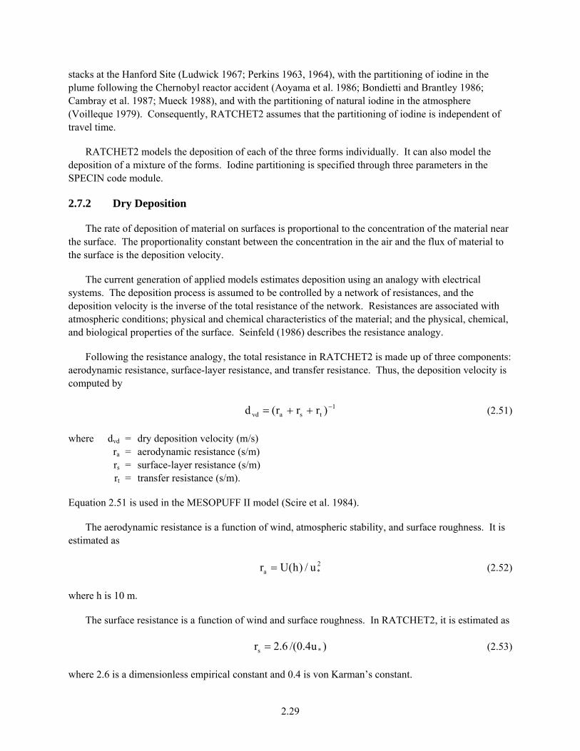
2.29

stacks at the Hanford Site (Ludwick 1967; Perkins 1963, 1964), with the partitioning of iodine in the plume following the Chernobyl reactor accident (Aoyama et al. 1986; Bondietti and Brantley 1986; Cambray et al. 1987; Mueck 1988), and with the partitioning of natural iodine in the atmosphere (Voilleque 1979). Consequently, RATCHET2 assumes that the partitioning of iodine is independent of travel time.

RATCHET2 models the deposition of each of the three forms individually. It can also model the deposition of a mixture of the forms. Iodine partitioning is specified through three parameters in the SPECIN code module.

2.7.2 Dry Deposition

The rate of deposition of material on surfaces is proportional to the concentration of the material near the surface. The proportionality constant between the concentration in the air and the flux of material to the surface is the deposition velocity.

The current generation of applied models estimates deposition using an analogy with electrical systems. The deposition process is assumed to be controlled by a network of resistances, and the deposition velocity is the inverse of the total resistance of the network. Resistances are associated with atmospheric conditions; physical and chemical characteristics of the material; and the physical, chemical, and biological properties of the surface. Seinfeld (1986) describes the resistance analogy.

Following the resistance analogy, the total resistance in RATCHET2 is made up of three components: aerodynamic resistance, surface-layer resistance, and transfer resistance. Thus, the deposition velocity is computed by

1tsavd )rrr(d −++= (2.51)

where dvd = dry deposition velocity (m/s) ra = aerodynamic resistance (s/m) rs = surface-layer resistance (s/m) rt = transfer resistance (s/m).

Equation 2.51 is used in the MESOPUFF II model (Scire et al. 1984).

The aerodynamic resistance is a function of wind, atmospheric stability, and surface roughness. It is estimated as

2*a u/)h(Ur = (2.52)

where h is 10 m.

The surface resistance is a function of wind and surface roughness. In RATCHET2, it is estimated as

)u4.0/(6.2r *s = (2.53)

where 2.6 is a dimensionless empirical constant and 0.4 is von Karman’s constant.

2.30

Finally, transfer resistance is associated with the characteristics of the depositing material and surface type. For example, Wesley and Hicks (1977) associate transfer resistance with stomatal openings in

plants. In RATCHET2, the transfer resistance is used as a mathematical means of placing a lower limit on the total resistance and the values are set within the SPECIN code module.

Both ra and rs become small as the wind speed increases. If the transfer resistance is set to zero for neutral conditions when the ratio of U/u* is typically about 10, the dry deposition velocity computed using Equation 2.51 increases from about 0.006 m/sec for a wind speed of 1 m/sec to greater than 0.06 m/sec when the wind speed is 10 m/sec. Deposition velocities at the upper end of this range are higher than normally assumed for most reactive gases, and the entire range of deposition velocities is above the range of deposition velocities measured for fine particles (~1 micron) and non-reactive gases. Assuming transfer resistances of 10 sec/m for reactive gases and 100 sec/m for fine particles yields dry deposition velocities that are more consistent with reported values. Figure 2.7 shows the variation in deposition velocity calculated for reactive gases with wind speed and stability using Equations 2.51, 2.52, and 2.53 and a 10-sec/m transfer resistance. The variation in deposition velocity for fine particles shown in Figure 2.8 assumes a transfer resistance of 100 sec/m.

Figure 2.7. Variation of Dry Deposition Velocities for Reactive Gases as a Function of Wind Speed and Stability Class

2.31

Figure 2.8. Variation of Dry Deposition Velocities for Small Particles as a Function of Wind Speed and Stability Class

Equation 2.51 applies specifically to dry deposition of gases. It may be extended to calculation of deposition velocities for particulate material with a relatively minor modification that incorporates the gravitational settling velocity of the particles. However, as a practical matter, deposition of fine particles (~1 micron) may be estimated using Equation 2.51 because the settling velocity is small compared to the ra

-1 and rs-1.

Droppo et al. (1983) and Droppo (1985) published dry deposition data for ozone that include values of U and u*. Figure 2.9 shows a comparison of deposition velocities predicted using Equations 2.51, (2.52), and (2.53), and a transfer resistance of 10 sec/m with Droppo’s measured values. The predicted values tend to be higher than the observed values, but the correlation between predicted and observed values is as expected. McMahon and Denison (1979), Sehmel (1980), and Seinfeld (1986) all show data indicating that elemental (reactive) iodine tends to have a higher deposition velocity than ozone. Thus, the bias in the model deposition velocity estimates shown in Figure 2.9 is consistent with use of the model for prediction of reactive iodine deposition velocities.

Separate dry deposition velocities are computed for each type of material in RATCHET2. If the material exists simultaneously in more than one form, RATCHET2 computes a weighted-average dry deposition velocity. Such is the case with iodine. The dry deposition velocity for iodine is the weighted average of dry deposition velocities computed for non-reactive gases, reactive gases, and particles. The averaging weights for each form are based on the fraction of the iodine in the form. These fractions are specified in the SPECIN code module, and for SAC they are set to 45%, 30%, and 25%, respectively.

2.32

Figure 2.9. Comparison of Predicted and Measured Dry Deposition Velocities for Ozone

2.7.3 Wet Deposition

RATCHET2 treats wet deposition of gases and particles separately. Wet deposition of gases is modeled assuming equilibrium between gas concentrations in the air and precipitation. Wet deposition of particles is modeled using a washout coefficient assuming irreversible collection of particles as the precipitation falls through the puffs. Slinn (1984) provides a comprehensive discussion of precipitation scavenging of particles and gases.

Scavenging rates for gases are based on solubility, assuming equilibrium conditions between the concentration of the gas in the air near the ground and in the precipitation. With this assumption, the scavenging rate for gases is expressed as a wet deposition velocity. Slinn (1984) gives the following equation for estimating wet deposition velocities for gases:

rvw PScd = (2.54)

where dvw is the wet deposition velocity, S is a solubility coefficient, Pr is the precipitation rate (water equivalent for snow) in mm/hr, and c is a conversion factor from mm/hr to m/sec.

RATCHET2 includes default precipitation rates of 0.1, 3 and 5 mm/hr for light, moderate, and heavy rain, respectively. The corresponding default precipitation rates for light, moderate, and heavy snow are 0.03, 1.5, and 3.3 mm/hr, respectively. These rates are consistent with hourly precipitation rates observed at the Hanford Site.

The solubility coefficients used in Equation 2.54 are inversely related to the Henry’s Law constant for the gas. Slinn (1984) provides guidance in their selection. Assuming a solubility coefficient of 500 for reactive gases gives the wet deposition velocities shown in Table 2.3 for the default precipitation rates in

2.33

RATCHET2. Wet deposition velocities for non-reactive gases are about three orders of magnitude lower. If both non-reactive and reactive gases are present, RATCHET2 calculates a weighted-average wet deposition velocity.

Table 2.3. Typical Wet Deposition Velocities for Gases and Particle-Washout Coefficients

Deposition Velocity (m/s) Reactive Non-Reactive

Particle-Washout Coefficient (1/hr)

Light Rain 1.4E-5 1.4E-8 0.254 Moderate Rain 4.2E-4 4.2E-7 3.26 Heavy Rain 6.9E-4 6.9E-7 4.78

Scavenging of non-reactive gases by precipitation is extremely limited. Scavenging of both highly reactive and non-reactive gases by snow when the temperature is less than -3°C is low. RATCHET2 ignores scavenging of gases under these conditions.

The wet deposition model for particles assumes that precipitation falls through the full vertical extent of the puffs and collects particles by collision. The scavenging rate for particles is expressed as a washout coefficient, which is the fraction of the airborne material removed by precipitation each hour.

RATCHET2 uses the following expression, which is discussed in Slinn (1984), for computing washout of particles by rain:

)P35.0/(PEC 4/1nr=Λ (2.55)

where Λ = washout coefficient (hr-1) C = empirical constant assumed to have a value of 0.5 E = average collision efficiency assumed to be 1.0 Pr = precipitation rate (mm/hr) Pn = normalized precipitation rate (Pr/l mm/hr).

Table 2.3 shows particle washout coefficients for the default rainfall rates in RATCHET2.

During periods of snow, the washout coefficient for particles is computed using

rP2.0=Λ (2.56)

Scavenging of gases takes place when the temperature is near freezing. When the temperature falls below -3°C, scavenging ceases because of changes in the physical character of the precipitation.

2.7.4 Surface Contamination

Given the dry and wet deposition velocities, the surface contamination that accumulated at any point during a short period is computed as

t)y,x(d)y,x(1SC ivi Δχ= (2.57)

2.34

where SCli(x,y) = mass or activity deposited (Ci/m2) at x,y from puff i dv = total deposition velocity, dvd+dvw (m/s) χi(x,y) = ground-level concentration (Ci/m3) in puff i Δt = time period (s).

Equation 2.57 simply states that surface contamination in an interval is equal to the product of a transfer coefficient (deposition velocity), the concentration in the air, and the time period.

To this contamination, RATCHET2 adds the contamination resulting from the washout of particles. This additional contamination is computed using

2r

2ri

i 2t])/r(5.0exp[Q

)y,x(2SCπσ

Δσ−Λ= (2.58)

where SC2i(x,y) = mass deposited at x,y from puff i by washout of particles Λ = washout coefficient (hr-l) Qi = mass in puff i r = horizontal distance of x,y from the center of the puff σr = horizontal diffusion coefficient (m) Δt = time period (hr).

Equation 2.58 is derived by substituting a washout coefficient for the deposition velocity in Equation 2.58 and then integrating the equation from ground level through the vertical extent of the puff.

The total surface contamination at x,y during any period Δt is the sum of the contributions of all puffs:

)]y,x(2SC)y,x(1SC[)y,x(SC ii

i +=∑ (2.59)

2.7.5 Depletion

RATCHET maintains a mass balance. Material deposited on the surface by dry and wet deposition is removed from the material in the puff by decreasing the total mass of the puff. Material is not selectively removed from the bottom of the puff.

In the atmosphere, deposition results in a mass deficit in the layer of air next to the surface. Source depletion models instantaneously propagate this deficit through the full vertical extent of the puff. This propagation is unrealistic, particularly in stable atmospheric conditions. Using the resistance analogy to estimate deposition velocities does not deal with this problem explicitly. However, using the resistance analogy results in lower deposition velocities during stable conditions, which reduces the magnitude of the error.

The mass removed from each puff is determined from analytical integration of the deposition flux over the area covered by the puff and computation interval. The mass removed from each puff to account for dry deposition of particles and dry and wet deposition of gases is computed using

2.35

∫ ∫π

=θ

∞

=

θχΔ=Δ2

0 0rvd ddrrdtQ (2.60)

Substituting the definition of χ from Equation 2.29 for χ and performing the integration, the decrease in material becomes

])2/[(t)z(GQd2Q z2/1

vd σπΔ=Δ (2.61)

During periods of precipitation, the additional rate of mass loss from a puff by washout of particles is determined by integrating the washout rate over the area covered by the puff

∫ ∫π

=θ

∞

=

θσπ

ΛΔ=Δ

2

0 0r2r

w ddrr2

)r(FQtQ (2.62)

When this integration is carried out, the rate of loss is equal to the product of the mass in the puff and the washout coefficient. Thus,

)]texp(0.1[QQ w ΔΛ−−=Δ (2.63)

This loss of mass is distributed throughout the puff.

RATCHET2 computes depletion at the end of each time step. If there is no precipitation, the mass remaining in the puff is computed assuming only dry deposition as

dij1ij QQQ Δ−=+ (2.64)

where i is the puff index and j is a time index. When there is precipitation, the depletion calculation is

dij1ij Q)texp(QQ Δ−ΔΛ−=+ (2.65)

2.8 RATCHET2 Model Evaluation

`The RATCHET code has been evaluated and benchmarked against measured data and compared, in a relative sense, to other model codes.

In regard to measurements, the original RATCHET codes were tested and validated against eight sets of monitoring data (Napier et al. 1993). The measured data in seven of the eight data sets are iodine-131 concentrations in vegetation or iodine-131 thyroid or body burdens. In these cases, comparisons of model predictions with measured data provide information on the performance of a sequence of models without providing information on the specific models in the sequence. The results of these comparisons are presented by Napier et al (1994). The eighth data set is a set of measurements of krypton-85 made between 1984 and 1987 at 12 locations on the perimeter of the Hanford Site and in nearby communities. These data may be compared directly with RATCHET2 output and are presented in this section.

2.36

More recently (Molenkamp et al. 2004), RATCHET has been compared, in a relative sense, with other transport and dispersion models. Specifically, RATCHET has been compared to the MACCS2 model (a straight-line, Gaussian-plume model) and the ADAPT/LODI model (a three-dimensional advection-dispersion code). A summary of this model comparison is provided in this evaluation section.

2.8.1 Krypton-85 Monitoring Data

Processing of reactor fuel is accompanied by the release of noble gas fission products, including krypton-85. The last processing of reactor fuel at Hanford occurred in the Plutonium-Uranium Extraction (PUREX) Plant in the 200 East Area intermittently from December 1983 through November 1987. Annual krypton-85 releases at Hanford for this period were reported in annual environmental reports. The total release for PUREX for the period was approximately 1.7 MCi. Krypton-85 activity released from other locations was significantly lower (~47 kCi) than the PUREX releases. The 1984 through 1987 krypton-85 releases were chosen for use in evaluation of RATCHET2, because the PUREX Plant was the dominant source during this period and the Surface Environmental Surveillance Project measured krypton-85 concentrations at a number of locations on and near the Hanford Site. Krypton data for 1983 were not included because the releases were not distributed throughout the year. For RATCHET2 evaluation for SAC Rev. 1, the releases were assumed to take place at a constant release rate from a 61-m stack in a nominal flow of about 9.4 m3/s at a temperature of about 25°C (77°F).

The Surface Environmental Surveillance Project collected air samples at a number of locations on site, near the boundary of the Hanford Site, and offsite during the period of interest. Twelve of the locations were within, or sufficiently close to, the RATCHET2 domain to provide measured concentration for comparison with model estimates. Of these locations, three were within 3 km (1.86 mi) of the PUREX stack, five were between 18 and 25 km (11.19 and 15.53 mi) from the stack, and the remaining four locations were between 38 and 45 km (23.61 and 27.96 mi) from the stack. One location at 25 km (15.53 mi) occasionally had two monitors running simultaneously. The air samples typically covered 28-day periods, with a range from 14 to 42 days. Average concentrations for each period were determined by counting the activity in the samples; typical counting errors were 10% to 15%. However, the monitoring was not continuous at any location. Consequently, annual average concentrations were estimated using a weighted average of the available data for comparison with concentrations predicted by RATCHET2. Ultimately, there were 41 usable estimates of annual concentrations at the 12 locations.

Figure 2.10 is a plot of predicted versus observed krypton-85 annual concentrations. RATCHET2 generally predicts the annual concentrations well (r2 = 0.81), although the model has a bias to slightly over-predict concentrations (geometric mean ratio between the predicted and measured concentrations = 1.26 with a geometric standard deviation of 1.7). Model errors were greatest for the three monitoring locations near PUREX, where the concentrations and concentration gradients are highest. Farther from PUREX, RATCHET2 predicted 28 of 33 concentrations within a factor of 2 and all 33 concentrations within a factor of 3. Neither the krypton-85 releases nor the monitoring were continuous. Thus, estimation of annual concentrations from the monitoring data is a source of uncertainty. However, it does not appear to have contributed to the differences between concentrations predicted by RATCHET2 and those estimated from monitoring data in a systematic manner.

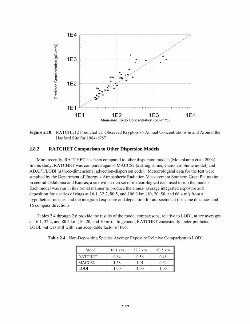
2.37

Figure 2.10. RATCHET2 Predicted vs. Observed Krypton-85 Annual Concentrations in and Around the Hanford Site for 1984-1987

2.8.2 RATCHET Comparison to Other Dispersion Models

More recently, RATCHET has been compared to other dispersion models (Molenkamp et al. 2004). In this study, RATCHET was compared against MACCS2 (a straight-line, Gaussian-plume model) and ADAPT/LODI (a three-dimensional advection-dispersion code). Meteorological data for the test were supplied by the Department of Energy’s Atmospheric Radiation Measurement Southern Great Plains site in central Oklahoma and Kansas, a site with a rich set of meteorological data used to run the models. Each model was run in its normal manner to produce the annual average integrated exposure and deposition for a series of rings at 16.1, 32.2, 80.5, and 106.9 km (10, 20, 50, and 66.4 mi) from a hypothetical release, and the integrated exposure and deposition for arc-sectors at the same distances and 16 compass directions.

Tables 2.4 through 2.6 provide the results of the model comparisons, relative to LODI, at arc averages at 16.1, 32.2, and 80.5 km (10, 20, and 50 mi). In general, RATCHET consistently under predicted LODI, but was still within an acceptable factor of two.

Table 2.4. Non-Depositing Species Average Exposure Relative Comparison to LODI

Model 16.1 km 32.2 km 80.5 km

RATCHET 0.64 0.56 0.48 MACCS2 1.58 1.01 0.64 LODI 1.00 1.00 1.00

2.38

Table 2.5. Depositing Species Average Exposure Relative Comparison to LODI

Model 16.1 km 32.2 km 80.5 km

RATCHET 0.79 0.81 0.88 MACCS2 1.41 1.05 0.81 LODI 1.00 1.00 1.00

Table 2.6. Average Deposition Relative Comparison to LODI

Model 16.1 km 32.2 km 80.5 km

RATCHET 0.67 0.66 0.71 MACCS2 1.21 0.96 0.78 LODI 1.00 1.00 1.00

3.1

3.0 RATCHET2 User’s Guide

This chapter is a user’s guide for the RATCHET2 computer code. All user interactions and data input are accomplished using data files. The sections in this chapter describe the input data files and their preparation, the output files, and program execution. The first section provides a detailed discussion of the run-specification file. The second section describes the selection of model parameters. The third section describes the remaining files used for data input, including the surface roughness length, default mixing-layer depth, and meteorological data files. The fourth section describes the output files created by RATCHET2. Finally, the last section describes program control in a production environment.

3.1 Run-Specification File

The run-specification file is the primary file used for setting up a model run in RATCHET2. The information in this file includes:

• run identification • model option controls • input data file names • output file names • source specification.

The name of the run-specification file must be specified in the execution command line and can be no longer than 100 characters. The file contains 18 records and some items within a given record are separated by a comma.

Table 3.1 provides a sample run-specification file that is the RATCHET2 control file used for SAC. All records shown are mandatory. The comments and category are included for reference; they are not part of the record. All records are read with the * format except for the first record, which is read as 80A1.

3.2

Table 3.1. Sample RATCHET2 Run-Specification File used in SAC. All inputs are read with the * format except for the first record.

Rec# Sample Input Comment Category

1 RATCHET2 test for Shakedown4 of SAC

Run title, read as 80A1

2 01 01 1998 Month, day, year of beginning of run 3 01 Hour of day of beginning of run 4 01 01 1999 Month, day, year of end of run 5 01 Hour of day of end of run 6 8760 Number of hours in the run

Run Description

7 46.3333 119.4167 Latitude and longitude of center of model domain (decimal degrees)

8 4000.0 Grid spacing on course grid 9 N 1000 Constant mixing height (Y or N) and value of

the constant height (m)

Model Parameters

10 met.dat Name of the meteorological data file 11 station.dat Name of the meteorological station file 12 z0_10cm.file Name of the surface roughness data file 13 def_mix.file Name of the mixing height file

Environmental Data Files

14 iodine.bin Name of the time-integrated air concentration and deposition output file for iodine

15 particle.bin Name of the time-integrated air concentration and deposition output file for particles

16 noble.bin Name of the time-integrated air concentration output file for noble gases

Output File Names

17 9.25 20.25 0.0 Grid coordinates (X,Y) of the source and height (Z) in meters above the ground

18 0.0 0.0 0.0 Stack radius, flow rate, and temperature

Source Characterization

3.1.1 Run Description

The first group of records in the run-specification file provide a description of the run, including a title and defining the period for the simulation.

Record 1 (80A1) is a character string that is used to identify the model run. This string may contain as many as 80 characters.

Record 2 specifies the date of the beginning of a model run. These values are used in searching the meteorological data file for the initial meteorological data record. The date must be entered as integers in the form mm dd yyyy, where mm is the month, dd is the day, and yyyy is the year. Leading zeros must be entered. Program execution will be aborted if either dd or mm is less than 1, if dd is greater than 31, or if mm is greater than 12.

3.3

Record 3 contains the hour in which the run begins. The day begins at hour 01 (1 a.m.), and the last hour of the day is 24 (midnight). Leading zeros may be dropped for the first nine hours of the day. Entries less than 01 or greater than 24 will cause program execution to abort.

Records 4 and 5 contain the date and time of the end of the run segment in a format similar to records 2 and 3, described above.

Record 6 specifies the number of hours that are in the run simulation.

3.1.2 Model Parameters

The second group of records in the run-specification file contains model parameters. These param-eters set the location and size of the domain as well as control calculation of the mixing-layer depth. This section briefly describes these records.

Record 7 specifies the latitude and longitude, in decimal degrees, for the center of the grid domain. Record 8 specifies the spacing between nodes on the environmental grid, which is stored in the variable DELXY. The spacing between nodes is entered in meters. It is the same in both the x and y directions. The spacing between nodes on the concentration grid used for model output is one half the environmental grid spacing.

Record 9 controls the mixing-layer depth. If an N is entered via this record, the program will use the mixing-layer depth file to limit vertical growth of the puffs. Otherwise, if a Y is entered, the program will use a constant mixing-layer depth that is specified by the value immediately following this parameter. The fixed mixing-layer depth is entered in meters.

3.1.3 Environmental Data Files

RATCHET2 uses several files to define the physical environment within the model domain. The names of the files are entered in records 10 through 13 of the run-specification file. These files are discussed in detail in Section 3.3.

Records 10 and 11 specify the names of files that contain the meteorological data and define the locations of the meteorological stations to be used in the model run. Both records must contain names of files that exist. If either file is missing or unreadable, program execution will abort.

Record 12 in the run-specification file is used to enter the name of a file containing surface roughness lengths for each node on the environmental grid. The file is required. If the file named in this record does not exist, program execution will halt in an error mode.

Record 13 is used to enter the name of a file containing default mixing-layer depths. The default mixing-layer depth file is required. If the file named in the record does not exist, program execution will halt in an error mode.

3.4

3.1.4 Output File Names

RATCHET2 creates binary output files for iodine, particles, and noble gases. The file names are specified on records 14, 15, and 16, respectively. Each binary file contains a header followed by gridded values of time-integrated concentration and deposition (iodine and particles, only) for the simulation period.

3.1.5 Source Characterization

The final group of records defines the source-term information for use in the RATCHET2 model. For SAC, a single source, with a unit release, is specified.

Record 17 contains the grid coordinate position of the source relative to the environmental grid as well as the source release height. Three entries are expected. The first two entries give the grid position of the release point relative to the southwest corner (1,1) of the model domain. These positions are entered as grid coordinates and must be within the model domain. The third entry is the height, in meters, of the release point above the ground.

Record 18 provides additional information about the source in the following order: stack radius (m), stack flow rate (m3/s), and stack exit temperature (ºC).

3.2 Selection of Internal Values for RATCHET2 Model Control Parameters

In RATCHET2, several model parameters that relate to transport and diffusion have been set internally within the code. These parameters, which are set within the module SPECIN, are described below along with the rationale for their selection. This section also describes the sensitivity of the code execution time and time-integrated air concentrations and deposition to variations in these parameters. The model sensitivity discussion follows directly from results of calculations performed for the HEDR project using RATCHET (Ramsdell et al. 1994).

3.2.1 Number of Puffs per Hour

The number of puffs per hour is set by the variable NPH within the module SPECIN. The parameter determines the NPH used in RATCHET2 to represent continuous plumes. The number of model calculations is directly related to the number of puffs released. However, Ramsdell and Athey (1981) indicate that increasing NPH beyond four to six does not result in a corresponding increase in precision of model-calculated concentrations.

Figure 3.1 compares time-integrated concentrations using data and locations from the HEDR dataset (Ramsdell et al. 1994), for NPH=4 and NPH=15. The solid diagonal line in Figures 3.1 indicates perfect agreement between the model predictions. Also note that in some instances data points overlie each other. The results shown in Figures 3.1 support use of NPH = 4 as an appropriate compromise between computational accuracy and code execution time in RATCHET2.

3.5

Figure 3.1. Comparison of Time-Integrated Concentrations for 50 Locations Computed with NPH=4 and NPH=15 (from Ramsdell et al. 1994)

3.2.2 Minimum Time Step for Calculations

The parameter IOPDTA, which is specified within the module SPECIN, is an index that is used in conjunction with the NPH and puff radius (σr) for determining the minimum time step used in diffusion and transport calculations. If IOPDTA is greater than one, the time steps used for young (small) puffs will be shorter than those used for old (large) puffs. Computational time does increase with decreasing minimum time step. However, the effect of IOPDTA on computational time is much less than the effect of other parameters, such as NPH.

Figure 3.2 compares time-integrated air concentrations computed for various locations using a 5-minute and 1-minute minimum time step. The solid diagonal line in Figure 3.2 indicates perfect agreement between the model predictions. The results suggest that use of a 5-minute minimum time step (NPH=4 and IOPDTA=3) is reasonable for use in RATCHET2.

3.2.3 Puff Consolidation

The RATCHET2 code includes an option to combine puffs that cover essentially the same area to decrease code execution time. This functionality is particularly important for larger domains, where puffs may significantly overlap as they grow in size due to dispersion. This option is selected by setting the puff consolidation flag (CLN_FLG) to true and entering a minimum separation criterion for the parameter CLN_CRIT. The parameter CLN_CRIT is the ratio of the separation between puffs divided by the average σr of the puffs that separates the conditions when puff consolidation occurs and when it does not occur. The puff consolidation criterion is applied to puffs from the same source. When the ratio of the separation between puffs to the average σr is less than CLN_CRIT, the puffs will be combined, and the consolidated puff will be placed at the center of mass of the original puffs.

3.6

Figure 3.2. Comparison of Time-Integrated Concentrations for 50 Locations Computed with 1-Minute and 5-Minute Time Steps (from Ramsdell et al. 1994)

In RATCHET2, puffs are not combined (i.e., CLN_CRIT is set to false) because its intended use is for domains that are relatively large and computationally inexpensive.

3.2.4 Puff Radius

The Gaussian curve has infinite tails. Therefore, when Gaussian models are used for dispersion calculations, the distribution has to be truncated at some point to avoid calculating a large number of extremely low concentrations. These concentrations are generally meaningless, and their calculation is time-consuming. In RATCHET2, the puff radius is controlled by the variable RADCNST within the SPECIN module.

Figure 3.3 compares surface deposition at 50 nodes for allowable puff radii of 3.7 σr, and 5.3 σr. The figure clearly demonstrates that the changes in surface deposition that result from changes in puff radius are small compared to the range of values within the model domain. Thus, using a smaller puff radius (3.7 σr instead of 5.3 σr) will not have a significant impact on the precision of model calculations. Truncating puffs at 3.7 gives a concentration at the puff edge that is three orders of magnitude lower than the concentration at the center.

3.2.5 De Minimis Concentration

RATCHET2 uses a de minimis concentration as another means of limiting the number of calculations and thereby decreasing the run time. The parameter, CHIMIN, within the SPECIN module, is used to set this threshold concentration. For use with SAC in which a unit source is modeled, a threshold value of 1x10-13 Ci/m3 was chosen to maintain mass balance in the system, yet limit simulation time.

3.7

Figure 3.3. Comparison of Calculated Surface Contamination Values for Puff Radius of 3.7 σr and 5.3 σr (from Ramsdell et al. 1994)

3.2.6 Horizontal Diffusion Coefficient Proportionality Constant

In RATCHET2, the horizontal diffusion coefficient is assumed to be proportional to time. For the first hour after a puff is released, the proportionality constant is a function of atmospheric turbulence and those parameters that affect the turbulence. After the first hour, factors other than atmospheric turbulence (e.g., wind shear) control horizontal diffusion. These factors are not modeled explicitly in RATCHET2. However, their effect on horizontal diffusion is modeled implicitly in the proportionality constant used in calculating increases in the diffusion coefficient after the first hour. This dimensional constant is controlled through the parameter, SY_CNST, within the SPECIN code module.

Large values of SY_CNST are associated with large puffs and low concentrations at the puff center, while small values of SY_CNST are associated with small puffs and high concentrations at puff centers. Thus, changing SY_CNST has two effects on time-integrated air concentrations and deposition at nodes. It changes the frequency of exposure at nodes, and it changes the concentrations during the exposure period.

Long-range diffusion data summarized by Gifford (1983) suggest the distribution in Table 3.2 with a median value of about 0.5 m/sec. For SAC, the model domain is sufficiently small so a fixed value of 0.3 has been used.

3.8

Table 3.2. Distribution of Horizontal Diffusion Coefficient, SY_CNST

SY_CNST Range (m/s) Probability (%)

0.14 to 0.28 20 0.28 to 0.56 60 0.56 to 1.40 20

3.3 Input Files

In addition to the run-specification file described in Section 3.1, four other files are used to supply input data to RATCHET2. The files and their associated characteristics are listed in Table 3.3. This section discusses the remaining four files.

Table 3.3. Summary of RATCHET2 Input Files

File Name Access Form Status

Surface Roughness Lengths Sequential Formatted Required Default Mixing Layer Sequential Formatted Required Meteorological Stations Sequential Formatted Required Meteorological Data Sequential Formatted Required

These files are formatted sequential files that are used for data input for each model run. They can be prepared using a text editor or a computer program and can be displayed on terminals or printed directly.

3.3.1 Surface Roughness Length File

The surface roughness length is a characteristic length that enters into many atmospheric boundary-layer calculations. It arises as a constant of integration in the derivation of the logarithmic wind profile. Section 2.2.1 describes the surface roughness length in more detail, and Table 2.1 relates surface roughness lengths to topographic and land-use characteristics.

The surface roughness length file contains two records. The first record is a file heading, and the second record is an array of roughness lengths. The heading is a 60-character string and should contain information to uniquely identify the file contents. The surface roughness length array contains one element for each node on the environmental grid. The order of elements in the file is important. The first element must be the roughness length for the node in the southwest corner of the grid. The next element must contain the roughness length for the node immediately to the east of the first. This pattern continues until the roughness length for the southeast corner node is entered. After the surface roughness length for the southeast corner node is entered, the roughness length is entered for the node immediately north of the southwest corner node. This pattern is continued until the surface roughness is entered for the last node. The last node should be the node in the northeast corner of the grid.

3.3.2 Default Mixing-Layer Depth File

The default mixing-layer depth file is a formatted, sequential file that contains 60 records. Each record contains the default mixing-layer depths for one stability group and month. Eight fields within the

3.9

record give the variation in default mixing-layer depth with the time of day. The format for the records is 11X, 8F7.1. The default mixing-layer depth file may be created with a text editor.

Only five stability classes are used for determining the default mixing-layer depth. Stability classes 1 and 2 (extremely unstable) are combined to form class 1. Classes 3, 4, and 5 are reduced by 1 (forming classes 2, 3, and 4, respectively) and are equivalent to the original stability classes used throughout the program. Stability classes 6 and 7 (extremely stable) are combined to form class 5.

Figure 3.4 shows the first 15 records of a default mixing-layer depth file based on mixing-layer depth estimates made by HMS forecasting staff from 1983 through 1987. The first set of five records is for January, the next set of five is for February, etc. Within each set of five records, the first record is for the most unstable atmospheric conditions. Each succeeding record represents an increase in stability. The time of day is represented by the columns, starting with midnight to 3:00 a.m. in the first column.

Figure 3.4. Default Mixing-Layer Depths at the Hanford Site for January through March

3.3.3 Meteorological Station File

Meteorological station locations are entered via the meteorological station file specified in the eleventh record of the run-specification file. This file is a formatted, sequential access file that may be created and edited with a text editor. The meteorological station file must include an entry for each location for which meteorological data are available. The order of the station locations must correspond to the order of the data in the meteorological data file.

Records in the file contain the station name, the latitude and longitude of the station location, and the height of the wind measurement. They also contain an estimate of the surface roughness at the station (m), wind reporting unit indicators for direction and speed, and a status flag. The format for the file is lX, A4, 2F10.0, 2F7.0, lX, 3I4.

Station names are selected and entered by the user. They are used only for identification in the RATCHET2 log and are not required.

Station position is required and is specified by a latitude and longitude pair, in decimal degrees. West longitudes are entered as positive values. Stations are not required to be in the model domain.

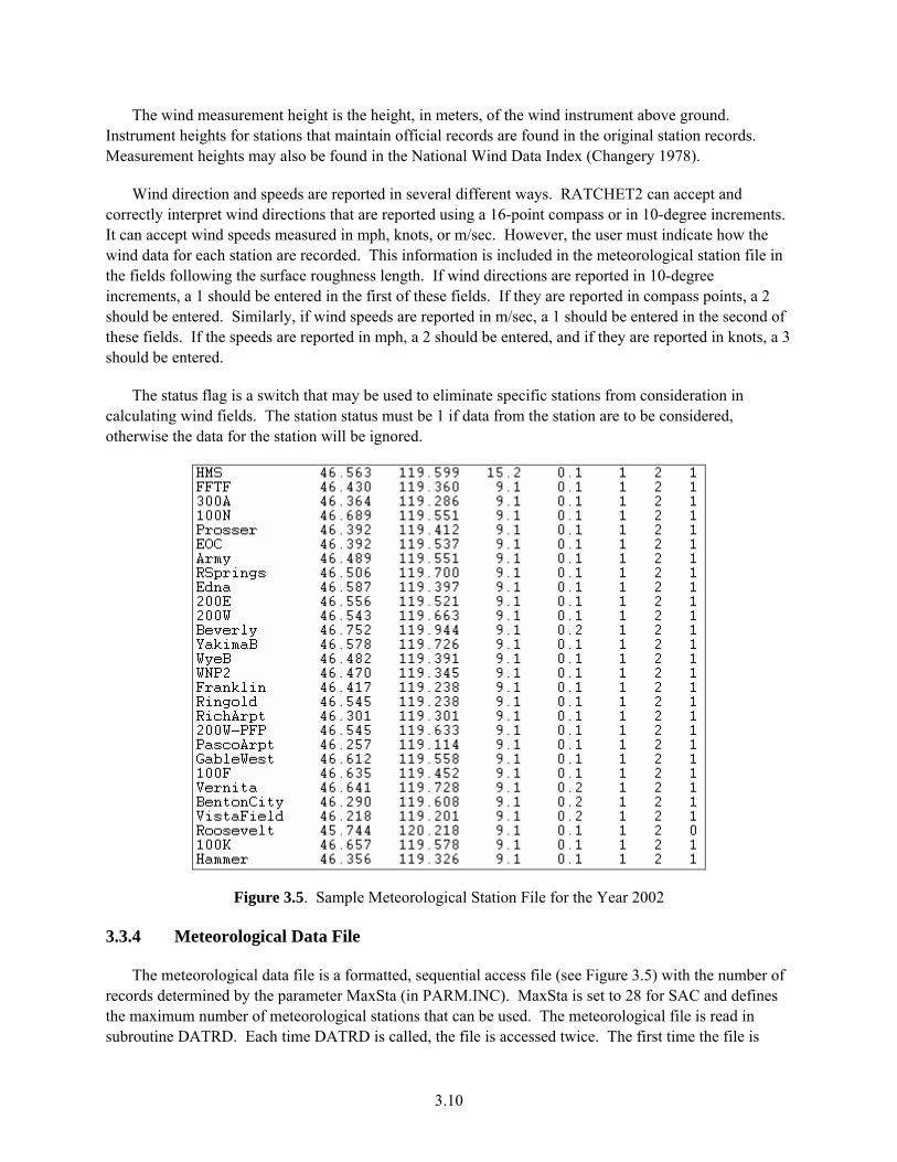
3.10

The wind measurement height is the height, in meters, of the wind instrument above ground. Instrument heights for stations that maintain official records are found in the original station records. Measurement heights may also be found in the National Wind Data Index (Changery 1978).

Wind direction and speeds are reported in several different ways. RATCHET2 can accept and correctly interpret wind directions that are reported using a 16-point compass or in 10-degree increments. It can accept wind speeds measured in mph, knots, or m/sec. However, the user must indicate how the wind data for each station are recorded. This information is included in the meteorological station file in the fields following the surface roughness length. If wind directions are reported in 10-degree increments, a 1 should be entered in the first of these fields. If they are reported in compass points, a 2 should be entered. Similarly, if wind speeds are reported in m/sec, a 1 should be entered in the second of these fields. If the speeds are reported in mph, a 2 should be entered, and if they are reported in knots, a 3 should be entered.

The status flag is a switch that may be used to eliminate specific stations from consideration in calculating wind fields. The station status must be 1 if data from the station are to be considered, otherwise the data for the station will be ignored.

Figure 3.5. Sample Meteorological Station File for the Year 2002

3.3.4 Meteorological Data File

The meteorological data file is a formatted, sequential access file (see Figure 3.5) with the number of records determined by the parameter MaxSta (in PARM.INC). MaxSta is set to 28 for SAC and defines the maximum number of meteorological stations that can be used. The meteorological file is read in subroutine DATRD. Each time DATRD is called, the file is accessed twice. The first time the file is

3.11

accessed, the subroutine reads the full data record to obtain data used in transport and diffusion calculations. The second time the file is accessed, the subroutine obtains the date and time of the next set of meteorological data.

Data are entered in each record in the file in the following order:

• year (four digits) • julian day (three digits) • hour (two digits) • release-height wind direction (two digits) • release-height wind speed (two digits) • release-height temperature (four digits) • precipitation type (one digit) • surface-wind direction (two digits) • surface-wind speed (two digits) • stability class (one digit) • surface temperature (three digits) • precipitation rate (three digits).

The last five items are repeated for each surface station, which is 28 times (i.e., 28 surface stations) for SAC. Each record must be complete and 9’s should be used to indicate missing data for a station. The format for a given record is I4, I3, I2, 1X, 2I2, I4, I1, 1X, 28 (2I2, I1, 2I3,1X). The units and ranges for meteorological variables are listed in Table 3.4. The release height temperature is entered as an integer value to the nearest tenth of a degree. RATCHET2 divides the value entered by 10 when the temperature is converted to degrees Celsius in subroutine MET_FLD. Precipitation is entered as an integer value to the nearest hundredth of an inch/hr. RATCHET2 divides this value by 100 when the precipitation rate is converted to inches/hr in MET_FLD. These numerical techniques were originally done to minimize file size (by using an integer type) while at the same time preserving numerical accuracy.

3.4 Output Files

RATCHET2 produces two types of output files:

• files containing annual time-integrated air concentrations and surface depositions • a file providing records of computer-run segments (i.e., a log file)

3.12

Table 3.4. Units and Ranges for Meteorological Variables

Variable Units Range Year none 0000 through 9999 Day none 001 through 366 Hour none 01 through 24 Release height wind direction as defined in Met Station file 00 through 36, 88 and 99 Release height wind speed as defined in Met Station file 00 through 80, 88 and 99 Release height temperature 0.1ºF none Precipitation type None 0 (none), 2 (any liquid precip.), 5 (only frozen

precip.), 9 (missing) Surface wind direction as defined for Met Station file 00 through 36, 88 and 99 Surface wind speed as defined for Met Station file 00 through 80, 88 and 99 Stability class none 1 through 7 Surface Temperature ºF < 150 Precipitation rate 0.01 inches/hr ≤ 200

A separate time-integrated file is created for iodine, particles, and noble gases. The iodine and particles files contain time-integrated results for both air concentration and surface contamination; the noble gas file contains results for time-integrated air concentration only. The period for the time-integration is specified on record 6 of the run-specification file. For SAC, this period is normally 1 year.

The following sections briefly describe the output files.

3.4.1 Time-Integrated Air Concentrations and Deposition

The time-integrated air concentration and surface deposition files are the primary output files generated by the RATCHET2 code. For SAC, the time integration is normally for one year and is specified on record 6 (in hours) of the run-specification file.

The output files generated by RATCHET2 are sequential, unformatted files. One output file is created for iodine, one for particles, and one for noble gases. The file names are entered in records 14 through 16, respectively, in the run-specification file.

Each file begins with a file header record of up to 80 characters. This record is followed by a set of records that contains the model output. The general form is:

• concentration header • time-integrated air concentrations • surface contamination header (iodine and particles, only) • surface contamination (iodine and particles, only).

Each header record identifies the data that follow and gives the simulation date and run-segment identification. The data records are binary copies of the model time-integrated air concentration and surface contamination arrays. For SAC, these arrays have dimensions of 41 (west to east) by 53 (south to north). The spacing between nodes is DELXY/2 in both directions. The binary write of the arrays starts

3.13

in the southwest corner and writes the array elements from west to east. The rows are written from south to north. The time-integrated air concentrations in the primary output files are accumulations in Ci-s/m3. The surface contaminations are given in Ci/m2.

3.4.2 Run-Log File

RATCHET2 generates a run-log file each time the code is executed; this file is the primary record of the model run. The log file name is specified on the command line after the run specification file. The filename can be up to 100 characters long and a default filename is used if no name is provided. The file is a standard, ASCII file that can be viewed in a text editor. The heading of the log file lists the program name and version; the remainder of the log file contains the following information:

• date and time that code execution is begun • run identification • fixed model parameters • input/output file names • data in run-specification file • mass-balance data • status and error messages.

If a model run segment terminates in a normal mode, the message *** SIMULATION TERMINATED *** is entered in the log. However, this message does not ensure that the model executed as intended. It may have been unable to read one of the optional data files and have simply continued in a default mode. If the program aborts while trying to read a required file, the terminal message in the log will indicate the file access that caused the program to terminate prematurely.

3.4.3 Run Indicator Files

As part of the modifications made for inclusion in SAC, RATCHET2 was modified to create the following run indicator files: ratchet.run, ratchet.done, and ratchet.fail. These files are created to assist the user in managing parallel simulations of the atmospheric transport model. The presence of the file ratchet.run in the run directory indicates that RATCHET2 is currently running. If the simulation encounters and error and terminates, the ratchet.fail file is created to indicate that the simulation did not reach completion. If the simulation completes normally, the ratchet.done file is created.

3.5 Program Control

User interaction with the RATCHET2 code takes place through the run-specification file and a series of other environmental input files (default mixing heights, surface roughness, meteorological data and meteorological station file). For simple applications, the executable code and all input files may be moved to a common subdirectory. Then the code can be executed by changing to that subdirectory, typing the name of the executable file followed by the name of the run-specification file and the run-log file on the command line, and pressing the enter key.

RATCHET2 can also be run in batch mode. Script files can also be created run the RATCHET2 code several times in sequence.

4.1

4.0 Programmer’s Guide

Chapter 2 discussed the technical basis for the RATCHET2 computer code. Chapter 3 discussed the computer code from a user’s point of view. This last chapter discusses the code from a programmer’s point of view. It covers programming style, hardware requirements of the code, and the individual program elements.

4.1 Program Development

This section discusses three components related to program development: programming language and style, the hardware for which the program was developed, and the size of the program and its files.

4.1.1 Language and Style

RATCHET is written in standard ANSI FORTRAN-77 programming language with extensions designed to enhance code maintenance and to promote a structured programming style. Specific extensions used include long variable names, IMPLICIT NONE, INCLUDE statements, and the DO WHILE and END DO statements.

In addition to formatted, sequential files, the code makes use of unformatted, binary data files. These files are computer-specific, but the read and write statements for the files follow the ANSI standard, except as noted above. The code also uses three computer-specific subroutines. One subroutine is used to read the command line argument that specifies the name of the run-specification file and the other two subroutines obtain the current date and time from the system clock.

The following coding standards are followed in the program:

• The code for each program unit includes a definition block and a code block. The definition block includes the program unit name, history, description, and relationship to other units and INCLUDE files. It may also contain references, describe algorithms, and define variables. The code block contains the code and comments.

• All program units begin with the statement IMPLICIT NONE. The type and dimensions of all variables are defined in type statements.

• Named common blocks are the primary method of passing variables between major program units. They contain generally related information with the block names indicating the general nature of the information. The common blocks are defined in code segments contained in INCLUDE files. INCLUDE files also contain PARAMETER statements, type definitions, and dimensions associated with all variables in the common blocks defined in the file.

• Functions are used in preference to subroutines when possible. Common blocks are not used to pass variables to functions.

4.2

• Argument lists are used to pass variables to functions and to some subroutines. The use of formal argument lists is preferred in functions and in subroutines where the formal argument list facilitates program development, verification, and maintenance.

• Parameter statements are used to define array dimensions that establish the model domain size and model limits. All of these statements are located in the PARM.INC file.

• Data statements used to define variables contained in common blocks are placed in the BLOCK DATA unit. The code for the BLOCK DATA unit is located at the end of the code for the main program.

• Use of system-dependent calls has been minimized. They have been limited to the calls to the system clock to determine the date and time of program execution.

• Structured programming techniques (IF ... THEN, ELSE IF ... THEN, DO WHILE) are used when appropriate. The use of statement numbers has been minimized.

4.1.2 Target Computer

RATCHET2 has been compiled for use on UNIX and PC-based operating systems. The PC-based version is compiled using Compaq Visual Fortran (version 6.6) and runs on personal computers using version 5.1 of the MS-DOS operating system.

4.1.3 Program Size

RATCHET2 is a sufficiently small program to fit within the memory limits of personal computers. However, RATCHET2 processes hourly meteorological data to produce annual time-integrated concen-tration and surface contamination output. As a result, the meteorological files used by the program are large and exceed 3,000 kb.

4.2 Program Organization

RATCHET2 is a highly modular code consisting of a main program and block data element, 26 sub-routines, and 19 functions. In addition, there are 10 INCLUDE blocks that contain parameter, type, and common statements. The main program provides a general framework for the code and controls the sequence of code execution. The subroutines and functions perform most of the calculations. The following sections describe the main program and the other program units.

4.2.1 Main Program

The main program provides the general framework for the code. It contains the six sections listed below:

• an initialization section • an hourly environment update section • a transport, diffusion, and deposition calculation section • an annual output section

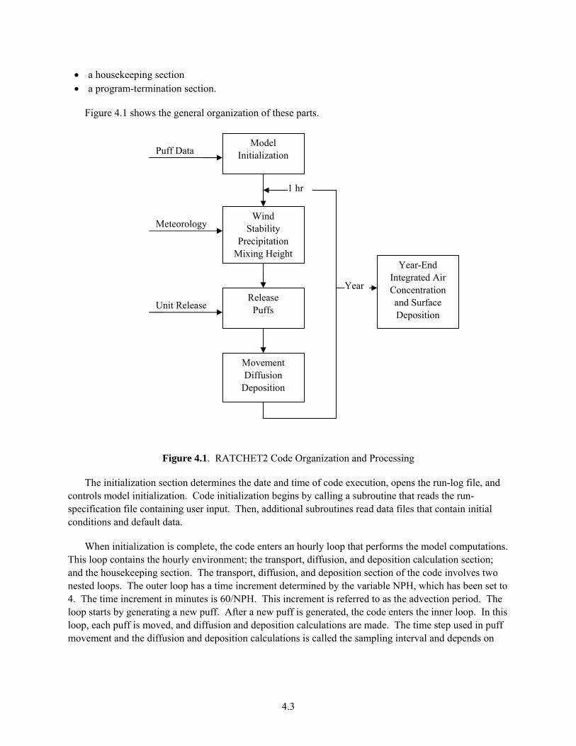
4.3

• a housekeeping section • a program-termination section.

Figure 4.1 shows the general organization of these parts.

Figure 4.1. RATCHET2 Code Organization and Processing

The initialization section determines the date and time of code execution, opens the run-log file, and controls model initialization. Code initialization begins by calling a subroutine that reads the run-specification file containing user input. Then, additional subroutines read data files that contain initial conditions and default data.

When initialization is complete, the code enters an hourly loop that performs the model computations. This loop contains the hourly environment; the transport, diffusion, and deposition calculation section; and the housekeeping section. The transport, diffusion, and deposition section of the code involves two nested loops. The outer loop has a time increment determined by the variable NPH, which has been set to 4. The time increment in minutes is 60/NPH. This increment is referred to as the advection period. The loop starts by generating a new puff. After a new puff is generated, the code enters the inner loop. In this loop, each puff is moved, and diffusion and deposition calculations are made. The time step used in puff movement and the diffusion and deposition calculations is called the sampling interval and depends on

Model Initialization

Wind Stability

Precipitation Mixing Height

Release Puffs

Movement Diffusion

Deposition

Meteorology

Puff Data

Unit Release

1 hr

Year

Year-End Integrated Air Concentration and Surface Deposition

4.4

puff size. Calculations for small puffs may be made at 1-minute intervals. As puffs grow, the time step increases until a maximum time step is reached. The maximum time step is the interval between puff releases (1/NPH hours).

Each hour, the code enters the housekeeping section in which the status of the puffs is examined. Puffs that have moved out of the model domain or have been depleted so that the concentrations in the puffs are negligible are deleted. The de minimis concentration set within the code is used as the basis for determining if a puff within the model domain may be deleted. The positions and dimensions of consecutive puffs from the same source are also examined.

After the transport, diffusion, and deposition calculations have been completed for the entire period, the code enters the output section. The primary code output is written to files for the period specified in the run-specification file. The output consists of sets of time-integrated air concentrations for depositing and non-depositing material, and surface contamination for depositing material. At the end of the period, the code also performs a set of mass-balance calculations and records the results in the program run-log file.

4.2.2 Relationships Between Program Units

The previous section provides a general overview of the structure of RATCHET2. This section provides more detail on the interrelationships between the program units. The next section contains a description of each of the units.

The subroutine calling sequence in RATCHET2 is shown in Figure 4.2. The main program sections are indicated by mixed upper- and lowercase headings. Subroutine names are shown in uppercase letters, and the indentation indicates the level of nesting of the subroutines. The comment to the right of the subroutine name gives an indication of the subroutine’s purpose.

Data are generally passed between subroutines using named common blocks. These common blocks are defined in INCLUDE files that are incorporated in the code of subroutines as the subroutines are compiled. In addition to the common block definitions, the INCLUDE blocks contain type statements and, where needed, parameter statements. All variables in the common blocks are included in type statements. Table 4.1shows the INCLUDE files associated with each subroutine.

Table 4.1. Cross Reference between Subroutines and INCLUDE Files

INCLUDE FILE

CONST DATES MASS_BAL MATRIX MET_DATA PARM PUFFS RAND_DAT REL STATION

RATCHET2 X X X X X X X X X X

ASCND X X

BALANCE X X X X X

CLEAN2 X X X X

DATACK X X X

DATRD X X X

DATWR X X X

4.5

DIFDEP X X X X X X X X X

FBALANCE X

GRlDlN X X X X X

INIT X X X X X X X

MET_FLD2 X X X X X X X

METOPN X X X

OUTPUT X X X X

PUFFM X X X X X X X

PUFFR X X X X X X

RELEAS X X X X

SPECIN X X X X X X X X X X

STRAY X X X

SUBST200 X X X

Special-purpose functions have been developed in RATCHET2 primarily for calculating variables used in the transport, diffusion, and deposition calculations. Special functions have also been developed for use in time conversions within the program. None of these functions use INCLUDE files; all data are passed to the functions via formal argument lists. Table 4.2 shows a list of the RATCHET2 functions used in each subroutine.

Table 4.2. Cross Reference between Subroutines and RATCHET2 Functions

RATCHET2 PLUMRISE ASCND None BALANCE HOURDT CLEAN2 None DATACK None DATRD DTHOUR DATWR None DIFDEP DDEPVEL, PUFFSIGZ, PUFSIGY, TURBSIGV, TURBSIGW, USTAR,

WDEPGAS, WDEPPART FBALANCE None GRlDlN DTHOUR INIT None MET_FLD2 HOURDT, INVMOL, MIX_HT, PROFILE, STABLIMT, USTAR METOPN DTHOUR OUTPUT HOURDT PUFFM PROFILE, USTAR PUFFR None RELEAS DTHOUR SPECIN DTHOUR, JULIAN STRAY None SUBST200 PROFILE, USTAR

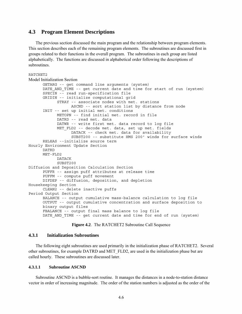
4.6

4.3 Program Element Descriptions

The previous section discussed the main program and the relationship between program elements. This section describes each of the remaining program elements. The subroutines are discussed first in groups related to their functions in the overall program. The subroutines in each group are listed alphabetically. The functions are discussed in alphabetical order following the descriptions of subroutines.

RATCHET2 Model Initialization Section

GETARG -- get command line arguments (system) DATE_AND_TIME -- get current date and time for start of run (system) SPECIN -- read run-specification file GRIDIN -- initialize computational grid

STRAY -- associate nodes with met. stations ASCND -- sort station list by distance from node

INIT -- set up initial met. conditions METOPN -- find initial met. record in file DATRD -- read met. data DATWR -- write first met. data record to log file MET_FLD2 -- decode met. data, set up met. fields

DATACK -- check met. data for availability SUBST200 -- substitute HMS 200' winds for surface winds

RELEAS --initialize source term Hourly Environment Update Section

DATRD MET-FLD2

DATACK SUBST200

Diffusion and Deposition Calculation Section PUFFR -- assign puff attributes at release time PUFFM -- compute puff movement DIFDEP -- diffusion, deposition, and depletion

Housekeeping Section CLEAN2 -- delete inactive puffs Period Output Section

BALANCE -- output cumulative mass-balance calculation to log file OUTPUT -- output cumulative concentration and surface deposition to binary output files FBALANCE -- output final mass balance to log file DATE_AND_TIME -- get current date and time for end of run (system)

Figure 4.2. The RATCHET2 Subroutine Call Sequence

4.3.1 Initialization Subroutines

The following eight subroutines are used primarily in the initialization phase of RATCHET2. Several other subroutines, for example DATRD and MET_FLD2, are used in the initialization phase but are called hourly. These subroutines are discussed later.

4.3.1.1 Subroutine ASCND

Subroutine ASCND is a bubble-sort routine. It manages the distances in a node-to-station distance vector in order of increasing magnitude. The order of the station numbers is adjusted as the order of the

4.7

distances is adjusted to maintain the correspondence between station numbers and distances. Subroutine ASCND is called from subroutine STRAY.

4.3.1.2 Subroutine DATWR

Subroutine DATWR writes the initial meteorological data record to the RATCHET2 log. It provides a check to ensure that the meteorological data file is being read correctly. DATWR is called from subroutine INIT after subroutine DATRD reads the first meteorological record and before the subroutine MET_FLD2 is called.

4.3.1.3 Subroutine GRIDIN

Subroutine GRIDIN sets up the model domain. It reads the surface roughness length and meteoro-logical station files. GRIDIN determines the position of the meteorological stations in environmental grid coordinates from the distance components in the meteorological station file and the node spacing. When the meteorological station positions have been defined, the subroutine deletes any stations that are marked as inactive. It then calls subroutine STRAY, which builds a look-up table for each node that gives the distance from the node to each meteorological station. STRAY, in turn, calls subroutine ASCND, which arranges the entries in the look-up table in order of increasing distance.

GRIDIN records information about the model domain and meteorological station in the log file; this information includes the number of nodes along each axis, the center of the model domain, and the spacing between nodes on the environmental grid. It lists the environmental grid coordinates, wind-measurement height, surface roughness length, wind-unit codes, and status for each station. Following the list of meteorological stations, GRIDIN writes arrays showing the station numbers for the three meteorological stations closest to each node. Finally, it calculates and records the area associated with each node in the concentration grids.

4.3.1.4 Subroutine INIT

Subroutine INIT is the primary initialization routine for diffusion and deposition calculations. INIT reads the default mixing-layer depth file, which is specified within the run-specification file. The subroutine then performs meteorological initialization, which includes (1) calling subroutine METOPN to find the initial meteorological data record for the simulation, (2) calling subroutine DATRD to read the initial meteorological data, (3) calling subroutine DATWR to copy the initial meteorological data record to the RATCHET2 log, and (4) calling subroutine MET_FLD2 to process the initial meteorological data set. If the “@” character is specified as the first character for the title in the run-specification file, then the initial stability and precipitation fields are written to the log file along with the mixing-layer depths calculated for each station.

When the meteorological data initialization is complete, INIT records the run title, date, and time on the log. Finally, INIT records the time that the simulation is to start in the RATCHET2 log.

4.3.1.5 Subroutine METOPN

Subroutine METOPN is used to open the meteorological data file and to set the meteorological record index to the proper set of observations for the start of the simulation. If there is an error in opening the

4.8

file or if an error is encountered in reading the date/time group in the first record, METOPN will write a message to the RATCHET2 log that identifies the problem. It will then abort execution of the program.

After the date/time group in the first record has been read successfully, an error in reading a subsequent date/time group will result only in writing an error message to the log. The simulation will continue. Data will be used as appropriate until the record in which the error occurred is encountered. The remainder of the simulation will use the data in the last good record.

4.3.1.6 Subroutine RELEAS

Subroutine RELEAS has two primary functions: (1) it determines release rates for the start of the run segment, and (2) it defines and checks the position of the source.

RELEAS sets an overall unit release rate for the source and determines the release rate for each run segment (1/NPH), where NPH is set to 4 in RATCHET2.

Subroutine RELEAS then defines the position of the sources. RATCHET2 simulates a single source with a unit release that may be located anywhere within the model domain with a release height from the ground to 300 m. If any of the positions are out of the model domain or are greater than 300 m, program execution will be aborted.

4.3.1.7 Subroutine SPECIN

Subroutine SPECIN has three primary functions: (1) it reads the run-specification file, (2) sets numerous values for model control parameters, and (3) records much of the run-specification file information to the RATCHET2 log file. The run-specification file is discussed in detail in Section 3.1. If SPECIN cannot open the run-specification file, program execution will be aborted.

SPECIN does not perform any calculations. However, it does call functions JULIAN and DTHOUR to convert dates and times entered by the user to internal model times. The internal model time is elapsed time from midnight beginning the first of January of the reference year supplied by the user in the run-specification file.

4.3.1.8 Subroutine STRAY

Subroutine STRAY sets up two three-dimensional arrays that relate the meteorological stations to the nodes on the environmental grid. One of these arrays contains the distance from each node to each meteorological station, and the other array contains identification numbers assigned to the meteorological stations. The distances in the first array correspond to the station identification numbers in the second.

The data for each node are initially entered into two vectors. STRAY calls subroutine ASCND to arrange the station data in the two vectors in order of increasing distance. After the order of the data has been established, the data are copied into the final three-dimensional distance and station number and arrays.

4.9

4.3.2 Hourly Update Subroutines

The four subroutines discussed in this section are used by RATCHET2 to update model status each hour. Two of the subroutines are called directly by the main program. They are DATRD, MET_FLD2. The subroutine MET_FLD2 calls DATACK and SUBST200.

4.3.2.1 Subroutine DATACK

Subroutine DATACK screens meteorological data records for valid temperature, wind, stability, and precipitation data prior to data processing in Subroutine MELFLD2. The results of the screening are stored in the logical variables tempck, windck, stabck, and precipck, which are returned to MET_FLD2.

The upper-level wind data are checked first, then the surface data are checked. After one valid wind data point is found, windck is set to .TRUE. Further checking of wind data is bypassed. A similar process is followed for the other variables.

Thus, all that .TRUE. logical variables indicate is that there is at least one valid value of the type in the current record. This is sufficient to prevent MET_FLD2 from replacing an hour-old field based on data with a field that has no data. In fact, an hour-old data field based on 10 or 12 data points may be better than a current field based on one or two data points.

4.3.2.2 Subroutine DATRD

Subroutine DATRD is used to read an hourly, sequential meteorological data file. METOPN reads date/time groups until it identifies the record containing the meteorological data to be used at the beginning of a simulation. The variable MINDEX contains the number of that record. When DATRD is called, it reads the complete record identified in MINDEX.

If an error occurs in reading the data, the record number and error condition are written to the RATCHET2 log. The simulation will continue using the last meteorological data read without error.

If the data record is read successfully, DATRD attempts to read the date/time group of the next record. If the attempt is successful, the date and time are converted to a time that is used to trigger the next meteorological data read, and MINDEX is incremented by 1. If an error occurs in reading the date/time group, the error is noted in the log, and an end-of-file flag is set for the meteorological data. In either case, the simulation will continue with the last set of meteorological observations that were read successfully.

4.3.2.3 Subroutine MET_FLD2

Subroutine MET_FLD2 processes the meteorological data each hour. It decodes wind, stability, and precipitation data from the meteorological stations; adjusts wind speeds to a common 10-m reference height; and generates the wind, stability, precipitation, and mixing height fields.

The first stage in processing the meteorological data is to check the station data read by subroutine DATRD. In this stage, DATACK is called to determine status of the meteorological data in the current record. Four logical variables―tempck, windck, stabck, and precipck―are used to indicate the status of temperature, wind, stability, and precipitation data, respectively. If the logical variables are .FALSE., the

4.10

record does not contain good data. When a record does not contain good data, persistence is assumed and the previous field is reused. A note is written to the log any time persistence is used. If the variables are .TRUE., the record contains data and data processing continues.

Decoding of the meteorological data record is the next stage of data processing. Wind speeds are converted from the units in which they were recorded to m/sec, and wind directions are converted to degrees. Stabilities are decoded and inverse Monin-Obukhov lengths are calculated. Precipitation classes are decoded, and the precipitation rate is selected if precipitation is occurring. At the completion of the decoding stage, all of the valid meteorological data for each station are ready for use in preparation of meteorological fields.

Following the decoding of the meteorological data, MET_FLD2 generates the stability and precipi-tation class fields. Stability and precipitation classes are estimated for each node on the environmental grid. In both cases, the values used for each node are the reported values for the meteorological station closest to the node that has valid data.

When the stability and precipitation fields are completed, the subroutine returns to the station winds. All wind speeds measured at heights below 8 m or above 12 m are adjusted to a reference height of 10 m using the diabatic wind profile. In this process, MET_FLD2 uses the INVMOL, USTAR and PROFILE functions. Wind speeds measured at heights between 8 and 12 m are not adjusted. At this time, MET_FLD2 also determines the mixing-layer depth. If a station wind is calm or the wind speed is missing, the estimation of mixing-layer depth is bypassed.

Following adjustment of the wind speeds and determination of mixing-layer depths, MET_FLD2 calls subroutine SUBST200 to substitute a 10-m wind estimated from the upper-level wind data for the surface data for the first meteorological station. This process ensures that the release-height wind controls the dispersion of material near the release point.

When the substitution is complete, the MET_FLD2 computes the "u" and "v" components of the transport vector at each station. A positive "u" indicates transport to the east, and a positive "v" indicates transport to the north.

Transport components at nodes on the environmental grid are then computed by weighted interpo-lation. The interpolation weights are inversely proportional to the square of the distance between the meteorological station and the node. Only the data from the closest meteorological stations are used for the interpolation. The maximum number of locations considered in the interpolation is five. If data are available from fewer than three locations, all data are used in the interpolation regardless of distance. If meteorological data are available from three or more locations, the data from the closest two stations are used regardless of distance, but the data from the next three stations are used only if the stations are within 20 km (12.4 mi) of the node.

The next stage in processing the meteorological data is to determine the spatial variation of the mixing-layer depth. RATCHET2 has two options related to mixing-layer depth―a spatially varying depth and a constant depth. If the option for a spatially varying mixing-layer depth is selected in the run-specification file, MET_FLD2 calculates the mixing-layer field using the RASCAL3 approach (NUREG-1741, Sjoreen et al. 2001). If the option for constant depth is selected, the constant value specified in the run-specification file is used.

4.11

In the final stage for processing meteorological data, the ambient air temperature is converted from degrees Fahrenheit to Kelvin. When this step is complete, MET_FLD2 returns to the calling program.

4.3.2.4 Subroutine SUBST200

Subroutine SUBST200 is used to ensure that the 200-ft level winds will be used in calculating the initial transport and dispersion of effluents from fuel-separation facilities at the Hanford Site. If the 200-ft level winds are good, the wind direction is substituted directly for lower direction and the speed is adjusted to the 10-m level and substituted for the lower speed.

SUBST200 performs a second function. If the wind observations at the 200-ft level and at the surface for the first station are incomplete, the subroutine will attempt to put together a composite observation for the first station from the available direction and speed information.

4.3.3 Transport and Diffusion Subroutines

Three subroutines are directly involved in the atmospheric transport and diffusion calculations. These subroutines are PUFFR, PUFFM, and DIFDEP. PUFFR creates the puffs; PUFFM computes puff movement; and DIFDEP moves the puffs, computes their diffusion, computes the time-integrated air concentrations and surface contamination, and makes corrections for puff depletion. PUFFR, PUFFM, and DIFDEP are called from RATCHET2.

4.3.3.1 Subroutine DIFDEP

Subroutine DIFDEP is the primary program element in the computation of diffusion, deposition, and depletion of the material in puffs. It implements the equations discussed in Sections 2.4 and 2.5. It also performs the transport computations for the puffs within advection periods.

DIFDEP is called once for each puff in each advection period. When DIFDEP is entered, the first function performed is the selection of the number of sampling intervals needed in the approximate integration of the concentrations and deposition at grid nodes. This determination is made on the basis of the ratio between puff movement during a sampling interval and the horizontal diffusion coefficient. The maximum number of intervals is set by the variable IOPDTA within the code module SPECIN. In RATCHET2, IOPDTA is set to 3. When the puff is small, the maximum number of sampling intervals may be used, but when the puff is large there is only one sampling interval. After the number of sampling intervals and the sampling interval duration have been selected, DIFDEP computes the distance traveled in each interval.

Having completed these preliminary steps, DIFDEP enters a computational loop that processes the puff. The code goes through the loop once for each sampling interval. The order of operations in the loop is:

• increment the puff age by the length of the sampling interval

• determine the surface roughness length and atmospheric conditions (stability, friction velocity, precipitation, etc.) at the position of the puff

4.12

• compute the diffusion coefficients, deposition velocity, and washout coefficient for the sampling interval

• compute the concentration at puff center, the vertical diffusion term, and ground-level concentration beneath the puff center

• compute time-integrated air concentrations and deposition at nodes near the puff

• adjust the mass in the puff to account for depletion resulting from deposition.

As the deposition and depletion calculations are made, the amounts of material being deposited and depleted are totaled for use in mass-balance calculations.

DIFDEP determines the diffusion coefficients for diffusion calculations using the approach described in Section 2.5.2 using functions PUFSIGY and PUFFSIGZ. The turbulence parameters used in computing the diffusion coefficients are estimated by functions TURBSIGV and TURBSIGW, which implement the equations presented in Section 2.5.3.

When the preliminary calculations are completed, DIFDEP determines the location of the puff and selects those computations that are appropriate for the location. If the puff is outside the model domain, the logical flag that indicates that the puff is active is set .FALSE., and the program returns to RATCHET2. Otherwise, DIFDEP checks the concentration at ground level.

If the ground-level concentration beneath the center of the puff is greater than a threshold value, CHIMDT, DIFDEP continues with the accumulation of the time-integrated concentrations and deposition computations. Section 2.5.1 discusses the accumulation of the time-integrated air concentrations. Sections 2.6.2, 2.6.3, and 2.6.4 discuss the deposition calculation.

If the ground-level concentration is less than CHIMDT, DIFDEP jumps to the section that computes wet deposition, if there is precipitation. If there is no precipitation, DIFDEP returns to the main program.

When all diffusion and deposition computations for the sampling interval are complete, the mass in the puff is depleted to account for deposition and decay. Depletion of the puffs is discussed in Section 2.6.5.

After depleting the puff, the pass through the sampling interval loop is complete. If there are more sampling intervals in the advection period, the process is repeated for the next interval.

4.3.3.2 Subroutine PUFFM

Subroutine PUFFM is used to determine the total puff movement during the advection period (60 min/NPH). The movement is computed in environmental grid units in four steps: (1) estimating the puff movement based on the winds at the puffs initial location, (2) using that movement to determine an approximate endpoint, (3) using the winds at the approximate endpoint and the initial position to estimate a second endpoint, and (4) averaging the two endpoint estimates.

4.13

If the puff transport height is above 10 m, puff movement is computed using winds at the transport height. The transport-height wind is determined by first computing the 10-m wind beneath the puff center and then adjusting the 10-m wind using the diabatic profile implemented in the PROFILE function.

The method of estimating the wind beneath the puff center depends on the location of the puff. If the puff is within the computational domain (Cartesian grid), the wind is estimated from the four surrounding nodes using bilinear interpolation. If the puff center is on a boundary of the computational domain, the wind is determined by linear interpolation between two adjacent nodes. Finally, if the puff is outside of the computational domain, the wind at the closest node is used.

4.3.3.3 Subroutine PUFFR

Subroutine PUFFR assigns initial characteristics to each puff. When PUFFR is called, the first actions taken are to increment the total number of puffs, increment the number of puffs released from a specific source, and set the flag that indicates that the puff is active to .TRUE.

The puff location and transport height are then initialized. Two variables, QP and QPI, are used to track the mass in the puff. Both variables are given a mass equal to the product of the release rate and interval between puffs. The mass of the first variable, QP, remains constant as the puff moves through the model domain. The second mass is depleted as material in the puff deposits.

Finally, each puff is assigned initial diffusion coefficients. The initial diffusion coefficient is a dimensional constant and is controlled through the parameter, SY_CNST, within the SPECIN code module. This parameter, which is discussed in Section 3.2.6, is assigned a value of 0.3 in RATCHET2.

4.3.4 Housekeeping Subroutines

RATCHET2 contains one subroutine for housekeeping purposes called CLEAN2.

4.3.4.1 Subroutine CLEAN2

Subroutine CLEAN2 is used to reduce the number of puffs that are being tracked by RATCHET2. It is called at the end of each hour. Puffs are eliminated because they have been marked inactive.

Puffs are marked inactive by changing the value of MF(puff) from one to zero. This change is made when a puff leaves the model domain. Puffs may also be marked inactive if the concentration at the center of the puff falls below the threshold concentration (see Section 3.2.5).

4.3.5 Segment-End Output Subroutines

The last three subroutines used by RATCHET write the mass-balance summary data and binary output files at the end of each segment. The information in the mass-balance summary can be used to evaluate code performance or track the fate of effluents.

4.14

4.3.5.1 Subroutine BALANCE

At the end of a run, subroutine BALANCE performs a series of calculations that provide checks on model arithmetic. The results of these checks are written to the log file. The individual elements of the mass balances are also written to the log file.

4.3.5.2 Subroutine OUTPUT

Subroutine OUTPUT writes binary files for time-integrated noble gas exposure, iodine exposure and deposition, and particle exposure and deposition. The time-integrated exposure and deposition are written to the same file, so there is a total of three files, one for each contaminant type. The name for each file is specified in the run-specification file (see Section 3.1.4).

4.3.5.3 Subroutine FBALANCE

Subroutine FBALANCE writes a complete mass summary for noble gases, iodine, and particles to the log file. Information includes the mass in the air in the domain at the beginning of the run segment, the mass released during the segment, and the mass transported out of the domain during the segment. For iodine and particles, the surface deposition (both on and off the grid) is also written to the log file.

4.3.6 RATCHET2 Functions

The RATCHET2 code includes 16 functions. Three of the functions are used for time conversion. Twelve functions provide information used in the transport, diffusion, and deposition calculations. The remaining function is the RATCHET random-number generator. This section briefly describes each of the functions. In general, the functions are short-code elements. They may include one or more branches, but the structure of the branches is simple.

4.3.6.1 Real Function DDEPVEL

Function DDEPVEL computes dry deposition velocities. It implements Equations 2.51 through 2.53 for highly reactive gases, slightly reactive gases, and small particles.

Function input consists of friction velocity, 10-m wind speed, effluent type, transfer resistances, and the fraction of the material in each partition. For noble gases (type = 0), DDEPVEL returns a deposition velocity of 0. For materials such as iodine (type = 4), DDEPVEL returns a weighted-average deposition velocity. The weights used in averaging are the partition fractions.

DDEPVEL assumes a minimum wind speed of 1 m/sec. If the wind speed passed to the function is less than 1 m/sec, the function uses a speed of 1 m/sec in computation of the aerodynamic resistance.

If the function encounters a type greater than 4, it will stop code execution and write an execution error file.

4.3.6.2 Integer Function DTHOUR

In RATCHET2, code actions, such as reading meteorological data and starting and stopping releases, are controlled by elapsed time in minutes from a predetermined reference. The reference time is specified

4.15

in the run-specification file, which is read in subroutine SPECIN. However, meteorological and source-term data records include dates and times given in the form year, day of the year, and hour. Integer function DTHOUR converts these dates and times to elapsed time. The conversion takes leap years into account.

All times are assumed to be standard times. The conversion process does not account for changes to and from daylight savings time.

4.3.6.3 Character Function HOURDT

Character function HOURDT converts the elapsed time used internally in RATCHET2 to an eight-character string that contains the day, month, year, and hour. The function is used in subroutines that write to output files to enable the program to provide dates and times in the familiar month/day/year hour:00 format.

The first two characters in the string returned by HOURDT are the last two digits of the year. The next two characters are the month (01 = January, etc.). The fifth and sixth characters are the day of the month, and the last two characters are the hour of the day. Hour of the day ranges from 00, for the hour beginning at midnight, to 23.

4.3.6.4 Real Function INVMOL

Function INVMOL converts a discrete atmospheric stability-class estimate into an estimate of the inverse of the Monin-Obukhov length (ID). The inverse of the Monin-Obukhov length is used in scaling heights in the atmosphere and enters into calculation of u*, wind profiles, mixing-layer depth and diffusion coefficients. The conversion is based on the relationship between surface roughness length, stability class, and 1/L discussed in Section 2.

The function is called with the following arguments: stability class, surface roughness length, lflg, and LSEED. Lflg is a logical flag used to control the selection of 1/L in the function. If lflg = .FALSE., the function will return a value for 1/L that is in the middle of the 1/L range, given the stability class and roughness length. If lflg = .TRUE., the function will select a value of 1/L at random from a range calculated from the stability class and surface roughness assuming a uniform distribution of 1/L in the range. LSEED is the seed for the random-number generator and is not used in RATCHET2.

4.3.6.5 Integer Function JULIAN

RATCHET2 requests dates for the beginning and end of the simulation and release. For convenience, these dates are requested in the standard month, day, year form. Integer function JULIAN takes this information and returns a day of the year ranging from 1 to 366. The conversion process accounts for leap years. These dates and times are converted to the elapsed time that RATCHET2 uses internally by function DTHOUR.

4.3.6.6 Real Function MIX_HT

Function MIX_HT is used to estimate the mixing-layer depth at meteorological stations. An estimate of the mixing-layer depth is calculated using Equations 2.10 or 2.11, as appropriate. This estimate is compared with a default value for the month and time of day, and a final value is selected using the rules

4.16

set forth in Section 2. Input to MIX_HT consists of the friction velocity, the inverse of the Monin-Obukhov length, the stability class, the month, the hour, the array of default mixing depths, a random-number flag, and a random number between 0 and 1.

The random number flag and random number are not used in RATCHET2. Instead, the functional form using the constants in Equations 2.10 and 2.11 are used.

MIX_HT sets a stability index for use in determining the default mixing-layer depth based on the input stability class. The index ranges from 1 to 5. Stability classes 1 and 2 translate to an index of 1, stability classes 6 and 7 translate to an index of 5, and the remaining stability classes translate to an index of one less than the stability class number.

The stability indices are checked for reasonableness based on time-of-day and season. If an unstable index is found at night, the index is changed to neutral. Similarly, if a stable index is found during the day in the summer, it is changed to neutral.

The rules used to select the mixing-layer depth are based on stability, time-of-day, and season. Stability classes are grouped into three categories: unstable, neutral, and stable. In selection of the mixing-layer depth, time-of-day is divided into day and night, and the year is divided into two seasons. The division between day and night is based on the hours of sunrise and sunset at HMS (46º34'N, 119º36'W). These times, which are contained in DATA statements in the function, should be changed if MIX_HT is to be used for a location other than the Hanford atmospheric model domain. The two seasons used by the function are summer and winter. Summer is defined as April through September, and winter is the remainder of the year.

The range of mixing-layer depths is limited to 10 to 2,000 m. If the selection rules give a mixing-layer depth outside of this range, the appropriate upper or lower bound is returned as the mixing-layer depth.

4.3.6.7 Real Function PLUMRISE

Function PLUMRISE implements Equations 2.12 through 2.23 described in Section 2. Input to the function consists of the stack height, radius and flow, effluent temperature, ambient air temperature, wind speed, stability class, and mixing-layer depth.

Two default conditions are included in the function code. If the stack height is greater than the mixing-layer depth, stability class 7 (extremely stable) is assumed for plume-rise calculations. Similarly, if the wind speed is less than 1.37 m/sec, the plume-rise calculations assume a speed of 1.37 m/sec.

4.3.6.8 Real Function PROFILE

Function PROFILE implements Equations 2.8 and 2.9 described in Section 2. The input to the function is reference height for the known wind speed, known speed, surface roughness, friction velocity, reciprocal of the Monin-Obukhov length, stability class, and height for which the wind speed is desired.

4.17

4.3.6.9 Real Functions PUFSIGY and PUFFSIGZ

Functions PUFSIGY and PUFFSIGZ are used to calculate diffusion coefficients. PUFSIGY implements Equations 2.40 and 2.41 and PUFFSIGZ implements Equations 2.42 through 2.44, also discussed in Section 2.

The input for PUFSIGY consists of the horizontal turbulence component (σv), the proportionality constant (csy), the age of the puff, the duration of the time step, and the previous value of the horizontal diffusion coefficient. Input for PUFFSIGZ consists of the vertical turbulence component (σw), the stability class, the age of the puff, the duration of the time step, the puff-transport height, the mixing-layer depth, and the previous value of the vertical diffusion coefficient.

The growth of the horizontal diffusion coefficient is limited in all conditions to 100,000 m. In contrast, the growth of the vertical diffusion coefficient is constrained by the depth of the mixing layer, which can change as a function of position. If the transport height is less than the mixing-layer depth, the vertical diffusion coefficient is limited to the depth of the mixing layer. If the transport height is greater than the mixing-layer depth, the vertical diffusion coefficient can only increase to the effective release height. However, in no case is a decrease in the mixing-layer depth permitted to cause a reduction in the vertical diffusion coefficient.

If the puff-transport height is greater than the mixing-layer depth, a slow increase in the vertical diffusion coefficient is assumed regardless of the stability class. The rate of growth assumed is the same rate used for stable atmospheric conditions.

4.3.6.10 Real Function STABLIMT

The STABLIMT function limits the stability as a function of wind speed, time of day, and the absence or presence of precipitation. If there is no reported stability, then a value is assigned. The assignment of stability class is described in Section 2.3.2.2.

4.3.6.11 Real Functions TURBSIGV and TURBSIGW

Functions TURBSIGV and TURBSIGW estimate the standard deviations of the horizontal and vertical components of the turbulence velocities, respectively. They implement Equations 2.45 through 2.50, which are discussed in Section 2.

The input to TURBSIGV consists of the stability class, friction velocity, puff transport height, mixing-layer depth, and reciprocal of the Monin-Obukhov length. Function TURBSIGW has the same input. In addition, input to TURBSIGW includes the horizontal turbulence velocity as the last argument.

Each function checks to ensure that the stability class is within the range 1 through 7. If it is not, code execution is stopped. If the stability class is within the range, the characteristic turbulence velocities are calculated by the appropriate equations for the stability.

The characteristic turbulence velocities, calculated by Equation 2.45 during stable conditions, go to 0 as the transport height approaches the top of the mixing layer and become negative when the transport height is above the mixing layer. To avoid any potential problems that this behavior might cause, Equation 2.45 is used only when the transport height is in the lower 90% of the mixing layer. When the

4.18

transport height is in the upper 10% of or above the mixing layer, the characteristic turbulence velocities are calculated using Equation 2.46, which is Equation 2.45 evaluated at a transport height equal to 90% of the mixing-layer depth.

A value of σv calculated in TURBSIGV may be used as input to TURBSIGW. If the stability class is greater than 3 (neutral or stable) and σv is greater than 0, TURBSIGW will be set equal to σv and return to the calling subroutine. Otherwise, TURBSIGW will compute a value for σw using the appropriate equations.

Ultimately, TURBSIGV and TURBSIGW have a minimum value of 0.01 m/sec. If the calculated values are lower than 0.01 m/sec, a value of 0.01 m/sec is substituted for the calculated value.

4.3.6.12 Real Function USTAR

Function USTAR calculates the friction velocity using the diabatic wind-speed profile equations, Equations 2.8 and 2.9. The input to the function includes the height at which the wind speed is known, the wind speed, the surface roughness length, the reciprocal of the Monin-Obukhov length, and the stability class.

The minimum friction velocity returned by the function is 0.01 m/sec. If a lower value is calculated, 0.01 m/sec is substituted for the lower value. A friction velocity of 0.01 m/sec is associated with wind speeds of less than 1 m/sec.

4.3.6.13 Real Function WDEPGAS

Function WDEPGAS calculates wet deposition velocities for slightly and highly reactive gases. It implements Equation 2.54 discussed in Section 2. Input to WDEPGAS consists of effluent type, fraction of effluent associated with each type, precipitation type and rate, ambient air temperature, and solubility coefficients.

WDEPGAS returns a value of 0 for the wet deposition velocity for type 0 (noble gas) and 3 (particulate) effluents. It will also return a value of 0 during snow when the temperature is less than -3.0°C. If the effluent type is 4, the function returns a weighted wet deposition velocity that accounts for wet deposition of both slightly and highly reactive gases.

WDEPGAS will stop code execution if it is called with a precipitation type that is less than 1 or greater than 6 and an error indicator file is written to indicate this failure (ratchet.fail).

4.3.6.14 Real Function WDEPPART

Function WDEPPART calculates a washout coefficient for particles. It implements Equations 2.55 and 2.56 in Section 2.7.3. Input to WDEPPART consists of effluent type, fraction of effluent associated with each type, precipitation type, and precipitation rate.

WDEPPART will return a washout coefficient of zero unless the effluent type is 3 (particle) or 4 (mixed). If the effluent type is 4, the washout coefficient returned by WDEPPART will be based on the fraction of the total effluent associated with particles. It will not include the wet deposition of any gases. Thus, if the mixture does not include any particles, the washout coefficient will be zero.

4.19

WDEPPART will stop code execution if called when the precipitation type is less than 1 or greater than 6.

5.1

5.0 References

Aoyama M, K Hirose, Y Suzuki, H Inoue, and Y Sugimura. 1986. “High Level Radioactive Nuclides in Japan in May.” Nature 321(6073):819-820.

ASME. 1989. Quality Assurance Program Requirements for Nuclear Facilities. ANSI /ASME NQA-1, American Society of Mechanical Engineers, Southwest Research Institute, San Antonio, Texas. Athey GF, AL Sjoreen, JV Ramsdell Jr., and TJ McKenna. 1993. RASCAL Version 2.0 User’s Guide. Vol. 1, Rev. 1 NUREG/CR-5247, U.S. Nuclear Regulatory Commission, Washington, D.C. Bander TJ. 1982. PAVAN: An Atmospheric Dispersion Program for Evaluating Design Basis Accidental Releases for Radioactive Materials from Nuclear Power Stations. NUREG/CR-2858, U.S. Nuclear Regulatory Commission, Washington, D.C.

Bondietti EA and JN Brantley. 1986. “Characteristics of Chernobyl Radioactivity in Tennessee.” Nature 322(6077):313-314.

Briggs GA. 1969. Plume Rise. TID-25075, U.S. Atomic Energy Commission, Washington, D.C.

Briggs GA. 1975. “Plume Rise Predictions.” Lectures on Air Pollution and Environmental Impact Analyses. American Meteorological Society, Boston, Massachusetts, pp. 59-111.

Briggs GA. 1984. “Plume Rise and Buoyancy Effects.” Atmospheric Science and Power Production, DOE/TIC-27601, U.S. Department of Energy, Washington, D.C., pp. 327-366.

Burger LL. 1991. Fission Product Iodine During Early Hanford-Site Operations: Its Production and Behavior During Fuel Processing, Off-Gas Treatment and Release to the Atmosphere. PNL-7210 HEDR, Pacific Northwest Laboratory, Richland, Washington.

Businger JA, JC Wyngaard, Y Izumi, and EF Bradley. 1971. “Flux-Profile Relationships in the Atmospheric Surface Layer.” Journal of the Atmospheric Sciences 28(2):181-189.

Cambray RS, PA Cawse, JA Garland, JAB Gibson, P Johnson, GNJ Lewis, D Newton, L Salmon, and BO Wade. 1987. “Observations on Radioactivity from the Chernobyl Accident.” Nuclear Energy 26(2):77-101.

Changery MJ. 1978. National Wind Data Index. HCO/T1041-01, U.S. Department of Commerce, National Climatic Center, Ashville, North Carolina.

Csanady GT. 1973. Turbulent Diffusion in the Environment. D. Reidel, Boston, Massachusetts.

Droppo JG. 1985. “Concurrent Measurements of Ozone Dry Deposition Using Eddy Correlation and Profile Flux Methods.” Journal of Geophysical Research 90(1):2111-2118.

Droppo JG, JC Doran, OB Abbey, and DW Glover. 1983. Dry Deposition Field Studies. EPRI EA-3096, Electric Power Research Institute, Palo Alto, California.

5.2

Eslinger PW, TB Miley, DW Engel, WE Nichols, LH Gerhardstein, DL Strenge, CA Lopresti, and SK Wurstner. 2004. User Instructions for the Systems Assessment Capability, Rev. 1, Computer Codes Volume 1: Inventory, Release, and Transport Modules . PNNL-14852 Vol. 1, Pacific Northwest National Laboratory, Richland, WA. Gifford FA 1983. “Atmospheric Diffusion in the Mesoscale Range: The Evidence of Recent PlumeWidth Observations.” Sixth Symposium on Turbulence and Diffusion, American Meteorological Society, Boston, Massachusetts. Golder D. 1972. “RelationsAmong Stability Parametersin the SurfaceLayer.” Boundary-Layer Meteorology 3(1):47-58. Hanna SR, GA Briggs, and RP Hosker. 1982. Handbook on Atmospheric Diffusion. DOE/TIC-11223, U.S. Department of Energy. Hoitink DJ, KW Burk, JV Ramsdell, Jr., and WJ Shaw. 2003. Hanford Site Climatological Data Summary 2002 with Historical Data. PNNL-14242, Pacific Northwest National Laboratory, Richland, WA. Horst TW and CE Elderkin. 1970. “Turbulence Studies in the Atmospheric Boundary Layer.” Pacific Northwest Laboratory Annual Report for 1969 in the USAEC Division of Biology and Medicine, Volume 11: Physical Sciences Part 1. Atmospheric Sciences. BNWL-1307 Pt. 1, Pacific Northwest Laboratory, Richland, Washington, pp. 36-41. Ludwick JD. 1967. “A Portable Boom-type Air Sampler.” Pacific Northwest Laboratory Annual Report for 1966 to the USAEC Division of Biology and Medicine Vol. 11: Physical Sciences, Part 1. Atmospheric Sciences. BNWL-4811. DW Pearce and MR Compton, eds. pp 87-92. McGuire SA, GF Athey, JV Ramsdell Jr., AL Sjoreen, TJ McKenna, and C Fosmire. 2003. RASCAL 3: Description of Models and Methods, NUREG-1741 Rev. 1. U.S. Nuclear Regulatory Commission. McMahon TA and PJ Denison. 1979. “Empirical Atmospheric Deposition Parameters-A Survey.” Atmospheric Environment 13(5):571-585. Mueck K 1988. “Variations in Activity Concentration and Radionuclide Ratio in Air After the Chernobyl Accident and Its Relevance to Inhalation Dose Estimates.” Radiation Protection Dosimetry 22(4):219-229. Molenkamp CR, NE Bixler, and CW Morrow. 2004. Comparison of Average Transport and Dispersion Among a Gaussian, a Two-Dimensional, and a Three-Dimensional Model. NUREG/CR-6853, U.S Nuclear Regulatory Commission, Washington, D.C. Monin AS and AM Obukhov. 1954. "Basic Laws of Turbulent Mixing in the Ground Layer of the Atmosphere." Trudy Geofizicheskogo Instituta, Akademiya Nauk, SSSR, 24(151):163-187. Napier BA, RO Gilbert, JC Simpson, JV Ramsdell, Jr., ME Thiede, and WH Waiters. 1993. HEDR Model Validation Plan. PNWD-2156 HEDR, Battelle, Pacific Northwest Laboratories, Richland, Washington.

5.3

Panofsky HA, H Tennekes, DH Lenschow, and JC Wyngaard. 1977. “The Characteristics of Turbulent Velocity Components in the Surface Layer Under Convective Conditions.” Boundary-Layer Meteorology 11(3):55-361.

Panofsky HA and JA Dutton. 1984. Atmospheric Turbulence. J. Wiley & Sons, New York.

Pasquill F. 1961. “The Estimation of the Dispersion of Windborne Material.” The Meteorological Magazine 90:33-49.

Pasquill F and FB Smith. 1983. Atmospheric Diffusion, 3rd Edition. Halsted Press, New York.

Paulson CA. 1970. “The Mathematical Representation of Wind Speed and Temperature Profiles in the Unstable Atmospheric Surface Layer.” Journal of Applied Meteorology 9(6): 857-861.

Perkins RW. 1963. “Studies of Radioiodine and Other Fallout Radionuclides in Air.” Hanford Radiological Sciences Research and Development Annual Report for 1962. HW-77609. CC Gamertsfelder and JK Green (eds.), pp. 3.36-3.48.

Perkins RW. 1964. “Physical and Chemical Forms of I-131 from Fallout and Chemical Processing Plants.” Hanford Radiological Sciences Research and Development Annual Report for 1963, HW-81746, CC Gamertsfelder and JK Green (eds.), pp. 3.55-3.58.

Peterson WB and LG Lavdas. 1986. INPUFF 2.0 - A Multiple Source Gaussian Puff Dispersion Algorithm: User’s Guide. EPA-600/8-86/024, Atmospheric Sciences Research Laboratory, U.S. Environmental Protection Agency, Research Triangle Park, North Carolina.

Powell DC. 1974. “Dependence of Site Evaluation of Roughness Length and Displacement Length on Value Chosen for von Karman’s Constant.” Pacific Northwest Laboratory Annual Report for 1973 to the USAEC Division of Biomedical and Environmental Research, Part 3: Atmospheric Sciences. BNWL-1850 PT3, Pacific Northwest Laboratory, Richland, Washington, pp. 30-32.

Press WH, BP Flannery, SA Teukolsky, and WT Vetterling. 1989. Numerical Recipes: The Art of Scientific Computing. Cambridge University Press, Cambridge.

Ramsdell JV. 1992. Summary of the March 25-26, 1991 Atmospheric Model Working Meeting. PNWD-1975 HEDR, Battelle, Pacific Northwest Laboratories, Richland, Washington.

Ramsdell JV and GF Athey. 1981. MESOI: An Interactive Lagrangian Trajectory Puff Diffusion Model. PNL-3998, Pacific Northwest Laboratory, Richland, Washington.

Ramsdell JV, GF Athey, TJ Bander, and RI Scherpelz. 1988. The MESORAD Dose Assessment Model, Volume 2: Computer Code. NUREG/CR-4000 Vol. 2, U.S. Nuclear Regulatory Commission, Washington, D.C.

Ramsdell JV, GF Athey, and CS Glantz. 1983. MESOI Version 2.0: An Interactive Mesoscale Lagrangian Puff Dispersion Model with Deposition and Decay. NUREG/CR-3344, U.S. Nuclear Regulatory Commission, Washington, D.C.

5.4

Ramsdell JV and KW Burk. 1991b. Atmospheric Transport Modeling and Input Data for Phase I of the Hanford Environmental Dose Reconstruction Project. PNL-7199 HEDR, Pacific Northwest Laboratory, Richland, Washington.

Ramsdell JV and KW Burk. 1992. Regional Atmospheric Transport Code for Hanford Emission Tracking (RATCHET). PNL-8003 HEDR. Pacific Northwest Laboratory, Richland, Washington. Ramsdell JV,Jr. and ED Skyllingstad. 1993. A Review of Wind Field Models for Atmospheric Transport. PNWD-2148 HEDR, Battelle, Pacific Northwest Laboratories, Richland, Washington. Ramsdell JV Jr., CA Simonen, and KW Burk. 1994. Regional Atmospheric Transport Code for Hanford Emission Tracking (RATCHET). PNWD-2224 HEDR, Battelle, Pacific Northwest Laboratories, Richland, Washington.

Randerson D. 1979. “Review Panel on Sigma Computations.” Bulletin of the American Meteorological Society 60(6):682-683. Sagendorf JF, JT Goll, and WF Sandusky. 1982. XOQDOQ: Computer Program for the Meteorological Evaluation of Routine Effluent Releases at Nuclear Power Stations. NUREG/CR-4380, U.S. Nuclear Regulatory Commission, Washington, D.C.

Scherpelz RI, TJ Bander, GF Athey, and JV Ramsdell. 1986. The MESORAD Dose Assessment Model, Vol. 1: Technical Basis. NUREG/CR-4000, U.S. Nuclear Regulatory Commission, Washington, D.C.

Scire JS, FW Lunnann, A Bass, and SR Hanna. 1984. User’s Guide to the MESOPUFF II Model and Related Processor Programs. EPA-600/8-84-013, Environmental Sciences Research Laboratory, U.S. Environmental Protection Agency, Research Triangle Park, North Carolina.

Sehmel GA. 1980. “Particle and Gas Dry Deposition: A Review.” Atmospheric Environment 14(9):983-1011.

Seinfeld JH. 1986. Atmospheric Chemistry and Physics of Air Pollution. John Wiley & Sons, New York.

Sjoreen AL, JV Ramsdell, Jr., TJ McKenna, SA McGuire, C Fosmire, and GF Athey. 2001. RASCAL 3.0: Description of Model and Methods. NUREG-1741, U.S. Nuclear Regulatory Commission, Washington, D.C.

Skibin D and JA Businger. 1985. “The Vertical Extent of the Log-Linear Wind Profile Under Stable Stratification.” Atmospheric Environment 19(1):27-30.

Slinn WGN. 1984. “Precipitation Scavenging.” Atmospheric Science and Power Production, D Randerson (ed.), DOE/TIC-27601, U.S. Department of Energy, Washington, D.C., pp. 466-532.

Stull RB. 1988. An Introduction to Boundary Layer Meteorology. Kluwer Academic Publishers, Dordrecht, Netherlands.

Taylor GI. 1921. “Diffusion by Continuous Movement.” Proceedings of the London Mathematical Society Series 2(20):196-212.

5.5

Turner DB. 1964. “A Diffusion Model for an Urban Area.” Journal of Applied Meteorology 3(1):83-91.

Voilleque PG. 1979. Iodine Species in Reactor Effluents and in the Environment. EPRI-NP-1269. Electric Power Research Institute, Palo Alto, California.

Voilleque PG and JH Keller. 1981. “Air-to-Vegetation Transport of 131-I as Hypoiodous Acid (HOI).” Health Physics 40(1):91-94.

Weil JC. 1985. “Updating Applied Diffusion Models.” Journal of Climate and Applied Meteorology 24(11):1111-1130.

Wesley ML and BB Hicks. 1977. “Some Factors that Affect the Deposition Rates of Sulfur Dioxide and Similar Gases on Vegetation.” Journal of the Air Pollution Control Association 27:1110-1116.

Zilitinkevich SS. 1972. “On the Determination of the Height of the Ekman Boundary Layer.” Boundary-Layer Meteorology 3(2):141-145.

PNNL-16071

Distribution U.S. Department of Energy, RL B. L. Charboneau (CD) A6-33 R. D. Hildebrand (CD) A5-13 J. G. Morse (CD) A6-38 K. M. Thompson (CD) A6-38 DOE Public Reading Room (2P) H2-53 U.S. Department of Energy, ORP R. W. Lober (CD) H6-60 CH2M HILL

F. J. Anderson (CD) E6-35 F. Mann (CD) E6-35

Fluor Federal Services R. Puigh (CD) E6-17 Fluor Hanford, Inc. T. W. Fogwell (CD) E6-35 Pacific Northwest National Laboratory

M. P. Bergeron (CD) K9-36 R. W. Bryce (CD/P) E6-35 J. G. Droppo (CD) K9-30 D. W. Engel (CD/P) K6-08 P. W. Eslinger (CD/P) K6-52 C. T. Kincaid (CD/P) K9-33 T. B. Miley (3CD/3P) K6-52 B. A. Napier (CD) K3-54 W. E. Nichols (CD/P) K9-33 J. V. Ramsdell (3CD/3P) K3-54 J.P. Rishel (CD/P) K9-30 S. K. Wurstner (CD/P) K9-36 Hanford Technical Library (2P) P8-55