PNL-10865 UC-2030

In Situ Determination of Rheological Properties and Void Fraction: Hanford Waste Tank 241-SY-103

C .L. Shepard C. W. Stewart J. M. Alzheimer G. Terrones G. Chen N. E. Wilkins(a)

November 1995

Prepared for the U.S. Department of Energy under Contract DE-AC06-76RLO 1830

Pacific Northwest National Laboratory Richland, Washington 99352

(a) Westinghouse Hanford Company

DISTRIBUTION OF THIS DOCUMENT IS UNLIMITED

ct'

DISCLAIMER

Portions of this document may be illegible in electronic image products. Images are produced from the best available original document.

Abstract

This report presents the results of the operation of the void fraction instrument (VFI) and ball rheometer in Hanford Tank 241-SY-103. The two instruments were deployed through risers 17C and 22A in July and August 1995 to gather data on the gas content and rheology of the waste. The results indicate that the nonconvective sludge layer contains up to 12% void and an apparent viscosity of 104 to 105 CP with a yield strength less than 210 Pa. The convective layer measured zero void and had no measurable yield strength. Its average viscosity was about 45 cP, and the density was less than 1.5 g/cc. The average void fraction was 0.047 ±0.015 at riser 17C and 0.091 ±0.015 at riser 22A. The stored gas volume based on these void fraction measurements is 213 ± 42 m3 at 1 atmosphere.

in

Summary

Hanford waste Tank 241-SY-103 is filled to about two-thirds capacity, and the current waste level is about 6.9 m. The waste consists of a relatively thin, incomplete crust layer floating on a convective layer about 3.6 m thick with a 3.3-m nonconvective sludge layer on the bottom. This tank has experienced gas release events (GREs) at irregular intervals of roughly three months since its last fill in 1988. Though these events are much smaller than those of its neighbor, Tank 241-SY-101, there is a need to obtain measurements of the void fraction profile and waste rheology in order to estimate the stored gas volume and the amount that could potentially be released.

The ball rheometer was deployed July 14 and August 8,1995, and the void fraction instrument (VFI) on July 19 and August 18, 1995, to supply this information. Each instrument was deployed in risers 17C and 22A, which are located in the southeast and northwest quadrants at 8.5 m and 6.1 m from tank center, respectively. Because riser 17C is not vertical, the ball rheometer cable rubbed on the riser lip, requiring a load cell of relatively low resolution.

The rheological properties of the convective layer were uniform and characterized by a low viscosity (about 45 cP), no yield strength (< 2 Pa), zero void fraction, and a density of about 1.5 g/cc. The nonconvective sludge layer had a yield strength of less then 210 Pa and an apparent viscosity of 104 to 105 c p . The rheology of the sludge varied widely with depth and was very sensitive to shear history, more so in riser 22A than 17C. The ball rheometer was not able to penetrate a heavier heel layer, about 120 cm thick, on the tank bottom.

The data also revealed much different void fractions in the nonconvective layers in each riser. The local void ranged up to 12.5% in the lower portion of the sludge layer. The average void fraction at 17C was 0.047 ± 0.015; it was 0.091 ±0.015 at riser 22A. This difference may be attributed to differences in GRE history at the two locations. The waste in the vicinity of 17C may have participated in more of the recent rollover events, while the waste around riser 22A may have remained relatively undisturbed. Assuming approximately equal portions of the tank are characterized by the void profiles of 17C and 22A, the average void fraction is 0.069 ± 0.014.

Based on the void fraction measurements and the dimensions of gas-bearing layers determined from the ball rheometer and temperature profiles, the total volume of gas retained in Tank 241-SY-103 at 1 atm is 213 ± 42 m3, of which 36 ± 19 m3 is estimated to be stored in the crust layer. This is consistent with the volume estimated from the observed response of waste level to atmospheric pressure. The degassed waste level is 659 ±10 cm. Given the GRE history since the last major fill, the apparent gas release fraction is 0.10 ± 0.03

The ball rheometer and VFI performed as intended and provided consistent and useful data on the state of the waste and the gas content in Tank 241-SY-103.

v

Contents

Abstract iii

Summary v

1.0 Introduction 1.1

1.1 Background 1.1

1.2 Fill History of Tank 241-SY-103 1.1

1.3 Tank Instrumentation and Monitoring 1.2

1.4 GRE History 1.3

2.0 Stored Gas Volume 2.1

2.1 Waste Configuration 2.1

2.2 Void Fraction 2.5

2.3 Gas Volume Calculation 2.5

2.4 Estimated Gas Release Fractions 2.7

2.5 Statistical Estimate of Gas Volume 2.9

3.0 Rheological Properties 3.1

3.1 Test Procedure and Observations 3.1

3.2 Density Measurements 3.4

3.3 Rheological Properties 3.4

3.3.1 Rheology of the Convective Layer 3.5

3.3.2 Rheology of the Settled Sludge . 3.8

4.0 Void Fraction 4.1

4.1 VH Deployment in Tank241-SY-103 . 4.1

vii

4.2 VFI Data 4.4

5.0 References 5.1

Appendix A: Raw Data from the Ball Rheometer A. 1

Appendix B: Selected Raw Data from the Void Fraction Instrument B.l

viii

Figures

1.1 SY-103 Riser Map 1.3

1.2 Recent Temperature Profiles 1.4

1.3 Temperature History at Riser 4A . .. 1.6

1.4 Temperature History at Riser 17B 1.6

2.1 Measured Waste Densities in SY-103 2.3

2.2 SY-103 Crust Layer - Region of Full Coverage 2.4

2.3 SY-103 Crust Layer - Region of Incomplete Coverage 2.4

2.4 Waste Level History of Tank 241-SY-103 2.9

3.1 Ball Passing the Liquid Level 3.2

3.2 Ball Force Versus Elevation in the Settled Layer 3.3

3.3 Density Profiles 3.5

3.4 Combined Ball/Cable Drag at 50 cm/s 3.7

3.5 Apparent Viscosities in Riser 22A 3.8

3.6 Combined Ball/Cable Drag from Riser 17C 3.9

3.7 Combined Ball/Cable Drag from Riser 22A 3.9

3.8 Apparent Viscosities in Riser 17C 3.11

3.9 Apparent Viscosities in Riser 22A 3.11

3.10 Global Strain Rate-Averaged Apparent Viscosities in Both Risers 3.12

4.1 Typical Surface Disturbance Due to Gas Release from Sample Chamber 4.2

4.2 Typical Surface Disturbance Due to Gas Release During Motion of VFI 4.3

4.3 Largest Surface Disturbance Due to Gas Release During Motion of VFI 4.3

IX

Tables

1.1 Tank 103-SY Fill History 1.2

1.2 Recent Gas Release Events in Tank SY-103 1.5

2.1 Data on Nonconvective Layer Thickness for SY-103 2.2

2.2 Parameter Values for Gas Volume 2.6

2.3 A Summary of GREs in Tank 241-SY-103 2.8

2.4 Estimates of Mean Void Fraction and Uncertainty 2.11

4.1 Zero Void Calibration of Line Volume 4.5

4.2 Average Void Fraction Each Traverse 4.6

4.3 Temperatures and Pressures Used to Calculate Void, July 19, 1995 - Riser 17C 4.7

4.4 Temperatures and Pressures Used to Calculate Void, August 18, 1995 - Riser 22A . . . 4.8

x

1.0 Introduction

1.1 Background

Tank 241-SY-103 (SY-103) is a double-shell, radioactive waste storage tank located in the 200 West Area of the Hanford Site. The tank is 22.9 m (75 ft) in diameter and 13.7 m (45 ft) high and is buried approximately 3.0 m (10 ft) below the ground. This million-gallon waste tank is structurally identical to its neighbor, Tank 241-SY-101 (SY-101) and, also similar to SY-101, produces and accumulates flammable gases, including hydrogen and nitrous oxide at approxi­mately the same concentrations. SY-103 contains about 691 cm (272 in.) of waste, of which 356 cm (140 in.) is supernatant liquid, lying over a 335-cm (132-in.) nonconvective layer. A non­uniform, incomplete crust floats on the liquid.

This tank has experienced periodic gas release events (GREs) since its last fill in 1988; however, the GREs are much smaller than those observed in SY-101 before the mixer pump was installed. GREs in SY-103 typically result in waste level drops of less than 5 cm (2 in.) that occur over a period of hours or days. Due to the lower waste level, the average hydrostatic pressure in the sludge in SY-103 is about 1.87 atmospheres (atm) compared with 2.4 atm or more in SY-101. Also, the headspace is over twice that of SY-101 (2461 m3 compared with 1116 m3). Therefore, even though the ventilation rate is less than half that in SY-101 (4-6 m3/min versus 14-16 m3/min in SY-101), SY-103 would have to release almost three times the volume of stored gas as SY-101 to create the same hydrogen concentration in the dome space.

This Section discusses the fill history, instrumentation installed, and the recent GRE history of SY-103 to introduce the discussion of the overall results and tank gas content in Section 2.0. Section 3.0 gives the details of the reduction and analysis of the data from the ball rheometer, and Section 4.0 describes the deployment of the VFI and derivation of the average void fraction.

1.2 Fill History of Tank 241-SY-103

From its initial filling during the second quarter of 1977 until the third quarter of 1980, concentrated complexant (CC) waste from B Plant was pumped in and out of SY-103. During the third quarter of 1980, the tank was pumped down to a heel of 466 kL (123,000 gal.). Double-shell slurry (DSS) was pumped in on top of the heel to a total volume of 2058 kL (543,000 gal.) by December 31, 1980. Uranium sludge from ion exchange processing was placed on top of the DSS in 1985. Interstitial liquid and water from Tank 241-SX-104 (SX-104) was added in 1988 for a total of 2,676 kL. Numerous other small additions were made to the tank, such as pumping out 200 West Area catch tanks, tanker trucks, the 003 UR sump, and 242-S Evaporator flushes during the period from January 1981 until March 1990, to bring the total volume up to the current 2,834 kL. The major additions to the tank are shown in Table 1.1. Further information on the late 1980 evaporator campaign that produced the DSS presently in Tank SY-103 can be found in Reynolds (1981). Waste characterization analyses, temperature and surface level data, and other miscellaneous information can be found in Brager (1994).

1.1

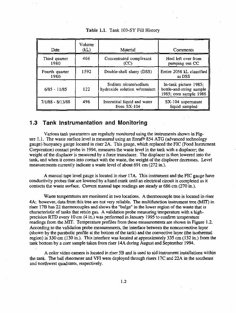
Table 1.1. Tank 103-SY Fill History

Date Volume

(kL) Material Comments

Third quarter 1980

466 Concentrated complexant (CC)

Heel left over from pumping out CC

Fourth quarter 1980

1592 Double-shell slurry (DSS) Entire 2058 kL classified as DSS

6/85- 11/85 122 Sodium nitrate/sodium

hydroxide solution w/uranium In-tank picture 1985;

bottle-and-string sample 1985; core sample 1986

7/1/88 - 8/13/88 496 Interstitial liquid and water from SX-104

SX-104 supernatant liquid sampled

1.3 Tank Instrumentation and Monitoring Various tank parameters are regularly monitored using the instruments shown in Fig­

ure 1.1. The waste surface level is measured using an Enraf® 854 ATG (advanced technology gauge) buoyancy gauge located in riser 2A. This gauge, which replaced the FIC (Food Instrument Corporation) contact probe in 1994, measures the waste level in the tank with a displacer; the weight of the displacer is measured by a force transducer. The displacer is then lowered into the tank, and when it comes into contact with the waste, the weight of the displacer decreases. Level measurements currently indicate a waste level of about 691 cm (272 in.).

A manual tape level gauge is located in riser 17A. This instrument and the FIC gauge have conductivity probes that are lowered by a hand crank until an electrical circuit is completed as it contacts the waste surface. Current manual tape readings are steady at 686 cm (270 in.).

Waste temperatures are monitored in two locations. A thermocouple tree is located in riser 4A; however, data from this tree are not very reliable. The multifunction instrument tree (MIT) in riser 17B has 22 thermocouples and shows the "bulge" in the lower region of the waste that is characteristic of tanks that retain gas. A validation probe measuring temperature with a high-precision RTD every 10 cm (4 in.) was performed in January 1995 to confirm temperature readings from the MIT. Temperature profiles from these measurements are shown in Figure 1.2. According to the validation probe measurements, the interface between the nonconvective layer (shown by the parabolic profile at the bottom of the tank) and the convective layer (the isothermal region) is 330 cm (130 in.). This interface was located at approximately 335 cm (132 in.) from the tank bottom by a core sample taken from riser 14A during August and September 1994.

A color video camera is located in riser 5B and is used to aid instrument installations within the tank. The ball rheometer and VFI were deployed through risers 17C and 22A in the southeast and northwest quadrants, respectively.

1.2

Tank 241-SY-103

Figure 1.1. SY-103 Riser Map

A standard hydrogen monitoring system (SHMS) was installed in the vent header in late June 1994. Hydrogen in the exhaust gas is detected with two Whittaker cells, which rely on the reaction of the gas with an electrode in an electrolyte. One cell has a range of 0-1%, and the other has a range of 0-10%. The cells are tested and calibrated quarterly.

1.4 GRE History

Between 1981 and mid-1985, when no large waste transfers occurred, waste surface level measurements with the FIC probe show a one- or two-inch level decrease about once a year. The shape of the cyclic variations is rounded, implying a slow accumulation and release of gas over periods of several days. Following the addition of uranium ion exchange wastes in 1985, the level decreases began to occur about three times per year. After adding the liquid from Tank SX-104 in 1988, the surface level fluctuations became even more frequent, occurring about every three months. The surface level fluctuations are now more "sawtooth" shaped, implying the more rapid release typical of a "rollover" event.

1.3

Temperature (F) 90 92 94 96 98 100

700 ~r—p—rjn—n—i !—i—P—r - -0- -17B MIT 7/14/95 ...#.... 4ATC Tree 7/9/95

I7B Val. Prb. 1/19/95

— 250

--200

150 .S

— 100 >

304 305 306 307 308 309 310 311 312 Temperature (K)

Figure 1.2. Recent Temperature Profiles

GREs have occurred about every three months since December 1994 (see Table 1.2). Baseline hydrogen concentrations have been about 100-200 ppm. The highest hydrogen concentration measured during the recent GREs was 0.294 vol% on May 2,1995.

Grab samples were taken from the SHMS cabinets to provide a baseline for the Whittaker cells. These samples were analyzed using a high-precision mass spectrometer at Pacific Northwest National Laboratory .(a) During the baseline period (August-September 1994), hydrogen concentrations in these grab samples ranged from 3 to 63 ppm. Nitrous oxide concentrations ranged from 4 to 39 ppm. Hydrogen to nitrous oxide ratios ranged from 0.3 to 5.5, similar to the ratios found in SY-101, which were about 1 at steady state before the mitigation pump was installed.

Two additional grab samples were taken during the gas release on March 2,1995. The hydrogen concentrations measured were 1070 and 1440 ppm, and the nitrous oxide concentrations were 630 and 900 ppm. The maximum hydrogen concentration measured during this release by the narrow range Whittaker cell (which measures hydrogen continuously) was 2230 ppm.

(a) Pacific Northwest National Laboratory is operated by Battelle for the U.S. Department of Energy under Contract DE-AC06-76RLO 1830.

1.4

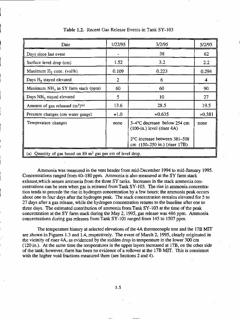
Table 1.2. Recent Gas Release Events in Tank SY-103

Date 1/22/95 3/2/95 5/2/95

Days since last event - 38 62

Surface level drop (cm) 1.52 3.2 2.2

Maximum H2 cone. (vol%) 0.109 0.223 0.294

Days H 2 stayed elevated 2 6 4

Maximum NH3 in SY farm stack (ppm) 60 60 90

Days NH3 stayed elevated 5 10 27

Amount of gas released (m3)<a) 13.6 28.5 19.5

Pressure changes (cm water gauge) +1.0 +0.635 +0.381

Temperature changes none 3-4°C decrease below 254 cm (100-in.) level (riser 4A)

2°C increase between 381-508 cm (150-250 in.) (riser 17B)

none

(a) Quantity of gas based on 89 m3 gas per cm of level drop.

Ammonia was measured in the vent header from mid-December 1994 to mid-January 1995. Concentrations ranged from 40-180 ppm. Ammonia is also measured at the SY farm stack exhaust,which senses ammonia from the three S Y tanks. Increases in the stack ammonia con­centrations can be seen when gas is released from Tank SY-103. The rise in ammonia concentra­tion tends to precede the rise in hydrogen concentration by a few hours; the ammonia peak occurs about one to four days after the hydrogen peak. The stack concentration remains elevated for 5 to 27 days after a gas release, while the hydrogen concentration returns to the baseline after one to three days. The estimated contribution of ammonia from Tank SY-103 at the time of the peak concentration at the SY farm stack during the May 2,1995, gas release was 486 ppm. Ammonia concentrations during gas releases from Tank SY-101 ranged from 145 to 1507 ppm.

The temperature history at selected elevations of the 4A thermocouple tree and the 17B MIT are shown in Figures 1.3 and 1.4, respectively. The event of March 2,1995, clearly originated in the vicinity of riser 4A, as evidenced by the sudden drop in temperature in the lower 300 cm (120 in.). At the same time the temperatures in the upper layers increased at 17B, on the other side of the tank; however, there has been no evidence of a rollover at the 17B MIT. This is consistent with the higher void fractions measured there (see Sections 2 and 4).

1.5

312

310 g IB 308

i % 306 H

304 -

302

~ i — i — i 1 — i — i — i — I — r

Nonconvective layer

Convective layer

i i i , i , • L

100

96 fe o t - i

S (53 92 pe

r

£ <o H 88

84 >o <n i n >n >n

995

995 ON o\ o\ ON ON

995

995

ON 0 \ ON ON ON 995

995

995

995

~^ • > * . O r» r~- • * <N § j ^ -t S ^ • 4 ^ H 1 — < ^ • H § j ^ -

?3 m ^ IO NO r-

Figure 1.3. Temperature History at Riser 4A

312

310

308 i | 306

304

302 ON

O N

C5

\ \

p _ ^ _ i i i T5

. ^ -^sus^Ci *"•""" Convective .

layer

88

84 ON ON

>n ON ON

f?5

«n ON ON

«n ON ON

«n

>n ON ON

NO

ON ON

Figure 1.4. Temperature History at Riser 17B

1.6

2.0 Stored Gas Volume

The best estimates for the void fraction in the nonconvective layer and the volume of stored gas in Tank 241-SY-103 are as follows:

Average void fraction 0.069 ± 0.014 (17C: 0.047 ± 0.015, 22A: 0.091 ± 0.015) Gas in sludge (1 atm) 177 ± 37 m3 (6,260 ± 1,300 SCF) Gas in crust (1 atm) 36±19m3 (1,270 ±700 SCF) • Total standard gas volume 213 ± 42 m3 (7,500 ± 1,500 SCF) Total in situ gas volume 131±28m3 (4,600 ± 980 ft3) Degassed level 659 ± 10 cm (260 ± 4 in.) Average release fraction 0.1 ±0.03

These volumes are based on the recent results from the void fraction instrument (VFI) and ball rheometer in risers 17C and 22A, temperature profiles from the MIT in riser 17B and the thermo­couple tree in riser 4A, and current estimates of waste properties.

The details of the calculations and assumptions leading to these estimates are described in this section. Except where specifically noted, the numerical uncertainty values given represent one standard deviation. Linear error propagation is used to combine uncertainties. The standard deviation, o y of a variable, y, that is computed as a function of N others, y = f (xj, X2,... XN), is determined by

! N r a f T 2

(2.1)

where Oj is the standard deviation of the variable Xj.

2.1 Waste Configuration

We need to establish the dimensions of the gas-bearing layers in the waste in order to com­pute the stored gas volume and potential releases. The most important of these is the nonconvec­tive sludge layer, because it contains most of the gas and is the source of GREs. The crust layer is much thinner and covers a smaller fraction of the waste surface than in SY-101, but it potentially contains a significant volume of gas and might contribute to releases if surface motion is suf­ficiently strong to disrupt the crust.

There is considerable uncertainty in quantifying the waste configuration in Tank" SY-103 because of its spatial and temporal variability. No steady state exists for the waste. Gas release events of various sizes (all considerably smaller than those in SY-101 prior to mitigation) have occurred about every three months and release some of the stored gas in the participating portion of the tank, leaving the rest of the waste relatively unaffected. Gas accumulates between GREs, causing the void fraction and dimensions of the waste layers to grow.

2.1

Waste configuration data are available at only a few specific points. The VFI and ball rheometer deployments in each of the two risers represent separate snapshots of the state of the waste at two locations. The two temperature profiles from risers 17B and 4A provide information on waste layer thickness at two more points. The core sample data at riser 14A add one more. We must assume that these data apply, on the average, to the entire tank, or we must partition the waste into different regions with specific properties and estimate the fraction of the total composing each region.

The information available to define the thickness of the nonconvective layer is summarized in Table 2.1. The data provide measurements from five different locations in the northwest and southeast quadrants of the tank (see Figure 1.1). These data imply a fairly uniform sludge layer height, and we will assume that is the case. The average and standard deviation of all the measure­ments is 335+ 17 cm.

The ball rheometer data also indicate a heel layer of 120-135 cm (47-53 in.) thickness on the tank bottom. Even though it has a higher strength, there is no evidence that this layer holds any more or less gas than the nonconvective material above it. It apparently participates to full depth in rollovers, as evidenced by the temperature change shown on the thermocouple tree in riser 4A for the March GRE in Figure 1.3.

It may be useful to compare the measured void fractions with the neutral buoyancy void fraction to estimate the potential for a local rollover. The void fraction required for neutral buoyancy in the nonconvective layer is determined by

PCL a N B = 1 - - ^ - (2.2) PNCL

where PCL and p N C L are the average densities of the convective and nonconvective layers, respectively. This is actually the incremental void fraction required for neutral buoyancy rather than an absolute value because the sludge density measurements include some relatively small unknown fraction of "unreleasable" gas (Stewart et al. 1994).

Table 2.1. Data on Nonconvective Layer Thickness for SY-103

Measurement Riser Date Height

MIT temperature profile (Fig. 1.2) MIT validation probe (Fig. 1.2) TC tree profile (Fig. 1.2) Core sample (Section 1) Ball rheometer force versus depth (Fig. 3.2) VFI non-zero void (Fig. 4.4) VFI non-zero void (Fig. 4.4)

17B 7/14/95 375 cm 17B 1/19/95 330 cm 4A 7/9/95 - 327 cm 14A 9/94 335 cm 22A 8/8/95 325 cm 17C 7/19/95 330 cm 22A 8/18/95 342 cm

2.2

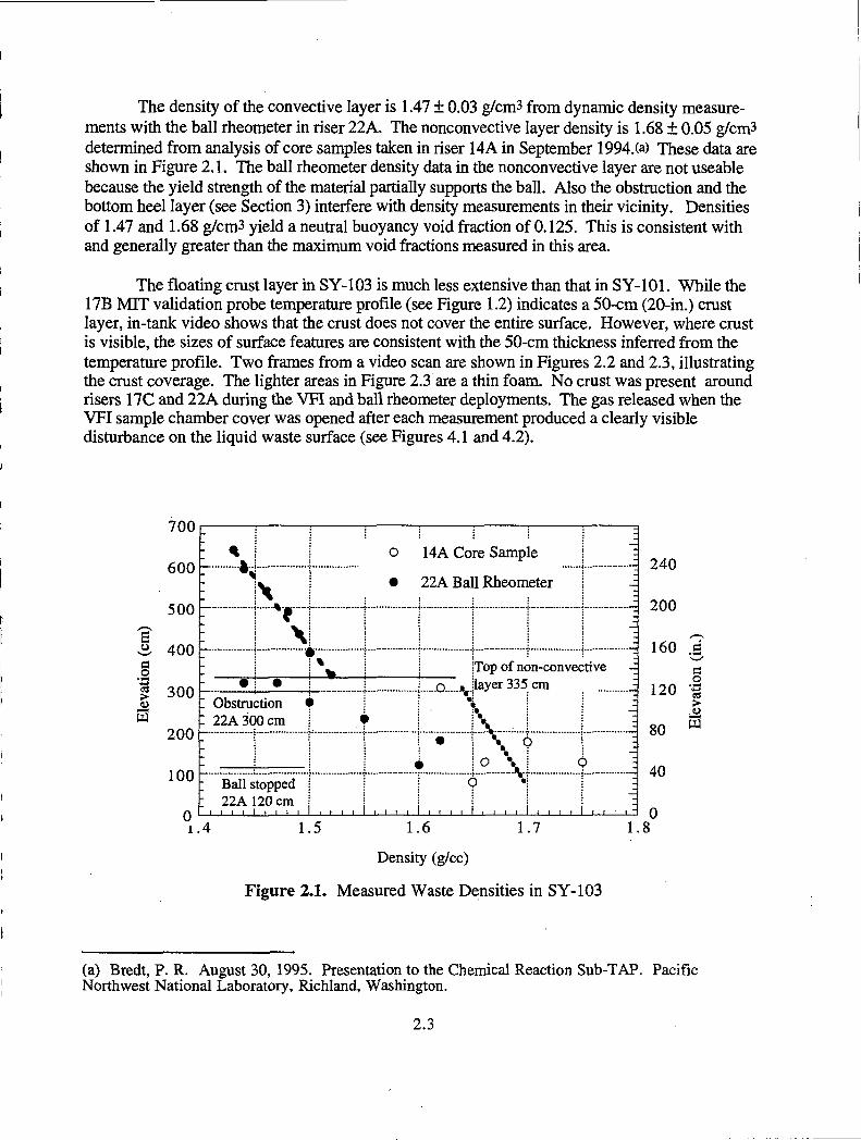
The density of the convective layer is 1.47 ± 0.03 g/cm3 from dynamic density measure­ments with the ball rheometer in riser 22A. The nonconvective layer density is 1.68 ± 0.05 g/cm3 determined from analysis of core samples taken in riser 14A in September 1994.(a) These data are shown in Figure 2.1. The ball rheometer density data in the nonconvective layer are not useable because the yield strength of the material partially supports the ball. Also the obstruction and the bottom heel layer (see Section 3) interfere with density measurements in their vicinity. Densities of 1.47 and 1.68 g/cm3 yield a neutral buoyancy void fraction of 0.125. This is consistent with and generally greater than the maximum void fractions measured in this area.

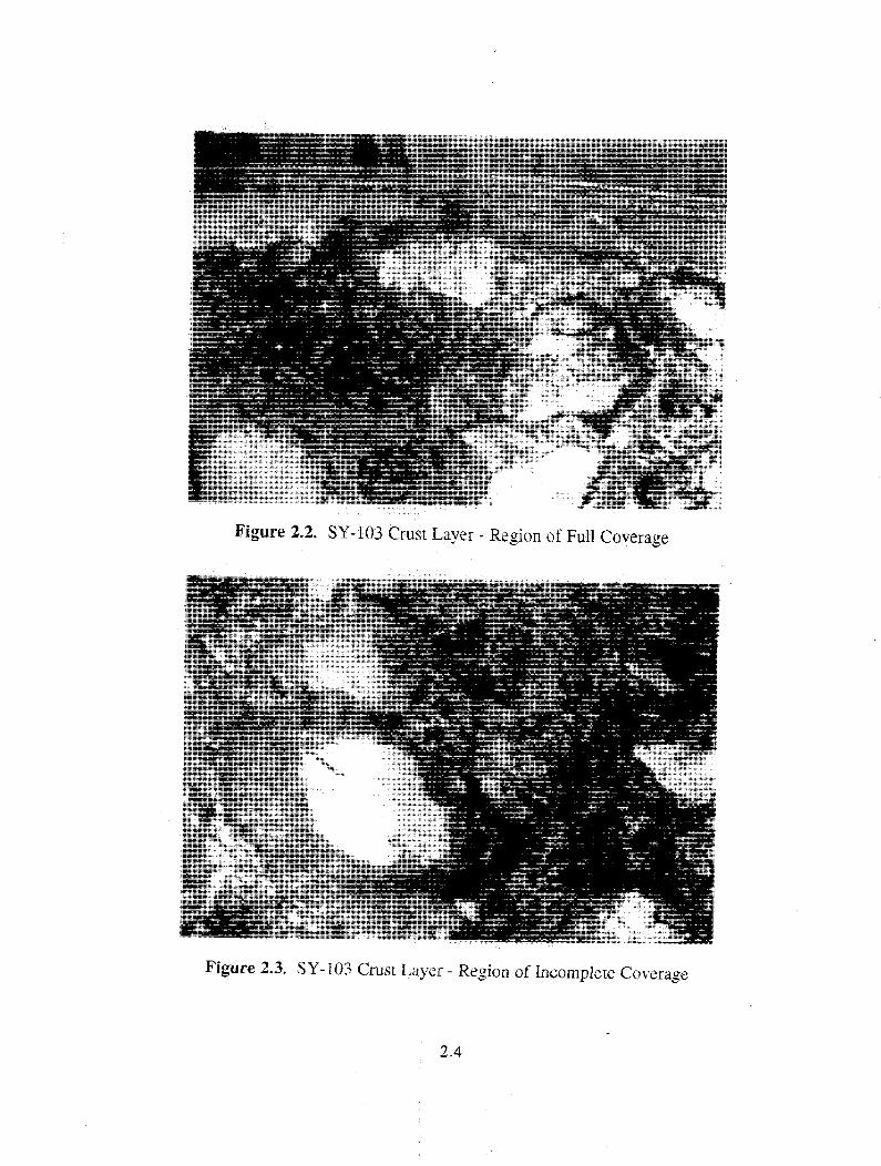
The floating crust layer in SY-103 is much less extensive than that in SY-101. While the 17B MTT validation probe temperature profile (see Figure 1.2) indicates a 50-cm (20-in.) crust layer, in-tank video shows that the crust does not cover the entire surface. However, where crust is visible, the sizes of surface features are consistent with the 50-cm thickness inferred from the temperature profile. Two frames from a video scan are shown in Figures 2.2 and 2.3, illustrating the crust coverage. The lighter areas in Figure 2.3 are a thin foam. No crust was present around risers 17C and 22A during the VFI and ball rheometer deployments. The gas released when the VFI sample chamber cover was opened after each measurement produced a clearly visible disturbance on the liquid waste surface (see Figures 4.1 and 4.2).

700

600

500 S & 400 a .2 | 300 55

200 -

i o o :

- - ( •>

*

o 14A Core Sample

• 22A Ball Rheometer • H = ;

£ -> * ( • !•

"I -M

ITop of non-convective • i • i......a...-vl l a>'e r 3 3 5 . c m

Obstruction • 22A 300 cm

i O

0 1.4

Ball stopped j 22A120cm j

J 1 I 1_1 I ' l ' l I I L_l l_l 1 I i

240

200

160 .5' S3

120 | >

80

40

m

1.5 1.7 1.6

Density (g/cc)

Figure 2.1. Measured Waste Densities in SY-103

1.8

(a) Bredt, P. R. August 30, 1995. Presentation to the Chemical Reaction Sub-TAP. Pacific Northwest National Laboratory, Richland, Washington.

2.3

• I " * " * ;

' * ^!' 4 v

/... Hv5_ ""*i Figure 2.2. SY-103 Crust Layer - Region of Full Coverage

Figure 2.3. SY-103 Crust Layer - Region of Incomplete Coverage

2.4

2.2 Void Fraction

The average void determined in Section 4.0 for risers 17C and 22A is 0.047 ± 0.015 and 0.091 ± 0.015, respectively. We believe that the void profiles at the two risers are sufficiently different that they represent different states of the waste. Thus we define the fraction of the waste volume that is characterized by the void profile measured in riser 22A as §22k- The average void fraction is then computed as

Since there is no way to measure or estimate ^ A mechanistically, let it be a random variable dis­tributed between zero and 1, with a mean and standard deviation of 0.5 ± 0.2. Though Equa­tion (2.3) degenerates to a simple average with this choice of <J>22A> it allows us to quantify the uncertainty of the waste configuration. Under this assumption, Equation (2.3) yields an average tank void fraction of 0.069 ± 0.014. However, the higher void fraction from riser 22A should be used in estimating the volume of potential gas releases because it probably represents conditions more likely to precede a rollover.

2.3 Gas Volume Calculation

The total volume of gas stored in the nonconvective layer, corrected to 1 atm, is expressed

H NC

by

VRET = A J a P d z ( 2 - 4 ) o

where A is the tank cross-sectional area, HNC is the height of the nonconvective layer, and P is the local pressure in atmospheres. Equation (2.4) can be approximated using the average void fraction and an effective pressure by

V ^ = A H ^ a ^ P ^ (2.5)

where aA v g is the average void fraction in the nonconvective layer, and Peff is the effective hydro­static pressure at which the gas is stored. Assuming a linear void distribution (a good approximation for the void profile in 17C and a slightly conservative one for 22A), performing the integration in Equation (2.4), and comparing it with Equation (2.5), we find the effective hydrostatic pressure is exactly the pressure at two-thirds the depth of the nonconvective layer, given by

Peff = 1 + - # - [ P C L ( H W - H N C) + } p N C H N C ] (2.6) r 0

2.5

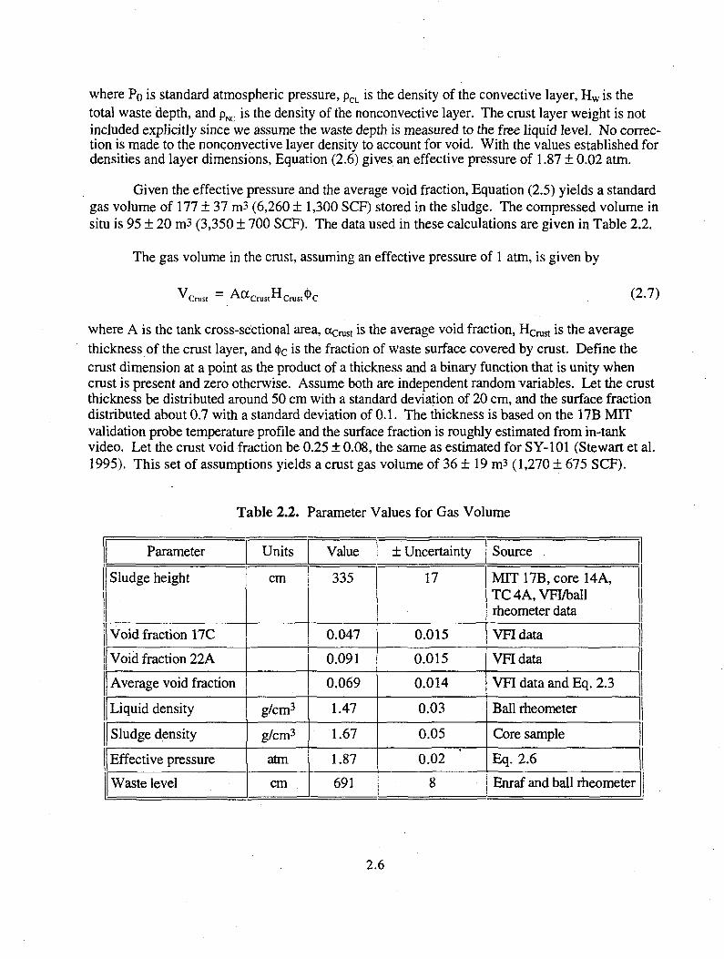
where Po is standard atmospheric pressure, pC L is the density of the convective layer, H w is the total waste depth, and pN C is the density of the nonconvective layer. The crust layer weight is not included explicitly since we assume the waste depth is measured to the free liquid level. No correc­tion is made to the nonconvective layer density to account for void. With the values established for densities and layer dimensions, Equation (2.6) gives an effective pressure of 1.87 ± 0.02 atm.

Given the effective pressure and the average void fraction, Equation (2.5) yields a standard gas volume of 177 ± 37 m3 (6,260 + 1,300 SCF) stored in the sludge. The compressed volume in situ is 95 ± 20 m3 (3,350 ± 700 SCF). The data used in these calculations are given in Table 2.2.

The gas volume in the crust, assuming an effective pressure of 1 atm, is given by

V C r u s , = Aa C r u s tH C r u s t( |> c (2.7)

where A is the tank cross-sectional area, a c ^ is the average void fraction, HC r Us t is the average thickness of the crust layer, and <)>c is the fraction of waste surface covered by crust. Define the crust dimension at a point as the product of a thickness and a binary function that is unity when crust is present and zero otherwise. Assume both are independent random variables. Let the crust thickness be distributed around 50 cm with a standard deviation of 20 cm, and the surface fraction distributed about 0.7 with a standard deviation of 0.1. The thickness is based on the 17B MIT validation probe temperature profile and the surface fraction is roughly estimated from in-tank video. Let the crust void fraction be 0.25 ± 0.08, the same as estimated for SY-101 (Stewart et al. 1995). This set of assumptions yields a crust gas volume of 36 ± 19 m3 (1,270 ± 675 SCF).

Table 2.2. Parameter Values for Gas Volume

Parameter Units Value ± Uncertainty Source

Sludge height cm 335 17 MIT 17B, core 14A, TC4A,VFI/ball rheometer data

Void fraction 17C 0.047 0.015 VFIdata

Void fraction 22A 0.091 0.015 VFIdata

Average void fraction 0.069 0.014 VFI data and Eq. 2.3

Liquid density g/cm3 1.47 0.03 Ball rheometer

Sludge density g/cm3 1.67 0.05 Core sample

Effective pressure atm 1.87 0.02 Eq. 2.6

Waste level cm 691 8 Enraf and ball rheometer

2.6

Summing up the gas content in the nonconvective layer and the crust, the total gas content in SY-103 as of August 1995 was 213 ± 42 m3 (7,500 ± 1,500 SCF). This is quite close to the 218 m3 (7,700 SCF) derived from the response of the waste level to barometric pressure varia­tion^3) The average pressure of the total gas content is about 1.6 atm. The equivalent waste level if all gas were removed ("degassed level") is computed from the compressed volume by

H n o g a s = H M - ^ (2.8)

where HM is the waste level corresponding to the time the gas volume was measured and Vjn sj^ is the compressed volume. Given the current waste level of 691 ± 8 cm (272 ± 3 in.) and an in situ volume of 131 ± 28 m3 (4,600 ± 980 ft3), the degassed level is 659 ± 10 cm (260 + 4 in.).

2.4 Estimated Gas Release Fractions

It is impossible for the entire free gas content of the waste to be released in a gas release event (GRE). Even if the entire volume of gas-bearing sludge participates, gas is released only until the sludge that has come to the surface returns below neutral buoyancy. Then the sludge and the gas still retained within it sinks back to the bottom of the tank. Also, bubbles smaller than approximately 100 microns in diameter attached to particles probably do not escape. Historically, this "unreleasable" gas fraction has been estimated at 6-8% void.

The actual fraction of the total retained gas volume released in each event represents the product of the fraction of sludge participating and the fraction of gas that is released from that sludge volume. This product is equal to the ratio of pre-GRE gas volume to the volume released. Since we have reasonably good estimates of the current total gas content in SY-103 the amount of gas stored in the waste prior to each historical GRE can be calculated from the waste level. No estimate of the effective pressure of the stored gas is necessary since the ratio of gas release to initial inventory is independent of pressure. The release fraction is calculated by

AH G R E

F r e ) = 7 5 _ u 7 (2-9) V n GRE n n o gas/

where AH G R E is the level drop, H G R E is the pre-GRE waste level, and H n o g a s is the degassed waste level from Equation (2.8).

(a) Private communication with J. D. Hopkins, WHC. August 1995. Also see Brewster et al.( 1995) for the theory and Screening the Hanford Tanks for Trapped Gas (Whitney 1995) for the data.

2.7

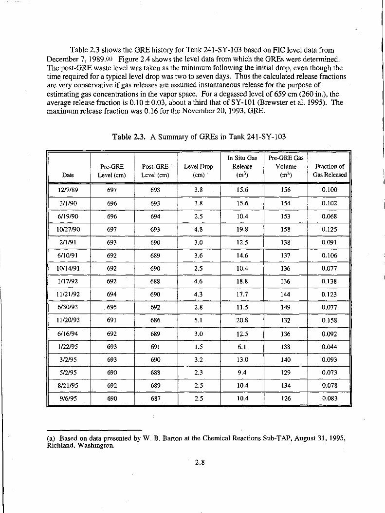
Table 2.3 shows the GRE history for Tank 241-SY-103 based on FIC level data from December 7, 1989.<a) Figure 2.4 shows the level data from which the GREs were determined. The post-GRE waste level was taken as the minimum following the initial drop, even though the time required for a typical level drop was two to seven days. Thus the calculated release fractions are very conservative if gas releases are assumed instantaneous release for the purpose of estimating gas concentrations in the vapor space. For a degassed level of 659 cm (260 in.), the average release fraction is 0.10 ± 0.03, about a third that of SY-101 (Brewster et al. 1995). The maximum release fraction was 0.16 for the November 20, 1993, GRE.

Table 2.3. A Summary of GREs in Tank 241-SY-103

Date Pre-GRE

Level (cm) Post-GRE Level (cm)

Level Drop (cm)

In Situ Gas Release

(m3)

Pre-GRE Gas Volume

(m3) Fraction of

Gas Released

12/7/89 697 693 3.8 15.6 156 0.100

3/1/90 696 693 3.8 15.6 154 0.102

6/19/90 696 694 2.5 10.4 153 0.068

10/27/90 697 693 4.8 19.8 158 0.125

2/1/91 693 690 3.0 12.5 138 0.091

6/10/91 692 689 3.6 14.6 137 0.106

10/14/91 692 690 2.5 10.4 136 0.077

1/17/92 692 688 4.6 18.8 136 0.138

11/21/92 694 690 4.3 17.7 144 0.123

6/30/93 695 692 2.8 11.5 149 0.077

11/20/93 691 686 5.1 20.8 132 0.158

6/16/94 692 689 3.0 12.5 136 0.092

1/22/95 693 691 1.5 6.1 138 0.044

3/2/95 693 690 3.2 13.0 140 0.093

5/2/95 690 688 2.3 9.4 129 0.073

8/21/95 692 689 2.5 10.4 134 0.078

9/6/95 690 687 2.5 10.4 126 0.083

(a) Based on data presented by W. B. Barton at the Chemical Reactions Sub-TAP, August 31, 1995, Richland, Washington.

2.8

7 0 5 ^

680 - -268

ov o _* <N en Tf »T> 00 ON OS ON ON ON ON ON Os Ov ON ON ON ON w « ^ ^ H T-M 1—4 ^ H *-M

--*. v-> w-> >o ^ Tf rf Tf 1—1 •— ^ H f H ^_4 V-H ^ M

ON ON ON ON ON ON ON

Figure 2.4. Waste Level History of Tank 241-SY-103

2.5 Statistical Estimate of Gas Volume

An alternative method of computing the average void from the VH measurements is using a statistical procedure called analysis of variance (ANOVA) with a model that captures the major sources of uncertainty. One advantage of the ANOVA procedure for void fraction estimation is that the underlying assumptions on the void fraction distribution are less restricted than those made by the curve-fitting procedure described in Sections 2.2 and 4.2. The latter assumes that the void fraction has a linear relationship with the depth in tank. The only assumptions behind the ANOVA model, on the other hand, are 1) the void fraction varies horizontally in the tank with a certain standard deviation; and 2) the mean void fractions of defined vertical layers may be different, but the vertical variation of the void fraction within each layer is negligible.

The model for applying the analysis of variance procedure was based on the void measurement process. The model has the form

Oijk = a Av g + Ri + Dj + RD y + e i j k (2.10)

i

2.9

where ocAvg = the mean void fraction in the tank Rj = deviation of the void fraction at riser i from the mean (horizontal variability),

i = 1 and 2 (representing riser 13A and riser 1C) Dk = the effect of kth elevation, k = 1,2, and 3 (see discussion below) RDjk = the void fraction deviation at riser i and elevation k from the mean ejj k = sampling and instrument error.

Each term in the model describes a step in the measurement process. All terms except the mean void itself and the effect of layer, D, have a zero mean and represent deviation from the mean. Deviation due to interaction of riser and elevation is included in the term RD.

The nonconvective portion of the tank was split into three layers with boundaries (in cm) of (0, 100), (100, 200), and (200, 335), respectively. The integers 1, 2, and 3 each represent one of the three layers in the model. The number and thickness of layers is rather arbitrary but should yield a fairly uniform vertical void distribution within the layer. The ANOVA model emphasizes predicting the mean void fraction in each layer of a tank. For estimating the total gas volume stored in a tank, this is more important than predicting the exact void fraction at a particular point in a tank.

With this model, the mean void fraction and its uncertainty estimate can be obtained for each of the three layers. The uncertainty due to traverse can be estimated using the model as well. Similar models have been used for estimating chemical contents of tanks from core sampling data, which have a sampling structure similar to the void fraction profile measures (Hartley et al. 1995; Remund et al. 1994).

The gas volume stored in each layer and its uncertainty value can be calculated by a method similar to that described in Section 2.3. The in situ volume is simply the product of the layer void fraction and the total layer volume. An effective pressure for each layer is calculated using a slightly modified form of Equation (2.6), and the standard volume of each layer is computed as the product of the in situ volume and effective pressure. The total volume of gas in the nonconvective waste is then the sum of the gas volumes in the three layers.

The MIXED procedure of SAS, a statistical software package (SAS 1992), was used to estimate the effects and deviations of the model in Equation (2.10) from the void data. The uncertainty due to riser R was estimated as 2.78%, which is the local horizontal uncertainty in Tank SY-103. The deviation due to the interaction of riser and elevation, RD, was 1.42%. The deviation due to sampling and instrument error was 2.11%, which means that the standard deviation of a single void measurement is on the order of 3.8%. However, the deviation of the average in each layer is less, around 2.3%, because there are many data points in the average.

The mean void fraction of the top layer is significantly different from the other two, but there is not enough evidence to show a significant difference between the bottom two. The estimates of mean void fraction and its uncertainty and the gas volume calculations for each defined

2.10

layer are given in Table 2.4. The total standard gas volume in the nonconvective layer is estimated at 154.6 ± 47 m3 (5,500 ± 1,660 SCF). Multiplying by the assigned sampling error correction of 1.1 ± 0.04 gives a total volume of 170 ± 52 m3 (6,000 ± 1,830 SCF). This is about 96% of the gas volume estimated for the sludge in Section 2.3 with a slightly higher uncertainty.

Table 2.4. Estimates of Mean Void Fraction and Uncertainty

Elevation (cm)

Mean Void (%)

In Situ Volume (m3)

Pressure (atm)

Standard Volume (m3)

0-100 9.05 ± 2.28 37.2 ± 9.4 2.00 ± 0.021 74.2 ± 18.7

100-200 7.74 ± 2.25 31.8 ±9.2 1.83 ±0.018 58.3 ± 17.0

200 - 335 2.41 ± 2.29 13.4 ± 12.7 1.65 ±0,016 22.1 ±21.0

Total/average 6.02 ± 2.08 82.8 ± 28.6 1.87 ±0.020 154.6 ± 47

2.11

3.0 Rheological Properties

The ball rheometer was deployed twice in Tank 241-SY-103; the first deployment was in riser 17C on July 14,1995, and the second in riser 22A on August 8,1995. Approximately 180 different tests were performed in riser 17C and 140 tests in riser 22A. The measurement proce­dures were essentially the same for each riser, and no distinction will be made between specific risers in this discussion. However, there were differences in the conditions found for each riser and in the observations made in each, and these differences will be pointed out below.

3.1 Test Procedure and Observations After water lancing was completed to ensure there would be no obstruction to passing

through the crust, the ball rheometer assembly was mounted onto the riser, and the ball was lowered into the tank dome space. A 2225-N (500-lb) load cell was used initially in both risers in case difficulties were encountered in lowering the ball through the riser. In-tank video showed that riser 17C was not vertical, and the ball swung to one side upon exiting this riser into the dome space. It also became evident that the cable rubbed on the riser opening whenever the ball was moved. In attempting to retrieve the ball back into the riser from the dome space, the ball caught momentarily on the riser lip before rolling up and into the riser, increasing the cable tension to several hundred Newtons. For this reason we retained the 2225-N (500-lb) load cell for all experiments in riser 17C rather than switching to a lower-range load cell with greater measurement precision. Riser 22A was sufficiently close to vertical that the cable did not rub on the riser opening, and retrieval back into the riser showed no significant increase in cable tension. For this riser we immediately retrieved the ball back into its enclosure and switched to the 445-N (100-lb) load cell. All experiments in riser 22A used this load cell, and the resulting data were considerably more accurate and precise than obtained in 17C.

Once the ball was lowered into the dome space, we performed measurements to determine pulley friction at all of the velocities of interest for the tests (0.1, 1.0, 3.0, 5.0, 10.0, 30.0, 50.0, and 100 cm/s). Static measurements (stationary ball) were also made of the ball and cable weight at several positions in the dome space to determine the reference ball and cable weight at the waste surface. These combined measurements showed a pronounced asymmetry in the pulley friction in riser 17C, which, as mentioned above, was not vertical. In addition, the pulley friction was somewhat larger for this riser. Both of these facts support the conclusion that the cable rubbed against the riser lip, and the pulley friction measured here included the cable friction with the riser opening. It was not possible to eliminate this difficulty in the field, and we continued testing. While we believe that the data obtained in riser 17C are still useful and valuable, the data gathered through riser 22A are, without question, more reliable and precise.

After these tests were completed, the ball was lowered into the waste. No crust was observed on the waste in the vicinity of the ball entry point. The waste surface was 1038 cm below the "home" position of the ball (fully retracted into the rheometer enclosure), which is

3.1

determined to be the midpoint of the zone where the force decreases as the ball enters the waste less one ball radius (4.55 cm), as shown in Figure 3.1. Tank bottom is expected to be at 1726 cm below home position, based on data from the SY-101 deployment. But, since the ball position reference is its center, we must add one ball radius (4.55 cm) to correctly reference the tank bottom. This makes the liquid level 1726 - 1038 + 4.55 = 692.5 cm (272.6 in.), which closely matches the 691 cm (272 in.) level measured by the Enraf buoyancy gauge in riser 22A. Here­after, ball position will refer to the elevation of the ball center above the tank bottom.

The first series of tests involved dropping the ball at 3 cm/s all the way to the tank bottom or until the ball stopped. Drag on the ball began to increase as it encountered an interface in the waste at about the 325 cm (128 in.) elevation, or about 366 cm (144 in.) below the liquid surface. The drag continued to increase with depth, and the ball finally became fully supported (stopped) at about 120 cm above the expected location of the tank bottom. Since drag increased steadily with depth, the upper part of this layer may be mostly fluid with low particle concentration, while the bottom portion contains an increasing fraction of settled solids.

In riser 22A, disturbances at the waste surface were observed on video when the ball passed into the settled layer. It is believed that gas bubbles were being released. Bubbling occurred throughout the experiment, even when the ball was back in the liquid layer. However, the major release appeared to occur on the initial passage of the ball through the settled layer, and only minor and sporadic bubbling was observed later in these tests.

o

72

70

68

66

64

62

60

58

56

17C (2225 N load cell)

22A (445 N load cell)

Liquid level: 1038.0 cm

Midpoint (22A): 1042.5 cm

1035 1040 1045 Depth below home position (cm)

1050

Figure 3.1. Ball Passing the Liquid Level

3.2

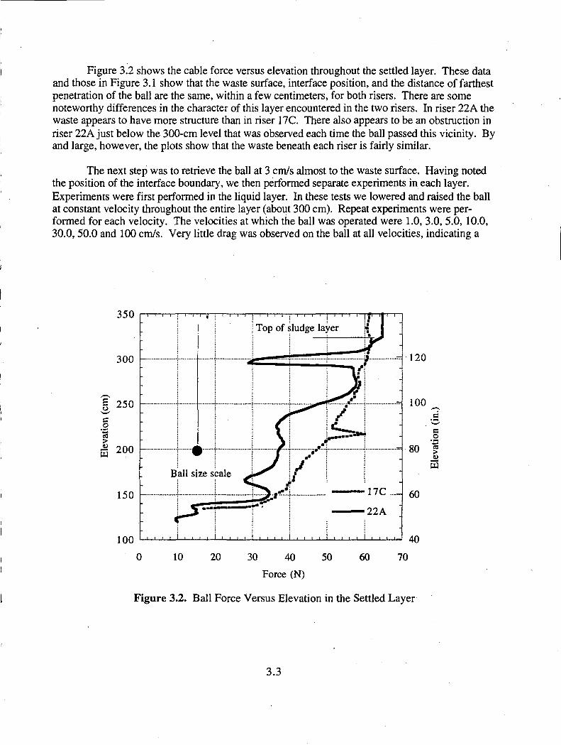
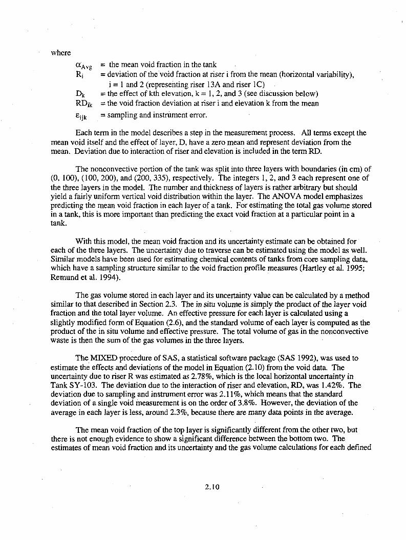
Figure 3.2 shows the cable force versus elevation throughout the settled layer. These data and those in Figure 3.1 show that the waste surface, interface position, and the distance of farthest penetration of the ball are the same, within a few centimeters, for both risers. There are some noteworthy differences in the character of this layer encountered in the two risers. In riser 22A the waste appears to have more structure than in riser 17C. There also appears to be an obstruction in riser 22A just below the 300-cm level that was observed each time the ball passed this vicinity. By and large, however, the plots show that the waste beneath each riser is fairly similar.

The next step was to retrieve the ball at 3 cm/s almost to the waste surface. Having noted the position of the interface boundary, we then performed separate experiments in each layer. Experiments were first performed in the liquid layer. In these tests we lowered and raised the ball at constant velocity throughout the entire layer (about 300 cm). Repeat experiments were per­formed for each velocity. The velocities at which the ball was operated were 1.0, 3.0, 5.0,10.0, 30.0,50.0 and 100 cm/s. Very little drag was observed on the ball at all velocities, indicating a

350

300

I 250 ^^ c o

I 2 0 °

150

100

j—|—i—i—i—I—|—i—i—i—i—j—i—i—;—i—]—i—i—i—i—p»i—r|-T—r

60

_J i i I i i i i I i i I_J I i i i ' I i i ' i I i i i i I i i i i_j 4 0

10 20 30 40 50 60 70 Force (N)

120

100

> E

Figure 3.2. Ball Force Versus Elevation in the Settled Layer

3.3

fluid of relatively low viscosity. When measurements were completed in the liquid layer the ball was lowered to just above the interface location, and the same experiments were performed in the settled layer (about 220 cm accessible thickness), except that falling ball experiments were not performed at 30,50, and 100 cm/s. Also, some measurements were performed over limited regions in the settled layer at 0.1 cm/s velocity. Interspersed among the constant velocity tests were static tests in which the cable tension was measured with the ball at rest in the fluid. These measurements allow the waste density to be determined. Density measurements were obtained at roughly 50-cm intervals throughout the waste.

3.2 Density Measurements The density of the waste was determined with the ball rheometer by measuring the apparent

weight of the stationary ball and comparing this value with the reference weight of the ball just above the waste surface. The difference is due to the buoyancy force exerted on the ball by the fluid, and this force is proportional to the fluid density. Effects of cable weight and buoyancy were included in these calculations. Density measurements were performed in both risers; how­ever, the results obtained in riser 22A are more reliable because we used the more precise 445-N (100-lb) load cell. The force measurement uncertainty for the 2,225-N (500-lb) load cell is about 1.0 N, while the uncertainty in the 445-N (100-lb) load cell is about 0.2 N.

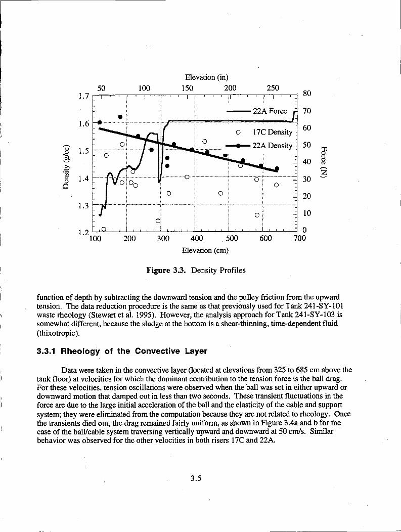
The density profiles for both risers are shown in Figure 3.3. For riser 17C we obtained a density of 1.4 ± 0.2 g/cm3 that did not appear to change with depth. For riser 22A the density appears to increase nearly linearly with depth, starting at 1.4 ± 0.05 g/cm3 near the surface and ending at 1.6 ± 0.05 g/cm3 near the bottom. Within measurement error the two plots are consis­tent, and the data obtained in riser 22A should be used as a more reliable indicator of the waste density.

In the settled layer density measurements might be affected by the material yield strength, which is not accounted for in the calculation. For this reason, density measurements in this region were performed near the end of testing, after the fluid had been well sheared. The measurement procedure is to oscillate the ball several times in the measurement region prior to making measure­ments with a stationary ball; this procedure is followed in order to shear the fluid in the vicinity of the ball and thereby relieve stresses on the ball due to the fluid. The densities reported here probably do not represent the densities of the undisturbed fluid, however, except in the liquid layer. In particular, if gas is released due to passage of the ball through the settled layer, then the measured density probably overestimates the undisturbed waste density.

3.3 Rheological Properties

The analysis strategy developed to infer the rheological properties of the waste in Tank SY-103 from the drag data was devised from the test procedure described in Section 3.1 accommodating the peculiarities of the data as a function of depth and velocity. The upward and downward tension measurements at various velocities were partitioned into ball and cable drag as a

3.4

Elevation (in) 150 200 250

100 200 300 400 500 Elevation (cm)

600 700

21

•-t o

Figure 3.3. Density Profiles

function of depth by subtracting the downward tension and the pulley friction from the upward tension. The data reduction procedure is the same as that previously used for Tank 241-SY-101 waste rheology (Stewart et al. 1995). However, the analysis approach for Tank 241-SY-103 is somewhat different, because the sludge at the bottom is a shear-thinning, time-dependent fluid (thixotropic).

3.3.1 Rheology of the Convective Layer

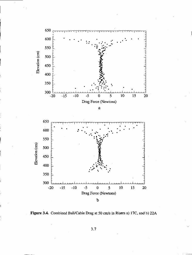
Data were taken in the convective layer (located at elevations from 325 to 685 cm above the tank floor) at velocities for which the dominant contribution to the tension force is the ball drag. For these velocities, tension oscillations were observed when the ball was set in either upward or downward motion that damped out in less than two seconds. These transient fluctuations in the force are due to the large initial acceleration of the ball and the elasticity of the cable and support system; they were eliminated from the computation because they are not related to rheology. Once the transients died out, the drag remained fairly uniform, as shown in Figure 3.4a and b for the case of the ball/cable system traversing vertically upward and downward at 50 cm/s. Similar behavior was observed for the other velocities in both risers 17C and 22A.

3.5

The data set taken at 50 cm/s in riser 22A was the most reliable, because it showed the smallest standard error (after the fluctuations were eliminated) of all the high-velocity data and because it was obtained with the 100-lb load cell. The apparent viscosity was calculated by using the average value of the combined ball/cable drag force, DBc, at each velocity and then solving for the viscosity, \i, from the equation for the balance of viscous forces. As discussed in detail in Stewart et al. (1995), this balance of forces can be written as

D B C = <FC> + FB (3-D

where ( F c ) is the average force that the fluid exerts on the cable after the completion of an up/down cyclic measurement, and F B is the drag on the ball. Both of these forces are proportional to the cable and ball drag coefficients, CDC and C D B , respectively. C D B is given by the empirical correlation

^ D B : 2.25 Re; 0 ' 3 1 + 0.36 Re°' 0 6 (3.2)

where Ree is the ball Reynolds number based on the ball diameter. The cable drag coefficient is different from that used in the SY-101 analysis because the traversing distance in SY-103 is 3.6 m, not 1 m as it was in experiments performed in the liquid layer in SY-101. By using the analytic expression for the drag on the cable and following the numerical procedure outlined in Stewart et al. (1995), the cable drag coefficient for the present case is

C D C=0.5547 R e " 0 7 7 0 1 (3.3)

where Rec is the cable Reynolds number based on the cable radius.

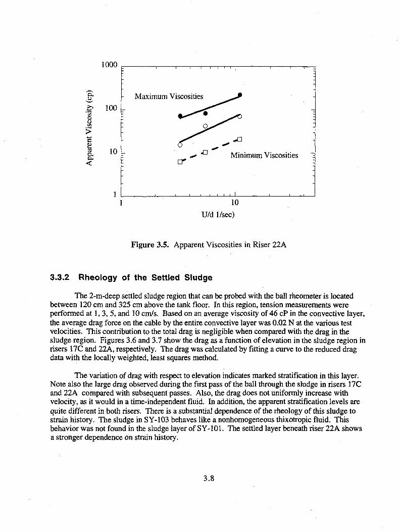
Upon substitution of Equation (3.3) and (3.2) into Equation (3.1), the resulting nonlinear equation in the apparent viscosity can be solved numerically by the Newton-Raphson iteration method. The results are shown graphically in Figure 3.5 for the data obtained from riser 22A. The data suggest that the fluid is shear-thickening over a limited range of velocity measurements between 30 and 100 cm/s. However, one must bear in mind that this range of velocities yields a very limited range of strain rates and that the standard deviation of the drag measurements is different for each velocity. There are fairly large uncertainties in the viscosity values (about a factor of 2) at these low values. Also, within experimental error, the data are consistent with a Newtonian fluid or even a shear-thinning one. The apparent average viscosity over this range is 46 cP. This value is consistent with the calculated apparent viscosity (at 50 cm/s) of 46.2 cP from data obtained from riser 17C. The drag data for the other two velocities do not seem to be very reliable because, in one case, the standard deviation is larger than me average even after the transient oscillations are removed.

3.6

650 600

550

(cm

)

500

/atio

n

450

Eto

400

350 i

300

-i—n—i—i—i—n~ ~i i i t i i i t | i i t i | i i r~

• •• • ••

i t i i i i i r

t i

I I [ I I I I I—L. - I L_J i i t i I i i i i I i i i i I t • -L -20 -15 -10 -5 0 5 10 15 20

Drag Force (Newtons) a

650

600 -

550

J, 500 c '•§ 450 > " 400 L

350 L

300

1 1

• i 1 i i i

• • i i i t i i i i i i I i i i i I i i

» / * . ' * • • • • *

V;*

• •

i i

| I'T

T'T

[

T 1

1 1

| 1

1 1

1 • •• •. *• .

•n-r

-p

i i i | i i i I |

t t i 1 i i i 1 1 1 1 1 1 1 1 1 1 1 1 1 1 > i 1 1 • i 1 i i i i 1 i i

i t

I

-20 -15 -10 -5 0 5 10 15 Drag Force (Newtons)

b

20

Figure 3.4. Combined Ball/Cable Drag at 50 cm/s in Risers a) 17C, and b) 22A

3.7

1000

a, o £> 100 C/3 o o

c 1 O H a, 10

-| i T 1 1—i—r

Maximum Viscosities

JO

Minimum Viscosities

_i i i i i i_

10 U/d 1/sec)

Figure 3.5. Apparent Viscosities in Riser 22A

3.3.2 Rheology of the Settled Sludge

The 2-m-deep settled sludge region that can be probed with the ball rheometer is located between 120 cm and 325 cm above the tank floor. In this region, tension measurements were performed at 1,3,5, and 10 cm/s. Based on an average viscosity of 46 cP in the convective layer, the average drag force on the cable by the entire convective layer was 0.02 N at the various test velocities. This contribution to the total drag is negligible when compared with the drag in the sludge region. Figures 3.6 and 3.7 show the drag as a function of elevation in the sludge region in risers 17C and 22A, respectively. The drag was calculated by fitting a curve to the reduced drag data with the locally weighted, least squares method.

The variation of drag with respect to elevation indicates marked stratification in this layer. Note also the large drag observed during the first pass of the ball through the sludge in risers 17C and 22A compared with subsequent passes. Also, the drag does not uniformly increase with velocity, as it would in a time-independent fluid. In addition, the apparent stratification levels are quite different in both risers. There is a substantial dependence of the rheology of this sludge to strain history. The sludge in SY-103 behaves like a nonhomogeneous thixotropic fluid. This behavior was not found in the sludge layer of SY-101. The settled layer beneath riser 22A shows a stronger dependence on strain history.

3.8

300

250

200 -

150

100 1 10 100

Drag Force (Newtons)

Figure 3.6. Combined Ball/Cable Drag from Riser 17C

300

250

200

150

100

- i 1 — i — i — i — r 1 ^ r -i 1 1 — ! — i — i — r

•e— First Pass at 3 cm/sec

B - - lcm/sec *— 3cm/sec o--- 5cm/sec * — lOcm/sec

_i i i_ _i I I I L

1 10 100

Drag Force (Newtons)

Figure 3.7. Combined Ball/Cable Drag from Riser 22A

3.9

A complete rheological characterization of these kinds of fluids is quite involved even for nonradioactive samples tested in the laboratory with a high-precision rheometer. The main difficulty encountered in characterizing thixotropic behavior using the ball rheometer is the disturbance of the sludge microstructure by the traversing ball. Once the ball has passed through the sludge layer, all subsequent measurements will depend on the strain that the ball imposed on this pass. This situation has led us to modify the procedure for future tests in sludge layers for other tanks. In forthcoming tests, the ball will be subjected to a staircase velocity function along the depth of the sludge layer on the first pass to obtain as much information as possible in undisturbed waste.

The one-dimensional version of the stress-strain ( T - t) relationship for the sludge layer in SY-103 can be described in principle by a generalization of the Herschel-Bulkley model for time-independent fluids. In this case, the apparent viscosity is

|i(z,y) = -[x 0{z,t(t)} + K{z,?(t)} f <*•*'»] ( 3 A )

where z is the vertical coordinate, t is the time, t 0 is the yield stress, K is the consistency, and n is the behavior index. When the fluid has been sufficiently sheared, the time dependency vanishes, and the thixotropic parameters will reach steady values for long time periods. Equation 3.4 can be viewed as a family of curves in the fi- 7 plane, where each curve represents a specific time.

Even though the functional form of Equation 3.4 cannot be explicitly constructed from the measured tension data, we can obtain an integrated global measure of the apparent viscosity over the range of strain rates covered during the experiments. This average experimental apparent viscosity [|i(z)] is given by

N

m(z)] = -^—s (3.5)

where denotes the strain rate in the ith of the N experiments performed.

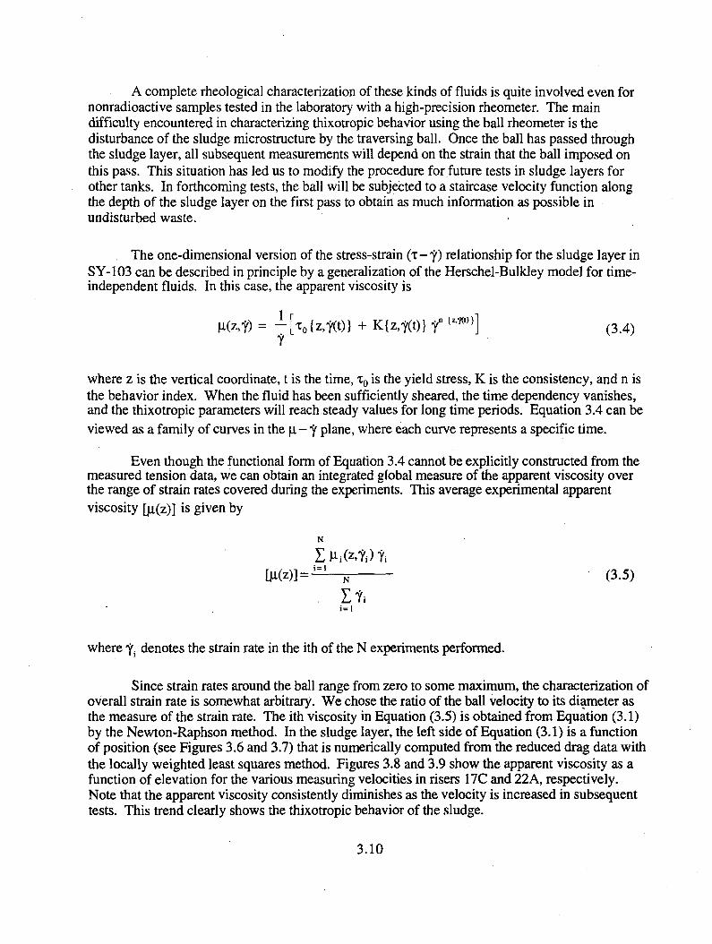
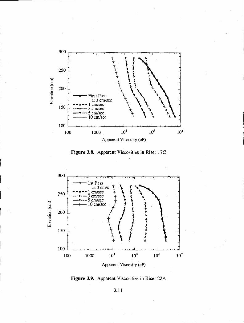
Since strain rates around the ball range from zero to some maximum, the characterization of overall strain rate is somewhat arbitrary. We chose the ratio of the ball velocity to its diameter as the measure of the strain rate. The ith viscosity in Equation (3.5) is obtained from Equation (3.1) by the Newton-Raphson method. In the sludge layer, the left side of Equation (3.1) is a function of position (see Figures 3.6 and 3.7) that is numerically computed from the reduced drag data with the locally weighted least squares method. Figures 3.8 and 3.9 show the apparent viscosity as a function of elevation for the various measuring velocities in risers 17C and 22A, respectively. Note that the apparent viscosity consistently diminishes as the velocity is increased in subsequent tests. This trend clearly shows the thixotropic behavior of the sludge.

3.10

300

250 -

S o | 200 >

150

100

i I I I r n - q — i i i i i r - n 1— i i i i i 11 j

T f i i A 1 ! 1 1 1 ! IT

X. T O 4k _

\ V 4- * \ — ] r V ^ L \ -

• • \ \ % K ~ - \ \ \ \ -

\ \ \ i \

at 3 cm/sec - _ _ A _ _ ] cm/sec

"T T O 4 \

-

- _--o-—3 cm/sec V <i ^ 4 \ — — * — 5 cm/sec

\ \ \

1 1 l l 1 1 1 1 1 1 1 1 1

h \ " '_ — i — 10 cm/sec

i i i i i i 1 1 ! i _ i . . i i i

\ \ \

1 1 l l 1 1 1 1 1 1 1 1 1

t 1

i i - i , . . i 1 1 1

100 1000 104

Apparent Viscosity (cP) 105 10e

Figure 3.8. Apparent Viscosities in Riser 17C

> 53

300

250

150

100

- I 1 I I l I 111 1 1 I I I l l l j 1 1 I I I I I I I 1 1 I I I I I I ! 1 1 I I I

100

- B — 1st Pass at 3 cm/s

•* - - 1 cm/sec -0-—3 cm/sec -T---5 cm/sec H — 1 0 cm/sec

• U J - d i ' i i 11 ill -I i i i i m l i i i i 11 II

1000 104 105 10e 107

Apparent Viscosity (cP)

Figure 3.9. Apparent Viscosities in Riser 22A

3.11

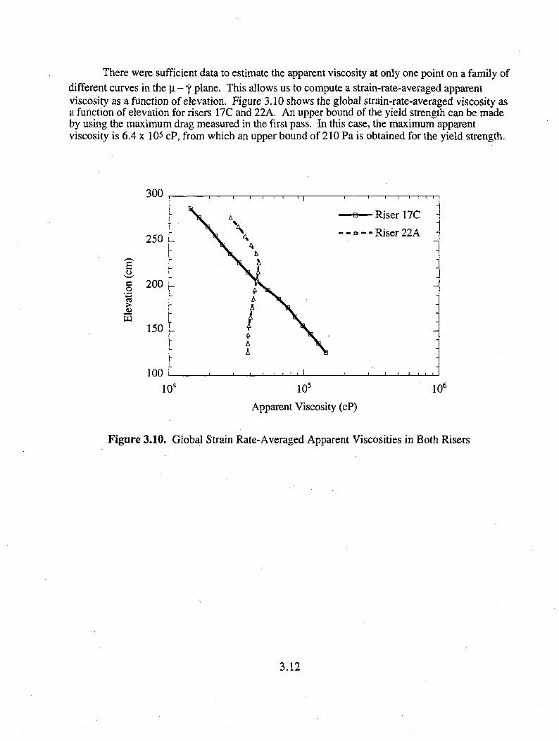
There were sufficient data to estimate the apparent viscosity at only one point on a family of different curves in the |x - 1 plane. This allows us to compute a strain-rate-averaged apparent viscosity as a function of elevation. Figure 3.10 shows the global strain-rate-averaged viscosity as a function of elevation for risers 17C and 22A. An upper bound of the yield strength can be made by using the maximum drag measured in the first pass. In this case, the maximum apparent viscosity is 6.4 x 105 C P, from which an upper bound of 210 Pa is obtained for the yield strength.

300

250 _

I 2 0° > a 150

100 104

_ i i i _

-1 1 1 1 — i — i — r

— a — Riser 17C - - * - - Riser 22A

-J I I I I I 1 L

105

Apparent Viscosity (cP) 106

Figure 3.10. Global Strain Rate-Averaged Apparent Viscosities in Both Risers

3.12

4.0 Void Fraction

The VFI is designed to measure the volume fraction of free gas, or void, at a specific location in a tank. This does not include the gas dissolved in the liquid or absorbed on the solid particles. The VFI neither measures nor depends on the composition of the gas; it is deployed vertically through a riser by means of a crane and measures the void fraction in waste samples collected over a radius of 76.2 cm (2.5 ft) about the riser center. Vertical spacing between samples is typically 30 to 60 cm (1 to 2 ft). Once the waste sample is isolated in the sample chamber, the chamber is pressurized with nitrogen gas. The void fraction is calculated from the initial and final pressures and temperatures and known system volumes. The physical description of the VFI and its theory of operation are described in Stewart et al. (1995).

This section describes the data acquisition and reduction for the VFI deployments in risers 17C and 22A in SY-103 on July 19,1995, and August 18,1995, respectively.

4.1 VFI Deployment In Tank 241-SY-103

The first VFI deployment took place on July 19,1995, through riser 17C in accordance with the Data Acquisition Plan for Tank 241 SY-103 Void Fraction Measurement Device.^ Three traverses were conducted at this riser. The lower arm was first pointed away from the center of the tank (ESE), then toward the center of the tank (WNW), and finally 90 degrees from the first two traverses (NNE).

The second deployment, on August 18,1995, was through riser 22A. The lower arm was first pointed toward the center of the tank (SSE), then away from the center of the tank (NNW), and, finally, 90 degrees from the first two traverses (ENE). For the second riser, the test plan was modified to reduce the spacing between sample location from 60 cm (2 ft) to 30 cm (1 ft) for the first traverse to increase the resolution on this traverse. There were concerns the VFI was possibly releasing gas from the waste at other traverse locations. A fourth traverse for each riser had been planned, but the lack of time prevented completion of those traverses.

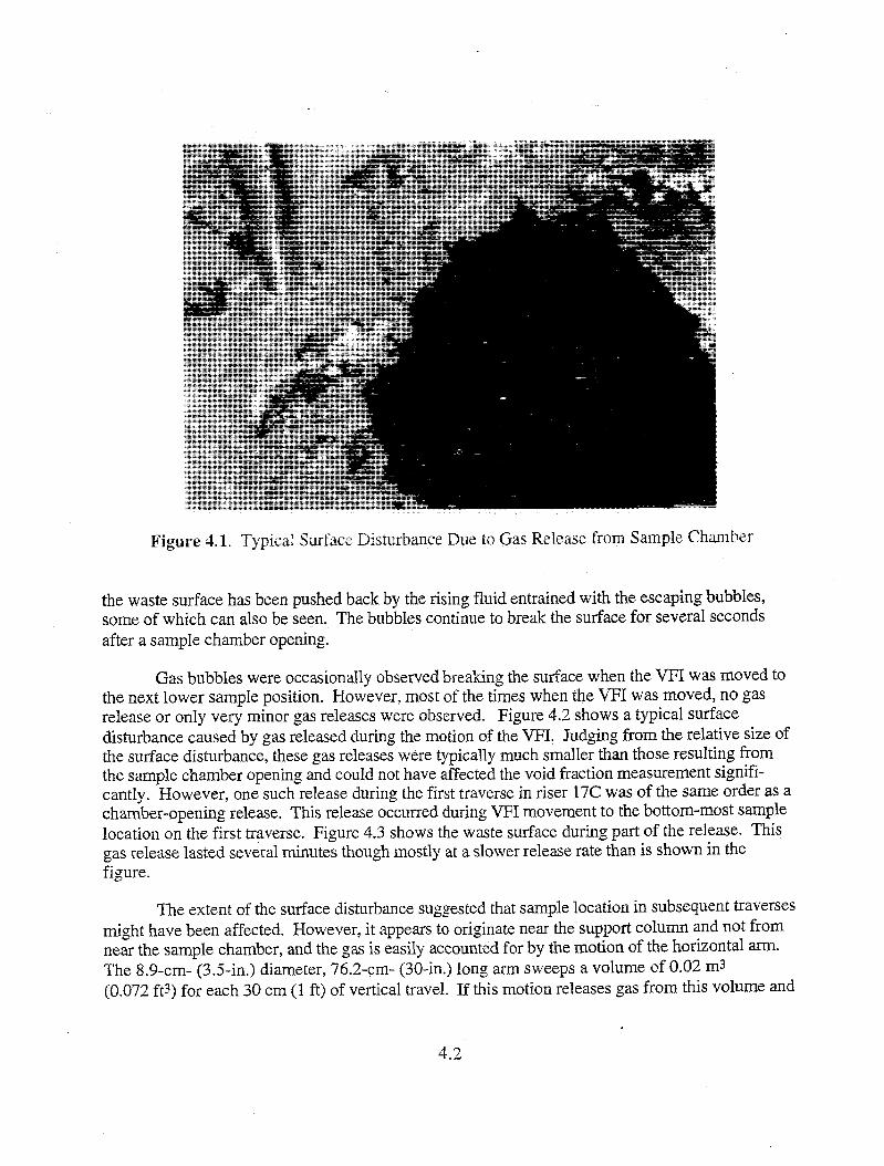
There was no crust layer in the immediate vicinity of the VFI in either riser, and this per­mitted direct observation of gas releases caused by the VFI disturbing the waste. The biggest dis­turbances resulted from the sample chamber cover being opened after a test, but these represented extremely small gas releases. If the sample chamber volume of 364 cm 3 containing 13% gas at a pressure of 34 atm is suddenly released, the volume of gas at the surface is only 1.6 (10-3) m3 (0.057 SCF). This is roughly the volume of air exhaled by a scuba diver at a depth of 6 m (20 ft). Even this small volume is sufficient for a swarm of over 3,000 1-cm-diameter bubbles, which would create a fairly dramatic surface disturbance. Figure 4.1 shows the disturbance on the surface due to gases released from a sample chamber opening. In the large dark area, the foam on

(a) Alzheimer et al. 1994. Letter report PNL-MIT:061794, Pacific Northwest National Laboratory, Richland, Washington.

4.1

t 4 «> i

•»; * — • ' • • • — - - . - S p * •

< !

* - * Vj fci ' ."58

Figure 4.1. Typical Surface Disturbance Due to Gas Release from Sample Chamber

the waste surface has been pushed back by the rising fluid entrained with the escaping bubbles, some of which can also be seen. The bubbles continue to break the surface for several seconds after a sample chamber opening.

Gas bubbles were occasionally observed breaking the surface when the VFI was moved to the next lower sample position. However, most of the times when the VFI was moved, no gas release or only very minor gas releases were observed. Figure 4.2 shows a typical surface disturbance caused by gas released during the motion of the VFI. Judging from the relative size of the surface disturbance, these gas releases were typically much smaller than those resulting from the sample chamber opening and could not have affected the void fraction measurement signifi­cantly. However, one such release during the first traverse in riser 17C was of the same order as a chamber-opening release. This release occurred during VFI movement to the bottom-most sample location on the first traverse. Figure 4.3 shows the waste surface during part of the release. This gas release lasted several minutes though mostly at a slower release rate than is shown in the figure.

The extent of the surface disturbance suggested that sample location in subsequent traverses might have been affected. However, it appears to originate near the support column and not from near the sample chamber, and the gas is easily accounted for by the motion of the horizontal arm. The 8.9-cm- (3.5-in.) diameter, 76.2-cm- (30-in.) long arm sweeps a volume of 0.02 m3 (0.072 ft3) for each 30 cm (1 ft) of vertical travel. If this motion releases gas from this volume and

4.2

I F #

Figure 4.2. Typical Surface Disturbance Due to Gas Release During Motion of VFI

Figure 4.3. Largest Surface Disturbance Due to Gas Release Durins Motion of VFI

4.3

adjacent material one-half a diameter on each side, the swept volume becomes 0.04 m3 (0.0144 ft3). The maximum gas released, if the waste contains 13% void at a pressure of 1.87 atm, is 0.01 m 3 (0.35 ft3). This is more than six times the volume of gas estimated for sample chamber opening, which was observed to cause approximately the same size of surface disturbance. We conclude that the disturbance does not indicate gas being removed from the sample volume.

4.2 VFI Data Appendix B contains the selected data sets used to establish the initial and final pressures

and temperatures for calculating the void fraction. The calculation methods used are the same as those described in Stewart et al. (1995) except for a revised treatment of the non-ideal gas correc­tion, a field calibration of the connecting line volume, and the treatment of sample capture error.

The non-ideal gas correction factor had been applied to the entire mass of gas in the sample chamber during each test regardless of the pressure. Actually, the effect should depend on the final-to-initial pressure ratio. The non-ideal gas correction on the first pressurization should be much more than on the second pressurization. The void fraction calculation was revised by making the correction a linear function of pressure ratio.

There are uncertainties in the temperature, pressure, and system volume measurements from which the void is calculated. The random errors are small, and their impacts are effectively already included in the data scatter. The small system bias observed in prior tests has been removed by field calibration of the connecting line volume. The original volume of 23.35 cm 3

(1.425 in.3) derived from laboratory measurements yielded slightly negative void fractions in the convective regions of both SY-101 and SY-103. To correct this, the connecting line volume was calibrated to six zero-void data points from the convective layer in SY-103.00 The line volume was then adjusted to minimize the sum of squares of the calculated void values, resulting in a new volume of 22.14 cm 3 (1.351 in.3).

The calibration is summarized in Table 4.1. The change shifted all void calculations upward by about 0.33%. The standard deviation of the six void fractions after calibration, a measure of random errors in the system, was 0.00089 (0.089% void). Prior error analysis estimated the rms error at 0.004 (0.4% void) at 2% void (Stewart et al. 1995).

The calculated void fractions for each traverse in the two risers are shown in Figure 4.4. The average void is plotted for double pressurizations since the two void values are not indepen­dent. Zero void was measured in the convective layer, and there was no systematic difference

(a) Since this tank is not mixed, the void fraction in the liquid will be essentially zero, in conformance with bubble dynamics calculations (Brewster et al. 1995). While this claim can also be made for the mixed slurry layer in SY-101, its high solids concentration casts some doubt on a truly zero void, and we chose not to use SY-101 data for the calibration.

4.4

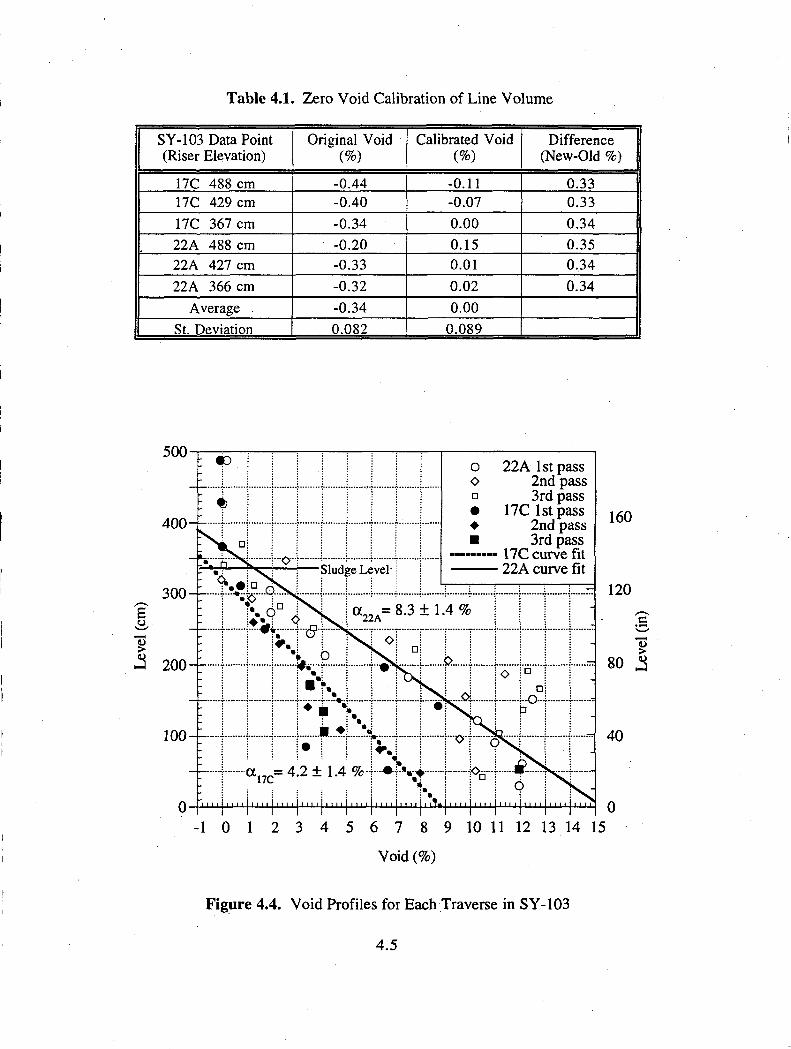
Table 4.1. Zero Void Calibration of Line Volume

SY-103 Data Point (Riser Elevation)

Original Void (%)

Calibrated Void (%)

Difference (New-Old %)

17C 488 cm -0.44 -0.11 0.33 17C 429 cm -0.40 -0.07 0.33 17C 367 cm -0.34 0.00 0.34 22A 488 cm -0.20 0.15 0.35 22A 427 cm -0.33 0.01 0.34 22A 366 cm -0.32 0.02 0.34

Average -0.34 0.00 St. Deviation 0.082 0.089

500

400

3 0 0 - -

g J 200

160

= 120

> 80 3

40

0 -1 0 1 2 3 4 5 6 7 8 9 10 11 12 13 14 15

Void (%)

Figure 4.4. Void Profiles for Each Traverse in SY-103

4.5

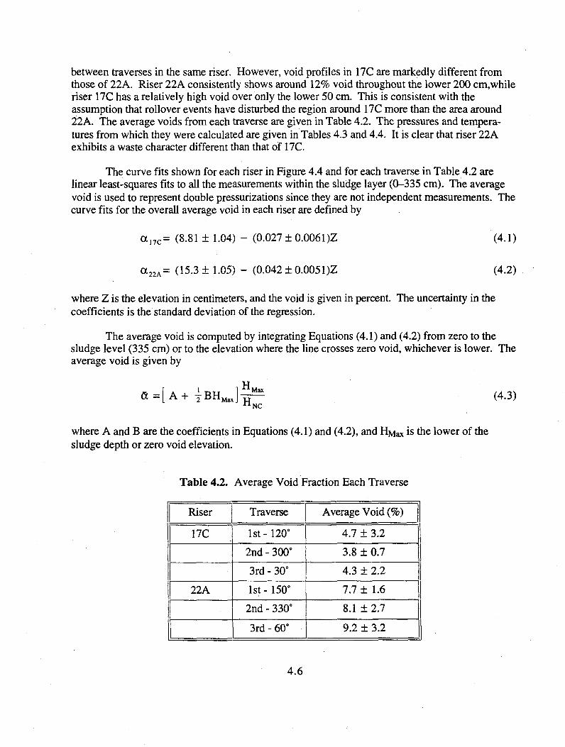
between traverses in the same riser. However, void profiles in 17C are markedly different from those of 22A. Riser 22A consistently shows around 12% void throughout the lower 200 cm,while riser 17C has a relatively high void over only the lower 50 cm. This is consistent with the assumption that rollover events have disturbed the region around 17C more than the area around 22A. The average voids from each traverse are given in Table 4.2. The pressures and tempera­tures from which they were calculated are given in Tables 4.3 and 4.4. It is clear that riser 22A exhibits a waste character different than that of 17C.

The curve fits shown for each riser in Figure 4.4 and for each traverse in Table 4.2 are linear least-squares fits to all the measurements within the sludge layer (0-335 cm). The average void is used to represent double pressurizations since they are not independent measurements. The curve fits for the overall average void in each riser are defined by

a 1 7 C = (8.81 ± 1.04) - (0.027 ± 0.0061 )Z (4.1)

a 2 2 A = (15.3 ± 1.05) - (0.042 ± 0.0051)Z (4.2)

where Z is the elevation in centimeters, and the void is given in percent. The uncertainty in the coefficients is the standard deviation of the regression.

The average void is computed by integrating Equations (4.1) and (4.2) from zero to the sludge level (335 cm) or to the elevation where the line crosses zero void, whichever is lower. The average void is given by

G = [ A + J B H j ^ (4.3)

where A and B are the coefficients in Equations (4.1) and (4.2), and HMax is the lower of the sludge depth or zero void elevation.

Table 4.2. Average Void Fraction Each Traverse

Riser Traverse Average Void (%)

17C 1st-120° 4.7 ± 3.2

2nd - 300° 3.8 ± 0.7

3rd - 30° 4.3 ± 2.2

22A 1st-150° 7.7 ± 1.6

2nd - 330° 8.1 ± 2.7

3rd - 60° 9.2 + 3.2

4.6

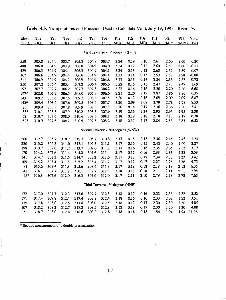
Table 4.3. Temperatures and Pressures Used to Calculate Void, July 19, 1995 - Riser 17C

Elev. Tli T2i T3i Tlf T2f T3f Pli P2i P3i Plf P2f P3f Void rem) (K) (K) (K) (K) (K) (K) (MPa) CMPa) CMPa) CMPat fMPat fMPa) (%)

First Traverse - 120 degrees (ESE)

550 305.8 304.9 303.7 305.8 304.9 303.7 3.24 0.19 0.10 2.61 2.60 2.60 -0.20 488 306.0 304.9 303.9 306.0 304.9 304.0 3.24 0.12 0.12 2.60 2.60 2.60 -0.11 429 306.3 304.9 304.1 306.3 304.9 304.1 3.24 0.13 0.12 2.60 2.59 2.59 -0.07 367 306.6 304.9 304.4 306.6 304.9 304.4 3.23 0.14 0.13 2.59 2.58 2.58 -0.00 311 306.9 304.9 304.7 306.9 304.9 304.8 3.22 0.15 0.14 2.54 2.53 2.53 0.73 250 307.2 306.4 305.4 307.2 306.4 305.5 3.22 0.15 0.15 2.47 2.47 2.47 1.69 197 307.7 307.7 306.2 307.7 307.8 306.2 3.22 0.16 0.16 2.20 2.20 2.20 6.68 197* 308.0 307.9 306.5 308.0 307.9 306.6 3.21 2.20 2.19 2.87 2.86 2.86 6.35 143 309.2 308.6 307.5 309.2 308.6 307.5 3.20 0.17 0.16 2.09 2.09 2.09 8.87 143* 309.4 308.6 307.6 309.5 308.6 307.7 3.20 2.09 2.08 2.79 2.78 2.78 8.53

85 309.9 308.3 307.8 309.9 308.3 307.8 3.20 0.18 0.17 2.36 2.36 2.36 3.41 85* 310.1 308.3 307.9 310.2 308.3 307.9 3.19 2.36 2.34 2.95 2.95 2.95 3.30 52 310.7 307.6 308.0 310.6 307.6 308.1 3.18 0.19 0.18 2.18 2.17 2.17 6.78 52* 310.9 307.5 308.2 310.9 307.5 308.2 3.18 2.17 2.17 2.84 2.83 2.83 6.52

Second Traverse - 300 degrees (WNW)

260 312.7 305.7 310.7 312.7 305.7 310.8 3.17 0.15 0.13 2.46 2.45 2.45 1.24 230 313.2 306.3 311.0 313.1 306.3 311.1 3.17 0.16 0.15 2.40 2.40 2.40 2.27 198 313.7 307.0 311.2 313.7 307.0 311.2 3.17 0.16 0.16 2.35 2.35 2.35 3.17 170 314.2 307.6 311.4 314.2 307.6 311.4 3.17 0.17 0.16 2.33 2.33 2.33 3.53 141 314.7 308.2 311.6 314.7 308.2 311.6 3.17 0.17 0.17 2.34 2.33 2.33 3.42 109 315.2 308.4 311.8 315.2 308.4 311.7 3.17 0.17 0.17 2.27 2.26 2.26 4.75

81 315.6 308.4 311.8 315.6 308.4 311.8 3.17 0.18 0.18 2.18 2.18 2.18 6.35 48 316.1 307.7 311.9 316.1 307.7 311.9 3.18 0.18 0.18 2.11 2.11 2.11 7.98 48* 316.3 307.6 312.0 316.3 307.6 312.0 3.17 2.11 2.10 2.79 2.78 2.78 7.65

Third Traverse - 30 degrees (NNE)

172 317.0 307.7 312.3 317.0 307.7 312.3 3.18 0.17 0.16 2.33 2.33 2.33 3.52 171 317.4 307.8 312.4 317.4 307.8 312.4 3.18 0.16 0.16 2.33 2.33 2.33 3.51 135 317.8 308.0 312.5 317.8 308.0 312.5 3.18 0.17 0.17 2.30 2.30 2.30 4.05 107 318.2 308.2 312.7 318.2 308.2 312.8 3.18 0.18 0.17 2.30 2.30 2.30 4.08

53 318.7 308.0 312.8 318.6 308.0 312.8 3.18 0.18 0.18 1.94 1.94 1.94 11.96

* Second measurement of a double pressurization.

4.7

Table 4.4. Temperatures and Pressures Used to Calculate Void, August 18, 1995 - Riser 22A

Elev. Tli T2i T3i Tlf T2f T3f PH P2i P3i Plf P2f P3f Void (cm) CK1 (K) (K) (K) (K) CK1 fMPal CMPal rMPal CMPa) flvIPa) fMPal f%)

1st Traverse - 150 degrees (SSE)

488 291.0 305.3 293.8 290.9 305.2 293.8 3.19 0.12 0.09 2.56 2.55 2.55 0.15 427 291.2 305.3 294.2 291.2 305.3 294.3 3.19 0.13 0.12 2.57 2.56 2.56 0.01 366 291.4 305.3 294.6 291.4 305.3 294.6 3.19 0.14 0.13 2.57 2.56 2.56 0.02 305 291.7 305.4 294.9 291.6 305.4 294.9 3.19 0.15 0.14 2.45 2.45 2.45 1.91 274 291.8 305.9 295.2 291.8 305.9 295.3 3.19 0.15 0.15 2.45 2.45 2.45 1.94 244 292.0 306.6 295.6 292.0 306.6 295.6 3.19 0.16 0.15 2.36 2.35 2.35 3.61 244* 292.1 306.7 295.7 292.1 306.7 295.7 3.18 2.35 2.35 2.96 2.95 2.95 3.43 213 292.2 307.3 296.1 292.1 307.4 296.1 3.19 0.16 0.16 2.34 2.33 2.33 4.11 183 292.3 308.0 296.8 292.2 308.0 296.8 3.19 0.16 0.16 2.17 2.16 2.16 7.66 183* 292.3 308.1 297.0 292.3 308.1 297.0 3.19 2.16 2.16 2.84 2.83 2.83 7.31 152 292.4 308.6 297.4 292.4 308.6 297.4 3.19 0.17 0.17 1.97 1.96 1.96 12.77 152* 292.5 308.7 297.7 292.5 308.7 297.7 3.19 1.96 1.95 2.69 2.68 2.68 12.21 122 292.6 309.0 297.9 292.6 308.9 297.9 3.19 0.17 0.17 2.06 2.06 2.06 10.28 91 292.7 309.0 298.3 292.7 309.0 298.3 3.20 0.18 0.17 2.04 2.03 2.03 10.99 61 292.9 308.8 298.6 292.8 308.8 298.6 3.20 0.18 0.18 2.00 1.99 1.99 12.07 30 293.1 308.3 298.9 293.1 308.3 298.8 3.20 0.19 0.18 2.00 2.00 2.00 11.95

2nd Traverse - 330 degrees (NNW)

347 293.8 305.6 298.8 293.8 305.6 298.8 3.20 0.14 0.11 2.42 2.41 2.41 2.54 320 294.1 305.5 298.9 294.1 305.5 298.9 3.20 0.15 0.14 2.58 2.58 2.58 -0.05 293 294.5 305.7 299.0 294.5 305.7 299.0 3.20 0.15 0.15 2.51 2.50 2.50 1.18 264 294.9 306.0 299.2 294.9 306.0 299.2 3.20 0.15 0.15 2.40 2.40 2.40 2.93 235 295.3 306.6 299.5 295.3 306.6 299.5 3.20 0.16 0.16 2.21 2.20 2.20 6.70 206 295.8 307.2 300.0 295.8 307.2 300.0 3.20 0.16 0.16 2.10 2.10 2.10 9.09 187 296.4 307.6 300.5 296.4 307.6 300.6 3.20 0.17 0.16 2.01 2.00 2.00 11.62 187* 296.7 307.7 300.9 296.7 307.7 300.9 3.20 2.00 1.99 2.72 2.71 2.71 11.15 156 297.3 308.0 301.4 297.3 308.1 301.4 3.21 0.17 0.17 2.10 2.09 2.09 9.37 126 297.9 308.3 301.8 297.9 308.3 301.8 3.21 0.17 0.17 2.06 2.06 2.06 10.20

96 298.5 308.4 302.3 298.4 308.4 302.3 3.21 0.18 0.18 2.09 2.09 2.09 9.58 51 299.1 308.3 302.6 299.0 308.3 302.6 3.21 0.19 0.18 2.07 2.06 2.06 10.21

3rd Traverse - 60 degrees (NNE)

370 300.1 305.9 302.5 300.1 305.9 302.5 3.22 0.14 0.11 2.53 2.53 2.53 0.79 341 300.5 305.8 302.6 300.5 305.8 302.6 3.23 0.14 0.14 2.59 2.58 2.58 0.05 312 300.8 305.7 302.8 300.8 305.7 302.8 3.23 0.15 0.14 2.52 2.51 2.51 1.27 283 301.2 305.8 303.0 301.2 305.8 303.0 3.24 0.15 0.15 2.46 2.45 2.45 2.30 252 301.6 306.0 303.3 301.6 306.0 303.2 3.25 0.15 0.15 2.39 2.38 2.38 3.64 222 302.1 306.5 303.6 302.1 306.5 303.6 3.25 0.16 0.16 2.18 2.17 2.17 7.76 192 302.6 307.1 304.0 302.5 307.1 304.0 3.26 0.16 0.16 2.00 1.99 1.99 12.30 167 303.1 307.7 304.5 303.1 307.7 304.5 3.26 0.17 0.16 1.98 1.97 1.97 12.78 137 303.6 308.1 305.0 303.6 308.1 305.0 3.26 0.17 0.17 2.01 2.00 2.00 12.11 104 304.1 308.3 305.4 304.1 308.2 305.4 3.27 0.18 0.17 2.05 2.05 2.05 11.16

42 305.1 308.3 306.0 305.1 308.3 306.1 3.30 0.19 0.18 2.10 2.09 2.09 10.48

Second measurement of a double pressurization.

4.8

The standard deviation of the average is computed by linear propagation from Equation (4.3). If aA and a B are the standard deviations of the linear coefficients, the standard deviation of the average is

G« = I ^ V ° A + [ iH M a x G B f (4.4) n N C

Equations (4.1) through (4.4) yield the average void values of 4.2 ± 1.4% at 17C and 8.3 ± 1.4% at 22A reported in Figure 4.4.

One final correction is required to these results. There is a systematic error induced by the hydrodynamics of the sample capture process that tends to make the void in the sample slightly lower than in the waste. This error is impossible to quantify exactly, but it must be accounted for. Experiments were conducted at LANL with gassed SY-101 chemical simulant and with neutrally buoyant spheres to investigate capture of bubbles in non-Newtonian fluids.(a) Though the resemblance of the tests and analysis to actual VFI measurements in SY-103 is questionable, the results showed the void of the sample to be less than the undisturbed waste by a factor of about 0.1 with an uncertainty of ± 0.04. Analysis of the Retained Gas Sampler also raised the possibility of incomplete capture due to shear stress of the sludge on the container walls.*) However, zero error is predicted for shear strength below 1,500 Pa (0.2 psi), which is the case in SY-103.

To account for this very real effect, although its value is unknown, we assume a 10 ± 4% sampling error consistent with the LANL results. That is, the indicated void should be multiplied by 1.1 ± 0.04 to give the correct value. This correction results in new average voids of 4.7 ± 1.5% for 17C and 9.1 ± 1.5% for 22A.

(a) Abbott, J. R., and C. Unal. November 16, 1994. Sampling Ability of the In Situ Voidmeter Instrument. Letter report TSA-6-94-316 (MHO), Los Alamos National Laboratory, Los Alamos, New Mexico.

(b) Shekarriz, A., and J. D. Norton. September 15, 1995. Retained Gas Sampler System Analysis. Letter report PNL-FG-091595, Pacific Northwest National Laboratory, Richland, Washington.

4.9

5.0 References

Brager, H. R. 1994. Summary of Information on Flammable Gas Watch List Tanks. WHC-EP-0711, Westinghouse Hanford Company, Richland, Washington.

Brewster, M. E., N. B. Gallagher, J. D. Hudson, and C. W. Stewart. 1995. The Behavior, Quantity, and Location of Undissolved Gas in Tank 241-SY-10X. PNL-10681, Pacific Northwest National Laboratory, Richland, Washington.

Hartley, S. A., K. M. Remund, B. C. Simpson, R. D. Cromar, and C. M. Anderson. 1995. Statistical Supplement to the Tank Characterization Reference Guide. WHC-SD-WM-TI-648 Rev. 0, Westinghouse Hanford Company, Richland, Washington.

Remund, K. M., J. Tingey, E. Albrook, and P. Heasler. 1994. Tank Characterization Report for Single-Shell Tank B201. PNL-10100, Pacific Northwest National Laboratory, Richland, Washington.

Reynolds, D. A. 1981. Double-Shell Slurry Campaign. RHO-CD-1268, Rockwell Hanford Operations, Richland, Washington.

SAS Institute, Inc. 1992. SAS Technical Report P.229, SAS/STAT Software: Changes and Enhancements, Release 6.07. SAS, Cary, North Carolina.

Stewart, C. W., C. L. Shepard, J. M. Alzheimer, T. I. Stokes, and G. Terrones. 1995. In Situ Determination of Rheological Properties and Void Fraction in Hanford Waste Tank 241-SY-lOl. PNL-10682, Pacific Northwest National Laboratory, Richland, Washington.

Whitney, P. D. 1995. Screening the Hanford Tanks for Trapped Gas. PNL-10821, Pacific Northwest National Laboratory, Richland, Washington.

5.1

Appendix A

Raw Data from the Ball Rheometer

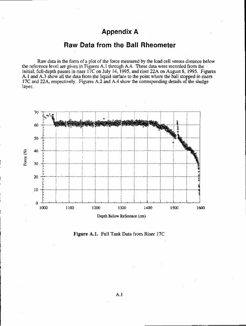
Appendix A

Raw Data from the Ball Rheometer

Raw data in the form of a plot of the force measured by the load cell versus distance below the reference level are given in Figures A.l through A.4. These data were recorded from the initial, full-depth passes in riser 17C on July 14,1995, and riser 22A on August 8, 1995. Figures A.l and A.3 show all the data from the liquid surface to the point where the ball stopped in risers 17C and 22A, respectively. Figures A.2 and A.4 show the corresponding details of the sludge layer.

1000 1100 1200 1300 1400

Depth Below Reference (cm) 1500 1600

Figure A.l. Full Tank Data from Riser 17C

A.l

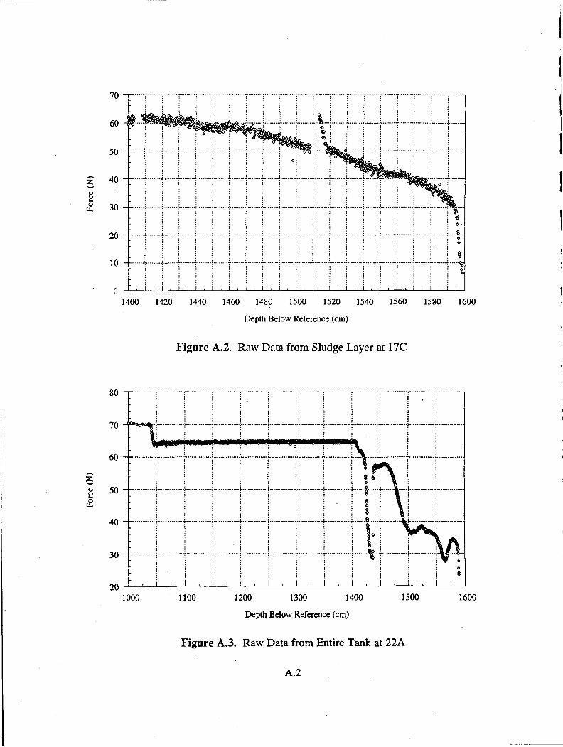
70 -r-

1400 1420 1440 1460 1480 1500 1520 1540 1560 1580 1600 Depth Below Reference (cm)

Figure A.2. Raw Data from Sludge Layer at 17C

80

70 - faooooc* . - ;

We* 60 —

8 50

I 40

30

20 J i J i L

niniipiin <wt»

i , i ,

1000 1100 1200 1300 1400

Depth Below Reference (cm)

1500 1600

Figure A.3. Raw Data from Entire Tank at 22A

A.2

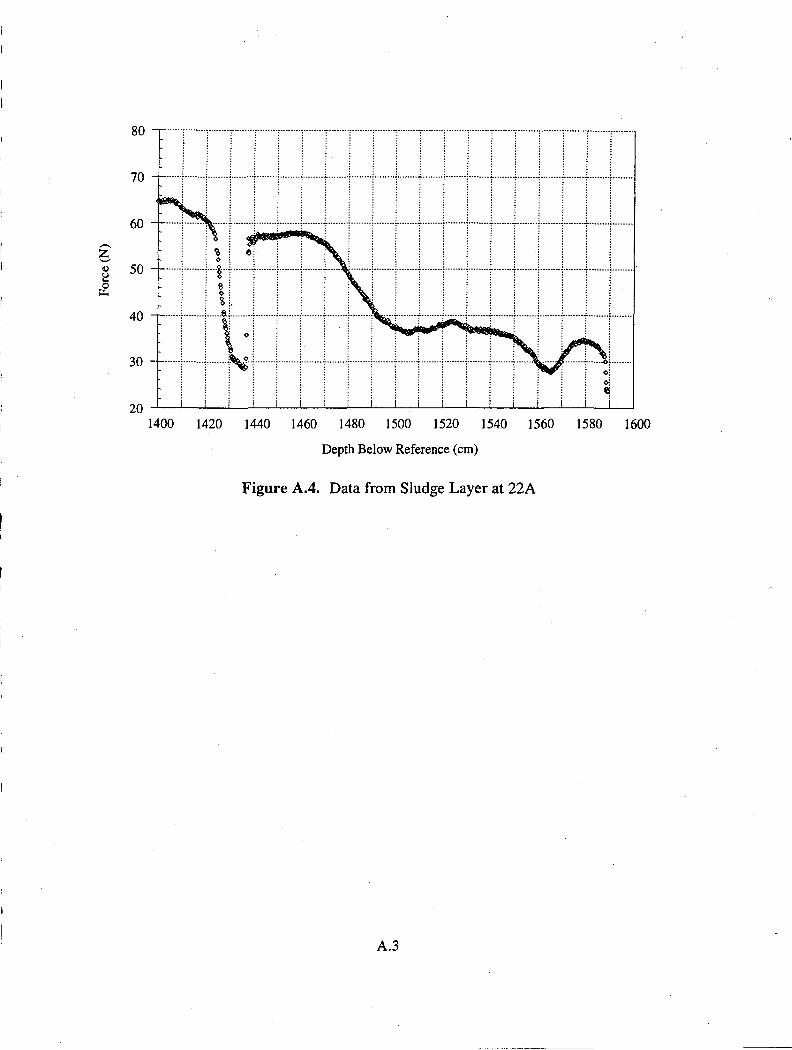
80-r

1400 1420 1440 1460 1480 1500 1520 1540 1560 1580 1600 Depth Below Reference (cm)

Figure A.4. Data from Sludge Layer at 22A

A.3

Appendix B

Selected Raw Data from the Void Fraction Instrument

Appendix B

Selected Raw Data from Void Fraction Instrument

For each of the void fraction measurements, five arm temperatures, two pressurization chamber temperatures, three enclosure temperatures, two pressurization chamber pressures, and one line pressure are recorded approximately every two seconds for almost the entire duration of the measurement, which can range from eight to fifteen minutes depending on whether one or two pressurizations are used. The initial reading from the position sensor is also recorded at the beginning of each data set. While most of these data are not used in the actual void fraction calculation, they are all recorded so that the time histories of individual sensor measurements can be examined if needed.

Tables B. 1 and B.2 present the data used for each of the samples for the deployments in risers 17C and 22A, respectively. Temperature readings TEl, TE2, TE3, and TE4 were all taken at locations in the equipment enclosure. TEl and TE2 measure the temperature inside the equipment enclosure; TE3 and TE4 measure the temperature of the pressurization chamber; TE5, TE6, and TE7 measure the line temperature in the mast. TE5 is near the top; TE6 is near the middle; and TE7 is near the bottom. TE8 and TE9 measure the temperature at the pivot and are used for the sample chamber temperature. All temperatures are in degrees Celsius.

Pressures PIT1, PIT2, and PIT3 are all located inside the equipment enclosure. PIT1 and PIT2 measure the pressure in the pressurization chamber. PIT3 measures the pressure in the connecting line just below the solenoid valve at the bottom of the pressurization chamber. All pressures are in psia.

B.l

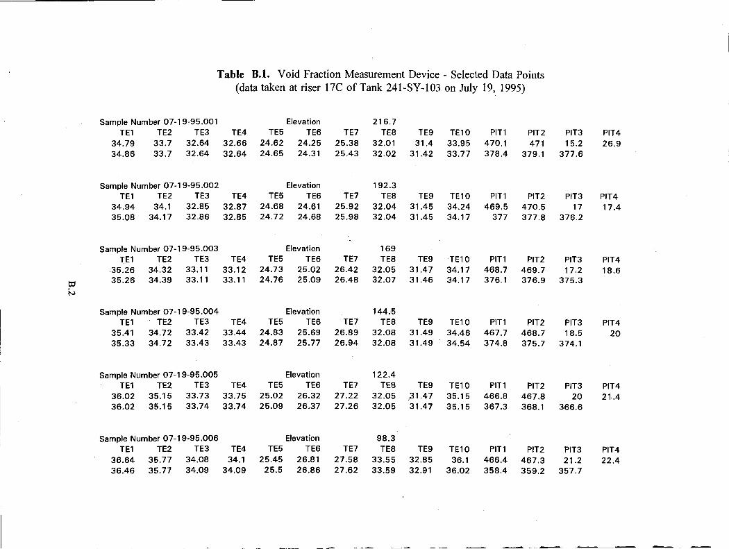
Table B.l. Void Fraction Measurement Device - Selected Data Points (data taken at riser 17C of Tank 241-SY-103 on July 19, 1995)

Sample Number 07-TE1 TE2

34.79 33.7 34.86 33.7

Sample Number 07-TE1 TE2

34.94 34.1 35.08 34.17

Sample Number 07-TE1 TE2

35.26 34.32 35.26 34.39

Sample Number 07-TE1 TE2

35.41 34.72 35.33 34.72

Sample Number 07-TE1 TE2

36.02 35.15 36.02 35.15

Sample Number 07-TE1 TE2

36.64 35.77 36.46 35.77

-19-95.001 TE3 TE4

32.64 32.66 32.64 32.64

-19-95.002 TE3 TE4

32.85 32.87 32.86 32.85

-19-95.003 TE3 TE4

33.11 33.12 33.11 33.11

-19-95.004 TE3 TE4

33.42 33.44 33.43 33.43

-19-95.005 TE3 TE4

33.73 33.75 33.74 33.74

-19-95.006 TE3 TE4

34.08 34.1 34.09 34.09

Elevation TE5 TE6

24.62 24.25 24.65 24.31

Elevation TE5 TE6

24.68 24.61 24.72 24.68

Elevation TE5 TE6

24.73 25.02 24.76 25.09

Elevation TE5 TE6

24.83 25.69 24.87 25.77

Elevation TE5 TE6

25.02 26.32 25.09 26.37

Elevation TE5 TE6

25.45 26.81 25.5 26.86

216.7 TE7 TE8

25.38 32.01 25.43 32.02

192.3 TE7 TE8

25.92 32.04 25.98 32.04

169 TE7 TE8

26.42 32.05 26.48 32.07

144,5 TE7 TE8

26.89 32.08 26.94 32.08

122.4 TE7 TE8

27.22 32.05 27.26 32.05

98.3 TE7 TE8

27.58 33.55 27.62 33.59

TE9 TE10 31.4 33.95

31.42 33.77

TE9 TE10 31.45 34.24 31.45 34.17

TE9 TE10 31.47 34.17 31.46 34.17

TE9 TE10 31.49 34.46 31.49 34.54

TE9 TE10 ,31.47 35.15 31.47 35.15

TE9 TE10 32.85 36.1 32.91 36.02

PIT1 PIT2 470.1 471 378.4 379.1

PIT1 PIT2 469.5 470.5

377 377.8

PIT1 PIT2 468.7 469.7 376.1 376.9

PIT1 PIT2 467.7 468.7 374.8 375.7

PIT1 PIT2 466.8 467.8 367.3 368.1

PIT1 PIT2 466.4 467.3 358.4 359.2

PIT3 PIT4 15.2 26.9

377.6

PIT3 PIT4 17 1 7.4

376.2

PIT3 PIT4 17.2 18.6

375.3

PIT3 PIT4 18.5 20

374.1

PIT3 PIT4 20 21.4

366.6

PIT3 PIT4 21.2 22.4

357.7

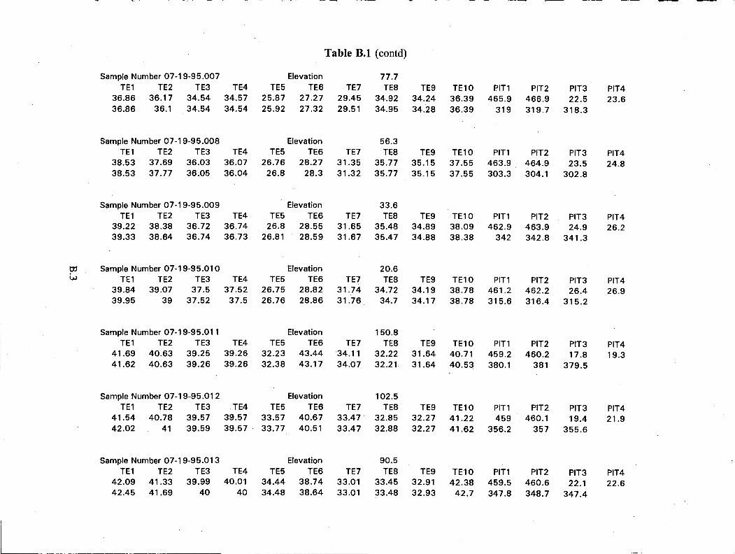
Table B.l (contd)

Sample Number 07-19-95.007 TE1 TE2 TE3 TE4

36.86 36.17 34.54 34.57 36.86 36.1 34.54 34.54

Sample Number 07-19-95.008 TE1 TE2 TE3 TE4

38.53 37.69 36.03 36.07 38.53 37.77 36.05 36.04

Sample Number 07-19-95.009 TE1 TE2 TE3 TE4

39.22 38.38 36.72 36.74 39.33 38.64 36.74 36.73

Sample Number 07-19-95.010 TE1 TE2 TE3 TE4

39.84 39.07 37.5 37.52 39.95 39 37.52 37.5

Sample Number 07-19-95.011 TE1 TE2 TE3 TE4

41.69 40.63 39.25 39.26 41.62 40.63 39.26 39.26

Sample Number 07-19-95.012 TE1 TE2 TE3 TE4

41.54 40.78 39.57 39.57 42.02 41 39.59 39.57

Sample Number 07-19-95.013 TE1 TE2 TE3 TE4

42.09 41.33 39.99 40.01 42.45 41.69 40 40

Elevation 77.7 TE5 TE6 TE7 TE8 TE9 TE10 PIT1 PIT2 PIT3 PIT4

25.87 27.27 29.45 34.92 34.24 36.39 465.9 466.9 22.5 23.6 25.92 27.32

Elevation

29.51 34.95

56.3

34.28 36.39 319 319.7 318.3

TE5 TE6 TE7 TE8 TE9 TE10 PIT1 PIT2 PIT3 PIT4 26.76 28.27 31.35 35.77 35.15 37.55 463.9 464.9 23.5 24.8

26.8 28.3

Elevation

31.32 35.77

33.6

35.15 37.55 303.3 304.1 302.8

TE5 TE6 TE7 TE8 TE9 TE10 PIT1 PIT2 PIT3 PIT4 26.8 28.55 31.65 35.48 34.89 38.09 462.9 463.9 24.9 26.2

26.81 28.59

Elevation

31.67 35.47

20.6

34.88 38.38 342 342.8 341.3

TE5 TE6 TE7 TE8 TE9 TE10 PIT1 PIT2 PIT3 PIT4 26.75 28.82 31.74 34.72 34.19 38.78 461.2 462.2 26.4 26.9 26.76 28.86

Elevation

31.76 34.7

150.8

34.17 38.78 315.6 316.4 315.2

TE5 TE6 TE7 TE8 TE9 TE10 PIT1 PIT2 PIT3 PIT4 32.23 43.44 34.11 32.22 31.64 40.71 459.2 460.2 17.8 19.3 32.38 43.17

Elevation

34.07 32.21

102.5

31.64 40.53 380.1 381 379.5

TE5 TE6 TE7 TE8 TE9 TE10 PIT1 PIT2 PIT3 PIT4 33.57 40.67 33.47 32.85 32.27 41.22 459 460.1 19.4 21.9 33.77 40.51

Elevation

33.47 32.88

90.5

32.27 41.62 356.2 357 355.6

TE5 TE6 TE7 TE8 TE9 TE10 PIT1 PIT2 PIT3 PIT4 34.44 38.74 33.01 33.45 32.91 42.38 459.5 460.6 22.1 22.6 34.48 38.64 33.01 33.48 32.93 42.7 347.8 348.7 347.4

Table B.l (contd)

Sample Number 07-19-95.014 TE1 TE2 TE3

42.85 42.09 40.54 42.92 42.09 40.55

Sample Number 07-19-95.015 TE1 TE2 TE3

43.54 42.63 41 43.54 42.7 41.04

Sample Number 07-19-95.0016 TE1 TE2 TE3

44.37 43.61 42.07 44.3 43.61 42.07

Sample Number 07-19-95.017 TE1 TE2 TE3

44.37 43.61 42.07 44.3 43.61 42.07

Sample Number 07-19-95.018 TE1 TE2 TE3

44.63 43.83 42.46 44.99 44.16 42.48

Sample Number 07-19-95.019 TE1 TE2 TE3

45.46 44.63 42.93 45.32 44.63 42.95

Elevation 77.8 TE4 TE5 TE6 TE7 TE8 TE9 TE10 PIT1 PIT2 PIT3 PIT4

40.55 33.75 37.11 32.26 34.13 33.6 43.54 459.8 460.8 22.5 23.3 40.54 33.75 37.02

Elevation

32.26 34.15

67

33.62 43.54 340.4 341.3 340.1

TE4 TE5 TE6 TE7 TE8 TE9 TE10 PIT1 PIT2 PIT3 PIT4 41.02 33.07 36.04 31.92 34.69 34.17 44.63 459.8 460.9 23.6 24 41.01

3

33.09 35.97

Elevation

31.92 34.72

43.1

34.18 44.7 337.7 338.6 337.4

TE4 TE5 TE6 TE7 TE8 TE9 TE10 PIT1 PIT 2 PIT3 PIT4 42.05 31.85 34.38 31.8 35.59 34.99 45.39 459.9 461 24.7 25.3 42.05 31.86 34.35

Elevation

31.8 35.59

43.1

35 45.39 328.2 329.1 327.9

TE4 TE5 TE6 TE7 TE8 TE9 TE10 PIT1 PIT2 PIT3 PIT4 42.05 31.85 34.38 31.8 35.59 34.99 45.39 459.9 461 24.7 25.3 42.05 31.86 34.35

Elevation

31.8 35.59

31.9

35 45.39 328.2 329.1 327.9

TE4 TE5 TE6 TE7 TE8 TE9 TE10 PIT1 PIT2 • PIT3 PIT4 42.45 31.45 33.91 31.78 35.54 34.94 45.75 459.6 460.7 25.5 25.9 42.45 31.43 33.87

Elevation

31.81 35.53

18.9

34.95 46.08 316.2 317.2 316.1

TE4 TE5 TE6 TE7 TE8 TE9 TE10 PIT1 PIT2 PIT3 PIT4 42.92 31.04 33.47 31.8 34.77 34.27 46.52 460.4 461.5 26.1 26.7

42.9 31.06 33.44 31.81 34.75 34.25 46.52 305.7 306.7 305.6

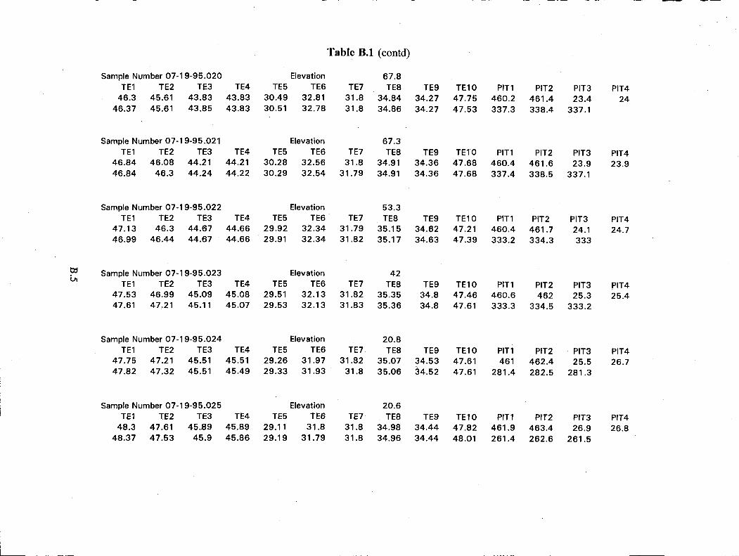
Table B.l (contd)

Sample Number 07-19-95.020 TE1 TE2 TE3 TE4

46.3 45.61 43.83 43.83 46.37 45.61 43.85 43.83

Sample Number 07-19-95.021 TE1 TE2 TE3 TE4

46.84 46.08 44.21 44.21 46.84 46.3 44.24 44.22

Sample Number 07-19-95.022 TE1 TE2 TE3 TE4

47.13 46.3 44.67 44.66 46.99 46.44 44.67 44.66

Sample Number 07-19-95.023 TE1 TE2 TE3 TE4

47.53 46.99 45.09 45.08 47.61 47.21 45.11 45.07

Sample Number 07-19-95.024 TE1 TE2 TE3 TE4

47.75 47.21 45.51 45.51 47.82 47.32 45.51 45.49

Sample Number 07-19-95.025 TE1 TE2 TE3 TE4

48.3 47.61 45.S9 45.89 48.37 47.53 45.9 45.86

Elevation 67.8 TE5 TE6 TE7 TE8 TE9 TE10 PIT1 PIT2 PIT3 PIT4

30.49 32.81 31.8 34.84 34.27 47.75 460.2 461.4 23.4 24 30.51 32.78

Elevation

31.8 34.86

67.3

34.27 47.53 337.3 338.4 337.1

TE5 TE6 TE7 TE8 TE9 TE10 PIT1 PIT2 PIT3 PIT4 30.28 32.56 31.8 34.91 34.36 47.68 460.4 461.6 23.9 23.9 30.29 32.54

Elevation

31.79 34.91

53.3

34.36 47.68 337.4 338.5 337.1

TE5 TE6 TE7 TE8 TE9 TE10 PIT1 PIT2 PIT3 PIT4 29.92 32.34 31.79 35.15 34.62 47.21 460.4 461.7 24.1 24.7 29.91 32.34

Elevation

31.82 35.17

42

34.63 47.39 333.2 334.3 333

TE5 TE6 TE7 TE8 TE9 TE10 PIT1 PIT2 PIT3 PIT4 29.51 32.13 31.82 35.35 34.8 47.46 460.6 462 25.3 25.4 29.53 32.13

Elevation

31.83 35.36

20.8

34.8 47.61 333.3 334.5 333.2

TE5 TE6 TE7 TE8 TE9 TE10 PIT1 PIT2 PIT3 PIT4 29.26 31.97 31.82 35.07 34.53 47.61 461 462.4 25.5 26.7 29.33 31.93

Elevation

31.8 35.06

20.6

34.52 47.61 281.4 282.5 281.3

TE5 TE6 TE7 TE8 TE9 TE10 PIT1 PIT2 PIT3 PIT4 29.11 31.8 31.8 34.98 34.44 47.82 461.9 463.4 26.9 26.8 29.19 31.79 31.8 34.96 34.44 48.01 261.4 262.6 261.5

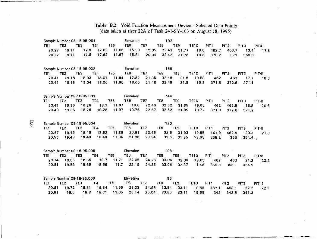
Table B.2. Void Fraction Measurement Device - Selected Data Points (data taken at riser 22A of Tank 241-SY-103 on August 18, 1995)

Sample Number 08-18-95.001 Elevation 192 TE1 TE2 TE3 TE4 TE5 TE6 TE7 TE8 TE9 TE10 PIT1 PIT2 PIT3 PIT4!

20.27 19.11 17.8 17.83 11.86 15.58 19.85 32.43 31.77 19.8 462.7 463.7 13.4 17.8 20.27 19.11 17.8 17.82 11.87 15.81 20.04 32.42 31.78 19.8 370.2 371 369.6

Sample Number 08-18-95.002 Elevation 168 TE1 TE2 TE3 TE4 TE5 TE6 TE7 TE8 TE9 TE10 PIT1 PIT2 PIT3 PIT4!

20.41 19.18 18.03 18.07 11.94 17.82 21.35 32.48 31.8 19.58 462 463 17.7 18.8 20.41 19.18 18.04 18.06 11.95 18.05 21.48 32.49 31.8 19.8 371.8 372.6 371.1

Sample Number 08-18-95.003 Elevation 144 TE1 TE2 TE3 TE4 TE5 TE6 TE7 TE8 TE9 TE10 PIT1 PIT2 PIT3 PIT4!

20.41 19.36 18.26 18.3 11.97 19.6 22.46 32.52 31.85 19.65 462 462.9 18.8 20.6 20.48 19.36 18.26 18.28 11.97 19.76 22.57 32.52 31.85 19.72 371.9 372.8 371.2

Sample Number 08-18-95.004 Elevation 120 TE1 TE2 TE3 TE4 TE5 TE6 TE7 TE8 TE9 TE10 PIT1 PIT2 PIT3 PIT4!

20.67 19.43 18.48 18.52 11.85 20.91 23.45 32.6 31.93 19.65 461.9 462.9 20.3 21.3 20.56 19.43 18.48 18.48 11.84 21.06 23.54 32.6 31.95 19.65 355.2 356 354.4

Sample Number 08-18-95.005 Elevation 108 TE1 TE2 TE3 TE4 TE5 TE6 TE7 TE8 TE9 TE10 PIT1 PIT2 PIT3 PIT4!

20.74 19.65 18.66 18.7 11.71 22.05 24.26 33.06 32.36 19.65 462 463 21.2 22.2 20.81 19.58 18.66 18.66 11.7 22.19 24.35 33.06 32.37 19.8 355.3 356.1 354.5

Sample Number 08-18-95.006 Elevation 96 TE1 TE2 TE3 TE4 TE5 TE6 TE7 TE8 TE9 TE10 PIT1 PIT2 PIT3 PIT4!

20.81 19.72 18.81 18.84 11.65 23.03 24.95 33.84 33.11 19.65 462.1 463.1 22.2 22.5 20.81 19.5 18.8 18.81 11.65 23.14 25.04 33.85 33.11 19.65 342 342.8 341.3

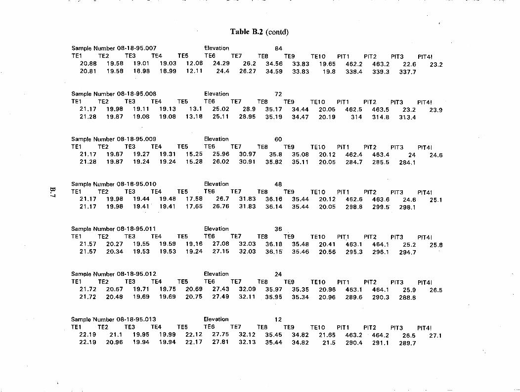
Table B.2 (contd)

Sample Number 08-18-95.007 Elevation 84 TE1 TE2 TE3 TE4 TE5 TE6 TE7 TE8 TE9 TE10 PIT1 PIT2 PIT3 PIT4!

20.88 19.58 19.01 19.03 12.08 24.29 26.2 34.56 33.83 19.65 462.2 463.2 22.6 23.2 20.81 19.58 18.98 18.99 12.11 24.4 26.27 34.59 33.83 19.8 338.4 339.3 337.7

Sample Number 08-18-95.008 Elevation 72 TE1 TE2 TE3 TE4 TE5 TE6 TE7 TE8 TE9 TE10 PIT1 PIT2 PIT3 PIT4!

21.17 19.98 19.11 19.13 13.1 25.02 28.9 35.17 34.44 20.05 462.5 463.5 23.2 23.9 21.28 19.87 19.08 19.08 13.18 25.11 28.95 35.19 34.47 20.19 314 314.8 313.4

Sample Number 08-18-95.009 Elevation 60 TE1 TE2 TE3 TE4 TE5 TE6 TE7 TE8 TE9 TE10 PIT1 PIT2 PIT3 PIT4!

21.17 19.87 19.27 19.31 15.25 25.96 30.97 35.8 35.08 20.12 462.4 463.4 24 24.6 21.28 19.87 19.24 19.24 15.28 26.02 30.91 35.82 35.11 20.05 284.7 285.5 284.1

Sample Number 08-18-95.010 Elevation 48 TE1 TE2 TE3 TE4 TE5 TE6 TE7 TE8 TE9 TE10 PIT1 PIT2 PIT3 PIT4!

21.17 19.98 19.44 19.48 17.58 26.7 31.83 36.16 35.44 20.12 462.6 463.6 24.6 25.1 21.17 19.98 19.41 19.41 17.65 26.76 31.83 36.14 35.44 20.05 298.8 299.5 298.1

Sample Number 08-18-95.011 Elevation 36 TE1 TE2 TE3 TE4 TE5 TE6 TE7 TE8 TE9 TE10 PIT1 PIT2 PIT3 PIT4!

21.57 20.27 19.55 19.59 19.16 27.08 32.03 36.18 35.48 20.41 463.1 464.1 25.2 25.8 21.57 20.34 19.53 19.53 19.24 27.15 32.03 36.15 35.46 20.56 295.3 296.1 294.7

Sample Number 08-18-95.012 Elevation 24 TE1 TE2 TE3 TE4 TE5 TE6 TE7 TE8 TE9 TE10 PIT1 PIT2 PIT3 PIT4!

21.72 20.67 19.71 19.75 20.69 27.43 32.09 35.97 35.35 20.96 463.1 464.1 25.9 26.5 21.72 20.48 19.69 19.69 20.75 27.49 32.11 35.95 35.34 20.96 289.6 290.3 288.8

Sample Number 08-18-95.013 Elevation 12 TE1 TE2 TE3 TE4 TE5 TE6 TE7 TE8 TE9 TE10 PIT1 PIT2 PIT3 PIT4!

22.19 21.1 19.95 19.99 22.12 27.75 32.12 35.45 34.82 21.65 463.2 464.2 26.5 27.1 22.19 20.96 19.94 19.94 22.17 27.81 32.13 35.44 34.82 21.5 290.4 291.1 289.7

Table B.2 (contd)

136.7 TE7 TE8

31.59 32.76 31.58 32.76

126.1 TE7 TE8

31.31 32.73 31.32 32.74

115.3 TE7 TE8

31.16 32.91 31.14 32.92

104.1 TE7 TE8

31.03 33.24 31.04 33.23

92.7 TE7 TE8

30.94 33.78 30.95 33.79

81.1 TE7 TE8

31.28 34.43 31.26 34.44

TE9 TE10 32.08 22.95 32.08 23.03

TE9 TE10 32.06 23.5 32.08 23.5

TE9 TE10 32.24 23.86 32.25 23.86

TE9 TE10 32.5 24.66

32.51 24.66

TE9 TE10 33.13 24.95 33.15 25.1

TE9 TE10 33.74 25.64 33.76 25.64

PIT1 PIT2 463 464.1

350.2 351.1

PIT1 PIT2 463.5 464.5 374.4 375.3

PIT1 PIT2 463.7 464.8 363.2 364

PIT1 PIT2 463.4 464.5

348 348.9

PIT1 PIT2 463.9 465 320.3 321.2

PIT1 PIT2 463.5 464.7 304.8 305.7

PIT3 PIT4 15.8 20.4

349.2

PIT3 PIT4 20.8 21.2

373.5

PIT3 PIT4 21.1 21.7

362.3

PIT3 PIT4 21.8 22.3

347.2

PIT3 PIT4 22.5 23

319.6

PIT3 PIT4 23 23.6

304

Sample Number 08-TE1 TE2

23.1 22.19 23.1 22.19

Sample Number 08-TE1 TE2

23.5 22.66 23.5 22.55

Sample Number 08-TE1 TE2

25.35 24.66 25.35 24.73

Sample Number 08-TE1 TE2

25.71 25.02 26.11 25.5

M8-95.014 TE3 TE4

20.66 20.71 20.67 20.69

-18-95.015 TE3 TE4

20.96 21.01 20.98 21.01

-18-95.019 TE3 TE4

22.67 22.71 22.69 22.69

-18-95.020 TE3 TE4

23.23 23.27 23.25 23.25

Elevation TE5 TE6

22.22 28.28 22.09 28.32

Elevation TE5 TE6

21.26 28.46 21.14 28.51

Elevation TE5 TE6

20.26 28.67 20.15 28.71

Elevation TE5 TE6

19.43 28.84 19.32 28.88

Elevation TE5 TE6

19.01 28.98 18.94 29.02

Elevation TE5 TE6

19.31 29.16 19.25 29.18

Elevation TE5 TE6

20.29 29.31 20.3 29.33

73.6 TE7 TE8

31.76 34.79 31.71 34.8

TE9 TE10 34.14 26.11 34.14 26.4

PIT1 PIT2 464 465.1

290.4 291.3

PIT3 PIT4 23.7 24.1

289.7

Sample Number 08-18-95.016 TE1 TE2 TE3 TE4

23.64 22.88 21.31 21.36 23.72 22.88 21.32 21.36

Sample Number 08-18-95.017 TE1 TE2 TE3 TE4

24.33 23.5 21.7 21.75 24.33 23.57 21.72 21.74

Sample Number 08-18-95.018 TE1 TE2 TE3 TE4

24.55 23.97 22.12 22.16 24.66 23.86 22.13 22.14

Table B.2 (contd)

Sample Number 08-18-95.021 TE1 TE2 TE3 TE4

27.09 26.48 24.14 24.17 27.02 26.4 24.17 24.16

Sample Number 08-18-95.022 TE1 TE2 TE3 TE4

27.35 26.8 24.72 24.75 27.35 26.8 24.75 24.75

Sample Number 08-18-95.023 TE1 TE2 TE3 TE4

28.18 27.64 25.31 25.33 28.18 27.57 25.33 25.32

Sample Number 08-18-95.024 TE1 TE2 TE3 TE4

28.47 27.96 25.89 25.91 28.73 28.11 25.92 25.9

Sample Number 08-18-95.025 TE1 TE2 TE3 TE4

29.42 28.4 26.9 26.93 29.34 28.55 26.92 26.92

Sample Number 08-18-95.026 TE1 TE2 TE3 TE4

29.71 28.65 f 27.31 27.32 29.56 28.73 ' 27.32 27.33

Elevation 61.6 TE5 TE6 TE7 TE8 TE9 TE10 PIT1 PIT2 PIT3 PIT4

22.15 29.48 32.08 35.23 34.56 27.57 464.3 465.5 24.2 24.7 22.12 29.52

Elevation

32.08 35.24

49.7

34.6 27.71 303.9 304.8 303.1

TE5 TE6 TE7 TE8 TE9 TE10 PIT1 PIT2 PIT3 PIT4 23.13 29.59 32.19 35.43 34.8 27.96 464.3 465.4 24.7 25.3 23.15 29.62

Elevation

32.2 35.44

37.8

34.82 27.86 298.9 299.8 298.1

TE5 TE6 TE7 TE8 TE9 TE10 PIT1 PIT2 PIT3 PIT4 24.23 29.69 32.25 35.6 34.93 28.33 465.1 466.3 25.4 26.1 24.25 29.7

Elevation

32.26 35.58

20.1

34.94 28.33 303.2 304.2 302.6

TE5 TE6 TE7 TE8 TE9 TE10 PIT1 PIT2 PIT3 PIT4 25.29 29.77 32.28 35.46 34.83 28.73 465.3 466.5 26.1 27.1 25.32 29.78

Elevation

32.28 35.45

145.7

34.82 28.94 299.7 300.7 299.1

TE5 TE6 TE7 TE8 TE9 TE10 PIT1 PIT2 PIT3 PIT4 25.33 29.72 31.81 33.12 32.47 29.42 466.3 467.5 16.1 19.8 25.29 29.76

Elevation

31.8 33.11

134.4

32.44 29.34 367 368 366.3

TE5 TE6 TE7 TE8 TE9 TE10 PIT1 PIT2 PIT3 PIT4 25.16 29.76 31.51 32.99 32.33 29.63 467.1 468.4 20.1 20.4 25.13 29.76 31.51 32.98 32.32 29.71 375.3 376.3 374.6

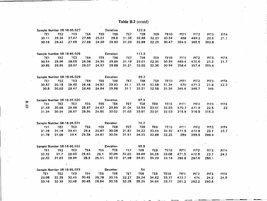
Table B.2 (contd)

Sample Number 08-TE1 TE2

30.11 29.34 30.18 29.42

Sample Number 08-TE1 TE2

30.54 29.96 30.65 29.85

Sample Number 08-TE1 TE2

30.87 30.18 30.8 30.03

Sample Number 08-TE1 TE2

31.49 30.65 31.34 30.54

Sample Number 08-TE1 TE2

31.78 31.16 31.78 31.09

Sample Number 08-TE1 TE2

32.32 31.7 32,32 31.63

Sample Number 08-TE1 TE2

33.08 32.25 33.16 32.39

i-18-95.027 TE3 TE4

27.67 27.69 27.68 27.68

1-18-95.028 TE3 TE4

28.05 28.08 28.07 28.07

-18-95.029 TE3 TE4

28.46 28.48 28.47 28.46

-18-95.030 TE3 TE4

28.96 28.97 28.97 28.95

-18-95.032 TE3 TE4

29.93 29.93 29.94 29.9

-18-95.033 TE3 TE4

30.45 30.45 30.48 30.45

Elevation TE5 TE6

25.01 29.8 24.99 29.83

Elevation TE5 TE6

24.95 29.89 24.97 29.89

Elevation TE5 TE6

24.87 29.93 24.84 29.96

Elevation TE5 TE6

24.67 29.99 24.65 30.02

Elevation TE5 TE6

24.67 30.06 24.67 30.04

Elevation TE5 TE6

25.1 30.09 25.11 30.13

Elevation TE5 TE6

25.78 30.15 25.84 30.15

122.9 TE7 TE8

31.35 32.88 31.33 32.88

111.3 TE7 TE8

31.19 33.01 31.21 33.02

87.3 TE7 TE8

31.04 33.59 31.03 33.61

75.7 TE7 TE8

31.51 34.22 31.51 34.25

65.9 TE7 TE8

32.02 34.89 31.99 34.91

54 TE7 TE8

32.27 35.24 32.28 35.25

TE9 TE10 32.23 30.54 32.25 30.47

TE9 TE10 32.35 30.94 32.36 30.94

TE9 TE10 33.01 32.03 33.01 32.03

TE9 TE10 33.64 32.32 33.68 32.25

TE9 TE10 34.28 33.08 34.29 33.16

TE9 TE10 34.62 33.77 34.64 33.77

PIT1 PIT2 468 469.2

364.5 365.5

PIT1 PIT2 469.4 470.6 356.4 357.4

PIT1 PIT2 470.7 471.9 315.9 316.9

PIT1 PIT2 471.5 472.8

289 289.9

PIT1 PIT2 471.5 472.8 286.6 287.6

PIT1 PIT2 472.7 474 291.2 292.2

PIT3 PIT4 20.5 21.1

363.8

PIT3 PIT4 21.2 21.7

355.6

PIT3 PIT4 22.5 23

315.3

PIT3 PIT4 23.1 23.7

288.4

PIT3 PIT4 23.7 24.2

286.1

PIT3 PIT4 24.3 24.9

290.5

18-95.031 TE3 TE4

29.41 29.4 29.4 29.38

99.3 TE7 TE8 TE9 TE10 PIT1 PIT2 PIT3 PIT4

31.1 33.19 32.58 31.34 470 471.3 21.8 22.3 31.1 33.21 32.58 31.34 345.6 346.7 345

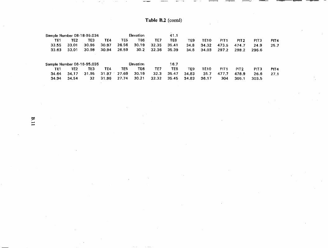
Table B.2 (contd)

Sample Number 08-18-95.034 TE1 TE2 TE3

33.55 33.01 30.96 33.63 33.01 30.98

Sample Number 08-18-95.035 TE1 TE2 TE3

34.64 34.17 31.95 34.94 34.54 32

Elevation 41.1 TE4 TE5 TE6 TE7 TE8 TE9 TE10 PIT1 PIT2 PIT3 PIT4

30.97 26.56 30.19 32.35 35.41 34.8 34.32 473.5 474.7 24.9 25.7 30.94 26.59 30.2

Elevation

32.36 35.39

16.7

34.8 34.03 297.2 298.2 296.6

TE4 TE5 TE6 TE7 TE8 TE9 TE10 PIT1 PIT2 PIT3 PIT4 31.97 27.69 30.19 32.3 35.47 34.83 35.7 477.7 478.9 26.6 27.1 31.96 27.74 30.21 32.32 35.45 34.83 36.17 304 305.1 303.5

w

Distribution

PNL-10865 UC-2030

No. of Copies

Offsite

12 DOE Office of Scientific and Technical Information

C. S. Abrams 1987 Virginia Idaho Falls, ID 83404

E. C. Ashby 225 North Avenue Boggs Chemistry Building Georgia Institute of Technology Atlanta, GA 30332

K. Bandyopadhyay Building 129 Brookhaven National Laboratory Upton, NY 11973

N. W. Bibler Westinghouse Savannah River Co. Building 773 A, Room B132 Box 616 Aiken, SC 29802

D. Campbell 102 Windham Road Oak Ridge, TN 37830

F. N. Carlson 6965 North, 5th West Idaho Falls, ID 83401

E. D. Collins Oak Ridge National Laboratory P.O. Box 2008 7930, MS-6385 Oak Ridge, TN 37831-6385

Morton Corn Room 6010 School of Hygiene and Public Health John Hopkins University 615 N. Wolf Street Baltimore, MD 21205

M. First Harvard School of Public Health 665 Huntington Avenue Boston, MA 02115

Charles W. Forsberg Oak Ridge National Laboratory P.O. Box 2008, MS-6495 Oak Ridge, TN 37831-6495

E. P. Horwitz Chemistry Department Argonne National Laboratory 9700 Cass Avenue Argonne, IL 60439-4831

Billy C. Hudson 202 Northridge Ct. Lindsborg, KS 67456

M. S. Kazimi Massachusetts Institute

of Technology Department of Nuclear Engineering 77 Massachusetts Avenue Cambridge, MA 02139

J. L. Kovach Nuclear Consulting Services, Inc. P.O. Box 29151 Columbus, OH 43229-0151

B. R. Kowalski Chemistry Department, BG-10 University of Washington Seattle, WA 98195

Distr.l

PNL-10865 UC-2030

No. of Copies

Thomas S. Kress 102-B Newridge Road Oak Ridge, TN 37830

Thomas E. Larson Los Alamos National Laboratory MS-P915,DX-DO P.O. Box 1663 Los Alamos, NM 87545

3 Los Alamos National Laboratory P.O. Box 1663 Los Alamos, NM 87545 Attn: W. L. Kubic, K557

K. Pasamehmetoglu, K555 J. Spore, K575

D. Meisel Chemistry Department Argonne National Laboratory 9700 Cass Avenue Argonne, IL 60439-4831

T. E. Larson Los Alamos National Laboratory MS-P915, DX-DO P.O. Box 1663 Los Alamos, NM 87545

D. T. Oakley Waste Policy Institute Suite 600 555 Quince Orchard Road Gaithersburg, MD 20878

DonOrth 124 Vivion Drive Aiken, South Carolina 29803

F. L. Parker Vanderbilt University P.O. Box 1596, Station B Nashville, TN 37235

D. Pepson U.S. Department of Energy Trevion II Building, EM-35 Washington, D.C. 20585-0002

No of Copies

G. E. Schmauch Air Products and Chemicals, Inc. 7201 Hamilton Boulevard Allentown, PA 18195-1501

Scott E. Slezak Sandia National Laboratory Org. 6471/MS 0741 P.O. Box 5800 Albuquerque, NM 87185-0744

Dana Powers Sandia National Laboratory Dept. 6404/MS-0744 P.O. Box 5800 Albuquerque, NM 87815-0744

W. J. Thomson Dept. of Chemical Engineering Washington State University Pullman, WA 99164

J. Tseng U.S. Department of Energy Trevion II Building, EM-35 Washington, D.C. 20585-0002

A. S. Veletsos 5211 Paisley Houston, TX 77096

Onsite

16 DOE Richland Operations Office

M. F. Campbell S7-73 R. E. Gerton S7-54 J. M. Gray (10) S7-54 C. A. Groendyke S7-54 D. H. Irby S7-54 M. F. Jarvis S7-54 G. W. Rosenwald S7-54

Distr.2

PNL-10865 UC-2030

No of No of Copies Copies

33 Westinghouse Hanford Company 37 Pacific Northwest Laboratory

H. Babad S7-30 J. M. Alzheimer K5-22 W. B. Barton R2-11 Z. I. Antoniak K7-15 R. E. Bauer L6-37 J. M. Bates K7-15 T. R. Benegas Nl-27 S. Q. Bennett K7-90 C. E. Hanson H5-09 P. R. Bredt P7-25 D. L. Herting T6-09 M. E. Brewster K7-15 J. D. Hopkins R2-11 J. W. Brothers K5-22 G. D. Johnson (5) S7-15 G. Chen K5-12 N. W. Kirch R2-11 J. B. Colson K5-10 J. R. Kristofzki T6-06 P. A. Gauglitz P7-41 D. C. Larsen Rl-51 W. B. Gregory K7-22 J. A. Lechelt R2-11 J. D. Hudson K7-15 J. W. Lentsch (5) S7-15 T. E. Michener K7-15 R. M. Marusich A3-34 F. E. Panisko P8-34 N. G. McDuffie S7-15 M. R. Powell P7-19 J, E. Meacham S7-15 K. P. Recknagle K7-15 R. E. Mendoza Rl-51 H. C. Reid K7-15 D. A. Reynolds R2-11 K. L. Rightmire K7-22 C. A. Rieck R3-27 P. A. Scott P7-43 C. P. Shaw L5-07 A. Shekarriz K7-15 T. I. Stokes L6-37 C. L. Shepard (5) K5-25 J. E. Van Beek R3-27 C. W. Stewart K7-15 R. J. Van Vleet A3-34 G. Terrones (5) K7-15 J. R. White H5-09 J. M. Tingey P7-25 N. E. Wilkins R2-11 Information Release (5)

Distr.3