IAEA-SMR-44

REACTOR THEORY AND POWER REACTORSPROCEEDINGS OF THE COURSE ON REACTOR THEORY AND POWER REACTORS

HELD AT TRIESTE, 13 FEBRUARY - 10 MARCH 1978DURING THE WINTER COURSES ON NUCLEAR PHYSICS AND REACTORS

JOINTLY ORGANIZED BY THEINTERNATIONAL ATOMIC ENERGY AGENCY,

THE INTERNATIONAL CENTRE FOR THEORETICAL PHYSICSAND THE

CENTRO Dl CALCOLO BOLOGNA OF THECOMITATO NAZIONALE PER L'ENERGIA NUCLEARE OF ITALY

AND HELD AT THEINTERNATIONAL CENTRE FOR THEORETICAL PHYSICS, TRIESTE

17 JANUARY - 10 MARCH 1978

INTERNATIONAL CENTRE FOR THEORETICAL PHYSICS, TRIESTE, 1980

L J

REACTOR THEORY AND POWER REACTORS

I

' (IAEA)in 1964 under an agreement with the Italian Government, and with the assistance of the City and University of Trieste.

The IAEA and the United Nations Educational, Scientific and Cultural Organization (UNESCO) subsequently agreed to operate the Centre jointly from1 January 1970.

Member States of both organizations participate in the work of the Centre, the main purpose of which is to foster, through training and research, theadvancement of theoretical physics, with special regard to the needs of developing countries.

J

IAEA-SMR-44

REACTOR THEORY AND POWER REACTORS

PROCEEDINGS OF THE COURSE ON REACTOR THEORY AND POWER REACTORSHELD AT TRIESTE, 13 FEBRUARY - 10 MARCH 1978

DURING THE WINTER COURSES ON NUCLEAR PHYSICS AND REACTORSJOINTLY ORGANIZED BY THE

INTERNATIONAL ATOMIC ENERGY AGENCY,THE INTERNATIONAL CENTRE FOR THEORETICAL PHYSICS

AND THECENTRO DICALCOLO BOLOGNA OF THE

COMITATO NAZIONALE PER L'ENERGIA NUCI.EARE OF ITALYAND HELD AT THE

INTERNATIONAL CENTRE FOR THEORETICAL PHYSICS, TRIESTE17 JANUARY - 10 MARCH 1978

INTERNATIONAL CENTRE FOR THEORETICAL PHYSICS, TRIESTE

REACTOR THEORY AND POWER REACTORS, IAEA, VIENNA, 1980

Printed by the IAEA in AustriaMatch 1980

J1

FOREWORD

The International Centre for Theoretical Physics has maintained an interdisciplinary character in its research and training programmes in differentbranches of theoretical physics. In pursuance of this objective, the Centre has organized extended research courses and workshops, including topicalconferences, with a comprehensive and synoptic coverage in varying disciplines. The first of these — on Plasma Physics — was held in 1964 and thenrepeated in 1977; the second, in 1965, was concerned with the Physics of Particles. Between then and now, the following courses were organized: four onNuclear Theory (1966,1969,1971,1973), six on the Physics of Condensed Matter (1967,1970,1972,1974,1976,1978), three on Atomic Physics(1973,1977,1979), two on Geophysics (1975,1977), one on Control Theory and Functional Analysis (1974), one on complex analysis (1975), one onApplications of Analysis to Mechanics (1976), one on Mathematical Economics (1978), one on Systems Analysis (1978), two on Teaching of Physics attertiary level (in English in 1976, in French in 1977), and two on Solar Energy (1977,1978). Most of the Proceedings of these courses have been publishedby the International Atomic Energy Agency (Vienna, Austria).

The present volume forms part of the Proceedings of the Winter Courses on Nuclear Physics and Re? ctors, conducted from 17 January to10 March 1978. This volume contains the Proceedings of the Course on Reactor Theory and Power Reactors, held at Trieste, 13 February to 10 March 1978.A separate volume contains the Proceedings of the Course on Nuclear Theory for Applications, held from 17 January to 10 February 1978. The WinterCourses were held in response to the growing need of developing countries which plan to establish a nuclear power programme to familiarize themselveswith the nuclear and reactor physics foundations of nuclear energy and their applications in the design of nuclear reactors.

The programme of lectures and working sessions was organized by Drs. J.J. Schmidt and J.A. Larrimore (International Atomic Energy Agency,Vienna, Austria), Professor V. Benzi (Centra di Calcolo of the Comitato Nazionale per l'Energia Nucleare, Bologna, Italy), and Professor L. Fonda (ICTP,Trieste, Italy).

Abdus Salam

PREFACE

This volume contains the text of the invited lectures presented during the Course on Reactor Theory and Power Reactors which was held at theInternational Centre for Theoretical Physics (ICTP), Trieste, Italy from 13 February to 10 March 1978. The course was jointly organized by the Divisionof Nuclear Power and Reactors of the IAEA, the International Centre for Theoretical Physics, Trieste, Italy and the Centro di Calcolo in Bologna of theComitato Nazionale per l'Energia Nucleare of Italy. The course was attended by 116 participants from 34 developing countries, 16 participants from6 developed countries and 4 participants from Geel and the Joint Research Centre, Ispra, of the Commission of European Communities.

The purpose of the course was to review the latest developments and problems in the theoretical and experimental physics of nuclear power reactorscooled and moderated by light water or by heavy water, which are the principal power reactor types of near term interest in developing countries planningto embark on a nuclear power programme. An introductory lecture on the reactor physics needs in developing countries was followed by a series oflectures devoted to theoretical and experimental bases for calculational methods in reactor physics, nuclear data used for reactor calculations, the reactorphysics of pressurized and boiling light water nuclear power reactors and of heavy water power reactors, computer codes for power reactor neutroniccalculations, including steady state and kinetic calculations, fuel depletion calculations and neutron and gamma-ray shielding. Some lectures were includedon the reactor physics of high temperature and fast breeder reactors.

As research in reactor physics is an important precondition for the development of nuclear power engineering, this text is expected to be of interestboth to scientists from countries with advanced reactor physics research, as well as to those from the countries where such research is just beginning todevelop.

The text is suitable for specialists engaged in research and development as well as in design and operation of nuclear power reactors. It can be used asa reference in the field or as an advanced textbook for postgraduate study.

The organizers are most grateful to the lecturers, workshop leaders and scientific co-ordinators for their very active engagement and co-operation in theobjectives of this Course, and to the Staff of the ICTP for their most pleasant and efficient help in the preparation and conduct of the Course.

CONTENTS

Reactor physics needs in developing countries 1R. Solanilla

Nuclear data and integral experiments in reactor physics 17U. Fartnelli

Calculational methods for lattice cells 41J.R. Askew

Reactor theory and Power Reactors 69A.F. Henry

The physics of irradiated nuclear fuel 129M. Robin

Physics of pressurized water reactors .-. 153A. Griin

Reactor physics aspects of CANDU reactors 215E. Critoph

General remarks on fast neutron reactor physics , , 263J.Y.Barre

HTR characteristics affecting reactor physics 281K. Ehlers

Nuclear reactor shielding 297C. Ponto

Nuclear data preparation and discrete ordinates calculation 325B. Carmignani

Notes on nuclear reactor core analysis code: CITATION (Sample P.W.R. reactor problem) 347D.G. Cepraga

Kinetic calculations "The AIREK code" 365St. Boeriu

Faculty and Participants 379

J

REACTOR PHYSICS NEEDSIN DEVELOPING COUNTRIES

R. SOLANILLAComision Nacional de Energia Atomica,Buenos Aires,Argentina

ABSTRACT

The aim of this paper the identification of needs on ReactorPhysics in developing countries embarked in the installation andlater on in the operation of Commercial Nuclear Power Plants.In this context the main task of Reactor Physics should be focusedin the application of Physical models with inclusion of thermohy-draulic process to solve the various realistic problems which appearto ensure a safe, economical and reliable core design and reactoroperation.The first part of the paper deals with the scope of Reactor Physicsand its interrelation with other disciplines as seen from the viewpoint of developing countries possibilities.Needs requiring a quick response i.e., those demands coming duringthe development of a specific Nuclear Power Plant Project, aresummarized in the second part of the lecture. Plant startup hasbeen chosen as reference to separate two categories of requirements:Requirements prior to startup phase include reactor core verifi-cation, licensing aspects review and study of fuel utilizationalternatives; whereas the period during and after startup mainlyembraces codes checkup and normalization, core follow-up and longtern prediction. The corresponding activities and the requiredtools are described and some applications are illustrated showingthr importancp in developing countries to dispose of: i) a computercode package for core analysis and ii) a trained group of ReactorPhysicists and Nuclear Engineers with good understanding of thephysical process involved into the reactor as well as the ap-proximations and structure of the computer codes.Reactor Physics needs non related with a specific project-longterm needs-are covered in the last part of the paper. Specialnention is made of:a) Comparative studies for Reactor type selection (with long termfuel cycle implication).b) Education of people for future use in Nuclear Power Programs.c) Theoretical foundation of Reactor Analysis Methods and codes

development.

1.- Introduction

The high investment and efforts spent in some industrializedcountries in the development of Nuclear Power Plants, whichgo from research up to industrial utilization, is the basisof the present high maturity of Nuclear Technology for ther-mal Reactors. It may seem wise and economic not to repeat thesame process in the domestic development of nuclear energy indeveloping countries, but rather to use the available experienceby means of special agreements with the suppliers of nucleartechnology and also by cooperation with various countries intechnological development.Within this context, the main task of Reactor Physics in develop-ing countries should be channeled towards the applicationof reactor computational models having reasonable accuracyin the prediction of the main reactor magnitudes, to over-come the various problems encountered in ensuring a safe,economical and reliable core design and reactor operation.It is the principal purpose of the paper to identify thedifferent needs on Reactor Physics in developing countriesembarked in the installation and operation of CommercialNuclear Power Plants. Basically, their needs on Reactor Physicsare not different from those of industrial countries. However,the priorities and the context where the reactor physicistlive are different, particularly the economic, financial andtechnical resources of the countries, which ultimately definethe scope of the activities to be undertaken. A typical con-dition in developing countries, at least during the earlystage of thir Nuclear Programs, is the way how they implementthe construction of the Nuclear Power Plants.A turn-key contract with foreign vendors for the initialPower Plant is the approach adopted by mostof the developingcountries with a trend towards increasing local participationin the decision-making area for the subsequent Plants. In thiscontext, the priority of the" Reactor Physicist should not bedirected to develop, for example a conceptual core design, butrather to get a comprehensive understanding of the differentphysical aspects of the core design. Further in the stage ofplant operation the worries on Reactor Physicist in develop-ing countries might not be so different from those whichexist in Nuclear utility industry in industrial countries.At least, the objectives become similar.Along these lines, the definition of the scope of ReactorPhysics and its interrelation with other disciplines, as seenfrom the viewpoint of developing countries'possibilities,

1

J

are discussed in the first part of this paper.One can establish two categories of needs on Reactor Physicsin developing countries:

a) - Demands appearing during the development of a specificNuclear Power Plant which require a quick response aredealt with in Section 2. The corresponding needs arereviewed along the various steps of the project, start-ing from the moment when the construction of the Plantis decided (excluding the feasibility study) and thenthe necessary assistance in Reactor Physics is analyzed.

b) - Reactor Physics needs non-related with a specific pro-ject are discussed in Section 3. The comparative studyfor Reactor Type Selection is specially mentioned, aswell as the activities related with the Theoricalfoundation of Reactor analysis methods, codes develop-ment and Education of pecple for future use in NuclearPower Programs.

But before going ahead, let me point out the necessity torely upon a minimum level of research and development capabi-lity in nuclear technology in the country, before a decisionconcerning the introduction of Nuclear Energy is made.From the Reactor Physics point view, a requirement should beto have a least a few experienced Reactor Physicists withaccess to large digital computers. Nevertheless, in any caseemphasis should be put on-the-job-training in special areassuch as Reactor Core Analysis by means of problem-orientedcourses during the earlie3t days of the Nuclear Power PlantProgram implementation.

2.- Reactor Physics: Its role and its interaction with other

disciplines.

At the early stage of Nuclear Energy development, Reactor Phys-ics was mainly Neutron Physics in the Reactor.During the last 20-25 years we can notice a continuous trend ofReactor Physics towards solving the real problems arising in de-sign, construction and operation of Nuclear Power Plant.Reactor Physics became more and more involved with the engineer-ing aspects of Nuclear Energy than ever before.The new role of Reactor Physics was the subject of some papers.In one of them, written by Dr. Critoph (•*•) the scope and

role of Reactor Physics in the design and operation of NuclearPower Plants was very well explained. Two approaches to under-stand the role of Reactor Physics were discussed in this paper.They are well applied to developing countries:When a Nuclear Power Plant Project has been ordered, theanswers to many questions arising during the development of theProject and operation of the Plant must be supplied within ashort time and with a minimun cost by using the available tools.In such a case, the Reactor Physicist acts by following an engi-neering approach or, in other words, using an engineering pointof view.The other approach - it was called the reasearch point of view-assumes that there is not a defined requirement, and in thiscase, the Reactor Physicist works, without any time constraints,in improving the accuracy and consistence of Reactor Physicsmethods and/or removing the defficiencies of Reactor Theory.In principle, both views - short and long term - are com-plementary and their validity will depend on each particularsituation and country.What can we say from the developing countries'point of view?Two facts can be pointed out:

- High degree of maturity reached in the design and perfomance ofthe present Commercial Reactor types, in coincidence with thebeginning of the nuclear era in most of -the developing countries.

- An orientation in the scientific community of these countriesto continue a research activity regardless of any practical ap-plication (perhaps due to the lack of experienced managers andof a strong industrial basis).

Both factors, as well as the scarcity of financial resourcesto assure a sustained high investment and effort - as requiredin Reactor Research projects - make it advisable that ReactorPhysics in those countries to be more concerned with the appli-cations than with Research.Along these lines, the scope of Reactor Physics as seen from thedeveloping country view point can be defined.As it is well known, the primary function of Reactor Phys-ics is the determination, at any time, of neutron and radiationdistribution through a finite site medium made up of many regionshaving different material compositions. In other words, it looksafter solutions - either analytical or computing machines-orien-ted numerical solutions- of the linear Transport Equation withrealistic assumptions concerning dimension and core representa-tion, neutronic material properties, energy and angular dependen-ce on neutron and gamma radiation destribution, etc. The basicnuclear data cross section as a function of energy for different

J

isotope and process - used to solve the problems currently en-countered in Reactor Physics, is evaluated on an experimentalbasis.At the present, the Nuclear Data are compiled in a comprehensivemanner in the Nuclear Data Library developed by many NuclearCentre. The results of the calculations, namely intensive lat-tice parameters, such as cell flux distribution, static reacti-vity, power distribution over the whole cell, isotopic composi-tion and heavy isotope production for different irradiations,etc., have been intensively measured for the present CommercialReactor types fuelled with uranium-oxide in critical facilities,mock-up experiments, or power reactors.Over the last 25 years nany basic reactor computer codes havebeen developed-and many of them are available- to cope withreasonable accuracy with the first physical problems ofNuclear Reactor, i.e. "cell calculation" - and they were testedagainst experimental results covering a wide range of geo-metric and material arrangements and physical conditions.At the present time, due to the powerful available methodsfor Reactor Core Analysis and the relatively complete nucleardata library for thermal reactor it is possible to perform awhole reactor core calculation, mainly for the present gene-ration of commercial reactor types, with an-accuracy betterthan 0.3£ in K effective and a few per cent of discrepancy inneutron flux, without making any expensive special experi-ments. That is a remarcable achievement of the reactor modelingnot usually encountered in engineering application.Consequently, it is advisable that the greater efforts ofthe Reactor Physicist in developing countries should beconcentrated upon the analysis of Reactor Core design andPerfomance.Reactor Core design and Reactor Perfomance Analysis is notan exclusive task of Reactor Physics. Many other disciplinessuch as Engineering, Material Science, Computer Technologyand Mathematics are deeply involved. Therefore, a successfulachievement of Reactor Physics will require a strong interac-tion among different fields.A typical activity in Nuclear Technology clearly show-ing this interdisciplinary orientation is Nuclear Core Design.It is not possible to imagine a reliable core design withouta succesive interaction between Reactor Physics and Thermohy-draulics passing through the material behaviour science,Mechanical design and Economics.Fuel management also shows a complex interrelationshipamong several fields ' * ) . Fuel management implies several areas of

decision, such as:- Energy Planning (Capacity factor, cycle lengh in LWR)- Fuel Design (technological fuel design limits).- Fuel cycle definition (refuelling rate, discharged fuel burnup and isotopic inventory, feed enrichment and size of thereload charges (both for LWR).

- Reactor Operation (peaking factor, control rod worths, shutdownmargins, axial offset, kinetic parameters, etc).

- Economics (cost of yellow cake, enrichment services, transpor-tation, storage, etc.).

The aim of fuel management in Power Reactors is the optimi-zation of the fuel cycle cost within the constraints imposedby core thermohydraulics, fuel linits, safety margins, powergrid flexibility, nuclear fuel resources and cost of the opera-tion involved in the fuel cycle.Core performance follow-up during the operation of the NuclearPlant also offers a wide variety of tight co-operative efforts.As example one can mention the determination of a specificheat transfer between fuel and cladding and fuel temperature reacti-vity coefficient from reactivity measurements in Power Reactor,(3)which shows the result of co-operative among Reactor Core ana-lysis, Reactor Control and instrumentation, Reactor operationand Fuel engineering.Many more examples can be given, showing that NuclearEngineering orientation in Reactor Physics education is advisable,particularly in developing countries where the introduction ofNuclear Energy faces a lack of trained personnel in areas relatedwith planning, design and operation of Nuclear Power PLants.As it was noted earlier in Dr. Critoph's paper, mentionedbefore, this is the way that the Reactor Physicists can playan important role in the coordination of activities fromdifferent fields of the Nuclear Technology which is ones of thedifficult and prior tasks of our age.3. - Needs on Reactor Physics during the developing of a specific

Nuclear Power Project *3.1 Description of areas, requirements and objectivesBriefly, the development of a specific Nuclear Power Plant Projectincludes the following steps:

"• The functions of core analysis that must be carried out inthe support of a specific Nuclear Plant Project have been thesubject of a recent paper (4) submitted to the Conference on"Nuclear Technology Transfer" held in Persepolls. Some needsand activities for an independant core analysis capability indeveloping countries reported in the above mentioned paper hasbeen incorporated in this section.

- Bid Evaluation and Contracts- Licensing- Fuel Specification- Commissioning- Commercial OperationThe principal functions of Reactor Physics during the abovementioned stages are to assist the staff responsible for theimplementation of the Nuclear Power Plant by providing reactorcore data on evaluated experience and by performing severalreactor calculations and analysis. In reactor commissioning,and during the operation of the Plant, the Reactor Physicist parti-cipates in measurements of the principal reactor characteristicsrelated with reactor safety, reactor performance and commercialguarantee.

To accomplish this broad spectrum of tasks, a trained staff ofengineering-oriented reactor physicists and soft-ware computa-tional package are needed from the earlist time.The software computational package should include codes for coredesign, transients/accidents analysis, in core fuel management,shielding calculations and reactor simulations.The local computer code package can be built up by collectingindividual codes from many sources - Public domain libraries,reactors/fuel vendors codes, commercial codes and home-madecodes - by making them operational, and then by coupling theminto a calculation system.

A successful implementation of this integrated system of codesshall require from the local physicists and nuclear engineersa good understanding of the physical and numerical approxima-tion as well as the structure of the codes.This integrated system of codes will become reliable after an ex-tensive integral validation against proper data taken from reactoroperation data banks and/or benchmark problems.Codes package tests could be carried out by the local personnel inco-operation with foreign experts or foreign organizations whichcan provide, among other assistance, operating data of power plantssimilar data of power plants similar to those to be constructed inthe country.

A permanent effort will be demanded to improve the accuracy andcomputer time running of the codes of the system as well as toexpend the scope of this integrated system of codes by incorpora-ting new development and requirements in them.The structure of this integrated system of codes will consist ofmany modules. The interrelationship among them and the flow of

information through the system is indicated in Fig.l. ReactorPhysics, therraohydraulics and fuel modelling codes are also in-cluded in the sketch to show the relations among them.The main objectives of this analysis capability c&n be summarizedas:- Ability to oerform detailed check calculations of vendor's data.- Ability to respond to safety requirements.- Ability to meet fuel -jrocurement requirements.How fast will this goals be reached?The availability of experienced Reactor Physicists, their perma-nence in their duties for a sufficiently long Deriod, and howeffectively they can be integrated into the oroblems encounteredduring the development of the Nuclear Program,should give theDroper answer. Ultimate achievement would be attained after ins-tallation of some Nuclear Power Plants if a continued effort inthe various nuclear engineering related areas is followe.l.3•2 Specific Activities and tools description:Comissioning of the first Nuclear Power Plant and oarticu-larly reactor start-up, clearly separates two categories ofwork \WPrior to start-up and first of all, a basic local computer codepackage installation is needed which will require an importantassistance in computer software; next comes reactor verification,reactor transients and accidents analysis needed to assist in li-censing aspects, and finally the stu'-Iy of fuel utilization alternati-ves. In a second stage, i.e. -luring and after reactor start-up,the activities are phannelled towars start-up analysis, corefollow-up and long term prediction.3.2.1 Preliminary activitiesBasic computer code package installation is the first activityto be undertaken.The calculations carried out during and after the installationof the computer codes package in the local digital computer willpermit local physicists and/or nuclear engineers to become familiarwith the input data preparation,which can be obtained from thecore design manual provided by the plant and fuel vendors.At the same time, the physicist or nuclear engineer will getconfidence about the theory,approximations,procedures, core re-presentation and the most important features of the codes beforehe begins to answer some of the questions arising during the de-velopment of the Project.3-2 2) Reactor core design verificationThe adequacy of the reactor design can be verified by designcontrol actions carried out by a group which chould be inde-pendent from the reactor vendor.The verification should consist of examining the reactor design

J

checking uo the calculations and comparing the results againstthe original design basis.The most relevant ohysical calculations included in the reac-tor core design verification to be mentioned are:a) Strady State criticality- Critical Boron concentration as a function of burnup.- Control Rod worth- Reactivity coefficients- Burnable absorbers- Reactivity balance for different reactor statesb) Steady state power distribution

Power distribution within a furl pin, standard fuel assemblywith absorbersPower distribution over the core as a function of burnupand reactor states.

c) Burnup and Core Depletion- Fuel pin and fuel assembly burnup and isotopic composition

Burnup and isotope inventory of discharged assemblies (orbatches) for equilibrium and transient phases.Burnup cycle length or refuelling rate.

- Loading and unloading pattern schemes.d) Xenon transient

Xenon release during power level changesAbsorbers management

e) Reactor ShieldingDose rates calculations near and inside primary circuits

- Neutron and Gamma—ray penetration and radiation heating.Short review of the methods usedGroup constantsDesign Codes use Spectrum Codes to generate few group crosssection. Thermal Spectrum Codes are based on analyticalsolutions for neutron thermalization and zero dimensionalmedium C . Collision probability methods for spatial treatmentover a lattice cell* with thermalization kernels and multi-grouns approach are also used to predict spatial spectrumdependence {<>.Approximation Bl or PI is the current practice to solve the fastspectrum zero dimensional homogeneous problem and few groupcondensation (S).Resonance capture calculation for heterogeneous geomet riesintermediate resonance treatment based upon equivalence princi-ples'9). Accurate methods for larger cells need Transport Theoryand Multigroup schemes.(1^)Depletion calculation with a special treatment for Xenon/iodineis also incorporated in these codes. The fission products arerepresented by a pseudo-fission product. For higher burn-up, a

detailed isotope inventory calculation cannot be ignored in thefission oroduct representation.Survey calculation for Heavy Water-Natural Uranium reactor doesnot fall into the aforementioned lines. Wescott formulism foraverage thermal cross section calculation in a well thermalized-reactor is used.'H) Fitted fast cross sections are adopted forcondensed two-group diffusion calculations. (1^) Coliv.sion Pro-bability Method or Diffusion theory are applied over the largercell} d-> 13) combined with fitted procedures to take into accountthermal-epithermal spectrum with spatial dependence over thelattice cellJ1'*)Group diffusion fluxes'Detailed diffusion theory calculation of a fuel assembly - withor without absorbers - and a whole or a quarter core with finitedifference approximation and coarse mesh representation is a currentpractice.(15) Absorbers are treated using Blackness theory with"effective diffusion constants", or an effectiv boundary conditionover the absorber surface. (16,17) The set of codes (lattice code)are coupled through cross section tables with suitable entry para-meters (for example fuel assembly type, point irradiation andpower level), or they can be grouped by using a modular structurein which the code modules communicate through suitable inter-faces.

Feed back effectsWhen the coolant density interaction on power distribution andspatial burnup becomes quite important, i.e. large void reacti-vity coefficient, the coupling of the neutronic and thermohy-draulic calculation is necessary. For example, in the absence ofaxial absorber distribution, a Boiling Water Reactor (BWR), at thebeginning of life, will give a power peak at the bottom of thechannel, which would be completely absent when the calculationis performed at constant water density.Temperature and water density feedback effects on neutroniccalculations of pressurized reactors have not the same intensityas in BWR, but -.pecial operation conditions, such as "stretch-outcondition", show a non-negligible feedback effect.Non-linear effects due to the interrelation between spatial powerdistribution and Xenon concentration are usually taken into accountby means of the quasi-static method, which asemes a constantspatial flux and power distribution during a given time interval.In this manner, the steady-state diffusion code coupled with pointXenon-Iodine kinetics equation can be used to study spatial Xenonfeedback effects or Xenon transient due to power level changes(start-up simulation or power cycles).Shielding calculations

J

Reactor Shielding design-oriented calculation is becoming animportant field for reactor physicists and nuclear engineers.Shielding problems are currently solved by using so-calledenpirical methods (adjustment of kernel, albedo and diffusionmethods) or transport theory (mainly discrete ordinate methodsand Monte Carlo methods). A fine energy group structure forneutron and gamma cross section data is needed for neutronand gamma penetration.(1°)

As it was recently reported (19), a major effort in reactorshielding should be focused to i) streaming problems in cavi-ties existing between the reactor vessel and the primaryshield, and ii) radiation level prediction in different placesaround the reactor during reactor operations, maintenanceoperations, as well as conditions after reactor accident.The radiation dose calculation concerns mainly the activationand transport of corrosion products in the heat trnsportsystem.Use of the codesThe local basic code packages should contain the necessarycodes to carry out the above calculations. Sometimes it isadvisable to use two or more codes to deal with th" samephysical problem, but with different approximationsIt is a very good practice for the physicist or nuclearengineer working in developing couritries to go through theavailable codes to improve some procedures such as schemesto spee:!-up the "inner-outer" iterative process currentlyused to solve the finite difference equations, or toircorporate new features in the codes,such as automizedfuel management strategy for reload and shuffling operationof thermohydraulic feedback effects. This seems to be thebest way for the users to get more and more insight intothe codes which, in this way, will no longer be seen as"black boxes". It should be recognized that, by leadingthe code user to examine reactor operation conditions inorder to prepare input data or

to compare vendor's data with his own calculations, he canget a better understanding of the process involved, to thepoint that he may also propose some valuable improvements.The advantages of this approach can be illustrated by thefollowing example: During the calculations of diffusiontheory applied to a larger PWR core corresponding to anIranian Nuclear Power "-, which were carried out with

"The calculation was performed during the permanence of theauthor in the Atomic Organization of IRAN.

the purpose of comparing two sets of different codes againsteach other and against vendor's data, two successive questionsarose:12°)- Accurate solution with the conventional finite

different coarse mesh method with corner of mesh (COM)scheme.

- Extrapolation of the magnitudes derived from coarse meshrepresentation to obtain axact values.

Benchmark calculations showing the comparison between centreof mesh representation, (CEM,i.e. the fluxes are defined inthe centre of each mesh box), and the conventional corner ofmesh (COM) method were available, but that comparison was notapplicable to modern power PWR core with fuel in a checkboardpattern where more interfaces are present than in the bench-mark problem. (The difference between COM and CEM dependson the way the interfaces are treated). A comparison studyof both methods applied to this core yielded some interestingresults particularly -the extrapolation of CEM results to mesh-width zero and the accuracy for the same number of mesh pointsof each method. (Fig. 2).3-2.3) Licensing aspects reviewLicensing aspects review includes seveial analysis requiredby the Regulatory Body. It is a common practice that thevendors submit to the Licensing Authority various technicaldocuments regarding the safety of the reactor design andoperation.In many developing countries, the regulatory functions areperformed by the same national agency in charge of the NuclearPower Plants construction and operation. Hence, an essentialfunction related with safety analysis review has to be in-corporated among the activities of the Reactor Physicistsand Nuclear Engineers of developing countries involved withNuclear Projects.To examine the safety-related documentations, a relativeability to review the vendor's calculation or to performalternative calculations is needed: As an example we couldmention the necessary calculations to provide informationon reactor control limits, such as:- Excess reactivity or reactivity balances- Stability condition (particularly Xenon instability)- Maximum controlled reactivity and reactivity insertion

rates.- Shutdown margin vith ejected rod.- Emergency shutdown efficiency.- Etc.

J

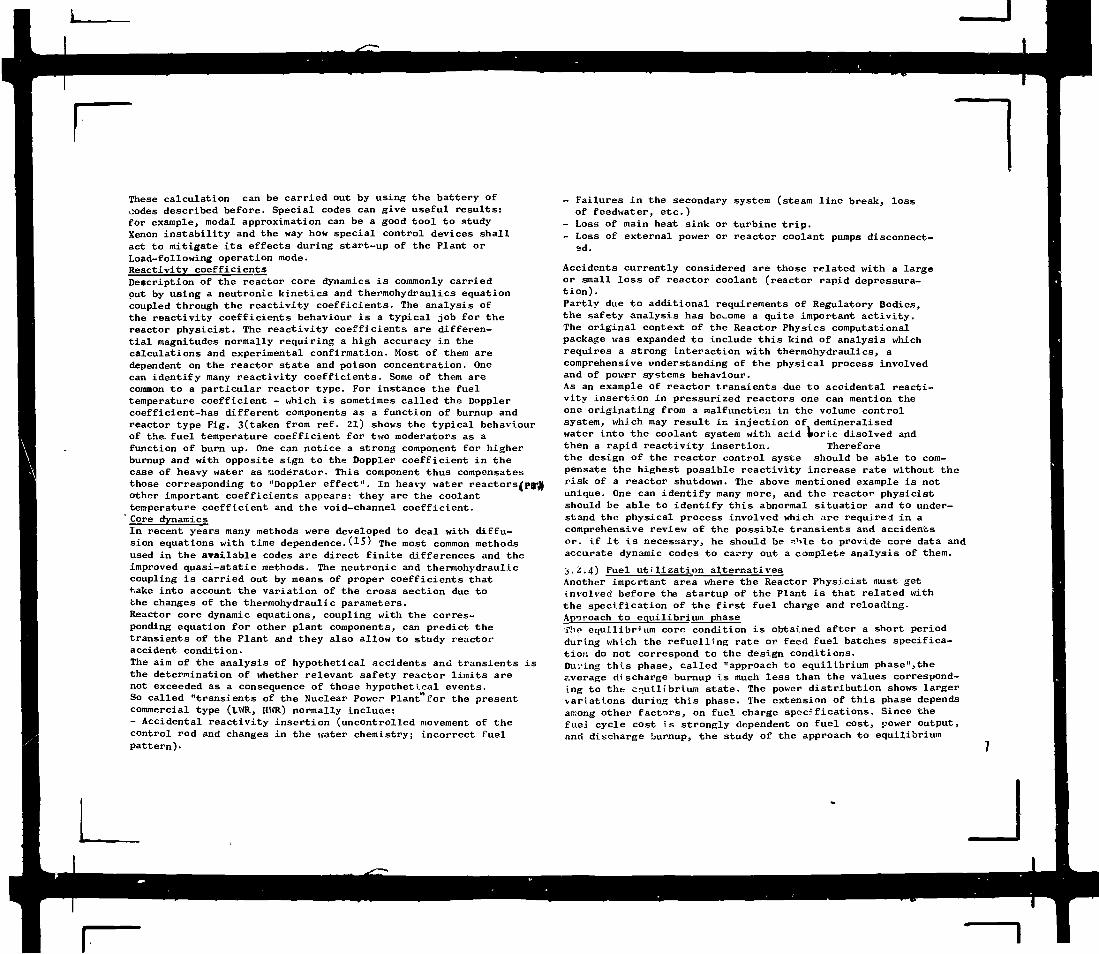
These calculation can be carried out by using the battery ofcodes described before. Special codes can give useful results:for example, modal approximation can be a good tool to studyXenon instability and the way how special control devices shallact to mitigate its effects during start-up of the Plant orLoad-following operation mode.Reactivity coefficientsDescription of the reactor core dynamics is commonly carriedput by using a neutronic kinetics and thermohydraulics equationcoupled through the reactivity coefficients. The analysis ofthe reactivity coefficients behaviour is a typical job for thereactor physicist. The reactivity coefficients are differen-tial magnitudes normally requiring a high accuracy in thecalculations and experimental confirmation. Most of them aredependent on the reactor state and poison concentration. Onecan identify many reactivity coefficients. Some of them arecommon to a particular reactor type. For instance the fueltemperature coefficient - which is sometimes called the Dopplercoefficient-has different components as a function of burnup andreactor type Fig. 3(taken from ref. 21) shows the typical behaviourof the- fuel temperature coefficient for two moderators as afunction of burn up. One can notice a strong component for higherburnup and with opposite si.gn to the Doppler coefficient in thecase of heavy water as moderator. This component thus compensatesthose corresponding to "Doppler effect". In heavy water reactorsother important coefficients appears: they are the coolanttemperature coefficient and the void-channel coefficient.'Core dynamicsIn recent years many methods were developed to deal with diffu-sion equations with time dependence.(15) xhe most common methodsused in the available codes are direct finite differences and theimproved quasi-static methods. The neutronic and thermohydrauliccoupling is carried out by means of proper coefficients thattake into account the variation of the cross section due tothe changes of the thermohydraulic parameters.Reactor core dynamic equations, coupling with the corres-ponding equation for other plant components, can predict thetransients of the Plant and they also allow to study reactoraccident condition.The aim of the analysis of hypothetical accidents and transients isthe determination of whether relevant safety reactor limits arenot exceeded as a consequence of those hypothetical events.So called "transients of the Nuclear Power Plant"for the presentcommercial type (LWR, HWR) normally include:- Accidental reactivity insertion (uncontrolled movement of thecontrol rod and changes in the water chemistry; incorrect fuelpattern).

- Failures in the secondary system (steam line break, lossof feedwater, etc.)

- Loss of main heat sink or turbine trip.- Loss of external power or reactor coolant pumps disconnect-

ed.

Accidents currently considered are those related with a largeor small loss of reactor coolant (reactor rapid depressura-tion).Partly due to additional requirements of Regulatory Bodies,the safety analysis has become a quite important activity.The original context of the Reactor Physics computationalpackage was expanded to include this kind of analysis whichrequires a strong interaction with thermohydraulics, acomprehensive understanding of the physical process involvedand of power systems behaviour.As an example of reactor transients due to accidental reacti-vity insertion in pressurized reactors one can mention theone originating from a malfunction in the volume controlsystem, which may result in injection of demineralisedwater into the coolant system with acid fcoric disolved andthen a rapid reactivity insertion. Thereforethe design of the reactor control syste should be able to com-pensate the highest possible reactivity increase rate without therisk of a reactor shutdown. The above mentioned example is notunique. One can identify many more, and the reactor* physicistshould be able to identify this abnormal situatior and to under-stand the physical process involved which are required in acomprehensive review of the possible transients and accidentsor. if it is necessary, he should be =>.'->le to provide core data andaccurate dynamic codes to carry out a complete analysis of them.

3.2.4) Fuel utilization alternativesAnother important area where the Reactor Physicist must getinvolved before the startup of the Plant is that related withthe specification of the first fuel charge and reloading.Approach to equilibrium phaseThe equilibrium core condition is obtained after a short periodduring which the refuelling rate or feed fuel batches specifica-tion do not correspond to the design conditions.Du'.'ing this phase, called "approach to equilibrium phase",theaverage discharge burnup is much less than the values correspond-ing to the equilibrium state. The power distribution shows largervariations during this phase. The extension of this phase dependsan:ong other factors, on fuel charge specifications. Since thefuel cycle cost Is strongly dependent on fuel cost, power output,and discharge burnup, the study of the approach to equilibrium

J

phase has an important economical incentive.Survey codes for fuel management coupled with fue1 cycle costcodes are very important tools to perform this study.The calculation must be made in such a way as to reduce thetransient period and ensuring at every time that the hotchannel factors F and F for pressurized reactors (22) (or

q A Hmaximum admissible channel power output for present CANDUversion) are within the design limits for a scheduled absorb-er management during this approach to equilibrium phase.F factor is important primarily from the fuel meltingQstandpoint, F is important from a departure of nuclear boiling

AHstandpoint. In channels with non-zero flow quality at the exit,the limit condition is given by the critical power or powerdensity needed to reach a dry-out condition in the coolantchannel.(22) Additional constraints introduced by the fueldesign limits are also included in the calculation among themare those concerning the "power jump" or sudden heat flux risewhen the fuel moves to positions of higher power, or when, dueto insertion of the control rod bank or other operation condi-tion, the heat flux is suddenly increased.A relatively faster transient period keeping the operatingcondition behind the limits is usually obtained by a loadingscheme with three or more different initial U-235 enrichments

or, in the case of a Natural Uranium reactor, by acharge of depleted uranium placed in some selected fuelchannels. (23) when no procedures are available to flatten thepower distribution at the beginning of the core life, the poweroutput must be reduced.

Fuel cycle coat calculationsCodes for fuel cycle cost calculation also play an importantrole. They can be locally developed to carry out sensitivitystudies in fuel cost, associated with a particular fuel load-ing scheme-proposed by the fuel vendors-varying the unitprice of raw material, tail assay, cost of fuel operationinvolved, etc.These codes can also provide information concerning the fueldemands in the electric power system, for near and long termprojections due to changes in (1) policy decisions on tailsassay and delivery timetable of the natural uranium,(2) thetime when the uranium recovered from the spent fuel is incor-porated into the system,etc.In the case of L.W.R. the well known limitation on fuelreprocessing capacity will incentivate the owner of the NuclearPlant to study new fuel alternatives, such as the change of

the present enrichment for first charges, of the number ofzones and of the cycle length for once-through cycle LWRdesigns.Ability to carry out this kind of analysis will allowdeveloping countries to take further decisions concerningthe change of fuel vendors (particularly to national vendors)without higher penalty.3.2.5) Plant startup phaseReactor physics measurementsDuring the testing run, the vendor currently carries outseveral measurements to ensure a safe and reliable operationof the Plant, and also to check several contractual guaranties(net power output, fuel consumption, load following capability,transient condition withstanding capability)Normally, the Reactor Physics measurements at lower levelinclude the following determinations:- Critical poison concentration (at zero power)- Control rod worth- Shutdown margin- Detectors calibration and flux shape determination- Reactivity coefficients- Correlation between in-core and out-or-core flux detectors.Previous activitiesSome time before the start-up of the Plant, the ReactorPhysicist should begin the study of the corresponding start-up procedures. It is advisable to have a good knowledge ofthe Engineering of the Plant, mainly for those systems rela-ted with the reactor behaviour, namely: Volume control andchemical systems, heat transport system, moderator system, coreinstruments,flux measurement devices, reactor control andprotection system, etc.Nuclear Power Plants are usually equipped with an on-linecomputer for monitoring and also to assist the core sur-veillance functions by checking core margins by generatingalarms. The computer collects data from core instrumentssignals and, by using appropiate algorithms, it performsseveral physical calculations.A processor digital computer is a central part of the controlsystem of CANDU type Power Plants. The digital computer isused for alarm annunciation and data adquisition, but it isalso used for other functions such as regulation of ReactorPower, primary heat transport pressures, steam pressure, etc.The Reactor Physicist must become familiar with the character-istics of the on-line computer and its software package andhe must also become aware of what the computer can do and

what it cannot Jo. In other words, the relationship betweenplant operation data bank and off-line computer Centre shouldbe established and clearly understood during this phase (Fig.4)In this manner, the information storage in the on-line com-puter allows the comparison of the operating data with thepredictive values which will be used for further decisionson in-core fuel management and operation support.Fuel loading and testing runThe Reactor Physicist should be present for initial fuelloading, low power testing and power escalation. He canparticipate with the operation crew and vendor personnelduring the preparation and execution of the test and instrumentscalibrations, and he should collect his own data,make his owninterpretations, and carry-out his calculations to normalizehis own computer code system. Further, he can assist themanagement staff of his Plant and then perform his own evaluationon a sound basis.An active participation of the local physicist during thestart-up phase can give fruitful results. During the start-up of the first Argentine Nuclear Power Plant, the localReactor Physicist detected the possibility of increasingthe net guaranteed reactor power without exceeding thereactor safety limits. This conclusion was made possibleby following the daily operation run of the Plant and bycomparing theoretical values with the in-core self-powereddetector.3.2.6) Commercial operationWhen the Nuclear Plant goes into commercial operation, theprincipal needs on Reactor Physics are those related withthe support of the operation and with long term prediction.Basically, the operation support is performed in responseto Plant Engineering requests, and it will require an up-dated core following, which is possible only with the help ofa detailed simulation code and a fluent communication withthe operation data.Simulation CodesSimulation codes are currently static 3-D-coupled nuclear-thermohydraulic computer programs representing the core.(24)Provisions are made to take into account different reactorstates (the cross section over the range from hot zero orlow power up to hot full power), and fuel elements designcontaining varying amounts of lumped burnable poison.Xenon transient can be treated using a quasi-equilibriumapproach.The model employs nodal or finite-differencemethods and few groups static diffusion code.Eigenvalues iteration is coupled to a close channel thermo-

hydraulic calculation which contains suitable correlationsfor void-quality and critical heat flux.These codes can be used for operational calculation of fluxesanrl power distribution and thermal performances, as a functionof control rod position, poison concentration, power leveland other operational data. Exposure distribution, cyclelength calculation and fuel failure prediction can also beincorporated into the codes. The simulation codes can beapplied to study the maneuverability of the Nuclear Plant,i.e. operational flexibility of the Plant for load follow-ing which - as it is known - is a basic condition in develop-ing countries. Normally, the LWR is designed to allow adaily 50% power load cycle with full recovery at peak Xenonat a certain ramp rate through 8O-9OSS of the cycle life (cladcyclic strain is an additional constraint to be considered inthe fuel element design).In HWR there is no restriction on cycle life, but the powerload following introduces changes in the nuclear designwhich lead to increased fuel cycle cost if a booster solu-tion (rod with high U—235 enrichment) is replaced by adjusterrods (stand-by reactivity).The study of different combinations to cope the reactivitytransient (control bank and boro feed and bleed system) withthe help of a simulation code, should allow the Plant owner tomeet grit requirements without exceeding design (reactor andfuel) limits and with minimum waste problems.The reactor simulation codes permit many more applicationsto support a safe and reliable Plant operation, such as:- Power distribution to be used for fuel performancemodelling (fuel failure rate) and in-core detector signalsprediction

- Power distribution to investigate power shaping for specialoperator action

- Control rod pattern and its efficient use- Reactor start-up form different conditions and its opti-mization

- Stretch-out operation- Updated burnup and heavy isotope production- X enon oscillations and their suppresionLong term prediction CodesCodes for long term prediction are similar to core-followingcodes but the emphasis is rather oriented to in-core fuelmanagement schemes and refuelling outage studies.Some of the most important outputs of these codes regard theoptimum cycle length, the number of assemblies required forrefuelling, the optimum fuel enrichment, the optimum refuel-

J

10

ling and fuel discharge pattern, etc.Most of the in-core fuel management codes use a "trial anderror" method for fuel management optimization.(25J Thr refuel-ling pattern is given as input or the code includes and auto-mated refuelling generation within a given condition, e.g.discharge of fuel elements with highest burnup but keepingthe power distribution (or F ) within specified limits.If this condition is not fulfilled, the code cancels theoperation and another operation is proposed.Optimization technique is sometimes used to generatefeasible fuel loading and fuel shuffling patterns as wellas for absorber management that minimize the levelized fuelcost and at the same time fulfill certain constraints suchas the maximum permisible exit burn up, and peaking factor.Dynamic programming procedure combined with a simple reactormodel have been succesfully applied to solve thr optimal fuelpolicy over a specified cycle length in LWR.(26)Finally, the last but not the least important activity of theReactor Physicist during the commercial operation of the Plantshould be to assist the operational staff in areas such as:- Interpretation of abnormal situations (detector failures,abnormal power distribution etc)

- Radiation dose in certain reactor conditions- Fuel perfoi'mance evaluation- Waste disposal and irradiated fuel storage problems- General operation support- Courses on Reactor Physics for operating crew.

4) Other neeas on Reactor PhysicsThis section is devoted to those long-term needs on ReactorPhysics which are not related with a specific project.A special comment will be made about the comparative studiesfor reactor type selection to be carried out in the prelimi-nary stage and before the initiation of a specific NuclearPower Plant project, as well as the activity serving as back-up of Reactor Physics design oriented and people's educationfor future use of Nuclear Power Plant Program.4.1) Comparative studies for reactor-type selectionComparative studies for reactor-type selection are an importantpart of the well-known feasability studies which play a vitalrole in the integration of nuclear energy into the whole powersystem, and also in the assessment of the impact of Nuclear Powernto the system.

Stfcj ye studies including an evaluation of commerciallyavaLlableSrtfcslear Power Plants were primarily conducted to

select the most convenient reactor among different reactortypes, to meet the national requirements - reasonable Capitalcost, local participation in equipment supplies, control ofthe fuel cycle, etc. In a second stage those studies wereexpanded to incorporate advanced reactor concepts or fuelcycle alternatives into a long term scenario.Long term study is a starting point for countries decided toembark on a Nuclear Power program which requires some pre-vious answers regarding:- Fuel cycle strategies- Relative potential of the present reactor design in the

local grid system- Role of advanced reactor concepts (Fast breeder reactors

or Advanced Converters reactors) in a future Nuclear Powerprogram.

The identification of the advantage of new reactor conceptsor fuel cycle alternatives to support future decisions con-cerning research-ori ented technology areas can also be esta-blished through a long term comparative study.The important role to be played by the Reactor Physicist inthe development of the comparative study is well understood.He elaborates and provides reactor core data, examines thecontrol and the safety features of the reactor concept,evaluates the different fuel management schemes,carries outthe fuel cycle calculation for single reactor or a coupledsystem, and he also investigates the optimum reactor strate-gy taking into account several conditions, such as economy,uranium resources utilization, and technical feasabilityof the reactor concepts and the advanced fuel cycles options.Recently, new constraints were introduced in the choice ofthe reactor system. They regard proliferation risk andenvironmental conditions. New initiatives to define the reactorconcept and the fuel cycle which avoids or minimizes the useof Plutonium are encouraged particularly advanced fuel cycle op-tions such as:

- Once through U-Pu cycle- Thorium-Uranium cycle

4.2) Theoretical foundation of reactor analysis methodsAs all young disciplines, the design-oriented Eeactor Physicshas known a rapid development in the last years. The adventof faster computers with larger fast memory and storage capa-city has made it possible to develop new and powerful numeri-cal methods to solve multigroup diffusion equations, transportequations, spatial kinetic equations, etc.

J

It is now possible to calculate neutron fluxes and gamma raydistribution at any time in complex material and geometryconfigurations with full representation of the reactor core.But there is still room for further improvements.The savings in computer time introduce an economical incentiveto the development of reactor analysis methods. As it isknown, the Finite element method and Coarse-mesh numericalmethods for reactor power calculations were introduced inthe last few years to reduce computing time and storagerequirements of the "conventional" fine mesh methods. Thenodal method, which is based on the coarse-mesh method,was also recently introduced with great success to dealwith time dependent problems. A variety of nodal codes usingmethods to couple the average flux in a node with thecurrent on its face have been developed. Improvements ofthe treatment of the flux solution within the nodes havealso been reported recently and surely will be the subject ofnew reports. (27)

Additional challenges for new developments in reactor compu-tational methods, such as: the reflector treatment, theconsistent homogeneization of group constants, the predictionof local power quantities ("fine structure") from globalreactor calculation, the neutronic thermohydraulics couplingmodelling, etc, have been recently reported.(2°)The Spatial Control Method and its applications for solvingstability problems in larger core or those problems regardingload-follow operation, require special mention. These me-thods using optimization techniques are very actual. Theycould improve the control system of the reactor in order toensure an economical and flexible plant operation.(29)Another important area to be mentioned is the development oftechniques and methods to determine perfomance - relatedand safety - related information from data that can becollected in Nuclear Plant transients.(3°)It becomes clear-that the Reactor Physicists associated withthe development of the project and later on with the opera-tion of the Nuclear Power Plant require a back-up from theReactor Physicists oriented in applied research areas, whichare much better placed to carry out comparison studies amongdifferent methods, and selection of the best theory foreach particular problem. They are also able to follow thestate-of-art of Reactor Physics and to propose improve-ments and/or applications of new theories to solve practi-cal problems encountered in reactor design and operation.But fruitful results of the research area in developingcountries will be possible when a suitable two-way communi-

cation with engineering-oriented Reactor Physics is estab-lished. This is the way to take advantage of the two differentbut in principle complementary views followed in the solutionof the Reactor Physics problems.4-3) Code developmentAn important effort of the Reactor Physicist orientedin reactor core analysis and not directly involved withthe project requirements, should be spent in Code develop-ments. The scope of code development is very wide. Itincludes codes with a new nature of problems to be solved,or with a new mathematical method, but it also includes acode built—up from available modules with some modifica-tions or improvements needed to tackle particular problems.Benchmark problem has proved very useful in the developmentof new mathematical methods and verification of computercodes. It can also be applied to compare Hifferent computercodes. Recently, eight different areas have been mentioned,where a well defined problem and corresponding solutions areavailable. (31)Comparison with vory well defined experiments or "Monte Carlosimulated experiment"(26) (clean homogeneous or heterogeneousexperiments) allow to check the physical data and physical models(particularly for shielding studies), and the developers ofcomputer codes should currently use both Benchmark problemsand clean experiments, for comparison, evaluation and verificationpurposes.Concerning the development, from available modules, of acode adapted to solve special problems, let me mention anexperience which happened some years ago.Reactor Vendors currently offer special training to customer'stechnical personnel in the venJor's facilities. This train-ing can sometimes produce benefits far beyond those one canenvisage. At the end of the last decade, Argentine decidedto construct its first Nuclear Power Plant called ATUC11A.The rpactor is a Heavy Water - natural uranium, pressurevessel type, designed for on—power refuelling in accordancewith a radial shuffling scheme. The loading machine is loca-ted in the upper part of the core and the reactor is equippedwith diagonal control rods extending from the upper outer partof the core to its lower central part. Reactor control isachieved by changing the moderator temperature and the depthof the control rod bank. A special bank of control rods -called "grey control rods", -is designed to control the Xenonoverride during power cycle.Upon technical agreement between CNEA and the Atucha reactorvendor, some engineers and physicists were sent to the vendor's

J

12

offices to participate in the reactor design. Accurate nucleardesign and operation simulation (particularly load-followingmode) of this reactor were not a simple job, due to highheterogenity of the reactor core. With a combined effort ofvendor's and customer's physicists, a development of a "tailor-ed fit" code was undertaken. The code assembled available"source-sink" codes and it incorporated a special treatmentof control rod movement, power cycle follow, fuel managementscheme prediction and thermohydraulics feedback effects.(32)The code was successfully applied to answer questions regard-ing the safety and operation modes aspects. At the presenttime, the code is still being used for fuelling strategycalculations and operation support.The above mentioned example shows a fruitful result of theseco-operative efforts to develop specific computer codes.However, to benefit from this experience it is mandatorythat the personnel trained abroad find an appropriatestructure allowing them to continue their work when theyreturn home.4-4) Education for future use in Nuclear Power ProgramAs it has already been pointed out, one of the crucialquestions in developing countries facing the introductionof Nuclear Energy, concerns the availability of skilledpeople for domestic Nuclear Programs development. It iswell recognized that the Nuclear Research Centres in de-veloping countries, trained technicians, specializedlaboratories and some flexible reactor facilities or spe-cial equipment (as reactor simulator) are essential toestablish the ground work for back-up industry in the de-sign, control and operation of the Power Plant. In thiscondition, the Centres can provide ex pertise and person_nel for future uses in the Nuclear Industry. The education ofthese people is one of the principal roles of the NuclearCentres and Reactor Physics, one of their major components.High education levels in developing countries shall be possibleif a Research program is encouraged and maintained by appropriateprojects. However, the selection of the Research Projects is alocal decision taking into account financial and technicalresources as well as national objectives.

5) Conclusion

In those developing countries embarked in the implementa-tion of a Nuclear Power Plant Program, Reactor Physicshas an important role to fullfil providing accurate reactor

core information and assistance in the planning, designreview and operation of Nuclear Power Plants.However, a successful achievement requires a positive dis-position of Reactor Physicists to be involved in the variousand practical problems encoutered during the developmentof a Nuclear Project and Plant operation.Research activity in the field must also be encouraged whenit is programmed as back-up of Reactor Physics - designoriented or for educational purposes.

References

1) Critoph, E., "The role of Reactor Physics in theDesign and Operation of Power Reactors". 3rd. Inter-national Advanced Summer School in Reactor Physics"Herceg-Novi-Yugoslavia IAEA - TRS 143 (1973)Silvennoimen, P. "Reactor Core Fuel Management"Perganon Press (1976) - Section II and Section III.Raum, H., Bronner, G., Krebs, W.D., "Determinationof the specific heat transfer between fuei and can-ning from reactivity measurements at the NuclearPlant KCB" Nuclear Technology Vol. 29, June 1976.J.R.Fisher, J.K.Davindson "Program Plan ror transferof core analysis techonology to the nuclear utilityindustry of a developing country" submitted to "NuclearTechnology and Transfer" Persepolis-Iran (1977)- AlsoAnnals of Nuclear Energy Vol. 4 pp 289-301, 1977.Cadilah, M. at all: "Methodes theorique pour l'etudede la thermalisation des neutron dans le milieu absorbantsinfinis et homogene" Rapport CEA 2368 (1964).AsKew, J.R. "Review of status of collision probabilitymethods" p.185 Numerical Reactor Calculation - IAEA -1972.

Honeck, H.C. "THERMOS . A Thermalization transporttheory code for Reactor lattice calculation" B N L -5826 (1961).Bohl, H, Hemphill, A.P. "MUFT. A fast neutronspectrum calculation" WAPD-TM.21S (1961).Seghal, S.R.,Goldstein R. "Intermediate resonanceabsorption in heterogeneus systems Nucl. Sci. and Eng.19, 449 (1962).

10) AsKew, J.R. at all "WIMS A general description of thelattice code" J.Brit. Nuc. Energy Soc. 564 (oct.1966).

11) Wescott, C.H. "Effective cross section values for wellmoderated thermal reactor spectra" AECL 1101 (I960)

2)

3)

4)

5)

6)

7)

8)

9)

I J

12) Gibson, I.H. "The physics of LATREP" AECL 2548 - 1966.13) Alpiar, R. "Methuselah A universal assessment programme for

liquid moderated reactor cells, using IBM 7090 or strechcomputer". AEEW - R135 '1964).

14) Green et al "Lattice studies at Chalk River and theirinterpretation".Girard et al "Physique des reacteurs a eau lourde'.1.Proceeding of the third International Conference inthe Peaceful uses of Atomic Energy Vol. 3 - 1964 -

15) Henry, A.F. "Calculation methods for reactor and reactorkinetics". Winter course on Nuclear Physics and ReactorsTrieste - Italy - ICTP Seminar Series - 1978 - (to bepublished)

16) Henry, A.F. "Atheoretical method for determining theworth of control rod" WAPD - 218 (1959)

17) Crowther, R.L., "Control of Power Reactor" 3rd. Inter-national Advanced Summer School in Reactor Physics"(Herceg Novig) Yugoslavia - IAEA TRS n° 143 (1973)

18) Ponti, C. "Reactor Shielding Lectures" Winter course onNuclear Physics and Reactors Trieste - Italy - ICTPSeminar Series - 1978 - (to be published).

19) "International Conference on Reactor Shielding" NuclearNews - June page 136.

20) Moberg, L., Solanilla, R. "Coarse mesh finite differencemethods applied to a large PWR-core" Trans, of A.N.S.June 1977

21) Lunde J.E. "Analysis of reactivity coefficients forpower reactors".3rd. International Advanced Summer School in ReactorPhysics (Herceg Novig) - Yugoslavia IAEA - TRS n°143(1973)

22) Weisman, J. "Elements of Reactor Design" Elsevierchap. 7 and 8 - 1977-

23) Critoph, E. "Fuel management in power reactors. Fuelmanagement and refuelling schems" 3rd. InternationalAdvanced Summer School in Reactor Physics (HercegNovig) - Yugoslavia - IAEA - TRS n° 143 (1973)

24) Ober, T.G., at all "Reactor operation and Controlsimulator (ROCS)" Nuc. Sci. and Enq. 64 1977.

25) Reactor Burn u? physics" Proceeding of a panelViena - July 1973 page 277 "Conclusion andRecommendation of the panel".

26) Crowther, R.L. "BWR Reactor Physics characteristics"Winter course on Nuclear Physics and Reactors.Trieste - Italy - ICTP Seminar Series - 1978 -(to be published).

27) Adams, C.H. "Current trends in Methods for Neutrondiffusion calculations" N.S. and E. 64, Oct. 1977.

28) FrShlich, R. Summary discussion and state of theart review for coarse mesh computational methods".Atomkernenergie. Vol. 30, N° 2, 1977.

29) Karppinen, J. "Spatial Reactor Control Methods" N.S.and E. 64, Oct. 1977.

30) Kerlin, T.W. "Identification of Nuclear Systems".Nuclear technology Vol. 36 Nov. 1977.

31) Dodd, H.L.(jr) "Computational Benshmark Problem -A review of receofc work within the A N.S. Mathematicsand Computational Division" N.S. and E. 64, Oct. 1977

32) Grant, C , Moldaschl, H., Solanilla R. "Applicationof a heterogeneous method in the simulation of heavywater reactor operation"Reactor Burn-up physics.Proceeding of a panel - IAEA Viena 1973.

Acknowledgements

The author wishes to acknowledge Dr. Fieroni ofReactor Physics Division in ATUCHA Nuclear Power Plant andDr. Paviotti of Reactor Calculation Section - CNEA - fortheir valuable contribution and critical remarks duringthe preparation of the manuscrit.

Besides, he also expresses his thanks to Mr. C.Kroll and Mrs. Edith M. Berninsone for their effort toproduce a readable text.

13

J

Material andGeometryS pecifications

Fuel pin andFuel assemblyDATA

1

ReactorCoreDATA

810H11

Survey Calculation

Reactor Simulation

Fuel manageiuentYFuel cycle cost

Reactor Core Transients and Accidents

Fuel performances

121. Nuclear Data L2. Multigroup Library3. Resonance data4. Scattering Matrices5. Spectrum Calculation6. Condensed fluxes oyer fuel pin

and fuel assembly. Fuel Burn up andisotope inventory.

7. Control rods and burnable poisons8. Overall reactor core calculation9. Thermo hydraulics calculation10. Neutronic kinetics11. Core Dynamics12. Fuel pin modelling

NuclearCharacteristics

CoolantDensity

Crossflow

\

. \

-e-

i

Fuel(Xenon,floppier)

Coolant(entnalpyquality)

lhermalPower

/

4-

14

STRUCTURE OF AN INTEGRATED CODE SYSTEM

FIG. 1.

J

I PEAK POWER FACTOR

IS.

IS.

l< .

13.

12

1.1*0-

1165-

Kett

1000.500

100.50 .

10 .

CPU- TIME

» e

50

f No. OF MESHPOINTS \I PER FUEL ASSEMBLY J

-i 1 1 1 r—-r100 h

R»activitr,peak power factor, CPU limt vs. mtshwidlft (from Rtf.ZOj

FIG. 2.

^D20 fc T IT

": " . FIG. 3. : "Fuel Temperature "coiiit\c\eni.(fti>m Ref.

NIJCLEAR PLANT ~ "CENTRAL 'COMPUTER

(Planning and evaluation functions)(Monitoring Functions)

Plant

Signals

Operating

Data

Fuel

Management

-j

-

On - lina

Computer

Datatransmission

Data

Handling—

—

—

Simulation

Code

Futl

failure

:Relationship between Plant operation data and off-line computer centre

FIG. 4. 15

J

I]

NUCLEAR DATA AND INTEGRALEXPERIMENTS IN REACTOR PHYSICS

U. FAR1NELLIComitato Nazionale per l'Energia Nucleare - RIT,Centro di Studi Nucleari,Casaccia (Rome),ItalySUMMARY - The material given here broadly covers the content of the 10 lecturesdelivered at the Winter Course on Reactor Theory and Power Reactors, ICTP, Trie-ste (13 February - 10 March 1978). However, the parts that could easily be foundin the current literature have been omitted and replaced with the appropriate re-ferences. The needs for reactor physics calculations, particularly as applicableto commercial reactors, are reviewed in the introduction. The relative meritsand shortcomings of fundamental and semi-empirical methods are discussed. Therelative importance of different nuclear data, the ways in which they can be mea-sured or calculated, and the sources of information on measured and evaluateddata are briefly reviewed. The various approaches to the condensation of nucleardata to multigroup cross sections are described. After some consideration to thesensitivity calculations and the evaluation of errors, some of the most importanttype of integral experiments in reactor physics are introduced, with a view toshowing the main difficulties in the interpretation and utilization of their re-sults and the most recent trends in experimentation.The conclusions try to assignsome priorities in the implementation of experimental and calculational capabi-lities, especially for a developing country.

1. INTRODUCTION

In order to be able to discuss the nuclear data and the experimentsneeded for thermal reactor calculations, it is important to have an ideaof the purposes of these calculations. My discussion will concern onlyproven reactors: PWR's (which are perhaps more common), BWR's. (which pre-sent very special problems) and, to a minor extent, the heavy water CANDUreactors.

So we shall be concerned in a first time more in the identificationof problems than in their solution - without anticipating too much of whatwill be said later concerning the specific reactor types. Moreover, it isa characteristic of thermal reactors that it is generally not possible toseparate nuclear data problems from calculational methods problems, so therewill be a strong correlation of subjects with what will be Dr Askew's (andto 6ome extent Dr Henry's) courses. Strong interrelations are also foundbetween neutronic calculations and calculations of other types, especiallythermal-hydraulics, but also mechanics, materials and others. In order tounderstand neutronic calculations, it will be necessary to keep in mind theexistence of these other problem areas.

What are the needs for thermal reactor calculations? For the provenreactor types, feasibility is of course out of the question. Are there inno-

vations to be expected? In the last several years, there has been a limitedintroduction of new concepts. The Plutonium recycle in PHR's and BWR's hasbeen a favourite investigation in the late 60's and the early 70's, althoughit is today somewhat in stand-by. The rod cluster control (ECC) replacingthe cruciform rods in PWR's has required an important adjustment ofmethods,with some; reflex on nuclear data and critical experiments. Bi'rnable poisonshave also been a major innovation, with gadolinium dominating the BWR scene,and more recently borated pyrex being introduced for PWR's. Operational ab-sorber;, in both reactor types are likely to present some neutronic problems.The extrapolation to larger unit powers has been in the past a major factorin requiring new calculations. Although many people seem to think that thepresent 1000 to 1300 MWe range is an asymptotic value, I have heard similarstatements made in the past for 400, 600, 800 MWe, and therefore I am incli-ned to disbelieve them. The Soviet Union has recently announced that pres-surized water reactors CVEK) of a power of 2000 Mlfe are being designed /I/.Each change in power \iivolves extensive re-designing, even if it is a minorone.

Much more important changes have been talked about lately, in the wakeof the new U.S. policy in nuclear energy. The attempt to achieve reasonableutilization of fuel although rejecting those options (like plutonium re-cycling) that are considered objectionable from the point of view of prolif-eration, has not only prompted studies for a better utilization of the tra-ditional fuel in the "throw-away" (or "once-through") option without repro-cessing, but have also re-launched all the exotic fuel cycles, including ma-ny that are variations of present reactor types: the spectral shift reactor,the light-water quasi-breeder, the various alternatives of the thorium cycle.It is quite obvious that such concepts would require a major effort in nu-clear data and perhaps in critical experiments.

But let us focus essentially on the more traditional types of reactorsand associated fuel cycles. Just to fix some ideas, the main characteris-tics of two reference reactors, one BWR and the other PWR, of 1000 MWe each,are given in Table 1. Although not updated with last minute improvements,these data are indicative of the present generation of commercial powerreactors. CANDU reactors will be considered a little later.

The main problems that involve reactor physics calculations concerndesign, operation and fuel management, and fall in turn under the two mainrelated headings of economics and safety.

For instance, the capacity to predict power peaking bcth at the designstage and during operation is essential for the safe operation of the reac-tor, and the uncertainty in this factor is directly reflected in a reduc-tion of the total power output of the plant, with very relevant economicconsequences :each 1% uncertainty in the power peak involves an annual lossof SS 1,000,000 or more in replacement power costs 111. Difficulties in ac-curate predictions of power peaks are met at the interfaces between elem-ents with different burn-ups, around the water gaps introduced by rod clus-ter control in PWR's and by the presence of control rod gaps in BWR's.

Fuel management must be accurately predicted, with a detailed distri-bution of burn-up. This is strictlj connected with the accuracy with which

17

J

_ J

18

reactivity at the end of cycle can be calculated. An uncertainty of 1% inthis quantity requires extra enrichment that is likely to cost t 2,000,000or more per cycle. It is a common experience for reactor operators that anequilibrium -.ycle is practically never reached; improvement or just changesin the characteristics of fuel make each refueling operation a new schemethat has to be recalculated; and this calculation must go to details, ave-rage quantities being certainly not sufficient. Moreover, a detailed pre-diction of fuel composition is important not only for reactivity considera-tions and for power peaking evaluations, but also for what concerns the fu-ture of the fuel after it is unloaded from the reactor (cooling, transpor-tation, processing and even waste disposal: think of the problem of actin-ides).

Control rod worth is important for operation and for safety, and accu-rate predictions are required in many conditions, including different burn-ups, temperatures and loadings. Tor instance, evaluations of the "stuckrod" condition and of the reactivity associated with partially insertedrods are among the prescriptions of most safety analyses.

Operational transients and stability with respect to Xenon oscilla-tions pose stringent requirements especially on calculational methods, butalso involve some nuclear data problems. In BWR's, the strict correlationbetween local power density, steam content (and therefore moderating power),neutron spectrum and average cross sections in an operational transient isan example of the most difficult calculational problems a reactor physicistis confronted with.

Even closer interactions between neutronics and thermal-hydraulicsare found in the study of accidents, when the feed-back from the plant out-side the reactor also has to be taken into account; fast transients requirethe ability to calculate the temperature distribution in the fuel pins,with consequences on reactivity through cross sections, and to separatefission heat from neutron and gamma generated power, since they have dif-ferent space and time distributions.

Shielding problems will be dealt with more extensively in anothercourse. I will just recall that they have to do not only with radiologicalprotection, but also with activation, radiation damage, nuclear heatingand, indirectly, also with instrumentation response. Shortcomings of shiel-ding calculations have recently become apparent in some new light waterreactors, with heavy economic consequences.

Finally, neutronic calculations have an impact on the specificationsone has to supply when ordering, for. instance, a fuel element, with greateconomic consequences. Not only nominal values, but also deviations fromthese values are important. For instance, how strict should be the specifi-cations concerning the admitted deviations of local enrichmert or densityfrom the nominal value? What will be the consequences of the random varia-tions of these quantities within the accepted range?

Although we have made reference up to now to "Western" reactors, muchthe same problems are met with the Soviet version of the FttR, the WERreactors. The main differences are in the hexagonal rather than square

geometry of the fuel elements, an-1, for the 440 MWe version, the long rangeperturbation introduced by th<; fluK-tTap concept of the control elements.

Somewhat different, but by no means easier problems are met with heavywater reactors. Table 2 lists some of the main data of a commercial CAiJDUreactor. The consideration that the input enrichment is fixed (natural ura-nium) is balanced by the problems connected with on-line refueling, and bythe use of adjuster rods to shape the neutron flux and to influence thespace dependence of the burn-up. The correlation of the indications fromthe in-core instrumentation with the state of the reactor itself, and thedevelopment of a predictive model that includes this real-tine informationare problems of particular importance for this reactor type.

This short and by no means exhaustive list of problems is intended toexamplify the nature of the task that the reactor physicist is confrontedwith when dealing with actual power reactors. His standpoint may be quitedifferent, according to whether his job is to design a reactor, to operateit, to review its safety and its environmental impact, or to manage itsfuel cycle. In a developing country, it is less likely to concern the de-sign of a new reactor; but some insight into the design, as well as thecapability of an independent assessment of the characteristics of the reac-tor (especially as concerns operational problems and economics) is neces-sary if one wants to be able to buy the system he really needs and to pre-dict the effects it will have on his economy. Consider the problem of autility receiving two bids for a core load, with different enrichments(and therefore different prices) both claiming to be the minimum compatiblewith a given core life. Will the utility choose the less enriched, cheaperfuel without independently assessing that it will actually meet the requi-rements? An independent safety analysis is rightly considered, in mostcases, a necessity for the country installing a reactor, at least as con-cerns the review of the major safety aspects and those which are relatedwith the particular conditions of the site and the environment. Operation,although often assisted by routines and instructions supplied by the ven-dor, always involves the insurgence of unforeseen, even if minor, compli-cations, which require the ability to perform quick calculations in orderto understand .what has happened and what course of action is advisable. Al-ternate operation strategies, moreover, may be required to meet conditionsdifferent from the reference ones, such as for instance additional shut-downs, reduced load operation, cycle-stretching otc.

To complete this picture, a couple of figures present cross sectionsof a BWR element (Fig.l) and of a PWR element (Fig.2).

J

2. THE ROLE OF NUCLEAR DATA

In the simplest case, neutronic calculations stand on three legs: thedescription of the system (geometric and material data), the nuclear data,and the calculational data. These three factors are independent only inprinciple: in fact, one finds inter-relations among them right from thestart. For instance, there must be soma degree of consistency in the degreeof approximation with which the geometry of the system is described, thedetail in the nuclear data, and the sophistication of the calculationalmethods. It would make little sense, in general, to use very many energypoints for the cross sections, to use a transport code, and then to repre-sent the reaci'or as a uniform sphere or cylinder! (although they do notmake much sense, similar calculations are sometimes done).

In the less simple cases, neutronic calculations have at least afourth leg: the thermohydraulics. For instance, in a BHR the coolant densi-ty (water plus steam) influences the neutron spectrum, therefore the crosssections, therefore the power distribution; and in turn, the coolant densi-ty (or the steam content) distribution is connected to the power distribu-tion in a feedback loop. This complicates the issue; it also introduces inthe results the uncertainties deriving from the thermohydraulics models,that have to be balanced against the uncertainties in other parts of thecalculation.

It would seem that the best way to calculate a rector would be to usethe most detailed description, the best and most finely specified nucleardata and the most sophisticated calculational methods. Well, most of thetime this is not true. First of all, it is impossible. As we have seen, apower reactor has close to 40 000 fuel pins; even if the original composi-tion of all these pins were the same, it changes with time in a differentway from one pin to another, due to differences in flux and spectrum induc-ed by overall distribution, water gaps, control rod positions, proximity toburnable poisons etc. In turn, the composition of each pin, and the neutronflux and spectrum to which it is exposed, varies also axially. The numberof space points that would have to be considered separately is already Coohigh to accomodate on a computer. The same is true for the energy represen-tation : an accurate representation of the resonance structure of interme-diate or heavy nuclei would require several thousand energy points. Even ifeither space or energy could be represented in such detail, this would cer-tainly not be true of both at the same time, not to speak of the angularvariable required for transport calculations. It is therefore necessary toproceed by homogeneization and synthesis, and often more than once. Thesehomogeneizations introduce by their nature some errors or uncertainties,that should be weighted against those deriving from the basic data. A cor-related factor is the use that is made of the information deriving from ex-periments and from existing reactors: we shall see that a little further on,but we can anticipate that this information will be fed into the processsomewhere in the middle (after some homogeneization and synthesis havetaken place) if not right at the end. In this way, this information willinfluence some combination of approximate geometry representation, nucleardata and calculational methods, tending to correct the combined errors re-sulting in the process.

Two basic approaches are possible for the problem of nuclear data forthermal reactors: one is a fundamental approach based essentially on detail-ed differencial information, the other is a semi-empirical approach basedmostly on integral experiments. Historically, the semiempirical approachcame first and is still predominant, at least as quantity of calculations.Basic methods have been applied from time to time, with little success, butonly recently have they started being applied with good results to practicalproblems, though still with a number of difficulties. There are reasons tobelieve that both approaches, or some combination of them, will play an im-portanc role in future calculations.

Why did semi-empirical methods come first? Well, there are many goodreasons. First of all, at the beginning of times there was no large scalecomputer; very little was known on basic data; lots of top scientists twis-ted their brains to find shortcuts to the answer. Then, the first reactorsthat were built had some characteristics that made them suited for simpli-fied methods. The graphite moderated (and then heavy water moderated), nat-ural uranium reactors first used to demonstrate the chain reaction, thenbuilt to produce plutonium for weapons and then turned into the first power-producing reactors, were very well thermalized reactors. In such systems,most events take place with thermal neutrons, which in turn can be well re-presented by a ilaxwellian distribution at the moderator temperature. Theaverage values of the cross sections over this distribution are the quan-tities of major interest for these systems. Again, for most cross sectionsof relevance in this region, the reaction cross section varies as 1/v, andtherefore its average over a Maxwellian can be readily calculated from onevalue, in general the reference value at 0.025 eV. For the slowing downneutrons, the spectrum follows very closely the 1/E law, so that the onlycross section average that is relevant in this region is the resonance in-tegral:

RI =

plus the information concerning the self-shielding, (especially importantfor U-238), which was generally obtained from integral experiments andsimply correlated with the surface-to-mass ratio of the fuel rod. So, es-sentially two numbers characterized each cross section, the 0.025 eV valueand the resonance integral. In the high energy region, the sper.crum can beassimilated to a fission spectrum, at least in order to calculate the fastfission factor, which is the only term of the neutron V->lance for whichthis energy range is important.

Well-thermalized reactors have long been calculated using a slight im-provement of this representation, the Westcott formalism, which adds oneparameter to the definition of the cross section: the so-called g-factor,by which the thermal cross section has to be multiplied when averaging itover the Maxwellian, in order to account for the possible deviations ofits shape from the 1/v law. Moreover, co account for the fact that thethermal neutrons do not reach complete thermal equilibrium with the medium,the neutron energy distribution is still considered to be a Maxwellian,but at a "neutron temperature" slightly higher than the moderator tempera-

19

20

ture, this temperature difference being related to the ratio between the ab-sorption and the scattering properties of the medium. Even now, this simplecross section representation is very widely used in calculating heavy waterreactors.

The simplicity of this view as concerns nuclear data, is balanced bythe greater complication of calculational methods that is needed for an ade-quate treatment: the relatively large diameter of the fuel rods makes hete-rogeneity effects very large; in heavy water reactors, the clustering ofrods in a bundle for each coolant channel introduces two steps of heteroge-neity. Much more emphasis had to be put into the development of adequatecalculational tools, and the final result was likely to be affected just asmuch by uncertainties in the methods as in the data.

With this background, it was quite natural that the next type of ther-mal reactors, the light water reactors, would be treated with some varia-tions of the same method. Important differences exist between light waterreactors and well-thermalized reactors. The methods, although important, areperhaps less critical, because the heterogeneities are smaller (especiallyfor fast and intermediate neutrons) . On the other hand, the range of pheno-mena to be investigated, and therefore of nuclear data, is increased: it isnecessary to take into account the fast and epithermal fissions in U-235;the slowing-down spectrum deviates markedly from the 1/E law, especiallyabove 200 KeV, where the hydrogen cross section decreases rapidly from the10 b which is characteristics of lower energies, and nearly constant, toabout 3 b at 2 MeV. Also the thermal neutron distribution is more markedlydifferent from a Haxwellian at the moderator temperature.

Despite all differences, variations of the original model and of thefour-factors formula were devised and applied rather successfully to thecalculation of the water reactors. Only occasionally did situations arisein which this model broke down: for instance, the studies of plutonium re-cycle in thermal reactors. Pu-239 has a resonance at 0.3 eV, in the upperpart of the thermal spectrum. The representation of this region by just oneenergy group does no longer yield satisfactory results for the balance offissile materials (although it is not too bad for reactivity evaluations) .However, these difficulties can be overcome by using just two energy groupsin the thermal region (typically one below 0.2 eV and the other between 0.2and 0.625 eV, or between 0.2 and 2 eV if one wants to include in the thermalregion the about 1.5 eV resonance of Pu-240). Moreover, the neutron spectrumin the thermal region is quite different from a Maxwellian, no matter atwhat temperature; and this is important both in correlating the averagecross section with the 0.025 eV value, and in calculating differential ef-fects like the temperature coefficient. Here, too, the use of very simplemodels (like the free gas model for hydrogen and the Wigner-Wilkins ap-proach) allows to obtain good results.

Moreover, using simple models makes the correlation with experimentsmuch easier. The "calculational package" which is used as a design tool andwhich consists of a combination of cross sections and approximate methods,is adjusted during the course of time to make its predictions consistentwith the experimental results, especially those deriving from operatingpower reactors of the same type one is interested in. This adjustment is a

semi-empirical procedure: it requires a good physical understanding of thephenomena one is describing, it involves the quantities that most readilyinfluence the quantity that one wants to change, and in most cases it is ap-plied to those factors that, from the status of the basic data, or from theuncertainties in the calculational procedures involved, are likely to pre-sent the largest error. However, it is to a large extent a subjective pro-cedure.

Conversely, when one obtains a good result, it is quite likely thatthis is dut: to a compensation of errors. Improvement in just one of thefactors, for instance a cross section, is likely to remove this compensationand therefore to worsen the final result. Improvement in everything (geome-trical description, nuclear data and theoretical models) is possible only toa limited extent, since an "absolute" method is practically impossible, aswe have seen, and inevitable steps of the calculation, like homogeneizationand synthesis, introduce in any case uncertainties and errors that are dif-ficult to evaluate.

Quoting from 111, "....the overall goal is to achieve reliable predic-tive capability. The reliability of the predictive capability can be testedby comparing calculated parameters with measured parameters. As long as thereactor behavior can be predicted to within acceptable accuracies using aparticular combination of cross sect-ions and approximate models, there isno real incentive -to change the cross sections or any other aspect of thetool In any svent, when looking for the best way to improve the accura-cy of some given calculated reactor parameters, the reactor designer mostoften takes the pragmatic engineering approach of semi-empirical adjustmentsbased on measured reactor parameters".

Actually, the precision which is obtained today with current designtools for light water reactors is often better than the precision that couldbe expected from the uncertainties in nuclear data alone. The most strikingexample is the K-eff, which is predicted in most cases to better than 1%,while there is a discrepancy (or at least there _was until a couple of yearsago, now it seems to be disappearing) in the V values (to which K-eff isproportional) of 2.5%!

After all we have said in favour of semi-empirical methods, why go tothe much more complicated methods based on detailed differential data infor-mation and on sophisticated calculational codes?

Well, there are several reasons for which, at least in some cases, sucha move can be judicious and even necessary.

The amount and detail of good differential information on the nucleardata, and their careful evaluation provide now a data base that, if not ade-quate, is certainly much better than it used to be. Very large computers atreasonable costs allow to use a detailed geometric representation and methods

that introduce a minimum of approximations. It is certainly now possible, forinstance, to represent a fuel element, or a few fuel elements, in two dimen-sions, in full detail, with each individual fuel pin, and to perform on itMontecarlo calculations that use a continuous energy representation and the-refore essentially all the information contained in the original data files.These calculations are not used directly for reactor design, but they arevery useful in calibrating design tools, and in providing a reference (likea simulated experiment) against which to compare and adjust the results ofmore cursory calculations.

But there are other reasons that push towards morn basic methods. Oneis to be able to extrapolate the calculations to situations for which thereis no direct experimental evidence. For instance, the conditions that wouldbe met in case of accident are difficult, or impossible, to reproduce in anexperiment, and one has to rely heavily on calculations. If the calculatio-nal method was adjusted to results obtained in rather different conditionsand this was obtained by some compensation of errors, this compensation maydisappear and results be off the mark in the case of the accident. Other si-tuations that are difficult to reproduce experimentally in advance may be asubstantial increase in burn-up, or the isotopic composition of the fuel de-riving from successive recyclings, or the inclusion of transplutonium elem-ents etc.

Even apart from the impossibility of having a direct experimental checkof a result, there is need to acquire credibility in front of an increasing-ly demanding public opinion; as long as it is not possible to reproduce withbasic methods, and without adjustments, the experimental results, it is dif-ficult to convince the public of any conclusion one draws from the calcula-tions.

But the recent development that is likely to stimulate a growth of rath-er basic methods and a new attention to basic data for thermal reactors issomehow a combination of the semi-empirical and the basic approaches, and itfollows a route that is now customary for fast reactor calculations. Thisapproach, that we will discuss in some detail for thermal reactors later,consists in using a "basic" approach to calculate the integral quantities ofinterest, then in making a sensitivity analysis of these results to the nu-clear data used, that is calculating the variations of the integral quantityper unit relative variations of the starting data. When one compares thecalculated results with experimental results, one is then able to introducecorrections in the nuclear data, that are consistent with the differentialinformation and at the same time allow to calculate the integral quantitieswith the required accuracy. If this is correctly done, compensating errorsare hopefully avoided. In thermal reactors this approach is more difficultthan in fast reactors, because in fast reactors the effects of calculationsare more readily separated from the effects of nuclear data, and it is pos-sible to use calculational methods that introduce no appreciable uncertain-ties. For thermal reactors this is more difficult, and a systematic approachof this kind is being attempted now for the first time: in this way the ad-justment procedure would be applied without introducing new ambiguities, atleast for those reference calculations using sophisticated methods that wehave mentioned, and that can in turn be employed to calibrate much simplermethods that can be used for the current design or operational requirements.

3. DIFFERENTIAL NUCLEAR DATA: THE MAINSTREAM

What cross sections and other nuclear data are necessary to calculatethermal reactors? Some of them are quite obvious. For instance, if onethinks of the k-eff based on the four-factor formula:

e " ha. 1 + L2 B2

v is essential, especially for U-235 at thermal energies; for Pu-239 it isequally important in case of plutonium recycle (where also Pu-241 plays arole), otherwise is less fundamental but still important, for the plutoniumwhich is bred during the fuel cycle (and which accounts, at equilibrium,for not much less than one-half of the fissions). The non-thermal fissionsare less important, so that it would be sufficient to know V at higherenergies with less precision (however, better data than needed here areavailable as a consequence of fast reactor programmes). Relatively smallcontributions come from the fast fission of U-238 (or Pu-240): £ is likelyto be not more than 1.03. Even smaller are the contributions from fissionsin nuclei heavier than Pu-241. The absorption cross section, which in theclassical four-factor formula is related only to thermal neutrons, involvesthe fissile isotopes, U-238, the moderator and the structural materials,p is based on the detailed resonance structure of U-238, and on the modera-ting power (hence scattering cross section) of the medium. The Fermi age Tdepends on the slowing-down properties of the moderator (elastic and in-elastic scattering) and on the diffusion coefficient (total cross sectionand differential scattering cross sections). The diffusion length L dependson the thermal absorption cross sections of all the nuclides present, andon the diffusion coefficient. While the dependence of k^ on the four fac-tors is straight-forward, the dependence of K-eff on the leakage terms in-cludes the buckling: for large reactors, like a commercial power station,the contribution of leakage is much less relevant than, for instance, inmost critical or subcritical experiments, including those that may havebeen used in the design of the plant.

Of course, when one goes from the simple four-factor formula to moresophisticated and more realistic representations, the situation becomesmore complicated. The same applies when one introduces many features thatare not contained explicitely there (for instance control) and even morewhen one looks at quantities other than the reactivity or the neutron bal-ance (e.g. power distribution, shielding, decay heat, isotopic compositionof fuel...). Table 3 gives a very partial survey of nuclear data of inter-est for the different materials used in a thermal reactor, with indicationof some applications, and is meant only as examplification.

For instance, a detailed knowledge of the spectrum requires the know-ledge of elastic and inelastic scattering and the scattering matrix, or theenergy distribution of the scattered neutrons; in the thermal energy range,one meets the problem of scattering from bound nuclei, and therefore of thescattering kernels (and of low-energy inelastic scattering). Calculation ofthe diffusion coefficient (or of the transport cross section) involves aseparate knowledge of the total and scattering cross sections and of the

21

mean cosine of the scattering angle : the determinationneutron fluxes.

of the life of the reactor components exposed to high

D =

22

or more detailed data on the differential neutron scattering when transportrather than diffusion is used.

The fission yields and the capture cross sections of the fission prod-ucts are necessary in order to evaluate the changes of reactivity withburn-up. Yield and decay data for the fission products are required for theevaluation of the decay heat, which is the basis for the design of theemergency core cooling system and the study of the most troublesome accid-ents. Data on the fission products and on the heavier elements are requiredin order to predict the composition of the fuel at discharge and for theinterpretation of the post-irradiation measurements (including the gamma-scanning that is now often routinely performad by the utilities on the fuelelements) in terms of burn-up and other quantities of interest to the reac-tor operator. Cross sections of the control elements (be it boron, or gado-linium, or europium, or the silver-indium-cadmium mixture) are necessarynot only to evaluate the controlled reactivity, but in many cases in orderto predict the burn-up of the control rod (which is often found to be im-portant, as it sets a limit to the useful life of the control element andit may introduce axial non-uniformities) and, for burnable poisons like ga-dolinium, to predict or to follow the changes in their isotopic composition.

Delayed neutron fractions are important, together with other delayedneutron data, in determining the kinetik parameters - especially (S-ef f "that are needed for operation and safety, and also for the interpretationof critical experiments.

Some other data may be less obvious, or relevant for problems lessfrequently associated with reactor physics. For instance, the prompt neu-tron lifetime (which depends on a combination of cross sections) is not im-portant for most cases of kinetic behaviour including accidents, but is im-portant for the interpretation of reactor noise data, which are becoming avery useful tool for reactor control. ( Y,n) reactions in deuterium, andthe characteristics of high-energy gamma emission from fission products,determine the photo-neutron emission in heavy water reactors, which is animportant contribution to the delayed neutron yield.

Special cross sections are connected with shielding calculations:first of all the cross section minima, in particular those deriving fromthe interference between potential and reaction scattering just below reso-nances, which have a great importance in determining the deep penetrationof neutrons in non-hydrogenous shields; the small-angle neutron scattering,important for both deep penetration and leakage in gaps; the (n,y ) and(n,n') cross sections, together with the spectrum of the emitted gammas(which is not important for core physics) determine the source of secondarygammas that are essential for shielding calculations.

The damage cross sections, which are related to the scattering crosssections and to the displacement model in the material, are necessary for

Some apparently unimportant cross sections may play an important rolein other cases: for instance, the large (n,a) cross section for thermalneutrons in the radioactive nuclide Ni-59 (which is in turn generated bythermal neutron capture in natural Ni-58) is responsible for the heliumformation in stainless steel exposed to intense thermal neutron fluxes,which can lead to dangerous swelling phenomena. The spontaneous fission oftransplutonium isotopes may lead to problems in the transportation cf high-exposure fuel, where the transport flask has to be designed for neutronshielding in addition to the usual gamma shielding.

Some nuclear data, finally, are hidden behind the measurements andthey may be very important, although one is often not aware of that. Astriking example is supplied by the half-life of fissile isotopes, likePu-239. Although this would not seem to be directly related to practicalapplications, actually the thin samples of Pu-239 that are used in the mea-surements of fission cross sections are calibrated by counting the alphaparticles they emit. The ratio between alpha emission and the number ofPlutonium atoms ia the sample is the decay constant:

N X H.'Pu

and the uncertainties in the half-life are directly transferred as uncer-tainties in the measured fission cross sections!

Some other data of interest involve for instance the detectors: bothdetectors such as beta-emitters and miniature fission chambers that areused to monitor in a continuous way the neutron flux distribution in apower reactor (and for which the evaluation of the response depends on theprogressive depletion), and the activation detectors used to monitor flu-ence and to obtain information on the neutron spectrum, for instance mthe surveillance of the damage produced by the neutrons in the pressurevessel.

Some other examples of nuclear data of interest can be inferred bylooking at the list of quantities contained in CINDA /3/ (see Table 4).

If it is not easy to set up a complete list of the cross sections andother data that are needed, it is much more difficult to determine the ac-curacy with which these quantities should be known, and even more diffi-cult to determine the detail in energy definition (and in the case of scat-tering also of angle) which is really needed or usable.

As concerns the energy representation, let us consider as an examplethe neutron capture in U-238. Two extremes, that are very far from eachother, can be considered. Above, say, 0.6 eV it may be sufficient to givethe resonance integral, which we have previously defined, and its self-shielding factor, as in the well-known narrow resonance approximation:

RI,,. » a * b . -

L

where S is the surface of the fuel, H is its mass, and a and b are tempera-ture-dependent coefficients. This of course implies that the slowing-downspectrum is 1/E and that the self-shielding resulting from all the resonan-ces can be well represented by a single expression of this type. At theother extreme, one can supply a detailed description over the whole energyrange, for instance by giving all the resonance parameters. There are manyhundreds resonances for U-238 in the region of interest. Table 5, takenfrom reference /4/, lists the most important ones (but by no means all ofthem!) in the energy region above 20 eV.

There are of course intermediate solutions. For the example that wehave just mentioned, for instance, it may be a good compromise (and it isoften used) to treat separately the most important resonance at about 6 eV(or, in some more sophisticated approaches, the 5 or 6 large resonancesbelow about 20 eV); to lump together all the other resonances up to 200 KeVin a resonance integral (since in this energy region the hydrogen crosssection is practically constant, and in a large reactor the spectrum istherefore 1/E with good approximation; a single formulation for the reso-nance self-shielding in this region is acceptable if one excludes the 6 eVresonance); and finally to consider the region above 200 KeV as a singleenergy group, where self-shielding and Doppler broadening play a minorrole. The resonance integrals below and above 200 KeV are generally obtai-ned from the energy-dependent data, and in particular from the resonanceparameters, but they are then adjusted to the results of integral measure-ments: so that pushing the detail of the description too far (as identify-ing the individual small resonances that barely emerge from the backgroundand that are not even considered in Table 5, rather than smoothing them outin the background) is really inessential and may even be a source of casualerrors, as any other large scale complication in the calculations.

There are three sources of basic information on the cross sections:the detailed measurements as a function of energy, generally carried out bymeans of accelerators; theoretical calculations based on nuclear models;and integral experiments.

"Differential" measurements of neutron cross sections as a function ofenergy are generally carried out by means of accelerators; the use of reac-tor neutrons, by extracting a collimated beam and either using a crystalmonocromator or obtaining a pulsed beam by means of a mechanical chopper,has very much decreased in the latter times, at least for this kind of mea-surements, because of competition from accelerator sources. Acceleratorexperiments can use either monocromatic neutrons or a neutron pulse and atime-of-flight technique; the second option is today more popular, althoughmonocromatic measurements still account for nearly one half of the experim-ents.

In these notes I will not discuss the various methods and techniqueswhich are used in the measurements of nuclear data important for reactors;this subject is well covered in the literature, and progress and new ideasare reviewed in frequent international conferences.

The. £ime.-o&-&Zight techniquei, the principle o£ meaiusiemzntt o$

tome. o& the. baAic cnoa teaUoni, [total, &lb&ion, icattening,

captwiz, activation, etc.), and the accelenatou actually uied

{on the meaAunementi wene ihontly de&cAibed and diicaiizd in

the. lexLtuAeA. The. leaden i& ne.ieAA.ed to IS I {on a simple ba&ic

explanation, and to 161 ion lateA development*.

In addition to a good neutron source, and to an appropriate instrumen-tation, a great deal of know-how and of patient drudging is required to ob-tain really good results. Systematic errors lurk everywhere: in the detec-tor and its response variable with energy and angle; in the possibility ofmultiple events in the sample or in the detector; in the composition andthe purity of the sample itself; in the selection and use of standards; inthe determination of the background and of all the possible sources of spu-rious signals; and in a thousand other tricks that are familiar only to theaddicts to this art.

This explains why the measurements of neutron data is a very special-ized, and often little rewarding, job that is carried out for the most partin a few, single-purpose laboratories that are part of the national insti-tutions in charge of reactor development: Oak Ridge, Argonne, Harwell, Geeland a few others. Useful results, particularly for special types of crosssections, come occasionally from other laboratories, of a more academic orpurely scientific nature, but they do certainly not make up for the main-stream of the data.

Theory cannot replace experiments, but it's a very effective and usefulsupport and complement to the measurements. The reason for which it cannotreplace experiments is that basic principles (like the two-nucleon interac-tion or meson theories) cannot be extended beyond three nucleons, except toidentify some basic properties of nuclear forces and nuclear states. Theoryhas therefore to be based on models, which are nothing but semi-empiricalmethods: intuitions that have to be verified and adjusted against the re-sults of experiments. For example, the Breit-Wigner formula describes verywell the energy dependence of the cross section in proximity of a resonance,but the resonance energy and the resonance widths have to be supplied fromexperiment. In the thermal region, which is the most important for thermalreactors, theory explains the 1/v behaviour of the cross section or its de-viation from it; but again, experimental data either at thermal energies orthroughout the vhole resonance region are necessary. At higher energies,statistical th"> ,ries predict average quantities for level spacings and lev-el widths, .ad the optical model supplies a prediction of the gross beha-viour of '.ue cross sections; but without experiments, the accuracy of thesepredictions is scarce and difficult to assess. Only potential scatteringcan be calculated with good accuracy in the absence of experimental evi-dence. The situation is quite different from the one relative to the elec-tromagnetic interaction of gammas, where the Klein-Nishina formula allowsthe cross sections of elements that have never been observed experimen-tally to be calculated with extremely good accuracy.

23

24

For neutrons, therefore, theory is a valid tool only in conjunctionwith experiment. The Breit-Wigner formula is of invaluable help in fittingexperimental data for a resonance. Multi-level Breit-Wigner or superposi-tion of resonances are used to fit data in the thermal region. When onehas a sound theoretical basis to assign a shape to a cross section andtherefore a fitting expression for the experimental points, this is of verygreat help, since each experimental point does no longer have to be treatedseparately, and the existence of a strong correlation among the variouspoints greatly reduces the errors. Statistical theory allows the extrapola-tion to the regions of unresolved resonances of the behaviour observed inthe resolved resonance region.

Theory can be used, and is currently used, to predict cross sectionsthat are not known from experiment. For instance, trans-plutonium nuclides,for which very few experimental data exist, or fission products, for whichmeasurements are very difficult because of the high radioactivity, oftendepend on calculations for their cross sections. In these cases, all theinformation available for neighbouring or otherwise similar nuclei is usedin order to deduce the parameters to be put into the calculations, so thatalso in this case theory performs some sort of interpolation or extrapola-tion of experimental results. This procedure is likely to supply reasonablyaccurate results at energies above a few KeV or tens of KeV, where individ-ual, isolated resonances are not dominant. Below that, at least a rough in-tegral measurement for the nuclide being considered is needed.

Finally, a very important field of application for theory is the eval-uation of cross sections. Theory is a fundamental tool in assessing theconsistency of a particular set of data, in deciding a discrepancy, insupplying a means of putting together different experimental data, in de-ciding the shape of an evaluated cross section curve, in interpolating andfilling up gaps, and in assessing the errors to be attributed to the data.

Integral experiments will be discussed in subsequent lectures.

4. INFORMATION ON NUCLEAR DATA

Putting together the information on nuclear data is a difficult job;finding one's way through it is even worse. Many helps are fortunately sup-plied for doing that.

First, the international compilation of the literature concerningmeasurements, calculation and evaluation of nutron data: CINDA (ComputerIndex of Neutron DAta). CINDA is prepared by the four regional data cen-tres: the USA National Neutron Cross Section Centre at Brookhaven NationalLaboratory, USA, serving the United States and Canada; the USSR Nuclear Da-ta Centre at the Fiziko-Energeticeskij Institut Obninsk, serving the USSR;the NEA Neutron Data Compilation Centre (now part of the Nuclear Data Bank)of the OECD at Saclay, France, serving the OECD countries of Western Europeand Japan; and the IAEA Nuclear Data Section at Vienna, Austria, servingall other countries. These centres review the literature from their area,and compile the relative CINDA entries which are put together and published

every two years (with updatings in-between) by the IAEA. The data files onthis literature are stored in magnetic supports, they are computer maintai-ned and can be selectively retrieved. Each entry contains the informationnecessary to identify the original contributions and some key indication asto their content.

The main problem is generally not the scarcity of data, but rathertheir abundance. CINDA contains some hundred thousand entries altogether.For instance, only the nu-bar value for U-235 includes over 300 references!If one wants the data actually measured for each cross section, these arecompiled in a convenient format called EXFOR and are available from thefour data centres on magnetic tapes; one can retrieve selectively the infor-mation by indicating the isotope, the type of cross section, the time-spanto be considered etc.

If a country (not a single person) is not satisfied with the status ofmeasurements for a particular cross section, it may request that a new meas-urement is made. The requests are compiled in a World REquest list fon Neu-tron DAta (WRENDA) which is compiled and periodically published by the IAEA.The request must specify the nuclide, the type of cross section, the energyrange, the required accuracy, the priority assigned to the measurement, thereason for the request and some background information (for instance, pres-ent accuracy, existence of discrepancies, etc.). The priority can be 1, 2or 3, according to rather stringent definition connected with the nationalprogrammes.

Entering a request in WRENDA does of course not mean that one will getthe answer. There is no money available for WRENDA; the prospective mersu-rer must find his financial support elsewhere. But people who make measure-ments with a certain technique usually look up WRENDA to see what data aremost required, and, other conditions being equal, start measuring high pri-ority data rather than cross sections that do not seem to interest anybody;this is, provided that the measurer can meet the accuracy requirements andthat he is interested in applications at all. These are tro more reasons whymost of the measurements of interest in this context are carried out at spe-cialized national laboratories, as we have mentioned before. First priorityrequests--should be screened very accurately; in the present edition of CINDAtheir number tends-to. J>e too large to allow identification of the real keyproblems that still have "t'o~&a-splved. It is understood, moreover, that acountry entering a first priority""r£s}aast^ into WRENDA should make at leastan attempt to satisfy it at home (provided~~Eiie-nee_essary installations areavailable). """""' ——-_

All this concerns the basic data that are measured. The next important—.step is the evaluation. The need for evaluation derives from the fact thatthere are many measurements for the same quantity, that the results ofthese measurements differ, that they are affected by errors of differentnature (random and systematic) and that there are very often large discrep-ancies among the measurements: that is, their result differ by an amountlarger (some times much larger) than the quoted errors. If the errors wereall of statistical nature, and if one could trust the error assignmentsgiven by the authors, if there were no major discrepancies... well, thingswould be simpler, and evaluation could be a straightforward procedure (a

J

weighted mean of the data with some interpolation) . Since this is generallynot the case, evaluation is a very difficult job, and something of an art.The evaluator must have a good appreciation of the experimental techniques,the causes of errors, the standards that have been used. He generally makesuse of theoretical models for the interpolation of results, the fitting toa theoretically predicted shape, the identification of possible inconsisten-cies. At the end, he often has to rely on his judgement for some selectionof data or bias factors that always involve some subjective criteria.

Evaluated data are collected in evaluated nuclear data files. For in-stance, the ENDF/A in the US contains a collection of evaluations: for eachnuclide and cross section type there is generally more than one evaluation,and the results of course differ. Actually, there may be a discrepancyamong different evaluations, which may not be easy to resolve. In somecases, just as discrepancies among measurements stimulate evaluations, dis-crepancies among evaluations stimulate new measurements, that should solvethis doubt. It is a cyclic process, that hopefully should converge at somepoint! It is however not sure that a new measurement will solve a dis-crepancy; it has been observed sometime that the cases for which there arefewer problems are those for which few measurements have been done, andlarge errors are present: it is then relatively easy to find values thatare consistent with the quoted results and their uncertainties! Improvementin accuracy often gives rise to discrepancies. An example of this type, ofinterest for thermal reactors, is given in /7/.

Finally, the reactor physicist has to use only one set of data for hiscalculations; and although he may sometime try several sets of evaluateddata and finally choose the one that is in better agreement with the resultsof integral experiments that are similar to the system he wants to calcul-ate, he more often prefers to start from just one evaluation, if he isgoing to use differential data at all. Therefore, a number of files contain-ning as a rule only one set of evaluated data for each material and crosssection type have been set up: the ENDF/B file in the United States, theUKNDL (United Kingdom Nuclear Data Library), the KEDAK library set up atKarlsruhe in Germany, the JAERI library in Japan, the SOCRATOR files in theUSSR. The ENDF/B is the most comprehensive and complete (as number of mate-rials and type of data covered) and is probably the most widely used on aworld scale; in the following, we shall refer only to this library, al-though the other libraries are also widely used, and in some cases may con-tain more or better information than ENDF/B. Moreover, the ENDF/B files arenot completely and freely available; only the "standard" cross sections andthe "special application" files (containing for example the dosimetry crosssections) are not subject to restrictions in distribution.

One of the recent advances in ENDF/B is the inclusion of the estimatederrors in the cross sections and of the presumable correlations among theseerrors (the so-called "covariance files"). This subject will be brieflydiscussed under point 6.

As I mentioned earlier, the approach to calculate thermal reactorsstarting from basic data has not been applied very often, nor very luckily,in the past. Be it an effect or a cause of this fact, evaluated nucleardata files have not performed well in the past when applied to thermal reac-

tor problems; only a number of data for particular applications were direc-tly derived from the files, the others were generally deduced from ad hocevaluations, integral experiments, empirical adjustments and so on. Specialevaluations of the thermal cross sections of key materials, especially thefissile isotopes, have however been performed, taking into account all theavailable information. This effort is discussed, for instance, in 111 and/8/. These limited, point-wise evaluations have been up to now more usefulthan the complete data files in putting thermal reactor calculations on afirmer, more fundamental basis. The new developments I have mentioned inpoint 2. are pushing towards evaluated files that perform better for ther-mal reactors: it is hoped that the next version of ENDF/B (version 5) willbe applicable with the same type of accuracy to all kinds of reactors.

The pioblem o£ unclean, data evaluation and t}\at o£ the £oxmati o£

the evaluated nuctean. data &ileA> usai di&cui&ed with iome. tnonz de-

tail, in the. lecXuxe&. HoiveveA, the&i pKobl&u, [and e&pecAalZy the.

&i>u>t) mate coveted natlien. exXemively In the lectaneA by J.J.

Schmidt -in the. iiMt pant o£ the. TnXxite couue ,")/; the. complete

deAOiiption o£ the. iotonati £oi ENPF/8 ie> given in 110/. The lead-

en. -U ie.deM.ed to theie. ioimcei £oi a complete coverage..

5. NUCLEAR DATA PROCESSING

Actual calculations for the design or operation of power reactors thattake into account the variety of geometries and materials, are performed byusing very few energy groups - typically between 2 and 8. If one wants tostart from basic data, how is the transition made from the essentially con-tinuous energy representation in the nuclear data files (based on hundredsor thousands of energy points and resonance parameters and the relative in-terpolation laws) to the few-group cross sections?

This process of "condensation" is generally accomplished in at leasttwo steps: the first from the energy representation of the data file toabout 100 groups (the "fine" or "narrow" groups); the second, from the finegroups to the final few groups (the "broad" or "coarse" groups) . Each ofthese steps can be (and often is) further subdivided (as we shall see forinstance in the case of the "ultrafine" group structure generated by MC2).Here we shall concern ourselves only with the first part of the condensa-tion, from the files to the fine groups. The further condensation will bedealt with elsewhere /11.12/.

25

I J

The principle of condensation is to calculate a group cross section inthe energy interval E. f E._. by averaging over the neutron flux energydistribution tt>(E): J J~

E.o(E) dE

This definition conservers the reaction rate. However, it is not theonly one possible. For instance, bilinear averaging over <j>(E)<tt(E) where<t>t(E) is the importance or adjoint flux, conserves reactivity:

E.J-lo(E) dE

•E.

E.*t(E) dE

Although this weighting can be more appropriate for some kinetics ordynamics calculations (and other kinds of weighting could be envisaged toconserve other integral quantities) we shall confine ourselves in the fol-lowing to straightforward flux averaging. This is actually the only proce-dure that is followed in the first part of the condensation, where a dis-tinction of this kind is hardly meaningful, since at this level of detail(i.e. within one fine group) the adjoint flux can be considered as con-stant. The average over $(E) is by far the most common procedure even inthe second part of the condensation.

For the transport cross section, however, the average is performed onthe reciprocal of the cross section (i.e. on the mean free path) ratherthan on the cross section itself:

(otr(E)} dE

26

J-1

<KE) dE

This conserves the leakage term in the diffusion equation.

One has three possibilities for the flux spectrum if(E) to be used inthe weighting procedure:(1) : use a pre-determined spectrum, obtained from other calculations, fromexperiment, or from a priori assumptions on the overall neutron energy dis-tribution in a reactor of a given type;(2) : perform a spectrum calculation specific to the composition being in-vestigated at the same type of the cross section averaging procedure;(3) : use a "flexible" representation, that will be explained a little fur-ther.

In principle, <f(E) varies from point to point in the reactor, and onewould have group cross sections that also vary from point to point. Atleast at the fine group level, this would be absolutely impossible to takeinto account, so that averaging over energy is performed after a firstrough averaging over space (or assuming the energy spectrum to be constantover space, which amounts to the same). In the most sophisticated calcula-tions, a few regions with different average compositions are identified inthe reactor, and for each region (e.g. core, reflector, shield) one con-siders an average composition, obtained by uniformly distributing (homoge-nizing) all the materials within this region.

The neutron spectrum has two kinds of variations with energy. Thefirst is the "gross" variation with energy, that depends mostly on themoderating power of the medium. The second is a "fine" variation, that isdue to the presence of the resonances, i.e. small energy regions in whichthe probability of scattering or absorption is very high. The various meth-ods used to process the nuclear data differ mostly for the way of dealingwith the fine variation of the spectrum; the gross variation is easier tomanage and much less important in generating the narrow group cross sec-tions (although it becomes a major factor in the following step of conden-sation) .

We shall briefly discuss here three of the most recent cross-sectionprocessing codes developed in the United Stated that start from the ENDF/Bdata files: the ET0E/MC2-2/SDX chain originating from Argonne; the MINX/SPHINX (now NJOY) system developed at Los Alamos; and the AMPX modular sys-tem from Oak Ridge. We will make use of a presentation and comparison ofthese codes made by Greene /13/ and of the results of a Seminar on Nu-clear Data Processing Codes held at Ispra at the end of 1973 /14/.

All these codes have been used in the past for fast reactors, forshielding and for other applications different from thermal reactors, and(except perhaps for AMPX) their original formulation did not allow the con-sideration of thermal neutron reactor problems, at least in any detail (forinstance, MCZ did not allow to consider hydrogen as a moderator) . The situ-ation is rapidly changing, and all these code systems have been, or arebeing, revised to include full capability of dealing with thermal reactorsituations. These codes are therefore going to effectively represent validtools for introducing basic data into thermal reactor calculations, even ifsome improvements will probably be necessary after the impact with actualpower reactor problems. The code systems we have mentioned supersede pre-

J

vious codes like ETOX, FLANGE-II, IDX, SUPERTOG and GAM-II, and their muchgreater flexibility should allow narrow group cross sections to be genera-ted for any thermal reactor application.

In the MC2-2 chain, a preprocessor (EIOE) is used to generate an ul-trafine (" 2000 groups) library; at this stage, a constant weight is used,since cross sections are practically constant (and therefore composition-independent) within such narrow energy intervals. For nuclides with massesless than about 100 (where only few, very broad resonances exist) the crosssections are pre-processed into "smooth" data. The energy distributions ofthe scattered neutrons are transformed into tabulations.

In MINX/SPHINX (or NJOY), all the cross sections and resonance para-meter data are converted into tabular cross section sets that are linear inenergy. The user can specify a tolerance for this fit. This linearizationsimplifies the following calculational routines.

AMPX processes directly the ENDF/B libraries, using also some fittingprocedures for secondary neutron spectra etc.

In ENDF/B, resolved resonances can be represented in 5 ways:(1) Single level Breit-Wigner parameters (SLBW)(2) Multilevel Breit-Wigner parameters (MLBW)(3) Adler-Adler parameters (A-A)(4) Reich-Moore parameters (R-M)(5) Tabulated points.

In some cases, the parameters will be augmented by "background" tabu-lations.

The various codes can use various of these forms. In the MCz-2 chain,for instance, all five forms can be used; but (2) and (4) are transformedinto (3). The SDX code uses the narrow resonance approximation, and it con-siders, for each resonance, the interference terms due to the 4 neighbour-ing resonances on each side. For low energy applications, where the narrowresonance approach can be invalid, a general integral transport calculationcan be used. This option can be particularly interesting for thermal reac-tor applications.

We have mentioned before the three ways of obtaining the spectrum tobe introduced into the cross-section averaging procedure. Our three codesystems examplify each of these approaches. The AMPX systira uses a pre-de-tertnined spectrum, which may be selected among given analytical forms withsome options (for instance on how to treat narrow resonances) or can begiven numerically (and it may be in that case the result of a separate cal-culation) .

MC -2 calculates the spectrum for each composition; this spectrum iscalculated in the ultrafine group mode by using Bn theory. It includeselastic and inelastic scattering and (n,2n) reactions explicitely, and itis the most complete and correct way of calculating the spectrum.

MINX (NJOY) uses the flexible approach, which is based on the conceptof the Bondarenko self-shielding factors. This concept is very useful and isreceiving increasing favour, because it allows to arrive to narrow groupcross sections (and even to broad group cross sections) that are valid for alarge range of compositions. I shall therefore digress here for a moment torecall the fundamentals of the Bondarenko formalism in its original formula-tion, which is well-known to most fast reactor physicist but much less so topeople who have only worked on thermal reactors.

The neutron s^ctrum is assumed to be the product of a gross distribu-tion *°(E) by a fine distribution f(E). The choice of the "gross" spectrum(i.e. the overall slow variation with energy) has limited importance at thisstage: MINX, for instance, allows the option among several common analyticalforms. The fine distribution, f(E), is assumed to be proportional to the re-ciprocal of the total macroscopic cross section in the medium, I (E):

This is the same as assuming a constant collision density within thefine energy group. Such as an assumption is well verified as long as in thisenergy range the macroscopic absorption cross section is much smaller thanthe corresponding scattering cross section, or, if it is larger, the energyinterval in which this happens (the resonance width) is much smaller thanthe average energy loss for elastic scattering (narrow resonance approx-imation) . Even if this is not true, the errors thus introduced are in mostcases very small.

Since <|>°(E) within a group varies practically as 1/E,

*°(E) E 1/lET.^E)}

and by introducing the lethargy u - In E°/E, du/dE - 1/E,

$(E) = l/rt(u)

The average cross section of type x for material m will then be:

u.

( 1

du

du

27

One then considers the "infinite dilution cross section", that is thecross section one would have if the total cross section were constant overthe energy group:

•Jiom(u) du

11< _

di

x,i 0 m ux«>.• f* 1 d' „}_£<»> + % i "

A distinction is made in I (u) between the contribution of material mand that of all the other materials. One defines the "background" crosssection o^u)o

nftn

as the total cross section of all other materials present per nucleus ofmaterial m. Since:

(u) = om(u)

one can write:

du

m 1-1a . -x,i u.

• du

Finally, we assume that ora(u) is constant within the fine group (inthis way we neglect the possible superpositions of resonances of material mwith those of other materials present in the medium):

One can then write:

<Au)

mo .X,l

f . aX, 1 X™,1

28where the self-shielding factor fm . is defined as:

In this way, the cross section for a given material in a given energygroup is obtained from an infinite-dilution cross section, which can becalculated just once, and a shielding factor that depends on the medium,but only through the background cross section; it is therefore sufficientto tabulate the self-shielding factor as a function of 0o. Although thisdependence is not linear, very few data in the table are sufficient to ob-tain f with reasonable accuracy by interpolation. It should be noted thatthese factors also depend on temperature through Doppler broadening of theresonances, so that the tabulation must also include temperature; but inthe range of interest, this dependence is again very smooth and easy totake into account by interpolation.

The Bondarenko method has the advantage that group cross sections (to-gether with self-shielding factors) are calculated just once, and the cal-culation does not have to be repeated for each composition.

MINX calculates tables of Bondarenko factors for severalcross sections by averaging in a selected group structure.

background

AMPX has a number of possible methods to calculate the average crosssections over resolved resonances, including an integration scheme with 4C0or 500 energy points for each resonance. Unresolved resonances are calcula-ted more or less in the same way by the different codes, by generating se-quences of overlapping resonances from a statistical distribution of levelspacing and level widths.

Doppler broadening is calculated by integration (partly analytical andpartly - optionally - numerical).

Transfer matrices are the most time-consuming part of multigroup crosssection processing (apart maybe from resonance processing). In ENDF/B thisinvolves elastic scattering, up to 40 discrete levels of inelastic scatter-ing, a variety of "inelastic" processes with reaction products other thangammas, like (n,2n) etc. Each of these processes can be calculated indepen-dently. In addition, thermal matrices can be determined.

As concerns thermal data, AMPX is the only code system among the threethat calculates thermal scattering matrices including upscatter terms. Thetreatments it uses have been extensively used in the past for light waterreactor calculations. However, these treatments are very dependent on groupstructure and mass. If one does not take these factors into account, onemay well end up with spurious results.

This short review of three of the most representative codes for crosssection processing is meant to give a feeling for the problems that willarise when trying to apply them to thermal reactor problems, and also toshow the high degree of complexity of the whole procedure. It is probablytoo early to derive any conclusions as to which approach may be more fruitful.A detailed calculation of the slowing-down spectrum, as performed by MC^ - 2,may be an unnecessary luxury; on the other hand, 100-200 group libraries gen-erated in this way using an average composition, may be used without recalcu-lating them for a large class of problems (fast reactor experience has shownthat only scattering cross sections of intermediate elements may have to berecalculated more often; but will this be relevant for thermal reactors?).Theself-shielding factor approach featured by MINX (NJOY) is very flexible andallows a quick generation of composition-dependent group cross sections. Thedetailed treatment of the resolved resonances through an appropriate space-de-pendent calculation (or collision probability method) may well be, on the oth-er hand, the most important factor to look at when evaluating the various ap-proaches.

To calculate sensitivity, one makes use of the generalized perturbationtheory as developed by Usachev 1151 and Gandini /16/.

In the. ZectwieA, tlie. puMLlplek o& ge.nenaJU.zed -importance, have. beenexplained bottoming tliz phj&icat apptoack given by Leuiini 111/. Theziciiting code* tluit altous csrfculctfion o& ietuiXivitieA in. 1 and 2dmen&ioni, u&ing eXtlieA. disunion oi tnantpoA£,have bean mentioned.

Another important problem appears when one tries to consider the combin-ed effect of uncertainties in several (or many) input data at the same time.Straightforward summation of the effects is obviously out of the question,because

would imply that all variations of the input data occur concurrently and inthe same direction. But also the RMS value:

6. SENSITIVITY TO NUCLEAR DATA AND ERRORS

Some of the questions that are met most frequently (and of the most dif-ficult to answer) can often be reduced to the following form: how much willan integral quantity, resulting from a calculation, change if I change one ormore of the input data?

Questions falling into this category are for instance the following:

what will be the uncertainty in the final result that I get (an integralquantity such as the K-eff, the physical burn-up, the isotopic composi-tion of the fuel at discharge, the temperature coefficient ) due tothe uncertainties in the nuclear data I hava used?

or the complementary ones:

- what is the accuracy I have to require for a given cross section (forinstance when entering a request in WRENDA) in order to obtain a certainaccuracy in the final results?

what may be the effect on reactivity, or on core life, of a certain tol-erance admitted on fuel density, enrichment, etc.?

One could try to answer these questions by performing many differentcalculations with different input data; however this is not only very time-consuming (and expensive), but the result may be very difficult to extrapola-te, since it is not easy to deduce differential effects by comparing the re-sults of several very large calculations.

The answer to this type of question is given in its most synthetic anduseful form by a direct calculation of the sensitivity.

The definition of sensitivity is the following: if I is the integralquantity of interest, and D the input data considered, the sensitivity ofI to D is the ratio of the relative variation occurring in I as a consequenceof a variation of D, to the relative variation of D itself:

I 'jl°0. D.J'

is a misleading indication, because it would assume independent (uncorrelated)input data. Correlations among the different input data exist, and they haveto be taken into account.

Several types of correlations between cross section uncertainties arepossible: for the same cross section at different energies (and even here,short, medium and long range correlations are sometime distinguished); fordifferent cross sections of the same nuclide (for instance when a scatter-ing cross section is deduced as the difference between total and absorp-tion cross sections); and finally between the cross sections of twodifferent nuclides, when one is measured with respect to the other. It isextremely difficult to have reliable information on all these correlations,and the problem of how to use this information consistently if it becomesavailable is only now being understood.

Attempts to calculate the sensitivity of integral quantities to nucleardata in thermal reactor calculations have not been tried (except for extre-mely simple cases) until recently. The intricate maze of approximate methods,semi-empirical cross sections, traditional bias factor presiding over thegreat majority of thermal reactor calculations have up to now discouragedthe application of advanced sensitivity methods.

The first serious effort in this direction is the one recently carriedout by Oak Ridge for EPRI on the sensitivity of the U-238 capture to the va-rious nuclear data in a thermal reactor benchmark experiment /18/. The resultsindicate that sensitivity analysis methods can be applied to thermal reactors,and that sensitivity profiles (or sensitivity coefficients as a function ofenergy) can be used as guidelines in setting up a data base for thermal reac-tors and eventually (as it is done for fast reactors) in adjusting the crosssections /19/.

23

J

_J

30

7. INTEGRAL EXPERIMENTS: AN INTRODUCTION

By integral experiments we understand here those measurements that donot refer to a single energy (or that do not directly yield a function ofenergy) and that are generally carried out on multiplying systems. This isnot meant to be a precise definition, and there are experiments that onewould doubt whether to consider differential or integral according to thisdefinition: for instance, the time-of-flight measurement of the spectrumof neutrons from a monoenergetic source that have propagated through athick layer of diffusive material. But our purpose here is not definitionor classification of integral experiments, but rather a discussion of someof their main features and of their possible use.

Integral experiments can be seen in many ways. A first, rather commondistinction is made between "clean" experiments and "mock-up" experiments,with a broad range in-between. Clean experiments arc those that try to in-vestigate one single quantity (for instance a cross section) in a simpleenvironment, that is amenable to precise (and hopefully simple) calcula-tions. The results of such measurements should have a rather general value,and be applicable to a large class of reactor calculations; on the otherhand, they do not shed any light on the possible errors introduced by thelater stages of the calculation, those that take into account the actualcomplexity of the real system.

Mock-up experiments are, of course, just the opposite: the simulationof the actual system, in all its material and geometrical complexity, by anexperiment that tries to reproduce as closely as possible the conditionsof the system under study. Mock-up experiments give a more direct answer tothe designer, as their results give a check of all the sources of error atthe same time. However, ther *t no way of attributing the observed discre-pancies to one or another step of the calculation (in particular, to sepa-rate between uncertainties in the nuclear data and in the calculationalprocedure). Therefore, it is not possible to extrapolate the conclusionsof mock-up experiments to systems that are quite different from the one re-presented by the mock-up, and the probability of cancelling errors (thatwould no longer cancel each other when the conditions are changed) is veryhigh.

Of course the best mock-up of a reactor is the reactor itself - and inthis sense, measurements on operating power reactors are a very importantsource of information for designing reactors of a similar type. Unfortu-nately, the priority which is given to electricity production in powerplants and the limited accessibility and adverse environment limit the typeand quantity of physics measurements that are actually carried out on powerreactors; moreover, the information is often considered as proprietory, andit is only used by the utility running the reactor and/or the company thatproduced the reactor. Some of the codes that are currently used by the ma-jor companies for reactor design (which are also generally proprietory) areheavily based on comparisons with or adjustments to unpublished results ofpower reactor operation.

In the light of the theoretical assumptions and the calculational proceduresneeded for the interpretation of even the "cleanest" experiments, the distinction

between "clean" and less clean (or'dirty"?) experiments is losing its popularity.This distinction, moreover, seems to imply a value judgement which has little todo with the actual usefulness of the experiments.

A concept which is becoming more widely used is that of "benchmark" experi-ments. A benchmark experiment is an experiment that can be used to check nucleardata and/or calculational methods; its main characteristic is that of being verywell documented, so that all the information for performing even sophisticatedcalculations is available; and it is generally an experiment that is recommendedfor the care that has been taken not only in performing, but also in documentingit and in discussing the possible causes of errors and the corrections needed. Abenchmark can be very simple and "cleaa", but it may also be a complicated andrealistic situation (such as a critical condition in an actual power reactor)that can be used to check the ultimate design methods.

One can also classify integral experiments on the basis of the quantity orquantities that are being measured. However, this classification way sometimebe misleading, because very few quantities are actually measured directly; inmost cases these quantities are inferred from other measurements. For instance,as we shall see later, material buckling derives in general from a combinationof power (or flux) distribution measurements and theoretical calculations; K-effor reactivity measurements may be calculated quantities based on measurementsof reactor periods or of the concentration of poison that makes a reactor justcritical. Interpretation of measurements, and the calculations that are necessa-ry, introduce uncertainties that may well be important.

fexperiments in subcritical and in critical facilities. Subcritical facilitiesrequire a source, which can be continuous or pulsed. Critical facilities can beused with a uniform loading, or multizone loading, or have a number of hetero-geneities. Tailored spectra, or substitution experiments, are very special waysof using critical facilities. Shielding experiments often make up a class oftheir own, and they are generally carried out by using a neutron source (mostoften a reactor) and non-multiplying media.

It is important to have documentation on critical experiments. Sorting outthis information from nearly three decades of literature is not easily or quick-ly done. Some compilations have therefore been provided to supply a quick listof the experimental results and to reference the original literature. For lightwater reactors, a very recent compilation /2O/ includes the data of previousefforts /21, 22/ and gives a rather complete and updated screening of the situa-tion. For heavy water lattices, a compilation has been maintained for severalyears by the NEA (then ENEA) /23/, but was discontinued around 1970 so that itis not uptodate (but not many experiments on heavy water lattices have beencarried out in recent years). Likewise discontinued was a compilation of neutronspectra /24/. A further step that largely remains to be done is a selection ofexperiments, so as to identify a set that is reliable, well-documented and thatat the same time covers very broadly the field (by compositions, geometries andtype of quantities measured): this would constitute a set of benchmarks of nolittle use in validating nuclear data and calculational methods. The closest onehas come to such a collection is the ENDF data-testing benchmark set 1251. How-ever, this selection is limited to US experiments, and only to experiments thatare adapted to data testing, and not to methods testing.

J

8. SOME IMPORTANT INTEGRAL EXPERIMENTS

We shall discuss here a few important integral experiments, with no pre-tension to completeness or detail,but mostly in order to show some of the mainproblems (which are not always the most widely known) and to discuss some ofthe present trends.

One of the most precise measurements in reactor physics is that of criti-cality; this means that it is possible to determine that K-eff = 1 with anaccuracy of about one part in a million. Actually, the fact that one is ableto spot criticality with such a good precision does not imply that the experi-ment itself is so precise. The uncertainties do not come from the k-eff, butfrom the description of the critical configuration: the chemical, isotopicand geometrical parameters describing the system are in general known lessaccurately than the k-eff itself. If criticality is established by actuallyreaching the condition k-eff * 1 in a critical facility, one must hav.i a wayof changing reactivity in a continuous way: for instance, by moving a controlrod, or by varying the level of the moderator, or by poisoning the moderator.The reproducibility of an experiment, for instance involving the critical po-sition of a control rod with shut-downs in-between is much worse than the ac-curacy with which the condition k-eff = 1 is checked. Moreover, the introduc-tion of control rods or (to a lesser extent) of variable moderator level orpoisoning introduce complications in the calculation that are fully justifiedonly when the purpose of the experiment is just to check such calculationalmethods.

For these reasons, measurements of critical conditions obtained by ex-trapolation from subcritical measurements have some justifications (in addi-tion to being usual operational routines) even if they are much less accurate(in terms of k-eff) than critical measurements: in this case it is possibleto keep the lattice very simple, without heterogeneities from control rodsand with essentially infinite reflectors. However, the usual inverse multipli-cation technique introduces large extrapolation uncertainties unless the dis-tribution of the source is close to the fundamental mode, or unless the systemitself is very close to criticality. The first condition is not practicallyachievable, and the second can only be reached in a critical facility (becauseof safety considerations) but then one has to introduce the complications ofcontrol that one wanted to avoid. Sophisticated calculational techniques,that take into account the contribution of the source to all the modes of theflux distribution; are available today for the interpretation of approach-to-critical measurements, but they are not often used.

If one wants to keep far away from criticality, material buckling measu-rements by exponential or pulsed techniques in subcritical facilities havebeen very popular in the past. For instance, the exponential measurements usea flat continuous neutron source (like the face of a thermal column in areactor) and a lattice in which the fuel rods are perpendicular to the sourceIf diffusion theory is applicable and if the flux is separable in space and en-ergy, at sufficient distance from the source the radial distribution approachesa fundamental mode, and the flux is again separable in r and z. In these condi-tions, one can write (in a simplified one-group representation):

dz

and

where

is the material buckling.

The experiments calls for the determination of the flux distribution alongthe z-axis and of the radial buckling. Classically, this was done in either oftwo ways:

determination of flux transverses <j>(r) for various values of z and theirfitting in the asymptotic zone with a single value of B

measurement of the flux distribution only along the z-axis,but correspond-ing to several values of the number of rods in the lattice, and thereforeto different values of B^; hopefully, the results could be extrapolated toan infinite number of roSs, and therefore to B = 0 .

Many drawbacks of the exponential method have shown up with time. First ofall, it has been shown that the experimental determination of B is practicallyalways less precise than a good calculation. Once the theoretical value of Bhas been introduced into the experiment, it has been clear that the measurementoften did not add much to what one already knew,especially because of the limi-ted validity of the assumption of separability between space and energy.

But the main limitation of the exponential experiments is that they canhardly be applied to light water systams when the uranium has an enrichment inthe range of practical interest. -Since the system must be rather long in orderto reach asymptotic conditions, B - 0. If the system is to be subcritical, theradial buckling must be greater tfian the material buckling. This gives a prac-tical limitation of

B2 > 100 in"2

and the corresponding radius is smaller than 30 cm: not enough (when compared toslowing down and diffusion lenght) to reach an equilibrium spectrum.

A detailed analysis carried out on exponential experiments in light waterlattices has therefore shown that there are often large errors associated withtheir interpretation, and that if one wants to extract meaningful and preciseinformation from them one has to go through a re-interpretation based on sophis-ticated methods that do not assume separability and that may also have to in-troduce explicit transport effects; this is of course quite far from the orig-inal simplicity of the exponential experiment that made up for a good part ofits appeal.

31

L J

I

32

Pulsed experiments (which are based on the setting up of an asymptoticflux distribution corresponding to the fundamental mode some time after aneutron burst has been introduced into the system) suffer of similar limi-tations as concerns the space and especially the energy separability.

An exponential experiment requires less fuel than a critical, but inmost cases not very much less than a minimum critical. A way of performingan experiment to find the material buckling (or related quantities) with alimited quantity of special fuel (but enough of some standard fuel) is theprogressive substitution experiment, which is sometimes also called an "in-ternal exponential" experiment. In a critical lattice of a standard compo-sition, a (limited) number of standard fuel elements are progressively re-placed by elements of the lattice under investigation. In the most commoncase, the variations of the moderator level necessary to keep the systemcritical are recorded, and they are used to infer the difference in bucklingbetween the two lattices. This technique is more precise when the characte-ristics of the two lattices are similar. A very comprehensive review ofreactor physics experiments using a limited number of fuel rods was carriedout at a conference held at Ispra in 1969 /26/. Such techniques are partic-ularly applicable to well-moderated, very heterogeneous lattices, such asheavy water systems. Heterogeneous calculational methods (of the Feinberg-Galanin type) have successfully been applied to the interpretation of theseexperiments.

A special experiment that employs small quantities of test fuel andthat has recently experienced some revivals in different contexts, is thenull-reactivity method, first applied in the PCTR experiments at Hanford.In this technique, one tries to realize the condition K *= 1 by poisoninga test cell. In order to allow a simple interpretation of the experiment,this neutron flux must approach equilibrium conditions in both space andenergy at the boundary of the test cell. The condition K » 1 is theneasily checked, because by replacing the test cell (in the"centre of thereactor) by a void zone there is no observable effect on the neutron mul-tiplication. This check is often done by means of an oscillator. The out-put of the experiment is the quantity of the poison (for instance, copperstrips - an essentially 1/v absorber - in the original experiments) thathas to be added to the test cell to make its K = 1 . The fine flux dis-tribution inside the cell has to be measured to assess the relative impor-tance of the poison. If the quantity of poison to be added is relativelysmall (i.e. the K^ of the unpoisoned cell was not much larger than 1) thesemeasurements allow the determination of the K m of the unpoisoned cell; oth-erwise, the interpretation of this measurement must be done in terras of theactual experimental situation, and it is then useful as a check of the cal-culational methods and especially of the nuclear data used. Variations ofthis method have been used in the fast critical facility ZEBRA in the U.K.in a systematic investigation of fast reactor cross sections /27/ and morerecently in the coupled thermal-fast facility RB-2 at Bologna, Italy, tomeasure the capture cross section of structural materials in the KeV region/28/.

Measurements that in principle are simple, for measuring some capturecross sections, consist in irradiating a sample in a known neutron spectrumand then measuring the activity induced in the sample. When there are noextra difficulties (like the difference between capture and activation dueto branching in the decay scheme), the main problem consists in knowing with

good accuracy the neutron spectrum. A program initiated by the IAEA to checkor measure the activation cross sections of detectors important for applica-tions in reactor dosimetry has tried to define neutron spectrum benchmarkenvironments with different degrees of accuracy and confidence in the know-ledge of the spectrum (standard spectra, reference spectra, controlled envi-ronments) in which to measure and intercompare such cross sections /29, 30/.

A similar measurement can be made by oscillating a sample in a reactor,and looking at the reactivity modulation induced by this oscillation. In thiscase, the capture cross section, rather than the activation cross section,enters directly in the interpretation; and if one chooses the two extremepositions of oscillations one in the centre of the reactor (where the fluxgradient is zero) and one outside the reactor (where the flux is virtuallyzero) the signal is independent of the scattering cross section of the sam-ple (but not to important variations in its moderating power) . However, thesignal is no longer dependent only on the neutron flux, but also on its ad-joint, the importance function.Although in many cases the importance is quiteflat with energy, this fact is an extra source of uncertainty. Of course,these methods are used in a relative way, by comparison with the signal ofreference samples with well-known cross sections. By measuring both the"global" oscillations of the reactor power (by means of a neutron chamberdistant from the oscillator) and the "local" oscillations of the neutronflux (by means of a detector close to the sample) one can separate, in thecase of a fissile sample, the positive contributions of fissions from the ne-gative contributions of absorptions, since they have different spacial ef-fects /31/. This is not an easy measurement and has not received widespreadapplication.

A set of classical measurements concern the investigation of the de-tailed neutron balance in a cell. They include the fine flux distributionwithin the cell, and the measurement of at least three factors:

<5n8, the ratio of fission rate in U-238 to fission rate in U-235

p 2 8 , the ratio of epithermal to thermal neutron capture rates in U-238

the ratio of epithermal to thermal fission rates in U-235.,,25.

The knowledge of these factors allows a check of the detailed break-down of the neutron balance in the cell, and helps identify possible compen-sating errors or the source of discrepancies. Unfortunately, none of thesemeasurements is very easy or very precise. For instance, the ratio of epi-thermal to thermal rates involves cadmium covers; these introduce some per-turbations in the fast and epithermal fluxes that are not easy to determine;the effective cut-off energy of the cadmium filters is also difficult to beaccurately evaluated, as it depends on the details of the neutron spectrumand even on the angular distribution of the neutrons. Measurements of quanti-ties involving U-238, and especially S'-8, require the availability of highlydepleted uranium, with only a few ppm of U-235. The measurement of neutroncapture in U-238:

BTY . 239D238,U(n,v)

239,, B.YU 2 ^ 9M Pu

is often done by counting the 103 KeV internal conversion line of plutoniumin coincidence with the 106 KeV Np line.

A great help to the measurement of 6-ftand p'5 has come in recent yearsby the use of SSTR (solid state track recorder) techniques. This techniqueallows a direct measurement of the number of fissions, introduces no appre-ciable perturbation, has the same response for all fissile materials (unlikethe counting of selected or gross fission products) and does not involve anyvariation with time.

The same SSTR technique can be used to measure the power distributionwithin a fuel pin;however,due to limitation in the density of tracks (unlessone uses sophisticated methods based on electron microscopes), this distribu-tipn can be measured with good accuracy only for relatively thick rods (forinstance, D«0 lattices).

The emphasis has shifted with time from the uniform,"clean" lattice si-tuations to non-uniform lattices, that include pins of various enrichment orcomposition, and heterogeneities, such as voids, water gaps, control rods,etc. Such heterogeneous experiments complement the clean ones by allowing totest calculational methods in conditions closer to those encountered in prac-tice. The two types of measurements more frequently performed in such experi-ments are power distributions and reactivity effects.Power distributions areof course measurements of immediate practical significance, as they are di-rectly related to the peak factor.

Measurements of power distributions can be made by gamma counting of se-lected fission products, or of the global gamma activity above a certain dis-crimination.The main problem here is the comparison between rods of differentfuel (for instance U and Pu). A calibration is needed,and it can be performedeither by calorimetric measurements or by reference irradiations h well-knownconditions. Here again the SSTR techniques allows a direct intercomparison offission densities (and therefore power densities,except for the small but non-negligible difference in energy release per fission); however.it is less prac-tical when one wants to measure a large number of rods,so that it tends to beused as a method to calibrate the simpler y-scanning procedures.

Measurements of reactivity effects can be examplified by the reactivityeffect of a control rod. Such measurements can be done by compensating thereactivity of the rod by some other effect (uniform poisoning, or moderatorlevel) that is easier to calculate;or by positive period measurement (in thiscase, an absolute measurement of reactivity requires a good evaluation of theinhour curve, which is affected by non-negligible uncertainties in the 8 f f ) ;or by subcritical measurements, such as rod drop, source multiplication orsome of the rather appealing noise techniques. The state of the art of allthe measurement techniques connected with control rods has been reviewed in arather comprehensive way in a Specialists' Meeting held in 1976 /32/.

The knowledge of the neutron spectrum can be useful to provide a furthercheck on the details of the calculations. Only in very special cases is a di-rect measurement of the spectrum possible, such as provided by time-of-flightmeasurement. In most cases, even the use of spectrometers such as the protonrecoil spectrometers introduces large perturbations in the flux. The most com-mon procedure is then the indirect measurement of the spectrum by means ofactivation detectors. The procedure for passing from the reaction rates of theactivation detectors:

Zk(E)(jj(E)dE (K = 1, N)

to the shape of the neutron flux, <j>(E), is called unfolding and has receivedfor many years a lot of attention, whilst remaining a substantially contro-versial issue /33/. Very recently, a complete solution that takes into ac-count all the information available to arrive at a unique solution has beenproposed /34/; this approach is likely to find wide application, althoughthe availability of the necessary input (uncertainties in cross sections,guess flux and reaction rates and in particular their co-variances) is notgoing to be easy.

A whole volume in itself would be required by the measurements on operat-ing power reactors. Although the importance of physics measurements on suchreactors has been recognized very early /35/, not many measurements are cur-rently performed, either at the start-up or during normal operation of commer-cial power reactors to back-up the development of calculational methods. More-over, the results of these measurements are very often (if not always) consid-ered of commercial value and therefore not freely available. It would certain-ly be of great help if detailed data on the operation of some power reactorsof different types, and of the isotopic analysis of spent fuel, were made free-ly available to constitute a set of benchmarks on which to calibrate calcula-tional methods.

9. CONCLUSIONS

Reactor design and support to operation will remain a compromise betweenempirical and basic methods, with fundamental nuclear data and integral expe-riments each playing an important part. There are indications, explained in§ 2, that basic methods may play a more important role in the future than theyhave done in the past.

Fig. 3 represents schematically the respective role of basic methods (onthe left) and semi-empirical models (on the right) and the interconnectionsbetween them and with experiments. Basic nuclear data and sophisticated meth-ods are used to predict the results of simple integral experiments, and theactual experimental result is used as a test. In case of discrepancies, thedetailed knowledge of sensitivities, errors and covariances may help in iden-tifying the cause of the discrepancy and in re-evaluating the nuclear data (orin some cases in adjusting them consistently with all the available informa-tion). Once the basic methods perform well with simple experiments, they canbe tested against more complicated experiments (typically, tho3e includingnon-uniform lattices and heterogeneities). Possible discrepancies are morelikely to be traced to the calculational methods employed than to the nucleardata. Once these methods are adequate, the "basic" chain can be considered astested. However, it will not be generally used in design and operational fol-low-up because of the very large amount of computer time needed and the diffi-culties involved in the procedure. The basic methods will rather be used togenerate a certain number of "theoretical benchmarks", in particular refer-ring to situations that it would not be possible (or easy) to realize experi-mentally, such as those involved in accident situations. These benchmarks willbe the ultimate tests (together with experimental data from power reactors)for the simple calculational models.

J

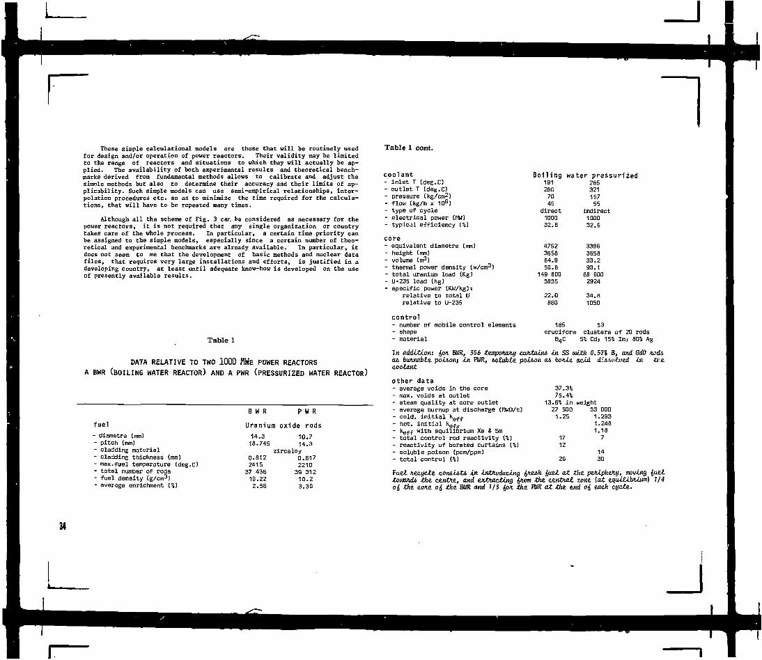
34

These simple calculational models are those that will be routinely usedfor design and/or operation of power reactors-. Their validity may be limitedto the range of reactors and situations to which they will actually be ap-plied. The availability of both experimental results and theoretical bench-marks derived from fundamental methods allows to calibrate and adjust thesimnle methods but also to determine their accuracy and their limits of ap-plicability. Such simple models can uss semi-empirical relationships, inter-polation procedures etc. so as to minimize the time required for the calcula-tions, that will have to be repeated many times.

Although all the scheme of Fig. 3 car. be considered as necessary for thepower reactors, it is not required that any single organization or countrytakes care of the whole process. In particular, a certain time priority canbe assigned to the simple models, especially since a certain number of theo-retical and experimental benchmarks are already available. In particular, itdoes not seem to me that the development of basic methods and nuclear datafiles, that requires very large installations and efforts, is justified in adeveloping country, at least until adequate know-how is developed on the useof presently available results.

Table 1

DATA RELATIVE TO TWO 1000 MWE POWER REACTORSA BWR (BOILING WATER REACTOR) AND A PWR (PRESSURIZED WATER REACTOR)

fuel

m)- diametre [mi- pitch (mm)- cladding material- cladding thickness (mm)- max.fuel temperature Cdeg.C)- total number of rods- fuel density (g/cm3)- average enrichment (%)

BWR PWR

Uranium oxide rods14.3

18.745

0.8122415

37 43610.222.56

10.714.3

zircaloy0.6172210

39 31210.23.30

Table 1 cont.

coolant- inlet T (deg.C)- outlet T (deg.C)- pressure (Kg/cm2)- flow (kg/h x 10s)- type of cycle- electrical power (MW)- typical efficiency (%)

core- equivalent diametre (mm)- height (mm)- volume (m3)- thermal power density (w/cm^)- total uranium load (Kg)- U-235 load (kg)- specific power (KW/kg):

relative to total Urelative to U-235

control- number of mobile control elements- shape- material

Boiling water pressurized191286

7045

direct100032.B

4752365864.950.8

149 BOO3B35

22.0860

185cruciform

285321157

55indirect100032.5

3396365833.293.1

88 6002924

34. B1050

53clusters

B4C 5% Cd; 15% I n ; 80% Ag

In addition.: &O1 BWR, 356 tempatoJm cwvtaim in SS with 0.57$ B, and GdO Acd&a& bu/inabte. poi&on; in PWR, iottxbZe. poiAon a& boiic acid dtaotved in -O'.ecoolant

other data- average voids in the core- max. voids at outlet- steam quality at core outlet- average burnup at discharge (MWD/t)- cold, i n i t i a l ke f f- hot, initial kef

- keff with equilibrium Xe & Sm- total control rod reactivity (%)- reactivity of borated curtains (%)- soluble poison (pcm/ppm)- total control (%)

Fua£ niLcycle. comiiti in inXn.odu.iUng (jneJ>h £u&l at tlie. pe/iipheny, mowing &ueZtcuxmdi the. centre, and extracting &iom the. ce.ntiurf. zone, [at e.qiUZib>uum) 1/4o& tkz cole. o£ the. BWR and 7/3 iot thz PWR at the. end o& each cycle..

37.3%75.4%

13.6% i n27 5001.25

1712

29

weight33

111

00D.293.248.187

1430

Table 2

DATA RELATIVE TO A HEAVY WATER REACTORCANDU TYPE (PICKERING POWER STATION)

fuel- material- diametre of rod (mm)- length of fuel element (mm)- cladding material- cladding thickness (mm)- number of rods per bundle- number of bundles per channel- pitch of rods in bundle (mm)

pressure channel- material- bore (mm)- pressure tube thickness (mm)- calandria tube thickness (mm)- calandria tube outer diametre (mm)- pitch of channels (mm)- number of channels in core- coolant- coolant to fuel volume ratio- moderator- moderator to fuel volume ratio- moderator temperature- power generated in moderator

natural uranium oxide14.026000

zircaloy0.5122812

about 19

Zr-2.5ZNb103.63

8.461.56

130.81285.75390

pressurized heavy water0.79

heavy water15.6263°C90 MW

core- shape- diametre (across flats) (mm)- length (mm)- volume (cubic meters)- thermal power (MW)- total uranium load (Kg)- specific power (w/g of U)

control and refueling- adjuster rods:

purposenumber of rodspositiontotal reactivity worthcomposition

- zone control systempurposenumber of absorber compartmentspoisontotal reactivity worth

- shutdown rodspurposenumber of rodspositionpoison

- other controlmoderator dumpboron poisoning of moderator

octagonal cylinder630060001921745'

93,13218.7

to shape neutron flux distrib.18

vertical1.87.

cobalt

to insure space stability14

flowing light water0.5%

safety11

verticalcadmium

35

J

Table 3

SOME NUCLEAR DATA OF INTEREST FOR REACTOR CALCULATION

Material•*•

Quantity +

V

a fission

o total

o elastic

a inelastic

a absorption

a capture

a activation

fission yield

fission spect.

decay schemes

delayed n data

spectrum (n,y)

o (y.n)

a for damage

FISSILE23SU5239pu

neutronbalance

n balancepower distr.neutrontransportdiff/trans,n spectrumneutronspectrum

n balanceconv.ration balanceconv.ratio

isot.anal.Decay heatage;high Espec.damage

kineticparameters

FERTILEzasu^opy

neutronbalance

MODERATORH, D, C

n balance 1power distr\neutron [transporttransport '(leakage)diff/trans, idiff/trans,n spectrum n spectrumneutronspectrum i

n balanceconv.ration balanceconv.ratio

isotopicanalysis

n balance

STRUCTURALFe,Ni,Cr,Zr

neutrontransportneutronspectrumneutronspectrumneutronbalance

Jwaste eval.maintenance

kineticparameters

D: delayedphotoneutr

lifetime ofcomponents

CONTROL -SHIELDING FISSION TRANS-PU 'B,Gd,Ag,Cd:O,Fe,Ba,C PRODUCTS (ELEMENTS ••

! ' •

leakageneutronspectrumneutronspectrum

neutron neutronbalance attenuationa balance; neutronisot.comp. attenuationwaste eval. access *transport 'decommiss.

neutronbalancen balanceisot.comp.

JFP inventorypecay heat

Y-shielding

heavy elem.inventory

OTHERS

Oxygen (transport,leakage)

I Oxygen (transport,• spectrum)'Oxygen (transport, ;spectrum) •

heavy elem.inventory

isotopicanalysis

n emissiontransport

detectors forspectrum meas.fissiondetectors252Cf spontaneousfiss.for calibr.detectors

I J

mr*m2

o©o©o©o©

oooo©oooooo©©oo®ooo©©oooooo©©oooooo©

oooo

1rn m

rn m

ro

sm

z30

It

OOOOOOOOOOOOOOOooooooooooooooooo«oo#ooo#oo#ooooooooo#ooooooooooo#ooooo#oooooo#ooooooooo#oooooooooooooooooooo#ooo®ooo#oooooooooooooooooooo#ooooooooo#oooooo#ooooo#ooooooooooo#ooooooooo#oo#ooo#oo#oooooooooooooooooooooooooooooooo

L_

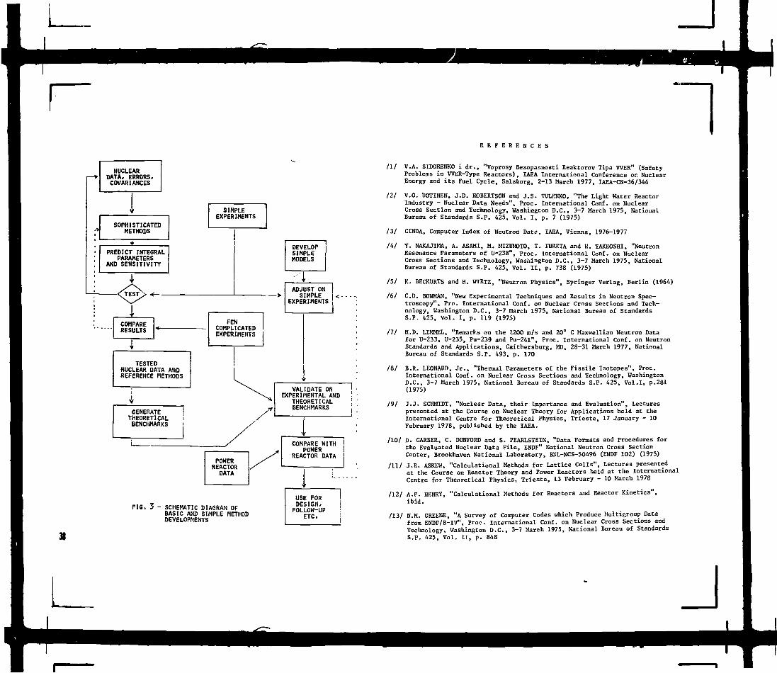
R E F E R E N C E S

NUCLEARDATA/ ERRORS,COVARIANCES

SOPHISTICATEDMETHODS

PREDICT INTEGRALPARAMETERS

AND SENSITIVITY

SIMPLEEXPERIMENTS

DEVELOPSIMPLEMODELS

COMPARERESULTS

ADJUST ONSIMPLE

EXPERIMENTS

FEWCOMPLICATEDEXPERIMENTS

TESTEDNUCLEAR DATA ANDREFERENCE METHODS

GENERATETHEORETICALBENCHMARKS

POWERREACTORDATA

FIG. 3 - SCHEMATIC DIAGRAM OFBASIC AND SIMPLE METHODDEVELOPMENTS

VALIDATE ONEXPERIMENTAL AND

THEORETICALBENCHMARKS

/ICOMPARE WITH

POWERREACTOR DATA

:- -

USE FORDESIGN/FOLLOW-UP

ETC.

HI V.A. SIDORENKO i dr., "Voprosy Bezopasnosti Reaktorov Tipa WER" (SafetyProblems in WER-Type Reactors), IAEA International Conference on NuclearEnergy and its Fuel Cycle, Salzburg, 2-13 March 1977, IAEA-CN-36/344

111 V.O. UOTINEN, J.D. ROBERTSON and J.S. TULENKO, "The Light Water ReactorIndustry - Nuclear Data Needs", Proc. International Conf. on NuclearCross Section and Technology, Washington D.C., 3-7 March 1975, NationalBureau of Standards S.P. 425, Vol. I, p. 7 (1975)

131 CINDA, Computer Index of Neutron Dat?, IAEA, Vienna, 1976-1977

/4/ Y. NAKAJIMA, A. ASAMI, M. MIZUMOTO, T. FUKETA and K. TAKEOSHI, "NeutronResonance Parameters of U-238", Proc. International Conf. on NuclearCross Sections and Technology, Washington D.C., 3-7 March 1975, NationalBureau of Standards S.P. 425, Vol. II, p. 738 (1975)

151 K. BECKURTS and H. WIRTZ, "Neutron Physics", Springer Verlag, Berlin (1964)

161 CD. BOWMAN, "New Experimental Techniques and Results in Neutron Spec-troscopy", Pro. International Conf. on Nuclear Cross Sections and Tech-nology, Washington D.C., 3-7 March 1975, National Bureau of StandardsS.P. 425, Vol. I, p. 119 (1975)

HI H.D. LEMMEL, "Remarks on the 2200 ra/s and 20° C Maxwellian Neutron Datafor U-233, U-235, Pu-239 and Pu-241", Proc. International Conf. on NeutronStandards and Applications, Gaithersburg, MD, 28-31 March 1977, NationalBureau of Standards S.P. 493, p. 170

181 B.R. LEONARD, Jr., "Thermal Parameters of the Fissile Isotopes", Proc.International Conf. on Nuclear Cross Sections and Technology, WashingtonD.C., 3-7 March 1975, National Bureau of Standards S.P. 425, Vol.1, p.281(1975)

19/ J.J. SCHMIDT, "Nuclear Data, their Importance and Evaluation", Lecturespresented at the Course on Nuclear Theory for Applications held at theInternational Centre for Theoretical Physics, Trieste, 17 January - 10February 1978, published by the IAEA.

/10/ D. GARBER, C. DUNFORD and S. PEARLSTEIN, "Data Formats and Procedures forthe Evaluated Nuclear Data File, ENDF" National Neutron Cross SectionCenter, Brookhaven National Laboratory, BNL-NCS-50496 (ENDF 102) (1975)

/ll/ J.R. ASKEW, "Calculational Methods for Lattice Cells", Lectures presentedat the Course on Reactor Theory and Power Reactors held at the InternationalCentre for Theoretical Physics, Trieste, 13 February - 10 March 1978

/12/ A.F. HENRY, "Calculational Methods for Reactors and Reactor Kinetics",ibid.

/13/ N.M. GREENE, "A Survey of Computer Codes which Produce Multigroup Datafrom ENDF/B-IV", Proc. International Conf. on Nuclear Cross Sections andTechnology, Washington D.C., 3-7 March 1975, National Bureau of StandardsS.P. 425, Vol. II, p. 848

J

IUI Proceedings of the Seminar on Nuclear Data Processing Codes, Ispra5-7 December 1973, OECD Nuclear Energy Agency, Computer Program Library,Newsletter N. 16 (EACRF-U-52), 1974

/15/ L.N. USACHEV, Atomnaja Energija 15_, (1963) 472

/16/ G. CECCHINI et al., Third International Conference P.U.A.E., Geneva,IAEA Vol. 2, (1965) 388

/17/ J. LEWINS, "The Time-Dependent Importance of Neutrons and Precursors",Nuclear Science and Engineering, 7, 268-274 (1960)

/18/ E.T. TOMLINSON, G. DESAUSSURE and C.R. WEISBIN, "Sensitivity Analysisof TRX-2 Lattice Parameters with Emphasis on Epithermal U-238 Capture"Electric Power Research Institute, EPRI NP-346 (ENDF-252), March 1977

/19/ U. FARINELLI, The Role of Integral Experiments in the Production of NuclearData for Reactor Core and Shield Design and for Irradiation Experiments",Proc. International Conference on Nuclear Data in Science and Technology,IAEA-SM-170/38, Vol. II, 103-119, Vienna (1973); see also: XI. FARINELLI,"The Role of Integral and Differential Measurements in Improving NuclearData for Shielding", Proceedings of the NEA-IAEA Specialists' Meeting onSensitivity Studies and Shielding Benchmarks, p.25, OECD, Paris (1975)

/20/ E. BERNOCCHI and R. MARTINELLI Eds., "Light Water Lattice Data", ComitatoNazionale Energia Nucleare, Roma, Report RIT/FIS(77)1 (NEACRP-U-190),December 1977

/21/ G.A. PRICE, "Uranium-Water Lattice Compilation. Part I: BNL ExponentialAssemblies", Brookhaven National Laboratories BNL 50035 (1966)

/22/ R.L. HELLENS and G.A. PRICE, "Reactor Physics Data for Water ModeratedLattices of Slightly Enriched Uranium", Reactor Technology Selected Reviews,USAEC-TID 8540, p. 529-609 (1964)

/23/ OECD-ENEA,"Heavy Water Lattice Data", EACRP-L-42

/24/ OECD-ENEA, "Neutron Spectra", EACRP-L-62

/25/ Cross Section Evaluation Working Group, "Benchmark Specifications", NationalNeutron Cross Section Center, Brookhaven National Laboratory, BNL 19302(ENDF-202)

/26/ S. TASSAN, "Proceedings of the Conference on Analysis of Few Rod Experimentsin Reactor Physics, JRC Ispra, May 12th-14th 1969:1 Euratom Report EUR 4470eMarch 1970 (EACRP-U-38)

/27/ A.M. BROOMFIELD et al., "Measurements of K-Infinity, Reaction Rates andSpectra in ZEBRA Plutonium Lattices", British Nuclear Energy Society Confer-ence, London, June 1969.

/28/ P. AZZONI et al., "Experimental Determination of Integral Capture CrossSections of Fe, Ni, Cr in the Intermediate Energy Region. Description of theMethod and of the Experimental Facility", Energia Nucleare (Milano) Vol.24,n.8/9 (1977)

/29/ Proceedings of the IAEA Consultants' Meeting on Nuclear Data for ReactorNeutron Dosimetry, IAEA Vienna, September 1973, INDC(NDS)-56/U.

/30/ Neutron Cross Sections for Reactor Dosimetry, IAEA-208, IAEA Vienna, 1978

/31/ R. VIDAL et al., "Mesure des Sections Effectives d'Echantilions Fissiles",Report CEA-R 2487 (1964).

/32/ Proceedings of the Specialists' Meeting on Control Rod Measurement Techni-ques: Reactivity Worth and Power Distributions, CEA-CEN Cadarache 21-22April 1976, CEA, Division d'Etude et de Developpement des Reacteurs, Re-port NEACRP-U-75 (1976).

/33/ W.L. ZIJP, J.H. BAARD and H.J. NOLTHENIUS, "Comparison of Neutron SpectrumUnfolding Codes", Proceedings of the 2nd ASTM-EURATOM Symposium on ReactorDosimetry, Palo Alto, October 3-7, 1977, Vol.Ill, p.1333-1364 (1978);C.A. OSTER, "Review of Unfolding Methods Used in the U.S. and their Stand-ardization for Dosimetry", ibid. Vol.Ill, p. 1365-1384.

/34/ F.G. PEREY, "Uncertainty Analysis of Dosimetry Spectrum Unfolding", ibid.Vol. Ill, p. 1449-1462; F.G. PEREY, "Spectrum Unfolding by the Least-Squares Method", IAEA Technical Committee Meeting on Current Status ofNeutron Spectrum Unfolding, Oak Ridge, October 10-12, 1977

/35/ Proceedings of the IAEA Seminar on Physics Measurements in Operating PowerReactors, Rome, May 1966.

L J

1

CALCULATIONAL METHODS FOR LATTICE CELLS/

J.R. ASKEWUKAEA Reactor Group,Atomic Energy Establishment,Winfrith,United Kingdom

1.1 INTRODUCTION

The basic equations governing the motion and reaction ofneutrons in nuclear reactors are of a very simple form, despitethe complexity of much of the underlying physics. Given the verylarge effort which has been devoted to the measurement of nucleardata - that is, the characterization of these physics processes,- it is in principle possible to model the behaviour of a reactorcore and shield to a level of accuracy far beyond that usuallyencountered in engineering applications.

The development of digital computers, and systematic develop-ment of calculational techniques, has revolutionized reactordesign in a comparatively short time, say 20 years. Experimentalstudies, which once involved a large outlay in time and money toexplore variations in fuel pin size, pitch, etc and were followedby progressive increases of scale of plant, have now been reducedto relatively specific and highly sophisticated experiments toconfirm specific performance predictions, often those with safetyimplications.

The cost of experimentation, partly associated with thestringent safety standards adopted in its conduct, is clearly oneof the factors encouraging improved modelling. So, at the otherend of the scale, is the large capital cost of the finished powerstation.

As computing capabilities have improved, it has provedpossible to produce more and more basic models, which have a widerrange of validity. For example, it is possible to use the sammodels for reactors with different moderators,| At the currentstage of development, direct simulation of all the processesinvolved in the reactor to the degree of accuracy required is notan economic proposition, and this is achieved by progressivesynthesis of models for parts of the full space/angle/energyneutron behaviour.

The split between reactor and lattice calculations is onesuch simplification. Most reactors are constructed of repetitionsof similar geometric units, the fuel elements, having broadlysimilar properties. Thus the provision of detailed predictionsof their behaviour is an important step towards overall modelling.We shall be dealing with these lattice methods in this series oflectures, but will refer back from time to time to their relation-ship with overall reactor calculation.

The lattice cell is itself composed of somewhat similar sub-units, the fuel pins, and will itself often rely upon a furtherbreak down of modelling. Construction of a good model dependsupon the identification, on physijal and mathematical grounds, ofthe most helpful division of the calculation at this level..H~/^- - /Figure 1 shows the type of subdivision adopted in the WIMS e &WLlattice code schemes which is characteristic of most subsequentmodels. We shall deal in turn with the problems is each part ofthe calculation.

1.2 CHARACTERISTICS OF THE UNDERLYING PHYSICAL PROCESS

From the modelling point of view we can distinguish threebasic regimes of neutron energy in which our preoccupations willbe different.

(i) The Fast Region E>100 KeV

Neutrons from fission are born in this energy range.It is characterized by a wide diversity of possibleneutron reactions, including sharp energy variations ofreactions probability at thresholds, for example of fastfission in Uranium-238. Scattering is often highlyanisotropic, even in the centre-of-mass frame ofreference. Cross sections are usually fairly small -that is, neutrons travel longer distances betweencollisions than is the case at lower energies - and therepresentation of geometric details is correspondinglyless important.

(ii) The Resonance Region 100 KeV > E > 4 eV

In this range the light .nuclides tend to have constantcross-sections dominated by potential scattering.Intermediate and heavy nuclides exhibit resonances in

/\,s ' „ • which capture and fission cross-sections reach highrf Jl values over small energy ranges and are teirparature

v dependent due to the relative motion of neutron andnuclide (Doppler Broadening). Given these rapid changes,or discontinuities, of cross-section respectively inenergy and space the modelling problem is at its mostdifficult. Because of the high cross-sections many ofthe effects are of short range.

(iii) The Thermal Region 4 eV > E

Here thermal motion of the light nuclides has a dominanteffect upon neutron behaviour. The width of resonancesis greater compared to possible energy change percollision, and in this sense cross-sections can beconsidered to be more slowly varying.

41

y

L J

1.3 THE BOLTZMANN EQUATION

Neutrons may be considered to travel in straight lines inbetween events ("collisons") which are relatively localized inspace and which can result in changes of direction and energy.The transmutation or displacement of nuclii is on such a smallscale that the properties of the medium are essentiallyindependent of the neutron flux, and the overall behaviour of theneutron flux is therefore described by the Boltzmann equation.

where N = N (r,E,Q) is the neutron flux

Zt = Zt (£, E) the total cross-section (isotropic)

Q = Q (£.£,£) is the neutron source

= 1 IE {£'•>•£, JJ'+n) N (E.E'.a1) dE' d'fi1

£ = transfer cross-section for all processes

s = space co-ordinate in direction &

Note that the total cross-section is related to the laboratoryframework, as is the transfer cross-section. Motion of the targetnucleus thus has to be allowed for in determining the constantsin the equations, rather than appearing explicitly in theequations. The most obvious instance is the Doppler effect inwhich a resonance, in which the reaction probability is fixedin terms of the relative velocity of incident neutron and targetnucleus, becomes temperature dependent in our formulation andexhibits an apparent spread.

It must not be assumed that because this equation is a gooddescription of neutron motion it will also hold exactly underapproximate conditions. In particular, condensation to group formin energy may be seen to introduce problems even if we know theexact solution. For if we define

S (r.,g, i N (£,E,fi) dE

we see that for consistency we require

J Zt (E) N (r,E,fl) = EtN(r,g,n)

and thus E = t (£,n) in general, unlike its point energy formwhich is independent of 0. Particular care has to be taken ingeneralizing from deductions made in one energy group.

An exactly similar problem arises in the representation ofscattering, in that transfers due to a genuinely isotropicscattering process may become anisotropic in group form. Elasticscatter.conforms to an angle/energy law, and of ocurse is notisotropic in the group to group form, but highly directional.This is especially easy to overlook in spherical harmonicsexpansions of the equation. Treatment of these effects is mostimportant in shielding and whole reactor calculations. In latticecalculations the problems are more usually introduced inattempting to simplify the equation in some way.

1.4 TRANSPORT CORRECTIONS

The most important practical simplifications lie in the treat-ment of scattering, to reduce it to a simpler, usually isotropicform. The right-hand side of the Boltzmann equation containsscattering terms of the form (dropping the spatial co-ordinate r ) .

II N (E'.a1) dE1 dfl1

and the aim is to relate these to the left-hand side term

(E) N (E,£2)

in an approximate way. This depends upon some knowledge of theangular flux. The standard treatment is to expand the scatteringcross-section in spherical harmonics

(E'*E) (v)

wherewhere g denotes group of width &E.

42

and furt-her by the addition theorem for spherical harmonics to

Thus if the angular flux N is also expanded in sphericalharmonics series in terms of &.

N (£•,£.') (a1)

and the orthogonality relationship used to simplify the result.Limiting the expansion to the lowest orders, our source termbecomes

2 Q <E'->-E) 0 O (E1) + 1/3 Z 1 (E'+E) 0y (E').a

and we can relate it to the LHS

0o 01

by equating appropriate moments.

Two main assumptions are made:-

(1) The diagonal approximation

Ix (E'*E) 0X (E') = Sj (E) (E)

hence

Ztr = E

(2) The row sum

" 1 / 3 r

These approximations have proved to be broadly adequate formany purposes, particularly for the calculation of leadage inwhich only low order movements are significant. For lattice cellcalculations. However it must be recognized that a very highorder expansion will be needed to represent the angle/energyrelationship in scattering (which, for a single nuclide, has aS-function form) and that low order expansions may be misleading.

2. COLLISION PROBABILITY FORMULATIONS

For many purposes it is convenient to use the integral formof the neutron transport equation.

Collisons at (£,E) = Et (r,E) 0 (r,E)

4itP(£'+r.,E) 0 (£',E,-a) dr dfl

P (£•£) represents the probability that a neutron born at r.and aimed in the appropriate direction, will have its nextcollision at r.

This formulation is especially convenient when the emissionof neutrons may be regarded as isotropic, and does not vary toorapidly in space. In this case we can integrate the probabilityover spatial zones such that

Collisions in volume at J V± P (I+J)

where P (I+J) is the probability that neutrons born uniformly involume I will have their next collision in region J-

This probability may be determined by numerical integrationalong a mesh of lines distributed uniformly in space and angle.Along a line intersecting I and J in intercepts £j and 4j we seethat the number of neutrons colliding in J is:

l)e-IL

(1-e

1/3 Z x (E'+E) 01 CE')/01 (E) is evaluated andsubtracted from 2 t (E) . This depends upon an orginalguess or calculation of the P- flux moment.

where £E is the distance between the surfaces of I and J expressedin mean free paths. As the number of neutrons in an elementaryvolume about the time is Qz 6S it will readily be seen that

43

J

along each line - and thus for the integral over all lines - areciprocal relationship holds + ..) dSdfi

escape ISdfiP(I+J) = P(J+I)

= 1 -The total escape probability from a non-re-entrant region, I,

may be determined by integration over all families of lines in alldirections.

i 2

a--**)escape If Q l d S d n

when d S is the element of projected surface. It will be seen thatin the limit as £-«».

Pescape ZSL I =4 x Volume

Surface Area

where I is the mean chord length of the body. Using this fact wemay extend our reciprocity relationship by considering one regionto be black

P(S-M)

where S is the surface of region I

P(S+J)

P(J->S) by reciprocity

Thus surface reciprocity may be deduced

SjP(S+J) = 4

and, incidentally, the neutron flux leaving I in this limit isisotropic outwards, Also of interest in some cases in the 'whitelimit1 of the escape probability which is seen to depend upon themean square chord

The exponential form of the integral suggests that anappropriate rational approximation might be

pescape 1/1 + 11

which has the desired behaviour in the black limit.

Generalization of these formulae to cylindrical geometry issimplified by the fact that only projections of the generatinglines into the plane need to be considered, and the exponentialfunctions are replaced by Bickley-Naylor functions. Simplegenerating formulae are available for multi-annular systems. Agreat deal of ingenuity was devoted to obtaining simplifiedformulae for such geometries; the THESEUS model in WIMS beingbased upon such a calculational method. With modern computers theneed for such approximations becomes significant.

3. REPRESENTATION OF RESONANCES

3.1 INTRODUCTION

Because of the rapid variation of cross-section with energyin the resonance region this represents one of the most difficultmodelling problems for the reactor physicist. The resonancestructure is of importance up to 10 KeV, even though the resonancescannot be resolved experimentally at such high energies. At thebottom end of the range the modelling is forced to change toaccomodate thermalization effects. In the WIMS lattice codes therange 4 eV - 9.2 KeV is treated by a special model; in some othercodes the resonances of Plutonium -240 and -242 at 1 eV areincluded in the resonance region, but this limits the modellingaccuracy achievable, especially for high temperature reactorcalculations.

Basic nuclear data for the most important nuclides areavailable as resonance parameters which are used in a multi-levelformalism to reconstruct cross-sections and their variation withtemperature (Doppler broadening). Where significant resonancestructure is not resolved experimentally it is necessary toconstruct appropriate distributions of resonances by a statisticalprocess. The uncertainly inherent in this is not very significantfor thermal reactors.

44

_l

Uranium-238, the most significant resonance absorber inthermal reactors, has resonance spaced at about 18 eV on average.The fissile nuclides have smaller resonances which are lessdistinct. The different nuclides compete with each other forneutron capture, and have to be represented together in a model -this requires a fairly fine mesh and of the order of 105 datapoints are needed to represent all resonances in the rangerequired.

3.2 EXACT MODELS

The neutron flux varies rapidly with space, energy and anglein the resonance region of typical thermal reactors. Resonantabsorbing nuclides in the centre of fuel pins are 'shielded' bythose on the outside. It is practicable to solve problems of theorder of 105 energy points for infinite homogeneous mixtures ofabsorbers and moderator 'exactly' (ie within the limitationsimposed by the knowledge of the nuclear data) . For realisticgeometries of pins and fuel assemblies this is more difficult, andtwo options are available.

The first involves some simplification of the geometry;possibly by the use of collision probability methods implyingspatially flat emission densities over spatial zones, sometimesrestricting the representation of angular scatter to isotropicor Pi approximations. This may be reasonable good but the errorsintroduced are difficult to quantify except for the simplestgeometries (plate, single pin etc).

The second is the use of Monte Carlo techniques. In thesethe modelling can be as detailed as one wishes, but a degree ofrandomness remains in the results which can only be progressivelyreduced with increased computing cost. Such methods are generallyinconvenient for design purposes because the stochastice elementis inconvenient in studying the effects of small design changes,and the method is most used to validate approximate methods.

3.3 EQUIVALENCE MODELS

The earliest practical models for obtaining solutions toheterogeneous geometries were based upon equivalence principles.These may be simply illustrated for a two-region system of a fuelpin surrounded by moderator. If we assume the resonances narrowcompared to the energy ?oss per collision in the moderator, andneglect moderation in the fuel, we may reasonably assume aspatially flat emission density V in the moderator. Then at eachenergy we can assume

where Vm (u) is the emission density slowly varying with lethargy

Z^ (u) is the total cross-section of the fuel

0f (u) is the scalar flux integrated over the fuel region

P(m*f, Etf) is the probability that a neutron 'born' in the

moderator has its next collision in the fuel

V1", V are volumes of moderator and fuel

by reciprocity

f) = EfcfVf P(f-m)

= EtfVf (l-Ptf+f))

and

0f(u) = (l-P(f-*f))

Use of the rational approximation

p<f-f) =

allows us to express the flux in a form familiar for homogeneousmixtures

Et( ,5 + t l

compared to

Z* (u) Vf 0 f (u) = 1/m (u) , Z*) 0£(u)=^-C+ s

t

45

I J

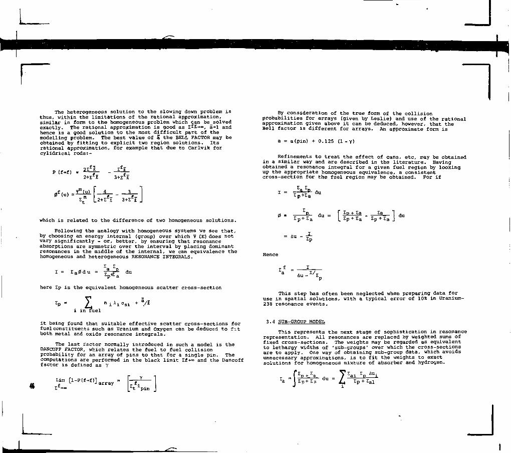
The heterogeneous solution to the slowing down problem isthus, within the limitations of the rational approximation,similar in form to the homogeneous problem which can be solvedexactly. The rational approximation is good as £fE-*», a+1 andhence is a good solution to the most difficult part of themodelling problem. The best value of a the BELL FACTOR may beobtained by fitting to explicit two region solutions. Itsrational approximation, for example that due to Carlvik forcylidrical rods:-

P (f+f)

which is related to the difference of two homogeneous solutions.

Following the analogy with homogeneous systems we see that,by choosing an energy internal (group) over which * (E) does notvary significantly - or, better, by ensuring that resonanceabsorptions are symmetric over the interval by placing dominantresonances in the middle of the internal, we can equivalence thehomogeneous and heterogeneous RESONANCE INTEGRALS.

By consideration of the true form of the collisionprobabilities for arrays (given by Leslie) and use of the rationalapproximation given above it can be deduced, however, that theBell factor is different for arrays. An approximate form is

a = a(pin) + 0.125 (1 - Y)

Refinements to treat the effect of cans, etc, may be obtainedin a similar way and are described in the literature. Havingobtained a resonance integral for a given fuel region by lookingup the appropriate homogeneous equivalence, a consistentcross-section for the fuel region may be obtained. For if

= Au -

Hence

E a0d u = du Au-

here Zp is the equivalent homogeneous scatter cross-section

i in fuel

This step has often been neglected when preparing data foruse in spatial solutions, with a typical error of 10* in Uranium-238 resonance events.

it being found that suitable effective scatter cross-sections forfuel constituents such as Uranium and Oxygen can be deduced to fitboth metal and oxide resonance integrals.

The last factor normally introduced in such a model is theDANCOFF FACTOR, which relates the fuel to fuel collisionprobability for an array of pins to that for a single pin. Thecomputations are performed in the black limit Zf-«o and the Dancofffactor is defined as Y

3.4 SUB-GROUP MODEL

This represents the next stage of sophistication in resonancerepresentation. All resonances are replaced by weighted sums offixed cross-sections. The weights may be regarded as equivalentto lethargy widths of 'sub-groups' over which the cross-sectionsare to apply. One way of obtaining sub-group data, which avoidsunnecessary approximations, is to fit the weights to exactsolutions for homogeneous mixture of absorber and hydrogen.

Lira [l-P(f-*f)]f J array

du = Zr, + Z•al

Thus for each broad group we can obtain sets of Au. which

fit the results over the desired range of Zp. It is found inpractice that 5 such sub-groups are adequate for uranium-238.

In this representation it is necessary to obtain P(f-*f) foreach fuel cross-section in turn in order to evaluate the resonanceintegral and flux. A further refinement is to use a fullspatial flux solution for each sub-group including the effect ofheavy cans, etc. This route is described by Roth (9) . Thismethod is capable of estimating cross-sections for sub-regionswithin the fuel to any degree of refinement for which anappropriate flux solution can be obtained for the sub-group. Asimple application is to determine the spatial build up ofPlutonium within a pin, shown compared to experiment in Figure 4.The method can also be used to determine cross-pin effects. Inits simple form it is limited, as is the equivalence method, totreating fuel of uniform temperature, and recourse is had toearlier results (10) to justify the use of mean fuel temperaturein such calculations.

3.5 RESONANCE OVERLAP

The overlapping of resonances has been referred to earlier.The effect of Uranium-238 resonances on Uranium-235 and Plutonium-239 fission was dramatically illustrated in an experiment bySanders (11) in which a fission chamber was moved through a centralhole in Cadmium covered rod of Uranium-copper-Uranium. Figures 5 to7 show the rise of fission rate when the fissile material was notshielded by uranium-238.

It can be shown that the effect is primarily one of reducedneutron flux in the resonances, and so long as this is correctlyall wed for in the calculational method the major part of theeffect will be modelled. A smaller effect of Uranium-235 onUranium-238 can be shown theoretically to be of the order of 1%enrichment. It is, however, just sufficiently important torequire modelling. A simple representation is used in the WIMScode (1).

3.6 GROUP REMOVAL DATA

The group removal cross-sections in the resonance region willbe sensitive to the amount of resonance absorption. In a few-groupmodel some correction must be made' for this effect.

The effect may be seen in its extreme form by comparing thegroup form of solution with the analytic one for a homogeneousmedium and relatively heavy scatterer which does not slow down morethan one group.

exp -

Now in the absence of absorption.

whilst we have determined that

we require

R "Aexp - CZs

if we write tR' = ER.f(p) vs obtain

gZs.f(p) I 1+ 2: (?z7)

(gZs.f(p>>

The correction is normally small for heterogeneous systemsexcept in the intermediate spectrum range. Alternative models arepossible, corresponding to higher order integration over lethargy.One such model is to retain the group representation but tointroduce non-physical transfers from higher energy groups so thatthe escape probability is maintained regardless of the withingroup absoption.

3.7 VALIDATION

By careful choice of models, and relating the solutions tothe most relevant situations which can be exactly modelled, it ispossible to -ninimize errors introduced, for example in thetreatment of resonance scattering. It is difficult to quantifythe residual model uncertainties, however, and it is highlydesirable that the eventual model be compared to Monte Carlosolutions - using an identical data base - for a number of casesin the range of practical interest. In the case of the models 47

J

used in the WIMS code it was found that even when oxide and metalfuels were represented by the same set of tabular data a few-groupequivalence medel could be relied upon to introduce errors of lessthan IX in resonance capture for a wide range of problems. Typicalcomparisons are shown in figure 3.

4. DISCRETE ORDINATE METHODS

4.1 BASIC FORM OF THE EQUATION

Having simplified the original problem into a few ( M O O )group form we have a choice of methods by which to obtain thedesired space/energy/angle solution. The simplest integraltransport formulations have been reviewed briefly. The mostcommon alternative is the discrete ordinate method, a differentialtechnique.

and the mean angular flux N can be deduced from neutron balanceto satisfy

Collisions = 5 (NQ - + SA

where NQ are fluxes entering and leaving the mesh interval.

Carlson uses the rational approximation

to give

Z A

In slab geometry, the version of the method due to Carlsonis simply described. The angular flux within a group determinedalong lines at discrete angles 8. with the normal to the slab

surfaces. The transport equation may be simplified within eachspatial region of constant material composition to be:-

E(g'*g)0g,

1 +J t A

to provide E tcicularlv simple set of equations. It has oftenbeen surprising that these equations gave good results outsidethe apparent limits of validity of the derivation; indeed forcourse meshes it could be better than the exact solution forconstant source in the mesh. The reason for this can beillustrated simply in =i one-cjroup form with fixed source Q bywriting

where = cos 8. "

N = N (X, vt) is the angular flux

E. = total cross-section

£(g'-*g) = Inter-group transfer (all processes)

0(ji = scalar flux in group g' =

If the source term S is taken to be constant over a meshinterval "A it will be seen that the equation can be integratedover the mesh to give

'dx N= Q (0-N)

It will be seen that the usual integration assumes 0 constantover the mesh. Suppose instead that we assume (0 - N) constant.This parallels the usual approximation of diffusion theory because0 - N is proportional to neutron current in diffusion likesituations.

The previous derivation is modified to tjive

exp ,-

N(x) = exp (--

48- exp NZaA = (No-N1)p +

L

Interestingly, if we make the same rational approximation as

before, -but for exp -EaA we find that the same equations are

obtained as in our original derivation. Thus — — << 2 is a

sufficient, but not necessary condition for Carlson equationsto held.

4.2 TREATMENT OF CYLINDRICAL GEOMETRY

The standard route for generalization of the discreteequations to cylindrical geometry follows earlier spherical

harmonics practice. The term in jj has now to be modelled, and

the equations, making the same assumptions as before, have theform

UJi T <Sj If

(a) Specular Reflection. In this case neutrons are perfectlyreflected as the cylindrical boundary of the model. Thismodel tends to error as the dimensions of the unit cellbecome small because the chord-lengths distribution isgrossly disturbed. As pointed out by Newmarch, pathsmissing the fuel on one cell crossing never intersectfuel, whilst those passing through the fuel do so onevery crossing.

(b) Isotropic Return at Each Altitude. In a discreteordinate calculation separate estimates of angular fluxare available at different angles to the pole. Outgoingneutrons are returned isotropicaaly in such a manneras to presume neutron balance separately at each suchangle. This retains one element of realism in themodel for cases in which the long paths in the outerregion at anles near the pole are important, but removesthe correlation inherent in specular reflection. Thiswas called a white boundary condition when firstintroduced.

"J i

(Sjir+Sjir-l> =

U . )

with

to integrate these it is necessary to start with the equationu = +1 which does not require a backward difference in u to solve,and then to step in Au. Examination of the procedure shows thatthe choice of constant set of u• corresponds to solutions alongequiangular spirals as shown in the right hand side of Figure 8.

dNThe terms in rr- clearly arise because the track leaving a spatial

mesh region is in a different direction from that entering it.

An alternative formulation is to track neutrons alongstraight-line paths as shown on the left of the Figure. Theequations to be solved along each line are then the same as thosein slab geometry, the characteristic form of the equation (14).The integrating mesh is then the same as that used in numericalestimation of collision probabilities.

4.3 BOUNDARY CONDITIONS

In order to reduce an infinite lattice problem to acylindricalized form, some approximate treatment of the boundaryis required. It is usual to define the outer cylindricalboundary in such a way as to pressure the volume of unit squareof hexagon (although there are some exceptions to this which arediscussed in a later section). Three major options are available.

(c) Isotropic Return Over all Angles. This is the conditionmost easily used in collision probability formalism,because reciprocity relations exist to determine theprobabilities of incoming neutrons with such adistribution colliding in each region in terms of thecorresponding outgoing probabilities. It can also besimulated by introducing dummy scattering zones outsidethe true boundary. For most cases this condition givesresults close the those of the previous case, but it isless good and should be avoided if possible.

In the case of characteristic formulations, betterapproximations to the true boundary can be obtained by avoidindexplicit cylindricalization. Consider a case in which a squareboundary is retained, and the same number of tracking lines isused as in the cylindrical model of Figure 8. We may, as analternative, use these in two families inclined to each other at45° and having boundary conditions determined correctly on physicalgrounds. This option is a new one and is currently being studied.

4.4 CHOICE OF INTEGRAL OR DIFFERENTIAL METHOD

Both solution techniques should be capable of giving thesame answer if a sufficiently high order of representation is used,with the exception of the limitation boundary condition for theintegral method. This will only be significant for very closepacked systems. The solution techniques used in the innermostloop may be contrasted on the assumption that the outerIteractive strategy is the same in both cases. For the integralmethod

I = P I 49

I J

where "P is scalar flux reactor over space

f is emission density reactor over space

P is (full) collision probability matrix

Whilst for the differential method

Ni.j = a N i - l . j + b * i j

50

Thus for m space regions the former requires a number ofoperations proportional to mr whilst the latter is proportionalto nm,h being the number of angles required, we may deduce thatthe differential method will be less expensive for problemsinvolving a large number of meshes, and a specific illustrationof this (using the two codes WDSN and PERSEUS) is shown inFigure 16. The relation normalization of the two methods will, ofcourse, depend upon efficiency of coding etc, but the basicbehaviour is clearly tending to the expected asymptote. In thiscase the break even point was less than 10 regions.

5. THE TREATMENT OF LEAKAGE

5.1 INTRODUCTION

Our presentation so far has been concerned with the solutionof infinite arrays of identical rods, and some more or lessarbitary eigenvalue has been introduced to permit solution of theequations. In real systems, neutrons pass from cell to cell andmay ultimately leak from the system. The case of all uniformlattice is a special one, and may simply be illustrated byconsidering an array of fuel pins of negligible size (line sourcesand sinks) finite in one dimension x. Suppose that a neutron bornin fission in a pin at xi has a probability of causing fissionsat Xj

ki j = k (| x £ - Xj | )

Suppose that there is a solution f. = f(x.) which is critical,then x x

k^ . f i = f for all j

as k^. is symmetric this clearly implies a condition on curvature,

and there will be solutions of the form

f, = Ae i B x

where B may be real or imaginary. The solution thus has a real

curvature B the critical buckling. Consider a pin at x = 0 .

Then for a regularly spaced lattice we have a critical condition

KQ + 2Kj cos BA + 2K2 cos 2BA + = 1

Now "our infinite lattice multiplication

K = KQ + 2K1 + 2KX +

hence Km - 1 = 2KX (1 - cos BA) + 2K2 (1- cos 2BA) +

expanding = B2 A2 + 4K2 + 9K3 +...]- B^-jk 1 +16K2 + 81K3+j+.

where X is the mean square distance travelled in one generationfrom fission to fission. In the limit as A-»-0 we obtained anhomogeneous result. Note that no constraints have been placedupon the energy/angle form of the solution at this stage.

5.2 HOMOGENEOUS MODELS

Homogenization of the model problems is practical so long as

at least the lower powers of X n are preserved in the process.If we wish to homogenize in a way that conserves all events inour multi-group model - including group-to-group transfer, thereis only one free parameter available to fit this - Egg intransport theory or the diffusion coefficient Dg in diffusiontheory. This can in principle be done exactly in the specialcase of a buckling mode.

Li

The basis of this method is treated in standard texts. Oneparticular restriction may be noted when diffusion theory is usedin the final modelling stage. This imposes restrictions on thepossible form of the kernel

,. _ » -<l x.-x.l When ic

hence

•..p.-- }o o

mCO

X4 = f x* e"K xdx f

o o

e-*xdx = 2/ 2

24/ 2

Hence 11 + B2 M2

M2 =

Age theory similarly serves to preserve the second moment.

5.3 TREATMENT OF VOIDS

The effect of cross-section differences in the medium, ofwhich voids are the extreme case, is traditionally described as'streaming1. In extreme cases it can be shown that no asymptoticsolution of a buckling form may exist, although in practicequasi-asymptotic solutions are observed. (An example is a semi-infinite slab system with cylindrical holes normal to thesurfaces).

Exact solutions may be obtained for such problems usingeither differential or integral formalism. Monte Carlo methodslend themselves to direct determination of the transport kernal,from which we may deduce either the successive moments needed forleakage calculation, or, more simply, determine the ratio ofmultiplication with and without leakage. For, in the simplestcase, suppose that a neutron standard at x = 0 yields or neutronsat x. By symmetry, the converse will apply in a cylindricallattice. Thus the sample may be considered to contribute

n^ to the estimate of k-infinity

nA cos BX to the estimate of k-effective

The differential formalism, for example in discrete ordinatemethods, involves a weighting of the angular fluxes. This caneasily be seen, for example in a one-dimensional geometry withleakage in a transverse direction.

Sao

keff = cos BXi>

The neutron leaving one face at z = 0 may be considered tobe 'replaced' at the second face by that from -z. Then the fluxis reduced by cos Bz = cos B 4 X/u compared to that in the nonleakage application. The method has been successfully used incylindrical geometry, but demands a higher order angularquadrature in the direction of the leakage than would normallybe used.

5.4 SIMPLIFIED MODELS

A number of simple prescriptions are available for treatingparticular types of streaming problem. The most commonly used arethose due to Behrens (for a range of hole geometries in an other-wise uniform medium) and Benoist (usually used in its simpler formfor a 3-region lattice of fuel, vcid, moderator).

5.5 RESTRICTIONS OF APPLIABILITY

Equilibrium leakage models, dependent upon the existence ofzones of asymptotic leakage properties, are useful models formany simple experimental applications. Because flux curvatureis the same in all groups they relate the leakage to a particularenergy-dependence. It is not necessary to apportion 'leakage'exactly over energy, and a diagonalized (diffusion-like) model isacceptable. Heterogeneous lattice problems are not necessarilysolved using the same approximation.

6. TREATMENT OF ASSEMBLY GEOMETRY - EXACT

6.1 INTRODUCTION

As the most common types of reactor exhibit a doubleheterogeneity of pins in assemblies a fully explicit spatialsolutions is difficult. In practice the only route which hasbeen exploited for this purpose is the collison probability one,usually with some restriction, for example to isotopic scatteringmodels.

The two major deterministic code options relating to clusterand box geometries are described briefly below. It isinteresting to note that differential methods, despite theadvantages to be expected in many region problems, have not been ,.seriously exploited, although one case has been reported in which 31

J

~lthe method of characteristics was applied to a simple BWRbenchmark problem.

It is usual to apply some form of condensation in energybefore using methods of this kind so as to reduce the labour ofsolution.

6.2 £Ii

Axially uniform, the code allows a basic r,6 geometry uponwhich can be superimposed rather general distributions ofcylindrical rods, themselves subdivided in r and 9. The 6 meshmay vary with r (mesh deletion) and periodicity in 8 can beallowed to reduce the number of regions solved.

The outer boundary may be determined by surfaces within thisco-ordinate system, as in the HTR case illustrated in Figure 9 ormay be square, an option convenient for pressure tube reactorsand the Advanced Gas-Cooled reactor. Rods at the boundary arepermitted so long as they as symmetrically placed; for exampleinterstitial rods are modelled.

6.3 CLUP

In the x-y plane a cartesian mesh is imposed. Within eachmesh a single nest of cylinders subdivided in radius may bespecified. The associated 'coolant' may be divided into quadrants.The geometry is that of PWR or BWR lattices, albeit with limitedpossibilities of sub-division.

6.4 MONTE CARLO METHODS

Monte Carlo methods are most commonly used in solutions ofproblems where a single parameter such as the multiplication ofan assembly is required. This reflects the underlying statisticalproperties of estimation inherent in the method. For the simplesttracking procedure consider an event having a probability p. Thestandard deviation on the estimation of this is

52

where n is the number of neutrons tracked. It will be seen thatthe determination of rating, say, in a particular pin of a 17 x 17assembly will require a large sample and correspondingly highusing such a direct method.

The technique does, however, permit simple codes to bewritten to deal with the most complicated geometries, and tomodel nuclear processes such as anisotropic scatter or resonancecapture to any desired degree. There are, as a consequence,certain types of calculation for which they are preferred.

A fairly new application is their use in determining neutronmigration in infinite systems to model leakage, especially incomplicated geometries.

For successful power distribution studies it is likely thatsome additional smoothing technique would be needed. One optionis to solve for the difference between the actual gpometry and anhomogeneous one of similar average properties. In this way theMonte Carlo would be sampling only for smaller quantities (pin topin difference in rating) which might be x 10 smaller than therating itself. In this case comparable accuracy could be achievedwith x 100 less neutrons tracked. The method has been applied toa few special problems but not widely exploited.

7. TREATMENT OF ASSEMBLY GEOMETRY - APPROXIMATE

7.1 THE PROBLEM

If the pins and their surrounding coolant can be smeared intoa single effective material the geometry usually reduces to asimpler form which can be solved using less elaborate codes. Inthe case of cluster gec.uetries a cylindrical approximation isoften adequate for the reduced geometry, whilst for LWR assembliesan x-y transport (or even diffusion) model will be needed. Asin the leakage treatment the only free parameters after all withingroup reaction rates are preserved will be the diffusioncoefficient or transport cross-section and this precludes an exactsolution.

7.2 THE PROCOL METHOD

andAlthough more applicable to grain in annulus geometry,used mainly for HTR and burnable poison calculations, theapproximation in PROCOL illustrates the most developed approach.In this, for each of the smallest units of geometry, say aspherical grain, the collision probabilities are calculated,including the probability of escaping to the boundary. Byreciprocity, the probability of neutrons isotropically incidentupon the sphere crossing it and escaping can be calculated.

P(S+S) = 1 - 2 P(S+j)j

= 1 - 4/S

The grain may then be replaced by an homogeneous one havingthe same transmission probability by choice of an appropriatetotal cross-section. Within the limitation of the isotropicboundary flux approximation, probabilities of transferring between

J

all homogeneous regions may be calculated. As the totalcollisions in the smeared region or regions have been preserved,it is possible to symthesize all the collision probabilities inthe original problem. For example if j is a sub-region of J wemay compute

It will be seen that reduction of the equations to anhomogeneous form requires a number of approximations which willbest be made allowing for the characteristics of the problem tobe solved. For example in a gas-cooled or voided lattice theneutron sources over most of the energy range will be negligible,but the total cross-section will be very different between fueland coolant. At the opposite extreme, for a water filled lattice,the transport cross-section will not vary markedly betweenmaterials but the correct treatment of source will present aproblem.

and similarly for all other collision probabilities.

7.3 FLUX SMEARING

The same problem may be posed in differential form. Forconsider a straight-line track crossing the region to behomogenized. The collisons within the zone lead to removal ofneutrons from the beam, and in the absence of sources we obtain

Nout = Nin e-EE

where

EE = (x) dx

region

It is easily seen that this component along each line isreproduced by the volume average cross-section along the line.To produce the total transmission probability over the zonerequires" that for each direction of incoming flux, N,

Current out = J in (y) e dy

region

The series/parallel element in matching this solution, evenfor known Nin(y) is seen to present a severe problem. Thepresence of sources Q in the region gives another companent ofoutgoing flux

I0(x)Z(x) (1 -< *) dx

I•boundary It(x) dx

The most commonly used approximation is to weight all cross-sections with an estimate of scalar flux obtained by somesubsidiary calculation. This preserves the relative reactionrates, for example in fuel and coolant, but will not be aparticularly good approximation for the transmission across theregion except in the limit as the heterogeneity tends to zero(either uniform cross-sections or many small sub-regions uniformlydistributed). In other cases, the model must be justified againstmore exact methods.

7.4 SOLUTION IN SMEARED GEOMETRY: AIMS OF HOMOGEHI2ATIOM

1% pressure tube reactor designs it is often sufficient tosolve the resultant problem using transport models in cylindricalgeometry. For water reactors the flux variations within the boxare generally smaller, at least in the absence of controlabsorbers, and the use of x-y diffusion theory is consideredadequate. Special problems arise if we wish to use x-y transporttheory in its usual form, the diamond difference scheme due toCarlson and used in codes such as TWOTRAN. Lack of detailedangular neutron balance in the formulation leads to ray effectswhich can distort the flux solution. The problem is not usuallynumerically important in single reflective assemblies compared tothe uncertainty introduced by homdgenization, but may become moresignificant if whole reactors are modelled. The effect can beillustrated simply for a special case of a square mesh in whichwe consider only neutrons travelling at 45° to the mesh lines

denoting the flux ir. this angle as N and neglecting sources forsimplicity, we have the usual transport equation in the plane

53

J

For our special case u = Jo.5 and we write

Y——Y. L.

Given incoming solution Xj,Y from previously solved meshes we seethat this equation is not sufficient to determine X,,Y2. Afurther condition is imposed depending upon smoothness of theangular flux

which yields the desired solution. The problem arises becausethe angular flux is generally not smooth in the directionperpendicular to the direction of neutron motion. Changes incross-section at material boundaries lead to singularities inslope in this direction. In our special case we can solve exactly

7.5 USE OF MODIFIED DIFFUSION COEFFICIENTS

Even for problems in which the conditions for directderivation of the diffusion equations do not hold, correctsolutions may be obtained by the appropriate choice of diffusioncoefficient. In one dimension it is always possible to matchdiffusion and transport solutions exactly by direct substitutionin Ficks Law once the answer is known. Although exactgeneralization to two or more dimensions is not possible, it isoften valuable to introduce a modification to the diffusioncoefficient based upon a simpler solution- A good example is thetreatment of cruciform control absorbers where constants deducedfrom one dimensional studies may be introduced into a twodimensional solution (especially one in which the diffusioncoefficient is allowed to be differed in x and y directions.Near black boundaries the transport solution exhibits greaterflux slope than the diffusion one, and the general effect is toreduce D below the value appropriable far from boundaries. Asimilar effect is obtained by the substitution of double-Po theoryfor diffusion theory as being more appropriate neardiscontinuities in cross-section. In this case we obtain

exp (- etc D (double Po) 1/4 Et D(diffusion) = X/3 Et

It will easily be seen that if the incoming fluxes X^Yj^

differ significantly - for example if one of them were adjacentb l k bto a black cruciform absorber

problem

Diamond Difference

Y- = 0 , we obtain for our simple

Direct Solution

X, (1 - E..A/

Y2 1 + Efl/d

2j[2 1 + E A/

54

v = &a.2 1 + EA/,

Thus although a similar neutron balance is obtained, neutronsare shifted in position as a result of the approximation. It iseasily seen that the effect is not removed as the mesh size isreduced. Great care is therefore required in the use of codes ofthis type for just the class of problems for which diffusiontheory is likely to prove inadequate.

As in cell calculations there is less interest in solutionfar from boundaries, it is not unreasonable to use thisapproximation throughout in the absence of better models.

7.6 USE OF MULTI-CELL COLLISION PROBABILITIES

One alternative to homogenization in the approximatetreatment of complicated geometries is the multi-cell method.Logically similar to the synthetic collision probability methodpreviously considered, its development started from a differenttype of problem. In many cases in which the problem may be seenas an aggregate of simpler geometries the boundary conditionslinking the regions are simply defined. This is normally linkedwith the situation in which transmission across the sub-units issmall. In such cases a collision probability matrix can besynthesized without recourse to an explicit solution in thehomogenized (highest level) geometry.

The first application of the method was to chequerboardgeometries. In this case all neutrons leaving a 'black' cellclearly enter a 'white' one and a simple generalization of theusual reflective boundaries condition is possible so long as thenett current between cells is sufficiently small to be treated asisotropic in the cylindrical approximation.

The method has since been generalized to treat a wide rangeof geometries. Two problems are highlighted in such applications.

1. Transmission across cells without collision. It isusually simple to define the probability that aneutron leaving a particular cell will enter each ofa number of other cells, but the synthetic collisionprobability route needs to determine the probabilityof colliding in it. As geometry units become smallerthis fraction becomes more important and someapproximation must be made to deal with it. The simplestroute is to estimate the transmission probability forthe region and to apportion the transmitted neutronsrather arbitarily in the same way as the total neutronsleaving the cell-type. Thus for two types, if theprobabilities of leaving type A entering type A or B isp P etc, we can determine the probability R orAA AB ADcolliding in type B as follows, if we write x as thetransmission probability of neutrons entering B and ythat of neutrons entering A

RAB P A B + X P A B P B A V P A B ( 1 - X )

+ XPAB PBB ( 1 - X ) P A B

( l - x ) P A B l +

more tractable is the form

Errors in the space/angle assumptions made in deriving themulti-cell equations lead to errors in determining inter-cellcurrent and thus relative fluxes or powers in the cells. Theycan often be minimized by suitable choices of boundary aimed atplacing these in positions of minimum gradient or current. Forexample if a chequerbaord contained alternate strong and weakabsorbers it would be helpful if a larger cell volume wereassociated with the former. Some additional model refinements,akin to course mesh corrections, are possible to dssl with tiltsin simple geometries.

Because of the problem of accurate determination ofboundary conditions, multi-cell models are usually avoided fordetermination of relative absorptions or powers where highaccuracy is needed. Good examples of their use are:-

1. Treatment of assemblies at the fine-group stage so asto give a representation of the interaction betweenregions in determining condensation spectra.

2. Treatment of detailed sub-geometries in repeatedcalculations, such as spatial depletion of burnablepoisons, where absolute normalization can beestablished by exact calculations at least for theinitial configuration.

The method has, however, been found to be of value inpractical problems, such as treating driver assemblies in reactorexperiments, where the geometry may be so complicated that nobetter model can be used.

AB= (1-x) PAB + X PAB BB

which leads to a matrix equation for R in terms ofP x and y. Note that R is now group dependent.

2. Different Cell Surface Areas

Implied in the geometric determination of the matrix ofprobabilities P is that the surface of a cell iscontiguous with a similar surface of other cells. Thisself-evident property may be lost aftercylindricalization - for example if the lattice isdivided into octagons and squares. In this case thereciprocal relationship is violated and significanterrors in cell-to-cell flux arise. The simplest optionis to choose a cylindricalized model preserving cellsurface area as well as conserving material; thisimplies a reduction in density of the outermost zonesof the cylindrical model. It is intuitivelysatisfactory to change ,the density only outside theinscribed circle of the true geometry, but within theerrors of approximation little difference has beenfound between different models.

8. MODELLING OF DEPLETION

Having obtained an adequate space-energy description of eventsin the lattice cell it will be necessary to relate this to eventsin the reactor in which depletion and various forms of controloperation are of significance. The modelling of this will besimplified in some way and the information from the cell calcula-tion needs to be passed to it in a usable form. We discusshere the most common these, homogenized cell data, but exactlysimilar considerations apply where heterogeneous models are used.

Depletion in the whole reactor geometry may be treated atdifferent levels. The most significant distinction lies in thedegree of representation of the isotopic composition of the fuel.At one extreme this may be determined from the lattice calculation,in which case only microscopic (smeared) cross-sections as afunction of irradiation need to be supplied to the main calculation.Such models mean that the environment has to be represented insome way during the cell burnup if high accuracy is to be achieved,especially in circumstances in which it would effect the conversionratio. Thus different sets of data for the same cell could beneeded, for example depending upon proximity to the reflector. 33

J

In particular, because a large part of the capture in Uranium-238 occurs at resonance energies, the balance between these andthermal flux is most important. In a light water moderated reactormost transfer of neutrons between assemblies takes place at highenergies and the method used to model it is of little importance.For graphite and heavy water moderated systems it is importantto maintain the cell critical by simulating its environment insome simple way, such as variation of a component of buckling, etc.

It is clear that when the composition of the lattice cellis fixed in this way as a function of irradiation the benefits ofdetailed energy solutions in the whole reactor environment mustbe relatively small, and it is uncommon to see such a routeimplemented in more than two energy groups.

The next highest degree of representation involves the explicitrepresentation of some number of nuclides in the whole reactorcalculation. The lattice cell or assembly calculation can thenbe less well represented, especially so far as environment isconcerned, because it will be a source only of few-group cross-sections for such nuclides. Models of this kind may be used forvarious levels of representation:-

1. For soluble poisons or other control optionswhich are essentially instantaneous changes.

2. For power dependent components, primarily Xenon.

3. For a small number of key quantities related toconversion ratio - perhaps 238u 235u 239pu_

4. For most burnable species, simplifying onlyfission products or other slowly varyingcomponents.

Even at this degree of representation the constants willrepresent significant condensation over space and energy, andwill thus be problem dependent. This is especially true forhigh cross-section materials reaching some sort of saturation(for example 24Opu) in which it is easier to determine themacroscopic cross-section £ = na than either number density ormicroscopic cross-section. For this reason it may be essentialto make the microscopic cross-section tabulations have a specifieddependence upon concentration, the equivalence of a shielding lawfor resonances. Thus the cross-section might be assumed to be ofthe form

and an appropriate interpolation procedure can then be devised toobtain an appropriate cross-section between tabular points, sayat two different irradiations.

ss

In all such cases the representation of changing waterdensity poses the most difficult problems.

9. BOUNDARY CONDITION PROBLEMS

9.1 INTRODUCTION

Most established calculatxonal methods rely upon the produc-tion of homogenized pin or assembly data and its subsequent use inwhole reactor calculations based upon diffusion theory. Newerapproaches are, however, under development and we explore thebasis of some of these.

The key question in all such approaches is to dientify anapproximately simplified boundary condition at an assembly inter-face. We consider a small number of possible ways in which thismight be done.

9.2 THE SNAPSHOT MODEL

Is particularly appropriate in situations in which a singleassembly has some unusual feature requiring special modellingmethods. A particularly simple case was the one illustrated inFigure 22 in which the central block of an HTR experimentalassembly had two non-symmetrically placed control rods, generatinga tilt across it, and across the otherwise uniform reactor.

In this case an appropriate set of boundary conditions weresought to model the remainder of the reactor at the surfaceindicated in the Figure. It is clear that if at any non-re-entrantboundary in the reactor we can establish for a neutron crossingin one direction the space/angle/energy probability of returningin the opposite direction then we can separately solve the twoparts of the total system. Suitable choice of boundary - preferablyin a large moderating region - may allow us to obtain adequateresults using a simplified boundary condition.

For the particular problem at issue the symmetry of thereactor outside the central block was a key issue, for thisensured symmetry in the boundary condition. The near homogeneityof the reactor as a whole, and absence of heavy absorbers,suggested that diffusion theory would be an adequate model.Then solution of the whole reactor problem on a triangular meshwith a number of arbitrary assymetric changes within the boundarywas interpreted in terms of gross ingoing and outgoing fluxesand currents to give the appropriate boundary condition.

The technique can be applied at two levels:-

1. A within-group boundary condition in whichall returned neutrons are redistributed onlyin space. This depends for its success upona good basic solution to the overall problem.

2. A full space-energy return condition. Thisis more labourous to construct and to use,but will be less sensitive to the model usedin generating it. Because of the importanteffect of fission in determining effectivereturns from a distance the form of thecondition will tend to be a localized space-energy return characteristic of return afterfew collisions, plus a smoother, space/energyreturn, independent of the outgoing neutronenergy except in its normalization.

Even the first of these models proved very effective forthe particular problem studied, and led to a good representationof across-cell tilts.

9.3 ASSEMBLY AND ASSEMBLY SOLUTIONS

The inverse problem is posed in terms of replacing a fuelassembly by a mechanism transferring neutrons to its boundaries.The reactor as a whole can then be modelled by connecting allthe assembly solutions. The same problems arise as in thesnapshot solution.

1. what degree of refinement is space/angle/enrgy is needed at the boundary tocharacterize the solution.

2. Should the transfer mechanism be a fullspace/angle/energy one or should it betruncated to some effective form (forexample to a within group representation).

Both types of model have been considered. We offer here somegeneral comments which may help to clarify the issues involved.

Firstly, on physical grounds, we can easily see that thegreat majority of neutrons leaving an assembly having enteredat its boundary will have undergone one or more fissions. Thisis especially true for all boundaries other than that of entry.Thus it is to be expected that the outgoing neutrons will be largelydecoupled in energy from the incoming ones. It would be perverse,in this case, to attempt to diagonalize the operator in energy.

Secondly, because only the total probability of emergenceis significantly affected by the energy or angle of entry, itshould not be necessary to operate the whole reactor calculationin many energy divisions.

In developing a scheme of this kind it is clear thatconsideration should be given to overlapping group or eigenvectorexpansion models as possible ways cf limiting the number of energyvariables.

This class of methods may be related to conventional coarsemesh models for whole reactor geometries for the special case inwhich few-group diffusion theory is an adequate model. It isinteresting and important to note that spatial condensation ofthe diffusion equations over an assembly does not in turn leadto a diffusion-like finite difference form except in the spatialcase of one group.

9.4 KERNEL METHODS

For pressure-tube reactors, and similar heterogeneous corelayouts, an alternative exploitation of this general type ofmodel is possible. A generalization of the method of Feinbergand Galanin, it involves a finite lattice due to a fission sourcein one of the channels. In the (unpublished) examples studied,this kernel was computed by a Monte Carlo simulation in groupform, which may be regarded as a special case of lattice cellcalculations.

Because the distribution of absorptions in the nearly blackfuel channels is not sensitive to small changes in absorptioncross-section, it is possible to use the same kernel for a rangeof situations. More precisely, for the case of fuel differingonly in enrichment in burnup, there are significant differencesin the distribution of events only at thermal energies. Supposethat we have available the kernel for the highest cross-sectionin the core. Then lower cross-sections may be modelled byrestarting an appropriate fraction of neutrons and 'tracking'them again with a different thermal kernel. Thus total transfersbetween two channels i and j may be written

A (i-j) = K(i-j) + K(i-k) y^ T(k-j)

It will readily be seen that because the fuel geometry isexplicitly represented, and thus the 'restarted' neutronscontributing to the thermal kernel T(k->-j) begin life withinfuel pins, this kernel will be highly diagonal and may in manypractical cases be neglected. The obvious exception arises inthe treatment of reflectors.

This group of methods, involving new ways of synthesizing thewhole reactor solution from the results of simpler calculations,are at present under active development. They represent anattempt to make best use of the information present in theassembly solution and to some extent duplicated in whole reactorsolutions of the usual kind. Whilst this potential differ fordifferent reactor types it is the writers view that emphasis willshift towards more elaborate assembly calculations of this kind.

57

10. CONCLUDING COMMENTS

In a presentation of this kind, it is usual, and proper, toemphasize the most difficult problems in the field, and to describethe most advanced methods which have been devised in attempting tosolve them.

By way of conclusion, it should equally be pointed out thatreactors can be, and have been, successfully designed and built,and safely operated, using simpler modelling techniques. The Keyto this is the systematic validation of methods against experimentaldata - the topic of a comparison series of lectures.

Although the ability to predict reactor behaviour to highprecision is of economic importance, the designer and operator needabove all to know what uncertainty is associated with any advicegiven to them. If I may presume to offer advice to physicistsfrom countries less experienced in the use of nuclear power, itis this: whatever choice of calculational methods is made, itis vital that the approximations involved in them are criticallyappraised, and the resulting uncertainties in prediction are fullyunderstood. That way success lies.

11. REFERENCES AND SUGGESTED READING

Lattice Calculation Schemes

1. ASKEW, J. R., FAYERS, F. J., KEMSHELL, P. B. A generaldescription of the lattice code WIMS. Jour. Brit. Nucl.Energy Soc 5. 4 p. 564, 1966.

2. FAYERS, F. J. et al. LWR-WIMS. A Modular code for theevaluation of LWR lattices. Pt 1 Description of methods.AEEW - R 785 (1972).

3. ASKEW, J. R. Modular coding systems for reactor calculations'.EACRP-A-135 ENEA Newsletter 11 (1971).

4. ROTH, M. J. Manual for Winfrith modular codes. AEEW - M 1001(1970).

Collision Probability Methods

5. ASKEW, J. R. Review of the status of collision probabilitymethods, p 185 Numerical Reactor Calculations (IAEA 1972).

6. ANDERSON, D. W. The WIMS-E module W-PIJ. A two-dimensionalcollision probability code with genral boundary conditions.

7. TSUCHIHASHI, K. CLUP 77. A FORTRAN program of collisionprobabilities for square clustered assembly. JAERI - 1196

JJ (1971).

Resonance Calculational. Models (see also References 1 and 2)

8. ASKEW, J. R. The calculation of resonance captues in few-group approximations. AEEW - R 489 (1966).

9. ROTH, M. J. Resonance absorption in complicated geometries.AEEW - R 921.

10. BEYNON, T. D., GRANT, I. S. Resonance capture and Dopple'coefficient in cylindrical uranium lattices. Nucl. Sci.Eng. 21 368 1965.

11. CARTER, D. H., SANDERS, J. E. Shielding of resonancereactions in Uranium-235 and Plutonium-239 by Uranium-238.Jour. Nucl. Energy 21. 565 1967.

12. ASKEW, J. R. The current UK position on Uranium-238 resonancecapture. (Seminar on 2 3 8 u resonance capture BNL-NCS-50451p45 1975).

Discrete Ordinate Methods

13. HENRY, A. L. Nuclear Reactor Analysis. MIT Press 1975(strongly recommended for general introductory material).

14. ASKEW, J. R. A Characteristics Formulation of the NeutronTransport Equation in Complicated Geometry. AEEW - M 1108(1972).

15. LATHROP, K. D-, BRINKLEY, F. W. Theory and use of theGeneral Geometry TWOTRAN Program. LA 4432 (1970) .

Calculation of Leakage

16. BENOIST, P. Formulation generale et calculpratique ducoefficient de diffusion dans un reseau comportant des cavites.Rapport CEA - 1354 (1959).

17. BRISSENDEN, R. J., GREEN, c. The superposition of bucklingmodels on to cell calculations and application in the computercode WDSN. AEEW - M 809.

IS. ALLEN, F. R., HAMMOND, A. D. The SGHWR version of the MonteCarlo code W-MONTE. AEEW - M 1158.

19. BEHRENS, D.J. The Effect of Holes in a Reacting Material onthe Passage of Neutrons. Proc Phys Soc 62. 607 1949.

Synthetic Geometry Approximations (see also Reference 2)

20. ASKEW, J. R. Some boundary condition problem arising in theapplication of collision probability methods, p 343'Numerical Reactor Calculations'. IAEA 1972.

Integral Validation of Lattice Calculations (see also References12 and 21) .

22. CHAWLA, R. Improvements in the prediction of reactivity andreaction rate ratios for Uranium lattices. Jour. Nucl.Energy 22 797, 1973.

23. ASKEW, J. R., FAYERS, F. J., FOX, W. N. Thermal reactortemperature coefficient studies in the UK. AEEW - R 886.

J

Slabgeometry

1-0 »

Compute symmetricdiffusion coefficients

by £tr option

either X or

Perform diffusiontheory leakage

estimate in main transportgroups

XUJC condensation spectrato expand main transportfluxes into library groups

Use Spectrox hyperfinestructure to separate flux in

smeared ring op'.ion into mean fluxIn fuel, can, and coolant

Calculate infinite latticereaction rates using expanded

fluxes and library cross*sections corrected for shielding

Apply leakage correctionsto expanded fluxes and

recalculate reaction rates

Perform 3, -leakageestimate in maintransport groups

_r

O-S

O-7

0-6

CM

O-J

O-2

O-l

\

\

\

\

\

• • ^

• « « .

•

0 K> 30 IO 4O SO tO TO to 7O 1OO IK> IIO HO I4O ISO ItO l » ItO

ATOMIC WEIGHT

2tO 33O 23O 24O

EXIT

FIG. 1.Block B n of compulalioiulsequences in W1MS F I G . 2. GRAPH OF A (l-GROUP) AGAINST ATOMIC WEIGHT

59

231 Resonance captures in WShtS normalized to one neutron slewing down past the top of the appropriate resonance regian

Resonance regions:5-53 keV to 4 eV for comparison with MOCUP75*5 eV lo 4 cV for comparison with SDR1 keV to 0-625 cV for comparison with REPETITIOUS

Lattice descriptionMethod of calculation

Light water and 3% V03 regular rod array. Volume ratio 1:1

As above

light water and 1% UOa regular rod array. Volume ratio 3:1

light water "and 3% UOa regular rod array. Volume ratio 4:1

As Above

Heavy water and 3% UO3 regular rod array. Volume ratio 4:1

37 rod cluster of 0-9% L O* rods. Light water cooled, heavy water moderated

37 rod cluster of 0-9% UOa rods. Air cooled, heavy water moderated

Light water and 1*3% mctat regular rod array. Volume ratio 1:1

Light water and 1-3% metal regular rod array. Volume ratio 1-5:1

Graphite and 01% metal regular rod array. Volume ratio 30:1

UHI/H regular slab array. M238) /, =U m / H regular slab array. A'(23S) t,W"tH regular slab array. A'(238j t, ••

0 00S489. N(H)tK =* 0 04S506= 0002472, NCHV. = 0007705OCO9391, JV(H)r. = 0 007705

11-48 err diameter U"' /H rod (W.-0OO990S WM=002469) in a sea or heavywaterAs above

11-48 cm diameter U""/H rod (W,=O-OO99O5 A'M=0-00777) in a sea of heavywater11-4* cm diameter U" 1 rod (N.=* 0 009905; in a sea of heavy water

W1MS

0-2121

0IJ27

009027

007240

0 05197

0 3350

01302

01727

O-2S85

0-IW9

0-2017

01055018660-3294

0-1736

01685

01737

01613

MOCUP

0-2105+00018

0-1495i 00013

00S7S±00013

OO6S5±00011

0-0480±00008

0-3345±00007

01255±00006

01733±00013

0-2S43±00021

0-194S±00025

0-2000±00026

01747±00009

0-1688±00010

SDR

0-1523

004958

01051018740-3302

• REPETITIOUS'

01694

01696

015 JO

n -5

a:

I' a.5.3

* Repelilious results were kindly communicated by Dr R. L. Hellens or D.N'.L. The Repetitious results are not expected 10 be in closeafreenKnt due lo minor dali differences and us; of a flat source at 1 keV.

O-

X

KPIMHEHTAl FO1NT F^O^^ MECHANICAL CUTTING METHOD

tJtpEWKEJTAL POINT FROM DISSOLUTION METHOD

W«\ES 1NCLUC1NC CORRECTION FOR MSONANCt SCATTER

V/ITHOUT COrWCTIOH FOR MSONAMC* SCATTER

NORMALISED AT THIS POINT

•3 -4 '5 'b

RADIAL DISTANCE FROM SURFACE OF

PIG. 3. FIG. 4.

60

_l

L

V///////// S/JLLL/ZLQ

77777777/77/////A

FIG. 5. Experimental Arrangement in Measuring Cell

H

II

Rt^cnl 1 Re or1 '. J 1 •

<

T » I ' l l 44

3 so :

1

1|1

i]

LI.L1 *• 1

1

11

' / X

I i

I

2 1 Regbn3•* 1 ' '

I lj

Ii

i

ii

J uIT T

r /fctr'id irtrunS/*> CO Oi 70 7S 80 8S 0 i irvi

Dill once from icurce, cm

FIG. 6. - ° * U fission chamber scan with KVcm lcad / m U

Re9'on2

(-2

f

S io r J 1[ f i l W

1

1

i

i

11i

1 i

1

iIi

c I I T t

SO 5 i tO d 70 75 , PO 8 i SO 95 100

Distance from tsurce, cm

FIG. 7. -*»»U fission chamber scan with 20-cm Itad/»"U sample.

(o)

Collision probobilites Discrete ordinoics

II I I I+l

I I)

(b)

. 8 . (a) Typ'wl tracking schemes for collision probabilities discrete ordinates. (b) Angularrepresentations at outer surface. Collision probability and discrete ordinate tracking schemes in

curved geometry.61

.S3

N£ OFSYMMETRY

FIG.9. ZENITH CENTRAL BLOCK SUB-DIVIDED INTO 139 REGIONS FOR PIJ CALCULATIONS.

62

FIG. 10.

BURNABLE POISONSUPERCELL PROBLEM(PROBLEM I )

FIG. 11.

'MINI-BWR'PROBLEM WITH DIFFERENTIALENRICHMENT AND CRUCIFORM ABSORBER(PROBLEM 2)

UNCLASSIFIED

I

ORDINARY CHECKERBOARD

FIG. 13.

REGIONS USED IN THE BRISTOL CALCULATION FOR PROBLEM 2

FIG. 12.

'ZERO CURRENT' CHEQUERBOARD

FIG. 14.

REGULAR LATTICE IN A CHEOUERBOARD APPROXIMATION

FIG. 15.

63

L

IOOO

IOO

IOONO RECIONS

VARIATION OF COST OF SOLUTION WITH NUMBER OF REGIONS

FIG. 16.

64

KEY PIN TYPE

I234

ENRICHMENT

2Ow/oNAT.U +2-5 % Pu2-O * / o + 2 %2-O"/o

HOMOGENISED CRUCIFORM ROD

BWR LATTICE CELL V/ITH URANIUM. PLUTONIUMAND POISONED PINS. ONE EMPTY PIN POSITIONAND A CRUCIFORM ROD (PROBLEM 4)

FIG. 17.

_ J

•9

as

67

• 6

85

64

• •3

\x \ AEEW(J)

\ X MSO (IXI)

X\ AEEW(I)X\ ASA/2Vx \ JAERI

x \ NAIC

. ; \

-

-

f t V

ABA/I

\ EIR

\

t

VX RISp\ (4X4) .

\

•24 -25ABSORPTIONS

K

66

89

«4

63

62

61

BO

-

•——ABA/KAbt

-

\ RISO (IXI)

\

\

"0 -1972 ) .

A6EW(2)

\EIR

\

1

« RISO (4X4)

\AEE»' (i)

»BA/2 \o< aRISTCL

JAERI \

•32 -53ABSORPTIONS

K109

I O 7

10b

1 0 5

1 04

I O J

-

V AEEW (2)\ t RISC (IXI) '•

\\*w> ID

. \ JAERI

' \

-

1 1

- ' •

-

\ EIR

\ RIS0\(4X4)

ItABSORPTIONS

EIGENVALUE VS ABSORPTIONS IN POISON PIN(PROBLEM I)

EIGENVALUE VS ABSORPTIONS IN CRUCIFORM ROD

(PROBLEM 2)

EIGENVALUE VS ABSORPTIONSIN POISON PINS

(PROBLEM 3)

FIG. 18. FIG. 19. FIG. 20.

65

~lX AEEWIII I ABA/2

X A M / X J A E « IX EIR

X AEEWI2)

AEEW (I) t ABA/1

IX ABA/I1 - JAERI

\X AEEWH)

HISS (IXI)

X R I S 0 ( 4 X 4 1

19 -2O -21CMJCIFORM ABSORPTIONS

•27 <2iTOTAL POISON A8SOMTIONS

•29

FIG. 21.

EIGENVALUE VS ABSORPTIONS INCRUCIFORM AND POISON PINS

(PROBLEM 4)

Jo

66F I G . 22.

BOUNDARY CONDITION FOR ASYMMETRIC ZONE

FIG. 23.

Thermal Absorption and Fi»aion Cross-Sections andResonance Absorption and Fission Integrals

leetope

HydrogenDeuterium

BoronCarbon

; Oxygen'Aluainlun

SiliconChromiumManganese

Iron"Iron"

Stainless Steel 304nickel

Inoonel 7501Ineoael 718

ZirconiuBZircaloy

Silver •CadmiumIndiun

0adol iniua-155Cadolinium-157

TJreniun-235 •Craniuffi-236 *TJraniuB-238 •TJraniuD-238 •

Septuniua-239Plutonium-239 •Plutonium-240 /Plutoaixus-241Flutoniua-242Aoerioium-241

Anericium-242ffiAnericiun-243

i/v aosoroer

Identifier

20018002

10/101012162729525556

10569056

5880589058

91909121092113211521552157

235236

22383238

93922391240

241242941942943

1000

2200 m/eecCross-Section

Absorption

0.332O.OOO56

3809.00.003400.000090.229 •0.1603.10*

13.02.532.532.904.604.143.850.1830.195

64.82400

20260050254000680

6.082.722.72

65.01029

2831387

17.3625

850094

1 .0

Fisfion

-——

—-—

• -

—

—

—

—

• —

—

—

—

—

—

5800 . 00 . 00 . 0—

7420.046

1031——

6800—

Resonance Integral0.55 eT - 2 K«V

Absorption

0.1400.00056

1667O.001430.000010.1810.06691.33

13.41.212.611.692.041.921.800.8910.883

33437

32151316

493412313272273

17.6446

7625/7735749

1043I64O£3001433

0.429

Fission

-—————-—-—--—--———---

3610.5170.1800.181—

2623.44

560——

18/O—

•These isotopes hare resonance crocn-sections tabulated as o function of tere^sra-ture f.nd o- I the infinite dilution ir.to£r£le ere quoted in this table.

/The absorption integral vhriee over the quoted range vith a ieaper&ture rtr.ji! of300°k to 1200°k.

J

,..»»ll>D (nr)

(.71

ll "1 1NP

[ (>th)|' t

\r1

u m

1241.)

1

2 4 0Np

(t<n/6S«l)

•

(

Il63dl —vsr*l«y|

c»"4

l i i y l

/ »

241n I

(n]f)

An141«Cibhl

»•"' 1/ ^ k

1

pu"j

ISM

ISOTOPES CALCULATED IN IWR-WIMS

ISOTOPES MOT CALCULATED

— REACTIONS CALCULATED

• • REACTIONS MOT CALCULATED

HALF LIVES LESS THAN 100 YEAHS INDICATED

(n()

137Np

Id"

(Id)

Kr-83

Ru-103

Pd-108

Ag-109

Xe-131

*0

Me-95

>• Sh-103

Tc-99 *Bu-101

\ 35 hoursBh-105 »• Pd-105

* C

C

\ Jn-115 \1-127

C«-133

Cs-134

\ 9.2 hours vXe-135 • Cs-135

\

\ Hd-lil3 \

\

Sm-lll9 '

iSm-150

Sm-151

Sm-152\ E J 5 3Eu-151

Eu-155

2.65 yrs 2.65 yVs»> Sm-117 * *Pn-l«7(llll7>

Kd-i«5

Pm-l«8 (1118)

\Gd-157

\ Yield from f i s s ion

—*• or 4 decay

1 Neutron capture

FIG. 24. PRINCIPAL LINKS IN THE HEAVY ATOM BURNUP CHAINS FIG. 25. FISSION PRODUCT CHAIHS IH WIKS LIBRARY

67

J

Read nj'-t gcoirtiiy i1 i •" itena's specification

Look up riiLroscopic ci"'.i-'t;tigns in 69 "reup library

Compute intcrosc^c ."^"-i«t ;cn$ from librarycross-section: z- <1 number dentines

Perform e^uiva'c-ic: •': rzrem cafcufjtionf.Look up resonance iv.,?r3l »bu!a;ion and

correct fuel cross-'cc;.^-'- far shielding cR'cct;

Enter Spcctrox calc»!^:ior. 10 obtain 69 groupspectra in few rations

Condense macroscopic Icross-sect ons to mmn transport groups I

Smear fuelled annuliif cluster option

either

Solve differentialtransport equation

Uiir»j WDSN

Cylindriut

(eometry

FIG. 26. gwmetry

Evaluate coHisionprobatifities throughTHESEUS fcylindrical)

or RIPPLE (sUb)

Solve muttigroupcollision probability

form of transport equation

rCylindricalgeometry

1

Slabgeometry

Compute asymmetric diffusioncoefficient! by

Arudne option

Compute asymmetricdiffusion coefficients

by Benoht cption

Calculate collisionprobabilities in explicit

cluster uunr; PIJ

Solve mukigro'jpcollision probabitu/form of transport

equation using diffusiontheory in outer morlcmor

CftOSS SECTION VS 1KKADIATIOH WITHNO MODIFICATION.

CONTINUOUSLY VARIAILE tttZ4Ct CROSSStCTION DERIVCD FKOH KUSHNChlUK METHOD.

F I G . 27 f"7A° RESONANCE CROSS SSC7ION' VS iRP.ADIATICK

REACTOR THEORY AND POWER REACTORS

1. Calculational methods for reactors2. Reactor kinetics

A.F. HENRY,Massachusetts Institute of Technology,Cambridge, MA,United States of America

ABSTRACT

1 Calculational Methods for Reactors

1) The Few-Group Diffusion Equations

Write the few-group equations in continuous space form

reviewing qualitatively the significance of the terms and the

approximations made in deriving the few-group parameters.

Discuss boundary and continuity conditions. Show a sketch of

a BWR fuel assembly for which the few group equations must be

solved.

2) The Finite Difference Method

Derive few-group finite difference equations first for a

homongeneous, one-dimensional case and then for a heterogeneous,

multidimensional case. Discuss the difference between mesh-

centered and interface centered schemes. Indicate the magnitude

of the problems of obtaining numerical solutions and sketch the

elementary iteration methods used to overcome these problems.

Ouote without proof some of the basic tneorems used to guarantee

convergence to a unique solution.

3) Advanced Methods for Cores with Explicitly Represented

Heterogeneities

Practical limitations of the finite difference method. The

synthesis approach - the basic idea and a derivation of the

fundamental synthesis equations by the weighted residual method.

Advantages and disadvantages of the synthesis approach.

The response matrix method - basic ideas, equations, virtues

and limitations of the method.

I

4) Methods for Cores Represented by Large Homogenized Modes

Uualitative review of the problem of determining equivalent

homogeneous few group parameters for heterogeneous nodes (covered

in more depth during the first week of course). The basic idea

of nodal methods. Derivation of nodal equations from an assumed

mathematical form for the group flux shapes throughout a node.

Virtues and deficiencies of the nodal approach.

The finite element method: a variational principle yielding

the group diffusion equations and derivations of the FEM from

tnat principle. Advantages and disadvantages of the method.

5) Extension of the Above Methods to Depletion

(Fuel depletion equations assumed covered in 2.2.)

The tandom method: block depletion; flux renormalization;

the use of fitted few group constants (if not covered in 2.2).

2. Reactor Kinetics

1) Space Dependent Kinetics Equations

Derivation of the time dependent few group diffusion equations

and discussion of the problems of extending the methods described

in (2.1) to transient cases. Finite difference treatment of the

time part of the equation. Qualitative sketch of matrix splitting

methods (alternating direction schemes). The quasi static method.

2) Point Kinetics

Derivation of the point kinetics equations. Definition and

interpretation of the point kinetics parameters. Computation of

the point kinetics parameters: use of the adjoint flux and the

meaning of neutron importance. The perturbation expression for

reactivity and approximate methods for computing reactivity based

upon it. Measurements of reactivity: period and rod-drop techniques.

3) Feedback Phenomena

Derivation of simple heat transfer equations. Reactivity

coefficients and their use along with the point kinetics and heat

transfer equations in analysing reactor transients. Limitation of

the point kinetics equations. The analysis of catastrophic

accidents. ss

_l

1 Calculational Methods for Reactors

Introduction

To determine the characteristics and behavior of a nuclear

power reactor it is necessary to know the nuclear reaction rates

throughout the reactor. These rates in turn depend on the local

concentrations of materials and the local concentration of neu-

trons. Thus, if there are n3 (r, t) nucleii of isotope-j

per unit volume present at point r in the reactor at time t and

if there are N(r,E,t)dVdE neutrons having energies E in the

range dE present in a small volume dV containing point r, then

the interaction rate for type a interactions (where a can stand

for fission, or absorption or scattering, etc.) is given by

# of type-a interactions between neutronsand isotope-j per second in dVdE

^ (1.1)

where a^-3 (E) is the microscopic cross section for interaction-tx

between neutrons of energy E and isotope-j, and v(E) is the

neutron speed corresponding to kinetic energy E. (Recall that

this relationship implies that an average over the thermal

motions of the nuclei has been made. Thus aa3(E) may depend

on the temperature of the medium at point r.)

If there are a mixture of isotopes within dV and we intro-

duce the standard notations

£a(r,E,t) s £ n3(£>t)aa

3 = microscope cross section (1.2)

for interaction a at

point r, time t

<j>(r,E,t) = v(E) N(r,E,t) = scalar flux density (1.3)

we may sum " Eq. 1.1 over all isotopes-j present within dV

to obtain

# of type-a interactions per second in dVdE

= 2a(r,E,t) (Kr.E.t) dVdE (1.4)

Integration of this result over all neutron energies gives the

total number of type-a interactions per second within dV.

Since the material configuration of a reactor is either

known (at beginning of life) or can be determined from past

flux history and since we shall assume that needed microscopic

cross sections are available, the principle problem of reactor

physics is to determine the scalar flux density $(r,E,t).

The present section deals with the few group diffusion

theory approximation for determining ij>(r,E). (Although the

methods we shall discuss can all be extended to the time de-

pendent case, we shall here be concerned only with static

solutions.) In what follows we shall sketch the derivation

of the few group diffusion equations emphasizing the physical

assumptions involved. Then we shall discuss solution methods -

finite difference, synthesis, response matrix, finite element

and nodal schemes. Finally, some of the mechanical problems

of extending the procedures to depletion will be discussed.

1,1 The Few-Group Diffusion Equations

a) Reaction Rates

To derive the few group diffusion approximation we shall

start with an exact relationship expressing mathematically the

physical statement that for a critical reactor in a stationary

condition the rate at which neutrons having energies in the

range dE appear within dV equals the rate at which they disappear.

Neutrons may appear in dEdV because of scattering from

other energies or as the result of fissions taking place within

dv. To describe the first of these processes we make use of

the macroscopic differential scattering cross section

Eg(r,E'-»-E)dE for neutrons at r scattering from energy E1 to

some energy E in the interval dE. In terms of this cross

section (and in analogy with (.1.4) we have

X(E)dE, the fraction of fission neutrons emitted in the energy

interval dE. Thus we have.

(# of neutrons/sec appearingin dVdE because of fission)

X(E)dE (r,E')<|>(r,E1)dE')dV ( 1.6)

(To simplify notation we neglect the fact that the "fission

spectrum" is different for different fissionable isotopes,

U 2 3 5, Pu 2 3 9, U 2 3 8, etc.)

The rate at which neutrons disappear from dEdV equals

the rate at which they interact (scatter to different energies

or undergo absorption) plus the net rate at which those in dE

leak out of dV. The first rate is given by

(t of neutrons/sec scattering from dE1 into dEwithin dV)

( 1.5)

Integration of this expression over all initial energies E1

gives the total rate at which neutrons appear in dEdV because

Of scattering.

The rate at which neutrons appear in dVdE because of

fission in dVdE equals the number of fissions in dVdE' per

second Ef(r_,E') <t>(r,E') dE'dV multiplied by v, the

average number of neutrons emitted per fission, and by

(total number of inter-actions in dVdE per second) Zt(r,EH(r,E)dVdE (1.7)

where Et(r,E) is the total macroscopic interaction cross section

(scattering, (ny), fission - any process that removes a neutron

from dE).

b) The Net Current Density

To derive an expression for the net rate at which neutrons

leak out of dV we introduce the net current density J(r,E).

This quantity is defined physically by noting that for any small

surface element dS containing point r and oriented suc!\ that

the unit vector n is normal to the surface there are a net

number of neutrons per second passing through dS (the difference

71

I

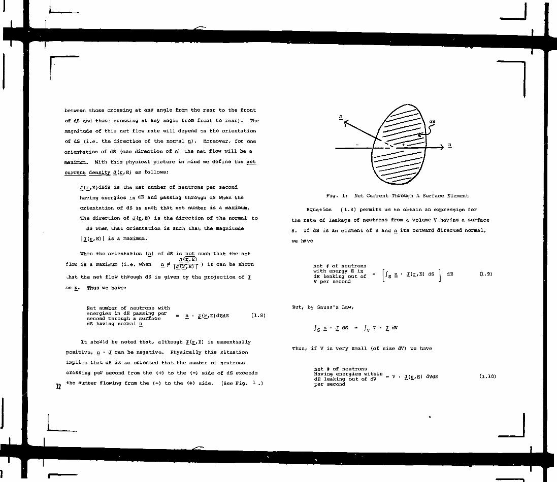
between those crossing at any angle from the rear to the front

of dS and those crossing at any angle from front to rear). The

magnitude of this net flow rate will depend on the orientation

of dS (i.e. the direction of the normal n ) . Moreover, for one

orientation of dS (one direction of n) the net flow will be a

maximum. With this physical picture in mind we define the net

current density J(r_,E) as follows:

J(£, E)dEdS is the net number of neutrons per second

having energies in dE and passing through dS when the

orientation of dS is such that net number is a maximum.

The direction of J(r,E) is the direction of the normal to

dS when that orientation is such that the magnitude

| J(r_, E) | is a maximum.

When the orientation (n) of dS is not such that the netJ(r,E)

flow is a maximum (i.e. when n ^ |j( r E ) I ' ifc c a n b e s n o w n

-hat the net flow through dS is given by the projection of J

on n. Thus we have:

Fig. 1: Net Current Through A Surface Element

Equation (1.8) permits us to obtain an expression for

the rate of leakage of neutrons from a volume V having a surface

S. If dS is an element of S and n its outward directed normal,

we have

net # of neutronswith energy E in _ [f T. „, .. 1dE leaking out of " U s "• i(r-'E) d s

V per second L ••

dE (1.9)

Net number of neutrons withenergies in dE passing persecond through a surfacedS having normal n

= n • j(r,E)dEdS (1.8)

72

It should be noted that, although J(r,E) is essentially

positive, n • J can be negative. Physically this situation

implies that dS is so oriented that the number of neutrons

crossing per second from the (+) to the (-) side of dS exceeds

the number flowing from the (-) to the (+) side. (See Fig. 1 .)

But, by Gauss's Law,

/ s n • J dS = Jv V • J dV

Thus, if V is very small (of size dV) we have

net # of neutronsHaving energies within ,. „. d v d EdE leaking out of dV ~ v i<E.'E' d v d E

per second

(1.10)

L _l

If V • J dVdE is negative there are more neutrons in dE leaking

into dV than there are leaking out.

c) The Balance condition

We now have all the terms needed to express mathematically

the criticality condition.

For a critical reactor in a steady state operating con-

dition the rate at which neutrons appear in any "volume of

phase space" dVdE exactly equals the rate at which they dis-

appear. Combining 1.5 (integrated over E') 1.6, 1.6 and

1.10, we get the fundamental equation

V • J(r,E) + Zt(r,E)*(r,E) = /" dE1 [£g(r,E'+E)

N(rfn.,E) = F(r,E) + £ • V(r,E) (1.12)

(E)vZf(r,EM (1.11)

d) The P-l Approximation

Insofar as statistical fluctuations in the neutron popu-

lation may be neglected, this equation is exact. However, since

it involves both J and <j>, it is not complete. We need another

relationship between J and <J> before either one can be solved

for. To obtain this second relationship we shall make what is

called the "P-l Approximation to the Transport Equation". This

approximation states that the "directional flux density"

v(E)N(r,£,E) (where N(r,£,E) dVdJJdE is the number of neutrons

in dV with energies in dE and all travelling with directions £

within the cone of directions dfl) can be approximated by

where F(r,E) is a scalar function and V(r,E) is a vector func-

tion, (fl - V(r,E) = ax Vx(r,E)+ nyVy(r,E) + fizVz(r,E),

flx, S2 and ftz being the components of the unit vector £ in the

coordinate directions X, Y and Z.)

Physically, Eq. 1.12 states that the angular distribution

of neutrons in dVdE is linear in the direction cosines fl , Si

and ftz- Thus 1.12) will never be a good representation of a

beam of neutrons. The P-l approximation will be valid only when

the angular distribution of H(r,S2,E) is almost isotropic.

The physical definitions of $(£.,E) and J(r,E) can be shown

to imply mathematically that

Jnv(E) N(r,£,E) d£2 (1.13)

and

J(r,E) = Jo £ v(E)N(r,£,E) (1.14)

Substitution of ( 1.12) into these relationships in turn implies

that (1.12) can be written

v(E)N(r,n,E) J(r,E) (1.15)

73

J

If we substitute this result into the basic equation for

N(r,£,E) (the neutron transport equation) and require the result

to be valid when integrated overall SJ we obtain (1.11). If

in addition we substitute (1.15) into the transport equation,

multiply by £ and then require the result to be valid when inte-

grated overall fl we obtain "the second P-l equation"

r,E) + 3Zt(r,E) J(r,E) « J™ £s (r,E'-»-E)J(r,E')dE'

where ( !•

(r E'-HE) = /*j Zs(r,E'->-E, cos 6) d(cos 8)

This is a vector equation relating the three components of

J to the gradient of <J>. It is approximate since it is based on

the approximation ..( 1.15). We shall use 1.11 and 1.16 to

derive the few group diffusion theory approximation.

e) The Few Group Approximation

The basis of the few group approximation is the fact that

several mean free paths inside a homogeneous medium the space and

energy parts of $(r,E) and J(r_,E) become separable so that these

quantities may be written

(1.17)

• (r,E) £ ^

J(r,E) - J(r) FJ(E)

r far inside homogeneous region j.

74

where the "spectrum funptions" F^(E) and F^(E) are characteristic

of medium-j. They may be found by substituting (1.17) into

(1.11) and (1.16) and making the assumption that

<Hr) £(£) ^ e * — , B being the "materials buckling" of

the homogeneous material.

Thus, if j and j+1 label two adjacent homogeneous regions,

the scalar flux density <p(r,E) is <f (r.) Fg1 (E) well within region

j and <i>(r)F + (E) well within region (j+1). However, these

separable expressions for $(r,E)cannot be physically valid at

the interface between regions-j and (j+1) since

Fo(E) f FQ (E), and thus the approximate representation of

$(r,E) must there be discontinuous at almost all energies -

an unphysical condition. He thus face the dilemna of wanting

to use ( 1.17) since it is known to be correct throughout most

of region j but not being able to, since it violates the continuity

of flux and current conditions on the interfaces between j and

its neighboring regions. In few group theory this dilemna is

resolved by abandoning the requirement that flux and current be

continuous at all energies and replacing it with the weaker

requirement that these conditions be obeyed in an integral sense

over each of certain energy intervals AE ir *-i which we split

the energy range 0 •• 15 MeV (the range of interest for fission

reactors). Thus for a G-group theory, rather than require that

<f>(r,E) and the normal component n • J(r,E) be continuous across

an interface at all energies we require merely that

/.„ *(r,E)dE and /.„ n • J(r,E)dE (g = 1, 2 ... G) be

continuous.

J

To construct expressions for <f>(r,E) and J(r,E) that meet

these integral conditions and yet obey ( 1.17) far inside

region j we renormalize pieces of F Q(E) and F^(E) by defining

FJit° 9

(1.18)

(E)

g = 1, 2, ...G; j = 1, 2, ... J

so that

E »*(E)clE = J T{ (E)dE =g * g

(1.19)

(1.21)

In words: the flux and normal component of the net current

will be continuous in an integral sense provided <|>a(r_) and

n • J_(r) are required to be continuous.

Moreover, it can be shown that for inside each homogeneous

region-j

/A E iFo ( E ) d E /AE/o ( E ) d E

G

(1.22)

Then we approximate the flux and net current densities throughout

region j as

(r,E) =

J(r,E) = Jg(r)

ECAE ; r C region j

g = 1, 2, ... G (1.20)

In view of Eq. -(1.19) we then have (with S and S~

referring to the (+) and (-) sides of the interface between j

and (j+1))

JA E g d E

dE n-J(r,E) n-J (r) |g - c-

_ dE n-J(r,E)Eg S4

J2(r)

/ A E / l( E ) d E

Eq. (1.18) then shows that, as desired, the group expressions

(1.20) reduce to the completely separable expressions

( 1.17).

These considerations suggest that the few group equations

we shall derive should describe quite accurately a reactor com-

posed of large homogeneous regions.

Unfortunately, most reactors are not so constructed. At

best they contain triform lattices of fuel rods, cladding and

associated coolant and moderator. For the fuel element "cells"

making up such lattices neither the basic assumption (1.12) of

the P-l approximation nor the asymptotic separability assumption 75

(1.17) are valid. For these situations it is necessary to

find "equivalent homogenized" group-parameters. Such matters

were discussed during the first week of this course. We shall

not repeat that material but rather shall continue the deriva-

tion of the few group diffusion equations assuming the reactor

regions to be homogeneous. It is important to note, however,

that the simple expressions we shall obtain for the few group

parameters must be modified to account for lattice effects when

real reactors are being analysed.

f) The Few Group Diffusion Equations

To obtain the few group diffusion equations we first sub-

stitute (1.20) into (1.11) and (1.16) and require the re-

sult to be true when integrated over each of the AE 's. When

(1.19) is applied, the result for ( 1.11) is

V-J (r) + Sf (r) 4 (r)9

<£> + JAEj:t<r,E)Fog(E)dE 4 (r) =

g. JAE

E dE Its I

JAE

, (r) (1.23)

(1.24)

where the total group-g interaction cross section (I. (r)), theg

transfer cross section from group-g1 to group-g (*•„_•(£), the

fission spectrum for group-g (xa) and the neutron production

cross section due to fission in group-g1 (v2f (r) are c.efinedby comparison with (1.23).

If we were to carry out an analogous procedure for the

P-l equation (1.16) (i.e. substitute (1.20) into (1.16) and

require the result to be valid when integrated over AE_) we

would obtain a P-l transfer term from group-g1 to group-g com-

pletely analogous to the E , <j> . terms of Eq. (1.24). As a

result, the diffusion aquation eventually obtained would involve

Laplacian terms and diffusion coefficients transferring neutrons

from one group to another. To avoid this complexity we make

an additional approximation in reducing the right hand side

of (1.16) to group form. Namely, rather than represent

J(r,E') on the right hand side by the second of Eq. (1.20) we

approximate it by the completely separable form (1.17).

where the appropriate value of j (and hence F^ (E)) will change

depending on the location of point r_.

w To simplify notation we rewrite ( 1.23) as

Thus substituting (1.20) for <j>(r,E) and J(r,E) on the left

hand side and the 2 d of Eq. (1.17) for J(r,E') on the right

hand side and integrating over AEg, we get

V«g(r) Finally, substitution of this result into (1.24) gives us the

few group diffusion equations

/AEgdE

'Z (r-E'+E) Fj(E) J(r)

(1.25)

where the last step comes from equating the expressions for

/ A E J(r,E)dE obtained from (1.12) and (1.20).

If we define the "transport cross section" for group-g as

dE/odE<Z:s (cr 1

Ztr g<£>'AE dE F^(E)

and the tiiffusion constant" for group-g as

(1.26)

We obtain Fick's Law for group-g neutrons:

Jg(r) = - Dg(r)V*g(r) (1.27)

(1.28)

g = 1, 2, ... G

In view of (1.21) and (1.27) we require that the *_<£)

and the normal components n - D (r)V<j>_(r) be continuous across

internal surfaces. On the outer surface we shall require that

the 9g(r) vanish. Alternative boundary conditions that

1 3*g(r)

3n~

2Dg(r)

- 2D (r) or that 4>q(r) vanish at a distance

2 2j- = 4- X, • ) are somewhat more physical in thattr g "

they are based on requiring that the integral over all incoming

directions of the P-l expression for the directional flux (1.15)

vanish. However, the zero-flux boundary condition is simpler,

and, when applied at the outer boundary of a reflector, all three

boundary conditions lead to indistinguishable results.

We note again that, for lattices, finding the group para-

meters is far more complicated than the simple procedure we have

sketched for a reactor composed of homogeneous regions. But the

methods discussed in the first week of the course show that

equivalent homogenized parameters can be found. It is also possible

to find equivalent constants for control rod material or lumps

of burnable poison. We shall not pursue the point other than to77

note that meaningful few group diffusion theory parameters can

be found for the fuel assembly shown in Figure 2 (containing three

zones of enrichment; the box shown is one of a cluster of four

surrounding a cross shaped control rod).

1.2 The Finite Difference Method

The solution of the group-diffusion equations by analytical

' methods is practical only for essentially one-dimensional situations

involving only a few homogeneous regions within which the group

CONTROL RODCHANNEL

ZONE l-y FLUXWELL,-ZONE 2 / SPACER

POISONWAFERS

FEDAL SPACER(TWO PER CLUSTER)

diffusion parameters are spatially constant. For mathematical

models of a reactor that are more realistic numerical schemes must

be used. The most common of these is the finite difference

method, we shall examine two forms of this method for the one

dimensional slab geometry case and then sketch generalizations

to more dimensions.

a) The One-Dimensional Interface Centered Scheme

If for a Cartesian (XYZ) coordinate system the group para-

meters depend only on X and the reactor extends from (-Z ) to

(+Z1) in the Z-direction and from (-Y^ to f+Y^ in the Y-direc-

tion, the solution for the <i> (r) is separable and may be written

*g(r) = Xg(x) cos ££ cos (1.29)

a solution that meets tne continuity conditions in the Y and

Z-directions and vanishes at y = +Y; z = +Z. Substitution of

(1.29) into (1.28) yields

Vx) =3x Dg(x)a5 Xg ( x )

g'=l[£gg>(x) + xgvZfgl(x)] V ( x ) ; = 1' 2' ••• 3

(1.30)

where B is the "transverse buckling".yz

78 Figure 2. Fuel Subassembly B 2 = (. *yz

+ <2^> (1.31)

Equations ( 1.30) are the one-dimensional group-diffusion

equations we wish to solve by the finite difference method. To

do so we partition the X-dimension of the reactor as indicated

in Fig. 3.h ,

Next we integrate Eqs. (1.30) from (xn • "•*• ) to

h(xn + -£•) for n - 2, 3 ... N-1. The result is

With these approximations Eqs. (1.32) becomes

(n) (n-1) (n+1) (n)x

( 1.33)

hr

J \xn~2

f

x g ( x ) d x

" Z / " h 1 fZgg'(x) + V Zfg l ( x )l

9"1 "n-r11 J

Xg(x)dx

g = 1 , 2 , . . . G; n = 2 , 3 , . . . N - 1

( 1 . 3 2 )

Finally, we approximate the group parameters within the

intervals h n by their average values (designated D '"', 2. *n'

etc.); we approximate the flux X (x) in the interval9

< xn ~

(n> s(xn + -^J by Xg(n> s X g(xn) , and we approximate

the derivatives ^ j X g ( x ) | x + h

n by

''

g = 1, 2, ... G; n = 2, 3, ... N-1 (1.34)

These are the interface-centered, finite-difference,

group-diffusion equ&tions. With X ( 0 > = X ( N ) = 0, there are

exactly G(N-2) equations in G(N-2) unknowns. If, on the other

hand, there is a symmetry boundary condition - for example at

( N )x = x N - then X

the symmetry condition X g

ft 0 and we extend (1.34) to n = N using

( N + 1 ) X g( N - 1 ) for the final equation.

b) Mesh Centered Difference Equations

To obtain mesh centered difference equations for ( 1.30)

we again partition the X-domain as in Fig. 3 and approximate

79

the group parameters within the intervals hn by their average

values. However, in this case we integrate Eqs. (1.30) over

intervals xn •* x n + hn. With notation that accounts for possibledX

discontinuities in the D and the -g3- at point x = x n we obtain

xndxg*,.(*> xn+lj

=• (n) _ 1 fxn + hn

g = ^ xn(1.36)

To express the derivatives at the end points of the inter-

vals in terms of the X_ we account for the fact that, if

Dg t Dg<n) these derivatives will be discontinuous at

Accordingly, we use the two approximations

VD(n) 2 _ (n).= (n)g yz tg )Xg

g'=i

h ._ (n) (nl.j (n)n(Zgg' +xgvZfg' )Xg-

g - 1, 2 ... G; n = 1, 2 ... N-l

where the X *n' are mesh-interval-average values:

.35)

(n-l)

Then since the normal current is_ continuous at x , we have

W.j (n-l)

- Dc.)

(1.37)

(1.38)

*n-l "n+1

Fig. 3: Partition of the X-Dimension of a Reactor

Solving the last equation for X_(xn) and substituting the result

into either the left or the right hand side yields

J (x ) - - Dn J-X (niJ g ( V " Dga5EXg(n) Dn-lh +D(n)hg n g n—1

(xg "xg

(1.39)

Substitution of this result into (1.35) then leads to the one-

simensional, slab-geometry, mesh-centered finite difference

equations:

2D(n+l)D(n)g g

G

g'=l

g = 1, 2, ...G; n = 1, 2, ... N-l"(1.40)

Boundary conditions at the outer surface of the reactor are sasily

accommodated. If, for example, Xg(x1) = 0, we simply use the

last term in (1.35) to approximate J (x^) in (1.35).

Similarly, if J (xN) = 0 we eliminate this term from (l.35) for

n » (N-l).

c.) Solution of One-Dimensional Finite Difference Equations

Both sets of equations (1.34) and (1.40) are called

"three point" difference equations, since at interior points the

interface or average flux for each group (Xgn' or X"*n') is

connected only to its two nearest neighbors. For the first and

last mesh point or interval only two neighboring fluxes appear.

From a mathematical point of view ( 1.34) and (1.40)

represent sets of (respectively) G(N-2) and G(N-l) simultaneous,

homogeneous, algebraic equations. If all terms are brought to

the left hand side and the equations are written in matrix form

the result can be expressed as

(1.41)

where X is a G(N-2) or G(N-l) column vector of the unknown group

fluxes and H is a G(N-2) x G(N-2) or G(N-l) x G(N-l)

matrix.

Equation (1.41) will have a non-trivial solution if and

only if the determinant of H vanishes. This mathematical con-

dition is a reflection that the reactor will be critical only

if the production rate of neutrons equals the destruction rate.

Rather than vary reactor loading, size or poison content

to attain the critical condition it is much more satisfactory

mathematically to attain criticality by dividing the fission

production term by a positive real number A (often called keff,

"the effective multiplication constant" of the reactor). It is

plausible and physical grounds that such a number X can always

be found, and it can be proved for finite difference approximations

in one, two, and three dimensions and any number of energy groups

that such is the case . In face there are a number of values

of X (XQ, A1# X2 ...) that can be found such that the determinant

|H[= 0, and it can be proved that there is one real, positive,

isolated X-value (call it XQ) such that XQ>|X |; p = 1, 2, ...

Furthermore, the solution X- associated with XQ is the only

solution of (1.41) that has positive fluxes for all groups at

all internal mesh points. Some of the elements X*"' of the

solution vectors iL associated with X 's for p ¥ 0 have signs

differing from others; such X_'s do not correspond to physically

acceptable solutions. Jt follows that, in attempting to solve

(1.41) we shall be looking for X o and X Q. g]

I J

The direct solution of (1.41) is not economical. Instead

powerful iterative methous have been developed ' ' . To illus-

trate we consider the mesh centered form (Eq. (1.40). With

the definitions

(n) _ _ (n) _ (n)- Ztg Zgg

and the assumptions 2ggi = 0, g1 > g, this equation may be

written in the form

group solution continued down in energy until values for all the

consistent with the initial fission source guess sin'(0)are found. This process is called an "outer iteration". We then

find a first estimate of the eigenvalue A(l)(keff) by forming

the fission rate term T. v2i , X , (1) and then computingg i = l *<3 <3

Z vE(n) X(nU)n,gf fg1 q'

I vZ ( n ) X(n)(0)n,g' fg' g'

(1.44)

an,n-lAg nAg ^"n.n+l^g g.<g Vgg'Xg-

g'=l

nnXgv£fg' g' - Sg (1.43)

where the a« „! are defined by comparison with ( 1.40). (Notelit n

that a 1 0 = aH-l,N=0 a n d a 1 1 o t h e r ann'' nfln' a r e ne9ative->

To solve (1.43) interatively we begin by guessing values

for the X ,<n) which we shall label X Jn) (0) and forming theG

fission source terms g S ^ j S J j ! X*n) (0) 5 S^n) (0) (normalized

in some arbitrary fashion). Next, we solve (1.43 for the

group-1 fluxes which we shall label X^n'(1). (The scheme for

doing this will be described below.) Then we compute thescattering-in terms £the

X£ (1) for group-2 and add them to

(0). The X~2 (n) (l) can then be found, and the group-by-

82

An improved normalized fission source sj?'(1) is then formed

and the iteration process continues. When the fluxes and eigen-

values from two successive iterations differ by less than some

prescribed amount the solution is said to be converged. It is

possible to prove that this iteration process converges to the

fundamental flux solution X and its corresponding eigenvalue

x(l)Xo *

The only part of the solution method that remains to be_(n)

discussed concerns the solution of (1.43) for the X 's.

Written in matrix form this equation becomes

A X-g

(1.45)

Where A is an (N-l) x (N-l) "three stripe" matrix (see Eq. Cl.46

below). To solve (1.45) we write A as the product of two

two-stripe matrices;

L

a 1 2\0 .

0 • •

a32 a33 a34~

1 0

b 2 1 *0 b32

0 0

0 0

1 0

V

0 0 .

C23° '

°33 C34

\

I

(1.46)

(1.49)

so that, defining Y by

(1.50)

we obtain

Thus, multiplying the two component matrices, we obtain 1.51)

A 5 B C

from which it follows that

cll

b21Cll

0

1

C12

b21c12+c22

b32C22

0

C23

b32C23+C331I

0

0

c11

34'

(1.47)

This last equation can be solved easily. Multiplying out g

we find

7 (1)Y

(1)

cn,n+l ~ an,n+lYg ~ sg

; n > 1 (1.52)

> 1n,n

Cn,n " an,n " bn,n-l cn-l,n (1.48)

Then, with the Y known, we obtain from (1.50)

CN-1,H-1

Thus the elements of § and Q can be found readily. Then

to solve (1.45) we writecn,n-l (1.53)

83

J

14

Thus, we can determine all (N-l) of the X 's by first

sweeping down the mesh points (to find the * g 's) and then

sweeping back. This method for solving (1.45) is called

"forward elimination, backward substitution".

d) Extension To More Dimensions

Extension of the finite difference method to more than one

dimension is straight forward. We simply impose the approximate

expressions (1.33) or (1.39) (relating net current across

an interface to the fluxes on adjacent sides) to all faces of a

mesh box. The result is a set of equations of the form (1.34)

or (1.40) except that the flux in a given mesh box is now

related (in two dimensions) to five nearest neighbors or (in

three dimensions) to six nearest neighbors. The outer iteration

scheme is the same as that described for the one-dimensional

case. However, the matrix analogous to the 3-stripe matrix A

of Eq. (1.45) is now 5 or 7-stripe.

The solution X^ of (1.45) for a a 5 or 7-stripe matrix

cannot be found by the forward elimination, backward substitution

method. Instead it is customary to use an iteration method.

One such method that is used frequently is the "Gauss-Saidel"

method . The basic idea of this scheme is to split A into

a sum of a lower-triangular, a diagonal and an upper-triangular

matrix:

A = J, + D + B = (1.54)

Then (1.45) is written

(L + B > X = - U X + S (1.55)

With S known after a given outer iteration, we guess at

Xg on the right side (or use its most recently computed value)

and solve for 5L on the left hand side. This latter quantity

can be found by a simple extension of the method employed

to solve (2.1.51). Then the newer value of X is multiplied

by U, the result subtracted from S^, and the iteration process

is continued to convergence. Such iterations are called

"inner iterations". It can be proved that this iteration process

will always converge for the finite difference form of the group

diffusion equations '.

The solution of the finite difference approximation to the

group diffusion equations in two or three dimensions thus involves

a double iteration. If several hundred thousand mesh points are

involved the method can become quite expensive. Very sophisti-

cated schemes have been devised to accelerate the convergence of

both the outer and inner iteration procedures . However, with

upwards to a million unknown group-fluxes to be found, one does

not ever expect the price of a calculation to become cheap.

1#3 Advanced Methods for Cores With Explicitly

Represented Heterogeneities

If control rods or rod channels, burnable poison lumps,

different zones of enrichment, structural materials between

fuel assemblies, etc. are represented as explicit regions having

individual group diffusion parameters, the finite difference

solution of the group diffusion equations becomes extremely

expensive. The reason is that the number of mesh points required

to describe the geometry and provide a solution that approximates

J

L

accurately the analytical result can easily be several million.

We shall consider two classes of approximate methods for

solving the group diffusion equations that retain the explicit

geometrical detail but (at some cost in accuracy) reduce the

computational cost. These schemes are the space-synthesis method

and the response matrix method.

a) The Space Synthesis Method (2)

The space synthesis technique is based on the observation

that reactors are generally fairly homogeneous in the axial

direction. In fact about the only severe heterogeneities in the

axial direction are due to partially inserted control rod banks

and the boundaries of the core itself. Thus the 10 or 12 foot

axial extension of a light water power reactor is generally com-

posed of four or five regions which, although quite heterogeneous

in the radial dimensions are (at any fixed radial point) homo-

geneous in the axial dimensions. Except at the axial interfaces

of these regions it is plausible to assume that the group-g

flux shape is approximately separable. Thus, within each axial

zone we expect that

• (x,y,z) = (1.56)

z axial zone k

where i|ij*(x,y) is the two-dimensional group-g flux shape appro-

priate to the radial configuration of reactor materials in axial

zone k.

Hear the interface between zone (k) and (k + 1) we expect

that (j> (x,y,z) can be represented by some linear combination of

^(x,y) and ^k+itxry) • Thus throughout the entire reactor it

is plausible to represent the group-g flux as

*gix,y,i

K

k=l

) Tk ( z ) '•

g = 1, 2, ... 6

( 1.57)

where the T^(z) are combining coefficients for the two dimensional

flux shapes characteristic of various radial cuts through the

reactor. If the axial level z is in the interior of, say,

zone-p, we expect T|(Z) will be much larger than all the other

J 's. similarly, on the interface between zone-p and zone-

(p+1) we expect that T^(z) and T ' J^Z) will be about equal,

both being larger than all the other TjJ(z)'s.

If the approximation (1.57) is to be used, we must specify

how to determine the expansion functions ^(x,y) and how to

determine the combining coefficients TjJ(z).

We have already indicated how the t j[(x,y) may be found. We

merely solve the two dimensional version of (1.28) using

group parameters (functions of x and y only) appropriate to the

various axial zones and applying the finite difference method.

It may be necessary to use in excess of 20,000 mesh points to

provide the necessary geometrical detail over the radial planes.

J

However, the cost of running four or five - or even ten - such

problems is far less than the cost of doing a single three dimen-

sional problem involving, say, 20,000 x 100 = 2 x 106 mesh points.

Each of the computations run to find the i|ijj!(x,y) in the

core region are eigenvalue problems and lead to values of keff

necessary to make the various radial slices critical in the

absence of the axial leakage of neutrons. For the axial reflector

zones this technique for finding the expansion functions is not

possible since the v£f vanish in the reflector zones. Instead

we find the i|>?(x,y) for the reflectors by solving a fixed source

problem, the source being the fission source of the adjacent core

region. Thus, if ^(x.y) is the desired expansion function

typical of the reflector zone and i(i (x,y) is the (previously

found) corresponding expansion function for the adjacent core

region, we solve the following reduced version of (1.28)

To find the one-dimensional "mixing functions" Tj[(z) we

shall use the weighted residual method. The basic idea of this

procedure is to recognize that the approximation 1.57) for

iji_(r) cannot in general be a valid solution of the group diffu-

sion equation (1.28) for all points £. However, we can force

it to be a solution in a weighted integral sense. Thus, to

determine the T|[(Z) we substitute (1.57) into (1.28), multiply by

K different G-group weight functions W 9{x,y); p = 1, ... K;

g = 1, 2 or G, and integrate over the XY plane. The result will

be KG coupled, one-dimensional equations in the KG mixing func-

tions T k9(z).

To show the algebraic details of this procedure it will be

convenient to represent the group equations in matrix form.

Accordingly we define the following GxG matrices by indicating

their gg' elements in brackets { ) :

G

g'=i

g <g

(x,y)

(x,y)

(1.58)

B(r) H Diag { Dg(r)

' " Zgg' (£» • (1.59)

(r)

86

where subscripts o or 1 on the group parameters indicate the

region to which they belong. (Also note that the definition

(1.42) has been applied.) Since the right hand side of

(1.58) is known, only one outer iteration is required to

determine the i(>og(x,y).

Then, if the G-element column vector <J> (r) is defined by

5 Col { *g(r) }

Equation v'1.28) may be written

. (1.60)

J

_J

-V-D(r)V£(r) ^ fy i(x'v)

where we have introduced the eigenvalue A explicitly.

Iff finally/ we define diagonal GxG matrices of expansion

and weight functions and a column vector of mixing coefficients

by

Xk=l

p = 1, 2, ... K ( 1-64)

]J(k(x,y) s Diag

Sk(x,y) 5 Diag

Tk(z) = Col

i|ij[(x,y)>

(1.62)

k = 1, 2, ... K

This equation may be rewritten in simpler notation as

K K

k=l Z k=l P

Equation (1.57) becomes

k=l(1.63)

The weighted residual procedure then consists of substituting

(1.63) into (1.61), multiplying by the K weight matrices

Wk(x,y) and integrating over the XY domain of the reactor. The

result is

xk=l

p = 1, 2, ... K (1.65)

where the GxG matrices Dpk, S p k and M k are defined by comparison

with (1.64).

Finally, (1.65) may be written in the "supermatrix" form

K

k=l

B(z) T(z) = T(z) ( 1.66)

where D(z) is a KxK supermatrix having the GxG matrix gpk(z)

. thas its (pk) element (similarly for fi and M) and T(z) is a

K-element column vector having as its k element the G-element

87

J

vector Tfctz)- In this supermatrix form the equation for the

mixing coefficient vector T(z) can be seen to be a matrix generali-

zation of the one-group diffusion equations 1.30 for G = 1),

and, in fact, a matrix generalization of the forward elimination

backward substitution technique can be used to solve ( 1.66).

We have not yet considered the problem of selecting the

GxG weight function matrices H ; p = 1, 2, ...K. A derivation

of (1.66) based on a variational principle suggests that the

adjoint functions (see Section 2 of these notes) corresponding

to the jlijj are the favored choice . However it has been found

that the spatial shapes of the regular and adjoint fluxes for a

given group do not differ significantly, and using the jj them-

selves for the 5J usually produces just as accurate results.

Moreover, with the j]jk used for the ij the cost of solving an

extra set of two dimensional difference equations is avoided.

This procedure is called "Galerkin weighting".

Many variants of the continuous space synthesis approxima-

tion have been investigated (see Kef. 3, Chapter 11, and Ref. 4).

For example, in the "collapsed group approximation" the

group-to-group ratios of the expansion and weighting matrices

are assumed to be fixed (Tk9(z)/(Tk

s+:L(z) = constant). Thus,

(1.63) becomes

iktx,y) (1.67)

where i£k(x,y) is a G-slemant column vector and T^fz) is a scalar.

Ttie weight function matrices g k (1.52) become row vectors (the

transposes of column vectors W k ) , and the size of the matrices

in (1.66) is reduced from (GK)x(GK) to KxK. If the collapsed

group approximation is made, it ?.s important that the group-to-

group ratios of the W k approximate those of the fluxes adjoint

to the i^. This is because, although adjoint and regular flux

shapes for a given group are similar, the group-to-group ratios

are usually very different.

Another variant of the space-synthesis approach is known

as "multichannel synthesis"' '. In this approximation the

ik(x,y) are partitioned into several segments over the XY plane

and the individual segments are treated as independent expansion

functions. For example, the portions of the i^tx.y) belonging

to the four quadrants of the XY plane may be allowed to vary

independently. The effects of flux tilting can then be accommo-

dated without introducing special, tilted functions. The dis-

continuities in radial flux shapes that result from the approxi-

mation can be avoided by defining expansion functions as

£n(,x,y)±k(x,y); n = 1, 2, ... N; where the fn(x,y) are scalar

functions equal to unity over most of the region where we wish

Jijj to be non-zero but then drop in a continuous fashion to zero

throughout the rest of the core . Figure 4 shows a sketch of

two such functions for a one-dimensional slab of thickness L.

One final variant of the space synthesis scheme is called

"discontinuous space synthesis"' '. The baeic idea of this

method is to discard expansion functions in regions where they

are not needed. For example, if ten radial ]fek(x,y)'s are

J

needed to account for all the different radial conditions in the

core, we use perhaps only three of them at a given axial location.

_ L 1/2

Fig. -1: Modulating Functions for a One Dimensional Situation

we use only !l!n_i» S n an<3 finri'

i n 1-62). Then when z moves

to zone n+i we discard ]fc _-, and add ^ n + 2 i-n i t s place. Thus,

although a total of ten expansion functional are used for the

overall calculation, only three are used at any given 2-location.

As a result in (1.62) K = 3 rather than 10, and ( 1.66) is

simplified accordingly.

Flux synthesis methods have been found to be accurate and

relatively inexpensive. However, they have several drawbacks.

First of all, implementation by a computer program is very com-

plicated. Secondly, there is no automatic way to select expansion

functions that are guaranteed to be optimal. Physical insight

and experience must be used, and if some physical behavior such

as a flux tilt is not an'-icipated so that tilted expansion func-

tions are not supplied, results can be seriously in error. Finally,

there is no way to establish error bounds. Adding more mesh

points in the case Gf finite difference approximation can be

proved to improve accuracy; for synthesis methods increasing the

number of expansion functions may actually reduce accuracy.

These difficulties suggest that space synthesis procedures are

best applied to problems for which the qualitative behavior of

flux shapes is well understood. For such cases the method pro-

vides reliable and very detailed information about criticality

and flux distribution throughout a geometrically complicated

reactor.

b) Response Matrix Techniques

In the response matrix technique the reactor is partitioned

into a number of fairly large subregions called nodes, and the

"partial neutron currents" crossing the faces of these nodes

from inside to outside and from outside to inside are treated

as unknowns. Preliminary calculations are performed for each

different node to determine "response matrix elements" specifying

the neutron currents emerging from a given face of the node due

to unit currents entering each of the nodal faces. The physical

fact that currents emerging from one face of a node must equal

those entering the adjacent face of the neighboring node is then

applied to derive a set of equations connecting all the partial

currents.

To describe the method in more quantitative detail we first

define a "partial current density" mathematically and show its

relationship to the scalar flux density and the net current

J

J

per second with energies in dE crossing a unit surface perpen-

dicular to the Z-axis and containing point r from the negative

side (z less than the Z-componet of r) to the positive side

(z greater than the Z-component c" r ) . The partial current

J ~(r_,E)dE is defined similarly except that it refers to neu-

trons crossing from the positive to the negative side of the

unit surface. Analogous partial currents Jx* and J * are defined

for unit surfaces perpendicular to the X and Y axis. It fo lows

that tba net current in the three coordinate directions are

Ju<r,B) - JU+(£,E)- J~(r,E); u - X,Y,Z

nuv(E)N<r,r,E)dfi

the latter expression coming from Eg. (1.14),Z

90 Pig. 5: Coordinate System for n

find these quantities by integrating nuv(E)N(r,r,E) ovsr a hemi-

sphere rather than over the entire sphere. Thus, for fi expressed

in spherical coordinates (Fig. 5) we have

sinede Slzv(E)N(r,n,E)

If we then approximate vN by the P-l expression (1.15) J

becomes

( 1.69a!

J*(r,E) sin8 cos8 [*(r,E)

3(sin8 cos* Jv{r,E) + sine sin* J,(r,E)x y ~~

cos8 Jz(r,E) Jz(r, (1.69b)

Similar calculations show that, in general, for the P-l

approximation, partial currents are related to net currents by

Ju(r,E) = £*(£,E) ± \ JuCr,E); u = x,y,z (1.70)

By adding and subtracting J* and J~ we find the inverse

relationships

ifi (r,E) = 2 [ Ju(r,E) + J~(r,E)l

J,,(r,E) = J*(r,E) - J,"(r,E) (1.71)

J

1These relationships can lead to mathematical problems at

points where the material properties of the medium are discon-

tinuous. Since we shall avoid these difficulties, they will not

be discussed explicitly.

The next step in the response matrix procedure is to define

response matrix elements. Roughly these are the partial currents

of group-g neutrons emerging from face-n of the node due to a

partial current of group-g1 neutrons entering across face-n',

where face-n' can be face-n itself or any other face of the node.

We shall designate this matrix element as R;(n'' To be precise

we must specify the spatial and angular shapes of the entering

and emerging current distributions. For the moment, however,

let us make the simplest approximation, namely, that the spatial

distribution of entering currents is flat along the respective

faces of the node and that the angular distribution is isotropic

over the entering hemispheres. Note that, even if the entering

current distrioutions are spatially flat and isotropic in angle,

the corresponding exiting quantities will not be. For the

moment we shall nevertheless assume they are.

With these approximations we can relate J^(out) the average

partial current of group-g neutrons emerging from face-n due to

group-g' currents entering faces-n1 (J^,(in)) by

n = 1, 2, N; g = 1, 2, ...G

(1-72)

If all the J^(out)'s and J^(in)'s are assembled into

column vectors, J(out) and J(in), Eq. (1.72) can be written

as a single matrix equation

J(out) J(in) (1.73)

Moreover, since the JJJ(out) of one node equal the J^,(in) of

adjacent nodes, the vector J(in) is simply a rearrangement of

the vector J(out),

J(in) = fi J(out) ( 1.74)

where 4 is a permutation matrix.

Thus the J(out)'s are solutions of the eigenvalue problem

Y J(out) = E S J(out! (1.75)

where y is an eigenvalue introduced to insure a non-trivial

solution (analogous to the X of Eq. (1.61). The matrix B £

is non-negative and irreducible. Under those conditions it is

possible to prove that there exists a simpls eigenvalue Y

equal to the spectral radius of g & and that the corresponding

eigenvalue is unique and has all positive entries. This is the

solution we seek. For y = 1, the reactor is exactly critical;

for y * 1 it is supercritical and for y * 1 it is subcritical.

If one wishes to find the raore familiar eigenvalue A (keff) by

the response matrix procedure it is necessary to divide the

91

J

J

values of vZ- used to determine E (see below) by a succession

of numbers, X, until that X is found for which y = 1. This

search procedure is time consuming, and it is difficult to see

what is gained by it.

To determine the R^'i auxiliary computations must be carried

out for each different node making up the reactor. The node is

isolated in a vacuum: a source of group-g' neutrons is allowed

to impinge on face-n1, and the group-g neutron currents emerging

from all faces are computed. By definition these are the RJjjfi

for inlet and outlet neutron beams assumed spatially flat and

isotropic over the inward or outward directed hemispheres. It

should be noted that any augmentation of the neutron population

due to fission is accounted for by this way of finding the

R ,. Also, most important, there is no need that the nodes

be homogeneous nor that the nodal calculation be carried out in

the diffusion theory approximation. Sophisticated transport

theory methods can be used to compute response matrices

Since these methods need be applied to only a few different kinds

of nodes rather than over the whole reactor, the computing cost

of finding the R^i is not prohibitive. Also, since the nodes

are large in size, there may be only several thousand of them.

Thus, the solution of .(1.75) is manageable.

The major drawback to the response matrix technique involves

the assumptions about the spatial and angular distributions of

the neutrons making up the incoming and outgoing partial currents.

We have so far assumed flat shapes and isotropic angular distri-

butions over the entering and exiting hemispheres. But this

restriction is not necessary in principle. Entering and exiting

currents can be decomposed into any number of fixed spatial and

angular shapes and response matrix elements R^n'-SB' c o mP u t e < J

specifying the number of group-g neutrons emerging from face-n

having angular distribution-a and spatial shape-s due to a unit

incoming current of group-g' neutrons entering face-n1 with

angular distribution-a' and spetial shape-s'. The trouble with

this generalization is that the magnitude of the calculations

quickly gets out of hand. Use of only two angular and two

spatial distributions on each face of a node increases the

number of unknowns in J(in) and J(out) by a factor of 4 and the

number of matrix elements by a factor of 16. Thus the practical

utility of the response matrix method depends on how well the

spatial and angular shapes of the neutrons entering and leaving

the faces of the nodes can be represented by a single function

or by a combination of a very few functions. If this number

can be kept small the method can account for both geometrical

complexity and transport theory phenomena within the nodes,

l.fl. Methods £or Cores Represented by Large Homogenized Nodes

The finite difference, synthesis and response matrix pro-

cedures are all directly applicable to the analysis of reactors

composed of heterogeneous assemblies such as the one shown in

Figure (2). Except with the response matrix technique it is

necessary to have group-diffusion parameters for each explicit

region when these methods are applied. Methods for determining

these group-diffusion theory parameters have been discussed in

the first week of this course. We shall call these methods the

J

L

"first stage" of homogenization. Homogenized group-diffusion

parameters representing fuel rod cells (composed of a fuel rod,

its cladding and associated moderator), control rod material,

structural zones (possibly mixtures of coolant and metal),

and lumps of burnable poison (and associated structural material)

result from this first stage of homogemzation. A group-diffusion

theory model in which a very large number of different material

regions are represented explicitly results, and a very large

number of mesh points must be used jus- *:o describe the geometry

of the reactor.

In order to reduce the number and - more important - in order

to permit the application of more efficient computational methods

a second stage of homogenization is often carried out. This

second stage of homogenization is usually accomplished by a

simple flux weighting procedure, although recently more sophisti-

cated methods have been suggested * ' . In the flux weighting

homogenization scheme a detailed flux computation is performed

for a large heterogeneous node (such as a 20 cm axial section

of a fuel assembly) with zero current boundary conditions applied

over the surface of the node. The resultant flux shapes ••f'J(r)

for the various groups are used to find average group parameters

IT (et standing for fission, absorption or scattering) according

to the formula

d v

ag «g(r) dV( 1.76)

where the volume integral is over the heterogeneous node. The

diffusion coefficients D are usually found in th^ same manner.

If homogenized group-diffusion parameters for the reactor

nodes are found by the two stage homogenization procedures, the

final mathematical model of the reactor is one composed of large

homogeneous zones. If finite difference solutions are carried

out, the number of mesh regions required is now determined by

the accuracy of the finite difference approximation (Eq. 1.33)

and (1.39) rather than by the geometry. For light water

reactors the nodes will be of size ~ 20 cm by 20 cm in the

radial plane. But accuracy may require use of mesh spacings of

less than a centimeter near the core-reflector interface and

of no more than 3 or 4 cm in the interior. The situation suggests

that approximation methods be used that require a fewer number

of unknowns for a given accuracy than the number needed for the

finite difference approximation. We shall outline two classes

of such methods: finite element techniques and nodal methods.

a) Finite Element Techniques

With the group diffusion theory parameters constant through-

out each node it is expected that flux shapes within the nodes

will be fairly smooth. This fact in turn suggests that the

flux sh, ->es within the nodes could be approximated well by

polynomials. The finite element method is a systematic way of

making such an expansion. Its chief distinguishing feature is

that the polynomial have "local support"; that is, they are

zero over all but small regions of the reactor (usually a node

and its nearest neighbors). Thus the group-g flux is expressed

93

J

(x,y,z) =

k=lgk)(x,y,z) H <f.g

a)(r) (1-77)

where the P^ are continuous functions composed of polynomials

of a certain value in x,y,and z. Each p' is now zero over

only a small portion of the reactor (although regions where the

polynomials are non-zero may overlap).

The unknowns of the problem are the coefficients of the

(k)P* . These may be found by a weighted residual method. Thus

we substitute the approximation •! (r) into (1.28), weight

by a sequence of weight functions w' (£) (equal in number to

the number of unknowns in if g ) and require the result to be

true when integrated over the reactor:

/Wgn' (r) -V >a>(r) 4 > g ( r(r> -

7-[wgn>(r)Dg(r) Wg

n> (r)V- [og(r)V*ga) (r)]

>['Wgn)(r)]-[Dg<r>7ij>g

a)(r)] (1.79)

and (since w' <£) = 0 on the outer surface S ) .

= o (1.80)

and the volume integrals of the two terms on the right hand side

of (1.79) are equal and opposite in sign. Thus (1.78)

becomes

G

g'=lg = 1, 2, ..., G

( 1.78)

We shall restrict our solution of trial and weight functions

so that ifi (r) and the W (£) are continuous and vanish on the

ojter surface of the reactor, and, for the moment, we shall also

assume that the normal component of the D (r)9ifg (r) are also

continuous across internal interfaces between nodes. Then, since

94

(1.81)

g'=l

He have derived the result under the assumption that the

normal components of D V<(> are continuous across internal

interfaces. Actually the limitation is not necessary. The

expression can be derived under the weaker assumption only that

<s'a' (r) and the w'n' (r) are continuous and vanish on S (seerg — g — o

Ref. 3, p. 500). For that space of functions (1.81) is known

as the "weak form" of the group diffusion equations.

To illustrate the finite element method we shall consider

the very simple example of an expansion in linear functions for

one-dimensional slab geometry. Fir this case we take

"k-1f o r xk-l i x ^ xk

0 for all other x

(1.82)

(k-2) ^ (k-1) ' (k) ^ (k+1) .T(k+2)

cj. 6: Expansion Function P (x! and Segment of <)> 'a'(x)

where the mesh layout is as shown in Fig. 3, all interfaces

across which material properties change being one of the xk's

and material properties being constant within each mesh inter-

val hk. Two expansion functions Pg(x) and (x) and a

'segment of the overall flux shape $' formed from them according

to (1.77) is shown in Fig. 6. The composite function <j>' (x)

in the range i < x < xic+i *s £°Ime& by the sum of the two

overlapping "tent functions" shown in the top of the figure,

all other expansion functions P n(x); n J k, k+1 being zero

in that range.

To determine the • we approximate as in (1.77)

k=l

and, substitute this result into (1.81) -.'sing (1.82) to

represent the P (x). If we use normalized tent functions

P n(x)" n — ; n = 1, 2 ... N-l as weight functions W lnJ (x),

V1.83)

95

J

Eq. (1.81) will yii»ld exactly G (N-l) equations for the

(n). Note that for a fixed H (n) (x) onlyG(N-l) unknown

three P (x) in the sum 1.83) survive. The result of

performing the differentiation and integration indicated for

(1.81) is

"k-1

•<*-!>, -

(Eq. continued)

ztg,l.k(3*g

,,ljk).1.(k+1),)lp , Vg'

= 0; 1, 2, ... N-l (1.84)

Note the similarity of this equation to the finite difference

result (1.34). Both theoretically and empirically the finite

element result can be shown to be more accurate. Thus, for

a given degree of accuracy, larger values of h. (and hence

fewer mesh points) can be used with the finite element equations.

96

Still greater accuracy can be achieved by using higher

order polynomials. For example, a set of three cubic poly-

nomials P ( k ) o ( x ) , P (k) + (x), P ( k )~(x) can be associated with

mesh point k, where P 'k) '°' (x) vanishes for x <_ x k - 1 <

t n e value

*k+l;

, (k)

of x

for

and a zero derivative at

at x = x. and has zero derivative

x) vanishes for x < x. ;

-| for x on the 1+) sidex k+

(k)-.i and P

side of x, and a zero derivative at xi-_i •

(x) vanishes

for x on the (-)

(These functions

are called cubic Hentiite polynomials.) There are then 3G

unknown coefficients at each mesh point, and the finite element

equations analogous to (1.85) are more complicated. On the

other hand, the equations are more accurate so that fewer mesh

points are required.

In two and three dimensions products of the one-dimensional

polynomials may be used. Coupling becomes more extensive than

for the finite difference case. For example, the extension

to three dimensions using expansion functions that are products

of »-ho functions (1.82) , one for each dimension, yields

difference equations for which one "rnsh point is connected to

26 neighbors rather than to 8. For this linear case, hov:°ver,

the total number of unknowns is the same - namely, the

$„(x^ y^ z^), and in general it is found that far fewer unknowns

are required for a finite element representation of uhe flux

than for a finite difference representation of equal accuracy.

J

The question of whether there is a net savings realized

by use of the finite element method (which involves fewer

unknowns but a much greater degree of coupling) seems to be

unsettled at the moment. Different groups have come to different

conclusions . Thus, it is not clear at this time whether

the finite element scheme actually can realize the great reduc-

tion in computing costs that would be expected from the reduc-

tion in the number of unknowns. Two other points, however, are

not in dispute. The method does provide continuous values of

the group fluxes throughout the reactor (not just at the mesh

points) and decreasing mesh spacing improves the accuracy of

the answer.

b) Nodal Methods

In nodal methods the primary unknowns are taken to be the

average fluxes in the various nodes. The basic equation for

such methods is then obtained by integrating ( 1.24) over the

volume V n of the n node (n = 1, 2, ... N). If we assume that

the group parameters are constant throughout each node and

designate them as Z^"' , l'"', etc., we obtain

where the average nodal flux for group-g is defined as

V n ) =v7 ( 1.86)

The various nodal schemes differ from each other through

the ways that currents across surfaces between nodes are related

to the average fluxes in those nodes. The older nodal

schemes ' ' ' establish this relationship by using escape

probability arguments. More recently, for Cartesian geometries,

a new class of nodal schemes have been developed (16, 17, 18)

These methods are based on relating the J-n's across a given

nodal face to the adjacent <Fg 's through the solution of

average one-dimensional equations. To indicate how this is done

we shall examine the two dimensional case.

Thus we consider a rectangular node of size h^ x nj

(h* = <xi+x " xi>; hV = (Vj+1 - y.)> and define nodal averaged

fluxes in the X and Y directions:

(x,y)dy

(n)(1.85)

(1-87)

97

J

Comparison with the two-dimensional analog of (1.86) shows

that

1 , i+

h? x ) xi <*>«*

To obtain an equation for the <f> we integrate the basic

group diffusion equation for the node (1.28) ovsr h'y at

a particular value of x within h£ '.

tx)

If the transverse leakages t'^' (X) were known, it could

be possible to solve for the <jf (x) within node (ij) in terms

ofg x

(xi) and -D at the interface between node (ij>

| x\ couldand node (i-1,j), and then by integrating over h|

be relaced to these two quantities. The 5 g (average

group flux in node (i-1, j)) could also be found in terms of

these same two quantities by a similar procedure carried out

for node (i-1, j) and taking advantage of the continuity of

flux and current across the nodal interface. Thus if the

L(y^'(X) and L'1" 1'^'(X) were aero it would be possible to

obtain two relationships of the form

9V=1

1, 2, ... G (1.88)

dx

(1.90)

the transverse leakage term being defined as

(1.89)

By integrating ( 1.28) over h^x^ at a particular y, an

analogous equation for $_ (y) can be obtained. In this equati

transverse leakage terms in the X-dii.ccri-.ion appear (L'^'(y)) .

Then by eliminating C g x ^ ) from these two equations we could

derive a relationship of the form

d' x i " '

dx

(1.91)

I

For the case at hand the basic nodal equation (1.85)

becomes

(1.92)

Hence by using ( 1.91) to eliminate Jgfx.J and expressions

analogous to (1.51) to eliminate the other three leakage

terms we could convert (1.92) into a "five-point difference

equation" relating <jT_ •* and its four rarest neighbors.

Standard finite difference procedures could then be used to

solve for the •" .

All this is rigorously possible only if the transverse

leakage terms in the Y-directions are neglected in the manipu-

lations leading to the transverse leakage formula (1.91) for

the X-direction. In fact, however, such neglect leads to

error, so that someway of dealing with the term Lyy (x) in

(1.88) must be concocted. The simplest procedure is to re-

place <t>g(xrVj+1) and *g(x,yj)jin_ ..(l-a9> by their average

values *gy(yj+i-) and $"gy(y..+) . Eq. (1.89) then becomes

(1.93)

The solution of (1.88) leading to (1.91) must then be

carried out with this (constant) valie of Ltij)•gy

treated as an

inhomogeneous source term. Thus the following iteration scheme

is suggested:

1) Solve (1.88) and determine (1.91) with

(ij)(x) = 0.

2) Substitute (1.91) and analogous expressions for the

three other average currents into ( 1.92) and solve the

resulting 5-point equations.

3) With the values of <f>£

J ( x ^ ' s e t c . using (1.91).

so obtained evaluate the

4) Use these to form the inhomogeneous tern L in

(1.88); solve that p^uation and continue the iteration procedure.

ing v

(19)

An improved way of dealing with the L g y (x) e t c- h a s

This is to fit L <ij)(x)been suggested by Finnemann

to a quadratic polynomial over the three-node range

x^_^ <_ x £ xi+2 expressing the coefficients of the polynomial

in terms of the average transverse leakages L ll-l,j)

and L_y • The resulting quadratic function i"S then used

to approximate the x-dependence of L '1]'(x) in (1.88) in

the range x± <_ x < xi+i- A s before, the transverse leakages

needed to generate polynomials are formed, using (1.91),

from the previous iterate for the 7- '.

The problem of solving ( 1.91) can be solved in a number

of ways. It can be done analytically (18) or by expanding the99

J

X-dependence of the <f (x) in polynomials, determining some of

the coefficients by applying continuity and boundary conditions

and determining the rest Dy weighted residual procedures.

These polynomial schemes can be carried out for a whole row of

nodes at once or one node at a time ' ' . In the latter

case it is convenient to express the polynomials in terms of

partial currents (1.70) across the nodal surfaces rather than

the flux and total current values on those surfaces.

Very encouraging results have been obtained with the new

nodal mecnods. For a given degree of accuracy they are one

or two orders of magnitude faster than finite difference methods.

They have been extended to time-dependent problems and to

situations in which the nodal group-parameters are mildly space

dependent (such as will occur if fuel depletion is not uniform

over the node). Approximate values of local power peaks can

be recovered from the nodal fluxs and surface currents generated

in the course of carrying out a solution. The major concerns

about them are that (to date) they deal only with Cartesian

geometries and they cannot be applied directly to reactors

composed of drastically heterogeneous nodes (such as the nodes

containing cross-shaped rods in a BWR). The latter problem can

be overcome by the use of nodal-homogenized group parameters

as explained earlier. Provided this is done accurately, the

nodal schemes appear to be a very powerful tool for the

analysis of light water reactors.

^5 Extension of Static Criticality Calculations to FuelDepletion Problems

The extension of criticality calculations to depletion is

straight forward but greatly increases the costs of calculations

unless it is carried out carefully.

At first the extension appears to raise major mathematical

problems. Depletion is a time-dependent phenomenon, the result

of which is to change local concentrations of fjel and intro-

duce fission products so that local group parameters change with

time m a way that depends on the local group fluxes. Moreover,

significant depletion takes place only in reactoxs operating

at high power. Thus local temperatures and densities may vary

in a manner that depends on the local fluxes and depleting fuel

concentrations. But the fluxes themselves also depend on the

local temperatures and densities. Tnjs at first it would appear

necessary to deal with non-linear, time dependent sets of

equations describing the depletion, heat transfer of phenomena

and the neutron flux behavior simultaneously.

In practice the situation is not nearly that bad. Deple-

tion effects are so slow that steady state neutron and heat

transfer equations can be used. Also, the depletion calculations

can be done separately from the nuclear-thermal calculations.

Thus the initial flux shape is assumed to remain constant during

the first depletion time step; then, with the newest material

concentrations, group parameters arc up-dated and a new flux

shape is determined. This latest shape is the one used for the

100

J

next time step. Thus the depletion and nuclear-thermal calcula-

tions are done in tandom and as far as depletion is concerned

the nuclear calculations are standard static, linear computations.

The thermal-hydraulic computations do complicate matters.

But this is a complication encountered whenever the temperature

and density distributions throughout a reactor affect flux

shapes. It is necessary to iterate between temperature density

distribution and flux distribution until the steady state tempera-

ture density profile associated with a particular flux shape is

consistent with the flux shape associated with that temperature-

density profile. A consistent equilibrium xenon concentration,

control rod position or soluble poison concentration leading to

criticality must also be found by iterative procedures. The

startegy for this typa of iteration is to try first to converge

the quantities that produce the greatest effects. Thus, if

the flux shape is quite sensitive to control rod bank position

but the control rod bank position is not very sensitive to the

temperature-density distribution (and hence to the flux shape),

first find the control rod bank position corresponding closely

to criticality but to a possibly incorrect temperature-density

profile. Then improve the temperature-density profile. Such

iterative searches are complicated. However, as previously

noted, they are a consequence of the reactor's being at power

rather than of depletion.

The real problems associated with depletion are the need

to determine changes in group-parameters due to depletion at

all mesh points in fuel regions for a large segment of the

reactor (symmetry usually permits dealing with only a quarter

or an eighth of the core) and the consequent amount of data that

must be handled. Thus, if it is necessary to keep track of

say 15 isotopic densities (U235, U 2 3 6, Pu 2 3 9, Pu 2 4 0, Pu 2 4 1,

B , several fission products, etc.), at 100,000 mesh points

comprising the fuel region for an eighth of the core, 1.5

million concentrations must be stored, 100,000 spectrum calcu-

lations must be run and ^ 40O,00OxG group-parameters must be

reconstructed each depletion time step.

Two simplifying approximations are generally made to over-

come these difficulties. The first is called block depletion

and consists simply in using the average fluxes throughout

nodal regions rather than the point fluxes to do the depletion

calculations. If nodal regions each containing, say, 100 mesh

cubes are selected the amount of data to be stored and the

amount of calculational work is cut by a factor of 100.

The second simplifying procedure used to make depletion

calculations manageable is to determine changes in group para-

meters by constructing them from what are called "fitted micro-

scopic cross sections". The idea is based on the observation

that at any time, t, in the course of reactor depletion a group

parameter, say, Z (r,t) can be expressed as

(1.94)

where n^(£, t) is the concentration of isotope-j at point £

J

102

and time t and a3 (r,t) is the microscopic group-g absorption

cross section for isotope-j at that point and time. The con-

centrations nJ(r_, t) change in time because of the depletion

processes. j.he microscopic group-cross-sections also change

since the local neutron spectrum itself depends on local isotopic

concentrations and hence on time. (See the discussion relevant

to Eq. 1.17 through (l.24.) In the fitted constants procedure

we try to estimate in advance how the local spectrum will change

as depletion proceeds. To do that we perform what are called

"point depleti.;/' calculations for each different fuel composition

making up the initial loading of the reactor. (Generally there

are only 3 or 4 such initial compositions.) To do a "point

depletion" we start with the initial concentrations of the fuel

composition and compute few group parameters in the usual way.

2 2 2

Then with 7 <f> set equal to —Bj^ <j>_ where B is the materials

buckling we deplete the composition for a depletion time step

(T 1000 hours). A new spectrum calculation is then performed;

new few group parameters are determined and another depletion

step is taken. Since microscopic group parameters corresponding

to the up-dated spectra can be obtained at each time step, we

can form a table of such quantities as o a^ vs. some parameter

{such as the total fission energy released) that characterizes

the degree of depletion. Then as the whole core depletion pro-

ceeds we can generate the o ^ for that fuel composition at any

time and location just by keeping track of how much energy has

been released at that location. Thus pointwise values of

Xag(r_,t) (Eq. 1.94) can be found as needed, and the need to per-

form a spectrum calculation at each mesh point ir nodal block

at every time step is reduced to that of doing one for each

initial composition. The saving is great since there may be

1000 nodal blocks but only 4 initial fuel compositions. The

error in the procedure is due to replacing the 7 "fg at points

by Bm2<!> . This error is usually small. Note that the n? in

(1.94) used with fitted the values o^ are those obtained

from the full core, space dependent depletion. The "point

depletions" are done only to generate the o a g •

With the block depletion and fitted constants procedures

(along with a few more minor approximations described in

Ref. (3) Chapter 6) the mechanical problems of data handling

associated with reactor depletion become quite tractable, and

depletion calculations are reduced to a manageable sequence of

steady state criticality computations.

2. Reactor Kinetics

In discussing the mathematical models used to describe

transients in nuclear reactors and the techniques used to solve

the relevant equations we shall assume a general familiarity

with the physical picture that underlies the kinetic behavior

of a reactor (large neutron population, very fast neutron

speeds, delayed neutron precursors and their relatively slow

decay periods, reactor parameters that are time dependent

because of temperature and density feedback phenomena). We

shall also assume a qualitative understanding of such terms

as subcritical, supercritical, prompt critical, reactor period,

scram, runaway, etc. With a general familiarity with such

J

~1concepts and terms assumed we shall then begin with a discussion

of the time dependent group diffusion equations and methods for

solving them and follow that by a derivation of the point kinetics

equations along with discussion of tne kinetics parameters and

the measurement of reactivity. Finally, we shall indicate how

feedback effects are accounted for.

2.1 Space Dependent Kinetics Equations

a) The Time Dependent Group Diffusion Equation?

We shall use the group diffusion model to describe space

dependent kinetics effects. Thus it will be necessary to extend

(1.28) to the time dependent ca ,e. This is a straightforward

procedure: We first note that, if the creation rate of neutrons

exceeds the destruction rate, the number of group-g neutrons

3(-=- * ) will increase at a rate ^* ) will increase at a rate ^ (^) (v is the averageq " g

speed of neutrons belonging to group-g). It is also necessary

to distinguish between prompt neutrons appearing directly as

the result of a fission and delayed neutrons appearing as the

result of the decay of a precursor. With these matters accounted

for and C.(r_,t), g? and X^ standing for the local concentration

of the i precursor group, the fraction of the neutrons from

a fission of isotope j that eventually appear from the decay of

precursor i, and \^ the radioactive decay constant of precursor

group-i, Equation (1.28) extended to the time dependent rase

becomes

9 1, 2, ... G (2.1)

where S3 = ZS^ ; x2g is the fraction of prompt neutrons

appearing in group-g from fission of isotope-j, and x^q *-s t'le

fraction of delayed neutrons emitted by decay of precursor-i

that appear in group-g. (Note that we have now accounted

explicitly for fissioning of a number of isotopes, j.) To

complete (2.1) we need equations specifying the rate of change

3t

G

j g=it) - AiCi(r,t);

i = 1, 2, ... I

(2.2)

Eq. (2.1) states mathematically that the rate of change

of the number of group-g neutrons per cc per second equals the

difference between the creation and loss rate of such neutrons

(a neutron can be -lost" from the -.nit volume about point x_ and

the energy group-g by leakage and scattering as well as by

absorption.) Eq. 2.2 makes an analogous statement about the

concentration of the i t h precursor group. Note that all the

group parameters are shown to be functions of time. We shall

not discuss at this time how such time dependence is accounted

for mathematically. (See Section 3.3 below.)

103

b) Finite Difference Solutions of the Group DiffusionEquations'

With Eqs. (2.1) and 12 2) taken as a basic numerical

model for the description of transient neutron behavior we shall

first indicate the matrix form which results when the spatial

parts of these equations are written in finite difference form.

Then we shall discuss methods for solving the time dependent

matrix equations that result. Only the simplest one-neutron

group, one-precursor-group, homogeneous slab geometry will be

shown in finite difference form explicitly. Generalizations

of the relevant matrices that result when more groups and more

dimensions are accounted for will merely be described qualita-

tively.

In finite difference form, for a homogeneous slab reactor,

the one-group time-dependent diffusion equation with one group

of delayed precursors is (see Eq. (1.34) and ( 1.46)

In matrix from Eq. (2.3 becomes

Dv

where

Dv

Dv

O-.-l

t

sy.-— i Xv..I %I »

i ^ ' • i

0 • ..... I -X 0«

0

I •I !

-X- —

(l-B)v - (Za + 2°) vh

•»-! (1at

(2.4)

(23)

In abbreviated form Eq. (2.4) may be written

(2.6)

j - XC.j -

wnere subscript j refers to mesh points (not precursor groups).

Bll §12

§21 S22

_ d

~ ar(2.T)

IW

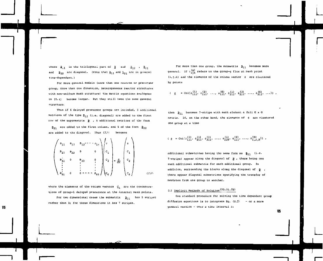
where B is the tridiagonal part of B and §.,and §22 a r e diagonal. (Note that E]^ and g 2 1 are in general

time-dependent.)

For more general models (more than one neutron or precursor

group, more than one dimension, heterogeneous reactor structures

with non-uniform mesh structure) the matrix equations analogous

to (2.4) become larger. But they still have the same general

structure.

Thus if 6 delayed precursor groups are included, 5 additional

matrices of the type § 1 2 (i.e. diagonal) are added to the first

row of the supermatrix B , 5 additional matrices of the form

B 2 1 are added to the first column, and 5 of the form E22

are added to the diagonal. Thus (2.71 becomes

"21

D12

"22

D61

33

0'66

_ d

- ar

where the elements of the column vectors C^ are the concentra-

tions of group-i delayed precursors at the internal mesh points.

For two dimensional cases the submatrix g ^ n a s ^ stripes

rather than 3; for three dimensions it has 7 stripes.

For more than one group, the submatrix B ^ becomes more

general. If $<?£. refers to the group-g flux at mesh point1J K

(i,3,k) and the elements of the column vector ij> are clustered

by points

4*211'

(2) •si.

then Bj, becomes 7-stripe with each element a full G x G

matrix. If, on the other hand, the elements of ij are clustered

one group at a time

* 2 1 1 ' V 3 1 1 ' •••'?IJK'

s'2'I,J,KJ

additional submatrices having the same form as B ^ (i.e.

7-stripe) appear along the diagonal of B , there being one

such additional submatrix for each additional group. In

addition, surrounding the blocks along the diagonal of B ,

there appear diagonal submatrices specifying the transfer of

neutrons from one group to another.

(i) Implicit Methods of Solution(20<?1'22>

One standard procedure for solving the time dependent group

diffusion equations is to integrate Eq. (2.11 - or a more

general version - over a time interval A:

105

J

(n)dT

and

B22,{n)

(2.10)

(2.T) -1

where g and g^ are diagonal matrices of numbers between 0 and 1.

All the elements of g are the same and all the elements of gd

are the same but not necessarily equal to those of g . The aim

is to choose the S's so that the integral in (2.1) is closely

approximated by some average of the values of the integrand at

the beginning and end of the time step.

To solve (2.9) , it is convenient to eliminate c'n+1>

To do so, we write out (2.3) as

(-.(n+1) .-

(n)

and

,(n+l)

(2.11)

,(n) If now we use the second of Eq. (2.11) to eliminate

f r o m t h e f i r s t eqUation, we obtain

106

L J L

(n+1)ap -

(n>

(n+l) n |-1 s(n)

(2.12)

where §}n' is a column vector involving only £*n' and c'

and all terms in the inverse are diagonal except Bl:L

-1

(n+1)

Thus the inverse

(n+l)fl 1-1

is no more difficult to take than

More important than that is the fact it is

only half the size of [j-AB§] . the matrix we would encounter

if we tried to solve (2.9) directly for (^-(n+l)) . Finally,

if 6 delayed precursor groups are considered (Eq. 2,8 1 an

equation of the form (2.12) can again be derived, the third

term in the inverse being replaced by a sum over 6 diagonal

matrices so that, again, taking the inverse

complicated than taking the inverse I - A B ^ > n + Spl

Finding £* n + 1' thus reduces to the problem of finding

the inverse of a 3, 5 or 7-stripe matrix depending on whether

the problem is in one, two or three dimensions.

This is a problem we have already discussed for the static

finite difference equations. (See Eqs. 1.45 - 1.55.) For

the one dimensional case the forward elimination-backward sub-

stitution method is used (generally with £'n' so arranged that

g 1 1( is a tridiagonal matrix each element being 6 x G ) .

For two and three dimensions E n is split into a lower and

upper triangular part and an iterative procedure is used (generally

one group at a time).

ii) Alternating Direction Methods t23' 2 4 )

Whether done directly (possible with 3-stripe matrices) or

iteratively (5 or 7-stripe matrices) the solutions (2.12)

we have been discussing yield if t n + 1 ) = M - 1 S ( n ) ; that is,

the inverse of the full matrix M is in effect found. There

is an alternate class of solution methods for Eq. (2.6)

called alternating direction methods that permit a solution of

(2i>) to be found for two and three dimensions by a non-

iterative method.

As developed, these deal with the spacially differenced

diffusion equations in the form (2.6) (rather than (2.7) ).

Further, it is assumed that g has some constant, average

value during two successive time steps. With these assumptions

the essential step in an alternating direction method is to

split the matrix § into a sum B^ + B 2 such that, while

I-| is not directly invertable, I~§i an<* I~§2 a r e-

Specifically we time-difference Eq. (2.6) as

E,,,(n)

Bl

so that

,.(n+2) ] [l-A§2] ~l [l+flEj ,.(n)

(2.14)

107

J

It might appear that reversing the order of the operations

.In the second of Eqs. (2.13) is a needless complexity. However,

this is not the case. Unless the reversal is carried out the

method is numerically unstable- It should also be noted that the

splitting in the second equation (2.13) need not be in the same

as in the first. We shall not, however, discuss this in greater

generality. In face we shall restrict further discussion to the

one-group case (Eq. (2.8) ) in two dimensions.

We consider three ways of splitting § so that the

inverses indicated in (2.14) can be found readily.

(1) Alternating Direction Implicit

Here we let §^ be 1/2 the diagonal of B , plus all the

submatrices §j. j > i in the upper triangular portion of §

plus that portion of the off-diagrnal parts of B.- associated

with diffusion in one of the two directions. The remainder of

B then consists of 1/2 the diagonal, plus all the S, -, i '" 1- ~ij

below the diagonal, plus the off-diagonal part of g ^ associated

with diffusion in the second of tne two directions. With this

splitting, taking the inverse of both I-AB.^ and I-i!2 is like

solving a sequence of one-dimensional problems in which g ^ is

3-stripe. We have already seen that this can be done by tho

forward-elimination-backward-substitution method. Thus finding

£ by (2.14) is a direct, non-iterative procedure.

(2) Alternating Direction Explicit

In this approach we take B^ to be 1/2 the diagonal part

of B and all the rest of B lying above the diagonal. Hence

8^ is 1/2 of the diagonal and all the lower triangular part

of g - Then operation of the inverse f I-rAg.,1 o n

i+ig, v. in Eq. >2. 14) can be found by a straightforward

extension of '1.52). The operation of [i- fijj on

fl+AB.,1 f I-i'.B.|| f I+AB, 1 i|'n' is found by an extension ofI- J L~ -*J L- -ij —

(2.1.53). Nott: that trie first inverse is taken starting with

the first clement of the column vector fl+ABj] i^'n) and the

second witn the last element of fl+AE^l [j^Agj] [j+Agj] V. •

(3) Tne Checkerboard Scheme

In botii the splitting schemes just described there is a

certain lack of symmetry in the way the flux precursor values

are advanced in time. In the implicit method new values at mesh

points on a given line are found using older values on adjacent

lines. In the explicit method the new value at a point is found

using two neighboring values just found during the present mesh

sweep and two others found on a previous sweep of the mesh in

the opposite direction.

An alternate splitting *-hat appears to be more symmetric is

one that advances in time all the x-points n: Figure (7)

X

o

X

o

X

o

X

o

X

o

X

o

X

o

X

o

o

X

o

X

O X O X O X O

Fig. 7: The Checkerboard Splitting

or ail tne o-points as a block. To develop such a splitting we

define a block diagonal matrix Jx , each block being a diagonal

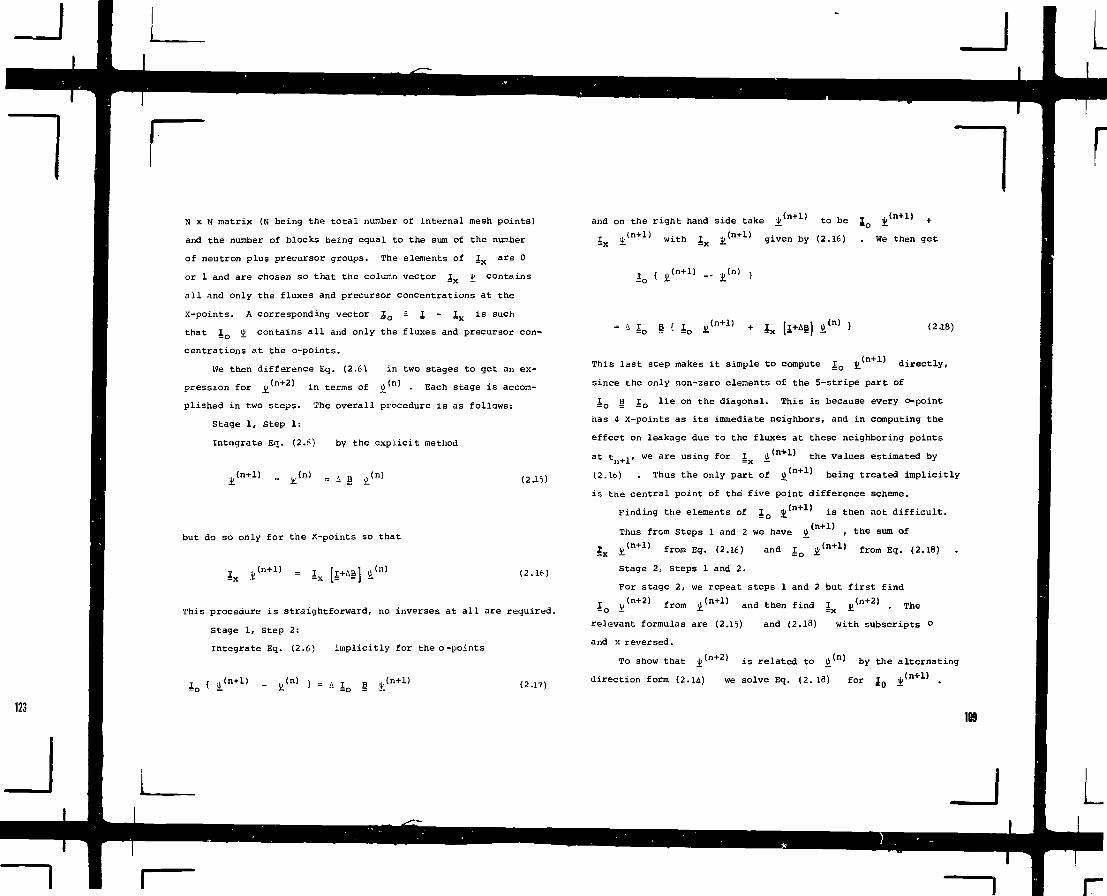
~\\rN x N matrix (N being the total number of internal mesh points)

and the number of blocks being equal to the sum of the number

of neutron plus precursor groups. The elements of Jx are 0

or 1 and are chosen so that the column vector Jx J contains

all and only the fluxes and precursor concentrations at the

X-points. A corresponding vector I o i I - I x is such

that I ^ contains all and only the fluxes and precursor con-

centrations at the o-points.

We then difference Eq. (2.6\ in two stages to get an ex-

pression for jj)'rl+ ' in terms of jjj'n' . Each stage is accom-

plished in two steps. The overall procedure is as follows:

Stage 1, Step 1:

Integrate Eq. (2.6) by the explicit method

(2.15)

but do so only for the X-points so that

(2.16)

This procedure is straightforward, no inverses at all are required.

Stage 1, Step 2:

Integrate Eq. (2.6) implicitly for the o-points

SL 1 • (2.17)

and on the right hand side take ij> tn+1) to be I £(n+1)

with given by (2.16) We then get

< Jo,,(n+l)

This last step makes i t simple to compute j o

(2J8)

directly.

since the only non-zero elements of the 5-stripe part of

lo | Jo lie on the diagonal. This is because every o-point

has 4 x-points as its immediate neighbors, and in computing the

effect on leakage due to the fluxes at these neighboring points

at t + w we are using for J j^'n+l' the values estimated by

(2.1b) . Thus the only part of ^'n+1' being treated implicitly

is the central point of the five point difference scheme.

Finding the elements of I Q j ' n + 1 ' is then not difficult.

Thus from Steps 1 and 2 we have * • t h e s u r a o f

Ix * < n + 1 ) fr<™ Eq. (2.16) and j Q i(,<n+1> from Eq. (2.18) .

Stage 2, Steps 1 and 2.

For stage 2, we repeat steps 1 and 2 but first find

io ^ < n + 2 > f r o m i < n + 1 ) a n d t h e n f i n d ix 4 < n + 2 ) • The

relevant formulas are (2.15) and (2.18) with subscripts °

and x reversed.

To show that i(i(n+2' is related to *'"' by the alternating

direction form (2.14) we solve Eq. (2. 18) for I- jj/'n+1' .

1B9

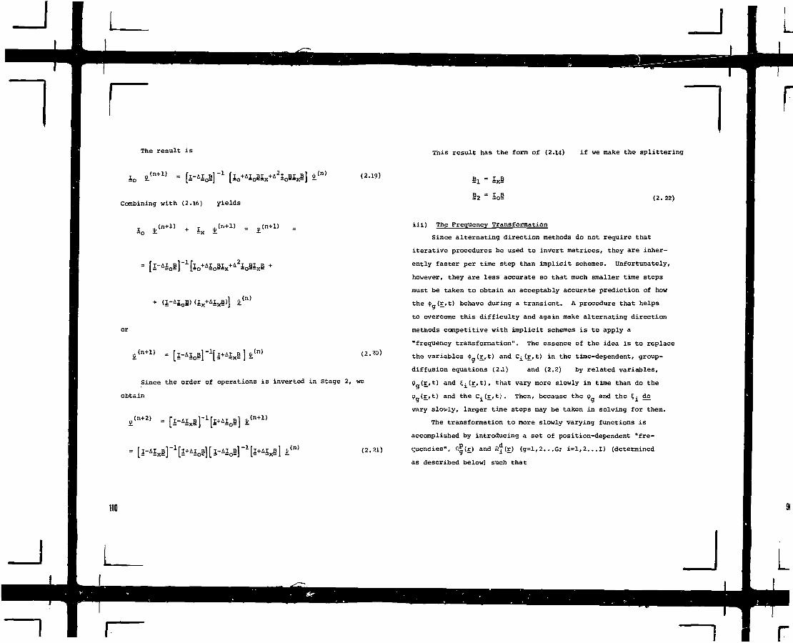
The result is

Combining with (2.16) yields

,(n) (2.19)

+ (I-aioB) (I^Ixg,(n)

,,(n) (2.20)

Since the order of operations is inverted in Stage 2, we

obtain

,,(n+l)

,,(n) (2.21)

This result has the form of (2.14) if we make the splittering

fii " 1x8

(2.22)

iii) The Frequency Transformation

Since alternating direction methods do not require that

iterative procedures be used to invert matrices, they are inher-

ently faster per time step than implicit schemes. Unfortunately,

however, they are less accurate so that much smaller time steps

must be taken to obtain an acceptably accurate prediction of how

the <?q(r,t) behave during a transient. A procedure that helps

to overcome this difficulty and again make alternating direction

methods competitive with implicit schemes is to apply a

"frequency transformation". The essence of the idea is to replace

the variables *g(r,t) and Ci{r,t) in the time-dependent, group-

diffusion equations (2.1) and (2.2) by related variables,

(i (r,tl and (^(r, t), that vary more slowly in time than do the

0 (r, t) and the Ci(r,t; . Then, because the <l> and the Kj_ do

vary slowly, larger time steps may be taken in solving for them.

The transformation to more slowly varying functions is

accomplished by introducing a set of position-dependent "fre-

quencies", P.P(r) and 2^(r) (g=l,2...G; i=l,2...I) (determined

as described below) such that

no

I J

*g(r,t) = e

CJ(£, t) = e ^i'E't'

Introducing this transformation into (2.1) and (22)

yields

(2.23)

* (r.t) ,t) .

t[v-Dg(r.t)V#g(r.t)

Ct) . n^(r,t)t*g(r,t)J e

g

r^t)] *g,(r,t)eng,(r,t)t•g' vi.'

-nP(r,t)t aft

Equations (2.24) have the same form as Eq. (2.1) and

((2.2) . However, if the frequencies flg(r) and £2i(r) are

properly chosen, j)(r,t) and the £^(r,t) will vary in time

much more slowly than <j>.(r,t) and the C^r.t). ";hus much

larger time steps can be used when solving (2.24) in finite

difference form.

The selection of the proper frequencies is still somewhat

of an art. Except for the trivial case of the reactor on an

asymptotic period the <|> (r_,t) will not exhibit a simple expon-

pntial rise, even if the single exponent is allowed to be group

and position dependent. Thus, in the general case, there is

no set of frequencies such that, even during a small time step,

the ipg and ^ in Eq. (2.23) will be completely independent of

time. All that we can hope for is that the transformation

(2.3.23) removes most of the time dependence from the $_ and C* •

Thus, since the frequencies are somewhat empirical, "best-fit"

numbers, current practice is to assume that the time behavior

during time step n will be fairly similar to that of time step

(n-1) and to determine the fl's for the interval t n

the known values, $ (r_,tn-1), • (r,tn), ci(£'fcn_i)

CJ(r,t ) according to the relations

from

e lein*J. (r,t)t

; i = 1, 2 ... I (2.24)

111

J

(2.25)

When Eq. (2.24) are differenced spatially, the r-dependence

of the frequencies reduces to there being a different set of

frequencies for each mesh point. In practice it is found that,

at a given mesh point, it is sufficient to use a single frequency

for all energy groups (£!^(r,Atn) = !2p(r,Atn); g=l,2...G). Even

with this simplification computing the frequencies is a bit

•jxpensive. Moreover, for some transients (for example starting

or ceasing to mo"e a control rod) the past history provides a

poor prediction of the future. When this happens, the frequencies,

as predicted by Eq. (2.25) , are not optimum, and shorter time

steps or iterative procedures have to be employed.

c) Alternative Methods for Solving Time DependentGroup Diffusion Equations

The finite difference approach to solving the time dependent

qroup diffusion equations is quite practical for one dimensional

geometries ar.d can provide numerical standards against which to

validate mere approximate two and three dimensional solution

methods by applying them b small test problems. However,

if more than about 20000 spatial mesh points are required for

reasons of accuracy or i.i order to represent geometrical

detail, the finite difference approach becomes extremely expen-

sive. Thus morr^ efficient methods must be usad for an accurate

analysis of large LWR's.

Fortunately all the advanced methods discussed in connection

with the static equations can be extended to the time-dependent

case. For the response matrix technique it is necessary to

define time dependent response matrices ' s' and this becomes

complicated when feedback effects must be accounted for .

The extension of the synthesis scheme is more straightforward:

the mixing functions Thg(z) of (1.57) simply become time-

dependent

k=l(2.%)

The resulting equations can be solved as if they were one-

dimensional, time dependent finite difference equations. O:io

serious potential problem arises; with the time dependent syn-

chesis method. The expansion functions ii*] (x,y) must be able

to represent any tilting effects occurring during the course

of the transient. Use of multichannel synthesis methods may

be very helptul for such situations since if flux tilting in

the redial plane occurs, they will provide it automatically

even if such til4-ing has not been anticipated.

112

J

Extension of the finite element and nodal methods to time

dependent situations is also straightforward ' '

Of the two, the nodal schemes se<...i to be much faster. In fact

the nodal method appears today to be the most efficient pro-

cedure for solving the time-dependent group diffusion equations.

2.2 The Point Kinetics Method

For many reactor transients the shape of the neutron flux

(as opposed to its magnitude) changes only slightly. For such

transients the "point kinetics equations" provide an accurate

and extremely simple method by which to predict the detailed

space ami—time behavior of the neutron pof-lation. To those

familiar with elementary derivations o£ the point kinetics

equations this staterent may be surprising. Nevertheless, the

statement is true. For many situations the point kinetics

equations can provide an excellent solution of the time-dependent

group diffusion equations (2.1, 2,2) . They are in no way

limited to a "point" or to a one-speed or one-group reactor

model. In fact a formal manner, the point equations can be

obtained from the time dependent Boltzmann transport equation

without making any approximations at all.

a) Derivation of the Point Kinetics Equations

Because the algebraic manipulations are a bit simpler to

follow we shall derive the point kinetics equations starting

from the continuous space-time-energy diffusion equations.

These may be written

3at v W •<E'E't>] Xp{E)(l-6

3)/°«3:f(r,E',t) *(r,E',t)dE-

+ E xi(E)Xici(r,t) + 7-D(r,E)7*(r_,E,t) - Zt(r,E, t) $ (r,E,t)

J™ £p(r,E' •* E,t) *(£,E'

3c. (r,t)Z &l Jo vlf

2r,E',t)*(r,E\t)dE' - Xj

i = 1, 2...I (2.27)

To reduce the algebraic complexity we introduce the net

absorption operator A and the fission neutron production operator

F3 defined by their operation on any function f(r,E,t) by

Af E Zt(r,E,t)f (r,E,t) - /"z (r,E"-^E,t) f (r.E1 ,t)dE'

f(r,£\t) (2.28)

In terms of these operators and with all functional depen-

dence repressed (2.27) take on the form

113

J

k ft = 7"DVl(' - /reactor

dv /°dE W(r,E) S(r,E,t) (2.32)

3c.

ji, 2, ... i (2.29)

The quantity of first importance in neutron kinetics is

the instantaneous total neutron population in the reactor. We

define as the unknown function to be obtained from solving the

point kinetics equations a closely related quantity T(t):

T(t) E / dV J°° dE W(r,E)reactor ° ~

(2 30)

where W(r,E) is a time-independent weight function introduced

for reasons which will become clear shortly. (Note that if

W(r,E) = 1, T(t) i£ the total neutron population in the reactor

at time t.)

Having defined ar. "amplitude function" T(t) we next define

a (time dependent) "shape function" S(r_,E,t) by the relationship

S(r,E,t) T(t) = <j>(r,E,t) (2.31)

Substitution of the expression into (2.30) and division by

T(t) yields

Thus the definitions (2.30) and (2. 31.) imply a kind of

time-dependent normalization for S(r,E,t) such that the integral

in (2.32) is independent of time even though S(r,E,t) is not.

To obtain the point kinetics equations in a formal manner

we now substitute (2.31) into (2.29) , multiply the results

by W(r,E) (Wtr.EJXitE) for the precurser equations) and inte-

grate over all energy and over the entire volume or the reactor

(out to where i|p(r,E,t) can be set to zero). If (to get the

customary form) we add and subtract S'x^l^F-1? in the first

of Eq. (2. 29) and define the total fission spectrum for isotope

j as

XJ(E) = X (3), + Zi

j

we obtain

JdV/dEW T(t) - /dV/dEwf E x ^ A ^ S ] T(t)

JiXi[/dV/dEWXici(t)]

114

J L J100

A (t) =Jdv/dfiW i S

JdV/dEW Ej

(2.37)

[jdV/dEW X^Si^s] T(t) - Xi [/dV/dEW Xi c^Along with

[/dV/dEW X i

x< °< <t)l

t y J (2.34)

Jdv/dEW(r,E) Xi(

,/dV/dEW i S

(2.38)

we obtain, after some rearrangement, the point kinetics equations:

where the second equalities are valid since (2.32) shows that

JdV/dEW i S(r,E,t) is not a function of time.

If now we divide by /dv/dEW Z x ^ S and define

P(t) =

/dv/dEW [v-D7S-AS+Z X

JdV/dEW I ^

/dvfdEW E

JdV/dEW Z<• B ( t ) s

i=l

(2.35)

(2.36)

r=- T(t) - Ci(t); i = 1, 2, ...5 (2.39)

Since we have derived them only by making definitions

rather than approximations, the point kinetics equations are

formally as accurate as the space-dependent equations from

which they were derived. However, the "kinetics parameters"

p(t) (reactivity), Bi<t) (effective delayed neutron fraction

of the i precursor group) and A(t) (prompt neutron lifetime)

depend on the shape function S(r,E,t) and hence on $(r,E,t).

115

J

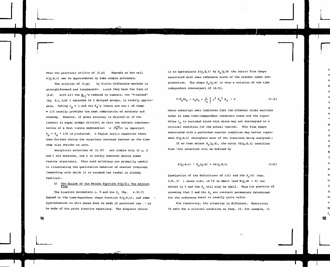
Thus the practical utility of (2.39) depends on how well

S(r,E,t) can be approximated by some simple procedure.

The solution of (2.39) by finite difference methods is

straightforward and inexpensivp. bince they have the form of

(2.8) with all the § — ' s reduced to numbers, the "8-method"

(Eq. 2.1, 2.22 ) extended to I delayed groups, is readily applic-

able. Taking 6 = 1 and the 8^'s {there are now I of them)

= 1/2 usually provides the best combination of accuracy and

economy. However, if great accuracy is desired or if the

reactor is super prompt critical so that the correct represen-

tation of a fast rising exponential ~e ( - )t is important

8 = 8 = 1/2 is preferred. A Taylor series expansion shows

that for that choice the equations converge fastest as the time

step size shrinks to zero.

Analytical solutions of (2..59) are simple only if p, 3

and A are constant, and p is rarely constant during power

reactor transients. Thus such solutions are primarily useful

in illustrating the qualitative behavior of reactor transient

(something with which it is assumed the reader is already

familiar).

b) The Choice of the Weight Function W(r.E); The AdjointFlux ""

The kinetics parameters p, A and the 6 (Eq. 2.35-7)

depend on the trme-dependent shape function S(r,E,t), and some

approximation to this shape must be made if practical use . -. to

be made of the point kinetics equations. The simplest choice

116

J

is to approximate S(r_,E,t) by SQ(r,E) the static flux shape

associated with some reference state of the reactor under con-

sideration. The shape SQ(r_, E) is

independent counterpart of (2.39).

= 0 (2.40)

where subscript zero indicates that the relevant cross sections

refer to some time-independent reference state and the eigen-

value XQ is included since this state may not correspond to a

critical condition for the actual reactor. (The flux shape

associated with a perturbed reactor condition may better repre-

sent S(r_,E,t) throughout most of the transient being analysed.)

If we then select SQ(£,E), the error SS(r,E,t) resulting

from *"his selection will be defined by

(2.41)

Examination of the definitions of Aft) and the S^(t) (eqs.

2.16,. 57 ) shows that, if «S is small (and W(r,E) > 0) the

errors in A and the B- will also be small. Thus tne practice of

assuming that A and the 8^ are constant parameters determined

for the reference state is usually quite valid.

For reactivity, the situation is different. Reactivity

is zero for a critical condition so that, if, for example, it

J

is changed by a perturbation in the cross sections specifying

the operator A(A » A + 6A) and if that same perturbation

changes the shape function S (So •«• SQ + 6S) , the resultant con-

tribution to the change in reactivity will come from the terms

-W(6A)SO - WAQ<5S in (2. 35) . If it is necessary to neglect

WA SS (6S being unknown) the resultant error could be of the

same magnitude as W(SA)S , the term being used v.o compute

P (t) .

It is to overcome this problem that we have introduced the

weight function W(r,E). It is possible to select it so that

all the first order error terms in (2. 35) involving SS vanish.

The procedure is a standard one in mathematical physics and con-

sists of selecting W(r,E) to be the solution <t>o*(£,E) of the

equation that is mathematically "adjoint" to the equation

(2.40) specifying the static reference state.

The equation adjoint to (2. 40) can be obtained by

reversing the E and E1 in the operators A and J X^F (Eq. 2.24)

j

Thus, we first define an operator

j

so that (2.40) becomes

V.n

j ? j (2..42)

We next define adjoint operators A£ and MJ by their operation

on any function f*(r,E)

A*f* 5 l t (r,E)f*(r,E) -o

(r,E - E1)f*(r.E'JdE1

lof* = P I xj(E')vE j(r,E)f*(r,E1)dE'

The equation mathematically adjoint to (2.43) is

(2.44)

(2. 4J)

(2.45)

The solution conditions imposed on <t>_(r_,E) are the same as those

imposed on <t>o(r,E), namely, <)>* and the normal component of

Do'*o a c r o s s internal interfaces i.-e to be continuous, and <(>*

is to be non-negative in the interior of the reactor and is to

vanish on the outer surface. For these conditions the eigen-

values \Q in (2. 45) and (2.43) can be shown to be the same.

To apply the adjoint equation to remove terms of order

SS in the expression for p we multiply (2. 45) by S(r,E,t)

and integrate over energy and reactor volume. Since the result

of the manipulation is still zero, we can subtract it from

(2. 35) (with W(r,E) taken as <t>J(r,E)) to obtain

117

J

p(t)Jdv/dE **(VDVS-AS+MS) - S (V*DOV**-A*(|>* + j

/dV /dE * o M S

Now by the chain law of differentiation we have

. (ij)*D7S)dV (VS)dV + /$* V-(DVS)dV

(2.46)

(2.47)

But, since (4>*DVS)is continuous across all internal inter-

faces, application of Gauss's Law to the divergence term yields

• 4i*DVS dV = i <**BVS) -NdS (2.48)

1 S(r,E.t) Ea (r,E * E')**(r,E')o

/"dE /°dE' •*(£,£) Zs (r.E1 * E) S(r,E",t)

and

/"dE /°dE' S(r,E,t) I'Xj (E1)vZ£

j (r.EJifJCr.

r,E') S(r,E',t)

(2.51)

(2.52)

where the surface integral in over the outer surface of the

reactor only. Since i(ij vanishes on the outer surface this

integral alsc vanishes and (2.47) yields

we have

/dV /dE -SA* 4* - JdV /dE •£ AnS

. (DVS)dV (2. 49) /dV /dE S M* ** • /dV /dE •* M S (2.5J)

Similarly, since SD*74>* is continuous across interval

interfaces Thus, without approximation (2.3.46) becomes

/S7-(DoVi)1*)dV = -

Finally, since

dV (2.50)

111

P(t) -/dV /dE [- - •• «A S + •• 6M

(2.54)

J

where

SD s D(r,E,t) - Do(r,E)

«A = Ztfr,B,t) - Zt (r,E) + /dE'fEjtr.E'+E.t)

6M s /dE1 I xjfv£#j(r,E'.t) - X vZt

j{r,E')]j L r ~ Ao *o '

(2.55)

sequence (after equilibrium has again been restored) of intro-

ducing the n neutrons will be an increase in the total steady

state neutron population of the critical reactor from N Q to

N Q + AN. The magnitude of AN will depend on where and with

what energy the neutrons were introduced (AN=AN(r,E)). It

turns out to be possible to show

zation

(3) that with proper nomali-

If now we approximate S by SQ, a perturbation SA contributes

a principle part *J4AS to p and require! neglecting only a

•econd order term •JSASS. Thus use of the adjoint flux as weight

function increases the accuracy of computations of p(t) made

using an approximation to S(r, E,t).

*o(r,E) = £ AN(r,E) (2.56)

c) Neutron ortance - Physical Significance of the

.(28)Kinetic* parameters

The adjoint function *;(r,E) has a physical interpretation1

which in turn leada to a precise physical interpretation of the

point kinetics parameters. This interpretation is given in

terms of a hypothetical experiment as follows:

Introduce a sample of n neutrons (n being large enough so

that statistical fluctuations may be ignored but small enough

so that no feedback effects occur) into the reference critical

reactor at sano point r. Let the neutrons in the sample all

have energy E and be travelling in directions that are isotropically

distributed. Since the reactor is critical, the ultimate con-

In words, the adjoint flux <t>£(£,E) in a critical reactor is

the asymptotic increase in the total neutron population of the

reactor due to the introduction at r of an average neutron out

of a sample all having energy E and an isotropic distribution

of directions of travel. Because of this interpretation

$*(r, is called the importance in the critical reference

reactor of a neutron at r_ having energy E.

With this interpretation of importance and with H(r,E)

in all definitions replaced by $o(r,E) the^physical significance

of the point kinetics parameters can be interpreted as follows:

T(t) (Eq. 2.39) is the total importance in the reference

reactor of all the neutrons present at time t in the perturbed

reactor.

C^t) (Eq. 2.?7) along with 2.3? is the importance in

the reference reactor of all the neutrons that would appear if

the Ci(r,t) decayed instantly at time t.

119

J

p(t) (Eq. 2.35) is the net rate of the production of

importance in the reference reactor assuming delayed neutrons

appear instantly divided by the rate at which importance is

produced in the reference reactor by the fission process at

tiine (t) - again assuming delayed neutrons appear instantly

(X - E<3- 2. 33 is the total spectrum). This interpretation

comes from multiplying numerator and denominator of (2. 35)

by T{t) and then replacing ST by <fi (r,E,t)' V'D<(>-AiJ+£x]F:'1t' dVdE

is then the net "instantaneous" production rate of neutrons

into dVdE and multiplication by W(r,E) = *o(r,E) followed by

integration over all r and E yields the rate at which these

neutrons would produce importanoe in the reference reactor.

6i{t) is the "instantaneous" rate at which the it h pre-

cursor group would produce importance in the reference reactor

divided by the corresponding instantaneous importance production

rate for all neutrons appearing from fission at time t.

A(t) (Eg. 2.37) is a characteristic lifetime of the

importance of all the neutrons present in the reactor at time t.

This interpretation is not as precise as the others except for

the reference reactor. For this critical case the creation

rate of importance must equal its decay rate and we have from

(2. 37).

/dV JdE** MQ*O . i/dV/dE $5 i (2. 57)

Thus the decay rate of importance equals the total importance

present divided by a time constant.

The more elementary notions of the kinetics parameters

can now be seen in relation to the precise interpretation just

given. Thus T(t) is usually thought of as total reactor power.

This is only an approximate interpretation unless W(£,E) is

taken as v(E)£f (r,E) (2..59) . The reactivity is often thought

of as the fractional change in the net numbers of neutrons

produced per generation. If W(r,E) = 1, this is an approximately

valid interpretation (although it is difficult to define a

"generation" for a reactor in a changing transient state).

Similarly the usual notion that the prompt neutron lifetime is

the average time that fission neutrons live once they appear

is more justified if W(r,E) = 1.

d) Computation and Measurement of Reactivity

The simplest choice for the shape function S(£,E,t) is

S0(r,E), the static flux shape in the reference reactor. When

this choice is made Eq. (2.54) becomes the "perturbation

formula for reactivity". This perturbation formula has the

extremely important property that the reactivity changes due to

different perturbations are additive. Thus if p, is the

reactivity change due to perturbing only A an amount 6A,f

P2 is that due to perturbing only M by SM,, and p3 is that

due to the perturbation (Sk^ + 6M2>. P3 will equal p 1 + p2

provided - and only provided - the same shape function So(r,E)

120

is used for all three perturbations. It is important to remember

that this additivity is lost if a time-dependent shape function

is used.

A more accurate choice of shape function is provided by

the "adiabatic approximation". Here the shape is the solution

of

M(t) (2.53)

where the diffusion coefficient D(t) and the operators A(t)

and M(t) are those appropriate to the reactor condition at time

t and At is adjusted to make the reactor artificially critical

at that time.

Substituting (2.58) into (2.35) gives

P>(t)/dV/dE W I - jt_ M + M I

/dV/dE W M Sx

(2.50)

since S^ does not account for the fact that the shape of the

delayed precursor population changes more slowly in time than

does the flux itself. A more accurate procedure is to compute

p(t) by the "quasi-static method" '29'. In this method values

of S(r,E,t) are recomputed periodically in such a way that both

the instantaneous reactor conditions and the instantaneous pre-

cursor concentration distributions are accounted for. The

essential assumption is that at a time, tn, when this recompu-

tation is made

*<r,E,tn)

(2.60)

This expansion for reactivity is often called the "static

reactivity" since it is most often used to compare the results

of a sequence of static calculations.

For dynamic problems p, is not very useful since it requires

that static solutions of (2.58) be obtained frequently and

The u^ and m are found from the point equation solution just

prior to time t. Then, if t n - 1, was the last time a space

dependent solution was obtained we assume that

(2.61)

121

J

Substitution of (2.60) and (2J51) into the first of Eq.

(2.29) then yields the inhomogeneous equation for $ at tn-

- V-DV<)> + A* -

The simplest way to infer reactivity experimentally is by

an "asymptotic period" measuremnet. As the name implies, one

introduces a step perturbation the reactivity worth of which

is to be measured and waits until the flux level is rising

everywhere as e u t. Then gf = i"T ; - g ^ = wC^ and (2.39) can

be manipulated to give

; <tj(2.64)

(2.62)

The second of Eq. (2. 29) together with (2.62)

an updating of thec^(r,t)

then permit

(2. 63.)

The quasi static method is really an approximate way of

solving (2 40) . If time steps are small and the shape functions

are updated every time step it converges to an exact solution.

Its great advantage for practical problems is that for many cases

the updating can be very infrequent.

Provided A and the S^ are known from a calculation, measurement

of u then leads to a value of p. Equation (2.64) is the

"inhour formula" for reactivity.

The inhour formula cannot be used to infer large negative

values of reactivity since then us is so close to the negative

of the smallest X^ that experimental error becomes very large.

For this situation a technique known as the "rod-drop" method

is sometimes useful.

In the rod-drop method one is interested in inferring the

decreasing reactivity when one or more control rods is inserted

into the reactor. If it is assumed that the counting rate D(t)

of a neutron detector is proportional to T(t) (D(t) = aT(t)),

the initial count rate for the critical reactor

= 0) is from (2.39)

122

S iD(0, = (2.65)

If the rods are then dropped into the core, there is a very

brief time during which the prompt neutrons readjust and T(t)

falls abruptly. However it quickly levels off to a new value

T(0+) and ji then becomes small in comparison with either

terra on the right hand side of the first of (2..39) . Moreover,

since the delayed precursors decay very little in the brief

time, (^(0+) is very little different from Ci(0). Thus we

have from (239) and (2. 65).

0 =i D(Q+)

(2.66)

Hence

p(0+) _ D(0) - D(0+)B D(0+) (2.67)

and if B is known p(0+) can be inferred from the counting rates

before and just after the rod-drop.

Experiments of this kind involving potentially large

changes in flux shape must be analysed with great caution.

Equation (2.67) is likely to be in serious error since we

have tacidly assumed in deriving it that 6/ A and a after

the drop are the same as before. However, that will only be

true in the unlikely event that reactor flux shapes are un-

changed. Thus careful theoretical corrections must be made

to analyse the rod drop experiment correctly. For the same

reasons one should not expect the reactivity inferred to equal

(1-f).*t

?.3 Feedback Effects

So far no explicit indication has been given of how the

time dependence of the group parameters and the reactivity

is to be determined. In so far as changes are externally

imposed (as with variations in control rod positions or soluble

poison concentration) accounting for alterations in the group

parameters is straightforward. Appropriate cross sections with

and without control rods present or for various concentrations

of soluble poison are generated, and the values to be used when

the rod is partly inserted in a node or mesh cube or when some

intermediate poison concentration is present are determined by

interpolation.

If the parameters vary because of local temperature or

density changes, the problem becomes non-linear since changes

in the local flux levels are in turn what induce the local

123

J

temperature and density variations. As with the non-linear

fuel depletion situation this problem is today attached by

running nuclear and thermal-hydraulic computations in tandom

{although several nuclear time steps may be taken per thermal

hydraulic time step). Thus it is necessary to augment the

group diffusion equations or point kinetics equations with a

model of thermal-hydraulic behavior in the core.

Generally the nuclear and thermal-hydraulic model interact

at only two points. The nuclear model accepts nodal average

temperature and densities at the beginning of a time step,

assumes these quantities remain constant during the time step

and supplies the thermal-hydraulic model with nodal averaged

powers at the end of the time step (or of several time steps).

In complementary fashion, the thermal-hydraulic model accepts

the average nodal powers, assumes they stay constant during a

time step and supplies the nuclear model with up-dated tempera-

tures and densities at the end of the time step. There are

some indications that a tighter coupling between the two models

might lead to a more efficient overall calculation, but the

matter is unresolved at present.

In any event the nuclear model receives nodal fuel tempera-

tures, coolant temperatures and coolant densities, a.id the

£?-fect of these on group parameters or on reactivity must be

taken into account.

For the full space dependent calculations changes in the

group parameters enter the calculation directly and, as with

the depletion problem, a table look-up method can be set-up

to circumvent the need to do frequent neutron spectrum compu-

tations. Depending on the sensitivity to changes in thermal-

hydraulic properties, the tables may be for macroscopic

parameters or for microscopic fitted cross sections (Eq. 1.94).

For some parameters it may be necessary to use two dimensional

tables. (The microscopic nodal-averaged fission cross section

for u in the resonance region may depend significantly both

on the fuel temperature and the coolant density.) Alternatively,

it may be possible to fit the group parameters to low order

polynomials in the thermal variables. Both the table look-up

and polynomial procedures thus involve complicated computer

programming and the running of many auxiliary computations prior

to performing any nuclear transient calculations.

With the point kinetic model it is possible to precompute

directly the dependence of reactivity on the thermal parameters.

To do this, we first assume that the perturbation formula for

reactivity is valid so that S(r,E,t) in (2. 54) may be replaced

by a constant shape SQ(£,E). Then we partition the total

reactivity change p(t) into contributions Pn(t) from each of

the N thermal-hydraulic nodes comprising the reactor. Thus we

define

Jv dV/dE [-pn(t) ,

SM SQ]

dV/dE 4>» M S Q

(2.6S)

n = 1, 2, ... N

124

where the volume integral in the numerator is over the n

node while that in the denominator is over the entire reactor.

(In practice the integral over energy would be a sum over energy

groups. We shall retain the simpler intergral notation.)

Since S (r, E) is being used as the shape function for all per-

turbations, the additivity property holds, and

P(t) = ] pn(t)n=l n

(2.69)

The nodal reactivities, pn, may be found by table look-up.

However, it is more common to define local temperature and3p 3p 3p

density coefficients — - I , —§• I , — - I , where

8°. dc and 8 are respectively coolant temperature, coolant

density and fuel temperature and subscripts n indicate an average

value for node n. Note that here the temperature coefficient of

the coolant is at constant coolant density whereas that of the

fuel is at constant pressure. Theoretical expressions for these

coefficients may be obtained directly from (2. 6S), For example.

(2.70)/dv/dE ** H SQ

where, for example, ^"—I is the change in the operator A for38= d=

node-n from i ts value for the reference core due to a unit

change (at constant coolant density) in coolant temperature

of node-n from that of the reference core. The local temperature

and density coefficients themselves may depend on the thermal

conditions and thus may have to be put in tables.

From the foregoing it follows that if nodal temperatures

and densities differ from those of the reference core at time t

by amounts A8°(t), A9*(t) and Ad°(tj, the reactivity at time

t can be determr ~ d as

P(t) =.=1 36= d= 6n P

3pn

3dc(2.71)

If the A8's and Ad are the same for all nodes or if we use

an average value (a questionable procedure) temperature and

density coefficients for the whole core (Z——| = —\ , etc.)n ° dc C c

\38C dc

can be used and (2.27) reduces to

£P_j38= d= 38r P

+i^.| Adc(t)3dc 8 C

(2.72)

Further, if there is no boiling and 8°, dc and P are

related by an equation of state, we can define' a coolant

temperature coefficient at constant pressure

3p | .. 3£_, 3£_, 3dci3 8 C P " 36c'dc 9 d c 8 0 36C P

(2.73)

125

J

It is this quantity that is usually referred to as "the

temperature coefficient of the coolant".

Finally, if c f= A9 we can define a "reactor temperature

coefficient"

P(t)

such that

A6(t) (2.74)

126

Thus there are many approximate ways of determining reactivity

changes due to changes in thermal conditions. In practice

Eq. (2.72) seems to be used most frequently. This is surprising

since use of (2.71) involves very little more computing effort

and the result is more accurate.

REFERENCES

1. Richard S. Varga, Matrix Iterative Analysis, Prentic=-HallEnglewood Cliffs, WTT. (1962) .

2. J.B. Yasinsky and S. Kaplan, "Synthesis of Three DimensionalFlux Shapes Using Discontinuous Sets of Trial Functions",Nuc. Sci. Eng. £5, 426 (1967).

3. A.F. Henry, Nuclear-Reactor Analysis (Cambridge, MA: MITPress), 1975.

4. w.M. Stacey, Jr., "Variational Methods in Nuclear ReactorPhysics", (New York, NY: Academic Press), 1974.

5. E.L. Wachspress, Variational Methods and Neutron Flux Synthesis,in Proceedings of Conference on Effective Use of Computersin the Nuclear Industry, CONF-690401 (1969) 271.

6. C.H. Adams and W.M. Stacey, Jr., Nuc. Sci. Eng. 5_4_, 20 (1974).

7. J.B. Yasinsky and S. Kaplan, "Synthesis of Three DimensionalFlux Shapes Using Discontinuous Sets of Trial Functions",Nuc. Sci. Eng. 2£, 426 (1967).

8. R.J. Pryor and W.E. Graves, "Response Matrix Method forTreating Reactor Calculations", p. VII-179, "MathematicalModels and Computational Techniques for Analysis of NuclearSystems". CONF 730414-P2, Ann Arbor, Mich. 1973.

9. Z. Weiss and S. Lindahl, "High Order Response Matrix Equationsin Two-Dimensional Geometry", NSE j>9, 168 (1975).

10. J.G. Kollas and A.F. Henry, "The Determination of HomogenizedGroup Diffusion Theory Parameters", Nuc. Sc:.. Eng. 60,464 (1976).

11. B.A. Worley and A.F. Henry, "Spatial Homogenization of DiffusionTheory Parameters", MIT Report MITNE-210 (September 1977).

12. A. Kavensky, "Neptune: A Modular Scheme for the Calculationof Light Water Reactors", Proc. Conf. on ComputationalMethods in Nuclear Engineering, CONF-750413, p. V-27,Charleston, S.C. (1975).

13. D.A. Botolho, "Multidimensional Finite Element Code",Ph.D. T.iesis, MIT Department of Nuclear Engineering (1976).

14. D.L. Delp, et al., "Flare, A Three Dimensional Foiling WaterReactor Simulation", GEAP-4598, General Electric Co. (1964).

15. L. Goldstein, F. Nakache and A. Varas, "Calculation of FuelCycle Burning and Power Distribution of Dresden-1 Reactorwith the Trilux Fuel Management Program", Trans. Amer. Nuc.Soc. 1^, 300 (1967).

16. S. Langenbuch, W. Maurer and W. Werner, "Simulation ofTransients with Space-Dependent Feedback by Coarse Mesh FluxExpansion Method", CSNI/NEACRP Specialists' Meeting on NewDevelopments in Three-Dimensional Neutron Kinetics and Reviewof Kinetics Benchmark Calculations, Garching (Munich),Jan. 22-24, 1975.

17. H. Finnemann and M.R. Wagner, "A New Computational Techniquefor the Solution of Multidimensional Neutron DiffusionProblems", presented at the International Meeting of Specialistson "Methods of Neutron Transport Theory in Reactor Calcula-tions" Bologna, Italy (Nov. 1975).

18. R.A. Shober, R.N. Sims, A.F. Henry, Nucl. Sci. Eng. 6_4_,(October 1977).

19. H. Finnemann and M.R. Wagner, "A New Computational Techniquefor the Solution of Multidimensional Neutron Diffusion Problems",International. Meetinf of Specialists on "Methods of NeutronTransport Theory in Reactor Calculations", Bologna, Italy,November 3-5, 1975.

L J

Xs

20.

21.

22.

23.

24.

A.V. Vota, N.J. Curies and A.F. Henry, WIGL-3 — A Programfor the Steady-State and Transient Solution of the One-Dimensional, Two-Group, Space-Time Diffusion EquationsAccounting for Temperature, Xenon and Control Feedback,Bettis Atomic Power Laboratory Report WAPD-TM-788 (1969).

J.B. Yasinsky, M. Natelson and L.A. Hageman, TWIGL — AProgram to Solve the Two-Dimensional, Two-Group, Space-TimeNeutron Diffusion Equations with Temperature Feedback,Bettis Atomic Power Laboratory Report WAPD-TH-743 (1968).

J.W. Stewart and M.R. Suckner, Trans. Amer. Nuc. Soc. 17,255 (1973). '

D.R. Ferguson and K.F. Hansen, "Solutions of the SpaceDependent Reactor Kinetics Equations in Three Dimensions",Nuc. Soi. Eng. 5_1, 189 (1973).

W. Werner, "Mathematical Methods Applicable to Space TimeKinetics", Proc. of Specialists Meeting on ReactivityEffects in Large Power Reactors, ispra, October 1970.

25. R.J. Pryor, "Recent Developments in the Response MatrixMethod", Proc. of Conf. on Advanced Rt .ctors: Physics,Design and Economics, Atlanta, Georgia, September 1974(p. 169).

26. C.U.D. deAlmeida and A.F. Henry, "Use of Response MatrixTechniaues in Nuclear Reactor Kinetics", MIT ReportMITNE-177 (October 1975).

27. Michael Todosow, "The Application of Finite Element Methodsto Reactor Kinetics Problems", MIT Doctoral Thesis,Department of Nuclear Engineering (1977).

28. L.N. Ussachoff, "Equations for Importance of Neutrons,Reactor Kinetics and Perturbation Theory", Proc. InternationalConference on the Peaceful Uses of Atomic Energy, Vol. 5,pp. 503-570 (19^5).

29. K.O. Ott and D.I. Meneley, "Accuracy of the QuasistaticTreatment of SF?tLal Reactor Kinetics", NSE: 36, 402-411(1969).

141127

_ J J

0) (M -H BA <D O4J T) 0.

r

L

THE PHYSICS OF IRRADIATED NUCLEAR FUEL

M. ROBINDepartement des reacteurs a eau,Commissariat a l'energie atomique,Centre d'etudes rmcleaires de Cadarache,Saint-Paul-les-Durance,France

ABSTRACTThe knowledge of the neutron irradiation effect is essential

in dealing with all subjects related to the fuel. Neutron irradiation provokes

fission reactions within the fuel and produces new nuclides. The formation

chains are described and the importance of each isotope in the fuel cycle is

explained with regards to its own characteristics. To solve the system of

equations giving the evolution of different nuclides concentrations, the cor-

responding effective cross-sections and flux received are ;;iven by standard

codes used for reactor calculations. A good test for calculation methods is

the experimental study of irradiated fuel. Many techniques have been developed

for this purpose. The last chapter compares fuel evolution in different reac-

tors, in connection with some specific characteristics.

1 - INTRODUCTION -

The development of nuclear energy implies a sound understanding of fuel

behaviour throughout its cycle from manufacture to reprocessing. New safer and more

economic working conditions are constantly sought.

A study of the fuel inevitably involves a great number of scientific fields

because of the multiplicity and complexity of the phenomena encountered. This course

will deal only with the neutronics i.e. with the study of the influence of the neutron

flux on the fuel composition and the energy liberation. A knowledge of the characte-

ristics, once determined is essential in dealing with subjects related to the fuel

such as : fissile material balance, metalwork, reprocessing, etc...

The neutronics engineer therefore is no longer limited to questions

concerning the isotopic comrosition of the reactor neutron balance. He is rather

faced, more and more often, with problems concerning the different stages of the

fuel cycle : fabrication, irradiation, handling, storage. In order to reply to these

questions, he must furthermore be able to draw on information provided directly or

indirectly by standard reactor calculations.

Neutron irradiation provokes fission reactions within the fuel giving rise

to the liberation if energy and fission products as well as capture reactions which

in turn produce new heavy nuclides. Firstly the formation chains shall be described

and the ijnportance of each isotope in the fuel cycle shall be explained with regards

to its own characteristics.

In order to solve the system of equations giving the evolution of the heavy

nuclide and fission product concentrations, it is necessary to know the correspon-

ding effective cross-sections and the flux received. Numerous standard calculation

codes are used. They may be divided into two categories depending on whether they

deal with a very localized : o n e o r w i t n t n e u-nole reactor.

A good test for the calculation methods used is the experimental study

of fuel unloaded from a reactor. For this purpose a certain number of techniques

have been developed which are remarkable for their ease of operation or their

precision.

Each reactor system is characterized by one or several particular types

of fuel element. The geoinetry, initial composition and the nature of the associated

moderator explain the specific characteristics of the evolution of heavy nuclei

concentrations in each system.

These characteristics along with the mode of unloading adopted define the

level of fuel usage on its withdrawal from the reactor. The respected value which

must be in keeping with the limit to technological performance is one of the essential

factors governing the co?t of the energy produced. This justifies the study of the

optimisation of the fuel cycle, before, duiir.g and after irradiation, for each parti-

cular case.

The principal aim of these conferences is to promote an understanding of

the fundamental phenomena which are linked to fuel evolution, and which have varied

implications in all operations undertaken on the fuel, from its fabrication to its

reprocessing. The techniques used lo determine irradiated fuel characteristics may

then be chosen with regard to the means available.

129

L J

A bibliography follows these lectures. We can distinguish four kinds

of references. Reference IM is a book, recently published in FRANCE, that gives

fundamental basis in neutronics and reactor physics. Each country with a nuclear

teaching Center disposes of so a book. The references HI to /7/ concern recent

data compilations that can be recommanded. The calculation and measurement techniques

described in these lectures are very widely used in the world and ever)' Laboratory

has published many publications about practical applications. The references /8/ to

111 I covers a large field of applications, concerning generally French Laboratories.

The last references concern the lectures given during this Winter Course which are

devoted to the description of reactor systems /28/ to /32/ and evolution codes

/33/ /34/ /35/.

In spite of the difficulties involved, the two isotopes of uranium may be

separated by one of several processes : gazcous diffusion, centrifugation, etc...

Uranium enriched in TJ may thus be obtained and opens the pathway to more varied

types of reactor than those using only natural uranium.

Thorium is composed of one single isotope T h , which as for U is not

very fissile. It leads, however, to the formation of a fissile nuclide, 2 3 3U, with

properties comparable to those of U and 239Pu. For this reason, thorium in a

reactor will always be accompanied by a fissile nuclide 2 j 3U, 2 3 5U or possibly239Pu in order to start off the 2 3 3U formation cycle.

2,2 - Evolution chains

2 - GENERAL LAWS GOVERNING FUEL EVOLUTION -

2.1 - The_natural_clements i.yrsiniuTn.cjGd tirarium

Uranium and thorium are the two naturally occurring elements which are

'.he origin of all fission reactions taking place in reactors.

Uranium is the source material which is most frequently used. In its natu-

ral state it is composed of three isotopes U, ' U and U in the following234

proportions, expressed in numbers of atoms : 0.0055, 0.7254 and 100. The U is in

fact a descendant of the U with which it is in radioactive equilibrium. The

abundance ratio is inversly proportional to the radioactive half-lives. The ura-

nium's composition is the same in all deposits which did not undergo chain reactions

in earlier geological periods such as in OKLO in Gabon. Taking into consideration the

radioactive half-lives of U and U,the isotopic abundance 2 billion years ago

attained 3.8 1 !.

Amongst the isotopes of uranium, 3'U proves to be very fissile when placed

in a flux of thermal neutrons. The fission and capture cross-sections for neutrons

of 2200 n/sec are 580 and 92 barns respectively. In spite of its small abundance in

natural uranium, this allows a chain reaction to be maintained in graphite or heavy-

water moderated reactors.

U is a "fertile" nuclide which is fissile only when subjected to high

energy neutron bombardement. It does however produce a very fissile nuclide, pluto-

nium 239 which plays an important part in nuclear reactors.

All nuclides to be considered in the study of irradiated fuel are given

in figure 1. Each is characterised by its atomic number, Z and its atomic mass,M.

They are sometimes denoted by a suscvipt formed from the last figures of Z and M ;239

e.g. for Pu (Z=94, M=239), the atomic concentration is written N^g. In certain

cases, an isomeric state more stable than the fundamental ~tate may be considered

(e.g. 2 4 2 mAm).

In figure 1, the isotopes with a very short half life have been omitted

and are only to be considered in special cases characterised by very high neutron

flux. So the transmutation from U to Pu takes place in three steps :

. •»»". (">ifl iSJir / 9 " *'»»# / 3 ~ * M t >1/ '" *• 14. • • " ^ * Y P ' "'" "" ^ fit-

r=43.J--m Tx2.i5U238In the case of a PKR, the capture rate for U

at equilibrium thereforeS.S . IB.9

239,

Ak9flig 239

The rate of capture reactions for U is negligible. The quantity of

/Via

Pu contained in the fuel during destructive testing analysis is slightly greater

than that present in the functionning reactor since one then measures ( Np+ Pu).

However, very often only the J U fn,S) Pu reaction is considered. In the case

of the transformation Th (n,(S) '"ll, it is indispensable that the presence of

Pa, with a half-life of 27 days, be taken into account.

The passage from one nuclide to another takes place either by nuclear

reaction or by radioactive decay.

130

L

The most important phenomenon to be considered in a reactor is the fission.

The absorption of a neutron by the nucleus renders the latter very unstable provo-

king quasi-instantanoously its division into two nuclei of approximately equal

mass and the liberation of some energy. All neutrons which are absorbed by a nucleus

do not produce fission. There may only result the creation of a heavier isotope

of the same element : e.g. 2 3 5U (n,*) 2 3 6u.

It must be noted that neutron emission which is a phenomenon often ignored,

occurs spontaneously in nuclear fuel whether irradiated or not. The resulting neutron

flux is of a totally different order of magnitude to that present in a reactor.

However, if no precautions were taken, the neutrons could in certain cases produce

significant biological effects on the personnel in charge of the fabrication, trans-

port or reprocessing of the fuel.

The probability of an absorbed neutron producing fission varies conside-

rably from one nuclide to another and with the energy of the incident neutron* In

the thermal neutron flux the fissile nuclei are in practice limited to U, U,

Pu and Pu. It must be noted that certain isotopes which are not very abundant

such as mAm are very fissile. In the spectrum of fast neutrons all the heavy

nuclides are fissile. Due to the abundance of U in thermal reactors moderated

with graphite, heavy water or light water, the participation of this nuclide in

the fission reactions is far from negligible, 4 to 8 *..

Each nuclide may be characterized by a quantity, o equal to the number

of neutrons emitted par neutron absorbed

In certain cases, the absorption of high energy neutron^, is followed by

the emission of 2 neutrons, giving rise to isotope of smaller mass. These rare

reactions do not influence significantly the neutron balance but produce nuclei

such as 237Np (reaction -n, 2n- on 2 3 8U) or 236Pu (reaction-n, 2n- on 2 3 7Np).

All heavy nuclei considered in figure 1 are radioactive, which would

explain their absence in nature excepting those with very long half-lives : " lh,

U and U. The stable isotopes corresponding to radioactive chains used in a

reactor are Pb (Th chain) ,

C235U chain).

(Np chain), 206Pb (238U chain) and 2O7Pb

The radioactive disintegration of a heavy nuclide may be described by the

half-life (T 1/2) and by the disintegration probabilities of different processes :

oi, B , "if emissions, electronic conversion, spontaneous fission ... The majority

of the nuclides given in figure 1 disintegrate practically only bye*, emission. The

nuclei with whort half-lives, which have been omitted, are /} emitters. In reactor?7Z 1/11 '

fuel, two important p emitters are found2 3 3Pa and 2 4 1Pu.

The following characteristics of the nuclides are given in table I : the

equivalent half-lives of each type of disintegration, the average energy of the <*.

emission, and the number of neutrons produced by a spontaneous fission.

This neutron emission has two origins : spontaneous fissionsand (d, n)

reactions. The principal spontaneous fission emitters may be distinguished by their

even Z and M values, e.g. 244Cm, 242Cm, 2 4 2Pu, 2 4 OPu. The bombardment of light

atoms (M<40) by t>£ particles may sometimes result in neutron emission although the

probability is small. This probability however increases with « particle energy thus

favouring the production from heavy nuclides such as

strong neutron emission are : F, Be, B, Al, 0.

242,Cm. The light elements giving

Obviously the presence of oxygen of the fuel "oxide" gives rise to a spon-

taneous neutron emission which is particularly strong when irradiated (presence of242 244

Cm and Cm).In order to calculate the neutron emission of a mixture as for

example Pu 02, it is first necessary to calculate the probability of the<x emission

being stopped by the oxygen, then to use the effective cross-section which is charac-

teristic of the o< particle energy.

Returning to figure 1, the importance of the different nuclides shall be

examined as regards their incidence in the fuel cycle and with respect to ''.ifferent

criteria ;

- highly fissile nuclides in thermal reactors : 2 3 3U, 2 3 5U, 2 3 9Pu, 2 4 1Pu,242m,"Am.

242,- nuclides with important capture resonances : 2 J 2Th, 2 3 6U, 2 3 8U, 2 4 0Pu,

Pu.- very fertile nuclides in thermal reactors : T h , U.

- fissile nuclides in fast neutron reactors : all the isotopes of U and Pu,

but chiefly <33U, 2 3 5U, 2 3 9Pu, 241Pu.

- most important <* emitters :

a) fresh fuel : 2 3 8Pu, 2 3 9Pu, 24OPu

b) irradiated fuel : 242Cm, 244Cm

- most important Remitters encountered in the fabrication of fresh fuel :2O8T1 (from 2 3 6PU/ 2 3 2U, 241Am (from 2 4 V ) )

- most important spontaneous fissile nuclides :

a) fresh fuel : 238Pu, 24OPu, 242Pu

b) irradiated fuel : Cm,A

Cm 131

J

and241.

2.3 -

The level of neutron irradiation of a nuclear fuel is defined by a quantity

called the specific burn-up whose value corresponds to a quantity of liberated energy

and a composition fnr the fuel.

In neutronics terms, the specific burn-up is defined as the number of

fission reactions undergone in an initial sample of 100 heavy atoms. This quantity

is called FBW, fissions per initial Metal Atom, and is expressed in the form of a

percentage (in French, T.C.F. taux de combustion en fissions).

The FIFA (Fissions per Initial Fissile Atom) considers only 2 3 5U, 239Pu

'Pu.lt appears preferable to use the FIMA rather than the FIFA since o all238

ir. ents and purposes, all nuclides are fissile and particularly the U pres^ 't

in thermal reactors.

The FBI/V is a quantity which does not require the setting of delicate

hypotheses on energy liberation and may be directly deduced from the results of

analysis.

Unfortunately, this notation does not involve the notion of the energy

provided and thus it is often preferable to express the specific burn-up in mega-

watt days per ton, i.e., in energy released per mass unit of fuel..

This notation requires us to accurately define the considered quantity of

fuel and the energy liberated by one fission.

For the considered quantity of fuel, one may speak in terms of a metric

ton of metal, oxide or other material. In France the word "metal" is applied to

theimal reactors and "oxide" to fast reactors. Metal applies only to the uranium and

plutonium i.e. without associated metals : Mo, Al, Zr...

The energy produced during fission lias several origins :

- kinetic energ/ of fission products which are brought to a halt almost

instantaneously and thus locally liberate the greatest part of the fission energy

- disintegration energy (8 and #) of fission products ; the majority of

disintegration occurs very soon after fission and the rest, in some cases, after

very long periods.

- energy of neutrons which are slowed down in the moderator to an energy

level at which they may give rise to another reaction (capture ou fission).

132

- energy released by capture reactions of neutrons not giving rise to

fission reactions, in uranium or other materials.

- energy of anti-neutrinos.

1The fission energy varies from one fissile nuclide to the next.Table 2

drawn up from a recent compilation /6/ gives the energies released by each type

of the more important fissile atoms.

The energy per fission which must be taken into account to determine

the burn-up in megawatt days per ton varies with the problem studied, accordingly

we consider the total energy evacuated by the coolant, the local energy' released

(fuel temperature), ...

The kinetic energy of fission products and fi disintegration energy is

liberated very close to the point where fission takes place. The Eradiation is

stopped at a distance which varies with its energy. It may by noted that the Jf

energy originating from a fissior. reaction is only partially liberated in the fission

zone but this :one, because of its high density, stops radiations originating from

other fission points within the same fuel rod or from another one. A part of jfenergy

is also liberated in structural materials (cladding . . . ) . This point is very important

in respect to irradiation loops.

In order to encompass the energy of fission producing neutrons, some

codes use different fission energies for each neutron group.

With the knowledge of the FIMA and the fission energies E. expressed in Mev,

the specific burn-up in megawatt days per ton is easily calculated.

Given that :

1 Mev = 1.602 x 10"13 joules = t.602 x 10"1S x g^jj Mh' days

The average atomic mass and fission energy are :

« z: Mi Ni

N;(Fi = number of fissions in the

isotope i)

I -I L

I t therefore follows that :T . . » / , Tn, •. 1.6O2x1O"19 6.O23X1O23 FIW (',)I MWd/t metal = E(Mev) x —afiiUV1 x — z x ^86400

I MWd/t tnotal = 11168 x ^ X ) x FIMA ('.)MCg)

I MVd/t oxyde = - ~ x I MVd/t metal(M32)

Very roughly spealting, then it may be said that a FIMA of 1 i corresponds

to a specific burn-up of 10000 MlVd/t metal.

2.4 - Fission_Products

To eadi fission reaction there corresponds the formation of 2 (possibly 3)

light atoms. Fission is a very rapid phenomenon and produces a cascade of radioac-

tive nuclei with very short half-lives. In practice, the nuclides with longer half-

li\res, these may be considered as originating directly from the fission, the limit

depending on the phenomenon considered : after-power, emitters ...

The emission of fission neutrons and the fission phenomenon itself occur

quasi-sunultaneously, excepting of course, those originating from the disintegration

of longer half-life nuclei and which are the delayed neutrons.

The probability of a nucleus of mass, A, being produced during a fission

reaction is given by a graph of characteristic shape. In practice only those atoms

with masses between 72 and 170 as well as the very light atoms ( T) originating

from ternary fissions, are considered.

The figure 2 gives an example of the repartition of fission products

following their atomic mass for " U HI .Fora heavy isotope characterized by

its M and Z values, the theoretical fission yield can be determined for each

atomic mass of fission products.

Wherever possible, this theoretical approach is coupled with experimental

findings and the compiled results aro often presented in international gatherings

II, 3, 4/. In general, fission yields are given for three neutron energies : thermal

neutrons, fission neutrons and 14 Mev neutrons. Nowadays, in effort is being made

to clarify the dependance of fission yield on neutron energy in fast neutron reactors.

Fission products are of great importance in the fuel cycle and play an

important role in the following ways :

- Variation of reactivity with irradiation. In every case this occurs in the negative

sense since the fission products may only capture the neutrons. Some product;

have very large effective cross-sections (e.g. Xe and Sin for thermal neutrons).

The effect of the fission products on neutron balance shall be considered later.

- After-poi.-er which is the energy liberated within the fuel, after the chain

reaction has ceased. This energy, which originates from the disintegration

of radioactive fission products, is particularly large in the first moments

after the reactor shut-down, be it norma? or accidental.

- Migration within the fuel which has direct efrects on the metallurgical proper-

ties of the fuel element.

- Reprocessing where, due to their raJioactivity, they render all operations diffi-

cult and costly, and pose particular problems of dissolution, of trapping in

wastes, of elimination from uranium and plutonium or of storage.

- Fuel characterization, particularly in the measurement of specific bum-up using

stable isotopes (neodymium) or ti emitters.

3 - CALCULATION OF FUEL EVOLUTION' -

3.1 - Evolution eguations

The formation of the nuclides produced within the fuel have been examined

previously and outlined in figure 1. In order to determine the corresponding concen-

trations, a system of equations shall be developed for the evolution chains.

For each nuclide considered, the balance between the number of atoms

appearing and disappearing may be expressed following the paths shown in figure 1.

Generally, the variation, as a function of time, of the concentration of an isotope i

may be expressed as :

dNi

~avP-D = Production - Destruction

As discussed previously, the nuclear processes considered in this study

of fuel evolution are :

- nuclear reactions including capture, fission and (n,2n) characterised by reaction

rates A

- Radioactive decay (^,y3,... disintegrations) characterised by the disintegration

constant A f X = 0.693/Tj .,}.Tj .,

i33

L.

Whatever the energy of the incident neutron, the same isotope is always

formed . For a reaction (n,$ on an isotope i, the reaction rate is given by :

Ai (2)

In the standard calculation codes for reactors, different conventions

may be used to represent the neutron flux : total flux, flux equivalent for

2200 m/s neutrons, multigroup flux, ... The integrated flux, g, is also defined as

/o

At(3)

To each flux representation, there corresponds an effective cross-section

so that the correct reaction rate may be determined for the whole spectrum or for

a given energy group i

»T?. _ Ait

The subscripts j, k and 1 evoke all other possible ways whether by nuclear

JPuor radioactive disintegration of forming the isotope i. Therefore gives

Ai) ( » (*tiA) (HiCm) (tit A)

Instead of associating a specific equation to each nuclide one might have

developed a general equation englobing all possible processes. This method, although

academically attractive, has the inconvenience of including nuclides with very short

half-lives which thus make the mathematical solution of the system of equations ex-

tremely difficult. Moreover, a representation of the division into different isomeric

states would prove difficult.

Depending on the problem dealt with, the system of equations (6) may be

simplified by a reduction of the number of isotopes (and hence equations) and by

the elimination of certain secondary reactions (n,2n). In many cases, in fact, the

following system is sufficient for thermal reactors.

In many cases, the flux is not explicitly known, but it is deduced from

a particular rate e.g. the power generated per fission reaction

•Sj.Ni Ofi Ei

where P is the total power and E. the energy by fission of the nuclide i.

(5)

In the particular problems, any representation of the effective cross-

sections may be employed with the one condition, that there be coherence between the

units used for flux and for all the cross sections (capture, fission, n,2n).

The collection of nuclidcs considered in figure 1 gives rise to a system

of first order differential equations

tit = t * eThe effective cross-section^a is the sum of the effective capture, fission

and (n,2n) reaction cross-sections for the isotope i.

PRINCIPAL EVOLUTION EQUATION'S FOR TllliRMM REACTORS

. <P

(ore.

x If there is the formation of an isomeric nuclide the branching ratio can bedependent on the neutron energy.

134

r. cp

To the system of equations(6) giving the number of heavy nuclei, may be

added :

- one or several equations giving the number of fissions in the fuel or in each

isotope.

d§i = Oei,tfi . £i . Cfat °

- equations describing the fission products

(8)

- additional equations dealing with a particular problem e.g. structural material,

burnable poisons, etc...

In the latter examples quoted, each of the isotopes present must be

considered separately,taking into account initial abundance and the possibility

of a different flux (as in the case of fuel cladding). Mien one wishes to study

the radioactivity of cladding, the reactions due to fast neutrons of the type

(n,p), (n,2n) ... must be considered.

For nuclei with very long half-lives, the variations of flux with time

have no effect on the number of nuclei which depends only on the fluence . This

point is important since it allows a parametric representation of composition as a

function of integrated flux or specific burn-up.

The resolution of a system of equations is complex as the flux and the

effective cross sections vary in the course of the irradiation wilh the spectrum

shape, the self-shielding effect... The problem is simplified, if it is considered

that some of these values are constant during the evolution. Very often, either

the flux or the pcwer (cf equation 5) is constant.

In a particular case, where it is supposed that the flux and thf* effec-

tive sections are constant, the analytical expression of each of the concentrations

can be given, but the formula obtained becomes \rery long after the third or fourth

nuclide of the chain. In practice, numerical methods of integration are preferred.

They make possible to resolve step by step the system of equations. These methods

have become relatively simple with the introduction in the computer of subroutines

which treat the problem of systems of differential equations. The physicist's work

is then limited to adapting the system of equations to the specifications of a sub-

routine and to supply at each "step" the correct values of the flux and of the

cross sections obtained by othci means. The division in "steps" depends

on the accuracy required, the performances of the numerical method of integration

and, also, the cost of the use of the computer.

Th*1 problems regarding the calculation of the evolution of the fuel

can be presented in three ways :

- the laws of variation of the effective sections and of the flux are taken on

priori, for instance deduced from previous calculations made with cell codes

or reactor codes.

- The evolution of the fuel can be treated locally by the use of the cell codes.

- The fuel evolution is studied in a reactor in function of spatial heterogeneity.

The last two cases will be studied in the following chapters.

The first case is particularly encountered in studies where the interest

is not in the reactivity balance but in the fuel composition, for example :

- correspondance between the burn-up and the composition in fissile nuclides,

- correspondance between the fundamental characteristics of the fuel (burn-up,

fissile material content, ...) and the experimental results obtained by different

ways : JC spectrometry, mass spectrometry, ...

- studies about the after-power and the emission of spontaneous neutrons ore/,fi, £

rays.

For these composition determinations, a previous calculation supplies,

the variation laws of the different cross-sections in respect to the fuel bum-up.

Implicitly, these laws take into account the effect on the neutron spectrum im!u<.cti

135

L

by the changes of the fuel composition and the moderator boron content. Kith this

cross-section bank, the calculations can be repeated with a simple and economical

code to take into account the exact variations of the level of power, especially

when we study radioactive emitters and the secondary processes of evolution not

included in the initial code. The cross-section bank can be constitued by a table

or by polynomial formulas depending on one (burn-up) or more parameters (fuel

enrichment, temperature, . . . ) .

Some codes are devoted to fission products, especially for after power

studies. Just after the shut-down, it is necessary to consider a great number of

very short half-life nuclides. A code calculates the variation with the cooling

tine, for all the nuclides issued from one fission occuring in each type of fissile

nuclide, the concentration, and the depending quantities (heat, ft, %,i) emissions...)

The french code PEPIN now takes into account more tfian 700 kinds of nuclides /9/.

The result obtained from these calculations are integrated by another code in order

to sum up the "elementary fissions" that occur in the fissile nuclides present in

the fuel /W.

3.2 - Local_eyolution

During this course, many other papers have emphased the neutronic ijnpor-

tance of cell calculations. They make it possible to resolve the transport equation

by calculating very exactly the spectrum of energy of the neutrons . The environ-

ment of the cell is taken into account either directly in a "multicell" code or in

form of particular conditions imposed at the limits. The cell codes use a very fine

division in energy groups. The multigroup data set associated with the code, contains

the cross-sections (capture, fission, transfer) of nuclides initially in the cell

(fuel, moderator, poison, ...) together with those of the most important isotopes

appearing during irradiation. The problem of resonances is treated very elaborately

in function of their energy width, thus taking carefully into account the self-

shielu.ig.

A cell in evolution does not present any particular characteristic, except

the presence of many different sorts of nuclides in the fuel. The cell code will thus

contaLi a mixing of the calculation of flux in the cell and a resolution of the

evolution equations. One m y possibly use in certain phases of the calculation

of the neutron spectrum, results previously obtained, notably in regard to a treat-

ment of resonances, as the competition of the fuel varies little from one step of

evolution to the next.

136

To resolve the problem of evolution, a series of very fine "steps" might

be used, during which, it will be supposed that the neutron energy spectrum and

hence the cross-sections remain constant. It would be prohibitively expensive to

repeat the cell calculations too frequently.

InpracticQ integration steps of much greater siie can bo effected by

using a method of "predictor-corrector" by using the values of the concentrations

and of the cross-sections, at the beginning at the middle and at the end of the

step under consideration.

er(t) <r(t*4t) <r(fc«*0

N(t)

The number of cell calculations is thereby limited to two per integra-

tion step.

The distribution of the flux not being uniform; the distributionof the

nuclides created by fission is not uniform and theoretically a special evolution

calculation should be therefore made at each point.

In practice, except for a few special cases, the resolution is only made

once and a mean value is obtained on the whole of the evolving medium ; it would

often be illusory to proceed otherwise, for, on one hand, this method would not

be coherent with the manner of treating resonances (formation of Pu) and on

the other hand, the l^cal metallurgical state would have to be taken into account.

The spatial problem has not to be considered, except for certain systematic

phenomenon, and in the case of poisoned fuel for which several zones involving

separately have to be considered.

The evolution code of the cell has to take into account the reactivity

effect of the fission products which intervene in the percentage of the neutrons

captured, between 6 J for the reactors of the natural uranium systems to 15 i in

those of fast neutrons system. We shall consider later the problem of fission

products.

The results of calculation of cell evolution are frequently used to obtain

effective sections destined to be introduced in other codes, for example, in the

spatial calculations for reactors or studies on the fuel cycle.

J

~lBecause of the importance of cell calculations in neutronics, a big expe-

rimental effort has been made to improve both the methods of calculation (with and

without perturbation) and the data set /*3/ /44/ /{S/ /4b/.

3.3 - Glgbal_eyolution_gf_the_core

The calculation of the reactor in evolution appears to be very complex.

In fact, it is not, as in the case previously treated, a question of an infinite

lattice formed by the repetition of a group of cells. The environment of the core

Creflector, diverse structures), the local effects such as control rods, and each

cell with its own irradiation have to be considered in their actual state. Cells

identical at the outset but submitted to different flux have not the same compo-

sition after irradiation.

It is impossible to consider each point of a reactor with the same rigour

as that used in a cell calculation to determine the energy distribution of the

neutrons.

In the two cases there must be taken into account the other parameters

independent of the fuel bum-up. These are :

- the concentration in a soluble poison (boron) of the moderator which is fixed

by the operator of the reactor.

- the xenon concentration which depends almost essentially on the level of power.

The"macroscopic" representation is generally used in spatial calculations

where the discretisation is made at the scale of the fuel element (one or several

meshes per subassembly) ; it is well suited to codes using a method with "finite

elements" and for those with "finite differences" where the evolution is treated

"by homogeneous zones" and not "mesh by mesh".

For a given irradiation stage, cross-sections are obtained from parame-

trical laws, and then a classical reactor calculation is established. The criti-

cality is obtained either by moving control rods or by changing the boron content.

From a cell calculation, can be deduced for different steps of irradia-

tion, a set of cross-sections, microscopic or macroscopic, condensed on one oi

several energy gTOups. These sections, used with the corresponding neutron flux

must give the same rate of reactions as in the cell calculation. From these dis-

crete values, mathematical functions depending on a characteristic parameter of

irradiation can be adjusted : fuel burn-up, nuclide content ... Those functions

can possibly take into account the incidence of other parameters, such as :

temperature of the moderator , boron content, ... In practice, it is impossible

to find a representation which takes all the phenomena affecting neutronic condi-

tions into account ; for each type of cell, a parametrisation is made.

In the calculation of the whole reactor, treated by a method of "finite

elements" or of "finite differencies" those functions are used. This makes possi-

ble to multiply the number of space points to the detriment of division in energy,

while taking advantage of the rigorous treatment of the energy problem carried

out in a cell code. As the case may be, it is possibl" :

- either to use the parametric representation of microscopic cross-sections, to

carry out the resolution of evolution equations in each mesh and to deduce from

it, the macroscopic cross-sections to be used in the calculation code of the

reactor.

- or to use directly macroscopic cross-sections.

The flux at each point of the reactor is needed in order to obtain the

local power and the total power discharged from the reactor. This power permits

us the normalize the values of flux. These "three-dimensional results" are obtained :

- directly (the case is very improbable as this requires a considerable number of

meshes in the calculation !)

- by the superposition of a fine structure taking into account repetitive local

phenomena, and the macroscopic distribution calculated,

- by the combination of results obtained with a bidunensionnal code radially at

different levels, and axially.

The local flux and associated power are, of course, useful in evolution

calculations to define the increase of the irradiation rate during the time At

and to calculate the concentrations in nuclides of radioactive chains where short

periods are concerned ( Xe, ^Pa). But it is of primary importance, to check

by each moment, and at each point of the reactor the agreement between the power

discharged, the fuel bum-up and the rules imposed by the manufacturer of the

fuel, the operator of the reactor and the Safety Organisation.

To these local values, may be added, informations concerning a reactor

zone which maybe asubassembly, the cartridges of a channcl,the amountof fuel pro-

vided by discharging the reactor...

137

The quantities obtained (mean fuel burn-up, composition in heavy nucIiJes)

are very important to know in every thing concerning the fuel cycle.

3.4 - Effect_of_the_fissio;i_products

The fission products are very numerous and it is impossible to describe

each one by an equation.

We shall limit ourselves to the study of certain nuclides which play

an important part in the field of the study in question :

- by the effect on the reactivity

- by their own characteristics.

Among the fission products which play a part in reactivity, Xe and

Sm, rtrtiich are often present with a concentration of saturation, must first be

pointed out.

The Xenon isotope has a big resonance in the thermal range.

Its high section of absorption (2.65 x 10 barns) makes of it an important poison

in the thermal neutrons reactors. It is produced on one hand, directly by fission

but with a very low yield and on the other hand, principally by radioactive decay

of iode 135. The

?LPTC\1 below.

Xe is itself very radioactive. The chain of evolution is rcpre-

The concentration in Xe is thus established as in function of a compo-

rt ion between the law of formation from a I and its disappearance in presence or

>n .licence of neutrons. As the reactor increases in power,thc concentration in "~Xe

• the associated antireactivity increased up to the values of equilibrium or

-...u: ition. When the reactor is stopped, I is transformed into " Xe more rapidly

tli... the latter disapeared which provokes a maximum antireactive effect after sonic

:-..iis. This phenomenon has to be taken into account if the reactor is restarted

Airing this period.

The "Xenon oscillations" con be explained qualitatively. If the power

i:v>eases locally, there is an important formation of precursors °f xenon. The loc.'.l

antireactivity which results some hours later provnkes a local diminution of the

power and of the formation of J"I. The problem of Xenon oscillations must be taken

into consideration in the case of reactor control by movement of the control rods.

Samarium 149 is an other ijnportant poison of thermal neutrons reactors.

At 2200 m/s, its cross-section is of 41COO barns. Unlike the xenon, it is a stable

nucleus obtained by the following chain.

449Nd-

M.S .

n-

Its appearance and disapca ranee are tied to flux level, the antireactivity149

supplied by the Sm is independent of the power level. Khen the reactor is stop-

ped the radioactive decay of 149ftn provokes an increase of the antireactivity which

is proportionally greater as a concentration in 149Pm is higher, that is when the

specific power is higher. The effect of 149Sm is particularly important in high

flux reactors.

In fast reactors, the 135 Xe and the 149 Sin dot not play a special part.

In calculations of reactivity, the fission products that have significant

yields and important cross-sections are treated independently of the others. They

are considered individually by a particular equation which makes possible to take

into account the specific fission yield for each fissile isotope, and a cross-section

weighted on the spectrum existing at this step of irradiation. According to the

complexity of the codes, 0 to 40 fission products can be considered.

All the other fission products are replaced by one or several fission

products, of use general or specific for each fissile isotope. The characteristics

of the pseudo-products of fission are deduced from codes which take into account the

chains of all fission products and calculate the capture cross-section in the consi-

dered spectrum of individualized fission products.

As we shall see, certain fission products which play a special part in

the metrology, are treated by a particular equation in the evolution codes.

j

4 - QUALIFICATION OF THE METIODS FOR TIE CALCULATION OF FUEL EVOLUTION -

4.1 - Introduction

The calculation codes layed down since some twenty years enable us from

now on, to be aware of practically all events which concern the life of a reactor

and particularly in the field of neutronics. The codes are a result of the coupling

of banks of data to mathematical methods for the solving of complex equations taking

into account physical phenomena /8/. Each element of the code represents the result

of both theoretical (comparison methods) and experimental tests /13, 14, 15, 16/.

The experimental investigations may be grouped under four categories :

- determination of basic data : physical constants, effective differential cross-

sections

- measurements on critical experiments

- measurements on the operating reactor

- measurements on the irradiated fuel.

We shall limit ourselves here to describing the last two types of measu-

rement and more particularly those on the irradiated fuel. It is however ijnportant

to stress the interdependance of the various methods of measurement, the different

pieces of information tending to fit together and to corroborate each other mutually.

This is particularly the case for the concentrations in the different sorts

of nuclides obtained from the same set of equations :

- the cross-sections are characteristic of the spectrum

- the flux law is the same for all equations

- many nuclides are issued from previously formed nuclides .

Very often, with the equipment available for irradiated fuel in the

laboratory (mass spectrotnetry for isotopic ratios, detector, ...) the concentrations

in some nuclides are more easily measured. A comparison between calculation and

measurement can be made. Thus, the physicist can judge the quality of the implicit

corroboration which results for other calculated concentrations, more difficult to

experimentally obtain. It is the basis of isotopic correlations that can be used

in irradiated fuel studies, for example, in safeguards /11/.

4.2 - Examination_of_a_reactor_in_oneration

It is obvious that the best test for reactor calculations is the running

of the reactor under conditions predicted by these calculations. It is, however,

often difficult to identify the origin of possible deviations due to the general

nature of experimental findings. Before associating any deviation to an error in

the fuel evolution calculation (heavy isotopes, fission products such as Xe

or poisons) it must be assured that all measurement apparatus and its calibration

are beyond reproach and that the error does not involve some parameter which may

be unmeasured or unaccounted for.

The main pieces of information gathered during operation of the reactor

concern :

- the control of the reactivity by movement of the control rods or by soluble

poison

- electronic measurement channels for safety and control

- temperatures and coolant flows

- the power distributions as measured by the "in-core" instrumentation.

The control rod positions, the boron content, and readings from the

control chambers (even when they deal with one zone of the core more than another)

can only provide general information which is not easily coupled directly to the

calculations of fuel evolution.

The temperature plots of the coolant leaving the reactor give the pcuer

distribution if the flow is well defined and known.

The "in-core" instrumentation where it exists yields the most precise data

for the verification of flux or power distribution calculations.

The positioning of the measuring device poses great technological diffi-

culties faced with the necessity of gaining access to the core vessel where a high

pressure is existing.

U fission chambers are frequently used and give a current which is pro-

portional to the reaction rate £j>,<f)at the point of measurement. Despite the teclinical

problems presented in doing so, the fission chambers are withdrawn from the core

between periods of measurement. This avoids U 1oss and any alteration of other

components. Furthermore, this method limits the number of chambers used, each of

which is able to take measurements at many different points. A comparison of chambers

is made at a common chosen reference point.

The mcasui ement technique with seli'pafcei'ed detectors is similar to that

of fission chambers. In this case the current originating from/3 particles emitted

by rhodium placed in the neutron fiux, is rceasured. The detectors are fixed in

139

L

place in the reactor core. An older technique is that termed "aer'balls" where

instead of irradiating a wire as in a critical reactor, a column of small manganese

steel balls, which are set in place and withdrawn pneumatically, is used.

Following the read-out of measurements (chamber and collectron currents,

}/activity of aeroballs) the corresponding reaction rates may be plotted and com-

pared with the "calculated" values. The modifications to be made to the latter in

order to produce a better description of the core are thus deduced. The result is

a new plot of power distribution (including the hot-spots) and of the specific

burn-up.

4.3 - Choice_of_gost-irradiation_technigues

The experiment study of irradiated fuel is particularly rich in infor-

mation for the qualification of fuel combustible and calculations of evolution

/13, 14, 15, 16/. Here, we are confining ourselves to this last point but we must

insist on a fact that it is rational and economical to carry out this two types

of study at the same time.

The interpretation of metallurgical phenomena makes it essential of know

the effect of neutron irradiation : the fuel burn-up, the composition in heavy

isotopes and fission products, the temperature reached which depends on the energy

released ... The methods of measurement used ir the two types are different with the

exception of the gamma spectrometry which uses the same apparatus, but the prepa-

ration of samples which contitutes a very important part of the cost of the expe-

riments is common to both : dismantling of a subassembly, transport to hot labo-

ratory, cutting, ...A supplementary economy is effected if the two experimental

programms have been prepared together before the start of irradiation because it is

possible to optimise the conditions required for a good interpretation of post

irradiation results : metrology, accurate analysis of the initial fuel.

The experimental programms of the neutronic type may have one or more

objects :

- the adjustment and control of a calculation formula,

- determination of the characteristics of an irradiated sample in conditions ill-

established in calculations,

- the control of the values stated for an irradiated fuel element, notably in the

context of safety and nuclear guarantees.

The techniques used depend on the objects of research and the cost accep-

table, as measurements of an irradiated fuel are generally very costly. On one hand,

a considerable mass of fuel has to be withdrawn from the normal circuit, on the other

hand the greater part of the work has to be carried out with biological protection.

To reduce the cost, the program can be coordinated with the metallurgical studies.

Nondestructive techniques like the gamma spectrometry can be used. Nevertheless,

the most accurate results for the measurement of calculation codes are obtained by

the destructive analysis of the fuel. Other techniques make possible to obtain parti-

cular characteristics : neutron capture of fission products, after power, neutron

emission, ...

4.4 - tfeasurements_by_ganma_SDectroinetry.

The measurement of gamma radiation is well developed and utilised in a

wide range of fields. It is obvious that irradiated fuel presents a very suitable

field of applications as many of the products resulting from fission are radioactive.

The gamma spectrometry is widely used on irradiated fuel, both for metallur-

gical and neutronic studies /21, 22/. It has been greatly improved by the development

of recent techniques, in particular in the following fields :

- Detector and associated electronical set : the replacement of the sodium iodide

detector by germanium detectors has considerably improved the resolution of spectrum

peaks ; the amplifiers make possible measurements with strong gamma activities.

- Analysis of the spectra : the very fine division of the spectrum in energy (utili-

sation of analysers with 4,000 channels) makes it possible to use accurate codes

/23/ /24/ for the calculation of the areas of the peaks, the calculations often

being made by computers on line.

1 Knowledge of the conditions of measurement : optimisation of the collimation, cali-

bration of the installation, controlled displacement of the fuel element in front

of the detector. The gamma emitter nuclides are very frequent in irradiated fi^l

elements. They have several origins : - fission products

- products of the activation of fission products

- products of activation of structural and clad-

ding materials,

- products of filiation of all these nuclides,

generally of short life and in radioactive equilibrium with them.

140

_ J

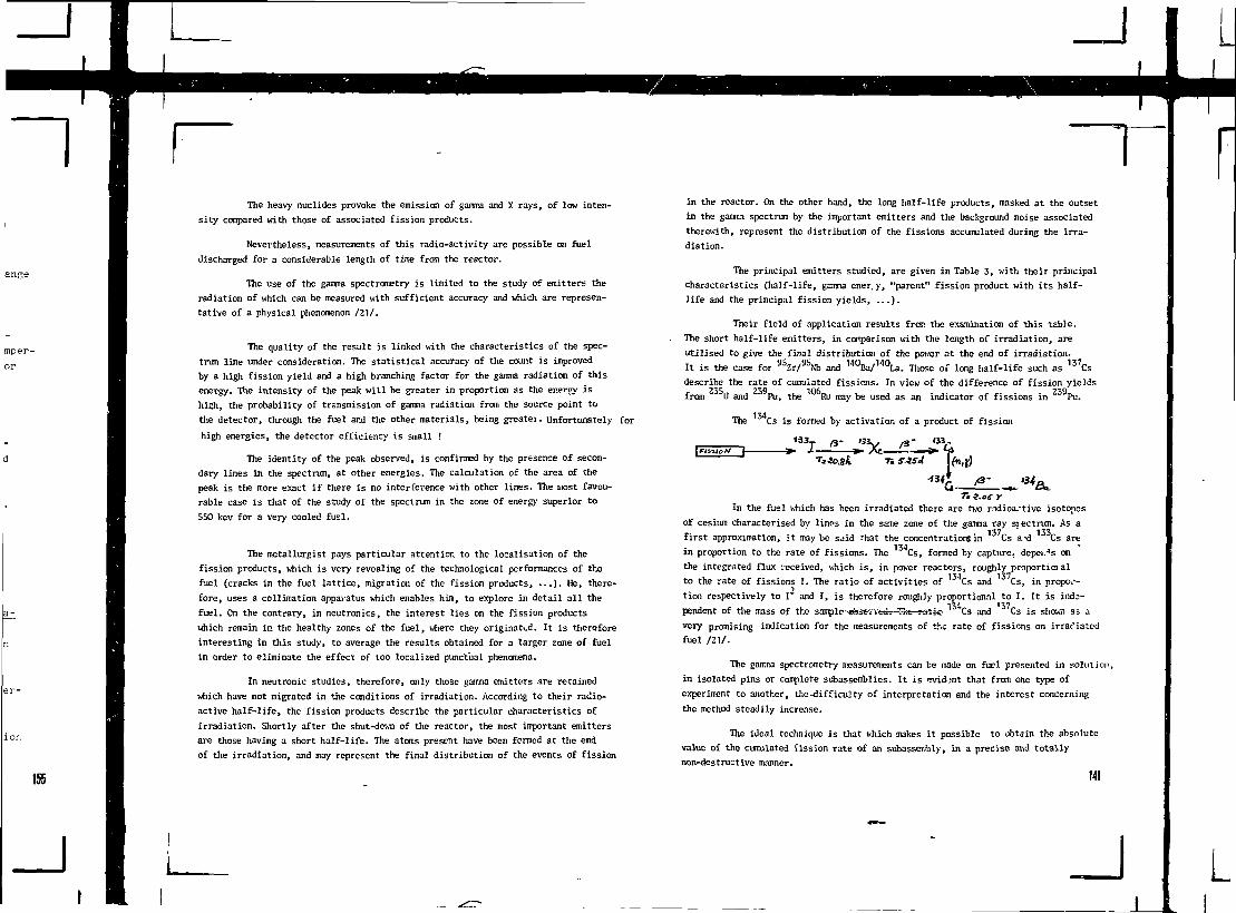
FThe heavy nuclides provoke the emission of gamma and X rays, of low inten-

sity compared with those of associated fission products.

Nevertheless, measurements of this radio-activity are possible on fuel

discharged for a considerable length of time from the reactor.

The use of the gamma spectrometry is limited to the study of emitters the

radiation of which can be measured with sufficient accuracy and which are represen-

tative of a physical phenomenon /21/.

The quality of the result is linked with the characteristics of the spec-

trum line under consideration. The statistical accuracy of the count is improved

by a high fission yield and a high branching factor for the gamma radiation of this

energy. The intensity of the peak will be greater in proportion as the energy is

high, the probability of transmission of gamma radiation from the source point to

the detector, through the fuel and the other materials, being greatei. Unfortunately for

high energies, the detector efficiency is small !

The identity of the peak observed, is confirmed by the presence of secon-

dary lines in the spectrum, at other energies. The calculation of the area of the

peak is the more exact if there is no interference with other lines. The most favou-

rable case is that of the study of the spectrum in the zone of energy superior to

550 kev for a very cooled fuel.

The metallurgist pays particular attention to the localisation of the

fission products, which is very revealing of the technological performances of the

fuel (cracks in the fuel lattice, migration of the fission products, . . . ) . He, there-

fore, uses a collijnation apparatus which enables h:un, to explore in detail all the

fuel. On the contrary, in neutronics, the interest lies on the fission products

which remain in the healthy zones of the fuel, where they originated. It is therefore

interesting in this study, to average the results obtained for a larger zone of fuel

in order to eliminate the effect of too localized punctual phenomena.

In neutronic studies, therefore, only those gamma emitters are retained

which have not migrated in the conditions of irradiation. According to their radio-

active half-life, the fission products describe the particular characteristics of

irradiation. Shortly after the shut-down of the reactor, the most important emitters

are those having a short half-life. The atoms present have been formed at the end

of the irradiation, and may represent the final distribution of the events of fission

in the reactor. On the other hand, the long half-life products, masked at the outset

in the gamma spectrum by the important emitters and the background noise associated

therewith, represent the distribution of the fissions accumulated during the irra-

diation.

The principal emitters studied, are given in Table 3, with their principal

characteristics (half-life, gamma ener. y, "parent" fission product with its half-

life and the principal fission yields, . . . ) .

Tneir field of application results from the examination of this table.

The short half-life emitters, in coprparison with the length of irradiation, are

utilised to give the final distribution of the power at the end of irradiation.

It is the case for 95Zr/95Nb and 1 4 OBa/ 1 4 OLa. Those of long half-life such as 1 3 7Cs

describe the rate of cumulated fissions. In view of the difference of fission yields

from * U and 3 Pu, the Ru may tie used as an indicator of fissions in Pu.

The 134,Cs is formed by activation of a product of fission

«3

155

•34c

In the fuel which has been irradiated there are two ridioa.-tive isotopes

of cesium characterised by lines in the same zone of the gamma ray sjectrum. As a

first approximation, it maybe said rhat the concentrations in 13 Cs a-d 1 3 3Cs are

in proportion to the rate of fissions. The Cs, formed by capture. depei.-*s on

the integrated flux received, which is, in power reactors, roughly proportioi al

to the rate of fissions I. The ratio of activities of Cs and Cs, in propor-

tion respectively to I" and I, is therefore roughly proportional to I. It is inde-

pendent of the mass of the sample-«b3ereetJT-S}ie-?3tie Cs and Cs is shown as ;i

very promising indication for the measurements of the- rate of fissions on irradiated

fuel /21/.

The gamma spectrometry measurements can be made on fuel presented in solution,

in isolated pins or complete subassemblies. It is evident that from one type of

experiment to another, thc-difficulty of interpretation and the interest concerning

the method steadily increase.

The ideal teclinique is that which makes it possible to obtain the absolute

value of the cumulated fission rate of an subasscmbly, in a precise and totally

non-destructive manner.

HI

L

The measurements on solutions of irradiated fuel arc mnde in conditions

which make possible, by using standardised sources, accurate measurements of concen-

trations in radioactive fission products. To obtain the corresponding number of

fissions, it is essential to take into account the radioactive decay in the reactor

(the half-life is not sufficiently long or short to describe the number of fissions

accumulated or existing at the end of irradiation) and the average fission yield

obtained by using the specific value of each fissile isotope. To obtain the fuel

burn-up, a number of fissions per unity of mass has to be determined. The use of

the spectrometer gamma for the determination of absolute values presupposes that

mass of fuelcontaincd in the solution measured is known. The difficulty disappears

if the ratio 34Cs/ Cs is considered, but in this case, the value of the effec-

tive cross section of capture of ~ Cs must be introduced.

When the measures are made on solid fuel, the phenomenon of transmission

of gamma radiation in the fuel and its cladding must be introduced taking into

account the distribution of the gamma emitters in the fuel pin or subassembly.

It may, however, be remarked that the coefficient of transmission of gamma radiation

remains sensibly constant in certain conditions of measurement, for instance when

the axial distribution is determined or when fuel elements of the same type arc

considered.

Because of its non-destructive characteristic for the fuel pin or the

subassembly, the gamna spectrometry is used intensively in all studies on irra-

diated fuel, in particular for the relative measurements of distribution of gairaia

emitters. Some laboratories have calibrated their installations to make absolute

measurements.

In the neutronic field, the relative measurements per gamma specrrometry

are particularly interesting to determine the global characteristics of an irra-

diated fuel element from the results of destructive measurement locally obtained.

In France, two special uses of the gamma spectrometer have been developed

- Measurements some tens of minutes after the end of the irradiation onto dischar-

ged apparatus from experimental reactors.

- Measurements on discharged subassemblies of PKR reactors, with an installation

submerged in the storage pool ; according to the time elapsed after the end of

the irradiation, either the final distribution of povcr ( La), or the distri-

bution of the specific burn-up (134Cs and 1:i7Cs) is obtained /21/.

142

4,5 - Analysis of irradiated fue2

The analysis of irradiated fuel undoubtedly constitutes the most accurate

and complete method of validating the calculations of evolution. By utilising the

appropriate techniques, it is possible to determine the composition of each of the

nuclides described by the evolution equations ; heavy isotopes, fission products,

poisons, ... The number of fissions may by obtained either in comparing the balance

in heavy isotopes before and after irradiation, or in determining the concentration

in a particular nucluic ( Nd).

The analysis of the fuel requires laboratO7-Jes which have very efficient

equipment : shielded dissolution cells, mass spectrometers

The analysis is a costly process which is only carried out on a limited

-number of samples chosen in function of their neutronic representativity. The grea-

test care must be taken in each operation, particularly to avoid pollution by fuel

from another source which would falsify the result of che measurement.

The sample is chosen in function of the position fchich it occupied in the

reactor and of the problem under consideration. In particular, in the case of the

qualification of a cell code, the sample is chosen in "an asymptotic spectrum" of

an infinite lattice, situated at a distance from the perturbations not taken into

account in the calculation.

The gamma spectrometry_ is particularly useful as a means of ensuring the

metallurgical quality of the zone examined and for the extrapolation of the results

obtained at some points to the whole fuel element.

The size of the sample used in analysis is the result of a compromise.

The larger is the sample, the better is the protection from local perturbations due

to metallurgic phenomena, to contamination or to a faulty cutting, but at the same

time the greater is the difficulty of the radiological protection of the operators.

The cutting must he made with great care. In general, a portion of cylinder

is taken which is limited by two cross-sections ; the result obtained described

a zone which is the same as that studied by the cell codes. The sample is then

totally dissolved by an appropriate technique.

From this solution, aliquots of some cubic centimetres are then extracted

which are sent to specialised laboratories ; the sample received is representative

of an important zone of fuel (homogenisatien by dissolution) but presents a mode-

rate danger of radioactivity.

J

The mass spectrometry is a very precise analysis technique well adapted

to the examination of irradiated fuels, on the one hand because it concerns the

concentration of each isotope, radioactive or otherwise, and on the other hand

because this technique only requires very small quantities of fuel. The spectro-

meter generally used is that of thermo-ionisation. Under the effect of heat, ions

are emitted from the fuel solution deposited on the filament and a magnetic device

separates the ion beams of the different atomic masses. This technique is very

accurate, if care has been taken, to f.-ee the solution from disturbing chemical

elements which could interfere with the same masses in the spectrum. With the mass

spectrometer, traces of one part in a million can be measured.

The isotopic abundance of the principal elements, uranium, plutonium

neodymium (fission product used to determine the specific burn-up) can be determined

together with elements such as americium, curium and gadolinium.

In addition to the isotopic abundance, the relative concentration in the

different elements are sought for. To avoid the difficulty of measuring masses and

of volumes, the technique of the simple or double isotopic dilution is used /17.18/

This eliminates the measurements of volume.

To a solution of irradiated fuel, a solution is added which contains in

a known proporticnof isotopes which are not present (or only in low quantities)

in the fuel ; U, Pu, Nd ... Measurements are made by mass spectrometry

after separation on aliquots of the solution of each of the elements. Thus, the

ratio "Pu/ U being known, the isotopic composition of U and Pu makes it possible

to determine the ratio U/ Pu characteristic of the irradiated fuel. In the

case of a PIVR fuel, the following results are obtained {2&)

R = ( j 2 3 5 / ^ % S R ^ 0 . C O 3 % R = u 2 3 (7u 2 3 8 % oR<0.003 °o

R = Pu24O/Pu239°. SR<0.05 %2^9 t 242 ^39 *

R = Pu 2 3 9/U 2 3 8 % 6R/R<07 % R = (Nd 1 4 8/U 2 3 8)

Neodymium isotopes, and more ospacially Nd are used as indicntors of

the specific burn-up. N'd has the advantage of similar fission yields for "' U239and Pu (y = 1.67 °. and 1.68 1 in thermal reactors /2/Jwhich are the main source

of fuel fissions. It has a good metallurgical behaviour and is not present in new

fuels. Chemical methods of separation of the ncodymium element among the rare earths

of irradiated fuel have been worked out, which makes it possible to make exact

R = Pu238/Pu239 % SR<TO.0O6 •.

R - Pu241/Pu2:

measurements by mass spectroinctry. The specific burn-up is determined from the

experimental ratio of concentrations in 148N'd and 2 J 8 U (148Nd/2;iSU):

148.,, , 148., ,x 238..

Z 3 / U

8,,.U)2 100

This formula contains various corrective terms, near to unity, \chich have to he

estimated :

- The determination of the fission yield -y- introduces the distribution of fissions

between JDU, "J U, *J Pu, " Pu, ... to minimise the importance of the evaluation

of the origin of fissions, certain experimenters suggest using other isotopes of

neodymium for fuels on a base of "^ U, or irradiated by fast neutrons /19/.

- The ratio ( Ndx/ l Nd) of concentrations of neodymium produced by fission to

neodymium present at the nd of irradiation, '-filch takes into account its disap-

pearance by capture and its appearance from Nd , fission product of 11.08 days

half-life.

, 238,- The disappearance of *" U during the course of irradiation.

The concentration in " '"U among the heavy isotopes present initially is

assumed to be well known.

The method of deteraination of the fuel burn-up, from its ncodymium conten".

is undoubtedly the nost exact method of attaining this result. The specific burn-up

may also obtained by comparing the composition in heavy atoms before and after irra-

diation. This method is well adapted for fuel having a high level of "*1SU.

On the aliquots of solutions of irradiated fuel, other measurement techni-

ques can be used ; these are principally spectromctries "t and jf.

The spectrometry o( is well suited to the determination of the concern rations

Of americium and curium /20/. The measurement made on a thin deposit of solution i:ives

icctrinn vith four principal lines each corresponding to one or several nuclidc^

first (f. = 5.15 Mcv) corresponds to 2o9l\j and 2 4 OPu, the second (E = 5.5 Mev) to41 244

)2 4 2Cm

a spect

'^Pu and "41Am, the third [Y, = 5.8 Mcv) to 244Cm, the fourth (E = 6.1 Mev) to 4*tiCni.

The content in ~'"Pu and " Pu having been obtained bv "the mass spectrometry, theM2 '44 ' 2 8

concentrations in *" Cm and " Cm are deduced from the spectrum o(. To examine ' Pu

143

i rand Am, the measurement must be completed by a spectrum e( obtained with a deposit

free from the americium element.

The spectrometry ctmakes possible measurements on minute quantities of

isotopes of short half-life. It is very difficult to obtain from it information

on nuclides of longer half-life. 2 4 2 % i , 243Cm ...

We have already insist upon the usefulness of measurements by the gamma

spectrometry. This method is particularly valuable when there is no mass spectrometry

laboratory available for treating irradiated fuel.

In the field of irradiated fuel, other analysis techniques, such as fluo-

rescenceX,have been developed by various laboratories.

4.6 - Other measurements technigues

In this chapter, two categories of measurements can be distinguished :

- Measurements of integral'quantities such as the neutron capture of fission products,

the after-powsr, the neutron emission.

- Measurements of the irradiation characteristics, using a physical phenomenon with

it is correlated.

The capture of fission products may be deduced from the difference of the reac-

tivity effects of two samples, the one irradiated and the other not. A previous

calibration malces it possible to take into account the effect of the variation of

cc ..position in heavy isotopes and to express the difference in reactivity in the

form of an equivalence in well known isotopes U, boron ... The measurement

technique most generally used is that of the oscillations in a critical reactor /",2/

With this integral measurement of the capture of fission products, it is possible to

assiriate measurements on individual fission products, using either an oscillation or

activation method, or an irradiation method followed by an analysis.

The after powsr can be measured in different scales of cooling times. The

.ludy of very periods is particularly useful, as this qualifies the results used in

the evaluations linked with the consequences of reactor accidents. For these measure-

ments, a fuel sample of small size is irradiated in a reactor of medium power and

transferred very, quickly into a calorimeter /2fi, 27/. For cooling periods of some

months, it is possible to make calorimetric measurements on portions of fuel elements

,'25/.

144

But in this case, the use of the result is only valid if it is used to

qualify a calculation which takes count of the history of the irradiation.

The neutron emission can be measured by placing a fuel sample in a modera-

ting medium in which neutron detectors are placed. The use of the latter makes it

necessary to the gamma radiation existing in the moderator.

An electronic apparatus may make it possible to distinguish the neutrons

emitted in groups (spontaneous fission) from those emitted individually (reaction: <,'"•).

To obtain the irradiation characteristics, for instance the spe-ific

burn-up, more and more use is made of analysis and the gamma spectrometry. But certain

laboratories which are specialised in experimental techniques use them for study

of irradiated fuels ; for instance, the measurement of after power, the irradia-

tion by a source of neutrons ... Often, these methods present difficulties of inter-

pretation and of calibration. They may be particularly suitable for certain problems.

5 - COMPARISON OF FUEL EVOLUTION IN DIFFERENT REACTOR SYSTEMS -

5.1 - Introduction

In precedent lectures, the stress was put on phenomena, calculation methods,

and measurement techniques common to all neutronic studies relative to the evolution

of irradiated fuels. The application to the concrete problems obviously depends on

the context in which they appear : type of reactor, available calculation code,

usable measuring techniques, type of required information and the needed precision ...

The specific aspects of evolution for each type of reactor appear in the

specialized lectures : heavy wcter moderated reactors /28/, pressurized water reactors

/29/, boiling water reactors /30/,high temperature reactors /31/ and fast neutron

reactors /32/. From these lectures, it would be interesting to do a complete comparison

of everything concerned, directly or indirectly, with fuel evolution : reactivity,

fuel composition, control, reactor operating rules, fuel management ... Complementary

aspects concerning the metallurgical properties, the fabrication and the reprocessing

of the fuel would be useful but they are beyond the objectives of this course. This

comparison would give a sound understanding of the fuel cycle to those people who

must propose the best reactor system for a particular energy need.

In this lecture we are going to limit ourselves to only same aspects of

the fuel evolution which are very important for reactor design.

_J

5.2 - Reactivitj;_evolution_and_characteristics_of_th;_fuel_element

The behaviour of a running reactor is dependent on the fuel element charac-

teristics. Most of them are defined from the choice of the fuel enrichment, the mode-

rator, and the coolant. For this reason, there is a convergence of retained technical

solutions in the old reactor systems. This situation does not yet exist for new types of

reactors, like high temperature reactors.

For example, the use of natural uranium and graphite leads to a metallic

fuel element of large diameter in order to reduce to the maximum the effect of238

resonance capture in U. The magnesium chosen as cladding material in function of

its neutronic and metallurgical properties fixes the operating temperature of the

coolant. The use of slighty enriched uranium authorize other materials : clusters of

uranium oxyde rods, stainless steel cladding ...

The evolution of the reactivity with time results from the balance between

the formation and the destruction of fissile atoms. In thermal reactors, it is239

often considered the initial conversion factor. That compares the appearance of Pu

to the disappearance of TJ. With usual notations, it is defined :

*-o =

Co is particularly important in the natural uranium reactors that are

moderated by heavy water or graphite. It is obvious that in the c&j.e of the uranium

enriched reactor (PUR).

Co is much less, although the captures in U are relatively favoured by

the "hardness" of the neutron spectrum. The Co value explains the evolution of the

reactivity in a thermal reactor. The figures 4, 5 and 6 give the variations of the most

important atomic ratios in respect to the burn-up in graphite, heavy water or pres-

surized water moderated reactors. The variation of the reactivity depends on the

•'U/-'8U and ""Pu/—U. The formation of

Plutonium isotopes of higher mass ( Pu, pu) is accelerated when the spectrum

difference between the curves that give

Plutonium isotop

is plus "hard".

In the breeder reactor systems, we consider the "breeding gain". In a fast

neutron reactor, "the breeding gain" is defined as being equal to the difference of

quantities of plutonium (equivalent to Pu) formed and destroyed in relation to the

total number of heavy atoms destroyed by fission in the reactor /32/. The breeding

gain varies from one area of the reactor to another, from the core ( internal

breeding gain) to the blanket (external breeding gain). It is the sum of these two

breeding gains that is taken into account in the calculation fo the fuel cycle cost.

The "doubling tune", time necessary to produce a quantity of fissile material

(equivalent "^ Pu) equal to the quantity present in the core, is directly connected

to the breeding gain.

5.3 - Fuel_management

In a reactor, the main objective is the optimal fuel usage for maximum

energy production. In an subassembly whose fabrication and reprocessing cost is

very high, the interest of the reactor operator would generally want to conserve

fuel the longest time possible in the reactor. The management plan depends on the

handling system, the safety rules, economical criterion, ...

In natural uranium reactors, the reactivity reserve is limited and it is

necessary to mix in the core fresh fuel with a reactivity excess and almost exhaus-

ted fuel. The loading plan is according adapted. This is possible because there is

a large number of channels that can be loaded and unloaded when the reactor is run-

ning. In heavy water rc3Ctors, the fuelof neighbouring channels is pushed across

the core following contrary directions /28/. If fuel is withdrawn when the reactor

is operating, fuel elements must be of a small size in comparison of the reactor

charge in order that the imput or the output does not lead to a significant jump

in reactivity.

The fuel handling in an operating reactor is certainly a desirable solution,

but it is a technically difficult problem. The machine is complicated because it

must insure no loss of pressure for the coolant, the removal of the after-power, and

the biological protection of the fuel element just leaving the core.

In the case of water moderated reactors, the fuel handling is done whenthe

reactor is stopped uhen is not possible to remove antireactive materials from the

core (boron in water, control rods) to compensate for the disappearance of fissile

nuclides. The vessel is op'-ied, which is a very important operation. Then, the

underwater handling poses only minor problems, because the water insures, at the

same time, the heat removal and the biological protection.

Fast neutron reactor are stopped for fuel loading. The handling machine

takes into account the necessity to conserve the subassembly in the same coolant

material as in the core. Sodium prohibits the use of a convenient water pool for the

initial storage of unloaded fuel.

145

It is useless to insist upon the importance of fuel management from an

economical or safety point of view. If the fundamental principle is to obtain the

maximum bum-up everywhere, other criterion can be retained for example available

fuol, performances of the handling apparatus, needs of the electricity network,

reprocessing possibilities, ... In fact the best economical choice of a management

plan is not made by individual elements, but by a group of assemblies and even by

a total of reactor charges. Thus in a PWR, the equilibrium**, is established while

definitively discharged a third of the core af•er one cycle and another after two

cycles stay in the pile.

Other fuel management plans can Lie considered if plutonium is introduced

in the fresh fuel with less enriched, natural or depleted uranium. To uranium economy

corresponds a higher fabrication cost.

The search for an optimal core loading must take into account the impera-

tive adherence to the safety of the reactor operation, that is to say to the tech-

nological limits fi-\ed by the fuel manufacturer : maximum linear power density,

burn-up, cladding temperature ... The conditions must be respected at each moment

of the reactor life, as well as during the normal running operation such as the

Transitory phenomenon. In particular, a movement of control rods must not lead to

the appearance of a peak in the flux distribution and consequently an inadmissible

v.iluo in the linear power density at any point of the reactor.

The pratical strategy used to define the configuration of the core in each

particular system is described in the specialized lectures /28, 29, 30, 31, 52/.

- CONCLUSION -

The objective of these conferences has been above all, to grasp

the fundamental laws of the evolution for fuel subzected to a neutron flux in

a reactor. If he knows well the phenomenon set into action, the engineer will be

ablu to answer the numerous questions better as they are presented along the fuel

:wlet in using a judicial way the calculation and measurement techniques which are

bailable.

corresponding to the best fuel utilisation.

In the developement of the reactors, very particular attention is brought

to the fuel cycle, from its fabrication to its reprocessing In the following years,

many studies wiii be undertaken in the field of irradiated fuel physics in order

to operate reactors even more economically and safely.

- REFERENCES -

IV J. BUSSAC - P. RRISS

Traite de neutronique : physique et calcul des reacteurs nucleaires

avec application aux reacteurs a eau pressurisSe et aux r£acteurs

a neutrons rapides.

Editeur : HERMANN - Coll. Enseignement des Sciences (1978)

HI J.G. CUNINGHAME

The status of fission product yield data (FPND) in 1977

IAEA Second Panel on Fission Product Nuclear Data

PETTEN - September 1977

III B.F. RIDER - M.E. MEEK

Compilation of fission product yields - Vallecitos Nuclear Center

Report NI-DO - 12154-21D

141 E.A.C. CROUCH

Fission Product yields, from Neutron Induced Fission

Atomic Data and Nuclear Data Tables - Vol. 19, N° 5 (1977)

IS/ J . BLACI0T - Ch. FIC1IE

Ganina ray and half- l i fe data for the fission products

Atomic Data and Nuclear Data Tables - Vol. 20, N° 3 (1977)

161 M.F. JAMES

Energy released in fission

Journal of Nuclear Energy - Vol. 23 - Pergamon Press 1969

171 M.F. JAMES

The useful energy released in the fission of 232Th, 233U, U, 2 3 6U,2 3 V 238Pu, 24OPu and 242Pu.

Journal of Nuclear Energy - Vol. 25 - Pergamon Press 1971

14.,

_l

161

J

/8/ A . BWENOKYNEPTUNE : Un systeme modulaire pour le calcul des rSacteurs a eau

legere.

Bulletin d'Informations Scientifiques et Techniques - Mars 1976 - N°212

/9/ R. de TOURREIL

Progrannie de calcul de l'activite des produits de fission

Note CEA w-324

/1O/ B. BHRRE

PICFFE - Programme d'integration de courbes de fissions 616mentaires

tenant compte de Involution de nuclides fissiles.

Note CEA N-1203

/11/ Safeguarding Nuclear Materials

IAEA Symposium - VIENNA - October 1972 (IAEA/SM/2O1)

/12/ J. BOUCHARD - P. MEXESSIER - R. VIDAL

Etude neutronique de milieux multiplicateurs a neutrons rapides sur

1'assemblage critique thermique-rapide ERMINE II.

Rapport CEA R-4246

/13/ B. LAPONCHE - R. VIDAL

L'Svolution neutronique des combustibles en fonction de l'irradiation

dans les rgacteurs thermiques.

IAEA Symposium - VIENNA - July 1971

/14/ M. ROBIN - J. LUTFIN

Etude neutronique des combustibles irradifis.

Bulletin d'Informations Scientifiques et Techniques N° 170 (May 1972)

/15/ J. LUFF1N - Z. SZATMARY - J. MNUXEEM

Adjustment of a burn-up code on chemical and isotopic analyses of

irradiated fuels.

Journal of Nuclear Energy - Vol. 26 (1972)

/ W J. BOUCHARD - J.Y. BARRE - M. DARROUZET - J. GOURDON - M. ROBIN

Fast reactor physics at CEA : higher plutonium isotopes and burn-up

studies.

IAEA Symposium - Tokyo 1973

/17/ G. FREJAVILLE - M. LUCAS

Dosage du neodyme de fission dans les combustibles irradiSs.

Rapport CEA R-4265

/18/ M. LUCAS - C. CHEVALIER

Analyses isotopiques et dosage du gadolinium et du nSodyme de fission

dans les combustibles nuclfiaires irradies

Analysis 1975 - Vol. 3 N° 10

/19/ W.J. MAECK

A review of fission product nuclear data requirements for investigation

of irradiated nuclear fuel : burn-up measurements, neutron dosimetry,

nuclear safeguards.

IAEA - Second Panel on Fission Product Nuclear Data

Petten - Septembre 1977

/20/ J. M5NIER

Determination a l'aide des spectrometries alplia et garnna du taux de

combustion atteint par les combustibles nucle*aires.

Rapport CEA R-4625

/21/ J. BOUCHARD - G. FREJAVILLE - M. ROBIN

Mesures de distribution de puissance et de taux de combustion par

spectrom6trie gamma sur les combustibles irradiSs de reacteurs a eau.

Note CEA N-1982

/22/ M. ROBIN - M. JASTRZEB - S. BOISLIVEAU - R. BOYER - R. VIDAL

Determination par spectrometrie gamma du taux d' irradiation des elements

combustibles de reacteurs de puissance.

Rapport CEA R-3863 (1969)

/23/ A. L'HttNE

SARA - Code de depouillement des spectres enregistrSs sur spectrometre

Ge_Li.

Note CEA N-1S06

/24/ J.C. PANISSH

Code de traitement sur ordinateur des histogramnes d'amplitude avec semic

teurs Ge-Li. Programme JONOUES.

Note CEA N-1S78

147

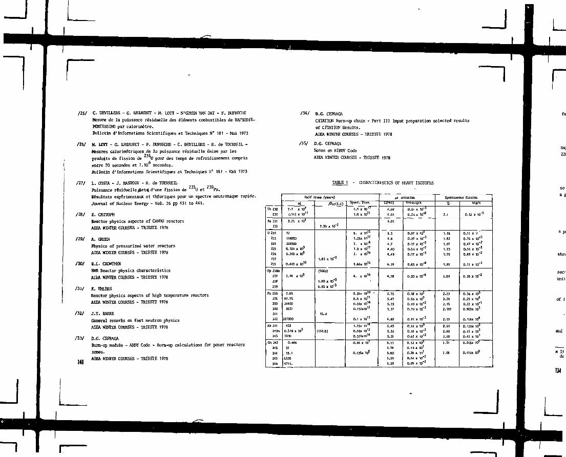
/2S/ C. DEVILLERS - G. LHIAUBET - M. LOTT - N'GUYEN VAN DAT - F. DUFRECIEMesure de la puissance rgsiduelle des elements combustibles de RAFSODIE-PORTISSIMD par calorimStre.Bulletin d'Informations Scientifiques et Techniques N° 181 - Mai 1973

/26/ M. LCfIT - G. LHIAUBET - F. DUFRECHE - C. DEVILLERS - R. de TOURREIL -Mssures caZorimfitriques de Ja puissance rSsiduelle fimise par lesproduits de fission de U pour des temps de refroidissement comprisentre 70 secondes et 7.10 secondes.Bulletin d'Informations Scientifiques et Techniques N° 181 - Mai 1973

111! L. COSTA - J. RASTOIN - R. de TOURREILPuissance r£siduelle/9et4 d'une fission de 2 3 5U et 239Pu.RSsultats exp5riraentaux et theoriques pour un spectre neutronique rapide.Journal of Nuclear Energy - Vol. 26 pp 431 to 441.

/28/ E. CRITOPHReactor physics aspects of CANDU reactorsAIEA WINTER COURSES - TRIESTE 1978

/29/ A. GRUENPhysics of pressurized water reactorsAIEA WINTER COURSES - TRIESTE 1978

/30/ R.L. CROWTHERBVR Reactor physics characteristicsAIEA WINTER COURSES - TRIESTE 1978

/31/ K. EHLERSReactor physics aspects of high temperature reactorsAIEA WINTER COURSES - TRIESTE 1978

/32/

;'33/

148

J.Y. BARREGeneral remarks on fast neutron physicsAIEA WINTER COURSES - TRIESTE 1978

D.G. CEPRAGABurn-up module - ARDY Code - Burn-up calculations for power reactors

zones.AIEA WINTER COURSES - TRIESTE 1978

/ W D.G. CEPRAGA

CITATION Burn-up chain - Part I II Input preparation s e l e c t e d r e s u l t s

of CITATION Resu l t s .

AIEA WINTER COURSES - TRIESTE 1978

/3S/ D.G. CEPRAGfl

N o t e s on RIBOT Code

AIEA WINTER COURSES - TRIESTE 1978

TABLE 1 - CHARACTERISTICS OF IEAVY ISOTOPbS

111 230

232

Pa 251

233

U 232

233

231

235

236237

23S

Kp 236a

237

239

239

Pu 236

233239

240

241

242

An 241

242m

243

0 1 212

243

244

245

246

Hal f l ives (years)

«

7.7 X 104

0.141 X 1 0 "

3.25 X 104

72

1S90CO

2480000.704 X 109

O.240 X 10°

0.449 X 10 1 0

2.14 X to 6

2.B5

87.75

244036537

337000

433

0.319 X 105

74TO

0.446

32

13.1

8530

4711.

A>r( I .C)

7.39 X 1C"2

l.BS X 1O"2

(SOCO)

S.80 x 10"5

6.45 I 10"S

15.0

(152.8)

l . S x i o "

1.0 x 1021

8. , , n 1 3

i.2Sx i n "

2. x 1O'6

1.9 X 10"2. X 10™

9.86X io'5

4. X101 6

O.35X 1O10 '

0.5 X lO11

0.S5X t o "

O.152xlO12

0.7 X lO11

1.1S, IO"

0.9SX Id ' 2

O.33SXIO"

0.66 X 1O'

O.125X 108

at e

t(McV)

4.G9

4.01

5.01

5.3

4.8

4.7

4.40

4.49

4.19

4.78

S.75

5.47

5.1S5.17

4.89

5.49

S.ZO

5.2S

6.11S.78

S.80

S.36

S.39

mission

Kntts/g/s

0.5» x 10"3

0.20 x 10"8

0.67 X 10°

0.27 x 10"3

0.17 x 10'3

O.SG X 10"'

0.17 X 10"S

0.83 X 10"'

0.20 X 10"*

0.18 X 102

0.56 X 10°0.19 X 10"2

0.70 X 10"2

0.11 X 10"3

O.U X 10U

0.14 X 10"2

0.62 X I0"2

0.12 X 10*

o.t6 x ro1

0.28 X 101

0.54 X 10"2

0.99 X 10"2

Spontaneous fission

2.1

1.55

1.62

1.67

1.73

1.76

1.95

1.89

2.23

2.26

2.1S

2.167

2.15

2.51

2.60

2.K>

2.51

2.68

n/E/s

0.12 X I0"6

0.11 X if

0.74 x 10"3

0.47 X 10"2

0.51 x 10"3

0.49 X 10"2

0.11 X 10"1

0.26 X 10"2

0.36 X 105

0.25 x to4

0.22 X 10"'0.90SX I03

0.1 OSx 104

O.120X 10U

0.15 X 103

0.42 X 10*

O.208X 10*

0.116X 108

-

J

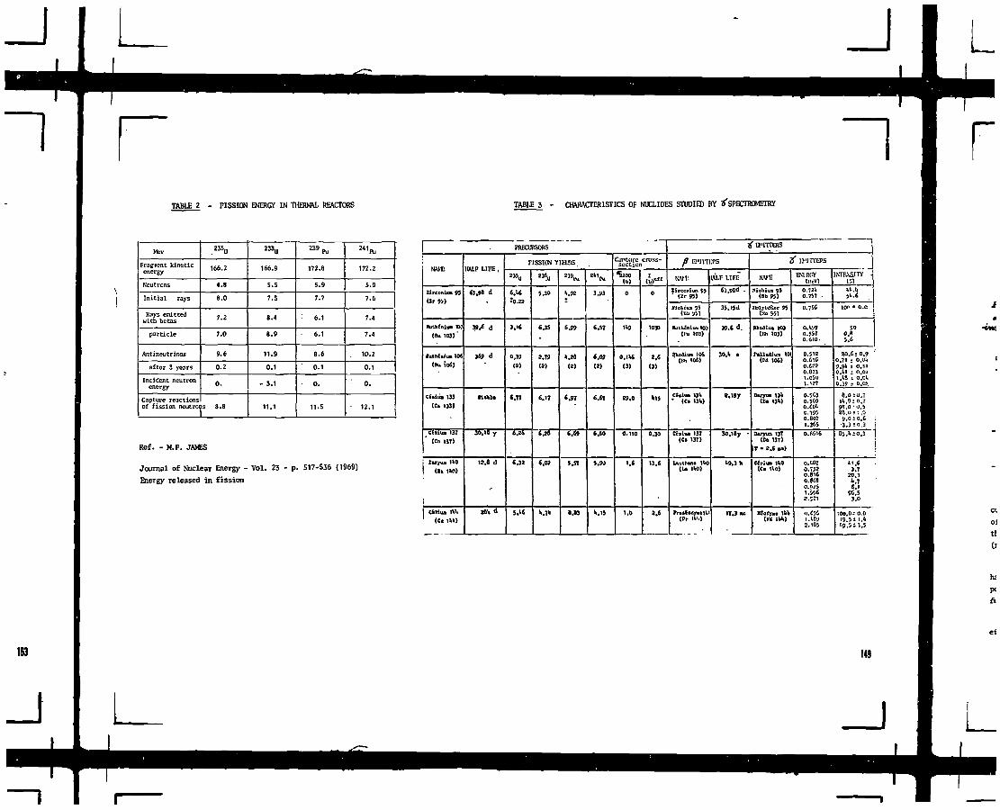
TABLE 2 - FISSION ENERGY IN THERNW. REACTORS TABLE 3 - CHARACTERISTICS OF NUCLIDES STUDIED BY jfsPECTROMETRY

~l

Mev

Fragment kineticenergy

Neutrons

Initial rays

Rays emittedwith betas

particle

Antineutrinos

after 3 years

Incident neutronenergy

Capture reactionsof fission neutro

235U

166.2

4 .8

8 . 0

7.2

7.0

9.6

0 . 2

0 .

s 8.8

236U

166.9

5.S

7.S

8.4

8.9

11.9

0.1

- J.I

11.1

2 3 9 ft,

172.8

5.9

7.7

: 6.1

6.1

8.6

0.1

0 .

11.5

24<Pu

172.2

5.9

7 . 6

7.4

7.4

. 10.2

0.1

: 0 .

• 12.1

Ref. - M.F. JAMES

Journal of Nuclear Energy - Vol. 23 - p. 517-536 (1969)Energy released in fission

PRECURSORS

Zlrconlia 93

(Jr 9 »

Ituthtniui K

(Su 103)'

Itucflfifua tO6<»u ioS)

Ciliu. 133«• 1311

^ cttiiai I3T

(c» U7)

(El 1«l)

Ciriu, | U

(C« ill,)

KLF LIFE ,

«.«a d

39/ d

3D d

tlttl .

30,l& y

1S.» d

FISSION Ytaos

I0.J2

3,<t

a,3t(2)

«.T?

t.3>

5.1.6

23«u

5.30

'.35

i.W

(2)

«.!»

«.0»

1..52•

6.09

»,!«(2)

' .97

6.G9

5.S1

«.«3

3.93

«.5T

«.0S

(il

6.(7

« . »

J.90

"..IS

Cantttre cross-section

^200Ib)0

HO

O.US(3)

S9.0

O.I 10

>.<

1.0

tlf"0

1030

*.<(3)

H5

0.30

I3.«

j ' U'lTTBlS j

/7 H'irrere

lireoniun S3' (ir 95)

Hiohiu 95(rib 'SA

JhithSniun tO'j(III! 1U1J

l)lu>li<j» 106(«» 104)

Cc ( lo HI• (Cl 13H

C<>iia 137(Ci 137)

uuihwi* no(U HO)

rrxtCo jMtil,trr Ikl.)

iu.r LIFE

6J.90d .

35.15J

39.C <!.

20.1, •

30.1»y •

».3>

2f 1?'[1TH>S I

Niobiua 95t»b 95)

UolyMvnr 93CKo 95)

Rkpdiua 103(UK 103)

r«iiKd]ua inIra loo)

(0 . I3O

lujva 137IE. 137)

T - 2,S sn)

C6r!m iltO(C« Ho)

XCoiim Ilk1M lU)

EM.nnyOlcV)

0.721*0.757

O.76C

O.l'/In.5570.610-

0.512O.C-.CO.6?2

can1.05U1.IJ7O.5C30.5WO.COl0.7950.8021.365

O.«16

0.1070.7520.616o.tcao.<«1.5162.;?i

o.WSi.ie»5.10}

STENSmr •(;>

51..6

ICC * O.C

500,85.6

S0.6s 0.90.71 ! O.<*9.9fc s O.HO.tl 1 0.0»1.1S i o.cl,0.39 2 o.cs.

8.OIU.7lli.Q 10,79"i.O-0.5fla.o; :,0

9,01 O.fi•3.3 =".3

05 .V; 0,3

3.720.3M« . l

9S.53,«

'•OO.O : 0.019.51 I , '''9.5 s 3,5

149

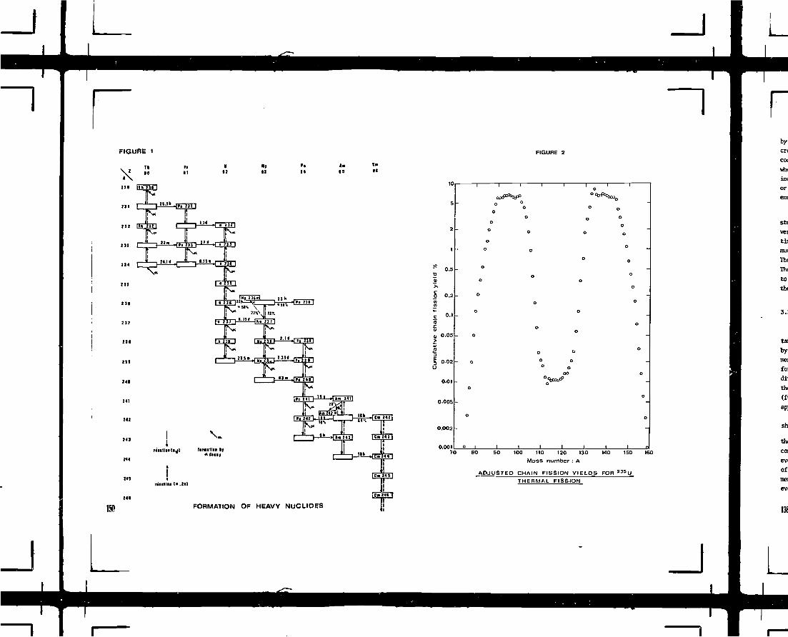
FIGURE 1 FIGURE 2

I11

*>I I

P i

14l a1 !

CaI I

ISO

riaillu (•.ID

10

5

2

1

18 0.5D

5>5 0.2

: 0.15z>

0 0.05>

3

5 0.02J

0.01

0.005

0.002

0.001

— — - i ' 1

ootr-o

o

oo

o

o

o

o

o

o

- 0

- o

o

o

° 1 1

1 • 1

oo

o

o

o

o

o

o

ooo

>

1 1

1 1 1 1o

° oo o

o

° o

o

° o_

oo

0

-

0

o* •

o

o

ou

oo

oo o

o-

0

-

1 1 . 1 ol70 80 100 110 120 130

Mass number : A140 150 160

ADJUSTED CHAIN FISSION V1ELDS FORTHERMAL FISSION

FORMATION OF HEAVY NUCLIOES

_J

185

GRAPHITE MODERATED REACTOR

1SOTOPIC COMPOSITION OF IRRADIATED FUEL

FIGURE 3

Pu 240/Pu 239

ISOTOPE RATIOS (aioms)

2 300

HEAVY WATER MODERATED BEACTOR

ISOTQPIC COMPOSITION Of IRRADIATED FUEL

FIGURE 4

ISOTOPE RATIOS (acomsJ^ k PRESSUHIZED WATER REACTOR

PU9 I Pu-_!ux

ISO7OPIC COMPOSITION OF IRRADIATED FUEL

FIGURE 5

151

>— P . — • " _C O

1 r

L

167

J

PHYSICS OF PRESSURIZED WATER REACTORS

A. GRUNKraftwerk Union A.G.,Erlangen,Federal Republic of Germany

1 Abstract

The objective of this lecture is to demonstrate typical problems

and solutions encountered in the design and operation of PWR power

plants. The examples selected for illustration refer to PWR's of

KWU design and to results of KWU design methods.

In order to understand the physics of a power reactor it is neces-

sary to have some knowledge of the structure and design of the

power plant system of which the reactor is a part. It is therefore

assumed that the reader is familiar with the design of the more

important components and systems of a PWR, such as

fuel assemblies

control assemblies

core lay-out

reactor coolant system

instrumentation.

2 Lattice design

2.1 Fuel assemblies

Fig. 2.1 shows a cross section of the pressure vessel and the

core of a 1300 MWe PWR. The core comprises 193 fuel assemblies

of square cross section and is surrounded by a shroud. The core

barrel separates the downward flow of the incoming cold coolant

from the upward flow within the core. The water-filled space

between core shroud and pressure vessel acts as a neutron

reflector.

Of the 193 fuel assembly positions of the core 61 can be

equipped with control rod assemblies (fig. 2.1).

Fig. 2.2 shows a schematic cross section of a fuel assembly. The

fuel rods and the guide tubes are arranged in a square array.

Each position of this array is indicated on fig. 2.2 as a square.

The positions form a square lattice. There are 16 x 16 lattice

positions, 20 of which are occupied by guide tubes, the remain-

ing 236 by fuel rods.

This square array constitutes the basic lattice structure of the

fuel assembly. Two types of lattice cells can be distinguished:

the fuel rod cells and the guide tube cells. When the control

rods are withdrawn, the guide tubes are water-filled.

Table 2.1 summarizes some design data of a fuel assembly for a

1300 MWe PWR core.

In initial cores some of the fuel assemblies contain boron glass

as burnable neutron poisons. The boron glass is placed into

special absorber rod assemblies, similar to control rod assemb-

lies, which are inserted in selected fuel assemblies. Accordingly,

the burnable poisons occupy lattice positions homologous to the

control rod absorbers.

Before we turn to the nuclear design of PWR latices, some de-

sign and operational characteristics of PWR cores should be men-

tioned :

1. For the control of reactivity PWR's have two independent

systems: the control rod assemblies and the soluble boron.

As a consequence, the control rod assemblies can be kept

nearly completely withdrawn from the core during steady-

state operation. The flux and the power distribution is

therefore only weakly disturbed by non-uniformly distribut-

ed absorbers.

153

1

ed-

2. The fuel assemblies have no shroud. The spacing between the

outermost fuel rods of adjacent fuel assemblies is of the

same order as the fuel lattice pitch. As a consequence,

the fuel lattice structure is nearly uniform and uninterrupt-

ed throughout the core, the only irregularities resulting

from the presence of the guide tube ceils which amount to

a fraction of about 8 % of all lattice cells.

Again, this feature leads to a lattice structure of relative

high uniformity throughout the core.

3. The fuel in each fuel rod of a new fuel assembly is of the

same enrichment. The neutron spectrum within one fuel ascemb-

ly is therefore sufficiently uniform to allow a homogeneous

representation of the assembly on the basis of a single

Wigner-Seitz cell.

That feature pertains to Uranium fuel only. Assemblies con-

taining both U and Pu rods require more detailed analysis.

2.2 Homogeni zat ion

154

The first step in nuclear analysis is the homogenization of the

heterogeneous core lattice structure. The purpose of the homoge-

nization procedure is to generate equivalent homogenized group

cross sections. The calculation of these few group cross sections

is known as ceil-calculation.

In the cell calculation the fuel assembly is represented by a

single representative lattice cell of circular cross section,

the so-called Wigner-Seitz-Cell (Pig. 2.3).

The cell is composed of several regions: fuel r^d, canning mate-

rial, moderator and in the outermost region an appropriate fraction

of the guide tube cells. (This representation of the guide tubes

is adequate because the guide tubes are distributed rather uni-

formly in the actual fuel assemblies).

The determination of homogenized group cross sections is sum-

marized on Table 2.2.

The results of the cell calculation are equivalent homogenized

microscopic cross section which, when multiplied by the cell

averaged nuclide densities yield the correct group average reac-

tion rates.

When control rods are inserted into the fuel assembly the cell

calculation is performed in the same way. The additional ab-

sorption rate caused by the absorber fingers is taken into

account of by considering a representative absorber cell (fig.

2.4). The effective absorption cross section of this cell is

calculated once with absorber material in the central region

and once with moderator in the central region. The difference

of the two results is the homogenized representation of the ad-

ditional absorption introduced by the insertion of absorber

rods into the fuel assembly.

The homogenized cross sections are, of course, functions of the

physical state and composition of the cell. The variables to

be considered are listed on table 2.J. They change with the

fuel depletion and with the operating conditions of the reactor.

It is therefore necessary to evaluate the variations of the cross

sections with these variables. This is done by repeated cell

calculations.

Starting from a reference state and zero burnup the parameters

specifying the operating state of the core are then changed and

for each change a further cell calculation is performed. The

change of the nuclide densities with increasing burnup is calcul-

ated in the next step. Again, starting from the reference state,

the state parameters are changed and so on.

jra-

sn-

the

pe-

o-

ture

he

oef-

.ent.

The results of such cell burnup calculation are equivalent homo-

genized cross sections as function of cell burnup and of the

state parameters (cross section library).

The relations between cross sections and the operating parameters

can for instance be expressed in the form of polynominals.

2.3 Basic lattice design principles

169

With given fuel enrichment and structural material selection the

most important variables to be optimized for PWR lattices are:

rod diameters

moderator-to-fuel volume ratio (lattice pitch).

It is customary to discuss the multiplication properties of a

fuel lattice in terms of the infinite multiplication factor

ka» . It is defined as the ratio of the equivalent homogenized

neutron production cross section y £ * and the equivalent homo-

genized absorption cross section £fc . Both refer to a specified

composition and are integrated over the whole neutron spectrum.

Pig. 2.5 shows the multiplication factor koo of a typical PWR

fuel lattice vs the water-to-fuel volume ratio for three different

fuel rod radii and three boron concentrations in the moderator.

The following facts can be duduced from the diagram:

1. The maximum reactivity of an unborated lattice occurs at

a H:U atomic ratio between 7 and 8, corresponding to a

HpO : UOn volume ratio (in tThe hot condition) between 3 and H.

2. An increase in <,he boron concentration causes a reduction

of the multiplication factor. This reduction is higher if the

moderating ratio is higher. From the difference between the

curves relating to different boron concentrations one can

deduce the so-called boron worth in an infinite lattice.

3. With increasing boron concentration the reactivity maximum

shifts towards smaller moderating ratios.

t. A difference of 1 % in fuel enrichment corresponds to a change

of approximately .8 % in koo•

5. Thicker fuel rods yield a somewhat higher reactivity than

thinner ones due to reduced resonance capture. That reacti-

vity effect is, however, partly offset by a higher fuel temper-

ature effect if the thicker rods are operated at the same or

a higher linear heat generation rate.

Of course, reactivity considerations are only one aspect of

lattice optimization. The final design of a fuel lattice is the

result of an over-all plant optimization involving thermohydrau-

lics, components design, fuel rod technology and fabrication and

long term fuel management. Optimization calculations have shown

that minimum kWh-costs are achieved at a water-to-fuel volume

ratio around 2 and at a pellet diameter of approximately .90 cm.

The costs vs moderating ratio curves are relatively flat.

Hence the cost optimized core in undermoderated with regard to

reactivity in the unborated condition. Undermoderation leads to

a higher power density and a higher conversion ratio.

Furthermore, undermoderation has a desired effect on the tempera-

ture coefficient of reactivity: with increasing temperature the

moderating ratio decreases, thus leading to a reactivity loss in

undermoderated lattices. A negative temperature coefficient of

reactivity is a desired lattice property because it leads to an

inherent stabilizing behaviour of the core during operational per-

turbations.

As car. bo seen on fig. 2. i, however, the amount of undermoderatior.

decreases with increasing boron concentration. This tendency

limits the possible amount, of dissolved boron which can be used155

Tto compensate the surplus reactivity which is required at beginning

of a burnup cycle to achieve a target discharge fuel burnup. With

present fuel management practice this limit is of importance in

initial cores only. In order to reduce the amount of dissolved boron

in these cases fixed burnable absorbers are used.

During the burnup cycle fuel depletion and accumulation of fission

products reduce the reactivity of the core. Fig. 2.6 shows k^, -va-

lues of fuel lattices with different enrichments vs cell burnup.

3. The operator does not have to shape the power distribution

in the horizontal (yy) plane. The radial power and burnup

distribution is self-adjusting due to inherent effects of

neutron transport, thermohydraulics and fuel depletion. It

is, accordingly, a task of the designer to achieve an opti-

mum radial power distribution. Since the power distribution

will change over core life as fuel depletion occurs, the

designer must be able to predict the power density through-

out the burnup cycle.

Some illustrative results of reactor calculations 3.2 Radial power distributions

3.1 General remarks

The calculational methods used in analysis and design of PWR

cores are not standardized. The problems to be solved and the

characteristics of the solutions may, however, be regarded as

specific to the PWR. In this section some typical examples of

problems and solutions are presented.

PWR's with reactivity compensation by chemical shim are opera-

ted with control rods alirost completely withdrawn. Consequences

of this mode of operation are:

1. The power and burnup distributions remain undisturbed by

control rods throughout the burnup cycle.

2. The radial (xy) and axial (z) components of the power

density distributions are sufficiently decoupled to render

a separate 2-dimensional (xy) representation meaningful.

This is particularly true in the first cycle of a PWR, whore

the 3-dimensi>_nal power distribution can be approximated by

the product of the radial (xy)-distribution and an axial

shape function.

The presented solutions were ohtained with a. calculational method

which is known as a higher order Nodal Expansion Method. It is

currently in use at KWU for design and analysis of LWR's. As

with other nodal metr.cis, the computational domain is subdivided

into a number of nodes or meshes.

The results shown here were obtained with a 5X5 mesh representa-

tion of each fuel assembly.

Pig. 3.1 shows oTIe octant of a 1300 MWe PWR core (hatched section

of core cross section). Each square represents one Tuel assembly.

The numbers give the average power densities within each fuel

assembly, normalized to the core average power density. In the

inner core region the distribution is almost flat; in the fuel

assemblies at the core periphery the power density decreases.

Por further analysis we take the highest rated fuel assembly.

The power distribution within this fuel assembly is shown on

fig. 3.2 in the 5X5 mesh representation mentioned. The squares

represent one mesh each; the numDers within the squares give

average power densities within each mesh, normalized to the

core average power density.

156

I

~1Of particular interest is the highest-rated mesh. The power

density within this mesh, normalized to the average core power

density, is designated as Fxy.

The mesh size shown on fig. 3.2 is the smallest one used in rou-

tine core calculations. The spatial resolution provided by this

mesh size is sufficient for many applicatious in core design

and fuel management. There are, however, important cases in

which the nuclear engineer needs more detailed information on

local power distribution within the meshes.

The power distributions mentioned so far were obtained as solu-

tions of the homogenized problem, so-called macroscopic solutions.

They cannot provide spatial details around lattice irregularities

such as water-filled guide tubes or burnable poisons. To obtain

such details solutions of the heterogeneous problem are needed,

the so-called pin power distributions.

In the heterogeneous problem each individual fuel pin cell is

represented explicitly. Calculations of this type are called

heterogeneous fine mesh calculations. Fig. 3.3 gives an example.

It refers to a fuel assembly with water-filled guide tubes, imbed-

ded in an infinite array of identical fuel assemblies. Each lat-

tice cell is represented by a square. The numbers indicate the

relative power of each cell, the so-called pin factors.

Several methods have been developed to obtain pin power distri-

butions in the actual core. The simplest one is the modulation

method. In it the smooth macroscopic power distribution is multi-

plied by precalculated pin factors as shown in fig. 3.3.

This method permits the identification of the hot rod, i. e. the

highest-rated fuel pin, and the calculation of the maximum pin

power occurring within the core.

Of great practical importance in thermohydraulic design and

safety-related analysis are the hot channel factors. They relate

maximum local 2-dim. power densities to the core average power

density. Two practically important definitions of hot channel

factors are given in Table 3.1.

Fig. 3*^ shows another example of radial power distribution,

in which theory and experiment are compared. It refers to the

Biblis A reactor.

3.3 Axial power distributions

The axial power distribution is subject to more or less pro-

nounced variations during operation. Causes of axial power

redistributions are

Control rod movements

Xe redistributions

-- Thermohydraulic feedback effects

Non-uniform axial burnup

Four typical shapes of axial power distributions are observed

(Fig. 3-5). They can be characterized by power shape indices,

which are also given in fig. 3.5.

An optimum axial power shape is one with minimum axial power

peaking factor Fz. Optimum shapes are symmetric ones such as

type 1 or 2. To maintain a symmetric power shape during oper-

ation, external control actions are required. This will be ex-

plained later.

In an axially uniform core without reflector the axial flux

and power density distribution would be cosine-shaped as indi-

cated in fig. 3.6.

157

-i rIn a real PWR core power- and burnup-dependent feedback effects

tend to flatten the axial power distribution. In a fresh core

such feedback effects originate from

the power-dependent fuel temperature distribution (the

so-called Doppler effect)

the power-dependent concentration of Xe and other fission

products.

The axial distribution of burnable poisons provides an additio-

nal means for flattening the axial power distribution. The ab-

sorber rods are cut back at their ends in order to allow the

power to increase near the upper and lower core edges.

The combined effect of all these power shaping influences at

beginning of the first cycle can be seen on fig. 3.6. The distri-

bution resembles a flattened cosine.

As fuel depletion proceeds during burnup the axial distribution

of nuclide densities varies. Fuel depletion and fission product

buildup proceed faster in the central regious of the core, thus

with increasing burnup displacing the flux towards the upper and

lower core edges. As a result, double peaked axial shapes

develop (fig. 3.6).

For a detailed theoretical analysis of the axial power distri-

butions a 5-dimensional treatment of the core is required. As an

example, fig. 3.7 shows results of such an 3-dimensional analysis.

In core design and optimization calculations it is not necessary

to consider the axial component of the real 3-dimensional power

distribution because the optimization of axial power shapes de-

pends largely on the operating mode and on external control actions.

3.H Reactivity and fuel depletion

The fuel composition changes with burnup during power operation

due to

fuel depletion

build-up of fission products

transmutation of fertile to fissile nuclides.

A loss of reactivity is associated with these changes. The reac-

tivity inventory of a power reactor must therefore provide a suf-

ficient amount of excess reactivity at the beginning of a burnup

cycle. In a PWR this excess reactivity is compensated by an appro-

priate amount of dissolved boron in the coolant, and, in initial

cores, also by burnable poisons. The concentration of soluble

boron is accordingsly a measure of reactivity available for burn-

up compensation (fig. 3.8).

At the beginning of a burnup cycle the boron concentration has

its highest value. As fuel depletion proceeds, the boron concen-

tration has to be reduced in order to maintain a stationary power

operation. The boron concentration changes almost linearly with

average core burnup (this last remark is not valid for first cycles

where burnable poisons are used).

At any time within the burnup cycle the boron concentration is a

simple and accurate measure of excess reactivity still available

for burnup. The cycle terminates when the boron concentration has

been reduced practically to zero. The so-called natural end of

the burnup cycle is reached at that point.

In practice, however, the burnup cycle may be extended beyond that

natural end by utilizing additional reserves of the reactivity

inventory at the expense of full power availability and coolant

temperature level. This mode of extended operation is called

stretch-out operation.

158

J

rCalculations of such boron rundown curves are of great practical

importance to the plant operator within the frame of fuel manage-

ment. They provide the basis for predictions of cycle lengths

and they yield the number and the enrichment of the new fuel

assemblies to be loaded into the core to obtain a specified cycle

length.

4 Principles of nuclear core design and optimization

The thermal output of a reactor is limited by the heat transfer

rate and thermal, hydraulic and metallurgical conditions that

exist in the fuel rods and cooling channels with the highest

power density. It is, therefore, a primary objective of nuclear

core design and optimization to determine a fuel assembly ar-

rangement which will yield an as uniform as possible power dis-

tribution throughout the burnup cycle. This design objective will

yield the highest average power density which is consistent

with the technological and thermohydraulic limitations existing

for the fuel rods.

enriched groups of fuel assemblies are arranged in a checker

board pattern in the center region of the core.

Burnable poisons are used in initial cores; these are also indi-

cated on fig. H.I. Their primary purpose is to reduce the cri-

tical boron concentration; they provide, however, an additional

means to influence and optimize the power distribution.

The multiplication properties of the differently enriched and

poisoned fuel assemblies can be characterized by th3ir k«e -va-

lues. In fig. t.2 is shown the distribution of the assembly-wise

koo -values for the same core.

Fuel with high neutron productivity (k») is positioned in the

core peripheral zone adjacent to the reflector. Neutron leakage

is high in that region. The highly enriched fuel boosts flux and

power density in that region thus restricting the high flux gra-

dient to the outermost row of fuel assemblies only.

S.2

te»ratsolres

ft*

re:

its

coc

UK

the

oft

to

In a uniformly loaded core the radial (xy) power distribution

has a maximum at the core center and decreases towards the core

edge, an unfavourable situation. However, by using the graded

enrichment concept, the designer of an initial core has the means

at hand to improve the radial power distribution. The fuel assem-

blies are subdivided into several, usually three, groups of dif-

ferent enrichment levels. The enrichments are distributed over

the core according to a scheme which improves radial power dis-

tributions. Pig. t.l shows such an initial core loading pattern

for a standard 1300 MWe PWR with 193 fuel assemblies.

There are three groups of fuel assemblies with three different

U-235 enrichments with the fuel rods of any one fuel assembly

being of the same enrichment. In order to achieve the desired

flat power density distribution, the assemblies with the highest

enrichment are positioned at the core periphery. The two less

In the center checker board region fuel assemblies of high and

of low ken alternate. The excess neutrons produced by the high-

k oo assemblies increase the power density in the low-ko* assem-

blies. It is interesting to note that the low-koo assemblies

alone would not be able to maintain a self-sustaining chain

reaction.

A further insight into the physical effects underlying graded

enrichment loading is given in fig. 4.3. Four quantities are

plotted along the principal axis of the core:

— koo

power density

fast "lux

thermal flux.

159

nod

ent

the

rea

imp

CUT

dii

pit

is

neu

qua

tot

gai

The high-k.e -fuel is located at the core periphery, thus res-

tricting flux and power gradients tc a narrow zone. In the inner

checker board region the fast flux varies only little because

of the relative high range of fast neutrons. The fast flux con-

stitutes the source of thermal flux.

As a consequence of the variation of absorption cross sections

with enrichment the thermal flux and the enrichment are varying

in the opposite sense, thus tending to smooth the power density

distribution.

As a result of this loading strategy a uniform over-all power

distribution is achieved over the major portion of the core, as

shown in fig. 4.4.

The core power distribution will change as fuel depletion occurs

during burnup. It is a general observation that these changes

tend to reduce spatial variations of the power density still

."urther. Fuel depletion proceeds faster at locations of high

power density than at locations of low power density. Power peaks

are reduced in this way. Thus the power distribution is self-stab-

ilizing itself towards the desired optimum. - This self-flattening

effect is possible because, as mentioned earlier, PWR cores are

controlled by a uniformly distributed poison (boric acid). Deple-

tion proceeds without the disturbing effects of control rods.

Pig. 4.5 shows as an illustration the decrease of the macroscopic

not channel factor with increasing cycle burnup.

,e inherent stability of the radial power distribution is a fea-

tre important to the designer: Once the radial power distribution

,as been optimized at the beginning of a burnup cycle, the opti-

mization criteria will continue to be met during depletion. - In

first cycles this last conclusion has to be modified somewhat, if

strong burnable poisons with high self-shielding are used. In this

ca:-o special attention has to be paid to the interaction between

fuel depletion and poison burnup to achieve a stable power distri-

bution.

By the end of the burnup cycle some of the fuel assemblies will

have to be discharged and to be replaced by fresh reload fuel. The

design of reload cores is based on the same principles as that of

initial cores. Instead of graded enrichment loading, however, grad-

ed burnup is used to achieve the desired flat radial power distri-

bution. This will be described in more detail in section 6.

Of course all theoretical design methods have to be validated

either by experience or by comparison with the solutions of so-cal-

led benchmark problems. Figs. 4.6 and 4.7 give examples of compa-

risons of experiments with theory.

Table 4.1 summarizes some characteristics of PWR core design and

operation, which have consequences on physics design and analysis.

Table 4.2 gives sore information on the analytic representation

of PWR cores and the neutron energy spectrum in steady-state

reactor calculations.

5 Principles of thermohydraulic core design

5.1 Introduction

Thermal and hydraulic conditions and limitations existing in the

core of a power reactor determine the nuclear design to a large

excent. For a complete understanding of core design objectives

and criteria it is therefore necessary to consider the principles

of thermohydraulic core design.

In the thermohydraulic analysis the reactor core is considered as

a heat source. Its thermal output has to be transferred from the

fuel to the primary coolant and to the steam generators without

exceeding fuel design limits.

Table 5.1 summarizes the thermohydraulio design data of a 1300 MWe

PWR plant.

The thermohydraulio analysis of a reactor is rather closely relat-

ed to the nuclear analysis. The correlation is shown schematically

on fig. 5.1.

In the thermohydraulic analysis the core is assumed to be composed

of coolant subchannels. The cross sections of the subchannels cor-

respond to the unit lattice cells of the nuclear analysis. The

fission power density resulting from the nuclear analysis consti-

tutes the primary input quantity to the thermonhydraulic analysis.

It gives rise to a heat flux, which influences the coolant condi-

tions.

The coolant conditions are described in terms of the thermohydrau-

lie variables: temperature, pressure, steam content. The energy

stored per unit mass of coolant is called the specific enthalpy.

it is a function of the fluid properties.

Local variations of the thermohydraulic conditions change the

local macroscopic cross sections and, consequently, the neutron

flux, power and burnup distribution. A coupling or feedback bet-

ween space-dependent thermohydraulic conditions and power density

distribution results. In calculations of core power distributions

these feedpack effects have to be accounted for.

The local feedback effects are relatively weak during steady-state

full power operation of a PWR, compared for instance with a BWR

with its large void fraction in the coolant. Unter operating con-

ditions deviating from steady-state full power operation local

feedback effects become noticeable in PWR#s also. Examples are

given in a later section.

A vertical section through a coolant subchannel is shown schema-

tically on fig. 5.2.

The coolant enters the channel from below. The mass flow rate and

the fluid conditions at the channel inlet are determined by the

design and operating state of the primary system.

The coolant is heated along its path from the channel inlet to

the channel outlet. As a result, the specific enthalpy of the

coolant rises. The difference in specific enthalpy between channel

inlet and outlet defines the channel enthalpy rise A H . In a

steady-state operating state the channel enthalpy rise multiplied

by the coolant mass flow rate is equal to the nuclear power gener-

ated in that channel, i. e. the integrated linear power density.

This quantity is called the channel power.

5.2 The hot channel concept

In the thermohydraulic analysis not all of the channels =of a core

need to be considered explicitly. It is sufficient to consider

two fictitious channels, the average and the hot channel.

The average channel represents the core average properties of all

channels, in particular the average channel power and average

enthaply rise £ H .

In the hot channel all possible deviations from the average are

combined so as to yield the maaimum possible enthalpy rise. As

the inlet coolant conditions are the same for all channels, the

maximum specific enthalpy occurs at the outlet of the hot channel.

The ratio of the hot channel enthalpy rise to the core average

enthaply rise is called the enthalpy rise hot channel factor P . H.

It is a key parameter in the thermohydraulic analysis. It relates

the hot channel conditions to the average channel conditions. A

breakdown of F « H is given on table 5.2.

161

The most important subfaetor of F . u is the nuclear hot channelN ^

factor F A U ' ** ^ s closely related to the 2-dimensional nuclearhot channel factor Fxy.

5.3 Power density and temperature distributions

One goal of the thermal analysis is to determine the temperature

distribution in the core in order to ensure that no thermal lim-

its are exceeded, The temperatures will remain within design lim-

its if one can ensure that the thermal conditions of the hot

channel remain below those limits.

Fig. 5.3 shows typical axial profiles of coolant and cladding tem-

peratures in the average and hot channels of a PWR. The coolant

temperature T« and TK[, rises continuously from the channel inlet

to the channel outlet. It reaches a value slightly below satura-

tion temperature in the hot channel at nominal power. One of the

thermohydraulic design criteria of a PWR cooling system requires

that no bulk boiling occurs at nominal power. At design overpower,

however, a minor amount of net steam generation may occur in the

hot channel.

The outer clad temperature T H a in the hot channel increases

relatively sharply to the boilding temperature of the coolant.

At this point the heat transfer conditions at the rod surfaces

change as nucleate surface boiling occurs.

The heat transfer from the rod surface to the coolant improves

markedly at that point so that the outer clad temperature does

not exceed significantly the saturation temprature even at higher

heat fluxes. Thus surface boiling limits the temperature of the

clad. This important effect prevents excessive corrosion and

embrittlement of the Zircaloy cladding which would occur at higher

temperatures.

The steam voids resulting from surface boiling are restricted

to a small surface layer surrounding the rods. They do not pene-

trate into the bulk volume of the coolant. Thus the average steam

content in the core is rather low, below 1 % by volume at nominal

operating conditions.

5.U Power peaking factor Fq

Heat fluxes as well as fuel and cladding temperatures are directly

related to the nuclear power density in the core. Obviously, the

power capability of a reactor is limited by the magnitude of the

peak power density occyring in the core. It is, accordingly, one

of the most important goals of core design to achieve an as uni-

form as possible power distribution. A convenient figure charac-

terizing the non-uniformity of the power distribution is the power

peaking factor Fq (also called heat flux hot channel factor). It

is explained on table 5.3.

Is is assumed in the definition of Fq that all adverse local

effects on power density add up in an unfavourable sense to yield

the power density at the hot spot. The Fq-factor is therefore to be

understood as relating to a maximum possible value of local power

density and not as an expected value.

The Fq-factor is an important parameter in the analysis of the

loss of coolant accident. The maximum possible clad demperature

during such an accident depends on the maximum possible power

density in the initial state. The design limit of Fq is therefore

determined in accordance with the capacity of the emergency core

cooling system.

5.5 Critical heat flux and DNB ratio

At a given power density the fuel rod temperature depends strong-

ly on the heat transfer at the cladding-coolant interface. The

162

J

heat transfer has a maximum within the nucleate boiling range.

If, however, the heat flux exceeds a critical level, a vapour

film will be formed on the rod surface which decreases the heat

transfer rate dramatically. As a consequence, a sharp rise of

the cladding temperature will occur which might result in a

failure or rupture of the canning. This unstable transition froni

nucleate boilding to film boilling in called "burnout".

The critical heat flux depends on a large number of factors,

indicated on table S.1*. It cannot be calculated from first prin-

ciples, as it is the case with the nuclear power density. Empirical

correlations of the critical heat flux and the above mentioned

factors are used, which are derived from special experiments.

It is one of the most important goals of thermohydraulic design

to avoid film boiling not only during normal operation but even

during operational transients which are classified as anti-

cipated operational occurences (AOO's). The limiting A00 with

respect to film boilding is the loss of flow accident (failure of

all recirculation pumps).

The margin to film boiling is usually expressed in terms of the

so-called DNB ratio (table 5.t).

For a given coolant channel geometry the critical heat flux de-

pends on the coolant conditions. It is, accordingly, a function

of the height z in the channel.

The limiting conditions with regard to DNB occur in the hot chan-

nel. They ars directly related to the enthalpy rise factor F * H -

Pig. 5.4 shows

the actual heat flux

the critical heat flux

the DNB ratio

vs channel height z

5.6 Summary and practical experience

in the hot channel of a PWR core.

Having now presented an overview of nuclear and thsrmohydraulic

core design principles, table 5.5 summarizes the core design

objectives and criteria.

This section concludes with some examples of practical results.

They refer to the not channel factors. These factors car. be

broken down into subfactors, the most important of which are the

nuclear subfactors, which refer to the macroscopic power density

distribution. This is a measurable quantity, so we can follow the

hot channel factors during operation. Fig. 5-5 and 5.6 give some

results.

6 In-core fuel management

6.1 Introduction

For economically optimized power reactor operation multi-cycle

fueling is required. In this mode of fueling some of the fuel

assemblies are replaced by fresh fuel at the end of an opera-

tional period called burnup cycle. The remaining fuel assemblies

are shuffled in such a way as to give, together with the fresh

fuel assemblies, a flat power distribution.

In-core fuel management concerns all preparations and operations

necessary to utilize the reload fuel in a most economic way in

the reactor according to the operator's requirements while main-

taining the power capacity of the reactor. It can be regarded as

part of the complete fuel cycle. A schematic representation of

in-core fuel management is shown on fig. 6.1.

163

In-core fuel management has long, medium and short term aspects.

Its 3hort term objective is the optimization of loading patterns

and shuffling schemes for actual refueling operations. The neces-

sary calculations to attain that objective constitute the bulk

amount of computational work to be done for sustaining continuous

operation of a power reactor.

6.2 Reload core design and optimization

6.2.1 Conditions and objectives

In table 6.1 are summarized some physics aspects of reload core

design.

Apart from the general core design objectives in-core fuel manage-

ment has to pay attention to the burnup distribution. It is one

of the medium term objectives of in-core fuel management to achieve

an uniform burnup distribution among the discharged fuel assemblies.

The fuel assemblies are depleted during several burnup cycles,

usually 3; they accumulate their final discharge burnup in diffe-

rent core positions. The optimization of the burnup distribution

has to consider, accordingly, several burnup cycles.

6.2.2 Equilibrium burnup cycle, cycle number

If the conditions of reload core design remain constant through

several cycles, the optimization procedure may finally result

in periodic self-replicating loading patterns and shuffling

schemes. The corresponding burnup cycles are called equilibrium

burnup cycles. Although in real burnup cycles the conditions of

an ideal equilibrium cycle may never be attained exactly, the

equilibrium cycle is a useful concept in demonstrating the prin-

ciples of in-core fuel management,

Some important quantities characterizing an equilibrium burnup

cycle are given on table 6.2. They are related to each other

according to a simple equation, which contains a number Z, called

cycle number. Z gives the average number of cycles a fuel assemb-

ly stays in the core. The reciprocal of Z is the fraction of fuel

to be discharged at the end of the equilibrium cycle.

Since for economical reasons bothj., and P.. should be as high

as can be justified by thermal and metallurgical limitations,

the ratio By/Py assumes a relatively fixed value. T and OC are

usually specified by the operator. The left hand side of the

equation therefore is influenced mainly by choosing a suitable

cycle number Z.

An integral cycle number Z means that all discharged fuel as-

semblies have been irradiated in exactly Z cycles. Non-integral

cycle numbers indicate that some of the discharged fuel assemb-

lies have been irradiated for Z - 1 or Z + 1 cycles, respective-

ly, the remainder for Z cycles. The consequences of non-integral

cycle numbers on the distribution of the discharge burnup are

illustrated in fig. 6.2.

A cycle number slightly exceeding an integral number (lower part)

leads to a relatively high peak burnup of a few fuel assemblies.

A cycle number somewhat below an integral number results in a

lower peaks average burnup ratio.

The choice of an optimum cycle number depends on the refueling

frequency, the load factor and the operation mode (base load or

load follow) to be specified by the utility. Host frequently a

value around 3 is chosen, which refers to base load operation

and a cycle length of 1 year.

6.2.3 Design principles

1M

The basic principles of designing reload cores will be demonstrat-

ed with an example. referring to the equilibrium burnup cycle of

_J

a 1300 HWe PWK with a cycle number Z about 3 and 193 fuel assemb-

lies.

In the upper half on Fig. 6.3 the burnup distribution before

refueling is shown as it exists at the end of the preceding

cycle. The depletion of each fuel assembly is characterized by

its average burnup. The burnup values are grouped more or less

around three values (8-10), (20-25), (31-37), corresponding to

the numbers of cycles (1, 2 and 3). in which the individual fuel

assemblies have been irradiated. (The central assembly is an

exception because the cycle number Z is slightly greater than 3).

Thus a considerable range of burnup values exists. The resulting

spread in reactivity values allows for a great deal of flexibi-

lity in determining an optimum fuel arrangement for the subsequent

cycle.

On the lower half of fig. 6.3 a shuffling scheme is shown, lead-

ing to an optimized new core loading. The principles underlying

its derivtion are:

1. The most depleted fuel assemblies being irradiated for

3 cycles are discharged from the core (arrows).

2. Fuel assemblies having only one irradiation cycle and ac-

cordingly low depletion are shuffled from the periphery into

the inner core zone (lines).

3. Fresh fuel assemblies are loaded into the outer core zone

into positions cleared by the 1-cycle assemblies (arrows).

4. The partially depleted fuel assemblies, being irradiated

for 1 or 2 cycles, respectively, are distributed in the

inner core zone in a pattern resembling a checker board.

(The arrows and lines in fig. 6.3 indicate the paths which re-

load assemblies take through the core in the course of consecu-

tive burnup cycles).

The result of the suffling operations is a new loading pattern.

It may be characterized by the new distribution of assembly

averaged burnup as shown in the upper half of fig. 6.h. The fresh

fuel tends to boost the power density in the outside high-leakage

region of the core. In the inner core region the reactivity varia-

tions between adjacent fuel assemblies of different exposure flat-

tens the power density distribution. As a result, an overall flat

power distribution is obtained as shown on the lower half of

fig. 6.0.

It is a characteristic of this loading scheme that highly deplet-

ed fuel assemblies are sustained by adjacent less depleted ones

thus improving neutron economy and fuel utilization.

The radial power distribution does not change significantly during

the subsequent burnup period (fig. 6.It, lower half). It tends to

flatten with increasing cycle burnup due to feedback interactions

between local power density and local fuel depletion. As a con-

sequence, a well optimized power distribution will remain so

throughout the burnup cycle.

6.3 Fuel management and reload design practice

The economical and technical implications of fuel management re-

quire long and medium term considerations as indicated on Tab-

les 6.3 and 6.1.

The design conditions of reload cores are, on the one hand, based

on long and medium term considerations as explained on Tables 6.3

its

_ J

and 6.4. On the other hand, however, design practice must consider

also short term needs of the actual operational conditions such as

short term changes of scheduled cycle length

premature discharge of defective fuel assemblies

reinsertion of temporarity stored fuel assemblies irradiated

in earlier cycles.

Thus the real short term in-core fuel management differs more or

less from the ideal equilibrium cycle. This is illustrated sche-

matically on fig. 6.5.

The aspects of short term fuel management are summarized on

Tables 6.5 and 6.6.

6.4 Examples of practical results

Examples of practical results are given on Figs. 6.6 and 6.7 and

on Table 6.7.

7 Reactivity and reactivity control

7.1 Introduction

In the design and operation of a PWR reactivity considerations

are of some importance; they refer to:

Provision of sufficient excess reactivity for burnup

Determination of subcriticality in the shut-down condition

Calculation of dynamic behaviour during accidents

Provision of sufficient shut-down margin in case of accidents

7.2 Definitions of reactivity

its

In a steady-atate operation state the rate of neutron production

by fission equals the rate at which neutrons are lost by absorp-

tion and leakage. A comparison of the neutron production rate

with the rates of absorption and leakage is called a neutron

balance. In steady-state operation the neutron balance is equal-

ized. In mathematical terms this condition is associated with a

solution of the corresponding steady-state eigenvalue problem with

eigenvalue K -- = 1 , known as criticality condition.

Table 7*1 contains as an example the global neutron balance of

a 650 MWe PWR. The neutron production rate was arbitrarily

assumed to be 100.

All factors that influence the global neutron balance in such a

way that a net production rate neutrons results fwhich -ray be

positive or negative) lead to a transient behaviour of neutron

flux and power. A new equilibrium state is reached only if the

neutron producing and removing reactions are balanced again. This

can be effected either by internal feedback effects or by exter-

nal control adjustments.

A fraction of the fission neutrons appear with a time delay. The

precursors of these delayed neutrons constitute an additional

source of neutrons. Under steady-state conditions the distinction

between prompt and delayed neutrons is irrelevant. This is the

reason why the production rate of delayed neutrons was not

quoted in Table 7.1. In transient states, however, the delayed

neutrons (and their precursors) influence the kinetic behaviour

of the reactor significantly.

In mathematical terms, transient states are associated with

eigenvalues K g f f i l of the corresponding static reactor problem.

The analysis of transient states is carried out under reactor

kinetics and will not be given here in detail. It is sufficient

to say that the simplest form of reactor kinetics is the point

kinetic model. The most important kinetic parameter appearing in

point kinetic is the reactivity.

Two definitions of reactivity are in use (table 7-2):

The dynamic definition in which the reactivity appears as

a measure of deviation from the balanced condition

the static definition which relates the reactivity to the

multiplication factor K e f f of the associated static reactor

problem.

Both definitions can be regarded as equivalent within the scope

of the present discussion.

7.3 Dynamic reactivity coefficients

7.3.I Point kinetic model with feedback

The point kinetic model (fig. 7.1) correlates the time-dependent

average power density f(t) with the reactivity J>(t). To describe

the interactions between the power density P and the state varia-

bles Xj, the model has to be incorporate feedback loops as indi-

cated in Pig. 1.1. The dynamic reactivity coefficients F i cor-

relate variations in the thermohydraulie state parameters X^ with

reactivity changes, as shown on Table 7.5. They describe the

inherent dynamic properties of the reactor based on the point

kinatic approximation. The coefficients 7^ can be regarded as

constant as long as the changes flX^ are small. In that range the

kinetic model is said to be linear.

The short term transient behaviour of a reactor is of interest

mainly in accident analysis. In these cases where the changes dX^

are large, the feedback reactivity is to be expressed in terms

of reactivity equivalents as indicated on Pig. 7.1. Although the

applicability of the point kinetic model is limited in these cases,

it may provide valuable insight into basic relations determining

such transients.

Without going into detail, it is clear that the sign of the

feedback reactivity determines the inherent stability charac-

teriatics of the reactor: A negative feedback reactivity tends

to stabilize the dynamic behaviour and vice versa. This is the

reason why negative feedback reactivities are generally con-

sidered as desirable or even essential. It must be noted, how-

ever, that the stability characteristics of a reactor are deter-

mined by the combined effect of-all feedback loops and not on

the sign of one individual loop alone. This last rewark is of

importance for PWR's. During start up at the beginning of a

new burnup cycle temporarily positive feedback reactivities may

occur without violating the requirement that the over-all feed-

back reactivity remains negative.

7.3.2 Moderator density and void coefficient

Variations of moderator density occur during normal operation

of a PKR only as a consequence of thermal expansion or contrac-

tion of the moderator due to temperature changes. In this con-

nection the density coefficient is to be considered as part of

the moderator temperature coefficient.

Large variations of moderator density may occur as a consequence

of accidents involving large pressure drops. The most important

accident of this type is the loss of coolant accident. In that

event steam voids may be formed reducing tho average moderator

density appreciably. In that context the moderator density co-

efficient is usually expressed as void coefficient.

In the analysis of the moderator density coefficient two contri-

butions to the neutron balance originating from density varia-

tions have to be considered:

1. The moderating ratio decreases with decreasing density.

As PWR cores are undermoderated in the boron-free condi-

tion (cf. sectiot. ,?}. rea'ctivity will also decrease with

decreasing density. This is illustrated in Pig. 7.1.

167

J

This Pig. shows the reactivity Jof of an infinite PWR fuel

lattice as function of the moderator density. At first we

consider the boron-free case (curve denoted by 2), which

refers to end-of-cycle-conditions, starting with nominal

operating conditions, the reactivity decreases as voids are

formed.

2. The second contribution to the moderator density coeffici-

ents comes from the boron concentration. The volumetric

boron concentration goes down with the moderator density.

If moderator is displaced there is also boron displaced.

That adds a positive contribution to the reactivity change

if density is reduced. Thus the magnitude of the density

coefficient decreases with increasing boron concentration.

This is illustrated by the curve 1 in Pis;. 7.1.

Regardless of the magnitude of the boron concentration a

s'trong reduction of reactivity occurs with high void contents.

This is an important feature with regard to safety considera-

tions as it constitutes an inherent shut down mechanism

limiting the consequences of accidents. Present design

practice and regulatory rules require that the void coeffi-

cient may not be positive at nominal operating conditions.

For practical reasons a corresponding design criterion is

stated in .terms of the moderator temperature coefficient

(cf. section 7.3.1).

7.3.3 Fuel temperature coefficient

168

The fuel temperature depends on the linear heat rate and the

over-all heat transfer characteristics of the fuel rod. The heat

transfer characteristics are comp?.icated functions of power den-

sity and burnup history of '-he rod.

They depend on

dimensional changes of fuel rod and canning during irradia-

tion, in particular changes of the gap width between fuel

and canning

changes of pressure and composition of the gas filling the

gap between fuel and canning

structural changes the fuel undergoes during irradiation.

The calculation of fuel temperature is based on a fuel rod model

which takes into account all effects mentioned above.

The fuel t&mperature coefficient is attributed mainly to the

Doppler broadening of the resonance absorption lines. According

to theory, the resonance absorption varies with the square root

of the fuel temperature. Consequently the fuel temperature coef-

ficient decreases with increasing power density. Typical values

are shown on Fig. 7-2.

The fuel temperature coefficient derives its importance mainly

from the fact that it provides a prompt feedback mechanism limit-

ing fuel temperature changes during power transients.

Fig. 7-3 shows as an extreme example the typical response of a

PWR to a step increase of reactivity. Starting with critical zero

power conditions a step increase of reactivity was assumed. The

magnitude of the step was chosen to be .8 % Af . This unrealistic

high value is large enough to drive the reactor into a super-

prompt-critical power excursion (Reactivity steps of that size

are purely hypothetical; they cannot occur in a PWR even under

accident conditions).

The power density (fission rate) rises rapidly. The Doppler feed-

back terminates the excursion promptly, reducing it to a short

-I'Tpower burst. The important result is that the fuel temperature"

rises to a new equilibrium value without overshoot. The equili-

brium value is still below the nominal value in the case shown.

7.3-t Moderator temperature coefficient

The moderator temperature coefficient can be though of as com-

posed of two components:

a density coefficient, associated with the thermal expansion

of the moderator, and

a spectral coefficient, associated with the change of the

thermal neutron spectrum with temperature. The thermal neu-

tron spectrum depends on the scattering properties of the

moderator; these change with the Maxwellian motion of the

moderator molecules.

A closer analysis shows that the density coefficient deter-

mines largely the moderator temperature coefficient, in par-

ticular the effect thereon of the boron concentration.

Fig. 7.5 shows typical values of the moderator temperature

coefficient at nominal PWR operation conditions. The magnitude

of the coefficient increases as the boron concentration decre-

ases with burnup. This observation is in accordance with the

expectation based on the relationship between moderator tempera-

ture and density coefficient and on the discussion of sec-

tion 7.3.2.

Present design practice and regulatory guides require that the

moderator temperature coefficient is to be negative at normal

operating conditions.

Because of the close relationship between the moderator tempera-

ture and the moderator density coefficient this requirement en-

sures that the void coefficient is also negative.

That design criterion sets an upper limit on the concentration

of soluble boron in the moderator and hence on the excess rea-

tivity at the beginning of a new burnup cycle, thus limiting the

achievable cycle burnup. In first cycles the excess reactivity

and hence the boron concentration is usually higher than in

later ones. To meet the criterion mentioned above, burnable,

non-soluble poisons are used in first cycles; they reduce the

required amount of soluble boron and shift the moderator tempe-

rature coefficient towards the negative direction.

7.3.5 Combined fuel and -nsderator temperature coefficient

During all operational transients and most accidents the rate

of coolant temperature change is slow enough to justify the

assumption that the fuel temperature remains in a quasistatio-

nary equilibrium with the moderator temperature. The temperature

coefficient to be introduced into the reactivity balance is

accordingly a combined coefficient, composed of the sum of the

fuel temperature coefficient and the moderator temperature coef-

ficient. Temperature coefficients measured by coolant tempera-

ture variations are always combined coefficients.

At zero power, where moderator and fuel are at the same tempe-

rature, the combined temperature coefficient is called the

isothermal temperature coefficient.

Pig. 7.6 shows values of the isothermal temperature coefficient.

Here again we see that the coefficient is shifted towards the

positive direction with increasing boron concentration.

169

_J. ; L

The isothermal temperature coefficient determines the reactivity

change during cool-down and heat-up of the subcritical reactor

over a wide temperature range. The temperature-dependent shut-

down margin available in that case may be estimated from a

reactivity balance which includes the integrated isothermal

temperature coefficient.

7.4 Reactivity equivalents and reactivity balances

In most cases in the analysis of normal operational transients

the time behaviour during the transient is not of interest. In-

stsad, the analysis can be restricted to the comparison of the

initial and the final steady-state critical states. This type

of analysis is called criticality analysis.

Typical problems to be solved by criticality analysis are for

instance:

1. Starting with a steady-state critical operating state, one

or more of the operational variables, i. e. power, is

varied. The question is: How are the remaining operational

variables to be changed in order to maintain criticality?

2. The reactor is shut down from a steady-state critical

operating state. The question is: What is the magnitude

of the reactivity in the shut down, subcritioal condition?

Of course, the reactivity would be negative in this case.

The operational conditions of a PWR are described by a number of

operational variables some of which are given on Table 7.3. The

reactivity is a function of all of these variables.

very large number of combinations of operating variables would

have to be considered with a corresponding amount of computa-

tional work. A different approach is therefore taken in practice.

In the analysis the real operational transition is decomposed

into a series of several fictitious steps- or partial transitions

(Table 7.3)- During each partial transition only one variable

is changed. Each partial transition changes the reactivity by an

amount called bhe reactivity equivalent of that transition.

The tctal change of reactivity is then expressed as the sum of

the individual reactivity equivalents. This sum is called a

reactivity balance.

In setting up a reactivity balance the problem of criticality

analysis is reduced to the problem of determining the reactivi-

ty equivalents. This approach is, however, capable of solving

criticality problems with much less computational effort com-

pared with direct calculations. The reasons are:

1. With a relatively small number of reactivity coefficients

cr equivalents, pre-calculated for typical reference con-

ditions, a great number of parameter combinations can be

analyzed.

2. The contributions of individual variables to the critica-

lity change may be assessed separately.

3. Generic information and experimental results may easily be

incorporated into the analysis.

170

Problems of criticality analysis may be solved by calculating

the reactivity directly for the operating conditions of interest.

To meet the requirements of operational practice, however, a

As an example of a reactivity balance, Table 7.4 illustrates

the determination of control rod requirements of a PWR.

_ J

_l

7.5 Boron equivalents

In criticality analysis of PWR's it is convenient to express

changes of the eriticality conditions in terms of boron equiva-

lents instead of reactivity equivalents. The boron equivalent

of a particular transition from one steady-state condition to

another is that boron concentration change which would have to

be made in order to maintain criticality.

Fig. 7.7 shows the boron equivalents of some important opera-

tional transitions of a PWR as a function of cycle burnup. The

lines represent critical boron concentrations for the operatio-

nal states indicated (The control rods are assumed to be fully

withdrawn). The differences of the critical boron concentrations

at a given burnup are the boron equivalents of the corresponding

transition.

7.6 Reactivity control

7.6.1 General

reactivity loss due to fuel burnup

changes in Xe- and Sm-poisoning

cold-to-hot temperature changes.

The boron concentration is usually given as a mass concentra-

tion in ppm (10 ).

The reactivity effect of dissolved boron is expressed in terms

of the so-called (differential) boron worth. It is defined as

the reactivity change per unit change of boron concentration.

Usually the inverse boron worth is quoted. Typical values are

90 ppm boron/* A? in the hot condition

70 ppm boron/? A f in the cold condition

7.6.3 Control rods

The more rapid reactivity changes are accommodated by mechani-

cal control rods. The control rods provide reactivity control

for

Reactivity control in a PWR is provided by fast shutdown

1. Chemical shim

2. Movable control rods

3. Fixed burnuppoison rods.

7.6.2 Chemical shim control

PWR's make use of chemical shim control to compensate for most

operational reactivity requirements. Boron acid is used a a

neutron absorber! it is dissolved in the primary reactor cool-

ant. Since changing the concentratior. of a dissolved poison is

inherently a slow process, the chemical shim control is used

only to compensate for slowly varying reactivity effects such

as

rapid reactivity changes associated with changes of power,

resulting from fuel temperature variations

reactivity changes associated with changes in the average

coolant temperature during some load changes

reactivity rate required for operational transients.

The control rod worth requirement including the most reactive

rod stueh in the withdrawn position is roughly 5 % A f •

A breakdown of the control rod worth requirement was given in

Table 7."t.171

The effect of small control rod motions on reactivity is ex-

pressed in terms of the differential rod worth. Pig. 7.8 gives

an example.

The integrated reactivity effect of large changes in control

rod position is the integral control rod worth. Fig. 7.9 gives

an example.

The reactivity effect of the control rods may be expressed in

terms of boron equivalents. These are derived from critical

boron concentrations as shown in Fig. 7.10. The differences

between the critical boron concentrations yield the boron equi-

valents (fig. 7.11). This example also demonstrates the depen-

dence of rod worths on moderator temperature.

8 Power redistribution effects and control of pwer

distribution

8.1 Gsneral

During power operation the local conditions within the core are

dependent on the power density distribution; conversely, the

power density and burnup distribution is influenced by the local

conditions. This type of interaction between power density and

burnup on the one hand and local conditions on the other hand

may be described in terms of a feedback interaction.

Local parameters leading to feedback interactions are

luel temperature

moderator temperature and density

burnup

Xe-concentration

Global changes of these parameters, i. e. changes of their spatial

averages, lead to criticality changes, which are described in

172

terms of reactivity feedback effects. Reactivity feedback effects

are compensated for by reactivity control and were discussed in

section 7.

Local variations of the parameters cause changes in the power and

burnup distribution. The local effects cause spontaneous redis-

tributions of power density. These are the s-jbject of this sec-

tion.

To describe redistribution effects it is convenient to break

down 3-dimensional power redistributions into different modes

according to the 3 space dimensions. Thus we distinguish axial,

radial and azimuthal modes of power redistributions.

3.2 Thermohydraulic feedback effect3

Thermohydraulic feedback effects are those which originate from

local variations of the thermohydraulic conditions. In calcula-

tions of core power distributions these feedback effects are ac-

counted for by an iterative procedure alternating between ther-

mohydraulic and flux-power calculations. This in indicated sche-

matically on Fig. 8.4.

As an example of pertinent results Fig. 8.5 shows the effect of

fuel temperature feedback or Doppler feedback on power distribu-

tion.

For illustrative purposes a disturbed operating state was

chosen because the effects are more pronounced in this case.

It can be seen on Fig. 8.5 that the local Doppler feedback appre-

ciably reduces the peak power density. It is typical that the

negative Doppler feedback tends to flatten the power density

distribution.

A second example illustrates power-dependent axial flux redistri-

butions (Fig. 8.6).

_ J

At a given power level the coolant conditions at the core inlet

are fixed by external plant control systems. Due to the heat

flow from the fuel to the coolant the coolant temperature rises

as the coolant flows upwards through the core. The resulting

temperature gradient tends to shift the axial power distribution

towards the lower core half, because the moderator tempeature

coefficient is negative. That effect, integrated over a

certain time, results in a slight axial burnup asymmetry. This

asymnetry tends to restore the axial power balance. That inherent

tendency is supplemented by actions of the axial power shape

control system. So in normal full power operation the axial power

distribution is symmetric.

With this feedback mechanism any axial_gradient of thermohydraulic

cojidi •'.''ons is compensated by a corresponding axial burnup asym-

metry. \s the thermohydraulic feedback effects are small in a

. PWR the resulting burnup asymmetry is also small).

That compensation effect disappears, however, when the thermohy-

draulic asymmetry disappears, for example after shut down. We

then observe a strong flux redistribution into the upper core

half at zero power (Fig. 8.6).

Such flux redistribution effects have an influence on reactivity

at zero power and have to be taken into account in calculating

shut down reactivities.

Axial power redistributions also occur during operational power

changes, for instance during start up or load follow operation.

Therefore j.^ PWR's systems to detect and control axial power

redistributions are provided.

3.3 Xe-oscillations

perturbations. This response can be either divergent or convergent

depending on the size of the reactor, its power density and the

mode of redistribution observed.

Pig. 8.1 shows an example of an axial. Xe-cispillation. The axial

power distribution is characterized there by the axial offset

ratio, defined in section 3. After an initial axial perturbation,

for instance a movement of control rods, the core operational

conditions were left constant. The ensuing axial power density

transient is called a free Xe-oseillation. In the case of Pig. 8.1,

the oscillation is convergent or damped, i. e. consecutive ampli-

tudes are decreasing in size. The period of the oscillation is

about 27 hours.

Reactors which are sufficiently large both in geometrical dimens-

ions and power output can be subject to divergent axial Xe-oscil-

lations, they are said to be unstable with respect to axial Xe-

escillations. Pig. 8.2 gives an example.

The disposition of a reactor .to develop divergent Xe-oscillations

increases with

reactor size

magnitude of neutron flux

decreasing axial bucklir.g of flux distribution.

It was pointed out in section 3 that the axial power distribution

flattens with increasing burnup; in terms of buckling this means

that the axial buckling decreases with burnup. As a result, the

axial instability increases with increasing burnup.

The core data pertinent to the examples are:

The dynamics of Xe-induced power redistribution effects is usually

characterized by the response of the power distribution to_ externalPig.

Pig.

88.1.2

KKS

Biblis A

Power

1892 MWfch

3517 MWth

Core

3,00

3,90

height

m

m

173

Other modes of Xe redistributions besides the axial one are of

much less impo.M-.anee because

1. they are much more damped, and

2. they are hot induced during normal operation.

As an example. Pig. 8.3 shows an azimuthal Xe-oscillation. This

oscillation was induced by deliberately inserting an off-center

control rod for 1 1/2 hours. The parameter used here to describe the

azimuthal power distribution is the quadrant tilt difference;

it is defined as the difference between the power generated

in two opposite quadrants of the core. As can be seen, this

oscillation is stronly covergent.

It must, be noted that changes of azimuthal power distribution

are always accompanied by changes of azimuthal distribution of

the moderator temperature. We expect therefore a dependence of

azimuthal transient power behavior on the moderator temperature

coefficient. The more negative this coefficient is, the more

stable the reactor will be with respect to azimuthal power per-

turbations. Therefore, the damping factor observed in Fig. 8.3

at BOC will increase still more with increacing cycle burnup

because with increasing burnup the moderator temperature coeffi-

cient will shift towards more negative values.

8.1 Control of axial power shape

174

Radial and azimuthal power distributions are stable even in the

largest PWR's in operation today. They are optimized by the

core designer and do not require control during operation.

In contrast to this, axial power redistribution effects are sig-

nificant and require external control to keep the axial power

shape within design limits.

Different strategies to control axial power shape have been de-

veloped in the past. One of the most widely proposed and applied

method was the utilization of part length rods. Part length rods

are movable absorber rods similar to normal control rods with

the exception that their absorbing length is less than the core

height. The control strategy consists of placing the part length

rods into those axial core sections which require additional ab-

sorption to suppress axial peaks.

Part length rods have some drawbacks. One of them is the flux

distortion which they cause during normal operation as well as

during possible misoperation. Therefore, in the last few years a

different method of axial power shape control was developed.

With this method , the normal control rods are used as a power

shape control device. To this purpose, some control rods are com-

bined into a power shaping bank. The number of control rods as-

signed to this bank is chosen to be high enough so that only a few

steps of bank movement are sufficient to shift the axial power

peak up and down. This is demonstrated in Fig. 8.7. (In this Fig.

the power shaping bank is called L-bank).

Of course, the power shaping function of this bank is also accom-

pmanied by a reactivity effect. This reactivity effect is compen-

sated for by a second weak control rod bank and by boron. It has

been found that it is possible by suitable control rod programming

and a suitable over-all control strategy, to separate the power

shape control and the reactivity control sufficiently to achieve

stable operation both with respect to power and power shape.

Fig. 8.8 illustrates the effect of power shape control. At

time 0 the axial power shape control was switched off and a

free axial Xe-oscillation was allowed to build up. After 55 hours,

when the power peak was in the lower half of the core, the power

shape control was again switched on. As a result, the axial off-

set ratio was reduced immediately to near zero and was subse-

quently held within a deadband provided for normal operation.

J

9.1

'In-core instrumentation

General

All PWR's are equipped with core monitoring instrumentation

systams and associated data processing systems. The purpose of

these systems can be summarized as follows:

1. Measurement of neutron flux and power distribution during

startup with new core loadings in order to verify design

calculation.

2. Continuous monitoring of neutron flux, power density and

burnup distribution during operation.

3. Continuous monitoring of core operating conditions to main-

tain required margins to fuel design limits (peak power

density, DNB)

Four types of measuring systems can be distinguished:

1. Fixed in-core neutron detectors. They are used for continuous

monitoring. Because they are subject to burnup they must be

either recalibrated at regular intervals or the loss of

sensitivity has to be inferred from the irradiation history.

2. Movable in-core detectors, also called travelling in-core

probe3. They are used for measurements on demand. The de-

tectors or probes are kept outside the core when not in use,

therefore their sensitivity remains unchanged. They are

suitable for calibrating fixed in-core detectors.

3. Out-of-core detectors. They are positioned outside the reactor

vessel and monitor the neutron current leaking from the core

to the outside.

l(. Transducers for monitoring coolant conditions, in particular

core inlet and outlet temperatures, coolant pressure and

flow.

For the purpose of operational surveillance the signals of these

detectors are processed to yield operational parameters that aid

the operator in maintaining the desired conditions of operation.

Of particular interest to the core designer and the reactor

physicist are the in-core detector systems. These systems yield

the most detailed experimental information on flux and power

distributions. On the other hand, to exploit the potential of

these systems fully, the detector signals have to be processed

by evaluation programs that require analytic factors obtained

from supporting off-line calculations with nuclear analysis

programs.

9.2 The aeroball system

As an example of an in-core detector system I will describe the

so-called aeroball system. With this system, the neutron flux

is sensed by a movable probe, consisting of a column of small

steel balls. The balls run in guide tubes which lead from the

outside of the reactor shielding into the core. Normally, the

balls are held in storage outside the core. When a measurement

is required the balls are pushed by compressed gas into the core.

The balls contain some percent of V as a detector nuclide.

The V is activated for about 3 minutes. After that the acti-

vated balls are transferred back into a detector position outside

t. c core.

The positions of the aeroball probes within the core are shown in

Figs. 9.1 and 9.2.

175

i rThe aeroball transport system, consisting mainly of small tubes

and electrically operated valves, is shown on Fig. 9.3.

The detector installation is shown on Fig. 9.4. Within this

installation a total of 256 semiconductor counters record the V

activation. The collected raw data are transferred to the plant

process computer which converts them into the final power and

burnup distribution and condenses the information into power

shape indices and thermohydraulie parameters.

The first step of the evaluation program consists of corrections

for decay time, counter dead time, counter sensitivity and others.

The results are numbers proportional of the V activation rates

appropriate to the nearly 1000 instrumented nodes.

The further steps in processing the relative activation rates are

described on Tab. 9.1 - 9.3.

Table 2.1 1300 W e PUR Plant:

176

Fuel Asseibly Design Data (approxinate values)

Fuel: U0 2

Cladding: Zircaloy

Kwber of Fuel Rods per Fuel Assembly 16x16-20 • 236

Nuaber of Guide Tubes per F'j?l Assenbly 20

Fuel Rod Outer Oiaaeter 10.7 1

Cladding Thickness 0.7 1

Pellet Diaieter 9.1 1

Fuel Rod Pitch 14.3 1

H^O : U02Volute Ratio 2.0

Outer Diaaeter of Guide Tube 13.7 1

Outer Oiaaeter of RCC Finger 10.2 1

Table 2.2 Uetermination of

Equivalent Homogenized Group Cross Sections

(Cell calculation)

Smallest repetitive structural element of aPWR core: Fuel Assenbly (FA)

1-dimensional representation of fuel as-embly:Wigner-Seitz cell.

Fig. 2.3: Representative fuel cell

Fig. 2M: Representative absorber cell

1. Step:1-din. multigroup spectral calculation.Result: Space-dependent micro i roup I luxes

,2. Step:Spatial homogenization:

>; J.V

V: Voluae of tf.-S. cell

Si • Equivalent homogenized nicroscopiccross section of group i

<Pj : Average group flux in V

n : Nudide density3. Step:Energy group condensation:

3

—v Equivalent homogenized nicroscopiccross section of •acrogroup g

Table 2.3

Cell Calculation with

Burnup and Parameter Variation

Fuel depletion is specified by cell burnup 8Cell burnup « Fission energy produced per unit mass of initial

Uranium contained in the cell

Kuclide densities = f(B)

Parameters specifying operating state:

Boron concentration c

Fuel temperature T{

Moderator density D B

Moderator temperature T D

Variations:

State parameters

/Spectrum calc./* y Depletion calc.

Reference

state Cell burnup 3

: x x

Result:

Cross section library (e.g. in polynomial representation)

(t> T f ) D,, Tu, B)

Table 3.1

2-Dim. Power Peaking Factors

Hacroscopic hot channel factor (honogeneous representation):

*•InesnFxy

Mesh size not greater than 3x3 unit cells

Radial pin peaking factor (heterogeneous representation):

«Vhet . tax, pin powercore averaje pin power

177

Table 4.1

Soise Characteristics of PHI! Core uesijn and Operation and their

Concequences on Physics uesign Analysis

1. Approximately regular fuel lattice structure, unifona enrichmentwithin fuel assembly

r- Hoisogenization based on single representative fuel cell

2. Two independent reactivity control systens(control rods • chemical shin)

— » Alsost contrrl rod free operation

— » - Small flux and power distortions

» 20 representation of power density distributions

3. Moderated and cooled by pressurized water

»> Small therisohydraulic feedback effects(compared to 3WRs).

4. Optimization of radial povsr distribution by loading schemes usinggraded fuel enrichments and/or burnups; in initial cores additio-nally by proper distribution of burnable poisons.

5. Axial power shape control using control rod ban!< of nininunbite; part length rods azi necessary.

178

Table 4 . 2

Analytic Representation of the Reactor and the lieutronEnergy Spectrum in stationary Calculations

2 Dissensions, 2 Energy Groups

Standard calculations for initial core and reload core design:

Optimization of fuel assenbly arrangement

Power distribution

depletion characteristics

(cycle lengths, burnup distributions, nuclide densities)Reactivity coefficientsControl rod

Analytic factors for the interpretation of in-corefieasurenents

2-3 Dimensions, 2-4 Energy Groups

Special studies such as:

2u-JO-correction factors to account for 3ii effects in

standard ^-calculations

2 group - 4 jroup correction factors

Verification of analytical uethods (comparison exp.-theor.)

Zero power critical states

r\j reload assenbhes

effective fractions tf delayed neutrons

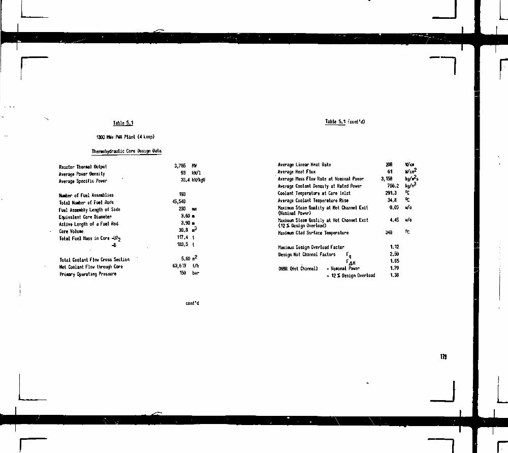
- I FTable 5.1

1300 MWe PWR Plant (4 Loop)

Theraohydraulic Core Design Data

Table 5.1 (cont'd)

Reactor Thereal OutputAverage Power OensityAverage Specific Power

Nuiber of Fuel AssembliesTotal Nurter of Fuel RodsFuel Assembly Length of SideEquivalent Core DianeterActive Length of a Fuel RodCore VoluieTotal Fuel Mass in Core -U02

-U

Total Coolant Flow Cross SectionNet Coolant Flow through CorePrinary Operating Pressure

3,765

9336.4

19345,548

2303.60

3.90

39.8117.4

103.5

5.6063,619

150

HWkW/1

kW/kgU

no•n.3tt

B2t/hbar

Average Linear Heat Rate

Average Heat FluxAverage Mass Flow Rate at Nominal Power

Average Coolant Oensity at Rated Power

Coolant Temperature at Core Inlet

Average Coolant Temperature Rise

Maximum Steam Quality at Hot Channel Exit(NoDinal Power)Maxioum Stean Qualify at Hot Channel Exit(12 % Design Overload)

Maximum Clad Surface Temperature

Maximum Design Overload Factor

Design Hot Channel Factors F .F 1 H

DN8R (Hot Channel) - Nominal Power- 12 % Design Overload

20861

3,158

706.2

291.3

34.8

0.00

4.45

346

1.122.501.651.79

1.38

K/Citfen2

kg/m2skg/m3

°C°Cw/o

w/o

*C

cont'd

179

I

F

•AH

Table 5.2

Enthalpy Rise Hot Channel Factor

. Enthalpy rise in hot channelCore average enthalpy rise

(Heat-input factors) ) * (Channel geometry andx (Flow factors) tolerance factors)

Heat-input factors:

1. F^j • Nuclear hot channel factor

In 2D representation (control rod free core):fAH"*1^xy " "acroscopic 20 hot channel factor (Table 3.f)

for stationary operation and nominal lattice parameters

2. Operational allowances (instationary flux redistributions)

Table 5.2 (cont'd)

Flow Factors

1. Non-unifor* flow distribution in inlet plenua

2. Reduced flow in higher rated coolant channels

3. Flow redistribution between adjacent channels

Channel geometry and tolerance factors

1. Fuel rod and pitch tolerances

2. Channel irregularities (guide tubes, snail water gaps)

Design targets at BOC:

F^ 41.40; FAH<1.«

cont'd

_ J

T

r

Table 5.3

Power Peaking Factor F-

p m Maximum possible pin power density1 Average pin power oensuy

(Nuclear subfactor) x (Engineering subfactor)

Nuclear subfactor

of linear pin power density

, q' (core max.)q' icons average;

Location of q' (core max.): Hot spot

Table 5.3 (cont'd)

Engineering subfactor:

Takes pellet tolerances into account

F- design Unit includes allowances for

- instationary power density redistributions (Xe, rod movements)

- control rod malpositioning

- neasurenent errors

Assuming approximate separability of radial (xy) and axial (z)distributions —•

Separation of ff"Xyz)het i n t o r a ( l i a l an(i a x i a l subfactors:

(Fxyzjhet * (Fxy) het ' Fz

(Fxy|het " Radia l P in Peking factor

fz , Haximua l i n e a | » powep densi ly

Average

cont'd

Typical values:

Steady state operation: F q

Design limit: F q

2.0

2.5

at BOC

181

112

Table 5.4 Table 5.5

Core Design Objectives and CriteriaCritical Heat Flux, W B - Ratio

Critical heat flux q"cri^(z) in height ; of a coolant channelvith fixed channel geometry and fixed inlet coolant conditionsdepends on

nass flow rate of coolant

coolant pressure

coolant temperature

enthalpy rise between channel inlet (z=Q)and height z.

Icrit

DUB

ONB-Ratio =

Design limits:

ONBR

ONBR >

obtained from empirical correlations

Departure from nucleate boiling

pritical heat flux q"crit(z5~|

[actual heat flux q"acf(z) Joccurs in hot channel

1.00 at nominal operating conditions

1.30 during loss of flow accident

I Limitations orconcequences on

Economic and technological optimization1. Flat power distribution2. Uniform discharge burnup3. Local burnup below limit

Fuel nanagetnent

Full power capability while maintaining steady state margins tofuel design limits (allowances for AOOs*^)4. Margin to fuel centerline melting5. Margin to minimum DNB ratio

Local power density, F,,Linear heat rate in hotchannel, F&H, F q

Capability to limit consequences of AflOs*' and accidents6.

7.

8.

Sufficient control rod worth(shut down margin)

Moderator temperature coeff .< 0(at full power, Xe equil.)

Fuel failure rate during LCCA**5

below limit

Design of control rod systea,core loading pattern

Soluble boron cone, at BGCBurnable poisonsCycle lengthLocal power density, Fg

*) A0O = Anticipated Operational Occurrences

*•) LOCA = Loss of Coolant Accident

_ J

Table 6.1

Reload Core Design

Fixed Conditions:

Core sizeControl rod patternCoolant conditions

Variable Conditions:

Fuel management considerations:

fiuaber and enrich/ment of fuel assemblies available for reload

Nunber of fuel assemblies to be discharged

Previous cycles:

Burnup of assemblies to be shuffled

Operator's specifications:

Cycle length

Operation mode (base load, load follow)

Qesign Objectives and Criteria

As given in Table 5.5

Table 6.2

Cycle Number Z

(Equilibrium Burnup Cycle)

T = cycle length in calender days

t • cycle length in equivalent full power days (efpd)

Oi = t/T = capacity factor

1/Z = frartion of fuel to be discharged at end of cycle

Z = average number of burnup cycles a fuel assemblywill be depleted

FJJ = averags specific fuel power /"HW/kgU_7

Bjj = average discharge burnup /~MWd/kgU_7

Z- T- <X = -!L

183

J

Table 6.3

Long Term Fuel Management

Based on equilibrium cycle concept

Range: 3...10 years

Operator's specifications:

Refueling frequency

Capacity factor

Operating node (base load, load follow)

Objective:

Result:

Burnup optimization

Number of FAs per reload batch(cycle number Z)

Feed enrichment

Use: Long tern contracts for fuel procurement

184

_l

Table 6.4

Medium term fuel management

Range: 1..3 years

Given:

Envisaged dates of refuelingUpdated capacity factorFeed enrichment

j -(Operator's specifications)

-(long term fuel management)

Objectives:

Specify number of FA's for next reload

Adjust feed enrichments and/or number of reload assembliesof subsequent batches

Use:

Fabrication of FA's for next reload batch

Update fuel procurement provisions for subsequent reload batches

Table 6.5

Short ten fuel aanagenent

Ideal cycle —•- real cycle

Range: Next cycle -

Given:Enrichment and nunber of fresh FA's available for next reload

Number and average burnup of- spare FA's and- partly depleted FA's put aside in former cycles

Capacity factorDate of refueling

Result:Preliminary shuffling scheme and loading pattern

Physics parameters (power distribution, hot channel factors,ciritical boron concentrations, reactivity coefficients,shut down margin)

Use:

Licensing application

Preparation fo shuffling operations

Table 6.6

Final reload core design

Date:

After.shut down and inspection of irradiated FA's

Time available: Few days

Given:

Actual burnup distribution at end of preceding cycle

Final decision on reinsertion of irradiated FA's.

Results:

Same as with short tern fuel management; in addition:

Data needed for evaluation of in-core detector signals during cycle

Use:

Final licensing docunent

Instructions for reload operations (shuffling sequence)

Design verification at startup

Core follow during depletion

185

^

Table Natural Cycle Lengths

Equivalent Full Power Days

Plant

Cycle No.

Calculated (0Measured (H)

(H-O/C (%)

1

507495

-2.4

KWO

2

261257

-1.5

(345 HWe)

3

298308

3.4

4

280282

0.7

5

222224

0.9

6

245242

-1.2

7

303303

0

Plant

Cycle No.

Calculated ( 0Measured (M)

(M-CVC «)

KKS (662 MVe)

1

408410

0.5

2

^ 240237

-1.2

3

275268

-2.5

4

298290

-2.7

5

334323

-1.5

KWB(A)

1

425429

0.9

1204 MWe)

2

247233

-5.7

Table 7.1

Neutron Balance in a 650 KWe PtiR, Nominal Operating Conditions, I.Cycle

Fast Neutrons Produced : 100

Neutron Lossesdue to)235

U 2 3 8 (1)

Zero Burnup

Captures! Fissions I Total

Burnup =. 19 500 llWd/t

Captures JFissions I Total

8.7 37.3 46.0 4.3

9.316.7

2.8

Pu239Pu240

S|n149

Xe 1 3 3

Fission ProdictsZircaloySteel3oronH,0Leakage-radialLeakage-axial

-

-

1.21.314.34.9

2.90.6

-12.116.7-

--

-

1.21.314.34.92.90.6

0.46.615.58.33.80.60.52.06.31.30.60.64.7

3.41.6

18.7

2.7

14.1

2.0

100.0

(1) Captures and Fissions in the Non-Kesonance Energy Region

(2) Captures in the Sesonance Energy Region

23.00.411.515.522.43.82.60.52.06.31.30.60.64.73.41.6

100.0

Table 7.2 Table 7.3

Definitions of Reactivity

Dynamic definition of reactivity:

P: Production rate of prompt fission neutronsand delayed neutron precursors

L: Rate of neutron losses due to absorption and leakage

P-L: Net production

? - p-LP

Static definition of reactivity:

keff • static multiplication factor (eigenvalue ofstatic reactor problem)

Ope.'atioru: Variables determining reactivity f (burnup fixed):

^"Control rod position'I doron cone.

j(. / Moderator tea?.I ruel ten?.I Xe cone.

Principle of a Reactivity Balance:

External

Control variables

Internalreedback variables

Operational Variables

Initial stationary

operational state

Intermediate

states and

partial transitions

Final stationary

operational state

1i*

1

1

1

x2

0

1

h

0

Q

1

h

0

0

0

1

...

0

111

Reactivity

equivalents

ANo.

...

Reactivity 3alance: A ? « X -i

201187

Table 7.4

Breakdown of Control Rod Worth Requirement in a PWR , EOC

(Reactivity balance pertaining to the transition

full power —*- hot shut down, stuck rod eondltiont)

Step

No.

1

1a

1b

2

3

4

Initial state:

Stationary, full power, control rods

in nominal position

Full power — » zero power

Fuel temp, chance (Doppler reactivity)

Moderator temp, change

Control rods out ("bite")

Control roc'3 in

(shut down worth of all rods)

Stuck rod out(stuck rod worth)

•1.3 %

+0.5 £

+0.2 %

-7.0 5!

+2.0^

?

0

+1.3*+1.8 i

+2.J»

-5.0 «

-3.0 i.

Final state:

Hot zero Power, shut down with stuck rod

Subcriticality

Kinimn required subcriticality

-3.0 ;;

-1.0 K

Shut down margin at hot zero power 2.0 I

Table 7.5

Dynamic Reactivity Coefficients

TjJJ « Moderator- (or Coolant-) temperature

yr « Fuel temperature

T « Temperature of zero power (• isotherial) reactorT ' \ - Tf

0 • Moderator density (including stean void content)

All values core averages.

hoderator temperature coefficient:

Fuel tenperature coefficient:

Moderator density coefficient

~ -void coefficient

Combined fuel and moderator coefficient

r T . rj(T() + r^ (T8)Isothermal temperature coefficient

Ff(isoth) = 1^ (T) + T^(T)

J

I

Tab. p.1

213

Evaluation of Aeroball Measurements

Subdivision of core height into 3? axial sections

Subdivision of core plane into N meshes,1 mesh/fuel assembly, N « number of fuel ass.(1300 W e plant : N . 193)« Subdivision of whole core into NX32 nodes

Nunber of aeroball probes: Nj (typically Nj • 28)

Simplified flow chart of evaluation program

as implemented on plant process computer

Activation rates

Hfi (node average)

Z^S (location of probe)

from external heterogeneous 20fine mesh calculations

( £ a * activation cross section)

cont'd

Tab.

Average PGRs (relative)in N, x 32 instrumentednodes

P-2 Table 1.4

PGR = Power Generation Rate

p.3

Interpolation strategy togenerate average node PGRsin non-instrumented nodes

Fuel ass. power ratios fromexternal 20 burnup calc.

Average node PuSs (relative)in (t'32 nodes (whole core)

i_Power shapeindices(axial, azimuthal)

Average coreburnup

^Plant heat balance(Normalization factor)

Average node PGKs (absolute)

Node burnups

Identification ofhot node

peak power density

Fq-f actor

Peak to averagepin power factors(20, precalculated)

cont'd

Peak to averagechannel power factors(20, precalculated)

Identification of hot channelHax. channel powerF& H"Factor

Coolant conditions

I DUB ratio

189

Reactor PressureVessel Core Shroud

Core Barrel

WaterReflector

Ass. withControl Rod Ass.

Fig. 2.1 1300 HWe PVRCross Section of Reactor Core and Pressure Vessel

ISO

16 x 16 lattice positions20 guide tubes16x 76 - 20 =236 fuel rods

o

o

o

o

o

o

o

o

0

o

23 cm

y

O

O

7

O

0

O

O

O

O

O

O

^Lottie• Lattice cetlwith fuel rod

Fig. 2.2

1300 MWe PWR:

Lattice Structure of Fuel Assembly

•Lattice cell with guide tube, containinga) water orbj control rod orc) burnable poison rod

_l

tr P(IJ

Region 1: Fuel (UOo)Region 2: Canning (Zircaloy)Region 3: Moderator (HgO + B + homogenized spacer grids)Region 4: Portion of guide tube cells

(HjO + B • Structural material)

/

Region 1: Absorber (Ag In Cd)Region 2: Canning (Steel)Region 3: Water gap (HoO + B)Region 4: Guide tube (Steel or Zircaloy)Region 5: Hoderator (KjO + B)Region 6: Representative fuel lattice (homogenized)

Fig.2.3 PUR Fuel AssemblyRepresentative Fuel Cell (Wigner-Seitz)

Fig. 2.4 PWR Fuel AssemblyRepresentative Absorber Cell (Wigner-Seitz)

205 191

_ J

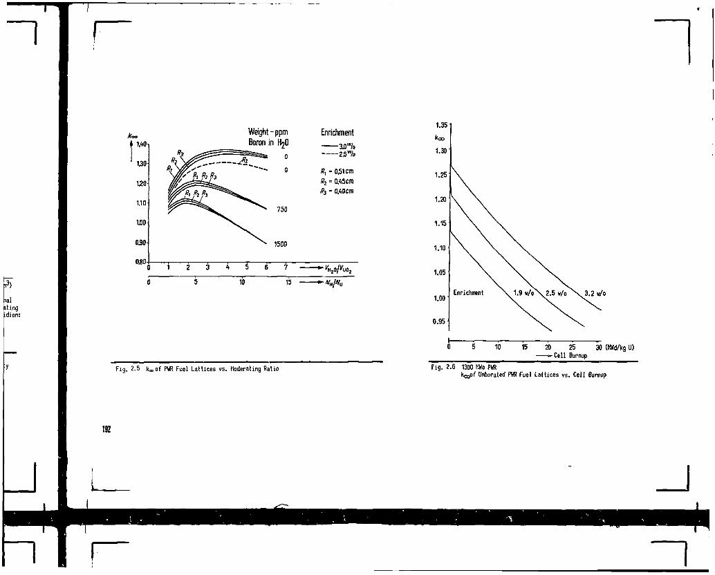
i 1,40

130

120

1.10

1.00

050

030

Weight - ppmBoron in IfyO

750

1500

10 15

Fig. 2.5 k«,of PWR Fuel Lattices vs. Moderating Ratio

Enrichmentaow/o25w/o

0,51 cm

0.«cmR3

0.95

3.2 w/o

0 5 10 15 20 25 30 (MWd/kg U)•—Cell Burnup

Fig. 2.6 1300 MWe PWRk f Unborated PWR Fuel Lattices vs. Cell Burnup

\1.096

highest-rated

1.185

1.094

1.091

1.179

1.085

V\

1.174

1.082

1.164

1.074

fuel assembly

1.090

1.158

1.054

1.134

1.194

1.179

1.057

1.093

.967

.839

1052

1.23 7

1.080

.913

1.013

.875

.532

\

.850

.661

.720

.601

1252

127(

1.290

127(

12521

Fuel

I.2S(

1.293

1.302I

11293

12S(

assembly

1.239

1.279

. — • — •

1.218

U7SI

1239

1.205

1.2(1

1.2(9

1.2(1

1205

U5,

1.153

1,3,

_ mrsh avtrogn

-highest- rated mesh

= max. mesh power

• >. 302

-idtn'iliclion at hot channel

Fny s max. total power density

x 1.310

Core

Fig 3.1

1300MWe PWR (193Fuel Ass.) BOC 1 :Normalized Assembly Po wer Distribution (118 Core)

Fig 3.2

2D Power Distribution (xy-Plane) in Highest-RatedFuel Assembly(Normalized to core - averaged power density)

5 x 5 meshes I assembly

193

\.ses

1.974

.99!

Water

filled

guide tube

\

/

/

1.003

1.027

1.02S

1.03!

o104!

1.015

/

Sector

Hot .

1.0)1

1.043

/

1.0(6

1.016

1.013

/

?od •

l.990

/

'1.025

o1.013

1.026

o

7.973

.949

1.01}

.990

.99*

1.007

.SSI

.962

.963

.97*

.97<

.973

.972

.965

.954

. 7.10

rations

Fuel Assembly

Pin Power Distribution =Hocogeneous Power Distribution * Pin FactorIdentification of Hot Rjd — » - Max. Pin Power

Fig. 3.3:

Pin Factors in PWR Fuel Assenbly (Exanplo)

(Heterogeneous Fine-tiesli Calculation,

based on Collision Probability Method)

\\

1.2071.191+1.6

1.2131.198+15uie1.205+U

1.3291.303+2.61.228.1.212+1.S1.2091.196+1.3

1.265U67-0.21.2691.273-0.41.1861.174+ 1.21.2321.215+1.7

1.1431.132+1.11.1331.121+U1.1881.171+1.71.0991.089+1.0

1.1491.132+1.7

1.0020.998+0.41.0491.040+0.90,9570.962-0 .50.9790.978+0.10.9610.982-2 .11.03S1.101-1 .3

1,0040.999+0.50.9570.988- 3 . 1

0.8630.900-3 .70.7660.773-0 .7

0.8040.828-2,40.6070.617-1 .0

0.8S60,845+2.1O.B40O.B22+ 1.8

0.7430.735+0.80.5G40.518-1.4

(1) Measurement(2) Thewy(1-2J-10O

Fig. 3.4 Biblis A, BOC 1, Full Power Radial Power Distribution (Assembly Averages)

194

_l

Axial Power Offset =(Power generated in upper half of the core) -(Power generated in lower half of the core) : (Total power)

q (z) Linear Power Density(Power per Unit CoreHeight)

Bottom

Axial Power Peaki-g Factor: F =

1: Cosine2: Saddle shaped3: Peak in Upper Core Half4: Peak in Lower Core Half

core-average

Aeroball activationrelative1.5-

1.0-

0.5-

oBesinning•End

of cycle1

•2***

' 4\ *\

'•+. ••

Fuel assembly K11

t t \ Spacer grids

top 1.0 0.8 0.6 0.4 0.2• * - — Fractional core height

• Burnable poisons

0 bottom

Fig.3.5 Types of Axial Power ShapesAxial Power Shape Indices

Fig. 3.6 KKS, Cycle 1, Axial Power Distributions

195

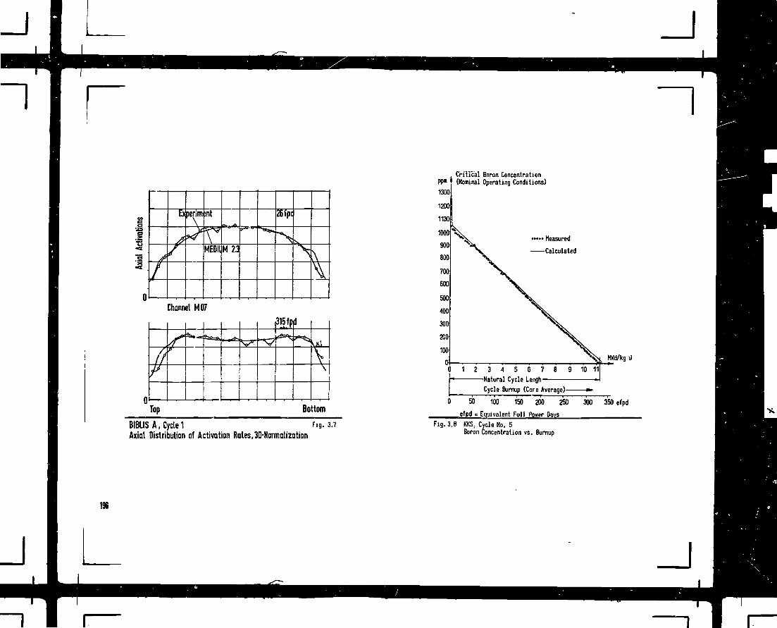
a

/

Ex

/

>enm sit

MEDIl M2i

ftfpi

\ \

if

Channel MO7,315 fpd

\\

Top Bottom

BIBUSA,Cycte1 Fig. 3.7Axial Distribution of Activation Rates,3D-Normalization

196

ppl

1300

1200

1100

1000

900

800

700

600

500

400

300

200

100rv0

0

Crit ical(Noninal

1 2

50

efpd =Fig. 3.8 KKS. C

Boron

Bnran ConcentrationOperating Conditions)

••••• Heasured

t Calculatedx\

xx^ ^ HWd/kgU

3 4 5 6 7 8 9 10 11ii-i 1 r..-i_ i 1.

Cycle Burnup (Core Average) m-

100 150 200 250 300 350 efpd

Equivalent Full Power Davsycle No. 5Concentration vs. Burnup

Enrichments: 1.9 2.5 3.2 W/. U 235

Control Rod. Pos." 1 2 J Burnable Poison Rods 'L

Fig. 4.<

1300 MWe PWR,Cross Section of Initial Core

1.9/ 0.999

2.S/H1.010

1.9/0.999

1.9/0

.999

2.5/81.010

1.9/0.999

2.1/S

1.010

1.9/0.999

2.S/S

1.010

1.9/0

.99B

1.9/ 0

.999

is/a1.010

1.9/0.999

2.5/8

1.010

25/0l.Ott

2.5/a

IJOW

1.9/0.9S9

2S/B

1.010

1.9/0

.999

131892i

3.2/0

1.163

23/0

lose

2.5/81.010

13/ 0.SS9

3.2/9

1WS

3.1/01J63

32/ a

1 09*

3.2/81091

3.2/01.163

3-2/ t

!.O9<

3-2/0

1.163

Pnncipol

Symmetry Axis

(2)

\

(1) Fuel enrichment £w/ojI Number of burnablepoison rods per fuel assembly

(2)Assembly -wise multiplication factor k <*>(full power. Xe- equilibrium!

Fig. 4.2

ISOOMWe PWR. Beginning of First Cycle:Radial Distribution ct Fuel Enrichment. BurnablePoisons and Multiplication Factor k o»

197

Enrichment/Burnable Poison Rods

11.9/012.5/811.9/d2.5/8| -|.9/d2.5/8l2.5/0|3.;

Principal Axis-

Core Center Core Edge-

Fig. 4.3 1300 HWe PVR, 80C 1Spatial Variation of Flux, Power and

196

1.091.01

(1)(2)

tie1.10

1.081.01

1.06tot1.171.10

1.091.02

1.171.11

1.081.02

1.161.12

1.071.04

1.081.03

1.1S1.12

1.05I.Oi

1.131.H

1.201.15

Beginning f

•.na ^

1.181.13

1.061.03

1.09112

.971.03

.84.98

1.061.07

1.241.10

1.081.08

.9237

1.021.09

.88.92

.54.62

.86

.04

.89.86

.72

.79

.61

.67

(1)(2)

Fig. 4.4

1300 MWe PWR. First Burnup CycleNormalized Assembly Power Distribution(Full Power. Xe- equilibrium)

J

Theory-Experiment (%)

1.3

1.2

1.1-

1.0

Hacroscopic Hot Channel Factor(5x5 meshes per fuel ass.)

50 100 efpd—*- Cycle Burnup

-0.8•1.8

1.0

2.1

2.1

2.9

0.8

as

1.0

05

1.2

(13

33

07

•ID

-1.0

-2A

-1.2

-1.6-2JJ

-1.0

-23

-12

•0B

•10

-1.6

/09

0

-2D

-1.8-1.8

BIBLISA.B0C297.7 % Power, Xenon-Equilibrium o -1.7 %Theory: MEDIUM-2, 2D, 9Box/Assembly

clppm]

ExperimentMEDIUM 23 (A)

Fig.4.5 1300 HWe PUR, 1. Cycle r i g . 4.6 Comparison of Predicted Aeroball Activations with BIBLIS A Fig. 4.7H p i c Hot channel Factor vs. Cycle Burnup Measurement Critical Boron Concentrations vs. Average Core Burnup

139

Correspondencebetween

Nuclear and Thtvmohydrauttc

Analysis

oooooo

l i n t lattice cel l

Nuclear po*erdensity (r.Vl)Une?r heat rate (W/cn)

Equivalent hoEogenized

cross sectio.is

Coolant Subchannel

Heat flux

Coolant conditions

Temperature -i

P r e s s u r C

Density j

Steaw content''Fuel tecperatureCi?(Mino. temperature

Vj

tnthatpy

2M. 4

Coolant temprise A T

Enthalpy rist &H

0 •*— f

Channtl outlet

-Coolant massflow ratt

—Linear heat generation *_jrate q'U) I W/cm)

Channel power

-Coolant Channel

Channel inlet

dz

Hot Channel: Max. AHAverage Channel: Core average AH

Inner Clod Temperature 1

Outer Clod Temperature [ in HOT CHANNEL

Coolant Bulk TemperatureJ

Bulk Temperature in AVERAGE CHAMJEL

Saturation Temperature

Nominal Power

Over-Power

feedback interaction

g. 5.1.Fig. 5.2 Coolant Channel Fig. 5.3 Axial Temperature Distributions

200

HMt Rux q"IW/on2)

Fig. 5.4 Margin against DNB in the HOT CHANNEL

A

1.5

1.0100 200

Fig.5.5 Hot Channel Factor ^ vs. Burnup

?2.0

1.5

1.0100 200

Fig. 5.6 Power Peaking Factor Fq vs. Burnup

KCB Cycle 2KCB Cycle 3KCB Cycle 4KKS Cycle 3KKS Cyrle 4KKS Cycle 5KKS Cycle 6

300-efpd

400

t A A* *^* a *

* •» * • *

» KCB Cycle 2

• KCB Cycle 3• KCB Cycle 4

• KKS Cycle 3« KKS Cycle 4o KKS Cycle 5

°* • KKS Cycle 6

300 400efpd

20I

Fabrication

Fresh FuelStorage

Reactor

IrradiatedFuel Storage

Reprocessing

RefuellingNo.it

O

FuelDisposition

--T~"rzb

RefuellingNo.n+1

1 T

- T -•

W//W/M

Fig. 4.1 Incore Fuel Management Scheme, Ideal Equilibrium Cycle

202

5 = 33.0 MWd/kg(A= average discharge burnup)

lCore with 157 fuel elementsZ =3.925

-5 -3 -1 A A

Fig. 6.2 Percentage of the fuel elements vhose discharge burnupexceeds A

_J

39.3 22.0

32.2

33.4

21.1

36.6

23.2

23.8

22.3

24.9

AverageAssemblyBurnup fiiWd/ kgUj

22.7

32.4

34 A

20.3

31.2

34.0

14.1

34.6

24.5

34.5

12.2

32.5

25.3

32.4

13 2

103

7.9

9.6

9.9

9.6

e.t

Shuffling

Scheme

Fig 6.3

1300 MWe PWR.

End of Burnup Cycle 8

(193 FA ) (Equilibrium Cycle)

Cycle number 3.016

31.2 9.0

20.3

22.0

0.1

24.9

BOC

9.9

10.9

9.6

12.2

AverageAssemblyBurnup [MWd/kg uj

9.9

21.1

23.0

7.9

20.3

23.2

0

25.3

13.2

24.5

0

22.7

14.1

223

0

0

0

\

0

0

0

0

-4

.66

.001.161.10

1.051.01

Fxy (B0C)*1.39 «Fxy(BOC)' 1.26 0

NormalizedAssembly PcDistribution

Fig. 6.4

1300MW* PtoEquilibrium I

1.071.00

1.2 SUS

1.01.97

liver

SiBurnup

1.311.16

1.251.13

1.211.13

1.101.13

Cycle

1.221.14

1.00.Si

.50.9*

1.131.14

.«7.55

.55.57

1.29

.02

.91

1.001.04

.02

.09

1.091.09

.02

.91

.961.01

.04.91

1.20US

J99.57

.65.72

\

.03.91

.05

.91

.63

.00

.70.73

~BOC•+EOC

213

Fabrication

Fresh FuelStorage

Reactor

IrradiatedFuel Storage

Reprocessing

RefuellingNo.n

FuelDisposition

Sft^4

RefuellingNo.n+1

%

Critical Boron Concentration

1500

ppm

1000'

500

KKSCycles 1-3Full PowerXt-Equil. i

V

• Meowed

— Cokulottd

' 0 2 I 6 « » 12 1410 12 V, 16 B 12 14 1 S U 20 MVWAg— Average Con Burnup

Critical Boron Concentration

C 1500 KKSCycle) t - 6Full PowerXc-Equil. Hcatured

Calculated

500

' » 12 U 16 18 2010 12 14 16 » 2tU2 U B W 20 2

—— Average Core Burnup

Fig. D.5 Incore Fuel Managenent Scheme, Real Cycle Fig. 6.6

214

J

rftKuOfl 4f AlMttlDNCS

40-

20-

Cak.Mess.

ReactorStait Voriabln(Coir Averages)

ReactivityEquivalents

ExternalPerturbancnS

*i

! ! I! I!10 15 20 25 30 35 MWd/kg

— Discharge Bumup (Assembly Average)

ivity (control rods, boron)

Power T(HReactor

Point KineticModel

internal —feedback

externalteedbockIrom plant model

/

Fig. 6.7

KM: Frequency Distribution of Discharge Burnup (Reload Assemblies, Dischargedafter Cycles 3 - 5 )

Point Kinetic Model with Feedback

205

-2

-1-

0.8

«)

0

Rtactivity

External

50 100 « of nominal

Average Fission Power Density(relative)

value; 500

E (s)Time

-5

0.6

Void Formation •

Cell burnup 0.1 HWd/kg U 18oron Cone. 1000 pptn }

Cel l burnup 14.2 MWd/kg U 1Boron Cone. 0 ppm ]

—NominalOperatingCondidion;

BOC

EOC

Fig. 7.2 Fuel Teiperature Coefficient Ty vs. Fig. 7.3 PW

Average Linear Heat Rate q1 T y p i c a l Response t o a U i"9 e S t e p l n c r e a s e o f R e a c t i v i t *

Fig. 7.4 PWR Fuel Lattice, 2.5 w/o U235Cell Reactivity9oo= (koo-D/kco vs. Moderator Density

206

_l

Fig.7.5

1200 :iWe PHR, 1. Cycle, Nominal Operating ConditionsHoderator Temperature Coefficient^ vs. Boron Cone, c

c

(ppm)

14004

1200

1000

Critical Boron Cone, (all rods out)

BoronEquivalents

Ac

100 200 (efpd) 300"-Cycle 8urnu|)

Boron equivalents: 1: Burnup reserve2: Transition fu l l power—zero pwer

( fuel - ind coolant temp.)3: Equilibrium Xe4: Transition hot—cold

Fig. 7.6 1300 KWe PWR, equilibrium burnup cycle, zero power, without Fig. 7.7control rods, without Xe iinn HV/P PWBIsothermal Temperature Coefficient TT (isoth) vs. ™ ° ™J ^ O n ? o n cTemperature T Cycle Bupnup

EquivalentsAc vs.

207

- Is (pcm/crn)

70

60

50

30

20

10

0

Experiment

-MEDIUM 23.

2

1QG 200 300 383 s{cm|

9 s ! L *D) l7o )

Experiment-MEDIUM

1200

400

100

ARO

200 \ 3 0 0 TM('C)

100 200 300 383 s|cm}

Differential Rod Worth, All RodsBIBUS A , DOC 1 , Zero Power, TM-288'C

Fig. 7.8 Integral Rod Worth, AU Rods Fig. 7.9 BIBLISA, Cyc le i . Zero Power F19.7.10BIBLIS A . 80C1, Zero Power, TM-26B°C Critical Borcn Concentrations c8 of Control Rod Configurations

as a Function of Moderator Tsmperature

288

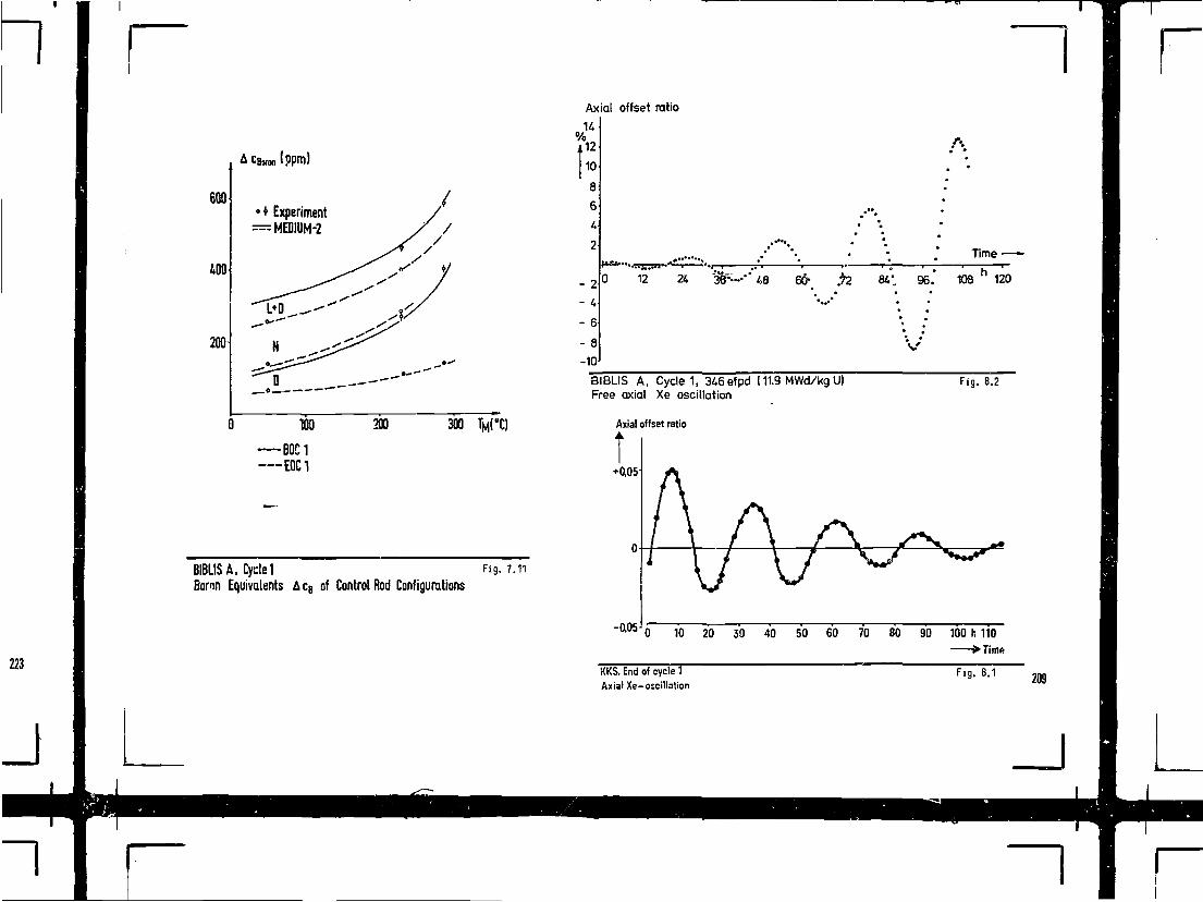
600

100

• * Experiment— MEDIUM-2

100 200 300 TMCC)

— B0C1EQC1

BIBLISA, Cycle 1 Fig. 7.11Boron Equivalents A cB of Control Rod Configurations

Axial offset ratio

14

°12

10

8

6

4

2

- 2

- 4

- 6

- 8

-10

Time •

0 12 24 ~36r»"'" 48 60* .72 84". 96. 108 120

BIBLIS A. Cycle 1, 346efpd [ 11.9 MWd/kg U)Free axial Xe oscillation

Axial offset ratio

Fig. 8.2

-0,05 0 10 20 30 40 50 60 70 80 90 100 h 110

KKS. End of cycle 1Axial Xe-oscillalion

Fig. 8.1 209

Quadranttilt difference

+0,05

-0,05-

-0.10

-0.15

A

V10 20 30 40 50 60 70 80 h 90

•Time

Biblis A beginning of cycle 1

Azimuthal Xe-oscillationFig. 8.3

\Nuclide Densities}

CrossSections

IterativeFlux Calc.

PowerDensity

ThermohydrauiicIteration

Fig

Fuel Temp.

Moderator Temp.Moderator Density

Burn upDistribution

Average power density and

Coolant U Moderator) inletconditions

set by external controls

Thermohydrautic Conditions

Iterative Calculation of Power Density and Burnup Distribution210 with Thermohydraultc Feedback

1.5

1.0

0.5

Assembly Power(relative)

withoutDoppler Feedback

Radial Core Traverse'

Control Rods(Irregular Configuration)

F ig . 8.5 1300 MWe PWREffect of Local Doppler Feedback on Radial PowerDistribution

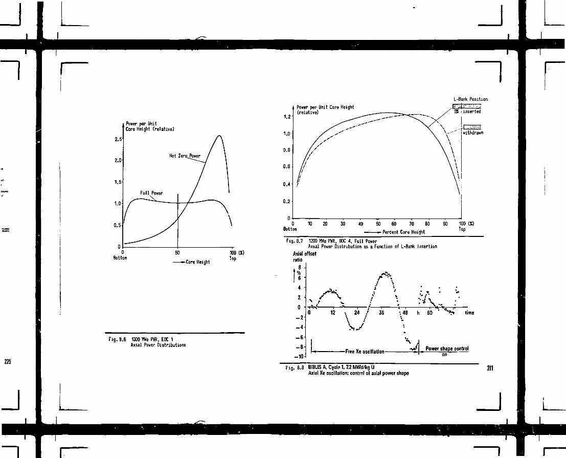
L-Bank Position

Power per UnitCore Height (relative)

2.5

2.0

1.5

1.0

Core Height

Fig. 8.6 1300 KWe Pffi, EOC 1Axial Power Distributions

1.2

1.0

0.8

0.6 -I

0.4

0.2

Power per Unit Core Height(relative)

0 10 20 30 40 50 60Bol to in — — - P e r c e n t Core Height

70 80 90 100 IX)Top

Fig. 8.7 1200 MWe PWR, BOC 4, Full PowerAxial Power Distribution as a Function of L-Bank Insertion

Axial offsetratio

6

4

2

0

- 2

- 4 -

- 6

- 8

-10-1

A• *«.—i •• 1 r 1 «—r-

12 •. 24 / 36 -.48 h 60 ' "** «me

Power shape control-Free Xe oscillation-

F ig. 8.8 BIBLIS A. Cycle 1,72 MWd/kg UAxial Xe oscillation; control of axial power shape

211

///

\\

\

/

Xd

\

/

Hid

>

\

/

\

d

s

y

\s

>

f

s

/

\

s

/q?«

\

!N

P

/•

\

N

>

\

V

/

\\\

//

/

Instrument lance

. Aeroball probe

Lance yoke

Self powered detectors

Lance shaft

Fig. 9.1 1300MWePWRIn-core Instrumentation (planar view)

212

CABLE DUCT.

INSTRUMENTATIONPORT

YOKE

REACTOR .. R/fPRESSURE VESSEL t | i

PROBE

PROBE ASSEMBLY

Fig.9.2 !n-core Neutron Flux Measurement System

COUNTERDIODES MEASURING BAR

MEASURING BAR

EACH 4 TO 8

. ! . EACH « TO 8

PROGRAMMING

MEASURING TABLE WITHAMPLIFIERS

AIR CONDUITSTO VALVE SUPPORT / - , \

A BCD

F ig . 9 3 Aeroball System Fig . 9.4 Aeroball Measuring Lievice

213

L

1 r

L

REACTOR PHYSICS ASPECTS OFCANDU REACTORS

E. CRITOPHAtomic Energy of Canada Limited,Chalk River Nuclear Laboratories,Chalk River, Ontario,Canada

ABSTRACT These four lectures are being given aT the Winter Course onNuclear Physics at Trieste during 1978 February. They con-stitute part of the third week's lectures in Part II: ReactorTheory and Power Reactors.

A physical description of CANDU reactors is given, followedby an overview of CANOU characteristics and some of the designoptions. Basic lattice physics is discussed in terms of zeroenergy lattice experiments, irradiation effects and analyticalmethods. Start-up and commissioning experiments in CANDUreactors are reviewed, and some of the more interesting aspectsof operation discussed - fuel management, flux mapping and con-trol of the power distribution. Finally, some of the charac-teristics of advanced fuei cycies that have been proposed forCANDU reactors are summarized.

A. A PHYSICIST'S GENERAL VIEW OF CANDU REACTORS

A.I DEFINITION AND HISTORY [1.2]

229

A CANDU* reactor is a heavy-water-moderated power reactor of thegeneral type developed in Canada by Atomic Energy of Canada Limited (AECL).There are other types of heavy-watei—moderated power reactors, bi't thesewill only be mentioned in passing.

It is somewhat of an accident of history that Canada focussed all hernuclear power development effort on heavy water reactors. During the SecondWorld War. as part of her involvement in military nuclear programs with theUS and UK, Canada took responsibility for heavy water reactor development.After the War, when civilian nuclear power was being considered, It wasnatural for Canada to pursue development of a reactor type for which she hadacquired some experience.

CAMDLJ nas- often been referred to as a physicist's reactor, due to thescientific elegance of the concept and its dogged adherence to fundamentalprinciples, I sense that this reference is used by some in a derogatoryway, but the current economic competitiveness of CANDU with other types of

•CANDU signifies a Canadian design using deuterium oxide (heavy water) asmoderator and uranium as fuel.

power reactors, ensures that it has appeal in the hard commercial world aswell as merely to physicists. It is interesting to speculate as to whetherthis illustrates a general principle. In our complex modern world it isoften difficult, if not impossible, to anticipate at an eat iy stage In thedevelopment of a project just how well the final product will compete. Byobserving fundamental physical principles (e.g., neutron economy) the chancesof eventual success can perhaps be maximized.

Before describing in more detail a typical CANDU reactor system, I wi11point out a few of the important distinguishing characteristics and features(Figure A-l).

Neutron Economy

While the CANDU concept can be adapted to enriched fusil ing, theorig-inal target was a system which could be operated competitively using naturaluranium as the fuel. In order to achieve this objective, a great deal ofattention had to be paid to neutron economy in the choice and use of corematerials and in the mode of operation.

Pressure Tubes

The CANDU concept is based on the use cf pressure tubes rather thana pressure vessel.

The reactor consists of an array of pressure tubes, generally arran-ged in a square lattice, which pass from end to end through a large cylin-drical tank. The reactor fuel resides inside the pressure tubes and thecoolant is pumped through them to cool the fuel. The fact that the coolantis at a high pressure gives rise to the term pressure tube.

While it would be possible to use a pressure vessel concept similar tothat used for a PWR, the vessel required would be considerably larger,because the required volume of D20 moderator is much larger than the volumeof H20 moderator in a PWR. In fact, early development of the CANDU conceptwas based on a pressure vessel approach. Since the limit on size of nres-sure vessel that could have been manufactured in Canada at the time wouldhave placed a limit on unit capacity, and since the development of a lowneutron cross section zirconium alloy had proceeds tu the point where thismaterial could be used for pressure tubes, the pressure tube concept wasdeveloped and adopted.

Separate Moderator

The heavy water moderator is held in the large cylindrical tank, calledthe calandria, that surrounds the pressure tubes.

Because the coolant, and hence the pressure tubes, must operate at hightemperature in a power reactor, and because it is desirable to operate themoderator at low temperature, the pressure tubes must be insulated from -"hemoderator. This is done by introducing a second tube surrounding the pressuretube but separated from it by a stagnant gas space. This second tube, thecalandria tube, is sealed at both ends to the calandria end plates or tube

215

_J

sheets, thereby completing the moderator containment. With this arrangementthe fuel coolant is completely separated from the moderator, permitting achoice of coolants.

There are several advantages of operating the moderator at low tempera-ture, as follows:

(a) the calandria can operate at atmospheric pressure, avoidingThe "?Rd for a heavy, hiph-pressure vessel,

f b) the co I d moderator cai1 act as a valuable heat sink undercerta in accident conditions,

(c) since the moderator is cold it c?nnot add to the energy tobe controlled under accident conditions, and

(d) the overall neutron economy is better.

On-Power Fuel I ing

The pressure tube approach lends itself to on-power refuelling, sincethe fuel residing in individual pressure tubes can be changed without affec-ting the other pressure tubes or the fueI in them. On-power refueI I i namaximizes the attainable burnup, since only a nominal excess reactivity isrequired at equilibrium. The reactivity gained by the continuous replace-ment of old fuel by new compensates for the genera I decrease i n reac t i v i ty«v i th f ue I i rrad iat ion.

A.2 STATUS OF CANDU REACTORS [3]

As mentioned previously, a choice of coolant is possible in the CANPUconcept. In general, attention ^zz focussed on three coolants - prcssuri/edneavy water (PHW), boiling light water (BIW) and organic (OCPl. Of these,only pressurized heavy water has been used so far in commorc id I -s i .'e unitb.•Joi I ing I ight water has been demonstrated in a 250 MWe prototype powerreactor at Gentilly in the Province of Quebec (0-1), rjnd organic h^s been.oed in a 60 MWt reactor fcxperiment at the whiteshell Muclojr Poscdrch E J I -iblishment in Manitoba (WR->^.

Table A-l summarises the current s!\)tus of CUIUU realtors in operation,under construction, committed and planned.

A,3 PHYSICAL DESCRIPTION[1.2]

216

I n o r d e r t o a p p r e c i a t e t h e r e a c t o r p h y s i c s o f r<Ulf ' ' '<•> i t - i s h r l c f u l t ,n i v e a g e n e r a l p h y s i c a l p i c t u r e o f tftc s y s t e m , ' ' r i o f d * 1 rr\\ t i o n o o f 1v*o~ A ! * J D U d e s i g n s - a C A N D U - P H W a n d d O k ' j U - H L W - aro n i v o n i n t h i r j s e c t i o n .

C A N D U - P H W

The CANDU-PHW is the pressurised neavy witer cooled vor^iun of CANDl'.• Life this version has a I way; employed .i horizontal reactor ^^.ro oriont-

• i , .-n (i.e., the pressure tube axes arc hori <ronti I ). Vortical nr i f-n t i tici.

have been studied several tines but no clear incentive to switch identified.For this description the units of the Pickering Nuclear Generating Stationwill be used as an exampIe.

For completeness, a schematic arrangement of the who Ie system i s showni n F igure A-2.

Pressurized heavy water coolant at a pressure of 9.9b MPa (-1440 psi)and a temperature of 249°C is supplied to each fuel channel (an assemblyconsisting of the zirconium alloy pressure tube with an alloy steel fittingattached ar each end) via an individual pipe, called a feeder pipe. As thecoolant passes through the fuel chanr.e-! <+ picks up heat from the fuel andleaves the channel ,-Wth a temperature of -294°C. It is conveyed to the

outlet header via the outlet feeder pipe. From the outiet header, thecooiant flows through the boiler heat exchangers where it is cooled backto 249°C, its heat being given up to produce stean at ~4 MPa (600 psi)rth ici is fed to the turb i ne. "ihe cool ant then enters the c i rcu I at i ngpumps which deliver it to the inlet header and, thence, to the inleTfeeder pipes.

A separate auxiliary circuit is employed to circulate the heavywater moderator through external heat exchangers. These reject to thestation cool ing water the heat generated in the moderator by the slowingdown of the neutrons, by the effects of -^-radiation, and also the heatleaking into the moderator across tne insulation qaps between the calan-dr i a tubes and the pressure tubes..

Figure A-3 is a better view of the major reactor components. Theseinclude the calandria with integral end snields and peripheral internalthermal shields, the dump tank with connections to the calan.dria, theholiun cover CMJ system connections, and the fuel channel assemblies andconnected feeder piping. The pressure tubes in which +he fuel sits, arelocated within 390 calandria tubes, spaced on ar. 11.25 in. square lattice,and are supported on slidina bearings in the end shields of the calandria.

nolow the ca'anoria, rind connected to it, is the cylindrical dumptank. Uur i no operrit i on t he he I i um in the dunp tank is he I d at a pressurein excess of lhat in the top of the calandria by an amount equal to thehpinht t f heavy water above the gas-liquid interface. When the heliumpressuro 3bove the moderator in the calandria and that in the dump tank aremade enuaI by i nter-connect ion, the moderator i s dumped by grav i ty i nto thedump tank, shuttinn down the reactot . In later designs this dump tankfeature has been replaced by alternative shutdown systems.

AI| react ivity ccntrol and shutoff mechan i sms penetrate the reactorf r.jr, t he top c<f the caIandrI a and are shown schematics M y in F i gure A-4.

Tho I." adjuster rodb ore designed to shape the thermal neutron fluxaistrimtion in the tore so that design limits en individual channel poweror bundle power jre not exceeded during normal operation. The rods arenormally fully inserted, providinq a load of 2 percent Ak/k. This providessufficient positive reactivity upon withdrawal to compensate for the xenonbuildup during the first *\b minutes (at least) following a shutdown fromfull power. Thu effective absorber is cobalt and the product is useful.

The zone control system consists of 14 individually adjustable com-partments which can be filled or emptied with light water, and providesspatial control of the power distribution. The system provides Independentcontrol of 14 zones in the core, preventing development of xenon-inducedflux distortions, and is also used for bulk control, by adjusting the levelof all compartments in unison. Measurements from the in-core detectors ineach zone provide the basis for changing levels.

II gravity-fall shjtoff rods are provided as the primary protectiveshutdown system. They are augmented by the moderator dump system.

Figure A-5 is an illustration of one of the 390 fuel channels. Thepressure tubes have the following parameters.

Minimum InternalDiameter

Minimum Wai 1Thickness

Approximate Length(trimmed for instal-lation)

Material

Units I and 2

103.4 mm(4.07 in.)

4.99 mm(0.1965 in.)

6.3 m(20 ft 8 in.)

Units 3 and 4

103.4 mmC4.07 in.)

4.06 mmCU.I60 in.)

6.3 m(20 -ft 8 in.)

cold drawn Zircaloy-2 zirconium 2.5?!autoclaveo at 400°C niobium cold drawn,

stress relieved at400°C.

Zirconium 2.5% niobium is the preferred pressure tube material, butthere was insufficient experience and data to use it in Units I and 2.

Fuel for the reactor is in the form of fuel bundles as shown inFigure A-6. Each bundle is 495 mm (19.5 In.) long, and consists of 28hermetically sealed elements containing compacted and sintered pellets ofnatural U02 in a thin (0.4 mm) Zircaloy sheath. The elements are about15 mm diameter and are attached mechanically at their ends to form a bundleabout 102 mm in diameter. A small space is maintained between the e I orientsby spacers attached to the element cladding. The bundle is 92 wt$ U02 and8 wti? Zr (sheaths, end-caps, structural end plates, and spacers). Thestructural material accounts for only 0.1% of the thermal neutron crosssection of the bundle, to give a fuel assembly thax is highly efficient inits use of neutrons.

Loading of new fuel into the reactor and removing spent fuel is carriedout vn-power by two co-ordinated fuelling machines (one at each end of thereactor) controlled from the station control centre. Fuel bundles are movedin opposite directions in adjacent channels, referred to as bi-directionalfuelling, to achieve an axially symmetric neutron flux distribution. Thecoolant flows in the sane direction as the fuel movement on refuelling andhence flows in opposite directions in adjacent channels. There are twelvefuel bundles per channel, and any even number of bundles can be replacedduring one refuel I ing visit.

CANDU-BLW

The CANDU-BLW is the boiling Jjght water cooled version of CANDU.For this description the Gentilly-I reactor wiii be used. GentiI Iy-1 usesa vertical orientation, i.e., the axes of the pressure tubes are vertical,and the coolant flows th~ough the reactor in an upward direction.

Figure A-7 is a schematic illustration of the concept which employsa direct cycle. Ordinary water is pumped to the bottom of each fuel channelvia an individual feeder pipe. As the water passes upward and absorbs heatfrom the fuel, a fraction (=18*) is evaporated to steam. The resultingsteam/water mixture flows to a conventional steam drum where the steam andwater are separated. The steam flows to the turbine and the water, mixedwith incoming feedwater in the drum, flows down to the circulating pumps,completing the cycle. The moderator cooling system is basically the sameas for a CANDU-PHW.

The major reactor components are shown in Figure A-8. From thephysics point of view, with the exception of the different coolant, thegeneral concept is very similar to the CANDU-PHW. Some of the differencesin detail will be mentioned.

The fuel channels are divided equally between two separate heat trans-port circuits. This reduces the severity of a loss of coolant accident,assuming the failure of only one of the circuits.

Reactivity control and shutdown mechanisms penetrate the calandriaboth vertically and horizontally. Control absorbers, injection shut downnozzles and in-core flux-monitor tubes enter vertically through the toptube sheet on inter-lattice positions. Booster rods penetrate the calandriahori zontalIy.

The booster rods, containing enriched fuel, repiace the adjuster rodsin the CANDU-PHW as far ab providing xorcn over-ride after a shutdown isconcerned. The adjuster rod function of radial shaping of the power dis-tribution is achieved in G-l by two zone differential refuelling - fuel ina central region is taken to higher burnups than fue* in the outer region.

Shutdown is by moderator dump backed up by a poison injection systemwhich provides rapid insertion of a highly absorbing liquid poison intothe moderator.

Solid absorbers, rather than the liquid water zone control chambersmentioned under CANDU-PHW, =are used for zone and bulk control.

The major pressure tube parameters are summarized below:

Minimum Internal Diameter: 103.2 mm (4.064 in.)

Minimum WaIt Thickness: 2.29mm (0.09 in.)

Approximate Lengih: 5.62 m (18 ft 5 1/8 in.)

Material: Heat-treated Zirconium-2.5* Niobium

217

The fuel for the reactor is in the form of bundles, with an outerdiameter of 102.4 mm. Each bundle is 495 mm (19.5 in.) long and contains18 fuel elements arranged in inner and outer rings of 6 and 12 elements,respccrively, about an unfuelled central position. This central positionis occupied by a tubular tie-rod which holds together the complete fuelchannel charge of ten bundles. The individual fuel elements consist ofcompacted and sintered natural UO2 pellets contained in thin (=0.5 mm)Zircaloy tuL-ular sheaths -19-7 mm (0.78 in.) outside diameter.

Fuel changing for the reactor is on-powev and is accomplished bya single fuelling machine which couples to a lower fuel channel end fittingand replaces the complete charge of fuel in the channel. Fuel bundles maybe re-inserted later into the sane or other channels and may occupy anyaxial position in the inserted fuel string.

A.4 AN OVERVIEW OF CANDU CHARACTERISTICS E4'5'6'7]

In this overview of CANDU characteristics, Pickering reactor unitswill be used as an example unless otherwise stated.

Critical Size and Reactivity

Measurements have been made of the buckling of cold, clean latticesof simulated Pickering fuel channels and the results are shown in FigureA-9 as a function of hexagonal lattice pitch. From these it can be seenthat, for a hexagonal lattice pitch of 30.7 cm (which corresponds to the28.575 cm square lattice pitch in Pickering), the buckling is about 3.8 m"2.This means that a bare critical cylinder with minimum volume would have aradius of about 1.5 m and a height of 2.8 m, giving a volume of 20 m3.

The actual Pickering units are, of course, not simple bare cylinders.The 6 m long fuel rods are enclosed in the calandria which has a radius of*4 m over most of its length. [There is a small st.jp decrease in calandriaradius at both ends.3 The 390 fuel channels on a 28.575 cm square latticepitch give an effective core radius of 3.184 m. The space between thisradius and the calandria is occupied by heavy water, to form a radialreflector. The geometric buckling of this arrangement is 0.65m-2, whichwould correspond to a minimum bare cylindrical volume of 283 m3.

This extra size provides about \0% CAk/k) in excess reactivity abovecold, clean critical. This excess reactivity is allocated approximatelyas in Table A-ll.

Neutron Spectrum

The neutrons in a CANDU reactor have a we I I-thermal 1 zed energy spec-trum. In fact, the spectrum is thermal enough that quite accurate esti-mates of reaction rates can be made using the approximation of a Weetcottspectrum* i.e., a neutron spectrum characterized by only two parameters,Tn and r. In this approximation, the thermal part of the spectrum is

assumea to have the form of a MaxwelIian distribution with a temperature,Tn (usually referred to as the neutron temperature), and the epithermalspectrum is assumed to have a I/E form, A joining function is also speci-fied to give a smooth transition between the two. r is approximately theratio of neutron density in the epithermal part of the spectrum to thetotal neutron density.

Typical values for these parameters in the fuel of a CANDU reactoroperating under standard operating conditions are: T n - 200°C, r = 0.045.

With this convention, effective cross sections for materials areexpressed in the form:

0 = ao tg + rs)

where a is the Westcott cross section,

ao is the 2200 m/s cross section,

g,s are tabulated for materials of interest asa function of Tn

Neutron Balance

In order to get a reasonable burnup with natural uranium fuel, greatcare must be taken not to waste neutrons. If l£ more of the neutrons couldbe made available to compensate for burnup effects, the burnup could beincreased by some 17*.

Table A-III Summarizes trie statistical fates of 1000 typical fastneutrons in a CANDU reactor operating under standard conditions with anequilibrium core. Note that the 1000 neutrons with which we start areassumed to be below the fast fission threshold En U-238. The value ofthe fast fission factor is about 1.027.

There are several interesting points which the table shows. Forexample, it can be seen that a very significant fraction of the power comesfrom fission in fissile plutonium isotupes. One can also estimate theConversion ratio by taking the ratio of U-236 plus Pu-240 absorptions toU-235 plus Pu-239 plus Pu-241 absorptions. The result is 0.73, althoughthis estimate is a bit low since it neglects U-238 absorptions above thefast fission threshold.

Fuel Burnup

Figure A-10 is an estimated curve of reactivity change as a functioncf uniform burnup for a Pickering lattice. Since there is nominally 3.0£Ak/k in reactiv'ty available to compensate for burnup effects, we can seefrom thi s f igure that, if the burnup were uni form throughout the core, theexcess reactivity could sustain a burnup of ~4500 MWd/TeU.

218

J

~lHowever, as we shall see in more detail later, since the reactors

are fuelled almost continuously on-power, there is always a range ofburnups in J>he fuel in the reactor - running from fresh fuel to fuel readyto be discharged. The fresher fuel helps to compensate for the extraneutron requ t rements of the fueI near discharge burnup. It turns out thata very good estimate of discharge burnup can be obtained by integratingthe curve in Figure A-10 to a point such that the area under the curve iszero - as shown in Figure A-1 I. This point qives an estimate of theaverage discharge burnup. Of course the achievable discharge burnupdepends on the fuel management scheme used and this topic will be discussedin some detail later.

Very good measurements of fuel burnup in the Pickering units are madeby keeping account of the fuel consumption as a function of total cumulativeheat produced. Figure A-12 is a typical plot of fuel added versus totalintegrated reactor heat output. The current burnup estimates from up-to-date measurements of this type are:

for Pickering Units I and 2 - 175 MWh/kq

for Pickering Units 3 and 4 - 190 MWh/kg

Discharge Fuel Composition

The discharge fuel from Pickering has the following approximate heavyisotope composition:

Isotope Content(g/kg of fresh U fed)

U-235U-238Pu-239Pu-240Pu-241Pu-242

Looking only at the plutonium isotopes we see that this leads to thefollowing percentage composition:

Isotope Compos it ion

Pu-240Pu-241Pu-242

Resource Utilization

662752

233

It can be seen from the figures given that, as thermal reactors go,CANDU has a favourable position with respect to uranium utU'zation. Thisis particularly true when one considers its potential for employingadvanced fuel cycles, as we will see in a later section.

Power Distributions

As a general rule the macroscopic flux distributions in C*NuJ arequite smooth with no steep gradients. We will discuss sone o' the dis-tortions f rom noni naI shapes wh ich can take pi ace in a Iater lecture.

In thft economics of power reactors it is important to achieve ahigh form factor for the power distribution (i.e., a high ratio of averagepower production per unit length of channel to maxinum power per unitlength). In a uniform bare cylindrical reactor the axial power distri-bution would be in the form of a cosine giving an axial form factor of 2/TT,and the radial power distribution would be in the form of a Besse' function,(Jo) with a radial form factor of 0.431. Therefore the overalI form factorwould be 0.274.

In CAND'J reactors higher form factors than this are achieved byflattening the power distributions. In Pickering, radial flattening isachieved through the presence of the relatively thick heavy water reflectorand by the positioning of the adjuster rods. The adjuster rods are alsodes i gned to g i ve some axial f1ux fIatten i ng. The resuIt is a nom i naI rad i a Iform factor of 0.82 and a nominal axial form factor of 0.71, giving an over-all nominal form factor of 0.574. In other CANDU designs radial powerflattening is achieved by two-zone differential burnup.

This is a noninal value of form factor because it does not take intoaccount effects which can lead to distortions of the nominal power distri-bution. Such effects include ripple caused by discrete fuel changing, dis-ruptions or peculiarities in the fuel management schedule, and cr.anges incontrol absorbers or adjuster rod configuration, we shal I discuss someof these effects in more detail later.

Reactivity Coefficients

The most important reactivity coefficients in CANDUs are associatedwith temperatures (fuel, coolant and moderator) and coolant density.

The fuel temperature coefficient is strongly negative for fresh fuel,due mainly to Doppler broadening of the U-238 resonances as the fuel temp-erature increases. As fuel burnup proceeds, and plutonium builds up, thiscoefficient becomes somewhat less negative.

Increases in cooiant temperature result in lower coolant density anda neutron spectrum with a higher nei'tron temperature. Since neutron spec-trum effects depend strongly on the amount of plutonium present, thecoolant temperature coefficient is strongly burnup dependent. Figure A-13shows react i v i ty change i n Picker i ng uni ts as a funet ion of heat transportsystem temperature, for fresh and equilibrium fuel. Mote that the coolanttemperature coefficient is strongly negative for fresh fuel but is veryclose to zero for equilibrium fuel.

The moderator temperature coefficient is balance among severaleffects. An increase in moderator temperature decreases the moderator

219

density, resulting in smali changes in moderator absorption and moderatingeffect, and also raises the neutron temperature. The net result is acoefficient with some burnup dependence, but always small. This coefficientis not very significant from the point of view of control or safety, sincechanges in moderator temperature occur relatively slowly.

The net effect of these coefficients is a negative power coefficientin Pickering at all fuel burnups.

The coolant void effect in Pickering is positive. For the hypotheti-cal case of complete, instantaneous loss of all coolant from a unit, oper-ating at full power with an equilibrium composition core, the reactivitygain would be just under \%.

All the above coefficients are affected to varying degrees by thepresence of boron in the moderator (used during the early life of thereactor to hold down excess reactivity).

Kinetics Parameters

The kinetics parameters for CANDU reactors are very similar to thosefor other thermal reactors. There are two notable exceptions: (I) themean neutron lifetime, of about I ms, is relatively long compared to manyother thermal reactors. (2) In heavy water moderated reactors, photo-neutrons from (Y,n) reactions on deuterium play a similar role to thedelayed neutrons from fission. While in a typical case the photoneutronsare only about 5% as abundant as delayed neutrons they tend to have muchlongar half-lives which leads to much longer reactor periods for smallreactivity changes and a higher neutron source after long shutdowns.

Control

Control of reactivity and core power distriDution is achieved inCANDUs by the use of several techniques and devices, each having a specificappIication.

(a) Long term control is achieved by fuel management. On-powerrefuelling starts after about 6 months operation and thecore reactivity and power distributions are stabilized to theequilibrium condition after approximately a further year ofrefuelling. Once the equi I ibrium condition is established itis maintained by refuelling about ten channels per weekaccording to an appropriate schedule.

(b) Fine control of both reactor power level and flux tiiv isachieved using light water rods (liquid zone controlsystem). This system consists of 14 light water compart-ments, with water level automatically adjusted by computercontrol to correct any power deviations from a desiredreference value. The light water acts as a neutronabsorber when introduced into the compartments.

(c) Radial and axial flux flattening and xenon override reactivitycontrol are achieved by IS cobalt control rods (adjuster rods)which are normally inserted into the core central region. Theserods form part of the automatic regulating system and willindividually withdraw to compensate for reactivity deficits.The adjuster rods provide sufficient xenon override to permitthe units to be shut down for one-half hour and then returnedto power.

(d) Additional automatic reactivity control is provided by adjust-able moderator level. This only functions in situations whichare beyond the capacity of the liquid zone control system.

(e) Medium term reactivity control, to compensate for start-uptransients and extra core refuelling, is available by addingboron to the moderator system. This is a manual control systemand is selected in preference to operation with reduced moder-ator I eve I.

We will discuss some of the effects of these systems in more detaillater.

A.5 DESIGN OPTIONS

There are several design options in the CANDU concept, some of whichhave been taken in designing ofher (than Pickering) reactors. These willnow be briefly discussed and their implications with respect to reactorphysics characteristics noted.

(a) Pressure Vessel vs Pressure Tube

AM the Canadian CANDU reactors use the pressure tube conceptrather than a pressure vessel. The decision was primarily madeon the basis that, at the time, the capability of Canadianindustry for pressure vessel fabrication would put a limit onthe capacity of CANDU reactors if the pressure vessel routewere adopted. Since that time a number of further advantagesof the pressure tube approach have become evident, includingsome safety advantages, ease of on-power refuelling and adapt-ability to changes in reactor size.

I'se of a pressure vessel could reduce pai .itic absorptionin the core and hence permit higher fuel burnup. This advan-tage does not appear to us to compensate for the disadvantages,and it is likely that Canada will continue with tho pressuretube approach.

Atucha, a heavy water moderated power reactor of German designin Argentina, uses a pressure vessel.

220

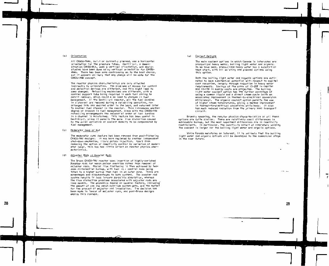
(b) Orientation

Alt CANDU-PHWs, built or currently planned, use a horizontalorientation for the pressure tubes. Gentilly-I, a demon-stration CANDU-BLW, uses a vertical orientation, and designstudies have been done using vertical orientation for CANDU-PHWs. There has been some controversy as to the best choice,but it appears unlikely that any change will be made for theCANDU-PHW concept.

The reactor physics characteristics are only affectedindirectly by orientation. The problems of access for controland detection devices are different, and this might lead tosome changes. Refuelling mechanisms are different, with acentral support tube being required in each fuel string topermit removal, which could also lead to changes in fuelmanagement. In the Genti My-I reactor, all the fuel bundlesin a channel are removed during a refuelling operation, re-arranged into any desired order in the bays, and returned laterto another fuel channel 'in the reactor. This introduces anotherdegree of freedom in fuel management, since with the CANDU-PHWrefuelling arrangements the sequential order of fuel bundlesin a channel is maintained. This feature has been useful inGentilly-I, since it permits the axial flux distortion causedby the axial variation of coolant density to be compensated byfuel management,

(c) Moderator Dump or Not

The moderator dump feature has been removed from post-PickeringCANDU-PHW designs. It has been replaced by another independentshut-down mechanism, liquid poison injection. Apart fromremoving the option of reactivity control by variation of moder-ator level, this has had Ifttie effect on reactor physics char-acteristics.

Cd) Adjuster Rods vs Booster Rods

The Bruce CANDU-PHW reactor uses insertion of highly-enrichedbooster rods for xenon poison override rather than removal ofadjuster rods. Radial flux flattening is then achieved by two-zone differential burnup, with fuel in i central zone beingtaken to a higher burnup than fuel in an outer zone. There areadvantages and disadvantages to both systems. The booster rodsystem results in less in-core parasitic absorption, whereasthe flux distortion problems associated with adjuster rods areless severe. The economics depend on several factors, including"the amount of use the xenon override system gets, and the marketfor the product cf adjuster rod irradiation. The decision hasbeen made in .'avour of adjuster rods, and post-Bruce designsemploy this concept.

(e) Coolant Options

The main coolant opt'ons in which Canada ;s interested arepressurized heavy water, boiling light water and organic.As we have seen, pressurized heavy water has 3 substantialhead start, with all existing and planned systems usingthis option.

Both the boiling light water and organic options are esti-mated to have substantial potential wit'i respect to capitalcost reduction, largely through reduction in heavy waterrequirements. Savings of the order of 15-20? in capitaland IO-I55& in energy costs are projected. The boilinglight water coolant option has the further advantage ofusing a common liquid and a direct j.team cycle (with anassociated improvement in thermal-to-electricaI conversionefficiency). The organic coolant option permits the useof higher steam temperatures, givinc a marked improvementin thermal-to-electrical conversion efficiency. It alsohas much reduced radiation from the primary heat transportcircuit.

Broadly speaking, the reactor physics characteristics of all theseoptions are quite similar. There are relatively small differences inachievable burnup, but the most important differerces are in reactivitycoefficients. In particular, the reactivity effect of completely voidingthe coolant is larger for the boiling lie,ht water and orgaric options.

While Canada ma i ntains an interest, it is unl i kely that the boiIi nglight water and organic options will be developed to the commercial stagein the near future.

221

'J

I D '

- '

I'1'II!.

. . L

4

;±C-HE

• - j -

. _ .

id t! «S

X

-

H1

- ; •

_ ) _

-j-

-j-—

—-

--

,-——-

—1

TABLE A -1

COW REACTORS I I OPERATION UNDER

CONSTRUCTION, COWITTED, AND PLANNED

r e I I I

Uae >

NPDDOUGLAS POINT

PICKERING A

GEBTII.LV 1

KANUPP

RAPP 1

RAPP 2

BRUCE A

GENTILLV 2

POINT LEPREAU

CORDOBA

PICKERING B

VOLSUNG 1

BRUCE B

DASLMGTOH

Locatfon

ONTARIO

OHTARIO

ONTARIO

QUEBEC

PAKISTAN

INDIA

INDIA

ONTARIO

QUEIEC

NEH BRUNSWICK

ARGENTINA

ONTARIO

KOHEA

ONTARIO

ONTARIO

PowerWe N«t

22208514 x 4

250125203203745 x 4

600'600

600514 x 4

600750 x 4

800x4

16,703TOTAL

NuclearDesiqner*

AECL £ CGE

AECL

AECL

AECL

CCEAECL

AECL

AECL

AECL

AECL

AECL

AECL

AECL

AECL

AEO.

FirstPmer

1962

1967

1971-3

197:

1971

1972

-

1976-9

1979

1980

1980

1981-3

1981

1983-6

19S6-S

Tvoe

CANDU-PHH

C M I U - B W

CAHDU-PHH

»•

•

•

•

•

-

•

NPO NUCLEAR POHEn DEMONSTRATION

KANUPP KARACHI NUCLEAR POWER PROJECT

RAPP WtJASTHAN ATCnlC POWER PROJECT

AECL «TO»IC ENERGY OF CANADA LIMITED

CGE CANADIAN « K : ~ ' i ELECTRIC COMPANY LIMITED

TABLE A-1I

ALLOCATION OF EXCESS REACTIVITY

AllocationExcess Reactiv' y AboveCold. Clean Critical

ADJUSTER RODS FULLY IN

MISCELLANEOUS STRUCTURAL MATERIAL

TEMPERATURE EFFECTS M

XENON AND SATURATING FISSION

PRODUCTS

CONTROL MARGIN

BUHNUP (°)

(I Ik/k)

2.0.1.

,0.3,3

3.3

0,3,

,2

,0

-ifr.8

(a) This Is the allowance which must be mode far goingto operating teofjeratures and pressures in .. freshcore. As the irradiation proceeds, the teirperatureeffects decease, and consequently more reactivity1s available to Increase burnup.

(b) Note that this burnup allowance 1s nominal. ThereIs about 0.51 nore excess reactivity available inUnits 3 and £ to compensate for the changes 1nreactivity due to burnup than in Unit1. 1 and 2.This Is because the Zr-2.5? Nt> pressure tubes inUnits 3 and 4 are thinnvr than the Zr-2 pressuretubes 1n Units 1 and Z.

TABLE A-1II

FATES OF 1000 TYPICAL FAST NEUTRONS

FAST LEAKAGE

THERMAL LEAKAGE

NON-FUEL ABSORPTIONS

- ADJUSTER RODS

CONTROL & KISCTLANEOUS

- MODERATOR

CALANDRIA TUBES

- PRESSURE TUBES

- COOLANT

- SHEATHS

FUEL ABSORPTIONS

- U-235- U-238

/RES. 93.3\\NON-RES. 2 4 2 . 0 '

- Pu-239- Pu-210- ?a-zm- Pu-242

- SATURATED FISSION PRODUCTS(XE, in, ETC.)

- OTHER FISSION PRODUCTS

9.80.4

15.78.8

23.10.3

_LS63,9

215.2335.3

232.120.811.90.1

32.127.5

905.0

12.7

18.4

63.9

905.0

222

NOT TO SCALE

FIGURE A-l

Picket i.iy Reactor Core Schematic

FIGURE A-3

Pickering Reactor Arrangement

CANDU PHU Schematic

Adjuster Rods- Zone Control and Flux Detectors Shutoff Rods

FIGURE A-4 Reactivity Control and Safety Devices223

11 r

FIGURE A-7

Simplified Station Flow DiagramCAMDU BLW

FIGURE A-8Gentilly Reactor Assembly

2B ELEMENT UO;

EXPERIMENT i D?O COOLANT

•5- AlR COOLANT

POWDERPUFSV '—-

HEXACONAL PITCH km

FIGURE A-9 Material Buckling versus Lattice Pitchfor a Pickering-type Fuel Channel

REACTIVITY VS BURNUP(NATURAL URANIUMI

1000 2000 3000 4000 5000 6000 7000 8000

IRRADIATION |MWD/1ONNE|

226 FIGURE A-10 Reactivity vs Burnup (Natural Uranium)

REACTIVITY VS BURNUP(NATURAL URANIUMI

1000 2000 3000 4000 3000 6000 7000 SOOO

IRRADIATION IMWD/TONNE)

FIGURE A- l l

Approximate Estimate of Discharge Burnup

0 5 10 15 20 25 30TOTAL HEAT OUTPUT (TWhlthl)

MEAT TRANSTORT SYSTEM TEUKRATURE I'-S

EXPERIMENT

M UNIT 3 INITIAL tTARTUT

j f t UNIT 4 INITIAL STARTUP

4 UNIT 1 STARTUP MTH IRRADIATED FUEL

KWtKIWJFS V RE1ULT1

FIGURE A-12 Fuel Consumption and Burnup forPickering Units 1 and 2

FIGURE A-13

Reactivity Change Due to Transport SystemTemperature Change in the Pickering ReactorTheory Compared with Experiment.(mk = milli-k, a change in reactivity of 10"3)

J

r ~iB. BASIC LATTICE PHYSICS

B.I INTRODUCTION

The original target for the CANDU design was a heavy water moderatedpower reactor capable of producing energy at competitive costs, usingnatural uranium as the fuel. The main uncertainties were associated withthe reactivity of natural uranium lattices with complex-geometry fuel underpower reactor conditions of temperature and pressure, and the change inthis reactivity with fuel irradiation. The key question was whether therewould be enough excess reactivity to support a fuel burnup which would behigh enough to make efficient use of uranium and provide competitive energycosts. The degree of freedom offered by enrichment was not available inthe design.

The fundamental nuclear data and the methods of analysis were notaccurate enough at the time that a reliable design could be based entirelyon calculation. As a result the development of the CANDU concept was tiedclosely to the results of integral physics measurements.

Three main types of integral experiments were used: zero energylattice experiments, measurements of reactivity change with irradiation, andmeasurements in power reactors. The results of these measurements were usedinitially in developing semi-empirical correlations for studying variousdesign options and predicting reactor performance characteristics, and laterin checking more sophisticated, fundamental lattice codes for the samepurpose.

The rationale behind the program is quite straightforward. It isvastly easier and cheaper to do measurements in a zero energy facility thandirectly in a facility operating under power reactor conditions. Thus manymore measurements can be made in a zero energy lattice test reactor and amuch more detailed understanding of the lattice physics obtained. By meas-uring separately the effects of changes in lattice conditions, perturbationsto the lattice, and fuel irradiation, the results can be satisfactorilyextrapolated to power reactors. The final check is by far less extensivemeasurements in the power reactors themselves.

B.2 ZERO ENERGY LATTICE EXPERIMENTS [83

Since 1945 there has always been at least one zero energy lattice testreactor at CRNL* (.Zero enevgij is a bit of an exaggeration since such reac-tors typically operate at powers of 100 W.) The first one was ZEEP - wellknown as the first reactor to operate outside the U.S. In I960 the larqerZED-2 was commissioned with the specific purpose of permitting accuratemeasurements for the large fuel assemblies and wide lattice spacings plannedfor Canadian D2O power reactors. Both reactors were operated until mid-1970when ZEEF was molhbaiied.

A zero enerqy lattice test reactor has two main functions. The firstis to provide a facility in which -1 broad range of lattices of a givengeneral type can be assembled and made critical - different fuels, withdifferent geometrical designs, at different lattice spacings. The proper-ties of these lattices are then studied to aid in assessment of conceptsand proposals, and in design of research or power reactors. The second isto provide a facility in which specific situations thai" arise in the designor operation of research or power reactors can be mocked-up in order tosolve specific reactor physics problems.

While operating conditions of research and power reactors cannot beexactly duplicated, many can be approximated. The usefulness of a latticetest reactor lies mainly in the wide variety of measurements that can bemade related to detailed neutron behaviour in the system. Therefore twovery important requirements of such a facility are flexibility and accessi-bility.

Careful attention was paid to these two requirements in the design of2ED-2 (Figure B-l). The facility consists basically of a reactor vessel(calandria) having an inside diameter of 336 cm and a depth of 334 cm, sur-rounded by a graphite reflector 60 cm in mean radial thickness on the sidesand 90 cm thick on the bottom, and both enclosed (afonq with a D2O pump anddrain circuits) in a 7.2 metre square reactor well having 45 cm thick con-crete walls. Fuel rods are suspended on offset hangers from eleven steelbeams straddling the top of the calandria. Remotely operated mechanical-hydraulic mechanisms are provided either to move the beams across thecalandria or to move a row of hangers along the beans, thus permitting achange in lattice spacing for either square or hexagonal lattices. Accessto the calandria can be had either by removal of a 3.3 metre diameterrevolving lid or through aluminum hatches which are clamped to this lid.Two rolling radiation shields provide easy access to the revolving lid.Heavv water can be transferred to the calandria from three dump tanks at arate co to that equivalent to 10 cm increase in the D2O level in the calan-dria per minute. Reactor control is achieved by adjustment of the D2O levelin the calandria. This level is measured roughly with a pressure transducerand accurately with a probe which gives an electrical signal when lowered totouch the surface of the D2O. Over the range 0 to 300 cm an absolute accur-acy of ±0.1 cm can be achieved with the probe and readings are reproducibleto a standard deviation of 0.003 cm. To shut down quickly, moderator isremoved rapidly from the calandria through three dump lines. A freezer-drier unit is used to dry the calandria when required. Heaters aro providedcapable of raising the moderator temperature to 90°C.

The experiments done in the lattice test reactors, particularly ZED-2,can be d i v ided i nto four genera I categories:

(a) uniform, cold, clean lattice experiments,

(b) effects of changes in temperature, coolant densilyand of uniform poisons,

(c) spatial perturbation effects, and

(d) kinetics experiments.

227

Each of these categories will be discussed in the following sec-tions. The experiments as a whole have provided a firm basis for most ofthe estimates of physics performance on which Canadian power reactorshave been conceived, designed and operated.

B.Z.I Uniform Cold Clean Lattice Experiments l.12.13.14]

During the period 1960-1969, ZED-2 was used mainly for studies oflattices in the range of interest of the Canadian power reactor program.Lattices were assembled at a variety of lattice spacinqs and with air, D 20,H20 and HB-40 coolants using the following fuel assemblies:

7-element U02

19-eIement UO228-element U0 219-element U-metal7-element UC19-element ThO2-UO231-element simulated irrad iated fuel.

Since that time further lattice experiments have been done withrods having other geometries. The most notable example is a series ofexperiments carried out with 37-element rods of U02, U3Si, UC and U-metalmade to identical geometries. The measurement techniques have improvedwith time to a degree that the later experiments have been done with substi-tution techniques using as few as seven test rods, rather than with full-sea le lattices.

Measurements were made in these lattices thdt give information onthe critical size of the lattice in any geometry, the ratio of fissions infertile isotopes (caused by high energy neutrons) to fissions in fissileisotopes, the ratio of fissile material produced Cby neutron capture infertile isotopes) to fissile material destroyed (by fission or neutron cap-ture), and the shape of the neutron energy spectrum. Measurements were alsomade of the spatial distribution of neutron flux within channels, latticecells and the lattice.

Buckling Measurements

is determined by the fitted distribut

For exper irnents w i th on I y a few rods in the test rod I aft ice, buck-Iings are measured by substitution techniques. Critical height changesassociated with progressive substitution of test rodb are used to determinethe buckling, employing a two-group, heterogeneous code.

Figure B-2 gives an example of buckling measurement results for28-element, natural U0 2 fuel assemblies having D2O, He and HB-40 coolants,over a range of lattice pitches.

Neutron Fine Structure Measurements

Distributions of neutron density within cells and fuel channelsare measured by neutron activation of Mn-Ni foils and wires in the centrallattice cell. Mn-Ni foils (-0.10 mm thick) are placed between fuel pellets,and Mn-Ni wires <0.5l mm diameter) in longitudinal holes in the fuel pel-lets and a1 various positions in the coolant and moderator. The activitiesmeasured are corrected for the macroscopic neutron density variation acrossthe cell and the Mn resonance activation (using measured neutron spectrumparameters). Average neutron densities in the various cell materials arefound by graphical integration.

Figure B-3 shows some typical results for * 28-element, naturalU0 2 fuel assembly having D2O coolant, in a hexagonal lattice with a 28 cmpitch.

Figure B-4 shows the total neutron densities in moderator andcoolant relative to that in the fuel, as a function of lattice pitch, forthe 28-element, natural UO2 fuel assemblies.

Neutron Spectrum Parameter Measurements (r and Tn)

Measurements of the Westcott epithermal index, r, and the effectiveneutron temperature, T n, are generally made in the fuel, at the cell boundaryand on the surface of the calandria tube. Thin In-AI and Lu-Mn-At foils areirradiated together at the test positions and at a reference position in thereflector. The value of r VT n/T o a+ the reference position is determined bymeasuring the Cd ratio for thick In-AI foils. The In/Mn and Lu-177/Mn ratiosat the test positions relative to the same ratios at the reference positionare used to determine rV Tn/fo and T n respectively, and hence also r.

Some typical results for 28-element natural UO2 fuel assemblies withD20 coolant, at two lattice pitches are shown in Table B-I.

Fast Fission Ratio Measurements

228

where

ar.d

6 = Ry(t) P(t)

Ry(t) is the ratio of U-238 activity to U-235activity, as a function of time after theirradiation, obtained from the natural anddepleted foiI measurements,

P(t) is a complex counter-efficiency factor.

P(t) is determined by measuring Ry(t) for a fastneutron facility of known S using the same foilsZ6 for the fast neutron facility was measured witha back-to-bsck fission chamber containing ~90 wt?U-235 on one side and either natural or depleteduranium on the other].

The measured value of fast fission ratio for 28-element naturalUO2 fuel assemblies with D2O coolant at a hexagonal pitch of 28 cm is 0.058.The value is only a weak function of lattice pitch over the range of inter-est but does depend on coolant. For example, the value for the sama latt-ice, but with air instead of D20 coolant, is 0.063.

Experimental errors in measurements of <5 are about ±355.

Initial Conversion Ratip Measurements

The initial conversion ratio for a fresh natural uranium latticeis defined as the ratio of Pu-239 production to U-235 destruction. It ismeasured by comparing the ratios of Np-239 activity to fission productactivity in identical natural UO2 wafers (0.1 mm thick) irradiated in thefuel and in a pure thermal neutron flux. Coincidence ycoun^lng is used tomeasure the Np-239 activities. Fission-product activities are measured byy-counting and are corrected for fast fission using Rv(t) values from thefast fission ratio measurements.

In order to derive the initial conversion ratio from these meas-urements, two additional factors, based on fundamental nuclear data, mustbe used. These are the relative ratios of U-235 destruction to U-235fission in the test location spectrum and in a pure thermal spectrum, andthe ratio of U-238 absorption to U-235 absorption in a pure thermal spectrum.

Relative initial conversion ratio measurements are accurate to±0.5?, but absolute values have a further 0.8? uncertainty associated withthe fundamental data used for the ratio of U-238 absorptions to U-235absorptions in a pure thermal spectrum.

Results of measurements of initial conversion ratio, for latlicesof D20-cooled, 28-element natural UO2 fuel assemblies are summarized below:

A Lattice Pitch (cm)

24283240

Initial Conversion Ratio

0.9258O.a4590.80540.7663

B.2.2 Effects of Changes in Lattice Conditions H4.15]

Temperature Effects

!n both ZEEP and ZED-2, provision is made for heaters in themoderator. Using these, the lattice temperature can be raised uniformly

by some 60°C. Tit is technique lias been used to measure effects of tempera-ture changes to provide a means of checking lattice codes, but it ;s along way from simulating operating power reactor temperatures.

In order to provide information more directly relevant to powerreactors, a series of experiments were carried out some time ago using asingle hot loop in ZEEP. This facility consisted of an 8.3 cm inner diam-eter insulated pressure tube through which water or air at temperatures upto 300cC could be passed. Various test sections were placed in the pres-sure tube and reaction rate measurements made in the test section andthrough the lattice cell, for various temperatures inside the pressuretuoe. These measurements were similar to those which have already beendiscussed under Neutron Fine Structure Measurements and Neutron SpectrumParameter Measurements, The results proved to be very useful in extrapo-lating the cold, clean lattice measurements to power reactor conditions.Figure B-5 summarizes measured average neutron temperatures vs coolanttemperature, for the case in which the test section was a CANDU-type UO2fuel cluster and various coolants, ranging from H2O through various H2O-C;0 mixtures to air, were used.

More recently we have acquired seven hot channel sites for use inZED-2. These facilities provide power reactor coolant temperature condit-ions in seven lattice sites. The imaginative design consists of well-insulated pressure tubes, having a nominal inner diameter of 10 cm, thatcontain an internal 3 kV electric heater which can raise tht temperature ofthe fuel plus liquid coolant to 300°C. The heat loss for operation at300°C is about 100 rt and only a fraction of this loss is to the moderator.With this lew neat loss, the flui.1 temperature can be kept very uniformaxially and moderator healing does not introduce experimental problems.These facilities make it possible to perform standard few-rod latticemeasurements by substitution techniques. They have been used for naturaluranium lattice measurements, but we expect them to be particularly usefulfor measurements with Pu-bearing and thorium fuels.

Coolant Density Effects

Of course, coolant density varies with coolant temperature andthese effects are simulated in the hot channel experiments. However, weare also interested in coolant density changes due to boiling.

Simulated boiling experiments have Deen done with lattices ofH20~cooled, 28-element natural U02 fuel assemblies in ZED-2 using the few-rod substitution technique already mentioned. Boiling coolant was simu-lated by bubblinq air through the H2O in a maximum of seven assemblies inthe central test zone, using an array of hypodermic neeales at the bottomof each channel to introduce the air. Coolant density was varied by adjus-ting the air flow rate and by addinq minute quantities of a surface tensionreducing agent. Figure B-6 shows the measured buck I ings as a function ofeffective coolant density.

229

1 1 I—Moderator Poison

We are currently introducing a moderator poison addition andremoval system into ZED-2. This will expand the range of possible experi-ments. Moderator poi sons are used i n many of our reactor des igns andsome reactivity coefficients depend significantly on the amount of moder-ator poison present.

B.2.3 Perturbed Lattices [16.17.18.19,20,21]

In a power reactor, the lattice is seldom uniform throughout thecore. Irregularities occur due to bundle-end effects, fuel changing oper-ations, non-uniform burnup, control absorbers and boosters. These effectshave also been studied extensively in zero energy lattice experiments.

Bundle-End Peaking

The fuel in a CANDU reactor channel is not axially continuous,since gaps containing no fuel occur at the bundle ends. Many of the uni-form cold clean lattice experiments are done with simulated bundle geome-tries, and the measured lattice properties include the effects of the gaps.Since it is important to understand the effect of such gaps in detail inorder to optimize fuel design, many additional experiments have been done.Reactivity affects are o* some interest but more attention is directed atthe detailed flux behaviour in the vicinity of the bundle ends since exces-sive peaks could cause fuei over-rating. Figure B-7 shows torn© typicalresults from such measurements.

Refuel ling Effects

During on-power refuelling operations, perturbations are introducedat the channel being refuelled. These ar'j most severe in the case ofGentilly-I, where a complete fuel string is removed during the refuellingoperation and then replaced by another. At one stage in this procedure thechannel contains no fuel but is filled with tight water.

The effects of such a perturbation have been studied in a simulatedCANOU-BLW lattice in ZED-2. The experiment consisted of measuring the reac-tivity and flux distribution effects of replacing the fuel in the centralchannel of the lattice with light water. Figure B-8 shows some typicalresults. The flux perturbation factor (defined as the ratio of perturbedflux to unperturbed flux where both are normalized to a constant flux farfrom the perturbation) is shown as a function of radial distance from theperturbation.

Absorber Effects

Since absorbers are used for control and shutdown, it is importantto be able to estimate their effects on both reactivity and flux distri-butions. Experiments in ZED-2 have been done for different absorber

materials, geometries, and configurations, with both reactivity effects andflux perturbation factors being measured.

Figure B-9 is an example of some results from one particular set ofmeasurements. Shown are radial flux perturbation factors caused by threedifferent absorbers located in the central position of a 27.94 cm squarepitch, open-centre lattice of 28-element, natural UO2 fuel assemblies withO2O coolant. The three absorbers consisted of a 6 cm nominal diameteraluminum tube filled successively with water and water having two differentconcentrations of dissolved boron (2.5 mg/m£ and 8.0 mg/mJt).

Booster Rod Effects

In some CANDU designs, booster rods (i.e., highly-enriched U-AIalloy rods) are used to override xenon poison in the startup after a shut-down. In general the flux distortions produced by booster rods are positiveand have the potential of being more serious than those produced by localabsorbers. Therefore accurate reactivity and flux perturbation estimatesare requi red.

Zero energy lattice experiments have provided data against whichto verify (and improve) the codes used for these estimates.

A set of measurements was performed in ZED-2 on simulated BLW 61-element booster rods containing 5.0, 6.56 and 7.46 g of U-235 per cm oflength. These booster rods either replaced the central fuel assembly in arod-centered lattice or were located interstitially at the centre of an open-centre lattice. Figure B-10 shows the measured radial flux perturbationfactor for the case of a 5 g/cm booster rod in an open-centre lattice of28-element, air-cooled fuel assemblies on a 27.94 cm square pitch. Otherexperiments have studied interaction effects among two or more booster rods.

B.2.4 Kinetics Experiments t22'23^

Point Kinetics

In a small reactor the time dependence of the neutron flux, fol-lowing a small change in reactivity from critical, can be well approximatedby assuming that the spatial flux shape is independent of time. The timedependence of the flux level can then be calculated using standard formulae.The data on which this time behaviour depends are the change in reactivity,the mean neutron lifetime in the cere, and the yields and half-lives ofdelayed and photoneutron precursors.

In heavy water reactors, in addition to the six delayed neutrongroups (corresponding to six precursors), nine photoneutron groups havebeen identified. While these photoneutron groups have relatively low yielas,seven of them have precursors with ha If-lives longer than the longest half-life of the delayed neutron precursors.

230

J

~i rExperiments in 2ED-2 and ZEEP have shown that good agreement can

be obtained with experimental transient behaviour using all fifteendelayed and photoneutron groups. Good agreement for times less than about100 seconds can be obtained by collapsing the photoneutron groups into thedelayed neutron group. Doing this gives the following effective yieldsand decay constants for the six delayed neutron groups:

Group Yield Decay Constant (s-1)

123456

0.00038080.0015240.0013920.0032780.0010770.000252

0.00073630.031710.11770.31391 .4023.919

0.0079038

Spatial Kinetics

In large reactors the assumption of constant spatial flux shapeafter a small reactivity change from critical is no longer valid, due tothe loose coupling between widely separated regions of the core. Theproblem faced was how to get relevant data from a small reactor. The sol-ution adopted was to do experiments in ZED-2 with split coves.

Figure B-ll shows a typical experimental arrangement. The coreconsists of two loosely coupled regions - the decoupling being achieved byseparating the core into two halves and, in some cases, putting a weakly-absorbing curtain of H2O-ffiled aluminum tubes between them. The separationbetween the two halves was also varied in some experiments.

Figure B-12 shows some typical results. An absorber rod wasdropped into the position shown in F igure B-l I and the flux measured as afunction of time after +he drop at detectors located in each core half, indiametrically opposite positions. The curves show the ratio of these detec-tor signals as a function of time for two cases, with and without the H2Oabsorber curtain.

Measurements of this type provide benchmark experiments againstwhich the codes used for Dower reactor design and operation can be checked.

B.3 IRRADIATION EFFECTS [24»25»26,27,28]

Zero energy lattice experiments give a firm basis for the physicscharacteristics of power reactors with fresh fuel, but do not give infor-mation on irradiation effects. Effects of saturating fission products, suchas xenon and samarium, are -*el I defined by researcn reactor operation andexperimentation and will iiot be discussed here.

Three experimental programs have provided data on the effects oflong irradiation of natural uranium fuel. These are designated as:

(a) NRX-GLEEP Measurements

(b) NRU-PTR Measurements

(c) NPD Fuel Analysis

The net reactivity change with irradiation of natural uranium fuelis a delicate balance between positive and negative effects. Thus integralexperiments were essential in order to attain a reliable estimate ofachievable burnup.

NRX-GLEEP Measurements

This program was carried out in the 1950s in a collaborativeeffort between staff at Chalk River and at Harwell. Natural uranium sam-ples were irradiated in the NRX reactor at Chalk River, measurements of thereactivity were made at the GLEEP oscillator at Harwell before and afterirradiation, and chemical and mass-spectrometric analyses of the sampleswere made at Chalk River. The results, summarized in Figure 8-13, show thenow faniliar curve of reactivity change with irradiation.

NRU-PTR Measurements

The results of these gross fission product determinations are sum-marized in Table B-.TI.

NPD Fuel Analysis

In 1968 a series of eight 19-element NPH bundles, with irradiationscovering the range 1000-10,000 MWd/TeU, was mass spectrometricaI Iy analyzedby the CEA in France. The bundles were selected to have an irradiation his-tory typical of an unperturbed CANDU-type rftactor with bi-directional on-power fuelling. The measurements provided relative concentrations of U-235,U-236, U-238,"Pu-239, Pu-240, Pu-24I, Pu-242 and Nd-148 in each ring of oacnbundle.

Figure B-14 shows measured bundle average nuclide ratios as a func-tion of I - a, where

I - a =N5/Na

Agreement with predictions is good. Agreement with detailed compositionswithin the bundle is slightly less satisfactory than for the bundle averagecompos it ions. 231

B.4 PHYSICS ANALYSIS OF PHW REACTORS SPECTRAL PARAMETERS

A major purpose of the experiments which have been discussed is toaid in the development and verification of computer codes.

Figure B-15 shows a simplified chart of the physics activities andsome typical codes used in the analysis of CANDU-PHWs. Power reactor oper-ation and experimentation also play a role in code verification and devel-opment as indicated in the figure, and this wiIf be discussed to a certainextent in the next lecture. Here we will only give an example of code dev-elopment and verification in terms of the experiments we have been dis-cuss ing.

The lattice code, LATREP, has been developed specifically to cal-culate the characteristics of heavy water moderated lattice cells. It is asemi-empirical code which can also treat fuel irradiation. LATREP is con-tinually being improved and updated, and is periodically checked against aset of measurements in some 60 lattices. A summary of the average errorsin the 1971 LATREP lattice parameters for all these lattices is givenbelow.

Parameter

Fast Fission RatioIn i t ia l Conversion RatioEpithermal Index (r)Effective Neutron Temp.Buckli ngReact i v i ty

Average Error

6.96-0.250.682.490.010.079

±9.92?±1.11?±4.02?±9.84°C±0.17 m-J

±0.775?

Experimental Error

±2.7?±0.82?±2.34?±2.39°C±0.07 m-2

Figure B-16 gives an indication of LATREP's performance in calcul-ating effects of irradiation.

As has already been mentioned, the perturbai icr, experiments andkinetics experiments are used extensively as benchmarks In checking Dothstatic and kinetic reactor codes.

Position

FUEL AVERAGE

CALANDHIA TUBE

CELL BOUNDARY

ZH cm A Pitchr

0.0522

0.0396

0.0320

Vt"CJ

30

55

11

si en a Mienr

0.0403

0.0295

0.0229

n

77

46

33

* Moderator physical temperature : 25°C

* * Moderator physical temperature : 26"C

Errors In r are *3J absolute or ±1X relat ive

and errors tn T are ±3°C

TABLE B-I

GROSS FISSION PRODUCT CROSS SECTIONS

IRRADIATION(tl/kb)

°o* (BARNS/FISSION)

0 0 S 0 " (BARNS/

FISSION)

U-235

2.031

38.6:3.2

292.0=53

2.261

38.4s3.0

252.0.50

Pu-239

2.150

50.7=4.8

242.0=100

2.609

50.8=5.1

199.0=100

U-233

2.286

32.0=2.8

235.0=51

2.899

:: . ;«2.5

227.0=46

232

Effective 2200 m/s cross section

Resonance absorption cross section, where the effective cross section 1s defined by:

a • oo • r «/ T/To oo So

TABLE B- I l

218

_ J

•REMOVABLE TOP SHIELD

+ D;O COOLANT IX Ml - COOLANT I-O HS-40 COOLANT J

» 29 30 32 34TRIANGULAR LATTICE PITCH (enl

CORRCCTEO TO 2 9 ' C . 19.72 ATOM % OgO

I • IJ* 31 40

FIGURE B-l

Vertical Section Reactor 2ED-2

FIGURE B-2

Bucklings for 28-Elcment Natural U02 FuelAssemblies in D20 Moderator

233

3 5

3 0

c, 25

I- 2 0 -

I .5-

0 0 I 0

X - COOLANT+ - MODERATOR(OPPOSITE COOLANT)• - MODERATOR (OPPOSITE ELEMENT)* - AVERAGE FUEL VALUES CORRECTED

FOR RESONANCE ACTIVATION

3 0 4.0 5 0 6.0CELL RADIUS (cm)

70 80 90 100CSEE FIGURE I - B 3

110 12 0 13.0 14.0 15.0'• FIGURE B-3

Fine Structure in Lattice Cell(28 cm Pitch, D20 Cooled)

2.60

2.90

2.40

2 2.10

£ 2.00

1

i aoat

1.12

I I I

, 07

1.06

V - MAXIMUM1 E R R O R

X 0 0 COOLANTO AIK COOLANT+ KB-40 COOLANT

23424 26 28 30 32 34

TRIANGULAR LATTICE PITCH (cm)36

FIGURE B-4

Total Neutron Density Ratios, ModeratorAverage and Coolant Average Normalized toFuel Average as a Function of TriangularLattice Pitch for 28-Element Natural U02Lattices

4.5 r-

4.0

— 3.0

O 2.5

2 *

1.5

1.0

(30 CM A PITCH)

$ FLUX MAP

• 2 REGION

A 3 REGION

I ERRORS

I I 1 1.1 .2 .3 /4 .5 .6 .7

EFFECTIVE COOLANT DENSITY (G.CM'3)COOLANT TEMPEMTUKE ("Cl

FIGURE B-5The Cluster Average Effective NeutronTemperature Dependence on CoolantTemperatures for Various IsotopicCompositions of the Coolant Derived fromLu-Hn Results

FIGURE 6-6Test Lattice Buckling vs Effective CoolantDensity (99.66 atom% 0,0, 21.5°C)

23S

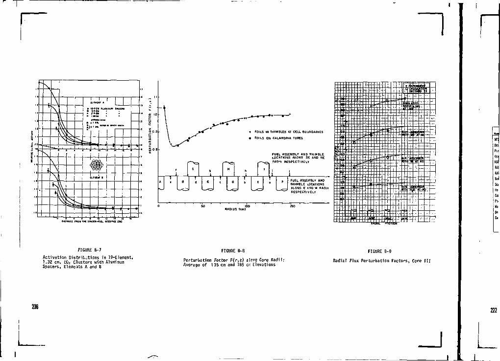
~l

i"S

"4-

• • L

r

\\

s,

i

ks

ILIWCMT t

; ' • 9-QCtt

V

L

• H 4 *

1

n o

• . *6 ii 14

1

; CLCMCHT •

1!

• i

* 6 ' ' '•• . . .

* ' « 1=

t FOILS IN THIMBLES « CELL BOUNDARIES

« FOILS ON CALANDRIA TUBES

n , n : nrFUEL ASSEMBLY AND THIMBLELOCATIONS ALONG SE AND NERAf' l RESPECTIVEL1

d • U ' L IPTI I : L J : FUEL ASSEMBLY ANDTHIMBLE IJDCATION5ALONG E AND W OADIRESPECTIVELY

DISTANCE FROM THE SMCEH-FUEL HTEHnCt ICW

FIGURE B-7

Activation Dist r i t , j t ions in 19-Element,1.32 cm, U02 Clusters with AluminumSpacers, Elements A and B

FIGURE B-8

Perturbation Factor F(r,z) alrng Core Radii:Average of 135 cm and 185 ci'. Elevations

FIGURE B-9

Radial Flux Perturbation Factors, Core I I I

238

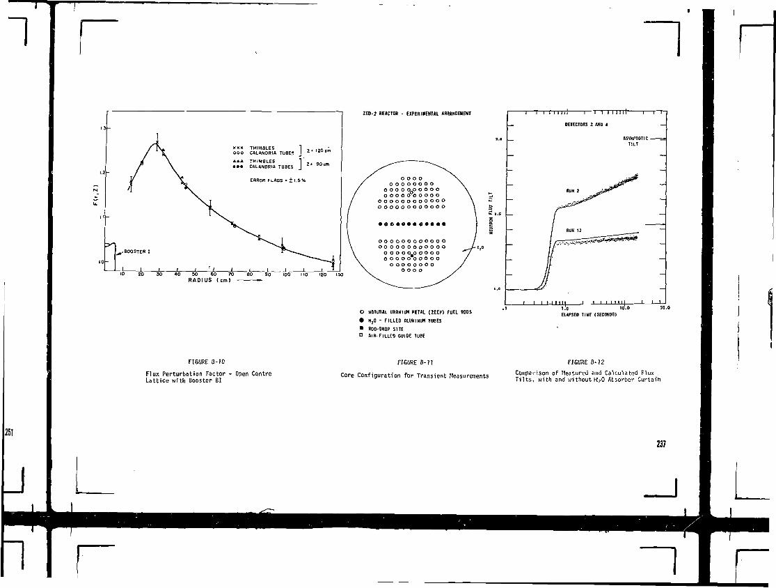
o o o ooooooooo

o o o oooo o o ooooooooooo

oooooooooooooooooooooooo

40 30 60 70RADIUS (cm)

ZEO-2 REACTOR • EXPERIMENTAL ARRANGEMENT ill mil

DETECTORS 2 AND «

ASYMPTOTIC -T I L T

' I I I I I l l [ 1 1 | I I

FIGURE B-10

Flux Perturbation Factor - Open CentreLatt ice with Booster BI

o NATURAL URANIUM METAL UEEP) FUEL RODS

• H,0 - FILLED ALUMINUM TUBES• FOO-OROP SITEO AIR-FILLEO CUIDE TUBE

FIGURE B-ll

Core Configuration for Transient Measurements

l.'O 10-0EUPSEO IIME (SECONDS)

FIGURE B-12

Comparison of Measured and Calculated FluxTilts, with and without H?0 Atsorbor Curtain

2S1237

J

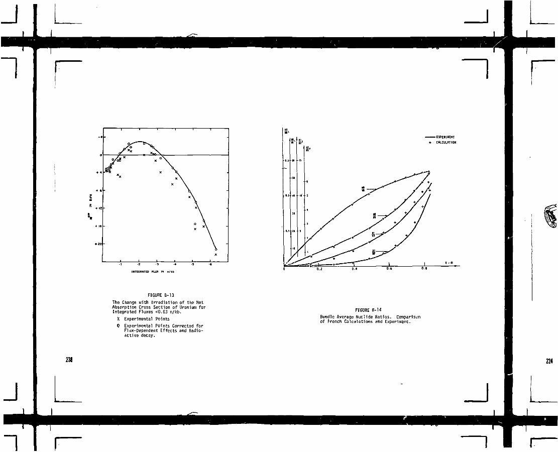
238

EXPERIMENTCALCULATION

INTEGRATE!) FUJI IN It/Hi)

FIGURE B-13

The Change with Irradiation of the NetAbsorption Cross Section of Uranium forIntegrated Fluxes <0.63 n/kb.

X Experimental Points

0 Experimental Points Corrected forFlux-Dependent Effects and Radio-active decay.

FIGURE 8-14

Bundle Average Nuclide Ratios. Comparisonof French Calculations and Experiment.

~1outrun1 • CMttMCTIORVVMMlmUP

•UMK.fl.ITC.

1 CONTROL MVICU LAYOUT• K M C R ommcMTioN rN m t com• MU1DOMW IVSTtMS- VOID IPFCCT, ITC

- HOUIMCIIOVinTMWARALOIIINKRTKM OF COWTIIOLDiVKfLITC.

o-

- HNMCATU FIIDBAGK•NFOWUrOMMIOM•KKRIIKMTAL AHO

coot OIUQHCONTMOL fit vie I ItHUTtXMNlVtTfMS

©—

4 0 ' • 10- 5 - '

20' ' 5- > 2 ^ - '

FIGURE B-15

A Simplified Chart of the PhysicsAnslysis of PHW Reactors

FIGURE B-16

NPD 19-Element Irradiated Bundles.Bundle Avoriige Isotope Ratios

239

I

"i rC, POWER REACTOR CORE PHYSICS

C.I INTRODUCTION

From the reactor physics point of view there are two aspects ofpower reactor operation of most interest. Firstly, a great deal of infor-mation can be derived from the start-up, comm'ssioning, and operation ofpower reactors that is valuable in verifying and improving design methods.Secondly, power reactor operation brings into focus a number of oper-ational factors requiring further reactor physics input, thus directingR&D effort into the most relevant channels.

In this lecture I wi 11 outline the reactor information obtainedfrom start-up and commission'ng of power reactors, then discuss three top-ics which have been emphasized by operating experience. These three topics,in which R&D is continuing, are fuel management, flux mapping and control.

C.2 START-UP AND COMMISSIONING MEASUREMENTS [31*32,33,34,35]

Critical Size

For all power reactors the initial approach-to-critical is care-fully monitored and the cold, clean critical size accurately determined.Monitoring for early units was done with in-core detectors. In the Picker-ing and Bruce stations, after proving in each case on the first unit thatout-of-core detectors provided adequate monitoring, out-of-core detectorswere used for initial approach-to-critical in subsequent units.

The initialcore in NPD contained depleted uranium fuel as well asnatural fuel. The first approach-to-critical was done by raising the moder-ator level wnil-3 measuring the neutron flux with three fission chambers nearthe centre of the core. As the moderator level was raised, the increases incount rates, corrected for flux shape, were plotted against the calculatedkeff- Figure C-l shows the results for one of the fission chambers. Thefunction f(h), is simply the calculated keff multiplied by 1000, As can beseen, the predicted reactivity was overestimated by some 1.256, correspondingto an underestimate of about 20 cm in moderator level.

Due to the horizontal orientation of NPD, both the core shape andaverage nuclear properties change as the moderator level is changed. Sincethis represented a situation which had not been studied experimentally,measurements were made in NPD of change in reactivity with moderator level.Cadmium sulphate was injected into the coolant system in carefully control-led amounts and the level response noted. The moderator level was cali-brated in terms of reactivity by means of a calculated curve of reactivityvs cadmium concentration. Figure C-2 shows the resultant variation ofreactivity with moderator level.

In general, estimates of cold, clean criticality for later powerreactors were closer +o the measurements. For example, in Bruce theapproach-to-critical In the first unit, which also contained depleteduranium fuel bundles, was done by removal of boron from the moderator, withthe moderator at full height. The variation of measured reciprocal countrate with boron content is shown in Figure C-3. The measured concentrationat criticality was 8.0 ±0.5 mg B/kg D2O, while the predicted critical boronconcentration was 8.3 mg B/kg D20. The difference corresponds to <0.3£ inreactivity.

Calibration of Reactivity Devices

The methods used to calibrate reactivity devices during Brucereactor commissioning are fairly typical.

First the light water zone control system was calibrated againstboron in the moderator. During low power commissioning the system was oper-ated without spatial control. The first step in the calibra;ion was tor&iseall the zone levels to "*90£ full by removing boron from the moderator. Thenaccurately weighed amounts of boron were added to the moderator system. Tomaintain reactor power, the regulating system compensated for each additionof boron by lowering the average zone level. Thus the change in averagezone level was equal to the reactivity worth of the added boron. Figure C-4shows the results of the calibration. The total <0£-l00* full) measuredworth of the zone system was 5.4 til* mk which agrees reasonably well witha calculated value of 5.9 mk.

Individual worths for the other reactivity devices (i.e., mechani-cal control absorber rods, shut-off rods, and booster rods) were determinedby noting the change in average light water zone level when each individualdevice was inserted in the core. The total reactivity worths of insertingall the boosters or removing all the shut-off rods were measured againstboron additions. All the results agreed with predictions to within %.

Reactivity Coefficient Measurements

The coolant temperature coefficient for all the reactors has beenmeasured, using pump heat to warm up the heat transport system. Some sam-ple results for Pickering were shown in the first lecture (Figure A-13) andthe results for other reactors are quite similar.

The moderator temperature coefficient has been measured in boti->NPD and Douglas Point. In Douglas Point, with 11.0475 ppm boron in themoderator, when no change in reactivity had been detected after a 6°C in-crease in moderator temperature, the slow process of heating up the moder-ator was terminated. In NPD, a reactivity loss of 3.9 mk was deduced fora change in moderator temperature from 2I°C to 74°C for a cold, clean fulltank (the value had to be deduced from values measured at full tank withcadmium sulphate in the coolant and at a lower moderator level with nocadmium sulphate).

240

_J

1Flux Distributions

in both Pickering and Bruce, extensive measurements of flux distri-butions were made during commissioning at low power (IO"J to I0"1* of fullpower) using wire activation. Some of the Bruce measurements will be givenas an example.

In Bruce, flux shapes associated with five different reactor coreconfigurations were measured by using wire activation techniques and bymonitoring the output of in-core self-powered neutron flux detectors withspecial instrumentation. For each core configuration, the radial flux shapeatrf-\n« an omn +w r sH i a I Ha-+a +/-%r- nil i Ha -t-iiKa z*c chnun In rinnro O*-R uac

11 n u m b d n u m e n w i i r n , " d w n , d i i u m e i i i a u t e o d t i i v u y a i b i i I U U I i o n m e d b u i a

with an Nal (T£) counter. The five configurations measured were: (a) thenominal reference core, (b) 28 shut-off rods inserted, (c) 2 control absor-bers partially inserted, (d) 3 booster rods inserted, and (4) 15 boosterrods inserted. As an example. Figure C-6 shows the measured radial distri-bution for the case of 2 control absorbers partially inserted. Also shownin the same figure is the radial distribution calculated from a simulationusing the three-dimensional two-group neutron diffusion code, CHEBY. Aleast squares normalization of the simulation to the measurements has beenmade. As can be seen from the figure, the agreement between the simulationand measurements is good. For the radial flux distribution, the standarddeviation is 4.5%.

The readings from a total of 107 in-core detectors, taken at thesame time as the wire actuation, were then compared to the simulation. Theresults of this comparison are shown in Figure C-7, where the distributionof a number of detectors having a given % deviation from the simulation isshown. The standard deviation of the distribution is 5.9$.

The standard deviations for the other configurations are summarized

Configuration

Norn i na1 Reference

28 Shutoff Rods in

2 Control AbsorbersPartially in

3 Boosters in

15 Boosters in

Standard DeviationsActivation/Simulation

<2.0?

<2? in high flux region

4.5?

3.0?

<3? in high flux region

Detectors/S imu1 at i on

6.2?

Current too low to monitor

5.9?

8.0?

6.7?

255

Dynamic Measurements

In Bruce, shutdown transients following the drop of 30 shut-offrods and 28 shut-off rods were obtained by recording the output of fluxdetectors (ion chambers) located at various positions. A typical set ofresults is shown in Figure C-8,

The dynamic experiments were simulated with CERBERUS, a two-groupthree-dimensional finite-difference code which uses the Improved Quasi-static {IQS) method. Results of this simulation are also shown in FigureC-8. Since out-of-core measurements showed some scatter in the rate of roddrop, two transients were calculated for each case. The FAST transient wasbased on the fastest drop measured in the laboratory tests and the SLOWtransient was calculated with a slower rod drop characteristic, to study thesensitivity of neutron transients to possible scatter in the rod drop rates.The measurements fall close to the FAST calculated transient, in accordancewith the fact that most rods were found to fall at the corresponding speed.

Figure C-9 shows the dynamic reactivity calculated by CERBERUS forthe 30-rod drop case. The static reactivity of the rods is also given. Thedynamic reactivity at full insertion is more negative than the static. Thisis because of the retardation of flux shape brought about by delayed neutronholdup, together with neutronic decoupling. This retardation enhances theimportance of the absorber rods and their reactivity.

An extensive program of dynamic measurements was carried out inGentilly-I and this will be mentioned again later under the discuss'on ofcontrol.

C.3 FUEL MANAGEMENT C36»37]

C.3.1 NPD

The original concept of bi-directional, on-power fuel managementis applied in NPD. One fuel bundle at a time is inserted and one removedby means of a pair of fuelling machines that can be attached to the ends ofany of the horizontal fuel channels while the reactor is at full power. Afresh bundle is inserted from the machine at one end of the channel while aspent bundle is ejected t"to the machine at the other end. Alternatechannels are refuelled in opposite directions. After an initial fresh-fue!reactivity transient was overcome (in about six months of operation) theequilibrium fuelling rate was quickly established.

Fuel management in NPD is based on a 3-dimensional diffusion cal-culation of burnup with one mesh point per bundle, and it is found thatclose to optimum burnup can be achieved by the fairly simple principle ofremoving the most highly irradiated bundle when more reactivity is needed.Some minor modifications to this scheme are required to ensure uniformfuelling over the reactor face and in the two fuelling dirsctions. Anyanomalous trend in behaviour can be detected by reactor and channel instru-mentation and can be compensated for in subsequent fuelling operations.

241

J

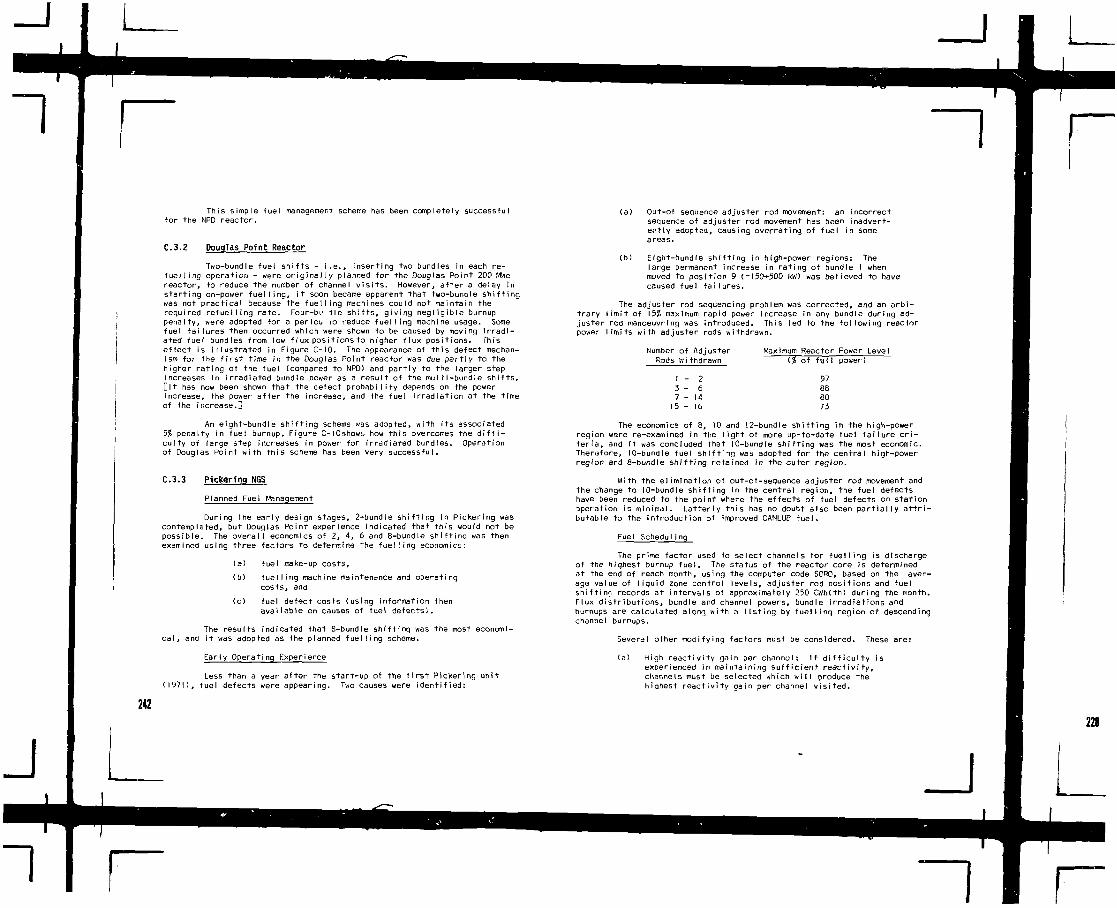
This simple fuel management scheme has been completely successfulfor the NPD reactor.

C.3.2 Douglas Point Reactor

Two-bundle fuel shifts - i.e., inserting two bundles in each re-fuelling operation - were originally planned for the Douglas Point 200 MWereactor, to reduce the number of channel visits. However, after a delay instarting on-power fuelling, it soon became apparent that two-bundie shiftingwas not practical because the fuelling machines could not maintain therequired refuelling rate. Four-bi* -jIe shifts, giving negligible burnuppenalty, were adopted for a period ro reduce fuelling machine usage. Somefuel failures then occurred which were shown to be caused by moving irradi-ated fuel bundles from low flux positions to higher flux positions. Thiseffect is illustrated in Figure C-10. The appearance of this defect mechan-ism for the first time in the Douglas Point reactor was due partly to thehigher rating of the fuel (compared to NPD) and partly to the larger stepincreases in irradiated bundle power as a result of the muiH-bundle shifts.L"lt has now been shown that the defect probability depends on the powerincrease, the power after the increase, and the fuel irradiation at the timeof the increase.D

An eight-bundle shifting scheme was adopted, with its associated5% penalty in fuel burnup. Figure C-lOshows how this overcomes the diffi-culty of large step increases in power for irradiated bundles. Operationof Douglas Point with this scheme has been very successful.

C-3.3 Pickering NGS

Planned Fuel Management

During the early design stages, 2-bundle shifting in Pickering wascontemplated, but Douglas Point experience indicated that this would not bepossible. The overall economics of 2, 4, 6 and 8-bundle shifting was thenexamined using three factors to determine the fuelling economics:

(a) fuel make-up costs,

Cb) fuelling machine maintenance and operatingcosts, and

(c) fuel defect costs (using information thenavailable on causes of fuel defects).

The results indicated that 8-bundle shiftinq was the most economi-cal, and it was adopted as the planned fuelling scheme.

Early Operating Experience

Less than a year after the start-up of the first Pickering unit(1971), fuel defects were appearing. Two causes were identified:

(a) Out-of sequence adjuster rod movement: an incorrectsequence of adjuster rod movement has been inadvert-ently adopted, causing overrating of fuel in someareas.

(b) Eight-bundle shifting in high-power regions: Thelarge permanent increase in rating of bundle I whenmoved to position 9 (-150*500 kW) was believed to havecaused fuel failures.

The adjuster rod sequencing problem was corrected, and an arbi-trary limit of 152 maximum rapid power increase in any bundle during ad-juster rod manoeuvring was introduced. This led to the following reactorpower limits with adjuster rods withdrawn.

Number of AdjusterRods W"i thdrawn

1 -3 -7 -

IS -

26

1416

Maximum Reactor Power Level(% of full power)

97868073

The economics of 8, 10 and )2-bundle shifting in the high-powerregion were re-examined in the light of more up-to-date fuel failure cri-teria, and it was concluded that 10-bundle shifting was the most economic.Therefore, 10-bundle fuel shtffng was adopted for the central high-powerregion and 8-bundle shifting retained in the outer region.

With the elimination of out-of-sequence adjuster rod movement andthe change to 10-bundle shifting in the central region, the fuel defectshave been reduced to the point where the effects of fuel defects on stationoperation is minimal. Latterly this has no doubt also been partially attri-butable to the introduction of improved CANLUP fuel.

Fuel Scheduling

The prime factor used to select channels for fuelling is dischargeof the highest burnup fuel. The status of the reactor core is determinedat the end of reach month, using the computer code SORO, based on the aver-age value of liquid zone control levels, adjuster rod positions and fuelshifting records at intervals of approximately 250 GWh(th) during the month.Flux distributions, bundle and channel powers, bundle irradiations andburnups are calculated along with a listing by fuellinq region of descendingchannel burnups.

Several other modifying factors must be considered. These are:

(a) High reactivity gain per channel: If difficulty isexperienced in maintaining sufficient reactivity,channels must be selected which will produce thehighest reactivity gain per channel visited.

242

1Cb) High temperature regions: Fuelling in high

temperature regions is deferred if it is likelyto produce a further increase in temperatureand a subsequent reactor derating.

(c) Symmetry: The reactor is fuelled symmetricallywith equal numbers of channels fuelled per liquidcontrol zone. Axial symmetry is maintained byfuelling alternately channels at each reactor end.

Fuel Scheduling Performance

The success of the fuel management program and some of the lessonslearned from it can be illustrated by examining operating data from thePickering station.

Figure C-lI shows a history of maximum bundle power as a functionof total reactor output for all four Pickering units. The shaded band isa ±10? variation about the nominal maximum of 640 kW, the upper end of theband being the maximum bundle power limit of 705 kW. The objective of thefuel management is to maintain the maximum bundle power close to the 640 kWvalue and below 705 kW. The data show that, with a few exceptions, thishas been achieved.

The first notable exception occurred at about II TWhCth) in UnitI. At this time defects due to out-of sequence adjuster rods were beingremoved and coincidentally there were problems in running the computersimulations, causing the monthly outputs to be late. As a result the705 kW limit was exceeded and this was discovered after the fact.

These events indicated that operating limits should be institutedfor temperature rise across each channel (AT) to ensure that the maximumrated bundle in the channel does not exceed 705 kW. These AT limits areshown in Figure C-l? but have been somewhat refined m light of laterexperience.

Figure C—13 shows a history of the maximum channel powers for allfour units. As seen from the data, maximum channel power has, with a fewexceptions, been maintained within ±10? of the 5.5 MW time averaged designvalue.

As we have mentioned in a previous lecture, fuel consumption ratesin Pickering are very constant after an initial six month period. Theburnup attained is very close to the designexpectatfon.

C.4 FLUX MAPPING[38]

257

It has become evident that accurate on-line flux maps would beextremely useful for large CANDU reactors. An on-line flux-mapping systemhas been developed for Bruce, and is currently being tested. The resultsof these tests are not yet available for discussion.

I will explain briefly the princip'es involved, using - as anexample - the design for Gentilly-2, a 600 KWe CANDU-PHW presently underconstruction and similar in basic design to Pickering units. The three-dimensional spatial reactor flux distribution is expanded in terms of aset of S realistic flux modes (i.e., the fundamental mode plus modesarising from various anticipated reactivity sources). For any given reac-tor condition, the coefficients in this expansion are determined from Rdetector readings (R>S), using a least squares fitting procedure. Oncethe coefficients have been determined, the fluxes at K map points are cal-culated. Typically S = 25, R = 100 and K = 1000. Computer on-line datastorage requirements are about 30,000 words. Computation times are -Isper flux map, and a flux map will be calculated every 2 minutes.

Propagation of detector errors can be minimized by retainingonly fairly distinct modes, as seen by the detectors. The number of modesshould also be kept to a minimum. They must, however, span the range ofoperation to be encountered. The modes should also be strongly coupledto the detectors.

The fundamental mode arises from the combined effects of the fuelcharge, ail adjuster rods inserted, eauilibrium xenon and liquid controlabsorbers at nominal level. This mode is simulated in detail using CHEBY.Figure C-14 gives examples of some transverse flux distributions in thismode.

The effects of changes in xenon, moderator poison, and boilinqnear the fuel channel outlets are of a global nature and lead to flux per-turbations which can be synthesized by a linear combination of the firstfew natural modes of the real reactor. The first ten harmonics have beenfound to be adequate for flux mapping purposes. These are calculated usinga three-dimensional, two-group finite difference diffusion code, MONIC,which, at each iteration, subtracts out the previously calculated lowermodes from the unconverged flux. The solution will then converge on thenext higher harmonic, and then this can be used in the next application ofthe code to get +he next higher harmonic, and so on.

The effects of insertion of solid control absorbers, or withdrawalof adjuster rods, are mapped by special modes describing their effects onthe flux. Sinre these devices will be used in predetermined banks and in aspec i f i ed sequence, it i s on Iy necessary to i nclude those modes wh ichreflect an actual anticipated configuration. About 10 modes will be usedfor the various adjuster configurations, and 4 distinct modes are expectedto suffice for mapping the effects of solid control absorbers. Figure C-l5gives an example of the flux perturbation arising from insertion of fourcontrol absorbers, which will be one of the special modes.

Perturbations arising from the 14 spatial controllers themselvesare sufficiently weak that they do not require separate perturbation modes.

Figure C-16 shows some results from a numerical test of this fluxnapping technique. The reactor condition of all liquid zone controllersdrained on one side of the reactor and filled on the other was simulated byCHEBY. Values at detector locations were taken, and errors sampled at

243

J

l rrandom from a Gaussian distribution with o = B% applied to them. Thesewere then assumed to be the detector readings, and a flux map was derivedfrom them. The figure compares the derived flux map with the originalsimulation, by showing two transverse distributions from each. In thistest case only 54 detectors were used, compared to about 100 in the refer-ence design.

This flux mapping technique is valid for CANDU-PHWs since in thesereactors the reactivity sources are relatively weak and few in number.

C.5 CONTROL OF POWER DISTRIBUTION

Primary control of the shape of the fundamental mode of the powerdistribution in CANDU-PHW reactors is achieved through continuous on-powerfuelling. However, some additional fundamental mode flux shaping can beachieved by intentional bias of the zonal controllers. The success ofthis concept has been demonstrated over many reactor years of operationalexperience, particularly at Pickering.

Higher mode instabilities in the power distribution are controlledby an on-line spatial control system. The essential components of thissystem are a set of in-core detectors, an on-line computer, and a set ofliquid control absorbers.

Control of Spatial Instabilities

A measure of the relative degree of instability of the higherflux modes is the difference in neutron leakage between the higher modesand the fundamental mode. For the first three flux harmonics of a 600 MWeCANDU-PHW these differences are:

Harmonic

1I) First Azimuthal(2) First Axial(3) Second Azimuthal

Difference in Neutron Leakage(Higher mode - fundamental)

0.0160.0240.044

Thermal-hydraulic feedback effects are small in CANOU-PHWs. Thenet thermal-hydraul ic reactivity effect is shown in Figure C-17 for the600 MWe design. The power coefficient is negative and small.

Xenon feedback alone causes higher mode instability. With axenon reactivity coefficient of -0.028, the first two harmonics are un-stable at full power, whereas the third and higher harmonics are stable.

The spatial control system is designed to equalize the averagepower produced in each of 14 reactor zones, one for each of the liquidabsorbers. The definition of zones is such that several higher harmonicsare controlled in addition to the two unstable ones.

Measurements

An extensive set of measurements has been carried out at Gen—tilly-l to determine the spatial flux distribution response to spatialreactivity perturbations. The perturbations were imposed by oscillatingcontrol rods with a wide range of effective frequencies. Since the firstazimuthal mode is the most responsive of the higher (than fundamental)modes, the program was directed towards study of this mode. CNote thatthe positive power coefficient in Gentilly-I contributes to instability inhigher modes.2

Figure C-18 is an example of some of the results and how theycompare with theory.

FIGURE C-lNPD First Approach to Critical, asMonitored by Fission Chamber "B"

244

i f | | ! i i i j | | | ! | | | j j j

ITO* LEVEL INCHEi (SC»U) |rirTTTBaMia latiill 11'lfflHHi

io» 110 119 ISO 129 130 135 140 145 ISO 159 110 1*5 ITO IT:

i«Ih

.:;

ft So S>• m i CONCENIR«TION dm IA | D]O>

\

0 10 20 30 40 50 60 70 80 90 100AVERAGE ZONE LEVEL (%)

FI3URE C-2Reactivity Load to Maintain ReactorCritical. Reactor Cold 70°F, CleanFuel

FIGURE C-3Boron Concentration vs BF-3 DetectorReciprocal Count Rate

FIGURE C-4

Calibration of Average Zone Level

245

NORTH WALL

Cu-WIRE

-~ 6.1

• SHIELD TANK

FIGURE C-5

The Horizontal Flux Monitor Tube

CALANDRIA

3.17Scm

CuWIRE -2SIMULATION

1 Au! y +

\t \

• CONTROLABSORBERS

\

246

-14 - 12 -10 - 8 - 6 - 4 - 2 Q 2 4 6 B 10 12 14

OISTANCE FROM CENTER LINE iLATTICE PITCH • 28.S75 cm)

FIGURE C-6

Radial Thermal Flux Distribution withControl Absorbers CA3 & CA4 502 Inserted -Thermal Flux in NFM 41

2 "o

S 12

, n_-35 -30 -25 -20 -15 -10 - 5 0 S 10 15 20 25 30

PER CENT DIFFERENCE

FIGURE C-7

Mechanical Control Absorber CA3 & CA4Partially Inserted. Comparison BetweenAll In-Core Detectors and Simulation

l IIN ION CHAMBER NtM? - NEAR SHISCOORDINATES I6JS05M J?7B9I cm

4-VISlCORDER DATA

I I I I

TIME I5ECONO5I

FIGURE C-8

SDS 1 Test - 30 Rods (Unit 1)

TIME {SECONDS!

FINAL STATUS

(A) AFTER 4-BUNDIE SHIFT

(B) AFTER 8-BUNDLE SHIFT

LEGEND

I IFBFSH FUEL

1 1

1

, 2

2

FUEL

3

4 , 5BUNDLE

4 1'

, 6 , 7 .

POSITION

2' 3'

8IN

4'

, 9 i 10 iCHANNEL

r 2" 3"

<2 i

4"

2 2'

NINITIAL POSITION IN CHANNEL

1 2 3 4 5 6 7 8 1' 2' 3' 4'

ONCE-SHIFTED FUEL i ^ B TWICE-SHIFTED FUEL2"

FIGURE C-9Dynamic Reactivity Curves - 30 Rods

FIGIMF. C-10

CAHDU Multi-Bundle Fuel Shifts

261247

I J

750

700

650

600

550

500

450

750

700

650

600

550

500

UNIT 1

1

" UNIT 2

vff...

V UNIT 4

0 5 10 15 20 25 30 35 40 0 5 10 15 20 25 30 35 40

TOTAL HEAT OUTPUT (TWh(lh))

FIGURE C-llPickering Bundle Power History

• • • • • • C

• • • • • • ~DED

anni ir II iimnrTTTi

OCDLJI i una nmi II II i^airrm

] • •

.nmHTTTnr.'.nt' n iHHIjinnii I I I I I I ifnfflfTTTTlliMl 11 11 I

! • •

l50°C mm 47»c

248

FIGURE C-12

4T Limits for Pickering Unit 1

MW U N | T i7

UNIT 2 UNIT 3 UNIT4

' 85% FP | 75% FP75% FP

V0 10 20 30 0 10 20 30 0 10 20 30 0 10 20 30

TOTAL HEAT OUTPUT (TWh|th|)

FIGURE C-13Pickering Channel Power History and Burnup

DISTANCE <tmi

FIGURE C-14

FundaniDntal Mode - Transverse FluxDistributions

1

300 400

DISTANCE (cm)

. • FLUX MAP IN PLANE OF LIQUID CONTROLLERS• » SIMULATION IN PLANE OF LIQUID CONT«0LL6RSa FLUX MAP I N PLANE 100 CM FROM L IQUID CONTROLLERSfi SIMULATION IN PLANE 100 CM FROM LIQUID CONTROLLERS

FIGURE C-1SControl Absorber Mode - TransverseFlux Distribution

FIGURC C-16

Typical Comparison Between Flux Hap andSimuliition for an Aiiimithal Flux l i l t

263 24S

+ 1

. 1

• 2

liA

CT

IVIT

Y E

FFE

CT

|mk

PERCENT P

• 20

\

WER CHANGE

+ 30

N

» 40

EQUILIBRIUM FUEL

%RESH FUEL

4

z

10'64

2

10*

•40

•20

0

-Z0

-40

-60

- S O

- 1 0 0

- 1 2 0

MEASURED VALUES• -UNCONTROLLED I . _ _ _ , „• -CONTROLLED I RESPONSE

SOLID L INE- THEORETICALMODEL RESULTS

2 4 6 KT> 2 4 S K T ' 2 4 6 10"* Z 4 6 K S i 2 4 6 l 0 »

FREOL'ENCr ( H , )

FIGURE C-17

Reactivity Effect of Changing the PowerFIGURE. C-18

First Aziinuth.il (Uncontrolled and Controlled)Response Functions for a Reactor Condition of30% lull Power, P.O. Full Flow and Top BoosterAssemblies Partially Inserted

250

D. ADVANCED FUEL CYCLES IN CANDU REACTORS

D.I INTRODUCTION E«.41.42.43.44.45.46]

In Advanced Fuel Cycles I i n c l u d e a Iconsidered for future use in CANDU reactors,once-through fuel cycles.

fuel cycles which are being.e . , non-natural uranium,

D.2 REASONS' FOR INTEREST IN ADVANCED FUEL CYCLES

The present Canadian nuclear power program based on the naturaluranium, once-through cycle in CANDU reactors looks pretty good. The prob-lems which we have are not related particularly to the fuel cycle. Publicattention is directed mainly towards safety and waste fuel management andindustry attention towards reliability, IicensabiIity, capital costs,schedules, etc. Why then is there much interest in advanced fuel cycles?

There are two main reasons. The first has to do with uraniumsupply and price, and the second with flexibility in design, and the resul-ting possibilities for capital cost reduction.

0.2.1 Uranium Supply and Price

Canada*s presently known uranium reserves (those costing <30$/poundto extract) are estimated at about 4.5 x I05 MgU. Some of this is committedalready for export, leaving, in round numbers, some 3 x 10s MgU for domesticconsumption. If used in CANDUs with the once-through, natural uraniumcycle, this would be enough to supply the present electrical demand inCanada for about 3 x IO5/6 x I03 = 50 years.

Canada is relatively well favoured among the nations of the worldwith respect to the ratio of uranium resources to electrical energy demand.If one does the same type of estimate for the world as a whole, the result isthat the known uranium reserves (<30S/lb) would supply the present electri-cal energy demand for only some !5 years.

No doubt more uranium will be discovered but at the same time efec-trical demand is rising. The point is that, used this way, this is a rela-tively small resource on which to pin long term hopes and major development.Some more effective way of using uranium would provide insurance that amajor program is really worth while.

Associated with this supply situation is the questic • of uraniumprice. As uranium becomes scarce it is expected that the r ice will rise -indeed the price has risen sharply over the last few year ,, The adoption ofthe natural uranium, once-through cycle was based on low cost uranium and itis possible that there would be a better choice on economic grounds if theprice of uranium changes drastically.

Therefore one reason for considering advanced cycles is uraniumconservation. AM the advanced cycles have the characteristics of pro-ducing more energy per unit of uranium consumed than the natural uranium,once-through cycle.

D.2.2 Flexibility in Design

A quirk of nature made the natural uranium, once-through cyci spossible. Figure D-l shows the effect of different concentrations of U-235in U on the efficiency of utilizing U-235 in once-through cycles. Obvious Ivif the U-235 content were appreciably lower in natural uranium than it is,a natural uranium-once-through cycle would not have been viable.

When we look at alternative options to the CANDU-PHW (e.g..CANDU-BLW and CANDU-OCR) having potential advantages with respect to capi-tal cost and D2O requirements, we find that we would really like to havemore flexibility than afforded bv natural uranium. This increased flexi-bility is not only desirable from the point of view of attainable burnup,but also for reasons such as decreasing the coolant void effect. Even forthe CANDU-PHW itself, advanced fuel cycles can provide some more flexi-bility for balancing capital savings and advantages in other parametersagainst fuel cost (e.g., through lower pitch, increased xenon override,other fuelling schemes, etc.)

This second reason for interest in the advanced fuel cycles is notcurrently receiving much emphasis but could be important in the long term.

D.3 DEFINITION OF ADVANCED FUEL CYCLES

There are three categories of advanced fuel cycles which we willconsider:

265

(1) enriched uranium, once-through(2) plutonium recycling, and(3) thorium cycles.

0.3.1 Enriched Uranium, Once-Through Cycle (Figure D-2)

In this cycle enriched uranium rather than natural uranium is fedto the reactor. The burnup of the fuel in MWd/Mg HE Is in generalincreased.

D.3.2 Plutonium Recycling (Figure D-3)

The spent fuel from a natural uranium CANDU-PHW contains about2.7 g/kg HE of fissile plutonium. In a once-through cycle this fissileplutonium is wasted. With plutonium recycling, the plutonium is separatedand some or all of it is added to the natural uranium feed. In the generalcase, additional plutonium from an external source may also be added. The

25!

_l

252

result is a higher burnup for the feed fuel than that attained in thenatural uranium, once-through cycle. This cycle is quite similar, fromthe point of view of reactor design problems, to the enriched uraniumonce-through cycle. Of course, reprocessing of spent fuel is requiredand the fabrication of plutonium-bearing fuels is more difficult andcostly due to the toxiclty of the plutonium. The fabrication must becarried out in glove boxes.

D.3.3 Thorium Cycles

In the once-through thorium cycle, highly enriched uranium (say,93£ U-235 in U) or fissile plutonium is added to the thorium and this fuelfed to the reactor. The discharged fuel is not reprocessed and the attain-able burnup depends on the amount of fissile material added to the freshfuel. It turns out that this cycle is not attractive relative to others.

In the thorium cycle with uranium recycle and U-235 externalfeed (Figure D-4)r highly enriched uranium is added to thorium to providefuel for the reactor. The discharged fuel is reprocessed and the uraniumcomponent (U-235 plus fissile U-233 produced by neutron absorption in thethorium plus other uranium isotopes) separated. This separated uraniumis added to thorium, along with more highly enriched uranium, and thecycle repeated.

The thorium cycle with uranium recycle and- external fissile plu-tonium feed (Figure D-5) is similar to the cycle just discussed, exceptfissile plutonium produced in a natural uranium fuelled reactor is theexternal fissile feed instead of highly enriched uranium.

It turns out, as we shall see later, that there is o special casewhen, at equilibrium, these last two cycles require no external fissilematerial feed and hence become the same cycle. This particular cycle werefer to as a self-sufficient equilibrium thorium cyale.

D.4 GENERAL CHARACTERISTICS OF THE ADVANCED FUEL CYCLES

D.4.1 Uranium Utilization

The outstanding characteristic of all the advanced fuel cycles isthat they tend to use urani urn more ef f ic ientIy than the naturaI uroni um,once-through cycle. This is illustrated in Figure D-6. Let me now txplainbriefly the basic reasons for this. To do this we will have to considereach of the three types of advanced cycles in turn.

Enriched Uranium Once-Through

As already mentioned, it is something of a fluke that the isotopiccomposition of natural uranium is such as to make the natural uranium once-through cycle a viable one in CANDU reactors. If we had a choice of iso-topic compositions for natural uranium to maximize the efficiency of useof U-235 in a natural uranium once-thrcugh cycle in CANDU reactors, wewould choose a higher content of U-235 - something around \.5%. The basicreason Is that the extra reactivity provided by the additional U-235 allowsus to burn the fuel enough longer that a higher proportion of the totalenergy output comes from the plutonium formed from neutron capture in U-238,and at the same time a lower fraction of the U-235 is left unburned.

We can change the isotopic composition of uranium by enrichment.This costs money and also leads to a foss of some of the U-235 in tailings.However, for tailings in a reasonable range (i.e., 0.2* to 0.3$ U-235 inU) there is still a net gain in the efficiency of uranium usage in anenriched uranium, once-through cycle. The optimum enrichment with respectto uranium utilization is in the neighbourhood of \.2%.

Plutonium Recycling

It is almost self-evidenT why plutonium recycling leads to a moreefficient use of uranium. By separating the fissile plutonium from spentfuel and adding it to natural uranium, we can obviously increase the burnup.Whether or not the economics of doing this are favourable depends primarilyon the cost of reprocessing spent fuel, and the extra cost penalty associ-ated with fabricating pIutoniurn-bear ing fuels.

Thorium Cycles

In all current large nuclear power reactor concepts, more neutronsare produced from fission than are required to sustain the chain reactionand provide for parasitic absorption in structural materials and leakage.These excess neutrons are absorbed in fertile isotopes to produce more fis-sile material. Some of the fissile material produced is fissioned duringthe lifetime of the fuel in the reactor, thereby increasing the efficiencyof utilization of the initial fissile feed. The remainder resides in thedischarged fuel, from which it can be chemically separated. If it IS sep-arated it can be used to further augment the fissile material available forproducing energy by fission.

Thus the utilization of the naturally-occurring fissile uraniumresource can be improved by recycling the fissile isotopes produced fromfertile isotopes. The improvement which can be obtained depends verystrongly on the reactor conversion ratio, c, defined as the ratio of totalfissile material produced to total fissile material destroyed. Figure D-7shows the ideal multiplication of fissile resource as a function of reactorconversion ratio.

The reactor conversion ratio depends primarily on the neutroneconomy of the reactor and the fuel composition.

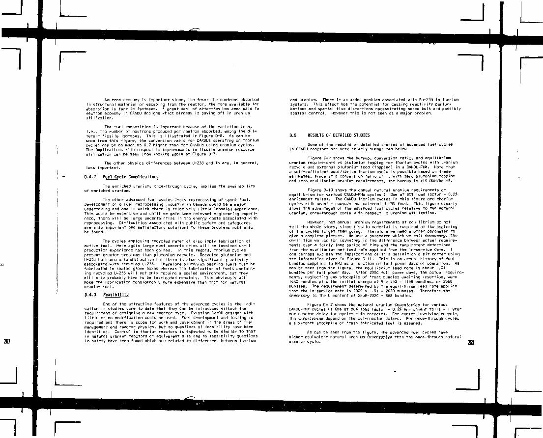
Neutron economy is important since, the fewer the neutrons absorbedin structural material or escaping from the reactor, the more available forabsorption in fer+fle isotopes. ,* great deal of attention has been paid toneutron economy in CANDU designs which already is paying off in uraniumuti I ization.

The fuel composition is important because of the variation in TI,i.e., the number of neutrons produced per neutron absorbed, among the dif-ferent fissile isotopes. This is illustrated in Figure D-8. As can beseen from this figure, the conversion ratio for CANDUs operating on thoriumcycles can be as much as 0.2 higher than for CANDUS using uranium cycles.The implications with respect to improvements in fissile uranium resourceutilization can be seen from looking again at Figure D-7.

The other physics differences between U-238 and Th are, in general,less important.

D.4.2 fuel Cycle Complications

The enriched uranium, once-through cycle, implies the availabilityof enriched uranium.

The other advanced fuel cycles imply reprocessing of spent fuel.Development of a fue! reprocessing industry in Canada would be a majorundertaking and one in which there is relatively little Canadian experience.This would be expensive and until we gain some relevant engineering experi-ence, there will be large uncertainties in the energy costs associated withreprocessing. Difficulties associated with public safety and safeguardsare also important and satisfactory solutions to these problems must alsobe found.

The cycles employing recycled material also imply fabrication ofactive fuel. Here again large cost uncertainties will be involved untilproduction experience has been gained. In this regard, thorium cyclespresent greater problems than plutonium recycle. Recycled plutonium andU-233 both are a tand B) active but there is a I so s igni f icant y activityassociated with recycled U-233. Therefore plutonium bearing fuels must befabricated in sealed glove boxes whereas the fabrication of fuels contain-ing recycled U-233 will not only require a sealed environment, but theywill also probably have to be fabricated remotely. This obviously willmake the fabrication considerably more expensive than that for naturaluraniurn fuel .

D.4.3 Feasibility

One of the attractive features of the advanced cycles is the indi-cation in studies done to date that they can be introduced without therequirement of designing a new reactor type. Existing CANDU designs withlittle or no modification could be used. Fuel development and testing isrequired and there is scope for work and development in the areas of fuelmanagement and reactor physics, but no questions of feasibility nave beenidentified. Control in thorium reactors is expected to be similar to thatin natural uranium reactors of equivalent size and no feasibility questionsin safety have been found which are related to differences between thorium

and uranium. There is an added problem associated with Pa-233 in thoriumsystems. This effect has the potential for causing reactivity pertur-bations and spatial flux distortions necessitating added bulk and possiblyspatial control. However this is not seen as a major problem.

D.5 RESULTS OF DETAILED STUDIES

Some of the results of detailed studies of advanced fue! cyclesin CANDU reactors are very briefly summarized below.

Figure 0-9 shows the burnup, conversion ratio, and equilibriumuranium requirements vs plutonium topping for thorium cycles with uraniumrecycle and external plutonium feed (topping) in a CANDU-PHW. Note thata self-sufficient equilibrium thorium cycle is possible based on theseestimates, since at a conversion ratio of I, with zero plutonium toppingand zero equilibrium uranium requirements, the burnup is >IO MWd/kg HE.

Figure D-10 shows the annual natural uranium requirements atequilibrium for various CANDU-PHW cycles (I GWe at 80$ load factor - 0.2$enrichment tails). The CANDU thorium cycles in this figure are thoriumcycles with uranium recycle and external U-235 feed. This figure clearlyshows the advantages of the advanced fuel cycles relative to the naturaluranium, once-through cycle with respect to uranium utilization.

However, net annual uranium requirements at equilibrium do nottell the whole story, since fissile material is required at the beginningof the cycles to get them going. Therefore we need another parameter togive a complete picture. We use a parameter which we calf inventory. Thedefinition we use for inventory is the difference between actual require-ments over a fairly long period of time and the requirement determinedfrom the equilibrium net feed rate applied from the in-service date. 1can perhaps explain the implications of this definition a bit better usingthe information given in Figure D-tI. This ts an actual history of fuelbundles supplied to NPD as a function of full power days of operation. Ascan be seen from the figure, the equilibrium feed rate is about I.01bundles per full power day. After 2000 full power days, the actual require-ments, neglecting any stockpile of fresh bundles awaiting insertion, were1680 bundles plus the initial charge of 9 x 132 = 1188 bundles, or 2868bundles. The requirement determined by the equilibrium feed rate appliedfrom the in-service date is 2000 x I.01 - 2020 bundles. Therefore theinventory is the U content of 2868-202C - 868 bundles.

Figure D-12 shows the natural uranium inventories for variousCANDU-PHW cycles (I GWe at 80?, load factor - 0.2$ enrichment tails - I yearout reactor delay for cycles with recycle). For cycles involving recycle,the inventories depend on the out-reactor delays. For once-through cyclesa six-month stockpile of fresh fabricated fuel is assumed.

As can be seen from the figure, the advanced fuel cycles havehigher equivalent natural uranium inventories than the once-through, naturaluranium cycle. 253

_l

r ~\

254

Table D-I combines the effect of these two parameters - equili-brium net feed rate and -inventory - to show the annual uranium requirementsfor CANDU-PHW systems with different fuel cycles at various system growthrates. This table shows that the advanced fuel cycle systems have sub-stantially lower annual uranium requirements, although the advantage de-creases as the growth rate increases.

In looking at actual systems, we can not use constant growth ratesfor a particular reactor plus fuel cycle combination. In this case ascenario approach is often used. An example of the results of such anapproach, applied to projected Canadian nuclear power programs, is shownin Figures D-13 and D-14.

Figure D-13 gives an assumed curve of nuclear generating capacityas a function of time (curve i). Various cases are then considered: forexample, once-through, natural uranium PHW reactors only (curve I), andintroduction of a PHW operating on a Pu-topped Th cycle in 1995 (curve 5gives the capacity of natural uranium, once-through reactors *or this case,and the difference between curve 1 and curve 5 gives the capacity ofreactors operating on the Th cycle). Other cases are similarly depicted -introduction of an OCR with 3.5 g fissile Pu topping/kg HE (curve 2),introduction of an OCR employing an U cycle with self-sustaining plutoniumrecycling (curve 3), and introduction of a BLW employing a U cycle withplutonium recycling (curve 4).

Figure D-14 shows the cumulative uranium requirements for thevarious scenarios of Figure D-13. Again this clearly shows the advantagesof the advanced cycles with respect to uranium utilization.

From the point of view of instilling confidence in the adequacyof uranium resources to provide large amounts of nuclear energy, advancedcycles can play ?n even larger role. Figure D-I5 shows estimates of thenuclear power capacity as a function of time (and hence energy production)which can be supported by 3 x I05 Mg of uranium (the amount we know atpresent is available in Canada) using various cycles. The values of Totalelectrical energy produced are proportional to the areas under the curvesand are listed below.

Natural uranium once-through cycle 1,800 GWe years

Plutonium recycling 3,500 " "

Th cycle - high burnup 6,900 " "

Th cycle - intermediate 17,000 " "

Th cycle - setf sufficient 79,000 " "(limited only by Th supply whichis assumed equal to the U supply)

The story on advanced fuel cycles would not be complete withoutsaying a few words about economics. This is rather difficult because thereare large uncertainties associated with reprocessing and active fabricationcosts. However to give some idea of trends, the comparisons in FiguresD-16 and D-1 7 are shown. Figure D-16 compares unit energy costs as a

function of U price, for PHW natural uranium cycles and PHW and BLWreactors with plutonium recycling, for one set of economic parameters.Figure D-17 gives a similar comparison among natural uranium, once-through and various thorium cycles in CANDU-PHWs. The important thing tonote is that the slope of the curves against U price are lower for theadvanced cycles, and therefore they will become competitive at some Uprice. The actual break-even uranium prices are very uncertain but theyare no doubt higher than to-day's prices.

Figure D-18 summarizes the situation for advanced fuel cycles inCANDU-PHW reactors. Here the regions of preference among once-throughnatural uranium, plutonium recycl ing, and Th cycles are shown in terms ofboth uranium price and reprocessing plus active fabrication cost penalty.

D.6 SPECIFIC REACTOR PROBLEMS IN IMPLEMENTING ADVANCED FUEL CYCLESIN CANDU REACTORS

I wiI I discuss very briefly some of the specific problems whichwill arise in implementing advanced fuel cycles in existing CANDU reactors.

A fairly detailed study of plutonium recycle in a CANDU(PHW) hasbeen done by AECL and Ontario Hydro. In this study, a conceptual design ofa 1200 MWe nuclear generating station was used, and some of the problemsof converting this to operation with plutonium recycle examined. The fueldesign assumed was 37-element bundles wHh graded enrichment, i.e., lessplutonium was added to the outer elements of the bundle than to otherelements. After a rough survey it was decided to assume that an average of3 g fissile plu^onium per kg heavy element would be added to the feed fuel.At equilibrium "this is a bit less than the fissile plutonium content of thedischarged fuel. The extra fissile plutonium would be used to initiatesimilar cycles ir other reactors. With this feed fuel it was estimatedthat a burnup of 16,000 MWd/Te per pass could be achieved.

deta iI.The transition to equilibrium operation has not been studied

Reactivity Worth of Control, Adjuster and Shut-down Absorbers

In general, these absorber worths are reduced by 10-15?. The zonalcontrol worth reduction ij about Q%.

Fuel Management

Channel power peaking with (U,Pu)02 fuel will be larger than withnatural UO2 fuel, leading to reduced margin to dryout or derating. Tominimize this effect, smaller amounts of Pu-recycle fuel are loaded perfuelling machine visit (4 bundles vs 8 for natural fuel). The longer burn-up means that fuelling machine use is approximately the same.

Controllability

The reactor with Tu-recycle fuel will have acceptable controlcharacterisiics, although not as good as with natural fuel. Assuming the

adjuster rods are not changed (and hence are reduced "\5% in reactivityworth), the xenon override capability is unchanged from the natural UO2case. There is then potential for improving this characteristic by in-creasing the adjuster rod worths.

Energy Release During LOCA

The average energy release during LOCA is increased by about 40%for the piutoniurn recycle core.

Fuel

Plenums should not be required. There would be problems with fuelfailures during refuelling with non-CANLUB fuel, but it is expected thatfuei development already under way will solve this problem.

Fuel Hand Ii ng

Fuel handling problems have not been studied.

Similar problems will arise in converting existing reactors to Thcycles but these are only now being studied in detail.

D.7 SUMMARY

Advanced fuel cycles provide insurance against uranium shortagesand very high ursr ium prices through better uranium uti Ii zation. They canalso provide increased flexibility in reactor design.

The main uncertainties (economic and political) associated withthe advanced fuel cycles are in the out-reactor portion of the cycles -reprocessing and active fabrication.

TABLE D - I

ANNUAL URANIUM REQUIREMENTS FOR CANDU-PHW SYSTEMS

AT VARIOUS GROWTH RATES

SYSTEM

ONCE-THROUGH NATURAL U CANDU-PHW ONLY

PLUTONIUM RECYCLING HITH NATURAL U FEED (CANDU-PHW)

NATURAL U CANDU-PHWS FEEDING PLUTONIUM TOCANDU-PHWs WITH:

"HIGH BURNUP" TH CYCLE

"INTERMEDIATE" TH CYCLE

"SELF-SUFFICIENT" TH CYCLE

ENRICHED URANIUM (U-235) FEED TO CANDU-PHWS WITH:

"JIIGH EURNUP" TH CYCLE

"INTERMEDIATE" TH CYCLE

•SELF-SUFFICIENT" TH CYCLE

ANNUAL URANIUM REQUIREMENTSPER GWE AT 802 LOAD FACTOR (MGU/A)

SYSTEM GROWTH RATES PER ANNUM

OS

133

56

36

17

0

26

10

0

3.33X

138

62

58

1)7

43

49

31

29

B:Ml

68

70

63

64

67

53

52

CANDU-PHVOXIDE FUEL

I 2

U23S IN UR1N1UH I I I

n l Fundamental Efficiency of Once-throughu-i vcyc}e a s a F u n c t i o n o f U.J35 1 n u

_l

uMINE

ENRICHMENTPLANT

REACTOR

FIGURE D-2

Once-through U Cycle

. W A S T E S

uMINE

UMINE

N.U.CANOUPHW

NAT

• > -

. U

REPR.

i

jpuI1

j SALE

FIGURE D-3

U with Pu Recycle and Net Natural U± Pu Feed

STORAGE

HOLDUP

uM I N E

ThM I N E

NAT.

U

A i «;L

ENRICH-HENT

0

Th

HIGHLYENR. U

WASTE

FIGURE D-4

Th wi th U Recycle and Net U-235 Feed

uMINE

ThMINE

N.U.CANDUPHW

Th

* WASTES

REPR.

>rPU

WASTE

FIGURE D-5

Th with U Recycle and Net Pu Feed

HOLDUP

.HOLDUP

2S6

HEY ASSERTIONS . ALL CANDU • PHI l

- ENRICWENT Tt lLS 0.2< UNLESS

OTHEMISE NOTED

LEGEND

~ 6r

£ o

V20.OOO

\

U ONCE THROUGH CYCLES

Tn • U235 ONCE THROUGH

- — Tn • U235 I I T H U RECYCLEO SEL'F-SUSTJUNING Pu RECYCLE

( I N U CYCLE)A SVSTEII CWPOSED OF T«0

REACTOK TYPES

-NAT. U CANOU-PHI Pu -

PRODUCER (J500 H l D / t l )-TH PHI BUDNING Pu WITH

BURNUP SHOW (U RECYCLE)D NAT. U CYCLE • ONCE THROUGH

40.000

3D.0C0-A

NUUBERS ON CURVES ARE

BURWS (UIO/t«>

O-IB.000

20,100 (TAILS OS) 4) .000

•—1 m i , , n ,,\ i " " ^ 82,00020,100 <TAIL5 0.3%) _,..'" - ^

,..••'" 41,000

I

N.U. 10 20

INITIAL U23S IN HEAVY ELEMENT It/kfl

{EXTERNAL FEED MATERIAL!

FIGURE D-6

Comparison of Fundamental EquilibriumEfficiencies for Various Cycles

.7 .8 .9

CONVERSION RATIO

FIGURE D-7

Ideal Multiplication of FissileResource vs Conversion Ratio

HEUTRDNS EMITTED

! NEUTRONS ABSORBED

IN THEtMAl ftEACtOXIUIK OF NEUTHON5 INTYPICAL FAST REACTOR

10' 10' 10° 10 10' 10" 10' 101 10* 10'

NEUTRON ENER6V |cV|

FIGURE D-8n-Values of Fissile Isotopes

70

z eo

5 so

l „£ 30

i !0

- ID

0

- i t

! 1 2

" 1 0

" g

. 6

! '

3 2in

oi

•

j o

118 N

O

«V

ER

SI

.5 ,

• . 2

0

5 vo

0 2 1 6 8 10 12 II

FISSILE Pu CONTENT OF F.0" FEED FUEL I t / « | H E I

[ I . e -Po TOPPING*)

FIGURE D-9

Thorium Cycle Characteristics as aFunction of Pu Topping

257

I

g

NUMBER OF FUEL BUNDLES

i S S ! o ! 3 S 8 8 6 SO O Q o O O O O o O p O ir T T T T i r T T T - T ' T "

\

= = -

8 " !

\

/ \

\

<= a

ANNUAL NATURAL U REQUIREMENTS (MgU/a)(IGWe 01 80% L.F )

dj ~

[v r* »NATURAL U "INVENTORY" (MgU)

(IGWe ol 80% LF )

8

L J

G W ( . |

SELF-SUFFICIENT Th CYCLE

— Th CYCLE • INTERMEDIATE

Th CYCLE • HIOH IUHNUP

1975 2000 2025 2050 2075 2100 2125 2150 2175

ctrnoc n in Energy from 3 x 10s Mg Uranium withFIGURE D-lb Various CANDU Cycles

too

000

900

800

-

-

-

BURN-UP

/ !

i

P H K N 1 T

BURN-UP = 7 . 0

" 7 . 5 M U d / k t U

A

i i

u) jA

TjXPHII(PB)

BLKPS)

1 1 1

FIGURE 0-16

20 2 5 30 3 5 1 0 1 5

U R I N I U H ORE P R I C E I S I 9 7 5 M H U , 0 , l

TUEC Comparison for PHW (Nat.U),PHW(PB), BLW(PB)

I 197B i l

/HIGH 8UBNUP

Th CYCLE

SELF-SUFFICIENTTh MCLE

INTERUEDIUTE Ttl CrCLE

FIGURE D-17

10(1 200 300 400 500URINIUH PRICE (S/kt U)

Effect of Uranium Price on EnergyCost for Various Thorium Cycles

THORIUM REPROCESSING jPLUS ACTIVE FABRICAT- ,ION PENALTY COSTK/kg HEI

ONCE-THROUGHPREFERRED

FIGURE D-18

100 200 300URANIUM PRICE O/kgU)

Preferred Cycles in CANDU-PHWsfrom Economic Considerations

259

BIBLIOGRAPHY

[I] BROOKS, G.L., Power Reactor Types, Lecture 3, Nuclear PowerSymposium, Atomic Energy of Canada Limited, Power Projects,Sheridan Park, Ontario

[2] PON, G.A., Introduction, Lecture I, Nuclear Power Symposium,Atomic Energy of Canada Limited, Power Projects, SneridanPark, Ontario

[3] FOSTER, J.S., RUSSELL, S.H., CANDV - Canadian Experience andExpectations with the Heavy-Water Reactor, Paper IAEA-CN-36/179,IAEA Int. Conf. on Nuclear Power and Its Fuel Cycle, Salzburg,Austria, 2-13 May 1977. Also Atomic Energy of Canada LimitedReport No. 5707

[4] MILLAR, C.H., Some Basis Physics Aspects oj the CanadianNuclear Power Program, Atomic Energy of Canada Limited ReportNo. 5229, July 1975

[5] JONES, J.E., and TURCOTT, G.E., Ontario Hydro, Pickering NGS,Pickering GS Start-up and Early Operating Experience, 1974 ANSAnnual Meeting, 1974 June 24, Philadelphia, Pa., USA

[6] PASANEN, A.A., Atomic Energy of Canada Limited, Power Projects,Sheridan Park, Ont., The Physios of CANDU On-Power Fuelling:From Design Objective to Pickering Demonstration, Paper IAEA-SM-I78/I3

[7] HALSALL, M.J., Graphs and Tables of the Isotopic Composition ofPlutonium Produced in Canadian DzO Moderated Reactors, AtomicEnergy of Canada Limited Report No. 2631, January 1967

[8] ZED-2, from Directory <-/ Nuclear Reactor, 5, 223-224, IAEA,1964. Also Atomic Energy of Canada Limited Report No. AECL-2132

[9] GREEN, R.E., et a I, Lattice Studies at Chalk River and TheirInterpretation, 3rd UN Int. Conf. on the Peaceful Uses of AtomicEnergy, Geneva, 1964. Atomic Energy of Canada Limited ReportNo. 2025

[10] SERDULA, K.J., Lattice Measurements with 28-Element Natural WiFuel Assemblies. Part I: Bucklings for a Range of Spacingswith Three Coolants, Atomic Energy of Canada Limited Report No.2606, July 1966

[II] OKAZAKI, A., and CRAIG, D.S., Determination of Lattice ParametersUsing a Few Rods, Atomic Energy of Canada Limited Report No.2593, March 1967

280

[12] SERDULA, K.J., and GREEN, R.E., Lattice Measurements with 28-Element Natural VO2 Fuel Assemblies. Part II: Relative TotalNeutron Densities and Hyperfine Activation Distributions in aLattice Cell. Atomic Energy of Canada Limited Report No. 2772,August 1967.

[13] MEHTA, S.L., and SERDULA, K.J., Integral Measurements for 28-Element UOz Assemblies with Air, HzO and Air-BiO Mixture Cool-ants, Atomic Energy of Canada Limited Report No. 3416, July1969

[14] GREEN, R.E., et al, Highlights of Chalk River Work on the Physicsof Heavy Water Lattices Since the 19SB IAEA Panel Meeting. IAEADanel on Heavy Water Lattices, February i963. Atomic Energy ofCanada Limited Report No. 1684, December 1962.

1.15] SRINIVASAN, M., and SERDULA, K.J., Experimental Bucklings ofSimulated Boiling RiO-Cooled 28-Element Natural V02 Fuel inHeavy Uatev Moderator. Atomic Energy of Canada Limited ReportNo. 3513, October 1969.

[16] ROBERTSON, L.P., and GREEN, R.E., Some Flux Peaking Experimentsin Cluster Type Fuel Rods, Atomic Energy of Canada Report No.925, November 1959.

[17] KAY, R.E., and TANNER, C.J., CANDU-BLW Experiments in ZED-2.Part I: Refuelling Experiment, Atomic Energy of Canada LimitedReport No. 2667, January 1967

[18] MCDONNELL, F.N., Liquid Absorber Experiments in ZED-2, AtomicEnergy of Canada Limited Report No. 5024, July 1975.

[19] JONES, R.T., Adjuster Rod Experiments in ZED-2, Atomic Energyof Canada Limited Report No. 5853, August 1977

[20] OKAZAKI, A., and JONES, R.T., Additional Shutoff Rod Experimentsin ZED-2, Atomic Energy of Canada Limited Report No. 5102,March 1975

[21] R0SHD, M.H.M., Gentilly BLW Booster Rod Experiments in the ZED-2Reactor, Atomic Energy of Canada Limited Report No. 3258,February 1969

[22] HINDS, H.W., et al, kinetics Experiments on Coupled Cores in theZED-2 Reactor, Atomic Energy of Canada Limited Report No. 4267,September 1972

[23] BAUD0UIN, A.P., and McDONNELL, F.N., Analysis of TransientMeasurements in the ZED-2 Reactor, Atomic Energy of Canada LimitedReport No. 5967, December 1977

275

[24] CRAIG, D.S., et al, Long Irradiation of Natural Uranium, PaperP/205(Canada), Session A-1 I: Nuc. Data, Proc. of the 2nd Int Confon Peaceful Uses of Atomic Energy, Geneva, Sept. 1958, Vol. 16,pp. 83-96.

[25] WARD, A.G., and CRAIG, O.S., Measurements of the ReactivityChange with Irradiation for Natural Uranium Samples Irradi-ated in NRXy Atomic Energy of Canada Limited Report No. 812,May 1959

[26] OKAZAKI, A., Atomic Energy of Canada Limited, Chalk River, Ont.,and SOKOLOWSKI, E.K., A.B. Atomenergi, Studsvik, Nykoping,Sweden, Hedetermination of the Thermal-Neutron Absorption Cross-Sections of Gross Fission Products of 233U, 23SU and 23*Pu,Paper IAEA-CN-26/58, Reprint from Nuclear Data for Reactors,Vol. I, IAEA, Vienna. 1970

[27] OKAZAKI, A., et a I, Neutron Absorption Cross Section of GrossFission Products of U233, U2is and Pu21*, Atomic Energy ofCanada Limited Report No. 2510, November 1965.

[28] DURET, M.F., Plutonium Production in UPD. A Comparison BetweenExperiment and Calculation. Atomic Energy of Canada LimitedReport No. 3995, August 1971

[29] ROSHD, M.H.M., The Physics of CASDU Reactor Design, ANS Conf.,Toronto, Ont., June 14-18, 1976. Atomic Energy of CanadaLimited Report No. 5803, April 1977.

[30] GRIFFITHS, J., The Effectiveness of LATREP Calculations: ASurvey and Detailed Comparison with Experim' it, Atomic Energyof Canada Limited Report No. 3739, September 1971

[3 ] TILL, C.E., and WHITTIER, A.C., Canadian General Electric Co.Ltd., Peterborough, Ont. Atomic Energy of Canada Limitedreprinted report No. 2155, February 1965

[32] HILBCRN, J.W., et al, NPD Start-up, Reactivity Balance andFuel Management. 3rd UN Int. Conf. on the Peaceful Uses ofAtonic Energy, Geneva, Aug.31-Sept.9, 1964. Atomic Energy ofCanada Limited Report No. 2009, September I9C4

[33] LOPEZ, A.M., ENSELMOZ, J.R., Ontario Hydro, and MOHINDRA, V.K.,Atomic Energy of Canada LimMed, Power Projects, Reactor PhysicsMeasurements at Bruce NGS-A. ANS 8th Biennial Topical Conf. onReactor Operating Experience, Chattanooga, Tenn., Aurj.7-10, 1977.Ontario Hydro Report No. CNS-54, October 1977.

[34] PASANEN, A.A., and BLANSCHE, J.F., Douglas Point HUR StartupPhysics Measurements and Predictions. ANS 1968 Annual Meetinq,Toronto, June 1968. Atomic Enerqy of Canada Limited ReportNo. 2712.

[35] DASTUR, A.R., et al, Confirmation of CANDU Shutdown SystemDesign and Performance During Commissioning. ANS ThermalReactor Safety Conf., Sun Valley, Idaho, Auq. 1977. AtomicEnergy of Canada Limited Report No. 5914.

[36]

[37]

[3BJ

[39]

[40]

[41]

[42]

[43]

[44]

BROWN, R.A., Ontario Hydro, CNS, Fuel Scheduling. 1974 CNAAnnual Meeting

MILLAR, C.H., Fuel Management in CANDU Reactors. Proc. of theEuropean Nuc. Conf., Paris, 1975: Nuclear Energy Maturity.Progress in Nuclear Energy Series. Atomic Energy of CanadaLimited Report No. 5090.

HINCHLEY, E., and KUGLER, G. , Atomic Energy of Canada LimiT<;d,Power Projects, On-line Control of the CAUDU-PHW Pouer Distri-bution. IAEA Specialists Meeting on Spatial Control Problems,Studsvik, Sweden, October 1974. Atomic Energy of CanadaLimited reprinted report No. 5045, June 1976.

SERDULA, K.J., Canadian Experience in the Area of ReactorNoise. Specialist Meeting on Reactor Noise from CriticalAssemblies to Power Plants, SM0RN-I, CSN Casaccia, Rome,October 1974. Atomic Energy of Canada Limited Report No. 5029,January 1975.

BANERJEE, S., et al, Thorium as a Nuclear Fuel for CANDUReactors. The Can. Journal of Chem. Eng., Vol. 53, June 1975

FOSTER, J.S., and CRiTOPH, E., The Status of the CanadianNuclear Pouer Program and Possible Future Strategies. Reprintedfrom Annals of Nuclear Energy, Vol. 2, Nos. 11/12, pp 689-704.Atomic Energy of Canada Limited Report No. 5225.

CRITOPH, E., et al, Prospects for Self-Sufficient EquilibriumThorium Cycles in CANDU Reactors. ANS 1975 Winter Mtg., SanFrancisco, November 1975. Atomic Energy of Canada LimitedReport No. 55CI, March 1976.

HATCHER, S.R., et al, Thoriw. Cycle in Heavy Water ModeratedPressure Tube (CANDU) Reactors. ANS Winter "tg.. Session on233U-Thorium Cycle, San Francisco, November 1975. AtomicEnergy of Canada Limited Report No. 5596, May 1976.

SLATER, J.B., An Overview of the Potential cas a Thermal Breeder IAFA Consultants Meetd P t f T

ER, J.B., An Overview of the Potential cf the C/u!"'J ReactorThermal Breeder. IAFA Consultants Meeting on the Status

Prospects of Thermal Breeders, Vienna, 5ept. 1976. Atomicgy of Canaan Limited Report No 51:79 Feb-uary 1977

a s <.z ^riernac DvenaKX'. in:n L o r i b u i i d r n i i w t f e i i r i q o n T n e D i d r

and Prospects of Thermal Breeders, Vienna, 5ept. 1976. AtoiEnergy of Canada Limited Report Uo. %79, February 1977.

[45] CPITOPH, E., The Thorium Fuel Cycle in Water-Moderated ReactorSystems. Paper IAEA-Ch-3o/l77. I ALA Int . Conf. on NuclearPower and i ts Fuel Cycle, Sal.'burg, Austria, wsy 1977. AtomicEnerqy of Canada L imited Report Wo. 57G5r May 1977,

[ 4 0 ] FOSTER, J . S . , and CRITOPH, E . , Advanced Fuel Cycles in HeavyWater Peacfiovs, ANS/FNS/AIF I n t . Conf. on World Nuclear Energy,Washington, D.C., November 1976. AN'S Trans. 25, 187-192 (1977) .Atomic Energy of Canada L imi ted Report No. 5735.

261

L

r

L

~i¥r

GENERAL REMARKS ONFAST NEUTRON REACTOR PHYSICS

J.Y. BARRECommissariat a l'£nergie atomique,Paris,France

Abstract

The main aspects of fast reactor physics, presented'in theselecture notes, are restricted to IMFBR's. The emphasis isplaced on the core neutronic balance and the burn-up, problems.After a brief description of the power reactor main componentsand of the fast reactor chronology, the fundamental parametersof the one-group neutronic balance are briefly reviewed. Thenthe neutronic burn-up problems related to the Pu productionand to the doubling time are considered.

TABLE 1

n-i

ex

Of born

t

235 U

1.07

2.42

.17

582

rHEEMAL

239 Pu

1.11

2.88

.36

743

233 U

1.28

2.49

.09

528

PAST

235 U

.88

2.43

.29

1.81

239 Pu

2.94

.26

1.76

233 U

1.27

2.53

.12

2.79

Don't forget also that the depleted Uranium, the waste of enrich-ment facilities, can be used without any problem in fast breeders.

It must also be mentionned that the use of sodium leads to goodtemperature and pressure vapor conditions giving a high thermo-dvnamic efficiency (40 to 45 %) s this is a really favorableenvironmental consequence.

Pu use and high specific powers are looked for :0,6 to 0,8 MWthAg Pu- Even with the high fissiledensity, that leads to high flux values, 3 to

7 10~ n. m s"1. That is one of the core fonda-mental characteristic for the design.

The fuel is usually made of sintered mixed oxidecylindrical pellets, 4 to 7 mm in diameter. Thesepellets are placed in thight stainless steelcylindrical clads, 0,4 to 0,8 mm thick, that repre-sent the first safety barrier for fission products.These pins are assembled in hexagonal stainlesssteel boxes that make the subassemblies : 169 to325 pins per subassembly. The subassembly repre-sents the elementary unit for core loading andunloading : it can contain between 1O and 20 Pu Kg.

1.1.2.

The high specific power per Pu mass leads to veryimportant volumic powers, between O.3 to O.5 MWthper core liter. Then, it is necessary to have largeexchange surfaces (pins) and to choose a coolingmaterial with high thermal performances, small neu-tron absorption and slowing down, small activationto neutrons.

The sodium, commonly used now, has the best charac-teristics for FBR's. Sodium volumic percentages varybetween 3O to 40 %, the sodium flows are of the orderof 3 to 2O tons per second. The sodium temperaturesare 38O-4OO°C at core inlet and at the maximum 550°-600° in normal conditions. Then, there is no need topressurize the circuits : that represents a veryimportant advantage for construction and operation.

Due to the remarkable sodium thermal properties, highsodium temperatures at the core outlet can be reachedleading to favorable vapor conditions for thermodyna-mic efficiencies.

Finally, the order of magnitude of the core volumicpercentages are :

mixed oxide fuel : 30 x.o 45 %sodium : 30 to 40 %structural materials, cladding : 20 to 25 %gas : 2 to 5 %

263

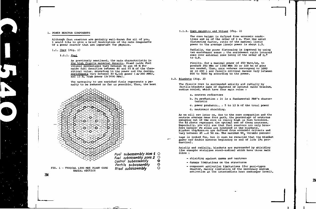
1. POWER REACTOR COMPONENTS

Although fast reactors are probably well-known for all of you,I would like to give a brief description of the main componentsof a power reactor that are important for physics.

1.1. Core (Fig. 1)

1.1.1. Fuel

As previously mentioned, the main characteristic isthe high fissile material density. Mixed oxide fuelvolumic percentages vary between 30 and 45 % foroxide fuel densities between 80 and 95 % of the theo-ritical value. According to the power and the design,enrichments vary between 30 %, low power ( Csf 2OO MWe),and 13 %, high power (if2000 MWe).

The necessity to use enriched fuels represents a pe-nalty to be reduced as far as possible. Then, the best

1.1.3. Core geometry and volume (fig• 2)

The core height is defined from economic condi-tions and is of the order of 1 m. Then the axialflatenning factor, ratio of the maximal lineicpower to the average lineic power is about 1.3.

Radially, the power flatenning is improved by usingtwo enrichment zones ; the enrichment ratio internalzone over external zone being of the order of 0,7to 0,8.

Finally, for a maximal power of 450 Watt/cm, toproduce 250 MWe or 120O MWe 20 or 100 km of pinsare needed. Then, core voliraes correspond to 1000or 1O 000 1 and fissile critical masses vary between800 to 5000 kg according to the power.

1.2. Blankets (fig. 2)

The fissile core is surrounded axially and radially byfertile blankets made of depleted or natural oxide Uranium,sodium cooled, which have four main roles :

a. neutron reflectors

b. Pu production : it is a fundamental FBR's charac-teristic

FIG. 1 - TYPICAL 1200 MWE PLANT CORERADIAu SECTION

Fual subasszmbty 20f» 1 OFua.1 subossembly zono. 2 OControl suhassambly OFarhla subassembly ©Shad subassambly O

c. power productici. s 5 to 12

d. neutronic shielding.

of the total power

284

As we will see later on, due to the core compaction and theneutron average mean free path, the percentage of neutronsescaping out of the core is really high in fast breeders.The blsnkets represent the optimal use of these neutrons.Especially, you will s3e that fast reactors are only bree-ders because Pu atoms are produced in the blankets.Blanket thicknesses are defined from economic criteria andvary between 25 ,i.id 50 cm. The maximum U0 2 volumic percen-tage is looked for, but it must be recalled that the blanketpower can doubie between beginning or end of life (Pu pro-duction) .

Axially and radially, blankets are surrounded by shielding(for example stainless steel-sodium) which have three mainroles :

- shielding against gamma and neutrons

- damage limitations on the structures

- component activation limitations (for pool-typesreactor, mainly limitation of the secondary sodiumactivation at the intermediate heat exchanger level).

J

~lZcm

290

ZT = Transition zone (rta-SS)

LOWER AXIAL -BLANKET\ V V X V \ "• V \ \ V X V

FIG. 2 - PHENIX TYPE PLANT-CORE

AXIAL SECTION

1.3. Control rod (fig. 1)

The reactor control is obtained by control rod subassembliesreplacing normal subassemblies. Boron carbide enriched ornatural is commonly used in pins stainless steel cladded,sodium cooled. Then, control rods have three fonctions :

- safety : ££ 3

- compensation

- operation.

• in keff

loss of reactivity due to neutronicburn-up, temperature and power rises( — 3 and 2 % in kef f depending onthe design)

At the end of the cycle, the absorber part is out of thecore, then sodium holes remain in the core.

The optimisation of the whole control rod system, takinginto account the global antireactivity needed (^8 to 10 %in keff), is performed on the composition, the number and thepositions of the control rods in the core : it is ratherdesign dependent.

However, for large power reactors, the most important phy-sics problem is the influence of control rods on radialpower distributions and the interactions between the controlrods. The control rod positions are commonly used to improvethe radial power flatenning and to control the radial powerdistribution during burn-up (hot spot control - fig. 3).

3501-

iOO-

250-

200'

1 q max/cm*

c CORE ZONE 1

- ,

\-

•' / v/ \ ./ \»

/ \/ \

Rods downRods Up

IJ

CC.9BZONE!

SI I \-• > \

\ \

A VI •I •

R(cm)SO 100 150

FIG. 3

RADIAL POWER DISTRIBUTION IN THE CORE

WITH TWO CONTROL ROD RINGS 265

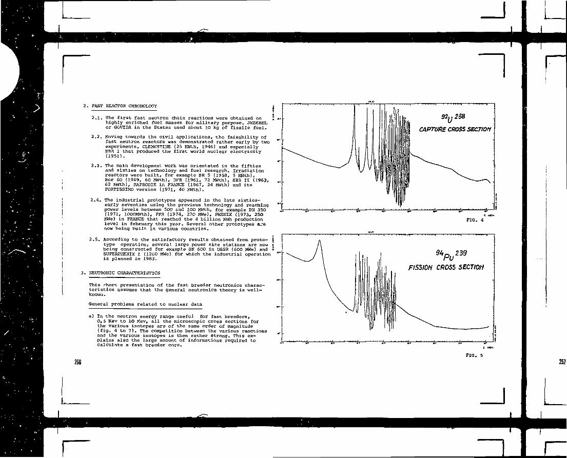
~l2. FAST REACTOR CHRONOLOGY

2.1. The first fast neutron chain reactions were obtained onhighly enriched fuel masses for military purpose. JEZEBELor GOVIDA in the States used about 10 kg of fissile fuel.

2.2. Moving towards the civil applications, the faisability offast neutron reactors was demonstrated rather early by twoexperiments, CLEMENTINE (25 KWth, 1946) and especiallyEBR 1 that produced the first world nuclear electricity(1951).

2.3. The main development work was orientated in the fiftiesand sixties on technology and fuel research. Irradiationreactors were built, for example BR 5 (1958, 5 MWth),Bor 60 (1969, 60 MWth), DPR (1961, 72 MWth), EBR II (1963,62 MWth), RAPSODIE in PRANCE (1967, 24 MWth) and itsFORTISSIMO version (1971, 40 MWth).

2.4. The industrial prototypes appeared in the late sixties-early seventies using the previous technology and reachingpower levels between 500 and 100 MWth, for example BN 350(1971, lOOOMWth), PPR (1974, 270 MWe), PHENIX (1973, 250MWe) in PRANCE that reached the 4 billion KWh productionlevel in february this year. Several other prototypes a 'enow being built in various countries.

2.5. According to the satisfactory results obtained from proto- Itype operation, several large power size stations are now ibeing constructed for example BN 600 in USSR (600 MWe) and 2SUPERPHENIX 1 (12O0 MWe) for which the industrial operationis planned in 1983.

3. NEUTRONIC CHARACTERISTICS

CAPTURE CROSS SECTION

FIG. 4

This -hort presentation of the fast breeder neutronics charac-teristics assumes that the general neutronics theory is well-known .

General problems related to nuclear data

a) In the neutron energy range useful for fast breeders,0,5 Kev to 10 Mev, all the microscopic cross sections forthe various isotopes are of the same order of magnitude(fig. 4 to 7). The competition between the various reactionsand the various isotopes is then rather strong. This ex-plains also the large amount of informations required tocalculate a fast breeder core.

FISSION CROSS SECTlOli

PIG. 5

266 252

TOTAL CROSS SECTION

FIG. 6

"tia"TOTAL CROSS SECTION

b) The isotopes called "light" as oxygen, sodium, iron,chromium, nickel, contribute to the elastic slowing downthey present very broad diffusion resonance (fig. 6-7)

Na

Oxygen

Energy (KeV)

2.85 + 0,015

440 + 4

Width (KeV)

0.41 + O.C.

45 + 5

Average spacing(KeV)

30 + 6

3OO + 50

c) The isotopes called" heavy"1 as Plutonium isotopes or 238 Upresent also resonances in the low energy range, below6O Kev. These heavy isotopes absorption resonances dif-fer largely from the light isotope diffusion resonancesas it is shown for the main resonance parameters of 238 Uor 239 Pu : (fig. 4-5)

Fission

Capture

Spacing

width :

width :

:

34

3,

239 Pu

or 2100

40 mev

2 or 9,6

mev

ev

24

23

238

mev

ev

d) The elastic slowing down is mainly due ( , 90 %) to lightelements in the order, oxygen, sodium, iron (table 2). Theelastic slowing down cross section represents approximati-vely 90 to 98 % of the total macroscopic cross sections,for a standard composition, below 10O Kev, where the inelasticslowing down remains small t

ENERGY

100 Kev

1.8 Mev

V cm"1

W

£ cm"1%

TOTAL

0.3

100 %

0.18

100 %

ABSOR-PTION

• O035

1,2%

.0056

3,1%

ELAS-TIC

.293

97,5%"

.138

76,2%

INELAS-TIC

.044

1,3 %

.037

20,7 %

FIG. 7 267

e) At the opposite, in the high energy range, the importantheavy isotope volumic percentage leads to a large inelas-tic slowing down, mainly by 238 Uranium (50 to 90 %between 300 Kev and 1 Mev).

f) The neutron mean free path is large compared to the fueland cell dimensions, decreasing from 5 cm at high —lergyto 2 cm at 1 Kev : then, the heterogeneity problems re-main simpler than in thermal reactors.

g) The threshold fission cross sections for example on 238 Uor 240 Pu,play a major role in the neutron balance due tothe fuel composition. Threshold reactions (n, 2n), (n,p),{n, st) can not be neglected either for heavy isotopes orfor structural materials although the energy thresholdsare above 2 Mev.

Table 2

AVERAGE ENERGY LOSS

BY ELASTIC COLLISION (IN KEV)

E

Oxygen

Sodium

Iron

238 U

1 MeV

115

60

275

100 KeV

12

8

3

0,8

1 KeV

0,12

0,08

0,04

0,00

3.1. Energy neutron balance

3.1.1. Neutron spectrum

Due to the competition between the various reac-tions, the energetic spectrum of the neutron fluxplays a really important role in FBR physics : itvaries continuously versus the reactor type (fig.8).

All the neutrons are born from fission with a max-wellian spectrum (average energy 2 Mev) : there is no

more neutron coming directly from fission below1OO Kev ( •«: 1,5 % ) . At high energy, the competitionexists mainly between the production on one side,the leakage and the inelastic slowing down on theother side.

Down to 1OO Kev, all the reactions compete includingthe absorption and the elastic slowing down. Below100 Kev, the absorption role increases and the slo-wing down is purely elastic. Finally, in the lowenergy range, the largest majority of the neutronsare absorbed, over the loo ev energy, by the 238 Ucapture resonances.

Finally, the greater the core power, the softerthe spectrum. An increase of the reactor power leadsto a core volume increase, a leakage decrease, thenan enrichment reduction giving a lower relative roleto the production compared to the other reactions.

The neutron spectrum is also strongly influencedby the large elastic diffusion resonance (see fig.8).

3,1.2. Slowing down

The variation of the slowing down densities versusenergy for the elastic and inelastic reaction ratesis given in figure 9.

For the integrated total slowing down densities, thepercentages for both reactions are t elastic 58 %,inelastic 42 %, but the energy distributions ofslowing down densities are rather different :

first moment elasticinelastic

350 Kev1,5 Mev

To characterize the neutron spectrum by only oneparameter, the r parameter, defined by R. NAUDETas the ratio of the average number of neutron pro-duced per fission V 71 p to the integral of the

slowing down density "fe 21^is commonly used inFrance. It can be easily shown that 1/r representsthe averaged lethargy interval covered by a neutronduring its life : it is the average lethargy shiftbetween the fission neutron spectrum and the dispa-rition neutron spectrum. The r parameter gives agood representation of the spectrum hardness, takinginto account not only the fuel but the whole cell.For power plants, r varies between 0,5-0,4 for 250MWe reactors and 0,4-0,3 for 1200 MWe.

268

NORMALISATION*p(E)c = 100

® FISSION SPECTRUM

© RAPS0DI6.

(D 250 MW&

© 1200 /We

FIG. 8. NEUTRON FLUX ENEQ6ETIC SPECTRUMIN A FAST REACTOR

3.2. Integral neutron balance

The knowledge of the integral neutron balance, or averagereaction rate neutron balance .represents the main role ofreactor physics work. If the analysis of the energy neu-tron balance is important for the detailed understanding ofthe phenomena, at the level of the definition and of theoptimisation of the plan characteristics, only integralquantities are needed for the design.

3.2.1. Global analysis of the integral balance

The decomposition of the neutron integral balancefor a typical 1200 MWe reactor into the usual balan-ce components is given table 3 for 1O0 neutronsproduced per fission.

This table shows firstly the importance of the lea-kage (22 % ) . The analysis of the isotope contribu-tions demonstrates the first role of 239 Pu for theproduction and the absorption per fission and thefirst role of 238 U for the capture rate (239 Puproduction).

The contributions of the other isotopes remainhowever important : Pu isotopes for fission andcapture, structural materials for capture.

3.1.3. Energy distribution of the neutron balance compo-

nents (fig. 10)

The neutron balance can be easily split up into fourcomponents :

production = capture + fission + leakage.

The energy distribution of these four components isrepresented fig. 10 for a 1200 MWe typical reactor.The probability energy threshold 50 % varies strong-ly for the various terms :

production =1,3 Mev leakage : 230 Kevcapture : 18 Kevfission : 150 Kev

3.2.2. Average microscopic cross sections per isotope

The various balance components are calculated fromaverage microscopic cross sections t an order ofmagnitude of these data is given table 4 for a typi-cal 1200 MWe reactor (enrichment : 15 % ) .

Outside the 235 U - 239 Pu comparison previouslycommented for FBR's, the favorable \> and fissioncross sections for 241 Pu, the positive (V«"F -<r«. )parameter £or 240 Pu and the low microscopic capturecross section for 238 U must be noted. The important238 U role in the capture balance comes from itsconcentration. The structural material cross sectionsshow the difficulty of high concentration in stainlesssteel of nickel, molybdenum or manganese. Finally,sodium and oxygen captures are negligeable in thebalance.

269

-10

- 9

_ a

_ 7

- 6

_ 5

_ 4

_ 3

_ 3

_ *

/" Q(EjdE = | Z 3

i i i ml

FIG. 9.IHELASTIC AND ELASTIC SLOWING DOWN DENSITIES

SLOV/IMG DOWN DEIiSITY TOTAL NORMALISATION

P(£)= f(E) REACTION RATS. PERCENTAGE

BELOW THE ENERGY £

NORMALIZATION .' F1S5I0H NEUTROH PRODUCTtOHziOO

i i i TTTTT I i t i 111 t i l i100 ev

270 FIG. 10. ENERGY DISTRIBUTIONS OF THE NEUTRONBALANCE MAIN COMPONENTS

TABLE 3 - DECOMPOSITION OF THE CORE INTEGRAL

NEUTRON BALANCE FOR A 1200 MWE TYPICAL

REACTOR

C0MP0ME/1T ISOTOPE TYPE ISOTOPE

PRODUCTIOn

100 neutrons

LEAKAGE22

ABSQRfmt

78

capture: iik

Fission : 34

FISSILE81.7

FERTILE

•E

•E

FISSILE

37.2 -cFISSION28.7

CAPTURE8.5

FERTILE

35.8 -GFission

s.6

CAPTURE30.2

hE-EhE

PARASITIC

5.0

239 Pu24* Pu255 U228 UZW Pu2t,2 Pu

239 Puzm Pu235 U239 Pu241 Pu235 U

238 U .21/0 Pu242 Pu238 U ,2W Pu242 Pu .

FaCr ,HiMoHn

77-54.22.0

12.04.20.1

26.5i.h0.88.00.30.2

4.2/.«0.0

28.12.00.1

1.90.60.91.00.6

J

r3.2.3. Cell parameters

a) Among the various parameters that characterizeglobally the cell neutron balance , the material

buckling B is the most important one :

with D the leakage coefficient.

The material buckling is proportionnal to thedifference between the neutron production and theneutron absorption, i.e. to the leakage and it isvery simply related to the critical dimensions ofthe bare medium.

The variation of the material buckling is givenfig. 11 versus the r parameter for three indepen-dent parameter changes :

TABLE 4 - AVERAGE MICROSCOPIC CROSS SECTIONS IN BARNS

235

238

239

240

241

242

FeCr

Ni

Mo

Mn

Si

0

C

Na

uuPuPu

Pu

Pu

1.951

. 040

1.810

.371

2.640

.252

2

2

22

2

3

V

.445

.900

.922

.976

.968

.087

\><J £

4

5

1

7

.771

.116

.284

.104

.836

.778

.584

.271

.547

.523

.568

.622

.0077

.0077

.0188

.157

.063

.0023

.0009

.9 10";

.0022

<^a

2.535

.311

2.357

.894

3.208

.874

.0077

.0017

.0188

.157

.063

.0023

.0009

.9 icrE

.0022

ocrf -cra2.236

-.195

2.932

.210

4.628

-.096

-.0077

-.0077

-.0188

-.157

-.063

-.0023

-.0009

-.9 10"5

-.0022

1

2

1

2

V

.882

.373

.244

.235

.443

.890

-2

— 40

-30

-20

_V0

- the enrichment : 12 to 30 % with constantfuel volumic percentage

- the fuel volumic percentage : 24 to 44 %with constant enrichment

- the stainless steel volumic percentage :17 to 32 % compensated on the sodium volu-m e percentage , with enrichment and fuelvolumic percentage constant.

The major importance of the enrichment E para-meter can immediately be noted.The second impor-tant parameter is the fuel percentage. The rela-tive sensitivities are :

dB~

250

12OO

%

MWe

MWe

Enrichment %

1,5

2,7

Fuel

1,3

2,1

% Stainlesssteel %

- 0,1

- O.I

(i) VARIABLE ENRICHMENT

© VARIABLE FUEL PERCENTAGE

@ VARIABLE STAINLESS STBELPERCENTA6E

FIG. 11.MATERIAL BUCKUN6 VARIATION VERSUS THE ENRICHMENT

AND THE VOLUMIC PERCENTAGES

_l

272

In a real design, should the fuel volumicpercentage increase, the enrichment decreasesto maintain the criticality : there is a strongcompensation between both effects.

It can be also noticed that for the full powerrange studied, the material buckling, then theleakage varies 3 to 4 times.

b) The variations of the leakage coefficient D forthe same parameter changes are relatively smallcompared to that of the material buckling, forexample :

Enrichment : 15 %

D : 1,4

c) The migration area ''. =

25 %

1,5

is naturally higher

in fast breeder compared to thermal reactors :

d) Ratio production over absorption : K*

That parameter defines the surcriticality poten-tiality of the lattice calculated on the fonda-mental mode.

At the criticality level, the cell balance can beexpressed by the ':~ll-known formula :

Keff = 1 K*

1 + M2Bg2

It is clear that the K* variation will be of thesame type that the leakage variation, especiallyK* increases with r :

Enrichment

K*

15 %

1,25

30 %

1,85

Prom the previous expression of the cell balance,it is rather simply to calculate the reactivityvariation due to the cell characteristics varia-tion (material buckling) or due to the reactorgeometry (leakage or geometrical buckling) :

d Keff

Keff

K* - 1

K*

d B2m

B2m

d B2g

This relation allows to calculate the reactivityeffect due to a 1 % critical mass variation obtai-ned either by enrichment variation (before fuelfabrication) or by radius variation (after fabri-cation), for example for a 1200 MWe reactor:

dkEnrichment

0,6

Radius

0,3

The interest to define accurately the reactivityuncertainty before fabrication appears clearly.

3.2.4. K* parameter analysis

The leakage represents a global property of thecell, but the ratio production over absorptioncan be decomposed between the various cell compo-nents. The well known four factors formula canalso be used in fast reactor physics with thefollowing definitions :

K* = £.T\..f. f, >JIIF (fertile) +-J E F (fissile)

7 2Z fissile

p =(fissile)

(fissile) + Z I A (fertile)

f =

2_ A (fissile)

^.(fertile) +^V, (fissile)

21A(fertile) + £ . (fissile) (Pasitic)

The table 5 presents this decomposition for a1200 MWe typical core. The main conclusions pre-viously mentionned can also be done on thisanalysis.

Finally, the previous remarks put in evidence themain problems to solve in fast reactor physicscalculationnal methods :

— large number of nuclear data ;- division of the calculations into two wellseparated problems as for thermal reactors

. the cell reaction balance problem forwhich a detailed energy analysis and anaccurate leakage treatment are needed,

. the global spatial calculation for whichthe energy treatment can be largely sim-plified but the geometry descriptiondetailed.

TABLE 5 - ANALYSE 0? K*

ON THE POUR FACTORS FORMULA

FACTOR

t

Vp

f

VALUE

1.194

2.243

.511

.936

1.282

np

i

f

ISOTOPE

238 U :240 Pu:242 Pu:

(239 Pu):

- 1 238 U:240 Pu:242 Pu:

- 1 Fe :

Cr :

Ni :

Mo :

Mn :

0 :

Na :

.1431

.0507

.0007

2.245

.8687

.0919

.0018

.0245

.0069

.0104

.0123

.0063

.0032

.0041

4. NEUTRONIC BURN-UP

The fuel cycle problem is especially important for FBR's ; onan economic basis, the main advantage of that reactors relieson their low fuel cycle cost that allows to accept an eventualhigher investment cost than light water reactors. The fuelcycle knowledge in-pile or out of pile represents a •fondamen-tal problem for FBR's physics.

4.1. Breeding gain and doubling time

4.1.1. 239 Pu eguivalent weight for Pu isotopes

Due to the different isotopic compositions usedin FBR's, it is necessary to define an equivalencebetween these isotopes for the design, fhe common-ly used equivalence,defined by A. BAKER,is areactivity equivalence in a 239 Pu - 238 U scalewhere the 239 Pu weight is 1 and the 238 U one is0.

The weight Wi o'. one isotope is defined by therelation :

WiJ-U 238U

Then, the equivalent enrichment E is expressedversus the Pu total enrichment in atoms E' andthe equivalent weight Wi for Pu isotopic composi-tion '{='• by the relation :

B - B' T P w

Figure 12 represents the Wi variations versus ther parameter for enrichment changes. The values ofthe different isotopes weights are present table 6for a 1200 MWe typical core.

273

I

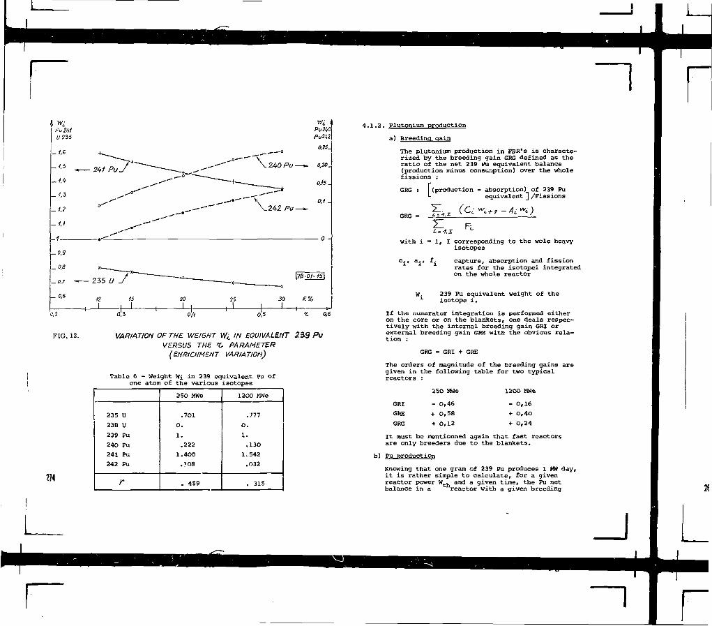
pu mt/235

-i.e

- • ' • 5 241240 Pu-

24-2 Pu-

fPu2',0PuW

0,20.

ojs.

0,1 -

-1- • 0 -

0.5 0.6

FIG. 12. VARIATION OF THE WEIGHT Wl IN EQUIVALENT 2Z9 PuVERSUS THE K, PARAMETER

(ENRICHMENT VARIATION)

Table 6 - Weight Wi in 239 equivalent Pu ofone atom of the various isotopes

235 U

238 U

239 Fu

240 Pu

241 Pu

242 Pu

r

250 MWe

.701

0.

1.

.222

1.400

.?08

. 459

1200 MWe

.777

0.

1.

.130

1.542

.032

. 315

4.1.2. Plutonium production

a) Breeding gain

The plutonium production in FBR's is characte-rized by the breeding gain GRG defined as theratio of the net 239 >>u equivalent balance(production minus consumption) over the wholefissions :

GRG :

GRG =

(production - absorption) of 239 PuL equivalent ] /Fissions

with i = 1, I corresponding to the wole heavyisotopes

c i ' a i ' i capture, absorption and fissionrates for the isotopei integratedon the whole reactor

W- 239 Pu equivalent weight of the1 isotope i.

If the numerator integration is performed eitheron the core or on the blankets, one deals respec-tively with the internal breeding gain GRI orexternal breeding gain GRE with the obvious rela-tion :

GRG = GRI + GRE

The orders of magnitude of the breeding gains aregiven in the following table for two typicalreactors :

GRI

GRG

GRG

250 MWe

- 0,46

+ 0,58

+ 0,12

12OO MHe

- O,16

+ 0,40

+ O.24

It must be mentionned again that fast reactorsare only breeders due to the blankets.

b) Pu production

Knowing that one gram of 239 Pu produces 1 MM day,it is rather simple to calculate, for a givenreactor power W.. and a given time, the Pu netbalance in a reactor with a given breeding

gain GRG. Table 7 presents, over a period of oneyear, the mass of Pu burnt and produced in a 1200MWe typical reactor with a 75 % load factor andthree radial blanket subassembly rows.

One can notice the decrease in the radial blanketsPu production versus the distance to the corecentre due to the flux attenuation. The differencebetween the upper and lower axial blankets comesfrom the control rod absorbers in the upper axial.

c) Doubling time

The Pu excess available m PBR's cycle is charac-terized by the doubling time.

The linear doubling time TEL is defined as the timenecessary for one reactor to produce in excess thePu inventory needed to operate a new identicalreactor. Then, TDL is proportionnal to the Pu cycleinventory MC for one reactor and inverselyproportionnal to the breeding gain :

TDL •

The Pu cycle inventory MC depends not only of thein pile inventory but also of the out of pileinventory (transport, storage, reprocessing, re-fabrication, . . . ) .

The combined doubling time TDC is defined as thetime needed for several fast reactors to producethe Pu inventory needed to operate a new one :

TDC = Log 2 TDL

For a typical equilibrum FBR's situation and 1200MWe typical plants (GRG = 0,24) the values arerespectively :

TDL :'<f 30 years

TDC ~ 20 years

It must be noted that the doubling time is extre-mely sensitive to breeding gain values :

4.2. Variations of cell characteristics versus burn-up

a) There are three mains problems related to the neutronicburn-up during the operating cycle s

- variation of 239 Pu equivalent enrichments and ofthe fuel heavy isotope volumie percentages

- variation of the isotopic compositions

- fission product effect.

Due to the high burn-up aimed at (100.000 MWD/T or 12 %fission burn-up), these problems remain rather complex,but fortunately there is no strong spectrum effect.

For the core burn-up, the internal breeding gain playsa major role and can be easily related to the 239 Puequivalent enrichment variation.

Table 7

Plutonium balance in a typical 1200 MWe reactor

in kilogramme for a one year operation time

GRG 0,40, TDC = 12 years.

core zone 1

CORE core zone 2

core

BLANKETS

Upper axial

Lower axial

Axial

Radial zone 1

Radial zone 2

Radial zone 3

Radial

Blankets

REACTOR

Burn-up

540

360

900

-

-

-

90O

Production

490

280

770

60

12O

180

90

40

20

150

330

11O0

Net balance

- SO

- 80

- 13O

+ 180

+ 150

330

200 275

J

239 Pu 76,7 %2WPU 20,i %

Pu 2,8%242 Pu OA %

13 it* FBU %

Pu ISOTOPIC COMPOSITION VERSUS BURfi-UP

(FBU Hi %)

The Pu isotopic compositions vary with burn-up : the239 Pu composition decreases, the 240 Pu accumulates(fig. 13).

Taking the hypothesis, in some years, of the Pu autore-cycling in PBR's, the equilibrum Pu isotopic compositionswill be :

Pu core recyclingalone :

Pu core + blanketrecycling :

239 Pu 240 Pu 241 Pu 242 Pu

58 % 34 % S % 3 %

70 % 25 % 3 % 2 %

This demonstrates an important FBR's characteristic :the Pu containing higher isotopes as 242 Pu that repre-sent a big penalty for thermal reactors is replaced bybetter Plutonium specially in the blankets by 238 Ucapture.

Among the fission products isotopes, there is no strongpoison as in thermal reactors : the average PP crosssection is about O,5 barn/fission.

b) Finally, at the reactor level, the reactivity loss percycle f due to enrichment, isotopic composition varia-tions and fission product effects depends on the spectrumand the reactor power. It can be divided into two terms,the fuel effect and the FP effect :

t( • '

fuel

fission

% for 1

products

year

25O75

25

6

MWe

%

%

% in keff

1200 MWe25 %

75 %

3 % in keff

276

Due mainly to the less negative internal breeding gain ina 12OO MWe typical reactor, the heavy isotope reactivityeffect remains largely smaller than in a 250 MWe reactor :the absolute global reactivity loss remains also smaller.

The power distributions vary also during burn-up due to thetwo enrichments zones and to the flux distribution. Thecharacteristics of the plant are chosen to limit the powerflatness variation during the cycle, especially radially,around the optimal value. The remaining power flatnessvariation is controlled usually by absorber control rodsmovements.

4.3. Consequences for the out of pile cycle

The fuel compositions in heavy atoms and fission productscorresponding to the in-pile neutronic burn-up define a largepart of the out of pile fuel cycle problems : handling, storage,transport, reprocessing, fabrication, waste.

It will only be possible here to mention the mainaspects :

The residual power comes mainly from fission products( > 80 %) and for a minor part from heavy isotopes( T 20 % ) , especially from the 'X. emission of curiumisotopes for cooling times longer than 5 days.

The neutronic emission of the unloaded subassemblies,important for the shielding problems in the transpor-tation and handling and for the operation is mainlydue to the spontaneous fissions of the Cm isotopes(70 %) and to the (i\,« ) reaction on the oxygen.

_ J

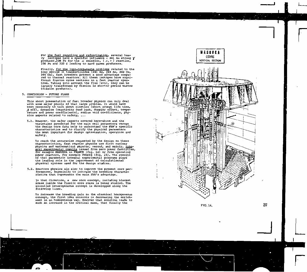
For the fuel recycling and refabrication. several hea-vy isotopes have a specific influence : 241 Am strong yproducer,238 Pu for the &i emission, ( i<, « ) reaction,236 Pu and 232 U leading to hard gamma producers.

Finally, for the long—term—waste problems related to thelone; period oc transactinides (241 Am, 243 Am, 242 Cm,244 Cm), fast breeders present a good advantage compa-red to thermal reactors. All these isotopes have signi-ficant fission cross sections in a -fast reactor spec-trum. Taking into account the flux level, they can belargely transformed by fission in shorter period wastes(fission products).

5. CONCLUSION - FUTURE PLANS

This short presentation of fast breeder physics can only dealwith some major points of that large problem. It would havebeen necessary to talk about cinetics (short prompt life time,A eff), dynamics (reactivity feed back, doppler effect, tempe-rature and power coefficients), sodium void coefficients, phy-sics aspects related to safety, ...

5.1. However., the major aspects covered here-above and thevariations presented for the main cell parameters versusthe design core data help to understand the FBR's specificcharacteristics and to clarify the physical parametersthe most important for design optimisation, operation andsafety.

To reach the accuracies requested by the design on thesecharacteristics, fast reactor physics use first nuclearphysics and mathematical physics, second, and mainly, inte-gral experimental results issued from zero power facilities,for example MASURCA in FRANCE (fig. 14) or from operatingpower reactors, for example PHENIX (fig. 15). The resultsof that parametric integral experimental programs playsthe leading role in the improvement of calculationnalphysical systems used for the design studies.

5.2. Reactors physics aim also to improve the present core per-formances, especially to increase the breeding characte-ristics that represents the main FBR's advantage.

In that direction, a new core concept, including blanketzones inside the fissile core zones is being studied. Theso-called heterogeneous concept is developped along thefollowing lines.

To increase the breeding gain in the classical homogeneousconcept, the first idea consists in decreasing the enrich-ment in an homogeneous way. However that solution leads tosuch an increase in the critical mass, that finally the

mmmFIG. 14. 277

rCONTROL RODMECHANISM~\

CELL- ROTATING'PLUG

HEATEXCHANGER

CORE.

PRIMARV __,CONTAINMENT

'-DIAGRID

TRANSFERARM

DOUBLEVESSEL

LOADINGRAMP

BI0L06IC'SHIELDING

NEUTRONICSHIELDING

\_MEASUREM£NTCHAMBERS

PRIMARY'VESSEL

278

PHENIX 250 MWe I BLOCK REACTOR

FIG, 15.

doubling time (see § 4.1.)r the only important parameterfor breeding, increases largely. But, if an heterogeneousdistribution of fertile zones inside the fissile ones isperformed, there exist optimal solutions leading to a mi-nimum ratio of the enrichment to the global breeding gain,the enrichment of the fissile zone being of the order of30 %. From a physical point of view, the main effect comesfrom spectrum differences in the internal blankets and inthe fissile zones compared to the homogeneous spectrum :

-the average 238 U capture cross section increases

—the average 239 Pu 1]_ parameter increases.

If the geometrical distribution of the internal blanketsis optimized to impi /e the radial power flatness, for agiven total power, the core volume then the doubling timecan be minimized. The following table compares relativelytwo 1200 MWe reactors on the homogeneous and heterogeneousbasis :

Homogeneous Heterogeneous

3,20 , 2

22

3 ,70,35

13

I n - p i l e c r i t i c a l mass tons Pu

GRG

Combined doubling time years

Outside the doubling time improvement, the heterogeneousconcept presents also other potential advantages :

- decrease of the reactivity loss per cycle due tothe GRI improvement, leading to decrease the num-ber of control rods

- decrease of the flux level due to the high fissilezone enrichment, then possibility for the samefluence to have higher burn-up

- improvement of the sodium void coefficient forsafety.

5.3. If the performances of such an heterogeneous concept areconfirmed by all the experimental programs carried out now,it is reasonnable to think that fast breeders reactors usingthe well-known mixed oxide fuel will potentially te ready tocover, around the end of this century, a larger part of thenew electricity needs.

~IGENERAL BIBLIOGRAPHY OP PAST REACTOR PHYSICS

1. London Conference on fast breeders reactorsBNES LONDON (1966)

2. Past reactor physics IAEA Symposium SM 101 KARLSRUHE(1967)

3. The physics of fast reactor operation and design BNESConference LONDON (1969)

4. International Symposium on physics of fast reactorsTOKYO (October 1973)

5. Past reactor power stations BNES Conference LONDON(1974)

6. Centrales de puissance a neutrons rapides : etudes etdeveloppament BIST - CEA - n° 182 (juin 1973)

7. La physique des reacteurs BIST - CEA n° 168 (mars 1972)BIST - CEA n° 170 (mai 1972)

293 279

"I

HTR CHARACTERISTICSAFFECTING REACTOR PHYSICS

K. EHLERSHochtemperatur-Reaktorbau GmbH,Mannheim,Federal Republic of Germany1. Introduction

The development of the high-temperature gas-cooledreactor was started in the late 1950's in Europe and in theUSA. Less than 10 years later the first experimentalHTRs reached their nominal power:GB Winfrith DRAGON 20 MW.US Peach Bottom 100 MWFRG JUlich AVR 50 MW

.th

.thth

196619671968

2S5

Over the following years, these three reactors havebeen operated with considerable success, demonstratingthe feasibility of the HTR and confirming the favorablecharacteristics claimed for it. Encouraged by the ex-cellent behaviour of these experimental reactors, theconstruction of prototype reactors in the USA and inGermany started in 1968 and 1972 respectively. Sincethen, the F.S.V. reactor at Fort St. Vrain near Denverhas reached 70 % of full power, and the erection of theheat exchanger in the THTR will start in the near fu-'ture. Critically and power raising are expected in 1981.

HTR characteristics

The temperature limitations of conventional reactorsimpose a low thermal efficiency, use of special tur-bines , and consequently cause higher fuel consumptionand thermal pollution of the environment.HTRs have been developed in order to avoid theselimitations using a core composed exclusively of ceramicmaterials and employing helium as an inert coolant. Heliumis chemically inert, shows no phase chcmyt, has goodheat exchange properties, and is not activated by neutrons.Hence in the event of an assumed loss of coolant accident,no reactivity change will occur. The coolant outlet tempera-tures of the HTRs now in operation range between 750°and 950°C with inlet temperatures around 300 °c.In Germany the experimental reactor AVR has been workingat a gas outlet temperature of 950 °C since early in1974.As the high temperature excludes the use of metallicfuel sleeves, the fission products are retained by theuse of coated fuel particles. These particles consistof oxide or carbide kernels of U and Th, whose diametersrange between 200 and 500 urn. Layers of silicon carbideimprove the retention of metallic fission products.

The coating thickness ranges between 150 and 200 um,depending on the burn-up to be achieved. The schematicdesign of a coated particle is given in Fig. 1.

Unless Sic layers are used the coating consists of aninner low- density buffer layer and an outer high-densitylayer (BISO or duplex particles). If SiC is used, thecoating consists of an inner low-density buffer layer,an inner high-density pyrolytic-carbon layer, a Sic layer,and ar outer high-density pyrolytic-carbon layer (Trisoor Triplex pax i_: cles) . These particles are dispersed ina grapi.ite matrix. In order to avoid corrosion due toimpurities in the coolant and to improve further thefission product retention, the fuel element matrix (coatedparticles in binder) is protected by an additional outergraphite shell.The basic concept provides the possibility of "^rious typesof fuel geometries. In practice two types of fuel ele-ments have been developed for the HTR: spherical fuel ele-ments of 6 cm diameter with an outer fuel-free zone of0,5 cm thickness as used in the AVR and manufactured forthe THTR, as well as hexagonal blocks of 80 cm height and 36cm width across flats as used in the Fort St. Vrain (Fig. 2 ) .In the Federal Republic of Germany the HTR concept withspherical fuel elements, the pebble bed reactor, has beendeveloped and only this reactor type is envisaged forfuture HTR-projects. Therefore only the main aspects ofthe block-type HTR which is under consideration in the USwill be described, whereas the pebble bed concept will bediscussed in more detail.Fig. 3 shows a sectional view of the pressure vessel ofan HTR with block-type fuel elements. The active core consistsof colums of block elements. Seven columns - except certainregions at the core periphery - are combined to form onefuel region.Each fuel region is located directly below a refuellingpenetration in the prestressed concrete reactor vessel head(PCRV). During reactor operation each of these penetration?houses a control rod drive and an orifice valve, which allowsthe control of the mass flow in each region depending on theage and power of this region.The coolant flow distribution, the arrangement of the heatexchangers and circulators are similar to those of a pebblebed reactor. Fig. 4 shows a sectional view of a pressurevessel of the THTR-pebble bed reactor. The THTR main designdata are given in Table 1.The active core consists of a loose bed of approximately675 000 spherical fuel elements. These spheres, which arecontained in a reflector of graphite blocks., are loaded via*-.ube.s in the upper reflector. The fuel elementspass downward slowly through the core by gravity and areextracted by one or - in case of larger plants - several tubeslocated in the bottom reflector. In the THTR each fuel elementpasses through the core 7 times on an average. 901

_ J _J

_ J I

Tab. 1: BASIC DESIGN DATA THTR 300

750300

5.66

MWMW

mm

675000125629:.2507503960,96(9310,24236

m1

MW/m3

5 kp/s°C°Cbarcmg U 235% enriched)g Th 232

Characteristics of the overall plant

Thermal core powerNet electrical power

Primary circuit data

Core diameterCc-Te heightNumber of fuel element spheresVolume of pebble bedPower densityHelium flow rateHelium temperature outlet steam generatorHelium temperature inlet steam generatorMean operating pressure of heliumFuel element diameterHeavy metal content

Number of incore rodsNumber of reflector rodeNumber of coolant gas circulators 6Number of steam generators 6

Dimensions of prestressed concrete pressure vessel

Inside diameter 15,9 mInner height 15,3 mWall .thickness of cylinder 4,45 mWall thickness of bottom slab 5,1 mWall thickness of top slab 5,1 mOperating pressure 39 bar

Test pressure 46 bar

Secondary circuit data

Turbine:Flow rate of superheated steamSteam pressure/temperatureReheated steam - pressure/temperatureFeed water end temperatureVacuum/coolant water temperatureFlow rate of cooling water

After each passage the burn-up will be measured and,depen-dinq on the burn-up, the fuel element will be either re-cycled to the outer or inner Dart of the core for esta-blishing a flat power and temoerature distribution, or itwill be discharged, if the full burn-up is reached. Due tothe continious reload and discharqe of fuel elements, excessreactivity for compensating burn-up effects is not re-quired. Hence, the insertion of absorber rods duringpower operation is only necessary for control purposesand for shutdown. For long-term shutdown in-core rods aredirectly inserted into the Debbie bed by pneumatic drives.The reactor is controlled by absorber rods which can befreely moved in bore holes in the side reflector. Thesereflector rods also act as the first shutdown device.The helium flows downard through the core and is heatedfrom 260 °C to 765 °C thus supplying conventional steamconditions in the secondary circuit. Surrounding the corethere are six steam generators, with a circulator coordina-ted to each of them. In contarast to other reactor typesall these components are integrated in a prestressed con-crete pressure vessel (PCRV).

2. Fundamental core design

2.1 Fuel cycles

Because of the rather homoqenous '-.ore geometry with littleself-shielding effect on U-238-absorptions, enriched ura-nium has to be used in HTRs. The HTR fuel cycle conceptis characterized by a high flexibility.The favourable neutron economy of the HTR core consistingof fuel and graphite only, permits to achievehigh conversion ratios in the thorium/uranium cycle.The use of highly enriched uranium (HEU) represents themost economic alternative. The HTR may also be operated -at a moderate cost penalty - in the thorium/uraniumcycle with medium-enriched uranium (MEU) or in the uranium/Plutonium cycle (LEU) at a low uranium enrichment. It iseven possible to change from one fuel cycle to another inthe individual HTS power plants during operation.

930 tons/hour177.5 bar/530 °C46.5 bar/530 °C180 °C0.0685 bar/26,5 °C31 720 ma/h1 H-p, 1 M-p, 1 L-p,stage, L-p stagedouble flow

HTR FUEL CYCLE ALTERNATIVES

Alternative Fertile Material Make-up Fuel

HEU

MEU

LEU

Th

ThU

U

232

232238

238

Uranium,

Urar.ium,

Uranium,

93% U 235

20% U 235

10% U 235

In this section the fuel cycle optimization for the above-mentioned possible fuel cycles (HEU, MEU, LEU) with andwithout recycling of the breed material will be discussedfor an HTR with spherical fuel elements and a thermaloutput of 300 M W ^ .

Usually the HTR fuel cycle is characterized by the follow-ing independent variables:

- power density- fuel residence time- carbon over heavy-metal atomic ratio

From these independent parameters the power density wasfixed at 5.5 MW/m' in order to reduce the damage of thetop and side reflectors due to fast neutrons to such alevel that replacement during the lifetime of thereactor would not be necessary. The residence time andthe carbon over heavy-metal ratio have been varied overa wide range to obtain minimum fuel cycle costs.For optimization, the following constraints must be satis-fied with respect to the fue] for keeping the fissionproduct release within specified values:

fuel center temperature °cfuel surface °Cburn-up % fimafast neutron dose nvt (E 0.18 MeV)heavy-metal content perfuel element g

1250105012.505.2 10

20

21

As mentioned before, the HTR fuel elements are composed ofceramic materials only. Graphite starts to evaporateonly at temperatures well in excess of 3000 °C. Melting ofthe kernel material can only affect the particle inte-grity at temperatures above 2200 to 2500 °C. Consequently,for typical operational and accident conditions with fueltemperatures below 2000 °C, maximum permissible tempera-tures can only be defined in combination with time attemperature. The overruling criterion is, in any case, therelease of fission products from the core. Nevertheless, forcore design purposes, maximum fuel temperatures of 1250 °Cand maximum surface temperatures of 1100 "C are specifiedas a guideline for optimization studies and for R & Dwork. These temperatures do not constitute technologicalperformance limits, but they represent practical boundariesfor acceptable fission product release values.The limits for burn-up and fast neutron dose values are essen-tially determined by the maximum permissible fraction offailed particles. The values quoted in the table above

represent the present status of fuel testing. Severalirradiation experiments have shown that significantlyhigher endurance limits can be achieved with HTR-fuel.To be conservative and reduce the R S D effort, theselower figures were used for the present design work.

The maximum heavy-metal content in the fuel elementsfor a given coated-particle design is determined by therequirements for a high mechanical strength of the fuelsphere and a low fraction of particle defects during thefabrication process. The value of 20 g /F.E. for thereference (Th, Ui O, - particles is related to the produc-tion process for the THTR fuel elements. For an advancedmoulding process currently under development, heavy-metal loadings up to 30 g/F.E. are envisaged.Fig. 5 shows the fuel cycls costs without recycling of breedand residual feed materials for the HEU cycle. As expectedminimum fuel cycle costs will be achieved with high burn-up and relatively low conversion ratios. The fuel cyclecosts are largely independent of moderation and residencetime, that means both variables could be varied withina wide range without markedly changing the fuel cyclecosts.Of the above constraints, only the burn-up and the fastneutron dose will be met, whereas the other values are wellwithin the given limits.

Table 2 summarizes the results of the optimization for thethree alternatives. In the HEU and LEU cycles the burn-upis clearly the limiting constraint.In case of recycling the breed and residual feed materials,the picture for the HEU and LEU cycles changes completely.In order to improve the neutron economy by reducing theamount of parasitic fission products, the burn-up and theresidence time will decrease which leads to an increaseof the conversion ratio.

Optimum Fuel Cycle Design for Open Cycle

C/HM-RatioFuel Residence Time a

Burn-up GWd/tConversion RatioHeavy-Metal per Fuel Element gThoriumUranium

HEU

3403.33

11.50.57

9.850.94

MEb

4302.81

1200.57

4.554.10

LEU

5042.38

1200.54

7.45

283

The increase of the fuel handling costs will be morethan compensated by the high value of the breed material.This procedure depends, of course, on the ore and separa-tive work prices.For the LEU-cycle there is no change of the optimum lay-out compared to the case without recycling. This meansthat the gain from improving the neutron economy by reducingburn-up and residence time will not compensatethe increase in handling costs.

Optimum Fuel Cycle Design for Closed Cycle

HEU MEU LEU

C/HM-RatioFuel Residence Time a

2253.12

3752.50

5002.40

Burn-up GWd/tConversion RatioHeavy-Metal per Fuel Element g

Table 3 shows the optimum layout for the three alternativesunder consideration.

Influence of Uranium Ore Price on Optimum Design (HEU; ClosedFuel Cycle

Fig. 6 and 7 show the ore and separative work require-ments for the considered alternatives in comparison withlight-water reactors.

Fuel Cycle Cost Comparison (Open Cycle)

HEU MEU LEU

DepletionFabricationShipping + Storage

0.923 0.940 + 2 0.878 -50.114 0.117 +3 0.130 +140.263 0.322 +22 0.377 +43

Total Fuel Cycle CostDpf/KWhe 1 .300 1.379 +6 1.385 +6

710.7216.6

950.629.8

1190.547.5

Uranium Ore:Difference:

30 $ lb U,0B

(5) relative to HEU

Table 5 and 6 show the fuei cycle costs for the differentalternatives. In both tables the HEU shows the lowestfuel cycle costs wi+h or without recycling of the breedand residual feed materials. The cost advantage of theHEU cycle doubles on assumption of an ore price escalationrate of 3%/a.

Fuel Cycle Cost Comparison (Closed Cycle)

C/HM-RatioFuel Residence Time

Burn-up GWJ/tConversion Ratio

30 60 120 HEU MEU LEU

2253.22

730.72

2252.84

650.735

2302.39

570.75

DepletionFabricationReprocessing +Waste Disposal

0.537 0.772 +43 0.798 +490.224 0.169 -24 0.130 -42

0.348 0.301 -13 0.293 -16

284

Table 4 shows the influence of the ore price on the optimization.With increasing ore prices the optimum conversion ratio in-creases, whereas the optimum residence time and burn-up de-crease. However, the optimum carbon-to-heavy-metal ratio re-mains constant.

Total Fuel Cycle CostDpf/KWhe 1.109 1.242 +12 1.221 +10

Uranium Ore : 30 g/lb U 3O S

Difference : (5) relative to HEU

2.2 Core Design

2.2.1 Fuel loading

During reactor operation the fuel elements will beloaded continuously through 12 pipes distributeduniformly at the outer part of the top reflec-tor and 3 pipes serving the centre part of the core.To achieve a flat radial power distribution the freshfuel elements or those with low burn-up will be placedin the outer core, whereas fuel elements with highburn-up will be distributed in the inner core. On anaverage, each fuel element pas.ses through the core7 times with a residence time of 3 full-power years.The core concept allows build-up of a two-zone coreby using one fuel element type only. For the corephysics calculations, knowledge of the flow behaviourof the fuel elements is very important.

2.2.2 Flow characteristics

Fig. 8 shows the model simulating the flow behaviouras used in the core physics calculations. In case ofthe THTR the core is devided into five axial channels.Each channel is separated axially into regions' of equalvolume. After a certain time - in case of the THTR after16 days - each region will be shifted into the region below,simulating the continuous flow by a differential method.As may be seen from Fig. 8, the passage time in-creases from the core center to the side reflector.The passage time of a fuel element in the outerregion is 4 times that of a fuel element in the centerof the ^ore. Furthermore, the flow velocity decreasesat the edge between lateral reflector ana bottomreflector.

2.2.3 Initial core, running-in phase, equilibrium core

The inital core consists of a homogeneous mixtureof fuel elements, absorberelements, and fuel-freemoderator elements, whose composition is differentin the inner and outer corezones. For costreasonsthe number of fuel elements should be as small aspossible. However at the same time the maximum fueltemperatures should not exceed maximum values ofabout 1250 °C. Therefore the initial core consistsof

53 * fuel elements41 % moderator elements6 % absorber elements.

A homogeneous axial distribution has been chosen insteadof a gradual distribution, which would result in lowerfuel temperatures, to circulate fuel elements during therunning-in phase without disturbance of the reactivity.

The absorber elements contain boron and hafniumas burnable poisons. The ratio of B and Hf has beenchosen so that the absorber burns out at the samerate at which the fission product concentrationbuilds up, and fissile and fertile materials willbe loaded. The requirement will be almost satisfied,if the absorber elements contain 40 mg B and 4.2 g Hf.The initial core contains several control rods in aposition allowing the correction of reactivity uncer-tainties within *_ 2 Miles.The change of the core composition during the running-in phase is shown in Fig. 9.Absorber elements are only introduced within the first6 months and then continuously removed. Fresh fuelelements are loaded at a constant rate from the be-ginning. Moderator elements are not added duringthe running-in phase, but are replaced by the loadingof the other elements. After 1.5 full-power yearsnearly all moderator elements will have been removedand the first fuel elements with the highest burn-up will be discharged.

Fig. 10 shows the burn-up spectrum of the fuel ele-ments at three different time steps. The curvesindicate the number of fuel elements having the sameaccumulated dose. After 258 full- power days the peakof the initial core can be clearly seen. With increas-ing full-power days this peak spreads and driftsto the right.

After three full-power years all burn-up classes con-tain almost the same number of fuel elements, i.e.the equilibrium stage has been reached.

The power distribution in the first core after threeyears of full power is shown in Fig. 11. Thepower step between the inner and outer core zonescan be clearly seen. Furthermore, in the initial corethe power maximum is located at the bottom reflectordue to the axially homogenous fuel distribution and thecontrol rods inserted into the core. This maximummoves to its equilibrium position within 6 months due tothe axial burn-up.

The SUCON program has been developed to describe therunning-in phase of pebble bed reactors. SUCON calcu-lates the reactivity flux and power distribution as afunction of time taking into account the burn-uproutine and the movement of the fuel elements. Itcontains a burn-up and a diffusion code. The two-dimensional diffusion calculation in r, Z-geometry iscarried out with the aid of the program CONDOR with 4energy groups. The group constants calculation is 285

based on a 43-group library taking into accountthe heterogenity of the fuel elements. The burn-upbehaviour of the Hf containing absorber elementshas been calculated with the zero dimensional multi-group programm GGC-4 tanking into account the doubleheterogenity of absorber elements (poison particleswithin the absorberelements) The selfshielding factorswerre calculated with the transport code ANISN, againas function of the burn-up of the absorbermaterial.Space dependent burn-up calculation is performed,considering each region as composed of large number offuel element classes representing different burn-upstages. The axial fuel element movement is simulatedby shifting axial zone into the next one.

systems must be provided for shutdown.In the THTR the following two systems are provided:The first shutdown system consists of 36 reflector rods,which can be freely displaced in bore holes in theside reflector. Furthermore it serves for partialload control.The second shutdown system consists of 42 in-corerods. These in-core rods alone can maintain thermalsubcriticality of the reactor over the total lifetime and compensate slow reactivity changes duringoperation. Thus they are safety-related as well as ope-ration-related equipment. To meet these require-ments they are equipped with two different types ofdrives.

2.2.4

286

The ability to follow changes in load - between 100 %and 40 % or more - is a general demand of customers.Often is required that the station should be able torestart at any moment after shut down.These demands lead to the installation of excessreactivity in the control rods to allow for Xe-135override. This Xenon-effect comes from a build upof Xe-135-concentration to a maximum several hoursafter load reduction or shutdown by the decay of1-135. Typical reactivity values for an HTR are of theorder 2-4 %, which must be invested as excess reac-tivity. Because of the resulting additional fuel cyclecosts a careful assessment of the increase in fuelcosts against the increased plant flexibility isnecessary.

In the THTR the excess reactivity for Xenon-override isinstalled mainly in the reflector rods together withsmall reactivity amounts for fine regulation.In similar way e.r. after load reduction an increaseof excess reacitivity is induced by load increasing frompart load to higher load due to a temperarily reducedX-135-level. This will be compensated in THTR by in-serting some of the core rods.During long-therm shutdown several months the reac-tivity rises mainly by decay of Protactinium in U233 toa maximum of 4 %. This has to be compensated by theshutdown systems. After start up of the reactor thisadditional excess reacitvity must be replaced by in-serted control rods.In THTR 12 control rods are inserted to approximately3 m. Again on full load the excess reactivity is de-creased within several weeks by build up of Pa andthe burn-up of U23 3.

The control and shut down system of the HTR must meetthe above mentroned requirements even if one or morecontrol rods fail to enter the core. Safety regu-lations demand further that two independent different

2.3 Thermohydraulics of the pebble bed core

The general layout of the.core cooling is dominated by therequirement of a stable core configuration under all anti-cipated flow conditions. In the case of a pebble bed coreconsisting of a loosely packed bed of spherical fuel ele-ments within a cavity, the drag forces of the coolant floware greater than the weight of the fuel elements. Conse-quently the coolant flow must be directed downward inorder to avoid core lifting. This leads to increasing gastemperature when moving downward through the active corewhich matches ideally with the decreasing power generationof the fuel elements as they move down gradually through thecore. The resulting axial to be rather flat, enabling thecore designer to make best use of given temperature limitationsof the fuel elements.Above the core the cold gas chamber serves to equalizethe gas flow entering the active core zone, whereas thebottom of the core is formed by the conical graphite reflec-tor guiding the fuel elements to the discharge pipe.Here, numerous small holes, having a diameter of approximatelya quarter of the pebble diameter, conduct the gas axiallydownward to the hot gas chamber, where it is led to the sixsteam generators.The size of the coolant holes in the bottom reflectoris gradually reduced from the innermost part near thedischarge pipe to the periphery in order to achieve auniform flow of fluid in the core region above. Coolingof the fuel elements in the discharge tube is achievedby a small bypass flow, flowing axially upward and emergingat the lower end of the core, into the main coolantflow.The mathematical simulation of the flow distributionis done within a two-dimensional network, assuming ahomogeneous field of flow resistances according to thepressure drop characteristic of a statistical pouring ofspheres. Based on a given mass flow the pressure and flowdistribution is calculated iteratively by a finite diffe-rence method, taking into account the local heat gene-ration of the fuel in order to evaluate the local gas

asto a

ofon

ielrtioneutrons

b e *

islue

rgy

v

releasedt be de-, re- 301

L

temperature and its influence on the flow charac-teristics. In other words:the pebble bed is treated as homogeneous materialwith interconnected flow channels and an internalheat generation. Based on the spatial flaw and tem-perature distribution in the core the temperaturesof different fuel element types are calculated accordingto the well-known equations of heat transfer andconduction within a spherical body taking into accountalterations of the thermal conductivity due to tem-perature and neutron dose.Numerous experiments were conducted in order to deter-mine the flow resistance, heat transfer, lateral con-duction, mixing, and radiation effects in randomly packedpebble beds. These experiments originated mainly inthe chemical industries, where beds of particles arewidely used to enhance chemical reactions. In addi-tion core models at a scale 1 : 7,5 were used tomeasure the flow distribution in the core, especiallynear the discharge pipe where the counterflow by-pass creates a zone of reduced gas flow. Fig. 12 showsa comparison between calculated and measured flowfields in the core model, showing the region of re-duced flow at the entrance of the discharge pipe and anincreased # 3Sw density at the junction of the lateral andbottom reflectors where no coolant holes in the bottomreflector are foreseen.

Typical results of the thermal core layout of the THTR area pressure drop of 0,6 bar: nd\ flow velocities of S to10 m/s between the spherical fuel elements, increasing fromtop to bottom as the density is reduced by the temperatureincrease of the gas, The radial i ariation of the flowdensity is rather small due to tne previously mentionedgagging in the bottom reflector - and is not greater than10 % of the average flow. The htiat transfer coefficientsare rather high - 2500 W/m'K - fchlch is predominantlydue to the high thermal conductivity of helium and - butis also characteristic of flow through particle beds.The general thermal parameters of core design are in-let temperature of 250 °C, an average outlet tempera-ture of 750 °C, at a system pressure of approximately40 bar.The temperatures of the fuel elements are a function oflocal gas temperature, being determined by the averagepower generation of the fuel, and their individua 3 heatproduction.At an avera e power output per fuel element of 1.1 KR, thetemperature difference between its surface and the surroun-ding gas is 40 °C whereas the temperature increase fromthe surface to the center of the fuel element amounts to 100

Fresh fuel elements producing approximately 3,5 to 4 KW areproportionally higher in temperature. As a design limitfor long-term steady-state temperatures a maximum fueltemperature of 1250 °C and a maximum power of 5,5 KW perfuel element are specified leaving a considerable marginto the failure temperature of the coated particles ofapproximately 1700 °C for short-term transients.The dynamic behaviour of the reactor core is mainlydetermined by the ratio of the volumetric power genera-tion and the heat capacity of the fuel, moderator andstructural graphite. Due to the relatively low powerdensity of 6 MW/m1 in the THTR in relation to the highheat capacity of the graphite fuel elements, temperaturetransients in HTRs at any disturbance in heat productionand/or heat removal are generally small compared to otherreactor types.If, for example, the heat removal ceases instantaneouslyat a 100 % load, the average core temperature increasesonly at a rate of 3 °C per second. Additional damping ofgas temperature fluctuations is achieved by the bottomreflector, thus the temperature increase at the steamgenerators is delayed by several minutes compared to theexit of the active core zone.Another inherent feature of the HTR (similar to otherreactor types) is the negative coefficient of the reacti-vity with respect to fuel and moderator temperature in-crease. This means, that any increase of the fuel andmoderator temperature reduces the reactivity and henceheat production of the core leading to a self-stabilizingbehaviour of the reactor. In case of the previously postulatedcessation of the core cooling, the fission power gene-ration of the core would fall below 10 % within approx.3 minutes if no reactor scram were initiated. Afterwardsthe decay heat is the dominating factor. During this event,the average core temperatures - initially at about 650 °C -would rise by 200 °C, whereas the temperatures of thehottest, i.e. fresh fuel elements will be reduced towardsthe local mean value.At decay heat power level the', firther temperature in-crease of the core will be in the order of 3 to 5 °C perminute. With respect to temperature limitations of anHTR-core, it must be kept in mind, that there are no fixedtemperature values, at which a spontaneous failure ofcore components occurs. Graphite - in pure helium at-mosphere - is stable beyond 3000 °C, imposing no realcriterion for the accident analysis, whereas the failuremechanism of the coated particles is a temperature-time depen-dent phenomen: At about 1700 °C the coated particles beginto fail, releasing their gaseous activity to the primarycoolant, whereas the release of metallic fission productsis controlled by the relatively low diffusion coefficient.In general it can be stated, that the dynamic behaviourof the pebble bed core with respect to power and/orcoolant flow fluctuations is rather slow and that the failure

287

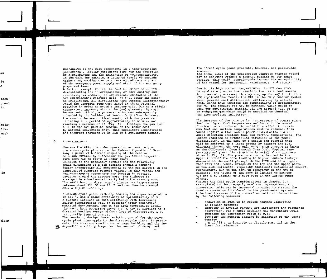
it;

brem-

, and

in

itain-

.low-

ons)

ir

ilear

mechanisms of the core components is a time-dependentphenomenon , leaving sufficient time for the detectionof disturbances and the initiation of countermeasures.In the THTR for- example, a delay of nearly 60 secondswithout any cooling can be tolerated before the startof the emergency power supply and start of the emergencypumps and fans.A further example for the thermal behaviour of an HTR,demonstrating the interdependency of core cooling andreactivity is shown by an experiment, conducted at theAVR experimental reactor: Here, at full power and xenonat equilibrium, all circulators were stopped instantaneouslywhile the absorber rods were fixed in their originalposition in order to avoid a reactor trip. Due to a slighttemperature increase within the fuel elements the corebecame subcritical, a process, which was subsequentlyenhanced by the build-up of xenon. Only after 24 hoursthe reactor became critical again, with the power os-cillating at a period of approximately 40 minutes andreaching a maximum of 5% (Fig. 13). Although the gas cir-cuit in the AVR permits removal of the decay heatby natural convection only, this experiment demonstratesthe inherent features of an HTR in a convincing manner.

3. Future aspects

Whereas the HTRs now under operation or constructionare steam cycle plants, in the Federal Republic of Ger-many a plant with direct coupling of the reactorto a gas turbine by increasing the gas outlet tempera-ture from 750 to 850°C is under study.Delation of the secondary circuit and the relativelysmall dimensions of a gas turbine permit a compactdesign integrating all components of the gas circuit in theprestressed concrete reactor vessel. In this vessel theheac-exchanging components are located in verticalcavities around the reactor core. The turboset isarranged in a horizontal cavity below the reactor core.The waste heat in direct-cycle plants has temperaturesbetween about 150 °C and 20 °C and can thus be removedover a diy-wat-cooling.

A direct-cycle plant with dry-cooling and a gas temperatureof 850 °C has a plant efficiency of approximately 41 %.A further increase of this efficiency with increasinghelium temperatures will be possible after respectivematerial development. Due to its high temperature level,the waste heat occurring above 110 °c may be supplied to adistrict heating system without loss of electricity, i.e.practically free of charge.The remaining design characteristics quoted for the steamcycle plant also apply to the direct-cycle plant, in parti-cular the concrete reactor containment building and the in-

2JJ dependent auxiliary loops for the removal of decay heat.

The direct-cycle plant presents, however, one particularfeature:the steel liner of the prestressed concrete reactor vesselmay be designed without a thermal barrier on its innersurface. This would considerably improve the accessibilityof the vessel for inspection, maintenance, and repair.

Due to its high coolant temperature, the HTR can alsobe used as a process heat reactor, i.e. as a heat sourcefor chemical processes, thus opening up the way for furtherHTR applications. Hence, the HTR is the only reactor systemwhich permits coal gasification exclusively by nuclearheat, since this requires gas temperatures of approximately9bO °C. The product ga"; may be methane, which could beused for substituting mineral oil and natural gas, or maybe reduction gas which could be supplied to chemicaland iron smelting industries.

The increase of the core outlet temperature of course mightlead to higher fuel temperature and hence to increasedfission product release. To avoid this effect the maxi-mum fuel and surface temperatures must be reduced. Thiswould require a flat radial power distribution and inaxial direction constant fuel and surface temperatures. Thelatter requires an exponential variation of the powerdistribution. In the case of a pebble bed reactor thiswill be achieved to a large extent by passing the fuelelements through the core only once, this concept is knownas the OTTO-cycle (Once Through Then Out). Typical tem-perature and power distributions in axial direction areshown in Fig. 14. The power maximum is located in theupper third of the core leading to higher neutron leakagecompared to the multi-passage in the THTR and to a higherfast flux and, hence, damage of the top and the upper partsof the side reflector, requiring additional engineering effort.Furthermore, due to the b.irn-up behaviour of the movingelements, the height of the core is limited to between4,5 and 5 m, leading to a flat core in the larger powerplants.Whereas the fuel cycle considerations in chapter 2.1are related to the presently used cost assumptions, theconversion ratio can be increased in order to stretch theuranium resources introduced in the pre-breeder system.A further increase of the conversion ratio can be achievedby the following measures:

Reduction of burn-up to reduce neutron absorptionin fission productsincrease of thorium content for increasing the resonanceabsorption. For example doubling the Th-content wouldincrease the conversion ratio by 0.15lowering the neutron leakage by reduction of the powerdensity

- use of 233 U exclusively as fissile material in thefresh fuel elements

By using these measures the so-called Near-breeder hasa conversion ratio of 0.97. The 233 U required must beproduced either in the thorium blanket of a fast breederor in an HTR pre-breeder reactor. Including this pre-breeder,a mean conversion ratio of 0.95 results for such a combinedsystem consisting of one pre-breeder and 8 near-breedersin equilibrium.

303

Graphrte Shell*Graphite MatrixCoated Particle

* Central Fuel Element1 Coolant Channel 4 Hole lor Control Rod2 Fuel Pin 5 Handling Hole3 Burnable Poiton 6 Reserve StuA Down Hole

HTR-Fuel Elemerffe - * ,

FIG. 1. FIG. 2.289

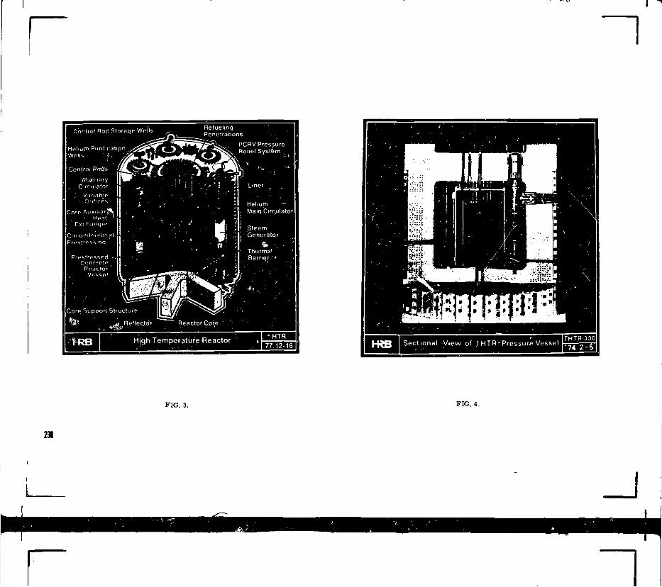
jntrol Rod Storage WPIIS

Control Rods

RefuelingPenetrations

PCRV PressureRelief System .

Reactor Core

High Temperature Reactor

Helium -*Mairj Circulator

SteamGenerator

ThermalBarrier ''•

H W Sectional -View of JHTR "Pressure Vessel

FIG. 3. FIG. 4,

290

~1

nFuel Cycle HEU

' Open Cycle

Uranium ore 3 0 S / l b U3O8Separative Work 100 $ /kg SWU

T = Residence Time FullPower Years

Conversion RatioBurn - up % fima

"2500 4S00 6500 8500 10500» Moderation Ratio N c / N f l s s

Fig. 5: Fuel Cycle Cost as Function ofResidence Time and Moderation Ratio 78.U-1

• 10% *\0%

si

VA

— 6 0 % '110%-85%

HTR PWRHEU MEU LEU

HTRHEU ME'J LEU

OPEN CYCLE CLOSED CYCLE

Tail 0 .25%HTR Plant Efficiency & 1 %

Fig. 6: Comparison of Natural UraniumRequirement of HTR and PWR 78.14-2

291

• 10°/

Is t

mCMin~i

HEU

» .10%

i n~~t

• ^

oi n

a

'//,'//

V/,V<• m

' - *

V/

• 85%+65%

o

o

n• s i

nn

o

H T R PWR H T RMEU LEU HEU MEU LEU

OPEN CYCLE CLOSE 0 CYCLE

Tail 0 2 5 %HTR Plant

HS Fig

Eff ic iency 4 1 %

7: Comparison of Separative WorkRequirement of HTR and PWR

<•if) '

* n .. CJ

-_Z

-»63%

3WR

78 K-3

292

- i

jnuwVorttangIlirFMMctorstiite

FIG. 8.

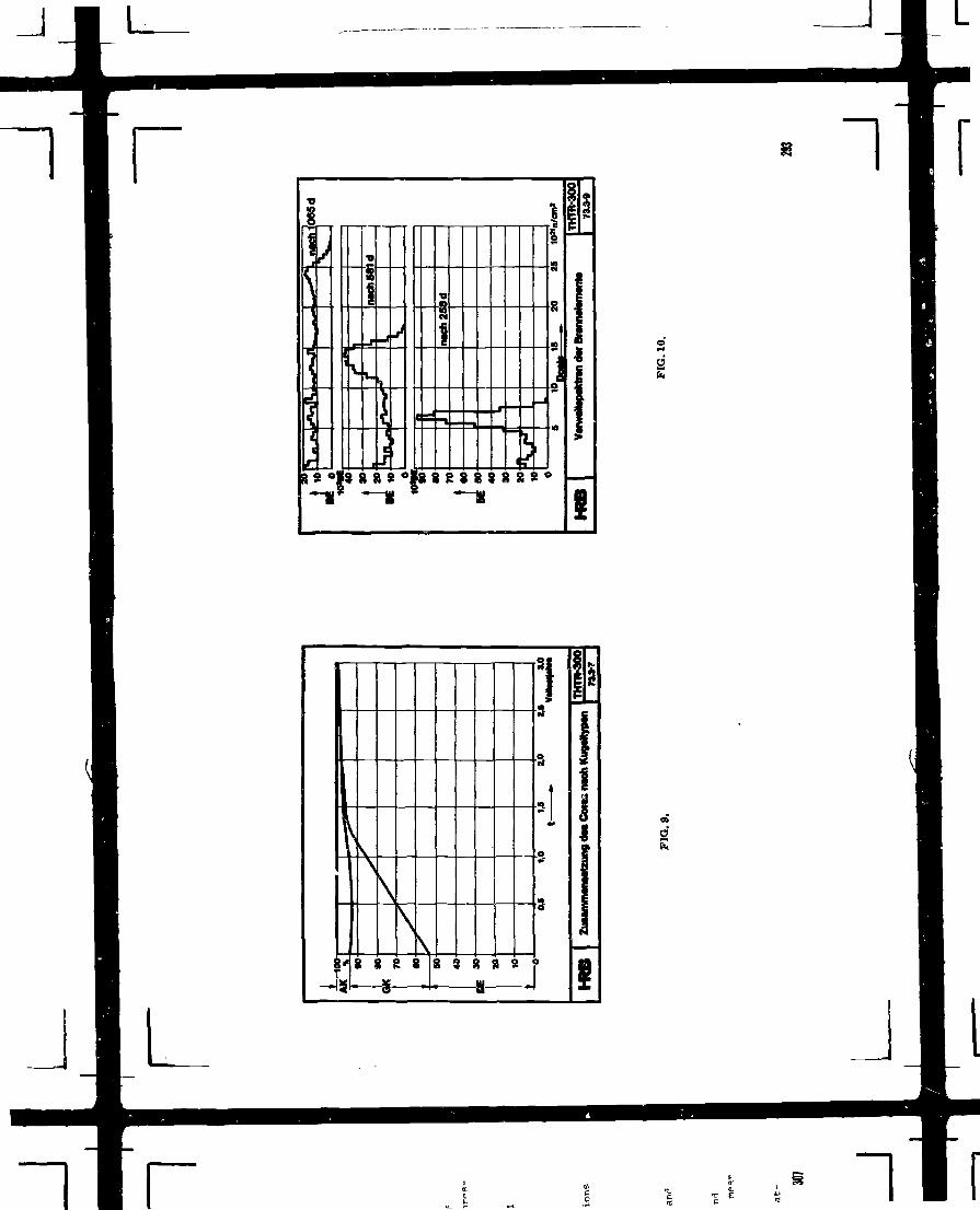
r "I

\

sL

\\

i SI 1 _

\

\

\I g 8 |S 9 \i i

a-i i>

—»

THTR-Erstcora THTR-QWchgawlchttcof (3 J«hr>>

LtMungtdtehtevartaihmgTHTR-XO

73.3-3

VERSUCHSERGEBMSSE

»»kcol /m>h*C

RECHENERGEBWSSE

»ieOkcol/m?h*C

BBC/KRUPP VERGLECH BEHeCHNETERMTM VERSUCHGEMES-)SBCNVW»CUBERG*NBSZ«Hfl<HSWUG£BET

THTR7MI-1

FIG. 11. FIG. 12.

2M

'J

Thermal Raaklor Powar P|h.

- 44004 kW10*

102

10

1,0

0,1

0,01

Reactor critical'///

r S0 2 4 6 8 1012141618 2222 23,5 24

Time •-» 26

(Hour*)

1 Reactor Powar2 Circulator Speed3 Mean Shutdown Rod Position

FIG. 13. AVR Rod Jamming Test 77.12-18

Tempi

Iooo-

800-

600-

400-

200-

rrature

/

y

/

-.

I°C !

\

•

—

• •

———

t f = Fuel Temperature

tg = Gas Temperature

p = Power Density

• ~ — — 1 .—• .

E

s

ia

t•16

12

- 8

- 4

0

00 0.2 0.4 06 OS 10•'Relative Core Depth

Br i g .U : Axial Temperature and Power-

Density Distribution HHT 78.14-4

2S5

_J I L

"1

§ » 5

qy

311

NUCLEAR REACTOR SHIELDING

C. PONTIJoint Research Centre,Commission of the European Communities,Ispra,Italy

1. INTERACTIONS BETWEEN IONIZING RADIATION AND MATTER

The aim of a shield is to attenuate and absorb the ionizing

radiation. It must be composed of materials with which the

radiation interacts losing its energy and its damaging power.

It is necessary to know how the radiation interacts with the

matter in order to choose the proper shield. In this section

the basic interactions between radiation and matter seen in

the optics of shielding are recalled and summarized.

1.1 Interactions of gamma-rays

Gamma-rays are electro-magnetic radiation (originated by thenucleus); as such they mainly interact with the electricalfield produced by the electrons or by the nuclei. There areabout twelve different prowesses of interaction between photonsand matter, but only three of them play an important part inattenuating gamma-rays. They are: photo-electric absorption,pair production and Compton scattering.

The photo-electric absorption is the interaction of a photonwith an atomic electron, to which it transfers all its energy.In this process the photon is completely absorbed and itsenergy is locally deposited. The behaviour of the cross sec-tion for photo-electric absorption vs. energy for a givennucleus, may be calculated; the result is rather complicatedand is generally represented by curves or tables. For ourpurpose it is important to note that the dependence vs. rand Z is

Zi /E 3 barn/atom

This behaviour shows that the phcto-electric effect is moreimportant for heavy elements and for low energies.

A photon with energy higher than 1.02 Mev may interact with

the electric field surrounding the nucleus and generate a

pair positron-electron.

In this process (pair production) the incident photon losesall its energy; the positron that has been produced will sooninteract with an electron (annihilation) and produce a newcouple of photons with energy greater or eoual to 0.51 Mev.In deep attenuation problems, these photons may be neglectedas their energy and penetrating power are lower than thoseof the incident photons from which they heve been produced.In the energy interval interesting shielding problems, thecross-section for pair production depends upon E and Z inthe following way:

In F.

This shows that pair production is more important for heavy

elements and high energies.

The Compton scattering is the elastic interaction of a pho-ton with a free electron (or with an electron whose binSinqenergy is negligible as compared to the energy of the photon).The emerging photon has a new direction and lower enerqy; theenergy loss (and the fractional energv loss) is higher forgreater, scattering angles and for greater incident oneraies. ^angular distribution of scattering anglf* is qiv*»n by theKlein-Nishina relation: this distribution is as amrc forwardas higher the incident enerciy.

The Compton scattering is an interaction with tho single

electron; the atomic tross section is then proportional to

Z. The behaviour of S vs. F is shown in Fin, 1.

297

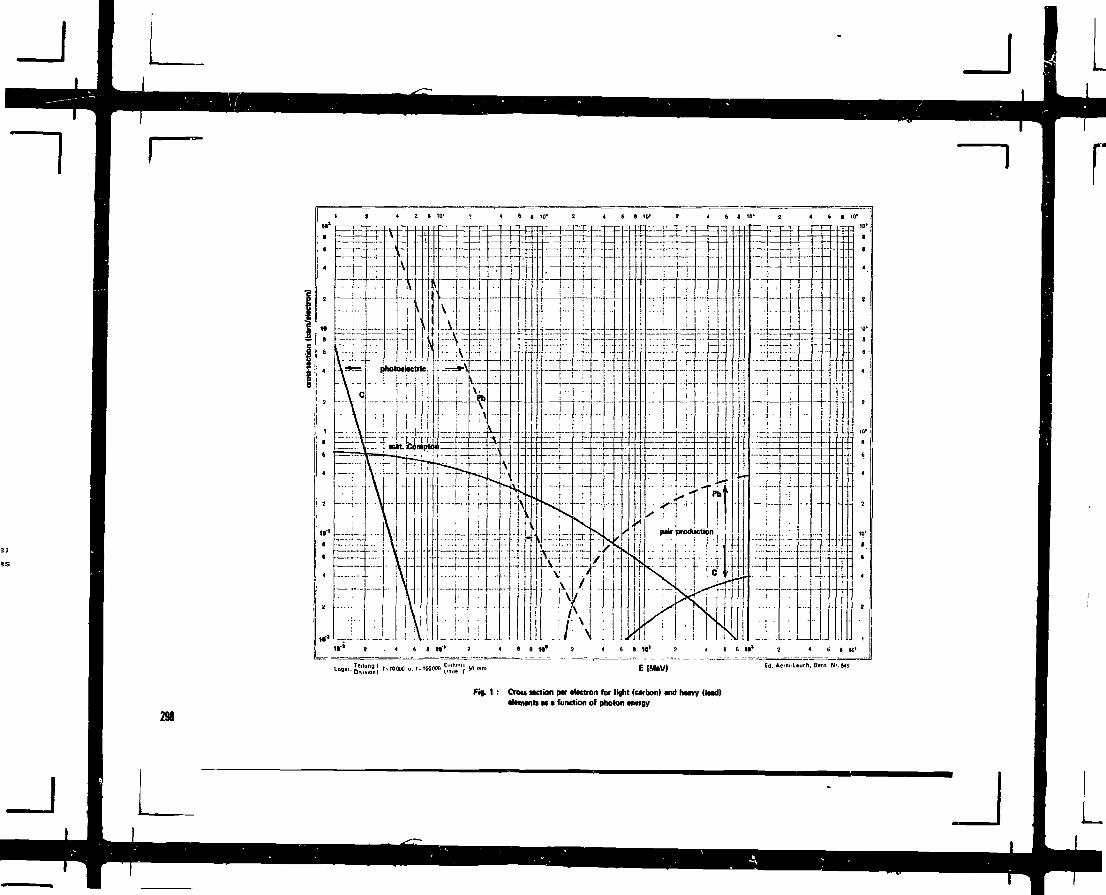
4 6 8 10* 2 4 6 a 10* 2 4 6 8 10* 2 4 i 1 ID'

291

Fif. 1 i Crou Mctkm ptr tltctron for light (cwbon) «nd htwy (Ittd)tttnwnn u • function of photon tmrgy

"J

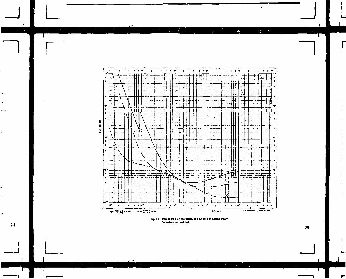
Fi|. 2 : Miltttttmition cMftictont, M • function of photon *n«w,for ctfhon, inn wtd tod

299

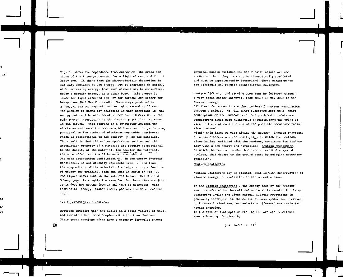
Fig. 1 shows the dependence from energy of the cross sec-

tions of the three processes, for a light element and for a

heavy one. It shows that the photo-electric absorption is

not only dominant at low energy, but it increases so ouicfcly

with decreasing energy, that each element may be considered,

below a certain energy, as a black body. This energy is

lower for light elements (20 kev for carbon) and hiaher for

heavy ones (0.5 Mev for lead). Gamma-rays produced in

a nuclear reactor may not have energies exceedinq 10 Mev.

The problem of gamma-ray shielding is then important in the

energy interval between about .1 Mev and 10 Mev, where the

main photon interaction is the Compton scattering, as shown

in the figure. This process is a scattering against the

electrons and hence the macroscopic cross section u is pro-^

portional to the number of electrons per cubic centimeter,

which is proportional to the density f> of the material.

The result is that the macroscopic- cross section and the

attenuation property of a material are roughly priportional

to the density of the mater.al: the heavier the material,

the more effective it will be as a gamma shield.

The mass attenuation coefficient fife , in the energy interval

considered, is not strongly dependent from Z and from

the composition of the material. Its behaviour as a function

of energy for graphite, iron and lead is shown in Pig. 2.

The figure shows that in the interval between 0.5 Mev and

5 Mev, f*l§ is roughly the same for the three elements (that

is it does not depend from Z) and that it decreases with

increasing energy (higher energy photons are more penetrat-

ing) .

1.2 Interactions of neutrons

Neutrons interact with the nuclei in a great varirty of wavs,

and exhibit a much more complex situation than photons.

Their cross saotions often have a strongly irregular shape:

300

physical models suitable for their calculations are not

known, so that they may not be theoretically predicted

and must be experimentally determined. Thrse measurements

are difficult and require sophisticated equipment.

Neutron diffusion and slowing down must he followed through

a very broad energy interval, from about in Mev down to thn

thermal energy.

All these facts complicate the problem of neutron penetration

through a shield. We will limit ourselves here to a short

description of the nuclear reactions produced by neutrons,

considering their more meaningful features,from the point of

view of their attenuation and of the possible secondary radia-

tion produced.

Within this frame we will divide the neutron induced reactions

into two classes: neutron scattering, in which the neutron,

after having collided with the nucleus, continues its trajec-

tory with a new energy and direction; neutron absorption,

in which the neutron is absorbed into an excitsfl compound

nucleus, that decays to the ground state by emittino secondarv

radiation.

Neutron scattering

Neutron scattering may be elastic, that is with conservation of

kinutic energy, or anelastic, in the opposite case.

In the elastic scattering , the energy lost by the neutron

(and transferred to the collided nucleus) is greater for large

scattering angles and light nuclei. Elastic scattering is

generally isotropic in the centre of mass system for energies

up to some hundred kev, and anisotrooic(forward scattering)at

higher energies.

In the case of isotropic scattering the? average fractional

energy loss g is given by

2A/(A D"

A ia the atomic mass of the collided nucleus.

Table I gives values of g ar.d N for several elements; N

is the mean number of isotropic elastic scattering collisions

required to slow down a neutron from 1 Mev down to 1 ev. The

table shows that elastic scattering is effective to slow

down neutrons in light elements but ineffective in heavy

elements.

Table I

Element

HD

Li

Be

B

C

0Ha

Fe

Pb

A

12

79

1112

1623

56

207

g

.5

.44

.22

.18

.15

.14

.11

.09

.04

.01

n

1622

61

77

93100

134190

457

1680

Elastic scattering parameters

When a part of the kinetic energy of the incident neutron is

transferred as excitation energy to the collided neutron, we

speak of anelastic scattering . The excited nucleus decays

with emission of one or more photons: this process is

mentioned in section 3 among the radiation sources.

Anelastic scattering may take place when neutrons have an

energy somewhat greater than the excitation energy 0 of the

first level of the collided nucleus. The enerqy loss is

greater than Q and the scattering angle has a distribution

which is roughly isotropic.

Anelastic scattering is very effective in slowinq down fast

neutrons; Q values are in the interval from 0.4 Mev to a

few Hew; one anelastic collision may reduce the neutron

energy by one or more Mev. It is more frecuent in heavy

elements, which have higher anelastic scattering cross sec-

tions and lower Q values.

Neutron absorption

As mentioned L.i the previous section, the neutron capture

is always followed by emission of secondary radiation.

Two reactions are mainly responsible for the absorption of

neutrons in nuclear reactors; they are the (n, y ) reaction

and the in, «) reaction.

The (n, ft) reaction or radiative capture produces the

more important radiation source inside the bioloqical shield

and quite often determines its thickness. The cross section

of this reaction is in general 1/v shaped and thermal neutrons

are the most interested ones.

The (n, <a ) reaction is very useful, from the point of vinw

of shielding, because it allows the neutrons to be absorbed

without producing new penetrating radiation and hence en-

ables capture gamma-rays to be reduced. The element that is

more frequently applied is boron, because of the high value

of the (n, a) c.s. of its isotope B-10 {18.81 of natural

boron). This reaction is 1/v shaped, with a thermal energy

value (2200 m/sec) of 760 barn; it is followed in 95% of

cases by emission of one photon of 0.45 Mev: a low enerqy

compared to that of capture gamma rays.

2. RADIATION EFFECTS

About 10% of the energy produced in a nuclear reactor is released

to neutrons and gamma-rays. Most of this energy will not be de-

posited into the coolant, but in other parts of the core, re- nm

-i rflector and shields. The heat deposition must be Known in order

t?> determine the temperature and the possible need of cooling or

of .shielding against the energy flux carried by the particles

(ti.ermal shield).

E. is the sum of the energies of the particles which have

entered the volume of the matter considered;

a is the sum of the energies of those which have left it;

a is the energy equivalent of any increase in rest mass

that took place within the volume.

In all the working areas of the reactor building the radiation

level should be kept as low as possible; it must however con-

form to the limits imposed by national and international regu-

lations. The shields required to reduce the radiation levels

below these limits are referred to as the biological shields.

The Kerma accounts also tor that secondary radiation, like brem-

sstrahlung, which is not deposited in the volume considered, and

is not taken into account by the dose. So that the dose is in

general lower than the kerma; but their difference, in the

energy range of interest to shield design, is negligible.

Materials subject to intense neutron fluxes may suffer important

changes to their crystal lattice structure; these may induce

alteration in shape, volume, composition and in the physical

properties of the irradiated material. The presence of a shield

with the specific purpose of reducing fast neutron fluxes, may

be sometimes required to avoid such effects.

Heat deposition, dose rates, structural damage, are basic magni-

tudes in any shield design. This section shows how these quanti-

ties may be calculated.

Names and definitions of radiation quantities and units will

follow the recommendations of 1CRU / I / .

The Kerma (K) produced by a fluence 0/(E) in a material contain-

ing N nuclei/barn.cm of the isotope m, is calculated follow-

ing its definition. The particles (either neutrons or photons)

may interact with the isotope m in several ways; each way

is specified by a cross section <J. , and gives rise to the

emission of

energy

a charged particle having an average kinetic

f.m(E). By definition it is

K(E) fja(E)/a Mev/g

d is the density of the material in g/cm . If the material

contains different nuclides, the sum is extended to all their

contributions:

2.1 Heat Deposition

The energy amount deposited by radiation in the unit mass of

irradiated matter may be expressed by two quantities:

KE3117V, Kinetic Energy Released to Matter,

is tiie sum of the initial kinetic energies of all the charged

particles liberated h\ the incident radiation.

DOSE or r.BSOREED DOSE

is the difference n. - r. - Q.

K(E) -

The quantity

km ( E ) fjm(E) barn-Mev

is a function of energy typical of the nucleus m, and is

referred to as the kerma factor of this nucleus.

Compilations of kerma factors may be found in different nuclear

data libraries: we mention here the DLC-29-MACKLIB/2 /for

302

neutrons, and the NBS report / 3 / for photons.

The total heat deposition of a radiation is calculated by inte-

gration on its energy spectrum:

K = ±- 0(E)T N k (E) dE Mev/q

Table IT

Conversion factors from neutron flux to dose cc-uivalont rntn

2.2 Dose Equivalent

The quantity that expresses by convention /I/ the biological

damage produced by ionizing radiation on organic tissue, has

been given the name dose equivalent (D ).

The unit of dose equivalent is the rem. A detailed calculation

of D is much more complicated than that of heat depc-

sition: for each possible interaction cf the radiation

with tissue, attention must be paid to the type and

energy distribution of the secondary radiation produced, and

to its biologica) effectiveness. It is enough for our purposes

to know that the final expression of D may be written as:

0(E)C(E>dE rem

C(E) is a function of energy that provides the conversion

factor from fluence to dose equivalent or from flux to dose

equivalent rate.

Valuss of C(E) for neutrons and photons are qivrn in tables II

and III.

neutron energy

ov

Conversion Factors

in ron/h

n/citi soc

5.

2.

5.7.

10.

14.

thermal

1

10

IC2

103

10 4

10 5

10 5

10 6

5 106

106

106

106

10*

4.14

4.82

4.36

3.C4

3.19

3.57

1.75

6.SO

1.17

1.26

1.59

1.45

1.55

2.21

in

mID

-3

-3

r3

- 3

r3

-3

r2

,-2- 1

- 1

"1

,-1- 1

From J.A. Auxier, W.S.Snyder, T.D.Jones /t/

317 303

.

L

Table III

Conversion factors from photon flux to dose equivalent rate

Photon Energy

(Mev)

14-16

12

10

8

7

6.5

6

5.5

5

4.5

4

3.5

3

2.6

2.2

1.8

1.35

.9

.6

.4

.2

.1

Conversion Factors

m rem/h

p/cm sec

1.33 10"2

1.17 10"2

1.02 10~2

8.73 10"3

7.62 10"3'

7.07 10"3

6.71 10~3

6.34 10"3

5.96 10"3

5.53 10'3

5.19 10"3

4.79 10"3

1.37 10"3

3.97 10"3

3.60 10"3

3.20 lo'3

2.73 10"3

2.14 10"3

1.58 10"3

1.17 10"3

7.21 10-"

4.51 10"4

From Claiborne s Trubay /5/

304

2.3 Structural Damage

A nucleus hit by a neutron receives a fraction of the energy

carried by the incident particle. If the energy of the recoil

nucleus is greater than 20-30 ev (the binding energy of the

nucleus into the lattice), it leaves its equilibrium position

within the lattice and may in turn hit other nuclei and produce

other dislocations. In this way a number of interstitials

(atoms that occupy a non stable position within the crystal

lattice) and vacancies (stable position with no atom in it)are

generated.

If the primary recoil atom carries enough energy/ it will pro-

duce a defect cascade with a number of vacancies inside and

interstitials outside. Vacancies and interstitials are unstable

and show a strong tendency to recombine; their mobility is

affected by temperature and presence of impurities.

Another type of damage to the lattice may be produced by other

nuclear reactions like (n,p) or (n, * ) . These reactions trans-

form the collided nucleus in a new one, with a different atomic

number, and hence they generate impurities within the lattice.

Furthermore the Hydrogen and Helium produced by these reactions

may come 'ogether to form bubbles. These bubbles are responsible

for the swelling induced in steel by intense neutron fluances.

These alterations in the atomic structure may generate important

changements in the mechanical properties and in the geometry of

irradiated metals. Volume increase up to 25% have been reported

for SS 316.

Radiation damage to structural materials becomes important at21 2

fluei.ee levels of about 10 n/cm for fast neutron fluences22 2

or 10 n/cm for total neutron flusnee. This damage may vary

by order of magnitude according to:

- temperature of the material irradiated

- neutron flux spectrum

- impurities present in the material

- composition

- manufacture

A meaningful quantity for estimating the damage is the num-

ber of displacements produced per unit volume or per aton. The

number of displacements per atom (dpa) is given by

""/*dpa

ff, is the displacement cross section (in cm ) of the atom consi-

dered, and is a sum of contributions from all the possible

nuclear reactions induced by neutrons on this atom:

(E)

.(E) cross section of reaction i

.(E) mean number of displacements produced by the primary

recoil atom

A comprehensive description of basic phenomena involved in

displacement production may be found in /6/.

Details of radiation damage calculations and values of displa-

cement cross sections are reported in /!/.

3. SOURCES OF NEUTRONS AND GAMMA-RAYS IN A NUCLEAR REACTOR

In this section wa are going to make up an inventory of the

radiation sources existing in a nuclear reactor.

We are not so much interested in studying the physical characte-

ristics of radiation producing reactions, as in finding out

where and when radiation is produced implying shieldinq problems.

Some radiation sources will be more important and they shall al-

ways have to be considered; other ones shall be considered

sometimes only; anyhow we should be able to foresee in which

situation shielding problems might arise.

Any shielding problem starts with the analysis of the source that

produces the radiation to be shielded: we need to knnw which

type of radiation it is, how intense, of what energy and how

it is distributed in space. The list that follows is not a com-

plete one. We will only describe the main sources of radiation

that may be present in a nuclear reactor, to show which typp of

problem they may produce.

We will first deal with neutron sources and then with qammn-ray

sources.

3.1 Neutron Sources

3.1.1 Fission neutrons

Almost all neutrons present in a reactor are producer! by nucj.par

fission. According as they are emitted simultaneously with a

fission event or owing to the decay of fission f raainents, we

shall distinguish between prompt and delayed neutrons.

There are other neutrons yet, which are emitted bv tho irra-

diated nuclear fuel with delays much lonqer than tho precoo'lino

ones; tney will be considered toqether with de]avp<l neutrons

in this section.

Prompt Neutrons

23!SThe thermal fission of a nucleus of U produces the pn>ipsiop

of 2.47 neutrons (mean value). The enemy spectrum of these

neutrons is protty well known: there arp various measurPR airl

representations not markedly different from each other.

Watt's formula is the most widely used:

n(D = .484 sinh J~2F exp (-P)

n(E)dE being the fraction of neutrons produced with .in enprqv

between E ant] E + dE (Mev) .

305

This energy distribution does not vary appreciably with the

fissile isotope nor with the energy of the neutron producino

fission.

Normalized fission spectra of U 2 3 5, Pu 2 3 9 and Pu 2 4 1 for the

100 groups structure described in section 5 are given in /8/.

As for V , that is the mean number of neutrons emitted by

fission, it varies with the isotope and with energy. It is a

common practice to day to list in nuclear data libraries, thp

product -i)^ rather than V and G", separately, as these two

quantities never occur separately in the eouations governing

neutron transport.

Delayed Neutrons and Other Neutrons

emitted by Fuel Elements

Fission fragments decay in various and complicated chains,

along which it may be produced a stronqly excited nucleus that

emits a neutron.

These neutrons are a little fraction, less than 1%, with respect

to the total amount of those produced by fission and they may

become important only owing to their characteristic of heincr

produced with more or less long delays with respect to prompt

fission neutrons.

The importance that they acquire in view of the control of a

reactor is well known. As regards shielding, their presence

may be important only when fuel is circulating. The diaqram

of delayed neutrons decay is well approximated by a sum of

six terms, each corresponding to a special decay process.

The mean energies of emitted neutrons and the decay constants

for U 2 3 5 are given in Table IV.

Table IV

Delayed Neutrons constants

group

1

2

3

4

5

6

1

3

.see-,

.0127

.0317

.115

.311

.40

.87

ai

.038

.213

.188

.407

.128

.026

E±(Mev)

.25

.46

.405

.45 A =

.52 r.ai =.016

1

If N- is the number of fission events occurred at time t=0,

the number of neutrons emitted at time t is:

N(t) = N. A £a<. X, e" '

A being the number of delayed neutrons per fission.

As one can see from Table IV, the values of energy are about

half a Hev or less. Data for this Table are taken from page 73

and following ones of Compendium /9/, where one can find other

data concerning delayed neutrons.

The half lives of these delayed neutrons are lower than 1 minute,

as one can notice from the Table, being T, ., = . 693/X .1/2

Consequently in one hour at most from shutting down the reactor,

they become quite negligible.

Anyhow the fuel elements of a power reactor, which are submitted

to a iong and intensive irradiation (of the order of tens of

MWd/ton), may emit neutrons even months after having been irra-

diated.

306

This second type of delayed neutrons is produced by twn ways:

a) spontaneous fission of isotopps (Pu, Cm, Cf) produced owina

to irradiation of U and/or of Pu, and (b) when fuel is in form

of oxide by ( ot ,n) reactions induced on oxyqen by alfa particles

coming from various decays. For a PWR element this neutron

emission is of the order of 500 n/sec ppr qram of irradiate

fuel. This source intensity implies the compulsory use of a

neutron shield also in containers desiqned for transport of

irradiated fuel elements. If fuel has been obtained from repro-

cessing of irradiated elements, then an important emission may

be present also in a new element.

The problem of computing the activity of a fuel element drawn

out of a reactor is solved in a fairly general way by the

code ORIGEN /10/. This code supplies activity, heath production,

neutron emission and gamma-ray emission in a fuel element,

taking account of the "story" and possible reprocessing,versus

cooling time.

3.1.2 Photo-neutrons

In a nuclear reactor ( )J ,n) reactions may occur with some light

elements. These are threshold reactions, and only a few nuclides

have a threshold energy low enough to allow such reactions in

the presence of the gamma-rays produced in a reactor.

These nuclides, the corresponding threshold energies and the in-

terval of variability of cross-sections are listed in the

following Table V.

In a medium "transparent" to gamma-rays and where, on the con-

trary, neutrons are largely attenuated, the presence of photo-

neutrons may become important. This may happen with heavy water,

berillium and sometimes with light water too.

In the presence of these moderators, ( )J ,n) reactions produce,

after shut-down, the most important source of neutrons.

Table V

Photoneutrons parameters

nuclide

H2

Be9

c13

Li6

threshold

energy(Mev)

2.23

1.67

4.90

b.iO

(mb)

1. - 2.

.5- 1.5

The energy of photor.eutrons produced by dputeriun is a h.Tlf

of the exceeding cnerqy of the photon with respect tn the thres-

hold energy; it may nonce exceed the value of 2 :1PV. In tlif-

other cases most of the exceeding enerqy is a\.snrl'Pd by thr

recoil nucleus, which is heavier than thr noutron: this will

receive some hundreds Kev or less.

3.1.3 Activation neutrons

The only situation of interest within this class of reactions

is that of the chain developing from the (n,p) reaction or.

0 present in water

017tr.,P) N 1 7 --> 0170lfl '1 .'lev)

n17The threshold enerqy of the (n,p) reaction on 0 is 8 'lev am'

the cross-section averaged on the fission spectrun is about

b for N is 4-14 soc" ° is Prc"lucp<? at a hiohTi/2excitation level (higher than the neutron binding cni>rnv) an'?

consequently it immediately decays emitting a neutron whos" mcar

energy is about 1 Mev.

0 is present at the rate of 0.037% in natural Oxyaen.

This source is of considerable effect in thp coolant circulat-

ing outside the reactor in LV'R. ...

308

3.2 Gamma-ray sources

3.2.1 Fission gamma-rays

All what one can say about gamma-rays emitter! by fission or bv

fission products is mainly based on the experimental information

acquired about fission of U J* These data are normally extra-

polated also to oi_her fissile isotopes, or which ipforration

is less complete.

From an experimental point of view the qamma-ray energy emitted

by fission is divided ir.to four tine intervals, nonsurpd start-

ing from the instant in which the fission event occurred:

1. Energy emitted within 0.05 /ASOC (7.25 <*ev)

2. Energy emitted between 0.05 and 1 ASOC (.43 Mev)

3. Energy emitted between 1 yjisec and 1 sre ( . J5 M.OV)

4. Energy emitted after 1 sec (6.50 'lev)

In view of our discussion, wo shall consider as prompt fission

gamma-rays those belonging to the first throe intervals and

delayed fission gamma-rays those belonging to the last one.

Among prompt gamma-rays are often included gamma-rays producer*

by capture of U as they are hardly separable from fission

gamma-rays by means of measurements. On thn other side we are

interested in them altogether also for practical purposes,

because they are always simultaneously presort and noreover

they are both produced by thermal neutrons.

Prompt fission gamma-rays.

These gamma-rays' spectrum has Leen measured ir laboratories;

Peele and Maienschein1s /ll/ measurements supplv the best

accuracy with errors lower than 15%.235

A fission reaction in U produces by average 8.1 prompt pho-

tons, the total amount of enornv beirg about L.2G Mev.

Their spectrum (number of photons/fission* Mev) above P.I Mev

may be represented by a discontinuous diagram.

6.C 0.1 < E < . 6 Mev

G(E)= 20.2 exp (-1.711 H) .6<E < 1.5 Mev

7.4 exp (-1.1 E) 1.5 <r<-'10. Mev

Gamma-rays emitted by fission products.

Gamma-rays are also produced by the decay of fission fraoments:

their spectrum varies considerably vs. the time after fission.

Consequently the spectrum of fission oroduets qamma-rays

emitted by nuclear fuel depends both on irradiation time (or

more generally on the "story" of the reactor) and on the cool-

ing time. Nevertheless 75% of delayed gamma-rays is emitted

within 1000 sec from the original fission event. Hence the

state of balance between prompt and delayed gamma-rays is soon

reached.

The spectrum of delayed gamma-rays, in condition of eouilibrium

is represented by the following formula:

Ga(E) = 7.4 exp (-1.1 E) E > .28 Mev

This expression for the delayed spectrum (number of photons/

fission event • Hev) is equal to that above mentioned for

prompt gamma-rays with E > 1.5 Mev; therefore the whole

spectrum consisting of prompt plus delayed gamma-rays can be

approximated, for energies higher than about 1 Hev and in

condition of equilibrium, by the formula

Gd(E) + G(E) = 15.exp(-l.l E) E > 1 . Mev

Table VI provides spectra corresponding to the various compo-

nents of fission gamma-rays divided in ten energy bands.

Among delayed fission gamma-rays there are some having a very

long mean life which, although unimportant when the reactor is

working, produce important gamma-ray sources when the reactor

is shut-down. The total gamma-ray energy emission rate

versus time t(sec) passed from the fission event, is provided

within 20% (for times greater then 10' and shorter then 30 days)

by the formula

G (t) =1.5 t"1"2 Mev/seo.fission event t >lf>'

(see page 66 of /12/)

The calculation of the spectrum versus time of these gamma-

rays is rather complicated. Startinq from the knowledcre of

yield and mean life of every possible fission fragment,of the

probability and energy of emission of photons, and with

similar data for all nuclides of the decay chains, it is possi-

ble to select the most important nuclides and chains, to in-

tegrate on irradiation time and consequently to compute in-

tensity and spectrum of delayed gamma-rays both versus working

time and cooling time of a reactor.

Table VI

Energy spectrum of fission gamma-rays

(Hev/fission)

Energy(Mev)

.1 -

.5 -1. -

1.5 -

2.0 -

2.5 -3.0 -

4.0 -

5.0 -6.0 -

0.1 -

.5

1.

1.5

2.0

2.5

3.0

4.0

5.0

6.0

7.0

7.0

Prompt

gamma-rays

.92

2.16

1.61

1.04

.79

.59

.62

.28

.12

.07

8.20

Delayed

gamma-rays

1.06

1.29

1.16

.92

.62

.54

.57

.25

.10

.04

6.55

Sum

1.98

3.45

2.77

1.96

1.41

1.13

1.19

.53

.22

.11

14.75

This work has been performed by Perkins and King /I3/: the

results obtained for instantaneous fission and working timesn

of 1, 1C, 100, 1000 hours, and cooling times up to in sec

are given at paqes 608-610 of /14/ and at panfs 83-84 of

Compendium /9/. These data include: [^ rav onernv release an''

gamma ray energy release, both total (for nhotors havino i>r»rov

higher than 0.1 Mev) and parted in sewn enorqy bsnr's dpfinry3

as follows:

0.1

0.4

0.9

1.35

1.8

2.2

- 0.4

- 0.9

- 1.35

- 1.8

- 2.2

- 2.6

Mev

Mev

Mev

Mev

lev

Mev

greater than 2.6 Mev

Tables of the same kind providina emission intensit" of

delayed gamma-rays, grouped following the same epprav structure

and of total emission intensity of /3 and ganna enprciv, are

published in /15/. These tables include irradiation times

from one minute up to 1000 years and coolinq tir>es from 1PP

sec up to 2500 years.

3.2.2 Capture and anelastic scattering gamma-rays

As it was said in section l,sone photons may be produced as a

result either of a neutron capture or of an anelastic scatter-

ing. Those coning fro;a the first reaction are often the most

important radiation component in view of dimensioning the biolo-

gical shield and they always are of primary importance. Those

coming from the second reaction may be important only in spe-

cial situations. The calculation of intensity, distribution

and energy spectrum of these q.imma-ray sources is complicated

because of the great amount of nuclear data renuired. For

capture gamma-rays it is necessary to know capture cross-

sections versus neutron energy and capture gamma-ray spectrum

for each element existing in the shield.

The spectrum of capture gamma-rays is often supposed to be

independent on the energy of captured neutrons. Some spectra

of capture gamma-rays for elements freouentlv found in shields 309

are given in Table VII.

These spectra refer the to thermal capturfs. They have been deter-

mined by Maerker and Muckenthaler /16/. Moreover Table VTI shows

that neutron capture often produces gamma-ravs with very hiqh

energy and therefore highly penetratinq.

The calculation of gamma-ray sources cominq from anelastic scat-

tering requires the knowledge of the cross-sections, versus

energy of incoming neutrons, of (n,n'if ) reactions for all

gamma-rays which may possibly be produced. Some values of these

cross-sections can be found at page 88 of Compendium /9/.

These sources are in fact computed by the same codes computing

the space-energy distribution of neutron flux, using proper data

libraries such as those treated in section 5.

3.2.3 Activation gamma-rays

When a nucleus absorbs a neutron, it becomes instable and its

instability gives rise to the emission of a particle, normally

a capture gamma-ray. After this emission, the nucleus in question

may still be unstable and decay in various ways. Decay is always

radio-active and often produces a further emission of photons.

These photons are emitted with more or less lonq delays: the mean

life of radio-active nuclei varies from the order of seconds

to that of many years. The activity of thes-a activated elements

is normally negligible with respect to the other sources ex-

isting in a working reactor; it becomes important in two situa-

tions: either when it is produced in the coolant medium and

hence, circulating together with this, it gets out of the core.

310

Table VII

Gamma-ray Spectra from Thermal Neutron Capture

Energy(Mev)

1-1.51.5-22-2.52.5-33-3.53.5-44-4.54.5-55-5.55.5-66-6.56.5-77-7.57,5-88-8.58.5-99-9.5

Silicon

15.30

23.04.65.4

76.60.870.36.40.2

12.20.89.702.200

Calcium

20.979.641.514.37.913.519.46.62.5

12.140.0000000

Potassium Sodium

Photon/100 capture

35.025.637.223.516.723.220.27.716.217.30.952.150.455.65000

14.811.926.947.614.234.06.42.652.25.9

21.5000000

Barium

63.434.634.324.317.616.028.112.67.69.54.01.01.01.00.30.20.45

Iron

5.015.03.96.09.23.57.23.31.09.910.10.55.530.60.30.53.3

Aluminum

18.610.4a13.120.515.914.316.117.6£.82.86.02.20.732.4000

StainlessSteel

14.59.76.14.47.43.75.83.23.59.47.54.18.533.63.6

12.23.7

a) Does not include the about 100 1.78 Mev photons following decay of Al28

"J ••••••

or when the reactor is shut down and certain parts must he-

come accessible.

The reactions which are most responsible for water activation are:

018 („, ) 0180

1 9

18

The isotopic abundance of 0 is 0.2%.

0 decays with T, ,, = 2® s e c emitting a aamma-ray of 1.6 Mev

in the ratio of 70% of disintegrations. The cross-section of

this reaction is of the form 1/v with a value eoual to 0.21 mt>

for v » 2200 nt/sec.016(n,P) N

1 6

is a threshold (•"11.Mev) reaction, with a cross-section aver-

aged on the fission spectrum of about 19y*b.N ' decays with

T, ,, = 7.4 sec emitting very hard photons: 6.1 Mev ip the

ratio of 75% and 7.1 Mev in the ratio of 7% of disintegrations.

The most important reaction as regards activation of sodium,

which is used as a thermal vehicle in fast reactors is:

Na 2 3 <n,f)Na24

-24N a " decays with T,,, = 14.8 hours emitting two camma-ravs of

energy 1.4 and 2.7 Mev. The thermal cross-section is ahout .53

b, but the resonance at about 2.8 Kev and the fast component of

the activation cross-section are important too, since in a

fast reactor's core the thermal flux is nearly ahsent. Sodium

activation in a power reactor takes values between about 1

and 10 mCi/cm3.

Other reactions may become important for cooling times loncrer

than one week, that is when the activity caused by the above

mentioned reaction is strongly attenuated. One has then to deal

with the activation of corrosion products: sodium removes these

products from the washed walls, transports them into the core

where they are activated and then it lays them down in certain

points of the circuit (generally the coldest ones}. These

corrosion products may have a vnrv long ljfo and aive rise to

proLlcras concerning accessibility there where thev are

Problems of the same kind are raised by the decay of "la

is produced by the reaction

'" which

:]a23 (n,2n) Na 2 2

22a22 2*Ka decays in 2.6 years to :»e " enittira or.e qamna-rav of

1.27 Mev. This is a reaction having a very hioh threshold eneroy

(12 Mev). It may produce an activation reaching, after an irra-

diation along sone years, orders of magnitude of Zflci/cn' air*

it causes the residual activation of sortiur for cooling times

longer then one woe):.

Also for steel, structural materials, concrete and other mate-

rials, activation calculations must take into account all the

elements and isotopes which are present in the mixture, even

at very low concentration levels, ft rough estimate of thp

order of magnitude involved in activation calculations may come

from the consideration that stairless steel structures, irra-

diated for long times with thermal neutron fluxes greater than

10 n/cm sec. provide equivalent dose rates higher than

2 mrem/h for many days after irradiation, other data and

formulas useful for activation calculations can be found in

/17/.

4. APPROXIMATr METHODS FDR SI'inTJiIIOT C?LC»I,ATIO"]S

The solution of any shielding problem r<?ruires the knowledge

of the radiation flux and of its space-enertjv distribution.

The determination of this flux by means of transport theory -

in one of its more or less riciorous forms - is therefore aJ.wavs

a necessary preliminary step. The methods of calculation which

have teen maie widely applied for solving shielding problems

are not tho same as those applied for neutronic calculations

311

_J

r

312

inside the core. Inside the core angular fluxes are nearly

isotropic and their space distribution is rather uniform.

Consequently the approximation provided by the diffusion theory

is generally suitable, except in case of local dishomoaeneities;

greater accuracy is required for the eigenvalue, that is Kefj;

fission and capture cross-sections must be well known and their

resonances also must be taken into account in detail.

The calculation of the flux inside a shield is a non-homoqeneous

problem (it is a source problem): annular fluxes may be stron-

gly anisotropic and vary quickly in space. Under these condi-

tions the approximation supplied by the diffusion theory is not

adequate.

The most important cross-sections are the total ones, the

differential elastic scattering which requires a P3 approxi-

mation (that is 4 terms of Legendre polynomial expansion), and

the inelastic c.s. for high energies. On account of these diffe-

rent characteristics, specific methods have been used in shield-

ing calculations.

As neutron transport models get more and more sophisticated,

rigorous and general, the same method may be applied to both

core and shield calculations. Thus, for instance, codes based

on discrete ordinates approximation or on Monte Carlo approach

may be applied to the solution either of core or of shieldino

problems. It is however significant, to point out that the

most advanced and reliable codes of this series are produced

by staffs (mainly in USA and in France) whose principal in-

terest is in shielding.

The discrete ordinates method has been described in another

part of this course. In the following chapters we arp qoin<r to

consider some calculation methods expressely elaborated to be

used in shielding problems. These are non-riqorous methods,

which introduce some simplifying hypothesis nnd can give

satisfactory results without expensive computing times. These

methods are largely supported by experimental evidence; they

can be applied in all the problems for which these basic

assumptions of the methods in question are satisfied.

4.1 The Build-up Factor

Boltzmann transport equation has its simplest solution under

the hypothesis of a perfectly absorbing medium. In this case,

the total flux coincides with the uncollided flux. For an iso-

tropic point source placed in P, emitting S(E,P) particles/

Mev.sec, there will be in Q an uncollided flux

(4.1) 4>(E,Q) = S(E,P)e

4 1TPQ2part/cm .sec.Mev

T being the distance from P to Q, in mean free paths.

Eq. (4.1) expresses the well known fact that the unccllided

flux attenuates like a two factors product: the first, a geo-

metrical factor, varies with the inverse square of the distance;

the second is the probability of non-collision and it diminishes

exponentially with the distance frost the source.

For an extended source emitting S(F,P) particles/cm-.Mev.sec,

in a space of volume V, the total flux in Q is obtained in-

tegrating eq. (4.1) over V.

In the calculation of high energy qamma-rays propagation,

eq.(4.1) can give results approximated within an order of

magnitude, the scattering cross-section being small in compa-

rison to the total cross-section. The total flux is obviously

greater than the uncollided flux, since it includes all the

components of the different scattering orders. One can take

into account the increase due to scattering contributions

by means of a dimensionless build-up factor B:

(4.2) f(Q) S(E.P) e B(*f,E)

4 Tf PQ£

1.

Q of alX the particles, of any energy.

Of course it is B ^

>P (Q) is the flux in

emitted with energy E in P. We specially refer now to gamma-

rays: the flux will be expressed in photons/cm .sec. The

problem of determining the flux distribution is thus reduced

to that of calculating the build-up factors.

Let us suppose that the point (isotropic) source is placed in

the origin and that it irradiates in an infinite homogeneous

medium. Let us suppose moreover that the source is unitary and

monoenergetic, with energy F.. From GO . (4.2) it fol lows:

(4.3)

The first method, by means of which build-up factors h aw Vpnp

computed and systematically tabulated, is thr method if

moments. The tables obtained by fToldstein and Will-ins, re?n-rn~

duced at page 367 of /12/ are still vidr»ly USP'1.

We point out that by this irethod we can get or.lv an ir.t nr.Tl

answer: eci.{4.4) supolies the total flux in 0, int"f?ratp^ over

the energy, and it does not give any information about thp

spectrum. If, on the contrary, besides thp total flux, wr wpulf1

like to know either the ecmivalcnt dosp P (O) or the hi?at

deposit H(0), what sould we do? It is not correct to mal-r sj'- ly

the product of the total flux tinp.s conversion cooFficjpp.ts,

since the flux in 0 is not monnenrrqptic ami its s^pctrum is

not frnown. it is therefore* necpss-iry to etormir0 ap nan1*

build-up factors as the different anstenrs vp are I O O M ^ T for.

We can write the equations sinilar to (<!.3) for tt>p ofiiiv=>1p"t

dose and the h^at deposit:

(4.5)

4 »

with V */*r: **{cm~ ) being the total attenuation coefficient

of the medium at the source energy.

If we know a suitable method, for this extremely simplified

problem, which allows to determine f (r), then eq.(4.3) will give

us the required function B(T?,E). Once this is known we have

the solution of the problem for an arbitrary source (provided

that it is isotropic) :

(4.4) f (Q) •H* pn2

(4.6)

4 ff r 2

C(E) is the conversion fnct-or fnr. flux to dose Rpuiv.tlont

ratp. K(r.) is the Ker.aa factor dcsrril ef' i r spotinn ?..• r n arr'

Dp are dimensionlosn factors, n-^nplv CIOFP hiiil^-ut"1 nw1 r^^^t'v

ci&posit Luil'1-un. Thn S_1H"? PCt!iO';! lP1(!irr; tn t h" ' ' " t i r r i ' lUnn

of b leads to C ar-1 iSj.. ".ofwllv, w'.pr thr flu!:<f(",r)

. roiiucort by the norornon.i">tic pnirt snurnp i <-. 1 r.n"*i, it i<=

possil-le tr> dctprmirr not nr.lv thr tnt^I f!u:r (i-i-^rrjr-i + i r'i

over V.) but alsn the '.lose aivl tbr l .n t do iosit ,V'y nil t i"l"lnn

313

it times the corresponding conversion factors and

integrating. D (

and (4.6) supply

integrating. D (r) and H(r) being determined, eq.(4.5)

314

and B_.

There exist several tables of build-up factors obtained by differ-

ent methods(/12,19/and data library annexed to/20/)and for differ-

ent materials. The available tables include the interval of t

from zero to 30 mfp, and the energies from 0.5 Mev to 10 Mev.

The build-up factors increase regularly with 1- ; thpy generally

diminish with increasing energy, but this is not always true

for heavy materials. Their trend is pretty regular; a rough ap-

proximation, valid in the interval from 1 to 3 Mev within a factor

of about 2, is:

B(X) = 1 + X

As it has been said in section 1, the attenuating properties of

materials, with respect to gamma-rays, depend mainly on the

number of electrons per cm existing in the material and conse-

quently on its density. Something similar is true for the

build-up factors: their variations according to materials mainly

depend on the density of these. This trend allows simple interpo-

lations to determine the build-up factors of a material, when

those of materials with similar densities are known. It is

sufficient to have at one's disposal tables for 5 or 6 materials

of density included between 1 and 11 g/cm (water and lead are

respectively the lightest and heaviest material for which build-

up factors are needed). For every other material it is then

possible to interpolate.

Up to now we have limited our attention to homogeneous

media • However eqs. (4.3), (4.5), (4.6) are applicable

even to non-homogeneous materials, provided that for the calcul-

ation of the answer in Q one applies the build-up factor of

the material where Q is placed. Attention should be paid to the

fact that near the interfaces errors will arise due to the

differences in the build-up factors of neighbouring materials.

In fact while the build-up factor strictly depends on all the

materials and thicknesses passed through, as a first approxima-

tion one can say that it depends essentially on the total

thickness (expressed in mean free paths) and on the scattering

properties of the last medium traversed.

It is actually this property which allows to apply the method of

build-up factors to many and several problems of gamma-ray

attenuation; and moreover the fact that the build-up factors

have a regular trend versus energy and materials' density.

When a better approximation is necessary or it is recmired

to reduce the errors present near the discontinuities

(specially between materials which exhibit strong differences

in density), ore can apply more complicated expressions which

allow to smooth away differences in build-up factors of

different materials (see for instance /20/ at page 34.)

The advantages of this ipethod are the remarkable conceptual

simplicity, -he possibility of application in situations in

which the source is extended and complicated, and a reasonable

approximation.

Among the disadvantages we point out: the lack of differential

information (the method gives the total flux, but it does not

give the spectrum); one must repeat the calculation as many

times as the required answers. Attention should be paid that

around the optical path PQ connecting the source-point

to the answer-point there are no preferencial paths such as

vacuums or materials lighter than those present along PQ.

The build-up factors method is applied exclusively to gairma-

ray calculations, for energies higher than 0.5 Mev. For lower

energies the build-up factors lose their regular behaviour and

the considerations we have just made are no more valid.

Codes using this method are: MERCURE - 3 /19/, MERCURE - 4 /22/

and SABINE - 3 /20,21/. They shall be described during the last

week of this course.

J

n4.2 Diffusion and Removal-diffusion Theories

4.2.1 The Diffusion Approximation

This subject has already been treated in previous parts of

this course. We will discuss in the following whether and

when the diffusion approximation is applicable for shielding

calculations.

From an analytical point of view, the hypothesis to be assumed

such that the diffusion equation can be valid are the followinq:

a) the space dependence of the scalar flux can be represented

by a Taylor expansion cut off at the second order term,

that is:

<f(X) = i (0) + X f ( 0 ) + X2 ifl"<0)

Hb) the scattering is isotropic in the laboratory system.

If these two conditions are met, then one can show the validity

of Fick's equation for the current J

(4.7) J = - D gradip

and consequently also of the diffusion equation:

<4.8) D V 2 f(X) - S(X)

D is called diffusion coefficient. It depends on the proper-

ties of the material) through the cress-sections:

(4.9) D = 1 / 3 It 2

The derivation of these equations can be found in Reactors's

Physics text-books (for instance in /23/ at page 92 and follow-

ing ones). We are interested here in the meaning and the conse-

quences deriving from the hypothesis which have been made.

In this frame it is interesting to remark how the same diffusion

equation (4.8) can be derived starting from different hypothesis,

(see /24/ at page 103) that is:

c) the angular flux be isotropic or linearly anisotropic (p^

approximation).

Also in this case eqs. (4.7) and (4.3) are valid, provided one

sets:

(4.10) 1/3 Za>where M is the mean value of the cosine of the scattering' oangle (in laboratory system).

Actually the hypothesis (a) + (b) and (c) do not differ so

much from each other, since one cannot have regularity in the

angular flux if there is no regularity in the spacial distri-

bution. One can see for instance eq. (4.7) or - more directly -

from P^ eqs. that the angular flux can be isotropic only if its

spacial distribution is flat, and viceversa.

The physical conditions which must be satisfied ip order that

these assumptions be valid are:

- low absorption;

- away from boundaries.

These conditions allow a regular trend both of spacial distri-

bution and of angular flux. It should hence be T. a <<• 2 t ,

that is Zl — 5Lfc, so that ea. (4.9) can be written in the

form:

D = l/3Z.t

This equation, provided that the scattering is isotropic

(/*« = 0), coincides wi*:h eq. (4.10). Condition (c) and per.

(4.10) are a little more general than (a) and (b) and connected

eq. (4.9), because they allow to taVe into account a possible

scattering anisotropy.

The diffusion equation (4.8) states a balance between entering

and emerging particles per unit volume and it snecifips that

(in stationary conditions) the balance must be levelled. It

is a monoenergetic equation, because it assumes that all the

neutrons have the same speed and the same cross-sections. The

energy dependence is generally considered in the multi-grour>

scheme: the energy range is divided in several intervals, with- 315

~lin each of which neutrons are assumed to have constant (suitably

averaged) cross-sections.

In this scheme, let us indicate:

i •* I,N the index of the energy group

..

the flux of group i

the transfer matrix from group to group; hence3'

is the number of neutrons/cm .see which,after scatter-

ing, are slowed-down from group i to group

is the total cross-section of qroup i.

j;

In this scheme the diffusion equation is written:

3=1.i

D. = 1/3

Actually one might say that each author has his own recipe to

define the multi-group diffusion coefficients; anyhow the

basic hypothesis for 14.11), which ought always to be re-

membered when applying the diffusion theory, implies for energy

dependent problems, not only lov; absorption but also scarce

slowing down.

4.2.2 The Penetration of Past Neutrons

Let us now see what is really happening in a typical shield.

Consider a hydrogenated infinite medium (water or concrete),

containing an isotropic monoenergetic point source placed in

the origin; let this be a fast source, of some Mev, the same

order of the energies present in the fission spectrum. The

typical trend of the total cross-section versus energy shows

a constant decrease with increasing energy; this trend is

specially relevant for hydrogenated materials, owing to the

shape of hydrogen's cross-sections.

We observe moreover that the possible events for a neutron of

316

a few Mev (in a hydrogenated medium) are in an approximate order

of probability:

- elastic scattering against light nuclei

- anelastic scattering

- elastic scattering against heavy nuclei

- absorption.

All these events, except the third kind, either eliminate the

neutron (absorption) or change substantially its speed and

direction. The elastic scattering against heavy nuclei, at these

energies, is anisotropic and forward; hence these collisions,

contrarily to the other ones, produce little variations both

in energy and direction of the neutron.

This allows to distinguish roughly the possible collision in two

classes: those which produce strong variations in the characte-

ristics of the uncollided neutron (removal collisions) and

those which produce little variations (weak collisions).

It is clear that the neutrons propagating far from source

are the ones that having not suffered collisions of the first

kind, maintain their direction and energy and consequently a

mean free path long enough to travel long distances.

On the contrary the nevtrons undergoing removal collisions,

that is collisions of the first type, will change not only their

direction, but also their energy, hence they will go down to

an energy interval where the mean free path is shorter and

will rapidly undergo further collisions and slowing down;

consequently they will not have the chance to run great distan-

ces.

For the reasons explained in the preceding chapter, these fast

neutrons do not satisfy the hypothesis of the diffusion theory,

because they move inside a medium where absorption (in this

case removal) is not at all negligible, but on the contrary

it is prevalent. Assuming then that the "weak" collisions,

leave direction and energy unchanged (straight ahead collisions)

the "uncollided" flux (that is having not suffered removal col-

lisions) may be written in the form:

_l

(4.12) .-zrr

331

where J r ia the removal cross-section, £ can be deduced

according to what we said about the different possible colli-

sions, that is it can be assumed equal to the difference

between the total cross-section and the elastic c.s.

against heavy nuclei.

It is clear that all the considerations made so far are empiric

and qualitative, and that the whole question must be verified

through experience.

Actually experience confirms this model, because it shows the

presence of an asymptotic equilibrium spectrum and of a trend

of the kind (4.12). That is it confirms that penetration

occurs mainly at energies near that of She source, and that

the removed neutrons produce the slowing-down spectrum, which

is typical of the material and hence independent from the posi-

tion. The shape described by (4=12) therefore applies not only

to the source energy but to any energy, included the thermal

one. This circumstance, experimentally verified, proves the

validity of the model, and supplies at the same time a method

for measuring the removal cross-section, from the asymptotic

trend of the thermal flux (that is more easy to be measured

than fast flux).

Measurements have been performed of the spacial distributions

of the neutron fluxes produc d by a monoenergetic source in a

water tank /25/.From these the values of the removal c.s. of

wster can te easily computed. Removal cross-sections for

materials other than water may be obtained by placing between

the source and the watar tank a layer of the sample material,

and measuring the amount by which the asymptotic thermal flux

has been reduced. Thip method is described ir> /25/.

4.2, "* The Removal - Diffusion Model

As previously stated, diffusion theory is not suitable to com-

pute fast neutron fluxes; but these mav be* computed by means

of formulas like (4.12).

The removed neutrons, slowed down bv anelastic collisions or

by elastic collisions against hydroqen, have an energy below

the anelastic scattering threshold. In this enerqy ranqe the

slowing down is poor, there is no absorption, and diffusion

theory may be applied. A diffusion equation can be written

where the source term accounts for the removed neutrons, that

is the product of times the removal cross-sections. This

source is p:-educed by anelastic collisions (that are isotropic)

and by collisions against hydrogen (that are isotropic in the

center of mirj system). Its angular distribution will not be

far from isotropy as requested by diffusion theory.

The removal model and the diffusion model may bn considered

as complementary to each other. Each of thorn applies where the

other fails, and together they provide a suitable approximation

for the calculation of neutron transport in hydrogpneous shields.

There are several computer cod^s in which this model is imple-

mented for one and two dimensional qeometries. One of these,

namely SABINn-3,will be described in the last part of this

course.

3. NUCLEAR DATA FOR SHIELDING CALCULATIONS

S.I. Nuclear Data Libraries

The problem of findinq cross-section dat.T is at present fairly

simplified by the different data libraries existing. First of

all we have basic data libraries: they are ppriodicallv set ur'

to date and collect the results obtained from new measurene '

selected by special committees or persons charger! of tho eva-

317

luation. Information about their composition, origin, formalism

and instructions for use is available. They are endowed of codes

for usage, that is of programs which read the magnetic tapes

containing the library data, so as to pick out the reouired

ones, to compute weighted averages or to elaborate them accord-

ing to necessities. The most widely applied nuclear data li-

braries are at present ENDF/B (evaluated Nuclear Data File)

and UKNDL (United Kingdom Nuclear Data Library).

These basic data libraries contain pointwise data, list of cross

sections vs. energy (or other variables). The enprqy values are

selected in such a way to provide a detailed description of the

cross section behaviour vs. energy. Between two consecutive

energy values, it is possible to interpolate linearly or with

other suggested interpolation rules.

Most shielding computing codes make use of an energy trroup

structure, hence they require suitably averaged data which

are provided by data processing codes.

Several group data libraries are now available in a fornat

which is becoming a standard (the FIDO format of AKIsy -

DOT - MORSE). Most of these libraries are supplied by the

Radiation Shielding Information Center) RSIC of Oak Ridge /26/.

If one applies a calculation method suitable both for neutrons

and photons (discrete ordinates or Honte Carlo), and if a

coupled neutron-gamma-ray c.s. library is available, them the

problem of neutron and photon transport can be solvoc) in the

same run.

Table VIII

Group cross-section libraries

Name Content Deliveredby

DLC - 2

DLC - 23/CASK

DLC - 24/SINEX

DLC - 29/MACKLIB

EL - 1

EL - 2

EL - 4

100-group neutroncross sections basedon ENDF/B

40 groups combined(n, y ) library

100 groups neutroncross sections forreaction rates calcul.

100 groups neutronfluence-to-kerma factorsand reaction cross-sections

19 groups photon inter-action library

21 groups photon inter-action library

(100 + 19) groups combin-ed (n, ft ) library

RSICUFA -

RsirT1FA -

RSICMEA -

RSICNEA -

rsisMFA -

CPL

CFL

CPL

CPI,

CPL

5.2 Uncertainties in nuclear Data _and.Accuracy _ir. 5 .iPlf1 *•rT

Calculations

318

A list of the most interesting group libraries now available,

concerning shielding, is given in Table VIII. Many of these

libraries apply the same 100 energy groups structure which is

defined as follows:

- upper energy bound is 14.918 Mev

- groups 1 to 49 have a constant lethargy width enual to 0.1

- groups 50 to 99 have a constant lethargy width eoual to 0.25

- groups 100(thermal group) below 0.414 ev.

We have previously considered the features and rpoular trend

of gamma-ray cross-sections versus energy. These cross-sections

are known in the ranqe of eneraips in which we arc intpreste''

with an error lower than 5%.

The same is not true for neutrons, whose cros.s-spctinrs cannot:

be calculated and must be measurer1.. 'leapurenents are subject

to experimental errors and instrumental limits ir enernv reso-

lution. It is hard to producp monochromatic sources of enerov.

J

specially at high energies. One can find several measurements

obtained at low neutron energies, but only a few more or less

isolated values at high energies: for instance those produced

by some nuclear reactions, such as the fusion reaction

D+T—»He+n,which provides neutrons at about 14 .'lev.For intervals

where no measurements are given one makes use of calculations

founded on models suggested by nuclear physics.

Transport calculations are generally carried out by means of

a groupwise energy representation: the independent variable

energy is eliminated using averaged values of parameters on

different intervals. These average values are not always easy

to ba obtained, mainly in case of resonances. The cross-sections

of some materials show sometimes, at certain energies, strongly

marked minima, hence maxima in mean free paths. Neutrons at these

energies have longer paths and can produce radiation leakage

in the material.

Uncertainty about cross-sections is variable with one-ray and

according to the elements considered. For a shield supplying a

10 decades attenuation, an error of 5% in total cross-section

produces an error of a factor 3 in the flux (and dose) escaping

from the shield. A double error, that is to say of 10%, in

total cross-section produces for the same shield an error of

a factor 10.

The above considerations lead to the following conclusions:

- total cross-sections should be known with an error non great-

er than 5%, at least for the main energy ranees, which are

usually the highest ones

- one should not ask an accuracy bette

the dose outconinq of a reactor shield

Generally a factor 3 is considered acceptable, mainly if onp

can state that it is in the right direction, i.p. if one is

sure it is an over-estimation rather than an under-esHmation.

Error in the evaluation of shield dimensions is much lower,

namely it is almost the same as that of cross-sections: an

error of 5% in total cross-section produces an uncertainty of

5% in the shield's thickness.

For the other cross-sections and mainly for thp diffprenti-il

ones, greater uncertainties can be afforded. Frrors of a factor

2 are as well acceptable in radiation damage? calculations, also

considering that nowadays knowledge in the matter does not

supply rigorous references.

A better accuracy is instead required in computing heat pro-

duction. Considerations on heat and mechanics are ofton deci-

sive in regard to the choice of materials and thp dpsian of

many parts of a reactor. Temperature determines thermic dila-

tion; but temperature gradient too must be Jrnwn ir order to

allow computing of thermal stresses and to gunrantpp from

faults' production. !lot rarely heat deposition is reouired

with an error within 20*. But problems of this kirr! arisp only

in case of high, and hence weakly attenuated fluxps, that is

there where they can bn known with bptfcer accuracy.

6. NEUTRON AND GA?1MA-RAY SHIELDS

In the light of what has teen said in the previous sections,

we can now see how to compose a shield aaainst ganma-rav sources

or neutron sources.

Gamma-ray shields are more effective thp heavier thpy arp, as

said in section 1. The design of a gamraa-ray shield is relative-

ly simple. In general, we choose the hr.wip.st material, which

is compatible with other structural or physical properties or

cost limitations.

Appendix A shows the thickness rociuired to attenuate by a fac-

tor of 10 the gamma-ray dose for several source eneray values,

and different shielding materials.

With the aid of tables like those giv^n in aopppdix A, many

problems of gamma radiation shieldjno may be solved with a few

hand calculations. If the tfeometrv of the source, or that of

the shipld are more complicated, other methods, like the ore

319

based on the Build-up factor concept described previously, have

to be applied with the help of a computer.

The shielding of neutrons is more complex. Specific risV proflu-

ced by neutrons is the activation of components and the radia-

tion damage to structural materials, that could shorten the life

of a nuclear reactor. In the first case we need to attenuate

the thermal neutron fluxes; in the second, we have to slow

down neutrons below the Kev region.

In general a neutron shield must provide two effects: slowing

down of neutrons to low energies , and absorption.

Slowing down below the inelastic scattering threshold energv

(0.5 - 1.0 Mev) may be accomplished by inelastic scattering

which is effective in many medium weight and heavy elements.

But slowing down below that energy may only be accomplished*

by elastic scattering, which reouires the presence of light

elements.

Absorption of slow neutrons in general is not a problem in it-

self: all the isotopes, with a few exceptions (deuterium, car-

bon and oxygen, for instance) capture neutrons, but this

capture produces secondary gamma radiation.

The most suitable element to absorb neutrons is Boron, main-

ly because it emits only low energy gamma-rays.

Often the shield is designed to attenuate both neutrons and

gamma-rays, which are simultaneously present. It must, there-

fore fulfil the requirements of both cases.

The choice of the materials that compose a shield must ful-

fil other requirements connected tfith their physical and

chemical properties as well: temperature and fire resistance,

mechanical properties, corrosion resistance and so on.

A thermal shield, which must attenuate the energy transported

and deposited by-radiation, will mainly reduce photon and

fast neutron fluxes. It should contain medium weiqht or heavy

elements. It will absorb important Quantities of energy

and hence resist to high temperatures or it will need cooling.

It may be composed for instance of alternate layers of iron

and air, where air acts as coolinq and insulator.

A biological shield must reduce the ecuivalent dose rate: it

must slow down and absorb neutrons, and attenuate photons

(either primary photons entering the shield or secondary

photons produced by neutron capture). The biological shield

of a nuclear reactor may be a few meters thick.

Concrete is the most used material in biological shields,

provided that the temperature is sufficientlv low to avoid

loss of water and crack formation. It is easy to use, cheap,

and has excellent structural properties; it can be reinforced

and its weight may be increased by agqreqates containing heavy

elements such as iron or barium.

"Water has no cracks" is the first sentence of a famous shield-

ing design manual. If the temperature is low and much snace is

available, water is a quite satisfactory shield, as is shown

by swimming-pool reactors.

When space or weight are limited, one has to look for a

proper mixture of materials to meet the attenuation require-

ments. A good solution to the problem of neutron shieldinq

is offered by a set of alternate layers of iron and water:

iron slows down fast neutrons by anelastic scattering, and

attenuates secondary qamma-rays and water slows down neutrons

by elastic scattering aqainst hydroqen. Besides its hiqh spe-

cific weight, iron has excellent mechanical properties and a

good thermal conductivity, which is useful for cooling purposes.

All ship propulsion reactors so far built, and many other power

reactors, have extensively used alternate iron-water shiplds.

To reduce secondary gamma-rays and activation of materials.

Boron may be used as neutron absorber. It can be mixed to

other materials - water,concrete or graphite for instance - or

concentrated like in Boral. This is a mixture of boron-carbide

and Aluminium that strongly attenuate slow neutrons: 0.5 cm of

boral reduces the thermal flux by more than 10 .

320

1 1 I - u rThe properties of shielding materials - nuclear, physical,

mechanical properties and technology, are extensively treated

in the second volume of the Compendium /9/.

REFERENCES

1. Radiation Quantities and Units

ICRU Report 11 (1968)

2. M.A. Abdou, R.W. Roussin. MACKLIB

100-Group Neutron Fluence-to-Kerma Factors.

ORNL-TM-399S (1974)

3. J.H. Hubbel. Photon Cross Sections, Attenuation

Coefficients, and Energy Absorption Coefficients from

10 KeV to 100 GeV.

NSRDS-NBS 29 (1969)

4. J.A. Auxier, W.S. Snyder, T.D. Jones. Neutron Interactions

and Penetration in Tissue.

Radiation Dosimetry, vol. 1, chap.6. F.H. Attix, W.C.Roesch

eds. Academic Press (1968)

5. H.C. Claiborne, D.K. Trubey. Dose Rates in Slab Phantom

from Monoenergetic Gamma-rays.

Wuel. Appl. & Techn. Vol. 8, pag. 450 (1970)

6. D.G. Doran. Fundamentals of Displacements Production in Irra-

diated Metals. HEDL-SA-1012 (1975)

7. T.A. Gabriel, J.D. Amburgey, N.M. Greene. Radiation Damage

Calculations: Primary Recoil Spectra, Displacements Rates,

and Gas Production Rates.

ORNL/TM-5160 (1976)

8. DLC-2D. 100 Group Neutron Cross-Section Data Based on

ENDF/B. Contributed by ORNL, distributed by RSIC and by

NEA-CPL.

9. Engineering Compendium on Radiation Shielding

Vol. I: Shielding Fundamentals and Method (1968)

Vol.11: Shielding Materials

Vol.Ill:Shield Design and Engineering (1970)

R.G. Jaeger (editor), Springer-Verlag

10. M.J.Bell, ORIGEN-The ORNL Isotope Generation and Depletion

Code. ORNL-4628 (73)

11. R.W.Peele, F.C.Maienschein. Prompt Gamma Rays from Thermal

Neutron Fission of U 2 3 5.

Nucl. Sci. Eng. 40, 485 (70)

12. Fundamental Aspects of Reactor Shielding

B. Goldstein, Addison-Wesley Pub.Co (1959)

13. J.F.Perkins, R.W. King. Energy Release from the decay of

fission Products.

Nucl. Sci. Eng. 3:726 (58)

14. Reactor Shielding for Nuclear Engineers

N.M. Schaefferted.) U.S.Atomic Energy Comm. (73)

15. A Handbook of Radiation Shielding Data

J.C.Courtney, editor. ANS/SO-76/14 (1976)

16. R.E. Maerker, F.J. MucVenthaler. Gamma-Ray Spectra Arisino

from Thermal Neutron Capture in Elements Found in Soils,

Concretes, and Structural Materials.

ORNL-4382 (69)

17. F.Baumgaertner. Table of Neutron Activation Constants.

Verlag Karl Thiemig KG-Munchen

13. Pilot Study on Shielding Programs.

Ed. by NEA-Computer Program Library, Ispra (1974)

19. C. Devi Hers, Programme Hercure 3 - Attenuation en ligno

droite dans une geometric a trois dimensions

CEA-R 3264 (67)

20. C. Ponti, H. Preush, It. Schubert. SAP-INK, A fine Dimensional

Bulk Shielding Program. fiUR 3636 (67)

21. c. Ponti, R.Van Iteusder.. SABINK-3, An Improved Version of

the Shielding Code Sabine. EllR 5159 (74)

22. C. Devillers, C. Dupont. Manuel, (^'utilisation du proqra""-i<*

Hercure-4. Rapport SERMA/S n. 1B8

23. The Elements of Nuclear Reactor Thoorv.

S. Glasstone, H.C.Edlund-D. Van Nostrand Co.(52)

24. Fisica dei Reattori Nucleari

S. Gallone, G. Ghilardotti

Feltrinelli editors 1964.

_l

25. G. Perlini et al. Attenuation of Monoenorqetic Source

Neutrons in Different Shielding Materials

Nucl. Eng. s Des. 13 (1970) 377-389

26. R.W. Roussin. Abstracts of the Data Library Pacfcnqes

Assembled by the Hadiation Shielding Information Center

ORNL-RSIC - 30 (72)

Appendix A: Photon Attenuation Tables

En« lv

(M.V)

8.0756.0

4.0

2.5

1.5

1.0

0.625

32

34

38

3S

33

24

13

•2

76

83

90

89

75

54

31

' 2 7

136

146

143

119

87

5 0

55.857.157.955.346.735.320.2

UIMHim

30

3 1

37

39

31

21

11

«2

73

79

86

8 6

70

48

2 6

«3

120

130

139

137

112

77

41

52.954.255.0b2.744.831.617.2

A frequent task for the shield designer is the prediction of the thickness of the wall requiredto attenuate by a given factor the gamma-radiation impinging on it. This task may be greatlysimplified by using the tables presented in this a p p e n d i x .Assume that a gamma-ray source of enerqy E, and isotropic angular distribution is presentwithin a room, and produces on the surface of the wall a gamma-dose Do. How thick shouldbe the wall to attenuate the gamma-dose by a factor 10" ?The answer to this question is given in the following photon attenuation tables, as afunction of the source energy E, for the following elements:

C, Na, Fe, Mo, Ba, W, Pb, U

as well as for light water and ordinary concrete. The values listed in the tables have beencalculated with the code ANISN, in plane geometry, Si approximation. The gamma-ray datalibrary EL I , with 19 energy groups, was applied in P, approximation.

6.0756 0

4.02.51.51.00.625

8.0756.04 .02.5

1.51.00.625

Gnphiu

«1

79

72

625143

3734

"J

178

160136

11291DO70

'3

281250

211172140121104

«•

ioa791.576.060.047.B41 133.3

MriyMMlMl

'»

44

4749474134

26

"2

106111114107

9 ?

7657

'3

172

180

182169143

12090

' .

69.870.463.662.152.244.934.2

Sodium

«1

726860SI4?3731

« !

164

153136113928 067

'3

261242

211174

142123103

' .

97.S88.176.661.840.743,134.7

•Irian

«1

4044

4ft47

403222

<J

95104

111

10B917250

«3

157

16S177

170142

us80

<•

66.187.567.462.8S3.044.531.6

l l M

'1

63

54544941

3527

«2

125

126122109917863

•s

202202193170141

1?197

"•

78.576.671.161.350.543.934.9

Twttmn

*1

33

3741

42352«16

«J

8188

9696808137

<J

134144

155153127

97

59

<•

68.459.860.557.74B.938.623.7

\ thickness Ig/cm^) needed to attenuate the gimmi dose by a factor 10'

\3 thickness needed to further ouenuaie the gimmi dote by a lector 10 tatymptouc value)

E M I Y(IfcV)

8.0756.0

4.0

2.5

1.5

1.0

0.625

WltH

t ,

696 3

54

45

37

3329

<2

157

142

120

99

81

70

60

«3

248

222

187

153

124

107

91

« .

92.381.767.753.842.837.130.0

(hCucyCMOM

«»

676 3

5 9

4 9

403429

«1

153

143

127

107

8 7

75

6 J

«3

244228193

105

135

116

as

«•

91.383.772.258.847.341.133.0

Ute of the Tables

The tables list for each notarial and for seven source energy valuss, from B.075 MeV downto 0.625 MeV, the .'Richnesses t , , t , , t , needed to attanuate the gamma-dose D o by a factor10, 1 0 \ 10s respectively. For each additional factor 10 attenuation a thickness ta has to beadded. The thickness is expressed in g/cm*; the values of t , , t , , t , are rounded to the nextinteger.The table shows f i r instance that for a 4.0 MeV sourca the thickness of iron needed toattenuate the gamma-dose by 10* is 193+ 3x71 .1 = 406.3 g/cm1. Dividing by the densityof 7.8 g/cm9 we have a thickness of about 52 cm.For a slab of an element not included in the tables, attenuation parameters t; and t , may becomputed by interpolating between the elements with nearest atomic numbers. Let x be theunknown value, and x , . x, the corresponding values for element 1 and 2 respectively, then

- Z) + X] na (Z - Z , )

n (Z, - Z , )(1)

where Z, is the atomic number of the first elementn, is the number of electrons per gram of the first element. Zj and n, refer to thesecond element. Z and n are the values for t l» new element, with

n = L Z / A g"1

L is the Avogidro's numberZ the atomic numberA the atomic weight (g).

_ J

"1 I F~Values of Z and n for the tabulated elements are the following:

Element Z nx10" ! *

carbd:sodiumironmolybdenumbariumtungstenleaduranium

611264256748292

.301

.288

.281

.264

.246

.243

.239

.233

Let us apply equation (1) for instance to compute the value of ta for aluminium at 4.0 MeV.For Al it is Z = 13andn = .290-10" . Reading the corresponding values of Na and Fe fromthe tables we have:

where fj is the weight fraction of the i t h element in the mixture. Equation (1) may be appliedalso to a mixture, provided that we use an equivalent Z defined as

2 ( n,Z|/n

that is an average 2 weighted on the electrons.We can for instance compute the value of ta for light water at 8.075 MeV; it is? = 6.6 and n= .335-10" g ' . Reading the corresponding values for carbon and sodium from the tables,we have from 11):

76.6x.28Bx 1 3 + 71.1x .281 x 2.290x15

5 , / c m 2

103.7 x .301 x 4.4 + 97.5 x ,28B x .6.335 x 5

= 92.1 g/cm2

For a mixture n =2,0;, where rij is the number of electrons of the i t h atom in one gram ofmixture.

in good agreement with x'ye value of 92.3 calculated directly with ANiSN.For the ordinary concrete of the table n = .302 •10 2 4 /gandZ=12 .0 .

323

_ J

~l

"ilr

NUCLEAR DATA PREPARATION ANDDISCRETE ORDINATES CALCULATION

B. CARMIGNANIComitato Nazionale per l'Energia Nucleare,Centro di Calcalo,Bologna,Italy

ABSTRACT These lectures deal with the use pf the GAM-GATHER and GAM-THERMOSchains for the calculation of lattice cross sections and within usethe of the discrete ordinates one dimensional ANISN code for thecalculation of criticality and flux distribution of the cell and ofthe whole reactor. As an example the codes are applied to the calcu-lation of a FWR. Results of different approximations are compared.

1 - INTRODUCTION

The characteristics and behaviour of a power nuclear reactor are deter-mined once the nuclaer reaction rates have been specified every where inthe ractor.The reaction rates are determined, in turn, by the knowledge of the localconcentration and properties of the materials and local neutron population.Once these quantities are known, a number of methods (transport equationsand related approximations) can be used to calculate reactivity worthsand neutron flux distribution throught the reactor.

This lecture will deal with some computational methods and related codes.which perform:

a) the calculation of the local neutron constants

b) the first-approximation calculation of the whole reactor

2 - CALCULATION OF NUCLEAR CONSTANTS

The final Keff and the neutron flux distribution can generally be obtain-ed by solving the transport or diffusion equation in a few-group appro-ximation and in one-two-or three-dimension geometry.However, in order to get sufficiently accurate solutions, the nuclearconstants in the above equations are to be obtained by properly averagingover a neutron spectrum which must be as similar as possible to theactual one.To this purpose9 it is usually requested to calculate the neutron spectrumwith a great nu-jiber of energy groups and then collapse the multigroupnuclear constants by averaging them over such a spectrum.The multigroup neutron spectrum computation is usually performed forvolume-cells representing different reactor regions and normally consistsof two parts: £&<st-epithermal spectrum and thermal spectrum computations.Generally speaking, the neutron up-scattering during slowing-down can beignored in the fast spectrum rangej on the contrary the resonance structu-re of some nuclides must to be taken into account.

In the thermal spacerum range, thcnealization is the relevant aspectand can cause a neutron energy increase which cannot be easily ignored.Furthermore whereas in the fast ranga (except the case of resonance assor-ption) the neutron flux is sufficiently flat throught the volume-cell,in the therlam range the neutron flux is lower inside the fuel then inthe moderator. It is therefore necessary to take into account the actualstructure of the volume-cell under consideration.

There exist a great number of codes for the computation of neutron spectrumand multigroup cross sections. Among them we choose the GAM code / 1,2,3,4 / for the fast and epithermal constants and the GATHER /l,2,3, 5/ andTHERMOS / 6 / for the thermal ones.Both GAM and GATHER solve the transport equation via PN or BN approxima-tion CPJ^.BJ.B or B for the GAM po»

pi*Bo»

Bi f o r c h e GATHER) for a homo-geneous medium and take into account the°spatial dependence through thegeometrical buckling which is considered independent of energy. GAMperforms resonance absorption calculation with the methods developed byNordheim .

Both codes are provided with multigroup cross-sections libraries(99 and 101 energy groups for GAM and GATHER respectively) fora great number of nuclides (> 200) and are provided as well withprogramnes which easily bring up-to-date tapes. They are suffi-ciently fast as well and results seem to be scarcely dependent onthe type of problem handled.The output data are the neutron spectrum, (for the fine energygroups), the microscopic and macroscopic cross sections and transfermatrixes ( for each nucKde for the broad energy groups), the fissionspectrum, the neutron speeds etc.Ttie THERMOS code differs from the GATHER code for the followingfeatures.

a) it solves the integral transport equation with isotropic scat-tering

b) it deals with a one dimension geometry for the cell (cylinder orslab)

c) it is provided with 30 energy-groups cross section library

d) it yelds one group output for:

1) assorption and scattering reaction rates at the mesh pointand for the cell

2) assorption, scattering and fission cross sections at thetoeph points

3) neutronic density and flux at the mesh points

4) it yelds too netronic densities at the mesh points foreach energy group.

3 - CALCULATION OF Keff AND FLUX DISTRIBUTION

Once the nuclear constants of various parts constituting the reactor areknown, the Keff and the flux distribution can be obtained performinga few-group calculation with a diffusion or transport code in one-,two,or (rarely) three-dimension geometry.

325

~l rDiffusion codes are usually faster than transport codes and normallyenough accurate to calculate reactor configuration if the control rodsare not inserted or, however, in absence of strong absorbers. In presenceof strong absorbers diffusion calculations are scarcely accurate; so withthe advent of large computing machines the discrete ordinates and relatedmethods of obtaining numerical solutions of the energy-dependent neutrontransport equation have been used extensively in reactor calculations.Several codes have been developped based on the discrete ordinates appro-ximation. We will present here some applications of the discrete ordinatesANISN code /7,8/ which solves the one dimensional Boltzmann transportequation for slab cylindrical or spherical geometry.

As a secondary calculation, the detailed flux generated as the solutionto the Boltzmann equation may be used in ANISN to perform a group redu-ction of the cross sections.

4 - APPLICATION OF THE GAM-GATHER CHAIN TO THE CALCULATION OF THECROSS SECTIONS OF A PWR

Aimed at explaining the use of GAM-GATHER we will describe the applicationsof these codes to the calculation of the cross sections of fuel elementsof a PWR. We have choosen, as an example, the Turkey Point reactor operat-ing in Florida. The main characteristics of this reactor are reported inTable 1.The reactor core is a three-region cycled core consisting of 157 fuel as-semblies (fig.l) with 41 rod cluster control (RCC) assemblies.The 157 fuel assemblies are divided into three concentric regions havingapproximately equal volumes with 2.28, 2.43 and 2.73 w/o enrichment in thecenter, intermediate and outer regions, respectively (fig.l) the fuel rodsare cold worked Zircaloy tubes containing uranium dioxide fuel.The fuel assembly (fig.2) is of the can less type with the basic assemblyconsisting of the RCC guide thimbles welded to the grids and the top andbottom nozzles.The active fuel lenght of the core is 144 inches and the equivalent dia-meter is 119.5 inches.More complete information can be found in / 9 /.Owing to the time limitsof these lectures it is of course impossible to perform the entire calcu-lation of cross sections for all operating conditions and for all thecomponents of the reactor, so we will restrict ourselves to calculate thecross sections for the elementary fuel cell. For didactic reasons we usea sofisticated method, too for fuel cell calculation, but applicable toother reactor components as, for istance, control rods.

4-a Calculation of multigroup cross sections of the fuel element

The calculations of cross sections of the fuel element was performedin two different ways!

1) without applying disadvantage factors to GAM and GATHER

2) applying the factors (obtained from ANISN calculation) for broadgroups.

Because of the small difference in enrichment of the three fuel zones,it suffices to perform the calculation of the spectrum ( of the micro-

326

scopic cross sections) for the fuel with intermediate enrichment.As element representative of the core at the conditions: control rodswithdrawn, cold, clean, without boron, we considered the cell B) offig. 3 chat differs from the actual fuel element cell (cell A) in fig.3)Really in the fuel assembly (fig.2) there are 225 elementary cells butonly 204 of these are fuel cells since 21 are water holes: 20 for theRCC and 1 ( at the center) for the in-core instrumentation.In order to simplify the calculations we adopted the preliminary roughapproximation of distributing the water of the 21 water holes amongthe 204 fuel cells.

Since both GAM and GATHER consider a homogeneous mixture of the e-lements that are present in the cell, we must give in input to the-se codes the cell-weighted atom densities of all materials. Thesedensities are reported in tables 2-3-4 together with the actualatom densities of materials in the three zones of the cell and withthe volume fractions of these zones.We do not found in / 9 / the amount of structural material presentin the core so we do not account for this material. However we givein input to GAM and GATHER the elements that constitute the SS 304with atom densities equal zero in order to obtain their microscopiccross sections(weighted on the fuel spectrum) to be used in subse-quent calculations.The number of energy groups we adopted to obtain microscopic crosssections is 24; 9 in the fast and epithermal range and 15 in thethermal; the groups boundary are reported in Tables 6 (GAM-GATHERinput data).Generally it is not necessary to adopt a so large number of groupsexpecially in the thermal range. However, as said above, it is dueto the aim of explaining the use of GAM and GATHER in connectionwith ANISN to account for spectral and spatial effects of the neu-tron flux on the cross section calculation.

4-a-l P§rameters-for_resonance_calculation

Considering for the rods the condition of fig.49 with p * 0.466d = 1.430 cm d_ = 2.022 cm,assuming \ = 1.430 cm in the epi-tnermal range from tables 4-25 of / S10/ we obtained onthe wohle

C = 0.1748

In GAM o_ =9,5 barn; with the values of table 3 sincea of the water in the epithermal range is = 3,75 barn weobtain

P S ±£ = 39,5

Hoi• * 56,7

4-a-2 Sp_ectrum_calculation

In both GAM and GATHER ve choose the B. approximation of thespectrum calculation.

4-a-3 Disadvantage_ior_selfshielding2_factors

We performed two calculations: in the first one we did not applydisadvantage factors in the second one we applied the broad groupdisadvantage factors of table 5 obtained from an ANISN calcula-tion.Input data for the second case are reported in table 6.

4-b Results

Isotropic components of the fast and thermal spectra vs letargyare reproduced in figs.5-6 and figs.7-8 for the first and se-cond case respectively.It can be noted that the largest differences appear in the thermalcomponent of the spectrum.

5 " APPLICATION OF THE GAM-THERMOS CHAIN TO THE CALCULATION OF CROSSSECTION OF A PWR

We can use the GAM-THERMOS chain to perform in a less sophisticated mannerthe calculations of the croas sections of components of the Turkey Pointreactor.In fact we can use GAM to obtain fast and epithermal cross sections atthree groups and THERMOS to obtain thermal cross sections in 1 group.The reason of this different choice of the number of groups is that THERMOSperforms its calculation using a 30-group library and accounts for theactual spatial distribution of the flux in the cell. On the other hand, inthe original version (") of the THERMOS it is not possible to obtain ther-mal cross sections at sore than one group. It is indeed unnecessary toconsider too many groups in the fast and epithennal range.The energy groups we considered have the following boundaries

1) 14,9 MeV 821 KeV

2) 821 KeV 5.53 KeV

3) 5.53 KeV 0.6825 eV

4) 0.6825 eV O.OOO25 eV

They represent respectively:

1) the group of the U fast fission

2) the slowing down group (with scarce absorption)

3) the resonance group

4) the thermalization group

Owing to the fact we used this calculational scheme with a so littlenumber of groups it is necessary to perform different spectrum calcu-lations for each fuel enrichment and for materials constituting the zonesof reflector, coolant, barrel, thermal shield and so on.

(") It has been recently set-up a new version / 11 / of the THERMOS codewhich uses a SO-group library and allows the user the choose the numberof energy groups for the output cross sections.

5-a GAM calculations

There is not so great difference between previous and present fuelcell calculations. The spectrum approximation is the same (B ) asbefore; the atom densities for the fuel mixtures are those of ta-bles 2-3-4. Resonance calculation data are obtained in the same wayused previously.For the calculation of the cross sections of the remaining materialsit is sufficient to perform:

1) a calculation for a cell of water (using atom densities of oxygenand hydrogen in pure water) or, at the most, of water with SS 304components ( in a little quantity) to account for the structuralmaterial.

2) a calculation for a cell of pure SS 304. GAM calculations are per-formed without disadvantage factors, owing to the fact that in fastand epithermal range these factors are not so important as they arein thermal range.In output, besides the microscopic quantities of single nuclides,macroscopic averaged cross sections of the cell are obtained.GAM input data for some cases are reported in Table 7 .

5-b THERMOS calculations

Since the THERMOS is a monodimeiisional code and so it can calculatethree (cylindrized) cell with the actual zones, it is not necessaryto apply the disadvantage factors. The atom densities to be utilizedfor the fuel cells (one calculation for each enrichment) are thoseof columns 2,3 and 4 of tables —2-3-4.Due to the fact that the actual cell is square shaped whereas THERMOSdeals with a cylindrical cell (Wigner-Seitz cell) it is necessary toadd to the cylindrized cell s. ring of a heavy scatterer. We assumedas thickness of scatterer the value S = 0.4 cm. Since in the THERMOS'library a pure 1/V scatterer exists (with a =0 and o =lb.) we usedthis element with atom density equal to 5 ac/barn.cm so that we haveEs-5 cm"

1

Each zone of the cell is divided into a number of subzones, that is:the fuel in 7 zones, the clad in 1 zone, the moderator in 5 zones andthe scatterer in 4 ones.It must be noted ti.ut the library of the original THERMOS does not con-tain the Zircaloy so that, to account in some way for the presence ofthis material, we simulate it using two fictious 1/V elements presentin the library: the aforesaid pure scatterer and a pure assorber(0 =lb,a =0). We assumed for these elements an a loin density ( inatfbarn.cm) equal to the SJ a n d £22OO Q £ Z r r e s p e c t i v e l y .As boundary conditions for the three fuel cell calculations (threeenrichments) we used reflecting conditions.

Since in the original THERMOS library groups with boundaries equalto 0,6825 eV do not exist,macroscopic constants must be obtainedinterpolating (linearly) between the values of constants in the ran-ge 0,00025 eV ? 0.77804 eV and those in the range 0.00025 eV -r 0.6327 eV.To calculate nuclear constants of the reflector, barrel and coolantoutside the barrel(to be utilized for the thermal shield and for the

327

outermost coolant too), we run, differently from the GAM calculation,a four zones THERMOS:

the innermost zone with a mixture of fuel clad and moderator (atomdensities of the 5th column of table 3), the second zone withwater, the third one with SS 304 (in r:tp.RMOS library there areconstants directly for this material) and L»»e fourth one yetwith water.The zones have following thickness and numbers of subzones

1)2)3)4)

Thickness (cm) Subzones

416

10

As boundary conditions for this THERMOS calculation we used vacuumconditions.Input date the THERMOS an reported in Tables 8 for the fuel celland the reflector coolant etc, respectively.Macroscopic cross sections obtained from GAM and THERMOS can be useddirectly as input of transport or diffusion codes for Kei'f and fluxdistribution calculations of the whole reactor.

6 - APPLICATION OF THE ANISN CODE TO THE CALCULATION OF CROSS SECTIONS

The ANISN code has been designed to solve numerically (by the discrete or-dinate, or Sn, method, with anisotropic scattering) the multigroup form ofthe one-dimension neutron transport equation in plane, cylindrical andspherical geometries.Thus the code is able to determine the energy andspatial flux distribution and the keff (or other kinds of eigenvalue). Asa secondary calculation the code can use the detailed flux distributionno produce flux weighted cross sections and to perform a reduction of thenumber of groups for the output cross sections.In this section the code has been used to obtain:

1) the cross sections of the components of the fuel cells ( 3 enrichments)weighted on the spatial distribution of the flux inside the cell.

2) the cross sections of reflector, barrel, coolant thermal shield etc.weighted on the spatial distribution of the flux inside the reactor.

Cross sections at 24 end 4 groups are requested in order to compare theresults of different approximations.Calculation were performed in S, and Po approximation using a symmetricquadrature set.In the 24 - group calculations the energy group boundariea are those ofthe GAM-GATHER calculations. In the 4-group calculations the energyboundaries are those of the GAM-THERMOS calculations.To perform the ANISN calculation we used the microscopic cross sectionsof the various nuclides obtained by GAM and GATHER for the fuel cellwith intermediate enrichment, without applying the disadvantage factors.(This was due to problems arising in passing automatic; lly GAM-GATHER

328 cross sections to the ANISN code).

6-a Weighting of the crc >s sections at 24 groups

To obtain the cross sections of the materials which appear in thefuel cell we considered the B) cell of fig. 3.To obtain the cross sections of reflector barrel, coolant and thermalshield we considered the whole reactor but with only a cylindricalomogeneous fuel zone with intermediate enrichment (fig.9).

6-a-l Fuel_ce^l__cross_sections

The B) cell represented in fig. 3 was subdivided into 13 zonesor mesh intervals : 8 equally spaced zones in the fuel rod, 1zone in the clad and 4 equally spaced zones in the moderator.For each enrichment we considered a mixing table in which thenumbers of mixtures (13,14 and 15 respectively) correspond tofuel (U0_), clad and moderator, while the number of componentscorrespond to elements in GAM-GATHER in the order of appearancein those codes.Owing to the code autor's suggestions, at the outer cell bounda-ry we applied the condition of white boundary or albedo (withthe albedo equal to one) instead of the reflecting condition.ANISN expects a table of cross sections for each group, g, ofeach material in the following format:

Position

IHT-2IHT-1IHTIHT+1

IHS-1

IHS

IHS+1

IHM

Cross section typt.

activity

absorptionnu x fissiontotal

CTg+NUS+g

upscatter

downscatter

g-NDS->g

Since we performed the ANISN calculations using for the scattering, the P approximation while GAM and GATHER gave in outputthe P and P. components of the scattering cross sections, itis necessary to replace a , with n _ _ . Then it is necesary to correct the o tota too,Cron balance will not8?! altered.

transport ""-" " " "=-" so that the neu-

Since we substitute the a with the a , the code can computea correction factor of ° the DB2 form for the finite trans-verse dimensions. As value of the height for this correctionwe uBed H - 420 cm.Input data of the ANISN for the fuel cell with intermediate enrich-ment are reported in Table 9(").In output we obtained;

1) Disadvantage factors

2) cell (flux and volume) weighted macroscopic cross section ofthe mixture in each cell zone.

In fig. 10 we reproduce as an example the flux distributionin the fuel cell (intermediate enrichment) for the 1st andthe 24 th energy groups

6-a-2 ^flector1barrglAcoolant_and_thermal_shield_cross_gectigns

A calculation of these quantities could be made running the GAMand GATHER codes for water and for SS 304, as in the GAM-THERMOScalculation.

Nevertheless we will show how to obtain them in a different way.We computed the flux distribution in a reactor composed as infig. 9 using for the various materials, the microscopic crosssections weighted on the spectrum of Che fuel cell with interme-diate enrichment. Then we requested in output the cross sectionsof the various zones weighted on the spatial flux distributionof the reactor.In the mixing table the components as before, are elements ofGAM and GATHER of the fuel cell while mixtures 13,14,15 and 16are respectively UO.+HjO+Zr, H-O+SS3O4 (the components of theSS304 have atom densities equal to zero), SS3O4,H2OWe considered a rough spatial structure with 35 mesh intervals:15 in the fuel zone, 8 in the reflector, 2 in the barrel, 2 inthe coolant (between the barrel and the thermal shield) 4 in thethermal shield and 4 in the outer coolant. The thicknesses of thesezones can be found in table 10 (ANISN input data). The height isstill H • 420 cm. Boundary conditions are the vacuum conditionon the right and reflection on the left (half cylinder).In output we obtained the macroscopic cross sections of eachcomponent of the material present in each zone, weighted on theflux of the zone (not volume-weighted).

6-b Weighting of the cross sections at 4 groups

The calculations performed to obtain the 24 group cross sections wererepeated to obtain 4 group cross sections, maintaining three upscat-tering groups. Input data for ANISN differ from previous data in thefollowing points:

(r) To^perform our calculations we used the modular system CARONTE / 12 /which passes automatically the GAM-GATHER cross sections fission spectrumand velocities to ANISN. So in input data they do not appear explicity thenumber of cross section sets to be read from cards or from tape, nor the14", 1::,5" cards. This number in our cases is ever equal to the number ofnuclides in GAM and GATHER.

1) the fission spectrum (1" card) changes from 24 to 4 values

2) the velocities ( 2" card) the same as above

3) the position of the a (27$ card) changes from 19 to 8(three.upscattering gfolps)

4) the cross section table length (27 $) changes from 35 to 11(three down-scattering groups)

5) in the 28$ card there are only 4 groups so formed:

- 1st the first GAM-GATHER group

- 2nd the next 3 " " groups

- 3 r d •• tl 5 It t. ti

- 4th the remaining 15 " " "

7 - USE OF THE ANISN CODE FOR REACTOR CALCULATIONS

Until now we used the ANISN code to obtain macroscopic cross sectionsweighted on the spatial distribution of the flux inside the cell orinside a rough representation of the whole reactor. Now we will presentthe use of the code to compute te keff and the flux distribution of thereactor wir.h its actual three fuel zones and the various components asreflector, barrel, coolant, thermal shield and so on.The calculations are performed, as in the previous cases, in the S, appro-ximation for the flux, P approximation for the scattering transfer matrixand using the u instead of the aThe entire reactor has been divided into 49 mesh intervals: 1/ in the innerfuel zone, 9 in the intermediate fuel zone, 7 in the outer fuel zono, 5 inthe reflector, 2 in the barrel, 2 in the coolant between the barrel and thethermal shield, 4 in the thermal shield, 3 in the outer coolant. The thick-nesses of the various mesh interials can be found in the tables reproduc-ing the ANISN input data. The height is the same we used in cell calcula-tions .In order to give an idea of the elfect of different approximations on thekeff and flux distribution, we performed the four following calculations:

7-a ANISN with 24 group cross sections obtained from GAM-GATHER withoutdisadvantage factors

For the fuel zones (mixtures 13,14,15) the macroscopic cross sectionsare obtained from the GAM and GATHER microscopic cross sections (24groups without disadvantage factors) of single nuclides in the cellmultiplied by the homogeneous, cell weighted, atom densities of tables2-3-4 rispectively and summed (multiplication and summation are per-formed by ANISN via the mixing table)

For the reflector and coolant (mixture 16) the macroscopic crosssections are obtained by the microscopic constants of hydrogen andoxygen (calculated in GAM and GATHER for the fuel cell) multipliedby the atom densities of this nuclides in pure water and summed. 329

For the barrel and thermal shield (mixtures 17) the SS3O4 macroscopicconstants are obtained by the microscopic cross sections of the compo-nents of the SS3O4 (weighted on the fuel cell spectrum) multipliedby che atom densities of each component and summed.

Input data to the ANISN are reported in table 11.

7-b ANISM with 24-group cross sections obtained from GAM-GATHERwith disadvantage factors

Macroscopic cross sections are obtained as at 7-a, but using for theelements the microscopic cross sections from GAM and GATHER withdisadvantage factors.The ANISN input (excepting the values of the cross sections) is thesane as before.

7-c ANISN with 24-group cross sections obtained from ANISN

For the fuel zones (mixtures 13,14,15) the macroscopic flux and vo-lume weighted cross sections are obtained by ANISN for the fuel cells(three enrichments) at 24 energy groups.- For the reflector, barrel,coolant, thermal shield, coolant (respecti-vely mixtures 16-17-18) the macroscopic flux weighted cross sections

are obtained by the rough reactor ANISN at 24 energy groups and 35mesh intervals.In t;-£ mixing tables atom densities equal to 1 are ufied.

7-d ANISN with 4-group cross sections obtained from ANISN

Macroscopic cross sections are obtained as at 7-c but using 4-groupcross sections from ANISN calculations at 24 groups subsequent collaps-ing into 4 groups.Input data are reported in Table 12.

7-e Comparison o£ results

The Keff obtained by ANISN for the four cases we have calculated arereported in Table 13- As it can be seen, except case 1 ( in this cal-culation we have computed cross sections without taking into accountthe spatial distribution of neutron inside the cell), the Keff agreeve ry we 1 i .As far as the spatial and energy flux distributions are concerned wecompare tor sake of clearness, all the results with those referringto the 4-group calculations. Thus in table 14 we list the valuesof the total flux (flux multipliFd by the volume of the reactor) foreach of the four energy groups on the whole reactor.In table 15 thetotal flux for each of the four groups in each Cuel zone is reported.The thermal flux distributions for the whole reactor (normalized to

the thermal flux of the fuel zones) are shown in Figs. 11,12,13,14".It can be seen that there are not so great differences in the nor-malized thermal flux distributions.In table 16 we reported the computation times ( on an IBM 370/168)needed for the various steps of the calculations with the GAM-GATHER--ANISN chain. It can be seen that the fastest type of calculationis that using GAM-GATHER-ANISN for cross section calculation andANISN for the 4-group calculation of the Keff and flux distribution.Finally in Table 17 we reported the computation times referring tothe GAM-THEBMOS chain.It can be seen that the time needed for the cross section calcula-tion by the GAM-GATHEK-ANISN chain is comparable with that neededby the GAM-THERMOS chain.

8 - CONCLUSIONS

It is evident that in a so short time it has not been possible to dealthroughly with the applications of the codes presented in this seminar.It is apparent too, that these lectures were not aimed at teaching howto calculate a nuclear reactor: other lectures in this course dealt withthis matter.We only hope these applications will be a useful approach for peopleintending to start computation of neutron constants and reactor properties

(") Since ANISN gives in output a mean flux value on each mesh interval,fluxdistributions obtained by ANISN really would be histograms. Weconsidered these mean values as values in the middle point of eachmesh interval.

330

_l

FREFERENCES

Table 1 Main characteristics of the Turkey Point reactor

Ill J.ADIR AND K.D. LATHROP " Theory of Methods Used in the GGC-3 Multi-group Cross Secstions Code", USAEC Report GA-7156(July 1967

111 J.ADIR, S.S.CLARK,R.FROELICH AND L.J.TODT "Users' anJ Programmers'Manual for the GGC-3 Multigroup Cross Sections Code",Volumes I and 2, USAEC Report GA-7157 (July 1967)

131 M.K. DRAKE,C.V.SMITH AND L.J.TODT "Description of Auxiliary CodesUsed in the Preparation of Data for the GGC-3 Code"USAEC Report GA-715B (August 1967)

Ikl G.D.JOANOU AND J.S. DUDEK " GAM-II a BjCode for the Calculation ofFast Neutron Spectra and Associated MultigroupConstants" , General Atomic Report GA-4265 ( Sept.1963)

15/ G.D. JOANOU, C.V.SMITH AND H.A.VIEWEG " GATHER-II, An IBM-7O9OFortran-II Program For the Computation of Thermal-Neutron Spectra and Associated Multigroup Cross Sections"General Atomic Report GA-4132 (1963)

161 H.C.HONECK "THERMOS, a Thermalisation Transport Theory Code forReactor Lattice Calculations" - BNL-5826

111 W.W.' ENGLE.Jr. "ANISN, A One Dimensional Discrete Ordinates TransportCode with Anisotropic Scattering" k-1693 (March 1967)

181 K.D.LATHROP "DTF-IV, a FORTRAN-IV Program for Solving the MultigroupTransport Equation rfith Anisotrpic Scattering" LA-3373(November 1965)

19/ FLORIDA POWER S LIGHT COMPANY : Turkey Point Nuclear Generating UnitsNo. 3 and No.4. Preliminary Safety Analysis ReportDocket 50250 - 50251

/10/ REACTOR PHYSICS CONSTANTJ - ANL 5800 1963

III! O.CHIOVATI.F.DI PASQUANTONIO " A new version of GGC code developedutilizing an advanced Intermediate Resonance Method andincluding a modified THERMOS code. Energia Nucleare Vol.25January 1978 p.31

1121 G.BUCCARI.G.FATTORI.C.MONGINI TAMAGNINI.F.ASTIGIANO "CARONTE The Euratommodulat calculatior.al system"- EUR 4779e (1972)

COSZ KECHAHICM. DESIGN PAXAHETEIG1'

Active Portion of the Core

Equivalent Diameter, la.Active Fuel Height, in.Length-to-Dlaaeter RatioTotal Crocs-Sectloa Area, ft2

Ri&berHod ArraySods per Assesbljtod Pitch, <=.Overall i&enslono. In.Fuel lMjht (as 002», poundsTotel Weight, poundsNuabrr of Grids per Asses-blj

HolerOutside Maceter, In.DivKtral Cap, in..Clsd Thickness, in.Clad Material

MaterialDensity (Z of Theoretical)Feed Enrichnenu, v/o

Kejlon 3

Length, in.

lod Cluatfr Control AitTPabllea

Keutrcn AbeorberClcddlus MaterialCUd YhSckllCtB, 10.Himber oC CluttersNuober o£ Control Hods per Cluster

Core Structure

Cote Barrel Z.D./O.D., in.Thettul Shield l.b./O.D., io.

119.5141.01.20576.3

157

0.5638.426 x 8.426179,000226,000

32,0280,4220.00650.0243

V02 sintered

1.2S2.i32.730.3C690.600

51 Cd-157. In-80I AsType 304 ss - Cold Vorteo0.0)9

133.5/1J7.25K1/14/.S

O) All dimensions are Tor cold conditions.(3) TventT-one rods ere emitted: tventv to prevli

Tods and cue to eo&taic In-core lDGlrvsentatl*

331

TABLE 2

Atom densities for the fuel cell with 2.28 W o enrichment

TABLE 4

Atom densities for the fuel cell with 2,73 v/o enrichment

VOL.FRACT.

HYDROGEN

OXYGEN

ZIRCONIUM

U-235

U-238

0

0

0

0

FUEL

.30243

-

.045965

-

.000518

.022464

CLAD

0.09766

-

-

0.03780

-

-

MODER.

0.59991

0.0670

0.0335

-

-

-

1

0

0

0

0

0

CELL

.00

.0402

.033998

.003692

.0001567

.0067938

TABLE 3

Atom densities for the fuel cell with 2,43 w/o enrichment

VOL.FRACT.

HYDROGEN

OXYGEN

ZIRCONIUM

U-235

U-238

0

0

0

0

FUEL

.30243

-

.045966

-

.000565

.022417

0

0

CLAD

.09766

-

-

. 03780

-

-

MODER.

0.5991

0.0670

0.0335

-

-

-

CELL

1.00

0.0402

0.033999

0.003692

0.0001709

0.0067796

ADVANTAGE FACTORS

VOL. FRACT.

HYDROGEN

OXYGEN

ZIRCONIUM

U-235

U-238

0

0

0

0

FUEL

. 3 0 2 4 3

-

.045478

-

.000628

.022111

0

0

CLAD

.09766

-

-

.03780

-

-

0 .

0 .

0 .

MODER

59991

0670

035

-

-

-

CELL

1.00

0.0402

0.03385

0.003692

O.OOO1899

0.006687

332

SET12345673

GRP.123456

7S9

101 1121314151617l b192 02 12 2Zi2 4

9

94

11

HAT.I4

101112131415

SET 1.7190OL-G1.77050E-O1.V5i61£-Ol.uuitoi:

l.CbolilE

111111

.01417b

-•JUIJii't.OiboUE,0ti33£

1.021d7E1

111111

•Ut5O9e

.0354^6

.C3*t5t£.O4J1J6.I.O31JE.u«44 ?E•11372E

1.1472CE1.19746E1 .28469E

COCOO J

uoUOoou GUO00OJ0000UO

ouoo0 0

0 0CO000 0

SET 2l.Oi*54bE 001.0U^j2E 001.0t:0t)5E 009.9S7i3b-019.9^3'»4E~019.9&9G3E-U1

9l*7337t-019.9 J27E-O19.9S469t-Cl9.972iGfc—<'l9.9&Z7UF-G19««Jt»29i.L— 019,.95il47E-Gl9»9»w7uE—019.944C0f-al9.9374^t^019.9^453t—019.90579t—019.!-P0!.7E-019.a->432t-0l9.7vi:13c—019.7IUG9E-019.Sb719E-01

TABLE 5 Di

SET 31.U0549L 001.CO55VE 001,,00121'E 009.V9b4UE—019.S940UC—019.9(l3dlt-01

9.98 399E-019.*>7"»16h—01i.tiOait-OX9.92H2E-OI9.*»lc49E—019.C9650E—01V.tl628bt— 019.U3404E-019.bJ4l'lL—Ol9.7O9D2E-019.<>t>]7Oc-Ol9.4972IE-019.2B442E-019.12072E-O18.83002E-O18.38350E-01

sadvantage f

SET 41.05396E 001.04375E 001.00679L 009.V7£'7Or— 019.94000t-Ol9.C8622E-01

9.730U1E-O19.<:9b31t-019.il'«5t>2r—019.7&6516-U19.60033E-019.59311c—019.53502C-019.43fc42E-0l9.350V5E—019.2746c6-019.119olE-018.856»7f.-01e.4bb70£—017.97512E-O17.36232E-016.46043t-014.B7450E-01

ictors for the

SET 52.05396E 001.04375L 00l«00l*79fc 009.97^o9E—1)19.94COBE-C1?.>.a62 2E-01

9l73CJlE-019.69H0E-O19.64561E-019.70fc51t-019.tu033b-019.5931lfc-01

'V.53S62E—019.436'ilE-Ol•/.35095E-019.2V4O5E-CI9.119oUc-01B.B56U7E-G1B.4BO70E-O17.97512E-0J7.36232E-016.46043E-014.B7450E-01

fuel cell with

SET 6l.G559e>E OG1.04375E 001.00&79E 009.972t9E-019.9400ct-01

9.73001E-019.rVB^9fc—019.U456CC-019.7U650L-019.60ui2C-019.5V310E-019.5JK.1E-019.4ifc41t-019.ji0'.14E-019.27*ito5t—019.ll96lt-018.65637c—01a.4U670E-Cl7.97511E-017.36232E-016.46043E-014.87449E-01

2.43 w/o enrichment

SET 71.00549F 001 .00550F 001.C012UE 0099

9

^

99

999999

99L4JF-01.V9401.L-G19i>3eiE-{.l

9^399E-01079K.E-01950tl<.'d-01S2712L-O19101VF-01B9650t-01b62B8t-— 0103<i0«i!-01

9.&1451E-01V .

9 .9 .

76Sti?fc—016bl79t -Cl4'?727t-01

9.2844?E-01 19 .8 .£ .

12072E-I11830O2E-O1 ]3B350E-01 1

SET 89.71906t9.77050E?.95361c1.00140LL.C03UE.00<>0iE01 ti 151

.C1417tL.00539E[.OUCl.'c.0156CE.Oil3jE.G21U7E•0^5C9t.03C64E.035-.it•03V5BE•04813k•GO313E•0644ft•11372E.1472bE.IV74SE.2B469E

- 0 1—uj- C l

0 0UO

i-C-oc00OS1/ JOb00u u

UO

GO000 0CO

00OD

00000 0co

1Table 6 Input data for GAM and GATHER with disadvantage factors

— GAM FOR MIODLfc f-OEL 1CIN6- 9-GROUPS-WITH S.S.FACTORS "-• :12.0 9.0 - - 1.0 1.0

. 2.0 1.0- 1.0 .- - 8 2 1 . *3111.0 -»3-i.4.7& - -+3 5.63- • ! 961. 130.07- -_. 1/,6 • 2 • 38 ©• boivb -— ——— - —

- 1 . 0 0.0*02 1 . 1 .0.972 - . . _ 0.977 0.995. 1.001 - 7..OO3 —-1.006-—

e U X O —"~~ ~ J . * b l * t " " " l i V C v " ~ — — — — — — -

- 5 0 . - - - n - — - —- - - •- •

8. «.033999-- - - - I . - - - - - • 1 . —— 1.005 1.004- 1.001 O.9997 -O.9994 0.9989-

0.99o — - 0.997 0.999 - *

- 1 2 .

4oll> •- - - oIoO3692 •- - - -- ---- 1 . - - - - 1 .1.006 1.006 1.001 0.9998 - 0 . 9 9 9 0.9980.9?9 — 0.9*66 — 0.998 •• - — - -92. 23* O.U0017O9 1 .1.054"- 1.U44 1.0D9 * . 9 9 7 - 0.99+0.96* 0.973 0.9e9892.2361 «.00677V6— 1 . - - 1 . - — 1.—- —1.05* 1.0*4- 1.009 O.99T 0.994 0 . 9 8 9 - -0.9C-4- 0 .9 i3 - - - Cl.94.VS — -•-- —

ft. 2. 0.*66 0.17*6- 56.59 -0.0221111 . lo. — 7.t.9 2 . - - —0 » • ~ " — "•• ~ " *~

0 « - — - ~ — • - • " — • — - - . - i

.CTE- GATHER2 — 1 - —:

GATHfcR-Ii MAiTcK DATA TAP£ - - --GATH6R FOR HIODLe FII&L Zt'NS IS GROUPS HITH S. S.FACTORS--

0 .663- O.*6 - 0.30 0 .20 - 0.16 — —0.12 --- O.OKS. O.t.i!> - O.OoO • O.i>40 •-- O.G£53 - C.&IS

0.006 — -0.005 0.001 -— —

0.8860.959

• rt

-1.0 l . u -296.16---

347333

_l

s•3

i I

i I !• i ;

i ! i

i U« o I I

j j

-t 3-

3 £

! SO

I + * ii i . I

i I

I i ! i I !I I I i I !

•

MMi l l '

.TV i> i-**fl -0 M t* O i» •

1 © 3 O J ! •»

I f l ' ift iv .n r(> . *. 1 . , .-.u-..- ^ C • • i-'OO 'I. 3 I

! « j

! I i !

M l

1 ' I

I :

' iftO

i s.1!

i - . -S

a! : I a

! I

d j

1 g O >a.H 3 # •

o 2 • -• •-• >- — -O ! 'iX ' i M•*: i ! •«*u -1> tu « N ;<J -a* o i

! , »H O ,flf ( ! M W (M

4> o

< ~J - J *4 Ki .0 -T

'A

3

1.1

•1" ~

: • • •

!§1I

! ! i -

* CM * *

i I

: i

! ! i

! i

i ,i •

I I I

!i

if

:?

i I

i !

i i

: i

! !

I I

iS

i in' A.

13,

•I

O% H -i '

N ..1 O O J O 5 O, (A (M (

O J' + I

u- • JJ r- -vj ;> .n s '• "5 > ^ O O O

>\j X. -M in o < • • • •Pvj < • • • • i<r f < <o JJ •N O O O ^ H d n n i ' M N N O

rTable 9 Input df.ta of the ANISN for the fuel cell ( r - 2.43 w/o) Table. lQ_InPU-t- data fi

T.P.15t

KICtOLE 7ONL Wfc&T. GROUPS- - 1 - 1 +"1 3 —4 19

3 _i

15-

bQ

DO

16*— 0.

0.- 2 * —— 4* ..

— 6*—7*-

- 9 * .- 10*-

11*

L13. 9

0. . 0

0 .

. -S_ . . 1 . - -b 1.4208- — 4 ^ . 0 . 1.0 i» - - • - 0-5

0 . . . . O. . _ - T__BR1. u . - .. - 4ku. . . _- T -. . -

. 7 1 0 . - . - - . - - C.'.4.5963 31C.53594 0.A47312fj^Q *.i-.u.ittibtti" - . 0.0 Z1O.1666666

- • -.9367418.. -.fefchfiSO-i -.35CC212 +.3500212

224

, 0O

- 5

J688903

8R - _ - ! - --li

.. - 4R 13 2R

2 4R

14 3R.

11 — .

. 3-15

15- -

12 _ .— 10-

.12*4.5966 .-2— i.65 -4 0.022417-

.7flu 1=2 -O.

, (^^_0^ O.0A7O -0.0335 -• -

. 25* Fl-0 —2 7 j -—?---. - 4 - 19

6 -7 8 - • - 91_ 13 —14.. - 15

- . 18 19 20 21-i4— T -

FINE— —

35

101022

15

111723

l b *

14

35-. _ ._.0

-o

oO b

1 9 - — - 3 5- - G -- - - - . - O

O O. . ^ - 1

- 0 .0 .

2 *4 *

420.O . 1 .

l .o a . .

O35£5

O- O. C-

- 4

- - - I— o. - - 0

- - - . o. . . . 0

1.42WJ. -0 . 5 - -

420.1.

2i.4

Ob

50I

- 3

-15R1. 20RO. T :110. 2.145. 2190- 120-

bi, — 139.765— 143.765- 1114O.765 91151.7657 311!.7.3^5 I97.4i)5

U.O ^h'J.lot>6667 O.O cKdm 1666666

128.11173.99

+.35CQ21.L 4.E6SU903-••V950046

fai4R9V

US

•-— *.35O'.'212l_flR £-2R- - 3 2R- 5

16- - l i

oR~ 13 VR—

-M

14 7fc

i5

15- 3R-

Ito—1

15

- o —- o —. 7 .

- I —_lft . . 12

-6-

a - — -.--9

li*0.0.u.0.0.

2 7 1

FINt

/ // /

0 . 0 4 0 2 - • --• .03399o.0t>70 0, .

3.692 - 3 — 1.709 -M 6.7796 -30.C335 Q. 6 .

3.2 1.7 — -3 -- o.01829'sOS'il

o.00173 0.05618-

0.0670 • 0.0335 —5 t,

» p. •* n

_., at _____ J

I?. 13—18 - -19 --A T , .

20 21 - 22

- - II-— 17

23

335

obtained from GAM-GATHER

24 GRPUPS

16* - -0 . - -

2 * - —4 *

- 411 b l . "

6 *7 *

8* - -2R

lo t

1 2 *0 .0 .U .0 .G .

1F1N£

336

1

- *

.

_

• li>

o

0

AhiiSM- FROM GiiC WITH S-S.FACTORS —

0 » -

__&> o >

— 4 i O » - -- — - 1 .

3 3 M . — — — 16K0.2 1 0 . - — — 3i; j '>1116V.7O&-- i ± 1 7

O.O - - 4K0 .- . 9 3 6 7 4 1 8 - - .

17R- - -1 SR

.17 .- .<jk —- 1 3 6R

. . . . 1 .... - _ 3

0.04^2 i .0.04...? >.\ . .V)4L>C • i . .0 C' 70 0

-

: . .„. . . .

. — . . _ .

m

Iot6667b6;-.69O3

- 2

161 4

. . . . 44

3999 — i>

«9

O1

- - } . ~5- 0 . -

1 -..-. __.

3JJ79.O70-

— 0.0 -• -.3M.0212

7K 3

6R • • - - IS

1 01 0

- 1 0

. . . . . 6

i.<.92 -3>.<>92 -3i.692 -3

0.0K.29

roup cross sect

1

--1.4208 - -• 0 . 5 - • - - - -

8168.1042Ilb?.325

-2R0.166ut.6b••3&00212

5R -4

3R 16

111111

- 7

• 1.5t7 -4-1.709 - 41.U99 - 4

0. 0017 a

24

420.2 . - 4

61124.C0919 7.4a S

••86B8903

2R - %

- - - 17

7R 17

121 2

- 12

.. - 8

t>. 793s - 36. 779«- - 3o*6£7 —3

0.0i<.16

Table

'•!. IE. .. «%-»*.*.

ANISN HJK15i . _

, . _ . ...

• - — -

—

16*

• 0 .14* . -0 A-klotii-

..3fiu - _ Li0 i j AJ»44—

. 6-6..-1—}<3~0 <t . O.-.

- 0 i.i.l'tlV-0-6 - M.

-O *.lt.^t-

- 0 < -2vO8C-

-4Kto-— Orf»

0 «.3ibJo-0- 4* - - -wf.

0 *< **JOW*-

0 t-IOoo-0 •<> . Uu

4k«, 0«.

0 t-t M*M'~

- 4iii. .\»

O «' ^tV0 i.-.oiil-0 c i77i i -3Uo - t.0 <-lll...-~0 i,tv..',i-0 e •--,•o > . ; . ; » < -

4k,. u »

12/1 Input dataobtained

TURKCV POINT

1-4

la

0

71/

;»

u- Jft

U-

• ' •

ha0

-t*-8if

j <

; .

u

7

o

o

u

• ' ,

...

'_

0

._

. . . . .^

_. . .

. 0...

0 .

0 i i4011-

0 io.62.i4-

U AbSli l-U it>i9«.-i-

3RA O<-

3Rft - d .t - i .4 i ,7 ' .^ .

-t»- ^^3o^ d—^H& - .- (>o.^ i.^44-^V-

i; <i-41<i4-O ^.1147.-.-

- ht). ()„

0 O../717-

c. «-/ij<..6-J..XO - . 1,1.

« «.t14l.J-

U <:i*.>97V —

offrom

t h e ANISfANISN

kUACTliK HiU

0

eu

u

7

u

«>

C

ut

10i .

4

7

i l

c .IJ

hLV

>H

7

..i>

- -

0h.

u<_•

0-

0

u

u

i -u

II^

(!

i .0

(•L.

i h

._ _ . .„

f o r the reactor

iOO*ub

- - - . . - 1 1. - - • -

_ - .

_i C0 .

A77i.it.-

*-'»L.71o-..7'italv-

A (j,_-i'(7250-

*2boK7---i... - i.cu Oi,-*.P*117—~*b&901-

^_ -^^.

.-.224-i-

«.-••; a . » ! > -

^ • u^»

ii Hi

*. ilc-». t .^uMil i S—

>• t j o

J77...-9-t. t f c v.., j . —

. >IA

• .')'•>.. 1-

0

0

77

-V6

Lu1:

h

t.0l .( >

c.ij

7

• '

V

uU

i<•

1.

c.

77C'/

v > . . « - I - c.. . O M . . . . . - 1 L ,

i tv.

u

L.(1

0

O

11

uI,

<.

(J

0

u0

o

I .

^.

„

. - - 0. .. 49

21(j

0

1 . —5Cu

r .-

;,<>3it»5- bulL't>jy- fa«-36ul9- 7clOUlo— i«-Jl34&j&— ^

«* - U& U

42VJ*4— tA Oo. t>

i47C6b- 9

i201^<.- bi. - J i 0

dl^l£i~ 4

toilJ.9- t.Witt,!- B

*..4i'/i- i;• li<v u

*-r.vio4— o

. - • o 9 i c - •>

..^ii'tt:— 4.

. . . . . . J * . : - - ^

..'.iS.i'.- o

,iti47S— 6.'.oi.CvY— ^, 44H--,. - •

clot.. ' .- ^

with A-griiup

1 . 4 ZUti0 . 5

3RA u iu Ali .142-O o l 9 1 1 0 -U »*7J'4^—0 Ai90bi>-

— .3R«. 0A.

U A2415J-

2Ro ill.iKi. .. Ui3K& 0&

2Ro Ci

3ki. L<-0 •-lil'.l-

0 i-75S>25 —C. t . iS ' iVJ-

i K i O.v

0 oi^iS^-

i i . . . U<.^Kd. 0c.

0 ijitSj-<_:•.<- its.

0 Aa. ' . i4t-

3Rt. Go,0 Ol iOlC-„ o < Luii; . -i, ..1*1111-o «h««

.<R* v»

cross sections

0

0

05o

u•>

(1

o

("

it

I,

t

c

5

C.

J

S

ut>

0

i.

0

24•t '0

42 0 . •

0

2 . — *

0 i 4 3£>?7-

U <".S94t>9-U i2ii4^1:—3R4. Hi

0 &1016H-

3f«i (;„

" " °a0 £ ^ 9 9 1 i -0 o.H43<i-2K& Coa 410U.2 -

C W i S l V -sr.c of.

0 A2b4U>?-i k c 1,4

J!M» LA(i :> u&

U .1 i'i--^-i fw DA0 .,101^1 —

0 44 303—

<. ; - i . . ' b i i -

6U(

u

ht>0

O

i>Ufa*J

<L-

U

(.•

6

6f.i

clJ

0

bi.

°{ >

351

Table 12/2 Input data of the ANISN for the reactor with 4-group cross sections obtained from ANISN

0 4 i l i u 4 3 - 7 3k& - 04 0 0 t»473i.u- HOC 04 U O i241S>7- b 2P£ 1/4 0_ U A2363O- «> 0 4 7 3 3 6 1 - 9 U i470*IJ-U 2ru. 04 Cl 0 446272- 6 0 6 04 0

0 ALtSVS- u 3K«.~ u4 U u i_i.Ji>jii- o U «.<ic.7.ii- 9 2Rt Oi 0Q 4 . ._ u t 0 u <li4o7o- i, u a . (Jd 0 0 > .9 i to t - o 3R«t Oi C 0 £29914- 64R& La U u o i j o i i - i t ; C t. - - Ua L 0 t u ^ l 2 7 - 2> JRa 04 L 0 A11437- &0 i u o ^ o i - a 3(«» Oi. O C 4iu9*.V- a 0 <. 04 0 0 &326S6— b i-'fw 04 00 i3o<t«j - J i. O.Z44V4- - t n o u l l J - t U u415M>— s i.f»fi Ca y 0 ol(/'C?<:— t>

. (j A. a i o 0 AAil*»7- 4 3fci O- 0 li 41 jOo i - •« 0 <l(J31i4— 6 0 410334— 9

. ._0 i Ui u u A42319- a 0 t . . . . . Oi C 0 ..16732- 3 3Rn 0£ 0 0 .55 Z303- 6__4K4.._. 0<t. u. 0 Aclw93-l'J L" c - . 0t_ U i.' i.i43«i4- i» 3K<i 04 O 0 ilUfc>l— >

0 « i i l 4S8 - S 3K4 ( i . 0 u u9iO51— b 0 »•> 04 fc 0 4*4627- S 2Ri uo 0

0 *k-- -Oto-0 0 «i237^^— 4 i»Rii - .- Ui* 0 0 u2354b- 4 0 ^.15626— i C 41»a711— 9

0 ^ i i i 0 u 4 1 i 3 i 5 - 7 O i. tit. a 0 J.19415- i. 3R4 . Oi 0 0 416620- i

0 a i 6 7 S 7 - u 3K4. Oi O L. i l ^ O I l - u O i US 0 0 . .91113- & 2R«* OS 00 .41uB£S- i0 .C i;VO 4— t L ».3ol/^—.7 0 f.iY43t— 9 2K« ud C C 617945— S0 * 0<i o li J]jOi7- 4 jKi Ui- 0 0 <.U«:6»7- S J A2&697- ? 2Rt 04 0Q ^ t,i u .u <»423*.V— i 0 t* i,<i t C L,le>7-i2- t» 3Ri . u& 0 C &5i3l'3— t>4R4 OL- O • 0 Aiteu&i—1U L .v Ui u 0 i.34-l«4— i ^k«. 04 0 O A191C2— 5

0 m i i . l - . t i O u3»314— 3 u A l i O / i - 5 0 £.71ZtyJ- & t R i 04, u O al fcOt> j— (a0 A -C«» -O Li.ii31j2— *•* 3Ri ..OtA -0 ii &229^9— "* 0 A15J.4&""Q i£0t84"*12 ... - - .- .- . . . ._

Z* - -_33R1. ibRii. . - 1 — ... -

__.4* 210. _ -.3124.. Vita. _ .. o l £ 8 . 1 0 4

5* i. 4 M . . - - — - -£ • O.J- ..4RC.Itcj6oc7 0.0 ... 2R0. 166&&6& . . _

_ 7« -.92>o741<> -.b<*uo9ii3 -.3&00212 >.3500^12 • . £638903

.8* * 17R * . * - . . i • » » . . . 2 7k 3 5fc ... 4 2R 5

JI9J. _ "T ._..."! . 13 ". -14 . . . - . - li .. 1«- 17. . . . . l a . . - - . - 17 — - - -IB - - - -

.10V - 5K • i J SK - 14 6k - - l i i.R • lt> 2R 1711* •-- - - - — -

_ . O- . . 1 i - - - 3 - 11. . . 0 - • - 4 - - 3 - o. 11

. . . _ .... . O . - - . 7 - i) - . 9 - 11. . _ . . . 0 10

</ - l i - - - _ . — — - — —- - i t -li.

iz* •- • - - •- • -._ - 0. 1. . J. 2.0 0.0

0. . 1. ! • <••- >>.OU» i . I . 1 . 0 0.0

— a. . . . i . • . . - -. u . 1 .

. 0. 1 . . . . . . . . .T

FINc

TABLE 13 Values of the Keff obtained by ANISN

CASE

1

2

3

It

Keff

1.34192

1.32278

1.3237S

1.32429

TABLE 14 Values of the reactor total flux for the four energy groups

GROU*--^f

1

2

3

4

8.

10.

9.

8.

1

33658

50787

06341

26240

8

10

8

9

2

.4OO4S

.63549

.99098

.02779

8

10

8

9

3

.42473

.63577

.99585

.03965

8.

10.

8.

9.

4

42666

6308

99154

00794

337

_ J

TABLE 15 Value of Che total flux for the four energy groups in each fuel zone TABLE 16 Computation times needed with the GAM-GATHER-ANISN chain.

ZONE

I

N

N

E

R

M

I

D

D

L

E

0

«

T

E

R

^^CASEGROUP^^

1

2

3

4

1

2

3

4

1

2

3

4

1

3.02809

3.83377

3.31476

2.87557

3.25753

4.11366

3.53363

2.89597

1.94394

2.43134

2.06922

1.63345

2

2.98375

3.79589

3.21723

3.11534

3.29565

4.18128

3.52075

3.21496

2.01015

2.52486

2.10598

1.85109

3

3.08958

3.91791

3.,2079

3.17972

3.28804

4.15841

3.50176

3.18526

1.94164

2.43184

2.02975

1.79048

4

3.20859

4.06861

3.44649

3.30583

3.27271

4.13600

3.48181

3.17138

1.84760

2.30922

1.93038

1.70713

CASECODE

GAM-GATHER-COMBINE

ANISN INNER ZONE CELL

AHISN MIDDLE ZONE CELL

A M S N OUTER ZONE CELL

ANISN REFLECTOR-BARREL.ETC.

ANISN REACTOR

TOTAL

1

i, 45"

-

-

-

-

^5'3O"

•v*'15"

2

"t 45"

-

-

-

-

•vs'so"

•>* l15" »

3

i. 45"

•v, 13"

<v, 1 3 "

•\. 1 6 "

•v. 1 ' 4 5 "

•v. 6*

-v. 9 '12"

4

T, 4511

•v 13"

•b 13"

•>. 16"

-bl'45"

•vl'

t4'12"

K At this value i t i s necessary to add >u 1" that i s the time required tocalculate the disadvantage factors

J331

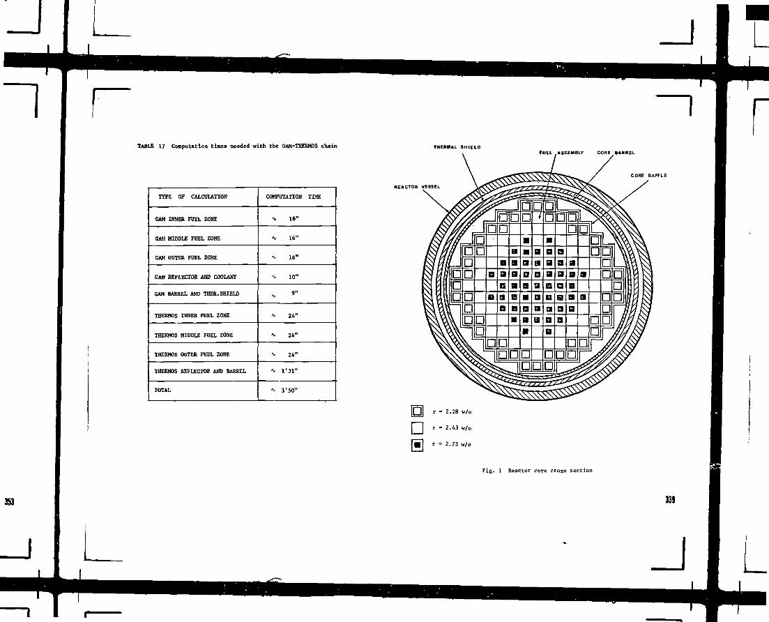
TABLE 17 Computation times needed with the GAM-THERMOS chain

TYPE OF CALCULATION

GAM INNER FUEL ZONE

GAM MIDDLE FUEL ZONE

GAM OUTER FUEL ZONE

GAM REFLECTOR AND COOLANT

CAM BARREL AND THER. SHIELD

THERMOS INNER FUEL ZONE

THERMOS MIDDLE FUEL ZONE

THERMOS OUTER FUEL ZONE

THERMOS REFLECTOR AND BARREL

TOTAL

COMPUTATION TIME

1. 16"

•V. 1 6 "

•v 16"

<\, 10"

,, »"

* 24"

* 24"

* 24"

•v. 1'31"

•\, 3'50"

THERMAL SHIELDFUEL ASSEMBLY CODE BARREL

CORE BAFFLE

REACTOR VESSEL

Fig. 1 Rea

33S

J

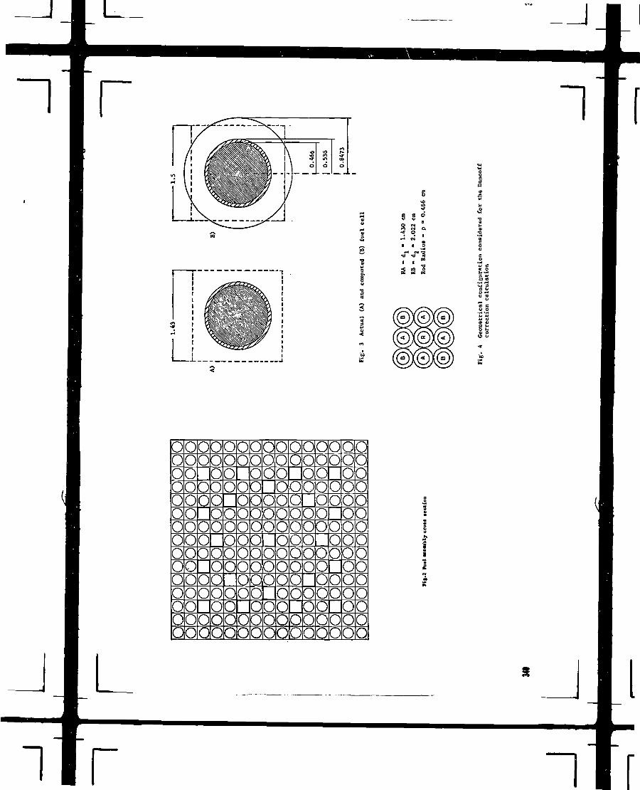
~ifrg

ei S

oo^ooooooooooooooooooooooOOOOOOQQQOOO

oo

oo)Ooooo

ooooooooooooooooooo

ooooooo

oo

ooo

oooooooo

QOOOOOOOOOQOS~S. ^^N. .* ~v v*"x. ^^v v-»v J^^V ~V x*»v ^—*. y^~V

OD

oooo^QOOO

)OOO

OOQ

o

oo

)OOOO

oo

oooo

o

oooo

oo

ooOQ

oooooo

ooooooooooooooo

I11A

5

2

70.

60

50

30

20.

10.

13 16 17 18 19 20 21 22 23

iotzopic ceqionut of th« fu t tptctru(without <Ill*4v«ausa factors) .

35S2 4

.6 laotrople eoapoesnt of tha tharmal apaetxua (without diaadvantaga factora)

341

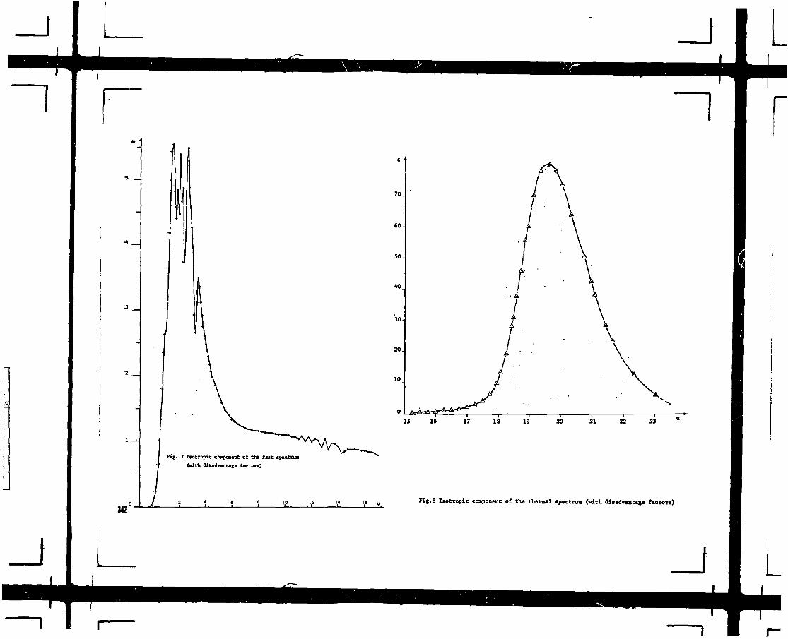
342

70.

SO.

50.

30

20

10

IS 16 17 18 19 20 21 22 23

10 u Fig.a laotropic component of the theraal apaetrum (with diaadvantaga factor*)

THERMAL: SHIELD

FUEL

CU3LAKT

REFLECTOR

1.2

1.0

0.8

F U E L

1.2

1.0

0.8

0.6

0.4

0.2 .

F BE I,

-I 1—' • r

COOLANT

0 0.2 0.4 0.6 0.3 R 0 0.2 0.4 0.6 0.8

Fig. 9 Reactor configuration used to calculate cross sectionso£ reflector barrel etc. Fig, 10 Flux distribution inside fuel cell (1st and 24ti. energy group)

343

I

B^A&,>

0 2<J 6b 86 100 V 0 U O 160 180 200 R0 JO 40 60 10 100 120 140 160 160 200

344

Fit. 11 Thermal flux distribution (c«e 1) Pi(.12 Thermal flux distribution (ease 2)

_l

o.e.

0.6.

0 20 «0 60 «0 100 120 HO 1(0 110 200

rlC'13 - Ihinul flux distribution (cat* ])

0.2 .

0 20 «0 60 CO 1 00 UO 160 180 200

Fi| . 14 Therat'v flux distribution (en*

359345

J

I V I g I s I s

u

r

361

NOTES ON NUCLEAR REACTOR COREANALYSIS CODE: CITATION

(Sample PWR, Reactor problem)

D.G. CEPRAGAInstitute of Power Reactors,Bucharest,Romania

ABSTRACT

The method which has evolved over the years for making powerreactor calculations is the multigroup diffusion method. The CITATIONcode is designed to solve multigroup neutronics problems with applicationof the finite-difference diffusion theory approximation to neutrontransport in up to three-dimensional geometry.

The first part of this paper presents information about the mathe-matical equations programmed along with background material and certaindisplays to convey the nature of some of the formulations.

The resultf. obtained with the CITATION code regarding the neutronand burnup core analysis for a typical PWR reactor are presented in thesecond part of this paper.

INTRODUCTION

The calculational methods and techniques used for evaluating the;r«<_iear design information vary with the type of reactor and with thepreferences and prejudices of the reactor-physics group responsible forthe calculation.

The method which, has evolved over the years for making power-reactorcalculations is the MULTIGROUP DIFFUSION METHOD. Power reactors are usuallylarge enough have a sufficient number of mean free path, to permit areasonably accurate description WITH DIFFUSION Theory.Furthermore, the most practical and convenient technique for handlingenergy variation is the multigroup approach.

There are two major components to a multigroup diffusion calculationwhich are often accomplished with separate computer codes. These are: 1) theevaluation of group constants required by the multigroup diffusion equationsand 2) the solution of the multigroup diffusion equations once the constantshave been established.

The code CITATION is designed to solve multi-neutron energy-group,multi-dimensional neutronics problems.This code is also designed to attack the reactor core depletion and dynamicsproblems in a general sense.At the time this is written the program will solve eigenvalue problems withina finite-difference representation of the diffusion theory approximation toneutron transport in multigroup form with arbitrary scattering.

The eigenvalue problem may involve the determination of the effectivemultiplication factor, or be a direct criticality search on buckling, on 1/vabsorber or on the concentrations of specified nuclides which may includefuel. Up to three geometrir dimensions may be considered including X-Y-Z,R-6-2, and Hexagonal-Z coordinate systems.

An inner, outer iteration scheme is used to solve problems. New fluxvalues are calculated from finite difference, neutron balance equations fora row of points simultaneously, and each new value is driven in the directionof the change from the old value.This procedure is continued over the space problem at one energy; it is re-peated for a number of inner iterations, and the calculation proceeds to thenext energy. At each energy the inscattering source and the fission source aredetermined.

After a complete sweep of the problem, the eigenvalue is estimated either froman overall neutron balance summed neutron balance equations, or from the sourceratio, and the calculation is continued to satisfy specif?ad convergence cri-teria.

This code has been designed to attack problems which can be run ina reasonable amount of time; storage of data is allocated dynamicallyto give the user flexibility in dimensioning.

2. MATHEMATICAL FORMULATIONS

2.1 The discrete-energy group diffusion equation

The neutron density in an operating reactor is at steady state onthe average due to natural reactivity compensation and control. In alarge fraction of the neutronics problems solved, it is the intent Coapproximate this condition. Any problem describing a geometry, nuclideconcentrations and cross sections, may represent a situation far froma steady state. The neutron population *jould actually rise or fall, anda steady-state solution only approximates the neutron distribution.

To effect this steady-slate condition, the multiplication factoris introduced.The multiplication factor is defined as:

v D neutron generation ratee neutron loss rate

A critical condition is one at steady state for which K is unity. Thepseudo steady-state equation with tho diffusion approximation to transportfor the neutron-flux at geometric location r and energy E using usualmacroscopic nuclear properties is expressed as

i*tr6 CvZ )f,, r, E.

347

The continous energy spectrum is divided into discrete energy groups, andusually a simplification is made in the transport term

r,n r,n

77 * « the laplacian geometric operator, cm

^K * the neutron flux at location r and in energy group g,»f> Q n/ser-cm ,

» the macroscopic cross section for absorption, normallyweighted over a representative flux energy spectrum, cm ,

= the macroscopic cross section for scattering of neutrons fromenergy group g to energy group n, cm" ,

» the diffusion coefficient, normally onethird of the reciprocalof the transport cross section, cm,

* the buckling term to account for the effect of the Laplacianoperator,

= the macroscopic production cross section, cm ,

- the distribution function for source neutrons

- the effective multiplication factor.

Generally it is desirable to increase the number of points in eachdirection (not just in one), and within each zone of uniform composition.About the same mean-free neutron path length between adjiacent points isdesirable in all directions; therefore increasing of the number of mesh pointsshould be done with this objective-decreasing large steps in the spacing.

Regarding local properties, it is a fallacy to believe that use of avery small finite-difference volume at one location will cause the estimateof local properties to have a high accuracy. We recommend against use of largechanges in mesh spacing. Further the interpretation of local quantitiesshould be of mesh-average properties rather than local at the actual meshpoint site.

FINITE DIFFERENCE APPROXIMATION ERROR

The solution obtained by application of a finite difference formulationis not precise; an error is associated with the approximation.The error in a point flux value depends on the problem, and it dependson the mesh, each coordinate making an independent contribution.Except for a small number of points, the error decreases as the sumof the reciprocals of thesquare9 of the numbers of mesh points along eachcoordinate. Doubling the number of points along each of the coordinates wouldbe expected to reduce the error by a factor of 4.

ID general,the errors in the point flux values and in the multiplicationfactor are inversely proportional to the square of the number of mesh pointsalong each coordinate.Changes made locally or to less than all coordinated treated should not beexpected to produce reliable extrapolation and error assessment, not is errorassessment of a course mesh result reliable.The reliability of such extrapolation in application to the general mulfci--group, complicated geometry problem is unknown. Extrapolation of integralquantities should be more realiable and an extreme may move from one locationto another. For reliable assessment, it is recommended that a uniformincrease in mesh points be made along all coordinate directions in each zone.

341

2.2 Finite difference representation of the Laplacian operator accuracy

The laplacian operator is to be represented in a finite-differenceform.It is well-known that the finite-difference approximation to the Laplacianoperator is accurate to the order of the mesh spacing squared. Vie recognizethaC the accuracy of ths mesh point centered approximation is slig,htly lowerthan that obtained with mesh points located in material interfaces.Of course they are identical within a homogeneous medium with uniform spacing.

Still the analyst wants to know how accurate are integral quantities (k) asas well as estimates of local properties (power density). We beliave thatexperience is the best guide here.It is possible to increase the number of mesh points and solve the new fine--mesh points and solve the new fine-mesh problem which normally improves theestimate of both integral and local quantities, but not necessarly. Care mustbe taken in allocation of mesh points and in selecting on energy group structureto Ret the best results.

2.3 Remarks on iteration strategy

The general procedure of solution employed is one of iteration. Forthe usual eigenvalue problem, the equation to be solved is

(2.3-1)

(2.3-2)

with special partitioning of the matrix A,

where:

J> * tha main diagonal term (loss due to absorption* buckling» outscatter),

J • contains the coupling terms for a block of points (as along a row inspace at one energy) for which the flux values are determined simultaneouslyprecisely given the current values of the other fluxes,

L • the lower triangular matrix containing coupling terms in space,

U M the upper triangular matrix containing coupling terms in space (excludingany appearing in J ) ,

S * the downscattering source matrix (group-to-group scattering terms at apoint,

T • the up scattering source matrix (group-to-group scattering terms at apoint,

F * the fission source component (from all groups at a space pointcontributing to the total at that point, a row matrix operator),

% - the source distribution (from the total to all groups at a point, acolumn matrix operator), and,

K • the unknown multiplication factor, a constant for any problem to bee determined.

To illustrate how an iterative procedure is formulated, (let us put theterm D0 on side of the equation, Eq. (2.3-2), and Che remaining on theother, giving

K*'If a set of fluxes is available for iterate n, namely 0r> then a simpleiterative scheme is expressed as

where the inverse D is of a diagonal, the reciprocals of terms in D.An estimate of K is required, K , and a continuing iterative process mayproduced.The above with all positive entries and 0 7 0 produces 0 ^ 0; only with0 70 can a unique and most positive valuenof K be assured. Eq. (2.3-3)does not even admit the use of newly calculated 0 values, so it representsa rather crude procedure.With downward sweep in energy and simple sweeps earring the simultaneoussolution for rows across the space problem, use of newly calculated fluxedcauses them to contribute throught the matrices J,L, and S,

(2.3-4)

The inverse shown would generally be impractical to obtain. It is not needed,however, but rather is a consequence of the process and the partitioning ofthe coupling terms.Over relaxation is a simple but power ful scheme for accelerating the rate ofconvergence of the iterative process. The basic equation is

(2.3-5)

overrelaxation factor, and X. is the overraxation value used thereafterfor this sweeep of the equatidns. Note that]S- = 1 causes the newly calcu-lated value to be used; overrelaxation is done for 1 ' 4 < 2 . A fixed valueof p may be used, or a different overrelaxation coefficient may be used forthe space problem at each energy. Also, the value of Jt used may be iterationdependent. This flexibility is shown in the equations by reparesenting theoverrelaxiation process with a matrix B containing only the values of Jfc onthe main diagonal, the subscript n indicating the values may be changed duringthe iterative history.

Overrelaxation changes eq. (2.3-4) to

(2.3-6)

Inner iteration may be done. For many types of problems additional calculationaletfort shows advantage to reduce the error associated with the space problemat each energy. Thus, several sweeps may be made of the space problem at eachenergy.

349

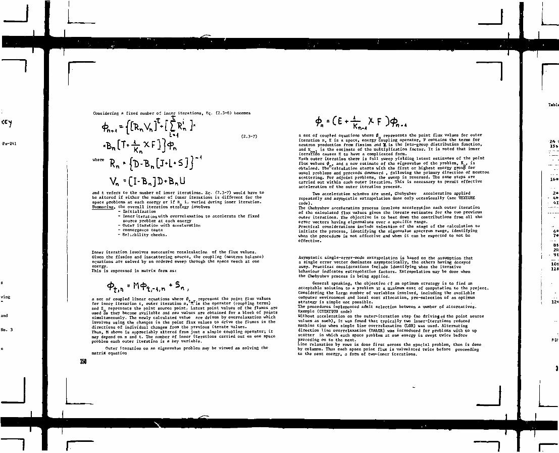
•Pu-241

rTabl<

ving

and

No. 3

J

Considering a fixed number of inner iterations, Eq. (2.3-6) becomes

(2.3-7)

and t refers to the number of inner iterations. Eq. (2.3-7) would have tobe altered if either the number of inner iterations is different for thespace problems at each energy or if B i^ varied during inner iteration.Summaring, the overall iteration strategy involves

- Initialization- Inner iteration with overrelaxation to accelerate the fixed

source problem at each energy- Outer iteration with acceleration- convergence tests- Reliability checks.

Inner iteration involves successive recalculation of the flux values.Given the fission and inscattering source, the coupling (neutron balance)equations are solved by an ordered sweep through the space mesch at oneenergy.This is expressed in matrix form as:

a set of coupled linear equations where #t r represent the point flux valuesfor inner iteration t, outer iteration n, H is the operator (coupling terms)and S represents the point source point. Latest point values of the fluxes areused as they become available and new values are obtained for a block of pointssimultaneously. The newly calculated value are driven by overrelaxation whichinvolves using the changes in the point flux values to drive the fluxes in thedirections of individual changes from the previous iterate values.Thus, H above is appreciably altered from just a simple coupling operator; itmay depend on n and t. The number of inner iterations carried out on one spaceproblem each outer iteration is a key variable.

Outer iteration on an eigenvalue problem may be viewed as solving thematrix equation

350

a set of coupled equations where 0 o represents the point flux values for outeriteration n, E is a space, energy coupling operator, F contains the terms forneutron production from fission and % is the into-group distribution function,and K , is the estimate of the multiplication factor. It is noted that inneriteration causes E to have a complicated form.Each outer iteration there is full sweep yielding latest estimates of the pointflux values 0 , and a new estimate of the eigenvalue of the problem, Kn, isobtained. Thencalculation starts with the first or highest energy group forusual problems and proceeds downward , following the primary direction of neutronscattering. For adjoint problems, the sweep is reversed. The same steps arecarried out within each outer iteration. This is necessary to permit effectiveacceleration of the outer iteration process.

Two acceleration schemes are used, Chebyshev acceleration appliedrepeatedly and asymptotic extrapolation done only occasionally (see VENTUREcode).The Chebyshev acceleration process involves acceleration each outer iterationof the calculated flux values given the iterate estimates for the two previousouter iterations. The objective is to beat down the contributions from all theerror vectors having eigenvalues over a specific range.Practical considerations include selection of the stage of the calculation toinitiate the process, identifying the eigenvalue spectrum range, identifyingwhen the procedure is not effective and when it can be expected to not beeffective.

Asymptotic single-error-mode extrapolation is based on the assumption thata single error vector dominates asymptotically, the others having decayedaway. Practical considerations include identifying when the iterativebehaviour indicates extrapolation factors. Extrapolation may be done whenthe Chebyshev process is being applied.

General speaking, the objective rf an optimum strategy is to find anacceptable solution to a problem it a minimum cost of computation to the project.Considering the large number of variables involved, including the availablecomputer environment and local cost allocation, pre-selection of an optimumstrategy is simple not possible.The procedures implemented admit selection between a number of alternatives.Exemple (CITATION code)Without acceleration on the outer-iteration step (no driving of the point sourcevalues as such), it was found Chat typically two inner-iterations reducedmachine time when simple line overrelaxation (LOR) was used. Alternatingdirection line overrelaxation (DALOR) was introduced for problems with no upscatter in which each space problem at one energy is swept twice beforepreceding on to the next.Line relaxation by rows is done first across the spacial problem, then is doneby columns. Thus each space point flux is valvulated twice before proceedingto the next energy, a form of two-inner iterations.

15V

16*

2*

41

6*7*

8$2R

- 9S

10111)

Flf

~1 rTest calculations indicated that the usual overrelaxation coefficients forone-directional line relaxation vere near optimum for the alternating directionprocess.Inner iteration was found to be ineffective when used with the alternatingdirection overrelaxation process (which in itself involves two inner iterations),except for the larger space problems. But the optimum strategy depends on relativecomputer times, varying from one computer installation to another.

2.4 Reliability of solution

A solution obtained by an iterative process is generally not entirelyconverged. It is uneconomical to satisfy trght convergence criteria, therefore,the user relaxes the criteria to the extent possible which will still causethe result to safisfy the particular needs.If the inner iterations were continued enough times, the flux 0 j in Eq. (2.3-7)would satisfy the relationship in Eq. (2.4-1) provided there where no up scatter:

(2.4-1)

'r»M

The process could now be written as

Under this condition, bounds on Ke can be identified and calculated assimply the maximum and minimum ratios of the source, components of V >between outer iterations, times K . Use has been made of these bounds,especially in the PDQ series of codes. Unfortunately, the bounded rangetends to be wide at low levels of convergence, and relaxation of the inneriteration convergence destroys the proof that estimates are bounds.Only with a relatively large number of inner iterations does one have assu-rance that bounds have been identified.The optimum number of inner iterarions for problem solution, considered hereto minimize the computation cost may be far fewer that are required toinsure that bounds on the eigenvalue are established.

The maximum relative flux change

The iterative process, Eq. (2.3-1), may be described as

(2.4-t)

where the flux vector from outer iteration n is operated on by the iterationmatrix M to generate the new estimate. The iteration matrix M is iterationdependent because it contains the latest estimate of K .Consider the set of components of the flux vector 0 toebe X.s and the elementsof M to be a... 1

Now consider the new matrix formed of the elements

The new matrix is the result of performing the operation P MP; therefore,it is similar to the matrix M and has the same eigenvalue.The spectral radius of this new matrix is bound by the maximum and the mini-mum of sums along columns or rows. The sum along a row is simply the ratio offlux values at one point between outer iterations. Therefore

Since J>(M ) must tend to unity, an idication that the iterative processis convergent is that

where

h

Further, fi(Nn) is bounded by 1 ^The CITATION and VENTURE codes test ^4>1 against a specified convergencecriterion as the primary way an acceptable solution is identified and theiteration process is discontinued.Thus, if the estimated K is desired to within 0.01 percent, the criterionon the convergence of the point fluxes should be 0.0001.

The Residues Estimate

The value of tv'e multiplication factor is determited which minimizesthe sum of the squares of the residues of the point neutron balance equationscast in the form of actual reaction rated. The residue R. is defined as

S;-77 351

where R, is the residue which would be zero if Che problem were completelyconverged, F. is the associated fission source, S. is the in-scattering plusir.-leakage term, and T. is the total removal and out-leakage term.Experience has shown tne residues estimate of the multiplication constant to bequite useful, especially when a problem solved has an unfamiliar iterativebehavior. If the residues estimate differs markedly from the value used inthe iterative process, then the problem is not converged.Results from a wide range of problems indicate that the residues estimate isoften pot superior to that from the neutron balance used in the calculation*We suggest simply averaging the two values.It should be noted that the discussion above is directed 3t the reliability ofa solution regarding the error due to lack of convergence of the iterativeprocess, not the error associated with the finite-difference approximations,the use of diffusion theory, or the discrete energy group representation.

3. SAMPLE P.W.R. REACTOR PROBLEM

The results obtained with the CITATION code regarding the neutron coreanalysis for a typical P.W.R. reactor are presented.The aim of this application is to facilitate the job of the user for:

- the understanding of input data requirements;- the correct geometrical simulation (2-D) of P.W.R. reactor;- the correct handling of a large amount of data (library sets, burnup chain

specifications etc.);- to clarify the mechanism of th iterative strategy (principal alternatives

for basic selection between procedures are under the control of user-inputoptions).

Our sample problem treats a typical P.W.R. reactor-pROVA- /4/. Themain features of this reactor general design parameters are reported inTable 1.The reactor core is a three-region cycled core consisting of 157 fuel assemblies(Fig. 1) with 41 rod cluster control assemblies.The 157 fuel assemblies are divided into three concentric regions. The two outerregions contain 52 fuel assemblies with the central region containing 53 fuelassemblies (Fig. 1).

The 157 individual replaceable fuel assembies will be held in positionbetween a lower core plate and an upper core plate. The core is surroundedby a form fitting baffle wihich confines all but a small portion of theupward flow of coolant within the fuel bearing zone.Outside the baffle and surrounding it, there is a core barrel. A smallamount of coolant is allowed to flow between the barrel and the baffle forcooling.

A. The first step of calculation is the BROAD-GROUP MICROSCOPIC CROSSSECTION LIBRARY PREPARATION

For this purpose, the chain of codes GAM-GATHER-COMBINE-ANISN wasused. The self explained illustrative scheme of this operative chain isshown in Fig. 1A.

We treat the following cases:

CASE 1 : Cold reactor (temp fuel, cladd, cooling-20°C)Cold reflector (temp reflector«20°C)

CASE 2A: HOT REACTOR (temp: fuel-1000°C, cladd-35O°C cooling-300°C)Fresh fuel (the densities of fuel isotopes at the biginning offuel life)

CASE 2B: HOT REACTORIRRADIATED FUEL (The densities of fuel isotopes at the end offuel life)

In both cases 2A and 2B, hot reflector (Temp*300*C).Both GAM and GATHER consider a homogeneous mixture of the nuclides thatare present in the cell. The nuclear densities of isotopes are reported inTable 2.The number of energy groups that we adopted during the cross sectionpreparation process is 24 t 9 groups in the fast and epithermal range (GAM)and 15 groups in the thermal range (GATHER).The broad groups structure are reported in Table 1A.

In our operative scheme, the ANISN code has been designed to produceflux weighted cross sections in 4 broad-group structure (see Table 1A) forcore isotopes and reflector isotopes.The geometrical ANISN structure of "core-cell" consists of: 3 Zones (thecross sections of the fuel isotopes are weighted on the spatial distributionof the flux inside the cell):

1 fuel zone; radius • 0.A66 cm2 cladd zone; radius » 0.536 cm3 cooling zone; radius * O.8A7 cm.

The densities of "core-cell" isotopes in ANISN zones are reportedin Table 3.The geometrical ANISN structure of "reflector" consists of 6 zones (the crosssections of the reflector isotopes are weighted on the spatial distributionof the flux inside the reactor):

1 Core zone; radius * 151.765 cm2 1LO+SS zone; radius * 169.54 cm3 So zone: radius • 173.99 cm4 H20 zone; radius - 179.07 cm

5 SS zone; radius - 187.33 cm6 H20 zone; radius • 197.49 cm

The densities of "REFLECTOR" isotopes in ANISN zones are reported in Table. A.

At the end, using the input section 000 of CITATION* the broad groupmicroscopic cross section library is prepared.This library consists of 5 sets

SET1 cold core )SET2 cold reflector ) c a s e L

352

SET3 hot corefresh fuel (biginning of life)

SETA hot reflectorcase 2A

"J i _

1 rSETS hot core

irradiated fuel (end of life) case 2B

Table 5 reports the values of microscopic cross section (capture, fission,total, ecc.) of U-235 isotope in different sets of library.The nuclides identification in CITATION library are presented in Table 15.

B. The second step of calculation is reactor neutron analysis in R-Z geometryin different operative conditions (cold reactor, hot reactor, etc.)

Static and burnup calculations have been performed. A "rich" outputof informations is obtained during the first cycle of reactor "PROVA" regarding:KEFF values (Tabel 13) , nuclide densities, FISSILE inventory (Table 12), fluxand power distributions (zone average flux values (Table 12 1 by group, pointflux values by group, zone average power densities (Tabel 12) , point poverdensities.

A geometrical R-Z simulation of reactor FUR "PROVA" is shown in Fig. 2(zone placement) and in Fig. 3 (geometric mesh description).The composition of reactor zones (nuclide densities) is reported in Tabel 6.The following cases have been treated:

A. STATIC CALCULATIONS1 COLD REACTOR CASE 12 HOT REACTOR CASE 2A (it used - biginning of fuel life » cross section

set)3 HOT REACTOR CASE 2B (it used • end of fuel life * cross section set)

The selected output results are presented in Table 9, 10, 11.

B. BUK1UP CALCULATIONS1 HOT REACTOR CASE 2A (it used » biginning of fuel life - cross section

set)2 HOT REACTOR CASE 2B (in used - end of fuel life - cross section set)

The selected output results are reported in Table 12.

No significant differences for flux and power distributions and fissileinventory are obtained in these two (2A and 2B) burnup calculations.

This demonstrates, that is correct to use the same set of micro-scopic cross sections (fresh fuel-biginning of fuel life) during burnupcalculation (for each burnup step) in the case of a typical FUR reactor.

Regarding the iterative procedures it was found to be ineffective,also more time consuming, when used with "complex" iterative strategy(line relaxation on rows and columns and CHEBYCHEV polynomialsjfor adjustingthe acceleration parameters).This is demostrated in Tables B, 9.The automatic selection of a strategy allows application with minimum burdento the user; however it involves compromises and can hardly be expectes torepresent the optimum in any given situation for a particular problem; ittakes time to accumulate experience.

We hope this application will be a useful support for peopleintending torun CITATION code for thermal reactor core analysis.

TABLE 1

GENERAL CORE DESIGN PARAMETERS REACTOR PWR - PROVA -

Total heat output, Mwth 2097

Active portion of the core

equivalente diameter, cm

active fuel height cm

length-to-diameter ratio

Totale

cm

cm

cm

cm

Fuel assemblies

number

rod array

rods per assembly

rod pitch

overall dimensions

Fuel rods

number

outside diameter

diameter Gap

clad thickness

clad material

Fuel pellets

material

feed enrichments, w/o

core 1

core 2

core 3

diameter cm

length cm

Core Structure

core barrel I.D./O.D. cm

thermal shield I.D./O.D. cm

303.53

365.76

3.061

72740.7

15x15

204

1.430

21.402x21.402

32028

1.072

0.017

0.0617

Zircaloy

2.28

2.43

2.73

0.9319

1.5240

339.09x348.62

358.14x374.65

353

354

TABLE 1 (continued)

Coolant temperatures °C

nominal inlet

average in core

average in vessel

Maximum clad surface temperature

Fuel central temperature

285

302

301

347

2243

.55

.77

.11

.2

.3

TABLE 2 - Nucleare densities of reactor PWR • PROVA * isotopes in GAM

e GATHER Codes.

NLUCLIDES

H

Oxy

Zr

Rh-103

Xe-131

Xe-135

Nd-143

Pm-147

Sm-149

Sm-150

Eu-153

U-235

U-236

U-238

Np-239

Pu-239

Pu-240

Pu-241

Pu-242

Non-sat 235

Non-sat 239

GAM-GATHER NUCLEAR DENSITY

CASE 2A

Beginning of

. 28538

. 2817

. 3692

0.0

0.0

0.0

0.0

0.0

0.0

0.0

0.0

.1709 x

0.0

.67796

0.0

0.0

0.0

0.0

0.0

0.0

life

xio"1

x lo"1

x lo"2

lo"3

x 10"2

CASE 2B

end of life

2.8538 x 10~2

2.8170 x 10"2

3.6920 x 10"2

1.65449x 10"6

1.5268 x 10"6

8.44549x 10"10

3.11919x 10~6

9.2920 x 10"7

1.20439X 10"8

1.3082 x 10"6

1.0882 x 10~7

8.268399 x lo"5

1.289599 x 10~5

6.7374595X lo"3

4.713099 x 10"5

1.9341996x 10"6

3.8126996x lo"7

1.303599 x 10"7

1.8410 x 1O"8

6.06959x 1O"5

1.3433 x 1O"6

rTABLE 3 - Nuclear densities of core (FUR • PROVA - Reactor) isotopes

in ANISN Zones

ANISN

ZONE

FUEL

ISOTOPEb

OXY

RH-103

Xe-131

Xe-135

Nd-143

Pm-147

Sm-149

Sm-150

Eu-153

U-235

U-236

U-238

Np-239

Pu-239

Pu-240

Pu-241

Pu-242

Non-sat-235

H

Oxy

ANISN ISOTOPES DENSITY - CORE

CASE 2A

BEGINNING OF LIFE

4.5966 x 10

0.0

0.0

0.0

0.0

0.0

0.0

0.0

0.0

5.6500 x 10"'

0.0

2.241? x 10~'

0.0

0.0

0.0

0.0

0.0

0.0

3.7800 x 10

4.757 x 10

2.3785 x 10'-2

CASE 2B

END OF LIFE

4.5966

5.4707

5.0481

2.7926

1.0314

3.0725

3.9824

4.3273

3.5982

2.7340

4.2643

2.2277

1.5584

6.3955

1.2067

4.3107

6.0868

2.007

x 10

X 10

x 10"

.-6

x 10

x 10'

x 10

x 10'

x 10-7

x 10

x 10"

.-5

x 10

x 10

x 10'

x 10

x 10

x 10"

.-8

3.7800 x 10,-2

4.7570 x 10

2.3785 x 10'

_J

~1 ~l rTABLE 4 - Nuclear densities of reflector (PWR » PROVA - Reactor ) isotopes

in ANISN zones

TABLE 5 - Microscopic cross sections of U-235 in CITATION Library (from

GAM-GATHER-COMBINE-ANISN Calculations)

lence,

rav.a

nver flis-

ited

rThe

NUCLIDES

H

Oxy

C

Si

Cr

Mn

Fe

Ni

Zr

U-235

U-238

NUCLIDES DENSITY IN ANISN ZONES OF REFLECTOR

Zone

Fuel+Zr+HjO

2.8538 x 1O"2

2.8170 x 10"2

0.0

0.0

0.0

0.0

0.0

0.0

3.6920 x 10"3

1.7090 x 10"4

6.7790 x 10"3

Zone

H20 + SS

4.777 x 10"2

2.3850 x 10"2

1.600 x 10"5

8.500 x lo"5

9.150 x 10"4

8.700 x 10"5

2.8090 x 10"3

4.460 x 10"4

0.0

0.0

0.0

Zone

SS

0.0

0.0

3.200 x 10"4

1.700 x 10~3

1.829 x 10"2

1.73 :t-10~3

5.618 x 10"2

8.910 x 10"3

0.0

0.0

0.0

Zone

5.0250 x 10"2

2.5125 x 10"2

0.0

0.0

0.0

0.0

0.0

0.0

0.0

0.0

0.0

ntr..

MICROSC.CROSSSECTIONS

(barn)

a 8

ABS

(barn)

°TOT

(barn)

Vs(barn)

BROADGROUPS(g)

1

2

3

4

1

2

3

4

1

2

3

4

1

2

3

4

CASE 1

COLD

REACTOR

1.26

1.79

23.91

379.53

1.32

2.27

38.74

446.17

4.70

9.30

50.13

460.25

2.32

7.03

11.40

15.27

CASE 2HOT REACTOR

CASE 2 ABegining of life

1.26

1.79

23.50

285.18

1.32

2.28

38.03

336.83

4.71

9.32

49.41

352.11

2.32

7.03

11.37

15.28

CASE 2 BEnd of life

1.26

1.79

23.52

299.39

1.32

2.28

38.07

353.36

4.71

9.33

49.47

368.55

2.32

7.03

11.39

15.19

389 355

TABLE 6 - Nuclide densities of reactor PWR - PROVA - isotopes in CITATION Zones.

NUCLIDES

H

Oxy

Si

Cr

Mn

Fe

Ni

Zr

U-235

U-238

colS FACTOR NUCLIDE DENSITIES

CORE 12x 10

4.020

3.3998

0.0

0.0

0.0

0.0

0.0

.3692

.01567

.67938

CORE 2 ,x lo"'

4.020

3.3999

0.0

0.0

0.0

0.0

0.0

.3692

.01709

.67796

CORE 3,x 10

4.020

3.3850

0.0

0.0

0.0

0.0

0.0

.3682

.01899

.6687

REFLECTORx 10"'

4.2886

2.1443

.0616

.6649

.0630

2.0098

.3535

0.0

0.0

0.0

HofftEACTOR maJm DENSITIES

CORE 1 ,x 10

2.8540

2.8170

0.0

0.0

0.0

0.0

0.0

.3692

.01567

.67936

CORE 2 ,x 10

2.8540

2.8170

0.0

0.0

0.0

0.0

0.0

.3692

.01709

.67796

CORE 3 ,i i o '

2.8540

2.8020

0.0

0.0

0.0

0.0

0.0

.3692

.01899

.6687

REFLECTOR,x lo"'2

3.0492

1.5246

.06160

.6649

.0630

2.0098

.3535

0.0

0.0

0.0

aid TABLE 7 - Typical machine time for reactor PWR - PROVA • (R-Z) Calculations

using different convergence procedures

TABLE 8 - Some selected flux and power density values (citation output)

/it refers to Table 7 Case calculations/

ll.

fcerval.

3Ulated.

Mid

3SG

CASE

1 A

COLD

REACTOR

1 8

COLD

REACTOR

CONVERGENCEPROCEDURE

Line relaxationonly on rows;no chebychev

Line relaxation onrows and columns;use cheby chevpolynomials

COMPUTETIMESEC

1 Min50 sec

3 Min

NPITERATIONS

101

122

Keff(I Test)

1.340619

1.340545

Keff(ResidueOption)

1.340569

1.340633

•J

ZONE

1

3

4

7

10

13

16

CASE 1A- COLD REACTOR

FUJX

GR 3xlO13

7.1408

1.0992

7.1562

7.1884

6.9975

5.9929

3.2463

FLUX

GR 4xlO13

6.3806

9.8868

6.3944

6.4133

5.8598

4.9973

2.5194

POWERDENSITYWATTS/cc

139.43

21.59

139.73

140.17

140.25

119.68

67.33

CASE IB - COLD REACTOR

FLUX

GR 3xlO13

7.0843

1.1236

7.0993

7.1301

6.9401

5.9438

3.2199

FLUX

GR 4xlO13

6.3306

1.0108

6.3440

6.3615

5.8118

4.9564

2.4990

ruwE?DENSIT/WATTS/cc

138.33

22.06

138.62

139.03

139.10

118.70

66.78

NOTE : Example of ineffectiveness of"complex" iterative strategy

~lTABLE 9 - Zone Average flux values by group.Zone power values

Case 1 Reactor PWR - PROVA -

Cold reactor (20°C)

refers to { core zones

TABLE 10 - Zone average flux values - Zone power values

Case 2A reactor PWR * PROVA- Hot REactor ( 300°C) "Fresh core"

It uses microscopic cross sections set -Beginning or life "

ZONE

NUMBER

1

2

3

4

5

6

7

8

9

10

11

12

13

14

15

16

17

18

19 R

20 R

CASE 1 COLD REACTOR

AVERAGE FLUX /n/cm s e c /

GRPlxlO13

B.6O84

4.8834

1.3225

8.6267

4.8932

1.3248

8.6676

4.9157

1.3304

8.5463

4.8465

1.3116

7.3256

4.1541

1.1243

4.0279

2.2841

.6186

.0933

.04033

GRP2xlO13

8.2481

4.6795

1.2677

8.2658

4.6889

1.2699

8.3053

4.7107

1.2754

8.1435

4.6185

1.2502

6.9801

3.9585

1.0717

3.8065

2.1587

.58477

.10357

.04471

GRP3xlO

7.1410

4.0517

1.0991

7.1562

4.0599

1.1011

7.1884

4.0775

1.1055

6.9975

3.9689

1.0759

5.9929

3.3990

.9215

3.2463

1.8411

.49949

.09488

.041021

CRP4xlO13

6.3806

3.6207

.9887

6.3945

3.628

.9905

6.4133

3.6382

.9929

5.8597

3.3239

.90737

4,9973

2.8346

.7739

2.5194

1.4290

.39055

.1626

.07019

POWER

/watcs/

3.O222xlO7

1.7149xlO7

1.3382xlO6

9.0864xlO7

5.1554xlO7

4.O217xlO6

1.51918X1O8

8.6179xlO7

6.72O7xlO6

1.22872X1O8

6.9696xlO7

5.4362xlO6

1.2422SX1O8

7.O4642X1O7

5.4967xlO6

1.30525X1O8

7.4O353xlO7

5.7807x10*

0 . 0

0 . 0

20NE

1

2

3

4

5

6

7

a9

10

11

12

13

14

15

16

17

18

19

20

. „ - . _ _ _ 1 I V "FRESH"CORE-HOIREACTORAVERAGE FLUX CROSS S E C . B E G M . 0 F L I F E ,

GRPixlO14

1.3649.8180

.24411.3106

.7856

.2344

1.2037

.7213

.2152

1.0772.6452

.1925

.8717

.5219

.1557.4734

.2834

.08458

.01670

,00914

GP2xlO14

1.4178

.8495

.25371.3614

.8158

.2436

1.2505

.7491

.2236

1.1124

.6662

.1988

.9002

.5389

.1608

.4846

.2900

.08661

.02127

.01161

GRP3xlO14

1.1620

.69£2

.2092

1.1158

.6685

.2009

1.0244

.6136

.1844

.9037

.5411

.1J25

.7305

.4372

.1334

.3917

.2344

.07046

.02230

.01213

PRP4xlOU

.9545

.5717

.1737

.9165

.5491

1.668

.8393

.5027

.1527

.6955

.4164

.1265

.5581

.3341

.1015

.2801

.1676

.05101

.02855

.01554

POWER

x 10 watts

71.339

42.740

3.705205.497

123.128

10.674

313.792

187.966

16.291

230.544138.044

11.969

219.486

131.383

11.392

229.676

137.447

11.931

0 . 0

1 . 0

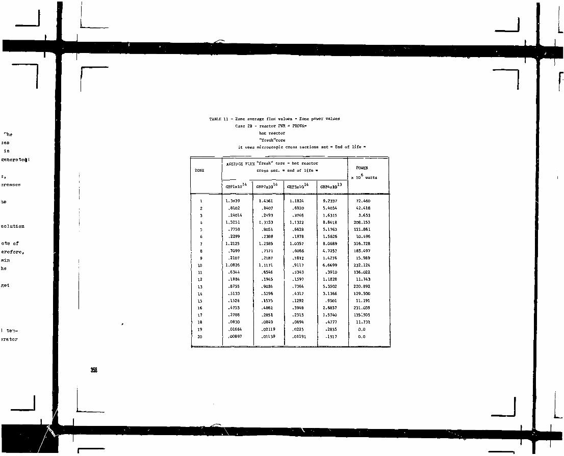
n r r

solution

TABLE 11 - Zone average flux values - Zone power values

Case 2B - reactor PWR - PROVA-

hot reactor

"fresh"core

it uses microscopic cross sections set = End of life •

ZONE

1

2

3

4

5

6

7

8

9

10

11

12

13

14

15

16

17

18

19

20

AVERAGE FLUX "fresh" core

GRPlxlO14

1.3t)39

.8102

.24014

1.3251

.7758

.2299

1.2125

.7099

.2107

1.OB26

.6344

.1884

.8755

.5133

.1526

.4753

.2788

,0830

.01664

.00897

cross sec. =

GRP2xlOU

1.4361

,8407

,2493

1.3753

,8051

.2388

1.2585

.7371

.2187

1.1171

.6546

.1945

.9034

.5296

.1575

.4862

.2851

.0849

.02119

.01139

- hot reactot

end of life •

GRP3xlO14

1.1824

.6920

.2066

1.1322

.6628

.1978

1.0357

.6066

.1812

.9117

.i343

.1597

.7364

.4317

.1292

.3948

.2315

.0694

.0225

.01191

GRP4xlO13

9.2337

5.4054

1.6315

8.8418

5.1763

1.5626

8.0689

4.7257

1.4276

6.6699

.3910

1.1828

5.3502

3.1366

.9501

2.6837

1.5740

.4777

.2835

.1517

POWER

x 10 watts

72.460

42.418

3.653

208.153

121.861

10.496

316.728

185.497

15.989

232.124

136.022

11.743

220.892

129.500

11.191

231.039

1351505

11.731

0.0

0.0

358

TABLE 12 - Selected results of burn-up calculations. Ilux, nouer, power density and fissile in PWR reactor * PROVA

zones during of burn-up cycle

ZONE

1

2

3

TIME

DAYS

0 . 0

2 . 0

1 5 2 .

2 1 2 .

272

0 . 0

2 . 0

1 5 2 .

2 1 2 .

2 7 2 .

0 . 0

2 . 0

152.

212

272

CASE 2 A - Hot reac tor .Se t : • Beginning of

FLUX

GR.3xlOU

1.1620

1.0742

.2111

.4798

.3912

.6962

.6998

.5519

.5168

.7319

.2092

.2287

.3548

.2821

.5302

FLUX

GR.4X1O13

9.5446

8.4652

2.1086

4.976

4.2182

5.7181

5.5268

5.1120

5.0818

7.5594

1.7374

1.8448

3.0208

2.4833

4.8103

POWERDENSITY

164.55

146.06

24.18

54.95

42.90

98.59

95.57

67.24

60.87

82.90

29.88

31. f>6

36.87

68.12

POWER

1IW

71.34

71.13

53.66

10.31

22.95

42.74

42.66

36.92

27.97

25.37

3.71

3.70

3.79

5.74

4.47

ife =

FISSILE

Kg

26.508

26.459

23.161

22.947

22.521

26.508

26.426

23.909

23.24722.717

7.581

7.577

7.271

7.099

6.172

CASE 2 B Hot react

FLUX

14GR3xln

1.1823

1.0721

.2134

.4836

.3918

.6922

.7021

.5522

.5175

.7309

.2066

.2298

.3547

.2821

.5296

FLUX

GR4xlO13

9.2337

8.0310

2.0277

4.7754

4.0263

5.4054

5.2709

4.8676

4.8469

7.1944

1.6315

1.762(1

2.8724

2.363P

4.5747

POWERDENSITYvatts/cc

167.14

145.47

24.41

55.34

42.92

97.84

95.69

5T.15

60.R7

82.67

29.46

31.96

47.47

36.82

67.98

POWER

MU

72.46

72.24

53.45

10.41

23.10

42.42

42.34

36.96

27.93

25.36

3.65

3.65

3.SO

5.73

4.47

FISSI-

26.508

26.425

23.165

22.949

22.519

26.508

26.459

23.905

23.24322.712

7.581

7.577

7.272

7.099

6.97

359

TABLE 12 (continued)

360

ZONE

4

5

6

BURN UP

TP1E

Days

0.0

2.0

152.0

212.0

272.0

0.0

2.0

152.0

212.0

272.0

0.0

2.0

152.0

212.0

272.0

TASE 2A H o t r e a c t o rLA A Set : = beginning of l i fe =

FLUX

GR.3xlOU

1.1158

1.0479

.2622

.5432

.4094

1.0244

.9926

.3747

.6987

.4756

.9037

.9056

.497 5

.8894

.7187

FLUX

GE4xl013

9.1646

8.2595

2.6051

5.6231

4.4376

8.3929

7.8058

3.6651

7.1771

5.1950

6.9555

6.6873

4.4668

8.4523

5.9820

POWERDENSITY

watcs/cc

158.0

142.55

30.15

62.15

44.67

144.76

134.84

43.35

79.54

51.10

131.58

126.84

60.73

105.92

64.86

POIJER

MH

205.50

204.91

157.62

38.43

77.49

313.79

312.97

250.34

91.31

163.51

230.54

230.04

193.72

102.67

174.17

FISSILE

KR

79.524

79.290

69.60

68.81

67.39

132.54

132.18

116.52

114.62

111.76

116.84

116.56

102.74

100.20

96.57

CASE 2 B B o t reaCtOr

set : = end of l i f e -

FLUX

14CR3xl0

1.1322

1.0470

.2648

.5465

.4099

1.0356

.9928

.3779

.7014

.4763

.9117

.9060

.5015

.8916

.5835

FLUX

GR4xlO13

8.8418

.7844

2.5031

5.3872

4.2354

8.0690

7.4222

3.5193

6.8640

4.9615

6.6699

6.3581

4.2840

8.0695

5.7142

POWERDENSITY

watts/cc

160.05

142.12

30.41

62.45

44.67

146.11

134.61

43.67

79.75

51.10

132.48

126.62

61.13

79.75

64.89

POWER

MW

208.15

207.55

157.15

38.74

77.84

316.11

315.89

249.87

91.95

163.85

232.12

231.61

193.37

103.30

174.28

FISSILE

KG

79.52

79.29

69.61

68.81

67.38

132.54

132.18

116.53

114.60

111.74

116.84

116.56

102.75

100.19

96.56

I

TABLE 12 - continued

ZONE

13

16

18

BURNUPTIME

DAYS

0.0

2.0

152.0

212.0

272.0

0.0

2.0

152.0

212.0

272.0

0.0

2.0

152.0

212.0

272.0

CASE 2A

FLUX

GR3xlO13

7.3048

7.5437

5.5047

9.8492

6.5599

3.9175

4.1775

3.9477

7.2382

5.0766

.70466

.9029

3.8315

2.2956

4.5649

TABLE 13 !

ralues during burn-up cycle

FLUX

GR4xlO13

5.5814

5.5381

4.7433

8.9856

6.5049

2.8012

2.8826

2.9782

5.6800

4.2432

.51012

.6425

2.7560

1.6892

3.4675

Hot reactoret: Beginning of life

POWER

watts/cc

105.72

105.26

68.28

118.46

73.32

59.23

61.24

54.47

97.90

65.54

10.76

13.59

56.59

32.81

65.07

BURNUP

TIME

DAYS

0.0

2.0

152.0

212.0

272.0

End of cycle

CASE

POWER

MW

219.48

219.10

194.47

136.38

229.67

229.68

229.47

222.47

205.72

361.81

11.93

11.03

14.8b

61.17

35.83

FISSILE

KG

138.44

138.18

123.78

120.24

115.25

287.31

287.01

267.17

260.53

248.91

82.17

82.16

80.73

78.47

77.18

CASE 2 B

FLUX

GR3x

7.3639

7.5471

5.5463

9.8668

6.5754

3.9478

4.1782

3.9750

7.2454

5.0888

.6939

.9075

3.8243

2.2933

4.5896

hot reactor

set: Begin of life

Outer

Iterations

68

26

58

47

44

48

Keff

1.263459

1.218008

1.103580

1.056587

1.009115

.999899

End of cycle

DAYS

283.58

Hot reactorset : end of life

FLUX

GR4x

5.3502

5.2670

4.5482

8.5750

6.2189

2.6837

2.7402

2.8515

5.4101

4.0496

.4777

.6142

2.6168

1.60S2

3.3028

POWERDENSITYWatts/cc

106.40

105.10

68.72

118.52

73.41

59.58

61.13

54.76

97.85

65 62

10.58

13.64

56.40

32.74

65.06

POWER

MW

220.89

220.50

194.17

137.19

229.71

231.04

230.83

222.10

206.77

361.56

11.73

11.73

14.90

60.98

35.75

FISSILE

KG

138.44

138.18

123.79

120.22

115.23

287.31

287.01

267.19

260.21

248.89

82.17

82.16

80.72

78.46

77.18

hot reactorCASE 2 B . , « , . ,set : end of life

Outer

Iterations

79

28

58

47

44

42

Keff

1.265735

1.219884

1.105607

1.058884

1.011541

.999634

End of Cycle

DAYS

286.66 3t1

TABLE 14 : Broad groups structure for microscopic cross section library

382

ENERGY

l.A92xlO

8.21xlO5

l.llxlO5

2.A8xlO4

5.53X1O3

9.61xlO2

1.3 xlO2

1.76X1O1

2.38

0.683

O.A60

0.300

0.200

0.160

0.120

0.085

0.075

0.060

O.OAO

0.0253

0.0150

0.008

0.005

0.001

INTERVAL

7 - 8.2!xlO5

- l.llxlO5

- 2.A8xlO4

- 5.53X1O3

- 9.61X1O2

- 1.3 xlO2

- 1.76X1O1

- 2.38

- 0.688

- O.A60

- 0.300

- 0.200

- 0.160

- 0.120

- 0.085

- 0.075

- 0.060

- O.OAO

- 0.0253

- 0.0150

- 0.008

- 0.005

- 0.001

- 0.0

GAM

1

2

3

A

5

6

7

8

9

BROAD

GATHER

1

2

3

A5

6

7

8

9

10

11

12

13

1A

15

GROUPS STRCUTURL

COMBINE

1

2

3

A

5

6

7

8

9

10

11

12

13

1A

15

16

17

18

19

20

21

22

23

2A

ANISN

1

2

3

A

CITATION

1

2

3

A

rTABLE 15 - Nuclides identification

NUCLIDES IN CITATION

CORE

NUCLIDE

H

B-Nat

U-235

U-236

U-238

Np-239

Pu-239

Pu-2A0

Pu-2A1

Pu-2A2

Oxy

Zr

Rh-103

Xe-131

Xe-135

Nd-1A3

Nd-1A5

Pm-1A7

Sra-1A9

Sm-150

Sm-151

Sm-152

Eu-153

Eu-15A

Eu-155

NSFP-235

NSFP-239

LIBRARY

IDENTIFICATION

1

A

10

11

12

13

1A

15

16

17

23

37

50

53

58

60

61

63

67

68

69

70

71

72

73

7A

91

LIBRARY REACTOR PHR

REFLECTOR

NUCLIDE

H

Oxy

Si

Cr

Mn-55

Fe

Ni

LIBRARY

IDENTIFICATION

1

23

28

31

32

33

35

_l

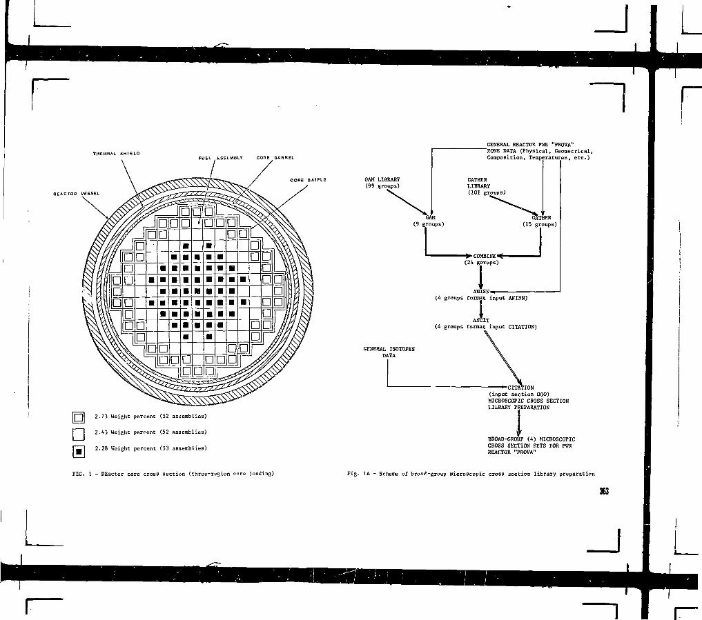
THERMAL SHIELDCOnE^BARREL

CORE BAfFLG

2.73 Weight percent (52 assemblies)

I I 2.43 Weight percent (52 assemblies)

| M | 2.28 Weight percent (53 assemblies)

GAM LIBRARY(99 groups)

(9 groups)

GENERAL REACTOR PWR "PROVA""ZONE DATA (Physical, Geometrical,Composition, Temperatures, etc.)

GATHERLIBRARY(101 groups)

GENERAL ISOTOPESDATA

- ^ COMBINE «t(24 gorups)

ANISN*-(4 groups format input ANISN)

(4 groups format input CITATION)

•CITATION(input section 000)MICROSCOPIC CROSS SECTIONLILRARY PREPARATION

BROAD-GROUP (4) MICROSCOPICCROSS SECTION SETS FOR PWRREACTOR "PROVA"

FIG. 1 - REactor core cross section (three-region core loading) Fig. 1A - Scheme of broad-group microscopic cross section library preparation

383

0.0 29.37 58.74 88.1 106.1 124 151.96

Zen

80.0

1

2

3

4

5

6

7

8

9

10

n

12

13

14

15

16

17

18

19

20

Rctn

190.06

160.0

182.08

208.28

Fig. 2 - Zone placement

R 59 points

58 points

29.37cm8 pts.

80 cm18 pts.

80 cm20 pts.

22.86 cm10 pts.

29.37cm• 8 pts.

29.27 cm9 pts,

7.95CC6 pts.

17.95OT6 pts. 27.95 cm

10 pts.

38.1 cm12 pts.

25.40 cm10 pts.

384Fig, 3 - Geometric mesh description

U-235

U-238

Pu-242

\ \ ld-145 »1\\ V%m-152 *iEu-AjPm-147 —»Sm-149

\»NSFP-235 —H

U-236

Np-239

HEAVY NUCLIDE CHAINS

Pu-239 Pu-240 •Pu-241

FISSION PRODUCT NUCLIDE CHAINS

153 • Eurl54

Sm-150

•• Em 155-1'Smrl51

A-» Sm-152 H

NSFP-239 — *

FIG. 4 : Nuclide chains(Citation-burn-up reactor PUR » PROVA -)

REFERENCES

III T.B. Fowler, D.R. Vondy, G.W. Cunningham "Nuclear Reactor Core AnalysisCode: CITATION" - ORNL-TM-2496,Rev.2.

Ill D.R.Vondy, T.B. Fowler, G.W. Cunningham "VENTURE: A code block for solvingmultigroup neutronics problems appling the finite-difference diffusion--theory approximation to neutron transport" " 0KNL-SQ62 (1975).

HI D.G. Cepraga "Notes on CITATION code - Winter Course on Reactor Theory andPower Reactors"(13 February - 10 March 1978) - SMR/44-18, 19.

/4/ Florida Power & Light Company "Turkey point nuclear generating" Units No. 3and No. 4 - Preliminary safety analysis report - DOCKET - 5O2SO-3

DOCKET - 50251-3.

151 B. Carmignani "Nuclear data preparation: GGC/ANISN chain" Winter courseon reactor theory and power reactors - Trieste 13.2.78 - 1O.3(78,

'J

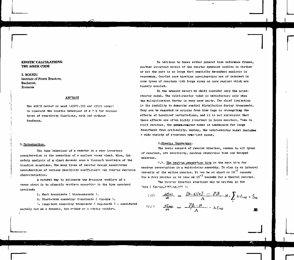
KINETIC CALCULATIONS:THE AIREK CODE

S. BOERIUInstitute of Power Reactors,Bucharest,Romania

ABSTRACT

The AIH7E method is used (AIICTMII anri AinrS codes 1

to simulate the kinetic behaviour of a ? I for varioun

tyres of reactivity functions, with find without

feedback.

1.Introduction.

The time behaviour of a reactor is a very

consideration in the oueration of a nuclear nower nlant. Also, the

safety analysis of a plant defends unon a thorourh know]edre of the

kinetics eouations. The many tyr>es of reactor design necesitates

consideration of various reactivity coefficient? and dynamic response

eharpcteristics.

A natural way to delineate the dynamics riroble-is of a

nower plant is to classify nrohle'">s aeeordin" to the time constant

involved:

1. Past transients ( micro-seconds ).

2. Short-term oneratinr transients ( -nin-hre ).

1. long-term onerating transients ( day-month ) - considered

normaly not as a dynamic, but rather as a static nroblei.

In addition to these rather general time reference franes,

another imnortant aspect of the reactor dynamics nroblem is whether

or not the core is so large that soatially dependent analysis is

necessary. Coupled core kinetics consideration are of interest in

some tyoes of reactors v.ith lsrge cores or core regions which are

loosely couplea.

In the uresent report we shall consider only the Tioint-

reaotor model. The Tioint-reactor -nodel is satisfactory only when

the multiplication factor is very near unity. Its chief limitation

is the inability to describe snatial distribution during transients.

They can be regarded as arising from time lags in rironaga ting the

effects of localized nerturbations, and it is not surnrisin<r that

these effects are offer, highly i-.mortant in larce reactors, ''ven in

s-!ia]l reactors, the polat-reactor model is inadequate for large

aenartures from criticality. Anyway, the noint-reactor model includes

a wide variety of i-mortant Tjractical cases.

2.Kinetic Parameters.

The basic concent of reactor kinetics, common to all tynes

of reactors, are reactivity, neutron generation time and delayed

neutrons.

?.1. The neutron generation ti'ne is the mean tine for

neutron reproduction in a multinlyinp assembly. It also is an integral_p

Tiroierty of the entire reactor. It -nay be as short ns ]0 seconds

for a fpst reactor or as lonp as 10 seconds for a thermal reactor.

The renetor kinetics equations may be written in the

"oral ( ree*>in,Ji6"-T>ff.:if«! 1:

T.l)

365

AN

J I _

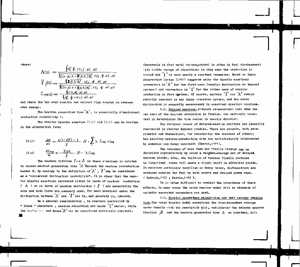
~]where:

anfl where the tar over spectra and adjoint flux denotes an average

over energy.

The neutron generation time A , is essentially al!reeiTirocal

production probability ".

The reactor kinetic equation (P.l) pnd (?.r1 can be written

in the alternative form:

(2.3)

(2.4)

AH _ K(«-r/i)-dt j

•X

The neutron lifetime l-K A in these e^uations is related

to nroant neutron generation time A "through the neutron reproduction

number K. By analogy to the definition of A' • £"inay be considered

as a "recinrccal destruction probability". It is clear that the reac-

tor kinetic equations exnressed either in terms of neutron production

C A ) or in terms of neutron destruction ( £ ) are essentially the

same and both forms are commonly used. For most practical cases the

distinction between A and i " can be, and generaly is, ignored.

Aa a general consideration , in reactors controlled by

" black " absorbers , neutron absorbtion and hence {/varies, while

the TITO^UC' •!:. and hence A ^ay be considnred relatively constant.

3K

Conversely in fast ietal syctemj,control is often by fuel displacement

' ith little chpnge of absorbtion; in this case the nroduotion is

varied and ^ is more nearly a constant parameter. Based on these

observation levins (lifiCl suggests usinp- the kinetic equations

narametric in A " for the first case (varying destruction in thermal

systems) and parametric in ' for the latter case of varyinr

production in fast systems. Of course, neither {. nor A remain

strictly constant in any chain -reacting syste-n, and the above

distinction is generally unnecessary in practical kinetics nro&leras.

2.2. Delayed neutrons,although representing less than one

ner cent of the neutron production in fission, are extrf.mely impor-

tant in determining the time scales in reactor dynamic?.

Six dip tine t Trouris of del ayea-neut^on emitters are penerally

recoTni7ed in reactor dynamic studies. There are wounds, both expe-

rimental and theoretical, for recopni^in/r the presence of others;

but existing neutron-irradiation data are satisfactorily interpreted

by assuming six decay constants (Keer>i?i,lriP^').

The nresence of more than one fissile isotope can be

described approximately by usinp a weigMed-average set of delayed

neutron yields. Also, the build-up of heavier fissile isotopes

in long-lived cores will cause a slight shift in effective yields.

In reactors containing beryllium or heavy water, photoneutrons are

produced outside the fuel by both promnt and delayed pamma rays.

( Hetrick,]<571 ; Keenin,lo65 ) .

It is often difficult to predict the importance of these

effects. In many cases the noint reactor model will be adequate if

suitable corrected narameters are used.

2.3. Kinetic parameters calculation and test reactor descrip

tion.The "Oint kinetic model correlates the time-dependent average

nower density vith the reactivity J U ) , considering'the delayed neutron

fraction fo and the neutron generation time A as constant. Cai-

rculation of different reactivities (one or more control rods, etc),

the delayed neutron fraction and the neutron generation time have

been made utilising the GGC-4/ANISN codes (homogenized , 2-group

cross section sets for various zones) and the CITATICII code ( /i ,/i.

and reactivity calculations).( Adir,l°6f ; WANL ANISN,iq6r. • Vondy,107l)

The reactor considered in calculation is a 2100 wtl1 P.'V.R.

( DOCKET - 5O251/*P2*O ). The reactor core , Fi.T.2.1, is a three-

region cycled cor? consisting of 1*57 fuel assemblies, r/ith 41 rod

cluster control assemblies ( RCC ) . A soluble neutron noison in the

form of boric acid is pr.nloyed for Ion." ter-n reactivity control. The

41 RCC assemblies are inserted into the /niide thi-nbles of the fuel

assemblies. The absorber sections of the control rods are fabricated

of Silver-Inrtim-Carlmiuii alloy sealed in stainless steel tubes.

The fuel assembly aoiears as si bundle of fuel rods held

to."hether by space ,<*rids. The fuel rods -ind the ruirie tuber ire

arranged into a square nrray. This square array constitutes the

b.isic lattice structure of the fuel assembly. ?ro tynes of lattice

cells can be distinguished : the fuel rod cells an^ the ruide tube

ce??n. The .-uide tubes ire v:ator-filleri, if the cor+rol roi s »re

•vi thdr?vn.

THERMAL SHIELDFUEL ASSEMBLY

REACTOn VCSSEL

CORE DAIT1L

2.73 Weight percent (52 assemblies)

I I 2.A3 Weight percent (52 assemblies)

I QJI 2.28 Weight percent (53 assemblies)

FIG.2.1. - Reactor core cross section (three-region core loading)

367

Table 2-]

Nuclear Design Data

A. Structural Characteristics :

1. Core Diameter, in.Core Height,in.Reflector Thickness ICoTiposition

Ton - '"ater r>lur steelBotton - '.','ater plus steelSide - V.'ater plus steel

2. H 0/U, unit cell (cola)

3• Number of Fuel Assemblies

4. HO, Rods ner Assembly

B. Control Characteristics :

1. Rod Cluster Control AssembliesKa terialNumber of HCC Asse-rfbliesNumber of Absorber Rods ner RCCTotal Reactivity Worth

2. 3oron ConcentrationTo shut reactor down -ith norods inserted, cleanCold/HotTo control at nower vith norod£s inserted , clean/equilib-rium xenon and samarium

3 44

10 in.10 in.15 in.

3.4f157204

5 ' Cd-l1} ' In-fC '4120

1O6

6

Table 2-2Hydraulic anfl Thermal Desi/31 Parameters

Total Heat Cutout,"' th 2007Heat Generated in Fuel, * 97.4System Pressure,Kominal,psia 2250

Coolant Plow ^Total Plow late,lbs/hr IOC.63ffective Flon Rate for Heat

Transfer , lbs/hr ~ 91.5 r. 10'Effective Plow Area for Heat Transfer,ft 30.0Average Velocity alon/r Fuel Roa§,ft/sec 13.9 g

Average "ass Velocity, lb/hr-ft 2.35 x 10

Coolant Te-iperatures, °PHoninal Inlet 546.5Average in Core 577.0Average in Vessel 574.0Nominal Outlet of H',t Channel 647.0

Heat Transfer at 3 00"? Power „Active Heat i^ansfer Surface-Area,ft 42,460Aver^^"; heat Plux,Btu/hr-ft 164,200Maxinun Heat Flux.Btu/hr-ft 533,600Average Thermal Output,lew/ft 5.3KaxiTOi-i Thermal Output,kw/ft 17.3

""aximum Clad Surface Temperature at

Hoiiinal '•resswri, "*? 65TFuel Central Tampersture, 'P

Kaxiraum at 100"^ Power 4C70

SSI

L .1_ J

~1Table 2-3

Core Mechanical Design Parameters

Active Portion of the CoreEquivalent Diameter, in.Active Fuel Height,in.lenght-to-Diameter Ratio 2

Total Cross Section Area,ft

Fuel AssembliesNumberRod Array

Rods ner AssemblyRoa Pitch, in*Overall Dimensions, in.

Fuel RodsNumberOutside Diameter, in.Diametral Gap, in.Clad Thickness, in.Clad Material

Fuel ™elletsMaterialDensity (•* of theoretical)Fuel Enrichments, w/o

Region 1Region 2Region 3

Diameter, in.lenrht, in.

Rod Cluster Control AssembliesNeutron AbsorberCladainr "TaterialClada Thickness, in.Number of ClustersHumber of Conti-ol "todo t>er Cluster

119.5144.01.2057E.3

15715 x 152040.5638.426 x f.42*

32,0260.4?20.00650.0243Zircaloy

UO sintered94-9^

?.2f2.432.73

C.PfO

5' Cd-1-5* In304 3S - Cold0.0] n41

Nuclear Desirn Dnta are riven in Table 2-1.

Hydraulic and Thermal Desifii Data are riven in Table 2-2.

Core and Ilec'ianical Desirn D?ta are riven in T?ble 2-3.

Reacti'v'ity control is provided by tvo independent systeT :

the control rod asseaMies and the soluble boron. As a consecuence,

the control rod assenblies can be ke*>t nearly completely withdraw

from the core rturin- ntation°ry operation. The flux and the nov.er dis-

tribution is therefore little disturber1 by nonunifoi-n distributed

absorbers.

3. The " AIR3K " ^

•^.1. The "AiaEJT.III" Code is a snace-inde^endent reactor

kinetics code f B?ue,lci63 ; Sch'-'artz.i^r ; Si1 berbery,I"fi5i. The

code solves the eau^tions:

(3.21 W T

" h e r e :

'J

; *

Uj -

'"'orked

?nfi -here r ( t l in a funct ion of ( t , N ( t 1 , P ft)> , P^ti nre

feedback vf>ri?>bler. pnfl P . , t!,, y T P feedback c o e f f i c i e n t s .

3SS

>H

The code allowes 15 delayed neutron eouations and 50 feedbackequations.

The equation describing the behaviour of the nroaut

neutrons is nonlinear , variable coefficient, 1 -order differentials t

enuation, where the remainder are linear, constant coefficient, 1' -

order differentia] equations. The method is a 5 -order corect

method (Coten,19^f). Since the equations are 1" -order, the problen

is an initial value problem,i.e: riven conditions at tine t, find

the solution at a later time t+h . The numerical integration

procedure continues until one of the following conditions is met:

a. t^TIJTEM, the maximum time for rhich calculation is desired

b. N(t) PK , the maximum neutron level allowed.

c. F.(t)7-P'.I., the maximal values of the feedback variables.

d. The number of time intervals calculated exceeds a siven

number HKM.

At this point, all IHFUT Data are printed as well as all OUTPUT

Data ,i.e: the values of H, F.,coand r as a function of time.

The reactivity equation built into the program is :

rft) = r(t=O) +l|Xtk + £ a..J\(t).This equation may be changed to the desired eiuation, by

chansin^ the function REAC in the program.

AIREK-.III, having an excelent feature - automatic interval

switching and an extensive grafical display of the results - has

been used as kinetic basic part, for a number of codes, as : AT33K-"'0D,

AIRCR, BIOOST, etc.

The AIR05 code ( Blaine,1064 1 differs significantly fro-n

AIREK.III only in tno respects, although other differences exists.

Of most significance is the feneraliration of the feedback equations:

P.Cti = P.-H(t) + U.-N(O) + Y -F, +yc/;:(tKF, (t).3 3 3 th '1 j *? J Hi

310

where K. . ir- the number of the i feedbr-ck "connected" xo the

j ,( i = 1,2, , {). In treating a tno temer-ture coefficient

feedback 'lonel (fuel and "loderntor^, '"'e have urert the \IRC3 code.

1 .T .Automatic Chan~in~ of th? Interration otep Sire. In any

eo-iputer nrorr"n for intecratin/» differential equations, it is

highly desirable to be able to automatically change the size of the

integration step,that it -npy be as large as possible when little infor-

mation is required , but is sufficiently small to achieve a certain

derree of accuracy.

In the AIZISK.III rodr, the afljustnent proceeds as follows.

At the enf of each time step integration the follor-in;- quantities

are calculated:

5 • - * • l n J 1 ^ a ) L

I

Cl-(The quantity 0 is then compared ^o tv:o input ouantities, AU and

AI, and the interval h is adjusted according to the follovity?

three-oart rule:

a. If 0 i Q i A l , then h is doubled for the next interval.

b. If AI^3 4AU, then h is kept th- same for the next interval.

c. If AU<J , then h is halved and the interval is recalculated.

The fol lowing if a tab] e sho'"inr- the relationship of the upper and

lower bounds of 0 to the Rrrors in the co-iputed values of N(t).lower Bound Error in N(t) h^c*aUpper Bound

10

10

- • 5

-6

10

10'

io

f6

-7

2

0

0

fl

.5

. q

.6

. 0

3O"3

io-4

io- 'io"6

0 .

0 .

0 .

0 .

rrr0140

oo^ •;

0017

•J

It hasbeen determined by subsequent rune, usinr 6 delayed

neutron groups and one temperature feedback eouation, that a " 0 "-1 -2

band with an upper limit of 10 ajid a lower limit of 10 , with

r(0) il.5 $, results in B H accurate calculation of N(t) to

3 - 4 significant figures with respect to the irniut data.

4. Samnle Results

"e consider different reactivity functions in order to shov:

the kinetic behaviour of a ->.»/.a. usin<r the AIR^JC.III code.

Reactivity insertions in a "V'.R. can be caused by flov

nerturbations, reactivity Tierturbntions and thermal nerturbations.

These may be brought about by external influences such as loss of

electric nower, mechanical malfunctions anrt seismic deformations.

Plow -rierturbaxions can be further classified into -numn failure snf1

loss of coolant through a leak or nrimory system break. Reactivity

nerturbations can be subclassified into control-rofl ~al"unctions,

addition or subtraction of moderator, and structural movement.

Thermal perturbation can arise because of secondary-nuitm failures,

uncontroled heat removal on the secondary side, and nudden initiation

of cold water flov; into one of several channels.

4.1. Sten-Innut Reactivity.

The use of sten-functionr. t' simulate reni -?rt.ur'"-> + i.->nr T-

sources is narticu3r>rly fruitful in re^ct-or dynamic.? becmirc of the

nresenee of one tiire conct"nt that i" m'ich "hoi-tor than •>]] t-io

other tire constants of the rynte-i. "he re cult, ir thr •• i;i -rry

-roble^is the spurious ^art of thn ror-^nrra th"+ -i-it-co -.-o- -nr' .-,-•"•'-

Nation dien out auic!:!.".

Consider the r.^sci-J c">."P of n nource-free cui Til^riu • ,

"ollcved by P ster. in^ut of vernt-.--\ty -1 +=C. Unroe o=c for -51 +,r =SJP'= ° for - < r "" r = TQ '"or t^t^.

For r,, = 0.2 J , r- del"yeu neutron ,-roi.n, A = 0.00*4 and

A = l.C ]C~ , the "lot of II(tl in function of ti"ie is r.hovn

in ?ir.4.1 .

Fir-AS. an'r" Fir.' .I. -ives the "lot of I;(t) for r^O.?^

anfl respectively r^C."^, v;ith all the other in^ut data unchan"er>.

The ranirt initi"1 riae, called the "irom^t iura"" is r!ue

to the f"ct that the delayed neu+ronE de"end on the ->nst history

of I!(t1. ?or a short time , delayea nent'onr- are ctill beinr

iroflucod at a n t o determined eorjentially by 11(0), anfl this rate

ir- initially nu^ficient to sustain a raiid raine in lift). The initial

~lo"e ir gortoJA(lietrick, 1 "71 \ .iwt •'" t'ou'-h all neut-onn '-ere

T O T 1 * . Tut vhen !7(t) hns riren nn^reciably, the delayed neu+ron

nror'uotior! cnnot ',-ee- "ce. ""ne oh"in repriiop mViBt itrelf until

both T!(t) "nr1 C.'f* are riain- with the r-p-ie ex^onentiil ti-ie

r'e^en^ence, nnr1 the r- te ir- r.)n-'r?r ( lve c'^^t^ti c "erio'1 is Inr'-er^

thnn it v.'ouiri he if "?1 rout'ons -.?!inre 'To^^t. ?nr lar e repr-ti ity

t'-'ir effect, vhil e f+ill nrerent, ir not r~> •-••arked.

As Qo increr:er tnrt A { p > l # l t the r.lov.'in- effect of

delayed neutron ir lo'-t . "he cross o'-er J0=/3f r = 1(1 is called

nroimt critical becaure -it thir roint the c)nin renr^tion ir r:olf-

oustr»inert or. "ron^t neutrons ->lonr. ?he -.Tot of rrftl for r. - 1.2^.

ir. "iven in Pi.-.4.'.

If n rope to-, initially crl tier! , if rui'^eily -inde sub-

criticfil by a n+e™ renc'lvity <*l>»ive (fron r=0 to r=-r ). ve hiveo

the ro-cn11cd"rod-dro"i"ex"'lri'ni3nt, Pir.'!.'>. rho- T the "lot of IT (11

for r. = -r-. <• ^ .

1.r?.Ttnni-Tn-iUt '.(!"ctivity.

hen the re^c^ivit" ic ,\ .linear fuiction of ti-ne, i . e :

r(t.) = r + rn t , <"e have the r.o-cillei1 "raa--iii~'it" reactivity.

371

Changes in control rod position, rerctor accident calculations

and reador start-uo ->roblemc utilises thi^ tyne of in-ut reactivity.

The nlot of H(t) for r r + r, to 1 vi t-h r - 0.3 4

and r = I.1* is Riven in Fi^.d.fi. The solution illustrate drama-

tically the practical need for safeguards desi,"ned to prevent

such reactivity increases.

& .1 .Reactivity escalations.

As the reactivity equation built into the ATR^K.III Code

is :

r(t) = r(t=O) + £ 1 ^ + £ a :?.(t)we must change this equation in ord'er to nermit the simulation of a

reactivity oscilation.i.e:

r(t) r(t=0) + a -sin( a.t + a ) + b .cos( b t + b I

An intresting feature of reactivity oscillation is that a steady

oscillation about zero reactivity causes a diver/tine: power fAkeasu,!""^

Consider r = r + ansin(aot + a.1 , with r = 0, a = C.7,o 1 2 3 o l

a_ = 1, and a, = 0. The variation of N(t) with tine is presented

in Fig.4.7 and Fig.4.C.

One can treat this nrnbi en by uain," a model for vhich •'n

T.alyticnl solution is possible, i . e . the nroT

vith one delay prout> (

the neutron density r>t a river time t in -i"en by

JO, the solution will be periodic (nomHverrer.t nn"er) if :

( 1 - rf .^=1v;hich gives the amount of nagative-bins reactivity, r dollars,

that is needed to maintain a ondy nov/er oscillation "'hen the

372

oocillatin™ rcnotv.-ify haf". aTilitnde a .

4.4. Reactivity rith Te-nnerature Fe

"'e >viil consider a T'R core with a two -nath feedback, "he

reactivity is diminished as the termerature of the fuel increases

due to the Donnler broadening of the resonances. This feedback is

instantaneous since the teranerature increase follows the nower penerate^l

i-nmediately. The second feedbnek -nath is that of the moderator

temperature coefficient. As the modTator tem-oerature increases,

the number density decreases and the neutron a n free nath increases

so that leakage increases and reactivity decreases.

The dynamic response denends u*-on the magnitude of the

temierature coefficients as well as that of the siras.

The thermal analysis really should iroceed by the solution

of the STiace-time heat conduction equation. This is a rather

complicated nrocedure and *ould also mean that spatial effects of

the kinetics equations should be taken into account, '"e, therefore,

vill assume that only a lunrned narameter model and will obtain

the time dependence of a reactor which is really one with the

average nronerties of the reactor under consideration.

let AT., be the deviation of the spatially averr.fted

'nodemtor ^emncrature rro™i its eiuii ibri'Jn value,i.e:

AT. (tl = T..ftl - T.

,ind similarly for the fuel i-emoerpture T_, ve have:

Aip(ti = y ti - TPO

'"here the ?... nnd ? nre equilibrium noderntor and fuel tem-

pr>r°turer respectively. Alno, l e t dn and oir be the moderator

and fuel tp'-oerr'ture coefficients of reac t iv i ty . T'ien:

The thermal analysia of the core must now be considered

and connected to neutronics. The heat generated denends u^on the

fission rate or the nower. v.'e will look at the fuel temperature

averaged over the cnre as well as an averaged coolant temnerature.

"e will ignore the oiadding of the fuel nins.

The heat balance for fuel and for water in the core

is given by ( Onega,1974)t

(4.2)

(4.3)

'."here:

S V / M = density of fuel/moderator (Ib/ft ) .

C p = snecifio heat of fuel (BTU/lb-°F).

V-,/,. = volume of fuel/moderator (ft ) .

T , = average temperature of the fuel/moderator (°P).t/ i

P(t) = total nower of the reactor (BTU/hr).

KL, = thermal conductivitv of fuel (Btu/ hr-ft-°F).

Lp = lenght of fuel nin (ft),

H = total nu-nber of fuel nins in the reactor.

m.. = mass flow rate of the water through the core,

moderator inlet temperature,

snecific heat of moderator ( Btu/lb-T).

T

hT

with

= heat transfer coefficient for the fuel -water2

interface ( Btu/ ft -hr - T ) .

Using in the AIRCS code a react ivi ty given by equation (4.1)

?•>//!

5. Conclusions

The standard rioint kinetics scheme, using the unnerturbed

flux shape a* the Shane function usea to co:.inute reactivity, can

lead to serious errors for nroblems with (Johnson,1165) or without

(Henry,196*) feedback.

In addition, it is known that the use of a shane function

representative of the nerturbed reactor stnte will alvays yield a

conservative solution in the absence of feedback. Thus, one can

use the noint kinetic with such a shane function for an accident

analysis on the ground that his estimates of the ieak core power and

fuel temnera+ures usin^- this shane function will be conservative.

However, with feedback effects nresent, it is not clear

exactly haw accurate any sneeific r>oint kinetics scheme vill be.

Thus, in annlying the noint kinetic renresentation to

reactor accident analysis, it annears to be difficult to assume that

a given model (of the shape function used) is conservative; nor can

one judge the accuracy of the method a nriori,(Yasinski,lri7C^.

"•'e hone that that the annlications nresented in the

renort will be useful for neonle intending to start kinetic and dynanic

calculations.

= 0.15-t and <>(„=- 1.12 10" 4 - 2.0 lo"5

we obtain the nlot of N(t) given in fig.4.9.(Boeriu,197P).

373

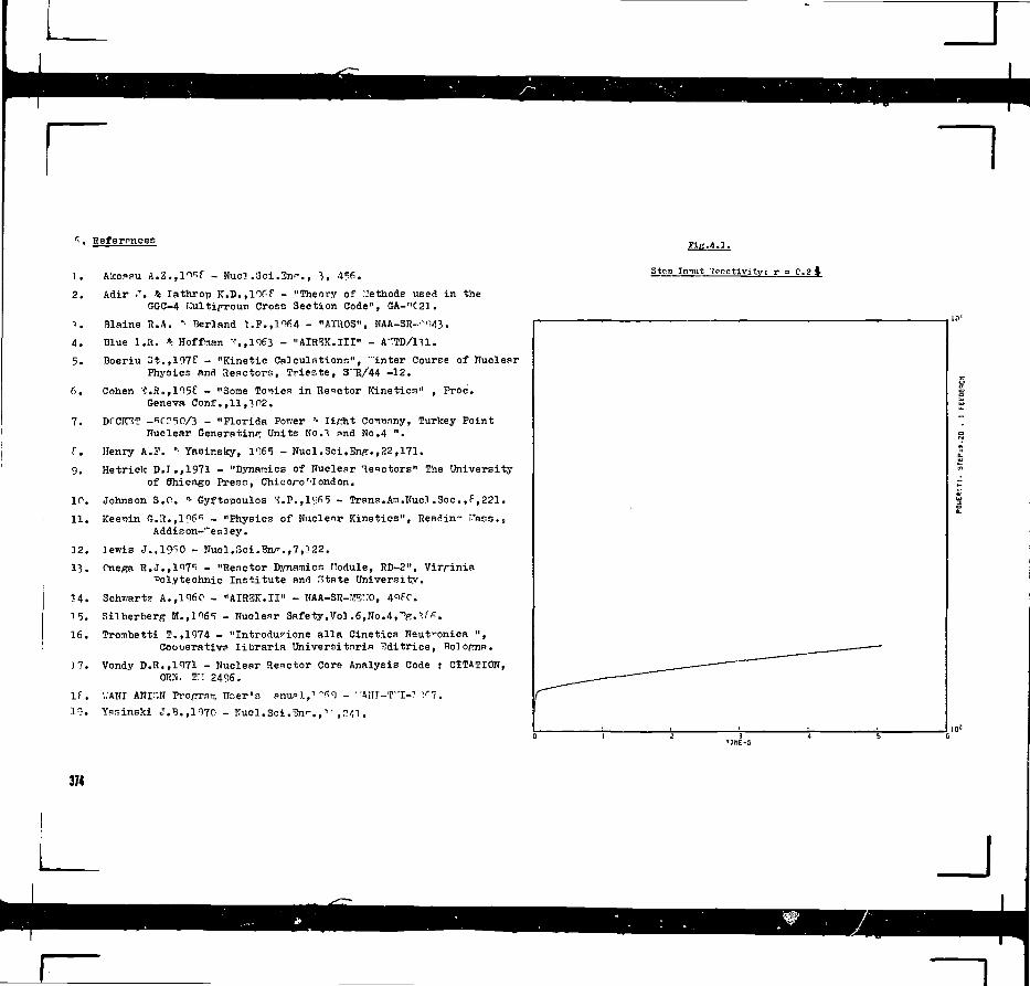
>. References

1 .

2 .

1 .

4.

5 .

6.

7 .

f.

9 .

10.

1 1 .

]2.

1 3 .

1 4 .

T5.

16.

]7.

If.19.

A'.ccasu 1.2..1W - Nuc?. .3ei.3n'-., 3, 456.

Aair .T. % lathrop K.D.,l°iC-t - "Theory of Methods ussa in theGGC-4 IIultipxouT) Cross Section Code", GA-nC21.

Blaine R.A. "• Berland 1.P.,1164 - "AIROS", NAA-SR-'-"i43.

Blue I.E. * Hoffman -\,1<T63 - "AIRSK.III" - A"TD/1U.

Boeriu ot.,197C - "Kinetic Calculations", "inter Course of NuclearPhysics ana Reactors, Trieste, S""R/44 -12.

Cohen 15.R.,195f - "Some Topics in Reactor Kinetics" , Proe.Geneva Conf.,11,^02.

DrCIC3T -*CViC/3 - "Florida Power '• light Co"iwmy, Turkey PointNuclear Generating Units No.^ and Ho.4 ".

Henry A.P. "• Yasinsky, 1065 - Nucl.Sci.Enp.,22,171.

Hetrick D.J.,1971 - "Dynamics of Nuclear Tenctors" The Universityof (Jhicago Press, Chiooro'-Iondon.

Johnson S.O. '• Gyftopoulos '7.P.>iyfi'5 - Trans.Am.Nucl .Soc. ,P,221.

Kee-oin G.R.jlf'e'i - "Physics of Nuclear Kinetics", Readin- "ass.,Aaaison-'"esley.

lewis J.,19^0 - Kucl.3ci.15np.,7,122.

Cne^a R.J.,197^ - "Reactor Dynamics Hoaule, RD-2", VirriniaPolytechnic Institute and State University.

i a t o n I n n u t ' j p n n t i v i t y i r = C . i l

Schwartz A.,I960 - "AIREK.II" - NAA-SR-?re?;O,

Silberbertf H.tli6<i - Nuclear Safety,Vol .6,No.4f"fl. V*.Tronibetti T.,1974 - "Introdus'ione a l ia Cinetica Neut-onica

Coouerativa l ibrar ia Universitnria Kaitrice,Vondy D.R.,1971 - Nuclear Reactor Core Analysis Code : CITATION,

ORN. T:: 2496.I,;ANI ARI"N Program Ucer'n anuplF

n^<) - •pAnr-T"I-7 >"7.Yasinski J.B.,1970 - Nucl.Sci.3n>-. ,•" ,r:/,l .

374

Step Input Reactivity : r ^ 0.5 Sten Trrvit Reactivity ; r = 0.9

i o ' ;•. i

. 10'

375

Stop Intuit Ttointivitv : rStOTi Tniut Tienctlvlty : r = -0.9

'IMF-5'TIMES 10' I

376

Fin.4.6.

Ramn Input Reactivity : r g 0.1+l>']t

Fir:.4.7.

neaotivit.v Qpniiliition ; r = d.7sint

T1ME-SITIMES I01 10.0 0.2 0.4 1.2 1.4 1.6

377

PiR.4.6.

Reactivity Oscillation : r = 0.TsintRCBOtiviiy with Tv.'o Teiperatura Feedback.

crcci—I—

en

z.i

_

enLL.

CL

•

1I

H ft /\ / W V/

. , , . . , . . i. i . . . i .

b .

|

to

iu.1

'11!

•

1

2.5

2.0

1.5

1-0

0.&

0.0

-0.50.0 0.2

311

F A C U L T Y A N D P A R T I C I P A N T S

D I R E C T O R S

BENZI, V. (Part II)C'NE HDipartimento Ricerca Tecnologica

di Basa e AvanzataDivieione FisicaVU'Hazzini 2C.P. 40133BolognaItaly

LABBHIOEE, J.A. (Fart II)General Atomic CompanyP.O.Box 81608San DiegoCalifornia 92138United States of America

CEPHAGA, D.(Present)Centro di CalcoloVia Mazzini 21-40133 BolognaItaly

(Permanent)Institute of Power ReactorsBucharestRomania

CRUIJ, A.Kraftwerk Union, RlPostfach 32 20D-8520 ErlangenFed. Rep. Germany

HENRY, A.F.Department of Nuclear EngineeringMassuchusetts Institute of TechnologyCambridge, Haas. 02139U.S.A.

FONDA, L.International Centre for Theoretical

PhysiosStrada Costiera 11P.O.B. 53634166 TriesteItaly

I B C I U B I 1 S

ASKEW, J.R.SGKH Development DivisionRoom 103, Bldg. A32U.K. Atomic Energy AuthorityAtomic Energy Establishment HinfrithDorchesterDorset DT2 8KIU.K.

BARRE, J.Y.D61tga& aux Applications IndustrielleS

Kucle'airesCommissariat a l'Energie Atoroique29 rue de la FSdSrationParis 15emeFrance

BCERIU, S.(Present)Centro di CalcoloVi.a Mazini 21-40138 BolognaItaly

(Permanent)Institute of Power ReactorsBucharestRomania

CARMIGNAM, B.Centro di Calcolo del CNEHVia Mazzini 21-40136 BolognaItaly

CRITOPH, E.DirectorAdvanced Projects and Reactors

Physics DivisionAtomic Energy of Canada LimitedChalk River Nuclear LaboratoriesChalk RiverOntarioCanada KOJ 1J0

CROWTHER, R.L.Nuclear Energy DivisionGeneral Electric Company175 Curtner AvenueSan Jose, California 95114U.S. A.

EHLEHS, K.Hochtemperatur Reaktorbau GmbHCottlieb-Daimler-Str. 86800 ManheimFed. Rep. Germany

FARINELLI, U.CNENCSN Casaccia00060 Santa Maria di GaleriaRomaItaly

NEAMU, I . (Resident Organizer)Division of Nuclear Power and ReactorsInternational Atomic Energy AgencyP.O.Box 590A-1011 ViennaAustria

PONTI, C.CCR, EUI1AT0M21020 I spra (Varese )Italy

REIJONEN, H.International Atomic Energy AgencyP.O.Box 590A-1011 ViennaAustria

ROBIN, H.DRE/SENCEN CadaracheB.P. No. 1Saint Paul lez DuranceFrance

379

J

SABTORI, E.(Present)NBA - OPCP.O.B. 1521027 IapraItaly

(Permanent)International Atomic Energy AgencyP.O.Box 590A-1011 ViennaAustria

SOLANILU, R.C U E *Malabia 2711 - 6 pisoBuenos AiresArgentina

P A R T I C I P A N T S

ABDUMOMEN, H.A.Physics DepartmentFaculty of ScienceRiyadh UniversityRiyadhSaudi Arabia

AHMED, F.Department of Physics and

AstrophysicsUniversity of DelhiDelhi - 110007India

ABZOUZI, A.Centre deB Sciencies et de laTechnologie Nucleaires

2 Bd Frantz FanonAlgerAlgeria

AHMED, I.Reactor Physics GroupNuclear Engineering DiviBionPINSTECHP.O.HiloreRawalpindiPakistan

AHHAD, M.Technical Development DivisionPakistan Atomic Enorgy CommissionP.'O.Box 1114IslamabadPakistan

AHSAN, H.Institute of Nuclear TechnologyAtomic Energy CommissionP.O.Box 153RaonaDacca - 2Bangladesh

3M

AHMAD, S.S.0 - 96Staff TownUniversity CampusKarachi 32Pakistan

ALAM, B.Department of PhysicsUniversity of DaccaDacca - 2Bangladesh

ALVEAR, c.Inatituto de FisicaUniversidadc Federal do

Rio de JaneiroIlha do FundaoRio de Janeiro - 20.000Brazil

BAHUTCUGIL, E.Ankara Nuclear Research and

Training CentreFen Fakultesi ArkaasiBesevlerAnkaraTurkey

AMUSA, A.Department of PhysicsUniversity of IfeI le-I feNigeria

BECK, R.Kernforschungszentrauin KarlsruheD-7514 Eggenstein-LeopolodshafenFed. Rep. Germany

ANDREOZZI, F.Istituto di Fisica TeoricaMostra d'Oltremare, Pad. 19NapoliItaly

BEN MOHAHED, A.K.Departament de PhysiqueUniversity de NiameyB.P. 237NiameyNiger

ANDRZEJEWSKI, K. (Affiliate)Institute of Nuclear ResearchO5-4OO OtwockPoland

ARREDOHDO, C.Inatituto Hacional de Energia

NuclearInBurgentes sur 1079Mexico IS, D.F.Mexico

BAK, H.-I.Department of Nuclear Engineering'College of EngineeringSeoul National UniversitySeoulKorea

BENWABALLAH, S.Centre des Sciences et de la

Technologie NucleaireB2 Bd. Frantz Fanon

Algeria

BERTI, R.C.I.S.E.C.P. 39861-20100 MilanoItaly

BIRO, L.Institute for Power ReactorsPitesti - ColibasiRomania

BARTAL, Y.TEOHNIONHaifaIsrael

BLESZJNSMI, M. (Affiliate)Institute of Nuclear PhysicsKrakowPoland

~lBOUBUECHAL, H.-E.Centre des Sciences et do la

Technologic NuclcaircsB.P. 1017, Algor-Gare2 Bd. f'rantz PanoriAlgerAlgeria

BUDNAR, M.O. (Affiliate)Instjtut "Jozef Stefan"Jamova 39f.p.Box 199LjubljanaYugoslavia

BUKBA, C.S.(Present)Advanced School of PhysiosUniversity of TriesteStrada Costiera 11TriesteItaly

(Permanent)St. Xavier's College30 Park: StreetCalcutta - 700216India

CATTANEO, UHIBAVia Serra 2GenevaItaly

CHSOH, I—T.Department of PhysicsYonBei UniversitySeoul 120-00Korea

COHVELLO, AiBtituto di Fisica TeoricaKostra d'Oltretnare, Pad. 19JJapoliItaly

COTITOSU, C.Institute for Nuclear Power ReactorsPitoBtiBucharestRomania

CRISTIAN, I.G.Institute for Nuclear Power fleactorsBucharest MagureleP.O.Box 520iliomania

DAYDAY, N.Gekmece Nuclear Research and

Training CenterP.K. 1 HavaalaniIstanbulTurkey

DJOKOLELONO, «.Puslit Gama BatonJl. BabarsariP.O.B. - 8YogyakartaIndonesia

DOBACZErfSKI, J. (Affiliate)Institute for Nuclear ResearchHor.a 6900-681 WarsawPoland

DONOSO, E.Junta Energia NuclearAvenida ComplutenseCiudad UniversitanaMadridSpain

DURACZ, T. (Affiliate)Computing Centre CYFHONETInstitute of Nuclear ResearchSwierk05-400 OtwockPoland

ERIiADI, L.Laboratoire de Physique NuclSairePaoult€ des SciencesUniversity Mohammed VAvenue Ibn BatotaRabatMorocco

CAAPEH, H.A.Reactor and Neutron Physics DepartmentAtomic Energy EstablishmentCairoEgypt

CABRAKOV, S.faculty of PhysicsUniversity of SofiaSofia 26Bulgaria

GADOHSKI, A.M.Reactor Physics DepartmentInstitute of Nuclear ResearchO5-4OO Swierk - OtwockaPoland

GAMBHIR, Y.K.Department of PhysicsIndian Institute of TechnologyPowaiBombay 400 076India

GARG, S.B.Bhabha Atomic Research CentreBombay 400 085India

OHEOROHIU, M.Institute for Nuclear Power ReactorsBuchare3t-Magure leP.O.Box 5204Romania

GHERMAN, 0.Department of PhysicsUniversity of CraiovaAl. J. Cuza 13Craiovaftwnania

EHO, C.J.Centro Atomico Bariloche840O BarilocheSio NegroArgentina

GIRAUD, B.Bivision de l i PhysiqueCentre d1Etudes Nucllaires de SaclayBoite Postale No. 291190 Gif-sur-YvetteSPrance

GOEKE, K.Ins t i tu t fur Kernphsyik der

Kernforschungsanlage Julich GmbHPoBtfach 1913B-5170 Julich 1i'ed. Hep. Germany

GliECO, G.A.N1RAVia Serra 8GenovaItaly

CUL, K.PIHSTIKHP.O.NiloreRawalpindiPakistan

GUNGOH, S.C.N.A.E.M.,KavaalaniIs tanbulTurkey

P.K.-l

381

GUPTA, H.P.5th Floor, T.R.P.S.Central ComplexBhabhi Atomic Research CentreTrorabayBombay 400 085India

CUPTA, R.K.Physics DepartmentVisva-BharatiSantiniketan 731235West BengalIndia

HAIDER, N.Centre for Nuclear StudiesPIHSTECHP.O.NiloreRawalpindiPakistan

HAIDER, H.Department of PhysicsAligarh Muslim UniversityAligarh 202001India

HAMDAN, M.A.Physics DepartmentBasrah UniversityBasrahIraq

HARES, H.E.Mechanical DepartmentFaculty of EngineeringP.O.Box 1098TripoliLibya

HOSSAIN, H.H.Department of PhysicsBangladesh Agricultural UniversityMymensinghBangladesh

HUSAIN, D.Department of MathematicsDacca UniversityDacca - 2Bangladesh

HUSAIN, M.M.Atomic Energy CentreP.O.Box I64RamnaDaccaBangladesh

JAdANNATHAH, U.Bhabha Atomic Research CentreTroobay, Bombay 400 O85India

JAKAB, J.Inst i tute of Nuclear Research250 68 RezCzechoslovakia

JAROSZEWICZ, T. (Aff i l iate)Inst i tute of Nuclear PhysicsRatlzikowskisgo 15231-342 KrakowPoland

KHADDUHI, I.T.Reactor DepartmentNuclear Research InstituteP.O.Box 765TuwaithaBaghdadIraq

KI1ADKIKAR. S.B.Physical Research LaboratoryNavrangpttraAhmedabad 38OOO9India

KHALID, Z.M.

Nuclear iiigincering DivisionPIHSTECHP.O. NiloreRawalpindiPakistan

KHAN, A.M.(Present - until Summer 1978)Research Institute of PhysicsS-104 05 Stockholm 50Sweden

(Permanent)Physics DepartmentUniversity of DaccaDacca - 2Bangladesh

KIM, C.H.Nuclear Engineering DepartmentSeoul National UniversityChungryangP.O.Box 105SeoulKorea

KOCIC, A.Institute "Boris Kidric"P.O.Box 522ilOOl BcogradYugoslavia

KPONOU, A.E.F.Department of PhysicsFourah Bay CollegeUniversity of Sierra LeoneFreetownSierra Leone

Kuaroso, A.Bandung Reactor CentreJ l . Tamansari 71BandungIndonesia

LASIJO, R.S.Bandung Reactor CentreJl. Tamansari 71BandungIndonesia

LATEK, S.Institute of Nuclear ResearchSwierk, OtwockPoland

LOLICH, J.V.Centro Atomico Bariloche8400 - S.C. de BarilocheArgentina

LOPAC, V.Institute "Ruder Boskovic"P.O.Box 101641001 ZagrebYugoslavia

382

HASHA.IN, S.A.PINSTECHP.O.HiloreRawalpindiPakisten

JOZEFOWICZ, E.T.Institute of Nuclear ResearchDepartment of Reactor Physics05-400 Otwock - SwierkPoland

KNAPP, V.Elektrotehnicki FakultetUnsku b.b.41000 ZagrebYugoslavia

MAHTABOALLY, Q.O.Department of PhysicsUniversity of RajahahiRajshahiBangladesh

J

HAKAI, H.Central Research Institute for

PhysiosKonkoly Thege utBudapest XIIHungary

MARTEJEZ, A.S.COPPEUaiversidade Federal do

fiio de JaneiroCaixa Postal 119120 00 - 20.000 Rio de JaneiroBrazi l

XEDJJLDI, D.E.Centre des Sciences et de la

Technologie Nucleaires2 Bd Fronts FanonJUgerAlgeria

JCEDRAHO, C.Intcrnacional de Ingenierfa y

Estadios Tecnicos (INTECSA)Power UivisionCondena de Venadito IMadrid 27Soain

MHAILOtflC, K.V.Ins t i tute "Jozef Stefan"Snivereity of LjubljanaJamova 39P.O.Box 1S961001 LjubljanaYugoslavia '

MIKHAIL, H . j .fieactor DepartmentAtonic Energy ComnispionCairo

KUMBA, S.National Council for Scientific

ResearchP.O.Box Ch. 158ChelstonLusakaZambia

HAHDI, K.A.Directorate General of Mineral

ResourcesP.O.Box 345JeddahSaudi Arabia

NAGARAJAN, M.A.Daresbury LaboratoryDaresburyU.K.

NASEEM, H.A.Department of PhysiosPanjab UniversityChandigarh I6OOI4India

NOTAHI, C.Comision Nacional de Energia AtomicaAv.- Libertador 8250Buenos AiresArgentina

OSMAK, A.M.Physics DepartmentUniversity of CairoCairoF-eypt

PAETHASAHATHY, R.Institute of Mathematical SciencesHATSCIEMCEMadras - 600020

KOO, S.P.Department of PhysicsUniversity of MalayaKuala Lumpur 22-11Malaysia

PASCHOA, A.S.Departanento de Fr.BicaPontifioia Universidade CatolicaRua Marques~de Sao Vicente, 209R^q de JanoiroBrazil

PATRULESCU, I.Institute for Nuclear Power

ReactorsPitestiColibasiRomania

PAUL, O.P.K.Bhabha Atomic Research CentreCIRUSTrombayBombay 400 O85India

PAUN, S.Institute for Nuclear PowerReactors

Bucharest - MagureleP.O.Box 5204Romania

PAVIOITI CORCUERA, R.A.Comision Hacional de Energia AtomicaAvda. del Libertador 825O1249 Buenos AiresArgentina

PERAZZO, R. (Group Associate)JEFE, Seccion PiBica TeoricaComicion Nacional de Energia

AtomicaAvenida del Libertador 8250Buenos AiresArgentina

PICON, C.L.Universidad Nacional de IngenieriaAv. Tupamac Amaru Sin.Apa'rtado 1301LimaPeru

PRUNA, L.H.Tarlac College of TechnologyTarluo ilOlPhilippines

RADOVICI, F.G.Institute for Nuclear Power ReactorsPitestiBucharestRomania

RAFALSKA, J.Reactor PhysicB DepartmentInstitute of Nuclear Research05-400 SwiarlcWarsawPoland

RANT, J.Institute "Jozef Stefan"Jamova 39P.O.B. 19961001 LjubljanaYugoslavia

RAOOP, M.A.Department of PhysicsUniversity of KarachiKarachi 32Pakistan

RATNA RAJU, R.D.Department of PhysicsAndhra UniversityVisakhapatnam 530 003India

RAVAJHSHID, H.

Atomic Energy Organization9 Rodsar StreetKftfe* StreetTshrenIran

EAVWK, M.Institute "Jpeef Stef«ui"Jsmova 39P.O.B. 19961091 LjubljanaYugoslavia

383

384

BECEV, D.Department of Nuclear EngineeringBen Svrion UniversityBeer-5hevalerael

ROBERTO, V.Istituto di FiaicaUniversita di TriesteTrieste

EAHTOS, S.Instituto di FisicaUniversidade Federal de

Bio de JaneiroBloco AIlns de PundaoJiio de JaneiroBrazil

Institute of PhysicsA/105 Saheed NogarBjB&oneBwar - 751007India.

ECHHOCKBR, U.Federal Institute for Reactor

BtsearchOH-5303 HUrenlingenSwitzerland

6EBTIWASH, P.Nuclear Engineering DepartmentArya Hehr UniversityP.O.Box 3406TehranIran

SHARHA, M.L.Reactor Research CentreKalpakkara 603102India

SHARMA, S.K.

(Permanent)Physical Research LaboratoryNavarangpuraAhmedabad 38O 009India

SHAYER, Z.Core Performance DepartmentIsrael Atomic Energy CommiBSionP.O.B. 17120Tel-AvivIsrael

SINGH, B.P.Department of PhysicsUniversity of RoorkeeRoorkee - 247 672India

SIPS, L."Ruder Boskovic" InstituteP.O.B. 101641001 ZagrebYugoslavia

SUBBA RAO, K.B^abha Atomic Aesoarch CentreBombay 400 08$India

SUKITRA, T.Department of Nuclear TechnologyFaoulty of EngineeringChulalongkorn University

BangkokThailand

TAY, Q.dhana Atomic Rncrgy CommiocionP.O.Box 80LogonOhana

TELLO-DUQUE, V.M.Departamento de FisicaFacultad. de Ingenier£aUniversidad de San CarlosZona 12Guatemala

TESTONI, J.E.Comision Maoional de Ensrgia

Atomica - ReactoresAvda. del Libertador 8250Buenos AiresArgentina

TILICA, I.Institute for Nuclear Power ReactorsBucharest-MagureleP.CBox 5204Romania

TOBOCMAN, W.Department of PhysicsCase Western Reserve UniversityClevelandOhio 44106U.S.A.

TRAORE, B.H.Direction Ggnfrale de l'Hydraulique

et de l'EnergieDiviBion EnergieB.P. 66BamakoMali

USHANI, Q.1J.Department of PhysicsAli(;arh Muslim UnxvcrsityAlicarh, U.P.India

VASILE, A.J.C.E.N. CadaracheBat. 233, B.H, 113115 Saint-Paul-lcz-D«rance

France

VASILIU, C D .Institute for Nuclear Power ReactorsBucharest - MagureleP.O.Box 5204Romania

VERTES, P.Central Research Institute

for Physics1525 Budapest 114P.O.Box. 49Hungary

VIHERCATI, 0.C.I.S.E.C.P. 39861-20100 HilanoItaly

VAGHHARE, Y.R. (Associate)Physics DepartmentIndian Institute of TechnologyKanpur - 208016India

HAHEED, A.Nuclear PhysicB DivisionPEISTECHP.O.NiloreRawalpindiPakistan

KANIEK, A.A.Institute for Nuclear Power ReactorsPitestiP.O.Box 5204BucharestRomania

WILLIAMS, V.A.Department of Electronic andElectrical Engineering

University of IfeIlc-IfeNigeria