HOMOGENIZATION METHODS IN REACTOR PHYSICS

IAEA-TECDOC-231

HOMOGENIZATION METHODSIN

REACTOR PHYSICSPROCEEDINGS OF A SPECIALISTS' MEETING ON

HOMOGENIZATION METHODS IN REACTOR PHYSICSORGANIZED BY THE

INTERNATIONAL ATOMIC ENERGY AGENCYAND THE

OECD NUCLEAR ENERGY AGENCYAND HELD IN

LUGANO, SWITZERLAND, 13-15 NOVEMBER 1978

A TECHNICAL DOCUMENT ISSUED BY THEINTERNATIONAL ATOMIC ENERGY AGENCY, VIENNA, 1980

HOMOGENIZATION METHODS IK REACTOR PHYSICSIAEA, VIEMA, 1980

Erinted by the IAEA in AustriaMay 1980

PLEASE BE AWARE THATALL OF THE MISSING PAGES IN THIS DOCUMENT

WERE ORIGINALLY BLANK

The IAEA does not maintain stocks of reports in this series. However,microfiche copies of these reports can be obtained from

I MIS Microfiche ClearinghouseInternational Atomic Energy AgencyWagramerstrasse 5P.O. Box 100A-1400 Vienna, Austria

on prepayment of US $1.00 or against one IAEA microfiche service coupon.

FOREWORD

To predict the criticality and other reactor characteristics it isnecessary to evaluate the fine-structure flux distribution causedby the heterogeneous structure of a reactor such as fuel elementsand control rods. Since it is usually impossible to consider theseheterogeneities directly during the computation of the overallflux distribution, the heterogeneities must be considered in oneor more separate calculations in which the "equivalent" homogenizedparameters are produced for use in subsequent calculations of theoverall flux distribution in the reactor. These separate homogeni-zation calculations should produce "equivalent" homogenized para-meters such that, when they are used in the calculation of thehomogenized lattice, the absorption, leakage, and fission rateare (in an integral sense) the same as obtained for the hetero-geneous lattice.

Unfortunately, such equivalent constants for many practicalsituations exist only in an approximate sence. Limitations ofinaccurate cross section data and computer speed and memory untilthe mid-1960's led to many approximations in the homogenizationmethods. For example, the white boundary condition (zero net-current)at the lattice surface was widely used. Therefore, during thepreparation of the equivalent homogenized parameters, only thematerials and geometrical structure inside the cell was considered.The influence of the surrounding cells was neglected. The 'introductionof high-speed, large memory computers during the last decade hasmade possible the development of multi-dimensional diffusion andtransport theory calculations. Their use in static, burnup, andkinetics studies for present-day reactors increases the importanceof using the most advanced homogenization methods, because this isthe only way to decrease computational cost while retaining accuracy.Therefore, much work has beenUmd must continue to be) invested inthe development of new homogenization methods. The influence of thesurrounding material, control rods, burnup, and streaming mustbe considered both in the static and transient states.

In order to summarize the existing methods, to discuss the mostimportant problems, to define the most promising, developmentpaths, and to address these problems at an international level,the IAEA Technical Meeting on "Homogenization Methods in Reactor

Physics" was organized by the International Atomic Energy Agencyand held in Lugano, Switzerland on November 13-15, 1978. Themeeting was hosted by the Swiss Federal Institute for ReactorResearch (EIR) in Wiirenlingen, Switzerland. The topics of themeeting were:

1. Regular Lattices2. Non-uniform Lattices3. Heterogeneous Assemblies4. Streaming and Interface Effects5. Homogenization Models.

Additional topics were originally proposed. These include partiallyinserted control rods, time-dependent homogenization, bilinearweighting, and non-linear techniques. Unfortunately, there wereso many papers submitted on the main five topics, and so fewon the secondary topics that the secondary topics were droppedfrom the program. From the papers submitted, 32 were selected andpresented at the meeting.

During the Round Table discussion held at the end of the meeting,many valuable proposals were made concerning future work in solvingthe problems in the field of homogenization methods in reactorphysics. A closer international cooperation in this field underthe sponsorship of the IAEA was proposed.

Jiri StepanekGeneral Chairman

CONTENTSFOREWORD.

SESSION A: REGULAR LATTICES (Chairman: A.F. Henry)

Size-dependent homogenized diffusion parameters for a finite lattice ............................. 1F. Premuda

On the boundary conditions in cyclindrical cell approximation ..................................... 27D. V. Altiparmakov

Homogenization of boiling water reactor control rods using the surfaceflux method................................................................................................................ 43C. Maeder, J. Stepanek

Some practical problems in LWR box homogenization................................................... 59M. Halsatt

A method to calculate flux distribution in reactor systems containing materials withgrain structure ............................................................................................................ 73/. Stepanek

Approximation theory and homogenization for neutron transport processes ................ 99M. Borysiewicz

The effects of subassembly heterogeneity and material boundaries on the sodiumvoiding and Doppler effects in a sodium cooled fast reactor........................................ 123A.T.D. Butland

Monte Carlo-based validation of the ENDF/MC2-II/SDX cell homogenizationpath............................................................................................................................ 137B.C. Wade

SESSION B: NON-UNIFORM LATTICES (Chairman: A. Kavenoky)

The SPH homogenization method ................................................................................ 181A. Kavenoky

Homogeneous cell parameters for 2-D reactor codes by axial averaging of thethird dimension........................................................................................................... 189W. Heeds and J.D. Irish

Methode d'homogeneisation utilisee pour les calculs neutroniques dans lesreacteurs a neutrons rapides........................................................................................ 233Y.H. Bouget, Ph. Hammer, F. Lyon

Calculation of a critical assembly of boiling water reactor fuel elementsbased on ENDF/B-IV data........................................................................................... 249R. Wartmann, W. Bernnat

Calculation of critical assemblies with local balance preserving diffusioncoefficient ................................................................................................................. 255K. Andrzejewski, A. Biczel, B. Szczesna

The spatial averaging of cross sections for use in transport theory reactorcalculations, with an application to control rod fine structure homogenisation ........ 261J.L. Rowlands and Mrs. C.R. Eaton

SESSION C: HETEROGENEOUS ASSEMBLIES (Chairman: M.R.Wagner)

Homogenization methods for heterogeneous assemblies. Introductory remarks .......... 271M.R. Wagner

Spatial homogenization of diffusion theory parameters................................................ 275A.F. Henry, B.A. Worley, A.A. Morshed

A new approach to homogenization and group condensation ....................................... 303K. Koebke

Methods used for calculating radial power distributions in large fuel pin bundlesirradiated in the BR2 materials testing reactor. Comparison withexperimental results.................................................................................................... 323Ch. De Raedt

Cross-sections for homogenized BWR fuel elements in Id-diffusion theory byId-transport calculations ............................................................................................ 343G. Ambrosias

Homogenization of light water reactor cells using a QPO first collision probabilitiesmethod in X-Y geometry ............................................................................................ 351/. Stepanek, H. Hager, C. Maeder

Fuel assembly cross-section averaging for PWR fuel........................................................ 383A. Jonsson, S.F. Grill

Determination de constantes equivalentes pour les calculs de diffusion auxdifferences fmies ........................................................................................................ 389/. Mondot

SESSION D: STREAMING AND INTERFACE EFFECTS (Chairman: P. Benoist)

Application of integral transport theory to the calculation of reaction ratesin the vicinity of boundaries between fast reactor zones ............................................ 407R. Bohme

Lattice cell diffusion coefficients definitions and comparisons ....................................... 431R.P. Hughes

Diffusion coefficients in uniform lattices with superimposed buckling .......................... 437T. Duracz

Neutron streaming in GCFRS and HTRs ........................................................................ 449P. Kohler

Methods for the calculation of streaming corrected diffusion coefficients for pinand plate cells in fast reactors .................................................................................... 461M.J. Grimstone

Status and validation of the fast reactor lattice code KAPER-2 for slab andpin cells ..................................................................................................................... 487E.A. Fischer and V. Brand!

ypaBHeHHH reieporeHHoro peaKiopa (ocHOBHue npuHUHnw nocTpoenna) ............................. 499H.H.JlafientH

'A new consistent definition of the homogenized diffusion coefficient of alattice, limitations of the homogenization concept, and discussion ofpreviously defined coefficients ................................................................................... 521V.C. Deniz

SESSION E: HOMOGENIZATION MODELS (Chairman: H. Honeck)

Homogenization models: Critique ............................................................................... 533H. Honeck

High order discrete ordinates transport in two dimensions.............................................. 539/./. Arkuszewski

Calcul des assemblages PWR — Qualification du systeme Neptune sur lesexperiences Melodie dans Minerve ............................................................................. 549A. Santamarina

The arts treatment of lattice heterogeneities................................................................... 581/. Gado

Light water reactor homogenization procedures ............................................................. 605B.P. Rastogi, S.R. Dwivedi, H.C. Gupta, N.K. Gupta, H.C. Huria, V. Jagannathan,D. Jain, V.K. Jain, P.O. Krishnani, S. V.G. Menon, P. Mohanakrishnan,S.D. Paranjape, K.R. Srinivasan, Vinod Kumar

Homogenization methods used by CNEN-Brazil............................................................. 641C.M.P. Santas and C. U. C. Almeida

CONCLUDING SESSION (Chairman: A.F. Henry)Round Table ................................................................................................................. 649

List of Participants ....................................................................................................... 665

SESSION A: REGULAR LATTICES

(Chairman: A.F. Henry)

SIZE-DEPENDENT HOMOGENIZEDDIFFUSION PARAMETERSFOR A FINITE LATTICE

F. PREMUDAComitato Nazionale per 1'Energia Nucleate,Dipartimento Ricerca Tecnologica di Base e Avanzata,Laboratorio Matematica Applicata,Bologna, Italy

AbstractA numerical technique is reported for solving the transcendental equation

for unknown Yn +^ The solution is expressed in terras of quantities related to Yn.•»Ihis is an iterative reversion technique which has already been proven to converge

rapidly in the homogeneous slab problem considered in (6).

1. INTRODUCTION

The integral neutron transport theory was already success_fully applied to treat a periodic cell lattice both in one|l| |2| and two dimensions |3| | 1 | |5|.Let us confine me to recall these only among many other, asthe most rigorous and familiar.

In |l| Kantorovich 's general approximation theory was a£plied to the expansion method for the kernel of the integraltransport equation for isotropically scattered neutrons; atthe same time the connections between the matrix elementsfor this problem and that arising for a finite also nonperi£die multilayer were investigated and accurate benchmarks forthe flux distribution were obtained.

Along a different line a non-asymptotic approach for de-fining size-dependent extrapolated end point Z and diffu -sion coefficient D was recently proposed |6| for a homoge-neous slab one-group reactor. The assumption of a so simplemodel was justified by the need of clarity in the presenta-tion of a completely unclassical way in defining Z and D ;in fact they are determined as functions of the finite thi£kness of the physical system through conditions realizingthe optimal agreement between the diffusion neutron flux di-stribution and the transport flux as a whole, i .e. includingboth the asymptotic and the transient parts.

Leaving to parallel works in progress the efforts- forextending these new concepts to curved geometries, to multi-layers with different values of TJ $$& t-& three-dimensional rea

1

ctors, we try now to take advantage both of this new theoryand of our previous transport calculational methods |l| ina homogenization problem. The aim is that of taking intoaccount not only the properties of the lattice but also itsfiniteness through an appropriately defined buckling to bedetermined in such a way that the present treatement holdsfor any size of the system under the unique condition thatthe number of cells in the lattice be sufficiently high forallowing a homogenization.

The presentation of this theory is irade in a one-groupcontext, in order to be clear in this first presentation ofso new concepts.Of course this imply we confine ourselves to treat a thermalsubcritical lattice, where neutrons are produced by a suita-ble buckling dependent slowing-down source; this will implysuccessive iterations for correcting the value of the buck-ling introduced "a priori" for the source.

Apart from the need of introducing the treatment of source shapes not considered previously, the transport methodsdeveloped in |l| can be used for obtaining accurate valuesfor the zero-th and second order moments of the total fluxspatial distribution and for the escape probability, as nee_ded when appropriate conditions are to be imposed for deter-mining the average diffusion coefficient of the whole finitelattice and an appropriate extrapolation distance accordingto the order of ideas proposed in |6|. So a first task fa -ced in. Part I is that of adapting the transport treatment in|l| to sources of the form

KS (B,x>) = x'K . cos (Bx1 + ,c-y-)q(xf), (K=0,l,2. . . )(1)

where x' is the optical distance from the central symmetryplane of the regular finite lattice and q(x') is a periodi-cal function inside the system. Once the solution is constru£ted for such a source, flux moments and escape probabilityare also calculated.

Part II is then devoted to the calculation of the escape probability and flux moments in diffusion theory and further to establish the transcendental equations which mustbe satisfied by the buckling B and Z and to find relationsbetween I D and B through the transport escape probabili-

3. 5ty and the average square distance of neutrons from the middie plane.

Since the transport quantities in previous treatmentsof the same kind |6j were known "a priori" when the tran-scendental equation for the unknown B was to be written and

on the other hand B appears now in the expression of the neutron source for transport calculations, we can choose betweentwo possible lines:

In following the first one we fix a trial B , whichmight be also B = 0, so determining the source S (B xf)° O 0 0 |

to be used in transport calculations and then we proceed toa sort of source iterations in which the value of B deter-• nmined in the n-th iteration by solving the above mentionedtranscendental equation, resulting from transport-diffusioncomparison, is used to determine the source S(B , x") onwhich are based the transport calculations in the (n+l)-thiteration and so the values of the constants in the transcendental equation determining B ,. The procedure is to be continued until convergence to a B^ is pratically reached.

Along the second line we develop the source S(B,x') ina Taylor series around the point B = B (eventually o) andso we obtain the transport results as series of powers of

B-B . In this case the transport calculations must be madefor a suitable number of sources of the kind (1) once for all.

So the unknown B appears explicitly not only in diffu -sion but also in transport quantities whose equality deterndnes the transcendental equation for B, which now can be sol-ved once for all.

A composition of the two lines, which should be thebest choice from the numerical point of view, constitutesthe more generaltreatement considered in this paper.

Once B, or rather the quantity y = Ba, with a opticalhalf-thickness- of the system, is determined, any other quan-tity of interest, as e.g. extrapolated end point and diffu -sion coefficient, can be calculated via simple relation-shipswith y.

Finally we present a numerical technique especiallyefficient for solving the transcendental equation for theunknown y +,, to be expressed in terns of quantities relatedto y , we encounter along the line previously proposed. Thisis an iterated reversion technique, which already proved tobe very fast convergent in the homogeneous slab problem con-sidered in |6|.

PART I : TRANSPORT CALCULATIONS

1) The integral transport formulation of the lattice problem.

The integral monoenergetic neutron transport equation forof infinite or finite hicknes-s as a whole may be written inthe form

The unknown <j>(x') is the neutron total flux as a functionof the optical abscissa x1, E-(x) is the exponential integralof order 1 and Q(y) is the neutron gource density. In our fi-nite lattice we assume that the source be truly

Q(x') = cos Bx1 . q(x') , (3a)

where q(x') represents an appropriate periodical function in-side the lattice and B is an unknown parameter. But in practjlce, for reasons we shall understand later on, we shall calcu-late the flux distributions for source of the more generalform (see (1) )

Q(x') = KS(B,x')=x'lc.q(xt)cos (Bx' + K-I-)<K = 0,1,2, ...) (3b)

The solutions of (2) corresponding to a source S(B,x')will be denoted as <f>(B,x'). According to |l| we shall iden-tify each layer of the system with an integer number from-M to +M with M>0 and rewrite Eq (2) as a system of integralequations where sources Q.(x) and unknown fluxes <j>.(x) arefunctions of the optical distances from the middle plane ofthe j-th layer.

The system of integral equations reads as

where c, and £, are the constant values assumed by the eannumber of secondary neutrons per collision c (x1) and-by thetotal cross section E(x') in the h-th layer, a, is the opti-

cal half-thikness of the h-th layer (a = 0 if the total num-ber of layers is even) and $,•. is the optical distance betweenthe middle planes of the h-th and j-th layers, considered .aspositive if h precedes j. This quantity may be expressed as

6hi = ah * 2 i °»+0i= I ( o tji+aji+i ) if h<3 < 5 a >n: n *=h+l * 3 A=h * * -1

«", • = -T., if h>j (5b)n j j n

so that the abscissa x for which -a. < x * + a. is related x'by the simple formula

X = X* - T , ,r \oh (5c)From Eqs. (3b) and (5c) it follows that for one < we are con-sidering

Q. (x) = ^S (B,x + T .)=<x -i- «".)*. cos [B(x + S"0j>+ K~Y~1 •

q (x) , <6a)

q.(x) denoting the behaviour of q (x + T .) in the j-th la-yer, so that we shall have

n (6b)

for any couple of integers n and 3 such that -M - j - + Mand - M - n L + j - + M , L being the number of layers percell. In practice q. (x) will be often a very simple fun -ction, e.g. a constant, and in any case a function easilytreated in analytical manipulations, but we can aysoid forthe time being any special hypothesis on the functional de-pendence of q. from x.

The relation (6a) can be rewritten as

1 r- iQ.(x) = S (B,x + 6 .)= S. (B,x)= J cos \BS .+ (K + s -5—)Jj < oj K 3 s=0 o:.cos (Bx + s J) . J (J)x*(T .)K"ft. q.(x)=

J cos fB6" . +(K + s)—5— ] £ ( ( . )K~A S. .(B,x), (6c)on ^ •* «»• ** on ~s~jS = O J ILSo J J

where

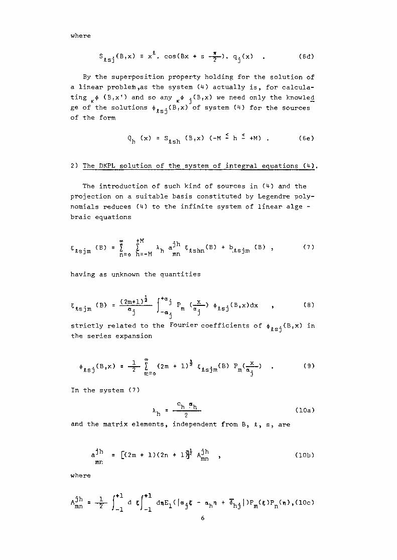
S .(B,x) = x*. cosCBx + s -5-). q.(x) . (6d)X.SJ i J

By the superposition property holding for the solution ofa linear problem,as the system (H) actually is, for calcula-ting <j> (B,xr) and so any <j> .(B,x) we need only the knowled

1C J """"ge of the solutions $ .(B,x) of system (4) for the sources

X.SJof the form

Qh (x) = S h (B,x) (-M - h - +M) . (6e)

2) The DKPL solution of the system of integral equations CO,

The introduction of such kind of sources in (4) and theprojection on a suitable basis constituted by Legendre poly-nomials reduces CO to the infinite system of linear alge -braic equations

+M . •having as unknown the quantities

strictly related to the Fourier coefficients of <}> .(B,x) inX/ S jthe series expansion

(2m2 *•m=o

In the system (7)c, ct,

X = h "h (lOa)h 2and the matrix elements, independent from B, Jt , s, are

jha:n = [(2m + l)(2n + I)]5 A3*1 , (lOb)mn mn

where

d

exactly as in |l|. The independence of the matrix elementson B, I and s, related to the physical independence of thelaws of neutron migration in the system from the specialneutron source considered, allows the repeated solution nee-ded for various values of B of system (7) through a uniqueinversion of the matrix of the system, while the differentsolutions for different B depend uniquely on the differentknown terms we shall define in a short time.

Another advantage of Eqs (10) is that matrix elements(lOc) were already investigated and accurately calculated[11 |7 j in many different forms, which have complementaryranges of numerical convenience and accuracy.

The convergence of the solution for truncated systems oforder N to a system of form similar to (7) was also alreadydiscussed in |1|.

Directly related to the source, and so specific for thepresent problem,are the t,s,B-dependent known terns in (7),we can define as

M j«-h(B) = / (B) (lla)

with

f+aj , p (.JL_Jah _ S <B,y)P

-a. - ^,3 -«>, h

(lib)

Exactly as the £ . (B) correspond to Fourier coefficients& s j inof the total flux in the j-th layer due to the sources S, ,for -M - h - +M, so b . (B) correspond to Fourier coeffi -Xi s j incients of the first-flight flux in the j-th layer due to sour

< < 3*hces S, , for -M - h - +M; the y! (B) coefficients are thenrelated to the partial contributions to the first flight-fluxin the j-th layer due to the source S , in the h-th layeronly.

3) Known terms calculation.On the basis of what already said in Sec.2 it appears cle_

arly that we can in practice consider our transport problemas solved if we are able to compute accurately the 's. Tothis aim we can try to expand S. , (B,y)into the series of Le-gendre polynomials

7 I 'n=owhere

r+a' f * P(——)S. , (B,x)dx.i ri d-r »• x« s n» n

o CD\ _ \*-JiTj./ i , i«^—-—"~>« ,,-u v" )A/u.«.. (12b)Sishn(B) -

The introduction of Eq.(12a) into (lib) shows that

Jfc!——X.sm

once Eqs.(lO) are accounted for. Eq(13)shows in matrix formhow the Legendre components of the source distributionS , (x)affects the m-th Legendre component of the first--flight flux through the matrix |\a^ \\ representing the efmri •"••facts of neutron migration without regeneration by collis_ions, but neutron removal only. Eq.(13) reduces known terms computation to that of the integral defining S£shn(B)viaEq.(12b).By substituting Eq.(6d)into this integral, it reads as

(B) -1 f'Ou±11! h

ah J'ahWhen the slowing down length is greater than the thickness ofmoderating layers we can assume that q(x')is a piece-wise function whose value is 1 for a moderating layer and 0 for afuel layer. Since S. hr.(B) for fuel layers is so vanishing, weare left with its calculation for moderating layers

S*shn(B) =

with

a(m cosCye+s-1 i. (15b)

These integrals can be determined by the recurrence

I (y)=__i__'{(n+l)I i +n'-I. i (T} } (16a^Jlsn J 2n+l f t-l,s,n+l fc-l,s,n-l s

directly derived from that holding for Legendre polynomials.

This recurrence allows the calculation of any In_,,(y)5 onceXfQ nthe I (y) are known as real and immaginary parts of the exo s n —ponential Fourier transforms of Legendre polynomials [8|

2 (16b)

For the more general case in which we assume q(x') to be ze-ro in the fuel and variable in the moderator, we can consider

i Pi

so that

S*shn(B> -

with1 = 0

(B«h) (17b)

J)lsni(y)r += J d?Pn(C)Pi(

A generalization of (I6a)

(17c)

might be used starting from the knowledge of integrals as

r+1= d?PJ •* II J.

or we can use (17d) in the form

(18a)

(17e)

starting from the knowledge of integrals as

(18b)

which were already calculated through Eqs(16).

The integrals (18a) can be evaluated since, due to |9J,the rhombus -relation

(2n+lHiI - -.(y),i-l __osn

os , .(y) + (n+l)I e ., _.(y>} (18c),n-l,i J os,n+l,iholds and can be used for evaluating all the IOSTl^V') once

I __..(yo s no

cos(yC+s--)=

the two first lines of the n, i matrix I __..(y) =o s no

(18d)

are known .In such a way we become able to compute via Eqs . (lla) , (13)

and (15-18) the known terms in the algebraic system (7); so wecan solve numerically this system and calculate the fluxdistributions <(> .(Btx), once a value is assigned to B.

4) Construction of the total flux for the source^defined inany layer by Eq.(6c) and evaluation of the moments ofsuch flux end sources.

According to the linearity of the system (H) the totalflux corresponding to the source S.(B,x) can be constructedt>e superposition of those of kind (9), exactly as KS.(B,x)is a superposition of sources S .(B,x)given by Eq.(6c). Sowe obtain

_s =o $,-$

(-M-J-+M) , (19)in which <j> .(B,x) is given by the series expansion (9).Nowx s 3we have at hand what we need for evaluating the moments of thesources (1) and of the corresponding flux distribution,whichare the transport quantities entering in the comparison oftransport with diffusion results.

The i-th order moments of the flux distribution ^<t>(B,x'')_ ,6" . +M

are <F J ( B ) = _°'+ (x ')1 (B.x' )dx' =16o,-M h=-M

+M . ., i *. j.6 (B x)dx = I (a ) T P,.-- PJ,.(B) (20a)q> V B , x j a x - £ ..vah * >ITI if h

" •* * 1» _ _ \A •? •• f

10

with

P (_-)^h(Btx)dx <20b)i_ h# h

and P- constituting the coefficients in the series expansion

(20c)(^- + sf-^ = f a o( 2 3 + 1 ) 1 p?ij Y^ •

The values to which we are interested are

P* =1 P* »-J_ P* r-i--k P*a 1 +(£h)2 . (20d)noo h22 ,^r h21 /- a, h20 3 a.

Through the introduction of Eqs.(19) and (9), the coeffi-cients defined by (2 Ob) assume the new form

(20e)

in terms of the vector solution of the algebraic system (7).Eqs.(20a) and (20e) can be rewritten for the source mo -

ments , once we remark the analogy between Eqs . (6c)+(12a)and(9)+(19). We obtain so

+M . _i .= 1 < a v > I P Qv <B) <21a>h=-M n j=o hij K n

with1 _ K _

0?(B)=7 cos FB6 ,+(K+s)5-iy (.*)(.$ ^)K~ S ,.(B) , (21b)K h s=o L oh 2 *=o l oh lsh3

wherethe sourcej-th Legendre component S. v-^B) is expressedby Eqs.(15-18).

Another quantity we need for future comparison with dif-fusion quantities is the average number of absorptions in thesystem. It can be easily seen that

I = _M«h5:ah KP°(B). (22)o,-M

Now we can pass to our comparison between homogenizeddiffusion results and transport results.

11

PART II :COMPARISON BETWEEN TRANSPORT AND DIFFUSION BALANCES AND DETER-

MINATION OF THE HOMOGENIZEDB,Z ,L2, D AND I .

5) Neutron flux calculation via classical diffusion for thehomogenized model of the physical situation.

In the homogenized model of the finite lattice under con-sideration we must introduce a source having a global shapecos Bx', but preserving the total number of neutrons producedin the system by the actual source of Eq.(3a),i.e.of Eq.(3b)with K=O. To this aim we must consider here a source

$ (x') = q (B) cos Bx' (23)with q (B) given by the average

+aq(x)cos Bxdx S^ (B)

If————————————— = £——————— (24)+a

cos Bx dx 2a-a Ba

of q (x1) weighted with the global buckling-dependent cosinedistribution.

From now on we drop the sign ' from the variable x forsimplicity sake, but of course now we continue to use thesystem, of coordinates with origin in the middle plane physi-cal system. Another simplification we shall use from nowon -is 'that of denoting as a the total optical half -thickness of the system.

The neutron diffusion one-group equation for a thermal subcritical homogeneous slab with the Q(x) source of slowing-downneutrons reads as

2__ $ . < x ) + c o s B x = 0 (25a)dx ir

with the boundary condition

<f>diff [±(a+Zo)]=0 (25b)

and its parameters defined as

- > B - (25c)a

12

Let us remark that, though Eqs.(25) remain formally theclassical ones, nevertheless we are looking to the quantities2L ,£ ,D,B and Z as to unknown parameters-to be defined later on;

we can adopt without difficulties this point of view as weknow the analytical solution of the problem posed by Eqs.(25a)and (25b). Of course the general integral of Eq.(25a),takinginto account the symmetry required by (25b), is the sum

*dlff<*>= G cosh + - cos Bx , (26)a XTts AJ

of an integral of the homogeneous equation corresponding toEq.(25a) and of a particular integral of Eq.(25a) itself.

The identification assumed between the geometrical bucklingdefined by Eq.(25c) and that appearing in the expression ofthe source, which can be considered as a criticality conditionfor the whole reactor system, implies that the conditions(25b)can be satisfied by the flux at the r.h.s. of Eq.(26) forG = 0 only; in fact with the buckling defined by (25c),cosB(a+Z0)=0, whereas the hyperbolic cosine function remainsnon-vanishing for any non-zero argument. So we obtain thatthe problem proved by Eqs.(25) is solved by

' <27)

which is the flux distribution implying at any point a numberof neutron absorptions equal to that of the neutron-s genera-ted by the slowing-down source multiplied by the non-escapeprobability in neutron diffusion for neutrons produced by asource shaped as we have.

This is the flux for which we are searching a global agreement with the transport flux. The possibility of obtaininga satisfactory agreement could be discussed in the light ofwhat already proved in |6|.

6) The conditions to be applied for determining the unknownhomogenized parameters.

The central idea developed in |6| for obtaining the agree-ment between the exact transport results and the diffusionones is the following: both transport and diffusion equationsare satisfying neutron balance, but in general with differentposition-dependent values for the terms representing the samephysical quantities in the two contexts; so the best globalagreement we can pretend from this point of view should be r£

13

alized when any couple of terms having the same physical mea-ning in the two global balances (i.e. in the two balances in-tegrated over the whole system) have exactly the same value(in transport and diffusion theories). The three kinds ofterms we consider in the global balances are neutron genera-tions, absorptions and escapes.

Since the two global balances are automatically satisfiedby both transport and diffusion solutions,at most two independent conditions can be imposed by the indicated procedure(this maximum value of independent conditions actually occurswhen generations are not equal "a priori", but undeterminedas in monoenergetic critical problems).

We must extend our order of ideas when, as often occurs,we have a number of independent unknown parameters greaterthan the independent conditions at hand. But this is not re-presenting a drawback,as, when the unknowns are in excess ,we are already sure to be able to determine sets of parame-ters for which the two global balances in transport and dif_fusion theories are completely equivalent and furthermorewe can apply additional conditions for obtaining an evenbetter agreement between diffusion and transport flux distri^butions. The unique problem is that of finding reasonableconditions to be imposed.

Since the conditions on the terms of the balance gaveoften rise, among others, to equality on the average fluxes,which are strictly related to the zero-th order moments ofthe flux space distributions, it seems reasonable to impose,when needed, additional conditions on the lowest order mo-ments of the total flux distributions having no trivial val-ues .

In the present problem, along the first order of conceptswe are led to impose that the escapes probabilities in diffusion and transport be equal, for the sources defined by(23)and (3a) respectively, i.e. that

This is sufficient to guarantee the agreement for any coupie of terms in the global balances; in fact generations are"a priori" equal, so that in view of Eq.(28a) the total neutron escapes are equal in turn; besides the same holds forthe differences between generations and escapes, which repre_sent, due to the automatic satisfiement of the neutron balances by both transport and diffusion solutions, the number ofneutron absorptions.

14

Since the remaining independent unknowns , once (25c) are sa_tisfied, are three, we can pretend the satisfiement of twofurther conditions on the zero-th and second order moments of

the total flux distributions^0 5 (B) andQ$"(2)(B) .As the constant multiplying cos Bx in Eq.(27), which is

a function of many unknown parameters , will appear in bothconditions , the elimination of different unknowns should beobtained by its combination.

The first condition reads as

1 sen Ba - _ rdiff I —— . -2.S —55 —— 2a V

3. XTD Jb

whereas the second one is of the form

272a j-Ttwith

r+ara 9 3 1"" 9 7KB, a) = x1 cosBx'dx'=a y cos Bay dy=a f(Ba) (28d)J-a J-land

f(y) = 2

So the conditions we have for the unknown parameters B,Z ,2L ,D,l can be rewritten together ascL

,2 _ D _ _ IT B2L2L - — ' B --(o)

(B)osen Ba

a 1+B L Ba 2aand

1 + B L

(29b)

(29c)

Eqs.(29b) and (29c) are very similar and can be combined toyield

f(Ba)2

= «L__ ———— = H _ (B) (30a)senBa T ( O ) / „ • » ~ tr~~B"a

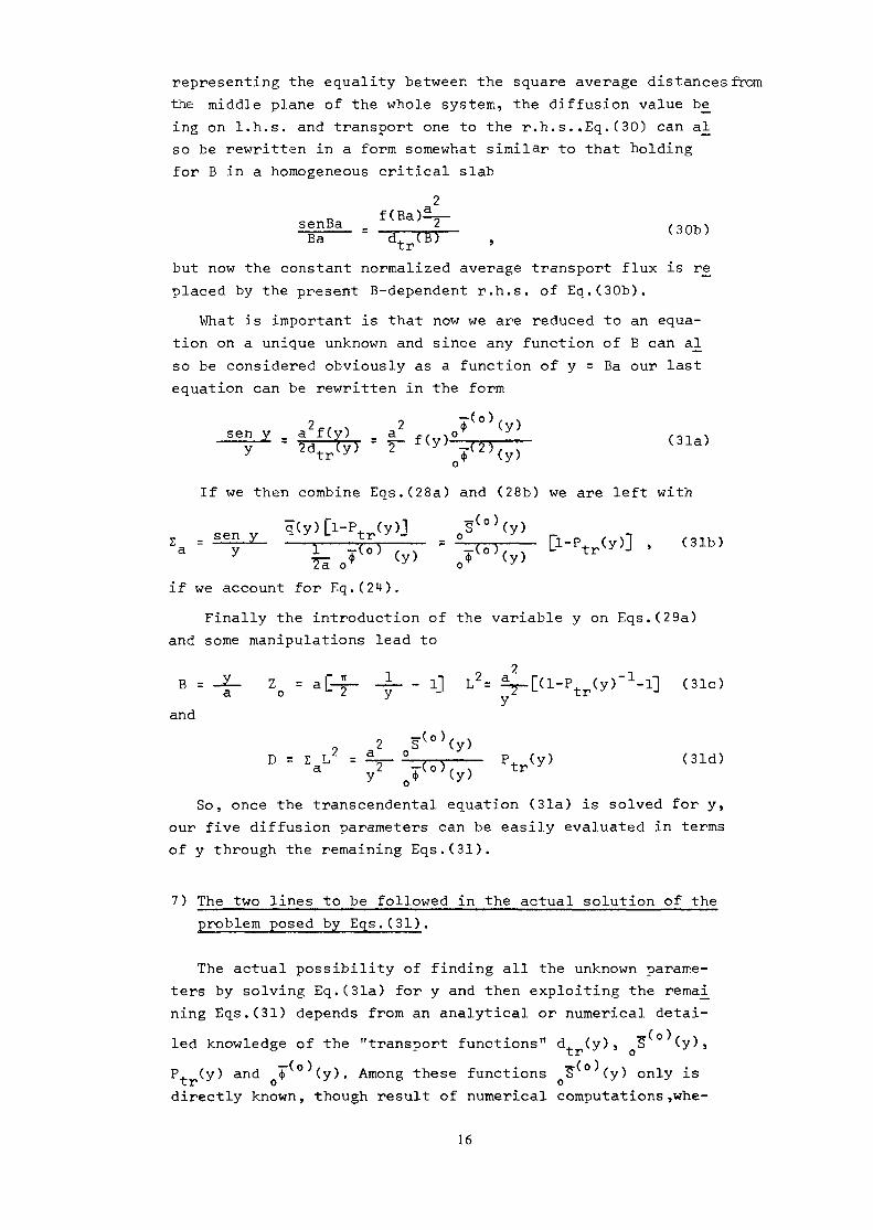
representing the equality between the square average distances fromthe middle plane of the whole system, the diffusion value b£ing on l.h.s. and transport one to the r.h.s. ,Eq. (30) can a_lso be rewritten in a form somewhat similar to that holdingfor B in a homogeneous critical slab

2senBa 2=Ba

but now the constant normalized average transport flux is re_placed by the present B-dependent r.h.s. of Eq.(30b).

What is important is that now we are reduced to an equa-tion on a unique unknown and since any function of B can also be considered obviously as a function of y = Ba our lastequation can be rewritten in the form

2ff . 2sen y _ a f(y) _ a_— 21 - - 2If we then combine Eqs.(28a) and (28b) we are left with

sen0

if we account for Eq.OH).Finally the introduction of the variable y on Eqs.(29a)

and some manipulations lead to

v r IT 1 -i 2R - __y 7 - = r - ii T -D - — £t — a. I* —""••— -L LJ —a o u 2 y y-and

9 2 S" (y)D = £ I/ = 5^- ° .——— p (y) (31d)

y ^ (y)So, once the transcendental equation (31a) is solved for y,

our five diffusion parameters can be easily evaluated in termsof y through the remaining Eqs.Ol).

7) The two lines to be followed in the actual solution of theproblem posed by Eqs.Ol).

The actual possibility of finding all the unknown parame-ters by solving Eq.Ola) for y and then exploiting the remai^ning Eqs.Ol) depends from an analytical or numerical detai-led knowledge of the "transport functions" d. (y), 13 (y),P (y) and ^ (y). Among these functions ^ ° (y) only isdirectly known, though result of numerical computations,whe-

16

reas for the others the value corresponding to a certain ycan be calculated provided a whole transport problem be sol-ved; this is only partially alleviated by the fact that,oncethe transport matrix of the system is inverted a single time,then in any successive calculation different known terms on-ly and a product of the transport matrix by the known termsvector are to be calculated for the new y to be considered.

So the use of numerical techniques for solving Eq.Ola)based on the computation of the above "transport functions"to be reapeated many times is completely beyond argument andin any case fast convergent techniques are to be used, evenif analytically complicated.

Two lines we can follow are here presented as announcedin the introduction.

The first is appropriate for situations, in which the"transport functions" are slowly varying with y, and is ba-sed on a treatment of Eq.Ola) during which a value d (y )is leaved invariant throughout the solution of the transcendental equations

sen Vn+1 = ——£———— f (y ,,) (32)yn+l 2 dtr(yn) n+1

for yn+1• For finding y , we can expand sen ^ and f(y) in-to power series of y and solve Eq.(32) by series reversion.Then y , is the value of y adopted when computing again ,via transport calculations, the average square distance d. (y) ;

so d. (y , ) gi-ves rise to a new iteration for solvingby series reversion Eq.(32) written for a value of n increa_sed by an unity.

In such a way simple operations are repeated many timesfor computing the functions analytically known, whereas theheavy and time-consuming transport calculations are repea-ted a much less number of times.

In this case the escape probability is evaluated by Eqs.(28a), (22), (20a), (20d), (20e) and (21) for K=O only ,exactly as happens for the flux and source moments in (31a)++ O0a) and Old), which are obtained from Eqs.(20a), (20d),(20e), (21), (15-18); the ?'s needed in moments computationsare then provided by solving the algebraic system (7)againfor the source S (B,x). The special case K=O only is so u-sed in transport calculations along this first line.

Once the iterations arrive to converge within a prescri-2bed error bound, B, £ , Z t L and D are evaluated once for

17

all on the basis of the transport functions computed for the"converged value" of y denoted as y .

The second line we can follow is based on the idea that atleast some number of terms in a series expansion into powersof (y-y ),for a suitable-starting value y , be needed (andsufficient) to represent accurately the flux moments repre-senting the numerator and denominator of d. (y) according toEq.OOa).

As well known«° cos(B x'-Hc—5—) . x'K

cos Bx' = 7 ————-————-——————— (B-B.)* (33)t 0<=0 <l

so that«• x' cos(B x' +ic—-x—)q(x')

oS(B,x')=q(x') cosBx' = £ ———————2————£—————— (B-BQ)K,(34)

i.e. taking into account the definition (3b)S(B ,x')

S(B.x') = y -——-———— (B-B )K . (35)0 i 0

Due to the linearity of our transport problem, the solu-tion in the j-th layer will be obtained as a sum of all fluxes ij>.(B ,x) obtained by Eq.(19) putting everywhere B=B ,

1Ceach multiplied by (B-Bo) ,i.e. as

oo 6 ( B x)<(.. (B,x) = I K 3 K°'—— (B-B )K (36a)

•^ K=O

So the flux moments will be represented as

= ? S.————2— (B-B )K (36b)<=o K! °

where-the coefficients are expressed by Eqs.(20a), (20d) and(20e) for K = O ,1,2. . . . . i°, in which B is replaced by B .

We can now understand the reason of the transport treat-ment made for sources of the general-kind S(B,x); of coursethe general expressions for the known terms are needed for theappropriate systems (7) in the unknown £'s, but actual calcu-

/ * \lations of "S """ (B) and P (B) are not necessary, as those"transport functions" can be computed at K=O only for the fiLnal converged value of B or y in order to be directly intro-duced into Eqs.Olb), (31c) and Old).

Once the flux moments are determined in the form (36b)wecan rewrite Eq.(36b) in terms of the variable y as

18

o* (y) = I f(y ) <y-y >* (37a)K=0

in order to be able of using these expressions, with

i J(i)(Vf*(v = ~K — r- > {37b)a K !

in Eq.Ola). The f (y ) represent transport functions to becalculated once for all for K = o,l,2...<» .

— ( i)Let us observe before that $ (y) for i even should notassume other than positive values whatever be the bucKling Bconsidered for the source in a range in which corresponding

2 2Z be positive. So if B < —— and conseguently y < —— weshould have $" (y) > 0 for i even.

2So for 0 < y < —— Eq.Ola) is equivalent to»

0?(o)<y> > <38a)

in which Eqs.(37a) can be introduced, truncated at an orderN in the two series expansions; we obtain thus

f°(y0)(y-y0)K. (39>K=O K=Oso that a finite number 2(N+1) of "transport functions f (y )are to be calculated".

A mixed method might be obtained replacing y with a geneo *™ral y in Eq.(39) and considering its solution as an n-th i-teration belonging to an iterative scheme such as that suggested in connection with Eq.(32). This new scheme , based onthe iterated solution of

•I 'ynK=0

is actually a generalization of both the two previous lines.In fact now we are no more truncating the expansions into N=0 as we made in (32) and we are not restricted to useso high N to be sure that our national approximation for dis very accurate, since we can repeatedly shift the starting point y of the expansions . This third scheme is so mo-re flexible than the previous two.

19

PART III :NUMERICAL TECHNIQUES FOR SOLVING EFFICIENTLY THE TRANSCEN-

DENTAL EQUATIONS FOR y .

8) Solution of the equation for y via series reversion.We shall face the most general equation already considered,

Eq.(40), simply considering the calculation of the unknown yfor

^r^-^l f 2 (y , ) (y -yJ K = -4-f<y>I f ° < y > < y - y >* , <* i>y ^2 £-„ K n n - > r - nCl Iv *" O f* ~ \J

which is written with y to substitute y ,for simplicity.We can try to obtain a power series expansion for the dif-

ference between the two sides of Eq.(tl).As well known

«• / , \K 2Ksen y _ y (-1) yy K=o

.K 2lCyand we can easily see that

f(y) = 2 JK

So Eq.(tl) becomes= » 0 0 N 0 . » 0 NI a2 y2K I b2 (y-y ): = I a° y2lc Ii. K -> L j n *• K J 'iK = 0 j = 0 J K = 0 j = 0

with the positions

2 _ (-1)* m _ 1 fm, , o __{3. _ ~ VLOTT i 1 V t ^.1 "~ -« -^ J V-, ' 3.._ -7-3——....-..-. . - u . — ——— j. • \ y / d — > o——r o \ / o—\ tK i V ^ * + l i " 1 Tn ~i n ^ f v ^ 4 ' ^ i [ V f l '\ i * v ~ J L y » I .Jll I Jl K~ \ i ^ * O / \ ^ . K . ^ »3.

Once Newton binomial formula is used,we arrive to Eq.(43a)in the new form

1C 1 1C ^K=0 1=0 K=0 1=0

with

^n r , n , i \ / \i~iB. = > b. ( J ) (y )J

Finally we can writefl.1

iH-o tc=M K K fc = o K=M K

20

with M = max ( 0,and subtract the r.h.s. from the left one to obtain

(a B - a B _ 2 r ) y = 01=0 K=M * K * **

we can put in the form

I An y* = -An (45)i = l A °

if we assume that

(a2 B* - a° B° )- -

I'Z'J r _ i iK IS •>-; ^_oj.o.. o.., T N

b2- ^i-b^l . (46)K=M

We are interested to express all the A coefficients interms of flux moments, so we combine Eqs.(43b) with Eq.(37b)to obtain

So Eq.C1*?) combined with Eq.(H6) yields the A coefficientsin terms of the flux moments in the form

Anic=M

_ / 2 )j'1' (Yr.) 2K+1 . (y) . (48)j ——— —Ji- - — _

aThe calculational procedure proposed starts so with tran-

sport calculations based on suitable expressions of theknown terms obtained in Sec. 3, continue with the flux andsource moments calculations according to Sec. 4 and arrivesto the determination of the An coefficients in terms of theflux moments by Eq.(48).

At this point we are left with the problem of solving Eq.(45).

In general let us consider the transcendental equationG (y) = 0 to be solved in the case that 6 (y) admits a se -

21

nes expansion00

= I A yK , (49)K = O

and the root is unique, as happens in many physically meaning-full problems. In the very special case for which the root isexpected to be much less than 1 a simple solution to Eq.(49)can be obtained by reverting the series in

00

I AK y* = - AO (50)

and yielding practically y as a truncated series

y - I BK (-A0)K (51a)

with

B2 = TA73 B3 = TA7T5 2(A2)- Al

[5A1A2A3-(A1)2A4-5(A2)3](51b)

But of course in general y can be not so small to guaran-tee a sufficiently fast convergence to obtain y with a reasonable accuracy through Eq.(51a) and the consideration of hi-gher order terms introduces B coefficients of more and morecomplicated form.

An the other hand we can try to take advantage of anyrough solution in order to restart with an already acquiredinformation and refine the previous result. This can be madeby the iterated procedure based on a Taylor series expansionof

oo<|> (y) = G(y ) - A = £ A yK=-A when y equals the root y

K=l (co\of Eq.(50). *• '

In fact if we assume that

* <y) - + <yn> + I A<n) (y - yn)K , (53)than Eq.(52) becomes

Let us remark that Eq.(53) can give even for low N a goodapproximation for $(y), with suitable A , if <|>(y) is a sufficiently wall behaved function. Further the r.h-.-s. of Eq.(54) will be already mucn smaller than 1 even for a somewhat

22

rough solution of Eq.(52). So a reversion technique can beappropriately used to solve Eq.(5U) giving an approximatedvalue hn for hn = y - yn> to be used in obtaining y +1 =

The derivatives of <j>(y) calculated at y = y in generalneeded for calculating An should imply the use of complicatedanalytical operations on <|>(y) and -special procedures diffe -rent in different problems, but it is also possible determi-ne any A by imposing that

_ . (55)

This implies the identity

+(yn) = I * <y )* (56a)n A=1 * n

and the conditions

A* <!!> <V*~K (56b)Jt=K

When these series are sufficiently fast convergent we cantruncate them at some moderated values N and M greater than4 and obtain the iterative procedure based on the formulas

yn+i = .yri *l_. B<n)(-Aon>K (57)PC *• -L

A(n)B(n) _ _1 (n) A2 (n) 1

- - ' B - - B - '3

A3(n)J (58)

7 [5

f. ~K *(* A ( y ) n ' ! (59a)X — 1C

Aon = Ao + * (^n) ' n * ! ' (59b)

A(K} = A K Aoo ' Ao ^o = ° > (60)

which were already translated into a numerical algorithm ve-ry efficient at least for quick convergent expansions of theform (49).

23

9. CONCLUSIONS

The object of this communication should be considered mo-re as a first unaccomplished theoretical trial of giving si-ze-dependent homogenized diffusion parameters than as a sy -stematic treatment of the problem.Now numerical applicationsare in progress and in practice any single step of the proce_dure is already translated into a subroutine, but a modifiedversion of a main program, calculating transport flux distributions, able to collect the different subroutines into a u-nique iterative algorithm and finally to compare the presentimproved diffusion and the transport results, is to be refi-ned. This comparison is essential to judge the validity ofthe proposed diffusion parameters.

A point interesting to be discussed on the basis of numerical results will"be the opportunity of introducing differentvalues of D in the different reactor regions or cells.

Another generalization of the present approach, essentialfor a truly efficient treatment of the homogenization pro -blems, is the extension to a multi-group treatment,which,among other things, should allow interesting applicationsto fast reactors, where size-dependence is especially impor-tant.

Both the extensions are surely possible, since generalizations in the same sense of the non-asymptotic approach |6|and multigroup DKPL transport calculations are already at anadvanced stage of preparation.

On the other hand the actual trial itself can constitutea tool in order to attain a detailed numerical investigationof the effect of the transient part of the flux distributiondue to the heterogeneity in big thermal systems and in anycase for avoiding the vicious circle generated by the depen-dence of Z from the homogenization through the transport m.f.p.,i.e. through D , and by the dependence of the homogenizedD values from the flux distribution, at least near the boun-dary, i.e. by the dependence from Z .

More questions are opened than answered hoping that thiscan nevertheless contribute to the development of new impro-ved diffusion models.

24

REFERENCES

F.Premuda, T.Trombetti "Integral transport theory inmultilayer plane geometry and in plane lattices", Italian contributions to IAEA's specialist meeting on"Methods of neutron transport theory in reactor calculations", Bologna, 3-5 november 1975.E.Larsen "A homogenized multigroup diffusion theoryfor the neutron transport equation", private communi-cation.J.Wood and M.M.R.Williams "An integral transport theory calculation of neutron flux distributions in rectangular lattice cells" J.Nucl.En.>vol.27 pp.337-394(1973)E.Cupini, A.De Matteis, R.Simonini "KIM - Un codiceMontecarlo bidimensionale per il calcolo di reattoritermici" in preparation.J.Carlvik "Calculations of neutron flux distributionsby means of integral transport methods", AB Atomenergireport AE - 279.A.M.Melandri, F.Premuda, W.A.Wassef "Non-asymptoticextrapolated end point and diffusion coefficient reprp_ducing the terms of global transport balance", CNEN report RT/FI in preparation.P.Landini, A.M.Melandri, F.Premuda, T.Trombetti "Eigenvalue problem of integral neutron transport for heterogeneous one-dimensional plane systems", Italian contributions to IAEA's specialist meeting on "Methods ofneutron transport theory in reactor calculations", Bologna, 3-5 november 1975.

A.Erd<alyi"Tables of integral transforms", McGraw -- Hill, New York, 1954.E.Cupini, A.De Matteis, F.Premuda and T.Trombetti"Numerical applications of a new approach to the S£lution of the neutron transport equation", CNEN Re-port RT/FI (69) 16, Rome (1969).

25

ON THE BOUNDARY CONDITIONSIN CYLINDRICAL CELL APPROXIMATION

D.V. ALTIPARMAKOVBoris Kidric Institute of Nuclear Sciences,Belgrade — Vinca, Yugoslavia

Abstract- A solution of the -integral transport equation for an

arbitrary boundary condition is obtained by solving the integraltransport equation for homogeneous (vacuum) boundary conditionand using the neutron balance condition. An effective boundarycondition satisfying the zero gradient of the neutron flux onthe cell boundary is assumed. The numerical solution is obtainedby using a pointwise approximation based on a polynomial fluxapproximation.

Disadvantage factor calculations of the Thie lattice cellsare car-Led, out. Comparisons are performed with the results obtai-ned for the actual cells by two-dimensional methods as well astheir cylindrical approximations applying various boundary con-ditions. It is obvious from the results shown here that theproposed boundary condition has advantages in respect to others.The errors introduced by the proposed boundary condition are ofthe lower order in respect to the inaccuracy of the existingtransport methods. Thus3 the applications of the two-dimensionalmethods for regular lattice calculations is unnecessary.

1. INTRODUCTION

The basic problem in the cylindrical cell approximation(Wigner-Seitz cell) is the choice of the boundary condition onthe outer surface. The reflective boundary condition, exact forthe square or hexagonal lattice cell, should be replaced byanother introducing the same effect. There is a wide choice ofboundary conditions, the only strong demand is that the neutronbalance condition should be fulfilled.

It has been shown by several authors, that the cylindri-cal cell approximation with reflective boundary condition resultsin small error when the cell is large compared to the neutronmean free path. However, serious errors may arise /1,2/ when itis used for calculation of the tightly packed reactor lattice.

This effect has initiated a great number of papers /3-19/ whichtreat the boundary condition problem. The various improvementsare proposed: zero gradient boundary condition /3/J cylindricalcell with an additive region of pure scatterer /4/ being an imi-tation of the white boundary condition defined later; modifiedwhite boundary condition /5/J effective boundary condition /6/jWigner-Askew cylindrical cell /?/ etc. The analyisis of thevalidity of boundary conditions was given in a series of papers/8-19/ in which the results of the various methods are compared.

27

From quite a number of different results, without separating theerrors due to boundary conditions, from the errors due to appro-ximate solution of the transport equation , contradictory conclu-sions where drawn sometimes . As an outcome from these papers theconclusion could be that the cylindrical cell white boundarycondition seems to be a good approximation, but if one would ventmore accurate results the two-dimensional calculations are nece-ssary.

In this paper, the boundary condition problem is treatedon the example of solving the integral transport equation in one-speed isotropic scattering approximation.

2. NEUTRON FLUX DISTRIBUTION IN CYLINDRICAL CELLWITH AN ARBITRARY BOUNDARY CONDITION

The space and angular distribution of the neutron fluxin an arbitrary medium of volume V and an outer surface T isdetermined by the neutron transport (Boltzmann) equation

'1j,(r ')+is(r) , (l)4TT

with the related boundary condition

, (2)

where F{r0,^) is the angular distribution of the incoming neutron flux on the outer surface r, and n is the exterior normalon the outer surface in the point r0.

Introducing the following function

the problem of an arbitrary boundary condition is reduced /20/to the problem of the homogeneous (vacuum) boundary condition

, raer. (4)

In the Eq. (3) 5o=5o(r,&) is the distance from r to the boun-dary surface T in the -$ direction, and r(7,r') is theoptical path between r and r".

Consequently the spatial distribution of the neutronflux <!>(r) may be determined in the following form, by integra

28

ting Eq. (3) over a solid angle

4lT

where <j>0(»") is the neutron flux distribution for the homoge-neous (vacuum) boundary condition.

The neutron balance condition for the considered mediumof volume V and an outer surface F, has the following form:

JdsJ(r)+JdrZa(rH(r) = JdrS(r), (6)r v v•*• +where the vector quantity 0(r) is the neutron current, and-*•Ea(r) is the absorption cross section.

For the reason of symmetry on the sides of the uniformlattice cell, the first term on the left of the Eq. (4) is equalzero. Thus, the neutron balance condition has the following form:

jdrza(?)<j,(r) = jdrS(f). (7)v v

This condition must be satisfied in the cylindrical cell appro-ximation as well*.

For a simple application of the neutron balance conditionthe boundary condition in the following form is assumed:

, r0er, (8)

where f(«) is the normalized angular distribution of the inco-ming neutron flux,

. (9)

The constant C is obtained by substituting Eq. (5) with theboundary condition (8) into Eq. (7) ,

jd?S(r)-JdrEa(f)<),0(r)(10)

* In the ref./2i/ an isotropic return boundary condition is usedand a related integral transport equation is derived. However,the neutron balance condition is not satisfied with this .boun-dary condition, that leads to an unrealistic increase of theneutron flux in the whole cell (see Fig.2).

29

The neutron flux distribution in cylindrical cell with arbitraryboundary condition satisfying the neutron balance condition isobtained in the following form:

*(r) = *0(r)+C6(r). (11)

In the above equations the function G(r) has the followingform:

(12)4ir

3. ANGULAR DISTRIBUTION OF THE INCOMING NEUTRON FLUX

In cylindrical geometry we have the following notation:

V* — I Y* D 7 \ n—tv »r ^' \' >O »*• I > »4 V X » V J >

v/here x ^s the angle between the projections of ^ and rinto a plane perpendicular to the z-axis, and p i-s the cosineof the angle between ft and z-axis.

When cylindricalizing the actual cell the biggest diffe-rences in the neutron flux are expected in the vicinity of thecell boundary (r = rfj) and for the directions ^ for which xtends to ir/2 or 3ir/2. Thus, these directions should be takeninto account with a lower weight in the boundary condition. Onthe contrary, in the case of the reflective boundary conditionthey are overestimated. That leads to an unrealistic increaseof the neutron flux in the moderator and its decrease in thefuel (see Fig.2). In the case of either white boundary conditionor its modification, all the directions are equally weighted inrespect to the angle x r that may be a cause of their possibleinadequacy.

On the other side, by replacing the actual cell by acylindrical one, the angular distribution is not changed sigifi-cantly in respect to the y coordinate. Thus, such an angulardistribution as like in the outgoing neutron flux should beassumed in the boundary condition.

In accordance with the above consideration we assume thefollowing form of the angular distribution in the boundary con-dition:

(13)

TT/2

v(v) = -j-ir/2

(14)

30

where the constant b=(l-a)4/y is determined from the zerocurrent condition, and ^{TDJ*') is the angular distributionof the outgoing neutron flux.

The constant a has a significant influence on thebehavior of the neutron flux in the vicinity of the cell boun-dary and may be determined from the following condition*:

dr __„~-~o= 0 . (15)

In practical calculations instead of Eg.(15) may be usedits finite difference approximation. Thus, the constant a isobtained in the following form:

A<Mro)jdrG2(r)Ea(r) - AGZ (r0 )|dr{S{r)-Za(r)<|>{1 (r)}______V____________________V__________________

(ro)|drGI(r)Za(r) - AG, (rD )|dr{S(r)-Ea(r )<(>„ (r)}A(J)0V V

where A is the finite difference operator in respect to rcoordinate, i.e. Au (r)=u(r,9 ,z)-u(r-Ar,6,z), and

G(r) = aGt(r) - G2(r) . (17)

The formula (14) is not practical. A more convenient formis obtained by Legendre polynomial expansion and cutting off theseries over the first L terms,

vOO -I ^-V2,P2£(y) (18)S.=0 2where {(M) are tne Legendre polynomials of the order 2£.For the reason of symmetry the odd coefficients are zero.

The coefficients V_, may be determined in an iterativeprocedure by using the definition formula and the angular distri-bution of the outgoing neutron flux,

1 it/2 to

-1 -IT/2 0

1 TT/2

+ I ±1V |dyP2)l(y)|dxcoSx{a- os(TT-x')}e"T('?:o':?:o" , (19)*-' = ° .1 -TT/2

* Such a boundary condition has been already used in Pj approxi-mation /&/, Unfortunately, the calculational results are notavailable.

31

where Q(r) is the neutron emission density

. (20)

The isotropic angular distribution in respect to u isassumed as an initial iteration. The iterative procedure (19)is fast convergent. The sufficient accuracy is obtained in 3-4iterations in practical calculations.

Some special cases of the proposed boundary conditionshould be emphasized:(1) <z=l , L=0 white boundary condition,(2) a-l , L->«> modified white boundary condition,(3) a "v , L-*-" effective boundary condition, where 'v denots

that the constant a is calculated using Eg.(15)

4. NUMERICAL APPROXIMATION

In the Section 2. the problem of an arbitrary boundarycondition is reduced to the problem of the homogeneous (vacuum)boundary condition. In this Section, an approximate solution ofthe neutron flux is obtained by solving the integral transportequation.

The integral transport equanon may be written in thefollowing form, in which the spatial dependence is expressedonly by r coordinate:

4>o(r) = jT(r,r'){Zs(r-)<|>Q(r-)+S(r')}dr . (21)0

where Rz is the outer radius of the cell.The above equation is solved numerically by using the

Improved Collision Probability Method /22/. It is in fact acolocation method for solving the integral equations, basedon the quadrature formulas of interpolation type.

In each material region of the cell, i.e. in each semi-interval

a set of the interpolation nodes

and a Chebishev set of functionsuzi(r) , (i=J,2,...nz)

are assumed; where z, Rz and z are the total number, the outerradius and the index of material region respectively; nz and iare the number and the index of the interpolation node in theregion z.

32

The functions of the neutron flux and source space dis-tributions are interpolated through their values (<J>ozj r$z±) inthe interpolation nodes (l"zi) ,

"z nz*o(r) = I 4>0zi Lzl(r) , S(r) = I SzjtLzi(r) , re[Rz_j,R2).(22 )

The set of the even powers of the radius {1 ,r2 , r1*,. . .} is usedas a set of the Chebyshev functions. Then the node influence fun-ctions Lz^(r) may be expressed in the Lagrangeian form:

t-zi(r) = H ———^ (23)

The interpolation nodes are choisen in order to obtainthe integral neutron flux in each region by using the Gaussianquadrature formulas. This choice enables the application ofonly the aporoximation skeleton {A_,•}., , ,..,•-f n in the' £, 3. Z — Jt f /t f JL — ^ , > ( »

further treatment.Using the above approximation, the integral transport

equation is reduced to the following set of linear algebraicequations:

z n7, / ~-1 •> •? \, — Y YT fv A 4*^ T 1 •*/•£/•»•« I (24^z'-i i'-i

The approximation skeleton of the neutron flux distribu-tion in the cylindrical cell with the proposed effective boun-dary condition is obtained using the following iterative proce-dure:

(i) _- rG

where Gzi~ are the discrete values of the function G(r)in the interpolation nodes rzi.

5. NUMERICAL RESULTS AND CONCLUSIONS

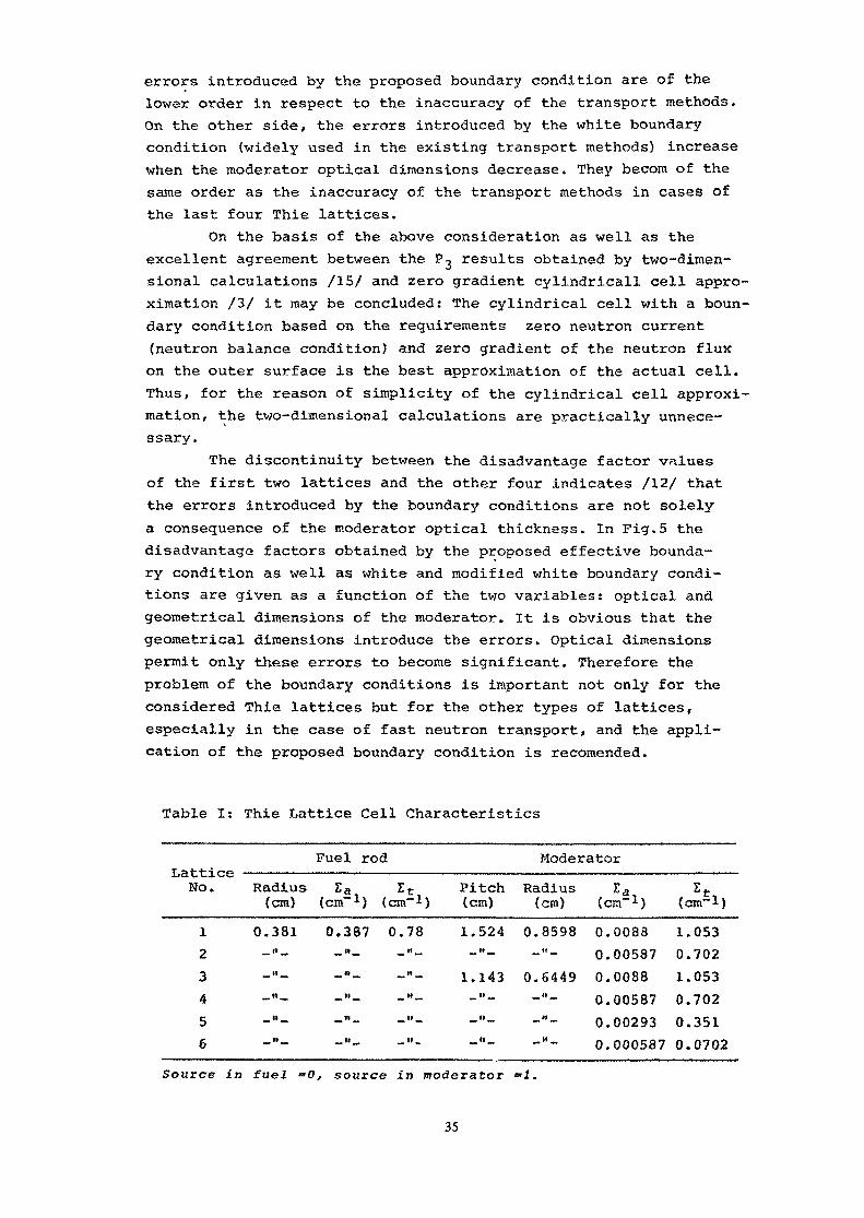
Numerical calculations are caried out for the six Thielattice cells. In fact, they are two BWR lattice cells of diffe-rent moderator densities, the characteristics of which are shownin Table I. The values of the disadvantage factors for theselattice cells calculated by the proposed method are given inTable II. They are obtained by the variations of the followingthree paramatres: a, L and N. The parametres a and L (L beingthe range of the series expansion (18)) determine the angulardistribution of the incoming neutron flux, and N=ni+n2 is the

33

total number of the interpolation nodes in which transport equa-tion is solved approximatively. The influence of the parameter aon the flux distribution is illustrated in Fig.l. In this figurethe flux distributions in the Thie cell 3 obtained for differentvalues of a are plotted. It is easily seen that the parametera has a significant influence on the flux distribution and mustbe determined from a strong requirement, for instance the. zerogradient condition. On the other side the influence of the higherterms in the expansion (18) is negligible, it is enough to takeinto account only the first two (L=l). Moreover, with a sufficientaccuracy, the boundary condition may be assumed isotropic (L=0)in respect to variable y.

The flux distributions in the Thie cell 3 obtained by thevarious boundary conditions are compared in Fig.2. The isotropicboundary condition from ref./21/ is an illustration of the factthat the neutron balance condition must be fulfilled in cylindri-cal cell approximation as well.

The Thie lattices have been widely used as test problemsfor comparing the different homogeneization techniques in thecases of closely packed reactor lattices. Numerous calculationresults of these lattices exist in literature. In Table III asurvey of the previous results, obtained by various methods isgiven. For the reason of simple visual analysis some of them aregiven in Fig.3 (similar as in ref./12/ they are plotted as a fun-ction of the moderator thickness).

From quite a number of shown disadvantage factor valuesthe following two groups of results are distinguished:

(1) Results obtained by the reflective boundary condition:These values are anomaly high when the optical thickness of themoderator i's small. This proves the conclusion that the cylin-drical cell approximation is not applicable in the case of clo-sely packed lattices.(2) Results obtained by Pj and ?3 approximations:Discrepancies of these values compared to others are of theorder of 10% and 6% respectively. Thus, they are not accurateenough for calculating the closely packed lattices.

Figure 4 shows the domains of values of the disadvantagefactors for the square cells and their cylindrical approximationswith different boundary conditions. These domains are obtainedon the basis of the results in Tables II and III, neglecting theresults which differ too much. The widht of the domain illustratesthe inaccuracy of the standard transport methods, and the distancebetween them shows the errors introduced by the certain boundaryconditions. The results obtained in this paper are in excellentagreement with those obtained by two-dimensional methods. The

34

errors introduced by the proposed boundary condition are of thelower order in respect to the inaccuracy of the transport methods.On the other side, the errors introduced by the white boundarycondition (widely used in the existing transport methods) increasewhen the moderator optical dimensions decrease. They becora of thesame order as the inaccuracy of the transport methods in cases ofthe last four Thie lattices.

On the basis of the above consideration as well as theexcellent agreement between the P.J results obtained by two-dimen-sional calculations /15/ and zero gradient cylindricall cell appro-ximation /3/ it may be concluded: The cylindrical cell with a boun-dary condition based on the requirements zero neutron current(neutron balance condition) and zero gradient of the neutron fluxon the outer surface is the best approximation of the actual cell.Thus, for the reason of simplicity of the cylindrical cell approxi-mation, the two-dimensional calculations are practically unnece-ssary.

The discontinuity between the disadvantage factor vnluesof the first two lattices and the other four indicates /12/ thatthe errors introduced by the boundary conditions are not solelya consequence of the moderator optical thickness. In Fig.5 thedisadvantage factors obtained by the proposed effective bounda-ry condition as well as white and modified white boundary condi-tions are given as a function of the two variables: optical andgeometrical dimensions of the moderator. It is obvious that thegeometrical dimensions introduce the errors. Optical dimensionspermit only these errors to become significant. Therefore theproblem of the boundary conditions is important not only for theconsidered Thie lattices but for the other types of lattices,especially in the case of fast neutron transport, and the appli-cation of the proposed boundary condition is recomended.

Table I: Thie Lattice Cell Characteristics

Fuel rodLattice ——————————————————No. Radius Ea Et(cm) (cm"1) (cm"1)1 0.381 0,387 0.78£t """* ""* ~" "•" *•» »•

•3 «. » «. — " .» «M " —

4 It tk II""•

5 11 « II _

6

ModeratorPitch(cm)1.524-*** —

1.143-"--"--"-

Radius(cm)

0.8598_«_0.6449

«v> ** ™*

1*

_B_

(cm"1)0.00880.005870.00880.005870.002930.000587

(0&)

1.0530.7021.0530.7020.3510.0702

Source in fuel =0, source in moderator <*1.

35

Table II: Disadvantage Factors for the Thie Lattice CellsObtained by the Proposed Method

Thie lattice

2+23+34+42+23+34+42+23+34+42+23+34+4

4+4

1.O i l .

1.1.

1 1 1 .1.1.

0 ^ 1.1.1.

1 "0 1.1.

0 1.1 1 1 .2 1.

157015621549157315651553160116211620159916201618154915531553

1.1.1.1.1.1.1.1.1.1.1.1.1.1.1.

151415001492151815041497155915731573155915721572149214971497

111111111I11111

.1408

.1391

.1386

.1341

.1322

.1315

.1492

.1506

.1511

.1501

.1513

.1516

.1386

.1315

.1315

1.1.1.1.1.1.1.1.1.1.1.1.1.1.1.

138913691364131212921283149315041511I48614971502136412831283

1.1.1.1.1.1.1.1.1.1.1.1.1.1.1.

138213591345129112711252150815171521146814781479134512521252

1.13971.1372

1.13171.1294

1.15431.1553

1.14781.1488

rtj anej n2 are the numbers of the interpolation nodes in the fueland moderator respectively; I is the range of the Legendre poly-nomial expansion; and ^ ctenots that the constant a is calculatedusing the zero gradien condition.

36

Table III: Disadvantage Factors for the Thie LatticesSurvey of the Previous Results

Model Method Ref.Thie lattice

cyli

ndri

cal

appr

oxim

atio

n

r-t

refl

ecti

ve

zerograd.

whi

te

mod.white

Dif.PiPKABHP3EFESeSBSisS8CPDITMC

PsPJPa.CPSisDO! 6CPDITS8SePiP3MC

14212221422115121615

333111111121655151515

1.0431.0511.1051.1701.1651.1461.2421.2331.2361.2291.2351.230

±0.607

1.1031.0991.1001.1491.1581.1541.1571.1581.1521.1531.0531.1011.162

+8.003

1111

1111

11

±0

111

1111111

±6

.033'

.039

.093

.169

.188

.136

.302

.239

.284

.290

.259•009

.074

.077

.077

.149

.152

.145

.146

.041

.078

.156.006

1.0291.0361.0901.1551.2071.1321.2911.2761.2711.2811.2841.281

±0-010

1.0861.0751.075

1.1411.1411.1341.1351.0391.0781.147±0 « 0 0 6

1.0231.0301.0841.1591.2651.1291.3861.3641.3751.3591.3711,372

±0 • 0 0 9

1.0501.0591.0591.1341.1381.1331.1381.1391.1311.1321.0311.0611.157io . o o >f

11111111

1111

.017

.023

.169

.440

.136

.625

.618

.672

.136

.137

.129

.131

1.0121.0181.186

1.259

3.3623.464

1.1351.1391.1291.1491.1391.1291.132

u0><0D1W

MCDIT

CPITCP

1516121719

1.1981.1701.155

1.1781.1601.152

1.148tO 0031.150io • o o 51.1611.1541.153

1.1461.1521.150

1.1431.1531.149

1.1691.1571.169

Dif - Diffusion theory^n ~ Spherical harmonics methodMC - Monte Carlo methodPC - Pomraningr and Clark asymptotic diffusion theoryABH - Amouyal, Benoist and Horowitz methodEFE - eigen function expansion methodSn - Cazlson methodDOn - Discreteordinates methodCP - Collision Probability methodDIT - Discrete integral theoryIT - Integral theory

37

01 02 03 04 0.5 06 I7n(

B o u n d a r y c o n d i t i o n s

(T) Reflective

(2) Wh i te modi f ied white

(3) p r o p o s e d ( e f f e c t i v e )

(JD Isolropic , ref Z\

O I n t e r p o l a t i o n nodes

f u <f I

I____ I _____I

m o d e r a t o r

I I

'Fig 1

FLUX DISTRIBUTION FOR DIFFERENT V A L U E SP A R A M E T E R a

0 01 02 03 04 0.5 O f a

Fig 2

F L U X DISTRIBUTIONS FOR DIFFERENC O N D I T I O N S

38

0m

*f

1.35

1.30

t.25

1.20

1.15

1.10

1.05

1i

_ .

I

t W«i 1i 4\ w.I ttt\\\\\\:i

Thie lattice6,\

VXD \ ^3*4i

5 '

v\$\%%vto<\

\

\\\

i

<1 $4

3 :

i

I

\

V

—

-

i

i 1>^ -'"[V^P ^S. _.1- —— 2**&

^"--^ o iVrrri--- — 3 ——— iih £Ni ^^^^^^^^i -^^

'

-•-*>«-c..~)}-•••-

)*

H —— -~

-^,u— -- ->*n' ' *i* ^^""e---i Lx./& v^

*?f

J-d*— -"" jit^-"* -*•»•$...••-•i

! \i

^^:r:---J!.••••**

I j

r^

i

&

?f

1.35

1.30

1.25

1.20

1.15

1.10

1.05

-

"hie la6 ;

SpHgii,.

in

.

1 #1IIIIf

tt ice5 A

i

|l.1

i ,i||

*JS£^a^ mi ,.,l r

10 0.1 0.2 0.3 OA xrm 0 O.I 0.2

1: ii1 f!

'

m^

i ;

1

r

III!

1

:i111!!,•i'Si"111

cr^rr^tt*

In1

_.1±ii

|

-

_

ifi

sgfis^§?=s=i ^

0.3

Fig. 3 DISADVANTAGE FACTORS BY Fig.4 DISADVANTAGE FACTOR

Sw*-$®«&

i

J-R^w

OA

DOMAINS

-

Cm

BYDIFFERENT METHODS DIFFERENT CELL MODELS

Methods: Models:————— Integral theory O 181 square cell——— — Collision probability Cylindrical cells

Sn * IIIIIIIIIH reflective boundary condition——— — P3 0 ^ white — ,.-— — • — PI A W%t. modified white — .. -................. Diffusion theory ^ •••. proposed (effective) -..-

Eigen function expansion ^ p zero gradient

————— ABH x other— _ _ _ _ —— Asvmntntir rliffustnn theory

ti

39

0 5

Fi r j .5

O.b 0.7 0-8 0.9 1.0 f

D I S A D V A N T A G E F A C T O R A S A F U N C T I O N O F G E O M E T R I C A L A N DO P T I C A L D I M E N S I O N S O F - T H E M O D E R A T O R

B o u n d a r y c o n d i t i o n ?

p r o p o s e d ( e f f e c t i v e ;CD( 9 1 w h i t e

m o d r f r d c t w h i t e

REFERENCES1. Newmarch, D.A.

Errors Due to the Cylindrical Cell Approximation in LatticeCalculation,AEEW-R-34 (1960).

2. Thie, J.A.Failure of Neutron Transport Approximations in Small Cellsin Cylindrical Geometry,Nucl.Sci.Eng., _9» 286 (1961).

3. Glendenin, W.W.Effect of Zero Gradient Boundary Condition on Cell Calculationin Cylindrical Geometry,Nucl.Sci.Eng., 14, 103 (1962).

4. Honeck, H.C.Some Methods for Improving the Cylindrical Reflecting BoundaryCondition in Cell Calculations of the Thermal Neutron Flux,Trans.Am.Nucl.soc., 5, 350 (1962).

40

5. Morozov, V.N.On the Boundary Conditions of the Cylindrical Cell OuterSurface in Nuclear Reactor,Atoranaja Energija, 43, 2 (1977) (in Russian).

6. Marchuk, G.I., Lebedev, V.I.Numerical Methods in the Theory of Neutron Transport,Atomizdat, Moscow (1971) p.88 (in Russian).

7. Askew, J.R.Some Boundary Condition Problems Arising in the Applicationof Collision Probability Methods,IAEA-SM-154/69-B, pp.343-356, Int. Atomic Energy Agency,Vienna (1972).

8. Pomraning, G.C.The Wigner-Seitz Cell: A Discussion and a Simple CalculationMethod,Nucl.Sci.Eng. , 1_7, 103 (1963).

9. Fukai, Y.Validity on the Cylindrical Cell Approximation in LatticeCalculations,J.Nucl.Energy, 18, 241 (1964).

10. Sauer, A.* Thermal Utilization in the Square Lattice Cell,

J.Nucl.Energy, 18, 425 (1964).11. Pennington, E.M.

Collision Probabilities in Cylindrical Lattices,Nucl.Sci.Eng., 19, 215 (1964).

12. Weiss, Z., Stamm'ler, R.J.J.Calculations of Disadvantage Factor for Small Cells,Nucl.Sci.Eng., !_£» 374 (1964).

13. Sims, R., Kaplan, I., Thomson, T.J., Lanning, D.D.The Failure of the Cell Cylindricalization Approximationin Closely Packed Uranium/Heavy Water Lattices,Trans.Am.Nucl.Soc. , T.' 9 (1964).

14. Ferziger, J.H., Robinson, A.H.A Calculation of the Disadvantage Factor in CylindricalGeometry,Trans.Am.Nucl.Soc., 1_, 264 (1964).

15. Dudley, T.E., Daitch, P.B.Transport Effects in the P-, Treatment of Cylindrical Rodsin a Square Lattice,Nucl.Sci.Eng., £5, 75 (1966).

16. Carlvik, I.Calculations of Neutron Flux Distributions by Means ofIntegral Transport Methods,AE-279 (1967).

17. Wood, J., Williams, M.M.R.An Integral Transport Theory Calculation of Neutron FluxDistributions in Rectangular Lattice Cells,J.Nucl.Energy, 27, 377 (1973).

18. Azekura, K., Sekiya, T.Comparison of Disadvantage Factor among Square, Hexagonaland Cylindrical Cells,J.Nucl.Sci.Technol., 11, 269 (1974).

41

19. Raghav, H.P.Disadvantage Factors for Square Lattice Cells Using aCollision Probability Method,Atomkernenergy, 27, 84 (1976).

20. Ershov, Y.I., Shikhov, S.B.Methods for Solving the Boundary Problem in Transport Theory,Atomizdat, Moscow, (1977) p.13 (in Russian).

21. Lev/is, E.E., Adler, F.T.A Boltzmann Integral Equation Treatment of Neutron ResonanceAbsorption in Reactor Lattices,Nucl.sci.Eng., 3J., 117 (1968).

22. BoSevski, T.An Improved Collision Probability Method for Thermal NeutronFlux Calculation in a Cylindrical Reactor Cell,Nucl.sci.Eng., .42, 23 (1970).

23. Kocid, A.KASETA - A Monte Carlo Program for PWR Fuel AssemblyCalculations,IBK-1377 (1975) (in Serbocroatian).

42

HOMOGENIZATION OFBOILING WATER REACTOR CONTROL RODSUSING THE SURFACE FLUX METHOD

C. MAEDER, J. STEPANEKSwiss Federal Institute for Reactor Research,Wurenlingen, Switzerland

ABSTRACT

The transport equation is solved in the elementary cell of a BWR con-trol rod. The angular zone surface flux is represented by a double PN-ex-pansion, and spatially constant sources and surface fluxes are assumed. Byeliminating the surface flux moments a direct solution for the average zonefluxes is derived. The method was implemented into the computer programBWRCONTROL. For two test problems an accuracy of 3% for the cell absorptionis obtained, and the worth of a cruciform control rod in a critical LWR ex-periment is underestimated by 4 mk.

1. INTRODUCTION

The cruciform control rods of boiling water reactors are composed ofrectangular cells consisting of a boron carbide absorber pin in a stainlesssteel clad, a water region and a stainless steel sheath [Fig. 1). The in-ternal flux distribution of the control rod cell is needed for the deter-mination of homogenized cross sections. In this paper the neutron transportequation is solved in a control rod cell containing an arbitrary number ofannular zones by means of the surface flux method. The incoming angularflux is assumed to be given at the outer sheath surface, and the reflectiveboundary condition is used at the cell interfaces. The collision probabi-lity method has been applied earlier to control rod cells consisting ofthree regions QQ •

As the related interface current technique [2] the surface flux method[3] , [14] considers only coupling between neighbouring meshes. In one-dimensionalgeometry it represents the mesh surface flux by a double PN-expansion inthe angular variables. In two dimensions the quadruple PN-expansion is thenatural approximation [4]. In contrast to Ref. [4], where the continuity ofthe surface currents was imposed, the flux moments are made continuous at thezone boundaries [3] , [14] . This procedure avoids the inversion of the matrix con-necting the flux and current moments which introduces numerical errors forhigh PN-order.

Because the water zone of the control rod cell with its internal cir-cular and external rectangular surfaces is geometrically complicated, thefollowing simplifications are made: The scattering is isotropic; only sphe-rical harmonics that are even functions in the azimuthal angle are consi-dered, and the incoming surface flux and the source are spatially constant.

In Section 2 of this paper an expression for the average scalar meshflux is derived from the basic transport equation. The outgoing mesh sur-face flux is determined from the integral equation. The reflective bounda-ries on which a CRN-approximation is used are included in the transmissionand escape probabilities of the corresponding meshes. By means of the for-ward-elimination backward-substitution procedure the surface moments areeliminated and a direct solution for the average mesh fluxes is obtained.

43

The method was incorporated into the computer program BWRCONTRQL whichis a module of the LWR fuel fuel element program system BOXER [$]. Applica-tions of BWRCONTRDL to three test problems are described in Section 3.

At present average cell cross sections are determined in BOXER by flux-weighting. More adequate procedures involving the outgoing current at thecell boundary have been proposed [l] , [6j . The method described in this pa-per could be coupled with these improved homogenization techniques.

2. SURFACE FLUX METHOD

2 .1 Flux Calculation

To determine the average scalar flux $ in the zones of the control rodcell the basic transport equation

CfiV-K<-Z) i|> Cx.fi) = q (x) / 4TT (1]

is integrated over the zone volume V and the unit sphere of the flight an-gles:

$ = q/£ + ( y A ,J - y AJ )/ CSV) , (2)\ L-, S ' S 1 L-j SB'

s' s

where the sum over s' refers to incoming and the sum over s to outgoingneutrons. The total source for energy group g is:

q = Y, $ +• 0 , C3)g g+g g gwhere the source to the group g is defined by

Q = Zu $.. (4)g £—, h-*g h

Each zone surface divides the unit sphere of the flight directions into twohalf spheres Ps Cs=1, 2. ...., S=2*NZ) whose enumeration is chosen accord-ing to Fig. 2. The angular domains Ps are defined by a vector ns which isorthogonal to the considered surface and is directed into Ps. The flightdirection is represented by the polar angle 6 and the azimuthal angle <f>between ns and the projection of fi onto the xy-plane. As is the area of thesurface belonging to Pg and Js the average current:

, 1Js = 7Ts

dA | dfi cosG cos<j) \p Cx.fi) , C5)

A Ps s

where dfi = cos8d9d(f) and NZ is the number of zones.

In each angular domain the flux is expanded into orthonormal sphericalharmonics functions C= double Pl\l-expansion] :

NYip Cfi) = y i|) Y Cfi) C6)s L-, ns n

n=1

44

corresponding to

ns dfi Y t£J) . [7)

If N is the order of the DPN-approximation, then NY=(N-H D (N+2)/2. Yn can bederived from the basic angular functions:

= f .C& = m+£ m~c o s 9 cos.n Amm=0,1,...,N £=0,1, ...,m n=1,...,NY

(8]

by means of Gram-Schmidt ' s orthogonalization procedure:

Y = 2 / /CZ ,Z D ,n n n nn-1

Z = f - y (f ,Y. ) Y. ,n n L-J n k k C9)

(f,g) =

The result isn

Y 07) = V a . f, (R) ,n Z_/ nk kK-1

a , = ? , / /(Z ,2 }nk nk n n

n-1

'nk ^ k'kk'=k n'=1n n

a, i , 3 ., k<nk'n' nn1

[Z ,Z ] =n nk=1 k'=1

where

andir/2

d<() coso

= TT/2 ,

C10)

- 1 (12)n = Cn-1] n „ / n.n n-2

45

For example, the angular functions of the DP1 -approximation are

f . = f = 1 ,1 oof = f = cos9 coscj) .

f3 - f^ - cos'e .Y = Y = 1 / v^TT ,1 00

Y = Y = (Cos6 cos<j> - 1/2) / /JrTs" ,

(13)

Y = Y = (cos29 - cos6 cos<(>/2 - 5/12) / /49TT/360 .

By inserting Eq. (6) into Eq. C53 one obtains the following relation betweenthe current and the corresponding flux moments

NYJ = Y ^ > (14)s *—> n ns

n = 1where

Y = Ccos9 cost)), Y ],n nwhich leads to:

Y2 =C15)

Y = o for n>2 .n

In order to determine the outgoing flux moments of the zone surfacesthe integral transport equation

ip Cx.fl) = Ql-exp(-T/cosef| q/(4irZ) + expC-T/cosG) i|i ,(x',fi) (16)

is multiplied by Yn(fi)/As and integrated over the surface and the angulardomain Ps- Tis the optical distance between s and s' in the xy-plane. Theresult is

\> = E q + / / T , , $ , , . C17)ns ns ^ i—' ns.n s n'sn'

The transmission probabilities from the surface s1 to the surface s are de-fined by

Tns.n's' AsdA Y m } Y [fi ) exp [-T/COS0) (18)n c n ' c 'n s n s

A Ps sand the escape probabilities by

E = -7TT 7 [T , , (o ) - T , , (Z)l . (19)ns 4irZ L-, Lns,1s' ns,1s' -1

s'

46

The surface currents and the total source are now eliminated from theflux and surface moment Eqs. (2] and (17] by means of Eqs. [3) and (14]:

s' n'

tf< = C Q + D , , * , , . (21]ns ns Z^ /_/ ns.n's' n's's1 n'

where

B , ( = ( Y , A , - > A > Y T ,,)/ (cEV) (22)n's' n' s' i-, s L-i 'n ns,n s' 's n

Cns = Ens (1+

Dns,n's' = Tns,n's' + E B ' ' ' C24]

- y AZ^ s -j n ns

c - 1 - b Z (25)and ^g

a = b/c .The given incoming flux moments on the cell boundary 5=2 NZ (cf. Fig. 2]are called (On. Let xns ^r be the solution of Eqs. (21] with the sourceterm equal to 6nj^ 6sr (on| is the Kronecker symbol]. The general solutionof Eqs. (21] may therefore be represented as:

G . Q. + H , (27)ns,i i ns

G . = x . C , (28]ns,i L-J i-> ns.kr krrei k

H = x , F, (29]ns t — i t - t ns.kr krrsNZ k

andD , 0 w , , s £ N Z . (30]ns Z_/ ns.n'S n'

n'After introduction of Eq. (27] into Eq. (20] one obtains finally for theaverage zone fluxes :

$. = d. .Q. * e. , (31)i £-, ij j i

d. . = a. 6. . + B , ,G . . . (32)ij i ij L-, LJ n's1 n's' ,js'ei n'

47

and

7 B -L-J n' c .S n Z Z Bn's'Hn's' 's'ei n'

(33)

2.2 Transmission and escape probabilities

On the reflective boundaries which appear in the water and the rectan-gular zones (cf. Fig. 1), a quadruple PN-approximation of the flux is used.Since the orthonormal spherical harmonics of a quadrant with surface rr areby a factor of v2 larger than the corresponding functions of the half sphere,the following formulas hold for the transmission and escape probabilities

n n1

T , , = 2K K , V V a a , , U 't?ns.n's' s s' t—i Z_r nv n'V' A+A' ',y-A,u'-A' (34]v=1 v'=1

ns

nV a fu s . to) - U^ S . ml£_, nV [_A+y,y-A,o A+y,y-A,o J (35)

withfor

s = half sphere

s = quadrant

The connection between A,y and V is given in Eq. (8). The transmission inte-grals U are defined by

IT/2

us'"s =-1pmm' AfdA m, rn" .cos d) cos m (T)

-7T/2

where

p = m+m',m+m'+2,..., 4N - (m+m')

with the Bickley functionTT/2

Ki Cx) = d8 cos 6 exp (-x/cos9)

The following symmetry relation can be proved:

J = A U 7 „ , / A .pmm s p,m +1,m-1 s

(36)

(37)

(38)

The indices m and m' run between 0 and N in Eq. (36). If the symmetry re-lation (37) is used, their definition intervals must be changed to m=D,1,..., N+1 and m'=-1,0,...,N omitting the coefficients with m=o, m'=-1 andm=N+1, tn'=N.

48

For an annular zone with inner radius r' and outer radius r the ex-pressions (36) for the U-integral lead to

TT/2

J<j> cosm+m <j> Ki0 (2Zr cos(j>) , (39)U .= 2pmm1 2+Parc sin (r'/r)

and TT/2

r'->r r' m'-1 m'+1U , = 2 — dtfi'cos d> cos V Ki0 (Z(rcosd>-r'cos*' )) . (40)pmm' r 2+p

To derive Eq. (40) the relation r' sin<f>'=r sin<}> was used. The calculationof the integrals U f can be simplified using the recursion formula:

r'->r 2 r'-*r 2 r'->rpmm1 p,m,m'-2 p,m+2,m'-2

where

a = r'/r .For the rectangular zone with sides a and b one obtains

*o

, = d<|> cosm+m'<f> (1-tg$/tg<j> ) Ki (Eb/cos4i) , (41)

° TT/2

and ir/2

, ,, d<(> cosm<|) sinm' (f) A , (43)pmm Ea 2+p

wherer Zb/cosif)A =

and} for (°!*!!°}

<(> = arc tg(a/b).

The water zone (cf. Fig. 3) is bounded on the interior side by a cir-cle with radius r and on the exterior side by a rectangle with sides a andb. For the angles <j>-] and $2 defined in Fig. 3 the expressions

, . ,ac - br,<f>1 = arc sin (—-—)

, . rac +_br,j>2 = arc sin (—-—)(44)

49

may be derived, where d2=(a/2}2 + (b/2)2 and C2=d2-r2. The transmissionprobabilities may by represented as

r->-a = 2rpmm1 a d<j> cos (J) d<j>' cos

-ir/2with

and

02+p (T)

7T/2X =•{ \- for

.arc sin [(acos<J>-bsin<j>)/(2r)]

T = E (b/2)cos<j> - rcos<j)' + rtg<}> sin<(>'

(45)

I*,, < d> < A J

TT/2

U^9 = J_pmm1 Sa d(J) cosm<j) s in m > + 1 ( (o) - Kiq+ tAJl ,3+p J (47)

ir/2U. _y_ —— ^

U a , C o ) = ^- Ki0pmm La 2+p Co) _., m, . m' +1 . .d<}> cos <j) sin <J) A C48]

with

A =2,b/cos) - r / C s i n < f > cos<j)J] L

for

In the program BWRCONTROL the BicKley functions are calculated by meansof the subroutine SICKLE [Yj with a relative accuracy of about 10~12.

The transmission integrals are integrated numerically by the method ofGauss. TABLE I shows how the cell absorption of the problem 1A defined inSection 3.1 depend on the number of integration points NINT. On the basisof these results the following formula for the number of integration pointsas a function of the flux convergence parameter e was established

NINT = Max 6, - 9.6 - 1.4 AnCe/3)| C49)

For problem 1A the total calculation time is 0.9 s of which 0.4 s areneeded to evaluate the double integrals CEq. C45)) and 0.2 s for the re-maining transmission integrals. It is possible to express certain integralsof the annular and the rectangular zones by analytical expressions [3] , [e] , [l4],

50

thus avoiding the numerical integration. Unfortunately, no simpler expres-sion for the transmission integral fromthe circle to the rectangular boundary(Eq. [45)) could be found.

The transmission integrals involving reflective boundaries are multi-plied by a factor which is equal to the number of equivalent angular domainson the considered boundary. Thus, ub"Va=2Llb~>'a and ub~Vr=4Utryr (the neutronsarrive from 4 quadrants to the circle).

The reflective boundaries R are included into the transmission and es-cape probabilities by means of the following matrix relations which can bederived from Eq. (17):

C • Tss' + TsR CI - V~1 TRs' ' C50)

< - Es + TsR Q - V~1 ER • C51)

*where I is the unity Matrix: I j,= n - If the corrected probabilities T andE* are used, Eq. (21) has the form of the one-dimensional transport theoryresponse matrix equations. Their solution is described in the next Section.

2.4 Forward-elimination backward-substitution technique

The forward-elimination backward-substitution method for the solutionof the one-dimensional diffusion equations with a tridiagonal coefficientmatrix is described in Ref. Qf| . The one-dimensional transport theory re-sponse matrix equations may be written in the following form:

A x + x + B x = C , C52)s s- s s s+ s

s = 1,2,..., n ,s- = s-1-0"ss+ = s+2-a

where

Co "I f even "")a = 4 > for s 4 >3 U J L odd J

M=2NZ-1 is the number of angular domains with unknown flux vectors xs. Thevector xs contains the NY surface flux moments of the DPN-approximation ascomponents. The forward-elimination backward-substitution method for Eq.C52) can be described as follows:

Forward elimination for even s :W = [I + A G ,)~1 ,s s s-1F = - W A ,

3 S (53)

andG = - W Bs s s

R = W C + F R „s s s s s-1

51

Forward elimination for odd s:

F = - A G „ ,s s s-2

andG = F G - B (54]s s s-1 s

R = C - A R + F R , .s s s s-2 s s-1Backward substitution:

x = R + G x . (55)s s s s +Eqs. (53-54)can be obtained by introducing Eq. (55) into Eq. (52).

2.5 Convergence acceleration

In the thermal energy range, where upscattering occurs, flux iterationshave to be performed. After each iteration one-region multi-group and one-group multi-region coarse mesh rebalancing methods are applied. The multi-group acceleration factors are obtained from the balance equations foreach group. The one-group scaling factors are derived from the summationof Eq. (31) over all groups.

This procedure leads to a rapid convergence of the iterations. In cal-culations with 42 thermal groups the maximum deviation of the zone absorp-tions is usually less then 10"3 after three iterations.

3. TEST PROBLEMS

3.1 One-group one-material problems

A slab with thickness h=0.8 cm is considered. On both surfaces neu-trons flow into the slab with an isotropic flux distribution so that thetotal number of incoming neutrons is equal to J=1 s"1. Calculations werecarried out with two sets of cross sections:

Problem 1A: E = 0.0 cm"1, E, = E =1.0 cm"1 .s t aProblem 1B: I = 0.9 cm"1, E. = 1 cm"1, E = 0.1 cm"1 .s t a

For the purely absorbing medium 1A the exact total absorption is givenby

h E $ = 1 - 2EJE h) J ,a |_ 3 t J

where EgCxJ is the exponential integral of order 3. In the BWRCONTROL-cal-culation the 4-zone geometry of Fig. 1 was used. TABLES II and III containthe total absorptions for the problems as a function of the DPN-order. Forproblem 1A the QP1-program [4] produced an error of 0.2%.

3.2 Three-group control rod cell problem

A more realistic control rod cell problem was constructed. It uses thegeometry of Fig. 1. Zone 1 is a boron-carbide absorber pin and the zones2 to 4 contain water. The cross sections (cf. TABLE IV) were generated in 3energy groups by means of the BOXER program [_5\ . The energy intervals15 MeV - 4 eV, 4 eV - 0.14 eV and 0.14 eV - 0 eV were used. The negativevalues of the self-scattering cross section are caused by the applied con-

52

densation and transport correction method [jio] . At the two outer sheath sur-faces spatially constant isotropic incoming angular fluxes are prescribedso that the numbers of incoming neutrons are 0.76, 0.13 and 0.11 s"1 in thethree groups corresponding to a total incoming current of 1 s"1. A QP1 re-ference solution and results obtained with BWRCONTROL in DP1- and DP5-ap-proximation are listed in TABLE V.

For decreasing mesh widths QP1 calculations do not converge to theexact solution of the transport equation but to its quadruple P1-approxima-tion in the angular variables. Problem 1A of this paper and the problemscalculated in Ref. [V] show a good accuracy of the QP1 results. In QP1 theabsorber pin had to be approximated by a sequence of rectangular meshes.Each grid is defined by a number L, where L(L+1]/2 rectangles are used torepresent a quarter of the circle. The rectangles are chosen so that thevolume is conserved and that the corners of the mesh grid have equal dis-tances from the circle [jlj. The QP1 reference solution was generated withL=1B. Its cell absorption differed by 0.06% from the case with L=13.

3.3 Critical LWR experiments

The eigenvalues of two critical LWR experiments [j2] were determinedwith the BOXER program [s] . One system contained a cruciform control rodcomposed of 840 absorber pins. In the second experiment the control rod wasreplaced by water. Homogenized control rod cross sections were generatedwith BWRCONTROL in the DP1-approximation. The flux calculation in the con-trol rod cell was carried out in 70 energy groups of which 42 were in thethermal range. BWRCONTROL needed 50 s to determine the coefficients of Eq.(31] and 8 s for the flux iterations. The final eigenvalues obtained withQP1 in 12 energy groups wsre 0.9927 for the experiment contain the controlrod and 0.9885 for the case with the water hole. These results indicatethat BWRCONTROL underestimates the worth of the control rod by 0.004=4 mk.The measured control rod worth was 60 mk.

4. CONCLUSIONS

The surface flux transport method with space-indepent neutron sourceand zone surface flux has been applied to the BWR control rod cell problem.Compared to the collision probability method it allows a more exact treat-ment of the reflective boundary condition and is less time-consuming forabsorber pins containing a large number of annular zones, but it needs ad-ditional approximations for the zone interface flux.

The calculated test problems show that the DPO-expansion is inadequate.Differences up to 1% in the cell absorption can be observed between the DP1-and higher order approximations. The target accuracy for eigenvalue calcu-lations in LWR systems is about 5 mk Ql3]. Since the reactivity worth of aBWR control is 250 mk, the corresponding target accuracy for the cell ab-sorption is 2%. For the considered test problems BWRCONTROL produces errorsup to 3% in the total cell absorption and up to 5% in the absorptions pergroup. The worth of a cruciform control rod used in a critical LWR experi-ment was underestimated by 4 mk.

The accuracy of the results could be improved by introducing space de-pendent surface fluxes and sources. Beyond the scope of this paper it ispossible to extend the surface flux method to multi-cell systems in orderto perform heterogeneous calculations of light water reactor fuel elementswith the correct fuel pin geometry.

53

REFERENCES

[l] PAYERS F., et al., UKAEA Rep. AEEW-R 785 Part 1 (1972],[2] ANDERSON M.M., HONECK H.C., CONF-730 414 C1973) 1-53.[3] STEPAIMEK J., The DPIM Surface Flux Transport Method with General PN

Polynomial Approximation, EIR Rep. (To be published][4] MAEDER C., EIR Rep. 290 (1975).[5] MAEDER C., PARATTE J.M., Trans. Am. Nucl. Soc. 20 (1975) 359.[6] WDRLEY B.A., HENRY A.F., Trans. Am. Nucl. Soc. 27 (1977) 392.[7] DAVIERWALLA D., EIR Rep. 243 [1973).[8] STEPANEK J., HAGER H., EIR Rep. 344 (1978).[9] DORSEY J.P., et al., USAEC Rep. GA-8272 (1969) 25.[10] GLASSTONE S., BELL G.I., "Nuclear Reactor Theory" (1970) 240.[11] CARLVIK I., AB Atomenergi Rep. 279 (1967) 29.Ql2] GLOOR B., Private communication.[13] CROWTHER, R.L., et al., CONF-780401 (1978) 285.[14] STEPAIMEK J., The QPN Surface Flux Transport Method in X-Y Geometry

Using General PN Legendre Polynomial Flux Expansions. (In preparation)

ACKNOWLEDGMENTS

The authors are indebted to J.M. Paratte for his interest and for use-ful remarks. A discussion with H. Haggblom, AB Atomenergi, Sweden influencedthe choice of the basic angular functions.

TABLE I: DP1-APSORPTION AS A FUNCTION OF NINT FORPROBLEM 1A

NINT 3

5678930

Absorption(s-1)

0.7319470.7319360.7319310.7319290.7319270.731926

Computing time(s)

0.750.861.011.191.348.49

a NINT = Number of points used in the Gauss integration method

54

TABLE II: ABSORPTION FOR PROBLEM 1A (E =0, E = 1]s a

Method

ExactQP1

BWRCONTROL1)

It

U

H

n

DPN-order

012345

Absorption(s-1)

0.711350.709690.782050.731940.731790 . 729210.728550.72737

Error(%)

-0.29.92.92.92.52.42.3

Computing time aCs)

_-

0.50.91.94.9

12.433.0

a On a CDC 6400 computer

TABLE III: ABSORPTION FOR PROBLEM 1B (E =0.9, Z =0.1]s a

Method

QP1BWRCONTROL

»»iiiin

DPN-order

012345

Absorption(s-M

0.141920.144920.143670.143470.142790.142630.14226

Errorm_

2.11.21.10.60.50.2

TABLE IV: CROSS SECTIONS OF PROBLEM 2

Material

B4C

H2D

Group g

123

123

Vg5.0-21.0-30.0

2.0-15.0-21.0-3

Vg0.0

-2.81.4-2

0.06.2-14.0-1

Vg

0.04.0-2

-3.0

0.02.2-12.2

't2.51-19.1242.24

2.512-11.0272.44

Ea

2.0-111.645.2

2.0-47.0-32.0-2

55

TABLE V: RESULTS FOR CONTROL ROD CELL PROBLEM 2

Material

B C4

H 02

Cell

Quantity

$1$2$3$1$2$3„1

AA2AA3A1+2+3Z ,a1Za2Ea3

QP1

2.6988.334-21.633-2

2.7453.041-12.517-1

5.508-21 .016-17.662-22.333-15.038-21.0249.987-1

BWRCONTROL

N = 1

2.6767.961-21 .641-2

3.0283.509-12.696-1

5.466-29.716-27.710-22.289-14.650-2.8.617-19.394-1

N = 5

9.6847.908-21.635-2

2.8673.438-12.682-1

5.480-29.651-27.682-22.281-14.858-28.727-19.411-1

Error (%) b

N = 1

- 0.8- 4.50.5

10.315.47.1

- 0.8- 4.40.6

- 1.9- 7.7-15.9- 5.9

N = 5

- 0.5- 5.10.1

4.413.16.6

- 0.5- 5.00.3

- 2.2- 3.6-14.8- 5.8

a The index refers to the energy group$ = Average flux in the materialA = Absorption in the cell (s"1]Z = Average macroscopic absorption cross section in the cell Com9

b Error = 100 • CBWRCOIMTROL/QP1-1)

.-!•

56

M = 2 N Z - 1

.15Iss

H20

0.5

I * Incoming flux givenR * Reflective boundary

FIG, 1, CONTROL ROD CELL WITHTYPICAL DIMENSIONS (CM)

R 3S « 2 N Z

S-3

FIG, 2. ENUMERATION OF ZONES AND ANGULAR DOMAINS

FIG, 3, WATER ZONE

57

SOME PRACTICAL PROBLEMSIN LWR BOX HOMOGENIZATION

M.J. HALSALLUnited Kingdom Atomic Energy Authority,Atomic Energy Establishment,Winfrith, Dorchester, Dorset,United Kingdom

Abstract

The UK approach to LWR calculations involves homogenization based upon asolution to a complete fuel assembly. This box solution, embodied in the LWRWIMS code, may represent pin geometries explicitly or may use a further levelof homogenization.

This paper illustrates three types of homogenization normally performedin calculations for design or core-follow purposes and shows how the modelsused may be validated by comparison with more exact calculations. The casesdiscussed are:-

1. the smearing of a cruciform control rod containing smallabsorber pins. Generally, the small pin geometry isincompatible with any reasonable x-y mesh required by thefuel of the assembly. A preliminary smearing algorithmin LWRWIMS uses a collision probability method whichpreserves the group dependent blackness of the rod. Theaccuracy of the method is examined for a special case.

2. the differential depletion within an assembly of pins ofthe same type. The simple approximation is to assume thatall such pins deplete at the same rate - to treat everypin as being of a completely independent type would bevery expensive. In LWRWIMS we compromise and assume thatall similar pins have the same few group microscopic crosssections and follow the same depletion curves, though atdifferent rates -which are determined from a 2D flux solution.Number densities appropriate to each pin can then beextracted for use in the next 2D flux solution.

3. the problem of following burnup in burnable poison pins. Thesepins present a special problem because they deplete rapidly andnon-uniformly with consequent rapid changes in fine structure.LWRWIMS estimates these changes without the need for frequentlattice calculations - the accuracy of the methods adopted isillustrated.

1. INTRODUCTION

The scheme adopted in the UK for performing LWR physics calculationsincorporates a lattice code, LWRWIMS , to generate assembly average two-groupcross sections, and a reactor code, JOSHUA, which uses these data for fu*=>lmanagement and core follow studies. JOSHUA requires the two-group cell averagedata to be tabulated against irradiation and coolant density, and hence thesolution of the microscopic depletion equations must be carried out in LWRWIMS.Reference 2 outlines the methods used in both LWRWIMS and JOSHUA and the datathat are transferred between them.

The general strategy adopted in all of the WIMS family of codes is tocombine a many-group few-region calculation with a few-group many-regioncalculation and thereby cut down on the expense of a detailed spatial calculationin the full energy group structure of the data library. In LWRWIMS adoption of

59

this strategy has resulted in the following sequence of operations in a basJcdesign lattice calculation:-

1. Microscopic cross sections are evaluated for each type of reactionfor every nuclide/material combination in the problem, taking intoaccount temperature and resonance shielding effects. The data arenormally obtained from a 28-group library which has been generatedby condensing a standard WIMS 69-group library over typical LWRspectra.

2. A multicell collision probability flux solution is carried out inthe library group structure. This uses an approximate geometricalrepresentation in which pincells and slab regions (water gaps forexample) are coupled using Roth's method .

3. Microscopic cross sections in the library group structure arecondensed to a "main transport" group structure (usually 6 groups)over spectra which are appropriate to the material in which thenuclide resides. At this stage there are now as many nuclides onthe module interface files as there were nuclide/materialcombinations in the original problem definition, and consequentlylarge numbers of cross sections have to be handled.

4. In a basic calculation, cross sections and atom number densitiesare smeared over each type of pincell, using disadvantage factorsderived from the multicell collision probability calculation.

5. A two-dimensional x-y diffusion solution is carried out in the maintransport group structure to produce a final spatial solution andpower map.

6. Further homogenization and condensation produces 2-group cellaveraged macroscopic data for JOSHUA.

7. Depletion equations are integrated by a simple stepwise method toderive new isotopic compositions for the next lattice calculation.

Throughout this sequence of calculational steps, approximations of manykinds are made, both in the spatial and in the energy representation of theproblem. In the development of LWRWIMS one of the aims has been to providesufficient flexibility in the choice of options to allow these approximations tobe tested in a completely self-consistent way and with the minimum of difficulty.All data storage in the code is variable dimensioned so that library and maintransport group structures can be changed at will, pincells can be subdividedradially for the multicell collision probability calculation and also in the x-and y-directions for the diffusion calculation. The adequacy of diffusiontheory can be tested by switching to a discrete ordinates S method, and theadequacy of.pincell homogenization procedures (step 4, above) can be tested byusing a collision probability module in which the full detail of a lattice canbe retained.

In this paper we shall examine three very specific features of LWR latticecalculations, describe briefly the methods coded in LWRWIMS, and show how theflexibility of the code has allowed self-consistent checks to be made of theadequacy of these methods. All three features are superficially questions ofspatial representation but all have energy spectrum implications in addition.Briefly, they are the spatial homogenization of a BWR cruciform control rod,the rapid spatial depletion of a burnable poison fuel pin, and the differentialdepletion of fuel pins of a given type within a fuel assembly. The basic testproblem used for all test cases is illustrated in Figure 1, and Sections 2 to 4deal with each feature in turn.

2. CRUCIFORM CONTROL ROD HOMOGENIZATION

A particularly difficult problem, primarily in BWR lattices, is presentedby a cruciform absorber rod containing small radius absorber pins (Figure 1).In practice, the positions of the small pins do not coincide with an x-y meshthat is useful for calculating the fuelled part of the assembly, and the blades

60

themselves are of a length that poses further problems. The test problem inFigure 1 has been idealised to the extent that the control rod pin pitch is justhalf that of the fuel pins, and the blades cover just seven fuel pin pitches.With such a geometry we have the options in LWRWIMS of treating the cruciformeither as a row of normal pin cells, or as an absorber blade requiring priorhomogenization. The homogenization procedures used in LWRWIMS are sufficientlygeneral to allow for any length of blade containing pins of any size and pitchbut for this special case we can make check calculations by an alternativeroute.

The CRUX module in LWRWIMS performs the task of blade homogenization andgenerates effective cross section data in the library group structure for thesmeared material within it. The LWRWIMS physics report describes themethods used for smearing a blade of indefinite length; more recently additionshave been made to allow the smearing of the end of a blade with other materials,usually water, within the same x-y calculation mesh.

The blade is assumed to consist of a single row of absorber pins, surroundedby a can material and separated by structural material or moderator. Themultigroup flux distribution is calculated for the heterogeneous problem fromstandard collision probability equations assuming no fission but an isotropicsurface source having a representative energy distribution. The requiredcollision probabilities are calculated by means of numerical integration usinga tracking technique. The equivalent homogeneous cross sections are thendetermined, not by flux and volume weighting the heterogeneous data but byinverting the homogeneous collision probability equation, using the known multi-group blade blackness.

In the heterogeneous blade, most of the absorptions occur in the pins near thecentre of the blade while most of the scattering collisions occur in themoderator region nearer the surface. The homogenized blade on the other handhas a uniform scattering to absorption ratio throughout and it is therefore notpossible for both the "transmission" and "reflection" leakage to be correct forthe uniform slab approximation. The method adopted in LWRWIMS is based ongetting the total of the multigroup transmission and reflection leakage rightwhich is a satisfactory criterion for blades that are situated on a zero currentboundary.

The basic blade homogenization procedure has been extended to take care ofthe situation where a blade extends part way through one of the x-y meshes thatare used for calculating the fuel pin array. Exactly the same technique isadopted; for the end of the blade, homogenized blade cross sections are used andin general numerical tracking routines are required only to evaluate theprobabilities for three adjacent rectangular regions of blade, shroud and water.The smeared data generated by this 'END-CRUX' option can then be used throughoutthe x-y mesh into which the blade extends.

For both types of smearing option,'the results obtained are only weaklydependent on the energy spectrum of the fixed surface source. Standard valuesare built into the code although these can be overwritten by the user ifrequired.

The problem illustrated in Figure 1 has been used as a test for the CRUXhomgenization option. The basic x-y calculation mesh was finer than wouldnormally be used in design calculations - each fuel pin occupied 2x2 meshesso that one absorber pin would occupy a single x-y mesh in the blade. Thefollowing methods were considered:-

1. Explicit - the absorber pins were treated as normal pin cells andwere smeared only after the multicell collision probability partof the calculation had been completed.

2. Volume Smearing - a simple volume smearing of the blade was madeby the user and the blade was represented as a homogeneous slab.

3. CRUX - the CRUX treatment was used to produce equivalenthomogenized data and the blade was then represented as a homogeneousslab in the main calculation.

61

For each of the above three methods the cell eigenvalue (k o ) was computedfor various blade lengths extending from 5 to 7 fuel pin pitches. The resultsare plotted in Figure 2 and are seen to be very nearly linear with length.Methods 1 and 3 yielded very similar results and the method 2 (volume smearing)results were about 1% higher. This is surprising; one would have expectedvolume smearing of absorber pins to increase absorption and reduce the eigen-value. Absorption cross sections for the main transport group below 0.14 eVare given in Table \ for the three methods. The volume smearing value isclearly a severe overestimate but is presumably more than compensated for bythe very low diffusion coefficient as the absorption figures show. Method 1(explicit pin) and method 3 (CRUX) are in good agreement. The CRUX calculationis the better of the two from a theoretical standpoint because accurate collisionprobabilities have been used for the row of absorber pins. The multicellcollision probability calculation used for normal fuel pins is based on theassumption that pin-cells can be cylindricalised and connected statistically.Both of these assumptions must be suspect for a linear row of touching pins.

Table 1Blade Data (length 7 fuel pin pitches)

1. Explicit

2. Volume Smearing3. CRUX

2 (< 0.14 eV)3t

1.75159.18621.3427

D « 0.14 eV)

0.11680.03360.1508

TotalAbsorptions

0.22920.22110.2283

Two further tests were considered for the situation where the bladeextended to 5-J- and &J fuel pin pitches. Because a 2 x 2 mesh was used for thefuel pins methods 1 to 3 were also applied, but in general, for a single meshrepresentation of fuel pins and general length blades this would not have beenpossible. The two additional methods were:-

4. End Smearing - equal volumes of CRUX smeared blade and water werevolume smeared by the user to produce a material that was placedin the last blade and the first water meshes, a region of lengthequal to a full fuel pin pitch.

5. END-CRUX - the END-CRUX collision probability treatment was usedto produce equivalent homogenized data for the last blade and firstwater meshes.

The k.,0 values obtained are indicated on Figure 2. The "END-CRUX" values(indicated by circles) are very close to the CRUX line and the "END smearing"values are substantially low. The END-CRUX option is thus seen to work well ina situation where simple volume smearing, even for a very small region of thetotal problem, produces non-negligible errors of over \% in k^ . Thecorresponding absorption cross sections and end-region absorptions are given inTable 2.

Table 2End-Blade Data (equal parts blade and water)

4. End Smearing

5 . END-CRUX

^. (< 0.14 eV)a.

0.6772

0.3607

D « 0.14 eV)

0.1795

0.2197

TotalAbsorptions

0.0372

0.0254

62

3. DEPLETION OF BURNABLE POISON PINS

The standard design method of treating normal fuel pins in LWRWIMS is tospecify one radial mesh point for each of the fuel, can and coolant regionswithin the pin-cell. This has been shown to work well despite the fact thatU resonance captures occur preferentially in a thin outer layer of the pin,so long as an appropriate average cross-section is used for this reaction.However, if a pin is poisoned with gadolinium for example, the single radialmesh in the fuel is no longer adequate for depletion calculations. Thegadolinium is effectively 'peeled off so that the radius and not the cross-section of the absorber is reduced. In practice three radial subdivisions ofthe pin provides sufficient resolution.

In LWRWIMS, pin-cells are smeared over the appropriate x-y mesh intervalsfor the two-dimensional x-y main transport calculation. This same smeared pin-cell data is presented to the burnup module, the number densities of eachnuclide being averaged over the pin-cell. A special provision has thereforebeen made in the code so that the user can define those nuclides which hewishes to burn out radially in a non-uniform manner. The code then generatesseparate nuclide identifiers for those nuclides in each of the radial regionsof the pin.

The multicell collision probability calculation generates a flux finestructure through the pin and this is used in the smearing algorithm so thateach of the separate gadolinium nuclides will deplete, initially, at therequired rate. However, because of the pin-cell smearing, the relative ratesof depletion in the fuel regions will not be changed until the next completelattice calculation is made. Because the fine structure in a poison pinchanges very rapidly this would imply very frequent lattice calculations.During a burnup interval of, say, 1000 MWd/te between lattice calculations, theuser can request a number of homogeneous calculations in which the whole cellis smeared and a new macroscopic flux spectrum is calculated. This permitsfrequent renormalisation of the fluxes to a specified rating (in MW/te) andalso gives an estimate of the current value of koo. In Figure 3, the dashedcurves indicate the calculated k « values that were obtained when the problemillustrated in Figure 1 was depleted without special provision for the burnablepoison pins. Because the fine structure within each poison pin is heldconstant during the 1000 MWd/te intervals between full lattice calculations thegadolinium reaction is progressively more seriously underestimated and k^ risestoo rapidly. Then at the next lattice calculation too much gadolinium remainsand the k^ curve starts off too low before again rising too rapidly. Acharacteristic sawtooth pattern is thus produced.

The continuous curve in Figure 3 was obtained using the so-called FINEoption in LWRWIMS. The user has already specified which are the poison pins andwhich are the important nuclides. Now, at each of the frequent homogeneouscalculations, the code performs a homogenization of the fuel pins surroundingsuch a poison pin and follows this by a pin-cell collision probabilitycalculation. In this calculation, the regions of the poison pin-cell arerepresented explicitly while being driven by a large surrounding source regionwhose neutron flux spectrum is assumed known. These calculations are thereforevery rapid, being in six energy groups, about six spatial regions and requiringonly about four iterations to converge. The poison pin fine structure thusobtained at each of the burnup homogeneous calculations is used to renormalisethe reaction rates in the specified nuclides. The success of this method isillustrated in Figure 3 by the near-continuous nature of the "FINE" optioncurve. The homogeneous and poison pin-cell calculations were made at 100 MWd/te intervals and the overall increase in computing time relative to the jobwithout the FINE option (the dashed lines in Figure 3) was about 10%.

4. DIFFERENTIAL DEPLETION OF PINS OF THE SAME TYPE

In the problem illustrated in Figure 1, four fuel pin types have beenidentified. (Pin types 1 and 4 are in fact physically identical but have beendistinguished for calculational purposes because the resonance shielding of'inner' and 'outer1 pins can be significantly different). For a start of lifecalculation there is no difficulty in lumping together all the pins of a giventype and in LWRWIMS this is done for the multicell collision probability

63

calculation. The number of coupled cell types in this part of the calculationis nine (4 pin-cell types, the empty pin position, the bundle shroud, thehomogenized blade, the blade shroud and the water gaps). All pins of a giventype, as designated in Figure 1, are treated as being equivalent in the 28-group approximation geometry part of the calculation and therefore the fuelmicroscopic cross section data in the main transport group structure dependsonly on pin type, and not on pin position.

There are, in fact, no limitations on the number of pin types that a usermay define, so that in this particular problem, the 35 differently situatedpins could all be different types. The resulting calculation would be veryexpensive for design purposes. The problem has been deliberately made moredifficult by the presence of the cruciform absorber which is assumed to bepresent throughout the burnup without itself being depleted. A large flux tiltacross the assembly is maintained, with a large consequent differential in thedepletion of the type 4 pins.

In the absence of the so-called 'DIFFERENTIAL' option in LWRWIMS all pinsof a given type are depleted identically. The x-y main transport calculation(the GOG diffusion module in this case) produces a flux spectrum for each pinposition and these spectra are volume averaged to determine a unique spectrumfor condensing the fuel nuclide data to a single cross section for depletionpurposes. Thus all pins of a given type deplete at exactly the same rateindependent of position. The curves in Figures 4-7 labelled "Average PinRepresentation" were obtained by calculations making this type of assumption.

In an attempt to improve on this approximation, the 'DIFFERENTIAL' optionwas added to LWRWIMS. In this option, the multicell collision probabilitycalculation is unaltered; average pin isotopic compositions are used for pinsof a given type. In the first lattice calculation of a burnup run the isotopiccompositions of pins of the same type are identical so no difficulties arise inthe diffusion module. The results of the diffusion module are however used toprovide a 'rating map' which is used in turn to define an effective irradiationfor each pin. If for example the depletion were to be carried out to 200 daysat 20 MW/te C4000 MWd/te), and we had two pins of a given type with relativeratings of 5:3, then we could integrate the depletion equations and storenumber densities for the lower rated pin at 150 days, for the average pin at200 days and for the higher rated pin at 250 days. By this method, in LWRWIMS,we obtain a set of burnable nuclide number densities for every pin in theproblem, while at the same time retaining a set of 'average' number densitiesfor the multicell collision probability calculation. In the second full latticecalculation at 4000 MWd/te, the 'differential' number densities are used todetermine position dependent macroscopic cross sections for use in the diffusionmodule.

This approach obviously has its limitations. If two pins of a given typeare in regions where the spectrum is significantly different then the assumptionof an average condensation spectrum will lead to an incorrect balance betweenfast and thermal events in the two pins. In such a -situation the onus is onthe user to differentiate between the pins by declaring them to be of differenttypes. For the present demonstration four types only have been declared and weshall see the effects of the spatial variation in neutron spectrum.

If we use the differential option, the highest rated pins will burn outmost rapidly with a consequent flattening of the two-dimensional powerdistribution relative to that obtained using the straightforward average pinrepresentation. Referring to Figure 4, we see that the pin power peakingfactor drops from 1.698 to 1.637 using the average pin representation and from1.698 to 1.539 using the differential pin representation.

A definitive calculation was made in which the fuel pins were divided into15 types with the peak pin in the lower left corner of the assembly and thelowest rated pin in the top right corner represented as distinct types. Thepower peaking factor curve so obtained is labelled as the "Multiple PinRepresentation" in Figure 4. The initial value of 1.708 is in very goodagreement with that obtained from the simpler model with four pin types, but theflattening with irradiation is much more marked; the peaking factor drops to1.343 at 20000 MWd/te.

64

To confirm that this discrepant behaviour arises from spatial spectrumeffects, isotopic compositions were examined. In Figure 5, U densities areplotted for the average, highest rated and lowest rated pins. For both thehighest and the lowest rated pins, the agreement between the differential andmultiple pin representations is excellent. The small differences observed areclearly not responsible for the discrepant power peaking factors. The239Pu situation, however, is less straightforward (see Figure 6). In the

differential option, the nuclide cross sections used in depletion are the samefor all pins (of a given type) regardless of position. The differential curvesin Figure 6 are therefore simply the average curve plotted to a different scaleon the MWd/te axis. In particular, this means that the highest and lowest

239rated pin curves both tend to the same Pu saturation level- as the averagepin, with the concentration climbing faster in the highest rated pin, andslower in the lowest.

The 'true' situation as calculated by the multiple pin representation israther different. The resonance flux (9 KeV - 4 eV) ratio between the highestand lower rated pins is 1.4 while the thermal flux ratio (below 0.625 eV) is3.4. Therefore the U capture rate distribution is spatially much flatter

239 ? Qthan the Pu destruction rate distribution. Initially the Pu density238distribution is determined only by the U capture rate distribution; the

multiple pin curves in Figure 6 therefore lie closer to th* average than the239differential pin curves. The eventual saturation levels of Pu are deter-

238 239mined by the ratio of U capture rate to Pu ' destruction rate and this is239low for the highest rated pin and high for the lowest rated pin. The Pu

concentration curves in Figure 6 for the multiple pin representation thereforecross over (at about 7000 MWd/te where they agree closely with the average pinvalue) and diverge with a very different irradiation dependence from that

239obtained by means of the differential representation. The low Pu concentra-tion in the highest rated pin and the high concentration in the lowest ratedpin are the cause of the pin power flattening observed in Figure 4.

The single most important parameter is the assembly eigenvalue (k,*, ) . Atthe start of life the average pin and differential pin models are of courseidentical. The 15 pin-type model gave a value which differed only by 0.000005which is some indication of how well the average pin model generates effective6-group cross sections for the diffusion module. As the burnup proceeds, theeigenvalues diverge slowly until at 20000 MWd/te, the average, 'differential andexplicit models yield values of 0.7385, 0.7360 and 0.7320 respectively. Thesedifferences are not large compared to other uncertainties in the calculationso that, despite the divergence of calculated power distribution, the averagepin model is still a very useful concept.

5. SUMMARY AND CONCLUSIONS

Three aspects of LWR lattice calculations have been examined in thecontext of the UK lattice code LWRWIMS. The flexibility of the code has beenused in attempting to demonstrate simply, and in an internally consistent way,that the methods and approximations normally adopted for design calculationsare adequate.

The collision probability procedures ("CRUX") for smearing cruciform bladesuse the criterion of equivalent energy dependent blackness and have been shownto give very satisfactory results irrespective of whether the blades are aconvenient length for the x-y calculation mesh.

The treatment of burnable poison pins has proved equally successful.Frequent six-group six-region pin-cell calculations were made with the poisonpins being driven by an outer paste of smeared standard fuel pins. Use of therecalculated fine structure to resmear the poison pins at the same frequentintervals (the "FINE" option) very effectively smooths out the sawtoothdependence of eigenvalue which is obtained when the spatial poison depletion isnot adequately calculated.

65

In the differential option study, the most important conclusion is thatthe simple approximation of allowing all pins which are physically alike atthe start of life (4 types) to burn up identically is a valid one for calculatingthe rate at which reactivity varies with irradiation. It is also an adequateapproximation for calculating start-of-life power peaking, although the rate atwhich the peaking flattens with irradiation is not well calculated. Thedifferential option attempts to improve this approximation by allowingphysically identical pins to burn up to different points on the same depletion

235curves. This seems to be adequate for spatial U depletion and does makesome improvement to the power flattening. It is however not adequate to treatthe balance between U capture and Pu ' depletion in this way because the U to239Pu reaction rate ratio is spectrum, and therefore spatially, dependent. As a

result of this study the differential option in LWRWTMS will be imoroved. Theconcept of an average pin will be retained in order to limit the complexity of themulticell collision probability calculation, but in addition the isotopiccomposition of each pin will be evaluated separately using the average-pin six-group microscopic cross sections and the six-group main transport spatial fluxsolution.

REFERENCES

1. FAYERS, F J et al. LWRWIMS, A Modular Computer Code for the Evaluationof Light Water Reactor Lattices. AEEW - R 785 (1972)

2. GIBSON, I H, NASH, G and HALSALL, M J. UK LWR Physics Codes and theirValidation. Proceedings of the 1st ENS Conferencer Paris, April-(1975)

3. ROTH, M J. The Estimation of Collision Probabilities in ComplicatedGeometries. AEEW - M 857 (1969)

I

PIN TYPE FUEL MATERIAL1 2V. U23S2 NAT. U + 2-5V. Pu» 2V. U23S + 2V. Gd203

4 2% U235

FIG. 1. TEST LATTICE CELL WITH URANIUM, PLUTONIUM ANDPOISONED PINS, ONE EMPTY PIN POSITION AND ACRUCIFORM CONTROL ROD

66

0-86 -

0-8A-

EXPLICIT ROW OF PINS

VOLUME SMEARED PINS

CRUX TREATMENT

CRUX + END-CRUX TREATMENT

CRUX -I- VOLUME SMEARED END

0-82 -

0-80-

0-78 -

CRUCIFORM BLADE LENGTH (PINS)

FIG. 2. REACTIVITY vs CRUCIFORM BLADE LENGTH

67

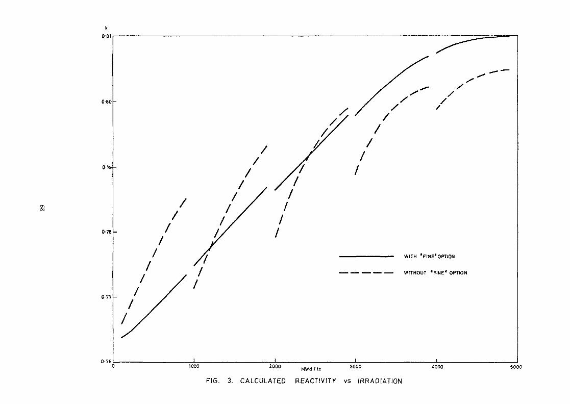
0-78 -

WITH "FINE* OPTION

—— —— —— —— —— WITHOUT "FINE* OPTION

0-77 -

0-761000 2000 3000MWd / te

FIG. 3. CALCULATED REACTIVITY vs IRRADIATION

4000 5000

1-7

AVERAGE PIN REPRESENTATION

DIFFERENTIAL PIN REPRESENTATION

•X-

Os

MULTIPLE PIN REPRESENTATION

4000

FIG. 4 POWER

8000 M W d / t e

PEAKING FACTOR

12000

vs IRRADIATION

16000 20000

4 -0 -

-jo

O MULTIPLE PIN REPRESENTATION

X DIFFERENTIAL PIN REPRESENTATION

4000

FIG. 5. U

8000 MWd / te 12000

235 CONCENTRATION vs IRRADIATION

16000

(PIN TYPE A)

20000

1-5

1-0

-To

o

0-5

"AVERAGE' PIN

— HIGHEST RATED PIN

— LOWEST RATED PIN

• O MULTIPLE PIN REPRESENTATION

•X DIFFERENTIAL PIN REPRESENTATION

4000

FIG. 6. Pu

eooo MWd/te 12000 16000 20000

239 CONCENTRATION vs IRRADIATION (PIN TYPE A)

A METHOD TO CALCULATE FLUX DISTRIBUTIONIN REACTOR SYSTEMS CONTAINING MATERIALSWITH GRAIN STRUCTURE

J. STEPANEKSwiss Federal Institute for Reactor Research,Wurenlingen, Switzerland

ABSTRACT

A method is proposed to compute the neutron flux spatial distri-bution in slab, spherical or cylindrical systems containing zoneswith close grain structure of material. Several different typesof equally distributpd particles embedded in the matrix materialare allowed in one or more zones. The multi-energy group struc-ture of the flux is considered.

The collision probability method is used to compute the fluxesin the grains and in an "effective" part of the matrix material.Then the overall structure of the flux distribution in the zoneswith homogenized materials is determined using the DPN "surfaceflux" method (JH . Both computations are connected using the ba-lance equation during the outer iterations.

The proposed method is written in the code SURCU-DH.

Two testcases are computed and discussed. One testcase is thecomputation of the eigenvalue in simplified slab geometry ofan LWR container of one zone with boral grains equally distri-buted in an aluminium matrix. The second is the computation ofthe eigenvalue in spherical geometry of the HTR pebble-bed cellwith spherical particles embedded in a graphite matrix. The re-sults are compared to those obtained by repeated use of theWINS Code (2).

1. INTRODUCTION

Several authors (_3) - (10) have developed methods in which thegrain structure of reactor materials was considered during theresonance computation or during computation of neutron fluxesin the thermal range. Unfortunately in each of these methodsdifferent approximations were involved.

73

So in Lane, Nordheim and Sampson (_3) the grain structure of fuelelements is considered during the resolved resonance computationderiving the modified Dancoff factor for the mutual shieldingof the grains. Only assymptotical flux is considered in the ma-trix material.

Doub (_4) has extended the Case at al. (11) method developed fora purely absorbing grain in an infinite scattering medium forthe case of purely absorbing grains closely spaced in a scatte-ring material. Dyos and Pomraning (_5) have developed theirmethod for cases where the ratio of scattering to total crosssections of grains is small. They neglect also the mutual shiel-ding of grains. The method was particularly suited for the cal-culations at thermal energies.

Adir (7] proposed a method for calculating resolved - region re-sonance absorption for fuel with equally distributed grain struc-ture, in which all microscopic cross- sections entering the Pdownscattering equation in the cylindrical cell are replaced byan effective cross section. This is determined by considering thateach grain builds with the matrix material a small spherical two re-gion microcell. The flux ratio in the microcell was determinedsimply by equating it to the escape collision probability, for apurely absorbing grain corrected for multiple scattering. Thismethod is programmed in the CAROL ( 12) code.

Askew and Carpenter (13)considered the naked grains and neglectedthe flux pertubation near the grains in the matrix material.

In contrast to the assumption of naked grains made by all authorsbefore, Teuchert et al. have considered overcoated particalsrandomly distributed in the matrix material.

In the range of the resolved resonances, they derived the conec-ted Dancoff factor for overcoated grains in the lattice of cy-lindrical fuel elements or in pebble-bed and neglect the fluxdepression near the grains in the matrix material (8.)» (9 ).

In the thermal energy range their method is based on the accuratenumerical computation of the penetration probability for a neu-tron traversing the coated particles (1.4) .Then comparing it to the related penetration probability for anhomogenized medium, the homogenized cross sections are derived.

74

2. COMPUTATION OF FLUXES IN GRAINS

One divides the slab, spherical or cylindrical macrosystem intoK spatial zones and considers that in the k-th zone (see Fig. 1 and2) NC different types of spherical particles with radius r . andvolumic ratio (effective volume of particles j to volume of zonek) VR. in an homogeneous matrix material are embedded.

One considers also that in the zone k, there are very many dis-tributed particles, so that the flux distribution within theparticles can be computed separately in each type of particleby the microcell method.

The effective moderator volume Vmj of each microcell is givenfrom the rest of the volume V of zone k by volumic ratio VR..

J

Then V is

Vmj = Vm VR.,J

where the total volume of the moderator in zone k isNC1

mV = V f-/ VR.) .

The outer radius of the microcell j is

r = JL VP^ + Vm^mj " 4ir

The flux in the microcell is given by the differential form ofthe transport equation

Et(r) »<r.fl) - q(r.fl) -

where <Hr,ft) is the neutron angular flux, q(r,ft) is the volumeangular source, £,(r) is the total macroscopic cross section.

tOne considers now only the isotropic form of the angular fluxwithin the microcell:

75

q ( r )

( 2 . 2 )

( 2 . 3 )

and dfi = 2ir s i n < J > d < J > .

The volumic source moments are

q(r) = Q(r) + Z (r) <J> (r), (2.4)^ sowhere Q(r) is the given volumic source moment which also in-cludes the contributions of other energy groups and the fissionsource. Z is the macroscopic isotrapic scattering cross sec-tion.In the following, one considers that each microcell has twozones, the particle and an effective part of moderator and thatthe flux is constant within each zone:

(2.5)

where

(2.6)I IV

and the volumic spatial source is given by

q - 0 + ESQ $. (2.7)

In Eq. (2.7) and also in the following, one considers the constantcross sections within each zone of the microcell.

76

Integrating Eq. [2.1) over fl and using the definition [2.3) onegets

r2 2 $(r) - r2q[r) - -^ (r2(J1(r) - J2(r))) , (2.8)

1 2where tho incoming and outgoing currents 3 and J (see Fig.3and 4) are

ir/2A _

3 (r) - 2ir / d<j) s in<J> cosij) $ ( r , f i ) ,o

and [ 2 .9 )

2 ir3 (r) = 2ir / d<J> s in<j) cosij) $ ( r , f J ) .

TT/2

Integrating now Eq. [2.6) over each of the microcell zones andusing Eqs. [5) and (6) one gets

ZPJ VPJ $PJ = VPJ qPJ . SPJ (JiPj .and

zmj ymj $mj m ymj mj + spj (^pj _

where p and m signifies particles and its moderator, resp. and jsignifies the type of the particle Vpj, Vmj, Spj and Smj arethe volumes and surfaces resp. of the particle and its moderator.J 1 pJ, J2pj, 31mj and J2mJ are the currents on the surfaces SpJand Smj (see Fig. 4).

The currents SpJ (J1pj - 32pj) and Smj U1mj - J2mj) are com-puted using the integral form of the transport equation. Whichhas the form

-T(r.r') _ -T(r,rg)ds q(r',5) e + $(r,-,,fi) e , (2.12)

77

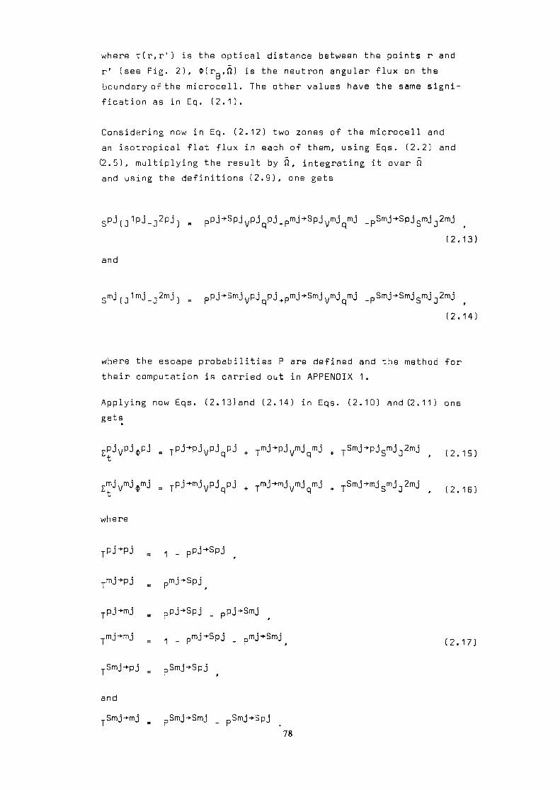
where f(r,r') is the optical distance between the points r andr' (see Fig. 2), *(rD,0) is the neutron angular flux on theDboundary of the microcell. The other values have the same signi-fication as in Eq. (2.1).

Considering now in Eq. (2.12) two zones of the microcell andan isotropical flat flux in each of them, using Eqs. (2.2) and(2.5), multiplying the result by fl, integrating it over ftand using the definitions (2.9), one gets

ypj PJ_pmj-*-SpJvmj mj _pSmj-»-SpJsmj.]2mj(2.13)

and

pp j-

(2.14)

where the escape probabilities P are defined and the method fortheir computation is carried out in APPENDIX 1.

Applying now Eqs. (2.13)and (2.14) in Eqs. (2.10) and (2. 11) onegets

where

TPJ+PJvPJqPJ +

Tmj->-pj

= ppj+Spj _ ppj->Smj

= 1 _ pmj^Spj _ pmj-»Smj^ (2 .17 )

= pSmj-»-Spj

and

TSmj->-mj m pSmj-t-Smj _ pSmj-*-Spj

78

The system of equations (2.15] and (2. 16) involve 2 NC equationsfor 3 NC unknowns. It will be therefore connected with the fallow-ing additional conditions:

andNC

, (QmJ=Qm) , j - 1, NC,

(VPVJ +

(2. 18]

(2.19)

where V$ is the integral "macroscopic" flux in the handled zone,which is solved by the "surface flux" method (^U . In Chapter 3,where the method to solve the resulting tranpsort matrices ofthis method is described for zone i:

,mm n

Eliminating J2^and (2.17) thengets

and q from Eq. (2.15) using Eqs. (2.16)using Eq. (2.18) and (2. 20) in Eqs. (2. 19) one

VPJ$PJ = W^VV * WPJVPJQPJ «- (2.20)

and

mj

NC . . .(wPJvPJgPJ t w^ (2.21)

where

mNC

IJ-1

mj

and

.J

79

where

CJ so

and. TSmj-*SpjpJ = j________

-j-Smj+Smj '

3. SOLUTION OF THE RESULTING MATRICES

The DPN "surface flux" method (_1_) used to compute the distribu-tion of the fluxes in the homogenized macrozones (see Fig. 1 or2) approximate the fluxes in each zone by Legendre polynomialswhereas the incoming and the outgoing surface fluxes are appro-ximated by double P.. Legendre or spherical polynomials. It re-sults in two types of coupled equation systems, one for outgoingDPN surface flux moments (see Fig. 5):

N n12 V V( Si2i1 i1 si2o2 o2 \

C D , = / / P i i i < PM-nm L-t L-i \ mm n + n n-n rn + n n-n mm n + n n-n Y n-n'n=o n'=o 'L n M-(n+n')/2Z V^ V^ Mi.2 yi -i

/, / . Pmm'nn'v nn'v 'n = o n '_ o , 1 v»o

(3.1)N n

o1 a V^ Y^/p30111 m11 + so1o2 o2 \ +mm' / . _/___,rmm'n + n ' n-n ' n+n'n-n' mm'n + n ' n-n n + n ' n-n') +n=o n'=o 'L n M-(n+n')/2

Z V~* V^ v°1 ui r,iZ, L Pmm'nn'v V Qnn'v •

n»o n'a,1 v=o

80

and one for the spatial flux moments:N n

cpi1 + wsio2 m°2 Nmm' yn + n ' n-n ' Yn + n ' n-n ' mm'yn+n ' n-n ' 9n + n ' n-n)'nao n =oL n M-(n+n')/2

I X I mm unn v nn'v 'n=o n'*o,1 v*o

whereV1 is the volume of the i-th zone,$1 . is the spatial flux moment in the i-th zone,mm'y p

(m,m'), (n,n') denote the angular moment in cylindrical geometry(for slab and spherical geometry m',n' are omitted),

y, v denote the spatial moments,_,i1 i2 o1 , o2<P ,, <P • » <P , and cp ,nn nn nn nn

are the incoming and outgoing surface fluxes onthe inner (left) and on the outer (right) side ofthe zone i,

Q1 . is the given spatial source moment,nn'v K

pV, pS, Wv, Ws are the collision probabilities,N is the surface flux approximation,L is the neutron scattering approximationf

n is the spatial approximation.

In method (_1_) are now the equations (3.1) for each of the spatialintervals coupled together with albedo conditions on outer boun-daries (the reflective and "grey" condition are considered) andthe resulting system of equations (see Fig. 5) is solved directly.

Then the derived equations for all DPN surface flux momentsare used in Tqs. (3.2) and tho system of equations for spatialflux moments in the dependence on the outer sources for eachenergy group is reached. So the direct solution is performed be-fore the multienergy flux computation in the outer iteration pro-cess.

81

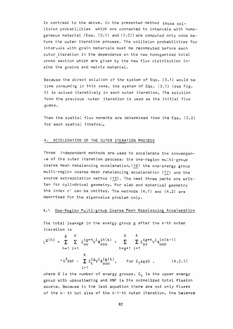
In contrast to the above, in the presented method those col-lision probabilities which are connected to intervals with homo-geneous material (Eqs. (3.1) and (3.2)) are computed only once be-fore the outer iteration process. The collision probabilities forintervals with grain materials must be recomputed before eachouter iteration in the dependence on the new homogenized totalcross section which are given by the new flux distribution in-side the grains and matrix material.

Because the direct solution of the system of Eqs. (3.1) would betime consuming in this case, the system of Eqs. (3.1) (see Fig.5) is solved iteratively in each outer iteration. The solutionfrom the previous outer iteration is used as the initial fluxguess .

Then the spatial flux moments are determined from the Eqs. (3.2)for each spatial interval,

4. ACCELERATION OF THE OUTER ITERATION PROCESS

Three independent methods are used to accelerate the convergen-ce of the outer iteration process: the one-region multi-groupcoarse mesh rebalancing acceleration, (16) the one-energy groupmulti-region coarse mesh rebalancing acceleration (1_7) and thesource extrapolation method (15) . The next three parts are writ-ten for cylindrical geometry. For slab and spherical geometrythe index n' can be omitted. The methods (4.1) and (4.2) aredescribed for the eigenvalue problem only.

4. 1 One-Region Multi-group Coarse Mesh Rebalancing Acceleration

The total leakage in the energy group g after the k-th outeriteration is

g K G Kig(k] = T T Eig*h

vi«ih(k) + r y zig*hvVh(k~1)

** *" SO 000 ** SO 000h«1 i=1 h-g+1 i-1

K+ X g XNF - 2 V V 1 0 , fo r G g s G , ( 4 . 2 . 1 )

where G is the number of energy groups, G. is the upper energygroup with upscattering and XNF is the normalized total fissionsource. Because in the last equation there are not only fluxesof the k- th but also of the k-1~th outer iteration, the balance

82

equation is not fulfilled for the flux of the k~th iteration.K G K

Lg(k) + £ Eigvi$ig(k) = ^ £ Eig-hvi$ih(k) + XNp > (4i2<2]t ooo so ooo

1 = 1 h=1 1=1One corrects therefore the fluxes and leakage by wighting fac-tors X and introduces them into the equation (4.2.2). One gets

h-1 i = 1 h=g + 1 j=1G<]-1 K G K

XgXNF + Z I zii*V»ih(k) + ZXgZzig'"hVi«ih(kl. C4.2.3)

"• ' SO 000 SO OOO

where leakage L^ in Eq. (4.2.2) was replaced by its valuefrom Eq. (4.2.1) .

After the weighting factors X are computed using Eqs. (4.2.3),one corrects the fluxes and currents by

mm'y mm'y *

,ixg(k)* ,ixg(k)YgU . J I A •mm mm

and the new eigenvalue is computed from

G KA C k ]* = I Z (v£f)1SV:V^k)* / XNF .

g-1 i«i

The method is applied only after the first outer iteration.

4.2 One-Group Multi-Region Coarse Mesh Rebalancing Acceleration

The coarse mesh method of acceleration described in (14) is usedafter each outer iteration in cases where G>1. In contrast to(1_7), the method is applied to each spatial mesh.

The basic balance equation for the mesh i can be written in theform

83

t 000 SO 000h=1

_3ii2g(k)oo oo

[4.3.1)

where i, g and k signify the mesh, energy group and number ofthe outer iteration, resp. Because in this equation occur notonly the values of the k-th iteration, but also the values ofthe (k-1)-thiteration, it is not satisfied for the k-th itera-tion.'We consider therefore that this will be satisfied for

(k) [ k)fluxes and currents of the k-th iteration $ and J if theyare corrected by the energy group independent weighting func-tion X. .i

One introduces therefore:

=nn'v ooo

= k) xi (4.3.2]nn' oo ' nn' oo '

(k)* ,ii1g(k) J-1 ,io2g(k)* ,io2g[k)I . - J A » J , * Jnn oo nn oo

into Eq. [4.3.1) and summates the result over all energy groups,One gets

X1 - . . .1 .. ( F i x 1 - ^ - ^ / - ) . (4.3.3)

G" a ooo

g-1

G:1 - I (vZfj

g-1

84

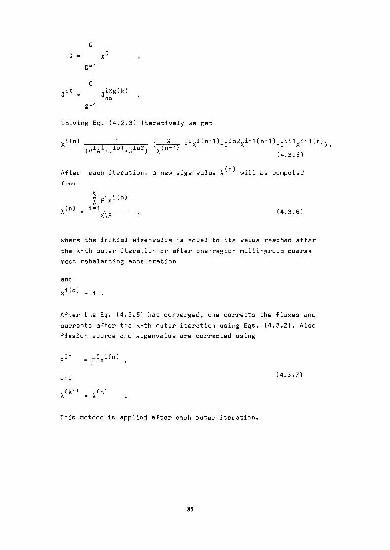
g-1G

-iX ,iXg(k)sJ 3 U •OQg-1Solving Eq. (4.2.3) iteratively we get

y 11 n J ______1 __ t__ G_ — iyiln~1J -j.ui.yj.' i t, 11 \ j .. j(vVo1".;,"'2) »<"-" " ;4.3.5)After each iteration, a new eigenvalue A will be computedfrom

I FixiCn)3.3.

where the initial eigenvalue is equal to its value reached afterthe k-th outer iteration or after one-region multi-group coarsemesh rebalancing acceleration

andxlCo:i - 1 .After the Eq, (4.3.5) has converged, one corrects the fluxes andcurrents after the k-th outer iteration using Eqs. (4.3.2). Alsofission source and eigenvalue are corrected using

,(k)* .Cn)A * A

This method is applied after each outer iteration.

85

4.3 Source Extrapolation Method

The total isotropic source moments (ooo) ar defined by:

1 = F1 + U1ooo ooo ooo

whereG

g=1and G G

V2,g=1 g'=g+1

Uooo= / / "8o

where i signifies the mesh, g and s' signify the energy groups,G is the number of energy groups and

•tCHI => Xg

where x is fission spectrum.After a few outer iterations, the source i|> will be extrapolatedusing the formula

i(k)* m i(k) + 0(k)/ i(k) i(k-1rooo rooo V ooo yooo

where i(j* is the extrapolated source, k is the number of the outer(k)iteration and 9 is the extrapolation factor. It is derived

after each outer iteration using the method described in (15]or in (_1_) .

The flux spatial moments are in each group extrapolated usingthe formula:

Also the outgoing current moments for each mesh and group areextrapolated using the formula:

ixtkj* ,Jnn' ' " .ilk) nn''J'aoo

86

The extrapolated eigenvalue is given byG K

A C K 1* = I I ^Vigvi$k)* / XNF 'g=1 k=1

5. TFSFCASrS

Probelm No. 1

k. Calculation for LWR-Fuel Storage .Container

Simplified slab geometry with reflective boundary conditions onboth sides, linear anisotropy of scattering, 217 energy groups(91 epithermal, 126 thermal)

In Boral are B.C spherical particles embedded in matrix radius ofB.C particals is 0.03375 cm volumic ratio V0 r/V0 . is 0.343964 840 Boral

Geometry

( _ I

0)D1-

B.75

oCM

X

0.425

0to.iCOCO

0.1

(-H(D

OCD

0.48

ocoiCOCO

0.3

aCM

X

1.47

Dimension in [cm]

Atomic .Densi t ies

Fue l :

H - 0.37125E-1

0 - 0.33283E-1

Zr - 0 .47318E-2

Fe - 0 .63966E-4

U235- 0.28313E-3

U238- 0 .70773E-2

[nuc l . /ba rn* cm"]H0

SS-3D4;FeNiCrMn

Borali

B4C: B1 Q

B11C

Al mat r ix ;Al

0.66751E-1 [nucl./barn.cm]0.33376E-1

0.60354E-1 [nucL/barn-cml0.83568E-20.16714E-10.175B3E-2

- 0.21890E-1 [nucl./barn-cm]

- 0.87558E-1- 0.17362E-1

- 0 .60494E-1 [nucl./barn-cm]

87

Problem No. 2

k ._ Calculation in HTR-Pebble-tbed Cell—eft————————————————————————————

Spherical geometry of cell with white boundary condition,217 energy groups [91 epithermal, 126 thermal]

Geometry

In the fuel zone the fuel particles are embedded in the carbonmatrix.

Radius of fuel particles is 0.02 cmVolumic ratio is: V ,. . , V n nparticle / fuel 0.0148 .

Atomic densitiesFuel:

Particles:0ThU233U235U238Pu239Pu240Pu241Pu242

- 0.431E-1- 0.121E-1- 0.211E-3- D.364E-3- 0.520E-2- 0.345E-4- 0.2B2E-4- 0.140E-4- 0.113E-4

(nucl./barn-cm)

Carbon matrix:

Moderator:

- 0.8758E-1

- 0.882BE-1

88

6. RESULTS

The 217 energy group ENDF-B/4 library was used for both the com-putation of the LWR container and for the computation of the HTRpebble-bed spherical cell.

This library contains 126 thermal and 91 epithermal energy groupsin the energy range from 0 to 3.059 eV and from 3.059 eV to14.92 MeV, resp. The epithermal groups were prepared by a GGC-4resonance computation. During this resonance computation thedouble heterogeneity of the HTR fuel was considered usingTeuchert's theory (J3), (£) .

Two computations were made, for the LWR container; on the firstwith homogenized fuel and the second considering the double hete-rogeneity in the multigroup computation.

Three computations were performed in the case of the HTR cell;the first with homogenized fuel, the second considering the doubleheterogeneity during the resonance computation and then homogeniz-ing the cross sections of the fuel for the multigroup computation,and the third in which the double heterogeneity was consideredduring the preparation of the epithermal cross section and alsoduring the multigroup computation by SURCU-DH.In the case of the LWR fuel storage container the fuel boralzone was subdivided into two intervals so that 8 zones compu-tations were performed. Because the boral particles are smallthe double heterogeneity was not very large. The convergenceof the used surface flux method is high. Already with a P~spatial approximation of the flux, one gets good accuracywithout any additional subdivisions of the zones into sub-intervals .

The HTR pebble-bed cell computation shows that also here thesurface flux method converges very fast, but the flux spatialdistribution is in this case very flat. The greatest contribu-tion to the double heterogeneity is caused by the considereddouble heterogeneity during the resonance computations bypreparing the epithermal multigroup cross section library. TheTeuchert's theory (_8) (_9) was used for this computation withthe resonance code GGC-4. In contrast to the above, contribu-tion effects of double heterogeneity during the multigroupcomputation is about 3 times smaller.

89

Making subdivisions of the fuel zones into the subintervals,one can consider different albedos on the outer boundaries ofthe micro cells in each of those intervals given by the balanceequations.

The SURCU-DH results are compared to the results obtained bythe WIMS code.

The code WIMS can compute a double heterogeneity calculationindirectly. It has only cylindrical geometry but sphericalgeometry can be simulated by making the radius of the centralabsorber zone equal to 2/3 of the radius of the central sphereand preserving the volume ratios of all materials. It was checkedby the code ANISN that the approximation of spherical geometryby cylindrical geometry causes a negligible error in the eigen-value. For a double heterogeneous lattice a microcell consistingof the fuel particle and a corresponding part of the graphitematrix is calculated first. The ratio of the mean fluxes in theparticle to the mean fluxes in the microcell gives particledisadvantage factors. The resonance cross sections are calcu-lated both for the heterogeneous and homogenized microcell andtheir ratios are calculated. The resonance cross sections forthe macrocell in which the fuel particles and the graphitematrix are homogenized are multiplied by these ratios. The soobtained double heterognnuous rfHsonnncn cross section and thedisadvantage factors are given as input for the final doubleheterogeneous macrocell.

The WIMS results are summarized in Table 3. In comparison tothe SURCU-DH results the eigenvalues of the homogenized caseare higher. This is caused probably by the different library.

Unfortunately the LWR SURCU-DH results could not be comparedto the WIMS results because the method used to consider thedouble heterogeneity by WIMS needs the fission sources insidethe microcell.

The? comparison to WINS is not representative because the samelibrary could not be used and also the method itself is onlyapproximate.

Because we had no possiblility to compare our results to otherexistent theories now, it will be presented later in another

90

paper. In future if our HTR PROTEUS experiments and somemeasurements on LWR fuel container will start the proposedmethod will be checked also by experimental results.

Very high efficiency of the DPN surface flux method used tocompute the macro-flux distribution is demonstrated in Fig. 6.The eigenvalue is computed for homogeneous slab of 10 mfp withvacuum boundaries using the surface flux method (SURCU], col-lision probability method (CP), SN theory (ANISN), S^ theory,and two dimensional diffusion method (CODIFF), transport S.,method (DOIT] and surface currents method (QP1).

Using the presented method (SURCU), the exact value is reachedalready for one interval and P3/P2 approximation of the surfaceflux and spatial flux distribution, resp. From a comparison withits P1/PO value or to the collision probability method (CP) onesees the importance of the higher Legendre polynomial approxi-mation of the spatial flux.

More discussions to this point and comparisons can be found in(_1_) where the efficiency of the surface flux method is shownfor spherical and cylindrical geometry also.

Acknowledgements

The author wishes to express his thanks to P. Koehler who hascontributed all WINS computations, prepared the LWR 217 grouplibrary and discussed the theory., to C. Higgs who has read themanuscript, and to K. Herda and C. Higgs for their collabora-tion in writing the code and to R. Chawla and S. Seth who haveprepared the H.TR 217 group library.

91

REFERENCES

1. J. Stepanek: The DPN "Surface Flux" Integral TransportMethod with General PN Polynomial Approximation, EIR Report[in printing] [1978) or A new Form of the "Surface Currents"Transport Method with GeneralPN Polynomial Flux Approxima-tion, TM-PH-669 (1977) (internal EIR Report)

2. J.R. Askew et al.: GBNES, p. 564 (Oct. 1966)

3. R.E. Lane, L.W. Nordheim and 3.B. Sampson: Nucl. Sci. andEng., 14, p. 390 (1962)

4. W.B. Doub: Naval Reactor Physics Handbook, A. Radkowsky,ed., I, USAEC, Washington DC, p. 537 (1964)

5. M.Y. Dyos and G.C. Pomraning: Nucl. Sci. and Eng., 25,p. B (1966)

6. G.L. Ragan: Trans. Am. Nucl. Soc., 10, p. 584 (1967)7. 3. Adir: Trans. Am. Nucl. Soc., 11 , p. 593 (1968)

8. E. Teuchert: Nucleonik, 11, p. 68 (1965)9. E. Teuchert and R. Breitbarth: Gul-551-RG (1963)

10. C. George, S. Jayl and W. Astley: Trans. Am. Nucl. Soc.,r\_, p. 439 (1968)

11. K.M. Case, F. de Hoffmann and G. Placzek: Introduction tothe Theory of Neutron Diffusion, I.

12. C.W. Stevens: GA-6637 (1965)

13. J.R..Askew and G.M. Carpenter: AEEW-M-236 (1969)14. U. Hansen and E. Teuchert: Nucl. Sci. and Eng., 44, p. 12

(1971)15. M.R. Wagner: GA-8307 (1968)

16. R.3.J. Stamrnler: Num. Reactor Calculations, IAEA Proceedings,Vienna (1972)

17. M.V. Gregory, H.C. Honeck: Nucl. Sci. and Eng., 61, p. 437(1976)

92

APPENDIX A

Computation of the escape probabilities P

The escape probabilities P are defined as fol lows:

pPJ+Spj _ 1P

pj+Smj = 1 (IEPJVPJ U1

mj

mj_ + - + -

4 1 2 3 6 7

where

I. = 2ir I du u e

o

r .

I_ = 2ir / du u eo

r .

I_ = 2ir / du u e

.PJ

V2

1/7. .mj pj

, 2 2 ,c = TT (r .-r . J ,6 mj pj

' (1*2V2

V2 . - .mj PJ

The integrals I., I_ and I_ are computed numerically using the

Caussian method of quadrature. About six points are used for an

accuracy of ^ 10~6 in all ranges of use.

93

PN

2

2

3

PL

1

pn0

\

2

KB

2

hornKeff

0.851013

0 . 912247

0.910033

. hetkeff

0.853124

0 . 913806

0 . 908276

. hornAk/k

0.00248

0.00171

0.00193

Tab. 1 LWR Fuel Storage ContainerSURCU-DH, 217 Energy Groups

P - Order of Surface flux approximationP. - Order of neutron scattering approximationP|v| - Order of spatial flux approximationKB - Number of subintervals in Boral zone

Numberof fuelzones

1

2

3

PN

2

2

3

2

2

PL

1

1

1

1

1

PM

0

1

2

0

1

0

1

Singlehet .

1.233179

1 . 2 2 8 3 1 5

1 . 2 3 1 4 0 3

1.233207

1.228476

1.233310

1.228930

Doublehet . Ix

1.279567

1.274522

1.277725

1.279628

1.274719

1.279731

1.275186

Ak/k. ham

0.03762

0.03762

0.03762

0.03764

0.03764

0 . 03764

0.03764

Doublehet ,2x

1.289570

1 .284038

1 .287913

1.292084

1.286831

1 .293852

1.2B9037

A k / Khom

0.04573

0 . D4536

0.04589

0.04774

0.04750

0.04909

0.04891

Tab. 2 HTR Pebble-bed CellSURCU-DH, 217 Energy Groups

;B _

Order of Surface flux approximationOrder of neutron scattering approximationOrder of spatial flux approximationNumber of subintervals in fuel zone

94

PL

pnKorr.

SN4

8

K

10

20

20

Single het.

1.252854

1.252856

1.252871

Double het.

1.285504

1 .285506

1 .285521

AK/KSH

0.02606

0 . 02606

0.02606

Tab. 3 HTR Pebble-bed CellWIMS, 36 Energy Groups

S - Order of S., approximationK. - Number of spatial intervals

0 1

©k-1 K-1 K

Fig. 1 Space distribution

Fig.2 Macrozones

95

Fig . 3 J2 Ha If spaces Fig . 4 Part icle j

o2 o2

12\>(2)

o2

11t > ( 3 ) '

o2f r ( 2 ) :

11<p12<t>m01

<P12

*C2)01

<f> ( 2)12

d> ( 3 )

01d> ( 3)o2

<(>( 3)

nmm ' n

4-001120001120001120001120001120001120001120GO1120

12 o1 12 o1 12 o1 o2

012010

012010

012010

012010

012010

012010

012010

012010

Q^Q*

n->-000n'

£*X EEEX

X

X

xx

xxxxXExXX

*s

XXXXXXXXXXXX

V-"000

EXXEXX

XXXX

Fig. 5 Surface F lux Transport Mat r ix( K = 3 , N = 1 , L = 0 , M = 0 ]

96

0.97

0.96-

0.95-

0.94-

0.93-

9.92-

0.91-

0.9

CODIFFSURCU P3/P2QP1+SURCU P2/P1

0.0 0.5 1.0 1.5 2.0 2.5

Mesh width (cm)

Fig.6 Critical Slab: Eigenvalues

97

APPROXIMATION THEORY AND HOMOGENIZATIONFOR NEUTRON TRANSPORT PROCESSES

M. BORYSIEWICZComputing Center Cyfronet,Institute of Nuclear Research,

,»

Swierk-Otwock, Poland

Abstract

In practical calculation of reactor systems homogeniaationis performed by some techniques mostly based on intuition andthere is no uniquely accepted approach to this problem.

In the first part paper an attempt is made to formulatemathematical basis of homogenization for the neutron diffusionand transport equations using recent developments in this field.The boundary volue problems for bpth equations for non smoothH — periodic coefficients are related to appropriate variationalproblems stated in terms of bilinear forms*

The behaviour of the solutins for H -* 0 is investigatedunder various assumptions coneerniny a limit process to getthe coefficients of homogenized equations*

In the second part of the paper the assymptotic equivalenceof the neutron diffusion to the transport eqution is studied.The relation betveen homogenization procedures for both equationsis also examined. As an example, the derivation of the equatinsof homogenization in the case of hexagonal geometry typical forV»V»E»R reactor is given* The obtained formulae for so calledeffective diffusion coefficient are analyzed for various typesof lattices,

1. IntroductionIn recent years many modern techniques solving boundary

value problem are developed on basis appropriate variationalformulations. This is usually done in terms of bilinearforms bounded in certain functions spaces. This techniqueeasily provides us with the so called a priori estimates,which imply the uniqueness of the weak solutions. At thesame time it is a convenient tool for investigation of theorder of convergence of various approximate methods solvingthe original boundary value problem.

99

In the paper M (and |2\ the theory of bilinear formssuitable for the neutron transport equation is developed.These bilinear forms are bounded with respect to both theirarguments, each of them belonging to an appropriate functionalspace. In general the spaces do not conicide. Moreover thesebilinear forms are not coercive in standard sense. Theauthors of \~ 1"\ and \ 2>. making use of the a priori estimates,L J >- _'found the convergence criteria for a wide class of projections!methods.

In the first part of the present paper the concepts ofr*T and 2 are developed such that they may be applied toanalysis of finite difference and hybrid method, the latterconcern nodal, response matrix or. local Green's functiontechniques.

In the second part of the paper the hotnogenization problemfor neutron transport equation is considered.

2. Weak solutions and approximate methods for 'the,equations related to the generalized coercivebilinear forms

Let B and L are two Hilbert spaces such that Sis a dense subsapce of L and

Thus we have

* *(2) 8 C L C 8 , IT Rul}54, ^ fluUL 6 Jc liu

where B is dual of B with the norm

(3) Hull.a

100

Consider the bilinear form CtC^iV) with the propertj

(4) t<U«*,v)S & C,

With the form 4X(u,v) we can associate thecontinuous linear operator A from B into L by therelation

(5)

The domain of A is given by:i there exists kw such that

We assume that X)C«"l)= B and A is one to onefrom B to L .To ensure this property it is sufficientto assume

(6)

The Eq {6} can be considered as a generalized coercivnesscondition for the form CL(,U,V) .

In similar way we can define the operator A by theform

(7) Ck*Cu.,v) *

_It can be proved that for each S € B there existsan unique solution of the variational problem.GVP. Find VIS L such that for each V6 B we have

(8) 0.(U,V) * (S,V).

101

Such a solution U& is called the weak solution of theequation:

(9) Au . S

Consider two families of the spaces L. and Si eW **1% & O^i il • WB define the approximate problem.AP Find U, 6 L. such that for each V. & B, we have— ft « t» K

(10) aCwj,,\) a (S,vThe set of assumptions concerning u^ and B,

relevant for further analysis we formulate asAssumption A.

£i) L» and B^ are dense in the limit in L.and B respectively.

(ii) There exists U6 O such that for U . U0the .projection "P, from L onto L,^ is also

*s» ibisection of L. onto L^ , whereVAX-

(iii) t s- lim \ > 0 , where

Under Assumption A for the problem AP we can prove thetheorem concerning the convergence of W. to the solutionU of -the problem GVP.The ode-em 1« There exists an unique solution of AP for each U t

The sequence {** converges weakly to the solution u*vof GVP. If moreover L^ » Ct then the sequence {^

converges in the norm of L • The rate of convergenceis determined by the best approximation of W by theelements of L •

102

Theorem 2. If(i) solution U of GVP belongs to B

(ii) L.J « S <C B(iii) condition (6) is satisfied

then the solution TJU of AP problems,are convergent in Lto ft

norm the solution -a of GYP. The rate of convergenceis given by

(11) Rw- & C i

where t£ is the solution of

a) <3L*(u,v5 s (S* v) , for each v 6 3 ,

with

We can consider more general case when S^, and L*are not subgpaces of S» and L respectively. That is wehave the situation

(12)

~>L

sv,V^W

The operator A^ is defined by the formsatisfying the properties {4) and (6) stated in terms ofthe spaces Bjj and L^ . The operators te , biand S^ and *k make the "correspondence" among theelements of B and Bi and. L and t-^ respectively

103

Under some additional compatability conditions for theoperators fc , '»,„ and S>^ , we can prove thegeneralizations of Theorems (l) and {2} , stating thecriteria of convergence in the norm of L. and i-^ spaces,Suppose now that C* (p# ,V, ) is of the form

(13)

Consider the approximate problem.AP" Find Vfc., 6 Lr such that for each V, 6 GK wehave

(H)

where the bilinear form £L u, V is definedby Eq (13)

Formulate the analogous of Assumption A.Assumption A*

(i) 5 1. and ^ S^ are dense in the limit in Land & respectively »

Cii) There exists UQ £ 0 such that for *^ & Uca projection from L onto s» L*. is also a

**j ** **

bisection of L{ onto

(ili) t « lira t^ > O ,

°104

Making i...e the technique developed in £l, ch.6] andch.4] we can prove the theorem.

Theorem 3. Under Assumption A* the results of Theorems 1 and2 can be extended to problem AP'; in paticular

/i) b U. converges weakly to the solution« «*U of GVP;

Arf <H» »^r ir*s

then

H-*0(iii) if u, 6 E , L^ » E^ and condition (6>

is fulfiled^then

vfe——v»

where w, is the solution of (llaj with

f*® U - fe U.

Theorems 1-2 form mathematical basis to analyze a certainclass of approximate methods solving GVP. This class includesthe promotional methods .therefore the finite element methods

| IT"1*with eoproximatirc spaces L^ and U^ satisfyinginteyelement continuity relations imposed by the propertiescf tine solutions to GVP, Theorem 3 is suitable to standardfinite difference approach to solve GVP. It should benoticed that one can considerably weaken the requirementof interelement continuity for the functions of 0-. and L*•i n

and still obtain a convergent method. One gets so callednonconforming methods. They are based on the extendedvariational formulation,often called hybrid one,in whichthe continuity constraints are removed in the expense ofintroducing nev> terms in the bilinear form. In the following•we formulate the hybrid method related to the bilinear

105

forms satisfying Eqs (4) and (6 in suitable functionalspaces*

Suppose we have three Hilbert spaces 3 , L and MLet the bilinear form &.($&, V) satisfy the conditionsanalogous to (4) and (.6) * Let finally (y*/*-) bea bilinear form on L U M such that the quantity\\ft-\\ „ given by the equation:

(17)

is norm on •We define the variational problem.

HVP For given linear forms £(v) andcontinuous on j& and H respectively find a pairsuch that for any v. £ B^M we have

In similar manner we introduce the approximate problemHAP in terms of approximate forms S.^ (u^ , V. ) , £, (V, ) f

^ continuous oni . i - j j' ' and resPec'fci'veli'« w^ assume

that the spaces E, , L^ and H^ are dense in thelimit in the corresponding spaces E , L and M .

Following the reasoning of [l, en. 3] and fe chap.l] viecan prove the existence and uniqueness of the pair(u,X) € L X M which solves HVP. If ffv}= (S(\i)with S 6 L then the solution ("«, X) belongs toB X H • The similar statement xs valid for a pair

being a solution of fi&P,

106

How we estimate the error bounds for [|u.U. jj—and ii^~^K^M * To do *kat WQ f*18* definesets V« and V,

(18)

If 0*V \) 6 ( &v M^) is a solution of HAPthen U. solves the problemHAP'Pind tJ. £ V, such that for any V, £V>

« «4 **

Lemma 1« Sufficient conditions for the existence o£) 6 B^ ** M^ - the unique solution

of HAP-are:(i) 1^*\(ii) the form C tV ) satisfies Eqs (4)

and/19\

(iii) on Hi , where

The proof of the lemma can based on that given in., chap. ll modified approprietly to take into account

the generalized coercivness condition (6) .Theorem 4« Suppose that the assumptions of Lemma 1 arefulfiled, then there exists a unique solution 1* 6 &^of HAP.' The error Ittt-W^lf^ , where tt is thesolution of HVP, can be estimated as follows:

107

+ SU).

(20)

The proof of The o:.- era 4.Prom the aefinitioas of E.VP and HAP 'we have

(20a)

Vttth the assumptions (4) and (.6) we obtain

Since

(22) U V -

and

108

then from Eq_ (20) we get Theorem 4»Theorem fi. We assume that the conditions of Lemma 1

are fulfiled. Then there exists a unique solutionof HAP. Besides of estimation of ||W-Ui ||— statedin Theorem 4 we have for

V

(24)

The statement of the theorem follows from the estimationof the following expression

(25)

when Eq (19) is taken into account.The error "bounds for H^-t&uif0- *n Theorems'4 and

fortiori that of Theorem 5 for H^uX^M involve thequantity

(261

109

with \ 6 V^In practice to estimate H'') we must know interpolation1 •««•properties of V» with respect to a subset of B whichwthe solution "W belongs to. The following theorem permitsus to avoid such an inconvenienceTheorem 6. Under the assumptions of Lemma 1 we have

iaf V|>(VK) £- ivkf vj/(vu) *V\

t

{2?) ) .}

To prove th« theorem we first examine the solution ofthe problem: Por fixed \*B, find

such that

awd(28)

where (. / y^ is the scalar product in 8oThere exists a unique solution Zr of Eq (28) . Thesolution ia the projection of Vi on Vi •Prom Eq (28) we get

(29)

no

where p. is a positive constant.* tft

On the other hand the same equation implies

(30) BVMThus we can write

Prom Eqs (29) and (31) we obtain

t

The following decomposition of

(33) W.2K 8

combined with the identity

Ill

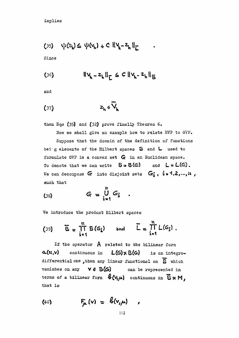
implies

(35)

Since

(36)

and

(37)

then Eqs (35) and (32) prove finally Theorem 6.How vie shall give an example how to relate HVP to GVP.Suppose that the domain of the definition of functions

bei~ g elements of the Hilbert spaces S and t- used toformulate GVP is a convex set Gp in an Euclidean space.To denote that we can write Bs»B(<5?) and LWe can decompose dr into disjoint sets G-j , i«^such that

(38) ^a L a TT

If the operator A related to the bilinear form,v) continuous in L(<?}>1 E(<») is an integro

diff erential one ,then any linear functional on B whichvanishes on any V € B(JS) can be represented interms of a bilinear form v(V/yiA.) continuous in UxMthat is

(40) 5112

where M is a suitably chosen Hilbert space of functionsdefined on , r; . where f is boundary of* *In this case the hybrid variational problem HVP whoseunique solution is also the solution of GVP can be definedby means of the forms 4-(V S.) and O.{u,v) ,where

(41) a(*,v) s

The formal definition of <X (tt,v) inis the same as the form C^Myv) of GVP in

3. Homogenization for neutron transport equation

Before we study the homogenization problem let us firstintroduce definitions useful for further analysis of theneutron transport equation.

We consider a subset & of the six dimensional Euclideanspace E . A point X of fi will be represented by a triple:X =(*", *,£*• ) > where £ is a point of a convex set G+in £ , 9- belongs to an interval £0, OL y , and Jnu isa point of the unit sphere <•»• in E » Th'e symbols canbe interpreted as follows. The point f is a position S^

<* •*where the neutron processes- occur., i>* 9" A. denotes theAneutron velocity and ^Jf is the maximal neutron energy.

Define the set 7TA to be an 'orthogonal projection of &0on a plane perpendicular to -A. and^ situated outside of <SP „

•* •* «wV/ith a fixed jv t ««> and /»fw £ 71* we associate the sets:•M. **.

n (42)

113

The values of •* corresponding to left and right end pointof the interval K(f*,*t) will be'denoted by *4( » , •** )and •*«'(/r » &) respectively. The collection of all thepoints d. and £_ induce the sets 9fi^ and 0 & — ,where

(43)and

How we consider the problem of neutron transport. Thedensity of neutrons TJ> (ff, *>, jt ) in (a due to adestributed neutron source ^{ffliylSi\ is a solution of theneutron transport equation

(44)

with the boundary condition

*.»,.«) •*(?.».•*) "ft (3- "I"*) 145)

The symbols in Eq. (44) are defined as follows:

> (46)(47)

(47 a)< ?(*.»;£')where St (#,!>) and K ( , a, (r* jSL • .&' ) havestandard meaning.

114

We donete by LJ (.X) , t»0,4,&,... ,the spaces of functions defined and summable with the power p

we

if X* G , and by the symbols , and , for

and weight O-^ on a set X • By the symbol (Ll) (X)shall understand the space dual to Lp (X) • The dual

product on Lp \Xf X (L.1 (X)) we be denoted by ( , A

and X* VS.. respectively,(V be the subspace of L.p(G) consisting of

functions if/ such that

f (i) Y« L;(G>« i/J'cs)(ii) for almost all fr± f Jfl > •*!,<«* ,

ifCJJ^, tiL)« y is absolutely continuous o

(48)

(iii) Ty € LJ (ft) for all ^ , ^ and

l>* satisfying (ii}

(. £ ^ A ) * ^ ^* exists, and belongs

to 'The properties of B_ have been extensively studied

in £lj • In CO and £2j it is proved that the operator

A« (T + 0'<2J ~ K / x is bisection

from ftp onto L. == L?^(Gt) X L* ( 96.. ) provided

zero does not belong to the spectrum of A ST+ 1^2 *"K

Moreover we have

IA"*I. . 4 c <

Similar conclusions are valid for the operatorA*

115

In the theorems ensuring (48 ) presented in Ll3 and £singular slowing down kernels and V 9 «o were admitted

rt

Define the form d( 11.14) bilinear on L-X B by1 ' ' P-* *the formula

(50)

where <U- s •

Take { < ? , £ { £ R» then by the results of £ 1 J there

exists a unique solution £ *»f / 1f{, J of G V P defined

by Eq. ( 8 ) and

where O is the constant of Eq. ( 49} . If £ <J f H Ithen

(52)

It should be noted that aftt^) defined by Eq. ( 50 )

is coercive in L. s Lt C^*) * L*if the following condition is .satisfied

Similar results are valid for the 6VP related to the

form

C54

116

with <**Thus finaly vs/e have provided a link between the theory

developed in Chap. 2 and the boundary valueproblem for the neutron transport equation.

Consider a family of forms OtH(tC,-w} defined byEq. (5o) with the cross section £ z Sto and the kernel of

f

K « K w depending on a parameter H^ 0 ° We assumeEq. (53) is valid with y such that

« r, > o . (55)We shall denote by Oto (**,«/) the bilinear form definedin terms of £c and K^ being limits of <*H and KMfor H"* 0 . How we formulate two theorems relating thesolution of two follovdng variational problems.

The problem SVP. .w9

Por given £„«{$„, %„find <1Hsuch that for any 0> C ft* B- v)e have

aH (<*„,*)* (*M, *)L (56)and the problem

Por given 5"p * t-« find *p* '-j. such that for anywe have

(57)

117

Theorem 7 Assume

IISH-Sjlt(ip38 0 ,

(ii) there exist an operator Jf and an integer suchthat (T P)* » <fi > «n_ is compact from L. into-B ( 6 ) and

» €L*(S) (58)then

The proof of the theorem is based on the observations.Since /I £,-5.11 -rrr£ £? therefore (I £H II, is•» ^ •» I H W v *&•-* . . "uniformly bounded. Using Eq. 152) we see that the solution

s { VM > *yr } of SVPH fulfil the conditions

4(60)

v?here and do not depend on H- -Thus we may select a sequence H£"^V such that 41 —> 44**lweakly in Ba Jf Lj C ^ ^ + ) .Let us recall well known lemma.Lemma 2, Let -U{ ~> -a* strongly in X ,weakly in X then ( J, ) —— > ( *t , -W

Making use of Lemma 2 we can easily prove that <* * "** * ,where .t* is the solution of &VP . Prom the definitionsof &VP and (SiVP, it follows

118

Take

Prom the assumption (ii) of Theorem 6 if follows: 4J — * 0strongly in L.^ (j& ) o Therefore all the terms on the lefthand side of Eq» (61 | tend to zero, which by Eq. (58) proves:

If we put in Eq0- (6l) +J * J, - f and make use of Eq0 (63)then get

which completg the proof of Theorem 7«Theorem 8 Suppose that

Z0 êakînLweakly in I

i) for any <P 6 L* C^} we have

....with the operator P bounded in L £ v VJ such that

« T and the set*? * îs compact in L*then '« - .where ^ and * are thesolutions of CVT^ and vVTp respectively*Pirst we notice that for any &•* 0 the solutions ^^ of£Vt?n are" unif ormaly bound^dlin «^fcTherefore there exists a sequence HA** Q sucb tha'fc

119

*iy «•» ***/TH- converges weakly in jj. to an element *|> y-Thus to prove the theorem it is sufficient to show that

It is easy to deraonstrake that the solution of Mn for

&M * X^H t*lni £ ^a,- satisfies the

equation

where the operator

~

A

is bounded bisection from L^ ' *'/ onto ^_ ; *£

is an element of \. 9 C ^^ uniquely determined by*r

and ^R .Define

(67)

Prom Eq. f 65 J we get

Nii 1 of Theorem 8 (fl

strongly in L« C^) , For any M£ L« C€T] we have

M :(69

120

which by Lemma 2 implies

Therefore(70)

and the proof of Theorem 8 is completed.It is easy to show that in the case of multigroup approximationand isotropie scattering the operator P in Theorem 7 and 8can be taken to be of the form

It seens to be safe to state, that no stronger resultsconcerning the convergence of solutions of &V r.^ to & V i^could not be obtained.

Both Theorems 7 and 8 along with the results of Chap. 2on estimation of various approximate methods solving theboundary problems could form a basis for the analysis of thehomogenization pro.blem for the neutron transport equation,

References1. M« Borysiewicz, R» Stankievd.cz , Weak Solution to the Transport

Equation and Approximate Methods, accepted for publicationin Jour* Math. Anal. Appl.

2. M. Borysievd.cz, R. Stankievdcz, Variational Formulation andPromotional Methods for the Second Order Transport Equation,ibidem.

3. Jo P. Aubin, Approximation des Espaces de Distributions et desOperateurs Differentials, Bull. Soc. Math. Prance, Memoire 12,1967.

4. J.M. Thomas, Sur 1 'Analyse Humerique des Methods d 'ElementsPinis By brides et Mixtes. These Universite Pierre et MarieCurie, Paris, 1977.

121

THE EFFECTS OF SUBASSEMBLY HETEROGENEITYAND MATERIAL BOUNDARIES ON THESODIUM VOIDINGAND DOPPLER EFFECTSIN A SODIUM COOLED FAST REACTOR

A.T.D. RUTLANDUnited Kingdom Atomic Energy Authority,Atomic Energy Establishment, Winfrith,Dorchester, Dorset, United Kingdom

Abstract

This paper outlines the procedures currently available in the UK for thegeneration of group constants to be used in the three main areas of fastreactor work - analysis and design of zero energy experiments, design ofcommercial fast power reactors and operation of fast power reactors; somebrief comments on methods validation are made. The paper then describesaspects of the application of these methods to the analysis of the SEFORDoppler experiments and the calculation of the Doppler and sodium voideffects in the currently proposed UK commercial fast power reactor ofconventional design. An investigation of whole reactor shielding effectsand material boundary effects is carried out. Calculations of subassemblyheterogeneity effects are described, including fuel pin resonance heterogeneityand flux fine structure, the latter including the effect of the subassemblywrapper. Work reported elsewhere is used to calculate the magnitude of theneutron streaming correction to the Doppler and sodium void effects.

1. INTRODUCTION

This paper outlines the procedures currently used in the UK for thegeneration of group constants to be used in the three main areas of fastreactor work - analysis and design of zero energy experiments, design ofcommercial fast power reactors, operation of fast power reactors. Somebrief comments on the validation of these procedures are made, althoughalready published material provide more detailed statements (1). The paperthen describes the application of these methods to the SEFOE (2) Dopplerexperiments and the Doppler and sodium void effects in the currently proposedUK commercial fast power reactor (1300 MW(E)) of conventional core design,generally known as the Commercial Demonstration Fast Reactor (CDFR), payingparticular attention to heterogeneity and material boundary effects.

2. HOMOGENISATION METHODS USED FOR UK FAST REACTOR WORK

Two main methods are used for the preparation of macroscopic groupconstants for reactor calculations. The first involves a simple numberdensity smear over subassembly regions or whole reactor zones, e.g. theinner core, the resulting smeared composition being used to prepare groupconstants from the FD5 (3) broad group (-J lethargy width) cross sectionlibrary, which treats resonance shielding using a shielding factor formulism.Smears over whole reactor zones are used for conceptual studies whilst smearsover subassembly dimensions are used to follow detailed burn-up histories,e.g. for the UK Prototype Fast Reactor.

The second method involves the use of multi-region cell calculationsto prepare broad group constants for use in whole reactor calculations. Thecell calculations are performed using the computer code MURAL (4,5) and theFGL5 (3) 2240 energy group (1/128 lethargy width) cross-section library.Certain types of cell can be treated using the linked computer codes MURALand PIJ (6). This second method is used in the analysis of Zebra (7)

123

experiments, in the investigation of special effects and in both thevalidation of the first method and the recommendation of any adjustment factorsrequired with it. Resonance shielding is treated in FGL5 by the use of alarge number of energy groups to describe resonances, supplemented by asub-group formulism with up to 50 sub-groups in certain FGL5 fine groups.

Details of the MURAL and PIJ codes are given below.

2.1 THE CODE MURALB

The code MURAL (4,5) will solve the one dimensional collisionprobability form of the multi-group neutron transport equation or the neutrondiffusion equation in many fine energy groups (with subgroups) and in amoderate number of spatial regions. Cylindrical, slab and spherical geometryoptions are available. Both cell and whole reactor calculations are possible.The latter are used to investigate special effects as described later.

The transport or diffusion equation is solved using simple sourceiteration. Firstly a converged solution is obtained in broad groups usingthe broad group library so producing a source, and optionally a criticalbuckling, for use in the fine group source calculation. The converged finegroup flux is used to condense the fine group cross-sections down to thebroad group library structure, those broad group constants are then used tosolve the broad group equations. The multiplication produced by this secondbroad group treatment is then compared with that produced by the fine grouppass, and if the difference is unacceptably large the fine group pass isrepeated with more accurate values of the spatial source (and, optionally,buckling) derived from the second broad group solution. Since the FD5/FGL5libraries are well matched for most fast reactor problems more than onefine group pass is not normally required.

The final cell averaged broad group cross-sections are used as thegroup constant data for whole reactor calculations.

Spectral transients near boundaries can be treated using whole reactor.MURAL calculations or by means of energy dependent bucklings in MURAL cellcalculations, the bucklings having been derived from homogeneous region wholereactor calculations. Spectral transients can be important at core-breederinterfaces, particularly when the breeder region cells are markedlyheterogeneous, or when a moderating or steel or nickel reflector is adjoiningthe core.

For the treatment of streaming effects in pin and plate geometry othercodes are used, although there is an option in MURAL to calculate anisotropicdiffusion coefficients in plate geometry cells. The treatment of theseeffects is described in Reference 8.

Further developments are required to treat some two dimensional aspectsof plate geometry cells. The currently adopted one dimensional representationinvolves a smearing of the composition which could lead to an underestimationof some fine structure effects, particularly at high energies. This isillustrated by results reported in Reference k.2.2 THE CODE PIJ

The PIJ (6) module was originally developed for thermal reactor studies,but has since been linked to the MURAL code as an optional replacement forthe MURAL routines used for the evaluation of collision probabilities. ThePIJ code evaluates first flight collision probabilities in a number ofenergy groups for systems contained within a cylindrical outer boundary andinfinite in the axial direction. Within the outer boundary the system maybe divided into annuli by concentric circles based on the origin and eachannulus may be independently divided into sectors. Onto this system dividedradially and azimuthally may be superimposed fairly general arrays of rods,themselves divided radially and azimuthally about their own centres; theazimuthal division may be different for each rod. Various symmetry optionsare available to reduce the calculational complexity and fairly generalboundary conditions, applied to pre-specified sectors of the outer surface,are available.

124

In fast reactor calculations MURAL is used to generate broad groupcross-sections using a simplified model of the cell. These cross-sectionsare then used by PIJ to calculate collision probabilities for a moredetailed cell model, which are in turn used by MURALB to solve the transportequation in broad groups to produce cell averaged group constants for usein whole reactor calculations. An example of the use of the MURAL/PIJtreatment is given below as part of the calculation of the heterogeneityeffects in the SEFOR Doppler experiments. The use of the method to treatcontrol rod fine structure effects has been described in Reference 9-2.3 METHODS VALIDATION

The techniques described above have been tested by their use in theprediction of experiments performed in the Zebra (1,7) zero energy fastreactor assemblies and in some foreign assemblies, e.g. SEFOR (10), andalso by comparison with more exact methods. The latter includes tests ofthe MURAL resonance shielding treatment by comparisons with the SDR code (11),which solves the collision probability approximation to the integral transportequation over an energy mesh of about 125,000 points below 25 keV, which issufficiently fine to allow a detailed representation of resonance structure.These comparisons Cf) confirmed the adequacy of the MURAL treatment, thedifferences in k^ calculated for Zebra 8 plate cells being /v 0.1%.

3. WHOLE REACTOR SHIELDING EFFECTS

In fast reactor design calculations the standard treatment involves theuse of a broad group nuclear data library containing shielding factorstabulated as a function of background cross-section for the important resonancematerials. Broad group cross-sections for use in multi-dimensional whole reactorcalculations are then prepared separately for each reactor material zone, e.g.the inner core, by essentially a fundamental mode treatment. This method doesnot allow for the effect of neighbouring reactor zones on the derived groupconstants.

The effect of using the standard single zone treatment or a onedimensional multi-zone treatment for the derivation of broad group constantshas been investigated for the sodium void and Doppler effects using MURAL andthe fine group library FGL5. The results are given in Table 1, from whichit is clear that the multi-zone treatment is not important to the calculationof these effects. It has however been found (10) that this is due to somecancellation of effects since the values of keff change by f^J 0.005 ( S k).

It has also been shown (4) that the multi-region technique is notimportant for calculation of central reaction rate ratios, where the differencesare less than 1.3%, but is important to the calculation of reaction rates inregions where medium weight resonant nuclei are important (such as iron, steelor nickel reflectors) and to the calculation of keff in systems with steelreflectors. These inadequacies result from differences in the calculate "flux changes below the 27-7 keV iron resonance and can be overcome in linegroups by the multi-region technique or by carrying out the single zonegroup constant derivation for the reflector regions using an imposed axialenergy dependent buckling typical of the material reactor environment ratherthan the usual zero buckling. It is proposed to overcome it in the broadgroup library used for design and operations calculations by the use of sub-group data rather than shielding factors tabulated as a function of the back-ground cross-section.

k. THE SUBASSEMBLY HETEROGENEITY EFFECTS IN THE SEFOR DOPPLER EXPERIMENTS

The SEFOR (2,10) cores were made up of subassemblies of the form shownin Figure 1. The contents of each subassembly zone are given in Table 2,from which it can be seen that the SEFOR 1 and 2 cores differed in that thecentral rod contained beryllium oxide in SEFOR-1 but stainless steel inSEFOR-2. The neutron spectrum in the SEFOR-1 core was therefore softerthan that in the SEFOR-2 core and in fact less like that of a conventionalLMFBR.

125

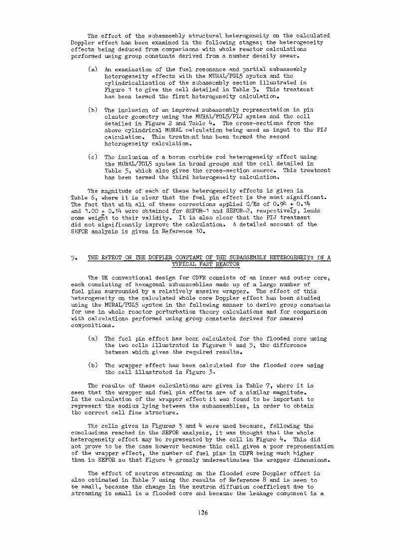
The effect of the subassembly structural heterogeneity on the calculatedDoppler effect has been examined in the following stages; the heterogeneityeffects being deduced from comparisons with whole reactor calculationsperformed using group constants derived from a number density smear.

(a) An examination of the fuel resonance and partial subassemblyheterogeneity effects with the MTJBAL/FGL5 system and thecylindricalisation of the subassembly section illustrated inFigure 1 to give the cell detailed in Table 3. This treatmenthas been termed the first heterogeneity calculation.

(b) The inclusion of an improved subassembly representation in pincluster geometry using the MURAL/FGL5/PU system and the celldetailed in Figure 2 and Table *t. The cross-sections from theabove cylindrical MURAL calculation being used as input to the PIJcalculation. This treatment has been termed the secondheterogeneity calculation.

(c) The inclusion of a boron carbide rod heterogeneity effect usingthe MURAL/FGL5 system in broad groups and the cell detailed inTable 5> which also gives the cross-section source. This treatmenthas been termed the third heterogeneity calculation.

The magnitude of each of these heterogeneity effects is given inTable 6, where it is clear that the fuel pin effect is the most significant.The fact that with all of these corrections applied C/Es of 0.9 + 0.1and 1.00 + O.l f were obtained for SEFOR-1 and SEFOR-2, respectively, lendssome weight to their validity. It is also clear that the PIJ treatmentdid not significantly improve the calculation. A detailed account of theSEFOR analysis is given in Reference 10.

5. THE EFFECT ON THE POPPLER CONSTANT OF THE SUBASSEMBLY HETEROGENEITF IN ATYPICAL FAST REACTOR

The UK conventional design for CDFR consists of an inner and outer core,each consisting of hexagonal subassemblies made up of a large number offuel pins surrounded by a relatively massive wrapper. The effect of thisheterogeneity on the calculated whole core Doppler effect has been studiedusing the MURAL/FGL5 system in the following manner to derive group constantsfor use in whole reactor perturbation theory calculations and for comparisonwith calculations performed using group constants derived for smearedcompositions.

(a) The fuel pin effect has been calculated for the flooded core usingthe two cells illustrated in Figures *t and 5, the differencebetween which gives the required results.

(b) The wrapper effect has been calculated for the flooded core usingthe cell illustrated in Figure 3-

The results of these calculations are given in Table 7» where it isseen that the wrapper and fuel pin effects are of a similar magnitude.In the calculation of the wrapper effect it was found to be important torepresent the sodium lying between the subassemblies, in order to obtainthe correct cell fine structure.

The cells given in Figures 3 and 4 were used because, following theconclusions reached in the SEFOR analysis, it was thought that the wholeheterogeneity effect may be represented by the cell in Figure ^. This didnot prove to be the case however because this cell gives a poor representationof the '.\rrapper effect, the number of fuel pins in CDFR being much higherthan in SEFOR so that Figure *t grossly underestimates the wrapper dimensions.

The effect of neutron streaming on the flooded core Doppler effect isalso estimated in Table 7 using the results of Reference 8 and is seen tobe small, because the change in the neutron diffusion coefficient due tostreaming is small in a flooded core and because the leakage component is a

126

small part of total Doppler effect. The same observation applies in thevoided core for the same reasons. The neutron streaming effect may howeverchange the spectrum in the important Doppler energy region (500 eV - 5 keV)and so change the wrapper and fuel pin effects, this point remains to beinves tigated.

6. THE EFFECT ON THE SODIUM VOID REACTIVITY OF THE SUBASSEMBLY HETERO3EITYIN A TYPICAL FAST REACTOR

These effects have been studied for the conventional design of CDFRusing the FGL5/MURAL system in the following manner.

(a) The fuel pin effect has been calculated using the cell illustratedin Figure 6 to prepare the group constants for the flooded andvoided core. The equivalent smeared results were obtained byperforming calculations with a similar shaped cell but with thedimensions reduced by 10 ; this ensures that the differences arenot due to the use of different algorithms. The whole corevoidage effects were calculated by whole reactor exact perturbationtheory calculations.

(b) The wrapper effect has been similarly estimated using the cellillustrated in Figure 7«

(c) The above calculations did not include an allowance for neutronstreaming, but a correction to the leakage terms in the perturbationexpression was made using the recommendations given in Reference 8.

The results of the calculations are given in Tables 8 and 9. From the wholecore voidage results given in Table 8 it can be seen that, as expected, the fuelpin and wrapper effects lead to changes in the c.entral perturbation term,whilst the streaming effect leads to a change in the leakage term. Theresults given in Table 9 for 'the maximum positive effect are not inconsistentwith this observation. Here the fuel pin and wrapper effects lead to changesin the maximum positive leakage term because they lead to a change in thespatial extent of the maximum positive region.

It is clear that the fuel pin, wrapper and streaming effects each leadto a decrease in the sodium void effect, the total reduction in the maximumpositive effect being 12$.

The energy dependence of the sodium void effect does not change markedlywhen these heterogeneity effects are included, the main change is in the fissioncomponent of the central term which becomes somewhat flatter.

7. CONCLUSIONSApart from the methods used to treat neutron streaming effects this

paper has described the essential features of the methods availabe in theUK for treating heterogeneity effects and spatial boundaries in fast reactorcalculations.

The influence of neighbouring reactor zones on the group constantsderived for a given zone has been shown to be insignificant for the Dopplerand sodium void effects, but special measures are required to allow forthese effects in calculations of reaction rates at core/breeder boundariesand in regions where medium weight resonant nuclei are important and forthe calculation of keff in systems with steel regions close to the core.These measures involve the use of an improved treatment of the energydependence of the spectrum when generating group constants for regionssuch as steel reflectors rather than the use of a fundamental modetreatment.

The influence of subassembly and resonance heterogeneity on thecalculated Doppler constant has been found to be significant in the SEFORcores (N 8-9$) but less so in CDFR ( rJ 5$). Neutron streaming effectsdo not appear to be important although they may lead to a significant change

127

in the neutron spectrum in the important Doppler region (500 eV - 5 keV) andso significantly change the central term in the Doppler reactivity expression;this awaits examination. Calculations have shown that the extra modellingcapabilities offerred by the PIJ code do not provide a significant improvementto the calculated SEFOR Doppler effects; the MURAL one dimensional cylindricaltreatment is adequate. This conclusion can be extended to CDFR.

The influence of subassembly and resonance heterogeneity on thecalculated sodium void effect has been found to be significant. The fuelpin (resonance), wrapper (fine structure) and streaming effects all leadingto reductions in the voidage effect; the total reduction being *for the maximum positive effect in CDFR.

REFERENCES

1. CAMPBELL C G, SANDERS J E, ROWLANDS J L, KOBAYASHI S (1973). The Scopeof the MOZART Programme and the General Conclusions Drawn from it.International Symposium on Physics of Fast Reactors, Tokyo, Japan,October 1973, Paper A.1k.

2. CALDAROLA L, FREEMAN D D, GREEBLER P, KUSSMAUL G, MITZEL F, NOBLE L D,PFLASTERER G R, OOSTERKAMP W J, WINTZER D (1972). SEFOR ExperimentalResults and Applications to LMFBR's. Proc Int Conf on Engineering ofFast Reactors for Safe and Reliable Operation, Karlsruhe, FederalRepublic of Germany, pp 1312-1330.

3. ROWLANDS J L, DEAN C J, MACDOUGALL J D, SMITH R W (1973). TheProduction and Performance of the Adjusted Cross Section Set FGL5.International Symposium on Physics of Fast Reactors, Tokyo, Japan,October 1973* Paper A30.

*t. MACDOUGALL J D (1973). The Use of the 2000 Energy Group Reactor PhysicsCode MURAL in the Investigation of Special Effects in Fast Reactors.International Symposium on Physics of Fast Reactors, Tokyo, Japan,October 1973, Paper A32.

5. MACDOUGALL J D (1977). MURALB - A Program for Calculating NeutronFluxes in Many Groups. AEEW - R 962.

6. ANDERSON D W (1973). The WIMSE Module W-PIJ - A Two DimensionalCollision Probability Code with General Boundary Conditions. AEEW - R 862.

7. SANDERS J E, BURBIDGE B H, CARTER M D, HARDIMAN J P, INGRAM G, JOWITT D,SWEET D W (1973). A Review of Zebra Techniques for the Measurement ofReactivity Parameters, Reaction Rate Ratios and S-pectra. InternationalSymposium on Physics of Fast Reactors, Tokyo, Japan, October 1973jPaper B18.

8. GRIMSTONE M J. Methods for the Calculation of Streaming CorrectedDiffusion Coefficients for Pin and Plate Cells in Fast Reactors.IAEA Technical Committee Meeting on Homogenisation Methods in ReactorPhysics, Lugano, Switzerland, 13-15 November 1978.

9. BROOMFIELD A M, COLLINS P J, CARTER M D, MARSHALL J (1973). The MOZARTControl Rod Experiments and their Interpretation. InternationalSymposium on Physics of Fast Reactors, Tokyo, Japan, October 1973,Paper A1?.

10. BUTLAND A T D (1975). Analysis of the SEFOR I and II Doppler Experimentsand their Use in Assessing the Accuracy of Calculated Fast Reactor DopplerEffects. UKAEA Report AEEW - R 986.

11. BRISSENDEN R J, DURSTON C (1968). A User's Guide to GENEX, SDR andRelated Computer Codes. DKAEA Report AEEW - R 622.

128

TABLE 1COMPARISON OF MULTI-ZONE AND SINGLE ZONE DERIVATION OF GROUP CONSTANTS FOR

DOPPLEE AND SODIUM VOID EFFECTS

Quantity Calculated Multi-Zone TreatmentSingle-Zone Treatment

SEFOR-1 Doppler Constant(see Heference 10)CDFR whole core sodiumvoid effect

0.998

TABLE 2ZONE CONTENTS 'IN SEFOR FUEL SUB-ASSEMBLY

Zone" Contents

23456

910

( (Lower core :Beo, stainless steel (SS-3l6;Fe,Cr,Ni,Mo)(SEFOR-1:(Main core :Beo( (Middle core :Beo(SEFOR-2: Stainless steel in all core regionsCANNING: Stainless steel (SS-3l6;Fe,Cr,Ni,Mo)SODIUMTIGHTENER SLEEVE: Stainless steel (SS-304;Fe,Cr,Ni)SODIUMFUEL:(Lower core :Pu02/U02

(Main core :Pu02/U02(Middle core:U02

CANNING: Stainless steel (SS-3l6;Fe,Cr,Ni,Mo)STAINLESS STEEL SIDE ROD (SS-304;Fe,Cr,Ni)OUTER CAN OF STAINLESS STEEL (SS-304;Fe,Cr,Ni)SODIUM

*See Figure 1

TABLE 3DETAILS OF LATTICE CELL ANNULI IN THE FIRST HETEROGENEITY CALCULATION FOR THE

SEFOR CORES

Annulus*

ABCDEF

G

Radius cm

1.13031.23191.51701 .63341.65961 .7204

SEFOR- 1:1. 72476SEFOR-2: 1.7222

Details of Contents

FuelFuel canMain sodium(Outer can of subassembly, inner tightener sleeve,(stainless steel side rodInner and outer sodiumSEFOR-1 : BeO + canningSEFOR-2: Stainless steel(Bij.C (amount of material equivalent to one fuel(rod)

*Cylindricalisation of part of Figure 1

129

TABLE

DETAILS OF THE PIN CLUSTER GEOMETRY CELL USED WITH.THE MURAL/FGL5/PIJ SYSTEMTO ANALYSE THE SEFOR CORES (SECOND HETEROGENEITY CALCULATION)

PIJ/MURALRegion

1

2345678910111213

Description

SEFOR-1:BeO + canSEFOR-2:Inner steel rodInner sodiumTightener sleeveMain sodiumMain sodiumFuelFuelFuel canFuel canSide rodOuter canOuter sodiumBi,C

Cross Section Data Sourcein First

Heterogeneous Calculation*Zone F

Zone EZone DZone CZone CZone AZone AZone BZone BZone DZone DZone EZone G

DimensionsAnnuli

(Outer Radii)1.1112 cm

1.2803 cm1.3755 cm2.7813 cm4.0377 cm

-----

4.2009 cm4.2142 cm

SEFOR- 1:4. 22476SEFOR-2:4.21870

Rod Sections(Outer Radii)

_

----

1.1303 cm1.1303 cm1.2319 cm1.2319 cm0.317 cm

--~

+See Figure 2•See Table 3

TABLE 5DETAILS OF THE CYLINDRICAL CELL USED TO REPRESENT THE CONTROL ROD HETEROGENEITY

IN THE SEFOR CORES

Annulus Contents

Bi,.C rodSEFOR-1:1/12th of the core

materials, apart fromBzfC

SEFOR-2:1/5th of the corematerials apart fromBifC

Cross Section Data Used*

PIJ/MURAL region 13

Flux and volume) average of PIJ/MURAL)regions 1—^ 12

*See Tables 3 and

130

TABLE 6THE MAGNITUDE OF THE HETEROGENEITY CORRECTIONS TO THE CALCULATED DOPPLER

CONSTANTS IN THE SEFOR CORES

HeterogeneityEffect

Resonance andsubassemblyheterogeneityBz,.C heterogeneity

SEFOR- 1

8%*

J>%

SEFOR-2

9°/+

'\%

*Made up of a 7.5% contribution from the first heterogeneity(FGL5/MURAL cylindrical model) calculation and 0.5% fromthe second (PIJ model).

+Made up of an 8.9$ contribution from the first heterogeneitycalculation and 0.1% from the second.

TABLEJ7THE MAGNITUDE OF THE SUBASSEMBLY HETEROGENEITY CORRECTIONS TO THE CALCULATEDFLOODED WHOLE CORE DOPPLER CONSTANT IN A 1300MW(E) CDFR OF CONVENTIONAL DESTGN

Heterogeneity Effect Magnitude of the Effect

Fuel pin effect(mainly resonance heterogeneity)S/A wrapper effectStreaming effect ' +1

in the positive central term*

in the positive central term*in the negative leakage term+

Wrapper + fuel pineffectCombination of allcorrections

in the total core Doppler effect

in the total core Doppler effect

*Central term = 0.2423& ( S k/k)^Leakage term = -0.00166% ($ k/k)^Estimated from Reference 8

131

TABLE .8THE MAGNITUDE OF THE SUBASSEMBLY HETEROGENEITY CORRECTIONS TO THE WHOLE CORE

SODIUM VOID EFFECT IN A 1300MW(E) CDFR OF CONVENTIONAL DESIGN

Heterogeneity Correction

Fuel pin effect(mainly resonance heterogeneity)Wrapper effect(cell fine structure)Streaming effect *

Wrapper + fuel pin effect

Combination of all thecorrections

Magnitude of the Effect

-J>°/c in the positive central term*

-2% in the positive central term*

+1C$ in the negative leakage term

-5$ in the positive central termor -S$ in the total whole corevoidage effect-16$ in the total whole corevoidage effect

*Central term -= if.624$ ( S k/k)+Leakage term = -1.994$ (6 k/k)•^Estimated from Reference 8

TABLE 9THE MAGNITUDE OF THE SUBASSEMBLY HETEROGENEITY. CORRECTIONS TO THE MAXIMUMPOSITIVE SODIUM VOID EFFECT IN A 1300MW(E) CDFR OF CONVENTIONAL DESIGN

Heterogeneity Correction

Fuel pin effect(mainly resonance heterogeneity)Wrapper effect(cell fine structure)

-±LStreaming effect

Wrapper + fuel pin effect

Combination of all corrections

Magnitude of the Effect

-4$ in the positive central term*-4$ in the negative leakage term"1"-J>% in the positive central term*-2% in the negative leakage term"1"+10$ in the negative leakage term"1"

-8$ in the total maximum positiveeffect-12% in the total maximum positiveeffect

*Central term = 3.936$ ik/k+Leakage term = -1.066$ •£> k/k^Estimated from Reference 8

132

Contents of the numbered zones given in Table 2-—. — .—BOUNDARY OF SEFOR CORE LATTICE UNIT

FIG. 1.

BOIWDARY OF LATTICE CELL USED ADAPTED FOR FIRST HETEROGENEOUSCALCULATION (MURAL/FGL5 CYLINDRICAL CELL)

SEFOR FUEL SUBASSBMBLY

r3.7813 cm

FIG. 2.

3.7207 cm

LATTICE CELL USED TR SECOND HETEROGENEOUS CALCULATION(MURAL/PIJ/FGL5 CLUSTER GEOMETRY)

(contents of the numbered zones given in Table 4)133

Region 1:FUEL, STEELSODIUM, ANDABSORBER CHANNELMIXTURE

Region 2:WRAPPER

Region 3sSODIUM

FIG. 3.

1

•ti

RADII (mm]1. 71.752. 74.563. 79.54

CDFR DOPPLER EFFECT: FULL SIZE SUBASSEMBLY WRAPPER CELL

RADII (am)

ABSOHBSR STEELIND SODIUM

FIG. 4.

2.5652.9491.2.3.s" 4..412I: *•<&(INNER CORE)6. 4.670(OUTER CORE)

CDFR DOPPLER EFFECT; FUEL PIN/SUBASSEMBLY WRAPPER CELL

Region 1:(FUEL, CANAND SODIDMMIXTURE)Region 2:WRAPPERRegion 3:SODIUMRegion ktABSORBER STEELAND SODIDM

1.2.3.k.

RADII (mm)3.9804.1364.4124.625

(INNER CORE)if. 4.669(OUTER CORE)

FIG. 5. CDFR DOPPLER EFFECT; SMALL SIZE SUBASSEMBLY WRAPPER CELL

134

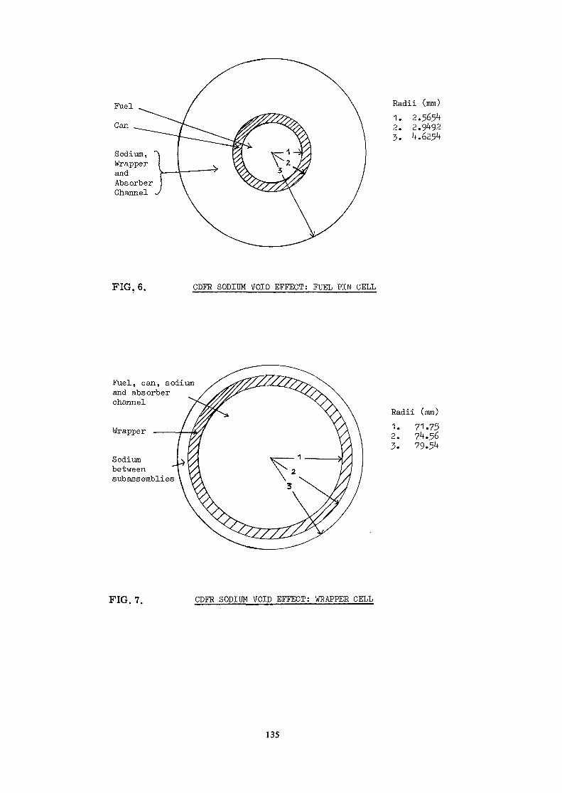
FuelCan

Sodium,WrapperandAbsorberChannel

Radii (mm)1. 2.56542. 2.94923.

FIG. 6. CDFR SODIUM VOID EFFECT: FUEL PIN CELL

Fuel, can, sodiumand absorberchannel

Wrapper

Sodiumbetweensubassemblies

Radii (mm)1.2.3.

71.7574.5679.54

FIG. 7. CDFR SODIUM VOID EFFECT: WRAPPER CELL

135

MONTE CARLO - BASED VALIDATIONOF THE ENDF/MC2-II/SDXCELL HOMOGENIZATION PATH

D.C. WADEApplied Physics Division,Argonne National Laboratory,Argonne, USA

Abstract

The MC -II and SDX codes are used to process the ENDF/B basic nucleardata into unit cell averaged multigroup transport or diffusion theory format foruse in reactor physics calculations of fast breeder reactor systems.

I. IntroductionThis paper summarizes the results of a program of validation of the unit

cell hotnogenization prescriptions and codes used for the analysis of Zero PowerReactor (ZPR) fast breeder reactor critical experiments. The ZPR drawer loadingpatterns comprise both plate type and pin-calandria type unit cells. A pre-scription is used to convert the three dimensional physical geometry of thedrawer loadings into one dimensional calculational models. The ETOE-II/MC2-II/SDX code sequence is used to transform ENDF/B basic nuclear data into unit cellaverage broad group cross sections based on the ID models. Cell average,broad group anisotropic diffusion coefficients are generated using the methodsof Benoist or of Gelbard. The resulting broad ( 10 to 30) group parametersare used in multigroup diffusion and Sn transport calculations of full core XYor RZ models which employ smeared atom densities to represent the contents ofthe unit cells.

This homogenization path has been extensively validated by detailed com-parisons against results produced by high precision Monte Carlo calculations ofthe unit cells. These calculations were produced by the VIM continuous-energyMonte Carlo code employing the ENDF/B basic data. The validation effort hassystematically progressed from homogeneous, zero-leakage tests through models ofinfinite arrays of heterogeneous plate or pin-calandria cells subject to an im-posed buckling, and from typical LMFBR compositions stressing the 100 keVrange through steam-flooded GCFR compositions -which exhibit a substantial sensi-tivity to the 'vJ.OO eV epithermal range,, In connection with the leakage aspectsof this effort, methods for treating neutron streaming have been developed andvalidated.

The fast breeder reactor critical experiment application to which the homo-genization procedure and codes are addressed:

a. stresses the fast energy range, 14«3 MeV to 0.4 eV. No thermalrange treatment is provided; and

b. addresses the composition, temperature, and geometry dependence ofresonance reaction rates.

c. No particular stress has been placed on depletion — e.g., the codepackage does not include an automatic cell depletion capability ora means to automatically generate depletion-dependent cell averagecross section fits or tables.

137

d. The emphasis has been placed on producing cell average cross sectionswhich accurately reproduce isotopic and total reaction rates, anddirection-dependent leakage rates. Accordingly, a flux, volumeatom density weighting for cell homogenization and energy collapse isused. However, these flux weighted cross sections currently are usedalso for computing material worths and kinetics parameters in the criti-cals analyses. A modest amount of work has gone into investigating theerror in computed worths due to the use of flux weighted rather thanbilinearly weighted cross sections0

The validation effort, up to this time, has focused on the asymptotic situa-tion — homogeneous compositions or unit cell lattices subject to an imposedbuckling. The end result of the validation effort has been to provide a highdegree of confidence in the accuracy of our methods, at least in the asymptoticcase (far from zone interfaces). Work has only recently started on validatingthe modeling of zone interfaces.

In the following sections we first describe the unit cells of interest andthe 3D -»• ID modeling prescription used to convert the cells into calculationalmodels for the cell homogenization calculations <> The codes used in the homo-genization are briefly described in an appendix. The validation strategy isthen outlined, and the validation results are displayed.II. ZPR Cell Homogenization Methods and Codes

A. ZPR Matrix LoadingsThe ZPR fast critical assemblies operated by Argonne National Laboratory

are split table machines holding lattices of stainless steel tubes with a squarecross section, two inches on an edge. These tubes are loaded with stainless steeldrawers filled with either plate-type or pin-calandria type unit cell loadings.Typical examples of the tube/drawer/plate or tube/pin-calandria unit cells areshown in Figs. 1 through 3.

The models for the validation effort have been selected from these ZPRunit cell loadings and have included:

- an LMFBR plate unit cell (Fig. 1)- a GCFR plate unit cell (containing void columns) (Fig. 2)- A sodium-voided LMFBR pin calandria unit cell (Fig. 3), and- a steam-flooded GCFR plate unit cell (Fig. 2 with void (V) replacedby a CHg steam simulant)

The compositions of one dimensional models of these unit cells are listed inTables I through IV.

The 2 in. x 2 in. plate and pin calandria cells are 1/2 to 2total mean free paths across for neutrons in the fast energy range. Peak toaverage fluxes within the cells are M..3 to 1.4. As an indication of the pro-perties and neutron balance of the cells, Table V shows the neutron balance forthe zero leakage homogeneous LMFBR composition.

B. The ETOE-II/MC2-II/SDX Cell Homogenization PathThe ETOE-II/MC2-II/SDX code package1 was developed by the Applied

Physics Division at Argonne National Laboratory to process the ENDF/B basicnuclear data into unit cell-averaged multigroup cross sections for applicationto fast breeder reactor diffusion and transport calculations. ETOE-II reformatsthe ENDF/B data into libraries for MC2-II and SDX; MC2-Il(2) is a zero dimen-sional -2000 ultra fine energy group (ufg) slowing down code which is used toproduce a 200 fine group (fg) library for SDX (which excludes the contributionsfrom heavy element capture and fission resonances); SDX3*1* is a one dimensionalcell homogenization code which collapses in space and energy from the <v200 finegroup level to M.O to 30 broad group cell average cross sections.

Broad-group microscopic cross sections are composition-dependentbecause of the composition-dependence of the neutron flux (and current) weight-ing spectrum. Elastic removal and heavy element resonance cross sections are

138

generally the most sensitive to composition due to intermediate element scatter-ing resonances and heavy element resonances. The SDX code is used for compositiondependent unit cell homogenization in space and energy. It treats slab or cy-lindrical geometry in one dimension, and is executed at the fine ( 200) energygroup level such that the energy detail is adequate to "trace out" the higherenergy scattering resonances in intermediate mass nuclei. For heavy nuclei cap-ture and fission resonances the SDX energy structure is too coarse for detailedrepresentation of resonances, and the resonance parameters from the ENDF filesare used directly for the generation of composition dependent fine group resonancecross sections.

The SDX calculation is designed to:a. Treat the composition dependence of the resonance absorption

cross sections on a plate-by-plate basis (heterogeneousresonance self shielding) „

b. Account for the detailed spatial dependence of the flux withinthe unit cell on a fine group basis, for the purpose of spatialhomogenization, and

c. Collapse cross sections over a cell average - fine group spectrumto a broad (M.O to 30) group basis.

The ETOE-2/MC2-II/SDX code system was developed on an IBM-370/195,and all programming was done in FORTRAN. The code system is operational onboth IBM and CDC equipment at several U.S. laboratories and is available fromthe Argonne Code Center and the NBA ISPRA Code Center. The program packageincludes the MC2-II and SDX codes with ETOE-II-processed libraries for theENDF/B Version IV data.

The ETOE-II, MC2-II, and SDX codes are briefly described inAppendix A.

C. Cell Anisotropic Diffusion CoefficientsExperience has shown that the structure of the ZPR unit cells gives

rise to anisotropic neutron leakage. This is particularly true in the case ofsodium-voided LMFBR and of GCFR cells where the void fraction of the cell isboth large ( 0-55 v/o) and distributed such as to induce streaming in the Zand Y directions (see Figs. 1 and 2). Two methods are in use to generate aniso-tropic diffusion coefficients at the broad group level; the method of Benoist9,and an extension of his method which was developed to deal with the high buck-lings encountered in fast reactors and the presence of planar void regions (whichcause the Benoist method to break down). This second (Gelbard) method10 wasdeveloped in connection with the validation work described here.

1. Benoist Method - A utility code, BENOIST, is used in connectionwith the ID models of the ZPR cells described in the next section to computeanisotropic diffusion coefficients. The form of the Benoist method employed bythe code is a commonly applied one that neglects so-called absorption correctionterms for the x-direction coefficients. These terms are omitted in part to avoiddouble-valued solutions11 for Di. The group g, unit cell-averaged Benoist dif-fusion coefficient in coordinate direction, k, is constructed from the formula

139

where V^ and <j>£ are the volumes and group g fluxes in subregions i of the unitcell, \§ is the transport mean-free path in region j, group g, and

pgV 1si j

rfr

is the directional probability that source neutrons of group g in region i suffertheir first collision in region j. Here fi is the direction cosine.

The BENOIST code works in both plate and pin geometry and uses algor-ithms for generating the directional collision probabilities, which are simplemodifications of those used in the SDX cell-hotnogenization code. The calcula-tions are made on the broad-group level using plate-wise transport cross sectionsobtained from SDX. The flux in Eq. 1 is assumed to be flat across the cell sinceit was determined that in our problems this approximation has negligible impacton the Benoist diffusion coefficients.

The Benoist formula cannot be applied when there are totally voidedstreaming paths. This can be seen from Eq. 1 in which D becomes undefined whenthe transport mean-free-path goes to infinity in any region. Infinite streamingpaths are a concern not only in the ZPR pin calandria and plate geometries butalso in voided hexagonal lattices with small pins spaced at large pitch.12

In addition to the above, the Benoist method could be expected tooverpredict leakage at the high buckling found in fast reactors because thederivation involves a Taylor series expansion in buckling, neglecting terms oforder B1*. For a homogeneous medium, the Benoist and conventional diffusioncoefficients coincide. In a sense, then, some features of diffusion theoryare built into the Benoist method. In general, diffusion computations tend tooverestimate the leakage more and more as the buckling increases and the Benoistmethod is no exception.

2. Gelbard Method - The inapplicability of the Benoist method to thepure-void model plus the error of that method at high bucklings motivated thedevelopment of a modified version of the Benoist method and correspondingly modi-fied diffusion coefficients. These modified coefficients, derived in Ref. 10, aredefined as in Eq. 2:

(1 - cos B. •

[1 - (1 - cos i • a. B2(1 - cos B a )v n n'

m - COS,1, (2)

where S? is the cell volume-averaged value of £§(*)• The term, BJI is thatpart of the critical buckling that is parallel to the plates while B? is thatpart which is perpendicular to the plates. The vector, £_, denotes a directedline segment drawn from where a neutron is born to where it gives rise to anext generation fission neutron. The overbar denotes an average over all neutronhistories where the cos JB • £_term is weighted by the number of neutrons emina-ting from the fission times the neutron importance at the point of birth.

The alternate method for computing anisotropic diffusion coefficientshas several useful properties:

1. The diffusion coefficients remain finite even when there aretotally voided streaming paths.

140

2. The derivation of Eq. 2 with leakage only in the "uniform" direc-tion is a generalization to the case of high buckling of the derivation of theBenoist method in the uniform direction. Uniform direction refers to our y or zdirections (see Figs. 1 and 2) for which the so-called Benoist absorption cor-rection terms vanish.

3. In the limit of low buckling, Eq. 2 reduces to a form equivalentto the Benoist formula (without the absorption correction term).

4. Equation 2 yields rigorous "transport-corrected" diffusion coeffi-cients for a homogeneous medium. That is to say that even for large buckling:

is the divergence of the current in group g in a homogeneous medium if scatteringis taken to be isotropic. This is true, of course, only for those bucklings,Bn which are used in Eq. 2 to define the diffusion coefficients, but is true nomatter how large these bucklings may be.

5. The factor in brackets, which splits the leakage into directionalcomponents, is a prescription suggested by an expansion of (1 - cosB • £) :which has the property that the leakage summed over all directions is rigorous.

- cos B (B • A)

(1 - COS B A )n n

A utility code, GELBARD, is used to evaluate Eq. 2 in a one dimensionalmodel for each multigroup, g, using Monte Carlo techniques. In the group g modelproblem, the materials in the cell are taken as pure absorbers such that

where z|(r) is the group g total cross section at r. The source density withinthe cell is taken to be equal to the total cross section,- i.e., S(r) = St(r).This source roughly simulates the combined net effects of scattering and fissionin the original multigroup problem. Broad-group regionwise total cross sectionsfrom SDX are supplied as input. The computation of the cell-averaged diffusioncoefficients for one-group to 0.5% standard deviation requires 4 min. on theIBM-370/195 computer.

The Gelbard diffusion coefficients used in criticals analyses are com-puted via the Monte Carlo method with a standard deviation of 0.5% to 1%. Sincethe leakage probability in the GCFR criticals is <0.5, a 0.5% error in every dif-fusion coefficient can produce, at most, a 0.25% error in k. But the diffusioncoefficient generation calculations in different groups were completely uncor-related, and therefore it is reasonable to expect a good deal of error cancella-tion in the total leakage. If one were to suppose, for example, that the first16 groups all contribute equally to the net leakage rate, one would concludethat the error in k, produced by the statistical errors in D's, is only 0.06%.In any case, it seems safe to assume that this particular error in k is sub-stantially smaller than 0.25%.

141

D. 3D ->• ID Modeling PrescriptionsBecause the codes available for cell homogenization are based on one

dimensional slab or cylindrical geometries, a modeling prescription which trans-forms the three dimensional ZPR matrix tube loadings as shown in Figs. 1 through3 to a one dimensional calculational model is an essential part of the homogeniza-tion process. However, a modeling that is appropriate for one phenomenon may notpreserve properties that are crucial in another process. For example, in computingplatewise resonance self shielding, it is important to preserve the absorber tomoderator atom ratio within the plate. On the other hand, to compute the fluxspectrum, cell average atom densities should be maintained (recall that the cellsare approximately one mean free path in extent). As will be shown below, for thegeneration of diffusion coefficients which preserve leakage rates, it is neces-sary to preserve cell average number densities and to preserve true void regionsif they exist.

The 3D •»• ID modeling prescriptions which are in use for the ZPR cellsand which have been validated are described in detail in Appendix B. Briefly,for both the pin calandria and the plate cell, two modelings are used:

a. the "reference" modeling in which the geometry and composition ofresonance-isotope-bearing regions are maintained at their physicalvalues and in which the structral materials from the periphery ofthe physical cell are smeared into the non-resonance-isotope-bearing regions (including void regions) of the ID model, and

b. the "pure void" modeling which is the same as the "reference"modeling except that if void regions are present in the 3D cell,they are maintained in the ID model.

The ID models of pin-calandria cells are one-pin cylindrical cells withassociated diluent annuli and a white boundary condition. The ID models of platecells are an array of infinite slab regions with either periodic or reflectiveboundary conditions.

III. The Validation ProcedureThe key to the successful validation effort has been the availability of high

precision Monte Carlo solutions to the unit cell problems against which the homo-genization results can be tested. Given the geometry and composition of the 3Dcells and the ENDF/B data, these Monte Carlo methods give a basically exact solu-tion of the Boltzman equation and low-variance estimates of the integral parametersof interest. The Monte Carlo solutions have been provided using the VIM code andits associated statistical editing packages.

A. The VIM Monte Carlo Code

The VIM Monte Carlo code13 permits an explicit three dimensional geo-metrical description of the unit cell, using a generalized geometry input processor.Neutron cross sections are derived from the ENDF/B data files and are treated ascontinuous functions of energy. Resolved resonances are "traced out" by a set ofpoint cross section values suitable for interpolation. Unresolved resonances aretreated by a probability table methodo During the first part of the validationprogram, the VIM code solved only down to 10 eV. This, was of course, quite ade-quate for fast breeder work. A thermal range capability has recently been addedto VIM, and has been used in the GCFR steam flooded cell homogenization valida-tion work.

B. Strategy of the Validation ProcedureFigure 4 displays the philosophy of the validation effort. Starting

from the 3D cell geometry and the ENDF/B cross sections, the 3D •»• ID cellmodeling and the ETOE-II/MC2-II/SDX and BENOIST or GELBARD cell homogenizationpath is followed to produce values for the cell integrated reaction and leakagerates. This is the path which is to be validated.

Alternately, starting from the 3D geometry and the ENDF/B cross sec-tions, the calculational path through the VIM Monte Carlo code leads to exactvalues for isotopic and total cell integrated reaction rates and total, direction-

142

dependent cell leakage rates. The agreement of the end products of the two pathsserves to validate the MC2-II/SDX homogenization codes and the 3D •> ID modelingprocedure for the class of cases considered.

To perform the validation in a way which permitted the isolation andelimination of errors, the class of cases considered has progressed in a system-atic fashion starting at the zero leakage homogeneous case and, to the extentpossible, introducing the complexities of heterogeneity, leakage, etc., one at atime.

(1) Nonleakage Integral Parameter Comparisons - The intercomparisonsin the zero leakage cases are quite straightforward. The cell integrated andintracell neutron flux and reaction rates by isotope, reaction type, and energyband, are available from both the reference VIM and the SDX or broad group dif-fusion codes and can be simply intercomparedo Similarly, the eigenvalue (whichin the zero leakage case is koo) can be directly intercompared. The VIM tracklength estimates provide high precision results even for groupwise, isotopic, reac-tion rates by plate with several hundred thousand neutron histories.

(2) Leakage Integral Parameter Comparison - The validation of the homo-genization of leakage properties is a many faceted problem and necessitated a lessstraightforward validation procedure.

i. First, an explicit treatment of anisotropic diffusion wasrequired because it was known that streaming affected bothsodium void reactivity and GCFR critical mass in the ZPRplate-type critical assemblies.

ii. To avoid ambiguity, buckling vectors were prescribed tointroduce leakage.

iii. Also it was necessary to consider both small and largebuckling cases. Most anisotropic diffusion coefficientprescriptions derive from the thermal reactor field andtheir derivations are based on the assumption of smallleakage (small buckling). However, in fast breeder reactorsboth the value of buckling is larger, and the cross sectionsare smaller than for thermal reactors. Thus in fast reac-tors, the B/Stot ratio is larger than for the thermal casegiving rise to a Bn/Pn type transport correction and in-validating the validity of the one-term buckling expansionsused in the anisotropic diffusion coefficient derivations.

Leakage-related parameters computed in the study included the groupwisetransport cross section 0tr, keff, and Ig, (the mean-squared distance traveledin the directions ±n from birth to fission). For the homogenized medium, it iswell known that a Taylor series expansion of the dependence of eigenvalue on funda-mental mode buckling is given by

1 0(B") . (3)

Then for a small change in buckling, 6B2, around the zero buckling case,

k 6B2(4)

eo

Alternately the most meaningful information about directional leakageat high buckling is obtained by computing the difference between koo and theeigenvalue itself for buckling vectors with differing orientations.

143

k - k (f )An = ———k —— n = -L' I '• y' Z' EQ

Buckled eigenvalues (ki, k , k , k i t , and k „) are defined in Table VI in termsJ_ y z | | EQof the associated buckling orientation. The mean-squared chord lengths, A*,are defined analogously.

In addition to the leakage-related integral parameters listed above,the neutron flux spectrum and isotopic reaction rates and reaction rate ratioswere sometimes intercompared for the buckled cases. The buckled spectrum in afast reactor composition is harder than the zero buckled spectrum because neutronswhich leak at high energy are unavailable to provide the slowing down source tolower energies.1

The benchmark solutions against which the homogenized diffusion theorycalculations were tested were obtained by Monte Carlo. An efficient methodhad been developed that yields Monte Carlo estimates of eigenvalue in an infiniteuniform lattice as a function of buckling.15 The technique, derived by perturbationtheory yields at a reasonable cost, essentially exact solutions for lattices evenwith very complicated unit cells. The expression for keff as a function of buck-ling can be written as

* [yA 5 k - k (B) / k = (1 - cos B. • «.) . (5)

and is evaluated by Monte Carlo techniques. Here ko> is the lattice eigenvalueat zero buckling. The bar in Eq. 5 denotes an average over all neutron trajectories(histories): i_ is a vector drawn from the birth site of a fission neutron to thepoint where that neutron induces a next-generation fission. Birth sites areselected from the zero-buckling fission source distribution. The average inEq. 5 is weighted by the number of next-generation neutrons produced when eachhistory terminates, multiplied by the adjoint source distribution S*. Thus if ahistory terminates with a capture, that history will not contribute to the indi-cated average.

The cosine term in the right member of Eq. 5 can be expressed as apower series, which in the limit of small buckling, produces an extension ofthe homogeneous theory results, Eq. 4, to the heterogeneous case,

B2=0 ~ k 3B2- j| ; k = x,y,z . (6)O K.2

The VIM Monte Carlo code was used to perform the zero-buckling infinite-lattice calculation yielding ka,, broad-group cross sections, reaction rates, etc.During the VIM calculation, a site tape was written containing birth and deathcoordinates of each neutron and its fission weight at death. A utility code thenevaluated Eqs. 5 and 6 using the VIM site tape, to provide the benchmarking leakageindicators at high and low buckling*,,

*Subsequent to the validation work described here, a "correlation correction" toEq. 5 for the case of At was identified.16*17 This correction, which isrelated to neglecting the effect of buckling on the source shape used in evaluatingEq. 5, was shown in Ref. 16 to have negligible impact on the validation resultsdiscussed here.

144

IV. Asymptotic Homogeneous CasesHomogeneous compositions were treated first to test the basic cross section

processing in the codes, independent of the 3D -»• ID modeling aspect of homo-genization. The nonleakage test calculations were based on an LMFBR composition,were done in 1975, and were based on ENDF/B-III data. The leakage test calcula-tions were based on a GCFR composition, were done in 1976, and were based onENDF-IV data.

A. Zero Leakage Tests; LMFBR CompositionIn the first comparison, the zero leakage slowing down equations were

solved for the homogenized LMFBR cell composition by VIM, MC2-II, and SDK usingENDF/B-III data.** The composition is shown in Table I. MC2-II produced tworesults — one using the NRAt and the other using the "exact" RABANL hyper-finegroup method in the resolved range.

Table VII shows the results for several integral parameters, and TableVIII shows the isotopic absorption fractions. It is seen that overall, excellentagreement is obtained between the three codes; ko, agrees to four significantfigures, and generally agreement on integral parameters is to a percent or better.Though not shown on the tables presented here, it was shown that the cell averageneutron spectra agree excellently except in the resolved resonance range — wherefor this composition there is very little flux.

However, several discrepancies may be identified in the tables. WhileSDX agrees with MC2 on c8/f9, both of them are low relative to VIM.tt Thisstems from a problem in the VIM treatment of unresolved 238U capture in theENDF/B-III VIM library: linear - linear interpolation was used on an energymesh which was coarse enough such that it produced errors relative to log linearinterpolation for which the ENDF data were generated,, This problem has beencorrected in the Version IV VIM library. Besides the discrepancy on 238U capture,MC2-II and SDX overpredict absorption in structurals (Cr and Fe) because of afailure to self shield their capture resonances. (Only heavy isotopes weretreated as resonance absorbers in MC2-II and SDX for this test.) This affectsthe neutron balance only slightly.

Table IX compares 238U capture cross sections produced by the threecodes. Two MC2-II solutions are shown: One using the rigorous RABANL "hyperfine group" calculation and the other using the NRA. The use of the NRA belowabout 750 eV introduces substantial errors in the 238U capture cross sectionwhen compared against VIM or the rigorous form of MC2-II. However, less than5 percent of 238U capture takes place below 750 eV in the spectrum of currentLMFBR's.

The net result of the zero leakage, homogeneous comparison was todemonstrate excellent overall agreement between VIM and MC2-II/SDX. The reasonsfor the existing discrepancies were identified (and were subsequently correctedor minimized).

"Bo Non-Zero Leakage Tests; GCFR CompositionThe homogeneous, nonzero leakage tests were made in 1976. The last column

in Table I shows the homogenized cell number densities for the GCFR unit cellfor which the homogeneous test case was run,. All calculations employed ENDF/B-IVbasic nuclear data. Comparisons were run at both low and high buckling; for lowbuckling, the mean squared cord length from birth to fission I2", was used asthe parameter for comparison; for high buckling, the parameter Ak = (ko, - k(B))was used.

**Prael and Henryson produced the VIM and MC2-II results.18tNRA refers to "Narrow Resonance Approximation". See the description of MC2-IImethods in Appendix A.

ttc8/f9 refers to the ratio of capture rate per atom in 238U to the fission rateper atom in 239Pu.

145

(1) Small Buckling — JJT was generated for the homogeneous compositionby both the VIM and the MC^-II/SDX procedures„ The VIM results were based on30,000 neutron histories,, The 27 broad group cross sections used in the dif-fusion theory calculations were obtained by collapsing an unbuckled (B2 = 0)156 group spectrum computed by SDX. atr was collapsed using an inconsistentP! ('f'/ tr) weighting. The SDX calculation employed a base library generatedby MC —II by collapsing an unbuckled 2000 group spectrum computed as the solu-tion of the consistent P} equations.

The results summarized in Table X show_that the diffusion theoryprocedure underpredicts the mean square cord length, £2, by 1.27% (two standarddeviations from the VIM result). A 1.27% underprediction of IT translates intoan eigenvalue overprediction of 0.5% Ak in a GCFR core for which the core leakageprobability is 30%.

To supplement the leakage probability information, (07), thek^ and several spectral indexes were also compared. The results are shownin Table X. The eigenvalues and f8/f9 ratio agree to within the Monte CarloCarlo la statistics. Relative to VIM the diffusion theory procedure under-predicts c8/f9 by 005% (two standard deviations from the VIM result). Thisdiscrepancy has been noted in the previous section for the zero leakage com-parisons (using Version III data) of VIM and MC2-II/SDX. It is due to dif-ferent ways of treating 238U capture in VIM and MC2-II, and the deviation ismuch smaller for the Version IV libraries of VIM and MC2-II than it was forthe Version III libraries.

A number of sensitivity studies were made on the homogeneousmodel to assess the impact of alternate options in the MC2-II and SDX crosssection collapse codes. Specifically, the Bl and PI options of MC2-II wereused in both their consistent and inconsistent (energy loss upon Pj scatteris neglected) forms. The results are summarized in Table XI.

a. roundoff in the MC2-II edit of k leads to -vO.4% un-certainty in IT; Cases 2 and 3, which should have identi-cal IT basically do;

b. any error in 1? due to the MC2-II "inconsistent approximationis masked by the roundoff; i.e. the difference in t? betweenCases 3 and 4 is not much larger than 0.4%

c. apparent discrepancies in ~8? from MC2-II CP1 vs. MonteCarlo is -2.6% which translates to approximately -0.0093 in Ak.There is uncertainty in IT; 0.7% for la Monte Carlo sta-tistics and for 0.4% for MC2-II roundoff. The error, whichis still outside statistics, may stem from neglect of Pnn > 1 scattering in MC2-II.

d. Cross section collapse to 27 groups for Cases 2-4 was done withzero buckling and used MC —II only. Cases 5-8 involve anMC2-II cross section collapse to a 156 group libr-ry followedby an SDX collapse to a 27 group library. Then 27 groupdiffusion theory calculations for buckling at and near zerodetermined IT. In the last three cases the cross sectioncollapse was done with a buckling near 801 x ID"4.

e. The standard procedure in fast criticals analysis is IP1collapse in both the MC2-II and SDX codes. None of thecases exactly matches this approach, but we estimate ITwould be 3004 based on reducing the Case 5 value by thedifference between ~s7 in Cases 6 vs. 7.

f. The estimated I2" = 3004 from MC2-II/SDX IP1 differs fromthe direct MC2-II value (Case 3) by 1.6%, which is muchlarger than roundoff can account for. The IT differencetranslates to a difference of 0.006 in Ak.

An important point obtained from Table XI is that the MC2-IIvalue of IT is not exactly preserved by the MC2-II/SDX two-stage cross section

146

collapse. Even though the IP1 approximation is used throughout, the leakagefrom MC2/SDX is larger than from MC2-1I. This could stem from the fact that fordirect MC2-II collapse to 27 groups, a current weighting of atr is used, whilefor the MC2-II/SDX path the following sequence occurs:

a. MC2-II current weighting of afcr for the nonresonanceisotopes and of osmOoth for the resonance isotopes isdone to produce the 156 group SDX base library;

b. the resonance isotope aa component to o T is calculatedin SDX and added to crsmOoth to produce a 156 group 0trfor the resonance isotopes, and

c. an approximate SDX current weighting j <f>/Itr is usedto collapse the isotopic atr's to a broad group level.(2) Large Buckling — Leakage for a homogeneous model at a high buckling

was compared between VIM and MC2-II for the composition shown on Table XII. Here,unlike in the limit of zero buckling, a theoretical difference exists between theBl and PI leakage rates. Table XIII shows the results where Ak = (k^ - k (B))is used to isolate the leakage component of the eigenvalue.

a. Consistent Bl, the most rigorous MC2-II option available,is underpredicting leakage relative to VIM by 1.07% of itsvalue

Ak (CB1 MC2-II) _ gAk (VIM) ~ °'9893

which is three standard deviations of the VIM result.b. Alternately, the less exact option, inconsistent PI, is in

agreement within statistics due apparently to a cancella-tion of errors.

Among the possible sources of the CB1 Ak error is inadequate repre-sentation of anisotropy in the scattering. This could be remedied by solvinghigher order Bn equations (allowing higher modes of anisotropic scattering) . Thisoption has not yet been explored.

It was found in studying the large buckling case that broad groupnon-leakage parameters (f28/f1*9, c2°/f , keff, etc.) were non-negligiblymispredicted if an unbuckled SDX fine group spectrum were used to collapse to thebroad group cross sections.* Thus in all subsequent work, pains were takento use a SDX collapsing spectrum which is buckled to the degree expected to beencountered in the subsequent broad group calculations.

In summary, the results of the homogeneous leakage probabilitytests showed that:

(a) at low buckling the MC2-II/SDX codes when run is theirusual (inconsistent P:) mode, underpredicted Ak due toleakage by 1% of its value.

(b) While at high buckling the most rigorous form of MC2-II(consistent Bl) underpredicts Ak due to leakage by M.% ofits value, when run in the inconsistent PI mode, MC2-IIcomputes a leakage probability in agreement with Monte Carlo.

(c) Finally, the MC2-II/SDX path yields a slightly differentleakage probability than the MC2-II path alone.

The MC2-II/SDX errors are small, affecting eigenvalues by 0.5%Ak. However they are not negligible. None-the-less it was decided to move on andinvestigate the heterogeneous case before pressing to further reduce leakage pro-bability errors in the basic MC2-II/SDX algorithms.

*Alternately, the broad group results were found to be insensitive to the buck-ling used in the MC2-II 2000 group calculation which produced the SDX 200group library.

147

V. Asymptotic, Heterogeneous Plate-Cell LatticesUpon completion of the homogeneous tests, the treatment of heterogeneous

cells was undertaken. First a study was made of a true ID slab cell with zeroleakage. This test, based on an LMFBR cell, again avoided the 3D ->- ID modelingaspect of homogenization and simply addressed the accuracy of the MC2-II/SDXtreatment of the intra cell cross sections and flux solution. This is describedin Section A, below.

Next, the 3D ->• ID modeling question was addressed for a GCFR plate cell bycomparing Monte Carlo solutions of the 3D cell with Monte Carlo solutions ofslab cells constructed according to the 3D •*• ID modeling prescriptions describedin Section II-D and Appendix B. Both leakage and non-leakage aspects of the model-ing were examined. It was found that both the "reference" and the "pure void"3D -v ID modeling prescriptions described in Section II-D would adequately pre-serve non-leakage properties of the cell. However, it was found that if voidregions existed in the 3D cell, they had to be maintained as true voids in theID model in order to preserve leakage properties„ This latter requirement rulesout the use of the BENOIST anisotropic diffusion method for plate cells contain-ing true void, though for non-void cases, the BENOIST method could still beconsidered. The 3D -> ID modeling tests are described in Section B below.

Based on the above information, two tests were made of the full 3D -»• IDmodeling, MC2-II/SDX, and anisotropic diffusion coefficient cell homogenizationpath for plate cells. The first case (discussed in Section C) tested MC2-II/SDXand the BENOIST method for a slab cell containing no true void,, The second(discussed in Section D) tested the MC2-II/SDX and GELBARD method for slabcells containing true void. The GCFR cell was used in both cases, and both lowand high bucklings were considered. In all cases, Monte Carlo provided thestandard of comparison and ENDF/B-IV data were used.

A. Zero Leakage, True ID LMFBR Plate Cell

This set of tests were made in 1975 'and employed ENDF/B-III data. Themodel of the unit cell represented an infinite array of infinite slabs of thecomposition and thicknesses of the LMFBR unit cell shown in Fig. 1. VIM pro-vided the reference solution. MC2-II was run in the inconsistent PI mode atzero buckling to provide a 156 group base library for SDX. SDX generated an intra-cell flux distribution and an unbuckled fine group spectrum which was used tocollapse to a 27 group cell averaged cross section set. This was then used ina zero leakage ID diffusion calculation of a homogeneous composition having thecell-averaged number densities.

Table XIV shows the results for several integral parameters: The eigenvalue,and the cell-average 239Pu absorption/fission ratio, 2^8U to 239Pu fission ratio,and 239Pu fission cross section agree to within the VIM statistics. As in thehomogeneous case, a disagreement exists in 238U capture.

Table XV shows that the SDX and VIM cell-integrated spectra agree withinstatistics down to the resolved resonance range,,

Table XVI shows a comparison of isotopic absorption fractions: Good overallagreement is obtained. The 238U problem is seen, as in the homogeneous case. Asin the homogeneous case, SDX overpredicts structural absorption due to the neglectof capture resonance self-shielding for materials of mass <100. However, only^6% of cell absorptions occur in structurals. Though not shown in the table,when normalized to equal absorptions, total fission production, capture and fissionall agree to better than 0.250%.

Table XVII shows the VIM and SDX cell-averaged cross sections for 238U fissionand capture. 238U fission agrees within statistics except in the high MeV region.38U capture is low relative to VIM; — in the unresolved range, it is due mostly

to the VIM interpolation problem; in the resolved range it is the combination ofthe NRA and equivalence theory used in SDX.

The comparison of VIM and SDX shows that overall SDX is producing an accuratesolution for a true ID slab heterogeneous cell problem at zero leakage. Severaldiscrepancies are seen which are common to the homogeneous and heterogeneous

148

modelso However, the tests have not addressed the non-leakage probability aspectsof the SDX homogenized cross sections or the 3D •*• ID modeling of the 3D cells„These aspects are discussed next.

Bo Monte Carlo Studies of Nonleakage and Leakage Aspects of3D •> ID Modeling

To examine the implications of the relocation of structural materialfrom the cell periphery into the slab regions of a one dimensional model, the3D •> ID modeling was performed to generate ID slab VIM models for comparison withthe exact 3D VIM model. The GCFR cell served as the model, and ENDF/B-III datawere used. Both the "reference modeling" (placing structure from the cell peri-meter in all non-resonance material slabs — including voids) and the "pure voidmodeling" (placing structure from the cell perimeter in slab regions excludingresonance material regions and void regions) were examined. The selection ofthe GCFR model emphasized anisotropic diffusion effects, since as shown in Fig. 2,the cell contains void slots comprising V55 v/o of the cell. The results areshown in Table XVIII.

(1) Nonleakage Parameters; Reference and Pure Void Modeling - Thefirst column of Table XVIII shows that either one of the two modeling prescriptionsadequately preserves kTO. Comparisons of other reaction rate related parametersshowed similar agreement and confirmed the conclusions of earlier studies11* thatthe 3D -*• ID modeling relocation of structural material is adequate for nonleakageparameters.

With the demonstration from the previous section that theMC2-II/SDX homogenization reproduces the VIM results for a ID cell, it may beconcluded that the 3D -> ID modeling followed by the MC2-II/SDX homogenizationwill reproduce the nonleakage parameters of a 3D cell.

(2) Leakage Parameters; Adequacy of ID Modeling - In the case ofleakage properties, the modeling considerations are different,, For example,the assembly structure in the x-y planes is different from the structure in thex-z planes. (See Figs. 1 or 2 for coordinate orientations <>) The streaming pathin the void plane (y-z) is interrupted in the z direction only by the drawerfronts and backs, while in the y direction the stainless-steel matrix structurehas a ten-fold larger optical thickness. Thus, the streaming is directiondependent within the void plane. Since no one-dimensional model can account forthis difference, it had to be verified that the structural differences do notlead to large differences between y and z leakages. This was confirmed by com-puting* Av and Az with the three-dimensional model by Monte Carlo:Ay = 0.2955 ± 0.0023 and Az = 0.2974 ± 0.0024. The two values agree to withinone-sigma uncertainties. The expected values of ky and -^z differ by 0.0027.

The relatively small difference between y and z leakages suggeststhat a one-dimensional modeling approach can be acceptably accurate.

(3) Leakage Parameters; Reference ID Modeling - In row 2 of TableXVIII, results are shown for the "reference" 3D -*• ID modeling procedure. Itmay be seen that leakage perpendicular to the plates is modeled adequately. How-ever, the reference one-dimensional model prediction of leakage parallel to theplates is not good, as shown by the values of IJTi and A i i . The error inAil translates to an error of 0.0123 in kii. The AII error leads to thedegree of anisotropy, A i i / A i , being underestimated by 3.2%. The AEQ values,which involve leakage both parallel to and perpendicular to the void slots, differby more than one standard deviation from the three-dimensional Monte Carlo result.Because of the serious leakage underprediction in the void planes, the "reference"one—dimensional modeling is considered unacceptable for the case at hand.

(4) Leakage Parameters; Pure Void ID Modeling - It is natural to sus-pect that the smearing of structural material from the periphery of the three-dimensional unit cell into the void slots of the one-dimensional cell model isresponsible for the underprediction of streaming with the reference one-dimensional

*See Eq. 5 and Table VI for notation.

149

model. Other three- to one-dimensional unit cell modeling prescriptions wereexamined, and it was found that best results are obtained when no structuralmaterial is included in the one-dimensional void slot regions. The procedure forconstructing the alternate, "pure-void" one-dimensional model from the three-dimensional cell is identical to the reference procedure except that the extrastainless steel is excluded from the void regions of the original 3D cell as wellas from the resonance-isotope-bearing regions.

Monte Carlo results using the "pure-void" one-dimensional modelare shown in row 3 of Table XVIII, where they are compared to the three-dimensionalmodel standard. The leakage parameters for the x direction, &T, and Ai arepredicted to within one standard deviation of the expected three-dimensional values.The complete absence of material in the void regions makes H/TI infinite so thatno comparisons can be made; AII on the other hand, remains finite and in goodagreement with the 3D value. The AM discrepancy is much less than one standarddeviation, and the one-dimensional kii is 1.0140 ± 0,0041 compared to the limit-ing three-dimensional values: ky = 1.0122 ± 0.0037 and kz = 1.0095 ± 0.0037.The anisotropy measure, A i i / A i , is computed to well within the one-sigmauncertainty. Thus, the pure-void one-dimensional model adequately preservesthe important leakage properties of the true three-dimensional unit cell.

C. Benoist Diffusion Coefficient Method for a ID Slab Cell ContainingNo True Void Regions

A direct consequence of the requirement to maintain true void slabregions in the ID model of the GCFR in order to preserve leakage propertiesrules out the use of Benoist diffusion coefficients for that case, since ascan be seen from Eq. 1, the Benoist D becomes undefined if any region haszero £tr. Despite the failure of the "reference" modeling to represent the GCFRunit cell adequately where totally voided regions exist, the accuracy of Benoistanisotropic diffusion leakage predictions for a one-dimensional model havinglow-density material in some regions is still of considerable practical interestfor other problems (e.g., partial sodium voiding in LMFBRs and steam entry in GCFRs),Therefore, it was important to assess the degree of error incurred when the Benoistmethod is used in systems where low-density (but not complete void) streaming pathsexist. For this reason the performance of the Benoist method for the "reference"GCFR one-dimensional model at both low and high buckling was examined.

Monte Carlo, Benoist diffusion theory, and conventional (D = l/3Str)diffusion theory results using the "reference" one-dimensional model and ENDF/B-IVdata are compared in Table XIX. The diffusion theory value of ko, is very accurate.This reinforces results from earlier phases of the validation effort.

Table XIX shows that both conventional and Benoist diffusion theory chord-length predictions are too low. Recall that in the homogeneous validation work,approximations in the MC2/SDX processing were observed to result in a 1.27% under-prediction of IT". This same error is occurring in the diffusion theoryresults here-and in subsequent work has been shown to account for a large frac-tion of the T2" error.

As expected, the Benoist method results are a major improvement overthose obtained by conventional diffusion theory. It is helpful to examine theperformance of the Benoist method at low buckling in terms of predicting the leakagecomponent of keff. With B2 = 2 x 1Q-5 cm"2, the error in ko> - ki is -0.0004and in kj,, - ki I is -0.0002, where the leakage components, k^, - k, are 'V-O.OIS.View in this perspective, the Benoist method is seen to be sufficiently ac-curate at low buckling.

The fourth and fifth columns of Table XIX show results at high buckling.The Benoist method now seems to overpredict streaming in the low-density planesand still underpredicts leakage perpendicular to the plates. (The errors, how-ever, are only M.-1/2 Monte Carlo standard deviations<>) There is a greater over-prediction of anisotropy at high buckling than at low buckling.

150

The Benoist method could be expected to overpredict leakage at highbuckling because the derivation involves a Taylor series expansion in buckling,neglecting terms of order B4. The results seen here support this expectation.

When considered separately, the errors in the leakage components of bothki and ki. are just on the borderline of acceptability. Since the errors areof opposite sign, however, a degree of cancellation occurs when a buckling vectorhaving components in both || and J_ directions is considered. This is shownin the last column of Table XIX, where k^, - k™ is displayed. Here, as aresult of partially compensating errors, the Benoist result is of high accuracy.

For practical calculations involving no planar slots of true void, theresults of the study show that the Benoist method could be expected to produceeigenvalues with errors ranging from a few tenths of a percent to ±0.5%, de-pending on whether the leakage is mostly || to or J_ to the low-density slots„The errors apparently stem from at least two sources — a carryover of theT2" underprediction from the homogeneous case which is attributable to theMC2-II/SDX atr generation and a tendency to overpredict leakage at highbuckling which is common to all PI diffusion methods,,

D. Gelbard Diffusion Coefficient Method for a ID Slab CellContaining Regions of True VoidThe Monte Carlo comparisons of 3D and ID cell calculations showed that

void regions must be maintained in the 3D •*• ID modeling if leakage rates are tobe preserved. However, Benoist D's become undefined for a slab cell containingpure void regions. This, coupled with the increasing error in the Benoist methodwith increasingly high buckling led Gelbard to the development of a modifiedanisotropic diffusion coefficient prescription.

This method was tested for the "pure void" ID slab model of the GCFRat both low and high buckling. Results are presented in Table XX. The ENDF/B-1Vcross sections were used. The infinite multiplication factor, k«,, though ap-parently less accurately predicted than it was in previous comparisons is stillwithin statistics.

The alternate diffusion theory method is seen to underpredict leakage atlow buckling. The error is only slightly outside the Monte Carlo standarddeviation, and the errors in k^ - k are similar in sign and magnitude to the Benoistlow buckling errors. The accuracy is acceptable and in sharp contrast to thevery poor predictions of conventional diffusion theory. Since the alternatemethod goes over to the Benoist method at low buckling, the similar results areexpected. Furthermore, both the Benoist and alternate methods rely on SDX-generated transport or total cross sections, which in the homogeneous model yieldsa value of H7 which is 1.27% low.

Leakage appears to be underpredicted by the Gelbard coefficients at highbuckling by upwards of 1% of its value. The ka> - kii and kx - kj.g are 1-1/2standard deviations low which are on the verge of being within statistics. Thoughnot completely satisfactory, these results are a substantial improvement over theconventional diffusion theory solution. Anisotropy, as measured by A i i / A i ,is well predicted, being 0.4% low and well within one standard deviation of theMonte Carlo value.

It may be noted here that the overprediction of leakage at high buck-ling which was found both in the homogeneous case and in the heterogeneous caseusing Benoist diffusion coefficients has been eliminated by the Gelbard methodwhich in its derivation retains the higher order buckling contributions to the dif-fusion coefficient.

The anisotropic diffusion coefficients in the alternate formulation are afunction of buckling. The coefficients depend on the direction as well as themagnitude of the buckling vector used to evaluate Eq. 2. Because in full-coreproblems the buckling may not be accurately known a priori, it is important thatthe eigenvalue be insensitive to the buckling used in computing the coefficients

151

with Eq. 2. An indication of the sensitivity is given in Table XXI, which showskEQ as a function of the buckling vector used in Eq. 2. All the diffusiontheory calculations listed in Table XXI had a leakage of:

Dg x 1 x 7 x3

i x 7 1Q

The first three columns show the buckling used in Eq. 2 to generate the valuesof D. It can be seen that only a modest error in kj.Q results when the directionof B is incorrect in the generation of the D's<> The last row demonstrates thatthe eigenvalue error can be substantial if an error in the amplitude of B usedin the generation of D's is sufficiently large. However, this 43% error in B2is much larger than would be expected for the asymptotic region of a criticalassembly. The buckling dependence of the anisotropic diffusion coefficients issufficiently weak to allow accurate calculations for the asymptotic regions of asystem.

E. Summary of the Plate Cell Results

The sequence of tests described above has shown that in the asymptoticcase, the 3D -»• ID modeling of ZPR plate type cells followed by a MC2-II/SDXunit cell homogenization of cell average cross sections and a BENOIST or GELBARDmethod generation of anisotropic diffusion coefficients will yield broad groupdiffusion theory group constants which accurately conserve the reaction ratesand directional leakage rates given by a Monte Carlo solution of the original3D cell.

If the original cell contained void columns, it is necessary to usethe "pure void" 3D -> ID modeling and to use the .Gelbard diffusion coefficients.If the original cell contained no void columns, the "reference" modeling and theBenoist diffusion coefficients are sufficient though there is a tendency to over-predict leakage at high buckling. In either case the reference modeling isused in connection with the SDX code to yield the cell average cross sections.

The Gelbard diffusion coefficients have the advantage that in the caseof high leakage rates (buckling) found in fast reactors, a transport correctionis automatically included which tends to eliminate the traditional diffusiontheory overprediction (relative to transport theory) of leakage.

VI. Asymptotic, Heterogeneous Pin Calandria Cell LatticesAfter completing the plate unit cell homogenization validation, the pin cal-

andria case was considered,. This was done in 1977 and used ENDF/B-IV basic datafiles. The unit cell loading selected for the study of pin geometry consistedof a 2 x 2 x 12 in. voided calandria loaded with a 4 x 4 array of 3/8 in. dia-meter by 6 in. mixed oxide rods (15% Pu02/U02). Figure 3 shows the dimensionsof the calandria unit cell. The atom densities of the ID model are given inTable IV.

This three dimensional calandria unit cell was modeled in full detail forthe reference VIM Monte Carlo calculations. For the SDX calculation, the"reference" 3D -*• ID modeling of the pin cell was used. As was described indetail in Appendix B, this modeling retains the diameter and composition of thefuel-bearing pin and smears all structure into a remaining annulus around the pin.

Table XXII shows the results of the VIM versus MC2-II/SDX reaction rate com-parison at zero leakage. It is clear that the combination of the "reference"3D -> ID modeling and MC2-II/SDX cell homogenization produce unit cellaverage reaction rates in excellent agreement with the true 3D pin calandriaresult. (A separate comparison not displayed here showed excellent agreementbetween VIM and MC2-II/SDX solutions of an infinite one-pin unit cell — there-fore the agreement displayed in Table XXII is not a result of a fortuitous cancel-lation of 3D -> ID modeling and MC2-II/SDX errors).

152

The last row of Table XXII shows that in opposition to the excellent agree-ment in nonleakage probabilities, the use of the SDX-produced conventional dif-fusion coefficient (D = 1/3 £tr) leads to a misprediction of leakage in thelimit of zero B2.

Thus, Benoist and Gelbard diffusion coefficients were tested for the voidedpin calandria. Benoist coefficients were generated using the "reference" ID model.Gelbard coefficients were generated using the "true void" ID model. The resultsin both cases were tested against the VIM result for the 3D pin calandria at bothlow and high buckling. The results are shown in Table XXIII (for high buckling)and Table XXIV for low buckling.

At high buckling, the results of Table XXIII show that the use of Benoist D'sconsistently (and significantly) underpredicts the Ak/k due to leakage. Al-ternately the use of Gelbard D's generated using the true void one dimensionalmodeling greatly improves the agreement„ In each case, the Ak/k obtained withGelbard D's is well within VIM statistics.

A number of buckling combinations were considered for the low buckling system.Gelbard diffusion coefficient multipliers were recomputed for each of these sys-tems using the SDX cross sections which were generated with zero buckling. Benoistdiffusion coefficients were obtained with the B2 = 0.0 SDX cross sections andthe reference one dimensional model. The results are compared in Table XXIVwith the results of the VIM calculations»

As noted with the high buckling systems, the 6k due to leakage is underpre-dicted with the Benoist method. In this case, however, the effect is small and,although the bias (relative to VIM) is larger than the Monte Carlo uncertainties,the overall impact on calculated eigenvalue is not significant. The Benoist dif-fusion coefficients indicate an axial-to-radial asymmetry of 10013, as comparedto 1.047 (±1.7%) from the VIM calculation.

The results given in Table XXIV for the SDX/GELBARD methods at low bucklingshow that they consistently overpredict the 6k due to leakage. The bias rela-tive to the VIM calculation is comparable in magnitude to the bias obtainedwith the Benoist method. It produces an insignificant overall impact on thecalculated eigenvalue. The Gelbard diffusion coefficients indicate an axial-to radial asymmetry of 1.074, which is 2.6% high relative to VIM.

For systems at low buckling the use of either Benoist or Gelbard diffusioncoefficients provides sufficiently accurate results which are a considerableimprovement over conventional diffusion theory.

VII. Conclusions and Discussion of Current Activities

The validation tests on ZPR critical assembly plate and pin calandria unitcell homogenization described above have relied on the availability of high-precision Monte Carlo solutions of unit cell problems with fully-detailed threedimensional geometry and pointwise representation of the ENDF/B neutron crosssections. The 3D •*• ID modeling prescriptions followed by the MC2-II/SDX unitcell homogenization followed by the Benoist or the Gelbard anisotropic diffusioncoefficient generation which are currently used in ZPR fast criticals experimentsanalyses have been shown in these tests to be highly accurate. The result of thesevalidation tests has been to foster a high degree of confidence in the correct-ness of methods and codes for predicting reaction and leakage rates in plate andpin calandria unit cells located in an asymptotic spectrum,, It is our belieftherefore, that for those cases which satisfy the above conditions, experimental/calculational discrepancies can be attributed to either experiment or basic nuc-lear data, but not to methods and codes,,

The Monte Carlo-based validation of calculational aspects of fast criticalexperiment analysis is currently being extended in a number of areas. We brieflydiscuss the work in progress below.

A. Epithermal Effects; Asymptotic, Steam-Flooded GCFR LatticesFor the LMFBR and GCFR compositions, the flux in the 100 eV range is

negligibly small, and errors associated with the use of the NRA contribute insigni-

153

ficantly to the overall neutron balance,, However, ±n the case of steam floodingof the GCFR cells — even at a density of 0.006 gm H20/cc — the epithermal reac-tion rates become non-negligible. Moreover, the introduction of steam into thecoolant channels decreases the leakage probability as well. The calculation ofthe eigenvalue change upon steam entry involves the cancellation of a positiveeffect due to decreased leakage and a negative effect due to a decreased k^associated which higher neutron absorption for the softer spectrum.

Monte Carlo-based validation studies currently in progress have shownthat by use of the RABANL option in SDX, the nonleakage component of the steamworth in asymptotic ZPR plate unit cell lattices can be very well modeled. Theuse of the "pure void" modeling procedure and the Gelbard diffusion coefficientspermits an adequate calculation of the leakage effecto The remaining error inthe leakage effect appears to be associated with the neglect of energy lose uponPj scattering events — i<,e«, upon the inconsistent PJ assumption required forthe diffusion theory form of slowing down equations solved by SDX<> (This is aproblem which can be corrected only by going to a Pn theory cell homogenizationcode.)

Bo Non-Asymptotic Cases

The cases discussed above have all been directed at asymptotic situationswhere the cells are assumed imbedded in an infinite lattice of similar cells — i.e.,far from zone interfaces. Little systematic work has yet been done to test theZPR modeling procedures where gross gradients in flux amplitude and/or spectrumoccur across the unit cells.

Several preliminary results are more confusing than illuminating. Inone case, an RZ model of a 1250 MWe LKFBR was computed by VIM and by diffusiontheory using a 29 group set of cross sections generated using MC2-II. Themodel had been used for an NEACRP benchmark comparison calculation19 and consistedof homogeneous inner core, outercore, blanket, and reflector regions. BothVIM and MC2-II made use of EWDF/B-IV data. Conventional diffusion coefficientswere used in the diffusion theory calculation.

The agreement between the VIM and MC2-II/Dif fusion theory calcula-tions was quite good as shown in Table XXV. The eigenvalue was predicted within0.0002 Ak by diffusion theory.

Alternately, Monte Carlo, diffusion theory, and S^/PQ transporttheory calculations of a ZPR critical mockup of a single-zone LMFBR core sur-rounded by a depleted uranium blanket have produced discrepant eigenvalues. Allcalculations employed ENDF/B-IV data,, The VIM calculation represented the ZPRcritical configuration in explicit platewise detail. The RZ diffusion calculationwas based on cell average cross sections and Gelbard diffusion coefficientsgenerated by the validated methods discussed above. The RZ S^/Pg calculationwas based on the same cross section set used in the diffusion calculation (but, ofcourse, employed no representation of anisotropic properties of the cell-averagedcomposition such as is possible in the diffusion calculation using Gelbard D's).The computed eigenvalues are displayed in Table XXVI. Also shown in the tableare a corresponding set of eigenvalues generated for a homogeneous RZ benchmarkmodel of a hypothetical core of about the same size and composition as the criti-cal experiment.

While the results in Table XXVI suggest a trend of Sn overpredictionand diffusion theory underprediction of eigenvalue relative to a Monte Carlostandard, the trend is not supported by the results in Table XXV. A systematicexamination of a sequence of simplified model problems is planned with an aimto isolate the nature and cause of the discrepancies.

C. Modeling of Detectors in Critical ExperimentsMeasurements of cell-average reaction rates in ZPR critical experiments

are made by two methods. One method is to perform an intracell activation foiltraverse using thin foils which are subsequently removed from the cell and counted.From the traverse, a numerical integration can be performed to produce the measuredcell integrated reaction rate. The second method is to create a two-inch cubiccavity in the cell and to place in it a small gas flow fission counter so as toachieve an on-line sampling of the fission rate on the fission counter deposit.

154

Capture foils irradiated in the cavity are counted off line to provide corres-ponding capture rates„

Diffusion theory modeling prescriptions for these experiments are inroutine use for the ZPR critical experiment analysis. Monte Carlo-based valida-tion of the diffusion theory modeling has established the accuracy of the foiltraverse modeling.20 However, Monte Carlo analyses of the cavity measurementmodeling procedures21 indicate that the diffusion theory methods currently in useoverestimate the threshold fission rates (e.g., f28, f40) and underestimate the238U capture rate. A deeper understanding of the causes of these discrepanciesand an improved procedure are under current investigation.

D. Worths and Bilinear Weighting

The goal of all the validation work discussed here has been to providediffusion theory methods which preserve rigorous reaction rates and directionalleakage rates. However, the cell-average multigroup cross sections produced topreserve reaction and leakage rates have traditionally been used as well for per-turbation theory worth and kinetics parameter (6eff, A, etc.) calculations.

It is known that for the preservation of reaction rates a flux weightingcell homogenization is required while bilinear weighting is required for the pre-servation of worths and kinetics parameters,, Preliminary investigations havebeen made22 to assess the size of errors introduced in worth calculations by theuse of cross sections generated by our flux weighting cell homogenization techni-ques. These studies lead to a tentative conclusion that only materials whoseworth is dominated by a net downscatter component are seriously miscalculatedusing flux weighted cross sections. Additional work in this area is clearlydesirable in view of the as-yet unknown origin of the central worth discrepancy*in the ENDF/B-based calculation of ZPR worth measurements. A search is currentlyin progress for a means of achieving a high precision Monte Carlo standard formaterial worth calculations,,23 Until such a standard is available, validationwork on diffusion theory worth calculations at the same level of detail as des-cribed above for reaction and leakages rates will be seriously hampered.VIII. Acknowledgements

The results summarized above derive from the work of the staff of theApplied Physics Division at AHL over a period of about four years. E. Gelbard,H. Henryson II, R. McKnight, R. Prael, R. Schaefer, and D. Wade have participatedin the validation work. The development and coding of the ETOE-II, MC2-II, SDX,and VIM codes have been the responsibility of H. Henryson II, E. Gelbard, R. Prael,C. Stenberg, B. Toppel, R. Hwang, and L. Milton. In many cases, this summarypaper draws verbatum from the original reports of the above individuals. It isa pleasure to acknowledge many helpful discussions with M. Lineberry, C. Beck,and P. Collins throughout the course of the work. The author is grateful to theeditors of Nuclear Science and Engineering for permission to reproduce resultsfrom Ref. 10. The work was supported by the U.S. ERDA and U.S. DOE.

*The worths of fissile isotopes are traditionally overpredicted by 15 to 20%when ZPR measurements are calculated using ENDF/B-based cross sections.

155

Referenceslo Bo J. Toppel, H. Henryson II, and C. A. Stenberg, "ETOE-II/MC2-2/SDX

Multigroup Cross Section Processing," RSIC Seminar Workshop on Multi-group Cross Sections, ORNL, March 14, 1978.

2» H. Henryson, II, B. J. Toppel, and C. G. Stenberg, "MC2-II A Codeto Calculate Past Neutron Spectra and Multigroup Cross Sections,"ANL-8144 (ENDF 239), (June 1976).

3. W. M. Stacey, et al., "A New Space-Dependent Fast-Neutron MultigroupCross-Section Preparation Capability," Trans. Am. Nucl. Soc., 15, 292(1972),,

4. W. M. Stacey, et al., "Studies of Methods for Fast Neutron MultigroupCross Section Generation and Their Effect Upon the Neutronics Propertiesof LMFBR Critical Assemblies," CONF-720901, Proceedings of the ANSNational Topical Meeting on New Developments in Reactor Physics andShielding, Kiamesha Lake, N. Y. (1972).

5o G. DeSaussure and R. B0 Perez, "POLLA, A Fortran Program to ConvertR-Matrix-Type Multilevel Resonance Parameters for Fissile Nucleiinto Equivalent Kupur-Peierls-Type Parameters," ORNL-TM-2599 (1969).

6. Wo M. Stacey, Jr., "The Effect of Anisotropic Scattering Upon theElastic Moderation of Fast Neutrons," Nucl. Sci. Eng., 44, 194 (1971).

7. W. Mo Stacey, Jr., "Continuous Slowing-Down Theory Applied to FastReactor Assemblies," Nucl. Sci. Eng., .41, 381 (1970).

80 Ro No Hwang, "Efficient Methods for the Treatment of ResonanceCross Sections," Nucl. Sci. Eng., 52, 157 (1973).

9. P. Benoist, "Streaming Effects and Collision Probabilities in Lattices,"Nucl. Sci. Engo, 34_, 285, (1968).

10. E. M. Gelbard, et al., "Calculations of Void Streaming in the ArgonneGas-Cooled Fast Reactor Critical Experiments," Proc. ANS NationalTopical Meeting on Improved Methods for Analysis of Nuclear Systems,Tucson, Arizona, March 28-30, 1977 (published in Nucl. Sci. Eng., 64,p. 624, October 1977).

11o Eo Mo Gelbard, "Anisotropic Neutron Diffusion in Lattices of the ZeroPower Plutonium Reactor Experiments," Nucl. Sci. Eng., 54, p. 327 (1974).

12» Po KoTiler and J0 Ligou, "Axial Neutron Streaming in Gas Cooled FastReactors," Nucl. Sci. Eng., j>4, p. 357 (1974).

130 Eo Mo Gelbard and R. E. Prael, "Monte Carlo Work at Argonne NationalLaboratory," Proc» of NEACRP Meeting of a Monte Carlo Study Group,ANL-75-2, Argonne National Laboratory (1975).

14. D. C. Wade and E. M. Gelbard, "Neutron Streaming in Plate Criticals,"Proc. of the ANS Topical Conference on Advanced Reactors; Physics,Design, and Economics, Atlanta, Georgia (September 1974).

15. E. M. Gelbard and R. Lell, "Anisotropic Diffusion in the Presence ofVoids," Nucl. Sci. Eng., _63, 9 (1977).

16. E. M. Gelbard, "Lattice Eigenvalue as a Function of Buckling: Correc-tion to First Order Perturbation Theory," Trans. Am. Nucl. Soc., 27,390 (1977).

17. E. M. Gelbard and R. P. Hughes, "Lattice Eigenvalue as a Function ofBuckling: Correction to First Order Perturbation Theory," (submittedto Nucl. Sci. Eng.).

156

18. R. E. Prael and H. Henryson II, "A Comparison of VIM and MC2-II — TwoDetailed Solutions of the Neutron Slowing Down Problem," Proc., Conferenceon Nuclear Cross Sections and Technology, Washington, D. C. (1975), and

R. E. Prael, "Cross Section Preparation for the Continuous Energy MonteCarlo Code, VIM," Proc., Conference on Nuclear Cross Sections and Tech-noloty, Washington, D. C. (1975).

19. L. G. LeSage, et al., "Assessment of Nuclear Data Files via BenchmarkCalculations - A Preliminary Report on the NEACRP/IAEA InternationalComparison Calculation of a Large LMFBR," CONF-780401, Proc. of an ANSTopical Meeting, Gatlinburg, Tennessee, April 10-12, 19780

20. D. C. Wade, M. J. Lineberry, and R. E. Prael, "Monte Carlo Analysisof ZPR Heterogeneity," Trans. Am. Nucl. Soc., 21, p. 446, (June 1975).

21. R. Johnson, J. Morman, and D. C. Wade, "Heterogeneity Effects onReaction Rates Measured in the Advanced Fuels Program Oxide ZoneAssembly," (to be presented at ANS Winter Meeting, November 1978).

22. D. C. Wade and R. G. Bucher, "Conservation of the Adjoint by Use ofBilinear-Weighted Cross Sections and Its Effect on Fast Reactor Calcu-lations," Nuclo Sci. Eng., (October, 1977).

23. E. M. Gelbard, "Experience with Correlated Sampling in PerturbationComputations," Trans. Am. Nucl. Soc., 27, p. 373 (November 1977).

APPENDIX A; THE ETOE-II (*>, MC -II (2). AND SPX 1*) CODES1» ETOE-II - The ETOE-II program performs six basic functions: 1) reformat

data; 2) preprocess "light" element (A - 100) resonance cross sections; 3) screenand preprocess "wide" and "weak" resolved resonances; 4) generate ultra-fine-group "floor" cross sections; 5) calculate function tables; and 6) convert allENDF/B formats to laws which are allowed by MC2-II/SDX.

At user option the ETOE-II code calculates resonance cross sectionsfrom ENDF/B resonance parameters for all materials of mass less than an inputvalue. Generally a mass of 100 is used. These "light" element resonance crosssections are then combined with the ENDF/B "floor" cross sections and integratedover ufg energy boundaries (Au /\J 0.008) to provide the ufg cross sectionsrequired by MC2-II/SDX<, It is assumed that "light" element resonance crosssections are composition-independent on the ultra-fine-group level.

The ENDF/B formats permit a large number of options in describingthe fundamental data but only a subset of the allowed ENDF/B laws are processedby MC2-II/SDX. The ETOE-II code processes data given by any of the other lawsand prepares these data in a format permitted by MC2-II/SDX. For example, theMC2-II/SDX resolved resonance algorithms assume a single or multilevel Breit-Wigner or a multilevel Adler-Adler description whereas ENDF/B also permitsR-Matrix (Reich-Moore) parameters. It is well known that equivalent multi-level Adler-Adler parameters may be derived from these models,5 and theseequivalent parameters are calculated by ETOE-II.

Since the library files generated by ETOE-II are not composition de-pendent, the program need be executed only when new fundamental data becomeavailable (e.g., each release of ENDF/B).

2. MC2-II - MC2-II is an ultra fine ( 2000) group, zero dimensionalslowing down code which, for a given composition, is used to process the ETOE-produced library data into fine ( 200) group libraries for the ID cell homo-genization code, SDX. The MC2-II-generated SDX libraries exclude the resonancecontributions to capture and fission cross sections. (This is the form of MC2-IIuse which has been validated here.) Alternately, however, for cases which aretruly homogeneous, MC2-II can be used to directly collapse (in energy only)the ETOE-produced ENDF/B libraries to a set of broad group cross sections.

The MC2-II code solves the neutron slowing-down equations in anyof the PI, BI, consistent PI, and consistent Bj approximations and makes use

157

of the extended transport approximation to account for high-order transport andanisotroplc scattering effects.6*7 Both the continuous slowing down and multi-group forms of the slowing-down equations are solved using an ufg lethargystructure. The energy boundary between the multigroup and continuous slowing-down formulations is user-specified but must lie above the top of the resolvedresonance energy region. This is a consequence of the resonance treatment dis-cussed below. The moderating parameters, in the continuous slowing-down formula-tion may be calculated using either Greuling-Goertzel or Improved Greuling-Goertzel6 algorithms. Only elastic scattering is treated continuously in thecontinuous slowing-down formulation. Inhomogeneous sources along with fission,inelastic and (n,2n) sources are represented in the ufg multigroup form.

The resolved and unresolved resonance calculations of MC2-II aremodeled after the work of Hwang. The resonance algorithms make use of ageneralized J*-integral formulation based on the narrow resonance approxima-tion including overlap effects. The J*-integral method provides an efficientmeans of accounting for resonance effects in the continuous slowing-down formu-lation. The equations are solved for the "asymptotic" neutron slowing-downdensity ignoring narrow resonances. Then the resonance reaction rates are com-puted using the flux resulting from the asymptotic slowing-down density attentu-ated by absorption in higher energy resonances. The ultra-fine-group flux derivedfrom the attenuated slowing-down is then used in the generation of fine-groupcross sections by flux weight group-collapsing methods. Current weighting col-lapse of a is used.

Alternately, for a more rigorous treatment of resolved resonances, ahyper-fine-group (hfg) integral transport capability RABANL, is available at useroption. The hfg width is defined to be small compared to the maximum lethargygain on scattering by the heaviest isotope in the problem. Since hundreds ofthousands of hfg may be involved, especially when including resonances of thestructural materials which occur at tens or hundreds of keV, attention to al-gorithm efficiency was essential in order to permit RABANL to be used forroutine calculations. One of the approaches taken was to have ETOE-II screenout and preprocess a significant number of the resolved resonances into composi-tion and temperature independent ufg "smooth" cross sections. Resolved resonancessuitable for such screening can be characterized as belonging to one of two types.The first are the extremely wide resonances with natural widths much larger thanboth the corresponding Doppler width and the ufg width. The second type ofresonance is typified by the extremely weak resonances belonging to the mediumweight nuclei of low natural abundance, or the p-wave resonances of the heavynuclei.

Options available in MC2-II include inhomogeneous group-dependentsources, group-dependent buckling, buckling search to critical, and isotope-dependent fission spectrum distributions. The user-specified cross-sectionfile generated by MC2-II is appropriate for neutronics calculations (£50groups) or for use in fine group (£200 groups) spectrum calculations. In parti-cular, MC2-II is used to produce the fine group cross-section library whichexcludes the resonance contributions to absorption cross sections which isused in the SDK capability described next.

3. SDX - The SDX code is used for composition dependent unit cell homo-genization in space and energy*, It treats slab or cylindrical geometry in onedimension, and is executed at the fine ( 200) energy group level such that theenergy detail is adequate to "trace out" the higher energy scattering resonancesin intermediate mass nuclei.

The SDX calculation is designed to:

a. Treat the composition dependence of the resonance absorptioncross sections on a plate-by-plate basis (heterogeneousresonance self shielding).

b. Account for the detailed spatial dependence of the flux withinthe unit cell on a fine group basis, for the purpose of spatialhomogenization, and

c. Collapse cross sections over a cell average - fine group spectrumto a broad (M.O to 30) group basis.

158

The calculation consists of four parts:a. First, fine group cross sections are produced for each plate

in the unit cell. For non resonance elements these are taken from the finegroup library produced by MC2-II. For resonance elements the nonabsorptioncross sections are taken from the fine group library while the fission andcapture cross sections are given as a sum of the "floor" cross section fromthe smooth library and the resonance cross-section evaluated from the resonanceparameters themselves.

The resonance calculation in SDX uses the same program modulesas MC2-II. In particular, either the narrow resonance J*-integral treatmentor the rigorous RABANL treatment may be used to provide the composition andtemperature dependent resonance cross sections. In the event the narrowresonance approximation (NRA) is used, account is taken of all material in theplate and account is taken of all materials in other plates within the unitcell by use of an equivalence principle. Alternately in the RABANL treatment,the plate and its environment is treated explicitly by a hyper fine group IDcollision probability method.

Fine-group resonance cross-sections are calculated assuming a con-stant collision density per unit lethargy in SDX rather than by use of the at-tenuation treatment used in MC2-II. Thus the resonance algorithms employed inthe SDX calculation combine a high degree of accuracy with modest computationtime.

bo Given the plate-wise, fine group cross sections, the second stepin SDX is to solve for the fine group flux by plate within the unit cell. Thisdone in the CALHET module of SDX using a one dimensional integral transportmethod. Then, using the platewise values of number density and cross sectionsand the platewise flux obtained by CALHET, the cell averaged, fine group, iso-topic cross section, isotope self shielding factor, and cell averaged isotopicnumber densities, are evaluated. The isotopic self shielding factor accountsfor the fact that the flux to which the isotope atoms are subjected equalsthe cell average flux only in the case where the atoms are uniformly distributedover the cell volume.

Steps a and b are repeated for each unit cell type present in thereactor of interest. This results in a set of fine-group cell-averaged valuesfor isotopic cross section, self shielding factor, and number density for eachunit cell.

c. Given the cell averaged data for each cell type, the one-dimensional, fine group diffusion theory module, SEF1D, in SDX is used togenerate a fine group spectrum over which the fine group product of isotopic cellaverage cross section and self shielding factor is collapsed by flux weighting toyield a broad group, cell-averaged cross section set. (Transport cross sectionsare collapsed using an approximate current-weighting: j(E) = 0(E)/2tr(E)).Two types of SEF1D calculation can be run:

i. A fundamental mode calculation in which it is assumed thata single cell type is imbedded in a repeating array ofsimilar cells, (a critical buckling search is available),and

ii. A space dependent calculation in which a one dimensional(Z or R) model of the reactor is solved which may consistof one or more cell types <> Radial segments of the modelare defined over which cross sections are to be collapsed.In this way, the influence of the environment on a unitcell's spectrum can be accounted for in generating thebroad group cross section set.

d. After collapsing the cell averaged cross sections over theSEF1D spectrum, a final, optional, step in the SDX calculation is to collapsethe plate-wise cross sections over the SEF1D flux spectrum obtained in Step c.The broad group plate cross sections are for use in generating broad group cellanisotropic diffusion coefficients.

159

APPENDIX B; 3D -»• ID MODELING PRESCRIPTIONS FOR ZPR CELLS

The 3D -*• ID modeling prescriptions which are in use for the ZPR cellsand which have been validated are described below.

1. Pin-Calandria Cells - The pin calandria 3D ->- ID modeling prescriptionfor cell homogenization consists of the following steps:

a. for the purpose of the SDX calculation — to produce cell averagecross sections — the pin calandria is modeled as a single fuelpin of physical radius and composition. This pin is surroundedby an annular diluent region, which has a volume equivalent to1/16 the total non-fuel volume in the pin calandria unit celland has a composition which comprises 1/16 of the non-fuelpin material in the pin calandria. In subsequent discussionsthis modeling will be called the "reference" modeling for pincells.This infinite, two region cylindrical cell is used in SDX to:i. generate fine group resonance cross sections in the pin,

ii. then do a fine group spatial flux calculation in the cellusing integral transport theory and a white boundary condi-tion,

iii. then collapse in space to produce fine group, flux, volume,number density weighted cell average isotopic cross sections.

The cell averaged cross sections are used with cell average numberdensities to calculate a fine group diffusion theory criticalitybuckled spectrum which is used to collapse in energy via a fluxweight prescription to produce broad group cell average crosssections. (Not only are cell average cross sections generated,but fuel pin cross sections are as well to use in steps (b) and (c)below.)

This modeling retains the proper absorber to moderator atom ratios inthe fuel rod and its surroundings for the generation of hetero-geneous resonance self shielded cross sections. It also retainsthe proper cell average atom concentrations for the spectrum calcu-lation.

b. This same modeling is used to generate the ID model to be used ingenerating the broad group Benoist anisotropic diffusion coeffi-cients according to Eq0 1. Alternately if the cell had beenvoided (as in a sodium voided LMFBR or a GCFR);

c. then, for the purposes of generating the broad group Gelbard aniso-tropic diffusion coefficients, the single pin cell of steps (a)and (b) is modified to collapse all diluent into a clad of thick-ness equal to the difference between the outer radius of thecalandria tube and the outer radius of the fuel rod. The remainderof the diluent region in the cell of step (a) becomes true void.In subsequent discussions this modeling will be called "true.void"modeling of pin cells.

d. The cross sections and the Gelbard D's are generated for thebuckling vector expected to be encountered in the subsequentdiffusion theory calculation since both the cross sections andD*s are buckling dependent.

2. Plate Cells - The plate cell 3D -»• ID modeling prescription for cellhomogenization consists of the following steps.

a. A ray is passed through the unit cell, perpendicular to the platesand half way up the height of the ZPR drawer. The plate widths ofthe ID model are taken to be the physical plate widths encounteredalong the ray. The compositions of the plates bearing resonance

160

materials are taken to be the physical compositions encounteredalong the ray. Alternately the compositions of the remainingnon-resonance material plates are taken to be their physical com-positions plus a contribution from the structural material from thetop, bottom, and end periphery of the 3D cell — distributed ac-cording to width fraction. This ID slab model is used to:

i. generate plate-wise resonance cross sections (the physicalabsorber to moderator ratio has been preserved), to

ii. solve for the fine group intra cell flux using integraltransport theory and reflective or periodic boundary condi-tions, and to

iii. spatially collapse using a flux, volume, number densityweighting to produce fine group cell averaged isotopiccross sections.

b. Physically, as shown in Figs0 1 and 2, each of the plates in the cellhas a slightly different height and all are less than the unitcell height. Therefore the ID model used in (a) is next modifiedby reducing the number densities in each plate by the ratio ofthe physical plate height to the full unit cell height. This newslab model preserves cell average number densities and, with thecell average cross sections generated in step (a) is used to solvefor a criticality buckled fine group diffusion theory flux spectrum,,This spectrum is used via a flux weight formula to collapse in energyto produce broad group cell average, isotopic microscopic crosssections. In addition this same cell average spectrum is used tocollapse the platewise cross sections to broad group plate crosssections.

The ID slab model described in (b) is used with the broad groupplate cross sections to generate Benoist diffusion coefficients.In subsequent discussions the modeling of item b will be calledthe "reference" plate cell modeling.Alternately, if the cell had contained voided regions as in asodium voided LMFBR or a GCFR, then for generating Gelbard dif-fusion coefficients, the slab regions of the ID model of (b)which had contained void in the original 3D cell are returned totrue void regions by redistributing the material they acquiredby the distribution of top bottom, and end periphery structuralmaterial back into other non-resonance material, non void slabregions. In subsequent discussions this modeling will be calledthe "true void" plate cell modeling.

TABLE I. LMFBR and GCFR Homogeneous Benchmark Number Densities

Densityatoms/cc *10~22

Isotope LMFBR GCFR

239pu2«*0Pu241pu235u238V16023NaCrNiFeMnMo

0.0886720.0119440.0013300.0012590.5780361.398000.929040.270900.124001.297000.021200.02357

0.091610.012140.001280.000940.426731.06854—

0.286060.13181.384680.022900.02341

161

TABLE II. Dimensions and Atom Densities for the IHFBR Heterogeneous ID Slab Cell

Region Label Cell EndKegion Width, cm 0.286

Elemsut or Isotope*

2*»0pu

B 23?

Ho 5.0Na0FeNlCrMa

2.54.4745.4791.2571.01

x 10"

x 1Q20x 10x 1Q21x 1Q22x 1Q21

U308 Plate SSTCNa Can)0.635 0.038

3.36 x 10"1.572 x 1Q22

7.5

4.201 x 1Q22 3.86.8119.8321.9391.47

x 10"

x 1Q20x 1Q22x 1021x 1022x lO2 1

NaCHa Can)1.193

2.379 x 1Q223.3 x 10"5.660 x 1Q217.091 x 1Q201.592 x 1Q211.24 x 1Q20

Fe203 Plate0.264

5.681 x 1Q224.350 x 1Q227.091 x 1Q201.592 x 1Q211.24 x 1Q20

SSTCPu Caa) Pu-U-Mo(Pu Can)0.052 0.512

6.3 x

3.2 x5.706 x8.118 x1.639 x1.41 x

1.0751 x 1Q221.427 x 1Q211.608 x 1020

6.73 x 10"3.0105 x 1022

10" 2.726 x 1Q21

1020 5.051Q22 4.3102110221021

x 1Q20x 10"

Cell Averaged

9.96471.32261.4904

1.39636.4045

2.61091.02761.51921.41881.36482.98352.3699

x 1Q20X 1020x 10"

x 10"x 1021

x 1020x 1Q22x 1022X 1022x 1021x 1021x 1020

&Atom densities are in atoms/cm3.

TABLE III. Dimensions and Atom Densities for the GCFR HeterogeneousID Slab Cell

^>Ss\. Regions: 1,16Isotopes"*-*.

239pu

2^0pu

241py

235|j

238U

MoFe

Cr

NissMn

0

z

AX

—

—

—

—

—

41.549

11,629

5.075

0.939

1.799

2 3,5,11,13

Atom Density

__ . —— —

— —

0.032 —

15.136 —

.. i " "— 59.240

— 16.604

— 7.727 ,

— 1.165

40.500 1.1886

4,12,14 6

(atoms/cc x lo~

——

—

—

—

—

4.218 37

1.185 1

0.520 0

0.094 0

0.170 50

Total Cross Section at ^240 keV

0.19

0.28215

0.29 0.28

Region

0.599 0.038a

0.02 0

Thickness (cm)

1.1 73b 0

,10 7

21)

_. —— —

— —

— —

— —

— —.979 55.156

.185 15.795

.520 7.837

.094 1.329

.783 0.170

(cm"1)

.31 0.26

.3175 0.0521

8

9.6241.295

0.135

0.061

27.310

2.4600.095

—

—

. —

0.130

0.34

0.510

9 15

— —

— —

— —

— —

— —

— 59.238

8.504 16.604

4.186 7.274

0.712 1.165

0.170 1.886

0.06 0.27

0.0521 0.038

'Region 13 is 0.076 cm.Region 14 is 0.528 cm,

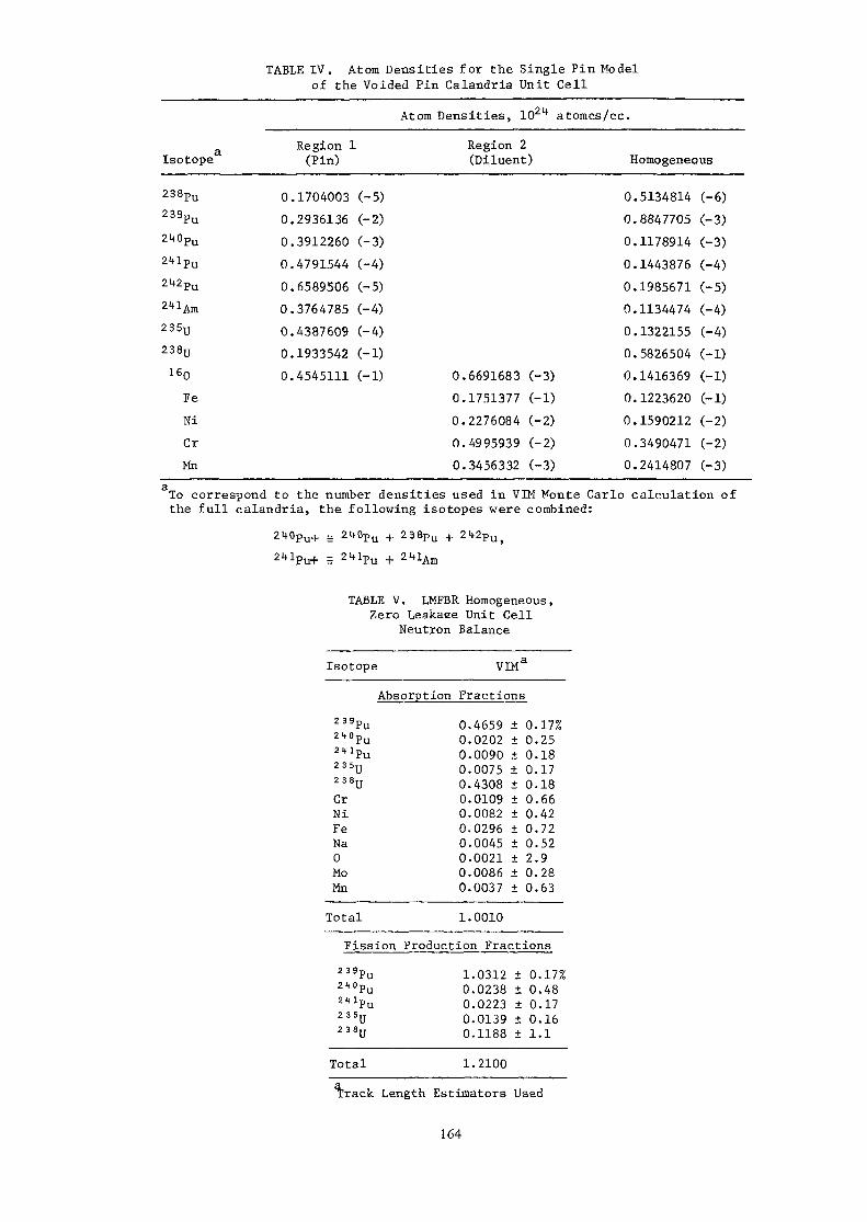
TABLE IV. Atom Densities for the Single Pin Modelof the Voided Pin Calandria Unit Cell

aIsotope

238pu239Pu240pu241pu242pu

2«Am23 5u238u160FeNiCrMn

Region 1(Pin)

0.1704003 (-5)0.2936136 (-2)0.3912260 (-3)0.4791544 (-4)0.6589506 (-5)0.3764785 (-4)0.4387609 (-4)0.1933542 (-1)0.4545111 (-1)

Atom Densities, 10Region 2(Diluent)

0.6691683 (-3)0.1751377 (-1)0.2276084 (-2)0.4995939 (-2)0.3456332 (-3)

atomcs/cc.

Homogeneous

0.5134814 (-6)0.8847705 (-3)0.1178914 (-3)0.1443876 (-4)0.1985671 (-5)0.1134474 (-4)0.1322155 (-4)0.5826504 (-1)0.1416369 (-1)0.1223620 (-1)0.1590212 (-2)0.3490471 (-2)0.2414807 (-3)

To correspond to the number densities used in VIM Monte Carlo calculation ofthe full calandria, the following isotopes were combined:

238Pu

TABLE V. LMFBR Homogeneous,Zero Leakaee Unit Cell

Neutron Balance

Isotope VIM

239Pu2*°Pu2*lpu235U238UCrNiFeNa0MoMn

Total

Absorption Fractions

0.4659 ± 0.17%0.0202 ± 0.250.0090 ± 0.180.0075 ± 0.170.4308 ± 0.180.0109 ± 0.660.0082 ± 0.420.0296 ± 0.720.0045 ± 0.520.0021 + 2.90.0086 ± 0.280.0037 ± 0.631.0010

Fission Production Fractions239Pu2*»Pu2lllPu235U238U

TotalCrack

1.0312 ± 0.17%0.0238 ± 0.480.0223 ± 0.170.0139 ± 0.160.1188 ± 1.1

1.2100Length Estimators Used

164

TABLE VI.EIGENVALUE NOTATION DEFINED INTERMS OF BUCKLING DIRECTION

Symbolkiky\>Kzk«kEQ

Fraction of Buck!In

X

10001/3

Direction3

y0101/21/3

inq

z0011/21/3

x-direction is perpendicular tovoid planes, {see Figs. 1 and 2.)

TABLE VII. LMFBR Homogeneous Zero Leakage Unit Cell;VIM/MC2-II/SDX Comparison of Integral Parameters

Parameter

kl + a«C28/£W

c28/(fW(1 + a.

£28/fWDifference is

1.1.0.

t9)) o.0.

VIM

2128 ±3223 ±

1690 +1278 ±01885 ±

0.00140.04%0.15%0.155%0.82%

KG

1.1.0.0.0.

2-II Differencea

212132321675126601862

-0•fO-0-0-1

.0007 Ak

.068%

.888%

.939%

.220%

11000

SDX

.2121

.3204

.1673

.1267

.01892

Di

-0

-0-1-0+0

f f erencea

.0007 Ak

.144%

.006%

.861%

.371%computed relative to VIM.

TABLE VIII. LMFBR Homogeneous, Zero Leakage Unit Cell;VIM/MC2-II/SDX Comparison of Isotopic Neutron Balance

Absorption Fractions

Isotope

239pu

2«0pu

2tlPu235y238y

CrNiFeNa0MoMn

Total

VIMa

0.4659 ± 0.17%0.0202 ± 0.250.0090 ± 0.180.0075 ± 0.170.4308 ± 0.180.0109 ± 0.660.0082 ± 0.420.0296 ± 0.720.0045 ± 0.520.0021 ± 2.90.0086 ± 0.280.0037 ± 0.63

1.0010

MC2-II

0.47650.02020.00900.00750.42870.01110.00820.03060.00450.00200.00870.0039

1.0019

Difference

+0.343%+0.000+0.000+0.000-0.487+1.835+0.000+3.378+0.000-4.762+1.163+5.405

SDX

0.46660.02020.00890.00750.42890.01110.00820.03050.00450.00210.00860.0037

1.0008

Difference

+0.150%+0.000-1.111+0.000-0.441+1.835+0.000+3.041+0.000+0.000+0.000+0.000

k Length Estimators Used.^Difference is computed relative to VIM.

165

TABLE IX. LMFBR Homogeneous iero Leakage Unit Cell;Comparison of VIM, MC2-II, and SDX Values of cr*8

028C

MC2-II (Rigorous)

Group

123456789

101112131415161718192021222324

252627

VIM

6.460-31.182-22.859-26.593-21.214-11.247-11.171-11.345-11.696-12.167-13.362-14.358-15.350-16.446-17.681-18.722-11.148-K)1.025-fO1.315-H)1.364-H)1.374-K)1.995402.146+08.374+0

±±±+±±±±±+±±±±±+±±±±±±±±

0.681 %0.4840.3310.2350.08890.02560.006630.02170.03280.03890.05930.09670.1660.1510.2710.3790.8980.6690.9081.241.641.334.42

11.0

Value

6.436-31.179-22.860-26.571-21.214-11.248-11.171-11.344-11.696-12.165-13.362-14.331-15.290-16.408-17.622-18.728-11.149+01.013+01.302+01.356+01.360+01.968+01.991+08.457+0

1.703+07.012-1

—

MC2~IL (NRA)

Difference Value Diffexence

-0.372%-0.254-0.035-0.334+0.000+0.080+0.000-0.074+0.000-0.092+0.000-0.620-1.121-0.590-0.768+0.069+0.087-1.171-0.988-0.567-1.019-1.353-7.223+0.991

"Same asRigorous"

811111111

177

.720-1

.137+0

.005+0

.299+0

.308+0

.324+0

.781+0

.418+0

.234+1

.512+0

.640-1

.640-1

-0 .023%-1.132-1—1

-4-3

-10-33+47

.951

.217

.106

.639

.727

.924

.361

SDX OTRA)Value Difference

6.431-31.178-22.858-26.569-21.214-11.248-11.171-11.344-11.696-12.165-13.363-14.327-15.288-16.403-17.613-18.720-11 .114+01.007+01.285+01.311+01.273+01.762+01.704+08.474+0

1.355+08.755-14.829-1

-0.449%-0.338-0.035-0.364+0.000+0.030+0.000-0.074+0.000-0.092+0.030-0.711-1.159-0.667-0.885+0.000-2.962-1.756-2.281-3.886-7.351

-11.679-20.965+1.012

TABLE X. GCFR Homogeneous Model Comparison Results

Code8 .,9c /f

VIM (30000 histories) 1.4333+0.00098 3052 + 18.5 (+0.61%) 0.1574+0.20%MC2-II/SDX/ARC 1.4324 3013.1 0.1566Error relative to VIM -0.0009 Ak -1.27% -0.51%

0.02091 + 0.53%0.02102

+0.53%

166

TABLE XI. Estimates of £2 for GCFR Homogeneous Composition

Case

12

3

4

5

MC2-II/SDX Option

Monte Carlo

MC2-2 IB1

MC2-2 IP1

MC2-2 CP1

MC2-2 CP1

a2(cm2)

3051

2943295629723013

Error

±21

-108-95

-79-38

SDX IP1MC2-2 CP1 (B2 ) 3032SDX IP1 Cr

MC2-2 IP1 (B2 ) 3023SDX IP1 C

MC2-2 CP1 (B2__,.J 2986SDX Flux Wt.

TABLE XII. Homogeneous Compositions For HighBuckling Leakage Tests

239Pu 2.0238U 8.8 x 1021

Fe 36.0 x 1021160 22.0 x 1021

TABLE XIII. Leakage Computed by Monte Carlo and theMC2-2 Code at High Buckling3

Monte Carlo CBI CPI IPI

k -k 0.4380 ± 0.0016 0.4333 (-0.0047) 0.4375 (-0.0005) 0.4363 (-0.0017)

V = 28.0 x lo"1* cm~2

167

TABLE XIV. Comparison of VIM, SDX, and ARC Integral Parameters for the Heterogeneous LMFBR True ID Slab Cell

Item DefinitionSDX

VIM27 Group Diffusion Theory

Value Difference Value Difference

eigenvalue 1.23961 ± 0.00165 1,24013 +0.00052 1.24029 +0.00063/

(1 + a«*9) eelO/

cell E

1,3074 ± 0 . 2 8 7 1.3073 -0.008 1.3073 -0.008

a,oo cell E

/ /N28cr28<j>dEdrcell E * cell

/N«drcell

0.01921+0.985% 0,01906 -0,781 0.01906 -0.781

cell E

cell E cell

0.-1664 ±0,316% 0.1640 -1.442% 0.1640 -1.442

28 cell E

cell E

cell/N23drcell

0.32032 ± 0.316 0,31679 -1.102

cell E

cell E<j)dEdr

d?cell

cell

1.9244 ± 0.218 1,9275 +0.163

TABLE XV, Comparison of VIM and Diffusion Theory Spectrafor the Heterogeneous LT1FBR True ID Cell

TABLE XVI. Comparison of VIM and Diffusion Theory Absorption byIsotope for the LMFBR True ID Slab Cell

Diffusion Theory

Group

123456789101112131415161718192021222324

252627

ETop

10 MeV6.0653.6792.2311.353

820.85 keV497.71301.97183.16110.0967.3840.8724.7915.039.125.533.352.031.23

748.52 eV454.00275.36101.3037.27

13.7110 VIM; 5.04 ARC

1.86

VIM

0.2375 ±0.9622 ±2.3127 ±3.4528 ±4.2530 ±8.3454 ±8.2742 ±10.6818 ±11.6024 ±10.3743 ±8.9662 ±7.1054 ±7.2675 ±5.3723 ±2.9958 ±1.9199 ±0.7072 ±2.1046 ±1.4533 ±0.8582 ±0.3980 ±0.3145 ±0.0381 ±0.0030 ±

0.0001 ±--

3.4 %1.91.20.640.660.540.310.260.300.280.250.290.330.300.370.430.280.350.551.01.11.73.412.0

45.0

Value

0.23450.95372.31563.47614.22668.33068.256210.649311.663110 '.36128.90047.05247.26645.38173.01711.93010.70592.12851.45840.88430.42020.34330.04150.0027

0.0001--

Difference

-1.263%-0.883+0.125+0.675-0.621-0.177-0.21.8-0 . 304+0.523-0.126-0.734-0.746-0.015+0.175+0.711+0.531-0.184+1.136+0.351+3.041+5.578+9.157+P,.924-10.000

-

Isotope

Pu240Pu24lU235U238Pu239

Cr

NiFeNa0-16

MoMnTotal

VIM Diffusion Theory

0.0205690 ± 0.339%0.0091534 ± 0.2470.0076793 ± 0.1730.4279200 ± 0.2240.4698700 ± 0.2070.0108640 ± 0.4920.0080455 ± 0.6170.0295640 ± 0.9870.0045924 ± 0.8730.0019000 ± 2.590.0085047 ± 0.4330.0042275 ± 0.6181.0028898

0.02057910.00918550.00773720.42405720.47119690.01125720.00812770.03097380.00466190.00191700.00879040.00441361.0028976

% Difference

•K).049%+0.351-t-0.755-0.903-f 0.282+3.620-KL.021

+4.769+1.513+0.896+3. 359+4.401

TABLE XVII. Comparison of VIM and'SDK-Generated Broad Group 238U CrossSections for the LMFBR True ID Slab Cell

Group

123456789

101112131415L61718192021222324

252627

VIK

7.208-3 ±1.276-2 ±3.010-2 ±6.772-2 ±1.243-1 ±1.262-1 ±1.176-1 ±1.347-1 ±1.687-1 ±2.160-1 ±3.349-1 ±4.307-1 ±5.270-1 ±6.287-1 ±7.365-1 ±8.335-1 ±9.979-1 ±9.174-1 ±1.191+0 ±1.187+0 ±1.130+0 ±1.755+0 ±1.476+0 ±6.765+0 ±

2.715-1 ±

c

[

1.54 %0.8380.6360.4690.2490.2540.2080.1940.1170.1640.1880.2360.2600.2840.3700.5331.090.8711.111.212.551.743.16

20.2

16.1

,28c

s:Value :

6.966-31.267-22.990-26.745-21.249-11.260-11.176-11.345-11.692-12.161-13.349-14.275-15.220-16.254-17.274-18.220-19.352-18.977-11.150401.144401.048401.474401.474406.51240

1.7191.0304.684-1

DX

Difference

-3.357%-0.705-0.664-0.39940.483-0.15540.000-0.148+0.29640.04640.000-0.743-0.948-0.825-1.236-1.380-6.283-2.147-3.442-3.622-7.257

-16.011-0.136-3.740

^

9.870-15.899-15.779-14.195-12.662-21.203-31.281-45.808-54.970-53.566-55.189-6

o

lift

± 1.53 %± 0.704± 0.527± 0.544± 0.979± 0.483± 0.366± 0.217± 0.116± 0.257± 0.663

28f

Value

9.453-15.878-15.762-14.161-12.646-21.205-31.276-45.802-54.987-53.578-52.205-6

SDX

Difference

-4.225%-0.356-0.294-0.810-0.60140.166-0,390-0.103+0.342+0.337

-57.482

TABLE XVIII.LEAKAGE PARAMETERS OBTAINED BY MONTE CARLO USING

THREE-DIMENSIONAL AND ONE-DIMENSIONAL UNIT CELL MODELS(AND ENDF VERSION 3 CROSS SECTIONS)

Model

3-D

1-D Reference

1-D Pure Void

k»

1.4368 ± 0.0022

1.4355 ± 0.0033

1.4355 ± 0.0017

if (cm2)

1022 ± 12

1015 ± 15

1011 ± 13

A2 (cm2)

1196 ± 14

T139 ± 13

——

1°

0.2706 ± 0.0021

0.2708 ± 0.0028

0.2695 ± 0.0027

sa

0.2961 ± 0.0027

0.2869 + 0.0029

0.2936 ± 0.0027

V

0.2894 ± 0.0030

0.2837 ± 0.0027

0.2887 ± 0.0027

W1.094 ± 0.013

1.060 ± 0.015

1.089 ± 0.015

aB2 = 7 x 10-"* cm-2.

TABLE XIX.

LEAKAGE PARAMETERS OBTAINED USING THE REFERENCE (NO PURE VOID) ONE-DIMENSIONAL MODEL(AND ENDF VERSION 4 CROSS SECTIONS)

Method

Monte CarloBenoist DiffusionConventional Diffusion

kM (error)

1.4340 ± 0.00331.4338 (-0.0002)1.4338 (-0.0002)

iz. cm2 (error)

1043 ± 111016 (-27)1007 (-36)

i2 cm2 (error)

1152 ± 10'1137 (-15)1007 (-145)

k^ - kj_a (error)

0.3962 ± 0.00320.3916 (-0.0046)0.3864 (-0.0098)

k«, " k.a (err°r)

0.4204 ± 0.00350.4262 (+0.0058)0.3864 (-0.0340)

k. - kEQa (error)

0.4140 ± 0.00290.4148 (+0.0008)0.3864 (-0.0276)

V = 7 x 10-" cm-2.

TABLE XX.

EIGENVALUES OBTAINED USING THE ONE-DIMENSIONAL PURE-VOID MODEL(AND ENDF VERSION 4 CROSS SECTIONS)

Method

Monte Carlo

Alternate Diffusion

Conventional Diffusion

k^ (error)

1.4315 ± 0.0018

1.4338 (+0.0023)

1.4338 (+0.0023)

B2 = 2.001 x ID'5 cm'2

k» - kii (error)

0.0184 ± 0.0003

0.0179 (-0.0005)

0.0142 (-0.0042)

k» ' kEQ (error)

0.0172 ± 0.0003

0.0168 (-0.0004)

0.0142 (-0.0030)

B2 = 7 x 10-1* cm'2

k« - kx (error)

0.3886 ± 0.0027

0.3860 (-0.0026)

0.3852 (-0.0034)

km - ku (error)

0.4266 ± 0.0031

0.4220 (-0.0046)

0.3852 (-0.0414)

k- " kEQ (error)

0.4183 ± 0.0030

0.4130 (-0.0053)

0.3852 (-0.0331)

TABLE XXI.SENSITIVITY OF k™ TO BUCKLING ERROR IN EQ. (2)

Buckling Used in Eq. (5)x 10" (cm-2)

B2 B| B2

7

7

7

10

1 x 7 2 x 7A / "•" ^ /

3 3

1 x 7 1 x 72 2

1x7 - x 74 4

1x10 - x 103 3

kpQa (error )

1 0224 ( }1 • \J L* t~~ \ /

1.0204 (-0.0020)

1.0228 (+0.0004)

1.0282 (+0.0058)

ag2 = 7 x 10"1* in diffusion theory calculation.

Error relative to firstCThe numbers in Table XXI

row in the table.

apply to the sensitivitytest only and are not totally consistent withthose in Table XX.

TABLE XXIL. Comparison of Results for the Vim Calculation of thePin-Calandria Unit Cell and the SDX Calculations

of the Single Pin Model .All at Zero Buckling

Three-Dimensional

Eigenvalue

Pin-CalandriaVIM

ks, 1.30184 ± 0.00318

One-DimensionalSingle Pin

Reference ModelingSDX

1.29935

SDX/VIMa'b

0.9981 ± 0.0024(50,000 Histories)

Reaction Rate Ratiosf25/f^9 1.07857 ± 0.01973f28/ft9 0.021342 ± 0.000517c28/ft9 0.15635 ± 0.00348Ci*9/f«t9 0.27984 ± 0.00773fi*0/f«t9 0.20120 ± 0.00291fH./f1*9 1.39678 ± 0.02536

1.081170.0211630.156690.281990.199971.40158

1.0024 ± 0.01820.9916 ± 0,02421.0022 ± 0.02261.0077 + 0.02760.9939 + 0.01451.0034 i 0.0181

Diffusion Characteristics (in units of cm2)

17X

I2-y~*Zz

If - 1/2(1* + J*)J*

764.2 ± 10.9

763.6 ± 9.9

800.3 ± 9.5

763.9 ± 7.4

2328.1 ± 17.5 2202.1° 0.9459 ± 0.0075

Uncertainties represent l-o.Only uncertainties from the VIM statistics are included.This value was obtained using conventional D's.

172

TABLE XXIII. Comparison of Eigenvalues for a High Buckling System

B2 = 7.0 x 10"1*

Case 1: B2 - 0.0, B2 - 7.0 * 10~"K. Z

Akkk

Case 2: B2 = 7.0 * 10"!; B2 = 0.0Akkk

Case 3: B2, = 2B2

Akkk

VIM (3-D)Pin-Calandria

-0.2240

1.01023

-0.2164

1.02012

-0.2200

1.01544

± .00206

± .00416

± .00221

± .00429

± .00250

± .00455

SDX/BENOIST (1-D)Single Pin

-0.2155

1.01915

-0.2131

1.02231

-0.2146

1.02125

Ratio Relative to VIM

0.9621 ± .0092

1.0088 ± .0041

0.9848 ± .0102

1.0021 ± .0042

0.9755 i .0114

1.0057 ± .0045

SDX/GELBARD (1-D)Single Pin

-0.2222

1.01040

-0.2160

1.01845

-0.2187

1.01493


0.9920 i .0092

1.0002 ± .0041

0.9982 ± .0102

0.9984 ± .0042

0.9941 + .0114

0.9995 ± .0045Note: Ak = k-k~ , where km (VIM) = 1.30184 ± .00318 and k» (SDX) = 1.29908.

k k»All uncertainties represent 1-a intervals and include only the VIM Monte Carlo uncertainties.

TABLE XXIV. Comparison of Eigenvalues tor a low Buckling System

VIM (3-D)Pin Calandria

Case I.

Case 2.

Case 3.

Case 4.

Case 5.

B2 = 2.0 x 10~5

B2 = 2.0 x 10~5, B2 •= 0.0R ' zAkkk

B2 - 0.0, B2 - 2.0 x 10~5Akkk

B2 - 2B*z RAkkk

B2 - 1.0 x io"5B2 - 2B2K. Z

Akkk

B2 = 7.0 x 10"SB2 - 2B2R z

Akkk

SDX/BENOIST (1-D)Single Pin

SDX/GELBARD (1-D)Single Pin


-0.00759 ±1.29196 ±

-0.00795 ±1.29149 ±

-0.00784 ±1.29163 +

-0.00387 i1.29680 ±

-0.02662 +1.26719 ±

.00010

.00318

.00009

.00318

.00010

.00318

.00005

.00318

.00036

.00321

-0.

1.

0.1.

-0.1.

-0.1.

-0.

1.

0074128946

0075128932

0074828937

0037329423

0256626575

0.9761 ±0.9981 i

0.9449 ±0.9983 ±

0.9538 ±0.9983 ±

0.9646 ±0.9980 ±

0.9639 ±0.9989 ±

.0132

.0025

.0113

.0025

.0128

.0025

.0129

.0025

.0135

.0025

-0.1.

-0.1.

-0.1.

-0.1.

-0.

1.


0078028895

0083828819

0081628848

0040229386

0271826377

1.0277 ±0.9977 ±

1.0541 ±0.9974 ±

1.0408 ±0.9976 ±

1.0388 ±0.9977 ±

1.0210 ±0.9973 ±

.0132

.0025

.0113

.0025

.0128

.0025

.0129

.0025

.0135

.0025Note. Ak = k-k«.. where k,,, (VIM) = 1.30184 ± .00318 and k» (SDX) - 1.29908.

k k.0All uncertainties represent 1-tj intervals and Include only the VIM Monte Carlo uncertainties.

173

TABLE XXV. Neutron Balance Comparison between VIM andMC2-2/Diffusion Theory Calculations

Diffusion TheoryVIM Diffusion Theory VIM

keffLeakage fromInner Core

Inner Core +Outer CoreLeakageReactorLeakage

1.00689 ± 0.00190 1.00710 1.00021 ± 0.00189

0.07863 ± 0.00486 0.07548 0.95998 ± 0.06179

0.16125 ± 0.00657 0.15618 0.96858 ± 0.04074

0.01304 ± 0.00679 0.00949 0. 72792 ± 0.52095

TABLE XXVI.

Eigenvalues For a ZPR LMFBR Mockup Core

ExperimentMonte CarloDiffusion Theory (Gelbard D's)

(TWOTRAN)

k1.00090.9939 ± 0.00150.99091.0033

Eigenvalues For a Hypothetical RZ Model

Monte CarloDiffusion Theory (Conventional D's)

TWOTRAN(DOT)

1.0045 ± 0.00110.99931.00931.0078

174

Figure 1 Figure 2

LMFBR Unit Cell(Dimensions in inches)

C£LL (AS BUILT)

SST-

UNIT CELL (MODEL)

Ii

OR*95

1hf

"~IL /

f

/

L) '/

/

/

/

r/f

SST MATRIX

CAN————————— k —— 4

Ss!LU0gz

4(£

s

•

3zD5oV)

CVJ

K

Q.

UlOXO

15?

=/=

Vu*-

z

ii(f

t

VOID

Ul

atunXooCE

s00

zo

DOO

"(M

Ul

Q.

OX0

2

! z 'IT

~

^

11 11 11 H 11 11 1*s .

71 ——— [/////

'. o"' 10

/

/

',

> '2 !; i

^~

*

^ '•>•*•

-4

1 ———

K> 1

<?*

y

'7

'6

L

- O

?a.

' /'9

' *

J —— l

' K)

»>N

;r,o

^ UUfU W«LL

• —— VOID0041"

I

A

z

*-'"

'«

/

3° //

r^

/^

r»

/

/

//

'•* —— SST

/////^f/

/- • —— *^- T

GCFR Unit Cell(Dimensions in cm)

CORE

y (height)

z (length)

x (width)

0.102i r

52**

,

i

5.08My*x.

ss

N

S

. 524J0.102 —— |

U0

v IFP"iI1ii1

r s 7 7 7 S

-• ^m w

PFu fe

i11I111

-r-U

.5245

V V

-sss

ssssss

s

'10 14

3 5 79^11 I3il5

2• •

4 6•i

8-\ r

12r i ^

16

-*——

/

/

/

/

X

^

/

/

X

/

**

REGIONNO.

^

5.524505.321305.17398-5.08258 —

• 5.17398

End View

_^w— _ -1 - <£- JEPR Pin clandria Uni Cell

5.5245

R - (£2/*)r - 0.4290 cm.

, ,„,,1.3811 cm.

= 0.7792 cm.

ca

176

VIM Edits

VIM Neutron Balance.A A

Physical Geometry

RZ or XY Diffusion Theoijt

3D-^OD Homogenize

3D- 1D Modelingfor plate resonanceself shielding

3D—>1D Modelingfor Diffusion Coeff.Generation

Fig. 4

177

SESSION B: NON-UNIFORM LATTICES

(Chairman: A. Kavenoky)

THE SPH HOMOGENIZATION METHOD

A. KAVENOKYService d'etudes de reacteurs et de mathematiques

applique'es,Centre d'etudes nucleaires de Saclay,Gif-sur-Yvette, France

AbstractThe SPH homogeneization method is an attempt to generate homogeneized

cross sections -for an irregular lattice. Reactions rates are determined by two-dimensional transport calculation for an irregular lattice made of heterogeneouscells. The SPH method provides homogeneized cross sections for each cell of theheterogeneous lattice : a calculation performed using these cross sections fur-nishes the same reactions rates as in the original calculation. Numerical resultsare presented for a PWR rod bundle assembly and for an interface between uraniumand plutonium lattices.

The homogeneization of a uniform lattice is a rather well understoodtopic while difficult problems arise if the lattice becomes irregular. The SPHhomogeneization method presented in this paper is an attempt to generate homo-geneized cross sections for an irregular lattice. Section 1. summarizes thetreatment of an isolated cylindrical cell with an entering surface current (inone velocity theory] ; Section 2. is devoted to the extension of the SPH methodto assembly problems. Finally Section 3. presents the generalisation to generalmultigroup problems. Numerical results are obtained for a PWR rod bundle assem-bly in Section 4.

1. The principle of SPH methodAn isolated heterogeneous cell is considered ; neutron sources may

exist inside the cell and an isotropic current C+ enters the outer surface ofthe cell. The problem is treated within the framework of the one-velocity theory.A standard collision probability treatment is applied to obtain a system oflinear equations for the mean flux $. in each region i :

J=N p r+ pV- v / \ ii si$. = > IE . $. + S. I Y^- + w—y— £1)

7 ' ' ^ tJ 1 U

In this equation ESJ and E.J.J denote respectively the mean scattering and totalcross sections in regions j, the volume of which is Vj ; P^j is the standardfirst flight collision probability and PS^ is the probability for a neutronentering isotropically by the surface to suffer its first collision in regioni ; S. is the average source density in region j.

181

Solving the system of Eq. 1, the fluxes $j_ are obtained j the averagecross section Zr and the integrated reaction rate Tr for each reaction r areobtained :

1=NY" V. $. i=N i=N

$ = ±_i———————— ; V = > V. ; S = -^ > V. S.i=N / > i V / * i iF v 1=1 1=1Z_< "•;, 1=1

C2)i=N

z = —• y^z . v. $. ; T = z v $r V $ / ri i i r r1=1

The index r may denote scattering, total or eventually fission crosssections.

An homogeneous cell is defined by the homogeneized cross section ofEq. 2, the geometry and the outer current is kept ; the complete cell is treatedwith the flat flux assumption. The collision probability equation is :

'('p

Where P is the collision probability for the homogeneized cell and s the outersurface of the cell. It easy to show that $ is not equal to $ because the colli-sions probabilities do not vary linearly with the cross sections. If the reactionrates are to be equal in the heterogeneous and homogeneous problems a more refinedhomogeneization process had to be used.

As previously an homogeneous medium is considered assuming a flat fluxand an entering current C+ ; the collision probability equation is :

t*\) 'XiThe cross sections of this homogeneous medium (Z - and Es) will be deter-

mined in order to obtain the same reaction rates as in the heterogeneous problem :

T =£s sV = Z * V

Tf = Zf $ V = Zf $ V

It is obvious that these relations imply :

s s t t f f

Where y is a parameter to be determined by the equation :

/ \ 4V Z C+ / \Tt = (Ts + V S) PCy Zt'1 + ——— —— u(l-PCu t] ) C6]

This equation is solved using the iterative scheme :["/ \ 4V Z C* / v"J

_ 1_ = JL (T + v s ) P [ y Z.] + ——— - —— y (1-PCy Z,.)] (7)Vl yn L\ s / n * s n\ n * /]

2This iterative scheme is accelerated using the Aitken A method.182

2. Treatment of an assemblyAn assembly is considered, it is made of a few different heterogeneous

cells. This assembly is treated using approximate two-dimensional transport theo-ry : collisions probabilities are calculated for each isolated two-dimensionalcells and the cells are coupled by boundary currents.

The collision probability for the region i of the cell I to the regionj of cell J may be represented by :

P = P * < 5 + P P P [ 8 )I. J. I. J. IJ I. S IJ S J. l ;i J i J i i

+Where P is the standard collision probability for cell I assumed to be iso-Ji J

lated, P_ is the probability for a neutron born in region i of cell I not toi b

suffer its first collision in the isolated cell I, P is the probability for aJ. J

neutron going out of cell I to enter in cell J and P is the probability for aO J .

neutron entering in J to suffer its first collision in region j.

The general collision probability equation for this assembly may bewritten as :

J=N j=M7 PT ,x-V / \ Ji Ji— (9)

When the system of Eq. 9 is solved, it is possible to transform thisequation using the definition (Eq. 6) of the collision probability :

J-M

J=IM j=M

Using the reciprocity theorems1

Where s is the outside surface of cell I -, the final form of the equationsbecomes :

(11)

with :

183

Comparing Eq. 11 with Eq. 1 showes that the assembly problem treated with theprevious assumptions is reduced to separated problems of heterogeneous cellswith an entering current given by Eq. 12. The determination of Cj requests theresolution of the transport problem in the assembly.

Using Eqs 11-12, the homogeneization process for an assembly of hete-rogeneous cells is reduced to several homogeneization problems for heterogeneouscells j the treatment of Section 1. is, in this way, extended to an assembly.

Using this treatment, an homogeneous cell equivalent to the hetero-geneous one is determined. The reactions rates calculated in the homogeneous cellare equal to those calculated in the heterogeneous one for scattering, absorptionand eventually fission. Therefore the outgoing current is also the same.

If the assembly made of all the equivalent homogeneous cells is consi-dered, the reactions rates will be the same as in the heterogeneous one.

The SPH homogeneization method provides a scheme to determine an assem-bly of homogeneous cells equivalent to an assembly of heterogeneous cells.

3. Treatment of an assembly in imiltigroup theoryIn the previous section, an homogeneization technique had been

presented in one-velocity theory ; this technique may be extended to mul-tigroup theory.

The aim of the SPH homogeneisation technique is to match thereactions rates in the homogeneous and heterogeneous calculations. If thistechnique is used in multigroup calculations the.absorption rate and thetotal slowing down source will be matched.

In multigroup theory, the heterogeneous calculation has to be doneand the SPH treatment is exactly the same as in one-velocity theory.

This homogeneization scheme may also be extended to group collap-sing calculations. If the heterogeneous calculation has been done using arefined group structure and if the reaction rates are calculated within aless refined mesh grid the SPH homogeneization technique allowes the deter-mination of an assembly of homogeneous cells, equivalent to the originalassembly using the collasped group structure.

4. Numerical resultsThe SPH homogeneization method had been implemented in the APOLLO

assembly calculation module [1] of the NEPTUNE system for reactor calculationsand it may be used with any of the two-dimensional approximations.

The tests presented here had been performed with the standard Rothapproximation of the assembly.

4.1. Treatment_of a_rod_bundle assemblyA nine cell bundle is treated ; eight cells are standard fuel cells

and the central cell is a control rod cell [the central rod is made of analloy of Ag, In, Cd).

oooo

.Control Rod

184

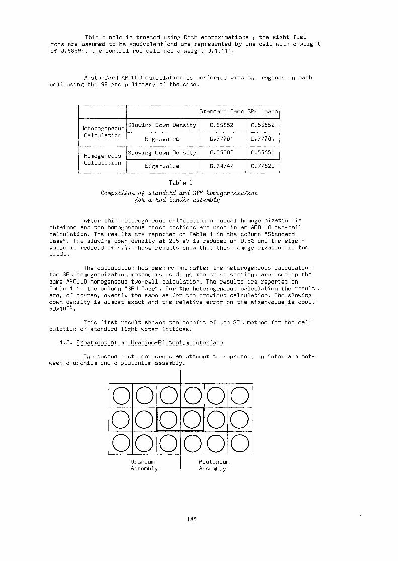
This bundle is treated using Roth approximations j the eight fuelrods are assumed to be equivalent and are represented by one cell with a weightof 0.88889, the control rod cell has a weight 0.11111.

A standard APOLLO calculation is performed with the regions in eachcell using the 99 group library of the code.

HeterogeneousCalculation

HomogeneousCalculation

Slowing Down DensityEigenvalue


Standard Case0.558520.777810.55502

0.74747

SPH case

0.55852

0.77781

0.55851

0.77829

Table 1£ Atandastd. and SPH

{,o>t a. fiod buutdte.

After this heterogeneous calculation on usual homogeneization isobtained and the homogeneous cross sections are used in an APOLLO two-cellcalculation. The results are reported on Table 1 in the column "StandardCase". The slowing down density at 2.5 eV is reduced of 0.6% and the eigen-value is reduced of 4.%. These results show that this homogeneization is toocrude.

The calculation had been redone :after the heterogeneous calculationthe SPH homogeneization method is used and the cross sections are used in thesame APOLLO homogeneous two-cell calculation. The results are reported onTable 1 in the column "SPH Case". For the heterogeneous calculation the resultsare, of course, exactly the same as for the previous calculation. The slowingdown density is almost exact and the relative error on the eigenvalue is about50x10-5

This first result showes the benefit of the SPH method for the cal-culation of standard light water lattices.

4.2. Jreatment_of_an_yranium3Plutonium interfaceThe second test represents an attempt to represent an interface bet-

ween a uranium and a plutonium assembly.

OooOooooo

UraniumAssembly

ooooooooo

PlutoniumAssembly

185

Only two cells are represented with equal weight the results obtainedusing the SPH homogeneization scheme are given on Table 2.

HeterogeneousCalculation

HomogeneousCalculation



0.76448

1.20647

0.76448

1.20643

Table 2Ru,uJLtt> ofa SPH nomo§e.n&ization

Uranium-Ptuton*.um

The homogeneous SPH calculation gives the same results as the hete-rogeneous calculation.

On Table 3 the four group fission rates and the average cross sec-tions are reported for the uranium cell ; the first line presents the hetero-geneous reaction rates obtained by the first APOLLO calculation and the secondline the homogeneized macroscopic fission cross sections obtained in this cal-culation. The last two lines give the results obtained in the SPH calculation :the reaction rates differ very slightly but the homogeneized section in group 4has been reduced from 0,0377 to 0.0361.

Group

Heterogeneous

Homogeneous

TfZfTfSf

19.9617.10"3

2.6087.10"3

9.9611.10"

2.6538.10"3

2

1.2856.10~3

2.4029.10"4

1.2856.10"3

2.4316.10"4

3

1.1480.10"2

2.8587.10"3

1'.1480.10~2

2.8359.10"3

4

i.ssgs.io"13.7694.1D"2

1.3593.10~2

3.6066.10~2

Table 3Reaction Ratu and O.OM Suction* the. iiw.ni.um

On Table 4 the same results are presented for the plutonium cell : forthis case the fission cross sections in group 4 is reduced from 0.1021 to 0.0893.

Group

Heterogeneous

Homogeneous

TfZfTfZf

11.7700.10"2

3.8126.10"3

1.7698.10"2

3. 9106. 10"

2

3.0272.10"3

5.0456.10"4

3.0272.10"3

5.1248.10"4

3

2.4369.10"2

6.1749.1D~3

2.4369.10"2

6.0965.10"3

4

2.4363.10~1

1.0213.10~1

2.4363.10"1

8.9305.10"2

Table 4Re.acti.on Ratu and CSLOAA Ae.cti.om> io>t tkz Plutonium CeM.

186

5. ConclusionsThe SPH homogeneization method represents an attempt to improve the

calculation of heterogeneous assemblies ; the first step allowes the determi-nation of an equivalent homogeneous assembly in transport theory. The secondstep will be an equivalence between transport and diffusion calculations.

Reference

[1] A. KAVENOKYAPDLLD : A General Code for Transport, Slowing-down and ThermalizationCalculations in Heterogeneous Media. Mathematical Models and Computa-tional Techniques for Analysis of Nuclear Systems.Ann Arbor, Michigan April 9-11, 1973. Conf-730414-P1.

187

HOMOGENEOUS CELL PARAMETERSFOR 2-D REACTOR CODESBY AXIAL AVERAGING OF THE THIRD DIMENSION

W. HEEDS, J.D. IRISHAtomic Energy of Canada Limited,Chalk River Nuclear Laboratories,Chalk River, Ontario, Canada

A B S T R A C T

The NRU and NRX research reactors at Chalk River NuclearLaboratories are very heterogeneous. Analyses of these reactors areperformed using "equivalent" axially averaged homogeneous cell parametersfor every lattice site. This allows a 2-D neutron diffusion code tobe used to calculate flux distributions, fuel powers and eigenvalues.

The axially averaged parameters are obtained from the code CELDATAwhich calculates "equivalent" homogeneous parameters for a cylindricalcell surrounded by two concentric environment annuli using neutrondiffusion and perturbation theories in R, Z geometry. Reaction rates,neutron flux distributions and eigenvalues calculated by CELDATA, forboth the axially heterogeneous central cell and its homogeneous"equivalent" are compared for three examples.

Some of the NRU loops contain bundles with azimuthal variationsin the outer fuel ring. An empirical method is presented whereby theindividual element powers for a bundle of this type can be obtained bymaking corrections to the outer element powers calculated for a bundlewith elements of an average composition. The method is tested againstan experiment performed in the ZED-2 reactor.

1. INTRODUCTION

There are two research reactors, NRX and NRU, at the Chalk River NuclearLaboratories (CRNL) of Atomic Energy of Canada Limited which are used for awide variety of experimental and commercial irradiations as well as providingneutron beams for solid state research. The cores of these reactors areextremely heterogeneous, both radially and axially, due to the complex natureof the experimental load and the differential axial burnup in the highlyirradiated enriched uranium fuel rods.

Among the major facilities in both reactors are loops, in which experi-mental fuels, for the CANDU* power reactors, are irradiated. Azimuthalheterogeneity occurs in certain, "demountable", 36 element loop fuel bundleswhen individual fuel elements in the outer fuel ring of these bundles arereplaced part way through the irradiation. This process allows similar fuelspecimens to be irradiated to different burnup levels and also, in principle,permits the irradiation and comparison of different fuel types, in the same ring.

Regular comparisons of measured and calculated fuel power distributionsare an essential component of the fuel management strategy employed to ensuresafe and efficient operation of these reactors. Hence a calculational modelwhich adequately predicts individual reactivity effects, flux and fuel power* Canada Deuterium Uranium

189

distributions is required. For this purpose, a two-group, two-dimensionalfinite difference neutron diffusion code employing hexagonal geometry is used.

In the first part of this paper, the methods used to determine theaxially averaged parameters that are required by this code are described. Theeffect of using such parameters to calculate powers and reaction rates, in asimple model, is discussed.

The second part of this paper deals with approximate methods to determinethe power distribution of the outer fuel pins in a "demountable" bundle, wherethe fuel pins have different enrichments. A comparison is also made with someexperimental results.

2. THE PRODUCTION OF AXIALLY AVERAGED LATTICE PARAMETERS

Lattice parameters required for reactor calculations can be obtained froma number of codes. In this paper, parameters D., E , E , v.E,.. and Q. are

f~ \ si)\ 3. A3- Kl 1 11 1derived from the lattice code LATREP for two neutron energy groups. Thesubscripts (A, R and f) on the cross sections, E, are defined in the conventionalway, namely absorption, removal and fission. D is the diffusion coefficient andv is the neutron yield per fission. For the fast group, i equals 1 and for thethermal group, i equals 2. The LATREP Q factor is defined as the cell fissionpower per cm length per unit cell average "Westcott" flux. Use of the Westcott

(3)flux convention in LATREP and conservation of the four factor formula definitionsfor the lattice parameters results in Q., V.E,.. and E ~ being set to zero.

i. i. I i. R^Axially averaged parameters are produced using a code called CELDATA

which calculates bilinearly weighted average values for use in the 2-D reactormodel. This choice of weighting was made in an attempt to conserve the criticaleigenvalue, k ,.,., in the reactor simulation. The method is based upon the useof perturbation theory and adjoint flux weighting thus permitting changes in to, theinverse period of a reactor, to be identified solely with the volume in whichthere is a change in lattice parameter. However the use of bilinearly weightedparameters in 2-D reactor calculations introduces errors in the calculation ofneutron reaction rate distributions in the model. In addition there is noguarantee that reactivity is necessarily conserved for the 2-D model and inprinciple, comparison should be made with a 3-D code to determine the fulleffects of the 2-D approximations. This comparison has yet to be made and sothis report details the limited comparisons that can be made within the CELDATAcalculation model to justify the use of bilinearly weighted average parametersin 2-D reactor codes.

Flux-weighted axially -averaged Q factors are calculated separately inCELDATA and are used, subsequently, in conjunction with flux distributionscalculated by the 2-D reactor model to obtain the reactor power distribution.The method in principle can be applied to all reaction rate distributioncalculations.

190

2.1 Objectives of Program CELDATAThe objectives are:

(a) To calculate neutron flux distributions along the axis of an axiallynon^uniform cylinder representing the actual contents of a reactorlattice site.

(b) To calculate a consistent set of bilinearly -weighted axially averagedcell parameters for use in 2-D reactor codes.

(c) To calculate the axial power distribution and total fission power forthe actual contents of a lattice site containing fuel and from theseto derive the average power per unit length per unit cell averageflux (called the site Q factor).

(d) To calculate the axial distribution of the total site energy output.(e) To calculate flux-weighted axially averaged reaction cross sections

and leakage factors which conserve total reaction and leakage ratesfor the actual contents of a lattice site.If parameters for burnup simulations are required, the results of (b),

(c) and (d) may be obtained as polynomial functions of total energy outputfor the actual contents of a lattice site.2.2 The CELDATA Model

The basic model used in CELDATA is a three zone cylindrical reactor. Theinner zone represents the single lattice site being averaged and the twosurrounding annuli simulate the first and second ring of neighbours in a 19 sitehexagonal lattice as shown in Fig. 1. Azimuthal averaging for each of the twoenvironment annuli is done internally in CELDATA using input weighting factors.This allows a two group, finite difference two-dimensional neutron diffusioncalculation using R-Z geometry to be made. ' For simplicity, the reactorlattice outside the ring of second neighbours is represented by a single radialextrapolation length. The use of this model is considered adequate forcalculating the axial flux distribution in the central site. In principle,two-group fluxes and adjoint fluxes in all three zones are readily calculable.

Axial details of all 19 lattice sites are required by the program.Elevations referenced from the bottom of the moderator are specified to delimitaxial regipns in which the lattice parameters are constant. An elevation specifiedin any of the 19 sites automatically specifies a mesh boundary in the Z planefor the finite difference neutron diffusion calculation in addition to theregular axial divisions required by the method.

Lattice parameters for each axial section in the 19 site model are obtainedfrom LATREP. Versions of LATREP exist which permit the use of non-zero fluxgradients at the cell boundary. This is done either by the use of a pitch largerthan the actual pitch and volume correcting back to the actual pitch or by theuse of albedos at the cell boundary. CELDATA contains an option which allowsiterations between CELDATA and LATREP to be performed in order to determine albedos.

191

2.3 Bilinearly Weighted Average ParametersA brief outline of the general theory used to derive formulas for

bilinearly weighted parameters is given below. A more detailed derivation canbe found in Appendix A.

The general approach used for calculating bilinearly weighted parametersin CELDATA is essentially a null method. A base case is calculated for a uniformrod in the central site of the 19 site, three zone model. The lattice parametersfor the uniform rod are denoted by a superscript o. Relative fluxes <j>. and

A •Ladjoint fluxes <J>. are obtained for this reactor by solving the two-group diffusionequations for the base case which are represented in matrix notation by

M 4,° = 01° £ (1)where v is the neutron velocityand by solving the corresponding adjoint equations

itA A o (f)M <j> = u> 2- (2)

The contents of the central site are then replaced by axial details representingthe actual rod to be averaged. The parameters for this rod are denoted by asuperscript A. This change is considered to be a perturbation from the base case

Aand new relative fluxes § are obtained by solving the corresponding equation^

(M + PA) / = WA £- (3)

Following a derivation similar to that outlined in reference 5, the followingA oequation for co -0) is obtained

* A Af> P <J> dV

(4)XA

where X"

The contents of the central site are then replaced by a uniform rod which producesthe same change in o> from the base reactor as did the actual rod. The parametersfor this rod are denoted by superscript B. The equation for this reactor is

TJ

(M + PB) <J>B = WB 4L_ (5)

and the following equation for u -u> is obtained

<J>* PB <f>B dV-oP = jV__________ (6)

xB

Since it is a condition of the null method that (to -o> ) = (to -u ),

f ()>* PA <()A dV I <j>* PB c|)B dV'V ^V (7)

If terms in like parameters from each side of equation (7) are equated, theT>

formulas for each of the bilinearly weighted parameters can be obtained. If S

192

A orepresents any bilinearly weighted parameter and S and S are the correspondingparameters for the actual rod and the base rod, then

B o X "D — o T —T~

(SA-S°) /dV

* B (8)R dv

where R indicates that the integration is performed over the volume of the centralsite. The weighting functions tj; and ty are shown below.

g

DlD2

Tl

Rl

ZA2

V2 Zf2

k

*

grad <()-

grad <j>2

*1

+1rf>

T O

A

Agrad <()

*grad <j>

A

*1A

<t>2

.*<t>2

*

1

note

To solve the diffusion equations for the various reactors, the w modeshould be used. However, in practice the standard k mode is used such that

V2 £f2co=0. This means that instead of simply weighting V9Efn, the parameter —— r ——B Bmust be weighted. V- Z__ can then be calculated using the known value of k.

R RWhen these formulas are used in CELDATA to obtain values of D. and D« thefurther assumption is made that it is sufficient to weight these parameters bythe gradients of the fluxes in the axial direction only.

To evaluate the bilinearly weighted parameters, it is necessary tocalculate(a) the adjoint flux for the base case(b) the fluxes for the case with the actual rod in the central site of

the reactor and(c) the fluxes for the case for the homogenized rod in the central site

of the reactor.T)

Since it is necessary to know <(> before the bilinearly weighted parameters canbe determined, an iterative solution is necessary. For the first iteration itis assumed that <f> = cj> . Subsequent iterations utilise the previously calculatedrelative flux distribution as the best estimate of the averaged rod case.Iterations are performed until either |k -k | <5xlO~5 or a maximum of three

A .Diterations have been performed. Convergence on k is rapid and if|kA~kB| >5xlO~5 after three iterations it is readily apparent that thecriterion will not be achieved by further iterations. The magnitude of Ik -k I

193

is regarded as an indicator of the applicability of the perturbation theory andbilinear-weighting methods used in CELDATA.2.4 Flux-Weighted Average Parameters

This method of axial averaging is incorporated into CELDATA primarilyto provide a simple way of relating the total power output of a fuel assemblywith a known axial cell flux distribution to the axial average of that distribution.For each site let:

The cell thermal flux at elevation z = (}>(z)The reactor extrapolated height = HThe LATREP Q factor at elevation z = Q2(z)The fuel power per unit length at elevation z, P(z), is

P(z) = Q2(z) <)>(Z)and the total site power output, P is

Ptot = I P<z> dz

Define the flux-weighted site Q factor, Q , as

- fH ,, /(HQ9 = Q0(z) <J)(z) dz / (j)(z) dzJo 2 /J0

Define the axially averaged cell flux, <j>, as•H / r H

Hence

f= <J>(z) dz / dz'o ' -"o

Ptofc = Q2 x * x H

Flux-weighted cross sections, Z, and leakage factors, F, are definedsimilarily to (L to relate the total site reaction and leakage rates to theaverage cell flux for the appropriate energy group. Thus

Total Reaction Rate = S x ^ x H x ATotal Leakage Rate = F x f x H x A

where A is the cell area.

The axial distribution of energy output per unit length I(z) at elevationz in a fuel site and the total energy output I of the fuel are calculatedby time integration of the fuel power distribution thus:

tP(z,t) dt

o

I(z) dz

2.5 Examples of CELDATA Calculations and Comparison with MeasurementsTo illustrate the method of axial averaging, calculations have been

performed for three different fuel assemblies located in the central site oftheir respective CELDATA models. In each case, the fuel assemblies and their

194

local environments are representative of actual experiments which have been orare being conducted at CRNL. The three cases are:(1) Experiments simulating NRX loop trefoil irradiations in the ZED-2

reactor.(2) The X6A-690 loop test irradiation currently in the X-6 loop of the

NRX reactor.(3) Experiments on TH02/U02 fuel bundles in the ZED-2 reactor.

For each example, the standard output set of billnearly weightedparameters and a flux-weighted site Q factor were obtained. However, to estimatethe magnitude of errors in reaction rate calculations caused by the use of theseparameters in two-dimensional models, additional information was extracted fromeach CELDATA case. The following output was obtained with the actual rod inthe central site:(a) Flux distributions and average fluxes for both energy groups in all

three radial zones of the CELDATA model.(b) Total reaction and leakage rates for each component of the two group

neutron balance equations in each radial zone.(c) From (a) and (b), flux-weighted equivalent cross sections and leakage

factors were derived using the methods described in section 2.4 toconserve the total reaction and leakage rates.

(d) The total fuel power output for each radial zone.

(e) The grand total of reaction rates, leakage rates and fuel power outputin the three zone model to demonstrate correctsolution of the global,two-group neutron balance equations normalised to a total fissionsource of unity, thus for all i mesh points of volume V.

? Vf2 *2 Vi - 1'°(f) The critical eigenvalue, k ff, for the calculation.

The above outputs (a) to (f) inclusive were then obtained with a uniformrod in the central site extending over the height of the moderator. Theuniform rod was given the bilinearly weighted parameters derived by themethods described in section 2.3 and is subsequently called the homogeneousequivalent rod. It should be noted here to avoid confusion, that the flux-weighted cross sections, derived in (c) to conserve total reaction rates,forthe homogeneous equivalent rod in general are not identical to the bilinearlyweighted parameters for that rod, since the flux-weighted average definitionsof section 2.4 relate to the extrapolated height of the reactor and cross sectionsare zero in the extrapolation regions. Details of the three cases follow:2.5.1 Trefoil Experiments in the ZED-2 Reactor

These experiments, which are described in reference 6, were designed toprovide a source of measured data against which to compare the LATREP/CELDATAmethods of loop site analyses. Briefly the irregular lattice of unirradiatednatural uranium rods in a non-uniform hexagonal array of 19.685 cm pitch shownin Fig. 2 was analysed with and without the simulated loop site shown in Fig. 3at the lattice centre (location P of Fig. 2). The loop site contained three

195

zirconium clad trefoil type bundles, fuelled with UO. (3.28 wt% U-235 in total U)inside a zirconium pressure tube and an aluminum calandria tube. A simplifiedcross section through the trefoil in the loop site is shown in Fig. 4 and thetrefoil components are shown in Fig. 5. The fuel is cooled by light water andmoderated by heavy water. The local environment of the loop site consisted of3 natural uranium rods and 3 heavy water filled sites as first neighbours plus6 natural uranium rods and 6 heavy water filled sites as second neighbours.The top and bottom extrapolation lengths which are required input for CELDATAcalculations were determined empirically for the reference ZED-2 lattice withoutthe loop site in core, to provide good agreement between the measured andcalculated axial flux distributions for that core. These values were thenassumed to be independent of the moderator (i.e. core) height in subsequentexperiments such as the case with the simulated loop site in the core.

The results of CELDATA calculations for this test are given in Tables 1to 5 inclusive. A calculation of the relative axial cell-average thermal fluxdistribution in the central site has been converted to a cell boundary relativeflux distribution and is plotted in Fig. 6 along with its measured counterpart.The agreement between measurement and calculation is better than ± 1% over mostof the core.

Four different LATREP cell types A, B, C and D are used in CELDATA tomodel the loop site. The axial range of applicability for each cell type isshown in Fig. 6. The LATREP cell parameters for each type are given in Table 1together with the bilinearly weighted average values calculated by CELDATA forthese data. Flux-weighted average parameters calculated for the actual rod andits homogeneous equivalent are compared in Table 2; reaction rates for thecentral site and its environment are compared in Tables 3 to 5 inclusive.2.5.2 The X6A-690 Loop Test in HRX

The CELDATA calculations made to predict fuel power ratings for thisexperiment in the X-6 loop of NRX are presented here as an example involving alarge distortion of the axial flux distribution in the reactor. The X-6 loopis a complex, real life version of the ZED—2 simulation described in section2.5.1. Between the pressure tube and the calandria tube, there exists a protectivewater jacket in which has been placed a variable neutron shroud, approximately 70 cmin length, which is centred on the axial flux centre line. This shroud enablesthe power of a fuel element, inside the pressure tube and centred on the fluxcentre line, to be changed by a factor of two in less than 30 seconds, if required,with the NRX reactor at full power. The physics design of this facility wasbased on the calculational methods described in this paper and accurately predictedactual performance on installation.

Two trefoil type fuel bundles, fuelled with UCv (5.92 wt% U-235 in total U)were placed in the X-6 loop in NRX. One trefoil near the flux centre line issurrounded by the neutron shroud while the second is located near the top of thecore above the shroud. The local environment consists of highly irradiated NRXenriched rods, empty sites and experimental rods. The top and bottom extrapola-tion lengths and moderator height for the CELDATA calculation are the standardvalues used for NRX.

196

The results of CELDATA calculations for this test are given in Tables 6to 10 inclusive. A calculation of the relative axial cell-average thermal fluxdistribution in the central site is plotted in Fig. 7 together with the rangeof applicability of the six different cell types (A to F inclusive) used in theCELDATA model of the loop site. The LATREP cell parameters for each type aregiven in Table 6 together with the bilinearly weighted average values calculatedby CELDATA for these data. Flux-weighted average parameters calculated forthe actual rod and its homogeneous equivalent are compared in Table 7, reactionrates for the central site and its environment in Tables 8 to 10 inclusive.2.5.3 Thorium-Uranium String in the ZED-2 Reactor

This case concerns a heavy water cooled fuel string composed of two19 element ThC>2 +1.45 wt% UO. (93.2 wt% enriched) fuel bundles sandwichedbetween 19 element natural UO,, fuel bundles. This fuel string was irradiatedin the central site of the ZED-2 reactor. The local environment consisted offuel strings made up of either 19 element or 28 element natural U0? bundles.

Two LATREP cell types A and B were used in CELDATA to model thisfuel string. An albedo version of LATREP was used to obtain parametersfor the (TH, U)0 bundles, type B, and the standard version of LATREP wasused for the natural U02 bundles, type A. The results of a CELDATA calculationfor this test are given in Tables 11 to 15 inclusive. A calculation of therelative cell-average thermal flux distribution in the central site has beenconverted to a calandria tube relative neutron density distribution andis plotted in Fig. 8 together with a suitably normalised experimentallymeasured copper foil activity distribution for the fuel string. The axialrange of applicability of both LATREP cell types used to model the fuel stringin CELDATA are also shown in Fig. 8. The top and bottom extrapolation lengthsused in the CELDATA calculation were determined by trial and error to givegood agreement between experiment and calculation. The one experimentalpoint in the midst of region B in Fig. 8, which is much higher than thesurrounding points is due to flux-peaking at a bundle end. This does notshow up in the calculation because bundle ends were not included in thecalculational model.

The LATREP cell parameters for each fuel type are given in Table 11together with the bilinearly weighted average values calculated by CELDATAfor these data. Flux-weighted average parameters calculated for the actualrod and its homogeneous equivalent are compared in Table 12 and reaction ratesfor the central site and its environment are compared in Tables 13 to 15inclusive.2.5.4 Discussion of the CELDATA Calculations

The CELDATA model may be regarded as representative of a three dimensional,three ring, azimuthally uniform reactor. Calculations of fluxes and fuel powersin each zone plus the reaction and leakage rates for all components of the twogroup neutron balance equations and the critical eigenvalue k -, are thereforeall theoretically correct for this model. The central site of this reactor maycontain two different fuel rods but the contents of rings 2 and 3 are invariant.

197

One of these fuel rods is designated the axially heterogeneous actual rod forwhich bilinearly weighted parameters are required. The second is the homogeneousrod which extends over the height of the moderator and which is given thebilinearly weighted parameters calculated for the actual rod. Thus it ispossible to test the tenet of conservation of eigenvalue on which our theoryof bilinear weighting is built and to investigate the errors in reaction ratecalculations produced by its use. The results of the three example calculationsclearly indicate that the critical eigenvalue, k .,., is conserved when the actualrod is replaced with its homogeneous equivalent and equally clearly indicatethat total reaction rates for these rods, are not.

Comparison of the example calculation results with first the actual rodand then its homogeneous equivalent in the central site of the model leads tothe following general observations:(1) The flux-weighted average values of S and £ for both rods are11 R-L

the same to within ±1%. This is because the primary component ofthese parameters is the down scatter occurring in the relativelylarge moderator volume of each cell. Therefore only minor variationsin the individual LATREP cell code values for these data in the actualrod occur and thus the average value is insensitive to the weightingmethod used to derive it.

(2) The average fast fluxes (4>-i) in the central site, for both rods, arethe same to within ±0.5% for two of the three example cases. However, forthe ZED-2 trefoil experiment, $.. for the homogeneous equivalent rodwas 5% greater than <)>.. for the actual rod leading to similar differencesin the appropriate fast reaction rates in this case.

(3) The flux-weighted average values of £ „ and the corresponding totalthermal absorption rates are up to 8% greater for the uniform equivalentrods than they are for the actual rods in the three examples.

(A) The flux-weighted average values of V?E,p and Q~ and the correspondingtotal neutron production rates and rod powers are 11.2% greater for theuniform equivalent rod than they are for the actual rod in the case ofthe ZED-2 trefoil calculation. The same comparison for the X6A-690 loopshroud calculation shows them to be 12.6% less, while the ZED-2 TH-U stringcalculation gives approximately equal values for the two rods.

(5) The axial, radial and combined leakage rates of both fast and slowneutron fluxes show large differences between similar calculations forthe heterogeneous rod and its homogeneous equivalent counterpart inthe central site of the CELDATA model.

(6) With the exception of the leakage calculations, the effect on the averagefluxes and reaction rates in the two environment zones when the actualrod in the central site is replaced with its homogeneous equivalentappears to be negligible.

(7) The average thermal fluxes (<!>„) in the central site, for both rods, arethe same to within 1.3% for all three examples. However, the calculationswith either rod in the central site are both normalised to a total fissionsource of unity in the model and it is perhaps more meaningful to re-

198

normalise the average thermal fluxes with the homogeneous equivalent rodin the central site to make the total zone 2 power equal, in this case,to its value with the actual rod in the central site. This is a verysmall effect but one which makes the average thermal fluxes in the centralsite almost equal for both rods.

(8) The axially averaged thermal flux in the central site is assigned anabsolute value as input data in CELDATA and the axial cell-average fluxdistribution with the actual rod in the central site is normalised tothis absolute value. Since the LATREP Q factors are defined relative toa unit cell average flux, the actual site power distribution and totalrod power calculated by CELDATA are absolute with respect to the inputflux value.

2.5.5 Conclusions From the CELDATA Calculations

Some conclusions which may be drawn are:(1) Replacing the actual rod by its homogeneous equivalent in the CELDATA

model conserves k „ in the model. The use of bilinearly -weighted parametersin 2-D reactor models might therefore be expected to calculate reactivityeffects reasonably well.

(2) The model adequately calculates the axial distribution of the cell averageflux with the actual rod in the central site and may be used to calculatelocal flux distributions for any reactor environment, provided that someknowledge of the axial extrapolation lengths is available for that reactor.

(3) The axially averaged fluxes in all three zones of the CELDATA model arenot influenced very much by replacing the actual rod in the central sitewith its homogeneous equivalent. This is taken as an indicator that theuse of bilinearly weighted parameters in 2-D reactor models might beexpected to calculate relative average fluxes reasonably well.

(4) Bilinear weighting introduces errors in fuel power and reaction ratecalculations but does not affect the axially averaged thermal fluxsignificantly. Some error in the axially averaged fast flux may beintroduced in certain cases.

(5) Fuel power and reaction rate errors may be minimised by using flux-weightedQ factors and cross sections derived for the actual rod in the central site.Because of this it is expected that the use of flux-weighted site Q factorsand cross sections with thermal flux distributions calculated by a 2-Dreactor model, using bilinearly -weighted parameters, would predict powerand thermal reaction rate distributions adequately.

3. HETEROGENEOUS FUEL ASSEMBLIES

New fuel element designs are tested in the NRU loops. The test elementsare normally enriched to provide element power ratings similar to those expectedin a CANDU power reactor fuelled with natural uranium. They are then placed inthe outer ring of a "demountable" bundle with a natural UO- core. All the outerelements have the same initial enrichment. However, if one of these elementsfails during the bundle irradiation it is removed and a fresh element is inserted

199

in its place. Therefore, after a while the outer ring of fuel may become veryheterogeneous due to the different burnups of the elements.

To gain meaningful information from these experiments it is necessaryto be able to calculate the power produced in each element. One method whichcan be used for this calculation is to represent the bundle exactly and use

/Q \the PIJ-PERSEUS transport routine of the code WIMS . The version of thiscode which is available at CRNL is WIMSD2. This method is fairly expensivebecause it requires substantial computing time and memory.

Because of this there is incentive to develop approximate calculationalmethods in which element powers are obtained by making empirical correctionsto the results of a calculation for a bundle with outer elements of an averagecomposition. This leads to a saving in computing time and memory requirementswhen using PIJ-PERSEUS because of the increased symmetry of the average bundle.Powever, once the bundle can be represented by an average outer ring compositionit is possible to make even greater savings in computing time and memory byusing a one-dimensional transport code such as LATREP .

This paper presents an empirical method of obtaining element powers fora fuel bundle containing azimuthal heterogeneities in the outer fuel ring.The method is tested against a ZED-2 experiment on a multi-enrichment bundle.3.1 Description of Empirical Method

The empirical method outlined here estimates the element powers in afuel bundle with azimuthal heterogeneities in the outer fuel ring. The elementpowers are estimated from the element powers predicted for a bundle of identicalgeometry in which each of the outer ring elements has a composition equal tothe average composition of the outer elements in the azimuthally heterogeneousbundle. The bundle with azimuthal heterogeneities will be referred to as theheterogeneous bundle and the bundle with outer elements of average compositionwill be referred to as the homogeneous bundle.

The element powers for all elements of the heterogeneous bundle otherthan those in the outer fuel ring (i.e. those in the bundle core) are assumedto be equal to the corresponding element powers calculated for the homogeneousbundle. Individual element powers in the outer ring of the heterogeneous bundleare obtained by applying correction factors to the power of an outer elementcalculated for the homogeneous bundle. This can be written in equation form as

P. = C. x F. x P 3.11 1 1where P. is the power of an outer element i in the heterogeneous bundle.

C. is a factor which corrects for the difference in fissile materialbetween an outer element i in the heterogeneous bundle and itscounterparts in the homogeneous bundle.

F. is the ratio of neutron density in an outer element i of theheterogeneous bundle to that in the outer elements of thehomogeneous bundle.

P is the power of an outer element in the homogeneous bundle.

200

The factor C. is defined by

N1 an nE N a*-^ n n n

where the numerator summations are performed for all fissile materials in outerelement i of the heterogeneous bundle and the denominator summations are performedfor all fissile materials in an outer element of the homogeneous bundle.

E is the energy per fission of fissile material n.O is the Westcott fission cross section for fissile material n inn

the outer elements of the homogeneous bundle.N is the atom density of fissile material n in the outer ring element i

in the heterogeneous bundle.N^ is the atom density of fissile material n in an outer ring element of

the homogeneous bundle.

The factor F. is defined by3.3

where f. is the ratio of neutron density in an outer element i of theheterogeneous bundle to the neutron density at the cell boundary,

f is the ratio of neutron density in an outer element of the homo-geneous bundle to the neutron density at the cell boundary.

The ratios f. for the heterogeneous bundle elements are estimated by thefollowing empirical procedures:(a) Identify the j generic fuel types present in a heterogeneous bundle

by virtue of the design, fuel composition or enrichment levels of theouter "demountable" elements. Note that differences in fuel burnup donot change fuel types.

(b) Calculate an f ratio for a fictitious, homogeneous bundle with outerelements consisting of just one of these fuel types. Perform thecalculation as a function of burnup, B, and repeat for all j types. Callthese data Y.(B) and store on a suitable file.

(c) For each outer element i of type j and burnup B in the heterogeneousbundle, evaluate the factor

Two alternative empirical equations for determining f. ratios for theheterogeneous bundles are,

Y +fMethod 1. f = —^2—— 3-4

2 Y + Y7. + Y"!".Method 2. f. = ——5J—__2J———il 3-5

where Y.. and Y.. represent Y.. factors for the nearest neighbours of30 1J 1J

element i.The two methods of calculating f. ratios for individual elements in hetero

geneous bundles produce different estimates of the element powers. Note that

201

method 1 predicts the same power for every element of the same composition butthe element power predicted by method 2 depends both on the element compositionand on the composition of its nearest neighbours.

3.2 Test of Method

The method was tested against an experiment performed in the ZED-2 reactorwith a bundle consisting of a natural UO- core and outer elements of variousenrichments. The PIJ-PERSEUS transport routine of the code WIMSD was used forall cell calculations.3.2.1 Description of Experiment

An H?0 cooled bundle containing an 18 element core of natural uraniumdioxide and 18 outer elements consisting of four enrichments ranging from

235natural U09 to 1.99 wt% U in U was irradiated at the centre of a D.O moderated(91lattice similar to that shown in Fig. 2 . Fig. 9 shows the geometry of the

multi-enrichment bundle. In the figure Dl, D2, . . ., Dll indicate locationsof copper foils and the numbers in the elements indicate enrichments with Nrepresenting natural. Note that the bundle has threefold rotational symmetry.

To obtain an estimate of the experimental power distribution a PIJ-PERSEUScalculation was performed in which each element was explicitly represented.Theoretical copper foil reaction rates and powers for each element were obtainedfrom this calculation. The measured and calculated copper reaction rates arecompared in Table 16. The results of this comparison show that the PIJ-PERSEUScalculation agreed with the measurements to within ±3.5%. The error attributedto the experimental values is ±0.8%. Since the deviation of the calculation fromthe experiment was significantly greater than the experimental error, experimentalpowers were determined for each element of the bundle by normalising thecorresponding theoretical powers to the measured copper foil reaction rates.3.2.2 Comparison With Experiment

The results of calculations of the outer element powers of this heterogeneousbundle using the empirical methods of section 3.1 are compared with the experimentalelement powers in Table 17. In general the agreement between experiment andcalculation by these methods is comparable to that obtained between experimentand calculation using the PIJ-PERSEUS detailed calculation. Also for this test,both alternative methods in the empirical approach gave results to within ±3.3%.

The cell average parameters obtained from the PIJ-PERSEUS calculationwith the exact representation of the heterogeneous bundle are compared with thoseobtained for a similar calculation on the homogeneous equivalent bundle in

Table 18. The k for these two calculations agreed to within 0.3% and theCO

cell average parameters are almost identical.3.3 Conclusions Regarding Azimuthally Heterogeneous Fuel Bundles

An empirical technique for obtaining individual element powers in a fuelbundle with an azimuthally heterogeneous outer fuel ring has been tested againstexperiment. Two alternative methods were investigated and both were shown toagree with measured values to within ±3.3%.

202

Cell average parameters obtained from the homogenised bundle calculationwere almost identical to those obtained from the calculation with the exactgeometry representation.4. SUMMARY OF CONCLUSIONS

The replacement of an axially heterogeneous rod in a three ring reactorby a homogeneous rod with bilinearly weighted parameters has been investigatedfor 3 reactor configurations. It was found that the replacement of the centrallylocated rod with bilinearly weighted parameters allowed the axially averagedfluxes, especially the thermal flux, to be calculated with resonable accuracy.However, it was found that the use of these fluxes with the bilinearly weightedparameters inadequately predicted reaction rates. This is not a serious draw-back since flux-weighted cross sections derived for the actual rod can be usedwith the axially averaged flux calculated with the homogenised rod in thecentral site to predict the reaction rates.

An empirical method of calculating the element powers for a bundle withazimuthal heterogeneities in the outer fuel ring has been tested against anexperiment and it was found that calculation and experiment were in reasonableagreement.AC KNOWL ED CEMENT S

He wish to acknowledge the assistance of P.M. Garvey in the preparationof this paper. His insight into the basic physics of bilinear-weighting techniquesand into the approximations inherent in the simulation of 3-D reactors by 2-Dmethods provoked much discussion. This resulted in an improvement in the mathe-matical rigor of the CELDATA theory and the removal of some unnecessaryapproximations.

We also wish to thank Mrs. S. Argue for typing this paper.

REFERENCES

1. G. Phillips and J. Griffiths, LATREP Users Manual, Atomic Energy of CanadaLimited, Report AECL-3857 (1971).

2. M. Milgram, A Guide to LATREP (1975), Atomic Energy of Canada Limited, ReportAECL-5036 (1975).

3. C.H. Westcott, The Specification of Neutron Flux and Nuclear Cross-Sectionsin Reactor Calculations, J. Nuclear Energy 2, 59 (1955).

4. H.E. Sills, TOOD: A Program Module for Calculating Few-Group Two DimensionalFluxes, "AECL Unpublished Internal Report", CRNL-793 (1972).

5. S. Glasstone and M.C. Edlund, The Elements of Nuclear Reactor Theory,Van Nostrand Company (1952).

6. R.E. Kay, NRX Analysis Support Experiments Performed in ZED-2: Descriptionof Experiments, and Results, Atomic Energy of Canada Limited, ReportAECL-6208 (1978).

7. P.M. French, personal communication.8. J.R. Askew, F.J. Payers, and P.B. Kemshell, A General Description of the

Lattice Code WIMS, J. British Nuclear Energy Society 5, 564 (1966).9. R.E. Kay, personal communication.

203

TABLE 1: ZED-2 trefoil LATREP input and CELDATA output.

too

LATREPCell Type

AB

C

D

CELDATAAverages

Dlcm

1.294631.347241.324291.32024

1.33017

D2cm

0.953810.956830.967191.02266

0.97478

—1cm

0.11359 x 10"1

0.12291 x 10"1

0.11359 x 10"1

0.11368 x 10"1

0.11406 x 10"1

cm

0.11781 x 10~3

0.96573 x 10~3

0.78163 x 10~3

0.36713 x 10~2

0.32214 x 10~2

—1cm

0.11359 x 10"1

0.12291 x 10"1

0.11359 x 10"1

0.11131 x 10"1

0.11193 x 10"1

cm

000

0.57897 x 10~2

0.48678 x 10~2

Q2-9 -1MW/ (n • cm «s )

000

0.25877 x 10~16

0.19370 x 10~16

A -

C -D -

D20 filled section.Calandria tube + HO filled pressure tube, no fuel.Calandria tube + H-O cooled trefoil end section and pressure tube.Calandria tube + ELO cooled trefoil fuel and pressure tube.

TABLE 2: ZED-2 trefoil flux-weighted average cross sections and leakageparameters.

too

ZT1EA2rV/-

ER1rviV2Zf2Q2Fast axial leakage

Slow axial leakageFast radial leakageSlow radial leakage

HeterogeneousActual Rod

0.11417 x 10

0.29488 x 10~2

0.11215 x 10"1

0.43338 x 10~2

0.19370 x 10~16

0.72267 x 10~4-

0.14911 x 100.28314 x 10~2

0.17667 x 10~3

HomogeneousEquivalent

0.11316 x 100.31893 x 10~2

0.11105 x 10'1

0.48193 x 10~2

0.21540 x 10~16

0.18479 x 10~3o

0.15115 x 100.34745 x 10~2

0.10774 x 10~3

Homo.Hetero.

0.99121.0816

0.99021.1120

1.11202.55701.0137

1.22710.6098

DATA

Extrapolated reactor height = 251.66 cm

Extrapolated reactor radius = 207.85 cmHexagonal lattice pitch = 19.685 cmEquivalent cell radius = 10.3354 cm

Top extrapolation length = 3.76 cmBottom extrapolation length = 15.71 cm

Moderator height = 232.19 cm

TABLE 3: ZED-2 trefoil CELDATA reaction rates region //I - central sitevolume = V ..K-L

Average fast flux <$>,

Average thermal flux <|>

ZT1 ' *1 • \1

A2 ' 2 VR1£ • d) • V

v T, cb • VFast axial leakage

Fast radial leakageTotal fast leakage

Slow axial leakage

Slow radial leakage

Total slow leakagek ffeffTotal power (MW)


0.64228 x 10~4-

0.21996 x 10~3

0.61929 x 10"1

0.54779 x 10"1

0.60831 x 10"1

0.80507 x 10"1

0.39199 x 10~3

0.15358 x 10"1

0.15750 x lO'1

0.27699 x 10~2

0.32818 x 10~2

0.60517 x 10~2

1.036410.10722 x 10"17


0.67467 x 10~4

0.21728 x 10~3

0.64478 x 10"1

0.58525 x 10~X

0.63274 x 10"1

0.88435 x lO'1

0.10529 x 10~2

0.19797 x 10-1

0.20850 x 10"1

0.27736 x 10~2

0.19771 x 10~2

0.47507 x 10~2

1.036390.11778 x 10~17

Homo.Hetero.

1.05040.98781.04121.06841.04021.09852.68601.28901.32381.00130.60240.78501.00001.0985

206

TABLE 4: ZED-2 trefoil CELDATA reaction rates region #2 - first neighboursvolume = V 0.Kz

Average fast flux <j>.

Average thermal flux <j)

ZT1 ' *1 ' VR2EA2 " *2 ' VR2ZR1 ' *1 ' VR2

Vf2 ' *2 ' VR2Fast axial leakage

Rast radial leakage (net)Total fast leakage (net)Slow axial leakageSlow radial leakage (net)Total slow leakage (net)

k ,-ef fTotal power (MW)

HeterogeneousCentral Site

0.54235 x 10~4

0.21711 x 10~3

0.306710.249320.297200.32080

0.33712 x 10~2

-0.55200 x 10~3

0.28192 x 10~2

0.16262 x 10"1

0.31624 x 10"1

0.47886 x 10"1

1.036410.43550 x 10~17


0.54308 x 10~4

0.21575 x 10~3

0.306800.247290.29732

0.318170.40103 x 10~2

-0.38090 x 10~2

0.20130 x 10~3

0.16924 x 10"1

0.33099 x 10"1

0.50023 x 10"1

1.036390.43194 x 10~17

Homo.Hetero.

1.00130.99371.00030.99191.00040.99181.1896

6.90040.07141.04071.04661.04461.00000.9918

207

TABLE 5: ZED-2 trefoil CELDATA reaction rates region #3 - second neighboursvolume = V q.

Average fast flux (j).

Average thermal flux <J>.

ET1 ' *1 ' VR3EA2 " *2 ' VR3ZR1 ' +1 " VR3V2Zf2 ' *2 ' VR3Fast axial leakageFast radial leakage (net)

Fast total leakage (net)Slow axial leakage

Slow radial leakage (net)

Total slow leakage (net)

k cceffTotal power (MW)


0.49522 x 10~0.20268 x 10~3

0.559940.465300.542610.59870

0.66941 x 10~2

0.11028 x 10"1

0.17722 x Kf1

0.30693 x 10"1

0.46609 x 10"1

0.77302 x 10"1

1.03641

0.48767 x 10~16


0.49177 x 10~4

0.20123 x 10~3

0.555870.461220.538680.59340

0.70350 x 10~2

0.96580 x 10~2

0.16693 x 10"1

0.31641 x ID'1

0.45816 x 10"1

0.77457 x 10"1

1.036390.48335 x 10~16

Homo.Hetero.

0.99300.99280.99270.99120.99280.9911

1.05090.8758

0.94191.03090.98301.00201.00000.9911

208

TABLE 6: NRX X-6A-690 loop test LATREP input and CELDATA output.

N)OVO

LATREPCell Type

AB

C

D

E

F

CELDATAAverages

Dlcm

1.599021.545511.498811.542461.541511.49793

1.56224

D2cm

1.428571.222431.280151.223721.196311.27797

1.31931

STicm

0.10448 x 10"1

0.11041 x 10""1

0.10156 x 10"1

0.10976 x 10"1

0.12205 x Kf1

0.11319 x 10"1

0.11122 x 10"1

yA2-1CE

0.14644 x 10~2

0.12038 x 10"1

0.13517 x 10"1

0.12151 x lO'1

0.25759 x 10~2

0.72914 x 10~2

0.45437 x 10~2

ZR1— 1cm """

0.10448 x 10"1

0.11041 x 10"1

0.99899 x 10~2

0.10976 x 10"1

0.12205 x 10"1

0.11147 x 10"1

0.11105 x 10"1

v,If2cm~~

00

0.69301 x 10~2

00

0.10600 x 10"1

0.53572 x 10~3

Q2-9 -1MW/(n-cia ~s )

00

0.24344 x 10~16

00

0.37235 x 10~16

0.21152 x 10~17

A - Section below the shroud.B - Section through the shroud, below the fuel trefoil.C - Section through the shroud and fuel trefoil.D - Section through the shroud, above the fuel trefoil.E - Section above the shroud.F - Section above the shroud and through a fuel trefoil.

TABLE 7: NRX X-6A-690 loop test flux-weighted average cross sections andleakage parameters.

DATAExtrapolated reactor height

Extrapolated reactor radius

Hexagonal lattice pitch

Equivalent cell radius

Top extrapolation length

Bottom extrapolation lengthModerator height

303.00 cm184.60 cm17.30375 cm9.0851 cm

4.0 cm4.4 cm

294.6

£T1EA2ER1

Vf2Q2Fast axial leakageSlow axial leakageFast radial leakageSlow radial leakage


0.11120 x 10

0.42445 x 10~2

0.11099 x 10"1

0.60214 x 10~3

0.21152 x 10~17

0.25645 x 10~3

0.24467 x 10~3

-0.90351 x 10~2~

-0.13458 x 10


0.11108 x 10

0.45378 x 10~2

0.11091 x 10"1

0.53503 x 10~3

0.18794 x 10~17

0.22109 x 10~3

0.19439 x 10~3

-0.92417 x 10~29

-0.16022 x 10

Homo.Hetero.

0.99891.06910.99930.88850.88850.8621

0.79451.02291.1905

210

TABLE 8: NRX X-6A-690 loop test CELDATA reaction rates region #1 - centralsite volume = V,Rl'

Average fast flux <f>

Average thermal flux <}>„

ZT1 ' *1 • VR1ZA2 ' *2 ' VR1f\ i- £. £V-L

£ • d> • VRl 1 RlV2 Zf2 ' % • VR1Fast axial leakageFast radial leakageTotal fast leakageSlow axial leakageSlow radial leakageTotal slow leakage

k ,,effTotal power (MW)


0.59576 x 10~4

0.21037 x 10~3•1

0.52051 x 100.70154 x 10"1

10.51951 x 10

ry

0.99523 x 100.12004 x 10~2

1-0.42292 x 10

,-0.41092 x 10

n

0.40440 x 10",

-0.22245 x 10-i

-0.18201 x 10~0.908133

0.13482 x 10~18


0.59284 x 10~4

0.21008 x 10~3-j

0.51741 x 100.74900 x 10"1

I0.51663 x 10

f\

0.88312 x 100.10298 x 10~2

1-0.43047 x 10

-,-0.42017 x 10

0

0.32086 x 101

-0.26445 x 10i

-0.23236 x 100.908098

1 A0.11963 x 10

Homo.Hetero.

0.99510.99860.99401.06770.99450.88740.85791.01791.02250.79341.18881.27661.00000.8873

211

TABLE 9: NRX X-6A-690 loop test CELDATA reaction rates region #2 - firstneighbours volume = V „.

Average fast flux <(>.Average thermal flux (j)

£T1 ' *1 ' VR2EA2 ' *2 ' VR2ER1 ' *1 ' VR2V2Zf2 ' *2 ' VR2Fast axial leakageFast radial leakage (net)Total fast leakage (net)

Slow axial leakage

Slow radial leakage (net)

Total slow leakage (net)k ,,ef fTotal power (MW)


0.79377 x 10~4

0.22302 x 10~3

0.39512

0.314770.395090.48100

0.82285 x 10~2

0.126310.13454

0.22491 x 10"1

0.57834 x 10"1

0.80325 x 10"1

0.9081330.63627 x 10~17


0.79485 x 10~4

0.22482 x 10~3

0.395680.315880.395640.48098

0.72950 x 10~2

0.126690.13399

0.19364 x 10"1

0.60403 x 10"1

0.79767 x 10"1

0.9080980.63623 x 10~17

Homo.Hetero.

1.00141.00811.00141.00351.0014

1.00000.88661.00300.99590.86101.0444

0.99311.00000.9999

212

TABLE 10: NKX X-6A-690 loop test CELDATA reaction rates region #3 - secondneighbours volume = V _.

Average fast flux <j>Average thermal flux <j>

ZT1 • *1 ' VR3ZA2 ' *2 ' \3ER1 ' *1 ' VR3Vf2 ' *2 ' VR3Fast axial leakageFast radial leakage (net)Total fast leakage (net)Slow axial leakageSlow radial leakage (net)Total slow leakage (net)

k ,,effTotal power (MW)


0.59879 x 10~4

0.21339 x 10~3

0.589240.449000.586420.50905

0.12923 x 10"1

-0.41619 x 10"1

-0.28696 x 10"1 .0.42755 x 10"1

0.94681 x 10"1

0.13744

0.908133

0.39597 x 10~16


0.60076 x 10~4

0.21563 x 10~3

0.591220.452920.588380.51018

0.11706 x 10"1

-0.41106 x 10"1

-0.29400 x 10"1

0.37778 x 10"1

0.97692 x 10"1

0.135470.908098

0.39672 x Hf16

Homo.Hetero.

1.00331.0105

1.00341.00871.00331.00220.90580.98771.02450.88361.0318

0.9857

1.00001.0019

213

TABLE 11: ZED-2 THHU string LATREP input and CELDATA output.

LATREPCell Type

A

B

CELDATAAverages

Dlcm

1.30043

1.32224

1.30233

D2en:

1.09540

1.09157

1.09461

~TI-1

0.10035 x 10"1

0.10030 x 10"1

0.99443 x Hf2

r"A2

cm

0.59732 x 10~2

0.81472 x 10~2

0.73658 x 10~2

r

cm ~

0.90434 x 10~2

0.93755 x 10~2

0.91937 x 10~2

cm

0.75235 x 10~2

0.87022 x 10~2

0.82372 x 10~2

Q

I0.53276 x 10~16

0.60895 x 10"16

0.55289 x 10~16

A - natural U0_ bundlesB - (Th,U)02 bundles

TABLE 12: ZED-2 Th-U string flux-weighted average cross sections andleakage parameters.

EA2ER1

Vf2

FastSlowFastSlow

DATA

axial leakageaxial leakage

radial leakageradial leakage


0.96597 x 10~2

0.69180 x 10~2

0.88980 x 10~2

0.78638 x 10~2

0.55289 x 10~16

0.18627 x 10~3

0.16877 x 10~3

0.32571 x 10~3

-0.47451 x 10~4


0.95751 x 10~2

0.70923 x 10~2

0.88522 x 10~2

0.79314 x 10~2

0.55764 x 10~16

0.18585 x 10~3

0.15620 x 10~3

0.34481 x 10~3

-0.13746 x 10~3

Homo.Hetero.

0.99121.0252

0.99491.00861.00860.99770.92551.0586

2.8969

Extrapolated reactor height = 259.48 cmExtrapolated reactor radius = 169.22 cmSquare lattice pitch = 22.86 cm

Equivalent cell radius = 12.8974 cm

Top extrapolation length = 3.58 cm

Bottom extrapolation length = 32.65 cm

Moderator height = 223.25 cm

215

TABLE 13: ZED-2 Th-U string CELDATA reaction rates region #1 - central sitevolume = V .KJ.

Average fast flux <(>-Average thermal flux <j>7 • rf> • VL1l *! Rlz._ • <(>, • vD1A2 2 RlE ' 4. • VKl 1 Kl

v E • <f> • V£.!.£. L Kl

Fast axial leakageFast radial leakageTotal fast leakageSlow axial leakage

Slow radial leakageTotal slow leakagek ,,effTotal power (MW)


0.40125 x 10/

0.50719 x 10-j

0.52559 x 10-I

0.47580 x 10•j

0.48414 x 100.54084 x 10"1

00.10135 x 100.17722 x 10~2

0.27857 x 10~2»

0.11607 x 100

-0.32635 x 10"o

0.83435 x 10"0.97722

•I O0.72764 x 10


0.40204 x 10"i

0.50062 x 10T

0.52201 x 1010.48146 x 10I

0.48261 x 100.53842 x 10"1

fy

0.10132 x 100.18798 x 10"2

0.28930 x 10~2T

0.10603 x 10-3

-0.93316 x 10-j

0.12714 x 100.97720

0.72438 x 10~18

Homo.Hetero.

1.0020

0.98700.99321.01190.99680.99550.99971.06071.03850.91352.85940.15241.00000.9955

216

TABLE 14: ZED-2 Th-U string CELDATA reaction rates region #2 - firstneighbours volume = V .

Average fast flux 4>iAverage thermal flux <j)

ZT1 ' *1 ' VR2£A2 ' *2 ' VR2ZR1 ' *1 ' VR2

Vf2 ' *2 ' \2Fast axial leakageFast radial leakageTotal fast leakageSlow axial leakageSlow radial leakage

Total slow leakagek ,.,.effTotal power (MW)


0.39002 x 10~4

0.50860 x 10~4

0.306470.236860.27628

0.298330.59876 x 10~2

-0.71799 x 10~2

-0.11923 x 10~2

0.66130 x 10~2

0.32801 x Kf1

0.39414 x 10"1

0.977220.40424 x 10~17


0.38990 x 10~4

0.50781 x 10~4

0.306530.236670.27634

0.298090.58866 x 10~2

-0.73785 x 10~2

-0.14919 x 10~2

0.64504 x 10~2

0.33211 x 10"1

0.39661 x 10'1

0.977200.40391 x 10~17

Homo.Hetero.

0.99970.99841.00020.99921.0002

0.99920.98311.02771.25130.97541.0125

1.00631.00000.9992

217

TABLE 15: ZED-2 Th-U string CELDATA reaction rates region #3 - secondneighbours volume = V ,.

Average fast flux (}>

Average thermal flux <J>-

ET1 ' *1 ' \3ZA2 ' *2 ' VR3ER1 ' +1 ' VR3

Vf2 ' *2 • VR3Fast axial leakageFast radial leakage

Total fast leakageSlow axial leakage

Slow radial leakage

Total slow leakagek ffef fTotal power (MW)


0.40664 x 10~4

0.39270 x 10~4

0.606370.51178

0.523090.64759

0.12646 x 10"1

0.43664 x 10"1

0.56310 x 10"1

0.10884 x 10"1

0.42200 x 10~3

0.11306 x 10"1

0.97722

0.52815 x 10~16


0.40685 x 10~4

0.39284 x 10~4

0.606910.512160.523550.64807

0.12497 x 10"1

0.43789 x 10"1

0.56286 x 10"1

0.10744 x 10"1

0.64400 x 10~3

0.11388 x 10"1

0.97720

0.52855 x 10~16

Homo.Hetero.

1.00051.00041.00091.0007

1.00091.00070.9882

1.00290.99960.98711.52611.00731.00001.0008

218

TABLE 16: Comparison of experimental and calculated Cu activities when thebundle was represented exactly in PIJ-PERSEUS.

Location

Dll

D7D10D8D9

D6D4D3DlD2D5

CalandriaTube

ExperimentalCu Activities

0.5550.6250.6310.6410.6560.7840.8050.8480.8560.8770.930

1.582

Calculated - Experimental ., ., nrtExperimental

0.542.081.580.00-1.682.813.48

-1.300.35

-1.48-2.80

-1.20

TABLE 17: Comparison of experimental and calculated element powers whenthe outer-ring elements were homogenized in PIJ-PERSEUS.

Location

Dll

D7D10D8D9D6D4D3DlD2D5

ExperimentalElementPowers

3.4053.8443.8713.9324.02212.9610.7511.339.019.225.66

Calculated - Experimental . nnExperimental

Method 1

0.432.201.48

-0.09-2.331.702.96

-2.260.70

-1.590.68

Method 2

0.432.201.48

-0.09-2.331.440.773.26

-3.281.850.45

219

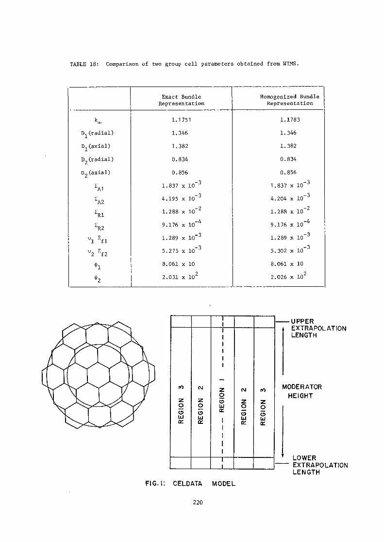
TABLE 18: Comparison of two group cell parameters obtained from WIMS.

*.DI (radial)D (axial)

D2 (radial)D2 (axial)

\2

ER2Vl Zfl

0(f)

Exact BundleRepresentation

1.17511.3461.3820.834

0.8561.837 x 10~3

4.195 x 10~3

1.288 x 10~2

9.176 x 10~4

1.289 x 10~3

5.275 x 10~3

8.061 x 102.031 x 102

Homogenized BundleRepresentation

1.17831.3461.3820.834

0.8561.837 x 10~3

4.204 x 10~3

1.288 x 10~2

9.176 x 10~4

1.289 x 10~3

5.302 x 10~3

8.061 x 102.026 x 102

ro

REG

ION

CM

RE

GIO

N

1111111I

zo0IL)CC

\\\

1111

CM

REG

ION

10

RE

GIO

N

UPPEREXTRAPOLATIONLENGTH

MODERATORHEIGHT

LOWEREXTRAPOLATIONLENGTH

FIG. I: CELDATA MODEL

220

NORTH

o o oo o o o

o o o o oo o o o

o o o o

• o o o

O O O O '9.685 cm

o o o oo o o o o

o o o oo o o

ZED-2 CALANDRIA WALL

FIG.2: CR-I LATTICE IN ZED-2

221

STRING OF THREETREFOIL

BUNDLES

ALUMINUM CALANDRlA TUBE

ZIRCALOY PRESSURE TUBE

FIG. 3: COMPONENTS OF SIMULATEDLOOP SITE

222

SCALE: APPROX. 3x FULL SIZE

ZIRCALOY-4 TIEBAR

COOLANT

AIR GAP

ALUMINUMCALANDRIA TUBE

STAINLESS STEELTIE ROD

ZIRCALOYPRESSURE

TUBE

F]6.4: TREFOIL IN LOOP SITE, A SIMPLIFIEDCROSS SECTION

223

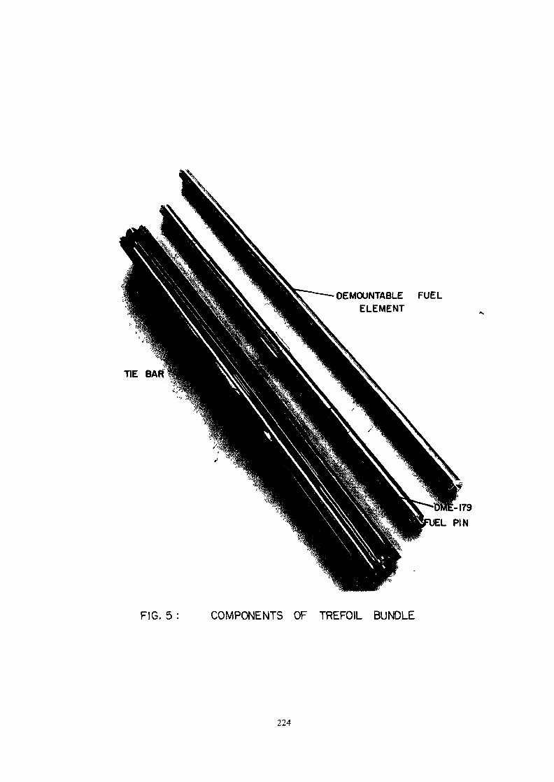
TIE

DEMOUNTABLE FUELELEMENT

FIG. 5 : COMPONENTS OF TREFOIL BUNDLE

224

1.0

0.8

3 0.6

tu> 0.4

UJo:

0.2

** * *LEGEND

x MEASURED VALUES+ CELDATA VALUES

A.B.C.D, REPRESENT LATREP

CELL TYPES

A B 1 D D D B *4

1 1 1100 ZOO

ELEVATION ABOVE CALANDRIA FLOOR IN CM

300

FIG. 6: ZED-2 TREFOIL EXPERIMENT: CELL BOUNDARY FLUX

DISTRIBUTION

I.Or—

0.8 -

LEGEND

+ CELDATA VALUES

A,B,C,D,E,F REPRESENTLATREP CELL TYPES

X

3 0.6u.

UJ> 0.4

UJac0.2

0C

+

- + \ +++ +,++ + +

+ •*•

— + +

+ +

+ • A B C D E F E +

1 1> 100 200

ELEVATION ABOVE CALANDRIA FLOOR IN CM

FIG.7: X6A-690 LOOP EXPERIMENT IN NRX: CELL AVERAGE FLUX

DISTRIBUTION

225

o.o

t-> 3.0i-0

3 2.5

o:o£ 2.0wzLJO

z L5oo:

g i.o

RE

LATI

VE

* Ul

0

0•»*

.

x

+x+X + +x^x

^ V+>< +X + x+ +

x

- x +

X +

— •*• ifeX +

+ x

x+ CALCULATED

~ x EXPT. CU ACTIVITY +

~ A B A

I 1 1 1 1>• 40.0 80.0 I2O. 160. 200- 240

ELEVATION ABOVE CALANDRIA FLOOR (CM)

FIG. 8: CALANDRIA TUBE NEUTRON DENSITY DISTRIBUTION FOR TH-USTRING IN ZED-2

ALUMINUMCALANDRIA

TIJBEFUELELEMENTS

AIR GAPANT

ALUMINUMSUPPORT

TUBE

AIR ALUMINUMPRESSURE

TUBE

FIG. 9: SCHEMATIC REPRESENTATION OF MULTI-ENRICHMENTBUNDLE

226

APPENDIX A

DERIVATION OF FORMULAS FOR BILINEARLY WEIGHTED PARAMETERS

The derivation of the bilinear-weighting method of axial averaging usedin CELDATA is given below. It follows very closely the method given inreference 5 for the use of perturbation theory in calculations related to thechange in reactivity of a reactor due to small changes in localised propertiesof core components and its application to two neutron energy groups.

The two group neutron diffusion equations solved by CELDATA for thebase case can be written in matrix notation as

div D- grad - Z, 2 f2'Tl

JR1 div D° grad - E.2

= 0)

v2

(A.I)

In operator notation this equation can be written

(A. 2)

The analogous equations solved by CELDATA for the perturbed cases are

divCo:;0^,0

V2 f'2+ 6< \

k'

R1where

<$( ') - represents the change in the bracketed quantity due to theperturbation represented by the prime, i.e. 6DJ = DJ -D°.

— represents the perturbed fluxes and can have the valuescorresponding to the case with the actual rod, andcorresponding to the case with the equivalent homogenizedrod.

73

- represents the reciprocal reactor period for the perturbedcase and can take the values and

This equation can be written in operator notation as

where

P« =

2 /V2 Zfgrad 6D|.grad + 6Dj\r-6Z.J1 6( fr

^Rl grad 6 D .

(A. 4)

(A.5)

227

where the identitydiv(D + 6D) grad = grad (D + 6D) .grad + (D + 6D)V2

2 2= grad D. grad + grad <5D. grad + DV + 6DVhas been used to obtain the terms involving D.

CELDATA also solves the equation adjoint to equation (A.2). NamelyM* <j,* = u0 &L (A.6)

where M* is the operator adjoint to Mand $* are the adjoint fluxes.

CELDATA solves the above equations under the assumption that both a) andcu" are zero and thus obtains values of k and k' which will satisfy these equations.However, to be consistent with the notation of reference 5, the u's will beretained in the equations.

Multiplying (A. 4) by (J>*(A.6) by <J>'

integrating over the full extrapolated volume of the reactor and rearrangingfactors, the following relationship is obtained:

<|>* P' 4>' dV(uT - u°) = 2V_______ (A. 7)

X'

where X' = I + ——- I dV (A.8)

Consider two perturbations from the base case denoted by A and B whereA denotes the actual rod for which one wishes to find axially averaged parametersand B denotes the rod which has these axially averaged parameters. It is desiredthat the axially averaged parameters will conserve reactivity. Since the k modeis used to solve the equations

to. - co = u_ - u> =0) =0A o B o oand the conservation of reactivity condition becomes

-A ,Bk = k

[ 4>* PB <(>B dV = T- [ ((>* PA <j)A dV (A. 9)Jv XA Jv

Equating terms involving the same parameters from both sides of theequation, the following equations are obtained:

grad 6D. .grad 01 +(j>1 6D1V cj), I dV• \^ l i i i iyXB I (<!>* grad 6DA grad 4>A+ <(>* 6 DAV2(J)A ) dV (A.10)~K J v V 1 x i i i i/XA

228

*2 grad 60^ grad + c}> SD dV

^- f U* grad <5DA grad <& + <!•* 6D^V2 ) dV (A. 11)XA JV\ /

& B r4>n 6 Z - ((>.. dV = —- (J), 6 Ivp (j).. dV (A. 12)

v 1 Tl 1 XA Jv 1 Tl 1

irB , ^

dV = —r I <)>„ „ ^R1 TI

I 4>2 5 Z.o 4*2 d^X JV

/ B -B \ I! f /A yA \

* /V2 f 2 1 B X * /V2 f 2 J Af) ol———— I d) dV = — I (b ol————Id) dV1 V B / 2 A V 1 \ A / 2

Using the identity* * * 2

div(4> D grad $) = grad <J> D grad <j) + (j) D V (J)

= D grad <|> grad <f> + <j> grad D grad <)> + <}> D V ((>

and rearranging one obtains

* * A A 2(J) grad D grad D V,

By applying Gauss' theorem

div(<J>* D grad <)))dV = J <j>* D gradn<J) dS = 0

because $ is zero on the surface of the reactor. Thus equations (A. 10) and(A. 11) can be rewritten as

grad <(>* 6 D^ grad <j>f dV = ^- f grad <f>* 6 DA grad <f£ dV (A. 16)y X - ' V

* *grad $ 6 D grad < dV = - grad <J> 6 D grad dV (A. 17)v ^ ^ ^ X A J V z ^ : 2

In equations A. 12, A. 13, A. 14, A. 16 and A. 17 the change in parameters associatedwith perturbations A and B are zero everywhere except at the central site sothat the integrations involving these parameters only have to be performed overthe central site denoted R. Further in these equations the change in any oneparameter associated with perturbation B is constant over the central site sothat in these equations the change in parameter can be factored out of theintegral .

This leads to the following expression for the change in parametersassociated with perturbation B.

229

B grad cf> 6 DA grad <j>A dVD

B = L_ JR_____X 1_____l _-——————-—————-————— (A. 18)grad <j> grad 4> dV

R

grad <J>* 6 DA grad (f>A dVZ Z

2 AX ^ grad <J>* grad <f>2 dV

f * . _A ,A<p, 6 L n $J 1 Tl 1B l H/-, VJ 0^^ 4/n dV

V

" ————————— (A. 20)•* J.B ,„<P- (J>1 dV

A* js- A ,A ,„? A2 2 dV'- Ai ^

2 dV<A'22'

2 f 2Equation (A.15) for the change in ——r—— must be treated differently becausethis perturbation extends over the whole core due to the fact that k is calculatedfor the full core.

Knowing that (1) k = k because we are attempting to conserve reactivityand (2) V2 Ef2 = V2 Z 2 everywhere except in the central site

and making the further assumption that the perturbed fluxes <j) and <J> are equaleverywhere except in the central site, it follows that contributions to theintegrals on both sides of equation (A.15) will be equal except in the centralsite. Therefore equation (A.15) can be rewritten as

*tt Zf2* I i ti *- j.t-1 J..D JIT _ ^ i j.-| <- i-i. .c. j.<. | Afi JT, .^ ^JN

s independent of position for the central site it can

be taken outside of the integral. Making use of the fact that k = k and doingsome rearranging, the following equation is obtained:

B 7B _ k_ x)° v° + X_ ;R \_______i______i_____ fA 24N^o ^-ro ~ —— vo ''co ^ A k".-^t,l2 f 2 o 2 f 2 ^. f .K A i75 , J3 1Tr

^ Tn

R

230

Adding the change in parameters defined by equations (A.18) to (A.22) to thecorresponding base case parameter gives the following equations:

grad <f>* (DA-D°) grad cf>A dV•R n Y" JPD? = D° + - ————————————————————————— (A. 25)1 1 -A f * Bgrad ()). grad <j) dV

R 1

^ A o Agrad if)- (D- -D2) grad 0- dV

XA I , * , ,Bgrad <))„ grad <J>- dV

(A. 27)* *?

Rl Rl ,^, ' * jjfr ^ dV

>R l L

* rA

2 (ER1(A-28)

,A ,,,* dV

. 29)dV

Equations (A.24) to (A.29) define the axially averaged parameters obtained fromthe bilinear weighting scheme.

231

METHODE D'HOMOGENEISATION UTILISEEPOUR LES CALCULS NEUTRONIQUESDANS LES REACTEURS A NEUTRONS RAPIDES

Y.H. BOUGET, Ph. HAMMER, F. LYONCommissariat à l'énergie atomique,Centre d'études nucléaires de Cadarache,Saint-Paul-lez-Durance, France

- INTRODUCTION -

J_. Pour les calculs de projet des réacteurs de puissance àneutrons rapides, deux types différents d'hétérogénéité doiventêtre pris en compte :

a) l ' h é t é r o g é n é i t é du réseau multipliant lui-même où le combusti-ble et le r é f r i g é r a n t sont j u x t a p o s é s sous la f o r m ed ' a i g u i l l e s f i s s i l e s ba ignan t dans le fluide caloporteur ;

b) les hétérogénéités macroscopiques créées dans le coeurpar la présence des barres de commande, le voisinage descouvertures ou l'insertion éventuelle de zones fertilesinternes (concept du coeur hétérogène).

2_. L'hétérogénéité des milieux fissiles de centrale depuissance à neutrons rapides est généralement faible par suite dela dimension des aiguilles combustibles (0 = 8 mm), et celle dupas du réseau ( 0 -9 mm), mais elle est importante pour les ré-seaux étudiés sur expérience critique de type MASURCA (utilisantdes réglettes) ou SNEAK (utilisant des plaquettes), en vue dequalifier et d'améliorer les méthodes de calcul du projet. Ladifférence d'hétérogénéité entre assemblage critique et réacteurde puissance croît au fur et à mesure que l'on va vers de faiblesenrichissements, c'est-à-dire vers des gros coeurs à spectresdégradés.

L'étude de cette hétérogénéité est donc nécessaire pourpermettre la transposition des résultats obtenus sur les assem-blages critiques aux calculs de projet de centrales à neutronsrapides.

^. L'hétérogénéité de structure du réseau fissile, ou laprésence d'hétérogénéités "macroscopiques" créées par les barres,les éventuels assemblages fertiles internes ou le voisinage descouvertures, influent directement sur les calculs de projet à deuxniveaux :

- définition des sections efficaces multigroupes des diffé-rents milieux du réacteur, utilisées pour les calculsspatiaux ;

- choix de l'approximation à utiliser pour effectuer cescalculs spatiaux (transport, diffusion).

4_. La prise en compte des diverses hétërogënëités intervientdirectement :

- sur le niveau de réactivité du coeur, donc la définitiondes enrichissements critiques ;

- sur les distributions de puissance, et par conséquent ladétermination des points chauds du coeur.

Dans le présent rapport, on peut faire le point des étudesmenées au CEA jusqu'à ce jour :

a) pour réduire les incertitudes liées à la transpositiondes résultats obtenus sur assemblages critiques auxcalculs de projet ;

233

b) pour recommander des méthodes de calcul à utiliser pourles projets qui permettent de traiter les perturbationsliées aux barres de commande, aux assemblages fertilesinternes ou au voisinage des couvertures. L'objectifrecherché est de réduire les facteurs correctifs etleurs incertitudes à appliquer aux paramètres intégrauxdes projets : Keff, distributions de puissance.

I - ETUDE DE L'HETEROGENEITE DES RESEAUX MULTIPLIANTS -

I-1 . Pos i t ion_du_p_roblème :Les études concernant les effets d'hétérogénéité dans les

réseaux multipliants à neutrons rapides ont été menées, au CEA,sur deux plans :

1°/ sur le plan théorique, développement de méthodes decalcul pour prendre en compte l'hétérogénéité des milieux étudiés

2°/ sur le plan expérimental, mise en oeuvre d'expériencesspécifiques destinées à vérifier la validité des moyens de calculainsi mis au point.

Le but de ces études est donc double :I°/ d'une part, et essentiellement, garantir la validité

de la transposition, aux réacteurs de puissance, des paramètresintégraux mesurés dans les assemblages critiques. Dans cettetransposition, qui se fait nécessairement par le calcul, ce sontles effets d'hétérogénéité qui jouent le rôle le plus important.Pour apprécier ce rôle, il suffit de comparer les chiffres sui-vants, concernant l'effet d'hétérogénéité sur la réactivité :

AK pcm\

PHENIX

SUPER-PHENIX

Effet d'hétéro-généité dû auréseau type MA-SURCA

700

1500

Effet d'hétéro-généi té lié auréseau du réac-teur de puissan-

ce200

300

II apparaît clairement que si les différences d'hétérogé-néité ne sont pas prises en compte, l'enrichissement critique,et donc la masse critique, des réacteurs de puissance serontsous-estimes de 1 à 4%.

2°/ D'autre part, permettre une interprétation aussi cor-recte que possible des expériences, c'est-à-dire en définitiveminimiser la part des ajustements de sections efficaces quiservirait en réalité à compenser les erreurs de calcul, en par-ticulier du calcul des effets d'hétérogénéité.

Les types d'hétérogénéités étudiés au CEA sont liés à laforme des matériaux de simulation des installations d'où provien-nent la majorité des informations expérimentales, à savoir, pourle formulaire CARNAVAL :

1°/ réseaux de réglettes cylindriques, à section circulairepour le combustible, carrée pour les autres matériaux de simula-tion (réseaux étudiés dans MASURCA, HARMONIE, ou ERMINE) ;

2°/ réseaux à plaquettes (réseaux étudiés à SNEAK ou ZEBRA,dans le cadre d'accords de coopération).

1-2. Traitement_de_l^hétérogénëité_dans_HETAIRE :

Dans le formulaire CARNAVAL qui est utilisé au CEA pour lecalcul des coeurs de réacteurs à neutrons rapides, l'hétérogénéitédes réseaux multipliant est traitée par le code de cellule HETAÏRE.

234

Les trois points importants dans le calcul d'un réseauhétérogène sont :

- le calcul de l'auto-protection des résonances ;- le calcul des fuites (streaming) ;- le calcul de la structure fine spatiale du flux.1-2. 1 . L'auto-protection des résonances est traitée dans

HETAÏRE par la méthode des sous-groupes décrite en détail dans /!/Il suffira de rappeler ici que l'intérêt de cette méthode est depermettre un calcul simple, précis et rapide de l'auto-protectionrésonnante dans les cellules hétérogènes complexes, situation oùles "théorèmes" d'équivalence sont défaillants.

1-2.2. Le coefficient de diffusion hétérogène est calculéselon la théorie de P. BENOIST /2/, avec les simplifications sui-vantes :

- on se limite au premier choc dans le calcul des probabi-lités de collision. Des tests numériques ont montré en effet queles corrections dues aux chocs secondaires étaient négligeablesdans les réseaux rapides /5/.

- On néglige 1'anisotropie du coefficient de diffusion, eton calcule un coefficient de diffusion "isotrope", qui est en faitune moyenne des coefficients de diffusion directionnels définispar P. BENOIST. Le tableau suivant montre que, compte-tenu deslaplaciens géométriques habituels, pour les réseaux à réglettes,l'effet de cette approximation est négligeable en assemblagecrit ique.

D2 -2B m mN/

R2

R I

R3

anisotrope

2 3 . 0 7 9 4

1 6 . 3 3 0 6

8 . 4 5 2 0

D

2 3 . 0 8 2 6

1 6 . 3 2 6 6

8 .4353

Eca r t

.003

. 0 0 4

. 0 1 7

1-2.3. Le calcul du flux se fait par résolution de l'équa-tion intégrale du transport, discrëtisée en espace (probabilitésde collision), à 25 groupes, et avec choc formellement isotrope(correction complète du transport).

La recherche du laplacien matiëre_se fait en itérant larésolution de cette équation. Le terme D B2 qui représente lesfuites est introduit comme terme d'une probabilité de non-fuite.Plus précisément, les probabilités de collision en mode fondamen-tal sont le produit des probabilités de collision en milieu infinisans fuite, par le rapport R :

_ taux de collision moyen dans la celluletaux de collision moyen + jj ]f x flux moyen

Cette approximation paraît plus justifiée que l'approxima-tion classique qui consiste à introduire les fuites comme unecapture fictive uniformément répartie dans la cellule.

1-2.4. Le calcul du bilan est suivi de celui des sectionsefficaces dites "homogénéisées", qui doivent servir dans lescalculs spatiaux de réacteur. Par définition, ce sont les sectionsefficaces qu'il faut attribuer au milieu homogène de même composi-tion moyenne que le réseau pour conserver tous les taux de réac-tion en mode fondamental et par conséquent tous les paramètresintégraux. Pour les calculs de diffusion, on attribue de plusà ce milieu homogène, le coefficient de diffusion du réseau.

235

1-2.5. HETAÏRE peut traiter n'importe quel type de réseaurégulier, à condition de lui adjoindre le sous-programme ad hocpour le calcul des probabilités de collision.

Actuellement, il contient les possibilités suivantes :I °/ cellules à une dimension, cylindrique (réseaux simples

à barreaux cylindriques), ou plane (réseaux à plaquettes). C'estl'option la plus utilisée.

2°/ Cellules à deux dimensions, pour le calcul des réseauxà barreaux cylindriques, mais de structure complexe (certains desréseaux du programme R,Z de MASURCA). Deux possibilités existent :

- calcul exact des probabilités de collision : cette optionn'est utilisée qu"exceptionnellement, son coût étant pro-hibitif ;

- calcul approché des probabilités de collision, par uneméthode de synthèse qui consiste à calculer en une dimen-sion les probabilités de collision dans les mailles élé-mentaires de la cellule puis à les combiner. Cette optiona été largement utilisée pour les réseaux du programmeR,Z de MASURCA. Elle nécessite cependant, pour chaquetype de réseau, une étude préalable pour "ajuster" laméthode de synthèse utilisée.

Avec HETAÏRE, l'hétérogénéité du réseau est traitée d'emblée,dans le calcul de cellule. Les calculs de réacteurs ultérieurspeuvent se faire en homogène, car les sections efficaces homogé-néisées issues du calcul de cellule contiennent déjà implicitementtoute l'information sur les effets d'hétérogénéité sur le bilan.

1-3. Progr_ammes_exp_ërimentaux :

Deux programmes expérimentaux, spécifiquement orientés versl'étude de l'hétérogénéité dans les réacteurs à neutrons rapides,ont été réalisés au CEA, l'un dans le réac'teur MASURCA en 1967-68,l'autre dans l'assemblage couplé rapide-thermique ERMINE en 1970-71

1-3.1. Exp_ériences_d^hétérggén|ité_dans_les_assemblages

Le but de ces expériences était de mesurer l'effet d'hété-rogénéité sur la réactivitë, en réalisant des réseaux de mêmecomposition moyenne mais d'hétérogénéités différentes.

- Dans l'assemblage 1A /4/, on a mesuré la variation deréactivité due au passage du réseau normal à un réseau d'hétéro-généité "double". Ce dernier est obtenu en groupant par quatreles réglettes de combustible, sur toute la hauteur du coeur,tout en c.onservant leur centre de masse de façon à minimiserl'effet dû au déplacement proprement dit du combustible dans legradient du flux direct et adjoint (Figure 1). Le groupement aété réalisé, tube par tube, dans un nombre de tubes suffisant pourdresser une carte à partir de laquelle l'effet global pour l'en-semble du coeur était obtenu. De plus, l'additivité des effetsmesurés a été vérifiée sur quatre tubes.

- Dans l'assemblage 1B , deux variations d'hétérogénéitéont été réalisées, le principe des mesures restant le même quedans 1A :

. le groupement des réglettes par quatre comme dans 1A ;

. la dispersion du combustible, en remplçant chaque réglettenormale par quatre réglettes de diamètre moitié (6.35 mm),toutes les fois qu'il était possible de le faire en conser-vant le centre de masse (Figure 1).

- A titre indicatif, les effets mesurés et cajlculës figurentdans le tableau 1 pour 1A et 1B. Ce*tableau appelle les remarquessuivantes :

236

1°/ pour l'assemblage 1A, il y a un accord parfait entrel'effet de groupement mesuré et calculé par CARNAVAL III. Cetaccord, compte-tenu de la méthode d'extrapolation (cf. réf. /3/)se maintient sur l'effet d'hétérogénéité du réseau normal. Lesvaleurs obtenues pour ce dernier sont aussi en très bon accord,avec le résultat d'un calcul MONTE-CARLO simulant tous les détailsde géométrie de l'assemblage 1A normal.

2°/ Pour l'assemblage 1B, on retrouve les mêmes conclusions.

1-3.2. Expériences d'hétérogénéité dans ERMINE /5/ :———————— = = = =:=:= = = = = = = =:=::= = = = = 5 = = = = :==: = = = = = = = =::=:=: = =

Le but de ces expériences était de contrôler la capacité desmoyens de calcul à prédire correctement la structure fine des tauxde réaction importants dans la cellule et à suivre la variation,avec l'hétérogénéité, des paramètres intégraux mesurables dansERMINE, essentiellement les indices de spectre et le bilan globalcaractérisé par le paramètre K /6/.

Cette série d'expériences a comporté la réalisation dequatre coeurs de compositions moyennes aussi proches que possible,mais d'hétérogénéités croissantes (Figure 2) :

- un coeur homogène Ho, constitué d'une matrice de graphitedans laquelle sont dispersées des microsphères de carbure d'Ura-nium enrichi à 30% ;

- un coeur hétérogène Hl, à réglettes cylindriques d'Ura-nium enrichi à 30%, de diamètre 6.35 mm, disposées en réseau à pascarré de 15 mm dans une matrice de graphite ;

- un coeur H2, d'hétérogénéité "double" de celle de Hl (ré-glettes de diamètre 12.7 mm, pas du réseau 30 mm) ;

- un coeur à plaquettes HP. Le combustible est constituéd'une plaquette d'Uranium enrichi à 20% en sandwich entre deuxplaquettes d'Uranium enrichi à 35%. L'épaisseur totale du combus-tible est de 9.45 mm, le diluant est du graphite, usiné en petitsblocs de 57.2 mm d'épaisseur. Le pas du réseau est de 66.7 mm.

Les quatre coeurs ont une composition moyenne assez voisinede celle du coeur 1B de MASURCA.

Parmi les nombreuses mesures effectuées, nous n'en retien-drons que deux types :

. Mesures de taux de réaction :Ces mesures fournissent deux types d'informations :- indices de spectres, mesurés (sauf pour la capture de

l'U 238) par chambres à fission 0 1.5 mm dans le diluant ;- la structure fine spatiale (rapports combustible/diluant)

des taux de réaction, mesurée par des détecteurs métalliques de0.2 mm d'épaisseur d'Uranium enrichi, d'Uranium appauvri et dePlutonium.

Ces mesures de structure fine permettent, moyennant descorrections d'auto-protection dans les détecteurs, de remonteraux indices de spectre dans le combustible. Cela est vrai saufpour l'indice de capture de l'U 238, qui est mesuré directementpar détecteur dans le combustible.

Quelques résultats de mesures de structure fine sont donnésà titre d'exemple dans le Tableau 3.

On observe un bon accord entre calcul et expérience, lesécarts étant généralement inférieurs ou de l'ordre des mesuresexpérimentales, à une exception près : la structure fine de lafission de l'U 235 dans les coeurs les plus hétérogènes. Il sembleque la variation de l'auto-protection de l'U 235 entre combustibleet diluant ne soit pas correctement rendue par HETAÏRE. En revanche,on peut noter que la variation importante de la capture de l'U 238est très bien rendue par le calcul.

237

Le Tableau 4 illustre la capacité d'HETAIRE à suivre cor-rectement la variation des indices de spectres avec l'hétérogé-néité. Les écarts calcul-expérience sont stables, alors que lesindices F8/F5 et C8/F5 varient de 15 à 25% entre Ho et HP.

. Mesures de K :Ces mesures sont réalisées par la méthode d'oscillation.

On mesure la variation de réactivitê due à un vide de cellule.L'effet mesuré est ensuite traduit en ct+ = (te* - I)/k+, par nor-mal i sation :

- soit à la réactivité d'une source de Californium ;- soit à la composante de production de la réactivitê de

l'isotope fissile principal de la cellule (ici l'U 235).Les mesures de K ont été réalisées dans Ho, Hl et H2,

suivant l'une ou l'autre technique, ou les deux, soit en créantun vide de cellule dans chaque réseau, soit par remplacement decellule H2 dans Ho ou Hl.

Des résultats de ces mesures figurent à titre d'exempledans le Tableau 5. On observe que le calcul suit bien la varia-tion de K+ entre les différents réseaux. Celaapparaît le plus clairement dans les deux dernières lignes dutableau issues des mesures par remplacement de cellules (et doncnon entachées des incertitudes dues a la normalisation).- CONCLUSION -

Les expériences d'hétérogénéité réalisées dans MASURCA etERMINE permettent de conclure à la validité des méthodes de cal-cul de l'hétérogénéité utilisées dans le formulaire CARNAVAL.

Cette conclusion est confirmée par toutes les mesures,devenues de routine, de structure fine de taux de réaction dansla plupart des réseaux réalisés dans MASURCA, dans HARMONIE oudans ERMINE.

II - ETUDE DES HETEROGENEITES CREEES DANS LES COEURS DE CENTRALESA NEUTRONS RAPIDES POUR LES BARRES, LES COUVERTURES OU LESASSEMBLAGES FERTILES INTERNES -

II-l. Barres_de_commande :. Les barres de commande du système primaire des centrales

à neutrons rapides sont constituées de deux zones concentriques dontla partie absorbante (B4C enrichi), qui plonge dans le fluide calo-porteur. La Figure 1 présente à titre d'exemple la section d'unebarre du réacteur SUPER-PHENIX. Pour les calculs de projet, on con-sidère ces barres comme des zones homogènes où absorbant et diluantsont mêlés. Les antiréactivitës et les perturbations des distribu-tions de puissance induites dans le coeur sont calculées dans l'ap-proximation de la diffusion. Dans le formulaire CARNAVAL, les sec-tions efficaces multigroupes des zones de barres sont définies enutilisant un spectre standard voisin du spectre moyen d'une centralede puissance à neutrons rapides pour calculer les sections de ra-lentissement élastique /!/.

. L'homogénéisation des zones absorbante et diluante desbarres conduit à surestimer d'environ 6% 1'antiréactivitë desbarres de SUPER-PHENIX. La surestimation dépend de la hauteur deBAC enrichi dans le coeur, comme le montre le tableau suivant quidonne les écarts entre calcul hétérogène et calcul homogène enfonction de l'enfoncement :

238

Hauteur colon-ne absorbanteenfoncée/hau-teur coeur

cil /o

2530405075100

AK ,, . ,-=r- (homogène)

97- 126- 183- 247- 359- 401

AK^r-(hétërogène)1s.

89- 118- 175- 229- 334- 378

Effet d'hétéro-généitéAK,, _ . AK,, .— (het)-jj-(hom)

AK,, .— (hom)

- 8.2- 6.3- 4.4- 7.3- 7- 5.7

Efficacité une barre en position centrale. Calculs (R,Z) à 6 groupesd'énergie. - e (Ho) efficacité dans le cas de la barre homogène

- e (HE) efficacité dans le cas de la barre hétérogène.

L'étude expérimentale de cet effet est en cours sur l'as-semblage critique MASURCA.

L'emploi de l'approximation de la diffusion au lieu de lathéorie du transport conduit à surestimer de façon différenteles antiréactivités des barres absorbantes (B4C) ou des partiessuiveuses de barre (Na). Comme le montre le tableau suivant àtitre indicatif pour des barres de type PHENIX :

Bar re

Na

B4C na t .

T - D vD

- 3.5

- 5

En ce qui concerne les distributions de flux dans les barres,l'approximation de la diffusion conduit à surestimer la dépressiondu flux par rapport à la théorie du transport.

Cette surestimation varie suivant la nature du milieu occu-pant l'emplacement de la barre : Sodium ou B4C. Le tableau suivantdonne à titre d'exemple les écarts entre calcul transport et cal-cul diffusion pour différents taux de réaction calculés au centrede la barre : le taux de fission <Ofc$> caractérise l'ensemble duspectre, alors que le taux de fission <Cff8<j>> décrit la partiehaute du spectre (E > 1 MeV) ; le milieu fissile entourant labarre est représentatif de la zone interne de SUPER-PHENIX :

T - D „D »

<afg *>

<af5 <|»$ total

Na

- 10

I

- 2

B4C

- 15

- 7

- 8

On voit que l'emploi de l'approximation de la diffusionconduit à surestimer la perturbation de flux dans les zones debarre : cette surestimation devra être prise en compte lors descalculs d'échauffement gamma dans les parties absorbantes pouravoir un dimensionnement correct des aiguilles de B4C à utiliser,

239

II-2. Couvertures :L'utilisation de l'approximation de la diffusion pour le

calcul de la masse critique et des distributions de puissancedans les réacteurs à neutrons rapides conduit à mal décrire leseffets d'interface entre coeur et couvertures.

En ce qui concerne la masse critique, ces effets d'inter-face sont pris en compte en appliquant des corrections de transportdont l'amplitude varie entre le cas des assemblages critiques etcelui des réacteurs de puissance comme le montre le tableau sui-vant :

AKTT Pcm xCorrection de

transpott radialCorrect ion de

transport axial

MASURCA

= 300

- 300

SUPER-PHENIX

= 50

* 150

En ce qui concerne les distributions de taux de fission, lesécarts entre la théorie du transport et l'approximation de ladiffusion sont particulièrement importants (= 10%) pour la fissionde 238 U (cf. tableau 5).

Ces écarts, liés principalement à la définition du coeffi-cient de diffusion au voisinage de l'interface devraient êtreréduitspar l'emploi d'une méthode originale "CADIEX", en coursd'élaboration actuellement, dont les caractéristiques sont résu-mées ci-après :

. Formalisme de la procédure CADIEX :

Pour évaluer les fuites dans les couvertures, on se fondesur le critère de SELENGUT. On préserve les longueurs d'extra-polation dites vraies, qui sont définies à partir du flux angu-laire total (y compris la partie transitoire).

Chaque région, coeur ou couverture, est découpée en troiszones : une zone centrale et deux zones frontalières. Les zonesfrontalières, d'épaisseur réduite (un ou deux pas du calcul dif-fusion), ont été introduites pour circonscrire les effets del'interface coeur-couverture et du bord de la couverture.

La relativement faible épaisseur des zones frontalièrespermet de calculer les longueurs d'extrapolation polaire et dipo-laire, aux frontières des différentes zones. On utilise pour celala méthode de CASE /6/. En confrontant les valeurs ainsi calculéesavec les formules correspondantes de la théorie de la diffusion,on obtient un jeu de données diffusion multigroupe pour chaquezone.

Le code CADIEX met en oeuvre cette nouvelle procédure.. Résultats numériques de la procédure CADIEX :

La validité de cette procédure est illustrée par les résul-tats que l'on a obtenu pour un système plan coeur/couverture (voirTableau 4). Le maximum des écarts transport-diffusion est réduitd'un facteur quatre pour l'évaluation du taux de fission de l'U 238.Les écarts sur les taux de capture de l'U 238 et le taux de fissionde l'U 235 ne dépassent probablement pas l'ordre de grandeur deserreurs numériques. La divergence sur la réactivité est devenueacceptable (nettement inférieure à 50 pcm). Cette méthode, quisemble très prometteuse, subit encore des tests avant d'être pro-posée pour les calculs courants de projet.

240

II-3. Assemblages_fertiles_internes :Pour optimiser le temps de doublement des réacteurs de la

filière à neutrons rapides, il est envisagé d'utiliser le conceptde coeur hétérogène : dans ce concept, des assemblages fertiles(UÛ2) sont insérés dans un coeur n'ayant qu'une seule zone d'en-richissement.

Actuellement, les méthodes de calcul utilisées pour lesétudes d'avant-projet sont identiques à celles retenues pour lescoeurs de type SUPER-PHENIX :

- définition des sections efficaces multigroupes par lecode de cellule HETAÏRE, avec les sections du formulaireCARNAVAL, séparément pour les milieux fertile et fissile.Les sections efficaces de la zone fertile sont obtenuesselon la procédure utilisée sur les barres de commandeou les couvertures externes / l/.

- calculs spatiaux dans l'approximation de la diffusion.

a) Définition des sections efficaces :

La définition des sections tnultigroupes séparément pourchaque milieu fertile ou fissile du coeur ne prend pas en comptel'influence du couplage entre les deux zones sur l'auto-protection.L'importance de cet effet est estimée en prenant les sec-tions à 1 groupe obtenues successivement en considérant :

- chaque zone comme un milieu indépendant ;- les deux zones comme les éléments constitutifs d'une

"macro-cellule".

On vérifie que les sections varient suivant le modèle uti-lisé, cependant des tests numériques montrent que des calculsspatiaux faits à partir de ces deux procédures précédentes pourdéfinir les sections efficaces ne conduisent pas a des écartssignificatifs sur les paramètres intégraux : masse critique( écart inférieur à 150 pcm), gain de régénération (GRI : écartinférieur à 1%) pour un coeur ne comportant qu'une zone fertilecentrale de 15 cm de rayon / 11. Les faibles écarts sont dus àdes compensations entre les variations des fissions et les capturesdes différentes zones. Des études complémentaires sont en courssur des configurations de type projet comportant plusieurs zonesfissiles concentriques.

L'influence du passage d'un découpage en énergie du décou-page à 25 groupes du formulaire CARNAVAL sur les paramètres inté-graux a été évalué en comparant les résultats :

A/ d'un calcul spatial fait en transport (1D cylindrique)à 156 groupes. Ces sections sont issues d'un jeu à 2000groupes par l'utilisation du code MC2-2 ;

B/ d'un calcul spatial fait dans les mêmes conditions avecdes sections à 25 groupes calculées suivant la même pro-cédure que précédemment ;

C/ d'un calcul spatial fait avec des sections à 25 groupesdéduits pour chaque zone des sections à 156 groupes parpondération sur le flux moyen de la zone considérée.

Les calculs décrivent un coeur comprenant une zone fertileU02~Na (50% - 50% v/o) insérée au centre d'une zone fissile au Pud'enrichissement -19% en Pu équivalent

241

A(référence)

B

C

Kef f

0.96981

0.97066

0.96900

Kef f-Kef f

pcm

/

85

9

0fg/af5 aucentre de lazone fertile

interne

0.0094

0.0099

0.0094

On observe que la procédure utilisée pour déduire les sec-tions efficaces correspondant au découpage en énergie du formulaireCARNAVAL correspondant à un découpage fin influe directement surla masse critique et sur le spectre dans les zones fertiles. Cepoint est en cours d'étude actuellement.

b) Calculs spatiaux :

L'emploi de l'approximation de la diffusion conduit à sures-timer le gain de régénération interne des différentes zones ducoeur de ^ 1% et celui des couvertures externes d'environ 8%, parrapport à la théorie du transport /?/.

- CONCLUSION -

l/ Les réseaux multipliant qui constituent les coeurs descentrales de puissance à neutrons rapides ne présentent pas d'hé-térogénéité importante par suite de la dimension des aiguillescombustibles utilisées (0 ^ 8mm), et du pas du réseau (0^9 mm).

Les méthodes de calcul utilisées permettent de traiter cor-rectement les hétérogénéités de réseaux plus complexes réaliséssur assemblages critiques, soit avec des réglettes ( MASURCA)ou des plaquettes (SNEAK), et donc de transport avec des incerti-tudes réduites (- 100 pcm) des résultats des expériences intégralesaux coeurs de réacteurs de puissance.

2/ Les perturbations de réactivité ou de distribution indui-tes dans les coeurs par des barres de commande ou par la présencedes couvertures sont traitées dans l'approximation de la diffusion.Cette approximation conduit à surestimer l'effet des barres(- 7%) par rapport à la théorie plus raffinée mais plus coûteusedu transport.

3/ Le traitement des coeurs de concept hétérogène est actuel-lement identique à celui des coeurs classiques (de type SUPER-PHENIX) : la procédure à retenir pour définir les sections multi-groupes fait l'objet d'études présentement en cours.

Le programme expérimental qui est développé à ce jour surMASURCA (programme PRE-RACINE /8/) doit permettre de qualifieret d'optimiser la méthode de calcul des sections multigroupespour ce type de coeur.

242

- REFERENCES -

/!/ - A. KHAIRALLAH et al. -IAEA - SPM - 154/37 (1972)

/2/ - P. BENOIST -Rapport CEA R-2278 (1964)

/3/ - A. KHAIRALLAH et al. -AIEA - SPM - 101/57 (1967)

/4/ - 0. TRETIAKOFF et al. -Note CEA - N-1483 (1971)

/5/ - A. FILIP -Thèse de Docteur Ingénieur - Faculté d'Orsay (1975)

/6/ - MOGILNER et al. -Energie Atomique (Traduction de Atomnaya Energia)Vol. 21, p. 75 (1960)Vol. 24, p. 65 et 119 (1968)Vol. 30_, p. 389 (197!)

/Il - Y.H. BOUGET et al. -Physics performances of heterogeneous fast reactorcore concept studied in MASURCAA.N.S. June Spécial Session - NEW-YORK. (JUIN 1977)

/8/ - Y.H. BOUGET et al. -Physics studies of neutronic problems related to théheterogeneous fast reactor core concept : expérimentalprogramme PRE-RACINE performed in MASURCA.A.N.S. Meeting on Advanced Reactor Physics - GATLINBURG(Avril 1978).

TABLEAU 1

Effet de groupement

Effet de dispersionEffet d'hétérogénéitédu réseau normal

1A

Expérience (pcm)

+ 1 140 ± 100

+2190 ± 260

Calcul (pcm)+1 140 ± 75

+2190 ± 180

1BExpérience (pcm)+ 730 ± 40- 670 ± 40

+1490 ± 100

Calcul (pcm)+ 740 ± 50- 620 ± 40

+1380 + 100

243

TABLEAU 2 TABLEAU 3

Rapport combustible/diluant de taux deréact ion

Variation des indices de spectreEcarts (Exp-Cal)/calcul en % (x)

F5

F8

C8

F9

Coeur

H.K2

HP

H,H2HP

HlH2HP

H2

Mesure (%)

0. 943 ±0.80.874 ± 0.6

0.773 ± 0.7

1 .068 ±0.8

1.167 ± 0.61 .265 ± 0.7

0.527 ± 1.70.377 ± 1 .0.268 ± 1 .

0.926 ±0.6

E - C „ri_i- 1 ±0.8- 2.7 ± C.6

- 5.1 ± 0.7

- 0.7 ± 0.8

H- 0.7 ± 0.6+ 1.6 ± 0.7

- 1.4 ± 1.7+ 0.3 ± 1 .+ 0.6 ± 1 .

- 0.6 ± 0.6

Ho

HlF8/F5 H2

HPHo

HlF9/F5H2HPHo

HlC8/F5TIH2HPHoo 1G, 10/F5H2HP

Combustible

+ 4.4+ 6.2 ± 1.6

+ 9.5 ± 1.4+ 9.2 ± 2.2

- 1 .5

+ 7.0+ 6.7 ± 2.+ 7.3 ± 2.+ 8.7 ± 2.

+ 7.0

Di luant

± 1 . 3+ 6 ± 1 . 2

+ 6.4 ± 1.1-i- 3. ±2.

± 1 .4- 2. ± 1 . 4- 0.1 ± 1.3

±2.0

+ 5.8 ± 2.+ 4.0 ± 2.+ 2 . ±2.5

±2.8

+7 ±2.8

(x) Calculs faits avec HETAÏRE, Jeu Version 2.Ces résultats ne sont pas représentatifsdu formulaire actuel CARNAVAL IV.

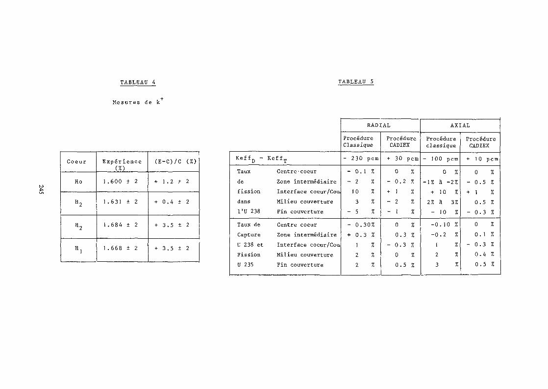
TABLEAU 4 TABLEAU 5

Mesures de k

Coeur

Ho

«2

«2

H l

Exper ience

1 .600 ± 2

1 .631 ± 2

1 .684 ± 2

1.668 + 2

( E - C ) / C ( % )

+ 1 . 2 + 2

+ 0.4 + 2

+ 3.5 ± 2

+ 3.5 ± 2

KeffD - KeffTTaux Centre • coeurde Zone intermediairefission Interface coeur/Cou.dans Milieu couverture1'U 238 Fin couvertureTaux de Centre coeurCapture Zone intermediaireU 238 et Interface coeur/CouFission Milieu couvertureU 235 Fin couverture

RADIAL

ProcedureClassique

- 230 pcm- 0. 1 %- 2 %10 %3 %

- 5 %- 0.30%+ 0.3 %

1 %2 %2 %

ProcedureCADIEX

+ 30 pcm0 %

- 0.2 %+ 1 %- 2 %- 1 %0 %0.3 %

- 0.3 %0 %0.5 %

AXIAL

Procedureclassique- 100 pcm

0 %-1% a -2%

+ 10 %2% a 3%- 10 %-0.10 %-0.2 %

1 %2 %3 %

ProcedureCADIEX

+ 1 0 pcm

0 %- 0.5 %+ 1 %

0.5 %- 0.3 %0 %0 . 1 %

- 0.3 %0.4 %0.5 %

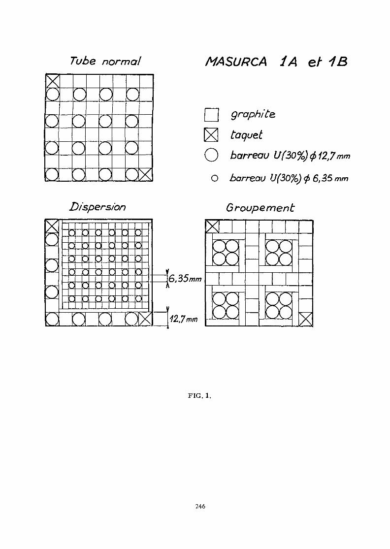
Tube normal

XDispersion

AO^

^J

; ;;

J

^

^ j)

u

j j

1

J]

Ju

)

s )

^ ^. )^Oi >o——

H 'v_^ ^> '/ 's

s-^*

*_ £

^ ^/ vJX

=1F

MASURCA 4A el- 1B

graphite

taquet

O barreau Iff30%) <f> 12,7mm

O barreau U(30%) <f>6,B5mm

Groupement

,35/wm

12,7mm

FIG. 1.

246

ERMINE. _ CCEURS H

^ 30 ^^ 30

Reseau

Demi-cellule HP

f~-fCotes: 0. 4,7251.575 t

TT !15.845 23.545 33.3*5

Umef-. 20%

If mek 35%

Graphite

FIG. 2.

247

R1 = 7,5 cm Rayon exterfeur zone absorbant

R2=9,5 cm Rayon exterieur zone sans absorbant

Coups radiale. d'une barro. type

FIG. 3.

248

CALCULATION OF A CRITICAL ASSEMBLYOF BOILING WATER REACTOR FUEL ELEMENTSBASED ON ENDF/B-IV DATA

R. WARTMANN, W. BERNNATInstitut fur Kernenergetik und Energiesysteme

der Universitat Stuttgart,Stuttgart, Federal Republic of Germany

Abstract

The paper describes the calculations of a critical assemblyperformed with the modular program system RSYST /1/ whichwere based on ENDF/B-IV data. The experiment was carriedout by the KWU /2/ using boiling water reactor fuel elementswhich contained Gadolinium-loaded fuel pins. The calculationswere performed in order to test the cross section libraries andthe homogenization methods.

1. INTRODUCTIONThe paper describes the calculations for a critical assembly

with BWR fuel elements performed with the modular program systemRSYST /!/. The purpose of the calculations was to test the homo-genization methods, the spectral codes, the cross section librariesand the accuracy of the diffusion theory in this case. The calcu-lations were based on the data of our ENDF/B-IV cross sectionlibraries GAM-99 and THERM-126. The fuel elements contained Gadolium-loaded pins.2. DESCRIPTION OF THE CRITICAL ASSEMBLY

The critical assembly was composed of four 8x8- and twelve7x7 BWR fuel elements (see fig. 1). The fuel elements of the typeW7G and W8G contained resp. five and six Gadolinium-loaded fuelpins. Fuel pins with four different enrichment levels were used.The mean enrichment level of the fuel was 2.6 w/o U-235. The assemblywas critical at a water height of 82.5 cm and at a water temperatureof 18.3 C. The source distribution was measured for a 8x8 fuel ele-ment.3. CALCULATION OF THE CRITICAL ASSEMBLY

At first we calculated cross sections for 99 fast groups fromthe data of our cross section library GAM-99 and a zero dimensionalB-]-spectrum with the RSYST module S PERT RUMS T and using the GGC-4 for-malism for the resolved resonances. For the energy range of the re-solved resonances of U-235 which was taken between 1.85 eV and1O1.3 eV the overlapping of the resolved resonances of U-235 andU-238 was considered in an additional resonance calculation.

The data for the thermal groups originated from our cross sectionlibrary THERM-126. The scattering matrices were calculated accordingto the free gas model for all nuclidas exept hydrogen in H2O. Inaddition to a zero-dimensional B-j-spectrum a one-dimensional spectrumwas calculated for the cell with the Gadolinum-loaded pin.

A microscopic cross section library with sixty groups wasfinally obtained by coupling the fast data with the thermal data andby condensing the data.

249

It was intended to perform 3D-Monte Carlo calculations withtwenty groups and 2D-diffusion calculations with four groups forthe calculation of the multiplication constant and the sourcedistribution for the critical assembly. To calculate the macro-scopic data it was necessary to carry out the basic physical cal-culations for the various cells. Calculations were performed forthe different lattices in the 7x7- and 8x8 fuel elements using thestandard Wigner-Seitz cell. The mean enrichment level was used forthe fuel. A so called super cell was used for the cell calculationfor the Gadolinium-loaded pin. An extra ring zone whose volume wasfor times that of the standard cell was added around the standardcell. The material of this ring zone consisted of the homogenizedmaterial of a standard cell with the mean enrichment. These cellcalculations were sufficient for the generation of the twenty groupdata.

For the calculation of the four group data the influence ofthe "softer" spectrum on the thermal data of the pins close to thewater gap was considered. Super cell calculations were performedfor a quarter of an 8x8 fuel element using plane and cylindricalgeometry. Finally the sixty group data were condensed to four groupsand homogenized using the spectra of the cell and the super cellcalculations.

For the full core, 2-D diffusion calculations were performed,while a Monte Carlo program with improved geometric subroutines wasused for 3-D calculations. The improvement referred to multi-shapedcylinders like the fuel pins.

4. RESULTSThe keff calculated with the diffusion program was 1.0O3. Themean quadratic deviation of the measured power factors from the

calculated ones was 2,76 %. The power factors together with a com-parison between the measured and calculated power factors, are shownin figs. 2 and 3.

Comparisons between calculations with two-dimensional planegeometry and one-dimensional cylindrical geometry, where second homo-genized group constants were used, showed that the difference in keffwas only O.14 %. Therefore it was possible to perform sensitivestudies due to the water height and a bottom water reflector usinga cylindrical r,z-geometry. Fig.4 represents the sensitivity ofthe reactivity.

The calculated keff from the Monte Carlo PI-calculation was1.00 at a standard deviation of 0.36 %. For this calculation abottom reflector was taken into account. The corresponding keff re-sulting from the diffusion calculation was 1.O05. The mean quadraticdeviation of the measured power factors from the calculated ones was3.15 %. The standard deviations of the calculated power factors dueto statistical fluctuations amounted to about 4 %. For the calculatedpower factors and the corresponding comparison see fig. 5 and 6.

5. CONCLUSIONS

The following results could be concluded:1. It is sufficient to condense and homogenize the cross sections

of Gadolinium-loaded fuel pins using the fluxes from the celland super cell calculations. It seems that it is not necessaryto fit the data to the experiment.

2. The power factors of the fuel pins - especially of theGadolinium-loaded pins - were correctly calculated with bothmethods.

250

3. The 2-D diffusion calculations are in accordance with themeasurement and with the 3-D Monte Carlo P1-calculations.

4. The application of the diffusion theory provides good resultsalthough the cells containing Gadolinium and the water gaps werenot further homogenized. The water gaps seemed to be moreproblematic than the cells containing Gadolinium.

5. Even if the cylindrical r,z-geometry and second homogenized groupconstants are used one can obtain a good value for keff with thediffusion calculation.

6. REFERENCES

/!/ Ruhle, R.RSYST, ein integriertes Modulsystem rait Datenbasis zurautomatisierten Berechnung von KernreaktorenIKE 4-12, Dissertation Stuttgart 1973

/2/ Shin, C.; Hofmann, H.P.Vergleich experimentell bestimmter Leistungsverteilungenvon GD-haltigen SWR-Brennelementen mit AuslegungsrechnungenKWU/R 122-F-2964

W7G———— <

87

B7

W7G

B7

W8G

W8G

87

B7

W8G

W8G

B7

W7G

B7

87

W7G

W8G 8x8 fuel element with6 Gd-loaded pins (Wiirgassen)

W7G 7x7 fuel element with5 Gd-loaded pins (Wiirgassen)

B7 7x.7 fuel element (Brunsbiittel)

-^-The circles denote the positions whichare far off the ordinary control rodpositions

Fig.1 Composition of the critical assembly

251

.17

.1911.20.232:

1.031.07t 2}1.051.07! 31l.OBUOBt 31l.lb1.20( 311.151.16[ 2]1.42

[*21

1.201.21( 2J1.03l.OJf 3),8J.8«5[ 31.2b.26[40)

1.00[ 411.101.08[ 4).95.94[ 311.281.27[ 31

1.031.05t 21.80.84

C 31.97.99

t 41.85.86

t 4)

.85t 41.2b.25

Ufa]1.071.05t 4]1.101.08( 3)

1.061.07[ 31.26.26[401

,8b.rib

t 4].91

t'41.94

t*41

.87[ 41

.93

.9?[ 4]

1.431.37[ 41

1 .( H

('31.99[ 41• S3.flb

C 41.94.97

C 41/0.00I. 00[ VWl.91

[ 4].25.25[4G]

1.331.27

1.1-[ 1)T.II 41

t *<> 1

C 41

.94( 41

.91

.94r 4)

.971.01{ 4]

1.431.35[ 41

l.l1-l.lbC 2].95.97

I 3)1.071.05[ 41.93.95[ 4]

Us.971.00[ 4]

lil7I 4]1.121*3)

I."-1

t «.')

I'j)

1.U9[ 31

['»]'1.J3

('•>•>

l.JSC -O1.121.1?t 3]1.40l.JSC 3]

calculated power factormeasured power factortype of fuel pin

1 1.33 w/o U-2352 1.74 w/o U-2353 2.01 w/o U-2354 3.05 w/o U-2354G 3.05 w/o U-235

+ 2.0 w/o GD203WW pin without fuel

Fig.2 Power factors in the 8x8 fuel element (diffusion calculation)IKE STUTTGART

900 t 000 t 100 1 200 t 300 1 4QO I 500CALCULATED VALUE

Fig.3 Comparison between the measured and the calculatedpower factors (diffusion calculation)

I2t= 0'I I L M 1

Fig.4 Sensitivity of the reactivity due to the water height252

1.191. 10*5.3

1.231.21±4.u

1.J71.0?U.9

i.J/1.03±3. ai .Ob1.04±•..0

l.igi.ia±t.i1.161.2013.4

1.4«

1.45±3.6

1.211.31±"t.u

i. v/31. u6±->.5

.35

.39±4.?

.36

.26±4.4

4. 0*»I .JOi-.ol.u*1. 11±4.3

.94

. 8d±3.9

1.371.27±4.7

1.0$1.07±3.9

.3'-,

.B9i<..7

.99

.98±6.2

.36

.87±5.2

.85

.83±*.8

.2b

.26±3.1

1.051.09±*.2

..v>91.08±3.6

1.07i .u3±3.8

.26

.20±3.3

.66

.87±5.2

.92

.«5

.97

.99±4.3

.87

.83±"••5

.92

.96»*.<.

i.371.40±3.9

1.081.05±<i.O

.991.00±<>.b

.8")

.83

.97

.99

/£.^o'/o.oo-

•'±j.o/.92.90

±4.5

.25

.25±3.i

1.271.29J4.1

1.1*1.11±4.1

1.011.11±4.1

. ?*

.26±3.1

.85

.8°

.94

.91±4.1

.04

."±6.6

l.OJ1.04±4.6

1.451.1*±4.0

1.151.20+ 3.B

.97

.")«±3.9

l .fl-i1.05± 4 . 2

.9-;

.<>•.±4.4

."!

.?•=±3.1

1.501.04±4.»i

1.171.10±•5.8

1.1»1.97l*.l

1.4J1.3S±3.6

1.2%1.27±3 .7

l.Jl1.01* 1 j

1.131.4 >±3.-*

1.2!!.">±4.1

1.351.35±4.0

1.121.07±4.1

1.35l .JS±*.l

measured valuecalculated valuestatistical standard deviation

Fig.5 Power factors in the 8x8 fuel element (Monte Carlo calculation)

IKfc STUTTGART

900 I 000 I 100 ! 200 I 300 I '00 I SOOCALCULATED VALUE

Fig.6 Comparison between the measured and the calculatedpower factors (Monte Carlo calculation)

253

CALCULATION OF CRITICAL ASSEMBLIESWITH LOCAL BALANCEPRESERVING DIFFUSION COEFFICIENT

K. ANDRZEJEWSKI, A. BICZEL, B. SZCZESNAComputing Center Cyfronet,Institute of Nuclear Research,*

Swierk-Otwock, PolandAbstract

Diffusion calculation of hexagonal critical assemblieswith macrocell structure is described. The tnacrocellsconsisted of central heterogeneity and few rings of fuelelement surrounding it,The heterogeneities trated were vrater and heavy boron

absorber. Exploiting quasi 1 <~ dimensional structure ofthe macrpcella the few - group diffusion coefficientsfor the heterogeneities ^ere fitted so aa to preservein diffusion calculations with particular mesh thebalanoa of neutrons as calculated with a 1- dimensionalmulti-group transport code.The effect of condensation of cross sections and

diffusion coefficient for reflector region was alsoaccounted for in a similar manner.

1. Description of .assemblies treated

Criticality calculations were performed for 2 configurationsof ZR-6 critical assembly in Budapest. The configurations werelight water, hexagonal, tight, low enriched with macrocellstructure and 30° symmetry. The macuocells consisted of centrallight water or control rod cell surrounded by 48 fuel cells,as shown in Pig. 1

Pig255

Because of the particular choice of the macrocell structure/half - cells at the "boundary/ the edge of the active zoneis of rather involved shape, as can be seen in Pig0 5 or 6depicting 1/12 of the core with symmetry axes intersecting inthe centfir of the left - most cell.

The control rods were nearly black which caused that theconfiguration with control rods was nearly 2 times higher thanthat with water holes.

2e Calculation of material aonatanta

Material conctants /macroscopic cross sections and diffusionconstants/ for diffusion calculations were obtained initiallyusing the following procedure:1o Calculation of 24 group cross sections for fuel cells,

control rod cells, water holes and1 reflector using theWIMS [l] code.

2. Cylindricalisation of the reduced /Pig.2/ macrocellsconsisting of the inner nonhomogeneity and 36 fuel cellssurrounding ito

Pig. 224 group, 1-dimensional calculation of the cylindricalmacrocells using AUISU [2] code with reflective boundaryconditions.Condensation of cross sections to 4 groups/10 MeV - 0.821 MeV - 5.53 keV - 0.625 eV - 0.0 eV/for the inner nonhomogeneity and each fuel ring surroundingit.

256

5* 4 group, 2-dimensional hexagonal diffusion calculationwith reflective boundary conditions of'the reducedmacrocells using CITATION [3] code.

6. Forcing agreement between diffusion /CITATION/ andtransport /ANISN/ calculation by means of effectivediffusion coefficients.

It \vas assumed that 12 fuel cells not considered in the reducedmacrocell will have asymptotic material constants. The procedureapplied in p. 6 consisted in assuming that the differencebetween the transport and diffusion solution is due toimprecise calculation of leakages in diffusion approximation.Therefore new diffusion coefficients were calculated forCITATION froc the equations of the type:

L = 1

where:DI 7 D& - diffusion coefficients for material 1 and 2,*y - the length of the boundary between point 1

and 2,A "*• - the distance between point 1 and 2,

<fi ? 9* - fluxes in point 1 and 2,L - leakage from ANISN.

Due to boundary conditions applied the diffusion coefficientscould have been calculated recursively.The procedure described above did not give proper constantsfor fuel cells laying near to the reflector, Needed werealso constants for reflector region. In order to fulfil theneeds another, slab - like, macrocell -was constructedconsisting of 12 layers of fuel cells and 15 cm. of water/Fig. 3/.

F U E L H,0

Pig. 3257

The 24 group fluxes in the macrocell were calculated as inp. 3 above, and the procedure of fitting diffusion constantsapplied.In case of the cylindrical macrocell with control rod in orderto get satisfactory results it was sufficient to fit diffusionconstants only for the rod cell.In case of macrocell with water trap it was necessary to fit 3succesive diffusion coefficients. The results for 1-dimensionaltransport and 2-dimensional diffusion calculation could nothave been matched precisely as the original hexagonal arrangementis essentially 2-diraensional, except for the first row of fuelcells surrounding water trap, and the influence of waterreaches further /in fast group/ than the first row.In case of flat macrocell only diffusion coefficients for thefuel and water adjacent to their boundary were adjusted.Prom preliminary calculations of the assemblies it could beseen, that results for fuel cells with 3 or more boundarieswith water are not satisfactory. The results was hardlyunexpected, as the above described methods of data preparationdid not take into account such a cases.In solving this problem the idea of a connection betweenmacroscopic group cross sections and spectral indices was veryuseful [4,5] * The idea can be ilustrated with Pig. 4, showingdependence of 2J*. on spectral index S. defined as:

(**\

o.S

-^——————•- "«•4258

Analogous curves were drawn for all the cross sections basedon the results from calculations of macrocellsc At the sametime the values of S. were calculated for these fuel cellsfrom the preliminary 2-dimensional calculations with CITATIONcode. Cross sections for the cells protruding into reflectorwere extrapolated from the above described curvese

3. Results

The results for the power generation and kQff can be seenin Pig. 5 and 6. K ^ ie greater than 1 by more than 2%0At the same time average discrepancy in.power generation is~\.5 %t which seems to suggest, that the library of WIMS isat least partially responsible for the fact.

4. Bibliog;raply

1. K.Kovialska: The S-WIMS code for the CYBER-72 computer.IJSR 1509/CYPR01TET/PR/A, Warsaw 1975.

2. T.Kulikowska: Description of three versions of AUISN codefor CYBER-72. IMR Report 0-109/CYF/75.

3. T.B.Fowler, D.R.Vondy, G.W.Cunninghara: Uuclear reactorcore analysis code: CITATION, ORKL-TM-2496, Rev 2; 1971*

4. A.U.Uoviko'W, Kurchatov Institute, private communication.

5. Molehraan, Skoda Works, private coramunicatione

259

Fig* 5 Diacrepanciee between calculated and measured power ( %for the oaae nith water holes . Keff . 1,013979

'-0.52?)——(-2.638

-0.025)——(-0.137)——(-4.952

+1.035)——(+0.2.84)——(-5.624+U50 >——(-O.H33

-0.036WW-6.450

-0.6<6 >——(+2.018+0/160)——(+Q.W -2.083)——(-0.036

+i.B35)——(-0.1*,)——(-i.031)——(-1.322,)——(-O.W2 ae-t-i)—(M.OS?

Fig* 6 Discrepancies betneen ealonlated and neaaorad power (for the eaae nith control roda&. K • 1.026740

260

THE SPATIAL AVERAGING OF CROSS-SECTIONSFOR USE IN TRANSPORT THEORY REACTORCALCULATIONS, WITH AN APPLICATION TO CONTROLROD FINE STRUCTURE HOMOGENIZATION

J.L. ROWLANDS, Mrs. C.R. EATONUnited Kingdom Atomic Energy Authority,Atomic Energy Establishment,Winfrith, Dorchester, United Kingdom

Abstract

Equivalent homogeneous cross sections must be produced for those regionsof a reactor which contain a fine structure which cannot be represented in awhole reactor calculation.

This paper discusses the derivation of spatially averaged cross sectionssuitable for use in transport theory whole reactor calculations. The spatiallyaveraged cross sections are derived from transport theory calculations for acell or supercell in which the fine structure is represented. The method isto average the cross sections for the region to be homogenised so that thereactivity of the cell or supercell is the same for the fine structurerepresentation and the homogenised region representation. This is achievedby spatial averaging with the neutron flux calculated for the fine structurerepresentation cell and the adjoint neutron flux calculated for thehomogenised region cell. (In the special case of homogenisation of all regionsin the cell, and leakage parallel to the fine structure, the adjoint weightingonly enters into the total or transport cross section averaging, theremaining cross sections being averaged with the scalar flux.)

The method is applied to the homogenisation of control rod finestructure for use in reactor calculations. A simple cylindrical representationof a control rod, consisting of an inner absorber region surrounded by acoolant and structural material region is homogenised, the homogenisationcalculation being made for a supercell containing the control rod regionsurrounded by core material. This model is used to illustrate the method.More detailed representations of the structure of the rod (treating pin clustergeometry, for example) are used in more refined calculations.

The method aims to preserve reactivity but it is also important that theabsorption rate in the rod and the fission rate at the surface of the rod shouldbe accurately preserved. It is found that the method reproduced these quantities toan adequate accuracy.

1. INTRODUCTION

The approach to homogenisation adopted in the present paper is toderive spatially averaged cross sections suitable for use in whole reactortransport theory calculations (rather than diffusion theory). Wholereactor transport theory calculations are required for the accurate treatmentof fast reactors and so an appropriate homogenisation method is needed.In general, homogenisation introduces total or transport cross sections whichhave a directional dependence (similar to the directional dependence ofdiffusion coefficients in diffusion theory). However, in the applicationconsidered in the present paper, which is the derivation of homogenised crosssections for control rods represented in a plan model of a fast reactor, thedifference between the axial and radial transport cross sections does notpresent a difficulty.

The procedure is to divide the reactor into cells, or supercells,for which the flux can be calculated and then to spatially average thecross sections either over all the regions in the cell or over a group of

261

regions in the supercell. The method of deriving the spatially averagedcross sections, 'SL , is to weight the cross sections, r, for each region, r,with the flux calculated for the cell containing the fine structurerepresentation, N ,, times the adjoint flux calculated for the homogenised cellor the supercell containing the homogenised region ,N*p. The reactivityof the homogenised representation is then equal to that of the detailedrepresentation. This follows from the exact perturbation theory expressionfor the reactivity difference between the detailed and homogenised cells

S? . JNU.(£ -lr).H^.dV = o*"for all reaction types and energy groups.

In the application to the homogenisation of the whole cell the adjointflux for the homogenised cell can be calculated analytically and has a simpleform. In the application to homogenisation of a group of regions in asupercell the adjoint flux must be calculated for a homogenised model whichuses approximate homogeneous cross sections, but these can be improvediteratively.

The averaging of cross sections other than the transport and moderationcross sections involves the scalar flux and scalar adjoint flux. Theaveraging of the moderation cross sections, or cross sections for scatteringfrom group g^ to gg > involves the differences between the scalar adjointfluxes for group gg and group gi. In the case of homogenisation of all theregions of a one dimensional cell and when the leakage is parallel to thefine structure (i.e. to the plates or pins) then the averaging of thesecross sections simplifies to flux weighting because the adjoint flux isthe same in all regions. The angular distributions of the flux and adjointflux enter into the averaging of the total or transport cross section. Inthe case of a flux which has the form of a cosine distribution in angle (ordiffusion theory) the averaging of the total or transport cross sectionreduces to averaging with the neutron current times the adjoint currentfor the homogenised cell.

The application to the spatial averaging of control rod region crosssections is illustrated in the present paper by supercell calculationsmade in cylindrical geometry. A three region supercell representation(consisting of a central absorber region surrounded by an annular regionof sodium and steel with an outer region of core material) is reduced toa two region representation by homogenising the two control rod regions.Different approximations are compared, including volume averaging, fluxaveraging and different approximations to flux times adjoint averaging.2. THff PERTURBATION THEORY EXPRESSION FOE CHANGE OF REACTIVITY RESULTING

FROM CROSS SECTION CHANGES

When the transport approximation is made the transport equationhas the form:

^ 4N?

where ^4a(_x,£Ul is the flux of neutrons in direction (ul>) in energygroup g at the point x

A•tf &) is the transport cross section

is the cross section for scattering from group g1to group g

A- 9 is the fission neutron spectrumand i (x.) is the fission neutron source at the point x.

262

The absorption cross section is~" O

and the scalar flux is

(the unit of solid angle being defined so that \«JJL =1)When the cross sections are uniform in a number of regions, r, then

the expression for the difference in reactivity resulting from differencesin the cross sections in region r, S^^ , between two systems having the samegeometries, can be written as the sum of a number of components:

- (T - C f M 4 F + N + K4) /

'- S3^

E = SSS Xv^J.^V-v-,,, '^r 9 9'

with - ^ <5>u, 5 ' , r = } 19

(15)

and

The superscripts, U and P denote the unperturbed and perturbed systems.The terms in the perturbation theory expression for the difference in

reactivity have the form

c I \ IV \ i

263

and so the reactivities of the fine structure cell and the homogenised cell canbe made equal by defining the'1 spatially averaged cross sections ^F so that

which is obtained when, for each type of cross section and for each energygroup

~- y.r .Wrthat is, by spatial averaging with the appropriate weighting factor Wr(There are other ways in which the homogenisation could be made topreserve reactivity because it is not necessary that each component shouldbe equal but only the sum over all components.)

In the application to the control rod homogenisation problem onlythe terms Tg, Cg and Mg,g' are involved and we see that the appropriateweighting factors, Wr, for spatial averaging are ^3;r , W a } f. and Vg,res pe c ti ve ly .

In a diffusion theory formulation tg,r would have the form:

where J c, i*) andT* tt") are the net neutron current and the adjoint flux netcurrent in the unperturbed and perturbed systems respectively.

The self scattering termt)X ^ is chosen to maintain consistency.J>. CELL AVERAGING

For the case of cell averaging, in which the cross sections of all the.cell regions are averaged to produce an equivalent homogeneous zone, theadjoint flux takes a simple form,

When the flux solution has the form I

and the scattering is isotropic, the kinetics equation has the form;

M, Cr, t TH- N> (r,&} + H N«where 1

For a homogeneous medium No (r, Sl> ) and N,(r,A) are uniform inspace and equal to V-4 0 (.&>} and ( (iTh

H KThe adjoint flux, or neutron importance, N C1 ) has a similar form with Sireplaced by - £1>

For the case of a slab geometry cell with leakage parallel to the slab,or a cylindrical cell with axial leakage, the flux x adjoint weighting reducesto flux weighting for all terms excepting the transport cross section. Thisis because the scalar adjoint for the hoiiogenised cell is a constant whichcancels in the cell averaging involving Wc),gi^<- . For the transport

264

cross section the angular dependence of N^ * (ffb) enters into theaveraging :

fr I-which, for small B2 approximates to t^r - JrJ p-ti,(r,&) dSldV(For leakage in more than one dimension the direction dependence must be treated)

When the averaging is only over part of the cell, or supercell, asin the case of the control rod region averaging, then the adjoint flux entersinto the averaging of all the terms.

When there is a buckling in the direction of the cell fine structure, thenthe adjoint scalar flux factor, cos Bx, enters into the averaging of all thecell region cross sections. A similar factor enters into the flux solution.

However, in the spatial averaging of the cells of fast reactor criticalassemblies this factor usually has a negligibly small effect.

^. METHODS OF CALCULATION AND THE CALCULATION MODEL

The one-dimensional transport theory code WDSN-ST and the associatedperturbation theory edit developed by Brissenden and co-workers ( 1 ) havebeen used to calculate the normal and adjoint fluxes and the associatedperturbation integrals. The spatial averaging of cross sections using thedifferent weighting functions has then been made using some special purposeaveraging codes.

The calculations were made in 37 energy groups using the FD5 groupcross section set.

The one dimensional cylindrical models for the unsmeared and smearedcontrol rod compositions and the atomic number densities are given inTable 1. Two sets of calculations were made, the first set with a zeroaxial buckling and the second set with an axial buckling of 5 m~2. Thereare two methods available in WDSN-ST to treat axial leakage. The first isby means of a uniform absorption equal to B2D = B2/3 2 tr and the secondis by solution of coupled equations for a two component flux of the form:

This latter method is called the ST option. The S4 approximation was used.

5. COMPARISON OF DIFFERENT METHODS OF SPATIAL AVERAGING

The following different methods for spatial averaging of the controlrod region cross sections have been compared:

(a) Volume averaging(b) Flux averaging(c) Averaging using the scalar flux times the scalar adjoint flux

calculated for the 3 region supercell model (<Pj X "(d) Averaging using the scalar flux calculated for the 3 region model

times the scalar adjoint flux calculated for the 2 region modelusing the cross sections from case (b) ( <f i? * <?* )

(e) As (d) but using the adjoint flux calculated using the averagedcross sections from case (d) ( d(v * <f *s )

(f) As (e) but weighting the transport and moderation cross sectionsappropriately ( N0 x rt*$s )

265

The main reactivity effect of the control rod is associated with thecapture cross section and so it was thought that it might be sufficient toaverage this cross section correctly and use the same averaging method forthe other cross sections. This is the reason for the calculations (d) and (e).

Eesults of calculations for these different cases are compared in Table 2,where a perturbation theory breakdown of the components of the differencebetween the 3 region and 2 region model is also shown. This is not anexact comparison because the adjoint flux is from case (d) for allcalculations. However, it does illustrate the relative importance of thechoice of averaging method for the capture, moderation and transportcross sections, C, M and T. For the cases in Table 2 the axial buckling iszero.

Flux averaging results in an error •£ of the value for volume averaging.However, when using the flux and adjoint from the 3 region model the error islarger than for volume averaging. Use of the adjoint from a 2 region modelcalculated using cross sections obtained by flux averaging and a scalar fluxtimes scalar adjoint flux weighting ( Cfo x <$>*f ) is no better than fluxaveraging. To get a significant improvement it is necessary to both improvethe adjoint calculation for the 2 region model by a further cycle and toaverage the moderation and transport cross sections appropriately (themoderation cross section averaging being the more important).

Table 3 gives the calculated values of the ratio of absorptions inthe control rod region to fissions in the core region, and the ratio ofthe fission rate in the mesh interval adjacent to the control rod to thatin the mesh interval at the outer boundary of the supercell. (Thesecalculations are also made with an axial buckling of zero.)

The control rod absorption is overestimated by 13$> by volume averagingand by k% by flux averaging. The absorption is underestimated by ~\% bythe full flux x adjoint averaging (transport and moderation cross sectioncorrected). The relative fission rate adjacent to the rod is underestimatedusing the spatially averaged cross sections, the underestimate being ~5%for volume averaging, 1.3%, for flux averaging and 0.^ for flux x adjointaveraging. This latter method gives the best estimates of the reactivity,rod absorption and the fission rates outside the rod.

Calculations have also been made for a supercell with an axialbuckling of 5 m~2. These calculations are summarised in Table k andthey show similar trends to the zero axial leakage cases. As a fractionof the reactivity worth of the control rod relative to a sodium filledchannel, flux averaging overestimates the worth by 3.2$, scalar flux timesadjoint (calculated using flux averaged cross sections) underestimatesthe worth by 3«9$ and, for an improved adjoint calculation, by 2.3$. Whenthe transport and moderation cross sections are averaged with the appropriateflux times adjoint weighting, this error is reduced to 0.2&.

6. CONCLUSIONSA method for the spatial averaging of cross sections suitable for use

in transport theory calculations has been outlined and applied to a simplerepresentation of control rod fine structure. The method requires thefine structure region to be represented by a cell or supercell and theaveraging involves the flux calculated for this cell and the adjoint fluxcalculated for the cell containing the homogenised region cross sections.In general the adjoint flux must be calculated using approximate homogeniseddata and it might then be necessary to make successive improvements to theadjoint flux calculation. In the special case of homogenisation of all theregions of the cell the adjoint flux can be calculated analytically. When theleakage is only parallel to the fine structure the weighting of all crosssections other than the total or transport cross section is with the scalarflux only.

In application to the control rod averaging problem it is shown thatsimple volume averaging and flux averaging overestimates the reactivityworth, control rod absorption and fission rate dip at the rod surface. Fluxaveraging overestimates worth by 3# in this simple model and the overestimate

266

could be larger for a rod consisting of absorber pins. An improved value canbe obtained by flux x adjoint averaging, but the adjoint must be calculatedwith homogenised cross sections which have already been improved by a firstcycle adjoint averaging. A simple scalar flux x scalar adjoint flux averaginggives a smaller discrepancy than is obtained by flux averaging, giving anunderestimate of about 2% in rod worth. To obtain an improved estimateit is necessary to average the moderation anu transport, cross sections in amore refined way.

8. REFERENCE

1. R J Brissenden and C Green. The Superposition of Buckling Modes on toCell Calculations and Application in the Computer Programme WDSN.AEEW M 809. (1968).

TABLE 1

CALCULATIONAL MODEL_OF _THE_CONTROL SOD IN THE SUPERCELL

1. Model dimensions and the calculational mesh

Zone

123

Outer Radius

53.712876.7773203.1336

Thickness

53.712823.0645126.3563

No of Mesh Points

424

2. Atomic number densities

Nuclide

B10B11C0NaAlSiTiVCrMnFeNiCuMoU235IJ238Pu239Pu240Pu24l

Zone 1

1.23904.98641.56590.5582

0.19690.01790.76020.12700.0185

Zone 2

1.53010.02980.01920.01990.00140.43990.01581.15360.61450.154?0.0232

Zone 3

1 .37690.940?

0.36731 .33010.2040

0.00230.56980.09300.01960.0033

267

TABLE 2THE ERROR IN KEFF FOR THE SMEARED CELL CALCULATION AND THE PERTURBATION THEORY

COMPONENT BREAKDOWN (ZERO AXIAL LEAKAGE CASES)

CaseCross Section Weighting Factor

1.2.3.

k.

5.

6.

Volume averagedFlux averagedScalar flux x adjoint (U)(from the unsmeared cell)Scalar flux x adjoint (s)(from the flux averaged cell)Scalar flux x adjoint (ss)(from case 4)Flux x adjoint (ss)(transport and moderationcorrected)

^KeffPer Cent

-?.82-0.923.11

0.9

0.52

-0.01

PerturbationC

-3.61-1.301.78

0.3

0.00

0.00

TheoryM

-0.030.320.73

0.52

OA9

0.09

ComponentsT

0.320.190.07

0.13

0.1

-0.01

TABLE 3

CONTROL ROD REGION ABSORPTIONS PER FISSION AND THE FISSION BATE PROFILE— — L F A K A G E ) " "

CaseCross Section Weighting Factor

1. Unsmeared cross sections2. Volume averaged3. Flux averagedk. Scalar flux * adjoint (ss)5= Flux * adjoint (ss)

(transport and moderationcorrected)

Absorptions.Region 1+2Fission. Region 3

0.8250.9300.8590.800.817

Overestimate13$W

-3/o-V/o

Core Region Fissions,. Inner Mesh pt

Outer Mesh pt

0.1130.1390.125O.H't0.116

Overestimate2310#r/oy/o

TABLE

KEFF CALCULATIONS WITH AN AXIAL BUCKLING OF 5m',-2

Case

1 . Unsmeared2. Sodium filled channel3. Flux averagedk. Scalar flux x adjoint (s)5. Scalar flux x adjoint (ss)6. Flux x adjoint (ss)

(transport andmoderabion corrected)

Keff

0.888601.095750.881980.896670.893350.88827

XKeff(Per Cent)

- •20.715-0.6620.807O.V75-0.033

Per Cent ofCR Worth

3.2-3-9-2.30.2

Calculated using the ST option and axial transport ct-oss sectionsequal to the radial values

268

SESSION C: HETEROGENEOUS ASSEMBLIES

(Chairman: M.R. Wagner)

HOMOGENIZATION METHODSFOR HETEROGENEOUS ASSEMBLIESIntroductory remarks

M.R. WAGNERKraftwerk Union AG,Erlangen, Federal Republic of Germany

The third session of the IAEA Technical Committee Meetingis concerned with the problem of homogenization of hetero-geneous assemblies. Six papers will be presented on thetheory of homogenization and on practical procedures forderiving homogenized group cross sections and diffusioncoefficients. We all agree that the problem of findingso-called "equivalent" diffusion theory parameters forthe use in global reactor calculations is of great prac-tical importance. In spite of this, I think, it is fairto say that the present state of the theory of secondhomogenization is far from being satisfactory. In fact,there is not even a uniquely accepted approach to theproblem of deriving equivalent group diffusion para-meters. Common agreement exists only about the factthat the conventional flux-weighting technique providesonly a first approximation, which might lead to accep-table results in certain cases, but certainly does notguarantee the basic requirement of conservation ofreaction rates.

This situation is very undesirable in view of the fact,that considerable progresshas been made, in recentyears, in developing improved, high order coarse meshmethods. It has been demonstrated by a number of authorsthat, using a spatial mesh as coarse as one single nodeper fuel assembly in solving realistic 2-D and 3-wD modelproblems with prescribed cross sections, the numericalerrors can be reduced to less than 1 % for predictingthe average assembly powers. There are many situationswhere the use of conventional flux-weighted cross sectionscause discrepancies that, by far, exceed these small re-maining truncation errors of the global coarse mesh diffu-sion theory calculation. With other words, because of thelack of rigorous methods of assembly homogenization, onecannot fully exploit the capabilities of these accurateand computationally cheap coarse mesh methods.

271

I am sure, therefore, that the papers on new consistentmethods for generating equivalent assembly-averaged fewgroup diffusion theory parameters will meet the fullattentionof the audience. One can expect, for the reasonsI just mentioned, that the theory and application of im-proved homogenization methods will become a focusing pointof research in the near future.

A "basic question to ask is that of the existence of equi-valent group diffusion parameters, assumed to be constantover entire assemblies. That is, given a transport theory so-lution for a heterogeneous reactor problem: Can one constructa unique set. of equivalent parameters such that diffusiontheory will exactly reproduce the reaction rates andneutron leakages of every assembly? I think, the answeris no, at least if it is also postulated that the averagegroup fluxes be conserved. If one insists on conservingall these integral data, one by one, it is necessary tointroduce additional degrees of freedom. This then leadsto a generalized form of diffusion theory such as theone discussed in one of the papers in this session.

It is generally recognized that the homogenized para-meters are functions of the local leakage. However, thedevelopment of practical procedures to generate and torepresent equivalent group parameters for varyingassembly boundary conditions or in terms of responsematrices has not yet received sufficient attention.This problem will be addressed in most of the papersof this session. Much further work remains still to bedone to investigate the errors resulting from the useof various approaches for generating homogenized effec-tive cross sections and their leakage dependence.

The picture becomes even more complex if the influenceof burnup is considered. Here I can only mention thatthe use of spatially constant cross sections in verycoarse mesh global calculations, without correction forthe effect of burn-up induced local variations, can leadto serious errors in the overall power distribution.

Before concluding, let me make one other comment which,I think, is appropriate at this point. It concerns aproblem that might be called assembly "de-homogenization".I use this word since it describes, in some sense, theinverse operation to assembly homogenization.

272

If coarse mesh methods are applied on a "broad scale tosolve global problems of reactor design,one soon is facedwith the difficulty that in the homogenized core repre-sentation the local detail within the assemblies is com-pletely washed out. However, very often one needs directinformation about the local pin power distribution in theactual heterogeneous assemblies. For instance, one needsto know values and positions of local pin power peaks foroptimizing fuel reload schemes and for many other im-portant reasons. Hence, methods are needed to obtain,after having solved the global problem, detailed in-formation about local distributions within the hetero-geneous assemblies.

Essentially, two different methods for reintroducinglocal heterogeneities have been suggested. A relativelysimple and cheap approach is to modulate the smoothpower distribution, obtained from a global coarse meshdiffusion theory calculation, by multiplying it withprecomputed assembly pin power distributions and re-normalizing. Another, more intricate and more accurateprocedure is to solve imbedded heterogeneous problemsfor single assemblies or a group of assemblies plusreflector. The boundary conditions are derived fromthe converged global solution to provide the couplingof the local problem to the overall reactor solution.An example of this technique will be discussed in thepaper by Jonsson. The modulation method is in standardproduction use at KWU for PWR design.

273

SPATIAL HOMOGENIZATIONOF DIFFUSION THEORY PARAMETERS

A.F. HENRY, B.A. WORLEY, A.A. MORSHEDMassachusetts Institute of Technology,Cambridge, Massachusetts, USA

Abstract

It is common practice in the determination of nuclear reactor crfticalityand power distributions to introduce two stages -of homogenization. This paperwill be concerned with the second stage in which group diffusion parametersfor homogenized fuel rod cells, explicitly represented control rods, poisonlumps and structural materials are further homogenized over fuel assemblies.

Henrv (l?76)He first extend some vatis oy Kbsias * dealing with the question of whether"exact" equivalent homogenized diffusion theory parameters exist. We provethat, if an assembly composed of heterogeneous slabs can be described bygroup-diffusion theory, it is possible to define group parameters spatiallyconstant over the entire assembly that reproduce exactly the average reactionrates and leakage rates of that assembly.

In general these parameters depend on the environment in which the assemblyis placed. However, for heterogeneous assemblies symmetric about the centerslab, we prove that the equivalent parameters a-re independent of the outsideenvironment. In both cases, however, the_equivalent parameters individuallyare unphysical. For example, if Zfq and 4>g(x) ar^ the homogenized group-gfission cross section and flux obtained when that parameter is used,/ If / (x)dx (where the integral is over the assembly) v/ill be exactlyV t9 9correct. But for some groups the individual Z^ can be negative.

At present the use of unphysical constants appears unattractive. Becauseof this and since the method used to obtain exact parameters in one-dimensionalgeometry is not extendable to two and three dimensions, we have developed adifferent approach for higher dimensional cases'. Specifically we ignore theimplication of the one-dimensfonal resit] ts that non-physical parameters shouldbe allowed and require that the equivalent group-g cross section for process-aobey

where <JT (rj is the flux shape when the homogenized parameters are used; 2 (r)and $Q(r_) are the corresponding quantities for the heterogeneous assembly, and theintegration is ever the assembly in question.

Vie find z" q by performing a response matrix_calculation for the assemblyin question ancrits nearest'neighbors. Thus the Z's, depend on the propertiesof neighboring assembly as well as on those of the assembly in question. Thegroup diffusion constants are found by matching heterogeneous and homogeneousresponse matrices.

In test cases involving assemblies containing cross-shaped control rodsor water holes errors in average nodal power are reduced from 6% (when con-ventional flux weighted constants are used) to 1%.

275

I. IntroductionNodal and finite element methods are very efficient schemes for solving

the group diffusion equations ^»2}p However, if this efficiency is to berealized, it is not possible to represent explicitly in the mathematical modelof the reactor small heterogeneous regions such as control rods or lumps ofburnable poison. Instead it is necessary to obtain "homogenized" group-diffusion-theory parameters which are spatially constant (or, at most, smoothlyvarying) over extended regions or "nodes" of the reactor. This paper is con-cerned with the determination of such parameters.

It is inevitable that the use of homogenized parameters to predict reactorcharacteristics will result in the loss of some information. For example,fine structure in the group flux shapes cannot be predicted directly if homogenizedparameters are used (although it may be possible to recover it by performingauxiliary computations). On the other hand it is possible to determine thehomogenized parameters so that certain characteristics of the system are pre-served. It is thus useful to consider what system properties are the mostimportant to preserve and to attempt to define the homogenized parametersaccordingly.

Highest on the priority list of characteristics to be preserved when homog-enized parameters are used are the ke^£ of the reactor, the average powers inthe nodes and the nodal neutron absorption rates. Also, since the prime motivefor determining homogenized constants is so that they can be used in codes de-signed to solve the group-diffusion equations, it is important that the equationsassociated with the homogenized parameters have the group-diffusion, theoryfrom and that the group fluxes associated with the homogenized equations obeythe usual diffusion theory continuity conditions. Of lesser importance, butstill desirable, is that the homogenized parameters for a given node be inde-pendent of the properties of surrounding nodes. Also, although convenient,it is not necessary that every reaction rate be preserved or that, for thosereaction rates that are preserved, there be preservation in each individualenergy group. Thus scattering rates need not be properly predicted by thehomogenized parameters. Similarly, if 4>g(r), £fg(i_.)> are_ the gr_oup-g flux andfission cross section for the heterogeneous reactor and tgCr). Sf^"5"' are thecorresponding quantities for the homogenized ifc" node, it is most importantthat

where v. is the volume of node-i. However it is not essential that the Z^be suchXthat g

, --'v lfg V-r)dv = /v fg(r)4)g(r)dv (2)

for each individual group.

The most commonly used procedure for obtaining homogenized parameters forheterogeneous nodes is to "flux -weight". Thus, if _£ (r) is the heterogeneousgroup-g cross section for interaction-a, an auxiliary ^usually two dimensional)computation is performed for node-i to determine heterogeneous flux shapes <J>£ 0__) >zero-current boundary conditions being used over the surface of the node. Tnehomogenized cross section for interaction-a is then defined by

_=

276

This flux-weighting procedure is questionable on several counts. Firstof all, the heterogeneous flux shapes <JV (£) are found by use of a zero-currentboundary condition. For certain nodes - for example those far subcritical orthose next to a reflector - the actual current at the nodal surface is far fromzero, and the true flux shapes in the node may differ significantly from the4>g (r_)• Moreover, even if the correct full core flux shapes for the heterogeneouscore were used in (3) , the resultant values of the £^ ' would still b_e suspectsince Equation (2) shows that the correct denominator for (3) is /v.$g(£)dv(where <j>e(r) and $ (r) are normalized to predict the same__total -1-reactor power). There is no reason to suppose that / <j>g(r_)dv = / 4> (r_)dv.In fact, if this condition is imposed (i.e. if Eq. (3) i& assumed to 3-be correct) the resultant homogenized parameters will yield a rigorously correctsolution only, if the group fluxes are permitted to be discontinuous at nodalinterfaces

The most severe shortcoming of (3) is that it jis .also generally applied tothe determination of the group diffusion constants D^1'. There is littlejustification for doing this (or for flux weighting 1/D (r)), and, for thosefew cases where "exact" homogenized perameters can be found , flux-weighted Dg'sare found to be seriously in error ^ '.

(3)In the present paper we shall begin by extending some previous work on"exact" equivalent homogenized parameters for slab-geometry. The connection betweenthe heterogeneous and homogenized nodes will be made by requiring that responsematrices determined for the heterogeneous node match those obtained for the homog-enized node by using the homogenized parameters. It will develop that there areseveral ways of defining the equivalent parameters depending on what reactionrates are to be preserved and on whether it is desired to have constants inde-pendent of the environment in which the node is embedded. One of these choicessuggests a way to extend the method to two and three dimensional geometries,and we shall develop that extension.

For the test problems to be presented in order to illustrate characteristicsof the method we shall assume that the group-diffusion equations applied to theheterogeneous reactor provide a numerical standard for the problem. Hence itwill be tacidly assumed that some way of determining group parameters for differentmaterial regions of the heterogeneous reactor is already available (fuel cellhomogenization). However such a multistage homogenization procedure is notnecessary for the methods to be developed. We shall make all connections betweenthe heterogeneous and homogenized reactor through response matrices for the nodesbeing homogenized. These response matrices can be determined by a group diffusiontheory model applied to the heterogeneous nodes. But they can also be determinedby more direct methods that avoid any intermediate cell-homogenization procedures.Most of the theory will be developed with the greater generality in mind. Atpresent it is not clear that any significant increase in accuracy or computationalspeed would result from use of such direct methods. But flexibility is usuallyan advantageous feature of any approximation scheme.

II. Analysis for Slab Geometry1. General Considerations

For the general three-dimensional case the group diffusion equations may bewritten for G-groups as

-V-[D]V[<j>] + [A - yM][(J>] = 0 (4)

277

where [D] , [A] and [M] are GxG matrixes

W = Col {<j>g(r)>

[D] = Diag {D (r)}

M , =Vx^gg L, Ag

with <j> (r) the group-g flux at point r_, a^—^ t*ie 8rouP~£ diffusion constant,Ztg(r_) the total group-g interaction cross_section, Egg'Cr) the transfercro=;g section from gro"p-g' to group-g, y^ the number of neutrons appearing ingroup g when isotope-j fissions and vEjgi, the group-g1 fission neutron produc-tion cross section for that same isotope.

If the group parameters are functions of x only and the y and z componentsof the flux are separable, Eq. (4) reduces to

= 0 (6)

where we assume the Z (x) now contain any transverse leakage terms of the formD (B 2+B 2). 8g y z '

For our purposes it will be convenient to represent the net group -currentsJ (x) explicitly. Thus we rewrite (6) asO

= o[J] + [A --][<j>] = 0 (7)

where [J] = Col {J (x)}.O

In (7) the GxG matrices [D] , [A] and [M] are in general functions of x.Also [D(x)] is generally diagonal although some diffusion theory models requirethat [D] have non-zero of f -diagonal elements *• ' , and nothing in our analysiswill prohibit this decree of generality. When the standard flux-weightingmethod (Eq. 3) is applied, to a node extending from x = a to x = b it is assumedthat these matrices are known in the range a < x <_ b, and (7) is solved subjectto the conditions [J(a>] H [J ] = [J(b>] = [J ] = 0. The individual elements ofthe resultant solution, [(x)J, are then used in (3). The fact that the eigenvalueA yielding a solution of (7) that obeys the zero current boundary conditions atthe nodal surfaces is in general different from the overall reactor eigenvalue(and different for each different kind of node) is accepted as an inevitableconsequence of the approximation.

With the alternative scheme we are proposing for finding homogenized con-stants we must also make an assumption about A. when we solve (7) for the isolatednode. However, since we shall deal with inhomogeneous rather than homogeneousboundary conditions we shall be free to set X to any desired value. If a goodestimate of the reactor keff is known, this is the A-value to choose. Howeverin the absence of such an estimate it seems quite plausible to set X equal tounity when determining equivalent homogenized parameters, and for the remainderof the paper we shall make that choice.

278

2. Determination of [D] and [A - M] , General CaseWith that understanding we can now state the basic requirement we shall

invoke to determine equivalent homogenized group_-diffusix>n heory parametersfor slab geometry nodes. We require that, if [D] and [A - M] are the(spatially constant) GxG matrices constructed from the homogenized group para-meters within a slab node extending from a to b, these matrices when used in(7) (with X = 1) should reproduce the correct (4>ajJ ) given the correct

as boundary conditions at x = b. (Strictly speaking, as we shall discusssubsequently, we should state this condition in terms of partial group currents.)

To make the condition more quantitative we let [<&.(x_)} and [J(x)] be thesolutions of (7) when the constant matrices [0] and [A-M] are used. Thus (7)(written in superaatrix form) becomes

o rA-M O

(8)

or -[U] = - [N] [U] (9)

where the 2G-element column vector [U] and the 2Gx2G matrix [Nl are definedby comparison with (8).

Since [N] is constant within (a,b), Eq. (9) can be integrated over theinterval (a,b) to give

= exp [NA][U(b)] (10)

where exp [NA] is defined by its power series expansion.

exp [NA] = I + [N] (11)

Since even powers of [N] are block diagonal, and odd powers are non-zeroonly in off diagonal blocks, the sum in (11) can be written as a block 2x2 matrixeach element of which is an infinite series. Doing so shows that

exp[N]A =cosh (sinh Y A)(DY)-1

(DY)(cosh Y A)(BY)-1(12)

where_ _ _

[Y J = [D] [A - M] (13)

and the GxG matrices cosh YA, sinh YA are defined by their series expansions.Equation (10) thus becomes

J Ja

cosh Y A (sinh YA )

(sinh Y A)(DY)(cosh Y A)(DA)~\ -V(14)

Restated (although still not completely precisely) the first condition weshall impose to determine the equivalent homogenized parameters for a heterogeneous

279

node in slab geometry is that, if the column vectors [()>,], [J,] are equal to _thegroup fluxes and currents actually present in the heterogeneous core, [<f> J,[J ]as found by (14) should also equal the corresponding vectors present in theheterogeneous core. Preserving group-currents at node interfaces guaranteesoverall neutron balance within each group, and preserving in addition group-fluxes implies that the regular diffusion theory continuity conditions should beapplied to both [<j>(x)] and [J(x)].

One straightforward way to guarantee that surface fluxes and currents forthe homogenized core model match those for the heterogeneous reactor is toderive an expression analogous to (14) for the heterogeneous node and then matchmatrix elements in order to determine [y] and [0] • To do this we make use ofresponse matrices.

We begin by defining partial currents J (x,E) and J (x,E) in terms of thedirectional flux density iji(x,(j,E) where u is the cosine of the directionof neutron travel relative to the X-axis:

J+(x,E) = I1 uiKx,p,E)

J~(x,E) = ' - wKx.n.E) (15)

Column vectors of partial group-currents are then defined by

J±(x) = / J±(x,E)dE (16)g AE

For the node extending from a to b we then define (GxG) reflection andtransmission matrices [R ], [RT] and [T ], [T, ] for the heterogeneous nodea t> a Dsuch that

CJa"] = [H] + tTb][Jb]

[<] = [T+][J+]+ [jgiJ-] (17)

where superscripts (+) and (-) refer to neutrons associated with partial currentsflowing in the 4X or -X directions, and subscripts refer to location (x = a orx = b). Thus [T,] is the matrix specifying the transmission to (a) of thepartial group currents of neutrons at (b) initially flowing in the (-X) directionAt present we take the transmission and reflection matrices to be general.They may be computed from models ranging from group-diffusion theory to MonteCarlo.

To make it possible to compare Eq. (17) with Eq. (14) we first rearrange(17) to express partial currents at x = a in terms of those at x = b. Theresult is

jlr~+

(18)

280

Next we note that in the diffusion theory model

3u J(x,E) (19)

so that, from (15)

j±(x,E) = - 2J(x,E) (20)

It follows that

J(x,E) = J (x,E) - J~(x,E)

<Kx,E) = 2[Jt~(x,E) + J~(x,E)] (21)

Hence, from (16), the group fluxes, currents and partial currents arerelated by

2 2

1 -1 (22)

If this result is applied to the homogenized node for which, by assumption<j>(x) an<i J(x) obey the group diffusion equations, we obtain from (14) and (22)

V"aJ~a _

2 2

1 -1_

-1cosh yA (sinh yA

(Dy)/sinh y A) (Dy)(cosh y A) (5y) -1

2 2

1 -1 L bJ (23)

We cannow state the basic equivalence requirement precisely: If the2G-element column Col{[T^J, [7^]} for the homogenized node equalsCol{[jt], [J~]} for the heterogeneous node, we wish y and D to be such thatCol{[J|],[J^]} given by (23) equals Col{[j£],[J~]} given by (18). Since thesecond of Eqs. (21) is exact only for diffusion theory, this statement of theequivalence is not precisely the same as that stated earlier in terms of [<J>]and [J].

Equating the response matrix, in Eq. i!8) to the corresponding matrix in(23), multiplying by [ j_^ ] and int<J [^ _il anc* equating term by terra yields

[cosh yA ] =

[sinh yA] [Dy]"1 - IT'] [r12]

[Dy][sinh [r2i]_

[DyHcosh yA ] [Dy]-1

(24)

281

3. Determination of [D] and [A - M] for Symmetric Slabs

At first glance, since the R's and T's refer only to the node beinghorn ogeni zed, it appears that solving (24) for [y] and [D] will lead to valuesof [A-M] and [D] that are independent of conditions external to the node.Unfortunately, however, Eq (24) can be solved only under special circumstances.This is because there are really only two matrices [y] and [D] to be foundfrom the four equations. Examining (24) indicates that for a solution to existthe T's and R's must be such that

2 2 2[T-Q] - [r12Hr21J = [cosh yA j - [ sinh yA ] = I

and [ r ] [ r ] - [*][*] = ° (25)

In terms of the transmission and reflection matrices these conditionsbecome

VR-] +

1 - = oV

(26)

In general these conditions can be met only if

[Rt] = [Rb] ~ [R]

[T*] - [T~] = [T] (27)

in which case

[cosh yA ] <= f[T] + -|[I+R] [T] [I-R]

I I ' 1[DYHsinh yA ] = - -|[T] + ±[I-R] [T] [I-R] (28)

Reflection and transmission matrices for different faces of a node willbe equal only if the node is symmetric about the center plane and if the angulardistributions of neutrons entering the two faces of the node are the same. Inpractice the latter condition is usually met by assuming that incoming distri-butions are isotropic in the entering hemispheres. This is equivalent toassuming a doubie-P0 angular distribution on the nodal surfaces. (See Ref. 4,Chap. 11.)

If conditions (27) are not met, Eq. (24) has no solution. As we shall see,there does not mean that equivalent homogenized constants don't exist, butrather that they depend on the values of fluxes and currents on the nodalsurfaces and hence on the nature of the outside environment. As a result,identical nodes may have different (exact) homogenized parameters. We expect thatthis fact bears on the result, noted by Gelbard and Lell ^ ', that a lattice ofidentical, but asymmetric slab cells may not have an asymptotic buckling.

For asymmetric nodes we must then try to find "exact." homogenized parametersthat depend on the entering partial currents. However, in general these currents(i.e. the angular distribution and group-to-group ratio of the neutrons making

282

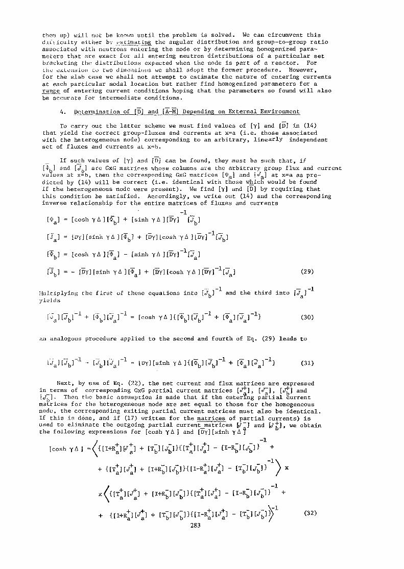
them up) will not be known until the problem Is solved. We can circumvent thisdiiiiculty either bv estimating the angular distribution and group-to-group ratioassociated with neutrons entering the node or by determining homogenized para-meters that are exact for all entering neutron distributions of a particular setbracketing the; distributions expected when the node is part of a reactor. Forthe uK.tuiibioii Co two dimensions we shall adopt the former procedure. However,for the slab case we shall not attempt to estimate the nature of entering currentsat each particular nodal location but rather find homogenized parameters for ajrangjs of entering current conditions hoping that the parameters so found will alsobe accurate for intermediate conditions.

4. Determination of [D] and [A-M] Depending on External Environment

To carry out the latter scheme we must find values of [y] and [D] in (14)that yield the correct group-fluxes and currents at x=a (i.e. those associatedwith the heterogeneous node) corresponding to an arbitrary, linearly independentset of fluxes and currents at x=b.

If such values of [y] and [D] can be found, they must be such that, if[$, ] and [J-0l are GxG matrices whose columns are the arbitrary group flux and currentvalues at x=b, then the corresponding GxG matrices [*a] and [ a] at x=a as pre-dicted by (14) will be correct (i.e. identical with those which would be foundif the heterogeneous node were present). We find [y] and [D] by requiring thatthis condition be satisfied. Accordingly, we write out (14) and the correspondinginverse relationship for the entire matrices of fluxes and currents

_ _ ~1 _[4a] = [cosh yA ][$b] + [sinh yA ][Dy] [^J

Ua] = [DyHsinh yA][*b] + [Dy] [cosh y A ] "

[*.] = [cosh YA][*J - [sinh YU 3 a.

[J"b] = - [DY][sirih yA][?a] + [By] [cosh YAHDyr1^) (29)

_ _-i _ __iMultiplying the first of these equations into [J,] and the third into [/ ]yields

fv^n^r1 + f n r1 = [cosh YAH^n^r1 + [¥a][7ai~1} (so)an analogous procedure applied to the second and fourth of Eq. (29) leads to

lJa][7b]~' - U^H^r = lDy][sinh yA H^JUy" + [*",,] [JJ'} (31)

Next, by use of Eq. (22), the net current and flux matrices are expressedin^terms of corresponding CxG partial current matrices [eT*] , [e/~] , [J*~] and[ jT] . Then the. basic assumption is made that if the entering partial currentmatrices for the heterogeneous node are set equal to those for the homogeneousnode, the corresponding exiting partial current matrices must also be identical.If this is done, and if (17) written for the matrices of partial currents) isused to eliminate the outgoing partial current_matrices [J~] and [J"t] , we obtainthe following expressions for [cosh yA] and [Dy] [sinh yAJ

[cosh yA] =/{[I+R+][Ja] + [Tb"n<7b"l}{[Tt][ja] ~ [I"V Cjb3 } +

""1

(32)283

-1

-+ Ul<][<] + [V mil-* ] - IV^l) (33)

These relationships permit [y] and [D] to be computed in terms of 2G arbitrary,G-element incoming partial current vectors. For heterogeneous nodes geometricallysymmetrical about the center plane (such that Eq. 27 is valid) any hoice ofincoming partial currents should yield the same values of [y] and [A-M]. Infact, although the algebra is complicated, it can be shown that (32) and (33)reduce directly to (28).

One characteristic of the [D] determined from both (28) and (33) should benoted, namely, [D] is a matrix and may have non-zero off-diagonal elements. Asmentioned previously, this situation already arises with certain diffusion theorymodels. It is not expected to lead to any computational difficulties.

5. Determination of Individual [A] and [M] Dependent on Outside Environment

_ _ Equation (13.1 shows _that finding [Y] and [D] permits the determination of[A-M]. To find [A] and [M] individually and to recover the individual homogenizedgroup cross sections out of which [A] and [M] are constructed according to Eq. 5requires further effort.

We shall find the individual homogenized group cross section by matchingreaction rates integrated over the nodal volume, again requiring that partialcurrents at the nodal surfaces of the homogenized nodes match those of theheterogeneous nodes. To do this we begin by noting that the column vector ofgroup fluxes [<J>(x)] f°r tne heterogeneous node at some point, x, in its interiordepends only on the directional fluxes i/j(a,y,E) and ip(b,y,E) at the nodal surfaces,and if the angular and energy dependences of these functions are known (orassumed), [<f>(x)] can be expressed as

[<K*>] = [Pa(x)][J*] + [Pb(x)][J~] (34)

where [pa(x)] and [p,(x)] are GxG "flux response matrices". It follows thatthe integrated group reaction rate vector, [Ial, for any interaction-a([£„] = Col{l }) taking place in the heterogeneous node can be writtenLX Otg

[Iaj = /atyx)2/[pa(x)][/] + [p b (x) ] [ J~] \dx (35)

where [E (x)] is a diagonal GxG matrix of group cross section for interaction-aat location x in the heterogeneous node.

For the homogenized node we find the group-flux vector [<Kx)] fromEq. (14) with A replaced by x. Use of (22) applied to the group-currents andfluxes of the homogenized node and of (23) leads to the relationship

(36)

where the GxG matrices [p (x)] and [pb(x)] are flux response matrices for thehomogenizednode expressed as functions of [y], [D] and the reflection andtransmission matrices. The integrated group reaction rate vector for interaction-ain the homogenized node then becomes

284

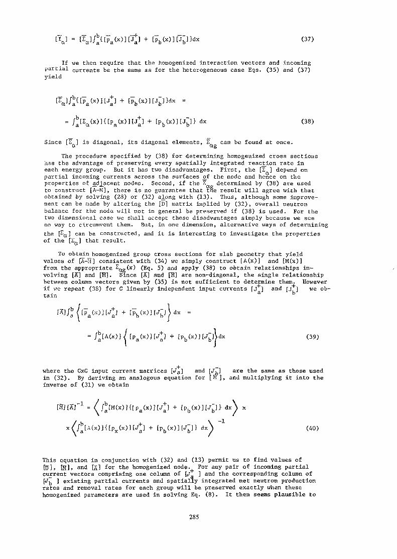
[p(x)][J~]}dx (37)

If we then require that the homogenized interaction vectors and incomingpartial currents be the same as for the heterogeneous case Eqs. (35) and (37)yield

= / [Ea(x)]{[pa(x)][J+] + [pb(x)][J~]} dx (38)

Since [E ] is diagonal, its diagonal elements, E can be found at once.

The procedure specified by (38) for determining homogenized cross sectionshas the advantage of preserving every spatially integrated reaction rate ineach energy group. But it has two disadvantages. First, the [Z ] depend onpartial incoming currents across the surfaces of the node and hence on theproperties of adjacent nodes. Second, if the E determined by (38) are usedto construct [A-M] , there is no guarantee that tne result will agree with thatobtained by solving (28) or (32) al^ong with (13). Thus, although some improve-ment can be made by altering the [D] matrix implied by (32) , overall neutronbalance for the node will not in general be preserved if (38) is used. For thetwo dimensional case wu shall accept these disadvantages simply because we seeno way to circumvent them. But, in one dimension, alternative ways of determiningthe [£a] can be constructed, and it is interesting to investigate the propertiesof the [Za] that result.

To obtain homogenized group cross sections for slab geometry that yieldvalues of [A-H] consistent with (34) we simply construct [A(x)} and [M(x)]from the appropriate 2 (x) (Eq. 5) and apply (38) to obtain relationships in-volving [A~] and [H] . Since [A~] and [B] are non-diagonal, the single relationshipbetween column vectors given by (35) is not sufficient to determine them. Howeverif we repeat (38) for G linearly independent input currents [J ] and [j ] we ob-tain a b

[pb(x)][Jb]> dx

[Pb(x)JKl>dx (39)

—where the GxG input current matrices [J"a] and [J ] are the same as those usedin (32). By deriving an analogous equation for [ M J > and multiplying it into theinverse of (31) we obtain

\ x

\dx (40)

This equation in conjunction with (32) and (13) permit us to find values of[UJ, [R]» and [A] for the homogenized node. For any pair of incoming partialcurrent vectors comprising one column of [J ] and the corresponding column of[J"b ] existing partial currents and spatially integrated net neutron productionrates and removal rates for each group will be preserved exactly when thesehomogenized parameters are used in solving Eq. (8). It then seems plausible to

285

assume that these quantities will be very nearly preserved when the incomingpartial currents to the node found when (8) is solved are not pairs from the[J"a ] and [J^ ] matrices used for (32) and (40).

6. Determination of Individual [S] and [H] Independent of Outside EnvironmentAs might he expected, for symmetric nodes, the homogenized values of [15],

[A"] and [M] become totally independent of [^a ] and [J~b ]. Equations (13)and (28) already show that this is true for [D] and [A-M] . To show it is alsotrue for [A] ar.d [K] separately we choose an axis system such that the pointx=0 is at the center plane of the symmetric node. Then a=-b and [A(x)] = [A(-x)].A] so, if incoming angular distributions are the same at a and b, p (x) = p (-x)and Pa(x) = p%j(-x). Then the right hand side of (39) becomes a

/°b[A(-x)][Pb(-x) ][</*] dx + /b[A(x)][pb(x)][c/-]dx =

//b[A(x)\ 0

)][p (x)]dx[] + (J-] (41)

Consequently, Eq. (40) reduces to

r , ,• •> -1[MHA]"1 = < / b [ M ( x ) ] [ P b ( x ) J d x W/ b [A(x)] [p b (x) ]dx\ (42)

Thus, for a symmetric node matrices [D] , [A] and [M] can be found that are exactin the sense we have defined and independent of the external environment.

fir i7. Determination of Individual Cross Section Matrices orWith [A] known we can go on to find a cross section matrix that will pre-

serve reaction rates for any reaction we desire. Thus if [Ea (x)] is a (diagonal)GxG matrix of group cross sections for interaction -a at location x in theheterogeneous node we define a corresponding homogenized cross section matrix[Ea] by replacing [A(x)] and [AT in (39) by [I, (x) ] and [E ]. If we then replace[M(x)l in (40) by [E .(x)] and [I ], Eq. (40) becomes

dx\ x

/ \ "1x//b(A(x)]{[pa(x)][c7+] + [pb(x)][c/b)} dx\ [A] (43)

Similarly, for symmetric nodes and the same angular distribution of neutronsentering both nodal faces, we replace [M(x)] and [M] in (A2) by [E (x) ] and[£„] to get

^ , , -1[EQ] = {/b[E a(x)][pb(x)]dx}{/°[A(x)][pb(x)]dx } (44)

_ _ _Unlike the [E ] of Eq. (33), the [Ea] are consistent with [A] and [D] and, forsynrrcctric nodes, are independent of the properties of neighboring nodes. However,they are unphysical in that off diagonal elements do not- in general vanish andmay in fact be negative. Thus E /b<j> (x)dx will not be the correct rate

286

at which group-e neutrons undergo interaction rate a in the node. Rather, thatrate will be ' otgg'/a o'(x)<3x. . This situation is unusual, but it createsno real practical difficulty since the Zagg' still produce correct average nodalpowers and depletion rates. Nor is the situation likely to cause numericalproblems, since only [5] and the entire matrix [A-MJ for the node are neededin (8).

8. Numerical ExamplesTo i':ple.Ter:t the methods we have developed for tba slab case it is necessary

to determine transmission, reflection and flux response matrix elements for theheterogeneous node. As mentioned in the introduction, this can be done by verysophisticated methods if they are available. However, for purposes of numericalexample we shall let the group diffusion model (specifically two groups) be thenumerical standard for the node. Also we shall assume that the heterogeneous nodeis composed of several (specifically three) homogeneous slabs. Equation (14)will then be valid for each individual slab making up the node and if the nodeextends from -L to +L we can find [u(-L)] H Col {[<}>(-L)], fJ(-L)]} in terms of[u(+L)] by successive applications of (14).

In performing the numerical calculations it is also necessary to determinefunctions such as cosh y A where y is GxG. This can be done by diagonalizationprocedures or by more sophisticated schemes involving iderapotent and nilpotentmatrices. The details of the procedures we have actually applied are given inReference (6).

To illustrate the nature of the homogenized parameters predicted for asymmetric node (Eq. 28, 42 and 44) we have analysed the heterogeneous node shownin Figure 1. The matrices [Dj, [A] and [M] were found from (13), (28) and (40).I.- "rMiuior. a neutron capture natr-'>. [C] was determined by letting [2a(x)] in Eq. (44)be the diagonal matrix Diag{Za(x), EQ, (x)} the entries of which are tabulatedunder Figure 1. Finally we computed a scattering-removal matrix [S] = [A] - [C].Results are displayed in Table 1.

Region 1Rgj2

b c

Region 1

2 (cm

(cm"1)

vE_ (cm"1)

VE (cm"1)2

Region 1 Region 2

0.008 0.050

AI = 9.25 era

0.053

0.0

0.07

0.02

1.40

D9(cm) 0 .40

Neutron Spectrum

0.450

0.0

0.01

0.01

1.000.75

A2 = 1.50 cm

Fig. 1 A 3-region Symmetric Node Usedin a Critical Reactor.

287

The unphysical nature of the homogenized parameters is apparent. For allregions of the heterogeneous node [D(x)] is diagonal, but, as is quite evidentin Table 1, [5] has non-zero off diagonal elements. There is no "up-scattering"(A (x)=0) for the heterogeneous node; yet A = .00060929 ("negative" up-scaEtering). The (1,1) element of the fission neutron production matrixM-. (x) = X-,v£f(>0 is zero for all regions of the heterogeneous node but negativefor the homogenized case. Finally, the absorption metrix [C] has off-diagonal(and in one case negative) entries, and the scattering-removal matrix has anon-zero second column.

It must be emphasized, however, that despite their unphysical nature, thesehomogenized parameters if used to analyse a critical reactor containing the nodein question will reproduce correctly all the nodal reaction rates. Thus, if</, (xl and <£-(>•) P.T- the flux shapes found whar. the homogenized parameters areused the nodal absorption rate will be fd [-0.00230358$ (x) 4- 0.0596217 8c}>2 (x) ]dxand will match exactly the heterogeneous result no matter what materialis outside the node in question.

TABLE 1

Homogenized Constants.for the Node of Fig. 1

D =1.2023299

-0.01639089

-0.05952299

0.35013581

A-M =0.03504833

-0.02109752

-0.07370149

0.05968812

A =0.02875870

•0.02109752

0.00060929

0.05968812

M =-0.00628962

0.00000000

0.07431078

0.00000000

/"» _

0.00996476-0.00230358

0.000675630.05962178

S =0.01879393-0.01879393

-0.000066330.00006633

288

Figure 2 shows the nodal dimensions and cross sections for a non-symmetriccase. The resultant homogenized parameters are given in Table (2) for threedifferent input flux-current matrices at x=d. (Each column of u is an inputflux-current vector Col {(j> (d) 4>2(d) J-(d) J (d)}). As is expected for anonsyiranatric case, the homogenized constants depend on the boundary conditionsat the surface of the node. (Specifying the 4x2 u, matrix on one face of thenode is equivalent to specifying the corresponding 2x2 input current matrices[Ja}> [J"d J on both sides. However the dependence on external conditions isslight. It seems reasonable to expect that a choice of u, (or [< +], [ T]close to those expected by the nature of the nodaJ environment should lead toaccurate predictions of criticality and reaction rates.

Region 1

•A*

Region 3

b c

A,=A3=9.25 cmA2=1.50 era

Region 1 Region 2 Region 3

0.008 0.050 0.008

£ (cm"1) 0.053 0.450 0.0583

vF., (cm"1) 0.0 0.0 0.0

(cm"1) 0.07 0.01 0.077

0.02 0.01 0.02

D, (cm)

D2(cm)

1.40

0.40

1.00

0.75

1.40

0.36

Neutron spectrum= 1*0? X = °-

Fig- 2 A 3-Region Non-symmetric Node Used in aCritical Reactor.

289

Table 2 Homogenized Constants for the Node of Fig. 2

Input

ud=

1.125 1.00.4 0.250.35 0.0120.035 0 .28

ud=

1.0 0.84

0.012 -0.0020.28 0.2696

u =d

"0.55 2.150.2 0.90.1 -0.80.01 0.0.12

Homogenized Constants

-D=

A-M=

A=

M=

D=

A-M=

1.2200983 -0.03682869"-0.02860269 0.33247074- ~

0.035252465 -0.07700762_-0. 021307264 0.0622724

0.02883137 0.00033343~|_-0. 02130726 0.0622724 J

-0.00642109 0.07734105*]_ 0.00000000 0.00000000 J

"1.2246737 -0.03576521"-0.03342377 0.33123439- _

0.03503387 -0.07699019-0.02113049 0.06226059

f 0.02833649 0.0003438?"]A= [-0.02113049 0. 06226059 J

{"-0.00619738 0.07733407"]M=j_ 0 .00000000 0.00000000 J

5=

A-M=

A=

M=

"1.2192740 -0,0-3186647"-0.02783785 0.32868762

0-03556261 -0.07796643_-0. 02155051 0.06301952_

"0.02886438 0.000230531-0.02155051 0.06301952J

"-0. 00669822 0.07819697~j0.00000000" O . O O O O O O O O j

III. Homogenized Group Diffusion Parameters for Two and Three Dimensional Kodes1. General Considerations

The homogenized parameters we have found for slab geometry possess mostof the ideal properties outlined in the introduction to this paper.Unfortunately the methods used to find them have no direct extension to higherdimensions. In fact, in more than one dimension, exact homogenized parametersdo not exist. - even if they are permitted to depend on boundary conditions onthe r3urface;3 of the node. We can nevertheless use some -of the ideas that werefruitful for the one dJmenstonal case to guide the development in two and threeditrensions.

The chief idea we shall adopt is to establish equivalence betweem homogeneousand heterogeneous nodes through the use of response matrices. Since exacthomogenized parameters independent of the boundary conditions do not exist forheterogeneous nodes in two and three dimensions we shall attempt to get greateraccuracy by accounting for such boundary conditions, although, even when thatis done the resulting parameters will reproduce those conditions onlyapproximately.

290

It Is also tempting to take advantage of the greater flexibility which the"non-physical" parameters provided in the one dimensional case. But we see noobvious way to do this and have not explored the matter. Accordingly, we take asthe fundamental relationship specifying homogenized cross sections for themultidimensional case an extension of Eq. (38). If [((>(r_)] is the GXG diagonalmatrix of group fluxes throughout a heterogeneous node at a given location ina vector and [£a(r_)] the diagonal matrix of group cross sections for anyinteraction-a throughout that node, and if [$(£.)) and [2a] are the correspondingquantities for the homogenized node, the extension to multidimensions ofEq. (38)can be written in the equivalent form

[Z"aJ/[$'(r)]dv = /[20(r)][*<r)]dv (45)

If the diagonal matrices [0(rJ] and [<}>(.£)] can be found, Eq (45)guaranteesth.it r.-ll volurae integrated reaction rates in the node will be preserved whenthe [£a]_are used. However, the previous one-dimensional analysis suggests that,if the '[Ea] for all reactions are found using (45), it will not be possible tofind a diffusion constant matrix [D] that preserves all leakage rates throughindividual nodal faces.

Implementation of (45) poses a number of problems. First of all, [0(r)}must be found. This can be done by the use of flux response matrices. However,that procedure requires that we know (or make assumptions about) the spatial,angular and energy shapes of the fluxes entering the surfaces of the node at itslocation in the reactor. Next we must determine [<j>0r)} for the homogenized node.This problem appears to be about as difficult as finding the hetergeneous fluxshapes; moreover, since [<)>(r_)] depends on the [?„]_ it is non-linear. Finally,we must determine the diffusion constant matrix [D] so that at least some of thecorrect leakage properties of the node a^t preserved. We shall attack theseproblems one at a time,

2. The Determination of ^q^ ] E4>(r) ]dv

The first step in finding total interaction integrals for the node is tocompute contributions to such integrals from incoming partial currents across thefaces of the node. Thus, for the moment we assume that we know the directionalflux density (j;(r_,Il,E) which will be present over the surface of a node when it ispart of a critical reactor. In analogy with (15) we then define partial group-gna'itro-n currents enforfng and leaving face £ of the node by

J^(in) = / dE/ dA/dfi ft (r.SJ.E)AEC8 ~ (46)

J'(out) = / dE/dA/ d& ft i(;(r,0,E)8 AE t, f2-n>0g -~

where the area integral (dA) is over surface £ of the node, n.being the outwarddirected normal to surface &.

Next we-define I' i(a)as the rate at which group-g neutrons undergo inter-action-^ in the node when a unit incoming partial current of group-g' neutron iscrossing surface-)?,. It follows that the total rate at which group-g neutronsundergo interaction-a in the node, is

/£ (r)<j> (r)dv = V I*, (a) /,(in) <47>ag ' g £_ gg 8

This result provides in a formal way the elements of the diagonal matrix on the righthand side of Eq. (45). However, to find the Igg»(a) and J .(in) , thedirectional flux <|>(r_,n,E) present when the node in question is part of the

291

critical re-ictor must be kncmi. This seems like aa impossible requirement untilwe recall that, for the slab case, values of the homogenized parameters are onlyslightly sensitive to the boundary conditions on the surfaces of the node.(See Table 2.) With this in mind we propose to estimate <Kj_,S7,E) over the surfaceof che node being homogenized by solving an auxiliary problem involving the node inquestion and its nearest neighbors with approximate boundary conditions(generally pure reflection) applied at those surfaces of the neighbors not adja-cent to the node being homogenized.

Such auxiliary problems could be very expensive if carried out by MonteCarlo or rrultigroup transport methods. Accordingly, for the analysis in thepresent paper we shall nake the assumption that G-group diffusion theoryparameters are already available for all material regions of the heterogeneouscore. Thus to compute the -'•gg1 it is necessary to know only the spatial shapeof the incoming partial group currents over the face of the node. Symmetryconsiderations suggest that the very simplest of all assumptions, namely that, underall conditions the incoming partial currents have a fixed shape (generally flat)over the nodal surfaces, may very well suffice. With this assumption made, allthe Igg'(<*) may be pre-computed by diffusion theory for the different hetero-geneous nodes making up the reactor.

The difficulty remaining before Eq. (47) can be used is to estimate therelative magnitudes of the Jgt(in) for different groups-a and different surfaces-2..This is done by performing stall response matrix calculations for the nodebeing homogenized and its nearest neighbors. Thus we define GXG partial

0 0 ' V Y i V P 1current response matrices [RXXl ] 5 {R~g'} such that R**I is the group-gpartial current emerging from face-£ We to a unit group-g' partialcurrent entering face-?,' when the node is in a vacuum.

£ $,^ As a result, for [J (in)] and [J (out)] (g-element column vectors of theJ (in) and J'(oui)), we obtain

CT f3

a y o p i 01[J*(out)J *LtlK^ }[J (in)] (48)

Note that because of the assumption that the group-diffusion theorymodel is applicable to the heterogeneous node and that the incoming partialcurrents have a known spatia] shape over the nodal surfaces the [R^ ] can befound readily. We now introduce the influence of neighboring nodes bydefining GXC albedo matrices [ot ] for each face & such that, for the nodebeing homogenized,

[/(in)] = [c/nAout)] (49)

Combining (48) and (49) yields the eigenvalue equation

YfJ(out)] = [RaJfJ(out)] (50)

£where [J(out)]is a super vector whose elements are the (g-element) t [J fout)];[Ret] is a supermatrix whose (££') element is (the GXG matrix) [R ][or ],and Y is an eigenvalue introduced to permit a non-trivial solution of (50).If the albedo matrices for the node embedded in a critical reactor were exactlycorrect, y would be unity.

£If the albedo matrices [a ] can be found, solving (50) and making use of(49) will yield the J^in) needed for (47). To find the Fa ]'s we shall applya response matrix calculation to each of the neighboring nodes making arbitraryassumptions about the values of albedoes for all sides of these neighbors ex-cept that one adjacent to the node being homogenized. Generally we shall assumethat these albedoes are identity matrices (zero net current across the nodalsurface). However, if information leading to a better approximation is availableit can be used.

292

Although the general case appears to offer ho difficulty we shall fromnow on specialize to two-dimensional nodes -in XY geometry having 90° rotationalsymmetry about a central axis. Figure (3) shows such a nodal assembly and itsfour adjacent neighbors. Numbers in the center of the squares label the nodesand those in parenthesis label the surfaces. Heterogeneous structure is notshown, but it is assumed not to destroy the 90° rotational symmetry. Becauseof this symmetry many of the [R 'j matrices for a given node are identical.Accordingly we shall adopt a more specific notation as follows:

For &=«,' (reflection): = [R]

For i and V opposite sides (transmission): [R ] 5 [T]n n iFor A and V adjacent sides (sidewise transmission): [R ] E [S]

Then in order to determine, for example, the albedo matrix [cto] for face (3)of noc'e-i (the core being homogenized) we use the properties of node (3) tofind [Ju; (out)] for face (1) of node (3) in terms of [J in)] for node (3).Thus, with all partial currents and response matrices referring to node-3 wewrite

[J(1)(out)] = [R][J (1)(in)] + [T][J(2)(in)] + [S] [J<3) (in) ] + [S] [J(4) (in) ]

To eliminate [J (in)] for sides 2, 3 and 4 we assume that we know albedoematrices [02], [a-,] and fa^J such that

(2) (2)[Jv"(±n)l = [<x2][J^'(out)l = [a2]{[T][J(1)(in)] + [R] [J(2) (in) ] +

+ [S][J(3)(in)] + fS][J(4)(in)]}

r(3)(in)] = [a3][J(3)(out)] = [a3]{[S][J(1)(in)] + [S][J(2)(in)] ++ [R][j(3)(in)J + tX][J(4)(in)]}

= [a4][J ( 4 )(out)] = [S] [J<2) (±n)]

(51)

+ [ T ] [ J ( i n ) ] + [ R ] [ J ( i n ) ] } (52)(2)These relationships can be used to determines [J (in)] ; £= 2, 3, 4 in

terms of [J^ (in)]. When the resultant expressions are substituted into (51)we obtain (with square brackets about the matrices omitted)

(3)

:2) 4 (i)(4)

(2)

(4) 2 (3)

CD

(2)

(43 i (3)

CD

CDC33 1 (4)

(2)

(4)

ll) 3 (2)

(3)

Repr

FIGURE 3

Representation of Assembly and Its FourAdjacent Neighbors

293

[J ( 1 )(out)J = <R + [S+T(I-a2R)~1a2S]{[ct3 1-R-T(R-T-ct4~1) (1

-i -i ~1 -1 ~^-S(I-a2R) a2S<I+(R-T-a4 ) (R-T-a^ )>] +

+[a4~1-R-T(R-T-a3~1) (R-T-a4~1)-S(I-a2R)~1a2S x

i -1 i -1 ,x ] }[S + S(l-a2R) a2T] +

+ la-a^r^T >[J ( 1 )(in)] (53)

For certain choices of the [ct?] this expression reduces considerably.For example, if node-3 is reflector material with side-2 its outer surface, areasonable choice of the[cc£]'s might be t0 ] = [o l = *; [<*2] = °'For this choice (53) reduces to

[J(1)(out)] = [R + 2S(I-R-T)~1S][J(1)(in)] (54)

Since [J(1)(out)J for node-3 is [J(3 (in)] for node-i and [J (in)] fornode-3 is [J^ (out) ] for node-i, Equation (49) shows that the GxG matrix onthe right hand side of (53) is the albedo matrix [a ] for node-i. Because ofthe labelling used for Figure (3) the same formula (with of course appropriateR,S,T and cc^'s gives the albedoes for the remaining surfaces of node-i. Thus,knowing the response matrices for all the nodes in the reactor we can find [Ra]and solve Eqs (50) and (49) for approximate values of [J (in)] for all surfacesof every node. Equation (47) then yields the integrated group-g reaction ratesfor nodes being homogenized. Thus we can determine the right hand side of Eq. (45).

3. The Determination of/[ (r) ]dv

The nodal volume integral of the flux vector [<j>(x)] is needed in Eq. _(45)in order to determine the homogenized cross section matrices [la]. However, [<f>(r_)]itself depends on these cross sections. This circumstance suggests that an ...,,.iterative process must be used to find /[<f>(r)]dv . Such a procedure is possible ' .However we have developed a faster scheme that avoids the need toiterate. This scheme is based on the fact that, when homogenized parametersare used, the flux shape throughout the node will be relatively^smooth, and, ifh and h are .the dimensions of the node, the integrals gx^x) = /o^g x>y^yand 'f'gyCy) = /nx<l)g(x,y)dx _ ought_to be smooth functions of x and y.Accordingly we express the <j> (x) and cj> (y) as polynomials in x and y and determine

h h h h| / <j> (x,y)dxdy = \ <j> (x)dx = / $ (y)dy (55)oo§ o g x o s y

The expansion functions chosen are_cubic Hermite polynomials. (See Ref. 4, p 506.)With such a selection we may approximate 'JwW by

9gx(x) -

x=hx^ (x) (56)

294

The cubic hermite polynomials are such that the coefficients in (55)have the physical interpretation indicated. Thus, for example,UQ (x> = uhx(x) = UQ 00 = ° and 4rui~ (x) = 1. These polynomia

at x = h ,polynomials are defined by

utx) = - 2 (1-z)3 +3 (1-z)2

= -2z3 + 3z2

(l-z)]h

z = x/h (57)

It follows from Eq. (55) that

h hI- x, yJ0 h

\l-2

12 dx Ygxv«=h J

(58)

The great advantage of expressing the volume integral of the homogenized flux inthis way is that in diffusion theory for the homogenized node

"j (x,y) =0 gx '" - D" -— (x)g dx gx (59)

Moreover /Q" -J^x(x,y)dy and<J)gX(x) are related through Eq. (27) to the partialcurrents entering and leaving the node. These in turn are, by the fundamentalequivalence assumption, the sane for the homogeneous node as for the hetero-geneous node. Thus we can use for them the values obtained by solving (50) andapplying (49). The net result of these manipulations is that for node-iof'Fig. (3)

)(in) + J(4)(out) + J(3)(in) + J(3)(out)} +

(60)

An exactly analogous procedure applied to <j> (y) yialds

(r)dv « h/J(1)(in) + J(1)(out)\ § s

(61)

295

Thus, we have two expressions for the volume integral of the group-gflux for the homogenized node. Both these expressions involve the homogenizednodal diffusion constant which we have not yet jibtained. We could proceedin an iterative fashion (^' , perhaps guessing r> » averaging (60) and (61) ,finding the Z 's , thence the Dg's and continuing the iteration. Howeverthere is an easie_r way which numerical tests show is quite_accurate (8) ,We simply regard D in (60) and (61) as a free parameter D* which can beadjusted to account for the fact that the expansion (56) is only approximate.Thus we choose 0* so that both (60) and (61) are simultaneously valid.Eliminating the %ommon parameter from these two equations yields

/jj1' ut)+J<2> <out)\/J<4> (in)+J<4) (in)}-//4' (out)«<3> (out)\{j > (in)«f> (in)}f-i Otrlv = ?'n *-* ————————— " —————— ^ — ° ———————— " ————— - —— ° ———————— & ______ v ° ________ & ________ J'

(62)

Equations (62) and (47) provide all the information needed to find [£a]using Eq. (45). Moreover, although we had to guess at the albedoes for the outersurfaces of nodes adjacent to the node being homogenized, the same partialcurrents that result are used in both (62) and (47). The expected cancellationof errors alone with the expectation that the homogenized group reaction crosssections are not unduly sensitive to the external environment leads us to expectaccurate results from the method.

4. Determination of [D]

Having selected all homogenized interaction cross sections £ag so thatthey have their usual physical significance, we cannot expect to match exactlythe neutron leakage rates for each energy group out of each face of the node.If we could do it in two dimensions, we could do it in one, and we have alreadyseen that that is in general not possible. Putting it another way: Havingdetermined all tin? I\-J matrices without any direct consideration of neutronleakage effects, we cannot reasonably hope to find_ a_ homogenized diffusionconstant matrix [DJ that if used along with the [A-M] „ , matrix implied by the[Za]' swill produce homogenized response matrices [R ] identical with theheterogeneous viatrices [R } of. Eq. (48). We can however determine [Bj so thatt ?i(-' largest homogenized response matrices match the corresponding heterogeneousR 's. This; is the procedure we have adopted for finding [5] . Several otherschemes were examined ' \ but this one seemed to produce the most accurateresults.

-* • Nu."eT leal Results

We have tested the two dimensional homogenization scheme just described forseveral reactor configurations (8). These were not realistic designs but werecreated to exhibit homogenization problems similar to those which might beencountered with light water reactors. We ran problems involving fuel assembliescharacteristic of a PWR and a BWR. For the PWR case we used fuel assembliescharacteristic of a real reactor having 5-pronged control rods or water holes.However, we could afford to run only a two-assembly problem, and for this theconventional flux weighted scheme and the new homogenization procedure bothgave accurate results. The nodal power prediction was poorer for the new scheme(-0.62% maximum error vs. -0.36%) but the eigenvalue prediction was better(+0.024% error vs. -0.098%).

Problems involving assemblies containing cross shaped control rods orwater ho]es showed a Much greater difference in the accuracy of the two methods.The assemblies used are shown in Figure (4). In that they contain cross shapedrods or water holes they are similar to those used in BWR's. However thedimensions are not at all typical. They were chosen to keep down the cost ofcomputations. All computations, both heterogeneous and homogeneous, for thedetermination of response matrices and for criticality calculations were run by

296

two-group finite difference diffusion theory methods using 0.5.or 1 cm meshspacings (See Figure 5). A water reflected quarter core problem composed ofassemblies A and B is shown on Figure (5). Homogenized two-group parameterscomputed according to the scheme presented in the paper marked EGDC - equivalentgroup diffusion coefficients) and standard flux weighted constants (FWC) foundusing Eq. (3) are shown in Table (3), There is clearly a small but realdependence on position for the EGDC. Identical assemblies (Type A-containingcontrol rods) are located at positions Q 1, 3, 5, 7 and 9 -while Type B assemblieswith control rods replaced by water are located at positions Q 2, 4, 6 and 8. Thedifferences between the FWC and the EGDC is much more striking. Figure (6)shows the errors in power distribution and eigenvalue when homogenization iscarried out according to the two different prescriptions. Clearly the EGDCprovide much wore accurate results (errors in nodal power of 0.7% vs. 5-2% for theFKC).

A half core model, with control rods asymmetrically distributed to createa tilted po;v-er distribution was also analysed. Figure (7) shows the distributionotf fuel asu^nblioK, and Table (4) displays those, position-dependent, homogenizedgroup parameters (EGDC) not already given in Table (3). Power distributionsresulting from use of the FWC and EGDC are shown in Figure (8). Again, errorsin nodal powers are significantly smaller (6.3% vs. 1.2%) when homogenizedparameters determined by the new method are used.

Two BWR assemblies have the above geometry butdiffer with respect to crossed-rod material.

Crossed RodAssembly A control rod materialAssembly B water

FIGURE 4BWR Assembly Compositions

297

Q.i

A

Q4

B

Q7

A

Q2

B

Q5

A

Q8

B

Q3

A

Q6

B

Q9

A

IV.

Assembly types A arid B refer to the assemblies shown jln.Figuro 4.

Numbers in upper right hand corner represent assembly ;posidtio.n.

An eight cm water reflector surrounds the core.

Mesh Spacing

Heterogeneous reference problem = 0.5 cm spacing throughoutcore and reflector

Homogeneous problems: 0.5 cm in reflector and fuel within 2 cmof interface and 1 cm elsewhere

FIGURE 5

BWR Quarter-Core Configuration

Conclusions

It is our feeling that the chief virtues of the one dimensional resultspresented in' this paper are the ideas that emerge which are applicable to themore than one-dimension. Not all the procedures used for one-dimension canbe extended. However, in developing the two dimensional homogenization methodwe have attempted to use those that are. With respect to the two dimensionalmethod, the test cases are too few to make any firm conclusion, but we feel theresults are encouraging with respect to the accuracy of the scheme. We believethat the new method is better grounded theoretically and hence is inherentlymore accurate. For example, it avoids the assumption of the usual flux weightingmethod that the net group currents across nodal boundaries vanish. This assump-tion can seriously distort the flux shape in a heterogeneous node. (We suspectit is the chief source of the major differences in Tables (3) and (4) betweenthe flux weighted thermal absorption and fission cross sections and those deter-mined by the new scheme).

It might at first seem that implementing the new scheme in two dimensionswould lead to high computing costs. This was not the case for the problems weran. The most expensive parts of the computations are the fine mesh computationsneeded to compute the response matrices for the heterogeneous nodes. But fora rotationally symmetric node only G of these are needed for each geometricallydifferent node. Moreover, the equations involved are inhomogeneous and can be

298

solved non-iterative3y. Only one fine mesh flux solution for each geometricallydifferent mode is needed for the standard FWC procedure. However this is aneigenvalue problem and an interative method is indicated. We believe thatproduction computer cod^s designed to implement the two methods would run inroughly the same time. It should be pointed out though that the number of finenesh problems required for the new scheme increases by a factor of six for threedimensional modes having no rotational symmetry.

TABLE 3

Diffusion Theory Parameters - FWC and EGDCBWR Quarter-Care Problem

EGDC

Position i1152

"al

"a.2

'fl

'f2

Ql

Q2,Q4

Q3,Q7

Q5,Q9

Q6,Q8

i. 4227+03.7917-1

1.4418+03.9236-1

1.4209+03.7991-1

1.4193+03.8037-1

1.4414+03.9252-1

9.6577-31.0887-1

9.3628-39.6631-2

9.6759-31.0843-1

9.6880-31.0814-1

9. 37 66 -39.6530-2

6.4599-31.3137-1

6.4635-31.4356-1

6.4735-31.2886-1

6.4824-31.2654-1

6.4732-31.4319-1

1.4137-2

1.7228-2

1.4167-2

1.4186-2

1". 7234-2

FWC

Assembly A

Assembly B

1.3884+03.8420-1

1.4470+03.7478-1

9.7122-31.2155-1

9.4224-38.9222-2

6.4987-31.4303-1

6.5050-31.3241-1

1.4222-2

1.7302-2

*Assenbly position refers to Figure 5

299

oo

XX

XX

Per cent error in Power - FWC

Per cent.error in Power - EGDC

Ql1.74

- .25

Q2-3.88

.48

Q55.63

- .47

Q3

3.67- .68

QS-3.18

.42

Q9

5.18

- .63

FWC EGDC

Per cent error in K ,.- -.847 -.379ef f

FIGURE 6BWR Quarter-Core Results

HI

A

H4

B

H7

A

H10

B

H13

B

H2

B

H5

A

H8

B

Hll

B

H14

B

H3

A

H6

B

H9

A

H12

B

K15

B

IAssembly types A and B refer to the assemblies shown in.Figure 4.Numbers in upper right hand corner represent assembly position.An eight cm water reflector surrounds the core.Mesh spacing for heterogeneous and homogeneous problemscorresponds to that used for guarter-core problems.

FIGURE 7BWR Half-Core Configuration

U)o

. XXXXXX

Reference per cent total powerPer cent error in power - FWCPer cent error in power - EGDC

TABLE 4Diffusion Theory Parameters - FWC and EGDC

BWR HaIf-Core ProblemEGDC

Position i*

H1-H7,H9 areidentical toQ1-Q7,Q9(Table 3)

D,

D,

'al

'a2

Keff

•fl'f2

3.76- .97

H104.238-1.39.17

HI 33.841-1.03- .05

-2.16.32

Hll5.164.80.60

H144.699.25.38

6.29- .64

H125.593.39.75

H155.167.36.41

H8 -1-3.

CTT n •*- •ii-LU3.

Hll -1-3.

H12 -1'3.

i H13 1-3,

FWC EGDCReference per cent error per cent error •,

H14,H15.842530 -.572 -,197 3'

4415+09246-1

4418+09236-1

4416+09242-1

4415+09243-1

4420+09220-1

4418+09234-1

FIGURE 8 FWC for Assembly A andProblem given in Table

•DT.T-D u^, T *_r-^>-^ r> ,-,, i j- ,- - ——————————— ~ —————————

99

99

99

99

99

99

.3745-3

.6568-2

.3629-3

.6631-2

.3724-3

.6584-2

.3731-3

.6579-2

.3466-3

.6695-2

.3628-3

.6632-2FWC

B are same as3.

6.4717-31.4326-1

6.4636-31.4355-1

6.4703-31.4332-1

6.4708-31.4330-1

6.4520-31.4382-1

6.4635-31.4356-1

those for

'21

1.7231-2

1.7228-2

1.7230-2

1.7231-2

1.7222-2

1.7228-2

*Assembly position refers to Figure 7.

The new scheme still requires much testing and development. Comparisonsbetween it and the standard flux-weighting method must be carried out forrealistic PWR and BWR reactors. The extension to three dimensions must be ex-plored. (When control rods pierce a surface it is no longer appropriate toassume that the shapes of entering partial currents are flat across that surfaceStrategies for dealing with depletion and thermal hydraulic feedback effectsmust be worked out. These difficulties have all been faced for the standardflux weighting method, and certainly application of the same techniques usedthere to the new method ought to be at least as successful. However, because ofits firmer theoretical foundation and greater flexibility, we feel that thescheme we propose can be developed into a practical procedure for predictingdetailed reactor behavior more accurately than can be done at present.

(1) H. Finnemann and M.R. Wagner, "A New Computational Technique for theSolution of MultidimensionaL-Neutron Diffusion Problems", presentedat the International Meeting of Specialists on "Methods of NeutronTransport Theory in Reactor Calculations", Bologna, Italy (Nov. 1975).

(2) A. Kavenoky, "Neptune: A Modular Scheme for the) Calculation of LightWater Reactors", Proc. Conf. on Computational Methods in NuclearEngineering, CONF-750413, p. V-27, Charleston, S.C. (1975).

(3) J.G. Kollas and A.F. Henry, "The Determination of Homogenized GroupDiffusion Theory Parameters", Nuc. Sci. Eng'. 6£ 464 (1976).

(4) A.F. Henry, Nuclear Reactor Analysis (Cambridge, MA: MIT Press), 1975.(5) E.M. Gelbard and R. Lell, Nucl. Sci. and Eng. 6>3_ 9 (1977).

(6) A.A. Morshed, "Equivalent Diffusion Theory Parameters for Slab Geometry",M.S. Thesis, Department of Nuclear Engineering, MIT (1978).

(7) A.F. Henry and B.A. Worley, "Determination of Equivalent DiffusionTheory Parameters", EPRI Report 305 (1975).

(8) B.A. Worley and A.F. Henry, "Spatial Homogenization of Diffusion TheoryParameters", ERDA Report COO-2262-10, MITNE-210 (September 1977).

(9) T.C. Sbarounis, "Treatment of the Spatial Shape of the Currents In theResponse Matrix Method", Ph.D. Thesis, Department of Nuclear Engineering,MIT (1977).

302

A NEW APPROACH TO HOMOGENIZATIONAND GROUP CONDENSATION

K. KOEBKEKraftwerk Union AG,Erlangen, Federal Republic of Germany

Abstract

A coarse-mesh few group neutron flux distribution in areactor core should conserve several integral quantitiesof the heterogeneous representation in every homogenizedregion. The homogenization theory described in this paperwill be called "equivalence theory".

All the information needed for the equivalent coarse-meshcalculation is taken from multigroup spectral calculationsof heterogeneous assemblies in their "typical" environment.A self-consistent system of differential equations andboundary conditions for the determination of equivalentgrout) parameters is derived. The theory is based on thepostulate, that the integral reaction rates, averagefluxes and average leakages are conserved.

The progress achieved is demonstrated by applying theproposed scheme to an idealized heterogeneous BV/R two-groupproblem defined by Henry and Worley / 1/. For this problemequivalent group parameters in a two-group and an one-grouprepresentation are determined. The numerical solution ofthe equivalence equations for this reactor problem reproducesthe integral quantities within five digits.

A unique feature of this theory is the fact that flux con-tinuity between adjacent homogenized regions is no longerpostulated. The discontinuity of the flux is represented byan additional equivalent parameter, the heterogeneity factor.For the description of the interaction between rectangularassemblies, it is necessary to use the direction dependenceof the diffusion coefficients and also of the heterogeneityfactors. These equivalent parameters and the flux and volumeweighted cross sections are represented as a function of theintegral quantities to be conserved, e.g. the total leakage.

This work has been supported by the "Bundesm'inisteriumfur Forschung und Technologie" / Federal Republic of Germany303

The similarity of the equivalence equation with the diffu-sion equation allows to apnly an extended form of the nodalexpansion method / 2/ to calculate the power distributionof thermal reactors.

A high order interpolation scheme and the application ofthe modulation method / 3 / allow to reconstruct a goodapproximation of the local heterogeneous power distributionin the entire reactor core. This regained heterogeneoussolution is approximately continuous along the boundariesof the assemblies.

1. Introduction

1The nodal expansion method and the subsequent application•">of a high order interpolation method is used at KWU/Erlangento solve the diffusion equation for global PWR-problems.These accurate coarse mesh methods presuppose the abilityto construct homogenized group diffusion theory parameters.

These parameters should be chosen such, that the resultingfew group coarse mesh solution in a reactor core conservesseveral integral quantities of a corresponding multigroupheterogeneous representation.

In the conventional procedure flux- and volume-weightedfew group cross sections are determined from one - or two -dimensional spectral calculations with zero current boundaryconditions. Assuming that a homogenized materialdistribution in every region has the same neutron physicalinteraction as in the heterogeneous representation, thediffusion coefficient can then be deduced from the P1-approximation of the transport equation.

However, conventional diffusion theory cannot exactlyreproduce all integral reaction rates, the average fluxesin every region and the averaged fluxes and currents atthe interfaces. To adjust a diffusion theory solutionto all these physical quantities additional degrees offreedom within the theory must be introduced.

The fundamental idea to adjust the few group solution ofthe diffusion equation to the known heterogeneous, multi-group solution by defining appropriate equivalent para-meters has been considered by Henry and Worley . Theirobjective was to define the diffusion coefficient and the cross

304

sections such , that the coarse mesh solution reproducesthe response matrix and the reaction rates of theheterogeneous cell calculation.

The hoinogenization theory, described in this paper, iscalled "equivalence theorv". It includes a new approachto the generation of equivalent parameters and may replacethe diffusion theory to describe the global powerdistribution in a reactor core.

Different to Henry and Worley^1 the equivalent parametersare adjusted directly to several integral physical quantitiesin every homogenized region, known from a heterogeneousspectral calculation. A self consistent system ofdifferential equations and boundary conditions betweenadjacent regions is derived to define equivalent parameters.

A major advantage is the similarity of these equivalenceequations with the diffusion equations. This allows to1apply a generalized form of the nodal expansion methodfor rectangular coarse mesh lattices to calculate the powerdistribution in large light water reactors.

In chapter 7 a heterogeneous B¥R-problem (fig. 1) definedby Henry and Worley is considered. With respect to theabove noted physical quantities, to be conserved in everyregion, a consistent homogenized reactor solution (fig. 2-4)is for the first time proven to exist.

2. The Formulation of the Homogenization Problem

Comparing a few-group coarse mesh solution of ahomogenized reactor representation with a multigroupreference solution of a heterogeneous reactor repre-sentation, the difficulty to define a consistent homo-genization procedure becomes obvious. The equivalencebetween these two representations can only be postulatedfor certain integral values in the homogeneous regionsof the few group representation.

The interaction between adjacent regions to be homo-genized is influenced by local and spectral interactioneffects between these regions. Burnup calculationsdepend on the local multigroup spectrum. These neutronphysical effects can only be described correctly by

305

heterogeneous spectral calculations, if the region tobe homogenized is embedded in its typical neutron physicalenvironment. This enlarged spectral geometry should bechosen in a way, that the distance of the consideredregion to the outer boundary exeeds the free mean pathlength of the neutrons. In that case the local spectrum0het i 0het in every macro group G (g6G) and the localflux variation, induced by the heterogeneous structure,will be relatively independent of the outer boundaryconditions. Despite the loss of this detailed informationin the few group homogenized representation, it will thenbe possible to account for the influence of adjacentregions.

The equivalent few group neutron flux distribution in areactor should conserve the following integral quantitiesin every macro group:

Postulate A: the integral reaction rates and fluxesin every homogenized region

and

Postulate B: the integral net currents and integralfluxes at the interface between adjacentregions.

The latter postulate asks for the conservation of theneutron physical interaction of the considered homo-genization region. If these integral boundary valuesare conserved, the respective response matrix will coin-cide in both representations.

Both postulates shall be satisfied simultaneously. Theglobal power distribution will only be identical in bothrepresentations, if the interaction between adjacentregions is described in an equivalent fashion.

3. The Generation of Equivalent Parameters

Performing heterogeneous spectral calculations, noassumption is made about the method to solve the transportequations (e.g. Monte-Carlo, collision-probability-methodor diffusion theory, SN-theory). It is always assumed, thata region to be homogenized is embedded in its typicalneutron physical environment. It should always be possible

306

to determine the integral few group quantities (seepostulat A and B) on the basis of the heterogeneous multi-group flux solution. These quantities, the integral reactionrates, fluxes and net currents establish the basis toconstruct an equivalent few group flux distribution in theconsidered regions. The respective prescription issimultaneously used to define equivalent parameters(chapter 4 and 5). This prescription to construct ahomogeneous few group equivalent flux distribution on thebasis of these integral quantities, is also used insucceeding independent coarse mesh calculations (chapter 6and 7). To achieve full equivalence between both repre-sentations, the equivalent flux distribution and theequivalent parameters should only depend on these physicalquantities, which are known in both representations.

To define an equivalent few group flux distribution in theregion to be homogenized a few group net current distributionJp°m(r) is constructed along the interfaces between adjacentregions. The few group flux distribution will then resultfrom a yet unknown differential equation system, the"equivalence equations". Together with the net currentdistribution and the eigenvalue k «- the solution of thisdifferential equation system exhibits an inhomogeneousboundary value problem.

This few group net current distribution should also only de-pend on the physical quantities to be conserved. The mainpoint is, that this distribution in every region isconstructed in the same way generating equivalent para-meters from heterogeneous spectral calculations and byperforming succeeding coarse mesh calculations. Theintegral over an interface of the few group net currentdistribution should always coincide with the respectiveintegral net current J e (r) (see postulat B), knownfrom the heterogeneous reference solution.

(Dinterface interface

Applying the integral physical quantities of adjacentregions, this few group net current distribution can berepresented as a polynomial expansion. In the case of arectangular coarse mesh lattice a respective interpolationscheme is used for the quadratic polynomial expansion ofthe transversal leakage in /1/.

307

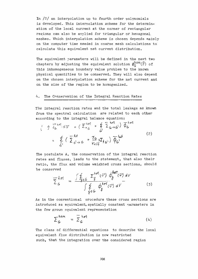
In /2/ an interpolation up to fourth order polynomialsis developed. This interpolation scheme for the determin-ation of the local current at the corner of rectangularregions can also be applied for triangular or hexagonalmeshes. Which interpolation scheme is chosen depends mainlyon the computer time needed in coarse mesh calculations tocalculate this equivalent net current distribution.

The equivalent parameters will be defined in the next twochapters by adjusting the equivalent solution 0G°m(r) ofthis inhomogeneous boundary value problem to the knownphysical quantities to be conserved. They will also dependon the chosen interpolation scheme for the net current andon the size of the region to be homogenized.

4. The Conservation of the Integral Reaction Rates

The integral reaction rates and the total leakage as knownfrom the spectral calculation are related to each otheraccording to the integral balance equation:

-fu*)

The postulate A, the conservation of the integral reactionrates and fluxes, leads to the statement, that also theirratio, the flux and volume weighted cross sections, shouldbe conserved

As in the conventional procedure these cross sections areintroduced as equivalent, spatially constant parameters inthe few group equivalent representation

The class of differential equations to describe the localequivalent flux distribution is now restrictedsuch, that the integration over the considered region

308

leads to a balance equation of the following form:

h>

xf r -»hoK* .^ , * orn \ X_ > < : , > ; ^G

(5)

The inhomogeneous leakage term is known from thedefinition of the inhomogeneous boundary value problem.Equation (1) guarantees, that the leakage terms in theequivalent and in the heterogeneous few group balanceequation (equation (2) and (5)) coincide.As a consequence of the definition of the equivalentparameters Eq. 4, the coefficient matrices of both balanceequations are identical. Hence, the solution of the linearinhomogeneous equation system (5) leads to the samesolution vector

how -7~bpt

as from the heterogeneous spectral calculation.

Using the flux and volume weighted cross sections (3) asequivalent parameters (4), all equivalent flux solutions ofthe inhomogeneous boundary value problem fulfil thenpostulate A.

The above statement does not depend on the local fluxdistribution, which must be taken into account in the nextchapter, considering the conservation of interaction.

The dependence of the flux and volume weighted crosssections (2) or of the equivalent parameters on the statevariables can be deduced by performing several heterogeneousspectral calculations. In addition to the physical quantitiesto be conserved, the boron concentration (P¥R) , the regionwiseaveraged parameters, the burnup and the fuel and moderatortemperature are introduced as state variables. If the outerboundary conditions of the spectral geometry are varied,the averaged cross sections of the embedded region can beapproximated as a linear function of the physical quantitiesto be conserved:

-V-T - 7<!_/• ~ £-

309

r (o) is the cross-section for zero total leakagee -* -*<t> Jp • do in all macro groups. The coefficient matrix

can be deduced from N^ + 1 spectral calculations(Np - number of the macro groups). This formula can beapplied, if the heterogeneities in all spatial directionshave the same structure. If this is not the case, as forLWR-assemblies in axial and radial direction an extensionof formula (8) can be applied. The matrix elements fe 'must be taken into account if the cross-section distribution£ Q (r) shows large variations or, if there is a largespectral shift 0het / 0 et within the region considered(see formula (3)]. The formula (7) should be applied, ifin a global reactor solution the neutron physics statesof the considered region differ considerably in leakages.Otherwise the neutron physics state of the region, embeddedin its typical environment, can be comprehended by onlyone spectral calculation.

The expansion formula (7) can be inserted as an equivalentparameter (4) in the few group balance equation (5). Thisequation is linear and describes the integral reactionrates and fluxes for different inhomogeneous boundaryvalue problems. This extended balance equation isequivalent to the heterogeneous balance equation in awide range of possible neutron physics states of theembedded region.

5. The Conservation of the Neutron PhysicalInteraction

To fulfil postulate B of chapter 2 one has to considerthe local equivalent flux distribution 0 ora(r). For theinhomogeneous boundary value problem, an appropriatesystem of differential equations and boundary conditionshave to be defined. Beside the integral reaction rates andfluxes the resulting few group flux solution should alsoconserve the integral fluxes at each interface of theconsidered region. With this procedure it is intended todescribe the functional dependence, the "response" of theseflux values from the net current distribution and the eigen-value in the same way as it results from the heterogeneousspectral calculation.

In the preceeding chapter the equivalent parameters 2. G°mof the postulated differential equation system were

310

introduced to conserve the integral reaction rates andfluxes. The integral balance equation (5) leads to anassociated differential equation system with a still un-known leakage terra. To keep continuity with conventionalreactor design methods this leakage term is chosen inanalogy to diffusion theory as

= - D . V 0°ffl(r) (8)

As an extension, the spatially constant equivalent para-meter D, the "diffusion coefficient", is assumed to bedirectional dependent.

This parameter is introduced to adjust the resulting equiva-lent flux distribution of the inhomogeneous boundary valueproblem to the integral fluxes, known from the heterogeneousspectral calculation (postulate B). In contrast to diffusiontheory the parameter D has no direct physical meaning.

With the leakage term, deduced from (8) and the balanceequations (5), the equivalence equation in two dimensionshas the following mathematical structure :

<9)It vi/T) L

The following discussion is restricted to rectangularcoarse mesh lattices. Only in this case an easy reductionof the multidimensional differential equation system toone dimension is applicable. The pin-cell-lattice and theassembly lattice of KVU light water reactors are based onthis geometry. The treatment of triangular or hexagonalhomogenization regions by a similar equivalence theoryshould be possible, but beyond the scope of this paper.

Integrating the differential equation (9) over they-direction (-^-£Y-^- ) the nodal equivalence equation

311

is given in the interval (- \ $ * 1 - ) by:

0 & do)/ hOlTi /v ^_ hOh\ 'V'T-hGt*.<* s--.fr +^f ^4. )&> <*>

i:'--<»)and the gradient of the nodal flux is connected(equation 8) with the known averaged currents at theinterfaces ( x= t w/a. ) by:

howkm

The nodal flux fpg, (x) and the transverse leakaged, (x) are defined by:-t .k

, A f "*• l'!0ttV , .

(X) *

(13)

The net current distribution (13), the two averagednet currents (11) and the differential equation system (10)defines a one dimensional boundary value problem. Forevery chosen diffusion coefficient the boundary valueproblem leads to a unique nodal flux solution.

To adjust this equivalent few group flux distributionto both - in every macro group known - integral fluxes

(|> (± f-) one needs beside the diffusion coefficientone additional degree of freedom.

The difficulty to find an appropriate equivalent parametercan be overcome by no longer postulating the continuitycondition of the equivalent flux at the interface. Thereis-from the viewpoint of this equivalence theory-nophysical reason for this assumption.

312

As the ratio between the known heterogeneous integral fluxand the equivalent flux one defines the heterogeneityfactors :

Because only one additional degree of freedom is needed,it is often convenient - also in the case of a asymmetricheterogeneous structure - to postulate :-t>The equation system (10, 11) and (14, 15) leads for theinhomogeneous boundary value problem and for the known

Y~r h^t & \integral heterogeneous fluxes <p, (± ~) to a uniquedefinition of Dx and f^et»x ±n every macro group. Only,ifthe boundary values are symmetric et(+ f) = -fand JQ6 (+ •?) = - On.6 (- -o) there exists a infinite numberof pairs of equivalent parameters (Dx, f&e x), which allowto fulfil postulate B.

This equation system can be solved for every direction andfor every rectangular region to be homogenized. The neutronphysical interaction of a considered two dimensional regionwith the environment is then comprehended in the fourequivalent parameters (Dx, f£et x, D^, f£et y) ,

These values depend on the chosen geometry of the homo-genization region, on the polynomial expansion of the fewgroup net current distribution along the interface andon the method to solve the nodal equivalence equation (10).

The local equivalent flux distribution 0G,om(x, y) resultsthen as a solution of the two dimensional equivalenceequation (9) for the known inhomogeneous boundary valueproblem. Another method to gain approximately this localflux distribution is to apply a high order interpolationmethod developed in /2/.The ratio of the known heterogeneous flux distributionto the equivalent few group distribution

• h#t(p. (x,v) ,T% v.~i i / f

313

defines the heterogeneous form function. This functionis relatively independent of the outer boundary conditionsof the spectral geometry. The relative local flux distribution,induced by the heterogeneous structure and the local multi-group spectrum, are then influenced very little.

6. Few Group Coarse Mesh Calculations

As a result of spectral calculations for every region,embedded in its typical environment, one gets as equivalentfew group parameters, the flux and volume weighted crosssections, the direction dependent diffusion coefficientand the heterogeneity factor. All these parameters andthe heterogeneous form function can be represented asfunction of state variables. This parameter library is usedto solve the equivalence equation (9) in every region insucceeding coarse mesh calculations.

Restricting oneself to rectangular coarse mesh lattices,>tan extended form of the nodal expansion method (NEM)

is applied to calculate the nodal equivalence equation (9).

In the numerical example of the next chap'ter the nodal1flux solution in every region and in the two directionsis determined by a cubic polynomial expansion, and thetransversal leakage is represented as a quadratic

p "~polynomial (NEM-f B'). For consistence reasons the sameexpansion has also been applied, when generating theequivalent narameters.

The continuity conditions of the equivalent partialcurrents between two adjacent regions (1 and 2) are givenby the continuity of the net current and the equation

6for the two equivalent fluxes at a interface. This equationmeans, that the integral heterogeneous flux at an interface,associated to the equivalent flux by (14), is assumed tobe continuous.

The nodal equivalent flux solution is discontinuousat the interfaces and conserves in every region thephysical quantities. The resulting local equivalentnet current distribution along the interfaces can be

314

used to define an inhomogeneous boundary value problemfor every region. Solving then the two dimensionalequivalence equation (9), one gets the local fluxdistribution in the considered region. Another method -with nearly the same accuracy - is the anplication of2an extended interpolation scheme .

The heterogeneous flux distribution can then be regainedby applying the modulation method, the multiplication ofthis local equivalent flux distribution with theheterogeneous form function (15).

7. A Benchmark Problem

The benchmark problem (Fig. 1, Table 1) defined byHenry and l/Torley^ is ap-olied to demonstrate the progressachieved. It represents an octant symmetric idealizedboiling water reactor problem with an checkerboard arrayof rodded and unrodded assemblies.

A heterogeneous two grouo diffusion theory referencesolution of this problem was generated. The eigenvaluekeff *s e3ual "to -60283 and the numerical values of thephysical quantities to be conserved (Table 2) are some-what different than the result of Henry and Worley .The dashed line in fig. 2, 3 and 4 describes the re-spective heterogeneous neutron flux distribution for theassemblies on the main axis of this boiling water reactorproblem. The averaged flux

•t- ~

is plotted as a function of x.

Fig. 2 shows the strong variation of the heterogeneousthermal flux distribution. The smooth behaviour of thefast flux distribution (Fig. 3) is caused by the relativelarge diffusion coefficient D^ (see Table 1) in allmaterial regions.

The sum of the fast (Fig. 3) and thermal (Fig. 2)heterogeneous flux distributions is plotted inFig. 4 as a dashed line.

315

This benchmark problem is applied to show, that a twoand one group equivalent flux distribution can becalculated by independent coarse mesh calculations.For this purpose the heterogeneous reference solutionwas simultaneously applied to generate equivalent para-meters for both energy group representations.

2The succeeding coarse mesh calculation (NEM-MoB ) shouldthen lead to a homogenized reactor solution, which conservesall integral quantities in each assembly of the reactor(Postulate A and B) .

The equivalent oarameters for the two group representationare given in Table 2. The diffusion coefficients markedby a star, refer to those assemblies and spatial directions,for which the flux distribution in the heterogeneouscalculation is symmetric. In those cases exists an infinitenumber of values (DQ, f e ), which fulfil postulate B. Thestar designates those diffusion coefficients, which werearbitrarily chosen by the author. The thermal heterogeneityfactor differs considerably from unity for many assemblies.In the reflector area this factor is approximately one.The flux and volume weighted cross sections are nearlyequal for all assemblies of the same type. This smallvariance can be described in a very good approximation bythe expansion formula (8).

In Table 4 the equivalent parameters for a one grouprepresentation of the reactor are given. Due to the spectralshift between the fast and thermal group, the variationsof the group condensed cross sections for the assembliesand in the reflector area are relative large. The neutronphysical two group interaction of the reflector is describedin this one group representation by a large deviationof the heterogeneity factor f = .845.

With both sets of equivalent parameters (Tables 3, 4)two independent coarse mesh calculations have been per-formed. The method, an extended form of the nodal ex->~fpansion method (NEM-M^B ) (see (1)), was applied to solvethe nodal equivalence equation with direction dependentdiffusion coefficients and heterogeneity factors. Thecontinuity condition of the flux is determined byequation (16).

316

According to convergence criterion used, the numericalcoarse mesh solution of the equivalence equations in bothgroup representations reproduces within five digits allintegral quantities to be conserved in every assembly.This means that the two-dimensional homogenization andcondensation problem has been solved.

pApplying the high order interpolation scheme , the localequivalent flux distribution (full line) can be determined.This flux distribution is discontinuous at the interfacebetween adjacent assemblies (see Figs. 2 and 4). The dottedlines describe the ratio between the heterogeneous (dashedline) and the equivalent flux. The symmetry of these curvesindicates the applicability of the modulation methoddescribed in /2/. The heterogeneous shape function isapproximately independent of the leakage state of theassembly. Thus it is possible, by applying the modulationmethod to regain the heterogeneous flux distribution onthe basis of an equivalent coarse mesh flux distribution.

8. An Outlook

The Henry-¥orley-benchmark problem is not very well suitedto demonstrate the transition from spectral calculationsof embedded assemblies to succeeding coarse mesh cal-culations. The geometry of this reactor problem is toosmall to show the efficiency of this method. The spectralgeometry for each assembly has almost the same size asthe whole reactor in an octant representation. The freemean path length of the fast neutrons is relatively largecompared with the size of the assemblies.

For pressurized water reactors with up to 200 assembliesthe situation is quite different. Most assemblies areembedded in a typical environment. Due to the stronglyabsorbing shroud the spectral influence of the reflectoron the equivalent parameters is smaller. The equivalencetheory was mainly developed to describe stronglyheterogeneous Pu-assemblies in U-lattice.

The present theory will be applied to generate equivalentparameters from 2-dimensional spectral calculations withthe program MULTI-MEDIUM (up to 10 groups, nodal collisionprobability method or nodal diffusion theory).

317

9. Literature

/1/ H. Finnemann, F. Bennewitz, M.R. Wagner:Interface Current Techniques for MultidimensionalReactor Calculations.Atomkernenergie 30, 123 (1977)

/2/ K. Koebke, M.R. Wagner:The Determination of the Pin Power Distributionin a Reactor Core on the Basis of Nodal Coarse-MeshCalculations.Atomkernenergie 30. 136 (1977)

/3/ A.E. Henry, B.A. Worley:Determination of Equivalent Diffusion TheoryParameters.EPRI 305 (1975)

Za1 (cm-1)

fZfl (cm-1)

DI (cm)

1 1-2 (cm-1)

Za2 fcm-1)

vZft fc"1"1'

D2 (cm)

fuelF

.01051

.0072931.436.01596

.1018

.1531

.3868

rodR

.003185—1.092——

.4021——

.3507

waterW

.000444—1.545.02838

.008736——

.3126

Table 1: The diffusion theory two group parametersfor the three material regions of theboiling water reactor problem.

318

BE-TYP

121W12W1WW

(x,y)-Koordmaten

(0,0)(10)(2,0)(3,0)(U)(2,1)(3,1)(2,2)(3,2)(3,3)

01cm-2-s'-1

.48926

.44655

.31114

.11299

.40279

.28462

.10338

.19702

.071072

.028762

Li10-2'cm-1

.68465

.983181.3529-2.8824.698601.7522-2.88242.0528-2.8824-2.8824

d>2.l-cm'2's-'

.62291

.77550

.51008

.'89449

.51590

.61891

.83209

.39859

.60218

.'32263

1-210-1-cm-1

-.10026.10990-.33542.27114-.10657-.10219.26523-.49054.24760.16546

d>cm-2'S-1

.55155

.52410

.36215

.20244

.45438

.34651

.18659

.23688

.13129

.Od1024

L10-2-cm-l

.494101.0003.68989-.41079.498281.2567-.41419.88193-.42472-.48278

Table 2: Several physical quantities to be conserved in every assembly.The relative leakage L is defined as the ratio of the integralleakage to the integral flux in every macro group. The lasttwo columns include the physical quantities to be conservedin a one group representation.

BE-TYP

1

2

1

W

1

2

W

1

W

W

(x,y)-Kootdinalen

(0,0)

(10)

(2,0)

(3,0)

(ID(2,1)

(3,1)

(2,2)

(3,2)

(3,3)

Za110-2-cm-

.970697

.940852

.970329

.044400

.970687

.940181

.044400

.969954

.044400

.044400

l>Zfi10-2.en)-

.649347

.649496

.648981

——

.649339

.649009——

.648609

——

——

Z1'210-1-cnH

.142103

.173191

.142023

.283800

.142101

.173274

.283800

.141941

.283800

.283800

Za2cm-1

.121639

.088737

.120174

.008736

.121602

.089904

.008736

.119217

.008736

.008736

"2f2cm-1

.142985

.131609

.143733

——

.143004

.133530

——

.144220

——

——

"?cm

1.4*

1.42901

1.43665

1.53503

1.39783

1.45321

1.54086

1.42585

1.51815

1.60215

D2cm

.4*

.400296

.514581

.314090

.365967

.358851

.310418

.500792

.324557

.291505

,xhel*1

1.00436

1.00557

1.00657

.999201

1.00442

1.00650

.998547

1.00748

.999357

1.00056

,xhet2

1.12853

.913781

1.14897

.994552

1.12488

.928362

1.00453

1.13325

.969477

1.01847

°\cm

1.4*

1.4*

1.4*

1.4*

1.39783

1.43136

1.55181

1.42585

1.54453

1.60215

0*cm.4*

.4'

A'

.4*

.365967

.396236

.310786

.500792

.297235

.291505

.yhetM

1.00436

1.00598

1.00507

1.00256

1.00442

1.00607

1.00123

1.00748

1.00159

1.00056

yhet'2

1.12853

.913951

1.11383

.997775

1.12488

.925948

.997281

1.13325

.995711

1.01847

Table 3: The equivalent parameters for a two group coarse mesh representationof the Henry-Worley-benchmark problem. This parameters result from anassembly-wise homogenization procedure and are defined for thesucceeding application of an extended nodal expansion method (NEM-M-B2)

319

too

BE-TYP

1

2

1

W

1

2

W

1

W

W

(*.v)-Koordmaten

(0,0)

(1.0)

(2,0)

(3,0)

0.1)

(2,1)

(3,1)

(2,2)

(3,2)

(3,3)

lacm~1

.0223485

.0211466

.0252630

.0041079

.0224114

.0237804

.0041419

.0281276

.0042473

.0048279

vlicrn~1

.0219087

.0250079

.0258204

——

.0219929

.0291808

——

.0296619

——

___

D*cm

1.25*

1.29386

1.71167

1.00119

1.28081

1.80340

.992640

1.65285

.969757

.830834

phet

1.02371

.988227

1.05163

.843589

1.02384

1.01215

.847985

1.05466

.845665

.931759

DVcm

1.25*

1.25*

1.25*

1.25*

1.28081

1.26657

1.01516

1.65285

1.09817

.830834

jyhet

1.02371

.988768

1.02617

1.00063

1.02384

.986901

.998839

1.05466

1.01025

.931759

assembly type 1 type 2-4cm-

aa3-

2-

1-

0-

-1

-2

-4cm-

nM*M1cm

o»r

a—8cm

-56cmvacuum

reflector

o1

2

1

2

1

2

1

2

1

2

1

2

1

2

1

2

1

2

1

2

1

2

1

2

1

-3 -2 -1

Table 4: Equivalent parameters for a one groupcoarse mesh representation

Figure 1:

The geometry of the Henry-Worley-benchmark problem.The cross sections of the three regions (R, F, W)of the two assembly types and of the reflector arespecified in table 1.

to

cm-2-s-1

3.5

Figure 2:The thermal flux distribution along the main axis.The equivalent flux distribution is discontinuousat the boundaries of the assemblies. This solutionconserves all integral physical quantities.

.01.5 2.5 f 3.5

Figure 3i

The fast flux distribution along' the main axis.The ratio of the flux in the heterogeneous andequivalent representation is given by the dotted line,

.0

Figure 4: The sum of the thermal and fast flux along themain axis. The equivalent flux in the one groupcoarse mesh representation results from theequivalent parameters (Ta"ble 4).

322

METHODS USED FOR CALCULATINGRADIAL POWER DISTRIBUTIONSIN LARGE FUEL PIN BUNDLES IRRADIATEDIN THE BR2 MATERIALS TESTING REACTORComparison with experimental resultsCh. DE RAEDTS.C.K./C.E.N.,Mol, Belgium

Abstract

Several large sodium cooled loops containing up to 30 fuel pins with variousenrichment zones have been irradiated in BE2 in epithermal (cadmium screened)neutron fluxes, and the irradiation in a thermal neutron flux of a watercooled loop containing ^5 fuel rods is foreseen. For both types of irradia-tions, neutronic calculations have been performed to determine not only thepower level but also the radial power profile through the fuel pin bundle.To represent the fuel pin region macroscopic cross-sections were utilizedobtained by mixing adequately the homogenized cell (macroscopic) cross-sectionsissuing from two types of cell-defining calculations in which the cells,detailed geometrically in a fuel, a cladding and a moderator zone, wereconsidered either as part of a large array or as isolated.The power distributions in sodium cooled loops with 18 U02-PuC>2 pins andwith 30 U02 pins were hence calculated both with a one-dimensional and witha two-dimensional (triangular mesh) neutron transport code and compared withmeasured or Monte Carlo-calculated distributions. For the water cooledirradiation devices the calculated one-dimensional distributions in 21 and^5 fuel rod bundles, with and without cadmium screen respectively, werecompared with experimental results. In all cases considered the agreementwas excellent.

1. INTRODUCTION

Among the irradiations performed in the Belgian high flux materials testing •reactor BE2 in the frame of the research work on fast reactor fuels, thoseof bundles of sodium cooled fuel pins occupy a major position. Bundles of3, 7i 18, 19 and 30 sodium cooled fuel pins have thus been irradiated duringthe last ten years [1 ... k~\ . These experiments in large loops supplementthe numerous irradiations of single fuel pins in smaller BR2 capsules [5 ...?]•In order to obtain irradiation conditions not too far from those prevailingin fast reactors, cadmium screens are put around the fuel pin bundles, hencecutting off the thermal component of the neutron flux.

More recently, the current light water reactor safety programmes haveincited BR2 to investigate the possibility of irradiating large PWR fuelrod bundles, containing up to ^5 fuel rods, this time in light waterreactor flux conditions

up to[8] •

For all these irradiations, both fast and thermal, one of the most impor-tant requirements of the experimenters is the exact knowledge of the radialpower distribution over the fuel pin bundles which in some cases has to beflattened by adopting various enrichments for the fuel pins throughout thebundle.

In the following paragraphs it will be explained how the power level andthe radial power distribution calculations are carried out for BR2 irra-diation devices at S.C.K./C.E.N. Mol. Comparisons between measured andcalculated results will be given for all cases where they are available.

323

2. CODES AND LIBEARIES USED

2.1. Only the codes and libraries used to calculate fission power levelsand fission power radial distributions in irradiation devices in BR2will be discussed here and not those used as an aid to the reactoroperation. The fine structure libraries with more than two hundredneutron energy groups utilized for spectrum calculations e.g. in thehigh energy range and the gamma flux calculation codes and librarieswill not be discussed either, although they can serve to characterizethe BR2 irradiation devices.As the irradiation devices are constituted of various materials andare hence essentially heterogeneous, which leads to strong radialflux gradients, especially when cadmium screens are present, onlyneutron transport codes are used, either one-dimensional or two-dimen-sional.

2.2. The basic code used for the fission power calculations of BR2 irradia-tion devices is the one-dimensional neutron transport code DTF-IV [9J •Some modifications were brought to the code at S.C.K./C.E.N. [lo] .The code is used together with a ko energy group library elaboratedspecially for BR2 [l1] .This library, useful mainly for the study of coupled fast-thermalsystems and of fast irradiation devices in thermal reactors, has asgroup scheme that of the KfK [12] and ABBN [13] libraries above 2.15 eV(22 groups). Below, 18 groups have been added taking into account acorrect description of the 39pu and "1pu resonances.To obtain group averaged cross-sections and resonance self-shieldingfactors for the energy range above 2.15 eV, the MIGROS code [12] wasused for all the isotopes available in the KEDAK file [14] while forthe other ones, the ABBN data [13] were taken over as such.For the energy range below 2.15 eV, the Dutch BCN (now ECN) codesSATAN [15] and MICROFLUX [16] were used to produce a basic 48 grouplibrary that was later reduced to 18 groups. The scattering matricesof the basic thermal library were calculated using the KOPPEL & YOUNGmodel for hydrogen and deuterium and the BROWN & ST JOHN model for theother isotopes.

The weighting function for the calculation of the group averaged cross-sections was the collision density of a typical BR2 fuel element for thefast energy range and the flux spectrum of such an element for the ther-mal range. Four temperatures (ranging from 300 to 600 or from 300 to2100 °K, according to the isotope) were considered.

The DTF-IV code used at S.C.K./C.E.N. is part of a code system calledMULCOS [1?J, consisting of- a PREPROCESSING part (calculation of macroscopic cross-sections)- the neutron transport calculation part (DTF-IV proper)(for this part, a version with burn-up exists)

- several POSTPROCESSING routines for the calculation of reaction rates,spectral indices, ...

- a COLLAPSING routine for energy-group reduction and/or space averagingof the fluxes and cross-sections

- a UTILITY routine- a two-dimensional (triangular mesh) neutron diffusion part TRIBU withburn-up and management options.

In the PREPROCESSING part of MULCOS, the resonances are treated accordingto a formalism very similar to the one used with the ABBN and GROUCOsets. The infinite dilution microscopic group cross-sections (CTtot iCTcapt ' CTfiss » ••• ai-*-i are multiplied by group self-shielding factors

324

f, tabulated according to a parameter °'0 covering the range 0 topossibly for several temperatures,as mentioned above.When a specific problem is run with the code, the og^ value, for eachgroup g of each isotope k of a given material (= composition) is cal-culated automatically by the PREPROCESSING routine according to theformula

where the summation is made over all isotopes k' of the material (= com-position) considered other than the isotope k.Since CTtot gk' is the effective total cross-section, including self-shiel-ding, a successive approximation method is used by the code to computethe first term of equation (1). For the calculation of the self-shieldingfactors for 235u and 239pu in the presence of 23oy, the potential scat-tering cross-section of Joy is Used instead of the total cross-section.The second term of equation (1), SHETk , which takes account of hetero-geneity effects - the default value is 0.0 - and is assumed to be thesame for all groups g, is calculated beforehand by the user, generallywith following formula :

SHETk =

where

V Vm £ + cV m Vo o

1 + £ (2 V + E V )S m m c c(2)

V moderator volumeVc cladding volumeV^ fuel volume

fuel surface areatotal cross-section of the moderatortotal cross-section of the cladding

£ and EC are in fact group-dependent. In practicehowever, the group-independent potential scatteringcross-sections are used instead of the total cross-sections.

This formula, directly applicable to periodic lattices (i.e. arrays)of fuel pins, reduces to

SHETk =

where 2 R = = the fuel diameter, i.e. the mean chord

when only one fuel pin is present (V -» oo) .mThe PREPROCESSING routine of MULCOS performs an interpolation betweenthe tabulated self-shielding factors on the basis of the thus calculatedao g k ' possibly followed by a temperature interpolation.

2.3- For the treatment of neutronic problems in two dimensions, the neutrontransport codes DIAMANT [18] with triangular mesh geometry and SNOW [19]with X,Y , R,Z or R,8 geometry are used, generally with a rather small(3 ... 20) number of energy groups. The macroscopic cross-section inputis obtained with MULCOS : PREPROCESSING - DTF-IV for a typical onedimensional geometrical model - COLLAPSING.The energy group scheme should be the most appropriate one for theproblem considered.

325

3. CALCULATION METHOD USED

Practically all neutronic calculations are made for the maximum flux planeof the reactor. Axial flux distributions are taken into account when globalquantities have to be determined. These axial flux distributions are deducedfrom measurements made either in mock-ups or in previous similar irradiationdevices.

3.1. Methods used for the study of fast reactor fuel pin bundles3.1.1. A cross-section of a typical fast loop irradiated in the BR2 reactor

is shown on fig. 1. This irradiation device, called MOL ?B, was irra-diated in BR2 from mid 1972 till the beginning of 197 . Fig. 1 infact represents a cross-section of the mock-up of the MOL 7B loop,manufactured specially for the experimental investigation of theneutronic characteristics of the loop in BR02, the full-scalezero-power model of BR2. The actual MOL ?B loop and its mock-uponly differ in small details in as far as neutronics are concerned.One of the differences is the replacement of the sodium coolant bysolid aluminium filling pieces in the mock-up.The loop is irradiated in the central H1 channel of BR2. A typicalBR2 loading used for this irradiation is shown on fig. 2 (BR2 reactorconfiguration 7B).

3.1.2. For the neutronic calculations of irradiation devices in general, theloop constituents can correctly be represented in one-dimensional,cylindrical geometry and the BR2 core loading can also be cylindri-calized with a reasonable degree of accuracy for practically allproblems aiming at the study of irradiation devices in the centralH-] channel.* An example is shown on fig. 3 for the MOL 7B loop (fig. 1).The six small fuel elements surrounding the loop can also be cylindri-calized into one homogeneous zone : the actual azimuthal lack ofsymmetry is of little importance for the study of the fuel pins.A double problem arises in the treatment of the fuel pin bundle itself :

- the subdivision into concentric annuli with two types of pins inthe outer annuli, as to their geometrical position

- the cell homogenization problem.

For the problems treated with one-dimensional codes, the fuel pin bundleis hence subdivided into three concentric annuli :annulus 1 : central (dummy) fuel cell :

11 : stainless steel pin1'': surrounding aluminium or sodium

annulus 2 : 6 intermediate fuel pin cellsannulus 3 : 12 outer fuel pin cells (6 "side" cells + 6 "corner" cells) .In the two-dimensional problems, each cell position will of course betreated correctly.Instead of determining the cell constants by classical three-zone cellcalculations : fig. 4.A, with "white" or "reflective" boundary condi-tions a more elaborate scheme was devised : indeed, the cell calcula-tion schematized on fig. 4.A corresponds to an infinite array ofidentical cells and hence represents conveniently far-from-frontierpositions in very large fuel bundles but not cells of relatively smallbundles such as those irradiated in BR2.For the cell determining calculations, the configurations shown onfigs 4.B and 4.C were used : hence, instead of small three-zonal cells,the central three zones of two large configurations were considered.The geometries and compositions of zones 1, 2 and 3 are the same inboth configurations (and also the same as those of the cell, fig. k.A).

Calculations of irradiation devices in eccentric BR2 H channels (H2are not considered in this note.

326

The immediate environment nevertheless differs : in fig. 4-.B there areother fuel cells around the central cell, in fig. .C only moderator.Also the heterogeneous self-shielding term SHET (see § 2.2) introducedinto the PREPROCESSING routine differs : in the case of fig. 4.Bformula (2) is used (fuel pin in an array of fuel pins), in the caseof fig. 4.C, formula (3) (isolated fuel pin).

By flux and volume weighting of the macroscopic cross-sections of thethree zones (1, 2 and 3) on the one-dimensional DTF-IV flux chartsfor the configurations on figures 4.B and 4.C, one obtains two setsof a kO group cell constants :

set a : valid for fuel pins in a large "array"set b : valid for "isolated" fuel pins.

When performing the complete one-dimensional DTF-IV calculation forthe irradiation device considered, one introduces as macroscopiccross-sections for the fuel cell annuli, adequate "mixtures" * of thetwo sets. The mixing proportions are determined by considering theimmediate neighbours of each fuel cell, as indicated in followingexample.

Fuel cell i of the sketch has6 fuel cell neighbours** :100 % ( = -r) set a constants6are used

Fuel cell s has k fuel cellneighbours :

t ^>\66.7 % (= ~Z! set a constants+ 33.3 % ( = —j set b constants

Fuel cell c has 3 fuel cellneighbours :50 % \- -r) set a constants\ o/

+ 50 % (= ~J set b constants» 6'As in the one-dimensional model no distinction can be made betweenthe "side" pins and the "corner" pins, an average (s + c) cell hasto be considered consisting of58.3 % (= -rz] set a constants + 41.7 %•(=. •—} set b constants .

Hence two types of macroscopic cross-sections are introduced intothe DTF-IV calculation, corresponding to the i and to the

cells .

In this way, account is taken of the more or less "array" or"isolated" character of each fuel cell, i.e. a quantitative dis-tinction can be made between the border and the inner cells as to- the flux depression in the cell constituents- the heterogeneity effects in the self-shielding (SHET) .

* a materials (= composition) mixing option is included in the DTF-IV code** if the central cell contains a dummy rod, it would be better to use

83«3 % ( = T) set a constants + 16.7 % (- T) se"t b constants .

327

Indeed, between the factors and parameters determining the twotypes of sets a and b , the differences are quite large :- the fuel disadvantage factors ( DAF -. , = & , _,/0 , , 1 are6 V gfuel *g fuel"g cell/nearer to unity, in most of the energy groups g, for set a thanfor set b, as appears clearly in following example (highlyenriched UC^-PuOg fuel with 60 000 MWd/t burn-up) :

group 1 : DAF (a) = 1.023(6.5- l0.

group 21 : DAF (a) = 0.947(4.65 - 10 eV)

group 29 : DAF, (a) = 0.849(0.5 - 0.

group 40 : DAFfuel (a) = 0.346(0.001 - 0.0125 )

- the parameter SHET is much smaller in case a than in case b .For the same fuel as that of the previous example :

SHET (a) = 0.339SHET (b) =1.965

for all groups g .For all, except the first (fission) energy groups, the flux de-pressions in the fuel are larger in the "isolated" pin cells (b)than in the "array" pin cells (a), whereas the self-shielding issmaller. The macroscopic cell cross-sections undergo these com-peting effects in their calculation procedure. An example of theresulting fission cross-sections (S .. .. ) follows, for the samefuel and the same groups as above : '

group 1 Z. .... (a) = 1.340 10~2 cm"1licell(b) = 1.461 10"^ cm"1

group 21 Z.f (a) = 1.370 10"1 cm"1

i icen - -(b) = 1.606 10"' cm"1

group 29 T ^ (a) = 3.763 10~1 cm-1i,ceil

(b) = 3-481 10"1 cm~1

group 40 Ef (a) = 2.837 10° cm"1

(b) = 1.349 10° cm-1

An additional advantage of calculating the cell constants with theconfigurations shown in figures 4.B and 4.C instead of with an ordi-nary cell model (fig. 4.A) is that in configuration 4B and 4C theaxial buckling to be applied to obtain criticality in the DTF-IVcalculation is the ordinary axial reactor buckling and hence hasa realistic value while in the cell calculations much larger bucklingshave to be introduced as there are no radial leakages : B^ total

328

3.1.3- A more detailed investigation of the power distribution in a fuel pinbundle such as the one shown on fig. 1 is made with the transport codeDIAMANT mentioned in § 2.3. For the two-dimensional treatment, thefuel pin bundle is subdivided into 19 cells as shown on the sketchp. 6 . These cells can each be treated individually. The nuclearconstants for these cells are determined as described in § 3.1-2.with the DTF-IV code (configurations fig. k.B and .C) with kOenergy groups and further reduced (with the COLLAPSING routine ofMULCOS) to a smaller number of energy groups. Three types of crosssections are hence used, corresponding to the i, the s and the c cells.The rest of the loop is represented as carefully as possible with acode with fixed triangular mesh : see fig. 5 (only 1/6 of the confi-guration has to be represented). The configuration is cut at a dis-tance equal to about 11 cm from the loop centre. Boundary conditions(fixed fluxes) obtained from a preliminary few-group one-dimensionalcalculation are imposed in the boundary region.

RemarkIt was first thought possible to represent more in detail the fuelpin bundle in two dimensions : see sketch.

In this case homogenized cells areno longer considered but insteadthe actual geometry : the fuel pin(composition F) and the moderator(composition M*). Due to the factthat only a limited number ofmeshes can be used, either thepitch, or the fuel geometry iscorrectly rendered in the calculation, but not both. If one choosesthe pitch p, as on the sketch (p = 3 m, where m represents the sideof an elementary triangle in the DIAMANT geometrical lay-out), theside of the hexagon that represents the fuel has to be put equal to

ooo

m = •?• , which in the case studied is too small. The fuel concentrationhence has to be increased by the appropriate volume ratio and, inver-sely, the concentration in the moderator and cladding region has to bedecreased in order to keep the correct material balance.The results obtained were nevertheless bad, probably because, as thegeometry was quite different from the real one, shadowing effects werenot correctly rendered (underestimated). This way of calculating fuelpin bundles was only tried once and was abandoned for the homogenizedcell method described in § 3.1.2. and § 3«1.3»

3.2. Methods used for the study of thermal reactor fuel rod bundles3.2.1. A typical example of a loop foreseen for the irradiation of a thermal

reactor (PWR) fuel rod bundle is given in fig. 6. In this loop, calledWRS, 45 fuel rods in a square lattice could be irradiated in the frameof a light water safety programme. The left hand part of the figureshows a possible irradiation device for BR2, the right hand part themock-up built in the beginning of 1978 to study experimentally theneutronic characteristics of the loop in BR02.

3.2.2. Exactly as for the fast reactor loop problems, fuel cells are definedwhich in the present case are square. Here also, two sets of macrosco-pic cell cross-sections ("a" and "b") are deduced using configurationssimilar to those of figures *f.B and k.C, except for the cell geometry.

*to this composition M, the cladding is added in the appropriate ratio

329

When preparing the configuration type 4C, used to determine the"isolated cell" constants, more attention should be paid : the layerof water surrounding the three central cell-constituting zones (1, 2and 3) should not be too thick - for sodium this was of little impor-tance - but should correspond approximately to the thickness of thewater layer around the fuel rod bundle. When mixing the macroscopiccell cross-section sets "a" and "b", the same philosophy is adoptedas described in § 3.1.2.

3.2.3. Although no two-dimensional calculations have been performed for thepresent case up to now, they could be carried out with a code such asSNOW (§ 2.3) but authorizing up-scattering in the thermal region asone has a strongly thermalizing medium (light water). DOT 3-5, thenew version of DOT III [2o] could be used. The calculation methodwould be the same as described in § 3«1»3«

4. CALCULATED FISSION POWER DISTRIBUTIONS. COMPARISON WITH EXPERIMENTAL

RESULTS

4.1. The calculation methods used to determine the fission power levels andradial distributions throughout fuel pin bundles have been detailed inthe previous paragraphs. For all important BR2 irradiations, measure-ments are carried out beforehand in 3R02 on mock-ups of the irradiationdevices, containing the same or similar fuel pins as those for BR2. Theexperimental methods employed and the interpretation of the results, incombination with the calculations and with certain measurements in BR2at low power have been explained in several papers [21 ... 24] .Experimental and calculated radial fission power distributions are henceavailable both for fast and for thermal irradiations.

4.2. Cadmium shielded sodium cooled fuel pin bundles (in the mock-ups, thesodium is replaced by aluminium) :

4.2.1. HOL ?B loop mock-up (fig. 1) containing 18 U02-Pu02 fuel rods, allidentical (Pu/(Pu + U) : 15 % ; 235u/U : 93 #) .The measured fission power distribution over the fuel rod bundle isshown on fig. 7. The calculated values, obtained both with theone-dimensional (fig. 3) and the two-dimensional (fig. 5) models areindicated in table 1 and compared with the experimental values (averagesof the results on fig. 7) .

location of the fuelpin in the bundle

inner pinouter "side" pinouter "corner" pinaverage outer pin

number offuel pins

66612

calculated resultsone-dimension :

DTF-IV40 energy groups

S40.866

1.067

two-dimensions :DIAMANT

5 energy groupsS20.8781.0321.0901.061

S40.8741.0311.0941.063

experimentalresults(+ 1 #)

0.8751.0241.1021.063

TABLE 1

The average value over all fuel pins was put equal to 1.000, in eachcolumn. One remarks that both the DTF-IV and the DIAMANT results arein good agreement with the experimental values. One also remarks thatthe accuracy of the DIAMANT results is only slightly dependent on theangular discretization order N (N=2 or N=4) .

330

4.2.2. MOL 7C loop (fig. 8*) containing 30ments (6 inner pins2>5u/U : 80 % ; 12 outer pins

90fuel pins with three enrich-

12 intermediate pins :: 65 %} .

The three enrichments werechosen (i.e. determined bycalculation) with a view toobtaining a flat radial powerdistribution over the fuelpin bundle. For this experi-ment no BR02 experimentalresults are available,although it is planned to per-form such measurements.Nevertheless, Monte-Carlocalculations have been per-formed [25] at KfK Karlsruhefor this loop with the codeKAMCCO [26] and are in goodagreement with the calcula-tions made with DTF-IV andDIAMANT at Mol, as can beseen in table 2. On thesketch, the position of thevarious cells is clearly indicated.

location of thefuel pin in the

bundle

1 : inner pin2a : intermediate

"side" pin2b : intermediate

"corner" pin(average interm.

pin)3 : outer pin

numb eroffuelpins66

6

(12)12

enrichment(atom $)

9080

80

(80)

65

calculated resultsone-dimension :

DTF-IV40 energy groups

1.001

1.001

0.999

two-dimensions :DIAMANT

5 energy groupsS2

1.001

0.967

1.024

(0.996)1.004

Monte-CarloKAMCCO

"with 238uPlug" [25]

0.986

0.985

1.027

(1.006)1.001

TABLE 2

Water cooled fuel rod bundles :- WRS loop with 21 fuel rods and cadmium screen (fig. 9)«Several cases were studied, differing by the number of fuel rods,

*the figure shows two possible executions of the irradiation. The right handone, with a driver fuel element surrounding the loop, was adopted for the BR2irradiations (1977 and 1978 - the irradiation of a third loop is foreseen in1979)« The left hand execution was considered in the one- and two-dimensionalcalculations discussed here (performed in 197 -1975) as well as in theMonte-Carlo calculations.

331

by the water gap thickness between the cadmium screen* and the fuelrod bundle and by the pitch. In these experiments not only the fissionpower distribution over the fuel rod bundle was measured (in BR02) andcalculated but also the average power level in the fuel rods, withrespect to

- (in the calculations) the average fission power in the firstcrown of fuel elements (A and B channels) in the BR02 core

- (in the experiments) the response of monitors placed in twoB channels of the BR02 core.

The calculated and measured fission power distributions are given infig. 10 for five cases, schematized on the inserts. The eye-guidecurves are free-hand fittings. The set of calculated values, norma-lized relatively to the A and B channels, and the set of experimentalvalues, normalized to the monitor channels, (as explained above), arepositioned with respect to each other on the figure in such a waythat the average value of the cases A, B, C and D coincides for thecentral fuel rod, i.e.

+ P + p +

PC + PDcentral fuel rod, experimental

\central fuel rod , calculated

From the figure it appears clearly that not only the calculated andmeasured fission power distributions, but also the relative fissionpower levels are in excellent agreement.

WRS loop with ^5 fuel rods without cadmium screen (fig. 6).Although causing the loss of some of the neutron flux shaping possi-bilities, the suppression of the cadmium screen (second conceptualdesign of the WRS loop) allows larger fuel rod bundles to be irradiated.By a convenient choice of the water layer thicknesses flat radialfission power distributions in the fuel bundles can still be achieved.Several cases were considered in the calculations and measured inparallel in BR02. The results for two cases are given in figure 11.One notices the fission power flattening due to the addition of alu-minium pieces (leading to the suppression of water) immediately aroundthe fuel rod bundle.

As with the 21 fuel rod bundle, the agreement between calculated andmeasured distributions is excellent.Other cases are at present being studied, in which the material of theouter neutron screen (see fig. 6) is varied (aluminium, stainlesssteel, boronated polyurethane, cadmium etc), as well as the thickness.

in this irradiation device (first conceptual design of the WRS loop, fig. 9left hand side), the experimental study of which was performed in the modelshown on fig. 9, right hand side, the thermal component of the spectrum of theincident neutrons is first completely cut off by the cadmium screen. As theneutrons proceed towards the centre of the device a new thermal component ofthe neutron flux is formed by the water layers. The importance of the re-thermalization depends on the water thickness, which can be varied to yieldexactly the flux spectrum required by the experimenters. In practice thisspectrum should be such that the power distribution over the fuel rods isflat.

332

5. CONCLUSION

An easy, universal (i.e. applicable both in 'the case of fast and in the caseof thermal irradiations) calculation method for investigating the neutroniccharacteristics of fuel bundles irradiated in BR2 has been elaborated duringthe past years, the aim being the determination for the BR2 experimenters ofaccurate radial fission power distributions and fission power levels. Themethod presented in the present paper, which is very near to the traditionalone indicated in many textbooks, gave excellent results for all cases thatcould be checked experimentally.

6. ACKNOWLEDGEMENTS

The work presented here results from a close and long collaboration betweenthe people who made or adapted the calculation codes and cross-sectionlibraries, those who worked with these codes and the people who performedmeasurements for BR2, hence checking the calculated results.

Should be specially acknowledged the work of Messrs J. Debrue (departmenthead), G. Minsart, P. Vandeplas, L. Fouarge, J. Tissot, N. Maene and R. Menil.All work was performed at the reactor physics department of S.C.K./C.E.N.,Mol.

REFERENCES

1. M. SOENEN. Experience gained with the in-pile sodium loop for fastneutron irradiation after the first run in the BR2 reactor.IAEA Symposium on alkali metal coolants, Vienna, Nov. 1966.SM-85/1 (1967).

2. M. SOENEN. Experience gained with the 200 kW integrated in-pile sodiumloop in the BR2 reactor. International conference on fast reactorirradiation testing. Thurso, Caithness, April 1969*

3. J. DEBRUE, Ch. DE RAEDT, H. LENDERS, F. LEONARD, N. MAENE, F. MOTTE,G. STIENNON. Utilization of the materials testing thermal reactorBR2 for fast neutron irradiations. Paper P/280, Fourth internationalconference on the peaceful uses of atomic energy, Geneva, Sept. 197"1«

4. J. VAN LOOY, G. VANMASSENHOVE, P. von der HARDT. Performance assessmentof fast reactor fuel in cadmium screened BR2 irradiation devices.IAEA symposium on fuel and fuel elements for fast reactors, Brussels,July 1973. SM-173A5 O974).

5. P« von der HARDT. Development and in-pile performance of some BR2irradiation rigs.EUR 3626 e (Aug. 196?).

6. P. von der HARDT. BR2 irradiation of fuel pins in liquid metal rigs.International conference on fast reactor irradiation testing.Thurso, Caithness, April 1969.

7. P. von der HARDT. Some BR2 irradiation devices for fast reactor fueland fuel elements.EUR 4632 e (March 197"1).

8. M. GARTNER, H. FIEGE, W. HEBEL, S.KRAWCZYNSKI. Technical aspects forPWR safety experiments with single rods and rod bundles in BR2, Mol.BR2 reactor review meeting, Mol, June 1978.

333

9. K.D. LATHROP. DTF-IV, a FORTRAN-IV program for solving the multigrouptransport equation with anisotropic scattering.LA-3373 (Nov. -1965).

10. G. MINSART, B. del MARMOL. Internal reports S.C.K./C.E.N., Mol(1971 ... 1976).

11. P. VANDEPLAS, J.-C. SCHEPERS. A forty group cross-section library forthe calculation of fast-thermal systems.Internal report S.C.K./C.E.N., Mol (Dec. 19?1).

12. H. HUSCHKE. Gruppen konstanten fiir dampf- und natriumgekiihlte schnelleReaktoren in einer 26-Gruppendarstellung.KFK 770 (April 1968).

13. L.P. ABAGJAN, N.O. BAZAZJANS, I.I. BONDARENKO, K.N. NIKOLAEV.Group constants for nuclear reactor calculations.Consultants Bureau 096 ).

11)-. J.J. SCHMIDT. Neutron cross-sections for fast reactor materials.KFK 120 (Dec. 1962).

15. A. TAS, A.W. den HOUTING. SATAN-2, a program for the calculation ofthermal group constants by means of converting the energy and spacedependent integral transport equation into an energy dependent one.RCN 95 (June 1968).

16. A. TAS, D. van LIGTEN, A.W. den HOUTING. MICROFLUX 2, a program for thecalculation of thermal group constants by solving the energy and spacedependent integral transport equation for slabs, cylindrical cellsand for hexagonal and square lattices. BCN 9^ (1968).

17. G. MINSART, G. PEPERSTRAETE, G. VAN BOOSBROECK, J. DANIELS,D. CHRISTYN de RIBEAUCOURT, F. BOSMANS. Internal reports S.C.K./C.E.N.,Mol (19?1 ... 1976).

18. B. del MARMOL. DlAMANT, code de transport multigroupe (approximation DS )en reseau triangulaire equilateral. Internal report S.C.Ko/C.E.N., Mol.

19. C. GUNTHER, W. KINNEBROCK. SNOW, ein zweidimensionales S^-Programm zurLbsung der Neutronentransportgleichung in Flatten- und ZylindergeometriecKFK 1826 (July 1973).

20. W.A. RHOADES, F.E. MYNATT. The DOT III two-dimensional discrete ordinatestransport code.ORNL-TM-^SO (Sept. 1973).

21. J. DEBRUE, M. DE COSTER, Ch. DE RAEDT, A. FABRY. Techniques de deter-mination des caracteristiques nucleaires de la boucle refroidie ausodium utilisee dans BR2 pour des essais de combustibles de reacteursrapides. IAEA Symposium on fast reactor physics, Karlsruhe,Oct.-Nov. 1967. SM-101/26 (1968).

22. J. DEBRUE, Ch. DE RAEDT, N. MAENE. Prediction of the irradiationcharacteristics of fast reactor fuel pins tested in cadmium screenedloops in BR2.BLG 488 (Feb. 1974).

23. J. DEBRUE, G. DE LEEUW-GIERTS, S. DE LEEUW, Ch. DE RAEDT, A. FABRY,L. LEENDERS, N. MAENE, R. MENIL. Dosimetry work in connection withirradiations in the high flux materials testing reactor BR2.First ASTM-EURATOM symposium on reactor dosimetry, Petten, Sept. 1975.

2k. J. DEBRUE, Ch. DE RAEDT, L. FOUARGE, N. MAENE, R. MENILo Neutronicstudies for the design of irradiation devices.BR2 reactor review meeting, Mol, June 1978.

334

25. J.V. LOLICH. Investigation of heterogeneity effects arising infast-thermal test loops.KFK 228? (July 1976).

26. G. ARNECKE, H. BOBGWALDT, V. BEANDL, Mo LALOVIC. KAMCCO, ein reaktor-physikalischer Monte Carlo Neutrontransportcode.KFK 2190 (June 1976).

Al cladded cadmiumscreen /

Eighteen U02 - KuU;fuel pins inside the

Fig. 1 MOL 7B mock-up in the Hi channel.

335

Fuel element

Safety rod

Fig.2: BR2 Core configuration 7 B.

10 FUEL CELLS «• 2 ROD FOLLOWERCELLS HOMOGENIZED

Be

6 THREE-TUBEFUEL ELEMENTSHOMOGENIZED

Fig.J_. MOL 7B sodium loop. Geometricaldescription for one-dimensional calculation.

336

rest of the loop x --the BR 2 'environment' / ' ^'/ / / s-

/ / // / // / / X'7 / / /'

/ /12 outer juel pin cellsboundary conditions:"white"or "reflective"o

zone 1 : fuelzone 2 : claddingzone 3 : moderator

\ \\\

rest of the loop " xv \""• + the BR 2 environment

moderator/ ' ^ \ x, / moderator \ \ \/ / / .N \ \

Fig. 4A Rg. 4B Fig. AC

Geometrical models used for the determination of the homogenized cell constants.

: central dummy cell

Rg. 5 MOL 7B - Sodium loopGeometrical description for two-dimensional calculation. (Na is replaced by Al)

337

3-H.wt 235UZr clad oxide fuel rods

OJOJoo

neutron screen (5S)

4V. wt 235U SSctad oxide fuel rods(pitch :14.Omm)

pressure tubes

stainless steel tubes

casing

neutron absorbing screen

(temperature simulation)removable aluminium____pieces_____

WRS LOOP.SECOND CONCEPTUAL DESIGN.

45 fuel rods

EXPERIMENTAL SET-UP FOR TESTINGNEUTRONIC CALCULATIONS IN BR02

A and C : Aluminium (simulation of Na )

B : Central SS tubeDand E : Containment and pressure SS tubes

F : Water gap(thickness: 2.4mm uniform)

G : Aluminium clad cadmium screen

S S clad cadmium screen

Fig. 7 Fission power distribution in MOL 7B Fig. 8 MOL7C loop in the H-j channel

3l1%wt 235U 2r clad oxide fuel rods(pitch:K.3mm}

U>4^O

4"/.wt 23SU SSclad oxide fuel rods(pftch:12.3mrn)

codmium scr&en

driver fuel .element

pressure tubes removablestainless steel piece

WRS LOOP.FIRST CONCEPTUAL DESIGN EXPERIMENTAL SET-UP FOR TESTING NEUTRONIC CALCULATIONSIN BR02

21 fuel rods-driver fuel element with cadmium screen

Fig,9_

UJ

2.0 -

1.5-

(>—

0.5O EXPERIMENT

A CALCULATION

DISTANCE TO BUNDLE AXIS

cm

WRS loop- First conceptual design.Comparison of calculated and mea-sured fission power distributions.

FigJO

FISSION POWER DISTRIBUTIONS MEASURED IN BR02

EFFECT OF STRUCTURAL MATERIALS AROUND THE BUNDLE

Type of pin

Central pin (1 )

Intermediate pins (8)

Intermediate pins (12)

Outer pins (24)

®Exp.

1.00

1.02

1.08

1.20

Calc.

1.00

1.02

1.07

1.22

®Exp.

1.00

1.01

1.02

1.05

Calc.

1.00

1.01

1.02

1.05

TEST OF CALCULATIONS ( 1 dim. approximation)

WRS LOOP -SECOND CONCEPTUAL DESIGN.

CROSS-SECTIONS FORHOMOGENIZED BWR FUEL ELEMENTSIN 2D-DIFFUSION THEORYBY ID-TRANSPORT CALCULATIONS

G. AMBROSIUSKraftwerk Union AG,Offenbach, Federal Republic of Germany

Abstract

Leakage has a large influence on the thermal spectrum in a fuel rod cellof a BWR and originatesa) from rods with different absorptions andb) from the different distances to the water gaps.Due to reason a) Gd-rods are treated together with a ring of the homogenizedeight nearest neighbours. The often used definition of homogenized cross-sections as the ratio of the integrated reaction rate to the integrated fluxproved to be inadequate.If they are defined as the ratio of the reaction rate to the product ofboundary, flux and volume, the flux in the homogenized part of the problembecomes such that the reaction rates are maintained and the flux distributionin the not homogenized region is not influenced by the homogenization inother regions. This can be verified by treating a rod cell surrounded byhomogenized rod cells of the same composition.This homogenization method is exact as far as the flux is constant over theboundary and as the leakage during calculating the homogenized cross-sectionsis similar to that during application.With respect to the condition b) a Id-transport calculation for the wholefuel element with rings or slabs of homogenized fuel rod cells is performed.With the definition above the flux distribution is that of the fluxes in themoderator regions. The spectrum within each fuel rod cell which includes theleakage is calculated by superimposing at each energy on the flux distributionin the cell the flux at the cell position from the bundle calculation.Changes in the flux ratio between fuel and moderator due to the leakage aretaken into account in a final few group 2d-diffusion calculation with fueland (moderator + cladding) taken separately.

1 Purpose of HomogenizationThe fuel element of a BWR is composed of several materials withdifferent absorptions which are distributed very nonuniformly.Therefore the leakage between these regions has a large influenceon the spectrum, especially on the thermal spectrum where the meanfree path is of the order of the dimension of these regions. Theinteraction originates (Fig. 1)a) from rods with different absorption, especially if Gd containing

rods or water rods are presentb) from the different distance to the water gaps, to control

elements, if present, and from the distribution of fuel types.

This work has been supported by the Bundesminister fur Forschung undTechnologie

343

To avoid a complicated twodimensional transport calculation whichincludes all effects it is the usual procedure to split up theproblem into detailed calculations with simple boundary conditionsand global calculations with homogenized regions between whichcurrents are taken into account.Besides a final twodimensional few-group diffusion calculation, allcalculations discussed here are multi -group transport calculations.

2 Limits of the present methodUsually a zero current is assumed on the boundary of a normal rodcell but for Gd rods a homogenized ring of the eight neighbours isincluded into the calculation (Fig. 2). When the scheme for Gdrods is applied to normal rods contradictions can be seen in thepresent methods.With the usual definition of homogenized cross-sections as integrat-ed reaction rate over integrated flux, the flux in the homogenizedring for an infinite array of identical cells should be constantand equal to the average flux. But the flux at the boundary of thenon-homogenized fuel rod cell in the center is larger than theaverage.Further, due to the continuity of the flux at the interfacethe flux distribution is distorted by the environment (Fig. 3).In the realistic case of a Gd rod cell with high absorption in aring with small absorption, experience showed that the error is lessimportant. Nevertheless an improvement is desirable, especially foralmost depleted Gd rods.

3 Development of boundary related homogenizationThe homogenization procedure must be defined in such a way that bythe homogenization of one region the flux distribution is not in-fluenced in other regions of the problem. If the problem dependson the azimuthal direction, only fluxes averaged over the azimuthaldirection can be maintained. As flux and current are con-tinuous at the interface, the integral of the flux and the currentover the interface must be the same with and without homogenization.The cross-section have to be defined accordingly.

3.1 General definition of homogenized cross-sectionsFrom the neutron transport equation one obtains for a region withvolume V and surface S the balance equation for the flux (r, E)and current J(r, E) for a particular thermal energy group g

where ZR is the removal cross-section. An analogous equation musthold after homogenization

In order to maintain the boundary conditions for flux and current atleast for the average over the boundary, the integrals

344

must hold. The latter in connection with the neutron bajance can befullfilled by defining all homogenized cross-sections <?, especiallyas

with some reference flux ^ f. To maintain the boundary conditionfor the flux the reference flux must not be the average of the flux? without homogenization, as usual, but the average of the homo-genized flux *.In the special case (Fig. 3) that the boundary current is zero forall energies, ? is independent of r and the reference flux isequal to the boundary value of <t>.

In the case of non vanishing boundary currents the local variationof f must be determined by the boundary conditions aboveand the differential equation, e. g. for cylindrical geometry usingthe P., approximation

T i)

-3 s,with

Q(r£)'

where 1.^ is the anisotropic scattering. To avoid that the radial _variation at some energy E depends on the radial variations of fat all other energies, it TS helpful to make the approximation thatthe source terms S and S. have the same variation at all energies,e. g. are constantse. g

f't&Ey.

and similarly for S..3.2 Application to Gd rod cells

For the calculation of the spectrum of a Gd rod cell the currentthrough the surface must be taken into account, by including somehomogenized neighbours into the calculation. During the calculationof the flux distribution for the normal fuel rod cells the leakagefrom these to the Gd rod cell is not known in advance. Therefore, asa first step, a zero current boundary condition must be assumed forall normal rod cells. The reference flux for the homogenization isthe boundary flux and the homogenized cross-sections are definedaccordingly.For a Gd rod cell a zero current boundary condition is assumedat the outer boundary of the cluster of nine cells. The boundaryconditions for the Gd cell itself, which must be used to calculatehomogenized cross-sections for this cell, are obtained from thecalculation for these nine cells.

345

Neglecting that the boundary condition of this nine rod problemmight be incorrect, the influence of the neighbouring normal rodson the Gd rod cell has been taken into account and therefore thespectrum in fuel and moderator of the Gd rod cell is sufficientlyaccurate.In the usual method the influence of the Gd rod on its neighbours isignored. But also the spectrum of fuel and moderator of the neigh-bouring normal rod cells under the influence of the Gd can be obtainedfrom this same calculation. This is done by applying at each energy anormalization factor to the flux distribution from the one rod cellcalculation in such a way that the reference flux, which was equalto the flux at the boundary, agrees with the average flux in the ringof the nine rod calculation to which it belongs.

rf, (9 tells),™

This flux adjustment accounts for the changed spectrum due to theleakage but not for changes of the ratio of the flux in fuel andmoderator. Since the variation with energy of this effect is small wefollow the usual procedure to account for the changed flux ratio onlyin a final two-dimensional few-group diffusion calculation in whichfuel and moderator are represented as separate materials.

3.3 Embedding of local solutions into the global oneAs a first approximation we assumed a zero current at the outerboundary of the normal rod cell and of the nine-cell bundle respec-tively. In reality the boundary current is different from zero anddifferent for cells at different positions of the bundle due to theinfluence of the water gaps and, if present, of the control elements.An improved boundary condition can be obtained by a multi-grouptransport calculation for the whole fuel element with homogenizedfuel rod cells. Besides the influence of Gd rods the main flux vari-ation is due to the water gaps (and control blades, if present) andthe fuel enrichments, which decrease regularly when approaching thewater gaps. Therefore, one can restrict oneself to an one-dimensionaltransport calculation with homogenized rings or rows of fuel rod cells.The flux in a certain region, e. g. the fuel region of a specifiedrod cell, can be obtained in analogy to what was described above inconnection with neighbours of a Gd-rod, by normalizing at each energythe flux distribution from the one-rod-cell calculation so that thereference flux (i. e. the boundary flux) becomes equal to the averageflux at the position of the specified rod cell.

The homogenized fluxes of the cells agree with the real ones attheir boundaries, i. e. in the moderator. The fluxes in the moderator of the various cells are more similar to one another than theaveraged fluxes in the cells and also more similar to theflux in the water gap. Therefore the flux distribution in thebundle with cells which are homogenized in the way describedin this paper is less heterogeneous than for cells which arehomogenized in the conventional manner based on the averageflux.Nevertheless the problem to solve for the fuel element is two-dimensional in nature due to irregularly distributed Gd rod cells.

346

3.4 Combined influence of global effects and Gd neighbours

The problem can be softened by homogenizing Gd rod cells not forthemselves but together with their neighbours. In addition thecalculation is simplified because for the nine-cell-arrangementwith the zero current boundary condition the reference flux isequal to the boundary flux and needs not to be calculated fromthe differential equation. The flux at a point within the Gd-rodcell is obtained by normalizing the flux distribution in thiscell by the factor average flux at the location of the Gd-rodcell over reference flux. Whether the average is taken over thelocation only of the Gd-rod cell or of the nine-cell cluster,is within the accuracy of the method because zero boundarycurrent had been assumed for the reference flux.

/+\ { Jfifrttffff / / t! /"* \

^. -> .* fa if Us}/ ^i JL._____(ce'i, £'

To get the flux at a point within a normal rod which is a neighbourof a Gd rod, two normalization factors must be applied: the ratioof the average flux in the ring around the Gd rod cell to the ref-erence flux of the one-rod-cell calculation and the ratio of theflux in the calculation for the whole fuel element at the locationof this rod cell to the reference flux in the ring of the nine-rod-ce11 arrangemen t (Fi g. 5).

A further refinement is possible if the eight neighbours of the Gdrod have different enrichments. Instead of using for all nine rodsthe same homogenized cross-section one can multiply the cross-sections in each of the eight cells of the ring by that factor thatwould be necessary to get the homogenized cross-sections of thenine-cell-arrangement from the average of the eight outer cells.This means to ignore completely the small leakage between the fuelrod cells of the ring.

General results

Due to the homogenization of the Gd rod cells and their neighboursthey do not give a reasonable irregularity to the distribution ofthe effective flux of the fuel element any more. Inhomogenities_come only from the water gaps and from the enrichment distributionwhich varies in a regular manner, when approaching the watergaps. Therefore with the exception of the corner rod cell thedistribution of the effective flux can well be represented by aonedimensional distribution and the twodimensional calculationscan be limited to a final few-group diffusion theory calculation.

The differences between the present approach and the older oneused so far becomes apparent, when in the same calculation homo-genized and non-homogenized reginos are considered simultaneously.This happens in the calculation of Gd rods and at the interfaceof the fuel rods with the water gaps. The spectrum in Gd rodsis softer with the present method than with the former one, forrods near the water gaps the opposite is true.

347

(D(D©©©©(D(D

(D©©©@©

© C D © © © ©

Fig. 1: Example for a BWR FuelElement

Gd rod cellwith neighbours

normal fuelrod cell

homogenizedfuel rod cell

Gd rod cell withring of homogenizedneighbours

Fig. 2: Flux calculation for a Gd rod cell

348

avg.flux^

^^Waited

homogenized flux

X.

flux from usual methods

flux distribution

fuel mode- homogenized fuel cellsrator

Fig.3: Infinite Array of Identical Cells

I Ihomogenized flux

••*•**"

detailed flux distribution(section through a fuel cell)

detailed flux distribution

fuel mode- homogenized fuel cellswith Gd rator

Fig. 4: Flux Distribution for a Gd Rod Cell

349

O)o

homogenized flux

detailed flux distribution

normalrod cell

Gd rod cell normalrod cell

Fig. 5: Gd rod flux and global fluxsolution (not to scale)

350

HOMOGENIZATION OFLIGHT WATER REACTOR CELLSUSING A QPO FIRST COLLISION PROBABILITIESMETHOD IN X-Y GEOMETRY

J. STEPANEK, H. HAGER, C. MAEDERSwiss Federal Institute for Reactor Research,Wiirenlingen, Switzerland

Abstract

For the space dependent condensation of cross section librarieswith a large number of fine energy groups a fast method is de-veloped to ""calculate the neutron spectrum in rectangular multi-cells. Material zones in any given arrangement are divided intounirorrn meshes using an n\/pnp]l mesh grid. Inside each mesh theneutron flux is assumed to be spatially constant. The boundarycurrents are approximated using quadrupole cosine distributions.QPO collision probabilities are represented as product sums ofa set of first collision probabilities for single meshes. Theefficiency of the subroutine COIMDXY, developed using this theoryand incorporated into the program BOXOL, is shown on two examples,

1. Introduction

Practical calculations of the space dependent neutron flux in areactor core often call for complicated and rather expensive com-putational methods. Integral transport theory, two dimensionalS -theory ,or so called mixed methods, like QP1 (JJ , have to beused. Onthe other side cross section libraries are available witha large number of fine energy groups. This necessitates precon-densation to a few number of broad groups. The usual way is tohomogenize the reactor cell and to compute the neutron spectrumusing P -or B -methods. Light water reactor cores on the otherhand require a knowledge of the space dependent flux already forthe condensation.

For routine calculations the method to find this space dependencyshould be very fast which naturally will limit the accuracy. Anew variant of the quadruple P expansion in the angle usingfirst collision probabilities Cfcp) was developed. The rectangu-lar "multicell" is divided into a set of likewise rectangular meshes,A cosine distribution of the angular neutron current is assumedon each inner boundary. In this way the individual meshes are

351

decoupled and the fcps can be calculated as product sums of simpleescape, absorption and transmission probabilities for a singlemesh (i,j). All these probabilities are functions only of theoptical side lengths A and B of the meshes and can be expressedusing three basic probabilities, which for fast computations aretabu lated.

The general formalism of the theory is developed in chapter 2.Chapter 3 presents the calculation of the single mesh probabili-ties. Results and comparisons with other programs are shown inchapters 4 and 5.

2. Theorie

The definition of the quantities used in this chapter is shownin figs 1 and 2 and appendix III.

2. 1 Collision probability formalism of the QPO transport theory

The system considered is divided into homogeneous material zones.These are not necessarely divided further into uniform meshes( cf fig 1).

We start from the general form of the integral transport equation(see figs. 2. 3):

T(S) T(3B)B COSB q(r!fi,E)+$(f,n,E)e COs9 , (2.1)

S1

where $(r_,J2,E) is the neutron flux on the system boundary and Tbdenotes the optical distances. The volume source q is defined asfollows :

fdn' I dE' 2,E '->•£) +ivZ (r' ,fj' ,E' }

X Cr , a -+Q, E '-»€)) $(rp ,n ,E'), (2.2)

where X denotes the system eigenvalue and Q(r,fl,E) is a givenfixed source.

352

In equation (2.1) the transport kernels exp (-T(s)/cos9) connectsthe fluxes <j)(r,ft,E) and the sources q(r,fi,E) directly over thewhole space. A direct numerical solution of this equation there-fore leads to asystemwith a complete transport matrix. The cal-culation of the first collision transport kernels in multidimen-sional problems leads, owing to the internal spatial heteroge-neity.to numerical difficulties and is very time consuming. Theaccuracy of this calculation is hard to evaluate.

In this case a decoupling of the spatial system may be advan-tageous .

One computes then for each mesh (i,j) the outgoing boundary fluxes$ (r ,fi,E) in the dependence on the volume source q(r ,J2,E)inside the mesh and on the incoming boundary fluxes $ (r ,fi,E).o

The eq. (2.1) then has the form:

S Z(s-s,.)cos6 qf^'.a.E) * *IN ( r f l ,E) , (2.3)

S1

where an incoming boundary flux $ (r ,fi,E) is given by contri-butions from the sources in the spatial system outside the meshCi.j).

If one approximates now the angular dependence of the boundaryfluxes, volumicfluxes and volumicsources by a series of sphericalfunctions and the spatial dependence of the volumicfluxes andvolume sources by a series of legendre polynomials, the task isto calculate the coefficients of all series under the additionaluse of the differential form of equation (2.3) which connects allcoefficients (9_) .

In the present work an approximative method will be developedfor the fast computation of the angle and space dependent neu-tron spectra needed to condensate cross sections from a largenumber of fine energy groups to a small number of broad ones.

One assumes, therefore that the following approximations are ade-quate:- The fluxes $(r,fi,F) and the sources q(r,S,E) are spatiallyconstant and isotropic inside each mesh,

- The energy dependence can be represented using discrete energygroups.

353

Because in the differential equation which will be used laterthe constant volumic source and volumic flux moments are rela-ted to P. boundary fluxes (currents), at least a P -approximationof the boundary fluxes should be considered (9).

One has then to solve for P and P. boundary fluxes in eq. (2.3).In order to simplify the method here we consider, in contrastto (£), only P boundary fluxes

IN(OUT) IN(OUT)(r,fi,E) = - $ (r,E) , (2.4)

and introduce one additional approximation:

IN(OUT) IN(OUT)

q q (2.5)

where q denotes the range of integration.

To better account for the angular distribution of the neutronsat the corners of (x,y) meshes, one will use a quadrupol Poapproximation of the boundary fluxes (Jl_) . That means one devidesthe boundary fluxes on each meshside according to the angle-quadrants (Fig. 1). The q in eq. (2.5) denotes each of the fourquadrants.

Multiplying now eq. (2.3) by, fi and integrating over the qua-drant q = 1 or q = 2 and over the side E of the mesh (i,j) f cf

INFig. 1) and using eqs to eliminate $ on the right hand side0 E1 E2one finds for the total out going currents 3.. and 3. .:

3E1. = V.. PVE q.. * PEW 3W1. * 2 PES 3S1,13 13 13 13 13 ij ij ij(2.6)

)E2 = V.. PVE q.. * PEW 3W2 + 2 PEN 3N2,ij iJ iJ 13 13 13 13 13

where, for each mesh (i,j)

q. . = Q. . + Is. .9. ., (2.7)HiJ ij iJ ij

354

V.. denotes the volume,ij

Q. . is the given volumic source. Q contains the inscatteringfrom the other energy groups and the fission source,

Z. . (£. .) is the macroscopic total (self-scattering) crosssection,

$. . is the neutron flux,ijH iJ. . is the outgoing neutron current in quadrant L on

side H,

VHP. . is the probability that a neutron born in mesh (i,j)leaves through side H,

i_j i/F. . is the probability that neutrons entering mesh (i,j)

with a cosine-distribution through side K leaves itthrough side H.

These possibilities will be calculated in chapter 3. The equationsfor the other curnto equation (2.6) .

HIfor the other currents JL. (L = 1,2 for H = W, N, S) are analogous

In mesh (i,j) the flux <|>. . obeys the following balance equation:

= V. .q. .

(2.8)- (JW 4

+JW 3+JE 1

+3E 2-3W 1-JW 2-JE 4-3E 3)V , ' J . . w . » ' J . « ^ J , . <J • • vJ • • "-J . , -J , t JIJ IJ IJ IJ IJ IJ IJ IJ

An elimination of the fluxes in equation (2.6) using equations(2.7) and (2.8) will lead to a (current x current) formalism ofthe QPO-method (This theory is to be described in reference (2HSuch a formulation is advantageous for exact zone or cell calculations to find the fluxes per mesh, at which the meshes are de-fined by an overall system mesh grid regardless of materialzones. For condensation purposes it is sufficient to have themean fluxes per material zone. In this case a (flux x flux)

355

formulation is better suited. Eliminating the currents in equa-tion (2.8) using (2.6) results on the following equation:

,i p ~t ,. ,B'ij'ij^ij / &m ij«-£m q£m ij ij ij

£=1,NXm=1,NY

where

NX(NY) is the total number of meshes in the x[y) direction(cf fig 1)

P-! ;^-om -'•s the probability that a neutron born in mesh (£,m)will have its first collison in mesh (i,j).

andNX

I «., k1k=1

+ R 1E3 +R 1E4 1ijf-kE3 kNY ij"<-kE4 kNY

(2.10)NY

^1 c;^f R ~\ + R 1-•-••'•n" NXk ijf-kS3 NXkk=1

+ R J )1k ij-«-kN4 1k J'where

R.. is the probability that a neutron entering the systemi j-<-kl\Lthrough interval k of side K with a cosine distributionin quadrant L has its first collision in mesh (i,j).

Equation (2.9) has the form known from fcp-theory, but in calcu-lating the probabilities P.. . > no direct optical connexion willbe considered here.

If we are interested only in the mean fluxes <(>., per materialzone I, the governing equation for this is found by summing equa-tion (2.9) over the meshes (i,j) in material zone I.

356

We set

t = t = B m B

for (i,j) el.

The resulting equation is:

MACNEW

P]>J qj * E V]. * , (2.11)3 =

where MACNEW denotes the total number of material zones and theright hand side express ions are given by:

£ IT PT -, = ) > V „ P. . „ , (2.12)I ]>J /__, ^ Am ij-f-Jlmi,jeI A,meJ

V t \ / AB - \ (R 1W1 + R TW2EIVI4'l ' L, (RI-kW1 Jk1 RI<-kW2 Jk1

k=1E3 ,E4 ,

I-<-kE3 kNY + I-«-kE4 kNY

(2.13)NY

I"-kS1 NXk I-^kS3 NXk

k=1

+R 1N2 + R 1N41^ T . I - M O ° 4 [^ ^T^-fM/l ^ ^ l U - 1i i>. X"*"MM *T i rs

with

RI«.kKL

357

2.2 Boundary conditions

Generally we assume that neutrons leaving the system produce aconstant isotropic source in a non-absorbing medium outside thesystem. We consider a so called "grey" boundary condition inwhich a part B of the neutrons leaving the system returns withan isotropic distribution. A "white" condition corresponds toB = 1, the vacuum condition is obtained with (3 = 0.

In the (current x current)-formalism of the QPO-method theseboundary conditions are natural, but they are somewhat compli-cated for the (flux x flux)-formalism (e.g. (3), U ) , (<5) ) .

In the first case, the unknown incoming current on the systemboundaries are expressed using the corresponding outgoing currents(cf fig. It:

W1-2 = W jW4-3 -,N2-4 = N jN3-1

(2.15)E3-4 = E -,£2-1 ,31-3 = S -.34-2iNY " Si iNY ' NXj " *i NXj '

RHere B, denotes the above defined reflexion coefficient for inter-Kval k of side B = W,N,E or S.

The system of the current-equations is therewith closed and can besolved.

Similarly the incoming currents in equation (2.10) or (2.12) ofthe (flux x flux)-formalism can be eliminated using again equa-tion (2.15), but now we have to construct auxiliary equations

W3-4 N1-3 E1-2 S2-4to determine the outgoing currents J.. , J. . , J - i v i y and ^MV • •For side W and quadrant 3 for example this equation is:

NX NY,W3

m=1NX NY (2'16]

V/_, T3 RE 1E2 + \ T3 ft5 I52iWf-kE pk JkNY /_, 'iW<-kS Pk JNXkk=1 k=1

and analogous for the remaining currents. Here the two probabi-lities R and T are defined as:

358

T.T ., is the probability that a neutron entering the systemi l-^klsthrough interval k of side K in quadrant 3 with the usualcosine distribution, leaves it through interval i ofside I in the same quadrant,

R. T n_ i_. is the probability that a neutron born in mesh (£,m)leaves the system through interval i of side I inquadrant 3.

The systems (2.11) and (2.16] can be solved eitherby couplediteration or separately. The first way often leads to numericalinstabilities and many known acceleration techniques can not beused. A separated solution therefore seams to be advantageous.

System (2.16) consists of 2(NX+NY) equations. The currents cantherefore be represented as a sum of a source term and 2CNX+NY)current terms. Inserting these solutions into eq. (2.11] we canrepresent the resulting system by using newly defined probabili-ties for the grey boundary condition, at which each grey probabi-lity is given by the old vacuum one with 4(NX+NY)2 current termsadded. This would lead to a rather complicated method.

For the purposeof condensation now it is sufficient to consideron each boundary side of the system only total outgoing and in-coming currents. Generally each grey probability will then con-sist of a vaccum term with 16 current-terms added.

On each of the four outer boundaries the total outgoing currentcan be expressed as:

MACNEW 4

3=1

whereR., . is the probability that a neutron born in zone 3 leavesK"*~ J

the system through side K,

is the probability that neutrons entering the system throughside L with a cosine distribution leave through side K.

359

Solving equations (2.17) for the four unknown currents and usingthe results in (2.11) we get:

MACNEW

(2.18)

where

P = P" (2.19)k=1 £=1

f _Here D is the determinant of the system (2.17) and D denotesthe subdeterminant.

In the case of certain symmetries (cf following fig.) the system(2.17) can be simplified using the identities J = J , J

,, = J , 3 = J for type II and J = J =, _ J, for type III. Similar relations hold for the escape prob-abilities RI/^-I-

for symmetry type I, J= 3

R.

s\\

V\3 1

/

/

//

3 1

^\

/

;-\/

/

\\

3

4 \ / 4 / 4 \I II III

culation of the first collision probabilities P. . andusing the QPO approximation

As remarked previously no direct optical connexion between meshes(i,j) and (£,m) will be considered, but the probabilities P andR will be approximated using product-sums of probabilities for

VAisolated meshes. These probabilities are the escape-p. P and\/R AV R\/ A A

P , the absorption-p. P and P and the transmission-p. pn/\AD D ft R RP , P"" and P where A(B) denotes the north- and south-side(east- and west-side), V the interior of a rectangular mesh(cf fig. 3).

360

Consider now a source mesh (&,m) and a target mesh (i,j). We haveto take into account all possible path combinations of the sameorder n [number of partial paths), which is the smallest onepossible (n = i+j-(Jl + m)+1 ) . All other combinations are at least oforder (n+2) and can be neglected.

The principle of the calculation of P and R is shown in the examplegiven by the following figure:

--1,3

A

We f i n d :

p 1 VB f BB BA AV2 Jim |_ Jlm+1 Jlm + 2 Jlm+

AB

2

BV5 2P PL

Jlm+1 £ + 1 m + 1 £ + 1 m - <

1 PVA

2PAB PBB

2 Urn J l+1m Jl+1,BV

RiKL<-Jlm1 PVB2 Jim

BB BA ABJlm+1 £m + 2 A+1

2PAB BB

1 PVB 2PAB PBB2 im £+1mBB

1J

Further we can use several recursion formulas:

T V/ Pij ij Jim

R = J v i i iJlm-^iKL " S. R.

where S. is the length of interval i,

361

3. Calculation of the single mesh probabilities

Since the probabilities depend only on the optical distances,and are not angle dependent, we have to distinguish only betweenthe two sides A and B of a mesh (i,j). Using the notation intro-duced in chapter 2.3 we have the following identities:

pVN = pVS = pVA^ pVW = pVE = pVB^ pNS=pSN=pAA( pWE = pEW = pBB

PSW pSE pNW_ pNE_ pAB PWN=pWS=pEN=P

ES=pBA

i — r — \ ~i ~l t

pSV=pNV=pAVf pWV = pEV = pBV_

For the probability P that neutrons born in mesh (i,j) have afirst collision in it, we can write:

PVV = 1 - 2 CPVA * PVB) (3.1)

Refering to fig. 3 we find the following expressions:

a. = tan'1 (A/B), a0 = | - a. , (3.2)A D ^ n

y = Acosa-Bsina, y_ = Bsina, y = Asing.

The different probabilities P are defined as multiple integrals.The integration over 9, which originates from a projection ontothe (x,y)-plane (cf fig. 2} introduces Bickley functions Ki_,where the n-th order Bickley function Ki is defined as:

T/2 /

/n_1 -x/cosS

d6 cos e ei (x) /

Also the integration overs can be performed analytically re-sulting in the following defining equations for the probabilities :

1 r ?* r^ r* „•^ ^Jda jdy [_ ?-K I :TtAB ) J "" J "* I 4 ^3 cosaJ

o o

(3.3)

362

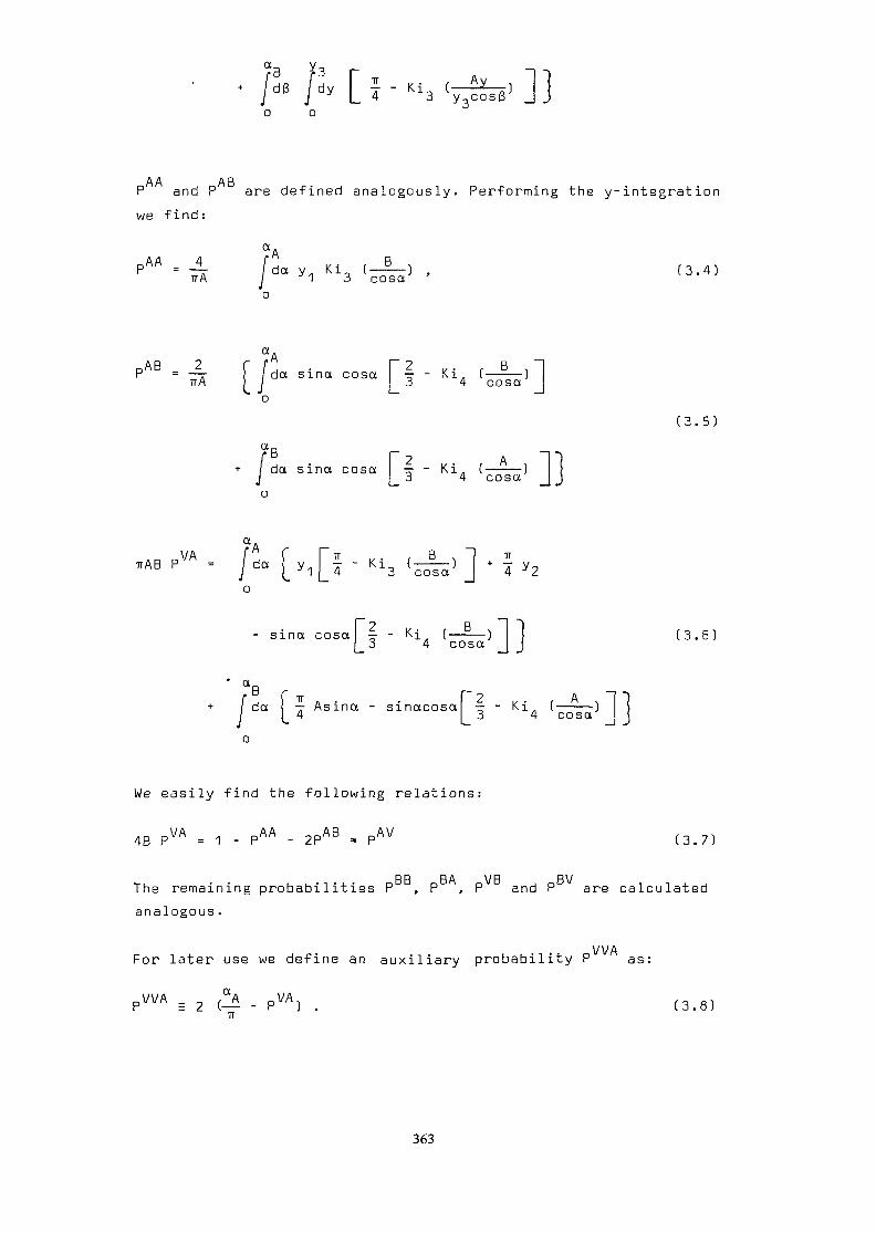
'' 5o o J J

AA ABP and P are defined analogously. Performing the y- integrat ionwe find:

K13

DAB 2 f [^ . r 2 , . . , 8 , 1P = —T- /da sina cosa -^ - Ki. (——— J?rA ) / 13 4 cosa Io

+ I da sina cosa •% - Ki. (———)J [_ 3 4 cosa J j

(3.5)

o

f2 K. f B .~n: - - KI (———)(_3 4 cosa J j- s ina cosa - - Ki (———) ( 3 . 6 ]

da Asina - sinacosar|.Ki (_A_ ) i - jj il C O S Ct I \L. _i J

We easily find the following relations:

4B PVA = 1 . pAA . 2pAB m pAV (3>?

The remaining probabilities P , P , P and P are calculatedanalogous.

For later use we define an auxiliary probability P as:

363

In an actual code we have two ways to introduce these probabili-ties: a straight numerical calculation or a use of precalculatedtabulated values. The direct numerical calculation uses analyti-cal solutions of most of the integrals , which gives a highaccuracy. For practical calculations on the other hand we will usetabulated values to accelerate the calculation. This is just asaccurate as the basic accuracy inherent in the OPO-method.

3.1 Tabulation

In the calculation of the different probabilities, which are func-tions of the (optical) side lengths A and B, it is useful to dis-tinguish the three domains defined in the figure below.

A4-

II

We have to consider only the case A < B, the case A > B is symme-tric. In each domain only three different probabilities will betabulated. The other probabilities can be represented with thesefundamental ones.

We define a term BKQR as the limit of P for very small valuesof A and B:

BKOR = HimA , B

0VVA 1 ,A . B . ,P = — [— &n cosan - -T- £n cosa.J,T T t j D M M

. . ,, -VVA . 5VVB ,and further P and P by

PVVA . BKOR - PVVA

PVVB -= BKOR * PWB

364

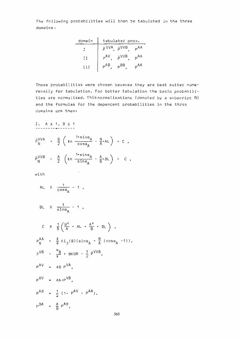
The following probabilities will then be tabulated in the threedomains :

domain

III

III

tabulatedPVVA,

PAV,PAB,

pWB-VVB

PBB,

prob .AA

> ~

pAA

PAA

These probabilities were chosen because they are best suited nume-recally for tabulation. For better tabulation the basic probabili-ties are normalized. This normalisations (denoted by a subscript N)and the formulas for the dependent probabilities in the threedomains are then:

I. A <, 1, B < 1

1+sinaA

-VVBPyBNA2

1+sisina•sinan

H'B

with

AL = cosa

BL = 1sina.

VB

AV

AL + _

f

!§ * BKOR - 1 PWB,

4B PVA

BV

AB (1. pAV . pAA)f

BA A pABB '

365

_ pBV

andVVB

II. A < 1, B > 1

A A 4C - ¥Ki3CEn (sinaA

A - Ki2(A)

PVVB = P - BKOR,

VA J_ AV4B V '

VB _ aB 1 0VVB= ~ ' 2 P '

PBV = 4A PVB,

(1. pAV

BA _ A

. pBV

andVV

III. A > 1, B > 1

PAA _ PAA |N ~ N j IIiRR 4.P° = 2E_(A)- \ (3Ki_(A)- 2Ki_CA)),N 3 TTD 3 2

where the exponential integral of n-th order is defined as

366

r- r 1 l-l ~ n ~ X UE (x) = / dn u e ,14

BA A ABB P '

pAA

PBV - 1 - PBB - 2 PBA,

VA _ _\_ AV,4B

VB _ 1 BV" 4A K '

VV = 1 - 2(PVA + PVB)

3.2 Analytical Calculation

The single mesh probabilities are defined by equations (3.4) to(3.6). To find an analytical solution we have to solve the fol-lowing integrals:

I = /da sinacosa Ki (———), (3.10)

/!I = da sina Ki () . (3.11)

ctI3 = da cosa Ki3 () . (3.12)

In fact this calculation is only semianalytical since it was notpossible to find analytical solutions of all the integrals. Thecalculation of I. and I_ is discussed in appendix I, wheras I_,for which no analytical solution is possible is calculated numeri-cally using the Gaussian method (6_) . To accelerate this calcula-tion the following substitution has proved to be useful forB < A:

T = £ E0(B) - / da sina- J3 2 3o

367

The method described above is used onlyfor A and B greater than0.5. For smaller values it is ,iiuch faster to calculate all theintegrals using a series representation of the Bickley functions(7_) , for which we refer to appendix I again. The resulting seriesconverge very fast and can be computed simultaneously.

4. Numerical solution and test problems

A computer subroutine CONDXY has been developed based on thistheory. The test calculations were performed with the programBOXOL, which combines CONDXY with routines from the program QP1(J_) to perform the outer iterations.

Two different test casoswere chosen to examine the efficiencyof the method. Reference solutions were established with QP1which uses a linear dependence on the space variables of theflux in a mesh and on its boundary, and a quadruple P. expan-sion of the angular dependence.

4.1 LWR-Cell

The simplified LWR-cell described in appendix II consists of ahomogenized pin cell surrounded by light water. In two seriesthe eigenvalue of the system and the critical albedo, respecti-vely, were calculated. The results are compared with calculationsbased on transport theory in the QP approximation (we use P_and P. in the program QP1; these cases are denoted as QP1 (P )i oand QP1 (P.), respectively) and with the diffusion theory codeCODIFF (_8). The results of the different calculations are sum-marized in tables 1 and 2.

4. 2 Storage pool problem

The compact storage pool, consisting of a homogeneous fuel zonesurrounded by two light water regions seperated by a layer ofstrong absorbing material is represented in appendix II. Thefigure shows the division of the system in the six zones used inBOXOL calculations. With QP1 a 5x5 mesh grid was calculateda P - and a P -approximation. As reference solution a QP1 calcu-lation with 13x13 meshes was taken (Its k ...-value differs fromef fthat of a 19x19 mesh case by 0.04%).

368

Two cases were considered: The quarter cell as it is given in ap-pendix II and a complete cell. In both cases reflective boundaryconditions were used for all sides. The results of the calcula-tions are listed in table 3.

5. Results and conclusions

Comparing the BOXOL results for various numbers of space intervalesin the x- and y-direction and various zonal arrangements (LWR-cell case, table 1) one finds only a small difference, which con-firms the validity of the QP -approximation in the calculationof the collision probabilities.

A comparison of CONDXY calculations using tabulated collision pro-babilities (CQNDXYM)) and numerical evaluation of these probabi-lities, respectively, shows the analytical-numerical method to bevery efficient and only a little slower than the tabulation method.

In table 1 we note some differences, although very small, betweenthe BOXOL- and the QP1 (P )-results, which in principleshould beidentical. They are caused by the homogenization of the boundarycurrents for a white boundary condition in CONDXY (cf. chapter2.2}. A vacuum boundary condition leads to identical results forBOXOL and QP1 (PQ) .

Table 2 compares the mean region fluxes for the LWR-cell casefound with the different codes. A comparison between the BOXOLand the QP1 (P,-,) fluxes shows that in this case the simplifica-tion of the white boundary condition has no substantial influ-ence. For the storage pool problem (table 3) there is, as oneexpects from the heterogeneous cell boundaries a large influenceof this boundary condition. A calculation of the complete cellin comparison, which eliminates the two complicated boundaries,gives a very good agreement. A small modification of the pro-gram to allow for this sort of symmetry directly in the calcu-lation of the probabilities and not by the use of reflectivboundary conditions will eliminate this discrepancy.

QP1 (Pp.) -values, because the albedos 3 are less than 1.0 and anThe BOXOL-results of the albedo search are very close to theQP1(Pn)-values, because the albedos 3 a;albedo £-0 will give identical results.

369

The errors in the flux relative to the results of the referencecalculation (table 2) are very small for the LWR-cell caseexcept for group 2, zone 2. They are much larger in the storagepool problem (table 3). In both cases this errors are caused bya large space dependence of the flux. This is better representedin QP1 (P,|), which uses a linear flux approximation in each meshthan in QP1(PQ) and BOXOL, which both assume a flat flux in eachmesh. The possible change of this approximation in BOXOL wouldincrease calculation times nearly by a factor of three.

Table 3 shows a large difference of 57 mk in the k ---valuesef ffound with BOXOL or with QP1 CPQ). Test calculations howeverhave shown almost no influence on the final results (cf. follow-ing table)

Program

BOXOLQP1 f)QP1

No. of groupes

126

12

No. of zones

1013x1313x13

kPff

0.73040.86110.8648

(1) Cross sections condensed with BOXOL-fluxes

The calculation time for the BOXOL-case with 12x12 meshes with-out symmetry (k=1.2175) is 16.3 sec. All other calculation timescan be found in table 1. The calculation time for QP1 is muchlarger than the respective BOXQL-time: the time factors are 17.5(for 3x3 meshes), 21.9 (6x6 meshes) and 9.3 (12x12 meshes), re-sprectively. The smaller time difference in the last-case is dueto the fact that CONDXY calculates the mean fluxes per materialzone and to find the mean fluxes in 144 meshes we therefore haveto define 144 materials. The collision probabilities are calcula-ted for each mesh, whereas in QP1 only optically different meshesare considered - these gives 6 values instead of the 144 in CONDXY.A small modification of the program will give a large acceleration.

We note that BOXOL is considerably faster than QP1 even in the Poapproximation. Therefore it may be useful to accelerate QP1 usingCONDXY-results as initial fluxes. In the tables these accelera-tions are denoted by QPO(3) and QP1(3) respectively for P - andP,j -approximation in QP1 . The calculation times to be compared arethen the times for CJP1 (PQ) or QPKP ) without acceleration andthose for QPO(3) plus CONDXY or QP1(3) plus CONDXY. This accele-

370

ration proves to be interesting mainly for QP1CP,.} which conver-ges slower for large cases; it amounts up to 50%.

Compared with diffusion theory (CODIFF), BOXOL is only a littleslower regarding eigenvalue calculations. Larger differences areobserved in the albedo calculations, due to the fact that inevery outer iteration the collision probabilities have to bechanged (cf eq. 2.195, which forces the use of gaussian elimina-tion repeatedly to solve equations (2.18). In this case an ite-rative method would give a substantial acceleration.

As for the CQDIFF-calculations, errors in other cases will bestill higher because the test case is rather suitable for diffu-sion theory.

If needed, the QPO approximation of the surface currents inCONDXY could easily be changed into a" QP1 -approximation withflat fluxes inside the meshes; the estimated calculation timeswill be about 15% higher at most.

Acknowledgements

The authors wish to thank P. Koehlerfor his correction of theoriginal draft and C. Higgs for supplying the subroutine GAUSS,

References

(_1_) Maeder C.QP1, a Transport Program in x-y Geometry Based onFunction Expansions in Angle and SpaceEIR-Bericht Mr. 290 (1975)/

(2) Stepanek 3.Surface Currents Transport Method in x-y GeometryUsing General P Legendre Polynomial Flux Expansionin Angle and SpaceIn preparation

(3) Carlvik 3.Integral Transport Theory in one-dimensional GeometriesAE-227 (1966)

371

(4^ Stepanek J., Ligou J.A Solution of the Coupled Integral and DifferentialForm of the Transport Equation.... for Slab GeometryEIR-Bericht Mr. 248 (1974)

(j5) Stepanek J., Ligou J., Maeder C.The "Mixed" Method, a Solution of the Transport Equationin Cylindrical Geometry Making Use of Both its Integraland Differential Forms in High Pn ApproximationEIR-Bericht Mr. 271 (1975)

(_6) Stroud A.M., Secrest D.Gaussian Quadrature Formulas,Prentice-Hall, Englewood Cliffs, N.J. (1966)

(7_) Davierwalla D.Tschebyscheff Rational Approximations to BickleyFunctionsEIR-Bericht Nr. 243 (1973)

(_8) Paratte 3.M.La base en gestion du combustible: un code de boitemoderneNeue Technik J[6 (1974) 461

(9_) Stepanek J.A new Form of the "Surface Currents" Transport Methodwith General P.. Polynomial Flux ApproximationEIR-Bericht (1978) in preparation.

(10) Maeder C., Paratte 3.M.Trans. Am. Nucl. Soc. 20 (1975) 359

372

Appendix I: Integrals

In chapter 3.2 solutions of three types of integrals were usedwhich are discussed here.

Using in integral I. the substitution u = 1/cosa and the recursionformula for the Bickley functions

Kin(u)

we easily f ind :

1/cosa 1/cosa. 1/cosa.

' - 2 (B"> * U1 1 1 (1.2)

Partially integrating the first integral on the right hand sidegives:

1/cosa^Ki2(Bu, ,i[Ki2(B) -

-i /1/cosaA (1.3)

Ki^Bu)U

Inserting this expression into equation (1.2) we finally foundafter some further manipulations:

2 RI, = K i _ ( B ) - K i . ( B ) - cos a. Ki_ (——=—) - Ki1 3 4 A 2 cosa. 4

Analogously integral I is evaluated and gives:

For argument values A and B smaller than 0.5 we use a series re-presentation of the Bickley function (_7) :

! / • / • • » n 7 r 2 3 \ n m , * i — m . A i , _ „ . ,K i 3 ( x ) = - -x+ - x -x \ f3 (x) | C, - Hn - \ ( 1 . 6 )

m=o

373

„ . , - • , 2 IT 12 ir 3 4 .KVX) = 3 - 4X * 2X " T2X * X ) f4m=o

where f and C are defined as

(1.7)

mrm - V - 1H ~ l_j n 2m+1

n=1- Y (1.8)

(x/2) 2m

(ml}2(2m+1)(2m+2)...(2m+£)(1.9)

for £, = 3,4 and y = 0.57721566490153 denotes the Euler-Mascherinasconstant .

Inserting these series into the integrals and integrating gives:

J + T 'n COS(XA "if B3 -^4 (BM C4 J2m+3 - K2m^

m = o.10:

where

sina(cosa)2m+3 2m+2 (cosa.)A

2m+2 - 1

andf , ' sina . , Bda —————- +3 £nJ (cosa)

(cosa.)AB n B ,s•=——=• £n -=———— - Jln TT - J0 ^2m+2 2cosa. 2 2m+3A

_ = (1-cosa.) + B An cosa. + B2(—-— -1)24 A A 4 cosa.

m=o

2 1+sina^ sina. - Ba. + ~ B in —————-4 A A 4 cosan

- KC 1^2 2m+2jm=o

(1.11)

(1.12)

374

where

2m+2

K2m+2

f/-1

da. ,(cosa)2m+2

1 F2m+1 L

sina

daIn B

2cosa(cosa) '

sina.

(cosa.)'A___ c-^——? + 2m J_2m+1 2m

r~—— + 2m K!T - Jc2cosa,, 2m 2m+2 2m

and J = a. .o A

Appendix II: Test examples

1. Storage pool problem

The geometry used for the calculation of a compact storage poolfor light water reactor fuel elements is shown in the followingfigure. We assume reflective boundary conditions on all sides.Three group neutron cross sections generated with the programBOXER (10) are tabulated below. The fission spectrum is 1.0 inthe fast group and 0.0 in the two thermal groups

Neutron corss sections

Material

1(fuel)

2CH2OJ

3absorber]

gri

123

123

123

Za

9.0-33.5-21.3-1

2.0-45.0-31.9-2

5.9-21.501.86

-f7.0-35.4-22.2-1

000

000

',2.4-16.85-11.6

2.322-18.65-12.189

2.898-11.952.55

^, grj1

2.0-13.0-21.0-3

1.8-15.0-22.0-3

2.3-18.0-10

2

04.3-12.2-1

04.9-13.7-1

04.3-12.02

3

03.0-21 .44

04.0-22.13

01 .0-26.8-1

375

6.438

M1M2

M3

M2

4.29

Z2

O.47S o.ae 1.42

22

\Z4 \

Z5\

Ml - M3 materials, Zl - Z6 BOXQL-zones

2. LWR-cell

X

We use a simplified LWR-cell with two material zones in (x,y)-geometry. Two energy groups are considered, scattering is iso-tropic. A reflective boundary condition is used. Eigenvalueand albedo are calculated.

1.5

6.4

1.0

1.5 6.4 1.0

376

Neutron cross sections

material

1

2

gri

12

12

Ea

8.62700-36.95700-2

6.84000-48.01600-3

vZ f

6.20300-31.10100-1

0.0.

Zt

1.96647-15.96159-1

2.22074-18.87864-1

zf^-J1

1.78000-11.00200-2

1.99500-12.18800-2

2

1.06900-35.25500-1

1.55800-36.78300-1

Appendix III: Definition of symbols

macroscopic fission cross section

fission spectrum

mean number of neutrons produced per fission

£ (r,fl-»-n, E-*E } macroscopic scattering cs,s

macroscopic total cs.

Y = 0.57721566490153 Euler Mascherinas constant

TT/2

.i (x) = fcn 1

n-1K i _ ( x ) = /d6 cos 9 exp ( - x / c o s 6 ] Bickley function

o

E fx) = / dn u exp (-X(j)1

Exponential integral

377

Case

CONDXY

(2)CONDXY

npi f p 1 ^ 3 )0

QPKP )o

f 31npi fp I '•-' J

(4)QPKP^

CODIFF

Numberof

meshes

3x36x63x3

3x36x63x36x6

3x36x6

3x36x6

12x12

3x36x6

3x36x6

12x12

3x36x6

12x12

Number ofgeometrical

zones

229

229

36

936

936

144

936

936

144

936

144

Eigenvaluek

1.22191.22231.2208

1.22191.22231.22081.2200

1.22011.2196

1.22011.21961.2171

1.21721.2131

1.21721.21311.2125

1.18541.21021.2178

T (sec)

withoutsym.

0.260.630.46

0.311.030.501.76

1.486.99

1.848.26

32.77

5.6524.19

8.0538.52

150.77

0.381.324.94

withsym.

0.220.520.31

0.290.720.361.06

1.295.23

1.546.11

10.15

4.2215.93

5.9022.3383.98

---

albedoS

0.968830.968720.96902

0.968830.968720.969020.96915

0.974680.97483

0.974680.974830.97527

0.975160.97577

0.975160.975770.97585

0.979610.976410.97537

T (sec)

withoutsym.

1.031.421.88

1.131.841.93

-

1.857.78

3.4012.6248.95

6.9230.19

11.6551.80

212.86

0.541.535.90

withsym.

0.710.971.08

0.781.221.10

-

1.705.71

3.129.21

30.27

5.1620.06

9.6132.91

128.96

---

-Joo

Table 1: LWR-cell results: eigenvalue, albedo, calculation time

(1) Collision probabilities tabulated(2) Collision probabilities calculated (4)

inital flux from CONDXYinitial flux <|> = 1.0

Case

CONDXY-BOXOL

QPKP )0

QPKP )

CDDIFF

Numberof

meshes

3x33x36x6

12x12

3x36x6

12x12

3x36x6

12x12

3x36x6

12x12

Number ofgeometrical

zones

29

36144

936

144

936

144

936

144

mean neutron flux

group 1zone 1

1.1.1.1.

1.1.1.

1.1.1.

1.1.1.

zone 2

0.934700.920450.937360.93965

0.931320.939820.94485

0.928760.918270.92741

0.922590.916940.96501

group 2zone 1

0.357960.357310.357810.35736

0.356500.358220.35837

0.354850.353180.35274

0.341400.343650.36310

zone 2

0.427830.430560.435050.44387

0.431620.437490.44780

0.438840.450950.45244

0.531030.455500.45649

errors relativ toQPKP-i) M2x12J-flux in %

group 1zone 1

0000

000

000

000

zone 2

0.79-0.75

1.071.32 ,

0.421.341.88

0.15-0.99

0

-0.52-1.13

4.05

group 2zone 1

1.481.301.441.31

1.071.551.60

0.600.12

0

-3.21-2.58

2.94

zone 2

-5.44-4.84-3.84-1.89

-4.60-3.30-1.03

-3.01-0.33

0

17.40.680.90

Table 2: LWR-cell results: mean neutron fluxes

Quantity

No. of zonesCP-time [s] (1)k eff

Flux

Material

1(fuel)

2(H20)

3(absorber)

Group

123

123

123

BOXOL

61.0

0.7694

1.41-11.72-22.17-2

9.50-21.03-21.75-2

9.83-24.29-35.01-3

BDXOL

6, complete cell (3)25.70.8225

1.45-11.81-22.34-2

8.96-29.56-31.60-2

9.33-23.96-34.58-3

QP1(P )0

5x56.3

0.8260

1.45-11.82-22.35-2

8.90-29.53-31.63-2

9.31-23.95-34.54-3

QPKP.)

5x526.3

0.9162

1.52-11.96-22.66-2

8.08-28.83-31.77-2

8.51-23.50-33.61-3

QPKP )1

13x13110 (2]

0.9210

1.52-11.97-22.67-2

8.06-28.83-31.78-2

8. 48-23.47-33.57-3

ooo

Table 3: Results for storage pool problem

(1) Central progressor time on a CDC 6400 computer(2) With diffusion theory flux guess(3) With use of symmetry type II

N,2 NY

1-1

NX

—

©

©!SW4

©

1N3 v 1 Nl

)K

N4 1 N2Wl | E3

\ 1"~"7W2 1 E4SN^S1

/i\S4 | S2

1

©

El

/____

E2

©

S,4

E,3

Figure 1: Principle of the division into material zones andmeshes; angle-quadrants(m\ ... material

*• Y

Figure 2: Neutron flight angles

381

^-__— J '"N

Figure 3: Geometrical parameters of the system

Figure 4: Geometrical parameters in mesh (i,j)

382

FUEL ASSEMBLY CROSS-SECTION AVERAGINGFOR PWR FUEL

A. JONSSON, S.F. GRILLPhysics and Computer Analysis,Nuclear Power Systems,Combustion Engineering, Incorporated,Windsor, Connecticut, USA

AbstractDIT, a fuel assembly cross-section homogenization and spectrum calculation

code, has been developed for use as a cross-section generator for large spatialdiffusion codes employed in power reactor design and analysis, the code is based ondiscrete integral transport theory (DIT/ as developed for one-dimensional cylindricalgeometry by Carlvik <y$) and extended to the explicit-pin, Z-D, geometry typical ofLWR fuel design by Jonsson et al

I. INTRODUCTIONBoth fine mesh diffusion theory methods andcoarse mesh methods are in use for the physics de-sign of pressurized water reactor cores. Fine mesh

models, such as PDQ, require cross-sections spat-ially averaged over individual pin-cells. Coarsemesh methods need an additional homogenization re-sulting in cross-sections averaged over typically1/4 of a fuel assembly. In either case, a com-monly made approximation is to use flux-volumeweighting with the spatial flux distribution ob-tained from a higher order, multigroup, solutionusing simplified boundary conditions on the geo-metry in question.

The DIT code, visualized in Fig. 1, has beendeveloped to perform the function of providingboth fine mesh cross-sections for PDQ and coarsemesh averaged cross-sections for coarse mesh codesat Combustion Engineering, Inc. A brief descrip-tion of the DIT code will be given with emphasis onthe differences between it and other similar codes.A discussion of the method used for calculatingequivalent, homogenized diffusion coefficients forfine mesh diffusion theory application is includedfollowed by a summary of verification analyses doneon critical experiments.

The paper concludes with a discussion of theeffects of realistic boundary conditions upon homo-genized, coarse mesh cross-sections. Effects onlocal reactivity and gross power distribution areillustrated and it is shown that proper account ofthese effects provides a refinement in coarse meshmethods and a reduction of the uncertaintiesassociated with calculated power distributions.

II. CALCULATION OF HOMOGENIZED CROSS-SECTIONSIN PWR FUEL ASSEMBLY GEOMETRY

II.1. Reactivity Effects of Spectral and SpatialInteractionsOne level of homogenization is required forfine mesh diffusion theory applications where eachindividual pin-cell is represented by an equiva-lent homogeneous medium. For coarse mesh applica-

tions, an additional level of homogenization isrequired. For this reason, as well as others, thecomputation of few-group cross-sections is bestcarried out in assembly geometry with a minimum ofapproximations to the details of this geometry.Consistent sets of fine mesh and coarse mesh crosssection table sets are thus guaranteed to resultand furthermore, spatial and spectral interactionsbetween various components of the fuel assembly canbe accounted for. Spatial interaction effects areautomatically represented correctly because theactual net currents crossing pin-cell interfacesare calculated rather than assumed to be zero or(as is often the case) approximated in a 1-D geo-metry surrounded by some equivalent, homogenizedenvironment. Spectral interactions can also beaccounted for more correctly if the calculation isdone explicitly in assembly geometry. Table 1below shows net reactivity effects attributableto spectral and spatial interactions in a fuelassembly containing burnable absorbers as well asempty control rod locations (water holes). Sim-ilar size effects are observed in the energy re-gion between thermal and a few keV (the resonanceregion) while at higher neutron energies littleerror usually results from approximations in thegeometric details of the assembly model as longas the fast fissions are accounted for in pin geo-metry. The results in Table 1 were obtained withthe DIT code described next.

II.2. Calculational ModelElimination of methods related uncertaintiesin the range 0.1 - 0.5%k as discussed above, re-quire explicit account of geometry-induced spectrum

and spatial interactions. The DIT computer codemodel is visualized in Fig. 1. Three major compon-ents make up computational models of this kind,viz., (1) A spectrum calculation in approximatedassembly geometry, (2) A spatial calculation inthe assembly geometry and (3) A depletion routinefollowed by editing routines. Although some im-portant differences are present, DIT is similar instructure to codes such as WIMS1 and EPRI-CPM2.

383

Table 1Non-Uniform Lattices. Effects of Thermal Spectrum and Spatial

Interactions on ReactivityFuel Type Temperature Physical Effect Effect on

ReactivityU02U02

U02Mixed oxideMixed oxideuo2

Operati ngOperating

Cold conditionOperatingCold conditionOperating

Hardening of spectrum for fuelclose to absorbers.Softening of spectrum for fuelclose to water holes.a) Effect due to change in aab) Effect due to change in vafc) Net effectAs above, net effectAs above, net effectAs above, net effectSoftening of spectrum in burnableabsorber relative to simple 1-Dmethod.

-0.10 to -0.15%k

-0.65%k+0.70%k+0.05%k+0.20 - 0.25%k+0. 7055k+0.25%k-0.15 to -0.30%k

DIT includes the following additional features:A. Spatial interaction uncertainties are mini-mized by eliminating homogenizations both inthe spectrum calculation (85 groups) and inthe assembly calculation (2-8 groups). Thus,the transport calculation is done in explicit-pin geometry for the assembly using integraltransport methods3'1*. Individual cells arecoupled by interface currents. The name DITrefers to the method of integrating the trans-port equation within each individual cell asoriginally developed by Carlvik5. The spatialmesh within cells may be both radial and azi-

muthal. Most frequently, one uses a radialmesh combined with an expansion in harmonicsazimuthally, subsequently referred to as thek=n option where n is the number of harmonicsretained in the expansion. (Fig. 2 shows anexample of thermal flux contours in a U02 pinnear a large water hole.)

Figure:THERMAL FLUX C O N T O U R S IN A U02 PIN

NEAR A WATERHOLE

B. Spectral interactions are accounted for in an85-group structure by performing explicit-geometry transport calculations for spectrumgeometries which are portions of the assemblyusing boundary currents generated in the assem-bly calculation. Typical spectrum geometriesconsist of 1 to 3 cells with diagonal symmetry.See Fig. 1.

C. Upon completion of the assembly calculation,excess reactivity (i.e., reactivity not account-ed for by chemical shim) is removed by leakagein an 85-group flux-volume weighted, homogenized,Bl calculation with the buckling search. Thus,criticality is always maintained and the few-group averaged cross-sections produced are al-ways obtained in a critical spectrum. A separ-ate option exists whereby the external leakagemay be accounted for by input of either net orpartial, few-group currents to be used as bound-ary conditions for the assembly. The use ofthis option results in more realistic coarsemesh averaged cross-sections for assemblieslocated in global flux gradients and is dis-cussed in Section III below.

D. The depletion takes place for each individualpin in the assembly and, when required, alsofor subdivisions of fuel or absorber pins.Editing routines supply cross-sections forboth fine mesh PDQ and coarse mesh nodal codes.

E. Cross-sections are processed from ENDF/B viaETOG6, FLANGE-II7, GGC-38 and RABBLE9. Thecosine current approximation has been removedfrom RABBLE and replaced by an integral trans-port routine. The fine-group averaged re-sonance cross-sections are converted to a two-dimensional table parametric in temperatureand a background cross-section via an equiva-lence theorem linking lattices of differinggeometry. Interaction effects between dif-ferent resonance absorbers are accounted forin the equivalence1. In the process of readingits library, DIT uses the same equivalencetheorem to interpolate in the table. Thismethod does not, therefore, rely on an equiva-lence theorem to perform the more difficultfunction of relating heterogeneous resonanceintegrals to homogeneous data. Its sole

384

function is to serve as a convenient means oftabulating and retrieving the data which it-self is generated with an accurate space de-pendent slowing-down calculation (RABBLE inthis case). A similar procedure based onhomogeneous slowing down calculations with theSDR code10, was originally developed for WINS1with suitable equivalence theorems by Leslieet.al.11.

11.3. Cross Section Requirements Dictated by theUse of Diffusion TheoryDesign analyses for power reactor cores arealways done using diffusion theory as the primary

means of predicting reactivity and core-wide reac-tion rate distributions. These analyses are per-formed with the few-group spectrum averaged cross-section data for which some methods-related un-certainties were quantified above. The twoelements of the analysis, viz., the diffusion theoryand the process for generating few-group data arenot independent however. Each supplies a componentto the overall uncertainty. One should thereforebe aware of the possibility that the contributionof the former may be significant and possibly bemistaken for uncertainties in basic cross-sectiondata. So that the diffusion approximation mayyield accurate results, the few-group data must bedefined and calculated to fit the particular formof diffusion theory used, i.e., to the finitedifference formulation employed and the mesh densitychosen. This is achieved by comparing the diffu-sion theory results with results from higher orderapproximations for some particular situation approxi-mating the end use. Absorption and slowing downcross-sections are thus routinely adjusted to com-pensate for the over-predicted flux level in thistype of region. In regions of the geometry whereflux peaking occurs, adjustments in the oppositedirection are required. Although this method iseffective in dealing with the reactivity contribu-tion of the non-diffusion region, there are certainside effects which are of interest, particularlywhen conclusions are to be drawn from benchmarkmeasumements of reactivity and reaction rate distri-butions. Thus, for example, one finds that by corn-

Table 2Non-Uniform Lattices.Comparisons of Reactivity Levels and Power Peaking

Calculation vs. ExperimentMODIFIED ENDF/B-IV

pensating in the absorption cross-section for anabsorber, the flux level predicted by diffusiontheory in that absorber does move further away fromreality and, since the spatially transient dif-ference between transport theory and diffusiontheory is not confined to the absorber itself butencompasses also the neighboring fuel, both reac-tivity and reaction rates in this fuel are affectedby the adjustments made. This type of effect is ofthe order of 1-2% equivalent cross-section uncer-tainty in the thermal energy range. To eliminatesuch errors, it is desirable to employ methods thatmodify the diffusion coefficients rather than thereaction rate cross-sections so that, ideally, thecorrect flux levels are predicted by diffusiontheory for all different components of the fuelassembly design. Such an approach is made possibleby edits in the DIT code. Agreement between dif-fusion theory and transport theory is accomplishedvia a definition of diffusion coefficients gearedto the particular finite difference formulationused. It has been found that this is most easilyaccomplished in a mesh centered formulation andFig.3 shows that the transport theory fission ratedistribution and reactivity are both essentiallyduplicated by such a diffusion calculation for anassembly octant. Global leakage is preserved bythe method utilized.

FiguresC O M P A R I S O N OF FISSION R A T E S

DIT (K-l l MS MESH CENTERED D IFFUSION THEORY

*DIFF-

-fl.2

DITKMCDI

(DIT-HC

•tO.5

-0.5

• 1) 1.3499FF THEORY 1.3502

1x100

W

40.6

•10.2

•K).5

•10.1

«U

rt.4

«.3

•KU

-0.7

•KU

-1.0

0.0

-0.2

-0.9

-o.r

w

•tfl. 6

Hfl.l

•10.9

•KU

-10.2

-0.7

CoreC-E Critical s2.7% U-235,68° F

#12#32#43#53#56

KRITZ3.1% U-235

HotCold

Vol. ModVol. Fuel

1.491.491.491.261.26

1.791.79

No. ofLargeWater holes

5175

1717

2121

SolubleBoron Cone.PPM

00

3230

302

9591060

keff*>

1.00020.99911.00171.00060.9991

1.00191.0014

(C/E-l)xlOOPeak Power

1.08%1.351.291.751.79

1.46

*) Radial leakage is explicitly calculated by PDQ using transport theory corrected reflectorconstants. Axial leakage is accounted for via experimental buck!ings.385

II. 4. Experimental VerificationVerification of an assembly spectrum codesuch as DIT is best performed by comparison with

critical experiments where detailed reaction ratesand flux distributions can be measured. Analysesof a series of such experiments for both uniformand non-uniform lattices were described in detailin Ref. 12. Table 2 summarizes results for thosenon-uniform lattices that correspond most closelyto moderator/fuel atom ratios of currently operat-ing cores.

Two modifications of ENDF/B-IV data weremade to achieve the observed good agreement onreactivity, viz. :(i) Fission spectra were generated from ENDF/B-Vrecommendations, i.e., Maxwell spectra werereplaced by Watt spectra.

(ii) U-238 resonance capture was reduced by a flat0.07 barns (i.e., about 2.5 - 3.0% of aresonance integral).

It is also worth noting that the cold-hot reactivitydifference is well predicted and that peak poweris overestimated by only about 1.5%.III. CALCULATION OF HOMOGENIZED CROSS-SECTIONS FOR

FUEL ASSEMBLIES WITH NQN-ZERO EXTERNAL NETCURRENTSIII.l. Introduction

The most common procedure for generat-ing coarse mesh cross-section table sets involvesthe assumption that the assembly depletes withboundary conditions of zero net current. Thisapproximation arises in those cases where theonly means of accounting for leakage is propor-tional to a buckling. A separate module of theDIT code allows other, and more realistic boundaryconditions for use with assemblies that are expect-ed to be located in strong flux gradients. Such amodule serves two purposes, viz.:a) When it is incorporated in the cross-sectiongeneration process it provides homogenized,few-group base cross-sections that morerealistically approximate actual conditions

in the core.b) When used standalone or as part of a 3-D

coarse mesh code, it permits the retrieval ofdetailed pin-by-pin power distributions in-side each coarse mesh node as well as "on-line" modification of the coarse-mesh cross-sections as they are affected by the evolvingburnup distribution internal to each node.The latter application, which may be referredto as an imbedded calculation and which has been

previously used for heavy water reactor applica-tions13, requires a fast, efficient calculation sothat all nodes or all nodes of interest in the 3-Dcore layout can be scanned. It cannot, therefore,be done with transport theory since such an appli-cation would be too computer intensive for practi-cal use. The mesh centered diffusion module men-tioned in II. 3 is very fast however (executiontime on CDC-7600 of about 0.7 sec. per coarse mesh

node comprising 49-64 internal fine-mesh nodes anddepleting one time point) and since it uses ad-justed diffusion coefficients it will retain ameasure of local transport theory effects. In thefollowing we will describe briefly the additionalverification performed for imbedded calculationsin a situation with a strong flux tilt and thenillustrate the effects on coarse mesh homogenizedcross-sections of various external conditionstypical of different locations in a power reactorcore.

III.2. Verification of Imbedded CalculationsImbedded calculations can be done eitherwith transport theory using a separate option ofDIT or with the diffusion theory module mentionedabove. Direct Monte Carlo calculations have beenperformed for the verification of DIT in bothtilted and flat situations. Figure 4 shows anexample in the former category represented by a1/4 assembly with fresh fuel located on a diagonalof a 217 assembly core and next to the reflector.This 1/4 assembly has an overall power tilt of

1.6 across it.The transport theory imbedded calcu-lation agrees with Monte Carlo to within 0.5% forthe peak pin and to within 1.5% for the maximumerror. The Monte Carlo calculations were carriedout with the MORSE code14 and had an accuracy of0.8% (standard deviation). The diffusion modulewas applied to the same case and the relativeerrors are shown in Figure 5. They are of thesame size as in Figure 4 which indicates that thediffusion module using diffusion coefficientscalculated to reproduce local peaking in the caseof zero external net currents does give good agree-ment also for tilted situations.

FIOJKI

DIT vs MORSE

IMBEDDED C A L C U L A T I O N S FOR

AN ASSEMBLY AT THE EDGE OF THE C O R E

oooooo

ooooo

oo

ooo

oo

o0 7

MORSEI0<>08%>DIT

-{DIT/MORSE 1|X

386

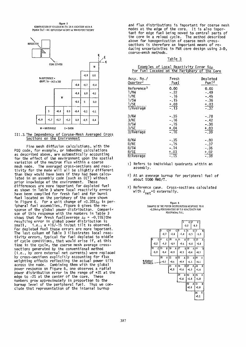
Figure 5COMPARISON OF FISSION RATES IN A LOCATION WITH A

POWER TILT - A1C DIFFUSION THEORY vs TRANS PORT THEORY

REFLECTOR

?,«CORE CENTER

* DIFFERENCE •(TRPT.TH-MCIxlOO

+1.9

S

+1.7

W

+0.4

+1.7

0.0

+1.2

-0.8

-0.8

-0.6

-0.4

0.0

-0.9

-0.7

0.0

S

-0.1

-0.5

W

0.0

-0.4

-0.1

0.0

-0.1

-0.4

W - WATERHOLE S-SHIM

111.3. The Dependency of Corase-Mesh Averaged CrossSections on the EnvironmentFine mesh diffusion calculations, with the

PDQ code, for example, or imbedded calculationsas described above, are automatically accountingfor the effect of the environment upon the spatialvariation of the neutron flux within a coarsemesh node. The averaged cross-sections and reac-tivity for the node will all be slightly differentthan they would have been if they had been calcu-lated in an assembly code (such as DIT) withoutprior knowledge of the environment. Thesedifferences are more important for depleted fuelas shown in Table 3 where local reactivity errorshave been compiled for fresh fuel and for burntfuel located on the periphery of the core shownin Figure 6. For a unit change of -0.35%Ap in per-ipheral fuel assemblies, Figure 6 gives the re-sponse of the global power distribution. Compari-son of this response with the numbers in Table 3shows that for fresh fuel(average Ap = -0.15%)theresulting error in global power distribution issmall, i.e., a +1X/-W in/out tilt is observed.For depleted fuel these errors are more important.The last column of Table 3 illustrates local reac-tivity errors, typical for fuel depleted to middleof cycle conditions, that would arise if, at thistime in the cycle, the coarse mesh average cross-sections generated by the conventional method(i.e., by zero external net currents) were replacedby cross-sections explicitly accounting for fluxweighting effects reflecting the actual power tiltacross the node. Combining them with the globalpower response on Figure 6, one observes a radialpower distribution error in the range of +3% at theedge to -2% at the center of the core. Thesenumbers grow approximately in proportion to theburnup level of the peripheral fuel. Thus we con-clude that representation of the internal burnup

and flux distributions is important for coarse meshnodes at the edge of the core. It is also impor-tant for edge fuel being moved to central parts ofthe core in a reload cycle. The method describedabove for homogenization of coarse mesh cross-sections is therefore an important means of re-ducing uncertainties in PWR core design using 3-D,coarse-mesh methods.Table 3

Examples of Local Reactivity Error %ApFor Fuel Located on the PeripheryAssy. No./Quarter1Reference31/NW1/NE1/SW1/SE1 /Average3/NW3/NE3/SW3/SE3/Average8/NW8/NE8/SW8/SE8/Average

FreshFuel0.00-.22-.16-.15+ .03Tn-.35-.16-.15+ .04-.16-.35-.15-.14+ .03

of the CoreDepletedFuel20.00-.49-.45-.36+ .03-.32-.78-.42-.38+ .03

-.80-.37-.36+ .02738

1) Refers to individual quadrants within anassembly.2) At an average burnup for peripheral fuel of

about 5000 MWD/T.3) Reference case. Cross-sections calculated

with Jnet=0 externally.

Figure 6EXAMPLE OF THE POWER DISTRIBUTION RESPONSE TO A

-0.35%Ap PERTURBATION OF THE REACTIVITY FORPERIPHERAL FUEL

* CHANGEIN POWER-

1 C 2 C-3.2 -3.3

8 C-2.2

14 C-1.0

BE

3 C-2.7

9 C-1.2

15 B-0.4

20 A-•(0.2

4 C-2.4

10 B•fl.9

16 A+0.0

21 B+0.6

25 A+1.1

5 C-1.4

11 A-0.6

17 B+0.3

22 A+0.9

26 B+1.4

29 A+1.6

6 C-1.5

12 B-0.4

18 A+0.4

23 B+1.1

27 A+1.5

30 B+1.8

32 A+2.0

7 B-1.5

13 A-0.4

19 B+0.5

24 A+1.1

28 B+1.6

31 A+1.8

33 B+2.0

34 A+2.1

387

IV. REFERENCES

1. J. R. Askew, et.al., "A General Descriptionof the Lattice Code WINS," Journal Brit.Nucl. Energy Soc., £,4, (1966).

2. B. A. Zolotar and W. J. Eich, "Advanced Re-cycle Methodology Program: PreliminarySpecifications for a New Nuclear Computa-tional Capability," EPRI SR-2 (July 1974);W, J. Eich, "Advanced Recycle Methodology Pro-gram: Project Status Report," EPRI 118-1(December 1975);R. D. Mosteller, et.al., "U02 and M(>2 AssemblyAnalysis: Collision Probability and Few-GroupDiffusion Comparisons," Trans. Am. Nucl. Soc.24, 443 (1976).

3. A. Jonsson, et.al., "Discrete Integral Trans-port Theory Extended to the Case with SurfaceSources," Atomkernenergie, 24, 79-84, (1974).4. A. Jonsson, et.al., "Integral Transport Theorywith Cell Couplings Involving Arbitrarily

Distributed Currents," Trans. Am. Nucl. Soc.,21_, 231, (1975).

5. I. Carlvik, "Integral Transport Theory in One-dimensional Geometries," Nukleonik, 10, 104,(1967).

6. D. E. Kusner, et.al., "ETOG-1, A Fortran IVProgram to Process Data from the ENDF/BFile to the MUFT, GAM and ANISN Formats,"WCAP-3845-1, (ENDF-114), (1969).

7. H. C. Honeck, D. R. Finch, "FLANGE-11, A Codeto Process Thermal Neutron Data from an ENDF/BTape," DP-1278, ENDF-152, (1971).

8. J. Adir, K. D. Lathrop, "Theory of MethodsUsed in the GGC-3 Multigroup Cross-SectionCode," GA-7156, (1967).

9. P. Kier, A. Robba, "RABBLE, A Program for Com-putation of Resonance Absorption in Multi-region Reactor Cells," ANO-7326, (1967).10. R. J. Brissenden, C. Durston, "The Calculation

of Neutron Spectra in the Doppler Region,"Conference on the Application of ComputingMethods to Reactor Problems, ANL-7050, P.51,(1965).

11. D. C. Leslie, et.al., "Improvements to theTheory of Resonance Escape in HeterogeneousFuel,"I. Regular Arrays of Fuel Rods. Nucl. Sci.

Eng. 22, 78, (1965).II. Dancoff Factor and Equivalence Theorem inCluster-type Fuel. Nucl.See.Eng. 23 , 82,(1965).

12. A. Jonsson, et.al., "Verification of a FuelAssembly Spectrum Code Based on Integral Trans-port Theory," ANS Trans.Vol. 28, P.778,(1978).

13. A. Jonsson, et.al., "Description of Hetero-geneous Programs for Macroscopic Reactor Calcu-lations," Part II. The Determination of Bound-ary Conditions in the Two-dimensional Case,"AB Atomenergi, RFR-663, 1967.

14. 'RSIC Computer Code Collection, MORSE-GC,"CCC-203, ORNL.

388

DETERMINATION DE CONSTANTES EQUIVALENTESPOUR LES CALCULS DE DIFFUSIONAUX DIFFERENCES FINIES

J. MONDOTCEA, Centre d'etudes nucleaires de Cadarache,Saint-Paul-lez-Durance, France

Abstract

Nowadays, we use very accurate transport codes for the fine treatment, inspace and energy, of the very heterogeneous reactor lattices.However, such a procedure is prohibitively expensive for the core calcu-lations and we only use it for the calculation of small subregions of thereactor (assemblies). The whole core calculation is generally performedusing few groups diffusion codes on a rather simplified geometry. Thiscalculation scheme implies the previous determination of broad-groupsconstants for homogeneized regions.

One of the most common methods to do this is called the flux weighted method.It is clear however that (for many well known reasons) using such groupconstants generally leads to unacceptable discrepancies in the reaction ratesand consequently in the multiplication factors, in particular when absorbingor strong moderating regions are present.

Despite those difficulties, if we want to perform diffusion calculations, wemust introduce effective constants that reproduce transport reaction rates.The diffusion calculation with these constants will be equivalent, in acertain sense, to a reference.To achieve this goal, a code (EQUIPAGE) was written. Using an iterativeprocedure, matching reaction rates, this code is able to generate for eachof the broad-groups a set of equivalent constants to be used in a finitedifference diffusion calculation.

For the same geometry and boundary conditions, these equivalent constantsreproduce all the reaction rates and the neutron balance, integrated overthe regions defined by the users, for whatever the number of mesh pointsused.

This method has been applied sucessfully to static and depletion calculationsof PWR reactors (pins and plates) containing control rods, burnable poisons,water holes and water channels.

389

I. - INTRODUCTIONNous disposons à l'heure actuelle de codes très sophistiqués qui

permettent, en résolvant l'équation du transport, d'accéder à la struc-ture fine du flux en espace et en énergie sur des géométries hétérogènestrès complexes. Malheureusement, de tels codes sont inutilisables, p.arceque trop onéreux, pour traiter un coeur entier de réacteur. On a doncrecours, la plupart du temps, à la théorie de la diffusion pour calcu-ler le comportement spatial du flux.

Pour ce faire, on utilise couramment des codes aux différencesfinies et à peu de groupes.

Bien que ce soit très important, nous n'aborderons pas ici leproblème de la condensation en énergie et nous supposerons que le décou-page en larges groupes est suffisant pour bien représenter le spectreneutronique en tout point.

Du point de vue spatial, la méthode d'homogénéisation la pluscourante est la pondération des sections efficaces par les flux. Malheu-reusement, le caractère très hétérogène des réseaux de réacteurs condamnel'utilisation directe de la théorie de la diffusion avec de telles sec-tions efficaces.

Nous avons donc été conduit à rechercher des paramètres équiva-lents (dans un certain sens) qui permettent de retrouver,par la théoriede la diffusion, le bilan neutronique d'un calcul de référence sur unepartie du réseau à traiter et pour des conditions aux limites données.

Dans ce but, un code appelé EQUIPAGE a été écrit.Cette méthode d'Equivalence a été appliquée avec succès à diffé-

rents calculs de réseau de réacteurs PWR à crayons et à plaques, autemps zéro et en évolution.

II. - LE PRINCIPE DE L'EQUIVALENCE

Soit un réseau composé de différentes compositions i. Chaquecomposition est caractérisée par un certain nombre de paramètres :S^ section efficace d'absorption moyennée sur le groupe g dans leai milieu i,

S^ section de removal moyennée sur le groupe g dans le milieu i,riD? coefficient de duffusion,

$? le flux intégré sur le groupe g dans le milieu i,

S V T.'f . ô? source de fission,

,8 _ Y* j« 'L. - £^t ±-E° = / j 2? —5" ° § source de ralentissement,

v Sf. section de production.Intégrons l'équation de la diffusion sur chaque milieu i de

surface S^ sur laquelle est présent le courant J? :

390

/„ 1 -1. -t- -Lsiavec S? = SS + D? Es + 1 a^ i Jri^axialNous avons ici le bilan neutre-nique classique :

? dS + S? ?? = S? + R? (1)

Fuites + Absorptions = Source de fission + Source de ralentissement

Normalisons les calculs à 1 neutron source :

Ds B2| $s = 1I L 1 2 .axial /

d'où : keff = Z-j X/ v 2f? $?i g

Le bilan ( 1 ) sera toujours respecté dans le calcul de diffusion;cependant le terme fuite (échanges entre les différents milieux) n'est—> j _^qu'approximativement représenté par la loi de Fick J = - D -— ndnavec ~n : normale à la surface S-.

Aussi allons-nous rechercher les coefficients a? tels que :

fà ) (if ) (v v*} (Df )«g _ V Veq _ V^i/eq _ V 1/eq _ \ axial/eq

Dfaxial

On procède d'une manière itérative en utilisant des calculs dediffusion successifs; pour l'itération n on aura :

référence

"'"'diffusionAinsi, en conservant pour chaque région et dans chaque groupe

toutes les probabilités d'absorption de fuite et de production, on ob-tient après convergence :

K* Diffusion - S? $? référence!/-_ 1 IX

et V'eq

où £ est le critère de convergence choisi par l'utilisateur.g

Ce processus converge généralement très rapidement et les cal-culs de diffusion sont très peu coûteux puisqu'à l'itération n on réini-tialise les flux en tout point aux valeurs trouvées à l'itération n-1.

Le jeu de sections efficaces ainsi déterminé n'est pas unique,seuls les taux de réaction obtenus gardent un sens physique. Ainsi, sui-vant la "stratégie" employée pour effectuer les corrections dans lesdifférentes compositions, on peut obtenir des sections équivalentes etdes distributions de flux différentes. Ceci importe peu lorsque le motifsur lequel on fait l'équivalence se répète à l'infini (condition decourant nul à la frontière).

391

Par contre, on procède couramment à des équivalences sur desmotifs distincts (par exemple deux types d'assemblage) qui sont adja-cents dans le coeur.

La continuité du flux est ensuite imposée sur l'interface.Il importe alors, pour ne pas créer des discontinuités artifi-

cielles des taux de réaction, de conserver la même définition des sec-tions efficaces de part et d'autre de l'interface.

Dans ce but, l'utilisateur d'EQUIPAGE peut conserver inchangéesles sections efficaces de la (ou des) régions périphériques de chaquemotif.

Il est à noter de plus que cette équivalence peut être effectuéequel que soit le découpage spatial du calcul de diffusion. On peut ainsisouvent économiser un grand nombre de points de calcul, à la seule condi-tion que l'équivalence et le calcul de diffusion définitif soient effec-tués avec le même maillage spatial.

III. - APPLICATIONS

III.1. - Géométrie plane une dimension

III. 1.1. Interface combustible-structureConsidérons un faisceau de réacteur composé de 19 plaques paral-

lèles entourées de structures (crémaillère, boîtier, cours d'eau). Uncalcul à une dimension sur une traverse perpendiculaire aux plaques(fig. 1) est effectué par le code APOLLO [1] résolvant l'équation inté-grale du transport avec 99 groupes (52 rapides, 49 thermiques). Un se-cond calcul de transport est effectué après avoir homogénéisé la celluleélémentaire (plaque, gaine, modérateur) avec courant nul sur les limites.

L'effet de cette homogénéisation sur la distribution de puis-sance est représenté sur la figure 2.

L'écart est inférieur partout à 2 %. L'homogénéisation par sim-ple pondération sur les flux avec condition de courant nul paraît doncjustifiée pour ce cas.

Considérons maintenant le même problème traité par un calculde diffusion aux différences finies avec 4 "macro-groupes" dont 1 seulthermique.

Nous avons le choix pour condenser les différents paramètres àpartir du calcul de transport.

Le spectre variant de façon continue entre le centre et le borddu faisceau, nous prenons en compte le transitoire introduit par la pré-sence de la région structure par l'intermédiaire de neuf "compositions"regroupant chacune une ou plusieurs plaques (fig. 1).

La distribution de puissance obtenue en diffusion est comparéeà la distribution de référence issue du calcul de transport sur la fi-gure 3- On constate un désaccord flagrant qui s'accentue au fur et àmesure que l'on s'approche de la région structure. Les écarts atteignent-4,8 % pour le calcul conventionnel alors que le calcul MND provoqueune remontée de puissance trop forte de 8 %.

L'utilisation de l'équivalence ramène ici bien sûr les écarts(trasports-diffusion) à ceux qui sont admis pour la convergence du cal-cul EQUIPAGE (< 0,5 % dans ce cas).

392

III.1.2. Coeur_à plaquée perturbé_par des lattes d'allumine-gadolignéeII s'agit ici d'un coeur composé de plaques combustibles paral-

lèles (fig. 4). One rangée de plaques est remplacée par des lattesd'Al203-Gds03. Dans le cas que nous considérons, la charge d'oxyde degadolinium est de 700 mg/cm . Comme auparavant, un calcul de transportà 99 groupes nous fournit une référence.

La figure k montre qu'un calcul de diffusion utilisant desconstantes pondérées par les flux conduit à des écarts sur les taux deréaction thermiques qui atteignent 17 % dans la région empoisonnée. Onremarque en outre que la répartition des taux d'absorption, donc de lapuissance, subit un important basculement.

La valeur propre obtenue en diffusion (0,97985) s'écarte d'en-viron 2 000 pcm de la valeur propre de référence (1. en l'occurrence).

L'utilisation de constantes équivalentes ramène les écarts surles taux de réaction à des valeurs inférieures à 0,5 % (critère choisi)et conduit à une valeur propre de 0,99910.

Le tableau suivant rassemble les valeurs de T, avantet après équivalence.

Région

1

2

J>

k

5

S (pondération sur les flux)a

1,392 cm-1

1,*f01 "

1,393 "

1 , 355 "

5,H8 "

E équivalenteQ.

1,392 cm-1

1,336 »

1,3^ "

1,301 "

3,575 "

atlxi

1

0,95^

0,965

0,961

0,69^

III.2. - Géométries à deux dimensions ; coeurs à crayonsNous avons choisi deux exemples d'utilisation du code EQUIPAGE

pour le calcul d'assemblages à crayons.Le premier, relatif à une expérience critique effectuée dans

la pile MINEBVE [2], concerne un assemblage 17 x 17 crayons dans lequelune distribution fine de puissance a été mesurée par spectrométrie Y-

La comparaison expérience-calcul [2] montre que les calculs de trans-port que nous utilisons permettent d'atteindre une très bonne précisionsur la distribution fine de puissance même dans les très forts gradientsentre barreau de poison et trous d'eau.

Sur la figure 5 sont indiqués les résultats obtenus en recalantuniquement les taux de réactions relatifs poison/combustible, les cons-tantes des autres régions étant simplement pondérées sur les flux. Sicette équivalence partielle permet de retrouver, avec une très bonneapproximation, la valeur propre du calcul de référence, elle conduitnéanmoins à des écarts systématiques de 2 à *f % entre deux crayons voi-sins entre Pyrex et trou d'eau.

L'équivalence EQUIPAGE,effectuée à la fois sur les poisons,les trous d'eau et les crayons combustibles adjacents, élimine cesécarts systématiques (fig. 6).

393

Le second exemple concerne le réacteur CAP (Chaufferie AvancéePrototype - Centre d'Etudes Nucléaires de CADARACHE).

Ce réacteur comporte des assemblages très hétérogènes (fig. 7et 8). Si l'on se fixe comme but le calcul fin d'un tel réacteur en évo-lution, c'est-à-dire le calcul des taux de réaction par cellule au coursdu temps et à trois dimensions, seule une méthode relativement simplecomme la diffusion aux différences finies peut être mise en oeuvre sansêtre prohibitive.

La première étape d'un tel travail consiste dans l'élaborationde bibliothèques dites "évolutives". Elles sont engendrées par un calculde transport de type multicellule prenant en compte l'interaction desdifférentes cellules au cours du temps. Ce calcul est effectué sur cha-que type d'assemblage avec comme hypothèse un courant nul sur la fron-tière extérieure. Ce calcul permet l'obtention de constantes condenséessur quatre macrogroupes et homogénéisées sur chaque type de cellule parpondération sur les flux.

L'utilisation directe de ces constantes est rendue impossiblepar le caractère très hétérogène du réseau qui rend abusives les hypo-thèses contenues dans la théorie de la diffusion.

L'équivalence obtenue par le code EQUIPAGE permet de retrouverpar un calcul de diffusion tous les taux de réaction du calcul de trans-port en moyenne sur chaque type de cellule. La bibliothèque évolutiveéquivalente sera donc constituée par la donnée des fonctions

effa = f (Burn-up)Nous avons choisi, pour illustrer notre propos, le calcul de

deux types d'assemblage.Le premier (A) (fig. 7) contient, outre des cellules U03 , des

crayons empoisonnés avec de l'oxyde de gadolinium et des trous d'eau.Le second (B) (fig. 8) contient en plus des crayons "noirs" de

hafnium et des crayons de Pyrex.

Les figures 9 et 10 représentent les valeurs propres obtenuesd'une part avec les constantes pondérées par les flux et d'autre partaprès équivalence. La valeur propre de référence est 1.0 (calcul àB critique); en abscisse nous avons représenté le burn-up moyen de1'assemblage.

Pour l'assemblage (A), on constate que le calcul de diffusionutilisant les constantes pondérées par les flux conduit à un écart de1800 pcm sur keff au temps zéro. Au fur et à mesure que les poisonspyrex et Gd303 s'usent, cet écart diminue. Vers 10 000 MWJ/T, l'équi-valence ne porte plus que sur la répartition de puissance et n'a plusd'influence sur la valeur propre (cf. Expérience MINERVE).

Par contre, pour l'assemblage (B) contenant des crayons de Hf"noirs" qui ne brûlent pas, le calcul sans équivalence conduirait à unécart constant d'environ J> 500 pcm jusqu'à 20 000 MWJ/T (c'est le casdes assemblages contenant des absorbants de contrôle).

L'évolution des sections efficaces d'absorption des différentescellules empoisonnées est présentée (avant et après équivalence) surles figures 11 à 14.

394

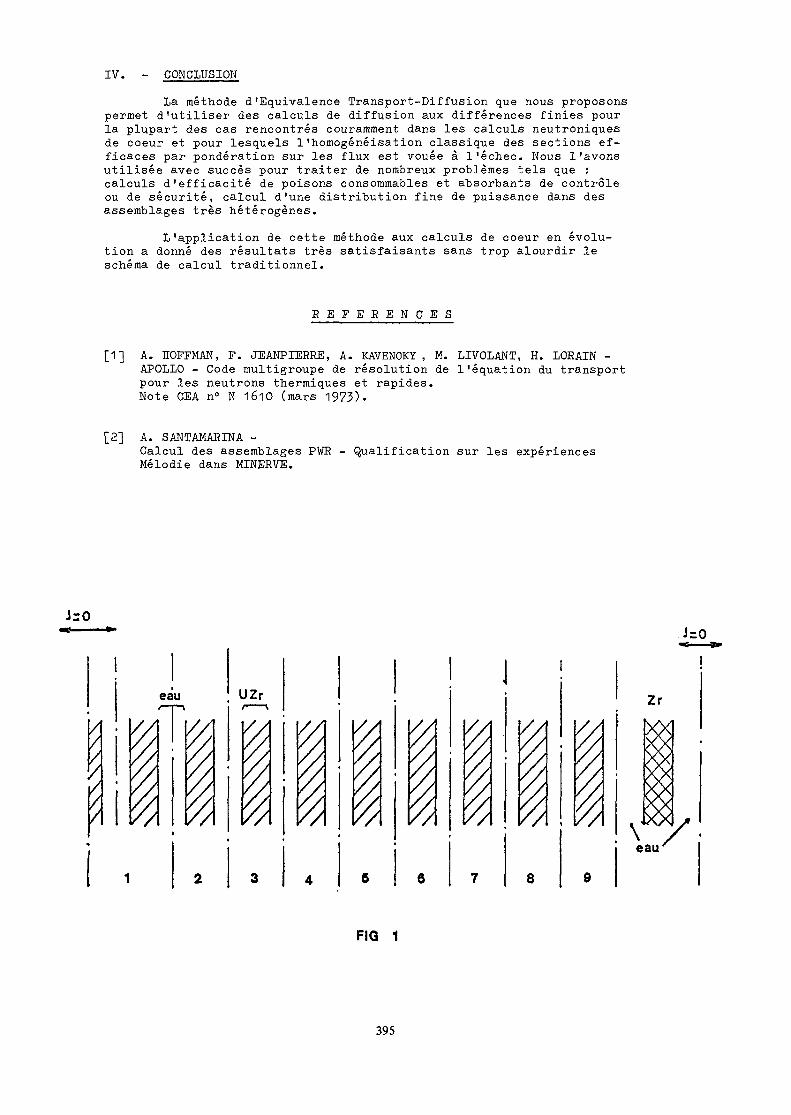
IV. - CONCLUSIONLa méthode d'Equivalence Transport-Diffusion que nous proposons

permet d'utiliser des calculs de diffusion aux différences finies pourla plupart des cas rencontrés couramment dans les calculs neutroniquesde coeur et pour lesquels 1'homogénéisation classique des sections ef-ficaces par pondération sur les flux est vouée à l'échec. Nous l'avonsutilisée avec succès pour traiter de nombreux problèmes tels que :calculs d'efficacité de poisons consommables et absorbants de contrôleou de sécurité, calcul d'une distribution fine de puissance dans desassemblages très hétérogènes.

L'application de cette méthode aux calculs de coeur en évolu-tion a donné des résultats très satisfaisants sans trop alourdir leschéma de calcul traditionnel.

R E F E R E N C E S

[1] A. HOFFMAN, F. JEANPIERRE, A. KAVENOKY , M. LIVOLANT, H. LORAIN -APOLLO - Code multigroupe de résolution de l'équation du transportpour les neutrons thermiques et rapides.Note CEA n° N 1610 (mars 1973).

[2] A. SANTAMARINA -Calcul des assemblages PWR - Qualification sur les expériencesMélodie dans MINERVE.

eau

T'A VA

6 8 9

eau

FIQ 1

395

- i.s

- i.s

- i.s

-

^

figure 2

>0__ heterogene

_»___ homogene

1.6 S. o <2.H 2.

X(GM)

396

TAUX V'ABSORPTIOHTHERMIfiUE 10-0.625 el/)

cellules UO2 lofte GdtOs .4.

FIG 4

.«!

....

•„-.

— San4 EqwLvaZzn&e.Kc.U-0, 97985

RejeAeMce Kt^'l. 00000

1 2 .3 4 S X397

e>

vvvvO ' Ii^^ \ I- 1

11 1 1 Ti '! i

^$^' ^^1 '

1

,

1{

i ! '11 i ' i

——— 1 1 !

:8 6 ! ' ii | '-^ 1 !

10

I CDO.x- c\j'

' l>r i '

IcoO'CM

!>?• -*• V i

I

i ^1i^ T!:s .i O ,O

I Si'N.|m

ICXl

,

1— •• —

J

5! w,W CO e

CO Vi-T OiV 4-'

i

i : i ; i ;1 . I ! i ;i ! , i ! ;

^]g $;§ «M| 3$ Sj fli i? "

<s)*e\tt)d

•ai -q O

-! ^ N•X3^

S 'O

d cJV~«oss3 Ss. -^

COOxCO

FIGURE

4.04-3.

4,22

4.CM3

1.206-0.5 -•i.O

-•14

224+0.3 4-0.7

-0.94.83640-5

d.O -4.0•4.092+ 4.-I

type* de.avec

Exp&Ue.nce.-Calcul (E-CJ/C I

399

FIG 7

ASSEMBLAGE (A)

Q U02

UD2-Gd2D3

c('eau

400

FIG 8

nmn

ASSEMBLAGE (B)

EH Cellules 1/02UQ2-Gd2Q3

Cellule. Jnou. d'eau

401

7.00

0.99

0.9$

(A)

Avcc Equiv:———9————2————a

// Sani Eqaiva^en'ce

0. 5. JO.

,—— .

FIG 9

BURM-UP (HWJ/Kg)

15. 20.

1.00

0.99

0.98

0.97

0.96

0.95

(8)

Avec E(jtti

FIG 10

Sani

8u/m-Up (MWJ/KgJ

0. 10. T5. 20.

402

Section E^icace d'abtoiption theAmtque.U02-Gd203 A4«cnif>£<uje (A)

PIG 11

0.20

55

Section E^ficace d'ab&oiption. thvtnique.CMule. PVKfX. a4ic»i6£agc (8)

50 FIG 12

San* Eqiuvatenee

20

.75

5. JO. to. AlWJ/Kg

403

Section E^icace d'abwiptutnCellule. U02-Gd203 a&temblage. (8)

FIG 13

Equivalence.

0.30

0.25Avae Equivalence. >s

s^

0.20

5. 10. 20.

Section ECellule. HAFNIUM Awem6.£a3e (8)

FIG 14

0.69 Sam Equivalence.

0.47 Avec

5. Ji:404

SESSION D: STREAMING AND INTERFACE EFFECTS

(Chairman: P. Benoist)

APPLICATION OF INTEGRAL TRANSPORT THEORYTO THE CALCULATION OF REACTION RATESIN THE VICINITY OF BOUNDARIESBETWEEN FAST REACTOR ZONES

R. BOHMEKernforschungszentrum Karlsruhe,Institut fur Neutronenphysik und Reaktortechnik,Karlsruhe, Federal Republic of Germany

AbstractThe accurate prediction of the distribution of reaction rates near boundaries

between reactor zones is of considerable interest for fast reactor design. There-fore, many experiments in fast zero power reactors are carried out to assess thereliability of such predictions. As most zones in fast zero power reactors aremade up of plate cells with pronounced heterogeneity of the neutron flux dis-tribution a method was developed to calculate reaction rates in the vicinity ofboundaries between finite slab zones where separability of neutron flux finestructure and global distribution cannot be assumed.

It was derived from the integral form of the Boltzmann equation with approx-imations suitable for the treatment of fast reactor lattices. Input data werethe neutron flux density and currents at a point some free mean paths remote fromthe boundary and broad energy group data of the Russian ABBN type, as used infast reactor design.

Effective broad group cross-sections for each slab near the boundary werecalculated with a formalism adapted from the cell code KAPER. Allowance was madefor linearly anistropic scattering within each energy group. Leakage perpendicularto the boundary was treated by a momentum method avoiding the difficulties arisingin diffusion theory approximations.

The method was applied to the analysis of reaction rate measurements in thevicinity of core-blanket boundaries simulated in two critical assemblies of thefast zero power reactor SNEAK, built in support of the German fast breederprogramme.

Discrepancies between measured and calculated reaction rate distributionsformerly encountered near those boundaries could be considerably reduced by use ofnuclear data presently chosen for core design and the new calculational method.Differences in the ratio of capture rate in U238 to fission rate in U235 wereLarger discrepancies found for the fission rate of U2J58 and the capture rate ofU23§ in the outer blanket regions were attributed to deficiencies in the broadgroup data of U2j8.

I INTRODUCTIONThe distribution of power generation in fast reactors is of major interest in

regions where gradients are steepest or discontinuities exist. Therefore, anincreasing number of experiments in zero power assemblies supporting fast reactordesign are aimed at the validation of predicted reaction rates in these regions.In several contributions to the IAEA International Symposium on Physics of FastReactors, Tokyo 1973 O), discrepancies of up to 10$ between calculated and measuredreaction rates were reported in the vicinity of boundaries between regions made upof different type plate cells. Only in some cases improvement could be achievedby application of more appropriate transport approximations.

Similar discrepancies were found in the evaluation of reaction rate measure-ments in the assemblies SNEAK 9B (2) and SNEAK 9C (3), built at Karlsruhe in supportof the German fast breeder reactor programme.

407

The commonly applied method of analysing the measured spatial distributions bymeans of a global reactor calculation and a superimposed cell calculation yieldedagreement within a few per cent in the core region but failed near boundaries andin the simulated breeder blankets. For this work it was thought that one of theweak points of former analysis was the factorisation of the neutron flux in theheterogeneous slab cells in fine structure and global distribution, applied inregions where the relative changes of the global distribution are not <§C1 withinone cell length.

Further, the calculation of effective cross-sections in the resonance regionand the treatment of leakage in directions not explicitly dealt with in the cal-culations had to be reconsidered.

The approximation of the Boltzmann equation finally derived was programmedand used for the new evaluation of the reaction rate experiments performed inSNEAK 9B and SNEAK 9C2 Cf).II DESCRIPTION OF THE EXPERIMENTS, AND THE MODEL FOR THEIR ANALYSIS

The reaction rate measurements to be analysed were carried out along thesymmetry axis of two cylindrical Pu- fuelled assemblies, the symmetry axis beingperpendicular to the plates used for building the cells (Figure 1 ) . The thickness-es of the oxide fuel plates was 6.3mm, including a stainless steel canning of2 x 0.3mm. Typical cell lengths were 13 to 20mm. The slabs considered to be ofuniform composition were actually made up of square plates in stainless steel sheathswith a pitch of ^ik.kmm. Special techniques were developed for measuring the fissionrates per nucleus of Pu239, U235 and U238 and the capture rate per nucleus U238 with aspatial resolution of the order of 0.2mm (5). Activation methods were chosen for allmeasurements. The probes were usually part of the fuel itself, thus minimal per-turbations were introduced by the activation detectors. After irradiation of thedetector probes in the lattice their X-activity was analysed to yield relativereaction rates. Absolute reaction rates R per nucleus were obtained by normal-isation to calibrated absolute fission chambers and an Am2it3/Np239 standard forcapture in U 38.

»*>i /•" iR (z) = / 0 (E,z) <T (E) dEX ' X

i = 25 (Ud35), 28x = f (fission), c (capture).

For the calculations it was assumed that the configuration sketched in Figure 1can be represented in vertical directions by a regular array of slab cells in thecore region and a different regular array in the blanket region, the two regionsbeing joined by a transition region containing cells of both types and being ofthe order of 'lOcm thick. In the horizontal plane all isotopes contained in a plateand the steel sheath housing it were smeared over the effective area of an element *)

The assumption was made that the neutron flux in the regular arrays can bef actor ised in a fine distribution as obtained from the cell code KAPER (6) super-imposed onto the global distribution of the cell average flux as calculated byreactor codes.

With known solutions in the arrays extending from the region of interest inboth directions the problem was reduced to that of a finite one-dimensional latticewith given boundary conditions.

Similar models were previously treated by collision probability methods (?, 8).Also for this work a collision probability method was adopted. The advantages ofthis approach were:-

*) This treatment of the steel sheaths is presently scrutinised. The revisedanalysis may decrease all C/E values for R2" by /u 1$.

408

a) The cell code KAPER (6) was available at Karlsruhe and proven to Toe acompetent tool in the analysis of central reaction rate measurements.

b) No difficulties were expected from the treatment of highly anisotropicneutron fields due to the plate geometry since an integration over theangular variable was carried out.

c) The division of the one dimensional spatial variable could be easilyadapted to suit the high resolution of the reaction rate measurements.

d) Within the cell code KAPER routines were available to calculate effect-ive neutron cross-sections of thin slabs in the resonance regionaccording to the theory of Wintzer(9), extended by Fischer and McGrath C'lO),It was considered essential that the basic data needed were tabulatedcross-sections and self shielding factors of the ABN type (11) also usedin fast reactor design work.

A straight forward application of a cell code to solve the boundary problem was notpossible, the reasons being:-

i) As in most cell codes scattering is assumed to be isotropic. The strongneutron currents across a boundary of reactor regions require anappropriate approximation.

ii) In KAPER leakage from unit cells is accounted for by D B -correctionsof the total cross-section,-where the D. are directional diffusionconstants of the cell and B^ are bucklings of the global flux distribu-tion in direction x,. Here the leakage probabilities are different atboth sides of the boundary and the cell concept cannot be used.

iii) The boundary conditions usually imposed in cell codes are not applicablefor the model.

Ill APPROXIMATIONS TO THE TRANSPORT EQUATION

If scattering is assumed to be anistropic to linear terms only, ie.

the integral form of the transport equation in the one dimensional slab arraycan be written:-

1

409

where:-0 neutron flux densityJ neutron currentE neutron energyz coordinate in the direction normal to the slabsyL cosine of the angle between the z direction and the neutron flight pathS source density, S source density of fission neutrons^- total cross-sect ion, vZ, number of neutrons per fissionV spectrum of the fission neutrons.Now the lattice is divided into thin slabs n, m with constant cross-sections

and volume V , V . The space dependence of the source density S within a slab benegligible and its components can be calculated from the volume averages of fluxdensity and current, 0 (E) and J (E). Further, the source density is assumedto vary slowly with energy over energy intervals of width & E . Thus a set ofmultigroup equations can be obtained:- s

v z*q>* - S ?* v' c) vVh *~n Tn \J I *»» u/l S,»i '•» I tB*'* S Ztlfe"*"* *»

For the accurate determination of a consistent set of group averages of cross-sections and collision probabilities P the execution of a large number ofweighting procedures is required.

For this study it was considered adequate to determine effective group cross-sections of type x by the method employed in the KAPER code (6):-

zJL s{ §« fe;> s:* u/5( - p>; > s:» vn w*,™ n \ z-t,<rn(£) A I n V-t,™ /°a-v^ /^The sum over all reactions x of these "flux weighted" cross-sections was used for thecalculation of collision probabilities in energy group g by the formula:-

/ - • <8)A separate set of "current weighted" cross-sections was not introduced, since

these cross-sections are needed for the calculation of corrections accounting foranisotropic scattering only. In a fast reactor lattice anisotropy is of majorimportance in the energy region above 100 keV neutron energy, where flux weightedand current weighted cross-sections are very much alike. As the spatial distributionof sources is not known initially, the calculation of effective cross-sections isstarted with an initial guess SnrM 2p ru the fully self-shielded cross-section ina slab. The repetition of the cross-section calculation with calculated sourcedensities changed the calculated cross-sections by only a fraction of a per cent.The influence of the different methods of cross-section preparation is shown inTable 1. Effective cross-sections in the slab cell of the core and in the adjacentdepleted uranium metal blanket are shown. The values given at positions 10cm offthe core-blanket boundary are identical with those calculated for an infinite celllattice.

410

The table shows the influence of the choice of the background cross-section <5~0on effective cross-sections and - by comparing the last two lines - the small in-fluence of the distribution of the source density on effective cross-sections. Inthe following examples <£ was calculated from the potential cross-section of U2J8and the infinite dilution cross-section of all other isotopes.

A further simplification of the system of' equations (5) (6) was introducedby assuming that anisotropic scattering into an energy group can be approximated bythe scattering out of this group. Thus, the only information about anistropicscattering needed and obtained from standard cross-section sets is the first momentof the elastic scattering cross-section and equation 6 can be written:-

„* »^n - S ?*** • 5(zs ? * r* vzJ')rf)k i/ (6'}with a transport cross-section given by

, p 1^ - ^ M4v, ^ . 7 -p^* / (6")

IV REMARK ON THE EFFECTS OF THE AMISOTROPY CORRECTION ON COLLISON PROBABILITIESIf the current calculated by equation 6'is inserted into equation 5 the

balance equation to be solved can be written:-

V -*<M. vSy?*1'* t ??* i •<?*'* i/* T*« V\ *"" mv * ^

rpj . <\ -*l£ pe*'» p%'2d ^.^ O ^ ^* r^^ ' r f c n« ^-Irf*

: : ; .tVK

For the case of an infinite homogeneous medium the corrections to the isotropiccollision probabilities to first order in the mean scattering angle are shown inFigure 3. The replacement of the total cross-section by the transport cross-section in the calculation of P overestimates the correction by approximately afactor of 2.V A MOMENTUM METHOD FOR LEAKAGE CORRECTIONS

So far all summations over the slab indices m and n have to be extended overall the lattice cells in core and blanket. To reduce the problem of the boundaryregion to one with a low number of regions (see Figure 2) the cells far off theboundary were treated by the factorisation method. The isotropic source densitycalculated by a cell code in a plate q of a cell in the regular lattice was multi-plied by a global distribution function of second order in the linear coordinatez and the perpendicular coordinates, y being the distance between the symmetryaxis and a point in the lattice:-

•>VS1 - i *U t - T'(^ ' i (*-*/

The energy dependent coefficients ^— , B- and B at a position z0 were estimatedfrom a reactor calculation by a polynominal fit.z Similarly, the source distributionin a slab n of the test region surrounding the boundary was modified by

411

This approximation was introduced to account for the finite extension of the slabsin the direction perpendicular to the z-axis. Two-dimensional diffusion calculationsfor the two SNEAK assemblies yielded only a few per cent variation of B2 in theregion of interest. Therefore the dependence of B| on z was neglected within thetest region. ne ratio of source densities in the two infinite lattices at 2 =zwas obtained from this calculation too. °

These global distribution functions were inserted into the integral formof the transport equation of the type equations 2 and 3 prior to the calculation ofcollision probabilities. In addition to the well known collision probabilitiesP and I^1 the moments Z P had to be calculated. The integration of:-

yields, eg.

Wl +1-1where (see Figure 2) :

The introduction of a space dependence of the isotropic source in directionsperpendicular to the z-axis can only be in accordance with the transport equationif components of the current in these directions exist. Therefore, the completeset of equations to be solved inside the test region becomes:-

- 5

Here, J is the component of the current in energy group g in a direction per-pendicular to the z-axis. The direction dependent transport cross-sections are ofthe type given in equation 6".

Similar equations were obtained for neutrons entering the test region but comingfrom a slab q in the regular lattice.

412

In these lattices with weak fine structure of the neutron flux density the com-ponents of the current in energy group g were approximated by:-

VI FURTHER APPROXIMATIONS IN THE COMPUTER PROGRAM GITAKSplitting up the z-component in intervals comparable with the high resolution

of the experiments and the high number of energy groups used in fast reactor cal-culations makes the system as given in equations 9 to 11 unsuitable for present daycomputers. Since only the scalar flux density is of interest in the calculationof reaction rates the components of the current as given in equations 10 and 11are directly inserted into equation 9-

The average cosine of scattering contained in the direction-dependent transportcross-sections was estimated by setting

2This holds in homogeneous media up to the order of B in the global distributionand is only considered a reasonable estimate in lattices of fast reactors showinga weak fine structure.

Thus, the collision probability formula finally obtained can be written as:-

2with SP given to first order in B by:-

413

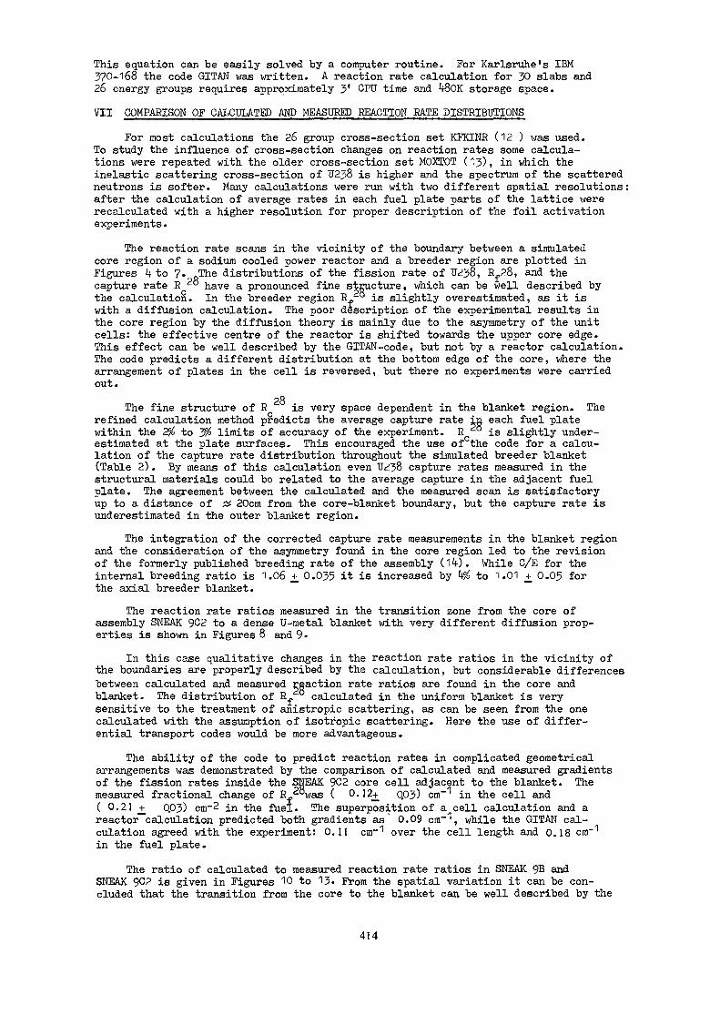
This equation can be easily solved by a computer routine. For Karlsruhe's IBM370-168 the code GITAN was written. A reaction rate calculation for 30 slabs and26 energy groups requires approximately 3' CPU time and kSOK storage space.VII COMPARISON OF CALCULATED AND MEASURED REACTION RATE DISTRIBUTIONS

For most calculations the 26 group cross-section set KFKINB (12 ) was used.To study the influence of cross-section changes on reaction rates some calcula-tions were repeated with the older cross-section set MOXTOT (13), in. which theinelastic scattering cross-section of U238 is higher and the spectrum of the scatteredneutrons is softer. Many calculations were run with two different spatial resolutions:after the calculation of average rates in each fuel plate parts of the lattice wererecalculated with a higher resolution for proper description of the foil activationexperiments.

The reaction rate scans in the vicinity of the boundary between a simulatedcore region of a sodium cooled power reactor and a breeder region are plotted inFigures k to 7. The distributions of the fission rate of U23§, Ef28, and thecapture rate R " have a pronounced fine structure, which can be well described bythe calculation. In the breeder region R~2° is slightly overestimated, as it iswith a diffusion calculation. The poor description of the experimental results inthe core region by the diffusion theory is mainly due to the asymmetry of the unitcells: the effective centre of the reactor is shifted towards the upper core edge.This effect can be well described by the GITAN-code, but not by a reactor calculation.The code predicts a different distribution at the bottom edge of the core, where thearrangement of plates in the cell is reversed, but there no experiments were carriedout.

?8The fine structure of R is very space dependent in the blanket region. Therefined calculation method predicts the average capture rate ig each fuel platewithin the 2% to 3% limits of accuracy of the experiment. R ° is slightly under-estimated at the plate surfaces. This encouraged the use of°the code for a calcu-lation of the capture rate distribution throughout the simulated breeder blanket(Table 2). By means of this calculation even Uc?38 capture rates measured in thestructural materials could be related to the average capture in the adjacent fuelplate. The agreement between the calculated and the measured scan is satisfactoryup to a distance of # 20cm from the core-blanket boundary, but the capture rate isunderestimated in the outer blanket region.

The integration of the corrected capture rate measurements in the blanket regionand the consideration of the asymmetry found in the core region led to the revisionof the formerly published breeding rate of the assembly (I'f). While C/E for theinternal breeding ratio is 1.06 +_ 0.035 it is increased by A$ to 1.01 +_ 0.05 forthe axial breeder blanket.

The reaction rate ratios measured in the transition zone from the core ofassembly SNEAK 902 to a dense U-metal blanket with very different diffusion prop-erties is shown in Figures 8 and 9«

In this case qualitative changes in the reaction rate ratios in the vicinity ofthe boundaries are properly described by the calculation, but considerable differencesbetween calculated and measured reaction rate ratios are found in the core andblanket. The distribution of E. calculated in the uniform blanket is verysensitive to the treatment of anistropic scattering, as can be seen from the onecalculated with the assumption of isotfopic scattering. Here the use of differ-ential transport codes would be more advantageous.

The ability of the code to predict reaction rates in complicated geometricalarrangements was demonstrated by the comparison of calculated and measured gradientsof the fission rates inside the SNEAK 902 core cell adjacent to the blanket. Themeasured fractional change of E_2owas ( 0.12+ Q03) cm in the cell and( 0.21 _+ 0.03) cm~2 in the fuel. The superposition of a cell calculation and areactor calculation predicted both gradients as 0.09 cm"'', while the GITAN cal-culation agreed with the experiment: 0.11 cur1 over the cell length and 0.18 cm"1in the fuel plate.

The ratio of calculated to measured reaction rate ratios in SNEAK 9B andSNEAK 9G2 is given in Figures 10 to 13- From the spatial variation it can be con-cluded that the transition from the core to the blanket can be well described by the

414

GITAN code. Deviations from 1 exist in both regions. They depend strongly on thecross-section set used for the calculation, as can be seen from the ratio of reactionrates calculated with two different cross-section sets.

The reasonable agreement found in the assembly SNEAK 9B suggests that thecross-section set KFKINR is suited for the calculation of reaction rates in the corezones of a 300 MW . LMFBR. This holds for adjacent breeder regions as well. Dis-crepancies between experiments and calculations exceed the error limits in thebreeder regions and in SNEAK 9C2, vrhere neutron spectra are different from the SNEAK9B core spectrum. The comparison with scans calculated from a different cross-section set indicates that the discrepancies can be caused by deficiencies in thenuclear data of U238. The transition region from the core to the breeder itselfposes no special problems if the calculational method is adapted to the experimentalsetup.VII SUMMARY

From integral transport theory a method was derived to calculate reaction ratesin the vicinity of boundaries between plate lattices of fast zero power reactors.Leakage parallel to the slabs is treated by a momentum method. Linearly anisotropicscattering and the space dependence of effective cross-sections is accounted for bysuitable approximations.

The method was used for the evaluation of reaction rate measurements in two Pu-fuelled SNEAK assemblies. Agreement within fd 23& could be obtained between calcu-lated and measured spatial distributions of the fission rates of Pu239i U235 andthe capture rate of U238 in a simulated transition zone between core and breeder ofa 300 MW . LMFBR. Discrepancies were found for U238 reaction rates, especially forthe capture rate of U238 in the outer breeder region, which can be due to de-ficiencies of the nuclear data of U238.

REFERENCES

('0 International Symposium on Physics of Fast Reactors, Tokyo Oct 16-19, 1973.G Ingram et al, Volume I, A16, p289C G Campbell et al, Volume I, A1*f, p259.

(2) F Helm et al.Summary of Results for the Sneak-9 Series of Critical Experiments andConclusions for the Accuracy of Predicted Physics Parameters of the SNR-300.KfK 2586 (1978).

(3) W Scholtyssek.Physics Investigations of Sodium-Cooled Fast Reactors: SNEAK-Assembly 9C.KfK 2361 (1977).I?

(k~) R Bohme.Integrale IVansporttheorie mit linearer Anisotropie der Streuung zur Berechnungder Neutronenverteilung in endlichen Plattenanordnungen Schneller Reaktoren.KfK 2501 (1977).

(5) H Kusters, comp.Progress in Fast Reactor Physics in the Federal Republic of Germany.KfK 1632 (1973).

(6) P E McGrath.KAPER - Lattice Program for Heterogeneous Critical Facilities (User's Guide).KfK 'I893 (1973).

(7) L Mayer.Journal of Nuclear Energy, 2k, 337 (1970).

(8) P E McGrath, W K Foell.Nucl Sci Eng 5, 7 (197D.

(9) D Wintzer. „Zur Berechnung von Heterogenitatseffekten in periodischen Zellstrukturenthermischer und schneller Kernreaktoren.KfK 7*f3 (1969).

415

(10) P E McGrath, E A Fischer.Calculation of Heterogeneous Fluxes, Reaction Rates and Reactivity Worthsin the Plate Structure of Zero Power Fast Critical Assemblies.KfK 1557 (1972).

(11) L P Abagjan, No Bazazjanc, II Bondarenks,tM N Nikolaev. )(Gruppenkonstanten Schneller und Intermediarer Neutronen fur die Berechnungvon Kernreaktoren.

r-lW (translation, 196?).(12) E Kiefhaber.

The KFKINR-Set of Group Constants; Nuclear Data Basis and First Results ofits Application to the Recalculation of Fast Zero-Power Reactors.KfK 1572 (1972).

(13) E Kiefhaber et al.Proceedings of the International Conf on the Physics of Fast ReactorOperation and DesignBNES, London, June A-26 (1969), p94.

(1A-) R Bohme, F Helm, S Pilate, M Pinter, W Scholtyssek in J M Kallfelz andR A Karam, Ed.Advanced Reactors, Physics, Design and Economics.

, Pergamon Press 1975.

TABLE 1Influence of the Calculation Method on EffectiveGroup Cross-Sections in the Resonance Region

Example: (infinite latticeKFKINR Set, Group 18, 6.5 - 100eV

Plate Type

Thickness/cm

Contribution ofU^38 to the back-ground cross-section: -

P

<"

cr (S estimated)"C

<r". (S calculated)t

Core 9C-2

10cm offBoundary

P.0^0,

0.626

1 .000

1.009

1.10*

-1.106

Na

0.62*48

1 .000

1 .000

1.002

1.002

1cm off Boundary

P»0/D02

0.626

1.085

1.093

1.*1.152

Na

0.62*t8

0.996

0.996

0.998

1 .001

Blanket 9C-2

At Boundary "lOcm off Boundary

TJ depl. + STST

30.5

'1. 257

1. 229

1.079

1 .081

1.000

0.975

1.003

'! .003

416

TABLE 2SNEAK 9B

Relative Capture Rate Per Nucleus U238in the Axial Breeder Blanket

distance fromcore-blanket-boundary (cm)

pQI measured R in centre of

U02 plate °

28II measured R in adjacentAl-plate

GITAN-calculatedcorrection for II in %

1 ¥ *»*£J

11 ££ ±n°/oE

1.3

•550

.577

-5-3

0.0

+O.lf

2.8

.559

.553

-6.1

+0.6+1.7

Jt.if

-6.6

6.0

. 83

.523

.523

-7-2

+0.8

-0.2-0.2

7-5

. 73. 63

-7.8

-1.7+0.5

9.1

. if

-8.

-0.7

13.8

.*H9

-10.8

- 1.1

20.0

.333

-12.3

- k.k

26.3

.2 1

-13.0

- 6.1

32.6

.162

-12.1

-16.5

j1

& &J/U »{J

.089

- 3.9

-68.

SNEAK-9 B SNEAK-9C2

Blanket

Core

Core

Blanket

Stainless SteelWall

FIGURE 1 Plate Structure in Assemblies SNEAK-9B and SNEAK-9C2

418

RegularLattice

z y

"cos'M

\

\

\

\

\

\

Test Region Rerular*————lattice

FIGUBE 2 Model of a Boundary Region in Slab Geometry

X '0.8-

0.6-

0.4 -

0.0

-0.2-

1 1 1 1- 11- \\\\\\\\\\\

/' ~x --/ ^. ^— —__/ ^ _____ ^^ ~--___,' /r l— — -

-

. . 1 , 1

, _ . _ pran

1——— iPmn" = (QITAN)

1mn ~ tr

Homogeneous medium, thin slabsG(m5Afn<£ 1) separated by regionof thickness X .

FIGURE 3 Change in CollisionProbability due toAnisotropic Scattering

1.0 2.0 3.0

419

0.50-

45 z(cm) 50

Puo2/uo2uo,,

Udepl.(0'4%)

O measurementGITAN-calculations

V fine structure— average in fuel

- — — -diffusion calculation

Al 25 % nat.density

Al 40 % nat.density

FIGURE k SNEAK-9B:

Relative Fission Rate per Nucleus 239Pu

420

E3

Udepl.(°'4%)

Al 25 % nat. density

Al 40 % nat. density

measurements inside fuel

measurements inside structuralmaterial

35

GITAN-calculations

x fine structure

— average in fuel

— — —dif fus ion calculation

235FIGURE 5 SNEAK-9B: Relative Fission Rate per Nucleus U

Rf28

0.70

0.60

8 0.50

0.40 COREleft scale

BLANKETright scale

-0.20

0.10

50 z(cm) 55

FIGURE 6 SNEAK-9B: Relative Fission Rate per Nucleus 238U

Na

Al 25 %nat. density

Al 40 %nat. density

MeasurementsO inside fuel plateletsD inside structural materials

GITAN-calculations" » fine structure— average in fuel

—. —.— average in oxide, isotropicscattering

•—•• — •• average in U-metal,isotropic scattering

• — —— — diffusion calculation

R,?8

0.70

0.60

0.50

0.40

z(cm) 55

uo2U depl.

Na

Al 25%

Al

MeasurementsO at surface of oxideD in structural materialA in oxide• in U-metalCalculations

—— at surface of oxide• — • — average in fuel— — — diffusion calculation

FIGURE 7 SNEAK-9B: Scan of the Capture Rate of U238

423

I I I I I I I I I0.04

0.03

0.02

0.01 CORE

MINIMI20 25 30 35 z(cm)

Na

U depl.

o Experimenta Experiment x 0.9

GITAH-Calculations— average in a slab"\ fine structure— isotropic scattering

— - — diffusion calculation

FIGURE 8 SNEAK-9C2: Spectral Index —-28(Tf

424

! MINIMIT I

0.140 -I error 01° °I calibration

Fl ' °I r relative .r.eas.urerr'ent

0.135

0.130

0.125hCORE

IIMMII20 25 30 35 40 , x 45z(crr\)

Na

U depl.

measurementsGITAN-calculationaverage in fuel

• — ratio at fuel surface••• ratio in Na•— diffusion calculation

- 28

EEGITRE 9 SNEAK-902: Spectral Index ~=

425

1.00

0.90

0.80

• Wi--i————m^———\->

o° °X O _n OO rv.

(O)

CO) ooo

(O)

CORE BLANKET

I——I

PUO./TJO.,uo2

U depl.

N*

Al 25%

Al

50 , x 55z(cm)O ratio experiment/calculation— ratio calculation (MOXTOT set)/

calculation (KFKINR set)

28

fffFIGURE 10 SNEAK-9B: E/C for -=:

426

1.05

1.00

0.95

<>• -a - 5 co -c O — r> —

oO

OO

(O) (O)

CORE

50 , x 55z (cm)

PuO^TJO,

U°,

U depl.

Na

Al ?$%

Al kO%

O ratio experiment/calculation_ _at.._. calculation (MOXTOT;

calculation (KFKINE)

28

FIGURE 11 SNEAK-9B: fiatio E/G for -ST..Of

427

>\<*»"£'->'"',, ,'*">"

1.00

0.90

0.80

COREliiiiiiii20 25 30

BLANKET

35 40 , v 45z(cm)

PuO,/UO?

Na

j | U depl.

o ratio experiment/calculation— ratio calculation (MOXTOT setV

calculation (KMINR-set)

-28FIGURE 12 SNEAK-9C2: E/C for -=?

428

1.05

1.00

0.95 COREiimim20 25 30

BLANKET

35 z(cm)

Na

U-Metal (depl.)

O ratio experiment/calculation— ratio calculation (MOXTOT set)/

calculation (KFKINR)

-28FIGURE 13 SNEAK-9C2: E/C for -=•

429

LATTICE CELL DIFFUSION COEFFICIENTSDefinitions and comparisons

R.P. HUGHESBerkeley Nuclear Laboratories,Berkeley, United Kingdom

Abstract

Definitions of equivalent diffusion coefficients for regular latticesof heterogeneous cells have been given by several authors. The paper beginsby reviewing these different definitions and the unification of theirderivation. This unification makes clear how accurately each definition(together with appropriate cross-section definitions to preserve the eigen-value) represents the individual reaction rates within the cell.

The approach can be extended to include asymmetric cells and whereasbefore, the buckling describing the macroscopic flux shape was real, here itis found to be complex. A neutron "drift" coefficient as well as a diffusioncoefficient is necessary to produce the macroscopic flux shape.

The numerical calculation of the various different diffusioncoefficients requires the solutions of equations similar to the ordinarytransport equation for an infinite lattice. Traditional reactor physicscodes are not sufficiently flexible to solve these equations in general.However, calculations in certain simple cases are presented and thetheoretical results quantified.

In difficult geometries, Monte Carlo techniques can be used to calculatean effective diffusion coefficient. These methods relate to those alreadydescribed provided that correlation effects between different generations ofneutrons are included. Again, these effects are quantified in certainsimple cases.

SYMMETRIC LATTICES

One particular problem in the homogenisation of a heterogeneous latticecell is the definition of a equivalent diffusion coefficient. For directionsalong which the lattice is heterogeneous, such definitions have been given byseveral authors '1-5). Each definition was derived differently from differ-ent starting assumptions. However, these definitions can be derived from acommon starting point and this unification ^ ' makes the advantages anddisadvantages of each definition apparent.

It is important that the diffusion coefficient is not considered inisolation. To give the correct lattice eigen-value in the presence of anasymptotic buckling, each definition of diffusion coefficient must be usedwith a corresponding smearing of the lattice cross-sections. In the notationof reference 6, the only definition which gives the true leakage from a unitcell of the lattice is DBC (Benoist corrected). The other definitions,although derived from the same unit cell neutron balance equation, arederived by a process of regrouping the individual terms. These cancellations(between leakage and absorption say) although preserving the overall neutronbalance in the unit cell, lead to unphysical reaction and leakage rates. Ifwe define the migration area M2 of the lattice by

keff kinf

431

then (in one group) the definition of Deniz ' ' and Gelbard ''*' is given by

DDG—— = M2 (2)la

DPHere the cross-sections that should be used with D are exactly the usualinfinite lattice flux and volume smeared cross-sections. In a multigroupformulation, the relative reaction rates are then exactly the same in thebuckled situation as in the infinite lattice apart from a multiplier on thefission source. It follows that leakage can only occur from a group whichcontains a fission source. The generalisation of (2) can be shown

h (v Vh *oh dV£. ,. / dinv dV°g

so that any group having no fission source will have a zero diffusioncoefficient. This is the most obvious example of an unphysical leakage rate.

•p>*~iThus, although D gives the usual expression for M2 (equation (2))

and requires the usual infinite lattice flux and volume smeared cross-sections to give the correct lattice eigen-value, it leaves us withunphysical reaction rates. For comparison with (2), we give thecorresponding (one group slab) formulae e' for the Benoist corrected(2)and uncorrected '1' definitions.

,2 DBCM1 = -— = M2

2 nBU r (VV IrM11 = -— = M2 + \ /(S - r-^-k W/ fa <|> dV (5)T J a inf ° / J a °a

2 2Thus if M1 or M11 is used in (1) in place of M2, the eigen-value will beincorrect, but if DB<-' or D ^ is used with its corresponding (bucklingdependent) cross-sections, it will give the eigen-value correctly. Only Dwill give the true cell reaction rates as mentioned earlier. For thesimplicity of equation (2), we must sacrifice the true cell reaction rates.To get the truecell reaction rates we must use D given by (4), and correctM1 if we want to use (1).

It was pointed out by Gelbard (^) that the unit cell of any symmetriclattice can be defined in two different ways (see figure 1). It can be shownthat both D and D"" (and their associated cross-sections) are independentof which definition we take. D however is not and is thus not unambiguouslydefined. Thus if we choose to get the average reaction rates in one cell,they will be wrong in the other. In order to remove this ambiguity,

developed one approach which fitted the reaction rates throughout thelattice in a least square sense and showed that this led to exactly thediffusion coefficient D .

The evaluation of the various diffusion coefficients given by (2), (4)and (5) requires aknowledge of the fluxes <f, £ and £. is/ is just theinfinite lattice angular flux. £ and £ however, satisfy equations like thetransport equation but with sources and boundary conditions that are notcatered for in standard codes. It is possible to obtain a simple relationbetween M2 and M1 however in a diffusion theory approximation. We find

432

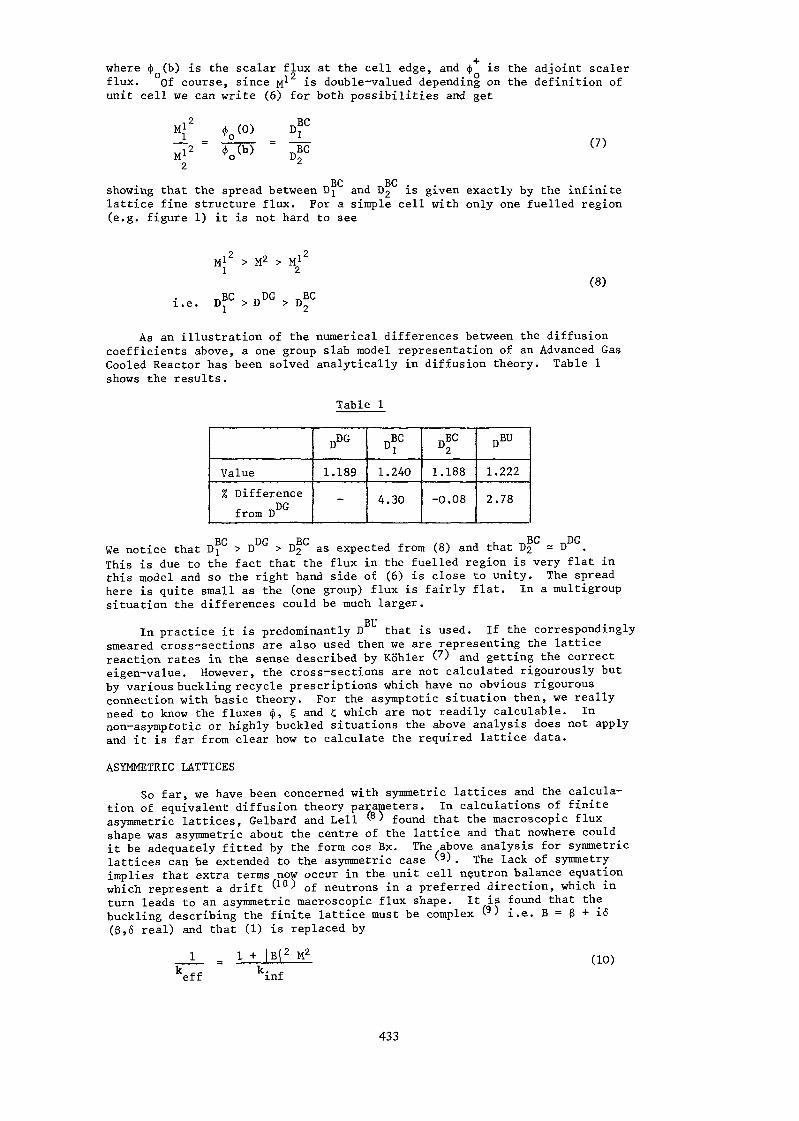
where <f> (b) is the scalar flux at the cell edge, and <ji is the adjoint sealerflux. of course, since n1 is double-valued depending on the definition ofunit cell we can write (6) for both possibilities and get

,EC (7)

showing that the spread between Dj and D2 is given exactly by the infinitelattice fine structure flux. For a simple cell with only one fuelled region(e.g. figure 1) it is not hard to see

Ml2 >

i.e.

> M1

DDG(8)

As an illustration of the numerical differences between the diffusioncoefficients above, a one group slab model representation of an Advanced GasCooled Reactor has been solved analytically in diffusion theory. Table 1shows the results.

Table 1

Value% Difference

from D

DDG

1.189

-

°r1.240

A. 30

Bf

1.188

-0.08

DBU

1.222

2.78

We notice that DDG> RP T)Pas expected from (8) and that D2 - DThis is due to the fact that the flux in the fuelled region is very flat inthis model and so the right hand side of (6) is close to unity. The spreadhere is quite small as the (one group) flux is fairly flat. In a multigroupsituation the differences could be much larger.

•OTT

In practice it is predominantly D that is used. If the correspondinglysmeared cross-sections are also used then we are representing the latticereaction rates in the sense described by Kb'hler (7) and getting the correcteigen-value. However, the cross-sections are not calculated rigourously butby various buckling recycle prescriptions which have no obvious rigourousconnection with basic theory. For the asymptotic situation then, we reallyneed to know the fluxes $, £ and C which are not readily calculable. Innon-asymptotic or highly buckled situations the above analysis does not applyand it is far from clear how to calculate the required lattice data.

ASYMMETRIC LATTICESSo far, we have been concerned with symmetric lattices and the calcula-

tion of equivalent diffusion theory parameters. In calculations of finiteasymmetric lattices, Gelbard and Lell '8' found that the macroscopic fluxshape was asymmetric about the centre of the lattice and that nowhere couldit be adequately fitted by the form cos Bx. The above analysis for symmetriclattices can be extended to the asymmetric case '9). The lack of symmetryimplies that extra terms now occur in the unit cell neutron balance equationwhich represent a drift ^10^ of neutrons in a preferred direction, which inturn leads to an asymmetric macroscopic flux shape. It:,i? found that thebuckling describing the finite lattice must be complex ™) i.e. B = 3 + i<5(3,6 real) and that (1) is replaced by

eff1 + |B[2 M2

k. cinf(10)

433

The macroscopic flux shape has the form e cos f3x, where $ is thendetermined hy the geometry and 6 is proportional to the lattice neutron driftcoefficient. Asymmetric lattices, therefore, need an extra lattice parameterto describe them, and require an extension of the concept of buckling to thecomplex plane. It can be shown that '°' a diffusion theory calculationcannot pick up this drift phenomenen implying that it is intrinsically atransport effect. Calculations of the magnitude of the drift for varioussituations are given by Larsen and Williams ' ' .

MONTE CARLO TECHNIQUES

Returning now to symmetric lattices, we shall briefly discuss Monte Carlotechniques for the calculation of M2 in equation (1) . Typically, leakage istaken into account by assuming the flux to factorise into the infinite latticefine structure flux and a macroscopic factor, and the fission yield of aneutron weighted accordingly. This leads to a value of M2 which is one halfthe mean square distance travelled by neutrons from birth to fission.Strictly, the assumption of factorisation is incorrect and similar approx-imations led Gelbard and Lell ( ' to the same definition of M2 exceptingthat the neutron flights are also weighted with the adjoint neutron sourcedistribution. If we expand the source distribution without the factorisationassumption (as in reference 6), then it can be shown that (-11) the extraterms must be added to the definition of Gelbard and Lell which representcorrelation effects between different generations of neutrons .

The relative contribution of these correlation terms to M2 is ingeneral small '11'. This is not necessarily so however. We can estimatetheir magnitude in a simple one group example of slabs of fuel separated byvoids (see figure 2) . Here the infinite lattice flux is flat (and theadjoint also, so that the typical method referred to gives the samedefinition as Gelbard and Lell) . By relating the Monte Carlo approach tothat used in reference 6, we can estimate the correlation terms since theflux £ can be calculated analytically in this example. We find that

correlation terms (b-a)2—————— ~

so that for voids small compared to the diffusion length in the lattice, thecorrelations can be neglected. This result is confirmed for GCFR latticesby Monte Carlo Calculations t11' . If the voids are large, the correlationsbecome more important.

CONCLUSIONS

The example lattice above is special in that the fluxes $, £ and c, canbe calculated analytically. We can therefore calculate exactly all thedifferent definitions of diffusion coefficient we discussed earlier. Wefind

D?C = Df = DBU = DDG = ^ J (12)

so all the definitions are equivalent and equal to the simple flux and volumeweighted cross-section prescription. It is unfortunate that more complexproblems cannot be solved as readily. In the absence of codes specificallydesigned to solve for the multigroup fluxes <(>, ? and t, in realisticgeometries the quantitative comparisons of the various diffusion coefficientsis difficult.

ACKNOWLEDGEMENT

This paper is published with the permission of the Central ElectricityGenerating Board.

434

REFERENCES

1) P. Benoist, "A General Formulation of the Diffusion Coefficient in a• Heterogeneous Medium which may contain Cavities", Translation 842,Atomic Energy Research Establishment, Harwell (1959).

2) P. Benoist, CEA-R-2278 (1964).3) V. Deniz, Nuclear Sci. Eng. 28, 397 (1967).4) E.M. Galbard, Nucl. Sci. Eng. 54, 327 (1974).

5) E.W. Larsen, Nucl. Sci. Eng. 60, 357 (1976).

6) R.P. Hughes, Nucl. Sci. Eng. 67, 85 (1978).7) P. Kb'hler, Nucl. Sci. Eng. 57, 333 (1975).8) E.M. Gelbard and R. Lell, Nucl. Sci. Eng. 63, 9 (1977).9) R.P. Hughes, Nucl. Sci. Eng. - to be published.10) E.W. Larsen and M. Williams, Nucl. Sci. Eng. 65, 290 (1978).

11) E.M. Gelbard and R.P. Hughes, - to be published.

GLOSSARY

(f> , £ , C. one group scalar fluxes in expansion of buckled lattice0 0 0 flux $

<f> multigroup infinite lattice scalar flux

<(> one group infinite lattice adjoint flux

k. . infinite lattice eigen— value

k ,, buckled lattice eigen-value

X * fission spectrum into group g from fission in group h.

Ml2 DBC/ I"3.

M"2 DBU/ -a

435

Unit cell

Unit cell 1

FIG. 1

Fuel

FIG. 2 .

436

DIFFUSION COEFFICIENTS IN UNIFORM LATTICESWITH SUPERIMPOSED BUCKLING

T. DURACZComputing Center Cyfronet,Institute of Nuclear Research,Swierk-Otwock,Poland

Abstract

The homogenization procedure for uniform lattices withsuperimposed small buckling is presented. Various ways ofdefining diffusion coefficients are indicated0 Problemsconnected with numerical evaluation are discussed andnumerical examples for plane lattices are given<,

1. Introduction

We consider uniform lattices with superimposed smallT>£buckling Jj> • he aim of the homogenization procedure pre-

sented in this paper is to obtain buckling independentconstants for diffusion calculations in a homogeneousmedium equivalent to the lattice in some specified sense.The formalism is developed for a general II group description,Por the sake of simplicity we confine ourselves to the caseof plane geometry but extension to XY geometry is straight-forwardo Moreover, after that extension is made one canproceed further with cylindricalization of the problem £l»We consider only the Ke|p eigenvalue problem which seemsto be more complicated aa compared with a problem of sub-critical lattice with given sources.

The basic assumption we make is that the flux isapproximated by a linear combination of tbe expressions

437

where H"B *//i ' has periodicity of the lattice,k-Q-x an^ £ = i?2 are directional cosines, Bx

and B^ are transverse and axial buddings. Y/e writesymbolically

The following expansions in powers of D^ and Dz areassumed

- e> = (

andkeff = k0(^~^Bx -^zBz) +... (5)

Terms of the order higher than two will not be needed infurther analysis. After inserting the Eqs./1-3/ into thetransport equation we obtain

XV A/i

L-Y«(*,yh0) = Z0where L denotes the transport operator

i /* ^_ \~ ZIT j - t (X ' - ) and O5, <?s and vOp are matrices

of total, scattering and fission crdss sections respectively.In order that the Eqs./5-8/ be solvable their free termsmust be orthogonal to the solution of the equation adjointto the Eq./4/ J

438

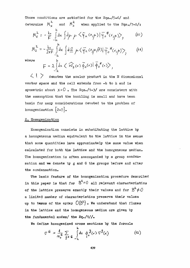
Those conditions are satisfied for the Eqs./5-6/ ando o

determine Mx and M2 when applied to the Eqs./7-8/!h

X " ~ ? - u

A.I ^ _ Ito

where

^ ' / denotes the scalar product in the U dimensionalvector space and the cell extends from -h to h and issymmetric about )(, = 0 . The Eqs./1-3/ are consistent withthe assumption that the buckling is small and have beenbasic for many considerations devoted to the problem ofhomogenization [2-7] •

20 Homogenization

Homogenization consists in substituting the lattice bya homogeneous medium equivalent to the lattice in the sensethat some quantities have approximately the same value whencalculated for both the lattice and the homogeneous medium.The homogenization is often accompanied by a group conden-sation and we denote by g and G the groups before and afterthe condensation.

The basic feature of the homogenization procedure describedOin this paper is that for B =0 all relevant characteristics

rt

of the lattice preserve exactly their values and for B ^ 0a limited number of characteristics preserve their valuesup to teams of the order 0(B ; » We understand that fluxesin the lattice and the homogeneous medium are given bythe fundamental modes/ the Bq«/1//»

We define homogenized cross sections by the formula

439

where ^^.Z. jdxf.V). (.3)

^ 6 -koIt is due to this definition that quantities that for B-0

can be expressed as functions of only the cross sectionss- j jCi are preserved exactly when g = t) /for example I/ ett

and flux ratios/.Before proceeding further we would like to make it clear

that transport and diffusion bucklings are generally slightlydifferent /even far a homogeneous medium/. However, we canargue that they coincide when B -°?0 and hence we shallnot discriminate between them.

To define diffusion coefficients we take some quantitiesj_ »K=/i.,.o, depending on them vihen calculated from thediffusion equation. We assume that the following expansionshold

T" Kwhere JLO do not depend on the diffusion coefficients.The expansions /14/ are true for physically meaningfulintegral characteristics of the lattice. Denoting by "tr"and "diff " quantities calculated from the .transport anddiffusion equations respectively we have

Next, by satisfying the equations

xx

TK Ir TK.dl'ffwe match 1 and JL up to terms of the orderThe Eqs«/I6,17/ determine diffusion coefficients. It isdesirable to have such a number of quantities ~£ thatthe diffusion coefficients be determined uniquely.

440

3» Diffusion ..coefficients

In this section we give a few examples of possible-*^ yfchoices of quantities 1 alon£ with corresponding

formulae for diffusion coefficients.Pirst we consider some cases known frou the literature.T61» -L is assumed to be the net leakage out of the cell

for the group G [4,5J . After some standard calculationswe obtain

2. With the condensation to only one group we take£-!< ff E2»3J» This Iea5s *° *he formulae

Por the case of no group condensation /though it can easilybe incorporated/ an approach has been proposed [?J that inthe case of one group leads to the formulae /20-21/.

3. Other well known diffusion coefficients [6j :

andUz = (»)

where

-can be obtained if we assume ttrat J_ is the net currentnormalized at the cell's edge :

441

Now we pass to examples not explored in the literature.

4. For the group G vie define

Q = L Ur cf^-r ) [ v G/ 00 -f (x)]36t cell

T 3where ^- y. denotes the cross section of scattering outof the group G, Q gives the number of neutrons deliveredto the remaining groups Q ^ ($ . Next, we define

A'=4rZ tfftr «"•where Al denotes the net current out of the cell.This term gives the number of neutrons lost in the group G.We hope that by putting

I6 = QS/A"T 6with 1 describing roughly the contribution of the group

G to the global balance of neutrons we can approximatelypreserve ^ef£ as v?e-'--'- as flux and reaction rates ratios.After some calculations we obtain

(*>)where

_6TXX

and

z: f r/- J L

5. We assume for simplicity that there are only two groups,no group condensation andeasily be relaxed /.We putno group condensation and ^^ = 0/ thesec.restrictions can

442

T- 4eff ; (33)

where

After some simple calculations we obtain

where

All the formulae presented in this section can be obtainedsolely on the basis of the expansions /1-3/ and the assumptionthat fluxes are given by fundamental nodes. Mome detailesconcerning the above presented results can be foundelsewhere [3].

4o ITuaerical evaluation

Calculation of the diffusion coefficients defined inthe points 1 and 3 of the section 3 requires knowledge ofof only iT0 , M'v and U-2 while definitions of thepoint 2 require also Lp^ and definitions of the points4 and 5 - Yo an< (-pxx * 'n 3:Lrec1' attempt to solvenumerically the Eqs./5-3/ is almost certain to fail. Toexplain why is that let us assume for simplicity that thespectrum of the operator L consists of discrete simpleeigenvalues c^p;^/))"- with corresponding eigenfunctions£o,f>|r" where a' = ° and -fo-^o /the actual

spectrum of the transport operator may be more complicated[9J/. Assuming that the functions LI form a completeset in a Hilbert space with a scalar product ( j ) andexpressing the source term as

443

= I V f I (35)where

we find the solution

The terra J-? is evidently infinite unless 0, •= 0 .How, the source terns of the Eqs./5-8/ satisfy formallythe requirement c|c-=0 but because of approximationsnecessary for numerical treatment of the equations somesmall 3/c-^0 will be generated.

Prom the above considerations it follows that to assureexistence of numerical solutions we should change the

T* ^-roperator U to a slightly subcritical operator L-^ 7 i 'close to L . <Xj; and J^i will be shifted to <X°

and f. and we assume that continuity:';1 holds : oC; ~ <X;and £, ~ f i /strict analysis could be based onperturbation theory for linear operators [lOj/. It can bechecked that terms of the form (X 0 > where (L denotesan arbitrary number, can be added to solutions of theEqs./5-8/ without affecting the values of diffusioncoefficients. Thus the effective error f ~ *f /where ydenotes the solution of the equation with the operator /is given by

The coefficient -^y may become large as L approaches/-*. &0l_ * As the same can be said of the cost of numerical

Tcalculations it is not obvious that the optimum L should/***.

be as close to L as possible0V/e have solved numerically the Eqs./4/,/5/,/7/ and /9/

and next calculated the values of diffusion coefficientsintroduced in the points 1,4 and 5 of the section 3» fortwo cases, under the assumptions of the point 5 /two groups,

444

no condensation, D^-O /• We have approximated the source

In the Eq./5/ by ~u.d>000 an^ "^^e source in the Eq./7/

by 1 __ _'00 + -

v- ex) =1 jdyu v j (>yand ™ (X,K" \ - Ji fx

/first of the approximations has been largely applied [7JA

Though these approximations are not necessary they simplify

calculations, llext, L for the Eq./5/ has been definedx\

as the streaming part of L :^ t ^ ^ <. £ / \L = Lx - f O"x W ••

Por the Eq,/7/ a few additional approximations have beenconsidered

where 'J ( denotes the selfscattering matrix,^N f S\

L = LAA(^where [ f,has been defined so as to yield the fraction V£ ofthe total fission. As we feel that ' M an< henceii '

~J) | raay be strongly influenced by the approximationsof sources and as we are mainly interested in correctionsto pi introduced by our diffusion coefficients, vje

* qhave developed a formula for T), in terns of integralsover the cell's volune. Writing the source as

^

:

vje obtain from the balance of neutrons:

Prom the formula /48/ we find

445

2.

The cases considered are a heavy water lattice /I/ anda light water lattice/II/. Cross sections [l1,12"j are givenin Table 1. Puel extends from -^ to hf . h and hare as follows

I : h = £. £ cm ; hF= » 6 ,II: h = 4, , h F ~ .

Calculations have been performed using the ANISE code vjiththe angular quadrature S^g [l3J . In Table 2 : DL>t have

*»teen obtained fro:.; /49-50/, ^[) L from /31/ and

where Dv are given by /36-37/j the column L refersA xxto approximation assumed for L in the Eq./7/ and inparticular the numbers given are the / approximated/ valuesof it assumed in the formula /45/»

l?ror. Table 2 it is seen that as far as correctionsand Ai' x are concerned sensitivity to the approximationassumed for L_ is lovi and already Lx gives reas-onable results. Uext, corrections 5D*. and APA havedifferent signs /both improve K ere -see Table 3/« As ithas been expected corrections for the widely spaced latticeare larger.

It ia possible to assess the influence of the correctionson the performance of diffusion coefficients by a simplenumerical experiment. 1-Tamely, we assume that the expansion/1-3/ is "exact" and calculate the "exact" quantities like

keif °r tlVll that serve as a basis of the assessment.On the other hand we calculate the same quantities fromthe diffusion equation /with the fundamental mode approxim-ation and up to terms 0(6 )/• In Table 3 results for the

e)

case I are given, for some values of B>x and withL = Lxx(^.-«0. Corrections £$ improve KP££ andP££

446

of course corrections AD improve both l^eff a^d H/11 •A ' '

Similar effects have been observed for the case II.Discrepancies that still exist between "exact" results andthe results for £)Lx + AP' are probably for the most partdue to the approximations assuued for source terms inthe Eqs./5/ and /7^ and if so give a measure of errorintroduced by those approxinations.

References

1. A.C0Clark,D.A.Newmarch, Report AERE RP/R 1657/1956/.2. M.M.R.Williams, Atorakernenergie, 18.31/1971/*3. B.Davison, J.UucloEnergy , .T.,51/1958/.4. D.C.Leslie, Report AEEW-M292/1964/.5. P.Benoist, Report CEA-R 2278/1964/060 R.A.Bonalumi, Energia Wucleare, .13,395/1971/.7. E.M.Gelbard, 3Jucl.Sci.Eng., ,327/19747.8. T.Duracz, "On the homogenization of uniform lattices",

submitted for publication.9. G.II.Wing, "Introduction to Transport Theory",

Wiley and Sons,Inc./1962/.10. T.Kato, "Perturbation Theory for linear Operators",

Springer-Verlag/1966/.11. H.K.Clark, Uucl.Sci.Eng., 21»55/1974/.12. IAEA Coordinated Research Program, Benchmark Problem

CEA/1975/.13. RSIC Computer Code Collection, Report CCC-82,

Oak Ridge National Laboratory /1971/.

447

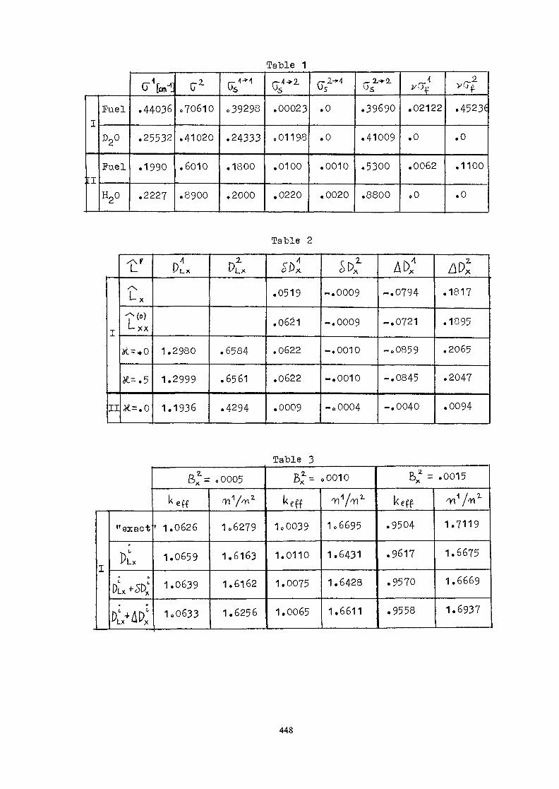
Table 1

I

[I

Puel

B20

Puel

H20

cr'fcm.44036

.25532

.1990

.2227

^

0 70610

.41020

.6010

.8900

r-1-*1§>o 39298

.24333

.1800

.2000

<%"*1.00023

o 01 1 98

.0100

.0220

,-2-H(fs.0

.0

.0010

.0020

,-Z 2.5s

.39690

.41009

.5300

.8800

1»%

.02122

.0

.0062

.0

vGV.45236

.0

.1100

.0

Table 2

I

II

t'^^Lx

•-^(o)>-xx

Jt=*0

at=.5

K=.0

Di.

1.2980

1.2999

1.1936

Pi

.6584

.6561

.4294

£i>x

.0519

.0621

.0622

.0622

.0009

&

-.0009

-.0009

-.0010

-.0010

-00004

At>x1

-.0794

-.0721

-00859

-.0845

-.0040

Ati.1817

.1895

.2065

.2047

.0094

Table 3

I

"exact

Ptx

DLX +$£

fcW*

BX = "0005

k e f |

1 1.0626

1.0659

1.0639

1o0633

•TiY'n2

1 06279

1.6163

1.6162

1.6256

B* = 00010

ke f f

1,0039

1.0110

1.0075

1.0065

^y/vi2-1o6695

1.6431

1.6428

1.6611

B* = .0015^

keff

.9504

.9617

.9570

.9558

•Yl1/^1

1.7119

1.6675

1.6669

1.6937

448

NEUTRON STREAMING IN GCFRS AND HTRS

P. KOHLERSwiss Federal Institute for Reactor Research,Wiirenlingen, Switzerland

Abstract

A numerical method for the calculation of diffusion coeffi-cients for GCFR and HTR lattices considering the exact geo-metry is developed. For infinite regular GCFR lattices re-sults for the axial buckling dependent streaming correctionare given. For irregular GCFR lattices whose coolant chan-nels can extend only within one fuel element the dependenceof both radial and axial streaming corrections on the fuelelement size is studied. For hexagonal HTR lattices a compa-rison of the numerically calculated diffusion coefficientswith the analytical formulae of Benoist is made.

1. Introduction

In the coolant channels of gas cooled reactors neutrons canfly very far without suffering a collision. As a consequenceof that the diffusion coefficients of lattices of these reac-tors have values which are greater than those which would beobtained by a simple homogenization of the transport crosssections. As the streaming paths through the coolant chan-nels in a GCFR and a block design HTR are longer in theaxial direction than in the radial direction, the diffu-sion in these lattices is also anisotropic. The aim of thetheory of neutron streaming is to calculate correctly thediffusion coefficients in both radial and axial directions.

The streaming problem is more difficult for a GCFR than foran HTR. The reason is that in an infinite regular lattice ofan HTR the coolant channels (which can be treated as voidchannels for both reactor types) are infinite only in theaxial direction whereas in an infinite regular lattice ofa GCFR they are infinite in both directions (see Fig. 1). Itwas recognized already in 1949 by Behrens (1) and later men-tioned by Benoist (2_) that the presence of such two dimen-sionally infinite gaps leads to divergence of the diffusion

449

coefficient in the case of an infinite lattice. This pointwas ignored in first theories of the GCFR streaming (3) andthe difficulty was simply avoided by defining a cylindricallattice cell with unrealistic boundary conditions. The theoryof Eisemann (4_), which gives a correct treatment of the geo-metry, leads, in fact to a diverging formula for the diffu-sion coefficient of the infinite lattice, However, Eisemannobtained by his formula a finite result due to an inaccuratenumerical integration. He also used the actual cross sectionof the coolant and, in this case, the formula for the diffu-sion coefficient does not diverge but it is clear that itwill give incorrect results for very small coolant crosssections.

In our first work (5_, 6_) only the axial streaming problem inGCFRs was studied. The actual reactor height and the axialflux shape were taken into account and a buckling dependentaxial diffusion coefficient [which diverges only for zerobuckling) was defined. A code DIFFAX was written which calcu-lates the buckling dependent axial diffusion coefficient nu-merically .

In a later work (_7) the code was generalized in the sensethat the finite size of the fuel element containing the hexa-gonal lattice of the fuel rods was taken into account, Thelattice inside a neighbouring fuel element and all followingfuel elements was shifted so that the streaming channels canextend only within one fuel element, For such a lattice theEisemann's method does not diverge and both radial and axialdiffusion coefficients can be calculated. For the axial diffu-sion coefficient also the non-zero axial buckling calculationwas kept.

The Eisemann's method was programmed also for a hexagonallattice of an HTR (8_) . For this lattice there are no difficul-ties with a divergence of the formulae because the cylindri-cal streaming channels are infinite only in one direction.The numerical results were compared with analytical ones ob-tained by Benoist's theory.

450

2. Formulae for the diffusion coefficients

Let us consider an infinite, axially homogeneous lattice, whoseidentical cells contain two materials; fuel with a total crosssection I and void. Because in both reactor types all the ma-terials except the coolant have total cross sections of thesame order of magnitude these materials can be smeared intoone called fuel. We consider only one energy group because itis known that the influence of the parameters of other groupson the diffusion coefficient of a given group is very small.We also consider that the scattering is isotropic. Eisemannshowed that scattering anisotropy can be taken inot accountby the following simple formula:

(1)

where Z, is the homogenized total cross section of the lat-tice cell and S, is the homogenized first moment of thehornscattering cross section.

The transport equation describing the one group isotropic caseis

f * ^ -T(r,£'J+ (r) = c dr'ZCr'H(r') -—-———=• (2)i 4ir|r-r'[

where i(r,r') is the optical path between the points r and r'and c is the number of secondaries.

We will now derive the formula for the buckling dependentaxial diffusion coefficient. Eisemann's formula will then beeasily obtained by putting the buckling equal to zero,

We assume that the flux is radially constant and has a co-sine shape in the axial direction. This means that the flux<j>(r) can be replaced by <f>(z) and, because of the cosine shape.

= <J>(z)cosBCz-z') - z sinBCz-z'J (3)

451

where B is the square root of the axial buckling B a'nd <t>'(z)is the first derivative of the flux <|>(z), Introducing thisinto equation C2) and separating the integration in r' intoa radial integration in p' and an axial integration in z'we obtain

i(z) = c<|>(z) [dp'Z(p') fdz' -—————=———M~^? cosB(z-z') (4)J 4ir[(p-p») +(z-z') ]

where x(p,p') is the projection of the optical path on theradial plane. The term containing the derivative of the fluxhas vanished because of the antisymmetry of the sine. Fromthis equation we can obtain the average collision density inthe cell:

iz« 2——^-5—5——r ^ 2 cosBCz-z')fuel ~ ,..,

Remembering that for zero buckling (flat flux) c must be unityand therefore

dz'cell

(6)

2 1we can replace cosBCz-z'J in equation (5) by 1-2 sin (j B(z-z'))and introduce(6) into (5), The resulting equation is

cell .V „ ,fuel

4Tr[Cp-p')2+Cz-z')2] 2sin24 B(z-z')) (7)

452

We require that the diffusion equation

__2 dz

or, in our case with the cosine flux shape, the simple expression

-D B2<j>(z) + Cc-DZ. 4>Cz) = 0 (9]z horn

should be equivalent to the transport equation (7). The compa-rison of equations (9) and (7) shows that this will be the caseif we choose the diffusion coefficient D as follows:

2

dp'S(p') I dx S————_ ^ ^ ;M H / sin"(^ Bx)cell oo 0 ^" (-^ K > ~ i

fuel (1Q)

The eigenvalue c can, in all practical cases be approximated byunity. (Theoretically it is possible to eliminate it using the

DB^formula c=1+ •=——.) Substituting for the integration variable.-». ->. ^-homx=|p-p'|tg9 we obtain as the final expression for the bucklingdependent axial diffusion coefficient:

D = ———=• I f dp f d p ' E t p 1 ) f d9B J J 1

7T/2 -T(p,p')/cose

r n o( B|p-p' |tg6 £ 1 1 )

For the irregular GCFR lattice and for the HTR lattice B can beput equal zero and we get

DzZ

TI/21cell

vfuel

453

The corresponding expression for the radial diffusion coeffi-cient is

(13)cell ./

Vfuel

3. Benoist's formulae for HTR lattice

For our purposes a cell of an HTR lattice consists of a centralcylindrical hole surrounded by fuel. Benoist gives in his work(9_) approximative formulae for a three zone cell. Formulae forthe HTR cell are obtained putting the radius a of the innerrod equal to zero. With our notations we get

Dr = -^ VCBll + Vvoid + 1. \/oid c (1. ^.j (14Jcell

n _ 1 cell___void <- vua.u r i c iuz - -—-——— - -——— c I isj^ cell

where c is the radius of the void channel and

(16)vC2j;2 - 3cE + 1 void

2 Vfuel

4. Results for GCFR lattices

Details about the numerical calculations using formula (11) forinfinite regular GCFR lattices are to be found in (5). Fig, 2shows the values of the axial streaming correction (defined asthe difference between the value obtained using (11) and thehomogeneous value of the diffusion coefficient) for the powerreactor design of the Nuclear Research Centre, Karlsruhe (KFZ).In this case the radius of the fuel rods is 0,37 cm, the pitch

-4 -2is 1,08 cm and a value of 10 cm was assumed for the axialbuckling, The calculation was performed for several values ofthe fuel cross section corresponding to different values ofthe homogenized diffusion coefficient, Fig, 3 shows similar

454

results for the EIR fast reactor design, The radius of thefuel rods is in this case 0,3 cm, the pitch 0,95 cm and the

-4 -2axial buckling is 2.47 x 10 cm . For the Karlsruhe designand for one particular value of the cross section the calcu-*

-3 -2lation was performed for three values (10 cm , -4 -210 cm-5 -2and 10 cm ) of the axial buckling. The results are shown

in Fig. 4 which indicates clearly the linear dependence ofthe streaming correction on the logarithm of the buckling.

The results for both the radial and axial streaming correctionfor the irregular infinite GCFR lattice (finite size of fuelelements) are shown in Tables 1 to 3. The calculations weremade again for the Karlsruhe design. Because the dependenceof the streaming correction on the fuel rod total cross sec-tion is very weak the value of the cross section was varied in-1 ,-ja very broad range between 0.3 cm and 3,0 cm although thevalue of 3.0 cm is no more caracteristical for the fast re-actor. For the dimension across flats of the hexagonal fuelelement the values 10 cm, 20 cm and 40 cm were chosen.

Table 1

Streaming correction of the diffusion coefficients-1for £ = 3.0 cm

AD z

AQr

^X^ dimension^x. across

\flats

z ^\

ID'3

ID'4

0

0

10

0,200

0,208

0.212

0.085

20

0.223

0,235

0.240

0,101

40

0.241

0 ,258

0.267

0.117

CO

0 ,254

0,304

CO

00

455

Table 2

Streaming correction of the diffusion coefficients-1for Z = 0.6 cm

dimensionacross 10 20 40

AD ID'4 0.151 0.163 0,191 0,243

0.155 0.168 0.200

AD 0.065 0,063 0 ,075

Table 3

Streaming correction of the diffusion coefficientsfor Z = 0.3 cm"

dimensionacrossflats 10 20 40

10-4 0.139 0,139 0.157 0.215AD

0.144 0,145 0.169

AD 0.064 0.059 0.062

5. Results for HTR lattices

We made test calculations which were typical for the planed plu-tonium HTR lattice of our reactor PROTEUS, The pitch of thevoid channels was 4.33013 cm, the void channel radius was 1.049 cm~1and for the total fuel cross section the values 0.094804 cm_1and 0.423494 cm were chosen. The smaller value is characte-ristical for the fast neutrons, the larger value for the ther-mal neutrons. The results of our numerical calculations andof the calculations using Benoist's formulae are summarized inTable 4. The second column of the Table 4 shows the value ofthe diffusion coefficient which is obtained through a simplehomogenization. This value neglect the streaming.

456

Table 4

Diffusion coefficients for an HTR lattice

I

0.094804

0.423494

horn.

4.46704

1.00000

D Benoistr

4.4394B

1.04165

D Benoist

4,41346

1.10356

D formula (13)r

4.55862

1.05955

D formula (12)z

4,62250

1.12095

6. Discussion of the results

The calculations for GCFR lattices show that in the neutron ener-gy range which is important the streaming correction dependsonly slightly on the fuel cross section. Also the buckling de-pendence of the streaming correction for an infinite regularlattice is not marked. For the irregular lattice and for zerobuckling there is a difference in the behvaiour of the streamingcorrection between large and small cross sections. For largecross sections (which are, however, not typical for the GCFR)both the radial and axial streaming correction depends loga-rithmically on the fuel element size. For small cross sectionsthe streaming corrections are almost independent of the sizeup to about 20 cm across flats and only for larger sizes beginto increase. The explanation for this effect is that for smallcross sections and small element size a large contribution tothe streaming correction comes not only from neutrons whichpass through the streaming channel of the reference elementbut also from neutrons which pass through the streaming chan-nel of a neighbouring element. For an HTR lattice the Benoist'sapproximative formulae give a reasonable estimation of the mag-nitude of the streaming corrections only for large values ofcross sections. Table 4 shows that for small values of crosssections the Benoist's streaming corrections become completelywrong. Both diffusion coefficients are smaller than the valueobtained by a simple homogenization and the axial diffusioncoefficient is smaller than the radial one. Both these effectsare physically impossible.

457

Literature

(1) D.J. Behrens:The Effect of Holes in a Reacting Material on the Passageof Neutrons,Proc. Phys. Soc. London 62A (1949)

(2) P. Benoist:Theorie du coefficient de diffusion des neutrons dans unreseau comportant des cavites,CEA-R 2278 £1964)

(3) B. Pellaud:The Physics Design of the Gas-Cooled Fast BreederReactor Demonstration Plant,GA-10509 (1971)

(4) E. Eisemann:Anisotrope Diffusion bei gasgekuhlten schnellen Brutreaktoren,KFK 1577 (1972)

(5) P. Kohler, J. Ligou:The Axial Streaming Problem in Gas-Cooled Fast Reactors,EIR 244 (1973)

(6) P. Kohler, J. Ligou;Axial Neutron Streaming in Gas-Cooled Fast Reactors,Nucl. Sci. Eng. J54, 357 (1974)

(7) P. Kohler:Einfluss der Grb'sse der Brennstoffelemente auf dasStreaming in gasgekuhlten schnellen Reaktoren,EIR internal report TM-PH-512 (1974)

(8) P. Kohler:Berechnung des radialen und axialen Diffusionskoeffi-zienten fur das hexagonale Gitter eines HTR Block-reaktors,EIR internal report TM-PH-666 (1977)

(9) P. Benoist:Streaming Effects and Collision Probabilities in Lattices,Nucl. Sci. Eng. 34, 285 (1968)

458

REFERENCCELL.

FUEL•••CLAD.

COOLANT(VOID)

Eu

0.30

6.C.F.R LATTICE

FIG. 1

^THERMAL ENERGY

0.25

0.20

[ JBCFR ENERGY RANGE j0.20<4D<0.23

0.15

X*-EISEMANN

,-BENOIST

FIG. 2

E>1MeV

I I

7 8 9D(hom) (cm)

459

AD (cm)0.30

0.25

0.20

GCFR Energy Range !

0.15D (horn) cm

FIG. 3

£U

0.35 0.35

0.30 GCFR 0.30

PROTEUS

0.25 0.25

0.2010-6 10' 10'

FIG. B2(cm'2)10,-3

460

METHODS FOR THE CALCULATION OF STREAMINGCORRECTED DIFFUSION COEFFICIENTS FOR PINAND PLATE CELLS IN FAST REACTORS

M.J. GRIMSTONEUnited Kingdom Atomic Energy Authority,Atomic Energy Establishment,Winfrith, Dorchester, Dorset,United Kingdom

Abstract

Methods are discussed for the calculation of equivalent homogeneouscell diffusion coefficients which reproduce the leakage from heterogeneouscells in sodium cooled fast reactors. The problem is considered for powerreactor pin fuel and for pin and plate fuel of the types used in zero energyassemblies. Alternative approaches have been compared including the use ofthe discrete Sn and collision probability methods as well as more approximatetechniques. The methods are described, and results of the validation testsare given. These include calculations for both the normal sodium floodedcondition and the voided condition. Typical values of the streaming correctionsto the cell diffusion coefficients are given and estimates of theirinfluence on the sodium void effect are made.

1. INTRODUCTION

In a sodium cooled fast reactor the leakage is enhanced by neutronstreaming in the sodium flowing between the fuel pins and in the sodium inthe gaps between subassemblies. The change in calculated keff values ifthis is taken into account has been estimated to be typically of the orderof -0.2$> under normal conditions. In the hypothetical sodium voidedcondition, however, the streaming effect is about twice as large, and thiscan lead to a significant increase in the magnitude of the negative leakagecomponent of the sodium void reactivity effect. Since the total sodiumvoid effect is the sum of a positive central term and the negative leakageterm, the streaming effect may become an impoi^tant contribution. In acompanion paper (1) it is estimated, for example, that the heterogeneitycorrection to the maximum positive sodium void effect in a 1300MW(e) reactoris -12% of which -\\% is the streaming correction. In zero energy fast reactorassemblies using either pin or plate fuel the configuration is often moreheterogeneous than in porfer reactors and the streaming effects are thereforegreater. This means in particular that the proper analysis of many sodiumremoval measurements requires an allowance for the effect of streaming.

When diffusion theory is used for whole reactor calculations theeffect of streaming may be taken into account by calculating homogeniseddiffusion coefficients chosen to reproduce as closely as possible theleakage from the actual heterogeneous cells. In general there will be adifferent coefficient in each direction. A programme of work is beingcarried out at Wiifrith to establish methods for deriving streamingcorrected cell diffusion coefficients for use in calculations for commercialfast power reactor designs and for zero energy assemblies, in particularZEBRA. As with other heterogeneity effects, streaming effects will becalculated usually for somewhat simplified geometric models of the cells,and the first stage of this work has been to study methods applicable tothese simple geometries. The purpose of this paper is to describe themethods which have been established and the calculations carried out toexamine their accuracy. From these studies, and from others such as thosecarried out at ANL (2), it is clear that the calculated streaming effectscan be very sensitive to the modelling procedure, and a further stage of thework will be to test modelling methods against three dimensional referencecalculations.

461

For pin fuel the simplified model considered here comprises a latticeof pins, uniform in the axial direction and regular in the radial plane.For fast power reactors this lattice is normally triangular, while the pinfuel used in zero energy assemblies is commonly on a square lattice.The simplified plate cells are represented in one-dimensional slab geometry.To preserve the composition of the cell the material of components such asthe fuel element wrapper or sheath is redistributed in some way over thesimplified system. An important feature of such systems is the presenceof regions extending infinitely in two-dimensions and containing either avoid or material with a low macroscopic neutron cross-section. In thecase of pin fuel these regions are the gaps between rows of pins. Theseregions can have a strong influence on the streaming effect, and thereforeon the choice of suitable methods of calculation. It is a property of buckling-independent definitions of the cell diffusion coefficient such as that ofBenoist (3) that the coefficient parallel to such regions becomes infiniteif they are completely voided. In view of this it is likely also that thecoefficient will be overestimated if only material with a very low cross-section is present in the regions. The methods chosen for study in this worktherefore include approaches in which buckling dependence is retained, andalso in which the introduction of cylindrical boundaries in pin geometry isavoided since this can mask the effect of the two-dimensional gaps. Thesemethods have provided reference results against which to test moreapproximate techniques. In the following sections the relationship of thestreaming calculations to the rest of the homogenisation route used in theUK is indicated, the theoretical basis of the streaming methods studiedis summarised, and some practical aspects of their implementation aredescribed. Finally, results of some of the calculations carried out to validatethe methods are given.

2. DEFINITION OF THE STREAMING CORRECTION

The UK methods for deriving average parameters for heterogeneous cellsare summarised in Reference (1). The code employed principally is MURAL (^)which carries out a fine group flux calculation for the cell using a fine groupcross-section library, and thus derives cell-averaged broad group cross-sections. The conventional method of obtaining diffusion coefficients is touse the normal homogeneous medium formula with the cell-averaged broad grouptransport cross sections from MURAL:

I _^.-fcr

The approach which has been adopted for obtaining streaming correctedanisotropic diffusion coefficients is to apply 'streaming corrections',one for each direction, to the value given by Equation (1). One of themethods described in the following sections is used to calculate adiffusion coefficient Dk in a particular direction using the broad groupcross-sections for each cell region produced by MURAL. The same method isthen employed to obtain the limiting value Djjom as the cell dimensionstend to zero or, equivalently, the value for the homogeneous cell withcross-sections which are a volume weighted average of those used for theheterogeneous cell. The streaming correction factor is then defined as

^

The results quoted in this paper are given in terms of this streamingcorrection.

3. THEORETICAL BACKGROUND OF THE MSTHODS USED

The methods for calculating cell diffusion coefficients which have beenused in these studies may be divided into the following classes: methods inwhich a buckling dependent coefficient is obtained by imposing a bucklingmode onto the flux and source in the cell, methods using simple finitesize core models, and methods Reading to buckling-independent coefficients.The theoretical background of these methods is summarised in this section.

462

3.1 METHODS F05 BJCKLING-DEPENDENT DIFFUSION COEFFICIENTS

The common feature of these methpds is that the transport equation issolved for an infinite lattice of cells by assuming the angular flux to beseparable into a slowly varying function of the form exp (iB.r) , where Bis the buckling vector, and a function W(r,A) which is periodic in thelattice. This commonly used separation is discussed for example byLeslie (5) and by Brissenden (6), and a similar approach has been describedby Rumyantsev (7). The neutron leakage . L^ in a direction k is calculated,and the diffusion coefficient D^ in this direction is then obtained fromthe relation

* = K (3)

where (]) is the integrated flux over the cell. In approaches such as thatof Benoist an expansion in powers of B is made, and this is truncated insuch a way that the resulting diffusion coefficient is independent ofbuckling. The methods described in this section do not make this expansion,and so produce a buckling dependent coefficient.

Brissenden (6) has applied this approach to the differential form ofthe transport equation in the one-dimensional Sn code WDSNST to enable leakagein the other coordinate directions to be calculabed. For example, inthe case of slab geometry, if there is a buckling B in one lateral direction,x say, the angular flux is assumed to be of the form

p(^8x)rw, (*,->!) * -c wjz/-ji)] (W, (Zyg) - SLU g*. W^Z, -H.)

A similar form is assumed for the source function, and if these aresubstituted into the transport equation

-f- Z_t T ~~ o

the result is a pair of linked equations

•fl-i "^T r ^e i = i "*" 'J x x (6)

which may be solved iteratively. It can be shown that the scalar flux isgiven by

and the x-direction current by

W, fz -0-N dA (8)— —,i

and by considering the leakage from any slice bounded by planes perpendicularto the x-axis it is found that the diffusion coefficient as defined byEquation (3) is given by

J(9)

463

A more detailed account of this method is given in Reference (6). The WDSNSTcode may be used in this way to calculate an axial diffusion coefficient fora cylindrical geometry cell uniform in the axial direction, or coefficientsin the lateral directions for a one-dimensional slab geometry cell. The useof WDSNST in cylindrical geometry for pin cells involves the approximationof having a cylindrical boundary for the single-pin cell, so its mainuse as a reference method is for plate cells, and in Section *+ some furtherdetails of its use in this context are given.

Leakage may also be treated in a similar way in the integral transportequation. To illustrate this we consider the one-energy equation withisotropic scattering:

where (r,]?') is the optical path length between two points. Supposefor example that the system is uniform in the axial (z) direction with abuckling B in this direction. The substitutions

(11)

where ^0 = ( *, , C_)lead to the modified equation

' dr' (12)4- ''I

If this equation is integrated over the regions of the cell the usualcollision probability equations

(13)

are obtained provided that the usual definition of the collision probabilityis modified by the inclusion of the factor cos Bz'. These modified collisionprobabilities satisfy the usual reciprocity relations, but because of theleakage the conservation relations do not apply i.e.

P-- < I (TOJj = l

If the collision probability equations are solved, the leakage can then becalculated from the neutron balance, giving finally the following expressionfor the diffusion coefficient

(15)-,X <c~i % , iB 4-jV- <p-

L. L *•

A more detailed account of this method is given by Doherty (8) for the caseof axial leakage from a cylindrical cell. MacDougal has applied themethod to the problem of lateral leakage from plate cells and this techniqueis available as an option in the MURAL code ('f). The method of Kohler andLigou (9) is similar except that instead of the collision probabilityequations being solved, a simple solution is assumed, viz

<$>i = constant (0, say)

464

where c is the eigenvalue representing the mean number of emergent neutronsper collision. The diffusion coefficient given by Equation (15) thenbecomes

2 ~ B X.C..C VC \jNote that c has been set to unity in this expression. This is acceptable

for the purposes of calculating a streaming correction provided that the sameassumption is made in obtaining the corresponding homogeneous coefficient.

This method is incorporated in the EIE Wurenlingen code DIFFAX forcalculating axial diffusion coefficients for GCFK pin cells, avoiding theuse of the cylindrical boundary approximation. This code has been implementedat Winfrith, and Section k gives some details of the code and of new optionswhich have been added. The method of Kohler and Ligou has also been used forplate cells in these studies.

The integral transport equation in the form of Equation (12) can alsobe solved for pin lattices using the Monte Carlo programme WMONTE (10).An example of the use of this code is given in Section 6, but at presentthe accuracy which can be achieved for the diffusion coefficients within areasonable running time is insufficient for the reliable estimation of thesize of the streaming effect. A similar Monte Carlo technique has alsobeen used by Gelbard (2).3.2 METHODS EMPLOYING SIMPLE FINITE REACTOR MODELS

In Section 3-1 Methods were described of calculating diffusioncoefficients by imposing onto a transport solution a flux shape in the formof a buckling dependent function across the call. An alternative approachis to arrange for the flux shape to be determined as part of the transportsolution. In this case a simple reactor model is set up, composed entirelyof the one type of cell, and of a size chosen to give the required bucklingand transport theory is used to calculate the leakage in the requireddirection. The cell averaged diffusion coefficient is again obtained from therelation of Equation (3) where j[ is the flux integrated over the reactor modeland Bjj is the geometric buckling in direction k with allowance for theextrapolation length. In Section 5 results are given which illustrate the useof this method to obtain diffusion coefficients for plate cells in both theparallel and perpendicular directions using WDSNST, and the two-dimensionaldiscrete Sn code DOT (11).3.3 ZERO BUCKLING FORMULAE

The formula of Benoist (3) is probably the most widely used of the classof definitions of cell diffusion coefficients in which the expansion interms of buckling is truncated so that the coefficient is effectively a zerobuckling value. If the absorption correction term is omitted the diffusioncoefficient for a direction k is given in terms of a weighted average of thetransport mean free paths:

\ '= i j ^ * t ;>b Zj (18)

* <•where Pij,k are 'transport probabilities'. For practical purposes thetransport probabilities are usually replaced by their principal terms PJJ jj,the directed first collision probabilities, defined by

p .. ~J I J-. / -I-' 3 0~ **PL~ "v- '- J I (19)rij,te

465

In fact if isotropic scattering is assumed and k is a direction in which.the material properties of the cell are uniform, then the angularcorrelation terras of Pij,k vanish, so that only its principal terra Pii kremains. The use of first-collisionprobabilities is thus an 'approximation only for non-uniform directions.In Appendix VIII of Reference (3) Benoist presents a method for calculating.diffusion coefficients for lattices having a pitch very much smallerthan the neutron mean free path. This is based on Equation (18), butuses approximations for the directed collision probabilities. A procedurefor evaluating this 'Tight-Packed Lattice Formula' for pin cells is describedby Gregory (12), and another procedure which avoids some of the approximationsis given by Pellaud (13). Examples are given in Sections 5 and 6 of the useof both of these methods for pin cells, together with results from theexact formula for plate cells.

Benoist shows that Equation (18) is equivalent to a formula involvingmean square projected distances to absorption which is a generalisationof the classical definition of the diffusion coefficient for ahomogeneous medium. Eisemann (I't) has employed the mean square distanceformulation to calculate diffusion coefficients for GCFR pin lattices. Hismethod can include an allowance for anisotropic scattering. In the case ofisotropic scattering, which is the form in which this method has beenused in the present studies, the diffusion coefficient for the k direction isgiven by _

(20)

where a T f (21)

Equation (20) is equivalent to

3> - i: dk (22)where 2. is the cell-averaged transport cross-section and djj is thecell-averaged mean square projected path length, the average beingcalculated by volume weighting i.e. assuming a flat flux. The classicaldefinition of D^ to which Benoist's formula, Equation (18), is equivalent is

1) = ± "V I? (23)

where 1^- is the mean square projected 'crow-flight1 distance from birthto absorption. This may be separated into a principal term, identical tothe right hand side of Equation (22), and a further term arising fromcross products of path lengths. These terms in fact correspond to theprincipal term and the angular correlation terms of Benoist's transportprobabilities. Thus Eisemann's formula with isotropic scattering isequivalent to the Benoist formula employing first collision probabilitiesand a flat flux. Finally it may also be observed that the mean squareexpression of Equation (20) also represents the limit as the bucklingtends to zero of the Kb'hler and Ligou formula, Equation (1?). The methodof Eisemann is used for certain options in the DIFFAX code, and these aredescribed in Section k. As stated in the introduction, these zero bucklingformulae diverge in the case of celldiffusion coefficients calculatedparallel to two dimensional infinite void gaps.

if. SOME DETAILS OF THE COMPUTER CODES

A-.1 VDSNST

In Section 3«1 a method was described for treating lateral leakage inthe one-dimensional differential transport equation and thereby calculatingcell diffusion coefficients. This method is incorporated in the discrete

466

ordinates Sn code WDSNST. The main problem encountered in the applicationof this code to plate cells was the choice of suitable angular quadraturesets; that is, the discrete directions at which the angular flux solution isobtained. The application of the discrete ordinates method to thin platecells has been studied by Meneghetti (15)) who examined the rate of convergenceof the solution with respect to the number of discrete directions for varioustypes of quadrature. He observed that convergence became slower as thethickness of the regions was reduced, and that very much more rapid convergencewas achieved with double Gaussian quadrature or with a modified double Gaussianquadrature, than with single Gaussian and uniform sets. This was becausein the former sets the directions are concentrated more closely towards thedirection parallel to the plates.

The discrete directions originally built into the WDSNST code areillustrated in Figure 1(b). The directions correspond to points on the surfaceof the unit sphere, and the points in one octant are defined in the followingmanner. For an Sn quadrature set the surface is first divided into n/2 'slabs'.The second slab is then divided into two equal areas, the third into three,and so on. The heights of the slabs are chosen so that all the divisionshave the same area. One quadrature point is placed in each division andequal quadrature weights are assigned to all the points. The positions ofthe points within their divisions are chosen in such a way that the mostimportant low order moments of an isotropic flux are integrated exactly.The programme automatically generates such sets for any Sn order specified.This uniform set performs well at low Sn orders for most applications.For treating axial leakage in. thermal reactor cell calculations, or fortreating whole sodium channels in fast reactors, orders no higher than S8 arerequired. The dimensions of the regions of fast reactor cells are so muchsmaller, however, that very high orders are required to achieve convergence.For both pin and plate cells, with region dimensions of the order of 3 to 6 mm,orders as high as 896 have been used without satisfactory convergencebeing achieved.

For more rapid convergence of fast reactor plate cell calculationsquadrature sets are required in which more directions are concentrated towardsthe x-y plane. In order to ensure a minimum of disturbance to the method ofsolution, the new sets developed for use in WDSNST preserve the existingorientation of the angular coordinate system and the arrangement of pointson levels of constant "Q . Thus, referring to Figure 1, the points must beconcentrated towards the u-iv plane. Clearly such a non-uniform set impliesthe introduction of unequal weights, and the further generalisation has beenmade of allowing the number of points on the first level to be greater thanone. The new sets are then defined in the following way, which is illustratedin Figure l(c). For an Sn quadrature set n/2 levels of constant 6 are placedin one octant. These are defined by taking ^ (= cos 6 ) as the positivepoints from the n-point Gauss-Legendre quadrature set in the range (-1,1).

On level i we place i + m - 1 points defined by 0 =Tf<*/2 where the valuesof oC are the positive points of the 2(i+-m-l)-point Gauss-Legendrequadrature set on the range (-1,1). This procedure tends to concentrate thepoints towards the u-w plane as required. The set is not symmetrical withrespect to the u and w directions, as would be preferred, but the value of mthe number of points on the first level, may be chosen to give the bestsymmetry. It has been found that a value of m = 4 gives reasonable symmetryover the range of Sn orders normally used. WDSNST has been modified tohandle this alternative type of quadrature set, and routines have beenadded which generate the directions and weights for any specified valuesof n and m.

Results obtained with the two types of quadrature set for simple platecells are shown in Figure 2. The cells comprise two regions representingfuel and coolant plates, and their dimensions and one group cross sections aregiven in Table 1. Because of the parameter m, the actual number of directionscorresponding to a given Sn order may be different in the two methods, thenumber per octant being given by

467

for the uniform quadrature sets, and byW - -s- ( /\ .*

for the Gaussian sets. In order to make a fair comparison the resultshave therefore been plotted on a scale linear in /N, and the Sn orders forboth quadrature sets are indicated. The Gaussian sets were all used -with thevalue of m = 4. For Cell 1, representing a plate cell containing sodium,the uniform set is only just approaching convergence at 896, while with theGaussian set convergence is achieved at about Sl6. For Cell 2, which representsa model of a sodium voided cell in which some structural steel has been smearedover the 'void' region, both methods appear to converge less rapidly, but onceagain the Gaussian set is clearly far better. Full convergence requires aboutS48, but the streaming correction at the peak value at S20 is only about 0.1%higher than the converged result. Cell 3 represents a model in which thecoolant region is completely voided. In such a model it is clear from thedivergence of the zero buckling diffusion coefficient that the behaviour of thesolution will be strongly dependent on the value of the buckling. In thiscase the value used was Bx2 = By2 = 3.9?6 x 1Cr cm"2. Only the Gaussian sethas been applied to this cell, and it may be seen from Figure 2 that this modelrepresents the most difficult problem, requiring an order of about S72 forconvergence.

The diffusion coefficient for a homogeneous medium, required in orderto define a streaming correction, may be calculated by WDSNST with order Sk.It has been verified that the value given by WDSNST agrees very closelywith the analytical formula which may be derived by applying the procedureof Section 3-1 to a homogeneous system. With isotropic scattering this is:

or with anisotropic (P1) scattering:£

where i^ is the first moment of the differential scattering cross section.

4.2 DIFFAXThe DIFFAX code was developed at EIR, Wurenlingen, to calculate diffusion

coefficients for GCFR cells. The original code treats an array of pinsseparated by a void and arranged on a triangi'lar lattice, so that the basicsingle-pin cell has a hexagonal outer boundary. Allowance may be made forthe disturbance of the regular pin lattice by subassembly boundaries. Thishas the effect of limiting the extent of the two-dimensional streaming gapsbetween rows of pins, and it is taken into account in the programme byspecifying the relative displacement, or shift, of rows of pins on either sideof a subassembly boundary. The axial diffusion coefficient is calculated bythe buckling dependent formula of Kohler and Ligou (Equation (1?)). Detailsof the method of evaluation are given in Reference (9). An important featureof the method is that buckling dependence is retained in those terms whichdiverge as the buckling approaches zero in an infinite regular lattice,but that the buckling is set to zero in the other terms. This leads tothe following expression for the axial diffusion coefficient:

(26)

where x^ is the sum of optical paths in the first to the (l-1)th pins ofintersection, €. 0 is the optical path in pin 0, and the other quantities

468

are defined in Figure 3- This expression is evaluated by numericalintegration in the variables <p and f , the integrations over 6 beingapproximated by series-expansions in terms of Bickley functions. Theradial diffusion coefficient is calculated by the method of Eisemann. Fulldetails of the evaluation of this formula for a triangular pin lattice aregiven in Reference (14). The evaluation proceeds in parallel with that of theaxial coefficient since it involves integrations analogous to those inEquation (26). This radial coefficient is valid only for calculationsin which the effect of subassembly boundaries is being taken into accountby means of a non-zero "shift1 so that there are no infinite two dimensionalstreaming gaps.

DIFFAX has been implemented at Winfrith and its facilities have beenextended so that it can be applied to sodium cooled fast reactor cellsincluding the type of pin cell, commonly used in zero energy assemblies,which has pins arranged on a square lattice. To treat sodium flooded cellsthe programme has been extended to allow for a non-zero coolant cross-section.In view of the small effect of buckling in the flooded situation observed incalculations for plate cells, Eisemann's zero buckling formula has beenemployed for this purpose, following the method described in detail inReference (1*0. For the square lattice option the main additions requiredwere in the calculation of distances to points of intersection with pinsalong the lines of the integration mesh.

Some care is required in the calculation of the homogeneous diffusioncoefficient used to obtain the streaming correction. The homogeneous limitof the buckling dependent formula of Equation (17) is

where HO. is the cell averaged transport cross section obtained withvolume weighting. (Note that the difference from the B1 formula ofEquation (24) occurs because the eigenvalue c is set to unity, as describedin Section 3«1«) However, this is not the appropriate value to use with thebuckling dependent axial coefficient is calculated by DIFFAX because of theapproximation made in setting the buckling to zero in some terms. If thehomogeneous limit of Equation (26) is determined by allowing the dimensionsof the cell to tend to zero it is found to be

(28)

where f is the void fraction. Clearly this is a weighted mean of thebuckling dependent and buckling-independent homogeneous coefficients. Thisformula should therefore be used in association with the axial coefficientcalculated by DIFFAX for the voided situation, while

should be used with the buckling-independent coefficients which arecalculated in all other cases.

A more flexible way of specifying the integration mesh has also beenintroduced, and tests have been carried out to establish suitable meshes.In general it has been found that to ensure an error of less than 0.1$in D requires of the order of 60 <p-meshes , concentrated towards the lowestangles, and about 40 ^ -meshes in voided cases or about 120 in caseswith coolant present.

4.3 DSLABAIn Reference (9) Kohler and Ligou apply their general definition of the

buckling dependent diffusion coefficient, Equation (17), to the particularcase of a two region cell in slab geometry, deriving an expression for the

469

coefficient parallel to the slabs. This expression allows for a bucklingand for a non-zero coolant cross-section, but a formula is also given for thecase of zero buckling, and another, applicable when the coolant cross-sectionis zero, in which the buckling is set to zero in those terms which do notdiverge. The latter is similar to the approach adopted in the DIFFAXprogramme. These formulae, which involve a double integration over angularvariables, have been programmed in a code, DSLABA, which also evaluates thecorresponding homogeneous coefficients. Results froir> DSLABA are comparedwith those from WDSNST in Section 5.

5. CALCULATIONS FOR PLATE CELLS

5.1 COMPARISON OF ONE GBOUP CALCULATIONS

One group diffusion coefficients have been calculated by severaldifferent methods for three simple slab geometry cells. These are simplifiedtwo region models of a typical ZEBRA plate cell both with and without sodium.One region represents a sodium plate or a voided region and has the samethickness as these regions in the actual cell, while the other region hasthe smeared composition of the remaining fuel and steel with a thicknesschosen to preserve the correct average cell composition. The dimensionsand cross-sections for the three cell models are given in Table 1. Thedimensions are the same in all three cases and the cross-sections forRegion 1, the fuel region, also remain constant. The cross-sections forRegion 2 represent the following cases:

Cell 1 : A sodium flooded cell with steel from the element sheathand the sides of the sodium can smeared in with the sodium.

Cell 2: A sodium voided cell with steel from the element sheath and thespacer smeared into the 'void' region.

Cell J: A different model of the sodium-voided cell with all steelremoved from the void region.

The third cell model is of interest since Gelbard (2) has shown that forplate cells used in GCFR critical assemblies at AWL a one dimensional modelwith completely voided regions gives best agreement with Monte Carlocalculations for a three dimensional model. The same may not necessarily betrue for ZEBRA plate cells because of their different construction.

The bucklings assumsd for all three cells are:B 2 = B 2 = 3.9765 x 10-/f cm"2 BZP = 6.103 x 10" cnf2X «/

where the z axis is perpendicular to the plates.Table 2 shows the streaming corrections both parallel and perpendicular

to the plates as calculated oy four methods. Details of these calculationsare as follows:-

(i) DOT: This result was obtained from an (R,Z) geometry discreteordinates SN calculation in which the cell extended radially toa vacuum boundary at a radius chosen to give the required tota]radial buckling, i.e. a radius R where

where X is the average transport mean free path for the cell.The diffusion coefficient was obtained from the calculatedleakage as described in Section 3.2. Reflecting boundaryconditions were applied at the axial boundaries, and axialbu;kling was treated by m-ans of a DB - absorption applied in theform of a reduction of the scattering cross-section. Thequadrature scheme employed was one in which the direction cosineswith respect to the z-axis formed a double-Gaussian set. An orderof S16 (i.e. double S3) was found to be necessary for convergence.

470

The homogeneous diffusion coefficient was obtained from a similarcalculation using volume weighted average cross-sections. Theresult of this calculation was vsry close to the BI homogeneouscoefficient given in Equation (2*0.

(ii) WDSNST for the parallel direction: These results were obtainedusing the leakage treatment described in Section 3-1- h-6convergence with respect to Sn. order for these cells was discussedin Section .1. For Cells 1 and 2 the ajcial buckling was treatedby means of DB'- absorption applied as a reduction of the scatteringcross-section. Tests proved, however, that the parallel diffusioncoefficients were unaltered if this buckli.ng treatment was omitted,so for Cell 3 the axial buckling was ignored. Calculations werealso carried out for the homogeneous cell, and it was againverified that the B1 diffusion coefficient was obtained.

(iii) WDSNST for the perpendicular direction: These results wereobtained by calculating the leakage in a reactor model of infinitelateral extent but finite height, constructed by stacking sufficientof the two region cells to give an axial buckling as close aspossible to the required value. The homogeneous coefficient wasobtained from a similar calculation for a homogeneous reactorof the same height. The effect of.radial buckling on the axialcoefficient was not examined.

(iv) DSLABA: This programme, described in Section .3, evaluatesthe formula of Kchler and Ligou for the parallel diffusioncoefficient and the corresponding homogeneous value. This formulais derived on the assumption that the buckling parallel to theslabs is in one direction only. It has been shown however, that theparallel diffusion coefficients calculated by WDSNST are dependentonly on the total parallel buckling, Bx- + By2, and not on thedirection of the buckling vector. The results of the DSLABAcalculations using this total buckling should therefore be comparablewith those from the WDSNST calculations with bucklings in both xand y directions.

(v) Benoist formula: The formula used was as given in Equation (18)except that directional first-collision probabilities were used inplace of the transport probabilities. Thus the absorption correctionterm and the angular correlation term were neglected. The latterdoes in fact vanish for the parallel direction. The collisionprobabilities were calculated by numerical integration, and a flatflux was assumed. The parallel correction is not given for Cell 3since the Benoist diffusion coefficient becomes infinite in thiscase.

The parallel corrections given in Table 2 show good agreement betweenWDSNST and DSLABA for Cells 1 and 2, and fair agreement for Cell 3 whereDSLABA gives a slightly smaller correction. The Benoist corrections areslightly larger as would be expected since this is a zero buckling formula.The DOT calculation for Cell 1 gives a slightly lower correction than WDSNSTdespite the fact that the diffusion coefficients calculated for thehomogeneous system agree very closely. The difference is therefore probablydue to the difference in the flux shapes in the heterogeneous system for thetwo methods. WDSNST imposes the same buckling dependent shape on the fluxin both regions, while the shape as calculated by DOT is slightly differentin the two regions, as indicated by the ratio of the flux at the centre ofthe fuel region to its value at the centre of the sodium region, which variesfrom 1.002 at the core centre to 0.991 at the radial boundary. Thus theeffective buckling is smaller in the sodium region than in the fuel region.If, as seems likely, the effect of the buckling change in the sodium is themore important, then the nett result would be a reduction in the leakageby comparison with the case of equal bucklings.

The perpendicular streaming corrections as calculated by WDSNST andthe Benoist formula show some variations, the reasons for which are not clear,but the absolute differences are not large and it is clear that theperpendicular correction is very small by comparison with the parallel correctionand can probably be neglected for most practical purposes.

471

5.2 MULTIGROUP CALCULATIONS

37 group calculations have been carried out with WDSNST to calculatediffusion coefficients for the two-region sodium flooded and voided cells,Cells 1 and 2, defined in the previous section. The results are shown inTables 3 and 4. In general the streaming correction increases as the energydecreases, but the absolute correction 6~D shows a much slower variationthan the correction expressed as a percentage. There are some localvariations, notably in the vicinity of the 3 keV sodium resonance in theflooded cell. The very large corrections at the lowest energies arisebecause the cross-sections used to calculate Duom were obtained by volumeweighting, so that the correction includes the effect of flux finestructure. The effect of this on the streaming correction is very smallexcept in these low energy groups. It should be noted that 99-7% of theleakage from the flooded cell occurs in groups 1 to 20, and 99-9 in thesegroups for the voided cell. The mean values quoted in the tables areobtained from the total leakages given by the WDSNST calculations. They areclose to the one-group results given in Table 5i "the difference beingattributable to the effect of the change in the shape of the flux spectrumbetween the homogeneous and heterogeneous calculations, which is not takeninto account by the one-group calculations.5.3 THE EFFECT OF BUCKLING

One-group calculations for the three test cells with several bucklingshave been carried out using WDSNST and DSLABA in order to examine thedependence of the parallel streaming correction on buckling. The resultsare shown in Table 5 from which it can be seen that the correction decreasesas the buckling increases and that the dependence on buckling becomes morepronounced as the coolant region approaches a complete void. The valuesgiven by DSLABA for zero buckling agree with those calculated by theBenoist formula (see Table 2), confirming the equivalence of the method ofKohler and Ligou in its zero buckling limit with the particular form ofBenoist's method which has been used in this work. The results given inthe final column of Table 5 were obtained from the approximate form of theformula of Kohler and Ligou in which the buckling is set to zero in thenon-diverging terms. It can be seen that this leads to a slightly highercorrection at the high buckling value. This may bo used as a rough indicationof the effect of the similar approximation which is made in the DTFFAXprogramme in the evaluation of the buckling dependent axial diffusioncoefficient for a voided pin array, although it is stated in Reference (9)that the approximation made in pin geometry has a smaller effect than thatmade in slab geometry.

5.if THE EFFECT OF ANISOTEOPIC SCATTERING

It is .of inberest to know whether an assumption of isotropic scatteringcombined with the usual transport correction to the cross-sections isadequate for the calculation of streaming effects in cells. Calculationshave therefore been carried out with WDSNST in which anisotropic (P1)scattering was treated explicitly. Results of one-group calculationsfor the three test cells are given in Table 6, which shows that the effectis fairly small, the largest difference being found in the presence ofa completely voided region (Cell 3)« A comparison of multigroupcalculations has also been made for Cell 1, in which it was found thatthe difference in the streaming corrections was less than 0.1$ for allgroups, reaching this maximum value at the highest energy.5.5 CONCLUSIONS

The main conclusions which are drawn from these calculations in slabgeometry are as follows:-

(i) For typical plate cells the streaming correction to the diffusioncoefficient perpendicular to the cells is only a fraction of oneper cent, and may be neglected for most practical purposes.

472

(ii) For the parallel correction the results given by WDSNST and byDSLABA (i.e. the formula of Kohler and Ligou) show good agreement.DSLABA is less costly to run, but WDSNST provides additionalinformation, viz an eigenvalue and a flux solution. DSLABA is atpresent restricted to a two region cell.

(iii) The zero buckling formula of Benoist gives adequate accuracy fora sodium-flooded cell. For a voided cell it is important to use abuckling-depcndent method such as WDSNST or DSLABA with anappropriate buckling value: the Benoist formula diverges if amodel containing completely voided regions is employed, and it cansignificantly overestimate the streaming correction i.f there areregions containing only very low density material.

(iv) Isotropic scattering with the usual transport correction to thecross-sections is adequate to represent P1 scattering in calculationsof streaming effects. The effect of higher order scattering termshas not, however, been assessed.

(v) The effect of streaming in a typical plate cell used in ZEBRA is toincrease the group-averaged parallel diffusion coefficient byabout 2% for the sodium-flooded cell and by about 5% for thevoided cell. In a ZEBRA core of the size of a 300MW(e) fast reactorof conventional design these corrections would reduce keff byabout O.kjS for the sodium-flooded core, and by 1$ in a completelyvoided core,

(vi) A comparison of the methods which assume a periodic fluxdistribution with a finite reactor calculation made using the2D transport theory code, DOT shows that these methods overestimatethe correction by about

(vii) It should be noted, however, that the one dimensional representationof the cell involves a radial smearing of the composition whichmight also introduce some error.

6. RESULTS OF CALCULATIONS FOR PIN CELLS

6.1 A POWER REACTOR PIN LATTICE

A simple model based on the fuel of the UK Prototype Fast Reactor (PFR)has been used to compare a number of methods for calculating streamingcorrected diffusion coefficients for power reactor pin lattices. The pinsare on a triangular lattice, so that the basic single-pin cell has a hexagonalboundary. The area of this basic cell is taken to be the sub-assemblylattice pitch divided by the number of pins in a sub-assembly. The steelof the hexagonal sub-assembly wrapper is added to the outside of the fuelcan, which is then smeared with the fuel to give a two region cellconsisting of a pin of fuel and steel surrounded by sodium. The pinradius is 0.32106 cm and the distance across the flats of the hexagonal cell(i.e. the pin lattice pitch) is 0.81 6 cm. The one-group cross sectionsused in the calculations are given in Table 7 for both flooded and voidedcells. It should be noted that in this model, the removal of sodiumproduces a complete void in the outer region. The axial buckling is5.76 x 10- cm"2.

The streaming corrections calculated for this cell by three methodsare compared in Table 8. The details of the calculations are as follows:-

(i) DIFFAX: Calculations were carried out with two values of the 'shift1parameter, i.e. the relative displacement of rows of pins inadjacent sub-assemblies. A zero shift produces a completelyregular lattice, while a shift equal to half the pin lattice pitch(s) ensures that the streaming gaps between rows of pins extendonly as far as the subassembly boundaries. The latter model ismore realistic since it is unlikely in practice that the streaminggaps in adjacent subassemblies would line up, and the gaps are inany case interrupted by the sub-assembly wrappers. The sub~assemblylattice pitch was taken as 15 cm in these calculations. The

473

effect of different axial bucklings was also examined. It shouldbe noted that it is only in the formula for the axial coefficientin a voided cell that buckling dependence has been taken intoaccount.

(ii) WDSNST: These calculations of the axial diffusion coefficient weremade in cylindrical geometry using the axial leakage treatmentdescribed in Section "5-1• A single-pin cell model was employedwith a cylindrical outer boundary at which a white boundarycondition (i.e. isotropic reflection) was assumed. Uniformquadrature sets tvere used, and calculations with orders up to S6'fwere run. This was not sufficient to achieve complete convergence,and the final results were estimated by extrapolation.

(iii) Benoist's Formula for a Tight Packed Lattice: The two versionsof this formula used were(a) that of Gregory (12)and(b) that of Pellaud (13)It should be noted that the voided regular lattice contains gapsinfinite in two dimensions and that under tnese conditions theexact Benoist formula diverges. However, the approximations madein the Tight Packed Lattice Formula cause it to remain finite, andit is therefore of interest to examine tie performance of the methodin this situation.

(iv) WMONTE: The axial coefficient was calculated with an axialbuckling of 5»?6 x 10" " cm~2 and the radial coefficient with a totalradial buckling of the same size. Separate calculations werecarried out for the heterogeneous and homogeneous systems toobtain the streaming correction.

It may be seen from Table 8 that th^ effect of taking account of thepin shift at subassembly boundaries is very small for the flooded cell, butslightly nore significant for the voided cell, where it reduces the calculatedaxial diffusion coefficient by 0.3% when the full buckling is used. Forthe case of zero shift the axial coefficient for the voided cell diverges asthe buckling approaches zero, but it can be seen that when the pin shiftis taken into account the variation of the axial correction with respectto buckling is quite snail. This gives some confidence that the zero bucklingforrrala used for the flooded cell is sufficiently accurate. It also showsthat, provided the shift is allowed for, it should be satisfactory formost purposes to calculate the axial correction in the voided cell by thezero buckling formula, which is considerably less costly in computing time.

The corrections calculated with WDSNST and with Benoist's Tight PackedLattice Formula are all smaller than those given by DIFFAX. This is mostprobably due to the effect of the approximation made in both methods ofreplacing the hexagonal boundary of the single-pin cell by a cylindricalboundary, rfhich causes the influence of the gaps between the rows of pinsto be underestimated. It was pointed out in Section 3»3 taat the zerobuckling formulae used in DIFFAX are equivalent to Benoist's basic formula,so that the differences shown in Table 8 are a measure of the effect of theadditional approximations made in the Tight Packed Lattice Formula. Theseappear to have a particularly large effect in the case of the radial coefficientcalculated by Gregory's version of this formula.

The results from WMONTE are consistent with those from DIFFAX whenallowance is made for their statistical errors, but these are very largesince the standard deviations of the diffusion coefficients calculatedindependently for the heterogeneous and homogeneous systems areapproaching 1$>.

474

6.2 PIN CELLS OF THE ZEBRA TYPE

Pin cells of the type used in zero energy reactors such as ZEBRA or ZPRconsist of a 4 x 4 square matrix of pins inserted into tabes in a 'mini-calandria' of approxirrate dimensions 5 cm x 5 cm r. 30 cm which may containsodium or may be voided. The simplified model usually employed for cellcalculations consists of a regular lattice of pins, uniform i the axialdirecbion, in which the material of the wa]Is of the trini-cslandria and itssurrounding fuel element sheath is either smeared into the region betweenthe pins or is added to the can and calandria tube surrounding each fuelpin. In Table 9 three cases, typical of different models of ZEBRA and ZPRcells, have been used to compare several methods for calculating streamingcorrections. The results given are for group 10 of the 37-group schemesho\im. in Table 3. In each case the basic single-pin cell is simplified totwo regions: a 'pin1 comprising the fuel, its cladding and the calandriatube smeared together, and a 'coolant region' containing sodium (if present)and possibly the other structural steel. Details of the cells are asfollows:-

Cell 1: A sodium flooded ZEBRA cell with structural steel smearedinto the coolant region.Pin radius = 0.5131 cm. Pin pitch = 1.35636 cm.Transport cross sections: Pin 0.323117 Coolant 0.087778

Cell 2: A sodium voided ZPR cell with structural steel smeared intothe coolant region.Pin radius - 0.5179. Pin pitch = 1.3811 cm.Transport cross-sections: Pin 0.318901 Coolant 0.051049

Cell 3: A sodium voided ZP3. cell with all structural sbeel in thepin region, and the coolant region completely voided.Pin radius = 0.5179. Pin pitch = 1.3811Transport cross sections: Pin 0.384313 Coolant 0.0

Details of the calculations are as follows:-DIFFAX: For Cells 1 and 2, which have a non - zero c^-oss-section in thecoolant region, the formula in DIFFAX is for zero buckling. For Cell 3,with a completely voided coolant region, only the axial coefficient canbe calculated, and the buckling for this case was 7.0 x 10~4 cm"2.

WDSNST: An approximate technique was used in which the streamingcorrections v/ere estimated from slab geometry calculations. If thelattice is smeared in one radial direct!on so that the infinite two-dimensional coolant gaps in this direct] or are prerrrved in the resultingnlab gecnetry system, and a parallel streamirg correction <£D is calculated,tuen if is gssuned that the corrections for ihe pin lattice can beobtained approximately by taking

£» = SI> SV - S> ?fc, - - £k*• jIt has been found that it is better to replace the circular pins bysquare regions of equivalent area before carrying out the smearing. Forthese calculations the total buckling parallel to the slabs was takento be 9.86952x10- -2 for Cell 1 and 7.0x10- cm-2 for Cells 2 and 3.

Benoist's Tight Packed Lattice Formula: As before, method (a) is thatof Gregory and (b) is that of Pellaud.

Table 9 shows that the approximate slab geometry technique used for theWDSNST calculations gives moderately good agreement with DIFFAX. Theapproximate Benoist formulae again underestimate the correction,especially for the radial direction, although the method of Pellandgives a considerable improvement radially. The large difference betweenthe results for Cells 2 and 3 shows how sensitive the calculatedcorrections are to the treatment of the structural steel. Table 10gives group-averaged streaming corrections calculated for two models ofa typical ZEBRA pin cell by the WDSNST slab geometry method. InModel A the structural steel of the calandria walls and the fuel

475

element sheath is smeared over the coolant region, while in Model Bit is added to the pin region, the radius of which is increasedappropriately.

6.3 CONCLUSIONS FROM THE PIN CELL CALCULATIONS

The main conclusions drawn from these calculations in pin geometryare as follows:-

(i) When DIFFAX is applied to power reactor cells the effect of sub-assembly boundaries should be taken, into account by using the'shift1 option, and, provided that this is done, the zero bucklingformulae should be sufficiently accurate for most purposes.

(ii) The use of WDSNST in cylindrical geometry for power reactor pincells presents the following problems:-

(a) the streaming effect tends to be underestimated because of theuse of a cylindrical cell boundary;

(b) the radial diffusion coefficient is not calculated directly(although Hughes (16) has described a method by which it maybe obtained);

(c) the uniform sets of discrete directions which are built into thecode give only very slow convergence with respect to Sn order.

(iii) Benoist's approximate formula for a tight packed lattice underestimatesthe streaming effect in fast reactor pin cells. In the radialdirection the calculated effect is too lorf by a factor of 2 or moreusing the Gregory procedure, but Pellaud's method for a sodium voidedcell is considerably better.

(iv) An approximate technique for calculating streaming corrections forpin cells with a square lattice structure gives reasonable accuracywhen tested against DIFFAX.

(v) In a power reactor cell the streaming correction to the one-groupaxial diffusion coefficient is of the order of 1.5$> for the normalflooded cell and 3% in the voided situation. The radial correctionsare about half of the axial values. In a ZFjBRA-type pin cell thecorresponding axial values are about 2% and 5$>; and the radialcorrections are again about half this size. The latter figures are,however, subject to a large uncertainty associated with the treatmentof the structural steel and the inter-element gaps in the modellingprocedure.

7. SUMMARY AND CONCLUSIONS

Practical methods have been established and tested for calculatingstreaming corrected cell diffusion coefficients for both pin and plate cellsin fast reactors. These include provision for the correct treatment of thehexagonal or square boundaries of single-pin cells and of bucklingdependence, but the accuracy of more approximate methods has also been examined.The following codes inay now be used:-

WDSNST: Special quadrature sets have been incorporated so that thiscode may be used to calculate diffusion coefficients for fast reactorplate cells.DIFFAX: This pin geometry code has been extended so that it can nowtreat flooded or voided cells with pins arranged on either a triangularor a square lattice.DSLABA: This evaluates the buckling-dependent formula of Kohler andLigou for the parallel diffusion coefficient of a two-region plate cell.

476

As a result of the calculations which have been carried out to validate thesemethods the following main conclusions can be drawn:-

(i) For plate cells the streaming correction perpendicular to theplates is much smaller than the parallel correction, and for mostpurposes it sho>£Ld be adequate to correct only the parallelcoefficient. The parallel correction may be calculated with WDSNSTor DSLABA, which show good agreement. Benoist's method is quiteaccurate for a flooded cell, but it overestimates the correction for avoided cell.

(ii) For pin cells both radial and axial corrections to the diffusioncoefficients are required, and these may be calculated by DIFFAX.For a porfer reactor pin lattice the zero buckling formal a is adequatefor flooded cells. It should also normally be sufficiently accuratefor voided cells provided that the disturbance of the regular pinlattice by the sub-assembly boundaries is allowed for. For pincells of the ZEBRA type the zero buckling formula may be less reliable,depending on how the cell is modelled.

(iii) An approximate method of deriving streaming corrections for asquare lattice of pins using slab geometry calculations gives quitereasonable accuracy when tested against DIFFAX. Either WDSNST orDSLABA can be used for this purpose.

(iv) Benoist's approximate method for a tight-packed pin latticeunderestimates the streaming effect in fast reactor cells,especially for the radial direction.

(v) The assumption of isotropic scattering combined with the usualtransport-corrected cross-sections should normally be adequatefor calculating streaming corrections to cell diffusioncoefficients.

(vi)

(vii)

(viii)

These studies have shown that calculated streaming effects can berather sensitive to the geometric modelling of the cell, especiallyin the sodium voided case. Further work is being carried out tocompare different methods of modelling, and to develop methods ofcalculation which can treat more complex models including for examplethe fuel element wrappers and inter-element gaps.Typical values of the parallel streaming corrections to one-groupdiffusion coefficients for ZEBRA plate cells are 2?/6 for a floodedcell and ^% for a voided cell. For a pin cell of the ZEBRA typethe axial one-group corrections are of the same order, with theradial corrections about half as great. For a power reactor celltypical of PFR or the UK Commercial Demonstration Fast Reactor (CDFR)design the axial corrections are of the order of 1.3& (flooded) andJ>% (voided), with the radial corrections again about half as large.The corresponding corrections to the leakage components of the sodiumvoid effect have been estimated to be of the following orders:-

Axial Component Radial ComponentZEBRA plate cellsZEBRA pin cellsPower reactor cells

ACKNOWLEDGEMENTS

The author is grateful to Dr R Richmond of EIR Wiirenlingen for makingthe DIFFAX Code available, and to Mr J L Rowlands for his helpful adviceduring this work.

477

REFERENCES

1. BUTLAND A T D (1978). The Effects of Subassembly Heterogeneity andMaterial Boundaries on the Sodium Voiding and Doppler Effects in aSodium Cooled Fast Reactor. IAEA Technical Committee Meeting onHomogenisation Methods in Reactor Physics, Lugano, November 1978.

2. GELBffiD E M, WADE D C, SCHAEFER R W , PHILLIPS R E (1977). Calculationsof Void Streaming in the Argonne Gas Cooled Fast Reactor CriticalExperiments. Nucl Sci Eng 64, 624-637.

3. BENOIST P (1964). Thgorie du Coefficient de Diffusion des Neutrons dansun Reseau Comportant des Cavites. CEA-R-2278.

4. MACDOUGALL J D (1973). The Use of the 2000 Energy Group Reactor PhysicsCode MURAL in the Investigation of Special Effects in Fast Reactors.Int Symp on Physics of Fast Reactors, Tokyo, Japan, October 1973)Paper A32.

5. LESLIE D C (1964). The Calculation of Leakage and of Flux Distributionsin Systems with Superimposed Buckling. AEEW - M 292.

6. BRISSENDEN R J, GREEN C (1973). Superposition of Buckling Modes on toCell Calculations and Application in the Computer Programme WDSN.AEEW - M 809.

7. RDMYANTSEV G Y (1962). Calculation of Neutron Diffusion in PeriodicLattices. Atomnaya Energiya, Vol 13, No 6.

8. DOHERTY G (1971). Collision Probability Calculations Including AxialLeakage. AAEC/E215-

9. KOHLER P, LIGOU J (1973). The Axial Streaming Problem in Gas-CooledFast Reactors. EIR Report No 244.

10. VEALE M E R. AEE Winfrith, Unpublished.11. MYNATT F R (1973). The DOT III Two-Dimensional Discrete Ordinates

Transport Code. ORNL-TM-4280.

12. GREGORY M V, DRISCOLL M J, LANNING D D (1973). Heterogeneous Effectsin Fast Breeder Reactors. COO-2250-1 (MIT).

13. PELLAUD B (1971). The Physics Design of the Gas-Cooled Fast BreederReactor Demonstration Plant. GA-10509.

1'+. EISEMANN E (1972). Anisotropic Diffusion in Gas-Cooled Fast BreederReactors. EURFNR-1019 (English translation of KFK 1577).

15. MENEGHETTI D (1962). Discrete Ordinate Quadrature for Thin Slab Cells.Nucl Sci Eng ri_, 295-303.

16. HUGHES R P (1978). A New Approach to the Calculation of Axial andRadial Neutron Diffusion Coefficients. CEGB Report RD/B/N4238.

478

TABLE 1ONE GROUP CROSS SECTIONS AND DIMENSIONS FOR SIMPLE PLATE CELLS

For isotropic scatteringwith transport correction:Transport 'SL rScattering 5. s

^ sAbsorption 5; aFission JT f

-ofCapture 21 cFor anisotropic (P1)scattering:Total 5 t1st scattering moment^

Full region thickness (cm)

Region 1

All Cells

0.2824950.2738881.00.0086070.0045752.927020.004032

0.3294990.047004

0.62724

Regi on 2

Cell 1

0.0869150.0868161.00.0000990.00.000099

0.1013060.014391

Cell 2

0.0226650.0225881.00.0000770.0

0.000077

0.0268660.00 201

Cell 3

0.00.0

0.00.0

0.0

0.00.0

0.54234

TABLE 2STREAMING CORRECTIONS TO ONE GROUP DIFFUSION COEFFICIENTS FOS PLATE CELLS

Method

DOTWDSNSTDSLABABenoist

% Streaming Correction (lOOSD/Dfjom)

Cell 1

//

1.771.931.952.05

1

0.23

0.08

Cell 2

//

A-. 854.806.06

1

0.490.15

Cell 3

//

6.145.76

1

0.01

0.16

479

TABLE 3MULTIGROUP DIFFUSION COEFFICIENTS FOE A PLATE CELL WITH SODIUM

Group

12345678910

111213141516171819202122232425262728293031323334353637Mean

UpperEnergy(MeV)

1-65,11.00,16.07,03.68,02.23,01.35,08.21,-14.98, -13.02,-11.83, -11.11.-16. 74, -24.09, -22. 48, -21.50, -29.12, -35.53, -33. 35, -32. 03, -31-23, -37. 48, -44.54, -42.75, -41.67, -41.01, -46. 14, -53- 73, -52. 26, -51.37, -58.31, -65. 04, -63. 06, -61.85, -61.12, -66. 83, -74. 14, -71.00, -7

DHom

4.04473.79863.34683.25622.83892.33122.25801.83841.79811.68871 .47651.35461.13401.29751.02150.71410.66630.43430.91960.95300.94910.76550.85380.86850.85830.78640.92510.78190.83020.75250.911?0.94040.80470.52090.57050.18690.22281 .77827

D

4.07203.82483.37813.29272.87672.36132.27231.87361.82811 .73081.51961.38661.17411.33181 .05490.74340.66980.43680.94601.00231.00500.82250.91620.93110<,92340.86140.98230.86500.90080.84570.96890.99210.87250.67740.68860.59030.52891.81215

BD

0.02730.02620.03130.03660.03790.03010.01430.03520.03000.0 210.0''-310.03200.04010.03440.03340.02930.00360.00250.02640.04930.05600.05700.06250.06260.06510.07500.05720.08300.07060.09320.05720.05160.06780.15650.11810.40330.30600.03388

100&)DHom

0.680.690.941.121.331.290.631.911.6?2.492.922.363-542.653.274.100.540.582.885.185.907.447.327.217.589-546.1910.628.5112.386.275.498.4330.0520.70215-79137.341.905

480

TABLE 4MULTIGROUP DIFFUSION COEFFICIENTS FOE"A SODIUM VOIDED PLATE CELL

Group

12345678910

111213141516171819202122232425262728293031323334353637Mean

UpperEnergy(MeV)

1.65,11.00,16.07,03.68,02.23,01.35,08.21, -14.98, -13.02,-11.83, -11.11,-16. 74, -24.09, -22. 48, -21.50, -29- 12, -35. 53, -33. 35, -32.03, -31-23, -37. 48, -44.54, -42. 75, -41.67, -41.01, -46. 14, -53-73, -52. 26, -51-37, -58.31, -65. 04, -63. 06, -61.85, -61.12, -66.83,-?4. 14, -71.00, -7

DHom

4.64004.36113.78583.61893.21492.78322.9552.18592.17401.94711.68761.61911.29201.53411.18530.82460.94960.87611.12021 .05171 .02880.81360.91430.93170.92050.83870.99900.83460.89030.80190.98591.02020.86290.54550.60050.19010.22792.19142

D

4.70804.42753.85693.69123.29892.88303.04902.29702.27762.05441.79341.72721.39121.63811.28100.9072'1.03800.96231.21781.14591.12510.89981.01451.03401.02830.96431.10300.96901.01540.95981 .09041.11260.97290.80490.79330.89280.75952.29561

&D

0.06800.06640.07110.07230.08400.09980.09360.11110.10360.10720.10570.10810.09920.10400.09580.08260.08840.08620.09760.09420.09630.08620.10030.10230.10780.12560.10400.13450.12520.15790.10440.09250.11000.25940.19290.70270.53160.10419

100&)DHom

1.461.521.882.002.613.593-175.084.775.516.276.687.686.788.0810.029.319.848.718.959.3610.5910.9710.9811.7114.9710.4116.1114.0619.6910.599.0712.7547.5432.12369.58233.284.754

481

TABLE 5THE EFFECT OF BUCKLING ON STREAMING CORRECTIONS TO ONE GROUP DIFFUSION

COEFFICIENTS FOR PLATE CELLS

B2(cm~2)

7.953,,i.o,-40.0

% Parallel Streaming Correction (lOoSD/DHom)

Cell 1

DSLABA

1.952.052.06

WDSNST

1.932.01

Cell 2

DSLABA

. 805.846.06

WDSNST

4.855.74

Cell 3

DSLABA

5-769.13

DSLABA(Approx)

6.429.40

TABLE 6THE EFFECT OF ANISOTBOPIC SCATTERING ON PLATE CELL DIFFUSION COEFFICIENTS

FROM WDSNST

Scattering

IsotropicAnisotropic

% Parallel StreamingCorrection (100<$b/DHom)

Cell 1

1.931.94

Cell 2

4.855.01

Cell 3

6.146.45

TABLE ?

ONE GROUP CROSS SECTIONS FOR A FAST REACTOR PIN CELL

Transport 'S-trScattering 2S

Absorption £Fission «r £

vfCapture «r c

Flooded

Pin

0.290650.282601.00.008050.003612.9269O.OOWt

Coolant

0.067110.067081.00.000030.0

-0.00003

Voided

Pin

0.283^80.276241.00.007240.003452.92690.00379

Coolant

0.00.0

_0.00.0-

0.0

482

TABLE 8

STREAMING CORRECTIONS FOR ONE GROUP DIFFUSION COEFFICIENTS FOE A FAST REACTORPIN CELL

Method

DIFFAX: Shift B2(cm"f)S/2 5.76,-*S/2 1.0,-S/2 0.00 5.76,o 1.0,-0 0.0

WDSNSTBenoist TPL (a)WMONTE

% Streaming Correction. (lOOdVDHom)

Flooded

Axial

--1.39

1.431.11.09-

Radial

_-

0.69

0.70-0.23-

Voided

Axial

2.832.922.983.183.40-

2.42.18l:*

Radial

__

1.40

--

0.441.11.9

TABLE 9STREAMING CORRECTIONS TO DIFFUSION COEFFICIENTS FOR ZEBRA AND ZPR PIN CELLS

Method

DIFFAXWDSNSTBenoist TPL (a)Benoist TPL (b)

% Streaming Correction (lOOo'D/rHoin)

Cell 1

Axial

2.872.492.25

Radial

1.471.240.59

Cell 2

Axial

4.744.153.18

Radial

2.392.080.86

Cell 3

Axial

11.7111.657.658.3

Radial

5-831.824.1

TABLE 10GROUP AVERAGED STREAMING CORRECTIONS FOE TWO MODELS OF A ZEBRA PIN CELL

FloodedVoided

% Streaming Correction(100c~D/DHom)

Model A

Axial

1.813.72

Radial

0.911.86

Model B

Axial

2.6?6.53

Radial

1.343.26

483

XA

00

Cc)

FIGURE 1. ANGULAR QUADRATURE SETS FOR WDSNST

484

§ W H ro O § Q O a w I M O O H § to

Per

cent

age

Stre

amin

g C

orre

ctio

n (1

00

—

H

w

XX

to ts H-

I

N

\

X"

I-1'H

j o

Q 01 H-

Q 0) H-

\ §" H-

O e

•

FIGURE 3. DEFINITION OF VARIABLES FOE DIFFAX

486

STATUS AND VALIDATION OF THE FAST REACTORLATTICE CODE KAPER-2 FOR SLAB AND PIN CELLS

E.A. FISCHER, V. BRANDLKernforschungszentrum Karlsruhe,Institut fiir Neutronenphysik und Reaktortechnik,Karlsruhe, Federal Republic of Germany1 . IntroductionThe cell progranan KAPER for the calculation of the neutronics parameters ofplate cells has "been used frequently for the analysis of experiments performedin fast critical assemblies, especially at the facility SNEAK at Karlsruhe /1/.KAPER determines cell-averaged group cross sections and diffusion coefficients .So far, it was restricted to slab geometry, because heterogeneity effects areusually much larger in plate-type critical assemblies than in fast power reac-tors. However, to allow an adequate prediction of the physics parameters of asodium-cooled fast power reactor, especially in voided configurations, wherestreaming is important, a pin-cell code is required. Therefore, the versionKAPER-2 was developed recently, which has options both for slab and for pincells.In this paper, the method and the approximations used in KAPER-2 will be dis-cussed. Probably the most serious limitation of the present version is the useof the simple Benoist formula to calculate anisotropic diffusion coefficients.Parallel with the code development, an effort is going on to check the validityof the different approximations by a Monte Carlo technique. The status of thisvalidation effort, especially concerning the range of validity of the Benoistequation for slab lattices, will also be described. A more accurate method tocalculate parallel streaming, similar to the method by Kohler and Ligou /2/, issuggested, which may be interpreted as including parallel leakage in the colli-sion probabilites. For pin lattices, the Benoist equation is compared with themost elaborate method available at Karlsruhe, the one developed by Eisemann /3/.

2. Outline of the KAPER MethodThe method used in KAPER was published earlier /1/; therefore, only a brief out-line will be given here.

The program performs flux and k ff calculations for periodic lattice cells in acoarse-group scheme; typically the 26-group scheme proposed by Bondarenko et al/k/ is used. It solves the integral transport equation in a collision probabi-lity formulation. It is assumed that scattering is isotropic, and that the fis-sion and scattering sources are regionwise constant. Then, the equations arethe following

V I «, = I P I | I + X X v E ^ I V $ (1)n tn n L mn L ' sm * fm ' mm

with the notation

V volume<(> fluxP first flight collision probabilityX fission spectrumt,f,s total, fission, scatteringm,n index of the region in the cellg,k index of the energy groupX eigenvalue

In addition to solving the equations (1), KAPER can calculate the adjoint fluxesand perform a perturbation calculation for a modified cell. This option is usedfor the analysis of central small-sample perturbation experiments in SNEAK.

487

KAPER uses a 26-group constant library with self-shielding factors ("f-factors")tabulated as in the Bondarenko scheme. It includes a routine to prepare self-shielded group cross sections from the f-factors.This basic concept was not changed for KAPER-2. It should be mentioned that theassumption of isotropic scattering was examined in detail by Bohme /5/« He con-cludes that anisotropy plays a role if significant flux gradients are present,and he suggests an approximate way to include linear anisotropy. However, it isfelt that for the cell sizes usually encountered in fast reactors, isotropicscattering is an acceptable approximation; which was therefore retained for theflux calculation in KAPER-2. The diffusion coefficients, however, are calculatedwith a transport approximation, using transport cross sections instead of totalcross sections to calculate the collision probabilities. As an option, this"transport approximation" can also be used for the flux calculation.

3. Option for Pin Geometry^ in KAPER-2The option for pin geometry is only available for the real flux calculation.One can either use the the approximation of a cylindrical Wigner-Seitz cellwith white boundary conditions; alternatively, the Dancoff factor for a squareor hexagonal lattice can be calculated using the approximate method by Sauer /6/.The collision probabilities are calculated by a routine PMNBIC. As is known in theliterature /7/, the within-cell collision probability can be obtained by asingle numerical integration over the Bickley-function Ki3. In the cylindricalcell approximation the collision probabilities for the lattice are then easilyobtained using white boundary conditions, and the reciprocity relation. Thissimple method can also be used to obtain the "directional" collision probabili-ties P required in the Benoist equation for anisotropic diffusion coeffi-cients; to find the "radial" P one just replaces the function Ki3 by theone with the index 5. If Dancof?nfactors are calculated, the extension to di-rectional collision probabilities is not so trivial. In this case, "radial"Dancoff factors are obtained by slightly modifying Sauer's method, assuming asource proportional to sin20 (6 = polar angle).For optically thin regions, the above numerical method fails to give the cor-rect diagonal term P.. if the optical thickness is < 10~"3. One finds that inthis case, the contribution P.. (1) of neutrons which collide without leavingregion i is given by

P..U' = 0.5 I.- (l/l)2x JL \j J.(1) =

L

where 1 is the mean chord length. One has approximately

(l/l)2 = 0.875 + 0.251n

(2)where k is the ratio of the radii R. , and R.. The second term P^. due toneutrons which traverse the inner regions is found approximately using a ra-tional approximation for the transmission probability.

b. Calculation of the Anisotropic Leakage

:inKAPER-2

The concept of leakage does not fit well into transport theory for a unit cell.Thus, the methods proposed for leakage calculation are not on a firm theoreticalbasis, and indeed, different authors arrive at different definitions of the celldiffusion coefficient /8/. In spite of this weakness, the simple methods in gene-ral use seem to work well, provided that the anisotropy due to the cell structureis not very strong.Most of the proposed methods are based on the assumption that the fluxes can beseparated into a global distribution, usual taken as exp(iBr), and a "finestructure" which has the period of the cell. The resulting equation can be solved

488

by elaborate methods, like modified S -technique, or Monte Carlo /9/» but ismuch too complicated to be used in routine calculations. Therefore, furthersimplifications are usually made. The most well known simplified expression forthe diffusion coefficient was derived by Benoist /10/

£ £ V 4 P /3Ln n m n*n nm/ tm , ~*" 3Z Vn

This equation is used frequently in production codes. It was found by Takeda etal 111 that this approximation works well for a typical sodium-cooled fast reac-tor cell. On the other hand, it is known that eq. (2) overestimates D(, for avoided, or nearly voided, slab lattice, and D.. goes to infinity in the trulyvoided case.In KAPER-2, eq. (2) for the diffusion coefficient is used. The leakage is thencalculated by scaling the collision probabilities in eq. (1) with a non-leakagefactor

I +DB2O

where Z is the cell-averaged total cross section. From what was mentioned above,this method is not expected to be suitable for the parallel leakage in voidedlattices. In the following, an improved method for slab geometry will be sug-gested, and comparison calculations with more accurate methods will be described.

l+._2_Slab Geometry: Collision Probabilities_Including_Axial_Leakage

A method to calculate the leakage parallel to the plates in plane geometrywhich is reasonably accurate even for voided cells must explicitly include theB2-dependence of the diffusion coefficient. Furthermore, it should be simpleenough to be used in routine calculations and fit well into a collision proba-bility formalism.The method by Kohler and Ligou /2/ fulfills these requirements. We are present-ly looking at a very similar method for potential use in a later version ofKAPER-2. The non-leakage factor (3) can be looked at as a cell-averaged loss-of -importance factor between two collisions, which is used to multiply all thecollision probabilities in an energy group. A straightforward refinement wouldbe to include such a factor in each single collision probability.Let us assume a slab cell with the variable z perpendicular to the slab; theusual probability for a neutron starting at z' to collide at z is then

P(z',z) = Et(z)/ J^pr dS (U)

where R is the distance traveled by the neutron, L is the same distance in meanfree paths, and the integral is over the plane z.Assume now that a buckling in the x-direction, parallel to the plates, exists.Then, one can define a modified collision probability, including a leakage fac-tor in the x direction, by the expression

-LP(z' ,z) = E(z)/ -r cos(Bx)dS (5)

489

This approach is similar to one examined by Doherty for pin cells /11/. Afterintroducing the variables

t = R/Az , Az = /z'-z/ , cos»f =R2-Az2

one obtains from (5)

P(z',z) = * Z /dfjf^ e~lU 'z)t cos(BAz fWcoaf) (6)ItTT t0where l(z'z) is the mean free path between z' and z. Note that this equation isequivalent to the Kohler-Ligou formulation.We are now interested in computing P(z',z) to the order of B2. However, an at-tempt to expand the cosine in powers of B2 fails, because the term proportionalto B2 is also proportional to !/£•(., thus leading to infinite leakage if E^ goesto zero. Therefore, a different method must be used.

We split the integral (6) in two termsT* t T* \ W ft}

• e' costCt)v ' ' 2ir ;(A) (7)

E. (z) IT *• . r "I+ —r—— / &ff± e l cos(cVt2-1) -cos(Ct)\2ir o 1 ^ X. •*

(B)where C = BAzcosf. The term (A) can be expressed by theintegral

2 °o(A) « 7T /T" e-ltJ (BAzt) (8)ii \\, O

Furthermore, the series expansions of Jo(z) and cos(z//2~~) are identical toterms of z2. Thus, if we write

(A) = / e' cosC t) + 2* /" e~lt[jo(BAzt)-cos(M%)l (9)

(Ax) (A2)the term (A2) is zero to the order of B2, and may be neglected in a first ap-proximation. (A},) can be written as

(10)

To evaluate the integral (B) in eq. (7)» we split the inner integral over t asfollows

«O —^^^_ "1 °°

J— e \ cos(Crt2-1) - cos(Ct)\ = /—T e (1-cos Ct) + *(x,C)it L J it (11)

Examining the function $(x,C), one finds that both $ and 32i)i/8C2'are zero, pro-vided x>0. Thus, assuming Z-^>0 from now on, we obtain, in the approximationunder discussion

490

. . «,+ ,.(B) = •£• E_( l ) - ^ /7T e"" /df cos(BAz t cos )

<- -5 <-~ i« 0 • _ - — *irJQ(yt)

(1) - Re E,(l+i X-n (12)3 >^J

Thus, the probability P(z'p) may be approximated by

P(z',z) = - fiefs,(1+i ^) * E_( l ) - E_(l+i ^)1 (13)= -*r - fiefs,(1+i ) * E_(l) - E (]>i £)l2 L ^ ^ J

where l(z'z) is the optical path between z' and z.Using these modified collision probabilities, one can define a cel-lnaveragedleakage factor by

(P -P )B ran ran <""m mmwhere Q are the sources due to fission and scattering, and the Pmn are obtainedfrom eq. (13) by integrating over regions m and n. If n m, AP^ is given bythe real part of the following expression

= p -p =mn mn mn 21. ,tm

where Az = z - z ,m m m-1

1 , = optical path between z and z.DIK lU K

o , = 1 , + ~| z, -z imk mk /^' k m1

E v? +iB6

Em

Work to further evaluate these equations on the computer is still underway. How-ever in the simple case of a two-region cell, an explicit expression was deve-loped in the limiting case of small £2*

491

With the notationgeometrical thickness Azj , AZ2

total cross section Ej , £2

optical thickness a = I^zj , b = E2Az2 , 1 = a + b

c = BAz2//2 , f = B£

one can make a series expansion with the parameter (b2 + c2) , assuming smallZ2 (nearly void) and small B2. In addition, the sources were taken as E! and £2.

Then, the leakage factor is approximately given by

LF = ~ r2S1(l,l)-2S3(l,l)+0.1t23- I In(b2+c2)j

B2 1(Az1-»-2Az2) - 7 (Term of third order), (15)1

where theTerm of third order = bcf f2S1(l,l)-2S3(l,l)- — In(b2+c2)+0.9231

. -1 B_ 2bf2 bcftan ——— + -—— - 2

and the S. are given by the infinite series of exponential integrals of index i40

S (1,1) = I E.((n+1)l)n=1

]t._3_A_Monte_Carlo_Method_for_the_Calculation_of_Anisotro£ic_Leakage_inSlab Geometry

For the validation of the approximations in use, or under consideration for usein KAPER-2, a Monte Carlo method to calculate leakage in a slab lattice wasdeveloped. One starts from the following general expression for the relativevariation of the eigenvalue (Ak/ko) 5 (k(l) - k($=0))/k(B"=0)) with S the buck-ling vector; An expression for Ak/kQbased on a perturbation approximation totransport theory is derived in /9/ under several rather general assumptions. Themost important one for our application: the cell contains only one fuel plate,which is small in mean-free paths. One obtains then in /9/ an expression, whichcan be evaluated by Monte Carlo methods:

A k . T r- cos(Bi '1,.)| i = 1, 2, 3

(B^ are the cartesian coordinates of the buckling vector, 1^ of a.'.vector reachingfrom the startpoint to the point of absorption of the neutron history. The barmeans average over the histories). It is important to note that this expressionis valid also if the cell contains voids. One now defines an effective diffusioncoefficient, requiring that transport theory and diffusion theory should yieldthe same Ak/k0. That is, one equates the right side of the equation above to anequivalent expression of the diffusion theory:

492

3, with

M.2 = D. / Si i a(D£ are the cartesian coordinates of the diffusion coefficient. Za is the absorp-tion cross section. ) This operation results in an expression for the directionaldiffusion coefficient which can be evaluated for different B^'s and different

(j- cos (B. • l.1 *1 cos(B.. li)

The Monte Carlo results vere calculated with a special adapted version of thegeneral purpose code KAMCCO /12/ which solves the above equation evaluated ina one-group model.

U^U Slab Geometry^ Comparison of_Different_Methods

To compare the Benoist equation (2) with more accurate methods, a simple seriesof one-group, two-region problems was suggested, which correspond to typicalcells encountered in fast critical assemblies. It is assumed that the volumeweighted cross sections is the same for all cases; however, the density inregion two is gradually reduced to void.The slab thicknesses are Azi =0.6 cm, 622 = 0.6 cm. The coolant cross section%2 takes the values shown in Table 1, while there is always Zj + £2 = O.U cm .Isotropic scattering is assumed throughout. The reference parallel buckling isB2 = 5*10 cm~ . Obviously, the homogeneous diffusion coefficient is 1.667 cm.The more important case of parallel leakage is shown in Fig. 1 and in Table 1.While the Benoist equation overestimates Dj, for small £2 > it is in g°o<i agree-ment with the Monte Carlo results in the range £2/^ - 0.1. Most non-void sodiumreactor cells would be well within this range. The Monte Carlo results flattenoff for small Z2J a result which seems physically meaningful. The evaluation ofthe "collision probability including leakage" from eq. (15) is only availablefor small £2; i* is in general consistent with Monte Carlo, though slightly high-er. It should be mentioned that the routine ASLAB, which is presently used inKAPER-2 to calculate the collision probabilities needed in the Benoist equation,fails to give meaningful results below E2/E - 0.2, for numerical reasons.The situation with the perpendicular leakage (Table 1) is much simpler. Both theBenoist and the Monte Carlo method give practically constant values. This seemsto be in agreement with what one expects intuitively: Neutrons traveling perpen-dicular to the plates see the integral cross section in the cell, provided thecell dimensions are still rather small.From these results, the range of validity of the present KAPER-2 is rather welldefined. Normal cells with sodium in are well in this range. For voided cells,the leakage is pverpredicted , and an improvement is desirable; for example, useof eq. (13) to calculate the parallel leakage. As long as this improvement isnot available, the closest practical approximation to a voided cell is to smearstructural material into the void region, in order to be in a range where theequations hold. Note that analyses of void experiments in SNEAK with KAPER,which were published earlier /!/, used a method of smearing the empty sodium canover the void region. Thus, the results should be in the right range.

ofMethods

The pin version presently available in KAPER-2 uses the Benoist equation (2) tocalculate the anisotropic leakage. On the basis of experience gained in thermalreactor physics, one expects that this method works well in cases where the cool-

493

ant is in the liquid state. Thus, no special effort to test KAPER-2 in thiscase was carried out.

On the other hand, the usual cell method can only be regarded as a first approx-imation for a voided pin lattice, or for a gas-cooled fast reactor. Like forslab geometry, one expects the diffusion coefficient to diverge as the coolantdensity goes to zero, in case the lattice involves planar voids. This diver-gence is artificially removed by the cylindrical cell approximation. To obtaininformation on its validity, it is, therefore, mandatory to carry out comparisonwith more accurate methods. So far, a detailed comparison was carried out withthe only alternate deterministic method presently available at Karlsruhe, themethod developed by Eisemann /3/. In addition, the total leakage was also cal-culated with the Monte Carlo KAMCCO /12/, and the result will be compared withKAPER-2.Eisemann expands the global flux in a Taylor series, and defines the diffusioncoefficient from the cell leakage by the equation

a2 32 32L = (D 7-5- + D -f-r + D *—T) $x ax'1 y 3yz z 82^ Y

The leakage is calculated using the mean square of the neutron free paths.Linear anisotropy is included, also in the elastic moderation terms. Thus, thediffusion coefficient depends also on the fluxes in the higher energy groups.Two comparisons are possible: The anisotropic Eisemann method can be comparedwith the Benoist equation, evaluated with the transport cross sections; alterna-tively, the assumption of isotropic scattering can be used in both methods.Both calculations were carried out, using the inner core region of the KFK1000 MWe gas-cooled breeder design /3/ as an example; this is a hexagonal lat-tice, with a pin radius of 0.37 cm, a pin-to-cell volume ratio of O.U258, andan equivalent cell radius of 0.56702 cm. The bucklings were taken to be B2 =3.27 m~2, and B2 , = 1.93 m~2.radThe calculations with isotropic scattering (Table 2) are more meaningful becausethe Benoist equation involves a one-group, isotropic scattering model. The paral-lel diffusion coefficients D(( agree quite well, whereas the perpendicular Dj_by PMNBIC are somewhat higher. The results with anisotropic scattering includedare shown in Table 3. In this case, Eisemann's method includes coupling betweenenergy groups, due to anisotropic elastic slowing down. Thus, the results do notshow as clear a tendency as in Table 2. PMNBIC in general gives lower diffusioncoefficients, but the differences are not very large.A more integral quantity, which shows the effect of anisotropic diffusion, isthe axial leakage factor LF, which is defined by keff = k,, (1-LF), where k^ isthe ratio of production to absorption. The results obtained from a zero dimen-sional calculation with KAPER-2, assuming B2. =• 0, are

k~ keff LF

Horn. 1.3035 1.0786 .1725Het. 1.3077 1.0695 -1822

Thus, the leakage increases by 5«6 % in the heterogeneous case. The heterogeneityeffect is therefore lower than the one reported by Eisemann, which is 6.5 %•This result is consistent with the fact that also the diffusion coefficientscalculated by PMNBIC are lower.

As mentioned above, the leakage factor was also calculated with the Monte Carlocode KAMCCO. It was assumed that the lattice is infinitely large in the x-yplane. The core height was 120 cm, and there was a blanket region of 60 cmthickness above and below the core. The net leakage out of the core region was0.166 in the homogeneous case, and 5«6 % larger in the heterogeneous calcula-tion. However, the relative uncertainty of this increase, due to statistics, is17 %.

494

It is clear that these comparisons do not provide a definite validation of themethod used in KAPER-2. In the Monte Carlo calculation, the statistical uncer-tainty is rather large. On the other hand, the approximations implicit in theEisemann method are rather complicated, arid it is not obvious how much one canrely on results produced by this method. Yet the above comparisons indicate thatthe KAPER-2 results are in the expected range, and it was decided to accept thepresent version as a first approximation until more sophisticated methods becomeavailable.

5. ConclusionsThe cell programm KAPER-2 for slab and pin cells seems to work adequately fornon-voided fast reactor cells and can be considered as a useful first approxi-mation for voided cells. However, an improvement of the leakage calculation forslab geometry along the lines described in Section k is desirable.

References

1. P.E. McGrath and E.A. Fischer"KAPER - A Computer Program for the Analysis of Experiments Performedin Heterogeneous Critical Facilities"

ANS Topical Meeting on Mathematical Models and Computational Techniquesfor Analysis of Nuclear Systems, CONF-T30M1+, Ann, Arbor, Michigan April 1973.

2. P. Kohler and J. Ligou" Axial Neutron Streaming in Gas-Cooled Fast Reactors"Nucl. Sci. Eng. 5 , 357 (197*0

3. E. Eisemann"Anisotrope Diffusion bei gasgekuhlten schnellen Brutreaktoren"KfK 1577 (1972)

U. I.I. Bondarenko et al."Group Constants for Nuclear Reactor Calculations",Consultants Bureau, New York (196 )

5. R. Bohme"Integrale Transporttheorie mit linearer Anisotropie der Streuung zurBerechnung der Keutronenverteilung in endlichen Plattenanordnungenschneller Reaktoren" KfK 2501 (1977)

6. A. Sauer"Approximate Escape Probabilites",Nucl. Sci. Eng, J16, 329 (1963)

7. T. Takeda und T. Sekeya"Space and Angle Dependent Collision Probability in Cell Problems"J. Nucl. Energy 2J_» 15 (1973)

495

8. R.P. Hughes"A Unified Derivation of the Various Definition of Lattice Cell DiffusionCoefficients"Hucl. Sci. Eng. 67, 85 (1978)

9. E.M. Gelbard and R. Lell"Monte Carlo Treatment of Fundamental Mode Neutron Leakage in thePresence of Voids"Nucl. Sci. Eng. 63, 9 (1977)

10. P. Benoist"Theorie du Coefficient de Diffusion dans un Reseau Comportant desCavites"CEA-R-2278 (19610

11. G. Doherty"Collision Probability Calculations Including Axial Leakage"AAEC/E215 (1972)

12. G. Arnecke, H. Borgwaldt, V. Brandl, M. LalovicKAMCCO, ein reaktorphysikalischer Monte Carlo Neutronentransportcode,KfK 2190 (1976)

Table 1: Diffusion Coefficients for the Reference Slab Cell (2 Regions)by Different Metho_ds

la

0.2

0.12

0.1

0.05

O.02

0.01

O.005

O.002

O.OO1

0.

DM

Benoisteq. (3)

1.667

1.701

1.760

1.839

1.899

1.956

2.029

Eq. (15) Monte Carlo

1.653

1.670

1.677

1.737

1.827 1.802

1.857

1.870 1.841

1.875 1.845

1.877

1.868

»x

Benoistea. (3)

1.667

1.668

1.670

1.671

1.672

1.672

1.672

Monte Carlo

1.653

1.653

1.651

1.625

1 .630

1.639

1.634

1.6132

496

Table 2: Calculated Diffusion Coefficients for a Gas-Cooled Fast Breeder, by two differentMethods (Assuming isotropic Scattering)

EnergyGroup(ABN)

123456789

1O1112

Average It(Coolant) ./ *Zt £t (Aver age)

.O9025 1.48

.10504 1.75

.11O95 1.9O

.10376 3.19

.12433 3.78

.14064 1.12

.15159 O.44

.17036 0.33

.18675 O.29

.23186 0.23

.35190 0.15

.41462 0.13

EisemannDA/Dhom D» /Dhom

1.O04 1.0341.009 1.0421.011 1.0441.0O8 1.O391.015 1.0491.021 1.0611.025 1.0671.030 1.0771.O35 1.O861.O45 1.1111.072 1.1841.086 1.223

PMNBIC

D /Dhom D" /Dhom

1.018 1.O371.O20 1.O451.022 1.O451.O195 1.0421.023 1.0511.O28 1.06O1.O31 1.0661.0346 1.0741.O39 1.O821.048 1.1041.O76 1.1611.092 1.193

Table 3: Calculated Diffusion Coefficients for a Gas-Cooled FastBreeder by tvo Different Methods

Eisemann PMNBIC

EnergyGroup(ABN)

123456789101112

AverageItr.O54O2.06146.07152.07761.1O288.10836.14338.15943.17918.22805.34750.40959

DJ.Dhom

1.0141.0231.0161.0261.0361.0351.0121.0201.0261.0311.0431.076

D,,horn

1.0441.0561.0491.0581.0711.0751.0531.0661.0771.0971.1521.213

Dj.horn

1.0111.0121.0141.0151.0191.0211.0291.0331.0371.0481.0751.091

D,,horn

1.0221.0251.0291.0311.0411.0451.O621.0691.0791.0971.1591.191

497

1.3

Dhorn

1.2

1.1

1.00.001 0.01 0.1 X2/2 1.0

Fig. 1 Diffusion Coefficient Parallel to the Plates in a 2-Region Cell

498

ÓÐÀÂÍÅÍÈß ÃÅÒÅÐÎÃÅÍÍÎÃÎ ÐÅÀÊÒÎÐÀ(ÎÑÍÎÂÍÛÅ ÏÐÈÍÖÈÏÛ ÏÎÑÒÐÎÅÍÈß)

Í.È.ËÀËÅÒÈÍÈíñòèòóò àòîìíîé ýíåðãèè èì. È.Â.Êóð÷àòîâà,Ìîñêâà,Ñîþç Ñîâåòñêèõ Ñîöèàëèñòè÷åñêèõ Ðåñïóáëèê

ÀÜàãàñã

À Í ü Î Ò À Ö 1} ß

Ïðåäëàãàåòñÿ ïðîöåäóðà ïîñòðîåí:^ Ð01ÈÑÏ11× êèíåòè÷åñêîãîóðàâíåíèÿ äëÿ ãåòåðîãåííîãî ðåàêòîðà. Ïðîöåäóðå ÿâëÿåòñÿ ñáñáï.å-êèåì ìåòîäà ãîìîãåíåçàöèè è ïðèâîäèò ê êîíå÷íî-ðàçíîñòíûåóðàâíåíèÿì ïîâûøåííîé òî÷íîñòè, ëåãêî ðåøîåì÷ì íà ÝÂÌ. Ïðåäëàãàåìûéìåòîä ñîõðàíÿåò ïðåèìóùåñòâî ìåòîäà ãîìîãåèåçàöèè â îñîáûõñëó÷àÿõ-âèé&éâ-ãåòåðîãåííûõ ñèñòåì.

Ïîëå íåéòðîíîâ â ðåàêòîðå ô{èã} , âîîáùå ãýâîðÿ ñòî÷íîé äëÿ ïðàêòèêè òî÷íîñòüþ, îïèñûâàåòñÿ ñëåäóþìèì óðàâíå-íèåì ïåðåíîñàÇÖô(û) - 1/Ê.ý?ñð ' Ì- (à) > (I)

ãäå —— - • þ-^^&¹'*¹)¹&112)Çäåñü 1/Êý4*ð - ñîáñòâåííîå ÷èñëî çàäà÷è, êîòîðîå ââîäèòñÿôîðìàëüíî äëÿ ñâåäåíèÿ àäà÷è ê ñòàöèîíàðíîé, êîãäà ^âîéñòâàðàññìàòðèâàåìîãî ðåàêòîðà îòëè÷àþòñÿ îò ñâîéñòâ êðèòè÷åñêîãîÎáîçíà÷åíèÿ â óðñ^âíåíèÿõ (I) è (2) îáû÷íû äëÿ ëèòåðàòóðû ïîòåîðèè ïåðåíîñà íåéòðîíîâ (ñì., íàïðèìåð, /I/).

Äëÿ ãîìîãåííîãî ðåàêòîðà ïî÷òè âñåãäà ïðèåìëåìûì îêàçû-âàåòñÿ èñïîëüçîâàíèå âìåñòî óðàâíåíèÿ (I) åãî ïðîñòåæåéïðèáëèæåííîé ôîðìû - èëè äèôôóçèîííîãî èëè Ð± - ïðèáëèæåíèÿ.Îäíàêî ïøäàâëÿãîùåå áîëüøèíñòâî ñóùåñòâóþùèõ ðåàêòîðîâ ÿâëÿþò-ñÿ ãåòåðîãåííûìè, ïðè÷åì ñå÷åíèÿ âçàè::îäåéñòâãÿ( îñîáåííî ñå-÷åíèÿ ïîãëîùåíèÿ, íåéòðîíîâ ñ ðàçíûìè êîìïîíåíòàìè ñðåä îáû÷-

499

A method of solving the kinetic equation for a heterogeneous reactoris proposed. The method is a generalization of the homogenization methodand yields more accurate finite-difference equations which can easily besolved on a computer. The proposed method retains the advantages of thehomogenization method in the special case of heterogeneous systems.

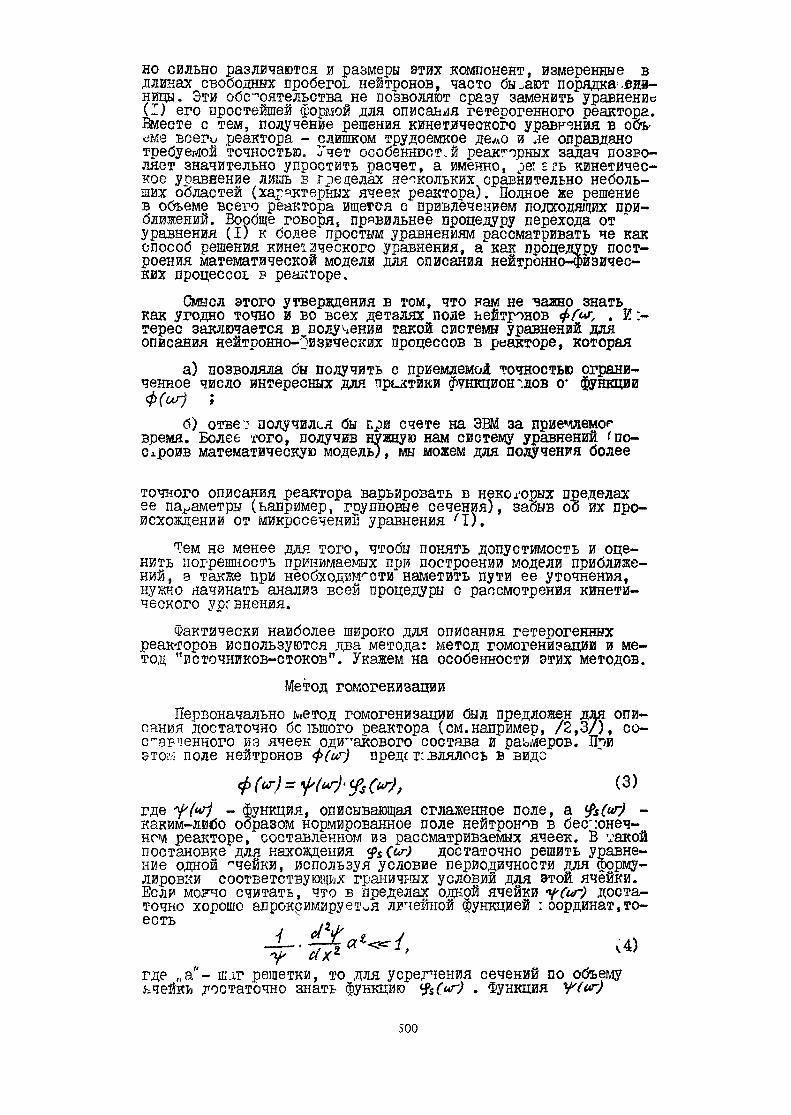
íî ñèëüíî ðàçëè÷àþòñÿ è ðàçìåðû ýòèõ êîìïîíåíò, èçìåðåííûå âäëèíàõ ñâîáîäíûõ ïðîáåãîü íåéòðîíîâ, ÷àñòî áûâàþò ïîðÿäêà .åäè-íèöû. Ýòè îáñòîÿòåëüñòâà íå ïîçâîëÿþò ñðàçó çàìåíèòü óðàâíåíèå(I) åãî ïðîñòåéøåé ôîðìîé äëÿ îïèñàíèÿ ãåòåðîãåííîãî ðåàêòîðà.Âìåñòå ñ òåì, ïîëó÷åíèå ðåøåíèÿ êèíåòè÷åñêîãî óðàâíåíèÿ â îáú-åìå âñåãî ðåàêòîðà - ñëèøêîì òðóäîåìêîå äå^î è ëå îïðàâäàíîòðåáóåìîé òî÷íîñòüþ. Ó÷åò îñîáåííã>ñò,é ðåàêòîðíûõ çàäà÷ ïîçâî-ëÿåò çíà÷èòåëüíî óïðîñòèòü ðàñ÷åò, à èìåííî, ýå! ÅÃÜ êèíåòè÷åñ-êîå óðàâíåíèå ëèøü â ã ðå äåëàõ íåñêîëüêèõ ñðàâíèòåëüíî íåáîëü-øèõ îáëàñòåé (õàðàêòåðíûõ ÿ÷ååê ðåàêòîðà). Ïîëíîå æå ðåøåíèåâ îáúåìå âñåãî ðåàêòîðà èùåòñÿ ñ ïðèâëå÷åíèåì ïîäõîäÿùèõ ïðè-áëèæåíèé. Âîîáùå ãîâîðÿ, ïðàâèëüíåå ïðîöåäóðó ïåðåõîäà îòóðàâíåíèÿ (I) ê áîëåå ïðîñòûì óðàâíåíèÿì ðàññìàòðèâàòü ÷å êàêñïîñîá ðåøåíèÿ êèíåòè÷åñêîãî óðàâíåíèÿ, à êàê ïðîöåäóðó ïîñò-ðîåíèÿ ìàòåìàòè÷åñêîé ìîäåëè äëÿ îïèñàíèÿ íåéòðîííî-ôèçè÷åñ-êèõ ïðîöåññî! â ðåàêòîðå.

Ñìûñë ýòîãî óòâåðæäåíèÿ â òîì, ÷òî íàì íå ÷àÿíî çíàòüêàê óãîäíî òî÷íî è âî âñåõ äåòàëÿõ ïîëå íåéòðîíîâ 4>(û, . Å:-òåðåñ çàêëþ÷àåòñÿ â ïîëó÷åíèè òàêîé ñèñòåìû óðàâíåíèé äëÿîïèñàíèÿ íåéòðîííî-'>çè÷åñê0õ ïðîöåññîâ â ðåàêòîðå, êîòîðàÿ

à) ïîçâîëÿëà áû ïîëó÷èòü ñ ïðèåìëåìîé òî÷íîñòüþ îãðàíè-÷åííîå ÷èñëî èíòåðåñíûõ äëÿ ïðèñòèêè Ôóíêöèîíàëîâ î- ôóíêöèè

á) îòâå!1 ïîëó÷èëñÿ áû ïðè ñ÷åòå íà ÝÂÌ çà ïðèåìëåìîå*âðåìÿ. Áîëåå òîãî, ïîëó÷èâ íóæíóþ íàì ñèñòåìó óðàâíåíèé 'ïî-ñòðîèâ ìàòåìàòè÷åñêóþ ìîäåëü), ìû ìîæåì äëÿ ïîëó÷åíèÿ áîëåå

òî÷íîãî îïèñàíèÿ ðåàêòîðà âàðüèðîâàòü â íåêîòîðûõ ïðåäåëàõåå ïàðàìåòðû (íàïðèìåð, ãðóïïîâûå ñå÷åíèÿ), çàáûâ îá èõ ïðî-èñõîæäåíèè îò ìèêðîñå÷åíèé óðàâíåíèÿ 'I).

Òåì íå ìåíåå äëÿ òîãî, ÷òîáû ïîíÿòü äîïóñòèìîñòü è îöå-íèòü ïîãðåøíîñòü ïðèíèìàåìûõ ïðè ïîñòðîåíèè ìîäåëè ïðèáëèæå-íèé, à òàêæå ïðè íåîáõîäèìîñòè íàìåòèòü ïóòè åå óòî÷íåíèÿ,íóæíî íà÷èíàòü àíàëèç âñåé ïðîöåäóðû ñ ðàññìîòðåíèÿ êèíåòè-÷åñêîãî óðãâíåíèÿ.

Ôàêòè÷åñêè íàèáîëåå øèðîêî äëÿ îïèñàíèÿ ãåòåðîãåííûõðåàêòîðîâ èñïîëüçóþòñÿ äâà ìåòîäà: ìåòîä ãîìîãåíèçàöèè è ìå-òîä "èñòî÷íèêîâ-ñòîêîâ". Óêàæåì íà îñîáåííîñòè ýòèõ ìåòîäîâ.

Ìåòîä ãîìîãåíèçàöèèÏåðâîíà÷àëüíî ìåòîä ãîìîãåíèçàöèè áûë ïðåäëîæåí äëÿ îïè-

ñàíèÿ äîñòàòî÷íî áñ 1üøîãî ðåàêòîðà (ñì. íàïðèìåð, /2,3/), ñî-ñ-çâ÷åííîãî èç ÿ÷ååê îäèíàêîâîãî ñîñòàâà è ðàçìåðîâ. 1Üèýòîãë ïîëå íåéòðîíîâ ô(èã) ïðåäå ò: êëÿëîñü â âèäå

ãäå óèã - Ôóíêöèÿ, îïèñûâàþùàÿ ñãëàæåííîå ïîëå, àêàêèì-ëèáî îáðàçîì íîðìèðîâàííîå ïîëå íåéòðîíîâ â áåñêîíå÷-íîì ðåàêòîðå, ñîñòàâëåííîì èç ðàññìàòðèâàåìûõ ÿ÷ååê. Â óàêîéïîñòàíîâêå äëÿ íàõîæäåíèÿ ô$(è~) äîñòàòî÷íî ðåøèòü óðàâíå-íèå îäíîé "÷åéêè, èñïîëüçóÿ óñëîâèå ïåðèîäè÷íîñòè äëÿ ôîðìó-ëèðîâêè ñîîòâåòñòâóþùèõ ãðàíè÷íûõ óñëîâèé äëÿ ýòîé ÿ÷åéêè.Åñëè ÌÎÓ×Î ñ÷èòàòü, ÷òî â ïðåäåëàõ îäíîé ÿ÷åéêè ^(èã) äîñòà-òî÷íî õîðîøî àïðîêñèìèðóåò^ÿ ëå÷åííîé ôóíêöèåé : îîðäèíàò.òî-åñòü _ / _ . à ^ ÷ó ñ(êã 'ãäå „à"- øàã ðåøåòêè, òî äëÿ óñðåò÷åíèÿ ñå÷åíèé ïî îáúåìóÿ÷åéêü äîñòàòî÷íî çíàòü ôóíêöèþ %(û) . Ôóíêöèÿ Ó (èã)

500

áóäåò óäîâëåòâîðÿòü êèíåòè÷åñêîå óðàâíåíèþ ñ óñðåäíåííûìèñå÷åíèÿìè, íî òàê êàê äëèíû ñâîáîäíûõ ïðîáåãîâ íåéòðîíîâ À ,êà- ïðàâèëî, ìåíüøå ..à; èëè íî êðàéíåé ìåðå ïîðÿäêà à," òî âû-ïîëíåíèå óñëîâèÿ (4) îçíà÷àåò è âûïîëíåíèå óñëîâèÿ '

Ïîñëåäíåå ëï óñëîâèå ïîçâîëÿåò çàìåíèòü êèíåòè÷åñêîå óðàâíå-íèå äëü ó (èã) íà äèôôóçèîííîå èëè Ðë - ïðèáëèæåíèå. Áé-üåïðèâåäåííûå îñóæäåíèÿ óäîâëåòâîðÿëè èññëåäîâàòåëåé äîòåõ ïîð, ïîêà çàáîòèëèñü î êîððåêòíîì óñðåäíåíèè ïî ÿ÷åéêåëèøü íàèáîëåå âàæíûõ ñå÷åíèé - ñå÷åíèÿ ïîãëîùåíà ^.à. , äå-ëåíèÿ 21^ , ïåðåõîäà 0ç ãðóïïû â ãðóïïó Å: ' .Êî^äà æå âñòàë çîïðîñ î ïðàâèëüüëì îïðåäåëåíèè ýôôåêò!.â-íîãî êîýôôèöèåíòà äè^^óçèè â ãîìîãåíèçèðîâàííîì ðåàêòîðå, þîêàçàëîñü, ÷òî ïðåäñòàâëåíèå (3) ÿâëÿåòñÿ íåäîñòàòî÷íûì. Â

ðÿäå ðàáîò, âûïîëíåííûõ â îñíîâíîì 50-õ è ç íà÷àëå 60-õãîäîâ /6*14/, áûëî ïîêàçàíî, ÷òî êðîìå ñèììåòðè÷íîé îòíîñè-òåëüíî öåíòðà ÿ÷åéêè ôóíêöèé &(è-) , îïèñûâàþùåé ìèò~þ-îòðóêòóðó ïîòîêà, òðåîó/âòñÿ åùå àíòò'ñèììåòðè÷«êå ïî êàêîé-ëèáî êîîðäèíàòå ôóíêöèè $ê(üã) , êîòîðûå íóæíû äëÿ ïîëó-÷åíèÿ êîððåêòíîãî çíà÷åíèÿ êîýôôèöèåíòà äèôôóç*.ë. Ïîäõîä êçàäà÷å, èñïîëüçóåìûå ïðèáëèæåíèÿ è äå àëüíîñò" ðàçðàîîòêèâîïðîñà â ðàçëè÷íûõ ðàáîòàõ, èç ÷èñëà óïîìÿíóòûõ âûøå, áûëèðàçíûìè, íî ñóòü äåëà, îáùóþ äëÿ íè^, ìîæíî êðàòêî èçëîæèòüñëåäóþùèì îáðàçîì:I) Ðåøåíèå â ïðåäåëàõ îäíîé ÿ÷åéêè ïðåäñòàâëÿëîñü ââèäå:

(Äëÿ ïðîñòîòû ïèøåì âûðàæåíèå ëèøã äëÿ ïîòîêà íåéòðîíîâ âîäíîé ãðóïïå è äëÿ ðåàêòîðà, áåñêîíå÷íîãî ïî îñè ã , íà-ïðàâëåííîé âäîëü îáðàçóþùåé êàíàëîâ).Çäåñü ÓÀÇ (%) è «/2Ó - ôóíêöèè, àíòèñèììåòðè÷íûå ñîîò-âåòñòâåííî ïî êîîðäèíàòàì X è Ó (X è Ó çäåñü äåêàðòîâû êî-îðäèíàî); óú ,ñ/ õ:,« / ã -ïîñòîÿííûå, èìåþùèå ñìûñëñðåäíåãî ïîòîêà ïî I ÿ÷åéêå è ñðåäíèõ ãðàäèåíòîâ ïîòîêà,ñîîòâåòñòâåííî.2) Èç óñëîâèÿ áàëàíñà íåéòðîíîâ â I -ÿ÷åéêå è íåïðåðûâíî-ñòè òîêà è ïîòîêà íà ãðàíèöàõ ñ ñîñåäíèìè ÿ÷åéêàìè, ïîëó÷à-ëèñü êîíå÷í*^~ðàçíîñòíûå óðàâíåíèÿ, ñâÿçûâàþùèå ñðåäíèå ïîòî-êè â ñîñåäíèõ ÿ÷åéêàõ. Êîýôôèöèåíòû ýòèõ óðàâíåíèé âûðàæà-ëèñü ÷åòýåç èíòåãðàëû îò ôóíêöèé <&/2Ì è $•3) Ïîëó÷åííûì êîíå÷íî-ðàçíîñòíûì óïàâ-.åíèÿì ñîïîñòàâ-ëÿëèñü äèôôåðåíöèàëüíûå óðàâíåíèÿ, èìåþùèå ëÈä èôôó çíîéíûõóðàâíåíèé äëÿ îäíîðîäíîé ñðåäû. Ýòîò ýòàï âûïîëíÿëñÿ â ñèëóòîãî, ÷òî äèôôåðåíöèàëüíûå óðàâíåíèÿ óäîáíåå äëÿ àíàëèçà èïîëó÷åíèÿ ðåøåíèé â ïðîñòûõ ñëó÷àÿõ, à òàêæå ïîòîìó, ÷òîðàñ÷åòû íà ÝÂÌ â òî âðåìÿ ÷å áûëè òàê ðàñïðîñòðàíåíû, êàêñåé÷àñ.Îòìåòèì ñëåäóþùèå îãðàíè÷åíèÿ ïîëó÷åííûõ ðåçóëüòàòîâ:I) ïðèìåíèìîñòü ðåçóëüòàòîâ áûëà îáîñãîâàíà òîëüêîäëÿ îïèñàíèÿ âíóòðåííèõ îáëàñòåé äîñòàòî÷íî ï þòÿæåíííõ îä-íîðîäíûõ ðåøåòîê, ïîñêîëüêó ïîïðåæíåìó òðåá'âàëîñü âûëîëíî-íèå óñëîâèÿ (4). Â ìåñòàõ æå íàðóøåíèÿ îäíîðîäíîñòè ðåøåòêè(ÿ÷åéêè ñ ïîãëîòèòåëÿìè â àêòèâíîé çîíå, ãðàíèöà àêòèâíîéçîíû ñ îòðàæàòåëåì è ò.ä.) ìåòîä ãîìîãåíèçàöèè â èçëîæåííîéôîðìå ïðèâîäèò ê çàìåòíûì íåòî÷íîñòÿì ( ë- 10-15$ â ñðåäíèõïî ÿ÷ é å ïîòîêàõ);

501

2) äîñòàòî÷íî ïîäðîáíûé à÷àëãç ïðîöåäóðû ïîëó÷åíèÿýôôåêòèâíû.* êîýôôèöèåíòîâ äèôôóçèè áûë âûïîëíåí ëøü äàëîäíîãðóïïîâîãî óðàâíåíèÿ.Îäèí èç âîçìîæíûõ ïóòåé óòî÷íåíèÿ* ìåòîäà ãîìîãåíèçà-öèé ïðè îïèñàíèè íåîäûîðîäíîñòåé ðåøåòêè çàêëþ÷àåòñÿ â óñò-ðîéñòâå ñëåäóþùåé èòåðàöèîííîé ñðîöå^/ðû:1) âíà÷àëå îïðåäåëÿþòñÿ <&^ â </à*(üã) äëÿ êàæäîãîòèïà ÿ÷ååê òàê, ñëîâíî îíè îêðóæåíû òàêèìè æå ÿ÷åéêàìè. Óñ-ðåäíãç ñ ïîìîùüþ ýòèõ ôóíêöèé ñå÷åíèÿ ïî ÿ÷åéêå, ðàññ÷èòû-âàþò ðàñïðåäåëåíèå íåéòðîíîâ ïî âñåìó ðåêòîðó;2) îïðåäåëèâ èç ïðåäûäóùåé èòåðàöèè óòå÷êó(èëè ïðèòîê)'íåé~÷ýîíîâ â êàæäîé ÿ÷åéêå, ïåðåñ÷èòûâàþò ñ ó÷åòîì åå ðàñ-ïðåäåëåíèÿ^ âíóòðè ÿ÷ååê 0 çàòåì ñíîâà âûïîëíÿþò ðàñ÷åò ðåàê-òîðà.Íåäîñòàòîê òàêîãî ïîäõîäà â íåîáõîäèìîñòè ïîâòîðÿòüòðóäîåìêóþ ïðîöåäóîó ïåðåñ÷åòà ÿ÷åå÷íûõ ðåøåíèé. Ïðè ýòîìäåëî îñëîæíÿåòñÿ òåì, ÷òî ÿ÷åéêè îäíîãî òèïà, íî ñòîÿùèå âðàçíûõ ìåñòàõ ðåàê*îðà} äîëæíû íà âòîðîé èòåðàöèè ñ÷èòàòüñÿ^àçëè÷íûìè, òàê êàê îíè ðàçëè÷àþòñÿ ïî óòå÷êå.Îäèí ñïîñîá óòî÷íåíèÿ ìåòîäà ãîìîãåíèçàöèè ðàññìîòðåíâ ðàáîòàõ 15/. Ñâîéñòâî ÿ÷åéêè ïðåäëñ*ãàåòñÿ îïèñûâàòü äâó-ìÿ ðÿäàìè ïàðàìåòðîâ: îäíè ñå÷åíèÿ ñâÿçàíû ñ "ñîáñòâåííûìè"íåéòðîíàìè, äðóãèå - ñ âòåêàþùèìè ñî ñòîðîíû. Èññëåäóåòñÿîäíîãðóïïîâîå óðàâíåíèå. Ñå÷åíèÿ, ñâÿçàííûå ÷. "ñîáñòâåííûìè"íÑòðîêàìè, ïðåäëàãàåòñÿ èñêàòü èòåðàöèÿìè.Áîëåå îáùèé è, íà íàø âçãëÿä, áîëåå ïîñëåäîâàòåëüíûéïîäõîä ðàçâèò â ðàáîòàõ /16,17/.Ñóòü åãî çàêëþ÷àåòñÿ â óòî÷-íåíèé ÿ÷åå÷íûõ ôóíêöèé, âõîäÿùèõ â âûðàæåíèå (5) è â íåêîòî-ðîì óâåëè÷åíèè èõ ÷èñëà. Ïðè ý.ñì îêàçûâàåòñÿ âîçìîæíûì ïðèðàñ÷åòå ðåàêòîðà â öåëîì âîñïîëüçîâàòüñÿ èìåþùèìèñÿ ïðîãðàì-ìàìè (âíåñÿ íåáîëüøèå èçìåíåíèÿ â áëîêè ââîäà èñõîäíûõ .".ýí-íûõ è âûâîäà ðåçóëüòàòîâ), ðåàëèçóþùèìè òó èëè èíóþ êîíå÷íî-ðàçíîñòíóþ ñõåìó, íî ïðÿäàòü *øîé ñìûñë âõîäÿùèì òóäà âåëè-òø ãàìÏðèíöèïû ïîëó÷åíèÿ óòî÷íåííûõ êîíå÷íî-ðàçíîñòíûõ óðàâ-íåíèé èç óðàâíåíèÿ (I) áóäóò èçëîæåíû ïîçæå. Ñåé÷àñ æå êðàò-êî îõàðàêòåðèçóåì ìåòîä "ò'ñòî÷íèêîâ-ñòîêîâ".

Ìåòîä "èñòî÷íèêîâ-ñòîêîã"Óðàâíåíèÿ ìåòîäà "èñòî÷íèêîâ-ñòîêîâ" ïüðþíà÷àëüíîáûëè ñôîðìóëèðîâàíû /18,19/ â ïðåäïîëîæåíèÿ, ÷ò ðåàêòîðïðåäñòàâëÿåò ñîáîé ðåøåòêó íèòåâèäíûõ ñòåðæíåé, ïîòóæåííûõâ áåñêîíå÷íûé çàìåäëèòåëü. Ïðè ýòî».. ñ÷"òàëîñü, ÷òî ë,-'ôôó èþíåéòðîíîâ ïîâñþäó â çàìåäëèòåëå ìîæíî îïèñàòü •" - ïðè-áëèæåíèÿ ìåòîëà ñôåðè÷åñêèõ ãàðìîíèê (ìíîãîãðóïïîâãÿ äèôôó-çèîííàÿ èëè äèôôóçèîííîâîç^àñòíã I ñõåìà). Âïîñëåäñòâèè âïåðâîíà÷àëüíóþ ñõåìó ââîäèëèñü ðàçëè÷íûå óòî÷íåíèÿ, íàèáîëååñóùåñòâåííûì èç êîòîøõ ÿâëÿëîñü îï ,åäåëåíèå åïëîâîé ïîñòî-ÿííîé èç åøåíè÷ ê: í¸òè÷åñêîãî óðàâíåíèÿ â áëîêå è ðÿäîì ñ

ÊÈÌ.

ÇÑ Ïîïûòêè óòî÷íèòü ðàñ÷åò ñ ÏÎÌÎÐÜÞ ôîðìàëüíîãî ïåðåõîäàê êîíå÷íî-ðàçíîñòíûì "ðàâíåíèÿì ñ íàãîì ñåòêè, ìåòûïèìøàãà ðåøåòêèV, ÿâëÿþòñÿ, êàê âèäíî èç èçëîæåííîãî,íåêîîðåêòíú.,ëè.502

Îñíîâíîé èäååé ìåòîäà ÿâëÿåòñÿ ñâåäåíèå çàäà÷; î äèô-ôóçèè íåéòðîíîâ â ãåòåðîãåííîé ñðåäå ê çàäà÷å î îàñïðîñòðà-íåíèè íåéòðîíîâ â áåñêîíå÷íîì çàìåäëèòåëå ( äàëüíåéøåå èçëî-æåíà îñíîâàíî íà ðàáîòàõ /20,21/*' Ïóñòü íåéòðîííîå ïîëåðåàêòîðà îïèñûâàåòñÿ óðàâíåíèåì (I). Ïðåäïîëîæèì, ÷òî ðåàê-òîð ñîñòîèò èç îäíîðîäíîãî çàìåäëèòåëÿ, â êîòîðîì ïîìåùàþò-ñÿ áë^êè (êàíàëû) ñ ðàçëè÷íûìè ðàçìíîæàþùèìè , ïîãëîùàþùèìè0 çàìåäëÿþùèìè ñâîéñòâàìè. Âñå áëîêè ïðåäñòàâëÿþò ñîáîé áåñ~êîíå÷íûå êðóãîâûå öèëèíäðû, îñè êîòîðûõ ïàðàëëåëüê. äðóãäðóãó.Îïðåäåëèì ôóíêöèþ Ãðèíà - <#~1üã' äëÿ áåñêî-íå÷íîãî îäíîðîäíîãî çàìåäëèòåëÿ ñ ïîìîùüþ óðàâíåíèÿÀ» Ñ-

(â)Èíäåêñ æ ïîêàçûâàåò ïðèíàäëåæíîñòü ÁÇËÈ×Ã-Ø ò çàìåäëèòåëþ.

Ïåðåïèøåì óðàâíåíèå (I) ñëåäóþùèì îáðàçîì:

Çàìåòèì, ÷òî ?(û)ãî àðå Ú $ó& ( ÈãÀ- îáúåì,çàíèìàåìûé áëîêàìè). Ñ ïîìîùüþ ôóíêöèè õðèíýóðàâíåíèå (I) ïðåîáðàçóéñÿ ê âèäó

(8)

Ïîñëåäíåå óðàâíåøãå. ÿíòåðåÿíî òåì- ÷òî îíî ïîçâîëÿåòîïðåäåëèòü äîëå íåéòðîíîâ ô?üã? òîëüêî â îáúåìå /ãà , çà-íèìàåìîì áëîêàìè, îòâëåêàÿñü îò ñîâå ;åíèÿ åãî â çàìå äëè òå-ëå. Åñëè ðåøåòêà áëîêîâ òàêîâà, ÷òî ïîëå íåéòðîíîâ â êàæäîìèç íèõ ìîæíî ñ äîñòàòî÷íîé òî÷íîñòüþ àëðîêñèìèðîâàòü ëêíåé-íîé êîìáèíàöèåé íåáîëüøîãî ÷èñëà èçâåñòíûõ (èëè ëåãêî îïðå-äåëÿåìûõ) Ôóíêöèé, òî -ïîäî .àíîâêà òàêèõ êîìáèíàöèé Á óðàâíå-íèå \8) ñâîäèò çàäà÷ó ê ðåøåíè» ñèñòåìû ÷èêåéíø: àëãåáðàè-÷åñêèõ óðàâíåíèé ïðèåìëåìîãî ïîðÿäêà. Íåèçâåñòíûìè ïðè ýòîìáóäóò àìïëèòóäû âõîäÿïøõ â óêàçàííûå êîìáèíàöèè ôóíêöèé.

Â ïðîñòåéøåì âàðèàíòå ìåòîäà "èñòî÷íèêîâ-ñòîêîâ" ïðåä-ïîëàãàþòñÿ4 âûïîëíåííûìè ñëåäóþùèå óñëîâèÿ:

1) à»Ú(Å) ÄË.Å äâáîãî Â , [2) à «ë . ãäå å% - ðãäâäñ ÎËÎÊÅ (9)

òî-åîòú çà?ë9äëåÅéå íåéòðîíîâ ç áëîêå îòñóòñòâóåò.

8 Ñì. òàêæå / 37 /.503

Ïðè çàïîëíåíèè â; þã óñëîçè'; ñ->ñã-'çú1âàåòñÿ çîçìîÿíüì îã-ðàíè÷èòüñÿ ïðè îïèñàíî- ïîëÿ éåéòîîíîâ â á^îêå ÷èñëîì ÔÓÍÊ-ÖÈÉ, ðàâíûì ÷èñëó ãðóïï, Îáû÷íî ñ÷èòàåòñÿ, ÷^î íåéòðîíû'î÷ñòðûõ ãðóïï ðàñëñåäåëåíû ïî áëîêó ïîñòîÿííî, à òåïëîâûåíåéòðîíû îïèñûâàþòñÿ ôóíçäâåé, êîòîðàÿ ìîæåò áûòü îïðåäåëåíàèç ðàñ÷åò . ðàñïðåäåëåíèÿ â áëîêå, ïîìåùåííîì â áåñêîíå÷íûé(êëé äîñòàòî÷íî òî.þøé) åëîê çàìåäëèòåëÿ ñ ïîñòîÿííûìè ïîïðîñòðð÷ñòâó âñòî÷ÿéêà÷é òåïëîâûõ íåéòðîíîâ. Çàäà÷à ñâîäÿò-ñÿ ê ñèñòåìå àëãåáðàè÷åñêèõ óðàâíåíèé ñ ãðóïïî^ø ïîòîêàìèíà ïîâåðõêîãòÿõáëîêîâ (èëý áëèçêèìè ê ÅØ âåëè÷èíàìè) âêà÷åñòâå íåèçâåñòíûõ.

Óøç÷åíÿÿ ã-çãæãîðü ç ïðîñòåéøåì âàýòàíòå ìåòîäà "èñòî÷--ñòî.õÎÁ" âêëþ÷àþò â ñåÇÿ âåò÷èíû," èìåþùèå î÷åâèäíûé

ôèçè÷åñêèé ñìûñë. Ïñ^ïìó îíã óäîáíû äëÿ: êà÷åñòâåííîãî àíà-ëèçà. Â ñëó÷àå, êîðäà èìååòñÿ êîíå÷íàÿ, êî îäíîðîäíàÿ ðåøåò-êà áëîêîâ, ðàçðàîîòà*ø ýôôåêòèâíûå ïðèçâàí âû÷èñëåíèÿ ñóìì,âîçíèêàþùèõ Å ìåòîäå /294/.

Îòìåòèì, îäíàêî, ñóùåñòâåííûé íåäîñòàòîê ìåòîäà, êîòî-ðûé ïðîÿâëÿåòñÿ óæå â ?òîì ïðèáëèæåíèé. Ïðè ïåðåõîä* ê ãðóï-ïîâîìó îïèñàíèþ, êàê ïîêàçûâàåò ^íàäïç (ñì.,íàïðèìåð, /21/),ïðèõîäèòñÿ äåëàòü ðÿä ïðåäïîëîæåíèé î âíóòðèãðóïïîâûõ ñï»êò-ðàõ, ïîñëåäñòâèÿ ÊÎÒÎÐÛÕ äëÿ ëåîäíîðîäíâõ ðåøåòîê òðóäíîîðîêîíòðîëíðîúàò?„ Âî" ÂÎËÓ îì ñëó÷àå êîððåêÿíðÈ ó÷åò ñïåêò-ðàëüíûõ ýôôåêòîâ â ýòîì ìåòîäå îêàçûâàåòñÿ áîëåå ñëîêíûì,÷åì, íàïðèìåð, â ìåòîäå ãîìîãåíèçàöèé. Äåëî ã àîãë, ÷òî çêçò^äå èéñòî÷íéêîý~ñ?îãîçÿ «îòîê íåéòðîíîâ îäíîé ãðóïïû ïå-ðåäàåòñÿ îò îäíîãî áëîêà ê äðóãèíã ÷åðåç çàìåääè^òåëü, êâòîøéâñþäó îïèñûâàåòñÿ ->äê;ãåç êîíñòàíòàë^, òî^-ýñòü âíóòðèãðóïüî-âîé ñã åêòð Ñ×Ð1ÒÝ8ÒÑÀ îäìîêîí^ â çàìåäëèòåëå âî I :åõÿ÷åéêàõ. Â ìå^-îäàç:» îñíîçàíííç: êÿ ðàçáèçíèâ çîíû ðåàêòîðàíà ÿ÷åéêè, ïîè ïåðåòå÷êå íåéòðîíîâ êàêîé-ë!.5î ãðóïïû èçîäíîé ÿ÷åéêè"â äðóãóþ ëåãêî îñóùåñòâèòü (è îîû^÷î ýòî äåëà-åòñÿ) êîððåêòèðîâêó ãðóïïîâûõ êîíñòàíò, ó÷èòûâàþùóþ ðãçëè-÷ÿå âíóòðèãðóïïîâîãî ñïåêòðà â ñîñåäíèõ ÿ÷åéêàõ.

Ïåðâîå èç óñëîâèé (9) îñòàåòñÿ âî âñåõ ïîñëåäóþùèõðàççèòèÿõ ìåòîäà ÿ îïðåäåëÿåò êëàññ ^åàêòîðîã (ñ ãðàôèòî-âûãä è òÿíåëîâîäíûì çàìåäëèòåëåì;, äëÿ êîòîðîãî îí ïðèìåíÿ-åòñÿ. 7çà äðóãèõ óñëîâèÿ ìîãóò áûò»- îñëàáëåíû èëâ ñíÿòû,÷òî âåñüìà ñóà1åñòâåííî äëÿ êàíàëüíûõ ðåàêòîðñç, òàê êàê âíèõ êàíàû çàèãðàþò çàìåòåòþ äîëþ ÿ÷åéêè ü çàìåäëåíèå âíåì ÷àñòî äîâîëüíî âåëèêî. Îòìå÷åííàÿ âûøå -"ðóäíîñòü ïðèïåðåõîäå ê ãðóïïîâîìó îïèñàíèþ îñòàåòñÿ â ñèëå.

äðóãîå îãðàíè÷åíèå ìåòîäà, ñóùåñòâåííîå ïðè ïîñòà-íîâêå çàäà÷è ïà âû÷èñëèòåëüíóþ ìàøèíó, ñâÿçàíî ñ ïðèñóùèìåì* äàëüíîäåéñòâèåì. Óðàâíåíèÿ ÑÅ 1çûâàþò çñå áëîêè, ò.å.';ëÿ ðåøåíèÿ çàäà÷è ïðèõîäèòñÿ îáðàùàòü ìàòðèöó âûñîêîãîïîðÿäêà, â êîòîðîé ïðàêòè÷åñêè âñå ýëåìåíòû îòëè÷íû îòíóëÿ. Äåëî îñëîæíÿåòñÿ òåì, ÷òî ìàòðèö÷ îáëàäàåò ïëîõèìèñâîéñòâàìè, ÷òî îáóñëîâëåíî ñóùåñòâîì çàäà÷è/20/. Ýòîîãðàíè÷åíèå áûëî ïðåîäîëåíî â ðàáîòàõ /23,24/, Â ðàáîòå/23/ ïðåäëîæåí ïîäõîä, íàçâàíü^-é, íà ìîé âçãëÿä äîâîëüíîíåóäà÷íî, êâàçèàëüáåäíûì ìåòîäîì. Ñóòü åãî çàêëþ÷àåòñÿ âïåðåõîäå îò óðàâíåíèé ìåòîäà "èñòî÷àèêîâ-ñòñäîâ" â ãðóïïî-âîé çàïèñè ê êîíå÷íñ-ðàç-þñòíûì. Â ïðîöåññå ïåðåõîäà èñ-ïîëüçóþòñÿ ïðèåìû, âî ìíîãîì ñõîäíûå ñ ïðèìåíÿåìûìè ïðèïîëó÷åíèé óðàâíåíèé â ìåòîäå ãîìîãåíèçàöèè Vðàçäåëåíèå ïî-òîêà íà áûñ.'ðîìåíÿãîøóþñÿ è ïëàâíóþ ñîñòàâëÿþùèå, ïðåäñòàâ-ëåíèå ðåøåíèÿ â ÿ÷åéêå â âèäå ñóììû íåáîëüøîãî ÷èñëà çàäàí-íûõ Ôóíêöèé, ç ðåçóëüòàòå ÷åãî ñâÿçûâàþòñÿ ìåòîäó îîáîéòîëüêî íåáîëüøîå ÷èñëî ñîñåäíèõ êàíàëîâ). Èñïîëüçîâàííûéíàáîð ÿ÷åå÷íûõ Ôóíêöèé ïîçâîëèë, îäíàêî, þ÷íåå, ÷åì âêëàññè÷åñêîì ìåòîäå ãîìîãåíèçàöèè, ó÷åñòü íåîäíîðîäíîñòüðåøåòêè. Ïîêàçàíî, ÷±ëî ïîè äçó.åðíîì ðàñ÷åòå èñïîëüçîâà-íèå â êîíå÷íî-ã"çíîåòíûõ~óðàâíåíèÿõ 9ãòî÷å÷íîãî øàáëîíà

504

(ñâÿçàíû ìåæäó ñîáîé' òîëüêî 9 êàíàëîâ) ïðèáëèæàåò èñõîäíûåóðàâíåíèÿ ñ çàâåäîìî ïðâåãëåìîé äëÿ ïðàêòèêè òî÷íîñòüþ.ýòîò ôàêò» ìåæäó ïðî^ãì. ñâèäåòåëüñòâóåò î òîì, ÷òî ä òàëü-íîå îïèñàíèå àçâäó ñàëüíîãî èçìåíåíèÿ ïîòîêà íåéòðîíîâ âçàìåäëèòåëå ÿ÷åéêà, êîòîðîå ñîäåðæèòñÿ â ìåòîäå "èñòî÷íèêîâ-ñòîêîâ" íå ÷-÷åíü âàæíî. Â ðàáîòàõ /23, 24/ äëÿ ÐÒÎÃÎ îïèñà-íèÿ èñïîëüçóåòñÿ âñåãî ÷åòûðå ôóíçöèè. Â ìåòîäå ãîìîãåíèçà-öèè, êàê âèäíî 158 âûðàæåíèÿ (5;, ìì ñîñ åòñò óþò òðè ôóíê-öèé.Óðàâíåíèÿ, åõäöêûå ñ ïîëó÷åííûìè â ðàáîòàõ 23,24/,ïîçäíåå áûëè âûâåäåíû â ðàèîòå /25/ äðóãèì ïóòåèã. Åñëè âðàáîòå /23/, òàêæå êàê è â ìåòîäå ãîìîãåíèçàöèè, èñïîëüçî-âàí ïîäõîä, êîòîðûé îòíîñèòñÿ ê êëàññó ñïîñîáîâ, ïîëó÷èâøèõ

â ïîñëåäíåå âðåìÿ â ëèòåðàòóðå íàçâàíèå âàðèüäèîííî-ðàçíîñëøõ (ñì. íàïðèìåð,. /21/) (èñïîëüçóåòñÿ òàêæå íàçâà-íèå - ìåòîä êîíå÷íûõ ýëåìåíòîâ /28/), "þ â ðàáîòå /25/ïðèìåíÿåòñÿ ïðÿìàÿ çàìåíà äèôôåðåíöèàëüíîãî îïåðàòîðà êî-íå÷íî-ðàçíîñðíûì. Ïîñêîëüêó ïðè çàïèñè óðàâíåíèè ìåòîäà"èñòî÷íèêîâ-ñòîêîâ*1 â äèôôåðåíöèàëüíîé ôîðìå ãðóïïîâûåóðàâíåíèÿ â çàìåäëèòåëå ñîäåðæàò îïåðàòîð Ãåëüìãîëüöàòî è âûïîëíÿåòñÿ çàìåíà ýòîãî îïåðàòîðà êîãý÷íî-ðàçíîñò-íêì. Äîêàçûâàåòñÿ, ÷òî â äâóìåðíîì ñëó÷àå èñïîëüçîâàíèå-.òî÷å÷íîãî øàáëîíà ïðè êâàäðàòíîé ñåòêå ñ øàãîì, ïàâíûìøàãó ðåøåòêè áëîêîâ, îáåñïå÷èâàåò âûñîêóþ òî÷íîñòü. Â îò-ëè÷èå îò èçâåñòíîãî â ëèòåðàòóðå (ñì., íàïðèìåð, /°9/)êîíå÷íî-ðàçíîñòíîãî îïåðàòîðà íà 9-òî÷å÷íîì øàáëîíå, ïðèáëè-æàþùåãî îïåðàòîð Ëàïëàñà, êîýôôèöèåíòû êîíå÷íî-ðàçíîñòíîãîîïåðàòîðà, ïðèáëèæàâøåãî îïåòçàòîð Ãåëüìãîëüöà, îêàçûâàþòñÿíå ÷èñëàìè, à ôóíêöãòìè îò øàãà ñåòêè^^ èçìåðåííîãî ç åäè-íèöàõ /ý% . Ýòè ôóíêöèè â ðàáîòå /25/ çàòàáóë^ðîâàíû.

Òàê êàê â îàáîòàõ /23*26/ èñõîäíûì* ÿâëÿþòñÿ ãðóïïî-âûå óðàâíåíèÿ ìåòîäà "èñòî÷íèêîâ-ñòîêîâ", òî óïîìÿíóòàÿâûøå òðóäíîñòü ïåðåõîäà ê ãðóïïîâîìó îïèñàíèþ îñòàåòñÿ.Â çàêëþ÷åíèå ðàçäåëà íåñêîëüêî ñëîâ åùå îá îäíîì(ìåíåå ðàñïðîñòðàíåííîì) ìåòîäå ðåøåíèÿ ðàññìàòðèâàåìîé çà-äà÷è - àëüáåäíîì ìåòîäå. Â ýòîì ìåòîäå, òàê æå êàê è â ìå-òîäå ãîìîãåíèçàöèè, îïèñûâàþò ïîëå íåéòðîíîâ â ÿ÷åéêàõ íå-áîëüøèì ÷çñëîì ïðîáíûõ ôóíêöèé. Îòëè÷èå â òîì, ÷òî óðàâíåíèÿñâÿçè ìåæäó ñîñåäíèìè ÿ÷åéêàìè ïîëó÷àþòñÿ èç óñëîâèé íåïðå-ðûâíèñòè îäíîñòîðîííèõ òîêñâ, à ÷å ïîòîêîâ è òîê'â. Òåýòîãî ìåòîäà, êîòîðûå èìåþòñÿ â îïóáëèêîâàííûõ ðàáîòà .36/, ïðîèãðûâàþò óðàâíåíèÿì ìåòîäà ãîìîãåíèçàöèè, ïðåæäåâñåãî ïîòîìó, ÷òî â êîíå÷íûõ óðãâíåíèÿõ ñîõðàíÿåòñÿ áîëüøåå÷èñëî íåèçâåñòíûõ íà ÿ÷åéêó è ãîïîëüçóåìûå ïðîáíûå ôóíêöèèíå óïîðÿäî÷åíû ïî ñòåïåíè âàæíîñòè, Â ðåçóëüòàòå, íàïðèìåð,

Â ðàáîòå /25/ çìååòîÿ ññûëêà íà ðàáîòû /26/ è ãîâîðèòñÿ,÷òî òàì ïîëó÷åíû' ñõîäíûå ðåçóëüòàòû.' Îïåðàòîð Ãåëüìãîëüöà â ðàáîòå /25/ çàìåíÿëñÿ ñëåäóþùèìãäå À, è ë± _ êîíå÷íî-ðàçíîñòòøå àíàëîãè îïåðàòîðà Ëàï-ëàñà òèïà "êðåñò" è "ïã âåðíó -÷àé êðåñò". Çàìåòèì, ÷òî ôóíê-öèÿ îñ îêàçàëàñü ñëàáî çàâèñÿùåé îò øàãà ðåøåòêè è áëèç-êîé ê âåëè÷èíå 2/3, ò.î. ê âåî÷èí^, ïîëó÷àþùåéñÿ ïðè àï-ðîêñèìàöèé îïåðàòîðà Ëàïëàñà íà 9-òî÷å÷íîì øàáëîíå /29/.Îñíîâíàÿ ïîïðàâêà çàêëþ÷àåòñÿ â ââåäåíèè âåëè÷èíû Ä .Êàêíàì óäàëîñü óñòàíîâèòü, çàòàáóëèðîâàííàÿ .â ðàáå ãå /25/ôóíêöèÿ ñ*-) ñ áîëüøîé òî÷íîñòüþ îïèñûâàåòñÿ ôîðìóëîé

505

äëÿ äâóìåðíîé çàäà÷è è âñå ïðîáíûå ôóíêöèè òðåáóþò ðåøåíèÿäâóìåðíûõ âñïîìîãàòåëüíûõ çàäà÷, òîãäà êàê â ìå:îäå ãîìîãå-íèçàöèè íàèáîëåå âàæíûå ñèììåòðè÷íûå ïðîáíûå ôóíêöèè ïîëó-÷àþòñÿ â áîëüøèíñòâå ñëó÷àåâ èç ðåøåíèÿ ïîäõîäÿùèõ îäãþìñð-êêõ çàäà÷. Óêàçàííûå íåäîñòàòêè ìîãóò áû.ü, íåâèäèìîìó, óñ--òðàíåíû (óïîðÿäî÷åíû ïðîáíûå ôóíêöèè, âûäåëåíà ï*-åäñòàâè~òåëüíàÿ êîìáèíàöèÿ íåèçâåñòíûõ, à îñòàëüíûå èñê^þ÷åø. èçðåøàåìûõ óðàâíåíèé), íî, ïî ìîåìó ëíåíèþ, â ðåçóëüòàòå îá-õîäíûì ïó-åì ïîëó÷àòñÿ óðàâíåíèÿ, ýêâèâàëåíòíûå óðàâíåíèÿìîáîáùåííîãî ìåòîäà ãîìîãåíèçàöèè.

Ïïèíöèïû ïîãó÷åíèÿ óòî÷íåííûõêîíå÷íî-ðàçíîñòíûõ óðàâíåíèé ãåòåðîãåííîãîðåàêòîðàÊàê óæå îòìå÷àëîñü, â ðàáîòàõ /16,17/ ïðåäëîæåí ñïîñîáïîëó÷åíèÿ êîíå÷íî-ðàçíîñòíûõ àíàëîãîâ óðàâíåíèÿ ïåðåíîñàäëÿ ãåîìåòðèé, õàðàêòåðíûõ äëÿ ÿäåðíûõ ðåàêòîðîâ. Ïðè âûáîðåïóòè â ýòèõ ðàáîòàõ èñïîëüçîâàëñÿ íåêèé âàðèàöèîííûé ïîäõîä,ïðèíöèïû êîòîðîãî êðàòêî èçëîæåíû â ýòîì ðàçäåëå.Óðàâíåíèå (I) âìåñòå ñ ïîäõîäÿùèì ãðàíè÷íûì óñëîâèåì( : àïðèìåð , <ô (ã,ÅÄ) = î ïðè ã å Ã&, , 8% > ñ , ãäå ã«, - âíåøíÿÿêóñî÷íîãëàäêàÿ Â1,íóêëàÿ ãòãëèöà ðåàêòîðà è è íîðìàëüê íåé, íàïðàâëåííàÿ âíóòîú) îïðåäåëÿåò ëèíåéíîå îïåðàòîðíîåóðàâíåíèå

Íàðÿäó ñ îäíîðîäíûì óðàâíåíèåì (10) ðàññìîòðèì íåîäíî-ðîäíîå ÑÏ)Òàêîå óðàâíåíèå âîçíèêàåò, íàïðèìåð, ïðè ðåøåíèè óðàâ-íåíèÿ (10) ñ ïîìîùüþ ñëåäóþùåãî èòåðàöèîííîãî ïðîöåññà

Ã12)Òîãäà íà êàæäîì èòåðàöèîííîì øàãå ïðàâàÿ ÷àñòü óðàâíå-íèÿ (12) îêàçûâàåòñÿ èçâåñòíî" è îíî ñâîäèòñÿ ê âèäó III).Äëÿ àíàëèçà ïðèáëèæåííûõ ïðåäñòàâëåíèé èñõîäíûõ óðàâ-íåíèé âîñïîëüçóåìñÿ ôîðìóëàìè òåîðèè âîçìóùåíèé /30/.Ïóñòü èìååì

[?ãäå I/1" - îïåðàòîð, ñîïøæåííüË îïåðàòîðó 1> (ò.å. âûïîë-íÿåòñÿ ðàü íñ âî ñêàëÿðíûõ ïïîèçâåäåíèè(«,/1.< ã ';ã.4«*),ð ««ã> -êàêàÿ-ð áî çàäàííàÿ ôóíêöèÿ, îïðåäåëÿþùàÿ èíòåðåñóþùèé íàñôóíêöèîíàë.

Åñëè òåïåðü ðàññìîòðèì óðàâíåíèå

òî ñ ïîìîùüþ ñòàíäàðòíîé ïðîöåäóðû ïîëó÷èì(/>,+'-+)*

506

Èñïîëüçóåì ýòó Ôîðìóëó äëÿ ñâîèõ öåëåé.õ Áóäåì èñêàòü ïðèáëèæåííîå ðåøåíèå óðàâíåíèÿ (II) â

âèäå* , Ë ã&(16)

Çäåñü * - íîìåð ÿ÷åéêè (âñÿ ïðîñòðàíñòâåííàÿ îáëàñòüà íà I ÿ÷ååê). Ïðîáíûå ôóíêöèè ó.- îïðåäåëåíû ñëåäó-þùèì îáðàçîì .,'. Ãë ="•> |/

ãäå &öÙ~12\^:^. > VI - îáúåì ñ -ÿ÷åéêè;

Ãã - ãðàíèöà /~ÿ÷åé"â, Ó^^{!0~ ñôåðè÷åñêèå ôóíãàãè,Å ,

/= 0 ïðâ ú*ˆ VI è ê ^ 1 * (18)

- ñèìâî".íåêîòîðûå çàäàøøå ôóíêöèé ˆ è Å, îñóùåñòâëÿþùèåàïðîêñéìàöèþ óãëîâûõ ìîìåíòîâ ðåøåíèÿ íà ãðàíèöàõ ÿ÷ååê.Âûáîð â êà÷åñòâå ïðîáíûõ ôóíêöèé ðåøåíèé íåêîòîðûõâñïîìîãàòåëüíûõ çàäà÷, ñôîðìóëèðîâàííûõ äëÿ îòäåëüíûõ ÿ÷ååê,ÿâëÿåòñÿ îáû÷íûì â òåîðèè ðåàêòîðîâ . Îí ñâÿçàí åå ñëåäóþùèìèîáñòîÿòåëüñòâà/è :1) âíóòðåííåå óñòðîéñòâî ë^åéêè äîñòàòî÷íî ñëîæíî èðàñïðåäåëåíèå íåéòðîíîâ â íåé ñëèñûâàåòñÿ òàêîé ôóíêöèåé, êî-òîðóþ íåâîç..;îéíî äîñòàòî÷íî òî÷íî åïðîêñèãëèðîâàòü íåáîëüøèì÷üñëîì îò*øäàðòíûõ, íý ÿ^çâñÿùéõ îò óñòðîéñòâà ÿ÷åéêè ôóíê-öèé; 2) ÷èñëî ÿ÷ååê$ ðàçëè÷íûõ íî ñâîéñòâàì, ìíîãî ìåíüøåîáùåãî êîëè÷åñòâà ÿ÷ååê. Ïîýòîìó, çàãîòîâèâ íåêîòîðîå ÷èñëîïðîáíûõ Ôóíêöèé, îïðåäåëåíèÿõ óðàâíåíèÿìè (17) è (18), ìûìîæåì õ"0ñïîëüçñâà.'Ü äëÿ ÿ÷ååê, ñõîäíûõ ïî âíóòðåííèìñâîéñòâàì, íî ðàñïîëîæåííûõ â ðàãíûõ ìåñòàõ ðåàêòîðà, â ðàç-ëè÷íîì îêðóæåíèè, à òàêæå èñïîëüçîâàòü ýòè ôó^ëñöéè äëÿ ðàñ-÷åòà ðàçëè÷íã'õ ñîñòîÿíèé þåàêòîðà,,Çàïèñü ðåøåíèÿ â âèäå (16) ÿâëÿåòñÿ ôîðìàëèçàöèåé èîáîáùåíèåì ïîäõîäà, èñïîëüçóåìîãî â èçâåñòíîì ìåòîäå ãîìîãå-íèçàöèè.Ïîäñòàíîâêà âûðàæåíèÿ (16) â óðòàíåíèå 'Ö) ïðèâîäèòê íåêîòîðîé íåâÿçêå, êîòîðóþ ìû çàïèøåì â âèäå

ì *" Ò ~ $4Çäåñü ñëàãàåìîå $1,Ô* ñâÿçàíî ñ òåì, ^?î <{>*, íåóäîâëåòâîðÿåò óðàâíåíèþ íà ãïàíèöàõ ÿ÷?åê, à §Ó */ íåòî÷íûì óäîâëåòâîðåíèåì óñëîâèé íà âíîëíåé ãðàíèöå.Îòâëåêàÿñü ïîêà îò âòîðîãî ñëàãàåìîãî (åã~> ðàññìîòðå-íèå ÏÐÎÂÎÄÅ õ-ñÿ àíàëîãè÷íî ðàññìîòðåíèþ ïåðâîãî ñëàãàåìîãî),âûïèøåì §Ü# â ÿâíîì âèäå. Î÷åâèäíî,

* Çäåñü âñþäó áóäåì èìåòü â âèäó çãäà÷ó äëÿ äâóìåðíîãî ðå-àêòîðà, àêòèâíàÿ çîíà íýòîðîãî ïðåäñòàâëÿåò èç ñåáÿ ïðà-âèëüíóþ ðåøåòêó áåîêîíå÷êàõëèëãïäðè÷åñê: õ ñòåðæíåé, âîîáùåãîâîðÿ, îòëè.àþùèõñÿ ïñ -ðîèñòâàì, ïîãðóæåííûõ â çàìåäëè-òåëü.507

ïîñêîëüêó òîëüêî îïåðàöèÿ äèôôåðåíöèðîâàíèÿ â îïåðàòîðå Ñ*ïðèâåäåò ê ñèíãóëÿðíîìó âêëàäó, ñ êîòîðûì ñëåäóåò ñ÷èòàòüñÿ.Çäåñü &(ú~ã) - äâóìåðíàÿ ôóíêöèÿ Äèðàêà, V - òî÷êèó Ã , Ã - ñîâîêóïíîñòü âñåõ ãðàíèö ÿ÷ååê (êðîìå âíåø-ÿ - íîðìàëü ê ãðàíèöå ÿ÷åéêè, À,. (û)=Èñïîëüçóÿ òåïåðü ôîð::óëó (15), ïîëó÷èì

(20)

Î 4òãÑòðåìëåíèå Ä/À/-» î ïðè À×îî îçíà÷àåò, ÷òî óê"*íûïàåò-èß ðàçëè÷èå ìåæäó òî÷íûì è ïðèáëèæåííûì çíà÷åíüåì èíòåðåñóþ-ùåãî íàñ ôóíêöèîíàëà. Â äåéñòâèòåëüíîñòè, â îòâåòñòâèè ñîñêàçàííûì â íà÷àëå çàìåòêè, íàñ íå ñòîëüêî èí^å^åò ñõîäè-ìîñòü ïðè Ë/-*îî , ñãçëüêî âîçìîæíîñòü âûïîëíåíèÿ ïðè íåêî-òîðîì æåëàòåëüíî íåáîëüøîì //ê äëÿ êëàññà èíòåðåñóþùèõíàñ çàäà÷ íåðàâåíñòâà ^/ê<å , ãäå â - íåêîòîðîå çàäàííîå÷èñëî, îïðåäåëÿþùååñÿ ôèçè÷åñêèìè è èíæåíåðíûìè ñîîáðàæåíèÿ-Çàìåòèì, ÷òî üëáðàâ ð(û}— 5Ò*Ã'-«Ã/Ë ãäå ÚÑèã-ì') -ìíîãîìåðíàÿ ôóíêöèÿ Äèàðêà, ìû ñ ïîìîùüþ âûðàæåíèÿ (20)àíà-ëèçèðîâàëè áí îøèáêó â ëîêàëüíîì çíà÷åíèè ðåøåíèÿ. Îäíàêî,âïîëíå äîñòàòî÷íûì, ïî-âèäèìîìó, ÿãëÿåòñÿ òðåáîâàíèå äîñòèæå-íèÿ íóæíîé òî÷íîñòè (÷- 1%) â ïîñëåäîâàòåëüíîå!! ôóíêöèîíàëîâ,çàäàâàåìûõ ôóíêöèÿìè ð1(û-}õÅ4>Ñ^,Å)&1.(^) (÷è~ëî äåëåíüë â

I -ÿ÷åéêå). Ïðè ýòîì îáëåã÷àåòñÿ è ïîëó÷åíèå îöåíîê ïîãðåøíî-ñòè, ïîñêîëüêó ñîîò: åòñòâóþùàÿ ôóíêöèÿ ô+(üã} ÿâëÿåòñÿ áîëååïðîñòîé è ãëàäêîé, ÷åì â ïåðâîì ñëó÷àå.Âûðàæåíèå (20) èñïîëã-çóåþÿ äàëåå äëÿ ï..ëó÷åí*.ë êîíå÷íî-ðàçíîñàíû/ óð„.âíåíèé. Ïðîöåäóðà òàêîâà: öåííîñòü ô ''(èã) ðàñ-êëàäûâðåòñÿ â ðÿä ïî çàäàííîé ñè^òåãå ôóíêöèé. Óäîáíûìè ÿâëÿþòñÿ ñôåðè÷åñêèå ôóíêöèè îò óãëîâûõ ïåðåìåííûõ 5ñ , ãð$ 1_-''âîå ðàçëîæåíèå ïî ýíåðãèè è ôóíêöèè Óîëøà /5/ îò êîîðäèíãòûãðàíèöû (èëè òðèãîíîìåòðè÷åñêèå ôóíêöèè). Æåëàòåëüíûì ÿâëÿ-åòñÿ, ìãîáû êîýôôèöèåíòû ðàçëîæåíèÿ ïî ýòèì ôóíêöèÿì êàêããîêíî ñêîðåå óáûâàëè. Îòñþäà ñòàíîâèòñÿ ïîíÿòíûì òàêîé âûáîðÿ÷ååê, ÷òîáû ãðàíèöû èõ ïðîõîäèëè â çàìåäëèòåëå, ÷åðåç òî÷-êè, íàèáîëåå óäàëåííûå îò ñêà÷êîâ ôèçè÷åñêèõ ñâîéñòâ. Â ýòèõòî÷êàõ <ô+(èã) , î÷åâèäíî, íàèáîëåå ãëàäêàÿ ôóíêöèÿ. Òîãäàïðèðàâíÿâ íóëþ ñëàãàåìûå ñóê..ëû, ïîëó÷èâøåéñÿ ïðè ïîäñòàíîâêåâ (20) ðàçëîæåíèÿ ô+(ê*~) , ñ íàèìåíüøèìè íîìåðàìè, ïîëó÷èìóðàâíåíèÿ, ñ çàçûâàþùèå àìïëèòóäû à,^ äëÿ ñîñåäíèõ ÿ÷ååê.Âèäèì, ÷òî ýòè óðàâíåíèÿ îçíà÷àþò ñøèâêó ìîìåíòîâÔóíêöèè (Éë)4>(èã} íà ãðàíèöàõ ÿ÷ååê. Îòìåòèì àíàëîãèþ ñãðàíè÷íûìè-óñëîâèÿìè, ðåêîìåíäóåìûìè â ðàáîòàõ /31,32/ äëÿìåòîäà ñôåðè÷åñêèõ ãàðìîíèê. Ìàòðèöà óðã^çíåíèé, ïð „äåëÿùèõî-ãê , îêàçûâàåòñÿ áëî÷íîé, ïðè÷åì ðàçìåð áëîêîâ ñ íåíóëå-ãë; òà ýëåìåíòàìè â íèçøèõ ïðèáëèæåíèÿõ ìåòîäà ìàë. Ïîýòîìó•/äîáíî èç âñåõ à.;* , îòíîñÿùèõñÿ ê ^ -ÿ÷åéêå, îñòàâèòüîäíó êîìáèíàöèþ, êîòñðàÿ ïðåäñòàâëÿëà áû êàêèì-ëèáî îáðàçîìóñðåäíåííûé ïî ÿ÷åéêå ïîòåò íåéòðîíîâ (íóëåâîé óãëîâîé êî-ìåíò ðåøåíèÿ), à îñòàëüíûå àíàëèò^÷çñêè èñêëþ÷èòü. Â ðåçóëü-òàòå ïîëó÷èì êîíå÷íî-ðàçíîñòíîå óðàâíåíèå, ñâÿçûâàþùåå ñðåä-íèå ïîòîêè íåéòðîíîâ â íåñêîëüêèõ ñîñåäÿõ ÿ÷åéêàõ. Ïðèýòîì êîíå÷íî-ðàçíîñòíûå óðàâíåíèÿ èìåþò òîò æå âèä è ìîãóòðåøàòüñÿ âî òåì æå ïðîãðàììàì, ÷òî è òðàäèöèîííûå ãøîãåíè-çàöèîííûå óðàâíåíèÿ. Ìåíÿåòñÿ òîëüêî ïðîöåäóðà þäãîòîüêèêîýôôèöèåíòîâ êîíå÷íî-ðàçíîñòíîãî óðàâíåíèÿ ã äîáàâëÿåòñÿýòàï ïåðåõîäà îò âñïîìîãàòåëüíîãî íåèçâåñòíîãî âåêòîðà, îï-ðåäåëÿåìîãî ò ðàñ÷åòå, ê èñêîìûì ñðåäíèì ïî ÿ÷åéêàì ïîòîêàì.

508

Àíàëîãè÷íîå ñàîñìñòñåíèå ìîæåò áûòü ïðîâåäåíî è äëÿóðàâíåíëÿ (10). Ñëåäóåò ïðèâëå÷ü ñîïðÿæåííûé îïåðàòîð+ À **) ~Ïîñêîëüêó ±/,"+ð×> - ñîáñòâåííîå ÷èñëî çàäà÷è, ôóíêöèèè é> ; äîëæíû óäîâëåòâîðÿòü ñîîòíîøåíèþ

(1°>Ô) = ÑÐ*,Ô)Ðåøåíèå (21) ïðåäñòàâèì â âèäåÔ+¹ = Ñ î Ì + Ô?(èã), (22)

ãäå ô^(èã} - ðåøåíèå ñîîòâåòñòâóþùåãî ó^àâíåíé*) (21) îäíîðîä-íîãî óðàâíåíè!. ×òîáû Ô^(^~) áûëà îïîåäåëåíà îäíîçíà÷íî, Íà-äî, ÷òîá}- êîíñòàíòà â (22; èìåë? îïðåäåëåííîå çíà÷åíèå, ò.å.òà ô1(èã) äîëæíî áûòü íàëîæåíî äîïîëíèòåëüíîå óñëîâèå. Ïðåä-ïîëîæèì, ÷òî îíî åñòü. Òîãäà, óìíîæàÿ (21) íà , , à óðàâíå-

íèå14, Iíà ô (èã) , âû÷èòàÿ ïîëó÷åííûå ðàâåíñòâà îäíî èã äðóãîãî,ïîëó÷èì ïîñëå íåñëîæíûõ ïðåîáðàçîâàíèé ñîîòíîøå-èå

Ñ23)Âûáåðåì â êà÷åñòâå óñëîâèÿ, Å âêëàäûâàåìîãî íà ô/ , ñëå-äóþùåå: À + = Î è /Òîãäà ïîëó÷èì

$„-<{>)= (ô+9 $Üô^ (24)Áûëè èñïîëüçîâàíû ñîîòíîøåíèÿ

òàê êàê (I, </>/• - ô ) = 0 ïðè îäèíàêîâîé íîðìèðîâêå À.åøåíèéîäíîðîäíûõ óðàâíåíèé ô/^/üã} è ^ë*ã/.

Ðåøåíèå ôë//Ê/ïîïðåæíåìó èùåòñÿ ÷ âèäå (16). Ïðè ýòîìïðîáíûå ôóíêöèè óäîâëåòâîðÿþò îäíîðîäíîìó /ðàâ1_ýíâþ&ô1ê(èã)- Êô1. {**-) à ðàçëè÷àéñÿ ïî ãðàíè÷íûì óñëîâèÿì.Çàìåòèì, ÷òî ïðè ðàñ÷åòå ïðîáíûõ ôóíêöèè ìû ñ÷ãòàåì Ê31)÷,=1.ââîäèòü çàâèñèìîñòü ïðîøëûõ ôóíêöèè ^ò çàðàíåå íåèçâåñòíîãî÷èñëà Ê^<ð íåò ñìûñëà, òàê êàê îíî ïðåäñòàâëÿåò ñîáîé

509

Êîíå÷íî-ðàçíîñòíûå óðàâíåíèãäëÿ ðåàêòîðîâ ñ êâàäðàòíîé ðåøåòêîé áëîêîâÎáùó÷ ïðîöåäóðó, î÷åð÷åííóþ â ïðåäûäóùåì ðãçäåëå, ïðî-äåìîíñãðèðóåì íà ïðèìåðå ïîëó÷åíèÿ óð -âíåíèé. öëÿ ðåàêòîðà ñêâàäðàòíîé ðåøåòêîé áëîêîâ. Âñþ ðàññ÷èòûâàåìà î^ãàñòü ðàçî-áüåì íà êâàäðàòíûå ÿ÷åéêè îäèíàêîâûõ ðàçìåðîâ. Ãðàíèöû ÿ÷ååê,â ñîîòâåòñòâèè ñ âûøåñêàçàííûì, à òàêæå î îáùåïðèíÿòûì ñïî-ñîáîì âûäåëåíèÿ ÿ åê, ïðîâåäåì â çàìåäëèòåëå.Ðàññìîòðèì ïðèáëèæåíèå, â êîòîðîì ðåøåíèåÿ÷åéêå èùåòñÿ â âèäå â I -îé

(25)

Çäåñü $ - èíäåêñ, íóìåðóþùèé ýíåðãåòè÷åñêèå ãðóïïû,êà êîã ðûå ðàçáèâàåòñÿ ðàñïðåäåëåíèå íåéòðîíîâ íà ãðàíèöåÿ÷åéêè, & - îáùåå ÷èñëî òàêèõ ãðóïï*** , <À,î(èã) -ïåðâûå á-èç ÷èñëà ÿ÷åå÷íûõ ïðîáíûõ ôóíêöèè ^«(û) , êîòîðûå ìû« ,áóäåã íàçûâàòü ñèììåòðè÷íûìè (ñóòü íàçâàíèé áóäåò ÿñíà çç2& ïðîáíûõäàëüíåéøåãî), ,(èã) « Ó*&( - ñëåäóþùèåôóíêöèé, íàçâàííûå øòèñèìéãòòà÷íûìè, îñ. è ö - îçíà÷àþòäåêàðòîâû êîîðäèíàòû, ïðè÷åì îñè íàïðàâëåíà òàê, êàê óêàçàíîíà ðèñ.1, ~~-é(èã) - îñòàëüíûå Ñ- -ïðîáíûå ôóíêöèé, êîòîðûå'" áóäåì íàçûâàòü äîïñëíèòåëüíûìèó* >àìïëèò,î &î

ë0*

<

<

*?0

3)

6îñ àã

7Î

X

.ôóíêöèëñîîòâåòñòâóþùèõ ïðîáíûõ

Âñå ïðîáíûå ôóíêöèè âíóòðè ^ÿ÷åéêè óäîâëåòâîðÿþò óðàâíåíèþ:

Îòëè÷àþòñÿ îíè ïî ãðàíâ÷íû»é óñëî-Ðèñ.1 Â0Ø-

Ãðàíè÷íûå óñëîâèÿ äëÿ ôóíêöèé >1ë(^~) èìåþò âèä:

ôîðìàëüíûé ïàðàìåòð, õàðàêòåðèçóþùèé ëèøü óäàëåííîñòü ðåàêòî-ðà îò êðèòè÷åñêîãî ñîñòîÿíèÿ ÷ ó÷åò èçìåíåíèÿ ñïåêòðîâ íåéòðî-íîâ â ÿ÷åéêàõ ïðè îòëè÷èè Êä(ÉÜ îò åäèíèöû íå èìååò ôèçè÷åñêî-ãî ñìûñëà. ***9 Îñíîâíûå ðåçóëüòàòû, ïðåäñòàâëåííûå â ýòîì ðàçäåëå, ïîäó÷åíûàâòîðîì ñîâìåñòíî ñ / .Â.Åäïèíû*!. Ü èçëîæåíèè, ïî îðàâíãòòîñ ïðåäûäóùèå ðàáîòàìè, èìåþòñÿ íåêîòîðûå ìåòîäè÷åñêèå

„ , ÿ÷åéêè êàæäàÿ ïðîáíà., ôóíêöèÿ ìîæåò ðàññ÷èòûâàòüñÿâ áîëåå äåòàëüíîì ýíåðãåòè÷åñêîì ïðåäñòàâëåíèè, ÷åì ïðèíÿ-òûå ß*À ãðàíè÷íîãî ðàñïðåäåëåíèÿ ($. -ãðóïïîâîå.

510

Çäåñü *? - íîðìàëü ê ïîâåðõíîñòè ÿ÷åéêè, íàïðàâëåííàÿ&à>(Å) - õàðàêòåðèñòè÷åñêàÿ ôóíêöèÿ §' - èíòåð-"" • ' - - - - àÿ ôóíêöèÿ Óîëøà /5/. Âèä ïåðâûõ ÷å-àçàí íà ð÷ñ.2 V Âñå áîëåå âûñîêèåíå÷åòíûå óãëîâûå ìîìåíòû ôóíùâé

Óüú(û) » òàêæå .ëàê è äðóãèõ èñïîëü-çóåìûõ ñäåñü ïðîáíûõ ôóíêöèé, áóäåìäëÿ îùãçäåäåííîñòè çàäàâàòü ðàâíûìèíóëþ, õîòÿ 1 ðåàëüíûõ ñëó÷àÿõ ïîðîé•÷ûãîäíåå ìîäèôèöèðîâàòü ãðàíè÷íûåóñëîâèÿ â ýòîì ïóíêòå.Ãðàíè÷íûå óñëîâèÿ äëÿ ôóíêöèé

±î

î

î

ë

î-~^

âàëà ýíåðãèè 4 Ó^Ê(×&}-òêðåõ ôóíêöèè Óîëøà ã

. , , 1 1/%.* & ñ ÿ ë

1 — I ó*õ

Ã 1 ×_

ÅÎÊ

Ëâûãëÿäÿò ñîîòâåòñòâåííî, ñëåäóþùèì

\3 ñÇðàçîãÐÿñ. 2

(27)

'Èç íàïèñàííûõ âûðàæåíèé âèäíî, ÷òî èñïîëüçóåìûå ïðîáíûåÔóíêöèè îòâå÷àþò ðàçíûì ñïîñîáàì ãåêàíèÿ íåéòðîíîâ * -ãðóïïû â ÿ÷åéêó. Íà ðèñ.3 èçîáðàæåíà ñõåìà, ïîÿñíÿþùàÿ õàðàêòåðâòåêàíèÿ íåéòðîíîâ äëÿ ðàçíûõ ëðîáíû:,. ôóíêöèé. "Âèäàì, ÷òî1!— »* •*~* *— * *-**• ë

Ðèñ.3 Òó

-" ó*' —— ^—— •'— ò îôóíêöèè 9Ú* (îò) äåéñò-âèòåëüíî ÿâëÿþòñÿ íàèáî-ëåå ñèììåòðè÷íûìè. Îíèâñþäó ïîëîæèòåëü-Ø âíóò-ðè ÿ÷åéêè.Ôóíêöèè Ó{ë (è% è Óö*(èÏ - àíòèñèììåòðè÷íèå ôóíêöèè,ÿâëÿþòñÿ íå÷åòíûìè ôóíêöèÿìè ñîîòâåòñòâåííî êîîðäèíàò X è Ó,îòîïèòüçàåìûõ îò öåíòðà ÿ÷åéêè. Îíè îáðàùàþòñÿ â íóëü íàñðåäíèõ ëèíèÿõ, ïåðïåíäèêóëÿðíûõ, ñîîòâåòñòâåííî, îñÿì X è Ó.Äîïîëíèòåëüíûå ôóíêöèè Ú« (û) îáðàùàþòñÿ â íóëü íà äèàãîíà-ëÿõ ÿ÷åéêè. Ñòàíîâèòñÿ ïîíÿòíûì ÷ âûáîð îáîçíà÷åíèè äëÿ àìï-ëèòóä ïðîáíûõ ôóíêöèé: ^5^* - îçíà÷àåò ñóììàðíûé ïðèòîê(òëè óòå÷êó, åñëè ýòà âåëè÷èíà îòðèöàòåëüíà) íåéòðîíîâ -ãðóïïû â ðàññìàòðèâàåìóþ ÿ÷åéêó, Ó& è ó& - ™™-°ñâåííî, ñêâîçíûå òîêè ïî îñÿì X è Ó. ^Îáðàòèì òàêæå âíèìàíèå íà òî, ÷òî ïðè íàëè÷èè îáû÷íîéñãììåòðéè ñâîéñòâ ÿ÷ååê ôóíêöèè '?<óã(è7 ÿëè÷àþòñÿ äðóã îò äðóãà ëèøü çàìåíîé À íà Ó.

- ñîîòâåòñò-

Ñ^ðåäåëèì ñëåäóþùèå,ìàòðèöû: Ô-;-ó^. */ •¸-ñâÿçàííûåýëåìåí ' ïðîáíü'ìè ôóíêöèÿìè,êîòîðûõ ðàãÅë

(28)

- ±&$®¹1#öùì* ° óë- /} "

^Èñïîëüçóåìûå üàø ôóíêöèÿ ÿýäÿþòñÿ äøåéííèè êîêáèíã,öèÿìè ïåðâûõ ÷åò÷ðåõ ôóíêöèé Óîäøà, îïðåäåëâíü«à â /5/.511

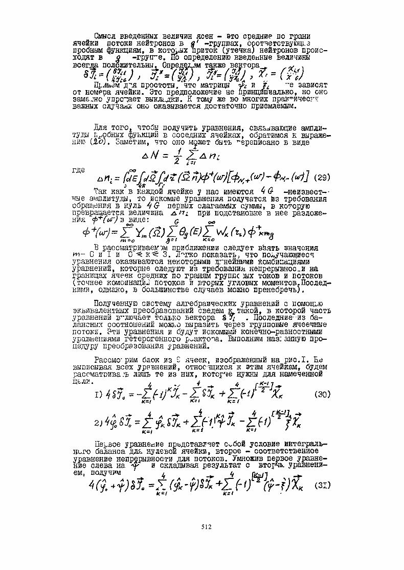
Ñìûñë ââåäåííûõ âåëè÷èí ÿñåí - ýòî ñðåäíèå äî ãðàíèÿ÷åéêè ïîòîêè íåéòðîíîâ â $' -ãðóïïàõ, ñîîòâåòñòâóþò! çïðîáíûì ôóíêöèÿì, â êîòîðûõ ïðèòîê (óòå÷êà) íåéòðîíîâ ïðîèñ-õîäÿò â ^ -ãðóïïå. Ïî îïðåäåëåíèþ ââåäåííûå âåëè÷èíûâñåãäà ïîëîæèòåëüíû. Îïðåäåëèì òàêæå âåêòîðà. ,- Ã. =ä"ë ïðîñòîòû, ÷òî ìàòðèöû ^ è /^ "å çàâèñÿò

îò íîìåðà ÿ÷åéêè. Ýòî ïðåäïîëîæåíèå íå ïðèíöèïèàëüíî, íî îíîçàìå. 'íî "ó ïðåéäåò âûêëüäêè. Ê òîìó æå âî ìíîãèõ ïðàê^è÷åñã÷âàæíûõ ñëó÷àÿõ îíî îêàçûâàåòñÿ äîñòàòî÷íî ïðèåìëåìûì.

Äëÿ òîãîã ÷òîáû ïîëó÷èòü óðàâíåíèÿ, ñâÿçûâàþùèå àìïëè-òóäû ïðîáíûõ ôóíêöèé â ñîñåäíèõ ÿ÷åéêàõ, îáðàòçàìñÿ ê âûðàæåíèþ (2,î). Çàìåòèì, ÷òî îíî ìîæåò áûòü "åðåïèñàíî Á âèäå

-1-1

(29)• ó .Òàê êàê â êàæäîé ÿ÷åéêå ó íàñ èìåþòñÿ ÷ 0- -íåèçâåñò--÷àå àìïëèòóäû, òî èñêîìûå óðàâíåíèÿ ïîëó÷àòñÿ èç òðåáîâàíèÿîáðàùåíèÿ â íóëü 46- ïåðâûõ ñëàãàåìûõ ñóììû, â êîòîðóþïðåâðàùàåòñÿ âåëè÷èíà ë^! ïðà ïîäñòàíîâêå â íåå ðàçëîæå-

íèÿ < ò Õ / ç âèäå:

Â ðàññìàòðèâàåì- æ ïðèáëèæåíèè ñëåäóåò âçÿòü çíà÷åíèÿò- Ñ è 1 è 0-^ê"$3. Ë^ãêî ïîêàçàòü; ÷òî ïîó÷àþùèåñÿóðàâíåíèÿ îêàçûâàþòñÿ íåêîòîðûìè ëãíåéíûìé êîìáèíàöèÿìèóðàâíåíèé, êîòîðûå ñëåäóþò èç òðåáîâàíèÿ íåïðåðûâíîå _è íàãðàíèöàõ ÿ÷ååê ñðåäíèõ ïî ãðàíÿì ãðóïïå çûõ òîêîâ è ïîòîêîâ(òî÷íåå êîìîèíàöè^ ïîòîêîâ è âòîðûõ óãëîâûõ ìîìåíòîâ. Ïîñëåä-íèìè, îäíàêî, â áîëüøèíñòâå ñëó÷àåâ ìîæíî ïðåíåáðå÷ü).Ïîëó÷åííóþ ñèñòåìó àëãåáðàè÷åñêèõ óðàâíåíèé ñ ïîìîùüþýêâèâàëåíòíûõ ïðåîáðàçîâàíèé ñâåäåì ê òàêîé, â êîòîðîé ÷àñòüóðàâíåíèé âêëþ÷àåò òîëüêî âåêòîðà 8 "5^ . Ïîñëåäíèå- -èç áà-ëàíñíûõ ñîîòíîøåíèé ìîæüî âûðàçèòü ÷åðåç ãðóïïîâûå ÿ÷åå÷íûåïîòîêè. Ýòè óðàâíåíèÿ è áóäóò èñêîìûìè êîíå÷íî-ðàçíîñòíûìèóðàâíåíèÿìè ãåòåðîãåííîãî ð~àêòî÷à. Âûïîëíèì íàç: ýííóþ ïðî-öåäóðó ïðåîáðàçîâàíèÿ óðàâíåíèé.Ðàññìî'ðèì áëîê èç 2 ÿ÷ååê, èçîáðàæåííûé íà ðèñ.1. Ååâûïèñûâàÿ âñåõ óðàâíåíèé, îòíîñÿùèõñÿ ê ýòèì ÿ÷åéêàì, áóäåìðàññìàòðèâàâ ëèøü òå èç íèõ, êîòîðîå íóæíû äëÿ íàìå÷åííîé

/ * _* « ã*'' 7.»ã) 4 «Ó. = -Ã&Ë7, - Ã«4 + ÃÛ "*"% (çî)2»Ïåðâîå óðàâíåíèå ïðåäñòàâëÿåò ñ^áîé óñëîâèå èíòåãðàëüíîãî áàëàíñà äëÿ. íóëåâîé ÿ÷åéêè, âòîðîå - ñîîòâåòñòâåííîåóðàâíåíèå íåïðåðûâíîñòè äëÿ ïîòîêîâ. Óìíîæèâ ïåðâîå óðàâíåíèå ñëåâà íà 4- 0 ñêëàäûâàÿ ðåçóëüòàò ñ âòîð÷ü. óðàâíåíèåì, ïîëó÷èì .*, 4

512

Çàìåòèì, ÷òî åñëè áû ìû íå ó÷èòãòàëè äîü^ äíè òåëüíûõïðîáíûõ ôóíêöèé, òî-åñòü ïîëàãàëè áû = Î, ãî óðàâíåíèåèìåëî áû âèäë ^ (ÇË

Îáîçíà÷èì - - è<Ó* ë

Òîãäà :'ðàâíå÷èå (32) ïðèîáðåòàåò âèäë *7 * 5. / >*÷ ^^^^

Çäåñü /\ Ä*" - 2*ÑÔ*~3%) - ïðîñòåéøèé ðàçíîñòíûéËóÕ ê÷ ä^àíàëñ.' îïåðàòîðà Ëàïëàñà (ñõåìà "êððñò"). Ò^êæ îáðàçîì,ïîëó÷åííîå óðàâíåëèå èìååò âèä îáû÷íûé äëÿ ìåòîäà ãîìîãåíè-çàöèè, íî ñ êîýôôèöèåíòàìè, îïðåäåëåííûìè èíà÷å. Îòëîæèâ íàâðåìÿ à :àë0ç êîìïîíåíò ìàòðèöû ýå* è âåêòîðà 3>^ , âåð-íåìñÿ ê óðàâíåíèþ (31). ^

×òîá÷ èñêëþ÷èòü âåëè÷èíû /\ < èñïîëüçóåì óðàâíåíèÿäëÿ óãäîøõ ÿ÷ååê áëîêà, ãçîáðàæåííîãî íà ðèñ.1, ñîîòâåòñòâó-þãèå èîâåðõíîñòíûãë ìîìåíòàì ÓÓÑ(ã&)+Ê ,Ú -\ë4(.*%). Îïóñêàÿòðèâèàëüíûå ïðåîá;àçîâàíâÿ ^òèõ óðàâíåíèé, ïðèâåäåì ðåçóëüòàò4 ÃÀ-'7-* 4 _^ <• ^

Èç ïîñëåäíåãî óðàâíåíèÿ è óðàâíåíèÿ (3±), ðèíèìàÿ âîâíèìàíèå ââåäåííûå îáîçíà÷åíèÿ, ïîëó÷ëì

Ïåðåïèøåì åãî â âèäå ..... (34)

ñ Ëñ-åäèíè÷íàÿ ìàçôèöà, À^*- ~ — ä —— "* ðàçíîñòíûéàíàëîã îïåðàòîðà Ëàïëàñà òèïà "ïîâåðíóòûé êðýñò*.

Óð< âüåíèñ (34) ìîæåà áûòü çàïèñàíî â âèäå. -ò*- Ë #-7*' ÷/\ôê - Õ0 ô0 = 0 (ÃÎ)

è. -±

Â óðàâíåíèè (35) ìîãóò áûòü ñäåëàíû íåêîòîðûå óïðîùå-íèÿ. Îòìåòèì çäåñü òîëüêî îäíî: êàê ïîêàçàë àíàëèç è ïðîá-íûå ðàñ÷åòû íåò íóàäû îàññ÷èòûâàòü ìàòðèöó ã- . .Äîñòàòî÷-íî.ðàñ÷åòû íåò íóàäû îàññ÷èòûâàòü ìàòðèöó ã- . .Äîñòàòî÷-õîðîøèì ïðèáëèæåíèåì ÿâëÿåòñÿ ~ ^ ^'Îáðàòèìñÿ òåïåðü ê âûÿñíåíèþ ñìûñëà âîøåäøèõ â óðàâíå-íèå âåëè÷èí.

513

Âûáîð âåêòîðà ãðóïïîâûõïîòîêîâÂ êà÷åñòâå^ âåêòîðà ãðóïïîâûõ ïîòîêîâ ìû âçÿëè âåëè÷èíóõ = (</ _ ø] § óë Çàìåòèì, ÷òî ïî îïðåäåëåíà ââåäåí-

íûõ âåëè÷èí & ÚÓ ÿâëÿåìñÿ âåêòîðîì ñðåäíèõ ïî ãðàíè-öàì ÿ÷åéêè ãðóïïîâûõ ïîòîêîâ. Åçêèì îáðàçîì, âîå åãî êîìïî-íåíòû ïîëîæèòåëüíû. Öàê êàê ïî ñìûñëó ââåäåííû* âåëè÷èíêñëïîíåíòû ìàòðèöû ÿ-ó-&-' _^ ^ ëë , íåîòðèöà-òåëüíû, òî êîìïîíåíòû âåêòîðà <« **(å- ó^ëòàõêå íåîò-ðèöàòåëüíû :; ìîãóò ñ÷èòàòüñÿ íåêîòîðûìè õàðàêòåðíûìè äëÿÿ÷åéêè ãðóïïîâûìè ïîòîêàìè. Óñòàíîâëåíèå ñìûñëà ýòèõ âåëè÷èí,âûïîëíåííîå â ïðîñòûõ ñëó÷àÿõ, ïîêàçûâàåò, ÷òî êîìïîíåíòûâåêòîðà ^ ÿâëÿþòñÿ çíà÷åíèÿìè â öåíòðàõ ÿò.çåê ïëàâíîéîãèáàþùåé; êàñàþùåéñÿ êðèâîé äåéñòâèòåëüíûõ ãðóïïîâûõ ïîòî-êîâ íà ãðàíèöàõ ÿ÷ååê.Ëåãêî âèäåòü, ÷òî îáîð â êà÷åñòâå íåèçâåñòíîãî âåêòîðàòàêîãî, ó êîòîðîãî êîìïîíåíòû áèëè áû ñðåäíèìè ïî ÿ÷åéêå ãðóï-ïîâüïèÂ ïñãîêîìè èëè ñðåäíèì1* ïî ãðàíèöàì ÿ÷ååê ïîòîêàìè, êàêýòî äåààåòñÿ â ñëó÷àå îäíîðîäíîé ðçøåòÿè, ïðèâåë áû ê áîëååñëîæíûì óðàâíåíèÿì.

Äðóãîé âîçìîæíûé âûáîð íåèçâåñòíîãî âåêòîðà, ïðèâîäÿ-ùèé ê äîñòàòî÷íî „.ðîñòø óðàâíåíèÿì , òàêîâ

Èç âûøåñêàçàííîãî ÿñíî, ÷òî âñå êîìïîíåíòû ýòîãî âåêòî-ðà ïîëîæèòåëüíû. Ñ èñïîëüçîâàíèåì âåêòîðà & ïîñëå íåêî-òîðûõ ëðîñòûõ ïðåîîðàçîâàíèé óðàâíåíèå Ò34) ïðèâîäèòñÿ êâèäó: $ À-Çäåñü = ± +> & = -

ë ËÌàòðèöà (Ã ñîîòâåòñòâóåò ìàòðùã Ó ñãìåòðè÷íûõïðîáíûõ ôóíêöèé äëÿ ÿ÷åéêè èç ÷èñòîãî çàìåäëèòåëÿ, ïîýòîìóîíà íå çàâèñèò îò íîìåðà ÿ÷åéêè (âïðî÷åì ìîêåò áüãü âçÿòàìàòðèöà è êàêîé-íèáóäü äðóãîé òèïè÷íîé äëÿ äàííîãî ðåàêòîðàÿ÷åéêè) .Åñëè ðàññìàòðèâàòü çàäà÷ó â äâóõã^óïïîâîì ïðèáëèæåíèèâ ñîîòâåòñòâåííà ïðåîáðàçîâàâ* âåêòîð • äèàãîíàëèçèðîâàòüìàòðèöû 3, » Â, , 3^ è 8? (êàê âèäíî èç ôîðìóë, óêà-çàííûå ìàòðèöû ìîãóò íûòü äèàæþíàëèçèðîâàíû îäãîâðåìåííî,åñëè èñïîëüçóåòå.': àüðîêñèìàöèÿ (36)), òî óðãçêåíèå (37) ïðè-îáðåòàåò âèä òàêîãî, ðåøåíèå êîòîðîãî ïîëó÷àåòñÿ â ïðîãðàì-ìàõ, îïèñàííûõ â ðàáîòàõ /23,24/. Ëëÿ òîãî, ÷òîáû âîñïîëüçî-âàòüñÿ ýòèìè ïðîãðàììàî, òðåáóþòñÿ ëèøü íåáîëüøèå üçìåíåíèÿíà ýòàïàõ ââîäà ïàðàìåòðîâ ÿ÷ååê èëîäó÷åíèÿ èíòåðåñóþùèõíàñ âåëè÷èí èç êîìïîíåíò âåêòîðà % ,

ËÌàòðèöû Ô è

514

Â óðàâíåíèÿõ (31-35,37) ïîñëå ïðèìåíåíèÿ àïðîêñèìàöèè(36) âñå "êîýôôèöèåíòû çàâÿîÿò ëøü îò êîìïîíåíò ìàòðèö ó è& . ×òîáû ïîíÿòü ñìûñë ýòèõ âåëè÷èí, âûïèæå*:: èõ ÿâíûéâèä â íåêîòîðûõ ïðîñòûõ ñëó÷àÿõ.Ìàòðèöà ó äëÿ êâñîôàòíîé îäíîðîäíîé ÿ÷åéêè, âíóòðèêîòîðîé ñïøãçäëèâî äâóõãðóïïîâîå äèôôóçèîííîå ïðèáëèæåíèå,åëååò âèä Ã

Çäåñü Ó, è ÝÀ - êîýôôèöèåíòû äèôôóçèè â ïåðâîé èâòîðîé ãðóïïàõ, ñîîòâåòñòâåííî, %± = ë&1> 1)^1.1- äëèíà ò'èô-ôóçèè â * -ãðóïïå, (. ÎÄçÛ2*/2; » òî-åñòü ïðè 2 -1 è(ã 1Ñëåäîâàòåëüíî, ïðè

Îáðàòíàÿ ìàòðãòà

Ïðè ^

_Òàêèì îáðàçîì, êîìïîíåíòà ìàòðèöû ^ ïðîïîðöèî-íàëüíà êîýôôèöèñíòàãé äèôôóçèè. Ãéíîæèòåëé è~(ã*) ìîãóò òðàê-òîâàòüñÿ, êàê ïîïðàâêè íà ïîãëîùåíèå.Çàìåíèì, ÷òð äëÿ ÿ÷åéêè ñ íèòåâèäíûì èñòî÷íèêîì-ñòîêîììàòðèöû (^ è ó~' ñîâïàäàþò ñ ñîîòâåòñòâóþùèìè ìàòðèöàìèäëÿ ÿ÷åéêè èç ÷èñòîãî çàìåäòçòåëÿ. Åñëè ìàòðèöà ó îïðå-äåëÿåò^ÿ äèôôóçèîííûìè õàðàêòåðèñòèêàìè ÿ÷åéêè, òî ìàòðèöà

& ñâÿçàíà ñ ïðîöåññàìè ïîãëîùåíèÿ è ðàçìíîæåíèÿ íåéò-ðîíîâ â ÿ÷åéêå.Ðàññìîòðèì ñíà÷àëà ýòó ìàòðèöó äëÿ ÿ÷åéêè áåç äåëåíèÿ.Äëÿ òàêîé ÿ÷åéêà îáîçíà÷èì </> = (ã . Äèàãîíàëüíûå ýëåìåíòûýòîé ìàòðèöû ìîãóò áûòü ïðîñòî èç áàëàíñíûõ ñîîáðàæåíèéçàïèñàíû â âèäå ñãä ± ãÃ%//ÉÃ«> , ãäå<^ãÀ5> - ñðåäíååâ<| ^ ' '*—* / * &

ïî ÿ÷åéêå ñå÷åíèå ïîãëîùåíèÿ â ãðóïïå ç , È(ãä) - êîýôôèöè-åíò íåðàâíîìåðíîñòè, òî-åñòü îòíîøåíèå ñðåäíåãî ïî ãðàíèöàìÿ÷åéêè ïîòîêà'â § -ãðóïïà ê ñðåäíåìó ïî ÿ÷åéêè ïîòîêó ÷ýòîé ãðóïïå. Â óðàâíåíèÿ âõîäèò ãîã.ñâäó îáðàòíàÿ ìàòðèöà•ö-"7 . Çàïèøåì åå â âèäå .

515

âûÿñíåíèÿ âåëè÷èíû è ñìûñëà íåäèàãîøëûøõ ýëåìåíòîâ,çàïèøåì ìàòðèöó 2^ äëÿ îäíîðîäíîé ÿ÷åéêè ñ äâóõãðóïïîâûìäèôôóçèîííûì ïðèáëèæåíèè!* Ïðè ýòîì

Çäåñü Ð- âåðîÿòíîñòü èçðåêàòü ïîãëîùåíèÿ â ïåðâîé ãðóïïå,

Ïðè 2;«1 ã (ã<) 2 I èë /5"5~ 2ã / é* 7

\~ð^_à4 ;ëÇüäèì, ÷òî ìàòðüäà ^ , êàê 0 ñëåäîâàëî îæèäàòü, îñòàåò-ñÿ òðåóãîëüíîé.

ÀÐàññìîòðèì òåïåðü ìàòðéöò Ó* äëÿ ÿ÷åéêè ñ äåëåíèåì.àçäåò ì, ÷òî ïðè ê^- =1* ìàòðèöà ^ áóäåò íå ñ :ðåäåëåíà,òàê êàê ïî ôèçè÷åñêîìó ñìûñëó ïðè Õ« I ýëåã íòû ìàòðèöûñòðåìÿòñÿ ê áåñêîíå÷íîñòè. Â óðàâíåíèå âõîäèò, :àê óæå îò-ìå÷àëîñü, îáðàòíàÿ ìàòðèöà <&-' . Åå ýëåìåíòû *.ëåþòñìûñë â ÿðÿ Êîå; = 1.À Îäíàêî, äëÿ óäîîñò à ïðîâåäåíèÿ îïå-ðàöèé íàä ìàòðèöåé & åå ñëåäóåò ïðåîáðàçîâàòü Êàê îòìå-÷àëîñü â ðàáîòå /17/, óäîáíî ïðåäñòàâèòå åå â âèäå

Çäåñü %*' - âåê-þð ãðóïïîâûõ ïîòîêîâ íà ãðãíèöàõ ÿ÷åéêè,âûâåäåííîé íà êðèòè÷íîñòü. Òî-åñòü

ãäå /V - ÷èñëî ãðàíåé ÿ÷åéêè. Ñîîòâåòñòâóþùàÿ âåëè÷èíàóäîâëåòâîîÿåò óðàâíåíèþ.

è óñëîâèÿì ïåðèîäè÷íîñòèÂåêòîð ï*^ =ã { $:•/ âûáèðàåòñÿ òàê, ÷òî ìàòðèöà <Ü

' I Ð1.6-/ïðè Êáî.; =? I áûëñ. îïðåäåëåãà. Îáîçíà÷åíèå äëÿ ýòîé ìàòðèöûâûáðàíî òàêèì ïáòðìó, ÷òî îíà äåéñòâèòåëüíî áëèçêà ê ìàòðè-öå ðåøåíèé â ÿ÷åééå-áåç äîåíèé.1*0* '* Ð÷ - ìàòðùà, êîìïîíåíòû êîòîðîé îïðåäåëÿþòñÿ

ñëåäóþùèì îáðàçîì:

Èñïîëüçóÿ ñâîéñòâ" ìàòðèöû (ô<>; *Ð*} ìîæíî ÿâíûìîáðàçîì âûïîëíèòü îáðàùåíèå ìàòðèöû ÷?4- . Ïðè ýòîì îáðàò-íóþ ìàòðèöó óäàåòñÿ ïðåäñòàâèòü â âèäå

ò - - êîýôôèöèåíò ðãçìÿîàãíèÿ áåñêîíå÷íî ç ðåøüãêè â?ÿ÷ååê *. -ñîðòà.516

Çäåñü ð1 ~(Êîà- 0/*×* , ìàòðèöà 21É4 - -~ %~'Ìàòðèöà 2Ã/ ë âåëè÷èíà ñäàâ äâóó^ðóïïîâîì ïðèáëèæåíèèèìåþòâèë å-

«

Çäåñü 1.04 - ñðåäíèå ïî ÿ÷åéêå ñå÷åíèÿ â § -ãðóïïå { î: ðåäåëÿåìûç ïî ðåøåíèÿì Î÷ / 2Ã* - àíàëîãè÷íûå âåëè÷èíû, îïðåäåëÿåìûå ïî ðåøåíâÿãë $/,*•« 'ç *ÿ° - îòíîøåíèÿñðåäíèõ ïî ÿ÷åéêàì ãðóïïîâûõ ïîòîêîâ ê ñðåäíèì ïî ãðàíèöàìÿ÷ååê, ñîîòâåòñòâåííî äëÿ ðåøåíèé 3;- è <?0,- , ð è ðññîîòâåòñòâóþùèå âåðîÿòíîñòè èçáåãàòü ïîãëîùåíèÿ â ïåðâîéãðóïïå, * - âåëè÷èíà» çàïñÿùàÿ îò êîýôôèöèåíòîâ ã. è (Â ñëó ]àå îäíîðîäíîé ÿ÷åéêè

Èç ïðèâåäåííûõ ôîðìóë âèäèì, ÷òî, êðîìå òðàäèöèîííûõðàñ÷åòîâ ÿíåéêè ñ íóëåâûìè ãðàíè÷íûìè òîêàìè, äëÿ îïðåäåëå-íèÿ ýëåìåíòîâ ìàòðèö & òðåáóåòñÿ ðàñ÷èòûâàòü ðàñïðåäåëå-íèå íåéòðîíîâ â ÿ÷åéêå ñ âòåêàþùèìè òîêàìè.

Çàêëþ÷åíèåÍåñêîëüêî ñëîâ î âåëè÷èíå ïîïðàâîê â ðåøåíèè, âîçíè-êàþùèõ ïðè èñïîëüçîâàíèè ðàçâèòîãî ôîðò àäèçìà. Îñíîâíîéó÷åò ðàçëè÷àÿ ñâñÇñòâ ÿ÷ååê ïðîèçâîäèòñÿ ñ ïîìîùüþ ââåäåíèÿâ ðàñ÷åò êîýôôèöèåíòîâÿíåðàâíîìåðíîñòè ïîòîêîâ ïî ÿ÷åéêå,êîòîðûå â íåîäíîðîäíîé ðåøåòêå åñòåñòâåííî ðàçëè÷íû â~ðàç-íûõ ÿ÷åéêàõ, â ðàçëè÷íîãî îïèñàíèÿ ïîãëîùåíèÿ, ðàçìíîæåíèÿè 1,åðåõîäîâ èç ãðóïïû â ãðóïïó "ñîáñòâåííûõ" íåéòðîíîâ(ñå÷åíèÿ ã: , 2:$ , âåëè÷èíû Êå« ,./>«) è ïðèòåêàþùèõ âÿ÷åéêó ñî ñòîðîíû (ìàòðüäà 2 / }.Ïðîîíûå ðàñ÷åòû ïîêàçàâ, ÷òî â ðåàëüíûõ ñèòóàöèÿõââåäåííûå ïîïðàâêè èçìåíÿëè ïîòîêè òåïëîâûõ íåéòðîíîü âìåñòàõ ðåçêèõ ÿåîòíîðîäøýñòåé ðåøåòêè ïî çðàâíåíèþ ñ òðàäè-öèîüøûìâ ãîãîãåí0çàöèîííû1ëà óðàãòãåíèÿìè äî 10+15 .Ñ äðóãîé ñòîðîíû, ÿâëÿÿñü îáîáùåíèåì ìåòîäà ãîìîãåíè-çã7û, ðàçâèòûé ïîäõîä ñîõðàíÿåò ïðèñóùåå ïîñëåäíåìó ïðåè-ìóùåñòâî î'îëåå ïîäðîáíîãî ýíåðãåòè÷åñêîãî îïèñàíèÿ ïîòîêîâíåéòðîíîâ ïî ÿ÷åéêàì ïðè ìàëîãðóïïîâîì îïèñàíèè ïåðåòå÷åêíåéòðîíîâ ìåçäó ÿ÷åéêàìè. Çàìåòèì, ÷òî äëÿ êàíàëüíûõ ãðàôè-òîâûõ ðåàêòîðîâ ñ íåîäíîðîäûøè ðåøåòêàìè ðàñ÷åòû ìåòîäîìèñòî÷íèêîâ-ñòîêîâ ñ äâóõãðóïïîüõø è äèôôóçèîííî-âîçðàñòíûìÿäðàìè äàþò îòëè÷èÿ â ïîòîêàõ òåïëîâûõ íåéòðîíîâ äî 10% èåùå áîëüøåå ðàçëè÷èå â ïîòîêàõ ýïéòåøøâûõ íåéòðîíîâ. Òàêêàê ñïîñîáû, ñâîäÿùèå óðàâíåíèÿ èñè-î÷íèêîâ-ñòîêîâ ê êîíå÷-íî-ðàçêñ òíûì /23- 6/ èñüîëúçóêã ãðóûîâîå îïèñàíèå íåéòðî-íñ÷, äëÿ óñòðàíåíèÿ óêàçàííîé ïîãðåøíîñòè â âõ ñàìêàõ ïðè-õîäèòñÿ óâåëè÷èâàòü ÷èñëî ãðóïï ïðè ðàñ÷åòå ðåàêòîðà â öå-ëîì. Èçëîæåííûé â ðàáîòå ïîäõîä ñâîáîäåí îò ýòî î íåäîñòàò-êà.

517

Çàìåòèì äàëåå, «òî ðàññìîòðåííàÿ ïðîöåäóðà ïîñòðîåíèÿêîíå÷íî-îàçíîñòíûõ óðàâíåíà? ÿâëÿåòñÿ ñ ìàòåìàòè÷åñêîé òî÷-êê çðåíèÿ ñïîñîáæ ïîëó÷åíèÿ êîíå÷íî-ðàçíîñòíûõ óðàâíåíèéïîâûøåííîé òî÷íîñòè. Òàêîé ïóòü ñîâåðøåííî åñòåñòâåí,ïðè ðàññìîòðåíèè ãåòåðîãåííîãî ðåàêòîðà, òàê êåä òðèâèàëü-íûé ïóòü ïîâûøåíèÿ òî÷íîñòè çà ñ÷åò óìåíüøåíèÿ øà~à ñåòêèçäåñü íå ïðèåìëåì. Îäíàêî è â òåõ ñëó÷àÿõ, êîãëÄ ÿ÷åéêèðåàêòîðà ìîæíî ñ÷èòàòü ãîìîãåííûìè (êàññëû ðåàêòîðà „ÿïàÂÂÝÐ ïðè ðàñ÷åòå ìàêðîïîëÿ â íåì), ðàçâèòûé ïîäçïä ìîæåòîêàçàòüñÿ áîëåå âûãîäíûì, ^åì äðîáëåíèã øàãà ñåòêè. Ãàêîáñòîèò äåëî, íàïðèìåð, ïðè îèëüíèë ðàçëè÷íà äëø äèôôóçèèíåéòðîíîâ â ðàçíûõ ãðóïïàõ.

Ë è ò å ð à ò ó ð à1. Äýâèñîí Á. Òåîðèÿ ïåðåíîñà íåéòðîíîâ. Ïåð. ñ àíãë.,Àòîìèçäàò, 1960 ã.2. Ãàëàíèí À. Ä. Òåîðèÿ ÿäåðíûõ ðåàêòîðîâ íà òåïëîâûõíåéòðîíàõ, Àòîìèçäàò, 1957ã.3. Âåéíáåðã À, Âèãíåð Å. Ôèçè÷åñêàÿ òåîðèÿ ÿäåðíûõ ðåàêòîðîâ.Ïåð. ñ àíãë., ÈÆ, 1961 ã.4. Ãàëàíèí À. Ä. Òåîðèÿ ãåòåðîãåííîãî ðåàêòîðà. Àòîìèçäàò,

'5. Ò. Ó. $**/, Ë. È/(ü*. Ò*^æ ó. ë. \*/Ì. Ë». Ó. ÿ*ì. $1, ,*• ã Ñ/ý

6. &1.$1»ËÀ<1/. Ó. ßË. Û4. 1^ .&% Ñ

7. Øåâåëåâ ß.Â. Àòîìíàÿ ýíåðãèÿ. Ò.2, ñ. 234, 1957ã.8. Ëàëåòèí Í.È. Òðóäû âòîðîé ìåæäóíàðîäíîé êîíôåðåíöèè ï0ìèðíîìó èñïîëüçîâàíèþ àòîìíîé ýíåðãèè, Æåíåâà, 1958ã.

Äîêëàäû ñîâåòñêèõ ó÷åíûõ, ò. 2, ñòð.634, ÃË., Àòîøçäàò,1953 ã.

9. Ñìåëîâ Â. Â. Àòîìíàÿ ýíåðãèÿ, ò.Ü, ñ. 546, õ95 ã.10. Üúí^ë4 Ð. Ó.11.12. Ðóìÿíöåâ Ã.ß. Àòîìíàÿ ýêåðãüë, ò. 13- ¹ 6, ÃÝ62 ã.,ò. 14, ¹ 4, 1963 : .13. Ãðèãîðüåâ È.Î., Íîüëñîâ Â.Ì» äèôôóçèÿ íåéòðîíîâ ò. ãåòå:,-ãåííûõ ñðåäàõ, Àòîìèçäàò, 1968 ã.14. Ñèäîðåíêî Â. Ä. / åëëåëåë /ë, , 12, ñ. 5, 19î9 ã.15. &ÔÏ4Ëü÷~Ë Ê.. ˆ*ëë%1à. Ë/èñßû: úå, , /À,ã/ ,16. ÅËÁØÈÍ À. Â., Ëàëåòèí Í.!*. (Ïîïåðå÷íàÿ äèôôóçèÿ íåéòðî-íîü â ïëîñêîé ðåøåòêå) , ïðåïðèíò ÈÀÝ-2721, Ä1, 1976 ã.17. Ëàëåòèí Í.È. , Åëüøø À.Â. Àòîìíàÿ ýíåðãèÿ, ò.43, ñ.247,-1977 ã.

518

18. Ôå¸íáåðã Ñ.Í. Â êí.Ìàòåðèàëû ìåæäóíàðîäíîé êîíôåðåíöèèïî ìèðíîìó èñïîëüçîâàíèþ àòîìíîé ýíãðãèè, Æå^åãà, 1955 ã,ò.5 Ð7669.19. Ãàëàíâí À.Ä. Òàè» æå Ð/1647 (ñì.òàêæå /2/).20 Ëàëåòèí Í.È. Äèôôóçèÿ íåéòðîíîâ â ãåòåðîãåííûõ ñðåçàõ(ìåòîä "èñòî÷íèêîâ-ñòîêîâ") ãðå ïðèíò ÈÀÝ-2807, Ì.,1977ã.21. Ëàëåòèí ×.È. Âûâîä óðàâíåíèé ìåòîäà "èñòî÷íèêîâ-ñòîêîâ"âç êèíåòè÷åñêîãî óðàâíåíèÿ, ïðåïðèíò ÈÀÝ-2808, Ì. ,1977ã.22. Â. Ëåëåê. Äèññåðòàöèÿ. 1967 ã.23. Ãîðîäêîâ Ñ. Ñ. Íîâûé ìåòîä ðàñ÷åòà ãåòåðîãåííûõ ðåàêòî-ðîâ, ïðåïðèíò ÈÀÝ-2251, 1973 ã.24. Ãîðîäêîâ Ñ. Ñ. Äâóõãðóïïîâîé ðàñ÷åò ãåòåðîãåííîãî ðåàê-òîðà êâàçèàëúáåäøø ìåòîäîì, ïðåïðèíò ÈÀÝ-2283, 1973ã.25* Êî÷óðîâ Á.Ì. , *1àëîôååâ Â.Ì. Àòîìíàÿ ýíåðãèÿ, ò. 42, ¹ ß,

( * I*»26.

Ó À (*****}

/36*,, /..5 ÇÀ27. Âàðèàöèîííî-ðàç! îñòíûå ìåòîäüã ðåøåíèÿ çàäà÷ ìàòåìàòè-÷åñêîé ôèçèêè. Ñáîðíèê íàó÷íüò òðóäîâ âîä ðåäàêöèåéÃ.È.Ìàð÷óêà, Íîâîñèáèðñê, 1076 ã.28. Ñòðç.ò Ã., Ôèêñ, Ä. Òåîðèÿ ìåòîëà êîíå÷íûõ ýëåìåíòîâ.Ì.» Íàóêà, 1Ñ77 ã.29å Òèõîíîâ À.ß. Ñàìàðñêè! À.À. Óðàâíåíèÿ ìàòåìàòè÷åñêîéÔÈÇÅÊÇ. Íàóêà, Ì. , 1966 ã.30. Ûàð÷ëã Ã.È. , Îðëãâ Â.Â. Â ñá. Íåéòðîííàÿ ôèçèêà. Ì. ,Àòîìïçäàò, ñ. 30, 1Ã$1 ã.31. Âëàäèìèðîâ Â. Ñ. Ìàòåìàòè÷åñêèå çàäà÷è îäíî îðîñòíî!òåîðèè ïåðåíîñà ÷àñòèö. Òðóäû ìàòåì.èí-òà ÀÉ Ñ" ÑÐ, Ì. ,1961 ã.32. ðóìÿíöåâ Ã.ß. Àòîìíàÿ ýíåðãèÿ, ò. 10, ñ. 26, 1961 ã.33. &>& *• , $Üü»èãè Ë. Ó. È^ñ^ -. Ï* Æ*. „-1 „ Ì ,4965)34.35. Ü1àéîðîâ ^.Â. , Ãðóõàíîâ Ã.ß. Ôðàíê-Êàìåíåöêèé À.Ä.

Ù)èìåíåíèå àëüáåæîãî ìåòîäà ê ðàñ÷åòó öóòêà ñòåðøåé.Ùþïðèíò ÈÀÝ-1981, 1970 ã. (Îÿëàêæå â êíèãå "Ìåòîäàðàñ÷åòà ï^ëåé òåîëîâëã íåéòðîíîâ â ðåøåòêàõ ðåàêòîðîâ"ïîä ðåäàêöèåé ß.Â.Øåâåëåâà, Àòîøçäàò, 1974 ã.)

36. Ñ.ß.Áàðêîâ. Àò-üáåäííÉ ìåòîä ðàñ÷åòà õàðáëòåðèñòèê ãåòå-ðîãåííîãî ðåàêòîðà. Öðåïðèíò ÈÀ0-2938, 1977 ã.

37.

519

A NEW CONSISTENT DEFINITIONOF THE HOMOGENIZED DIFFUSIONCOEFFICIENT OF A LATTICE,LIMITATIONS OF THE HOMOGENIZATION CONCEPT,AND DISCUSSION OF PREVIOUSLYDEFINED COEFFICIENTS

V.C. DENIZReactor Group,Bhabha Atomic Research Centre,Bombay, India

Abstract

The problem concerned with the correct definition of the homogenizeddiffusion coefficient of a lattice, and the concurrent problem of whetheror not a homogenized diffusion equation can be formally set up, is studiedby a spac«-energy-angle dependent treatment for a general lattice cellusing an operator notation which applies to any eigen-problem. A new de-finition of the diffusion coefficient is given, which combines within it-self the individual merits of the two definitions of Benoist. The relationbetween the new coefficient and the "uncorrected* Benoist coefficient isdiscussed by considering continuous-spectrum and multi-group diffusionequations* Other definitions existing in the literature are briefly dis-cussed* It is concluded that a diffusion coefficient should representonly leakage effects. A comparison is made between the homogenizationapproach and the approach via eigen-coefficients, and brief indications aregiven of a possible scheme for the latter.

1. DffRCDOCTICN AND DEFINITKK CF THE PRCBLEM

In view of the practical utility of multi-group diffusion equations inreactor analysis of heterogeneous media, there exists the important theoreticalproblem of determining to what extent the prescriptions for the homogenizeddiffusion equation can be formally defined and to what extent the applicationof the equation is heuristic in nature. The theoretical problem thus concernsthe definition of the homogenized diffusion coefficient and the associatedhomogenized diffusion equation. A number of definitions for the diffusioncoefficient have been proposed in the literature. In the present paper a newdefinition is derived, on the basis of which homogenization can be discussed.The previously defined coefficients are commented upon. Indications are giventhat there are limitations in the homogenization concept, and an alternativeapproach to reactor analysis is discussed.

The configuration studied in this paper is that of an infinite uniformlattice with superimposed buckling. The primary balance equation is expressedin the form of an eigen-value problem. There could be instances where thepostulation of the primary balance equation in the form of an eigen-problemmay not be strictly applicable. For example if the uniform lattice containsvoid regions which permit infinite neutron trajectories in voids, the neutronsmoving along such trajectories are for all practical purposes lost to thedetermination of the overall neutron balance.

The infinite uniform lattice with superimposed buckling is a representa-tion of a one-region finite reactor. This representation implies that theformal discussion is in terms of asymptotic theory, that is, a study of thesituation in the deep interior of the corresponding finite lattice. A dis-cussion of the various proposed definitions is possible within this context,since these definitions have been proposed in terms of periodic fluxes appro-priate to asymptotic (deep-interior) theory. Within the framework of thistheory, it is possible to formally define a number of equations, each of whichhas the form of a diffusion equation which represents a correct statement of

521

neutron balance. The arbitrariness results from the fact that one is free toregroup the terms of the balance equation, and uae arbitrary weighting factorsand arbitrary normalization factors. From among this infinite set of possibledefinitions, the choice of what is an appropriate definition vdll depend on thecriterion that the definition should be derivable, or at least interpretabicfrom physical considerations. A further criterion would be that the appropriatedefinition should not have any identifiable defects. For example the appropriatediffusion coefficient is not expected to be double- valued. As another example,the diffusion coefficient should not lead to problems of interpretation underany condition, whether one is examining a multigroup form, or a continuous.spectrun form, or a one-group form.

For practical applications, one is interested in examining the diffusionequation for use in the treatment of multi- region reactors. A formal treatmentfor such systems is difficult. The use of asymptotic theory for discussingmulti-region systems would raise questions regarding the validity of asymptotictheory at and near the interfaces between different regions. Nevertheless, onedoes expect that the use of Fick' s law to apply the current-continuity boundarycondition at the interface between two homogenized media implies that the homo-genized diffusion coefficient of each homogenized medivan should be restrictedto leakage effects alone.

2. THE EIGEN-PROBI3EH AND ITS FORMAL SOLUTKK

The formal transport- theoretic solution of the eigen-problem clarifiesthe content of the primary equations and serves as a reference against whichhomogenization and reduction to diffusion equation forms can be discussed*

Consider an infinite uniform lattice with a sunper imposed bucklingrepresented by 1? . Let FO^.V;^) be the angular flux, which is a functionof position yi , velocity V , and direction ^5. . Defining the net lossoperator 34 by

ir, a.)

the eigen-equation and its adjoint become the following}

where -TJ is real and ,T -depends on the eigen-problem chosen. For the decayconstant eigen-problem y =. i/ir and '•'j is the decay constant; for thekeli *ig«n-problem "3° is the fission source operator and -^ equals

Cancellation of ^xp^jS-JO} l«ads to the equations

M*ZA.ff)^*o , W*-l2^)f*»o ,where ^ "S o4 -*VJT • Separation into real and imaginary parts gives

(4a'b>

Considering only Eq.(3a), and noting that the identity of "shape* betweenEqs(O or Eqs(5) permits a similar treatment for either set, we expand -^B ,which is a periodic function having the periodicity of the lattice, as follows*

where we have used the tensor notation. The indices represent the principaldirections of the lattice, and B1*1 is the component of t? along direction "Vn .A sane index occuring once as superscript and once as subscript implies animationover that index. No animation is involved if the index occurs twice as subscript

.522

or twice as superscript . Similar expansions hold for j-^ , with %% beingthe leading term of ^-^ . Since the principal axes are orthogonal, Oi -S.for Avi^n .

Introduction of Eqs(6) in Eq.(3a) leads to the following equations forthe periodic functions* —

t X*? t^mta. > (7)

/where -H </=.${ -/x}(!?"> and Xi,^ is the component of -*5 along direction "Hi .

A perturbation operation between Eq(3a) and the zero-buckling equivalentof Eq(3b) leads to the equation

being the complex conjugate of 14 . This leads to

We will here term •*) >tvw and the higher order coefficients as eigen-coefficientsin order to distinguish them from diffusion coefficients which occur in theleakage term of the diffusion equation. Eigen- coefficients take account of allbuckling- dependent effects and not only of leakage.

The symmetry properties of the periodic functions and the above formalsolution for the two standard eigen-problems have been discussed earlier byDenial*2. Me see that a unique treatment exists for any eigen-problem onemight wish to postulate.

3. THE HOMOGENIZED. DIFPOSIQt COEFFICIENT AND^ DIFFUSION EQUATION

3.1 Formal Derivation

We formalise the homogenization process by means of an EquivalencePrinciple} We visualize an infinite homogeneous medium which is the homogeneousequivalent of the infinite lattice, and which has the same superimposed buck-ling vector 1? . This homogeneous medium is physically anisotropic in thesmall, since it must represent the "in-the-large" anisotropy of the lattice.A neutron at point (/it"v-t J5.) of phase space will see a different environmentin the lattice and in the homogeneous mediun. We hence expect that equivalencemust be established not by direct physical balance of neutrons but by takingaccount of the importance function of the homogeneous medium. We henceformalize the equivalence mathematically by making a perturbation operationbetween the adjoint equation of the homogeneous medium and the direct equationof the lattice. This idea of equivalence via perturbation theory is not new;it has been mentioned by Marchufex, but the treatment in the present paper iadifferent .

Since the purpose of this equivalence is to define the constants of thediffusion equation of the homogeneous mediun, the perturbation operation hasto be performed at the level of the angle-integrated balance equations.

Let vj, be the domains ot^/ilV')sL respectively, and let us use thenotation

The angle-integrated direct equation of the lattice is i ^ f j ^ O * Letus assune that the corresponding equation of the homogeneous medium, and theadjoint equation, can be written as follows*

523

there

. , , . .where s$- ivSwy>'J>'trJ *8 t"9 Xc»b ^rf.'w') of the homogeneous median. <p andare the ztagle-integrsfced flux and adjoint function. The assumption in postvt-lating the Eqs.(l2) lies in the appearance of the self-adjoint operator MuS torepresent leakage, with its leading term being £3VB>t • For a homogeneo®*1'mediuai, the true leakage terms are given ty K > g

which implies that one must have

Now, if we take Eqa(5) for a homogeneous medium with isotropic scattering(which wa can adopt for our equivalent medium), multiply then by -3/eJ from theleft and integrate over angle, we obtain the relations

(15b)where ^tofiVS/v? «qaals S^ \Jg-j for the KeU. eigen-problem, and equals•^fcrt-UwX1^— yy\/iy for tne' decay constant eigen-problem. We have to considerwhetner Eqs(l5) can be reduced to the forms given in Eqs(l3)«

In an isotropic homogeneous medium, whether multiplying or non-multiplyingthe periodic functions are isotropic and «ft Lean hence be put as 4a bnJi&iHfi •The HHS of Eq(l5a) win hence become equal'to* 4^ ^^^/^^fSt^s^Llariy,the RHS of Eq(l5b) will become ^ri^Jiv) ft'"/'* £ fcA. (TV") , scFthat Eqs(l5) doreduce to Eqs(l3), with AivwJ^" ^"/^MiuS^' * ***« case °^ a" anisotropicmedian containing only moderating materials' we can show that,even for a lattice,the required reduction is possible since we can show, by using the equation ofdetailed balance for the scattering cross-section, that j'ft(/£|'V-yjL')«<v\(y^^(*^ir-'^for the decay-constant eigen-problem, where (^(t^is Haxwellian. A similar re-'duction is possible for an anisotropic non-scatter ing multiplying medium, or inthe case of a one-velocity problem. However, for the realistic practical spec-tral case of an anisotropic multiplying medium with non-zero scattering, thereduction to the forms in Eqs(l3) is not evident, and the arguments by whichthe possibility of reduction is demonstrated for the other cases indicate thatthe reduction will not be possible in this case. The very concept of homogeni-zation is hence suspect, notwithstanding its practical utility.

Assuming that the reduction is possible, the perturbation operation betweenthe angle-integrated direct equation of the lattice and the Eq(llb) leads tothe formal equivalence relation

524

The exponential terms cancel out, leading to the relation

{iiMa*>Wa>*4~W u^,^^which, since "tfoX, depends only on V- , can be written

« . (17b>

The Eqs(i?) are the only statements of equivalence from the mathematicalpoint of view. For defining the homogenized constants we can further decomposethem into sets of equations in any manner which permits Eqs(l7) to be satis-fied. We decompose them in such a way that there is term-by-term equivalencefor each type of reaction. Equating the leakage terms, we get

and, if the leading term of j JLs put as ^ * - & i ? ~ » w* obtain

EqdfSb) is our new derived definition of the diffusion coefficient for theone-group case. It reduces to the * unconnected" Benoist^ coefficient in theone-velocity case or if the flux in the homogeneous medium is Maxwellian. Ifwe assume equivalence within each velocity- group separately the forms (l8a),(iSb) are also applicable for each group, and then this new definition reducesto the "uncorrected" Benoist definition in the case of a large number ofnarrow groups, where <^* can be considered as constant within each group. Thenew definition is not double-valued, and is representative of the leakage effectsdt» to F$ , and of only leakage effects.

The RHS of Eq(l7b)-equated to zero represents a homogenized diffusion equa-tion. As it stands, with integration performed over the whole domain •'Kx'D'x il iit is merely a relationship; but it brings out the essential characteristicsof the homogeniaation process via perturbation theory.

3.2 Diffusion Equations for the Continuous Spectrum Case

For the continuous spectrum case, the Eqs(l2) themselves constitute thehomogenized equations for flux and adjoint flux. The expressions for the homo-genized cross-sections and for Av^&^are obtained by decomposing Eq(l7b) insuch a way that there is term-by-term equivalence, that this equivalence isvalid at each V and, for the in-scattering and the fission source terms, theequivalence is also valid at each v' . We obtain

- Uv (19a)HIT v 7 '

<l9b)•f cv x - e^s

The above is the "natural" *et of definitions. The requirement%s U*wtt'v>)= S"10 v/ ^s KW>K^U"^V'' is Sati8fied> and tne set ^•o satisfiesEq(l6a) which fs the primary equival«ice relation.

525

The diffusion coefficient following from Eq(l9a) is the "uncorrected*Benoist coefficient. This however does not mean that Eq(l9a), integratedover a unit cell, gives the true reaction rates or leakage rate*. W« cansee this by examining only the flux: In view of Eq(3a), Eq(l7b) written tobe true at each "V implies that 22-JkvwvHV •=• C , where y -5 i§-ft\n *<a •

ttiin a multipn-v *<

In view of Eq(l2a), tyî?) and <?§ u*^**6 "«nce equal to vdttiin a multipcative constant. Replacing ^ ^ by HWVcU.1 , the integrated flux ina unit cell volume of the homogenized median would be V^y1 ^V&lC «k(i>)?J/?which is not the same as the corresponding flux in the lattice", which Is givenby ^tKS? i^ftljjj^B^ • The equality is established only for the adjoint-weighted flux, since / • • , * » -

"^

where 1*J *j Îfl^^ I^^.D-. The same argument holds for leakage ratesand reaction rates: The equivalence is for importaice-weighted quantities or,as seen from Eqs(19), for quantities related only to the periodic part of theflux.

The effect of adjoint weighting is seen quite directly by considering onlythe real parts of the quantities. The real part of Fft is Cd -Ska >whftre

C =- Ci_v»(.£?"#) j & '=- SXvutB*. £) • Th« importance-weighted cell flux is£fÂ -în, ^"fcftV,,u3j<ixv Nh^h ** have to interpret by considering a spaceintegral over the whole of space, or, more specifically, over the volume of thewhole finite "slab" system. Ch an average, we will then replace C** by itsaverage value, 3/2, and <2S by its average value, zero. On the average, theweighted cell flux is then g- t$d!jO-> ^ft tUvu^l &XT~ ' an<î another equal con-tribution will come from the imaginary part' orthe solution. Che expects, infact, that Eqs(l2)i which are independent of JL , represent an average situationover the whole finite reactor. Che also sees that double-valuedness disappearsprecisely because the value of dS is zero on the average.

The utility of the homogenized diffusion equations (Eqs(l2)) hence lies onlyin the determination of the eigen-value. They cainot be used to determine truereaction rates (or reaction rate ratios) in a unit cell of the lattice, much lessin a region of the unit cell. However, even limited to eigen-value determina-tion, the Eqs(l2) are implicit since Eqs(l9) depend on the unknowns <ftn and -Vv^ .For large systems, one could assume that ^ and *v,a are well represented approxi-mately by their leading terms fc and ft^jb respectively and, assuning j-c , faknowa, convert Eqs(l2) to approximate explicit forms. This approximation cannotapply to small systems and besides, even when the approximation is valid, itsacrifices formal rigour: A consistent truncation of Eqs(l2) to a given order ofbuckling requires each term to be approximated to that order. Such a consistenttruncation will destroy the "shape" of the diffusion equations since the leadingterm of/\iîs of order fiA , whereas the leading terms of the other homogenizedquantities1" are of order zero in the buckling.

3.3 Multi-group Diffusion Equations

These equations for the flux and adjoint flux c«i be derived as follows* Themathematical properties of the continuous spectrum model discussed in 3.2 aboveare not destroyed if TX,1>-' , instead of being point-velocities in a continuum,are considered to be elements of a discrete infinite or finite set, which neednot even be a set of velocities. We c?n then replace, in Eqs(l2), V and V-'by indices x- and ^. respectively, and the integrations over vt V-' by summationsover XJ(J. . If the indices represent bands of velocities, i.e., velocity groups,Eqs(l2) reduce to the standard multi-group form. The defining Eqs( 19) get modi-fied in such a way that, wherever îr1 appeals in the functions of the lattice,they are replaced by integrals over groups x ^ respectively. For instance, ,the leakage^term and the in-scattering term of Eq(22a) will be replaced by /\"v<$v

and vS \<t*i d> j- , where<)•" ^

(20)

526

^t^+ "«<£•«*

This is again a "natural" set of definitions, Chce again, adjoint weightinghas disappeared, this time because we have ab initio eliminated all wLthin-groupspectral structure in the homogeneous median. However, the averaging effectof the adjoint weighting is present, and all essential characteristics are thesame as in the continuous spectrum case.

The multigroup diffusion equation which admits within- group spectralstructure in the homogeneous medium is the equation for importance weightedflux and represents transport of importance rather than of neutrons. Theconstants are obtained by postulating that Eq(l?a), or Eq(l7b), holds truefor,, each group separately. We then get two forms of the equation f orK.'*' '= <.•}>& 'b&t&y^t one of which nas the "shape1* of a direct diffusionequation, and the 'other that of an adjoint dif fusi on t equation. For exanple,the "inscattering" term will be represented by ,S Xs* "" c K* or S-ll^ K^where 6 *

Xi trj- '

The constant for theleakage term is given byEqs(lS) written separately foreach group. Ws see that the adjoint flux is an additional unknown thatenters in the definition of the homogenized constants. The practical impli-cations of this non- disappear ing adjoint weighting need to be considered inthe context of procedures for condensing many groups to few groups, Th«many-group solution for <^* may be taken as the one supplied by the multi-group system whose constants are typified by Eqs(20), so that an initialvague feeling that the <£&. weighting may involve an additional iterative pro-cess appears to be incorrect.

3.4 Other Forms of the Multi-group Diffusion Equation

The primary equation • r ^ - O could be multiplied by any arbitrary func-tion Cr and the set <.^pR Cr">^ -O cast irvto diffusion equation shape bymultiplying and dividing eac"h tfcra by <CF"6>Gt><h of tne group j. in vAichthe reactions occur. The resultant "diffusion equation1* conserves the eigen-value.

If Cr=l , the diffusion equation is the one appropriate to the "correc-ted" Benoist' coefficient. It has the merit of directly giving the true re-action rates due to F^ , but has the problem of double-valuedness (though theequation taken as a whole is a correct statement of neutron balance). IfCr •=. |o*e,* '- , where |o*('!ijv;.it') is any arbitrary periodic function satis-fying ^Ij^/fo* *e equation reduces to <^-J-g,Hs2l|^6,^o. The eigen-value continues to be preserved, but now the system has no douhle-valuedness.If \>*~\ we get the diffusion equation appropriate to the "uncorrected"Benoist* coefficient which has been seen to be a particular case of the equa-i . . t j . _ . . _ • • _ - _ * • / » _ • . * - 1

the first. - - - . - . . . o f

Selengut , where net current is conserved, but where replacement of a unit cellof the lattice by the equivalent homogeneous medium does not leave cell-edgeflux unchanged

nThe Bonaluni' definition assumes that cell-edge flux is unaltered and is

hence not satisfactory fron the physical point of view though, formally, if•celL-edge flux normalization is -used for every term, the equation is a correctstatement of neutron balance, and is an equation for cell-edge flux.

527

We see that we have no basic reason left to use other ^ than those con-sidered above, The diffusion equations appropriate to |»* =- -J* are of theGelbard8-LaTsen^ variety. This weighting function appears suggested because itis the weighting function of the eigen- coefficients, which take account of allbuckling-dependent effects. We will call the diffusion coefficients followingfrom this weighting as transformed eigen- coefficients since, in the one-groupcase, they are in fact dimensional transformations of ^^L • (Gelbard usedunit weighting function in the transformation factor, whereas Larsen used ^0* ;and the numerical differences noticed by Larsen? stem solely from this differ-ence in the cases studied, i.e., one- velocity case with criticality at zero-buckling). A diffusion coefficient designed to take account of all buckling-dependent effects is not appropriate for use in Fick1 s law at the interfacesbetween homogenized regions of a multi-regicn system and, besides, in the one-group case, the equation with ff£ weighting leads to interpretational diffi-culties.

We have discussed existing defintions from the formal view-point, thoughit could happen that two different definitions give approximately the samenumerical values in certain cases. The two Benoist definitions did not givevery different values for large graphite reactors. We also expect that, as theheterogeneity of a lattice (at small g*) becomes less and less, the numericaldifferences between the case of £>* ' = A^* and i3*" .."fo* become less «ndless, since ffl approaches closer and closer to ^fcV^/HTT . This statementimmediately suggests that, for a homogeneous isotrop'ic medium, as B?-*C theleakage effects predominate over other buckling-dependent effects so that, forlarge systems, it is a valid approximation to truncate the constants of thediffusion equation to their leading terms.

4. REACTCR ANALTSIS 7IA EJ5EH-CCEFFIC IBM'S

The shortcomings of the homogenizaticn approach are not present in thedirect transport- theoretic approach summarized in Section 2 above, where itis seen that"*] is accurately expressed to any chosen order of buckling with-out needing to know the terms in $„ of that order of buckling. It would beuseful to have some approximate analytical method of computing "Vj , directly.

It is possible to cast the definition of TIU, into the following varia-tional form>

which is stationary with respect to V^ and $-* « *** can hence searchapproximate expressions for ^ and y* •

We can treat the Eqs(7) as actual tensor equations, with respect toJ?-space, instead of being merely equations written in tensor notation. Theindexed entities in the expansions given in Eqs(6) satisfy the test of tensorcharacteristics! Since dL>j? is a vector and the contraction S'-eUiS is ascalar, S* is a vector in the tensorial sense. Since P^-f^, which is theleading term of 4v& , is a scalar, •jr-Vvvare the components of a vector in thetensor sense. Similarly £?*$* ^-w^ which is a scalar, is obtained by con-traction twice by using the vector QJ"1*, and hence •f-w^ are the conponents of atensor of valence two. And so on.

Considering the equation -nc7"Vw* "-^-vn/To » which is now understoodas a tensor equation which could be written j3cVJ =-3.fe » where Vj i» *vector function whose components are : represented by' the 4-, , we can searchfor an approximate paranetrized form for Vj > whose parameters could be deter-mined from the, equation. Since, for an isotropic homogeneous medium thehodograph of V, (i.e. the envelope of the end-point of V( (#,v-, &} for a fixed(J^v} as J? sweeps out the JflT solid angle) is a sphere, one can envisage that,in a heterogeneous medium, this hodograph is deformed into an egg-shaped figure,properly oriented with respect to the local franc of reference, and possiblydisplaced along the axis of the local net current. A possible parametrizedform for a cylindrical cell, for exanple, would be

V, •* a-l - h l c » -0.il +• •^•T^ (23a)

528

for each ^Ir , where U? is a unit vector along the direction of local netcurrent, TA, is a tensor of valence two which is diagonal in the local fraaeof reference, and OL)^J\^ are functions of 5? and V- , The term iE-Tjjrepre-sents an ellipsoid, which would be a sphere if the components of Ta when dia-gonalised were equal. The term 4H?.sL3. deforms the ellipsoid into an egg-shapedfigure, and is conceptually equivalent to adding a P, term in spherical harmo-nics representations. The term A.t? represents the displacement of the deformedellipsoid.

The form for V, can now be introduced in the equation >7^0V, =• -~-5. -c in

order to determine the parameters A^T~j, . By taking moments in the jj -space,one obtains more equations than the number of parameters, but the extra equa-tions serve as controls as to how good the form chosen is. An appropriatehodograph for thejjector Ji?j-0 is less easy to find, since &jrc is collinearwith ^ whereas V, is not required to be so. A possible form is

~- e . X T L f - ' t £ , (23b)where C is a scalar and vp a tensor of valence two.^

A similar approach applies to -jr» though, in certain cases, like in theone-velocity case, there are pre-determined relations between Jy. and Jjjf sothat, knowing one, tone knows the other. * "*

The above indications represent a scheme of approach which has to be prac-tically useful in velocity-dependent problems before it can be considered asestablished.

5. CCNCLUSICT1S

We have seen that, with reference to representing the leakage term of thehomogenized diffusion equation by a DB^e^ form, the homogenization process issuspect in the practical case of a velocity-dependent treatment of a multiplyingheterogeneous anisotrppic medium with scattering. Furthermore, the diffusionequations for flux do not directly give true reaction rates in the finitelattice; the reaction rates due only to the periodic part of the flux are given,unless one uses the diffusion equation appropriate to the "corrected" Benoistcoefficient. As a result, diffusion equations are useful primarily for thedetermination of the eigen-value. However, the diffusion equation form is impli-cit, since the homogenized quantities depend on buckling-dependent fluxes whichare unknown to start wL th; and furthermore, a truncation of the equ»tions to agiven order of buckling destroys the standard diffusion equ»tion shape. One can'get round these last two problems by making some approximations which can bejustified only for large systems.

Though the analysis has been made only for the case of a uniform one-region system by using asymptotic theory, the basic ideas are applicable tomulti-region systems. A formal discussion of homogenizaticn theory for multi-region systems is difficult, and it would appear that the use of diffusiontheory for such systems is basically a heuristic generalization of its utili-zation for one-region systems, in much the same way as its ad-hoc utilizationfor one- region heterogeneous media is a generalization of its use for homo-geneous media. Nevertheless, one would expect the homogenized diffusion co-efficient to be limited only to leakage effects, since it appears in Pick'slaw and the current- continuity at interfaces between homogenized regions isexpected to be based on leakage effects alone. The diffusion coefficientswhich are generated by the formal analysis in this paper are restricted toleakage effects alone.

In contrast to the various difficulties generated as a result of thehomogenization idea, the approach via eigen- coefficients, which is also dis-cussed in this paper, has formal clarity and is an explicit approach.

Some further details on the analysis of the homogenization process areavailable in a report by this author^0. A full detailed study is made in anarticle which has been submitted for publication in Nuclear Science andEngineering.

529

References

1. V.C. Deniz, Report CEA-R-2702, Cadarache (1965)2. V.C. Deniz, Report CEA-R-3060, Saclay (1967). See also Nucl.Sci.Etig.

28»397 (1967)3. G.I. Marchuk, Ch 13 of Numerical Methods for Nuclear Reactor Calculations.

Consultants Bureau Inc, N.Y. (1959)4. P. Benoist, Report CEA-R-1354, Saclay (1959)5. P. Benoist, Report CEA-R-2278, Saclay (1964)6. D.S. Selengut, Report HW-60220 (1959), p.657. R.A. Bonalumi, Ehergla Nucleare. ig, 395 (1971)8. E.M. Gelbard, Nucl.Sci.Eng.. Ji, 32? (1974)9. E.W. Larsen, Nucl.Sci Jhg.. 60, 357 (1976)

10. V.C. Deniz, Report BARC-989, Trombay (1978)

530

SESSION E: HOMOGENIZATION MODELS

(Chairman: H. Honeck)

HOMOGENIZATION MODELS: CRITIQUE

H. HONECKE.I. Du Pont de Nemours & Co.,Savannah River Laboratory,Aiken, South Carolina, USAThe methods for predicting neutron reaction rates in nuclearreactors have envolved in a rather continuous manner sincethe early 1940's. It is convenient to discuss this evolutionin terms of three separate stages of development which corre-spond, very roughly, to the decades of the 1950's, 1960's andthe 1970's. The methods are traditionally divided into twocategories; cell homogenization, and global reactor fluxcalculations. While the main topic here is cell homogenizationmethods, it is essential to also discuss the manner in whichhomogenized parameters are used in the global flux calculations.

It must be remembered that the methods for computing reactionrates are dependent on the availability of basic cross sectiondata and computing capacity. Until the late 1960's it was fairto say that the methods were constrained by the availablecomputing power and accurate high-resolution cross sections.Today, both of these contraints have been largely removed andbeen replaced by the constraint of computational cost.

Heterogenous reactor theory was developed in the 1950's to treatrather large uniformly loaded thermal reactors. This theorywas implemented as a set of computational procedures which canbe summarized as follows:

1. For each different type of cell perform a multigrouptransport theory calculation assuming zero net-currentat the cell boundary. The neutron flux is used as aweighting function to obtain homogenized few-group cross-sections for each cell.

2. Use few-group diffusion theory to compute the flux inthe complete reactor (the global flux)

3. Compute a detailed flux (if needed) as the product of theglobal flux and the cell fine-structure flux.

These procedures work quite well in asymptotic regions of thereactor.

533

Actual reactors contain many non-asymptotic regions such asthe core-reflector interface, control rods or blades, burnablepoison pins, and checkerboard loadings. The simple proceduresoutlined above are not adequate to treat these non-asymptoticregions. Therefore, during the 1960's many improvements to thebasic cell homogenization procedure were developed. For themost part, the emphasis was on providing a more realisticenvironment for the cell fine-structure calculation. Zeroleakage boundary conditions were moved outward from the cell.In effect, the cell of interest was isolated from the unknowncurrent boundary condition by a buffer of typical material.In the case of light water reactors it was necessary to use atwo step homogenization. Pin cells in a typical environment arefirst homogenized using multi-group transport theory calculations.Second, the homogenized pins are assembled into a box which ishomogenized using many-group diffusion or transport theory. Manypapers in the conference report on these procedures. Unfortunately,there is no basic underlying theory for these methods. In someinstances the method is little more than a prescription whichwas found to work in a few cases. In other instances extensivecomparisons with exact calculations support the method. In allinstances, however, the lack of a firm theoretical basis castsdoubt on all of the methods when they are used outside the domainwhere they have been tested.

Several approaches emerged in the 1970's that represent majordepartures from traditional heterogeneous reactor theory. Asyet these new approaches are incomplete but they indicate thata new heterogeneous reactor theory is evolving. Several papersin this conference described facets of these new approaches.

These new approaches will be described as they relate to thethree procedures of traditional heterogeneous reactor theory.

Response matrix theory assumes that the neutron currents enteringa cell boundary have an unknown distribution in space, energy,and angle. The reaction rates in the cell and the neutron currentsleaving the cell are computed using multi-group transport theoryas a function of the distribution of currents entering the cellresulting in a response matrix. The practical necessity ofapproximating the space, energy, and angular distributions inno way detracts from this major change in approach to cell calcu-lations. Instead of assumina a known cell boundary condition

534

(either at the cell boundary or removed from the cell boundary),the response matrix method assumes the boundary condition isunknown and computes a response matrix valid for all boundaryconditions. There are many variations to the response matrixmethod (each with its own name) and many unsolved problems existfor each variation. The term response matrix is used here todescribe any method which treats the cell boundary condition inparametric form.

Diffusion theory is an attractive method for computing theglobal flux distribution in a large reactor with slowly varying,weakly absorbing material properties. Traditional heterogeneousreactor theory attempts to homogenize regions of rapidly varying,highly absorbing material properties into a suitable "paste"for use in diffusion theory calculations. The methods used tosolve the diffusion equation have changed dramatically in thepast decade. The nodal methods treat large homogenized regions(cells) as a calculational node. Leakage rates from nodes areiterated to produce a global solution. Diffusion theory isusually used to relate node surface currents to volume reactionrates, but response matrices are used in some cases. Whendiffusion theory is used^it is often modified (directionaldiffusion coefficients, discontinuous flux at cell boundaries)to better represent the homogenized cells. It is obvious thatwe are moving away from the diffusion equation for globalreactor calculations toward some new (and as yet undefinedequation. The new equation will probably not be a differentialequation, but will be a nodal equation which will preserve thenearest neighbour coupling of finite difference diffusion theory.Most importantly, the new equation will be consistant with thecell fine-structure calculations so that the combination of celland global methods will form a unified heterogeneous theory.

The complete fine-structure flux distribution in the reactor isneeded to accurately compute isotope depletion. The complete fluxdistribution can be obtained from additonal cell calculationsusing the flux (or currents) from the global flux calculationas boundary conditions. Further, the results of these new cellcalculations can be used to compute a new global flux, and theentire procedure iterated to convergence. One paper in thisconference discusses the errors made by not iterating the celland global calculations. Clearly, iteration of the cell and globalcalculations is expensive and is required only when high precision

535

is required or when the cell calculation is done using veryunrealistic boundary conditions. However, any new heterogenousreactor method must be capable of computing cell homogenizedproperties either in a parametric form (response matrices) orby using the results of the global flux calculation. Further,the global flux calculation must provide sufficient detail inspace, angle, and energy to realistically describe the environmentof the cell. As was suggested in the discussions, a few-groupglobal calculation may not provide enough energy detail toimprove the cell calculation.

The past two decades have produced a dramatic shift from simplecell calculations and complex global calculations to complexcell calculations and single global calculations. This shiftcoupled with the new numerical methods for solving the nodalequations means that today we spend most of our computing timefor cell calculations. Any new heterogeneous reactor theory 'should recognize this situation and shift more of the calcu-lational burden back to the global flux calculation.

Conclusions

1. Traditional flux weighting methods are widely used and areadequate in asymptotic regions of the reactor.

2. Traditional method consists of homogenization followed byglobal reactor calculation.

3. In some cases there is a need to reconstruct the flux finestructure from the cell fine structure and global flux.

4. Most problems are associated with non asymptotic regions.Core-reflector interface, checkerboard arrays, contact blades.

5. There may be a need to re-homogenize (especially in nonasymptotic regions) using the global spatial fluxdistribution in few groups.

6. Most homogenization methods use zero current boundaryconditions and are no suitable for rehomogenization.

536

7. New methods should have a rehomoganization capability(surface current method is easiest)

8. Response matrix th<=or" should solve rehomogenization problembut need to solve burnup problem.

9. Need to formulate new global equation which resembles themultigroup diffusion equation in finite difference form,e.g. a nodal equation better suited to a homogenized region.

10. Traditional balance between homog compute time and globalcompute time has been upset by nodal methods. Can affordto spend more time on global flux. Perhaps use many moregroups to solve non-asymptotic problems.

537

HIGH ORDER DISCRETE ORDINATES TRANSPORTIN TWO DIMENSIONS

J.J. ARKUSZEWSKIComputing Center Cyfronet,Institute of Nuclear Research,Swierk-Otwock, Poland

Abstract

A two-dimensional neutron transport equation in /x,y/geometry is solved "by the subdomain version of the weight-ed residual method. The weight functions are chosento be characteristic functions of computational boxes/subdomains/. In the case of bilinear interpolantthe conventional diamond relations are obtained, whilethe quadratic one produces generalized diamond relationscontaining first derivatives of the solution. The balanceequation remains tha same* The derivation yields alsoadditional relations for extrapolating boundary valuesof derivatives and leaves the room for supplementingthe interpolant with specially curtailed higher orderpolynomials. The method requires only slight modificationsin inner iteration process used by conventional discreteordinates programs, and has been introduced as an optioninto the program DOT2.She paper contains comparisons of the proposed methodvath conventional one based on calculations of IAEA-CR?transport theory benchmarks.

The one-speed neutron transport equation in (x,y) geo-metry has a form:

(i)where /_ is the streaming- cum-removal operator:

and o - source density. In the classical projectionalmethod the approximate solution to the Eq..(l) is soughtin the form of an expansion:

/H*

539

where l*(it} is a basis set for a subspace belonging tothe domain of L , while the coefficients &% are definedby a settof linear equations:

Here t denote some linear' continuous functionals.In this paper two approaches are discussed, both baseda quadratic interpolant for an elementary computationalbox:

They differ in the choice of functionals •£/ . In bothcases the averaged values of solution on West and Southedges of the considered box are assxmed to be known.Due to this a traditional explicit scheme for evaluatingthe box averaged value K. as well as East and North onesis preserved. It is also assumed that S and o*areconstant wnthin the box shown on Fig. 1.

>

w *

s

t fv

E

SL

Pig. 1. Computational box

1. Generalized Diamond ApproachHere the following relations of the type (2) are considered:

(3)

(4)

540

(5)

The analogous expressions for M*,Kf/^X/Yr are a^-so used.This leads to the following set of formulae forfrit* :

_ AVS + 3ClHUyWwi |4?|4x«4j)4 5;u = -——————————————————

i.e. both solutions at the edges and their normal derivatives are extrapolated. It can be easily seen that ifCtf ~ O A.€ cs= O the above equations reduce tothe diamond ones. In this case:

and consequently

This scheme is nonpositive and requires the first sweepto be done by other method in order to obtain a firstguess of -V/ and Vj along the edges of the system.Numerical results obtained for model cases were notencouraging and this scheme has been abandoned. Most pro

541

bably the method sensitivity to the derivatives valuesis at fault, where the round-off error is the most significant .

2. Weighted Diamond ApproachThis method is based on Eq.(4) and the following set ofrelations of type (2):

4v_IT 2

where W^ i 4 f U^—*, W3 = / - • The firstequation leads to the balance equation

M^2.4~/>?^3 -f-vUz='J5where

while the remaining three are :

+• [^ +2*1*6 - 0

Since the edge values are:

the following set of formulae can be obtained:

-i. (6)

542

_*

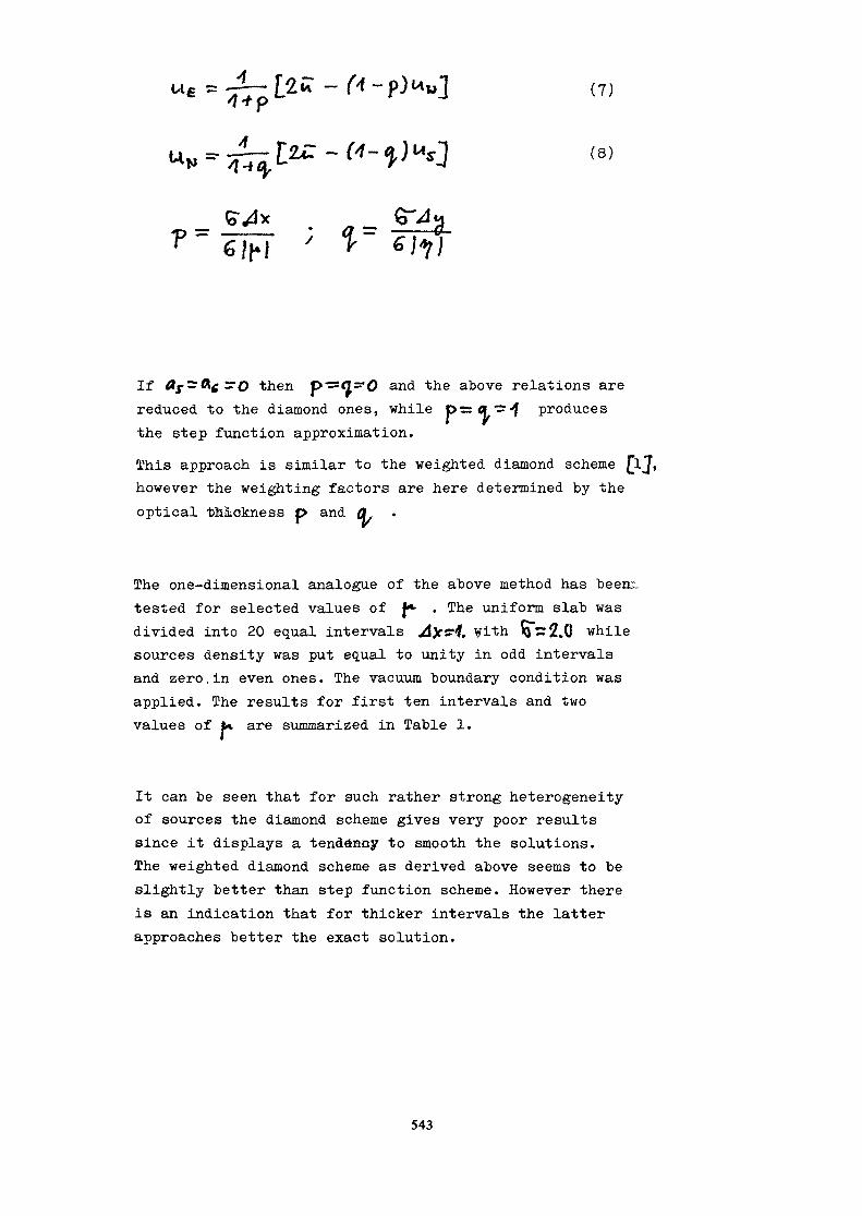
If #jSfttf~O then p^Os^O and the above relations arereduced to the diamond ones, while p=<*~^ producesthe step function approximation.This approach is similar to the weighted diamond schemehowever the weighting factors are here determined by theoptical thickness p and fl

The one-dimensional analogue of the above method has beeni.tested for selected values of J* . The uniform slab wasdivided into 20 equal intervals A)c~4. with Q~2.0 whilesources density was put equal to unity in odd intervalsand zero.in even ones. The vacuum boundary condition wasapplied. The results for first ten intervals and twovalues of u are summarized in Table 1.

It can be seen that for such rather strong heterogeneityof sources the diamond scheme gives very poor resultssince it displays a tend^nay to smooth the solutions.The weighted diamond scheme as derived above seems to beslightly better than step function scheme. However thereis an indication that for thicker intervals the latterapproaches better the exact solution.

543

p-O.ZS-interval12345678910

Step.44444.04938.44993.04999.*5.05.45.05.$5.05

Diamond.4.16.304.21760.26944.23834.25700.24580.25252. 24849

WD.45161.03746.46007.05937.46050.03947.46053.03947.46053.03947

pi=rf.O12345678910

•33333.11111.37037.12436.37449.12483.37494.12498.37499.12500

.25

.25

.25

.25

.25

.25

.25

.25

.25•25

.28571

.18367

. 31195

.18742

.31249

.18750

.31250

.18750

.31250

.18750

Exact.43752.06246.43754.06246.43754.06246.43754.06246.43754.06246

.28383

.18691

.30913

.19033

.30959

.19040

.30960

.19040

.30960

.19040

Table 1. One-dimensional model solutions

For two-dimensional case it is necessary to examinethe positivness of the scheme. A combination of Eqs.(6.),C7),(8) gives:

and analogous expression for MJJ where D,<l and Uw, Mrchange places respectively. It is interesting to seethat for p>4 coefficient of Uw is always positive,hence a rather crude sufficient condition for nonnegati-vity is £ £ 4 > $ i • This will occur for ratherthick mesh. If JK4, q*;f then the conditions fornonnegativity are:

544

4- — t

- S £ Owhere

p(4-f>)$ ~ —

I _,

It is easy to see that the denominators in these expressions are always positive. After some algebra the aboveconditions can be written as follows:

v < -)'Tf

VThe situation is presented on Fig. 2. Points {f*S) loca-ted in the shaded area lead to an unconditionally positive-scheme .

3. Results and conclusionsThe tests were carried out for the IAEA Benchmark ProblemEIR-2a £2]| . The problem requires to compute the scalarflu« and total absorption in a rectangle presented on Fig. J.

1//3 1Fig. 2. Scheme positivity area (shaded)

545

The solution is to be obtained with vacuum boundary con-ditions in one energy group. Plat and uniform sourceswith the density equal 1 are located in zones 1 and 3.The material properties are given in Table 2.

Material

12345

s;.07.28.04.15.01

«*.60.48.70.65.90

Table 2. Benchmark cross sections

The calculation was performed with the moment modifiedset of angular constants in S4 approximation (12 angulardirections with equal weights) in a 16*16 meshKJjiOwer meshdivisions correspond to very large values of p and q andthe results were either poor (proposed scheme, step function)or unconverged (diamond). For S4, 16*16 calculation the valuesof p and q vary between 0.7 and 3.2, i.e. they are near top for the presented ID example (0.3 to 1.3). Therefore a reaso-nable basis for comparison could be expected.

€tO

4S.O-

5.0Fig. 3. Benchmark geometry

546

D

WD

SF

1

11.826

10.382

10.514

Mean flux2

0.5611

0.8131

0*802'

3

18.954

15.000

15.371

4

0.9293

1.3389

1.3115

5

1.5193

1*9452

1.9685

Totalabsorption

1491.8

1418.6

1432.6

Table 3« Benchmark results. D - diamond,WD - weighted diamond (proposed scheme),SF - step function.

The results are presented in Table 3. They are by no meansconclusive and only indicate, that the proposed scheme mightbe of some use in case of strongly heterogeneous media.The method certainly needs further development. For example,for too large values of p or q. an apropriate fix-up techniqueshould be devised.

4. References1. K. D. lathrop, J. Comp. Phys., 4, 475 (1969)2. IAEA Benchmark Problem N2 (EIR-2a) (unpublished)3. J. J. Arkuszewski, Swiss Report EIR-232 (1973)

547

CALCUL DES ASSEMBLAGES PWRQualification du système Neptunesur les expériences Mélodie dans Minerve

A. SANTAMARINACommissariat à l'énergie atomique,Centre d'études nucléaires de Cadarache,Division d'étude et de développement des réacteurs,Département des réacteurs à eau,Sain-Paul-lez-Durance, France

Abstract

A parometric study of thé différent multicell designs was performedin relation to thé 2D transport calculations (DOT: Sy method and APOLLO-MARSYAS:exact 2D collision probabilities), Two particularly significant configurationsstudied were reported in détail,

- thé first is realistic and corresponds to a 17x1? assembly with12 water holes and 13 pyrex pins;

- thé second maximises thé problems of calculating thé flux gradientsarising from thé heterogeneities: a water hole situated nert to afuel pin doped with 2$ of

I - INTRODUCTION

Le calcul de la distribution fine de puissance dans lecoeur d 'un réacteur PWR peut être effectué en représentationshomogène ou hétérogène de l 'assemblage.

La représentation homogène pose d'une part, le problèmede l'homogénéisation de l'assemblage (généralement réaliséeen milieu infini) et, d'autre part nécessite l'hypothèse dedécouplage de la forme macroscopique et de la structure finedu flux pour le calcul des points chauds.

Nous nous intéressons ici à la stratégie hétérogène ducalcul de coeur, qui évite ces difficultés, mais laisse subsis-ter le problème de l'homogénéisation des cellules contenantdes hétérogénéités (poisons consommables, grappes de commande,trous d'eau) et des cellules UO- perturbées. Pour alléger lecoût lie à la représentation explicite de toutes les cellules,on doit d'une part, utiliser une théorie simplifiée, la diffu-sion nultigroupe ' et une discrétisation sommaire (une maillepar cellule) , et d'autre part simplifier le schéma de calculdes données à utiliser dans chaque maille par une condensationen espace mais également en énergie (un groupe rapide et ungroupe thermique).

549

La philosophie adoptée consiste à ne pas séparer ces différen-tes sources d'erreurs mais à les corriger simultanément parune équivalence sur un calcul de référence hétérogène. La tailledes hétérogénéités étant faible devant celle du coeur PWR, lesproblèmes liés à la structure fine ainsi qu'à l'équivalence peu-vent être traités sur une situation de référence multicellulesc'est-à-dire sur une situation limitée à un groupe de cellules,l'assemblage par exemple.

Le calcul multicellules de référence doit être aussi précisque possible et est effectué par le module de transport multi-groupe APOLLO /!/ du système de codes NEPTUNE /2/ développéau CEA pour le calcul des réacteurs à eau.

Pour juger des performances des différentes approximationsphysiques (calcul à 1 dimension, choix de la cylindrisation,probabilités de collision approchées à 2 dimensions, modèlede calcul des PSSJ représentation azimutale du flux intégral)liées aux différents modules multicellules d'APOLLO, une étudeparamétrique sur différents motifs multicellules (avec des cellu-les homogénéisées) a été réalisée par rapport à des calculs detransport 2D (DOT , méthode SN et APOLLO-MARSYAS : probabilitésde collision 2D exactes). Nous présenterons ici cette étude surles deux configurations les plus significatives :

- la 1ère est réaliste et correspond à un assemblage 17x17avec 12 trous d'eau et 13 pyrex,

- la 2ème maximise les problèmes de calcul de gradientsde flux engendrés par les hétérogénéités : un trou d'eaujouxte un crayon combustible dopé à 2% d'oxyde de gado-

linium.

Cette étude nous a permis de définir les schémas de calculmulticellules optimaux du point de vue qualité-prix pour traiterce type d'hétérogénéités.

L'équivalence transport- diffusion, fondée sur la conserva-tion des taux de réaction, est effectuée sur ces géométriesmulticellules avec EQUIPAGE /3/.

Ces configurations ont été. réalisées au centre du coeurMINERVE, dans le massif MELODIE U02 enrichi à 3% représentatifdu réseau d'un réacteur PWR type 17x17 aux conditions de puissan-ce nominale . Les taux de fission au voisinage des hétérogénéitésont été mesurés par spectrométrie y et par détecteurs UA1. Des

550

mesures par chambres à fission dans les trous d'eau permettentde simuler les mesures d'activités fournies par l'instrumentationinterne d'un PWR et de les comparer à la puissance dans lescrayons voisins et à la puissance dégagée sur tout l'assemblage.

L'interprétation de ces expériences par un calcul de diffu-sion à 2D du coeur de MINERVE, faisant intervenir dans la zonecentrale expérimentale les constantes issues d'EQUIPAGE, montrel'aptitude de notre schéma de calcul à donner avec précisionles structures fines du flux et les distributions locales de puis-sance radiale dans un coeur PWR.

II - DEFINITION D'UN CALCUL DE REFERENCE : Etude des différentsmodules multicellules d'APOLLO.

II -1. Géométrie ; outils de calcul ; conditions de l'étudemulticellules

II -1.1. Géométries_étudicesLes deux configurations présentées, assemblage PWR 17x17

empoisonné avec 12 crayons pyrex (figure 1) et interactiontrou d'eau- poison consommable UO^-Gd^O, (figure 2) ont étéréalisées au centre du massif MELODIE du réacteur expérimentalMINERVE.

Le réseau eau légère MELODIE est constitué de 801 crayonsUC»2, enrichis à 31 en U, gainés de zircaloy 4. La cellule(figure 3] conserve les caractéristiques du réseau 17x17 : pasde 1,26 cm et surgaine en aluminium qui impose à froid un rapportde modération représentatif d.'un PU'R de puissance à chaud.

Le trou d'eau est une cellule de base d'où l'on extraitle crayon combustible.

c Le crayon pyrex a la même géométrie que le crayon combusti-ble. Il est gainé en zircaloy et est chargé à 13,61 en anhydrideborique (soit une teneur de 4,21 en bore naturel comme dans lespoisons consommables des PWR).

Les crayons gadolinium que l'on glisse dans les surgaincssont identiques du point de vue réalisation au crayon standard,

551

Dans les pastilles d'oxyde mixte U02-Gd20^, l 'u ranium estenrichi à 3°ô e't la teneur en gadolinium est de 2l en masse(Gd/U0 2 -Gd 2 0 3 ) .

II -1 .2 . APOLLO et ses modules mult icel lules.

APOLLO permet de calculer le f lux, direct ou adjoint , enénergie et en espace, en résolvant l 'équation du transport soussa forme intégrale, dans l 'approximation multigroupe.

Le traitement spatial en gêométries plane, cylindrique ousphérique utilise le calcul de probabilités de collision.

Il permet d'obtenir les propriétés neutroniques d'une celluleou d ' un groupe de cellules.

Le module multicellules standard d 'APOLLO utilise le forma-lisme de ROTH /4/. Dans ce modèle , le flux angulaire entrantet sortant de chaque cellule est supposé uniforme et isotropesur tout le contour de la cellule. Par ailleurs, parallèlementà cette hypothèse ce module mult icel lules , que nous appellerons"ROTH", conjugue un modèle cylindrique de la cellule.

D'ores et déjà deux autres modules mult icellules NAUSICAAet CALLIOPE /5/ sont opérationnels dans APOLLO. Ces deux codestraitent un assemblage rectangulaire composé de cellules carréesou rectangulaires avec des condit ions aux limites imposées sur lesquatre cotés. Ces deux modules s 'af f ranchissent des hypothèses deROTH en autorisant le -flux angulaire, d 'une part à être différentsur chaque face de la cellule rectangulaire, et d 'autre part àêtre représenté par un développement P.. . C ' e s t la repré-

sentation du flux intégral dans la cellule qui just if ie princi-palement l 'existence de deux programmes multicellules distincts.

- Dans NAUSICAA on a un vrai calcul à 2D dans les cellules : discréti-sation R-0 et le flux est calculé dans chaque secteur angulaire.

- Dans CALLIOPE on utilise un modèle cylindrique de la cellule : danschaque couronne le flux intégral est représenté par un développementà 1 (flux plat) ou 3 termes (flux. DIPOLAIRE). D'autre part, en plusdu modèle de cylindrisation (WIGNER, ASKEW/6/, WIG-ASK /7/},on utiliseun modèle de calcul des Pcc (ROTHx4 ou HMDGENE /?/).

oo

552

II -1.4. Philosçi2hie_de_1^6tude_et_de_l^utilisation_des

Pour juger des performances associées à chaque hypothèsephysique des modules multicellules, il est nécessaire de réaliserune étude paramétrique : cette étude doit comparer les résul-tats donnés par chaque option de chacun des modules multicellules.Ceci permet de quantifier les imprécisions introduites par l'uti-lisation de chaque hypothèse physique.

On part ainsi d'un calcul le plus précis possible (calculde référence 2D) et on introduit successivement des modèlesde plus en plus grossiers (modèle multicellule-s, modèle cylin-drique, représentation dipolaire du flux intégral, modèle PSS>hypothèse de ROTII) .

En fait la philosophie adoptée est de mener l'étude surun jeu de sections efficaces représentatif des hétérogénéitésréelles étudiées. On a donc dans le calcul APOLLO-KERA prélimi-naire, à la fois condensé en énergie et homogénéisé les cellules.Nous n'avons pas utilisé le nouveau module d'homogénéisation /8/qui conserve les taux de réaction, mais la technique classiquede pondération des sections par les flux. En effet ce qui estimportant c'est de disposer d'un jeu unique de sections effi-caces (par cellule et à 8 groupes) représentatif des propriétésneutroniques des hétérogénéités, qui sera utilisé dans tous lescalculs, qu'ils soient multicellules ou de référence (DOT, APOLLO-MARSYAS). L'intérêt de l'homogénéisation des cellules au delàde la simplification géométrique et de la réduction du coût calculest de ramener le réseau à une géométrie XY : les calculs àdeux dimensions DOT XY et APOLLO-MARSYAS sont alors réaliséssur la géométrie réelle et deviennent donc des calculs exactsIls serviront alors de référence dans l'étude paramétriquedes options des différents modules multicellules et dans ladéfinition de schémas de calculs multicellules et dans la défi-nition de schémas de calculs multicellules optimaux.

II -1.5. Mise_en_oeuvre_d^APOLLO

Le calcul APOLLO préliminaire de la géométrie hétérogèneréelle est réalisé avec le multicellules ROTH. Les 'bibliothèquesde sections efficaces utilisées sont à 99 groupes, dont 52 rapideset correspondent aux jeux recommandés par le Département desRéacteurs à Eau /9/.

553

Dans le calcul des flux, 1'anisotropie du choc est priseen compte par une correction de transport. Les coefficients dediffusion sont calcules en milieu homogénéisé dans l'approxima-tion B1. Les fuites sont simulées par un laplacien quasimentcritique.

En sortie le module KERA crée un jeu de sections efficacescondensées à 8 groupes (4 rapides et 4 thermiques dans chaquecellule pour chaque isotope directement utilisable par APOLLO.

Les calculs multicellules en homogène réalisés avec ce jeude sections sont effectués en imposant le même laplacien que celui,du calcul ROTH en hétérogène.

II -1.6. Calcul de référence

Le calcul de référence est donné par le code S,, DOT /Jo/ quitraite le transport des particules par la méthode des ordonnéesdiscrètes. Nous utilisons la procédure automatisée mise au pointau Département des Réacteurs à Eau /11/.

Le programme d 'interface KERADOT transforme la bibliothèqueAPOLLO créée par KERA en des bibliothèques de sections efficacesdirectement utilisables par DOT. Le prcprocesseur permet d'utili-ser la bande DOT créée, et d'entrer les données sans format sousune forme plus adaptée aux problèmes posés par la neutronique.

Un autre calcul de transport -à deux dimensions : APOLLO-'MARSYAS /12/ a également été effectué dans l'étude en homogènede la configuration d'interaction trou d'eau-poison U02-Gd?0,Le module MARSYAS d1APOLLO résout l'équation du transport pour unegéométrie bidimensionnelle XY quelconque par une méthode exactede probabilités de première collision. Actuellement, dans chaquerégion rectangulaire le flux est constant (flux plat).

554

II -2. Etude malticellules d'un assemblage 17x17L'étude détaillée a été réalisée /13/ et nous en résumons

ici les résultats.

II -2.1. Comp_araison_des_différents_modules_multicellulesNous présentons les flux moyens dans les hétérogénéités et

les puissances normalisées (puissance moyenne unité sur la géo-métrie) pour les calculs multicellules à 7 cellules génératricesl'étude a montré que deux types de cellules "face" et "angle"par hétérogénéité suffisaient pour donner les bonnes valeursmoyennes.

Définition du calcul

Kf6rcncc(DOT SS;16 milles/Ce

NAUSICAA

CALLIOFH (rUT.KlG-ASK.r ICI

xm

XT C P

30 s*"

8

6

S

UC *

85**

Î7

34

32

keff

1.00C53

0.99S-3

1. '001 96

(**>}kraa?V ,/rap.

0.974

0.969

0.967

0.955

($»)Y5 /thcrn.

1.278

1.278

1.262

1.29S

gPyrejA

FHr /«P-0.969

0.96J

0.964

0.952

if P/rcàâï7xn~)^ ythero

0. "32

0.732

0.744

0.719

x Temps d'unité centrale et unités de compte sur le calculateur IBM. 360/91xx Performances correspondant au calcul DOT optimisé :S4 avec 4 mailles par

cellule.

Puissance moyennepar cellule

RSfcrcncc (POT 58, 16 iaaillcs/C<

NAUSICAA

CALUOPE (PLj\T,KIC-ASK,Pss I»,\lJ

ROTI1

face eau

1.072

J.064

1.0S4

1.066

angle eau

1.031

1.025

1.021

1.022

face poison

0.936

0.938

0.947

0.936

angle poison

0.963

0.973

0.977

0.975

asynptotiquc

0.995

0.998

0.99S

0.997

La comparaison des calculs DOT et NAUSICAA donne approxi-mativement l'erreur liée aux approximations multicellules (fluxangulaire sur la surface des cellules^isotrope et uniforme parface) : lissage de la distribution de puissance de 1%.

L'écart des calculs NAUSICAA et CALLIOPE montre que la priseen compte des effets 2D est fondamentale : une discrétisationazimutale sommaire du flux intégral est suffisante (cf. Fig.4a :découpage du calcul NAUSICAA ; les calculs CALLIOPE et ROTHutilisent les mêmes couronnes).

555

Les résultats du multicellules ROTH montrent que l'hypothèsede ROTH compense sur la distribution de puissance les erreursliées à la représentation nonodimensionnelle de la cellule.

Pour ce type d'assemblage, le multicellules ROTH associeà la simplicité d'utilisation et au coût économique, une précisionsuffisante pour les calculs de projet. Nous nous attachons doncmaintenant à définir l'utilisation optimale du multicellulesROTH sur l'assemblage 17x17.

II -2.2. Comp_araison_des_diffêrentes_stratégies_^RQTH^

L'étude de ces différentes stratégies est réalisée ici, direc-tement en géométrie homogène. Le but recherché est de simplifierau maximum la représentation du voisinage des hétérogénéités(en effet une cellule tampon coûte 3 points de calcul supplémen-taires). Les différentes représentations multicellules du17x17 étudiées sont présentées sur la figure 5.

a) Les résultats dans les hétérogénéités sont ici normalisésaux valeurs moyennes des cellules combustibles. D'autre part,dans le poison on présente les taux d'absorption.

Définition ducalcul

NAUSICAA

ROTH 10 cellules

7 cellules

5 cellules zone tampon "en croi

5 cellules zone tampon "enro-bante"

3 cellules pas de zone tampon

3 cellules STATISTIQUE

T CP

100 s

74

50

c" 36

36

25

24

uc

180

96

76

56

57

42

41

l^ \

\?C' /-p.

0.9S82

0.9444

0.9444

0.9490

0.9515

0.9592

0.9540

teM\fc /ther*

1.3143

1.3336

1.3337

1.3240

1.3124

1.2647

1.2659

fep'p ]'Ac0c7rap.

1 .4666

1.4491

1 .4491

1.4515

1 .4543

1.4668

1.4629

'-a^ç/then?..

2 .84Q3

2.791S

2 .7921

2.8114

2.8501

2.9733

2.9781

Les calculs à zone tampon "en croix" ou "enrobante" donnentles résultats les plus satisfaisants pour les niveaux de fluxdans les hétérogénéités. Dans la représentation à 5 cellules"en croix" seules les 4 cellules combustibles jouxtant l'hétéro-généité sont représentées par une cellule tampon. Dans la repré-sentation "enrobante" on a également un seul type de cellulespar zone tampon (8 cellules autour de l'hétérogénéité) ; cepen-dant ici l'idée est différente : on ne cherche plus à respecterla position géométrique des cellules mais on associe dans un' mêmetype de cellules celles qui ont un spectre comparable.

556

Les multicellules sans zone tampon (seule le bilan matièredifférentie les types de cellule) lisse le flux thermique dansles hétérogénéités. L'option STATISTIQUE, qui suppose que l'imbri-cation des cellules est statistique ne modifie pas les résultats.

b)Pour les puissances, on gardera à l'esprit que le calculNAUSICAA n'est plus une référence puisqu'il lisse leur distributionde quelques pour mille.


NAUSICAA

ROTH 7 cellules {face*anglc)

5 cellules "en croix"

face eau

1.060

1.065

1.056

angle eau

1.023

1.021

'*m%

faco poison

0.946

0.942

0.94S

angle poison

0.976

0.976

''//////'/<

asyrnptotique

0.994

0.991

0.997

La représentation ROTH à cellules tampon "face" + "angle"permet de calculer avec précision le pic de puissance.

Contrairement à la zone tampon en croix, la représentationà zone tampon enrobante ne permet plus d'accéder directement entransport au point chaud. Elle donne cependant une excellenteprécision sur la puissance moyenne autour des hétérogénéités,ce qui est fondamental dans un schéma de calcul fondé sur l'équiva-lence transport-diffusion.

La stratégie multicellules sans zone tampon ne peut être uti-lisée que pour des calculs de coeur en .représentation homogènede l'assemblage : elle est moins coûteuse (3 types de cellulesseulement) mais elle fournit des constantes qui donnent uneerreur de 4% sur l'absorption des poisons.

II -3. Etude multicellules d'une interaction trou d'eau-gadolinium

La géométrie étudiée est un carré de 12x12 cellules avecreflexion sur ses 4 côtés (cf. Fig. 6) contenant un crayonUO^-Gd-O, (chargé à 2l en Gd) et un trou d'eau accolés. Nous

557

présentons ci-dessous les résultats des calculs les plussignificatifs de l'étude menée en /13/.

Référence (DOT S8)

MARSYAS

XWSICAA

CALLIOPL (DII>,l\IG-ASK,ID\0

CALLKTC (Dli'.'.lIGNtR, l»0

CALUOPL CPLAT.MC, JOM)

CAlLIOI'k (rUT.hlG, RJJIh.4)

CU1.IOPL (PLAT,hlG)!Wlll

ROTI1_ ——————— _ ________ .. _____ --

T C P

176 s

57

27

17

17

10

10

9

7

UC

248

119

64

63

63

42

41

40

35

i**°\Ifl?x7«p.0.937

0.935

0.936

0.934

0.929

0.933

0.933

0.906

O.D04

//° \V"2X>eo

1.165

1.159

1.163

1.186

1.190

Kl 58

1.158

1.175

1.175

"W \g! 2x121

V AaP-

0.938

0'.941

0.937

0.935

0.928

0.934

0.934

0.910

0.90S

V « \«12x12r /thom

0.68S

0.694

0.696

0.683

0.676

0.703

O."04

0.6S9

0.6CO

Puissance noyenne parcellule

K£fcici<.e tror)

VAKSI \S

NAISICAA

CALLIJPi. CDIP,1\IG-ASK,!»I)

CAUtûPt (DIi>,UICO.Il,l»y

CAIUOPc (M-\T,MG,1W<)

CVU.IOPE (PLAT,hIG,RQTUvl)

C\LLIOPL iI'l.M ,MC)Run[

KTTO

P3face poison

O.SS1

O.SSo

0.899

0.898

0.881

0.902

0.904

0.8»

O.SÏW

P2face poisonangle eau

0.919

0.920

0.928

0.9ÎO

0.916

0.928

0.927

0.921

0.918

P8angle poison

0.932

0.936

0.952

0.952

0.944

0.954

0.954

0.955

0.954

PSface eauangle poison

1.034

1.031

1.037

1.038

1.045

1.tT«

1.036

1.011

1.010

P7angle eau

1.046

1.038

1.036

1.039

1.044

1.032

1.032

1.031

1.031

P6face eau

t. 038

1.080

1.078

1.086

1.100

1.069

1.066

1.070

1.070

P9inter poison

0.970 !

0.968 j

o.ss:

0.9S2 ]—————————— |

0.9SO

0.9-9

0.9-9 I

0.978

0.979

La discrétisation R-0 du calcul NAUSTCAA est présentée surla figure 4b. Les calculs CALLIOPE et ROTH utilisent lesmêmes couronnes.

Les effets 2D étant très importants dans ce multicellules,les écarts entre le représentation plate et dipolaire du fluxintégral atteignent avec la cylindrisation de WIGNER :

. -2.7 \ sur le flux thermique du trou d'eau

. + 4.0 \ sur le flux thermique dans le poison5 % sur le gradient de puissance entre les cellules

face eau et face poison.

558

L'influence du modèle de calcul des P dans CALLIOPEest négligeable. Les faibles écarts, entre les modèles ROTHx4et HOMOGENE, signifient que "l'effet de traversée sans choc"à travers la cellule a peu de poids dans l'erreur liée àl'approximation de ROTH : le modèle ROTHx4 (P proportionnel

S î>à la surface de sortie) n'élimine que l'effet "de retour" alorsque le modèle Pgs HOMOGENE élimine de plus partiellement "l'effetde traversée sans choc". La comparaison des résultats, entreROTH et l'hypothèse de ROTH dans CALLIOPE, montre que c'estl'effet de retour qui est responsable de la majeure partie del'erreur associée à la méthode de ROTH.

Les deux derniers calculs montrent l'équivalence des multi-cellules ROTH et CALLIOPE dans ses options : flux PLAT, cylindri-sation de WIGNER, hypothèse de ROTH.

III - CONSTANTES POUR LE CALCUL DE DIFFUSION : Equivalence

transport-diffusion.

III -1. Calcul de référence en hétérogèneLes calculs multicellules en hétérogène doivent servir de

référence-pour l'équivalence transport-diffusion et donc^pourl'interprétation des expériences : on choisit donc pour les mo-dule? utilisés la représentation multicellules optimale définiedans l'étude en homogène ; la discrétisation spatiale adoptée(figures 9a et 9b respectivement pour le 17x17 et l'interactiontrou-d'eau-gadolinium) découle donc directement de celle miseau point en homogène. Nous avons vérifier que les deux pointsadoptés dans le crayon poison sont suffisants (en fait un pointunique suffit pour calculer correctement l'absorption du poisondans le cas d'un creusement de flux à une dimension radiale).

L'erreur associée à l'homogénéisation des cellules dansl'assemblage 17x17 se déduit des tableaux ci-dessous :


iiORl 7 cellules

XAUSICAA

7 cellules

Hétérogène

Homogène

Hétérogène 9a

Hpmogene

T C P

47 s

S s

100 s

8 s

UC

71

32

180

37

ftà> \^r?xi7\f /m,,

0.949

0.9SS

0.962

0.969

II*™ \iF*17

\» /thcrn.

1.333

1.295

1.312

1.278

' jrPyrexX0 ' \¥7^7I./ Jrap.

0.947

0.952

0.958

0.964

'jï P>™\TfTxTVr ythcrn

0.632

0.719

0.693

0.732

559


liOni 7 cellules

NAUS1CAA

7 cellules

Hétérogène

HomogèneHétérogène 9a

Homogène

face eau

1.064

1.0661.061

1.064

angle eau

1.021

1.0221.023

1.025

face poison

0.942

0.9360.946

0.938

angle poison

0.977

0.9750.976

0.973

asymptotique

0.994

0.9970.994

0.997

L'er reur engendrée par l 'homogénéisation classique estfaible sur la distribution de puissance mais lisse le flux ther-mique dans les trous d 'eau et les pyrex de 2 ,71 et 5% respective-ment.

Dans le cas de la configuration avec gadolinium on a :


R0TH

10 cellules

NAUSICAA

12 cellules

Hétérogène

Homogène

Hétérogène 9b

Homogène n°3

T CP

75 s

7

494

27

UC

119

35

1383

64

l**° \Ipxid\f ' /rap.

0.901

0.904

0.931

0.936

'V~° \1 r7F5d2\f /ther,.

1.233

1.175

1.224

1.168

''0Gd \^2x12)

\. /rap.

0.908

6.908

0.934

0.937

£Cd \£12x12\ J*™

0.643

0.690

0.653

0.696

Puissance nojenne par cellule

ROTH

1Q cellules

X\US:CAA

12 cellules

Itëtfrogcne

Homogène

HC-tC'rogèno 9b

HonojCne n°3

PSface poison

0.915

O.S96

0.915

O.S99

P2face poisonangle eau

0.9J3

0.91S

0.946

0.928

PSangle poison

0.964

0.954

0.963

0.952

PSface eau

angle poison

1.049

1.040

1.015

1.037

P7angle eau

1.035

1.031

1.038

1.036

P6face eau

1.074

1.070

1.079

1.078

P9intcr-poisoii

0.986

0.9'9

0.987

0.932

L'erreur engendrée ici par l'homogénéisation est de :

. - 2% sur la puissance des crayons U02 autour du poison

. - 4,6 % sur le flux thermique dans le trou d'eau

. + 6,5 | sur le flux thermique de la cellule poison.

560

Dans les deux configurations étudiées, l'écart calcul enhomogène-calcul en hétérogène est indépendant du multicellulesutilisé : l'homogénéisation ne modifie donc pas les résultatsrelatifs entre multicellules ce qui confirme à posteriori notrehypothèse de découplage des effets et le bien fondé de l'étudemulticellules en homogène.

III -2. Calcul de diffusion

Le calcul de diffusion .que nous préconisons pour le calculen hétérogène (1 maille par cellule) d'un coeur PWR, est uncalcul aux différences finies à deux groupes d'énergie. Cecalcul de diffusion est relativement peu coûteux mais imprécisdu fait de l'insuffisance de la discrétisation en espace et enénergie. Cependant ces erreurs numériques ne sont pas pénalisan-tescar elles vont être, dans notre schéma de calcul .rattrapéesparallèlement aux erreurs de diffusion et d'homogénéisation parl'équivalence transport-diffusion.

Une quantification sommaire de ces différentes sourcesd'erreurs dans le calcul de diffusion, ainsi que la stratégie àadopter pour l'obtention de meilleures constantes de diffusionpour le 17x17, a fait l'objet d'une étude /14/ que nous ne présen-terons point ici.

III -3. Equivalence transport-diffusion : programme EQUIPAGE

L'équivalence réalisée est du type : conservation dequantités intégrales. Elle est effectuée avec le code.EQUIPAGE/3/qui, par modification des constantes, assure la conservation destaux de réaction de référence sur toute les compositions.

L'écart transport (ROTH 7 cellules hétérogènes)-diffusionsur les flux thermiques et rapides et la correction EQUIPAGEassociée sur les sections, sont présentées ci-dessous pour l'assemblase 17x17.

Type de la cellule

Groupe

rapide

Croupe

thermique

f W fr-Tr.insp)/Trans

1 acteur correctif

(Di f f-Transp)/Trans

Facteur correctif

1Tro» d'eau

» 4. S

0.9SJ

- 19.6

1.216

Zface eau

« 0.3

0.993

- 4.3

1.016

3anj»lc eau

- 1.0

1.006

- 2.1

0.992

4pyrex

+ -1.5

0.9S3

+ 25.0

0.746

Sfnce pyrex

4 0.6

1.000

- 2.6

0.97S

6ajt^te pyrex

- 0.8

1.004

- 4.6

1.004

?

asynvtot '*w

- 0.6

I.POS

- 2.0

1.001

L'équivalence NAUSICAA (12 cellules hétérogènes)-Diffusionsur la configuration d'interaction trou d'eau-gadolinium donneles résultats ci-dessous :

561

Type de la cellule

Groupe

rapide

Croire

thcrràque

fniff-Tr=u-s?)/Ti-ans

Iscteur correctif

{Diff-Tr&nspyTrans

J-'acteur correctif

Gadol ïnitm

* 1.7

0.974

• 29.8

0.703

3

face ]»ison

- 0.8

0.907

- 5.6

0.989

2face poisonangle eau

- 0.9

0.999

- S. 2

0.98Î

4trou d'eau

» 2.8

0.%S

•-21.9

1.206

5f.ice eauangle poison

- O.S

0.?!>8

- 7.2

1.026

6face eau

- 1.0

l.POJ

- S.O

1.027

Sinter-poifons

- 1.9

1 .005

-s.:1.016

Après deux premières itérations EQUIPAGE sur le poisonqui corrigent les taux de réaction dans cette cellule, deuxitérations générales sur toutes les compositions suffisent pourdonner la solution convergée.

IV - QUALIFICATION DU SCHEMA DE CALCUL : Interprétation

des expériences sur les configurations assemblage 17x17et eau-poison réalisées dans MINERVE.

IV -1. Présentation du réacteur et des moyens expérimentaux

MINERVE est une pile expérimentale de type piscine comprenantune zone nourricière d'éléments MTR (plaques métalliques contenantde l'UAl fortement enrichi) entourant la zone expérimentale.Dans l'expérience MELODIE IV la cavité centrale est occupéepar un massif de 801 cellules simulant une portion de réseau PWR17x17 (figure 7 ). Les mesures sont effectuées dans le carré cen-tral 17x17, les couronnes périphériques servant à l'adaptationde spectre.

Les éléments de contrôle (barres de contrôle et de sécurité,chambres de contrôle) et le pilote automatique permettant de mesu-rer les variations de rêactivité lors de mesures par oscillationet de maintenir très stable la puissance, sont placés dans lazone nourricière ou le réflecteur en graphite, donc hors de lazone de mesure.

Les mesures de distribution radiale de puissance /15/ sontréalisées soit par spectrométrie Y sur crayons irradiés (méthodeintégrale,méthode du Sr ou du La ) soit par détecteurs feuilleà activation (UA1 fortement enrichi gainé aluminium).

Des chambres à fission miniatures 0 1,5mm permettent de mesu-rer les flux dans les trous d'eau. Leur utilisation en parallèleavec les détecteurs UA1, moyennant le dispositif expérimental

562

schématisé sur la figure 8 , donne le rapport entre l'activitémesurée dans les trous d'eau et le taux de fission dans les com-bustibles .

IV -2. Calcul du coeur MINP.RVE

IV -2.1. Philoso£hie_du_schéma_de_calculLe coeur MINERVE est constitué successivement de 4 zones

distinctes: le réflecteur en graphite, la zone nourricière, lazone aluminium, le massif U02 à 31. Ces quatre types de milieux"homogènes" déterminent la forme de flux macroscopique dans lecoeur.

Les hétérogénéités liées à l'expérience (crayons de poison,trous d'eau etc...) créent des perturbations locales qui détermi-nent la "structure fine" du flux au centre du massif MELODIE.

C'est le découplage objectif du flux en une forme macrosco-pique et une structure fine qui est à la base de notre schémade calcul du coeur ; les calculs d'équivalence transport-diffu-sion permettant de calculer correctement à 2 groupes d'énergieen théorie de diffusion sont scindés en :

- une équivalence sur la forme macroscopique du flux dansle coeur de référence (sans hétérogénéités expérimentales),

- une équivalence de la "structure fine" sur la massif U02en milieu infini (géométries multicellules étudiées).

Ce sont les constantes engendrées par ces calculs d'êquivalenctransport-diffusion qui seront injectées dans le calcul dediffusion DIANE (module différences finies du système NEPTUNE/2/)du coeur où le massif PWR est décrit en représentation hétérogène:chaque cellule hétérogène est décrite explicitement et il est doncévident que l'on n'utilise pas l'hypothèse de découplage.

IV - 2.2 Calcul_des_p_aramctres_du_cgeurDans une première étape on homogénéise les milieux fissiles :

le calcul des constantes homogènes du réseau UO, et des faisceauxnourriciers est réalisé en milieu infini.

L'homogénéisation des éléments de la zone nourricière estréalisée en deux étapes :

563

- dans une première étape, un calcul APOLLO plan de laplaque et de la demi lame d'eau associée fournit lesconstantes de la "cellule",

- ces constantes macroscopiques à 99 groupes, correspondantà" la partie fissile (appelée "viande") sont insérées dansune deuxième phase, dans un calcul APOLLO plan ou multi-cellules de l'élément à deux dimensions.

Disposant ainsi de sections efficaces multigroupes pourtoutes les régions du réacteur, le calcul du spectre dans lecoeur peut enfin être réalisé.

Ce calcul est réalise avec APOLLO en géométrie cylindrique.Du fait de la faible taille des milieux aluminium et

nourricier devant le libre parcom-s des neutrons, l'approximationdiffusion se trouve sérieusement mise en défaut quelle que soitla stratégie adoptée pour le calcul des coefficients de diffu-sion } il en résulte que le calcul APOLLO a une double fonction :fournir les constantes de diffusion des différentes zones etservir de référence dans la nécessaire équivalence transport-diffusion sur le coeur de MINERVE.

Cette équivalence est de type "réflecteur" : elle vise àrétablir dans'le calcul de diffusion, par l'ajustement des para-mètres des zones non fissiles (principalement réflecteur), ladistribution de flux dans le modèle cylindrisé du coeur.

IV -3. Interprétation des expériences sur l'assemblage 17x17empoisonné.

9 configurations simples avec pyrex et trou d'eau permettantde docoupler les effets (effet d'ombre, effet d'interaction.trou d'eau pyrex) ont d'abord été expérimentées. Leur interpréta-tion sommaire a déjà" été présentée /16 / . Nous ne présenteronsici que l'interprétation de l'assemblage 17x17 contenant 12pyrex.

Les calculs .sont normalisés à l'unité dans l'angle du 17x17.L'écart expérience-calcul en ce point est de l'ordre de 2 à 3%à cause de l'équivalence transport-diffusion sur le coeur quin'est pas parfaite. Les différentes séries de mesures /17/sont normalisées séparément de telle manière que pour chaquesérie la somme des valeurs mesurées soit égale à la somme destaux de fission calculés dans les crayons comptés. Les résultatssont reportés sur un quart de coeur.

564

L'interprétation des mesures réalisées par spectrométrie y(méthode intégrale : comptage de tous les photons y émisau-dessus de 511 keV) est résumée sur les figures 9. En 9ales valeurs théoriques découlent d'un calcul de base du 17x17 avecle multicellules ROTH en stratégie "zone tampon en croix".On vérifie que ce calcul est incapable de donner le gradientde puissance dans les deux crayons combustibles situés entrele trou d'eau et le pyrex : ce calcul sous-estime de 121 enmoyenne la variation de puissance entre le crayon jouxtant lepoison et le crayon jouxtant le trou d'eau. Les figures. 9b et9c correspondent à des calculs multicellules à 7 cellules,respectivement ROTH avec zone tampon "face+angle"et NAUSICAAavec secteurs angulaires : les écarts sur les gradients de fluxentre les hétérogénéités sont résorbés.

L'interprétation des mesures d'activité relatives par détec-teurs UA1 et chambre à fission- est présentée sur la figure 10. Lesdétecteurs UA1 donnant une précision moins bonne que la spectro-métrie y> l'intérêt principal de ces mesures est de donner leniveau de flux thermique dans les trous d'eau : la figure 10aconfirme que le calcul ROTII a zone tampon face+angle surestimenettement ce niveau de flux alors que NAUSICAA (figure 10b) donnedes résultats à l'intérieur des 3% de la fourchette expérimentalede cette manipulation.

IV -4. Interprétation de l'expérience trou d'cau-gadolinium

Dans cette expérience, les crayons combustibles ont étémesurés par spcctrométrie Y" (méthode intégrale). Les écartsexpérience-calcul(valeurs moyennes sur les différentes sériesde mesure) correspondant aux différents schémas de calcul sontprésentés sur la figure 11.

Les figures 11a et 11b correspondent à un calcul multicellulesde base avec le module ROTH : on constate qu'une équivalencerigoureuse sur toutes les compositions (figure 1lb) améliorenettement le calcul du gradient de flux (en lia seuls les tauxd'absorption et de fission du poison sont conservés : ajustementmanuel de "ap p dans chaque macrogroupe conformément àOC"l'ancien schéma de calcul /18/).

L'interprétation 11c fondée sur NAUSICAA améliore encorelégèrement les résultats. C'est l'équivalence sur le calculCALLIOPE conformément au schéma de calcul proposé pour ce type de

565

multicellules, qui donne les meilleurs résultats : les écartsn'excèdent pas l'incertitude expérimentale voisine de 2l (fig. 11 d)Aucun schéma de calcul ne réduit l'écart de l'ordre de 2\ surles cellules inter-poison : ces écarts doivent être liés à l'uti-lisation d'une cellule génératrice unique dans les calculs multi-cellules.V - CONCLUSIONS

L'étude des deux configurations multicellules présentéesici, avec les différents modules du code de transport APOLLO,nous a permis de définir les schémas de calcul multicellulesoptimaux. Ainsi pour le calcul d'un assemblage PWR type 17x17,avec ou sans poison consommable, le module multicellules utili-sant la méthode de ROTH est tout à fait adapté, moyennant unecertaine représentation des cellules génératrices (stratégies"enrobante" ou"mixte " pour les zones tampons autour des hété-rogénéités) .

Pour le traitement des forts gradients à deux dimensions[interaction de cellules diffusantes et absorbantes) il devientindispensable d'utiliser les modules multicellules à deux dimen-sions ; le module CALLIOPE, qui représente le flux intégral 2Dpar un développement dipolaire dans chaque couronne, s'avèreparticulièrement bien adapté.

L'interprétation des expériences, réalisées sur ces assembla-ges au centre de MINERVE, a montré le bien fondé des conclusionsde notre étude multicellules : les stratégies multicellulesproposées, couplées à une équivalence transport-diffusion, donnentune distribution de puissance fine telle que les écarts expérien-ce-calcul restent dans la marge d'incertitude expérimentale del'ordre de 1 à 2%.

Le succès de l'interprétation des expériences MELODIE confirmel'aptitude du schéma de calcul NEPTUNE à déterminer les distribu-tions fines de puissance dans un coeur PWR.

566

REFERENCES

- A. HOFFMANN et Al"APOLLO - Code multigroupe de résolution de l'équationdu transport pour les neutrons thermiques et rapides.Note CEA -N-1610 (1973)

/2/ - J, BOUCHARD - A. KAVENOKY - P..REUSSNEPTUNE : un système modulaire pour le calcul des réacteursà eau ordinaire.Conférence Nucléaire Européenne. PARIS -Avril 1975.

/3/ - J. MONDOT"Détermination de constantes équivalentes pour les calculsde diffusion aux différences finies".Communication à cette conférence.

/4/ - M.J. ROTH"The estimation of Collision Probabilities in Complicatedgeometries".AEEW-M 857, UK Atomic Energy Authority, WINFRITH (1969)

/5/ - R. SANCHEZApproximate solutions of thé two-dimensional intégraltransport équation by collision probability methods.Nuclear Science and Engineering -1977

/6/ - J.R. ASKEW"Some boundary condition problems arising in thé applicationof collision probability methods".IAEA-SM-154/69-B, VIENNA (1972)

IH - R. SANCHEZ"Approximate solutions of thé two dimensional transportéquation by collision probability methods".Meeting IAEA, BOLOGNA Italy (Novembre 1975).

/8/ - A. KAVENOKYHomogénéisation SPHCommunication à cette conférence.

567

/9/ - P. REUSS"Schema standard du calcul neutronique des reactcursa neutrons thermiques".Conmunication personnelle.

/10/ - F.R. MYNATT et Al"The DOT III - Two Dimensional Discrete ordinatesTransport Code".ORNL -TM- 4280 (1973)

/11/ - J. GONNORDCommunication personnelle

I Ml - Z. STANKOWSKY

These de 3eme cycle - ORSAY (1978)

/13/ - A. SANTAMARINA - B. NOUVEAU"Calcul de la structure fane des coeurs P1VR'

/14/ - A. SANTAMARINA - A. ARRIOLAApplication du schema NEPTUNE au calcul des distributionsfines de puissance au temps 0 dans un assemblage PWRtype 17x17 avec poisons consommables en milieu infini.

/15/ - M. DARROUZETRgactcur MINERVE. Experience MELODIE IV. Descriptionde I1assemblage et des techniques de mesures utilisees.

/16/ - A. ARRIOLAEtudes expcrimentales descaracterist:ques neutroniquesde reseaux de reacteurs a eau pressurisee.These de 3cme cycle ORSAY (1978)

/17/ - M. DARROUZET - P. MARLMBEAU - F. BERGER - A. SANTAMARINA"Experience MELODIE IV - Configurations avec trousd'eau et pyrex. Resultats des mesures".

/18/ - J. MONDOT"Mise en oeuvre des methodes pour le calcul despoisons consommables dans les r^acteurs a eau ordinaire".Note CEA - N - 1725 (1973)

568

D

Cellules combustibles

Cellule contenant un pyrex

Trou d'eau

Figure 1 : Assemblage 17x17 avec 12 crayons pyrex

569

E S T

NORD

HI J1 K I. M. M O1 P O ft'

OOOOOOOOOoooooooooQOOCOOOOooooooocooGooooooooooocoooooooooooooooooooooooooooc

oooooooooooOOOOOCOOOOCOOOOO DOOOOOOoooooooooo

SuD

Q U E S T

Cellule U02-Gd203Cellule trou d^eauCellule U0 standard

Figure 2 : Interaction trou d'eau-gadoliniumau centre du massif l»2 MELODIE

570

uoH 2O

Zr4

AL

0 uo = 8.0 mmLi

0Zr4 = 8.2x9.4 mm0A1 = 9.7x11.0 mmpas cellule = 12.6 mm

Figure 3 : Cellule U02 34 du massif ffiLODIE

571

Pyrex Trou d'eau Cellules tampon Asymptotique

3 couronnes dememe volume

4 couronnes dememe volume

5 points dememe volume

1 point

Figure 4a : Dlcoupage de 1'assemblage 17x17 (7 cellules, 22 points)

Gadolinium

r, = 0.4cmr2 = 0.6

Trou d'eau

rn = 0.25r' = 0.46

Cellules tampon Inter-poisons

= 0.32

Figure 4b : Cellules generatrices du multicellules trou-d'eau-gadolinium

Figure 4 : Discretisation R-0 dans les calculs multicellules NAUSICAA

572

Representation a 10 cellules Zone tampon "face+angle": 7 cellules

Zone tampon "en croix" Zone tampon "enrobante"

Representation mixte Pas de cellules combustiblestampons

Figure S : Representation du 17x17 dans le multicellules ROTH

573

10109999

10108389

10102

129

10105459

101076710

101010101010

101010101010 *

Figure 6 : Cellules generatrices du multicellules 12x12 de 1'interactiontrou d'eau - U0-Gd0

574

COEUR MINERVE ; CONFIGURATION "MELODIE IV

Reflecteur graphite

x XXX x

reflecteur graphitex \y/7,j Paisceaux nourriciers a 18 plaques-

~\-i v^J Faisceaux 10 plaques a barre de commande

Chaussette thermique

Pilote automatique

Element reflecteur graphite

FIGURE 7

575

C.F.0 1,5

DetecteurUAP

C.F. plate+ Detecteur UAP

IntercalibrationCF 0 1,5CF plate

en colonne thermiqueou

en une positionreference

TROU D'EAU COMBUSTIBLE CHAUSSETTETHERMIQUEt

Mesure relative combustiblechaussette thermique

(detecteur)

Mesure relative trou d'eau, chaussette thermique(chambres a fission)

Mesures par chambres a fission et detecteur

Schema de principe

FIGURE 8

576

+ 1.0

-1.0 -0.8 -1.1

-3.1

+1.5

K1.6

+0.2

-0.9

-0.1

-1.9

-1.9

-0.6

+2.4

+2.9

+1.9

+0.5

-0.9

+1.1

-1.0

+0.1

+0.2

-2.1

+1.5

+0.1

+0.2

-1.2

-0.6

-0.7

+0.3

+2.7

+2.8 +1.9

+2.4

9a : Equivalence sur ROTH avec zone tamponen croix 9b : Equivalence sur ROTH avec zone

tampon face+angle

+0.9 -2.7 -1.4 3.0 +1.9

-1.1 -0.4 -1.4

+0.5 -1.2 -1.4

+0.5

+0.3 -0.2 -1.5

D +0.4

+2.5

9c : Equivalence sur NAUSICAA

Figure 9 : Ecarts (exp-calc)/calc sur la spectromgtrie V dans 1'assemblage 17x17

577

+2.1 +1.0

+0.9 -2.5 +0.5 +0.1

-2.1 -0.5

+0.5 -0.3

0.0

+2.6

10 a : Equivalence sur ROTH (zone tampon face+angle)

+2.4 -3.2 +1.2

+ 0.9 -2.5 0.0

-1.5 -1.1

+0.3 +0.1

0.0

+2.1

10 b : liquivalencc sur NAUSICAA

Figure 10 : Ecarts (exp-calc)/calc sur les mesures par detecteursUA1 et chambre § fission 0 1,5mm dans 1Tassemblage 17x17

578

+3.7

-2.1

-6.0

-Z.5

-1.9 +2.9 +1.7

+5.4

+2.4 -1.5

-2.4

-3.3

-4.2

+2.2 +1.9

+4.6

+1.1

11:: : ajustcmcnt nanucl dc E P et Ir?ci X

sur ROTH

-2.3

+1.9

-2.5

-0.1

-1.6

+2.2 +1.7

+4.2

+2.2

11c : fccuivalence sur NAUSICAA

11b : equivalence EQUIPAGE sur Icmulticellules ROTH

-2.1

+2.0 -1.5

+1.3

+2.1

-0.1

11d : equivalence sur CALLIOPE(DIPOLAIRE, WIGNER, P

+2.3

Figure 11 : Ecarts (exp-cal)/cal sur 1'interaction eau-gadolinium

579

THE ARTS TREATMENTOF LATTICE HETEROGENEITIES

J. GADOCentral Research Institute for Physics,Budapest, Hungary

Abstract

A calculational model for producing effective few-groupconstants for heterogeneous light-water lattices is presented.Different kinds of heterogeneities /such as absorber rods,water holes, water gaps, casette walls and reflectors/ canbe treated in the model.

The calculational scheme is based on a Monte Carlo code/RAM/, which calculates the parameters of logarithmic boundarycondition at the surface of the cells, containing the hetero-geneity. In this code the parameters referring to boundaryfluxes and to slowing-down sources are separately calculated..For the description of the surrounding homogenized mediuma ID P, slowing-down code /SOPHIE/ is applied. The ratios ofthe boundary fluxes to slowing-down sources are determinedin this code, giving the actual logarithmic boundary conditions.The THERMOS code is also applied in the calculational scheme.

This system of programs results in the distributions ofdifferent reaction rates and fluxes, providing the diffusionprograms with few-group constants. The only trivial exclusionsare the diffusion coefficients, which are obtained from aninverse solution of the diffusion equation describing theactual reactor region. In this way the definition of thediffusion coefficients through averages of 1/3 Z^r is

avoided and one can maintain the definition of the neutronflux in the diffusion code as a cell-averaged quantity. Thisis especially important,when the calculational results areto be compared to the results of activation measurements.

581

Some calculational results are compared with experimentaldata /such as keff» power distributions, distributions ofactivations and microflux distributions/ based on zeropower measurements. The agreement of calculational andexperimental results is satisfactorily good.

1. IntroductionIn this paper the ARTS calculational model and its first applications

are briefly presented. The aim of the model is to give a good description ofpower and activation distributions in heterogeneous hexagonal lattices atzero burnup.

In Sec.2. the programs of the calculational model are shortly des-cribed. In Sec.3. the problems of the correct definition of diffusioncoefficients and the preparation of few-group detector activation crosssections are analyzed. In Sec.4. the geometrical models for treating differenttypes of heterogeneities are given.

In Sec.5. some calculational results are compared with measurements.The corresponding experiments have been performed at a critical facility inCRIP, Budapest and a summary report on these measurements will be publishedsoon. It turns out, that the ARTS calculational model gives reasonableresults in the considered cases.

2. Programs of the calculational model ARTSIn this Section the programs of the ARTS calculational model are

briefly accounted. For the solution of different problems, these programsshould be applied in a proper order*

a./ THERMOSThis program is a variant of the well-known THERMOS program, mostly

reminiscent to Stamm'ler's K-7 THERMOS [2} . The maximum number of energygroups is 35, the thermal cutoff energy is usually chosen to 0.625 eV/in the absence of plutonium isotopes/. Scattering models of Brown-St.Oohn,Nelkln and Koppel-Young are available.

582

b./ GRACE [l]Th« program GRACE solves the raultigroup B^-equations for homogeneous

media. It is similar to any MUFT-type program' . The resonance treatment istaken from the BIGG-II program [3] . The number of epithermal energy groupsis 37 /in case of thermal cutoff at 0.625 eV/, and a single thermal groupwith pre-determined homogenized constants is taken into account, makingpossible the criticality calculation or buckling search. A special optionof treating reflector regions is available, which is based on an energy-dependent buckling approximation. Few-group constants are calculated fromthe ratios of reaction rates and fluxes, while the diffusion coefficientsare determined from the ratios of currents and fluxes.

c./ SOPHIE [4]The SOPHIE program is prepared for the solution of the 10 P, -equations

in slab, cylindrical and spherical geometries with reflective of blackboundary conditions* Axial leakage is treated in asymptotic B, -approximation.Group structure and resonance treatment is identical with those of theGRACE program. As many as 10 homogeneous regions and 8 different mixturesare allowed. Energy dependent logarithmic boundary condition can be pres-cribed at a given point below a given energy group. In this case boundaryfluxes and total slowing-down densities are determined for the inner reglon/s/using boundary condition parameters in the corresponding energy groups.They are determined on the basis of the following formulae:

where j is the energy group index, 0. and <$> are boundary current and fluxand QJ is the volume integrated slowing-down density. Q^^ is known from thesolution for the last group treated in P^-approximation. The coefficients

are input data of the program. Flux distribution in the inner region/s/is determined as

<K = li to + *& QHlc kwhere k is the space point index and ^ and *fcg. are pre-determined

coefficients.583

d./ RAM [5]The RAM program calculates the above mentioned YL a°d •*< co-

efficients for a heterogeneous medium in slab or cylindrical geometries usingMonte-Carlo methods* assuming that the diffusion or P, approximation holdsfrom outside. In the program 15 thermal and 9 epithermal groups are allowedand the resulting yf and +j{k coefficients are condensed into singlevalues in the thermal range. Neutrons are started either from distributionsof slowing-down densities or from the boundary. The thermal spectrum at theregion boundary is an input data, leading to some arbitrariness in theresults. Detailed investigations showed, that the results are only slightlysensitive to the choice of this spectrum, if it is selected from properones [ej . It was shown also, that RAM and THERMOS give identical results inthe case of reflective boundary condition [6] .

In the RAM program axial leakage can be handled, linear anisotropy ofelastic scattering is allowed and Brown-St.John, Nelkin and Koppel-Youngscattering models can be applied.

e./ NI-7QOO [7]N1-7000 is a few-group hexagonal diffusion code, which solves the

diffusion equation for a 30° symmetry sector of the reactor. Elementary cellsare represented by mesh points. Axial leakage is treated by using axialbuckling. Axial diffusion coefficient can be space dependent. Normallyfour-group calculations are made. Up-scattering is not allowed. In thepresent version of the code asymmetry of the diffusion coefficient in thehorizontal plane can be taken into account.

f./ RIFFRAFF [e.9,lo]

The RIFFRAFF program can be used for the description of resonanceabsorption. The energy range of resolved resonances is subdivided into mini-groups with a constant lethargy width of 0.001. A two-region cell can betreated in cylindrical geometry. Flux and source spatial distribution trialfunctions are introduced for the rod and the moderator , which are connectedwith first-flight collision probabilitiesi whereas slowing-down is treatedexplicitely. The choice of trial functions has been tested by Monte-Carlo

584

calculations. The applied trial functions make possible to treat isolatedrods, too*

g./ ARTS [11]The ARTS program was written for the calculation of foil activation

distributions within elementary cells and for the determination of effectivefew-group constants of detector foils, positioned at given places. In thecode the actual neutron spectrum at a given place is calculated by combiningTHERMOS, RAM and SOPHIE spectra.

h./ DIFFThe DIFF program can be used for the determination of effective

diffusion constants of such regions, where the diffusion approximation is notvalid* As the reaction rates and fluxes are known for each elementary cell,the inverse solution of the fine mesh diffusion equation gives the effectivediffusion coefficients. This topic is more widely analysed in section 3.

This set of programs is written in FORTRAN for a ROBOTRON R-40computer which is very similar to IBM-360 machines /memory capacity 1 Mbyte/.Data transfer between codes is a atomized in some cases. Computation time andstorage requirements are not very serious. Each program requires less than250 kbyte memory and maximum computation time required by any program is

3. Some remarks on the definitions of effective diffusion coefficients andof effective detector few-group constants

The basic reactor physics characteristics of a reactor configuration/criticality, power distribution, etc*/ are to be described ultimately by afine mesh few-group diffusion program in the ARTS model* In the case ofheterogeneous configurations /with absorber rods, water gaps, etc./ thediffusion approximation of the transport equation is not valid, and it istrivially not valid even for the description of elementary cells. The neutronflux distribution and reaction rates in an elementary cell are thereforealways described by multigroup transport approximations. The correspondingfew-group constants are determined as ratios of reaction rates and fluxes,

585

while diffusion coefficients are calculated as ratios of currents and fluxesof the homogenized medium:

where 0 is the few-group index and the summations hold for the correspondinggroups of the multigroup model. The introduction of these diffusion co-efficients .which satisfy Pick's law at this stage of calculation leads tosatisfactory results in the case of unperturbed lattices. The application ofany averages of l/3£tr1 in the definition of the diffusion coefficientswould falsify the results.

In the vicinity of lattice heterogeneities /such as absorber rods,water gaps, etc./ the use of averages of Ctr1 are to be avoided, too, in thedefinition of diffusion coefficients. Effective diffusion coefficients shouldbe defined which give the true reaction rates, when the diffusion equationis solved. For example, let us take the case of an absorber rod in ahexagonal lattice /see Fig. I/. The diffusion equation for the mesh pointswith absorber rod /index O/ and for its nearest neighbours /index I/ reads as

/4b/

absorber tod or water holeposition

position

Fig.l. Typical macrocell with an absorber rod /N7/

586

Here the few-group index is omitted and it is assumed that the second, etc.neighbours of the absorber rod cell can be treated in asymptotic approxi-mations, i.e. there the asymptotic diffusion coefficients are valid /°2/and the fluxes of the second neighbour cells are identical. A. and S. theabsorption /absorption + removal + axial leakage/ and the source /fissionsource + in-scattering/ reaction rates and P is the lattice pitch. As A^, S,and (p. are known from the multigroup transport-approximation solution inID cylindrical geometry and D2 is assumed to be the asymptotic diffusioncoefficient, eqs /4/ can be solved for 0 and D,, providing the effectivediffusion coefficients.

Similarly, one can obtain effective diffusion coefficients in watergaps /with or without casette walls/ and in its neighbourhood or in thevicinity of core-reflector interface. These cases can be treated in ID slabgeometry and diffusion equations, similar to eqs. /4/ are to be solved forthe diffusion coefficients, as unknown parameters* Casette corner positionscannot be treated in 10 geometries, so a 2D transport code would be neededfor the similar procedure. The calculational model ARTS does not containsuch a code at the present stage of development. From the above describeddefinition of effective diffusion coefficients follows that

- they are interrelated with the finite difference scheme appliedfor the solution of the diffusion equation;

- one has to define clearly the fluxes in the finite differencediffusion equations /e.g. as cell averaged fluxes/ and all thefew-group cross sections are to be defined in accordance with thisdefinition;

- the solution of the finite difference diffusion equations willgive the same results as the approximate transport solutions forthe same one-dimensional problem.

The only limitation of such a definition of the diffusion coefficientslies in the one-dimensional description of the physical situation, and inthe neglection of cross-currents through the boundaries of the one-dimensionalregion. Nevertheless, for the description of the heterogeneities, consideredin this work, these limitations do not seem very serious and they can be

587

overcome at a later stage of developing the present calculational model.The reasons, why the above mentioned limitations have only a slight effecton the calculational results are further analysed in S ec.4.

The experiments performed at a critical facility in CRIP, Budapest,provide the theory with numerous possibilities of testing calculationalmodels. Along with criticality and power distribution measurements a lot ofactivation measurements were also performed, using different foil materials.From among these latter experiments determination of macroflux by means ofactivation distributions and determination of spectral indices and disad-vantage factors are especially interesting, as the spatial and energydependence of neutron flux distribution can be widely studied on this basis.Few-group absorption cross sections of foil materials used in macrofluxmeasurements and relative foil activities used in spectral index and dis-advantage factor measurements evaluated by means of the ARTS code. In thiscode microflux distributions within elementary cells calculated by the RAMor THERMOS programs are combined with the space and energy dependent neutronflux distribution, arising from the solution of the one-dimensional problemfor the chosen symmetry element containing several cells. The activationsare always calculated for those /sometimes very small/ regions which corres-pond to the actual measurements. Few-group constants are defined as theratios of these activations to cell-averaged fluxes. As the effectivediffusion coefficients are defined in accordance with cell-averaged fluxesarising from the solution of the diffusion equation, activations calculatedfrom the diffusion equation fluxes /i.e. cell-averaged fluxes/ and from theabove defined foil few-group constants lead to consequently calculatedactivation distributions.

4. Geometrical models for the treatment of different types of heterogeneitiesThe programs of the ARTS model are applied in different types of

heterogenities. In this Section three different lattice heterogeneities areconsidered: absorber rods /or water holes/, water gaps /without or withcasette wall/ and the core-reflector interface.

588

Absorber rods or water holesThe most common lattice heterogeneities are absorber rods or water

holes. In the considered cases they were arranged into a macro-lattice, i.e.absorber rods /or water holes/ were uniformly spaced in a hexagonal latticeof identical fuel pins. So the lattice can be divided into hexagonal macro-cells with a macro-lattice pitch being an integer multiple of the regularlattice pitch. The calculational model is as follows:

- It is assumed that the hexagonal macro-cell can be substituted bya cylindrical one assuming white boundary condition along its surface*

- Thermal group-constants are assumed to be asymptotic /calculated bythe THERMOS code/ for each cell in the macrocell,with the exceptionof the central cell, containing the heterogeneity.

- Logarithmic boundary condition coefficients tfi /i«»l,2,3,4/ arecalculated for the surface of the cylindricalised central cell byusing the RAM program. The number of epithermal groups where thelogarithmic boundary condition is applied is changing from nine tozero, depending on the "blackness" of the absorber rod, while it isalways applied in the thermal group.

- Epithermal neutron flux distribution in the macro-cell is calculatedby the SOPHIE code, where the heterogeneous central cell is treatedin P, approximation /in the upper energy groups/or by means oflogarithmic boundary condition /in the lower energy groups/. Theouter zone is treated in P, approximation and fuel pins, claddingsand the moderator are homogenized. Axial leakage is treated inasymptotic B,-approximation and diffusion coefficients are obtainedfrom the ratios of currents and fluxes /for the outer zone/ or bythe method of effective diffusion coefficients described in Sec.3./for the central cell/.

- The few-group constants obtained as ratios of reaction rates andcell-averaged fluxes and the diffusion coefficients are used in thefew-group 2D diffusion code NI-7000 for determining k ** and macro-distributions. Effective water height is determined either from Azor from ^9/bH measurements.

- Micro-distributions are calculated by the ARTS code, using theresults of the THERMOS, RAM and SOPHIE programs.The main limitation of the described method /which can be refined

589

several ways/ lies in the assumption of the identity of macro-cell fluxdistributions in each macro-cell. If the number of macro-cells is high enough,this assumption seems to be reasonable. Nevertheless* the obtained diffusioncoefficients assure only the fulfillment of local neutron balance, but theydo not reflect the response of the neutron field to cross-currents. Theextension of the calculations! model in this direction is in due course, butin the considered cases the effect of cross-currents is probably small.It has to be mentioned that for absorber rods containing isotopes withresonances /e.g. europium isotopes/ a special treatment is applied. Themultigroup effective absorption constants are calculated by the RIFFRAFFcode, assuming isolated rods, as the absorber rods are in such positionswhere this assumption is valid. In such a way self-shielding effects aretaken into account in a fairly good manner. Mutual shielding of resonancesof the absorber rod isotopes and those of fuel isotopes is neglected.

Water gapsIf a row of lattice positions does not contain fuel pins, the few-

group constants for this water gap and its neighbourhood are determined bythe method described below. The water gap may contain also structuralmaterial layers, corresponding to the casette walls. For the present worklattice pitch distortions in the vicinity of casette walls are not allowed,but the model can be easily extended to take into account such effects bythe re-definition of effective diffusion constants. Casette corner positionsand the intersection or end positions of water gaps cannot be treated inthis way, but a special treatment should be elaborated for their description.Cross-currents are once more neglected.

The calculational model for water gaps differs from that of forabsorber rod macro-cells in the following:

- The water gap and its neighbourhood is described in slab geometry,the spatial variable is in the direction perpendicular to the watergap. At the surfaces of the considered region white boundary con-dition is prescribed, while axial and tangential leakage are treatedseparately. The considered region consists of one or more layers ofthe water gap /including eventually also casette wall layers/ andthree cells to the left and to the right from the water gap*

590

- Logarithmic boundary condition coefficients are calculated at thesurface of the water gap by using the slab variant of the RAMprogram* This boundary condition is applied only for the thermal group.

- Epithermal neutron flux distribution is calculated by the slabvariant of the SOPHIE code. The outer zone is again homogenized.Axial and tangential leakage are treated in asymptotic B,-approximation,

Core-reflector interfaceThe core-reflector interface is a special heterogeneity which occurs

also in so called "homogeneous" systems* The combined spatial-spectraleffects lead to few-group constants very different from the asymptoticvalues.The calculational model is as follows:

- First a THERMOS calculation is made for a cylindrical core-reflectorsystem. The core is homogenized /possible heterogeneities are nottaken into account/ in an effective way, i.e. flux and volumeweighted number densities are used* The thermal data for the twooutermost core rings and for the innermost reflector ring areobtained* Each ring corresponds to a row of positions.

- Using the obtained thermal group constants a SOPHIE calculation isperformed, where the core is homogenized through volume weightednumber densities. From this calculation the epithermal few-groupconstants are obtained*

- Effective diffusion coefficients are calculated by a special codeDIFP for the outermost cells of core and for the innermost cells inreflector. The method is similar to that one described in Sec.3.These effective diffusion coefficients are applicable in thedirection, perpendicular to core-reflector interface. In the tan-gential direction asymptotic diffusion coefficients are assumed.

- Asymptotic few-group constants for the reflector region are obtainedfrom the GRACE code.

- The NI-7000 hexagonal diffusion code is applied for the solutionof the whole problem making use of the above derived few-groupconstants. Direction dependence of the diffusion coefficients in thehorizontal plane is allowed. /Axial diffusion coefficients arealways obtained from asymptotic calculation/.

591

It is worthwhile to mention that the effect of different number offuel cell - reflector interface edges has not been studied yet, though thiseffect is probably not negligible.

5. Comparison with experimental resultsA systematic experimental study of different kinds of heterogeneities

has been performed at a critical facility of CRIP, Budapest. A full accounton these studies is planned to be published in the next years. Lackingpublished experimental data, in this Section only the differences of calcu-lational and experimental results are given. Only the results for uniformlyrodded lattices are studied here.

The lattices are denoted by symbols Nm, whereN - type of the heterogeneity /A,B,C denote absorber rods with

different boron concentrations, 0 denotes B.C rods, E denoteswater hole, F denotes Eu2°3 rods, 0 denotes fuel, i.e. regularlattice/;

m - macro-lattice step in units of normal lattice stepiEach heterogeneity has 6 neighbouring heterogeneity positions at mP

distance in the hexagonal lattice, where P is the normal lattice pitch. Allthe other positions contain fuel rods. The heterogeneity and its hexagonalsurroundings form a so called macrocell. The number of macrocells is aninteger. All experiments studied here were performed in a nearly cylindricallight-water moderated,slightly enriched U02 lattice with uniform enrichment.In some cases boric acid was dissolved in water /these lattices are denotedby symbols NmB/. The reactor was regulated by water level, so each criticalstate is wholly described by water level and by the number of macrocells.

First let us have an account of critical states. In Table 1. thecalculated kQff values are given for as many as 22 lattices. bg/ciH wasdetermined in nearly all cases. The difference of calculated and measuredbg/bH values are also shown in Table 1. In all cases the axial extra-polation length / Xz / was estimated from a correlation measured in cleanlattices. The uncertainty of X2 leads to uncertainties in k ff up to0.001-0.003 depending on critical water level /H _/• p>eft values neededfor the comparison of <bg/oH values were obtained from special calculations.

592

One can state that both k^^ values and the deviations inare generally acceptable* In the case of B.C and Eu2°3 absorber rods thekeff values are too low, referring either to some defects of the calculationalmodel or to problems of nuclear data.

Table 1. k ff and A(&Q/&H)* for critical states

Symbol ofthe lattice

A7A6A5A5

B6

C7C6C5C5C5C5C5

07D7

E7E7E6E5

E7B

F7

F7B

07B

Number ofmacrocells

31557367

55

31557367554949

3137

31375573

31

31

31

31

Hcr/cm/

39.535.644.449.7

37.2

40.336.646.852.864.576.683.7

57.748.0

31.428.326.983.3

40.1

47.5

75.7

32.0

keff

0.99991.00111.00071.0005

0.9988

0.99000.99660.99820.99790.99660.99560.9974

0.99210.9933

1.00291.0O331.00110.9985

0.9989

0.9924

0.9895

1.0023

A(£9/6H>*

-0.6+0.3+4.1+2.5

+2.8

-4.7-0.7+0.6-0.6-1.0-1.9—

+1.8

-4.9

--0.3

+2.4

-1.1

-

•»

* A(&9/&H is the relative difference of calculated andmeasured values in %.

593

Power distributions were measured in 30 symmetry sectors of somelattices. The deviations of calculated and measured power distributions areshown in Figs.2. and 3. for lattices 07 and E7, respectively. The normali-zation of the distributions was jmede in the most accurately measured 10positions. As one can see from these Figures, the deviations are generallyless than 2%, while the accuracy of measurements is ^- 1%. No systematicdistortions in the vicinity of the heterogeneities can be detected, with theexception of the positions lying between the core-reflector interface andthe outermost absorber rod /or water hole/. This can be explained by theneglection of cross-currents in treating macrocells. The similar characterof the discrepancies in case of absorber rods and water holes seems to bepeculiar.

o absorber rod or water holeposition

fuel position

reflector position

Fig.2. Power distribution in lattice 07

/Deviations of calculated values

from measured ones In % /

594

\/x~' obsorber rod or water holeposition

fuel position

reflector position

Fig.3. Power distribution in lattice E7/Deviations of calculated valuesfrom measured ones in % /

A series of experiments with activation foils were performed fordetermining macroflux distributions. From among them Cu and Oy activationdata are compared for lattices D7, E7,F7 in Figs. 4-6. Normalization wasmade for all measured positions, with the exception of heterogeneitypositionsj positions lying in the neighbourhood of heterogeneities andpositions lying in the neighbourhood of core-reflector interface. The over-all agreement of calculated and measured activation distributions seems tobe surprisingly good, also in the most important positions which are notincluded into normalisation.

Power and activation distributions can be further analyzed forchecking some assumptions of the calculational model.As a first step, the following quantities were calculated:

—. oiV / . j •> *% \

where aik is the power /or activation/ value at point Rik, lying in macro-cell i at a distance of r. from the center of the corresponding macrocell

595

/r. a k.P, k « 1,2,3/, B is the radial buckling estimated from the averageradial size of the lattice and 3 is the Bessel-function. The macrocelllying in the center of the lattice is numerated by i«*l. In the followingonly this macrocell and its two neighbours are taken into account.Linear fit to values

£Rik

gives "radial bucklings" Bpk/kslt2.3/. Some results of such fits are givenin Table 2.

absorber rod or water holeposition

\ y fuel position

reflector position

Fig.4. 63Cu activation diatribution In lattice 07

/Deviations of calculated values from

measured ones in % /

596

f \ absorber rod or woter hole'•"' position

( \ fuel position

reflector position

Fig.5. 63Cu activation distribution in lattice E7/Deviations of calculated values frommeasured ones in % /

absorber rod or water holeposition

\ ^ fuel position

\~o\ reflector position

Fig.6. 164Dy activation distribution in lattice F7/Deviations of calculated values frommeasured ones in % /

597

Table 2. Radial buckling values B .

Lattice

D7

E7

Distribution

power

63Cuactivation

power

63Cuactivation

calc.exp.

calc «exp.

calc.exp.

calc,exp.

Position*IP

0.072420.06827

0.072250.07128

0.072860.06833

0.072830.07057

2P0.072730.07365

0.072710.07400

0.073010.07305

0.073050.06996

3P0.073740.07216

0.072240.07255

0.07291••

0.073300.07233

Positions are denoted by the distance from the centers of macrocells/in lattice pitch units/

Fitting to calculated values leads to nearly identical B , values whichproves the consequent use of separability of macrocell flux from reactormacroflux. B . numbers fitted to experimental values are in a satisfactorilygood agreement with the previous B. values /experimental errors of B . arenot determined/, which gives an experimental evidence for the above mentionedseparability.As a second step the calculated

3i.W v (\, - A t -5 . : _ A t\Jo(B,-Ru«) '

values were compared with the macrocell solution. The results are given inTable 3. The very good agreement of these data proves the correct definitionof effective diffusion coefficients.

A lot of spectral index, disadvantage factor and microflux measurementswere performed by different foil detectors in the considered lattices. Theseexperiments are used for testing the 10 transport-type spectral calculations.

598

Table 3. Ratios of power distributions obtained from 20 diffusionand ID transport-type calculations

Lattice

D7

E7

Macrocell

1

2

1

2

Position*1

1.0

1.0046

1.0

1.0177

2

1.0095

1.0132

1.0000

1.0161

3

1.0131

1.0150

1.0000

1.0161

Positions are denoted by the distance from the centers of macrocells/in lattice pitch units/

In the unit cells with the heterogeneities such measurements can be performedonly with a limited accuracy due to gap effects in absorber rods, etc. Thecorresponding correction factors are not always fully trustable, thereforeonly some interesting results are shown.

and R \^} from the positionFirst the dependence of R (Dy)» Rin the central macrocell is investigated. Here

* (8) 'measured in the actual spectrum divided by the same ratiomeasured in a thermal column,

R (DV) " the ratio of 235u and 238u fissions to l64Dy foil acti-vation measured in the actual spectrum divided by the same

the ratio of 238U captures to 164Dy foil activation

ratio measured in a thermal column,/ Np\ /R (Ce\( oy] '* \oy)Dy foil data.

R164

, measured directly, i.e. not using

These spectral indices were measured in the first and second neigh-bouring positions of the heterogeneity and in the position.lying at theboundary of the macrocell, in lattices E7B and F7B. The deviations of

599

experimental and calculated data from the asymptotic values are shown inTable 4. The agreement is again nearly perfect, though the asymptotic valuesthemselves deviate from each other up to 3% due to nuclear data disrepancies.

Table 4. Measured and calculated deviations of epithermal spectral indicesfrom asymptotic values

Spectral indexLattice

E7B

F7B

Position*P2P

3.5P

3.5P2PIP

• (K)meas.

0.94oio.0130.972 0.0130.997-0.013

0.971 0.0331.002 0.0251.134-0.014

calc.0.9300.9750.990

1.0161.0291.098

R /CeR (DVmeas.

1.004-0.0141.020-0.0111.027 0.019

0.935 0.0390.956-0.0311.063 0.019

)calc.0.9860.9950.998

1.0031.0061.018

• (X)meas.

0.943 0.0110.957 0.0140.962-0.014

l.OOlio.0151.031-0.0171.091-0.013

calc.

0.9430.9800.992

1.0131.0291.078

* Positions ere denoted by the distance from the center of macrocell/in lattice pitch units/

Secondly, calculated and measured disadvantage factors are compared.As an example, the Mn disadvantage factors are studied in lattices E7Band F7B in the heterogeneity and in the first two neighbouring cells. Thedisadvantage factor changes from s; 0.8 /in the water hole/ up to ^ 3.2/in the absorber rod cell/. The deviations are given in Table 5. It seemsthat the effect of both types of heterogeneities is slightly underestimatedby calculations, nevertheless the disrepancies do not seem very serious, ifone takes into account some difficulties, connected with these measurements.

Finally some results are shown concerning the azimuthal activitydistributions in the moderator regions of the cells, neighbouring to theabsorber rod or water hole cell in lattices F7B and E7B. The measurementswere made by 3Cu foils, cut into six parts. The deviations of experimentaland calculational results are shown in Figs. 7-8. The agreement is again verygood and the physical effects are clearly seen.

600

Table 5. Deviationa of calculated and measured Mn disadvantage factors

Lattice

E78

F7B

Position**

0P2P

2PP0

Deviation1**

+0.062-0.030+0.026-0.022+0.020-0.023

+0.013 0.022-0.023-0.022-0.207 0.090

"Positions are denoted by the distance from the center of macrocell/in lattice pitch units/

^^/Calculation-measurement/ - exp. error

0*044 ±0.04H

water holecoFig.7. Az^muthal Cu activation distribution

deviations in lattice E7B

601

-0.003 ±0.008

-O.OO3±O.OO5

absorber rodFig.8. Azimuthal 63Cu activation distribution

deviations in lattice F78

The relatively good agreement of calculated and experimental micro-distributions proves the applicability of the ID transport-type calculationsand that of the ARTS program for the determination of the very complexbehaviour of the corresponding quantities. It turns out that the separabilityof microcell and macrocell fluxes, as it is assumed in the ARTS code is areasonable approximation.

6. ConclusionsThe ARTS celculational model and its first applications for hetero-

geneous lattices are described in this report. The following conclusionsare to be made:

- Few-group constants and especially effective diffusion coefficientshave to be determined with a special care in case of heterogeneouslattices. Avoiding the use of EL in the definition of the diffusioncoefficients and consequently defining fluxes and few-group constantsin transport-type and diffusion calculations good agreements withexperimental data can be achieved.

- One-dimensional transport .-type calculations give satisfactorilygood few-group data for 20 diffusion calculations in the consideredcases. The neglection of cross-currents leads to some discrepancies

602

in the vicinity of heterogeneities lying near to core-reflectorboundaries-^ but generally the assumptions concerning neutron fluxseparability problems are proved by experimental data.

- Sophisticated experimental results give evidence on the quality oftransport-type spectral calculations* Some discrepancies found inconnection with micro-distributions /and to some extent also inconnection with kef^ values/ have to be explained yet.

- The ARTS model, if it is further developed and verified by using theentire experimental information, can be used for checking moreeffective calculational tools. Its limited computer time and storagerequirements are attractive feature compared to calculational modelsbased purely on Monte Carlo methods. In the future the ARTS model canbe used for checking lattice homogenization models, where properly de-fined regions of several elementary cells are represented by coarsemesh effective fen-group data.

Literature

jlj Z.Szatmary, J.Valko, GRACE - a Multigroup Fast Neutron Spectrum Code,KFKI-70-14 report, 1970.

[2] R.3.0.Stamra*ler, K-7 THERMOS, KR-47 report, 1963.[3] O.P.Tverbakk, D.M.Ddderlein, BIGG-II - a Multigroup Neutron Spectrum

and Criticality Code, KR-75 report, 1965.[4] D.Gado, Z.Szatraary, SOPHIE and CECILY - Two Codes for Calculating

Space Dependent Fast Neutron Spectra, KFKI-72-64 report, 1972.[5] Z.Szatmary, A.Bagyinszki, RAM-1 - A Monte Carlo Code for the Calcu-

lation of Effective Logarithmic Boundary Condition at the Surface ofControl Rods, Kernenergle 15, p.41, 1972*

[s] O.Gadd, M.Makal, M.Telbisz, KFKI internal report, 1978.[7] V.S.Ionov, P.VeYtes, KFKI internal report, 1975.

P.H.Kier, RIFFRAFF - a Program for Computation of Resonance Integralsin a Two-Region Cell, ANL-7033 report, 1975.

603

Fg] O.Gado, Z.Szatmgry, Resonance Integral Calculations - the CodesRYF4-RIFFRAFF and RYF5-RIFFHOM, KFKI-73-49 report, 1973.

Flo] A.Biczel, O.Gadd, I.Lux, Z.Szatmiry, KFKI internal report, 1975,[ll] O.Gadd, M.Makai, KFKI internal report, 1977.

604

LIGHT WATER REACTOR HOMOGENIZATIONPROCEDURES

B.P. RASTOGI, S.R. DWIVEDI, H.C. GUPTA,N.K. GUPTA, H.C. HURIA, V. JAGANNATHAN, D. JAIN,V.K. JAIN, P.D. KRISHNANI, S.V.G., MENON,P. MOHANAKRISHNAN, S.D. PARANJAPE,K.R. SRINIVASAN, K. VINODTheoretical Reactor Physics Section,Bhabha Atomic Research Centre,Bombay, India

Abs tract

The physics design problems of light water reactors could be effectivelysolved "by invoking a three stage homogenisation procedure. A multigroup integraltransport theory method was first developed to obtain the pin cell parameters ofthermal reactor lattices. It was then extended to take into account ihe hetero-geneities such as differential enrichments, presence of burnable absorbers,poison curtains, control rods, variable coolant'densities due to boiling ( inBv/Hs) and burnup depletion effects found in lA-Tl fuel boxes. The procedure for thefuel box calculation was essentially based on supercell approach wherein thehomogenised multigroup cross-sections are used to derive the global box spectra.These are then condensed to few group parameters for use in the diffusion theoryformalism for local power distribution within the box. Another fuel box modelin which interaction of various pin cells is taken into account by proper leakagewas also developed. For validation of both these models, a Monte-carlo code forgeneral geometries was written, and the GG-TWGERAW Code was also adapted. Thesecodes were further tested with the data on nine local power peaking experimentsconducted in Japan, four NEACRP benchmarks on B1VR lattice problems, and threebenchmarks proposed by GEN de Saclay.

For the overall reactor calculations, a three dimensional BffR COresimulator v/as developed based on a new nodal coupling kernel. Results of somecore simulations with this model and using the nuclear parameters calculated bysupercell procedure for an operating power station are also presented. It hasbeen shown in the paper that by having a judicious balance between simplicity andaccuracy, it is possible to have a complete BYiR code package on a medium sizedcomputer of 32 ^ memory.

1. IMSOKJCTIOH

A direct detailed space-energy treatment of an ESR is not possible, -Hiecomplications being enormous. To solve the physics problems of BBBa , a threestage homogenisation procedure is normally applied. The first stage consists ofobtaining detailed neutron flux distrlbuticin and reaction rates in tixe various

605

pJn cells rf the box. The smo?red cross-sections therefrom are used to derivefew group cros<3 sections through either supercell approach or leakage model toaccount for the interact-'on between the pin cells. The few group cress-sections£.re then used to evaluate reactivity and pow^-r distribution in the fuel box atthe second stape by diffusion theory. The third step makes use of the nuclearparameters of the pecond st«.ge for eventual global reactor calculations.

Galculational procedures for all the three stf,ges of honogenisation havebeen developed with special emphasis on 3-R type reactors. These have beenverified with the pin cell lattice exper'ments at the first stage, and againstthe box power distribution experiments and benchmarks suggested by NllACRP andC E N de ^aclay for the second stage. It is shown that by having a judiciousbalance between simplicity and accuracy, it is possible to have a code systemwhich could work on a medium sized computer of 32 K memory.

The paper is divided into three parts. The first part deals withthe pit: cell calculations. In the second part, the fuel box homopenisationprocedure and its verification with the Japanese experiments and benchmarksare discussed. The third part touches uron the reactor core homogenisotionprocedure and discusses some results obtained from the simulations of theTarapur Atomic Power Station.

2. THE FIK CELL CALCULATIOIS

The lattice cells of a power reactor are very complex in geometryand composition. Therefore, it is not possible to obtain exact analyticalsolution of the Boltzmann equation in this case. The diffusion theory methodscannot be applied due to strong absorbing properties and relatively smalloize(compared to the mean free path) of the lattice cell components. On theother hand, accurate numerical transport theory approaches such as Sjf or %become impractical, for the repeated calculations due to large computingtime. They are mostly employed to calculate some special effects and toexamine the soundness of various physical approximations. These remarks applyto Monte-Carlo methods as well which are now gaining importance as standardsagainst which to compare less accurate nethods for calculation of spatialeffects in complex lattices.

An effective approach to override these difficulties is the use ofcollision probability methods based on integral transport theory. They providea fast and reliable tool for computing neutron distributions in the elementarycells of reactor lattices. The results obtained by the collision probabilityintegral transport theory method have been shown to be in reasonable agreementwith the much more time consuming Monte-Carlo calculations.

In a typical collision probability calculation for the cell fluxdistribution, the cell js divided into a finite number of regions and it isassumed that the neutrons are produced uniformly and isotropically in eachregion. The neutrons colliding in a region must have originated either in the

606

same region or in anv other region of the system. There are two approachesto obtain this latter contribution viz., multisone first flight collisionprobabilities (Pij-concept) and interface currents ( J- -concept).

In the Pi,j-ccnoe-nt, each region is coupled with a]] the other regionsof the system by first flight collision probabilities, while in the J— -concept,each region is coupled to its adjacent ones by surface currents. Both tiieconcepts are equivalent as far as correct space an& anpular distributions forsource and current densities are concerned. They are, of course, validassuming isotropic scattering in laboratory system and constancy of fluxes andsources within each region.

Thus, in the flat flux approximate on, the space and energy dependentintegral transport equations are reduced to merely energy dependent ones. Thefinal system of equations can be (and is) effectively used for calculating thethermal, resonance, and fast neutron fluxes an? relevant parameters in latticecells.

The energy dependence may be treated by the standard multigrouptechnique, which is, in fact, an analogue in energy of the inultiregion technique.In the multigroup picture, the energy range of interest is divided into a finitenumber of discrete energy groups. The selection of group boundaries may bedecided by the energy behaviour of important cross-sections.

For predicting the nuclear characteristics of thermal reactors, the mostcommonly employed code in the US js the HAMMER {1} system. It has resultedfrom a combination of MJFT(?) and THERMOS(3) codes. MUFT incorporates a 54-group Pi approximation method for slowing down spectrum calculation inhomogeneous media. TKERKCS, on the other hand, obtains thermal neutron spectrumby multi-region collision probabilities method in a 30 group picture.

On the other hand, the ViIIG(4) code of ^K comprises a most comprehensivescheme for thermal reactor lattice calculations. It is applicable to a widerange of reactor types. The entire energy range is divided into 69 groups with14 of these spanning the fast range from 10 MeV to 9*118 KeV, 13 groups describing-

the resonance range between 9-118 KeV and 4eV, and 42 groups covering thethe.rmal range below 4 *V.

The French are, at present, using a code called APOLIO(5) in the designstudies of light water reactors. This code is also quite extensive in thesense that it can do calculations not only for a single cell but also for agroup of cells in a reactor and in a variety of geometries. It makes use ofa 99 group cross-sections library with 47 groups describing thermal rangebelow 2.5 eV. For the spatial treatment APOLLO uses the collision probabilitymethod either in the isotropic or linearly anisotropic scattering approximations.The isotropic collision probabilities are generalised to account for fluxgradients in different regions.

It will be noticed that all the three aforesaid codes being used inDSA, UK and France incorporate comprehensive schemes and, thus, tend to be

607

quite costly computation wise, and call for large computer storage. Nevertheless,they lead to accurate prediction of physics performance characteristics ofthermal reactors.

In our attempts to evolve a code system •sdiich should not only be fastand accurate but also be made operational on -the small computer available atBAHC, viz., BE8I/-6 computer with J2 K memory, we first realized a combinationof EPITHET 6) and THKKlOriL (7). These two codes deal with respectivelyepithermal and thermal events using nultigroup multiregion collisionprobabilities, spatial coupling being achieved through Ji" and Pij methods.This packagr, which gave reasonable results, turned out to be quite expensivecomputationally. The next code in line was SUCCESSOR (a) which used Pijconcept to solve integral transport equations in cylindricalised cell. Thefirst flight collision probabilities were calculated by Carlvik's (9) method.Although this code gave very good results for reactivity predictions for uniformsingle rod lattice experiments, work on this was not pursued further becauseof high computational cost for repeated applications.

MJBLI CODE

The interface currents J— concept wherein each region is coupled toits immediate neighbours through surface currents could be used to advantage torealise a. substantial reduction in computer time. This advantage resultsfrom the fact that herein one deals with only a 2x2 matrix of incoming andoutgoing currents at each surface vis a vis the complete spatial transfermatrix in Pij method. Although this method is numerically less accurate thanthe Rtj one, but the reduction in computational cost outweighs considerablythe marginal loss in accuracy. This approach was adopted in the latticephysics code MjRLl(lo). As an illustration of the advantage of using thisapproach, it can be mentioned that analogous calculations by S6 method, P*^method and CT* (MURII) method would take respectively 10', 3« and 15" ofBESM-6 computer time. There is, thus an order of magnitude saving in thecomputational time.

In-this formalism, the collision density in any region of the systemis expressed as tie sum of three contributions, viz. (i) collisions madeby neutrons produced in the same region, (i?) collisions caused by neutronsentering from its outer surface, and (iii) collisions resulting from neutronsentering from its inner surface. The neutron currents across each surfaceare, in turn, computed from the conservation relations. All the expressions(for collision density and for currents) involve multiple collision and escapeprobabilities which are eventually given In terms of well known first flightprobabilities.

For the treatment of energy variable, the group structure of WBKcode was used. Some of the group cross-sections were also derived from -the69 group WINS library. The resonance range cross-sections for fissile andfertile isotopes are obtained using equivalence theorems taking into accountgeometry (or composition) and temperature effects. Interaction effects

608

between resonances of different isotopes are also taken care of approximately.Thermal energy transfer matrices for the moderating materials at the desiredtemperature are obtained by interpolating between the tabulated ones.

Besides the flux distribution and relevant reaction rates, anotherkey item in the calculation of physics characteristics of power reactors isthe burn-up prediction. It supplies information on isotopic changes in thereactor core and consequences cf these changes on reactivity, power distribution,kinetic characteristics, etc. Changes in the isotopic composition occur dueto isotope formations and destructions both caused by fission, capture andradioactive decay. In the MDRLI, equations governing the build-up anddepletion of all isotopes of interest-fissile, fertile, fission products,and additional absorbers are solved numerically either by Runge-Kutta methodor by trapezoidal rule. These equations are, in general, non-linear becausethe neutron flux is dependent on buraup. However, they are linearised byassuming the neutron flux to be constant over a given time interval so thattheir integration becomes straight forward. This procedure naturally callsfor periodic recomputation of the coefficients of equations using updatedneutron flux corresponding to new isotopic composition.

In the IklJRLI code, isotropic scattering and cosine angular currentapproximation are used while calculating the collision probabilities. Thelatter approximation was investigated in detail (11). It was found thatcosine angular current approximation at spatial mesh interfaces givesresults close to the results of accurate neutron transport calculations aswell as experimental measurements. This is especially true for tight lightwater moderated lattices. The main reason for this close agreement is the

use of white boundary condition necessitated by the approximation of thetwo-dimensional reactor lattice cell by a one-dimensional one.

MURLI formulation was further extended to develop a multigroupcollision probability code for uniform slab lattices- MJCOPS(i2). In thiscode use of cosine and (cosine) angular distribution of neutron currentsat fee region interfaces was assumed. It was found that even for slabgeometry J— method could give sufficiently accurate results at a fractionof computing time of other one dimensional transport theory methods.

4. COMPARISON WITH EXPSRIMEMAL RESULTS OF PET CELLS

Reliability of any calculational model must be established bychecking it against a variety of experimental data. In this context,experimental information on clean uniform lattice experiments conducted atdifferent laboratories was analysed (13,14,15). Table-1 gives the list ofthe experiments analysed by MDRLI code. The parameters compared includereactivity, ratio of epithermal to thermal captures ( and fissions),conversion ratios and neutron density disadvantage factors in moderator. Thecross-sections used were derived from WINE library and also from KNDF/B-TV.Excellent agreement ( within < 1$) was observed in the reactivity predictionof enriched uranium and plutonium lattices moderated by light water for wide

609

ranges of moderator to fuel volume ratios and U-235 or Pu enrichments. Theresults further indicated -that for enriched-^ fuelled light water moderatedlattices, the resonance integral of U-238 should be reduced by about 4 percent.Similar reduction for natural uranium heavy water moderated lattices wouldreoult in slight underprediction of reactivity but good agreement in thecomparison of relative reaction rates. These conclusions are in conformityvjith the recommendations emanating from other laboratories. Also the groupstructure and cross-sections used in WDS library for plutonium isotopes werefound to be quite adequate for reactivity prediction of plutonium fuelledsystems.

Part-IT

5. FOEL BOX HETEROGENEITIES

The light water reactor fuel box designs are highly heterogeneousboth in geometry and composition. A EVE fuel box consists of rods ofdifferent enrichments to minimise pokier peaking. The water gap around thebox is non-uniform to facilitate the insertion of control rods. Additionalsingularities are introduced with the presence of burnable absorber rods withinthe box. The non uniform water gap around the box makes the Dancoff resonanceinteraction effect to be non uniform. The thermal spectra of various rodsalso become non uniform. Insertion of control rods displaces water affectingboth thermal and epithermal spectra. Occurrence of boiling makes themodprator density axially varying and, thus, introduces a strong couplingbetween thermal hydraulics and neutronics.

All these aspects pose challenging physics problems. Ideally, ofcourse one would like to use two dimensional multigroup transport theory toobtain accurate predictions of reactivity and power distribution. But thecomputational cost as well as storage requirements become formidable. Suchan approach is clearly impractical on BESE-6.

Another approach to account for the environmental effects on thespectra of various pins in the box is the "multicell" model, where variouscell types are considered explicitly through collision probabilities. Thisprocedure has been adopted in UK and French codes for light water reactors,viz., IiVR_WDB(l6) and NEPTUUE (17). This approach was also considered tobe impractical on BESM-g for design work.

In order to make the code package operational on BESM-6 computer,a simpler yet accurate technique has been incorporated in MJH1I for obtainingreactivity and local power distribution of BVR fuel boxes. This involvesusing the "SUEERCELL" concept to take into account the effect of environmentalconditions on ihe spectra of individual pin cells in the base.

6. SUPERCELL MODEI

In this model, the position dependent neutron spectra in the fuel boxare obtained by performing a supercell calculation representing the whole fuelbox. For this purpose, the neutron flux distributions in the pin cells orefirst obtained using MORLI in the Wigner-Seitz cell approximation. The

610

homogenised multigroup cross-sections are then used in a supezcell calculationrepresenting 1he two dimensional fuel box geometry approximately in onedimension (fuel region surrounded by water), to derive the space dependentneutron spectra. This calculation is also dnne by MURLI with appropriatecross-sections in each region of the supercell. The supercell spectra soobtained are used to condense the multigroup cell and water cross-sectionsto derive few group cross-sections for performing two dimensional diffusiontheory calculations to obtain reactivity and local power distribution.

For fuel burnup calculations also, it has to be emphasised that theneutron spectrum encountered by each pin in the fuel box is different.Consequently, the relevant reaction rates in the pins are different eventhough their enrichments may be same. Thus, it is necessary to keep trackof fissile, fertile and fission product number densities in each of thesepins seoarately. By grouping the pins that face nearly the same spectrumand making use of the diagonal symmetry of the box, it is possible to reducethe types of pins for burnup to typically 15 to 20. TShen a burnable poisonlike gadolinium is also present in any pin, additional 3 to 4 burnable regionsare introduced in that pin to represent the self shielded burning of gadoliniumisotopes. The spectrum used in obtaining the microscopic cross-sections forburnup in these types of pins is a combination of the cell spectrum, supercellspectrum and the two dimensional few group box spectrum. While the boxspectrum is updated at each burnup step, the cell and supercell spectra can berecalculated at desired intervals.

Some of ttie additional features of the supercell model are

(i) Detailed calculation of position dependent Dancoff correction,(ii) Variable mesh representation of the fuel box,

(iii) Control rod treatment by P-1 blackness theory or collisionprobability approach,

( iv) Provision for calculation of adjoint fluxes,

( v) Provision for leakage correction for burnup calculations,

(vi) Provision for calculation of parameters required to interpretthe reactor instrument readings,

(vii) Option for plate type fuel boxes, and(viii) Incorporation of numerical techniques like successive line-over-

relaxation, row and column rebalancing, additional iterationloops over upscattering groups and use of progressive inneriteration convergence criterion in the diffusion theory part.

Supercell model has been perfected and is now being used to generateparameters for BVJR fuel box designs. It has been thoroughly tested withexperiments. A single calculation for reactivity and power distribution ofa typical fuel box on BESM-6 takeajO 10 mts. POT lattice parameters as a.function of burnup for a typical lattice it takes about 2.5 hours.

611

7. LEAKAGE HOTEL

In addition to 1he supercell model a leakage mo^el code and s. Monte-Carlo code were also developed for intercomparison studies. In the supercellmodel, interaction of various pin cells is accounted for by solving thetransport equations in cylindrical geometry using tiie smeared cross-sectionsof individual pin cells. Another model to account for these interactioneffects has been developed. It is called the leakage model. In this model thepin cells are first cylindricalised and MCULI code is used to obtain neutrondistribution under the assumption of isotropic reflecting boundary conditionat the cell boundary. These homogenised cross-sections are used in the twodimensional box calculations with the help of code DIMPLE. Herein, a neutronbalance in terms of group dependent absorption, source and leakage in eachmaterial of the box is prepared. The leakages so obtained are used to modifythe boundary condition for the various pin cells and the cylindricalised cellcalculations are repeated, ^his procedure is continued till leakages from thebox calculations converge.

DIKPIE code is a mesh-centered multigroup diffusion theory code tosolve the diffusion equations in rectangular geometry. The code is particular-ly suited to the needs of K?H fuel assemblies, for it has the provision ofupscattering. Eigenvalues are computed by source-iteration technique. Fluxesare obtained by using successive over-relaxation method. Variable dimensioningis used to make best use of the available computer memory.

8. MONTE-CARLO MODEL

To evaluate various box homogenization models, one needs eitherexperimental results or an accurate calculational model which treats all thespatial complexities and heterogeneities in complete detail. With this inview, a Monte-C?rlo code MOMLI was written. To save -fiie computer timethe energy details were restricted to the extent used in usual box homogeniza-tion methods, for example , 2? or 69 groups. Geometrical specifications of thefuel box are taken in the code to their maximum details. The code is writtenfor general geometries.

Batch method is used to solve the transport equation with a batch ofaround 500 fission neutrons. The origin of the fission source neutron isobtained by a source routine which generates uniformly distributed sourceneutrons from different types of fission source regions. The histories ofall these neutrons are traced till they are either killed by Russian rouletteor leaked out of the system. Fission weight at every collision is storedalong with its location. The origin of the fission source neutrons for thenext batch is obtained from these locations. First four or five batchesare not included in statistical averages of the required quantities so as toavoid the error introduced by flat source distribution taken in the firstbatch. The calculations can be terminated either at -ftie given computer timeor when the required'accuracy is achieved. Neutron fluxes in various zones

612

are calculated either by track length estimation or collision rate distribution.Similarly, eigenvalue is calculated either by fission weight averaging or byusing the estimated fluxes in each region. Best estimate of the eigenvaluehaving minimum variance can be taken as the final value. Variances of all therequired parameters are calculated along with their averages. External sourceproblem is solved by replacing fission neutron batches to source neutronbatches .

9. ANALYSIS OF JAPANESE EXPERIMENTS OK LOCAL POVER PEAKIH& IK BWB TY£B FUELASSEJ.'SLIBS

In order to supplement the calculations to obtain local power peakingin BVVR type fuel assemblies, nine experiments have been carried out in thezero power critical facility TCA in Japan (18). Several loading patternsmade of 1.9, 2.1 , 2.3 and 2.6 W$ U " enriched rods have been studied. Sixof these were with poison curtains and other three without them. Theexperimentally measured power distribution in different fuel rod plans asshown in Figure-1 have been used to study the adequacy of MttRLI- supercellmodel for B'<VR box calculations. The results so obtained are presented inTables -2 through -4 along with the percentage deviation from the correspond-ing measured values. It is seen from the tables that our predictions ar«satisfactorily consistent with the experiment*; and well within the targettedcalculational accuracy (+5$) for power distribution.

It may be noted that for conciseness the local power maps have beengiven in tabular form in Tables-2, 3 and 4. All experiments had diagonalsymmetry, so that only half the map is specified starting at the diagonalpin of each row of pins and working downwards from the top row.

10. MEACRP BEMCHKARE3 OH BWS LATTICE CELL PROBLEMS

A set of four B5TR benchmark problems (19) posed by Muclear EnergyAgency Committee on Reactor Physics have been examined by us to assessour capability for BWE box calculations. The benchmarks proposed were

9-pi1! supercell with central burnable poison pin,(2} Mini-K^K with 4 pin -cells and water gaps and control rod

cruciform,(3) lull 7x7 BWR iKttice cell with differential TJ-235 enrichment, and(4) Full 8x8 WE lattice cell with water-hole, Pu-loading,

burnable poison, and homogenised cruciform control rods,

The benchmarks have been described in Figure-2. For each problem,the dimensions, material layout and 6 group macroscopic cross-sections foreach material were provided. We have solved the problem-1 with both supercelland leakage models taking into account 1x1 and 4*4 mssnes per cell, Monte-Qarlomethod and transport theory code. The problem-2 was solved by leakage model,Monte-Carlo method and transport theory method. For Problem-3 supercell andleakage models and for problem-4 only leakage model were applied. Solutionof both these problems by Monte-Carlo and transport theory methods was nottaken up due to enormous computer time requirements.

613

The results of the analyses as obtained by us are summarised inTables 5 through 1J along with the results obtained from AiSi.1.", ETR, JAERI,R3SO and ABA. TCe have compared eigenvalues as well as material absorptionand fission rates for each problem. The calculated values show Hie sametrend as the AEjSir results and there is a good agreement between the two setsof results. In ^igure-J through 6 eigenvalues Vs absorptions in poison pinand absorptions in cruciform rod for the four problems are plotted alongwithOther results.

In the problems-1 and -"$ , the supercell model was used to condense6 group cross sections into 2 groups. Therefore, these results should beconsidered as 2-group results. Inspite of this approximation, it is surprisingthat material absorptions and fission rates are in agreement with other results.

11. OTO-PBEISISIOML TRANSPORT BENCHMARKS PROPOSED BY CM de SACLAY

CEN de Saclay (20) has also proposed four benchmarks to study two-dimensional transport problem. We have studied only three of these bench-marks. The first benchmark is a JX3 cell which is assumed to be repeatedcovering the whole plane. The eight outer rods are fuel rods and the innerone is a burnable poison rod. The second benchmark is an assembly composedof 7x7 cells. There is a water gap in the centre and there are eight poisoncells. For both these problems one group cross-sections •sore provided. Thethird benchmark was * mini-4x4 -^H lattice surrounded by water. There was onepoison pin and other 15 pins were the fuel rods. The surrounding water wasrepresentative of V/-W and N-N gaps found in B'»TR lattice cells. For thisproblem two group cross-sections were provided. All the three problems aredescribed in Figure-7. Tables 14 and 15 give the results of our Monte-Carlocalculations for problems-1 and -2. Mean fluxes and absorption rates ofvarious material regions are presented in these tables. The results obtainedby Sanchez of Saclay using the collision probability code are also given.It is noted -Siat Monte-Carlo results are in very good agreement with thecollision probability results.

Problem-J was solved by Monte-Carlo , OWOTRAN (21) with 84, SQ and S-|gapproximations) and by diffusion theory code DIMPIE (with 5xJ, 5*5 an5 8x8 m*shesper cell). The results of eigenvalue and total absorption in differentmaterials are given in Table 16. It is noted that transport theory K^ffg arein good agreement with the Monte-Carlo values. So far diffusion theoryresults axe concerned, only the Keff value of 5^5 meshes per cell is near tothe Monte-Carlo result.

In Tables 17 through 19 flux maps for group-1 and group-2 and fissionrate maps are presented. It is noted from these tables that both 84 anddiffusion theory results are in reasonable agreement with Monte-Carlo results.

614

Part- III12. TEE BfiR SIMTIATOR OCMBTG

In CO/IETG(22), the three dimensional core is divided into rectangularparallelepipeds with one mesh per fuel "box in horizontal plane and with 24meshes along the axial direction. The meshes are nearly cubical in shape.A full or quarter core analysis can be performed taking into acount thecore symmetry if necessary. The mesh dimensions are of the order of fastneutron mean free pa-Bi. Like FLAKE (23) , the neutron balance equation iswritten in terms of sources rather than fluxes. This facilitates power- voiditerations to be performed in a straight-forward manner since power is directlyrelated to source. However, for coupling of sources in adjacent meshes,the coupling kernel is derived from fast neutron diffusion theory.

The nodal coupling kernel used in CCKETS is

. •+ DC mwith P--/PI approximated by M*»«//vie • Here Waives the probability thatneutrons produced in node * i ' would be absorbed in any one of its nearest

n

neighbours 'm1. 55t , Ko*£ j 2>C denote the migration area, infinite multiplica-tion factor and diffusion coefficient respectively of node i- , ££mis the

* 41 ' * Jmesh spacing between nodes t and w> . The above kernel improvesconsiderably the accuracy of source distribution in a very heterogeneous corecompared to PLAHB kernel, requiring no additional input parameters. Thearbitrary mixing parameters of PIARE coupling kernel, have also been eliminated.The reflector region is treated by albedo parameters which help in reducingcomputer memory requirements. Different sets of albedo values are chosen forcold and hot conditions of the reactor. Variation of albedo with irradiationof the core is not considered.

The infinite multiplication factors are supplied in tabular form foreach type of fuel bundle as a function of exposure and instantaneous voidvolume fraction. Linear interpolation scheme is used for burn-up and fourthorder polynomial interpolation is used for void. The reactivity loss due tocontrol at zero burn-up is supplied for different voids and is assumed to beindependent of exposure. The Doppler and xenon reactivity losses are computedin a manner similar to FLARE. The migration area is assumed to be second orderpolynomial in relative moderator density.

Hadical changes were implemented in the thermal hydraulic model ofCOMBTG in order to eliminate arbitrary fitting procedures adopted in FLARE.The phenomena of subcooled, transition and bulk boilings are treated in amore physically realistic manner. Detailed pressure drop and mass-flowdistribution calculations are performed by a separate program wiUi COMETSpower distributions. The channel flows are then supplied to COMETG as alinear function of channel power for two types of channels and for twoorifice factors. Afiy change in these flow-power correlations during aparticular cycle is ignored.

615

The source equations are solved by Liebmann iterative scheme withalternate sweeping in "both radial and axial directions. This procedure wasfound to be necessary to eliminate power asymmetry due to mono sweeping.

The other features of the simulator are,

(i) Optimum power distribution calculation using Halingprinciple,

(ii)Partially comnuterised refuelling pattern studies for thedesign of the reconstituted core for every fresh cycle operation, and

(iii) A special routine to derive from the calculated powerdistribution a set of heat flux values which aredirectly comparable to those measured in the plant orvice versa

COMPARISON WITH OPERATTOMAL DATA OF TAPS BWR STATION

In -this Section the comparison of calculated results with someoperational data of Tarapur Atomic Power Station is discussed. The tworeactors at TAPS are of GR,BWR type and use 6x6 fuel boxes having threedifferent enrichments viz., 2.66, 2.1 and 1.6 wt$ of U-255. There aretwo types of fuel boxes -Reload- 1 and Reload-2, the latter differs from theformer in that it has two rods containing 1.5 wt$ Gd-0,.

Homogenised parameters for the R-1 and R-2 fuel were generated withthe help of KURLI- superc*!1 model (as described earlier) as a functi enof exposure and void. A comparison of supercell box power distribution withMonte-Carlo results is given in Table-21, it is seen that the agreementis good except for the W-W corner pin. These parameters were used tosimulate reactor cores through iJie code CUMEKr. The results of two typicalTIP trace analyses for the two units are presented in Table-2 . It isnoted that the calculated Keff of the Unit-1 differs by 6 mk andthat of Unit-2 by 2 mk from the experimental values. As the calculationsdo not take into account the cruc! deposition, which could account for fewmk, it is concluded -ttiat agreement is satisfactory. In the table, radialTIP comparison for bo-tfa the units is also given. It is noted that exceptfor the TIP locations A-6 of Unit-1 and B-6 of Unit-2 , the experimental andcalculated values of the heat fluxes agree within 10#. For most of the otherlocations the agreement is much better. Deviations of more than 15$observed at the two aforesaid locations cannot be attributed to calculation-al uncertainties. These may be due to the malfunctioning of the TIP tubesat those positions. In fact similar situation was found in Unit- 2 Cycle-5at location B_5. During refuelling time the LPRM tube was found broken.

14. OOWCLUSIOHS

The following main conclusions are derived from this studyj

(i) The interface currents approach for pin cell parameters is veryfast and satisfactory in explaining reactivity and variousreaction rate measurements.

616

(ii) The supercel] approach to take into account the heterogeneitiesof BVVB fuel boxes was found satisfactory. This model could predictthe measured local power peaking of various BWR experimentsconducted in Jacan within <$> , Comparison of this model >-;ithMonte-Carlo showed that it could predict adequately the powerdistribution in "the burnable poison pin also.

(iii) The leakage model also showed good agreement of powerdistribution predictions.

( iv) As in both the supercell and leakage models, diffusionthpory is used, 1x1 mesh per cell approximati-n givesbetter results for eigenvalue. This conclusion is inconformity with the observations made by Hals all (19) «

(v) Nodal coupling method for global reactor calculations issatisfactory as far as the reactivity is concerned. However,therr are deviations of the order of 4- 10$ in powerdistribution, which could be improved"if more than one energygroups are used.

References

1. Suich, J.E. and Honeck, H.C., The HAMMER System, DP-1064 096?)2. Bohl, H. and Hemphill, A. p., MJFT-5, WAPD-TM-218 (1961)3. Honeck, E.G., THERMOS Code, BNL-5826 (19~61)4. Askew, J.R., A General Description of the Lattice Code WIKS, J. Brit.

Nucl. Energy Soc., 5_, 564 (1966)5. Kavenoky, A., APOLLO- A General Code Tor Transport Slowing down and

Thermalization Calculations in Heterogeneous Media, Conf- 73041 4-Pl( 1973)6. triggers, F.E. , EPITHET Code, AECL-19967. Lawande, S.V. , and Jain, V.K., THHiaWL- A code for Thermalization in Lattices,

Proc. Symp. Nuel.Phys. & Solid State Phys., Bombay(l966)8. Srinivasan, K.R., et al, Multigroup codes for lattice calculations,

Indo-German Seminar, Julich (1972)9. Carlvik, I., A Ivlethod for Calculating Collision Probabilities in General

Geometry and Applications to Flux Distributions and Dancoff factors,Proc. 3rd Conf. Peaceful Uees of Atomic Energy 2, 225 (19^5)

10. Huria, E.G., IffiBLI- A Multigroup Integral Transport Theory Code for ThermalReactor Lattice Studies, Atomkeraenergie , Bd. 31 (1978)

11. Mohanakrishnan, P., Effect of Cosine Current Approximation in Lattice CellCalculations in Qylindrical Geraaetry, Atomkernenergie , Bd 3.1 (1978)

12. Deepak Jain, MTCOPS- A Kultigroup Colt is i en Probability Program for UniformSlab Lattices, (Accepted for publication in Atomkernenergie;

13. Mohanakrishnan, P. and Horia , H.C., Reactivi-ty Prediction of UniformPuO_-U02 Fuelled Lattices and Pu (NO,). Solutions in Light Water (Acceptedfor publication in BUG. Sci. and Engg.J

14. Huria, H.C. et al, An Assessment of -foe Cross-sections used in ThermalReactor Lattice Studies sPaper NO. 144, Int. Conf. Neutron Thy. and Nuc. Data for Reactors ,Harwell( 1978s

15. Huria, H.C. et al. , An Analysis of Enriched Uranium Lattices. Paper NO. 147,Int. Conf. Neutron Phy. and Nuc. Data for Reactors, Harwell (1978)

16. Fayers, F.J., et al, LWR-WIMS- A Modular Comouter Code for the Evaluationof Light Water Resurtor Lattices, AEEff-R 785~(1972>

17. Bouchard, J. et al, HEPTUNE _ Un Systeme Moa^iaire pour le Calcul desReacteurs (A Eau Legere)', Proc. Eur. Nuc. Conf. (1975)

18. Kobayashi, I. et al. Experiment on Local Power Peaking in BTSE Type FuelAssembly, J. Nuc. Sic. and Tech., 12 (10^, (1975)

617

19. Halsall, M.J., Review of International Solutions to HEACSF BenchmarkBV/R Lattice Cell Problem, AEI?;,_R In5?d977}.Also,A Comparative Study of Two-Dimensional Transport Methods forB';R Lattice Geometries, Amis of Nuc. Energy, 4 (1977)

20. A Benchmark Calculation} Two Dimensional Transport Problem, C E H de Saclay ,private 6'ornmunication (197?)

21. Lathrop, K.D. and Brinkley, P.W., Theory and Use of the General GeometryTffOTRAN Program LA-44J2 (1970)

22. Srinivasan, K.R. et al, The Taranur Reactor Core Simulator- COMETG, Pro.Sym. on Reactor Physics, Bom'iay (1976)

23. Delp, D.L. et al, FLARE- A Thr?c-DimensTonaJ Boiling Water ReactorSimulator, GEAP- 4598 (1964)

618

TftblC-1 A, Summary ?f the Data Analysed

S.No.

1

2

3

4

56

7

8

910

11

12

13

14

Lattice Description

Enr iche a -UCL/H20

Enriched -U-metal/H 0(Exponential experimentsEnriched-UO /K 0(TBX lattices)Natural U/D^O

U-233-Th oxide/H20

U-233-Th oxide/D20

Enriched -U/D 0(Co-axial fuel)Pu02+U02/H20

Pu(NO-) solution in HgO

(Pu-Al) Alloy/H20

Spectral Shift Controllattices/H20, DgO

Nat.-U/D20

Enriched -U02/H20 andIfat.-U/i320

U-metal 7 rod clusters /D (

Sub-Total

Total experiments

Laboratcny

BAPLWAEDBNLANLBNL

BNL

MIT

BNL

BNL

SRL

BKWLWECBKWL

BWL

BAW

Sac lay

NPY

) SaclaySHISweden

K

2444

4

38

48

27

6

8

20

6

40

202

425

a&Jc«.P«Jc

20

4

38

4

24

12

75

f

23

4

38

24

15

69

s**trt.s"

4

3

2

24

33

T

8

7

15

C.E.

4

3

24

31

K-reactivity5C28- ratio of epithermal to thermal TJ-238 captures@02- ratio of epithermal to thermal Th-232 captures•/cr25- ratio of epithermal to thermal U-235 fissionsC28- ratio of U-238 to U-235 fissions

C 25- ratio of Th-232 to U-233 fisions°025 - disadvantage factor in moderatorC.R-ratio of U-238 captures to U-235 fissions

619

fable - "2. Comparison Between Experimental And Calculated (Supercell method) Power Distribution in L«VR Fuel Assemblies

ASSEMBLY-AEXPT.

1.48J1.2741.2371.2341.2571.2401.2381.0580.9680.9870.9610.9570.9950.8970.8650.8710.8550.9010.8220.8340.8500.8690.8400.8520.8710.8600.899

0.988

SOTERCELL1.5201.3111.2661.2501.2341.2091.2231.0650.9950.9670.9540.9490.9860.9110.8770.8660.8710.9120.8420.8310.8380.8780.8220.8300.8750.8380.890

0.983

ERROR 5&

2.52.92.31.3

-1.8-2.5-1.20.70.7

-1.0-0.7-0.8-0.91.51.4

-0.61.81.12.4

-0.4-1.41.1

-2.1-2.60.5

-2.5-1.0

-0.6

ASSEMBLY-BEXFP.

1.2061.2911.2621.2501.2541.2371.2281.0660.9850.9680.9570.9721.0280.8750.8610.8680.8720.906

0.8130.8470.8470.8970.8220.8440.8850.8320.923

1.026

SUJERCELL

1.2251.3391.2791.2581.2401.2141.2291.0781.0020.9710.9580.9530.9900.9150.8810.8690.8740.9160.8450.8350.8420.882

0.8250.8340.8770.8420.895

0.988

ERROR $1.63-71.30.6

-1.1-1.90.11.21.70.30.1

-2.0-3.74.62.30.10.31.0

3-9-1.4-0.6-1.70.4

-1.2-1.01.2

-2.9

-3.7

ASSEMBLY-CEXPT.1.2481.0951.0591.0561.3231.2951.2751.1651.0621.0261.0030.9851.0080.9460.9080.8900.8880.9230.8720.8560.8510.8910.8290.8400.8870.8620.913

1.007

SUEERCELL

1.3001.1241.0771.0481.2931.2481.2571.1541.0601.0170.9870.9751.0120.9500.9070.8909.8930.9370.8640.8520.8600.9030.8430.8530.8980.8620.917

1.012

ERROR %

4.22.71.7

-1.1-2.8-3.6-1.4-0.9-0.2-0.8-1.6-1.00.40.4

-0.10.00.61.5

-0.9-0.51.01.31.61.51.30.00.4

0.5

too

10

Table -5 Comparison Between Experimental And Calculated (Supercell method) Power Distribution in LWR Fuel AssembliesASSEMBLY J>

EXPP.

1.2771.1271.0911.0571.5161.2971.2730-9331.0841.0300.9930.9891.0260.9620.8990.8890.8990.9350.8520.8510.8550.8980.8220.8280.8860.8500.924

1.013

SUIERCELL

1.3091.1371.0851.0521.2961.2511.2600.9241.0791.02?0.9900.9781.0150.9590.9110.8930.8960.9400.-8680.8550.8630.9050.8450.8550.9010.8650.920

1.015

ERROR $

2.50.9

-0.6-0.5-1,8-3-5-1.0-1.0-0.5-0.7-0.3-1.2-1.0

-0.31.20.5

-0.30.51.70.40.90.82.83.21.71.8

-0.50.2

ASSEMBLY-EEXPT,

1.3551.1811.1241.1471.2921.2731.2731.1191.0510.9960.9810.9780.9950.9240.8950.8660.8730*9230.8360.8480.8600.8860.8300.8420.8760.8500.890

0.994

SUEERCELL

1.3691.1831.1361.1101.2741.2351.2461.1261.0401.0020.9770.9671.0040.9380.8970.8820.8860.9290.8570.8460.8530.8950.8360.8450.8900.8550.908

1.003

ERROR <f»1.00.21.1

-5.2-1.4-3.0-2.10.6

-1.10.6

-0.4-1.10.91.50.61.81.50.62.5

-0.3-0.81.0

0.70.41.60.62.0

1.0

ASSEMBLY-*1

EXPT.

1.2741.1001.1481.1681.1501.1501.1151.H31.0631.0331.0081.0141.0230.9550.9150.8960.9210.9300.8630.8650.8739.9210.8400.8590.9220.8810.946

1 .032

SUH3RCSLL1.3101.1311.1721.1491.1321.1051.1071.1611.0661.0271.0121.0061.0430.9570.9160.9030.9090.9540.8730.8620.8700.9150.8510.8620.9080.8710.927

1.023

ERROR $

2.82.8

+3.1-1.6-1.6-5.9-0.71.60.3

-0.60.4

-0.82.00.20,10.8

-1.32.6Ov8

-0.4-0.4-0.61.30.4

-1.5-1.1-2.0

-0.9

Table — A Comparison Between Experimental And Calculated \Supercell method) Power Distribution in I«'«'H Fuel AssembliesASSEMBLY-G*

EXPT.

1.J161.1371.1131.1231.1641.2161.4070.9450.8810.8710.8920.9591.1400.8090.7970.8100.8651.0440.7820.7870.8451.018

0.8130.849f.0350.9271.130

1.298

SUPERCELL

1.3301*1491.1201.1271.1531.2061.3940.9330.8790.8670.8850.9441.1400.8100.7910.8060.8711.0700.7690.7830.8471.0440.7960.8581.052

0.9121.098

1.275

EEROR i*

1.11.00.60.3

-0.9-0.8o.9

-1.3-0.2-0.5-0.80.50.00.1

-0.7-0.5

0.72.5

-1.7-0.50.22.5

-2.11.11.6

-1.6-2.8

-1.7

ASSEIvtBLY-H*

EXPT.

1.0751.1061.0681.0941.1181.1931.1750.9790.9290.9240.9480.9831.2040.8540.8280.8450.9111.0720.8050.8120.8761.0330.8410.8801.0750.9291.1491.070

SUPERCELL1.1141.1161.0811.0831.1091.1651.1690.9840.9180.9030.9210.9821.2190.8360.8130.8280.8931.1280.7870.8000.8641.0930.8130.8761.1040.9351.1641.068

EEROR %

3.60.91.2

-1.0-0.8-2.3-0.50.5

-1.2-2.2-2.8-0.11.4

-2.1-1.8-2.1-1.95.2

-2.0-1.4-1.45.8

-3.3-0.53.00.61.3

-0.2

ASSEMBLY I*

EXPT.

1.1111.0491.0881.1011.1461.1181.2061.0270.9800.9230.9521.0151.0340.8420.8380.8450,9081.1210.8070.8380.8931.0740.8360.8991.102

0.9941.0141.092

SUPERCELL

1.1371.0611.1021.1011.1311.1101.2001.0060.9330.9160.9371.0111.0620.8470.8240.8400.9111.1590.7970.8110.8791.1170.82^0.8951.1350.9701.018

1.106

ERROR %

2.31.11-30.0

-1.3-0.6-0.5-2.0-4.8-0.8-1.6-0.32.70.7

-1.6-0.6

0.43.4

-1.2-3.0-1.64.0

-1.3-0.53.0

-2.40.41.3

o\toto

Table-5 Summary of Eigenvalues- KEACRP Benchmark Problème

Bcnc

hmar

ks

1

2

3

4

BARC

SÏÏHERCELL

1x1

0.8874

-

1 .0747

-

4x4

0.8482

-

1.0468

-

lEAKàGE

1x1

0.8857

0.8412

1.0716

0.8138

4*4

0.8395

0.8124

1 .0387

0.8000

MME-CAKLO

1x1

0.8854+0.0031

0.8267+0.0044

-

-

OTO-IRAN

(84)

0.8564(4x4)

0.8467(1x1)

-

-

AEE.V

BEST

0.8825

0.8200

1.0662

0.8237

DESIGîf

0,8888

0.8398

1.0754

0.8141

EIR

0.8554

0.8321

1.0437

0.8170

JÀERI

0.8768

0.8078

1.0579

0.8175

R3SO

I 1x1

0.8862

0.8540

1.0710

0.8127

4x4

0.8401

0.8242

1.0350

0.7986

ABà

0.8810

0.8152

1.0656

0.8235

0\toOJ

Table-6 NEACRP Benchmark Problem-1 : Material Absorptions

3.$h«-pJ

12345678

4+5*65+8

B A R CSUEERCELL

1x1

.7269

.0097

.0242

.0623

.0394

.1341

.0012.0022.235641264

4x4

.7922

.0094

.0234

.0690

.0436

.1487

.0013

.0025

.2613

.0259

LEAKAGE1x1

.730t

.0104

.0221

.0587

.0387.1365

.0012

.0022

.2339

.0243

4x4

.7022

.0103

.0206

.0613

.0415

.1603

.0012

.0025

.2631

.0231

MONTE-CARLO

".7255.0105.0227.0590.0402.1386.0012.0024.2378.0250

WO-THANS4 (4x4)0.71080.00950.02370.05880.03990.15370.00120.00240.25240.0261

AESffBEST

.7269

.0106.0226.0579.0393.1392.0012.0023.2364.0249

DESIGN

.7315

.0105

.0225_--

.0012

.0023

.2322

.0248

EIR

.7105

.0104

.0212

.0607

.0423

.1512

.0012

.0025

.2542

.0237

JAi?RI

.7241

.0105

.0223

.0600

.0405

.1390

.0012

.0024

.2595

.0247

RISO

1x1

.7267

.0105

.0221

.0592

.0406

.1374

.0012

.0023

.2372

.0244

4x4

.7022

.0103

.0207

.0607

.0429

.1594

.0012

.0026

.2630

.0233

ABA

.7264

.0104-

.0568

.0399

.1408

.0012-

.2375

.0245

Table-7 NEACHP Benchmark Problem-1 » Fission Rate Map

B A B CSUPERCELL

1x1

1.0841.0381.084

0.5121.038

1.084

4x4

1.0741.0361.0740.5611.036

1.074

LEAKAGE

1x1

1.0871.0371.0870.5051.0371.087

4x4

1.0781.0341.0780.5531.0341.078

MONTECARLO

1.0871.0371.087

0.5041.0371.087

(TOOTHAN344x4

1.0821.0351.082

0.5341.0351.082

AEStf

DESIGN

1.0871.0381.087

0.4991.038

1.08?

EIR

1.0821.0351.082

0.5341.0351.082

JAERI

1.0781.0431.0780.5151.0431.078

SEC

1x1

1.0871.0371.0870.5051.0371.087

4x41.0781.0341.0780.5521.0341.078

ABA

1.0861.0401.086

0.4951.040

1.086

( For coneiseness the flux maps are given in tabular form. The problem has diagonal symmetry, sothat only half the map is specified starting at 1he diagonal mesh point of each row ofmesh point and working downwards from the top row)

Table-8 NEACRP Benchmark rtotrtem-2 : Material Afcsorotions

3•H

1

1

23456789

1011

346+9

BARCLEAKAGE

1x1

.1556.0020.0099.3219.0037.0173.1333.0015.0055.3261.0232,0}24

4*4

.1503..0020.0094.3106.0036.0165.1335.0015.0055.3451.0220.0314

HOME-CARLO

.1521

.0020

.0099

.3130

.0037

.0172

.1334

.0015

.0056

.3*73

.0244

.0326

Tï»U-TRAN1xt

.1549.0020.0097.3251.0039.0170.1347.0015.0058.3219.0236.0525

AEES7BEST

.1533

.0020»0098.3144.0037.0170.1305.0015.0055• 3387.0237.0323

DESIGN

.1552

.0020

.0100

.3211

.0037

.0175

.1332

.0015

.0056

.3270

.0233

.0331

EIB

.1537

.0020

.0098

.3178

.0037.0172.1342

.0015

.0056.3312

.0232

.0326

JAERI

.1496

.0019

.0095

.3097

.0036

.0167

.1521

.0015

.0056

.3466

.0231

.0318

RISO

1x1

.1573

.0020

.0101

.3262

.0037

.0177

.1348

.0015

.0056

.3173

.0238

.0334

4x4.1519.0020.0096.3145.0037.0169.1350.0016.0056.3369.0225.0321

ABA

.1488

.0019

.3114

.0036

.1321

.0015

.3425..0224.0316

o\10(Jt

Table-9 NËACRP Benchmark Eroblem-2 : FissiorfRate Map

B A R CLEAKAGE

1x1

0.9891.071

0.871

4x4

0.9801.060

0.901

MONTE-CARLO

0.9831.062

0.893

OWO-THAÎT

1x1

0.9751.075

0.876

AEB.V

DESIGN

0.9881.070

0.871

EIR

0.9841.065

0.887

JAEIU

0.9801.062

0.896

RISO

1x1

0.9871.072

0.868

4x4

0.9791.061

0.900

ABA/2

0.9721.067

0.893

Table-10 NEACEP Bonehmark £roblem-3, Material Absortpions

Mat

eria

ls1

123456789

1011121314151617181920212213+21+22

3(3)18

BARCSTOERCELL

" 1x1

.2406

.0029

.0068

.1477

.0019

.0050

.1116

.0015

.0043

.0191

.0003

.0009

.0849

.0008

.0015

.2478

.0031

.0070

.0108

.0344

.0414

.0259

.1522

.0255

3x3.2362.0029.0067.1449.0019.0049.1100.0015.0042.0189.0003.0009.0955.0009.0016.2395.0030.0068.0106.0335.0465.0291.1711

.0251

LEAKAGE

1x1

.2345

.0025

.0077

.1490

.0017

.0059

.1148

.0013

.0053

.0202

.0003

.0011

.0943

.0006

.0015

.2464

.0029

.0076

.0109

.0355

.0318

.0245

.1506

.0291

3x3.2302.0024.0075.1458.0016.0058.1129.0013.0051.0200.0003.0011.1116.0006.0017.2368.0028.0072.0106.0343.0336.0268.1720

.0284i

AEEffBEST DESIGN

.2548

.0025

.0078

.1476

.0017

.0059

.1153

.0013

.0052.0199

.0003

.0011

.0984

.0006

.0016

.2458

.0029

.0076

.0112

.0367

.0308

.0230

.1522

.0292

.2346

.0025

.0078

.1490

.0017

.0060

.1147

.0014

.0053

.0202

.0003

.0011_

.0006

.0016

.2469

.0029.0077.0109.0356

_.1494

.0295

BIR

.2329

.0025

.0077

.1454

.0016

.0058

.1117

.0013

.0052

.0195

.0003

.0011

.1087

.0006

.0017

.2391

.0029

.0073

.0109

.0354

.0333

.0252

.1672

.0288

JAERI

.2355

.0025

.0078

.1453

.0016

.0058,1106.0014.0051.0189.0002.0011.1012.0006.0016.2472.0029.0079.0109.0349.0328.0246.1586

.0291

EJSO

1x1

.2342

.0024

.0077

.1488

.0017

.0060

.1148

.0013

.0053

.0203

.0003

.0011

.0954

.0006

.0015

.2462

.0029

.0076

.0109

.0361

.0315

.0234

.1503

.0292

4x4

.2295

.0024

.0075

.1453

.0016

.0058

.1128

.0013

.0052

.0201

.0003

.0011

.1148

.0006

.0018

.2358

.0028

.0072

.0106

.0349

.0332

.0256

.1735

.0286

ABA

.2372

.0025_

.1467

.0017•"•

.1119

.0013_

.0197

.0003„^

.0006

.2473

.0029_

,0106.0356

—

.1525

.0291j

NJ0\

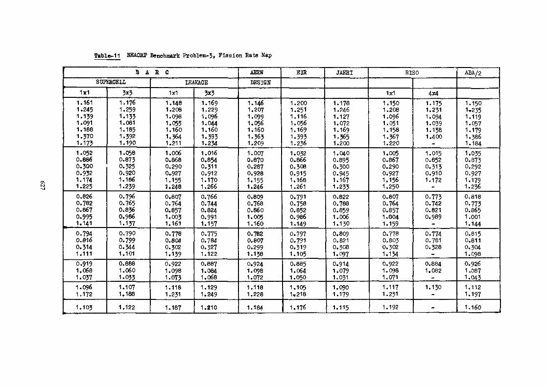
Table-11 KEACRP Benchmark Protlem-3, Fission Rate Map

B A S CSUFERCELL

1x11.1611.2451.1591.0911.1881.3701.1731.0520.8860.3000.9321.1741.2250.8260.7820.8670.9951.1410.7940.8160.3141.1110.9191.0681.0371.0961.172

1.103

3x31.1761.2591.1331.0811.1851.3921.1901.0580.8730.3250.9201.1861.2390.7960.7650.8360.9861.1370.7900.7990.3441.1010.8881.0601.0331.1071.188

1.122

LEAKAGE1x1

1.1481.2081.0981.0551.1601.3641.2111.0060.8680.2900.-9271.1551.2480.8070.7640.8571.0031.1610.7780.8040.3021.1390.9221.0981.0731.1181.231

1.187

3x31.1691.2291.0961.0441.1601.3931.2341.0160.8540.3110.9121.1701.2660.7660.7440.8240.99-11.1570.7750,7840.3271.1220.8871.0841.068

1.1291.249

1.210

AEEWDESIGN

1.1461.2071.0991.0561.1601.3631.2091.0070.8700.2870.9281.1551.2460.8090.7680.8601.0051.1600.78?0.80?0.2991.1380.9241.0981.0721.1181.228

1.184

SIR

1.2001.2511.1161.0561.1691.3931.2361.0320.8660.3080.9151.1681.2610.7910.7580.8520.9861.1490.7970.7910.3191.1050.8851.0641.0501.1051,218

1.176

JAERI

1.1781.2461.1271.0721.1691.3651.2001.0400.8950.3000.9451.1671.2330.8220.7880.8591.0061.1300.8090.8210.3081.0970.9141.0791.0311.0901.1791.115

S3SO

1x11.1501.2081.0961.0511.1581.3671.220

1.0050.8670.2900.9271.1561.2500.8070.7640.8571.0041.1590.7780.8030.3021.1340.9221.0981.0711.1171.231

1.192

4x41.1751.2311.0941.0391.1581.400

1.0150.8520.3130.9101.172

0.7730.7420.8210.989

0.7740.7810.328

0.8841.082

1.130

-

' ABA/2

1.1501-2351.1191.0571.1791.3861.1841.0350.8730.2920.9271.1791.2360.8180.7730,8651.0011.1440.8150.8110.3041.0980.9261,0871.0431.1121.1971.160

to-J

Table-12 NEACEP Benchmark Problem-4, Material Absorptions

Material

12

3456789

101112

131415161718192021227+8+93+6+11+14

BAHC

3 LEAKAGE

1x1

.1602

.0033

.0051

.1984

.0024

.0030.0108

.0157

.0428

.0005

.0007

.2976

.0056

.0100

.0005

.0060

.0195

.0157

.1614

.0275

.0114

.0021

.0694

.0187

3x3

.1570

.0033

.0049

.1980

.0024

.0030

.0112

.0169

.0492

.0005

.0007

.2930

.0055

.0097

.0004

.0059

.0191

.0158

.1630

.0274

.0109

.0021

.0773

.0184

AE37?

BEST

.1612

.0033

.0052

.1994

.0024

.0031

.0108

.0148

.0447

.0005

.0007

.3014

.0055

.0103

.0005

.0060

.0202

.0151

.1544

.0269

.0118

.0021

.0703

.0193

DESIGN

.1602

.0033

.0051

.1980

.0024.0031

---

.0009

.0007

.2973

.0056

.0101

.0005

.0060

.0196

.0157

.1618

.0276

.0114

.0021

.0689

.0190

E3H

,1602.0033.0051.19?2.0025.0031.0115.0163.0476.0005.0007.2992.0056.0102

.0005

.0061

.0200

.0149

.1537

.0265

.0114

.0021

.0754

.0191

JAERI

.1614

.0033

.0052

.2034

.0025

.0032

.0113

.0157

.0442

.0005,0007.2938.0055.0099.0005.0060.0191.0150.1588.0264.0116.0021.0712.0190

EISO

1x1

.1598

.0033

.0051

.1977

.0024

.0031

.0109

.0151

.0430

.0005

.0007

.2974

.0056

.0100

.0005

.0061

.0205

.0163

.1617

.0268

.0115

.0022

.0690

.0189

4x4

.1565

.0033

.0049

.1974

.0024

.0030

.0113

.0163

.0501

.0005

.0008

.2927

.0055

.0098

.0004

.0061

.0200

.0161

.1627

.0267

.6114

.0022

.0777

.0185

ABA

.1614

.0033-

.2027

.0024----

.0005-

.2977

.0055-

.0005

.0060

.0197.0148.1561.0260.0118.0021.0700

.0193

628

Table-13 NEACRP Benchmark Problem-4, Fission Rate Map

B A R 0

LEAKAGE

1x1

1.6811.48J1.3581.2301.1591.1881.26614051.2581.0950.9580.3880.9101.0071.0941.6731.4691.2491.5560.8250.8650.0001.1771.1660.7150.7361.0551.0440.6510.6700.3050.6200.6430.6400.650

0.674

3x3

1.6991.4921.3771.2111.1321.1681.2561.3951.2591.0890.9330.4070.8901.0001.0951.7171.4721.2781.3730.8200.8660.0001.1871.1860.7080.7341.0711.0610.6410.6670.3180.6120.4370.6350.655

0.684

AEEW

DESIGN

1.6521.4581.3171.2111.1411.1701.2441.380

1.2371.0790.9460.3800.8970.9901.0761.6451.4471.2321.3330.8120.8510.0001.1611.1470.7050.7251.0401.0270.6430.6600.2990.6120.6340.6300.640

0.662

EIR

1.7131.4941.3421.2171.1331.1751.2671.4251.2571.0910.9320.3980.8901.0071.1061.6791.4521.2551.3440.8260.8720.0001.1821.1660.7150.7421.0601.0420.6480.6780.3110.6150.6520.6400.660

0.691

JAERI

1.5931.4211.2921.1801.0981.1331.1981.3061.2291.0860.9430.3800.8910.9801.0541.6851.4711.2891.3570.8170.8560.0001.2021.1830.7170.7361.0881.0660.6530.6720.3020.6200.6460.6380.650

0.671

R3SO

1x1

1.6781.4681.3181.2081.1371.1711.2581.421

1.2441.0790.9430.3820.8970.9951.081

1.6491.4471.2291.3330.8090.8390.0001.1561.1430.6980.7101.0551.0220.6350.6460.2990.6060.6230.6280.638

0.682

4x4

1.6981.4771.3171.1871.1081.1501.2501.4161.2441.0730.9160.4020.8770.9911.0861.6951.4501.2591.3520.8060.8440.0001.1671.1640.6910.7081.0511.0390.6240.6430.3120.5950.6210.6200.637

0.679

ABA/2

1.6321.4431.3031.1901.1011.1421.2121.3341.2341.0770.9230.3630.8780.9811.0491.6581.4611.2441.3440.8160.8510.0001.1961.1710.7140.7381.0711.0500.6550.6800.2890.6210.6600.6540.6750.720

629

Table-14 Mean Flux and Absorption Rate in Various Regions ofCBN de Saclay Benchmark Prfeblem-1

REGIONNo.

1

2

54

56

MEAN FLUXi

MONTE-CARLO*

0.3180+0.00303.252 +0.0213.940+ 0.0204.462+ 0.020

3.663+0.019

4.179+0.018

001113 IONPROBABILITY

0.32043.2103-9424.400

3.637

4.110

ABSORPTION BATE

MCNTE-CARtO*

2.833+ 0.0270.02410+0.000150.6768+ 0.00340.03307+ 0.00015

0.6292+ 0.0033

0.03097+0.00013

COLLISIONPROBABILITY

2.8530.023790.67710.03261

0.6247

0.03046

* BESK-6 CPU fime » 42.0 mtsNumber of histories-* 33,000

Table-15 Mean F]Ux and Absorption Rate in Various Regions of CEN deSaclay Benchmark Problem-2

RegionNo.

12.

3.4.

5.6.7.8.

9.10.11.12.

13.141516171819

MEAN FLUXMONTE-CARLO

5.182 + 0.0473.684 + 0.028

4.184 + 0.0313.171 + 0.025

3.564 + 0.0213-575 + 9.0264.060 + 0.0233.151 + 0.0273-572 + 0.0190.2840+ 0.00122.909 + 0.012

3-475 + 0.0203.940 + 0.0203.251 + 0.0293.698 + 0.018

3.805 + 0.0264.293 + 0.0234.072 + 0.0394.592 + O.OJ8


5.068

3-717

4.1653.077

3.4963.5863.9993.0883.5300.28872.889

3.4093.8613-1543.592

3.7744.2414.0164.502

ABSORPTION RATEMONTE-CARLO

0.06477 + 0.000590.63290 + 0.00490

0.03101 + 0.000230.54460 + 0.00430

0.02641 + 0.000160.61400 + 0.004500.03009 + 0.000170.54120 + 0.004600.02647 + 0.000142.52900 + 0.011000.02156+ 0.000090.59690 + 0.003400.02920 + 0.000150.55830 + 0.005000.02741 + 0.00013

0.65360 + 0.004400.03181 + 0.000170.69950 + 0.006600.05403 + 0.00028


0.063350.63840

0.030870.52850

0.025910.615900.029630.530300.026162.571000.021400.585600.028610.541700.02662

0.648300.031430.689800.03336

630

Table-16 Eigenvalue, Total Absorption and CPU Time by VariousMethods for CEN de Saclay Benchmark Problem-?

METHOD

MOHTE-CAR10

TIO-TRAJT S .4

WG-TRAN SgOTO-TBAN S16

DIMPLE (jxj)

DIMPLE (5x5)

DIMPLE (8x8)

KEPF

0.876+0.002

0.87948

0.878780.87888

0.90665

0.87164

0.85205

CPU time(sec)

8400

222

5041320

29

58

185

TOTAL ABSORPTIONMWKRfikL

1149.92

145-57

--

148.47

149.34

149.85

M&TiaaAi,2

52.56

52.79

--

48.05

55-7360.28

MATERIAL3

19.82

19.80

--

19.09

19.30

19.44

Table-17 Flux Map For Group-1 by Various Methods for CEN de SaclayBenchmark Problem-3

MOHTECAHLO129.2132.4133.2134.2131.7130.0141-4143.3143-7141.6133.8143.3145.6145.5137.1149.7146.1136.9145.0157.1

133.7

S4127.7128.9132.4133.3132.3132.9136.1139.4141.5140.9135.6142.0145-9145-3140.0147.8146.3140.8144.3138.4

138.6

DBtPLE( 3x3)

127.3129.2130.9131.7131.6130.8

132.5134-4135.6135.3133.3136.3137.9137.6135.4139.0138.4136.2137.7135.6

134.5

DIMPLE (5x5)132.2134.1135.9136.9136.8136.1137.6139.6140.9140.6138.7141.6143.3143.1140.9144.6144.1141.8143.3141.2

140.1

DIMPLE (8x8)

135.1137.1138.9140.0139.9139.2140.6142.7144.1143.8141.9144-8146.5146.4144.2147.9147.4145.1146.7144.5

143.4

631

Table-18 Flux %p for Group-2 by Various Methods for GEN <Je Saclay————— Benchmark Problem-3

MONTE-CARLO

61.855.450.852.056.558.941.632.937.543.752.0

6.428.438.547.432.639.247-4

43.250.1

54.5

S4

60.7154.1949.9550.9755.9559.5841.1932.7836.9844.2852,576.45

27.9939.0351.5932.1239.4848.57

44.6352,38

56.81

XHMPI£(3x3)

58.5352.7148.5849.2455-1256.6141.7934.9737.5243.6650.305.85

30.0738.7246.0432.7038.9445.87

43.0449.10

52.81

DIMPLE(5x5)

58.5952.4848.2949.2253.5657.2340.8833.6236.8843.8350,706.83

29.0938.8446.3832.2639.2046.30

43.6449-79

53.63

DIMPIE(8x8)

58.6452.3848.1249,2*53-8657.6740.4032.7936.5443.9651.057.41

29.4538.8946.6832.0139.3746.69

43.9950.30

54.24

Table-19 Fission Rate Map by Various Methods for CEN de Saclay*———— Benchmark Problem?-3

MONTE-CARLO2.2111.8252.0332.3070.6321.6272.0821.8262.115

2.292

S4

2.1801.8102.0042.3310.6311.6102.1051.8002.128

2.555

DIB!PLE(3x5)2.1981.8962.0142.2890.5901.6842.0731.8052.084

2.267

DIMPLE (5^5)2.1701.8481.9982.3100.6471.6532.0911.7992.110

2.306

DIMPffi (8x8)

2.1551.8181.95P2.3240.6811.6322.1011.7952.125

2.351

632

Table -20 Comparison of Supercell Power Distribution with that fromMonte-Carlo Calculations for Tarapur Reload-2 Fuel Box

KQO M.C.

K &> Supercell

1.179+0.002

1.179

W-W

Monte-Carlo

Supercell

1.16+0.02

1.23

1.10+0.01

1.16\

0.227+0.005

).222

1.04+0.01

1.110.84+0.01

0.87

0.77+0.020.81

1.10+0.02

1.130.95+0.01

0.950,85+0.010.83

0.77+0.02^

0.80

1.22+0.02

1.21

1.09+0.02

1.050.92+0.010.90

0,82+0.01

0.81

0.234+0.005

>£.220

1.21+0.01

1.20

1.14+0.02

1.12

1.21+0.02

1.171.15+0.01

1.11

1.17+0.02

1.131.26+0,021.22

Burnable Poison Pin

Total number of histories

Total time taken

32,000

6 b and 40 mts.

N-N

633

Table 2>'Comparison Between Operational Data of Tarapur Reactors andCalculated Heat Fluxes

S.No.

1.2.

3-

4.

5-

6.

7.

TAIS UNIT

Cycle No.Date

Core Average Exposure (CfWD/ST)

Power (Mivt)

Inlet Water Subcooling (BTi/lbJ

No. of Control Rode IN

Calculated K-EPF

1

5May, 1978

12.45

433

12.6

2.75

1.006

2

6April, 1978

9.48

635

27.9

6.58

1.002

DO38.0A-1037.5

37-2B-6

41.02626 40.4

A_ Q

41.1

32.7B-533.4

ii

50.9 '"A-641.8

47.3A-7

43-6

40.5A-8

42.7

32.1B-4

32.2i|

*»43-8B-842.4

40.7B-7

43-5

39-5B-9

39.6ii

!r

30.A-;34

32A.

32

9

2

,0•4.9

TAPS TInit-1 Cycle-5Radial TIP Comparison

TIP heat flux

(Blank, C.R. OUT)

A-1060.6

Ofo06 51 .6

B-661.5

60.3A-9

61.7

20 48.9B-5

45.8*ii

40 64.2A-659.0

OSOS

59.3A-7

58.4

61.4A-861.9

45.8B-446.3

ii.

61.9B-857-3

088 56. 2

B-7

58.9B-9

56.4t «1 1

4

11

43A

46

42'A-44

J

.8

-5.1

.64•4

---

hes OTJT

^ v x

• < ——

XX

TAPS TJnit-2 Cycle-6Ra<?1al TIP Comparison

TIP locatifinCalculated heat flux

634

Assembly A

O

Assembly B

0ooo

ooo

Assembly C

0ooo

o0

oo

Assembly B Assembly E

O0\\\\\

0\\\\\

N

Assembly P

Assembly G*

qxxVyxo

XxxXx0

o

o\yVx\O

\

N

Xxx\

\

IQ\

\oAssembly H* Assembly I*

D £.,^> 1\l\i ^""^JJ

2.3 w/o »

2.1 W/0 "

1.9W/0 »

Control rod followers

* Ass.emb]ies G,H and I are without poison curtains

Figure-1 Fuel Rod loading Patterns of Nine Japanese Experiments

635

Proble»-1 t Burnable Poison Supercell

oo

oo

Problea-2 > JOII-BSa Frool«« with DifferentialEnriehaent and Crucifora Absorber

©©©©©

©

© ©

©

@©

©©©©Q

Problem-? « MB Lattice Cell With Several Fuel EnrichBentsand Poisoned Fuel PinsPin type Enrichnent

2.702.101.751.552.702.70

+ J w/o (H20-

Froblem -4 t WE Lattice Cell with Uranium, Plutonian aPoisoned Fins, One Empty Fin Poeition andA Cruciform Bod

Pin type Enrichment1 2.0 W/o2 Hat.D + 2.5J6 Po5 2.0 w/e + vf. 02054 2.0 W/o

Pigure-2 Four NEACRP Benchmark BV/R lattice Cell Problems

636

Figure-3 Eigenvalue Vs Absorptions inPoison Pin (Problem-1)

Pigure-4 SigenTalue Vs Absorptions in Cruciform' H o d (Problem-2)

.OS

- -84

-'83

Figure-5 Eigenvalue Vs. Absorptions inPoison Pin (Problero-3)

Figure-6 Eigenvalue 7s Absorptions in Cruciform andPoison Pins (Problem-4)

-1*07

-1-06

-I-05"

- f - 04

RiSG

•15" '17

ooo

O•o

C3y

t?r^-/e-

O

-— -

^-^- -*

-— "

Rroblem-2: 7x7 Celli-ssembly Wita a Water Gapind 8 Poison Pins

Burnabl

Water g<

e Poisor1 ———————

ap ——— —— ———

2 Problem -1 : 3x3 Cell with a Burnable^, \ Poison Hod

— fe

\

Ooo— .uooo

os-o-©oo

of?^

O

oso

ooo

1

ooo

Q\

©9©

o©o

o\<S1^

5

©oo

©

<§>®n

7ooo

w-w

3

1

1

1

1

2

1

1

1

1 1

N-N

Problem-3 : Mini 4x4 KVR Lattice Cell

1 Fuel

2 Poison Fin

3 Water

Figure-7 Two-Dimensional Transport Benchmarks Proposed by CEN de Saclay

639

HOMOGENIZATION METHODS USED BYCNEN - BRAZIL

C.M.P. SANTOS, C.U.C. ALMEIDAComissao Nacional de Energia Nuclear,Rio de Janeiro, Brasil

Abstract

The paper describes homogenization methods used by theCore Analysis Group of the Brazilian Nuclear Energy Comission (CNEN)for safety analysis review of PWR reactors. Computer codes usedare public domain codes with modification introduced in order toadapt to peculiarities of core design. Intercomparison betweendifferent methods are made. No experimental verification is presented,but is expected to be carried on during start-up tests.

INTRODUCTION

This work describes homogenization methods used by theCore Analysis Group (CAN) of the Brazilian Nuclear Energy Commission(CNEN) for the safety analysis review of the first PWR presentlyunder construction in Brazil.

All computer codes used are public domain codes whichhave undergone some modifications in their structure or usage in orderto adapt to some peculiarities of core design or computationalnecessities.

Since the objective of the calculations was to checkresults presented by Westinghouse, through the applicant, in thelicence procedure, whenever possible, two different methods were usedby CNEN to cross check their own results before comparing them withthe Westinghouse ones.

2. OVERALL CALCULATION SCHEMEThe computation scheme of CNEN for neutronic calculation

is represented in Fig. 1.

LEOPARD^, HAMMER^ and XSDRN^ codes can be used forcell calculation. Two interface routines, LEOCIT and CITHAM weredeveloped to prepare few group microscopic cross section files tothe finite-difference-diffusion-theory code CITATION ).

An intermediary assembly calculation is performed withCITATION using one mesh point per cell and reflected boundaryconditions. An homogenization subroutine was developed in order toobtain "assembly microscopic cross sections". This procedure isnecessary due to the presence of Borosilicate rods (burnable poison)in some assemblies and also for assemblies and also for assembliescontaining control rods.

Core calculation are performed in XY using quarter of coresymmetry. Macroscopic cross sections, homogenized by zone, can beobtained as a standard CITATION output for RZ calculation.

DOT III code, which solves Sn equation, is used inconjunction with XSDRN whenever a more precise calculation isneeded.

641

1r

COMPARE

) ———— — . ——

1

CITATION

XY -ASSEMBLY

CALCULATION

Fig.1 -CNEN CORE SIMULATION SYSTEM

3. CELL HOMOGENIZATION

The core of Angra 1 reactor, shown in Fig. 2, has sixdifferent types of cells: fuel cells with 2.1, 2.6 or 3.1 w/oenriched UO- cladded in Zircalloy 4; cells containing Zircalloy 4 guidethimbles; burnable poison cells, containing Borosilicate glass claddedin SS; and control rod cells, with Ag, In, Cd absorber cladded in SS.

255

A: Control Bank8: Number of BP rods

Fig. 2- ANGRA1 - CORE

642

The moderator contains soluble Boron as a long termreactivity compensator.3.1. Fuel Cell

Fuel cells can be calculated with LEOPARD, HAMMER or XSDRNcodes. In all cases, an "extra region" is added to the actual cell totake into account guide thimble cells present in the lattice. (Fig.3).

WATER*B'°+INCONELZ1RCALLOY 4

EXTRA REGIONIWATER»B'°» INCONEL*

ZIRCALLOY)

FUEL CELL FUEL SUPER-CELL

Fig. 3 - FUEL CELL MODELING

Results comparison between LEOPARD and HAMMER have showndiscrepancies within 3% in homogenized microscopic cross sectionvalues.

In order to investigate such discrepancies, homogeneouscell calculations were, performed with both codes. These resultshave shown discrepancies within only 1.5%, which were attributed todifferences in the multigroup cross section libraries and in thermalspectrum treatment (LEOPARD uses Wigner-Wilkins while HAMMER usesHelkin's Kernel). \

In order to take into account the influence of neighbor-ing fuel cells in determining the energy spectrum, and consequentlythe homogenized few group cross section for burnable poison cells,calculations are performed by modelling one of these cells with 8fuel cells aroud it as a "super-cell" (Fig. 4).

9 CELL ARRAY

HAMMER-SUPER-CELL

BURNABLE B'° » VOID (»AI TRACE)

SS CLAD

H20 + SOLUBLE BIO(*D20 TRACE)"EXTRA"( H0 *B|0« Zr « INCONEL )

LEOPARD SUPER-CELL Fig.4 - BURNABLE POISON CELL MODELLING

643

This "super-cell" is modelled in LEOPARD code by a borosi-licate central region, a second region containing the SS clad, a mode-rator region containing borated water plus guide thimble material andan "extra-region", with a "NON LATTICE FRACTION" equal to 8/9,containing fuel cell material.

It is also necessary to make a distinction between the"soluble Boron" present in the moderator and the "burnable Boron"contained in the glass rod. Since they are subject to differentspectra, this should lead to two different cross sections for B*".

Since LEOPARD had no possibility to make such distinc-tion, a scheme was developed in which average Boron cross sectionsfor this "super-cell" are multiplied by two different disadvantagefactors (DF), one for the moderator and another for the poison rod.In order to obtain these disadvantage factors, traces of D-0 and Alare simulated in the moderator and rod region respectively. Thedisadvantage factors can be calculated as the ratio of flux-weightedto volume-weighted number-densities of the trace components, astandard LEOPARD result.

More precise HAMMER calculations can also be performed forburnable poison "super-cell". For this purpose, HELP and LITHEauxiliary libraries were modified: Two identical Boron cross sectionsets were introduced with different identification numbers, so that"soluble" and "burnable" Boron behave as two different isotopes.Although HAMMER gives zone average cross sections, one can easelyobtain burnable poison cell average cross sections, since detailedflux distribution is available.

B thermal absorption cross sections obtained for Angra1 burnable poison cells, are presented on Table I. One can see thatcorrected LEOPARD results are 5% and 17% lower for "burnable Boron"and "soluble Boron" respectively, than the more precise HAMMERcalculation. These discrepancies result partially from differencesin cross section libraries but, mainly due to difference in thetreatment of the space and energy variables.

TABLE. I

LEOPARD

HAMMER

SUPER CELL, CELL(DF. correc-tion)

SUPER CELL

CELL

SULUBLE B10

1960. A

1985.6

2021.9

2321.8

BURNABLE B10

1960.4

1334.9

1733.4

1407.9

B Thermal Absorption Cross Sectionfor Burnable Poison Cell (barn)

These results have shown the inadequacy of LEOPARD totreat strong absorbers, even when spectrum influence and disadvantagefactors are taken into account.

644

3.3. Control Rod CellA group of 8 fuel cells around a control rod cell is also

modelled in a "super-cell" for control rod calculations using HAMMERor XSDRN, Fig. 5.

Fig.5-CONTROL ROD SUPER-CELL

In the case of HAMMER calculation, a fine group crosssection set, had to be incorporated in the original library sincethis element was not present.

Group parameters -were obtained from the XSDRN auxiliarylibrary, but some interpolation had to be made due to differences ingroup structure.

Like in the case of burnable poison, zone average crosssections, have to be corrected to obtain control rod cell averagecross sections.

Since homogenized control rod cell cross sections areused later in assembly calculations (see section 4 below), and sincefinite difference solution are not able to represent geometricself-shielding effects, and adjustment has to be made in thevalues of absorber cross sections.

The following scheme is used:First, a macroscopic cross section set is calculated for

all absorbing material. Then a finite-difference (CITATION) calcula-tion is performed for the 9 cell array using one point per homogenizedcell. Absorbing'material macroscopic cross sections are input asmicroscopic cross sections and its number density is set equal to one.Integral parameters calculated by finite difference are compared withHAMMER results and modifications in the number density, are made untila reasonable agreement is achieved.

kt .^Several parameters can be used for this fit: eff'

<j) cell/cj) supercell; cell thermal absorption/supercell thermalabsorption; production/absorption reaction rate. It is impossibleto obtain a good match in all these parameters at the same time.Later core calculation have shown that' the best adjustment parameteris the thermal absorption reaction rate.

645

4. ASSEMBLY HOMOGENIZATION

Although only three enrichment levels are present atbeginning of life in the core of Angra 1 reactor, the presence ofdifferent number of burnable poison rods in the assemblies makesnecessary an intermediary "assembly calculation".

For each one of the 8 combinations of enrichment and numberof poison rods, and alsc5 for rodded assemblies, a one point per cellfinite-difference diffusion calculation is performed using CITATION.Reflected boundary conditions are used.

A homogenization subroutine was introduced in the codeto generate flux-volume-weighted microscopic cross sections, inCITATION input format, for later core calculations.5. CORE RESULTS

Since there is no lattice experiments in Brazil to testintermediary results, only integral parameters will be tested,during the start-up program of the Angra 1 reactor.

Meanwhile, beside the cross-cheking of results of dif-ferent codes, Westinghouse results, presented in the FSAR havebeen compared with CNEN's finite difference results using thehomogenized cross sections obtained by the above mentioned methods.

The comparisions have shown a good agreement with respectto assembly or rod power distribution. Results are within 5% discre-pancies.

Critical Boron concentration at beginning of life is 1364ppm according to CNEN calculation whereas Westinghouse predicts1290 ppm.

Integral rod worth for a single control bank has beencalculated as 1116 pcm, while Westinghouse presents a value of1073 pcm.

Differential rod worth have been calculated in RZ geo-metry, using a series of 6 concentric homogenized rings, but the methodof calculus still needs some improvement.

The computation scheme has also been used for reactivitycoefficient estimations with good performance.

6. CONCLUSION

CNEN has developed and tested, from public domain codes,a system capable of performing the necessary calculation for safetyanalysis review in the area of core physics.

Experimental data for the verification of the systemwill be collected during start-up tests of Angra 1 reactor.

646

REFERENCE

(1) BARRY, R.F. - LEOPARD - A Spectrum Dependent Non-SpatialDepletion Code, WCAP-3269-26, (September 1963)

(2) SUICH, J.E. and H.C. HONECK - The HAMMER System HeterogeneousAnalysis by Multigroup Methods of Exponentials and Reactors,DP-1064 (January 1967).

(3) GREENE, N.M. and C.W. CROVEN - XSDRN: A discrete OrdinatesSpectral Averaging Code. - ORNL - TM 2500 (July 1969)

(4) FOWLER, T.B., D.R. VONDY, and G.W. Cunningham - NuclearReactor Core Analysis Code: CITATION - ORNL-TM-2496 Rev. 2(July 1971).

(5) RHOADES, W.A., and F.R. MYNATT - The DOT III Two-DimensionalDiscrete Ordinates Transport Code - ORNL-TM - 4280 C.

647

CONCLUDING SESSION (Chairman: A.F. Henry)

Round Table

J. Stepanek:Let me now open our Round Table Discussion for the final session.Because our time is very short, I would suggest that our dis-cussions be confined to the following three topics: firstly,to discuss once more the most important problems from ourpresentations, secondly, to seek and discuss the most promisingpaths for our future work in the field of homogenization inreactor physics, and thirdly, we would like to ask you alsoto prepare a few benchmark problems which could be submittedas the basis for future international cooperation in the fieldof homogenization methods in reactor physics under the sponser-ship of IAEA. The chairman for this" session is Prof. Henry andI shall now let him chair this difficult session.

A.F. Henry:Before I begin the discussion and people start to drift away assometime happens, I should like to take again the opportunityto thank our host for this very, very excellent meeting. TheSwiss Institute of Reactor Research worked extremely hard tomake this meeting so successful. We have been fed sumptuously;we have sailed all over the lake; we have walked all over hills,and we have enjoyed it all thoroughly. I want to thank you andI want to thank the IAEA for the assistance that organizationhas given to ogranize an extremely informative and also an ex-tremely enjoyable meeting. Applause. As for the topics whichMr. Stepanek brought up for discussion at this round table, Iam not going to push for the first item since it seems to methat we have already had a great deal of technical discussion,and I don't think we should get into detailed arguments whichtend to run on - particularly if they involve specializedcomments. The other two items are the question of futuremeetings of this nature and then of benchmark problem areas.I don't think that we can be specific about such meetings orsuch benchmarks. However, general comments would be very help-ful since they would give us ideas of how to define futuremeetings.

649

I think I should now call on the session chairmen to make theircomments.

R. Stammler:I have a little paradox which I would like to show you. I have asimple cylindrical system consisting of two regions - an innerregion without a source and an outer region, which is very thinand which contains a source. The inner region is heavily absor-bing and has no scattering. That means that, on the average, foreach neutron that is born in the outer region, one half willleave the system and the other half will be absorbed in theinner region. Thus, the escape probability for the neutrons, P,is equal to 1/2. On the other hand, the blackness for neutronsentering the system, r , will be practically equal to 1.

Now we homogenize this system and obtain homogenized crosssections for absorption, scattering, fission, etc. In thishomogenized system you may have defined Z in whatever waycLyou like - but I know from primitive but correct reactor physicsreasoning that the ratio P/ T should be equal to !/££ , where Si

3,is the mean chord length of the system and £ its macroscopicSLabsorption cross section. If I wish to preserve both P and rthen I must substitute P = 1/2 and r = i. This gives me directlythat £ must be equal to 1/R, where R is the radius of the system.3.Now it is hard to believe that in a ease where the system hasa radius of 1 cm - so that £ should be 1 - the blackness r willabe 1. Indeed, if you look it up in Case, de Hoffmann and Placzekyou will find a r that is far away from 1. Prom this simpleexample I have found that one single adjusted parameter - E ,

clto preserve the ratio P/r - cannot solve the homogenizationproblem. That means that homogenization is impossible if onedoes not add more information to the system.

A. Kavenoky:Of course you are completely right Dr. Stammler, in this caseit is impossible to match P and r . But in this case also thisseems to be an academic one and you have only to match r and Pis not any interest in this case.

R. Stammler:This was never meant to be a realistic case, it is a dreamedup situation that ... (interrupted by Kavenoky)

650

A. Kavenoky:Yes, but you have no scattering inside the house so you needto be good for ingoing current.

R. Stammler:Although this is an extreme situation, the reasoning was simple.I meant to say that if you cannot match everything in this casethen you may not expect that you will match everything with onesingle £ in a more normal situation.cL

A.P. Henry:I don't understand the problem; especially I don't know why theequivalent parameter should reproduce the escape probability asgiven by a transport calculation.

R. Stammler:I thought that in those cases where you use a certain transportmethod on a heterogeneous system, you would like to homogenizethe system such that when using the same transport method on thehomogenized system you get the same results. That is the sameresponse to my source neutrons as well as the same response tothe neutrons that enter the system. But I agree with you thatthis is an extreme example although it could be a control rod.

A. Kavenoky:Yes, but there is only one answer to you, homogenization willnever be rigorous, you cannot replace a heterogenenous regionwith a homogenous one which has all the properties of the hete-rogeneous one,in only some cases of interest it is possible,and we have to chose what are the cases of interest.

R. Stammler:I think that the method that I proposed at the ANS meeting inNew York, last year June, is similar to the method that Dr. Koebkehas presented here for big assemblies. In my case, where I hadto homogenize pin cells, I introduced temporarily an additionalsource which fixes the discrepancies that exist at the cellboundaries and I got the correct net out-current. The 6<j> , theresulting flux difference^ I subtract afterwards. This leavesme with a discontinous flux, but at least the overall reactionrates are preserved and also the contact with the surroundingpin cells has been correct during the iteration process in thesystem of homogenized pin cells.

651

H. Honeck:One of the subjects that has come up is somewhat disturbing tome. In the past we have always approached homogenization assomething we do in advance - we homogenized things based onsome assumption and then we do global calculations. In somecases, from the global calculations we go back and ask.whatis the fine structure. But this is not very often, so we neverreally addressed that problem and suddenly this presentationby A. Johnson yesterday, was very disturbing. He said that ifyou compute the global structure and use that to go back andrehomogenize, look at the error and the differences that youget compared to your first homogenization. I think that is avery significant result. It seems to me that, in the future,methods of homogenization should be different in the sense thatwe should be more prepared to look at different techniques, suchas surface currents, and that the research should be more orientedto the rehomogenization rather than assuming that the first ho-mogenization as being adequate. I just want to throw that outas a question.

K. Koebke:Defining equivalent parameters for a heterogeneous region onehas mainly to take into account the boundary conditions. By pre-forming several fine mesh calculations of this region, embeddedin its neutron physical environment, one can deduce a linearapproximation of the dependence of these equivalent parametersas a function of the leakage rates and of the boundary condi-tions of the considered region.

M. Wagner:What Dr. Koebke mentioned there was a very important point thatthe homogenization process depends on the boundary conditions.Since we have to think out methods how to represent this in aproper way. It would be very nice to have a benchmark problemwhich would be suitable to check various approaches. The problemthat Prof. Henry referred to would be a possible example. Buthe is too far from reality for practical applications.

A.F. Henry:I assume that you are referring to the problem with the littlecross shaped rods. It is quite unrealistic. It came from a seed-blanket reactor design, and seed-blanket reactors are not common.

652

Thus it is not clear that this problem should serve as a bench-mark. It does, however, have the virtue that it is simple. Also,it is not an expensive problem to analyse. However, it is notvery realistic.

J. Stepanek:I think that the idea of rehomogenization is important, inprinciple. We have used it for homogenization of the HTR'Sfuel elements which contains the fuel in the form of the parti-cals or for the homogenization of the boral zones containingthe boron particals in LWR fuel element storage container. Inthe both cases, we have calculated using outer iteration schemethe "macro" flux distribution in the space meshes and the "micro"flux distribution in the particals and the matrix zone. Aftereach outer iteration the "micro" fluxes were used to rehomogeni-ze the cross sections of the zones with particals for the followingcalculation of the "macro" flux.

Naturaly, we could do this homogenization only one times beforethe outer iteration process like Tenckert or Pomraning, Dyos,but the system would not be in the balance. Therefore we repeatthe homogenization after each outer iteration.

We have found by many cases that only homogenization can lead toconsiderable differences in the results in the comparision to therepeated homogenization.

The method should be used also by the homogenization of the meshes,with other types of the heterogenities like control cods etc.

In our work with C. Maeder the currents incoming into the cellwith control rod were not recalculated using the balance equationand I think this should be done in future.

A.P. Henry:If I understand the present argument, let me say something thatI think applies - viz. that homogenization schemes which connectheterogeneous nodal regions to each other by surface currentsare to be preferred. Having found approximate surface currentsone could go back and perform some kind of an iteration to improvethe coupling coefficients and hence the overall solution. Thatkind of correction may be more useful than trying to correctthrough adjusting the equivalent homogenized cross sections forreaction rates.Are there other topics to be discussed further?

653

M. Wagner:I would like to point out that this saheme that was just mentionedby A. Henry is being used in our coarse mesh nodal method. Werehomogenize during the iteration process over mild heterogeni-ties which develop during burnup. These effects are not very largeif you look at a single assembly. But they can lead to accumulatederrors if all fuel assemblies behave in the same way. And that iswhat happens at the beginning of a following cycle, when the re-load has occurred. Fuel assemblies which had been positioned atthe reflector boundaries and where gradients of burnup have beendeveloped are moved then into the core. There are regions insidethese assemblies which have higher reactivity, namely the areaswhich were adjacent to the reflector. They have a burnup deficit.After reloading, the flux in those areas will increase relativeto a homogenized bundle and this will lead to higher reactivitiesthan you would expect from using constant coefficients. This in-fluences the whole power distribution. The accumulated error isabout the order of 10 %. This applies only to coarse mesh cal-culations in a one node per assembly representation,

A. Kavenoky:Dr. Wagner declared the need for finer representation of anassembly near the reflector where there are gradients of irra-diation in the fuel.It is of course incredible to use one nodeper assembly and probably the kind of computation we have beenusing in our 2-Dimension code with finite elements, finiteelement representations at the cross sections should be used.Suddenly if we take one assembly from one position to anotherone in the reactor we also take the finite element representa-tions of the cross sections - It is one possibility to takeinto account this phenomenon.

J. Arkuszewski:I would like to express an opinion on the subject. I haven'theard at this meeting about one problem - probably it was hiddenin the presentations and in discussion. The problem I'm talkingabout is a uniqueness of homogenization procedures. It is knownfrom more theoretical work e.g. of Dr. Hughes and Dr. Duracz,that for one dimension the homogenization is a unique procedureand may be considered to be a constructive theory. But I'm notcertain this is the case for two dimensions and if there areready to use recipes concerning how many parameters we fit tohow many data, they lack general theoretical justification.

654

Even then, if there is an agreement and the homogenizationproblem is solved there exist some degrees of freedom. There-fore I doubt that, in general, the homogenization process isunique one, and I would be grateful to hear other opinions onthe subject.

A.F. Henry:In slab geometry, when one finds homogenized group diffusiontheory parameters for heterogeneous nodes, if these nodes aresymmetric about the center plane and if the angular flux enteringboth faces of a node is the same then it is possible to defineunique parameters which reproduce exactly every reaction rateand the leakage out both sides for each energy group.

Furthermore, the parameters are independent of the conditionsexternal to the node - the proof of this assertion was the partof my paper omitted in the oral presentation. It involves somecomplicated algebra and isn't of a real practical interest sinceit applies only to one dimensional cases.

If in slab geometry the nodes are not symmetric about the centerplane or if the angular distribution of the flux entering acrossthe nodal faces is not the same on both sides of the node so thatyou don't have complete symmetry, then parameters can still bedefined which are unique and "exact" for a selected group of in-coming partial currents on both sides. The cross sections thatdo this are, however, not physically meaningful. For example,the fission cross section in one of the groups can be negative -although the total fission rate (sum over all groups) will beexactly correct. These facts lead me to believe that if you matchcorrectly all reaction rates in all groups, you cannot matchleakage rates at both ends of the node. As Dr. Koebke pointsout, if you don't require continuity of flux you can get aroundthis limitation. In two dimensions I think the situation is thesame: You can't match all reaction and leakage rates and stillkeep the usual continuity of flux and current conditions.

F. Premuda:I think that there is some sort of connection between the problemof the unicity in homogenization procedures and the possibilityof doing something better in homogenization. First, if there isa unique finite set of parameters, it is of course that repeatinghomogenization the set vary going to a limiting one. Otherwise

655

if we have two or more possibilities perhaps it would be probablyimpossible to find the same convergence. On the other hand thepossibility of convergence is related physically to the factthat the neutronic balance be preserved; so this is furtherconnected probably to the possibility of getting in homogeni-zation the same eigenvalue we have in actual transport calcu-lations. I try to make this in practice, to repeat homogenization,in the procedure presented here the 13 november. I am startingfrom some buckling defining the global slowing-down source shape;then from the corresponding transport flux calculations the ba-lance preserving conditions are derived to which a new buckling,together with a set of homogenized parameters, must satisfy.This rehomogenization is iterated by adopting the new bucklingfor the source shape in the successive cycle of calculations;convergence both to the homogenized parameters and to the cri-tical buckling is expected theoretically. Of course, there aremany negative observations you could make about my work because,firstly I was not so clear in my exposition, secondly the geometryis very simple for a finite lattice in plane geometry only and,thirdly a discussion of what is happening in three-dimensionalgeometry is very difficult. It is possible perhaps to extendsome ways or ideas to two-dimensional geometries. This is relatedto the possibility of extending the DKPL transport techniquesused in one-dimensional integral transport calculations, by adop-ting kernel factorization into products of functions of two va-riables only (x, x', or y, y1 or z, zf e.g.) In any way we shouldlose a great part of the simplicity of the one-dimensional trans-port scheme and of the corresponding conditions for the equivalentdiffusion parameters when embedded in the two-dimensional treat-ment many aspects related to the consideration of currents andescape probabilities in different directions.

B.P. Rastogi:I want to make a very simple suggestion. I do not know whethersomething could be done for it. It seems that it is necessaryto have some benchmarks for -fuel boxes (BWRs) as a function ofburnup. The fuel box assemblies, to begin with, are enricheduranium assemblies, however, as burnup proceeds plutonium iso-topes are formed. The formation of plutonium isotopes is verysensitive to the homogenization model. In view of this I wonderwhether it would be possible for Dr. Honeck to develop somebenchmarks as a function of burnup.

656

A.P. Henry:I think it would be a very good idea. We had two burnup suggestionsnow that we're sort of passed over I think rarely, one that was avery heterogeneous 2-D PWR like assemblies be homogenized and nowone which has continous homogenization procedures into the bench-mark. There was another topic which Dr. Stepanek introduced whichwas a general one. Have we said everything at this meeting or isthere much more to do - is it worthwhile to think in terms of afollow up kind of meeting in several years? Does anyone have anyideas?

I would like to remark that we haven't settled everything. I guessthe right question to ask is whether anyone has a program thatwill be finished in two years which will answer everything. Doesanyone have any opinions in this area?

Y.S. Gur:Usually when you want to test a method of homogenization you reallyhope to find a simple method by which you get the same resultsobtained by more elaborate and sophisticated other methods. Havingmeasurements only to test the new method is not enough, for agood method might fail to reproduce the measurements due to in-accurate cross sections used when checking it. Now if there werebenchmarks which are not only measurements but carefully computedcells, by the most sophisticated methods, with input cross sections,fictitious or not, given exactly, then the checking of a new methodagainst a sophisticated method would be possible.

A.F. Henry:I strongly subscribe to that way of doing it because, althoughchecking theory vs. more accurate theory is not the whole answer,it is unambiguous. Then one can design simple experiments to testthe Cross-sections in an integral way. I've always favored this:

One should check theoretical models against more accurate theore-tical models using the same cross sections throughout the check.Then one should validate cross sections by designing clean expe-riments which are analysable by the same numerical standards thatconstitute the calculational benchmarks.

A. Kavenoky:You know perhaps, in Prance we have done some of these smallexperiments for"light water reactor lattices. And it could be

657

perhaps possible that this lattice could be given for benchmarkcalculations. It is a possibility and I cannot say if it issure.

A.P. Henry:Are you suggesting that the benchmark would be a theoretical onefor which cross sections would be supplied but would also happento be something that could be done experimentally?

A. Kavenoky:No, I was thinking of Mr. Gur: one benchmark for us has to be atheoretical benchmark with given cross sections, and the mostsimple one possible with a small number of rows. We don't haveto take thousands of sigma values to compute a benchmark. Ifwe decide a benchmark it must be a simple one but with somephenomenon and some principle. Another problem, one for answeringProf. Henry, we have some clean experiments done specially forPWR lattices and perhaps this can be discussed from anotherpoint of view to take for calculations - but it is completelydifferent from benchmark applications.

M. Melice:As a user of codes, I would like to make a few remarks, prettymuch along Dr. WAGNER1s comments. I believe that our meetingshould have given more attention to some topics which are ofpractical interest.

The first one is the spacial range the homogenization and theseparability between homogenization and core calculation. Ob-taining fewgroup diffusion cross-sections for complete fuelbundles is indeed attractive, especially for nodal codes, butthe boundary and critically conditions assumed in the bundlecalculations are not always sufficiently representative of theactual bundle situation in the core and various correctionscan be introduced.

The second topic is fine structure recovery, to the extent thatthe core power capability and fuel mechanical performance arestill evaluated in terms of fuel rod power.

K. Koebke:The problem of rehomogenization can be solved either by a highorder interpolation method, determining the local equivalent

658

flux distribution, and by the succeeding application of themodulation method, multiplying the heterogeneous form functionon this continuous flux distribution, or you can regain theheterogeneous power distribution by performing fine mesh cal-culations with boundary conditions known from the global equi-valent reactor solution.

The inconsistency between a heterogeneous multigroup and anequivalent and rehomogenized global reactor solution is mainlyinfluenced by the definition of appropriate equivalent para-meters. If these parameters are not correct you can not performconsistent coarse mesh calculations and the basis for a rehomo-genization method is not well established. I believe that themethods, described in the paper, will lead to homogenized andrehomogenized accurate coarse mesh solutions.

A.F. Henry:Indirectly you are suggesting a good topic for a future meeting.In a few years we'll probably know more about recovering finedetail from coarse mesh calculations. That subject plus the threebenchmarks suggested could perhaps constitute the basis for afuture meeting.

Do you, Dr. Stepanek, have any concluding remarks?

J. Stepanek:I think in our papers and during this discussion it was shownthat there are still many problems in the field of the homoge-nization methods which are unfortunately not solved or notsolved well enough. This was particularly the reason why wehad a lack of papers for some topics which were originallyproposed but later unfortunately had to be removed from theprogramme of this meeting.

I think that the meeting should therefore be the starting pointto an international cooperation for solving the outstandingproblems and this should be done under the sponsorship of IAEA.

The benchmark problems could give a basis for this cooperation.Mr. Neamu could have perhaps some remarks to this point.

I. Neamu:Many thoughtful proposals and recommendations have been addressedto the Agency during our Round Table discussion for the final

659

session. It is too early to comment on these, but I would liketo give an assurance that they will be carefully considered bythe Division of Nuclear Power and Reactors and will be reflected,if feasible, in the programmes to be submitted to the DirectorGeneral as the basis for future international cooperation in thefield of homogenization methods in reactor physics under thesponsership of IAEA.

J.L. Rowlands:I would like to suggest that participants at the meeting shouldbe invited to consider proposing to the IAEA possible fast reactorbenchmark homogenization problems. Different benchmarks would berequired to examine different types of homogenization and differentaspects of the homogenization problem. Examples of the differenttypes of homogenization are the fuel pin and subassembly structu-re of power reactors, the treatment of singularities, such ascontrol rods and in-core breeder elements, and the plate and pinstructure of zero-power critical assemblies. Different aspectsof the homogenization problem are leakage effects and streaming,resonance shielding, broad group flux fine structure and spectraltransients at boundaries between zones.

P. Premuda:To return to the discussion about the benchmark problems, towhich I am interested, there are in fact two different kindsof benchmark problems. One is a benchmark problem which is tryingto treat a very realistic situation. The calculation can be per-formed by a very flexible, but not so accurate, numerical algo-rithm; this calculation must be combined with a Monte Carlonumerical experiment or with a true practical experiment toyield an external control, whereas an internal control of theaccuracy of the method is absent. Another kind of benchmark isthat which is prepared not for those working in the design butfor people working theoretically in preparing codes. One canconsider idealized situations not so complicated and developa method, for which an internal accuracy control is possiblethrough the observation of a numerical fast convergence to somelimiting value for eigenvalues and other physical quantities orfor flux distributions at increasing orders of approximation. Ithink that both kinds of benchmarks have the same importance. Wepreviously heard that there was a brief discussion about thedefinition of diffusion coefficient for a one-dimensional problemand other one-dimensional problems were treated, in this meeting,

660

which are of course out of any consideration about a realisticreactor situation. Perhaps in the future it will be possible totreat in a theoretically rigorous form more and more realisticsituations, but I think we should have in any way a class ofproblems that we cannot hope will be treated rigorously in thefuture according to a realistic model. So we have two aspectsto consider.

J. Stepanek:As we are running out of time, we can only have one final remarkor suggestion.

Y.S. Gur:Suppose one has a new method and-wants to try it. One could startwith the elaborated procedure of computing a cell, which has ana-lytic solution, using the new method as a first check of themethod, or one could try to obtain an cell which was computedaccurately, using a sophisticated method. But one does not havethe sophisticated code and does not know who could do thesophisticated computation. There should be established a bodythat knows where sophisticated computation can be done, sothat one could address him and specify the system he wants,and the body will transfer the request to the appropriate center.This would be helpful to those who try to simplify methods aswell as to those who are building their library of elaboratecodes.

J. Stepanek:Thank you Very much. Before we close our meeting I would liketo introduce IAEA secretary Mr.Chernyshev. He would like to sayyou a couple of words to our meeting and to our propositionsconcerning our future cooperation.

V. Chernyshev:I think it is a fine time to have a few words about your proposalto find some ideas for benchmark or future cooperation in thereactor physics area. I would like to give some information aboutthe activity in the field of reactor physics which we have inInternational Atomic Energy Agency. You know that this agencyhas a special division of Nuclear Power and Reactors in whichwe concentrate the international activity in the field. Usuallyit is connected with organization of symposiums or seminars, twoor three specialist meetings, and a Course on Reactor Theory

661

and Power Reactors which is necessary for developing countries.Moreover, the research coordinated programme on Neutron TransportTheory and Advanced Reactor Calculation was organized. I wouldlike to say a few words about such a type of cooperation becausethe agency has several coordinated programmes and intends tocontinue this work. For exapmle, the agency has several suggestionsfor future activities in the field of reactor physics. One ofthem which was supported by the scientific committee of theagency is dealing with Multi-dimensional calculations of reactorkinetics. It probably will be the future coordinated researchprogramme based on international cooperation. Several scientificteams from different institutes and countries will work underthis scientific problem, in accordance with conditions ofresearch agreements or contracts signed with the Agency.

We intend to include the comparison of experiments and calcula-tions in the programme on multi-dimentional reactor kinetics.Under this programme we would like to consider the verificationof current calculational methods, their description and applica-tion to the large reactor core. We would like to compare thepromising methods for 2D and 3D calculations of some reactorkinetics and reactor control problems. We hope that the CRPmay provide a suitable framework for future panel on ReactorKinetics and Control Calculations.

I would like to finish my talk with an announcement that we arelooking forward to your new proposals especially in this areain order that the new coordinated research programme could start.

J. Stepanek:A now a final word from our IAEA secretary Mr. Neamu.

I. Neamu:I would like once again to express my thanks to the general chair-man Dr. Jiri Stepanek and his collaborators from the Swiss FederalInstitute for their effort in organizing the meeting and also tothe session chairman and all participants for helping to ensurethe success of the meeting. I am sure I express the sentimentof all participants in thanking again the Government of Switzer-land and City of Lugano for their generous help and hospitality.

J. Stepanek:I thank Mr. Neamu for his kind words.

662

I hope you have not found the program committee to be too hardon you, because we were working to a very heavy schedule, whichwas going each day up to 17.20. We agreed to the suggestionmade by Prof. Benoist to put one additional paper on the programmeand shorten your coffee break to the minimum. And finally duringthe programme preparations I have decided to put the presentationof our only woman delegate at the end of our programme so as toguarantee that everybody else stays to the end of the meeting.This was a good decision. In spite of the pleasant weather wehave had, the attendance to our sessions was very good.

We would like to express to you our thanks for your active co-operation.

I hope you have found many nice aspects to the meeting in Luganoand I hope you will remember them.

I wish you pleasant journing home and hope that many of us willmeet in the future at other meetings. Goodbye.

663

LIST OF PARTICIPANTS

BELGIUM

de Raedt, Ch.

Melice, M.

S.C.K./C.E.N.,Boeretang 200, B-2400 Mol

Electrobel,1 place du Trone, B-1000 Brussels

BRAZIL

Santos, Mrs. C.M.P. Comissao Nacional de Energia Nuclear,Rua General Severiano 90-Botafogo,Rio de Janeiro, Guanabara

CANADA

Heeds, W.

Irish, J.D.

Atomic Energy of Canada Limited,Chalk River Nuclear Laboratories,Chalk River, Ontario KOJ 1JO

Atomic Energy of Canada Limited,Chalk River Nuclear Laboratories,Chalk River, Ontario KOJ 1JO

DENMARK

Petersen, T. Ristf National Laboratory,DK-4000 Roskilde

FINLAND

Anttila, M. Lonnrotinkatu 37, SF-00180 Helskini 18

FRANCE

Benoist, P.

Bouget, Y.H.

Gouret, M.

A. Kavenoky

CEA, Centre d'etudes nucleaires de Saclay,B.P. 2, F-91190 Gif-sur-Yvette

CEA, Centre d'etudes nucleaires de Cadarache,DRNR/SEDC, B.P. 1, F-13115 St-Paul-lez-Durance

CEA, Centre d'etudes nucleaires de Saclay,B.P. 2, F-91190 Gif-sur-Yvette

Centre d'etudes nucleaires de Saclay,Service d'etudes de reacteurs et de mathematiques

appliquees,B.P. 2, F-91190 Gif-sur-Yvette

665

FRANCE (cont.)

J. Mondot

A. Santamarina

P. Therond

CEA, Centre d'etudes nucleaires de Cadarache,Service d'etudes nucleaires (SEN),B.P. 1, F-l 3115 St-Paul-lez-Durance

CEA, Centre d'etudes nucleaires de Cadarache,Service d'etudes nucleaires (SEN),B.P. 1, F-13115 St-Paul-lez-Durance

Residence St-Donnat BtL,Chemin St-Donnat,F-l 3100 Aix-en-Provence

GERMANY, FEDERAL REPUBLIC OF

G. Ambrosius

R. Bohme

E.A. Fischer

K. Koebke

M.R. Wagner

R. Wartmann

Kraftwerk Union AG,Department R121,Berliner Str. 295-299,D-6050 Offenbach

c/o Atomic Energy Establishment,Winfrith, 004/D53, Dorchester, Dorset DT2 8DH,United Kingdom

Kernforschungszentrum Karlsruhe,Institut fiir Neutronenphysik und Reaktortechnik,Postfach 3640, D-7500 Karlsruhe 1

Kraftwerk Union AG,Department R121,Postfach 3220, D-8520 Erlangen

Kraftwerk Union AG,Department R121,Postfach 3220, D-8520 Erlangen

Institut fur Kernenergetik und Energiesystemeder Universitat Stuttgart,

Postfach 801140, D-7000 Stuttgart-80

HUNGARY

J. Gado Central Research Institute for Physics,P.O. Box 49, H-1525 Budapest

INDIA

B.P. Rastogi Bhabha Atomic Research Centre,Trombay, Bombay 400085

666

ISRAEL

M. Caner

D. Gilai

Y.S. Gur

Soreq Nuclear Research Centre,Yavne 70600

Nuclear Research Centre Negev,P.O. Box 9001, Beer-Sheva 89190

Soreq Nuclear Research Centre,Yavne 70600

ITALY

B. Carmignani

F. Premuda

Centre di Calcolo del CNEN,Via Mazzini 2,1-40138 Bologna

CNEN,Dipartimento Ricerca Tecnologica di Base e Avanzata,Via Mazzini 2,1-40138 Bologna

POLAND

K. Andrzejewski

J.J. Arkuszewski

M. Borysiewicz

T. Duracz

Computing Centre Cyfronet,Institute of Nuclear Research,05-400 Swierk-Otwock




SWEDEN

R. Stammler ASEA-ATOM ABP.O. Box 53, S-72104 VasterSs 1

667

SWITZERLAND

D. Davierwalla

H. Hager

G. Hauser

W. Heer

H. Honeck

P. Köhler

C. Maeder

Ch. McCombie

G. Meier

S. Rizvi

U. Schmocker

J. Stepanek

P. Stüler

P. Wydler

UNITED KINGDOM

R. F. Burstall

A.T.D. Butland

Swiss Federal Institute for Reactor Research,CH-5303 Würenlingen


Nordostschweizerische Kraftwerke AG,Parkstrasse 23, CH-5401 Baden






Kernkraftwerk Gösgen-Däniken AG,Postfach 55, CH-4658 Däniken

Nordostschweizerische Kraftwerke AG,Parkstrasse 23, CH-5401 Baden





Atomic Energy AuthorityRisley, Warrington, Cheshire WAS 6AT

UK Atomic Energy Authority,Atomic Energy Establishment,Reactor Physics Division,Winfrith, Dorchester, Dorset DT2 8DH

668

UNITED KINGDOM (cont.)

C.R. Eaton UK Atomic Energy Authority,Atomic Energy Establishment,Reactor Physics Division,Winfrith, Dorchester, Dorset DT2 8DH

M.J. Grimstone UK Atomic Energy Authority,Atomic Energy Establishment,Reactor Physics Division, Room 204, Bldg. B21,Winfrith, Dorchester, Dorset DT2 8DH

MJ. Halsall UK Atomic Energy Authority,Atomic Energy Establishment,Winfrith, Dorchester, Dorset DT2 8DH

R.P. Hughes Berkeley Nuclear Laboratories,Berkeley, Gloucestershire GL13 9PB

J.L. Rowlands UK Atomic Energy Authority,Atomic Energy Establishment,Reactor Physics Division,Winfrith, Dorchester, Dorset DT2 8DH

UNITED STATES OF AMERICA

A.F. Henry Massachusetts Institute of Technology,77 Massachusetts Avenue,Cambridge, MA 02139

A. Jonsson Nuclear Power Systems,Combustion Engineering Incorporated,1000 Prospect Hill Road,Windsor, CT 06095

D.C. Wade Argonne National Laboratory,Applied Physics Division,9700 South Cass Avenue,Argonne, Illinois 60439

YUGOSLAVIA

D.V. Altiparmakov Boris Kidric Institute of Nuclear Sciences,P.O. Box 522, Belgrade-Vinca

669

IAEA

I. Neamu (Scientific Secretary) International Atomic Energy Agency,PO Box 100, A-1400 Vienna, Austria

OBSERVER

V. Chernyshev International Atomic Energy Agency,PO Box 100, A-1400 Vienna, Austria

ORGANIZATIONS

OECD NUCLEAR ENERGY AGENCYR. Richmond Institut federal de recherches en matiere de reacteurs,

CH-5303 Wiirenlingen,Switzerland

General J. STEPANEK Swiss Federal Institute forChairman: Reactor Research,

Wiirenlingen, Switzerland

Scientific I. Neamu International Atomic Energy Agency,Secretary: Vienna, Austria

670

HOMOGENIZATION METHODS IN REACTOR PHYSICS

Documents

Transcript of HOMOGENIZATION METHODS IN REACTOR PHYSICS