at*'- i

*llf

••.-.it

•.1S

XA0.101359

I N T E R N A T I O N A L A T O M I C E N E R G Y A G E N C Y

ISES-TCS--12

Reactor SimulatorDevelopment

Workshop Material

" "fl:

3 2 / 28T R A I N I N G C O U R S E S E R I E S

PLEASE BE AWARE THATALL OF THE MISSING PAGES IN THIS DOCUMENT

WERE ORIGINALLY BLANK

TRAINING COURSE SERIES No. 12

Reactor simulatordevelopment

Workshop material

INTERNATIONAL ATOMIC ENERGY AGENCY, 2001

The originating Sections of this publication in the IAEA were:

Nuclear Power Technology Sectionand

Nuclear Power Economic Planning SectionInternational Atomic Energy Agency

Wagramer Strasse 5P.O. Box 100

A-1400 Vienna, Austria

REACTOR SIMULATOR DEVELOPMENTIAEA, VIENNA, 2001

IAEA-TCS-12

© IAEA, 2001

Printed by the IAEA in AustriaApril 2001

FOREWORD

The International Atomic Energy Agency (IAEA) has established a programme innuclear reactor simulation computer programs to assist its Member States ineducation and training. The objective is to provide, for a variety of advancedreactor types, insight and practice in reactor operational characteristics and theirresponse to perturbations and accident situations. To achieve this, the IAEAarranges for the supply or development of simulation programs and trainingmaterial, sponsors training courses and workshops, and distributes documentationand computer programs.

This publication consists of course material for workshops on development ofsuch reactor simulators. Participants in the workshops are provided withinstruction and practice in the development of reactor simulation computer codesusing a model development system that assembles integrated codes from aselection of pre-programmed and tested sub-components. This provides insightand understanding into the construction and assumptions of the codes that modelthe design and operational characteristics of various power reactor systems.

The main objective is to demonstrate simple nuclear reactor dynamics withhands-on simulation experience. Using one of the modular development systems,CASSIM™, a simple point kinetic reactor model is developed, followed by amodel that simulates the Xenon/Iodine concentration on changes in reactorpower. Lastly, an absorber and adjuster control rod, and a liquid zone model aredeveloped to control reactivity.

The built model is used to demonstrate reactor behavior in sub-critical, criticaland supercritical states, and to observe the impact of malfunctions of variousreactivity control mechanisms on reactor dynamics. Using a PHWR simulator,participants practice typical procedures for a reactor startup and approach tocriticality.

This workshop material consists of an introduction to systems used fordeveloping reactor simulators, an overview of the dynamic simulation process,including numerical methods, and an introduction to the CASSIM™ developmentsystem. Techniques and practice are presented, with exercises, for developmentand application of reactor simulators.

The workshop material was prepared by W.K. Lam, Canada, for the IAEA. TheIAEA officer responsible for this publication was R. Lyon from the Division ofNuclear Power.

EDITORIAL NOTE

The use of particular designations of countries or territories does not imply anyjudgement by the publisher, the IAEA, as to the legal status of such countries orterritories, of their authorities and institutions or of the delimitation of theirboundaries.

The mention of names of specific companies or products (whether or notindicated as registered) does not imply any intention to infringe proprietaryrights, nor should it be construed as an endorsement or recommendation on thepart of the IAEA.

CONTENTS

1.0 Introduction to Modular Modeling Systems 1

1.1 Modular Model Generation Process 1

1.2 Integral Components of a Modular Modeling System 41.3 Simulation Development System for Control Room Replica Full Scope Simulators ...A1.4 Simulation Development System for PC Based Desktop Simulators 51.5 Technology Trends for Modular Modeling System 71.6 Simulation Fundamentals 8

1.6.1 Dynamic Simulation Versus Steady-State Simulation 81.6.2 Mathematical Modeling 81.6.3 Model Specification 91.6.4 Basic Physical Laws 111.6.5 Physical Process Characteristics of a Control Volume 16

2.0 Overview of Dynamic Simulation for Power Plant Process 23

2.1 Introduction 232.2 Basic Equations 242.3 Mass and Component Balance Equations 242.4 Rate of Change of Pressure in a Control Volume 262.5 Momentum Equation for Links Joining Control Volumes 272.6 Linearized Momentum Equation 272.7 Pressure Drop Calculation 282.8 Pump Flow Equation 282.9 Flow Equation in Link with Pump and Valve 302.10 Pump Cavitation Factor 302.11 Flow Equation to Match Specific Pump Curve and Incompressible Flow 302.12 Energy Balance Equations 302.13 Rate of Change of Fluid Temperature in Control Volume 312.14 External Heat Transfer Rate in Control Volume 322.15 Equations of State 322.16 Two Phase Systems (Simple Equilibrium Model) 32

3.0 Numerical Methods and Other Important Model Considerations 35

3.1 Introduction 353.2 Explicit Euler Integration 353.3 Implicit Euler Integration 383.4 System of Equations 403.5 Other Important Model Considerations 42

3.5.1 Range of Validity 423.5.2 Reliability 433.5.3 Real Time Simulation 44

4.0 Cassim™ Based Simulation Methodology and Simple Modeling Exercises 46

4.1 Introduction to Cassim™ Modeling 464.2 Block Oriented Modeling Concept 464.3 Cassim™ Simulation Development System 494.4 Simulation Modeling Using CASSBASE 524.5 Opening The Two Tanks Model 534.6 Browsing The Algorithms Library 54

4.6.1 The NON-MOVEABLE BLOCKS Algorithm .564.6.2 The DEMO 1ST ORDER VALVE Algorithm 57

4.7 Opening a Block in The Model 594.7.1 Browsing Block #1 60

4.8 Two Tanks System Modeling Analysis and Design 614.8.1 Description of the Two Tanks System 614.8.2 Algorithms Selection 634.8.3 Initial Conditions 644.8.4 Flow Calculation Method 64

4.9 Two Tank System Modeling 654.9.1 Creating Block #2 — VALVE 1 654.9.2 Creating Block #3 — FLOW1 684.9.3 Creating Block #4 — TANK1 694.9.4 Creating Block #5—FLOW4 714.9.5 Creating Block #6 — PID Controller 714.9.6 Creating Block #7 — VALVE3 734.9.7 Creating Block #8 —FLOW3 744.9.8 Creating Block #9, 10, 11, and 12 744.9.9 Creating Block #13 764.9.10 Creating Block #14 76

4.10 Hands-On Testing and Debugging the Simple Two Tanks Process 774.10.1 Verifying the Model 774.10.2 Exporting Model Data File For Cassim™ Simulation

Engine — CASSENG 784.10.3 Testing the Simulation Using Cassim™ Debugger 79

4.11 Running the Simulation Model with Labview® Screen 884.11.1 Running the Two Tanks Simulation 88

4.12 Merging Models 914.13 Review of Thermalhydraulic Network Modeling 91

4.13.1 Cassim™ Thermalhydraulic Modeling Simplifications 954.13.2 How to Create a Hydraulic Network System 96

4.14 Algorithm Source Code Development 974.14.1 Fortran Algorithm Coding Standard 974.14.2 Algorithm Source Code Standard 994.14.3 Simple Algorithm Exercise 99

5.0 Reactor Simulation Model Development 100

5.1 Quick Review of Nuclear Reactor Neutron Physics 1005.1.1 Rates of Neutron Reactions — Reactor Power 1005.1.2 Multiplication Factors for Thermal Reactors 1015.1.3 Steady-State Neutron Balance 1035.1.4 Mean Neutron Lifetime and Mean Effective Neutron Lifetime 1045.1.5 Reactivity Units 1045.1.6 Changes in Neutron Flux Following a Reactivity Change in Reactor with

Prompt Neutrons Only 1055.1.7 The Reactor Period for Reactor with Prompt Neutrons Only 1055.1.8 Power Changes with Prompt Neutrons Only 1065.1.9 The Effect of Delayed Neutrons on Power Changes 106

5.2 Point Kinetic Model — Delayed Neutrons 1085.2.1 Analytical Solution to Point Kinetic Reactor Model Equations.... 109

5.3 Modeling Exercise — Simple Point Kinetic Model 1135.3.1 Problem Description: 113

5.3.2 Point Kinetic Reactor Simulation Model Using Cassim 1145.3.3 Simple Point Kinetic Model Algorithm Formulation (Solution) 1155.3.4 Simple Point Kinetic Reactor Model Fortran Program (Solution) 117

5.4 The Effects of Neutron Sources on Reactor Kinetics 1215.4.1 The Neutron Sources 1215.4.2 The Effect of Neutron Sources on the Total Neutron Population 1215.4.3 The Effect of Neutrons Sources on a Reactor At Power 1225.4.4 The Effect of Neutron Source on Reactor Shut-Down 1235.4.5 Photoneutrons Sources in Heavy Water Reactor 123

5.5 Modeling Exercise — Point Kinetic Reactor Model with Photoneutrons 1245.5.1 Point Kinetic Reactor Model with Photoneutrons Sources (Solution) 126

5.6 Reactivity Feedback Effects 1265.6.1 Long Term Reactivity Effects — Fuel Burnup and Buildup 1265.6.2 Intermediate Term Reactivity Effects — Xenon Poison 1295.6.3 Short Term Reactivity Effects 133

5.7 Modeling Exercise — Poison Reactivity Effects 1345.7.1 Problem Description 1345.7.2 Modeling Steps 135

6.0 Reactor Control Simulation Model Development 138

6.1 Brief Review of BWR Reactor Power Control 1386.2 Brief Review of PWR Reactor Power Control 1416.3 Brief Overview of RBMK Reactor Power Control 1436.4 Pressurized Heavy Water Reactor 146

6.4.1 Pressurized Heavy Reactor Control System General Description 1476.4.2 Moderator Liquid Poison Addition And Removal System 1526.4.3 Reactor Trip System 152

6.5 PHW Reactor Regulating System Brief Overview 1536.6 Generic CANDU Simulator — RRS Familiarization 156

6.6.1 Familiarization with CANDU Generic Simulator 1576.6.2 Simulator Exercise Related to PHW Reactor Control 161

6.7 Modeling Exercise — Reactivity Control Mechanism: Liquid Zone 1676.7.1 Liquid Zone Hydraulic Modeling and Approach 1676.7.2 Liquid Zone Reactivity Control Modeling 171

6.8 Solution to Modeling Exercise — Reactivity Control Mechanism: Liquid Zone 172

7.0 Development of Adjuster, Absorber, Shutdown Rods Model 173

7.1 Development of Adjuster and Absorber Rods Model 173

7.2 Development of Shutdown Rods Model 175

8.0 Reactor Startup and Approach To Criticality 177

8.1 Subcritical Reactor Behavior 177

8.2 Reactor Instrumentation 1798.2.1 Startup Instrumentation 1798.2.2 Ion-Chamber Instrumentation 1838.2.3 In-Core Flux Detectors 183

8.3 Methods for Approaching Criticality 1848.3.1 Approach Reactor Criticality by Raising Moderator Level 1858.3.2 Approach Reactor Criticality by Removing Boron Absorber 185

8.4 Practice Reactor Startup and Approach to Criticality Using Simulator 187

9.0 From Simple Point Kinetic Reactor Model To High Fidelity Model 193

9.1 Spatial Kinetic Model for PHW Reactor 1939.2 Nodal Approach for Simulating Space-Time Reactor Kinetics 1939.3 Summary of Model Formulation for PHW Reactor 1989.4 Coupled Reactor Kinetics Reference 209

Typical Workshop Agenda 210

APPENDIX: SELECTED CASSIM™ ALGORITHMS' DESCRIPTIONS

Algorithm # 102: PUMP_SIM, Simple centrifugal pump 213

Algorithm # 106: VLV_ONOFF_SM, Simple on-off valve 216Algorithm # 108: CV_SIM, Simple control valve 219Algorithm # 128: TANK, Simple storage tank with heating 222Algorithm # 133: BREAKER, Breaker 225Algorithm # 134: MOTOR, Simple motor model 227Algorithm # 140: CONDUCTJFI, incompressible flow conductance 229Algorithm # 223: RSFF, Reset— Set (RS) flip flop 231Algorithm # 232: COMPARATOR, Single analog comparator with deadband 233Algorithm # 236: DELTA_INP, A Input = (current input — previous input) 235Algorithm # 241: SPEEDER_GEAR, Steam turbine speed/load changes gear 237Algorithm#312: 5_SUM, Sum of 5 inputs 239Algorithm # 332: PID_MALF, Proportional + integral + derivative controller

with controller malfunction 241Algorithm # 398: MARKER, Dummy marker for model identification 247Algorithm # 399: DUMMY_DISPLAY, Dummy display of 20 output tags 248Algorithm # 401: H_NET_INT, Internal node 249Algorithm # 402: H_NET_EXT, External node 251Algorithm # 403: H_NETJLLNK, Hydraulic network link 253Algorithm # 451: Timekeeper 257Algorithm # 452: NON-MOVEABLE, Non-moveable block NMB 259

1.0 Introduction to Modular Modeling Systems

In 1968, General Electric equipped its training center with the first full-scope training simulator. That was followed by all the major manufacturersof light water reactors in the U.S., and subsequently, by several utilitiesand training institutes, both in the U.S. and overseas. Nowadays, powerplant simulators have become necessities among nuclear utilitiesworldwide and have become much more than a training tool. In addition toimparting to the operator an extensive "hands-on" experience in startups,power maneuvering and shutdown operations, they give them theopportunity to face more emergency and abnormal situations. They alsoconstitute a valuable tool during licensing examination and in thedevelopment of operating procedures. As well, they have been used inplant design validation as engineering simulators.

Over the span of the last 30 years, the simulator technologies havechanged significantly due to the rapid advances in computer hardware andsoftware. 15 years ago, computers that were used to simulate a completenuclear power plant down to the last electrical fuse occupied a full roomand cost millions of dollars. Nowadays, the same full scope simulation canbe accommodated by a high-end multi-Pentium chips PC sitting on yourdesktop, and it only costs few thousands of dollars.

Despite these advances and dramatic price/performance improvement incomputer hardware and software, the essential development cost of apower plant simulator remains to be the knowledge intensive mental laborthat is required in mathematical modeling — representing the physicalsystems by algebraic and differential equations, and subsequentlytransforming these equations into computer codes, followed by endlessprocess of model tuning and enhancements.

In the past, mathematical modeling was a very labor intensive processbecause any minor change in the equations, or some adjustment in numericconstants, necessitated repeated program re-compiling and debugging.Therefore, the development of complex models simulating large scalesystems was a very difficult and time consuming task. Then in the mid80's, the use of a modular approach for the model development of largescale systems began to appear and evolved rapidly. Nowadays, almostevery simulator development will involve some kind of a ModularModeling System (MDS). However, the ease of use and the capabilities ofthe individual MDS often vary with different vendors.

1.1 Modular Model Generation Process

In general, the modular model generation processes include:

1. Based on inspection of the whole plant, the basic units of componentlike a valve, pump, heat exchanger etc. will be identified. Individualmathematical model for each of these components will be developed to

cover various operating conditions. It is important that the model willbe generic and flexible enough to facilitate easy customization of thecomponent for specific application. For example, to change a valvemodel from a first order linear valve to a quick-opening non-linearvalve only requires changing certain parameters in the model. Somevendors called these basic units "generic algorithms"; some call them"standard model handlers"; others call them "model objects" (a moremodern terminology). In essence, they all amount to the same thing —that is, they are all compiled into object files and stored in a library thatis readily called upon by the main simulation program.

2. The next step is modularization of the whole plant into subsystemmodules — reactor, heat transport system, boiler, feedwater system etc.Each subsystem model is further broken down to process model,electrical power distribution model and control logic model. This is acritical process in which modularization guidelines will be establishedin sub-dividing the system into manageable units. When these criteriaare combined in the definition of the borders of the system's modules,the result will be a set of well designed easily manageable moduleswith a low level of coupling with them.

3. The third step is to develop specialized algorithms specific to therequirements of the particular modules — for example, specialized twophase flow modules for reactor thermalhydraulics to cater for loss ofcoolant accident (LOCA) simulation, or special 3D spatial kineticreactor model etc.

4. The fourth step is to build subsystem models using basic blocks ofgeneric algorithms, as well as the specialized algorithms. Generallyspeaking, the simulation model is described as a sequence ofinterconnecting blocks where each block has defined inputs andoutputs, whose relationships are characterized by a set of differential-algebraic equations — mathematical representation of a basiccomponent. Specific component block can be created by specifyingparameters to the generic algorithm. The output(s) of one block feedsinto one or more subsequent block(s) downstream. When thesimulation runs, each block is executed in sequence, producingoutput(s) which is passed onto the next connected block(s). This nextblock in turn executes the simulation based on its inputs andcoefficients (parameters), and produce outputs for subsequent blocksconnected to its outputs. When all the blocks in the model have beenexecuted once in the sequence, the simulation has completed oneiteration.

5. The fifth step is testing to ensure that the subsystem model satisfies themodeling requirements specification. Such requirements will include:range of operating conditions; model fidelity ( % deviation fromoperating data); model performance on selected malfunctions etc.

6. As the several interrelated subsystem models are completed, they willbe integrated to form a large size system model, followed by testingand model tuning etc. leading to the final plant model.

The process for building generic algorithm library and the large scalemodel is illustrated in Figure 1.

Determine SimulationRequirements

Partition Physical System to jbe modeled into a number of j

subsystems with distinct jphysical boundaries - steam, i

water, air, etc. !

Within each subsystem, identify mainprocess and other support processes.Assign each process with a process

module name e.g. AAA

| For each process module, jJ identify the simulation !H specification in meeting thei

simulation requirements i

Specifications for allprocess modules

complete ?

Y

Review Simulation Specifications withrespect to the Simulation Requirements.and client approves the Specifications

Develop model for individualprocess module using generic

algorithms and specialalgorithms

Each Physical Process jModule to be modeled !

i Identify standard componentsjH in the process i

Simplifications andAssumptions specified for

each component

Develop mathematical model(algorithm) for each standard

component

Algorithms Testing

Algorithm Modelsatisfactory

Store Algorithm in Generic AlgorithmLibrary with documentation on

interfaces and boundary conditions,and operating limits

Process model testing satisfactory withoperating data, with regard to specification ?

Generic Algorithmsfor all modules

complete ?

Identify deficiencies. Modify model and/orgeneric algorithms if required

Integrate all Process Modules in a Subsystem;and perform Subsystem testing !

t - ^ 'Subsystem testing satisfactory with

operating data, with regard to specification?.

Identify deficiencies. Modify model and/orgeneric algorithms if required

Integrate all Subsystem Models into an iOverall System Model and perform testing

„ +. - ^Overall system testing satisfactory wit!

operating data, with regard to specification ?

^j | identify deficiencies. Modify model and/or' I generic algorithms if required

I Simulation Model Complete

Figure 1.

1.2 Integral Components of a Modular Modeling System

Basing on the above described process of modular model development, atypical MDS typically consists of the following integral components:

(a) Generic Model Algorithm Library Management — create genericalgorithms and store them into libraries.

(b) Model Development System — to create blocks, arrange blocksequence, make block connections, extract or merge portion of themodel with another model.

(c) Model Testing and Debugging Environment — to change blockconnections; change model parameters; change block sequences.

(d) Thermal Hydraulic Flow Network Solver — to create a networktopology consisting nodes and branches representation of a hydraulicflow circuit in the plant, where pressures are calculated in controlvolumes known as nodes; and the flow between these nodes can beobtained from the application of momentum equations in the branchesbetween adjacent nodes. By specifying nodes and branches, a system oflinearized algebraic equations will be formulated and solved by fastmatrix methods.

hi the sections below, we will briefly describe the SimulationDevelopment System from various vendors, ranging from Full ScopeSimulator Development System to PC based Desktop SimulatorDevelopment System. As there are many simulation vendors worldwide,the ones selected below are only considered as representative samples.

1.3 Simulation Development System for Control Room Replica Full ScopeSimulators

(a) ROSE (Real time Object oriented Simulation Environment) fromCanadian Aviation Electronics (CAE), Montreal, Canada.

ROSE from CAE is an object oriented, icon-based design and simulationdevelopment system and has been used for full scope training simulatorapplications for nuclear power plant and fossil fuel power plant. Thelibrary objects, the lowest level building blocks in the simulation, aredeveloped using the Object Editor. A ROSE Object consists of agraphical icon and corresponding object definition information, hi theROSE environment, models are represented graphically by Schematics.Schematics are drawn by dragging objects from the Library Window ontothe Schematic Window, then by connecting objects to one another.Simulation configurations may be loaded and run through the runtimeexecutive. A suite of simulation and monitoring tools allows users to openschematics and display, plots or update any simulation variable. TheModel Builder groups the schematics and passes them to the appropriatecode generators. The Code Generators are a set of tools used to parse the

schematics and generate simulation model codes in C and FORTRAN.Specialized Code Generators include: (a) Hydraulic and Electrical NetworkSolvers (2) Relay Logic Model Generator (3) Sequential Logic Generator

(b) CETRANfrom Asea Brown Boveri (ABB), Connecticut, USA

ABB's CETRAN has been used for real time full scope simulatorsapplication for nuclear and fossil power plants. CETRAN software is blockstructured, hi block structured approach, the model development engineercreates blocks from an algorithm library, enters physical andthermodynamic coefficients to make the model match the physical plant,and then links the blocks together interactively and on-line. A CETRANModel is created by interconnecting pre-programmed blocks (e.g. heatexchanger, time delay etc.). The CETRAN Executive controls all of thesimulation software modules and performs the following simulationcontrols : (a) creates the necessary initialization before simulation runs (b)controls the timing based on the real time clock (c) Passes necessaryinformation to other modules (d) activates/deactivates the other modules.The CETRAN Graphics Package generates a variety of displays for theinstructor and operator stations. This software allows the user to buildtabular, graphic, or trend displays, and to make the displays interact withany simulated variables of the model. CETRAN Network Solvers areprovided for Thermal hydraulic (THLF) Network Models and Electrical(ELNET) Network Models.

1.4 Simulation Development System for PC Based Desktop Simulators

(a) The Modular Modeling System (MMS) from FramatomeTechnologies, Lynchburg, Virginia, USA

Modular Modeling System (MMS) is Simulation Model Developmenttool targeted for Desktop Simulators applications. It includes aComponent Modeling Library which contains generic pant components.The Model source code generation is aided by the use of a GraphicalModel Builder — models are built by placing graphical icons on theworksheet representing a module from the Component Library. Once thecomponents are placed, connections are made between ports on themodules to define the flow of fluids, control signals etc. Each module hasan interactive input form that allows the entry of component data (i.e. pipelength and diameter). MMS makes use of the general purpose simulationlanguage — Advanced Continuous Simulation Language (ACSL) fromMitchell and Gauthier Associates (MGA). The model source codegenerated by the Graphical Model Builder is an ASCL source code macro,which requires ASCL macro translator and FORTRAN compiler to convertthem to object codes. Therefore, the ASCL software and the FORTRANCompiler are prerequisites for running MMS.

(b) The APROS — APMS (Advanced PROcess Simulator — AdvancedPaper and Pulp Mill Simulator) from Technical Research Institute ofFinland

The APROS — APMS concept can be explained by comparing it to aspreadsheet program, where the configuration of the calculationscorresponds to the configured process model in APROS — APMS, and thefigures input into the calculation compares to the dynamic variables of thePROCESS model. The simulation system can be defined by using theAPROS — APMS graphic client interface. Also, model definitions can becreated and manipulated using the APROS command interpreter fromASCII command files. The simulated process is described by means ofmodules. A module represents a well defined part or component in aphysical process. The modules and their mutual connections are mappedonto a computational network and the process model can be simulated andmodified without any program recompilations. APROS — APMSsimulation environment consists of an intuitive user interface program, theAPROS simulation server program with toolkits, simulation softwarelibraries and application model specific files.

(c) CASSIM (CASsiopeia SIMulation) Simulation Development Systemfrom CTI (Cassiopeia Technologies Inc.), Toronto, Canada

The CASSIM™ based simulation development software (www.cti-simulation.com) is made up of a Dynamic Linked Library (DLL) ofgeneric algorithms, consisting of supporting FORTRAN subroutines thatmodel various types of power plants using CASSIM™ block orientedmodeling methodology. Generic software algorithms were developed tocorrespond to physical plant components such as a process, a logical unit,or equipment (e.g. valve). The block oriented modeling techniquesimulates a large complex process system as a collection of these smallercomponents, each representing a subset of the larger system, and each isconnected to one another to represent the detailed interactions between thesubsystems.

CASSIM™ is a simulation development system based on three commoncore technologies: (1) CASSBASE: the database engine which is used tomanage the library of generic algorithms, and to manage theinterconnections between the blocks in a model. In addition, it is also usedto manage the Hydraulic Flow Networks. More importantly, as the modelis being developed into a number of blocks, it is used for debugging so thatthe model developer can view each block's input and output values duringeach simulation iteration. Furthermore, the developer can dynamicallymodify these values, or even block interconnections on-line withoutrecompiling the simulation code. In support of the model maintenance andupgrade, CASSBASE can be used for model "merging" and "extraction".(2)CASSENG is the real time simulation run-time engine. It is used to runthe model data file produced by CASSBASE, and to control the simulationsuch as "freeze", "iterate", "run" in response to user's command. To enable

inter-task communication within Microsoft Windows operating system,CASSENG supports Dynamic Data Exchange (DDE), so that CASSBASEcan view block's details during debugging, and Lab View can represent theplant's simulated data via its graphical user interface. (3) LABVIEW:LAB VIEW for Windows is the user interface development environmentfrom National Instruments of Texas, U.S.A., with many value-addedfeatures provided by C.T.I, for the purpose of developing user-friendlygraphical interfaces for simulator applications. Graphical screens withbuttons, icon symbols, pop-up dialogs, etc. are developed using Lab Viewfor Windows. User interface symbols, and special-purpose modules areprovided in the form of Lab View libraries. CTI has the custom Lab Viewlibraries which provide power plant simulation related symbols, modulesfor pop-up's, for performing Microsoft Windows Dynamic Data Exchange(DDE) and TCP/IP communication with CASSENG, and more. Througheither DDE or TCP/IP, user interface screens request data from thesimulation running in CASSENG for display and monitoring. Likewise,user input interactions such as specific control actions and setpoint changescan be transmitted via button status changes sent to the running simulationin CASSENG.

1.5 Technology Trends for Modular Modeling System

1. Object Orientation — the current prevailing MDS technology ispredominantly block oriented; each block is defined by a set of input-output equations. With the advent of object oriented software design,object oriented modeling languages begin to appear. Object orientationallows for a definition of classes which group components withcommon properties. These classes can then be extended to form morerefined components by simply adding to the properties which areinherited from the parent class, thus maximizing the reuse of existingmodels and minimizing the amount of programming.

2. Distributed Computing — standalone workstations delivering severaltens of millions per second are commonplace, and continuing increasesin power are predicted. When these computer systems areinterconnected by an appropriate high speed network, their combinedcomputational power can be applied to solve a variety ofcomputationally intensive applications. Indeed, network computingmay even provide supercomputer-level computational power. Further,under the right circumstances, the network based approach can beeffective in coupling several similar multiprocessors, resulting in aconfiguration that might be economically and technically difficult toachieve with supercomputer hardware.

1.6 Simulation Fundamentals

1.6.1 Dynamic Simulation versus Steady-State Simulation

Process simulation is the use of mathematical models to develop arealistic representation of the real process behavior, as measured by thedynamic responses of the monitored process variables such as levels,temperature, pressures, and materials compositions etc. Process simulationcan be divided into two categories: Steady-State and Dynamic.

• Steady-State simulation usually consists of groups of algebraicequations solved iteratively to account for the steady-state heat andmaterial balance calculations of the process under various steady-stateconditions, hi all these steady state conditions, mass flow and energyflow equilibrium are always assumed. That is, the rates of change ofmass and energy hold up hi the process, known as accumulation terms,are set to zero. Steady-state simulation programs are commonly usedin the process industry such as sizing a boiler, turbine equipment for aspecific plant's heat rate requirements.

• Dynamic simulation is not only concerned with the steady-state heatand material balance calculations, but also the transient conditions ofprocess evolution — for example, the dynamic response of boiler leveldue to sudden loss of turbine generator in a power plant. This isaccomplished by solving a large set of coupled, non-linear differentialequations in real tune, that represent the dynamic material and energybalances for the process being simulated. The mass and energyaccumulation rates are computed continuously and integrated oversmall time intervals, to produce realistic dynamic responses imitatingprocess levels, temperatures, pressures, and materials compositions etc.Because dynamic simulation can provide dynamic responses of processover time, it is widely used in:

1. The development of training simulators (for operator training).

2. Safety analysis for nuclear power plant.

3. Control design studies for process controls.

1.6.2 Mathematical Modeling

Mathematical Models of process are obtained by applying to eachprocess component the laws of conservation of mass, energy andmomentum, and the laws of physics, as well as the appropriate semi-empirical correlation of flow and heat transfers etc. This results in a set ofcoupled Differential, Algebraic and Boolean equations that are solved bydigital computer in time series manner.

Formulating real time simulations of physical process are, to a largeextent, very much situation-dependent. There is no one "all-encompassing"model which covers every possible situation of the process conditions. For

example, the technique which applies to a single phase heat exchangerdiffers considerably from those which apply to a two phase heat exchanger.Hence, correct simulation problem definition is the first and the mostcritical step in simulation. This is commonly known as "ModelSpecification".

The simulation analyst must identify all of the "situations" which are tobe "simulated" by his/her model over the entire operating range, including"situations" mitigated by component malfunctions (valves, pumps etc.). Aswell, it is important to identify simulated conditions (single phase; twophases) in an equipment such as heat exchanger so that the model will givecorrect dynamic responses. However, as a caution, one must be able tobalance the needs for accurate models versus expensive modeldevelopment cost, and NOT to "over-specify" the requirements for themodel, resulting in paying for an expensive model feature for insignificanttraining (or design) value.

Therefore development of physical process models utilizes intuition andgood judgment which comes with experience; as well as classical scientificmethod of observation, classification, hypothesis, and test.

• Intuition is required to established the basic assumptions, majorrelationship between key variables, and the initial approaches toestablishing the physical process model.

• Judgment is required to preserve a balance between accuracy andcompleteness versus complexity and cost.

The generic modeling techniques discussed in this lesson cover onlybasic process simulation of flow and heat transfer. It should be noted thatsome complex systems and important plant processes would require morecomplex modeling techniques to simulate specific phenomena such as twophase flow and steam bubbles formation. Examples for these systems arefound in a nuclear power plant (e.g. reactor coolant system; steamgenerator; pressurizer; etc.); as well as in a fossil-fired plant (e.g.waterwalls; furnace boiler system etc.)

1.6.3 Model Specification

Prior to developing the physical process model, as stated previously, thepurpose and objectives of the model should be clearly stated. This isknown as "Model Specification", hi general, the following parametersshould be kept in mind for the development of the physical process model:

• Scope or boundary of the process under study — practically speaking,scope and boundary definition would require "marking" up Process &Instruments Devices (P & ID) Diagram (diagram detailing the processflow, pipework arrangement, equipments and instruments associatedwith a process subsystem.)

• Depth of the details — specify whether every process, every equipment(pump, valve, etc.), every instrument (pressure transmitter, temperaturetransmitter etc.) shall be simulated. If simulation is required, should itbe a detailed simulation (down to the single electrical fuse); orfunctional simulation is adequate?

• Physical and Safety constraints — In case the process model is requiredto simulate the extreme physical and safety constraints such as pipebreak; two phase phenomenon; reverse flow; boilerimplosion/explosion, how long should the simulation last under suchextreme constraints?

• Steady-State and Dynamic responses — these responses should beobtained from actual process operational data.

• Accuracy required — also called model fidelity. How accurate shouldthe simulation be, when compared with the actual process transients?

• Need and method for updating model

• State variables and available control variables — State variables of adynamic system are the smallest set of variables which determine thestate of the dynamic system. For instance, if at least N variables (XI (t),X2(t), ... Xn(t) — e.g. pressure, flow etc.) are needed to completelydescribe the behavior of a dynamic system, then such N variablesXI (t), X2(t), ...Xn(t) are a set of state variables for the dynamicprocess. State variables need to be identified in the model.

A simple input-output Block Diagram is shown in Figure 2 for atypical control system associated with a plant process. The controllerproduces control signals (Control Variables) based on thediscrepancies between the reference Input Variables (setpoints) andthe Manipulated Variables (e.g. tank level, a subset of the statevariables) from the plant process, hi practical situations, there arealways some disturbances acting on the plant. These may be externalor internal origin, and they may random or predictable. The controllermust take into consideration any disturbances which will affect theOutput Variables.

10

Disturbances

Reference InputVariables -Setpoints

Controller

ControlVariables

PlantProcess

Output Variablesor State Variables

-fr-i' t

j ,

w

T

Figure 2 —

ManipulatedVariables

Block Diagram of a simple input-output system model

Typical Block Diagram of a control system associated with aplant process

• Disturbances — all disturbances to the process need to be identified.

We have only presented here a general introduction of ModelSpecification. Detailed discussion is a course by itself and is not within thescope of this course.

1.6.4 Basic Physical Laws

The foundation for the development of physical process models consistsof the basic physical laws of the following types of systems: pneumatic,hydraulic, thermal, mechanical, and electrical.

(A) Unified Approach of System Analysis

Despite the fact that there are distinct types of systems (pneumatic,hydraulic, thermal, mechanical, and electrical), a Unified Approach ofSystem Analysis can be applied to these systems so that the same basiclaws of system analysis can still apply to them, regardless of the type ofsystem it belongs.

The following notions and definitions should be introduced before theUnified Approach of System Analysis is explained:

• Control Volume - also known as "element", or "block" — ControlVolumes are physical objects whose behavior may be defined bymeasurements performed with respect to two points in space. They arethe unit building blocks of a system. Control Volume may store,

11

transmit, convert, and dissipate energy. Typical control volumes arevalves, pipes, generators, motors, vessels, and heat exchangers.

• Junctions — Junctions are points which join together one or moreControl Volumes together. No energy, storage, transmission,conversion, or dissipation of energy takes place in junctions. Typicaljunctions are electrical busses, and connectors of pipes to vessels.

• System — a collection of Control Volumes where the net sum ofenergy is zero. Or energy generated is equal to energy converted anddissipated.

• Quantity Variable — a State Variable which describes the quantitycontained in a Control Volume. A Quantity Variable is a "one-point"variable; i.e. it can be defined by one point in space. Example ofquantity variables are volume, enthalpy, momentum, and electricalcharge etc. Junctions cannot contain quantity variables, since they onlyjoin elements together.

• Flow Variable — the rate of change of Quantity Variable with respectto time. It is also a "one-point" variable. Examples are flow rate,enthalpy-flow, force, and electrical current, etc.

• Potential Variable — a State Variable which measures across the twoends of a Control Volume, i.e. it is a "two-point" variable in space.Examples of Potential Variable are pressure, temperature, velocity,and voltage, etc. In many cases, one of the point in this "two-point"variable is a reference point, e.g., melting point of ice, groundpotential, and atmospheric pressure.

Figure 3 illustrates the definition of Quantity, Flow, Potential Variablesof a Control Volume. Figure 4 illustrates Junctions as points which jointogether one or more Control Volumes.

12

F = Flow Variable (through Control Volume)

Q = Quantity Variable(contained in ControlVolume)

P = Potential Variable(across the ControlVolume)

Figure 3 Quantity, Flow and Potential Variable of a ControlVolume

ControlVolume 1

ControlVolume 2

ControlVolume 3

Junction A Junction B Junction C

Figure 4 - Junctions defined as points which join together one or moreControl Volumes

13

The following Table 1 summarizes the Quantity Variables, Flow Variables,and Potential Variables used for pneumatic, hydraulic, thermal,mechanical, and electrical systems. The units for these variables are listedbelow:

Type of System

Pneumatic

Hydraulic

Thermal

Mechanical

Electrical

QuantityVariable

Weight (lb)

Volume (ft**3)

Enthalpy(BTU/lb)

Momentum (lb-sec)

Charge(Coulomb)

Flow Variable

Flow Rate(lb/sec)

Flow Rate(ft**3/sec)

Enthalpy Flow(BTU/lb-sec)

Force (lb)

Current (ampere)

PotentialVariable

Pressure (Psi)

Head (ft)

Temperature(Degrees)

Velocity (ft/sec)

Voltage (volt)

(B) Two Basic Laws For System Analysis

There are two basic laws for system analysis which are based on thelaws of "Conservation of Energy", and the "Continuity of Materials".

1. The sum of all flow variables for any Junction is equal zero.

2. The sum of all potential variables for any closed loop in the system isequal to zero.

As shown in Figure 5, these two laws can be expressed:

For Junction n,

.(1.1)

where Fni is the Flow Variable from ith Control Volume going into (oraway) from Junction n.

For the mth Loop,

.(1.2)

14

F2

ControlVolume 2

F3 ControlVolume 3

ControlVolume 1

Junction A s* " ^ Junction B

Inner Loop

Junction COuter Loop

Figure 5 Typical System used to illustrate the two laws of system analysis

where Pmj is the Potential Variable for jth Control Volume

Applying the First Law for Junctions A, B, C, respectively,

Fl - F2 - F3 = 0

F2 + F3 - F4 = 0

F4 - Fl = 0

Applying the Second Law for Inner and Outer Loops, respectively,

PI + P2 + P4 = 0

P1 + P3 + P4 = 0

Note that the direction of flow should be taken into account in the flowequations, hi the potential equations, the potential variable is assumed tobe measured in the direction of the flow variable. Thus PI is the potentialvariable measured across junctions C to A.

Therefore applying the Two Basic Laws of System Analysis to thedifferent types of system, we have:

15

Type of System

Pneumatic

Hydraulic

Thermal

Mechanical

Electrical

First Law: FlowVariable connected toa Junction

2, (flow rates) = 0

2^ (flow rates) = 0

2* (enthalpy flows)=0

2* (forces) = 0

2* (currents) =0

Second Law: PotentialVariable around aloop

2-J (pressures) = 0

^ (heads) =0

2* (temperatures)=O

2-i (velocities)=0

2* (voltages) =0

1.6.5 Physical Process Characteristics of a Control Volume

This section will discuss the physical process characteristics of aControl Volume, particularly:

• the relationship between the Quantity Variable and the PotentialVariable

• the relationship between the Flow Variable and the Potential Variable

• the concept of Resistance and Capacitance

First the general case will be developed, then the characteristics oftypical pneumatic, hydraulic, thermal, mechanical, and electrical systemswill be presented.

(1) General Case

Let the following symbols be assigned:

Q = Quantity Variable

F = Flow Variable

P = Potential Variable

R = Resistance

C = Capacitance

16

The Resistance of a Process Control Volume is defined as the rate ofchange of the Potential Variable with respect to the Flow Variable, and isgiven by:

dP

dF (1.3)

The Capacitance of a Process Control Volume is defined as the rate ofchange of the Quantity Variable with respect to the Potential Variable, andis given by:

dP (1.4)

If a Control Volume has both Resistance and Capacitance, it is furtherassumed that this Control Volume is divided into two elements, with oneResistance element connected in series to the other Capacitance element.Thus the Change in Potential Variable of this Control Volume can beexpressed as :

C (1-5)

The Resistance and Capacitance for the various physical systems areintroduced below as illustration of the concepts, without the detailedderivation of the appropriate equations.

(2) Pneumatic Systems

Gas flow through small orifice can often be considered as turbulent,whereas gas flow at certain velocities through larger pipes is oftenconsidered as laminar. Elements which often produce turbulent flow areorifices, valves, and small pipes. Elements which subsequently producelaminar flow are circular tubes and pipes. The Quantity variable forpneumatic systems is Weight, the Flow Variable is Flow Rate, and thePotential Variable is Pressure.

Thus the Resistance to laminar gas flow in an adiabatic condition is

_ dP _ 12$/rL

db M > D (1.6)

Where R = Pneumatic resistance (sec per square foot)

P = Pressure across the Control Volume, in (Psi)

F = Flow rate through the Control Volume (lb/sec)

L = Length of the pipe (ft)

17

D = Inside Diameter of pipe (ft)

g = gravitational constant, (ft/sec* *2)

K = flow coefficient, dimensionless

A = area of restriction, (ft**2)

Y = rational expansion factor (lb/ft**3)

'> = Gas density (lb/ft**3)

/'{ = Absolute viscosity, (lb-sec/ft**2)

The resistance to turbulent gas flow in an adiabatic condition is

f . ^ 0 . 5

« = ^ =

( L 7 )

K = Vand V i, .. (i.8)

Where V is the head; f is the friction factor; D is the inside diameter of theorifice, and L is the equivalent length.

The Capacitance of a pneumatic vessel is given by:

dO Vft — ^ =

dP nGT (1.9)

Where C = Pneumatic capacitance, (ft**2)

Q = Weight of gas in vessel (lb)

V = Volume of vessel (ft**3)

G = Gas constant for specific gas (ft/deg. C)

T = Temperature in (Degrees C)

n = polytropic constant = ratio of specific heats for adiabatic expansion

(3) Hydraulic System

Hydraulic systems also have two types of flow: turbulent flow where theReynolds number ( a function of geometry, flow rate and viscosity) isgreater than 4000; and laminar flow if Reynolds number is less than 2000.The Quantity Variable of Flow Rate; Potential Variable is pressure.

The Resistance of laminar flow hydraulic flow is:

18

_ dP _ 12%/cL

~ dF~ *'rL)4 (1.10)

The Resistance of turbulent hydraulic flow is:

dP FR

1 \1P

^ " ^ ^ (1.12)

Where R = Hydraulic resistance (sec per square foot)

C = Hydraulic capacitance (ft**2)

P = Head, in (ft)

F = Flow rate through the Control Volume (ft**3/sec)

Q = Volume (ft**3)

L = Length of the pipe (ft)

D = Inside Diameter of pipe (ft)

g = gravitational constant, (ft/sec**2)

K = flow coefficient, dimensionless

A = area of restriction, (ft**2)

'> = fluid density (lb/ft**3)

&' = Absolute viscosity, (lb-sec/ft**2)

The hydraulic capacitance for a uniform cross-section tank is:

dQC — — A

dP (1.13)

where A is the cross section of the tank at the liquid surface.

(4) Thermal SystemsThere are three types of heat transfer: conduction, convection and

radiation. Conduction takes place when heat is transferred through a solidobject. Convection takes place when heat is transferred through themovement of liquid or gas in a vessel. Radiation is the transfer of heatfrom the surface of one object to another object at a distance. The Quantity

19

Variable is Enthalpy, or commonly known as heat; the Flow Variable isEnthalpy-Flow, or Heat Flow; the Potential Variable is Temperature.

The thermal resistance for conduction through a homogeneous material is

dP Xp —

dF KA (i.i4)

The thermal resistance for forced convection is

dP 1

HA (1.15)

Where F = heat flow through the Control Volume (BTU/sec)

P = temperature across the Control Volume (deg.)

R = Thermal resistance (deg-sec/BTU)

C = Thermal capacitance (BTU/deg)

K = Thermal conductivity (BTU/ft-sec-deg)

H = Convection coefficient of the Control Volume (BTU/ft**2-sec-

deg)

A = Cross-sectional area of the Control Volume (ft**2)

X = Thickness of the Control Volume (ft)

The thermal capacitance of a block is

dQ

dP (1.16)

Where Q = heat stored (BTU)

W = Weight of block (lb)

S = Specific heat at constant pressure (BTU/deg-lb)

(5) Mechanical Systems

There are two kinds of mechanical systems: translational and rotational.Mechanical systems have an additional characteristic that differentiateform pneumatic, hydraulic and thermal systems, hi addition to resistanceand capacitance, mechanical systems have the characteristics of mass,known as Moment of Inertia.

Only translational mechanical system is presented here. Consider amechanical spring system. The Quantity Variable is Momentum; Flow

20

Variable is Force; Potential Variable is Velocity. According to Hooke'sLaw, the spring constant is the inverse of the derivative of displacementwith respect to force.

1 _dD_d%_ VelocityA. — dF dF/ Momentum

/at (1.17)

where D = displacement (ft)

F = Force (lb)

1 _ dD _ /(it _ VelocityA. — ~" ~ . - . — — . . ...

/ dF dF/ MomentumdF /dt (1.18)

Recall the definition of Capacitance = dQ/dF = Momentum/Force.Hence the spring constant is analogous to Capacitance.

Recall that the definition of Resistance = dP/dF = Velocity/Force. Thisis analogous to damping in a hydraulic piston system, where viscousdamping is the result of the force resisting the rate of change pistondisplacement.

(6) Electrical Systems

The Quantity Variable of an Electrical System is Charge; Flow Variableis Current; Potential Variable is Voltage. The three characteristics of anelectrical system are: resistance, capacitance, and inductance.

The Resistance is equal to the derivative of the voltage across anelement with respect to current

R = dP/dF = dV/dl, (1.19)

where V = Voltage (volts)

I = Current (Amp)

Capacitance of a electrical element is

C = dQ/dP = d(Charge)/dV, (1.20)

The Inductance is equal to

L = dV/dI (1.21)

21

(7) Summary

Table 2 summarizes the physical characteristics for various physicalsystems:

Type ofSystem

Pneumatic

Hydraulic

Thermal

Mechanical

Electrical

QuantityVariable

Weight (lb)

Volume(ft**3)

Enthalpy(BTU/lb)

Momentum(lb-sec)

Charge(coulomb)

FlowVariable

Flow rate(lb/sec)

Flow rate(ft**3/sec)

Enthalpyflow(BTU/lb/sec)

Force (lb)

Current(ampere)

PotentialVariable

Pressure (psi)

Head (ft)

Temperatures(degrees)

Velocity(ft/sec)

Voltage (volt)

Resistance

Laminar flow:

dP 128/«f-Zi? — —"'df' rrD*

Turbulent flow

dP F

"~dF gK2A2

Laminar flow:

dP 11%//-L

"'dp- rr&

Turbulent flow

dP F1 ~ dF~ gK2A2

Conduction

Forced Convection

dP 1

dF HA

Viscous DampingConstant

V/I

Capacitance

rJQ_ v

dP nGT

C-dQ -AdP

C~1P~W'S

Spring Constant

Q/V

22

2.0 Overview of Dynamic Simulation for Power Plant Process

2.1 Introduction

Formulating real time simulations of physical processes is, in somerespects, more difficult than formulating other quantitative models. This isso because as of to date, there is no cogently expressed situation-independent theory of real time simulation. Over the years, variousmodeling techniques have evolved; the more successful survived and theless successful have not. What is presented here then is a compendium oftechniques which are of necessity situation-oriented.

The fundamental mathematical modeling approach to the simulation ofpower plant processes is based on the systematic application of firstprinciples to all principle plant systems. We have discussed the concept of"Control Volume" in Chapter 1. Thus:

• Each system is segmented in a number of "Control Volumes" or"Blocks" in which volume averaged properties (e.g. enthalpy, pressure,flow) are obtained from the application of conservation of mass, energyand momentum. The resulting equations are obtained in the transientform, unless the time constants associated with the variables theyrepresent cannot be perceived by the operator.

• State of the art engineering equations and/or correlations are used inorder to describe accurately energy and mass transfers from one"Control Volume" to another, over the entire operational range to becovered by the models.

• Equations of the State are approximated by the ideal gas law or byaccurate curve-fits to Steam Tables over the entire operational range ofthe simulated plant.

• Local distributions of a variable within a Control Volume are obtainedfrom the volume averaged quantities and an appropriate correlationtaking into consideration local effects such as temperature distributionin containment atmosphere in a nuclear plant.

It should be emphasized that the fundamental properties of the simulatedsystems are represented, whether they are directly observable from thecontrol room instrumentation or not. However, depending on the purposeof the simulation, typically, when there is limited instrumentationconnected to those systems, their simulation may be simplified and limitedto the extent that they can be operated from the main control room. Forexample.

• Alarms associated with auxiliary tank levels may be logicallysimulated.

23

• Indications associated with water chemistry, which are not influencedby operator actions may be made parameters adjustable by instructorinputs.

• Loads of small components (e.g. valves) may be lumped.

2.2 Basic Equations

In general, most process algorithms are based on the principles of:

• Overall Mass Balance

• Component Mass Balance

• Heat (energy) Balance

• Momentum Balance

The general unsteady-state equation that applies in all cases is:

Accumulation = Input — Output

Where accumulation term is usually time derivative of:

• Mass for liquid mass balance

• Pressure for vapor or gas mass balance

• Temperature or enthalpy for heat balance

• Mass flow rate for momentum balance

2.3 Mass and Component Balance Equations

Consider overall mass balance is applied to a "Control Volume"containing a liquid. It has i inlet streams and j outlet streams:

Rate of Mass Accumulation = Rate of Mass flow in — Rate of Mass flowout

Where:

M = Mass of liquid in the "Control Volume" at any given time.

wii)

m = Flow rate of inlet stream i into the "Control Volume".

urU)"vovi = Flow rate of outlet stream j from the "Control Volume".

24

Normally, the level of liquid in the tank is the desired variable to becalculated:

ML = ~— (2.2)

p-A

Where

L = level

P = liquid density

A = tank cross-sectional area (assuming constant cross-sectional area)

Substituting equation (2.2) into (2.1), assuming constant density,

f ^CS^S^) (2-3)

If concentrations of substances which are tracked by instrumentation(e.g. chemical composition), the component balance can be applied to the"Control Volume", assuming perfect mixing. Consider a Control Volume,with i inlet streams going into the Control Volume. Each inlet flow streamcontains concentration of a given component xi. The question is to find theresulting of concentration X of the given component in the ControlVolume, after mixing i inlet streams.

^(M.X) ^W%\x)(2W$).XS (2.4)i 3

where

""™ = concentration of given component in inlet stream i

X = concentration of given component in the Control Volume

S = rate of depletion (or creation) of component by chemical reaction, ifapplicable.

It is also assumed that under perfect mixing, the concentration of anystream leaving the "Control Volume" is the same as that of the "ControlVolume".

Expanding the left hand side of equation 2.4, and substituting equation2.1. After re-arranging, we have:

25

2.4 Rate of Change of Pressure in a Control Volume

Equation (2.1) can be re-written as:

Assuming the fluid is incompressible, i.e. constant volume, (2.6) becomes

hi general, density is a function of pressure and enthalpy (energy), h,expanding the time derivative of density, we have:

dt ?P ?t ?h dt V ' }

Generally speaking, enthalpy changes very slowly in a Control Volume,when compared to pressure changes. That is

3k«

Hence dropping the second term in (2.8):

( 2 . 9 )

dt

Substituting (2.9) into (2.7),

C-77or ! ;

Where C is defined as the Capacitance of the Control Volume

C = F. — (2.12)

26

<?PNote that is a measure of fluid compressibility. For instance, for

incompressible fluid such as water, has the value of 4.43E-4kg/m**3/KPa.

2.5 Momentum Equation for Links Joining Control Volumes

Consider two Control Volumes 1 and 2 are connected by a pipe. There isfluid flow from Control Volume 1 to Control Volume 2. In "hydraulic flownetwork" terminology, this pipe is known as a "link". Fluid flow in the linkbetween two Control Volumes depends upon the physical nature of theflow path, as well as the flow conditions: laminar flow or turbulent flow,etc. For passive paths such as a pipe with a valve, the relationship forturbulent flow and constant density can be expressed by (Bernoullimomentum equation):

W = C^T2 forPl>P2 (2.13)

Where:

W = Mass flow rate

C = Flow conductance including valve position

PI = link's upstream pressure (i.e. Control Volume 1 pressure)

P2 = link's downstream pressure (i.e. Control Volume 2 pressure)

If the pipe has a "check valve" (i.e. only allows flow in one direction),the flow rate will become zero whenever downstream pressure is greaterthan upstream pressure. On the other hand, if flow reversal is possible for aparticular situation, equation (2.13) becomes:

W = -CyjP2 - P{ if..P2 > Px (2.14)

If the fluid is gas, or vapor, the flow in the link connecting the twoControl Volumes also depends on density. Hence the following equationmay be used:

-(2-15)

Where C is flow Conductance including valve position.

2.6 Linearized Momentum Equation

For the ease of computation, it is necessary to have the momentumequation in linearized form. Thus equation (2.13) can be written as:

27

W = A.(Pl-P2) (2.16)

Where A is defined as Admittance and is expressed as:

CA = , (2.17)

IP p

Note that as the pressure difference goes to zero in equation (2.17), theAdmittance, A, will go to infinity. This can be prevented by limiting thevalue of A to some maximum value when the pressure difference goesbelow a predetermined valve.

2.7 Pressure Drop Calculation

If the flow in a link is known, but the pressure drop (difference) acrossthe flow path is required, this can be easily done by re-arranging equation(2.13):

.(2.18)

2.8 Pump Flow Equation

The pressure/flow relationship for a typical centrifugal pump inside alink connecting two Control Volumes 1 and 2 having pressure PI and P2respectively is expressed as (assuming incompressible flow):

V ^ ] (2.19)

Where:

Wl,2 = flow from Control Volume 1 to Control Volume 2

Cp = Constant representing pump flow conductance

Sp = Normalized pump speed

A P

^ = Maximum possible pressure rise across the pump. This alsocommonly known as pump's Design Static Head.

AP = Pressure rise across pump due to pumping action. This is alsoknown as pump's Dynamic Head.

= Pump Discharge Pressure — Pump Suction Pressure

= (P2 - PI)

Note that the pump's actual static head is related to the Design Static headas follows:

28

Actual Static Head = Design Static Head * (Pump Speed)2 *

(Fluid Density/Fluid Design Density) * (1 - degradation factor)

(2.20)

Thus at 100 % rated pump speed, if there is no fluid density change, andif the pump runs at 100 % efficiency (i.e. no degradation), then the ActualStatic Head is equal to Pump Design Static Head.

Again converting equation (2.19) into linearized form,

Wl2 = Av -S] - hP) (2.21)

Where the pump Admittance Ap is defined as:

.(2.22)

As pressure rise increases to maximum pressure rise, Ap will approachinfinity. This is prevented by limiting the value of Ap to some maximumvalue when the pressure rise increases above a predetermined value. Theresulting pump model for pump flow as a function of pressure rise can beseen in Fig. 6.

W

<D

APtims2

Figure 6 Pressure Rise (dynamic head)

With this model, it can be seen that as the pump is started, the dynamichead = (discharge pressure — suction pressure) is at its maximum. Aspump flow is increased, the dynamic head decreases accordingly.

29

2.9 Flow Equation in Link with Pump and Valve

Consider a "link" connecting two Control Volumes 1 & 2 has a pumpand a valve in series, the flow equation for this link can be expressed as:

PDYH ~ P2

Where:

Cl,2 = Link conductance

VA = Valve port area

PI = Pressure at Control Volume 1

P2 = Pressure at Control Volume 2

PDYH = Pump Dynamic Head

2.10 Pump Cavitation Factor

In simulation, it often necessary to find out when pump will cavitate.The Pump Cavitation Factor (normalized) is given by:

{Suction Pressure - Saturation Pressure)Cavitation Factor = - — (2.24)

Where N.P.S.H = Net Positive Suction Head required for the pump tofunction.

2.11 Flow Equation to Match Specific Pump Curve & IncompressibleFlow

In certain simulation situations, it is necessary to model pump behaviorto match manufacturer's pump performance curve, rather than the standardpump equation as described in equation (2.13). As well, the incompressibleflow equations should be modified to reflect compressible flowcharacteristics for steam flow, gas flow etc. These are advanced topicswhich will be discussed in a more advanced course.

2.12 Energy Balance Equations

For a "Control Volume" containing a liquid, or vapor, or gas, the energybalance is generally expressed in terms of enthalpy. It is assumed that allthe entering streams are perfectly mixed with the contents of the "ControlVolume" and thus the volume averaged value of enthalpy is calculated as afunction of time. As well, all outlet streams from the "Control Volume" areassumed to have the same volume averaged enthalpy. Hence,

The Rate of Energy Accumulation in Control Volume =

30

Rate of energy inflow from the incoming streams — Rate of energy outflowfrom, the outgoing streams + (or-) Rate of external energy gain (or loss)

Mathematically,

£ ^ ^ -H^ + ior-) Q (2.25)

Where:

M = Mass of fluid in Control Volume

H = Volume averaged enthalpy in control volume

Win = Mass flow rate for incoming stream

Wout = Mass flow rate for outgoing stream

Hin = Enthalpy of incoming stream

Hout = Enthalpy of outgoing stream

Q = rate of external energy gain (or loss)

Expanding the left side and substituting for dM/dt from equation (2.1),after re-arranging, equation (2.25) will become:

dH 1 { (0 (0 ]— i x . y\f. ' t jrj . ' £~2 ) T iCff ) (_y I ( 2*. 2* U )

dt M\*? m m JAfter integration of (2.26), the temperature can be calculated by means

of a thermodynamic functions which relates temperature to enthalpy andpressure: T = f(H, P).

2.13 Rate of change of fluid Temperature in Control Volume

In some cases, if the fluid specific heat can be considered as constantover the operational range, then

(2.27)

Equation (2.26) will become

dT 1(2.28)

dt M-Cp _

Where Cp = Volume average specific heat of fluid in control volume

In the derivation of equation (2.28), it is assumed that the specific heatof inlet and outlet streams are equal.

31

2.14 External Heat Transfer Rate in Control Volume

The external heat transfer, Q, is normally calculated from:

Q = UA-(T-T5) (2.29)

Where UA = Heat transfer coefficient * Heat Transfer Area

Ts = External Source temperature

2.15 Equations of State

Power plant processes mainly consist of heating water to make steam,passing steam through turbine, and then condensing the exhaust steam intowater. This means thermodynamic properties of water and steam must beevaluated inside various equipments throughout the power plant. Theapproach usually taken is as follows:

• Material mass balance gives pressure, P (equation 2.11).

• Heat balance in control volume gives enthalpy, H (equation 2.26)

• All other thermodynamic properties can be calculated using establishedcurve-fit of the steam table functions, using pressure and enthalpy asinputs:

for example:

Saturated Water Entropy = f (P)

Saturated Steam Entropy = f (P)

Saturated Steam Temperature = f(P)

Density of water, or steam, or saturated water/steam mixture = f(P, H)

Subcooled water temperature = f(H, P)

Superheated steam = f (P,H)

Subcooled water density = f(P,H)

Superheated steam temperature = f(P.H)

2.16 Two Phase Systems (Simple Equilibrium Model)

The following two-phase system model can be used in all vessels wheretwo phase conditions exist under thermodynamic equilibrium. Examples ofsuch applications include most vessels in the plant such as feedwaterheaters. Exceptions are the specialized equipments such as steamgenerator, and the primary heat transport system in a nuclear plant. Thevessel in this model has n inlet streams for steam flow. Steam condensesinside the vessel, due to heat transfer to external source (feedwater). At the

32

same time, the condensate is drained out from the vessel at a certain rate. Ifthe drainage rate is less than the steam condensation rate, condensate willaccumulate inside the vessel to form level L.

Incoming streams of steamvapors

WUHX WvHt Wn,Hn

i, ,1, ,1

lT P H

Heat transfer

Rf, H f

VWtHf

Outgoing stream of condensateFigure 7 • An example of simple two phasesystem model

Symbols Definition:

W! = Steam flow rate for inlet stream i, i = l...n

IT3 = Enthalpy of inlet stream i, i = l....n

Tv = Saturated steam temperature in vapor space of vessel

pv = Saturated steam pressure in vapor space of vessel

TJ

A g = Saturated steam enthalpy

f = Density of condensate

f = Saturated liquid enthalpy

W = Condensate outflow rate

*^v = Heat transfer from vessel vapor space

L = Level of Condensate

Mass Balance in the steam space —

33

dP 1 "-jr = 7;-CLwt-*rc)

Where C is the Capacitance of the Vessel Steam Space. We is the steamcondensation rate.

It can also be shown that by using Ideal Gas Law, assuming constantvolume and constant temperature (recall Chapter #1 - on pneumaticsystem)

Where Z = Compressibility Factor

R = Ideal Gas Law constant

M = mass of steam vapor

Vv = Volume of steam space

We = steam condensation rate

• Mass Balance of liquid space gives:

Where A is the cross sectional area of the vessel, assuming constant

• Overall Energy Balance to give condensation rate We -

J / g - H i ) + Qv..... (2.32)2 = 1

T J~~f J-f P.Compute v" ^' ± g' $ using saturated steam table curve fit, using Pv asinput.

34

3.0 Numerical Methods & Other Important Model Considerations

3.1 Introduction

The real time solution of a set of ordinary differential equations (ODE's)in a digital computer based simulator requires the application ofappropriate numerical integration techniques to provide numerically stablesolutions, given a specific integration time step.

In general for real time computation, classical Euler's first orderintegration techniques are employed in most simulation applications,because of simplicity of its integration scheme, stability control, and fixedtime step.

Two Euler techniques are presented here:

• Explicit Euler Integration Technique

• Implicit Euler Integration Technique

The selection of Euler techniques depends on the analysis of thenumerical stability conditions for the equation set to be solved. It isimportant to note that the selection of the proper technique ensuresnumerical stability of the algorithms, and does not require any artificialtreatment of the equation set to mask local stability problems.

Other important modeling considerations that will be discussed include:

• Range of Validity

• Realism

• Reliability

• Real time Simulation

3.2 Explicit Euler Integration

Consider the following ODE:

dX= • « * >

Where f can be either a linear or non-linear function of the dependentvariable X.

The solution of X(t) of equation (3.1) is defined in the interval ° if

an initial value of X is known for ° , that is

X(to)=Xa

35

A numerical solution of equation (3.1) can be obtained byapproximating the time derivative of X by a "backward difference" overthe time interval &£:

dX X - X*

where:

X=X(t)

X* = X(t - M)

With this Explicit Euler Integration Technique, the solution X at theinstant t can be found as a function of the solution at the previous time step

tt-M) from (3.2):

X=X* + M-f{X*') (3.3)

with initial value ^ o ) = ^o

This integration technique is computationally most efficient. As forevery first order integration algorithm, it can be shown that its accuracy isof the order of At . Therefore, the error on the transient solution isproportional to the time step. Hence, the smaller the integration time step,the more accurate solution will be.

The drawback of the Explicit Euler integration method is that it isconditionally stable, that is, a stable solution will be obtained only undercertain conditions.

The stability condition can be studied as follows. Consider at the instantt, the calculated solution is equal to the exact solution, plus an error term

(3.4)

Thus , at each time step, the calculated c is obtained from (3.3) bysubstituting (3.4):

X+ <r= X* + J +At-f(X* + J) (3.5)

Replacing ^ s> by its Taylor expansion, limited to first orderterms:

J) = /(X> J -± (3.6)

Substituting (3.6) into (3.5), we obtain:

36

X • £ • £L .(3.7)

Again substituting (3.3) into (3.7), after re-arranging, we have obtaineda relationship between the error term at the current time and that at the pasttime step:

.(3.8)

Re-arranging to obtain ratio of error terms, and taking absolute value onboth side of the equation:

.(3.9)<9X

In order for the solution to be stable,

.(3.10)

<1That is,

<9X

Thus, to obtain a numerically stable solution, the following conditionsmust be satisfied:

£L(a)

(b)

.(3.11)

At- .(3.12)

Condition (a) is a measure of the equation's natural time constant and isalways satisfied if the equation is properly formulated.

Condition (b) depends on the value of partial derivative off, as the timestep At is fixed.

Examples where this technique is applied are:

• Valve actuators

• Thermocouples

Typically the differential equation describing these devices is :

37

dX Xn-X(3.13)

dt r

Where XO = initial value of X

7 = time constant

Clearly, this integration technique works well with sufficiently largetime constant. (Why ? )

3.3 Implicit Euler Integration

A numerical solution of equation (3.1) can also be obtained byapproximating the time derivative by a forward difference over the timeinterval &:

dX X- X'

dt(3.14)

and (315)

Applying the same error analysis as in Explicit Euler hitegration, weobtain

X+ <? = X* + s + M • f{X + <?) (3.16)

With Taylor's expansion,

(3.17)

Substituting (3.15), we obtain:

£ 1

£T .(3.18)

1-At

Hence a numerically stable solution will be obtained if

.(3.19)

or,

1 - M .(3.20)

which requires the following condition to be met:

38

<0 (3.21)

Therefore, the Implicit Euler integration technique is unconditionallystable, as long as the partial derivative of f is negative, which is alwaysmet, as long as the equation is formulated properly.

One drawback of the Implicit Euler integration technique is that f(X) isevaluated at the current time t, which yields an implicit algebraic equationto solve for X.

For linear equations, the implicit integration can be applied easily, forexample, consider the following differential equation:

dX— = -aX + b (3.21)

Applying Implicit Euler technique:

X= X* + At-(-aX + b) (3.22)

re-arranging:

( , 2 3 )X

l + a-At

For non-linear equation, it is possible to eliminate the implicit characterof the equation by linearizing the non-linear function f on the right handside by Taylor's expansion.

For example, if the function fin (3.15) is non-linear

X=X* + At-f(X) (3.24)

With Taylor's expansion:

) (3-25)

Let

a = -

(3.27)

then (3.25) becomes:

39

X = X' -a-M-X + .(3.28)

or,

X =X* +b-M

1+a-At.(3.29)

It can also be shown that the linearization of f(X) does not affect thestability conditions.

Let us apply the same reasoning as before:

X+ £ = X* + £ +M-(f{X* + £ ) + {X+ £- X* - £ )—4-) (3.30)

After rearranging and substituting, we arrive at the same stability conditionas (3.18):

I-At

.(3.31)

3.4 System of Equations

Real simulation applications involve solving a large sets of ordinarydifferential equations and algebraic equations, which can be written inmatrix form:

.(3.32)dt

Where:

X =

11

F(X,t) =

• F »

40

G =

The same techniques for Explicit Euler and Implicit Euler can beapplied to the solution of the system of ODE's.

hi the linear case, or in the non linear case after linearization, a typicalequation can be written as:

.(3.33)

or,

.(3.34)

! in the right side of equation (3.34) can be evaluated either at currenttime (Implicit Euler) or at past time (Explicit Euler), as shown before.

At-If

.(3.35)

, that means the system is looselycoupled. Explicit Euler integration will give stable solution, and eachequation can be solved individually.

However, if the system is strongly coupled, implicit Euler integrationmust be used. The equation (3.34) will become:

.(3.36)

Therefore, the system to be solved can be written in matrix form:

A-X=X* +At-G (3.37)

Where:

A =

1- At-

-At-

-At-

-At-

I- At

1- At

~^-Fln

- At • F,,

41

The matrix solution to equation (3.37) becomes:

X=A~l-{T +&-G) (3.38)

It should noted that if the size of matrix A is large, and if it contains verylarge and very small values, (such as the case for solving mass andmomentum conservation equations (pressure and flow have small timeconstants) and thermodynamics (temperature has large time constant)), thematrix A is called "stiff matrix.

Finding the inverse of a "stiff matrix A is computationally "expensive"and may not be obtained in real time usually PC platform. This advancedtopic will be dealt with in more details in an advanced course.

3.5 Other Important Model Considerations

There are a number of important considerations in simulation modeling,and they are introduced in the folio wings:

3.5.1 Range of Validity

hi contrast to most engineering applications which are designed to meetvery specific design situations, dynamic simulation models have to bevalid in the whole range of plant operations, for example, cold start, plantwarmup, loading, full load, unloading, cooldown, shutdown. In addition,the models may have to cover also the abnormal or emergency situationsresulting from operator actions or malfunctions. In some instance, somemodels function normally; in other instances, the model gives wrongresults.

Consider an example of a heat exchanger between a one phase fluid anda two phase fluid, such as the heat exchange between reactor coolant andwater/steam mixture in a nuclear steam generator, the heat balance on theprimary side can be written as (recall equation 2.8):

(3.39)

Where:

T Tif o = inlet and outlet coolant temperatures respectively.

T* = the temperature of secondary mixture at saturation temperature

W = Coolant mass flow rate

c cv, -^ = specific heats at constant pressure and at constant volume

M = mass of coolant

42

UA = overall heat transfer coefficient, multiplied by the average heattransfer area

For a constant temperature in the secondary, corresponding to a constantpressure, the steady state solution to (3.38) is given by

To - r 2m-1— - = (3.40)

Where

m is a dimensionless factor, defined by:

C..W

i ( 3 4 1 )

This shows that for low flow, m could be small and less than 1/2. Insuch case, the right hand side of equation (3.39) is negative, which meansthe ratio of temperature differences is negative. This implies either TO isless than Ts, or Ti is less than Ts. hi either case, this is physicallyimpossible.

Therefore the point illustrated here is that model should be validatedunder all possible operating conditions, and in the case of the above heatexchanger model, the use of another method such as NTUs ( number oftransfer units) method, also known as Effectiveness method will avoidsuch problem, but the detailed discussion of this topic is beyond the scopeof this introductory course.

(B) Realism

Realism is one of the key ingredients in real time simulation foreffective training applications. It requires that the control room hardwareand indications of the instrumentation look almost identical to those in realcontrol room. The fidelity of the instrument indications requires that theresults provided by the model must satisfy some performance criteria. Forexample, there is an ANSI Standard for Nuclear Plant Training Simulator(ANSI/ANS-3.5-1981), which stipulates that steady state computed valuesfor the principal mass and energy balances and for critical parameters shallbe within + or - 2%.

3.5.2 Reliability

The effectiveness of a simulator can be greatly reduced, if it ofteninterrupted by a failure of the simulator, either in the hardware, or in thesoftware model. An example of model failure is the case of division - anumber divided by another number, which suddenly becomes zero, causingcomputer to "crash". To obtain a highly reliable software model,unconditional stability of the numerical techniques may have to used tosolve ODE's, and the implicit algebraic equations. As well, model may

43

have to undergo "stress testing" to ensure proper behavior outside expectedrange covered by the model. For example, in addition to testing a boilermodel under all operating conditions, it may have to be tested underextreme conditions such as all water inventory evaporated, and see whetherthe model can survive and still gives reasonable results.

3.5.3 Real time Simulation

As discussed above, all ODE's and algebraic equations representingpower plant process, as well as Boolean equations representing controlsystem logic are solved in time marching process. Here are some importantpoints that should be presented before we understand the meaning of realtime:

• When all ODE's have been integrated once with a fixed time step Af ;as well all other equations — algebraic and logic, are solved once, thisprocess is then called one ITERATION of the model equations.Digital computer via a special "simulation executive" will execute themodel equations iteration by iteration continuously in time, unlessstopped by human intervention (in this case, we call it simulation"freeze").

• The time interval between the start of two consecutive model iterationsis call "Iteration Interval".

Usually the simulation executive allocates a fixed Iteration Interval forsimulation, say T sec.

If the current iteration is completed in ^ sec, which is less than T sec,the simulation executive will not start the next iteration until T sec. haselapsed in real time.

Should the current iteration take longer than r sec. to complete, i.e. & >r then the simulation executive will wait until the current iteration isfinished and will immediately execute the next iteration.

Now we can discuss the meaning of real time and other terms:

• REAL TIME:

1. If we choose an Iteration Interval such that F = At (that is, theIteration Interval is equal to the integration time step), AND

2. If ^ ^ T (that is, model iteration time is less than or equal to IterationInterval)

If these conditions are achieved, real time simulation is achieved.

44

• FASTER THAN REAL TIME:

1. If T < At (that is Iteration Interval is less than the integration timestep)

AND

2. If ^ ^ r (that is, model iteration time is less than or equal to IterationInterval)

• SLOWER THAN REAL TIME:

If F > At 5 regardless whether ^ is less than or longer than r .

OR

Despite that fact that we set the Iteration Interval to be equal to theintegration time step (i.e. T = ^ ) , b u t #> I \

It should be noted that there are limitations (such as numerical stability)that would limit the size of the integration time step to be used. Hence,once a certain time step is chosen, the Iteration Interval will be set to beequal to that time step size accordingly. This would then impose a upperbound for the time to complete one complete model iteration, in order tomeet real time criterion. For an exceeding large model, and depending onthe computer to be used, this is often a challenge.

45

4.0 CASSIM™ based Simulation Methodology & Simple Modeling Exercises

4.1 Introduction to CASSIM™ Modelmg

• The objective of this lesson is to introduce you to block orienteddynamic modeling using the CASSIM™ Simulation DevelopmentSystem.

• You will be given the assignment of building a simulation model of aprocess system with two tanks. Detail instructions will be given toguide you step by step to build the simulation model for this system.When you are done, you will be able to run the simulated system,operate all the equipment and see the effects of such a system in action.Along the way, you will be using many of the powerful simulationmodeling tools in CASSIM.

• One final note, the completed solution to the simulation model you areabout to build is included to help you as a reference guide. It isinstalled in the directory called 2TANKS.SOL. Please feel free toreference this model solution in the CASSIM™ CD.

4.2 Block oriented Modeling Concept

The block oriented modeling technique simulates a process system as acollection of small components connected to one another to perform as asystem. A component may be a process, a logical unit, or a piece ofequipment like a pump or a valve. Each component can be described byone or more attributes. Some attributes can be manipulated by externalforces (e.g., moving the plug in a valve), some attributes uniquelycharacterize a specific component (e.g., the stroking time of a particularvalve), and some attributes change over time as the component operate(e.g., the port area opening of the valve), taking into account the effects ofthe other attributes.

In simulation terms, a component is called a block. The attributes of acomponent are categorized as follows: attributes which can be manipulatedby external forces are inputs to the block, attributes which uniquelycharacterize a specific component are called coefficients and attributeswhich change over time as the component operate are block outputs. Anexample of a component block is a valve:

46

Input

Output

t oefficiert

Block Representation of a Valve Valve

In block oriented modeling, a simulation model is described as asequence of interconnecting blocks, where each block represents acomponent in the simulation. The output(s) of one block feeds into one ormore subsequent block(s) downstream. When the simulation runs, eachblock is executed in sequence, producing output which is passed onto thenext connected block(s). This next block in turn operates based on itsinputs (and coefficients), and produce outputs for subsequent blocksconnected to its outputs. When all the blocks in the model has executedonce in sequence, the simulation has completed one iteration.

CAS SIM™ models are real time dynamic models which are based onsystematic application of first principles of mathematical modeling of plantprocess systems.

47

LOGIC MODEL

MODEL(COLLECTION OF BLOCKS CONNECTED IN A MEANINGFUL WAY)

BLOCK I -.BLOCK 21 .BLOCK 31 .BLOCK 41

C | bate 2) | bate 3) | bate 4) I(gatel) r «• f

: ' - 'NOT GA^E::— :: : :; : : : < 3 ^ G ^ | : ; :

PROCESS MODEL

MODEL(COLLECTION OF BLOCKS CONNECTED IN A MEANINGFUL WAY)

1 I/

: iV: ̂ W.GORiTHM:LJBRARY!:;!

i

,:;••. : - ; ; i ; : " : : : : - ; ^ : ; : ; p ' ; ;

: ; : : ; : - : : • " " : • - ; . • • • ' . ' " : • " '

• • • • • : - ^ Jv

J K . . - y ; : ^:; : : ;;.-.;.•

48

INPUTS. OUTPUTS & COEFFICIENTS

Block name: CTRL1_SIG

Outputs:

CTRLJ_SIG/A2 -0.01

Block name:

Inputs:> CTRL1_S1G/A

VALVE1 Algorithm name:

Outputs:0.56 VALVEL2A1

VALVE]/ZSJVALVEI/FOI

Cofs:Stroking timePlugtype(i=!ir

108) CV_SIM

0.560.560

10ear;2=equiil %) 1

Outputs:CTRL2_S1G/AJ 0.56 ~ VCTRL2_SIG/A2 -0.01

Block name.

Inputs:WPfRL2 SIG-'Av > — -—

\

VALVE2 Algorithm name:

Outputs:TN 0.56 VALVE2 /ZA

VALVE2/ZS1VALVE2.TO

Cofs:Stroking timePlug typed =li

108) CV_SIM

0.7480.560

5ear:2=equal %) 2

TAGNAME

Block name: INFLOW1

Inputs:VALVE1/ZA1 0.56

Block name: INFLOW2

Inputs:,> VALVE2&2A1J 0.748

TRANSFORM -

Each generic component is called an "algorithm". Other specialpurpose algorithms can be added to a library of generic algorithms, hi anyblock structured model, a "block" is a customized version of one of thealgorithms from the library. For example, a customized valve block can becreated if the generic valve algorithm is customized with a stroking timeparameter of, say, 5 seconds, while another valve can be created using thesame generic valve algorithm, but with different stroking time parameter.The stroking time parameter in the valve algorithm is called a"coefficient". The relationship between model, algorithm, and block isillustrated in Figures 3, 4; whereas the relationship of Inputs, Outputs andCoefficients is illustrated in Figure 5.

Quick Quiz

1) What are the three categories of attributes of a block?

2) What attributes of one block connect to what attributes of other blocksdownstream?

3) Define iteration.

4.3 CASSIM™ Simulation Development System

CAS SIM™ is a simulation development system based on threecommon core technologies:

• CASSBASE: the block oriented simulation modeling tool.

• CASSENG: the simulation run time engine

• LAB VIEW® for Windows: the graphical user interface from NationalInstruments.

49

The seamless integration of these three tools provides a powerfulMicrosoft Windows-based dynamic real time model developmentenvironment, and a user interface development environment for producinghigh fidelity, user-friendly simulation applications. The CASSIMdevelopment system is also capable of producing stand-alone simulationrun time applications.

CASSBASE and CASSENG together form a robust modeldevelopment environment. CASSBASE is the block oriented simulationmodeling tool used for building, debugging and maintaining simulationmodels. CASSENG is the simulation run time engine. Models developedusing CASSBASE are run in real time using CASSENG. CASSIM™provides an on-line, interactive debugging facility which allows adeveloper to debug a simulation while it is running. Furthermore, thedeveloper can dynamically modify simulation values on-line withoutrecompiling the simulation code.

LABVIEW for Windows is the user interface developmentenvironment from National Instruments, with many value-added featuresprovided by CTI for the purpose of developing user-friendly graphicalinterfaces for simulator applications. Graphical screens with buttons,iconic symbols, pop-up dialogs, etc. are developed using Lab VIEW forWindows. User interface symbols, and special-purpose modules areprovided in the form of Lab VIEW libraries. CTI has custom Lab VIEWlibraries which provide power-plant simulation related symbols, modulesfor pop-up's, for performing Microsoft Windows Dynamic Data Exchange(DDE) and TCP/IP communication with CASSENG, and more. Througheither DDE or TCP/IP, user interface screens request data from thesimulation running in CASSENG for display and monitoring. Likewise,user inputs such as specific control actions, button presses, and setpointchanges are transmitted to the simulation running in CASSENG.

Lab VIEW Application Builder for Windows is a Lab VIEW forWindows add-on utility for compiling a collection of Lab VIEW userinterface screens into a run time executable. The resulting executable is astand-alone application that runs without the Lab VIEW developmentsystem. A run time simulation application would consist of the Lab VIEWexecutable, and CASSENG, running the corresponding simulation model.The following diagram illustrates where each component of CASSIM fitsinto the simulation development life cycle:

50

CASSIMModel Development Run-time System

CASSBASE LABVIEW

Model Development

alg2G3.£a~

alg201.fcr

CASSBASE

tModel Data Algorithms

DliL I

( CASSENG )

Run-time System

In summary:

• CASSBASE is used for managing block oriented modeling, such assequencing, and interconnecting blocks, and generatingthermalhydraulic flow networks.

• CASSENG enhances the model development facility by providing theability to ran the simulation model dynamically while debugging themodel in CASSBASE.

51

• Lab VIEW is used for user interface development. The user interfacescreens communicate with the simulation model running in CASSENGto allow user interactions with the simulation. Lab VIEW ApplicationBuilder is used to produce a stand-alone executable applicationconsisting of the user interface screens.

The remainder of this Chapter is a series of step by step exercises whichguides you through the process of building a simulation model for the twotanks system described earlier. You will be using CASSBASE andCASSENG to develop and run the simulation model. After successfultesting, you will be running a Lab VIEW runtime screen interact with thesimulation.

4.4 Simulation Modeling using CASSBASE

A CASSBASE model is composed of a sequence of interconnectedblocks. Each block represents a component in the process or controlsystem. For example, a valve is represented as a block in a simulationmodel of a plant.

In the same plant, there may be many other valves similar to it. From asimulation development standpoint, it would be cumbersome to modeleach and every individual valve separately in the plant when they all havesimilar characteristic. It would be more efficient to model a generic valveonly once, with some configurable parameters (or attributes as describedearlier), and store it as a template in a library. Subsequently, every valvecreated will be based on the generic template stored in the library, with theconfigurable parameters filled in to describe the particular instance of thevalve being modeled.

An example of a configurable parameter for a valve is the stroking time.One valve may have a stroking time of five seconds while it may be onesecond for another valve.

hi CASSBASE, each generic template is called an algorithm. CTIincludes with the CASSEVI product a library of over 200 genericalgorithms. Other special purpose algorithms can be added to this library.In any model, each and every block defined is a customized version of oneof the algorithms from the library.

The relationship between model, algorithm, and block is illustrated inthe following diagram.

52

: • : : • : r - : - : - . ; : : - . . . ; : • • • • : . : ; : • : • . ; . . : . • ; • • • :•:•;••:•: >•:.;.-,:•:: : • • . . ; - • • . : : • • . • • • • : • . ; y f • : • : • • * • ^ T ^ : ' n

VALVEHEAT

EXCHANGER

-vM

PUMP

i:ilts:-fHlFAN

- 8

SS30f"w^\u

ATTEUP I TURBINE ^

A CASSBASE simulation model consists of blocks which arecustomized versions of generic algorithms from the algorithm library. Weare going to illustrate CASSIM™ based modeling using a simple two tankprocess. Before we start, we should first describe the process.

4.5 Opening the Two Tanks Model

• Let's open up CASSBASE, the simulation modeling tool. In yourProgram Manager, double-click on the icon that looks like a baseballdiamond.

The first screen displayed is a product introduction panel. Click on thepicture to make it disappear (or admire it quickly for the next fiveseconds after which it will disappear all by itself). The top menu bar ofCASSBASE looks like this:

• Each menu item will open up a drop-down menu. The first three drop-down menu: Model, Algorithm, Block are used for managing models,algorithms, and blocks respectively. The rest of the drop-down menusare productivity tools to assist you in simulation modeling. The drop-down menu items will be presented in more detail later. You will alsobe using quite a few of these items to build the two tanks system.

• Let's open up a simulation model and begin building the two tankssystem. A model has already been started for you. From the top menu

53

bar, select the menu item Model. The drop-down menu list looks likethis:

Open

Ejgt

• Select Open (hold down the left mouse button, drag the mouse pointeronto Open, and let go of the left mouse button). This will open up thefile dialog for accessing a model.

• A model is a collection of files stored under a Windows directory. Thename of the model is the directory name.

• The model you want to open now is called: C:\CASSDEMO\2TANKS

• Keep in mind that you will be building the 2TANKS model. Acompleted solution is also available in the modelC:\CASSDEMO\2TANKS.SOL. You can reference the finished modelin 2TANKS.SOL to help you out in case you are stuck.

• Using the directory list on the right hand side of the file dialog,position yourself into the C:\CASSDEMO\2TANKS directory. Youshould see a list of files ending with .dbf in the file list on the left handside of the file dialog.

• Click on any one of these files, for instance, blk.dbf, and press the OKbutton in the top right hand corner of the file dialog.

• The file dialog will disappear. A few windows will flash by and youshould see the message:

Model C:\CASSDEMO\2TANKS opened.

4.6 Browsing the Algorithms Library

• The first thing to do when building a simulation model in CASSBASEis to look at the algorithm templates available in the algorithm library.It is from these templates that model blocks are created. From the topmenu bar, select the menu item Algorithm. The drop-down menu listlooks like this:

54

". J

Select Open Algorithm (hold down the left mouse button, drag themouse pointer onto Open Algorithm and let go of the left mousebutton). This will open up a list of algorithms. The dialog looks like thefollowing:

Select an algorithm to open

Algorithm Descriptions

101 SIMPLE COMPRESSOR102) SIMPLE CENTRIFUGAL PUMP106) SIMPLE ON_OFF VALVE108) SIMPLE CONTROL VALVE109) RELIEF VALVE110)2 WAY VALVE112) MOTORIZED VALVE113) DUCT BURNER114JDESUPERHTR115) SUPERHEATER116) SIMPLE HX(LIQ TO LIQ)117) STEAM HEATER118) WET SURFACE AIR COOLER119) NATURAL CIRCULATION BOILER1701 DFAFRATOR

•I- ifi h

( . i l l ! • I

I:I-|II- il

• This list allows you to choose an algorithm template to look at. Byusing scroll bar on the right, click the "down arrow" until you seealgorithm #452 in the Algorithm List Window. Let's look at algorithm#452 called NON-MOVEABLE BLOCKS ALGORITHM. To openthis algorithm's template definition, click on this line with the mousepointer. The line will be highlighted. Now move the mouse onto theOpen button and click. This will open an algorithm template windowlike the following.

55

fllg 8 452

Aldorfthm;452 ••

CTX Gener ic ftlg

fllg Name NON-MOUEABLE

fllg Desc NON-HOUEflBLE BLOCKS flLGORITHM

Num Inps ["99] Num Outs [~9J]Alg F i l e Name | c . \SRCLIB\flLG452 . FOR

1 clit Alcj

\.'. Hi- r.l

4.6.1 The NON-MOVEABLE BLOCKS Algorithm

This algorithm is a CTI Generic Algorithm that comes with the fullCAS SIM Simulation Development System. It is a very simple algorithm.Its purpose is to bring together outputs (signals) from specific blocks in themodel to this one block for displaying the simulation values. You will seelater on when debugging the simulation that this block is very useful formonitoring the running simulation values.

The algorithm is called non-moveable because once a block is definedbased on this algorithm template; its location in the model should be fixedfor convenient future access.

This simple algorithm works as follows: There are 99 inputs and 99outputs. When the simulation runs, each value coming into the non-moveable block via an input is transferred unchanged to the correspondingoutput. Thus, if you keep you eyes on the 99 outputs while the simulationruns, you will see the values changing as the corresponding input valueschange.

(a) The Inputs

Click on the Edit hips button to open the table for editing the inputdescriptions, hi the demo version of CASSBASE, you can not change thecontents of the table, hi the first column (labeled PINNUM) are the inputnumbers, hi the second column (labeled DESC) are the descriptions foreach input. (When we developed this algorithm, there really wasn't muchto say about each input. Note that we simply use the input number as thedescription). The last column is the data type of each input. The letter Ameans analog, which is the same for all the inputs of this algorithm. An

56

analog value is a real numeric value. The data type can be digital, in whichcase, the letter D is used. A digital value can have two possible values:TRUE or FALSE, represented by 1.0, and 0.0 respectively.

Let's close this table by pressing Close hips.

(b) The Outputs

Next press Edit Outs to open the table for browsing the outputdescriptions. The columns are similar except there is one more columncalled TRANSFORM. This column is where you would give short namesto the outputs. You will see later that these short names are used whenconnecting blocks. Press Close Outs to close the table.

There are no coefficients in a non-moveable block algorithm.

The Alg File Name field specifies where the FORTRAN source code forthis algorithm is stored. Note: If the Algorithm is CTI's generic algorithm,source code file is not included. For this reason, if you click Edit Algbutton, you will not be able to see the source file.

Press Cancel to close the algorithm template window.

Let's move on to look at another algorithm, hi the Two Tanks problem,you will be needing some valves. So let's look at a valve algorithm. SelectOpen Algorithm from the main menu. Select algorithm # 857) DEMO 1STORDER VALVE and click Open.

4.6.2 The DEMO 1ST ORDER VALVE Algorithm

This algorithm models a valve which operates based on a 1st ordersystem.

cci.vcc-c

Given an opening demand, the valve port area will open quickly and willslow down when the opening approaches the demand. This behavior isdifferent than that simulated by algorithm #856 DEMO LINEAR VALVE.The linear valve algorithm simulates a valve whose port area openslinearly based on the demand signal.

57

input:

Seek Representation of a Vaive

The DEMO 1ST ORDER VALVE algorithm has one input, three outputs,and one coefficient.

• Press Edit Inps to open the input description table. The one input isPort Area Opening Demand. It is an analog value specified as apercentage (decimal value between 0 and 1) opening.

• Press Edit Outs to close the input description table and open the outputdescription table. There are three outputs: Effective Port Area, ValveFully Opened, Valve Fully Closed.

1. Effective Port Area is the actual port area opening of the valve.Although the demanded port area opening may be a certain value, ittakes some time before the valve drives to the desired opening.This output simulates over time the action of driving the valve.

2. Valve Fully Opened is a digital value indicating whether the valveis fully opened. A 1.0 (or TRUE) means fully opened. A 0.0 (orFALSE) means not fully opened.

3. Valve Fully Closed is a digital value indicating the opposite of theValve Fully Opened output.

• Press Edit Cofs to close the output description and open the coefficientdescription table. There is only one coefficient: Stroking Time. This isuse to set the stroking time characteristic of this particular valve. Thestroking time is defined as the amount of time it takes to drive thevalve from fully closed to 90% opened.

• Press Cancel to close the algorithm template.

The CTI Generic algorithm #108 Simple Control Valve incorporatesboth of these valve port area opening types in addition to an EqualPercentage opening type. The selection of which valve type to simulate isdone by specifying one of the coefficients in that algorithm. Feel free toexamine this and other algorithms in the algorithm template library.

Let's have look at how the two algorithm templates: 1) 452 NON-MO VEABLE BLOCKS ALGORITHM, and 2) DEMO 1ST ORDERVALVE are used as blocks in a model.

58

4.7 Opening a Block in the Model

One block of the two tanks system has been created for you.

• To open it and see its content, use the Block menu. From the top menubar, select the menu item Block. The drop-down menu list appears asshown below:

Move Bl6ck(s) •

Delete Blobk(s)

Copy Block

Print Blocks)"

RerismePrefix"

Toggle State

Unaltet Blki's)

Select Open Block. This will open up a list of blocks defined in themodel in a block selection window.

The block selection window appears as shown below:

SEQ

Select a block to open for editing:

BLK BLKNAME

lop

Mulfllf

Suk'c! l«-or<1pr

• This window is used for browsing the list of blocks in the model.Scroll up and down the list by pressing the PgUp and PgDn buttons.Use the Top, Middle, Bottom buttons to jump to the respective sectionof the model. The Search and Repeat buttons are used to locate to ablock beginning with a specific string. We will not be needing theSearch and Repeat functions.

• The blocks in the list are listed in execution sequence order (i.e.,ordered by the numbers under the SEQ column). To change the displayorder, press the Reorder button to display the blocks in order by the

59

numbers under the BLK column. Usually, the sequence numbers andthe block numbers are the same. After moving and deleting blocks inthe model, the numbers in the two columns may no longer match. Thesimulation always execute in the order by sequence numbers.

• Since there is only one block in the model, the cursor is on this block.Press Select to open this block in a block edit window for browsing.

4.7.1 Browsing Block #1

Block 1 in the block edit window looks like the one below:

Block

Block

Block

State

«

Name

Desc

1

(DISPLAV

H Active

mSeq

Alg

tt

Name

JiliilltsMJfflllHlllBBMi1

452) NON-MOVEABLE [ j j

• The block number and the sequence number are both 1. The name ofthe block is DISPLAY. There is currently no block description text forthis block. The block is active. Inactive blocks will not be executed bythe simulation engine.

• The next four items concern the algorithm template which this block isbased on. The box following the title Alg Name is used for selectingwhich algorithm template to base this block on.

• This block is currently based on algorithm #452 NON-MOVEABLEBLOCKS ALGORITHM. The block inherits the characteristics ofalgorithm 452 and thus has: 99 inputs, 99 outputs, and no coefficients.

• Press Edit Inps to see the input connection table. Many of the entrieshave been filled in. Use the scroll bar to the right of the table to scrollup and down to see the various connections. There are connectionswhich connect to other blocks' outputs that currently do not exist in themodel. You will be building them shortly.

• You can also move the highlighted cell within the table. Note that asthe highlighted cell moves from one row to another, the gray areabelow the input table shows the algorithm description of the input thatthe highlighted cell is on. Recall that the algorithm input descriptionsfor the algorithm that this block is based on is just the input number.

60

• Press Edit Outs to open up the output table for browsing. Scroll up anddown the table to see other outputs.

• Press the Cancel button to close this block. When prompted whether tosave the changes or not, press No.

• You are now back at the block selection window. Press Close to closethis window.

4.8 Two Tanks System Modeling Analysis and Design

The best approach to block oriented modeling is to first analyze theproblem and design a block representation of the solution before usingCASSBASE to build the model.

4.8.1 Description of The Two Tanks System

The Two Tanks SystemV&s«; 2

ExternalSource

Pump 2

• The process system to be simulated has two tanks, each receivingliquid from external sources. The objective is to combine these twosources of liquid and deliver the liquid through the output of thesmaller tank.

• In reality, the flow from the external sources are available onlyintermittently. Therefore, the tanks are used as reservoirs to hold liquidfrom these sources for use in the system regardless of whether there isflow or not from the external sources.

• For the purpose of simulation, the flows from the external sources areavailable at all times. This facilitates testing of the rest of the system. Apossible future enhancement to the simulation would be to simulate thepattern of availability of liquid from external sources.

61

• A line is provided for pumping liquid from the larger tank to thesmaller tank. Likewise, a similar line is available for transferring liquidfrom the smaller tank to the larger tank. This is to facilitate the storingof as much reserve liquid as possible utilizing the larger tank to meetthe demands of when the external sources are not available.

• The delivery of the liquid out of the smaller tank is controlled by alevel controller monitoring the tank level. The level controller adjuststhe valve on the outlet pipe to let liquid out so as to maintain tank levelat or below the controller set point.

• The following are some technical specifications of the systemdescribed above. These specifications will be referenced later as youbuild the simulation model of the system.

Tanks

Tank height

Tank Diameter

Height of outlet pipefrom bottom of tank

Tankl

10m

0.5 m

0.5 m

Tank2

20 m

0.5 m

0.5 m

Pumps

Maximum FlowCapacity

Run Up/Rundown Time

Pump 1

5Kg/s

5 Seconds

Pump 2

15Kg/s

5 seconds

Valves

Valve Type

Valve Control

Port Area Type

Stroking Time

Valve 1

Linear PlugValve

Port area openingis proportional tocontrol signal (0-100 %)

First ordersystem

5 seconds

Valve 2

Linear PlugValve

either ON orOFF

Constant speedmotorized valve

5 seconds

Valve 3

Port area openingis proportional tocontrol signal (0-100 %)

First ordersystem

5 seconds

62

Physical Properties

Liquid density

Flow Rates

Flow Rate

Flow into Valve 1

5Kg/s

1000 Kg/m3

Flow into Valve2

lOKg/s

Flow into Valve3

20Kg/s

Control Specifications

• Valve l's port area restricts the flow through the cross-section area inthe pipe and can be adjusted by controlling the stem position of thevalve to the desired position of opening. This control action is achievedby manual control.

• Valve 2 is an on-off valve and can be opened or closed under manualcontrol.

• A simple PID loop is used to control the outflow from tank 1 throughvalve 3 by opening or closing valve 3 to maintain a tank level ofmaximum 8 m. The PID loop can be put into manual mode to allow formanual adjustment of the valve 3 port area opening.

• Both pumps 1 & 2 can be started or stopped under manual control.

4.8.2 Algorithms Selection

Based on the P&ID diagram plus the data given in the description of thetwo tanks system, most of the components can readily be modeled asblocks.

EquipmentPumpsValvesTanksPID Level Controllers

Represented by Algorithm855856 or 857858859

One concept to emphasize is that flows are modeled as blocks althoughthey are not usually drawn on the P&ID diagram. A revised diagramshowing the flows is given below:

63

F[qw2 «10 kg/sExterns!

The Two Tanks System , , Sotrcp

Wowi» 5 kg/sExSource

Flow3 ~ 2Q kg/s5/stemOutput

• Rowt = 5 kq/s

FIQWS - 15 ktj/s

4.8.3 Initial Conditions

• Tank 1 initial level = 5 m.• Tank 2 initially empty.• Valve 1, 2, 3 closed.• Pump 1 & 2 stopped.

4.8.4 Flow Calculation Method

In this lesson, a flow is represented as a block using algorithm #860. Infact, it should be computed as proportional to the square root of thepressure drop between two points — part of the Hydraulic NetworkSolution schema provided by CASSIM™. Since it will involve detailsbeyond the scope of this lesson, we are going to take a simpler approachhere. However, future Lesson will involve detailed Hydraulic NetworkSolutions.

Therefore, in this lesson here, each flow block represents a flow pathwhich can carry a specified maximum flow rate. The same flow block alsoallows the inclusion of one valve and one pump on the flow path to affectthe effective flow rate through the path. As depicted above, there are fiveflow paths in the two tanks system.

Algorithm #860 calculates the effective flow in a path using the followingequation:

Effective Flow = Maximum Flow * Valve Opening * Pump Power

where• Maximum Flow is in kg/s

64

• Valve Opening is % port area opening of the valve (in the range 0.0 to1.0)

• Pump Power is % of full power (in the range 0.0 to 1.0)

Suppose we use algorithm #860 in a flow block to represent flow 1, theflow from an external source through valve 1 into tank 1. An input into thisflow block is valve l's port area opening. The effective flow rate output ofthe flow block is input to tank 1. Depicted as a block diagram illustratingdata flow:

Tanki

In fact, if we look at the entire two tanks system, a suitable blockdiagram illustrating data flow could be:

You can follow this block diagram design to build a CASSBASE modelrepresenting the two tanks system.

Let's begin by creating a new block to represent valve 1.

4.9 Two Tank System Modeling

4.9.1 Creating Block #2 — Valve 1

• From the top menu bar, select the menu item Block. From the drop-down menu list, select New Block. You will get a dialog like thefollowing:

65

| v ; : :vj :

New Block

;;:;;,:; Create New Block & V:. i P €:. HS-m WM

Number: 2

OK j Cancel j

Press OK to create the new block.

• You are now looking at a new block in a window similar to the one youused when browsing block 1. The difference is, this one is empty. Youwill fill in the block entries, select an algorithm to base this block on,and fill in the inputs, outputs, and coefficients.

• In the Block Name entry box, type in VALVE 1 and press Enter.

• In the Block Desc entry box, type in a description describing thepurpose of this block. For example "VALVE #1". After you have typedin a description, press Enter to go to the next item.

• The next item is the Active item. This specifies whether or not thisblock is executed when the simulation runs. By default, it is markedwith an "X" to indicate active. You can toggle the active/inactiveselection by clicking in the box.

• The next item is the algorithm selection for this block. By default, thefirst algorithm in the list is selected. For this block, you want the blockto be based on algorithm #857 DEMO 1ST ORDER VALVE. To selectalgorithm #857, click on the downward pointing arrow to drop-down alist of algorithms. Scroll down and select the entry 857)DEMO_VALVE.

• Press Edit hips to open the input table for editing. There is only oneinput for this block, the port area opening demand.

• For this simulation, the input comes from the user interface, where anoperator would control the valve by typing in a port area openingdemand. This demand value will be passed to the running simulation.

• The block where the input is passed to is the DISPLAY block. If youhad noticed before, input #3 of the DISPLAY block was reserved fortaking the port area opening demand for valve 1. Knowing that theDISPLAY block transfers the value coming into input #3 to output #3,VALVE 1 block's port area opening demand input should be connectedto output #3 of the DISPLAY block.

66

User Input

—•Input 3DISPLAY Valve 1

• hi general, an input can be specified in two different ways:

1) input can be a constant value, or

2) input can come from the output of another block.

• To specify a constant value, enter a constant tag name in theTAGNAME column, and enter the constant value in theDAT A VALUE column. A constant tag denotes that the value for inputis stored in the DATA VALUE column. A constant tag name beginswith a '$' and can be up to 17 characters consisting of letters, numbers,and underscore. Examples of constant tag names are: $VALVE_ON,$PUMP_OFF, etc.

• To specify an input from the output of another block, enter in theTAGNAME column the output tag name to connect to. An output tagname consists of the output block's name followed by a '/', followed bythe transform of the particular output of the block to connect to. Recallthat transforms are names associated with the outputs of an algorithm;one unique transform per output.

• Instead of typing in the output tag name to connect to, use the Connectbutton to the right of the input table. For the VALVE 1 block's port areaopening demand (input 1), move the highlighted cell inside the inputtable to the cell to the TAGNAME column corresponding to the rowwith pinnum = 1.

• Note that as the highlighted cell moves within the table, the gray areabelow the input edit table show the algorithm description of the inputthat the highlighted cell is on.

PINNUBM1

TAGNAME• • • 1Edit Inputs

j DATAVAMJE1 oooooooo

• Click the Connect button to the right of the input table. A blockselection window opens to allow for selection of the block to connectto. Select block #1, the DISPLAY block and click the Select button.This opens up a Select Transform dialog listing the output transformsfor the DISPLAY block. Select output #3 (XX03) and click the Selectbutton.

Connect

67

Because this input gets its value from another block's output, there isno need to enter any value into the DAT A VALUE column.

PINNUMEdit Inputs

TAGNAMEDISPLAY/XX03

DATAVALUE.00000000

Press Edit Outs to open the output table. Values can be entered into theDATAVALUE column to initialize the outputs produced by this blockbefore the simulation begins to run. In this case, the valve is initiallyclosed, therefore you have to configure the VALVE FULLY CLOSEDoutput to be TRUE (1.0).

Edit OutputsPINNUM

1

2

3

TAGNAME.VALVE1 /A01

VALVE1/D01

DATAVALUF.00000000

.00000000

VALVE1 /D02 ^^ESSMM^^M

• Press Edit Cofs to open the coefficient table. Position the highlightedcell to enter the DATAVALUE for VALVE l's Stroking Time.According to the specification given for VALVE 1, the stroking time is5 seconds.

I.."":.!?"

PINNUM1

UA 1 AVAL.UF5.00000000

Edit

•Coeffs

• Press Close Cofs to close the coefficient table.

• Press Save to save the editing you have done.

• You are now presented with the Create New Block dialog. Press OK tocreate block #3.

4.9.2 Creating Block #3 — FLOW1

• The output of the VALVE 1 block is the valve's port area opening and itis used in the calculation of the flow path called FLOW1. Make block#3 this flow calculation. Enter FLOW1 as the block name. Enter ablock description. The block should be active. The algorithm this blockis based on is algorithm #860 DEMO FLOW CALCULATION.

Connect

68

Press Edit Inps to open the input table. There are two inputs.

For input #1, the port area opening of the valve on the flow path, theinput comes from output #1 of the VALVE 1 block. Position thehighlighted cell on the TAGNAME column for output #1. Press theConnect button to the right of the input table. Select the VALVE 1block from the block selection window. Select the Effective Port Areaoutput (A01) transform.

For input #2, the pump power of the pump on the flow path, there is nopump on this flow path. To make the flow calculation work, enter aconstant value of 1.0 for this input. To do this, enter a constant tagname for input #2 in the TAGNAME column. Type in $NO_PUMP.Also enter 1.0 into the DAT A VALUE column for input #2.

| H U H VAM8»

PINNUM1

2

TAGNAMEVALVE 1 /A01

*NO_PUMP

Edit InputsDATAVALUE.00000000

1.00000000 ^ ^ ^ ^ ^ m m mConned

• Press Edit Outs to open the output table. Initially, this calculationshould show no flow. Therefore, leave the ACTUAL FLOW output'sDATAVALUE as 0.0.

• Press Edit Cofs to open the coefficient table. According to thespecifications given, the flow from an external source coming intoVALVE 1 is 5 kg/s. This means that if VALVE 1 is completely opened,the maximum flow in the flow path is 5 kg/s. Enter 5.0 in theDATAVALUE column for coefficient #1.

• Press Close Cofs to close the coefficient table.

• Press Save to save the editing you have done.

• You are now presented with the Create New Block dialog. Press OK tocreate block #4.

4.9.3 Creating Block #4 — Tankl

• You have just finished created the first two blocks in the followingflow path:

Valve 1 Flow 1 Tankl

69

• If you refer to the block diagram earlier, you will notice that before wecan create a block for tank 1, there are other flow paths that are input totank 1.

• Let's chose another flow path to model.

Pump 1 Flow 4 Tank 1 I

• Make block #4 represent pump 1. hi the empty block edit window, typein PUMP1 as the block name. Enter a block description. The blockshould be active. The algorithm that this block is based on is algorithm#855 DEMO PUMP.

• Press Edit Inps to open the input table.

• There is only one input to PUMP1, either request it to turn on, orrequest it to turn off. This input comes from the user interface and istransferred through input #1 and output #1 of the DISPLAY block.Connect this input to output #1 of the display block. Press Connect,select block #1, the DISPLAY block, and select output #1 (XX01)transform.

• Press Edit Outs to open the output table.

• There are two outputs. By default, PUMP1 is not energized (i.e., nopower) and is off. Therefore, the default DATAVALUES of 0.0 forboth output is fine.

• Press Edit Cofs to open the coefficient table.

• There is only one coefficient for PUMP1: the pump run up time. Oncethe pump is turned on, it takes some time for it to run up to full power.The pump run up time is reflected in the pump power output.According to the specifications given, PUMP1 runs up in 5 seconds.Enter 5.0 in the DATAVALUE column.

• Press Close Cofs to close the coefficient table.

• Press Save to save the editing you have done.

• You are now presented with the Create New Block dialog. Press OK tocreate block #5.

70

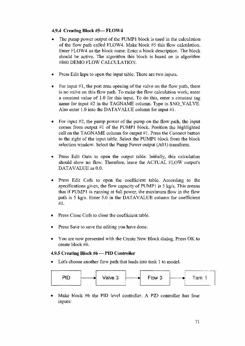
4.9.4 Creating Block #5—FLOW4

• The pump power output of the PUMP1 block is used in the calculationof the flow path called FLOW4. Make block #5 this flow calculation.Enter FL0W4 as the block name. Enter a block description. The blockshould be active. The algorithm this block is based on is algorithm#860 DEMO FLOW CALCULATION.

• Press Edit hips to open the input table. There are two inputs.

• For input #1, the port area opening of the valve on the flow path, thereis no valve on this flow path. To make the flow calculation work, entera constant value of 1.0 for this input. To do this, enter a constant tagname for input #2 in the TAGNAME column. Type in $NO_VALVE.Also enter 1.0 into the DAT A VALUE column for input #1.

• For input #2, the pump power of the pump on the flow path, the inputcomes from output #1 of the PUMP1 block. Position the highlightedcell on the TAGNAME column for output #1. Press the Connect buttonto the right of the input table. Select the PUMP1 block from the blockselection window. Select the Pump Power output (A01) transform.

• Press Edit Outs to open the output table. Initially, this calculationshould show no flow. Therefore, leave the ACTUAL FLOW output'sDATAVALUE as 0.0.

• Press Edit Cofs to open the coefficient table. According to thespecifications given, the flow capacity of PUMP 1 is 5 kg/s. This meansthat if PUMP 1 is running at full power, the maximum flow in the flowpath is 5 kg/s. Enter 5.0 in the DATAVALUE column for coefficient#1.

• Press Close Cofs to close the coefficient table.

• Press Save to save the editing you have done.

• You are now presented with the Create New Block dialog. Press OK tocreate block #6.

4.9.5 Creating Block #6 — PID Controller

• Let's choose another flow path that leads into tank 1 to model.

•I Tank

Make block #6 the PID level controller. A PID controller has fourinputs:

71

1. Controller setpoint2. Present value of the process variable being controlled3. AUTO/MANUAL mode request4. Manual control signal

• In AUTO mode, the controller automatically adjusts its output controlsignal to drive the process variable (level) being controlled to maintainits value at the controller's setpoint. This is done by comparing thecurrent value of level vs. the controller setpoint and adjust outputcontrol signal accordingly.

• hi MANUAL mode, the manually entered control signal is directlyused as the controller's output control signal to drive the processvariable.

• hi the two tanks system, the PID controller is used as a tank levelcontroller to maintain the level of the liquid in tank 1 such that it doesnot exceed a specific height. The specified height is used as thecontroller setpoint. The PID level controller's output control signaldrives valve #3 which will open to relief some liquid inside tank 1 ifthe level rises above the height setpoint.

• hi the empty block edit window, enter PID as the block name, Enter ablock description. The block should be active. The algorithm this blockis based on is algorithm #859 DEMO PID CONTROLLER.

• Press Edit hips to open the input table.

• The controller setpoint input (#1), AUTO/MANUAL mode requestinput (#3), and manual control signal input (#4) all come from the userinterface and goes through input/output #5, #6, and #7 of theDISPLAY block respectively.

• Input #2, the present value of the process variable being controlled, isthe tank level output of tank 1. The Connect button can not be used forspecifying this connection because the block representing tank 1 hasnot been defined yet. However, you can still specify the connection ifyou know what the tag name of tank l's level output is. Since you didthe analysis and design, a likely name for the tank 1 block is TANK1.And knowing that the transform for the tank level output is A01, youcan enter into the input table's TAGNAME column TANK1/A01 forinput #2.

• Another approach to handling this situation of having to connect to ablock not yet defined is to enter in an arbitrary tag name and later useother tools to identify the arbitrary connections and correct it.

• The input table should be as shown below:

72

i I_UJ* veuia

Edit InputsPINNUM

2

3

A

TAGNAME,DISPLAY/XX05

TANK1/A01

DISPLAY/XX06

DISPLAY/XX07

DATAVALUE.00000000

.00000000

.00000000

.00000000

Conrkii

• Press Edit Outs to open the output table. The default values of 0.0 forall of these outputs are just fine. Therefore, leave them as they are.

• Press Edit Cofs to open the coefficient table. There are fourcoefficients. These are values for tuning the controller so that it makesits automatic adjustments smoothly. Enter the values as shown below:

PINNUM1

2

3

A

L..r_i."."."rr I

DAIAVAI UF1.00000000

10.00000000

0.01000000

.00000000

Edit Coeffs

•

• Press Close Cofs to close the coefficient table.

• Press Save to save the editing you have done.

• You are now presented with the Create New Block dialog. Press OK tocreate block #7.

4.9.6 Creating Block #7 — VALVE3

• The output control signal from the PID level controller controls valve3. Make VALVE3 the name of block #7. Enter in a block description.The block should be active. The algorithm that this block is based on isalgorithm #857 DEMO 1ST ORDER VALVE.

• Press Edit hips to open the input table.

• VALVE 3's port area opening demand signal comes from the outputcontrol signal of the PID block. Press Connect and make theappropriate selections to form the tag name PID/A01 for input 1.

• Press Edit Outs to open the output table. VALVE3 is initially closed,therefore you have to configure the VALVE FULLY CLOSED outputto be TRUE (1.0). Leave the other output DATAVALUES.

73

• Press Edit Cofs to open the coefficient table. According to thespecification given for VALVE3, the stroking time is 5 seconds. Enterthis into the DATA VALUE column.

• Press Close Cofs to close the coefficient table.

• Press Save to save the editing you have done.

• You are now presented with the Create New Block dialog. Press OK tocreate block #8.

4.9.7 Creating Block #8 — FLOW3

• Block #8 is the block representing FL0W3.

• Enter FL0W3 as the block name. Enter a block description. The blockshould be active. The algorithm this block is based on is algorithm#860 DEMO FLOW CALCULATION.

• The inputs are: VALVE3/A01 for input 1, the port area opening of thevalve on the flow path, and $NO_PUMP with a DATAVALUE of 1.0for input 2, the power of the pump on the flow path.

• The output is just fine. Press Edit Outs to check the table and pressClose Outs to close it.

• The stroking time coefficient according to the given specification is 5seconds.

• Press Save to save the editing you have done.

• You are now presented with the Create New Block dialog. Press OK tocreate block #9.

4.9.8 Creating Block #9,10,11, and 12

• You create the blocks #9, 10, 11, and 12 to model the flow pathsshown below:

• Make block #9 VALVE2, block #10 FLOW2, block #11 PUMP2,block #12 FLOW5. These blocks are very similar to blocks #2, 3, 4,and 5 respectively. Use the specifications given earlier.

74

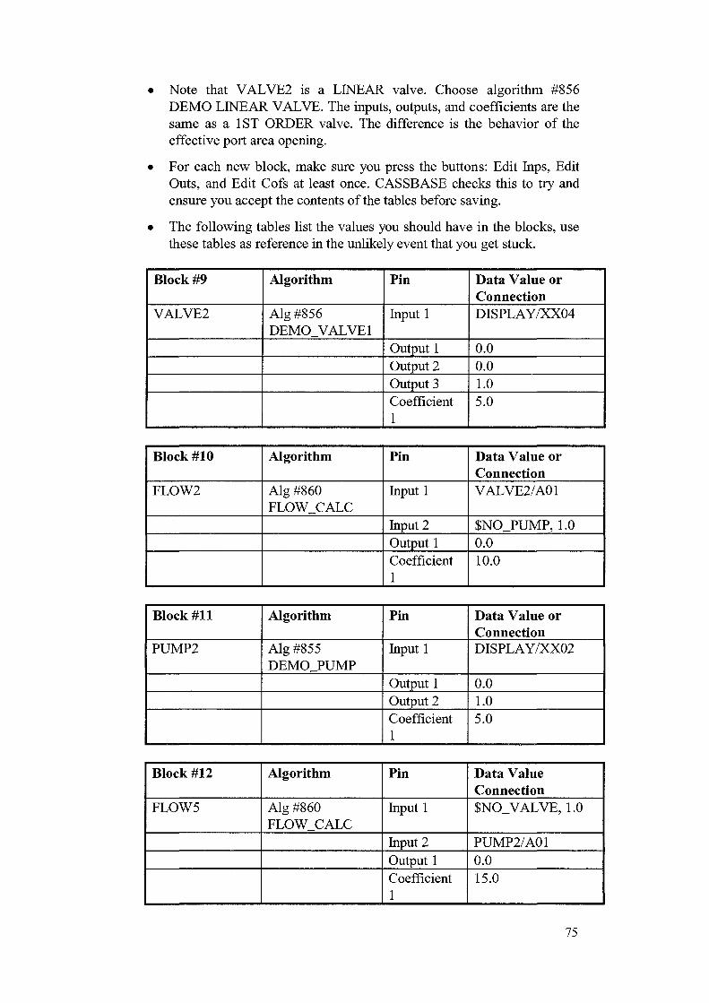
• Note that VALVE2 is a LINEAR valve. Choose algorithm #856DEMO LINEAR VALVE. The inputs, outputs, and coefficients are thesame as a 1ST ORDER valve. The difference is the behavior of theeffective port area opening.

• For each new block, make sure you press the buttons: Edit Inps, EditOuts, and Edit Cofs at least once. CASSBASE checks this to try andensure you accept the contents of the tables before saving.

• The following tables list the values you should have in the blocks, usethese tables as reference in the unlikely event that you get stuck.

Block #9

VALVE2

Algorithm

Alg #856DEMO_VALVE1

Pin

Input 1

Output 1Output 2Output 3Coefficient1

Data Value orConnectionDISPLAY/XX04

0.00.01.05.0

Block #10

FLOW2

Algorithm

Alg #860FLOW_CALC

Pin

Input 1

Input 2Output 1Coefficient1

Data Value orConnectionVALVE2/A01

$NO_PUMP, 1.00.010.0

Block #11

PUMP2

Algorithm

Alg #855DEMO PUMP

Pin

Input 1

Output 1Output 2Coefficient1

Data Value orConnectionDISPLAY/XX02

0.01.05.0

Block #12

FLOW5

Algorithm

Alg #860FLOW_CALC

Pin

Input 1

Input 2Output 1Coefficient1

Data ValueConnection$NO_VALVE, 1.0

PUMP2/A010.015.0

75

• When you are done saving block 12, you are presented with the CreateNew Block dialog. Press OK to create block #13.

4.9.9 Creating Block #13

• You have now created all the flow paths. It is time to create the tanks.Let's make block #13 TANKl. The algorithm that this block is basedon is algorithm #858 DEMO TANK.

• Press Edit Inps to open the input table.

• The TANKl block has four inputs. The tank in this demo has twoinlets and two outlets. The algorithm takes into account the flow ratesentering and leaving the inlets and outlets and adjusts the tank levelaccordingly.

• Based on the P&ID diagram with the flow rates given, the flow rateswhich are input to TANKl are FLOW5/A01 and FLOW1/A01.Likewise, the flow rates which deplete from TANKl are FLOW4/A01and FLOW3/A01. Make these connections. Connect FLOW5/A01 toinput #1, FLOW1/A01 to input #2, FLOW3/A01 to input #3, andFLOW4/A01 to input #4.

• Press Edit Outs to open the output table.

• TANKl has two outputs: tank level and tank overflow indicator. At thestart of the simulation, TANKl should be set to a level of 5 meters. Ata level of 5 meters, there is no overflow. Therefore, the tank overflowindicator having a 0.0 (FALSE) value is fine.

• Press Edit Cofs to open the coefficient table. The four coefficients forTANKl are: tank height (10 m), tank radius (0.25 m), liquid density(1000 kg/m3), and height of outlet from the bottom of the tank (0.5 m).Enter these values into the DAT A VALUE column.

• Press Close Cofs to close the coefficient table.

• Press Save to save the editing you have done.

• You are now presented with the Create New Block dialog. Press OK tocreate block #14.

4.9.10 Creating Block #14

• Tank 2 is very much like tank 1. You fill in the details.

• Set the initial TANK2 level to 0.0. Also note that there is only oneoutlet in TANK2.

76

The following tables list the values you should have in the TANK2block, use this table as reference.

Block #14

TANK2

Algorithm

Alg #858DEMO_TANK

Pin

Input 1

Input 2Input 3Input 4Output 1Output 2Coefficient1Coefficient2Coefficient•3Coefficient4

Data Value orConnectionFLOW4/A01

FLOW2/A01FLOW5/A01$NO_FLOW, 0.00.00.020.0

0.25

1000.0

0.5

4.10 Hands-on Testing and Debugging the Simple Two Tanks Process

4.10.1 Verifying The Model

On the Model drop-down menu, you will find a Verify menu item.Select this now to verify that there are no errors within the model. TheVerify process performs three checks. Examples of potential errors are:connections not specified, or an input connection specifies a block oroutput connection that does not exist. If you have followed the stepspresented in this manual, you should not have any errors. A successfulModel | Verify will produce the following messages.

(14:10:36) Model Uerify begin ...(14:10:37) Performing sequence numbers check(14:10:37) Performing inputs, outputs, coefficients checkProcessing block 14

(14:10:38) Performing hanging tags check(14:10:38) Model Uerify end.

If you are unfortunate enough to run into some errors, the listing oferrors are captured in a text file. The Verify process will display a messagenotifying you that there are errors and will ask you if you want to see theerror listing text file. Press OK to open this text file using MS Write. Thefirst MS Write dialog will prompt you whether you want to convert the textfile to Write format. Press No Conversion.

The most common error are hanging tag errors. A Hanging Tag is anerroneous connection (hanging connection) specified under the

77

TAGNAME column in the input table. That is, the TAGNAME entry forthe input is suppose to be the output tag name of a block output to connectto, but instead is a tag name which does not identify any output tag name inthe model. This usually occurs as a result of typing errors. If you used theConnect button to specify connections, then you would not have hangingtag problems.

Once you have corrected the errors (if any) ... YOU ARE DONE! Allthe detailed work is done. Now comes the fun part of running thesimulation!

4.10.2 Exporting Model Data File for CASSIM™ Simulation Engine —CASSENG

The model you have finished building is now ready for testing. To testthe simulation, you need the Simulation Engine — CASSENG and theDebugger.

• First, the simulation engine requires a compact data file fromCASSBASE to run the simulation.

• To produce this file, select the menu item Export from the Model drop-down menu. You are immediately presented with a file dialog to enterthe name of the compact data file to export to. Using the directoryselection list on the right hand side of the dialog, position yourself tothe \CASSDEMO\2TANKS directory. Then, in the entry field underthe File name:, type in the filename TANKS.DAT. Press OK.

• CASSBASE will create the compact data file\CASSDEMO\2TANKS\TANKS.DAT.

• Let's start up CASSENG and open the compact data file. Firstminimize CASSBASE. In your Program Manager, double-click on theicon that looks like a train engine.

CASSENG opens up a small window in the lower right hand corner ofthe screen. Once the CASSENG window is opened, select the Filemenu, scroll down and select the Open menu item. You are presentedwith a file dialog for selecting the data file to open. Select theTANKS.DAT file in the \CASSDEMO\2TANKS directory.

The simulation model runs inside CASSENG. There are somesimulation controls under the Control menu. You can FREEZE (stop),and RUN the simulation. In addition, the simulation can be steppedthrough by ITERATION, or by BLOCK. When the simulation is

running, the *r*i icon is displayed. Select the RUN option and seewhat happen !

78

• These controls are not very exciting since you cannot see the modelvalues change as the simulation runs. There is a debug tool inCAS SIM™ that allows you to watch the inputs, outputs, andcoefficients of any block while the simulation is running.

The above only demonstrates that CASSENG and the model data filecan run by itself, but you do not see much going on. hi order to visualizethe simulation data, you need to invoke the CASSIM Debugger:

• Quit CASSENG by selecting File menu in CASSENG and scroll downto select EXIT.

• Exit CASSBASE by selecting the menu item Model | Exit. Someprompt are displayed:

Close C:\CASSDEM0\2TANKS model? Select OK.

Do you want to make a backup? Select OK

Exit CASSBASE? Select OK.

4.10.3 Testing the Simulation Using CASSIM™ Debugger

(A) Block Debugging

• Go to Window Program Manager and invoke CASSIM Debugger withthis icon

! CASSIM :^Debugger

The following CASSIM Debugger Menu will appear.

CASSIM Model Debugger

1 i

Click on the Model folder (yellow color). A "Model Open" Dialog boxshows up.

Press "Model" button. A dialog box will appears, requesting your inputfor the directory where the Model resides. SelectCASSBASE\CASSDEMO\2TANKS directory, and click on any .dbffile in the directory. The model will be loaded.

79

Open CASSIM Model and Data File

Mods! Filename

JC \CASSBASE\2tanks\

Data Filename

•' Date ' ! Perse Cancel

Press "Data" Button. A dialog box will appear, requesting your inputfor model data file. Click "Tanks.dat" to select the model data file.

Open CASSIM Model and Data File

Model Filename

C\CASSBASE\2tanks\

Date Filename

C \CASSBASE\2tsnks\Tanks dat

Motiei ! Done \i

j Cancel !

Press "Done" Button. You will see the Debugger is loading up theModel.Use the mouse to click on "Engine Control" and "Block List" Menuitems. (Note if you do not know where they are, move the mousecursor to any of the menu items, you will see a "tail-tips" behind it).You will see the following dialog boxes.

80

CASSIM Model Debugger

! Total number of blocks

i , ^ , -•

FL0W1

VALVE2

FL0W2

PUMP1

FL0W4

PUMP?

FL0W5

PID

VALVE3

FL0W3

TANK1

TANK2

Block Nsme Searc

34

5

67

8

9

1011

12

13

1

-i

I

8

1CV.

IJ

1-1

Engine Control

' - I I C I -

- -.-'I

t-.

• Double-click on the first block on the list "DISPLAY". The DISPLAYblock will be presented.

DISPLAY (1) : 452 - NON-MOVEABLE [active]

Input:.

" « - • ISPUMP1_ONOFFSPUMP2 ONOFF$VALVE1_ONOFFSVALVE2_ONOFF$PID SP$PID_AUTOMAN$PID_UANOUTSCONSTANTSCONSTANTSCONSTANTTANK1/A01TANK2/A01PUMP1/D01

i PUMP2/D01I VALVE1/A01i iVALVE27A6i !i VALVE3/A01i DISPLAY/W06i DISPLAY/W05

TANK1/D01TANK2/D01FLOW3/A01FLO. <4/*Q1

1.1

1 .--0.000000000.000000000.000000000.000000008.000000000.000000000.000000000.000000000.000000000.000000005.000000000.500000000.000000000.000000000.000000000.000000000.000000000.000000008.000000000.000000000.00000000nnrnnnnn1 ' i i : MM

1

12

3456789101112131415161718192021no

r *Outputs

i

LH5FLAY/><X01niSPLAY/W02IISPLAY/W03)ISPLAY/X*;04HSPLAY/XX05

1 )ISPLAY/X><06UISPLAY/XX07UISPLAY/XX08IISPLAY/W09)ISPLAY/X><10>ISPLAY/X*:I i

1ISPLAY/XK12JISPLAY/XX13niSPLAY/W14UISPLAY/XX15

i DISPLAY/XX16( ~ "

Ct i»'flii it'iits[ . = • - - i.

| . ,- . . J r , - - .0.00000000 '0.00000000 _0.00000000 3 —0.00000000 48.00000000 50.00000000 60.00000000 70.00000000 80.00000000 90.00000000 105.00000000 110.50000000 120.00000000 130.00000000 140.00000000 150.00000000 1E• ^

:

I •' • ! - • - • t ^ _ . .

81

• The debug block window communicates with CASSENG viaMicrosoft Window's Dynamic Data Exchange (DDE) facility. Thedebug block window requests data from CASSENG and displays thereturned data. Likewise, input from the user is sent by the debug blockwindow to CASSENG and these inputs are integrated into the runningsimulation by CASSENG.

If you wish to know more about debugging operations, press "HELP"menu item to read more details.

(B) Controlling the Simulation

• The "Engine Controls" can be used to Freeze or Run the simulation.• Press Iterate to step the simulation through one iteration of all the

blocks in the model.• Press Block to step the simulation one block at a time.• The Iteration count shows how many iterations the simulation has run.• The Sequence count shows the sequence number of the block that has

just completed execution. The Block value shows the block numbercorresponding the sequence count shown. When the simulation isrunning, the Iteration counter will be counting.

Exercises:

If the simulation is frozen (i.e., counter not counting), press Run now.The Iteration count will count up. Press Freeze to stop the simulation.Press Step Iteration once and notice the iteration count go up by one.

(C) Jumping between Connections

• The inputs of the current block may be connected to outputs of otherblocks. Likewise, the outputs of the current block may be connected toinputs of other blocks.

• Use the "left" mouse button to click on the first block outputDISPLAY/XX01. It will be highlighted in "blue".

• With DISPLAY/XX01" highlighted, click the "right" mouse button todisplay a "drop-down" menu for "Connection List" or "jump". SelectJump to trace the connections from one block to another.

• If the selection is connected to another block, that connected block willbe displayed in a separate debug block window. In this case, PUMP1block will be displayed, because its input is connected to output:DISPLAY/XX01. Note: if there is no connection to the selected inputor output, a message is displayed " No Jump Point".

• For outputs, it is possible that one output is connected to many inputs.If this is true, a connection list is shown after you select the"Connection List" in the drop-down menu. Select one of the blocks inthe connection list to open the debug window for that block.

82

Exercise:

• Single-click on the 1 lth input line, it looks like:

TANK1/A01

• This selects the input and it will be highlighted in "blue". This input isconnected to the block TANKl's A01 output. Try to display the debugwindow for block TANK1. Loading Initial Conditions

• Single-click on Debugger Menu item "Model", a drop down menu willappear.\.:f CASSIM Model Debugger

LmmcClose

Save Model w#fBig*#s Data

Evjf

• Select "Load IC", meaning to load an Initial Condition. The followingdialog box will appear.

Open CASSIM data IC file

• Backup• Debug

2tenks id ic

Pile name

CASSIM IC tiler ic) tayatl

Note that the 2 tanks process that you are simulating can be at differentprocess conditions — that is, some pumps may be turned on and somevalves may be opened. So during debugging, you can store and reload aparticular process condition of interest. These initial conditions arestored as IC files with *.ic file extension.

83

• Select 2 tanks_icl.ic. This is a pre-stored IC for a normal condition forthe process.

• You will see the IC file is loaded via the "progress indicator".

Now, we can do some on-line tuning.

(D) On-line Tuning of Simulation

• Double-click on any Input, Output, or Coefficient line of any block tobring up the Tune dialog for manually changing that value on-line.

• The output and coefficient tune dialog are virtually the same,displaying all information about the selected item and allowing input ofa new Data Value.

• After modifying the data value, press Tune to send this updated valueto CAS SENG to include in the simulation. The input tune dialogoptionally allows for modifying a constant data value (in this case, tagname would start with a $), or modifying a tag name to change theoutput to which this input is connected to.

• If the current input is defined as a constant value, either change thevalue or press Output Tag Name and enter a valid tag name in the entrybox. If the current input is defined as a output tag name, either changeto another tag name using the Connect button, or press Constant Valueand enter a data value in the entry box. Press Tune to send this changeto CAS SENG to include in the simulation.

Exercise:

• Let's tune some of the inputs of TANK1. First bring up the debugwindow for TANK1.

• First run the simulation by pressing Run on "Engine Control". Notethat there is an inflow of 15 kg/s (input 1 connected to FLOW5/A01)and an outflow of 5 kg/s (input 3 connected to FLOW4/A01). The tanklevel output of the tank (TANK1/A01) is increasing because there ismore flow coming in than going out.

• Let's turn off the inflow at input 1. Double-click on the input 1 line.This will bring up a Block Inputs Editor dialog as follows:

84

FLOVV5/A,01

FL0W1 /A01FLOW4/A01FLOW3/A01

15 00U00000 INLET 1 FLU*'R«0.50000000 INLET 2 FLOW R«5.00000000 OUTLET 1 FLO'.'..1 F

11.42294478 OUTLET 2 FLOW F

TAtJl 1,«TANK1/D01

7.3:719705 TrtNIs LEVEL tM0.00000000 TANKOVERFLC

Stock Ntimtjet 1] Rn Nymber 1Pin Description INLET 1 FLOW RATE fKG/S;

ie Analog

15 00000000

. HEIGHT (M); RADIUS (M)0

10.00000000 Analog0.25000000 Analog

1000.00000000

Press Output Tag Name, you will see the Input Tagname FLOW5/A01.Put a $ sign in front of FLOW5/A01. In other words, you havedisconnected the output connection from Block FLow5 output A01,and in its place, you have put a constant tag name called $FLOW5/A01as input.

Block Inputs Editor

Block Number 13 Pin Number 1

Pin Description INLET 1 FLOW F W E (KG/S)

Analog

Constant Value | Output Tag Name

|$FLOW5/A01

Connect T o .

Press "Constant Value" in the Block Input Editor dialog box. This willswitch the Data Value area to allow entering a constant value. Enter 0.0in the entry box, and press Tune. The input is now tuned to have aconstant inflow of 0 kg/s.

85

Total nutsBlodr Haf

FL0W1

FL0W2;PUMP1IFL0W4PUMP2JFLOWSPID |/ALVE"

FLOV./3;• • T A N K i l

TANK2;

1

TANK1 (13): 858 - DEMCMTANK [active]

Inputs

""HFLCW5/A01FLOVV1 /A01FLOW4/A01FLOW3/A01

Outputs

znn0 000000000.500000005.000000000.00000913

TANK1 /A01TANK! /D01

6.94754456 T0.00000000 T

" t i t ' HEIGHTfM)~l IK RADIUS (\A)

10 0000000010 25000000,

• You will see "red" arrow pointing input $FLOW5/A01 in TANK1Block. As well, you will see "red arrow" pointing the block TANK1,indicating tuning changes are made to this block.

• Now press Run and notice that the tank level output is decreasingbecause there is no inflow and still an outflow of 5 kg/s.

• Repeat the steps similar to above to tune the outflow input currentlyconnected to FLOW4/A01 to have a constant outflow of 0 kg/s. Runthe simulation and notice that the tank level output is constant becausethere is no inflow and no outflow.

(E) Restoring Original Model Values and Saving Tuned Values

• Note that tuning modifies the ran time values used by CAS SENG inthe running simulation. The tuned values are not stored in the modeldatabase.

• For any tuned input or coefficient, the original model value in themodel database can be restored to replace the tuned value in thesimulation.

• Conversely, the tuned value can be saved to the model database toreplace the original model value.

• For any input or coefficient that has been tuned, it is possible to discardthe tuned value and restore the running simulation to use the originalmodel value defined in the model database.

• To do this, single click the tuned input $FLOW5/A01. It will behighlighted in "blue", then press the "right" mouse button and select"Restore".

• Once the value has been restored to that defined in the model database,the line will no longer have a red arrow pointer.

86

• All tuned values are used in the running simulation only and are notstored in the model database if not saved. To save the tuned values intothe model database, single click anywhere in a block debug window(but not on any input, output or coefficient line); then click the "right"mouse button. A drop-down menu will appear, then select "saveblock".

• Caution for Saving Block Tuning Changes

1. Before you save the block changes into the model, make sure thechanges are final and not temporary ones, because after you have"saved" the block changes, you have to re-export the model data fileTANKS.DAT.

2. If the change is temporary, it is recommended to save the block tuningchanges in a new IC file. You can do that by clicking on the DebuggerMenu "Model" and select "Save IC" in the drop-down menu. You willbe asked to enter a new IC file name. As debugging progresses, youcan continue to make incremental "save" of the tuning changes into thisIC file, or if you wish, you can save into another new file, as thesituation requires. If there are numerous IC files, it is recommendedthat you should label the IC files succinctly so that you may easilyrecall what tuning changes those files have had, by looking at theirnames.

3. After numerous testing, and if you are satisfied that the tuning changesare final, you can select to update the model database with your IC file.The way to do it is to first load the IC file as you have done previouslyin "Loading Initial Conditions". After the simulation engine is loadedwith IC data, you select Debugger menu item " Save Model withengine data", the tuning changes will be saved into the model database.You have to re-export the model data file TANKS.DAT.

Exercise:

• Open TANK1 block and tune the inlet flow to be 10 Kg/s. As well,tune the outlet flow to be 5 Kg/s.

• Save an IC file for this condition, and call this file tanks_ic2.ic• Exit the Debugger, and make sure to exit the CASSENG as well.• Now re-invoke the Debugger, load the original Model Data file

TANKS.DAT.• Load the IC file tanks_ic.ic• Restore all the tuning changes that you have made previously.

You should now have an idea of the debug capabilities of CASSBASE inproviding dynamic debugging at simulation ran time, and you are nowready to ran the graphical user interface to interact with the simulation youbuilt using CASSBASE.

87

4.11 Running the Simulation Model with Lab VIEW® Screen

4.11.1 Running the Two Tanks Simulation

A graphical interface program is distributed with the CASSIMdemonstration software to allow you to interact with the CAS SENGsimulation engine. This program is a Windows executable program called2TANKS.EXE installed in the C:\CASSDEMO directory.

2TANKS.EXE is a runtime program developed using Lab VIEW forWindows. Lab VIEW for Windows is included in the CASSIM product.Normally, you would use Lab VIEW to develop the screen display programfor interacting with the simulation. But using Lab VIEW can be a course byitself and is beyond the scope of this Lesson. However, if you haveLab VIEW, it is recommended to go over the Lab VIEW tutorials.

Lab VIEW uses a graphical programming environment for developingdata acquisition and display programs. The user displays are built bydragging and dropping graphical components like buttons, digital readouts,graphs, etc. onto a front panel. After completing the front panel, theprogram which operate with the front panel is built by assembling andconnecting icons in a diagram, instead of writing text-based programs. ALab VIEW diagram resembles a traditional engineering flowchart withcomputational icons, programming structure icons, communication icons,etc. The icons are connected together with lines, or wires, to direct the flowof data within the program.

A running Lab VIEW program communicates through DDE withCASSENG in the same way the debug block window of CASSBASEworks with CASSENG. A LabVIEW program can request data fromCASSENG for display. A LabVIEW program can also send user input toCASSENG for integrating into the running simulation. CTI includes withCASSIM a customized library of LabVIEW components specificallydesigned for building simulation user interface programs.

• Before running 2TANKS.EXE, start CASSIM Debugger, and load the2 tanks model, as well as the Model data file.

C:\CASSBASE\CASSDEMO\2TANKS\TANKS.DAT.

• After the Debugger is loaded, minimize it.

• Open Program Manager and double-click on the icon that has twotanks:

This program sets the CASSENG simulation into run mode. The screenappears as shown on the next page.

Wink 1 I cvfil Controller

VJOut(%)i I'V SP

Pump 2 ROn

kg/s

| kg /s

20 0-

175-

150-

125-

10 0-

7 5-

50-

25-

o.o-i

1

• •as

TankZ

At this point, you will notice there are THREE tasks running inWindows: (1) CASSENG (2) Debugger (3) LabVIEW graphicsexecutable.The equipment that you modeled in CASSBASE are presentedgraphically in the program window. There are two tanks, with pumpson the pipes connecting them. Valves 1 and 2 control the inlets to tanks1 and 2 respectively. There is a level controller on tank 1 controllingthe outflow through valve 3.Valves are green in color when they are fully closed, and red when theyare fully opened.Turn on valve 2 now by clicking the On/Off switch besides the valve.Notice the pipe flowing into tank 2 fill up and the level of tank 2 rises.The level of tank 2 is shown along the scale to the left of the tank andas a numeric display to the left of the tank.Recall that tank 2 is the reservoir tank. Let's try to fill this tank's levelup to 10 m. To speed things along, it may help to use tank 1 to fill uptank 2. First open the flow from tank 1 to tank 2 by turning on pump 1.Turn on pump 1 now by clicking the On/Off switch besides the pump.Notice the pipe connecting pump 1 to tank 2 fill up. This flow into tank2 will speed up the fill of tank 2.At the moment there is only outflow from tank 1 and no inflow.Eventually, this will deplete the liquid from tank 1. To add someinflow, turn on valve 1 controlling the flow from an external source.Turn on valve 1 now to fully opened by typing in 100.0 in the numericcontrol besides valve 1 and press Enter. Recall that valve 1 can becontrolled to be partially opened.

89

• A couple of things to take note of here

1. Notice that although you typed in 100.0% opening, the valve still takestime to stroke, hi fact, the valve was modeled to take 5 seconds tostroke for 0 to 90% opened. The 100.0% entered is the demandopening only. There is no numeric display shown of the actual valveopening. The color of the valve helps in this case. When the valve wasfully closed, the color was all green. When the valve is stroking, thecolor is half red and half green. When the valve reaches 100.0%opened, the valve color changes to all red.

2. Also notice that once the valve has completely opened to 100.0%, thetotal inflow rate (with pump 2 off) is 5 kg/s as modeled. The totaloutflow rate (with valve 3 off) is also 5 kg/s. This effectively makes thelevel in tank 1 remain constant.

3. Is tank 2's level filled up to 10 m yet? Once the level gets close to 10m, turn off first pump 1, then valve 2. This shuts off all flow into tank2.

4. Time to squeeze some juice out of valve 3! That is, let's use the levelcontroller to operate valve 3 to let out the liquid hi tank 1.

5. All along, valve 3 is being controlled by the level controller which is inautomatic mode. The setpoint is at 8 m. That means as long as the levelin tank 1 is below 8 m, then the controller will keep valve 3 close.Once the level goes above 8 m, the controller will open up valve 3accordingly to let out some flow from tank 1.

6. The following diagrams show how to use the level controller inautomatic mode and in manual mode.

• If the level in tank 1 has not reached 8 m yet, wait for it. If you areimpatient, you can lower the setpoint to a lower level. Try typing 7.0into the setpoint (SP) numeric control. The controller will adjust itscontrol on valve 3 accordingly.

• Once the tank level has reached the setpoint, valve 3 opens. Turn offvalve 1 now to shut all flow into tank 1. Watch the controller slowlyclose valve 3 as the level in tank 1 comes below the setpoint.

• Another method of letting some liquid out of tank 1 is to manuallyoperate valve 3. To do this, switch the controller to manual mode.Switch to manual mode now by pressing on the MAN button. Thepointer will switch to point to MAN. You can now control valve 3 byentering the desired opening hi the numeric control under the label V3Out (%). Open valve 3 completely now to 100.0% by typing in thenumeric control. Notice the flow out of valve 3 increase up to themodeled maximum flow of 20 kg/s.

• At this point, you have interacted with most of the equipment modeledusing CASSBASE. Feel free to continue to run the simulation, tryingout different operating scenarios.

90

Level in Tank 1

Valve 1

^ \Change setpolnt by:1) Entering In numeric control, or2) Clicking up/down arrows to Increment/decrement setpoli3) Drag green pointer to new setpolnt

Valve 3's opening

Controller is in automatic mode.

Outflow from tank 1 through! valve 3

[.ink I

Xt>

Valve 3

K

lank

•fclM,

1 Level

)

Controller

•QgSmL i

/ Setpoint is ii

| kg / s '

lOn

irrelevant in manual mode.

Change Valve 3's opening by:1) Entering In numeric control, or2) Clicking upfdown arrows to Increment/decrement opening

Controller is in manual mode.

NOW maximize Debugger, practice some tuning changes and observethat the changes can be seen in the screen — e.g. change the tankdiameter.

4.12 Merging Models

It is highly desirable in simulation modeling that some sub-systemmodules can be extracted and recycled for different simulation projects.For example, the feedwater model for power plant can be used for anotherplant if similar feedwater design is used. CAS SIM™ has a "modelmerging" feature which facilitates easy model copying and merging of themodel. The merging of models will be demonstrated.

4.13 Review of Thermalhydraulic Network Modeling

Solutions to differential equations representing the thermalhydraulicsof a power plant process contain a wide spread of time constants, i.e. somecomponents of the solutions have a fast response, while the remainingcomponents are slow varying. The eigenvalues caused by the mass and

91

momentum conservation equations (flow and pressure) are generally verylarge while the eigenvalues caused by thermodynamics (temperature) aresmall. Therefore a system of coupled differential equations describingmass, momentum and energy dynamics of a large process could containwide spread of eigenvalues, and thus is usually referred to as "stiff set ofequations. Stiff equations are usually solved by implicit methods due totheir inherent stability. However, standard implicit methods usually requirefinding the Jacobian for the equation set during each iteration (Newton'smethod), as well as solving the resulting set of linear algebraic equations.These solution techniques can provide solutions with high degree ofaccuracy and stability; however, they cannot be solved "economically" inreal time.

CAS SIM™ employs a real time solution technique for thermalhydraulicmodeling, which involves identifying control volumes within the simulatedsystem, where pressures are calculated. These control volumes are knownas nodes. The flows between these nodes can be obtained from momentumequations, and are known as links. Each node pressure can be obtainedfrom mass balance around the node. A linearized solution method isemployed for the nodal representation of the flow network. This methodinvolves linearizing the momentum equations, and solving the resultant setof linear algebraic equations implicitly by matrix methods.

Figure 8 illustrates the mass and momentum equations set for a typicalflow path containing equipments such as pumps and valves, anddemonstrates how these equations can be linearized to be solved by matrixmethods. By specifying nodes and links, the flow network problem can bedefined using modular block structured modeling, that is, each node blockand link block can be created by using generic node and link algorithmrespectively.

Hydraulic properties of the nodes and links blocks (e.g. node size, valvesize, pump dynamic head etc.) are either treated as coefficients or inputs tothese blocks. CASSBASE, the database engine of CASSIM™, has acomputerized network generation program which will automatically creatematrix elements for the network defined by the connected nodes and linksblocks.

As the flow network problem generally creates "sparse" type ofalgebraic systems, the network generation program can reduce thecomputation time required to obtain a solution by rearranging the algebraicequation set. This computerized network generation program produces adata file which can be run during each simulation iteration. If the topologygoverning the nodes and links has been changed, the network generationprogram has to be used to re-generate the network again.

92

HYDRAULIC NETWORK FLOW DIAGRAM

NHZ X02

Valve 1

Assuming incompressible flowP - P

XI r N

EXTERNAL NODE

INTERNAL NODE

NETWORK BLOCK NAME

W = KVVX1N1 ^ X

V12

WN1N2 V N1w = K V C P - P -VVN2X2 rXN2X2VAV N2 r ELV

\1/2

\1/2

Linearizing equation by defining admittance= W

X 1 N 1 V " X

A = WMN1N2 V VN"N2X2 ~ ™N

/ (P - P" X 1 N 1 ' V X 1 N

I (P + P2 ' v N1 '2' (°N2 " P

X N

I (P + P - P ^N 1 N 2 ' v N1 ' D Y H

rN 2 '

ELV

Performing mass balance on N1 and N2; assuming constant densityCN1(dPN1/dt) = <CN2(dPN2/dt) = i

N1/dt) vvx1lsl1 - vvN1N2

' N 1 N 2 ' " N 2 X 2

Using backward Euler; and substitute admittanceCN1«PN1 " P ' N i V A t ) = AX1Ni(PX1 " P Ni ) " A f W P N 1

CN2«PN2 " P ' N 2 ) / A *) = AN1Nd(PN1 + PDYH " PN2)

Legend

W. = flow from node i to j= pressure in node i= valve port area

YH = pump dynamic headLv = elevation head

= admittance between node i and j= conductance between node i and

C,' = capacitance of node iAt = time increment

I = Pi at previous iterationM;; = matrix element ij

= source element i

rpN2)

N 2 " ELV" ' X2^

Rearranging to matrix form

IvU M,,\ / PM

where" )22/

M , , = -AM

/A t) + AX1 N 1M 1 2 - A N 1 N 2

M22=(CN2/At) + AN1 2+AN2X2

AX1N1PX1 '

Procedure for solving pressure solution:1) Calculate admittance from flow, P'N1, and P'N2

2) Solve PN1, PN2from matrix3) Calculate flow from PN1, PN2

Figure 8 — CASSIM™ Hydraulic Flow Network Numerical MethodTechnique.

The above diagram illustrates a simple hydraulic circuit which involvesa flow path from an open tank#l, through a suction header Nl, a pump PI,a discharge header N2, a valve#l, and lastly another open tank#2.

hi hydraulic network terminology, we call open tank#l, #2 as "externalnode" XI, X2 respectively; whereas for the suction and discharge headers,we call them "internal node" Nl and N2 respectively. According to

93

CAS SIM™ Network naming convention, we give this network a 3 letterpre-fix NHZ. Hence, all nodes and branches block name will have this pre-fix identifier. For instance, Nl will be labeled as NHZ_N1; the branchconnecting Tank #1 and Node Nl , is labeled as NHZX1_N1.

The equation sets in the above diagram can be summarized as follows:

(a) The flow in each link is computed using momentum balance for eachlink.

(b) The pressure in each node is computed using mass balance equation foreach node.

The calculation scheme is as follows:

(1) Users create node blocks and link blocks. The node block outputcontains node pressure values; whereas the link block output containslink flow values.

(2) After users have constructed all the node and link blocks with theequipment (pumps and valves), and with proper initializations, users"generate" the network using CASSIM.

(3) After "network generation", the CASSIM utility has already built thematrix equation similar to that shown in the above diagram.

(4) In the first iteration, for each link, given the initial flow, initial pressurein upstream node i and downstream node j respectively, admittance iscalculated in each link block (see equation above); and hence all theM's and S's in the matrix elements can be calculated. When thesecalculations are all done, the Network Solver inside CASSIM solvesthe matrix equation in real time to give the pressure values for all thenodes. Once the pressures of the nodes are solved, they update all thenode blocks' pressure output.

(5) After the pressure update in the node blocks is completed, flow canthen be calculated from executing the link flow block algorithm (seeequation above).

(6) Now it is ready for the next iteration with exactly the same iterationscheme as described in (4) above.

Note:

(1) The equations formulated below for the hydraulic network pressure andflow calculations are only good for incompressible flow. Forcompressible flow (steam, air systems etc.), users have to consider theuse of "variable" conductance in the link, in order to use the same setof incompressible flow equations. See explanation below.

(2) The hydraulic flow/pressure calculation is decoupled from the energytransfer calculations. The energy transfer in the link of a network (e.g.

94

heat exchanger) is done outside the hydraulic network blocksboundary. It can be achieved by using "mixing node" algorithm, inwhich the output temperature or enthalpy of the mixing node iscalculated from the inlet streams' temperatures or enthalpies, assumingperfect mixing. The effect of temperature change can lead to a changein the flow in the link due to the change in the fluid density (input # 7of the link algorithm).

4.13.1 CASSIM™ Thermalhydraulic Modeling Simplifications

• It should be mentioned that, for computational efficiency, there are twoimportant simplifications taken by the CASSIM™ thermalhydraulicmodeling approach:

• The hydraulic flow/pressure calculation is decoupled from the energytransfer calculations in the flow network. For example, the heat transferin the link of a network (e.g. heat exchanger) is done outside thehydraulic network solution schema. It can be achieved by using"mixing node" algorithm, in which the output temperature or enthalpyof the mixing node is calculated from the inlet streams' temperatures orenthalpies, assuming perfect mixing. The effect of temperature changecan lead to a change in flow in the link due to the change in the fluiddensity.

• The numerical solution technique for solving the network pressuresand flows, as formulated in Figure 8, generally applies forincompressible flow. For compressible flow such as steam, gassystems, etc., the following momentum equations should have beenused instead, assuming constant temperature:

For non-choked flow:

For choked flow:

Flow = Kc-Vx-Pup

where Kc = link conductance; Vx = Valve port area in the link between the

upstream and downstream nodes; Plip,Pdmm = upstream and

downstream node pressure respectively.

• However, in CASSIM™, a "variable conductance" technique isdeveloped, by which the same set of incompressible flow equationscould be used for compressible flow systems. In this technique, whenlinks flows are calculated by using the incompressible flow equations,they are substituted back into the above compressible momentumequations using the initial pressure conditions, to back calculate thelink conductance Kc. The calculated link conductance, a block output,

95

is then connected to the link block as input, hi other words, thistechnique "allows" the link momentum equation to be an"incompressible" flow type; however in this instance, the linkconductance should not be fixed, but rather a "variable'" one and iscalculated in each iteration from the compressible momentumequations using back-substitution. The application of this techniqueallows the same numerical solution methodology formulated for"incompressible" systems (Fig. 8) to be applicable for "compressible"flow systems, with the additional computation of "variable linkconductance".

4.13.2 How to Create a Hydraulic Network System

REMEMBER in CASSIM Hydraulic Network,

• Internal Nodes = Control volumes whose pressures will vary with time.

• External Node = Control volumes of constant pressures which do notvary with time.

• Branches/Inks =Flow between each node.

The procedure for creating a hydraulic network system is:

1) Create a Nodal Diagram

• Identify location of the equipment and headers with respect to thenodal diagram.

2) Calculate/estimate the pressure drop between each node.

(A) Pressure drop can be calculated using Darcy's Law of the exactpiping configuration is known.

(B) An estimate of the pressure drop can be made if:

• The overall pressure drop of the system is known.

• The number of valves involved is known.

• Sharing the overall pressure drop between the branches and thevalves.

3) Create the external nodes, internal nodes and branches/links blocks.Note it is very important to label the node blocks in increasing order,i.e. NH?_N01, NH?_N02, NH?_N10 etc., as you traverse theNodal Diagram from the "starting" node to the "ending" node in thedirection of flow. Note that the order 1-5-4-2-3-6 will not work.

4) The following block naming convention for branches should befollowed: NH?N01_N02 is the branch connecting node NH?_N01 toNH? N02. See more details in CASSIM™ in the User Manual.

96

4) Create Network Control Block with Blockname NH?_CTRL and moveit ahead of the network marker block NH?_END

5) Run the Network "Generate" Utility.

4.14 Algorithm Source Code Development

4.14.1 FORTRAN Algorithm Coding Standard

In creating new FORTRAN Algorithm for CASSIM, the followingFORTRAN coding standards should be adhere to when creatingalgorithms. These standards help ensure that double precision calculationsare performed with as much accuracy as possible.

1. Declare all variables. By default, FORTRAN will give undeclaredvariables starting with particular letters default data types. The defaultdata type may not be what you want.

Why?

If a variable is not declared, it may default to a wrong type. Forexample, according to the FORTRAN 77 language specification, anyvariable not explicitly declared and beginning with a letter other than I,J, K, L, M, and N will be of type REAL by default. Let's say youassigned a value to a variable called SPEED, and you did not explicitlydeclared SPEED as DOUBLE PRECISION. The value may loseprecision because REAL (single precision) can only hold six to sevendigits of precision.

Hint

Microsoft FORTRAN 5.1: Use the /4Yd option when compiling togenerate warning messages when undeclared variables are encountered.

Watcom FORTRAN-77 10.5: Turn on the Require symbol declaration(option exp) when compiling to generate warning messages whenundeclared variables are encountered.

2. Assign a value to a variable before referencing it in an expression orusing it on the right hand side of an assignment statement.

Why?

If a variable has not been assigned a value, the memory space occupiedby it contains garbage data. When you reference this undefinedvariable, the garbage data will be interpreted as legitimate data and willcause unexpected results.

This problem can be hidden within code. For example, an IF-THEN-ELSE structure assigns a value to a variable only when the condition is

97

TRUE but does nothing if the condition is FALSE. A reference to thatvariable just after the IF-THEN-ELSE structure will return the assignedvalue if the condition was TRUE and will return garbage data if thecondition was FALSE.

3. Explicitly declare all floating point constants as double precision byusing a D to indicate the exponent.

Examples:

123.764 Incorrect

.4352344 Incorrect

1423.34E12 Incorrect

+345.E-4 Incorrect

-.4565788E3 Incorrect

2E6 Incorrect

1234. Incorrect

The above constants are all interpreted as single precision floatingpoint numbers. The following constants are double precision floatingpoint numbers.

123.764D0 Correct

1423.34D12 Correct

+345.D-4 Correct

-.4565788D3 Correct

2D6 Correct

1234.D0 Correct

4. When assigning a value to a double precision variable, do not assign aninteger, or a single precision floating point number.

Examples:

TLOAD = 0 IncorrectTLOAD = 0.0 IncorrectTLOAD = 0.0E0 Incorrect

98

TLOAD = 0.0D0 Correct

5. When writing a mathematical equation, Use the same data type in allparts of the calculation to ensure that precision is not lost.

4.14.2 Algorithm Source Code Standard

See details in CASSIM™ User Manual Section 2.3.2.

4.14.3 Simple Algorithm Exercise

1) Develop an FORTRAN Algorithm for the simple ordinary differentialequation:

dY/dt = AY + C

where A and C are constants and treated as coefficients.

The initial condition is: Y(0) = 0.

2) Use Euler integration method for solving the ODE numerically.

3) After the algorithm is developed, create a block using this algorithm.Use Debugger to change values of A = 2.0, -2.0, 0.000001, and valuesofC=10.

99

5.0 Reactor Simulation Model Development

5.1 Quick Review of Nuclear Reactor Neutron Physics

5.1.1 Rates of Neutron Reactions - Reactor Power

• Reaction Rate:Consider n neutrons per unit volume move with velocity v towards a thin

target. From experiment with nuclear physics, it is found that the rate Rat which a particular neutron-nucleus reaction occurs is proportional tothe neutron flux <j) . That is,

R = </> »S (5.1)where flux <j> = n • v = number of neutrons crossing 1 cm2 per sec.E = proportionality constant, or defined as the macroscopic cross section

for the reaction.

It is the probability of the reaction occurring in 1 cm. of travel of 1 neutronthrough the reacting medium. It has units - reactions/(neutron.cm).

• Macroscopic Cross-section:The macroscopic cross-section E is also proportional to nuclei densityof the medium; hence

E = N « a (5.2)where N = number of nuclei per cm

<7 = microscopic cross-section for the medium in cm2.

• Mean free Path of neutron:If A, is the average distance a neutron travels before undergoing acertain reaction, then the average number of reactions per sec is v / X,since in 1 second, the neutron would have traveled v cm.

With neutron density n, it follows that the rate of neutron reactionsR = n * x/X = <j> IX (5.3)

Equating (5.1) and (5.3), we haveX = 1 / E .(5.4)

Hence X is also known as the mean free path of neutron.

• Fission Cross-Section:Since different reactions occur with different probabilities, they will be

associated with different cross-sections:(a) fission cross-section Xy',

(b) absorption cross-section Z f l ;(c) elastic scattering cross-section S s ;(d) inelastic scattering cross-section Z , .

100

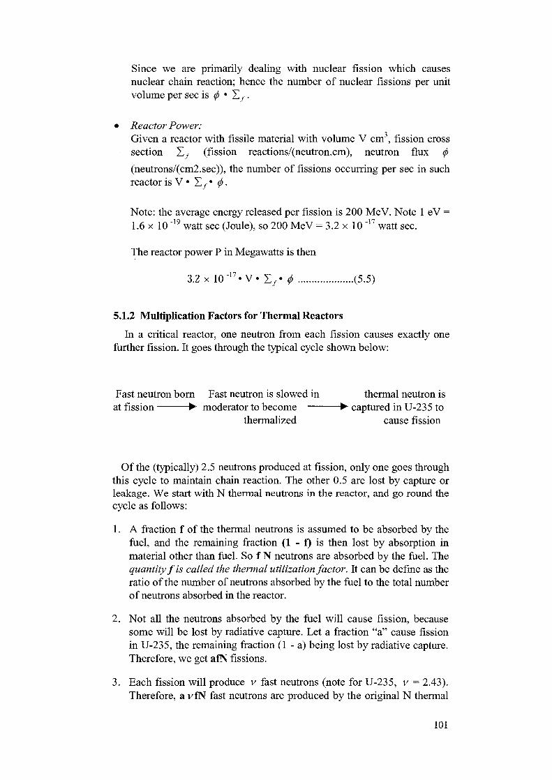
Since we are primarily dealing with nuclear fission which causesnuclear chain reaction; hence the number of nuclear fissions per unitvolume per sec is <j) • Zy •

• Reactor Power:Given a reactor with fissile material with volume V cm3, fission crosssection E / (fission reactions/(neutron.cm), neutron flux tp(neutrons/(cm2.sec)), the number of fissions occurring per sec in suchreactor is V • Zy • (j) •

Note: the average energy released per fission is 200 MeV. Note 1 eV =1.6 x 10 ~19 watt sec (Joule), so 200 MeV = 3.2 x 10 "17 watt sec.

The reactor power P in Megawatts is then

3.2 x 10 "17« V- Tf- <t> (5.5)

5.1.2 Multiplication Factors for Thermal Reactors

hi a critical reactor, one neutron from each fission causes exactly onefurther fission. It goes through the typical cycle shown below:

Fast neutron born Fast neutron is slowed in thermal neutron isat fission • moderator to become • captured in U-235 to

thermalized cause fission

Of the (typically) 2.5 neutrons produced at fission, only one goes throughthis cycle to maintain chain reaction. The other 0.5 are lost by capture orleakage. We start with N thermal neutrons in the reactor, and go round thecycle as follows:

1. A fraction f of the thermal neutrons is assumed to be absorbed by thefuel, and the remaining fraction (1 - f) is then lost by absorption inmaterial other than fuel. So f N neutrons are absorbed by the fuel. Thequantity f is called the thermal utilization factor. It can be define as theratio of the number of neutrons absorbed by the fuel to the total numberof neutrons absorbed in the reactor.

2. Not all the neutrons absorbed by the fuel will cause fission, becausesome will be lost by radiative capture. Let a fraction "a" cause fissionin U-235, the remaining fraction (1 - a) being lost by radiative capture.Therefore, we get afN fissions.

3. Each fission will produce v fast neutrons (note for U-235, v = 2.43).Therefore, a vfN fast neutrons are produced by the original N thermal

101

neutrons. The product a v is usually replaced by one symbol 77 so that77 fN fast neutrons are produced by U-235 fissions. The factor 77 iscalled the thermal fission factor. It represents the number of fastneutrons produced from each thermal neutron captured in the fuel;whereas v represents the number of neutrons produced from eachthermal neuron actually causing fission.

4. A small fraction of the fast neutrons produced by these fissions willcause fast fission of U-238 before they are slowed down. The total fastneutrons population will therefore be a slightly greater than 77 fN. Thisadditional contribution (typically 2-3 %) is allowed for by increasingthe fast neutron population by a factor s, commonly known as the fastfission factor. The total number of fast neutrons produced by both U -235 and U- 238 fissions is therefore e 77 fN.

5. These fast neutrons (~ 10 MeV) now have to be thermalized (~ 0.025eV). Some of them escape from the reactor due to leakage before theyreach the resonance energies. Let Pf be the fast neutron non-leakage

probability, then the number of fast neutrons which do not leak fromreactor while slowing down is e TjfPffi.

6. Some of the non-leaked fast neutrons will be lost due to resonanceabsorption in the moderator while slowing down. Let p denotes theresonance escape probability, then the number of fast which havethermalized in the reactor is s rj iPf p N.

7. Some thermal neutrons will be leaked out from the reactor. LetPthbe

the thermal neutrons non-leakage probability, then the number ofthermal neutrons which do not leak from the reactor is

Now these non-leaked thermal neutrons will be absorbed in the fuelagain. Each thermal neutron has a probability to produce newgeneration of fast neutrons again. So we have complete the completeneutron cycle.

If we define the effective multiplication factor Keff =s TJ iPf p Pth. The

effective multiplication factor Keff can be defined as number of

neutrons produced in one generation divided by that of the previousgeneration.

For very large reactors, leakage is very small, hence Pf~\ and Pth~ 1,

we get

Kx =s 77 f p (5.6)

102

KK is called the infinite multiplication factor, meaning that it is the factorthat would apply if the core in question were made so large that theneutron leakage became negligibly small. Hence, this called the "four-factor formula"

• For Keff > 1, = 1, < 1, the neutron population increases, is constant,

and decreases, respectively; and the reactor is said to be"Supercritical", "Critical", "Subcritical". Note Keff is also called

Ke in some literature.

5.1.3 Steady State Neutron Balance

We are now in a position to write the neutron balance equation, hi asteady state reactor, the rate of change of neutron density is zero. Thatmeans the production rate of neutrons is exactly equal to the loss rate ofneutrons. In a critical reactor, the production is only from fissions in thefuel, while in a subcritical reactor, one has to take into account anyexternal neutron sources intentionally introduced. The loss of neutrons isprimarily due to leakage out of the reactor, as well as absorption in reactormaterials such as fuel, moderator, coolant, control rod, etc. Thusmathematically, one can write:

• Time rate of change of neutron density = 0 = neutron production Rate -neutron loss rate.

• Neutron Production Rate = <j> • Ey • Keff neutrons/(cm3 sec)

• External source = S neutrons/(cm3 sec)

• Loss rate due to leakage: Fick's law states that assuming that scatteringis isotropic; neutron flux is a slowly varying function of position; nosource in the medium, then neutrons flow from regions of higherdensities to lower densities, i.e. the neutron current (number ofneutrons crossing unit area in unit time in the normal direction isrelated to the neutron flux -

J = -D- grad(j) = -D • V2</> (5.7)

where D is the diffusion coefficient constant.

• The loss rate due to absorption = <j> * Ea

• Thus the steady state diffusion equation with source is:

rtyi

— = 0 = Keff-(j>^f+S-(-D-V2<l) + (t>-I.a), or

0 (5.8)

103

• The diffusion equation is the basic equation which will be used byreactor engineers in designing the reactor. However, since diffusiontheory makes the basic assumption that all neutrons have the samethermal energy, the multiplication factor or critical size calculations aretherefore not very accurate. Application of the slowing down theoryimproves the result somewhat since the neutrons are classified intoepithermal (slowing down region) and thermal (diffusion region). Eventhis two energy group representation might not be adequate for actualdesign of power plant. In order to circumvent this problem, multigroupdiffusion theory equations have been developed. In practice the totalneutron energy spread from 10 MeV to thermal energy (0.025 eV) maybe divided into 100 groups. To account for leakage and other spatialeffects, one has to divide the reactor into some spatial mesh points atwhich the diffusion equations are solved by applying the boundaryconditions. For example, if there are 100 spatial points in eachdirection, then there are 106 points in the reactor at which one has tosolve the diffusion equations. Since we are primarily interested in thedynamic behavior of the reactor, we conclude the steady state designtopic discussion here.

5.1.4 Mean Neutron Lifetime & Mean Effective Neutron Lifetime

• In an infinite reactor, there is no leakage, so the mean free path A is

equal that for absorption, i.e. \ = — . Since neutrons travel at v cm

per sec, therefore the mean neutron lifetime for infinite reactor is

/ o = A = - ^ (5-9)v vLa

• For a finite reactor, the mean neutron lifetime l = lo-Pth, where Pth isthe thermal neutrons non-leakage probability.

• Since in time / , N neutrons are absorbed, and Keff • N neutrons are

born, therefore, let us define A as the mean effective neutron lifetimefor each neutron to be born, hence:

l-N = A-Keff-N

or A = ^ ~ • (5-10)Keff

• We can see that / is based on the death of neutrons; whereas A isbased on their generation

5.1.5 Reactivity Units

• Define Excess Multiplication factor Kex = Ke -1 (5.11)

104

The reactivity, denoted by AK or p, is defined in some literature bythe equation

Ke Kee

• Reactivity is normally measured in milli-k, or 0.001k. Example, if k =1.002, AK = 2 milli-k ( 2 mk). The reactor is then said to be 2 mksupercritical or to have 2 mk positive reactivity. If k =0.995, the reactoris 5 mk subcritical or you can say that it has 5 mk negative reactivity.

5.1.6 Changes in Neutron Flux Following a Reactivity Change in Reactorwith Prompt Neutrons Only

Consider a reactor to be operating in the steady state with Ke = 1,when reactivity is suddenly increased by an amount AK and then heldfixed. This known as step change. Assume that just before the reactivitychange was made, the number of neutrons in the reactor was N. They willnow multiply themselves from one generation to the next generation with amultiplication constant - the gain in neutrons will N. (Ke -1), therefore therate in neutron population will be given by:

dN (Ke-\)-N N-AK

dt~ I " A P ^

The solution to this ordinary differential equation is

(5.14)

Since neutron flux and reactor power are both proportional to neutrondensity, and they will have the similar exponential behavior as the neutronpopulation growth equation above.; that is

AK

A• Neutron density : nt=n0-e (5.15)

AK

Neutron flux: O, = O0 -ev A J (5.16)

AK

• Neutron power : Pt=P0-eKA ' (5.17)

5.1.7 The Reactor Period for Reactor with Prompt Neutrons Only

If we define the reactor period T as the length of time required for thepower (or flux or neutron density) to change by a factor e. That is:

105

The previous equations now become:

nt = n0 • e

P - P •

(5.19)

You can see that the shorter the reactor period, the faster the powerchanges will be. Conversely, should the reactor period be infinite, thereactor would be critical.

5.1.8 Power Changes With Prompt Neutrons Only

• If all the neutrons in the reactor were prompt neutrons, the neutronlifetime, A, would be about 0.001 seconds. The neutron lifetime islargely dictated by the diffusion time in the moderator. Hence thereactor period resulting from a step reactivity change from 0 to +0.5mk will be given by:

A 0.001 „T = = = 2sec

AK 0.0005

In one second, reactor power would increase by a factor of e05 =1.65.

• For a reactivity change of + 5mk (i.e. 10 times increase in reactivity);

The reactor power increase per second is e5, or 148 times.

• These two examples show how rapid the power increases would be -even for small reactivity changes of a order of a mk - if all theneutrons were prompt neutrons.

5.1.9 The Effect of Delayed Neutrons on Power Changes

Fortunately, delayed neutrons are generated by the decay of unstablefission products precursors, of which 6 groups are usually identified. Thesedelayed neutrons, which only represent 0.65 % (/?) of the neutronsgenerated by fission, prolong the reactor period considerably, and as aresult, reactors can be controlled quite easily. If it were not for the presenceof these delayed neutrons, controlled nuclear power from fission would notbe possible.

The weighted average lifetime of all neutrons, prompt and delayed, is0.085 seconds. It represents the average length of time for all neutronsgenerated by fission to be "born". The lifetime of a generation, r , is then

106

this weighted average lifetime plus the slowing-down time and thediffusion time in the moderator. The latter is typically 0.001 sec, and sowe arrive at r - 0.085 + 0.001 = 0.086. Hence, when compared withlifetime of prompt neutrons of 0.001 sec, delayed neutrons increase theaverage lifetime of all neutrons by 86 times.

Consider the previous example of reactivity increase by 5 mk, thereactor period is

T =T 0.086

AK 0.005= 17.2

P -LThe relative power increase per second is —- = e112 = 1.05986; that is 5.9

% per sec. corresponding to +5 mk increase in reactivity. Therefore, thepower increase is much less rapid than with prompt neutrons alone.

Table 3 showing Delayed Neutrons Groups for a Typical HWR.

DelayedNeutrons

Group

6

5

4

3

2

1

Mean Lifetime

0.33 sec

0.88 sec

3.32 sec

8.98 sec

32.78 sec

80.40 sec

Yield (%)

0.025

0.075

0.257

0.127

0.142

0.0215

Total = 0.65 %

107

5.2 Point Kinetic Model — Delayed Neutrons

Given total m groups of fission precursors, the decay of the ith groupprecursor is described by the following differential equation:

j-ArCi i = l m (5.20)

where Ct = Concentration of i-th group precursor

m

ft = Fraction of neutrons in i-th delayed group. Note /3 = 2 ft

A. = Decay constant of i-th group precursor

ftKe — = Neutrons born to the i-th group precursor

?iiCi = Rate of decay of the i-th group precursor concentration, or it canalso be interpreted as the number of delayed neutrons born per sec due todecay of i-th group precursor.

The neutron differential equation with delayed neutrons is then:

dN= Rate of birth of Prompt Neutrons - Rate of loss of Neutrons + Rate

atof birth of Delayed Neutrons (5.21)

Rate of birth of Prompt Neutrons = Ke(l-j3)- (5.22)

NRate of loss of Neutrons = — (5.23)

m

Rate of birth of Delayed Neutrons = 1.X-C .(5.24)

Therefore neutron differential equation becomes:

^ = ( t f e ( l -£ ) - l ) .y+S4 .C , • (5-25)

or ^ = (Kex-Keft)-7j+l_Xl-Ci (5.26)

m ln + l {521)at A t=i

hi summary, the Point Kinetic Model Equations for m groups of delayedprecursors are:

108

J-4-CI i = 1 m (5-29>

5.2.1 Analytical Solution to Point Kinetic Reactor Model Equations

In order to study the dynamics of Point Kinetic Reactor Model, wesolve the single group model equation using Laplace Transform, for a stepchange in reactivity AK, from an initial equilibrium of No, Co for t < 0(AAT=Ofort<0).

Single delayed group model:

^- = ̂ j^-n + A-C (5.30)at A

= -@-n-A-C (5.31)dt A

Applying Laplace Transform,

0 - AK^).N(s) = A• C(J) + No (5.32)

(s + A)- C(s) = — • N(s) + Co (5.33)

Rearranging the second equation and substituting expression for C(s) intothe first equation, we have:

A A(s + A) s + A s + A

= 0 for t < 0, hence Q = -<—at A-A.

because -77 = 0 for t < 0, hence Co = -J—-No (5.35)

(5.36)

. . . * t\, • J.\. i-vxv i p A • AK.The characteristic equation is: s +( )s- = 0

(5.37)

109

If A-A« /?, the characteristic equation for single precursor modelreduces to:

2s +A

)s-A

= 0, .(5.38)

The roots are :

I (P-AK)2 A

4AAAK

(J3-AK)2

and noting that the series approximation:

(5-39)

We can keep the first two terms as approximation if x « 1 . For small AKand the fact that A- A« P, this approximation is valid. Hence, the rootsequation can be approximated as:

H/3-AK)

A

MK

2AAAK

(P-AK)r) (5-40)

.(5.41)

s - > = -A (J3-AK)

(5.42)

(B-AK)* - — since X-A« p (5.43)

By partial fraction expansion, one finds that the approximate solution tothe one delayed group precursor neutron differential equation:

= Nrp

AAK (fi-AK)

P-AK P-AK.(5.44)

The roots si, s2 depend on AK. For AST to be positive, one root ispositive (growing exponentially); the other root negative; whereas for AKto be negative, both roots become negative. This has found to be true formultiple precursor case; for AK positive, one root is positive and all otherroots negative; for AK negative, all roots negative, and after a while, theslowest delayed neutron group dominates the response.

Returning the subject matter of "Reactor Period", for prompt neutronmodel, the reactor period T is

110

T = (5 45")p AK { }

For the delayed neutron model, for positive AK,

Case (1) if AK«J3, the reactor period is dominated by first exponentialterm :

T (T AAK AKA (

Plugging in some numbers: AST =0.003; /? = 0.0065; A =0.077

T = 28 sec.

This is intuitive because in our approximation, we a s sumeA-A«/3. Dividing both side of this inequality by AAK, we have

A ^ 4 ( 5 . 4 7 )AK AK A

That is Tp « T, as we would expect.

For multiple precursors model, the reactor period is given by:

1

(5.48)tt At

Case (2) if AK» /?, the reactor period is dominated by secondexponential term:

AK

This is the same as the prompt neutron model. This implies that ifAK» j3, the beneficial effect of the delayed neutrons has been lost, andprompt neutrons dominate the response.

Some single precursor model responses for different constant values ofAK are shown in figure below by substituting value of /? = 0.0064;A =0.076, A =0.001 and for AK= 0.001, 0.002, 0.003 into equation:

^oP

-e(/S-AK)

P-AK /3-AK

111

2.2 T-

1.8-

Ak=0.003

1.2 1.4

The behavior of the single precursor model can be explained as follows:

The number of delayed neutrons contributed to the chain reaction at anyinstant is proportional to the thermal flux at some previous time, but thenumber of precursors being produced by fission (i.e. the number ofneutrons being delayed) is proportional to the flux at the given instant. Assoon as reactivity is increased above unity, the fission rate will increase,and prompt neutrons will immediately be generated from the promptneutrons and delayed neutrons already there._Hence, for a very short time,the reactor behaves as if all the neutrons were prompt, and the fluxincreases very rapidly. This is known as "Prompt Rise". When the veryshort lived neutron precursors formed before the reactivity change have alldecayed (in this case 0.5 seconds), this delayed neutron deficiency must becompensated by the neutrons delayed after the reactivity change.Therefore, the rate of flux increase gradually falls off as it has to wait forthese delayed neutrons, and ultimately the rate of flux growth will begoverned entirely by the new delayed neutrons. The net result is that after astep change in reactivity, there will be a sudden fast prompt rise followedby the more leisurely growth in neutron flux (or reactor power).

112

Dollars: one dollar is defined as the magnitude of AK which is equal to/3. Thus for Uranium 235 fueled reactor, one dollar is equal to 0.0065,or+6.5 mK. When the reactivity is one dollar, the reactor is critical onprompt neutrons alone (since dn/dt = 0; if AK=f3). Normally reactoroperates near delayed critical with AK near zero.

In-Hours: One in-hour corresponds to that magnitude of AK whichproduces a reactor period of one hour. For example,/? = 0.0065; A, =0.077,for reactor period T = 3600 seconds,

1 B 0.0065

Note: for inherent safety of the reactor, if the period is smaller than 10seconds, the reactor control is designed to automatically shutdown thereactor.

5.3 Modeling Exercise - Simple Point Kinetic Model

5.3.1 Problem Description:

Create a simple point kinetic model for a PHWR type reactor core.

The following equations described the reactor kinetics assuming a pointkinetic model:

dt NLIFE

dt NLIFE

Data:

NLIFE = 0.0008 sec

bl= 0.000329

b2 = 0.001003

b3 = 0.000856

b4 = 0.002319

b5 = 0.000587

113

b6 = 0.000206

11=0.01261 sec"1

12 = 0.03051 sec"1

13 =0.12 sec 1

14 = 0.3209 sec-1

15 = 1.262 sec"1

16 = 3.239 sec'1

NFLUX = neutron Flux(normalized from 0 to 1)

Ci = concentration of delayed neutron groups(normalized)(i=l,6)

Dk = overall reactivity change (K)

bi = delay neutron fraction of delay group i(normalized)(i=l,6)

NLIFE = mean neutron lifetime(sec)

li = decay constant of delayed neutron groups(/sec)

5.3.2 Point Kinetic Reactor Simulation Model using CASSIM

1. Create a custom FORTRAN algorithm using the above equations withoverall reactivity change Dk as input, and neutron flux NFLUX andDelayed neutron group precursor, Ci as outputs.

2. Remember to follow the CASSIM release notes(document #1)guidelines for calculations involving double precision numbers.

3. Use Euler's backward difference(implicit method) to model the aboveequations. Try to reduce the two equations to one equation byeliminating the time dependent variable Ci. Why is it best to use theimplicit Euler's method?

4. Identify the necessary outputs, and coefficients

5. Use CASSBASE to overwrite ALG802, and replace it with youralgorithm. Remember to define your inputs and outputs for thetemplate in CASSBASE, and save your FORTRAN algorithm asALG802.FOR.

6. Exit CASSBASE, and go to SRCLIB directory, and recreateCASSIM.DLL with the new ALG802 using the ADDTOLIB batch file.

114

7. Copy the new CASSIM.DLL to the CASSENG directory.

8. Use CASSBASE to create a new model and call it IAEA1.

9. Create a NMB block(ALG452) for communication with LABVIEW.

10. Create a block for calculating the reactor neutron flux using the customalgorithm ALG802. Remember to initialize the neutron concentrationsby depositing their values in the output section.

11. A LABVIEW executable, TRENDS.EXE is provided for you to trend8 variables that is connected as input 1 to 8 to block NMB. Trend theneutron flux as calculated from the reactor block.

12. Try to maneuver the reactor power to 80% by depositing the liquidzone reactivity change to no more that -0.1 mK.

13. Shutdown the reactor with large negative reactivity, and observe thereactor power decay.

5.3.3 Simple Point Kinetic Model Algorithm Formulation (Solution)

The following equations described the reactor kinetics assuming a pointkinetic model:

dt NLIFE

dG $ * NFLUX

^ - = t-— Ai*Odt NLIFE

NFLUX = neutron Flux(normalized from 0 to 1)

Ci = concentration of delayed neutron groups(normalized)(i=l,6)

Dk = overall reactivity change (K)

bi = neutron flux(normalized from 0 to 1)

NLIFE = mean neutron lifetime(sec)

li = decay constant of delayed neutron groups(/sec)

115

Use Backward Euler's to approximate the above equations:

1) delay neutron concentration

dO J$*NFLUX• — Xi*

dt NLIFE

G-GAt

i* O

NLIFE

re - arranging C>

NLIFE

Ci =

ft*NFLUX*At —

NLIFE

O

2) neutron flux calculation

dNFLUX

dt

FLUX N FLUX

At/=!

' FLUX 6

+Z/t.-C,.LIFE ,=i '

Substituting for Ci,

(AK-Xfi)-NFLUFLUX

' FLUX A v FLUX

At N, yi

LIFE

N LIFE

A.-At)

116

Multiply both sides by At,

(AAT-S

FLUX -^ FLUX

defining Ai and Bi

As * At * OAi — -

•At

rAt1=1

FLUX ^+c,(1 + A,-At)

{\ +Ai* At)

The equation reduces to:

NFLUX- NFLUX =NLIFE

re - arranging for NFLUX:

- + ^(Bi * NFLUX* At) + Ai

1NLIFE V (Bi * At) = NFLUX+ V Ait i

NFLUX +

NFLUX =

5.3.4 Simple Point Kinetic Reactor Model FORTRAN Program (Solution)

SUBROUTINE ALG802(INP,OUT,COF,DT)CC ALGORITHM NUMBER: 802C

117

cC ALGORITHM NAME: SIMPLE POINT REACTOR KINETICS &C REACTIVITYCC AUTHOR DATECQ

CC THIS ALGORITHM CALCULATES CANDU REACTOR KINETICS&C REACTIVITYCQ

CC INPUTS: 2CC INP(l) = DKXE, reactivity change due to xenon(K)C INP(2) = DKLZ, reactivity change due to liquid zone(K)CcC OUTPUTS: 9C OUT(l) = NFLUX, neutron flux (normalized)C OUT(2) = DK, overall reactivity change (K)C OUT(3) = BETA1, Total delayed neutron fractionC OUT(4) = C(l), neutron concentration, group 1 (normalized)C OUT(5) = C(2), neutron concentration, group 2(normalized)C OUT(6) = C(3), neutron concentration, group 3(normalized)C OUT(7) = C(4), neutron concentration, group 4(normalized)C OUT(8) = C(5), neutron concentration, group 5(normalized)C OUT(9) = C(6), neutron concentration, group 6(normalized)C

cC COEFFICIENTS: 13C COF(l) = TNEUTRON, mean neutron lifetime(sec)C COF(2) = BETA(l), delayed neutron fraction, group 1 (normalized)C COF(3) = BETA(2), delayed neutron fraction, group 2(normalized)C COF(4) = BETA(3), delayed neutron fraction, group 3(normalized)C COF(5) = BETA(4), delayed neutron fraction, group 4(normalized)C COF(6) = BETA(5), delayed neutron fraction, group 5(normalized)C COF(7) = BETA(6), delayed neutron fraction, group 6(normalized)C COF(8) = LAMDA(l), delayed neutron decay constant, group 1 (1/sec)C COF(9) = LAMDA(2), delayed neutron decay constant, group 2 (1/sec)C COF(IO) = LAMDA(3), delayed neutron decay constant, group 3 (1/sec)C COF(11) = LAMDA(4), delayed neutron decay constant, group 4 (1/sec)C COF(12) = LAMDA(5), delayed neutron decay constant, group 5 (1/sec)C COF(13) = LAMDA(6), delayed neutron decay constant, group 6 (1/sec)C

cC PROGRAM DECLARATIONS

118

cIMPLICIT NONE

CINTEGER IDOUBLE PRECISION INP(*), OUT(*), COF(*), DT

CDOUBLE PRECISION DKXE,DKLZDOUBLE PRECISION NFLUX,DK,C(6), BETAlDOUBLE PRECISION BETA(6),LAMDA(6), TNEUTRONDOUBLE PRECISION A(6), B(6)

CC INPUTS, OUTPUTS, AND COFS SETUPC

DKXE = INP(l)DKLZ = INP(2)

NFLUX = OUT(1)DK = OUT(2)BETAl = OUT(3)C(l) =OUT(4)C(2) =OUT(5)C(3) =OUT(6)C(4) =OUT(7)C(5) =OUT(8)C(6) =OUT(9)

CTNEUTRON = COF(1)BETA(l) = COF(2)BETA(2) = COF(3)BETA(3) = COF(4)BETA(4) = COF(5)BETA(5) = COF(6)BETA(6) = COF(7)LAMDA(1)=COF(8)LAMDA(2)= COF(9)LAMDA(3)= COF(IO)LAMDA(4)=COF(11)LAMDA(5)= COF(12)LAMDA(6)=COF(13)

CC TOTAL REACTIVITY CHANGE (K)C

DK = DKLZ + DKXECCC TOTAL DELAYED NEUTRON FRACTIONC

119

BETA1 = BETA(l) + BETA(2) + BETA(3) +& BETA(4) + BETA(5) + BETA(6)

CC DEFINE Ai,C

DO 1 1=1,6A(I) = LAMDA(I) * C(I) * DT / ( 1D0 + DT * LAMDA(I))

1 CONTINUECC DEFINE BiC

D O 2 I = 1 , 6B(I) = LAMDA(I) * DT * BETA(I) /

& (TNEUTRON * ( 1D0 + DT * LAMDA(I)))2 CONTINUECC NEUTRON FLUX CALCULATION (NORMALIZED)C

NFLUX =DMAX1(((NFLUX + A(l) + A(2) + A(3) + A(4) +& A(5) + A(6)) /& (1 DO - DT * ((DK -BETA1 )/TNEUTRON +& B(l) + B(2) + B(3) + B(4) + B(5) + B(6)))),0.0D0)

CC DELAYED GROUPS CONCENTRATIONC

DO 3 1=1,6C(I) = (C(I) + (DT * BETA(I) * NFLUX/TNEUTRON)) /

& ( 1 DO + DT * LAMDA(I))3 CONTINUE

C

OUT(1) = NFLUXOUT(2) = DKOUT(3) = BETA1OUT(4) = C(l)OUT(5) = C(2)OUT(6) = C(3)OUT(7) = C(4)OUT(8) - C(5)OUT(9) = C(6)

CRETURNEND

120

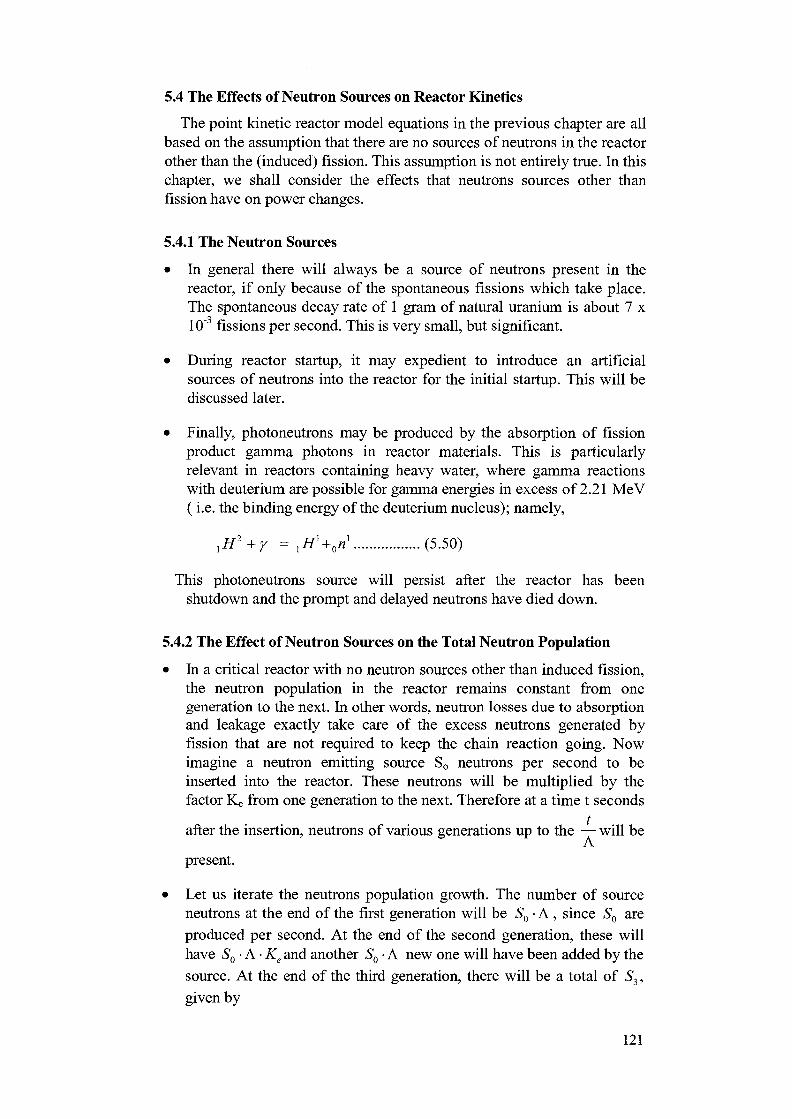
5.4 The Effects of Neutron Sources on Reactor Kinetics

The point kinetic reactor model equations in the previous chapter are allbased on the assumption that there are no sources of neutrons in the reactorother than the (induced) fission. This assumption is not entirely true. In thischapter, we shall consider the effects that neutrons sources other thanfission have on power changes.

5.4.1 The Neutron Sources

• hi general there will always be a source of neutrons present in thereactor, if only because of the spontaneous fissions which take place.The spontaneous decay rate of 1 gram of natural uranium is about 7 x10~3 fissions per second. This is very small, but significant.

• During reactor startup, it may expedient to introduce an artificialsources of neutrons into the reactor for the initial startup. This will bediscussed later.

• Finally, photoneutrons may be produced by the absorption of fissionproduct gamma photons in reactor materials. This is particularlyrelevant in reactors containing heavy water, where gamma reactionswith deuterium are possible for gamma energies in excess of 2.21 MeV(i.e. the binding energy of the deuterium nucleus); namely,

,H2+y = xHl+,nx (5.50)

This photoneutrons source will persist after the reactor has beenshutdown and the prompt and delayed neutrons have died down.

5.4.2 The Effect of Neutron Sources on the Total Neutron Population

• hi a critical reactor with no neutron sources other than induced fission,the neutron population in the reactor remains constant from onegeneration to the next. In other words, neutron losses due to absorptionand leakage exactly take care of the excess neutrons generated byfission that are not required to keep the chain reaction going. Nowimagine a neutron emitting source So neutrons per second to beinserted into the reactor. These neutrons will be multiplied by thefactor Ke from one generation to the next. Therefore at a time t seconds

after the insertion, neutrons of various generations up to the — will be

present.

• Let us iterate the neutrons population growth. The number of sourceneutrons at the end of the first generation will be So • A , since So areproduced per second. At the end of the second generation, these willhave So • A • Ke and another So • A new one will have been added by thesource. At the end of the third generation, there will be a total of S3,given by

121

= (S0AKe + S0A)Ke + S0A = 5OA(1 + Ke+ K]) (5.51)

thHence after mth generation, the total neutron population due to the sourcewill be:

Sm = SOA(1 + Ke + K2e+ +Krl) (5.52)

since m = —, therefore the number of source neutrons at time t is given

by:

Let us now look at three cases:

Case (1) Ke< 1: As t approaches infinity, St will reach an equilibriumvalue given by:

< 5-5 5 )

Case (2) Ke =1: hi this case, S0A neutrons will be added to the neutronpopulation in every generation, so that after a time t equivalent

to m = — generations, the number of source neutrons will be:A

.(5.56)

Case (3) Ke> 1: For a supercritical reactor, the neutron population willincrease very rapidly. The fission neutrons already there willincrease at rate governed by the reactor period and the sourceneutrons will multiply as given by equation (5.54)

5.4.3 The Effect of Neutrons Sources on a Reactor at Power

Let us consider the implications of the neutron sources by using a typicalheavy water reactor as an example.

• When the reactor is at power, photoneutrons will be produced by(j, ri) reactions with deuterium nuclei. The gamma source is made upof fission gammas, capture gammas and fission product and activationproduct decay gammas. The photoneutrons flux will typically be of theorder of 10"6 of the thermal flux. If reactor power is held constant, the

122

total flux will be constant, so will the neutron density. Suppose thereare n neutrons in any generation, they will related by :

nKe + Wbn = n (5.55)

• That means Ke = 1 -10~6 = 0.999999. It should be interesting to notethat when Ke is exactly unity, we should expect the neutron population

to grow by a factor of 1(T6 per generation. Hence the effect of thephotoneutron source on critical reactor operation at power istherefore seen to be quite negligible.

5.4.4 The Effect of Neutron Source on Reactor Shut-Down

Let us now consider what happens when the reactor, which has beenrunning at power, is suddenly made subcritical. In the absence of neutronsource, the reactor power would diminish to zero at a rate ultimatelygoverned by the longest lived delayed neutron group. However, with aneutron source present, the neutron population will never decrease belowthe equilibrium value

We can therefore say that the final power level, PK , will be given by:

where Ps is the neutron source strength, expressed in watts. It is the fissionpower produced in a reactor by a source of So neutrons per second. Itshould be noted that the final power level of the reactor depends on theamount of negative reactivity inserted. For example, if Ps = 30 W, and

30AK=-30 mk, then PM = = 1000JF

5.4.5 Photoneutrons Sources in Heavy Water Reactor

There are 9 photoneutron groups, analogous to the 6 delayed neutrongroups, categorized according to their respective half-lives. They are listedin Table 4. The photoneutrons constitute about 4 % of the delayed neutronproduction, and that shortly after shutdown, the photoneutrons yield isdecreasing rapidly. In fact after a couple of days or so, the photoneutronsource will be down by the order of a thousand or so, and only the lastgroup of photoneutrons will be effective.

They will decay with a half life of 18 days and will therefore set limiton the length of time during which the reactor may still be restartedwithout special instrumentation.

123

Table 4 - Photoneutron Groups for a typical HWR.

Photoneutrons 7

8

9

10

11

12

13

14

15

3.6 sec

57 sec

3 minutes

18 minutes

40 minutes

2.5 hours

6.3 hours

2.2 days

18.5 days

19xl0~3

5.7 xlO"3

1.3 x 10"3

1.11 xlO"3

0.61 x 10"3

0.64 xlO"3

0.08 x 10"3

0.02 x 10"3

0.02 x 10"3

Total=28 xlO"3

%

5.5 Modeling Exercise - Point Kinetic Reactor Model with Photoneutrons.

The modeling equations should be changed to:

15

dn

Iti=\

A 7=1

A,-Ct

for i = 1,... 15

Note that i = 1 to 6 belong to delayed neutron groups; whereas i = 7 to 15belong to photoneutron groups.

Data:

NLFE = 0.0008 sec

bl = 0.000329 Delayed Neutron Group Fraction

b2 = 0.001003 "

b3 = 0.000856 "

b4 = 0.002319 "

b5 = 0.000587 "

b6 = 0.000206 "

b7 = 0.00019 Photoneutron Group Fraction

b8 = 0.000057 "

124

b9 = 0.000013 "

t>10 = 0.0000111 "

bl 1=0.0000061 "

bl2 = 0.0000016 "

bl3 = 0.0000008 "

bl4 = 0.0000002 "

bl5 = 0.0000002 "

11 = 0.01261 sec"1 Delayed Neutron Group Decay Constant

12 = 0.03051 sec"1 "

13 = 0.12 sec'1 "

14 = 0.3209 sec"1 "

15 = 1.262 sec"1 "

16 = 3.239 sec"1 "

17 = 0.2778 sec"1 Photoneutron Group Decay Constant

18 = 0.01754 sec"1 "

19 = 0.00556 sec"1 "

110 = 0.000926 sec"1 "

111 =0.0004167 sec"1 "

112 = 0.0001111 sec 1 "

113 = 0.0000441 sec"1 "

114 = 0.00000526 sec"1 "

115 = 0.00000063 sec"1 "

NFLUX = neutron Flux(normalized from 0 to 1)

Ci = concentration of neutron groups(normalized)( delayed neutrongroup i=l,6 ; Photoneutron Group i = 7, 15)

Dk = overall reactivity change (K)

bi = neutron fraction (normalized) of delay group (i =1,6);

photoneutron group (i= 7, 15)

NLIFE = mean neutron lifetime(sec)

li = decay constant of neutron groups(/sec); Delayed group i = 1 to 6 ;

Photoneutron group i = 7 to 15

125

1. Modify the Algorithm # 802 to incorporate these changes. Be sure toinclude additional inputs, outputs and coefficients

2. Shutdown reactor power with insertion of large negative reactivity.Observe reactor power decay transient.

5.5.1 Point Kinetic Reactor Model with Photoneutrons Sources (Solution)

To be included in the class

5.6 Reactivity Feedback EffectsN error U

N desired ReactivityControl Devices <-

Reactor

p feedback

N

Figure 9 - control block diagram for reactor reactivity control

In a reactor control system such as in Figure 9, the power error (neutrondensity error) is used to adjust the control reactivity U by adjustments ofthe reactivity control devices. The actual reactivity p (= AK) is thealgebraic sum of U an the inherent reactivity feedback effects due to thechanges of the system variables affecting reactivity. These reactivityfeedback effects can be classified into three categories:

1. Long term effects which consist of fuel burn up, conversion of fertilematerial into fuel material (build up), and the accumulation of fissionproducts. Time scale is in months.

2. Intermediate effects where the time scale is in the order of severalhours consist of reactivity changes due to xenon and samariumpoisons.

3. Short term effects which arise due to temperature changes in fuel, heattransport fluid (void) and moderators, The time scale for these shortterm effects are of the order of minutes.

Let us discus each of these effects briefly.

5.6.1 Long Term Reactivity Effects - Fuel Burnup & Buildup

• The composition of the fuel will change quite significantly during itslife in the reactor. There are two predominant effects - the burn up offissile U-235 and the conversion of non-fissile U-238 into fissilePlutonium.

126

• The rate at which this occurs depends on the neutron flux, because therate dC/dt at which U-235 is destroyed by neutron capture is given by :

(5.57)

where C = the concentration of U-235

<7a = absorption cross section for U-235

<f> = neutron flux

This depletion of U-235 is offset by the conversion of U-238 into Pu-239:

I

• The conversion ratio is the number of Pu-239 nuclei formed for eachU-235 nuclei consumed. In typical CANDU Heavy Water reactor, it isabout 0.8.

• The Pu-239 that is produced will eventually build up to equilibriumwhen its rate of production will be equal to its rate of removal. The Pu-240 formed by neutron capture has properties very similar to U-238,but if it captures another neutron, it will form fissile Pu-241. Thereforeafter a long period of reactor operation, power will be produced by U-235, Pu-239 and Pu 241.

• The rate of change in the concentration Ci of the ith isotope in the fuelin a flux of <j> is in general given by:

dq= Cj^&j^cCi^tp + CjX j — Cj&jft — CjX j (5.58)

where cr. is the absorption cross-section,

X t is the radioactive decay constant

af is the probability of an absorbed neutrons producing a radiativecapture (n,y) event.

The first term C^cr^a^ij) is the production of the ith isotope byneutron capture in the (i-l)th isotope.

127

The second term C.A j is the production of ith isotope from radioactive

decay of a parent j t h nuclide.

The last two terms are the losses due to neutron absorption andradioactive decay of the ith isotope respectively.

The composition of the reactor fuel after a given time t can be obtainedby solving the set of simultaneous equations (5.58) and inserting as aboundary condition the initial fuel composition at t = 0. This change infuel composition will affect both thermal fission factory , and the

thermal utilization factor, / , and hence t] f. This will be given by:

f = C5vf5 v5 + C9af9vg+ q ofl vx

S mC5a5 + C8o-8 + C9a9 + Coao

Here the subscript 5 and 8 refer to U-235 and U-238, and subscript 9, 0and 1 refer to Pu-239, Pu-240 and Pu-241. The absorption in materialswith concentration Cm in the fuel other than fuel isotopes is included inthe last term of the denominator.

• In general, it has been found that the changes in the composition of thefuel will not change the value of the fast fission factor s, or theresonance capture probability p, since both of these are dependent onthe U-238 concentration in the fuel, and this will not changesignificantly with time.

• Thus the change in reactivity after a specified burnup can bedetermined by solving equations (5.58) and plugging the answers intoequation (5.59) to obtain new value of t] / , and hence the new valueof reactivity. Numerous computer programs exist to carry out suchburnup calculations. But general observations of the burnup are asfollows:

1. Initially the burnup of U-235 and its replacement by a smallernumber of Pu-239 (conversion factor 0.8) leads to an increase inreactivity. This is due to higher cross section of Pu-239 relative toU-235, leading to higher value off.

2. At higher irradiations, the U-235 is still being removed, but thebuildup of Pu-239 becomes less rapid since it will eventually reachan equilibrium level when the production of Pu-239 will equal theremoval due to absorption. Consequently, at higher irradiations thereduction in the number of fissile nuclei causes a reduction onreactivity.

• Previously, we saw that the small fraction of delayed neutronssubstantially increases the reactor period for a given reactivity. Thedelayed neutrons yields from U-235 are such that the generation

128

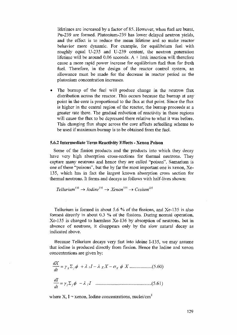
lifetimes are increased by a factor of 85. However, when fuel are burnt,Pu-239 are formed. Plutonium-239 has lower delayed neutron yields,and the effect is to reduce the mean lifetime and so make reactorbehavior more dynamic. For example, for equilibrium fuel withroughly equal U-235 and U-239 content, the neutron generationlifetime will be around 0.06 seconds. A + lmk insertion will thereforecause a more rapid power increase for equilibrium fuel than for freshfuel. Therefore, in the design of the reactor control system, anallowance must be made for the decrease in reactor period as theplutonium concentration increases.

• The burnup of the fuel will produce change in the neutron fluxdistribution across the reactor. This occurs because the burnup at anypoint in the core is proportional to the flux at that point. Since the fluxis higher in the central region of the reactor, the burnup proceeds at agreater rate there. The gradual reduction of reactivity in these regionswill cause the flux to be depressed there relative to what it was before.This changing flux shape across the core affects refuelling scheme tobe used if maximum burnup is to be obtained from the fuel.

5.6.2 Intermediate Term Reactivity Effects - Xenon Poison

Some of the fission products and the products into which they decayhave very high absorption cross-sections for thermal neutrons. Theycapture many neutrons and hence they are called "poison". Samarium isone of these "poisons", but the by far the most important one is xenon, Xe-135, which has in fact the largest known absorption cross section forthermal neutrons. It forms and decays as follows with half-lives shown:

Tellurium135 ->• Iodine135 - > Xenon135 ->• Cesium135

Tellurium is formed in about 5.6 % of the fissions, and Xe-135 is alsoformed directly in about 0.3 % of the fissions. During normal operation,Xe-135 is changed to harmless Xe-136 by absorption of neutrons, but inabsence of neutrons, it disappears only by the slow natural decay asindicated above.

Because Tellurium decays very fast into idoine 1-135, we may assumethat iodine is produced directly from fission. Hence the Iodine and xenonconcentrations are given by:

—— = yxY,f</) + X il - X xX - ax (j> X (5.60)Cti

df „-,} -Xil (5.61)

where X, I = xenon, Iodine concentrations, nuclei/cm3

129

(f) = neutron flux in neutrons/cm2.sec

Ey = macroscopic fission cross section

yx, y1 = fractional yield of xenon and Iodine (7^=0.003; yt =0.056)

,-5.Ax,Ai = decay constants of xenon and iodine (A x-2A x 10";

A 7=2.9 xlO"5 sec"1)

The terms on the right hand side of the ODEs can be described as follows:

• Yx^ffi a nd Yi^f^ a r e production rates of X and I, directly from

fission.

• A 11, A xX are loss rates of Iodine, xenon due to natural decay.

• GX (j) X is the loss of Xe-135 due to conversion to Xe-136 by neutroni R o

capture. (crx= 3.5 x 10" cm is the microscopic capture cross-sectionof xenon for thermal neutrons.)

Under steady state condition, (dX/dt = 0; dl/dt = 0) for a constant neutronflux (f> o, the solutions are:

f> 0h - • (5-62)

A I

{A iL +yJLf<j) o)X, = ° ! x f,\ (5.63)

(A x + <7XY o)

Substituting (5.62) into (5.63), we have

(Tr +YX) ^f<?>o

Xo = K/!, f (5.64)

Ax + ox(j) o

For small flux (f) o,

{jj +yx) I,f0 oXo « therefore proportional to flux (5.65)

Ax

For large flux (j) o,

(Yi+Yx) 2 rXo « , therefore constant (5.66)

130

So for high power reactor, the steady state xenon concentration isindependent of power.

xenon Poison Reactivity Feedback:

A reactor which is critical with xenon will certainly be supercriticalwithout its xenon. The reduction in reactivity caused by the xenon is called"xenon Load", and is expressed in mk. The xenon load is due to the changein thermal utilization factor f.

S ILet f — without xenon, and / ' = with xenon

2 + 2 Z + 2 + ^

Note that Zmis the absorption cross section of all materials in the reactorthat is not fuel or xenon.

Now

K - Ke

K / ' f E + E E + EJ a "' " "' (5.67)

= -R-f

where R is called poisoning factor. It is a ratio of absorption by Xe-135 to

absorption by the fuelE.

At equilibrium, -*- = ° ' x (5.68)

Substituting equation (5.64) into (5.68), we have

When the reactor is critical with its xenon load (i.e.K'e =1), and - Rfrepresents the reactivity loss due to the xenon. In other words, the xenonload is the product of R and f.

For example; a reactor with man fuel flux of <j> o = 3 x 1013 n.cm^.s"1

\ax= 3.5 x 10"18 cm2 ; yx-0.003; ^=0.056; X x=2.1xlO"5; ^ = 0 . 5 4

(for natural uranium), substituting these numbers into (5.69), we have R =0.028. Given f = 0.9, the xenon load R will be 0.0252. This means that thisreactor would suffer a reactivity loss of 25.2 mk caused by equilibriumxenon poisoning.

131

The presence of an equilibrium xenon load means that enough excessreactivity must be built into the reactor so that the regulating system cancompensate for the loss in reactivity as the xenon builds up.

Let us consider xenon transients after sudden reactor shutdown orfollowing power reductions.

Let at t=0 the reactor be shutdown suddenly from a steady state flux </>

with corresponding xenon and iodine concentrations Xo Io. Putting <f> = 0

in equation (5.60), (5.61), we have:

— = -A,xX + ZII

% (5.70)

The solution is:

; , (5.71)X{t) = Xoe~^ + '—I0(e-;->' - e-x*)

A X — A I

It can be seen that for initial steady flux of <f> = 1014 n.cm~2.sec"1, thexenon reactivity load rises from an equilibrium value of - 28 mk at t — 0 toa maximum value of -132 mk somewhere between 7 and 12 hours aftershutdown. Note that the peak xenon load level depends proportionally onthe reactor flux level before shutdown. Physically, after shutdown, thereare no neutrons to convert the xenon, so it disappears only by slow naturaldecay. But xenon is being produced at a faster rate by the decay of iodine,so its level increases. Due to the decay of iodine, a maximum is reached,and the xenon decays thereafter.

To find the peak xenon load, we differentiate (5.71) with time and putdX/dt = 0, we have

- A je-*)- A xXoe-* = 0 (5.72)^ \ (A xat A x — A i

The time where peak xenon load occurs is:

A x — A I A I l0

Substituting this into X(t) gives:

^-f (5.74)

(5.73)

132

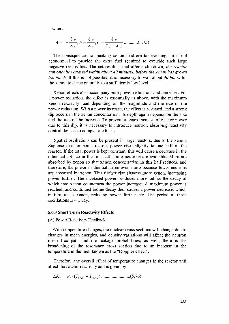
where

^ ^ ^ (5.75)A i — A x

The consequences for peaking xenon load are far reaching - it is noteconomical to provide the extra fuel required to override such largenegative reactivities. The net result is that after a shutdown, the reactorcan only be restarted within about 40 minutes, before the xenon has growntoo much. If this is not possible, it is necessary to wait about 40 hours forthe xenon to decay naturally to a sufficiently low level.

Xenon effects also accompany both power reductions and increases. Fora power reduction, the effect is essentially as above, with the maximumxenon reactivity load depending on the magnitude and the rate of thepower reduction. With a power increase, the effect is reversed, and a strongdip occurs in the xenon concentration. Its depth again depends on the sizeand the rate of the increase. To prevent a sharp increase of reactor powerdue to this dip, it is necessary to introduce neutron absorbing reactivitycontrol devices to compensate for it.

Spatial oscillations can be present in large reactors, due to the xenon.Suppose that for some reason, power rises slightly in one half of thereactor. If the total power is kept constant, this will cause a decrease in theother half. Since in the first half, more neutrons are available. More areabsorbed by xenon so that xenon concentration in this half reduces, andtherefore, the power in this half rises even more because fewer neutronsare absorbed by xenon. This further rise absorbs more xenon, increasingpower further. The increased power produces more iodine, the decay ofwhich into xenon counteracts the power increase. A maximum power isreached, and continued iodine decay then causes a power decrease, whichin turn raises xenon, reducing power further etc. The period of theseoscillations is ~ 1 day.

5.6.3 Short Term Reactivity Effects

(A) Power Reactivity Feedback

With temperature changes, the nuclear cross sections will change due tochanges in mean energies, and density variations will affect the neutronmean free path and the leakage probabilities; as well, there is thebroadening of the resonance cross section due to an increase in thetemperature in the fuel, known as the "Doppler effect".

Therefore, the overall effect of temperature changes in the reactor willaffect the reactor reactivity and is given by

AKT = aT-(TFPSS-TZER0) (5.76)

133

where aTis the temperature coefficient ( -15.06 x 10~6 /deg. C for freshfuel)

TFPSS is the fuel temperature at reactor hot full power condition.

TZERO is the fuel temperature at reactor zero power cold condition

For example, in order to bring the reactor power from cold 25 deg. C to hotcondition at 271 deg, C, the reactivity needed to compensate for reactivityloss due to temperature effects is

AKT = -15.06 x 10"6 x (271 - 25) = - 0.3705 x 10"2 = -3.705 mk

Reactor Coolant Void Reactivity Feedback

It has been shown that reactor core voiding (due to boiling or in extremecase, loss of coolant accident) will lead to positive reactivity excursion. Isgenerally expressed as:

*Kv = ^ m a x -F-(X-XFPss)- (5-77)

where AKVmax =the maximum reactivity from coolant voiding (typically 2mk)

F = Flux shape weighting factor (typically 0.68)

X = Coolant quality

XFPSS = Coolant quality at reactor full power (for CANDU, it is typically

2 to 4 %)

5.7 Modeling Exercise - Poison Reactivity Effects

5.7.1 Problem Description

1. Create a model which will predict the xenon concentration on a stepchange of neutron power.

2. Use the model to predict the following:

• poison-out period for a reactor trip from 100% full power

• the poison-prevent power level.

The following equations described the formation of xenon and iodine in aCANDU-type nuclear reactor.

134

— = 9A45E - 3 * N- 2.8111 E- 5 * Cidt

—— = 9.167£-4*iV +dt

AKXE = (27.93 - CXE) * IE - 3

CI = concentration of iodine(mK)

CXE = concentration of xenon(mK)

DKXE = reactivity change due to xenon(K)

N = neutron flux(normalized from 0 to 1)

5.7.2 Modeling Steps

1) Create a custom FORTRAN algorithm using the above equations, withneutron flux as an input to the algorithm, and concentration of iodine,concentration of xenon and the reactivity change due to xenon asoutputs.

2) Remember to follow the CAS SIM Technical Notes: algorithmdevelopment guidelines for calculations involving double precisionnumbers.

3) Use Euler's forward difference (explicit method) to model the aboveequations, and introduce an extra input, for varying the integrationtime-step, and call it the speed-up factor.

4) Use CASSBASE to overwrite ALG801, and replace it with youralgorithm. Remember to define your inputs and outputs for thetemplate in CASSBASE, and save your FORTRAN algorithm asALG801.FOR.

5) Exit CASSBASE, and go to SRCLIB directory, and recreateCASSIM.DLL with the new ALG801 using the ADDTOLIB batch file.

6) Copy the new CASSIM.DLL to the CASSENG directory.

7) Use CASSBASE to create a new model and call it IAEA2.

8) Create a NMB block(ALG452) for communication with LABVIEW.

135

9) Create a block for calculating the xenon/iodine concentration transientusing the custom algorithm ALG801. Remember to initialize the xenonand iodine concentration by depositing their values in the outputsection.

10) USE CASSBASE COPY BLOCK function to create 3 more blocksusing ALG801.

11) A LAB VIEW executable, CURVES.EXE is provided to display theresults. This LABVIEW custom trends executable requires anadditional block calls TIMEKEEPER(ALG451) which calculates theiteration count. The LABVIEW executable will convert the count tosimulation time. Connect the OUPUT(l) of this block to INPUT(l) ofthis block, and OUTPUT(2) of this block to INPUT(2) of this block.

12) Since all 4 xenon/iodine transient calculation block is required to usethe speedup factor, is there a quicker way than to change the inputs forall four blocks before running the model?

13) LABVIEW executable, CURVES.EXE expects the display variables inthe following order:

INPUTS TO BLOCK NMB

1) TIMEKEEPER/IT 1

2) X E N O N J / A 2 (xenon cone)

3) XENON_2/A2 (xenon cone)

4) XENON_3/A2 (xenon cone)

5) XENON_4/A2 (xenon cone)

note: NMB must be block 1.

14) Use the above model and create transients for the cases of a stepchange of:

a) 100% power reduction

b) 80% power reduction

c) 60% power reduction

d) 40% power reduction.

15) Use a speedup factor of 600. Why is it better to use a smaller speedupfactor, i.e. a smaller integration time-step?

16) Using the model and with the help of the LABVIEW executable,CURVES.EXE, can you find the following:

136

a) If a reactor core is tripped from full power, what will be the poison-out period? When must the reactor be re-started before a 'poison-out' occurs? And if a 'poison-out' did occur, how long before thereactor can be re-started?

b) What maximum step-change in power will never give rise to a'poison-out' reactor?

Note: the LABVIEW executable, CURVES.EXE can be found indirectory CAS_TRN. Double-clicking the file from file manager willstart the executable. It is best to start CASSENG before CURVES.EXEis started.

17) Try repeating the exercise with a different speedup factor.

137

6.0 Reactor Control Simulation Model Development

6.1 Brief Review of BWR Reactor Power Control

Reactor vessel head

Steam dryer

Cotft spr^y inlet nozzta

Sore yrtd

In-ccre neutrtfnfluxrfeteCtOr

Pump iinptiffer

tjy heusimj

Head cooling spray system

Steam outlet nozzle

Support flango

Steam separator

Reactor pressure vessel

feedwater inlet mzz\t

rod yuide ttitna

IVtain circulation pmrep

(Courtesy of ABB)

BWR is the abbreviation for the Boiling Water Reactor. These reactorswere originally designed by Allis-Chambers and General Electric (GE).The General Electric design has survived, whereas all Allis-Chambersunits are now shutdown. The first GE US commercial plant was atHumboldt Bay (near Eureka) in California. Other suppliers of the BWRdesign world-wide include - ASEA-Atom, Kraftwerk Union, Hitachi.Commercial BWR reactors may be found in Finland, Germany, India,Japan, Mexico, Netherlands, Spain, Sweden, Switzerland, and Taiwan.

138

Electric power output and grid frequency

Feedwater flow

Reactor pressure

Reactor water level

Neutron flux

Recirculation flow

Control rodoperation {532}

Reactc*' power)ry) '* •

Feedwaterpumps

FC Frequency converterHC Hydraulic coupling

(Courtesy of ABB)

In the figure above, water is circulated through the Reactor Core pickingup heat as the water moves past the fuel assemblies. The water eventuallyis heated enough to convert to steam. Steam separators in the upper part ofthe reactor remove water from the steam.

The steam then passes through the Main Steam Lines to the Turbine-Generators. The steam typically goes first to a smaller High Pressure (HP)Turbine, then passes to Moisture Separators (not shown), then to the 2 or 3larger Low Pressure (LP) Turbines. In the sketch above there are 3 lowpressure turbines, as is common for 1000 MW(e) plant. The turbines areconnected to each other and to the Generator by a long shaft (not onepiece).

The Generator produces the electricity, typically at about 20 000 voltsAC. This electrical power is then distributed to a Generator Transformer,which steps up the voltage to either 230 000 or 345 000 volts. Then thepower is distributed to a switchyard or substation where the power is thensent offsite.

The steam, after passing through the turbines, then condenses in theCondenser, which is at a vacuum and is cooled by ocean, sea, lake, or riverwater. The condensed steam then is pumped to Low Pressure FeedwaterHeaters (shown but not identified). The water then passes to the FeedwaterPumps which in turn, pump the water to the reactor and start the cycle allover again.

The BWR is unique in that the Control Rods, used to shutdown thereactor and maintain an uniform power distribution across the reactor,

139

are inserted from the bottom by a high pressure hydraulically operatedsystem. The BWR also has a Torus or a Suppression Pool. The torus orsuppression pool is used to remove heat released if an event occurs inwhich large quantities of steam are released from the reactor or the ReactorRecirculation System, used to circulate water through the reactor.

The BWR reactor typically allows bulk boiling of the water in thereactor. The operating temperature of the reactor is approximately 570Fproducing steam at a pressure of about 1000 pounds per square inch.

The reactor power output control system in BWR plant consists of acontrol rod made of neutron-absorbing materials, rod drive system andrecirculation flow control system. The control rod and its drive systemmaintain a constant desired power level by adjusting the position of the rodinside the core. The recirculation flow control system also controls thereactor power level by changing the recirculation flow to alter the densityof the water, a moderating material use to slow down the fission neutrons.This recirculation flow control is capable of changing the reactor poweroutput rapidly over a wide range while keeping the power distribution inthe core constant.

A BWR plant has numerous control rods installed inside the core. Eachcontrol rod is provided with a drive system and hydraulic control system.Rod position is adjusted by drawing out or insertion by means of thehydraulic pressure that is remotely controlled in the control room. Onlyone rod is operative at a time.

When the power output is changed by using a control rod, the changingrate is approximately 2 % power per minute. In the event of emergencyshutdown of the reactor, all control rods are promptly inserted at once(scram) by the reactor trip system.

The coolant recirculation flow is controlled by a recirculation pump.The pump speed changes according to the change of the power frequencyof the induction motor that drives the pump. Thus recirculation flow isregulated via a flow control system which consists of a recirculation pumpmotor generator set with a variable frequency generator and drive motorbetween which a hydraulic coupling is provided. The Flow MasterController controls the speed of the motor generator set, thus providing thecapability to change the reactor power output at a rate of 30 % per minute.

140

6.2 Brief Review of PWR Reactor Power Control

PWR is the abbreviation for the Pressurized Water Reactor. Thesereactors were originally designed by Westinghouse Bettis Atomic PowerLaboratory for military ship applications, then by the WestinghouseNuclear Power Division for commercial applications. The first commercialPWR plant in the United States was Shippingport, which was located nearPittsburgh, Pennsylvania.

In addition to Westinghouse, Asea Brown Boveri-CombustionEngineering (ABB-CE), Framatome, Kraftwerk Union, Siemens, andMitsubishi have typically built this type of reactor throughout the world.Babcock & Wilcox (B&W) built a PWR design power plant but usedvertical once-through steam generators, rather than the U-tube design usedby the rest of the suppliers. Refuelings must be done with the plantshutdown.

The Pressurized Water Reactor (PWR) has 3 separate cooling systems.Only 1 is expected to have radioactivity - the Reactor Coolant System. TheReactor Coolant System, shown inside the Containment, consists of 2, 3,or 4 Cooling "Loops" connected to the Reactor, each containing a ReactorCoolant Pump, and Steam Generator. The Reactor heats the water thatpasses upward past the fuel assemblies from a temperature of about 5 3 OFto a temperature of about 590F. Boiling, other than minor bubbles callednucleate boiling, is not allowed to occur. Pressure is maintained by aPressurizer (not shown) connected to the Reactor Coolant System. Pressureis maintained at approximately 2250 pounds per square inch through aheater and spray system in the pressurizer. The water from the Reactor ispumped to the steam generator and passes through tubes. The ReactorCooling System is expected to be the only one with radioactive materialsin it. Typically PWRs have 2, 3, or 4 reactor cooling system loops insidethe containment.

In a Secondary Cooling System (which include the Main Steam Systemand the Condensate-Feedwater Systems), cooler water is pumped from the

141

Feedwater System and passes on the outside of those steam generatortubes, is heated and converted to steam. The steam then passes through thea Main Steam Line to the Turbine, which is connected to and turns theGenerator.

The steam from the Turbine condenses in a Condenser. The condensedwater is then pumped by Condensate Pumps through Low PressureFeedwater Heaters, then to the Feedwater Pumps, then to High PressureFeedwater Heaters, then to the Steam Generators. The diagram abovesimplifies the process by only showing the condenser, a pump, and thesteam generator.

The condenser is maintained at a vacuum using either vacuum pumps orair ejectors. Cooling of the steam is provided by Condenser Cooling Waterpumped through the condenser by Circulating Water Pumps, which take asuction from water supplied from the ocean, sea, lake, river, or CoolingTower (shown). A discussion of cooling towers is provided in the photosection.

Light water PWR plants have four main control systems: control rodcontrol (reactor power control), steam generator level control, pressurizerpressure control and pressurizer level control.

The control rod control is used for reactor power control (Figure 10).The control rods are moved up and down when a deviation between"primary power ", PPRI, and the "reference power ", PREF, formed by theturbine first-stage pressure (secondary power) exceeds the predeterminedsetpoint.

Reactor Coolant Avg. Temp.

Turbine load

PPRI .

Neutron flu:

Control RodControlSystem

Figure 10 - Control Block Diagram for Reactor Control for a typical PWR.(Courtesy of IAEA)

Reactor power change due to PPRI change is compensated for byintroducing the differentiated deviation signal between neutron flux andturbine 1 stage pressure (power demand) into this system.

142

The boron concentration control system (which requires manual action)is used for the relatively long-term and slow core reactivity control,whereas the reactivity control (including reactor trip) responsive to loadchanges during normal operation is performed by controlling the rodpositions

6.3 Brief Overview of RBMK Reactor Power Control

(Courtesy of Argonne National Lab.)

1. Reactor core - produces heat for converting water to steam2. Steam-to-water pipes - carry steam to dram separator for moisture

separation of steam3. Drum Separator - used to separate water from steam4. Main circulation pumps - used to circulate water through reactor for

cooling5. Group dispensing headers - headers coming from main circulating

pumps6. Water pipelines - headers supplying each channel in the reactor7. Upper biological shield - protect operators and other personnel from

radiation while working above reactor, e.g. during daily refueling8. Refueling machine - used to place new fuel assemblies into the core

and remove spent fuel assemblies9. Lower biological shield - used to protect personnel from radiation

while working in lower areas adjacent to reactor

The Soviet designed RBMK (a Russian acronym meaning Reactor High-Power Boiling Channel Type) is a pressurized water reactor withindividual fuel channels and using ordinary water as its coolant and

143

graphite as its moderator. It is very different from most other power reactordesigns as it was intended and used for both plutonium and powerproduction. The combination of graphite moderator and water coolant isfound in no other power reactors. The design characteristics of the reactorwere shown, in the Chernobyl accident, to cause instability when lowpower. This was due primarily to control rod design and a positive voidcoefficient. A number of significant design changes have now been made toaddress these problems.

The RBMK reactorpile cap

see enlargementT

containmenti l

turbine generator

steamseparator

pressuretube

fuel rod

pump

graphitemoderator

controlrod

7J ^ 7 — watercoolant

Reactor core enlargement

(courtesy of Uranium Institute)

Fuel rods - Pellets of enriched uranium oxide are enclosed in a zircaloytube 3.65m long, forming a fuel rod. Two sets of 18 fuel rods arearranged cylindrically in a carriage to form a fuel assembly of about 10m length. These fuel assemblies can be lifted into and out of the reactormechanically, allowing fuel replenishment while the reactor is inoperation.

144

2. Pressure tubes -within the reactor each fuel assembly is positioned inits own pressure tube or channel. Each channel is individually cooledby pressurized water.

3. Graphite moderator - a series of graphite blocks surround, and henceseparate, the pressure tubes. They act as a moderator to slow down theneutrons released during fission. This is necessary for continuousfission to be maintained. Conductance of heat between the blocks isenhanced by a mixture of helium and nitrogen gas.

4. Control rods - boron carbide control rods absorb neutrons to controlthe rate of fission. A few short rods, inserted upwards from the bottomof the core, even the distribution of power across the reactor. The maincontrol rods are inserted from the top down and provide automatic,manual or emergency control. The automatic rods are regulated byfeedback from in-core detectors. If there is a deviation from normaloperating parameters (e.g. increased reactor power level), the rodscan be dropped into the core to reduce or stop reactor activity. Anumber of rods normally remain in the core during operation.

5. Coolant - two separate water coolant systems each with four pumpscirculate water through the pressure tubes. Ninety-five percent of theheat from fission is transferred to the coolant. There is also anemergency core cooling system which will come into operation ifeither coolant circuit is interrupted.

6. Steam separator - in the RBMK design, boiling occurs. The steamproduced passes to the Steam Separator which separates water from thesteam. The steam then passes to the Turbine as in the Boiling WaterReactor design. Similar to the BWR case, the steam is radioactive,however, the steam separator introduces a delay time so radiationlevels near the turbine may not be as high as in the BWR case.

7. Containment - the reactor core is located in a concrete lined cavity thatacts as a radiation shield. The upper shield or pile cap above the core,is made of steel and supports the fuel assemblies. The steam separatorsof the coolant systems are housed in their own concrete shields.

In the RBMK design, water coolant slows the reaction down, meaningthat the water coolant absorbs the neutrons, a necessary part of thereaction, hi other words, the water coolant additionally serves to controlthe reaction. The lack of water increases the reaction in the RBMK design,due to positive void reactivity feedback. This is one chief differencebetween the power plants in the United States, known as the LWR (LightWater Reactors), and the RBMK type. In the LWR the lack of water killsthe reaction, opposite of a RBMK.

145

6.4 Pressurized Heavy Water Reactor

SHIELD TANK OVERPRESSURE RUPTUREDISC AND PIPING

REACTIVITYMECHANISMSDECK

REACTOR VAULTROOF

VERTICAL REACTIVITYCONTROL UNITS

LIQUID ZONECONTROLTRENCHES

CALANDRIAOVERPRESSURE RUPTUREDISC AND PIPING

SHIELD TANKBALL SHIELDING

FEEDERS

FUEL CHANNELTRANSFER

END FITTINGS

STEEL BALL SHIELDING(END SHIELD)

HORIZONTAL REACTIVITYCONTROL UNITS

FUELLING MACHINE.SIDETUSESHEET..

LATTICE TUBES

CALANDRIASIDETU8ESHEET .

END SHIELD

SEMI-FLEXIBLE JOINT-SHIELD TANK END WALLTO VAULT END WALLEMBEDMENT

BUILDING INTERNALCROSSWALL

340180 2-3-2-lT

REACTOR VAULTENOWALL

(Courtesy of AECL)

The CANDU-PHW (CANada Deuterium Uranium, Pressurized HeavyWater) nuclear reactor is a heavy-water-moderated, heavy-water-cooled,natural uranium-fueled reactor which utilizes the pressure tube concept.The pressure tubes containing the fuel run horizontally through the reactorcore. Pressurized heavy water carries the heat from the fuel to the steamgenerators.

146

Each pressure tube is isolated and insulated from the heavy watermoderator by a concentric calandria tube and a gas annulus. Consequentlythe moderator system is operated at low temperature and pressure. Thereactivity control and shutdown mechanism reside in the low-pressuremoderator, thus simplifying their design, construction and maintenanceand eliminating the possibility of their ejection in an accident situation. Aswell, this cool moderator can act as a heat sink under certain accidentconditions.

The use of natural uranium fuel in an optimized lattice, and heavy wateras moderator and coolant, combined with the capability to refuel thereactor while at full power, gives the CANDU reactor its good economyand low excess reactivity. This results in a power with very low fuel costs.

The only reactivity feedback effects that are of any consequence are thecoolant density (or void), fuel temperature and xenon effects. Since themoderator temperature is controlled independently of the primary coolant,it does not contribute any significant reactivity feedback. The fueltemperature reactivity coefficient is negative and therefore stabilizingwhereas the coolant void reactivity coefficient is positive and thereforedestabilizing. The sum of these, and lesser reactivity feedback effects, is apower reactivity coefficient that is near zero under normal operatingconditions.

6.4.1 Pressurized Heavy Reactor Control System General Description

A simplified diagram of a generic CANDU nuclear power plant and itsdigital computer control system is shown in Figure 11. Circulating pumps,also known as primary heat transport pumps maintain the flow of heavywater coolant around the "primary heat transport circuit" which transportsfission energy from the reactor to the boiler. Inside the reactor, this coolantpasses through fuel channels which contain cylindrical bundles of fuel.Heavy water "moderator" fills the space between the channels.

A surge tank, or pressurizer tank is used to absorb shrinkage and swelldue to coolant temperature changes and to help maintain steady pressure inthe circuit. The controls needed to control this circuit are basically:

(A) Heat Transport Pressure - it is controlled by electric heaters and steambleed valves on the surge tank.

(B) Surge Tank Level - it is controlled by the feed and bleed valves shownon the circuit.

In the boiler, the energy is transferred to ordinary light water steam, andthe steam drives a conventional turbine-generator set. The feedwatervalves, pumps and preheaters complete the chain from the condenser backto the boiler. Steam can also be discharged directly to the condenser via thedischarge valves with a capacity of 68 % of full power steam flow, or tothe atmosphere via atmospheric steam discharge valves with a capacity of

147

10 %. The need for these valves is related to xenon poison effectsexplained earlier.

The boiler level control system (not indicated on the diagram) controlthe light water level in the boiler drum via feedwater valves.

REACTOR BUILDING POWERHOUSE

FUEL

II

I I•

REACTORCONTROL

(RRS)

REACTOR

<OPERATOR\ /OPERATORSINPUT J \^ INPUT J " *

HEAT TRANSPORTPRESSURE AND

INVENTORYCONTROL (HTSP)

BOILERPRESSUREANDLEVEL CONTROL

(BPC, BLC)

HEATTRANSPORT

STEAMGENERATOR

MODERATOR

CONTAINMENT

UNIT POWERREGULATOR

(UPR)

TURBOVISORYCONTROL

TURBINEGENERATOR

Legend:p. Process

System & Flow

• Control Signal

+ ParameterMeasurement

FEEDWATER

t t t t tCOMMONSERVICES

Figure 11- A simplified diagram of a generic CANDU nuclear power plant and its digitalcomputer control system (Courtesy ofAECL)

148

The three main control programs are:

• Unit Power Regulator (UPR) - it controls the generator output to thedesired setpoint, which is set locally by the operator or remotely by thecentral load dispatch system, by adjusting the turbine load setpoint viathe speeder gear of the turbine governor.

• Boiler Pressure Controller (BPC) - in the normal mode of operation,boiler pressure is controlled by adjusting the reactor power setpoint. Itcan also be controlled by adjusting the governor valves, and by openingthe atmospheric or condenser steam discharge valves.

• Reactor Regulating System (RRS) - this is the control system whichcontrols reactor power. It attempts to make the actual reactor power(determined by a Power Measurement Program), equal to thedemanded reactor power (determined by Demanded Power Routine) byadjustment of the reactivity control devices via the ReactivityMechanism Control Program. A "Flux Tilt" control program is used toprevent non-uniform flux distributions throughout the reactor bydifferential adjustment of reactivity control devices in different part ofthe reactor.

Three types of reactivity control devices are shown :

1. 14 light water zone control absorbers - these are vertical cylindricalcompartments, distributed strategically through the core, which canbe filled to any desired level with light water, a neutron absorber.Differential adjustment of levels in individual compartments isused for spatial (zonal) control. Platinum in-core flux detectorsprovide the neutron flux feedback signals required by the digitalcontrol algorithms for the regulation of the both the bulk andspatial flux.

2. 8 banks of Adjuster rods (total # of rods ~ 21)- these are neutronabsorbers which are situated in various locations in the core and arenormally fully inserted in the core. Being neutron absorbers, theywill increase reactivity in the reactor by pulling themselves awayfrom the core. They are withdrawn in symmetrical banks, under thecontrol of the digital control computer, to provide positivereactivity for shimming the zonal light water control absorbers aswell as for xenon override following a shutdown. The totalreactivity worth of all fully pull-out adjuster rods is approximately+ 17 mk. Each adjuster bank is assumed to have the same reactivityworth. In the event of a shutdown of reactor from full power, theadjuster rods have enough reactivity to restart the reactor withinhalf an hour, before poisoning out.

149

3. 2 banks of mechanical Absorber rods (total # of rods = 4) - theseAbsorber rods decrease the reactivity inside the reactor by insertingthemselves into the core. Being neutron absorbers, insertion intothe core means more neutron absorption, thereby reducing thereactivity and the neutron power of the reactor. The total reactivityworth of both fully inserted absorber rods is approximately - 9mk.Each absorber bank is assumed to have the same reactivity worth.

VFDif=

V F D 2 F = ,

DIRECTION C

" * \

> <

DIRECTION B

DIRECTION D

\ -\

DIRECTION A

CO-AXIAL ZONES

1, 132, 143, 104, 115, 126. 87, 9

Figure 12-14 Liquid Zone Configurations in a typical CANDU Reactor

(Courtesy of AECL)

150

203 203

ZONE CONTROLLERf ~ j ADJUSTER

CONTROL ABSORBER ( f t SHUTDOWN ROD (SA)

• VERTIOU.RUXDETECTOR

VCW1NGPORT

Figure 13 - Reactivity Mechanism Desk - showing the arrangement ofAdjuster rods, Control Absorbers, Shutdown rods, and Zone Controllers.

(Courtesy of AECL)

151

6.4.2 Moderator Liquid Poison Addition and Removal System

Here the "poisons" refer to boron or gadolinium, which have largeneutron capture cross section for thermal neutrons. They are added to themoderator to provide large negative reactivities under certain conditions:

• For instance, a typical CANDU has available excess reactivities of +1 lOmk at an initial startup with fresh fuel. For the reactor to be critical,reactivity usage must equal to available reactivity. Therefore, tocompensate for fresh fuel, the equivalent of -60 mk is added to themoderator in the form of boron. As the fuel burns down, the boronmust be gradually removed.

• Poison is also used at reactor startup after a long shutdown. Theequivalent of - 30 mk of gadolinium must then be added to compensatefor the absence of xenon, and gradually removed as xenon build up.

• Poison is also used to compensate for transient dip in xenon loadduring reactor power increase

Poison is removed by the ion exchange purification system. But the timeconstant of the removal is of the order of hours. Operation of poisonaddition and removal is controlled manually.

6.4.3 Reactor Trip System

Two safety shutdown system exist for CANDU; each with its ownseparate trip system. One is a high capacity system for direct poisoninjection into the moderator. Gadolinium, through more corrosive, is usedas poison. It has the advantage of being much more easily removable byion exchange, facilitating removal of the large quantity of poison in lesstime.

The second system consists of a number of shut-off rods, which can bedropped into the core in 2 seconds by de-energizing clutches in the drives.They are essentially the same as Absorber rods and are made of a stainlesssteel cadnium.

Conditions which cause reactor trips are:

• High neutron power > 115 % full power.

• High rate of power increase > 10 % per sec.

• Dangerous pressures or flows in certain parts of the system.

Triplicated instrumentation channels, with 2 out of 3 to be actuated tocomplete a trip, are used to avoid unnecessary trips due to spuriousoperation of one channel.

152

*«•

POA

HARDWAREINTERLOCKS

SON/NDRE

\DD1TION!MOVAL

REACTIVITYDEVICES

REACTOR

VANADIUM FLUXDETECTORS

ION CHAMBERS

INCONEL FLUXDETECTORS

FEEDWATERFLOW

STEAM GENERATOR

, , , , REACTOR

ADJUSTERS

MECHANICAL CONTROL ABSORBER DRIVE

SHUTDOWN RODS (WITHDRAWAL ONLY)

LIQUID CONTROL UNITS

•

MECHANICAL CONTROL ABSORBER CLUTCHES

•

REACTIVITYDEVICE

CONTROLS

STEPBACK

DEMANDPOWER

ROUTINE

j

SETBACK

POWER

^ ( _

1

FLUXPOWER

1

FEEDWATERTEMP.

STEAMFLOW

FLUXDISTRIBUTION

f

FLUX MAPPING

w \ f

THERMALPOWER

1 1

POWER MEASUREMENT AND CALIBRATION

REACTOR POWER SETPOINT{FROM STEAM GENERATOR PRESSURECONTROL OR MANUAL INPUT)

i

i

1

1I

STEPBACKPARAMETERS

SETBACKPARAMETERS

REACTOR POWER CONTROL

OfQ

S3 0014 2.18-11

• The Power Measurement & Calibration Program determines averagereactor power and its distribution through the reactor.

• The Demand Power Routine sets the desired reactor power whichdepends on the mode of reactor operation. In the "Normal" mode ofoperation, reactor power is set to follow turbine generator power suchthat boiler pressure is kept constant under all conditions, hi this mode,the setpoint demand signal comes from the Boiler Pressure Controller(BPC). In the upset conditions, the mode of plant operation is switchedto "Alternate" Mode, in which case the reactor setpoint is manuallyadjusted or adjusted via a Reactor Power Setback Routine.

• The Reactor Setback Routine monitors a number of essential plantparameters and ramps the reactor power down if any one parameter isout of permissible limits. One of these parameters is provided by thePower Mapping Routine, which measures neutron flux in 54 locations,and uses these and other measurements to determine whether there areindividual fuel bundles in certain locations whose power ratings hasbeen exceeded.

• The Reactor Stepback Routine monitors a critical plant parameters andinitiates a very fast power reduction if any one of the parameters is outof limits.

• Three types of Reactivity Control Mechanisms are available toimplement desired power changes. Under normal circumstances, poweris controlled only via the 14 liquid zonal absorbers. The PowerMeasurement Program provides the power in each zone. The zonecontrollers are adjusted in unison to control overall bulk reactor powerwith the use of the Flux Tilt Control, which is used to equalize thepowers in the zones in order to prevent "flux tilt".

The reactivity mechanism control logic is summarized in Figure 15.

1. The primary method of short-term reactivity control is by varying theliquid level in the zone controllers. Normally, the adjusters are fullyinserted , the control absorbers are fully withdrawn and the averageliquid zone control compartment level is between 30 % and 50 %. Thetotal control signal to the zone control valves consists of the bulkpower control term plus a differential component proportional to thatzone's power error.

2. In case of a shortage of negative reactivity, indicated by high zonecontroller level or a large positive power error, the mechanical controlabsorbers are driven in, one bank at a time.

3. In case of a shortage of positive reactivity, indicated by a low zonecontroller level or a large negative power error, the adjusters are drivenout in a specific sequence.

154

4. The adjusters and mechanical control absorbers are driven at a speedproportional to power error to minimize, at low power errors, the shimreactivity rate which must be canceled by zone controllers.

(a)

(b)

2 B

AM

1 B

AN

*DRIVE ADJUSTERS OUT " " '

i 1 1| 1 (.

100%

75%

; • -

" NORMAL CONTROL [>ANGENO CHANGE IN DRIVF

s

1

15%

1

DRIVE ADJUSTERS IN

;

i—i—i-2 -1 0 +1 +2

EFFECTIVE POWER ERROR %

100%

+3 +5 +6

•j-, Ai irff-80%

DRIVE CONTROL. ABSORBERS IN

v-x.f' fsTOP CONTROL ABSORBERS •

2 CONTROL ~ABSORBERS DRIVE CONTROL

ABSORBERS OUT

75% 2 CONTROLABSORBERS

4 CONTROLABSORBERS

(C)

ircr111 O

-1 O +1

EFFECTIVE POWER ERROR %

100%

40%

+2 +3 +6

-6 -2 -1 0 +1 +2

EFFECTIVE POWER ERROR %

+3 +4 +5

Figure 15 - Reactivity Control for a typical CANDU Reactor

EFFECTIVE POWER ERROR % (INCLUDES A RATE TERM)

(Courtesy of AECL)

155

6.6 Generic CANDU Simulator - RRS FamiliarizationSummary of Simulator Features.

SYSTEM SIMULATION SCOPE

REACTOR • neutron flux levels over arange of 0.001 to 110% fullpower, 6 delayed neutrongroups

• decay heat (3 groups)• all reactivity control devices• xenon and boron poison• reactor regulating system• reactor shutdown system

HEAT • two phase main circuit loopTRANSPOR with four pumps, four steam

T generators, four equivalentreactor coolant channels

• pressure and inventorycontrol (pressurizer,degasser condenser, feed &bleed control, pressurerelief)

• operating range is zeropower hot to full power

STEAM & • boiler dynamics, includingFEED WATER shrink and swell effects

• steam supply to turbine andreheater

• turbine by-pass to condenser• steam relief to atmosphere• extraction steam to feed

heating• steam generator pressure

control• steam generator level control• boiler feed system

TURBINE- • very simple turbine modelGENERATOR • mechanical power and

generator output areproportional to steam flow

• speeder gear and governorvalve allow synchronizedand non-synchronizedoperation

OVERALL • fully dynamic interactionUNIT between all simulated

systems• unit power regulator• unit annunciation• computer control of all

major system functions

DISPLAYPAGES

• reactivitycontrol devices

• shutdown rods• reactor

regulatingsystem

• main circuit• pressure control• pressurizer

control• feed and bleed

control• inventory

control• degasser

condensercontrol

• steam generatorfeed pumps

• steam generatorlevel control

• steam generatorlevel trends

• steam generatorpressure control

• extraction steam

• turbine-generator

• overall unit• unit power

regulator

OPERATORCONTROLS

• reactor power andrate of change(input to controlcomputer)

• manual control ofreactivity devices

• reactor trip• reactor setback• reactor stepback• circulating pumps• pressurizing pumps• pressurizer pressure• pressurizer level• degas cond.

Pressure• degas cond. Level• feed & bleed bias• isolation valves for:

pressurizer,degasser cond., feedand bleed

• level controllermode: computer ormanual

• manual levelcontrol gain & resettime

• level control valveselection

• level controlisolation valveopening

• extraction steamvalves

• feed pumpoperation

• turbine trip• turbine run-back• turbine run-up and

synchronization• atmospheric and

condenser steamdischarge valves

MALFUNCTIONS

• reactor setback andstepback fail

• one bank of controlrods drop into thereactor

• main circuit reliefvalve fails open

• pressurizer reliefvalve fails open

• pressurizer isolationvalve fails closed

• feed valve failsopen

• bleed valve failsopen

• reactor headerbreak

• all level controlisolation valves failclosed

• one level controlvalve fails open

• one level controlvalve fails closed

• all feed pumps trip• all safety valves

open• steam header break• flow transmitter

fails

• turbine spurious trip• turbine spurious

run-back

156

6.6.1 Familiarization with CANDU Generic Simulator

(1) First load the CANDU generic Simulator up as per instructions givenin the class.

The generic CANDU Compact Simulator is made up of numerousinteractive display screens or pages. All of these screens have the sameinformation at the top and bottom of the displays, as follows:

• top of the screen contains 21 plant alarms and annunciations; theseindicate important status changes in plant parameters that requireoperator actions;

• top right hand corner shows the simulator status:

• the window under 'LabVIEW (this is the proprietary software thatgenerates the screen displays) has a counter that is incrementing whenLab VIEW is running; if Lab VIEW is frozen (i.e. the displays cannot bechanged) the counter will not be incrementing;

• the window displaying 'CASSIM' will be green and the counter underit will not be incrementing when the simulator is frozen (i.e. the modelprograms are not executing), and will turn red and the counter willincrement when the simulator is running;

• to stop (freeze) Lab VIEW click once on the 'STOP' sign at the top lefthand corner; to restart 'LabVIEW' click on the => symbol at the topleft hand corner;

• to start the simulation click on 'Run' at the bottom right hand corner;to 'Stop' the simulation click on 'Freeze' at the bottom right handcorner;

• the bottom of the screen shows the values of the following major plantparameters:

1. Reactor Neutron Power (%)

2. Reactor Thermal Power (%)

3. Turbine Power (%)

4. Main Steam Header Pressure (kPa)

5. Steam Generator Level (m)

6. UPR Mode ('Normal' or 'Alternate')

the bottom left hand corner allows the initiation of two major plantevents:

1. 'Reactor Trip'

157

2. 'Turbine Trip'

these correspond to hardwired push buttons in the actual control room;

• the box above the Trip buttons shows the display currently selected(i.e. 'Plant Overview'); by clicking and holding on the arrow in thisbox the titles of the other displays will be shown, and a new one can beselected by highlighting it;

• the remaining buttons in the bottom right hand corner allow control ofthe simulation one iteration at a time ('Iterate'); the selection ofinitialization points ('IC'); insertion of malfunctions ('Malf); andcalling up the 'Help' screen.

(2) Explore the SHUTDOWN RODS PAGE.

• The screen shows the status of Shutdown System (SDS) #1, as well asthe reactivity contributions of each device and physical phenomenonthat is relevant to reactor operations.

• The positions of each of the two SDS1 SHUTDOWN ROD banks areshown relative to their normal (fully withdrawn) position.

• REACTOR TRIP status is shown as NO (green) or YES (yellow), thetrip can be reset here (as well as on the RRS / DPR page); note thatSDS1 RESET must also be activated before RRS will beginwithdrawing the Shutdown Rods.

• The REACTIVITY CHANGE of each device and parameter from theinitial 100% full power steady state is shown, as well as the range of itspotential value.

• Note that reactivity is a computed not a measured parameter, it can bedisplayed on a simulator but is not directly available at an actual plant.

• Note also that when the reactor is critical the Total Reactivity must bezero.

(3) Explore the REACTIVITY CONTROL PAGE

• This screen shows the Limit Control Diagram, and the status of thethree reactivity control devices that are under the control of the ReactorRegulating System (RRS).

• The Limit Control Diagram displays the Operating Point in terms ofPower Error and Average Liquid Zone level.

POWER ERROR = ACTUAL POWER - DEMANDED POWER*

* magnitude as well as rate differences are computed and multipliedby appropriate constants.

158

• If power error is negative, more (positive) reactivity is needed, henceliquid zone level will decrease and if this is insufficient, absorber rodsand adjuster rods will be withdrawn from the reactor.

• If power error is positive, negative reactivity is needed, hence liquidzone level will increase and if this is insufficient, absorber rods andadjuster rods will be driven into the reactor.

• The ABSORBERS are moved in two banks, and are normally outsidethe core. They can be moved by RRS if AUTO is selected, or manuallyif they are placed in MANUAL mode.

• The ADJUSTERS are moved in eight banks, and are normally fullyinserted into the core. They can be moved by RRS if AUTO is selected,or manually if they are placed in MANUAL mode.

• A single controller representation of the 14 liquid zone controllers isused in the simulation: the in-and out-flow rates, average zone level,inlet flow control valve position are shown, and it is possible to placethe liquid zone controller on MANUAL and directly control theposition of the Zone Level Control Valve.

• The speed of the Absorbers and Adjusters is displayed but cannot becontrolled from this page.

(4) Explore the RRS /DPR PAGE.

• This screen permits control of reactor power setpoint and its rate ofchange while under Reactor Regulating System (RRS) control, i.e. in'alternate' mode. Several of the parameters key to RRS operation aredisplayed on this page.

• The status of reactor control is indicated by the four blocks markedMODE, SETBACK, STEPBACK AND TRIP. They are normallygreen but will turn yellow when in the abnormal state.

• MODE will indicate whether the reactor is under NORMAL toALTERNATE control, this status can also be changed here.

• SETBACK status is indicated by YES or NO; Setback is initiatedautomatically under the prescribed conditions by RRS, but at times theoperator needs to initiate a manual Setback, which is done from thispage on the Simulator: the Target value (%) and Rate (%/sec) need tobe input.

• STEPBACK status is indicated by YES or NO; Stepback is initiatedautomatically under the prescribed conditions by RRS, but at times theoperator needs to initiate a manual Stepback, which is done from thispage on the Simulator: the Target value (%) need to be input.

159

• TRIP status is indicated by YES or NO; trip is initiated by theShutdown Systems, if the condition clears, it can be reset from here.Note however, that the tripped SDS#1 must also be reset before RRSwill pull out the shutdown rods, this must be done on the ShutdownRods Page

• Key components of RRS and DPR control algorithm are also shown onthis screen.

• The ACTUAL SETPOINT is set equal to the NORMAL SETPOINTunder UPR control ('normal mode'), the upper and lower limits on thissetpoint can be specified here.

• The ACTUAL SETPOINT is set equal to the ALTERNATESETPOINT under RRS control ('alternate mode'); the value ofALTERNATE SETPOESfT is input on this page.

• HOLD POWER 'On' will select 'alternate mode' and stops anyrequested changes in DEMANDED POWER SETPOINT.

• It is important to note that Reactor Power Setpoint Target and Rate arespecified on the Simulator in terms of %FP and %FP/sec, i.e. as linearmeasurements, instead of the logarithmic values used in practice. Therequested rate of change should be no greater than 7% of actual powerper second in order to avoid a reactor LOG RATE trip. This is readilyachieved in the 'at-power' range (above 15%FP), but only very smallrates should be used at low reactor power levels (below 1%FP), such asencountered after a reactor trip.

(5) Explore the UPR PAGE.

• This screen permits control of station load setpoint and its rate ofchange while under Unit Power Regulator (UPR) control, i.e. 'normal'mode. Control of the Main Steam Header Pressure is also through thisscreen, but this is not usually changed under normal operatingconditions.

• OUC (overall Unit Control) MODE can be changed from NORMAL toALTERNATE.

• TARGET LOAD - on selection Station Load (%) and Rate of Change(%/sec) can be specified; change becomes effective when 'Accept' isselected.

• The OPERATOR INP TARGET is the desired setpoint inserted by theoperator; the CURRENT TARGET will be changed at a POWERRATE specified by the operator.

• Note that the RANGE is only an advisory comment, numbers outsidethe indicated range of values may be input on the Simulator.

160

• MAIN STEAM HEADER PRESSURE SETPOINT (MPa) - alters thesetpoint of the Steam Generator Pressure Controller, which is rarelydone during power operation. Caution must be exercised when usingthis feature on the Simulator, since the requested change takes place ina step fashion as soon as the change is made; changes should be madein increments of 0.1 MPa.

6.6.2 Simulator Exercise related to PHW Reactor Control

(A) POWER MANEUVER: 10% Power Reduction and Return to FullPower

• initialize Simulator to 100% full power

• verify that all parameters are consistent with full poweroperation.

• select the UPR page, and change the scale on the "Reactor Pwr &Thermal Pwr" and "Current Target Load & Turbine Pwr" graphsto be between 80 and 110 percent, the "Main Steam Hdr Pressure& SP" to 4500 and 5000 kPa, "Boiler Level" to 13 and 15meters, and set "Resolution" to "Max Out".

• reduce unit power in the 'normal' mode, i.e.

=> using the UPR display

=̂> select 'TARGET LOAD (%)' pop-up menu

=> in pop-up menu lower 'target' to 90.00% at a 'Rate' of 1.0%/sec

=> 'Accept' and 'Return'

• observe the response of the displayed parameters until thetransients in Reactor Power and Steam Pressure are completed(approximately 4 minutes and full time scale on the graph)without freezing the Simulator and/or stopping Lab VIEW, andexplain the main changes

• continuing the above operation, raise "UNIT POWER" to 100%at a rate of 1.0%FP/sec.

(B) REACTOR REGULATING SYSTEM EXERCISES

(1) UNIT RESPONSE TO POWER MANEUVER IN 'ALTERNATE'MODE

• initialize the Simulator to 100%FP, record parameters• reduce power using RRS to 50% at 0.5%/sec, observe

parameter changes during transient, and freeze as soon asReactor Neutron Power reaches 50% and record parametervalues

• unfreeze and let parameters stabilize, record parameter values

161

• return reactor power to 100%FP at 0.5%/sec, freeze as soon asReactor Neutron Power reaches 100% and record parametervalues

• unfreeze and let parameters stabilize, record parameter values

(2) RESPONSE OF RRS CONTROL ALGORITHM TO POWERMANEUVER

• initialize the Simulator to 100%FP and from the Reactivity Controlpage note the position of the operating point on the attacheddiagram (confirm the value of Average Zone Level on the PlantOverview page):

• insert a power reduction request using RRS to 70%FP at 0.8%/secand freeze the simulator

• go to the Reactivity Control page, unfreeze, and note the path of theoperating point on the attached diagram, until power error hasstabilized at or near zero (about 3 - 4 minutes)

• confirm the value of average zone level on the Plant Overview page

AVEZONELEVEL

9 0 -

80 -

70 -

60 -

en

40 -

30 -

2 0 -

10 -

r

-7.0 -6.0 -5.0 -4.0 -3.0 -2.0 -1.0 0.0 1.0 2.0 3.0 4.0 5.0 6.0 7.0

POWER ERROR (%FP) = ACTUAL - DEMANDED(error amplitude and rate)

Question - Why is the final zone level higher than the original zonelevel?

162

(3; REACTOR AND RRS RESPONSE TO POWER MANEUVER

• initialize the Simulator to 100%FP and from the Reactivity Controlpage note the position of the operating point on the attacheddiagram

• insert a power reduction request using RRS to 10%FP at 0.8%/secand freeze the simulator

• go to the Reactivity Control page, unfreeze, and note the path of theoperating point on the attached diagram, until at least one AdjusterRod bank is out of the reactor (about 20 minutes) - once the firstAdjuster Bank is more than 50% withdrawn, place Absorbers onManual and drive them fully OUT.

• compare the response to previous case and explain the maindifferences, particularly the 'end' state

(4) RESPONSE TO POWER MANEUVER UNDER MANUAL CONTROL

• initialize the Simulator to the ZONESMAN initialization point(note if you do not have this initialization point, put all liquid zoneon manual and create an initialization point accordingly - asinstructed by instructor.)

• on the Reactivity Control page place the Absorbers and Adjustersto Manual

• using Absorber and Adjuster drives on Manual, maneuver reactorpower to keep generator power between 80+l%FP

• note the time taken from the start of lowering reactor power untilsteady operation within the specified error limits is achieved

(5) RESPONSE TO MANUAL WITHDRAWAL OF ADJUSTER RODS

• initialize the Simulator to the ZONESMAN initialization point(note that all liquid zone controllers are on Manual - they are not tobe used during this exercise)

• on the Reactivity Control page place the Absorbers and Adjustersonto Manual

• manually withdraw the Adjuster rods

• describe and explain the response of the system

(6) RESPONSE TO MANUAL WITHDRAWAL OF ADJUSTER RODS

• initialize the Simulator to the ZONESMAN initialization point(note that all liquid zone controllers are on Manual - they are not tobe used during this exercise)

163

• on the Reactivity Control page place the Absorbers and Adjustersonto Manual

• manually drive both banks of Absorbers into the core, and by thesimultaneous withdraw of one or more the Adjuster banks keepreactor neutron power within 2% of 100%FP

• once all the Absorbers are fully in the core, attempt to drive allremaining Adjusters simultaneously out of the core

• describe and explain the response of the system

(7) RESPONSE TO MALFUNCTION "ONE BANK OF ABSORBER RODSDROP"

• initialize the Simulator to 100%FP and from the Reactivity Controlpage note the position of the operating point on the attacheddiagram

• insert the Malfunction "One Bank of Absorber Rods Drop" (use afive second time delay)

• observe system response on the Reactivity Control page and notethe path of the operating point on the attached diagram

AVEZONELEVEL

9 0 -

sinou

7 0 -

an _ou —

4 0 -

3 0 -

2 0 -

1 0 -

! :

-7.0 -6.0 -5.0 -4.0 -3.0 -2.0 -1.0 0.0 1.0 2.0 3.0 4.0 5.0 6.0 7.0

POWER ERROR (%FP) = ACTUAL - DEMANDED(error amplitude and rate)

164

• note OUC mode and reactor power

• clear the malfunction

• once the Absorbers have fully withdrawn from the reactor, raisereactor power to a level dependent on the number of Absorberbanks out of the reactor: for each bank partially or fully out, reactorpower is limited by 5% (i.e. one bank - 95%FP, two banks -90%FP, etc.)

Question - what is the maximum power level that can be achieved?

(8) RESPONSE TO SDS#1 REACTOR TRIP AND RECOVERY

• initialize the Simulator to 100%FP

• manually trip the reactor

• observe the response of the overall unit

• wait until Generator power is zero and reactor neuron power lessthan 0.1%

• reset Reactor Trip and SDS#1

• record the time (using the display under the chart recorders) neededto withdraw all shutdown rods

• raise reactor power to 60%FP

• observe the response of the reactor regulating system and thereactivity changes that take place

(9) RESPONSE TO SDS#1 REACTOR TRIP AND POISON-OUT

• initialize the Simulator to 100%FP

• manually trip the reactor

• observe the response of the overall unit

• wait one hour before resetting Reactor Trip and SDS#1 (useinitialization point given by instructor).

• after the shutdown rods have been withdrawn observe the status ofthe reactivity control devices

• attempt to raise reactor power - why is it not possible?

• note the reactivity changes that have taken place, in particular notethe magnitude and estimate the rate of change of Xenon reactivitybuildup

165

(10) RESPONSE TO SDS#1 REACTOR TRIP AND POISON OVERRIDE

• using the data from the previous two exercises, estimate the timeavailable to the operator from the initiation of the reactor trip untilthe trip must be reset to avoid a poison outage: the desired end stateof this exercise is reactor power at 60%FP and less than one bankof adjuster rods left in the core (i.e. the last bank is partiallywithdrawn)

• initialize the Simulator to 100%FP

• manually trip the reactor

• wait until the above calculated time has expired

• reset Reactor Trip and SDS#1

• raise reactor power to 60%FP

• note the final state of the adjuster rods and Average Liquid Zonelevel

166

6.7 Modeling Exercise - Reactivity Control Mechanism: Liquid Zone

6.7.1 Liquid Zone Hydraulic Modeling & Approach

Liquid Zone Hydraulic Model

Problem Description:Create a process model as presented in the figure below.

liquid zone outlet isolation valve (V2)

Delay Tank(TANK1) Liquid

zonepump(P1)

liquidzoneinletcontrolvalve(V1)

Liquid zone(TANK2)

PIDLevel setpoint

Level controller

1)Delay tank:

2)Liquid zone:

Design Pressure = 135 KPaaDesign temperature =30 deg CDimensions: radius = 0.5m

height = 4mFull power design level = 2mElevation head = 5m

Design Pressure = 500 KPaaDesign temperature = 3 0 deg CDimensions: radius = 0.224m

height = 4mFull power design level = 2m

3)Liquid zone pump: Design flow = 12.6 Kg/secNo load maximum static head = 1177 KPaaDynamic head = 1001 KPaaRun-up/down time = 10 seesPower requirements = 4.16 KV

4)Liquid zone isolation valve: stroking time = 2 secondsplug type = lineardesign flow = 6.3 Kg/sec

5)Liquid zone inlet control valve: stroking time = 2 seesplug type = equal %design flow = 12.6 Kg/sec

6)Properties of water: density = 1000 kg/m3

heat capacity = 4.16 KJ/Kg/deg C

7) Temperature of water in the system can assumed to be constant.

167

1. Identify the process equipment which will be required to be modeled,and find the corresponding generic algorithms to match the equipment.

2. Identify which method of flow calculation will be used for each flowpaths in the system.

3. Create a nodal diagram to represent the hydraulic network circuit.

Liquid Zone ProcessNetwork Nodal Diagram

EXTERNAL NODE INTERNAL NODE INTERNAL NODE INTERNAL NODE EXTERNAL NODE

X01 N01 N02 N03 X02

Equipment locations:NHAX01_N01: ELEV HEAD OF 5 metresNHAN01_N02: PUMP PINHAN02_N03 : VALVE VI

Full power design value:NHA_X01: 135 KPAANHA_X02: 500 KPAANHA_N01: 134 KPAANHA_N02: 1100 KPAANHA_N03: 900 KPAA

FLOW: 12.6 KG/S

4. Use CASSBASE to create a new model and call it IAEA3

5. The system ID chosen is AAA.

6. The flow between TANKl and TANK2 will be calculated using thenetwork method, and the return flow from TANK2 to TANKl will be doneoutside of the network.

7. The process/non-network flow blocks required to be created are asfollows:

168

Equipment/function

Pump 1 Breaker

Pump 1 Motor

Pump 1 Hydraulics

Valve 1

Valve 2

Conductance ofTANK2 return flow

TANK 2 return flowcalculation

TANK1 total inletflow

TANK1

TANK2

Block name

AAA_P1_S

AAA_P1_MTR

AAA_P1

AAA_V1

AAA_V2

AAA_V2_COND

AAA_RETURN

AAA_RET_TOT

AAA_TANK1

AAA_TANK2

Genericalgorithm used

ALG133,BREAKER

ALG134, MOTOR

ALG102,PUMP_SIM

ALG108, CV_SIM

ALG106,VLV_ONOFF_SI

M

ALG301,2_MULTI

ALG140,CONDUCT_FI

ALG_311,2_SUM

ALG128, TANK

ALG128, TANK

Connectioncomments

The inputs tocontrol the breakerwill be constanttags.The inputs tocontrol the motorwill be from thebreaker status fromthe breaker block.The main inputswill be the motorspeed from themotor block, andthe flow from thenetwork blockThe inputs to thevalve position willbe from thecontroller block.The inputs tocontrol the valveposition will be aconstant tag.Valve 2normalized port-area is multipliedtogether willTANK2 levelfactor, such that ifTANK2 runs dry,it will stop thereturn flow.The input will theTANK2 returnflow conductanceTANK1 total inletflow is sum of thereturn flow fromTANK2 and theoverflow fromTANK2

The inlet flow iscalculated fromTANK1 total inletflow block and theoutflow from thenetworkThe inlet flow iscalculated from thenetwork, and theoutlet flow from theTANK2 return flowcalculation

169

8. Create a NMB block(ALG452) for communication with LAB VIEW.

9. Use CASSBASE and create the blocks for modeling the processequipment, and non-network type flow calculations.

• Remember to create marker blocks for enclosing the processequipment blocks.

• Input connections can be done after all the blocks are created.

10. Use CASSBASE and create the blocks related to the hydraulicnetwork. Remember to create marker blocks for enclosing the networkrelated blocks.

• An initial node capacitance of 0.001 can be used..

• Tank level factor must be set to one if no tank is connected directlyto the link.

• Remember to create a network control block and call itNHAjCTRL, after you have created the last link block.

• Remember to create marker blocks for enclosing the networkrelated blocks. The NETWORK GENERATE routine requires it.

11. Use CASSBASE and run NETWORK GENERATE to produce theauxiliary network blocks.

12. Create a PID controller to control TANK2 level by controlling valveVI.

13. Use CASSBASE to EDIT the blocks and make the connections to theblock inputs.

14. Make sure the connections between the blocks are made correctly, usethe VERIFY command to locate any hanging tags, and clear thesehanging tags by reconnecting the correct output tags to the inputs inquestion.

15. Connect the variables you would like to trend to block NMB (up to 8 isavailable).

• Start LABVIEW executable TRENDS.EXE.

• Observe the transient when you try to set the level setpoint ofTANK2tol.5m.

• Use CASSBASE DEBUG functions to change controller constantsto find optimum settings.

• Remember to save the controller constants by pressing SAVE onthe DEBUG screen in CASSBASE.

170

16. Operate set the level setpoint back to 2m.

• When steady-state is reached, save an Initial Condition(IC)

• Also save an IC file data into CASSBASE using the CASSIMDebugger.

• Exit CASSENG, and load up CASSBASE, check that the initialcondition will now be transferred into the database. Now export anew Data File.

6.7.2 Liquid Zone Reactivity Control Modeling

liquid zonejxitlet isolationvalve

>©-

DK fromLiquidzone

reactivity change due toliquid zones(+3 to -3 mK

Delay Tank Liquidzonepump

liquidzoneinletcontrolvalve

Liquid zoneREACTOR

PID

reactor flux

reactor powercontroller

| demanded setpoint

Rate limitto 0.8%

actual setpoint J

(A) PROBLEM DEFINITION

Create a model to control the reactor power using the liquid zone.

• Include the effects of xenon poisoning.

• The reactor power can be controlled using a simple PID loop,though the reactor demanded setpoint should ramped towards theactual setpoint at 0.8% per second.

(B) MODELING APPROACH

1. Use CASSBASE and merge 3 model databases to form a combinedModel IAEA4 :

• the Point Kinetic Reactor Model with photoneutrons, IAEAl.

• the xenon/iodine poison model, IAEA2.

171

• the liquid zone hydraulic model, IAEA3.

2. Delete the unnecessary NMB block using the DELETE BLOCKfunction.

3. Connect the reactivity change "output" from xenon/iodine poison blockto the designated reactivity change "input" in the reactor block.

4. Create a block converts the TANK2 level to reactivity change, suchthat when TANK2 level is 4m, the reactivity change is -3mK, andwhen TANK2 level is Om, the reactivity change is +3mK. (hint: uselinear function Y = mX + c, and use generic algorithm ALG#311).

5. Connect the reactivity change due to liquid zone level to the reactorblock.

6. Convert the level controller to a reactor power reactor controller, byreconnecting the process variable as the reactor flux.

7. The reactor setpoint should be limited to a rate of change of 0.8% persecond. Create a block to calculate the demanded power setpoint byincreasing it to the actual setpoint at the rate of 0.8% per second.(Hint:try ALG326, VR_LIMITER)

8. Connect the demanded reactor setpoint to the reactor power controller.Tuning constants may need to be changed. (Optimum Gain and resettime will be different)

9. Select the parameters you wish to trend (e.g. reactor flux, TANK2level.) and connect it to the NMB block. Use the LABVIEWexecutable TRENDS.EXE to trend the variables.

10. Try lowering the reactor setpoint to 2%.

• Can you control reactor power at 2%? If not, why?

• If you are successful, can you raise the reactor power back to100%? If not why?

Any suggestions on what we might need ?

11. Use CASSBASE to extract the whole model out, and call it IAEA5.

12. Perform NETWORK GENERATE, and EXPORT on the new model.Have you notice any difference to the model?

6.8 Solution to Modeling Exercise - Reactivity Control Mechanism:Liquid Zone

To be included later in the class.

172

7.0 Development of Adjuster, Absorber, Shutdown Rods Model

7.1 Development of Adjuster and Absorber Rods Model

(A) PROBLEM DEFINITION:

• The overall reactivity change for a reactor can be expressed as:

AK = AKc + AKP + AKV + AKXE + AKSDs + AKFUEL (7.1)

where

AK = overall neutron reactivity change (K)

AK<3 = neutron reactivity change due to control devices (K)

AKp = overall neutron reactivity change due to power changes (K)

AKy = overall neutron reactivity change due to channel voiding (K)

overall neutron reactivity change due to xenon poisoning (K)

= overall neutron reactivity change due to safety shutdown

systems (K)

- overall neutron reactivity change due to fuel burnup (K)

The reactivity change due to control devices consists of reactivitychange due to adjusters, absorbers and liquid zone.

AKc - AKADJ + AKCA + AKz (7.2)

where

= neutron reactivity change due to control devices (K)

= neutron reactivity change due to adjuster banks (K)

= neutron reactivity change due to absorber banks (K)

= neutron reactivity change due to liquid zone (K)

• We have already developed model for liquid zone. Now we willdevelop models for reactivity changes due to adjuster rods andabsorbers rods.

173

The reactivity change worth of the adjuster banks and absorbers areassumed to be:

Normalizedlength ofAdjusterrod inside

core

1.0

0.9

0.8

0.7

0.6

0.5

0.4

0.3

0.2

0.1

0.0

Adjusterreactivity

change (perunit rodworth)

0.0

0.0

0.02

0.09

0.2

0.34

0.5

0.68

0.86

0.97

1.0

Normalizedlength of

Absorberrod inside

core

0.0

0.1

0.2

0.3

0.4

0.5

0.6

0.7

0.8

0.9

1.0

Absorberreactivity

change (perunit rodworth)

0.0

-0.00617

-0.0544

-0.1532

-0.2525

-0.3552

-0.4809

-0.6336

-0.7907

-0.9321

-1.0

We have already correlated the rod's position versus reactivity change :

AKCA = ̂ JBSRiwoRTH* (MAX(-\, MJN(0,

(-0.001267 + 0.13904*Sc«- 2.32103 * SCA? + 1.16576 *SCA?)))

Where

= J^.JDJWORTH * (MAX(0, MIN{\,

(1.02293 - 0.484729 * S* - 2.8621 * S*2 + 2.34474 * S

= neutron reactivity change due to absorber banks (K)

= neutron reactivity change due to adjuster banks (K)

174

A B S R J W O R T H = total reactivity change worth of absorber bank

ADJ^ORTH = total reactivity change worth of 1 adjuster bank (K)

i = absorber bank i position (norm)(i=l,2); SCAI = 0 means

absorber completely out of core; SCAI = 1 means absorber completely in

core;

J = adjuster bank i position (norm)(i=l,8); SAI = 0 means adjustercompletely pulled out of core; SAi = 1 means adjuster completely incore.

• The total reactivity worth for the 2 absorber banks in core is -9 mk; thetotal reactivity worth for all 8 banks of adjuster out-of-core is + 17 mk.

• At full speed, an adjuster rod takes 60 seconds for full travel; at fullspeed, an absorber rod takes 150 seconds for full travel.

(B) MODELING APPROACH

• Develop simulation model "IAEA5" for absorbers and adjusters rodsusing generic algorithms. It is expected you will use ALG #241, #301,#312, #322, #323.

7.2 Development of Shutdown Rods Model

(A) PROBLEM DEFINITION

• The reactivity change due to safety-shutdown rods are assumed to be:

AKSDS = ^ AKsDsmx * (MAXiQ, MIN(l, (SDSiPos)))

= neutron reactivity change due to shutdown rods (K)

AKgDSMAX = reactivity change due to shutdown rods when fully

inserted(K)

• The total reactivity worth for the 2 shutdown rods is - 68 mk, whenfully inserted in the core. The maximum time for full rod drop shouldbe less than 2 sec.

(B) MODELING APPROACH

• Develop the Shutdown Rod model "IAEA6" using genericalgorithms. By now, you probably know which algorithms to use.

• Design a reactor tripping logic. Make this trip is a latch in once set.

trip the reactor if d(log n)/dt > 10 % per sec.

175

Can you model this using generic algorithm?

• Integrate IAEA4, IAEA5 and IAEA6 to form one combined modelIAEA7.

• Make the necessary connections and create blocks, if necessary toadd the individual reactivity contributions together.

• Now test the model by manually tripping the reactor at foil power.Monitor xenon-iodine poison buildup. Try to speed up the xenonpoison buildup, if you can.

• Now remove the shutdown rods manually by resetting the trip"latch-in".

• Use the liquid zone to raise reactor power. If liquid zone cannotrecover foil power, use adjuster rod to help. Do it slowly, and makeIC points on the way.

176

8.0 Reactor Startup and Approach to Criticality

The commissioning of PHW reactors usually takes place in four distinctphases:

• Phase A - Fresh fuel is loaded into the reactor; heat transportsystem is filled with heavy water. Moderator is overpoisoned —Guaranteed Shutdown State (GSS) (> - 475 mk).

• Phase B - Approach to first criticality, check-out of reactivitymechanism.

• Phase C - Gradual runup to full power.

• Phase D - Reactor at full power and establish normal operation.

The approach to critical is a procedure that is undertaken with a greatdeal of respect, because during this time, the reactor is in the most"dangerous" condition. The reasons are as follows:

1. The available reactivity is at its maximum, since the fuel has sufferedno burnup and fission product poisons do not exist yet.

2. The regulating system will be inoperative because it is "off-scale" atthe low count rates encountered here. The approach to criticality istherefore manual, rather than an automatic one.

3. The response of the neutron instrumentation depends on the fluxdensity in the sense that the speed of response is slow at low countrates. At very low power, this could result in high power increasesoccurring without them being detected quickly enough.

4. The critical value of the variable that is used for the startup isunknown, For instance, if the approach is used by gradual removal ofpoison, then how much of poison removal is enough for criticality isunknown.

So in this section, we are going to experience a simulated reactor startupsituations using the CANDU simulator, which will illustrate the importantpoints as mentioned above.

8.1 Subcritical Reactor Behavior

During the approach to critical, the reactor will be subcritical (Ke <1). Inprevious chapter and modeling exercise, we have discussed the behavior ofa subcritical reactor. Let us review the essential concepts here again.

In earlier chapter, we discuss the effect of neutron sources on the totalneutron population in a reactor:

177

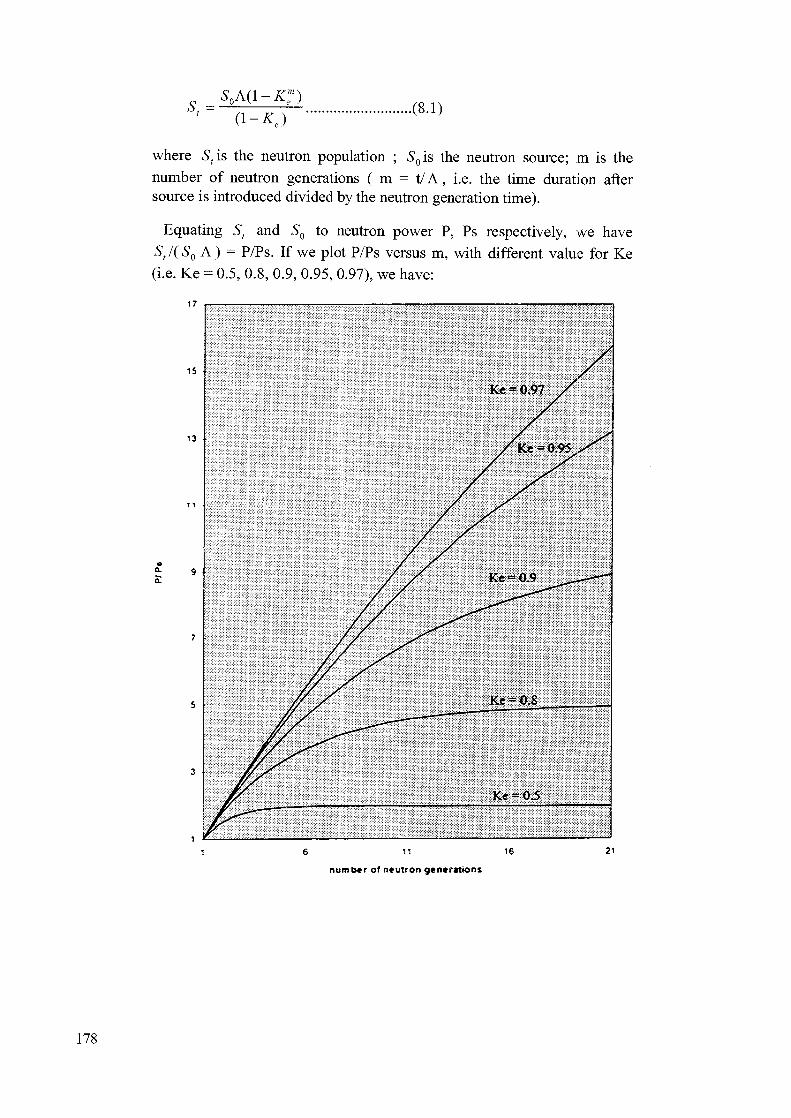
o .(8.1)

where Stis the neutron population ; >Sois the neutron source; m is thenumber of neutron generations ( m = XIA, i.e. the time duration aftersource is introduced divided by the neutron generation time).

Equating St and So to neutron power P, Ps respectively, we haveSt/(S0 A) = P/Ps. If we plot P/Ps versus m, with different value for Ke(i.e. Ke - 0.5, 0.8, 0.9, 0.95, 0.97), we have:

a. 9

6 11 16

number of neutron generations

178

For a subcritical reactor, as Ke is increased, the power levels off moreslowly. As Ke is increased further step by step, a point will finally bereached when the power will increase steadily without leveling off at all,and this is the point where criticality (sustained nuclear fission chainreaction) has been reached i.e. Ke =1. This is the basic method we use forapproaching criticality, by gradually increasing Ke. First let us review thereactor startup instrumentation which makes this startup possible.

8.2 Reactor Instrumentation

Three instrumentation systems are provided to measure reactor thermalneutron flux over the full power range of the reactor.

• Startup instrumentation covers the eight-decade range from 10"14 to 10"6 of full power;

• The ion chamber system extends from 10"7 to 1.5 of full power.

• The in-core flux detector system provides accurate spatialmeasurement in the uppermost decade of power (10 percent to 120percent of full power).

• The fuel channel temperature monitoring system is provided forchannel flow verification and for power mapping validation.

Figure 16 illustrates the range of sensitivity of nuclear instrumentationfor reactor power measurement.

8.2.1 Startup Instrumentation

This system is used on initial plant startup or after a prolongedshutdown, and performs a dual regulating and protective role over thelowest power range when the normal flux measuring instrumentation of theregulating and shutdown systems is off scale. This occurs on the initialreactor startup and during a shutdown of 40 to 70 days or more when thephoto-neutron source decays below the sensitivity of the ion chambersystem.

Two sets of neutron detectors (BF3 counters) are used covering the rangefrom 10~14 of full power up to 10"6 of full power. One set, located in-core,covers the range from spontaneous source level (10~14 full power) to 10"9

full power. The in-core detectors are installed via the vertical viewing portpenetration from the reactivity deck. This instrumentation is removed afterthe low power commissioning period.

179

00

o

fON

o1

o1o

o1

<D

o1

COq1

o01

I J I

s.

II

MX

MX

MX

toX

I

KJX

I J

M

uI

MX

o

J I

» I

097?

IN-CORe INSTRUMENTATION '

IN-CORE FLUX (VIEWINQ PORT)

CO

K

COX

03X

00X

o09

0UT-0F-COR6 (ION CHAMBER HOUSINQ)

8l

OUTOF-COHE INSTRUMENTATION

00

a.o

pwt

mmmJUION CHAMBER SYSTEM .

f

Pft

>

IN-CORE FLUX OETECTOR

The other set of neutron detectors is located out of core in the three sparecavities of the shutdown system number 2 ion chamber housings.

The detector outputs are connected to startup monitoringinstrumentation located temporarily in the main control room. The signalsare processed to give log and linear count rate indications and rate ofchange information. This information is used for protection and monitoringduring the approach to criticality.

In this range, the reactor is controlled manually by the operator fromthe control room. The operator monitors and records the output of theneutron counting instrumentation which is mounted in a mobile cabinet.This instrumentation is divided into three redundant channels and includestrip comparators which are connected into the D, E and F channels of thetrip logic of the shutdown system number 1. Shutdown rods will drop intothe core under any one of the following three conditions:

• The count rate exceeds the setpoint,

• The rate of change is excessive,

• Two or more channels of the instrumentation fail.

On restart after an extended shutdown, the system is normally on-scalewith the out of core detectors; in-core counters are used only on the initialstartup. The arrangement of the system is shown in the following Figure17.

The in-core detectors (or sometimes called counters, or ratemeters),have the flexibility of being moved further out from the core to preventthem from saturating due to increased neutron density during reactorstartup. Typically when counts in the detectors at a particular core positionexceed a certain counts per sec, it is required to move the detectors furtherout to another core position in order to keep its counting rate within theuseable range.

181

oo

a

iera

IBoinB

O

\\

PREAMPLIFIERSCH-D

CH-E

J (JUNCTIONBOXESi i

i ,

DO

CH-FI |

\

—DRYTHIMBLE

IN-COREDETECTORS

\\ DRY HOUSING

\

/ OUT OF CORE/ OETECTORS

P

i

I

L .1 I

PREAMPLIFIERS JUNCTIONBOXES

REACTOR BUILDING

INSTRUMENTATIONCABINET

INTERFACEPANEL

TEST EQUIPMENT

CHANNEL D

CHANNEL E

CHANNEL F

SPARE CHANNEL

6 6

CONTROL ROOM

8.2.2 Ion-Chamber Instrumentation

The ion chamber system is a part of the on-line power measurementequipment of the reactor control system. This instrumentation is on-scaleduring normal operation, and remains on-scale during a normal shutdown.If the shutdown lasts more than 40 to 70 days (depending on reactoroperating history and ion chamber neutron and gamma sensitivity), the fluxdecays below 10"7 of the full power value and startup neutron detectors areneeded.

The ion chamber units consist of lead-shielded housings mounted onthe outside of the calandria shell, in which ion chamber instruments andcalibration shutters are installed. The lead attenuates gamma radiation sothat the ion chambers measure neutron flux, primarily. The output currentfrom separate ion chamber instruments is amplified to generateindependent inputs for the reactor control system and each shutdownsystem, as follows:

a. log neutron power, 10"7 to 1.5 full power,

b. linear neutron power, 0 to 1.5 full power,

c. rate of change of log power, -15 percent to +15 percent of presentpower per second.

Ion chambers measure only the average flux, as seen at the side of thecore, but are sensitive to very low flux levels, for monitoring sub-critical aswell as full power behavior. Because they are outside the calandria, theneutron flux they detect has been attenuated by the moderator and anypoison dissolved in the moderator.

8.2.3 In-Core Flux Detectors

In-core flux detectors are used at high power levels (above 10 percentof full power) because they provide spatial information needed, at highpower, to control xenon-induced flux tilts and to achieve the optimum fluxdistribution for maximum power output.

• Vertical Flux Detector Assemblies

The control system flux detectors are of two types. One type has anInconel emitter and is used for the zone control system. The other type hasa vanadium emitter, and is used for the flux mapping system.

Both types of control system detectors, along with the Inconel detectorsused for the shutdown system number 1 high neutron power trip, arecontained in vertical flux detector assemblies located throughout the core.These assemblies extend from the reactivity mechanisms deck to thebottom of the reactor.

183

• Zone Control Flux Detectors (Inconel)

The self-powered in-core flux detectors are installed in flux detectorassemblies to measure local flux over two decades, 10"1 full power to 1.2full power, in the regions associated with the liquid zone controllers. Ateach location there are two detectors for redundancy.

• Flux Mapping Detectors (Vanadium)

The flux mapping system (described in previous Section) uses vanadiumdetectors distributed throughout the core to provide point measurements ofthe flux. These detectors are almost totally neutron-sensitive; however,their response is delayed by 5.4 minutes due to the half-life of the betaemission from vanadium-52. The signals, approximately 3 uA at fullpower, are fed to amplifiers in a stand alone distributed control systemstation inside the reactor building, where they are multiplexed and sent tothe plant display system computer.

8.3 Methods for Approaching Criticality

For a PHW reactor such as CANDU, there are two methods forapproaching criticality:

1. Remember K^ =s TJ fPfpPth. For large reactor, leakage is very small,hence the fast neutrons non-leakage probabilityPf~\ and the thermalneutrons non-leakage probability Pth~ 1. So the idea for approachingcritically is to maintain moderator level at some low level initially toincur large neutron leakage; then keeping the four factors unchanged,gradually reduce leakage by raising moderator level until enough fuel iscovered to sustain a chain reaction.

2. An alternate method is start at a certain moderator level (nominallynear full calandria) with a high enough boric concentration in themoderator to ensure that criticality cannot be possible. The boron"poison" is then gradually removed until criticality is reached. In thiscase, the leakage is held constant, and the value of f, the thermalutilization factor is increased until Ke becomes equal to 1.

The first method was used in earlier generation of CANDUs - NPD,Douglas Point and Pickering Units 1 and 2. Later generations of CANDUssuch as Bruce, Darlington, which do not have moderator level control; thusthey use the second method for approaching criticality.

Note that these two approaches to critical do not of course have to berepeated every time the reactors are shutdown. Under normal conditions,the photoneutron source provided by the fission product gamma reactionswith deuterium is sufficiently large for the reactor to be started usingautomatic regulation. Only when a reactor has been shutdown for a periodof 3 or 4 months, by which time this photoneutron source will havedecayed, will a manual startup be necessary again.

184

Reactors which do not have a natural photoneutron sources like CANDUsare usually equipped with an artificial source, in the sense that someBeryllium is included in the core which undergoes (y, n) reactions in muchthe same way as deuterium.

8.3.1 Approach Reactor Criticality by Raising Moderator Level

In the first method, the approach to criticality is monitored by devisingan approximate linear plot which can readily be extrapolated to predict thecritical moderator level. From equation 8.1, you will see that

1

count rate• = constant x (1 - Ke) (8.2)

As the moderator level is raised in small steps, the count rates willincrease, and the reciprocal count rates are plotted against moderator level.A plot of inverse count rate versus moderator level will look like this:

ReciprocalCount Rate(cp.s) Critical Moderator Level

Moderator Level (m)

8.3.2 Approach Reactor Criticality by Removing Boron Absorber

In the second method, the approach to criticality is monitored bydevising an approximate linear plot which can readily be extrapolated topredict the critical Boron concentration. It was discussed previously that:

1- = constant x ( 1 - Ke)

count rate

As you recall the definition for AK, this becomes

1 AK

count rate Ke

= A-B-(C-Ccmcal) (8.3)

where A, B are proportionality constants.

185

C - Boron concentration at time t.

CCRITICAL- Boron concentration at criticality.

The procedures used are as follows: the count rate is measured for theinitial boron concentration, and the moderator purification circuit is thenvalves in. Boron is removed for an interval of time ~ 20 minutes, and thecount rate were recorded again. This procedure is repeated a number oftimes and the inverse count rate is plotted against total boron removal time.

ReciprocalCount Rate(cp.s)

Critical Boron Concentrationat this moment

Boron Removal Time (minutes)

hi conjunction with the measurement of inverse count rate vs. Boronremoval time as an indication of criticality, liquid zone control response isalso used by some CANDU station (e.g. Darlington GS) for indication ofcriticality.

The theory is simple: if all the adjuster rods are in "Manual", and theliquid zone control is in "Auto". As Ke gradually approaches 1 by slowlyremoving Boron, liquid zone controllers always control water level atsetpoint, thus making zero reactivity contribution from liquid zone. As Keis very close to 1, and if Boron removal is stopped at that time, and onemakes a small step change in reactor power increase by RRS, the averageliquid zone level will drops (for power increase), if in fact Ke =1, after thedesired power level is reached, the liquid zone level will eventually returnto its original level setpoint after a few minutes. However, if in fact Ke isless than 1, as we explained earlier, the neutron power after initial increasewill level off quickly. Because reactor power cannot reach setpoint, liquidzone level cannot recover quickly to setpoint, and in fact it will continue todrop in order to contribute reactivity for power increase. This is theindication of a subcritical reactor, so Boron removal is resumed for sometime, and then the small step change in reactor power is repeated and theliquid zone level response will be assessed again to determine criticality. hithe simulated reactor startup that we are going to practice, we will use theliquid zone response technique to determine reactor criticality.

186

8.4 Practice Reactor Startup and Approach to Criticality UsingSimulator

1. First load the simulator up and initialize the simulator with the IC =GSS_SD.ic (that is, Reactor in Guaranteed Shutdown State withmoderator overpoisoned).

2. In the Plant Overview screen, you will see the overall plant conditionfrom the annunciators: Turbine trip; Primary Heat Transport System isdepressurized at low pressure < 300 KPa, at temperature 54 deg. C;PHT pumps shutdown.

3. Go to another screen called Reactor SU/SD (startup/shutdown)controls. Here the display represents the reactor startupinstrumentations in combination with certain controls for RRS andLiquid Zone. The details are described as follows :

(a) Special Liquid Zone Controls under the box titled "LIQUID ZONECONTROL MODE". A control push-button is provided forswitching the Liquid Zone Control between "Standard" and"Special Shutdown" Mode. Some explanations are necessary forthese two modes - under normal operating conditions, that is whenreactor power is > 0.1 %, the liquid zone controller is in "standard"mode, that is, the zone level controller signal is proportional to thecombination of reactor power errors and flux tilt errorscomponents. However, when reactor power is less than 0.1 % andat such low power, flux tilt control is not necessary and operatorwill put the zone controller in " Special Shutdown" Mode, meaningthat the zone level controller now responds to local level setpoint asinputted by the operator. The zone level controller is nowproportional to the level errors only. As you will see later, as weapproach criticality, the liquid zone controller will be "kicked" outof "Special Shutdown Mode" into "Standard" mode, when powerlevel is > 0.1 % (-3 decades) and there is a positive power errorpresent.

(b) The reactor startup instrumentations under the box titled "POWERLEVEL READINGS". The instrumentation simulated here are :

• the in-core detectors (counters), which have 3 ranges : Long(long distance from the core); Medium (middle position in thecore); Short (short distance from the core). The IC indicates it isnow in "Long" range.

• as well, the Ion Chambers and Flux Detectors are simulated, butthey are all off-scale, meaning the reactor power is below -6decades.

(c) The reactor power maneuvering rates - PWR LOG rate (DEC/sec);and power error (DEC) are also indicated here for monitoring

187

purposes. The Xenon Load (mk) normally would not be displayedin real situation, but is displayed here for our study and analysis.

(d) SDS1 Reactor trip Setpoint can be set here under titled box "SDS1Trip Setpoint". For safety concern, you always set trip setpoint justslightly above the current the reactor power level, to prevent theunlikely situation of reactor power running away. You can set thesetpoint in % full power or in decades. Currently the SDS1 setpointis set at -2 decades. Remember to raise the SDS1 trip setpoint asthe reactor power level reaches -2 decades. In real situation, therewill be a warning message informing a "pending" reactor NOP(neutron overpower) trip, when the trip setpoint is approaching.

(e) Specific RRS controls are included to provide:

• Alternate Mode reactor power setpoint input. This setpointinput will be processed by RRS to indicate an allowable"Demanded Power Setpoint", which is a slowly rampedsetpoint calculated by the RRS.

• RRS Startup Flag Control - ON/OFF. Note RRS Startup Flag"On" means that the RRS will use a minimum reactor power of-5.9 decades in its calculation.

• Hold Power control - to hold reactor at any time.

(f) Poison Controls are included here for adding (pointer"ADDITION"), removing (pointer "REMOVAL"), or stopping(pointer "STOP") the boron process. For the boron removal, thereis a button that you can use to speedup the boron removal process,but use it with care\ This speedup is not applicable in real lifesituation. The Boron poison load is also indicated for our study andanalysis. It is normally not displayed in real situation. Right now,the boron load is approximately - 60 mk.

(g) The graphical trends are provided here for count rate (counts persec); power log rate (dec/s); ion-chamber detectors (dec); boronpoison load (mk); power error (dec); average zone level (%).

Let us follow the procedures outlined in the table below to performour simulated reactor startup and approach to criticality. The sequenceof steps to be performed should follow the numerical order of the stepsindicated. The symbol =̂> only gives you the highlights on the statusesof the subsystem conditions.

Note:

(1) For our purpose, we can ignore the first step regarding operationsin the PHT regarding the warming up of the pressurizer liquid, andgo to Step #2 right away.

188

(2) The currently simulated startup counters will saturate at 6000 cps atthe "Long" position. One should take the approach of plotting theinverse counts rate versus total boron removal time in order toarrive at the extrapolated "critical" boron concentration. But to savetime for our exercise, we are using the method of liquid zonecontroller response as an approximate indication of "criticality".

Operating Phases1. Initial State: De-

pressurizedcooldown state:HTS temperature <54°C and pressure< 300 KPa. Reactorhas been down for 4weeks.

1. Continued: InitialState: De-pressurizedcooldown state:HTS temperature <54°C and pressure< 300 KPa. Reactorhas been down for 4weeks.

Unit Load

=> Reactorpowerleveldependson howlong thereactorhas been'down'for. Thelast groupof photo-neutronsmodeledhas a halflife of theorder ofdays.

Reactor RRS=> Liquid zones

control inSpecial S/Dmode with alevel setpointof 40%.

=> Adjusterscontrol inmanual

=> Absorbercontrol inauto.

=> Ion chamberwill be off-scale if thereactor power< -6.25Decades

PHT=> HTS in a cold

de-pressurizedstate:

=> HTStemperature <54°C

=> HTS pressure< 300 KPa

=> HTS inventorycontrol is in'SOLID' modeas both thepressurizer andthe bleedcondenser areisolated

=> Bleed flow iscontrolled byCV15, thebleedcondenserlevel controlvalves and thepressureletdown valveMV10 whichis opened at10%.

SDC=> Both side of

the SDC is inservice under'SDC pump'mode.

=> For SDC #2,the flow pathis MV23,MV45, SDCP2, MV31(bypass MV18is closed),Bleed cooler,MV20, MV28,MV29 to RIH#1 &#3.

=> Some bleed toMV10(10%open)&CV15(BleedcondenserLCV) toPurification.The temperingvalveMV19should beclosed.

=> For SDC#1,the flow pathis MV12,MV46, SDCPI, MV2, SDCHX, MV8,MV9 to RIH#2 & #4. Thebypass linevalve MV4 isclosed and theTempering lineMV5 is closed.

SGPC=> In 'Hold'

mode withaSGpressuresetpoint of461 KPa

Check/Monitor

189

2. ReactorApproachingCriticality - Phasel

2. Continued: ReactorApproachingCriticality - Phasel

2. Set RRSStartup flagto 'ON'.(from screenReactorSU/SDControls)

=> Startup flagwill ensurethat the RRSuse aminimumreactor power

•value of-5.9decades in itscalc.

3. RemovePoison by IXcolumnsuntil IonChambersare on scaleand fluxdetector'sresponse topoisonremoval issignificant(powerchangeswithin 1-2minutes).(from screenReactorSU/SD

4. If IonChamber isless than -5.9 decades,inputdemandpower of -5.9 decades.(from screen

SL5. Place all

adjusterrods onManual andfully insertthem intothe core(from screenReactivityControl)

=> LZCSremains inSpecial SDwith a levelsetpoint of40%

1. Turn allpressurizerheaters to'auto' and setthe solidmodepressurizerpressuresetpoint to 7.3MPa(from screenPHT PressureControl)

=> Thepressurizermay take along time towarmupdepending onits initialcondition.(warmup timecan take up to9 hours)

=> Speedupcontrol isavailable toartificiallyspeedupwarmupprocess

=• Circuit #1 & 2both in service.

=> In 'Hold'mode withaSGpressuresetpoint of461 KPa

=> SDS1 poisedwith NOP set atLOW POWERTRIP- 1 %

=> ModeratorPoison additionavailable.

=> Note PowerLevel and ZoneLevel

190

3. ReactorApproachingCriticality- Phase 2

3. Continued: ReactorApproachingCriticality- Phase 2

9.

6. Stop poisonremovalwhen IonChamberindicatesreactorpower > -6decades.(from screenReactorSU/SD

7. Raise powerby inputtinga reactorpowersetpointwhich is 0.3decadeabove thepresentpower, (from

8. Monitor theaveragezone level. Ifthe averagelevelshould dropbelow 25 %,pressthe 'HOLDPOWER'button.(from screen

Note: theaverage zonelevel isavailable asone of the 6trends on thescreen'ReactorSU/SDControls'

Resumepoisonremoval sothat thezones mustrise to holdpower.Monitor thezone levelrises and thereactorpower. As

Monitor time todouble thecount, whichgives someindication ofproximity toCriticality.Adjust range ifcount saturates

LZC will be"kickout" ofSpecial S/DMode onpositive powererror.

191

3. Continued: ReactorApproachingCriticality- Phase 2

the zonesrises to 70%, stoppoisonremoval.Note reactorpower andzone level.(from screenReactorSU/SDControls)

10. Repeat Steps7, 8, 9 untilafter areactorpower SPincrease, theaveragezone leveldrops, andreturns towithin 5%of theoriginallevel after afew minutes.(from screenReactorSU/SDControls)

11, Stop Poisonremoval.Enter aslight powerSP decrease.If the zonerises andpower dropsand then thezones returnto theoriginal

level (+/- 5 %),thenReactor isdeclaredCRITICAL.(from screenReactorSU/SDControls)

12. ResumePoisonremovaluntil theaveragezone level isaround 60%, andpowerholding.(from screenReactorSU/SDControls)

192

9.0 From Simple Point Kinetic Reactor Model to High Fidelity Model

9.1 Spatial Kinetic Model for PHW Reactor

Now that we have developed a simple point kinetic reactor model with 6fission products groups and 9 photoneutron groups, it would be a logicalevolution at this point to consider a more sophisticated model such as thespatial kinetic reactor model. In the following sections, we will bediscussing the techniques used in building such model. Because thedevelopment of a spatial kinetic reactor model will involve certain amountof time, so we might just discuss the underlying theories and thetechniques and it is hoped that the materials that we cover here willprovide enough background materials for the students to try out thesimulation development by themselves.

9.2 Nodal Approach for Simulating Space-Time Reactor Kinetics

Traditionally, two different approaches have been proposed in the real-time simulation of space-time kinetics. One Approach is based on modalkinetic formulation (1). The other approach is based on Avery's coupledregion kinetics theory (2).

hi a typical coupled nuclear reactor model, the reactor core is dividedinto a number of nodes axially and radially. The usual considerations forthe choice of the nodes are the core symmetry and the accuracy required inthe description of neutron flux distributions, and the execution time of thenodal kinetic model. For a reactor core divided into 14 zones, the temporalnodal fluxes are computed by the following nodal kinetic equations usingAvery formulation (3).

(9.1)

For Zone

dN.1 dt

dt

i,

(1-

i-

A

/ :/

14

= 1,2,3

Nj A"

= 1,2,

= 1,2,..

vNj N

14

l C ^

14

...6

14

/=1

(9.2)

where:

Nj = Neutronic fluxes in Zone i, respectively (nodal fluxes)

lm = Decay constants of the mth delayed neutron group

b = Total delayed neutron fraction

193

j3m = Delayed neutron fraction of the mth group

Kij = "Coupling Coefficient" determining the probability of a neutronborn in zone j producing a fission neutron in zone i in thenext generation.

AmCmj = Partial power of zone j contributed from the mth delayedneutron group.

Cmj = Concentration of delayed neutron group m in zone j

// = Mean neutron life time

Equation (9.1) can be rewritten by regrouping the couplingcoefficients for zone i,

1 4

m=\

i = l,2,3 14

The above respective terms represent the various contributions ofneutronic flux changes in zone i from the following sources:

(a)

is the rate of neutronic flux changes in zone i due to the its zone reactivity.

(b)

K 6

h m=\

is the rate of neutronic flux changes in zone i due to its concentration ofdelayed neutron groups.

(c)

(X-B) 14

is the rate of neutronic flux changes in zone i due to the coupling effects ofthe neutronic fluxes in the other 13 zones.

194

(d)

is the rate of neutronic flux changes in zone i due to coupling effects fromthe concentration of delayed neutron groups in the other 13 zones.

By introducing the definition of reactivity AKi = (Kii -1)/Kii, equation(9.3) can be written as:

dNj (AKj -p) , . \ p i* ^ v^ v -KT +

at J\j m=i i=i,i*ii 14 6

7 ^^^ ij ^^^ w mjL' MJ« m=I (9.4)

Where

K

Equation (9.4) is almost identical to point kinetic model for reactor zone i,with the exception of an extra zone coupling source terms:

14 ^ 14

a,. Y,ijj 7 2 Xl m=l

If we absorb the "zone coupling effects" into "the zone i reactivity termApii" and rewrite the point kinetic equations for zone i:

14

Ni

at A, m=i (9-5)

Where

Apii is the zone i reactivity change.

Apij is the reactivity change for zone i due to coupling effects in zone j

195

It can be seen that equation (9.6) involves the calculation of couplingcoefficient Kij. These coefficients Kij define the probability of a neutronborn in node j producing a fission neutron in node i in the next generation.

In Avery's formulation(2), the coupling coefficients for the two energygroups of neutrons are given by the following equations:

(jhh(f) = real thermal flux at position r

(j) /r) = adjoint fast flux at position r

(/>jth(r) = contribution to §th(r) from fission neutrons produced innode

j in the previous generation with distribution Ef(jhh(r)

Kij involves the computation of the distribution of the real thermal fluxand adjoint fast fluxes which usually involves a lot of CPU time. It wouldbe impractical to compute these fluxes in real-time environment. To dealwith this problem, an approximate method (3) is implemented to computethe coupling coefficients in real time using a perturbation form (relative tothe equilibrium values):

Ky = Ky + gy (y.5)

where Ky = nominal value of Kij (nominal coupling coefficients)

gy = change in coupling coefficients in node i due to perturbation

in node j

gy can further be defined as

14

k=\

where Pk = net reactivity perturbation in zone k (mk).

KiJk= change in coupling coefficient in node i due to node j with +1.0

mk change in reactivity in node k (normalized perturbationgradient).

Rewriting equation (9.8),

• It can be seen that the implementation of this approximation methodinvolves two major components - the nominal couplingcoefficients, Ky , and the normalized perturbation gradients, Kijk.

• Ky can be computed off-line for a given (nominal) core condition and

configuration by using equation (9.7), for all i, j .

• The core is perturbed from nominal core condition by changingreactivity in one zone, say zone #1 and equation (9.7) is used again to

197

calculate the new coupling coefficients Kij off-line, for all i, j . With theuse of equation (9.10), KtJl can be obtained for all i, j . Repeat the same

for other zone to obtain Kijk, for k= 2, ...14.

• Store K°j and Kjjk as coefficients in the computation for Ap y in

equation (9.6).

Equation (9.6) is computed every simulation iteration, and Ap tj is14

obtained for all i, j and they provides inputs to a summer 2^ P v •> which

in turn inputs into the reactivity change "input" of the affected reactorzone.

9.3 Summary of Model Formulation for PHW Reactor

Here is the summary of the essential modeling details for the spatialkinetic model:

• 14 point kinetic models are used respectively to simulate the 14 reactorzones inside the core.

• Each point kinetic model will calculate the neutron power based on 6different neutron delay groups and 9 photoneutron groups, and theoverall change in reactivity.

• The change in reactivity will be a function of control devices (e.g.adjusters), concentration of xenon, voiding in channels, power changes,reactor zones reactivity coupling effects and safety shutdown devices. (See Fig 18, and Fig. 19).

• The decay heat calculation assumes that 3 separate decay productgroups exist, each with a different decay time constant.

• An arithmetic average flux from the 14 reactor zones is used in thedecay heat calculation.

• The reactor fuel elements are divided into 4 lumped channels. The totalheat generated from the fuel as calculated using the average reactorflux is assumed to be divided equally among the 4 lumped channels.

• Each channel is assumed to have its own coolant flow, and its ownlumped fuel element. The temperature of the lumped fuel element ineach channel is calculated, and the lumped fuel sheath temperature willbe used in the coolant heat transfer calculation.

• hi the spatial reactor, the reactivity change includes:

1. 8 independent lumped adjuster banks, there is an equal reactivitysplit between 14 zones

198

2. 2 independent lumped absorber banks, there is an equal reactivitysplit between 14 zones.

3. liquid zones; the individual zone level will affect the respectivereactivity change in its designated zone reactor.

4. reactivity changes due to temperature changes, which is assumed tobe proportional to the power changes.

5. reactivity change due to voiding.

6. reactivity due to burnup in fuel.

Fig. 18 Spatial Kinetic Reactor Model

RRS

Power Error

Reactivity Change due toadjusters, absorbers,shutdown rods and fuelburnup

Average Zone Level

Average Reactor Flux

Zone Controller 1Zone 1 CV Position

Reactor Zone V

Reactor Zone 1 Flux & Level

Zone Controller 2Zone 2 CV Position

Reactor Zone 2*

Reactor Zone 1 Flux & Level

Zone 3 to 13 Zone 3 to 131

Zone Controller14

Zone 14 CV PositionReactor Zone 14*

Average ReactorFlux Calculation

To Decay Heat,RRS

Average ZoneLevel Calculation

Flux Mapping

LTo Display

Reactor Zone 14 Flux & Level

reactivity changes due to temperature change, xenon poisoning and voiding arewithin each reactor zonecoupling is modelled between each neighbouring zones according to prescribed formula

199

Fia.19 Reactor Model Zones Configuration

(A) For each Zone Reactor, the point kinetic equations and the governingequations for various reactivity feedbacks are:

1. The total delayed neutron fraction is the summation of the neutronfraction of the 6 neutron groups, 9 photoneutron groups

is

(9-3-1)

Pi — total delayed neutron fraction

Pi = group i delayed neutron fraction (i=l,2,3,4,5,6);

for i = 7, ...15, Pi is the photoneutron delayed group faction.

2. The delayed neutron groups concentration can be expressed as:

dO &

dt TNEUTWN i=l,....15 (9.3-2)

Ci = concentration of 6 delayed neutron groups,

and 9 photoneutron groups.

X[ = decay constant of delayed neutron groups.

Pi = group i delayed neutron fraction (i=l,2,3,4,5,6)

( i = 7, ....15 for photoneutrons delayed fraction)

NpLUX = t°tal neutron flux in zone(norm)

^NEUTRON = mean neutron lifetime(sec)

200

3. The rate of change of neutron flux in a point kinetic model can beexpressed as:

(AK-J3i)*NFLUX

dt TNEUTRON (9.3-3)

NpLux = total neutron flux in zone(norm)

^NEUTRON = m e a n neutron lifetime(sec)

Ci = concentration of delayed neutron groups.

X{ = decay constant of delayed neutron groups.

Pi = group i delayed neutron fraction (i=l,2,3,4,5,6)

i = 7,... 15 belongs to photoneutron delay groups fraction

AK = overall neutron reactivity change (K)

4. NpLux c a n b e calculated by solving above equations, using backwardEuler's expansion.

NFTJIX1 +X. , AiNFLUX =

TNEUTRON

where:

t Ai*Ci*AtAl = ;

M*/3i*AtBl —

(1 + M * At) * TNEUTRON (9.3-4)

Npj^ux'= total neutron zonal flux from previous iteration(norm)

5. The overall reactivity change is expressed as:

AK = AKC + AKP + AKV + AKXE + AKSDS + AKFUEL + AKDIFF

(9.3-5)

AK = overall neutron reactivity change (K)

AKc = neutron reactivity change due to control devices (K)

AKp = overall neutron reactivity change due to power changes (K)

201

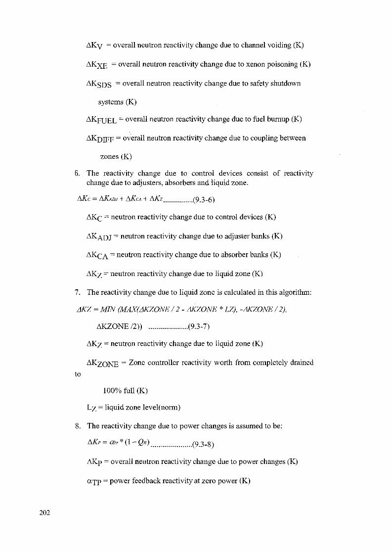
AKy = overall neutron reactivity change due to channel voiding (K)

= overall neutron reactivity change due to xenon poisoning (K)

= overall neutron reactivity change due to safety shutdown

systems (K)

= overall neutron reactivity change due to fuel burnup (K)

AKrjjpp = overall neutron reactivity change due to coupling between

zones(K)

6. The reactivity change due to control devices consist of reactivitychange due to adjusters, absorbers and liquid zone.

AKc = AKADJ + AKCA + AKz (9.3-6)

= neutron reactivity change due to control devices (K)

= neutron reactivity change due to adjuster banks (K)

- neutron reactivity change due to absorber banks (K)

= neutron reactivity change due to liquid zone (K)

7. The reactivity change due to liquid zone is calculated in this algorithm:

AKZ = MIN (MAX(AKZONE / 2 - AKZONE * LZ), -AKZONE / 2),

AKZONE12)) (9.3-7)

= neutron reactivity change due to liquid zone (K)

Zone controller reactivity worth from completely drained

to

100% full (K)

Lz — liquid zone level(norm)

8. The reactivity change due to power changes is assumed to be:

AKP = OTP * (1 - QR) (9.3-8)

AKp = overall neutron reactivity change due to power changes (K)

a j p = power feedback reactivity at zero power (K)

202

= heat transfer to coolant(norm)

9. Assuming there are I coolant channels in the reactor zone, the reactivitychange due to channel voiding is assumed to be:

NI

wherePu = XEi - XEFP (Q 3_m

AKy = overall neutron reactivity change due to channel voiding (K)

AKyo = maximum neutron reactivity change due to channel voiding

(K)

N = neutron flux squared weighting factor for channels

Pl i = effective boiling length in channel i(i=channel 1,...I)

XEi = effective exit quality in channel i(i=channel l,...I)(norm)

XEpp- effective exit quality in channel at full power(norm)

10. The reactivity change due to xenon poisoning is assumed to be:

AKXE = 0.001 *(27.93 - CXE)/14 (9.3-10)

= overall neutron reactivity change due to xenon poisoning (K)

= xenon concentration

11. The formation of xenon is assumed to be from the decay of iodine aswell as from the initial fission products. The concentration of xenoncan be found using the following rate equations.

= 9.445£ - 3 * NFLUX - 2.2,1 HE -5*Cidt

= 9.167E- 4* NFLUX + 2.8717E- 5* Ci-dt

(2AE- 5 + 3.5E - 4 * NFLUX) * CXE (9.3-11)

Cj = iodine concentration

~ xenon concentration

= tota^ neutron flux in zone(norm)

203

12. The reactivity change due to Zone Coupling effects:

Ap v = A,X

6 A

N, 1 z°W+

N, /, N,.(9.3-12)

Where

14

(9.3-13)k=\

a,=

(see previous section 9.2 for definition of symbols).

(B) The Overall Reactor

• Referring to figure 18 above. Reactivity changes AK due totemperature change, xenon poison buildup, voiding, are modeledwithin each point kinetic reactor model.

• The reactivity changes due to zone coupling effects are calculatedseparately for each zone. The zone coupling effects for a particularzone due to all other zones are then summed up and entered as one ofthe reactivity change inputs for that reactor zone.

• The reactivity change due to fuel burnup are calculated for one wholereactor, and split up among the 14 zones according to certain criteria -e.g. zones near the center of the reactor would have more contributionthan the outer zones.

• The reactivity change due to 2 banks of absorbers (total reactivityworth - 9 mk) are calculated for one whole reactor, and split up amongthe 14 zones according to certain criteria - e.g. some weighting factorsrelated to the proximity of the absorber location relative to the zones

• The reactivity change due to 8 banks of adjusters (total reactivity worth+17 mk) are calculated for one whole reactor, and split among all the14 zones according to certain criteria - e.g. some weighting factorsrelated to the proximity of the adjuster location relative to the zones

204

The total neutron power from the 14 zones reactor (each normalized)will be summed up and then divided by 14 to get the normalizedoverall reactor power. As well, each zonal power will provide into toFlux Mapping routine for display.

All the zone levels will be summed up and divided by 14 to get theaverage zone level to RRS.

The power error inside the reactor is defined as:

_, NFLUX - PDEM , , . , NFLUX — NFLUX _ .PERR = h KRATE * ( RD)

NFLUX At * NFLUX

However, under reactor trip, stepback, or if the shutdown rods are fullyinserted, the power error is always set to 0.05.

power error(norm)

= average corrected neutron flux(norm)

' = a v e r a S e corrected neutron flux at the previous iteration

(norm)

= demanded reactor power(norm)

= power error control gain

= demanded power rate of change(/sec)

The absorber banks drive logic is as follows:

1. If the absorber banks control is set to auto mode, then the absorberbanks will move according to the power error versus zone levelplot below.

2. In the 'DRIVE 1 BANK IN' region, the absorber bank 1 will bedriven in first, and bank 2 will start to drive in when bank 1 iscompletely driven in.

3. In the 'DRIVE 2 BANKS IN' region, both banks will be driven insimultaneously.

4. Similarly, in the 'DRIVE 1 BANK OUT' region, the absorber bank2 will be driven out first, and bank 1 will start to drive out whenbank 2 is completely driven out.

5. In the 'DRIVE 2 BANKS OUT' region, both banks will be drivenout simultaneously.

205

DRIVE 2BANKS OUT

1

ABSORBER BANKS AUTO MODE CONTROL

11

h * |

r

i i

_ty

DRIVE 1BANK OUT

I I

100

LIQUID ZONE

-80 * —

-T5

50

I |

LEVEL(%)

DRIVE 1BANK IN

" "1i

i

1

1

1

1

1

1

1i

1 1

DRIVEBANK!

-6 -5 - 3 - 2 - 1 0 1 2

POWER ERROR(%)

The adjuster rods banks drive logic is as follows:

1. If the adjuster banks control is set to auto mode, then the adjusterbanks will move according to the power error versus zone levelplot below.

2. In the 'DRIVE 1 BANK IN' region, the adjuster bank will be drivenin an 'ascending bank number' manner, i.e. only one bank will betraveling at a time, and the next bank will start to drive in when thelast bank is completely driven in, and the rest of the banks will bedriven in this sequential order.

3. In the 'DRIVE 2 BANKS IN1 region, both banks will be driven insimultaneously.

4. Similarly, in the 'DRIVE 1 BANK OUT' region, one adjuster bankwill be driven out in the 'last in first out' manner, and next bankwill start to drive out when the traveling bank is completely drivenout.

5. In the 'DRIVE 2 BANKS OUT' region, 2 banks will be driven outsimultaneously.

206

ADJUSTER BANKS AUTO MODE CONTROL

100

DRIVE 2BANKS OUT

— •

DRIVE 1BANK OUT

I I I I

t

|

.

Ti

LIQUID ZONE

, - - t -

50

I

13— " — -

| |

LEVEL(%)

I

DRIVE 1BANK IN

I

I I I I-5 -4 - 3 - 2 - 1 0 1 2

POWER ERROR(%)

• The absorber and adjuster traveling speed is calculated based on powererror and is described below. Under reactor stepback conditions, theabsorber will take 3.5 seconds to completely dropped into the core.

ADJUSTER/ABSORBER RODS SPEED PLOT

ABSORBER/ADJUSTERTRAVEL SPEED(%)

- 1 0 1 2

POWER ERROR(%)

• The actual absorber/adjuster position will be calculated from theprevious absorber/adjuster position and its speed, if electrical power isavailable.

207

• The reactivity change worth of the adjuster and the absorber banks areassumed to be:

AKCA = ^~_ABSRiwoRTH * (MAX(-l,MIN(0,

(-0.001267 + 0.13904 * Sou + 2.32103 * SCAI2 +1.16576 * SCM3 )))

AKADJ = J^.ADJWORTH * (MAX(0, MIN(l,

(1.02293 - 0.484729 * SM - 2.8621 * SA,2 + 2.34474 * 5A;3 )))

= neutron reactivity change due to absorber banks(K)

= neutron reactivity change due to adjuster banks (K)

A B S R J W O R T H = total reactivity change worth of absorber bank

i(K)(i=l,2) = total -9 mk for 2 banks

= total reactivity change worth of 1 adjuster bank (K) =

total +17 mk for 8 banks

i = absorber bank i position (norm)(i=l,2)

S>Ai = adjuster bank i position (norm)(i=l,8)

2 banks of shutdown rods of equivalent worth are modeled. Whenreactor trips, the banks of shutdown rods will drop in together. Therods will remain "in" until the shutdown system is "reset". (This occursafter the reactor trip button has been reset). Once the shutdown systemis "reset", shutdown rods bank 2 will be pulled out first. AfterShutdown rod Bank 2 is completely pulled out, Shutdown rod bank 1begins to withdraw. Note the rods insertion speed is different than thatof the rods 'pull-out' speed.

The reactivity change due to safety-shutdown rods are assumed to be:

AKSDS = ] T ^ AKsDSMAX * (MAX(0, MIN{\, (SDSIPOS)))

AKgj)g = neutron reactivity change due to shutdown rods (K)

AKSDSMAX = reactivity change due to shutdown rods when

fully inserted(K) = total -68 mk for 2 shutdownrods

208

9.4 Coupled Reactor Kinetics Reference

1. Luxat, J.C., " The Potential of a Generalized Modal Analysis ofPostulated Loss-of-Coolant Accidents in CANDU Reactors", NuclearTechnology, Vol. 46, Mid-Dec 1979.

2. Avery, R., "Theory of Coupled Reactors", Proc. 2nd Int. Conf. OnPeaceful Uses of Atomic Energy, Geneva, September 1958, 8/1958,p.182-191.

3. Chou, Q.B., et al, "Development of a Low-Cost Spatial CANDUReactor Simulation Program for Power Plant Control Studies",Proceedings of 1975 Summer Computer Simulation Conference, SanFrancisco, California, July 21-23, 1975.

209

Typical Workshop Agenda

Session 1 -

1. Introduction to Various Modular Modeling Systems

1.1 Integral Components of a Modular Modeling System

1.2 Simulation Development System for Control Room Replica FullScope Simulator (ROSE, CETRAN)

1.3 Simulation Development System for PC based Full Scope, PartScope, or Principle Simulator (MMS, APROS, CASSIM)

1.4 Technology Trends for Modular Modeling System

1.5 Introductory Hands-On Exposure to CASSIM™

2. Dynamic Simulation Fundamental

2.1 Introduction to Mathematical Modeling and Physical Laws

2.2 Overview of Dynamic Simulation for Power Plant Process

2.3 Numerical Methods & Other Important Model Considerations

2.4 Simple Modeling Example (2 Tanks) with CASSIM™

3. CASSIM™ Simulation Fundamentals

3.1 Merging Models with CASSIM™

3.2 Thermalhydraulic Modeling with CASSIM™ Hydraulic FlowNetwork (HFN)

3.3 Creating a simple CASSIM Algorithm

4. Reactor Model Development

3.4 Quick Overview of Nuclear Reactor Kinetics

3.5 Simple Point Kinetic Reactor Model - Basic Equations &Analytical Solution

3.6 Development of the Point Kinetic Reactor Algorithm

Session 2 -

1. Wrap Up Point Kinetic Reactor Model Development

2. Effects of Neutron Sources on Reactor Kinetics

2.1 Effects of neutron sources on Reactor at Power and Shutdown

210

2.2 Photoneutron Sources in Heavy Water Reactors

2.3 Modify Point Kinetic Reactor Algorithm with PhotoneutronSources

2.4 Discussion

3. Reactivity Feedback Effects

3.1 Overview of Reactivity Feedback Effects: Fuel Burnup andBuildup; Fission Products Poisoning; Coolant Void ReactivityFeedback; Temperature Feedback Effects

3.2 Xenon/Iodine Poison - Basic Equations and Dynamics

3.3 Developing Xenon/Iodine Model

3.4 Discussion

Session 3 -

1. Overview of Reactor Control for Different Reactors

1.1 Brief Overview of BWR, PWR, RBMK Reactor Controls

1.2 Overview of PHWR Reactivity Control Mechanisms & ReactorRegulating System (RRS)

2. PHW Reactor Regulating System (RRS) Familiarization UsingSimulator

2.1 Familiarization with Generic CANDU Simulator

2.2 Simulator Exercises related to PHW Reactor Control

3. Simulator Exercises continued for PHW Reactor Control

4. Reactivity Control Mechanism Modeling - Liquid Zone

4.1 Liquid Zone Hydraulic Modeling

4.2 Liquid Zone Reactivity Control Modeling

Session 4 -

1. Reactivity Control Mechanism Modeling Continued

1.1 Develop Adjuster Rods Model

1.2 Develop Absorber Rods Model

2. Reactor Shutdown System Modeling

2.1 Develop Reactor Shutdown Rods Model

211

3. Model Integration for Simple Reactor

3.1 Integrate Reactor Model + Xenon-Iodine Poison Model +Adjuster& Absorber & Shutdown Rods Model + Liquid Zone Model

3.2 Testing & Discussion

Session 5 -

1. Practice Reactor Startup and Approach to Criticality using PHWR

Simulator

2.1 Subcritical Reactor Behavior

2.2 Reactor Instrumentation

2.3 Methods for Approaching Criticality2.4 Practice Reactor Startup and Approach to Criticality Using

Simulator

2. From Simple Model to Higher Fidelity Nuclear Reactor Models

2.1 PHWR Model with Spatial Kinetics & Demonstrations

2.2 Nodal Approach for Simulating Space-Time Reactor Kinetics

2.3 Summary of Model Development for PHW Reactor

2.4 Model Development Roadmap & Discussion

212

APPENDIX

Selected CAS SIM™ Algorithms Descriptions

Algorithm #102: PUMP_SIM, Simple Centrifugal Pump

Purpose & Descriptions:Note: the pump manufacturer normally provides pump performance diagramsfor users -(a) Pump power (at certain specific gravity and speed) versus mass flow rate.(b) Total dynamic head (at certain specific gravity and speed) versus massflow rate andNet Positive Suction Head (N.P.S.H.) required.

The pump model is a simple centrifugal pump dynamic model which utilizesthe pump's manufacturer performance data for the following computation:1. The pump static head is calculated as proportional to the product of the

design static head and the square of normalized pump speed. Otherfactors such as pump degradation and fluid density changes relative to thedesign density are taken into account in the calculation. That means as thepump is starting up, the pump static head will be increasing and will be ona quadratic rise to the design static head as the speed increases.

2. The pump power is computed as quadratic function of pump mass flow,using curve-fit technique on the pump performance curve to obtainrespective constants (KP1, KP2, KP3) for the quadratic function.

3. Heat dissipated by the pump frictional loss is calculated as a fraction ofpump power

4. Cavitation factor is calculated as (suction pressure - saturation pressure) /N.P.S.H.

Note that the CAS SIM hydraulic network solution scheme is represented by anodal diagram which involves identifying control volumes (known as nodes)within the simulated hydraulic flow circuit. The flow between these nodes,called link flow, can be obtained from the linearized momentum equationgoverning the pressure differentials across these nodes. Each node pressurecan be obtained from mass balance around the nodes. In the present networksolution scheme, the pump static head is assigned to the link in which themomentum equation is expressed as :link mass flow is proportional to the square root of {pressure at suction nodeof the pump + the static head of the pump - discharge node pressure}. Thepump dynamic head is calculated in the link block in which the pump islocated. For details on additional hydraulic flow network solution techniques,refer to CTI's document "CASSIM™ Thermohydraulic Flow NetworkSolutions - Techniques & Examples"

Scope of Application:Physical effects simulated:• Static head calculation as function of speed, fluid density changes and

pump efficiency.• Pump power as a function of mass flow.

213

• Heat dissipation as pump frictional loss.• Cavitation factor is calculated.

Limitations or effects not simulated:• Pump rundown and flywheel effects are not simulated.

Validity check:• Cavitation factor should be checked if it is near or equal to 1.

Range of Operation:• Full range of operation with the exception of pump cavitation.

Special Requirements & Assumptions:• None.

Input Specifications (ALG102):

Input Descriptions

1. Pump motor speed

2. Pump mass flow

3. Not used4. Fluid density

5. Pump suctionPressure

6. Fluid saturationpressure

7. Pump degradationfactor

Analog(A)/Digital (D)A

A

A

A

A

A

EngineeringUnits

Normalized

Kg/sec

Kg/m3

KPa

KPa

Normalized

Connection Details

Connect to the speed output tag of the motor block forthe pump.Connect to the link flow output tag of the link block inwhich the pump is located

This can be inputted from a table look-up function orjust a constant tagname (SConstant) if it is a constantConnect to pressure output tag of the suction pressurenode blockThis can be inputted from a table look-up function orjust a constant tagname (SConstant) if it is a constant0 - no degradation; 1-100 % degraded. This can beinputted from a table look-up function or just a constanttagname (SConstant) if it is a constant. Usually it isobtained from the pump efficiency specification.

Output Specifications (ALG102):

OutputDescriptions/

Transform1. Pump static head

(Gl)2. Cavitation factor

(G2)3. Pump power (PM1)4. Heat loss (Ql)

Analog (A)/Digital (D)

A

A

AA

EngineeringUnits

KPa

Normalized

KWKW

Connection Details

Connect to pump static head input tag of the linkblock in which the pump is located.For indication

For indication and electrical motor current calculationFor calculation of pump heat to the pumping fluid.

214

Coefficient Specifications (ALG102):

CoefficientDescriptions

1. Design static head2. Fluid Design

Density3. Required NPSH4. Pump power factor

KP15. Pump power factor

KP26. Pump power factor

KP3

Analog (A)/Digital (D)AA

AA

A

A

EngineeringUnitsKPa

Kg/M3

KPaKW

KW/(Kg/sec)

KW/(Kg/sec)2

Calculation Details

This is normally obtained from pump specificationThis is normally obtained from pump specification

This is normally obtained from pump specificationThis is obtained from curve-fit to pump performancecurveThis is obtained from curve-fit to pump performancecurveThis is obtained from curve-fit to pump performancecurve

215

Algorithm # 106: VLV_ONOFF_SM, Simple ON-OFF Valve

Purpose & Descriptions:1. This simple valve model allows user to specify the type of valve to be used:

linear; equal percentage; quick opening.2. The model checks for motive force for the valve. Usually for pneumatic

control valve, the motive force is instrument air with a constant pressure asspecified by the valve manufacturer. On total loss of motive force, the valveis either failed open, or failed closed. On partial loss of motive force, thevalve will fail in mid-position on a graduated scale between fully open tofully closed position, being proportional to the value of the degraded motiveforce signal at the time.

3. The valve model accepts the solenoid valve status and drives the valve stemposition to the fully opened position when the solenoid is energized and fullyclosed when the solenoid is de-energized. The stem position will travel in afirst order lag fashion. The time constant for the lag is a function of thestroking time constant for the valve.

4. The stroking time for the valve is defined as the time required for the valvestem to travel from the fully closed position to the stem position at maximumCv on a step-change in control signal from fully closed requested to fully

opened requested.5. The normalized valve port area is calculated based on the type of valve

specified by the user. For linear valve, the normalized port area is equal tothe stem position; for equal percentage valve, the normalized port area is aquadratic function of valve stem position; for quick opening valve, the portarea is proportional the cube of stem position.

Scope of Application:Physical effects simulated:• Motive force (e.g. instrument air signal) for the valve.• 3 types of valve can be specified: linear, equal %, quick opening• Valve can fail open, closed, or failed to desired position.

Limitations or effects not simulated:• Valve cavitation is not calculated in the model• If the valve characteristics is known, and it does not fit the linear, equal

% or the quick opening, an extra block(ALG152-CURVEFIT) can becreated to calculate the effective port-area, using the stem positionoutput(OUT(2)) from this block as an input to the CURVEFIT block.

Validity check:• Valve will not operate if motive force is not provided.

Range of Operation:• Full range of valve operation, provided motive force is kept constant and

is greater than the motive force required to fully open and close thevalve.

Special Requirements & Assumptions:• None

216

Input Specifications(ALG106):

Input Descriptions

1. Valve solenoidsignal2. Valve Malfunction -

"Fail to position -On":

3. Valve Malfunction -"Fail to position-magnitude ":

4. Motive Force

Analog(A)/Digital (D)D

D

A

A

EngineeringUnits

nil

nil

Normalized

Depends onmotive forcemedium:Pneumatic(KPa);electronic (mA,ormV)

Connection Details

Connect to the solenoid valve status. A datavalue of 1=fully open, and 0= fully closedConnect to Non-Moveable block which gets inputs fromgraphical user interface for inserting malfunction.1 means malfunction active; 0 means malfunctioninactiveConnect to Non-Moveable block which gets inputs fromgraphical user interface for inserting malfunction. Thedatavalue of this input represents the stem position thevalve is failed to.(e.g.:l=open, 0 =close, 0.5=half open)This can be connected to instrument air source, orpower supply source, depending on the motive forcemedium. If these sources are not modelled, just enter aconstant with appropriate value ($Constant). For thevalve to stroke the full range, the datavalue of this inputmust be greater than the data-value of COF(3)(motiveforce required to fully open) and the data-value ofCOF(4)(motive force required to fully closed)

Output Specifications(ALG106):

OutputDescriptions/Transform1. Valve port area(ZA1)2. Valve stem position

(ZS1)3. Valve fully opened(FO1)

4. Valve fully closed(FC1)

5. Valve stem positionin%(ASl)

Analog(A)/Digital (D)A

A

D

D

A

EngineeringUnits

Normalized

Normalized

Nil

Nil

%

Connection Details

Connect to the valve area input tag of the link block inwhich the valve is located.For indication

Connect to logic blocks for control or indication. Thisfully opened limit switch is set at stem position > 98%Connect to logic blocks for control or indication. Thisfully closed limit switch is set at stem position < 2%Connect to logic blocks for control or indication

217

Coefficient Specifications(ALG106):

CoefficientDescriptions1. Valve stroking time

2. Type of Valve3. Motive forcerequired

to fully open

4. Motive forcerequired

to fully close

5.Stem position atmaximum Cv

Analog (A)/Digital (D)A

AA

A

A

EngineeringUnitssec

NilDepends onmotive forcemedium:Pneumatic(KPa);electronic(mA, or mV)Depends onmotive forcemedium:Pneumatic(KPa);electronic(mA, or mV)Normalized

Connection Details

This is normally obtained from the valve specification.This stroking time is defined as the time required toopen the valve from fully closed to a stem position atmaximum Cv

1 = Linear; 2= Equal %; 3= Quick OpenThis is normally obtained from the valve specification

This is normally obtained from the valve specification

This is normally obtained from the valve specification.A typical value of 90% can be assumed.

218

Algorithm # 108: CVJSIM, Simple Control Valve

Purpose & Descriptions:1. This simple valve model allows user to specify the type of valve to be used:

linear; equal percentage; quick opening.2. The model checks for motive force for the valve. Usually for pneumatic

control valve, the motive force is instrument air with a constant pressure asspecified by the valve manufacturer. On total loss of motive force, the valveis either failed open, or failed closed. On partial loss of motive force, thevalve will fail in mid-position on a graduated scale between fully open tofully closed position, being proportional to the value of the degraded motiveforce signal at the time.

3. The valve model accepts control signal (normalized) from controller anddrives the valve stem position to follow the control signal command in a firstorder lag fashion. The time constant for the lag is a function of the strokingtime constant for the valve.

4. The stroking time for the valve is defined as the time required for the valvestem to travel from the fully closed position to the stem position at maximumCv on a step-change in control signal from fully closed requested to fully

opened requested.5. The normalized valve port area is calculated based on the type of valve

specified by the user. For linear valve, the normalized port area is equal tothe stem position; for equal percentage valve, the normalized port area is aquadratic function of valve stem position; for quick opening valve, the portarea is proportional the cube of stem position.

Scope of Application:Physical effects simulated:• Motive force (e.g. instrument air signal) for the valve.• 3 types of valve can be specified: linear, equal %, quick opening• Valve can fail open, closed, or failed to desired position.

Limitations or effects not simulated:• Valve cavitation is not calculated in the model• If the valve characteristics is known, and it does not fit the linear, equal

% or the quick opening, an extra block(ALG152-CURVEFIT) can becreated to calculate the effective port-area, using the stem positionoutput(OUT(2)) from this block as an input to the CURVEFIT block.

Validity check:• Valve will not operate if motive force is not provided.

Range of Operation:• Full range of valve operation, provided motive force is kept constant and

is greater than the motive force required to fully open and close thevalve.

Special Requirements & Assumptions:• None

219

Input Specifications(ALG108):

Input Descriptions

1. Control Signal

2. Valve Malfunction -"Fail to position -On":

3. Valve Malfunction -"Fail to position-magnitude ":

4. Motive Force

Analog(A)/Digital (D)A

D

A

A

EngineeringUnits

Normalized

nil

Normalized

Depends onmotive forcemedium:Pneumatic(KPa);electronic (mA,or mV)

Connection Details

Connect to control signal output tag of PID controllerblockConnect to Non-Moveable block which gets inputs fromgraphical user interface for inserting malfunction.1 means malfunction active; 0 means malfunctioninactiveConnect to Non-Moveable block which gets inputs fromgraphical user interface for inserting malfunction. Thedatavalue of this input represents the stem position thevalve is failed to.(e.g.:l=open, 0 =close, 0.5=half open)This can be connected to instrument air source, orpower supply source, depending on the motive forcemedium. If these sources are not modelled, just enter aconstant with appropriate value ($Constant). For thevalve to stroke the full range, the datavalue of this inputmust be greater than the data-value of COF(3)(motiveforce required to fully open) and the data-value ofCOF(4)(motive force required to fully closed)

Output Specifications(ALG108):

OutputDescriptions/Transform1. Valve port area(ZA1)2. Valve stem position

(ZS1)3. Valve fully opened

(FO1)4. Valve fully closed

(FC1)5. Valve stem position

in%(ASl)

Analog(A)/Digital (D)A

A

D

D

A

EngineeringUnits

Normalized

Normalized

Nil

Nil

%

Connection Details

Connect to the valve area input tag of the link block inwhich the valve is located.For indication

Connect to logic blocks for control or indication. Thisfully opened limit switch is set at stem position > 98%Connect to logic blocks for control or indication. Thisfully closed limit switch is set at stem position < 2%Connect to logic blocks for control or indication

220

Coefficient Specifications(ALG108):

CoefficientDescriptions1. Valve stroking time

2. Type of Valve3. Motive forcerequiredto fully open

4. Motive forcerequired

to fully close

5.Stem position atmaximum Cv

Analog (A)/Digital (D)A

AA

A

A

EngineeringUnitssec

NilDepends onmotive forcemedium:Pneumatic(KPa);electronic(mA, or mV)Depends onmotive forcemedium:Pneumatic(KPa);electronic(mA, or mV)Normalized

Connection Details

This is normally obtained from the valve specification.This stroking time is defined as the time required toopen the valve from fully closed to a stem position atmaximum Cv

1 = Linear; 2= Equal %; 3= Quick OpenThis is normally obtained from the valve specification

This is normally obtained from the valve specification

This is normally obtained from the valve specification.A typical value of 90% can be assumed.

221

Algorithm #128: TANK, Simple Storage Tank with Heating

Purpose & Descriptions:1. An overall mass balance is performed by this algorithm to calculate the

mass accumulation in the tank based on the inlet and outlet flowrate. Thelevel in the tank can also be calculated based on the mass accumulation inthe tank, the fluid density, and the tank's orientation.

2. An energy balance is also used to calculate the temperature of the fluid inthe tank. The temperature is calculated assuming a constant heat capacity.Enthalpy can also be used in place of temperature, as long as the units forINP(3), and OUT(3) are consistent. However, if OUT(3) is chosen torepresent enthalpy, COF(6) the Cp of the fluid must be set to 1.

3. If the level in the tank is greater than the overflow height, overflow of theliquid will result. A simple first order lag is used to model the overflow.

4. When the level in the tank falls below the elevation at which the outletpipe is connected to the tank(KEMPTY), the outlet flow should decrease.The outlet flow is assumed to be decreased to zero, when the level falls to20% of KEMPTY. The tank level factor is used as a measure to reduce theoutlet flow when the level in the tank falls below KEMPTY.

Scope of Application:Physical effects simulated:• Overall mass balance to calculate the liquid level inside the tank• Overall energy balance to calculate the liquid temperature inside the tank• Liquid overflow will occur, when the liquid level inside the tank exceeds

the overflow limit• Tank level factor reflecting the required reduction in outflow when the

tank liquid level falls below the elevation at which the outlet pipe isconnected to the tank.

Limitations or effects not simulated:• Only fluid in single phase can be considered.• Reverse flows at the input of the tank is not allowed.• No pressure calculation inside the tank. The pressure is assumed to be

constant.• The density of liquid in the tank is assumed to be constant

Validity check:• If reverse flows are simulated, additional blocks must be used to calculate

overall input and output flowrates with respect to the tank.• Check for two phase fluid.

Range of Operation:

222

Special Requirements & Assumptions:• All fluids are in single phase, no boiling or condensation takes place in

the tank.• The properties Cp of both fluids are assumed constant within the range of

their temperature range.• Only 1 overall inlet flow and 1 overall outlet flow is modelled. If more

than one inlet flow or outlet flow exists, additional blocks will berequired to calculate the overall inlet and outlet flows.

• The energy balance for the tank assumed perfect mixing for the tank.

Input Specifications(ALG128):

Input Descriptions

1. Inlet flowrate

2. Outlet flowrate

3. Inlet temperature

4. Heat input

Analog(A)/Digital (D)A

A

A

A

EngineeringUnits

Kg/sec

Kg/sec

°C

KJ/S

Connection Details

Connect to the link flow, output tag of the link block inwhich the fluid stream 1 is located. Or if more than oneinlet flow exists, use a mixing node block(ALG151) tocalculate the combined inlet flowrate.Connect to the link flow, output tag of the link block inwhich the fluid stream 2 is located. Or if more than oneinlet flow exists, use a summer block(ALG312) tocalculate the combined outlet flowrate.Connect to the block which calculate the temperature ofthe inlet stream. Or if more than one inlet flow exists,use a mixing node block(ALG151) to calculate thecombined inlet temperature. If enthalpy is used insteadof temperature, COF(6) must be set to one.Connect to the block which calculate the external heatinto the tank. Any heat loss should be combined to thisvalue.

Output Specifications(ALG128):

OutputDescriptions/Transforml.TankLevel(Ll)

2. MassinTank(Ml)

3. Temperature in Tank

4. Tank Overflow(FMl)

5. Tank levelFactor(Gl)

Analog(A)/Digital (D)A

A

A

A

A

EngineeringUnits

M

Kg

°C

Kg/sec

Normalized

Connection Details

Connect to equipment requiring the tank level. Thisoutput is required to be initialized with the design dataat the full power steady state point.This output is required to be initialized with the designdata at the full power steady state point.Connect to equipment or heat balances requiring thetemperature of the liquid in the tank or leaving thetank. This output is required to be initialized with thedesign data at the full power steady state point.This can be connected to the hydraulic flow network asan external flow.Connect to the hydraulic flow link which calculate theoutlet flow from the tank. If the tank level is greaterthan level at which outlet flow begins to reduce, thevalue of this output should be one.

223

Coefficient Specifications(ALG128):

CoefficientDescriptions1. Orientation flag2. Tank radius

3. Tank height/length

4. Overflow height

5 Maximum outflow

6: Cp of liquid7: Density of liquid

8: Overflow lag9: level at which outlet

flow begins to reduce

Analog (A)/Digital (D)DA

A

A

A

AA

AA

EngineeringUnitsNilM

M

M

Kg/sec

KJ/Kg/°C

Kg/M3

secM

Calculation Details

0 = horizontal; 1 = verticalThis value should be obtained from the equipmentmanufacturerThis value should be obtained from the equipmentmanufacturerThis value should be obtained from the equipmentmanufacturerCan be estimated from the normal outlet flows bymultiplying that value by 130%For water Cp = 4.16 KJ/Kg/°C

For water at 40 °C density =992.3 Kg/M3

A default value of 2 seconds can be assumedThis value should be obtained from the equipmentmanufacturer

224

Algorithm # 133: BREAKER, Breaker

Purpose & Descriptions:1. This algorithm simulates a typical breaker, with breaker close and breaker

open status as outputs. Breaker alarms indications are also modelled.

2. The inputs for the breaker algorithm includes close and open command,trip command, trip relays, and malfunctions.

3. The operation of the breaker can be summarized by the following logicdiagram.

CLOSECOIvl

OPENCOM

TRIPCOM

OLTRIP

UVTRIP

ELTRIP

MALFO

IvlALFCMALCPF

BCSTAT

BOSTAT

BTRBL

BPROT

BDEMT

BCPFI

CLOSECOM = command to close breakerOPENCOM = command to open breakerTRIPCOM = command to trip breakerOLTRIP = overcurrent trip relay 51UVTRIP = undervoltage trip relay 27ELTRIP = ground protection trip relay 64MALFO = failed open malfunctionMALFC = failed close malfunctionMALCPF = control power failure relay 8BCSTAT = breaker closed statusBOSTAT = breaker open statusBTRBL = breaker trouble alarmBPROT = breaker protection trip operatedBDEMT = breaker demanded to tripBCPFI = breaker control power failure indication

Scope of Application:Physical effects simulated:• Breaker status• Breaker alarm indications

Limitations or effects not simulated:Validity check:

225

Range of Operation:Special Requirements & Assumptions:

Input Specifications (ALG133):

Input Descriptions

1. Command to close

2. Command to open

3. Command to trip

4. Overcurrent trip

5. Undervoltage trip

6. Ground protectiontrip

7. Failed openmalfunction

8. Failed closedmalfunction

9. Control powerfailure

Analog(A)/Digital (D)D

D

D

D

D

D

D

D

D

EngineeringUnits

Nil

Nil

Nil

Nil

Nil

Nil

Nil

Nil

Nil

Connection Details

Connect to the block where the command to close thebreaker is calculated. Typical a control macro block isused, and the On/start command should be connected tothis input.Connect to the block where the command to open thebreaker is calculated. Typical a control macro block isused, and the Off/stop command should be connected tothis input.Connect to the block where the command to trip thebreaker is calculated. Typical a control macro block isused, and the trip open command should be connectedto this input.Connect to the block where the overcurrent trip iscalculatedConnect to the block where the undervoltage trip iscalculatedConnect to the block where the ground protection trip iscalculatedConnect to the non-movable block which modelled thismalfunctionConnect to the non-movable block which modelled thismalfunctionConnect to the non-movable block which modelled thismalfunction

Output Specifications (ALG133):

OutputDescriptions/Transform1. Breaker close status(BC1)

2. Breaker open status(BO1)

3. Breaker trouble alarm(Dl)

4. Breaker protectiontrip

operated(D2)5. Breaker demanded to

trip(D3)6. Control power failure

indication(D4)

Analog(A)/Digital (D)D

D

D

D

D

EngineeringUnits

Nil

Nil

Nil

Nil

Nil

Nil

Connection Details

This output should be initialized. This breaker outputcan be connected to motor blocks as a command tostart.This output is for indication only. This should alwaysbe the inverse of OUT(l)

If the electrical circuit is modelled, then this outputshould be connected to the electrical circuit blocks.

Coefficient Specifications (ALG133): None

226

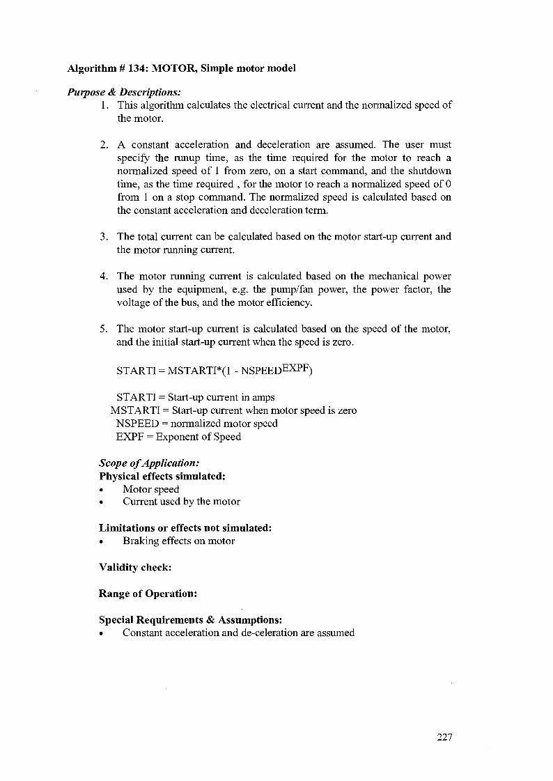
Algorithm # 134: MOTOR, Simple motor model

Purpose & Descriptions:1. This algorithm calculates the electrical current and the normalized speed of

the motor.

2. A constant acceleration and deceleration are assumed. The user mustspecify the runup time, as the time required for the motor to reach anormalized speed of 1 from zero, on a start command, and the shutdowntime, as the time required , for the motor to reach a normalized speed of 0from 1 on a stop command. The normalized speed is calculated based onthe constant acceleration and deceleration term.

3. The total current can be calculated based on the motor start-up current andthe motor running current.

4. The motor running current is calculated based on the mechanical powerused by the equipment, e.g. the pump/fan power, the power factor, thevoltage of the bus, and the motor efficiency.

5. The motor start-up current is calculated based on the speed of the motor,and the initial start-up current when the speed is zero.

STARTI = MSTARTI*(1 - NSPEEDEXPF)

STARTI = Start-up current in ampsMSTARTI = Start-up current when motor speed is zeroNSPEED = normalized motor speedEXPF - Exponent of Speed

Scope of Application:Physical effects simulated:• Motor speed• Current used by the motor

Limitations or effects not simulated:

• Braking effects on motor

Validity check:

Range of Operation:

Special Requirements & Assumptions:• Constant acceleration and de-celeration are assumed

227

Input Specifications(ALG134):

Input Descriptions

1. Start/stopcommand

2. Pump/fan power

3. Bus voltage

Analog(A)/Digital (D)A

A

A

EngineeringUnits

Nil

KJ/sec

KV

Connection Details

Connect to the block where the command to start/stopthe motor is calculated. Typical a breaker block is used,and the breaker close status is used to drive this input.Connect to the block where the pump/fan power iscalculated. For centrifugal pumps, the pump power iscalculated in the pump dynamics blocks(ALG102,PUMP_SIM)Connect to the block where the bus voltage is calculated

Output Specifications(ALG134):

OutputDescriptions/Transform1. Motor Speed

2. Acceleration3. Start-up current4. Running current5. Total current

Analog(A)/Digital (D)A

AAAA

EngineeringUnits

Normalized

norm/secamperesamperesamperes

Connection Details

This value should be connected to a pump dynamicsblock(ALG102 PUMP_SIM) as an indication of motorspeed. It can be connected to any block which requirednormalized motor speed.

If the electrical circuit is modelled, then this outputshould be connected to the electrical circuit blocks.

Coefficient Specifications(ALG134):

CoefficientDescriptions

1. Run-up time to fullspeed

2. Run-dwon time tozero speed

3. Current calculationflag

4. Power conversionfactor

5. Reference powerfactor

6. Motor efficiency

7. Motor start-upcurrent

8. Exponent of speedin currentcalculation

Analog (A)/Digital (D)A

A

A

A

A

A

A

A

EngineeringUnitssec

sec

Nil

Nil

Normalized

amperes

Nil

Calculation Details

This value should be obtained from the equipmentmanufacturer.This value should be obtained from the equipmentmanufacturer.If this coefficient is set to zero, then the currentcalculation is by-passed.This value should be set to 1 if the bus voltage and thepump power are in the units KV, and KW.A typical value of 0.85 can be assumed

This value should be obtained from the equipmentmanufacturer. A typical value of 0.9 can be assumedThis value should be obtained from the equipmentmanufacturer. A typical value of 5*the running currentat design conditions can be assumed.A typical value of 0.25 can be assumed

228

Algorithm # 140: CONDUCTJFI, incompressible flow conductance

Purpose & Descriptions:1. This algorithm predict the flow in a link using incompressible flow

momentum equation.

W = K*VAL*(Pup-Pdown)0-5

2. Check valve is modelled for this link.

Scope of Application:Physical effects simulated:• The flow through the link as predicted by incompressible flow equation

Limitations or effects not simulated:• Static head from pump or elevation difference are not considered. The

user has to modelled static heads in a separate block and account for themin the upstream pressure input term.

• 2-phase flow effects are not modelled.

Validity check:

Range of Operation:

Special Requirements & Assumptions:• If more than 1 valve exists on the same link, the effective valve port-area

can be found by assuming the overall effective port-area = themultiplication of all the port-areas on the same link.

229

Input Specifications(ALG140):

Input Descriptions

1. Inlet Pressure

2. Outlet Pressure

3. Valve position

Analog(A)/Digital (D)A

A

A

EngineeringUnits

KPaa

KPaa

Normalized

Connection Details

Connect to node pressure output tag of the node blockin which the inlet pressure is located.Connect to node pressure output tag of the node blockin which the outlet pressure is located.Connect to the block where the overall valve port-areais calculated.

Output Specifications(ALG140):

OutputDescriptions/Transform1. Total outflow(FMl)

Analog(A)/Digital (D)A

EngineeringUnits

Kg/sec

Connection Details

May be connected to the hydraulic network or tankblock to preserve mass balance or use as indication.

Coefficient Specifications(ALG140):

CoefficientDescriptions1. Rated flowconductance

2. Check valve status

Analog (A)/Digital (D)A

D

EngineeringUnitsKg/KPa0-5

Nil

Calculation Details

This value is calculated by dividing the mass flow by thesquare root of the pressure difference of the upstreamand downstream node at design conditions.Enter 1 if check valve is present else enter 0

230

Algorithm #223: RSFF, Reset — Set (RS) Flip Flop

Purpose & Descriptions:This algorithm simulates a logical R-S Flip flop element:• Input #1 designates the "Set" signal; whereas " Input #2 designates the

"Reset" signal; Coefficient #1 dictates whether "Set" Overrides "Reset" ( ifvalue of the coefficient #1 = 1), or "Reset" overrides "Set" (if value of thecoefficient #1 =0).

• Assuming that Coefficient #1 = 0, (i.e. Reset overrides Set), when the Setsignal is equal to 1 (logical true) and Reset signal is equal to 0 (logicalfalse), then Output 1 is equal to 1 and "latched in". Output 2 is theinversion of Output 1, therefore equal to 0.

• hi the event that Reset signal is equal ! (logical true) when the Set signal isequal 1, Output 1 is always equal to 0 (logical false); Output 2 is alwaysequal to 1 (logical true), due to the Reset override.

• The output 1 latched-in state will be reset to 0 (logical false), as soon as theReset signal becomes 1 (logical true).

• The truth table representation for the R-S Flip Flop is as follows:Note that Output 1 & 2 in each row represent logical states correspondingto different logic states of inputs and coefficients.

Set InputState00011110

Reset InputState01100110

CoefficientState10101010

Output 1State00011010

Output 2State11100101

The truth table below represents a typical sequence of events for the outputlogic states evolution corresponding to Set Signal & Reset Signal withCoefficient = 0

EventSequence1234

Set InputState

1000

Reset InputState

0010

CoefficientState

0000

Output 1State

1100

Output 2State

0011

Scope of Application:

Physical effects simulated: Not applicable.

Limitations or effects not simulated: Not applicable.

Validity check: Not applicable.

231

Range of Operation:• Input values are either 0 (logical false) or 1 (logical true). No

intermediate values between 0 and 1 are allowed.Special Requirements:• None.

Input Specifications (ALG #223):

Input Descriptions

1. Set Input2. Reset Input

Analog(A)/Digital (D)DD

Output Specifications(ALG #223)

OutputDescriptions/Transform1. Output 12. Output 2

Analog(A)/Digital (D)DD

EngineeringUnits

NilNil

Connection Details

•

EngineeringUnits

NilNil

Connection Details

Coefficient Specifications (ALG #223):

CoefficientDescriptions1. Coefficient 1

Analog (A)/Digital (D)D

EngineeringUnitsNil

Calculation Details

0 = Reset overrides Set; 1 = Set overrides Reset

232

Algorithm #232: Comparator, Single Analog Comparator with Deadband

Purpose & Descriptions:This algorithm simulates a single analog comparator (e.g. level switch,temperature switch, pressure switch, etc.) with the following functions::1. Using the coefficient #1, the user specifies whether the comparator is to

check if the input is "less than" the comparator setpoint (coefficient #1 =0), or "greater than" the comparator setpoint (coefficient #1 = 1).

2. The comparator setpoint is entered by the user in coefficient # 2.3. If deadband for the comparator setpoint is required, it will be entered by

the user in coefficient #34. Output #1 provides status indication on whether analog input is "less than"

or "greater than" the comparator setpoint (see (1) above).5. Output #2 provides comparator setpoint as specified by the user in

coefficient #2.

Scope of Application:Physical effects simulated:

• The effects of a comparator switch (e.g. level switch etc.)

Limitations or effects not simulated: Not applicable

Validity check: Not applicable

Range of Operation:• Input values can assume any values from -99999999.99999999 to

+99999999.99999999Special Requirements:• None

233

Input Specifications (ALG # 232):

Input Descriptions

1. Analog Input

Analog(A)/Digital (D)A

EngineeringUnits

Nil

Connection Details

Connect to process variable (e.g. flow, temperature,pressure, etc.)

Output Specifications (ALG #232):

OutputDescriptions/

Transform1. Digital Output (Dl)

(status indication onwhether analog inputis less than orgreater thansetpoint.)

2. Comparator setpoint(Al) (equated tocoefficient #2)

Analog(A)/Digital (D)D

A

EngineeringUnits

Nil

Nil

Connection Details

If the analog input is less than or greater than thesetpoint (depending on coefficient #1); this output willbe "1" ; else, it will be "0". This output is usuallyconnected to alarm and control logic etc.

mainly for announcing the comparator setpoint valueto other blocks.

Coefficient Specifications (ALG #232):

CoefficientDescriptions1. Comparison

specification: "Lessthan" or Greaterthan"

2. ComparatorSetpoint

3. Comparatordeadband

Analog (A)/Digital (D)D

A

A

EngineeringUnitsNil

Theengineeringunit is thesame as thatfor analoginputTheengineeringunit is thesame as thatfor analoginput.

Calculation Details

0 = less than setpoint1 = greater than setpoint

If no deadband is required, enter 0

234

Algorithm #236: DELTAJNP, A Input = (Current Input — Previous Input)

Purpose & Descriptions:This algorithm performs the following functions:1. It stores the input value from the previous iteration, then it takes the

difference between the current input value (in current iteration) and theprevious input value (in previous iteration).

2. The difference ( or called A input) is equated to output #1.3. Output #2 provides the absolute value of the A input.4. Output #3 stores the input value for the previous iteration.5. Output #4 is a flag to indicate whether the algorithm has executed at least

once.

Scope of Application:

Physical effects simulated: Not applicable

Limitations or effects not simulated: Not applicable

Validity check: Not applicable

Range of Operation:Input values can assume any values from -99999999.99999999 to+99999999.99999999

Special Requirements:• None

235

Input Specifications (ALG #236):

Input Descriptions

1. Analog Input

Analog(A)/Digital (D)A

EngineeringUnits

Nil

Connection Details

Output Specifications (ALG #236):

OutputDescriptions/

Transform1. (Current Input -

Previous Input)(Al)

2. Absolute value of(Current Input -Previous Input)(A2)

3. Previous InputValue (A3)

4. First time throughflag (Dl)

Analog(A)/Digital (D)A

A

A

D

EngineeringUnits

Nil

Nil

Nil

Nil

Connection Details

Mainly for storing previous input value

Mainly for storing flag status

Coefficient Specifications (ALG # 236): None.

236

Algorithm #241: SPEEDER_GEAR, Steam Turbine speed/load changer gear

Purpose & Descriptions:This algorithm simulates a simple speed/load changer gear for a rotationalequipment such as a steam turbine, or gas turbine etc. Usually the position of thespeeder gear controls the position of the speed/load governor:1. Users can specify the rate of the speeder gear movement from 0 % governor

position to 100 % governor position (or vice versa). The rate can beexpressed respectively as Fast Time or Slow Time in the coefficientspecifications:

2. Fast Time (coefficient #1) is the tune in seconds specified by the user for thespeeder gear to move from 0 % to 100% position, if the gear is selected (viaInput #4 = 1) to move at the fast rate.

3. Slow Time (coefficient #2) is the time in seconds specified by the user for thespeeder gear to move from 0 % to 100% position, if the gear is selected (viaInput #5 = 1) to move at the slow rate.

4. Control commands to raise or lower the speed/load changer gear are receivedat Input #1 and #2 respectively. If there is no speeder gear failure signal (atInput #3 (Fail to Position) = -1), and there is no Manual control signal (atInput # 6 = 0), the speeder gear will move to a new position with eachincrement of DT, the rate of gear movement is determined by whether thefast or slow rate is selected (Input #4 = 1 or Input #5 = 1).

5. The normalized speeder gear position is continuously updated hi Output # 1.6. When the speeder gear has reached its maximum limit, Output #2 will be

equal to 1.7. When the speeder gear has reached its minimum limit, Output #3 will be

equal to 1.8. Malfunction signal of the speeder gear can be sent to Input #3. Any value

other than "- 1.0" will be treated as the speeder gear "fail-to-position" value.9. If manual control of the speeder gear is required, send a digital signal to Input

#6 which will switch the gear to manual control. The analog value specifiedin Input #7 will indicate the desired manual controlled position of the gear.

Scope of Application:Physical effects simulated:• Simple turbine speed/load changer gear.

Limitations or effects not simulated:• Effects of governor hunting are not simulated

Validity check:• None

Range of Operation:• All digital input signals assume value either "0" or " 1".• All analog input signals assume normalized value.

Special Requirements:• None

237

Input Specifications (ALG # 241):

Input Descriptions

1. Raise Speed/LoadGear

2. Lower Speed/LoadGear

3. Speeder Gear"Fail-to-position"value

4. Fast Rate Selected5. Slow Rate Selected6. Manual Control

Selected7. Manual Control

Signal

Analog(A)/Digital (D)D

D

A

DDD

A

EngineeringUnits

Nil

Nil

Normalized

NilNilNil

Normalized

Connection Details

Connect to control signal

Connect to control signal

Connect to malfunction block output. If there is nomalfunction, enter $ constant with value = -1.

Connect to governor control logicConnect to governor control logicConnect to manual control logic

Connect to manual control logic

Output Specifications (ALG #241):

OutputDescriptions/Transform1. Speed/Load Changer

Gear Position (Zl)2. Gear at maximum

position (HL)3. Gear at minimum

position (LL)

Analog(A)/Digital (D)A

D

D

EngineeringUnits

Normalized

Nil

Nil

Connection Details

Connect to speed relay, servomotor and governorcontrol valveFor status indication

For status indication

Coefficient Specifications (ALG # 241):

CoefficientDescriptions1. Fast Time2. Slow Time

Analog (A)/Digital (D)AA

EngineeringUnitssecondsseconds

Calculation Details

NilNil

238

Algorithm #312: 5_SUM, Sum of 5 Inputs

Purpose & Descriptions:This algorithm add 5 Analog Inputs together and produce the sum at the

Output:

Output #1 = Input #1 * Coefficient #1 + Input #2 * Coefficient #2 +Input #3 * Coefficient #3 + Input #4 * Coefficient #4 +Input #5 * Coefficient #5

1. Coefficient #1 to #5 are multiplying factors to be used for individualAnalog Input, if it is necessary to scale respective inputs for the addition.

Scope of Application:

Physical effects simulated: Not applicable

Limitations or effects not simulated: Not applicable

Validity check: Not applicable

Range of Operation: Not applicable

Special Requirements: Not applicable

239

Input Specifications (ALG #312):

Input Descriptions

1. Analog Input # 12. Analog Input #23. Analog Input #34. Analog Input #45. Analog Input #5

Analog(A)/Digital (D)AAAAA

EngineeringUnits

NilNilNilNilNil

Connection Details

Output Specifications (ALG # 312):

OutputDescriptions/

Transform1. Output (A 1)

Analog(A)/Digital (D)A

EngineeringUnits

Nil

Connection Details

Coefficient Specifications (ALG # 312):

CoefficientDescriptions1. Multiplying Factor

for Input #12. Multiplying Factor

for Input #23. Multiplying Factor

for Input #34. Multiplying Factor

for Input #45. Multiplying Factor

for Input #5

Analog (A)/Digital (D)A

A

A

A

A

EngineeringUnitsNil

Nil

Nil

Nil

Nil

Calculation Details

240

Algorithm #332: PIDJMALF, Proportional + Integral + Derivative Controllerwith Controller Malfunction

Purpose & Descriptions:This algorithm is exactly the same as ALG #330, except that controllermalfunction is added for its output to fail to any demanded position.1. This algorithm represents a proportional + Integral + Derivative Controller.

2. The mathematical formulation for the simple controller is as follows:Output = Proportional Term + Integral Term + Derivative TermThe normalized controller output is continuously updated at Output #1.;whereas the controller output signal in % is displayed at Output #15Output #2 displays Error signal = Process Variable (PV) - Setpoint (SP).Output #3 displays the Proportional Term calculated in the algorithm.Output #4 displays the Integral Term calculated in the algorithm.Output #5 displays the Derivative term calculated in the algorithm.

3. The controller algorithm computes the error signal at Output #2 based on a"forward-acting" action: i.e. Forward-Acting: Error = Process Variable(PV) - Setpoint (SP). However, most controller action is Reverse-Acting:Error = Setpoint (SP) - Process Variable (PV). Hence Coefficient #4 canbe used to determine what the controller action should be( Coefficient #4: 0 means Forward Acting; 1 means Reverse Acting).

4. The controller has 4 modes of operations:(a) Auto Mode - In Auto Mode, the Setpoint (SP) is provided by local userinput. The

controller output is determined by the P + I + D control action taken bythe controller.Auto mode can be requested from two sources :(i) Man-Machine Interface (MMI) - Input #2(ii) Internal logic from Model - Input #3When Auto mode request is accepted, Output #6 will indicate that thecontroller is in Auto Mode.In Auto Mode, the Setpoint signal comes from Man-Machine Interface(MMI)-Input #16.

(b) Manual Mode - In Manual Mode, automatic controller action isdisabled. User manually

controls the controller's output.Manual Mode request is received at Input #4 through MMI request andwhen it is accepted, Output #7 will indicate that the controller is inManual Mode.In Manual Mode, the Manual control signal comes from Input #20 viaMMI input.

(c) Remote Setpoint Mode (RSP) - In RSP Mode, the Setpoint (SP) isprovided NOT by the

user, but by the internal logic.RSP Mode can be requested from two sources:(i) Man-Machine Interface (MMI) - Input #6(ii) Internal logic from Model - Input # 7

241

When RSP mode requested is accepted, Output #8 will indicate that thecontroller is in RSP Mode.In RSP Mode, the Setpoint signal comes from the Model via Input #17.

(d) Tripped-To-Manual Mode - When the controller is in any of theabove control modes, if Input #5 is "true" (= 1), the controller will be"tripped to Manual". Output #7 will indicate that the controller is inManual; whereas Output #27 will indicate that the controller has been"tripped to manual". Logic Model may send a Manual Control signalat Input #21, in order to set the controller output to a desired value,should the controller be "tripped to Manual".The " Tripped to Manual" mode will be reset when Input #27 is "true".When that happens, Output #27 will be reset to "0", and the controllerwill remain in "Manual" mode ((b) above).

5. There is a provision to "track" a controller when Input #14 (TrackCommand) is "true" ( = 1). When that happens, regardless of what modethe controller is in, the controller output #1 will follow the signal providedat Input #15 (Track Value). Output #9 will indicate that the controller is in"TRACK".

6. The controller can be locked in a particular mode:Input #11= Lock AutoInput #12 = Lock ManualInput #13= Lock RSPIt is important for the user to make sure that the'lock" signals for the 3modes (Input #11, #12, #13) cannot be applied simultaneously.When the mode "lock" signal is accepted, Output #10 will indicate that thecontroller is in "lock".

7. The controller can be inhibited from "Auto", "Manual" or "RSP" mode viarespective Input #8, Input #9 and Input #10. The "Inhibit" function willprevent the inhibited mode from being set. When a mode inhibit functionoccurs, Output #12, #13, #14 will display the mode inhibited functionrespectively.

8. The controller accepts "feedforward" bias via Input #18 for MMI, or viaInput #19 for Model input.

9. Usually the controller tuning constants: Proportional Gain, Reset Time, SetTime are set by the respective coefficient #1 , #2, #3. However, thisalgorithm provides a tuning provision with which the user can tune thecontroller "on-line" by sending a "controller tune" request at Input #22.When that happens, Proportional Gain can be provided at Input #23; ResetTime at Input #24; Set Time at Input #25.

10. The controller output can have a low and high limits specified by the userrespectively at the Coefficient #5 and #6.

11. Note that for the purpose of interfacing to Labview GUI, a specialalgorithm #457 has been designed to interface with this algorithm. Seedetails in ALG # 457.

12. This algorithm accepts controller malfunction request via Input #28 (failedcontroller flag); and via Input #29 (failed controller output position) If thecontroller has failed, then the controller output will be set to equal Input#29.

242

Scope of Application:

Physical effects simulated: Not applicable

Limitations or effects not simulated: Not applicable

Validity check: Not applicable

Range of Operation: Not applicable

Special Requirements: Not applicable

243

Input Specifications (ALG # 332):

InputDescriptions

1. Process Variable(PV)

2. MMI Auto ModeRequest

3. Model Logic AutoMode Request

4. MMI ManualMode Request

5. Model Trip toManual Request

6. MMI RSP ModelRequest

7. Model Logic RSPRequest

8. Inhibit Auto Mode9. Inhibit Manual

Mode10. Inhibit RSP Mode11. Lock Auto Mode

Request12. Lock Manual

Mode Request13. Lock RSP Mode

Request14. Controller Track

Command15. Controller Track

Value16. MMI Setpoint

Signal17. Model Logic

Setpoint Value18. MMI

Feedforwardbias

19. Model LogicFeedforward bias

20. MMI ManualControl signal

21. Model LogicManual ControlSignal

22. MMI ControllerTuning Request

23. MMIProportional Gain

24. MMI Reset Time25. MMI Set Time26. MMI to set

Controller Action:Forward Acting orReverse Acting.

Analog (A)/Digital (D)A

D

D

D

D

D

D

DD

DD

D

D

D

A

A

A

A

A

A

A

D

A

AAD

EngineeringUnitsto follow input

Nil

Nil

Nil

Nil

Nil

Nil

NilNil

NilNil

Nil

Nil

Nil

Normalized

to follow input

to follow input

Normalized

Normalized

Normalized

Normalized

Nil

Units of PropTerm/Units ofErrorsecsecNil

Connection Details

See 4(a) above

See 4(a) above

See 4(b) above

See 4(d) above

See 4(c) above

See 4(c) above

See 7 aboveSee 7 above

See 7 aboveSee 6 above

See 6 above

See 6 above

See 5 above

See 5 above

See 4(a) above

See 4(c) above

See 8 above

See 8 above

See 4(b) above

See 4(d) above

See 9 Above

See 9 above

See 9 aboveSee 9 aboveSee 9 above.0 = Forward Acting; 1 = Reverse Acting

244

27. MMI to Reset"Tripped toManual"

28. Controller FailedFlag

29. Controller OutputFailed Position

D

D

A

Nil

Nil

Normalized

See 4(d) above

See 12 Above

See 12 Above

Output Specifications (ALG # 332):

OutputDescriptions/

Transform1. Controller Output

Signal (Zl)2. Error Signal (ER1) =

(PV - SP)3. Proportional Term

(Al)4. Integral Term (A2)5. Derivative Term (A3)6. Controller in Auto

Mode (Dl)7. Controller in Manual

(D2)8. Controller in RSP

(D6)9. Controller in Track

(D3)10. Controller in Lock

(D4)11. Controller Mode

(A13)0 = Auto; 1=Manual; 2 = RSP

12. Auto Mode Inhibited(D7)

13.Manual ModeInhibited (D8)

14.RSP Mode Inhibited(D9)

15.Controller OutputSignal (A4)

16.Controller Tune Flag(D5)

17.Proportional Gainregistered (A5)

18. Reset TimeRegistered (A6)

19. Set Time Registered(A7)

20.Controller ActionRegistered: ForwardActing or ReverseActing (A8)

Analog(A)/Digital (D)A

A

A

AAD

D

D

D

D

A

D

D

D

A

D

A

A

A

A

EngineeringUnits

Normalized

to follow PV &SPNormalized

NormalizedNormalizedNil

Nil

Nil

Nil

Nil

Nil

Nil

Nil

Nil

%

Nil

Units of Prop.Term/Units ofErrorsec.

sec.

Nil

Connection Details

Connect to control device

For algorithm internal use

For algorithm internal use

For algorithm internal useFor algorithm internal useFor Labview pop-up interface, see connection detailsin ALG # 457For Labview pop-up interface, see connection detailsin ALG # 457For Labview pop-up interface, see connection detailsin ALG # 457For Labview pop-up interface, see connection detailsin ALG #457For display.

For Labview pop-up interface, see connection detailsin ALG #457

For Labview pop-up interface, see connection detailsin ALG #457For Labview pop-up interface, see connection detailsin ALG # 457For Labview pop-up interface, see connection detailsin ALG # 457

For Labview pop-up interface, see connection detailsin ALG # 457For Labview pop-up interface, see connection detailsin ALG # 457

For Labview pop-up interface, see connection detailsin ALG #457For Labview pop-up interface, see connection detailsin ALG # 457For Labview pop-up interface, see connection detailsin ALG #457

245

21.Controller OutputLow Limit (A9)

22.Controller OutputHigh Limit (A 10)

23.Controller SetpointRegistered (All)

24.ControllerFeedforward BiasRegistered (A 12)

25. MMI ManualControl SignalUpdate Request (D10)

26. MMI SetpointUpdate Request (D11)

27. Controller Trippedto

Manual (D12)

A

A

A

A

D

D

D

Normalized

Normalized

to follow SP

Normalized

Nil

Nil

Nil

For algorithm internal use

For algorithm internal use

For Labview pop-up interface, see connection detailsin ALG #457For Labview pop-up interface, see connection detailsin ALG # 457

For Labview pop-up interface, see connection detailsin ALG # 457

For Labview pop-up interface, see connection detailsin ALG #457For Labview pop-up interface, see connection detailsin ALG #457

Coefficient Specifications (ALG # 332):

CoefficientDescriptions1. Proportional Gain

2. Reset Time forIntegral Term

3. Set Time forDerivative Term

4. Controller Action:Forward Acting orReverse Acting

5. Controller OutputLow Limit

6. Controller OutputHigh Limit

Analog (A)/Digital (D)A

A

A

D

A

A

EngineeringUnitsUnits of PropTerm/UnitsErrorssec.

Sec.

Nil

Normalized

Normalized

Calculation Details

0 = means Forward Acting1 = means Reverse Acting

246

Algorithm #398: MARKER, Dummy Marker for Model Identification

Purpose & Descriptions:This algorithm performs no operation at all. It is intended to be used only as a

Model Identifier.

Scope of Application:

Physical effects simulated: Not applicable

Limitations or effects not simulated: Not applicable

Validity check: Not applicable

Range of Operation: Not applicable

Special Requirements: Not applicable

Input Specifications (ALG # 398):No Inputs.Output Specifications (ALG # 398):No Outputs.

Coefficient Specifications (ALG # 398):No Coefficients.

247

Algorithm #399: DUMMY_DISPLAY, Dummy Display of 20 Output Tags

Purpose & Descriptions:1. This algorithm is designed for debugging the model, where the user wants

to display a group of output tags, along with their values updatedcontinuously from the model. These output tags may come from variousoutputs from different blocks in the model.

2. Insofar as the algorithm is concerned, there is no computation at all insidethis algorithm.

3. User may delete the block using this algorithm after model debugging.

Scope of Application:

Physical effects simulated: Not applicable

Limitations or effects not simulated: Not applicable

Validity check: Not applicable

Range of Operation: Not applicable

Special Requirements: Not applicable

Input Specifications (ALG # 399):

Input Descriptions

1. Analog Input #12. Analog Input #23. Analog Input #3

18.Analog Input #1819. Analog Input #1920. Analog Input #20

Analog(A)/Digital (D)AAAIf

t l

t i

AAA

EngineeringUnits

NilNilNilt l

Tl

M

NilNilNil

Connection Details

Connect to the Output tag of a specific block's outputConnect to the Output tag of a specific block's outputConnect to the Output tag of a specific block's output1!

Tt

t l

Connect to the Output tag of a specific block's outputConnect to the Output tag of a specific block's outputConnect to the Output tag of a specific block's output

Output Specifications (ALG # 399):

No Outputs.

Coefficient Specifications (ALG # 399):

No Coefficients.

248

Algorithm #401: H_NET_INT, Internal Node

Purpose & Descriptions:1. This algorithm is used in conjunction with H_NET_ID(network ID block),

H_NET_EXT(external node block), and H_NET_LINK(network linkblock).

2. The pressure and flow calculation is performed by reducing the momentumequation to a linear form, and from the mass balance on each of the node, asystem of linear algebraic equations can be formed. The solution of thealgebraic system will give the pressure for each of the node.

3. Please see CASSIM USER MANUAL section 2.3.4 and CASSIMTUTORIAL section 2.3 on hydraulic flow networks for furtherexplanations.

4. Each node can be considered as a control volume with a constant pressurewithin the control volume.

5. Any flows to and from the node that are not related to the network link canbe inputted to INP(l) from the node.

Scope of Application:Physical effects simulated:• Pressure in the node will respond to a mismatch between the inflow and

outflow of the node.

Limitations or effects not simulated:

• The node pressure calculation due to boiling is not modelled

Validity check: None

Range of Operation:• network flows remain in a single phase, for 2 phase systems, a 2 phase

friction factor has to be calculated outside the network blocks.Special Requirements & Assumptions:• This block must be used in conjunction with other blocks to form the

network system.

249

Input Specifications(ALG # 401):

Input Descriptions

1. Sum of externalflows

Analog(A)/Digital (D)A

EngineeringUnits

Kg/sec

Connection Details

Connect to link flow output tag of the link block inwhich the inlet stream 1 is located.

Output Specifications(ALG # 401):

OutputDescriptions/Transform1. Node pressure(Pl)

2. Capacity/dt(Gl)3. Node pressure*

capacity/dt(G2)4. Sum of external

flows (FM1)5. Not used

Analog(A)/Digital (D)A

AA

A

A

EngineeringUnits

KPaa

Kg/sec

Connection Details

May be used as indication, control or other networkcalculation. This output is required to be initialized atthe design node pressure.This output is only required by the network solverThis output is only required by the network solver

This output is the same as ESfP(l)

Coefficient Specifications(ALG # 401):

CoefficientDescriptions1. Node capacity

Analog (A)/Digital (D)A

EngineeringUnitsKPaa/Kg

Calculation Details

The capacity of the node can be derived from thevolume of the control volume(e.g. a mixing header) *the change of density with pressure for the fluid in thenode. See CASSIM TUTORIAL section 2.3.4.

250

Algorithm #402: H_NET_EXT, External Node

Purpose & Descriptions:1. This algorithm is used in conjunction with H_NET_ID(network ID block),

H_NET_INT(internal node block), and H_NET_LINK(network linkblock).

2. The pressure and flow calculation is performed by reducing the momentumequation to a linear form, and from the mass balance on each of the node, asystem of linear algebraic equations can be formed. The solution of thealgebraic system will give the pressure for each of the node.

3. Please see CASSIM USER MANUAL section 2.3.4 and CASSIMTUTORIAL section 2.3 on hydraulic flow networks for furtherexplanations.

4. This block can be seen as the interface block to represent the existence ofan external node.

5. The external pressure is usually calculated outside of this block.

Scope of Application:

Physical effects simulated: None

Limitations or effects not simulated: None

Validity check: None

Range of Operation:

See CASSIM USER MANUAL section 2.3.4 and CASSIM TUTORIALsection 2.3 on hydraulic flow networks for further explanations.

Special Requirements & Assumptions:• This block must be used in conjunction with other blocks to form the

network system.

251

Input Specifications(ALG # 402):

Input Descriptions

1. External Pressure

Analog(A)/Digital (D)A

EngineeringUnits

KPaa

Connection Details

Connect to the block which calculate the external nodepressure. It can be a constant tag, e.g. atmosphericpressureOr the pressure may be from an internal node blockfrom another network circuit.

Output Specifications(ALG # 402):

OutputDescriptions/Transform1. Node pressure(Pl)

Analog(A)/Digital (D)A

EngineeringUnits

KPaa

Connection Details

May be used as indication, control or other networkcalculation.

Coefficient Specifications(ALG # 402): None

252

Algorithm #403: H_NET_LINK, Hydraulic Network Link

Purpose & Descriptions:1. This algorithm is used in conjunction with H_NET_ID(network ID block),

H_NET_EXT(external node block), and H_NET_INT(internal nodeblock).

2. The pressure and flow calculation is performed by reducing the momentumequation to a linear form, and from the mass balance on each of the node, asystem of linear algebraic equations can be formed. The solution of thealgebraic system will give the pressure for each of the node.

3. With the pressure difference between the two connected nodes, the linkflow can be calculated using a linearized form of the momentum equation.

4. Please see CASSIM USER MANUAL section 2.3.4 and CASSIMTUTORIAL section 2.3 on hydraulic flow networks for furtherexplanations.

4. The link flow as per the momentum equation is calculated in thisalgorithm.

5. The momentum equation used is assuming incompressible flow, thereforethe momentum equation can be reduced to the form:

W = KCOND*TANK_LVL_FAC*VALl*VAL2*(Pup+Peiev +Pstatic-

Pdown)0'5

where:

KCOND, the link conductance is calculated based on the link mass flowand the link pressure drop at design conditions. For cases, where themomentum equation for the link does not follow the above form, e.g.compressible flow, or pump head/flow curve, an external conductancehas to be calculated external to this algorithm, and connected to INP(9)of this algorithm. COF(8) has to be set to one, if external conductance isused.

TANK_LVL_FAC is the tank level factor (see ALG128 and inputspecifications below for more details)

VAL1, VAL2, is the normalized valve port-area for the valves in the link

PUp is the pressure at the upstream node

I*down is the pressure at the downstream node

253

P e ] e v is the elevation head of the piping arrangement in the link

connecting the two nodes.

^static *s m e static head for the pump located in the link

6. If there are valves located on this link, the normalized valve port-areasmust be connected.(INP(3), INP(4)). These valve port-areas will reduce theconductance of the link thereby reducing the link flow.

7. Any elevation head related to this link must be connected to INP(6).

8. Non-return valves can be modelled in the link, such that if downstreampressure is greater than the upstream pressure, the flow is equalled to zero.(Set COF(l) to 1 if a non-return valve exists in the link.)

Scope of Application:Physical effects simulated:• Flow calculation based on incompressible flow• Reverse flows can be simulated.

Limitations or effects not simulated:• 2-phase flow not modelled. If it is required, then calculate flow external

to this block, obtain an equivalent conductance, and connected to theexternal conductance input for the link block.

• Link algorithm only allows 2 valve in parallel in the link. If more than 2valve exists in the link. The overall valve port-area must be calculated ina separate block, by multiplying all the effective normalized valve port-area together, before connecting to this link block.

• Link algorithm assumes the link's momentum equation is of theincompressible form. For compressible flows or a link flow which has tomatch a pump head curve, the suitable momentum equation has to becalculated outside the network blocks, and has to be connected to the linkblock using the external conductance input. See CASSIM TUTORIALsection 2.3.3.3 & section 2.3.3.4.

Validity check: None

Range of Operation:• network flows remain in a single phase, for 2 phase systems, a 2 phase

friction factor has to be calculated outside the network blocks.

Special Requirements & Assumptions:• This block must be used in conjunction with other blocks to form the

network system.• Non-return valves are assumed to be perfect.

254

Input Specifkations(ALG # 403):

Input Descriptions

1. Upstream pressure

2. Downstreampressure

3. Valve area 1

4. Valve area 2

5. Pump static head

6. Elevation head

7. Density of fluid

8. Tank level factor

9. Externalconductance

Analog(A)/Digital (D)A

A

A

A

A

A

A

A

A

EngineeringUnits

KPaa

KPaa

Normalized

Normalized

KPaa

M

Kg/M3

Normalized

Kg/KPaa0-5

Connection Details

Connect to the network node block which calculate theupstream node pressureConnect to the network node block which calculate thedownstream node pressureConnect to the valve block port-area output. If no valveexists on this link, then a constant value of 1 must beinputted.Connect to the valve block port-area output. If no valveexists on this link, then a constant value of 1 must beinputted.Connect to the pump dynamics block(ALG102), statichead output. If no pump exists for this link, set this termto zero.Connect to the a block which calculate the elevationhead. For static elevation head, a constant tag with avalue representing the elevation should be used.(note:the elevation head is defined as (the elevation at theupstream node - the elevation at the downstream node.))Connect to the a block which calculate the density offluid for the link. Density can be made a function oftemperature using a curve-fit block.If the upstream node of the link is an external noderepresenting an accumulation vessel.(e.g. a tank, ordrum), connect this input to the block output simulatingthe vessel's tank level factor. Otherwise, set this input asa constant tag with a value of 1. (see ALG128 forexplanation of tank level factor. Note: some algorithmrequires extra block to calculate tank level factor, e.g.deaerator)Connect to link conductance output tag of the link blockwhere the flow is calculated using a different form ofthe momentum equation.

Output Specifications(ALG # 403):

OutputDescriptions/Transform1. Link flow(FMl)

2. Link admittance(AA1)

3. Link admittance*head (Gl)

4. Conductance (CN1)

5. Pump dynamic head(G2)

Analog(A)/Digital (D)A

A

A

A

A

EngineeringUnits

Kg/sec

Kg/KPaa0-5

KPaa

Connection Details

May be used as indication, control or other networkcalculation.This output is only required by the network solver

This output is only required by the network solver

This output is only required by the network solver

255

Coefficient Specifications(ALG # 403):

CoefficientDescriptions

1. Check valve status

2. Design flow3. Design delta

pressure4. Gravitational

constant5. Design valve

opening6. Design pump static

head

7. Design pumpdynamic head

8. Use externalconductance as input

Analog (A)/Digital (D)D

AA

A

A

A

A

D

EngineeringUnitsNil

Kg/secKPaa

KPa*M2/Kg

Normalized

KPaa

KPaa

KPaa/Kg

Calculation Details

If a non-return valve is present in the link, set thiscoefficient to 1, else set it to 0Refer to CASSIM TUTORIAL section 2.3.4.Refer to CASSIM TUTORIAL section 2.3.4.

The value is 0.00981

Refer to CASSIM TUTORIAL section 2.3.4.

This value should be obtained from the equipmentmanufacturer. This value is the no load static head andshould match with the value specify in the pumpdynamics block.This value should be obtained from the equipmentmanufacturerIf conductance of the link is variable, and is calculatedoutside of this algorithm, set this coefficient to 1, elseset it to 0.

256

Algorithm #451: TIMEKEEPER

Purpose & Descriptions:This algorithm outputs current simulation time and current simulation iteration count.

• Simulation TimeThe simulation time is represented as an eight-digit double precision number.Starting from the left, digits 1 and 2 represent the hour, digits 3 and 4 represent theminute, digits 5 and 6 represent the second, and digits 7 and 8 represent halfsecond.

There are two ways to use the simulation time with TIMEKEEPER:1) Use the PC's current clock time as the initial simulation start time

Code the data value at output 1 as zero.2) Specify a particular initial simulation start time

Code a non-zero time as the data value at output 1. Use the eight-digit formatas described above.

Each iteration increments the simulation time by dt (the iteration time stepspecified in the model).

• Simulation Iteration CountThere are two ways to use the simulation iteration count with TIMEKEEPER:1) Start the simulation count initially at zero

Code the data value at output 2 as zero.2) Specify a particular initial simulation count

Code a non-zero count as the iteration count at output 2

Each subsequent simulation iteration will increment the iteration by 1.

• Output 1 must be hooked up to input 1. Output 2 must be hooked up to input 2.

Scope of Application:

Physical effects simulated: Not Applicable.

Limitations or effects not simulated: Not Applicable.

Validity check: Not Applicable.

Range of Operation: Not Applicable.

Special Requirements: Not Applicable.

257

Input Specifications (ALG # 451):

Input Descriptions

1. Simulation Time2. Simulation

Iteration

Analog(A)/Digital (D)AA

EngineeringUnits

nilnil

Connection Details

Connect to simulation time output of this same block.Connect to simulation iteration output of this sameblock.

Output Specifications (ALG # 451):

Output Descriptions/Transform1. Simulation Time

(TM1)2. Simulation Iteration

(IT1)

Analog (A)/Digital (D)A

A

EngineeringUnitsnil

nil

Connection Details

Connect to simulation time input of this same block.

Connect to simulation iteration input of this sameblock.

Coefficient Specifications (ALG # 451):None.

258

Algorithm #452: NON-MOVE ABLE, Non-moveable Block NMB

Purpose & Descriptions:A non-moveable block is to facilitate external applications reading and writingsimulation data.

This algorithm copies each of the 99 inputs to the corresponding output.

• To facilitate external applications reading data from the modelSimulation data is made available to external applications by connecting the datato the inputs of this block. The algorithm will copy the input data to the outputs.When an external application wants to read simulation data, read from the outputs.

• To facilitate external applications writing data to the modelTo pass input data from the external application to the simulation, write to theinputs. The algorithm will copy the input data to the outputs. The outputs areconnected to the blocks which will accept and process the inputs. Note that theinput data is a steady signal (value) which remains at the input once written. Theoutput will continue to show the same value until the value is changed in asubsequent write.

External Application Reading Data

ExternalApplication

Non-MoveablBlocks /

NMB

Model

External Application Writing Data

ExternalApplication

Non-MoveablpBlocks

NMB

Model

Scope of Application:Physical effects simulated: Not Applicable.

Limitations or effects not simulated: Not Applicable.

Validity check: Not Applicable.

Range of Operation: Not Applicable.

Special Requirements: None.

259

Input Specifications (ALG # 452):

Input Descriptions

1. Input 1

99. Input 99

Analog(A)/Digital (D)A

A

EngineeringUnits

nil

nil

Connection Details

If used for outputting a value to an external application,connect to the block output where the value originates.The value will be copied to this block's correspondingoutput for reading by external application.If used for accepting input from external application,configure as a CONSTANT tag. Externalapplicationwill be writing to this input.t !

M

It

If

Output Specifications (ALG # 452):

OutputDescriptions/Transform1. Output l(XX01)

99. Output 99 (XX99)

Analog(A)/Digital (D)A

A

EngineeringUnits

nil

nil

Connection Details

If used for accepting input from external application,the external application will be writing to thecorresponding input. The value will be passed to thisoutput. Connect this output to the block which willaccept the input value.n

i t

i i

tt

Coefficient Specifications (ALG # 452):None.

260