Proceedings of the International Conference on ...

[在此处键入]

Editors: G. R. Liu, Nguyen-Xuan Hung

Proceedings of the International Conference

on Computational Methods (Vol. 7, 2020)

11th ICCM, 9th-12th August 2020

ICCM2014 Proceedings ICCM Proceedings

ISSN 2374-3948 (online)

ICCM2020, 9th-12th August 2020

i

ICCM2020

Proceedings of the International Conference on Computational Methods (Vol. 7, 2020)

11th ICCM, 9th-12th August 2020, Virtual Conference

Edited by

G. R. Liu University of Cincinnati, USA

Nguyen-Xuan Hung

HUTECH University of Technology, Vietnam


ii

Proceedings of the International Conference on Computational Methods, Vol.7, 2020

This volume contains full papers accepted by the 11th ICCM, 9th-12th August 2020.

First Edition, August 2020

International Standard Serial Number: ISSN 2374-3948 (online)

Papers in this Proceedings may be identically cited in the following manner: Author names, Paper title, Proceedings at the 11th ICCM2020, 9th-12th August 2020, online, Eds: G.R. Liu, Nguyen-Xuan Hung, ScienTech Publisher.

Note: The papers/data included in this volume are directly from the authors. The editors are not responsible of the inaccuracy, error, etc. Please discuss with the authors directly, if you have any questions.

Published by Scientech Publisher LLC, USA http://www.sci-en-tech.com/

http://www.sci-en-tech.com/


iii

WELCOME MESSAGE Dear Colleagues and Friends, It is our great pleasure to welcome you to the 11th International Conference on Computational Methods (ICCM2020) which will be held virtually through Zoom from August 9th to 12th, 2020. Due to the Covid-19 pandemic, this year’s conference becomes the first ICCM virtual conference since its establishment. Rather than viewing this unprecedented change caused by the pandemic as an obstacle, we, as part of the scientific community, take it as an opportunity to reinforce our commitment to always staying adaptable in order to continuously demonstrate our meaningful and high-quality research work and exchanging our scientific ideas in our community.

Since its establishment, the ICCMs have been an international forum for academic and industrial researchers to exchange ideas on recent advances in areas related to computational methods, numerical modelling & simulation, and machine learning techniques. It will offer presentations on a wide range of topics to facilitate the inter-disciplinary exchange of ideas in science, engineering and related disciplines, and foster various types of academic collaborations. Publications, which have been peer-reviewed and accepted, will be showcased through oral presentations at the conference. All presentations, including abstracts and papers, will be published online at our website, as usual.

The ICCM conference series were originated in Singapore in 2004, followed by ICCM2007 in Hiroshima, Japan; ICCM2010 in Zhangiajie, China; ICCM2012 in Gold Coast, Australia; ICCM2014 at Cambridge, England; ICCM2015 at Auckland, New Zealand; ICCM2016 at Berkeley, CA, USA; ICCM2017 at Guilin, China; ICCM2018 at Rome, Italy; ICCM2019 at Singapore, and this on the Cloud.

We would like to express our gratitude to all members of the Organizing Committee, the International Scientific Committee, and other supporters who have been working relentlessly in order to make this conference possible. Also, we would like to express our sincere appreciation to international reviewers for their diligent work on reviewing the submitted abstracts and papers.

Lastly, we would like to thank you for your contributions to the ICCM2020 conferences. We are excited to welcome you to this special virtual conference and looking forward to your continued engagement for future ICCM conferences.

Professor Nguyen-Xuan Hung Conference Chairman Director, CIRTECH Institute, HUTECH University of Technology President, Vietnam Association of Computational Mechanics Vietnam

Professor Gui-Rong Liu

Honorary Conference Chairman University of Cincinnati

USA


iv

ORGANIZATION COMMITTEES

Conference Chairman Nguyen-Xuan Hung, Ho Chi Minh City University of Technology (HUTECH), Vietnam Honorary Chairman Guirong Liu, University of Cincinnati, United States International Co-Chairs Magd Abdel-Wahab, Ghent University, Belgium Stephane P.A. Bordas, Luxembourg University, Luxembourg Tinh Quoc Bui, Tokyo Institute of Technology, Japan Daining Fang, Beijng Institute of Technology, China Jaehong Lee, Sejong University, South Korea Hua Li, Nanyang Technological University, Singapore Tuan Ngo, The University of Melbourne, Australia Hiroshi Okada, Tokyo University of Science, Japan Timon Rabczuk, Bauhaus University Weimar, Germany Dia Zeidan, German Jordanian University, West Asia Local Co-Chairmen Canh Van Le, International University-VNU-HCMC Hung Quoc Nguyen, Vietnam-German University, Vietnam Kien Trung Nguyen, Ho Chi Minh City University of Technology and Education, Vietnam Trung Nguyen-Thoi, Ton Duc Thang University, Vietnam Secretary General Nhung Ngoc Hoang, Ho Chi Minh City University of Technology (HUTECH), Vietnam Vuong Van Nguyen, Ho Chi Minh City University of Technology (HUTECH), Vietnam Local Organizing Committee Anh Ngoc Lai, Binh Anh Tran, Bang Quang Tao, Cuong Huu Ngo, Chien Hoang Thai, Hai Van Luong, Hieu Van Nguyen, Long Minh Nguyen, Linh Ngoc Nguyen, Lieu Bich Nguyen, Phuc Hong Pham, Phuc Van Phung, Phuong Tran, Phuoc Trong Nguyen, Nam Van Hoang, Nghi Van Vu, Son Hoai Nguyen, Thanh Dinh Chau, Truong Van Vu, Viet Duc La, Thuc Phuong Vo, Tuan Ngoc Nguyen


v

International Scientific Advisory Committee

Armas Rafael Montenegro (Spain) Bui Ha (Australia) Chen Bin (China) Chen Jeng-Tzong (Taiwan) Chen Jiye (UK) Chen Shaohua (China) Chen Songying (China) Chen Weiqiu (China) Chen Zhen (USA) Cheng Yuan (Singapore) Cheng Yumin (China) Cui Fangsen (Singapore) Dias-da-Costa Daniel (Australia) Dong Leiting (China) Fan Chia-Ming (Taiwan) Fu Zhuojia (China) Gan Yixiang (Australia) Gao Wei (Australia) Gravenkamp Hauke (Germany) Gu Yuantong (Australia) Gupta Murli (USA) Hou Shujuan (China) Jabareen Mahmood (Israel) Jacobs Gustaaf (USA) Jin Feng (China) Jiang Chao (China) Kanayama Hiroshi (Japan) Kang, Zhan (China) Kougioumtzoglou Ioannis (USA) Le Van Canh (Vietnam) Lee Chin-Long (New Zealand) Lee Ik-Jin (South Korea) Lenci Stefano (Italy) Li Chenfeng (UK)

Li Eric (UK) Li Qing (Australia) Li Yue-Ming (China) Liu Yan (China) Liu Yinghua (China) Lombardi Domenico (UK) Miller Karol (Australia) Nguyen Anh Dong (Vietnam) Nguyen Duc Dinh (Vietnam) Nguyen Giang (Australia) Nithiarasu Parumal (UK) Niu Yang-Yao (Taiwan) Ogino Masao (Japan) Onishi Yuki (Japan) Peng Qing (USA) Picu Catalin (USA) Quek Jerry Sinsin (Singapore) Reali Alessandro (Italy) Rebielak Janusz (Poland) Reddy Daya (South Africa) Sadowski Tomasz (Poland) Saitoh Takahiro (Japan) Shen Lian (USA) Shen Luming (Australia) Shioya Ryuji (Japan) Son Gihun (South Korea) Song Chongmin (Australia) Stefanou George (Greece) Su Cheng (China) Tadano Yuichi (Japan) Tian Zhao-Feng (Australia) Trung Nguyen-Thoi (Vietnam) Tsubota Ken-Ichi (Japan) Wan Decheng (China)

Wang Dongdong (China) Wang Hu (China) Wang Jie (China) Wang Lifeng (China) Wang Yue-Sheng (China) Wu Bin (Italy) Wu Wei (Austria) Xiang Zhihai (China) Xiao Feng (Japan) Xiao Jinyou (China) Xu Chao (ZJU, China) Xu Chao (NPU, China) Xu Xiangguo George (Singapore) Yang Judy (Taiwan) Yang Qingsheng (China) Yang Zhenjun (China) Yao Jianyao (China) Ye Hongling (China) Ye Qi (China) Yeo Jingjie (USA) Zhang Chuanzeng (Germany) Zhang Guiyong (China) Zhang Jian (China) Zhang Lihai (Australia) Zhang Yixia Sarah (Australia) Zhang Zhao (China) Zhao Liguo (UK) Zheng Hui (China) Zhong Zheng (China) Zhou Anna (Australia) Zhou Kun (Singapore) Zhuang Zhuo (China)


vi

Contents

Welcome Message

iii

Committees

iv

Contents vi

Localisation of fire source in a warehouse using plume-tracing method 1 Zeqi Li, Zhao Tian, Tien-fu Lu, Houzhi Wang

Moving Polyhedral Mesh Finite Volume Method for Compressible Flows 6 Masashi Yamakawa, Daichi Tanio, Shinichi Asao, Mitsuru Tanaka, and Kyohei Tajiri

Debonding analysis of adhesively bonded pipe joints subjected to combined thermal and mechanical loadings

17

Hong Yuan, Jun Han, Huanliang Zhang, Lan Zeng

Numerical Simulation of Incompressible Flows Around a Flat Plate Using Immersed Boundary Method with Pressure Boundary Condition

32

Kyohei Tajiri, Yuki Okahashi, Mitsuru Tanaka, Masashi Yamakawa, Hidetoshi Nishida

Effect of Mechanical and Chemical Constraints on Swelling of Polyelectrolyte Gels 40 Isamu Riku, Tomoki Sawada and Koji Mimura

Development of the numerical method for simulation of ship motions in regular waves with changing wave direction

46

Kunihide Ohashi

Numerical Analysis for Promotion of Concentration Diffusion by Rotational Motion of Circular Object

52

Kohei Ueda, Masashi Yamakawa, Shinichi Asao

Simulation of Flow in Pressure Tank of Water Rocket 61 Shinichi Asao, Masashi Yamakawa, and Kento Sawanoi

Coupled simulation of Influenza virus between inside and outside the body 71 Kiyota Ogura, Masashi Yamakawa, Shinichi Asao

Tensegrity form-finding using measure potential and its influential coefficients on the solution 83 Cho Kyi Soe, Shuhei Yamashita, Katsushi Ijima, and Hiroyuki Obiya

Homogenization approach for representative laminate plate using Hsieh-Clough-Tocher element

91

Nguyen Hoang Phuong, Le Van Canh, Ho Le Huy Phuc


vii

Automatic Adaptive ES-FE Approach for Limit Load Determination of Engineering Structures

109

Vu Le Hoang, Sawekchai Tangaramvong

Convolution quadrature time-domain boundary element method for viscoelastic wave scattering by many cavities in 3-D infinite space

121

Haruhiko Takeda, Takahiro Saitoh

Numerical Simulation of Incompressible Flows Around a Rotating Object Using ALE Seamless Immersed Boundary Method with Overset Grid

128

Kyohei Tajiri, Akihiro Urano, Mitsuru Tanaka, Masashi Yamakawa, Hidetoshi Nishida

Effect of nano silica on fracture properties and crack extension resistance of high-performance concrete

137

Van Thuc Ngo, Tien Thanh Bui, Thi Cam Nhung Nguyen, Thi Thu Nga Nguyen, Duyen Phong Nguyen, and Thanh Quang Khai Lam

A node-based smoothed point interpolation method for coupled hydro-mechanical analysis of geomechanical problems

149

Ashkan Shafee, Arman Khoshghalb

Higher-order mixed finite elements for nonlinear analysis of frames including shear deformation

164

Joe Petrolito, Daniela Ionescu

Dynamic analysis of a FGM beam with the point interpolation method 175 Chaofan Du, Xiang Gao, Dingguo Zhang, Xiaoting Zhou, Junwen Han

Entropy-regularized Wasserstein Distances for Analyzing Environmental and Ecological Data 192 Hidekazu Yoshioka, Yumi Yoshioka, Yuta Yaegashi

U-Net-based Surrogate Model for Evaluation of Microfluidic Channels 199 Quang Tuyen Le, Pao-Hsiung Chiu, and Chinchun Ooi

Response spectrum method considering specific dominant natural modes of double layer truss domes subjected to earthquake motions

209

Koichiro Ishikawa

Intelligent Robust Control based on Reinforcement Learning for a kind of Continuum Manipulator

218

Da Jiang, Zhiqin Cai, Xiaolu Qiu, Haijun Peng, and Zhigang Wu

Simulation of metal Grain Growth in Laser Powder Bed Fusion Process using Phase-field Thermal Coupled Model

228

Zhida Huang, Jian Lu, Chong Liu, and Bo Li

Improvement of a ceramic head in the design of a total hip arthroplasty 245 Aleksandr Poliakov, Vladimir Pakhaliuk


viii

Contact analysis based on a linear strain node-based smoothed finite element method with linear complementarity formulations

256

Yan Li, Junhong Yue

Boundary element of B-spline wavelet on the interval 275 Qi Wei, Jiawei Xiang

A global sensitivity analysis method for multi-input multi-output system 280 Qiming Liu, Nichen Tong, and Xu Han

Contact analysis within the bi-potential framework using cell-based smoothed finite element method

287

Qianwei Chen, Yan Li, Zhiqiang Feng, and Huijian Chen

Symmetry and superposition rules proposed to apply in engineering design 307 Janusz Rebielak

Dynamic response of the piezoelectric materials based on cell-based smoothed finite element method in hygrothermal environment

311

Liming Zhou, Jinghao Tang, Ming Li

Author Index 330

Localisation of fire source in a warehouse using plume-tracing method

*Zeqi Li

1, †Zhao Tian

1, Tien-fu Lu

1and Houzhi Wang

2

1School of Mechanical Engineering, The University of Adelaide, Australia.

2School of Chemical Engineering and Advanced Materials, The University of Adelaide, Australia

*Presenting author: [email protected]

†Corresponding author: [email protected]

Abstract

There has been a high demand for fire prevention in large warehouses and workshops for

many years. It is important to localise inconspicuous potential fire, which is called

smouldering, timely and precisely in order to prevent significant damage. Different from a

flaming fire source, smouldering source emits less smoke and sustains little heat so it can be

challenging for smoke detectors and heat detectors to detect. Recent research shows that

unmanned robots that are equipped with plume-tracing algorithms are capable of sensing

chemical emission and localise its source. Under the condition that gas and smoke may also

form plume, it is promising to apply plume-tracing robots in the localisation of smouldering

source. In this paper, a novel approach to localise early stage fire using plume-tracing robot is

presented. The robot is tested in a virtual warehouse environment created by computational

fluid dynamics (CFD) and proved to be capable of detecting and localising the smouldering

source in a warehouse environment successfully.

Keywords: Computational fluid dynamics; Robotics; Fire prevention; Plume-tracing

algorithms

Introduction

To minimise the damage caused by industrial fires, it is best to detect and localise the fires at

an early stage. In this circumstance, this paper proposes a novel approach to detecting and

localising fires at an early stage, particularly the slow smouldering fires, by using plume-

tracing methods. The slow smouldering fires are dangerous and can cause significant damage

if growing into flaming fires. Smouldering is often characterised by low-temperature and

flameless, which make it difficult to detect by using convention fire prevention equipment

such as heat detectors and smoke detectors [1]-[3]. Often locating inside the cargo,

smouldering sources can also be difficult to capture by using cameras. Moreover, smouldering

sources usually emit a variety of gases and this provides the potential for detection and

localisation of smouldering source by using mobile robots that are equipped with gas sensors.

In this case, the expectation is that the plume-tracing robots will detect and localise

smouldering sources by tracking in the plume.

Analysis of gases from smouldering sources shows that smouldering sources emit a higher

level of carbon monoxide concentration than that of a flaming combustion [2][3]. Unlike

carbon dioxide, the concentration of carbon monoxide in the air is very low, therefore being

an ideal target gas species for plume-tracing proposes. In this paper, carbon monoxide is

selected as the target gas species, and a virtual robot equipped with carbon monoxide sensors

and wind sensors is adopted. A bio-inspired plume-tracing search algorithm [4] is introduced

to navigate the robot to approach the smouldering source by continuously moving upwind the

plume. People found that chemicals like pheromone may influence the moments of insects

like moths [5]. A great deal of investigations on plume-tracing behaviours have been carried

out and then the plume-tracing algorithms were summarised and proposed [5][6]. Unmanned

ICCM2020, 9th -12th August 2020

1

robots equipped with plume-tracing algorithms are widely used in the detection and

localisation of the sources of gas leakage, explosive and fires. Based on the simplest

implementation of plume–tracing algorithms, called ‘surge anemotaxis’, an algorithm that

makes robot surge upwind when maintaining in the plume, novel localisation and framework

have been added to improve the searching efficiency. In this case study, the variable step size

mechanism [4] and 3D simulation framework [7] are combined to provide a novel approach to

detecting and localising a smouldering fire at its early stage in a warehouse environment. The

plume-tracing search algorithm is tested in a virtual environment created by CFD, which

already proved to be a good simulation tool and used to simulate various indoor and outdoor

gas propagation [4][7][8].

Methodology

Plume-tracing Algorithm

The plume-tracing algorithm used in this paper was firstly investigated by [4] and proved to

be a good tool for detecting and localising H2S leakage sources in an office-like indoor

environment. Figure 1 shows how this plume-tracing algorithm works. The surge anemotaxis

plume-tracing algorithm, which navigates the robot to surge upwind every step, has been

optimised in the current study. Unlike the normal surge anemotaxis investigated in [9][10]

with the constant step size, for the novel iSCA-taxis [4] with variable step sizes, the robot will

increase step sizes when the concentration of the target chemical decreases. Also, the robot

will decrease the step size when the local gas concentration increases. This mechanism helps

the robot move faster by surging a longer distance when species concentration is low,

therefore reducing the searching time and improving the searching efficiency. A simple

equation to determine the surge distance is adopted as:

XY=C (1)

where X is the chemical concentration and Y is the normal surge distance. C is constant and

can be adjusted case by case.

Figure 1: Mechanism of a typical plume-tracing process


2

Simulation Setup

CFD is used to simulate the airflows in a warehouse with a smouldering source inside. The

commercial CFD software, ANSYS Fluent 19.2, is used to simulate the gas concentration

distribution as well as the wind fields in the warehouse by using the k-ω SST model. The

combination of CFD-generated data and Matlab search algorithms has been validated in

[4][7][8], confirming that testing the robot in virtual environment is applicable. The data

generated by CFD including gas concentration, wind fields and geometry information are

imported to the Matlab for testing and training the robot. A general view of the warehouse

geometry is shown in Figure 2, and the CFD-predicted wind field and gas concentration

distribution of carbon monoxide at 0.3m high is shown in Figure 3. The chemical

concentration legend is logarithmic to present a clearer distribution. The warehouse is 100

metres long in the X direction and 60 metres long of the long margin in the Y direction (see

Figure 2). The length of the wall with air inlet windows is 40m and the height is 6m, while the

height of the part with reserved load area is 8m. A smouldering source is maintained on a

stack of cargo and is modelled as a small surface continuously emitting carbon monoxide and

carbon dioxide at the temperature of about 300°C. A steady state model is used with an air

inlet speed of 1m/s at four windows and one small door as shown in Figure 2. The large door

at the other side of the warehouse is set as a pressure outlet boundary (see Figure 2). The

initial position of the robot is near the air outlet door.

Figure 2: The geometry model of the warehouse

3D Simulation Framework Consisting of Matlab and CFD

In addition to the iSCA-taxis, a 3D simulation framework combining Matlab and CFD

together, which was firstly performed by [7], is applied. For the 3D simulation framework, the

CFD data at different horizontal levels (for example in this paper, 0.3 m, 0.5 m, 1.0 m and 1.5

m above the ground) are used for the Matlab search algorithms. In general, 3D framework is

more realistic than 2D framework in testing the search algorithms as plumes are always three-

dimensional. More details of the 3D framework can be found in [7].


3

Results and Discussion

Figure 3 shows the CFD-predicted wind field and concentration of carbon monoxide along a

horizontal plane with a height of 0.3 meters above the ground. The smouldering source is

located at a top edge of a goods , as shown in Figure 2. The wind enters the warehouse from

the windows and the door on the right wall. A plume of CO emitted from the smouldering

source is formed downstream of the source. Figure 4 shows the trajectory of the robot

tracking the plume in the warehouse. The robot was released from a location closed to the

outlet door (see Figure 4). The trajectory demonstrates that the robot controlled by the

Figure 3: Concentration of carbon monoxide and wind field at height of 0.3m

Figure 4: Trajectory of a plume-tracing robot searching for a smouldering source in a

warehouse


4

plume-tracing algorithm successfully localised the smouldering source. The robot initially

surged in a large step size (first two steps from the releasing point) in the region close to the

outlet door where very low CO concentration is found. After the plume was detected (the

third step shown in Figure 4), the robot surged in a smaller but constant step size within the

plume. When approaching the source, the local concentration increases and the robot

continued moving in a shorter step size to avoid missing the source when surging. Finally the

robot found the smouldering source successfully.

Conclusions

To summarise, as afore demonstrated, the plume-tracing robot successfully detected and

localised a smouldering source in a large warehouse. The iSCA-taxis [4] with a variable step

size mechanism proved to be a suitable solution for enhancing the plume-tracing algorithm.

More tests will be carried out to test the effect of releasing locations, source locations, wind

fields, etc. on the performance of the robot in detecting and localising the smouldering source.

Furthermore, as more literatures on plume-tracing algorithms are carried out, novel search

algorithms with higher searching efficiency have the potential to be applied on fire

prevention. Hence, future works of this study conclude testing more times with the

smouldering source located at different positions within warehouses with different geometry

design and optimise the plume-tracing algorithm with recently-proposed improvement

methods.

References

[1] G. Rein, "Smouldering Combustion Phenomena in Science and Technology," International Review of Chemical Engineering, vol. 1, pp. 3-18, 2009.

[2] H. Wang, P. J. van Eyk, P. R. Medwell, C. H. Birzer, Z. F. Tian, and M. Possell, "Identification and Quantitative Analysis of Smoldering and Flaming Combustion of Radiata Pine," Energy & Fuels, vol. 30, no. 9, pp. 7666-7677, 2016.

[3] H. Wang, P. J. van Eyk, P. R. Medwell, C. H. Birzer, Z. F. Tian, and M. Possell, "Effects of Oxygen Concentration on Radiation-Aided and Self-sustained Smoldering Combustion of Radiata Pine," Energy & Fuels, vol. 31, no. 8, pp. 8619-8630, 2017.

[4] T.-F. Lu, "Indoor odour source localisation using robot: Initial location and surge distance matter?," Robotics and Autonomous Systems, vol. 61, no. 6, pp. 637-647, 2013.

[5] M. A. Willis and R. T. Cardé, "Pheromone-modulated optomotor response in male gypsy moths, Lymantria dispar L. :Upwind flight in a pheromone plume in different wind velocities," Joumal of Comparatove Physiology A, vol. 167, pp. 699-706, 1990.

[6] T. C. Baker and K. F. Haynes, "Pheromone-mediated optomotor anemotaxis and altitude control exhibited by male oriental fruit moths in the field," Physiol. Entomol, vol. 21, pp. 20-32, 1996.

[7] M. Awadalla, T.-F. Lu, Z. F. Tian, B. Dally, and Z. Liu, "3D framework combining CFD and MATLAB techniques for plume source localization research," Building and Environment, vol. 70, pp. 10-19, 2013.

[8] T.-F. Lu, "Indoor odour source localisation using robot: Are there advantageous initial locations?," in 2011 IEEE International Conference on Robotics and Biomimetics, 2011, pp. 384-389: IEEE.

[9] D. J. Harvey, T.-F. Lu , and M. A. Keller, "Comparing Insect-Inspired Chemical Plume Tracking Algorithms Using a Mobile Robot," IEEE Transactions on Robotics, vol. 24, no. 2, pp. 307-317, 2008.

[10] Z. Li, Z. F. Tian, T.-f. Lu, and H. Wang, "Assessment of different plume-tracing algorithms for indoor plumes," Building and Environment, p. 106746, 2020.


5

Moving Polyhedral Mesh Finite Volume Method for Compressible Flows

*Masashi Yamakawa¹, Daichi Tanio1, Shinichi Asao2, Mitsuru Tanaka1 and Kyohei Tajiri1

1Faculty of Mechanical Engineering, Kyoto Institute of Technology, Japan.2Department of Mechanical Engineering, College of Industrial Technology, Japan

*Presenting and corresponding author: [email protected]

AbstractAn polyhedral mesh method with hundreds or thousands faces has been proposed as a kind of unstructured mesh method. In particular, at computation for compressible flows, contrast of mesh element size is very high. Thus, it is useful from the viewpoint of computational efficiency as there is large possibility of reducing unnecessary grid points. In this paper, the polyhedral mesh method was improved for moving boundary problems which requires high computational cost. Specifically, the polyhedral mesh method was combined with the unstructured moving grid finite volume method. Then, the moving polyhedral mesh method which satisfies both physical and geometric conservation laws was proposed. The method allows moving grid computation with high accuracy. In this paper, the new method was formulated. Then, the reliability of its scheme was shown by confirming the geometric conservation law to apply the moving grid problem in a uniform flow. Furthermore, to confirm its code for compressible flows, it was applied to a shock tube problem. Then, the complete matching with exact solution was shown. At last, the method was applied to piston problem for compressible flow. By comparing with exact solution of the shock wave position, effectiveness and promising future of the method were shown.

Keywords: Computational fluid dynamics, Moving mesh, Polyhedral mesh, Compressible flows

Introduction

Choosing computational grid system for flow fields is very important, because the system directly affect to computational efficiency. For a large scale computation, structured mesh system is usually chosen as parallel computation using a lot of cores like a supercomputer. On the other hand, for a relatively small CFD using PC or WS, unstructured mesh system is useful, because of not only high compatibility with body shape but also high expectations of computational efficiency improvement. In general unstructured grid system, prism and pyramid as pentahedral element and tetrahedral element are adopted. Mainly tetrahedron is used. For boundary layer, prism is located. Then, pyramid connects tetrahedron with prism. Also hexahedron is used occasionally. In the unstructured mesh system, by limiting the number of element type as three or four, simplification of computational code and computational efficiency by parallelization are expected. However, the limitation of the number of element type also restricts computational efficiency itself. Thus, to receive benefit of the unstructured mesh system, we should select the most convenient element type according to flow fields. As for this issue, an polyhedral mesh method [1][2] has been proposed. In the method, computational elements with hundreds or thousands faces are used. For example, a large flow domain which has constant physical value can be expressed by only one element. Thus, salient efficiency can be obtained.


6

On the other hand, some mesh methods that do not depend on a grid system also have been proposed. In overset grid method [3][4], a sub-grid located around a body is put on a main grid which covers a whole flow field. The sub-grid also can be moved according to motion of the body. But it is difficult to satisfy a physical conservation law because of interpolation of physical value between main grid and sub-grid. While, solution adaptive grid method [5][6] is also convenient from the viewpoint of computational efficiency. In the method, size of computational element is changed according to physical value on its element. In particular, AMR(Adaptive Mesh Refinement) [7][8] is more efficient grid method, because the method can change the size of element dramatically. Furthermore, the AMR using above mentioned polyhedral mesh [9] also has been proposed. However, the AMR method required an experience of choosing its sensor for adaptation of solution.By the way, unsteady flows around a body are often seen in practical. As for the flows, if a body fitted coordinate system is adopted, moving mesh method is used. In this case, the moving mesh method [10][11] for conventional unstructured mesh has been already proposed. However, more efficient moving mesh method using polyhedral mesh is not proposed yet. In this paper, the moving polyhedral mesh finite volume method which combines moving mesh method with polyhedral mesh is proposed and formulated. The method satisfies a geometric conservation law [12] on polyhedral mesh by applying finite volume method for four dimensional space time unified domain. Then, the method is applied for compressible flows and its availability is shown.

Polyhedral MeshPolyhedral mesh consist polyhedral element which is surrounded by more than four polygons like a pentagon, a hexagon, a nonagon. Then, a schematic of the polyhedral mesh is shown in Fig. 1. In two dimensional polygon, computational element is defined by the number of edge, as the number of edge and vertex is same. However, in three dimensional polyhedron, the number of face (NF), edge (NE), and vertex (NV) are required to define the geometry, for example, as shown in Fig. 2.

Figure 1. Schematic of polyhedron

NF:4, NE:6, NV:4 NF:6, NE:12, NV:8 NF:12, NE:30, NV:20Figure 2. Tetrahedron, Hexahedron and dodecahedron as a polyhedron


7

Procedure of Mesh Generation

Although there are several procedures for generating the polyhedral mesh, we adopt follows:1. Find the center of gravity point in the tetrahedron.2. Generate the center of gravity on each face and the middle point on each edge.3. Count the number of vertex which is belonged to cell shares one vertex ‘it’, as shown

in Fig. 3 step1.4. Find the cells share the edge defined by one vertex ‘it’ and other adjacent vertex in one

cell. Generate a polygon which is made by connecting the center of gravity points in their cells, as shown in Fig. 3 step2.

5. Generate other polygons around one vertex ‘it’ by repeating the procedure from 2 to 4. By connecting the polygons, the tetrahedron is generated, as shown in Fig. 3 step3.

Figure 3. Generating a polyhedral mesh

Numerical ApproachGoverning Equations

In this study, three-dimensional Euler equation is adopted as governing equation. It is written in conservation law form as follows.

0

zyxtGFEq . (1)

Where,

)(

,

)(

,

)(

,2

2

2

pewpw

vwuww

pevvw

pvuvv

peuuwuv

puu

ewvu

GFEq . (2)

The unknown variables , u, v, w, and e represent the gas density, velocity components in the x, y and z directions, and total energy per unit volume, respectively. The working fluid is assumed to be perfect, and the pressure p is defined by

)(21

1222 wvupe

, (3)

where, the ratio of specific heats is typically taken as being 1.4.


8

Moving Polyhedral Mesh Finite Volume Method

To satisfy a geometric conservation law under a moving grid environment, the moving polyhedral mesh finite volume method is formulated. A control volume is defined as space time unified domain. Thus, for three-dimensional computation, the control domain is generated as a four-dimensional domain. For example, in the case of a polyhedron which has 22 vertices, the control volume is created by moving the polyhedron from n time step to n+1 time step as shown in Fig. 4-left. Thus, the control volume is constructed by 44 vertices. The face of the four-dimensional control volume is three-dimensional volume. For example, one face painted in yellow in Fig. 4-left is expressed in Fig. 4-right. It is created by sweeping the face from n time step to n+1 time step.

Figure 4. 4-dimensional polyhedral control volume(Left: Control volume, Right: One face of the control volume)

The governing equation (1) is rewritten in divergence form as follows,

0~~ F . (4)

Where,

tzyx

,,,~ , (5)

),,,(~ qGFEF . (6)

Here, Eq. (4) is integrated for the control volume as follows,

0~~~~ dF . (7)

Then, Eq. (7) is rewritten using Gauss’ theorem as

dSd ~~~~~~~ kFF . (8)

Where, k~ is outward normal unit vector for the surface of the control volume ~ . S is surface of the control volume ~ . Eq. (8) is rewritten using nk ~~ dS as


9

0)~~~~(

)~,~,~,~(),,,(

~~~~

2)(

1

2)(

1

2)(

1~

iNF

lltzyx

ltzyx

iNF

ll

iNF

lll

nnnn

nnnn

dS

qGFE

qGFE

nFkF

(9)

Where, NF(i) is the number of face of the polyhedral element. For example, if NF(i) = 12, the polyhedron is a dodecahedron. Then, the subscript l (= 1, 2, 3, …., NF(i)+2) indicates the number of face of control volume. Here, face number l = NF(i)+1 and NF(i)+2 indicate polyhedron itself at n and n+1 time step respectively. Then, Eq. (9) is discretized as

)(

1

212121211)(2)(

1 0~),,,()~()~(iNF

ll

nnnniNFt

niNFt

n nn nqGFEqq , (10)

where,

)(21

),(21

),(21

),(21 121121121121 nnnnnnnnnnnn qqqGGGFFFEEE . (11)

To solve Eq. (10), we can get physical value at new time step. Here, the flux vectors are evaluated using the Roe flux difference splitting scheme [13] with MUSCL approach, as well as the Venkatakrishnan limiter [14]. Then, to solve the implicit algorithm, the RRK scheme is adopted under the OpenMP parallel environment [15].

Numerical ResultsVerification For Computation Using Polyhedral Mesh

To verify the computation using polyhedral mesh, it is applied to a shock tube problem as shown in Fig. 5.

Figure 5. Shock tube problem

As initial conditions, high pressure air is put in left hand side and low pressure is right hand side. Specifically, density = 1.0, pressure p = 1.0/ ( = 1.4), velocity u = v = w = 0 in the left hand side and = 0.1, p = 0.1/, u = v = w = 0 in the right hand side are given. Then, a flow is computed after removing the diaphragm instantaneously. By the high pressure air compresses the low pressure air, a moving shock wave is generated.The polyhedral computational mesh is shown in Fig. 6. Then, density contours at t = 0.0 – 2.0 are shown in Fig.7. We can confirm the moving shock wave.


10

Figure 6. Polyhedral mesh (Upper: Outer boundary, Lower: Cut section)

t = 0.0 t = 0.5

t = 1.0 t = 1.5

t = 2.0Figure 7. Density contours from t = 0.0 to 2.0


11

Fig 8. shows a comparison between numerical and exact solution. They are locations of moving shock wave, expansion wave and contact surface on the center line of computational domain at t = 0.5. We can confirm that the numerical solution corresponded with the exact solution. Therefore, the validity of the computation using polyhedral mesh was shown.

Figure 8. Comparison of density between numerical and exact solution

Verification For Moving Polyhedral Mesh Method

To confirm a verification of the formulation of the moving polyhedral mesh finite volume method, a geometric conservation law on moving polyhedral mesh was checked. A satisfaction of the law indicates that the motion of the mesh don’t affect a flow field. Thus, capturing a uniform flow on moving polyhedral mesh was tried.Computational domain is put in a uniform flow, as shown in Fig. 9. Then, the computational mesh is shown in Fig. 10. The number of computational elements is 583. As an initial condition, = 1.0, p = 1.0/, and velocity u = v = w = 1 are given.

Figure 9. Computational domain for checking a geometric conservation law


12

Figure 10. (Left: Outer boundary, Right: Cut section)

The computational mesh is moved using Eq. (11) as follows,

𝑥 = 𝑥 + cos𝜃 , 𝑦 = 𝑦 + sin 𝜃 , 𝑧 = 𝑧 + sin 𝜃 , (11)

𝜃 = 𝑛(𝑥 + 𝑦 + 𝑧 ).

Where, x0, y0 and z0 are grid points on initial mesh.

Figure 11. History of the error of density

Fig. 11 shows the history of error of density on moving mesh. The error is defined as Eq. (12).

i

error

max (12)

The order of the error is between 10-14 and 10-15. It is under the machine zero. Thus, we can confirm that the scheme satisfy the geometric conservation law on moving polyhedral mesh.


13

Application To Piston Problem

The moving polyhedral mesh finite volume method is applied to a piston problem as practical example. By moving piston, compressible air generates a moving shock wave in a cylinder as shown in Fig. 12. As an initial condition, = 1.0, p = 1.0/, and velocity u = v = w = 0 are given in the cylinder. At t = 0.0, the piston starts traveling and accelerating toward the end wall. The piston speed Up

is expressed as Eq. (13). Fig. 13 shows the computational mesh. As boundary conditions, a reflection condition is obtained for the cylinder wall. Then the piston speed on each time is given for the piston wall. The number of computational elements is 30,727. The mesh is shrunk for x direction only according to motion of the piston.

Figure 12. Piston problem

Figure 13. Polyhedral mesh for piston problem

1.00.11.010

ttt

U p (13)

Fig. 14 shows pressure contours at t = 0.0, 0.4, 0.6, 0.8, 1.0 and 1.2. The traveling shock wave generated by moving piston can be seen. Then, a comparison between between numerical and exact solution of position of shock wave is shown in Fig. 15. We can also confirm that the numerical solution corresponded with the exact solution. Then, the validity and promising future of the method was shown.


14

t = 0.0 t = 0.4

t = 0.6 t = 0.8

t = 1.0 t = 1.2Figure 14. Pressure contours ( t = 0.0 – 1.2)

Figure 15. Comparison of location of shock wave between numerical and exact solution

Conclusions

For efficient computation and high flexibility of mesh generation, the moving polyhedral mesh finite volume method was proposed in this paper. Then the method was formulated using space time unified domain which constructs complicated polyhedral elements. First, as a result of shock tube problem, that the numerical solution corresponded with the exact solution of density


15

was confirmed. Thus, the validity of the computation using polyhedral mesh was shown. For formulation of the method, moving mesh on a uniform flow was checked. The order of the error on moving polyhedral mesh reached machine zero. So, the scheme can satisfy a geometric conservation law completely. Furthermore, the method was applied to the piston problem. As the result, we can also confirm that the numerical solution corresponded with the exact solution.Thus, the validity and promising future of the method has been shown.

Acknowledgments

This publication was subsidized by JKA through its promotion funds from KEIRIN RACE.

References

[1] Vanecek, G. Jr., Nau, D. S., and Karinthi, R. R. (1991) A simple Approach to performing Set Operation on Polyhedra, University of Maryland, Technical Research Report, TR 91-34, pp.1-24.

[2] Chazelle, B., and Palios, L. (1984) Convex partition of polyhedra: A lower bound and worst case optimal algorithm, SIAM J. Comp., 13-3, pp.488-507.

[3] Steger.J.L,and Benek.J.A, (1987) On the use of composite grid schemes in computational aerodynamics,computer methods applied mechanics and engineering,vol.64,nos.1-3, pp.301-320.

[4] Matsuno, K., Yamakawa, M., and Satofuka, N. (1998) Overset Adaptive-Grid Method with Applications to Compressible Flows, Computers and Fluids, Vol.27, Nos 5-6, pp.599-610.

[5] Gottlieb, J. J., Hawken, D. F., and Hansen, J. S. (1991) Review of some adaptive node-movement techniques in finite-element and finite-difference solutions of partial differential equations, Journal of Computational Physics, 95, pp.254-302.

[6] Crumpton, P. I., and Giles, M. B. (1995) Implicit time accurate solutions on unstructured dynamic grids, AIAA Paper 95-1671-CP, pp.284-294.

[7] Berger, M. J., and Colella, P. (1989) Local Adaptive Mesh Refinement for Shock Hydrodynamics, Journal of Computational Physics, 82, pp.64-84.

[8] Quirk, J. J. (1994) An Alternative to Unstructured Grids for Computing Gas Dynamic Flows around Arbitrary Complex Two-Dimensional Bodies, Computers and Fluids, 23-1, pp.125-142.

[9] Yamakawa, M., Konishi, E., Matsuno, K., and Asao, S. (2013) Adaptive Polyhedral Mesh Generation Method for Compressible Flows, Journal of Computational Science and Technology, Vol. 7, No. 2, pp. 278-285

[10]Yamakawa, M., et al. (2012) Numerical Simulation for a Flow around Body Ejection using an Axisymmetric Unstructured Moving Grid Method, Computational Thermal Sciences, Vol.4, No.3, 217-223.

[11]Yamakawa, M., et al. (2017) Numerical Simulation of Rotation of Intermeshing Rotors using Add-ed and Eliminated Mesh Method, Procedia Computer Science 108C, 1883-1892.

[12]Obayashi, S. et al. (1992). Freestream Capturing for Moving Coordinates in Three Dimensions, AIAA Journal, Vol.30, pp.1125-1128.

[13]Roe, P.L. (1981) Approximate Riemann solvers parameter vectors and difference schemes. J. Comput. Phys. 43, 357–372

[14]Venkatakrishnan, V. (1993) On the accuracy of limiters and convergence to steady state solutions. AIAA Paper, 93-0880

[15]Yamakawa, M., et al. (2011) Domain decomposition method for unstructured meshes in an OpenMP computing environment, Computers & Fluids, Vol. 45, pp.168-171.


16

Debonding analysis of adhesively bonded pipe joints subjected to combined

thermal and mechanical loadings

Jun Han1, Huanliang Zhang1, †Lan Zeng1, *†Hong Yuan1

1 MOE Key Lab of Disaster Forecast and Control in Engineering, School of Mechanics and Construction

Engineering, Jinan University, Guangzhou 510632, China

* Presenting author: [email protected]



Abstract

In this paper, an analytical solution for the full-range behavior of pipe joints under combined

thermal and mechanical loadings is presented. The solution is based on a rigid-softening

bond-slip model and compared with finite element results. Through the nonlinear fracture

mechanics, the analytical expressions of the interfacial shear stress and the load-displacement

relationship could be obtained. The stress transfer mechanism, the interface crack propagation

and the ductility behavior of the joints could be explained.

Keywords: debonding, temperature, pipe joints, interface

1 Introduction

Pipe structures are a very important structural form for energy, aerospace and construction

industries. In consideration of whole weight, strength and maintenance workload, it is

commonly accepted that there should be less joints in a piping system at first design. Due to

the limitation of transportation, installation and rehabilitation, a joint seems essential for a

large structure system containing different components. The limitations of the overall system

performance usually come from the capacity of pipe joints.

For most piping system, the joints can be divided into three types: flange coupling, welding

and adhesive bonding. The first two traditional connections have the same shortage, such as

high stress concentration. However, the adhesively bonded pipe joint can effectively lower the

stress concentration.

Among all the possible loading configurations, tensional loading is one of the fundamental

loading types. Because of the difficulties in the analysis of interfacial behavior, there are just a

few theoretical studies available in the previous references. Lubkin and Reissner [1] used the

ordinary thin-shell theory to study the calculated adhesive shear and normal stresses. An

explicit closed-form solution was obtained by means of the Laplace transform based on

Lubkin and Reissner model [2-3]. By means of the principle of minimum complementary

energy, closed-form solutions are obtained by Shi and Cheng [4]. Nemes et al. [5-6]

introduced all the components of the stress field into the potential energy formulation to

predict the intensity and the distributions of stresses. In order to understand the mechanical

behavior, Yang [7] developed an analytical model based on the first-order laminated

anisotropic plate theory. All the existing analytical studies were focused on the elastic region

of interfacial behavior. However, the interfacial failure always experiences much more


17

complicated processes. So the softening and debonding of the adhesively bonded interface

should be taken into consideration.

To understand the interfacial behavior of plane joints exposed to different temperature

variations, the pull test has been used [8-10]. The results reflect the combined effects of a

number of factors, including temperature-induced interfacial shear stresses change in the

bondline as well as the adherends if the temperature becomes sufficiently high. The whole

joints should be subjected to normal work temperature because a large temperature variation

will induce complicity of the interface bond property [11]. Some other researchers have also

conducted single-lap or double-lap shear tests to understand interfacial bond behavior at

different temperatures [12-18].

Interfacial behavior is the key factor that affects the total performance of bonded joints. A lot

of studies have been done in this research area to predict the shear stress distribution and

ultimate load of different adhesively bonded joints [19-25]. However, there are very few

studies focusing on the analytical solution of interfacial fracture problems of pipe joints

subjected to combined thermal and mechanical loadings in the literatures[13,26]. To the best

knowledge of the authors, linear elastic properties are assumed for the entire pipe joints and

very few researchers have taken interfacial softening and debonding into consideration.

This paper presents an analytical solution for the full-range behavior of an adhesively bonded

pipe joint under combined thermal and mechanical loadings. The expressions for the interface

slip and shear stress are derived for the different failure stages. The present research improves

and clarifies the understanding of the interfacial debonding of bonded pipe joints under

combined thermal and mechanical loadings. By modifying different material parameters, the

present results may be further extended to composite pipe joints, composite-metal pipe joints

or metallic pipe joints.

2 Interface model of pipe joints

2.1 Interface model and assumptions

The inner and outer pipes are bonded together by a thin and soft adhesive layer shown in Fig.

1. Here the inner and outer pipes are defined as pipe 1 and 2, respectively. For the sake of

clarification, only the right half of the pipe joints is considered due to symmetry. The distance

between the left end of pipe 1 and the right end of pipe 2 is expressed by L.

(a) A cross-sectional view (b) A side view

Fig. 1 Adhesively bonded pipe joints

Before starting the derivations, the basic assumptions adopted in the present study are

summarized as follows:

1) The adherents are homogeneous and linear elastic;


18

2) The adhesive is only under pure shear;

3) The pipe joint is under pure tension which is resisted by the main pipe and coupler pipe,

that is, the adhesive layer is assumed to only transmit shear stresses between Pipes 1 and

2, not contribute to any direct resistance to the external force;

4) The radius of the pipe is much larger than the thickness of the pipe and the thickness of

the pipe is much larger than the thickness of the adhesive layer.

2.2 Governing equation

If at the given cross-section as illustrated in Fig.2, the slips of pipe 1 and 2 are different from

each other, a relative slip occurs accompanied by a longitudinal relative displacement at the

bond layer. Considering the elastic constitutive law of two tubes, their axial force F1 and F2

are written as:

11 1 1 1

duF E A T

dx

(1)

22 2 2 2

duF E A T

dx

(2)

Where Ei, Ai, ui, αi are Young’s modulus, cross section, axial displacement and thermal

expansion coefficient of pipe i=1 and 2, respectively. Ri, Rii, Rio, ti are the average radius,

inner radius, outer radius, thickness of pipe i=1 and 2, respectively. Ea and ta are Young’s

modulus and thickness of adhesive layer. ΔT is the temperature variation. According to the

above assumptions, the tension load carried by the soft and thin adhesive layer is ignored. As

the pipe joints used in the industry area are very thin, no radial temperature gradient is

considered in the present study. Thus, the equilibrium between external and internal tension

load in the pipe joints requires:

1 2F F F (3)

Differentiating Eq. (3) yields

1 2 0dF dF dF

dx dx dx (4)

(a) Schematic for the right half of pipe joints

(b) Infinitesimal isolated body

Fig. 2 Deformation and equilibrium in the bonded joints

The interface slip δ is defined as the relative displacement of two bonded pipes:

1 2u u (5)

In this model the study starts from the axial equilibrium, considering pipe 1 in Fig. 2


19

http://cn.bing.com/dict/clientsearch?mkt=zh-CN&setLang=zh&form=BDVEHC&ClientVer=BDDTV3.5.0.4311&q=%E5%B9%B3%E5%9D%87%E5%8D%8A%E5%BE%84

http://cn.bing.com/dict/clientsearch?mkt=zh-CN&setLang=zh&form=BDVEHC&ClientVer=BDDTV3.5.0.4311&q=%E5%B9%B3%E5%9D%87%E5%8D%8A%E5%BE%84

11

2

dF

R dx

(6)

where τ is the interfacial shear stress along the axial direction and R is the distance between

the center of the pipe and mid-height of the adhesive layer. Substituting Eqs. (1)-(5) into Eq.

(6) yields, by introducing interfacial fracture energy Gf

2

2

2 2

20

f

f

Gd

dx

(7)

2

1 1 22

2 2

2

2

f

f

R d FF T

G dx E A

(8)

Where

2

2

1 1 2 2

1 12

2

f

f

RG E A E A

(9)

Equation (7) is the governing differential equation of the adhesively bonded joints in Fig. 1.

When the local bond-slip law τ=τ(δ) is found, this equation can be solved to predict the

interface slip and shear stress distributions along the bond length subjected to combined

thermal and mechanical loadings.

The interfacial fracture energy parameter Gf is determined by the interfacial bond slip law.

The interfacial fracture energy, which is simply the area under the local bond-slip curve, is

introduced because once it is known it can be used regardless of the exact shape of the local

bond-slip curve where a particular quantity (e.g. the ultimate load) depends on the interfacial

fracture energy but not on the shape of the bond-slip curve. Therefore, the interfacial fracture

energy parameter is introduced in governing equation.

2.3 Bond-slip law

Researchers have proposed various bond-slip models. Experimental results indicate that the

bi-linear model which features a linear ascending branch followed by a linear descending

branch provides a close approximation [21]. The elastic deformation at the peak bond stress τf

is much smaller than the ultimate slip δf when the shear stress reduces to zero, which signifies

the shear fracture (or debonding or macro-cracking) of a local bond element. Therefore, the

rigid-softening model as shown in Fig. 3 can be treated as simplifications of the bi-linear

bond-slip law by omitting the elastic stage.

Fig. 3 Rigid-softening bond-slip model

For simplification, it is assumed that the bond-slip law is fully reversible if slip reversal

occurs during the failure process. The rigid-softening model is described by the following

equation:

-δf

δf

-τf

τf

δ

τ

Gf

Gf

0


20

0

0

0

f

f f

f

f

f f

f

f

f

(10)

When δ=0, it is called a rigid stage which is simplified as R. When -δf≤δ<0, it is called a

softening stage which is simplified as S’. When 0<δ≤δf, it is called a softening stage which is

simplified as S. When δ<-δf, it is called a debonding stage which is simplified as D’. When

δ>δf, it is called a debonding stage which is simplified as D. Once the bond-slip law is defined,

the governing equation (i.e. Eq. (7)) can be solved to find the shear stress distribution along

the interface and the load-displacement response of the bonded joints. The states of the

interface and the possible debonding processes are discussed below.

Substituting Eq. (10) into Eq. (7) givens the following differential equations for different

stages:

2 2

1 1 0f fx x (11)

2 2

1 1 0f fx x (12)

2

20 f

d

dx

(13)

Where

2 2

1 2

1 1 2 2

2 1 12

f f f

f f f

GR

E A E A

(14)

3 Initial state subjected to thermal loading

At the beginning of interfacial debonding, we just take the effect of thermal loading into

consideration. The effect of mechanical loading is then added. Superposition will not change

the results but the derivation can be simplified. If the adhesively bonded pipe joints are

subjected to thermal loading only, the interfacial shear stress resulting from a temperature

increase is anti-symmetrically distributed, with shear stress at the left end being negative. The

differential equations for this stage are Eqs. (11)-(13). If the lengths of the left and right

softening regions are denoted by aL and aR, respectively, the boundary conditions at the two

ends and the softening fronts (x=aL, L-aR) can be obtained for the condition of thermal loading:

1 0 0F (15)

1 0F L (16)

0La (17)

0RL a (18)

On the whole bond length, the distribution of axial normal stress is continuous. Therefore, it

can be known from Eq. (8) that δ’(x) is also continuous as expressed below:

x is continuous at Lx a (19)

x is continuous at Rx L a (20)


21

The interfacial slip and shear stress can be found by solving Eqs. (11)-(12). If (α1-α2)ΔT>0,

the thermal expansion of pipe 1 is constrained and negative (i.e. compressive) axial stresses

are induced in pipe 1. Within the rigid region of the interface (aL≤x≤L-aR), there is no

interface slip or shear stress. Under these conditions, the solutions for the left softening region

of the interface (0≤x≤aL) are given by

1cosf f Lx a (21)

1cosf Lx a (22)

and for the right softening region (L-aR≤x≤L) are given by

1cosf f RL a x (23)

1cosf RL a x (24)

If there is no mechanical loading (i.e. F=0), the interfacial shear stress is anti-symmetrically

distributed. The slips at the left and right ends can be obtained as follows, respectively

1cosL f f La (25)

1cosR f f Ra (26)

Substituting condition (15) and (16) into Eqs. (21) and (23), respectively, the expression of

softening length can be obtained as

1 2

1 1

1arcsinL R

f

Ta a

(27)

If (α1-α2)ΔT<0, the thermal contraction of pipe 1 is constrained and tensile (positive) axial

stresses are induced in pipe 1. The solutions presented above are also valid with the interface

slip responses redefined as 0≤δ≤δf within 0≤x≤aL and -δf≤δ≤0 within L-aR≤x≤L. Due to

symmetry of interfacial behavior, the authors only take the case (α1-α2)ΔT>0 into

consideration in the present study for the sake of clarification. The whole interface is in a

S’RS stage. In this paper, the slips at the two ends are assumed less than debonding slip which

means that the interface state induced by thermal loading is within softening region. By

letting ΔL=-δf and ΔR=δf, the maximum of softening length induced by thermal loading can be

written in the form

12

L Ra a

(28)

From Eqs. (27)-(28), the following equation can be obtained

1 2 1fT (29)

For the convenience of research, a critical parameter K1 can be introduced as:

1 1fK (30)

If 0<(α1-α2)ΔT<K1, the interface state induced by thermal loading is S’RS stage and no

debonding occurs.

4 Failure process subjected to combined loading


22

If a pull load is now applied on the pipe joints after the application of thermal loading, the

softening region near the right end increases while the softening zone near the left end

diminishes gradually. The governing equations (i.e. Eqs. (11)-(13)) are valid for the interface

whereas the boundary condition (15) at the right end changes to

1F L F (31)

As the pull load increases, the interface enters into S’RSD stage when the slip at the right end

reaches δf. Or else when the slip at the left end reaches zero while the slip at the right end is

less than δf, the interface enters into SRS stage. By letting ΔL=0 and ΔR=δf, the following

expression can be obtained from Eqs. (15), (21), (23) and (31) through complicated analytical

derivations

1

1 21

fT

(32)

Where

2 2

1 1

E A

E A (33)

For the convenience of research, another critical parameter K2 can be introduced as:

1

21

fK

(34)

If 0<(α1-α2)ΔT <K2, the slip at the left end reaches zero and the interface enters into SRS stage

as the pull load increases. But if K2<(α1-α2)ΔT <K1, the slip at the right end reaches δf and the

interface enters into S’RSD stage. The effect of ratio ρ should be taken into consideration

when the pipe joints are only subjected to tension loading. The relationship of interface slips

at the two ends is related to the non-dimensional parameter ρ. If ρ=1, the interface slips at the

two ends are the same and the two ends enter into debonding at the same time. If ρ is not

equal to 1, the interface slips at the two ends are different and the sequence of entering into

debonding should be considered. The interface slip at the right end reaches δf first when ρ>1

since slip at the right end is larger than that at the left end. When ρ<1, the interface slip at the

left end is larger than that at the right end. But when the pipe joints are subjected to combined

loading, the effect of (α1-α2)ΔT is the key factor that affects failure process. So the effect of

ratio ρ is not considered in this paper.

4.1 Case 0<(α1-α2)ΔT <K2

For this case, the left softening region diminishes as the pull load increases. When the slip at

the left end reaches zero, the interface enters into SRS stage and the following equation can be

obtained by letting ΔL=0

1 2

1 1

1 1arcsinR

f

a T

(35)

4.1.1 SRS stage

The lengths of the left and right softening regions are denoted as aL and aR respectively which

are the same as in the previous section. The differential equations for this stage are Eqs. (12)-

(13) with the conditions (15), (17)-(20) and (31). Based on the conditions (17) and (19), the

solutions of Eq. (12) for the relative shear displacement and stress of 0≤x≤aL can be written in

the form:

1cosf f Lx a (36)


23

1cosf Lx a (37)

In addition, based on the conditions (18) and (20), the solutions of Eq. (12) for the relative

shear displacement and stress of L-aR≤x≤L can be obtained

1cosf f RL a x (38)

1cosf RL a x (39)

Substituting conditions (15) and (31) into Eqs. (36) and (38), respectively, the following

relationships can be obtained

1 1 1 2

2 2

sinf L

Fa T

E A (40)

1 1 1 2

1 1

sinf R

Fa T

E A (41)

In addition, the following relationship can be easily obtained by solving Eqs. (40)-(41)

simultaneously

1 2 1 1

1

1sin sinR L

f

T a a

(42)

The slip at the right end is the same as Eq. (26) and the slip at the left end can be obtained as

1cosL f f La (43)

When the interface slip at the right end reaches δf, the interface enters into SRSD stage. And

the length of left softening region can be calculated as

1 2

1 1

1 1 1arcsinL

f

a T

(44)

Substituting Eq. (41) into Eq. (37), the expression of load can be written as

1 1 1 1 2fF E A T (45)

4.1.2 SRSD stage

During this stage, debonding (or macro-cracking or fracture) commences and propagates

along the interface. It is assumed that the length of debonding region starting at the right end

is dR. The differential equations for this stage are Eqs. (12)-(13) with the conditions (15), (17),

(19), (31) and

0R RL d a (46)

R fL d (47)

x is continuous at R Rx L d a (48)

x is continuous at Rx L d (49)

The relative shear displacement and stress of 0≤x≤aL can be written the same as Eqs. (36)-(37).

Based on the conditions (46) and (48), the solutions of Eq. (12) for the relative shear

displacement and stress of L-dR-aR≤x≤L-dR can be written in the form:

1cosf f R RL d a x (50)

1cosf f R RL d a x (51)


24

In addition, based on the conditions (47) and (49), the solution of Eq. (13) for the relative

shear displacement of L-dR≤x≤L can be written in the form:

1 1sinf f R Ra L d x (52)

The slip at the left end is the same as Eq. (43) and the slip at the right end can be obtained as

1 1sinR f f R Ra d (53)

Substituting condition (47) into Eq. (50), the following result can be obtained

12

Ra

(54)

In addition, substituting conditions (15) and (31) into Eqs. (36) and (52), respectively, the

same relationships as Eqs. (40)-(41) can be obtained. The same equation as Eq. (44) can be

obtained as well in this stage. From the above discussion, it can be concluded that the lengths

of softening regions stay the same during this stage and the right softening region moves

towards the left end as the length of rigid region decreases. When the rigid region vanishes,

the interface enters into SD stage and the length of the whole softening region is defined as au

which can be obtained from Eqs. (41) and (51):

1 2

1 1

1 1 1arccosu

f

a T

(55)

4.1.3 SD stage

When the stress peaks reach together, the rigid region vanishes. This stage is governed by Eqs.

(12)-(13) with boundary conditions (15), (31), (47) and (49). The length of the softening

region in this stage is defined as a. Based on the conditions (15) and (47), the solutions of Eq.

(12) for the relative shear displacement and the shear stress of 0≤x≤a can be written in the

form:

1

1 2

2 2 1 1

sin1

cosf

a xFT

E A a

(56)

1

1 2

2 2 1 1

sin1

cos

f

f

a xFT

E A a

(57)

In addition, based on the conditions (47) and (49), the solution of Eq. (13) for the relative

shear displacement of a≤x≤L can be written in the form:

1 2

2 2 1

1

cosf

FT a x

E A a

(58)

The slips at the left and right ends can be obtained as follows, respectively

1 2 1

2 2 1

1tanL f

FT a

E A

(59)

1 2

2 2 1

1

cosR f

FT L a

E A a

(60)

Substituting condition (31) into Eq. (58), the expression of softening length can be obtained

2 2 1 2

1 1 1 1 2

1arccos

F E A Ta

F E A T

(61)

The above equation indicates the softening length decreases as the pull load decreases. If only

taking the effect of mechanical loading into consideration, ΔT equals zero and the softening


25

length remains constant during this stage. The load-displacement relationship can be obtained

from Eqs. (60)-(61).

4.2 Case K2<(α1-α2)ΔT <K1

When the slip at the right end reaches δf and the left part of the interface is in S’ stage, the

interface enters into S’RSD stage. The same expression as Eq. (54) and the following one can

be obtained

1 2

1 1

1 1 1arcsinL

f

a T

(62)

And the expression of load is the same as Eq. (45).

4.2.1 S’RSD stage

The length of the right softening region is denoted as aR which is the same as in the previous

section. The differential equations for this stage are Eqs. (11)-(13) with the conditions (15),

(17), (19), (31) and (46)-(49). Based on the conditions (17) and (19), the solutions of Eq. (11)

for the relative shear displacement and stress of 0≤x≤aL can be written the same as Eqs. (21)-

(22). Based on the conditions (46) and (48), the solutions of Eq. (12) for the relative shear

displacement and stress of L-dR-aR≤x≤L-dR can be written the same as Eqs. (50)-(51). In

addition, based on the conditions (47) and (49), the solutions of Eq. (13) for the relative shear

displacement of L-dR≤x≤L can be written the same as Eq. (52). The slips at the left and right

ends can be obtained as Eqs. (25) and (53), respectively. Substituting condition (47) into Eq.

(50), the same result as Eq. (54) can be obtained.

In addition, substituting conditions (15) and (31) into Eqs. (21) and (52), respectively, the

expressions can be obtained as (41) and

1 1 1 2

2 2

sinf L

Fa T

E A (63)

The same equation as Eq. (62) can be obtained as well in this stage. From the above

discussion, it can be concluded that the lengths of softening regions stay the same during this

stage and the right softening region moves towards the left end as the length of rigid region

decreases. When the rigid region vanishes, the interface enters into the next failure process.

4.2.2 S’SD stage

This stage is governed by Eqs. (11)-(13) with boundary conditions (15), (17), (19), (31), (47)

and (49). Based on the conditions (17) and (19), the solutions of Eq. (11) for the relative shear

displacement and the shear stress of 0≤x≤aL can be written in the form:

1 1 1cos cot sinf f L f R L Lx a L d a x a (64)

1 1 1cos cot sinf L f R L Lx a L d a x a (65)

Based on the conditions (17) and (47), the solutions of Eq. (12) for the relative shear

displacement and the shear stress of aL≤x≤L-dR can be written in the form:

1

1

sin

sin

R

f f

R L

L d x

L d a

(66)


26

1

1

sin

sin

R

f

R L

L d x

L d a

(67)

In addition, based on the conditions (47) and (49), the solutions of Eq. (13) for the relative

shear displacement of L-dR≤x≤L can be written in the form:

1

1

1

sinf f R

R L

L d xL d a

(68)

Substituting conditions (15) and (31) into Eqs. (64) and (68), respectively, the relationship of

aL and dR can be obtained by combining the following two equations

1 1 1 1 1 1 2

2 2

sin cot cosf L f R L L

Fa L d a a T

E A

(69)

1 1 2

1 11

1

sinf

R L

FT

E AL d a

(70)

The slip at the left and right ends can be obtained as follows, respectively

1 1 1cos cot sinL f f L f R L La L d a a (71)

1

1

1

sinR f f R

R L

dL d a

(72)

When the left softening region vanishes and aL equals zero, the interface enters into SD stage.

4.2.3 SD stage

This stage is the same as the stage in 4.1.3, thus the expressions of the interface slip, the

interface shear stress, as well as the relationship of the load-displacement are also the same.

5 Numerical Analysis

In this section, numerical examples and parametric study are conducted for the bonded pipe

joints. The failure processes identified above are analyzed. The material properties and

geometry parameters in the numerical analysis are chosen as: t1=5 mm, R1=147.5 mm, t2=5

mm and R2=153 mm. Young’s modulus for the two pipes are given as: E1=120 GPa and

E2=200 GPa. Thermal expansion coefficients for the two pipes are gives as: α1=2.1e-5/ and

α2=1e-5/. And the interfacial characteristic parameters are selected as: τf=7.2 MPa, δf=0.16

mm and Gf=0.58 N/mm. The bond length is taken as 600 mm. K1 and K2 are calculated as

17.6e-4 and 6.4e-4, respectively.

5.1 Finite element model

Considering the assumptions given above, bending and Poisson's effect are neglected. The FE

model is implemented in the software package ABAQUS. In the model, the two pipes are

idealised as two-node truss elements. As the bondline is assumed to withstand pure shear

deformation, four-node two-dimensional interfacial cohesive element is used to represent the

adhesive layer. The cohesive elements share common nodes with the truss elements. Cohesive

element cannot be treated as line in ABAQUS. Therefore, the thickness of adhesive layer

should be given and it is chosen as 0.5mm. The size of mesh along vertical direction is 0.5mm

the same as thickness of adhesive layer in the model. The size of mesh along horizontal


27

direction is 1mm. It should be noted that the properties of the cohesive elements are

independent of its nominal thickness if traction-separation type constitutive law is used. All

the results presented in this paper are obtained using the arc-length method which is capable

of obtaining the full-range load-displacement response of the bonded joints.

5.2 Interfacial stress states and load-displacement curves

The test results showed that the ultimate load increased initially as the temperature increased

until it was around the glass transition temperature of the bonding adhesive. The average

ultimate load and the failure mode at 50 were similar to those obtained at the reference

temperature (20) [8]. After that, a further temperature increase resulted in a decrease in the

ultimate load resulting from the softening of the adhesive [9]. When the temperature is higher

than 50, the property of adhesive layer may change significantly. The bond-slip law used in

the present study is not valid anymore. The real bond-slip law may become very complicated

and it is not the main focus of this work. Therefore, a temperature variation of 30 is taken

into consideration. The value of expression (α1-α2)ΔT is calculated as 3.3e-4 which is less

than K2. The load-displacement curve for a temperature rise of 30 is shown as in Fig. 4. OA

is the S’RS stage, AB is the SRS stage, BC is the SRSD stage and CD is the SD stage.

Fig. 4 Load-displacement curve

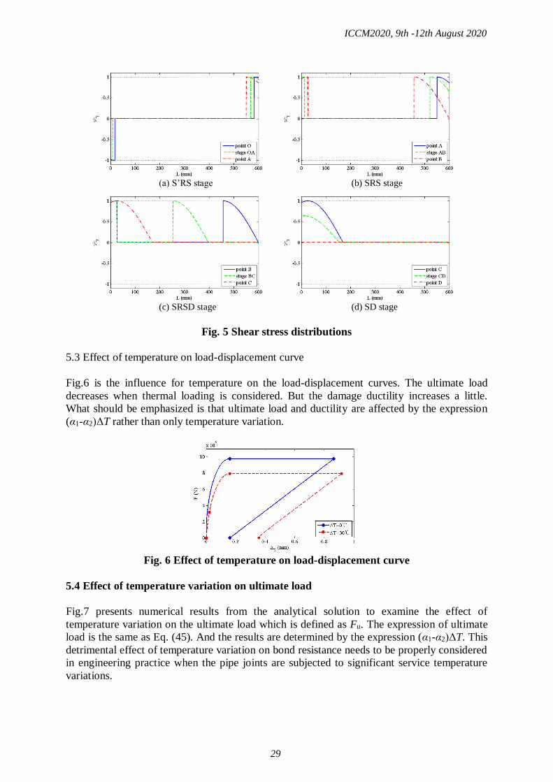
Interfacial shear stress distributions at different failure processes are shown in Fig. 5. And the

shear stresses are all normalized by the value of τf for easy comparisons. When only the

thermal loading is applied [point O in Fig. 4], the interfacial shear stress resulting from a

temperature increase is anti-symmetrically distributed with shear stress at the left end being

negative. Once the interface slip at the left end reaches zero [point A in Fig. 4], the interface

enters into SRS stage. Afterwards, the length of softening region at the left end increases.

Debonding initiates first at the right end [point B in Fig. 4] and then propagates along the

bond length while the softening region at the left end stays unchanged. When the rigid region

disappears [point C in Fig. 4], the interface enters into SD stage. Furthermore, Fig. 5(d) shows

that the debonding zone expands towards the left end in the last stage. Then the interfacial

shear stress at the left end reduces to zero which signifies complete debonding of the entire

interface.

The load displacement curves of analytical and FEM results are almost the same shown as in

Fig.4. Such as the load displacement curves, the curves of shear stress distribution by

numerical and FEM results are almost the same as well. Therefore, the curve of shear stress

distribution by FEM results is not given here.


28

(a) S’RS stage (b) SRS stage

(c) SRSD stage (d) SD stage

Fig. 5 Shear stress distributions

5.3 Effect of temperature on load-displacement curve

Fig.6 is the influence for temperature on the load-displacement curves. The ultimate load

decreases when thermal loading is considered. But the damage ductility increases a little.

What should be emphasized is that ultimate load and ductility are affected by the expression

(α1-α2)ΔT rather than only temperature variation.

Fig. 6 Effect of temperature on load-displacement curve

5.4 Effect of temperature variation on ultimate load

Fig.7 presents numerical results from the analytical solution to examine the effect of

temperature variation on the ultimate load which is defined as Fu. The expression of ultimate

load is the same as Eq. (45). And the results are determined by the expression (α1-α2)ΔT. This

detrimental effect of temperature variation on bond resistance needs to be properly considered

in engineering practice when the pipe joints are subjected to significant service temperature

variations.


29

Fig. 7 Effect of temperature variation on ultimate load

6 Conclusions

This paper has presented a closed-form analytical solution for the full-range behavior of

adhesively bonded pipe joints under combined thermal and mechanical loadings. A rigid-

softening local bond-slip law is thus adopted to simulate the initiation, growth and failure of

interface debonding. The solution provides closed-form expressions for the interface slip and

the interfacial shear stress in addition to the load-displacement responses for the entire

deformation processes. The predictions of the closed-form solutions have been compared with

the finite element results. The solutions are also applicable to similar adhesively bonded joints

made of other orthotropic materials, such as fiber reinforced material pipe joints. Furthermore,

the solutions can also be applied to study the interfacial behavior of pipe joints in moist

environment by introducing coefficients of wet expansion.

References

[1] Lubkin, J.L. and Reissner, E. (1956) Stress distribution and design data for adhesive lap joints between

circular tubes,Transactions of the ASME, 1213-1221.

[2] Dragoni, E. and Goglio, L. (2013) Adhesive stresses in axially-loaded tubular bonded joints-Part I: critical

review and finite element assessment of published models, Int. J. Adhes. Adhes 47, 35-45.

[3] Goglio, L. and Paolino, D.S. (2014) Adhesive stresses in axially-loaded tubular bonded joints-Part II:

development of an explicit closed-form solution for the Lubkin and Reissner model, Int. J. Adhes. Adhes

48, 35-42.

[4] Shi, Y.P. and Cheng, S. (1993) Analysis of adhesive-bonded cylindrical lap joints subjected to axial load,

J. Eng. Mech 119(3), 584-602.

[5] Nemes, O., Lachaud, F. and Mojtabi, A. (2006) Contribution to the study of cylindrical adhesive joining,

Int. J. Adhes. Adhes 26, 474-480.

[6] Nemes, O. and Lachaud, F. (2009) Modeling of cylindrical adhesively bonded joints, J. Adhes. Sci.

Technol 23, 1383-1393.

[7] Yang, C. (2000) Design and analysis of composite pipe joints under tensile loading, J. Compos Mater 34,

332-349.

[8] Klamer, E. (2006) The influence of temperature on concrete structures strengthened with externally

bonded CFRP, Research Report, Eindhoven University of Technology, Eindhoven, The Netherlands.

[9] Klamer, E. (2009) Influence of temperature on concrete beams strengthened in flexure with CFRP, Ph.D

thesis, Eindhoven University of Technology, Eindhoven, The Netherlands.

[10] Leone, M., Matthys, S. and Aiello, M.A. (2009) Effect of elevated service temperature on bond between

FRP-EBR systems and concrete, Compos. Part B-Eng 40(1), 85-93.

[11] Ahmed, A. and Kodur,V. (2011)Effect of bond degradation on fire resistance of FRP-strengthened

reinforced concrete beams, Compos. Part B-Eng 42(2), 226-237.

[12] Dai, J.G., Gao, W.Y. and Teng, J.G. (2013) Bond-slip model for FRP laminates externally bonded to

concrete at elevated temperature, J. Compos. Constr 17, 217-228.


30

[13] Gao, W.Y., Dai, J.G. and Teng, J.G. (2015) Analysis of mode II debonding behavior of fiber-reinforced

polymer-to-substrate bonded joints subjected to combined thermal and mechanical loading, Eng. Fract.

Mech 136, 241-264.

[14] Gao, W.Y., Teng, J.G. and Dai, J.G. (2012) Effect of temperature variation on the full-range behavior of

FRP-to-concrete bonded joints, J. Compos. Constr. 16, 671-683.

[15] Dai, J.G., Gao, W.Y. and Teng, J.G. (2015) Finite Element Modeling of Insulated FRP-Strengthened RC

Beams Exposed to Fire, J. Compos. Constr 19, 04014046.

[16] Shawaf, A., Mahaidi, A. and Zhao, X.L. (2009) Effect of elevated temperature on bond behavior of high

modules CFRP/steel double-strap joints, Compos. Part B-Eng 10(1), 63-74.

[17] Nguyen, T.C., Bai, Y. and Zhao, X.L. (2011) Mechanical characterization of steel/FRP double strap joints

at elevated temperatures, Compos. Struct 93(6), 1604-1612.

[18] Kim, H.S. and Shin, Y.S. (2011) Flexural behavior of reinforced concrete (RC) beams retrofitted with

hybrid fiber reinforced polymers (FRPs) under sustaining loads, Compos. Struct 93(2), 802-811

[19] Ouyang, Z.Y. and Li, G.Q. (2009) Cohesive zone model based analytical solutions for adhesively bonded

pipe joints under torsional loading, Int. J. Solids Struct 46, 1205-1217

[20] Wu, Z.S., Yuan, H. and Niu, H.D. (2002) Stress transfer and fracture propagation in different kinds of

adhesive joints, J. Eng. Mech 128, 562-573.

[21] Yuan, H., Teng, J.G., Seracino, R., Wu, Z. S. and Yao, J. (2004) Full-range behavior of FRP-to-concrete

bonded joints, Eng. Struct 26(5), 553-565.

[22] Yuan, H., Lu, X.S., Hui, D. and Feo, L. (2012) Studies on FRP-concrete interface with hardening and

softening bond-slip law, Compos. Struct 94(12), 3781-3792.

[23] Biscaia, H.C., Chastre, C. and Silva, A.G. (2013) Nonlinear numerical analysis of the debonding failure

process of FRP-to-concrete interfaces, Compos. Part B-Eng 50, 210-223.

[24] Chen, F.L. and Qiao, P.Z. (2009) Debonding analysis of FRP-concrete interface between two balanced

adjacent flexural cracks in plated beams, Int. J. Solids Struct 46, 2618-2628

[25] Lorenzis, L.D. and Zavarise, G. (2009) Cohesive zone modeling of interfacial stresses in plated beams, Int.

J. Solids Struct 46, 4181-4191.

[26] Liu, Z. Q., Yue, Q. R., Li, R. and Chen, X. B. (2020) Experimental study and modeling of bond of

carbon-fiber-reinforced polymer grids to polymer mortar at room and elevated temperatures, Research

Article ,https://doi.org/10.1177/1369433219899784.


31

Numerical Simulation of Incompressible Flows Around a Flat Plate Using

Immersed Boundary Method with Pressure Boundary Condition

*†Kyohei Tajiri¹, Yuki Okahashi1, Mitsuru Tanaka1,

Masashi Yamakawa1 and Hidetoshi Nishida1

1 Department of Mechanophisics, Kyoto Institute of Technology, JAPAN.



Abstract

In this paper, the immersed boundary method (IBM) with the pressure boundary condition is

applied to a plate of infinitesimal thickness that the boundary is not along the grid and its

effectiveness is discussed. In the original IBM, unphysical pressure oscillations appear near the

object boundary, and as a result, it is difficult to correctly estimate the drag and the like. In the

previous study, the present IBM has been applied to a plate of infinitesimal thickness whose

boundary is along the computational grid and its effectiveness was shown. Therefore, in this

paper, the present IBM is extended to be applicable to a plate of infinitesimal thickness whose

boundary is not along the computational grid. Then, in order to validate the present IBM, the

flow around a 2-dimensional flat plate of infinitesimal thickness of various attack angles is

considered. As a result, unphysical pressure oscillations appear near the boundary in the original

IBM, whereas in the present IBM, the oscillations do not appear at any attack angle. The drag

and the lift coefficients in the present IBM are in good agreement with the reference results at

any attack angle. Therefore, the IBM with the pressure boundary condition is very promising

as a means to suppress unphysical pressure oscillations near the virtual boundary of an object

of infinitesimal thickness in the original IBM. In addition, the present pressure estimation at the

virtual grid point allows the IBM to be applied even when the virtual boundaries are not along

the grid. From the above, it can be concluded that the present IBM is very promising as a

Cartesian grid approach for a very thin object.

Keywords: Computational Fluid Dynamics, Cartesian Grid Approach, Immersed Boundary

Method, Incompressible Flow, Pressure Condition

Introduction

In the development of products closely related to flow phenomena, flow simulations are often

performed to understand flow phenomena. In order to develop higher performance products,

the shapes of objects to be subjected to fluid simulations have become complicated. Therefore,

it is important to develop a method for efficiently performing a flow simulation on such an

object.

In recent years, flow simulations for insects such as butterflies and dragonflies have been

performed for the purpose of developing high-performance small flying objects called micro

air vehicle (MAV). These models have multiple wings that are extremely thin compared to the

fuselage, and these wings move in a complex manner. In the simulation of flows including such

models, the Cartesian grid approach is considered to be suitable because of the ease of grid

generation.

In the Cartesian grid approaches, the immersed boundary method (IBM) [1] is very popular. In

the IBM, object boundaries are represented by a gathering of virtual points (virtual boundary),


32

and the additional forcing terms are added to the momentum equations at the grid points near

the virtual boundary so as to satisfy the velocity condition on the virtual boundary. As for the

estimation of the additional forcing term, the direct forcing term estimation [1] is well adopted.

However, the conventional IBM with the direct forcing term estimation generates the

unphysical pressure oscillations near the virtual boundary because of the pressure jump between

inside and outside of the virtual boundary. In order to remove the pressure oscillations, the

seamless immersion boundary method (SIBM) was proposed [1]. In the SIBM, the additional

forcing terms are added not only near the virtual boundary but also inside the virtual boundary.

However, even if the SIBM is applied to a very thin object such as an insect wing, suppression

of the pressure oscillations cannot be expected much because the number of grid points inside

the virtual boundary is very small. In particular, if there are no grid points inside the virtual

boundary, the SIBM cannot be applied to the object. Therefore, Okahashi et al. [1] has applied

IBM with the pressure boundary condition [1] to a plate of infinitesimal thickness and has

verified its effectiveness. However, the verification is limited only when the virtual boundary

is along the grid. Therefore, the IBM with the pressure boundary condition is applied to a plate

of infinitesimal thickness that the virtual boundary is not along the grid and its effectiveness is

discussed.

Immersed Boundary Method for Object of Infinitesimal Thickness

Governing Equations

The non-dimensional continuity equation and incompressible Navier-Stokes equations are

written as,

𝜕𝑢𝑖

𝜕𝑥𝑖= 0, (1)

𝜕𝑢𝑖

𝜕𝑡= 𝐹𝑖 −

𝜕𝑝

𝜕𝑥𝑖+ 𝐺𝑖, (2)

𝐹𝑖 = −𝑢𝑗𝜕𝑢𝑖

𝜕𝑥𝑗+

1

𝑅𝑒

𝜕2𝑢𝑖

𝜕𝑥𝑗𝜕𝑥𝑗, (3)

where 𝑅𝑒 denotes the Reynolds number defined by 𝑅𝑒 = 𝑈𝐿/𝑣. 𝑈, 𝐿, and 𝑣 are the reference

velocity, the reference length and the kinematic viscosity, respectively. The last term of Eq. (2),

𝐺𝑖, denotes the additional forcing term for the IBM. 𝐹𝑖 denotes the convective and diffusion

terms.

Computational Methodology

The incompressible Navier-Stokes equations (2) are solved by the second order finite difference

method on the collocated grid arrangement. The convective terms are discretized by the second

order fully conservative finite difference method [6]. The diffusion and pressure terms

discretized by the usual second order centered finite difference method. However, at the grid

point near the virtual boundary, the convective and diffusion terms are discretized by the second

order one-sided finite difference method in order to avoid using the velocity at the position

across the virtual boundary. For the time integration, the fractional step approach based on

forward Euler method is applied.

Forcing Term Estimation

In order to estimate the additional forcing term in the Navier-Stokes equations, 𝐺𝑖, there are

mainly two ways, that is, the feedback [7][8] and direct [2] forcing term estimations. In this

paper, the direct forcing term estimation in Fig. 1 is adopted. For the forward Euler time

integration, the forcing term can be determined by


33

𝐺𝑖 = −𝐹𝑖𝑛+

𝜕𝑝

𝜕𝑥𝑖

𝑛+

𝑖𝑛+1−𝑢𝑖

𝑛

∆𝑡, (4)

where 𝑖𝑛+1denotes the interpolated velocity by linear interpolation. Namely, the forcing term

is specified as the velocity components at next time step satisfy the relation, 𝑖𝑛+1 = 𝑢𝑖

𝑛+1.

When the object has the infinitesimal thickness, the pressure oscillations appear near the virtual

boundary because the SIBM cannot be applied to it.

Figure 1. Direct forcing term estimation

Pressure Estimation

In the original IBM, the pressure boundary condition is not considered. As a result, the pressure

oscillations appear because of the pressure jump across the virtual boundary. In the present

method, the pressure boundary condition is considered in order to avoid the pressure jump. In

order to estimate the pressure gradient considering the pressure boundary condition on the

virtual boundary, the virtual grid points are provided at grid points located across the virtual

boundary. Therefore, some pressure values are defined at these grid points. In this study, the

pressure is imposed the Neumann condition on the normal direction on the virtual boundary

(𝜕𝑝 𝜕𝑛⁄ = 0). For example, in Fig. 2 (a), the x-direction pressure gradient at grid point (𝐼, 𝐽) is

written as

𝜕𝑝

𝜕𝑥|

𝐼,𝐽=

𝐼+1,𝐽−𝑝𝐼−1,𝐽

2∆𝑥, (5)

where 𝐼+1,𝐽 denotes the pressure at the virtual grid point that satisfies the pressure condition

on the virtual boundary. The pressure on the virtual grid point is estimated by using the Taylor

series expansion in two variables with reference to the points 𝑚 = 1 to 2 and the pressure

condition on the virtual boundary 𝑣𝑏 [5][9]. 𝒏 denotes the unit normal vector at the virtual

boundary point. The reference points are chosen from the surrounding grid points in the normal

direction. The relationship between pressure on the virtual boundary and reference points is

approximated by

𝑝𝑚 = 𝑝𝑣𝑏 + (𝑙𝑚𝑥𝜕𝑝

𝜕𝑥|

𝑣𝑏+ 𝑙𝑚𝑦

𝜕𝑝

𝜕𝑦|

𝑣𝑏), (6)

where 𝑙𝑚𝑥, 𝑙𝑚𝑦 are the distance components from the virtual boundary point to the reference

points. The pressure condition on the virtual boundary is written by

𝜕𝑝

𝜕𝑛|

𝑣𝑏= 𝑛𝑥

𝜕𝑝

𝜕𝑥|

𝑣𝑏+ 𝑛𝑦

𝜕𝑝

𝜕𝑦|

𝑣𝑏= 0. (7)


34

By substituting Eq. (7), Eq. (6) is rewritten to

𝑝𝑚 = 𝑝𝑣𝑏 + (𝑙𝑚𝑥 −𝑛𝑥

𝑛𝑦𝑙𝑚𝑦)

𝜕𝑝

𝜕𝑥|

𝑣𝑏. (8)

By using 𝑝𝑣𝑏 and 𝜕𝑝

𝜕𝑥|

𝑣𝑏, the pressure on the virtual grid point is expressed by

𝐼+1,𝐽 = 𝑝𝑣𝑏 + |𝑙𝑥|𝜕𝑝

𝜕𝑥|

𝑣𝑏, (9)

where 𝑙𝑥 is the distance in x-component from the virtual boundary to the virtual grid point.

If the virtual boundary is along the grid (Fig. 2 (b)), the pressure on the virtual grid point is

expressed by

𝐼+1,𝐽 = 𝑝𝐼,𝐽. (10)

(a) Virtual boundary not along the grid (b) Virtual boundary along the grid

Figure 2. Pressure estimation on the virtual grid point

Flow Around a Plate of Infinitesimal Thickness

In order to validate the present IBM, the flow around a 2-dimensional flat plate of infinitesimal

thickness is considered. The present IBM is compared to the original IBM. The computational

domain is shown in Fig. 3. The reference length is the plate length. 𝜃 is the attack angle of the

plate. When 𝜃 = 0° , 90° , the virtual boundary of the plate is along the grid. In this paper,

numerical simulations are performed at various attack angles. The computational grid is the

hierarchical Cartesian grid that is fine near the plate. The grid resolutions near the virtual

boundary are ∆= ∆𝑥 = ∆𝑦 = 0.0125. The grid points are arranged so as not to be located on

the plate at any attack angle. On the inflow boundary, the velocity is fixed by the uniform flow

(𝑢 = 1, 𝑣 = 0) and the pressure is imposed by the Neumann condition obtained by the normal

momentum equation. The velocity is extrapolated from the inner points and the pressure is

obtained by the Sommerfeld radiation condition [10] on the outflow and side boundaries. On

the virtual boundary, the velocity condition is the non-slip (𝑢 = 0, 𝑣 = 0) condition. In the

present IBM, the pressure condition is the Neumann condition on the normal direction

(𝜕𝑝 𝜕𝑛⁄ = 0 ). In the original IBM, the pressure is not imposed condition on the virtual

boundary. The Reynolds number is set as 𝑅𝑒 = 20. Under these conditions, the flow field is

steady.


35

Figure 3. Computational domain

In Figs. 4-7, the pressure contours around the plate at each attack angle are shown. When 𝜃 =0°, there is no difference in the pressure field between the two methods. This is because the

Neumann condition of the pressure on the virtual boundary is naturally satisfied in the original

IBM because the flow field is vertically symmetric. Therefore, unphysical pressure oscillations

do not appear. However, at other attack angles, unphysical pressure oscillations appear near the

virtual boundary in the original IBM. On the other hand, unphysical pressure oscillations do not

appear at any attack angle in the present IBM. Therefore, even when the virtual boundary is not

along the grid, the effect of suppressing unphysical pressure oscillations by the IBM with the

pressure boundary condition is effective.

(a) Original IBM (b) Present IBM

Figure 4. Pressure contours (𝜽 = 𝟎°)


36


Figure 5. Pressure contours (𝜽 = 𝟑𝟎°)


Figure 6. Pressure contours (𝜽 = 𝟒𝟓°)


Figure 6. Pressure contours (𝜽 = 𝟗𝟎°)


37

In Figs. 7, 8, the drag and the lift coefficients are shown at each attack angle with the reference

results [11]. In this paper, the drag and the lift coefficients are estimated by

𝐶𝐷 =∫ 𝑝𝑥𝑑𝑠𝑏 +∫ 𝜏𝑥𝑑𝑠𝑏

1

2𝜌0𝑈0

2𝑆, (11)

𝐶𝐿 =∫ 𝑝𝑦𝑑𝑠𝑏 +∫ 𝜏𝑦𝑑𝑠𝑏

1

2𝜌0𝑈0

2𝑆, (12)

where 𝑏 denotes the virtual boundary, 𝑝𝑥 and 𝜏𝑥 is the 𝑥 direction components of the

interpolated pressure and shear stress on the surface of the plate 𝜌0 and 𝑈0 denote the reference

density and velocity of the flow. The drag and lift coefficients in the present method are in good

agreement with the reference results. On the other hand, the drag and lift coefficients in the

original IBM are very different from the reference results. This is because it is difficult in the

original IBM to correctly estimate the pressure on the plate surface because of unphysical

pressure oscillations near the virtual boundary. Therefore, it can be seen that the pressure field

is greatly improved by applying the present IBM. Therefore, the effectiveness of the present

IBM can be confirmed.

Figure 7. Drag coefficients Figure 8. Lift coefficients

Conclusions

In this study, the IBM with the pressure condition was applied to a flat plate of infinitesimal

thickness of various attack angles and its effectiveness was verified. Except when the attack

angle was 0°, unphysical pressure oscillations appeared near the virtual boundary in the original

IBM. On the other hand, at all attack angles, unphysical pressure oscillations did not appear in

the present IBM. As a result, the drag and the lift coefficients in the present IBM wear in good

agreement with the reference results at all attack angles. Therefore, the IBM with the pressure

boundary condition is very promising as a means to suppress unphysical pressure oscillations

near the virtual boundary of an object of infinitesimal thickness in the original IBM. In addition,

the present pressure estimation at the virtual grid point allows the IBM to be applied even when

the virtual boundaries are not along the grid. From the above, it can be concluded that the

present IBM is very promising as a Cartesian grid approach for a very thin object.


38

References

[1] Peskin, C.S. and McQueen, D.M. (1989) A three-dimensional computational method for blood flow in the heart I. Immersed elastic fibers in a viscous incompressible fluid, Journal of Computational Physics, 81(2), 372-405.

[2] Fadlun, E.A., Verzicco, R., Orlandi, P. and Mohd-Yosof, J. (2000) Combined immersed-boundary finite-difference methods for three-dimensional complex simulations, Journal of Computational Physics, 161(1), 35–60.

[3] Nishida, H. and Sasao, K. (2006) Incompressible Flow Simulations Using Virtual Boundary Method with New Direct Forcing Terms Estimation, Proceedings of International Conference on Computational Fluid Dynamics 2006, 185–186.

[4] Okahashi, Y., Tajiri, K. Tanaka, M. and Nishida, H. (2020) Immersed Boundary Method with Pressure Boundary Condition for Moving Object of Infinitesimal Thickness, 43(1), 113–126.

[5] Tajiri, K., Nishida, H., and Tanaka, M. (2016) Numerical simulation of incompressible flows using immersed boundary method considering the pressure condition, Proceedings of 9th International Conference on Computational Fluid Dynamics, 1–12.

[6] Morinishi, Y., Lund, T.S., Vasilyev, O.V. and Moin, P. (1998) Fully conservative higher order finite difference schemes for incompressible flow, Journal of Computational Physics, 143(90), 90-124.

[7] Goldstein, D., Handler, R., and Sirovich, L. (1993) Modeling a no-slip flow boundary with an external force field, Journal of Computational Physics, 105(2), 354–366.

[8] Saiki, E.M. and Biringen, S. (1996) Numerical simulation of a cylinder in uniform flow: application of a virtual boundary method, Journal of Computational Physics, 123(2), 450–465.

[9] Nishida, H. (2015) Development of Seamless Immersed Boundary Method to Various Partial Differential Equations, Proceedings of Korea-Japan CFD Workshop 2015, 1-15.

[10] Kawakami, K., Nishida, H. and Satofuka, N. (1994) An open boundary condition for the numerical analysis of unsteady incompressible flow using the vorticity-streamfunction formulation (in Japanese), Transactions of the Japan Society of Mechanical Engineers Series B, 60(574), 1891–1896.

[11] In, K.M., Choi, D.H., Kim, M.-U. (1995) Two-dimensional viscous flow past a flat plate, Fluid Dynamics Research, 15, 13-24.


39

Effect of mechanical and chemical constraints on

swelling of elastomeric gel

†*Isamu Riku, Tomoki Sawada and Koji Mimura

Department of Mechanical Engineering, Osaka Prefecture University, Japan

†*[email protected]

Abstract

A nonaffine model is proposed for the elastomeric gel to account for the change of the

entangling structure of molecular chains during the free swelling and simple tensional process,

in which the change in the number of polymer chains per unit volume, N , is depending on the

first invariant of right Cauchy-Green tensor, 1I , and on the volume ratio of the gel, J ,

separately. It is found that the dependency of the entangling structure of molecular chains on

1I has a remarkable effect on the deformation response of the gel compared to that on J .

Moreover, the effect of the nonaffine movement of molecular chains is non-negligible for the

gel contacting with the solvent in liquid phase.

Keywords: Elastomeric gel, Free swelling, Simple tension, Chemical potential, Entangling

structure

Introduction

The elastomeric gel, consisting of cross-linked polymer molecules and discrete solvent

molecules, have a high permeability to small molecules and undergo reversible volume

change by exuding or absorbing solvent in response to a wide range of stimuli, such as light,

temperature, pH, ionic strength and chemical reactions. As a result, the gel has been

developed for diverse applications and used as smart materials in sensors and actuators [1-3].

To characterize how mechanical constraint affects the amount of swelling, and how chemical

processes generate forces, several nonlinear field theories have been developed [4-7]. Flory

and Rehner proposed a statistical mechanical model for the network of polymer molecules

and indicated that the swelling capacity of the gel is diminished by the application of an

external stress [8]. In our former study [9], we focused on the discussion of the mechanical

behavior of the elastomeric gel based on a nonaffine molecular chain network model

(nonaffine model) [10], which was originally developed for the orientation hardening of

amorphous polymers and may account for the change in the entanglement situation for the

physical linkages during the deformation processes. It was found that the free swelling

process may lead to a larger change of the entangling structure of molecular chains compared

to the tensional process. Moreover, the various combination of the effect of each process on

the nonaffine movement of molecular chains may lead to some interesting mechanical

responses of the gel, such as yield.

On the other hand, the elastomeric gel can undergo large deformation of two modes. The first

mode results from the fast process of short-range rearrangement of molecules, allowing the

gel to change shape but not volume. The second mode results from the slow process of long-

range migration of the solvent molecules, allowing the gel to change both shape and volume.

As we have discussed the first mode in our former study [9], in this study, we will focus on

the second mode, namely, the state of equilibrium achieved when a network has been in

contact with a solvent for a long time. The condition of equilibrium between the gel and the


40

solution is derived based on the variational principle and the dependency of the entangling

structure’s effect on the deformation response of the gel under different mechanical and

chemical constraints is to be clarified.

Conditions of Equilibrium

The basic idea of the derivation of the conditions of equilibrium for the dry polymer and the

solvent is from the work done by Hong et al. [4]. It is convenient to consider that, in the

reference state, a block of network of dry polymers is a unit cube, and contains no solvent and

subject to no applied forces. In the current state, the network is submerged in a solvent-

containing environment, and the six faces of the block are subject to applied forces. When the

network, the solvent, and the applied forces equilibrate, the network absorbs C number of

solvent molecules, and deforms homogeneously into the shape of a parallelepiped. When the

deformation gradient of the network is expressed by F , the ratio of volume of the swollen gel

and that of the dry network is determined as FdetJ . As an idealization, it is assumed that the

volume of the gel is a function of the concentration of the solvent:

CJ 1 . (1)

That is, all molecules in a gel are incompressible, and the volume of the gel is the sum of the

volume of the dry network and the volume of the pure liquid solvent, where is the volume

per solvent molecule. Eq. (1) determines the concentration of solvent, C , once the

deformation gradient is known. Consequently, the nine components of the deformation

gradient F specify the state of the gel. Let W be the Helmholtz free energy of the gel in the

current state. The Helmholtz free energy of the gel can be taken to be a function of the nine

components of the deformation gradient, F , and is assumed to be separable into contributions

from stretching the network and mixing the polymer and solvent [8]:

JWWW mixstretch F . (2)

The free energy due to the stretching of the network, FstretchW , is a function of the deformation

gradient, and depends on the density of crosslinks. The free energy due to the mixing of the

polymer and the solvent, JWmix, is a function of the concentration of the solvent in the gel,

but is independent of the density of crosslinks. Introduce another free energy function W by

using a Legendre transformation:

CWW ˆ , (3)

where is the chemical potential of the solvent molecules. Eq. (1)~(3) form the basis for the

model of ideal elastomeric gels. In equilibrium, the change of the Helmholtz free energy of

the composite vanishes and one can obtain that

ik

kiF

Ws

,ˆ F ,

,ˆ FWC , (4)

where kis is the nominal stress.

Free Energy Functions

In the original Flory-Rehner model [8], specific functions are adopted for FstretchW and JWmix.

In this study, we employ the best known formulation as:

CCC

TkJFFTNkW B

ikikB

1

11loglog23

2

1F , (5)


41

where N is the number of polymer chains per unit volume, Bk is Boltzmann constant, T is the

temperature and is a dimensionless measure of the enthalpy of mixing. A combination of

Eq.(1), (3) and (5) gives the desired free energy function:

11

log1log232

1,ˆ

J

JJ

JJ

TkJFFTNkW B

ikikB

F . (6)

Furthermore, to account for the effect of the nonaffine movement of the polymer chain on the

deformation behavior of the gel, similar to our former study [9], we employ the simplest

version of the nonaffine model [10] to accommodate the change in the number of polymer

chains per unit volume, N , depending on the first invariant of right Cauchy-Green tensor, 1I ,

or on the third invariant of right Cauchy-Green tensor, 3I , separately.

max

1

1

0

31

I

I

N

N ,

ikik FFI 1, or (7)

max

3

3

0

11

I

I

N

N , 2

3 JI , (8)

where 0N is the number of polymer chains per unit volume of the gel in the reference state,

max

1I and max

3I are the limit value of 1I and

3I , separately.

Stress-Stretch Relations

Inserting Eq. (6) into Eq. (4), we obtain that

ik

ik

B

ikik

B

ki

F

NJIHJ

TkJJJHFN

Tk

s

log23

2

11

11log

/1

. (9)

Recall an algebraic identity, JHFJ ikik / , where ikH is the transpose of the inverse of the

deformation gradient F . For simplicity, we describe the deformation of the gel in the

coordinates of principal stretches. Let 1 ,

2 , 3 be the principal stretches of the gel, so that

321 ,,diag F , 321 J and 2

3

2

2

2

11 I .

Free Swelling State

Submerged in the solvent-containing environment but subject to no applied forces, the

elastomeric gel attains a state of equilibrium, the free swelling state, characterized by an

isotropic swelling ratio, 3/1

321

J . Therefore, based on Eq. (9), the relation between

the principal stretch and the chemical potential of the solvent molecules can be written

as:

TkI

NN

B

633

2

max

1

0

3

111loglog21

311 , (10)

when Eq. (7) is applied, or can be written as:

TkI

NN

B

633

23

max

3

0

3

111loglog21

311 , (11)

when Eq. (8) is applied.

Simple Tension State

A unit cube of the elastomeric gel is equilibrated in a solvent of chemical potential , and is

subject to a uniaxial stress 1s along the longitudinal direction. The state of deformation can be


42

characterized by the longitudinal stretch 1 and two transverse stretch

32 . The stresses in

the transverse directions vanish, so that Eq. (9) gives

01

11

1loglog2321

2

2

212

21

2

21

2

21

2

21

2

2

2

12max

1

0

2

2

TkI

NN

B

, (12)

when Eq. (7) is applied, or gives

01

11

1loglog2321

2

2

212

21

2

21

2

21

2

21

2

2

2

1

3

2

2

1max

3

0

2

2

TkI

NN

B

, (13)

when Eq. (8) is applied. Eq. (12) and Eq. (13) determine the transverse stretch 2 for a given

longitudinal stretch 1 . Eq. (9) also relates the longitudinal stress to the stretches as:

1

2

212

21

2

21

2

21

2

21

2

2

2

11max

1

0

1

11 1

11

1loglog2321

/

TkI

NN

Tk

s

BB

, (14)

when Eq. (7) is applied, or as:

1

2

212

21

2

21

2

21

2

21

2

2

2

1

4

21max

3

0

1

11 1

11

1loglog2321

/

TkI

NN

Tk

s

BB

, (15)

when Eq. (8) is applied.

Results

In this study, we have normalized the chemical potential by TkB, and normalized the stress by

/TkB. The Flory-Rehner free energy function introduces two dimensionless material

parameters: N and . In the numerical results below, we take the values 3

0 10N and

1.0 . On the other hand, the values of the two parameters introduced in the nonaffine model

are taken as 50max

1 I and 8000max

3 I .

In Fig. 1(a), the stretch of an elastomeric gel at the free swelling state is plotted as a function

of the chemical potential of the solvent. When the solvent is subject to a pressure p greater

than the vapor pressure, 0p , the solvent is in the liquid phase, and the chemical potential of

the solvent molecules is 0pp . When the solvent is subject to a pressure p less than the

vapor pressure, 0p , the solvent in equilibrium becomes a gas, which we assume to be an ideal

gas, so that the chemical potential of the solvent molecules is 0/log ppTkB . When the

phase of solvent changes from gas to liquid, the stretch of the gel increases exponentially.

With regard to the effect of the nonaffine movement of the polymer chain on the swelling

deformation of the gel, no effect can be observed when the solvent is in gas phase. However,

when the solvent is close to its liquid phase, the nonaffine movement of the polymer chain

leads to a relatively early increase of the stretch. In Fig. 1(b), the variation of the number of

polymer chains N during the free swelling of the gel are shown. It is obviously that the

decrease of the number of polymer chains N is remarkable when the development of its value

is dependent on 1I .

When an elastomeric gel is subject to a uniaxial stress, and is in contact with a solvent of a

given chemical potential, the state of equilibrium is assumed to achieve after a long time. In

Fig. 2(a), the applied stress is plotted as a function of the stretch, while the solvent is held at

several levels of the chemical potential. As shown in Fig. 1(a), the gel can swell to a stretch of

3.5 when the solvent is in liquid phase. Therefore, if the longitudinal stretch 1 is limited to

the value smaller than 3.5, compressive stress is necessary. However, when the solvent is in

gas phase, the applied stress is almost tensional stress. With regard to the effect of the


43

nonaffine movement of the polymer chain on the applied stress, no effect can be observed

when the development of the number of the polymer chain N is dependent on 3I . However, if

the development of N is dependent on 1I , the change in the entanglement situation for the

physical linkages leads to the decrease of the applied stress of the gel when it is in contact

with the solvent in gas phase. Interestingly, when the solvent is in liquid phase, the nonaffine

movement of the polymer chain leads to a lower value of compressive stress at the small

stretch region and a higher value at the large stretch region compared to that of the affine

model. In Fig. 2(b), the variation of the number of polymer chains N of the gel during the

simple tension state are shown. For the gel that is in contact with the solvent in gas phase, the

number of polymer chains N decreases the stretch increases. On the other hand, for the gel

that is in contact with the solvent in liquid phase, the value of N increases at the small stretch

region and decreases at the large stretch region.

Conclusions

In this study, a nonaffine model is proposed for the elastomeric gel to account for the change

of the entangling structure of molecular chains during the free swelling and simple tensional

process. It is found that the dependency of the entangling structure of molecular chains on 1I

has a remarkable effect on the deformation response of the gel compared to that on J .

Moreover, the effect of the nonaffine movement of molecular chains is non-negligible for the

gel contacting with the solvent in liquid phase.

References

[1] Liu, Z. and Clavert, P. (2000) Multilayer hydrogels as muscle‐like actuators, Advanced Materials 12, 288–291.

[2] Beebe, D. J., Moore, J. S., Bauer, J. M., Yu, Q., Liu, R. H., Devadoss, C. and Jo, B. H. (2000) Functional hydrogel structures for autonomous flow control inside microfluidic channels, Nature 404, 588–590.

[3] Cai, S. Q., Lou, Y. C., Ganguly, P., Robisson, A. and Suo, Z. G. (2010) Force generated by a swelling elastomer subject to constrain, Journal of Applied Physics 107, 103535.

[4] Hong, W., Liu, Z. S. and Suo, Z. G. (2009) Inhomogeneous swelling of a gel in equilibrium with a solvent and mechanical load, International Journal of Solids and Structures 46, 3282-3289.

[5] An, Y. H., Solis, F. J. and Jiang, H.Q. (2010) A thermodynamic model of physical gels, Journal of the Mechanics and Physics of Solids 58, 2083–2099.

[6] Hui, C. Y. and Muralidharan, V. (2005) Gel mechanics: A comparison of the theories of Biot and Tanaka, Hocker, and Benedek, Journal of Applied Physics 123, 154905.

[7] Chester, S. A. and Anand, L. (2010) A coupled theory of fluid permeation and large deformations for elastomeric materials, Journal of the Mechanics and Physics of Solids 58, 1879–1906.

[8] Flory, P. J. and Rehner, J. (1943) Statistical mechanics of cross‐linked polymer networks II. swelling, Journal of Applied Physics 11, 521.

[9] Riku, I., Ueda, M., Sawada, T. and Mimura, K. (2019) Study on the change of entangling structure of molecular chains during the tensional and swelling process of elastomeric gel, Proceedings of the 10th International Conference on Computational Methods, 391–396.

[10] Riku, I. and Mimura, K. (2010) Computational characterization on mechanical behavior of polymer electrolyte membrane based on nonaffine molecular chain network model, International Journal of Mechanical Sciences 52, 287–294.


44

(a) (b)

Figure 1. Characteristics of the elastomeric gel in the free swelling state

(a) stretch – chemical potential relations; (b) variations of the entangling structure

(a) (b)

Figure 2. Characteristics of the elastomeric gel in the simple tension state

(a) stress – stretch relations; (b) variations of the entangling structure


45

Development of the numerical method for simulation of ship motions in regular waves with changing wave direction

†*Kunihide Ohashi¹

1 National Maritime Research Institute, Japan.

*Presenting author: k-ohashi @m.mpat.go.jp †Corresponding author: [email protected]

Abstract

Numerical simulation of the ship motions in regular waves with changing a wave direction is carried out. An in-house structured CFD solver which is capable of the overset-grid method is employed. The case in the CFD workshop Tokyo 2015 which the ship type is the container hull with the rudder, and the ship motions are the three degrees of the freedom, the heave, pitch and roll motions, is selected. The use of the characteristics of the overset grids method is made, which means the background rectangular grids which generate the incoming waves are replacing along with the wave direction while the other grids are maintained. The present method shows the effectiveness through the comparisons with the experimental and existing computational results.

Keywords: Regular wave, Wave direction, Ship motion, Overset grids method

Introduction

The numerical simulation of the ship motions with changing the wave direction is performed. The overset grids method and the in-house CFD solver which have the capability to the present test case are employed. The background rectangular grids are prepared and replaced along with the wave directions while the other computational grids including the ship and rudder grids are maintained. The present method is examined on the test case in the CFD workshop Tokyo 2015 [1]. Through the comparisons of computational results of the amplitudes of the ship motions which are introduced by the Fourier analysis with the measured and existing simulated results, the effectiveness of the present method is examined.

Computational Method

Base Solver

An in-house structured CFD solver [2] is employed. The governing equation is 3D RANS equation for incompressible flows. Artificial compressibility approach is used for the velocity-pressure coupling. Spatial discretization is based on a finite-volume method. A cell centered layout is adopted in which flow variables are defined at the centroid of each cell and a control volume is a cell itself. Inviscid fluxes are evaluated by the third-order upwind scheme based on the flux-difference splitting of Roe. The evaluation of viscous fluxes is second-order accurate. For unsteady flow simulations, a dual time stepping approach is used in order to recover incompressibility at each time step. It is consisted from the second order two-step backward scheme for the physical time stepping and the first order Euler implicit


46

scheme for the pseudo time. The linear equation system is solved by the symmetric Gauss-Seidel (SGS) method. For free surface treatment, an interface capturing method with a single phase level set approach is employed. Incoming Regular waves are generated at the region inside of the computational domain. The wave direction is determined with changing the regions which generate the regular waves. The ship motions are determined by solving motion equations, and the motions are strongly coupled with the governing equations. The computational domain is deformed under the criterion of the distance from the ship hull. The ship motions are accounted for by a moving grid technique. The grid velocities are contained in the inviscid terms to satisfy the geometrical conservation law. The grid velocities are derived from the volume where each cell face sweeps. The boundary condition on a body is given as the velocities of the ship motion.

Overset Grids Method

The weight values for the overset-grid interpolation are determined by an in-house system [3]. The detail of the system can be found on [3], the summary is described. The priority of the computational grid is set. The cells of a lower priority grid and inside a body is identified (called as in-wall cell in

here). Receptors cells which the flow variables have to be interpolated from donor cells are

defined. Two cells on a higher priority grid and facing to the outer boundary are set as receptor cells to satisfy the third order discretization of NS solver. Additionally, two cells neighborhood of in-wall cells, the cells of a lower priority grid and inside the domain of a higher priority grid are also set as the receptor cell.

The weight values for the overset interpolation are determined by solving the inverse problem based on Ferguson spline interpolation.

Flow variables of the receptor cell are updated when the boundary condition is set. The forces and moments are integrated on the higher priority grid to eliminate the lapped region on body surfaces. At first, the cell face of the lower priority grid is divided into small pieces. Secondly, the small piece is projected to the cell face of the higher priority grid by using the normal vector of the higher priority face. Then the 2D solid angle is computed and the small piece is decided in or out of the higher priority face. Once the small piece is in the higher priority face, the area ratio of the piece is set to zero. Finally, the area ratio is integrated on the lower priority face, then we have the ratio to integrate the forces and moments on lower priority face.

Computed Results

The container hull form which is utilized on the case in CFD workshop Tokyo 2015 is selected [1]. The model ship length is approximately 2.7m and the Reynolds number is R=3.738 x 106. Froude number is Fn=0.26. The wave length ratio of incoming regular waves is /L=1.15, and the wave height ratio h/L is approximately 0.0167. The wave directions are set as 5 directions which are defines as 0 degree (head sea condition), 45 degrees, 90 degrees (beam sea condition), 135 degrees and 180 degrees (following sea condition). The motions


47

are free to pitch, roll and heave which are designated in the instruction of the workshop. The non-dimensional physical time step size is always set to 0.005. Table 1 shows the division number of computational grids arranged with the priority of the overset grids method. Figure 1 shows the grids near the hull body. The computational grids consist of the rudder grid, the refined rectangular grid for the arrangement of the overset relation, the ship hull and background rectangular grids. IM means the ship length direction, JM is the width direction, and KM is the division number in the direction along with the depth for the rectangular grids while IM means the spanwise direction, JM is chord direction, and KM is the division number for the normal direction from the rudder surface on the rudder grid. For the ship hull grid, IM means the ship length direction, JM is the girth direction, and KM is the division number in the normal direction from the hull surface. The minimum spacing on the wall surface is set as the non-dimensionalized distance y+=100 applying k- SST turbulence model with the wall function type [4]. The five rectangular grids are chosen in accordance with the wave direction. The grids except the background rectangular grids are maintained, and the overset relation is generated with replacing the background rectangular grid for the wave direction. Computational domain is set as 0.30.2 x and

155.02 z excepting the grid for the 180 degrees case has the range 0.20.2 x to adapt for the following waves. The domain size for the y-direction is set as 0.20.2 y excepting the grid for the 90 degrees case has 575.20.2 y to set the wave damping zone in the wave direction. The division number JM in the width direction also changes to the adequate number to resolve the wave length along with the wave direction.

Table 1. Division number of the computational grids.

Grids IM x JM x KM Rudder 45 x 89 x 9 Refined Rect. 49 x 49 x 49 Hull 257 x 161 x 61 Rect.(0 degree) Rect.(45 degrees) Rect.(90 degrees) Rect.(135 degrees) Rect.(180 degrees)

193 x 65 x 57 193 x 161 x 57 193 x 177 x 57 193 x 161 x 57 201 x 65 x 57


48

Figure 1. Computational grids

Figure 2 shows the instantaneous view of the free surface in the oblique and lateral sea conditions. The wave pattern indicates the direction of the waves, and the disturbed wave due to the interactions between the incoming waves, ship and its motions can be found. Figure 3 shows the amplitude of the heave motion, Figure 4 shows the amplitude of the roll motion and Figure 5 shows the amplitude of the pitch motion along with the wave directions. All the amplitudes are introduced by the Fourier analysis which is indicated on the web-site [1], and the amplitudes on the component of the first encounter frequency are compared. Present results show agreement with the measured data and indicate similarity with the other computational results excepting the heave motion at 180 degrees and roll motion at 45 degrees. The heave motion seems to be affected by the surge motion which is accounted for in the experiment while the numerical simulations do not consider the surge motion based on the instruction [1] for this case. The time history of the heave motion has the component of the secondary encounter frequency [1], consequently, the simulation with the surge motion may become the solution to be solved the problem of this small disagreement. All the computational results indicate relatively very small difference comparing with the measured data on the roll amplitude at 45 degrees. The experimental condition may differ from the ideal condition which is achieved by the numerical simulations.

Rudder Refined Rect.

Hull

Rect.


49

oblique sea condition lateral sea condition

Figure 2. Instantaneous view of the free surface

Wave direction(deg.)

z/

0 50 100 1500

0.5

1

1.5 Meas.[1]PresentIIHR/CFDShip-Iowa V4.5[1]UNIZAG-FSB/swenseFoam[1]

Figure 3. Comparison of the amplitude of the heave motion


/k

0 50 100 1500

0.5

1

1.5

2

2.5

3

Meas.[1]PresentIIHR/CFDShip-Iowa V4.5[1]UNIZAG-FSB/swenseFoam[1]

Figure 4. Comparison of the amplitude of the roll motion


50


/k

0 50 100 1500

0.5

1Meas.[1]PresentIIHR/CFDShip-Iowa V4.5[1]UNIZAG-FSB/swenseFoam[1]

Figure 5. Comparison of the amplitude of the pitch motion

Conclusions

The numerical simulation of the ship motions in regular waves with changing wave direction is carried out. The case in the CFD workshop Tokyo 2015 is selected, and the overset grids method is applied with replacing the background rectangular grid to generate the incoming regular waves while other grids are maintained. The present results indicate the similarity with the other computational results, and the present method shows the effectiveness through the comparisons with the experimental data.

Acknowledgement

This work has been supported by JSPS KAKENHI Grant Number JP19K04869.

References

[1] Larrson, L., Stern, F., Visonneau, M., Hirata, N., Hino, T., Kim, J., (2015) Proc. Tokyo 2015 workshop on CFD in ship hydrodynamics

[2] Ohashi, K., Hino, T., Kobayashi, H., Onodera, N., Sakamoto, N. (2019) Development of a structured overset Navier–Stokes solver with a moving grid and full multigrid method, JMST 24(3), 884–910.

[3] Kobayashi H. and Kodama Y. (2016) Developing Spline Based Overset Grid Assembling Approach and Application to Unsteady Flow Around a Moving Body, Journal of Mathematics and System Science 6, 339-347.

[4] Ohashi, K., Hino, T. (2012) Numerical study on the applicability of wall function models for the flows around an appendage attached to a body, AIAA paper 2012-0445


51

Numerical Analysis for Promotion of Concentration Diffusion by

Rotational Motion of Circular Object

†Kohei Ueda¹, Masashi Yamakawa2, and Shinichi Asao3

1 Graduate School of Science and Technology, Kyoto Institute of Technology, Matsugasaki, Sakyo-ku, Kyoto, Japan.

2 Department of Mechanophysics, Kyoto Institute of Technology, Matsugasaki, Sakyo-ku, Kyoto, Japan. 3 Department of Mechanical Engineering, College of Industrial Technology,

1-27-1, Nishikoya, Amagasaki, Hyogo, Japan.


Abstract

The main current communication method is electromagnetic (EM) wave communication.

Then, it is necessary technology for human life. EM wave system has conveniences that high-

speed and large capacity communication. On the other hand, it also has disadvantages that it

requires much energy and the facilities. In contrast, molecular communication (MC) that uses

biological molecules as an information carrier is noticed as a new communication method,

because it requires little energy and is expected application for micro-scale. However, in

general MC is difficult to communicate at high-speed and to control communication itself

comparison with EM wave communication. Because most of MC is diffusion-based. In this

study, numerical simulation for the promoting effect of concentration diffusion by flow

caused by the movement of a circular object is performed to solve the problem of

communication speed. As a result, diffusion phenomenon was promoted in response to the

object condition.

Keywords: Molecular communication, Concentration diffusion, Communication speed,

Promotion, Numerical analysis

Introduction

There are various technologies around us, and communication technologies to make them

function are indispensable. At present, most of communications rely on methods using

electromagnetic (EM) wave. EM wave communication is a common method for devices that

people usually use. Because it has some advantages that can communicate with high-speed,

large capacity and high accuracy. Whereas, it also has disadvantages that requires much

energy and the facilities such as base stations or radio towers, and difficult to micronize for

communication devices. Against these, a new communication method called molecular

communication (MC), which does not require EM wave, has been devised and researched [1].

MC is a method that uses chemical substances (biological molecules) such as proteins and

DNAs as the signal transduction carrier. Then, it is different to traditional communication

methods. The molecules released by the transmitter propagate in fluids, and the signal

transduction is completed when they reach at the receiver. This communication method is

common for many creatures. For example, a pheromonal communication [2][3] is typical, ants’

procession and moths’ courtship are the best examples. In addition, transportation of body

hormones is also a kind of MC [4].

MC is attracting attentions because it has three advantages. First, MC requires no or little

energy. The main propagation method of MC is free diffusion. Therefore, energy such as


52

mailto:[email protected]

electricity is unnecessary. Directional transportation of molecules also requires no external

energy because they use chemical energy generated in vivo. Second, applications can be

expected even in micro environment where EM cannot be applied [1][4]. Biological

molecules are almost nanoscale size. Thus, MC is considered to be able to operate in very

small systems. Finally, MC has high biocompatibility. The substances and methods that are

harmful to living things cannot be used, when considered to application for them. However,

MC is very little adverse effects on organisms, because MC’s signal carriers are biomolecules.

Using bio-nanomachines for biomolecules transmission/reception may contribute to the

practical applications of drug delivery systems and health monitoring [1][2][4].

Contrary these advantages, MC also has disadvantages that slow communication speed [1],

small information capacity and the characteristics of susceptible to communication distance

[5], obstacles and disturbances. To solve these problems, Sun et al. (2016) [6] have suggested

the method of adding advection to diffusion for faster communication. Sun et al. (2019) [7]

have considered method to divide and transmit data by using DNA molecules like packets to

improve the amount of information. Turan et al. [8] have devised a method remedy the

communication stability problem of MC. They use the vessel-like channel, and restrains the

movement by reflecting and absorbing molecules that collide with the channel wall. Guo et al.

[9] have performed the numerical simulation in the unique situations, such as differences in

the location of a receiver, computational systems with a high wall and the interference of

meshes. They reported results that the communication reliability of MC is higher than EM in

these situations. In these previous studies, although various approaches have been tried to

improve the problems of MC, there are few studies on improving the diffusion phenomenon

to solve the problem of communication speed.

This study promotes diffusion by intentionally generating flow by rotating a circular object

placed in the computational system in order to improve communication speed of MC. In this

paper, the computational methods, conditions and their results are described. Then, the

promoting effect of concentration diffusion is evaluated.

Governing Equations and Numerical Methods

As governing equations, the continuity equation and the two-dimensional incompressible

Navier-Stokes equation are written as follows:

0

y

v

x

u, (1)

and

yxyxyxt

ppaa FEFEFEq, (2)

where x and y are coordinates, t is time. u and v are velocities in x and y directions,

respectively. q is the velocity vector. Ea and Fa are the advection flux vectors, Ep and Fp are

the pressure flux vectors, and Eν and Fν are the viscous flux vectors in x and y directions,

respectively. The elements of flux vectors are:


53

v

uq ,

uv

ua

2

E ,

2v

uvaF ,

0

ppE ,

pp

0E ,

x

x

v

u

Re

1E ,

y

y

v

u

Re

1F ,

(3)

where p is the pressure, Re is the Reynolds number. The subscripts x and y indicate

derivatives with respect to x and y, respectively. Reynolds number defined as:

00ReLU

, (4)

where 0U is the characteristics velocity, 0L is the characteristics length and is the

kinematic viscosity. Over bar shows the dimensional quantity. In discretization for the

Navier-Stokes equation, we applied Moving-Grid Finite-Volume Method [10]. Eq. (2)

becomes:

0~~~~4

1

2

1

56

1

ll

n

t

n

t

n nn nAqq , (5)

and

q

FFF

EEE

A

pa

pa~

, (6)

where the tilde is the quantity in unified space of time and space. n is the outward normal

vector of the control volume. To solve Eq. (5), we adopted SMAC method [11].

In this study, in order to simulate concentration diffusion, we also consider the concentration

equation. The concentration equation was nondimentionalized and written as follows:

y

F

x

E

y

F

x

E

t

c ddcc

, (7)

where c is the concentration. Ec and Fc are the advection terms of concentration and Ed and Fd

are the diffusion terms of concentration in x and y direction, respectively. The advection terms

and the diffusion terms are:

cuEc , cvFc , xd cEScRe

1 , yd cF

ScRe

1 , (8)

where Sc is the Schmidt number. The Schmidt number defined as:

D

Sc , (9)


54

where D is the diffusion coefficient. We also applied Moving-Grid Finite-Volume Method for

the concentration equation. Eq. (7) becomes:

0~~~~4

1

2

1

56

1

ll

n

ct

n

t

n ncnc nA , (10)

and

c

FF

EE

dc

dc

cA~

. (11)

At each time step, we solved the concentration equation after solving the Navier-Stokes

equation, because the concentration does not affect to a flow. To solve Eq. (10), we adopted

LU-SGS method [12]. In evaluation of the flux vector for the concentration equation, we

adopted QUICK method [13] for the advection grid term and the concentration advection term.

Then, we use central differential approximation method for the concentration diffusion term.

Computational conditions

Computational system

The rectangular two-dimensional computational domain and the evaluation domain were

provided. In this study, we discuss about concentration diffusion in the evaluation domain. In

the evaluation domain, the circular object was located and rotated. This object generates a

flow and promotes concentration diffusion. The concentration was released from the right end

of the evaluation domain (transmitter), and measured by three measurement points at the left

end of the evaluation domain (receivers). Table 1 and Figs. 1, 2 show the details of the

computational system. As shown in Fig. 1, the computational domain is larger on the left side,

the top and the bottom with respect to the evaluation domain. The reason of it is that the

measurement points located near the boundary are greatly affected by the boundary. Besides

that, the air was used as the computational fluid. Table 2 shows the conditions of the density,

the kinematic viscosity, the diffusion coefficient and the pressure.

Table 1. Details of computational system

150×50

50×30

1

3.5

20, 15

x = 50

(Right end)

Upper 0, 29

Center 0, 15

Lower 0, 1.0

Concentration

measurement points

[mm, mm]

Computational domain [mm2]

Evaluation domain [mm2]

Object radius [mm]

Rotational radius [mm]

Rotation center [mm, mm]

Concentration release surface

[mm]

Density [kg/m3] 1

Kinematic viscosity [m2/s] 1.0×10

-5

Diffusion coefficient [m2/s] 1.0×10

-5

Pressure [kPa] 101.325

Table 2. Fluid condition


55

Boundary condition

Table 3 shows the boundary conditions of the velocity, the pressure and the concentration for

the around the computational domain and the object in this study.

Grid condition and object velocity

In this study, we dissected some velocity conditions of the object and verified the differences

in effect on diffusion. As the grid condition, the non-uniform grid was applied for the cases

that the object rotated, and the uniform grid was applied for the case that the object was

stationary. The minimum grid size near the object and time step size needed to be modified

for each velocity condition. Table 4 shows the details of grid, time step size and the object

velocity.

Table 3. Boundary condition

Except for the right end Right end

Velocity Non-slip

Pressure Linear extrapolation

Concentration Linear extrapolation 1.0 Linear extrapolation

Around the computational domainObject

Linear extrapolation

Linear extrapolation

Figure 2. Evaluation domain

Figure 1. Computational domain

Table 4. Grid and object velocity condition

Case 1 2 3 4

Number of grid points 114×95 160×141 160×141 160×141

Max grid size 10 10 10 10

Min grid size 0.2 0.1 0.1 0.1

Time step size Δt 0.02 0.01 0.02 0.02

Object velocity [mm/s] 50 100 200 300

Case 5 6 7

Number of grid points 170×151 170×151 751×251

Max grid size 10 10 0.2

Min grid size 0.09 0.09 0.2

Time step size Δt 0.02 0.02 0.005

Object velocity [mm/s] 500 1000 0


56

Results and Discussions

Fig. 3 shows that the computational results for time variation of concentration at three

receivers. The case 7 condition in Table 4 plotted in each result of the case 1 to 6 by a broken

line.

As shown in Fig. 3, the cases with using the rotating object promoted concentration diffusion

than the case with stationary object. However, the cases that the object was rotated with

extremely high-velocity such as the cases 5 and 6 were invalid shown in Fig. 3 (e) and (f).

This is because the signal noise can be confirmed. In addition, as the object velocity was

higher, concentration diffusion was more promoted. Although there are differences by each

velocity conditions, concentration diffusion was promoted at least more than double in several

seconds.

(a) Case 1 (b) Case 2

(c) Case 4

(d) Case 5 (e) Case 6

Figure 3. Time variation of concentration

(f) Case 3


57

Concentration diffusion promoting effect

In the cases with using rotating object, we obtained interesting results that the concentration

diffusion was promoted. It is surmised that this effect is conspicuous because the rotational

motion of the object generates the directional flow rather than stirring. The object rotates

counterclockwise; thus, there should be the leftward flow at the top and the rightward flow at

the bottom. Fig. 3 (b) and (c) show that concentration at the upper measurement point is

higher than the lower, and strengthen the possibilities of the existence of the directional flow.

In fact, the visualization of the velocity vector in the evaluation domain prove it. Fig. 4 shows

the velocity vector of each case at t = 10 sec.

Fig. 3 shows that the concentration diffusion was more promoted as the object velocity was

higher. The reason is that the faster the object rotates, the larger the flow around the object

grows, and it is illustrated in Fig. 4.

Turbulence of flow and concentration

In the case that the object velocity is extremely high, the object created large disturbance as

shown in Fig. 3 (e), (f). It is the problem to measure concentration. In these two cases, the

phenomenon that the flow generated by the object disturbed diffusion and it pushed back

concentration. Thus, the computational domain was filled rapidly with high concentration

were identified. The sharp increase in Fig. 3 (e), (f) was caused by this phenomenon. The

source of this phenomenon cannot be revealed. However, there is a possibility that the

concentration diffuses avoiding the measurement points by the flow and the disturbance. In

addition, there is also possibility that the concentration of outside of the evaluation domain

flowed into the evaluation domain near the measurement points rapidly by something trigger,

and it affects result. Fig. 5 shows the turbulence of the flow and the concentration in case 6.

(a) Case 1 (b) Case 2

(c) Case 3 (d) Case 4

Figure 4. Velocity vector


58

As shown in Fig. 5, the upward flow was generated in the right side of the evaluation domain

and it disturbed the concentration diffusion. It was also confirmed that the concentration

distribution was collapsed.

The results of case 5 and 6 prove that it is difficult to control the promotion of the

concentration diffusion for the high object velocity. Therefore, there is the appropriate range

to promote. Although they are small, the disturbances exist in case 2 to 4. These disturbances

can be considered the communication noise. When the promoting effect is applied for MC,

this noise effects the communication stability; thus, the best computational condition is

required.

Conclusions

In this study, the circular object was located in the two-dimensional computational domain

and rotated by some velocity conditions, and we obtained conclusions as follows:

[1] The concentration diffusion was promoted by the rotating of the circular object.

[2] The higher the object velocity, the more promote the concentration diffusion. It is related

to the scale of the flow generated by the circular object.

[3] The object velocity has the upper limit to gain the stable promotion effect of the

concentration diffusion.

Acknowledgements

This publication was subsidized by JKA through its promotion funds from KEIRIN RACE.

References

[1] Hiyama, S., Moritani, Y., Suda, T., Egashira, R., Enomoto, A., Moore, M. and Nakano, T. (2005) Molecular

Communication, Proceedings of NSTI Nanotechnology Conference 3, 391-394.

[2] Pierobon, M. and Akyildiz, I. F. (2010) A Physical End-to-End Model for Molecular Communication in

Nanonetworks, IEEE Journal on Selected Areas in Communications 28, 602-611.

[3] Wyatt, T. D. (2009) Fifty years of pheromones, Nature 457, 262-263.

[4] Nakano, T., Moore, M. J., Wei, F., Vasilakos, A. V. and Shuai, J. (2012) Molecular Communication and

Networing: Opportunities and Challenges, IEEE Transactions and NanoBioscience 11, 135-148.

[5] Llatser, I., Alarcón, E., Pierobon, M. (2011) Diffusion-based Channel Characterization in Molecular

Nanonetworks, IEEE Conference on Computer Communications Workshops, Shanghai, China, 467-472.

Figure 5. Turbulence of flow and concentration


59

[6] Sun, Y., Ito, M., Sezaki, K. (2016) Adaptive Code Width Protocol for Mitigation Intersymbol Interference

in Diffusion-based Molecular Communication with Mobile Nodes, Proceedings of 2016 IEEE International

Conference on e-Health Networking, Applications and Services.

[7] Sun, Y., Ito, M., Sezaki, K. (2019) Buffer Aided Receiver for Diffusive DNA Based Molecular

Communication, Proceedings of IEICE General Conference 2019, Tokyo, Japan, S-39-S-40.

[8] Turan, M., Kuran, M. Ş., Yilmaz, H. B., Demirkol, I., Tugcu, T. (2018) Channel Model of Molecular

Communication via Diffusion in a Vessel-like Environment Considering a Partially Covering Receiver,

Proceedings of 2018 IEEE International Black Sea Conference on Communications and Networking,

Batumi, Georgia.

[9] Guo, W., Mias, C., Farsad, N., Wu, J. L. (2015) Molecular Versus Electromagnetic Wave Propagation Loss

in Macro-Scale Environment, IEEE Transaction on Molecular, Biological and Multi-scale Communications

1, 18-25.

[10] Matsuno, K. (2010) Development and Applications of a Moving Grid Finite Volume Method, Developments

and Applications in Engineering Computational Technology, Chapter 5, Topping, B. H. V., Eds, Saxe-

Coburg Publications, 103-129.

[11] Amsden, A. and Harlow, F. (1970) A Simplified MAC Technique for Incompressible Fluid Flow

Calculations, Journal of Computational Physics 6, 322-325.

[12] Yoon, S. and Jameson, A. (1988) Lower-Upper Symmetric-Gauss-Seidel Method for the Euler and Navier-

Stokes Equations, AIAA Journal 26-9, 1025-1026.

[13] Leonard, B. P. (1979) A Stable Accurate Convective Modelling Procedure Based on Quadratic Upstream

Interpolation, Computer Methods in Applied Mechanics and Engineering 19, 59-98.


60

Simulation of Flow in Pressure Tank of Water Rocket

†*Shinichi ASAO¹, Masashi YAMAKAWA2, and Kento SAWANOI2 1Department of Mechanical Engineering, College of Industrial Technology, Japan

2Department of Mechanical Engineering, Kyoto Institute of Technology, Japan

*Presenting author: [email protected] †Corresponding author: [email protected]

Abstract

Compressible-incompressible flows such as gas-liquid two-phase flows and jets are very interesting phenomena. The construction of a method which is able to analyze complex phenomenon is expected to be applied to various real phenomena. The purpose of this study is to simulate the flow in the pressure tank of a water rocket with gas-liquid two-phase flow. First, we developed a coupled calculation method for compressible flow and incompressible flow. Next, the calculation just before the gas-liquid two-phase flow was performed and compared with the experiment, and a reasonable thrust was obtained.

Keywords: Water rocket, Compressible-incompressible flows

Introduction

Flows are classified into two types: compressible flows and incompressible flows. In compressible flows, the density changes according to the change in pressure, while incompressible flows ignore the change in density. The effect of compressibility can be summarized by Mach number. If the Mach number is smaller than 0.3, it is treated as incompressible flow. It is said that compressibility is considered when the density change is greater than 5%. For example, in air at 20 °C, compressibility must be considered when the flow velocity is greater than about 100 m/s. In the other words, at a flow velocity of 100 m/s, it is needed to change the governing equation. There are few examples of CFD analysis under the situation where a compressible flow and an incompressible flow are mixed, such as the discharge of the ink jet in the ink jet printer. In order to analyse the phenomenon that a compressible flow and an incompressible flow are mixed by CFD, a method of the coupled calculation for the compressible flow and the incompressible flow is necessary. Therefore, in this paper, a water rocket, which is a familiar toy and is also fluidly interesting, is selected as a coupled problem for a compressible flow and an incompressible flow, and its flight simulation is attempted. Only water and air exist in the pressure tank of the PET rocket. As for the movement of the water, the water has been injected within one second, and sloshing and wave phenomena occur in the flow field. As for the movement of the compressed air, this compressed air in the tank expands with the injection of water. The air expands until it reaches the same pressure as the surroundings after the water is blown out. For the flow in the pressure tank of the water rocket, the optimal thrust control by Watanabe et al. [1], the unsteady thrust characteristics by Itakura et al. [2], and the calculation by Ohta et al. There are several academic papers on flight conditions [3]. However, these are mainly comparisons between experimental results and theoretical calculations, and simulations using CFD have not been performed. This may be due to the high cost calculation for two-phase flow with complicated interface inside the pressure tank. Thus, applications of dynamic phenomena analysis can be expected by constructing the simulation method inside the pressure tank.


61

The purpose of this study is to simulate the flow in a pressure tank using the combined calculation of compressible flow and incompressible flow, and to calculate the thrust received by the water rocket. The usefulness of the thrust data obtained by comparing with the experiment is confirmed.

Numerical Approach

Governing Equations

For the flow of water in the pressure tank, the governing equations are the continuity equation and the incompressible Navier–Stokes equation in conservation law form. These are written as

𝜕𝜕𝜕𝜕𝜕𝜕𝜕𝜕

+𝜕𝜕𝜕𝜕𝜕𝜕𝜕𝜕

+𝜕𝜕𝜕𝜕𝜕𝜕𝜕𝜕

= 0 (1)

𝜕𝜕𝒒𝒒𝑖𝑖𝜕𝜕𝜕𝜕

+𝜕𝜕𝑬𝑬𝑖𝑖𝜕𝜕𝜕𝜕

+𝜕𝜕𝑭𝑭𝑖𝑖𝜕𝜕𝜕𝜕

+𝜕𝜕𝑮𝑮𝑖𝑖𝜕𝜕𝜕𝜕

= 𝟎𝟎 (2)

𝑬𝑬𝑖𝑖 = 𝑬𝑬𝑎𝑎 + 𝑬𝑬𝑝𝑝 − 𝑬𝑬𝑣𝑣 ,𝑭𝑭𝑖𝑖 = 𝑭𝑭𝑎𝑎 + 𝑭𝑭𝑝𝑝 − 𝑭𝑭𝑣𝑣 ,𝑮𝑮𝑖𝑖 = 𝑮𝑮𝑎𝑎 + 𝑮𝑮𝑝𝑝 − 𝑮𝑮𝑣𝑣,

where qi is the velocity vector, Ei, Fi, and Gi are respectively flux vectors for incompressible flow in the x, y, and z directions, Ea, Fa, and Ga are respectively advection flux vectors, Ev, Fv, and Gv are viscous-flux vectors, and Ep, Fp, and Gp are pressure terms. The elements of the velocity vector and flux vectors are

𝒒𝒒𝑖𝑖 = 𝜕𝜕𝜕𝜕𝜕𝜕 ,𝑬𝑬𝑎𝑎 =

𝜕𝜕2𝜕𝜕𝜕𝜕𝜕𝜕𝜕𝜕

,𝑭𝑭𝑎𝑎 = 𝜕𝜕𝜕𝜕𝜕𝜕2𝜕𝜕𝜕𝜕

,𝑮𝑮𝑎𝑎 = 𝜕𝜕𝜕𝜕𝜕𝜕𝜕𝜕𝜕𝜕2

,

𝑬𝑬𝑝𝑝 = 𝑝𝑝00 ,𝑭𝑭𝑝𝑝 =

0𝑝𝑝0 ,𝑮𝑮𝑝𝑝 =

00𝑝𝑝,

𝑬𝑬𝑣𝑣 =1𝑅𝑅𝑅𝑅

⎝

⎜⎜⎛

𝜕𝜕𝜕𝜕𝜕𝜕𝜕𝜕𝜕𝜕𝜕𝜕𝜕𝜕𝜕𝜕𝜕𝜕𝜕𝜕𝜕𝜕𝜕𝜕⎠

⎟⎟⎞

,𝑭𝑭𝑣𝑣 =1𝑅𝑅𝑅𝑅

⎝

⎜⎜⎜⎛

𝜕𝜕𝜕𝜕𝜕𝜕𝜕𝜕𝜕𝜕𝜕𝜕𝜕𝜕𝜕𝜕𝜕𝜕𝜕𝜕𝜕𝜕𝜕𝜕⎠

⎟⎟⎟⎞

,𝑮𝑮𝑣𝑣 =1𝑅𝑅𝑅𝑅

⎝

⎜⎜⎛

𝜕𝜕𝜕𝜕𝜕𝜕𝜕𝜕𝜕𝜕𝜕𝜕𝜕𝜕𝜕𝜕𝜕𝜕𝜕𝜕𝜕𝜕𝜕𝜕⎠

⎟⎟⎞

,

(3)

where u, v, and w are respectively the velocity components of the x, y, and z directions and p is pressure. Re is the Reynolds number. These equations are non-dimensionalized using equation (4).

𝜕𝜕 =

𝜕𝐿𝐿0

,𝜕𝜕 =𝜕𝜕𝐿𝐿0

, 𝜕𝜕 =𝜕𝜕𝐿𝐿0

, 𝜕𝜕 =𝜕𝜕𝑈𝑈0

, 𝜕𝜕 =𝜕𝑈𝑈0

,𝜕𝜕 =𝜕𝜕𝑈𝑈0

, 𝜕𝜕 =𝜕𝜕

𝐿𝐿0 𝑈𝑈0⁄,𝑝𝑝 =

𝑝

𝜌 𝑈𝑈02

𝑅𝑅𝑅𝑅 = 𝜌𝑈𝑈0𝐿𝐿0𝜇

(4)

Here, represents a dimensional quantity, and 𝐿𝐿0 , 𝑈𝑈0 , 𝜌 , and, 𝜇 represent the characteristic length, representative velocity, density, and viscosity coefficient, respectively. Next, for the flow of air in the pressure tank, the governing equations are the Euler equations in conservation law form. These are written as


62

𝜕𝜕𝒒𝒒𝑐𝑐𝜕𝜕𝜕𝜕

+𝜕𝜕𝑬𝑬𝑐𝑐𝜕𝜕𝜕𝜕

+𝜕𝜕𝑭𝑭𝑐𝑐𝜕𝜕𝜕𝜕

+𝜕𝜕𝑮𝑮𝑐𝑐𝜕𝜕𝜕𝜕

= 𝟎𝟎 (5)

where qc is the conservative quantity vector, Ec, Fc, and Gc are respectively flux vectors for compressible flow in the x, y, and z directions, which include advection and pressure term. The elements of the velocity vector and flux vectors are

𝒒𝒒𝑐𝑐 =

⎝

⎜⎛𝜌𝜌𝜌𝜌𝜕𝜕𝜌𝜌𝜕𝜕𝜌𝜌𝜕𝜕𝑅𝑅 ⎠

⎟⎞

,𝑬𝑬𝑐𝑐 =

⎝

⎜⎛

𝜌𝜌𝜕𝜕𝜌𝜌𝜕𝜕2 + 𝑝𝑝𝜌𝜌𝜕𝜕𝜕𝜕𝜌𝜌𝜕𝜕𝜕𝜕

𝜕𝜕(𝑅𝑅 + 𝑝𝑝)⎠

⎟⎞

,𝑭𝑭𝑐𝑐 =

⎝

⎜⎛

𝜌𝜌𝜕𝜕𝜌𝜌𝜕𝜕𝜕𝜕

𝜌𝜌𝜕𝜕2 + 𝑝𝑝𝜌𝜌𝜕𝜕𝜕𝜕

𝜕𝜕(𝑅𝑅 + 𝑝𝑝)⎠

⎟⎞

,𝑮𝑮𝑐𝑐 =

⎝

⎜⎛

𝜌𝜌𝜕𝜕𝜌𝜌𝜕𝜕𝜕𝜕𝜌𝜌𝜕𝜕𝜕𝜕

𝜌𝜌𝜕𝜕2 + 𝑝𝑝𝜕𝜕(𝑅𝑅 + 𝑝𝑝)⎠

⎟⎞

, (6)

where 𝜌𝜌 is density and e is internal energy per unit volume. Assuming an ideal gas having a specific heat ratio of 𝛾𝛾, it can be expressed as equation (7) using the equation of state.

𝑝𝑝 = (𝛾𝛾 − 1) 𝑅𝑅 −12𝜌𝜌(𝜕𝜕2+𝜕𝜕2 +𝜕𝜕2) (7)

where the ratio of specific heats γ is typically taken as being 1.4. These equations are non-dimensionalized using equation (8).

𝜕𝜕 =

𝜕𝐿𝐿0

,𝜕𝜕 =𝜕𝜕𝐿𝐿0

, 𝜕𝜕 =𝜕𝜕𝐿𝐿0

,𝜕𝜕 =𝜕𝜕𝑐𝑐∞

, 𝜕𝜕 =𝜕𝑐𝑐∞

,𝜕𝜕 =𝜕𝜕𝑐𝑐∞

, 𝜕𝜕 =𝜕𝜕

𝐿𝐿0 𝑐𝑐∞⁄,

𝜌𝜌 =𝜌𝜌∞

,𝑝𝑝 =𝑝

𝜌∞ 𝑐𝑐∞2 , 𝑅𝑅 =𝑅

𝜌∞𝑐𝑐∞2 (8)

Here, represents a dimensional quantity, and 𝐿𝐿0, 𝑐𝑐∞, and, 𝜌∞, represent the characteristic length, the speed of soundand representative density, respectively.

Unstructured Moving-grid Finite-volume Method

The flow of air and water in the pressure tank is a moving boundary problem. To solve the moving boundary problem, it is necessary that the movement and deformation of the grid do not affect the flow, that is, it must satisfy the law of conservation of geometry [4]. In this study, we used the moving-grid finite-volume method [5][6] that strictly satisfies the conservation law as a discretization method. The three-dimensional unstructured moving-grid finite-volume method is useful for compressible and incompressible fluids. To assure the geometric conservation laws, we use a control volume in the space-time unified domain (x, y, z, t), which is four-dimensional in the case of three-dimensional flows. Now, Equations (2) and (5) can be written in divergence form as

∇ ⋅ 𝑭𝑭 = 𝟎𝟎 (9)

where

∇ =

⎣⎢⎢⎢⎢⎢⎢⎢⎡𝜕𝜕𝜕𝜕𝜕𝜕𝜕𝜕𝜕𝜕𝜕𝜕𝜕𝜕𝜕𝜕𝜕𝜕𝜕𝜕𝜕𝜕𝜕𝜕⎦⎥⎥⎥⎥⎥⎥⎥⎤

,𝑭𝑭 =

⎣⎢⎢⎡𝑬𝑬𝑖𝑖𝑭𝑭𝑖𝑖𝑮𝑮𝑖𝑖𝒒𝒒𝑖𝑖⎦⎥⎥⎤ (for incompressible flow), (10)


63

https://ejje.weblio.jp/content/speed+of+sound

𝑭𝑭 =

⎣⎢⎢⎡𝑬𝑬𝑐𝑐𝑭𝑭𝑐𝑐𝑮𝑮𝑐𝑐𝒒𝒒𝑐𝑐⎦⎥⎥⎤ (for compressible flow)

The present method is based on a cell-centered finite-volume method. Thus, the flow variables are defined at the center of the cell in the (x, y, z) space. The control volume becomes a four-dimensional polyhedron in the (x, y, z, t)-domain, as schematically illustrated in Figure 1.

Figure 1 Schematic view of control volume 𝜴𝜴 in (x, y, z, t) space-time unified domain.

We apply volume integration to Eq. (9) with respect to the control volume illustrated in Figure 1. Using the Gauss theorem, we can write Eq. (9) in surface integral form as

∇ ⋅ 𝑭𝑭𝑑𝑑𝑉𝑉

𝛺𝛺= 𝑭𝑭 ⋅ 𝒏𝒏𝜕𝜕 𝑑𝑑𝑆𝑆

𝜕𝜕𝛺𝛺≈𝑭𝑭 ⋅ 𝒏𝒏𝑙𝑙

6

𝑙𝑙=1= 𝟎𝟎 (11)

Here, 𝒏𝒏𝑢𝑢 is an outward unit vector normal to the surface of the polyhedron control volume 𝛺𝛺 (𝜕𝜕𝛺𝛺 ). The term 𝒏𝒏 = 𝑛𝑛𝑥𝑥,𝑛𝑛𝑦𝑦, 𝑛𝑛𝑧𝑧 ,𝑛𝑛𝑡𝑡𝑙𝑙 , (l=1, 2,... 6) denotes the surface normal vector of control volume and its length is equal to the boundary surface area in four-dimensional (x, y, z, t) space. The upper and bottom boundaries of the control volume (l = 5 and 6) are perpendicular to the t-axis. Therefore they have only the 𝑛𝑛𝑡𝑡 component, the length of which corresponds respectively to the cell volume in the (x, y, z)-space at time tn and tn+1. Thus, Eq. (11) can be expressed as

𝒒𝒒𝑖𝑖𝑛𝑛+1(𝑛𝑛𝑡𝑡)6 + 𝒒𝒒𝑖𝑖𝑛𝑛(𝑛𝑛𝑡𝑡)5 +𝑭𝑭 ⋅ 𝒏𝒏𝑙𝑙𝑛𝑛+1/2

4

𝑙𝑙=1= 𝟎𝟎 (for incompressible flow) (12)

𝒒𝒒𝑐𝑐𝑛𝑛+1(𝑛𝑛𝑡𝑡)6 + 𝒒𝒒𝑐𝑐𝑛𝑛(𝑛𝑛𝑡𝑡)5 + 𝑭𝑭 ⋅ 𝒏𝒏𝑙𝑙𝑛𝑛+1/2

4

𝑙𝑙=1= 𝟎𝟎 (for compressible flow) (13)


64

Numerical Procedure

To solve Eq. (12) for incompressible flow, we apply the Fractional Step method [7]. Thus, Eq. (12) can be solved in the three following stages. The equation to be solved at the first stage contains the unknown variables at n+1-time step in the flux terms. Thus, the equation is iteratively solved using the LU-SGS method [8]. The equation to be solved at the second stage is the Poisson equation about the pressure. This equation is iteratively solved using the Bi-CGSTAB method [9]. The flux vectors are evaluated using the QUICK method, whereas the flux vectors of the pressure and viscous terms are evaluated in the central-difference-like manner. On the other hand, the flux vectors of Eq. (13) for compressible flow are evaluated using the Roe flux difference splitting scheme [10] with MUSCL approach, as well as the Venkatakrishnan limiter [11]. Then, to solve the implicit algorithm, the two-step Rational Runge-Kutta scheme [12] is adopted.

Procedure on Coupled Computation for Compressible flow and Incompressible flow

Compressed air pushes water in the pressure tank. As a result, the compressed air expands and pushes water out by the reduced flow rate of water. The calculation procedure is as follows: ( i) The outflow velocity 𝜕𝜕𝑒𝑒 of water is estimated from equation (14) using the initial pressure

of air only at the first hour stage. (ii) The moving speed of the interface between water and air 𝜕𝜕𝑏𝑏 is calculated using the

continuous equation and 𝜕𝜕𝑒𝑒. (iii) The incompressible fluid is calculated using 𝜕𝜕𝑏𝑏 to obtain the water outflow speed 𝜕𝜕𝑜𝑜𝑢𝑢𝑡𝑡. (iv) The pressure loss 𝑝𝑝𝑙𝑙𝑜𝑜𝑙𝑙𝑙𝑙 is calculated using equation (15). On the other hand, the interface

pressure 𝑝𝑝𝑐𝑐 is obtained by using the 𝜕𝜕𝑏𝑏 in the calculation of the compressible fluid. (v) The interface moving speed 𝜕𝜕𝑎𝑎𝑎𝑎 is calculated using 𝑝𝑝𝑐𝑐, 𝑝𝑝𝑙𝑙𝑜𝑜𝑙𝑙𝑙𝑙, and, equation (16). (vi) Repeating (iii) ~ (v). (𝜕𝜕𝑏𝑏 = 𝜕𝜕𝑎𝑎𝑎𝑎)

𝜕𝜕𝑒𝑒 = 2(𝑝𝑝𝑐𝑐 − 𝑝𝑝∞ + 𝜌𝜌𝑎𝑎𝑔𝑔ℎ)

𝜌𝜌𝑎𝑎 1− 𝜉𝜉 𝑆𝑆2𝑆𝑆12

(14)

𝑝𝑝𝑙𝑙𝑜𝑜𝑙𝑙𝑙𝑙 =12𝜌𝜌𝑎𝑎𝜕𝜕𝑜𝑜𝑢𝑢𝑡𝑡2 (𝜁𝜁 − 1)𝜕𝜕𝑜𝑜𝑢𝑢𝑡𝑡𝑆𝑆2∆𝜕𝜕

(15)

𝜕𝜕𝑎𝑎𝑎𝑎 = 2(𝑝𝑝𝑐𝑐 − 𝑝𝑝∞ − 𝑝𝑝𝑙𝑙𝑜𝑜𝑙𝑙𝑙𝑙 + 𝜌𝜌𝑎𝑎𝑔𝑔ℎ)

𝜌𝜌𝑎𝑎 𝑆𝑆1𝜉𝜉𝑆𝑆2

2− 1

(16)

Here, 𝜕𝜕𝑒𝑒 is the outflow velocity, 𝑝𝑝𝑐𝑐 is the pressure of air at the boundary surface with water, 𝑝𝑝∞ is the pressure at the outlet, 𝜌𝜌𝑎𝑎 is the density of water, 𝑔𝑔 is the gravitational acceleration, ℎ is the height of the liquid surface, 𝜉𝜉 is the nozzle flow coefficient, 𝑆𝑆1 is the cross-sectional area of the interface between air and water, 𝑆𝑆2 is the cross-sectional area of the outlet, and 𝜁𝜁 is the ratio of the cross-sectional area of the outlet to the contraction part. In this paper, 𝜉𝜉 and 𝜁𝜁 are is respectively taken as 0.8 and 1.64.


65

Numerical Results

The flow simulation in the pressure tank of the water rocket is performed to derive the thrust necessary for the flight of the water rocket. There are compressed air and water in the pressure tank, and thrust is obtained by the ejection of water by the expansion of the compressed air.

Calculation Model

Figure 2 shows the pressure tank part (the part surrounded by a red frame) of the water rocket. The diameter of the plastic bottle is 80 mm, the diameter of the outlet from which the water gushes out is 10 mm, and the height is 320 mm. This is modeled using Metasequoia [13], and a computation grid is created using MEGG3D [14], as shown in Figure 3. It has 126,625 grid points and 575,495 elements. Figure 4 shows the dimensions of the model created.

Figure 2 A tank of PET-bottle rocket.


66

Figure 3 Calculation model and mesh of tank for PET-bottle rockets.

Figure 4 Size of the tank model for water rocket at t = 0.

Calculation Conditions

For compressed air, the initial conditions are assumed to be 4 atmospheres (gauge pressure). The pressure is 𝑝𝑝𝑐𝑐 = 2.921, velocity is 𝜕𝜕𝑐𝑐 = 𝜕𝜕𝑐𝑐 = 𝜕𝜕𝑐𝑐 = 0, and dencity 𝜌𝜌(= 𝑝𝑝𝑐𝑐γ) = 4.08 . The characteristic length is a PET bottle diameter of 80 mm and a density is 1.2 kg/m3. The boundary condition is a wall reflection boundary on the entire surface, assuming that the water surface is a rigid body.

As initial conditions for water, the pressure is 𝑝𝑝 = 0, and the velocity is 𝜕𝜕 = 𝜕𝜕 = 𝜕𝜕 = 0. The characteristic length is PET bottle diameter 𝐿𝐿0 = 80 mm , characteristic velocity is 𝑈𝑈0 = 15 m/s, density is 1000 kg/m3, viscosity is 1.0 × 10−3 Pa ∙ s, as with compressed air. In this case, the Reynolds number Re = 1.2 × 106.

As the boundary conditions, pressure is fixed at the outflow surface and velocity is linear extrapolation on BC1. The air-water interface BC2 is considered a wall. The pressure is Neumann type boundary and velocity fixed (w = −𝜕𝜕𝑎𝑎𝑎𝑎) on BC2. At the wall boundary BC3, the pressure is Neumann type boundary and the velocity is reflection boundary. The time step size is ∆𝜕𝜕𝑐𝑐 = 0.0226 for the calculation of the compressed air flow and ∆𝜕𝜕𝑖𝑖 = 0.001 for the calculation of the water flow due to the difference in the characteristic velocity. The calculation is performed until immediately before the diameter of the pressure tank changes.

Simulation of Flow in Pressure Tank

Figure 5 shows the velocity results for this calculation at 𝜕𝜕 = 0.18 s. In the vicinity of the outlet, we confirmed that a flow like Poiseuille flow, whose velocity increases at the center of the outlet. Figure 6 shows a velocity vector near the outlet at 𝜕𝜕 = 0.18 s. We confirmed that the water flows along the shape of the model. In this paper, the calculation is performed before the diameter of the pressure tank changes, which is about 0.2 s. According to Itakura et al. [2] and Ota et al. [3], the injection time of only water is about 0.3 s. After a gas-liquid two-phase flow in which air and water are mixed, only air is injected in 0.5 s. Figure 7 shows the velocity vector near the outlet at 𝜕𝜕 = 0.1 s. Comparing Figure 6 and Figure 7, we confirmed


67

that a positive flow in the z-axis direction near the outflow nozzle at 𝜕𝜕 = 0.18 s is larger than at 𝜕𝜕 = 0.1 s. This shows that vortices and complicated flows occur over time.

Figure 5 Velocity distribution of water flow in a tank of water rocket at 𝒕 = 𝟎𝟎.𝟏𝟏𝟏𝟏 𝐬𝐬.

Figure 6 Velocity vectors about outflow in a tank of water rocket at 𝒕 = 𝟎𝟎.𝟏𝟏𝟏𝟏 𝐬𝐬.


68

Figure 7 Velocity vectors about outflow in a tank of water rocket at 𝒕 = 𝟎𝟎.𝟏𝟏 𝐬𝐬.

The thrust 𝐹𝐹 obtained by the plastic rocket by water injection was calculated using equation

(17). 𝐹𝐹 = 𝑚𝜕𝜕𝑒𝑒. (17)

Here, 𝑚 is the mass flow rate of the outflowing fluid, and 𝜕𝜕𝑒𝑒 is the outflow velocity. Figure

8 shows the comparison between the thrust obtained by this calculation and the experimental results by Itakura et al. [2]. The red line in the figure represents the results of this calculation. This shows that the slopes at which the thrust decreases approximately match though the absolute values of thrust do not match. According to Itakura et al. [2], "The net thrust is obtained by subtracting the injection weight at each time. At this time, the value cannot be accurately estimated, then the thrust obtained by the force sensor was used as it was". In fact, it is presumed that the thrust value is actually a little smaller. Therefore, the result of the thrust by this calculation is reasonable.

Figure 8 Thrust data compared with experimental data.

(Red line: present method, Blue line: experimental data)


69

Concluding Remarks

In this paper, the thrust was derived by using the coupled calculation for compressible and incompressible flow. As a result, the thrust agreed qualitatively with the experimental results. This suggests that this coupled calculation method was valid. However, in this calculation, we consider the outflow stage of water only in the pressure tank. Therefore, in order to achieve quantitative agreement, it is necessary to consider gas-liquid two-phase flow in the actual pressure tank and more complicated flows such as a sloshing.

Acknowledgements

This publication was subsidized by JKA through its promotion funds from KEIRIN RACE, and by JFE 21st Century Foundation.

References

[1] Rikio Watanabe, Nobuyuki Tomita and Toshiaki Takemae (2003) Thrust Characteristics of Water Rocket and Their Improvement, JOURNAL OF THE JAPAN SOCIETY FOR AERONAUTICAL AND SPACE SCIENCES, 51, 593, 314-320, DOI: 10.2322/jjsass.51.314

[2] Yoshiya ITAKURA and Yuki HONDA (2010) Unsteady Thrust Characteristics of Water Rocket, JAXA Special Publication, 09-011, pp. 105-110.

[3] Takayuki OTA and Akira UMEMURA (2001) Parametric Study of Water Rocket for Optimum Flight, JOURNAL OF THE JAPAN SOCIETY FOR AERONAUTICAL AND SPACE SCIENCES, 49, 574, pp. 382-387, DOI: 10.2322/jjsass.49.382

[4] S. Obayashi (1992) Freestream Capturing for Moving Coordinates in Three Dimensions, AIAA Journal, Vol.30, pp.1125-1128.

[5] M. Yamakawa and K. Matsuno (2003) An Iterative Finite-Volume Method on an Unstructured Moving Grid: 1st Report, The Fundamental Formulation and Validation for Unsteady Compressible Flows, JSME, Series B, Vol. 69-683, pp. 1577–1582, DOI: 10.1299/kikaib.69.1577

[6] S. Asao, K. Matsuno, and M. Yamakawa (2014) Simulations of a Falling Sphere with Concentration in an Infinite Long Pipe Using a New Moving Mesh System, Applied Thermal Engineering, 72, pp. 29-33, /10.1016/j.applthermaleng.2014.06.059

[7] N. N. Yanenko (1971) The Method of Fractional Steps, Springer-Verlag Berlin Heidelberg, DOI: 10.1007/978-3-642-65108-3

[8] S. Yoon and A. Jameson (1988) Lower-Upper Symmetric-Gauss-Seidel Method for the Euler and Navier-Stokes Equations, AIAA, Vol. 26, pp. 1025–1026.

[9] H. A. van der Vorst (1992) Bi-CGSTAB: A Fast and Smoothly Converging Variant of Bi-CG for the Solution of Nonsymmetric Linear Systems, SIAM Journal on Scientific Computing, Vol. 13-2, pp. 631–644.

[10] Roe, P., L. (1981) Approximate Riemann Solvers Parameter Vectors and Difference Schemes, Journal of Computational Physics, Vol. 43, pp 357-372.

[11] Venkatakrishnan, V. (1993) On the Accuracy of Limiters and Convergence to Steady State Solutions, AIAA Paper, 93-0880.

[12] A. Wambecq (1978) Rational Runge-Kutta methods for solving systems of ordinary differential equations, Computing 20, pp. 333–342.

[13] Metasequoia, http://www.metaseq.net.jp/ [14] Y. Ito and K. Nakahashi (2002) Surface Triangulation for Polygonal Models Based on CAD Data, Internal

Journal for Numerical Methods in Fluids, Vol. 39, Issue 1, pp. 75–96.


70

Coupled simulation of Influenza virus between inside and outside the body

†* Kiyota Ogura1, Masashi Yamakawa1, and Shinichi Asao2

1Department of Mechanical Engineering, Kyoto Institute of Technology, Japan 2Department of Mechanical Engineering, College of Industrial Technology, Japan



Abstract

Several numerical infection simulations have been performed to identify the transmission

route of influenza virus. In this case, the most important issue is shortening the calculation

time. Thus, according to different calculation condition, whole recalculation is not required.

Then, only the necessary parts of the numerical model can be used for calculation by

calculating for multiple numerical models separately and applying the results to the

calculation of other models. That leads to a shortening of overall calculation time. In this

study, as the first step, to construct a coupled calculation method, the calculation for a room

model was performed using the calculation results of a respiratory organ model. Then, the

result obtained by the calculation for the respiratory organ model was coupled on the

respiration flow of a human model in the room model. That showed the possibility that the

method could be applied to coupled calculation for multiple numerical models and contribute

to shortening of calculation time.

Keywords: Coupled simulation, Influenza virus, Computational fluid dynamics, respiratory

organ

Introduction

Computational Fluid Dynamics (CFD) has been used for the design and development of

industrial products by reproducing actual phenomena related to fluids. In accordance with the

development of a computer hardware and software, both calculation speed and computation

memory have been improved. Together with them, the computational target also becomes

more complex and large-scale. Several numerical infection simulations have been performed

to identify the transmission route of influenza virus. The transmission route of the virus

released from the patient to the infected person was studied. Similarly, in this study, the

calculation time for one case become longer as the computational target becomes complicated.

In a large-scale calculation, the conditions at the local part of the numerical model are often

changed to study some cases. If the numerical model is only the whole model, it is necessary

to recalculate including the unnecessary part, which takes time.

Ito et al. [1] has united a human respiratory organ model and outside of a human model with a

continuous mesh. Then, a space from the inside of the respiratory organ to the indoor space

through the nostrils and mouth was handled as a series of the analysis models. In this case,

tens of millions elements were required for expression of the model to obtain detailed results.

If the number of elements is large, it takes time to calculate for one case. Thus, it is important

to be able to shorten the calculation time. For example, it is necessary to perform the

recalculation including the respiratory organ according to changing indoor conditions such as

a ventilation volume. Even if the ventilation volume is changed, the velocity in the respiratory


71

organ does not change. So, it is unnecessary to perform the recalculation for the inside of the

respiratory organ. Then, we tried to construct the method that the calculation of a flow in the

room is performed using the calculation result of a flow for the inside of the respiratory organ.

Then, it should be performed is useful for shortening the calculation time. If that is

constructed, the calculation for only the necessary part of analysis models can be performed

and the calculation time should be shortened. Also, a characteristic value can be set for each

model.

In addition, several studies have been conducted to identify the transmission routes of viral

droplets and to take effective prevention by applying the effects of breathing and coughing.

Studies using CFD include study of the behavior of droplets discharged by breathing and

coughing in an aircraft environment [2], study of the behavior of droplets discharged by

breathing in a room [3], and study of the behavior of droplets and the location of attachment

in a respiratory organ [4]. However, there are few cases that study the behavior between

inside and outside the body, and it is necessary to do so. When coupled calculation for a air

flow is performed, it is necessary for coupled simulation to be able to be performed for viral

behavior. If a method of the coupled calculation for multiple models is constructed, it is

expected to apply the method to complex and large-scale calculations.

In this study, the behavior of viral droplets was calculated using two models, a room model

with human models and a respiratory organ model, in order to investigate coupled

calculations between multiple models. Specifically, the viral behavior was calculated under

the condition that one person models was coughed, and another one was performed using the

calculation results for the respiratory organ model. The objective of the study is to construct a

coupled calculation method. The behavior of the droplet was calculated using the result of the

indoor air flow. The behavior of the viral droplets was reproduced by introducing the radius

change, the survival rate, and the combination of the droplets.

Numerical Approach

Governing equations

In this study, the incompressible Navier-Stokes equations and continuity equations are used.

These expressions are nondimensionalize, and they are written as

， (1)

(2)

， (3)

where, q is the velocity vector, E, F, and G are inviscid flux vectors in x, y, and z directions

respectively, and Ev, Fv, and Gv are viscous flux vectors in x, y, and z directions respectively,


72

u, v, and w are velocities in the x, y, and z directions, p is pressure, and Re is Reynolds

number. The subscripts x, y, and z in Ev, Fv, and Gv represent the differential in each direction.

Numerical Method

Unstructured grid that can represent complicated shapes is adopted because human and

respiratory organs have complex surface profile. In this study, the method based on the cell-

centered finite-volume method is used. Equation (1) is volume integrated using the Gauss

theorem, and it can be rewritten as follows:

，

(4)

，

(5)

where, is a control volume, l = 1,2,3,4 is the number of each surface in the control volume,

and nx, ny, and nz are outward normal vectors in the x, y, and z directions respectively. The

Fractional Step method is used to solve Equation (4), and it divides Equation (4) into two

stages. One contains the unknown variables at the n+1 time step in the flux terms. The other

contains Poisson equation for pressure. As an iterative method, the former is used the LU-

SGS method [5], and the latter is used the Bi-CGSTAB method [6].

Parameter of viral behavior

Viral droplets are extremely small compared with the size of the room. Therefore, it is

considered that the influence of the droplet on the airflow is small. Then, in this study, the

influence of viral droplets on the airflow is ignored, and the calculation for the behavior of the

virus is performed using the calculation result for the airflow. In order to approximate the real

behavior of the virus, some parameters are introduced.

The sedimentation velocity of the droplet is decided by a formula [7] considering a

temperature and a relative humidity. In addition to the airflow, the droplets are affected by

gravity which is determined by the droplet radius. First the vapor pressure is calculated from

relative humidity and temperature using the Clausius-Clapeyron relation [8]. Using the vapor

pressure, the change in the droplet radius due to evaporation is evaluated as follows:

， (6)

where, r is the droplet radius, D is the diffusion coefficient of water vapor, es is the saturated

vapor pressure, e is the vapor pressure, ρw is the density of water, Rv is the gas constant of

water vapor, and T is the temperature.

Next, the horizontal and vertical velocity of the droplet is evaluated as follows:

， (7)


73

where, u and v are droplet velocity in the horizontal and vertical direction, η is the surface air

viscosity and ρd is the density of droplet. Considering the influence of the gravity, the

sedimentation velocity of the droplet is evaluated as follows:

， (8)

where, w is the sedimentation velocity, and g is gravitational acceleration.

When the virus droplet contacts with another droplet, the two droplets are combined. The

radius of the combined droplet is determined so that the volume of the combined droplet is

equal to the sum of each volume of the two droplets. The central position of the combined

droplet is determined by the inverse ratio of the two droplets radius.

It is known that the survival rate of influenza virus is defined by temperature and humidity. G.

J. Harper [9][10] studied the survival rate experimentally. Considering the results, the survival

rate was approximated as via and defined as following equations, where t is real time.

In the case of relative humidity 50%:

. (9)

In the case of relative humidity 80%:

. (10)

Airflow Calculation

Numerical Model for respiratory organ

In this study, two numerical models, respiratory organ model and room model, are used. For

respiratory organ model, the model used by Yamakawa et al. [4] was revised and used. For

computational mesh, Fig. 1 shows mesh for the respiratory organ. The total number of

elements is 462,141.

(a) Overview (b) Mesh around a nasal cavity

Figure 1. Mesh for the respiratory organ


74

Calculation conditions for respiratory organ

In this study, the simulation is performed for nasal breathing. Fig. 2 shows the flow rate of

breathing described in the Handbook of Physiology [11]. For the flow rate, the positive flow

rate indicates inspiration and the negative is expiration. In the respiratory model, the unsteady

cycle is reproduced by giving the flow rate to the bronchi according to this waveform. Also,

because the respiratory organ model has left and right bronchus, half of the flow rate in the

figure is given to each bronchi. The characteristic length is 0.018 m, the characteristic velocity

is 1.8 m/s, and the Reynolds number is 2100. As the initial condition, p = 0.0 and u = v = w =

0.0 are given.

Figure 2. Breathing flow rate

Calculation result for respiratory organ

Fig. 3 shows the velocity distribution at sagittal plane during inhalation. It can be confirmed

that the velocity increases at the nasal cavity and the pharynx where the cross-sectional area

of the respiratory tube is small. In this study, the calculation was performed for nasal

breathing, so the velocity near the mouth was zero. The calculation results were similar than

the results calculated by Yamakawa et al. [4].

Figure 3. Velocity distribution at sagittal plane

inspiration

expiration


75

Numerical Model for inside of room

For room model, Fig. 4 shows the room model used in this coupled calculation. The size of

the room is 6.0m × 6.0m × 3.5m, and two human models are located face to face in the room.

A human model placed in the room is shown in Fig. 5.

Figure 4. A room model with human model

Figure 5. A human model

3.5 m

6.0 m

6.0 m

1.7m

1.5 m

Air vent


76

Fig. 6 shows mesh around humans and a head in the room. The mesh around a human model

is fine, especially near the nose and mouth, and becomes coarser toward the wall. The total

number of elements is 991,611

(a) Mesh at sagittal plane (b) Mesh around a face

Figure. 6 Mesh for the inside of the room

Calculation conditions for inside of room

In this study, we performed the simulation for two human models in the room, assuming that

one person coughs and another breathes at the nose. First, for the one human model, Fig. 7

shows the flow rate of coughing experimented by Gupta et al. [12]. The unsteady cycle is

reproduced by calculating under the condition that the flow rate from the mouth flows out

according to this waveform. After coughing, mouth respiration starts using the flow rate

shown in Fig. 5. For another human model which performs nasal breathing, breathing is

performed using the results obtained by the airflow calculation in the respiratory organ model.

The characteristic length is 0.3 m, the characteristic velocity is 1.0 m/s, and the Reynolds

number is 19500. As the initial condition, p = 0.0 and u = v = w = 0.0 are given.

Figure 7. Flow rate of coughing


77

Calculation result for inside of room

Fig. 8 shows the calculation results when coughing. It shows the velocity distributions at t =

0.03 s, 0.12 s, 0.24 s, and 0.54 s. It was confirmed that the air discharged from the mouth of

one human model spread as time went on.

(a) t = 0.03 s (b) t = 0.12 s

(c) t = 0.24 s (d) t = 0.54 s

Figure 8. Velocity distribution when coughing

Then, Fig. 9 shows the calculation results when breathing. It shows the velocity distributions

at t = 1.95 s, 2.55 s, 3.6 s, and 4.2 s. The flow rate of coughing and breathing was given to left

human model. The results for the respiratory organ model was used for the value of breathing

at right human model. It was confirmed that the air was discharged by expiration and

weakened gradually to shift to inspiration.

(a) t = 1.95 s (b) t = 2.55 s

(c) t = 3.6 s (d) t = 4.2 s

Figure 9. Velocity distribution when breathing


78

Then, in order to confirm the coupled calculation, Fig. 10 shows the velocity distribution near

the face of the right human model at t = 1.95 s, 2.55 s, 3.6 s, and 4.2 s. For the expiration, it

was confirmed that a change of velocity was similar to the waveform of breathing, which

gradually becomes stronger and weaker.

(a) t = 1.95 s (b) t = 2.55 s

(c) t = 3.6 s (d) t = 4.2 s

Figure 10. Result of coupled calculation

Simulation of viral behavior

In this calculation, the simulation of viral behavior is performed using the results of the

airflow calculation. We aim to construct a method to perform the simulation of viral behavior

using the results for the airflow calculation of different models.


In this study, the calculation is performed at temperature 25 and humidity 50% in the room.

The initial position of the viral droplets is located in front of the mouth, as shown in Fig. 11. It

is arranged in the red part of Fig. 11. For the initial droplets, the droplets are divided into 16

kinds of radius based on the number of droplets discharged by cough reported by Duguid et al.

[13]. Table 1 shows the distribution.

Figure 11. Initial position of droplets


79

Table 1 Distribution for the number of droplets

Radius ( ) The number of droplets Radius ( ) The number of droplets

2.0 219 75.0 410

4.0 1241 100.0 355

8.0 4138 125.0 206

16.0 6346 150.0 149

24.0 3494 200.0 114

32.0 1647 250.0 138

40.0 916 500.0 157

50.0 410 1000.0 60

Total 20,000

Calculation result for inside of room

As the calculation result of the viral behavior in the room, Fig. 12 shows the distributions of

viral droplets at t = 0.09 s, 0.3 s, 4.5 s, and 9.0 s. It is a droplet with larger diameter as the

color turns red. It was confirmed that they were diffused by coughing regardless of size and

large droplets were influenced by gravity as time went on. In particular, it could be confirmed

that the blue droplets (small droplets) are distributed above and the red droplets (large

droplets) are distributed below at t = 9.0 s. This suggests that the risk of infection is high for

small droplets that float for a long time because large droplets fall immediately. At t = 9.0 s,

14 droplets adhered near the nose of the human model, and 55 droplets combined. In addition,

some of the droplets were influenced by the nasal respiration, as shown by the circles in (c). It

was confirmed that the viral behavior was affected by the respiration based on the result of the

calculation for the respiratory organ.

(a) t = 0.09 s (b) t = 0.3 s

(c) t = 4.5 s (d) t = 9.0 s

Figure 12. Distribution of viral droplets in the room


80


In this study, the calculation is performed at temperature 35 and humidity 80% in the

respiratory organ. 14 droplets adhered for total of 20,000 droplets in the last subsection. It is

supposed that 100,000 droplets are discharged and 70 droplets are adhered. In order to

confirm the behavior in more detail, this calculation is performed assuming that 70 droplets

are inhaled. Because the time of adhesion is different each droplet, the droplets are placed in

the nostrils according to each adherent time.

Calculation result for respiratory organ

As the calculation result of the viral behavior in the respiratory organ, Fig. 13 shows the

distributions of droplets at t = 4.6 s, 6.0 s, 7.5 s, 10.5 s, 15.0 s, and 60.0 s. The droplets went

and returned in the model. It is supposed that this development has been caused because of

expiration and inspiration. It could be seen that most of the droplets adhere to the nasal cavity

as time went on. On the other hand, as shown in (f), it could be seen that some droplets enter

the trachea through repeated breathing and adhere to the trachea or bronchi. Through these

results, it could be confirmed what behavior was shown by viral droplets influenced by

coughing and breathing.

(a) t = 4.6 s (b) t = 6.0 s (c) t = 7.5 s

(d) t = 10.5 s (e) t = 15.0 s (f) t = 60.0 s

Figure 13. Distribution of viral droplets in the respiratory organ


81

Conclusions

The objective of the study is to construct a method of coupled calculation using multiple

models. As the application, the calculation for the behavior of viral droplets influenced by

coughing and breathing was performed. The airflow calculation and the simulation of viral

behavior were performed using the two models, and the following conclusions were obtained.

First, the airflow calculation in the room was performed using the result of the airflow

calculation in the respiratory organ and it could be confirmed that the calculation could be

applied to the room model. Second, the simulation of viral behavior for inside and outside the

body was performed and it could be confirmed that coughing and breathing influenced the

behavior of viral droplets. Thus, the possibility of coupled calculation for multiple models

could be shown.

References

[1] Kazuhide Ito. (2016) Toward the development of an in silico human model for indoor environmental design,

Proceedings of the Japan Academy, Series B 92-7, 185-203. [2] Jitendra K. Gupta, Chao-Hsin Lin, Qingyan Chan. (2011) Transport of Expiratory Droplets in an Aircraft

Cabin, Indoor Air 21-1, 3-11. [3] M. Yamakawa, N. Hosotani, K. Matsuno, S. Asao, T. Inomoto, and S. Ishihara. (2015) Viral infection

simulation in an indoor environment The Asian Symposium on Computational Heat Transfer and Fluid Flow 2015.

[4] M. Yamakawa, H. Takemoto, S. Asao, and Y. M. Chung. (2018) Influenza viral infection simulation in human respiratory tract, International Symposium on Transport Phenomena.

[5] Yoon, S., and Jameson, A. (1988) Lower-Upper Symmetric-Gauss-Seidel Method for the Euler and Navier-Stokes Equations, AIAA BJ.26, 1025-1026.

[6] Van der Vorst, H. A. (1992) Bi-CGSTAB: A Fast and Smoothly Converging Variant of Bi-CG for the Solution of Nonsymmetric Linear Systems, SIAM Journal on Scientific Computing 13-2, 631-644.

[7] Jeffrey Shaman, Melvin Kohn. (2009) Absolute humidity modulates influenza survival transmission and seasonality, PNAS 106, 3243-3248.

[8] Wallace, J. M., and Hobbs, P. V. (2006) Atmospheric Science, Second Edition: An Introductory Survey,

Academic Press. [9] G. J. Harper. (1961) Airborne micro-organisms: survival tests with four virus, Journal of Hygiene 59, 479-

486. [10] G. J. Harper. (1963) The Influence of Environment on the Survival of Airborne Virus Particle in the

Laboratory, Archives of Virology 13, 64-71.

[11] W. O. Fenn, H. Rahn. (1965) Handbook of Physiology, Section3: Respiration, American Physiological

Society Washington DC.

[12] Gupta. J., Lin, C.‐H., Chen, Q. (2009) Flow dynamics and characterization of a cough, Indoor Air 19, 517-

525.

[13] J. P. Duguid. (1946) The size and the duration of air-carriage of respiratory droplets and droplet-nuclei, J.

Hyg 44-6, 471-479.


82

Tensegrity form-finding using measure potential and

Its influential coefficients on the solution

*Cho Kyi Soe¹, Shuhei Yamashita2, Katsushi Ijima1, and †Hiroyuki Obiya1

1Department of Civil Engineering and Architecture, Saga University, Japan. 2Miyaji Engineering Co.,Ltd, Japan



Abstract

Tensegrity is a unique geometric morphology which is composed of discontinuous compression

members with a continuous network of tension members. It can be stabilized in a self-

equilibrium state and can deform by itself without the application of external force. Finding its

equilibrium shape has become one of the key points for the tensegrity design structures, which

is known as form-finding analysis.

In this study, the form-finding problem of tensegrity structure will be carried out by the tangent

stiffness method which is quite effective in the geometrical nonlinear analysis due to its strict

rigid body displacement of elements. The nonlinear analysis based on the tangent stiffness

method allows us to describe the element behavior freely, even real or virtual, by defining the

measure potential. In this study, power function is proposed for the form-finding analysis and

it is evaluated by the influence of each coefficient on the shape formation. From this analysis,

it can be expected to develop more equilibrium solutions in a more efficient way.

Keywords: Tensegrity structures, measure potential, influential coefficients

Introduction

Tensegrity is a unique class of structural morphology which is a combination of disconnected

compression members with connected tension members. The structure can maintain the

stabilization in its self-equilibrium state and can deform by itself without loading of external

force [1]. Tensegrity possesses the superior characteristics than other ordinary structures since

they are architecturally aesthetic, structurally lightweight, and mechanically flexible to be

deployed or folded in a large-scale structure. The application of the tensegrity concept becomes

wider in various fields from structural fabrication, ultra-lightweight space structures [2] to

biomedical science [3]. Due to the advance in material science and computational capability,

membrane structures are found to be in association with tensegrity structures. The utilization of

the tensegrity structures can widely be seen in public services such as open-space pavilion or

landmark sculpture or bridge structure. Therefore, it is basically important to find out the

equilibrium configurations to design the tensegrity structures. Since the introduction of the concept on tensegrity, many researchers have been trying to find

out the characteristic behavior of tensegrity and its response in various analyses by approaching

in numerous ways [4] [5]. One of the widely used methods is the force density method [6] and

it can be applied to structures where the lengths of the elements are not specified in the initial

stage. However, it has a deficiency of controlling the variation of lengths of the elements of the

structures [7]. Dynamic relaxation method has been effectively used in the cable structures [8]

and in truss and frame structures [9] and it is also applied in tensegrity structures as another


83

approach. However, Motro et al. concluded that its efficiency decreases with an increased

number of nodes of large-scale tensegrity although it has convergence for the structures with

only few nodes [10]. Masic et al. extended the force density method in an algebraic approach

with the involvement of shape constraints to the symmetric tensegrity structures with a

nonlinear optimization method [7]. S. Lee and J. Lee modified the force density method by

combining with a genetic algorithm to determine the self-equilibrium and stability properties

of tensegrity structures [11]. The integrated method does not need the requirement of any

symmetric condition which has been particularly considered in the existing force density

method for the form-finding process. On the other hand, the authors have studied the form-finding process from the viewpoint of the

geometrically nonlinear analysis [12] [13]. Since the tensegrity structure can largely deform in

its self-equilibrium state, the geometrical nonlinearity is needed to be considered in the large

deformational structures. In this study, the tangent stiffness method is applied to conduct the

form-finding analysis since it is quite effective in the geometrical nonlinear analysis due to its

strict rigid body displacement of elements [14]. In the form-finding process by the tangent stiffness method, we can set the element behavior

by defining the measure potentials. The “virtual” potential functions have the parameters of

element measurement and its differential functions as the element force equations prescribing

the element behavior [15]. Therefore, many types of the element can be used according to the

purpose of the analyses. In this study, the measure potential is defined by power function and

the component of each coefficient is examined in a wide range of variation in order to

investigate their influence on the resulted equilibrium solutions.

Tangent Stiffness Method (TSM)

The tangent stiffness method evaluates the geometrically nonlinearity caused by elements’ rigid

body displacement strictly, because of the tangent geometrical stiffness derived by the

differential calculus calculation of balance equation between the element edge force vector and

the nodal force vector. Thus, we can make rules about the element behavior inside of the

element local coordinate no concern with the tangent geometrical stiffness, and the obtained

equilibrium solutions adjust to defined element behavior. Namely, the tangent stiffness method

gives us the usefulness that the element behavior can be defined “freely”.

General Formulation of TSM

Let S be the vector of the element edge forces independent of each other, and the matrix of

equilibrium J corresponding to S in the general coordinate system. Then the nodal forces U

expressed in the general coordinate will be as follow.

𝑈 = 𝐽𝑆 (1)

The tangent stiffness equation can be expressed as the differential calculus of Eq. (1).

𝛿𝑈 = 𝐽𝛿𝑆 + 𝛿𝐽𝑆 = (𝐾0 + 𝐾𝐺)𝛿𝑢 (2)

In which, 𝐾0 is the element stiffness which provide the element behavior in element (local)

coordinate, and 𝐾𝐺 is the tangent geometrical stiffness. 𝛿𝑢 is nodal displacement vector in

general coordinate.


84

Potential Function of Element Measurement

In order to regulate the element behavior in element (local) coordinate, we define the element

measure potential, which is expressed as the function of measurement such as element length

or element area. On the other hand, defining element potential can be described as assuming

the “virtual” elemental stiffness that does not relate to the material’s stiffness.

Let element measure potential is P, and let the vector of elements’ measurements whose

component is independent of each other is s, then the element edge force S can be expressed as

follow.

𝑆 =𝛿𝑃

𝛿𝑠 (3)

Element Force Equation for Tensegrity Form-finding

In the form-finding process by the tangent stiffness method, we can set the element behavior

by defining the measure potentials. Therefore, many types of the element can be used according

to the purpose of the analyses. In this study, we proposed the power function of Eq. (4) as the

measure potential whose differential calculus gives the corresponding element force equation

as in Eq. (5) in which P is the measure potential, N is the axial force, C is the coefficient of

stiffness, 𝑙0 is the non-stressed length, l is the current length and n is the multiplier

respectively.

𝑃 = 𝑐(𝑙 − 𝑙0)𝑛+1 (4)

𝑁 = (𝑛 + 1)𝑐(𝑙 − 𝑙0)𝑛 = 𝐶(𝑙 − 𝑙0)𝑛 (5)

Tangent Stiffness Equation for Each Element

Let α be the components of cosine vector of an axial force line element, which connects node

1 and node 2, and we can rewrite Eq. (1) as follow.

[𝑈1

𝑈2] = [

−𝛼𝛼

] 𝑁 (6)

Substituting Eq. (6) to the above Eq. (2), and make it matrix form.

𝛿 [𝑈1

𝑈2] = (𝐾0 + 𝐾𝐺)𝛿 [

𝑢1

𝑢2] (7)

The tangent geometrical stiffness 𝐾𝐺 can be used for any types of elements regardless of the

definition of the element potential. Therefore, the form of 𝐾𝐺 is always as following.

𝐾𝐺 =𝑁

𝑙 [ 𝑒 − 𝛼𝛼𝑇 −𝑒 + 𝛼𝛼𝑇

−𝑒 + 𝛼𝛼𝑇 𝑒 − 𝛼𝛼𝑇 ] (8)

On the other hand, 𝐾0 should be prepared according to the element force equations.

𝐾0 = 𝑛𝐶(𝑙 − 𝑙0)𝑛 [ 𝛼𝛼𝑇 −𝛼𝛼𝑇

−𝛼𝛼𝑇 𝛼𝛼𝑇 ] (9)


85

Numerical Example

Figure 1. Connectivity and support condition of primary unbalanced configuration

The proposed model is a triple-layered hexagonal tensegrity consisted of 18 stiffer elements

(struts) and 78 softer elements (cables) as shown in Fig. 1. Taking the advantage of the tangent

stiffness method, it is possible to set the element behavior freely, even real or virtual. Therefore,

referring to Eq. (5), the stiffer element is designated as behavior of linear steel rod with a real

constant stiffness(𝐶𝑠 = 2 × 109, 𝑛𝑠 = 1). For the softer element, we propose three kinds of

virtual coefficients. In each analysis, the setting is made with respect to coefficient of

stiffness 𝐶𝑐, the multiplier 𝑛𝑐 and for the non-stressed length ratio R.

In the case of coefficient of stiffness, we found that setting the amount of 𝐶𝑐 at different values

(1, 10, 100, 1000 and 10000) has only a slight difference in finding the equilibrium solutions

as shown in Fig. 2 since the softer element’s stiffness is much lower than compared to that of

stiffer element. On the other hand, the application of the multiplier 𝑛𝑐 (setting from 1 to 10)

gives more options in finding the solutions. As shown in Fig. 3, the multiplier 𝑛𝑐 with odd

number has a typical tendency to capture more equilibrium solutions than with even number.

For the coefficient of non-stressed length, we define it in terms of ratio 𝑅 = 𝑙𝑐 𝑙𝑠⁄ (cable/strut)

in the range of (0 to 1) with 5% increment. And we conduct the shape analysis and evaluate the

influence of the non-stressed length ratio against the variation of the coefficient of stiffness (𝐶𝑐

= 1~10000) and the odd number of multiplier (𝑛𝑐=1, 3. 5. 7 and 9) based on the observation of

the variable coefficients. Therefore, 25 trials are conducted for each non-stressed length ratio

R. Among those 25 trials in each analysis, we collect all the equilibrium solutions and analyze

the shape formation of the solutions.

Depending on the combination of 𝐶𝑐 and 𝑛𝑐, the out coming solutions may have similar or

different configurations against with the relative non-stressed length ratio R. Therefore, we pick

up the example solution which appears the most among 25 trials at each ratio R as shown in

Fig. 4. As for example, at the ratio R=0.00, the coincidence of obtaining configuration “A” has

72% out of 25 trials. Moreover, it is found that the lower non-stressed length ratio till R=0.3 is

occupied by the appearance of configuration “A”. Similarly, some of the non-stressed length

ratio are found to be represented by the similar configuration. However, the appearance of

configuration becomes different as the ratio R becomes larger. In other words, the formation of

various configurations can be expected in large ratio R against for its corresponding 𝐶𝑐 and 𝑛𝑐.

Each configuration is demonstrated in bird eye’s view, plan view and two side views as

illustrated in Fig. 5.

In each illustration, the brown color describes the compression of stiffer element while the red

color refers to the tension of softer element. Meanwhile, the blue color means the tension of

stiffer element and the grey is for the compression of softer element. For example, illustration

(a) Plan view (b) Side view (c) Bird’s eye view


86

“A” is composed of brown and red color where the compression members of stiffer elements

are in discontinuous in term of an ordinary sense of tensegrity. However, such as in illustration

“E”, the softer elements also suffer the compression force as in grey color and these

compression members are found to be in contact each other which is beyond the general sense

of tensegrity. However, the principle of self-equilibrium condition under no external force is

not changed. In another word, it allows the compression members to come close in contact

under the equilibrium state in our form-finding analysis with the application of virtual stiffness

defined by the measure potential. In this way, we can expect the higher possibility to explore

the various shape formation of tensegrity corresponding to the different setting of each

coefficient.

Figure 2. Result of coefficient of stiffness 𝑪𝒄 Figure 3. Result of the multiplier 𝒏𝒄

Figure 4. Result of the non-stressed length ratio R against the designated 𝑪𝒄 and 𝒏𝒄


87

Configuration “A” Configuration “B”

Configuration “C” Configuration “D”

Configuration “E” Configuration “F”

Configuration “G” Configuration “H”


88

Configuration “I” Configuration “J”

Configuration “K”

Figure 5. Illustration of configuration “A” to “K”

Conclusions

Based on the analysis results, it can be concluded that application of the measure potential is

able to find out numerous equilibrium solutions even under the same connectivity of the primary

configuration. Meanwhile, the tangent stiffness method allows us to prescribe the element

behavior freely to conduct the nonlinear analysis because of strict rigid body displacements.

Therefore, it is possible to set a wide range of coefficients while maintaining the equilibrium

condition.

The measure potential of the power function gives a wide option to define the virtual

coefficients freely. Among them, variation of the coefficient of stiffness 𝐶𝑐 shows no big

effect while the multiplier 𝑛𝑐 with odd number has more influence to find out the equilibrium

solutions. On the other hand, the non-stressed length ratio R seems to be a complex factor in

the shape analysis. From the numerous solutions, it is found that the possibility to obtain the

equilibrium solutions can be increased by defining and selecting the appropriate combination

of coefficients. All in all, this study highlights the application of the virtual coefficients and

their influence on the out coming configurations. And it is expected to be a reference in

prescribing the various coefficients and utilizing them in more efficient way in the form-finding

analysis and related studies in the future.


89

References

[1] A.G. Tibert, S. Pellegrino, "Review of form-finding methods for tensegrity structures," International

Journal of Space Structures, vol. 18, no. 4, pp. 209-223, 2003.

[2] Shu Yang, Cornel Sultan, "Modeling of tensegrity-membrane systems," International Journal of Solids and

Structures, vol. 82, pp. 125-143, 15 March 2016.

[3] G. Scarr, "Simple geometry in complex organisms," Journal of Bodywork and Movement Therapies, vol.

14, pp. 424-444, 2010.

[4] H. Furuya, "Concept of deployable tensegrity structures in space application," International Journal of

Space Structures, vol. 7, pp. 143-151, 1992.

[5] C. Paul, H. Lipson, F. Valero-Cuevas, "Design and control of tensegrity robots for locomotion," IEEE

Transaction on Robotics, vol. 22, pp. 944-957, 2006.

[6] K. Linkwitz, "Form-finding by the "direct approach" and pertinent strategies for the conceptual design of

prestressed and hanging structures," International Journal of Space Structures, vol. 14, no. 2, pp. 73-87,

1999.

[7] M. Masic, R.E, Skelton, P.E, Gill, "Algebraic tensegrity form-finding," International Journal of Solids and

Structures, vol. 42, pp. 4833-4858, 2005.

[8] M. Huttner, J. Maca, P. Fajman, "The efficiency of dynamic relaxation methods in static analysis of cable

structures," Advances in Engineering Software, vol. 89, pp. 28-35, November 2015.

[9] M. Rezaiee-Pajand, S.R. Sarafrazi, H. Rezaiee, "Efficiency of dynamic relaxation methods in nonlinear

analysis of truss and frame structures," Computers & Structures, Vols. 112-113, pp. 295-310, December

2012.

[10] Motro, R., Belkacem, S., and Vassart, N., "Form finding numerical mehthods for tensegrity systems," in

Proceedings of IASS-ASCE International Symposium on Spatial, Lattice and Tension Structures, Atlanta,

USA, 1994.

[11] Seunghye Lee, Jaehong Lee, "Form-finding of tensegrity structures with arbitary strut and cable members,"

International Journal of Mechanical Sciences, vol. 85, pp. 55-62, August 2014.

[12] H. Obiya, K. Ijima, S. Goto, G. Aramaki and N. Kawasaki, "Shape analyses of inflation surface by the

simultaneous control (in Japanese)," Transactions of JSCES, vol. 4, pp. 37-44, 2002.

[13] H. Obiya, K. Ijima, N. Kawasaki and A. Matsuo, "Form-finding of tensegrity structures with rigid bodies

and axial line elements (in Japanese)," Journal of applied mechanics, vol. 9, pp. 33-40, 2010.

[14] H. Obiya, "A study on accuracy and versatile of the tangent stiffness method by separation of element

stiffness from geometrical stiffness (In Japanese)," Saga University, Japan, 1998.

[15] C.K. Soe, Obiya H, Koga D, Nizam Z.M, Ijima K, "Potential function of element measurement for form-

finding of wide sense tensegrity," in IOP Conference Series: Earth and Environmental Science, Langkawi,

Malaysia, 2018.


90

Homogenization approach for representative laminated plate usingHsieh-Clough-Tocher element

∗Nguyen Hoang Phuong1, †Le Van Canh1, and Ho Le Huy Phuc1

1Department of Civil Engineering, International University - VNU, Vietnam*Presenting author: [email protected]† Corresponding author: [email protected]

Abstract

This paper presents a homogenization approach for laminate plate. The laminate theory iscombined with homogenization methods in thin bending plate. Micro plate, made of cross-plylaminate materials with circular or rectangular hole, is discretized by compatible plate elementas Hsieh-Clough-Tocher element. The porosity has effects on elastic behavior of laminate plate.The homogenization technique is used to determine the effective material constant matrix ofrepresentative laminate plate element. The numerical example is micro laminate plate withcircular or rectangular holes and the porosity Vf from 0.1 to 0.4. Then, macro homogenizedplate is considered in static analysis under uniform loads. The results get good similaritieswhen compared with analytic and other numerical methods.

Keywords: homogenization theory, classical plate, representative plate element.1 Introduction

In general, there are various types in mechanical modeling for elastic behavior of compositeplate such as 3D finite element model, heterogeneous bending plate and homogenized bendingplate with a heterogeneous representative volume element. Using bending plate model getmore attractive than other model, because of saving the cost of calculation. However, it hasdifficulty for modeling the accurate geometry in the case of the plate with complex shape. Thisis solved when applying the heterogeneous representative volume element. A representativeplate element take the complexity of the micro-structure and get average overall volume. Then,macro plate is considered as homogenized plate.

The homogenization theory for the periodic plate problem in elasticity has been studied bythe authors [1–3]. Analytical approach in [4–10] proposed the methods based on the classicalvariational principles to determine the effective constant of composite materials. The study,using series approximation techniques are developed for a three-dimensional representationelement to give the average effective material overall the representative volume domain, wasextended to the case of laminated panels and shell structures by Lewinski [11]. The researchesare presented to determine the approximation of the effective properties of the sheet structurealways considered. The study conducted by Kolpakov has determined the approach for effectiveelastic parameters of plate structure with first-order relationship. In addition, the Fast FourierTransform (FFT) series approximation method performed by Nguyen has determined the elasticconstants for the thin sheet structure. The approach of FE2 numerical simulation for three-dimensional plate structure micro composite was performed. However, with the increasingcomplexity of micro problems, simulation of three-dimensional structures can lead to memory


91

overload during simulation. Proposed numerical approach to replace three-dimensional platestructure model but still ensure accuracy.

In this study, the homogenization approach for bending laminate plate can be obtained. Thehomogenization technique is used to determine the effective elastic constants of bending repre-sentative plate. Two examples are implemented as the rectangular or circular hole in bendinglaminate plate made of many layers. The results are compared with other theoretical and nu-merical studies.2 Hsieh-Clough-Tocher element

The Hsieh-Clough-Tocher (HCT) element method is a C1-compatible element with the approx-imation of the tertiary function of the element’s local coordinates. The HCT element will beused to disjointed the transition field for the article. The distinctive feature of the HCT elementis that a centre point is added to subdivide into three inner triangles. Then, three degrees of free-dom at the centre of triangle are eliminated by continuous conditions of three internal edges.This makes the HCT element possible to ensure the accuracy is equivalent to divide into threeelements but reducing the three degrees of freedom at the centre of the plate in the calculationprocess.

u = Nd (1)

Where N is a Herminia function. d are the degrees of freedom at the corner nodes.

(a) sub element (b) Element’s connection (c) eliminated rotation

Figure 1: The compatible element with C1 HCT with 9 degrees of freedom.

The determination of a compatible shape function includes compatible triangle elements, usingonly a third order, the triangle is divided into three internal triangles as shown in the figure1.Point O is the center of the initial triangle and the three sub-triangles are numbered corre-sponding to the number of opposite corners. Numbers of sub-triangles are defined in algebraicexpressions.

Each element has 12 degrees of freedom including the deflection at the corner of triangle ele-

mentwi with i = 1, 2, 3; rotation at each corner nodes θxi = ∂wi

∂xi

and θyi = ∂wi

∂yi

with i = 1, 2, 3

and the rotation at the point between the edges θi = ∂wi

∂ni

with i = 4, 5, 6.

The displacement w(x, y) is approximated on each sub triangle element

w(k)(x, y) = N(k)(x, y)d(k), with k = 1, 2, 3 (2)


92

Where d is the node displacement of the element

d =[w1 θx1 θy1 w2 θx2 θy2 w3 θx3 θy3 wo θxo θyo

]T=[dC dO

]T(3)

Where dC is the degrees of freedom at the corner of the triangle and dO is the degrees offreedom at the center of the triangle.

The rotation on the edges of sub element

θkn|i =

[Bk

C BkO

] dC

dO

, k = 1, 2, 3; i = 7, 8, 9 (4)

From the compatible conditions for the rotation wn at the edges 7,8,9

θ1n|7 = −θ3

n|7θ1

n|8 = −θ2n|8

θ2n|9 = −θ3

n|9(5)

Equilibrium equation from compatible conditions

BCdC + BOdO = 0 (6)

So we have a relationship between displacement at the center and displacement at the corners

dO = −B−1O BdC = RdC (7)

The deflection w(x, y) can be rewritten in the form

w(k) = (N(k)C + N(k)

O R)dC (8)

Determining the angle of rotation along edges 4,5,6 is complicated. However, the angle ofrotation at the middle node is ignored if the angle of rotation at the middle node ij is theaverage of the angle of rotation of the node i and the node j:

θk =(θxi + θxj

2

)cosαij +

(θyi + θyj

2

)sinαij (9)

where αij is the angle of edges ij = 23, 31, 12.

So, HCT element only has 9 degrees of freedom and achieved compatibility of normal slopealong the boundary edges.3 The representative laminate plate

Consider a heterogeneous thin plate with area Ω ∈ R2 associated micro-structure such as rep-resentative laminate plate element. In homogenization theory, one key assumptions is that themechanical problem contains two separate scales: macroscopic (or overall) and microscopic(or local) scales. This means that the microscopic scale is small enough, compared with a el-ement of the structure, for the heterogeneity to be separately identified, and the macroscopicscale is large enough for the effects of the heterogeneity to be smeared-out. The connectionbetween them involves two stages: down-scaling (or localization) and up-scaling (or globaliza-tion). Down-scaling is the macro-to-micro translation, in which the macroscopic quantities aretransformed to the RPE as boundary conditions. The inverse procedure, the micro-to-macro


93

translation by which the microscopic properties originating in the RPE are averaged at themacroscopic level, is called up-scaling.

Figure 2: Homogenization of periodic plate under uniform load

3.1 Homogenization theory

The macroscopic moment are equal to the mean of microscopic moment over all area of RPE.

MM = 1|Ω|

∫Ω

Mm dΩ (10)

Where Mm is the microscopic moment in local scale MM is the macroscopic moment at amaterials point in macro-structure.

The macroscopic curvature are equal to the mean of microscopic curvature over all area of RPE.

κM = 1|Ω|

∫Ωκm dΩ (11)

Where κm is the microscopic curvature in micro scale; κM is the macroscopic curvature atmaterials point of macro-structure and Ω is the area of the RPE.

The relationship between internal work in a macro point and average internal work over RPE inthe form of Hill-Mandel’s theorem

MMκM = 1|Ω|

∫Ω

MmκmdΩ (12)

In micro scale, the curved deformation at a macro point κM can be applied as boundary condi-tion of displacement (deflection and rotation) for micro plate problem.

The displacement field of the micro plate problem is according to

w = 12XTκMX + w (13)

3.2 Laminate plate

Apply to the plane stress stress problem, the effective material constant matrix Qij of the axialmaterial

Qij =

Q11 Q12 0Q12 Q22 00 0 Q66

(14)


94

The coefficients in the effective material matrix of the k layer of micro plate

Qk11 = Ek

11− νk

12 × νk21

Qk12 = νk

12 × Ek2

1− νk12 × νk

21= νk

21 × Ek1

1− νk12 × νk

21

Qk22 = Ek

21− νk

12 × νk21

Qk66 = Gk

12

(15)

Composite materials are made up of many consecutive layers, in which the fiber directions ofeach layer are different. Therefore, the overall coordinates are chosen as local axis for thematerial layers. The material matrix of each layer will be rotated to return to the global axis asfollows

Qij =

Q11 Q12 Q16Q12 Q22 Q26Q16 Q26 Q66

(16)

The effective material constant matrices after rotating the axis α

Q11 = Q11 × cos4 α + 2× (Q12 + 2×Q66)× sin2 α cos2 α +Q22 × sin4 α

Q21 = (Q11 +Q22 − 4×Q66)× sin2 α cos2 α +Q12 × (sin4 α + cos4 α)Q22 = Q11 × sin4 α + 2× (Q12 + 2×Q66)× sin2 α cos2 α +Q22 × cos4 α

Q16 = (Q11 −Q12 − 2×Q66)× sinα cos3 α + (Q11 −Q12 + 2×Q66)× sin3 α cosαQ26 = (Q11 −Q12 − 2×Q66)× sin3 α cosα + (Q11 −Q12 + 2×Q66)× sinα cos3 α

Q66 = (Q11 +Q22 − 2Q12 − 2Q66)× sin2 α cos2 α +Q66 × (sin4 α + cos4 α)

(17)

The angle α is the angle between the fiber direction and the overall x axis.

The matrix of the global effective material based on plate thickness

Db =n∑

k=1

∫ zk+1

zk

Qkz2dz = 1

3

n∑k=1

(z3k+1 − z3

k)Qk(18)

The stiffness matrix of the plate element is assembled

K =∫

ABT DbBdA (19)

The system equation of the problem of micro bending plate is as follows

Ku = f (20)

3.3 Periodic boundary for micro plate

Application of periodic boundary conditions for the representation of a thin plate at corner nodes

w = 0 (21)

The curvature from the macro problem is transferred to the deflection at the corner nodes of


95

micro-plate element determined by the following expression

w(x, y) = 12XTκMX (22)

Thereby, the displacement of the nodes at the corner is determined as follows

ui = TipκM (23)

The periodic boundary conditions in the bending micro plate problem show the relationshipbetween the displacement of the independent nodes, the symmetric nodes on the boundary andthe displacement at the corner of the plate.

Cu = 0 (24)

The periodic boundary conditions for the problem of micro-bending micro-structure are ex-pressed in degrees of freedom [

Ci Cd

] ui

ud

= 0 (25)

The relationship between independent degrees of freedom and dependent degrees of freedom isshown by the formula

ud = −C−1d Ciui = Cdiui (26)

System equations are rearranged according to independent and dependent degrees of freedom[Kii Kid

Kdi Kdd

]ui

ud

=

fi

fd

(27)

Apply periodic boundary conditions in the system equation

K∗ = Kii + KidCdi + CTdiKdi + CT

diKddCdi

f∗ = fi + CTdifd

K∗ui = f∗(28)

The matrix of effective material constant of micro bending plate

MM = DMκeff (29)

The displacement at the corner nodes of the micro plate

ub =[T1

p T2p T3

p T4p

]TκM = TpκM (30)

The system equation is rewritten in degrees of freedom at the corner nodes[Kaa Kab

Kba Kbb

] [ua

ub

]=[0fb

](31)

Condensation method to transfer in the form of the d.o.f at the corner of RPE

K∗bb = Kbb −KbaK−1aa Kab

K∗bbub = fb(32)


96

The stress of the macro scale is calculated by the formula

MM = 1A

TTp fb = 1

ATT

p K∗bbub = 1A

TTp K∗bbTpκM (33)

The effective material constant matrix of the RPE

Deff = 1A

TTp K∗bbTp (34)

4 Numerical example4.1 Fully laminated plate

First, the fully laminated plate under uniform load is in implementation. The HCT elementare used to discrete the displacement field. There are three type of laminated plate such asthree layer [0/90/0], four layer [0/90/90/0], and five layer [0/90/0/90/0]. The material matrixis standardized with the following elastic parameters E2 = 1; E1 = 25E2; G12 = 0.5 × E2;ν12 = 0.25. The bending stiffness matrix of each layer with angles 0 and 90 is determined asfollows

D0 =

25.06 0.25 0.000.25 1.00 0.000.00 0.00 0.50

;D90 =

1.00 0.25 0.000.25 25.06 0.000.00 0.00 0.50

(35)

The numerical computation is implemented in MATLAB R2018a (version 9.4.0) and the pro-gram is compiled by a computer with Intel Core i5 CPU-1.8GHz and RAM-4GB.

(a) Geometry

0 0.5 10

0.2

0.4

0.6

0.8

1

(b) mesh

Figure 3: Fully laminated plate: Geometry and mesh of plate under uniform load.

The normalized central deflection of plate is expressed as

w = 100E2w(a/2, a/2, 0)t3qa4 (36)

The simply supported and clamped laminate plate is under uniform vertical load q and geometryand mesh are shown in Fig. 3. The number of node per edge is from 3 to 15. Table 1 displaysthe normalized center deflection of laminated plate with supported and clamped boundary. Incomparison with analytic result of Reddy [12] and numerical results of Phan [13] in Table 2.The obtained results rapidly converge on analytic solutions provided by Reddy [12] (0.47 %


97

difference with three layer plate, 0.64% difference with four layer plate, and 0.70% differencewith five layer plate with mesh 15× 15).

Table 1: The normalized deflection of laminate plate in two case of boundary condition.

Boundary nlayer

mesh

3x3 5x5 7x7 9x9 11x11 13x13 15x15

SupportedThree 0.5871 0.6252 0.6486 0.6563 0.6598 0.6617 0.6629Four 0.5722 0.6282 0.6561 0.6663 0.6711 0.6737 0.6753Five 0.5627 0.6288 0.6588 0.6698 0.6750 0.6779 0.6796

ClampedThree 0.1349 0.1341 0.1367 0.1369 0.1370 0.1370 0.1370Four 0.1349 0.1356 0.1401 0.1416 0.1423 0.1427 0.1430Five 0.1349 0.1363 0.1415 0.1435 0.1445 0.1450 0.1454

Table 2: Compare normalized center deflection of simply supported laminate plate.

Method three layer four layer five layer

Present 15× 15 CLT, HCT element 0.6629 0.6753 0.6796Reddy [12] CLT, Navier’s solution 0.6660 0.6796 0.6844Reddy [12] FSDT, a/h=100 0.6697 0.6833 0.6874FEM-T3 [13] FSDT, a/h=100 0.5744 0.5795 0.5812FEM-Q4 [13] FSDT, a/h=100 0.6307 0.6430 0.6465DSG3 [13] FSDT, a/h=100 0.6642 0.6744 0.6688ES-DSG3 [13] FSDT, a/h=100 0.6743 0.6854 0.6799

The convergence of the normalized central deflection in case of full plate (Vf = 0) are shownin Fig.4 and compared with Reddy’s exact solution [12]. The descending slope and gradualtransition to the horizontal line present the convergence of the method when using the HCTplate element.

200 400 600 800 1000 1200Total degree of freedom

0.85

0.9

0.95

1

w/w

exac

t

exact solutionthree layerfour layerfive layer

(a) Supported plate

200 400 600 800 1000 1200Total degree of freedom

0.94

0.96

0.98

1

w/w

15x1

5

three layerfour layerfive layer

(b) Clamped plate

Figure 4: Fully laminated plate: Normalized central deflection of simply supported plate.


98

4.2 Square plate with periodic circular hole

The next, we consider a square laminated plate with 64 periodic circular holes, which geometryand mesh are shown in Fig. 5. Square plate, length a = 1m and thickness t = 0.1m, subject anuniform load q = 1.

(a) Geometry (b) Mono-scale plate

Figure 5: The geometry and mesh of mono scale plate with 64 holes and Vf = 0.1.

In the homogenization approach, we divide the problem into two problems, such as a homoge-nized plate for macro scale and a representative plate for micro scale. The mesh of macro andmicro plate are shown in Fig. 6 with increasing porosity Vf from 0.1 to 0.4.

0 0.5 10

0.2

0.4

0.6

0.8

1

(a) Homogenized plate-0.5 0 0.5

-0.5

0

0.5

(b) Vf = 0.1-0.5 0 0.5

-0.5

0

0.5

(c) Vf = 0.4

Figure 6: Periodic circular hole: The mesh of homogenized plate and representative bend-ing plate with Vf = 0.1 : 0.4.

In micro scale problem, the curvatures from macro scale can be applied as boundary conditions.The displacement of the micro three layer plate in the case of porosity Vf = 0.1 correspondingto macro curved deformation κxx = 1 are shown in Fig. 7; κyy = 1 in Fig. 8 and κxy = 1 inFig. 9. It can be seen that the relationship between deflection and curvature κxx, κyy is secondorder and first order in case of κxy.

In macro scale problem, the homogenized plate as macro plate is the same with full plate prob-lem. The normalized central deflection of macro plate with fully supported and clamped bound-ary are shown on Table 3. The normalized central deflection of macro plate under uniform loadstends to increase with increasing pore volume is reasonable. Table 4 shows the comparison ofthe normalized center deflection of homogenized plate and mono scale plate. The result ofhomogenized plate get good agreement with mono scale plate. Note that, the total degree offreedom in homogenized plate is less many times than mono scale plate. It shows the effects ofpresent approach.


99

(a) 3D deflection w (b) Rotation θx (c) Rotation θy

Figure 7: Circular hole: Displacement field of micro laminated plate with κxx = 1 andVf = 0.1.


Figure 8: Circular hole: Displacement field of micro laminated plate with κyy = 1 andVf = 0.1.


Figure 9: Circular hole: Displacement field of micro laminate plate with κxy = 1 andVf = 0.1.


100

Table 3: Circular holes: the normalized center deflection of homogenized laminate platewith various porosity.

Boundary Porositymesh

3×3 5×5 7×7 9×9 11×11 13×13 15×15

Supported

0/90/0Vf =0.1 0.7028 0.7501 0.7790 0.7887 0.7932 0.7956 0.7971Vf =0.2 0.7872 0.8413 0.8741 0.8854 0.8905 0.8933 0.8950Vf =0.3 0.8575 0.9166 0.9526 0.9649 0.9706 0.9737 0.9756Vf =0.4 0.9209 0.9840 1.0225 1.0358 1.0419 1.0452 1.0472

0/90/90/0Vf =0.1 0.6805 0.7482 0.7821 0.7944 0.8003 0.8034 0.8054Vf =0.2 0.7631 0.8397 0.8781 0.8921 0.8987 0.9024 0.9045Vf =0.3 0.8290 0.9120 0.9539 0.9692 0.9764 0.9803 0.9827Vf =0.4 0.8846 0.9724 1.0169 1.0332 1.0408 1.0450 1.0476

0/90/0/90/0Vf =0.1 0.6675 0.7464 0.7825 0.7958 0.8021 0.8055 0.8076Vf =0.2 0.7491 0.8380 0.8788 0.8938 0.9009 0.9048 0.9071Vf =0.3 0.8125 0.9086 0.9529 0.9692 0.9769 0.9812 0.9837Vf =0.4 0.8638 0.9651 1.0121 1.0294 1.0376 1.0420 1.0447

Clamped

0/90/0Vf =0.1 0.1604 0.1596 0.1631 0.1635 0.1637 0.1638 0.1639Vf =0.2 0.1796 0.1789 0.1829 0.1836 0.1839 0.1841 0.1842Vf =0.3 0.1959 0.1952 0.1997 0.2004 0.2008 0.2010 0.2011Vf =0.4 0.2109 0.2101 0.2150 0.2158 0.2162 0.2164 0.2165

0/90/90/0Vf =0.1 0.1575 0.1584 0.1638 0.1657 0.1666 0.1671 0.1674Vf =0.2 0.1754 0.1765 0.1826 0.1848 0.1858 0.1864 0.1867Vf =0.3 0.1904 0.1916 0.1983 0.2006 0.2018 0.2024 0.2028Vf =0.4 0.2038 0.2051 0.2122 0.2147 0.2159 0.2166 0.2170

0/90/0/90/0Vf =0.1 0.1559 0.1574 0.1636 0.1660 0.1671 0.1677 0.1681Vf =0.2 0.1728 0.1746 0.1815 0.1841 0.1854 0.1861 0.1865Vf =0.3 0.1870 0.1889 0.1965 0.1993 0.2007 0.2014 0.2019Vf =0.4 0.1998 0.2019 0.2098 0.2129 0.2144 0.2152 0.2157


101

Fig.10 and Fig.12 shows the displacement fields of mono scale plate, made of three layer, withsupported and clamped boundary and porosity Vf =0.1. Besides, Fig.11 and Fig.13 display thedisplacement fields of homogenized plate, made of three layer, with supported and clampedboundary and porosity Vf =0.1. It can be seen that the displacement fields of homogenized plateis similar with the mono scale plate in two type boundary conditions. The maximum of threelayer mono scale plate’s deflection at the center of plate agree with the homogenized plate intwo case of boundary. The rotation about x θx is equal to zero belong the vertical edge and therotation about y θy is equal to zero belong the horizontal edge in the supported plate. In theclamped plate, the deflection w, rotation about x θx, and rotation about y θy is equal to zero.

Table 4: Circular holes: Compare between normalized deflection of mono-scale plate andhomogenized plate.

Boundary Porosity Method Dof Three layer Four layer Five layer

Supported

Vf =0.1Mono scale plate 31491 0.7949 0.8051 0.8080Homogenized plate 1263 0.7971 0.8054 0.8076




Clamped





(a) Deflection w (b) Rotation θx (c) Rotation θy

Figure 10: Circular holes: Displacement fields of supported three layer plate with 64 holesand Vf = 0.1.


102


Figure 11: Circular holes: Displacement fields of simply supported homogenized platewith Vf = 0.1.


Figure 12: Circular holes: Displacement fields of clamped three layer plate with 64 holesand Vf = 0.1.


Figure 13: Circular holes: Displacement fields of clamped homogenized plate with Vf =0.1.


103

4.3 Square plate with periodic rectangular holes

In this example, a square laminate plate with 64 periodic rectangular holes, which geometry andmesh are shown in Fig. 14, is studied. Square plate, length a= 1m and thickness t= 0.1m, subjectan uniform load q= 1. Fig.15 displays the mesh of homogenized plate and the representativeplate with rectangular hole. The porosity Vf is from 0.1 to 0.4 and the length of hole a0 =√Vf × a× a

(a) Geometry

-0.5 0 0.5-0.5

0

0.5

(b) Mono scale mesh

Figure 14: Rectangular holes: Geometry and mesh of mono-scale plate with periodicrectangular holes and Vf =0.1.

0 0.5 10

0.2

0.4

0.6

0.8

1

(a) Homogenized plate mesh

-0.5 0 0.5-0.5

0

0.5

(b) Vf =0.1

-0.5 0 0.5-0.5

0

0.5

(c) Vf = 0.4

Figure 15: Rectangular holes: Mesh of homogenized plate and representative elementplate with rectangular hole and Vf =0.1:0.4.

In macro scale problem, the homogenized plate as homogenized plate with rectangular holesis the same with full plate problem. Table 5 shows the normalized central deflection of macroplate with fully supported and clamped boundary. Table 6 shows the comparison of the nor-malized center deflection of homogenized plate and mono scale plate with periodic rectangularholes. The displacement, consistent deflection w, rotation about x θx and rotation about y θy,of homogenized plate is plotted in Fig.17 with supported boundary and Fig.19 with clampedboundary. There is the similar with results of mono scale plate Fig.16 with supported boundaryand Fig.18 with clamped boundary. Note that, the total degree of freedom in mono scale prob-lem is larger than homogenized problem. By applying homogenization approach, the computa-tional costs are reduced, but the accuracy in this approach with representative volume elementand rectangular holes is still ensured.


104

Table 5: Rectangular holes: The normalized deflection of homogenized laminate platewith various porosity.

boundary Porositymesh

3×3 5×5 7×7 9×9 11×11 13×13 15×15

Supported

0/90/0Vf =0.1 0.7009 0.7483 0.7769 0.7866 0.7911 0.7935 0.7950Vf =0.2 0.7801 0.8333 0.8655 0.8764 0.8815 0.8842 0.8859Vf =0.3 0.8411 0.8980 0.9326 0.9444 0.9498 0.9528 0.9545Vf =0.4 0.8931 0.9529 0.9895 1.0019 1.0075 1.0106 1.0125

0/90/90/0Vf =0.1 0.6780 0.7455 0.7792 0.7915 0.7972 0.8004 0.8023Vf =0.2 0.7569 0.8325 0.8702 0.8840 0.8905 0.8940 0.8962Vf =0.3 0.8178 0.8987 0.9393 0.9541 0.9611 0.9649 0.9672Vf =0.4 0.8689 0.9540 0.9968 1.0125 1.0199 1.0239 1.0263

0/90/0/90/0Vf =0.1 0.6645 0.7431 0.7789 0.7921 0.7983 0.8017 0.8038Vf =0.2 0.7432 0.8309 0.8711 0.8858 0.8928 0.8966 0.8989Vf =0.3 0.8039 0.8980 0.9413 0.9572 0.9647 0.9688 0.9713Vf =0.4 0.8541 0.9533 0.9990 1.0158 1.0237 1.0281 1.0307

Clamped

0/90/0Vf =0.1 0.1608 0.1601 0.1635 0.1639 0.1641 0.1643 0.1643Vf =0.2 0.1796 0.1789 0.1828 0.1834 0.1837 0.1838 0.1839Vf =0.3 0.1942 0.1934 0.1977 0.1983 0.1986 0.1987 0.1988Vf =0.4 0.2070 0.2061 0.2106 0.2112 0.2115 0.2117 0.2118

0/90/90/0Vf =0.1 0.1583 0.1592 0.1647 0.1666 0.1675 0.1680 0.1683Vf =0.2 0.1771 0.1781 0.1843 0.1864 0.1875 0.1880 0.1884Vf =0.3 0.1920 0.1932 0.1998 0.2021 0.2032 0.2039 0.2042Vf =0.4 0.2051 0.2063 0.2134 0.2158 0.2170 0.2177 0.2181

0/90/0/90/0Vf =0.1 0.1569 0.1585 0.1647 0.1671 0.1682 0.1688 0.1692Vf =0.2 0.1754 0.1773 0.1843 0.1869 0.1882 0.1890 0.1894Vf =0.3 0.1908 0.1928 0.2003 0.2032 0.2046 0.2054 0.2059Vf =0.4 0.2041 0.2062 0.2143 0.2174 0.2189 0.2197 0.2202


105


Figure 16: Rectangular holes: Displacement fields of supported-mono scale plate withVf = 0.1 and three layer.


Figure 17: Rectangular holes: Displacement fields of supported-homogenized plate withVf = 0.1.


Figure 18: Rectangular holes: Displacement fields of clamped mono scale plate with Vf =0.1 and three layer.


106


Figure 19: Rectangular holes: Displacement fields of clamped-homogenized plate withVf = 0.1.

Table 6: Rectangular holes: Comparison the normalized center deflection between ho-mogenized plate and mono scale plate.

Boundary Vf Method Dof Three layer Four layer Five layer

Supported

0.1Mono-scale plate 5379 0.7642 0.7732 0.7747Homogenized plate 1263 0.7950 0.8023 0.8038




Clamped






107

5 Conclusions

A novel computational homogenization approach for a representative laminate plate element ofperiodic boundary conditions has been described. The laminate plate has been used for repre-sentative plate element. Another theory such as Mindlin’s plate, functionally graded materialsplate can be extended for this approach. These aspects with the variable geometry of hole willbe the subjects of future research.

The study was supported by The Youth Incubator for Science and Technology Programe, man-aged by Youth Development Science and Technology Center - Ho Chi Minh Communist YouthUnion and Department of Science and Technology of Ho Chi Minh City, the contract numberis ”17/2019/ HD-KHCN-VU”.References

[1] Duvaut, G., Metellus, A.M., (1976). Homogeneisation d’une plaque mince en flexion periodique etsymetrique. Comptes Rendus l’Academie des Sci. Paris - A 283, 947–950.

[2] Caillerie, D., Nedelec, J.C., (1984). Thin elastic and periodic plates. Math. Methods Appl. Sci. 6,159–191. https://doi.org/10.1002/mma.1670060112

[3] Kohn, R. V., Vogelius, M., (1984). A new model for thin plates with rapidly varying thickness. Int.J. Solids Struct. 20, 333–350. https://doi.org/10.1016/0020-7683(84)90044-1

[4] Voigt, W., (1889). Ueber die Beziehung zwischen den beiden Elasticitatsconstanten isotroperKorper. Annalen der physik, 274(12), 573-587.

[5] Reuss, A., (1929). Berechnung der fließgrenze von mischkristallen auf grund der plas-tizitatsbedingung fur einkristalle. ZAMM-Journal of Applied Mathematics and Mechan-ics/Zeitschrift fur Angewandte Mathematik und Mechanik, 9(1), 49-58.

[6] Eshelby, J. D., (1957). The determination of the elastic field of an ellipsoidal inclusion, and re-lated problems. Proceedings of the Royal Society of London. Series A. Mathematical and PhysicalSciences, 241(1226), 376-396.

[7] Hill, R., (1963). Elastic properties of reinforced solids: some theoretical principles. Journal of theMechanics and Physics of Solids, 11(5), 357-372.

[8] Hashin, Z., and Shtrikman, S., (1963). A variational approach to the theory of the elastic behaviourof multiphase materials. Journal of the Mechanics and Physics of Solids, 11(2), 127-140.

[9] Hashin, Z., and Rosen, B. W., (1964). The elastic moduli of fiber-reinforced materials. Journal ofapplied mechanics, 31(2), 223-232.

[10] Mori, T., and Tanaka, K., (1973). Average stress in matrix and average elastic energy of materialswith misfitting inclusions. Acta metallurgica, 21(5), 571-574.

[11] Lewinski, T., Telega, J.J., (1999). Plates, laminates, and shells: asymptotic analysis and homoge-nization. World Scientific.

[12] Reddy, J.N., (2003). Mechanics of laminated composite plates and shells: theory and analysis. CRCpress.

[13] Phan-Dao, H.H., Nguyen-Xuan, H., Thai-Hoang, C., Nguyen-Thoi, T., Rabczuk, T., (2013). Anedge-based smoothed finite element method for analysis of laminated composite plates. Int. J. Com-put. Methods. 10, 1340005.


108

Automatic Adaptive ES-FE Approach for Limit Load Determination ofEngineering Structures

Vu Le Hoang1, *†Sawekchai Tangaramvong2

1Faculty of Civil Engineering, Mientrung University of Civil Engineering, Tuy Hoa, Vietnam2Applied Mechanics and Structures Research Unit, Department of Civil Engineering, Chulalongkorn University,

Bangkok 10330, Thailand.

*Presenting author: [email protected]†Corresponding author: [email protected]

AbstractThis paper proposes a novel automatic adaptive iterative edge-smoothed finite element (ES-FE)analysis method that captures the collapse load limit of ductile structures under applied forces.Underpinning the algorithm is the implementation of a so-called modified elastic compensationmethod. It performs iteratively a series of standard elastic ES-FE analyses each involvingappropriate adjustments of elastic moduli at some critical elements. The computationallyefficient automatic adaptive ES-FE construction is incorporated directly within the elasticmodulus variation procedures. The modulus compensation rate error indicator decides at eachiteration the specific yield locations requiring non-uniform mesh refinements. The robustnessand accuracy of the proposed analysis scheme are illustrated through the available benchmarks,one of which given herein. The automatic non-uniform mesh construction gives rise to the fastconvergence of collapse load limit computed with modest computing resources.

Keywords: Automatic adaptive mesh, Elastic compensation, Limit analysis, Modulus variation,Smoothed finite element

Introduction

Limit analysis [1] presents one of the most powerful approaches that assesses the maximum loadmultiplier of ductile structures at failures. The classical method is based on the two well-knownlower (static) and upper (kinematic) bound theorems. It has attracted the interest from bothresearchers and practical engineers owing to its favorable computation as a one-step analysisapproach.

The implementation of limit analysis within a mathematical programming setup was pioneered inthe 1970s by Maier and his group, see e.g., [2][3]. In essence, the piecewise linearization ofnonlinear yield loci enables the formulations and solutions of governing limit analysis relationsthrough the use of duality primal and dual properties as the two couple standard linearprogramming problems. Further developments were the applications in the plastic analysis, andthe design of engineering structures, such as frictional masonry blocks [4][5], pipelines [6],associative and/or non-associative nonlinear materials [7]-[9], etc. Underlying these works are


109

the formulations and solutions of a challenging class of mathematical programming problemsinvolving complementarity constraints [7][9].

The alternative approach known as an elastic compensation method proposed by Mackenzie andBoyle [10], one of a wide class of modulus variation procedures [11]-[13], favorably estimateslimit loads of practical engineering structures. The successful applications were the limit load(shakedown limit) predictions of various engineering designs, such as 3D nozzle/cylinderintersections under monotonic (cyclic) internal pressure [14], thin plates with generalized yieldcriteria under transverse forces [15], thin plate and shell structures [16] and so on. The success ofthese work relies on the robustness of ground structural modeling and analysis framework.

The standard finite element method appended with some strain smoothing technique was coinedby Liu et al. [27] as the growing class of smoothed finite element (S-FE) models. It providesvarious superior properties as coarse mesh accuracy, numerical stability and locking-free modelwith optimal computing efforts [18]. The mathematical programming based S-FE techniqueshave shown the computational efficiency and accuracy in obtain the solutions of general plasticanalysis problems [19]-[21]. The edge-based smoothed finite element (ES-FE) method adoptingthe same low-order shape function offers various advantages over the conventional approach, viz.the numerical stability under an incompressibility condition, fast convergence of solutions andcourse-mesh accuracy [22]. The problems associated with localized plastic zones drasticallyreduce the accuracy of limit load solution procedures. A special treatment of non-uniformdiscrete model construction is required. An error indicator reduces the difference between upperand lower bound limit load solutions [23]. The yield stress-based error indicator was introducedfor a quasi-lower bound limit analysis by Le [24].

In this work, we propose a novel error indicator so-called the posteriori method characterized bythe modulus compensation rate. This is different from the plastic dissipation based techniquewidely adopted for kinematic limit analysis method [21][25]. The analysis framework employsthe three-node triangular elements that are most flexible to model arbitrary geometry andappropriate for the fully automatic adaptive algorithms (viz., in this study a newest vertexbisection [26]) giving the good computational performance. More explicitly, the modifiedversion of elastic compensation method [27] within automatically adaptive three-node ES-FEanalysis framework is proposed to converge the collapse load solutions of structures. Theunderlying concept is the implementation of sequential elastic ES-FE analyses. Each of whichperforms the progressive adjustment of elastic Young’s moduli of some critical elements at someexcessive stress values. The proposed modulus compensation rate error indicator is directlyincorporated as the main adaptive mesh process. The scheme satisfies simultaneously the staticadmissible stress and yield conformity conditions, and the computed solution thus presents thelower-bound collapse load limit when sufficiently discretized structural models attained [28]. Italso overcomes the problems associated with stress singularity and volumetric locking conditionsresulting the fast solution convergence over a series of elastic analysis procedures.


110

ES-FE Based Iterative Plastic Analysis

ES-FE Model and Governing Formulations

The structure is discretized, as for the standard finite element (FE) procedure, into Nn nodes, Nmmembers, Nd degrees of freedom and Ns smoothing domains. A set of edge-based smoothingdomains Ωs

k is established over the whole problem domain, for example, by connecting betweentwo endpoints of the edge and central points of adjacent elements as shown in Fig. 1.

Figure 1. Generic three-node ES-FE model with smoothing (shaded) domains.

The strains k developed within Ns smoothing domains Ωsk (for all k = 1,,Ns) of the generic

three-node ES-FE model in Fig. 1 are smoothed and result in a weight-averaged strain field

/ 0( , ) ( , ) 0 / ( , ) ( , ) ,

/ /s sk k

k

xx y W x y d y u x y W x y d

y x

(1)

where ( , )x y is the compatible strain field underlying a standard three-node finite elementmethod and W (x, y) ≥ 0 a Heaviside-type weight smoothing function

1/ ,( , )

0

( , )

, ( , )

s sk k

sk

x y

x

AW x y

y

, ( , ) 1sk

W x y d

, (2)

sk

skA d

the total area of an individual smoothing domain Ωs

k .

A Green’s divergence theorem is applied on Eq. 1, and the smoothed strain field then becomes


111

01 1( , ) ( , ) ( , ) , ( , ) 0 ,

s sk k

x

k n n ys sk k

y x

nx y d L x y u x y d L x y n

A An n

(3)

where Ln (x, y) is a matrix collecting outward normal (nx, ny) acting on the boundary Γ sk of Ωsk

and u(x, y) the displacement field. The smoothed strain vector k developed within the three-node finite element model then reads

4

13

1

for over an interior edge ,

for over a boundary edge

si i k

ik k k

si i k

i

B d kB d

B d k

(4)

where Bi , di are the smoothed strain-displacement matrix and the nodal displacements of the i-thnode, respectively encompassing the smoothing domain Ωs

k .

The strain compatibility matrix Bk and displacement vector dk of a generic smoothing domain Ωsk

containing three-node finite elements in Fig. 1 collect the corresponding submatrices Bi andvectors di of all enveloping i-th nodes, respectively. An area-weighted average formulation [18]then gives

2

1

1 1 for of an interior edge 31 ( , ) ( , ) ,

1 1 for of a boundary edge 3

sk

sj ks

jkk n is

k sj ks j

k

jA kA

B L x y N x y dA

B

B A kA

(5)

where jB is a compatible strain-displacement matrix extracted from the standard FEM. Theglobal stiffness matrix K assembled from the element matrices Kk of all k = 1, ,Ns smoothingdomains Ωs

k is expressed by

T sk k k k kK A tB D B , (6)

where Dk a standard constitutive matrix written in terms of elastic Young’s modulus Ekassociated with a smoothing domain Ωs

k .

Modified Elastic Compensation Algorithm

The algorithm develops the modified elastic compensation method [27] within a three-node ES-FE framework to estimate the collapse load limit of structures made of the von Mises materialsrealistically describing ductile steels. The procedure runs a series of standard elastic analysissolves with each iteration i appropriately modifying the values of elastic moduli i

mE associatedwith the set of elements m developing the intensity of stresses exceeding a predefined nominalvalue determined in the previous iteration i 1. It accounts for the progressive stress distribution.


112

The stress tensors 1ik x y xy, , associated with a generic smoothing domain k are

calculated in the previous iteration i 1, and the von Mises (plane stress and strain) materialyield functions are written as functions of stress resultants 1i

v,k and yield limits c,m by

2 2,

1,

2 2,

for a plane strain,

for a plane s

3 / 4

tress

4

3

x y xy c miv k

x y x y xy c m

(7)

Moreover, the von Mises stress 1iv,m of a general three-node element m reads the maximum of

three subdomain stress resultants 1iv,k .

At each iteration i, the modulus variation of a generic element m complies with:1

1 1 1,m1

,m

1 1 1,m

for

for

ii i iom v oii

vmi i im v o

EE

E

with 1 1 1 1,max ,max ,min

i i i io v v v , (8)

and1 1,max ,

1 1,min ,

max( | 1, , N )

min( | 1, , N )

i iv v m m

i iv v m m

m

m

, (9)

where (0,0.5] is a modification factor. The value of is problem dependent, and influencesthe numerical stability during sequential elastic analyses [28]. The nominal stress 1i

o in the

previous iteration i 1 is described in Eq. 8 in terms the maximum 1,maxiv and minimum

1,miniv von Mises stresses for all elements m = 1 to Nm.

At the end of each analysis iteration i, the yield conformity of all statically admissible stresses isensured by the load multiplier i , namely

c,c,1

,1 ,min ,..., m

m

Nii iv v N

. (10)

The collapse load capacity col of the structure is computed from

max | 1, , icol i imax , (11)

where imax is the maximum number of analysis iterations.


113

Modulus Smoothing Process

The modulus smoothing technique processes the computation of ikE in each analysis iteration by

considering the weight average of the member modified modulus values imE enveloping the

domain Ωsk , and can be written using a Heaviside-type weight smoothing function W(x, y) as

1( , ) ( , ) = ( , ) .s sk k

sk

i i ik m mx y W x y d x yE dE

AE

(12)

The elastic modulus imE of a smoothing domain Ωs

k adopted in Eq. 8 and hence Eq. 6 reads

2

1

1 1 for of an interior edge 3

,1 1 for of a boundary edge

3

ij

ik

i

sj ks

jk

sj ks

kj

A kA

A kA

EE

E

(13)

where ijE is an elastic modulus i

mE associated with the j-th subdomain enveloping thesmoothing edge k.

Automatic Adaptive ES-FE Module

Modulus Compensation Error Indicator

The error function adopted within the automatic adaptive elastic ES-FE analysis procedures isbased on the variations of some elastic moduli. In essence, the m-th ES-FE enters plasticity withthe reduction of its stiffness (or modulus i

mE ) value. Hence, the specific error indicator observesthe changes of elastic moduli i

mE of all generic members 1 mm , ,N obtained at an initialiteration i = 0 and one at i

col (called i = icol), and can mathematically be expressed by

0 1,...,icolm m m mE E m N (14)

A global error indicator collected for the whole structure system containing Nm ES-FEs is

1

mN

mm

(15)

where 0mE and icol

mE are the elastic moduli of the m-th element at i = 0 and icol, respectively.

Adaptive Mesh Algorithm

The well-known Dorfler criterion [29] is adopted to determine the set M containing allpotential ES-FEs to be refined in the step, where the minimal set m M satisfies


114

m M

m with (0, 1) (16)

where (0, 1) is known as an adaptive coefficient. The set N contains the structural arealying outside the set M of potential member refinements, and as is clear Ω=Ω Ω M N andΩ Ω M N , where Ω is the set containing all ES-FEs.

The proposed method applies the algorithm [26] that automatically refines the meshes m M

(i.e., the regions contain expansive plastic stress distributions) and coarsens the meshes n N (those with relatively uniform moduli developed), simultaneously. The adaptive meshes followsuit the newest node bisection. Fig. 2 graphically depicts the three-node ES-FE mesh m M

refined into two new children triangles (viz., connecting the peak to a midpoint of the longestedge of the element). The midpoint is set in a subsequent refinement as the peak point. Viceversa, the coarsen scheme combines the two adjacent meshes defined within the set n N into a single larger-size mesh.

Figure 2. Newest node bisection implementation for refining and coarsening ES-FE meshes.

The pseudo code summarizing the automatic adaptive iterative elastic ES-FE analyses is

described.

Step I: Initialization

Initialize ES-FE structural model and parameters at i = 0: material properties (i.e., elastic

Young’s moduli 0imE , yield stresses c ,m and Poisson’s ratio v), modification factor

0,( 0.5] , threshold coefficient 1)(0, , maximum number of analysis iterations imax

and adaptive steps rmax.

Update: i = i + 1 and 1 0i im mE E for all m three-node elements. Go to Step II.

Step II: Adaptive iterative elastic ES-FE analyses

For r = 1 to rmax (called the maximum number of adaptive steps)


115

o For i = 1 to imax

Perform the elastic ES-FE analysis by assembling the stiffness equations in Eq. 6, and

determine the stress resultants iv ,m in Eq. 7 for all Nm three-node elements.

Calculate the maximum load multiplier i in Eq. 10.

Adjust the elastic Young’s moduli imE of critical elements m in Eqs. 8 and 9.

Determine the elastic moduli ikE associated with all smoothing domains Ωsk using an

area-weighted average Eq. 13.

End;

o Determine the collapse load limit rcol and associated mechanisms.

o Compute the modulus compensation error indicators m and the global indicator in

Eqs. 14 and 15, respectively.

o Determine the set M in Eq. 16 and the remaining one N for refining and/orcoarsening the localized areas of the domain based on the newest vertex bisection.

End;

The proposed analysis approach was completely encoded within a MATLAB modellingenvironment.

An Illustrative Example

This example considers a plane strain double-edge notched specimen in Fig. 3. The automaticadaptive iterative elastic ES-FE approach was adopted to capture the collapse load limit solutionαcol of the structure. The problem establishes the computational burdens associated withvolumetric locking at an incompressibility condition. Such condition describes plasticdeformations, and often establishes in standard elastic analyses having the value of Poisson’sratio close on 0.5 as concluded in [30][31]. The structure adopted the Poisson’s ratio of 0.499999and von Mises yield criterion throughout. A uniform lateral load of 0.144α was applied at bothedges. The von Mises material (unitless) properties were E = 70, v = 0.3 and the yield stress ofσy = 0.243.

The upper-right quarter of the specimen in Fig. 3b was modeled with 16 initial ES-FEs. Thereference collapse load solution was reported for αcol,ref = 1.1316 (e.g., [32][33]). The approachadopted a modification factor of λ = 0.05 and the maximum number of analysis iterations ofimax = 300. The threshold (adaptive) coefficient θ = 0.6 was adopted. Both the simple uniformand adaptive mesh constructions were performed.


116

Figure 3. Double-edge notched specimen (a) geometry and loading, (b) ES-FE model with 16initial elements.

The proposed numerical methods successfully processed the collapse load solutions for uniformmesh refinement in one case (called ES-FEM) and automatic mesh adaptivity in the other case(adaptive ES-FEM). The results reported are plotted in Fig. 4, in which both analyses obtainedthe solution convergence to the lower-bound limits as the number of meshes are sufficient.Clearly, the automatic adaptive mesh scheme performed better, and computed the collapse loadlimit of αcol = 1.117 with 2392 ES-FEs.

Figure 4. Collapse load solutions αcol computed for various degrees of freedom Nd.

The numerical stability was obtained by the present analysis scheme. As shown in Fig. 5 for themodel with 2452 degrees of freedom, the progress increment of load multipliers i was achievedthrough a series of successive elastic ES-FE analysis solves. Moreover, the plot in Fig. 6 displayssome adaptive meshes performed during the analysis procedures. It is clear that the discrete meshpattern progressively refined over the structural body with localized stress singularity. Thisagrees very well with the literature [25]. The corresponding distributions of elastic moduliillustrate in Fig. 7 the development of inelastic stresses (yield line pattern) of the structure.


117

Figure 5. Load multiplier responses α i associated with analysis iterations i for the adaptive ES-FE model with 2452 degrees of freedom (Nd = 2452).

Figure 6. Automatic adaptive ES-FE meshes.

Figure 7.Modified modulus distributions associated with adaptive ES-FE meshes.


118

Conclusions

The paper presents an iterative automatic adaptive ES-FE analysis approach that efficientlycaptures the collapse load limit of ductile material structure. The scheme is based on theimplementation of a simple three-node ES-FE method incorporating the newest node bisectionalgorithm enabling the simultaneous non-uniform mesh refining and coarsening processes. Thisadvantageously provides the computational advantages, in which the plastic limit analysis can beperformed by the solutions of elastic analysis approaches. What is important is it well preservesthe distinct features underpinning the ES-FE framework in overcoming the challenges related tostress singularity and volumetric locking at modest computing efforts.

Acknowledgements

This research was supported under the Thailand Research Fund (Grant No. RSA6280089). Thesupport from Chulalongkorn University under Ratchadaphiseksomphot Endowment Fund to thecorresponding author is acknowledged.

References

[1] Kamenjarzh, J.A., Limit analysis of solids and structures. 1996: CRC press.[2] Maier, G., A matrix structural theory of piecewise linear elastoplasticity with interacting yield planes. Meccanica, 1970.

5(1): p. 54-66.[3] Maier, G. and J. Munro, Mathematical programming applications to engineering plastic analysis. Applied Mechanics

Reviews, 1982. 35: p. 1631-1643.[4] Ferris, M.C. and F. Tin-Loi, Limit analysis of frictional block assemblies as a mathematical program with complementarity

constraints. International Journal of Mechanical Sciences, 2001. 43(1): p. 209-224.[5] Gilbert, M., C. Casapulla, and H.M. Ahmed, Limit analysis of masonry block structures with non-associative frictional

joints using linear programming. Computers & structures, 2006. 84(13-14): p. 873-887.[6] Chen, H.F. and D. Shu, Simplified limit analysis of pipelines with multi-defects. Engineering structures, 2001. 23(2): p. 207-

213.[7] Bolzon, G., Complementarity problems in structural engineering: an overview. Archives of Computational Methods in

Engineering, 2017. 24(1): p. 23-36.[8] Le, C.V., M. Gilbert, and H. Askes, Limit analysis of plates and slabs using a meshless equilibrium formulation.

International Journal for Numerical Methods in Engineering, 2010. 83(13): p. 1739-1758.[9] Tangaramvong, S. and F. Tin-Loi, An FE-MPEC approach for limit load evaluation in the presence of contact and

displacement constraints. International Journal of Solids and Structures, 2012. 49(13): p. 1753-1763.[10] Mackenzie, D. and J.T. Boyle, A method of estimating limit loads by iterative elastic analysis. I—Simple examples.

International Journal of Pressure Vessels and Piping, 1992. 53(1): p. 77-95.[11] Yu, B. and L.F. Yang, Elastic modulus reduction method for limit analysis considering initial constant and proportional

loadings. Finite elements in analysis and design, 2010. 46(12): p. 1086-1092.[12] Mackenzie, D., J.T. Boyle, and R. Hamilton, The elastic compensation method for limit and shakedown analysis: a review.

The Journal of Strain Analysis for Engineering Design, 2000. 35(3): p. 171-188.[13] Barrera, O., A.R.S. Ponter, and A.C.F. Cocks, Extension of the Linear Matching Method to frame structures made from a

material that exhibits softening. European Journal of Mechanics-A/Solids, 2011. 30(6): p. 783-793.[14] Nadarajah, C., D. Mackenzie, and J.T. Boyle, Limit and shakedown analysis of nozzle/cylinder intersections under internal

pressure and in-plane moment loading. International journal of pressure vessels and piping, 1996. 68(3): p. 261-272.[15] Hamilton, R. and J.T. Boyle, Simplified lower bound limit analysis of transversely loaded thin plates using generalised yield

criteria. Thin-walled structures, 2002. 40(6): p. 503-522.[16] Yu, B. and L. Yang, Elastic modulus reduction method for limit analysis of thin plate and shell structures. Thin-walled

structures, 2010. 48(4-5): p. 291-298.[17] Liu, G.R., K.Y. Dai, and T.T. Nguyen, A smoothed finite element method for mechanics problems. Computational

Mechanics, 2007. 39(6): p. 859-877.[18] Liu, G.-R. and N. Trung, Smoothed finite element methods. 2016: CRC press.[19] Tran, T.N., et al., An edge‐based smoothed finite element method for primal–dual shakedown analysis of structures.

International Journal for Numerical Methods in Engineering, 2010. 82(7): p. 917-938.[20] Nguyen‐Xuan, H., et al., Computation of limit and shakedown loads using a node‐based smoothed finite element method.

International Journal for Numerical Methods in Engineering, 2012. 90(3): p. 287-310.


119

[21] Le, C.V., et al., Computation of limit load using edge-based smoothed finite element method and second-order coneprogramming. International Journal of Computational Methods, 2013. 10(01): p. 1340004.

[22] Liu, G.R., T. Nguyen-Thoi, and K.Y. Lam, An edge-based smoothed finite element method (ES-FEM) for static, free andforced vibration analyses of solids. Journal of Sound and Vibration, 2009. 320(4-5): p. 1100-1130.

[23] Ciria, H., J. Peraire, and J. Bonet, Mesh adaptive computation of upper and lower bounds in limit analysis. Internationaljournal for numerical methods in engineering, 2008. 75(8): p. 899-944.

[24] Le, C.V., Yield-stress based error indicator for adaptive quasi-static yield design of structures. Computers & Structures,2016. 171: p. 1-8.

[25] Nguyen-Xuan, H., C.T. Wu, and G.R. Liu, An adaptive selective ES-FEM for plastic collapse analysis. European Journal ofMechanics-A/Solids, 2016. 58: p. 278-290.

[26] Funken, S., D. Praetorius, and P. Wissgott, Efficient implementation of adaptive P1-FEM in Matlab. ComputationalMethods in Applied Mathematics, 2011. 11(4): p. 460-490.

[27] Yang, P., et al., Limit analysis based on a modified elastic compensation method for nozzle-to-cylinder junctions.International journal of pressure vessels and piping, 2005. 82(10): p. 770-776.

[28] Mellati, A., et al., An iterative elastic SBFE approach for collapse load analysis of inelastic structures. AppliedMathematical Modelling, 2020. 81: p. 320-341.

[29] Dörfler, W., A convergent adaptive algorithm for Poisson’s equation. SIAM Journal on Numerical Analysis, 1996. 33(3): p.1106-1124.

[30] Ponter, A.R.S. and K.F. Carter, Limit state solutions, based upon linear elastic solutions with a spatially varying elasticmodulus. Computer Methods in Applied Mechanics and Engineering, 1997. 140(3-4): p. 237-258.

[31] Ponter, A.R.S., P. Fuschi, and M. Engelhardt, Limit analysis for a general class of yield conditions. European Journal ofMechanics-A/Solids, 2000. 19(3): p. 401-421.

[32] Nagtegaal, J.C., D.M. Parks, and J.R. Rice, On numerically accurate finite element solutions in the fully plastic range.Computer methods in applied mechanics and engineering, 1974. 4(2): p. 153-177.

[33] Christiansen, E. and K.D. Andersen, Computation of collapse states with von Mises type yield condition. InternationalJournal for Numerical Methods in Engineering, 1999. 46(8): p. 1185-1202.


120

Convolution quadrature time-domain boundary element method

for viscoelastic wave scattering by many cavities in 3-D infinite space

*Haruhiko Takeda¹ and †Takahiro Saitoh¹

1Department of Civil and Environmental Engineering, Gunma University, Japan.



Abstract

This paper presents a time-domain boundary element method (BEM) for viscoelastic wave

scattering by many cavities in 3-D infinite space. The convolution quadrature method (CQM)

is applied to the convolutions of a time-domain boundary integral equation (BIE) to improve

the numerical stability of BEM. Scattering of an incident plane wave by cavities is solved by

the developed time-domain BEM. The incident plane wave propagating in a viscoelastic solid

in time-domain is obtained by using the inverse Fourier transform of that in frequency-domain.

The hybrid parallelization using OpenMP and MPI is used to save the computational time and

memory. Large-scale multiple scattering wave fields in a viscoelastic solid are demonstrated to

verify the time-domain BEM discretized by the CQM.

Keywords: Convolution quadrature method, boundary element method, time-domain,

scattering problems, viscoelastic wave propagation

Introduction

The boundary element method (BEM) has been applied to various engineering problems for

several decades [1]. In particular, the BEM is known as a powerful numerical technique to solve

scattering problems in an infinite space. Therefore, many numerical examples obtained by using

BEM for scalar and elastic wave propagation can be seen in papers. In general, the time-domain

BEM [2] needs the closed form of the fundamental solutions for the problem to be solved. Such

closed form of the fundamental solutions can be obtained for scalar and elastic wave

propagation in a homogeneous, isotropic and infinite space without any difficulties. However,

the explicit fundamental solutions cannot be derived mathematically in time-domain for the

problems where we have to consider the dispersion of wave propagation, such as viscoelastic

and poroelastic wave propagation [3]. Fukui et al. proposed a time-domain BEM for 2-D

viscoelastic wave propagation using the Fourier transform [4]. Schanz [3] has solved

viscoelastic and poroelastic problems using the convolution quadrature method for the time-

discretization of the time-domain boundary integral equation, which is called CQBEM. The

convolution quadrature method (CQM) [5] is a method to overcome the stability of the

numerical calculation of convolution integrals. 2-D Elastic wave scattering by cavities in

viscoelastic and poroelastic infinite media has been solved by using the CQBEM by Saitoh et

al. [6][7]. The fast multipole method (FMM), proposed by Greengard and Rokhlin [8], was used

in [7] to accelerate matrix-vector products of boundary integral equations. It is necessary to

solve various viscoelastic wave problems using the CQBEM for the further development of the

time-domain BEM.


121

In this research, 3-D elastic wave scattering by cavities in a viscoelastic infinite space is solved

by using the CQBEM. This type of 3-D scattering problem was solved by the classical time-

domain BEM for a homogeneous isotropic elastic medium [9]. In general, solving 3-D wave

problems using the time-domain BEM requires much computational time and storage. The

supercomputer of Kyoto University is utilized to solve large-scale wave problems in this

research. First, in this paper, the CQM is reviewed in brief. Then, the classical time-domain

BEM formulation and application of the CQM to convolution integrals of time-domain

boundary integral equations are described following an examination of governing equations for

3-D viscoelastic wave propagation. Problems involving the scattering of an incident plane wave

by cavities in a 3-D viscoelastic medium are solved to confirm the developed code. A hybrid

parallelization using MPI (Message Passing Interface) and OpenMP is utilized for efficiently

solving large-scale wave problems.

Viscoelastic wave problems

Let us consider the elastic wave scattering by an object with surface 𝑆 = 𝑆1 ∩ 𝑆2 in a

viscoelastic solid 𝐷, as shown in Fig.1. The displacement 𝑢𝑖(𝒙, 𝑡) at the position 𝒙 and time 𝑡

satisfies the equation of motion in time-domain as follows:

𝜇(𝑡) ∗ 𝑖,𝑗𝑗(𝒙, 𝑡) + (𝐾(𝑡) +1

3𝜇(𝑡)) ∗ 𝑗,𝑖𝑗(𝒙, 𝑡) = 𝜌𝑖(𝒙, 𝑡) in 𝐷

(1)

𝑢𝑖 = 𝑖 on 𝑆1, 𝑡𝑖 = 𝑡 on 𝑆2, 𝑆2 = 𝑆 \ 𝑆1

(2)

where 𝜌 is the density, 𝜇(𝑡) and 𝐾(𝑡) are the relaxation functions for share modulus and bulk

modulus. The symbol * shows the convolution. In addition, ( ),𝑖 and ( ) show the partial

derivative with respect to the space 𝜕/𝜕𝑥𝑖 and time 𝜕/𝜕𝑡. The bar ( ) indicates prescribed

boundary conditions for the displacement 𝑢𝑖 and its corresponding traction component 𝑡𝑖 .

When an incident wave 𝑢𝑖in(𝒙, 𝑡) hits the boundary surface 𝑆 at time 𝑡 = 0, the time-domain

boundary integral equation (BIE) can be obtained as follows:

𝐶𝑖𝑗(𝒙)𝑢𝑗(𝒙, 𝑡) = 𝑢𝑖in(𝒙, 𝑡)

+ ∫ 𝑈𝑖𝑗(𝒙, 𝒚, 𝑡) ∗ 𝑡𝑗(𝒚, 𝑡)𝑑𝑆𝒚 − ∫𝑇𝑖𝑗(𝒙, 𝒚, 𝑡) ∗ 𝑢𝑗(𝒚, 𝑡)𝑑𝑆𝒚𝑆𝑆

(3)

Figure 1. Viscoelastic wave scattering model.


122

where 𝐶𝑖𝑗 is the free term which depends on the boundary surface of the position 𝒙. 𝑈𝑖𝑗(𝒙, 𝒚, 𝑡)

and 𝑇𝑖𝑗(𝒙, 𝒚, 𝑡) are the fundamental solutions for displacements and tractions for 3-D

viscoelastic wave propagation in time-domain. In general, the fundamental solutions

𝑈𝑖𝑗(𝒙, 𝒚, 𝑡) and 𝑇𝑖𝑗(𝒙, 𝒚, 𝑡) cannot be obtained by an explicit form in time-domain for

viscoelastic wave propagation as mentioned in previous section. This fact causes the difficulty

of the time-domain BEM formulation for viscoelastic wave propagation. Therefore, in this

research, the convolution quadrature method (CQM), first proposed by Lubich [5], is applied

to the time-convolutions of BIE in Eq. (3). Applying the CQM to the time-convolutions of

Eq.(3) and taking the limit as 𝒙 ∈ 𝐷 to 𝒙 ∈ S, Eq. (3) can be written at 𝑛-th time step as follows:

1

2 𝑢𝑖(𝒙, 𝑛Δ𝑡) = 𝑢𝑖

in(𝒙, 𝑛Δ𝑡)

+ ∑ ∑[𝐴𝑖𝑗𝑛−𝑘(𝒙, 𝒚𝛼)𝑡𝑗

𝛼(𝑘Δ𝑡) − 𝐵𝑖𝑗𝑛−𝑘(𝒙, 𝒚𝛼)𝑢𝑗

𝛼(𝑘Δ𝑡)

𝑛

𝑘=1

𝑀

𝛼=1

]

(4)

where Δ𝑡 shows the time increment, 𝑦𝛼 is 𝛼-th representative point of boundary elements and

𝑢𝑗𝛼(𝑘𝛥𝑡) and 𝑡𝑗

𝛼(𝑘𝛥𝑡) are displacements and tractions at 𝑦𝛼 , respectively. 𝐴𝑖𝑗𝑚(𝒙, 𝒚) and

𝐵𝑖𝑗𝑚(𝒙, 𝒚) are influence functions, which are defined as follows:

𝐴𝑖𝑗𝑚(𝒙, 𝒚) =

ℛ−𝑚

𝐿∑ ∫𝑖𝑗(𝒙, 𝒚, 𝑠𝑙)𝑒

−2𝜋𝑖𝑚𝑙𝐿

𝑆

𝑑𝑆𝒚

𝐿−1

𝑙=0

(5)

𝐵𝑖𝑗𝑚(𝒙, 𝒚) =

ℛ−𝑚

𝐿∑ ∫𝑖𝑗(𝒙, 𝒚, 𝑠𝑙)𝑒

−2𝜋𝑖𝑚𝑙𝐿

𝑆

𝑑𝑆𝒚

𝐿−1

𝑙=0

(6)

In Eqs.(5) and (6), ℛ , 𝐿 , and 𝛿(𝑧𝑙) are the CQM parameters. The Laplace-parameter 𝑠𝑙 is

defined by 𝑠𝑙 = 𝛿(𝑧𝑙)/𝛥𝑡, 𝑀 is the number of boundary elements and 𝑖 is the imaginary unit.

In addition, 𝑖𝑗(𝒙, 𝒚, 𝑠𝑙) and 𝑖𝑗(𝒙, 𝒚, 𝑠𝑙) are the fundamental solutions for the displacements

and tractions in Laplace-domain, which are obtained by the Laplace-transform of 𝑈𝑖𝑗(𝒙, 𝒚, 𝑡)

and 𝑇𝑖𝑗(𝒙, 𝒚, 𝑡), respectively. The form of Eqs. (5) and (6) is identical to the Fourier transform.

Therefore, Eqs. (5) and (6) can be rapidly calculated by using the FFT when the total time-step

number 𝑁 is equal to 𝐿. The discretized time-domain BIE (4) is rearranged at 𝑛-th time step as

follows:

1

2𝑢𝑖(𝒙, 𝑛Δ𝑡) + ∑[𝐵𝑖𝑗

0 (𝒙, 𝒚𝜶)𝑢𝑗𝛼(𝑛Δ𝑡) − 𝐴𝑖𝑗

0 (𝒙, 𝒚𝛼)𝑡𝑗𝛼(𝑘Δ𝑡)

𝑀

𝛼=1

= 𝑢𝑖in(𝒙, 𝑛Δ𝑡)

+ ∑ ∑[𝐴𝑖𝑗𝑛−𝑘(𝒙, 𝒚𝛼)𝑡𝑗

𝛼(𝑘Δ𝑡) − 𝐵𝑖𝑗𝑛−𝑘(𝒙, 𝒚𝛼)𝑢𝑗

𝛼(𝑘Δ𝑡)

𝑛−1

𝑘=1

𝑀

𝛼=1

]

(7)

In the 𝑛-th time step, the incident wave term 𝑢𝑖in(𝒙, 𝑡) and the rest terms in the right hand side

of Eq.(7) are known in advance. Therefore, the discretized time-domain boundary integral

equation (7) is solved by step-by-step from the first time step 𝑛 = 0.


123

Incident waves in time-domain

As mentioned before, the longitudinal and shear waves possess the dispersion property. The

wave velocities cannot be obtained in closed forms as in the case of the fundamental solutions

for 3-D viscoelastic wave propagation. Therefore, the incident wave 𝑢𝑖in(𝒙, 𝑡) also cannot be

obtained in the closed forms as well as the wave velocities. Two incident waves 𝑢𝑖in(𝒙, 𝑡) used

in the following sections are defined in this section in advance. For example, assuming the

Ricker wavelet [10] propagating to 𝑥1 direction as the incident wave 𝑢𝑖in(𝒙, 𝑡) in time-domain,

we can obtain 𝑢𝑖in(𝒙, 𝑡) using the inverse Fourier transform of 𝑢𝑖

in(𝒙, 𝜔) in frequency-domain

as follows:

𝑢𝑖in(𝒙, 𝑡) = 𝑢0𝛿𝑖1𝐹−1 [2𝑡0√𝜋 (

𝜔𝑡0

2)

2

𝑒−(𝜔𝑡0

2)

2

𝑒𝑖(𝑘𝑥1+𝜔𝑡𝑠)]

(8)

where 𝜔 is the angular frequency and 𝐹−1 shows the inverse Fourier transform. In addition, 𝑘

is the wave number and 𝛿𝑖𝑗 is the Kronecker delta. 𝑢0 is the amplitude of an incident wave. 𝑡0

and 𝑡𝑠 correspond to the peak frequency 𝜔0 = 2𝜋/𝑇0 and maximum peak, respectively, in

time-domain. Figure 2 shows the time histories of the non-dimensional displacements 𝑢1/𝑢0

versus non-dimensional time 𝑡/𝑇0 for 𝑡0 = 𝑇0 and 𝑡𝑠 = 3𝑇0 where 𝑇0 = 2𝑎/𝑐𝐿0 . 𝑐𝐿0 is the

initial wave velocity given by 𝑐𝐿0 = √(𝐾 + (4/3)𝜇0)/𝜌 where 𝜇0 is relaxation function for

initial share modulus. Three-element standard linear model is considered for viscoelastic effect.

As seen in Fig.2, the Ricker wavelet decays with time and space.

Next, the following incident wave propagating in an isotropic material is considered:

𝑢𝑖in(𝒙, 𝑡) =

1

2𝛿𝑖1𝑢0 1 − cos𝜔0 (𝑡 −

𝑥1

𝑐) for

𝑥1

𝑐≤ 𝑡 ≤ (2𝜋 +

𝑥1

𝑐)

1

𝜔0,

0 for otherwise,

(9)

If the problem is isotropic and homogeneous, the incident wave velocity 𝑐 takes a constant

value. Extending Eq. (9) to viscoelastic and homogeneous, we obtain

Figure 2. The time variations of 𝒖𝟏/𝒖𝟎 of

the incident wave calculated by Eq.(8) at

𝒙𝟏/𝒂 = 0.0, 1.0, 2.0 and 3.0.

Figure 3. The time variations of 𝒖𝟏/𝒖𝟎 of

the incident wave calculated by Eqs.(9)

and (10) at 𝒙𝟏/𝒂 = 0.0, 5.0, 10.0 and

15.0.


124

𝑢𝑖in(𝒙, 𝑡) = 𝑢0𝛿𝑖1𝐹−1 [

𝜔02(1 − 𝑒𝑖𝜔𝑇0)

2𝑖𝜔(𝜔2 − 𝜔02)

𝑒𝑖𝑘𝑥1]

(10)

Figures 3 shows the incident wave forms obtained by calculating Eqs. (9) and (10). Three-

element standard linear model is also considered. As you can see, the incident wave amplitudes

𝑢1/𝑢0 decrease as the incident waves propagate to 𝑥1 direction and as time advances because

of viscoelastic effect. These incident waves are used for the following numerical examples.

Numerical examples

Two kinds of numerical examples are shown in this paper. In the following numerical examples,

The boundary of a spherical cavity with radius 𝑎 is discretized into 384 boundary elements

using a piecewise constant approximation. A supercomputer at Kyoto university in Japan, is

utilized for the computation. The three-element standard linear model as shown in Fig.4 (d) is

considered.

Wave scattering by a spherical cavity in 3-D viscoelastic medium

As a first numerical example, the scattering problem of the incident plane wave defined by Eq.(8) hitting a spherical cavity with radius 𝑎 in a viscoelastic solid D, as shown in Fig.4(a), is

solved by the CQBEM. Figures 4(b)-(c), and (e)-(f) show the total displacements around the

cavity at 𝑥1-𝑥2 (𝑥3 = 0) and 𝑥2-𝑥3 (𝑥1 = 0) plane in Fig.4(a). The CQM parameters, 𝑁 and 𝐿,

are given by 𝑁 = 𝐿 = 256. In addition, time increment 𝑐𝐿0Δ𝑡/𝑎 is set as 𝑐𝐿0Δ𝑡/𝑎 = 0.0611.

The parameters of the three-element standard linear model are 𝜇𝑅/𝜇0 = 0.5, 𝐾/𝜇0 = 1.0,

Figure 4. Time histories of boundary displacement 𝒖𝟏/𝒖𝟎.

(a) analysis model (b) 𝒕/𝑻𝟎 = 𝟐. 𝟗𝟑 (c) 𝒕/𝑻𝟎 = 𝟓. 𝟗𝟗 (d) three-element standard

linear model (e) 𝒕/𝑻𝟎 = 𝟓. 𝟗𝟗 and (f) 𝒕/𝑻𝟎 = 𝟕. 𝟖𝟐.


125

𝜏𝜎 = 𝑇0 and 𝜏𝜖 = 0.5𝑇0 where 𝜇𝑅 is relaxation function for share modulus, and 𝜏𝜎 and 𝜏𝜖 are

stress relaxation time and strain relaxation time, respectively. We set time 𝑡/𝑇0 = 0.0 at the

moment the incident wave in Eq. (8) hits a boundary of the spherical cavity of Fig.4(a). As

shown in Fig.4(b) at 𝑡/𝑇0 = 2.93 and (c) at 𝑡/𝑇0 = 5.99 , the incident Ricker-wavelet is

scattered by the cavity. Then, scattered waves are generated by the interaction between the

incident wave and the cavity and propagate isotropically, as shown in Fig.4(e) at 𝑡/𝑇0 = 5.99

and (f) at 𝑡/𝑇0 = 7.82.

Wave scattering by many cavities in 3-D viscoelastic medium

Next, wave scattering by many cavities, as shown in Fig.5(a), is solved using the CQBEM. The

numerical calculation in this section is made for the rectangular arrangements of 4 × 4 × 4 =64 spherical cavities, and the cavity spacing 3𝑎 between two adjacent cavities along the 𝑥1, 𝑥2

and 𝑥3 axis as shown in Fig.5(a). The incident plane P-wave defined in Eq.(10) is considered

for this calculation. The CQM parameters, 𝑁 and 𝐿, are given by 𝑁 = 𝐿 = 128. In addition,

time increment 𝑐𝐿0Δ𝑡/𝑎 is set as 𝑐𝐿0Δ𝑡/𝑎 ≃ 0.0346. Time 𝑡/𝑇0 = 0.0 was set at the moment

the incident waves hit the far left cavities in Fig.5(a). The parameters of the three-element

standard linear model are 𝜇𝑅/𝜇0 = 0.85, 𝐾/𝜇0 = 5/3, 𝜏𝜎 = 0.5𝑇0 and 𝜏𝜖 = 17𝑇0/40. There

are a total of 384 × 64 = 24576 boundary elements with 24576 × 128 × 3 (element number

× time steps × unknowns per element) = 9,437,184 unknowns. A hybrid parallelization using

MPI and OpenMP is applied to solve this large scale problem efficiently [7]. Figures 5(b)-(f)

show the total displacements |𝒖| = √𝑢12 + 𝑢2

2 + 𝑢33 on each cavity surface at 𝑡/𝑇0 =

0.28, 1.04, 2.56, 4.09 and 5.54. As can be observed in these figures, the total displacement |𝒖| shows large values according to the incident wave propagation. The maximum values of the

total displacement |𝒖| in each time-step show smaller values as the incident wave propagates.

Figure 5. Time histories of boundary displacement 𝒖𝟏/𝒖𝟎. (a) analysis model (b) 𝒕/𝑻𝟎 =𝟎. 𝟐𝟖 (c) 𝒕/𝑻𝟎 = 𝟏. 𝟎𝟒 (d) 𝒕/𝑻𝟎 = 𝟐. 𝟓𝟔 (e) 𝒕/𝑻𝟎 = 𝟒. 𝟎𝟗 and (f) 𝒕/𝑻𝟎 = 𝟓. 𝟓𝟒.


126

The computational time required for this case was about 550s using 64 MPI processes and 68

OpenMP parallelization per node.

Conclusions

In this paper, a convolution quadrature time-domain boundary element method for 3-D

viscoelastic wave propagation in an infinite space was developed. The CQM and piecewise

constant approximation were used for time and spatial discretization of the boundary integral

equation. Incident plane waves which propagate in viscoelastic solids were defined using the

Fourier transform. A large scale scattering problem was efficiently solved by using the

supercomputer of Kyoto University. This method has a potential to investigate a wave scattering

by cracks and inclusions. The fast multipole method (FMM) and H-matrix method will be

applied to the formulation introduced herein for efficient calculation in the near future.

Acknowledgement

This work was supported by "Joint Usage/Research Center for Interdisciplinary Large-scale

Information Infrastructures" and "High Performance Computing Infrastructure" in Japan

(Project ID: jh190073-NAH and jh200052-NAH).

References

[1] Kobayashi, S. et al., (2000) Wave analysis and boundary element method, Kyoto University Press (in Japanese).

[2] Mansur, W. J. and Brebbia, C. A. (1983) Transient elastodynamics using a time-stepping technique, In; Boundary Elements, C. A. Brebbia, T. Futagami and M. Tanaka (Eds), pp. 677-698.

[3] Schanz, M. (2001) Wave propagation in viscoelastic and poroelastic continua: A boundary element approach, Springer.

[4] Fukui, T. and Funato, K. (1996) Time domain boundary element method in anti-plane viscoelastic wave propagation problems, Proc. 7th Japan-China Symp. Boundary element methods, M. Tanaka and Z. Yao (eds.), Elsevier, pp. 47-56.

[5] Lubich, C. (1988), Convolution quadrature and discretized operational calculus I, Numer. Math., 52, pp.129-145.

[6] Saitoh, T. Hirose, S. and Fukui, T. (2009) Convolution quadrature boundary element method and acceleration by fast multipole method in 2-D viscoelastic wave propagation, Theoretical and Applied Mechanics Japan, 57, pp. 385-393.

[7] Saitoh, T. Chikazawa, F. and Hirose, S. (2014) Convolution quadrature time-domain boundary element method for 2-D fluid-saturated porous media, Applied mathematical modelling 38, pp.3724-3740.[

[8] Greengard, L. and Rokhlin, V. (1987) A fast algorithm for particle simulations, J. Comput. Phys. 73, pp.325-348.

[9] Hirose, S. (1991) Boundary integral equation method for transient analysis of 3-D cavities and inclusions, Eng. Anal. Bound. Elem., 8 (3), pp. 146–153.

[10] Ricker, N. (1945) The computation of output disturbances from amplifiers for true wavelet inputs, Geophysics, 10, pp. 207-220.


127

Numerical Simulation of Incompressible Flows Around a Rotating Object

Using ALE Seamless Immersed Boundary Method with Overset Grid

*†Kyohei Tajiri¹, Akihiro Urano¹, Mitsuru Tanaka¹,

Masashi Yamakawa¹ and Hidetoshi Nishida¹

1 Department of Mechanophisics, Kyoto Institute of Technology, JAPAN.



Abstract

In this paper, the ALE (Arbitrary Lagrangian-Eulerian) seamless immersed boundary method

(ALE SIBM) with the overset grid for a rotating object is proposed and its effectiveness is

discussed. In the ALE SIBM with the overset grid system, a main-grid and sub-grids are the

Cartesian grids and the main-grid is generated throughout the computation domain and the sub-

grids are generated only around each object. This sub-grid moves following the object by the

ALE approach. Therefore, even if the object moves, the position of the object on the sub-grid

does not change. In the past study, this method has been applied only to translating the object,

not to rotating the object. In the present method, independent coordinate systems are set for the

main-grid and the sub-grid in order to apply to rotational movement. As a result, coordinate

transformation of the governing equations by rotation of the sub-grid following the object is

unnecessary. In order to verify the effectiveness of the present method, flows around a 2-

dimensional rotating circular cylinder and an elliptic cylinder ware considered. In the

simulation of the flow around a 2-dimensional rotating circular cylinder, the results obtained

by the present method ware in good agreement with the reference results. Therefore, it was

shown that good results were obtained even when the sub-grid was rotated in the present method.

In the simulation of the flow around a 2-dimensional rotating elliptic cylinder, it is expected

that the results are improved by applying the present method because the position of the

boundary of the elliptic cylinder changes on the single grid. From the above, it can be expected

that flow simulations including an object with translation and rotation can be efficiently

performed by applying the present method.

Keywords: Computational Fluid Dynamics, Cartesian Grid Approach, Immersed Boundary

Method, Incompressible Flow, Overset grid

Introduction

In recent years, various kinds of flows are handled by computational fluid dynamics, and the

moving boundary problem is handled more and more. Conventionally, the boundary fitted

coordinates are used for simulations of flow including objects and the grid is regenerated with

a movement of the objects. However, automation of the grid regeneration is difficult for the

objects with complicated shape. Whereas, in the Cartesian coordinates, the grid generation is

easy and computational efficiency is very good. One of the Cartesian grid approach for the

objects with complicated shape is Immersed Boundary Method (IBM) [1]. In the IBM, the

object is expressed as a cluster of virtual spots (virtual boundary). And the additional forcing

term is added to the governing equation so as to satisfy the velocity condition on the virtual

boundary. In order to estimate the additional forcing term, the direct forcing estimation [2] is

well adopted. However, in this method, the unphysical pressure oscillations occur near the


128

virtual boundary because of the pressure jump. In order to remove these pressure oscillations,

the Seamless Immersed Boundary Method (SIBM) [3] was proposed. In the IBM or the SIBM

for the moving boundary problem, it is necessary to update the position of the virtual boundary

on the grid with the movement of the object. This causes an increase in the computational time.

Therefore, the simulation of the flow around a moving object by the ALE (Arbitrary

Lagrangian-Eulerian) SIBM combining the ALE approach [4] and the SIBM was performed

[5]. In the ALE SIBM, the position of the virtual boundary on the computational grid does not

change because the computational grid follows the movement of the object. As a result, the

computational time can be reduced. However, in the conventional ALE SIBM, it is difficult to

apply it to independently moving multiple objects because the entire computational grid follows

the object. Therefore, the ALE SIBM with the overset grid system for independently moving

multiple objects was proposed [6]. In the ALE SIBM with the overset grid system, only sub-

grid follows each moving object on the main-grid fixed in the computational domain. In the

study, the movement of the object and the sub-grid was limited only to translational motion.

However, the motion of an actual object includes translational motion and rotational motion.

Therefore, in this paper, the ALE SIBM with the overset grid system corresponding to rotational

motion is constructed and its effectiveness is verified.

ALE Seamless Immersed Boundary Method with Overset Grid

Governing Equations

The governing equations are the continuity equation and the incompressible Navier-Stokes

equations based on ALE formulation. In the Navier-Stokes equation based on the ALE

formulation, the moving velocity of the computational grid is considered in the advective term. The non-dimensional continuity equation and incompressible Navier-Stokes equations are

written as,

𝜕𝑢𝑖

𝜕𝑥𝑖= 0, (1)

𝜕𝑢𝑖

𝜕𝑡= 𝐹𝑖 −

𝜕𝑝

𝜕𝑥𝑖+ 𝐺𝑖, (2)

𝐹𝑖 = −(𝑢𝑗 − 𝑐𝑗)𝜕𝑢𝑖

𝜕𝑥𝑗+

1

𝑅𝑒

𝜕2𝑢𝑖

𝜕𝑥𝑗𝜕𝑥𝑗, (3)

where 𝑅𝑒 denotes the Reynolds number defined by 𝑅𝑒 = 𝑈𝐿/𝑣. 𝑈, 𝐿, and 𝑣 are the reference

velocity, the reference length and the kinematic viscosity, respectively. The last term of Eq. (2),

𝐺𝑖, denotes the additional forcing term for the IBM. 𝐹𝑖 denotes the convective and diffusion

terms. And, 𝑐𝑗 is the moving velocity component of the computational grid for the ALE method.

In this paper, 𝑐𝑗 = 0 at the main-grid because the ALE method is only applied to the sub-grid.

Computational Methodology

The incompressible Navier-Stokes equations (2) are solved by the second order finite difference

method on the collocated grid arrangement. The convective terms are discretized by the second

order fully conservative finite difference method [7]. The diffusion and pressure terms

discretized by the usual second order centered finite difference method. The time derivative

terms are discretized by the forward Euler method. For the time integration of the Navier-Stokes

equations, the fractional step approach [8] based on the forward Euler method is applied. The

resulting pressure equation is solved by the SOR method.


129

Seamless Immersed Boundary Method

In order to apply the SIBM, it is necessary to estimate the additional forcing term in the Navier-

Stokes equations, 𝐺𝑖. In order to estimate the additional forcing term, there are mainly two ways,

that is, the feedback [9][10] and direct [2] forcing term estimations. In this paper, the direct

forcing term estimation is adopted in accordance with the previous studies [3]. The direct

forcing term estimation is shown in Fig. 1. In the figure, 𝐼, 𝐽 are the grid index. For the forward

Euler time integration, the forcing term can be determined by

𝐺𝑖 = −𝐹𝑖𝑛+

𝜕𝑝

𝜕𝑥𝑖

𝑛+

𝑖𝑛+1−𝑢𝑖

𝑛

∆𝑡, (4)

where 𝑖𝑛+1 denotes the velocity linearly interpolated from the velocity on the near grid point

and the velocity (𝑢𝑣𝑏) determined by the velocity condition on the virtual boundary. Namely,

the forcing term is estimated as the velocity components at next time step satisfy the relation,

𝑢𝑖𝑛+1 = 𝑖

𝑛+1. In the SIBM, the forcing term is added not only on the grid points near the virtual

boundary but also in the region inside the virtual boundary shown in Fig. 2 in order to remove the

unphysical pressure oscillations near the virtual boundary. In the region inside the boundary, the

forcing term is estimated by satisfying the relation, 𝑖𝑛+1 = 𝑏, where 𝑏 is the velocity which

satisfies the velocity condition at the grid point.

Figure 1. Direct forcing estimation. Figure 2. Forcing points in SIBM.

ALE Method with Overset Grid System

In this paper, the overset grid system as shown in Fig. 3 is used to apply the ALE SIBM to flow

including a moving object. The overset grid system consists of a main-grid and sub-grids. In the

ALE SIBM with the overset grid system, a main-grid and sub-grids are the Cartesian grids and

the main-grid is generated throughout the computation domain and the sub-grids are generated

only around each object. This sub-grid moves following the object by the ALE approach.

Therefore, even if the object moves, the position of the object on the sub-grid does not change.

That is, the forcing point does not change. In this paper, independent coordinate systems are set

for the main-grid and the sub-grid in order to apply to rotational movement. As a result,

coordinate transformation of the governing equations by rotation of the sub-grid following the

object is unnecessary.

In the present method, physical quantities are interpolated at grid points as shown in Fig. 4. The

quantity values at the boundary cell on the sub-grid are interpolated from the main-grid. In


130

addition, on the main-grid, the quantity values in the region overlapping the sub-grid are

similarly interpolated from the sub-grid. At this time, each component of the velocity vector is

converted according to the coordinates of each grid. The grid points associated with these

interpolations in the main-grid change as the sub-grid moves. However, these grid points can

be easily determined in the present method because both the main-grid and the sub-grid are the

Cartesian grid.

Figure 3. ALE method with overset grid. Figure 4. Interpolated points.

Flow Around a 2D Rotating Circular Cylinder

In order to validate the present method, the flow around a 2-dimensional rotating circular

cylinder is considered. The computational domain is shown in Fig. 5. The reference length is

the diameter of the circular cylinder and it is 1. The center point of the circular cylinder is

located to (𝑥, 𝑦) = (5, 5.5) . The circular cylinder rotates counterclockwise at an angular

velocity 1 around the center point.

Regarding the computational grid, the grid resolution of the main-grid is 1 40⁄ and the grid

resolution of the sub-grid is 1 80⁄ . The size of the sub-grid is a square with 1.2 sides. In this

paper, a simulation using the single grid is also performed for comparison with the present

method using the overset grid. The grid resolution of the single grid is 1 40⁄ . In the rotating

circular cylinder, the virtual boundary does not change even in a single grid. Therefore, the

result of this simulation using the single grid can be expected to be as reliable as the result of a

stationary object.

On the inflow boundary, the velocity is fixed by the uniform flow (𝑢 = 1, 𝑣 = 0) and the

pressure is imposed by the Neumann condition obtained by the normal momentum equation.

The velocity is extrapolated from the inner points and the pressure is obtained by the

Sommerfeld radiation condition [11] on the outflow and side boundaries. On the virtual

boundary and inside the virtual boundary, the velocity condition is imposed by the angular

velocity of the circular cylinder. The Reynolds number is set as 𝑅𝑒 = 20 . Under these

conditions, the flow field is steady.

In Figs. 6, 7, the pressure contours around the circular cylinder are shown. The pressure

contours around the circular cylinder on the overset grid are in good agreement with ones on

the single grid. In Fig 7, there is a difference in the pressure contours inside the virtual boundary

between There is a difference between the grid. This is expected to be due to the difference in

numerical error caused by the rotation of the sub-grid. However, the pressure contours inside


131

the virtual boundary are not very important. Therefore, the pressure contours in the present

method using the overset grid is good.

Figure 5. Computational domain for rotating circular cylinder

(a) Overset grid (b) Single grid

Figure 6. Pressure contours around the circular cylinder


Figure 7. Close-up view of pressure contours


132

In Table 1, the comparison of the drag and the lift coefficients are shown. In this paper, these

coefficients in the single grid and reference results [12] are shown for comparison. The drag

and the lift coefficients in the present method are estimated by

𝐶𝐷 =− ∫ (𝐺𝑥−𝑢𝑖

𝜕𝑢

𝜕𝑥𝑖−

𝜕𝑢

𝜕𝑡)𝑑𝑠𝑂

1

2𝜌0𝑈0

2𝐷. (11)

𝐶𝐿 =− ∫ (𝐺𝑦−𝑢𝑖

𝜕𝑣

𝜕𝑥𝑖−

𝜕𝑣

𝜕𝑡)𝑑𝑠𝑂

1

2𝜌0𝑈0

2𝐷. (12)

where 𝑂 indicates the region to which forcing term is applied in the SIBM (see Fig. 2). And, 𝜌0

is the reference density, and 𝐷 is the diameter of the circular cylinder. These coefficients are

estimated similarly in the single grid case. In the present method using the overset grid, these

quantitative values slightly fluctuate as seen in Fig. 8 because the sub-grid rotates. Therefore, the

quantitative values obtained by the present method in Table 1 are time average values. The

quantitative values obtained by the present method are in good agreement with reference ones.

Therefore, it was shown that good results were obtained even when the sub-grid was rotated in

the present method.

Table 1. Drag and lift coefficients

𝑪𝑫 𝑪𝑳

Overset grid 2.29 -1.20

Single grid 2.26 -1.40

Ta [12] 2.12 -1.10

Figure 8. Time histories of the drag and

lift coefficients for the circular cylinder

Flow Around a 2D Rotating Elliptic Cylinder

Subsequently, the present method is applied to the flow around a 2-dimensional elliptic cylinder.

When IBM is applied to a rotating elliptic cylinder on the single grid, the force points are

updated each time because the position of the virtual boundary changes with time. In the present

method, the position of the virtual boundary does not change because the sub-grid follows the

elliptic cylinder. The computational domain is shown in Fig. 9. The reference length is the

length of the major axis of the elliptic cylinder and it is 1 and the length of the minor axis is

0.5. The center point of the elliptic cylinder is located to (𝑥, 𝑦) = (5, 2.5). The elliptic cylinder

rotates counterclockwise at an angular velocity 2𝜋 10⁄ around the center point. Regarding the

attack angle of the elliptic cylinder, the peak of the long axis is initially oriented in the flow

direction (𝑥-direction) and the attack angle at this time is defined as 𝜃 = 0°.


133

The grid resolution and boundary conditions are the same as in the case of the rotating circular

cylinder. The Reynolds number is set as 𝑅𝑒 = 40.

Figure 9. Computational domain for rotating elliptic cylinder

In Fig. 10, the pressure contours around the elliptic cylinder at 𝜃 = 72° (𝑡 = 22) are shown.

Although these pressure distributions are almost the same, it is observed that the pressure values

are different behind the elliptic cylinder. This is considered to be because of that the position

of the virtual boundary changes on the single grid unlike in the case of the circular cylinder. It

is expected that the pressure contours near the elliptic cylinder are improved by applying the

present method because the validity of the present method was shown in the simulation of the

flow around a rotating circular cylinder.


Figure 10. Pressure contours around the elliptic cylinder (𝜽 = 𝟕𝟐°)

In Fig. 11, the time histories of the drag and the lift coefficients for one cycle of the rotation are

shown. Regarding the drag coefficient, these phases are slightly shifted however are in good

agreement with each other. Regarding the lift coefficient, it is observed that a difference occurs

in the process of changing from 𝜃 = 180° (𝑡 = 22.5) where the major axis is in the 𝑦-direction

to 𝜃 = 180° (𝑡 = 25). It is considered that the difference between these methods has been

greatly expressed at this time because the boundary of the elliptic cylinder moves largely against

the flow.


134

Figure 11. Time histories of the drag and lift coefficients for the elliptic cylinder

Conclusions

In this paper, the ALE SIBM with the overset grid for a rotating object was proposed and its

effectiveness was was verified. In the simulation of the flow around a 2-dimensional rotating

circular cylinder, the results obtained by the present method ware in good agreement with the

reference results. Therefore, it was shown that good results were obtained even when the sub-

grid was rotated in the present method. In the simulation of the flow around a 2-dimensional

rotating elliptic cylinder, a difference was observed between the result on the single grid and

the result obtained by the present method because the position of the virtual boundary changes

on the single grid. Therefore, it is expected that these results are improved by applying the

present method. From the above, it can be expected that flow simulations including an object

with translation and rotation can be efficiently performed by applying the present method.

In this paper, the size and rotation speed of the sub-grid were limited. In the present method, it

is desired to investigate the influence of these because the grid point at which the physical

quantity is interpolated changes. It may also be promising to consideration of the introduction

of the shape adapted Cartesian sub-grid [13].

References

[1] Peskin, C.S. and McQueen, D.M. (1989) A three-dimensional computational method for blood flow in the heart I. Immersed elastic fibers in a viscous incompressible fluid, Journal of Computational Physics, 81(2), 372-405.

[2] Fadlun, E.A., Verzicco, R., Orlandi, P. and Mohd-Yosof, J. (2000) Combined immersed-boundary finite-difference methods for three-dimensional complex simulations, Journal of Computational Physics, 161(1), 35–60.

[3] Nishida, H. and Sasao, K. (2006) Incompressible Flow Simulations Using Virtual Boundary Method with New Direct Forcing Terms Estimation, Proceedings of International Conference on Computational Fluid Dynamics 2006, 185–186.

[4] Chan, R.K.-C. (1975) A generalized arbitrary Lagrangian-Eulerian method for incompressible flows with sharp interfaces, Journal of Computational Physics, 17(3), 311-331.

[5] Tajiri, K., Nishida, H. and Tanaka, M. (2014) Large eddy simulation of turbulent flow using seamless immersed boundary method, Proceedings of 8th International Conference on Computational Fluid Dynamics, 1-13 (ICCFD8-197).


135

[6] Tajiri, K., Nishida, H. and Tanaka, M. (2018) ALE Seamless Immersed Boundary Method with Overset Grid System for Multiple Moving Objects, Proceedings of 10th International Conference on Computational Fluid Dynamics, 1–10 (ICCFD10-47).

[7] Morinishi, Y., Lund, T.S., Vasilyev, O.V. and Moin, P. (1998) Fully conservative higher order finite difference schemes for incompressible flow, Journal of Computational Physics, 143(90), 90-124.

[8] Rhie, C.M. and Chow, W.L. (1983) Numerical Study of the Turbulent Flow Past an Airfoil with Trailing Edge Separation, AIAA Journal, 21(11), 1525-1532.

[9] Goldstein, D., Handler, R., and Sirovich, L. (1993) Modeling a no-slip flow boundary with an external force field, Journal of Computational Physics, 105(2), 354–366.

[10] Saiki, E.M. and Biringen, S. (1996) Numerical simulation of a cylinder in uniform flow: application of a virtual boundary method, Journal of Computational Physics, 123(2), 450–465.

[11] Kawakami, K., Nishida, H. and Satofuka, N. (1994) An open boundary condition for the numerical analysis of unsteady incompressible flow using the vorticity-streamfunction formulation (in Japanese), Transactions of the Japan Society of Mechanical Engineers Series B, 60(574), 1891–1896.

[12] Ta. P. L. (1975) tude numerique de l’ coulement d’un fluide visqueux incompressible autor d’un cylinder fixe ou en rotation, Journal de mcanique, 14 (109).

[13] Urano, A., Tajiri, K., Tanaka, M., Yamakawa, M. and Nishida, H. (2020) ALE Seamless Immersed Boundary Method with Overset Grid System Adapted to the Shape of an Object, Journal of Mechanical Engineering Research and Developments, 43-1, 67-75.


136

Effect of nano-silica on fracture properties and crack extension resistance of high-performance concrete

*Ngo Van Thuc1, †Bui Tien Thanh2, Nguyen Thi Cam Nhung2, Nguyen Thi Thu Nga3, Nguyen Duyen Phong4 and Lam Thanh Quang Khai1

1Mien Tay Construction University, Vietnam.

2Department of Bridge and Tunnel Engineering, University of Transport and Communications, Vietnam. 3Facility of Technical Fundamental, University of Transport Technology, Vietnam

4Department of Underground and Mining Construction, University of Mining and Geology, Vietnam.


Abstract: Concrete in the curing process will appear microcracks inside. They will grow and be connected to form some obvious cracks due to temperature and load changes during extraction. With the propagation of cracks, the sudden fracture can occur to concrete structures. The paper will evaluate the effect of nano-silica on the fracture properties and crack extension resistance of high-performance concrete during the complete fracture process. The crack extension resistance of high-performance concrete including nano-silica will be calculated based on the softening laws and the results obtained from the three-point bending test of beam samples with a notch according to Rilem's recommendation. In addition, the initial fracture toughness and unstable fracture toughness will be determined to estimate the crack propagation stability. Mechanic properties such as compressive strength, tensile strength, and elastic modulus are also determined to calculations in the model. Finally, the crack extension resistance curves for high-performance concrete are established based on a programming method.

Keywords: fracture, high-performance concrete, nano-silica, crack extension resistance 1. Introduction The incorporation of nanomaterials into high-performance concrete has been documented, which can significantly improve the mechanical properties and durability of concrete. The use of nanometer-sized silica materials in high-performance concrete is considered a new step compared to silica fume materials (micrometer sizes). Nanometer-sized ultrafine silica particles help trigger pozzolanic reactions, which remove the unstable components of Ca(OH)2 that produce high-performance pozzolan gel products. For high-performance concrete (HPC) with nano-silica (NS) added, the mechanical properties such as compressive strength, flexural strength, elastic modulus, and stress-deformation characteristics are significantly improved according to Recent studies of the author [1]. In the studies using NS in HPC [2] [3] [4], the influence of nano-silica on the fracture characteristics of concrete was mentioned, but there were no specific studies for evaluation.

According to Mindess [5], fracture mechanics can now be used to design and evaluate concrete structures. According to Ricardo et al. [6], concrete containing silica fume will have better fracture parameters than. Silica fume has the effect of increasing the consistency, improving the C-S-H structure, and increasing the quality of the interface transition zone between mortar and aggregate. Fracture energy, fracture toughness, length characteristics are all developed higher when using silica fume, the brittleness of HPC tends to decrease.


137

According to Zhang et al. [2], fracture characteristics are essential for the safety and durability of HPC structures. The improvement of pore structures in HPC with chemical and mineral admixtures increases the density of the interface transition zone of mortar and aggregate, thus affecting the fracture properties of concrete. Silica ultrafine particles will help mortar's performance and consistency is higher than, increasing the cohesion between cement particles and aggregate, the fracture characteristic of concrete is also improved significantly. The presence of ultrafine particles will improve the microstructure and change the fracture behavior of concrete.

In recent decades, many researchers have described the crack extension resistance of concrete through typical R and KR curves such as Hilsdorf and Brameshuber [7], Karihaloo [8], Mai [9], Bazant and Jirasek [10], Planas et al. [11], Reinhart et al. [12], Xu and Reinhart [13], Kumar and Barai [14], Dong et al. [15]. Among them, a proposed method for assessing crack extension resistance according to the KR curve is based on studies of Reinhart et al. [12], Xu and Reinhart [16] [ 17] [18]. In the studies of Xu et al., the fundamental relationship between the cohesion force operating in the fictitious crack zone and the KR crack extension resistance curve for the fracture completely in concrete when considering the cohesive stress along the fictitious zone is considered to be a critical factor.

To understand the fundamental relationship between cohesive stress operating in the virtual crack zone and the crack extension resistance curve KR for the fracture process of high-performance concrete as well as the influence of nano-silica to the cohesive stress along the fictitious crack zone, the method of assessing the resistance to crack extension under the KR curve based on stress intensity coefficients and the fictitious model will be used. In this method, the KR crack resistance is obtained by combining the initial crack toughness ini

IcK , which is the inherent strength of the material against the crack's appearance, with cohesive toughness C

IK representing the contribution of cohesive stress along the fictitious crack area. The KR crack extension resistance curve was calculated by equations established based on the softening rule of concrete proposed by Reinhart and Xu [12]. Parameter of fracture characteristics and two load curves - crack mouth extension displacement (P - CMOD), load - deflection (P - δ) of concrete from a three-point bending test following the standard with crevice primer will be used for calculation.

2. Effect of nano-silica to fracture characteristics of high-performance concrete

2.1. Nano-silica

Research using NS product (Aerosil 200) of Evonik chemical company (Belgium) with dimensions from 5-50nm, the typical surface area of (200 ± 25)m2/g. The results of SEM analysis experiments to evaluate nano silica's size and shape are shown in Figure 1. From Figure 1, it can be seen that the nanoparticles are spherical with an average size of about 13nm.


138

Figure 1. Nano-silica and SEM analysis results

2.2. Prepare the experiment

2.2.1. Mix proportions

HPC contains NS is designed with typical intensity of 70MPa calculated by the ACI method [19]. HPC's composition with 0%, 0.5% and 1.5% NS ratios were used for the fracture characterization test. The percentage of superplasticizer is selected according to the manufacturer's recommendations and is adjusted in practice to ensure the workability of the concrete mixture.

Table 1. Composition of high-performance concrete using nano-silica

Mix code

Material

Cement Fine Aggregate

Coarse Aggregate SF NS SP Water

W/B

(kg) (kg) (kg) (kg) (%) (lit) (lit)

0%NS 544.21 674.68 1049.75 28.64 0.00 5.44 154.67 0.27

0.5%NS 541.34 673.68 1049.75 28.64 0.50 6.53 154.67 0.27

1.5%NS 535.61 671.67 1049.75 28.64 1.50 7.62 154.67 0.27

Note: NS – Nano-silica, SF – Silica fume, SP – Superplasticizer, W/A – Water/Binder.

2.2.2. Manufacturing experimental samples The study used a three-point bending test of beam samples with a notch to determine the fracture characteristics of concrete according to Rilem's recommendation [20]. The beam sample used in the three-point bending test is a prism of size 500x100x100mm with a 2mm widens of the notch. The notch depth is 25mm, and the ligament area is 100x75mm2 (Figure 2).


139

Figure 2. Three-point bending test of the beam sample

All notches are cut on a surface perpendicular to the top of the sample during casting. Test beams after 28 days shall be made the notch on the 21st day. After that, the samples are cured until the day of testing.

2.3. Experimental methods

Experiment with three-point bending beams with the notch used to determine the fracture parameters of concrete, and the test is described as shown in Figure 3. The fracture test is not the same as the strengthen test or other mechanical properties, load control is not used but instead by controlling displacement or crack mouth opening displacement on the sample. All three-point bending tests are carried out in closed-loop condition, using the Control experiment machine. The parameters measured during the experiment were the load, the displacement of the beam measured by the linear variable differential transformer (LVDT), the crack mouth open displacement (CMOD) was measured by using an extensometer with an experimental layout as shown in Figure 3.

Figure 3. Three-point bending test of HPC beam sample using nano-silica

In RILEM's recommendations [20], it is necessary to conduct experiments so that the rate of increase in mid-span displacement is a constant of 0.2 mm/min. However, the study proposes a small change can be made to this requirement. Instead of performing experiments under mid-span displacement control, the tests were performed under crack mouth open displacement (CMOD) control.

2.4. Experimental results

Extensometer

LVTD


140

2.4.1. Effect of nano-silica on the relationship of load and crack mouth open displacement (P - CMOD)

The P - CMOD curve of non-NS concrete has a significant slope after reaching the peak (Pmax), the force value decreases rapidly when the CMOD is very small. When adding nano-silica into the concrete at a rate of 0.5% and 1.5%, the resulting P - CMOD curve has a marked change. In the early stages, the concrete is still in the elastic stage; all samples' curves tend to grow the same, as shown in Figure 4. The difference begins to appear at the stage when the curves are about to peak, the top of the curve of concrete using NS is higher than unused concrete. These can easily understand that the concrete's tensile strength using NS is higher than not using.

Figure 4. Relationship diagram between load and crack mouth open displacement

Crack mouth open displacement corresponding to Pmax (CMODc) of beam samples using 0.5% and 1.5% NS increased compared to control samples (0%), respectively 77.80% and 107.40%. The displacement of cracks widened when the sample was completely destroyed (CMODmax) of beam samples using 0.5% and 1.5% NS increase compared to the control sample (0%), respectively 18.75% and 39.31%. From the CMOD results, the contribution of nano-silica particles in minimal amounts can significantly improve the toughness of concrete.

2.4.2. Effect of nano-silica on the relationship between load and deflection (P-δ))

The relationship between the load and deflection (P-δ) of high-performance concrete with additional NS ratios is shown in Figure 5. For the NS-using concrete, the curve P-δ thicker, the nonlinear phase of the curve becomes longer, and the load decreases more slowly.

The displacement between maximum spans (δmax) of the three-point bending test surveyed on the concrete beam, based on Figure 5, can be seen that δmax increases when comparing samples using NS from 0.5% to 1.5 % of the control sample (0% NS).

0.0 0.1 0.2 0.3 0.4 0.5 0.6 0.70

2000

4000

6000

8000

10000

Load

(N)

CMOD (mm)

NS0.0 NS0.5 NS1.5


141

Figure 5. Relationship diagram between load and deflection

Observation Figure 5 shows the change of the relationship curves between the load and deflection in the middle of the span showing that the area under the P-δ curve and the horizontal axis (WF) of the graph vary in the proportion of NS. Use the integral method to calculate the area under the P- δ curve. The results showed that WF increased by 21.42% when the NS ratio was 0.5% and 58.71% when the NS ratio was 1.5%.

2.4.3. Effect of nano-silica on fracture energy (GF) The change in the value of fracture energy when the ratio of NS varies from 0%, 0.5%, 1.5% is shown in Figure 6. Compared to concrete samples without NS, the beams using NS with fracture energy increased by 21% and 58%, respectively, NS ratio is 0.5% and 1.5% of binder.

Figure 6. Facture energy results of HPC using NS

From the GF results of the gradation of concrete using more NS, it shows that the energy required for fracture is higher.

0.0 0.1 0.2 0.3 0.4 0.5 0.6 0.70

2000

4000

6000

8000

10000

Load

(N)

Deflection (mm)

NS0.0 NS0.5 NS1.5

0.2

0.242

0.316

0%NS 0.5%NS 1.5%NS0.00

0.05

0.10

0.15

0.20

0.25

0.30

0.35

0.40

GF

(N.m

m/m

m2 )

nano silica (%)


142

2.4.4. Effect of nano-silica to characteristic length (lch) Basing on the characteristic length of the fracture process zone to evaluate the brittleness of high-performance concrete mixes with the change of NS content. This parameter was determined based on the energy parameters of GF, tensile strength, and elastic modulus. In particular, the tensile strength and elastic modulus were taken from the previous research results of the authors [1]. The result of the calculation is shown in Figure 7.

Figure 7. Calculation results of characteristic length

The results of calculating the lch of the samples using NS are higher than the samples without NS. Based on the assessment, according to the CEB-FIP standard [21]. It can be seen that non-NS concrete is more brittle than aggregate using NS.

3. The crack extension resistance of high-performance concrete using nano-silica 3.1. Approach to calculate the resistance to crack expansion of concrete To evaluate the effect of nano-silica on the crack extension resistance of concrete, the evaluation method, according to KR(Da) of Xu et al., Is based on the concrete softening law applied [22] [17] [23]. In this method, the KR crack propagation resistance is obtained by a combination of initial crack toughness ini

IcK , which is the inherent intensity of the material against the occurrence of propaganda cracks, together with, C

IK is the cohesive toughness of the crack propagation strength due to the contribution of the cohesive stress along the crack propagation zone.

ini CR Ic IK K K= + (1)

In the finite element calculations for concrete structures based on Hillerborg's cohesive crack model [24], a bilinear softening rule to describe the softening properties of concrete materials was used and widely used by many researchers. The bilinear softening traction-separation law has also been used in the search for analytical expressions of the crack resistance curve [23].

308.52

347.46

408.15

0%NS 0.5%NS 1.5%NS200

250

300

350

400

450

500

l ch (m

m)

nano silica (%)


143

Figure 8. The bilinear softening traction-separation law

According to Xu and Reinhardt [23], the general formula for calculating the cohesion strength for three-point bending test of beams is as follows:

0

1( ) 2 ( ) , /a

CI

a

x aK a x F adxa D

σ π D = ∫ (2)

while:

1 3/2 1/2

3/2

2

3.52(1 / ) 4.35 5.28 /,(1 / ) (1 / )

1.30 0.30( / ) 0.83 1.76 1 11 ( / )

x a x a x aFa D a D a D

x a x x aa a Dx a

− − = − − −

− + + − − − −

(3)

The stages of fracture can be characterized by four different crack propagation sites [52]. The first station is a = a0, and the second is a0 ≤ a ≤ ac, the third is ac ≤ a ≤ aw0 and finally a > aw0.

According to the four different stages of crack propagation, the cohesive strength is calculated using the general formula (2). The cohesion stress corresponds to the four crack propagation phases proposed by Xu and Reinhardt [23]:

(a) Case: a = a0

σ(x) =0 (4)

(b) Case: a0 ≤ a ≤ ac

Figure 9. Cohesion stress distribution during crack propagation stage a0 ≤ a ≤ ac

Cohesive stress distribution function along the coherent cracking area:

0 0( ) (w) ( (w))( ) / ( ) tx f x a a aσ σ σ= + − − − (5)

(c) Case: ac ≤ a ≤ aw0

ft

0 W0 WWs

ft

a0

xa

D


144

Figure 10. Cohesion stress distribution during the crack propagation stage ac ≤ a ≤ aw0

Cohesive stress distribution function along the coherent cracking area:

[ ] [ ]

[ ]1 0 0 0

2

( ) ( ) ( ) ( ) ( ) / ( ) ( )( )

( ) ( ) ( ) ( ) / ( )

s c c c

s c t s c c c c

x w CTOD w x a a a a khi a x a ax

x CTOD f CTOD x a a a khi a a x a

σ σ σ σσ

σ σ σ

= + − − − + D ≤ ≤ − D= = + − − + D D − D ≤ ≤

(6)

(d) Case: a > aw0

Figure 11. Cohesion stress distribution form during crack propagation stage a > aw0

Cohesive stress distribution function along the coherent crack zone:

[ ]

0

0 0 0

1 0 w 0

2 0 w w w 0

3

( ) 0 ( ( )

( ) ( ) ( )( ) / ( ) ( ) ( )

( ) ( ) ( ) / ( )

s c c c

s c t s c c c c

x khi a x a a a

x x CTOD x a a a a a khi a a a x a a

CTOD f CTOD x a a a khi a a x a

σ

σ σ σ

σ σ σ

= ≤ ≤ − += = − − + − − + ≤ ≤ − D = + − − + D D − D ≤ ≤

(7)

3.2. The result of calculating resistance to crack extension

The sequence of calculations is set in a series programmed by commercial software Mathcad. The fracture parameters and the P - CMOD relationship curve of high-performance concrete using NS obtained from the experiment will be applied to the calculation.

Table 1. Criteria for calculating cracking resistance

Mix code

f'c (MPa)

ft (MPa)

E (MPa)

GF (N.mm/mm2)

W0 (mm)

H0 (mm)

S×D×B (mm)

0%NS 82.10 5.43 45533 0.200 0.133 3.0 400×100×100

0.5%NS

84.09 5.76 47620 0.242 0.151 3.0 400×100×100

1.5%NS 87.10 6.23 50131 0.316 0.183 3.0 400×100×100

ft

(CTODc)

W a0x

aD

W(a0)

ft

(CTODc)

W0

a0

xa

Daw0 - a0


145

3.2.1. Initial crack toughness

Hình 12. Effect of NS to initial crack toughness of HPC

Observe Figure 12, showing that the NS content significantly influences the initial crack toughness of the HPC. When the ratio of NS increases, ini

IcK increases accordingly, indicating that when using NS will help HPC prevent cracks from appearing better.

3.2.2. Cohesive crack toughness

The calculation results of cohesive toughness were base on the crack propagation length Da is shown in Figure 13.

Figure 13. Effect of NS to cohesive crack toughness of HPC

Observe the curves in Figure 13, in the segment after the crack propagation, the values CIK

corresponding to the crack propagation lengths (Da) of the HPC using NS are higher than the available type. This change influence of NS to the cohesive characteristic of the surfaces after cracking, which enhances the strength of cohesive.

1.175

1.273

1.32

0%NS 0.5%NS 1.5%NS0.8

1.0

1.2

1.4

Kin

iIc

(MP

a.m

1/2 )

nano silica (%)

0.0 0.2 0.4 0.6 0.8 1.00.0

0.5

1.0

1.5

2.0

2.5

3.0

3.5

4.0

4.5

5.0

KC I (M

Pa.m

1/2 )

Da/(D-a0)

0%NS 0.5%NS 1.5%NS


146

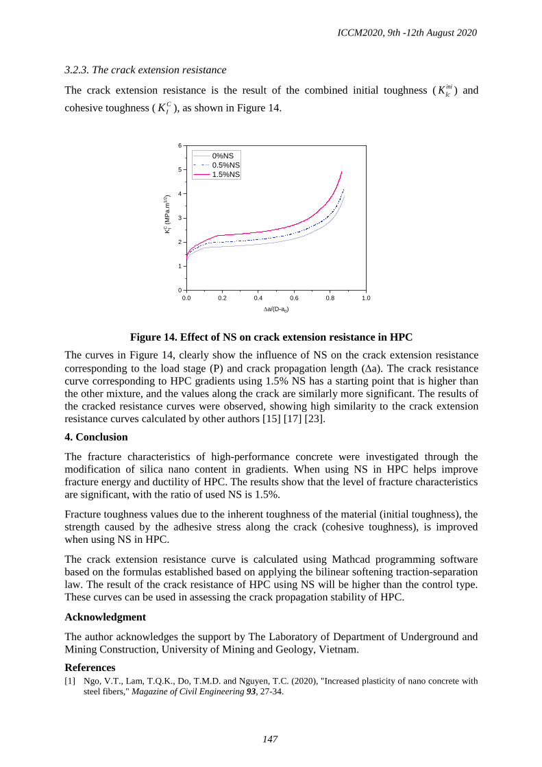
3.2.3. The crack extension resistance

The crack extension resistance is the result of the combined initial toughness ( iniIcK ) and

cohesive toughness ( CIK ), as shown in Figure 14.

Figure 14. Effect of NS on crack extension resistance in HPC

The curves in Figure 14, clearly show the influence of NS on the crack extension resistance corresponding to the load stage (P) and crack propagation length (Da). The crack resistance curve corresponding to HPC gradients using 1.5% NS has a starting point that is higher than the other mixture, and the values along the crack are similarly more significant. The results of the cracked resistance curves were observed, showing high similarity to the crack extension resistance curves calculated by other authors [15] [17] [23].

4. Conclusion

The fracture characteristics of high-performance concrete were investigated through the modification of silica nano content in gradients. When using NS in HPC helps improve fracture energy and ductility of HPC. The results show that the level of fracture characteristics are significant, with the ratio of used NS is 1.5%.

Fracture toughness values due to the inherent toughness of the material (initial toughness), the strength caused by the adhesive stress along the crack (cohesive toughness), is improved when using NS in HPC.

The crack extension resistance curve is calculated using Mathcad programming software based on the formulas established based on applying the bilinear softening traction-separation law. The result of the crack resistance of HPC using NS will be higher than the control type. These curves can be used in assessing the crack propagation stability of HPC.

Acknowledgment

The author acknowledges the support by The Laboratory of Department of Underground and Mining Construction, University of Mining and Geology, Vietnam.

References [1] Ngo, V.T., Lam, T.Q.K., Do, T.M.D. and Nguyen, T.C. (2020), "Increased plasticity of nano concrete with

steel fibers," Magazine of Civil Engineering 93, 27-34.

0.0 0.2 0.4 0.6 0.8 1.00

1

2

3

4

5

6

KC I (M

Pa.

m1/

2 )

Da/(D-a0)

0%NS 0.5%NS 1.5%NS


147

[2] Zhang, P. ,Wan, J.,Wang K. and Li, Q. (2017), "Influence of nano-SiO2 on properties of fresh and hardened high performance concrete: A state-of-the-art review," Construction and Building Materials 148, 648-658.

[3] Khaloo, A., Mobini, M. H. and Hosseini, P. (2016), "Influence of different types of nano-SiO2 particles on properties of high-performance concrete," Construction and Building Material 113, 188-201.

[4] Chithra, S., Kumar S. R. R. and Chinnaraju, K. (2016), "The effect of Colloidal Nano-silica on workability, mechanical and durability properties of High Performance Concrete with Copper slag as partial fine aggregate," Construction and Building Materials 113, 794-804.

[5] Mindess.S (2002), "Applications of fracture mechanics to concrete: Where do we go from here?," Material Science to Application 206, 475-485.

[6] Ricardo, A.E. and Marta, S.L.V. (2006), "Fracture parameters for high-performance concrete," Cement and Concrete 36, 576-583.

[7] Hilsdorf, H.K. and Brameshuber, W. (1984), "Size e€ects in the experimental determination of fracture mechanics parameters," Shah SP, editor. Application of fracture mechanics to cementitious composites. NATO-ARW,361-397.

[8] Karihaloo, B.L (1987), "Do plain and ®bber-reinforced concretes have an R-curve behaviour?," Shah SP, Swartz SE, editors. Fractures of concrete and rock, 96-105.

[9] Mai, Y.W. (1984), "Fracture measurements of cementitious composites," Shah SP, editor. Application of fracture mechanics to cementitious composites. NATO-ARW, 399-429.

[10] Bazant, Z.P. and Jirasek, M. (1993), "R-curve modeling of rate and size effects in quasibrittle fracture," International Journal of Fracture 62, 355-373.

[11] Planas, J., Elices, M. and Ruiz, G. (1993), "The equivalent elastic crack: 2. X-Y equivalences and asymptoticanalysis," Journal of Fracture 61, 231-246.

[12] Reinhardt, H.W., Cornelissen, H.A.W. and Hordijk, D.A. (1986), "Tensile tests and failure analysis of concrete," Journal of Structural Engineering, ASCE 112, 2462-2477.

[13] Xu, S. and Reinhardt, H.W. (1999), "Determination of double-K criterion for crack propagation in quasi-brittle materials - part II: analytically evaluating and practically measuring methods for three-point bending notched beams," International Journal of Fracture 98, 151-77.

[14] Kumar, S. and Barai, S.V. (2008), "Influence of specimen geometry and size-effect on the KR-curve based on the cohesive stress in concrete," International Journal Fracture 152, 127-148.

[15] Dong, W., Wu, Z.M. and Zhou, X.M. (2013), "Calculating crack extension resistance of concrete based on a new crack propagation criterion," Construction Building Material 38, 879-889.

[16] Xu, S. and Reinhardt, H.W., "Crack extenstion resistance and fracture properties of quasi-brittle materials like concrete based on the complete process of fracture," International Journal of Fracture 92, 71-99.

[17] Xu, S. and Reinhardt, H.W. (1998), "Crack extension resistance and fracture properties of quasi-brittle softening materials like concrete based on the complete process of fracture," complete process of fracture 92, 71-99.

[18] Reinhardt, H.W. and Xu, S. (1999), "Crack extension resistance based on the cohesive force in concrete," Engineerig Fracture Mechanics 64, 563-587.

[19] ACI 211.4R-08 (2008), Guide for Selecting Proportions for High-Strength Concrete Using Portland Cement and Other Cementitious Materials, American Concrete Institute.

[20] RILEM (1985), "Determination of the fracture energy of mortar and concrete by means of three-point bend tests on notched beams," Materials and Structures 18, 285-290.

[21] Fib (2008), Constitutive modelling Constitutive modelling high performance concrete, Stuttgart: Task Group 8.2.

[22] Xu, S. and Reinhardt, H.W. (1998), "Crack extenstion resistance and fracture properties of quasi-brittle materials like concrete based on the complete process of fracture," International Journal of Fracture 92, 71-99.

[23] Reinhardt, H.W. and Xu, S. (1999), "Crack extension resistance based on the cohesive force in concrete," Engineerig Fracture Mechanics 64, 563-587.

[24] Hillerborg, A. (1976), "Analysis of crack formation and crack growth in concrete by means of fracture mechanics and finite elements," Cement and Concrete Research 6, 773-782.


148

A node-based smoothed point interpolation method for coupled

hydro-mechanical analysis of geomechanical problems

†*Ashkan Shafee¹, Arman Khoshghalb¹

1 School of Civil and Environmental Engineering, UNSW Sydney, Sydney, NSW, 2052, Australia



Abstract

A node-based smoothed point interpolation method based on the generalised gradient

smoothing technique is proposed for coupled hydro-mechanical analysis of geomechanical

problems. In the proposed method, the problem domain is first discretised with the use of a

simple triangular background mesh which is used for the selection of the supporting nodes for

shape function construction as well as forming node-based smoothing domains. Weakened

weak formulation is applied for spatial discretisation of the coupled partial differential

equations. Both displacement and pressure fields are interpolated over the problem domain

using the point interpolation shape functions. A three-point time discretisation scheme with

variable time steps is used for temporal discretisation of the governing equations. Two

benchmark numerical examples with analytical/reference solutions are then used to investigate

the accuracy and the efficiency of this method compared to the conventional finite element

method.

Keywords: Geotechnical engineering, coupled analysis, saturated porous media, smoothed

point interpolation method, meshfree methods.

1 Introduction

Smoothed point interpolation methods (SPIMs) are a rather new class of numerical methods in

which the generalised gradient smoothing technique is used, making the calculation of the

derivative of independent variables unnecessary. In these methods [1], governing equations are

written in the weakened weak (𝑊2) form which, unlike the weak form used in the conventional

finite element method (FEM), eliminates the necessity of the compatibility of the approximation

functions over the problem domain. This brings several advantages to the SPIMs with respect

to the FEM such as being computationally efficient and having superior accuracy in stiffness

estimation which has been extensively investigated in solid mechanics problems [2].

However, applications of SPIMs to coupled geomechanical problems are limited in the

literature [3-6] and the main focus of these studies have been on the edge-based SPIMs

(ESPIMs) and cell-based SPIM (CSPIMs). The goal of this paper is to study the application of

two different node-based SPIMs i.e. NSPIM and NSRPIM in linear and nonlinear coupled

geomechanical problems to investigate how gradient smoothing operation in NSPIMs affects


149

the accuracy and the efficiency of the calculated property matrices of the domain. The

performance of the NSPIMs are compared to that of the linear FEM using the same triangular

background mesh for benchmarking. The comparative study is performed through two

numerical examples with benchmark solutions.

2 Notation

The compact matrix-vector notation where bold letters indicate matrices and vectors are

adopted in this paper. A two-dimensional plane strain setting is assumed. The differentiation

operator is defined as follows,

𝑳𝑑 =

[

𝜕

𝜕𝑥10

0𝜕

𝜕𝑥2

𝜕

𝜕𝑥2

𝜕

𝜕𝑥1]

(1)

with 𝑥1 and 𝑥2 being space coordinates. 𝜵 is the gradient operator expressed as 𝜵 = 𝑳𝑑T𝜹, with

𝜹 = [1 1 0]T. The divergence of a vector is shown with 𝑑𝑖𝑣(𝒗) = 𝜵𝑇𝒗. The outward unit

normal matrix at any point of interest is expressed as,

𝑳𝑛 = [𝑛1 00 𝑛2

𝑛2 𝑛1

] (2)

in which 𝑛1 and 𝑛2 are the components of the unit normal vector at the point of interest in the

𝑥1 and 𝑥2 directions, respectively. An over-dot indicates time derivative of the corresponding

parameter. Voigt notation is adopted throughout where second order stress and strain tensors

are written as column matrices, and the fourth order constitutive tensor is written as a square

matrix [7]. The sign convention of geomechanics is adopted where compressive stresses and

strains are taken as positive.

3 Governing equations

The equations governing the behaviour of a saturated porous medium are obtained based on

two interacting models: the deformation model and the flow model. The deformation model is

based on the equilibrium of the porous medium. Assuming small strains and ignoring inertia

forces, the deformation model is expressed as [8].

𝑳𝑑𝑇𝝈 + 𝜌𝒈 = 𝟎 (3)

where 𝛔 is the total stress vector, 𝜌 is the density of the porous medium, and 𝐠 = [0 𝑔 0]T

is the gravity acceleration vector with 𝑔 being the gravitational constant.


150

The flow model can be obtained from the combination of mass balance equation for the fluid

phase with Darcy’s law for the fluid flow in porous media, resulting in,

𝑑𝑖𝑣 [𝒌𝑓

𝜇𝑓(𝜵𝑝𝑓 + 𝜌𝑓)] − 𝑎𝑓𝑓 + 𝑑𝑖𝑣() = 𝟎 (4)

where = [0 𝑔]T, 𝒖 is the displacement vector of the soil skeleton, and 𝑝𝑓 is the fluid

pressure. 𝐤f is the intrinsic permeability of the medium, 𝜇f is the dynamic viscosity of the fluid,

and 𝜌f is the density of the fluid. Assuming the solid grains are incompressible, 𝑎f = 𝑛𝑐f where

𝑛 is the porosity of the porous medium and 𝑐f is the compressibility of the fluid phase.

Equations (3) and (4) are further coupled through the Terzaghi’s effective stress principle:

𝝈 = 𝝈′ + 𝑝𝑓𝜹 (5)

where 𝛔′ indicates the effective stress. To complete the governing equations, an incremental

constitutive law is also needed,

𝑑𝝈′ = 𝑫𝑒𝑝𝑑𝜺 (6)

where 𝐃ep is the tangent elasto-plastic constitutive matrix, and 𝑑𝛆 is the strain increment for

the solid matrix obtained as follows,

𝑑𝜺 = 𝑳𝑑(𝑑𝒖) (7)

Elastic isotropic material is considered in the first example and for the nonlinear example

associated Mohr-Coulomb behaviour is assumed. The formulation and implementation of the

elastic isotropic, and Mohr-Coulomb constitutive models can be found in the standard literature

[9], hence they are not discussed here.

The required boundary conditions for solving the governing equations can be expressed as

follows for the deformation model,

𝒖(𝒙, 𝑡) = 𝑜𝑛 𝛤𝑢 (8-1)

𝑳𝑛𝑇𝝈(𝒙, 𝑡) = 𝑜𝑛 𝛤𝑡 (8-2)

where 𝛤𝑢 and 𝛤𝑡 are restricted regions of the boundary of the domain corresponding to the

prescribed displacement () and prescribed traction (), such that 𝛤 = 𝛤𝑢 ∪ 𝛤𝑡 and

𝛤𝑢 ∩ 𝛤𝑡 = ∅ with Γ being the external boundary of the domain of interest.

For the flow model, the boundary conditions are as follows,


151

𝑝𝑓(𝒙, 𝑡) = 𝑓(𝑡) 𝑜𝑛 𝛤𝑝 (9-1)

−𝑳𝑛𝒗𝑟(𝒙, 𝑡) = (𝑡) 𝑜𝑛 𝛤𝑞 (9-2)

where 𝒗𝑟 is the fluid velocity relative to the solid phase. 𝛤𝑝 and 𝛤𝑞 are regions of the boundary

of the domain corresponding to the prescribed pore fluid pressure () and prescribed flux (),

again satisfying 𝛤 = 𝛤𝑝 ∪ 𝛤𝑞 and 𝛤𝑝 ∩ 𝛤𝑞 = ∅.

Finally, the initial conditions at 𝑡 = 0 are given as

𝒖(𝒙, 0) = 𝒖0(𝒙) 𝑜𝑛 𝛺 (10)

𝑝𝑓(𝒙, 0) = 𝑝𝑓0(𝒙) 𝑜𝑛 𝛺 (11)

where 𝛺 is the problem domain.

4 Node based smoothed point interpolation method

4.1 Construction of smoothing domains and support nodes selection schemes

In NSPIMs, a triangular background mesh is first generated over the domain and then, the

smoothing domains are constructed around the nodes of the background mesh as shown in

figure 1. Similar to the standard FEM, the domain is discretised into 𝑛𝑒 elements with 𝑛𝑛 nodes

such that Ω = ⋃ Ω𝑖𝑒𝑛𝑒

𝑖=1 and Ω𝑖𝑒 ∩ Ω𝑗

𝑒 = ∅ for 𝑖 ≠ 𝑗 where Ω𝑖𝑒 stands for the domain of the 𝑖th

element. The total number of 𝑛SD smoothing domains are then constructed on top of the

triangular background mesh, again in such a way that Ω = ⋃ Ω𝑖𝑆𝐷𝑛𝑆𝐷

𝑖=1 and Ω𝑖𝑆𝐷 ∩ Ω𝑗

𝑆𝐷 = ∅ for

𝑖 ≠ 𝑗 where Ω𝑖𝑆𝐷 is the domain of the 𝑖th smoothing domain. The triangular background mesh

also serves as a means for the selection of the supporting nodes at each point of interest. In this

study, T3 scheme is used for NSPIM (i.e. NSPIM-Tr3) in which the three nodes of the cell

hosting the point of interest are adopted. On the other hand, T6 scheme is used for NSRPIM

(i.e. NSRPIM-Tr6) in which in addition to the three nodes of the host cell, another three remote

nodes of the three neighbouring cells are also adopted.


152

Figure 1. Schematic representation of a typical node based smoothing domain (blue

nodes are adopted in T3 scheme and All blue and red nodes are considered for T6

scheme)

4.2 Function approximation

The point interpolation method (PIM) using polynomial basis functions is used in this study to

construct shape functions in the NSPIM-Tr3 and for the NSRPIM-Tr6, the polynomial bases

are augmented with the radial basis functions resulting in the radial point interpolation method

(RPIM) shape functions. Interested readers are referred to [2, 10, 11] for more details on these

shape functions.

4.3 Strain field construction

In NSPIMs, unlike the FEM that uses the compatible strain, a constructed stain field is used in

the formulation. The strain field is constructed using the assumed displacement filed, without

introducing additional degrees of freedom. The constructed strain in NSPIMs are referred to as

the smoothed strain which is constant over each node based smoothing domain, and defined as

follows [10]:

𝑘 =1

𝐴𝑘𝑆𝐷 ∫ 𝑳𝑛𝒖(𝒙) 𝑑𝛤

𝛤𝑘𝑆𝐷 (12)

where 𝑘 is the smoothed strain over the 𝑘th node based smoothing domain (𝛺𝑘SD) having the

area of 𝐴𝑘𝑆𝐷 and the boundary of 𝛤𝑘

SD(𝑘 = 1,… , 𝑛SD), and 𝑳𝑛 is the outward normal matrix

defined earlier in the paper. Writing displacements in terms of shape functions, the smoothed

strain for the 𝑘th smoothing domain can be related to the nodal displacements,


153

𝑘 = (1

𝐴𝑘𝑆𝐷 ∫ 𝑳𝑛𝑵𝑢(𝒙) 𝑑𝛤

𝛤𝑘𝑆𝐷 )𝒖 = ∑ [

1𝑖0

0 2𝑖

2𝑖1𝑖

] 𝑢1𝑖𝑢2𝑖

𝑞𝑖=1 = 1𝒖 (13)

with

𝑵𝑢(𝒙) = [𝜑1(𝒙) 0

0 𝜑1(𝒙)…

𝜑𝑞(𝒙) 0

0 𝜑𝑞(𝒙)]2×2𝑞

(14)

1 = [

110

0 21

2111

…

1𝑞0

0 2𝑞

2𝑞1𝑞

]

3×2𝑞

(15)

𝒖 = [𝑢11𝑢21

𝑢12𝑢22

⋯ 𝑢1𝑞𝑢2𝑞]𝑇 (16)

and

𝑖𝑙 =1

𝐴𝑘𝑆𝐷 ∫ 𝜑𝑖(𝒙)

𝛤𝑘𝑆𝐷 𝑛𝑙(𝒙)𝑑𝛤, 𝑙 = 1,2 (17)

where 𝑞 is the total number of supporting nodes of all the Gauss points on the boundaries of the

𝑘th smoothing domain. 𝑢1 and 𝑢2 are the components of displacement in 𝑥1 and 𝑥2 directions,

respectively. 1 is constant over each smoothing domain. The integration in Eq. (17) can be

easily obtained using the Gauss integration scheme, by summing the contribution of all the

segments of the boundary of the 𝑘th smoothing domain.

5 Discretisation of the governing equations and numerical algorithm

Fully discretised governing equations obtained by applying three-point time discretisation

approach with variable time steps presented in [12] are as follows,

𝐊Tt+α∆t𝐔t+α∆t + η𝐐𝐏t+α∆t − 𝐅u

t+α∆t = 𝟎 (18)

𝜂𝑸𝑇(𝑎𝑼𝑡+𝛼∆𝑡 − 𝑏𝑼𝑡 + 𝑐𝑼𝑡−𝛥𝑡) − 𝛥𝑡𝑯𝑷𝑡+𝛼∆𝑡 − 𝑎𝑓𝑺(𝑎𝑷𝑡+𝛼∆𝑡 − 𝑏𝑷𝑡 + 𝑐𝑷𝑡−𝛥𝑡) −

𝛥𝑡𝑭𝑝𝑡+𝛼∆𝑡 = 𝟎

(19)

where 𝐔 is the vector of nodal displacements, 𝐏 is the vector of the nodal pore fluid pressures,

𝐅u is the vector of nodal forces, 𝐅p is the vector of nodal fluxes, and 𝐐, 𝐒 and 𝐇 are the global

property matrices of the system, evaluated by assembling the corresponding local property

matrices computed over the smoothing domains.


154

Eq. (18) and Eq. (19) form a fully coupled equation system that must be solved at each time

step. The system of equations is nonlinear in general; hence a modified Newton-Raphson

iterative process is adopted in this study to obtain the numerical solutions at each time step.

More details are reported in [3-6].

6 Numerical examples

Two benchmark examples are studied in this section to thoroughly examine the NSPIMs

discussed in the previous sections in coupled problems of geomechanics. At each case, the

numerical solutions of the NSPIMs are compared to those of the standard linear FEM obtained

using the same triangular mesh for benchmarking. Analytical solutions are available for the first

example, hence thorough error analyses are performed. For the second example, analytical

solutions are not available, therefore numerical solutions obtained using the FEM with a very

fine mesh is adopted as reference solutions.

For quantitative assessment of each numerical technique, few error norms are adopted. The

displacement and pore pressure error norms are defined as follows:

𝐸𝑑 = √∑ ((𝒖𝑖

𝑒𝑥𝑐−𝒖𝑖𝑛𝑢𝑚)

𝑇(𝒖𝑖

𝑒𝑥𝑐−𝒖𝑖𝑛𝑢𝑚))

𝑛𝑛𝑖=1

∑ ((𝒖𝑖𝑒𝑥𝑐)

𝑇𝒖𝑖

𝑒𝑥𝑐)𝑛𝑛𝑖=1

(20)

𝐸𝑝 = √∑ (𝑝𝑓𝑖

𝑒𝑥𝑐−𝑝𝑓𝑖𝑛𝑢𝑚)

2𝑛𝑛𝑖=1

∑ (𝑝𝑓𝑖𝑒𝑥𝑐)

2𝑛𝑛𝑖=1

(21)

in which the superscripts exc and num for both 𝒖 and 𝑝𝑓 stand for the exact and numerical

solutions, respectively, and subscript 𝑖 denotes the node number. Similarly, to measure the error

in stress solution at nodes, we use,

𝐸𝑠 = √∑ ((𝝈𝑖

𝑒𝑥𝑐−𝝈𝑖𝑛𝑢𝑚)

𝑇(𝝈𝑖

𝑒𝑥𝑐−𝝈𝑖𝑛𝑢𝑚))

𝑛𝑛𝑖=1

∑ ((𝝈𝑖𝑒𝑥𝑐)

𝑇𝝈𝑖

𝑒𝑥𝑐)𝑛𝑛𝑖=1

(22)

6.1 Example 1: One dimensional consolidation

The first example involves Terzaghi’s one dimensional consolidation problem, as illustrated in

Figure 2. A fully saturated porous medium with the height of 𝐻 = 10𝑚 and width of 𝐵 = 1𝑚

is subjected to a sudden loading of 𝑞 = 10 𝑘𝑃𝑎 at time 𝑡 = 0. The surface of the medium is

assumed to be fully drained and the other boundaries of the domain are impermeable. The base

of the domain is fully fixed, and the left and right sides of the domain are fixed against

horizontal displacement only. Isotropic linear elastic behaviour is assumed for the solid


155

skeleton, with the following properties: 𝜇𝑓 = 1 × 10−6 𝑘𝑃𝑎 𝑠, 𝑘𝑓 = 10−12 𝑚2, 𝐸 = 10 𝑀𝑃𝑎

and 𝜈 = 0.3. This problem involves both deformation and flow through the porous media, so

the combining effects of the stiffness matrix, permeability matrix and the coupling matrix of

the domain are studied.

Figure 2. Schematic representation of the computational domain along with the

observation points used for analyses of the one-dimensional consolidation problem.

The numerical results obtained using different methods in terms of dimensionless surface

settlement (𝑢

𝑢𝑢𝑙𝑡 with 𝑢𝑢𝑙𝑡 being the ultimate surface settlement) versus dimensionless time

(𝑡𝐷 =𝐸𝑘𝑓(1−𝜈)

𝜇𝑓(1+𝜈)(1−2𝜈)𝐻2 𝑡), and dimensionless excess pore fluid pressure (𝑝𝑓

𝑞) versus

dimensionless time at three depths of interest (points A, B and C shown in Figure 2), are

presented in Figures 3. Also included in these figures are the analytical solutions to the problem

[13].The numerical results are obtained using a regular triangular mesh consisting of 63 nodes

and 80 elements (mesh #1 in Table 1). Initial dimensionless time step of ∆𝑡D0 =

0.0001346 (∆𝑡0 = 1𝑠) and the time step growth factor of 𝛼 =1.1 are used in the analyses.


156

(a)

(b)

Figure 3. Analyses of the one-dimensional consolidation problem with different methods

for

(a) 𝒅𝒊𝒎𝒆𝒏𝒔𝒊𝒐𝒏𝒍𝒆𝒔𝒔 𝒔𝒖𝒓𝒇𝒂𝒄𝒆 𝒔𝒆𝒕𝒕𝒍𝒆𝒎𝒆𝒏𝒕 ; (b) 𝐝𝐢𝐦𝐞𝐧𝐬𝐢𝐨𝐧𝐥𝐞𝐬𝐬 𝐞𝐱𝐜𝐞𝐬𝐬 𝐩𝐨𝐫𝐞 𝐩𝐫𝐞𝐬𝐬𝐮𝐫𝐞

For all methods, excellent agreement exists between the numerical and analytical solutions. In

order to quantitively compare the NSPIMs with FEM, various error norms of the solutions are

obtained for different discretisation densities detailed in Table 3 at two dimensionless times of

𝑡𝐷 = 0.1083 and 𝑡𝐷 = 0.8018 reached using ∆𝑡𝐷0 = 0.0001346 and 𝛼 = 1.1.

Table 1. The properties of different mesh configurations used for the analysis of the one-

dimensional consolidation problem.

Mesh number Number of nodes Number of elements Average nodal spacing, h (m)

1 63 80 0.4558

2 104 150 0.3437

3 205 320 0.2374

4 306 500 0.1917

Figures 4 to 6 compare the convergence rates of the solutions in terms of displacement, pore

fluid pressure and stress of the solutions.


157

(a)

(b)

Figure 4. Displacement error norms versus mesh size for one-dimensional

consolidation problem at dimensionless time (a) 𝒕𝑫 = 𝟎. 𝟏𝟎𝟖𝟑 ; (b) 𝒕𝑫 = 𝟎. 𝟖𝟎𝟏𝟖

(a)

(b)

Figure 5. Excess pore fluid pressure error norms versus mesh size for one-dimensional

consolidation problem at dimensionless time (a) 𝒕𝑫 = 𝟎. 𝟏𝟎𝟖𝟑 ; (b) 𝒕𝑫 = 𝟎. 𝟖𝟎𝟏𝟖


158

(a)

(b)

Figure 6. Stress error norms versus mesh size for one-dimensional consolidation

problem at dimensionless time (a) 𝒕𝑫 = 𝟎. 𝟏𝟎𝟖𝟑 ; (b) 𝒕𝑫 = 𝟎. 𝟖𝟎𝟏𝟖

According to Figures 4,5 and 6 all of the error norms indicate that the NSRPIM-Tr6 is more

accurate than the NSPIM-Tr3 and FEM. In general, the results of the FEM are similar to those

of the NSPIM-Tr3, although the FEM is more accurate than the NSPIM-Tr3 at early stages of

the consolidation in estimation of the displacements.

To quantitatively assess the efficiency of different NSPIMs and FEM in this example, the values

of various error norms and the computational time of the analyses for each NSPIM, normalised

by those of the FEM and presented in Table 2. Efficiency of each NSPIM compared to the FEM

is defined as the inverse of the product of the normalised error norms and the computational

time ratios. The efficiency assessment is performed using mesh configuration number 1 (Table

1) at an arbitrary time of 𝑡𝐷 = 1.0.

Table 2. Comparison of the computational efficiency of the NSPIMs and FEM

in terms of various error norms in 1D consolidation problem.

Numerical

method Displacement

Excess pore

water

pressure

Stress CPU

time

Relative

efficiency

FEM 1.000 1.000 1.000 1.0000 1.00

NSPIM-Tr3 0.829 0.912 0.930 1.0662 1.334

NSRPIM-Tr6 0.248 0.299 0.797 1.9560 8.651

Table 2 shows that although CPU times are higher in NSRPIM-Tr6 compared to the FEM, this

method is more efficient that FEM owing to its higher accuracy. The NSPIM-Tr3 and FEM are

similar considering the efficiency.


159

6.2 Example 2: Two-dimensional consolidation

Performance of the NSPIMs in elasto-plastic problems of saturated porous media are studied in

this example where consolidation of a saturated soil layer subjected to a strip loading is

considered. No analytical solution is available for this problem, hence the reference solution is

obtained using an FEM analysis with a very fine mesh, which is in perfect agreement with the

solutions reported in [14].

The load is applied through a flexible, smooth, and impervious strip footing of a half width 𝑎,

placed on a free draining soil surface, as shown in Figure 7. The lateral extent of the soil layer

from the centre of the strip load is assumed to be 𝑊 = 16𝑎 and the depth of the clay layer is

taken as 𝐻 = 8𝑎, as also shown in Figure 7. The soil layer is assumed to be on an impervious

nondeformable bedrock.

Figure 7. The geometry and boundary conditions, along with the mesh used in the

numerical analysis of the problem of two-dimensional elasto-plastic consolidation.

It is assumed that the soil skeleton is an ideal elasto-plastic material obeying a Mohr-Coulomb

yield criterion and the flow rule is associated. The material parameters are assumed 𝐸 =

2000 𝑘𝑃𝑎, 𝜈 = 0.3, 𝑐 = 10 𝑘𝑃𝑎, 𝜑 = 𝜓 = 20°, where 𝜑 is the friction angle and 𝜓 is the

dilation angle. Soil permeability is assumed 𝑘𝑓

𝜇𝑓𝛾𝑤 = 1 × 10−5 𝑚/𝑑𝑎𝑦. Due to symmetry, only

half of the domain is modelled in the numerical analyses, as shown in Figure 7. A non-uniform

triangular mesh consisting of 508 nodes and 952 elements (shown in Figure 7) is used in all the

analyses.


160

It is assumed that the vertical pressure of the footing is increased linearly from zero at 𝑡D = 0

to 𝑤 = 100 kPa at time 𝑡D = 0.01, and remains constant afterwards, with the dimensionless

time defined 𝑡𝐷 =𝐸𝑘 𝑡

2𝛾w(1+𝜈)(1−2𝜈)𝑎2 [4, 14].

The linear loading is simulated through 10 steps of 𝛥𝜔 = 10 kPa with ∆𝑡D = 0.001 and

𝛼 = 1.0. The time step growth factor is subsequently increased to 𝛼 = 1.1 for the rest of the

analysis in all cases. 𝑎 = 3 m is used in the numerical analyses.

The variations of the dimensionless settlement (defined as 100𝑣 𝑎⁄ where 𝑣 is the settlement)

at the centre of the footing (point A in Figure 7) with dimensionless time is shown in Figure 8

for different methods. From the zoomed section of the plot shown in the inset, it is seen that

again FEM produces the most accurate results in this problem.

Figure 8. Variation of the dimensionless settlement with dimensionless time at the

center of the footing obtained using different methods

Figure 9 shows the variation of the dimensionless pore fluid pressure (defined as 𝑝f 𝑤⁄ ), at

point A with respect to the dimensionless time obtained using different methods, along with the

reference solution. This figure shows that in terms of pore water pressure calculations, NSPIMs

yields the most accurate results.


161

Figure 9. Variation of the dimensionless pore fluid pressure with time at the center of

the footing obtained using different methods.

To compare the computational efficiency of the SPIMs to that of the FEM in non-linear

analyses, the total number of Newton-Raphson iterations, average time of the analyses for each

iteration, and the total time of the analysis for the first 25 time steps of the solution are presented

in Table 3 for the NSPIMs (again normalised with respect to the FEM).

Table 3. Comparison of the computational time required by different techniques for

the two-dimensional elasto-plastic consolidation problem

Numerical

method

Total number of

iterations in the first

25 time steps

Average analysis time of each

iteration for the first 25 time steps

with respect to that of FEM

Total time of the analysis for the

first 25 time steps with respect

to that of FEM

FEM 162 1 1.000

NSRPIM-Tr6 158 1.022 0.996

NSPIM-Tr3 161 1.015 1.009

The third column of Table 3 shows that both NSPIMs are slower than the FEM in each iteration.

This is consistent to the performance of SPIMs in single phase materials too [2] and can be

related to more complicated shape function constructions in SPIMs. However, from the last

column of Table 3, which shows the total time of the analyses, it can be seen that NSRPIM-Tr6

is slightly more efficient than the FEM due to a lower number of iterations it requires for

convergence, which is in turn due to its higher solution accuracy compared to the FEM. Overall,

the efficiency of the NSPIMs is very similar to that of the FEM in this example.


162

7 Conclusions

The application of two different NSPIMs in coupled problems of geomechanics was

investigated using various error norms of the solutions, and compared to those of the standard

linear FEM. Overall, NSRPIM-Tr6 was the most accurate and efficient numerical method

among the three techniques investigated. The performance of the NSPIM-Tr3 was similar to

that of the linear FEM. It was observed that the superiority of the NSRPIM-Tr6 over the FEM

is less prominent in coupled flow-deformation problems when material nonlinearity is involved.

8 References

[1] Liu G, Nguyen-Thoi T, Nguyen-Xuan H, Lam K. A node-based smoothed finite element method (NS-FEM)

for upper bound solutions to solid mechanics problems. Computers & structures. 2009;87(1-2):14-26.

[2] Liu G-R, Zhang G-y. Smoothed point interpolation methods: G space theory and weakened weak forms:

World Scientific, 2013.

[3] Ghaffaripour O, Esgandani GA, Khoshghalb A, Shahbodaghkhan B. Fully coupled elastoplastic hydro‐

mechanical analysis of unsaturated porous media using a meshfree method. International Journal for Numerical

and Analytical Methods in Geomechanics. 2019.

[4] Ghaffaripour O, Khoshghalb A, Khalili N. An edge-based smoothed point interpolation method for elasto-

plastic coupled hydro-mechanical analysis of saturated porous media. Computers and Geotechnics. 2017;82(99-

109.

[5] Khoshghalb A, Shafee A, Tootoonchi A, Ghaffaripour O, Jazaeri S. Application of the smoothed point

interpolation methods in computational geomechanics: A comparative study. Computers and Geotechnics.

2020;126(103714.

[6] Tootoonchi A, Khoshghalb A, Khalili N. Meshfree Method Analysis of Biot's Consolidation Using Cell-

Based Smoothed Point Interpolation Method. Applied Mechanics and Materials: Trans Tech Publ, 2016. p. 409-

14.

[7] Belytschko T, Liu WK, Moran B, Elkhodary K. Nonlinear finite elements for continua and structures: John

wiley & sons, 2013.

[8] Khoshghalb A, Khalili N. A stable meshfree method for fully coupled flow-deformation analysis of saturated

porous media. Computers and Geotechnics. 2010;37(6):789-95.

[9] Potts DM, Zdravković L, Addenbrooke TI, Higgins KG, Kovačević N. Finite element analysis in

geotechnical engineering: application: Thomas Telford London, 2001.

[10] Liu G. AG space theory and a weakened weak (W2) form for a unified formulation of compatible and

incompatible methods: Part I theory. International Journal for Numerical Methods in Engineering.

2010;81(9):1093-126.

[11] Liu G. AG space theory and a weakened weak (W2) form for a unified formulation of compatible and

incompatible methods: Part II applications to solid mechanics problems. International journal for numerical

methods in engineering. 2010;81(9):1127-56.

[12] Khoshghalb A, Khalili N, Selvadurai A. A three‐point time discretization technique for parabolic partial

differential equations. International Journal for Numerical and Analytical Methods in Geomechanics.

2011;35(3):406-18.

[13] Terzaghi K. Theoretical soil mechanics. johnwiley & sons. New York. 1943:11-5.

[14] Manoharan N, Dasgupta S. Consolidation analysis of elasto-plastic soil. Computers & structures.

1995;54(6):1005-21.


163

Higher-order mixed finite elements for nonlinear analysis of framesincluding shear deformation

†∗J. Petrolito and D. IonescuDepartment of Engineering, La Trobe University, Australia.

∗Presenting author: [email protected]


Abstract

In past practice, linear analysis was generally consideredsufficient for the static analysis ofstructural frames. Nonlinear effects, such as column buckling, were considered at the elementlevel rather than at the complete structure level. However,recent codes of practice often requirea more complete nonlinear analysis to be performed. While these requirements lead to a moreaccurate analysis, there has been little guidance given to the type and implementation of suchan analysis. Moreover, different implementations have been adopted by various commercialsoftware.

In this paper, we discuss the use of mixed finite elements for the large deflection analysis of two-dimensional frames including shear deformation. In particular, we develop various higher-ordermixed elements that can be combined with different nonlinear models and discuss the effectsof various assumptions and approximations that are commonly used to simplify the analysis.Examples are given to illustrate the various issues discussed.

Keywords: Frame analysis, nonlinear analysis, shear deformation, mixed finite elements.

Introduction

Prismatic structural frames are an essential part of structural engineering, and their efficientanalysis and design are fundamental requirements for the profession. Linear analysis of suchframes can generally be used under working load conditions,and standard software packagesbased on matrix methods [1] are readily available. However,many design codes have introducednonlinear analysis requirements, and this type of analysisis required to characterise the failureconditions of frames [2].

In many structural frames, shear deformation is small and can be ignored during the analysis.However, shear deformations is important in sandwich construction, built-up columns and tallbuilding frames [3][4]. Shear deformation reduces the buckling capacity of a structure, andhence ignoring this effect can lead to an unsafe design. For example, the failure of the first Que-bec bridge resulted from ignoring shear effects [3]. Shear deformation can also be significant invibration analysis. Finally, as Reissner [5] noted, the inclusion of shear effects in a beam theoryis more consistent with elasticity theory.

Nonlinear analysis methods of frame analysis are not as well-developed as linear analysis meth-ods, and many methods have been proposed. Most of these methods use a numerical approachthat is combined with ad-hoc simplifying assumptions of thestructural behaviour under large


164

deflections. However, some of these ad-hoc simplifying assumptions can lead to significanterrors [6].

These errors can be eliminated by using a general nonlinear beam theory. Moreover, the generalnonlinear theory can also be used to systematically derive simplified nonlinear theories, and tostudy the errors that arise from the simplifying assumptions. Simplifying assumptions can beintroduced through the governing differential equations or the associated variational formula-tion [7][8]. While both routes can be used, the latter approach is more suitable for a standardfinite element formulation.

Most finite elements for nonlinear frame analysis are based on a displacement approach [1, 9].In this formulation, the stresses are related to the derivatives of the displacements, and they gen-erally converge slower than the displacements. This issue can be alleviated by adopting eithera hybrid or mixed formulation, whereby the displacements and stresses are element variables.While these formulations can sometimes have convergence and robustness issues, they oftenwork well and produce elements with good accuracy for both displacements and stresses. Inaddition, some mixed elements can be related to displacement elements with alternative inte-gration schemes [10].

This paper details the derivation of various higher-order mixed finite elements for nonlinearframe analysis including shear deformation. The elements can be used with different nonlinearbeam models, and the effects of simplifying assumptions can be evaluated in a systematic way.Examples are given to illustrate the various issues discussed.

Governing Equations

We use Reissner’s nonlinear beam theory [5] as the underlying theoretical model. This theoryincludes the effects of large displacements and shear deformations, and it is an extension ofTimoshenko’s beam theory [11]. It is denoted as the shearable elastica theory below.

Fig. 1 shows an element of a straight beam whose centroidal axis is initially along thex axis,where i and j are unit vectors along thex and y axes, respectively. After deformation, theaxis deforms into a smooth curves(x) and the pointP is mapped to the pointP ∗. The beamdisplacements areu(x) and v(x), and the angle betweens and thex axis atP ∗ is β(x) =

φ(x)+χ(x), whereφ(x) is the angle between the normal vector for the deformed cross-sectionand thex axis andχ(x) is the shear angle.

An element∆x on the original centroidal axis is deformed into an element∆s. From thegeometry,

s′ =

√

(1+ u′)2 + (v′)2, cosβ =1+ u′

s′, sinβ =

v′

s′(1)

where a prime denotes differentiation with respect tox.

The strain measures for the deformation of the beam are the extensional strain,ǫ, the bendingstrain,κ, and the shear strain,γ. These are defined as

ǫ = (1+ e) cosχ − 1, κ = φ′, γ = (1+ e) sinχ (2)


165

P

P ∗

ui + vj

β

∆x

∆s

x, u, i

y, v, j

H

V

M

(1+ u′)∆x

∆v∆s

β

NQ

φ

Figure 1. Sign convention

wheree = s′ − 1 (3)

is the extensional strain that occurs when shear effects are ignored.

The force resultants on the deformed cross-section of the beam are the horizontal and verticalforce components,H andV , and the bending moment,M. The normal and shear forces arerelated toH andV by

N = H cosφ + V sinφ, Q = −H sinφ + V cosφ (4)

The equilibrium equations for the beam are

H ′+ px = 0, V ′

+ py = 0, M ′ −Hv′ + V (1+ u′) = 0 (5)

wherepx andpy are the distributed loads acting on the beam in thex andy directions, respec-tively.

The strains and internal forces are linked by constitutive relationships, which can be linearor nonlinear depending on the material. The appropriate constitutive relationship for shear ina nonlinear beam theory has been the subject of some discussion [12]-[14]. We use linearrelationships in this paper for simplicity. If required, other nonlinear effects, such as plasticity,can be incorporated using the techniques discussed in previous work [6].

ǫ =N

EA, κ =

M

EI, γ =

Q

kGA(6)

whereE is Young’s modulus,G is the shear modulus,A is the cross-section area,I is the secondmoment of area andk is the shear correction factor [3].

The governing equations need to be supplemented by appropriate boundary conditions for aparticular problem. Exact solutions can only be obtained for simple problems [13]. Hence,practical problems are often solved by using a simplified theory combined with a numericalapproach. However, this approach can lead to significant errors for some problems [15].


166

Variational Formulation

Using standard results from the calculus of variations [16], it can be shown that the governingequations of the problem are the Euler-Lagrange equations of the functional

Π[u] =∫L

0F [u] dx −H∗u(x∗) − V ∗v(x∗) −M∗φ(x∗) (7)

In Eq. (7),

F [u] = Hu′ + V v′ +Mφ′ −M2

2EI−

fH2c2

2−

H2

2kGA+

fV 2c2

2−

V 2

2EA

− fHV cs +H (1− c) − V s − pxu − pyv (8a)

u = u, v, φ, H, V, M (8b)

f =1EA

−1

kGA, s = sinφ, c = cosφ (8c)

In addition,L is the length of the beam andH∗, V ∗ andM∗ are specified loads at pointx∗.This functional is related to the Hellinger-Reissner functional in elasticity theory [16]. Bound-ary conditions associated withu, v andφ are essential and must be enforced, while boundaryconditions associated withH, V andM are natural, and need not be enforced by the approxi-mation.

The functional in Eq. (7) is nonlinear due to the trigonometric terms associated withφ. Itis possible to derive simplified variational principles by expanding the trigonometric terms asTaylor series and truncating the series as required. The expansions of sinφ and cosφ are

sinφ = φ −φ3

3!+

φ5

5!− · · · , cosφ = 1−

φ2

2!+

φ4

4!−

φ6

6!+ · · · (9)

The use of these expansions in Eq. (7) produces annth order functional when terms inφn+1 andhigher are dropped from the expansions.

Element Formulation

The functional in Eq. (7) allows independent approximations to be used for all the problemvariables, and this leads to a mixed finite element formulation. The displacement variablesu, vandφ must beC0-continuous across elements, because the functional contains first derivativesof the displacements. In contrast, the functional does not contain any derivatives ofH, V andM. Hence, the force variables can be discontinuous across elements, and they can be definedlocally within each element.

Many mixed elements can be derived to use with Eq. (7), and various higher-order elements aredeveloped below. Fig. 2 shows the geometry of a typical three-node element,e, of lengthLe,that connects nodesi andj in the finite element mesh. The internal node,k, is used for defininghierarchical shape functions.


167

i j

kui, vi, φi uj, vj, φj

Le/2 Le/2

x

Figure 2. Typical element,e

The element approximations are taken as

ue(x) =(

1−x

Le

)

ui +x

Leuj +

Pu∑

p=1

Npd(x)ukp (10a)

ve(x) =(

1−x

Le

)

vi +x

Levj +

Pv∑

p=1

Npd(x)vkp (10b)

φe(x) =(

1−x

Le

)

φi +x

Leφj +

Pφ∑

p=1

Npd(x)φkp (10c)

He(x) = Hk +

PH∑

p=1

Npf (x)Hkp (10d)

V e(x) = Vk +

PV∑

p=1

Npf (x)Vkp (10e)

Me(x) = Mk +

PM∑

p=1

Npf (x)Mkp (10f)

whereNpd(x) and Npf (x) are hierarchical shape functions of increasing orders [10]. Thelowest-order shape function inNpd(x) is quadratic, while the lowest-order shape function inNpf (x) is linear. Equating the external nodal variablesui, vi, · · ·φj across adjacent elementsensures thatu, v andφ are continuous in the mesh. All the hierarchical variables are local tothe element. The global variables for the mesh are the collection of the nodal and hierarchicalvariables, and they are denoted by the vectora below.

The approximations in Eq. (10) allows elements of any order of approximations for each ofthe variables to be systematically generated using the sameformulation. The order of theapproximations is simply varied by changing the number of terms taken in the summations.This provides the most flexible approximation scheme, whereconvergence can be achievedby using more elements (h-refinement), higher-order approximations (p-refinement) or both(hp-refinement). Generally,hp-refinement is the most computationally-efficient method forachieving accurate results [10].

Many combinations of the displacement and force approximations in Eq. (10) can be success-fully used, subject only to the basic requirements for a mixed element to work [10]. However,the approximations in this paper are restricted to satisfy

Pu = Pv = Pphi = PH = PV = PM = P (11)


168

Although these restrictions are not necessary for the elements to work, they are safe choice.Hence, the lowest-order element that can be used for the analysis is obtained by takingP = 0.This corresponds to using linear approximations for the displacements and constant approxima-tions for the forces. Results for this simple element were presented previously [17].

Substituting Eq. (10) for each element into Eq. (7) and setting the first variation ofΠ to zerogives a set of nonlinear equations

f(a) = R (12)

whereR is the global load vector. The global equations in Eq. (12) are assembled from theelement equations using standard finite element procedures[10], and the equations are solvedby a nonlinear solution technique. The solution process canbe augmented by an arc-lengthprocedure [9] if the task is to trace the equilibrium path past a limit point.

Using a Newton-based method for solving Eq. (12) requires the calculation of the symmetrictangent stiffness matrix,K , where the terms inK are given by

Kij =∂fi

∂aj=

∂2Π

∂ai∂aj(13)

The element contributions toK andR are evaluated analytically to improve the computationalefficiency of the method.

Examples

Three examples are considered to demonstrate the performance of the elements and the effectsof simplifying approximations. Exact solutions for the examples were obtained using the pro-cedure detailed in [15].

For simplicity, all members in each example are assumed to have the same properties. Therelative influence of the axial and bending deformations is governed by the slenderness ratioλ = L/r, whereL is a characteristic length of the structure andr is the radius of gyration of thecross-section. A value ofλ = 100 is used for the examples.

The relative influence of the bending and shear deformationsis governed by the shear ratio

µ =EI

kGAL2=

E

kλ2G(14)

Shear deformations can be excluded by puttingµ = 0. A value ofµ = 0.1 is used for theexamples.

The results are quoted in terms of non-dimensional displacement and force quantities that aredefined as

u =u

L, v =

v

L, R =

RL2

EI, M =

ML

EI(15)

Fig. 3 shows a cantilever beam under end loads, withR = 2 used as the reference load. Theproblem was analysed using a uniform mesh ofN elements and withP = 0. The buckling load


169

R

R/1000

L

B A

Figure 3. Cantilever beam under end loads

for this problem,Rbuck, is [18]

Rbuck =

√

1+ π2µ − 1

2µ≈ 2.05 (16)

Hence, the applied load is close to the buckling load, and nonlinear effects are significant.

Table 1. Vertical displacement and bending moment for cantilever beam under end loads(R = 2,P = 0, shearable elastica results: 100vA = 3.415, 100MB = 7.029)

100vA 100MB

N n = 1 n = 2 n = 3 n = 4 n = 1 n = 2 n = 3 n = 4

2 0.110 1.200 1.200 1.199 0.180 2.309 2.309 2.308

4 0.114 2.362 2.361 2.351 0.210 4.775 4.773 4.753

8 0.116 3.103 3.099 3.071 0.225 6.351 6.345 6.287

16 0.116 3.366 3.361 3.322 0.232 6.913 6.906 6.825

32 0.116 3.438 3.434 3.391 0.236 7.070 7.063 6.975

Exact 0.116 3.463 3.459 3.415 0.240 7.127 7.120 7.029

Values for the vertical displacement at point A and bending moment at point B are given in Ta-ble 1. The displacement and bending moment converge to the exact solutions with increasingN.The displacement converges more rapidly, and engineering accuracy is obtained withN ≥ 4.However,N ≥ 16 is required for acceptable accuracy for the bending moment. The accuracyof the results is similar for the different theories used. The accuracy is also a function of thechosen load value. In general, the accuracy is better at loadvalues that are not close to thebucking load.

As expected, the simplified theories approach the shearableelastica theory with increasingn.The simplified theory withn = 1 does not provide an accurate nonlinear model for this exampleand the given load. Usingn ≥ 2 provides a theory that is acceptably close to the shearableelastica theory for the given load. Again, these results area function of the load value, sincenonlinear effects become more significant at higher loads and the simplified theories becomeless accurate as the load increases.

The problem was re-analysed using one element and increasing hierarchical terms, and theresults are given in Table 2. Convergence is rapid with increasing hierarchical terms for boththe displacement and bending moment, withP ≥ 2 being sufficient for engineering accuracy.

Fig. 4 shows a one-bay frame subjected to point loads. The frame has a limit load ofRlim ≈ 4.05.The applied load was taken asR = 4 to again ensure that nonlinear effects are significant. The


170

Table 2. Vertical displacement and bending moment for cantilever beam under end loads(R = 1,N = 1, shearable elastica results: 100vA = 3.415, 100MB = 7.029)

100vA 100MB

P n = 1 n = 2 n = 3 n = 4 n = 1 n = 2 n = 3 n = 4

0 0.092 2.652 2.764 0.380 0.120 4.258 6.564 0.599

1 0.116 2.766 3.443 2.747 0.240 6.568 7.219 6.523

2 0.116 3.447 3.459 3.399 0.240 7.226 7.102 7.128

3 0.116 3.463 3.459 3.414 0.240 7.109 7.118 7.011

4 0.116 3.463 3.459 3.415 0.240 7.125 7.118 7.028

Exact 0.116 3.463 3.459 3.415 0.240 7.127 7.120 7.029

R/100

R R

L

L

B

A

Figure 4. One-bay frame under point loads

structure was analysed usingN elements per member and an increasing order of approxima-tion for the element variables. Values for the horizontal displacement at point A and bendingmoment at point B are given in Table 3 forn = 4. The results show that convergence is rapid,and this can be achieved by either increasing the number of elements, increasing the order ofthe approximations or a combination of both. The results arealso very close to the shearableelastica results, and show that the simplified model is acceptable for the chosen load value.

As a final example, we consider a shallow toggle frame subjected to a point load in the centreas shown in Fig. 5. The structure exhibits snap-through behaviour under increasing load, with alimit load ofRlim ≈ 1.19. The applied load was taken asR = 1, which is close to the limit load.Using symmetry, half the structure was analysed usingN elements and an increasing order ofapproximation for the element variables. Values for the vertical displacement at point A andbending moment at point B are given in Table 4 forn = 4. Once again, convergence is rapid,and the results are very close to the shearable elastica results.

Fig. 6 shows the load-deflection curves past the snap-through point for n = 4, P = 0 andvarying values ofN. A value ofN ≥ 8 provides acceptable results for the range shown. Fig. 7


171

Table 3. Horizontal displacement at point A and bending moment at point B for one-bayframe under point loads (R = 4, n = 4, shearable elastica results: 10uA = 1.440,

10MB = 3.528)

10uA 10MB

P N = 2 N = 4 N = 8 N = 16 N = 2 N = 4 N = 8 N = 16

0 0.273 0.723 1.155 1.355 0.543 1.645 2.740 3.274

1 1.383 1.435 1.439 1.439 3.656 3.597 3.547 3.532

2 1.438 1.439 1.439 1.439 3.547 3.529 3.527 3.527

3 1.439 1.439 1.439 1.439 3.525 3.527 3.527 3.527

4 1.439 1.439 1.439 1.439 3.527 3.527 3.527 3.527

R

L L

L/15

A

B

Figure 5. Toggle frame under point load (vertical scale distorted)

Table 4. Vertical displacement at point A and bending moment at point B for toggle frame under point load (R = 1, n = 4, shearable elastica results: 100vA = 1.359,

100MB = 3.991)

100vA 100MB

P N = 2 N = 4 N = 8 N = 16 N = 2 N = 4 N = 8 N = 16

0 1.299 1.335 1.352 1.357 3.135 4.026 4.164 4.115

1 1.345 1.358 1.359 1.359 4.983 4.294 4.068 4.010

2 1.359 1.359 1.359 1.359 4.094 3.994 3.991 3.991

3 1.359 1.359 1.359 1.359 3.965 3.989 3.991 3.991

4 1.359 1.359 1.359 1.359 3.990 3.991 3.991 3.991

Conclusions

The paper has presented the derivation and performance of higher-order mixed finite elements for nonlinear frame analysis. The formulation can be used with various nonlinear beam theories, and it enables the effects of simplifying assumptions to be systematically studied. The element equations are derived in an analytical form, and hence this procedure avoids the use of numerical integration techniques. The resulting nonlinear global equations are assembled and solved using

shows the load-deflection curves past the snap-through point for N = 16, P = 0 and varying values of n. Using n = 1 gives erroneous results, while a value of n ≥ 2 provides acceptable results for the range shown.


172

0

0.2

0.4

0.6

0.8

1

1.2

1.4

0 0.02 0.04 0.06 0.08 0.1

Nor

mal

ised

load

Normalised vertical displacement

N = 2N = 4N = 8N = 16

Figure 6. Load-deflection curves for toggle frame (n = 4,P = 0)

0

0.2

0.4

0.6

0.8

1

1.2

1.4

0 0.02 0.04 0.06 0.08 0.1 0.12 0.14

Nor

mal

ised

load

Normalised vertical displacement

n = 1n = 2n = 3

Figure 7. Load-deflection curves for toggle frame (N = 16,P = 0)


173

standard finite element techniques, and an arc-length solution method is used to track the load-deflection curve past a limit point. The examples show that engineering accuracy is obtainedwith few unknowns over a wide range of nonlinear effects. The elements are also capable ofaccurately tracking complex nonlinear load-deflection curves.

References

[1] McGuire, W., Gallagher, R. and Ziemian, R. (2000)Matrix Structural Analysis, 2nd edn, Wiley, New York.[2] Standards Australia (1998)AS4100: Steel Structures, Standards Australia, Sydney.[3] Bazant, Z. and Cedolin, L. (1991)Stability of Structures, Oxford University Press, Oxford.[4] Ziemian, R. (2010)Stability Design Criteria for Metal Structures, 6th edn, Wiley, New York.[5] Reissner, E. (1972) On one-dimensional finite-strain beam theory: The plane problem,Journal of Applied

Mathematics and Physics, 23, 795–804.[6] Petrolito, J. and Legge, K. (2012) Benchmarks for elasto-plastic analysis of steel frames,Australian Journal

of Structural Engineering, 12, 237–250.[7] Petrolito, J. and Legge, K. (1999) Levels of nonlinearity in frame analysis,Proceedings of 16th Australasian

Conference on the Mechanics of Structures and Materials, Sydney, 659–664.[8] Petrolito, J. and Legge, K. (2004) Consistent variational approximations in nonlinear frame analysis,Pro-

ceedings of 18th Australasian Conference on the Mechanics of Structures and Materials, Perth, vol. 2, 1277–1282.

[9] Zienkiewicz, O., Taylor, R. and Fox, D. (2014)The Finite Element Method for Solid and Structural Mechan-ics, 7th edn, vol. 2, Butterworth-Heinemann, Oxford.

[10] Zienkiewicz, O., Taylor, R. and Zhu, J. (2013)The Finite Element Method: Its Basis and Fundamentals, 7th

edn, vol. 1, Butterworth-Heinemann, Oxford.[11] Timoshenko, S. and Gere, J. (1961)Theory of Elastic Stability, 2nd edn, McGraw-Hill, New York.[12] Bazant, Z. (2003) Shear buckling of sandwich, fiber composite and lattice columns, bearings, and helical

springs: Paradox resolved,Journal of Applied Mechanics, 70, 75–83.[13] Antman, S. (2005)Nonlinear Problems of Elasticity, 2nd edn, Springer-Verlag, New York.[14] Simao, P. (2017) Influence of shear deformations on the bucklingof columns using the generalized beam

theory and energy principles,European Journal of Mechanics - A/Solids, 61, 216–234.[15] Petrolito, J. and Legge, K. (2006) Nonlinear analysis of frames including shear deformation,International

Journal of Structural Stability and Dynamics, 6, 179–192.[16] Reddy, J. (2017)Energy Principles and Variational Methods in Applied Mechanics, 3rd edn, Wiley, New

York.[17] Petrolito, J. (2012) Mixed finite elements for nonlinear analysis of frames including shear deformation,Pro-

ceedings of 10th International Conference on Advances in Steel Concrete Composite and Hybrid Structures,Singapore, 11–18.

[18] Reissner, E. (1982) Some remarks on the problem of column buckling,Ingenieur Archiv, 52, 115–119.


174

Dynamic analysis of a FGM beam with the

point interpolation method

*Chaofan Du1, Xiang Gao1, †Dingguo Zhang2, Xiaoting Zhou1, Junwen Han1

1.College of Civil Science and Engineering, Yangzhou University, Yangzhou 225127, Jiangsu, China

2.School of Science, Nanjing University of Science and Technology, Nanjing 210094, China

*Presenting author:[email protected]


Abstract

The dynamic characteristics of a hub-functionally graded material beam undergoing large

overall motions are studied. The deformation field of the flexible beam is described by using

the assumed mode method (AMM), the finite element method (FEM) and the point

interpolation method (PIM). Assuming that the physical parameters of functionally graded

materials follow certain kind of power law gradient distribution and vary along the thickness

direction. The longitudinal deformation and transversal deformation of the beam are both

considered, and the nonlinear coupling term which is known as the longitudinal shortening

caused by transversal deformation is also taken into account. The rigid-flexible coupling

dynamics equations of the system described by three different discrete methods which have a

uniform form are derived via employing Lagrange’s equations of the second kind. The

validity of the point interpolation method established in this paper is verified by comparison

with the numerical simulation results of the assumed mode method and the finite element

method. On this basis, the influence of functional gradient distribution rules on the dynamic

characteristics of flexible beams undergoing large overall motions is discussed. The results

show that the assumed mode method cannot deal with large deformation problem. Remaining

other physical parameters of functionally graded materials beam unchanged, the maximum

displacement of the beam increases with the increase of functionally graded materials index.

The natural frequency of transverse bending of beam increases with the increase of rotational

speed, when rotational speed is constant, the natural frequency will decrease with the increase

of functional gradient index.

Keywords: Point interpolation method; Functionally graded material beam; Rigid-flexible

coupled; Natural frequencies

1. Introduction

With the rapid development of science and technology, the disadvantages of traditional

materials in heat resistance and strength are more and more obvious, especially in some

cutting-edge technologies, such as aerospace engineering, medicine, biological science and so

on. In order to meet the needs of practical engineering, it is urgent to meet the needs of new

composite materials under complex working conditions. Therefore, functional gradient

materials have been proposed by scholars. Functionally gradient materials have the unique

advantages in the field of materials, which attracts the attention of scholars all over the world.

In the field of Aeronautics and Astronautics, functional gradient materials are used for

helicopter rotors and space manipulators. The behavior of these components can be simplified

as large overall motions. Many scholars have applied the assumed mode method, finite


175

element method, mesh free method, Bezier interpolation method and so on to the deal with

discrete problems of flexible body under large overall motions [1]-[8]. The assumed mode

method only needs a set of modal functions to describe the deformation of the beam, and does

not need to divide several elements along the beam, so it greatly improves the efficiency of

programming. However, the limitation of the assumed mode method based on small

deformation assumption is illustrated by the example of large deformation [9]. The finite

element method needs to divide the deformation field into several elements, and then generate

the element shape functions through the element information [10]. The mesh free method

overcomes the shortcomings of the above methods. Chaofan Du [11]-[15] applied the mesh

free method to the dynamic calculation of beams or plates. The results are compared with the

results of the assumed mode method and the finite element method. Therefore, the results of

finite element method and mesh free method are more accurate. The natural frequency of the

beam with fixed axis rotation motion is studied, and the difference of the natural frequency of

different models is obtained [16].

Nowadays, most of the scholars simulate the homogeneous beam with large-scale motion

[17]-[20]. The assumed mode method with low accuracy and small application range is used

in the dynamic simulation of FGM beams [21]. In this paper, the deformation of FGM beam is

described by the point interpolation method (PIM) of mesh free method. Considering the

transverse and axial deformation of the beam and the coupling deformation caused by the

transverse bending deformation, the rigid flexible coupling dynamic equations of FGM beam

are established. The floating coordinate system is used to describe the motion of the system.

The second kind of Lagrange equation is used to deduce the dynamic equation of the system,

and the simulation program of the rotating FGM beam is compiled. The simulation results of

mesh free method (PIM) are compared with those of assumed mode method and finite

element method, which shows the correctness and superiority of this method.

2. Dynamic model of rotating FGM beams

2.1 Physical model for rotating FGM beams

Fig.1 shows the central rigid body functional gradient material beam system with fixed axis

rotation in the horizontal plane. OXYZ is the inertial coordinate system; the radius of the

central rigid body is a; the external transmission moment is ; and the rotational inertia

around the axis is Joh. The FGM beam is an equal section beam, and the physical parameters

of FGM are: the length of the beam is L, the width is b, and the thickness is h. The floating

coordinate system is Oxy along the FGM beam. The deformation of any point P on the beam

is shown in Figure 1. Different from the traditional homogeneous beam, the physical property

of FGM beam distribute along the thickness direction according to a certain power law

gradient. In this paper, it is assumed that the elastic modulus E(y) and density ρ(y) of the beam

are functions of coordinate y.


176

O

y

x

o

X

Y

L

a

(a) Rigid flexible coupling system (b) Deformation of flexible beam

Fig.1 Deformation diagram of rotating FGM beam

2.2 Kinetic energy and potential energy of the system

In the inertial coordinate system OXY, the vector diameter of any point on the FGM beam

after deformation is

0( )r =Θ R+ ρ + u (1)

Where

( )T

,0a=R (2)

( )T

,x y=0ρ (3)

( )T

,x yu u=u (4)

cos -sin

sin cos

=

Θ (5)

Where, Θ is the normal cosine matrix of the floating base relative to the inertial coordinate

system, and the deformation vector u in the floating coordinate system can be expressed as:

1 c( , , )xu x y t w w= + (6)

2( , )yu x t w= (7)

Where,1w is the axial deformation of the flexible beam,

2w is the deflection of the transverse

bending of the flexible beam, andcw is the shortening of the longitudinal deformation caused

by the transverse bending of the flexible beam, i.e. the nonlinear coupling deformation. The

expression is:

22c

0

1( , ) ( ) d

2

x ww x t

= −

(8)

The velocity of any point of the flexible beam in the inertial coordinate system can be

obtained by calculating the first derivative of Eq.(1). It can be expressed as:

0( )r =Θ R+ ρ + u +Θu (9)

Therefore, the total kinetic energy of the system can be expressed as:

T 2

oh

1 1( ) d

2 2VT y V J = + r r (10)

According to the continuum mechanics, the longitudinal positive strain 11

at any point P of

the flexible beam can be derived, and the expression is as follows:

px

y

o

0ρ u

X

Y

O

R

r


177

2

1 211 2

w wy

x x

= −

(11)

Ignoring the shear and torsion effects of the beam, the deformation potential energy U can be

expressed as:

2

11

1( ) d

2 VU E y V= (12)

2.3 Point interpolation method (PIM)

In the discrete field Ω, a continuous function u(x) can be represented by a set of field nodes,

and the continuous function u(x) at the calculation point P can be approximately expressed as

follows:

1

2

1 2

1

( ) ( ) ( ) ( ) ( )m

i i m

i

m

a

au x p x a p x p x p x

a

=

= = =

p aT

(13)

In the above formula, pi(x) is the monomial given by the basis function in the space

coordinates xT=[x y], ai is the undetermined coefficient of pi(x), and m is the number of

monomials. For linear basis function PT in one dimension (1D) and two dimension (2D) space,

it can be expressed as follows:

( ) [1 ] 2 (1 )x m D= =p xΤ (14)

( ) [1 ] 3 (2 )x y m D= =p xΤ (15)

The second basis functions are as follows:

2( ) [1 ] 3 (1 )x x m D= =p xΤ (16)

2 2( ) [1 ] 6 (2 )x y x xy y m D= =p xΤ (17)

The basis function of order p can be expressed as follows:

2( ) [1 ] (1 )px x x D=p xΤ (18)

2 2( ) [1 ] (2 )p px y x xy y x y D=p xΤ (19)

In point interpolation, the number of nodes n in the support domain is equal to the number m

of the base function, that is, n = m. Therefore, the undetermined coefficient ai in Eq. (13) can

be determined by the function u(x) equal to the value on n nodes; that is

1 1

1

2 2

1

1

( )

( )

( )

m

i i

i

m

i i

i

m

n i n i

i

u p x a

u p x a

u p x a

=

=

=

=

=

=

(20)

Therefore, Eq. (20) can be expressed as:

c mU = P a (21)

Where

1 2

1 2

[ ]

[ ]

n

n

u u u

a a a

=

=

cU

a

Τ

Τ (22)


178

1 1 2 1 1

1 2 2 2 2

1 2

( ) ( ) ( )

( ) ( ) ( )

( ) ( ) ( )

m

m

n n m n

p x p x p x

p x p x p x

p x p x p x

=

mP (23)

In the above formula, UC is the node deformation, and a is the unknown coefficient vector. Pm

is dimension and order moment n n square matrix.

The unknown coefficient matrix of Eq. (21) can be obtained from n equations:

-1

m ca = P U (24)

Substituting eq. (24) into eq. (13) can obtain:

-1

m c cu(x) = P (x)P U =Φ (x)UΤ Τ (25)

Where, ( )Ψ xΤ can be expressed as:

1 2( ) ( ) ( )nx x x -1

mΦ (x) P (x)PΤ Τ

= = (26)

PIM shaped functions have kerKronec function properties, those properties can be

described as:

1 , 1,2,3 ,

( )0 , 1,2,3 ,

i j

i j i j nx x

i j i j n

= == =

= (27)

Therefore, boundary conditions can be applied in the same way as FEM. In this paper, the

corresponding boundary conditions of the cantilever beam are that the longitudinal

deformation, transverse deformation and rotation angle of the fixed end of the beam are zero.

In the integration process of PIM, different integration points correspond to different domains,

that is, the shape function matrix corresponding to different integration points may be

different, which is different from the finite element method. In the finite element method, all

integral points in an element are interpolated by the same nodes.

Fig.2 Discretization of FGM beams in mesh free method

The axial and transverse displacement functions of the beam can be expressed as

1

1

2

2

1

( ) ( )

( ) ( )

n

xi xi x

i

n

yi yi y

i

w u x t

w u x t

=

=

= =

= =

Φ A

Φ B

(28)

Where n is the number of nodes in the support region, ( )x xΦ and ( )y xΦ are the shape

function row matrix of the beam axial and transverse deformation respectively; ( )tA is the

column vector of the axial deformation of the node with time, and ( )tB is the column vector

of the lateral deformation and rotation angle of the node with time. They are expressed as

y

x0

1x 2x 3x 1jx −

Integral background grid

jx1Nx − Nx


179

follows:

1 2 1

1 2 1

1 2 1

1 2 1

( ) ( )

( ) ( )

( ) ( )

( ) ( )

x x x xn xn

x x xn xn

y y y yn yn

y y yn yn

x

t u u u u

x

t u u u u

−

−

−

−

=

=

= =

Φ

A

Φ

B

(29)

Where xnu is the axial deformation of the nth node and

ynu is the row array composed of the

transverse deformation and rotation angle of the nth node. The coupled quadratic term of

deformation displacement is as follows:

1

( )2

cw x= − ΤB H B (30)

Where ( )xH is the coupled shape function, and the expression of the shape function is

'

0( ) ( ) ( )d

x

y yx = H Φ Φ (31)

Where ' ( )y Φ is the first derivative of ( )y

Φ .

2.4 Dynamic equations

The axial and transverse displacement functions of functionally graded beams are substituted

into the expressions of kinetic energy and deformation potential energy of the system, and the

generalized coordinates q=(θ, AT, BT)T are taken, using the second kind of Lagrange equation:

d

( )d

T T U

t

− = − +

F

q q q (32)

F=( τ ,0 ,0) Tis the generalized force; τ is the principal moment of the resultant external force

on the rigid body with respect to the center of mass O of the rigid body. Replace Eqs. (10) and

(12) into Eq. (32), After complicated derivation, the dynamic equation can be expressed as:

21 22 23

31 32 33

=

11 12 13 θ

A

B

M M M Q

M M M A Q

QBM M M

(33)

The expression of correlation matrix in dynamic equation (33) is as follows:

T T T

oh ob 1 2

T T T T T

0 0

+ +2 + +

1[ ( ) ]d [ ( ) ( ) ]d

4

x

L L

x

J J -

bh x x bh x x x

= −

+

11M S A A M A B M B B CB

A B H B B H B B H B (34)

22 1=M M (35)

T

33 20

[ ( ) ( )]dL

bh x x x= + M M H BB H (36)

T

21 12 3= = −M M M B (37)

T T T T T

31 13 30 0

1[ ( ) ]d [ ( ) ]d

2

L L

y y ybh x x bh x x = = + + − M M S M A H B B B H B (38)

T

32 230

[ ( ) ]dL

xbh x x= = −M M H B (39)


180

T T T

1 2

T T T T T T T T

0

T T T

0

2 [ ]

[ (2 ( ) ( ) ) ( ) ]d

+ d

x

L

x y

L

x

bh x x x x

bh x

= − + + − +

− −

θQ S A A M A B M B B CB

A B HB B H BB H B B B H B

A B HB

(40)

2 T 2

3 1 1 2

T T 2 T T

0

2 ( )

1[ ( ) ( ) ]d

2

A x

L

x xbh x x x

= + + − +

+ −

Q S M B M K A K B

B H B B H B (41)

2 T T

2 3 3

T T

0

2 T

0

( ) 2

[2 ( ( ) ( ) ) ( ) ( ) ]d

1+ [ ( ) ( ) ( ) ]d

2

B

L

y y

L

x

bh x x x x x

bh x x x x

= − − − +

− − +

−

2Q M C B M A K B K A

H B B B H B H BB H B

H BB H B H B A

(42)

The expression of correlation matrix coefficient in kinetic equation (34) ~ (42) is as follows:

0

( ) ( )dL

x xbh R x x x= +S (43)

0

( ) ( )dL

y ybh a x x x= +S (44)

T

10

( ) ( )dL

x xbh x x x= M (45)

T

20

( ) ( )dL

y ybh x x x= M (46)

T

30

( ) ( )dL

x ybh x x x= M (47)

0

( ) ( )dL

bh R x x x= +C H (48)

T

1 10

( ) ( )dL

x xE b x x x = K (49)

T

2 20

( ) ( )dL

x yE b x x x = K (50)

T

3 30

( ) ( )dL

y yE b x x x = K (51)

2

2

( )h

h y dy −

= (52)

21

2

( )h

hE E y dy−

= (53)

22

2

( )h

hE E y ydy−

= (54)

22

3

2

( )h

hE E y y dy−

= (55)

Where1M 、

2M 、3M are elastic mass matrix;

1K 、2K 、

3K are elastic stiffness matrix; and

C is the first coupling term.

The FGM studied in this paper consists of ceramic and metal materials, The expression of


181

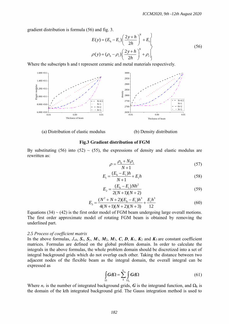
gradient distribution is formula (56) and fig. 3.

h t

h t

2( ) ( )

2

2( ) ( )

2

N

t

N

t

y hE y E E E

h

y hy

h

+ = − +

+ = − +

(56)

Where the subscripts h and t represent ceramic and metal materials respectively.

-0.01 0.00 0.016.00E+010

8.00E+010

1.00E+011

1.20E+011

1.40E+011

1.60E+011

Ela

stic

modulu

s

Thickness of beam

N=0.5

N=1

N=2

N=5

-0.01 0.00 0.012650

2700

2750

2800

2850

2900

2950

3000

den

sity

Thickness of beam

N=0.5

N=1

N=2

N=5

(a) Distribution of elastic modulus (b) Density distribution

Fig.3 Gradient distribution of FGM

By substituting (56) into (52) ~ (55), the expressions of density and elastic modulus are

rewritten as:

h t

1

N

N

+=

+ (57)

h t1 t

( )

1

E E hE E h

N

−= +

+ (58)

2

h t2

( )

2( 1)( 2)

E E NhE

N N

−=

+ + (59)

2 3 3

h t t3

( 2)( )

4( 1)( 2)( 3) 12

N N E E h E hE

N N N

+ + −= +

+ + + (60)

Equations (34) ~ (42) is the first order model of FGM beam undergoing large overall motions.

The first order approximate model of rotating FGM beam is obtained by removing the

underlined part.

2.5 Process of coefficient matrix

In the above formulas, Joh, Sx, Sy, M1, M2, M3, C, D, K1, K2 and K3 are constant coefficient

matrices. Formulas are defined on the global problem domain. In order to calculate the

integrals in the above formulas, the whole problem domain should be discretized into a set of

integral background grids which do not overlap each other. Taking the distance between two

adjacent nodes of the flexible beam as the integral domain, the overall integral can be

expressed as

d dc

k

n

k

= G G (61)

Where nc is the number of integrated background grids, G is the integrand function, and Ωk is

the domain of the kth integrated background grid. The Gauss integration method is used to


182

solve the numerical integration, and ng Gauss points are used in each integration background

grid, and the Eq. (61) is described as

1

d d = ( )gc c

k

nn n

i Qi ik

k k i

w x J=

= G G G (62)

Where iw is the Gauss weighting factor of the ith Gauss integral point

Qix , and ikJ is the

Jacobi matrix integrating the background grid k at the integration pointQix .

In order to obtain the numerical solution of each constant matrix, the field nodes in the whole

problem domain are numbered from 1 to N. taking the square matrix K1 as an example, The

Eq. (49) is described as

' '

1

1

( ) ( )gc

nn

IJ i xI Qi xJ Qi ik

k i

E bw x x J

=

=K (63)

Where

' '

1 ( ) ( )ik

IJ i xI Qi xJ Qi ikE bw x x J =K (64)

Therefore, The Eq. (63) can be described as

1

, 1, 2,3, ,gc

nnik

IJ IJ

k i

I J N=

= =K K (65)

Eqs. (63), (64) and (65) represent the numerical result of the node matrix IJK obtained by

the sum of the contributions of the integral points including nodes I and J in the local support

domain. If nodes I and J are not in the local support domain of the integral pointQix , then

ik

IJK is zero. Then the form of K1 is

11 12 1N

21 22 2N

1

N1 N2 NN

=

K K K

K K KK

K K K

(66)

Similarly, Matrix Sy can be expressed as

Τ

1

= ( ) ( )gc

nn

y i Qi yI Qi ik

k i

bhw a x x J =

+S (67)

Where

Τ( ) ( )ik

I i Qi yI Qi ikbhw a x x J = +S (68)

Therefore, The Eq. (67) can be described as

1

= 1,2,3, ,gc

nnik

y I

k i

I N=

=S S (69)

According to the above matrix and array method, the form of matrix in formulas from Eq. (43)

to (51) can be obtained.

3. Dynamic simulation

3.1 Model parameters

The specific physical parameters of FGM beam are as follows: 11=1.51 10 PahE ,10=7 10 PatE , 3 3=3 10 kg / mh , 3 3=2.707 10 kg / mt . N is the functional gradient index.

5ml = ,22 10 mb −= ,

22 10 mh −= . In this paper, different discrete methods under the

first-order model are simulated.


183

3.2 Natural frequency of FGM beams

The transverse bending vibration of a flexible beam is usually obvious when the cantilever

beam system is rotating undergoing large overall motions, while the longitudinal vibration of

the beam can be neglected. Therefore, the transverse bending vibration without considering

the influence of longitudinal deformation is studied in this section. In order to simplify the

analysis, the large-scale rotation speed is assumed to be uniform, =0. By equation (33) the

transverse bending vibration equation of the beam can be obtained

[ ] 2

2 2 3M B+ (C - M )+ K B = 0 (70)

Eq. (70) was dimensionless and the following dimensionless variables were introduced

=t/T / / ; /x L R L B L = = =；； (71)

/ /h t h tT E E = = =；； (72)

4 2 1/2

t tT L E h=（12 / ） (73)

Eq. (70) can be rewritten as follows:

1[ ] 2

2 2 3M δ+ (C - M )+ K δ = 0 (74)

1

0y y d = 2

M (75)

1

1 10

( ) d = C H (76)

1 , ,0

( ) [ ]

= y y d H (77)

1

3 , ,0[ ]y y d = K

(78)

23( 2) 1

( 1)( )( 2)( 3)

N N N

N N N N

+ + += − +

+ + + + (79)

Table 1 and Table 2 show the variation of transverse bending natural frequency with rotating

speed of FGM beam obtained by the assumed mode method, the finite element method and

the point interpolation method when the radius of central rigid body is zero. When calculating,

the function index is as follow 0.5N = ; 151 / 70 = ; 3000 / 2707 = .It is assumed that the

mode method takes the transverse fourth order mode; the finite element method takes 10

elements and the point interpolation method takes 11 nodes. It can be seen from table 1 and

table 2 that the first natural frequency increases with the increase of rotation speed. The error

between the results of the assumed mode method, the finite element method and the point

interpolation method increases with the increase of rotating speed, which indicates that the

accuracy of hypothetical modal method will be reduced under high-speed rotation; while the

results of the finite element method and the point interpolation method are basically

consistent at different speeds, which shows that the point interpolation method can meet the

accuracy requirements and the correctness of the method. Fig. 4 shows the comparison of the

first and third natural frequencies of transverse bending of the three methods under different

non dimensional angular velocity ratios. It can more vividly illustrate that the simulation

results of the assumed mode method have more and more errors with the increase of rotating

speed. The simulation results of the point interpolation method are basically consistent with

those of finite element method.


184

Table 1. The first order natural frequency with three different discrete methods

Index N Speed ratio AMM FEM PIM

0.5 1 4.4845 4.4846 4.4845

0.5 2 4.5471 4.5471 4.5470

0.5 3 4.6488 4.6487 4.6484

0.5 4 4.7813 4.7803 4.7800

0.5 5 4.9354 4.9326 4.9321

0.5 10 5.9013 5.8553 5.8540

0.5 20 8.0050 7.5431 7.5400

Table 2. The third order natural frequency with three different discrete methods

Index N Speed ratio AMM FEM PIM

0.5 1 78.6623 78.6821 78.6821

0.5 2 78.7407 78.7599 78.7598

0.5 3 79.5085 79.5262 79.5259

0.5 4 80.2414 80.2548 80.2545

0.5 5 80.9592 80.9646 80.9639

0.5 10 88.4284 88.2771 88.2749

0.5 20 113.0945 111.7220 111.7152

4 8 12 16 204

6

8

10

Th

e fi

rst

ord

er n

atu

ral

freq

uen

cy

Speed ratio

AMM

FEM

PIM

4 8 12 16 2075

80

85

90

95

100

105

110

115

120

Th

e th

ird

ord

er n

atu

ral

freq

uen

cy

Speed ratio

AMM

FEM

PIM

(a) The first order natural frequency (b) The third order natural frequency

Fig.4 Natural frequency

Fig.5 shows the variation of the natural frequency of the FGM beam with the function

gradient index obtained by using the assumed mode method, the finite element method and

point interpolation method when the radius of the central rigid body is zero and the rotational

speed of the FGM beam is constant. The function index is as follow 3 = ; 151 / 70 = ;

3000 / 2707 = . It can be found from Fig.5 that when the speed is constant, the natural

frequency will decrease with the increase of functional gradient index N, indicating that the

greater the flexible beam system, the greater the flexibility, which is consistent with the

conclusion shown in Fig. 14.


185

0 100 200 300 400 5003.6

3.8

4.0

4.2

4.4

4.6

Th

e fi

rst

ord

er n

atu

ral

freq

uen

cy

Index N

AMM

FEM

PIM

0 100 200 300 400 50062

64

66

68

70

72

74

76

78

80

Th

e th

ird

ord

er n

atu

ral

freq

uen

cy

Index N

AMM

FEM

PIM

(a) The first order natural frequency (b) The third order natural frequency

Fig.5 Natural frequencies of different functional gradient indices

3.3 Characteristics of system dynamics

The assumed mode method, finite element method and point interpolation method are used to

describe the deformation field of the flexible beam. It is assumed that the mode method takes

the transverse fourth order mode; the finite element method takes 10 elements and the point

interpolation method takes 11 nodes. It is assumed that the law of the large-scale motion of

the FGM beam is known

2πsin( ) 0

= 2πt t T

T t

t T

−

(80)

After 15s, the FGM beam rotates at a constant speed. We first study the difference between

the zero-order model (Deleting the underlined items of Eqs. (34)~(42)) and the first-order

approximate model (Deleting the double underlined items of Eqs. (34)~(42)). The dynamic

characteristics of FGM beams with FGM index N = 2 are studied by taking 4, 10 and 20 rad/s

respectively. Then, the dynamic characteristics of the functional gradient index N with 0, 0.5,

1, 2, 5 are studied when the speed is 4rad/s.

Figs. 6~7 show the comparison between the zero-order model (ZOAC) and the first-order

model (FOAC) of PIM at different speeds. When the speed is 0.4rad/s, the zero-order model is

almost the same as the first-order model. When the speed is 5rad/s, the calculation result of

the zero-order model is divergent, and the result of the first-order approximate model is

convergent. Therefore, as the speed increases, the calculation results of the first-order

approximate model are more reliable.

Figs. 8~13 show the lateral deformation displacement and lateral deformation velocity at the

end of flexible beam. The physical parameters are as follows: N = 2, 4,10,20 rad/s=. It

can be seen from the figure that the simulation results of the assumed modal method, the

finite element method and the point interpolation method are basically consistent when the

speed is low, which indicates the correctness of the model established by the finite element

method in this paper. With the increase of the rotating speed, the deviation between the

assumed mode method and the finite element method and the point interpolation method

becomes larger and larger, and the calculation results of the finite element method and the

point interpolation method are almost the same. This is because the hypothetical modal

method is based on the hypothesis of small deformation. With the increase of the rotational

speed, the deformation is becoming larger and larger, and the error of the hypothetical modal

method is bound to increase. It can be seen from the enlarged transverse deformation

displacement drawings in each figure that the vibration balance position is not on the beam


186

axis, but has an offset, and the greater the speed, the more obvious the offset. This is because

when N > 0, the metal and ceramic materials are not evenly and symmetrically distributed on

both sides of the beam axis, and the axial and transverse coupling potential energy is

produced in the calculation of deformation energy.

Fig. 14 shows the variation of lateral deformation of flexible beam end with functional

gradient index N. It can be seen that the maximum transverse deformation of the beam end

increases with the increase of the functional gradient index N in the process of accelerating

the deployment of large-scale motion. It can be seen from the enlarged figure of lateral

deformation displacement that when N=0, the material degenerates into homogeneous

material, and the vibration equilibrium position is on the beam axis. When N>0, the vibration

equilibrium position shifts.

Fig. 15 shows the large lateral bending deformation at the end of the beam. The specific

physical parameters are as follows: N=0, 11

h =1.51 10 /20PaE , 1 =10rad/s . As shown in the

figure, the maximum deformation of the beam exceeds 3.2m, which belongs to the case of

large deformation. The result of the finite element method and the point interpolation method

is converged while the result of the assumed mode method is diffuse.

0 4 8 12 16 20-0.015

-0.010

-0.005

0.000

0.005

Tip

tra

nsv

erse

def

orm

atio

n w

2/m

Time t/s

ZOAC

FOAC

PIM

15 16 17 18 19 20-0.0002

0.0000

0.0002

0.0004

Tip

tra

nsv

erse

def

orm

atio

n w

2/m

Time t/s

ZOAC

FOAC

PIM

(a) 0～20s Transverse deformation (b) 15～20s Transverse deformation

Fig.6 Comparison of a FOAC model and a ZOAC model (1=0.4rad/s )

0 4 8 12 16 20-0.16

-0.14

-0.12

-0.10

-0.08

-0.06

-0.04

-0.02

0.00

0.02

Tip

tra

nsv

erse

def

orm

atio

n w

2/m

Time t/s

ZOAC

FOAC

PIM

Fig.7 Comparison of a FOAC model and a ZOAC model ( 1=5rad/s )


187

0 4 8 12 16 20-0.15

-0.10

-0.05

0.00

0.05

Tip

tra

nsv

erse

def

orm

atio

n w

2/m

Time t/s

AMM

FEM

PIM

15 16 17 18 19 20-0.001

0.000

0.001

0.002

0.003

0.004

0.005

Tip

tra

nsv

erse

def

orm

atio

n w

2/m

Time t/s

AMM

FEM

PIM


Fig.8 Tip transverse deformation of the FGM beam(1=4rad/s )

0 4 8 12 16 20-0.04

-0.02

0.00

0.02

0.04

Tip

tra

nsv

erse

vel

oci

ty (

dw

2/d

t)/(

m/s

)

Time t/s

AMM

FEM

PIM

15 16 17 18 19 20-0.02

-0.01

0.00

0.01

0.02

Tip

tra

nsv

erse

vel

oci

ty (

dw

2/d

t)/(

m/s

)

Time t/s

AMM

FEM

PIM

(a) 0～20s Transverse velocity (b) 15～20s Transverse velocity

Fig.9 Tip transverse velocity of the FGM beam( 1=4rad/s )

0 4 8 12 16 20-0.30

-0.25

-0.20

-0.15

-0.10

-0.05

0.00

0.05

Tip

tra

nsv

erse

def

orm

atio

n w

2/m

Time t/s

AMM

FEM

PIM

15 16 17 18 19 200.006

0.007

0.008

0.009

0.010

0.011

0.012

Tip

tra

nsv

erse

def

orm

atio

n w

2/m

Time t/s

AMM

FEM

PIM




188

0 4 8 12 16 20-0.10

-0.05

0.00

0.05

0.10

Tip

tra

nsv

erse

vel

oci

ty (

dw

2/d

t)/(

m/s

)

Time t/s

AMM

FEM

PIM

15 16 17 18 19 20-0.020

-0.015

-0.010

-0.005

0.000

0.005

0.010

0.015

0.020

Tip

tra

nsv

erse

vel

oci

ty (

dw

2/d

t)/(

m/s

)

Time t/s

AMM

FEM

PIM


Fig.11 Tip transverse velocity of the FGM beam(1=10rad/s )

0 4 8 12 16 20-0.6

-0.4

-0.2

0.0

0.2

Tip

tra

nsv

erse

def

orm

atio

n w

2/m

Time t/s

AMM

FEM

PIM

15 16 17 18 19 200.014

0.016

0.018

0.020

0.022

Tip

tra

nsv

erse

def

orm

atio

n w

2/m

Time t/s

AMM

FEM

PIM



0 4 8 12 16 20-0.20

-0.16

-0.12

-0.08

-0.04

0.00

0.04

0.08

0.12

Tip

tra

nsv

erse

vel

oci

ty (

dw

2/d

t)/(

m/s

)

Time t/s

AMM

FEM

PIM

15 16 17 18 19 20-0.04

-0.02

0.00

0.02

0.04

Tip

tra

nsv

erse

vel

oci

ty (

dw

2/d

t)/(

m/s

)

Time t/s

AMM

FEM

PIM


Fig.13 Tip transverse velocity of the FGM beam(1=20rad/s )


189

0 4 8 12 16 20-0.16

-0.12

-0.08

-0.04

0.00

0.04

Tip

tra

nsv

erse

def

orm

atio

n w

2/m

Time t/s

N=0 N=2

N=0.5 N=5

N=1 PIM

15 16 17 18 19 20

-0.001

0.000

0.001

0.002

0.003

0.004

0.005

Tip

tra

nsv

erse

def

orm

atio

n w

2/m

Time t/s

N=0 N=2

N=0.5 N=5

N=1 PIM



0 4 8 12 16 20-4

-3

-2

-1

0

1

Tip

tra

nsv

erse

def

orm

atio

n w

2/m

Time t/s

AMM

FEM

PIM


4. Conclusions

1. The accuracy of the first-order approximate model is better than that of the zero-order

model.

2. The maximum tip transverse deformation of the FGM beam increases with the increase of

the functional gradient index N. When N>0, the equilibrium position of steady-state

vibration will shift and not be on the beam axis.

3. It is assumed that the results of modal method are divergent when the deformation is large,

so it can not deal with the problem of large deformation. The results of the finite element

method and the point interpolation method are convergent and can be used to solve large

deformation problems.

4. The transverse bending natural frequency increases with the increase of rotating speed and

decreases with the increase of functional gradient index N.

Acknowledgment

The authors are grateful for the support from the National Natural Science Foundation of

China (Grant Nos. 11802263,11272155), the Fundamental Research Funds for the Central

Universities of China (Grant No. 30917011103), the Natural Science Foundation of the

Jiangsu Province of China (Grant No. BK20180895).


190

References

[1] Cai G, Hong J. (2005) Assumed mode method of a rotating flexible beam, Acta Mechanica Sinica 37, 48-56.

[2] Jeong S, Yoo H H. (2017) Flexibility Modeling of a Beam Undergoing Large Deflection Using the Assumed

Mode Method, International Journal of Mechanical Sciences 133, 611-618.

[3] Yue J, Dong Y, Guedes Soares C. (2018) An experimental-finite element method based on beach marks to

determine fatigue crack growth rate in thick plates with varying stress states, Engineering Fracture

Mechanics 196, 123-141.

[4] Yoneta S, Koshiba M, Tsuji Y. (1999) Combination of Beam Propagation Method and Finite Element

Method for Optical Beam Propagation Analysis, Journal of Lightwave Technology 17, 2398-2404.

[5] Santos C F, Belinha J, Gentil F, et al. (2018) The free vibrations analysis of the cupula in the inner ear using

a natural neighbor meshless method, Engineering analysis with boundary elements 92, 50-63.

[6] Sadek S H M, Belinha J, Parente M P L, et al. (2018) The analysis of composite laminated beams using a

2D interpolating meshless technique, Acta Mechanica Sinica 34, 99-116.

[7] Fan J H, Zhang D G. (2014) Bezier interpolation method for the dynamics of rotating flexible cantilever

beam, Acta Physica Sinica Chinese Edition 63, 761-761.

[8] Fan J H, Zhang D G. (2012) The Discretization Methods of a Rotating Flexible Cantilever Beam, Applied

Mechanics & Materials 226-228, 697-707.

[9] Nobakhti M, Dehkhoda P, Tavakoli A. (2014) Improved modal method of moments technique to

compensate the effect of wall dimension in shielding effectiveness evaluation, Science Measurement &

Technology Iet 8, 17-22.

[10] Xu G L, Zhang W S, Zhu D B, et al. (2011) Analysis of Residual Stresses Distribution Based on the Finite

Element Method for Beam-Column Connections of Steel Frames, Applied Mechanics & Materials 71-78,

4421-4424.

[11] Du C F , Zhang D G, Liu G.R. (2018) A cell-based smoothed finite element method for free vibration

analysis of a rotating plate, International Journal of Computational Methods 15, 1840003.

[12] Du C F , Zhang D G, Li L, Liu G.R. (2018) A node-based smoothed point interpolation method for dynamic

analysis of rotating flexible beams, Acta Mechanica Sinica 34, 409-420.

[13] Du C F , Zhang D G , Zhang J S , et al. (2019) Predicting Dynamic Behavior of Rotating Mindlin Plate

Using Radial Point Interpolation Method, International Journal of Structural Stability & Dynamics 19,

1950070.

[14] Du C.F., Zhang D.G. (2015) Dynamic analysis of rotating cantilever beam based on meshless point

interpolation, Acta Physica Sinica 64, 406-415.

[15] Du C.F., Zhang D.G., Hong J.Z. (2015) A meshfree method based on radial point interpolation method for

the dynamic analysis of rotating flexible beams, Chinese Journal of Theoretical and Applied Mechanics, 47,

279-288.

[16] He G L, Ding K, Wu X M, et al. (2019) Dynamics modeling and vibration modulation signal analysis of

wind turbine planetary gearbox with a floating sun gear, Renewable Energy 139, 718-729.

[17] Wu S.B. Modeling and simulation of rigid-flex coupling dynamics of flexible beam and flexible thin plate, Master's Thesis, Nanjing University of Science and Technology, Nanjing, 2009.

[18] Zhang Ch, Fan J.H., Zhang D.G., et al. (2018) Dynamic study of central rigid body-tapered beam system

with tip mass, Chinese Quarterly of Mechanics 39, 270-279.

[19] Rezaei V, Shafei A M. (2019) Dynamic Analysis of flexible robotic manipulators constructed of

functionally graded materials, Iranian Journal of Science and Technology, Transactions of Mechanical

Engineering 43, 327-342.

[20] Sun C Y, Gao H J, He W, et al. (2018) Fuzzy neural network control of a flexible robotic manipulator using

assumed mode method, IEEE Transactions on Neural Networks and Learning Systems 29, 5214-5227.

[21] LI L, Zhang D.G., Hong J.Z. (2013) Dynamics of hub-functionally graded material beam system, Journal

of Mechanical Engineering 49,77-84.


191

Entropy-regularized Wasserstein Distances for Analyzing Environmental

and Ecological Data

†, *Hidekazu Yoshioka 1,2, * Yumi Yoshioka 1, and Yuta Yaegashi3

1 Graduate School of Natural Science and Technology, Shimane University, Japan 1 Fisheries Ecosystem Project Center, Shimane University, Japan

2 Independent Researcher, Dr. of Agr., Japan



Abstract

We explore applicability of entropy-regularized Wasserstein (pseudo-)distances as new tools

for analyzing environmental and ecological data. In this paper, the two specific examples are

considered and are numerically analyzed using the Sinkhorn algorithm. The first example is

the inflow and outflow discharges of a dam-reservoir system. The inflow and outflow

discharges are described as discrete-time Markov chains, and their transition rates among the

discharge regimes and the corresponding stationary probability distributions are identified.

The optimal transport plan leading to the regularized Wasserstein distance between the two

Markov chains is considered as the system optimization policy decided by the operator. The

second example is the body weight distributions of a fish serving as a major inland fishery

resource in Japan. We quantify differences of the collected body weight distributions among

the different years focusing on the summer growing season. The obtained analysis results

imply usefulness of the regularized Wasserstein distances for assessing probability

distributions arising in environmental and ecological problems.

Keywords: Aquatic environment and ecology, Optimal transport, Entropy-regularized

Wasserstein distance, Sinkhorn algorithm

Introduction

Environmental and ecological dynamics in our world are inherently uncertain. The probability

density functions or equivalently probability distributions can effectively quantify

uncertainties involved in the target phenomena. Quantifying and comparing the probability

distributions play an essential part in understanding and managing environmental and

ecological dynamics [1].

The Wasserstein distances [2] are the metrics to rigorously measure difference between

probability distributions. They originate from an optimization problem of transportation plans

of materials from a set of starting points to a set of terminal points. They have been applied to

a wide variety of research areas in both science and engineering, such as image processing,

machine learning, and mathematical analysis and discretization of partial differential

equations [2]-[3]. However, their applications to problems of environment and ecology have

been far less explored to the best of the authors’ knowledge. This is the motivation of our

research.

In this paper, we apply the robust entropy-regularized Wasserstein (pseudo-)distances to

unique environmental and ecological data collected in a river environment. The first

application is to the discrete-time Markov chains representing inflow and outflow discharge


192

processes of an existing dam-reservoir system. The optimal plan as a minimizer in a

Wasserstein distance is computed as the system optimization policy of the operator. The

second application is to the body weight distributions of a fish in different years. We quantify

difference among the distributions. The entropic regularization allows us to efficient as well

as robust numerical computation of the Wasserstein distances. Our results would advance

understanding and assessment of environmental and ecological data from a new viewpoint

based on the Wasserstein distances.

Wasserstein distances

Standard Wasserstein distances

Wasserstein distances are the distances that can measure the differences between probability

distributions [3]. For finite discrete probability distributions, namely for the two normalized

histograms 1i i n

a a

= and 1i i n

b b

= with some n , the p th-order Wasserstein

distance ( ) ( ), ,p p pW W a b W b a= = between a and b is set as

, 1

minn

p

p ij ijP

i j

W C P=

= with p

ijC i j= − (1)

subject to the constraints

1

n

ij i

j

P a=

= , 1

n

ij j

i

P b=

= , 0ijP , (1 ,i j n ). (2)

Here, ijC is the transportation cost quantifying the difference between the classes ,i j and the

matrix 1 ,ij i j n

P P

= is referred to as a plan. A minimizing plan of (1) is called an optimal

plan. This is a linear programming problem subject to constraints, but the resulting optimal

plans are possibly not robust against the uncertainties in a and b because they are often non-

unique and are of the non-interior type [2].

Regularized Wasserstein distances

The above-explained formulation would not be appropriate for problems under uncertain

environment, where the histograms are not always accurate. This is often the case in handling

histograms of environmental and ecological data. In such a case, it is more reasonable to

consider the penalized problem subject to the same constraint (2):

( ),

, 1 , 1

min ln 1n n

p

p ij ij ij ijP

i j i j

W C P P P = =

= + −

(3)

with a penalty parameter 0 . This , pW is not a distance due to not satisfying the triangle

inequality, but we call it a “distance” for the sake of brevity. The added term is understood as

the penalization against model uncertainty to improve the robustness, which formally

vanishes as 0 → + [4]. The problems (1) and (3) coincide under this limit. Furthermore, the

minimizer P P= of (3) converges to an optimal plan of the problem as 0 → + [3].

Using the penalized formulation has the following two computational advantages. Firstly, the

optimal plan P P= is unique in (3) because the regularized problem is -convex. Secondly,


193

there exists a simple, fast, and stable algorithm for numerically finding P : the Sinkhorn

algorithm [3]:

( )

( )

1

1

m ii n

m

ij j

j

au

K v

+

=

=

and

( )

( )

1

1

1

m j

j nm

ji i

j

bv

K u

+

+

=

=

(1 ,i j n , 0m ) (4)

with positive initial guesses ( ) ( )0 0,i iu v (1 i n ), from which P is obtained as

( ) ( )

, limm m

ij i ij jm

P u K v→+

= (1 ,i j n ). (5)

Here, we have set ( )exp /ij ijK C = − . Computational efficiency of the algorithm has been

demonstrated in Cuturi [5]. Our implementation of the algorithm is based on the logarithmic

rewriting [3] to avoid computational instability with small . Notice that ,

p

pW is increasing

with respect to . We terminate the algorithm if the differences ( ) ( )1ln ln

m m

i iu u+− and

( ) ( )1ln ln

m m

i iv v+− become smaller than a sufficiently small error threshold ( 710− in this paper).

Wasserstein distances

Regularized Wasserstein distances

The first application is the inflow and outflow discharges of a dam-reservoir system in H

River in Japan. The system has been operated from 2011 for multiple purposes including

water resources supply and flood mitigation. Hourly inflow and outflow discharges data of the

dam-reservoir system are available from April 1 in 2016.

We identify hourly discrete-time and discrete-state Markov chains of the inflow and outflow

discharges using the collected data from April 1, 2016 to September 31, 2019. Seasonality of

the data is not considered in this paper for the sake of simplicity, but will be addressed

elsewhere. The discharge regimes are classified as follows: )1,i i iS s s += ( 1 i n ) with

1is i= − (m3/s) (1 11i ) and ( )10 8 11is i= + − (m3/s) (12 i n ), 41n = , and 42S = + .

This non-uniform partition has been employed because the average discharges are around 5.5

(m3/s) for both the inflow and outflow records. We remark that, in this case, the system

operation policy depending on the cost ijC and the penalty parameter can be identified as

the probability matrix 1

, 1 ,i ij i j na P−

if 0ia for all i .

Fig. 1 shows the estimated transition matrices ijq q= of the Markov chains of the inflow

and outflow discharges. The estimated results show that the Markov chain for the outflow is

closer to diagonally-dominant, meaning that the regime transitions occurred less frequently

than in the inflow. The stationary probability distributions of the inflow ( 1i i n

a a

= ) and

outflow discharges ( 1i i n

b b

= ) are used to numerically compute the regularized

Wasserstein distances. Although not presented, it has been found that they are indeed

increasing with respect to as theoretically expected.


194

Figs. 2 and 3 show the optimal plans P for 1,2p = with 0.01 = and 10 = . The optimal

plan is sparser for smaller , implying its less robustness against perturbation of the input

data. The computational results clearly indicate that the optimal plans are such that the

discharges are significantly decreased through the dam-reservoir system for the lower regimes

1 11i where the discharges are smaller than 10 (m3/s). Considering the Markov chains

estimated in Fig. 1 and the optimal plans in Figs. 2 and 3, this dam-reservoir system is serving

as a filter to lower the lower flow and to a less transient flow. It is important to see that this

characteristic of the system is visible both for the cases 1p = and 2p = , although they are

somewhat different for relatively high flow regimes , 12i j .

Figure 1. Transition probabilities of the Markov chains for the inflow discharge (Left)

and outflow discharge (Right)

Figure 2. Optimal plans with 1p = for 0.01 = (Left) and 10 = (Right)


195

Figure 3. Optimal plans with 2p = for 0.01 = (Left) and 10 = (Right)

Body weights of a fish species

The second application focuses on the collected body weight distributions of the fish

Plecoglossus altivelis altivelis as a major inland fishery resource in Japan [6]. The fish is one

of the most important incomes for inland fishery cooperatives in the country. In addition, the

fish is a key species in the aquatic ecosystems in and around river environment. Therefore,

their growth dynamics are of critical importance. The life history of the fish is not explained

here, but is found in Yoshioka et al. [7]. An important fact is that they have a one-year life

history and grow significantly in summer, during which harvesting the fish is carried out.

We collected the body weight distributions of the fish at the beginning of August in 2017,

2018, 2019 in H River, and obtained the statistical estimates as demonstrated in Table 1. The

data for 2017 and 2018 is found also in Yoshioka et al. [6, 8]. Fig. 4 plots their distributions.

The average values are around 56 to 57 (g) and the standard deviations around 18 to 19 (g).

All the distributions have positive skewness values around 1. The collected data implies that

the distributions are qualitatively the same.

An interest from a fisheries viewpoint is whether there exist significant quantitative

differences among the three distributions. Figs. 5 and 6 plot the computed regularized

Wasserstein distances , pW for 1,2p = with respect to the different values of . There are at

least two important findings from the figures. Firstly, the distance between 2017 and 2018 are

the largest for both 1,2p = . On the other hand, the relationship of the distances between 2018

and 2019 and that between 2017 and 2019 are opposite between 1,2p = , especially when

is small. In fact, 0.01,1W are 0.159 and 0.193 between 2018 and 2019 and that between 2017

and 2019, respectively. On the other hand, 0.01,2W are 0.222 and 0.201 between 2018 and 2019

and that between 2017 and 2019, respectively. This finding suggests that exploring a more

biologically reasonable ijC would be required. Nevertheless, the results suggest a significant

difference between the data of 2017 and 2018.


196

Table 1. The collected data of the body weights of the fish

2019 2018 2017

Total number of caught fishes 227 189 234 Average (g) 56.4 57.3 55.6

Standard deviation (g) 18.2 18.5 19.1 Skewness 0.95 1.16 0.78

Figure 4. The body weight distributions in 2017 (Red), 2018 (Green), and 2019 (Blue)

Figure 5. , pW W= for 1p = with respect to : The distance between 2017 and 2018

(Red), 2018 and 2019 (Green), and 2019 and 2017 (Blue)

Figure 6. , pW W= for 2p = with respect to (the same legend with Fig. 5)


197

Conclusions

The entropy-regularized (pseudo-)Wasserstein distances were applied to analyzing the unique

environmental and ecological data. The application to the dam-reservoir system identified the

optimal plan representing the system operation policy. Another application on the fish growth

distributions quantified the differences among the collected distributions of the fish in

different years.

Our results suggest that the regularized Wasserstein distances can serve as new tools for

analyzing environmental and ecological data. A future reach topic would be computing the

optimal plans of different dam-reservoir systems across the country, or across the globe, with

which actual operational characteristics among them can be clarified. Analyzing applicability

of the Wasserstein distances to other species, such as recently-found unique land-locked P.

altivelis in Japan, is also an interesting topic.

Acknowledgements

JSPS Research Grant 19H03073, Kurita Water and Environment Foundation Grant 19B018,

grants from MLIT Japan for ecological survey of a life history of the landlocked Plecoglossus

altivelis altivelis and management of seaweed in Lake Shinji, and a research grant for young

researchers in Shimane University support this research.

References

[1] Folke, C., Hahn, T., Olsson, P. and Norberg, J. (2005) Adaptive governance of social-ecological systems, Annual Review of Environment and Resources 30, 441–473 (2005)

[2] Santambrogio, F. (2015) Optimal Transport for Applied Mathematicians, Birkäuser, New York. [3] Peyré, G. and Cuturi, M. (2019) Computational optimal transport, Foundations and Trends in Machine

Learning 11, 355–607. [4] Rigollet, P. and Weed, J. (2018) Entropic optimal transport is maximum-likelihood deconvolution, Comptes

Rendus Mathematique 356, 1228–1235. [5] Cuturi, M. (2013) Sinkhorn distances: Lightspeed computation of optimal transport. In Advances in neural

information processing systems. (pp. 2292–2300). [6] Yoshioka, H., Yaegashi, Y., Yoshioka, Y. and Tsugihashi, K. (2019) A short note on analysis and

application of a stochastic open-ended logistic growth model, Letters in Biomathematics 6, 67–77. [7] Yoshioka, H., Tanaka, T., Aranishi, F., Izumi, T. and Fujihara, M. (2019) Stochastic optimal switching

model for migrating population dynamics, Journal of Biological Dynamics 13, 706–732. [8] Yoshioka, H., Yoshioka, Y., Yaegashi, Y. and Tsujimura, M. (2020) Chapter 2. Growth of the fish

Plecoglossus altivelis altivelis. In Ayu and River Environment in Hii River, Japan -Research results from 2015 to 2020-. (pp. 13–26), Laboratory of Mathematical Sciences for Environment and Ecology, Shimane University, Matsue, Japan.


198

U-Net-based Surrogate Model for Evaluation of Microfluidic Channels

Le Quang Tuyen

1, Pao-Hsiung Chiu

1, and *†Chinchun Ooi

1

1Department of Fluid Dynamics, Institute of High Performance Computing, Singapore.



Abstract

Microfluidics have shown great promise in multiple applications, especially in biomedical

diagnostics and separations. While the flow properties of these microfluidic devices can be

solved by numerical methods such as computational fluid dynamics (CFD), the process of mesh

generation and setting up a numerical solver requires some domain familiarity, while more

intuitive commercial programs such as Fluent and StarCCM can be expensive. Hence, in this

work, we demonstrated the use of a U-Net convolutional neural network as a surrogate model for

predicting the velocity and pressure fields that would result for a particular set of microfluidic

filter designs. The surrogate model is fast, easy to set-up and can be used to predict and assess

the flow velocity and pressure fields across the domain for new designs of interest via the input

of a geometry-encoding matrix. In addition, we demonstrate that the same methodology can also

be used to train a network to predict pressure based on velocity data, and propose that this can be

an alternative to numerical algorithms for calculating pressure based on velocity measurements

from particle-image velocimetry measurements. Critically, in both applications, we demonstrate

prediction test errors of less than 1%, suggesting that this is indeed a viable method.

Keywords: Computational Fluid Dynamics, Microfluidics, Convolutional Neural Network,

Surrogate Model

Introduction

Microfluidics have been applied to a variety of areas, especially in the area of biomedical

diagnostics and cell separations [1-5]. Certain common features within these devices are the

placement of solid columns, such as in the case of deterministic lateral displacement devices for

cell separation, or for flow field sculpting [6, 7]. While it is possible to do a parametric

optimization of these designs via actual experiments, these experiments can be difficult and time-

consuming. Numerical methods such as computational fluid dynamics (CFD) can thus be useful

as a means of narrowing the design space prior to any actual fabrication, and are commonly used

as part of the design process [8, 9].

In addition, it can often be difficult to obtain full knowledge of pressure fields within

microfluidic devices, even as pressure is typically used as a means of active control of valves

within such devices [10]. In particular, while experimental methods such as particle image

velocimetry (PIV) can be applied to obtain velocity field, other numerical methods have to be

developed for calculating the pressure fields from the measured velocities [11-13].


199

Hence, in this work, we further explore the use of data-driven machine learning methods for the

above-mentioned two potential use cases in microfluidics: 1) predicting velocity and pressure

fields for new microfluidic channel designs; and 2) predicting pressure fields from velocity field

information. In particular, developments in methods such as neural networks have shown great

promise as a surrogate model across multiple engineering domains in recent literature [14-16].

The convolutional neural network (CNN) architecture in particular, has been applied to several

fluid dynamic problems with some success, with the U-Net model being a particularly promising

choice [17, 18]. Importantly, we evaluate the sensitivity of the U-Net architecture to the choice

of normalization parameter for the target outputs in this work, and show that the U-Net

architecture can indeed be applied to the prediction of flow and pressure fields with root mean

square errors below 1%. In addition, we also propose that the use of a dual model system,

whereby we create a secondary model to predict the normalization parameter, can further

improve the accuracy of the model with regards to the full pressure field.

Methods

Microfluidic Flow Scenarios

For this work, the microfluidic scenario as depicted in Figure 1 was studied, representing a

continuously repeating array of solid pillars in a microfluidic channel. The individual pillars

extend for 10 μm, while the design parameters are assumed to be the gap between the pillars (G),

and the lateral dimension of the individual small pillars (S). In total, simulations were run for S

ranging from 10 to 30 μm in steps of 2 μm and G ranging from 20 to 50 μm in steps of 2 μm to

create a total dataset of 176 individual flow scenarios.

Figure 1. Schematic of microfluidic channel scenarios studied. Two parameterizations are

studied in this work: 1) width of small pillar (S), and 2) width of inter-pillar gap (G).

The Dirichlet input boundary condition is stipulated as a uniform velocity (Vin) of magnitude

0.001 m/s, while a Dirichlet boundary condition of P = Pa is applied at the outlet. Periodic

boundary conditions are specified on the two sides to simulate a continually repeating array of

pillars in the flow. The steady-state velocity and pressure fields were obtained based on a

pressure-projection scheme, with second order spatial discretization. Sample plots of the velocity


200

fields obtained for 1) S = 10 μm and G = 20 μm, and 2) S = 30 μm and G = 50 μm are provided

in Figure 2.

Figure 2. (a) and (b) are the U and V velocity fields obtained by CFD for the flow scenario with S = 10 μm and

G = 20 μm while (c) and (d) are the U and V velocity fields obtained by CFD for the flow scenario where S =

30 μm and G = 50 μm.

U-Net Architecture and Model Training

Based on prior positive results in literature, the U-Net architecture was selected for use in this

work, as illustrated in Figure 3 [17]. The model was created in Python, and all network

mathematical operations used were as implemented in the base Keras and Tensorflow packages.

Briefly, the U-Net has a bowtie structure, comprising separate encoder and decoder halves. Each

half is made up of sequential layers that comprise of a convolutional layer, a batch normalization

layer and a non-linear activation component, with the choice of activation function being the

leaky ReLU (0.2) in the encoder half and the ReLU function in the decoder half. Default network

hyper-parameters were used based on prior work by Thuruey et al., with no further optimization,

although a convolutional kernel of size 8x8 was used instead [17]. The Adam optimizer was used

for training over 10k epochs, with a learning rate of 0.0004, and ‘mean squared error’ (MSE) as

the loss function. In each of the following models, the dataset was split into a training dataset

consisting of 150 cases, while a random subset of 26 cases was used as the test set for evaluation.


201

Figure 3. Schematic of the U-Net CNN architecture as implemented in this work. Different color arrows in

the schematic represent the operations that were used at each stage.

In order to enhance predictive performance, pre-processing of the data is crucial. Prior literature

in the machine learning domain typically also recommends normalization of the input and output

as the gradient descent-based optimization process can be hindered by extremes in input or

output value magnitude [19, 20]. Hence, a few different normalization methods for the input and

output data are evaluated in this work.

U-Net Model Prediction for Pressure based on Velocity

For the first scenario, we assume that the velocities are provided, and the pressure field is to be

predicted (Models A1, A2 and A3). Hence, the x and y velocity fields (U and V) are specified as

inputs, while the output field is pressure (P). Utilizing typical scales that would be used for non-

dimensionalization of the Navier-Stokes equations, we elected to normalize the input velocity

fields by the magnitude of the input velocity (Vin).

Inputs for Models A1, A2 and A3:

𝑈𝑛𝑜𝑟𝑚𝑖 =

𝑈𝑖

𝑉𝑖𝑛 (1)

𝑉𝑛𝑜𝑟𝑚𝑖 =

𝑉𝑖

𝑉𝑖𝑛 (2)

Similarly, for Model A1, we used a scaling factor commonly used for non-dimensionalizing

pressure in creeping flows, and further de-meaned the output pressure field by subtracting a

‘typical’ pressure profile as obtained by averaging across all the training data.

Output for Model A1:

𝑃𝑛𝑜𝑟𝑚𝑖 [: , 𝑦] =

𝐿

𝜇𝑉𝑖𝑛∗ (𝑃𝑖[: , 𝑦] −

1

𝑛𝑡𝑟𝑎𝑖𝑛∑ 𝑃𝑗[: , 𝑦]𝑛𝑡𝑟𝑎𝑖𝑛

𝑗=1 ) (3)

where the superscripts i and j represent the individual flow scenarios, and y represents the yth

coordinate of the domain. L and μ represent the length scale and the fluid viscosity respectively,

and were defined as L = 0.001 m, and 𝜇 = 0.001 𝑃𝑎 ∙ 𝑠.


202

In addition, a second choice for renormalizing the pressure was by re-scaling the individual

output pressures for every parametric flow scenario by the expected pressure difference between

the input and output planes of the flow domain. Hence, we created a regression function for the

average pressure difference due to the choices of S and G, and used that as a normalization

function instead.


𝑃𝑛𝑜𝑟𝑚𝑖 [: , : ] =

𝑃𝑖[:,:]

𝑓(𝑆,𝐺) (4.1)

𝑓(𝑆, 𝐺) = 𝑒5.9205𝑆0.093691𝐺1.931052 (4.2)

where i represents the individual flow scenario, and f(S,G) is the regression function obtained for

the dependence of pressure on S and G, as obtained by least-squares regression.

Lastly, as a further proof-of-concept, in most typical microfluidic set-ups, the input and output

pressures are typically easy to measure, or are actual control parameters for operation. Hence, in

such experiments, we anticipate being able to use actual measurement values for the pressure

differential between the inlet and outlet planes. Thus, we assumed the average pressure along the

inlet plane of the fluid domain is known from experiments, and used that as a normalization

factor in Model A3.


𝑃𝑛𝑜𝑟𝑚𝑖 [: , : ] =

𝑃𝑖[:,:]1

𝑤∑ 𝑃𝑖[𝑘,1]𝑤

𝑘=1

(5)

where i represents the individual flow scenario, and w represents the fluid cells along the inlet

plane of the fluid domain.

U-Net Model Prediction for Velocity and Pressure Fields

For the second scenario, we assume that both velocity and pressure fields are unknown, although

the geometry of the domain is specified. Hence, the following input and output fields are used

instead:

Inputs for Models B1 and B2:

𝑈𝑖𝑛𝑝𝑢𝑡 = 0 , 𝑠𝑜𝑙𝑖𝑑 𝑑𝑜𝑚𝑎𝑖𝑛0 , 𝑓𝑙𝑢𝑖𝑑 𝑑𝑜𝑚𝑎𝑖𝑛

(6)

𝑉𝑖𝑛𝑝𝑢𝑡 = 0 , 𝑠𝑜𝑙𝑖𝑑 𝑑𝑜𝑚𝑎𝑖𝑛1 , 𝑓𝑙𝑢𝑖𝑑 𝑑𝑜𝑚𝑎𝑖𝑛

(7)

𝑉𝑂𝐹𝑖𝑛𝑝𝑢𝑡 = 1 , 𝑠𝑜𝑙𝑖𝑑 𝑑𝑜𝑚𝑎𝑖𝑛0 , 𝑓𝑙𝑢𝑖𝑑 𝑑𝑜𝑚𝑎𝑖𝑛

(8)

The input velocities are normalized to be of values 0 or 1, rather than the characteristic input

velocity, for similar reasons to the normalization of input velocities in Models A1 to A3. In

addition, we add an input parameter, VOF, which is the inverse of the Volume-of-Fluid


203

parameter that is commonly used in immersed boundary methods to demarcate solid and fluid

domains. In particular, the VOF parameter is assumed to be 1 when the component overlays a

solid object in the domain, and is 0 otherwise. While the encodings for velocity and VOF appear

similar, and the input field for U appears redundant in that it is uniformly 0 in this instance, the

two input fields have been retained for generalizability across future scenarios, whereby the

velocity boundary conditions might be non-zero in both spatial axes.

A similar normalization was chosen for the output values for both velocity and pressure,

whereby we re-scaled the velocity and pressure fields to optimally shift their range to be between

0 and 1 or -1 and 1. Two separate models were compared, with a slight difference observed for

the two instances.

Outputs for Model B1:

𝑃𝑛𝑜𝑟𝑚𝑖 [: , : ] =

𝑃𝑖[:,:]1


𝑘=1

(9)


𝑈𝑖

𝑉𝑖𝑛 (10)


𝑉𝑖−𝑉𝑖𝑛

3∗𝑉𝑖𝑛 (11)

Outputs for Model B2:

𝑃𝑛𝑜𝑟𝑚𝑖 [: , : ] =

𝑃𝑖[:,:]1


𝑘=1

− 0.5 (12)


𝑈𝑖

𝑉𝑖𝑛 (13)


𝑉𝑖−𝑉𝑖𝑛

2∗𝑉𝑖𝑛 (14)

In particular, we vary the normalization parameters across Models B1 and B2 in order to further

evaluate the impact of the normalization on the predictive accuracy of the model.

Results

U-Net Model Prediction for Pressure based on Velocity

After training, the root-mean-square errors (RMSEs) of the 3 models (A1, A2 and A3) are

calculated on the test set, and the respective errors are presented in Figure 4. Sample pressure

predictions are also presented in Figure 5. Based on the results from models A1 and A2, we

noticed that the RMSE was significantly improved in variance by using the pressure difference

between the input and output planes of the microfluidic component as a scaling parameter as

compared to the average of the data-set. More importantly, when the pressure difference is

accurately defined, as in Model A3, the U-Net model test RMSE is also best minimized with an

average value of about 0.7%.


204

Figure 4. Test RMSEs for the 3 different ways of normalizing the pressure output field as defined by models

A1 to A3.

Figure 5. Sample U, V and P contour plots as obtained for this work for a flow scenario with G = 30 μm and S

= 16 μm. (a), (b) and (c) are the U, V and P contour plots as obtained from CFD, while (d) is the pressure

contour plot as obtained by the U-Net Model A3.

U-Net Model Prediction for Velocity and Pressure Fields

Similarly, two different normalization models are tested, and their test RMSEs are plotted in

Figure 6, while sample velocity and pressure contour plots as obtained by CFD and Model B2

are plotted in Figure 7. The results indicate that the choice of normalization can also impact the

accuracy of the model, and indicate that Model B2 performs slightly better, with average RMSEs

of 0.5% for pressure and 0.7% for velocities.


205

Figure 6. Test RMSEs for the 2 different ways of normalizing the velocity and pressure output fields as

defined by models B1 to B2.

Figure 7. Sample velocity magnitude and pressure contour plots as obtained by CFD and via our U-Net

(CNN) Model B2 as presented in this work for the flow scenario with G = 34 μm and S = 14 μm. (a) and (b)

are obtained by CFD while (c) and (d) are obtained by Model B2.

Conclusions

In this work, we demonstrate the application of a U-Net-based model to rapidly predict the

pressure fields for a set of microfluidic channel designs, when velocity fields are known, such as

in the case of PIV experiments, and also, for the prediction of both velocity and pressure fields

when new designs are to be evaluated. We demonstrate that we can obtain prediction errors of

less than 1% with an appropriate choice of normalization parameters, and also highlight that the

normalization parameters can improve model prediction.

While the microfluidic designs here are only a subset of many more complicated possibilities,

this proof-of-concept work shows the potential for utilizing deep learning methods, and U-Net

specifically, as a surrogate model for design evaluation and optimization in microfluidic

applications. We anticipate that this method would be of interest to microfluidic

experimentalists, as an easy to use surrogate model for rapid evaluation of different designs prior

to fabrication.


206

Acknowledgments

This study is supported by research funding from the Agency for Science, Technology and

Research (A*STAR), Singapore under Grant No. A1820g0084.

References

1. Whitesides GM. The origins and the future of microfluidics. Nature.

2006;442(7101):368-73.

2. Bhagat AAS, Bow H, Hou HW, Tan SJ, Han J, Lim CT. Microfluidics for cell separation.

Medical & biological engineering & computing. 2010;48(10):999-1014.

3. Joanicot M, Ajdari A. Droplet control for microfluidics. Science. 2005;309(5736):887-8.

4. Chin CD, Laksanasopin T, Cheung YK, Steinmiller D, Linder V, Parsa H, et al.

Microfluidics-based diagnostics of infectious diseases in the developing world. Nature medicine.

2011;17(8):1015.

5. Pandey CM, Augustine S, Kumar S, Kumar S, Nara S, Srivastava S, et al. Microfluidics

based point‐of‐care diagnostics. Biotechnology journal. 2018;13(1):1700047.

6. Stoecklein D, Lore KG, Davies M, Sarkar S, Ganapathysubramanian B. Deep learning

for flow sculpting: Insights into efficient learning using scientific simulation data. Scientific

reports. 2017;7:46368.

7. McGrath J, Jimenez M, Bridle H. Deterministic lateral displacement for particle

separation: a review. Lab on a Chip. 2014;14(21):4139-58.

8. Glatzel T, Litterst C, Cupelli C, Lindemann T, Moosmann C, Niekrawietz R, et al.

Computational fluid dynamics (CFD) software tools for microfluidic applications–A case study.

Computers & Fluids. 2008;37(3):218-35.

9. Zhou T, Liu T, Deng Y, Chen L, Qian S, Liu Z. Design of microfluidic channel networks

with specified output flow rates using the CFD-based optimization method. Microfluidics and

Nanofluidics. 2017;21(1):11.

10. Oh KW, Lee K, Ahn B, Furlani EP. Design of pressure-driven microfluidic networks

using electric circuit analogy. Lab on a Chip. 2012;12(3):515-45.

11. Santiago JG, Wereley ST, Meinhart CD, Beebe D, Adrian RJ. A particle image

velocimetry system for microfluidics. Experiments in fluids. 1998;25(4):316-9.

12. Van Oudheusden B. PIV-based pressure measurement. Measurement Science and

Technology. 2013;24(3):032001.

13. Williams SJ, Park C, Wereley ST. Advances and applications on microfluidic

velocimetry techniques. Microfluidics and Nanofluidics. 2010;8(6):709-26.

14. Lore KG, Stoecklein D, Davies M, Ganapathysubramanian B, Sarkar S, editors.

Hierarchical feature extraction for efficient design of microfluidic flow patterns. Feature

Extraction: Modern Questions and Challenges; 2015.

15. Guo X, Li W, Iorio F, editors. Convolutional neural networks for steady flow

approximation. Proceedings of the 22nd ACM SIGKDD international conference on knowledge

discovery and data mining; 2016.

16. Mengistu T, Ghaly W. Aerodynamic optimization of turbomachinery blades using

evolutionary methods and ANN-based surrogate models. Optimization and Engineering.

2008;9(3):239-55.


207

17. Thuerey N, Weißenow K, Prantl L, Hu X. Deep learning methods for Reynolds-averaged

Navier–Stokes simulations of airfoil flows. AIAA Journal. 2020;58(1):25-36.

18. Ribeiro MD, Rehman A, Ahmed S, Dengel A. DeepCFD: Efficient Steady-State Laminar

Flow Approximation with Deep Convolutional Neural Networks. arXiv preprint

arXiv:200408826. 2020.

19. Sola J, Sevilla J. Importance of input data normalization for the application of neural

networks to complex industrial problems. IEEE Transactions on nuclear science.

1997;44(3):1464-8.

20. Kim D. Normalization methods for input and output vectors in backpropagation neural

networks. International journal of computer mathematics. 1999;71(2):161-71.


208

Response spectrum method considering specific dominant natural modes of

double layer truss domes subjected to earthquake motions

K. Ishikawa Department of Architecture and Civil Engineering, University of Fukui, Japan.

[email protected]

Abstract This study deals with a practical calculation method of seismic design loads of double layer truss domes considering the vibration characteristics such as the participation factor and the specific dominant mode. The purpose of this study is to investigate symmetry and asymmetry shapes of the vibration mode and the static equivalent seismic load due to earthquake motions. The calculation method of the seismic load is proposed using the response spectrum method and the validity is shown in comparison with the time history analysis. The characteristic response of the dome occurs subjected to vertical and horizontal earthquake motions. The seismic response is easily obtained by means of the eigenvalue analysis. The accuracy is also verified by a good agreement with the time history analysis of the dome subjected to the artificial vertical and horizontal earthquake motions. The proposed method can be used to predict statically the performance to transmit horizontal seismic loads.

Keywords: Double layer truss domes, Response spectrum method, Time history analysis, Vertical and horizontal earthquake motions, Equivalent static load, Dominant natural mode.

Introduction

This study deals with a practical calculation method of the earthquake responses such as the acceleration, the velocity and the displacement of double layer latticed domes subjected to vertical and horizontal earthquake motions. It is known that time history analyses is effective to obtain the responses of the dome precisely. On the other hand, the analysis of the dome is carried out by means of computer simulation systems. Several performance prediction methods have been developed for this purpose, however, the earth-quake resistance capacity of spatial structures re-quires the variation of the form and the support con-dition. On the other hand, it is very difficult to apply them to wall type spatial structures. For the perfor-mance design, several prediction methods such as a pushover analysis and an adaptive capacity spectrum method have been developed for structures such as buildings and bridges. The purpose of this study is to propose the calculation method using the equivalent static seismic load by means of a response spectrum method. The vibration characteristics of the dome are obtained by the eigenvalue analysis. The seismic responses are also easily calculated by using the vibration characteristics such as the participation factor and the specific dominant mode. The accuracy is shown in comparison with the time history analysis of the dome subjected to vertical and horizontal earthquake motions. In addition, it is seen that the proposed method can be used to predict the earthquake responses of the dome by means of static analysis.

Configurations of Double Layer Truss Domes

At first, the time history analysis is carried out in order to investigate dynamic responses of the domes subjected to vertical and horizontal earthquake motions.


209

H

R1 θ

R2

L

Analysis Domes and Member Characteristics

The analysis model deals with the double layer truss domes which have around 30m in the span and 1.5 m in the layer spacing as shown in Fig.1. The other configurations of the analysis domes are shown in Table 1. The member characteristics are also shown in Table 2 and Fig.2. As far as the boundary condition is concerned, the nodes in the outer circumference of the domes are constrained for all directions as a pin support.

Figure 1. Analysis models of double layer truss domes

Table 1. Configuration of analysis models Half open angle (deg) θ 30 45 60 Span (mm) L 30000 30000 30000 Rise (deg) H 4000 6000 8000 Rise-Span ratio H/L 0.133 0.200 0.267 Layer spacing (mm) h 1500 1500 1500 Radius of curveture of upper face(mm) R1 30125 21245 17381

Radius of curveture of lower face(mm) R2 28625 19745 15881

Table 2. Member characteristics Critical slenderness ratio 120 Upper and lower slenderness ratio 80 Web slenderness ratio 100 Yield stress（N/mm2） 235 Allowable tension stress （N/mm2） 156 Upper and lower allowable compression stress

107

Web allowable compression stress（N/mm2） 86 Upper and lower compression strength（N/mm2） 161 Web compression strength（N/mm2） 129

X


210

Figure.2 Member characteristics (A: sectional area, λ: slenderness ratio)

Static Equivalent Seismic Loads

An earthquake proof design of ordinary buildings is carried out using the seismic load and distribution according to the standard seismic design code of each country. It is difficult for structural engineers to determine the loads and distributions applied on spatial and shell structures, which have a unique structural configuration.

Seismic design coefficients

Seismic design coefficients of the domes are neccesary to calucalate the design seismic load applied on roof type domes for their safety verification against earthquake motions.

θ=60°

θ=45°

θ=30°


211

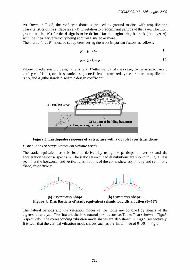
As shown in Fig.3, the roof type dome is induced by ground motion with amplification characteristics of the surface layer (B) in relation to predominant periods of the layer. The input ground motion (C) for the design is to be defined for the engineering bedrock (the layer A), with the shear wave velocity being about 400 m/sec or more. The inertia force FH must be set up considering the most important factors as follows:

FH=KH ∙ W

KH=Z ∙ kH ∙ K0 Where KH=the seismic design coefficient, W=the weight of the dome, Z=the seismic hazard zoning coefficient, kH=the seismic design coefficient determined by the structural amplification ratio, and K0=the standard seismic design coefficient.

Figure 3. Earthquake response of a structure with a double layer truss dome

Distributions of Static Equivalent Seismic Loads

The static equivalent seismic load is derived by using the participation vectors and the acceleration response spectrum. The static seismic load distributions are shown in Fig. 4. It is seen that the horizontal and vertical distributions of the dome show asymmetry and symmetry shape, respectively.

(a) Asymmetry shape (b) Symmetry shape Figure 4. Distributions of static equivalent seismic load distribution (θ=30°)

The natural periods and the vibration modes of the dome are obtained by means of the eigenvalue analysis. The first and the third natural periods such as T1 and T3 are shown in Figs.5, respectively. The corresponding vibration mode shapes are also shown in Figs.5, respectively. It is seen that the vertical vibration mode shapes such as the third mode of θ=30°in Fig.5.

B: Surface layer

C: Bottom of building basement A: Engineering bedrock

(1)

(2)


212

(1)

(2)

(3)

(4)

(5)

First mode: T1=0.162(s) Third mode: T3=0.131(s) Figure 5. The first and third vibration mode shapes and natural periods T1 and T3

Response Spectrum Method by means of the Static Equivalent Static Seismic Load applied at the Dome

In the earthquake-proof design of the dome, the design seismic load is calculated considering the vibration characteristics of the substructure. On the other hand, the methodology and the calculation standard are not enough to calculate the seismic design load. The practical estimation method is proposed by the response spectrum and the participation factor. The estimation equation of the maximum response acceleration of each node in the dome is proposed and verified with respect to the accuracy in comparison with the dynamic numerical analysis. The maximum acceleration of the node “i” in the “j”th vibration mode is given as follows:

𝐴𝐴𝐴𝐴𝐴𝐴𝑖𝑖𝑗𝑗 = 𝛽𝛽𝑗𝑗 ∙ 𝑆𝑆𝐴𝐴𝑇𝑇𝑗𝑗 ,ℎ𝑗𝑗 ∙ 𝐷𝐷𝑗𝑗 𝑖𝑖

Where jAcci is the estimated acceleration of the node “i”. βj is the modal participation coefficient of the “j”th vibration mode. SA(Tj , hj) is the acceleation response spectrum with respect to the “ j” th natural period Tj and damping ratio hj. And jDi is the “j”th vbration mode value of the node “i” . The earthquake-proof design of building structures is carried out by means of the static analysis using the seismic load and the load distribution. The static seismic load distribution is also used in the design of the dome. The horizontal distribution on the dome is affected by the first vibration mode value and the vertical distribution is affected by the second vibration mode, respectively. The horizontal static seismic load “Fi

H” at the node “i” is given by using the “j”th modal participation coefficient jβand the first mode value j𝐷𝐷𝑖𝑖𝐻𝐻.

𝐹𝐹𝑖𝑖𝐻𝐻 = 𝑆𝑆𝑖𝑖𝐻𝐻 ∙ 𝐴𝐴0 ∙𝑊𝑊𝑖𝑖

𝑁𝑁

𝑖𝑖=1

The horizontal static seismic load “FiV” at the node “i” are given by using the “j”th modal

participation coefficient jβand the second mode value j𝐷𝐷𝑖𝑖𝑉𝑉.

𝐹𝐹𝑖𝑖𝑉𝑉 = 𝑆𝑆𝑖𝑖𝑉𝑉 ∙ 𝐴𝐴0 ∙𝑊𝑊𝑖𝑖

𝑁𝑁

𝑖𝑖=1

The horizontal seismic load of the design static is given by

𝑆𝑆𝑖𝑖𝐻𝐻 =𝑚𝑚𝑖𝑖 ∙ 𝐷𝐷𝑖𝑖𝐻𝐻𝑗𝑗

∑ 𝑚𝑚𝑖𝑖 ∙ 𝐷𝐷𝑖𝑖𝐻𝐻𝑗𝑗 𝑁𝑁

𝑖𝑖=1

𝑆𝑆𝑖𝑖𝑉𝑉 =𝑚𝑚𝑖𝑖 ∙ 𝐷𝐷𝑖𝑖𝑉𝑉𝑗𝑗

∑ 𝑚𝑚𝑖𝑖 ∙ 𝐷𝐷𝑖𝑖𝑉𝑉𝑗𝑗 𝑁𝑁

𝑖𝑖=1


213

Where Co= SA(Tj , hj) /g, mi is mass of node “i”, j Di H is the “j”th horizontal vibration mode value at node “i”. Wi is the weight at node “i”, SA(Tj , hj) is the acceleation response spectrum (Fig.8) with respect to the “j” th natural period Tj and damping ratio hj=0.02 and g is the gravity acceleration. j Di

V is the “j”th vertical mode vibration value at node “i”, Wi is the weight at node “i”.

Vibration Characteristics such as Natural Period and Dominant Mode of the Domes

The natural period and the effective mass ratio of the domes are obtained by means of the eigenvalue analysis, respectively. The dominant mode are determine by the effective mass ratio. The obtained vibration characteristics such as the natural period and the dominant mode are shown in Table 5. The two corresponding vibration modes are also shown in Fig.5, respectively. It is seen that the dome appears in the first ( θ=30°and 60°)or second ( θ=45°) vibration mode. On the other hand, the vertical vibration shape of the dome appears in the third ( θ=30°

and 45°) or fourth ( θ=60°) vibration mode. The study focuses on the horizontal and vertical earthquake response of the dome subjected to horizontal and vertical earthquake motions.

Table 3. Eigenvalue analysis

θ (degree)

Dominant mode No.

Effective mass ratio

Natural period of “j” th : Tj (sec)

H V H V T1 T2 T3 T4 30 1 3 0.290 0.399 0.162 0.162 0.131 0.105 45 2 3 0.545 0.276 0.155 0.155 0.109 0.102 60 1 4 0.593 0.192 0.162 0.162 0.136 0.104

Dynamic Responses of the Time History Analysis

The time history analysis of the dome is carried out to verify the accuracy of the estimation value of the static equivalent seismic load applied on the dome by the proposed method. The numerical integration method uses the Newmarkβ method in the vibration equation. Since it has been known that the case of β=1/4 will be unconditionally stable for most nonlinear problems, β=1/4 is used in this study. The Rayleigh damping is used and both of the first and second damping factors are taken to be 0.02.

Input Vertical and Horizontal Artificial Earthquake Motions on Surface Ground

In conventional earthquake-response analysis, the most common approaches to use waves observed either at the ground surface. The basic thinking behind setting up input ground motion for the seismic design and the analyses is described in this section. There are two basic focal points: (1) Designing is to basically a two-phase design procedure, Level 1 (moderate earthquake motion) and Level 2(severe earthquake motion), with seismic design carried out for these earthquake inputs. (2) The time history analysis of the dome is carried out using the vertical and horizontal motions. The artificial seismic waves with the phase of the five observed earthquake motions are used. The surface layer amplification is considered in the waves. The motion fits the target acceleration response spectrum in Fig.6 of the damage limit artificial earthquake motion with a phase characteristic (Level 1) and the damping factor 0.05. The peak ground accelerations of the vertical and the horizontal earthquake motions are shown in Table 4. The average value of the horizontal and vertical motions is 119 and 62 cm/sec2 , respectively.


214

0

50

100

150

200

250

300

0 0.5 1 1.5 2 2.5 3

El-Centro (1940)Taft (1952)Hachinohe (1968)Tohoku (1978)Kobe (1995)

Natural period（sec）

Acc

eler

atio

n（

cm/𝐬𝐬𝐬𝐬𝐬𝐬

𝟐𝟐 ）

Horizontal wave

Vertical wave

0

50

100

150

200

250

300

350

400

450

500

0 0.5 1 1.5 2 2.5 3

El-CentroHachinoheKobeTaftTohoku

Acc

eler

atio

n (c

m/s

ec2 )

Natural period（sec)

Table 4. PGA (Peak ground acc.: cm/sec2) of the used input earthquake motion

Used phase characteristic PGA Used phase characteristic PGA El Centro-NS (1940) 112 El Centro-UD (1940) 62 Taft-EW (1952) 129 Taft-UD (1952) 57 Hachinohe-NS (1968) 120 Hachinohe-UD (1968) 75 Tohoku-NS (1978) 102 Tohoku-UD (1978) 64 Kobe-NS (1995) 133 Kobe-UD (1995) 52

Figure 6. Target acceleration response spectrum (damping factor h=0.05) of the damage limit artificial earthquake motion with a phase characteristic (Level 1) (moderate earthquake motion) The acceleration response spectrum SA(T, h=0.02) in case of in case of the damping factor h=0.02 is shown in Fig.7 using the input horizontal and vertical earthquake motions. The spectrum such as SA

H(T, h) and SAV(T, h) are used in the proposed equations (2) and (3).

Figure 7. Acceleration response spectrum (damping factor h=0.02) of the damage limit artificial earthquake motion with a phase characteristic (Level 1:moderate earthquake motion)

Horizontal wave

Vertical wave


215

Comparison between the Time History Analysis and the Response Spectrum Analysis

The time history analyses are carried out to verify the accuracy of Eqs. (2) and (3) by using the damage limit earthquake motions with the phase of the observed earthquake motions. It is seen in Fig. 9 that the values of the horizontal and vertical maximum response displacement by means of proposed static method show a good agreement with the time history analyses. It is noted that the values are calculated by using just the modal participation coefficient and the vibration mode value at the dominant mode.

Figure 8. Node number of dome ridgeline

Figure 9. Accuracy verification of response disp. using equivalent seismic force in comparison with time history analyses at max. disp. (The node no. is shown in Fig.8.).

(b) Max disp. occurs at nodes 4, 8 and 6, respectively (θ=45°).

(a)Max disp. occurs at nodes 4, 5 and 7, respectively (θ=30°).

(c) Max disp. occurs at nodes 5, 8 and 6, respectively (θ=60°).


216

Conclusions

The study deals with the dynamic responses on the domes subjected to vertical and horizontal earthquake motions. The design seismic coefficient of the applied load distribution considering the vertical response effect is also actually necessary for the safety study in the earthquake proof design. The study proposes the response spectrum method of calculating the static equivalent seismic loads for the applied load for the earthquake-proof design on the domes. The loads are easily obtained by means of the eigenvalue analysis. The accuracy is also verified by a good agreement with the time history analysis of the domes subjected to the damage limit artificial vertical and horizontal earthquake motions. The static equivalent seismic loads can be used to obtain statically the stress and the displacement for the seismic design.

Acknowledgment This work was supported by JSPS KAKENHI Grant Number 18K04427.

References

[1] Ishikawa, K. (2009) Effects of resonance between spatial structures and ceiling systems on the seismic response”, Proceedings of the International Association for Shell and Spatial Structures (IASS) Symposium 2009, Valencia Evolution and Trends in Design, Analysis and Construction of Shell and Spatial Structures Universidad Politecnica de Valencia, Spain Alberto DOMINGO and Carlos LAZARO (eds.).

[2] Ishikawa, K., Kato S. (1997) Elastic-plastic dynamic buckling analysis of reticular domes subjected to earthquake motion, International Journal of Space Structures, 12, 205-215.

[3] Ishikawa K, Okubo S, Hiyama , Kato S. 2000. Evaluation method for predicting dynamic collapse of double layer lat-ticed space truss structures due to earthquake motion. In-ternational Journal of Space Structures, Vol.15, 249–257.

[4] Okubo S, Hiyama Y, Ishikawa K, Wendel R, Fischer L. (2001) Load capacity and plastic deformable ability of aluminum alloy double layer latticed wall subjected to plane load, IASS Symposium 2001, Nagoya, TP101.

[5] Ishikawa K, Kato S. (1997) Elastic-plastic buckling analysis of reticular dome subjected to earthquake motion. Interna-tional Journal of Space Structures, Vol.12, 205–215.

[6] Taniguchi Y, Gould P L, Kurano M. (2008) Earthquake input energy at dynamic collapse for double-layer cylindrical Lattice roofs. Journal of the IASS, Vol.49,No. 2.

[7] Fan F, Shen S Z, Parke G A R. (2004) Theoretical and experi-mental study of vibration reduction in braced domes using a viscous damper system. International Journal of Space Structures, Vol.19, No.4, 195-202.

[8] Midorikawa M. (2005) Performace-based seismic design provi-sions for buildings in Japan. Proceedings of the IASS 2005, Vol.I, 307-316.

[9] Giuliani G C. (2002) Overview on the dynamic control of struc-tures. Proceedings of the IASS 2002:561-567. [10] Zeng Z P. 2007. Structural analysis and design of the latticed shell for Fujian Gymnasium. Journal of Spatial

Structures, Vol.13, No.2, 44-48. [11] Ilzarbe L. Álvarez, M.J. Viles E. Tanco M. (2008) Practical ap-plications of design of experiments in the field

of engineer-ing. Abibliographical review, Qual. Reliab. Engng.Int., Vol.24, 417-428. [12] European Committee for Standardization(CEN), Eurocode 8: Design of structures forearthquake resistance

Part 1: Gen-eral rules. (2004) seismic actions and rules for buildings (EN 1998-1: 2004). Brussel. [13] FEMA-356. (2000) NEHRP Guidelines for the Seismic rehabili-tation of buildings. Building seismic safety

council, Wash-ington DC.


217

Intelligent Robust Control based on Reinforcement Learning for a kind of Continuum Manipulator

Jiang Da¹, *Zhiqin Cai¹, Xiaolu Qiu¹, Haijun Peng¹ and Zhigang Wu2

1Department of Engineering Mechanics, Dalian University of Technology, Dalian 116024, P.R.China. 2State Key Laboratory of Structural Analysis for Industrial Equipment, Dalian University of Technology,

Dalian 116024, P.R.China.

*Corresponding author: [email protected]

Abstract Designing a controller with strong coupling dynamic model is extremely challenging and is more serious in continuum manipulator control problems. In this article, a dynamic control method based on deep reinforcement learning (RL) is used for the robust control of a continuum manipulator. According to the dynamic equation of the continuum manipulator, a model-based reinforcement learning optimized sliding mode controller is proposed. According to the limited observation state of the system, the agent learns and corrects the control parameters online to optimize the slope of the sliding surface, and realize the dynamic adaptive tracking control under the uncertainty of the model. Under the dynamic adaptive tracking control, the results show that the strategy network can give the appropriate control parameters according to the system state and output mechanism saturation problem. The efficacy of the approach on a difficult tracking control problem with highly nonlinear dynamics is demonstrated. Results indicate that the RL optimized sliding mode method is faster than the sliding mode method and only requires a small control increment.

Keywords: Robust Control, Reinforcement Learning, Continuum Manipulator

Introduction

Since the introduction of the continuum robot[1], its good bending performance has made it very adaptable in many nonstructural environments as well as narrow and limited working environments with many obstacles, and the continuum manipulator has broad application prospects in special environments. However, compared with the traditional discrete manipulator, the continuum manipulator has difficulty with the estimation of the deformation state under the action of external force or contact with the environment, and it also has great difficulty with the modeling and control of the continuum manipulator. In the case of inaccuracy and poor controllability, the accessibility and accuracy at the end are likely to be greatly reduced. Therefore, reasonable and effective modeling and controller design is necessary.

Several research studies have been performed for kinematic and dynamic modeling of continuum robots[2]-[7]. For this kind of nonlinear model with strong coupling, Te[8] proposed the head following control method to realize the navigation of continuum robots in the complex nonstructural environments. Thomas[9] learned a particular global solution for inverse kinematics problem by supervised learning without any prior knowledge about the system. Michael[10] presented a model-less hybrid control approach that regulates the tip position/force of continuum manipulators under unknown constraints along the manipulator's body. Falkenhahn[11] developed a model-based dynamic PD-controller to address the tracking issue for continuum robots. Many controllers on continuum manipulator control are


218

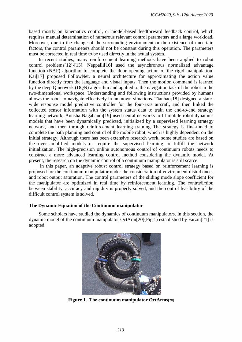
based mostly on kinematics control, or model-based feedforward feedback control, which requires manual determination of numerous relevant control parameters and a large workload. Moreover, due to the change of the surrounding environment or the existence of uncertain factors, the control parameters should not be constant during this operation. The parameters must be corrected in real time to be used directly in the actual system.

In recent studies, many reinforcement learning methods have been applied to robot control problems[12]-[15]. Neppalli[16] used the asynchronous normalized advantage function (NAF) algorithm to complete the door opening action of the rigid manipulation. Kai[17] proposed FollowNet, a neural architecture for approximating the action value function directly from the language and visual inputs. Then the motion command is learned by the deep Q network (DQN) algorithm and applied to the navigation task of the robot in the two-dimensional workspace. Understanding and following instructions provided by humans allows the robot to navigate effectively in unknown situations. Tianhao[18] designed a state-wide response model predictive controller for the four-axis aircraft, and then linked the collected sensor information with the system status data to train the end-to-end strategy learning network; Anusha Nagabandi[19] used neural networks to fit mobile robot dynamics models that have been dynamically predicted, initialized by a supervised learning strategy network, and then through reinforcement learning training The strategy is fine-tuned to complete the path planning and control of the mobile robot, which is highly dependent on the initial strategy. Although there has been extensive research work, some studies are based on the over-simplified models or require the supervised learning to fulfill the network initialization. The high-precision online autonomous control of continuum robots needs to construct a more advanced learning control method considering the dynamic model. At present, the research on the dynamic control of a continuum manipulator is still scarce.

In this paper, an adaptive robust control strategy based on reinforcement learning is proposed for the continuum manipulator under the consideration of environment disturbances and robot output saturation. The control parameters of the sliding mode slope coefficient for the manipulator are optimized in real time by reinforcement learning. The contradiction between stability, accuracy and rapidity is properly solved, and the control feasibility of the difficult control system is solved.

The Dynamic Equation of the Continuum manipulator

Some scholars have studied the dynamics of continuum manipulators. In this section, the dynamic model of the continuum manipulator OctArm[20](Fig.1) established by Farzin[21] is adopted.

Figure 1. The continuum manipulator OctArms[20]


219

As shown in Fig.2, the continuum single section analytical model introduced here consists of three modules stacked together in series. The three modules effectively represent the dynamic behavior of the hardware, so more complex models are not motivated[20]. Each module is considered to consist of two symmetrical spring-damped structures with the constant curvature bending assumption. ijk and ijc are the elastic coefficient and damping coefficient for the drivers. Therefore, there are 6 degrees of freedom for a continuum manipulator with 3 modules, including the local centroid coordinates l and rotation angle α in each module.

13k23k

11k

12k

21k21c

13c

22k22c

23c

11c

12c

1l

2l

3l

1α

2α

3α

4F

2F

3F

5F

6F

1F

Figure 2. Assumed structure for the analytical model of a section of a continuum

manipulator

Define generalized coordinates T321321 ,α,α,α,l,ll ][=q .

The dynamic control equation established by Farzin can be written as : = ( ) + ( ) + ( )GQ M q q C q,q q G q (1)

where 66R ×∈M is the inertia matrix of the system, 66R ×∈C is the stiffness matrix of the system, and 16R ×∈G is the coefficient matrix caused by the elastic potential energy and gravitational potential energy of the system:

+++++−+−

+++

++++++−+−

−−

+

−−++

+−+−−−++++

=

333

323332

2233

23332

2332133

32233

23332

2233233

223321

222

2232332133

123122

233323213

23323323321312

21332133

1231222131312321

000

cos20sin)sin(

cos2cos2sinsin)sin(sinsin

00sincos)cos(

0sinsincoscoscos

0)sin()sin(sinsin)cos(coscos

III

IlmIIllmlmIIlmlm

IllmlmII

llmlmlmIIIlmlmlmlm

lmlm

lmmmm

lmlmmmmmm

lmlmlmlmmmmmmm

αααα

αααααααα

αααα

ααααα

αααααααααα

M


220

111 21 2 3 2 1 12

11 21 2 3 1 1 3 1 2 1 2 3 3 1 23 3 1 1 2

112 22 3 1 2 2 12 22 3 3 2 2 1 3 3 1 2 22

3

( ) ( ) cos2( ) sin 2 ( )sin( ) sin( ) 0

cos( )

2 ( )sin ( ) [ (1 cos ) ] (2 )cos 00

0 2

c c m m lc c m m m m l

m l

c c m c c m l s m l

m

α αα α α α α α α α

α α α

α α α α α α α α

α

++ −+ − + − + + − +

− +

+ − + + − + + − +

=C

11 2 13 23 3 3 2 2 1 3 3 1 2 13 232

1 111 21 1 3 3 2 3 2 2 2 3 3 2 2 1 2 3 3 2 2 2 11 21 3 3 2 2 22 4

13 3 1 2 11 21 3 3 1 22

sin (1 cos ) (2 ) ( )

( ) 2 ( cos ) 2 ( cos )( ) 2 sin ( ) sin 0

0 2 cos ( ) 2 ( )

c c m l l m l c c

c c m l m l m l m l l m l l c c m l l

m l c c m l

α α α α α

α α θ α α α α α α

α α α α

−

+ − + − + +

+ + − + + +

+ + +

13 3 2 1 2 12 224

1 113 23 13 232 4

sin ( ) 0

0 0 ( ) 0 0 ( )

m l l c c

c c c c

α α

−

+ +

−−−−+−−−−+++

−−−−+++++−−+−+++−

−−−+−++−−−−+−++−−

=

)()()()()sin(

)()()sin(sin)()()()cos(

cos)()(cos)()(

03321

32321

03321

31321

02221

22221

02221

21221

2133

01121

12121

01121

11121

21331232

03321

32303321

313213

1302221

22202221

21212

301121

12101121

11121

llkllkllkllkglm

llkllkglmglmmllkllkgm

gmllkllkgmgmllkllkgmgm

αααααα

ααααααααα

αααααα

G

where iI is the moment of inertia of the rigid rod in each module, il0 is the initial the value of il .

The generalized force in the system FQQ FG = is expressed as an appropriate weighted

FQ combination with input force F :

−

−−

+−+−−

++

=

21

21

21

21

21

21

2221

2221

21

21

21

21

22

212111

000000

sinsin110000

coscos1100)cos()cos(coscos11

αα

αααααααα

llFQ

The Robust Controller

As shown in the previous section, the dynamic model of continuum manipulators has higher nonlinearity. Considering external disturbances, modeling errors, and limited output of the actuator, it is difficult to perform online real-time tracking control. The sliding mode control algorithm is an excellent nonlinear control algorithm. Well-designed sliding surface parameters can improve the dynamic quality of the system's response process. Reinforcement learning provides feasibility to optimize control parameters online. By reinforcement learning of the deep deterministic policy gradient (DDPG) algorithm, the controller performance is optimized to achieve stable and efficient tracking results. Fig.3 shows the structure of this controller.

DDPG

Sliding Mode Controller

Dynamic Model

u qdqc

e

Figure 3. Reinforcement learning optimized robust controller


221

A. Sliding mode controller

Consider the modeling error, parameter variation and other uncertain factors as external disturbance f , and the control input vector u=F, then the dynamic equation can be written as:

( ) ( , ) ( )u u u+ + = +M q q C q q q G q u f

(2)

where MQM 1-

Fu = CQC 1-

Fu = GQG 1-

Fu = Δ -Δ -Δ -Δu u u=f u M q C q G (3)

Define the sliding mode surface function as: ecexs +=)( , ),,,diag(= 621 ccc Lc (4)

The tracking error vector q-q=e d , dq is the expected value of the generalized coordinates. Take the exponential approach law as:

ηssεs -)sgn(-= (5)

ε , η are the coefficient matrices of the approach law. Then the sliding mode control protocol of the system can be derived as:

fGqCηssεceqMu -))sgn(( uud

u +++++= (6)

B. Reinforcement learning optimized sliding mode controller

In this paper, the deep reinforcement learning algorithm of the deep deterministic policy gradient is used to optimize the control parameters of the sliding mode controller online.

We adopt the standard Markov decision process (MDP) formalism for this work, which is composed of the state ts in state space S, the action ta in action space A, a stationary transition dynamics distribution 1( | , )t t tp s s a+ described by the discrete dynamic equation of the manipulator, and the reward function ),( ttt asre .The goal of reinforcement learning is to obtain the optimal strategy θπ parameterized by θ to maximize the return expectation reward

∑=−=

T

ti tttti asreasR ),(),( γ of long-term T in which ),( ttt asre is the reward value obtained

by taking action ta under state ts , and γ is the discounting factor. Thus, the action value function can be represented by Eq.(7).

])([][)( ∑=−====

T

ti iiiti

ttttt ,asreγEa,as|sRE,asQ (7)

The deep deterministic policy gradient is a typical improved actor-critic (A-C) framework algorithm, which absorbs the characteristics of the replay buffer and independent target network in the deep Q network (DQN).

The main net contains two deep neural networks, actor net ( | )s µµ θ parameterized by uθ and critic net ( , | )QQ s a θ parameterized by Qθ , used to approximate the deterministic

policy ( )sθµ and action-value function )(s,aQ . The DDPG algorithm has an independent target network. After each iteration, the parameterτ of the main net is updated to target network parameters by the moving average(AG) method according to Eq.(8).

(1 )θ τθ τ θ′ ′= + − (8) For N transitions ( 1,,, +iiii sreas ), the critic network updates the value function by

minimizing the loss function:


222

∑=

−=N

i

QiiQi asQy

NL

1

2))|,((1 θ (9)

where )|)|(,( 11Q

iiiQi ssQrey ′′++ ′′+= θθµγ µ

The actor network updates the action policy using the sampled policy gradient:

, ( )

1

1 ( , | ) | ( | ) |i i i

NQ

a s s a s si

J Q s a sNµ µ

µµθ θ

θ µ θ= ==

∇ ≈ ∇ ∇∑ (10)

It is difficult to calculate the exact optimal value of Eq.(6) directly through reinforcement

learning, since the dynamics and reward functions are nonlinear which might cause the controller to fail to obtain a reasonable solution in a wider action space. However, it makes a good effect on optimizing control parameters to improve control quality issues. For control from Eq.(6), good sliding mode parameters c can effectively reduce the approach time and weaken the chattering. The learning network is trained by the DDPG algorithm. The critic net evaluates the control performance according to the current state of the system, and the actor net optimizes the sliding mode controller parameters c .

Simulation Result

Table 1 shows the parameters of a single module of the continuum manipulators.

Table 1. Parameters of the Continuum manipulator

Parameters Symbol Value

Mass of single modules m(kg) 0.5

Moment of inertia J(kg·m2) 49.375 10−×

Elastic coefficient k 1.2

Damping coefficient c 0.03

For the DDPG network structure, the input of the actor net is the state vector s , and the

output is the action vector a corresponding to the six control parameters. Actor net includes two layers. The first layer contains 300 nodes, the activation parameter is relu, and the second layer dimension is 6, the activation function of which is tanh so that the network output falls within the action’s boundary. The critic network consists of a three-layer neural network. The input layer contains two branches, corresponding to the state vector s and the action vector a . After the combination, the corresponding action-values are output through the two-layer fully connected layer. The Gauss noise is added to the actor policy as the action noise caused by f in Eq.(2).

During this simulation, the environment is updated at 0.1 s intervals, and the observations we can use are only the elongation and rotation angle of the three-section arm. Based on this result, the reward function can be designed. It is necessary to simultaneously measure the control accuracy and control time caused by the dynamics with strong nonlinearity and coupling. The reward function is as shown in Eq.(11). We assume that the target control effect is achieved when the angle of various sections of the robot is stable, and the reference trajectory error is more than 50 time steps within a certain range (0.1s per time step).


223

6

,21

( )u n n goaln

re u t k=

= − − − Γ ∆ +∑dq q (11)

10goal

goal Truek

goal Flase==

= ==

The reward value is negatively correlated with the Euclidean distance of tracking error. nu ,Γ is the weighting factor of the control increment. When nu ,Γ becomes larger, it suggests

that the smaller the corresponding torque change is, the higher the corresponding reward value. Goal indicates whether the current manipulator has reached the control target, and if so, the reward value will increase.

In this experiment, the learning rate of the actor network and the critic network is 0.01, the reward discount value is 0.9, and the soft replacement value is 0.01. We consider the control target region to be the range interval value of the reference trajectory tracking error: 001.0±=rangee The model trains 300 episodes, and each episode contains 3000 steps. The desired general coordinate is defined as:

0.35 0.01sin(0.2 )0.35 0.01sin(0.2 )0.4 0.01sin(0.2 )0.5 0.2sin(0.2 )

0.6 0.25sin(0.2 )0.4 0.15sin(0.2 )

tttttt

ππππππ

+ + +

= + +

+

dq

Figure 4. Tracking error for length nl

Figure 5. Tracking error for angle nα


224

Fig.4 and Fig.5 show the control effects of the sliding mode controller optimized by

reinforcement learning in terms of module length and angle. The controller designed in this paper can keep the tracking error of the system stable after 15s, and the desired tracking effect can be achieved under the interference of the system.

Take module 2 as an example for the tracking angle 2α . Fig.6 shows the module 2

tracking error based on the sliding mode controller and reinforcement learning optimized sliding mode controller under a disturbance. The tracking error of the reinforcement learning optimized sliding mode controller is always lower than the sliding mode controller during the adjustment process. The former has a shorter settling time than the latter, which indicates that in the case of external disturbance, the controller designed in this paper has better control performance than the sliding mode controller.

After achieving the stable goal defined by goalk , the controller of the reinforcement learning optimization does not cause the tracking error develop to a more stable direction, which is related to the the reward function setting and the stable target definition. This result will continue to be explored in subsequent studies.

Figure 6. Angle comparison for two controllers

Fig.7 shows the module 1 control input 1u based on the sliding mode controller and the reinforcement learning optimized sliding mode controller under a disturbance. During the adjustment process, the control input of the former changes significantly less than the latter, and it has a shorter settling time. This indicates that under the interference, the controller designed in this paper has good robustness and can generalize further optimization according to the direction of the reward function.

Figure 7. Control input comparison for two controllers


225

Conclusions

By studying the motion of continuum manipulators, a trajectory tracking controller based on reinforcement learning is proposed to satisfy the performance objectives required in the presence of interference, parameter disturbance and model uncertainty. From the simulation results, in the presence of interference, a robust sliding mode controller that achieves good tracking performance using reinforcement learning. Reinforcement learning adjusts the control parameters online to prevent system oscillations caused by disturbances, and to improve the system robustness.

In future research, we will focus on the use of learning algorithms for autonomous online planning and tracking control on prototypes of continuum manipulators.

Acknowledgments This work is supported by the National Natural Science Foundation Key Foundation No.91748203 and Qian

Xuesen Laboratory of Space Technology Seed Fund QXSZZJJ03-07.

References [1] Robinson G., Davies J. B. C. Continuum robots - a state of the art, Proceedings 1999 IEEE International

Conference on Robotics and Automation, Detroit, MI, USA, 1999, 1050-4729 [2] Rone W. S., Ben-Tzvi P. (2014) Continuum Robot Dynamics Utilizing the Principle of Virtual Power, IEEE

Transactions on Robotics 30(1):275-287. [3] Wu G., Shi G., Shi Y. Modeling and analysis of a parallel continuum robot using artificial neural network,

2017 IEEE International Conference on Mechatronics (ICM). Churchill, VIC, Australia, 2017,153-158, doi: 10.1109/ICMECH.2017.7921096.

[4] Amouri A., Mahfoudi C., Zaatri A., et al. A new approach to solve inverse kinematics of a planar flexible continuum robot, American Institute of Physics Conference Series. 2014, 1618:643.

[5] Godage I. S., Guglielmino E., Branson D. T., et al. Novel modal approach for kinematics of multisection continuum arms, 2011 IEEE/RSJ International Conference on Intelligent Robots and Systems, San Francisco, CA, USA, 2011,25-30.

[6] Li Z., Ren H., Chiu P. W. Y., et al. (2016) A novel constrained wire-driven flexible mechanism and its kinematic analysis, Mechanism & Machine Theory 95:59-75.

[7] Greer J. D., Morimoto T. K., Okamura A. M., et al. Series Pneumatic Artificial Muscles (sPAMs) and Application to a Soft Continuum Robot, 2017 IEEE International Conference on Robotics and Automation (ICRA). 2017 : 5503-5510. doi:10.1109/ICRA.2017.7989648.

[8] Li T , Liu K , Liu H , et al. Head Following Control Method of a Mobile Continuum Robot for Deep-Cavity Inspection, 2017 2nd International Conference on Cybernetics, Robotics and Control (CRC). Chengdu, China, 2017, 1-5, doi: 10.1109/CRC.2017.13.

[9] Thuruthel T. G., Falotico E., Cianchetti M., et al. Learning Global Inverse Kinematics Solutions for a Continuum Robot, ROMANSY 21- Robot Design, Dynamics and Control. Springer International Publishing, 2016.

[10] Yip M., Sganga J., Camarillo D. (2017) Autonomous Control of Continuum Robot Manipulators for Complex Cardiac Ablation Tasks, Journal of Medical Robotics Research, 2(1): 1750002.

[11] Falkenhahn V., Hildebrandt A., Neumann R., et al. (2015) Model-based Feedforward Position Control of Constant Curvature Continuum Robots Using Feedback Linearization. IEEE International Conference on Robotics & Automation 17(3): 261-272.

[12] Zhu Y. (2018) Policy Iteration for Hinfinity Optimal Control of Polynomial Nonlinear Systems via Sum of Squares Programming, IEEE Transactions on Cybernetics 48(2): 500-509.

[13] Zhou M., Qu X., Jin S. (2017) On the Impact of Cooperative Autonomous Vehicles in Improving Freeway Merging: A Modified Intelligent Driver Model-Based Approach, IEEE Transactions on Intelligent Transportation Systems 18(6), 1422-1428.

[14] Zhu Y., Zhao D., He H., et al. (2016) Event-triggered Optimal Control for Partially-unknown Constrained-input Systems Via Adaptive Dynamic Programming, IEEE Transactions on Industrial Electronics 64(5): 1-1.


226

[15] Gu S., Holly E., Lillicrap T., et al. Deep reinforcement learning for robotic manipulation with asynchronous off-policy updates, 2017 IEEE International Conference on Robotics and Automation (ICRA), 2017,3389-3396

[16] Neppalli S., Csencsits M. A., Jones B. A., et al. (2009) Closed-Form Inverse Kinematics for Continuum Manipulators, Advanced Robotics 23(15):2077-2091.

[17] Kai X., Simaan N. (2008) An Investigation of the Intrinsic Force Sensing Capabilities of Continuum Robots, IEEE Transactions on Robotics 24(3): 576-587.

[18] Zhang T., Kahn G., Levine S., et al. Learning Deep Control Policies for Autonomous Aerial Vehicles with MPC-Guided Policy Search, 2016 IEEE International Conference on Robotics and Automation (ICRA), 2016, 528-535.

[19] Nagabandi A., Kahn G., Fearing R S., et al. Neural Network Dynamics for Model-Based Deep Reinforcement Learning with Model-Free Fine-Tuning, Proceedings - IEEE International Conference on Robotics and Automation, 2017, 7579-7586.

[20] Mcmahan W., Chitrakaran V., Csencsits M., et al. Field trials and testing of the OctArm continuum manipulator, IEEE International Conference on Robotics & Automation. Orlando, FL, USA, 2006, 2336-2341, doi: 10.1109/ROBOT.2006.1642051..

[21] Salehi A., Piltan F., Mousavi M., et al. (2013) Intelligent Robust Feed-forward Fuzzy Feedback Linearization Estimation of Pid Control with Application to Continuum Robot, International Journal of Information Engineering & Electronic Business 5(1): 1-16.


227

Simulation of metal Grain Growth in Laser Powder Bed Fusion Process using Phase-field Thermal Coupled Model

*Zhida Huang1, †Jian Lu2, Chong Liu2, and Bo Li1 1Department of Mechanical and Aerospace Engineering, Case Western Reserve University, Cleveland, OH 44106,

USA

2Guangdong Institute of Aeronautics and Astronautics Equipment & Technology, Zhuhai, Guangdong 519000, China


Abstract

Laser Powder Bed Fusion (LPBF) is a metal additive manufacturing method that manufactures products with high density and quality. The LPBF process, involving multiple physical phenomena, is controlled by several parameters such as laser power, scanning speed, material properties, etc. We present a coupled grain growth and heat transfer modeling technique to understand the materials microstructure evolution during the cooling process of LPBF. In specific, the phase-field model is considered as functions of temperature combined with transient heat transfer equation to simulate the crystallization of the melt pool. In the simulation, the computational domain for phase-field calculation and the magnitude of the driving force of order parameters are defined using current temperature distribution. Additionally, the change of order parameters generates latent heat to affect the cooling process. The finite element method using a staggering strategy is employed to solve the coupled governing equations on an irregular geometry.

1 Introduction

Metal Additive Manufacturing comparing to traditional manufacturing methods, possesses higher flexibility and efficiency. Among all the metal Additive Manufacturing methods Powder Bed Fusion (PBF) method provides the highest density. The basic idea of PBF is to wield a horizontally distributed metal particles, namely Powder Bed, using high power laser beam iteratively into an objective geometry. In each iteration, a new layer of metal particles is paved on the previous layer, and the laser will scan through the section of objective geometry at current heights.[1]

During the PBF process, the laser scanning through the powder bed generates temperature high enough to completely melt the particles resulting in a melt pool on the track of the laser. Studies show that material particles usually experience extreme conditions such as large temperature gradient, large stress, etc. which makes the result hard to predict. The controllable parameters, including size distribution of powder particles, power, and scanning speed of laser, scanning strategy including depth of powder bed, could also impact the geometry and temperature distribution of melt pool thus final result. Both experimental and numerical studies have been carried on in understanding the mechanisms. [2]-[9]

As the melt pool cools down, material with temperature lower than melting point starts to solidify. This phase change process determines the final microstructure, which is closely related to material properties, at that position since previous studies have pointed out that the trend of grains growth


228

is related to the temperature gradient and cooling rate. To better understand how manipulating the PBF process could influence the result, an approach is necessary for simulating the microstructure development during the cooling down of the melt pool.[11][12]

There are many numerical methods available for simulation of the Grain Growth process, among which the most popular ones are Monte Carlo model, Cellular Automata model, and the Phase-field method. Monte Carlo model demands the calculation region be a regular lattice. Each lattice will be assigned a grain orientation, and it has a probability of shifting to a neighbor orientation on each time step.[13][14] Cellular Automata is a collective name for a certain kind of models. Same as Monte Carlo method Cellular Automata is carried on regular square lattices. Those methods are inspired by topological behaviors of the grains, for example, the grain boundary moving speed relating to boundary curvature or grain growing speed relating to the temperature gradient, etc., and emphasize those behaviors using specific algorithms in the simulations. [15][16][17] Monte Carlo model and Cellular Automata model are not so computationally intensive. Generally speaking, neither of them demands governing equations. However, the limitation is visible too. Monte Carlo method only fits the grain size with the experiment result, but the anisotropic behaviors of grains, namely the shape of the grains, are hard to capture. Also, these two methods require regular lattices, so they may not be suitable for geometry with high complexity.

Phase-filed method has been applied to study many microstructure evolution problems and interface development problems such as solidification, fraction, etc.[18][19][20][21] Generally phase-field models introduce a specific form of free energy and develop its governing equation based on it.[22] In its interpretation of Grain growth, each orientation of grain is represented by an order parameter. The boundary of the grains forms a thin stripe area in the 2D scenario or a thin membrane area in 3D. The order parameters are ranged between 0 and 1 where 0 means that this point is not occupied by this orientation, and 1 means this point is occupied by this orientation. When crossing over the boundary, order parameters vector changes drastically from one representing an orientation to one representing another. On the whole computational area of order parameters, there is no specific mark discriminating boundary and cells, for example, a list of elements that are on cell boundaries, other than the order parameters, which are all smoothly changing variables. So almost all space discretization methods for calculation PDE on a particular area could be applied like finite element method or finite difference method etc. As a result, Phase-field method has high flexibility to fit in more complex geometries.[23][24][25]

We represent a numerical method to predict grain structure in high-temperature gradient metal solidification scenarios such as the solidification in the PBF process. The numerical method would be based on the Phase-field method coupled with thermal information. Finite element method (FEM) is employed to solve the coupled phase-filed governing equation. And an example of simulation of a benchmark result is given.


229

2 Methodology

To describe the crystallization process during a laser-based AM process, a coupled, transient grain growth and heat transfer framework is developed in this section. We combine the phase-field model with the transient heat transfer equation followed by the Finite element solution to predict the grain structure, including the grain size, shape, and orientation, during the cooling process.

2.1 Governing equations

The grain growth process can be modeled by the phase-field model in which order parameters are introduced to described the orientation of a grain. In specific, the order parameter equation is modified from the Allen-Cahn equation, which was used to describe grain growth process by LQ Chen [8], by involving a temperature coefficient γ as

( ) 3 2 22 )(ii i i j i

j iL T k

tη η η η ηγ η

≠

+ + − ∇

∂− −

=

∂ ∑ , (2.1)

Where iη is the i th order parameter, T the temperature, L the mobility, and k the gradient coefficient. The order parameter iη is picked form a set of order parameters [ ]iη η which has in all en elements. Each order parameter stands for a possible cell orientation. Two types of boundary are applied which are Dirichlet boundary condition and Neumann boundary condition for order parameter calculation which are

η η= on d∂Ω (2.2)

i n hη∇ = on n∂Ω (2.3)

In this model the order parameter simulation is triggered and couple with temperature distribution of the cooling down process of the melt pool. For temperature calculation, consider employing heat transfer equation which is

( )2

p diff Li i

T TC k Q Qt x x

ρ η∂ ∂− = +

∂ ∂ ∂ , (2.4)

where T , ρ , diffk and pC stand for temperature density, heat diffusion coefficient, and heat

capacity. On the RHS of the equation Q is the general heat source, ( )Q η is the latent heat generated due to change of order parameter. Eq. (2.1) and (2.4) are the coupled governing equations that are solved for. Three types of general heat boundary conditions are considered in this work which are essential condition, fixed flux condition, and conduction boundary conditions:

T T= on e∂Ω (2.5)


230

diff i ui

Tk n hx

∂ = ∂ on flux∂Ω (2.6)

( )diff i ci

Tk n h T Tx∂

= −∂

on cont∂Ω (2.7)

2.2 Numerical Solutions

The governing equations can be solved by employing the finite element method. The weak form of Eq. (2.1) and (2.4) could be gained from applying the Weighted Residual method which leads to

( ) ( )

3 2( 2 )

n d

ie i i i j e e i

j i

e en h dl dl

ds L L k dst

γ γη φ η η η η φ φ η

η φ η η φ

Ω Ω

∂Ω ∂

≠

Ω

∂

−

= − − +∂

−

+ + ∇ ∇

∇ − −

∫ ∫ ∑

∫ ∫

, (2.8)

( )( ) ( )

( )( ) ( )

2

flux

cont cont

t t t ti

fp diff L dif u

di f c

i

t tf

T ds ds dlx x

dl dl

TC k Q Q k T n ht

k T n h T T T T

φ φ

φ

ρ φ φ

φ

ηΩ Ω Ω

Ω∂ ∂Ω

∂

∂= −

∂

−

∂

−

∂− + ∇ −

∂

∇ − − −

∫ ∫ ∫

∫ ∫

, (2.9)

where eφ and tφ are the weighted functions for the governing equations and boundary conditions of the order parameters and temperature field, respectively. Since the finite element interpolation scheme satisfies the Kronecker Delta property at the Dirichlet boundary, the essential boundary condition can be applied by adding an additional term on the residual after rearranging the global matrix. So the last term in LHS of both (2.8) and (2.9) is canceled.

Applying divergence theorem on Eq. (2.8) gives

3 22( )ie i i i j e e i e

j in dlds L Lk ds

tη φ η η η η φ φ η η φ

≠Ω Ω ∂Ω

+ +∂

− ∇ ∇= ∇− − +∂∫ ∫ ∑ ∫ . (2.10)

In this work, only case for Neumann boundary condition is insulation so 0h = . Substitute (2.3) into (2.10) we have:

3 22 )(ie i i i j e e i

j ids L Lk ds

tη φ η η η η φ φ η

Ω Ω≠

+ +∂

− ∇= − −∂

∇∫ ∫ ∑ . (2.11)

Similarly, applying divergence theorem gives

( )( ) ( )flux cont

p diff L ut t ct t tTds ds dl dlTC k Q Q h h T Tt

φ φ φ φ φρ ηΩ Ω Ω ∂∂ Ω

∂+ + −

∂∇ ∇ = + +∫ ∫ ∫∫ . (2.12)


231

Eq. (2.11) and (2.12) are the final weak form of the governing equations.

For time discretization Euler Implicit Method is applied for Eq (2.12) which gives

( )( )

1 11

cont

flux cont

t tt t t c

tp diff

tL pt t t u t c l

C T tk t

t t

T ds h

C

T dl

ds h dl h TdQ Q T t

φ φ φ

φ φ φ φ

ρ

η ρ

++

Ω Ω

Ω

∂

∂Ω Ω

+

∂

∇

∆

∇ +

+

=

+∆ +

+ ∆ ∆

+ ∆

∫∫ ∫

∫∫

. (2.13)

While discretizing Eq. (2.11) the value of order parameters is taken from the previous time step because it’s a third-order polynomial of order parameter which is less computational efficient in implicit form. In addition, the cross-terms for the order parameters and temperature, i.e., 𝛾𝛾(𝑇𝑇) and 𝑄𝑄(𝜂𝜂), in the governing equations are evaluated explicitly based on the information at time t to avoid nonlinearity of fully-discretized equations. Use the value of the next time step for gradient energy term for stability. Eq. (2.11) could be rewritten as

( ) 1 3 2( )( 2 )t

ti e e i e i i i i j

j i

tLk ds t dsLηφ φ η φ η η η η η+

Ω Ω≠

−+ ∆ ∇ ∇ = ∆ + +− ∑∫ ∫ . (2.14)

Consider the Petrov-Galerkin Method, namely the test functions and order parameters use the same shape function which could be written as

i i

e ep

p

p p

p p

p

tp

t

T

NNNN

T

η ηφ φ

φ φ

≈ ≈

≈ ≈

(2.15)

where pN indicates the shape function corresponding to the pth node while pφ and piη are the

nodal values. Here the Einstein summation convention is employed for the repeated index.

Doing the substitution rewrite Eq. (2.13) and (2.14) into

( )

( )( )( )

1 1

cont

flux

cont

t tq p q qc

qp qu

q

L

p

q

q

p p qp diff r r

tq q pp

c

q

l

C N N tk B B t

t Q Q

T ds h N N T dl

ds N N h dl

N N h

N

T d

C T N t

t

ρ

η ρ

+ +

∂

∂Ω

∂

Ω Ω

Ω

Ω

+ ∆ ∆

∆ + +

∆

+

+

+ ∆

=∫

∫ ∫

∫

∫ , (2.16)

and


232

1

3 2

(

(

)

( ( ) 2 ( ) ))

tq p pr r i

t

q p p p p p p r r p pi i i i

q p

jj i

tLkB B ds

N N t N N N N ds

N N

L

η

η η η η η

+

≠

Ω

Ω+− −

+ ∆ ==

∆ +

∫

∑∫ (2.17)

Where prB is the Cartesian coordination rx derivative of shape function pN .

In this work, isoparametric elements are employed. In 2-D cases Shape Functions could be expressed using isoparametric coordinate such as

( )

1

2

,

M

N

NN

N

θ γ

=

(2.18)

The derivative matrix of shape function in isoparametric coordinate is then

1 1

2 2

M M

N N

N NB

N N

θ γ

θ γ

θ γ

∂ ∂ ∂ ∂

∂ ∂

= ∂ ∂ ∂ ∂ ∂ ∂

, (2.19)

Which can be transformed into Cartesian coordination using the Jacobian matrix such that

1 11 1

2 2 2 2

1* *

M M M M

N NN Nx y

N N N N x yB B Jx y

x yN N N N

x y

θ γθ θ

θ γ γ γ

θ γ

−

∂ ∂ ∂ ∂ ∂ ∂∂ ∂ ∂ ∂ ∂ ∂ ∂ ∂ ∂ ∂ = = =∂ ∂ ∂ ∂ ∂ ∂ ∂ ∂ ∂ ∂ ∂ ∂ ∂ ∂ ∂ ∂

(2.20)

Rearranging Eq.(2.16) and Eq.(2.17) gives the final form of Finite element equation which is


233

( )

( )1

1,

,

t tqp p qT T

q t tp qi

p

K T

TK R

R T

η ηη

η

η+

+ =

=

, (2.21)

where

( )( )pqp qr r

q p tL T kB B dsK N Nη γΩ

+= ∆∫ , (2.22)

( )

( )3 2

(

( ) 2 ( ) )

(

)

q

i

q p p p pi i

p p r r p pi i j

j

t

T

i

N N t N

N N N ds

R L Tη γη η

η η η≠

Ω∆ +− −

+

=

∑∫

, (2.23)

( )cont

qp p q p qT p diff r r

p qcds h N N dlK C N N k tB B tρ

Ω Ω∂= + ∆ + ∆∫∫ , (2.24)

and

( ) ( )( )( ),

flux cont

q qp q p qdif

tt q

c

q q p qL p

f

T

u

ds

k N N h dl N N h T dl

R T t Q Q C T N N

t t

η η ρΩ

Ω∂ ∂Ω

= ∆ + +

+ ∆+∆∫ ∫

∫ . (2.25)

qpKη and qpTK are defined as the global stiffness matrix.

Equation (1.20) can be solved using a fully implicit approach. Nevertheless, the solution of the order parameters requires a frequent update of the variable domain, which is determined by the current temperature distribution. Solving the order parameters and temperature field simultaneously may lead to convergence issues. Thus, a staggering strategy is adopted for the numerical solutions of Eq(2.21). In specific, the order parameters are calculated, assuming isothermal condition by using the temperature from the previous time step. Then the latent heat is given using the order parameters from both time steps as

( )1t t

i i i iQ Ht

ηη ηηη

+−

=∆

(2.26)

Secondly, substitute the latent heat into (2.21) for the temperature of the next time step. After the temperature of the new time step is solved, the next iteration starts.


234

2.3 Initial and boundary conditions for the order parameters

The global geometry is meshed into separated elements, but only some of them are involved in the Phase-field simulations. The global stiffness matrix and Residual are constructed with their element matrices. Those elements together are referred to as the computational area of order parameters in this work.

For the initial condition of Grain Growth simulation using Phase-field starting from the liquid phase, all the order parameters are initialized with a random value distributed in a very small range centered at zero. The free energy tends to minimize itself, and the liquid phase is not a minimum, so the order parameters would start developing to a solidified phase. Around the vicinity of zero, the dominant driving force for the order parameters is provided by the derivative of free energy. When the value of order parameter is among 0 to 1, the first-order term of Eq. (2.1) in the bracket is dominating while the contribution of the third-order term could be ignored. That gives exponential-like growth to order parameters when they are all around zero. Among them, there will be an orientation that preserves the largest order parameter. The max order grows much faster than the others and suppresses them because of the third term in the bracket. As the value of order parameters gets close to the solid phase, the gradient term starts to become the main influence. The influence is not on the value point itself, but the points around it. If a value point has already solidified and the points around it are still near the liquid phase, it tends to turn the around points into the solid phase the same to itself. As a result, there will be some points sporadically distributed on the computational area of order parameters where the cores of the cells are formed and propagate. When two cells meet during development, they merge into one if they are of the same order, or an interface would be formed if they are different.

The same initialization method for the liquid phase would be used in this work. During the simulation, when the average temperature of an individual element drops below maxT which is a given constant, the values of all parameters would be initialized, and the element would be included in the computational area of order parameters. On the other hand, if the temperature of a solidified element rise above maxT , the order parameters would be reset to zero, and the element would be removed from the computational area of order parameters.

As the solidified material cools down, the grain growth process stops, giving the final grain structure. In the simulation, when the temperature of an element drops below a given constant minT , the element would be removed from the computational area of order parameters, and all the order

Figure 1 Staggering stragtegy


235

parameters of it would remain fixed at that time step. Moreover, if the temperature of a solidified element reaches minT , it would be included in the computational area of order parameters.

The temperature coefficient ( )Tγ is defined among the range [ ]min max,T T . ( )Tγ should be an increasing function for the grain growth process is more active when the temperature is higher.

There are three kinds of boundaries of the computational area of order parameters, namely liquid boundary, solid boundary, and geometry boundary. The solid boundary and liquid boundary are self-explaining while the geometry boundary refers to the boundary that the computational area of order parameters coincident with the global geometry’s boundary.

According to the experiment result, the grain growth direction is the same as the temperature gradient. The interfaces propagate nearly perpendicular to the contours of the temperature field. So the boundary between the computational area of order parameters and liquid is set to insulation

because on insulation boundary 0nxη∂

=∂ , which means that the cell interface would be

automatically perpendicular to the boundary. Also, insulation boundary is applied to the geometry boundary. The solid boundary is applied to fixed boundary conditions for the continuity of the boundary in final results.

2.4 Spatial discretization

For the finite element method, the meshing strategy is always a critical issue impacting the result. As mentioned above, interfaces are formed during the simulation. Unlike Monte Carlo method or Cellular Automata, the interfaces in phase-field method the interfaces have space continuity. So the mesh for Phase-field calculation must be fine enough to capture the interfaces otherwise the

Figure 2: Grain boundary


236

result would be unjustifiable. Depending on the type of element and shape function applied, the mesh size could vary. However, the element size should always be larger than the interface width.

Due to the fact that the heat conduction equation has been proved to be stable and converging, and the order parameter simulation is only carried on at high-temperature area, The mesh for the parts that probably only temperature calculation is involved, on the other hand, could be much coarser. This strategy of meshing can improve the efficiency of the simulation significantly.

Algorithm

Table 1 Algorithm

Algorithm

Step 1: Update the computational area of order parameters ( )TΩ using temperature information. Set all elements with average temperature among [ ]min max,T T activated in Phase-field calculation.

Step 2: Update the global stiffness matrix Kη and residual t

Rη for the new computational area of order parameters.

Step 3: Apply fixed boundary condition to solid boundary condition. Solve for swap matrix Ls using

[ ]

1

1

2

1

1

i

i

iM mi

iM m

iM

iM m

Free DOF

Fixed DOF

Ls Ls

η

ηηη η

ηηη

η

η

−

− +

− +

=

Step 4: Solve for stiffness matrix and residual for order parameters in new DOF coordination :

T

K KLsK Ls

K Kη η

ηη η

=

,

i

i

i

RLsR

Rη

η

η

=

.


237

Step 5: Solve for new order parameters under boundary condition 1

i

t t t

i iK R Kη η ηη η+= −

Step 6: Swap order parameter back to original coordination [ ]

11

tt

Lsη

ηη

+

+ =

Step 7: Solve for the latent heat

1t t

i i i iLQ H

t

ηη ηη+−

=∆

Step 8: Solve for temperature ( )1,

t tqp p qT TK T R T η

+=

Step 9: Back to Step 1 if the max simulation time is not reached yet, otherwise terminate.

3 Simulation Example

The scenario of the simulation is the solidification of a melt pool of the PBF process. All the initial temperature information and the shape of the melt pool is gained from a PBF simulation.

Figure 3: Geometry and initial temperature distribution

The result of the simulation has been validated with the experiment result. The dimension of the geometry is 1000 800 360 mµ× × . The material is set to be aluminum. During the PBF simulation, a Gaussian distributed heat flux simulating laser beam is applied which takes form as

( )( ) ( )( )

2 2exp 2 c cx x t y y tAPqr rπ

− + −= −

(3.1)


238

where A is a constant related to laser absorption, P and r are power and radius respectively. The approach employed for PBF simulation is the Hot Optimal Transportation Meshfree Method (HOTM). [26]

The simulation of this work takes place on a section of the geometry at the center of the laser beam on the last time step. No heat source is introduced to simulate the scenario when the laser is suddenly retracted.

The size of the geometry is 800 mµ in width and 360 mµ in height. For the right, the left and bottom edge of the geometry insulation boundary condition is applied. For the top boundary, the convection boundary condition is applied.

As mentioned above the simulation for order parameters is not carried on for the whole geometry. Only a part of the geometry that contains the whole melt pool is employed as the computational area for the order parameters. Consider a half ellipse area centered at the middle point of the top edge with semi-major axis equals to 75 mµ and semi-minor axis equals to 60 mµ . At the initial time step, all nodes on the edge of the half ellipse are below the melting temperature. Since the melt pool is shrinking as cooling, the liquid area will not exceed this half ellipse area. So it’s justifiable to define the half ellipse area as order parameters computational area of order parameters, which has a much finer mesh than other areas. The average element size for order parameter computational area is 0.5. The initial grain is generated next. Set all the element activated then do the pure Phase-field simulation until all the domain has been covered by completely developed grains.

Table 2: Constants specification

Constant Value

Dimension of the order parameter vector 2 10.1k m sµ −=

/K

Figure 4: Mesh for the whole geometry and Mesh for the melt pool


239

Mobility coefficient

12 10 ^ 6L s−= ×

Time step interval

0.2 10 ^ 8dt s= × −

Dimension of the order parameter vector 25grainN =

Activated temperature min max[ , ] [800 ,900 ]T T K K=

Latent heat coefficient over density and h i

/ 350pH C Kρ =

Heat diffusivity 7 2 2 1/ 9.75*10pk C kg m s Kρ µ − − −= ⋅ ⋅ ⋅

All the coefficients of the Phase-field model are the same as how they were set in grains initialization. As the simulation goes on the liquid melt pool shrinks and the grains start to grow at the direction the liquid-solid interface proceeds. The trend of growing coincident with the temperature gradient as the melt pool cools down. The result is shown in Fig 5.

How the temperature range affects the final result is also examined, simulations with different temperature windows have been done for comparison. Three different temperature ranges are tested: [750,900] , [800,900] and [850,900] . From the comparison of the results from different activate temperature ranges, some conclusions could be made. As the temperature range decreases, the average time for a particular location to be activated for Phase-field simulation gets longer. With larger temperature range the cell boundary tends to be smoother, and the average grain size increases, the average length-width ratio decreases.

Next, the effect of the heat coefficient function ( )tγ

is investigated. In the examples above ( )tγ is just a linear function with value 0.5 at minT and 2 at

maxT . Although how the temperature affects the grain growth is unknown, the way ( )tγ affects the

final result can be studied. ( )tγ is an increasing function for grain growth is more activated when the temperature is higher. In this work, three types of ( )tγ are considered which is

Table 3: Average length width ratio for different temperature range

Temperature range Value

[750,900] 10.418

[800,900] 9.788

[850,900] 9.511


240

( )

( )

( )

min

1max min

min2

max min0.3

min2

max min

exp 1101.5 0.5

exp 110

1.5 0.5

1.5 0.5

T T

tT T

T TtT T

T TtT T

γ

γ

γ

− − = +− −

− = + − − = + −

. (3.2)

Figure 5 shows the development of order parameter vector magnitude of time step 1, 2500, 5000, 9050 and temperature

distribution of time step respectively. At time step 9050 all the average temperature of the elements drop below Tmin, so the

grains development is completed.


241

The total time steps for ( )1 tγ , ( )2 tγ , ( )3 tγ to complete calculation is 9000, 9050, and 9000, which are very resembling. That suggests the average developing time period for elements are not affected. However, for convex ( )tγ the Phase-field driving force higher at the same temperature comparing to concave one. So the cells in Fig A are more coarsened and developed than ones in Fig C while the linear scenario is between them.

In the results above, the figures shown are all contour of the magnitude of the order parameter

vector [ ]η . The orientation of each cell is stored in [ ]η . Figure 8 is the contour of 1

Ngrain

ii

Arg iη=

= ×∑ ,

from which the difference between each orientation is represented. Figure 8 shows the result of Benchmark 2018-002

A B

C

Figure 7: A: Final result for convex heat coefficient function; B: linear; C: concave. Time step of A,B and C: 9000, 9050, 9000

Figure 6 Heat coefficient functions

Figure 8 Orientations for cells

Figure 9 Experimental result of AM Benchmark 2018-002


242

4 Conclusion and Discussion

In this work, a thermal coupled phase-filed model is presented. The model is based on Allen-Cahn equation and heat transfer equation. By introducing latent heat and temperature coefficient, order parameters and temperature field are coupled. Finite element method is introduced to solve the weak forms of the governing equations numerically. An example of benchmark simulation is shown. The model demonstrates the feasibility of simulating microstructure development in the PBF process using phase-filed method. The phase-field model for the grain growth process can be applied to irregular geometry by using the Finite Element method. The columnar shaped cell with the growing direction compatible to the temperature gradient is generated as a result which resembles the experiment results. By adjusting minT , maxT and ( )tγ the grain structure can be manipulated. In addition, the model is based on solving a set of governing PDEs such that many mature numerical methods can be applied to ensure accuracy, efficiency, and stability.

Currently, the result provides shapes of the grains and interfaces, but specific orientation is not given. A method is needed for assigning orientations to each order parameter according to statistic results from the experiment. Improvement of the governing equations and the form of free energy density for different materials and scenarios and higher accuracy may be investigated. Though the columnar shaped cells are simulated, the definition of the coefficient related to the coupling of heat and Phase-field model, namely the heat coefficient function ( )Tγ , maxT and minT are based on the assumption made from basic material properties. More works are needed for investigating the mechanism of the coupling and matching up the simulation results and experiments. These improvements should be addressed in more details.

Acknowledgement

The corresponding author is grateful for the support provided by the GDAS' Project of Science and Technology Development under Grant Number 2018GDASCX-0804.

References [1] D D Gu, W Meiners, K Wissenbach & R Poprawe (2012) Laser additive manufacturing of metallic components:

materials, processes and mechanisms, International Materials Reviews, 57:3, 133-164, DOI: 10.1179/1743280411Y.0000000014

[2] C. Korner, A. Bauereiß, and E. Attar. Fundamental consolidation mechanisms during selective beam melting of powders. ¨ Modelling and Simulation in Materials Science and Engineering, 21(8):85011, 2013.

[3] Trevor Keller, Greta Lindwall, Supriyo Ghosh, Li Ma, Brandon M. Lane, Fan Zhang, Ursula R. Kattner, Eric A. Lass, Jarred C. Heigel, Yaakov Idell, Maureen E. Williams, Andrew J. Allen, Jonathan E. Guyer, Lyle E. Levine. Application of finite element, phase-field, and CALPHAD-based methods to additive manufacturing of Ni-based superalloys. Acta Materialia,Volume 139,2017,Pages 244-253,ISSN 1359-6454,https://doi.org/10.1016/j.actamat.2017.05.003.

[4] Liu, Xiaogang & Guo, Haiding & Yu, M.. (2017). Numerical Simulation of the Grains Growth on Titanium Alloy Electron Beam Welding Process. International Journal of Computational Methods. 16. 1840023. 10.1142/S0219876218400236.

[5] Zhao, C., Fezzaa, K., Cunningham, R.W. et al. Real-time monitoring of laser powder bed fusion process using high-speed X-ray imaging and diffraction. Sci Rep 7, 3602 (2017). https://doi.org/10.1038/s41598-017-03761-2

[6] Kappes, Branden & Moorthy, Senthamilaruvi & Drake, Dana & Geerlings, Henry & Stebner, Aaron. (2018). Machine Learning to Optimize Additive Manufacturing Parameters for Laser Powder Bed Fusion of Inconel 718. 10.1007/978-3-319-89480-5_39.


243

https://doi.org/10.1179/1743280411Y.0000000014

[7] A. V. Gusarov, I. Yadroitsev, P. Bertrand, and I. Smurov. Heat transfer modeling and stability analysis of selective laser melting. Applied Surface Science, 254(4):975–979, 2007.

[8] Yuan, B., Guss, G. M., Wilson, A. C., Hau‐Riege, S. P., DePond, P. J., McMains, S., Matthews, M. J., Giera, B., Adv. Mater. Technol. 2018, 3, 1800136. https://doi.org/10.1002/admt.201800136

[9] Fan Zhang, Lyle E. Levine, Andrew J. Allen, Carelyn E. Campbell, Eric A. Lass, Sudha Cheruvathur, Mark R. Stoudt, Maureen E. Williams, Yaakov Idell. Homogenization kinetics of a nickel-based superalloy produced by powder bed fusion laser sintering. Scripta Materialia,Volume 131,2017,Pages 98-102,ISSN 1359-6462,https://doi.org/10.1016/j.scriptamat.2016.12.037.

[10] S. A. Khairallah, A. T. Anderson, A. Rubenchik, and W. E. King. Laser powder-bed fusion additive manufacturing: Physics of complex melt flow and formation mechanisms of pores, spatter, and denudation zones. Acta Materialia, 108:36–45, 2016.

[11] M. E. Glicksman. Principles of solidification: an introduction to modern casting and crystal growth concepts. Springer Science & Business Media, 2010

[12] Jie Gao, Hao Li, Zhen Luo, Liang Gao,Peigen Li. Topology Optimization of Micro-Structured Materials Featured with the Specific Mechanical Properties. International Journal of Computational Methods. 10.1142/S021987621850144X

[13] Y Tan et al, Monte Carlo grain growth modeling with local temperature gradients Modelling Simul. Mater. Sci. Eng. 25 065003, 2017

[14] Zhang, Z., Wu, Q., Grujicic, M. et al. Monte Carlo simulation of grain growth and welding zones in friction stir welding of AA6082-T6. J Mater Sci 51, 1882–1895 (2016).

[15] S. Raghavan, Satyam S. Sahay. Modeling the grain growth kinetics by cellular automaton. Materials Science and Engineering A 445–446 (2007) 203–209

[16] Lian, Y., Lin, S., Yan, W. et al. A parallelized three-dimensional cellular automaton model for grain growth during additive manufacturing. Comput Mech 61, 543–558 (2018).

[17] Lian, Y., Gan, Z., Yu, C., Kats, D., Liu, W. K., & Wagner, G. J. (2019). A cellular automaton finite volume method for microstructure evolution during additive manufacturing. Materials and Design, 169, [107672]. https://doi.org/10.1016/j.matdes.2019.107672

[18] Benitez, Raul & Ramírez-Piscina, L.. (2004). Stochastic phase-field simulations of symmetric alloy solidification. Fluctuation and Noise Letters. 4. 10.1142/S0219477504002063.

[19] Kobayashi R. 1993. Modeling and numerical simulations of dendritic crystal growth. Physica D 63:410 [20] Ghoneim, Adam. (2017). The Meshfree Interface Finite Element Method for Numerical Simulation of Dendritic

Solidification with Fluid Flow. International Journal of Computational Methods. 15. 10.1142/S0219876218500573.

[21] C. Miehe,F. Welschinger,M. Hofacker. Thermodynamically consistent phase‐field models of fracture: Variational principles and multi‐field FE implementations. Int. J. Numer. Meth. Engng 2010; 83:1273–1311

[22] I. Steinbach, F. Pezzolla, B. Nestler, M. Seeßelberg, R. Prieler, G.J. Schmitz, J.L.L. Rezende. A phase field concept for multiphase systems. Physica D: Nonlinear Phenomena,Volume 94, Issue 3,1996,Pages 135-147,ISSN 0167-2789,https://doi.org/10.1016/0167-2789(95)00298-7.

[23] Chen LQ, Yang W. Computer simulation of the domain dynamics of a quenched system with a large number of nonconserved order parameters: The grain-growth kinetics. Phys Rev B Condens Matter. 1994;50(21):15752-15756. doi:10.1103/physrevb.50.15752

[24] LQ Chen. Phase-field Models for microstructures evolutions. Annu. Rev. Mater. Res. 2002. 32:113–40 [25] C.E. Krill III, L.-Q. Chen,Computer simulation of 3-D grain growth using a phase-field model,Acta

Materialia,Volume 50, Issue 12,2002,Pages 3059-3075,ISSN 1359-6454,https://doi.org/10.1016/S1359-6454(02)00084-8.

[26] Wang, Hao & Liao, Huming & Fan, Zongyue & Fan, Jiang & Stainier, Laurent & Li, Xiaobai & Li, Bo. (2020). The Hot Optimal Transportation Meshfree (HOTM) method for materials under extreme dynamic thermomechanical conditions. Computer Methods in Applied Mechanics and Engineering. 364. 112958. 10.1016/j.cma.2020.112958.


244

https://doi.org/10.1002/admt.201800136

Improvement of a ceramic head in the design of a total hip arthroplasty

Pakhaliuk Vladimir *, †Poliakov Aleksandr

Polytechnic Institute, Sevastopol State University, Russian Federation.



Abstract

It is known that one of the most progressive and most used in world medical practice friction

couples in total hip arthroplasty (THA) is a couple including ceramic elements. This is due to

the fact that currently, due to the influence of negative factors of a deteriorating environment,

the age rejuvenation is noted for patients who already need a total hip replacement (THR) in

terms of indicators and for which it should has the longest service life. The popularity of

ceramics is due to the fact that it has the highest wear resistance, it and its wear products are

bio inert and practically do not cause osteolysis due to the response of the immune system to

these ones.

But ceramics has a very important drawback: it is fragile and with significant dynamic loads,

for example, when jumping from a height, it can be destroyed in mating with the tapered neck

of the THR stem. To prevent this factor, a number of known designs have been proposed in

which a ceramic head mates with the neck of a stem by means of a plastic or metal sleeve that

is not fixed motionlessly to the head. This creates a movable joint in the indicated site during

THR operation due to the effect of cyclic loads. The presence of a soft plastic sleeve

aggravates the process, leading to loosening of the unstable connection between the head and

neck, instability in the elements of the THR, impaired joint biomechanics and manifestation

of pain syndromes, and, consequently, the need for revision arthroplasty.

The main goal of the work is to develop the design of a THR with a modular ceramic head

having metal properties in mating with the tapered neck and ceramic properties on the bearing

surface of a friction couple by creating a low-cost, low-toxic, durable joint of alumina or

zirconium ceramic and titanium alloy to obtain a soldered connection, operable in human

synovial fluid. Using finite element analysis, a qualitative and quantitative assessment of the

strength and stiffness of the proposed head design was performed.

Using a head of this design will allow not only to realize the main advantages of a ceramic-

ceramic friction couple in THR, but also ensure that there are no breaking loads for ceramics

at the tapered place of the head and stem, as well as undesirable physicochemical processes in

this conjunction, for example, fretting-corrosion which is also known to be present and in

existing commercial ceramic THR. The indicated advantage is due to the presence of

homogeneous biocompatible metal materials (Ti-based alloy) in their join.

Keywords: total hip replacement; ceramic friction couple; ceramic head; soldering

Introduction

In world medical practice, there are currently many different designs of total hip arthroplasty

(THA), the use of which is due to certain clinical indications. They differ both in the method

of fixation (cement and cementless) and in the clinical frequency of use (primary and revision

hip replacement). But they all represent a modular design of an artificial spherical joint of


245


total hip replacement (THR), which usually includes a prosthesis stem jointed to the spherical

head by means of a conical neck, and an acetabular cup, in turn, consisting of several

components including a liner. In this case, the head and liner compose a friction couple,

which can be divided into two groups according to the hardness characteristics of the

materials used in it. The first is a solid head (metal or ceramic) and a soft liner made of ultra-

high molecular weight polyethylene (UHMWPE), and the second is a solid head and liner

(metal, ceramic, or sapphire single crystal).

As practice shows, approximately 85% [1] of all THR failures occurs due to the response of

the human immune system to debris (wear products) released in the friction couple, which

leads to osteolysis and aseptic loosening of the THR elements, i.e. disturbance of its fixation

in bone tissues and the need for further revision arthroplasty. For this reason, the use of

friction couples with solid materials aims to reduce the wear rate compared with a friction

couple including UHMWPE, and thereby extend the lifespan of the THR. However, according

to literature, the THR with an ideal friction couple has not yet been obtained, since these

couples with solid materials have a number of significant drawbacks that limit their clinical

use [2].

Briefly, these friction couples can be described as follows. As the metal in the friction couple

including metal, CoCr alloy is used, which has a significantly lower wear rate than

UHMWPE, the wear particles are much smaller in size, and their number is much larger. In

addition, it turns out that the sensitivity of the immune system is affected by the total surface

area of the particles, which in the case of a metal on metal pair is only 30% less than that of a

couple including UHMWPE [2]. At the same time, the join of the THR stem neck made of

VT1-0 titanium alloy with the head is an electrolytic couple, where fretting-corrosion occurs

in the host environment, adding the amount of foreign particles to the body. VT1-0 titanium

alloy is such a grade in the classification of materials of the Russian Federation and

corresponds to approximately the well-known grade of Ti-6Al-4V titanium alloy. Moreover,

Co and Cr ions are toxic in nature, have the ability to spread throughout the body and

accumulate in its vital tissues, which in more than 5% of cases can lead to very serious

allergic complications.

Another couple of ceramics includes components (head, liner) made of alumina or zirconium

ceramics, the latter of which can be stabilized with yttrium. Ceramics have high hardness and

wear resistance, are almost bio inert, and, it would seem, have ideal properties as the material

of a friction couple. But it has a very important drawback - fragility, and when the head is

coupled with the conical neck of the stem there is a possibility of a ceramic head cracking in

case of intense dynamic loads. In this case, at the revision arthroplasty, it becomes necessary

to hip replacement only with a ceramic couple, since it is not possible to extract from the

tissues all small sharp fragments of collapsed ceramics, which, if they fell into a friction

couple, especially with using UHMWPE, would lead to catastrophic avalanche-like wear of a

new couple. In addition, in some cases, a squeak occurs in the ceramic friction couple, which

reduces the quality of life, especially in young patients who are shown such THR with a high

level of resource. In [1], it was studied that a friction couple of ceramic head on UHMWPE

liner has one of the lowest friction coefficients, which, moreover, is a low-cost friction couple

in all respects, which would be a serious incentive to increase the number of hip arthroplasty

by reducing the cost of the implant while increasing its reliability and resource. In addition,

the wear of a friction couple with UHMWPE was evaluated numerically in studies [3-5].

It becomes obvious that it is possible to increase the reliability of the THR if it were possible

to solve the issue of high-quality motionless fixation of the ceramic head with the stem neck.

For this, a number of designs have been proposed in which a cylindrical hole is made in the

ceramic head for mating with the stem neck, into which a plastic gasket is inserted [6]. Since

the head, as a rule, is secured from axial movement in the acetabular component while during


246

Figure 1. Scheme of a two-

element head [8]

THA, if there are certain dynamic loads during the THR operation, this will contribute to the

creation of axial cyclic forces leading to relative displacement of the head and stem in their

cylindrical join. The presence of a soft plastic gasket sharps the process, leading to loosening

of the weak connection between the head and neck, instability in the THR elements, impaired

joint biomechanics and the manifestation of pain syndromes, and, therefore, the need for

revision arthroplasty.

A different solution was proposed and promoted by Smith & Nephew, which made a head of

all-metal zirconium alloy (97.5% zirconium and 2.5% niobium), and on its surface formed a

layer of zirconium ceramic (zirconium oxide), called OXINIUM, by a special process of

blowing the head oxygen and its diffusion into the crystalline structure of a metal alloy [7].

According to the advertising of the company, such a head has the property of metal and

ceramics at the same time, which should prevent the breaking of ceramics and increase the

wear resistance of the THR. But the thickness of the ceramic layer at the specified head does

not exceed 7 microns, at the border of which there is a sharp decrease in hardness. In addition,

despite the advertising materials of the company, the degree of adhesion of the ceramic layer

to the base metal at such a thickness remains debatable. At the same time, there is a high

probability of breaking the ceramic layer when foreign abrasive bodies get into a friction

couple, since there is still not enough long-term reliable information on the performance of

THRs with such materials in vivo. In addition, the head has an increased mass due to the high

specific gravity of the zirconium alloy, which shifts the center of mass of the entire THR from

the position of the center of mass of the natural joint, increasing the shoulder of the dynamic

component of the load at the THR and stimulating the weakening of its fixation.

Also known is the design of the head, consisting of two elements, external and internal [8].

The outer element 1 is made of hollow alumina (Al2O3) or zirconium (ZrO2) ceramics and its

outer surface has a spherical convex shape, and the inner cavity can have any shape

convenient for the manufacturing process, for example, close to spherical (Fig. 1). At the

same time, this surface should have rough processing for

good adhesion with the internal element 2, which is a

metal base with an axial conical hole 3 made in it. The

metal for the internal element can serve as the titanium

alloy VT1-0, as the purest alloy and biocompatible with

the autoimmune system of the body. The conical hole

serves to securely join the THR stem neck 4 and has the

dimensions of Morse cones traditionally used in the

manufacture of hip replacements (16/14 or 14/12 over a

length of 1 inch). The thickness of the ceramic layer is

determined by its sufficient strength and rigidity when

working with both a UHMWPE liner and a ceramic one.

But the indicated head design does not indicate how it is

possible to obtain the upper ceramic layer on the spherical

surface of the titanium alloy and their strong adhesive

bonding with significantly different coefficients of

thermal expansion of these materials.

A more detailed analysis of the use of the above friction couples used in modern THA is

considered in the study [2].

The aim of this study is to develop the design of the head of a THR, which has the properties

of a metal in join with the stem neck and the properties of ceramics on the bearing surface of a

friction couple and having a lower mass than the head of an all-metal zirconium alloy.


247

Figure 2. 3-D model of a THR

assembly composition

Figure 3. An axisymmetric finite element

model of the head with liner and stem neck

one of the analyzed options for such a model

Development of the THR head design

To achieve the stated goal, the head design is proposed as the head much more

technologically advanced which is presented in the THR assembly composition in Fig. 2 and

is in the stage of process on patenting for invention. Here 1 is the liner for acetabulum cup, 2

and 3 are the elements of the composite head, 4 is the THR stem neck, on which the head is

installed. Element 2 of the head can be made of ceramic based on zirconia partially stabilized

with yttrium oxide ZrO2(Y2O3), corundum-zirconium composite ceramic Al2O3 – ZrO2

(Y2O3) or ceramic based on alumina Al2O3. Element 3 of the head acts as an intermediate

sleeve between the ceramic element 2 and the stem neck 4 and is made of titanium alloy VT1-

0, has an external cylindrical or conical shape with a deaf end and contains an axial deaf

conical hole for a taper 16/14 or 14/12. The THR stem is also made of VT1-0, which thereby

eliminates the occurrence of fretting corrosion in their join. In the indicated figure, elements

at positions 1 and 4 are shown only as conjugate elements. Elements 1 and 2 constitute a

couple of sliding friction in the THR. The elements of the head 2 and 3 are interconnected

motionless by means of high-temperature soldering, the technological process of which is

currently developed and is in the process on patenting for invention.

Materials and methods

To theoretically substantiate the proposed head design, a three-dimensional model was

developed in which the analyzed head is articulated on one side with the conical THR stem

neck and, on the other, with liner 1 of the acetabulum (Fig. 2). The end face of the liner is

perpendicular to the longitudinal axis of the neck. To simplify the simulation model, a force F

is applied to the stem neck and acts along its axis. Then, through the Morse cone, it is

transmitted to the corresponding elements of the head and then the liner, the outer surface of

which is fixed from all movements. The magnitude of the force is 2.6 kN, which exceeds the

weight of a person with support on one leg by more than 2.5 times and is a projection onto the

longitudinal neck axis of the maximum value of the vertical force of 3 kN acting on the joint,

according to ISO Standard [9]. Such a solution allowed us to create an axisymmetric finite

element model of the head with liner and cup in only one quarter of it and thereby

significantly increase the accuracy of the calculation by increasing the number of finite


248

elements without thereby increasing the calculation time. Fig. 3 shows one of the analyzed

options for such a model. There is no gap between the head and the liner, which provides a

solution in excess.

Three standard external head diameters are used in the designs of THR: 22, 28 and 32 mm.

Moreover, the larger its diameter is, the higher the reliability of the implant, since it is more

resistant to dislocation. From these positions, a head with a diameter of 32 mm was adopted

for study.

During the study, the following parameters were used as variable values. Material for

the ceramic layer: alumina ceramics (Al2O3) - with Young's modulus = 370 ... 380 GPa,

Poisson's ratio = 0.22, tensile strength in bending = 300 ... 350 MPa; yttrium stabilized

zirconia ceramics (ZrO2 / Y2O3) - with Young's modulus = 200 ... 210 GPa, Poisson's ratio =

0.3, ultimate tensile strength in bending = 750 ... 1050 MPa. Materials for liner: UHMWPE

obtained by melting from GUR 1020 resin, with Young's modulus = 1400 MPa, Poisson's

ratio = 0.46, yield strength = 21.9 MPa; two mentioned types of ceramics. For the inner

element of the head and for the stem neck, VT1-0 titanium alloy was used: Young's modulus

= 112 GPa, Poisson's ratio = 0.32, and yield strength = 265 MPa. With these materials, the

thickness of the outer ceramic element of the head at its end with hole was varied for the two

standard cones mentioned above.

In the ANSYS software environment, the contact problem of the interaction of the outer

ceramic element of the head with the inner element of titanium alloy was solved, while both

the inner surface of the ceramic element with the rough option was accepted as the contact

surface, the most relevant to the actual contact conditions, and the outer surface of the element

made of titanium alloy. As a result of the solution, we obtained patterns of the distribution of

contact pressures and strains on the contact surface, as well as stresses and strains in all

components of the finite element model over the thickness of their section.

To be sure of the reliability of the results, the developed model was divided into a grid of

finite elements bricks and wages, giving the values of the simulation parameters closest to the

actual values. In this case, the calculations were performed for various mesh sizes, i.e.

different amounts of finite elements, until the error in the magnitude of the obtained contact

pressures, as the most sensitive to the accuracy of the calculations, turned out to be less than

5%.

a) b)

Figure 4. Chats of changes in contact pressure on the number of finite elements for a

head with ceramic: a) alumina; b) zirconium

This study was performed for two types of ceramics with a liner made of UHMWPE. It turned

out that the necessary accuracy of calculations is already being achieved, approximately, with

48500 elements. Fig. 4 shows the dependence of the maximum contact pressure on the

number of finite elements for a head with two types of ceramics. In addition, the figure also

shows the values of contact pressures if the outer surface of the titanium element also acts as a


249

contact surface. As can be seen from Fig. 4a, alumina ceramics are most sensitive to the

number of finite elements and the contact pressures for it and the titanium alloy are different,

since the mechanical characteristics of these two materials are quite different, and in the case

of zirconium ceramics, the pressures practically coincide (Fig. 4b), which due to the very

close mechanical characteristics of the materials.

Based on the analysis performed, all further calculations were carried out in the presence of

48500 finite elements in the model, varying the thickness of the ceramic element of the head

from 1 to 3 mm at its end with hole, the size of the Morse cone, the type of ceramics, and the

liner material (UHMWPE or ceramics).

Results and discussion

Initially, a study was made of the head design, where aluminum oxide ceramics acts as a

ceramic element, the liner is made of UHMWPE and the size of the cone is 16/14. Fig. 5a

shows charts of maximum contact pressures on the contact surfaces of both ceramics and a

titanium alloy depending on the thickness of the ceramic element at its end with hole.

a) a)

b) b)

c) c)

Figure 5. Charts of changes depending on the thickness of the alumina ceramic element:

a) maximum contact pressures on the surfaces of ceramics and titanium alloy; b)

maximum stresses and c) von Mises strains in the stem neck, in two elements of the head

(titanium alloy and ceramic) and the liner. Vertically left is for Morse cone 16/14, right

is for 14/12 one


250

Figures 5b and 5c show charts of the maximum stresses and von Mises strains also depending

on the thickness of the ceramic element in the stem neck, in two elements of the head

(titanium alloy and ceramics) and liner. In this case, the calculation results for the cone 16/14

are shown vertically on the left, and for 14/12 on the right.

Looking at the results (Fig. 5) vertically from the left for the cone 16/14, it can be seen that, as

the thickness of the ceramic element of the head increases, the contact pressures both on the

ceramic surface and on the surface of the titanium alloy increase uniformly, since the contact

area in this case decreases. Moreover, they differ by a certain amount, since the mechanical

characteristics of this ceramics and titanium alloy differ. The equivalent stresses and von

Mises strains in terms of the thickness of the solid components (ceramic and titanium

elements of the head) and the stem neck tend to increase, varying slightly from 1 to 2 mm in

thickness and increasing more intensively from 2 to 3 mm. The highest stresses and least

strains among these components are experienced, apparently, by ceramics for the reason

indicated above. The maximum stresses in it at a thickness of 3 mm are approximately 94

MPa. The above parameters practically do not change depending on the thickness of the

ceramics with UHMWPE liner, since it has the weakest mechanical characteristics in this

composition.

a) a)

b) b)

c) c)

Figure 6. Charts of changes depending on the thickness of the zirconium ceramic

element: a) maximum contact pressures on the surfaces of ceramics and titanium alloy;

b) maximum stresses; and c) von Mises strains in the stem neck, in two elements of the

head and in the liner. Vertically left is for cone 16/14, right is for 14/12 one


251

If we now pay attention to the results of the right vertical part of Fig. 5 for the cone 14/12, we

can see a decrease in contact pressure in magnitude with a ceramic thickness of 3 mm by

about 35%. But the von Mises stresses in ceramics and in the titanium components of the

composition practically switched places in magnitude. This is because the dimensions of the

titanium element in the head have increased.

a) b)

c) d)

Figure 7. Charts of changes depending on the thickness of the zirconium ceramic

element of the head for cone 16/14: a) and b) maximum contact pressures on the

surfaces of ceramics and titanium alloy with liner from alumina and zirconia ceramics,

respectively; c) and d) the maximum von Mises stresses in the stem neck and in two

elements of the head with similar liner materials

Next, a study was made of the head design, where zirconia ceramics were adopted as a

ceramic element for a head with a cone 16/14 (Figure 6 vertically to the left) and for a cone

14/12 (Fig. 6 vertically to the right) and UHMWPE liner. Considering the presented charts, it

becomes obvious that the qualitative picture of changes in the analyzed parameters of strength

and stiffness of the proposed THR composition for two sizes of cones approximately

coincides with the above study. Existing differences are observed in the quantitative

assessment of contact pressures and von Mises stresses in solid components (elements of the

head and stem neck). The contact pressures in the ceramic element of the head decrease in

magnitude by approximately 35%, and the von Mises stresses decrease by 25%. Moreover,

the pressure on the contact surfaces of both ceramic and titanium elements of the head almost

coincided. All this is due to the very close mechanical characteristics of these materials.

A THR composition was also studied, where aluminum oxide or zirconium ceramic 4 mm

thick with a zirconium ceramic element of the head was adopted as the liner material. Fig. 7a

and 7b show charts of changes in the maximum contact pressures on the surfaces of ceramics

and titanium alloys with liner from alumina and zirconia ceramics, respectively, depending on

the thickness of the zirconium ceramic element of the head for cone 16/14. And in Fig. 7c and

7d there are charts of the maximum von Mises stresses in the stem neck and in two elements

of the head with similar liner materials. Unlike the UHMWPE soft liner, with a solid ceramic

liner for these two types of ceramics, the contact pressure decreases with an increase in the

thickness of the ceramic element of the head from 1 to 2 mm (by about 12%), and from 2 to 3


252

mm, it remains practically unchanged. This is due to the presence of a solid liner that

contributes to an increase in contact area. Von Mises stresses uniformly increase in thickness

by 20 ... 30% depending on the type of ceramics and stronger in alumina, due to its greater

rigidity.

a) b)

c) d)

e) f)

Figure 8. Von Mises stress distribution in the components of the analyzed THR assembly

composition: a) zirconia ceramic liner; b) head element made of zirconium ceramic; c) a

head element made of titanium alloy; d) the stem neck; e) UHMWPE liner; f) pressure

distribution on the contact surface of the zirconium ceramic element of the head


253

For a more complete analysis, Fig. 8 presents the von Mises stress distribution patterns in the

components of the analyzed THR assembly composition: in the head element made of

zirconium ceramic, the head element in titanium alloy, the stem neck, the liner made of

zirconium ceramic, the liner made of UHMWPE. Fig. 8f shows the pressure distribution on

the contact surface of the zirconium ceramic element of the head.

Consider the distribution of the indicated stresses and pressures and their topology on the

presented components of the THR. The picture of maximum stresses and their location on the

ceramic element of the head (Fig. 8a) in the area of join with the cone once again confirms

the dangerous place of ceramic failure, when stresses from the inner surface contribute to its

rupture. In the head element with a titanium alloy (Fig. 8b), the maximum stresses were found

in the depth of the conical hole in the area of mating with the edge of the stem neck, where the

thickness of the specified head element is practically maximum and, therefore, its minimum

compliance. This is also confirmed by the place of their occurrence on the very stem neck

(Fig. 8c). In addition, such a picture can also be strengthening due to the presence of an edge

effect. As for the liners, on a rigid ceramic liner (Fig. 8d), the maximum stresses are located

on its inner surface near the equator, where the place of action of the maximum contact

pressures is located (Fig. 8e). On a soft liner made of UHMWPE (Fig. 8e), the maximum

stresses also act in the equator region, but from the outside, due to the low rigidity of the liner.

It should also be noted that in all elements of the head and liners there are no serious stresses

in the area of their dome, and pressures at this place on the contact surface, which confirms

the relative safety of these areas for indicated THR components.

Conclusion

A two-element head design of the THR has been developed, which has the properties of a

metal in join with the stem neck and the properties of ceramics on the bearing surface of a

friction couple and having a lower mass than the head of an all-metal zirconium alloy. This

has become possible, since the titanium alloy VT1-0 is used for the internal element of the

head, which has a specific gravity of almost 2 times less. For the first time, one of the possible

technologies for the production of this head design was proposed and developed, which

consists in the motionless connection of its ceramic and titanium element by high-temperature

soldering.

To justify the found constructive solutions, a three-dimensional model of the THR

composition was developed, consisting of a two-element head, mated on one side with a

tapered stem neck of a titanium alloy and on the other hand with an liner made of UHMWPE

or ceramics, as well as a finite-element model of the specified composition and selected the

accuracy of it calculation.

As a result of the calculations, a qualitative and quantitative assessment of the strength and

stiffness of all components of the composition was made, where the thickness and grade of

the material of the ceramic element of the head, the size of the standard Morse cone for the

stem neck, and the liner material (UHMWPE or the ceramics mentioned above) were adopted

as variable parameters. Based on the analysis of the distribution of stresses and strains, the

zones of their maximum values were revealed, which confirmed the initial assumptions that

the most dangerous area for the ceramic element of the head is the zone at the beginning of

the conical hole in the head, where they contribute to the rupture of this element. The

magnitude of the stresses also depends on the size of the Morse cone: with a decrease in its

diameter, the stresses decrease, since the thickness of the titanium element in the head

increases with the same thickness of the ceramic.

The grade of ceramics also affects the stresses in the ceramic element of the head, which

increase for alumina ceramic, since it is more rigid, and decrease for zirconium ceramic, since

it is less rigid and very close in mechanical characteristics to the titanium alloy.


254

Similarly, the contact pressure depends on the material of the liner, which increases with the

thickness raise of the ceramic element of the head with a soft liner made of UHMWPE, and

decreases with a rigid ceramics, since the deformation of the elements of the head increases,

which contributes to an increase in the contact area and a decrease in the intensity of stress

growth.

Summing up the results of the research, it can be noted that the THR assembly composition,

which needs to be treated with great attention, includes an UHMWPE liner and an aluminum

oxide ceramic element of the head, the thickness of which can be recommended to be taken

within 2 ... 3 mm, without increasing it more, so as further increases in the intensity of stress

growth are observed. With a thickness of 3 mm, the safety factor of the respective

components, based on the above mechanical characteristics of their materials with a standard

cone 16/14, is approximately: for a liner made of UHMWPE - 6; for aluminum oxide ceramic

liner - 5; for a head element made of alumina ceramics - 3.2; for a head element made of

titanium alloy - 3.7; for the stem neck - 4.3. The obtained values of these factors show a

sufficient margin of safety for all components and make it possible to increase the load for the

THR. Refinement of the magnitude of the indicated thickness can be carried out in accordance

with technological expediency.

Further research can be directed towards a similar analysis of standard head diameters of 22

and 28 mm, as well as clarification of the calculations performed in this study, when the

necessary clearance will be present between the head and liner adopted in the practice of THR

production. In addition, it is supposed to carry out simulation study of the developed head for

impact in the LS Dyna software environment, conduct such test on the actual unit and

compare the results.

Thus, the studies performed make it possible to advance along the path of creating a high-

quality THR.

Funding

The reported study was funded by Russian Fund for Basic Research (grant No. 20-03-

00046A).

References

[1] Tankut O.V., Substantiation of hip arthroplasty using single crystal sapphire in the joint of hip prosthesis, PhD Thesis, Sytenko Institute of Spine and Joint Pathology, Ukraine, 2010.

[2] Poliakov, A., Pakhaliuk, V., Popov, V. L. (2020). Current Trends in Improving of Artificial Joints Design and Technologies for Their Arthroplasty, Frontiers in Mechanical Engineering 6, Art. 4, 16 p.

[3] Pakhaliuk, V., Poliakov, A., Kalinin, M., Kramar, V. (2015). Improving the Finite Element Simulation of Wear of Total Hip Prosthesis’ Spherical Joint with the Polymeric Component, Procedia Engineering 100, 539–548.

[4] Pakhaliuk, V., Poliakov, A., Kalinin, M., Pashkov, Y., Gadkov, P. (2018). Modifying and expanding the simulation of wear in the spherical joint with a polymeric component of the total hip prosthesis, Facta Universitatis. Series: Mechanical Engineering, 14(3), 301–312.

[5] Pakhaliuk, V. and Poliakov, A. (2018). Simulation of wear in a spherical joint with a polymeric component of the total hip replacement considering activities of daily living, Facta Universitatis. Series: Mechanical Engineering, 16(1), 51– 63.

[6] Korzh, M. O., Filipenko, V. A., Radchenko, V. O., Litvinov, L. A., Voloshin, O. V., Sliunin, Y. V., et al. (2007). Hip Endoprosthesis, UA Patent No 79,551. Kharkiv: Ukrainian Institute of Intellectual Property.

[7] Smith & Nephew. OXINIUM: Oxidized Zirconium. Available at: http://www.smith-nephew.com/professional/products/all-products/oxinium/ (Accessed May 29, 2020).

[8] Volkov, V. V., Kovalenko, O. V., Kalinin, M. I., Pakhaliuk, V. I., Poliakov, A. M., Brekhov, A. N. (2011). Hip replacement head, UA Patent No 95,382. Kharkiv: Ukrainian Institute of Intellectual Property.

[9] Implants for surgery – Wear of total hip-joint prostheses – Part 1: Loading and displacement parameters for wear-testing machines and corresponding environmental conditions for test, ISO 14242 – 1: 2002 (E).


255

http://www.smith-nephew.com/professional/products/all-products/oxinium/

http://www.smith-nephew.com/professional/products/all-products/oxinium/

Contact analysis based on a linear strain node-based smoothed finite

element method with linear complementarity formulations

*†Yan Li¹, Junhong Yue2

1School of Mechanics and Engineering, Southwest Jiaotong University, Chengdu, China.2College of Data Science, Taiyuan University of Technology, Taiyuan, China.


Abstract

In this paper, the node-based smoothed finite element method is improved with linear strainfunctions (NS-FEM-L) and applied for contact analysis using triangular elements. Thesmoothed strains are formulated by a complete order of polynomial functions and normalizedwith reference to the central points of smoothing domains. They are one-order higher thanthose adopted in the finite element method (FEM) and the standard smoothed finite elementmethod. When using linear functions to describe strains in smoothing domains, solutions aremore accurate and stable. The contact interfaces are discretized by contact point pairs using amodified Coulomb frictional contact model. The contact problems are solved via convertedinto linear complementarity problems which can be tackled by using the Lemke method.Numerical implementations are conducted to simulate the contact behavior, including thebonding-debonding, contacting-departing and sticking-slipping. The effects of variousparameters related to friction and adhesion are intensively investigated. The comparison ofnumerical results produced by the NS-FEM-L and those of the FEM-Q4 demonstrates thevalidity and efficiency of the proposed method.

Keywords: Contact analysis, Node-based smoothed finite element method, Linear strainfunction, Linear complementarity problem

1 Introduction

Contact problems play important roles in many fields such as mechanics and civil engineering[1][2]. Due to the non-smooth contact interfaces and uncertain contact regions, they arestrongly nonlinear and difficult to be analytically solved. Many numerical methods have beenproposed to solve these problems, including the finite element method (FEM) [3]-[5],boundary element method [6] and meshless methods[7][8]. The FEM is the most widely usedapproach because it is efficient and stable. Different kinds of elements can be selected in thecomputation, such as triangle, quadrangle, hexagon and polygon. Triangular elements areoften preferred because of the simplicity and the adaptability for complex geometries.However, FEM models meshed by triangles have the over-stiff behavior. To overcome thisproblem, Liu et al. proposed the smoothed finite element method (S-FEM) within the G spacetheory and using the gradient smoothing technique [9]-[11]. In this method, structures arediscretized by smoothing domains, which can be created based on nodes, edges or faces of theelements, instead of original triangles. Each smoothing domain contains sub-regionscontributed by several neighboring elements [12][13], which makes S-FEM softer than FEM.


256

Some models have special properties, for example, the edge-based smoothed finite elementmethod (ES-FEM) models are often ultra-accurate [14]. The node-based smoothed finiteelement method (NS-FEM) often produces upper bound solutions [15]. Based on the gradientsmoothing technique, the approximated smoothed strain in each smoothing domain is aconstant. However, it is in fact a piecewise constant function. Because the smoothing region isconstructed based on several nearby elements. The constant smoothed strain can be regardedas a weighted average of compatible strains in the sub-regions. It is evident that someinformation is omitted in such a rough operation. This approximation makes the modelover-soft and may cause spurious non-zero energy modes when applied for vibration analysis[16]. Recently, Liu and Li improves the S-FEM by reconstructing high-order strain functionswhich are normalized with reference to the center point in smoothing domains [17][18].Different from the constant strains in existing approaches, the reconstructed strains could belinear or second order while described by a set of polynomial functions. The unknownparameters are determined based on the equivalence of compatible strains and smoothedstrains for the same region in an integral sense. It was found that the linear strain NS-FEMsuccessfully avoid the spurious non-zero energy modes. Besides, the accuracy of stresssolutions are improved greatly [18].

When solving contact problems numerically, one of the key challenges lies on the constraintsat the contact interfaces, especially when the geometric domains of contact bodies havecomplex boundaries. The well-known techniques to deal with constraints includes theLagrangian multiplier method [19][20], penalty method [21] and the augmented Lagrangemethod [22][23]. The augmented Lagrange method is a combination of the penalty and theLagrange multiplier techniques. The contact constrains can also be treated by formulated intomathematical programming [24][25] or linear complementarity problems (LCP) [26][27].Lotstedt proved that a properly formulated LCP can always produce effective solutions [28].These techniques are always incorporated with numerical methods in discrete calculation.

In this work we extend the linear strain NS-FEM with linear complementarity formulation tosolve contact problems. The rest of the paper is organized as follows: Section 2 is a briefproblem statement. In Section 3, the NS-FEM is introduced, including the reconstructionprocess of linear strain functions. Section 4 presents the discretized equations. Finallynumerical results of three examples are given and examined.

2 Problem statement

For the elastic solid contact problems with bn bodies under external forces. Theconfiguration of the entire system can be assumed as i

nib 1 , where the thi contact body

i is bounded by )()()( ic

iiu , where )(i

u , )(i and )(i

c denote respectively thedisplacement boundary, the traction boundary and the contact boundary (Fig. 1).

Figure 1: The configuration of the ith contact body.

Considering the modified Coulomb friction contact with small displacement on the contact


257

interface, as shown in Fig. 2, the contact interface between body i and j is consist ofsurface )(i

c and )( jc . )(i

tx and )( jtx represent respectively the position of contact

point-pairs on the corresponding contact interfaces at time t . The position of contact points attime tt are denoted as:

,, ,)()()( jikkkt

ktt uxx (1)

where )(ku is the displacement increment during time interval t .

Generally, the contact traction and the contact gap g between contact point pairs are

analyzed using local coordinate systems. Assume body i and j as master and slave contact

bodies respectively and set a local coordinates on master contact surface )(ic , the contact gap

at tt can be represented in this system as:

),()(ˆ )()( ggθxxθg titt

jtt (2)

where Tsn ]ˆ,ˆ[ˆ ggg , )()( i

tjtt xxg and )()( ij uug are the initial and incremental gaps

described by global coordinates. Thus Tsn ],[ θθθ can be regarded as a transfer matrix from

global to local coordinates, where ],[ yxn nnθ , ],[ xys nnθ are respectively the unit

normal and tangential vectors at point )(itx on the master surface. Similarly, the contact

traction in local coordinates can be written as Tsn ]ˆ,ˆ[ˆ τ .

Figure 2: The configuration of contact interfaces at time t (left) and tt (right).

For the modified Coulomb friction contact model with normal adhesion and tangentialslipping strength. The Kuhn-Tucker condition [29] between the contact traction and gap is:

,0|ˆ| ,|ˆ| with 0|ˆ|)|ˆ(| :tangental,0ˆ ,ˆ with 0ˆ)ˆ( :normal

ssssss

nnnnnn

gggg

(3)


258

where n and s are respectively the threshold of normal adhesion for tension and

tangential strength for slipping. Take into account the tangential adhesion in the Coulomb

friction model, nss ˆ , where s and denote the tangential adhesion for slipping

and the frictional coefficient, respectively.

When the normal adhesion in Eq. (3) becomes zero ( 0n ), it will be degraded to the

classical unilateral contact model. Then the relationship between the normal traction and gap

becomes: (1) 0ˆ n and 0ˆ ng when the bodies are departing; (2) 0ˆ n and 0ˆ ng , when

they are contacting. If the normal adhesion is positive ( 0n ), the normal model could be:

(1) 0ˆ n and 0ˆ ng when the bodies are debonding; (2) 0ˆ nn and 0ˆ ng when

the normal adhesion occurs.

Similarly, for tangential model, the tangential traction in the contact interface is within the

maximum critical value and they stick when ss |ˆ| , that is 0ˆ sg . When the tangential

traction approaches the threshold ( ss ˆ ), the contact bodies start to slip ( 0ˆ sg ).

The normal and tangential contact models are similar to the constitutive model of ideal plasticmaterial. They can be coupled together and the contact constraint complementarity can berepresented as:

,0)ˆ()ˆ(

,0|]ˆ|,ˆ[)ˆ(,0]ˆ|ˆ|,ˆ[)ˆ(

gTc

Tsng

Tnssnnc

ff

gggff

(4)

where )ˆ(cf and )ˆ(gf g denote respectively the contact yield function and distance function.

Eq. (4) represents the contact yield criterion, that is the modified Coulomb friction law here.When the normal and tangential adhesion become zero, it will degrade to the classicalCoulomb friction contact model. It is evident that this contact can represent almost all thecontact behaviors. When the contact yield criterion is not satisfied, the contact gap is zero. Inother words, the contact bodies are contacting or sticking in the normal direction or sticking inthe tangential direction. When the contact yield criterion is satisfied, the considered bodieswill separate or slip in one or both directions. For the convenience of computation, the slack

variables λ and δ are introduced into Eq. (4):


259

0ˆˆˆ0ˆˆˆ

0ˆˆ

sssn

sssn

nnn

(5)

and

sssnn gg ˆˆˆ ,ˆˆ (6)

where ]ˆ,ˆ,ˆ[ˆ_ssn λ and ]ˆ,ˆ,ˆ[ˆ

ssn δ denote respectively the normal, positive and

negative residual strength of tangential contact traction and the slack variables of contactinterval. Then we have the following equations while coupled with the linearlycomplementarity problem:

,0ˆ ,0ˆ ,0ˆˆ,0ˆˆˆ

,0ˆˆˆˆ

δλδλ

gδH

λατH

T

g

c

(7)

in whichT

c

110

1ˆ H ,

T

g

110001

H , Tsn αα ],[ˆ α . Here Eq. (7) are

respectively the matrix form of the contact yield criterion, the flow equation of the contactdistance and the complementarity function showing the relation between the residual strengthof contact traction and the contact distance obtained by the Kuhn-Tucker condition.

3 Node-based smoothed finite element method

3.1 Smoothed Galerkin weak form

For a solid occupying domain subjected to body force b , displacement boundary

conditions on u and the external applied traction t on t . It undergoes arbitrary virtual

displacement u which will give rise to virtual strain ε and internal displacement, wehave:

t cdδdδdδdδ TTTTT 0τθutubucεε (8)

where c is a matrix of material constants, τ is a unknown traction.

The smoothed strain ε at location x is generally obtained by using the strain smoothingoperation as:

dsk

)()(~)( xxxεxε (9)

where )(xε is the compatibility strain used in FEM, sk is the thk smoothing domain and

is a weight function which satisfied:

1)( dsk

xx (10)

There are several types of smoothing domains: edge-based, node-based, face-based and


260

cell-based. In this work we concentrated on only the node-based model whose smoothingdomains are obtained by connecting the center of elements and the mid-point of edges, asshown in Fig. 3.

Figure 3: The node-based smoothing domain based on triangular elements.

3.2 Smoothed strain functions

3.2.1 Constant strain function

The weight function should satisfy the locally support, positive and the unity properties. Inthis work we use the Heaviside-type function:

,0

/1)(

sk

sk

skA

xx

xx (11)

where skA is the area of the smoothing domain. Then the smoothed strain can be regarded as:

,1

sk

sk

dA

d nsk

uLLuε (12)

where

.0

0 T

xy

yxn nn

nn

L (13)

When using linear displacement functions, the smoothed strain ε in the smoothing domainis a constant.

Note that compatible strains in each finite element is a constant when using lineardisplacement functions. Node-based smoothing domains are constructed by several parts ofneighboring finite elements. Thus the smoothed strains in smoothing domains are piecewiseconstant functions. Therefore, the constant strain is a rough approximation for the real strainwhich may loss accuracy.

3.2.2 Linear strain function

In this work we construct linear strain fields by using a set of polynomial functions which are


261

normalized with reference to the central point of the smoothing region (such as ),( ccc yxx )

),()()( 0c

yc

x yyxx εεεxε (14)

where 0ε , xε and yε are undetermined coefficients. Based on the theory of the smoothing

technique, the compatible strain ε~ and the smoothed strain ε for the same computation

region are equal in an integral sense when weighted by a continuous function )( cxx , that

is:

.)()()()(~ s

ksk

dωdω cc xxxxεxxxxε (15)

Substituting Eq. (14) into Eq. (15), we have:

.)(])()([)()(~0 xxxεεεxxxxε dyyxxd cc

yc

xc

sk

sk

(16)

To determine the three unknown coefficients, three linearly independent weight functions arecreated based on the first and the second moment of the smoothing domain with respect to itscenter as:

223

112

01

)()( ,)()( ,1)(myy

mxx

m

cc

ccc

xxxxxx (17)

where 0m is the zeroth moment of the area, that is skAm 0 , and

).2,1,( ,))((

)2,1( ,)(

jidm

idm

sk

sk

cjj

ciiij

ciii

xxxxx

xxx(18)

Substituting the new weight functions into Eq. (16), we have:

.))((~1

,))((~1

,)(~1

22

12

22

20

22

11

12

11

10

11

0

2

0

10

0

yxc

yxc

yx

mm

mmdyy

m

mm

mmdxx

m

mm

mmd

m

sk

sk

sk

εεεxxε

εεεxxε

εεεxxε

(19)

Then we have a system of linear equations which can be written in matrix form as:

),(~)( ccd xεxεM (20)

where

.

))((~1

))((~1

)(~1

)(~ ,)( ,

1

1

1

22

11

00

22

12

22

2

11

12

11

1

0

2

0

1

sk

sk

sk

dyym

dxxm

dm

mm

mm

mm

mm

mm

mm

c

cc

y

xc

d

xxε

xxε

xxε

xεxεM

(21)


262

The above moments can be obtained by formulas provided by Liggett [30]. Since the threesmoothing functions are nominal of different orders, the columns and rows of M arelinearly independent and reversible. Then the unknowns can be solved by

).(~)( 1 ccd xεMxε

(22)

Besides, by using the Green’s divergence theorem for )(~ cxε , we have:

.

)()())((1

)()())((1

)(1

)(~

22

11

0

sk

sk

sk

sk

sk

dyydyym

dxxdxxm

dm

cd

cn

cd

cn

n

c

xxuLxuL

xxuLxuL

xuL

xε (23)

Assume

,,,2,1,)()( Nkk uxφxu (24)

Eq. (23) can be written as:

.

)()())((1

)()())((1

)(1

)(~

2

1

0

22

11

0

kc

c

c

k

cd

cn

cd

cn

n

c

sk

sk

sk

sk

sk

dyydyym

dxxdxxm

dm

uBBB

u

xxφLxφL

xxφLxφL

xφL

xε

(25)

Finally the linear strain function can be expressed as:

kkccccc yyxx uxBuBBBMxε )()]()([)( 210

1 (26)

where )(xB is the new strain-displacement matrix. The NS-FEM with linear strain functions

is briefly named as NS-FEM-L.

4 Discretized equations

In contact analysis, contact constraints are imposed by contact point-pairs and all these nodesshould satisfy contact equations. As shown in Fig. 4, the contact interface consists of contactboundary of the master body and the slave body. In order to avoid the master contact surfacefrom penetrating too much into the slave contact surface, the grid of the slave contact surfaceshould be properly refined.

4.1 Search for contact point-pairs

Because the master and slave contact points on the contact interface are normally incompletematch and the slave contact points should be denser, it is necessary to construct the contactpoint pairs on the master and slave contact surfaces, including the node-to-node contact (A-F)and node-to-projected point (C-C0) (Fig. 4). When using the Penalty method or Lagrangemethod, multiple searches either before or after the contact are required. The linear


263

complementarity formulas used in this article requires search only once before contactanalysis.

To set up the contact point-pairs, we first compute the distance between the slave contactnode and all the nodes on the master contact surface and remember the nearest one. If theshortest distance is zero, then this is a node-to-node contact point-pair. Otherwise a localsearch is required to set up a node-to-projected point. For example, the nearest master contactnode for slave contact node C is node G and the distance between them is not zero. Then wefind its neighboring master contact points are node F and node H, in which the node F iscloser. Thus the slave contact node C corresponds to the master contact block F-G. Bycomputing the projected point on the this block the node-to-projected point is created.

Figure 4: Contact point pairs in the discretized contact interface.

4.1 Discrete formulation for contact interfaces

The contact gap between the contact point pair is:

.)()(ckck

mF

sAk uψuug (27)

When point-pair A-F is a node-to-node pair, ],[ IIψ ck , TFAck ],[ uuu . When it is a

node-to-projected point pair, Tkkck ],,[

21ψψIψ , T

kkAck ],,[21

uuuu , where iu and

),( 21 kkii ψ represents the displacement increment and shape functions at the support nodes

of the projected point on the master contact surface. The contact traction can be representedwithin local coordinates as:

,ˆˆ ktkk τττ (28)

in which tkτ and kτ represent respectively the initial and incremental contact traction of the

thk contact point-pair. Assume there are cn contact point-pairs on the contact interface, the

displacements can be expressed as:

,,,2,1 ,)()()(c

ick

ick

ik nk uψu (29)

where TA

ick uu )( , Iψ )(i

ck for the slave contact point. And Tkk

ick ],[

21

)( uuu ,


264

],[21

)(kk

ick ψ for the master contact point and there are two support nodes on the master

contact surface. Then by using the constraints of contact point-pairs, the fourth item in Eq. (8)can be discretized as:

,1

)()()()()()()()(

c

ick

ic

n

k

ik

Tik

Tick

iTiTi dδdδ τGuτθu (30)

where )()()( ick

iik ψθG . By substituting Eq. (29) and using linear integration, we have:

,)()()()(

1

)()()()()()()()(

iic

Tik

Tin

k

ick

ik

Tik

Tick

iTiTi δLδdδc

ic

LGUτGuτθu

(31)

where ),,2,1]([ )()(c

ick

ic nkLdiag L , )(i

ckL is the length of the contact point-pair. Finally, Eq.

(8) can be written in matrix form as:

,)()()()()( iiiii FτCUK (32)

where )()()( ic

Tik

i LGC , )(iΚ is the smoothed stiffness matrix and )(iF can be obtained as

those in FEM.

4.3 Linear complementary formulations

When using the modified coulomb contact model, the increment form of the complementaryequations can be obtained by substituting Eq. (2), (27) and (28) into Eq. (7):

, , ,0

,,ˆ

0δ0λδλ

GuGδHτHαλτH

kkkTk

tkckkkgk

tkckkkkck

(33)

in which )(ˆ cck HH , kα , ggk HH ˆ , ckkk ψθG , )( kk nθθ , kk λλ ˆ , kk δδ ˆ ,

tkktk gθG , where and α are the frictional coefficient and adhesion of the contact

interface, kn is the unit outward vector at slave contact point of the thk point-pair at the

initial time. After assembling all the contact point pairs on the contact interface we have:

, , ,0

,,ˆ

0δ0λδλ

GGuδHτHαλτH

T

tcg

tcc

(34)

where ][ ckc diag HH , ][ gkg diag HH , tG , τ , λ , α , tτ and δ are obtained by

assembling sequentially all tkG , kτ , kλ , kα , tkτ and kδ . G is assembled by

sequentially in row and as global numbering of nodes in column for kG .

Finally, by assembling all the discretized formulations on the contact interface, the abovecomplementarity equations can be rewritten as:


265

,0 ,0 ,0

,,ˆ

,

δλδλ

GGUδHτHαλτH

FCτKU

T

tg

tcc (35)

where C , F and U can respectively obtained by assembling all )(iC in row and all )(iF ,)(iU in column as global numbering of nodes.

Note that when the thi contact body is suspended without displacement boundaries orconstraints for rigid body movement, the stiffness matrix maybe singular. Then it should bemodified to avoid the singularity, such as:

)()()( ˆ iiiKKK (36)

where ][ )(max

)( IK ii Kdiag is a small artificial damping matrix and ,,max )(11

)(11

)(max

iiiK KK

is the maximum value of diagonal elements in matrix )(iK . is a undetermined parameter.

By eliminating U and τ from the first three equations, we have the following standardlinear complementarity problem with the fourth constraints:

,0 ,0 , ,δλ0δλ

qHδλT (37)

where gc HHHH 1

, tctc τHαFGHGHHq )( 11

, CGHH 1

. By using the

Lemke method [31], the contact traction and the displacement of the entire domain areobtained as follows:

).(

),(1

11

CτFKU

FGKGδHKτ

tg

(38)

5 Numerical results

In this section three examples are presented to examine the introduced method. To investigatethe convergence of strain energy, the relative error E is defined as:

,ref

refnum

eee

E

(39)

where nume and refe are numerical and reference solutions of the strain energy, respectively.

5.1 Contact between two elastic bodies

Firstly, consider the contact between two elastic bodies A and B with the dimensions of2m110 and 2m48 , respectively, as shown in Fig. 5. The upper body A is subjected to a

uniform pressure MPa1p on the top. They are under plane stress conditions and the

material parameters of Young's modulus and Poisson's ratio are MPa102aE , MPa106bE


266

and 35.0 ba , respectively. Due to the symmetry, only the right half is modeled.

Symmetric boundary conditions are considered along the symmetric axis.

Figure 5: (a) Contact between two elastic bodies subjected to uniform pressure on thetop; (b) the right half model with symmetric conditions.

Fig. 6(a) shows the convergence of strain energy calculated by different methods with respectto the number of degrees of freedom. Contact parameters of the tangential adhesion and

frictional coefficients are chosen as MPa10s and 0.9 . The reference value of the

strain energy in this situation is 258.187KNm , which is obtained by using the FEM-Q4 on amesh with 25600 quadrilateral elements. All the solutions approach the reference solutionwith the increase of degrees of freedom and it is evident that the NS-FEM-L is the mostaccurate. Fig. 6(b) compares the relative errors of the above strain energies with thecharacteristic length of mesh. All the models converge linearly with the decrease of lengths ofelements and solutions of the NS-FEM-L has the smallest error. The standard NS-FEM hasthe largest convergence slope due to the super-convergence property.

(a) (b)Figure 6: Numerical strain energies with degrees of freedoms (a) and the relative errors(b) for the contact of two elastic bodies.


267

Fig. 7 investigates the effect of the tangential adhesion on normal and tangential contacttraction as well as the tangential relative slip with the tangential adhesion from MPa1.0 to0.25MPa using a mesh with 686 nodes. We find that the normal contact traction increasefrom the center to right and become nearly singular on the right end. The tangential contacttraction gradually increase until reaching the tangential adhesion. Thus the larger is thetangential adhesion, the slower is the increase rate of the tangential contact traction. Thetangential relative slip will not occur before the tangential contact traction reaches the valueof the tangential adhesion. While compared with those produced by FEM-Q4 (with 629elements), the solutions of the NS-FEM-L agrees well.

(a) (b)

(c)Figure 7: Normal (a) and tangential (b) contact traction and tangential relative slip (c)on contact interface for the contact of two elastic bodies with different tangentialadhesion.


268

(a) (b)

(c)Figure 8: Normal (a) and tangential (b) contact traction and tangential relative slip (c)on contact interface for the contact of two elastic bodies with different frictionalcoefficients.

5.2 Contact of a semi-cylinder on a flat foundation

Consider an infinitely long elastic semi-cylinder on a flat elastic foundation, which issubjected to a triangular distributed load P, as shown in Fig. 9. Here a half model is usedbecause of the symmetry. The dimensions of the two elastic bodies are m1R and

20.25m2 and the material parameters are taken as MPa21aE , 0.3a and

MPa996bE , 245.0b , respectively. The potential contact area equals to )8sin(R . To

investigate the effect of the load magnitude we use a discretization of 478 nodes for body Aand a 103 mesh for the elastic foundation in the computation. Fig. 10 presents the normalcontact traction and the tangential relative slip at the contact interface with loads equal to

MPa35.0 , MPa54.0 and MPa55.0 . We can observe that the length of contact region, themaximum normal contact traction and the tangential relative slip all increase as the load rises.The results of the NS-FEM-L are in good agreement with those of the FEM-Q4 also in thiscase.


269

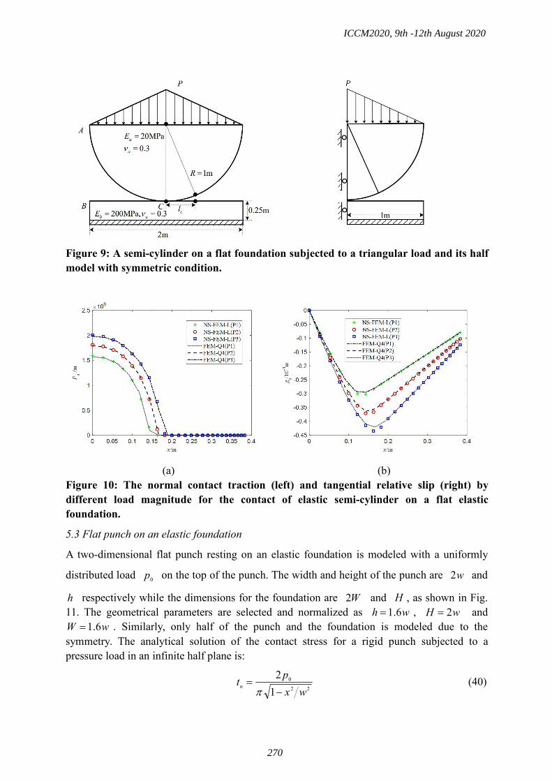
Figure 9: A semi-cylinder on a flat foundation subjected to a triangular load and its halfmodel with symmetric condition.

(a) (b)Figure 10: The normal contact traction (left) and tangential relative slip (right) bydifferent load magnitude for the contact of elastic semi-cylinder on a flat elasticfoundation.

5.3 Flat punch on an elastic foundation

A two-dimensional flat punch resting on an elastic foundation is modeled with a uniformly

distributed load 0p on the top of the punch. The width and height of the punch are w2 and

h respectively while the dimensions for the foundation are W2 and H , as shown in Fig.11. The geometrical parameters are selected and normalized as wh 6.1 , wH 2 and

wW 6.1 . Similarly, only half of the punch and the foundation is modeled due to thesymmetry. The analytical solution of the contact stress for a rigid punch subjected to apressure load in an infinite half plane is:

22

0

12

wxptn

(40)


270

Figure 11: A flat punch on an elastic foundation subjected to a uniform load.

Fig. 12 shows the normal and tangential contact traction on the contact interface calculatedwith different frictional coefficients: 0.1, 0.15, 0.2 and 0.25. They increase significantly whenapproaching the right end because of singularity. Then the effect of the tangential adhesion isconsidered on the same mesh. Fig. 13 presents the normal and tangential traction with thetangential adhesion from 1MPa.0 to MPa52.0 . Compared with those with differentfrictional coefficients, these solutions are more stable near the right end. All these figuresdemonstrate the accuracy of the NS-FEM-L which agrees well with the reference values.

(a) (b)Figure 12: The normal (a) and tangential (b) contact traction for the flat punch on theelastic foundation with different frictional coefficients.


271

(a) (b)Figure 13: The normal (a) and tangential (b) contact traction for the flat punch on the

elastic foundation with different tangential adhesion.

Next we investigate the effect of the ratio of Young’s modulus of the punch ( pE ) and the

foundation ( fE ) fp EEk . Using the model as shown in Fig. 11 with coefficients of

friction and adhesion equal to zero. Both the punch and the foundation are homogeneousmaterials and the ratio of k between them are selected as 0.01, 1/3, 1, 3 and 100,

respectively. The other parameters are selected as MPa10fE , the Poisson's ratio

3.0 pf and the uniform load MPa10 p . Fig. 14 (a) shows the normal contact traction

on the contact interface with different ratio. We find that: (1) the stiffer is the punch(such as100k ), the smaller is the normal contact traction at the region away from the right end; (2)

Because of the singularity, when the punch become stiffer, the normal contact traction at theright corner point increases significantly; (3) When the punch is much softer, such as

01.0 , the normal contact traction is approaching the value of 0p .

(a) (b)Figure 14: Normal contact traction with different ratio of Young's modulus (a) andr (b) for flat punch on an elastic foundation.


272

To investigate the effect of the functionally graded materials on the normal contact tractionbetween the punch and the foundation, we assume the Young's modulus of the foundation as:

,)()( 00 WxEEExE Rf (41)

where 0E and RE denote respectively the Young's modulus at the middle and the right of

the foundation. The ratio of the Young's modulus at the punch and the middle of the

foundation is chosen as 1000 EEk p . Other parameters are 3.0 pf , MPa10 p

and MPa100 E . The ratio of the Young's modulus between the right and middle of the

foundation is 0EEr R , whose value is taken as 1, 2, 5 and 10 in the computation. Fig. 14(b)

shows the variation of the normal contact traction on the contact interface with different ratior . We can observed that when r increases, the normal contact traction in the centerdecreases while the values at the right end augmented greatly. This is due to the singularity atthe right end corner. It demonstrated that when the Young's modulus gradually decreases fromthe center of the foundation to its right end, the singularity at the right end reduces.Meanwhile the toughness of the elastic foundation maintains.

6 Conclusion

In this paper, the node-based smoothed finite element method with linear strain field(NS-FEM-L) is presented and applied for contact analysis incorporating with a formulation oflinear complimentarity problems. The smoothed strains in smoothing domains are constructedby a complete order of polynomial functions instead of using the gradient smoothingtechnique which produce a constant strain. Unknown parameters are determined based on theequivalence of compatible strains and smoothed strains for the same region in an integralsense. Three contact models are investigated with the modified Coulomb friction. The effectof the tangential adhesion and the friction coefficient are considered. Numerical results showand compare solutions of the normal and tangential contact traction as well as the tangentialslip. The NS-FEM-L can well simulate the contact/departing, adhesion/debonding andsticking/slipping. And all the solutions are in good agreement with reference values as well asthose produced by FEM-Q4.

Acknowledgement

We gratefully acknowledge the financial support of the Fundamental Research Funds for theCentral Universities (Grant No.2682019CX42), the National Natural Science Foundation ofChina (Grant No.11772274), the National Youth Science Foundation of China (GrantNo.11901423) and the Youth Science and Technology Research Foundation of ShanxiProvince (Grant No.201901D211104).

References

[1] Johnson, K. L., & Johnson, K. L. (1987). Contact mechanics. Cambridge university press.[2] Wriggers, P., & Zavarise, G. (2004). Computational contact mechanics. Encyclopedia of computational

mechanics.


273

[3] Papadopoulos, P., & Solberg, J. M. (1998). A Lagrange multiplier method for the finite element solution offrictionless contact problems. Mathematical and computer modelling, 28(4-8), 373-384.

[4] Hild, P., & Renard, Y. (2010). A stabilized Lagrange multiplier method for the finite element approximationof contact problems in elastostatics. Numerische Mathematik, 115(1), 101-129.

[5] Oden, J. T., & Pires, E. B. (1984). Algorithms and numerical results for finite element approximations ofcontact problems with non-classical friction laws. Computers & Structures, 19(1-2), 137-147.

[6] Eck, C., Steinbach, O., & Wendland, W. L. (1999). A symmetric boundary element method for contactproblems with friction. Mathematics and Computers in Simulation, 50(1-4), 43-61.

[7] Li, Y., Liu, G. R., Dai, K. Y., Luan, M. T., Zhong, Z. H., Li, G. Y., & Han, X. (2007). Contact analysis forsolids based on linearly conforming radial point interpolation method. Computational Mechanics, 39(4),537.

[8] Rabczuk, T., & Belytschko, T. (2007). A three-dimensional large deformation meshfree method for arbitraryevolving cracks. Computer methods in applied mechanics and engineering, 196(29-30), 2777-2799.

[9] Liu, G. R., & Trung, N. (2016). Smoothed finite element methods. CRC press.[10] Liu, G. R. (2008). A generalized gradient smoothing technique and the smoothed bilinear form for Galerkin

formulation of a wide class of computational methods. International Journal of ComputationalMethods, 5(02), 199-236.

[11] Liu, G. R., Zhang, J., Lam, K. Y., Li, H., Xu, G., Zhong, Z. H., ... & Han, X. (2008). A gradient smoothingmethod (GSM) with directional correction for solid mechanics problems. Computational Mechanics, 41(3),457-472.

[12] Li, Y., Li, M., & Liu, G. R. (2014). A modified triangulation algorithm tailored for the smoothed finiteelement method (S-FEM). International Journal of computational methods, 11(01), 1350069.

[13] Li, Y., Yue, J. H., Niu, R. P., & Liu, G. R. (2016). Automatic mesh generation for 3D smoothed finiteelement method (S-FEM) based on the weaken-weak formulation. Advances in Engineering Software, 99,111-120.

[14] Dai, K. Y., & Liu, G. R. (2007). Free and forced vibration analysis using the smoothed finite elementmethod (SFEM). Journal of Sound and Vibration, 301(3-5), 803-820.

[15] Liu, G. R., Nguyen-Thoi, T., Nguyen-Xuan, H., & Lam, K. Y. (2009). A node-based smoothed finite elementmethod (NS-FEM) for upper bound solutions to solid mechanics problems. Computers & structures, 87(1-2),14-26.

[16] Zhang, Z. Q., & Liu, G. R. (2010). Temporal stabilization of the node-based smoothed finite elementmethod and solution bound of linear elastostatics and vibration problems. Computational Mechanics, 46(2),229-246.

[17] Liu, G. R. (2018). A novel pick-out theory and technique for constructing the smoothed derivatives offunctions for numerical methods. International Journal of Computational Methods, 15(03), 1850070.

[18] Li, Y., & Liu, G. R. (2019). A novel node-based smoothed finite element method with linear strain fields forstatic, free and forced vibration analyses of solids. Applied Mathematics and Computation, 352, 30-58.

[19] Bertsekas, D. P. (2014). Constrained optimization and Lagrange multiplier methods. Academic press.[20] Carpenter, N. J., Taylor, R. L., & Katona, M. G. (1991). Lagrange constraints for transient finite element

surface contact. International journal for numerical methods in engineering, 32(1), 103-128.[21] Weyler, R., Oliver, J., Sain, T., & Cante, J. C. (2012). On the contact domain method: A comparison of

penalty and Lagrange multiplier implementations. Computer methods in applied mechanics andengineering, 205, 68-82.

[22] Heegaard, J. H., & Curnier, A. (1993). An augmented Lagrangian method for discrete large‐slip contactproblems. International Journal for Numerical Methods in Engineering, 36(4), 569-593.

[23] Mijar, A. R., & Arora, J. S. (2004). An augmented Lagrangian optimization method for contact analysisproblems, 1: formulation and algorithm. Structural and Multidisciplinary Optimization, 28(2-3), 99-112.

[24] Conry, T. F., & Seireg, A. (1971). A mathematical programming method for design of elastic bodies incontact.

[25] Hung, N. D., & De Saxcé, G. (1980). Frictionless contact of elastic bodies by finite element method andmathematical programming technique. Computers & Structures, 11(1-2), 55-67.

[26] Meingast, M. B., Legrand, M., & Pierre, C. (2014). A linear complementarity problem formulation forperiodic solutions to unilateral contact problems. International Journal of Non-Linear Mechanics, 66, 18-27.

[27] Gholami, F., Nasri, M., Kövecses, J., & Teichmann, M. (2016). A linear complementarity formulation forcontact problems with regularized friction. Mechanism and Machine Theory, 105, 568-582.

[28] Lötstedt, P. (1982). Mechanical systems of rigid bodies subject to unilateral constraints. SIAM Journal onApplied Mathematics, 42(2), 281-296.

[29] Bhatti, M. A. (2012). Practical Optimization Methods: With Mathematica® Applications. Springer Science& Business Media.

[30] Liggett, J. A. (1988). Exact formulae for areas, volumes and moments of polygons andpolyhedra. Communications in Applied Numerical Methods, 4(6), 815-820.

[31] Cottle, R. W., Pang, J. S., & Stone, R. E. (2009). The linear complementarity problem. Society for Industrialand Applied Mathematics.


274

Boundary element of B-spline wavelet on the interval

*Qi Wei¹, †Jiawei Xiang¹1College of Mechanical and Electrical Engineering, Wenzhou University, China


AbstractIn this paper, a novel boundary element method (BEM) is proposed, which is based on thescaling functions of B-spline wavelet on the interval (BSWI). The conventional interpolationfunctions are replaced by scaling function to develop the basic functions and BSWI elements.Different from other wavelet methods is that we are supposed to transform the coefficientmatrix from wavelet space to physical space through a transformation matrix, which is anextremely necessary tool to allocate nodes with freedom, but there is an additional conditionthat we have to guarantee its non-singularity. At last, the numerical example verifies thatcomparing with traditional boundary element method, the BSWI elements have a desirableperformance, such as higher precision and fewer elements. Furthermore, it effectivelyenriches the wavelet-based boundary element method library.Keywords: B-spline wavelet; Wavelet boundary elements; Transformation matrix;Scaling function; Integral equation

Introduction

Inspired by the finite element method, boundary element method was developed as anaccurate and efficient numerical analysis method in engineering domain. By means of itsadvantages of reducing dimension, high precision, and handling infinite fields easily, it isargued by many researches. Basu considered that boundary element method and FEM havesuccessfully taken over the finite difference method and Ritz type method [1]. However, thebeginning of BEM is so late than FEM that many aspects are not mature, it is very necessaryto solve various problems of BEM. Due to many basis functions for structural analysis and thesuperiority of multiresolution properties, the wavelet numerical methods play an importantrole in engineering fields, which by using the scaling or wavelet functions to defineinterpolating functions [2], furthermore, the wavelet scale could be altered freely to meetspecific requirements and improve calculated accuracy. Recently, the adaptive wavelet BEMwas used to deal with boundary integral equations and getting excellent fruits [3].1D and 2D wavelet-based elements have been constructed and employed to beam-bendingand plate-bending problems, respectively [4][5]. But Daubechies wavelets have a bigdrawback which is lacking a specific expression, which may cause some traditional integralmethods are not provide ideal accuracy [6]. Therefore, to compute link coefficients is critical,but the variant Jacobians may bring about many limitations, the paper [7] has a detailedintroduction. It is worth noting that B-spline wavelets have specific expressions and betterfitting characteristic. However, Owing to the original B-spline wavelets are defined on thewhole square integrable real space )(2 RL , employing it as interpolating functions would leadto the data unstable [8]. For the purpose of breaking this limitation, Quak and Chui developedBSWI elements and proposed the reconstruction algorithm and fast decomposition, and hadbeen used to handle the first-kind integral equations [9][10]. However, the construction of B-


275


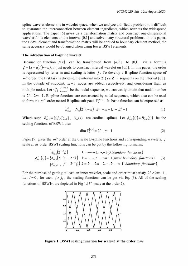
spline wavelet element is in wavelet space, when we analyze a difficult problem, it is difficultto guarantee the interconnection between element ingredients, which restricts the widespreadapplications. The paper [6] gives us a transformation matrix and construct one-dimensionalwavelet finite elements on the interval [0,1] and solve many structural problems. In this paper,the BSWI element and transformation matrix will be applied to boundary element method, thesame accuracy would be obtained when using fewer BSWI elements.

The introduction of B-spline wavelet

Because of function xf can be transformed from ],[ ba to ]1,0[ via a formula abax / , it just needs to construct interval wavelet on ]1,0[ . In this paper, the order

is represented by letter m and scaling is letter j . To develop a B-spline function space ofthm order, the first task is dividing the interval into )(2 Zjj segments on the interval ]1,0[ .

In the outside of endpoint, 1m nodes are added, respectively, and considering them as

multiple nodes. Let 121

mmk

jk

j

be the nodal sequence, we can easily obtain that nodal numberis 122 mj . B-spline functions are constructed by nodal sequence, which also can be usedto form the thm order nested B-spline subspace ]1 ,0[

jV . Its basic function can be expressed as

12,12, jjm

jkm mkkxNB ， (1)

Where supp ],[,jkm

jk

jkmB , )(xNm are cardinal splines. Let j

kmjkm B ,, be the

scaling functions of BSWI, then 12dim 1,0 mV jj (2)

Paper [9] gives the thm order at the 0 scale B-spline functions and corresponding wavelets, jscale at m order BSWI scaling functions can be got by the following formulas:

functionsboundarymmkfunctionsboundaryinnermkk

functionsboundarymk

jjljlkmm

jlljlm

ljlkm

jkm

j 12,,22221122,,022

01,,12

2,

0,

,

,

(3)

For the purpose of getting at least an inner wavelet, scale and order must satisfy 122 mj .Let 0l , for each 0jj , the scaling functions can be got via Eq. (3). All of the scalingfunctions of BSWI23 are depicted in Fig 1.( th3 scale at the order 2).

Figure 1. BSWI scaling function for scale=3 at the order m=2


276

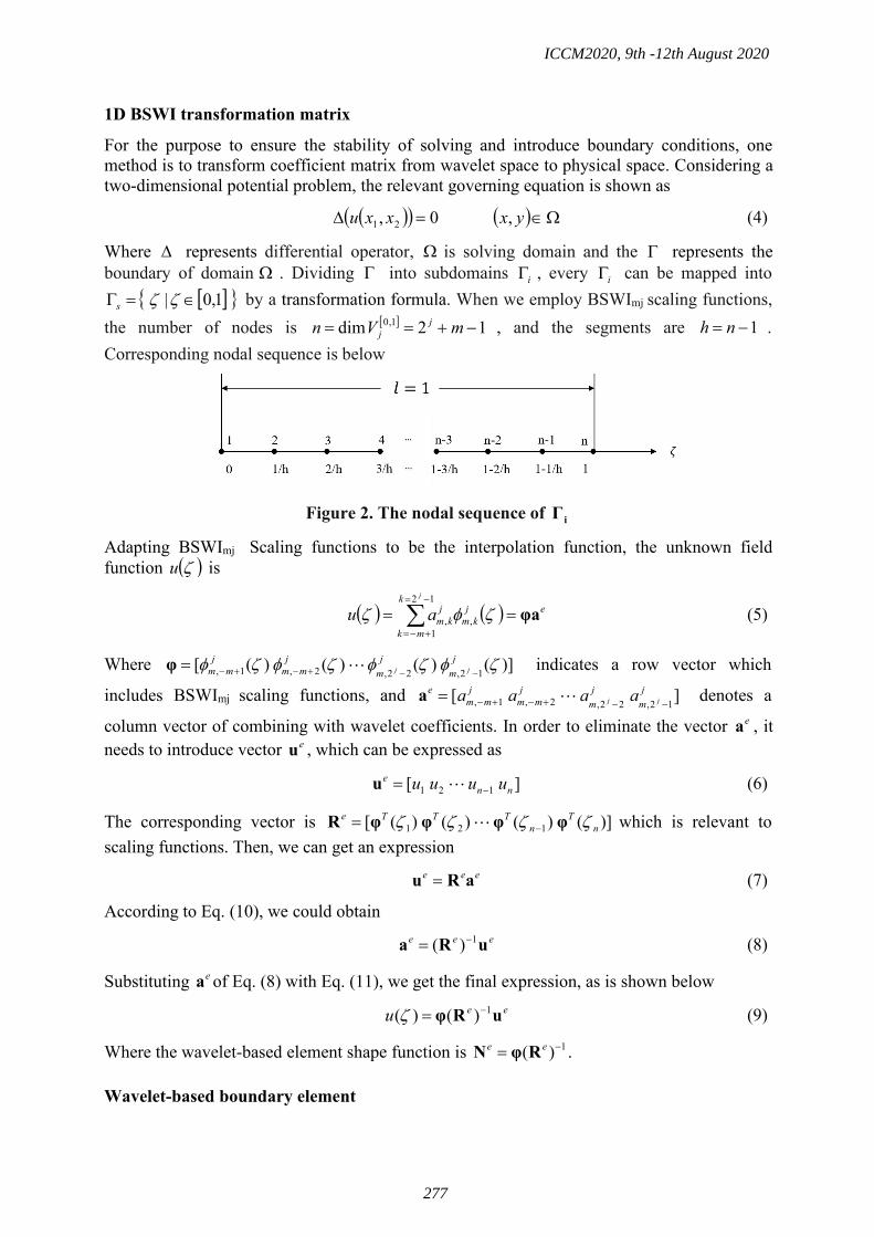
1D BSWI transformation matrix

For the purpose to ensure the stability of solving and introduce boundary conditions, onemethod is to transform coefficient matrix from wavelet space to physical space. Considering atwo-dimensional potential problem, the relevant governing equation is shown as

yxxxu ,0, 21 (4)

Where represents differential operator, is solving domain and the represents theboundary of domain . Dividing into subdomains i , every i can be mapped into

1,0| s by a transformation formula. When we employ BSWImj scaling functions,the number of nodes is 12dim 1,0 mVn j

j , and the segments are 1 nh .Corresponding nodal sequence is below

Figure 2. The nodal sequence of iΓ

Adapting BSWImj Scaling functions to be the interpolation function, the unknown fieldfunction u is

ejkm

k

mk

jkm

j

au φa

,

12

1, (5)

Where )]()()()([ 12,22,2,1, jm

jm

jmm

jmm jj φ indicates a row vector which

includes BSWImj scaling functions, and ][ 12,22,2,1,jm

jm

jmm

jmm

ejj aaaa a denotes a

column vector of combining with wavelet coefficients. In order to eliminate the vector ea , itneeds to introduce vector eu , which can be expressed as

][ 121 nne uuuu u (6)

The corresponding vector is )]()()()([ 121 nT

nTTTe φφφφR which is relevant to

scaling functions. Then, we can get an expressioneee aRu (7)

According to Eq. (10), we could obtaineee uRa 1)( (8)

Substituting ea of Eq. (8) with Eq. (11), we get the final expression, as is shown beloweeu uRφ 1)()( (9)

Where the wavelet-based element shape function is 1)( ee RφN .

Wavelet-based boundary element


277

The relevant governing equation was shown in Eq. (4) and boundary conditions are shown inEq. (10)

221121 ),(),(

xxqnuqxxuu (10)

Where u and q indicate the known value of the potential on the boundaries 1 and thepotential gradient on the boundaries 2 , respectively, n is the outward unit normal directionvector of the boundary. The fundamental solution of 2D potential problems is

ru 1ln

21

(11)

Where QPr xx . According to Gauss formula and Green’s function and let the sourcepoint locate on the boundary, the boundary integral equation can been given as

)()(

),()()()(),()( '

'

'''

'

'''' Qd

QnQPuQu

QnQuQPuPcu

(12)

Where 'P and 'Q represent the source and field points on the boundary, respectively,

2

c , denotes the angle between tangents of 'P on . After discretizing the boundary

, )( 'Qu and )( 'Qq (the value of)()(

'

'

QnQu

)of each element can be interpolated by BSWI

scaling functions, that iseeeeu uNuRφ 1)()( (13)eeeeq qNqRφ 1)()( (14)

Where ][ 121 nne uuuu u , )]()()()([ 121 n

Tn

TTTe φφφφR

][ 121 nne qqqq q , )]()()()([ 12,22,2,1, j

mjm

jmm

jmm jj φ

From now on, we can deal with the other processes easily, which is same to the conventionalboundary element method. It is necessary to say that singular integrals can be handled withtraditional methods.

Numerical example

In this section, we take an example of temperature field. The solving domain and boundaryconditions are shown in Fig.3, where a=10, b=20. Analytical solutions are 2/22 yxu .For comparison, we also adapt the traditional 3-node quadratic element, and define an errorformula ( merror mi

i ii /)(1

Uu ) between calculated and actual solutions where m

represents the number of interior points in the domain, U denote the actual solutions and uare the calculated results. Four-point Gaussian integral and Logarithmic integral are used inthe whole processes.Table 1 demonstrates the results of BSWI23 (8 elements), BSWI22 (14 elements) andtraditional 3-node quadratic element (24 elements), all of them are close to actual values.Compared with traditional method, the numerical example fully verifies that BSWI elementshave a better computational precision with few elements.


278

Table 1. The results of different elements

Coordinate x Temperature

(y=0) Actual 3-node BSWI22 BSWI23

11.5 -132.25 -132.18 -131.99 -132.06

13 -169.00 -168.91 -168.63 -168.74

15 -225.00 -224.82 -224.47 -224.64

17 -289.00 -288.59 -288.31 -288.53

18.5 -342.25 -343.72 -341.37 -341.68

Error 0 0.4405 0.5492 0.3717

Conclusions

In this paper, the 1D BSWI elements are applied to the boundary element method. Thenumerical example testifies its good performance, such as higher precision and efficiency,few elements. Especially when we ensure that the transformation matrix is not singular, thenode could be allocated freely as needed. Therefore, BSWI elements are an efficient tool thatcan be employed to boundary element method.

ACKNOWLEDGEMENT

This work was supported by the National Natural Science Foundation of China (Nos. U1909217, U1709208).

References

[1] Basu, P. K., Jorge, A. B., Badri, S. and Lin, J. (2003) Higher-order modeling of continua by finite-element,boundary-element, Meshless, and wavelet methods. Computers and Mathematics with Applications 46, 15–33.

[2] Dahmen, W. (2001) Wavelet methods for PDEs — some recent developments. Journal of Computationaland Applied Mathematics 128, 133-185.

[3] Dahlke, S., Harbrecht, H., Utzinger, M. and Weimar, M. (2018) Adaptive Wavelet BEM for BoundaryIntegral Equations: Theory and Numerical Experiments. Numerical Functional Analysis and Optimization,208-232.

[4] Ma, J. X., Xue, J. J., Yang, S. J. and He, Z. J. (2004) A study of the construction and application of aDaubechies wavelet-based beam element. Finite Elements in Analysis & Design 39, 965-975.

[5] Chen, X. F., Yang, S. J., Ma, J. X. and He, Z. J. (2004) The construction of wavelet of wavelet finite elementand its application. Finite Elements in Analysis & Design 40, 541-554.

[6] Xiang, J. W., Chen, X. F., He, Z. J. and Dong, H. B. (2007) The construction of 1D wavelet finite elementsfor structural analysis. Computational Mechanics 40, 325-339.

[7] Wu, C. W., Chen, W. H. (1996) Extensive of spline wavelets element method to membrane vibrationanalysis. Computational Mechanics 18, 46-54.

[8] Xiang, J. W., Chen, X. F., He, Y. M. and He, Z. J. (2006) The construction of plane elastomechanics andMindin plate elements of B-spline wavelet on the interval. Finite Elements in Analysis & Design 42, 1269-1280.

[9] Goswami, J. C., Chan, A. K. and Chui, C. K. (1995) On solving first-kind integral equations using waveletson a bounded interval. IEEE Transactions on Antennas and Propagation 43, 614-622.

[10] Chui, C. K. and Quak, E. (1992) Wavelets on a bounded interval. Numerical Method Approximate Theory 1,53-57.

Figure 3. Boundary conditionsand solving domain


279

https://link.springer.com/journal/466

https://ieeexplore.ieee.org/xpl/RecentIssue.jsp?punumber=8

A global sensitivity analysis method for multi-input multi-output system

†Qiming Liu¹

,2, *Nichen Tong

1,2, and †Xu Han¹

,2

1 State Key Laboratory of Reliability and Intelligence of Electrical Equipment, School of Electrical Engineering,

Hebei University of Technology, Tianjin 300401, P. R. China 2 School of Mechanical Engineering, Hebei University of Technology, Tianjin 300401, P. R. China

*Presenting author: [email protected].

†Corresponding author: [email protected], [email protected]

Abstract

Commonly, variance-based global sensitivity analysis methods are popular and applicable to quantify the impact of a set of input variables on output response. However, for many engineering practical problems, the output response is not single but multiple, which makes some traditional sensitivity analysis methods difficult or unsuitable. Therefore, a novel global sensitivity analysis method is presented to evaluate the importance of multi-input variables to multi-output responses. First, assume that a multi-input multi-output system (MIMOS) includes n variables and m responses. A set of summatory functions G x and H x are constructed by the addition and subtraction of any two response functions. Naturally, each response function is represented using a set of summatory function. Subsequently, the summatory functions G x and H x are further decomposed based on the high dimensional model representation (HDMR), respectively. Due to the orthogonality of all the decomposed function sub-terms, the variance and covariance of each response function can be represented using the partial variances of all the decomposed function sub-terms on the corresponding summatory functions, respectively. The total fluctuation of MIMOS is calculated by the sum of the variances and covariances on all the response functions. Further, the fluctuation is represented as the sum of the total partial variances for all the s-order function sub-terms and the total partial variance is the sum of n partial variances for the corresponding s-order function sub-terms. Then, the function sensitivity index (FSI) sFSI for s-order function sub-terms is defined by the ratio of the total partial variance and total fluctuation, which includes first-order, second-order, and high-order FSI. The variable sensitivity index (VSI) iVSI of variable ix is calculated by the sum of all the FSIs including the contribution of variable ix . Finally, numerical example and engineering application are employed to demonstrated the accuracy and practicality of the presented global sensitivity analysis method for multi-input and multi-output system.

Keywords: Global sensitivity analysis (GSA), High dimensional model representation

(HDMR), Variance and covariance decomposition, multi-input multi-output system (MIMOS)

1 Introduction

Sensitivity analysis (SA) is an effective tool for quantifying the influence of input variables to

output response and can identify the influential variables and help designers clearly recognize

what should be of great concern [1, 2]. It has been widely used in many engineering practical

problems, such as structural design [3, 4], parameter identification [5]. In order to solve

different types of engineering problems, researches on sensitivity analysis methods have been

continuously promoted. Generally, SA is classified into two categories: local sensitivity

analysis (LSA) and global sensitivity analysis (GSA). LSA methods are usually used to

evaluate the local effect on output response when the small perturbation occurs on the

nominal value of input variable. The main disadvantages of LSA are that it does not account


280


for interactions between parameters. GSA as a general and comprehensive approach takes into

account all the variation range of the parameters in entire range space. It aims at determining

which input variables have more important influence on the output response and shows the

ranking of influential variables [6, 7]. The frequently-used GSA methods include regression

methods, screening-based methods, variance-based methods, and meta-model methods, and so

on [7, 8]. Although Sobol’ method based on variance decomposition is more popular among

these GSA methods, its interactions cannot be further decomposed, which makes the ranking

of influential variables highly likely to be wrong, especially strong non-linear system [7-10].

To further decompose the effects of interactions, Liu et al. [7] improved the Sobol’ method by

the combination of variance decomposition and partial derivation integral. However, these

GSA methods that are only effective for a multi-input single output system (MISOS) are not

suitable for a multi-input multi-output system (MIMOS).

Recently, it has attracted wide attention in terms of SA to MIMOS. Scholars have done some

work. Gamboa et al. [11] defined a generalization of Sobol sensitivity indices based on the

trace of covariance matrix for multi-output system. Cheng et al [12] developed a multivariate

output GSA method by employing multi-output support vector regression (M-SVR). Xu et al.

[13] proposed a mapping-based hierarchical sensitivity analysis method to calculate

sensitivity indices of multilevel systems with multidimensional correlations. Nevertheless,

these multivariate output GSA methods are used to assess the effects of multi-inputs to multi-

outputs only considering the contribution of variances but ignoring the contribution of

covariances. Hence, this paper presents a novel GSA method for MIMOS comprehensively

considering the influence of variance and covariance.

2 Global Sensitivity Analysis Method for Multi-inputs Multi-outputs ICCM 2020

2.1 Variance Decomposition

Consider a square-integrable-function xf defined in the unit hypercube

| 0 1, 1,2 ,n

iR x i n x ， . The performance function decomposition can be given as:

0 12 1 2

1 1

, , , ,n

i i ij i j n n

i i j n

f f f x f x x f x x x

x (1)

If the integral with respect to its own variable is zero for any function term of HDMR, namely

1 2 1 2

1

1 2 1 20

, , , d 0, , , , ,1s si i i i i i k s sf x x x x k i i i i i i n (2)

The Sobol’ function sub-terms can be uniquely determined as follows:

0 df f x x (3)

0 di i k

k i

f x f f x

x (4)

0

,

, dij i j i i j j k

k i j

f x x f f x f x f x

x (5)

Any two different Sobol’ functions satisfy the orthogonal condition as follows,

1 2 1 2 1 2 1 2

1

0, , , , , , d 0.

s s s si i i i i i j j j j j jf x x x f x x x x (6)

The variance decomposition can be given by integrating 2f x ,

12

1 1

n

i ij n

i i j n

D D D D

(7)

The sensitivity index and total sensitivity index is calculated respectively

1

1 1 21 1 .s

s

i i tot

i i i i s

DS S S i i i n

D ，， (8)


281

2.2 Multivariate Output Sensitivity Indices

For a multi-inputs multi-outputs system, its output responses can be represented as follows,

1 2 1 2[ , , , ] [ , , , ].m my y y f f f y x x x (9)

First, a set of summatory function is constructed using any two output responses as follows,

,

,,1 , .

k l k l

k l k l

G f fk l m

H f f

x x x

x x x (10)

According to the high dimensional model representation in Eq. (1), the Eq. (9) can be

rewritten by

, , , , ,

0 12 1 2

1 1

, , , , ,

0 12 1 2

1 1

, , , ,

.

, , , ,

n nk l k l k l k l k l

i i ij i j n n

i i j n


i i ij i j n n

i i j n

G G G x G x x G x x x

H H H x H x x H x x x

x

x

(11)

The function sub-terms of Eq. (10) can be calculated referring to the Eqs. (3)~(5). According

to Eq. (9), its response functions can be respectively represented by ,k lG x and ,k lH x as

follows,

, , , ,

0 00

, , , ,

0 00

2 2and .

22

k l k l k l k lk k

k l k l k l k lll

G H G Hf f

G H G Hff

x xx

x xx

(12)

The sum of the variances of kf x and lf x can be calculated by

, ,1Va +Va = Va Va

2

k l k l k lf f G H

x x x x (13)

where Va is a variance operator. In Eq. (12), ,Va k lG x and ,Va k lH x can be

represented by

, , , , ,

0 12 1 2

1 1

, , , ,

0 12

1 1

, , , , ,

0 12 1 2

1 1

Va =Va , , , ,

Va =Va , , , ,


i i ij i j n n

i i j n

n nk l k l k l k l

i ij n

i i j n


i i ij i j n n

i i j n

G G G x G x x G x x x

DG DG DG DG

H H H x H x x H x x x

x

x

, , , ,

0 12

1 1

n nk l k l k l k l

i ij n

i i j n

DH DH DH DH

(14)

The covariances of kf x and lf x can also be calculated as follows,

, ,1Cov , = Va Va

4

k l k l k lf f G H

x x x x (15)

where Cov is a covariance operator.

The total fluctuation of kf x and lf x can be calculated by the sum of variances and

covariance, namely

, =Va +Va Cov ,k l k l k lTF f f f fx x x x (16)


282

Substituting Eqs. (12)~(14) into Eq. (15), it can obtain the total fluctuation as follows,

, , , , ,

0 0

1

, ,

1

, ,

12 1 2 12 1 2

, , ,

0

1 1

3 1 3 1= D D D D

4 4 4 4

3 1D , D ,

4 4

3 1D , , , D , , ,

4 4

nk l k l k l k l k l

i i i i

i

nk l k l

ij i j ij i j

i j n

k l k l

n n n n

n nk l k l k l

i ij

i i j n

TF G H G x H x

G x x H x x

G x x x H x x x

TD TD TD TD

,

12

k l

n

(17)

where

, , ,

0 0 0

, , ,

, , ,

, , ,

12 12 1 2 12 1 2

3 1Va Va

4 4

3 1Va Va

4 4

3 1Va , Va ,

4 4

3 1Va , , , Va , , ,

4 4

k l k l k l

k l k l k l

i i i i i

k l k l k l

ij ij i j ij i j

k l k l k l

n n n n n

TD G H

TD G x H x

TD G x x H x x

TD G x x x H x x x

(18)

For a MIMOS with n input variables and m output responses, a more general decomposition

can be given as follows,

1,2, , 1,2, , 1,2, , 1,2, , 1,2, ,

0 0

1

1,2, , 1,2, ,

1

1,2, , 1,2, ,

12 1 2 12 1 2

1

0

3 1 3 1= D D D D

4 4 4 4

3 1D , D ,

4 4

3 1D , , , D , , ,

4 4

nm m m m m

i i i i

i

nm m

ij i j ij i j

i j n

m m

n n n n

TF G H G x H x

G x x H x x

G x x x H x x x

TD

,2, , 1,2, , 1,2, , 1,2, , 1,2, ,

12 0

1 1

, where 0.n n

m m m m m

i ij n

i i j n

TD TD TD TD

(19)

The sensitivity index for each decomposed function sub-term can be defined by

1

1

1,2, ,

1 21,2, ,,1

TF

s

s

m

i i

i i sm

TDFS i i i n (20)

The sensitivity index of variable is given by

1tot

i iVS FS . (21)

3 Numerical Example and Engineering Application

To demonstrate the feasibility and practicability of the proposed GSA method, a numerical

example and an engineering application are considered.

3.1 Numerical Example

A set with two functions is constructed as follows,


283

1 2 2

1 2 1 2

2 2 2

1 2 1 2

, 0,1 .f x x x x

f x x x x

xx

x (22)

According to the variance decomposition, the partial variance matrix of 1f x and 2f x is

0.154,0.189,0.007

0.022,0.154,0.007

. According to the covariance decomposition, the partial covariance

vector of 1f x and 2f x is 0.053 0.169 0.007 ，， . The SA results based on the average

method and trace of covariance matrix are 0.311 0.720， and 0.358 0.670， , respectively.

Obviously, the results of these two methods ignore the influence of covariance. The SA

results using the proposed method is 0.577 0.442， , which is different from the results of the

average method and trace of covariance matrix due to taking into account the contribution of

covariance. The comparisons of SA results are provided, as shown in Fig. 1. The numerical

example demonstrates that the proposed method is more suitable for MIMOS than some

traditional methods.

0

0.1

0.2

0.3

0.4

0.5

0.6

0.7

0.8

Average values

Trace of covariance matrix

The proposed SA method

1x 2x

Fig.1 Comparison of SA results using different methods.

3.2 Engineering Application

Nowadays, vehicle lightweight and safety design becomes an increasingly critical issue. Liu

et al. [3] presented a composite B-pillar structure with ply drop-off to improve the

crashworthiness of side impact and roof crush. The finite element model of the ply drop-off

B-pillar consists of four parts, as shown in Fig. 2. The thickness of each part which depends

on the number of lay-up is regarded as design variable. The design objectives consist of roof

strength which stands for the maximum crushing force in roof crush, B-intrusion which stands

for the intrusion of B-pillar in side impact, and B-velocity which stands for the maximum

intrusion velocity of B-pillar in side impact. According to the samplings in Table 3 from Ref.

[3], the response surface models on roof strength, B-velocity, and B-intrusion can be

established as follows,


284

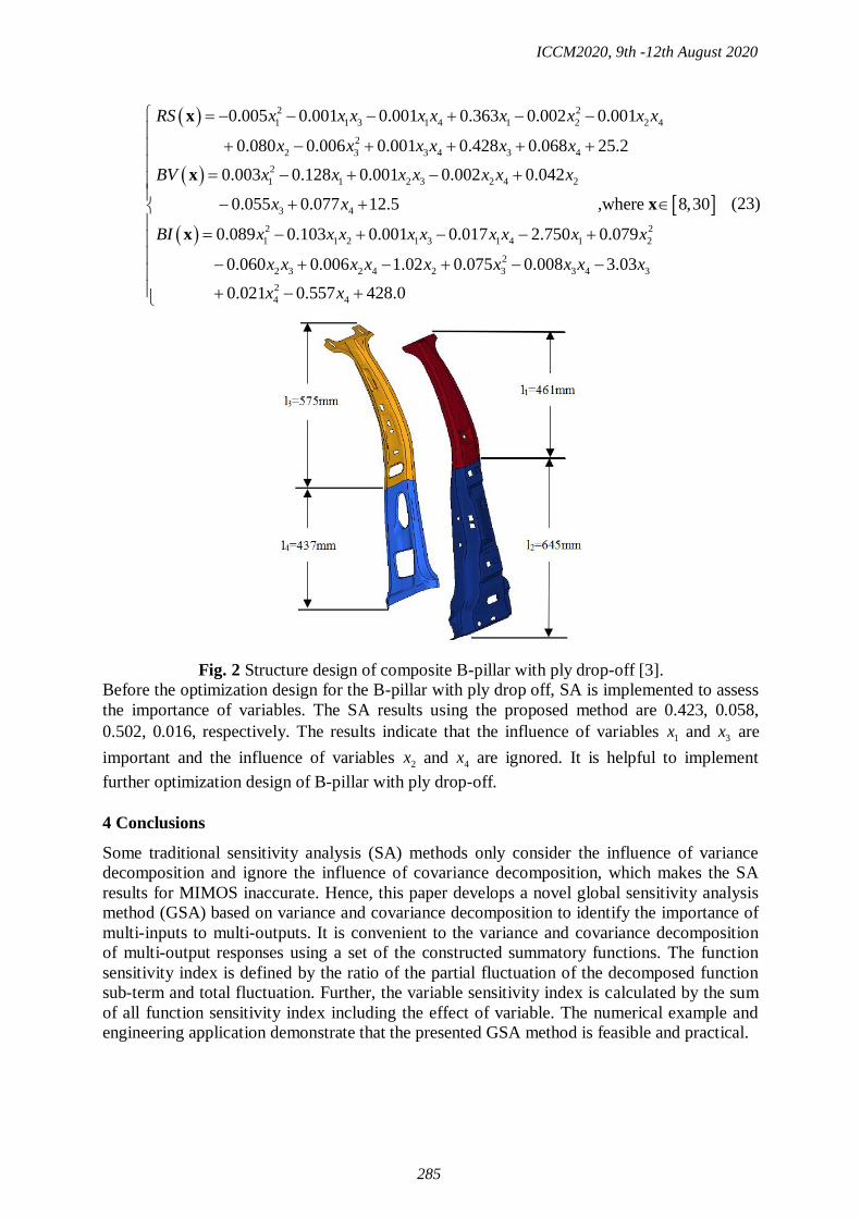
2 2

1 1 3 1 4 1 2 2 4

2

2 3 3 4 3 4

2

1 1 2 3 2 4 2

3 4

1

0.005 0.001 0.001 0.363 0.002 0.001

0.080 0.006 0.001 0.428 0.068 25.2

0.003 0.128 0.001 0.002 0.042

0.055 0.077 12.5 ,where 8,30

0.089

RS x x x x x x x x x

x x x x x x

BV x x x x x x x

x x

BI x

x

x

x

x2 2

1 2 1 3 1 4 1 2

2

2 3 2 4 2 3 3 4 3

2

4 4

0.103 0.001 0.017 2.750 0.079

0.060 0.006 1.02 0.075 0.008 3.03

0.021 0.557 428.0

x x x x x x x x

x x x x x x x x x

x x

(23)

Fig. 2 Structure design of composite B-pillar with ply drop-off [3].

Before the optimization design for the B-pillar with ply drop off, SA is implemented to assess

the importance of variables. The SA results using the proposed method are 0.423, 0.058,

0.502, 0.016, respectively. The results indicate that the influence of variables 1x and 3x are

important and the influence of variables 2x and 4x are ignored. It is helpful to implement

further optimization design of B-pillar with ply drop-off.

4 Conclusions

Some traditional sensitivity analysis (SA) methods only consider the influence of variance

decomposition and ignore the influence of covariance decomposition, which makes the SA

results for MIMOS inaccurate. Hence, this paper develops a novel global sensitivity analysis

method (GSA) based on variance and covariance decomposition to identify the importance of

multi-inputs to multi-outputs. It is convenient to the variance and covariance decomposition

of multi-output responses using a set of the constructed summatory functions. The function

sensitivity index is defined by the ratio of the partial fluctuation of the decomposed function

sub-term and total fluctuation. Further, the variable sensitivity index is calculated by the sum

of all function sensitivity index including the effect of variable. The numerical example and

engineering application demonstrate that the presented GSA method is feasible and practical.


285

Acknowledgment

This work is supported by the National Natural Science Foundation of China (Grant No.

11902110), the Natural Science Foundation of Hebei Province (Grant No. A2019202171), the

Project Funded by China Postdoctoral Science Foundation (Grant No. 2019M660963), the

High-level Talent Support Project of Hebei Province of China (Grant No. B2019003012),

Independent Research Project of State Key Laboratory of Reliability and Intelligence

Electrical Equipment, Hebei University of Technology (No. EERIPD2018002), the Open

Fund of State Key Laboratory of Advanced Design and Manufacturing for Vehicle Body

(Grant No. 31915004).

References

[1] Sudret B. Global sensitivity analysis using polynomial chaos expansions. Reliability Engineering & System Safety 2008; 93(7): 964-979.

[2] Blatman G, Sudret B. A comparison of three metamodel-based methods for global sensitivity analysis: GP modelling, HDMR and LAR-gPC. Procedia-Social and Behavioral Sciences 2010; 2(6): 7613-7614.

[3] Liu Q, Li Y, Cao L, et al. Structural design and global sensitivity analysis of the composite B-pillar with ply drop-off. Structural and Multidisciplinary Optimization, 2018, 57(3): 965-975.

[4] Liu Q, Wu X, Han X, et al. Sensitivity Analysis and Interval Multi-Objective Optimization for an Occupant Restraint System Considering Craniocerebral Injury. Journal of Mechanical Design, 2020, 142(2): 1-31.

[5] Liu Q, Liu J, Guan F, et al. Identification of the visco-hyperelastic properties of brain white matter based on the combination of inverse method and experiment. Medical & Biological Engineering & Computing, 2019, 57(5): 1109-1120.

[6] Chen W, Jin R, Sudjianto A, et al. Analytical Variance-Based Global Sensitivity Analysis in Simulation-Based Design Under Uncertainty. Journal of Mechanical Design, 2005, 127(5): 875-886.

[7] Liu J, Liu Q, Han X, et al. A new global sensitivity measure based on derivative-integral and variance decomposition and its application in structural crashworthiness. Structural and Multidisciplinary Optimization, 2019, 60(6): 2249-2264.

[8] Tian W. A review of sensitivity analysis methods in building energy analysis. Renewable & Sustainable Energy Reviews, 2013: 411-419.

[9] S. Arwade, M. Moradi, A. Louhghalam, Variance decomposition and global sensitivity for structural systems, Engineering Structures 32 (1) (2010) 1–10.

[10] IM. Sobol’, S. Kucherenko, Derivative based global sensitivity measures and their link with global sensitivity indices, Mathematics and Computers in Simulation 79 (10) (2009) 3009-3017.

[11] Gamboa F, Janon A, Klein T, et al. Sensitivity indices for multivariate outputs. Comptes Rendus Mathematique, 2013: 307-310.

[12] Cheng K, Lu Z, Zhang K, et al. Multivariate output global sensitivity analysis using multi-output support vector regression. Structural and Multidisciplinary Optimization, 2019, 59(6): 2177-2187.

[13] Xu C, Zhu P, et al. “Mapping-Based Hierarchical Sensitivity Analysis for Multilevel Systems with Multidimensional Correlation.” Journal of Mechanical Design, 2020, pp. 1–26.

[14] Sobol’ I M, Sensitivity estimates for nonlinear mathematical models, Mathematical Modeling and Computational Experiment 1993, 1: 407-414.


286

Contact analysis within the bi-potential framework using cell-based

smoothed finite element method

*Qianwei Chen1, †Yan Li1, Zhiqiang Feng1,2 and Huijian Chen1

1School of Mechanics and Engineering, Southwest Jiaotong University, Chengdu, China 2 LMEE Univ-Evry, Université Paris-Saclay, Evry, France



Abstract

This paper presents a cell-based smoothed finite element method (CS-FEM) for solving two-

dimensional contact problems with the bi-potential formulation. The contact force and the

relative displacement are coupled with each other and solved by Uzawa algorithm. Three

contact states are investigated accurately. The CS-FEM is performed with six different kinds

of smoothing domains which are constructed by dividing the background element into

different regions. Three numerical examples are presented to verify the accuracy of the

method. The effect of the friction coefficient for the contact are also investigated. All

solutions agree well with reference values. The results produced by the CS-FEM are more

accurate than those of the traditional FEM. Besides, the CS-FEM can provide both upper

bound and lower bound solutions for the strain energy while using different smoothing

domains.

Keywords: Contact analysis, CS-FEM, Bi-potential formulation, Uzawa algorithm

1. Introduction

The contact problems exist everywhere in life. For example, the contact between the tire and

the road, the contact between the shaft and the bearing, the contact between the knife and the

flesh in virtual surgery, etc. They play important roles in many engineering applications [1][2].

There are two reasons contributed to the non-linearity of the contact problems [3][4]. One is

that both the contact surfaces and their positions change during the contact process. The other

one is the non-linearity of contact conditions, including the non-penetration of contact bodies

and the tangential friction conditions. The widely used contact algorithms in engineering

applications are the penalty function method [5]-[8], the Lagrange multiplier method [9]-[12]

and the linear complementarity techniques [13]-[16]. The bi-potential method proposed by De

Saxcé and Feng provides an effective tool for dissipative constitutive modelling [17][18].

Applying the augmented Lagrangian method to the law of contact, the implicit equation of the

projection on the Coulomb’s cone is equivalent to the original contact inequality. There has

demonstrated that the Uzawa algorithm is more efficient when compared with the Newton

method [19]. There are many researches and applications in impact, hyperelasticity, wear and

other problems [20]-[23].

The finite element method (FEM) is one of the most effective numerical methods for solving

contact problems. Other widely used approaches include the boundary element methods

[24][25] and the meshless methods [26]-[28]. The smoothed finite element method (S-FEM)

proposed by Liu et al. is a weakened weak form method based on the G-space theory [29].

When using different kinds of smoothing domains which are based on cells, edges, nodes and

faces of the background elements, the cell-based smoothed finite element method (CS-FEM),


287

the edge-based smoothed finite element method, the node-based smoothed finite element

method and the face-based smoothed finite element method are created [30]-[33]. So far, the

S-FEM has been widely used in various fields, including the acoustics [34], materials science

[35], vibration [36], fluid-structure coupling [37], and electromagnetics [38]. The S-FEM has

also been applied to solve contact problems [16][26][39][40].

In this paper, the CS-FEM with quadrilateral elements is used to solve the two-dimensional

contact problems within the bi-potential framework. The contact forces can be solved using

the Uzawa algorithm. The rest of the paper is organized as follows: in Section 2, the

governing equations and the contact criterion are introduced. Section 3 illustrates the

smoothed finite element method, especially the CS-FEM. The smoothed Galerkin weak form

is obtained by using the smoothing strain technique. In Section 4, the contact analysis is

performed within the bi-potential framework. The Uzawa algorithm is applied to solve the

contact force. Finally, three numerical examples are presented to examine the numerical

accuracy of the proposed method.

2. Problem statement

2.1 Governing equations

Considering an elastic contact body with domain i and the force boundary condition i

f ,

the displacement boundary condition iu , the contact boundary condition i

c as shown in Fig.

1.

Figure 1. Contact body

The governing equation of this contact body is:

0Tf + = (1)

with

T

T

on

on

on

f

c

u

=

= =

t

r

u u

L

L

(2)

where is a differential operator which can be written for 2D problems as follows:

0

0

x

y

y x

= (3)


288

The stress T

xx yy xy = . The body force T

x yf f = f and displacements T

= x yu u u .

t , u and r are the loads, displacements and contact forces on the boundary, respectively. L

is the matrix of the unit normal vectors defined by:

0

0

x n

y n

y n x n

=

L . (4)

2.2 Contact criterion

The Signorini condition mainly describes a normal contact relationship. It has the following

three characteristics at each contact point, they are the geometric condition of non-penetration,

the static condition of non-adhesion and the mechanical complementary condition. Therefore,

the following formula expresses the relationship between the normal distance nx and normal

contact force nr for any contact point . The Signorini condition is defined as:

0

( , ) 0 0

n

n n

n n n

xSignor x r

r x r

=

(5)

In order to satisfy the tangential criterion of contact, the Coulomb friction rule is adopted and:

0

( , ) 0

t t n

t t tt t n

t

r

Coulr

=

= −

x r

x r xx r

x

(6)

where t

x and

t

r are the tangential components of the spacing vector and the contact force

vector for contact point α, respectively. is the friction coefficient.

Let K represents the Coulomb’s cone which is expressed as:

3 such that 0t nK r

= − r r (7)

The contact satisfies a complex non-smooth dissipative law including the separating, sticking

and sliding. By combining Eqs. (5) and (7), the contact criterion can be written as:

: 0 and r 0

: 0 and int( )

: 0 and bd( ) with

n n

t t

tt t t n

t

Separating x

Sticking K

Sliding K r

=

=

= −

x r

xx r r

x

(8)

where int( )K and bd( )K represent the interior and the boundary of Coulomb’s cone. Eq.

(8) is called the Signorini-Coulomb conditions.

3. Cell-based smoothed finite element method

3.1 Galerkin weak form

For problem domain , by introducing a weight function , Eq. (1) can be transformed into

an equivalent integral form:

T Τd d 0

+ = f (9)


289

Using Green’s divergence theorem, we can convert Eq. (9) to:

T T Td d d d 0f c

( − − − = C φ f t r) (10)

where C is the material matrix. The physical equation is =C , where ε is the vector of

strain. The weight function takes the variation of displacement as = u and the Galerkin

weak form can be got:

( ) ( ) ( )T T TT( ) d d d d 0

f c

δ δ δ δ

− − − = C u f u t u r (11)

where δ = u .

3.2 Smoothed Galerkin weak form

In S-FEM, the smoothed strain is calculated by the strain smoothing operation as:

( ) ( ) ( )ds

W

= − x x x x (12)

where s is the smoothing domain which can be created based on nodes, edges, cells of the

background elements. In this work the CS-FEM model is adopted with six different kinds of

smoothing regions as shown in Fig. 2. W is a smoothing function that should be positive over

the local support domain and satisfies the unity property ( )d 1s

W

− = x x .

Figure 2. Six different smoothing domains based on a quadrilateral element: 1SD, 2SDs,

3SDs, 4SDs, 8SDs, 16SDs

Here the Heaviside-type smoothing function is adopted:

1/

( )0

s

s

AW

− =

xx x

x (13)

where A is the area of the smoothing domain. Substituting Eq. (13) into Eq. (12) and using

the Green’s divergence theorem, the smoothed strain can be obtained:

( )d

1 ( ) d d

1 d

s

s s

s

W

WA

A

= −

= − − +

=

u x x

x x u Lu

Lu

(14)

where s is the boundary of the smoothing domain. Note that only boundary integration

instead of domain integral is required in this calculation.

By substituting Eq. (14) into Eq. (11), the following smoothed Galerkin weak form can be

obtained:


290

( ) ( ) ( )T T TT( d d d d 0

f c

δ δ δ δ

− − − = C u f u t u r) (15)

3.3 Discretized system of equations

Assume the displacement function as:

su(x) = N(x)d x (16)

where vector ( )N x and d represent the shape function and nodal displacements respectively.

Substituting Eq. (16) into Eq. (14), the smoothing strain can be written as:

1

dsA

= = Lu d (17)

where denotes the smoothed strain matrix which can be calculated as:

01

d 0 s

x

y s

y x

b

bA

b b

= =

LN(x) x (18)

with

,

1

1( ) ,

pN

G

h h p p p

p

b n l h x yA =

= = N x (19)

where pN represents the number of segments of the boundary s ,

,h pn and G

px are

respectively the outward unit normal and Gauss points on each segment, pl represents the

length of the p-th segment.

Substituting Eq. (16) and Eq. (17) into Eq. (15), we can get the discretized algebraic system of

equations:

T T T T

1 1 1 1 1

d d d 0e s e e e

e ef ec

N N N N N

s

e s e e e

A

= = = = =

− − − = B CBd N f N t N r (20)

where eN and sN represent the number of background elements and smoothing domains. e

represents background element. ef and ec represent the boundary of forces and contact

forces per element. For simplicity of description, we can use the following symbols:

T T

1 1

d de e

e ef

N N

ext

e e

= =

= + F N f N t (21)

T

1

de

ec

N

e

=

= R N r (22)

T

1 1

e sN N

int s

e s

A= =

=F B CBd (23)

where extF is the external forces. R is the contact forces. intF is the internal forces.

The Eq. (20) can be rewritten as:

ext +Kd = F R (24)

where K is stiffness matrix obtained by:

T

1 1

e sN N

s

e s

A= =

=K B CB (25)


291

Here Eq. (24) cannot be solved directly because both d and R are unknown quantities. In our

work we compute the contact force R on the contact surface first. Then the displacements d

can be solved by taking R as an external force.

4. The contact within the bi-potential framework

4.1 Contact kinematics

Considering two elastic bodies 1 and 2 coming into contact, as shown in Fig. 3. 1P is the

contact points on the boundary 1 . 2P is the normal projection point of the contact point 1P

on the boundary 2 . For 2D problems, we can set up a local coordinate system based on the

normal and tangential vector at point 1P . The initial gap g between 1P and 2P is determined

by a contact collision detector as shown in Fig. 3:

Figure 3. Contact kinematics

Assuming:

1 1 1 2 2 2(P ) (P )= =d d dΦ Φ d (26)

where 1d and 2d denotes respectively the nodal displacements in 1 and 2 . 1Φ and 2Φ are

integration matrix in corresponding regions. If we consider the case with cN contact points

1P ( )1 cN = on 1 , and 2P is the normal projection points of the contact points

1P on

2 . The relative position between 1P and

2P is:

2 1(P ) (P ) = −d d d (27)

In local coordinates it can be expressed as:

t nx x = +d t n (28)

where

T

T

t

n

x

x

= =

t dx

n d. (29)

Substituting Eq. (26) and Eq. (27) to Eq. (29), we get:

1

T T11 2

T T

21 2

2

d

d 0 0

d 0 0

d

x

yt

xn

y

x

x

− =

−

t ΦtΦ

n Φ Φn (30)

By defining the transformation matrix T as:

T

1 2 T

0

0

k

k

k

= − =

tT T

ΦT T

n

Φ (31)


292

Eq. (30) can be written as:

=x T d (32)

whose incremental form is:

( 1) ( )i i + = +x T d g (33)

where (0 ) g =g .

In the local reference coordinate system, the contact force r can be defined as:

t nr r = +r t n (34)

Applying the contact virtual work principle:

T T =r x R d (35)

We have:

T =R T r (36)

The whole system of equations of cN contact points can be written as:

T =

= +

R T r

x Td g (37)

with T

1 = T T T , T

1 Nc = x x x , T

1 Nc = r r r ,T

1 Nc = g g g .

4.2 The contact solution method

For a contact point, the bi-potential function of the contact law can be written as:

( , ) ( ) ( )c n K n tb x r

−

− = − + +x r r x (38)

where ( ,0− = − , and ( )K

r is the indicator function and it can be described as: if

K

r , ( ) 0K

=r ; otherwise ( )K

= +r .

The Eq. (38) can be further expressed as an implicit subnormal form:

( , )

( , )

( )

c

c

b

r

b

x

−−

−

−

x rx

x r r

(39)

So, using the augmented Lagrangian method [41], the Eq. (38) and Eq. (39) can be equivalent

to the following projection form on the Coulomb’s cone:

*Proj ( )K

=r r (40)

where *r represents the vector of augmented contact force, and it is given by:

* * * with t

= − = +r r x x x x n (41)

where is the bi-potential coefficient. In this work, the reciprocal of the maximum value of

the diagonal elements of the matrix D as given in Eq. (45) is selected.

By summarizing the above equations and Eq. (8), there will be three contact situations within

the bi-potential framework. They are * K

r (sticking), * *K

r (separating) and

* 2 *( )K K

−r (sliding), respectively, as shown in Fig. 4.


293

Figure 4. Coulomb cone and contact projection operators

Consequently, we can define the projection operation by:

* * *

* * * *

* * ** *

2 *

: Proj ( ) 0 if

: Proj ( ) if

: Proj ( ) ( )( ) else1

K t n

K t n

t n tK

t

Separating r

Sticking r

rSliding

= −

=

−= − −

+

r r

r r r

r rr r n

r

(42)

4.3 Equilibrium equations of contact points

The system of equations related to each contact point is:

T

*Proj ( )

ext

K

= +

=

+Kd = F T r

x Td g

r r

(43)

eliminating d leads to the following system of equations:

1 T 1

*Proj ( )

ext

K

− − = + +

=

x TK T r TK F g

r r (44)

Here, we can define some variables to make the equation more intuitive.

1 T

1ˆext

−

−

+

D = TK T

x = TK F g (45)

where D is named as the global Delassus operator [42].

For a contact system containing cN contact points, the contact points are coupled with each

other. So, Eq. (44) can be transformed into an implicit system of equations.

1,

*

ˆ( , ) 0

Proj ( )

cN

K

=

− − −

= = −

x D r D r xr x

r r

(46)

Where 1 T −=D T K T , T

1( , ) 0Nc = = r x .

4.4 Uzawa algorithm

Uzawa algorithm is a local iterative algorithm to solve implicitly Eq. (46). The calculation

procedure mainly includes predictor and corrector for contact forces.


294

*( 1) ( ) ( ) ( ) ( )

( 1) *( 1)

: ( )

: Proj ( )

i i i i i

t

i i

K

Predictor

Correntor

+

+ +

= − +

=

r r x x n

r r (47)

where i and 1i + are iteration numbers.

Algorithm Uzawa algorithm to solve contact problem

assume: (0) 0=r , (0) (0 g)=g , (0) 1 (0)

ext

−= +x TK F g .

for ( 1 to i = )

for ( 1 to cN = )

*( 1) ( ) ( ) ( ) ( )( )i i i i i

t

+ = − +r r x x n ;

( 1) *( 1)Proj ( )i i

K

+ +=r r ;

( 1) ( 1) ( ) ( )

1,

ˆcN

i i i i

+ +

=

= + +x D r D r x ;

end for

if (

( 1) ( )

( 1)ε

i i

gi

+

+

−

r r

r )

break ;

end if

end for

where is the total number of contact iteration. ε g is a user-defined convergence coefficient.

5. Numerical examples

In this section, we will use three numerical examples to examine the efficiency of the contact

analysis while combining the CS-FEM and the bi-potential formulation. For Q4 element, the

characteristic length can be defined [29]:

/ eh A N= (48)

where A is the area of whole body. The strain energy error errore and the convergence ratio

k are defined as:

n r

error

r

E Ee

E

−= (49)

10 10 10

1 1

2

10 10

1 1

1log ( ) log ( ) log ( )

k1

log ( ) log ( )

N Nm m

error i i i

i im

N Nm m

i i

i im

e h hN

h hN

= =

= =

−

=

−

(50)

where nE and rE are the numerical solution and reference solution of the strain energy,

respectively. mN is the number of mesh models. In this work 6mN = .

5.1 Frictionless contact of the flat and cylindrical bodies

Consider the contact of a crossed cylindrical-flat arrangement as shown in Fig. 5 (a). The

diameter of the cylindrical sample is 12 mm . The bottom is a block, and its thickness is

10 mm [41]. This problem can be simplified to a plane strain model as shown in Fig. 5 (b).


295

The displacements are uniformly distributed on top of cylindrical body Ω1 while a full

constraint is applied at the bottom of the flat body Ω2.

(a) (b)

Figure 5. (a) Model of the crossed cylindrical-flat; (b) Plane strain model

In this example, the Young’s modulus and Poisson’s ratio of the two bodies are 7

1 2 10 Pa= ME , 1 3=0. and 8

2 2 10 Pa= ME , 2 3=0. respectively. When using different

number of nodes and elements are listed in Table 1, the problem domain meshed with

quadrangles are given in Fig. 6.

Table 1. The number of nodes and elements of two elastic bodies.

No. M1 M2 M3 M4 M5 M6 Ref.

Nodes 345 767 1237 1977 3050 4272 36175

Elements 299 699 1151 1871 2920 4118 35755

M1 M2 M3

M4 M5 M6

Figure 6. Six different mesh models

5.1.1 Convergence of strain energy solution


296

While choosing U 0. = 01y mm− . Fig. 7 (a) compares the solutions of CS-FEM with different

number of smoothing domains. From which we observed that all the solutions converge to the

reference solution with the number of degrees of freedom increases. The reference value of

the strain energy is obtained by the FEM-Q4 with 35755 quadrilateral elements, as shown in

Table 1. And Fig. 7 (b) shows the convergence of the strain energy with respect to the

characteristic length. Note that although the accuracy of CS-FEM-1SD is higher, it is unstable

when the constraint is insufficient.

0 1500 3000 4500 6000 7500 9000440

442

444

446

448

450

452

Str

ain

en

erg

y (

Nm

m)

Degree of freedom

CS-FEM-1SD

CS-FEM-2SD

CS-FEM-3SD

CS-FEM-4SD

CS-FEM-8SD

CS-FEM-16SD

FEM-Q4-4GP

Reference solution

-1.6 -1.5 -1.4 -1.3 -1.2 -1.1 -1.0 -0.9-4.5

-4.0

-3.5

-3.0

-2.5

-2.0

log

10 (

e err

or)

log10 (h)

CS-FEM-1SD(k = 1.8733)

CS-FEM-2SD(k = 1.4263)

CS-FEM-3SD(k = 1.5197)

CS-FEM-4SD(k = 1.5377)

CS-FEM-8SD(k = 1.5614)

CS-FEM-16SD(k = 1.564)

FEM-Q4-4GP(k = 1.5661)

(a) (b)

Figure 7. Numerical solutions (a) and the convergence of strain energy (b)

According to the above figures, several phenomena can be drawn: 1) As the number of

degrees of freedom increases, the strain energy solution of CS-FEM-1SD converges from the

lower bound and CS-FEM-2SD to 16SD converges from the upper bound. 2) When using the

displacement boundary condition, the CS-FEM-1SD provides a lower bound solution while

the other models provide upper bound solutions. All the results produced by CS-FEM are

more accurate than those of the FEM-Q4. 3) These calculation methods are approximately

linear convergent, CS-FEM-1SD has the largest convergence ratio 1.87, the others

convergence ratios are from 1.52 to 1.56. 4) The accuracy of CS-FEM-1SD is almost 5 times

higher than the FEM-Q4 when using the same quadrilateral elements. CS-FEM-4SD is more

stable, and its accuracy is more than 40% higher than the FEM-Q4.

5.1.2 Hertz contact verification

In order to investigate the accuracy of the CS-FEM within the bi-potential framework to solve

the contact problem, here we adopt the Hertz theoretical solution for comparison [43]. The

contact pressure distribution of this model is:

2

1 2

0 2( ) (1 )

xp x p

a= − (51)

where x is the distribution of nodes on the contact surface. a and 0p are the half-width of the

contact area and the maximum contact pressure, respectively, which can be expressed as:

1 2

*

4( )

Pra

E= (52)

*

1 2

0 ( )PE

pr

= (53)

where P is the contact reaction force, *E is the composite modulus and it can be written as:


297

2 2

* 11 2

1 2

1 1( )E

E E

−− −= + (54)

r is the relative curvature:

1

1 2

1 1( )rr r

−= + (55)

The flat body 2 is an infinite plane and 2r → . thus, we have 1r r= .

For comparison, we use three boundary conditions: 1U 0.002= y mm− ,

2U 0.006= y mm− and

3U 0. = 01y mm− . CS-FEM-4SD and the mesh M6 are adopted for discretization. Then, the

contact reaction forces corresponding to different boundary conditions are 1 14983= .471 NP ,

2 52873= .824 NP and 3 96133= .574 NP respectively. Fig. 8 (a) shows the normal contact

stress and the analytical solution of Hertz contact. We can find that the contact reaction force

and the normal contact stress will increase when using larger displacements on the boundary.

All the solutions agree well with the theoretical solution. Fig. 8 (b) shows the tangential

relative slip on the contact surface with respect to the contact length.

-0.10 -0.05 0.00 0.05 0.10 0.15

0.0

2.0x105

4.0x105

6.0x105

8.0x105

1.0x106

CS-FEM-4SD(Uy1)

CS-FEM-4SD(Uy2)

CS-FEM-4SD(Uy3)

Hertz(Uy1)

Hertz(Uy2)

Hertz(Uy3)

No

rmal

co

nta

ct s

tres

s (M

Pa)

x (mm)

-0.10 -0.05 0.00 0.05 0.10-1.2x10-4

-6.0x10-5

0.0

6.0x10-5

1.2x10-4

Tan

gen

tial

rel

ativ

e sl

ip (

mm

)

x (mm)

CS-FEM-4SD(Uy1)

CS-FEM-4SD(Uy2)

CS-FEM-4SD(Uy3)

(a) (b)

Figure 8. Normal contact stress (a) and tangential relative slip on the contact surface (b)

5.1.3 Analysis of penetration

Fig. 9 shows the penetration of different methods for solving the contact problem within the

bi-potential framework. Since the largest penetration produced by CS-FEM-1D is less than 203 10 mm− , it can be neglected in the calculation.

-0.10 -0.05 0.00 0.05 0.10-2x10-20

-1x10-20

0

1x10-20

2x10-20

3x10-20

Pen

etra

tio

n (

mm

)

x (mm)

CS-FEM-1SD

CS-FEM-2SD

CS-FEM-3SD

CS-FEM-4SD

CS-FEM-8SD

CS-FEM-16SD

FEM-Q4-4GP

Figure 9. Penetration by using different methods


298

5.2 Contact between two elastic bodies

Considering the two elastic bodies 1 and 2 as shown in Fig. 10. The displacements are

uniformly distributed on top of cylindrical body 1 while a full constraint is applied at the

bottom of the flat body 2 .

Figure 10. Contact between two elastic bodies

In this example, a plane strain model is used. When using different number of nodes and

elements are listed in Table 2, the problem domain meshed with quadrangles are given in Fig.

11.

Table 2. The number of nodes and elements of elastic body Ω1


Nodes 66 231 496 861 1326 1891 51681

Elements 50 200 450 800 1250 1800 51200

M1 M2 M3

M4 M5 M6

Figure 11. Six different mesh models for two elastic bodies


While choosing U 0. = 04y m− and the friction coefficient =0.8 . Fig. 7 (a) compares the

solutions of CS-FEM with different number of smoothing domains. From which we observed

that all the solutions converge to the reference solution with the number of degrees of freedom

increases. The reference value of the strain energy is obtained by the FEM-Q4 with 35755

quadrilateral elements, as shown in Table 1. Fig. 7 (b) shows the convergence of the strain


299

energy with respect to the characteristic length. Note that although the accuracy of CS-FEM-

1SD is higher, it is unstable when the constraint is insufficient.

0 800 1600 2400 3200 40001.970x105

1.972x105

1.974x105

1.976x105

1.978x105

1.980x105

1.982x105

Str

ain e

ner

gy

(N

m)

Degree of freedom

CS-FEM-1SD

CS-FEM-2SD

CS-FEM-3SD

CS-FEM-4SD

CS-FEM-8SD

CS-FEM-16SD

FEM-Q4-4GP

Reference solution

-0.9 -0.8 -0.7 -0.6 -0.5 -0.4 -0.3 -0.2 -0.1-4.5

-4.0

-3.5

-3.0

-2.5

-2.0

-1.5

log

10 (

e erro

r)

log10 (h)

CS-FEM-1SD(k = 1.6915)

CS-FEM-2SD(k = 1.5308)

CS-FEM-3SD(k = 1.5432)

CS-FEM-4SD(k = 1.5464)

CS-FEM-8SD(k = 1.5653)

CS-FEM-16SD(k = 1.567)

FEM-Q4-4GP(k = 1.5699)

(a) (b)

Figure 12. Numerical solutions (a) and the convergence of strain energy (b)

According to the above description, this example can also get a similar phenomenon to Fig. 7:

As the number of degrees of freedom increases, the strain energy solution of CS-FEM

converges from the lower bound and the upper bound. When using the displacement boundary

condition, the CS-FEM-1SD provides a lower bound solution while the other models provide

upper bound solutions. All the results produced by CS-FEM are more accurate than those of

the FEM-Q4. The difference is (1) The CS-FEM-1SD has the largest convergence ratio 1.69,

the others convergence ratios are from 1.43 to 1.49. (2) When using the same quadrilateral

elements, the accuracy of the CS-FEM-1SD is almost 6 times higher than the FEM-Q4. The

CS-FEM-4SD is more stable, and its accuracy is more than 30% higher than the FEM-Q4.

5.2.2 Effect of friction coefficient

In the following contact analysis, we consider the effect of friction coefficients. The CS-FEM-

4SD and M6 model are selected. The friction coefficients are selected as 0.1, 0.15, 0.2, 0.25.

0 1 2 3 41

1.5

2

2.5

3

No

rmal

co

nta

ct s

tres

s (M

Pa)

x (m)

CS-FEM-4SD(0.1)

CS-FEM-4SD(0.15)

CS-FEM-4SD(0.2)

CS-FEM-4SD(0.25)

0 1 2 3 4

0

0.15

0.3

0.45

0.6

0.75

Tan

gen

tial

co

nta

ct s

tres

s (M

Pa)

x (m)

CS-FEM-4SD(0.1)

CS-FEM-4SD(0.15)

CS-FEM-4SD(0.2)

CS-FEM-4SD(0.25)

(a) (b)

Figure 13. Normal contact stress (a) and tangential contact stress (b)

Fig. 13 (a) and (b) shows the normal and tangential contact stress of the contact point using

different friction coefficients. We can find that the normal contact stress will become higher at

the right end, and the tangential contact force will rise first, and then will become higher at the

right end when the friction coefficient increases. Fig. 14 (a) and (b) shows the tangential


300

relative slip and the ratio of contact forces which we can observe the contact states (sticking

or sliding) of different contact points.

0 1 2 3 4

0

0.004

0.008

0.012

0.016

Tan

gen

tial

rel

ativ

e sl

ip (

m)

x (m)

CS-FEM-4SD(0.1)

CS-FEM-4SD(0.15)

CS-FEM-4SD(0.2)

CS-FEM-4SD(0.25)

0 1 2 3 40

0.05

0.1

0.15

0.2

0.25

r t/r n

x (m)

CS-FEM-4SD(0.1)

CS-FEM-4SD(0.15)

CS-FEM-4SD(0.2)

CS-FEM-4SD(0.25)

(a) (b)

Figure 14. Tangential relative slip (a) and the evolution of contact states (b)


Fig. 15 shows the penetration of different cases. Since the largest penetration produced by

CS-FEM-1D is less than 168 10 m− , it can be neglected in the calculation.

0 1 2 3 4-1.6x10-15

-1.2x10-15

-8.0x10-16

-4.0x10-16

0.0

4.0x10-16

8.0x10-16

Pen

etra

tio

n (

m)

x (m)

CS-FEM-1SD

CS-FEM-2SD

CS-FEM-3SD

CS-FEM-4SD

CS-FEM-8SD

CS-FEM-16SD

FEM-Q4-4GP

Figure 15. The comparison of penetration when using different methods

5.3 Contact between two elastic bodies with large slips

Finally, we consider the two elastic bodies 1 and 2 with large slip as shown in Fig. 16.

The displacements are uniformly distributed on top of 1 while a full constraint is applied at

the bottom of 2 .

In this example, a plane stress model is used. When using different number of nodes and

elements as listed in Table 3, the problem domain meshed with quadrangles are given in Fig.

17.


301

Figure 16. Contact between two elastic bodies with large slip

Table 3. The number of nodes and elements of two elastic bodies Ω1 and Ω2.


Nodes 65 214 449 770 1177 1670 27377

Elements 43 172 387 688 1075 1548 26875

M1 M2 M3

M4 M5 M6

Figure 17. Six different mesh models for two elastic bodies


While choosing U 100 = 15 = Ux ymm mm−， and the friction coefficient μ = 0.2. In the

following analysis, the multi-step loading is used with 100 load steps. Fig. 18 (a) compares

the solutions of CS-FEM with different number of smoothing domains. From which we

observed that all the solutions converge to the reference solution with the number of degrees

of freedom increases. The reference value of the strain energy is obtained by the FEM-Q4

with 26875 quadrilateral elements, as shown in Table 3. And Fig. 18 (b) shows the

convergence of the strain energy with respect to the characteristic length. Note that although

the accuracy of CS-FEM-1SD is much higher than the other models, it could be unstable

when the constraint is insufficient.


302

0 500 1000 1500 2000 2500 3000 35005.650x106

5.655x106

5.660x106

5.665x106

5.670x106

5.675x106

5.680x106

Str

ain e

ner

gy

(N

mm

)

Degree of freedom

CS-FEM-1SD

CS-FEM-2SD

CS-FEM-3SD

CS-FEM-4SD

CS-FEM-8SD

CS-FEM-16SD

FEM-Q4-4GP

Reference solution

1.4 1.5 1.6 1.7 1.8 1.9 2.0 2.1 2.2-4.5

-4.0

-3.5

-3.0

-2.5

-2.0

-1.5

log

10 (

e err

or)

log10 (h)

CS-FEM-1SD(k = 1.0005)

CS-FEM-2SD(k = 1.4374)

CS-FEM-3SD(k = 1.4667)

CS-FEM-4SD(k = 1.4822)

CS-FEM-8SD(k = 1.4623)

CS-FEM-16SD(k = 1.468)

FEM-Q4-4GP(k = 1.4643)

(a) (b)

Figure 18. Numerical solutions (a) and the convergence of the strain energy (b)

According to these figures, we can get the similar phenomenon with the previous two

examples: 1) The CS-FEM-1SD has the least convergence ratio 1.0, the others convergence

ratios are from 1.43 to 1.48. 2) When using the same quadrilateral elements, the accuracy of

the CS-FEM-1SD is almost 5 times higher than the FEM-Q4, and the accuracy of the CS-

FEM-4SD is more than 30% higher than the FEM-Q4, Note that the CS-FEM-4SD is more

stable.

5.3.2 Effect of friction coefficient and load step

In the following contact analysis, the CS-FEM-4SD and M6 model are selected. The friction

coefficients are 0.05, 0.1, 0.15, 0.2, respectively. Fig. 19 (a) and (b) shows the normal and

tangential contact stress of the contact point using different friction coefficients at load step

100. We can find that as the friction coefficient increases, the upward trend of normal contact

stress on the contact surface will be more obvious. The left end of the contact surface

decreases while the right end of the contact surface increases. The tangential contact stress

will become higher at the right end.

-250 -125 0 125 2500

1000

2000

3000

4000

Norm

al c

onta

ct s

tres

s (M

Pa)

x (mm)

CS-FEM-4SD(0.05)

CS-FEM-4SD(0.1)

CS-FEM-4SD(0.15)

CS-FEM-4SD(0.2)

-250 -125 0 125 250-800

-600

-400

-200

0

Tan

gen

tial

conta

ct s

tres

s (M

Pa)

x (mm)

CS-FEM-4SD(0.05)

CS-FEM-4SD(0.1)

CS-FEM-4SD(0.15)

CS-FEM-4SD(0.2)

(a) (b)


We define the friction coefficient is 0.2 to calculate the normal and tangential contact stress of

the contact point at different load steps as shown in Fig. 20. We can find that both normal and

tangential contact stress increase steadily in the process of loading.


303

-250 -125 0 125 250

0

1000

2000

3000

4000N

orm

al c

on

tact

str

ess

(MP

a)

x (mm)

Step = 1

Step = 20

Step = 40

Step = 60

Step = 80

Step = 100

-250 -125 0 125 250-800

-600

-400

-200

0

Tan

gen

tial

co

nta

ct s

tres

s (M

Pa)

x (mm)

Step = 1

Step = 20

Step = 40

Step = 60

Step = 80

Step = 100

(a) (b)


Fig. 21 shows the ratio of contact forces which we can observe the contact states (sticking or

sliding) of different contact points A, B and C. We can find that during the loading process,

they are all in a sliding state, and as the loading progresses, the sliding will be more stable.

0 20 40 60 80 100

0.1999990

0.1999995

0.2000000

0.2000005

0.2000010

|rt|/

r n

Step

Point A

Point B

Point C

0 20 40 60 80 100-1.5x10-17

-1.0x10-17

-5.0x10-18

0.0

5.0x10-18

1.0x10-17

1.5x10-17

Pen

etra

tion (

mm

)

Step

Point A

Point B

Point C

Figure 21. Evolution of contact states Figure 22. Penetration


In the penetration analysis, the CS-FEM-4SD model is selected. The friction coefficient is 0.2.

Fig. 22 shows the penetration of the three points A, B and C during the loading process within

the bi-potential framework. We can find that the contact force is different, and the

corresponding penetration is also different. This is because the accuracy of the contact

criterion is controlled by contact forces rather than displacements. We also find that the

penetration can reach the order of 171.5 10 mm− , which shows a very high precision of our

approach.

6. Conclusion

In this work, the CS-FEM is applied with six different smoothing domains based on

quadrilateral background elements for solving contact problems. The smoothed Galerkin

weak form and the discrete form are derived at first. Then multi-points coupling effect is

considered within the bi-potential framework with the exact Signorini-Coulomb condition.

The Uzawa algorithm is used to solve the contact force. This method can effectively simulate

the three states of separating, sliding and sticking.


304

Through the study of numerical examples, we can get the following conclusions:

(1) As the number of degrees of freedom increases, the strain energy solution obtained by CS-

FEM with different smoothing domains can converge to the reference solution with

different smoothing domains. CS-FEM-1SD converges from the lower bound and CS-

FEM-2SD to 16SD converges from the upper bound.

(2) When using the displacement boundary condition, the CS-FEM-1SD provides a lower

bound solution while the other models provide upper bound solutions. All the results

produced by CS-FEM are more accurate than those of the FEM-Q4.

(3) The solution of CS-FEM-1SD is the most accurate. When using the same background

elements, its accuracy more than 5 times higher than those of the FEM-Q4. But this model

could be unstable when the constraint is insufficient. CS-FEM-4SD has a higher stability

in solving contact problems, and its accuracy can be more than 30-40% relative to the

FEM-Q4 solution when using the same background elements.

Acknowledgement

We gratefully acknowledge the financial support of the National Natural Science Foundation

of China (Grant No. 1177020241), the National Key Research and Development Project of

China (Grant No. 2017YFB0703202) and the Fundamental Research Funds for the Central

Universities (Grant No.2682019CX42).

References

[1] Wriggers, P. (2002) Computational Contact Mechanics, John Wiley & Sons.

[2] Johnson, K. L. (1985) Contact mechanics, Journal of Tribology 108, 464.

[3] Zienkiewicz, O. C. and Taylor, R. L. (2005) The Finite Element Method. [4] Bathe, K. J. and Chaudhary, A. (1985) A solution method for planar and axisymmetric contact problems. International

Journal for Numerical Methods in Engineering 21, 65-88.

[5] Weyler, R., Oliver, J., Sain, T., and Cante, J. C. (2012) On the contact domain method: a comparison of penalty and

lagrange multiplier implementations, Computer Methods in Applied Mechanics & Engineering 205, 68-82.

[6] Biotteau, E. and Ponthot, J. P. (2012) Modeling frictional contact conditions with the penalty method in the extended

finite element framework, Journal of Business Ethics.

[7] Okabe, M. and Kikuchi, N. (2010) Penalty method to a two-body contact problem, Engineering Mechanics, 700-703.

[8] Belytschko, T. and Neal, M. O. (1991) Contact-impact by the pinball algorithm with penalty and lagrangian

methods, International Journal for Numerical Methods in Engineering 31, 547-572.

[9] Carpenter, N. J., Taylor, R. L., and Katona, M. G. (1991) Lagrange constraints for transient finite element surface

contact, International Journal for Numerical Methods in Engineering 32, 103-128.

[10] Pitkaranta, J. (1980) The finite element method with lagrange multipliers, Mathematics of Computation 37, 13-30.

[11] Baillet, L., and Sassi, T. (2002) Finite element method with lagrange multipliers for contact problems with

friction, Comptes Rendus Mathematique 334, 917-922.

[12] H. Barbosa. (1991) The finite element method with lagrange multipliers on the boundary: circumventing the Babuka-

Brezzi condition, Computer Methods in Applied Mechanics & Engineering 85, 109-128.

[13] Farnood Gholami, Mostafa Nasri, József Kövecses, and Marek Teichmann. (2016) A linear complementarity

formulation for contact problems with regularized friction. Mechanism & Machine Theory 105, 568-582.

[14] Li, J., Zhang, H., and Pan, S. (2010) A second-order cone linear complementarity approach for contact problems with

orthotropic friction law, Chinese Journal of Solid Mechanics 31, 109-118. [15] Li, J., Pan, S., and Zhang, H. (2009) A second-order cone linear complementarity approach for three-dimensional

frictional contact problems, Lixue Xuebao/Chinese Journal of Theoretical and Applied Mechanics 41, 869-877.

[16] Yue, J. H., Liu, G. R., Li, M., and Niu, R. P. (2018) A cell-based smoothed finite element method for multi-body contact

analysis using linear complementarity formulation, International Journal of Solids and Structures, 110-126.

[17] De Saxcé, G. and Feng, Z. Q. (1991) New inequality and functional for contact with friction: the implicit standard

material approach, Mechanics of Structures and Machines 19, 301-325.

[18] De Saxcé, G. and Feng, Z. Q. (1998) The bipotential method: A constructive approach to design the complete contact

law with friction and improved numerical algorithms, Mathematical and Computer Modelling 28, 225-245.

[19] Joli, P., and Feng, Z. Q. (2008) Uzawa and Newton algorithms to solve frictional contact problems within the bi-

potential framework, International Journal for Numerical Methods in Engineering 73, 317-330.


305

[20] Feng, Z. Q., Magnain, B., and Cros, J. M. (2006) Solution of large deformation impact problems with friction between

Blatz-Ko hyperelastic bodies, International Journal of Engineering Science 44, 113-126.

[21] Feng, Z. Q., Peyraut, F., and Labed, N. (2003) Solution of large deformation contact problems with friction between

Blatz-Ko hyperelastic bodies, International Journal of Engineering Science 41, 2213-2225.

[22] Ning, P., Feng, Z. Q., Quintero, J. A., Zhou, Y.J,, and Peng, L. (2018) Uzawa algorithm to solve elastic and elastic–

plastic fretting wear problems within the bipotential framework, Computational Mechanics 62, 1327-1341.

[23] Peng, L., Feng, Z. Q., Joli, P., Renaud, C., and Xu, W. Y. (2019) Bi-potential and co-rotational formulations applied for

real time simulation involving friction and large deformation. Computational Mechanics 64, 611-623.

[24] Eck, C., Steinbach, O., and Wendland, W. L. (1999) A symmetric boundary element method for contact problems with

friction, Mathematics and Computers in Simulation 50, 43-61.

[25] Zhu, C. (1995) A new boundary element/mathematical programming method for contact problems with

friction, Communications in Numerical Methods in Engineering 11, 683-690.

[26] Li, Y., Liu, G. R., Dai, K. Y., Luan, M., Zhong, Z. H., Li, G. Y., and Han, X. (2007) Contact analysis for solids based on

linearly conforming radial point interpolation method, Computational Mechanics 39, 537-554. [27] Rabczuk, T., and Belytschko, T. (2007) A three-dimensional large deformation meshfree method for arbitrary evolving

cracks, Computer Methods in Applied Mechanics and Engineering 196, 2777-2799.

[28] Rabczuk, T., and Ren, H. (2017) A peridynamics formulation for quasi-static fracture and contact in rock, Engineering

Geology, 42-48.

[29] Liu, G. R., and Trung, N. T. (2010) Smoothed Finite Element Methods. [30] Liu, G. R., Dai, K. Y., and Nguyen, T. T. (2007) A smoothed finite element method for mechanics

problems, Computational Mechanics 39, 859-877. [31] Liu, G. R., Nguyen, T. T., Dai, K. Y., and Lam, K. Y. (2007) Theoretical aspects of the smoothed finite

element method (SFEM), International Journal for Numerical Methods in Engineering 71, 902-930. [32] Thaihoang, C., Nguyenthanh, N., Nguyenxuan, H., Rabczuk, T., and Bordas, S. (2011) A cell — based

smoothed finite element method for free vibration and buckling analysis of shells, Ksce Journal of Civil Engineering 15, 347-361.

[33] Nguyenthoi, T., Rabczuk, T., Lamphat, T., Hohuu, V., and Phungvan, P. (2014) Free vibration analysis of cracked Mindlin plate using an extended cell-based smoothed discrete shear gap method (XCS-DSG3), Theoretical and Applied Fracture Mechanics, 150-163

[34] Li, E., He, Z. C., Xu, X., and Liu, G. R. (2015) Hybrid smoothed finite element method for acoustic

problems, Computer Methods in Applied Mechanics and Engineering, 664-688.

[35] Nguyenxuan, H., Tran, L. V., Nguyenthoi, T., and Vudo, H. C. (2011) Analysis of functionally graded plates using an

edge-based smoothed finite element method, Composite Structures 93, 3019-3039.

[36] Dai, K. Y., and Liu, G. R. (2007) Free and forced vibration analysis using the smoothed finite element method

(SFEM), Journal of Sound and Vibration 301, 803-820.

[37] He, T. (2018) Towards straightforward use of cell-based smoothed finite element method in fluid–structure

interaction, Ocean Engineering, 350-363.

[38] Li, S., Cui, X., and Li, G. (2017) Multi-physics analysis of electromagnetic forming process using an edge-based

smoothed finite element method, International Journal of Mechanical Sciences, 244-252.

[39] Li, Y., Zhang, G., Liu, G. R., Huang, Y. N., and Zong, Z. (2013) A contact analysis approach based on linear

complementarity formulation using smoothed finite element methods, Engineering Analysis with Boundary Elements 37,

1244-1258.

[40] Li, Y., Liu, G. R., and Zhang, G. (2011) An adaptive NS/ES-FEM approach for 2D contact problems using triangular

elements, Finite Elements in Analysis and Design 47, 256-275.

[41] Klarbring, A. (1992) Mathematical programming and augmented Lagrangian methods for frictional contact problems,

Proceedings Contact Mechanics International Symposium, 409-422.

[42] Francavilla, A. and Zienkiewicz, O. C. (1975) A note on numerical computation of elastic contact

problems, International Journal for Numerical Methods in Engineering 9, 913-924.

[43] Mccoll, I. R., Ding, J., and Leen, S. B. (2004) Finite element simulation and experimental validation of fretting

wear, Wear 256, 1114-1127.


306

Symmetry and superposition rules proposed to apply in engineering design

*Janusz Rębielak1

1Chair of Structures and Construction Engineering, Institute of Building Design, Faculty of Architecture,

Cracow University of Technology,

ul. Warszawska 24, 31-155 Kraków, Poland.


Abstract

The basic principles of symmetry together with rules of the method of superposition are often

applied in science, technology and in engineering. In Ancient Greece the term “symmetria”

related to art as well as to science. In art principles of symmetry are considered with esthetic

aspects particularly in area of searching of good proportions. In science the concept of

symmetry was extended to the study of periodic structures and later to consider invariance in

physics, while in mathematics especially importance took new meaning of mirror or bilateral

and later rotational symmetry [1]. The method of superposition refers in particular for all the

linear systems states and implies, that the net response caused by two or more stimuli is the

sum of the responses that would have been caused by each stimulus individually [2]. Due to

application of such properties one can solve a complex or difficult problem in at least two

relatively easy and simple stages. The paper presents some selected examples of

implementation of rules of symmetry and principle of superposition in the methods of

architectonic and engineering design worked out by the author.

Keywords: Computational method, truss system, statically indeterminate system, symmetry,

principle of superposition, space structure, tall building, foundation, airplane structure.

1. Two-stage method of computation of statically indeterminate trusses

There are numerous methods commonly used for calculation of statically indeterminate

systems starting from e.g. the force method, the displacement method, iterations methods like

the method of successive approximations, the finite elements method etc., which were

invented in the past and they are still modified and adapted to requirements of needs of the

appropriate computer software [3]. The two-stage method of approximate calculation of

statically indeterminate trusses has been developed during initial static analyses of certain

types of tension-strut structures, see Fig.1.

Fig. 1. Schemes of plane tension-strut truss systems, a) basic configuration, b) configuration of the overloaded structure

The overloaded basic plane truss, see Fig. 1b, can be considered as the statically determinate system, what directly indicates that it can be calculated by application of one of the simple methods like e.g. Cremona’s method, Ritter’s method or some of other methods appropriate for this purpose. Taking into consideration elementary conditions of equilibrium it is proposed to introduce the two-stage procedure of calculations, general scheme of which is shown in Fig. 2. The point of proposed method is to carry out static calculations in two


307

https://en.wikipedia.org/wiki/Linear_system

independent stages for statically determinate trusses, shapes of which are received by removing from space of the basic truss the number of members equal to its statically indeterminacy. The calculated statically determinate truss has in each stage the same geometric parameters like clear span L and construction depth H, but it is loaded by forces of half values applied to the same nodes like in area of the basic truss [4][5]. Values of the final forces computed in the basic truss will be resultants of forces obtained in each stage for members having the same position in area of considered truss.

Fig. 2. General schemes of two-stage method proposed for approximate calculation of

statically indeterminate trusses

In order to verify correctness of theoretic assumptions of the two-stage method there were

carried out series of computations of simple form of the plane statically indeterminate truss

having form of basic truss shown in Fig. 2, built of steel members, having clear span equals

5.00 meters and of construction depth equal to 1.00 meter. In the basic case the truss is

symmetrically loaded in all nodes of the upper chord by concentrated forces, each of value

1.00 kN. In the first stage four members of the upper chord are removed and concentrated

forces of value equal to 0.50 kN are applied to all nodes of the upper chord. The own weight

of truss is not taken into consideration. After this operation the investigated truss become the

statically determinate system what empowers to apply, for instance, the Cremona’s method

for computation values of forces acting in component members of the truss. Keeping rules of

the proposed method the final values of forces acting in particular members are determined as

resultants of forces calculated in two independent stages in the counterpart members of trusses

considered in each stage, see Fig. 3a. The same form of the basic indeterminate truss was

calculated under the same conditions by application of Autodesk Robot Structural Analysis

Professional 2016, which software takes into consideration all requested mathematic tools

necessary for precise computation of the force values in members of the statically

indeterminate systems, see Fig. 3b.

Fig. 3. Values of forces calculated in the same members of basic structure by application of, a) proposed two-stage method, b) suitable computer software


308

2. Proposals of shaping of various types of spatial structural systems

Shapes of the next presented structural systems can testify usefulness of the symmetry rules

applied in processes of their invention. Tension-strut space structure called VA(TH)No2, see

Fig. 3a and Fig. 3b, is created by two groups of tetrahedron modules arranged above and

below the triangular-hexagonal grid located in the middle layer of the structure. Half the

number of these modules are directed up and spread on each second triangle over the central

network surface, while the second half of these modules is directed down, and they are also

spread on each second triangular field but of the other group of triangles [6]. The space

structure VA(TH)No2 can also be applied for constructions of vertical system having e.g. the

hyperbolical form, see Fig. 3c.

AB

F

U

L

M

M

U

L

B

A

F

U1

B1

A1

L1

B2

A2

Fig. 3. a) Scheme of the vertical cross-section, b) the overall view of an example of

geodesic form of the VA(TH)No2 tension-strut structure, c) hyperbolical form of the

structure, d) scheme of structure of a tall building located onto the composite foundation

system

Safety is the most important feature of the bearing structural system of the building and

especially of its foundation under acting of extremely big values of horizontally and vertically

loads. The foundation should provide the stable position for the building even during the

biggest earthquakes and after large casual translocations of the ground beneath the building

foundation. The required foundation structure should make possible to locate the heavily

loaded buildings on the grounds of extremely small load carrying ability without necessity of

application of the deep foundation pile systems, which are expensive and which usually

constitute a severe interference in the underground water system. The proposed composite

foundation system, see Fig. 3d, makes possible the construction of the very heavily loaded

objects on subsoil of extremely small load carrying capacity [7]. It is possible due the uniform

way of distribution of reaction forces along the large foundation surface, which horizontal

dimensions are theoretically unlimited. In these cases even a large displacement of ground

beneath the foundation will have a scant influence on stability of the supported building.

Application of this structural system does not need to prepare deep trenches, what implies that

costs of this type of foundation can be relatively low. It means also that the underground

water system can be untouched. Structural features cause that the combined foundation has

significant features of a specific type of the passive vibration damper. It is very important for

objects situated in seismic areas. Features of effective absorbing the vibration energy will be

significantly enhanced due to the appropriate arrangement of e.g. computer controlled

a

b

c d


309

hydraulic jacks. With this equipment the composite foundation system can also be applied to

straighten buildings being previously inclined.

Basic rules of symmetry have been also taken into consideration in process of working out the

structural concept of an airplane with rotated fuselage, see Fig. 4 [8]. The main goal of the

proposed structural system is striving after to shape the airplane of a large range of the flight

speed, in particular of high cruising speed by the airplane equipped with propulsion of

relatively low power.

Fig. 4. Visualizations of selected stages of the rotation sequences of the proposed

structure of an aeroplane

Conclusions

The above presented examples may testify that the principle of superposition as well as the

rules of symmetry or dissymmetry - applied for many centuries in science and technology -

can be still very helpful in creation of new methods of calculations of the statically

indeterminate systems and in the design of innovative and structurally efficient support or

bearing systems of various types of objects.

References

[1] Nagy, D. (2019) Symmetry 30 and “symm-fest” looking back and forth asymmetrically, Symmetry: Art and

Science, Special Issue, Nos 1-4, 234-237. [2] Timoshenko, S.P. (1966) History of strength of materials, Arkady, Warszawa, - in Polish. [3] Zienkiewicz, O.C. and Taylor R.L. (2000) The finite element method, Oxford Press, UK. [4] Rębielak, J. (2018) Simple method of approximate calculation of statically indeterminate trusses,

International Journal of Computational Methods, DOI: 10.1142/S0219876218400261. [5] Rębielak, J. (2020) Two-stage method applied for approximate calculations of selected types of statically

indeterminate trusses, International Journal of Computational Methods, DOI: 10.1142/S0219876220410042.

[6] Rębielak, J. (2005) Shaping of space structures. Examples of applications of Formian in design of tension-strut systems, Oficyna Wydawnicza Politechniki Wroclawskiej, Wroclaw.

[7] Rębielak, J. (2011) Systemowy fundament zespolony (Composite foundation system – in Polish), Patent No 221971, Patent Office of the Republic of Poland, Patent Application No P.394745.

[8] Rębielak, J. (2004) Koncepcja struktury i model numeryczny płatowca z obracanym kadłubem (Cocept of structure and numerical model of a plane with rotated fuselage – in Polish), VIII Szkoła Komputerowego Wspomagania Projektowania Wytwarzania i Eksploatacji, Wojskowa Akademia Techniczna, Wydział Mechatroniki, Warszawa, 173-180.


310


311

Dynamic response of the piezoelectric materials based on cell-based smoothed finite element method in hygrothermal environment

†Liming Zhou1, Jinghao Tang1, †*Ming Li1

1School of Mechanical and Aerospace Engineering, Jilin University, China.

*Presenting author: [email protected] † Corresponding author: [email protected] (L. Zhou), [email protected] (M. Li).

Abstract In this paper, the dynamic response of piezoelectric structures under hygrothermal environment is studied by using cell-based smooth finite element method (CS-FEM). Ignoring the influence of temperature and moisture on the response of elastic matrix, we derive the basic equations of the piezoelectric materials under hygrothermal environment. Then the CS-FEM equations of piezoelectric problem are deduced based on the constitutive equation of the material. The improved Newmark scheme is used to solve the transient response of this problem. Several numerical examples are given to illustrate the advantage of CS-FEM in dealing with piezoelectric materials in hygrothermal environment. Results of this study provides some ideas for the design and manufacture of piezoelectric smart structures in hygrothermal environment.

Keywords: Piezoelectric materials, Hygrothermal effect, Cell-based smoothed finite element method, Natural frequency, Transient response.

1. Introduction

Piezoelectric materials have outstanding performance in many smart structures like sensors, energy harvesters and others due to their excellent properties of energy conversion [1]-[5]. To cope with different working conditions, in recent years, researchers have begun to explore the mechanical properties of piezoelectric materials in the extreme thermal or moist environments. The combined effect of atmospheric temperature gradient and moisture concentration is called hygrothermal effect. A series of studies have shown that the exploration of the hygrothermal effect of piezoelectric structures is very helpful for the design and development of smart structures.

Akbarzadeh and Chen [6] presented analytical solutions for the hygrothermal stress in one-dimensional functionally gradient piezoelectric media. Mahsa et al. [7][8] studied large amplitude vibration behaviors and the hygrothermal postbuckling behavior of multiscale double curved piezoelectric shells. Zahra et al. [9] studied the vibration of rotating composite blades with piezoelectric layers in hygrothermal environment and found that an increase in


312

temperature and humidity would lead to a decrease in the non-dimension natural frequency. The hygro-thermo-elastic responses of piezoelectric exponentially graded fiber-reinforced hollow circular cylinders were presented by Ashraf et al. [10]. For piezoelectric cylinders, Allam et al. [11] described the hygrothermal response under mechanical loads and electrical potentials, Hossein and Nan [12] solved the problem of wave propagation coupled between the cylindrical shell and the upper and lower surface piezoelectric layers. Yang and Chen [13] studied the nonlinear dynamic response of piezoelectric cylindrical shells under hygrothermal conditions. These theoretical studies will face difficulties when applied to practical projects, because the actual piezoelectric structures and boundary conditions are often more complex. In order to meet the practical application, the Finite Element Method (FEM) and other numerical calculation methods have been proposed.

FEM is a mature numerical method, which can be well combined with commercial software. FEM has an advantage in analyzing practical problems in multiple physical fields. Shravankumar et al. [14] used FEM to analyze piezoelectric composites under a combination of mechanical, hygrothermal and electrical loads. Wang et al. [15] studied the failure modes of composite materials under the influence of hygrothermal environment and cyclic loading by FEM. Madhusmita et al. [16] studied the effects of temperature and moisture on the buckling of composite laminates and obtained FEM results. Mahapatra et al. [17][18] used FEM to study the nonlinear free vibration characteristics of composite laminates under high temperature and humidity. In addition, Nanda et al. [19][20] studied geometrically nonlinear free vibration and transient response of piezoelectric plates and shells in hygrothermal environment with FEM. Obviously, FEM has unique advantages in analyzing the hygrothermal effects of piezoelectric materials in practical problems, but the traditional FEM also has defects including ‘overly-stiff’ and volume locking. In addition, FEM is sensitive to mesh distortion which could reduce the accuracy of FEM.

In order to optimize FEM, Liu et al. [21][22] presented the smoothed finite element method (S-FEM) by applying the strain smoothing to the existing FEM. According to the types of smoothing domain, S-FEM could be classified as cell-based S-FEM [23]-[26], node-based S-FEM [27]-[30], face-based S-FEM [31][32] and edge-based S-FEM [33]-[36]. The stiffness matrix in S-FEM does not involve the derivation of shape function, and the model established by using S-FEM is ‘softer’ than that established by FEM. At the same time, the S-FEM is stable, free from volumetric locking and robust on highly distorted meshes [37]. When solving large deformation problems, S-FEM can use low-quality meshes and provide accurate solutions. S-FEM can make up for the deficiency of FEM in some situations [38].

The smoothing operation of CS-FEM is carried out without crossing element manipulation; thus, this algorithm is easy to implement via user-defined elements in ABAQUS, which is an advantage of CS-FEM [39]. Now, CS-FEM has been integrated into ABAQUS to solve common mechanical problems [40], which proves that CS-FEM has a good application prospect. Moreover, CS-FEM has low requirements for the smoothness of the shape function, and the derivative of the shape function is note required in the calculation [41]. Therefore, we


313

chose CS-FEM for further research.

In the present work, we investigate the responses of piezoelectric structures in hygrothermal environment by CS-FEM. The constitutive equations and discrete equations for solving multi-field coupling problems are derived. The Newmark method is employed to calculate the dynamic problems. Piezoelectric structures under different boundary conditions and variable hygrothermal loadings are studied by CS-FEM and the results of CS-FEM are compared with FEM.

2. The basic formulations

l

w

x

y

z

Figure 1. Piezoelectric composite structure.

Fig. 1 shows a piezoelectric structure defined in Cartesian coordinates on the domain Ω. It is made by piezoelectric material with length l, width w, and thickness t.

Ignoring the effect of temperature and moisture dependence of the elastic coefficient on the piezoelectric response, the linear constitutive equations of the piezoelectric structure in hygrothermal environment can be expressed as

mϑ∆ ∆σ CS eE Cα Cβ= - - - (1)

T mϑ∆ ∆D e S εE= + + +m ν (2)

where σ and D are the stress vector and electric displacement vector, respectively. S, E, ϑ∆and m∆ are strain vector, electric field vector, temperature change and moisture concentration change, respectively. C, e and ε denote the elastic coefficient matrix, the piezoelectric coefficient matrix and dielectric constant matrix, respectively. α and β are the thermal expansion coefficient vector and moisture expansion coefficient vector while m and ν are the pyroelectric and hygroelectric coefficients, respectively. It's necessary to point out that 0= -ϑ ϑ ϑ∆ ( 0= -m m m∆ ) denotes the difference between the absolute temperature (moisture concentration) and the stress-free temperature (moisture concentration).

The generalized geometric equations expressed in the form of tensor are as follows:

( ), ,12ij i j j iS u u= + (3)


314

,i iE Φ= − (4)

where u and φ are the displacement and electric potential, respectively.

Assuming the body force, free charge, heat source and moisture source or sink do not exist, the equilibrium equations of the system can be described as

, 0ij jσ = (5)

, 0j jD = (6)

The natural and essential boundary conditions of the elastic and electric fields are as follows:

i iu u= , on uΓ ; ij jn Tσ = , on TΓ , u TΓ = Γ Γ (7)

Φ Φ= , on ΦΓ ; i iD n Q= , on qΓ , Φ qΓ = Γ Γ (8)

where Γ is the global boundary, uΓ and TΓ are the boundary related to the displacement, ΦΓ

and qΓ are the boundary related to the electric potential. iu and Φ denote the specified

displacement on uΓ , electric potential on ΦΓ , which satisfied the Dirichlet conditions. T and

Q denote the specified traction vector on TΓ , electric displacement vector on qΓ , which

satisfied the Neumann conditions.

3. CS-FEM

After using gradient smoothing technique, a so-called local smoothing zone is established in the element of CS-FEM firstly. Then, least-squares and reproducing kernel approximation are used to improve the accuracy of the direct node integration meshless method [42]. Like FEM, the domain of CS-FEM is discretized yet based on elements.

Assuming a piezoelectric solid 3RΩ∈ is divided into np elements, the approximation displacements u and the approximation electrical potential Φ can be expressed as

p

u

1

n

i ii

N u=

= ∑u (9)

p

Φ

1

n

i ii

N Φ=

= ∑Φ (10)

where uiN and Φ

iN note the displacement shape function and electrical potential shape function of the CS-FE model, respectively; u and Φ denote the vectors of displacement and electrical potential, respectively.


315

1kA 2

kA

3kA

4kA

1kΩ 2

kΩ

3kΩ

4kΩ

Figure 2. A schematic of the smoothing subcells and the values of shape functions at nodes.

Fig. 2 shows the divisions in the element, each quadrilateral element is divided into four smoothing sub-domains in order to ensure the stability of the element in practice application. Field nodes, midside points, center smoothing nodes, edge Gaussian points and the shape function values are shown in Fig. 2.

According to strain ( )S x and electric field ( )E x in the FEM, the corresponding smoothed

form of strain S and electric field E at point xk in the smoothing domain kiΩ are given as:

( ) ( ) ( )ki

k k dkΩ

= − Ω∫S x S x x x (11)

( ) ( ) ( )ki

k k dkΩ

= − Ω∫E x E x x x (12)

where ( )kk −x x is the constant function

( ) 1/0

k

k ki i

ki

Ak

∈Ω− = ∉Ω

xx x

x (13)

where ki

kiA d

Ω

= Ω∫ is the area of the smoothing cell kiΩ .

Substituting Eq. (13) into Eqs. (11) and (12) and applying Gauss divergence theorem, we obtain the smoothed strains and the smoothed electric fields as follows:


316

( )c

u c1

ki

k kki

dA

Γ

= Γ∫S x n u (14)

( )c

Φ c1

ki

k kki

dA

Γ

= Γ∫E x n Φ (15)

where ukn and Φ

kn are the outward normal matrix on the smoothing domain boundary ckiΓ ,

whose expressions are:

u

00

kx

k kz

k kz x

nn

n n

=

n ,k

k xkz

nnΦ

=

n (16)

Eqs. (14) and (15) can be written in matrix form

( ) ( )eu

u1

nk i k

ii=

= ∑S x B x u (17)

( ) ( )eu

Φ1

nk i k

ii

Φ=

= −∑E x B x (18)

where neu is the number of smoothing elements; ( )ui kB x and ( )Φ

i kB x are assessed by:

( )c

c

c c

uc

uu c

u uc c

1 0

10

1 1

k

k

k k

ki xk

i

i k ki zk

i

k ki z i xk k

i i

N n dA

N n dA

N n d N n dA A

Γ

Γ

Γ Γ

Γ = Γ

Γ Γ

∫

∫

∫ ∫

B x (19)

( ) c

c

Φc

ΦΦ

c

1

1

k

k

ki xk

ii k

ki zk

i

N n dA

N n dA

Γ

Γ

Γ =

Γ

∫

∫B x (20)

At the Gaussian point Gbx , Eqs. (19) and (20) are

( )

( )

( )

( ) ( )

b

b

b b

u G

1

G u Gu

1

u G u G

1 1

1 0

10

1 1

nk k

i b x bkbi

ni k k

b i b z bkbi

n nk k k k

i b z b i b x bk kb bi i

N n lA

N n lA

N n l N n lA A

=

=

= =

=

∑

∑

∑ ∑

x

B x x

x x

(21)


317

( )

b

b

Φ G

1GΦ

Φ G

1

1 ( )

1 ( )

nk k

i b x bkbii

b nk k

i b z bkbi

N n lA

N n lA

=

=

=

∑

∑

xB x

x (22)

where nb is the number of boundaries for each sub-domain, kbl is the length of the smoothing

boundary.

Consider the mechanical load and electric load nonexistent, the discretized equations are written as

uu u u uM[ ] +[ ] Φ Θ= +K u K Φ F F (23)

Tu M[ ] [ ] Φ ΦΦ ΦΘ Φ− = − −K u K F FΦ (24)

where uΘF , uMF , ΦΘF and MΦF are the vectors related to global thermal load,

hygroscopic load, pyroelectric and hygroelectric load, respectively. The specific formulas are as follows:

n

Tuu u u

1[ ]

Ni i

ii

A=

= ∑K B CB (25)

n

Tu u

1[ ]

Ni i

ii

AΦ Φ=

= ∑K B eB (26)

n

T

1[ ]

Ni i

ii

AΦΦ Φ Φ=

= ∑K B Bε (27)

n

Tu u

1

Ni

ii

A ϑΘ=

= ∆∑F B Cα (28)

n

TuM u

1Δ

Ni

ii

A m=

= ∑F B Cβ (29)

n

T

1

Ni

ii

A ϑΦΘ Φ=

= ∆∑F B m (30)

n

TM

1

Ni

ii

A mΦ Φ=

= ∆∑F B ν (31)

n

ei

Λ

∑M Mi

= , 1 1, ,e i i i ii n ndiag m m m m=M (32)

The natural frequency fn of the system satisfies the relation

2uu 0nfK M− = (33)


318

Eqs. (23) and (24) can be rewritten as matrix form

uu u u uMTu M

Φ Θ

Φ ΦΦ ΦΘ Φ

K K F FuK K F FΦ

+ = − − −

(34)

According to the above equation, the displacement and electric potential can be obtained

1

uu u u uMT

Mu

Φ Θ

ΦΘ ΦΦ ΦΦ

K K F FuF FK K

−+

= Φ − −− (35)

4. The modified Newmark scheme

The improved Newmark scheme is an implicit integration algorithm for dynamic problems [43]. The integral

constant λ and δ determined the numerical integration scheme. This method is unconditionally stable when λ=0.25 and δ=0.5. The process is as follows

a. Initial calculation:

(1) Establish stiffness, mass and damping matrices [K], [M], [P];

(2) Assign initial values to 0θ , 0θ , 0θ ;

(3) Calculate the integral constant and select a suitable time step t∆ ;

20 1 /a tλ= ∆ , 1 / ( )a tδ λ= ∆ , 2 11 /a tλ= ∆ , 3 1 / 2 1a λ= − , 4 / 1a δ λ= − , (36)

( )5 / 2 / 2a t δ λ= ∆ − , ( )6 1a t δ= ∆ − , 7a tδ= ∆ (37)

(4) Establish an effective stiffness matrix K ;

[ ] [ ] [ ]0 1a a K K M P= + + (38)

b. For each time step:

(1) Calculate the payload *t t+∆ F at time t+∆t;

[ ] ( ) [ ] ( )* *0 2 3 1 4 5t t t t t t t t t ta a a a a a+∆ +∆ = + + + + F F M θ + θ θ P θ + θ θ (39)

(2) Calculate the displacement t t+∆θ at time t+∆t;

*t t t t+∆ +∆ = K θ F (40)


319

(3) Calculate the velocity t t+∆θ and acceleration t t+∆θ ;

( ) 0 2 3t t t t t t ta a a+∆ +∆= − − −θ θ θ θ θ (41)

6 7t t t t t ta a+∆ +∆= + +θ θ θ θ (42)

5. Numerical examples

5.1 Transient response of cantilever beam

30mm

2mm

A

Figure 3. Geometry of a piezoelectric cantilever beam.

Fig. 3 shows a piezoelectric cantilever beam made from the piezoelectric material (PZT4). Material properties of PZT4 are given in Table 1. The beam with 30mm in length and 2mm in width is in the hygrothermal field, free from other mechanical loads.

Table 1. Material properties of PZT4 [6][44][45] Material PZT4 c11 (GPa) 139.0 c12 (GPa) 77.8 c13 (GPa) 74.3 c33 (GPa) 115.0 c44 (GPa) 25.6 e31 (C/m2) -5.2 e33 (C/m2) 15.08 e24 (C/m2) 12.72 ε11 (10-9C2/Nm2) 13.05 ε33 (10-9C2/Nm2) 11.505 α1=α2=α3 (10-6/K) 2.0 β1 (m3/kg) β2=β3 (10-4 m3/kg)

0 1.1

m1=m2=m3 (10-4C/m2K) -2.5 ν22 (cm/kg) 0 ρ (kg/m3) 7600


320

The temperature change ϑ∆ is shown in Fig. 4 is a sinusoidal curve, 0 100Kϑ∆ = , frequency ω=2 Hz, and time step ∆t=0.01 s, while the moisture concentration change is 2m∆ = . The responses during 4 cycles of loading are obtained. The boundary condition of the beam is ux= uz= Φ= 0 at the left side.

0= sin(2 )tϑ ϑ π ω∆ ∆ ´ ´ ´ (43)

0.0 0.5 1.0 1.5 2.0

-100

-50

0

50

100

∆ϑ/ K

Time/s

Sine-wave load

Figure 4. Temperature change.

The model is divided into 30×2, 60×4 and 90×6 meshes. We adopted the CS-FEM to analyze the natural frequency of the beam and compared the results with FEM. Besides, the solution of FEM with 120×8 meshes was adopted as a reference solution. Moreover, the displacement and electric potential at point A were also calculated.

1 2 3 4 5 6

0

1x104

2x104

3x104

4x104

5x104

6x104

7x104

Freq

uenc

y/H

z

Mode

FEM 30×2 CS-FEM 30×2 FEM 60×4 CS-FEM 60×4 FEM 90×6 CS-FEM 90×6 Reference solution

Figure 5. The natural frequency of the piezoelectric cantilever beam.


321

0.0 0.5 1.0 1.5 2.0-7.0x10-6

-6.0x10-6

-5.0x10-6

-4.0x10-6

-3.0x10-6

-2.0x10-6

-1.0x10-6

0.0

u x/m

Time/s


0.0 0.5 1.0 1.5 2.0

-2x10-5

-1x10-5

0

1x10-5

2x10-5

3x10-5

u z/m

Time/s


(a) (b)

0.0 0.5 1.0 1.5 2.0

-4.0x104

-2.0x104

0.0

2.0x104

4.0x104

Φ /V

Time/s


(c)

Figure 6. The displacement and electric potential at point A. (a) ux and (b) uz; (c) Φ.

Fig. 5 shows the natural frequency and Fig.6 shows the displacement and electric potential at point A calculated by CS-FEM and FEM with different meshes. The results show that the generalized displacement of the model has obvious response with the change of the temperature, which demonstrates the excellent performance of PZT4. The results of CS-FEM approach the reference solution with the increase of number of meshes. In addition, the results of CS-FEM are very close to the reference solution, which proves the convergence and accuracy of CS-FEM in solving the hygrothermal problems.

5.2 Transient response of clamped-clamped beam

40mm

4mm

A10mm

Figure 7. Geometry of a clamped- clamped beam.


322

Fig. 7 shows a clamped-clamped (C-C) piezoelectric beam made from PZT4. Material properties of PZT4 are given in Table 1. Length l=40mm and width h=4mm. The beam is in the hygrothermal field, free from other mechanical loads.

The same temperature load as in Section 5.1 is applied to the clamped-clamped beam,the moisture concentration change is 2m∆ = . The responses during 4 cycles of loading are obtained. The boundary condition of the beam is ux= uz= Φ= 0 at both clamped sides.

0.0 0.5 1.0 1.5 2.0

-1.0x10-7

-5.0x10-8

0.0

5.0x10-8

1.0x10-7

1.5x10-7

u x/m

Time/s

CS-FEM 160meshes FEM 640meshes

0.0 0.5 1.0 1.5 2.0-1.5x10-6

-1.0x10-6

-5.0x10-7

0.0

5.0x10-7

1.0x10-6

u z/m

Time/s


(a) (b)

0.0 0.5 1.0 1.5 2.0-4x103

-3x103

-2x103

-1x103

0

1x103

2x103

3x103

Φ /V

Time/s


(c)


The displacement and electric potential at point A are shown in Fig.8, which shows how the model responds to temperature changes. Compared with the cantilever beam, the generalized displacement of C-C beam has less variation, but the influence of load is still obvious. Though fewer meshes (160) are used in CS-FEM, the results are in good agreement with FEM which uses more meshes (640), which further verifies the correctness and accuracy of CS-FEM.


323

5.3 Dynamic response of a piezoelectric sensor

20mm 20mm 20mm 20mm 20mm

8mm

10m

m

100mm

A

Figure 9. Geometry of the piezoelectric sensor.

The geometric dimensions of a piezoelectric sensor are shown in Fig. 9. The sensor is made of PZT4, whose material properties can be found in Table. 1. The left end of the sensor is fixed and the sensor is placed in a hygrothermal environment.

The moisture concentration change m∆ shown in Fig. 10 is a sinusoidal curve, 0 2m∆ = , frequency ω=2 Hz, and time step ∆t=0.01 s, while the temperature change is =100Κϑ∆ . The responses during 4 cycles of loading are obtained. The boundary condition of the beam is ux= uz= Φ=0 at the left side.

0= sin(2 )m m tπ ω∆ ∆ ´ ´ ´ (44)

0.0 0.5 1.0 1.5 2.0

-2

-1

0

1

2

Dm

/%

Time/s

Sine-wave load

Figure 10. Moisture concentration change.

The model is divided into 230 meshes, and CS-FEM and FEM are used to calculate the displacement and potential at point A.


324

0.0 0.5 1.0 1.5 2.0-1.4x10-5

-1.2x10-5

-1.0x10-5

-8.0x10-6

-6.0x10-6

-4.0x10-6

-2.0x10-6

0.0

2.0x10-6

4.0x10-6

6.0x10-6

u x/m

Time/s

CS-FEM FEM

0.0 0.5 1.0 1.5 2.04.0x10-5

4.1x10-5

4.1x10-5

4.1x10-5

4.1x10-5

4.1x10-5

u z/m

Time/s

CS-FEM FEM

(a) (b)

0.0 0.5 1.0 1.5 2.0-4x103

-3x103

-2x103

-1x103

0

1x103

2x103

3x103

Φ /V

Time/s

CS-FEM FEM

(c)


As shown in Fig. 11, the generalized displacement of the model was also affected by the moisture concentration change. The change in electric potential was more pronounced. It means that the sensor is sensitive and performs well. The displacement uz in the z direction did not change much relative to itself, it means uz was less sensitive to changes in moisture concentration. The results of CS-FEM and FEM were approximate for the same hygrothermal condition, which prove the accuracy of CS-FEM in solving the hygrothermal problems.

5.4 Dynamic response of a piezoelectric energy harvester

12mm 30mm 12mm

12m

m 16m

m

a

aa

a

a54mm

A

a=4mm

Figure 12. Geometry of the piezoelectric energy harvester.


325

The piezoelectric energy harvester made by PZT4 is discussed in this case. The geometric dimensions of the piezoelectric energy harvester are shown in Fig. 12. The length l=54mm and the whole width h=16mm. The material parameters of PZT4 can be found in Table. 1. The piezoelectric energy harvester is placed in the hygrothermal environment and free from mechanical loads.

The boundary condition of the beam is ux= uz= Φ = 0 at both clamped sides. The following three hygrothermal conditions were designed to study the hygrothermal effects of the model.

Condition 1 (C1), =100sin(4 )tϑ π∆ , =2sin(4 )m tπ∆ . Condition 2 (C2), =100ϑ∆ , =2sin(4 )m tπ∆ . Condition 3 (C3), =100sin(4 )tϑ π∆ , =2m∆ .

The model is divided into 178 meshes, and CS-FEM and FEM are used to calculate the displacement and potential at point A.

0.0 0.5 1.0 1.5 2.0

-2.0x10-6

-1.5x10-6

-1.0x10-6

-5.0x10-7

0.0

5.0x10-7

1.0x10-6

1.5x10-6

2.0x10-6

2.5x10-6

u x/m

Time/s

FEM C1 FEM C2 FEM C3 CS-FEM C1 CS-FEM C2 CS-FEM C3

0.0 0.5 1.0 1.5 2.0-2.0x10-6

-1.5x10-6

-1.0x10-6

-5.0x10-7

0.0

5.0x10-7

1.0x10-6

1.5x10-6

2.0x10-6

2.5x10-6

u z/m

Time/s


(a) (b)

0.0 0.5 1.0 1.5 2.0

-4x103

-3x103

-2x103

-1x103

0

1x103

2x103

3x103

4x103

5x103

Φ /V

Time/s


(c)


Some conclusions can be drawn from the displacement and potential changes shown in Fig. 13. Changes in moisture concentration have a greater effect on electric potential than on displacement, this means that it is easier to detect changes in moisture concentration by observing changes in electric potential. Both temperature change and moisture concentration change affect the generalized displacement of piezoelectric materials, and the influence of temperature change on generalized displacement is greater than that of moisture concentration change. The energy harvester made from PZT4 performed well. Moreover, the results of

http://www.ase.uc.edu/%7Eliugr/software.html


326

CS-FEM and FEM were approximate for the same hygrothermal condition, which prove the accuracy of CS-FEM in solving the hygrothermal problems.

6. Conclusions

In this paper, the dynamic response of piezoelectric materials under the change of temperature and moisture concentration was studied. Several numerical examples about hygrothermal effects of piezoelectric materials are calculated by using CS-FEM, and the results were compared with FEM. The conclusions are as follows

(1) CS-FEM is convergent and accurate in the analysis of piezoelectric structures in hygrothermal environment.

(2) Electric potential is more sensitive to hygrothermal loads.

(3) Both temperature change and moisture concentration change affect the generalized displacement of piezoelectric materials, and the influence of temperature change on generalized displacement is greater than that of moisture concentration change.

(4) The study and results of CS-FEM on piezoelectric materials can provide reference for the design and manufacture of piezoelectric smart structures.

Author Contributions

The authors thank Professor Guirong Liu (University of Cincinnati, Cincinnati, USA) for the Smoothed Finite Element Method (SFEM) source code (http://www.ase.uc.edu/~liugr/software.html). Liming Zhou, Jinghao Tang and Ming Li performed the simulations, analysis and the wrote the manuscript.

Conflicts of interest

The authors declare that they have no conflicts of interest.

Acknowledgment

This work was supported by National Natural Science Foundation of China (grant no. 51975243) and Jilin Provincial Department of Education (grant no. JJKH20180084KJ).

References [1] Ghosh, S., and Guo, S. (2019) Developing a virtual damage sensor using a coupled electro-mechanical FE

model of a piezoelectric material, International Journal for Multiscale Computational Engineering 17, 447-468.

[2] Alnasser, E. (2020) A Novel Low Output Offset Voltage Charge Amplifier for Piezoelectric Sensors, Ieee Sensors Journal 20, 5360-5367.

[3] Asthana, P., and Khanna, G. (2020) Modeling and optimization of a wide-band piezoelectric energy harvester for smart building structures, International Journal of Modeling Simulation and Scientific


327

Computing 11, 2050009. [4] Chahar, R. S., and Kumar, B. R. (2019) Effectiveness of piezoelectric fiber reinforced composite laminate in

active damping for smart structures, Steel and Composite Structures 31, 387-396. [5] Meyer, Y., Lachat, R., and Akhras, G. (2019) A review of manufacturing techniques of smart composite

structures with embedded bulk piezoelectric transducers, Smart Materials and Structures 28, 053001. [6] Akbarzadeh, A. H., and Chen, Z. T. (2013) Hygrothermal stresses in one-dimensional functionally graded

piezoelectric media in constant magnetic field, Composite Structures 97, 317-331. [7] Karimiasl, M., Ebrahimi, F., and Vinyas, M. (2019) Nonlinear vibration analysis of multiscale doubly

curved piezoelectric composite shell in hygrothermal environment, Journal of Intelligent Material Systems and Structures 30, 1594-1609.

[8] Karimiasl, M., Ebrahimi, F., and Mahesh, V. (2020) Hygrothermal postbuckling analysis of smart multiscale piezoelectric composite shells, European Physical Journal Plus 135, 242.

[9] Arabjamaloei, Z., Mofidi, M., Hosseini, M., and Bahaadini, R. (2019) Vibration analysis of rotating composite blades with piezoelectric layers in hygrothermal environment, European Physical Journal Plus 134, 556.

[10] Zenkour, A. M. (2017) Bending analysis of piezoelectric exponentially graded fiber-reinforced composite cylinders in hygrothermal environments, International Journal of Mechanics and Materials in Design 13, 515-529.

[11] Allam, M. N. M., Zenkour, A. M., and Tantawy, R. (2014) Analysis of Functionally Graded Piezoelectric Cylinders in a Hygrothermal Environment, Advances in Applied Mathematics and Mechanics 6, 233-246.

[12] Bisheh, H., and Wu, N. (2019) Wave propagation in smart laminated composite cylindrical shells reinforced with carbon nanotubes in hygrothermal environments, Composites Part B-Engineering 162, 219-241.

[13] Yang, J. H., and Chen, D. L. (2012) Nonlinear Dynamic Response of Piezoelectric Cylindrical Shell with Delamination under Hygrothermal Conditions, Prgo Org Coat 204-208, 4698-4701.

[14] Kerur, S. B., and Ghosh, A. (2013) Geometrically non-linear bending analysis of piezoelectric fiber-reinforced composite (MFC/AFC) cross-Ply plate under Hygrothermal Environment, Journal of Thermal Stresses 36, 1255-1282.

[15] Wang, Y. L., Guo, X. Y., Huang, P. Y., Huang, K. N., Yang, Y., and Chen, Z. B. (2020) Finite element investigation of fatigue performance of CFRP-strengthened beams in hygrothermal environments, Composite Structures 234, 111676.

[16] Biswal, M., Sahu, S. K., Asha, A. V., and Nanda, N. (2016) Hygrothermal effects on buckling of composite shell-experimental and FEM results, Steel and Composite Structures 22, 1445-1463.

[17] Panda, S. K., and Mahapatra, T. R. (2014) Nonlinear finite element analysis of laminated composite spherical shell vibration under uniform thermal loading, Meccanica 49, 191-213.

[18] Mahapatra, T. R., and Panda, S. K. (2016) Nonlinear free vibration analysis of laminated composite spherical shell panel under elevated hygrothermal environment: A micromechanical approach, Aerospace Science and Technology 49, 276-288.

[19] Nanda, N., and Pradyumna, S. (2011) Nonlinear dynamic response of laminated shells with imperfections in hygrothermal environments, Journal of Composite Materials 45, 2103-2112.

[20] Nanda, N., and Sahu, S. K. (2013) Nonlinear Free and Forced Vibrations of Delaminated Composite Plates in Hygrothermal Environments, Advances in Vibration Engineering 12, 349-355.

[21] Liu, G. R., Nguyen-Xuan, H., and Nguyen-Thoi, T. (2010) A theoretical study on the smoothed FEM (S-FEM) models: Properties, accuracy and convergence rates, International Journal for Numerical Methods


328

in Engineering 84, 1222-1256. [22] Liu, G. R., Dai, K. Y., and Nguyen, T. T. (2007) A smoothed finite element method for mechanics problems,

Computational Mechanics 39, 859-877. [23] Yue, J. H., Liu, G. R., Li, M., and Niu, R. P. (2018) A cell-based smoothed finite element method for

multi-body contact analysis using linear complementarity formulation, International Journal of Solids and Structures 141, 110-126.

[24] Luong-Van, H., Nguyen-Thoi, T., Liu, G. R., and Phung-Van, P. (2014) A cell-based smoothed finite element method using three-node shear-locking free Mindlin plate element (CS-FEM-MIN3) for dynamic response of laminated composite plates on viscoelastic foundation, Engineering Analysis with Boundary Elements 42, 8-19.

[25] Zhou, L. M., Li, M., Meng, G. W., and Zhao, H. W. (2018) An effective cell-based smoothed finite element model for the transient responses of magneto-electro-elastic structures, Journal of Intelligent Material Systems and Structures 29, 3006-3022.

[26] Zhou, L. M., Ren, S. H., Liu, C. Y. and Ma, Z. C. (2019) A valid inhomogeneous cell-based smoothed finite element model for the transient characteristics of functionally graded magneto-electro-elastic structures, Composite Structures 208, 298-313.

[27] Li, Y., Liu, G. R., and Yue, J. H. (2018) A novel node-based smoothed radial point interpolation method for 2D and 3D solid mechanics problems, Computers & Structures 196, 157-172.

[28] Li, Y., and Liu, G. R. (2019) A novel node-based smoothed finite element method with linear strain fields for static, free and forced vibration analyses of solids, Applied Mathematics and Computation 352, 30-58.

[29] Liu, G. R., Nguyen-Thoi, T., Nguyen-Xuan, H., and Lam, K. Y. (2009) A node-based smoothed finite element method (NS-FEM) for upper bound solutions to solid mechanics problems, Computers & Structures 87, 14-26.

[30] Zhou, L. M., Ren, S. H., Meng, G. W., Li, X. L. and Cheng, F. (2019) A multi-physics node-based smoothed radial point interpolation method for transient responses of magneto-electro-elastic structures, Engineering Analysis with Boundary Elements 101, 371-384.

[31] Nguyen-Thoi, T., Liu, G. R., Vu-Do, H. C., and Nguyen-Xuan, H. (2009) A face-based smoothed finite element method (FS-FEM) for visco-elastoplastic analyses of 3D solids using tetrahedral mesh, Computer Methods in Applied Mechanics and Engineering 198, 3479-3498.

[32] Nguyen-Thoi, T., Liu, G. R., Lam, K. Y., and Zhang, G. Y. (2009) A face-based smoothed finite element method (FS-FEM) for 3D linear and geometrically non-linear solid mechanics problems using 4-node tetrahedral elements, International Journal for Numerical Methods in Engineering 78, 324-353.

[33] Chen, L., Zhang, J., Zang, K. Y., and Jiao, P. G. (2011) An edge-based smoothed finite element method for adaptive analysis, Structural Engineering and Mechanics 39, 767-793.

[34] Cui, X. Y., and Chang, S. (2015) Edge-Based Smoothed Finite Element Method Using Two-Step Taylor Galerkin Algorithm for Lagrangian Dynamic Problems, International Journal of Computational Methods 12, 1550028.

[35] Phan-Dao, H. H., Nguyen-Xuan, H., Thai-Hoang, C., Nguyen-Thoi, T., and Rabczuk, T. (2013) An edge-based smoothed finite element method for analysis of laminated composite plates, International Journal of Computational Methods 10, 1340005.

[36] Nguyen-Xuan H., Liu G. R., Thai-Hoang C. and Nguyen-Thoi T. (2009) An edge-based smoothed finite element method (ES-FEM) with stabilized discrete shear gap technique for analysis of Reissner–Mindlin plates, Computer Methods in Applied Mechanics and Engineering 199, 471-489.


329

[37] Lee, C. K., Mihai, L. A., Hale, J. S., Kerfriden, P., and Bordas, S. P. A. (2017) Strain smoothing for compressible and nearly-incompressible finite elasticity, Computers & Structures 182, 540-555.

[38] Nguyen-Xuan H., Bordas S., Nguyen-Dang H.. (2008) Addressing volumetric locking and instabilities by selectiveintegration in smoothed finite elements, Communications in Numerical Methods and Engineering 25, 19-34.

[39] Zeng, W. and Liu, G.R. (2018) Smoothed Finite Element Methods (S-FEM): An Overview and Recent Developments, Archives of Computational Methods in Engineering 25, 397-435.

[40] Cui, X., Han, X., Duan, S.Y. and Liu, G.R. (2020) An ABAQUS Implementation of the Cell-Based Smoothed Finite Element Method (CS-FEM), International Journal of Computational Methods 17, 1850127.

[41] Nguyen-Xuan H, Nguyen H. V., Bordas S., Rabczuk T. and Duflot M. (2012) A cell-based smoothed finite element method for threedimensional solid structures, Ksce Journal of Civil Engineering 16, 1230-1242.

[42] Chen, J. S., Wu, C. T., Yoon, S., and You, Y. (2001) A stabilized conforming nodal integration for Galerkin mesh-free methods, International Journal for Numerical Methods in Engineering 50, 435-466.

[43] Soares, D. and Mansur, W. J. (2005) A time domain FEM approach based on implicit Green’s functions for non-linear dynamic analysis, International Journal for Numerical Methods in Engineering 62, 664-681.

[44] Dini, A., and Abolbashari, M. H. (2016) Hygro-thermo-electro-elastic response of a functionally gtaded piezoelectric cylinder resting on an elastic foundation subjected to non-axisymmetric loads, International Journal of Pressure Vessels and Piping 147, 21-40.

[45] Alashti, R. A. and Khorsand, M. (2011) Three-dimensional thermo-elastic analysis of a functionally graded cylindrical shell with piezoelectric layers by differential quadrature method, International Journal of Pressure Vessels and Piping 88, 167-180.


330

Author Index

Asao, Shinichi…………………………..6, 52, 61, 71 Bui, Tien Thanh…………………………………..137 Cai, Zhiqin………………………………………...218 Canh, Le Van……………………………………….91 Chen, Huijian……………………………………..287 Chen, Qianwei……………………………………287 Chiu, Pao-Hsiung………………………………..199 Du, Chaofan………………………………………175 Feng, Zhiqiang……………………………………287 Gao, Xiang………………………………………..175 Han, Jun…………………………………………….17 Han, Junwen………………………………………175 Han, Xu…………………………………………….280 Hoang, Vu Le…………………………………….109 Huang, Zhida……………………………………..228 Ijima, Katsushi……………………………………..83 Ionescu, Daniela………………………………….164 Ishikawa, Koichiro……………………………….209 Jiang, Da…………………………………………..218 Khoshghalb, Arman……………………………...149 Lam, Thanh Quang Khai………………………..137 Le, Quang Tuyen…………………………………199 Li, Bo………………………………………………228 Li, Ming……………………………………………311 Li, Yan……………………………………….256, 287 Li, Zeqi………………………………………………..1 Liu, Chong………………………………………...228 Liu, Qiming………………………………………..280 Lu, Jian…………………………………………….228 Lu, Tien-Fu…………………………………………..1 Mimura, Koji……………………………………….40 Ngo, Van Thuc……………………………………137 Nguyen, Duyen Phong…………………………..137 Nguyen, Thi Cam Nhung………………………..137 Nguyen, Thi Thu Nga…………………………….137 Nishida, Hidetoshi…………………………...32, 128 Obiya, Hiroyuki……………………………………83 Ogura, Kiyota………………………………………71 Ohashi, Kunihide………………………………….46 Okahashi, Yuki……………………………………..32 Ooi, Chinchun…………………………………….199

Pakhaliuk, Vladimir……………………………...245 Peng, Haijun………………………………………218 Petrolito, Joe……………………………………..164 Phuc, Ho Le Huy…………………………………..91 Phuong, Nguyen Hoang…………………………..91 Poliakov, Akeksandr……………………………..245 Qiu, Xiaolu………………………………………..218 Rebielak, Janusz………………………………….307 Riku, Isamu…………………………………………40 Saitoh, Takahiro………………………………….121 Sawada, Tomoki……………………………………40 Sawanoi, Kento…………………………………….61 Shafee, Ashkan……………………………………149 Soe, Cho Kyi………………………………………..83 Tajiri, Kyohei……………………………...6, 32, 128 Takeda, Haruhiko………………………………...121 Tanaka, Mitsuru…………………………..6, 32, 128 Tang, Jinghao…………………………………….311 Tangaramvong, Sawekchai…………………………...109 Tanio, Daichi………………………………………...6 Tian, Zhao……………………………………………1 Tong, Nichen……………………………………...280 Ueda, Kohei………………………………………..52 Urano, Akihiro……………………………………128 Wang, Houzhi………………………………………..1 Wei, Qi……………………………………………..275 Wu, Zhigang………………………………………218 Xiang, Jiawei……………………………………..275 Yaegashi, Yuta…………………………………….192 Yamakawa, Masashi………...6, 32, 52, 61, 71, 128 Yamashita, Shuhei…………………………………83 Yoshioka, Hidekazu………………………………192 Yoshioka, Yumi……………………………………192 Yuan, Hong…………………………………………17 Yue, Junhong……………………………………..256 Zeng, Lan……………………………………………17 Zhang, Dingguo…………………………………..175 Zhang, Huanliang………………………………….17 Zhou, Liming……………………………………...311 Zhou, Xiaoting……………………………………175

Proceedings of the International Conference on ...

Documents

Transcript of Proceedings of the International Conference on ...