
Proceedings of the 11th International Conference on NDE in ...
457
Kaisa Simola (Ed.) 19-21 May 2015 Jeju, KOREA Proceedings of the 11th International Conference on NDE in Relation to Structural Integrity for Nuclear and Pressurized Components 2016 EUR 27790 EN
-
Upload
khangminh22 -
Category
Documents
-
view
0 -
download
0
Transcript of Proceedings of the 11th International Conference on NDE in ...

Kaisa Simola (Ed.)
19-21 May 2015
Jeju, KOREA
Proceedings of the 11th International Conference on NDE in Relation to Structural Integrity for Nuclear and Pressurized Components
2016
EUR 27790 EN

Proceedings of the 11th International Conference on NDE in Relation to Structural Integrity for Nuclear and Pressurized Components

This publication is a Conference and Workshop report by the Joint Research Centre, the European Commission’s
in-house science service. It aims to provide evidence-based scientific support to the European policy-making
process. The scientific output expressed does not imply a policy position of the European Commission. Neither the
European Commission nor any person acting on behalf of the Commission is responsible for the use which might
be made of this publication.
Contact information
Name: Kaisa Simola
Address: Institute for Energy and Transport, P.O. Box 2, 1755 ZG Petten, The Netherlands
E-mail: [email protected]
Tel.: +31-224-565180
JRC Science Hub
https://ec.europa.eu/jrc
JRC100801
EUR 27790 EN
ISBN 978-92-79-57266-1 (PDF)
ISSN 1831-9424 (online)
doi: 10.2790/13215 (online)
© European Union, 2016
Reproduction is authorised provided the source is acknowledged.

2
Table of contents
Abstract ............................................................................................................... 3
1. Introduction ................................................................................................... 4
2. Organising Committees ................................................................................... 5
3. Technical Programme ...................................................................................... 7
4. List of Authors .............................................................................................. 25
5. Conference Papers ........................................................................................ 33
6. List of participants and exhibitors ................................................................. 444

3
Abstract
This Conference, the eleventh in a series on NDE in relation to structural integrity for
nuclear and pressurized components, was held in Jeju Island, Korea, from 19th to 21st
of May 2015. The scientific programme was co-produced by the European Commission’s
Joint Research Centre, Institute for Energy and Transport (EC-JRC/IET). Previous
conferences were held in Amsterdam in October 1998, New Orleans in May 2000, Seville
in November 2001, London in December 2004, San Diego in May 2006, Budapest in
October 2007, Yokohama in May 2009, Berlin in September 2010, Seattle in May 2012,
and Cannes in October 2013. All were highly successful in the quality and scope of the
technical programs and the number of attendees from all countries with an interest in
the structural integrity of nuclear and pressurized components.
The overall objectives of the Conference were to provide an up-to-date assessment of
the development and application of NDE and to allow technical interchange between
experts on an international basis. The Conference covered all aspects of this extremely
important subject, with special regard to the links between structural integrity
requirements and NDE performance. The development of improved NDE systems and
methods was highlighted. Determination of NDE performance by development of
qualification systems or performance demonstration, and experience of their use in
practice was prominently featured.

4
1. Introduction
We are very pleased to introduce the proceedings of the Eleventh International
Conference on NDE in Relation to Structural Integrity for Nuclear and Pressurized
Components.
This Conference, held in Jeju Island, Korea, from 19th to 21st of May 2015, was the 11th
in a series devoted to the use of NDE to demonstrate the structural integrity of nuclear
and pressurized components. Previous conferences were held in Amsterdam in October
1998, New Orleans in May 2000, Seville in November 2001, London in December 2004,
San Diego in May 2006, Budapest in October 2007, Yokohama in May 2009, Berlin in
September 2010, Seattle in May 2012, and Cannes in October 2013. All were highly
successful in the quality and scope of the technical programs and the number of
attendees from all countries with an interest in the structural integrity of nuclear and
pressurized components.
The overall objectives of the Conference were to provide an up-to-date assessment of
the development and application of NDE and to allow technical interchange between
experts on an international basis. The Conference covered all aspects of this extremely
important subject, with special regard to the links between structural integrity
requirements and NDE performance. The development of improved NDE systems and
methods was highlighted. Determination of NDE performance by development of
qualification systems or performance demonstration, and experience of their use in
practice was prominently featured.
In the event, the Conference was highly successful. The 111
presentations maintained the high promise suggested by the
written abstracts and the programme was chaired in a
professional and efficient way by the session chairmen who
were selected for their international standing in the subject.
The number of delegates, 175 representing 19 countries
showed the high level of international interest in the subject.
We want to express our thanks to all chairmen – without their
support, the conference could not have been the success that
it was. We also acknowledge the authors themselves, without
whose expert input there would have been no conference.
Finally, our thanks are due to Prof. Sung-Jin Song, Prof. Hak-
Joon Kim, and our fellow members of the Local Organising
Committee for excellent arrangements for the conference,
making a great contribution to its success. The conference was
co-ordinated jointly by Safety and Structural Integrity
Research Center at Sungkyunkwan University (SAFE/SKKU),
Korea Institute of Nuclear Safety (KINS), Korea Atomic Energy
Research Institute (KAERI) and Korea Research Institute of
Standards and Science (KRISS).
These Proceedings provide the permanent record of what was
presented. They indicate the state of development at the time
of writing of all aspects of this important topic and will be invaluable to all workers in the
field for that reason. The proceedings were prepared by the European Commission Joint
Research Centre, whose support to the conference is acknowledged.
We are looking forward to a continuous success of this conference series, and meeting
all NDE experts at the 12th ICNDE to be held in Dubrovnik, Croatia, 4-6 October 2016.
G. Selby, T. Takagi and K. Simola
Country Participants
Austria 1
Canada 5
China 7
Croatia 2
Czech 1
Denmark 1
Finland 5
France 22
Germany 3
Hungary 1
Japan 20
Korea 76
Singapore 1
Spain 1
Sweden 8
Switzerland 3
UK 6
USA 11
Vietnam 1
Total 175

5
2. Organising Committees
International Organising Committee
Prof. Takagi Toshiyuki
Tohoku University
Institute of Fluid Science, Katahira 2-1-1, Aoba-ku, Sendai 980-8577
JAPAN
Mr. Greg Selby
Electric Power Research Institute
1300 West W. T. Harris Boulevard
Charlotte, NC 28262
USA
Dr. Kaisa Simola
European Commission
DG JRC, Institute for Energy and Transport (IET)
P.O. Box 2, 1755 ZG Petten
THE NETHERLANDS
Local Programme Committee
Prof. Sung-Jin Song
Safety and Structural Integrity Research Center (SAFE) /
Sungkyunkwan University (SKKU)
School of Mechanical Eng. 23340, 2066, Seobu-ro, Jangan-gu, Suwon
KOREA
Dr. Sung-Sik Kang
Korea Institute of Nuclear Safety (KINS)
62 Gwahak-ro, Yuseong-gu, Daejeon 305-338
KOREA
Dr. Yong-Moo Cheong
Korea Atomic Energy Research Institute (KAERI)
111, Daedeok-Daero 989Beon-Gil, Yuseong-gu, Daejeon
KOREA

6
Dr. Dong-Jin Yoon
Korea Research Institute of Standards and Science (KRISS)
267 Gajeong-ro, Yuseong-gu, Daejeon 305-340
KOREA
Secretary
Prof. Hak-Joon Kim
Sungkyunkwan University (SKKU)
1st Research Complex Building. 81507, 2066, Seobu-ro, Jangan-gu, Suwon
KOREA

7
3. Technical Programme
Day1 (Tuesday, 19 May)
Time Plenary Session
09:15 Opening
09:30 NDE Research Issues Focus for Integrity of NPPs in Korea
Sung-Jin Song, Sungkyunkwan University, Korea
10:00 Deep Learning in the Future of NDE
G.Selby, EPRI Charlotte Office, USA
10:30 Break
10:50 Activities and Future Trends of the ENIQ Network
Etienne Martin, EDF Generation Nuclear Engineering Division, France
Oliver Martin, European Commission, Joint Research Centre, Institute for Energy
and Transport, Netherlands
Tommy Zetterwall, Swedish Qualification Centre (SQC), Sweden
Anders Lejon, Vattenfall, Ringhals NPP, Sweden
Samuel Perez, Iberdrola, Madrid, Spain
11:20 Fukushima Daiichi Muon Imaging
Haruo Miyadera, Toshiba Corporation Power Systems Company, Japan
11:50 Lunch

8
Time Session A
InspectionQualification
Ⅰ
Session B
Pipe inspectionⅠ
Session C
Reactor Pressurized
Vessel
Co-chairpersons:
Tommy Zettervall
Keiji Watanabe
Co-chairperson:
Kyung-Cho Kim
Ari Koskinen
Co-chairperson:
Yong-Sang Cho
Jason Van Velsor
TUE.1.A TUE.1.B TUE.1.C
01:20 TUE.1.A.1
Development of a
Comprehensive Risk-
informed Categorization
Process for CANDU
Conventional Systems
and Components
Mehdi Rezaie-Manesh,
Ontario Power
Generation, Canada; Paul
Lafreniere, CANDU
Owners Group, Canada;
Patrick O’Regan, Electric
Power Research Institute,
USA; Scott Chesworth,
Structural Integrity
Associates, Inc., USA
TUE.1.B.1
Development of
Ultrasonic Techniques for
the Examination of ITER
VV T-joint Welds
P.I. Resa, F. Fernández,
C.M. Pérez, R. Martínez-
Oña, Tecnatom Group,
Spain; P. Vessio, Ansaldo,
Italy; A. Dans, A. Bayón,
Fusion for Energy, Spain
TUE.1.C.1
Human Errors of Reactor
Pressure Vessel
Examinations in Korean
Nuclear Plants
Euisoon Doh, Chang-
Hun Lee, Jae-Yoon Kim,
Wi-Hyun Kim, Plant
Service & Engineering,
Korea Electric Power
Corporation, Korea
01:40 TUE.1.A.2
Inspection Qualification
of a FMC/TFM Based
UT System
R.L. ten Grotenhuis,
Y.Verma, A.Hong,
Ontario Power
Generation, Canada;
N.Saeed, Toronto
University, Canada;
E.Schumacher,
EXTENDE Inc, USA;
S.Bannouf, EXTENDE
S.A., France;
M.Hetmanczuk,
McMaster University,
Canada
TUE.1.B.2
The Study on Defect
Quantified Program of
the Inside Wall Thinning
Pipe Using Infrared
Thermography
KooAhn Kwon, Man-
Yong Choi, Jung-Hak
Park, Won-Jae Choi,
Korea Research Institute
of Standards and Science;
Hee-Sang Park, Korea
Research Institute of
Smart Material and
Structures System
Association; Won-Tae
Kim, Kongju National
University, Korea
TUE.1.C.2
Understanding of Sub-
cooled Nucleate Boiling
on the Nuclear Fuel
Cladding Surface Using
Acoustic Emission
Energy Parameter
Kaige Wu, Seung-Heon
Baek, Hee-Sang Shim,
Do Haeng Hur, Deok
Hyun Lee, Korea Atomic
Energy Research
Institute, Korea

9
02:00 TUE.1.A.3
The EPR’s NDE
program: a technical and
industrial challenge
Pascal Blin, EDF Nuclear
Engineering Division,
France
TUE.1.B.3
Conceptual Optimization
of Sample Size for POD
Determination for Cast
Austenitic Stainless Steel
Components
Owen Malinowski, Jason
Van Velsor, Timothy
Griesbach, David Harris,
Nat Cofie, Structural
Integrity Associates, Inc.,
USA
TUE.1.C.3
Implementation of
Special PA UT
Techniques for
Manufacturing Inspection
of Welds in Thick Wall
Components
Dirk Verspeelt, Dominic
Marois, Guy Maes,
Zetec, Canada; Jean Marc
Crauland, Michel
Jambon, Frédéric
Lasserre, AREVA
Nuclear Power, France
02:20 TUE.1.A.4
Consideration of
Operators in the
Qualifications of Non
Destructive Testing
Systems
P. Jardet, V. Didier, P.
Huet, EDF Qualification
Body, France
TUE.1.B.4
Influence of the
dimensions of an elbow
on defect sensitivity of
guided wave testing at
elbow part
ToshihiroYamamoto,
Takashi Furukawa, Japan
Power Engineering and
Inspection Corporation,
Japan; Hideo Nishino,
Tokushima University,
Japan
TUE.1.C.4
Energy Contour Map
Based Acoustic Emission
Source Location for
Pressurized Vessel
Byeong-Hee Han,
Chungnam National
University; Il-Sik Kim,
Korea University of
Science and Technology;
Choon-Su Park, Dong-Jin
Yoon, Korea Research
Institute of Standards and
Science, Korea
02:40 TUE.1.A.5
Modeling-Assisted
Justification of the
Ultrasonic Inspection of a
Clad Repair in NI-Based
Alloy
Lhuillier Pierre-Emile,
Chassignole Bertrand,
EDF R&D, MMC
Department, France;
Gelebart Yann, Deydier
Sébastien, EDF CEIDRE,
France
TUE.1.B.5
Guided Wave Signals for
a Monitoring of Buried
Pipe Mockup by a
Magnetostrictive Sensor
Method
Yong-Moo Cheong,
Duck-Hyun Lee, Korea
Atomic Energy Research
Institute, Korea
TUE.1.C.5
Defect Sizing using
Ultrasonic Phased Array
Techniques and SAFT
A. Erhard, Th. Heckel, R.
Boehm, J. Kitze,
Bundesanstalt für
Materialforschung und –
prüfung, Germany
3:00 Break

10
Time Session A
Inspection Qualification
Ⅱ/ Steam Generator
PrimaryⅠ
Session B
Pipe InspectionⅡ
Session C
ModelingⅠ
Co-chairperson:
Patrice Jardet
Ki-bok Kim
Co-Chairpersons:
Satoshi Okada
Sung-sik Kang
Co-Chairpersons:
Seung-Hyun Cho
Erhard Anton
TUE.2.A TUE.2.B TUE.2.C
03:20 TUE.2.A.1
Qualification pursuant to
EPRI PDI methodology
of Phased Array UT
techniques for the
inspection of PWR
reactor vessels using
advanced robot
equipment
José R. Gadea, Francisco
Fernández, Pablo
González, Pedro Gómez,
Tecnatom, Spain
TUE.2.B.1
Evaluation of Thinning
Pipe Wall Having
Complicated Surface by
EMAR
Tetsuya Uchimoto,
Toshiyuki Takagi,
Ryoichi Urayama,
Shoichiroh Hara, Tohoku
University, Japan;
Kazuhiro Tanji, Tohoku
Electric Power Co., Inc.,
Japan
TUE.2.C.1
Model Based Simulation
of Liquid Level
Measurement using
Ultrasonic Lamb Wave
Ziqiao Tang, Maodan
Yuan, Hak-Joon Kim,
Sung-Jin Song,
Sungkyunkwan
University, Korea
03:40 TUE.2.A.2
Assessment of Reliability
of NDE for CSS and
DMW Components
Lili Ducousso-Ganjehi,
Damien Gasteau, Fréderic
Jenson, CEA, LIST,
France; Gérard Cattiaux,
Thierry Sollier, Institut de
Radioprotection et de
Sûreté Nucléaire, France
TUE.2.B.2
Detection of Incipient
SCC Damage in Primary
Loop Piping Using
Acoustic Emission &
Fiber Optic Strain Gages
Benjamin K. Jackson,
Jonnathan L. W.
Warwick, Intertek AIM,
USA; James J.Wall,
Electric Power Research
Institute, USA
TUE.2.C.2
Evaluations of Various
Scan-Images with
Ultrasonic NDE
Simulator
Yasushi Ikegami,
Yukihiro Sakai, ITOCHU
Techno-Solutions
Corporation, Japan

11
04:00 TUE.2.A.3
Safety Improvements and
Burden Reductions Using
a Streamlined, Risk-
informed, Approach to
Inspection Program
Development
James Agold, Southern
Nuclear Company, USA;
Kimberly Herman,
Dominoin Generation,
USA; Patrick O’Regan,
Electric Power Research
Institute, USA
TUE.2.B.3
An Innovative Steam
Generator Dissimilar
Metal Weld Inspection
System Using Phased
Array Ultrasonic and
Eddy Current Techniques
Steven J. Todd, Ramon
Villagomez, and Carlos
M. Barrera, IHI
Southwest Technologies,
Inc., USA
TUE.2.C.3
Validation of an EMAT
Code based on a Two-
Dimensional FEM
Coupled
Electromechanical
Formulation
D. Garcia-Rodriguez, O.
Mihalache, T. Japan
Atomic Energy Agency,
Japan; T. Yamamoto, W.
Cheng, Japan Power
Engineering and
Inspection Corporation,
Japan
04:20 TUE.2.A.4
Assessing Reliability of
Remote Visual Testing –
Status of Round Robin
Exercise
John Lindberg, Jeff
Landrum, Chris Joffe,
Electric Power Research
Institute, USA; Pradeep
Ramuhalli, Michael
Anderson, Aaron Diaz,
Pacific Northwest
National Laboratory,
USA
TUE.2.B.4
Comparison of
Conventional and Phased
Array TRL Ultrasonic
Testing for Case
Austenite Stainless Steel
in Nuclear Power Plant
Byungsik Yoon, Yongsik
Kim, Chanhee Cho,
KHNP Central Research
Institute, Korea
TUE.2.C.4
Conventional X-Ray
Radiography versus
Image Plates :
A Simulation and
Experimental
Performance Comparison
David Tisseur, B. Rattoni,
CEA, LIST, France; G.
Cattiaux, T. Sollier,
Institut de
Radioprotection et de
Sûreté Nucléaire, France
04:40 TUE.2.A.5
Separator Reheater
Tubes:
38 Years of Experience In
Non Destructive
Examination
Mathieu Lheureux,
Vallourec Heat
Exchanger Tubes, France
TUE.2.B.5
On-line Monitoring of
Pipe Wall Thinning for
Flow Accelerated
Corrosion in a Piping at
High Temperature
Yong-Moo Cheong,
Dong-Jin Kim, Duck-
Hyun Lee, Korea Atomic
Energy Research
Institute, Korea
TUE.2.C.5
Simulation Based Design
of Eddy Current Sensor
for Thickness Change
Measurement of Multi-
Layer
Seul-Gi Lee, Hak-Joon
Kim, Sung-Jin Song,
Chang-Sung Seok,
Sungkyunkwan
University, Korea

12
05:00 TUE.2.B.6
Sizing of Pipe Wall
Thinning using Pulsed
Eddy Current Signals
Shejuan Xie, Zhenmao
Chen, Xi'an Jiaotong
University, China;
Toshiyuki Takagi,
Tetsuya Uchimoto,
Tohoku University, Japan
Day2 (Wednesday, 20 May)
Time Session A
Inspection
QualificationⅢ
- Performance
Demonstration
Session B
Pipe Inspection Ⅲ
- Nozzle / Complex
Session C
Advanced
TechnologiesⅠ
Co-Chairperson:
Greg Selby
Jin-yi Lee
Co-Chairperson:
Hitoshi Ishida
Yong-Moo Cheong
Co-Chairperson:
Frédéric Lasserre
Martin Bolander
WED.1.A WED.1.B WED.1.C
09:00 WED.1.A.1
Technical Support
Developing Performance
Demonstration Programs
in Japan
P. Ashwin, C. Latiolais,
L. Esp, R.Grizzi, J.
Langevin, Electric Power
Research Institute, USA
WED.1.B.1
Austenitic Weld
Inspection for Long-Term
Fuel Storage Canisters
A. Brockett, J. M. Dagen,
R. Hague, Doosan
Babcock Ltd, Scotland
WED.1.C.1
Development of the
improved PECT system
to evaluate thermal
degradation of thermal
barrier coatings
Zhang Jianhai, Hak-Joon
Kim, Sung-Jin Song,
Chang-Sung Seok,
Sungkyunkwan
University, Korea; Koo-
Kab Chung, Korea
Institute of Nuclear
Safety, Korea

13
09:20 WED.1.A.2
The Progressive
Statistical Analysis
Results of Performance
Demonstration for Piping
Welds
Hung-Fa Shyu, Institute
of Nuclear Energy
Research, Taiwan ROC
WED.1.B.2
Ultrasonic Phased Array
Technique for Check
Valve Evaluation in
Comparison with
Magnetic Flux and
Acoustic Method
H. Calás, B. de la Fuente,
V. Barcenilla, R.
Martínez-Oña, F.
Fernández, Tecnatom
Group, Spain
WED.1.C.2
Effects of Metallic
Diaphragm on Sensitivity
Characteristics of Optical
Ultrasonic Sensor for
Under-Sodium Inspection
Koichi Saruta, Toshihiko
Yamaguchi, Masashi
Ueda, Japan Atomic
Energy Agency, Japan
09:40 WED.1.A.3
Current Status of
Japanese Performance
Demonstration in FY
2014
Keiji Watanabe, Hajime
Shohji, Koichiro Hide,
Joji Ohta, PD center,
Central Research Institute
of Electric Power
Industry, Japan
WED.1.B.3
Detection of Artificial
Defects at Storage
Vessels for Liquefied
Hydrogen by Ultrasonic
Guided Wave
Mu-Kyung Seo, Hak-
Joon Kim, Sung-Jin
Song, Sungkyunkwan
University; Ki-Bok Kim,
Korea Research Institute
of Science and Standards;
Geonwoo Kim,
University of Science&
Technology; Chi-Hwan
Oh, Daum Energy
Co,,Ltd; Minsu Park,
KEPCO plant service &
Engineering Co.,Ltd;
YongSang Cho, Korea
Electric Power
Corporation Research
Institute, Korea
WED.1.C.3
Liquid Sodium Test
Results of an 8 Element
Phased Array EMAT
Probe for Nuclear
Applications
Florian Le Bourdais,
Thierry Le Pollès, CEA,
LIST, France

14
10:00 WED.1.A.4
Development of Virtual
Ultrasonic Testing
System
Hajime Shohji, Koichiro
Hide, Central Research
Institute of Electric
Power Industry, Japan.
WED.1.B.4
Development of Sizing
Techniques of SCC
Height in Dissimilar
Metal Welds of Vessel
Nozzle Safe-End by
means of Phased Array
TOFD Technique with
Asymmetrical Ultrasonic
Beams and Multi-Angle
Synthesis Technique
K. Endoh, J. Kitasaka,
Non-Destructive
Inspection Co., Ltd.,
Japan; H. Ishida, Institute
of Nuclear Safety
System, Inc., Japan
WED.1.C.4
Open Phased Array
Ultrasonic Instrument for
Advanced Applications
and Full-Matrix Capture
Gavin Dao, Advanced
OEM Solutions, USA;
Dominique Braconnier,
The Phased Array
Company, USA
10:20 Break
Time Session A
Steam Generator
Primary Ⅱ
Session B
Emerging Techniques
Ⅰ
Session C
Modeling Ⅱ
Co-Chairperson:
Kwang-Hee Im
Sung-Sik Kang
Co-Chairperson:
Dong-Jin Yoon
Koichi Saruta
Co-Chairperson:
Ovidu Mihalache
Yong-Sang Cho
WED.2.A WED.2.B WED.2.C
10:40 WED.2.A.1
High Performance
Equipment for the Steam
Generator Tubes
Inspections
Hervé Gac, Rock
Samson, SG NDT Sarl,
France
WED.2.B.1
Effect of Vibration
Reflection on
Vibrothermography
Wonjae Choi, Manyong
Choi, Jeounghak Park,
Korea Research Institute
of Standards and Science,
Korea
WED.2.C.1
Computation of
Inspection Parameters on
Complex Component
using CIVA Simulation
Tools
Arnaud Vanhoye,
Séverine Paillard,
Stephane Leberre,
Commissariat à l’Energie
Atomique, France

15
11:00 WED.2.A.2
Effect of NDE Signal
Variation by Chemical
Cleaning on the Steam
Generator Tube Integrity
for Axial Cracks
Yong-Seok Kang, KHNP
Central Research
Institute, Korea; In Chul
Kim, Jai-Hak Park,
Chungbuk National
University, Korea
WED.2.B.2
Comparison of PZT and
PMN-PT Based Sensors
for Detection of Partial
Discharge at Electric
Transformer
Geonwoo Kim,
Namkyoung Choi,
University of Science &
Technology; Mu-Kyung
Seo, Sungkyunkwan
University; Ki-Bok Kim,
Korea Research Institute
of Science and Standards;
Jae-Ki Jeong, Hong-Sung
Kim, Hanbit EDS. Co.,
Ltd.,; Minsu Park,
KEPCO Plant Service &
Engineering Co. Ltd.,
Korea
WED.2.C.2
Numerical Study of
Ultrasonic Nonlinearity
Parameter in Solids with
Rough Surfaces
Maodan Yuan, Jianhai
Zhang, Hak-Joon Kim,
Sung-Jin Song,
Sungkyunkwan
University, Korea
11:20 WED.2.A.3
Advanced Inspection
Technique for Tube Seal
Welds of Steam
Generators
H. Yonemura, N. Kawai,
M. Morikawa, H.
Murakami, T. Hanaoka,
T. Tsuruta, K. Kawata, M.
Kurokawa, Mitsubishi
Heavy Industries, Japan
WED.2.B.3
New Improved
Piezoelectric Detection
Method to Measure
Ultrasonic Nonlinearity
Parameters for Incipient
Damages in Nuclear
Engineering Materials
To Kang, Jin-Ho Park,
Korea Atomic Energy
Research Institute, Korea;
JeongK.Na, Wyle Lab,
USA; Sung-Jin Song,
Sungkyunkwan
University, Korea
WED.2.C.3
Eddy-Current Non
Destructive Testing with
the Finite Element Tool
Code_Carmel3D
Thomas P., Goursaud B.,
EDF R&D, France;
Maurice L., Cordeiro S.,
EDF CEIDRE, France

16
11:40 WED.2.A.4
Automated Correlation of
Historical with Present
Eddy Current Inspection
Data Using HDC® for
Understanding Change in
Steam Generator Tubing
Conditions and Visual
Flaw Morphology
Tom O’Dell, Tom Bipes,
Kevin Newell, Zetec,
USA
WED.2.B.4
Application of Fiber-
optic Sensors to CFRP
Pressure Tanks for
Internal Strain
Monitoring
Donghoon Kang, Korea
Railroad Research
Institute, Korea
WED.2.C.4
Modelling Ultrasonic
Image Degradation due to
Beam-Steering Effects in
Austenitic Steel Welds
O. Nowers, D.J. Duxbury,
Rolls-Royce plc, UK;
B.W. Drinkwater, Bristol
University, UK
12:00 Lunch
Time Session A
PARENT
Session B
Pipe Inspection Ⅳ
- Weld
Session C
Reactor Pressurized
Vessel / BOP
Co-Chairpersons:
Ryan M. Meyer
Kyung-cho Kim
Co-Chairpersons:
Younho Cho
Joe Agnew
Co-Chairpersons:
Phil Ashwin
Euisoon Doh
WED.3.A WED.3.B WED.3.C
01:20 WED.3.A.1
Overview and Status of
the International Program
to Assess the Reliability
of Emerging
Nondestructive
Techniques
Ryan M. Meyer, Pacific
Northwest National
Laboratory, USA; Ichiro
Komura, Japan Power
Engineering and
Inspection Corporation,
Japan; Kyung-cho Kim,
Korea Institute of Nuclear
Safety, Korea; Tommy
Zetterwall, Swedish
Qualification Center,
Sweden; Stephen E.
Cumblidge, Iouri
Prokofiev, Nuclear
Regulatory Commission,
WED.3.B.1
Experimental
Visualization of
Ultrasonic Wave
Propagation in Dissimilar
Metal Welds
Masaki Nagai, Shan Lin,
Central Research Institute
of Electric Power, Japan;
Audrey Gardahaut,
Hugues Lourme, Frédéric
Jenson, CEA, LIST,
France
WED.3.C.1
New Magnetic Crawler
Inspection Manipulators
Mats Wendel, Torbjörn
Sjö, David Eriksson,
DEKRA Industrial AB,
Sweden

17
USA
01:40 WED.3.A.2
Challenge for the
Detection of Crack in the
Dissimilar
Weld Region using
PECT(Pulsed Eddy
Current Technology)
Duck-Gun Park, M.B
Kishore, Korea Atomic
Energy Research
Institute, Korea
WED.3.B.2
Application of a 3D Ray
Tracing Model to the
Study of Ultrasonic Wave
Propagation in Dissimilar
Metal Welds
Audrey Gardahaut,
Hugues Lourme, Frédéric
Jenson, CEA, LIST,
France; Shan Lin, Masaki
Nagai, Central Research
Institute of Electric
Power Industry, Japan
WED.3.C.2
CRONOS, an Advanced
System for RCCA
Inspection
A Sola, F.Fernández,
Tecnatom, Spain
02:00 WED.3.A.3
TOFD Technique and
Field Applications in
Korean Nuclear Plants
Euisoon Doh, Jae-yoon
Kim, Chang-ho Song,
Tack-su Lee, KEPCO
Plant Service &
Engineering Co., Ltd,
Korea
WED.3.B.3
Comparison of Artificial
Flaws in Austenitic Steel
Welds with NDE
Methods
Ari Koskinen, Esa
Leskelä, VTT Technical
Research Centre of
Finland, Finland
WED.3.C.3
Nondestructive Testing of
Ferromagnetic Heat
Exchanger Tube using
Bobbin-Type Solid-State
Hall Sensor Array with
Low Exciting Frequency
Jung-Min Kim, Jong-
Hyung Seo, Sol-A Kang,
Jinyi Lee, Chosun
University, Korea

18
02:20 WED.3.A.4
Nonlinear Ultrasonic
Technique for
Assessment of Thermal
Aging
Jongbeom Kim, Kyung
Young Jhang, Hanyang
University, Korea
WED.3.B.4
Manufacturing of a New
Type of NDE Test
Samples with Laboratory-
grown Intergranular SCC
Cracks in a Nickel Base
Weld-Comparison of
Various NDE Techniques
Applied to a Challenging
Crack Morphology
Klaus Germerdonk,
Swiss Federal Nuclear
Safety Inspectorate;
Hans-Peter Seifert, Paul
Scherrer Institute; Hardy
Ernst, Swiss Association
for Technical Inspections
–Nuclear Inspectorate;
Alex Flisch, Swiss
Federal Laboratories for
Materials Science and
Technology; Dominik
Nussbaum, ALSTOM
Power Products,
Switzerland
WED.3.C.4
Development of ROV
systems for Narrow
Environment Inspection
Satoshi Okada, Ryosuke
Kobayashi, Hitachi, Ltd,
Japan
02:40 WED.3.A.5
A Feasibility Study on
Detection and Sizing of
Defects in the Reference
Block Specimen by
Using Ultrasonic Infrared
Thermography
Hee-Sang Park, Korea
Res. Institute of Smart
Material and Structures
System Association;
Jeong-Hak Park, Dong-
Jin Yoon, Man-Yong
Choi, Korea Res. Institute
of Standards and Science;
Kyoung-cho Kim, Korea
Institute of Nuclear
Safety, Won-Tae Kim,
Kongju National
University, Korea
WED.3.B.5
Advanced Ultrasonic
Technologies Applied to
the Inspection of HDPE
Piping Fusion Welds
Andre Lamarre, Olympus
NDT Canada, Canada
WED.3.C.5
Helium Leak Test In-
Line: Enhanced
Reliability for Heat
Exchanger Tubes
Mathieu Lheureux, Pascal
Gerard, Vallourec Heat
Exchanger Tubes, France
03:00 Break

19
Time Session A
PARENT
Session B
Pipe InspectionⅤ
Session C
Advanced
TechnologiesⅡ
Co-Chairperson:
Yongsik Kim
Toshiyuki Takagi
Co-Chairperson:
Philippe Benoist
Ki-bok Kim
Co-Chairperson:
Masaki Nagai
Donghoon Kang WED.4.A WED.4.B WED.4.C
03:20 WED.4.A.1
Effectiveness Evolution
of DMW Inspection
Techniques Assessed
Through Three
International RRT's
Tommy Zettervall, SQC
Swedish Qualification
Centre, Sweden; Steven
R Doctor, Pacific
Northwest National
Laboratory, USA
WED.4.B.1
Higher Harmonic
Imaging of SCC in
Dissimilar Metal Weld
with Ni-Based Alloy and
Fatigue Crack in Cast
Stainless Steel
Hitoshi Ishida, Institute
of Nuclear Safety
System, Japan, Koichiro
Kawashima, Ultrasonic
Material Diagnosis Lab.
Ltd, Japan
WED.4.C.1
Improvements to Surface
Detection Algorithms for
the TFM Beam Former
R.L. ten Grotenhuis, N.
Saeed, A. Hong, Y.
Verma, Ontario Power
Generation, Inspection &
Maintenance Division; R.
Fernandez-Gonzalez, M.
Wang, T. Zulueta,
Toronto University,
Canada;
03:40 WED.4.A.2
Integrity Evaluation Case
Subject to Replacement
& Preventive
Maintenance for NPP Ni-
alloy Components
Changkuen Kim, Jooyoul
Hong, Dongjin Lee,
Doosan Heavy Industries
& Construction, Korea
WED.4.B.2
Automated Ultrasonic
Nondestructive
Evaluation of High
Density Polyethylene
Mitered Joints and Butt
Fusion Welds
Jeff Milligan, Cliff
Searfass, Joseph Agnew,
Structural Integrity
Associates, Inc., USA
WED.4.C.2
Evaluation of Interface
Property for Thin Film by
Laser Interferometer
Hae-Sung Park, Ik-Keun
Park, Seoultech, Korea,
Sanichiro Yoshida, David
Didie, Southeastern
Louisiana University,
USA
04:00 WED.4.A.3
Long Range Guided
Wave technique for
Nuclear Power Facility
Jaesun Lee, Younho Cho,
Pusan National
University, Korea
WED.4.B.3
Developments of Portable
Pulsed Eddy Current
Equipment for the
Detection of Wall
Thinning in the Insulated
Carbon Steel Pipe
Duck-Gun Park, M.B.
Kishore, D.H. Lee, Korea
Atomic Energy Research
Institute, Korea
WED.4.C.3
Development of
Ultrasonic Inspection
Techniques using a
Matrix Array Transducer
for Acoustical
Anisotropic Media
Naoyuki Kono, So
Kitazawa, Hitachi, Ltd,
Japan

20
04:20 WED.4.A.4
Simulation of Inspection
for Dissimilar Metal
Welds by Phased Array
UT with Focusing
Techniques
Young-In Hwang, Jae-
Hyun Bae, Hak-Joon
Kim, Sung-Jin Song,
Sungkyunkwan
university, Korea; Kyung-
Cho Kim, Yong-Buem
Kim, Korea Institute of
Nuclear Safety, Korea;
Hun-Hee Kim, Doosan
Heavy Industries &
Construction, Korea
WED.4.B.4
New Developments in the
use of Flexible PCB-
Based Eddy Current
Array Probes for the
Surface Inspection of
Welds and Pipes
Andre Lamarre, Tommy
Bourgelas, Benoit
Lepage, Olympus NDT
Canada, Canada
WED.4.C.4
A Study of Laser
Generated Guided
Ultrasonic Waves for
Measuring Elastic
Modulus of Metal Thin
Film Layers on Silicon
Substrate
Taehoon Heo, Bonggyu
Ji, Bongyoung Ahn,
Seung Hyun Cho, Korea
Research Institute of
Standards and Science,
Korea; Gang-Won Jang,
Sejong University, Korea
04:40 WED.4.A.5 WED.4.B.5
A Study on Development
of RFECT System for
Inspection of
Ferromagnetic Pipelines
Jae-Ha Park, Hak-Joon
Kim, Sung-Jin Song,
Sungkyunkwan
University, Korea; Dae-
Kwang Kim, Hui-Ryong
Yoo, Sung-Ho Cho,
Korea Gas Corporation,
Korea
WED.4.C.5
Real-time Adaptive
Imaging for Ultrasonic
Nondestructive Testing of
Structures with Irregular
Shapes
Sébastien Robert,
Léonard Le Jeune,
Vincent Saint-Martin,
CEA, LIST, France;
Olivier Roy, M2M,
France
05:00 WED.4.A.6 WED.4.B.6
Evaluation of Effect of
the Magnetic Field on the
Exciter Tilting of RFECT
System Module in
Pipeline
Jeong-Won Park, Jae-ha
Park, Sung-Jin Song,
Hak-Joon Kim,
Sungkyunkwan
University, Korea
WED.4.C.6
Improved Inspection
Technique for Large
Rotor Shafts, Using a
Semi-Flexible Phased
Array UT Probe
Guy Maes, Dany Devos,
Patrick Tremblay, Zetec,
Canada; Nobuyuki Hoshi,
Hiroki Nimura, Hideaki
Narigasawa, The Japan
Steel Works, Ltd., Japan

21
Day3 (Thursday, 21 May)
Time Session A
Surface Examination
Session B
Emerging Techniques
Ⅱ
Session C
Material Properties
/ Concrete
Co-Chairperson:
Shan Lin
Yong-Moo Cheong
Co-Chairperson:
Dong-Jin Yoon
Hajime Shohji
Co-Chairperson:
Tetsuya Uchimoto
Jin-yi Lee
THU.1.A THU.1.B THU.1.C
09:00 THU.1.A.1
Evaluation of dispersion
characteristics for leaky
surface acoustic wave on
aluminum thin film with
scanning acoustic
microscopy
Byung-seok Jo, Tae-sung
Park, Seung-bum Cho,
Ik-keun Park, Seoul
National University of
Science and Technology,
Korea
THU.1.B.1
Acceleration of Total
Focusing Method for
Ultrasonic Imaging
Ewen Carcreff,
Dominique Braconnier,
The Phased Array
Company, USA
THU.1.C.1
Residual Stress
Evaluation of an IN 600
Shot Peening Specimen
by using the Minimum
Reflection
Taek-Gyu Lee, Hak-Joon
Kim, Sung-Jin Song,
Sungkyunkwan
University, Korea, Sung-
Sik Kang, Korea Institute
of Nuclear Safety, Korea;
Sung-Duk Kwon, Andong
National University,
Korea
09:20 THU.1.A.2
Study for Microcrack of
steel wire rods using
EMAR Method
Seung-Wan Cho,
Sungkyunkwan
University; Taehoon Heo,
University of Science and
Technology; Seung-Hyun
Cho, Korea Research
Institute of Standards and
Science; Zhong-Soo Lim,
Research Institute of
Industrial Science &
Technology, Korea
THU.1.B.2
Experimental
Visualization of
Ultrasonic Pulse Waves
Using Piezoelectric Films
Yoshinori Kamiyama,
Takashi Furukawa, Japan
Power Engineering and
Inspection Corporation,
Japan
THU.1.C.2
Monitoring
Microstructural Evolution
in Steel Components with
Nonlinear Ultrasound
James J. Wall, Electric
Power Research Institute,
USA; Kathryn Matlack,
Eidgenösische
Technische Hochschule,
Switzerland; Jin-Yeon
Kim, Laurence J. Jacobs,
Georgia Institute of
Technology, USA;
Jianmin Qu,
Northwestern University,
USA

22
09:40 THU.1.A.3
Surface Property
Measurement of the
Cylinder Liner Using the
Honing Polishing
Ho-Girl Lee, Taek-Gyu
Lee, Hak-Joon Kim,
Sung-Jin Song, Seung-
Mok Kim, Yeong-Jae
Lee, Sungkyunkwan
University, Korea
THU.1.B.3
Monitoring of Pipe Wall
Thinning Using High
Temperature Thin-Film
UT Sensor
T.Kodaira, I. Seki,
N.Kawase, T. Matsuura,
Y.Yamamoto, S.
Kawanami, Mitsubishi
Heavy Industries,
Ltd,Japan
THU.1.C.3
Corrosion Behavior of
304L Stainless Steel
using Confocal Laser
Scanning Microscopy
(CLSM) and Atomic
Force Microscopy (AFM)
Joe-Ming Chang, Tai-
Cheng Chen, Hsiao-Ming
Tung, Institute of Nuclear
Energy Research Atomic
Energy Council, Taiwan
ROC
10:00 THU.1.A.4
Study on Ultrasonic
Method for Detection of
Micro-Defects in Pipeline
Using the Rayleigh Wave
Yun-Taek Yeom, Hak-
Joon Kim, Sung-Jin
Song, Sungkyunkwan
University; Sung-Duk
Kwon, Andong National
University; Ki-Bok Kim,
Korea Research Institute
of Standards and Science,
Korea
THU.1.B.4
THU.1.C.4
Water Content
Distribution in Concrete
using the FDR Method
Denis Vautrin, F. Taillade,
EDF R&D STEP, France;
T. Clauzon, A. Courtois,
EDF DPIH DTG, France
10:20 Break

23
Time Session A
Modeling III / Others
Session B
Pipe Inspection VI -
Embedded
Session C
Advanced Technologies
III / Alternative to RT
Co-Chairpersons:
Wonjae Choi
Yasushi Ikegami
Co-Chairpersons:
Jaesun Lee
Myles Duncan
Co-Chairpersons:
Seung-Hyun Cho
Toshihiro Yamamoto
THU.2.A THU.2.B THU.2.C
10:40 THU.2.A.1
Two Dimensional FEM
Simulation of Ultrasonic
Guided Wave
Propagation in
Multilayered Pipe with
Delamination
Vu Anh Hoang, Sung-Jin
Song, Hak-Joon Kim,
Sungkyunkwan
University, Korea
THU.2.B.1
Inspection of Inaccessible
Areas: The Heysham
Case
Martin Bolander,
WesDyne International,
Germany
THU.2.C.1
A New State of the Art
Portable Phased Array
Equipment Dedicated to
Defect Characterization
Philippe Benoist, Olivier
Roy, M2M, France;
François Cartier, CEA,
France
11:00 THU.2.A.2
Advanced Tools Based on
Simulation for Analysis
of Ultrasonic Data
Souad Bannouf,
Sébastien Lonné,
EXTENDE, France;
Stéphane LeBerre, David
Roué, Florence Grassin,
CEA, LIST, France
THU.2.B.2
Short-Range Guided
Wave Testing of Dry
Cask Storage Systems
Using EMATs
Matthew S. Lindsey,
Jason K.Van Velsor,
Owen M.Malinowski,
Structural Integrity
Associates, Inc., USA;
Jeremy Renshaw, Nathan
Muthu, Electric Power
Research Institute, USA
THU.2.C.2
Detection and Sizing of
Cracks in Bolts Based on
Ultrasonic Phased Array
Technology
Shan Lin, Central
Research Institute of
Electric Power Industry,
Japan

24
11:20 THU.2.A.3
Model-Aided Design of
Purpose Built Ultrasonic
Probes
Lars Skoglund, WesDyne
Sweden AB, Sweden
THU.2.B.3
Detection of Corrosion on
Non-Accessible Areas
using Rayleigh-like
Waves
Laura Taupin, Frederic
Jenson, CEA, LIST,
France; Sylvain Murgier,
EDF CEIDRE, France;
Pierre-Emile Lhuillier,
EDF Lab Les
Renardières, France
THU.2.C.3
Ultrasonic Phased Array
Inspection of Small Bore
Tubing - A Replacement
for Radiography
Toufik Cherraben,
Francis Hancock, Doosan
Babcock, UK; Jérôme
Delemontez, EDF,
Division Technique
Générale, France; Thierry
Le Guevel, Philippe
Cornaton, EDF, Centre
d’Ingénierie Thermique,
France
11:40 THU.2.A.4
THU.2.B.4
Use of Creeping
Wave/Head Wave
Ultrasonic Method for
Inspection of a Carbon
Steel Pipe Hidden Areas
Under Bedplate
S. Murgier, C. Herault,
EDF CEIDRE, France; P.
Bergalonne, COMEX
Nucléaire, France
THU.2.C.4
Development of
Alternatives to
Radiographic Testing at
AREVA. Comparison and
Challenges
Frédéric Lasserre, Sophie
Hem, Bruno Bader, Jean-
Marc Crauland, AREVA
Nuclear Power, France

25
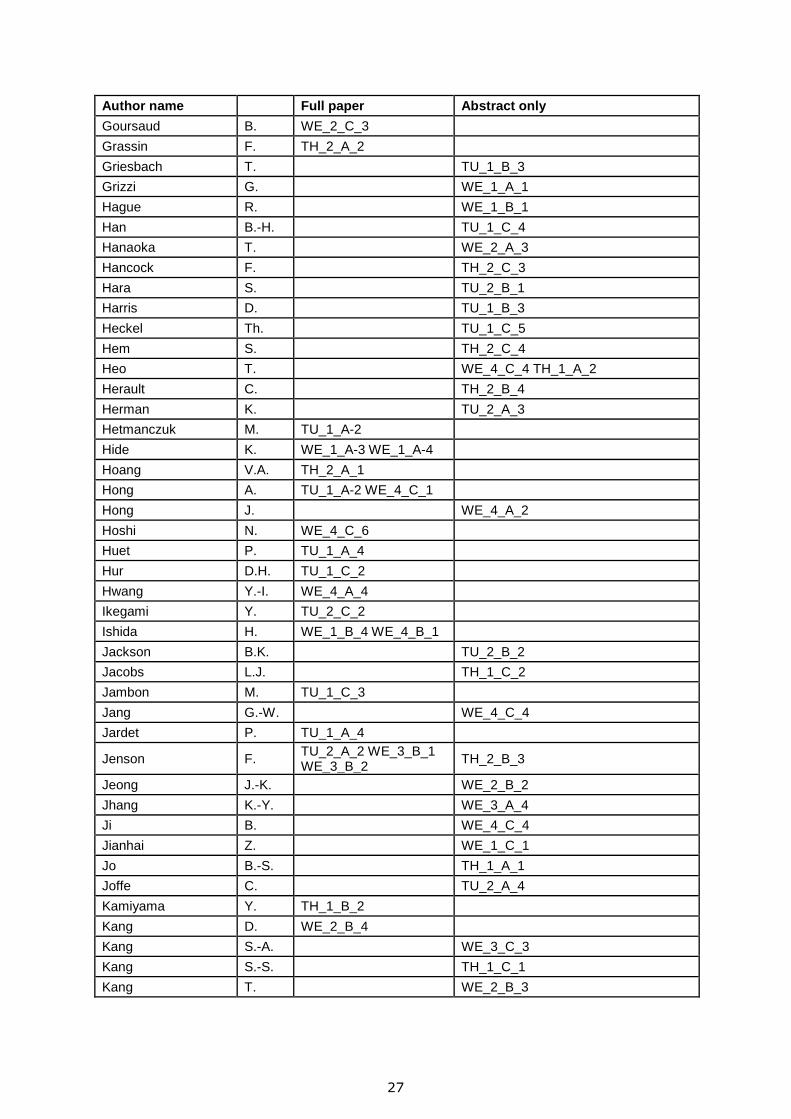
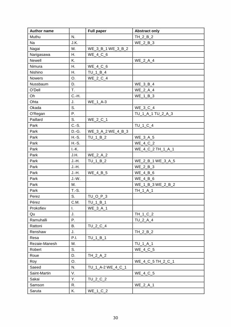
4. List of Authors
Author name Full paper Abstract only
Agnew J. WE_4_B_2
Agold J. TU_2_A_3
Ahn B. WE_4_C_4
Anderson M. TU_2_A_4
Ashwin P. WE_1_A_1
Bader B. TH_2_C_4
Bae J.-H. WE_4_A_4
Baek S.-H. TU_1_C_2
Bannouf S. TU_1_A-2 TH_2_A_2
Barcenilla V. WE_1_B_2
Barrera C.M. TU_2_B_3
Bayón A. TU_1_B_1
Benoist P. TH_2_C_1
Bergalonne P. TH_2_B_4
Bey S. WE_2_C_1
Bipes T. WE_2_A_4
Blin P. TU_1_A_3
Boehm R. TU_1_C_5
Bolander M. TH_2_B_1
Bourgelas T. WE_4_B_4
Braconnier D. WE_1_C_4 TH_1_B_1
Brockett A. WE_1_B_1
Calás H. WE_1_B_2
Carcreff E. TH_1_B_1
Cartier F. TH_2_C_1
Cattiaux G. TU_2_A_2 TU_2_C_4
Chang J.-M. TH_1_C_3
Chassignole B. TU_1_A_5
Chen T.-C. TH_1_C_3
Chen Z. TU_2_B_6
Cheng W. TU_2_C_3
Cheong Y.-M. TU_1_B_5 TU_2_B_5
Cherraben T. TH_2_C_3
Chesworth S. TU_1_A_1
Cho C. TU_2_B_4
Cho S.-B. TH_1_A_1
Cho S.H. WE_4_C_4 TH_1_A_2
Cho S.-H. WE_4_B_5
Cho S.W. TH_1_A_2
Cho Y.S. WE_1_B_3
Choi M.-Y. TU_1_B_2 WE_2_B_1 WE_3_A_5

26
Author name Full paper Abstract only
Choi N. WE_2_B_2
Choi W.-J. TU_1_B_2 WE_2_B_1
Clauzon T. TH_1_C_4
Cofie N. TU_1_B_3
Cordeiro S. WE_2_C_3
Cornaton P. TH_2_C_3
Courtois A. TH_1_C_4
Crauland J.-M. TU_1_C_3 TH_2_C_4
Cumblidge S.E. WE_3_A_1
Dagen J.M. WE_1_B_1
Dans A. TU_1_B_1
Dao G. WE_1_C_4
De la Fuente B. WE_1_B_2
Delemontez J. TH_2_C_3
Devos D. WE_4_C_6
Deydier S. TU_1_A_5
Diaz A. TU_2_A_4
Didie D. WE_4_C_2
Didier V. TU_1_A_4
Doctor S.R. WE_4_A_1
Doh E. TU_1_C_1 WE_3_A_3
Drinkwater B.W. WE_2_C_4
Ducousso-Ganjehi L. TU_2_A_2
Duxbury D.J. WE_2_C_4
Endoh K. WE_1_B_4
Erhard A. TU_1_C_5
Eriksson D. WE_3_C_1
Ernst H. WE_3_B_4
Esp L. WE_1_A_1
Fernández F. TU_1_B_1 TU_2_A_1 WE_1_B_2 WE_3_C_2
Fernandez-Gonzalez R. WE_4_C_1
Flisch A. WE_3_B_4
Furukawa T. TU_1_B_4 TH_1_B_2
Gac H. WE_2_A_1
Gadea J.R. TU_2_A_1
Garcia Rodriguez D. TU_2_C_3
Gardahaut A. WE_3_B_1 WE_3_B_2
Gasteau D. TU_2_A_2
Gelebart Y. TU_1_A_5
Gerard P. WE_3_C_5
Germerdonk K. WE_3_A_5
Gómez P. TU_2_A_1
González P. TU_2_A_1
27
Author name Full paper Abstract only
Goursaud B. WE_2_C_3
Grassin F. TH_2_A_2
Griesbach T. TU_1_B_3
Grizzi G. WE_1_A_1
Hague R. WE_1_B_1
Han B.-H. TU_1_C_4
Hanaoka T. WE_2_A_3
Hancock F. TH_2_C_3
Hara S. TU_2_B_1
Harris D. TU_1_B_3
Heckel Th. TU_1_C_5
Hem S. TH_2_C_4
Heo T. WE_4_C_4 TH_1_A_2
Herault C. TH_2_B_4
Herman K. TU_2_A_3
Hetmanczuk M. TU_1_A-2
Hide K. WE_1_A-3 WE_1_A-4
Hoang V.A. TH_2_A_1
Hong A. TU_1_A-2 WE_4_C_1
Hong J. WE_4_A_2
Hoshi N. WE_4_C_6
Huet P. TU_1_A_4
Hur D.H. TU_1_C_2
Hwang Y.-I. WE_4_A_4
Ikegami Y. TU_2_C_2
Ishida H. WE_1_B_4 WE_4_B_1
Jackson B.K. TU_2_B_2
Jacobs L.J. TH_1_C_2
Jambon M. TU_1_C_3
Jang G.-W. WE_4_C_4
Jardet P. TU_1_A_4
Jenson F. TU_2_A_2 WE_3_B_1 WE_3_B_2
TH_2_B_3
Jeong J.-K. WE_2_B_2
Jhang K.-Y. WE_3_A_4
Ji B. WE_4_C_4
Jianhai Z. WE_1_C_1
Jo B.-S. TH_1_A_1
Joffe C. TU_2_A_4
Kamiyama Y. TH_1_B_2
Kang D. WE_2_B_4
Kang S.-A. WE_3_C_3
Kang S.-S. TH_1_C_1
Kang T. WE_2_B_3

28
Author name Full paper Abstract only
Kang Y.S. WE_2_A_2
Kawai N. WE_2_A_3
Kawanami S. TH_1_B_3
Kawase N. TH_1_B_3
Kawashima K. WE_4_B_1
Kawata K. WE_2_A_3
Kim C. WE_4_A_2
Kim D.-J. TU_2_B_5
Kim D.-K. WE_4_B_5
Kim G. WE_1_B_3 WE_2_B_2
Kim H.-H. WE_4_A_4
Kim H.-J. TU_2_C_5 WE_2_C_2 WE_4_A_4 WE_4_B_5 TH_2_A_1
TU_2_C_1 WE_1_B_3 WE_1_C_1 WE_4_B_6 TH_1_A_3 TH_1_A_4 TH_1_C_1
Kim H.-S. WE_2_B_2
Kim I.C. WE_2_A_2
Kim I.-S. TU_1_C_4
Kim J. WE_3_A_4
Kim J.-M. WE_3_C_3
Kim J.-Y. TU_1_C_1 WE_3_A_3
Kim J.-Y. TH_1_C_2
Kim K.-B. WE_1_B_3 WE_2_B_2 TH_1_A_4
Kim K.-C. WE_3_A_1 WE_4_A_4 WE_3_A_5
Kim S.-M. TH_1_A_3
Kim W.-H. TU_1_C_1
Kim W.-T. TU_1_B_2 WE_3_A_5
Kim Y. TU_2_B_4
Kim Y.-B. WE_4_A_4
Kishore M.B. WE_3_A_2 WE_4_B_3
Kitasaka J. WE_1_B_4
Kitazawa S. WE_4_C_3
Kitze J. TU_1_C_5
Kobayashi R. WE_3_C_4
Kodaira T. TH_1_B_3
Komura I. WE_3_A_1
Kono N. WE_4_C_3
Koskinen A. WE_3_B_3
Kurokawa M. WE_2_A_3
Kwon K.-A. TU_1_B_2
Kwon S.-D. TH_1_A_4 TH_1_C_1
Lafreniere P. TU_1_A_1
Lamarre A. WE_3_B_5 WE_4_B_4
Landrum J. TU_2_A_4
Langevin J. WE_1_A_1
Lasserre F. TU_1_C_3 TH_2_C_4

29
Author name Full paper Abstract only
Latiolais C. WE_1_A_1
Le Berre S. WE_2_C_1 TH_2_A_2
Le Bourdais F. WE_1_C_3
Le Guevel T. TH_2_C_3
Le Jeune L. WE_4_C_5
Le Pollès T. WE_1_C_3
Lee C.-H. TU_1_C_1
Lee D. WE_4_A_2
Lee D.H. WE_4_B_3
Lee D.-H. TU_1_C_2 TU_1_B_5 TU_2_B_5
Lee H.-G. TH_1_A_3
Lee J. WE_3_C_3
Lee S.-G. TU_2_C_5
Lee T.-G. TH_1_A_3 TH_1_C_1
Lee T.-S. WE_3_A_3
Lee Y.-J. TH_1_A_3
Lejon A. TU_O_P_3
Lepage B. WE_4_B_4
Leskelä E. WE_3_B_3
Lheureux M. TU_2_A_5 WE_3_C_5
Lhuillier P.-E. TU_1_A_5 TH_2_B_3
Lim Z.S. TH_1_A_2
Lin S. WE_3_B_1 WE_3_B_2 TH_2_C_2
Lindberg J. TU_2_A_4
Lindsey M.S. TH_2_B_2
Lonne S. TH_2_A_2
Lourme H. WE_3_B_1 WE_3_B_2
Maes G. TU_1_C_3 WE_4_C_6
Malinowski O.M. TU_1_B_3 TH_2_B_2
Marois D. TU_1_C_3
Martin E. TU_O_P_3
Martin O. TU_O_P_3
Martínez-Oña R. TU_1_B_1 WE_1_B_2
Matlack K. TH_1_C_2
Matsuura T. TH_1_B_3
Maurice L. WE_2_C_3
Meyer R.M. WE_3_A_1
Mihalache O. TU_2_C_3
Milligan J. WE_4_B_2
Miyadera H. TU_O_P_4
Morikawa M. WE_2_A_3
Murakami H. WE_2_A_3
Murgier S. TH_2_B_3 TH_2_B_4
30
Author name Full paper Abstract only
Muthu N. TH_2_B_2
Na J.K. WE_2_B_3
Nagai M. WE_3_B_1 WE_3_B_2
Narigasawa H. WE_4_C_6
Newell K. WE_2_A_4
Nimura H. WE_4_C_6
Nishino H. TU_1_B_4
Nowers O. WE_2_C_4
Nussbaum D. WE_3_B_4
O’Dell T. WE_2_A_4
Oh C.-H. WE_1_B_3
Ohta J. WE_1_A-3
Okada S. WE_3_C_4
O'Regan P. TU_1_A_1 TU_2_A_3
Paillard S. WE_2_C_1
Park C.-S. TU_1_C_4
Park D.-G. WE_3_A_2 WE_4_B_3
Park H.-S. TU_1_B_2 WE_3_A_5
Park H.-S. WE_4_C_2
Park I.-K. WE_4_C_2 TH_1_A_1
Park J.H. WE_2_A_2
Park J.-H. TU_1_B_2 WE_2_B_1 WE_3_A_5
Park J.-H. WE_2_B_3
Park J.-H. WE_4_B_5 WE_4_B_6
Park J.-W. WE_4_B_6
Park M. WE_1_B_3 WE_2_B_2
Park T.-S. TH_1_A_1
Perez S. TU_O_P_3
Pérez C.M. TU_1_B_1
Prokofiev I. WE_3_A_1
Qu J. TH_1_C_2
Ramuhalli P. TU_2_A_4
Rattoni B. TU_2_C_4
Renshaw J. TH_2_B_2
Resa P.I. TU_1_B_1
Rezaie-Manesh M. TU_1_A_1
Robert S. WE_4_C_5
Roue D. TH_2_A_2
Roy O. WE_4_C_5 TH_2_C_1
Saeed N. TU_1_A-2 WE_4_C_1
Saint-Martin V. WE_4_C_5
Sakai Y. TU_2_C_2
Samson R. WE_2_A_1
Saruta K. WE_1_C_2

31
Author name Full paper Abstract only
Schumacher E. TU_1_A-2
Searfass C. WE_4_B_2
Seifert H.-P. WE_3_B_4
Seki I. TH_1_B_3
Selby G. TU_O_P_2
Seo J.-H. WE_3_C_3
Seo M.-K. WE_1_B_3 WE_2_B_2
Seok C.-S. TU_2_C_5 WE_1_C_1
Shim H.-S. TU_1_C_2
Shohji H. WE_1_A-3 WE_1_A-4
Shyu H.-F. WE_1_A_2
Sjö T. WE_3_C_1
Skoglund L. TH_2_A_3
Sola A. WE_3_C_2
Sollier T. TU_2_A_2 TU_2_C_4
Song C.-H. WE_3_A_3
Song S. TU_2_C_1
Song S.-J. TU_2_C_5 WE_2_C_2 WE_4_A_4 WE_4_B_5 TH_2_A_1
TU_O_P_1 WE_1_B_3 WE_1_C_1 WE_2_B_3 WE_4_B_6 TH_1_A_3 TH_1_A_4 TH_1_C_1
Taillade F. TH_1_C_4
Takagi T. TU_2_B_1 TU_2_B_6
Tang Z. TU_2_C_1
Tanji K. TU_2_B_1
Taupin L. TH_2_B_3
ten Grotenhuis R.L. TU_1_A-2 WE_4_C_1
Thomas P. WE_2_C_3
Tisseur D. TU_2_C_4
Todd S.J. TU_2_B_3
Tremblay P. WE_4_C_6
Tsuruta T. WE_2_A_3
Tung H.-M. TH_1_C_3
Uchimoto T. TU_2_B_1 TU_2_B_6
Ueda M. WE_1_C_2
Urayama R. TU_2_B_1
Van Velsor J.K. TU_1_B_3 TH_2_B_2
Vanhoye A. WE_2_C_1
Vautrin D. TH_1_C_4
Verma Y. TU_1_A-2 WE_4_C_1
Verspeelt D. TU_1_C_3
Vessio P. TU_1_B_1
Villagomez R. TU_2_B_3
Wall J.J. TU_2_B_2 TH_1_C_2
Wang M. WE_4_C_1
Warwick J.L.W. TU_2_B_2

32
Author name Full paper Abstract only
Watanabe K. WE_1_A-3
Wendel M. WE_3_C_1
Wu K. TU_1_C_2
Xie S. TU_2_B_6
Yamaguchi T. WE_1_C_2
Yamamoto Y. TH_1_B_3
Yamamoto T. TU_1_B_4 TU_2_C_3
Yeom Y.-T. TH_1_A_4
Yonemura H. WE_2_A_3
Yoo H.-R. WE_4_B_5
Yoon B. TU_2_B_4
Yoon D.-J. TU_1_C_4 WE_3_A_5
Yoshida S. WE_4_C_2
Yuan M. WE_2_C_2 TU_2_C_1
Zetterwall T. TU_O_P_3 WE_3_A_1 WE_4_A_1
Zhang J. WE_2_C_2
Zulueta T. WE_4_C_1

33
5. Conference Papers
This section contains the full papers of the conference. When a full paper was not
submitted, the abstract is provided.

NDE Researches for Structural Integrity of Nuclear Power Plant
Components in Korea
Sung-Jin Song
Sungkyunkwan University, School of Mechanical Engineering, 300 Chunchun-dong, Jangan-
gu, Suwon 440-746, South Korea
E-mail address : [email protected]
Since Kori Nuclear power Plant (NPP) operated from 1978, 23 NPPs are currently operating
for generation of electric power and 5 more plants are under construction in Korea. More than
30 year nuclear power plant operation history, various accident including S/G tube rupture at
2002 have experience. Especially, after Fukushima accidents, safety of nuclear power plants
is one of major concern. Nondestructive evaluation (NDE) techniques play key role for
insurance of structural integrity of NPPs.
In this presentation, review of NDE issues related on technical and/or social needs to NPPs
in Korea during last 30 years. Also, technical progress or movement of NDE in order to meet
those needs for NPP’s safety will be discussed. Especially, research activity by SAFE (Safety
and structural Integrity Research Center), established at 1997 in Sungkyunkwan University
and carried out many researches including NDE fields for insuring safety of NPPs, related to
NDE issues focused on structural integrity of NPPs. Also, major stream of NDE research
topics in KOREA during last three decade will be touched in this presentation.
34

Deep Learning in the Future of NDE
Greg Selby
Electric Power Research Institute, USA
Three factors are coming together to bring a revolution in the way people interact with the
electronic environment and with data. They are: first, the development of deep neural
networks (also called deep convolutional networks, or deep learning); second, the rapid
development of massively parallel, low-cost supercomputing systems using general-purpose
graphics processor units; and third, the availability of huge amounts of data to train the
systems.
The NDE community will access the first item through the efforts of large commercial
enterprises such as Google, Microsoft, Baidu, Facebook, NVIDIA, Tesla, and Apple, all of
whom are investing heavily in deep learning research. Our small industry of nuclear NDE
cannot contribute meaningfully to these seminal developments, but as the research progresses
and the field matures, powerful general-purpose deep learning engines will become available
to us, perhaps even before the next conference in this series.
The second item, the computing platform, is not an issue; today a researcher can purchase for
USD15k a desktop workstation that five years ago would have been one of the world's top
500 supercomputers. Also, engines will become available as netware.
The biggest question for us is the third item, the data. To work robustly, deep learning
engines require huge amounts of training data. It's possible that no single NDE institution
will be able to gather enough information to train the systems; will we be able to work
together to accomplish it, when the prize at the end of the work could be uniform NDE
reliability and repeatability for the world fleet of nuclear power plants?
Keywords:
Deep learning
GPU computing
Artificial intelligence
Deep neural networks
35

Activities and future Trends of the ENIQ Network
Oliver Martin1, Tommy Zetterwall
2, Etienne Martin
3, Anders Lejon
4, Samuel Perez
5
1European Commission, Joint Research Centre, Institute for Energy and Transport, Petten,
Netherlands 2Swedish Qualification Centre (SQC), Täby, Sweden
3EDF Generation Nuclear Engineering Division, Ceidre, France
4Vattenfall, Ringhals NPP, Sweden
5Iberdrola, Madrid, Spain
Abstract
The European Network for Inspection and Qualification (ENIQ) is a utility driven network that works towards a
harmonized European approach on reliable and effective in-service inspection (ISI). It is Technical Area 8 (TA8) of
the international association NUGENIA on R&D on Gen II / III reactors. ENIQ has a steering committee and two sub-
areas: the sub-area on Qualification (SAQ), which works on issues related to the qualification of in-service inspection
(ISI) systems and the Sub-area on Risk (SAR), which is focused on risk-informed ISI (RI-ISI).
Recently SAQ launched a comprehensive study on the performance of computed and digital radiography (CR / DR)
with the name COMRAD. The aim of the study is to identify the essential parameters that affect the performance of
CR and DR and thereby providing a consistent approach to inspection design and the production of technical
justifications. Also SAQ is currently performing a study to identify the main barriers for transport of qualifications
between countries and how to overcome these and recently drafted a position paper on the re-qualification and
maintaining proficiency of ISI personnel. The reason for this paper is the significantly different practices of countries
with operating NPPs on re-qualification of ISI personnel. Some countries require re-qualification of ISI personnel
every five years, where as others do not demand such (re-)qualifications at all. The on-going discussion inside SAQ
on re-qualification and maintaining proficiency of ISI personnel will most probably result in a study on the issue.
SAR is currently launching a study to quantify the benefit from ISI and to indicate the level of risk reduction that can
be expected from ISI and is currently updating the ENIQ Framework Document on RI-ISI. The aim of this paper is to
describe these activities in more detail plus the challenges for ENIQ in the next couple of years.
Keywords: ENIQ, in-service inspection, inspection qualification, inspection qualification body, risk-informed in-
service inspection, NUGENIA
1. ENIQ: Objectives and Organisation
The European Network for Inspection and Qualification (ENIQ) is a network dealing with the reliability and
effectiveness of non-destructive testing (NDT) for nuclear power plants (NPP). ENIQ is driven by European nuclear
utilities and is working mainly in the areas of qualification of NDT systems and risk-informed in-service inspection (RI-
ISI). Since its establishment in 1992 ENIQ has performed two pilot studies on in-service inspection (ISI) qualification [1]
[2] and has issued 50 documents. Among them are the two ENIQ framework documents, the “European Methodology for
Qualification of Non-Destructive Testing” [3] and the “European Framework Document for Risk-Informed In-Service-
Inspection”1 [4], 11 recommended practices [5] [6] [7] [8] [9] [10] [11] [12] [13] [14] and a significant number of
technical reports and discussion documents2. ENIQ is recognized as one of the main contributors to today’s global
qualification guidelines for in-service inspection (ISI).
ENIQ is part of the European based R&D association on Gen II & III reactors NUGENIA established in November
2011. NUGENIA has more than 100 member organisations with all major nuclear organisations (i.e. utilities, reactor
vendors, nuclear research organisations, technical service organisations, universities with nuclear faculties) among
them. NUGENIA has 8 technical areas (TA), in which then scientific / technical work of the association is carried out, 1 The European Framework Document for RI-ISI is currently revised and the revised version will be published later this year. 2 All valid ENIQ documents can be found on the website of NUGENIA (www.nugenia.org).
36

with ENIQ being the 8th TA. ENIQ has two sub-areas (SA), the Sub-area for Qualification (SAQ), which is dealing
with ISI qualification, and the Sub-area for Risk (SAR), which is dealing with RI-ISI. Beside these two ENIQ used to
have a separate Sub-area for Inspection Qualification Bodies (SAIQB) for two years, which served as an exchange
forum for IQBs. Because there was quite some overlap in topics and members SAIQB and SAQ were merged to one
sub-area called SAQ. ENIQ has a steering committee (SC), which is the decision making body of ENIQ. It approves
all the documents drafted inside the SAs, but also serves as an exchange forum for ISI related issues in NPPs of ENIQ
members. ENIQ SC members have contributed to the recently published NUGENIA Global Vision Document, which
summarizes all the scientific / technical challenges (short-, mid- and long-term) of the individual TAs, including the
ones of ENIQ (TA8) [15].
2. Current Activities of ENIQ
2.1 Sub-area for Qualification
COMRAD
Since May 2014 SAQ members are performing a comprehensive study on the performance of computed and digital
radiography called COMRAD. The aim of this study it to identify the essential parameters that affect the performance
of both methods and thus provide a consistent approach to inspection design and production of technical justifications.
Computed radiography (CR) and digital radiography (DR) are two contenders as replacement technologies for
traditional film based industrial radiography. In CR the film is replaced by an imaging plate containing
photostimuable storage phosphors, which store the radiation level received at each point in local electron energies. A
scanner employs a laser beam to read out the imaging plate via photostimulated luminescence, where the emitted light
in the visible spectrum is detected by a photomultiplier and converted to an electronic digitised signal. In DR a digital
detector array (DDA), also known as flat panel detector, the image is directly captured in the detector.
Both techniques share a number of potential advantages over film, such as their linear detection characteristics over
a wide dose range, allowing the examination of a wider range of thicknesses in one exposure and making CR and to a
lesser extent DR less vulnerable to under- or overexposure, unlike conventional film. Another potential advantage
concerns the increased sensitivity at lower energies and the consequential ability to reduce the radiation exposure
(which in turn reduces inspection times and the potential radiological hazard). However, the transition from traditional
silver film to digital radiography requires an in-depth understanding of the relative performances of CR/DR and film
based radiography. As detection, processing and interpretation of the two methods are significantly different there are
many technical aspects that need to be explored.
COMRAD was launched in May 2014 has a duration of two years. The first stage of the project is a review of the
state-of-the-art of CR / DR and identification of key aspects that determine their performance. The second stage of the
project is the writing of a recommended practice on qualification of CR and DR, which is the final output of the
project.
MUREC
In 2011 SAQ carried out a survey to identify the barriers that preclude transfer of inspection qualifications from one
country to another. The survey involved a questionnaire on different aspects of inspection qualification. Beside a
section with general questions (e.g. if ENIQ Methodology is followed, which codes & standards are followed, etc.) the
questionnaire contained sections with questions on regulatory requirements, IQB requirements, test pieces and
practical trials, use of modelling, utilisation of foreign validations and personnel qualification. The questionnaire was
sent to one organisation per country with ENIQ members, either IQB or utility, and with one exception all countries
submitted answers.
Based on the outcomes of the above survey the idea was to launch a project on the transfer of inspection
qualifications between countries called MUREC3. In the first stage of the project a comparison of the inspection
requirements and inspection specifications of different countries was planned. In a second step a pilot study was
planned, in which each participant is requested to perform a qualification on a simple case (real or fictitious)
according to his national rules, guidelines and methodologies. In the third and last stage of the project the results of
these qualifications are compared with each other and recommendations are formulated. In particular the second step
would require significant efforts (personnel & time) from the participants and for this reason SAQ members decided
to take a different approach. 3 MUREC = Pilot study on mutual recognition of inspection qualifications between countries.
37

SAQ will perform an in-depth review of the questions of the questionnaire and decide for each question whether it
is relevant or non-relevant for the transfer of inspection qualifications between countries and thus re-write the
questionnaire. The resulting re-written questionnaire will be distributed to one organization per country with ENIQ
members again and the answers will be reviewed. By taking this approach SAQ members are confident to infer the
possibility to facilitate transfer of inspection qualifications between countries and at least achieve transfers of parts of
technical justifications, since there are practically only two scenarios for the exchange of parts of a technical
justification, either that providers want to use the same NDT system in different countries or that utilities operate the
same type of plant in different countries and use the same provider with the same specifications. The survey based on
the re-written questionnaire might evolve into an ENIQ position paper.
Maintaining proficiency of ISI personnel
In the last 1 ½ years there was quite some discussion within SAQ on (re-)qualification of ISI personnel. The
discussions revealed that there are different approaches with regards to (re-)qualification of ISI personnel in different
countries. Where as some countries require re-qualification of ISI personnel after a couple of years, normally 5 years,
as it is the case for e.g. Finland, others have no legal requirements concerning re-qualification of ISI personnel (e.g.
France). The discussions also revealed that two items need to be distinguished:
Re-qualification in general (which rather concerns systems than ISI personnel alone) and
Maintaining proficiency of ISI personnel.
The latter is a matter of demonstrating of maintaining the proficiency of ISI personnel and some ENIQ members
perform it already via technical justifications. Discussions focused on the issue of maintaining proficiency of ISI
personnel and a position paper was produced [16]. In the position paper it was concluded that a study on the needs,
experience, benefits and recommended approaches for maintaining the proficiency of ISI should be carried out. The
study should answer the following questions:
What similar schemes exist in the nuclear industry or other relevant industrial areas, where an individual is
expected to maintain his proficiency, e.g. qualification of welders?
What is the experience and lessons learned with existing schemes?
What are the arguments in favor and against re-qualification of ISI personnel?
What is the recommended common approach for future qualification of ISI personnel?
ENIQ will discuss the issue of maintaining proficiency of ISI personnel further and will launch a study with the aim
of answering the above questions later this year.
2.2 Sub-area for Risk
Lessons learned from the application of RI-ISI to European NPP
SAR is currently in the process of finalizing a report on the lessons learned from the application of RI-ISI to
European NPPs. It summarises the experience from RI-ISI programs of Finland, Spain and Sweden, where RI-ISI is
commonly used (i.e. where RI-ISI is approved by the regulator), and the experience of pilot studies performed in
Bulgaria, Lithuania and Romania. The report covers the experience from different types and designs, such as BWR
(Asea-Atom, GE), PWR (Westinghouse), VVER, Candu and RBMK. The report is in the final editorial stage and will
be published within the next months. The main conclusion from the RI-ISI programs is that they help to focus on most
risk significant locations of the plants and thus lead to a reduction in ISI efforts. Also RI-ISI led to a reduction in doses
of ISI personnel.
Update of the ENIQ Framework Document on RI-ISI
The ENIQ Framework Document on RI-ISI was firstly published in 2005 and the experience gained from RI-ISI
programs since then prompted SAR members to update the document. The updated document also contains
considerations on external events, which was one of the main drivers for updating the document. The new version of
the ENIQ Framework Document on RI-ISI will be published later this year.
REDUCE
A month ago a number of SAR members launched a project on risk reduction through ISI called REDUCE. The
main objective of the project is to evaluate the parameters that influence the risk reduction that can be achieved via ISI.
38

In the project the effect of alternative ISI strategies on the level of risk reduction will be investigated for different
situations that are typical for European NPPs. The influence of key parameters will be systematically analysed by
using structural reliability models, considering a range of components, materials, degradation mechanisms, loading
conditions, NDT reliability (POD4 curves) and inspection intervals. The final output of the project will be a document
that supports utilities in assessing risk reduction when applying RI-ISI approaches. When entering long-term operation
(LTO) the number of positions susceptible to fatigue is expected to increase when considering environmental effects
and the document will cover issues of an ISI strategy for control of this specific degradation mechanism.
3. Summary
The main activities of ENIQ SAQ at the moment are the comprehensive study on the performance of computed and
digital radiography (COMRAD), the transfer of inspection qualifications between countries (MUREC) and
maintaining the proficiency of ISI personnel and linked to the latter the re-qualification of ISI personnel. Main
activities of ENIQ SAR are the recently launched project on risk reduction through ISI and the update of the ENIQ
Framework Document on RI-ISI. With its on-going and new activities ENIQ will maintain its role as one of the main
contributors to today’s global ISI qualification codes and guidelines.
References
[1] ENIQ technical report, “Final Report of the 1st ENIQ Pilot Study”, ENIQ Report no. 20, EUR 19026 EN, 1999.
[2] ENIQ technical report, “Final Report of the 2nd
ENIQ Pilot Study”, ENIQ Report no. 27, EUR 22539 EN,
2006.
[3] ENIQ, “European Methodology for Qualification of Non-Destructive Testing – Issue 3”, ENIQ Report no. 31,
EUR 22906 EN, 2007.
[4] ENIQ, “European Framework document for Risk-Informed In-Service Inspection”, ENIQ Report no. 23, EUR
21581 EN, 2005.
[5] “ENIQ RP1: Influential / Essential Parameters – Issue 2”, ENIQ Report no. 24, EUR 21751 EN, 2005.
[6] “ENIQ RP2: Strategy and Recommended Contents for Technical Justifications – Issue 2”, ENIQ Report no. 39,
EUR 24111 EN, 2010.
[7] “ENIQ RP4: Recommended Contents for the Qualification Dossier”, ENIQ Report no. 13, EUR 18685 EN,
1999.
[8] “ENIQ RP5: Guidelines for the Design of Test Pieces and Conduct of Test Piece Trials”, ENIQ Report no. 42,
EUR 24866 EN, 2011.
[9] “ENIQ RP6: The Use of Modelling in Inspection Qualification – Issue 2”, ENIQ Report no. 45, EUR 24914
EN, 2011.
[10] “ENIQ RP7: Recommended General Requirements for a Body operating Qualification of Non-Destructive
Tests”, ENIQ Report no. 22, EUR 20395 EN, 2002.
[11] “ENIQ RP8: Qualification Levels and Approaches”, ENIQ Report no. 25, EUR 21761 EN, 2005.
[12] “ENIQ RP9: Verification and Validation of Structural Reliability Models and associated Software to be used
in Risk-Informed In-Service Inspection Programmes”, ENIQ Report no. 30, EUR 22228 EN, 2007.
[13] “ENIQ RP10: Personnel Qualification”, ENIQ Report no. 38, EUR 24112 EN, 2010.
[14] “ENIQ RP11: Guidance on Expert Panels in RI-ISI”, ENIQ Report no. 34, EUR 22234 EN, 2008. 4 POD = Probability of detection
39

[15] NUGENIA Association, “NUGENIA Global Vision Report”, 2015.
[16] ENIQ position paper “NDE Personnel Re-Qualification or a Need to Maintain Proficiency”, ENIQ report no.
49, 2015, in press.
40

Fukushima Daiichi muon imaging
Haruo Miyadera
Power and Industrial System R&D Center, Toshiba Corporation,
8 Shinsugita-cho, Isogo-ku, Yokohama 235-8523, Japan
E-mail address : [email protected]
Japanese government announced cold-shutdown condition of the reactors at Fukushima
Daiichi by the end of 2011, and mid- and long-term roadmap towards decommissioning has
been drawn. However, little is known for the conditions of the cores because access to the
reactors has been limited by the high radiation environment. The debris removal from the
Unit 1 – 3 is planned to start as early as 2020, but the dismantlement is not easy without any
realistic information of the damage to the cores, and the locations and amounts of the fuel
debris.
Soon after the disaster of Fukushima Daiichi, several teams in the US and Japan proposed to
apply muon transmission or scattering imagings to provide information of the Fukushima
Daiichi reactors without accessing inside the reactor building. GEANT4 modeling studies
of Fukushima Daiichi Unit 1 and 2 showed clear superiority of the muon scattering method
over conventional transmission method. The scattering method was demonstrated with a
research reactor, Toshiba Nuclear Critical Assembly (NCA), where a fuel assembly was
imaged with 3-cm resolution.
The muon scattering imaging of Fukushima Daiichi was approved as a national project and is
aiming at installing muon trackers to Unit 2 in FY15. A proposed plan includes installation of
muon trackers on the 2nd floor (operation floor) of turbine building, and in front of the
reactor building. Two 7m x 7m detectors are assembled at Toshiba and tested.
Keywords: Fukushima Daiichi, muon scattering, imaging, core damage, fuel debris
41

Inspection Qualification of a FMC/TFM Based UT System
R.L. ten Grotenhuis1, Y. Verma
1, A. Hong
1, N. Saeed
1,2, E. Schumacher
4 , S. Bannouf
5 and M.
Hetmanczuk1,3
1Ontario Power Generation, Inspection & Maintenance Division, Toronto, Canada
2University of Toronto, Division of Engineering Science, Toronto, Canada
3McMaster University, Mechanical Engineering Department, Hamilton, Canada
4EXTENDE Inc., Ballston Spa, USA
5EXTENDE S.A., Massy, France
E-mail address (corresponding author): [email protected]
Abstract
The Matrix Inspection Technique (MIT) consists of the Full Matrix Capture (FMC) UT acquisition technique in
combination with an automated analysis beamformer applying the Total Focusing Method (TFM) algorithm. The MIT
system was developed by Ontario Power Generation (OPG) and deployed in several field inspection campaigns
beginning in 2010 to the most recent work in spring 2015. During this time a series of enhancements have been
implemented to improve overall system performance. Thus while the system has evolved, a sufficient body of
operational experience (OPEX) has been obtained to enable inspection qualification efforts to proceed.
The Canadian Nuclear Safety Commission (CNSC) is the regulatory authority for all nuclear facilities operating in
Canada. The CNSC has mandated all nuclear utilities to qualify their inspection systems as a condition of their
operating license. The European Network for Inspection Qualification (ENIQ) methodology has been adopted as the
basis for inspection qualification programmes. An organization known as the CANDU Inspection Qualification
Bureau (CIQB) has been tasked by the CNSC with programme oversight as well as evaluation of the licensee’s
submissions. The ENIQ methodology tailors the scope of the Technical Justification (TJ) effort based upon the degree
of novelty of the inspection system and the severity of the consequence of failure of the component inspected. MIT’s
use of automated FMC and automated TFM for inspection is unprecedented in any industry. Furthermore the
components inspected are part of the nuclear pressure boundary, failure of which could result in a single channel Loss
of Coolant Accident (LOCA) and a potential release of activated products. Thus in both respects the MIT system is
obligated to undergo the complete process defined by ENIQ. Major sections of the TJ will address
simulation/modelling, parametric studies, experimental studies and examination of ex-service samples.
This paper summarizes the application of the ENIQ process to the MIT system as well as the progress to date in
preparation of the Technical Justification.
Keywords: Inspection Qualification, FMC, TFM
1. Introduction
Over several decades of commercial operation most CANDU nuclear units have experienced varying degrees of Flow
Accelerated Corrosion (FAC) in the carbon steel piping components of the Primary Heat Transport system, see Figure
1. Thinning rates were found to vary in a range of 0.01mm/EFPY to 0.14 mm/EFPY where EFPY stands for Effective
Full Power Years. In extreme cases the FAC progressed to the stage where replacement of the components was
necessary in order to maintain pressure boundary thickness margins. Regions prone to acute attack are the surfaces
under and immediately downstream from the weld as shown in Figure 2. Fitting geometry, access, as fabricated weld
caps combined with the Inspection Specification requirements make this inspection particularly challenging. At
Ontario Power Generation an inspection system was developed that applied the FMC data acquisition technique with a
proprietary version of the TFM beam former, [1] and [2]. The system, called the Matrix Inspection Technique or MIT,
has been deployed since mid-2010 and in four separate inspection campaigns has inspected 83 locations comprising
not fewer than 115 welds.
42

Figure 1 Portion of the reactor face with associated carbon steel piping - left, isometric of piping spool piece with
inspection zones - right.
Figure 2 Examples of localized FAC located at weld root.
Typical profiles for fitting to fitting welds and the 3D evolution are presented in Figure 3. The results have generally
exceeded expectations with respect to coverage and accuracy particularly in the volume of the weld material under the
weld cap. The MIT system represents the first large scale application of this method in the power generation industry.
Understandably there have been changes to the system reflecting the OPEX obtained in the field. The changes are
directed toward three general objectives:
• enhancement of system capabilities,
• remediation of system deficiencies,
• efficiency/productivity improvements
43

Figure 3 Typical axial cross sections through the weld - left, 3D colour coded thickness map - right.
Facets of the MIT system that were identified for modification were: manipulators, analysis software, acquisition
software and instrumentation. Many of the desired changes have been implemented to date. Some enhancements to
the manipulators and analysis code remain outstanding and are to be addressed within the next year. The ultrasonic
parameters and underlying methodology on the other hand were deemed to be apposite in their initial form adopted.
2. Inspection Qualification
In Canada, the CNSC has mandated licensees to implement a qualification programme for inspections performed.
The licensees in concert with the CNSC have adopted the ENIQ qualification regime under the administration of the
CIQB. At this juncture in the MIT system development it is appropriate to begin the preparation of the TJ document
based on the body of inspection OPEX established. High level objectives for the TJ of the MIT system may be
identified as:
• Demonstration of performance meeting the Inspection Specification (IS) [4] over the target volume for the
range of inspection geometries encountered
• Identification of influential and essential variables as well and factors that ultimately manifest in unit time or
distance error
• Provide evidence that the acquisition system and analysis software are capable of yielding consistent results
when applied with the established procedures.
Now many readers will be familiar with the ENIQ recommended structure of the TJ in general as found in Error!
Reference source not found.. The ENIQ TJ guidelines allow for a simplified approach if the conditions of a
reasonably well established inspection technique are coupled with a relatively low consequence as a result of
component failure. In the case of the MIT system the technology is both novel and relatively complex. Furthermore,
the consequence of a failure of the subject component is potentially a single channel LOCA. Clearly then, in light
both of these factors, the MIT TJ requires the full rigour as defined by ENIQ.
44

Figure 4 ENIQ recommended structure of the Technical Justification as adopted by CIQB.
With reference to Error! Reference source not found., the full format TJ introduces additional avenues for
investigation beyond that of the basic structure. This includes: Prediction by Modelling, Experimental Evidence,
Parametric Studies and Equipment, Data Analysis & Personnel Considerations. The section, Analysis of Influential
Parameters, remains at the core of the MIT TJ. The MIT system has few analogues to conventional UT approaches
that would be applicable as a reference. Hence the Physical Reasoning portion of the MIT TJ has a somewhat reduced
significance relative to the corresponding element in TJs for standard techniques. The principal focus of the MIT TJ
then is to direct efforts to the four additional areas introduced in the extended TJ structure as to support the Influential
Parameters section.
Prediction by Modelling and Experimental Evidence sections are treated as complementary avenues of investigation
within the MIT TJ. The transducer beam characteristics are modelled using EXTENDE’s CIVA application and then
confirmed via an immersion test rig, see Figure 5. The purpose is to verify the beam characteristics and then establish
the statistical variation for the series of essential variables that define the transducer performance. Simulations of the
UT responses for the range of Test Geometries are created with CIVA and then will be verified in the immersion
scanning apparatus. The simulations generate FMC data sets containing idealized UT responses. These data sets
once converted into the appropriate format, are processed by the MIT automated analysis software. The goal of the
exercise is to demonstrate accurate reconstruction of the test geometry. Idealized data sets are used in the Parametric
Study to isolate the effects of parameter variation from those introduced by experimental error.
45

Figure 5 Beam modelling with CIVA, active plane - left, passive plane – centre. Relative amplitudes at 8, 15 and 22
mm water column denoted as black, red and blue profiles respectively. Five axis immersion tank - right.
2.1 Test Geometry Design
The function of the test geometry series is to facilitate demonstration of adequate inspection coverage, accuracy and
repeatability of the inspection. These samples are a series of controlled surfaces that bound the range of inspection
geometries encountered. Five basic samples are simulated: planar, plano-convex, plano-concave, double convex or
dome, convex-concave or saddle. A concave-concave sample would be required if inspection from the interior of the
specimen were contemplated. Since the application is thickness monitoring of fitting to fitting welds, a series of
contours for the interior surface would seem to be an obvious choice. However this choice would have required an
inordinate number of samples to address the possible configuration permutations. Conventional reflectors,
specifically side drilled holes and EDM notches were used instead. These reflectors are widely accepted, easier to
control to the desired accuracy, and less expensive to produce. Use of samples with conventional reflectors provides
an opportunity to evaluate volumetric inspection performance should this type of inspection become necessary. The
permutations of geometry, water path distance to sample with the number of target reflectors resulted in 192
individual simulations to be performed. Examples of the Test Geometries are given in Figure 6.
Figure 6 Test Geometry Samples: left - dome, centre - saddle, right - weld cap
Initial attempts at machining controlled surfaces with characteristics representative of weld pool ripple did not meet
with success. The characteristic response from the machined ripples did not match that of ex-service samples.
Furthermore the cost to manufacture these samples was substantial relative to the benefits obtained. Rather than
pursue manufacture of idealized welds it was decided to fabricate welds according to the original weld procedure,
acquire and process the FMC data sets and then destructively analyse the welds.
46

2.2 FMC Simulations
The Inspection Specification requires a precision of measurement of 0.03 mm with an accuracy of +/- 0.06 mm. As a
consequence a higher degree of resolution is required for both simulations and experimentation in order to observe
and assess the contribution of individual 3rd
order effects. Recall application of the FMC acquisition method results in
dramatically larger data sets compared with other UT methods. With respect to the MIT application, the data sets are
roughly 2 orders of magnitude larger than the corresponding linear electronic B scan sets. Commensurate simulation
of FMC data sets consumes markedly greater computation resource. Careful consideration must then be given to the
design of the simulation and the input parameters. The simulation parameters were optimized following several test
runs and with consultation of the CIVA specialists at EXTENDE. Factors considered were: Level of Accuracy,
Computation mode, Number of modes and reflections calculated, and Sampling frequency, see reference [6]. Though
CIVA can simulate basic weld configurations in plate or pipe welds, complex geometries such as dome, saddle and
weld cap do not pre-exist in CIVA and must be imported as 3D CAD models. Discrepancies between surface of the
specimen defined by the original 3D CAD model and the surface automatically meshed by CIVA do influence
simulation accuracy. In CIVA, the mesh accuracy corresponds to the maximum discrepancy between the surface of
the specimen defined by the CAD file and the surface meshed into triangles. Decreasing the size of the mesh accuracy
reduces the discrepancy but requires more computation time. Typical responses to reflectors in; weld, dome and
saddle geometries are found in Figures 7, 8 and 9 respectively.
Figure 7 Simulated response to 1 mm diameter SDH under weld cap, main diagonal of the FMC data array. Adjacent
cap- left, under weld toe – centre, mid weld – right.
Figure 8 Simulated response to 1 mm diameter SDH in the dome geometry, main diagonal of the FMC data array. 10
mm from centreline - left, mid dome – centre, 1 mm EDM notch – right.
Figure 9 Simulated response to 1 mm SDH in saddle geometry, main diagonal of FMC data array. Centre saddle –
left, 15 mm offset from centre line – centre, and 1 mm EDM notch 5 mm offset – right.
47

There are slight differences between the CIVA treatment of waveforms and the conventions adopted for inspection
with MIT. The most realistic signal type for the transducer excitation waveform built-in CIVA is a Gaussian
envelope, which departs from that of the actual UT signals. As a consequence there are slight variations between
simulated and experimental results. The convention used within CIVA to define the distance to the target is the peak
of the simulated waveform envelope, whereas MIT defines the onset of the waveform envelope as the distance to the
target. These differences, while subtle, must be accommodated when comparing simulation results with experimental
results.
The simulations were run on a dual processor, 6 core PC workstation operating in batch file mode. Computation times
ranged from a low of 4 hours to a maximum of 133 hours. The median computation time was 48.1 hours with over
9000 hours required to complete all simulations. The entire effort was performed over a period of 15 months. Figure
10 illustrates the computation times for a range of simulations performed.
Figure 10 Simulation times versus geometry and reflector location.
2.3 Experimental Evidence
Verification of the UT beam characteristics, see Figure 11, and test geometry responses are two fundamental
components of the Experimental Evidence. But in addition to these, the experimental evidence also includes results
from controlled samples such as reference blocks, fabricated spool pieces and ex-service components. When MIT was
first commissioned, the validity of the results was established via a performance demonstration exercise on reference
blocks and ex-service samples. The results obtained on the blocks were accurate to within 0.01 mm and on ex-service
samples to within +/- 0.02 mm. Going forward, once all the desired changes are implemented, the Experimental
Evidence will expand upon this base to improve the statistical significance of the results.
48

Figure 11 Element sound field plot in water, right - active plane, left - passive plane.
2.4 Parametric Study
The Parametric Study portion of the TJ is divided into three main sections. One section addresses the essential
parameters underpinning the TFM analysis code; the second examines the essential parameters of the UT data
acquisition system, while the third examines the essential parameters introduced by factors related to materials,
geometry, inspection conditions, and manipulator performance. At the current stage a cursory effort has been directed
to the Parametric Study, however even this limited effort has already identified desirable changes to the MIT system.
Some examples are:
1. Increasing the reconstructed sampling rate from 100 MHz to 200 MHZ enhanced with linear interpolation.
2. Compensation for temperature based velocity variation in the carbon steel media.
3. Correction for transducer element to element delay variation.
Figure 12 Enhanced analytic signal resolution - up sampling to 200 MHz combined with linear interpolation.
49

When reconstructing the interior volume TFM image, for any given focal point P, the time index of the analytic signal
will most often not correspond precisely to the point imaged. The magnitude of the error is a function of the TFM
grid spacing and the sampling frequency. This intrinsic error can be reduced by up-sampling to 200 MHz, see Figure
12. Further improvement to the estimate of the analytic signal is obtained via linear interpolation. For a focal point P
the worst case timing error using this strategy is typically on the order of 1 ns.
Figure 13 Velocity of ASME SA106 Gr. B as a function of temperature.
Error can be introduced under the assumption that velocity remains fixed. Rather, velocity of ASME SA106 Gr B is a
function of temperature as shown in Figure 13. For a mean path to the interior surface of 15 mm given a nominal
aperture, the resultant timing error can be as large as 6.47 ns or equivalently 19.1 µm. A linear velocity correction
with a coefficient of -0.7% per 55 C is applied to reduce the error, see reference [5].
Figure 14 Transducer element delay variation, left - as found, right - corrected.
The distribution of timing errors associated with variation in transducer element delay is unique to each transducer. A
statistical approach is necessary to quantify this effect. An example is shown in Figure 14. Observations to date
report a nominal range of +/- 35 ns with a standard deviation of 14 ns. Compensation of this variation is performed by
measuring arrival of the peak of the signal envelope. Individual element delay compensations are calculated and
applied as needed during the TFM imaging operations. Applying compensation reduces the timing error to +/- 5 ns
with a standard deviation of 2 ns.
Further changes arising from Parametric Study work are anticipated. As the changes are identified they will be
incorporated into the MIT system. Near term activities will include: procurement of Test Geometry samples,
completion of the experimentation on the Test Geometry samples and initiation of work on the Equipment, Data
Analysis & Personnel Considerations document.
50

3. Conclusions and Summary
The Canadian nuclear power industry has adopted the ENIQ strategy for inspection qualification. Since its
introduction in 2010, the MIT system has developed a body of inspection OPEX over the course of four inspection
campaigns. The nature of the inspection coupled with the characteristics of the MIT system mandates the use of the
enhanced format ENIQ TJ. Several changes have been made to the system, however many the fundamental aspects of
the original approach remain intact.
The TJ for the MIT system is in progress. A series of bounding geometry samples incorporating standard reflectors
have been developed. UT beam characteristics have been evaluated via modelling with CIVA, confirmation of which
is provided by direct measurement. Inspection coverage has been demonstrated via simulation. Judicious selection of
parameters (such as sampling frequency, computation mode, etc.) is required for balancing both simulation accuracy
and efficiency. FMC data sets generated using CIVA are exported to the MIT analysis software to support parametric
study of the analysis code. Initial efforts in the Parametric study have identified desirable improvements. Going
forward further improvements to the MIT analysis code are anticipated. The current schedule projects the completion
date of the TJ in mid-2016.
References
[1] ten Grotenhuis R, Hong A and Sakuta A, “Inspection of complex geometries using the full matrix capture (FMC)
method”, 9th Int Conf on NDE in Relation to Structural Integrity for Nuclear and Pressurized Components,
Seattle WA, USA, 2012.
[2] ten Grotenhuis R and Hong A, “Imaging the weld volume via the total focus method”, 9th Int Conf on NDE in
Relation to Structural Integrity for Nuclear and Pressurized Components, Seattle WA, USA, 2012.
[3] CANDU Inspection Qualification Bureau, “Instructions for the Contents of a Technical Justification” , Toronto,
Ontario Canada August 28, 2008
[4] CANDU OWNER’S GROUP, “Feeder Pipes Inspection Specification”, COG-JP-4059-V03 Rev3, Toronto,
Ontario, Canada March 2011
[5] Biagiotti S, “Effect of Temperature on Ultrasonic Velocity in Steel”, NACE Corrosion ’97, New Orleans LA,
USA 1997
[6] “CIVA 2015 (V11.1) User Manual” by CEA List
51

The EPR’s NDE program: a technical and industrial challenge.
Pascal BLIN
EDF Nuclear Engineering Division, Ceidre, 2 rue Ampère, 93206 ST DENIS, FRANCE
The “Flamanville 3” EPRTM
unit is the first one to be subjected to the French Ministerial Orders of the
10th November 1999 and of the 13
th December 2005 from the design phase. According to these orders,
the non destructive examination (NDE) planned for the in service inspection (ISI) and for the pre
service inspection (PSI) must be operational with a compulsory formal qualification. The PSI is a
complete inspection of the main primary and secondary systems. The PSI’s objective is to perform
before the first core loading all the NDE planned for the future ISI in the same conditions, in order to
have a reliable reference for the detection or for the evaluation of the possible damages during the ISI.
The program consists of the development and the qualification of the NDE compatible with this new
generation reactor’s challenges. This program, composed of 40 NDE applications is today achieved.
At present, EDF is preparing the PSI implementation planned from 2015 until 2016.
The paper is about:
- the main EPR’s objectives and the approach to set up the ISI program,
- the mainlines of the ISI program,
- a reminder of the NDE qualification process,
- the exchanges with the design, the manufacturing and the regulatories,
- a presentation of the main NDE: MCL welds (UT), CRDM housing welds (UT & ET), RPV (UT)..
- the first feed-back (difficulties, good practises),
- the organization for the PSI,
- the future prospects.
52
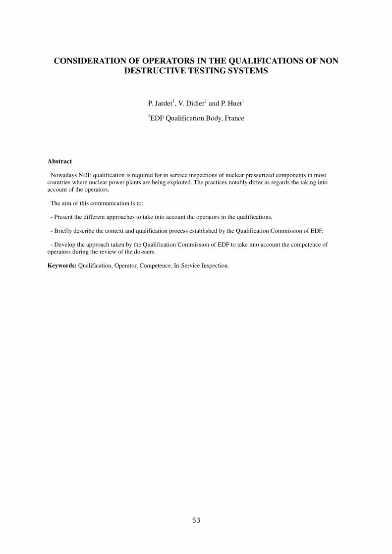
CONSIDERATION OF OPERATORS IN THE QUALIFICATIONS OF NON
DESTRUCTIVE TESTING SYSTEMS
P. Jardet1, V. Didier
1 and P. Huet
1
1EDF Qualification Body, France
Abstract
Nowadays NDE qualification is required for in service inspections of nuclear pressurized components in most
countries where nuclear power plants are being exploited. The practices notably differ as regards the taking into
account of the operators.
The aim of this communication is to:
- Present the different approaches to take into account the operators in the qualifications.
- Briefly describe the context and qualification process established by the Qualification Commission of EDF.
- Develop the approach taken by the Qualification Commission of EDF to take into account the competence of
operators during the review of the dossiers.
Keywords: Qualification, Operator, Competence, In-Service Inspection.
53

1. Different Qualification Approaches – Taking operators into account
Providing a performance guarantee for the tests carried out on in-service surveillance of components important for
security or safety (see example in Figure 1) is an expectation common to various industries in many countries. As far as the
nuclear industry is concerned, the question on NDE reliability was asked in the mid-sixties, in the framework of an
American committee involved in the behaviour of reactor pressure vessels (specifically for ultrasonic testing): the Pressure
Vessel Research Committee (PVRC). International programs based on blind trials aimed at comparing the results of the
various procedures and teams operating worldwide were therefore launched.
The variability of the results obtained led to the establishment of performance demonstration methodologies and to
gradually taking into account the obligation to qualify in-service inspections in the regulations of the various countries.
Figure 1. Examples of primary circuit components in the EDF fleet, inspected with NDE systems submitted to
qualification
The references dedicated to qualification or performance demonstration of NDE systems which are applied in Europe
and in the United States for the in-service inspection of nuclear components are the following (see their distribution in
figure 2):
- the ASME Code, section XI appendix VIII [1],
- the European methodology by ENIQ (European Network for Inspection Qualification) [2],
- the RSE-M code, appendix 4.3 [3],
- the IAEA methodology for VVER type reactors [4].
In some countries, article 14 in the ASME code section V [5] is used complementarily to the references listed above.
54

Figure 2. Qualification references used in Europe and North America
In the following sections, we shall limit our analysis to the Appendix VIII of section XI in the ASME code, the ENIQ
methodology, and the appendix 4.3 in the R-SEM code. Indeed the IAEA methodology established in the 90s to
consolidate the safety of VVER plants built in Eastern Europe is directly derived from the ENIQ methodology. As for
article 14 in the ASME V, not specifically dedicated to nuclear components, it is used in some countries complementarily
to section XI in the ASME XI.
A comparison between the main elements in the three references is given in Table 1.
When specifically comparing the dispositions for taking into account operators, then significant differences exist
between the three qualification references.
Appendix VIII of ASME XI is essentially based on blind trials on blocks featuring artificial defects. Operators’
qualification is almost not separated from the NDE system qualification.
The ENIQ methodology clearly separates the system qualification (NDE equipment and procedure), based on technical
justifications complemented or not by open trials (defects with characteristics known by the operators), from personnel
qualification, which, if requested or required, is performed through blind trials (defects in mock-ups are not known by the
operators, the comparison between test results and defects characteristics is carried out by a specific organisation).
Finally, the RSE-M, rather similar to the ENIQ methodology as far as system qualification is concerned (technical
justifications, open trials on realistic mock-ups…), does not request blind trials to qualify the personnel but prescribes that
the operators expected competencies be formalised and justified as well as the dispositions taken to reach them and verify
them. The complete file is submitted to a qualification body.
55

Items ASME XI, Appendix VIII ENIQ Methodology RSE-M Appendix 4.3
Scope Ultrasonic examination for
crack detection and sizing (mainly
fatigue cracks)
Any inspection (any method)
enabling detection, sizing and
location of a specified defect.
Any inspection (any method)
enabling detection, sizing and
location of a specified defect, or
the surveillance for in-depth
defence when no defect is
postulated
Input data - Component type
- Examination procedure
-Description of UT equipment.
- qualification objectives (what
shall be demonstrated)
- precise description of the
components to be inspected.
- size, orientation, location and
morphology of the defects to be
detected/sized
- inspection objectives
- precise description of the
components to be inspected.
- size, orientation, location and
morphology of the defects to be
detected/sized
- or conventional threshold to
be applied (defence in depth)
Technical
Justifications
(TJ)
Not required Recommended, TJs are based
on:
- results of tests on blocks or
mock-ups
- engineering reasoning
- elements of feedback from
experience
- elements from previous
qualifications
- modelling results
- laboratory studies
-…
Required, separating the NDE
technique, and the in-situ
implementation.
TJs are based on:
- results of tests on blocks or
mock-ups
- engineering reasoning
- elements of feedback from
experience
- elements from previous
qualifications
- modelling results
- laboratory studies
-…
Mock-ups, test
blocks;
Associated
trials
Blind trials are required. The
test blocks must fulfil precise
specifications. (dimensions,
defect type: crack, semi-elliptic
notch …), and number of defects
per size category.
Acceptance criteria are defined
in terms of minimum number of
defects to be detected, maximum
number of false calls and RMS
error on height measurement.
It is found preferable to perform
open trials for the qualification of
the procedure and the equipment
and blind trials for personnel
qualification.
Mock-ups are intended to be
representative of the components
but the use of simpler mock-ups is
also accepted (extrapolation shall
then be justified).
Open trials are required for
NDE systems where searched
defects are specified.
The number and type of defects
in the test mock-ups is justified in
a case-by-case mode, coherent
with the TJs.
Trial acceptance criteria are also
defined in a case-by-case mode
coherent with TJs.
NDE
Equipment,
procedure
qualification
NDE equipment, procedure and
personnel are qualified
Procedure and NDE equipment
may be qualified by TJ, open
and/or blind trials.
Required
Personnel
Qualification
See above. If required, then a combination
of the following :
- certification according to a
national NDE certification system
- theoretical exam and/or open
trial
- blind trial
Not required.
The procedure shall specify
whether a specific training or
qualification is expected. In the
latter case, the qualification
content is documented (training,
test…).
Qualification
Body
Not specified Required : independent, third
party, internal or ad-hoc
Required, organisation in
conformity with ISO 17020
Table 2. Comparison between ASME XI Appendix VIII, ENIQ Methodology and RSE-M appendix 4.3 references
56

2. Qualification Process in place at EDF- Role of the Qualification Commission Section
EDF, a pressurised water reactor Utility, is bound as such to obey the 10 November 1999 order [6], which defines the
expectations as far as NDE system qualification is concerned. As a reminder:
- obligation to qualify NDE systems prior to their implementation,
- qualification consists in the demonstration that inspection performance is sufficient to reach the expected
objectives when the degradation mode is presumed or established, or to specify the performance in all other cases.
- qualifications shall be awarded by a competent independent authority, accredited by COFRAC or equivalent,
chosen by the Utility,
- NDE operators implementing those systems shall be certified by an independent organisation.
Note: the application letter of the order stipulates that qualification shall « specify how the specific competency of
operators is verified for the operation submitted to qualification».
The Commission, internal organization accredited by COFRAC, consisting of a college of experts, is the body chosen by
EDF to award qualification of NDE systems in the framework of the compliance with the 10 November 1999 order.
Several actors are involved in the qualification process (see Figure 3):
- the Utility, defines the objectives in terms of performance requirements,
- the Instruction organisation to which the utility has delegated the project management for the design and
constitution of the qualification file, establishes a checking form specifying the performance and presents elements of
its demonstration (gathered in a qualification synthesis) to the Commission,
- the Contractor, who designs and develops the NDE system and establishes the elements of the qualification file,
assists the Instruction organisation during the presentations to the Commission.
The Commission testifies the qualification of the NDE systems by examining the files submitted to it. The files brought
before the Commission are in conformity with qualifications according to appendix 4.3 of the RSE-M code.
Figure 3: EDF qualification process, links between parties
57

3. Approach chosen by EDF’s qualification Commission for taking operators into account.
The Commission examines the conformity of a file in three steps in connection with the qualification process:
- the first step occurs at the stage of the qualification approach and of the design of test blocks and mock-ups,
- the second one, prior to the performance of qualification trials,
- the third and last one, once the trials have been carried out and the elements of the file are gathered.
At each of these steps, the Commission gives an approval or formulates reservations or a refusal. The third step
ratifies the award of the qualification.
Elements concerning the operators are examined at each step.
3.1 Examination of the qualification approach and of the design of test blocks and mock-ups Subsection
At this stage, the Commission assesses that the defects which will be in a block are appropriate for the performance to be
demonstrated. Defects shall be representative of the investigated degradation modes and the physical phenomenon being
exploited. Concerning more specifically operators, the Commission verifies that the difficulties in accessing the area to be
examined (see the example in Figure 4) have actually been taken into account in the actions planned (qualification
approach) and in the test blocks. It must be stressed that this notion of accessibility and neighbourhood constraints has a
most significant impact when the inspection is carried out manually (probe scanning movement, source and film
positioning more or less difficult ….). For automated inspections, these considerations essentially influence the design of
robotic tools. However the set-up and steering of a manipulator generally requires adequate competencies from the
operators.
Figure 4. Example of manual UT test performed in a rather awkward position
58

Figure 5. Example of robot installation for automated UT on the pressurizer surge line
3.2 Examination prior to the performance of the tests
When presenting qualification trials, all the equipment (instrument, probe, manipulator…), the software and the
inspection procedure are defined and settled (the inspection procedure shall specify the operators’ qualifications required
for its implementation). The constitution of the inspection team is also defined. The qualification trials are aimed at
carrying out all the phases of the inspection procedure on blocks with realistic defects and to verify the achievement of the
assumed performance.
The Commission makes sure that inspection conditions are actually representative of the environmental constraints in
the real situation as far as obstacles, nearby walls and inspection zone location are concerned. In the case of manual NDE,
the Commission sees that inspection in the most unfavourable positions (for example in UT, testing in lower position, close
to the ground….) be performed. The Commission is led to ask the trial supervisors to specifically report that the inspection
is operable and to point out any specific skill needed for a correct inspection.
3.3 Examination at final stage
At final stage and complementarily to the examination before tests, the Commission makes sure that the prescriptions in
the inspection procedure concerning the qualification of operators are sufficient. In the case of manual NDE, a certification
in accordance with ISO 9712 may be enough. However, complements are sometimes indispensable due to the specificity
of the inspection. It is frequently the case for automated inspections which require on the one hand a specific know-how for
the installation of the manipulator on the component (see illustration in figure 5) and on the other hand, the control of
signal analysis software and the associated analysis rules, (examples of automated UT and ET inspection signals are shown
in figure 6 and 7). The Commission then examines the pedagogic files including the specific training syllabi and the
conditions for the delivery of a qualification for such or such position in the inspection team. 59

Figure 6. L0° UT and TOFD inspection of bottom mounted instrumentation nozzles: Example of signals
Figure 7: SG tube inspection using a rotating probe: examples of ET signals
4. Conclusion
NDE performance partly depends on the competencies of the personnel carrying out the inspections. The main NDE
system qualification references implemented for the in-service inspection of nuclear plant components i.e. Appendix 8 of
ASME XI, the ENIQ qualification methodology and appendix 4.3 of the RSEM, deal with this point but in different ways.
Indeed, performance demonstration in conformity with the ASME code covers altogether the procedure, the equipment
and the personnel and is pronounced for each operator implementing the inspection, while qualification in accordance with
the R-SEM code is established for one system, taking into account the expected necessary competencies; the ENIQ
methodology includes individual qualification prescriptions for operators without explicitly requiring them.
EDF’s qualification commission, in conformity with the regulatory national reference, examines the files and awards
qualification of NDE systems excluding the personnel.
While not formally considering the qualification of each operator in charge of implementing an NDE system submitted
to qualification, the Commission is extremely careful regarding the adequacy of the operator’s competencies required to
achieve the expected performance. The three steps of the conformity examination by the Commission are turned into
account to assess the dispositions taken to ensure the competency of operators.
60

References
[1] ASME Section XI - Rules for Construction of Nuclear Facility Components, 2011.
[2] ENIQ- European Methodology for Qualification of Non-Destructive Testing- 3rd
Issue, 2007.
[3] RSE-M - Règles de surveillance en exploitation des matériels mécaniques des îlots nucléaires REP –
AFCEN, 2010.
[4] IAEA-EBP-WWER-11 - Methodology for Qualification of In-Service Inspection Systems for WWER
Nuclear Power Plants, 1998.
[5] ASME Section V - Non-destructive Examination, 2011.
[6] 10 November 1999 order, concerning operating surveillance of the main primary and secondary circuits in
pressurised water reactors.
61

Modeling-assisted justification of the ultrasonic inspection of a clad REPAIr in
Ni-BASED ALLOY
LHUILLIER Pierre-Emile1, GELEBART Yann
2, CHASSIGNOLE Bertrand
1, DEYDIER Sébatien
2
1 EDF R&D, MMC Department, EDF Lab Les Renardières, France
2 EDF CEIDRE, Saint Denis, France
Abstract
The Ni-based alloy clad repairs encountered on the primary circuit of nuclear power plant exhibit complex anisotropic
and heterogeneous structures which lead to important disturbances of the ultrasonic waves. During ultrasonic
inspections, the structure is thus responsible for beam skewing or splitting, attenuation, and the appearance of spurious
echoes. The objective of this study is to show the benefits of the numerical simulation by finite elements in the frame
of the performance evaluation of a Non Destructive Examination (NDE) system.
The inspection of a clad repair has been investigated for two particular welding positions with the use of the finite
element code ATHENA 2D. The description of the weld repair was obtained from metallurgical observations. The
simulation of the amplitudes of the tip diffraction echo of notches and side drilled hole echoes located in the weld were
compared with experimental acquisitions. A good agreement between simulation and experiment was found. In
particular, the simulation tool has enabled to predict the influence of the welding position on the inspection
performances.
In addition the implementation of the complex and anisotropic structure of the weld has enabled to highlight particular
configurations which lead to the appearance of spurious echoes. The origin of these echoes was identified thanks to
advanced simulation tools such as the visualization of the ultrasonic beam and wavefront propagation. Finally, this
study demonstrates that the finite elements simulation code which takes into account the complexity of the clad is an
efficient tool both to demonstrate the performance of the NDE system and also to identify the configurations which
will require a particular analysis.
1. Introduction For several years, EDF R&D has launched a consistent research program on ultrasonic inspection of austenitic
stainless steel welds. In particular, a methodology was developed to improve the understanding of the disturbances of
the ultrasonic waves (beam deviation, distortion and attenuation) in components welded with a SMAW process
(Shielded Metal Arc Welding) [1]. This methodology, based on UT modelling, was applied to various components
such as: a butt weld of the surge line [2], the branch pipe weld connecting the Chemical and Volume Control System
(CVCS) and the primary coolant piping of PWR circuits [3], or even nickel-based alloy welds [4]. This study deals
with the application of the methodology to a Ni based alloy clad weld repair of the primary circuit of Nuclear Power
Plant. This work is based on both experimental analyses on representative welded mock-ups and the use of a finite
element modeling tool (ATHENA 2D code) which allows realistic simulation of the propagation phenomena in
complex mediums. The aim of this study was to provide quantitative and qualitative estimations of the performances
of the ultrasonic NDE system.
2. Inspection configuration
2.1. Inspected component
The inspected component is a special area of the inner surface of cladded primary circuit pipes. During manufacturing,
defects were revealed by Non Destructive Examinations, the affected zone was removed by machining and repaired by
manual Shielded Metal Arc Welding (SMAW). The welding material is a Ni based alloy (alloy 182). The generic
geometry of the welded zone is given in Figure 1. The inspection zone is thus composed of a trapezoidal welded zone
filled by manual multi pass welding.
Owing that the components have been repaired in place and that the repaired defects might have been observed all
around the circumference of the pipe, the welding position might differ from one weld to another. In addition, the
results of former studies [5] suggest that the welding position is most likely to show a major influence on the
performances of the ultrasonic NDE system. Two particular welding positions have been analyzed: the Horizontal /
vertical and Flat welding position (see Figure 1).
62

Figure 1 : Schematic view of (left) horizontal / vertical
and (right) Flat welding position.
Base metal
He D1 D2
Austenitic cladding eNi based alloy
αR
αL
8 MHz ultrasonic focused probe
h
Figure 2 : Generic geometry of the weld repair inspected
area.
Table 1 : Geometric parameters of the configuration.
Left and right weld chamfer angle αL & αR ° 10 to 40 depending on the welding position
Weld depth h mm 20
Cladding thickness e mm 9
2.2. NDE System
The weld repair is inspected by a focused single element ultrasonic probe at the frequency of 8 MHz with longitudinal
waves. The probe is designed in order to get a good sensitivity of the ultrasonic beam in the range of 3 to 10 mm
depths in steel. The main characteristics of the inspection probe are given in Table 2.
Table 2 : Characteristics of the ultrasonic inspection probe.
Mode
Immersed / focused
P-Wave
Frequency 8 MHz
Water height 60 mm
Refraction angle 50°
3. Material and method
3.1. Mock-ups
A preliminary study has thus been performed in order to evaluate the impact of the welding position on the inspection
performances. The weld microstructures have been modeled with the MINA [6, 7] code for both flat and horizontal /
vertical welding positions and used as input of the finite elements code ATHENA 2D for the weld description. The
results of this study have shown that the horizontal / vertical welding position might affect the inspection
performances. The horizontal / vertical welding position exhibits a main columnar grain orientation at about 45° from
the piece surface normal. Thus in the particular inspection configuration displayed in Figure 3 (left), the angle between
the ultrasonic beam and the main axis of the columnar grain is close to 90°. In this configuration the ultrasonic
attenuation reaches its higher value as it is shown on the Figure 3 (right). It induces a drastic decrease of the echo
amplitude of calibrated defects located in the weld. In particular, the echo amplitude of a 2 mm side drilled hole (SDH)
at the depth of 12 mm is 17 dB lower than the same SDH located in the base metal. As a comparison, the modeling
predicts that the same SDH located in a flat weld exhibits an echo which amplitude is only 2.5 dB lower than the
reference configuration. The conclusion of this preliminary study has led to the manufacturing of 2 different
representative mock-ups respectively executed in horizontal / vertical and flat welding position (see Figure 1).
Different calibrated flaws have been machined in the mock-ups:
- 4 SDH, at the depth of 9, 15, 15 and 9 mm (of length 80 mm)
- 3 vertical notches in the weld with a tip located at the depth of 5 and 10 (of length 15 mm).
The Figure 4 and Table 3 show the location of the calibrated defects in the flat and horizontal / vertical mock-ups.
63

8 MHz
focused probe
Beam / grains angle
~90°Columnar
grains main
orientation
50°
Horizontal / vertical weld
Side Drilled Hole
Echo amplitude
-17 dBas regard to weld-free configuration
0 10 20 30 40 50 60 70 80 90
0,0
0,1
0,2
0,3
0,4
Atten
uation
(dB
/mm
)
Beam / columnar grains angle (°)
Figure 3 : (Left) Special inspection configuration of the horizontal / vertical welding position causing a highly
degraded inspection performances. (Right) Variations of the anisotropic ultrasonic attenuation as a function of the
angle between the ultrasonic beam and the columnar grain axis.
Figure 4: General Implantation scheme of the calibrated defects in the (Left) horizontal / vertical (Right) and Flat
welding position.
Vetcical Notch
Side Drilled Hole
Legend
VN1
VN2
VN3_REF
SDH1 to 4
A A'
B B'
B B' A A'
VN3_REFVN2 10 10
Section A -A' et B -B'
Horizontal / vertical welding position
B B'A A'
VN3_REFVN2 10 10
Section A -A' et B -B' Flat welding position
Top view
Both mock -upsC C'
C
SDH1
9
Section C -C'
Horizontal / vertical welding position
C'
15 C C'
Section A -A' et B -B' Flat welding position
9 15
64

Table 3: Dimensions of the calibrated defects.
Horizontal / vertical and Flat welding position mock-up
Vertical Notch (VN) Side Drilled Holes (Φ 2mm)
Defect Height (mm) Length (mm) Defect Depth (mm) Length (mm)
VN1 5 15 SDH1 9 80
VN2 10 15 SDH2 15 80
VN3_REF 10 15 SDH3 15 80
SDH4 9 80
3.2. Modeling approach – The ATHENA Code
The main features of the 2D version of the ATHENA code are presented here, more details can be found in [8].
ATHENA 2D is a finite element code for elastodynamic developed by EDF R&D. The code solves the equation of
elastodynamic expressed in a mixed formulation combining stress and velocity terms. The code is dedicated to the
simulation of wave propagation in all kinds of elastic media and in particular, heterogeneous and anisotropic
materials. One important feature of the code is the use of the fictitious domain method [9]. It relies on the
combined use of a regular discretization of the calculation zone with a non-regular meshing of the defects. It
takes advantage of the rapidity of regular mesh calculation with the possibility to model arbitrary shaped defects.
Furthermore, ATHENA 2D gives the possibility to use Perfectly Matched Layers (PML) to define the
boundaries of the calculation domain [10]. The use of PML removes spurious reflections on artificial edges of the
calculation zone and thus enables to model virtually infinite components. Finally, ATHENA 2D integrates the
possibility to simulate various inspection configurations (pulse-echo, tandem, TOFD) with a wide range of
transducers (single element and phased array), inspection mode (contact or immersion), materials and defects. The code has been widely used by EDF to simulate the inspection of complex structures such as austenitic welds [4,
11, 12].
3.3. Weld characterizations and simulation inputs
On each mock-up, a sample has been removed for metallographic characterization (see Figure 3 for position). Figure 5
shows the metallographic pictures and the resulting grain orientation maps. The regular discretized orientation maps
have been obtained with an image processing tool based on Hough transform. Those maps have been integrated as
input in the ATHENA 2D code to describe the welds. Each square of the maps represents an homogeneous area of the
weld with anisotropic and constant elastic properties. The contrast of acoustic impedance from one area to another –
which lies at the origin of the beam disturbances in the weld – comes from the difference of grain orientation from the
different zones. The elastic properties assigned to each area are the same and are given in Table 4.
3.4. Data analysis
In order to ensure the comparison between the experimental and simulated data, each echo amplitude, respectively in
experiment and simulation, have been compared to the echo amplitude of a SDH located at the depth of 10 mm in an
isotropic and homogeneous ferritic steel plate.
For the notches, only the tip diffraction echoes have been analyzed.
Horizontal / Vertical welding position Flat welding position
Figure 5 : (Top) Metallographic cliches of the weld area. (Bottom) Columnar grains orientation map obtained from an
image processing tool based on Hough transform (regular grid of 2*2mm²).
Table 4 : Elastic coefficients (in GPa) of Ni-based alloy (alloy 182) deposited by Shielded Metal Arc Welding
(SMAW). The 3rd
axis corresponds to the fiber axis.
C11 C22 C33 C44 C55 C66 C12 C13 C23
265 264 247 111 111 84 121 139 140
4. Results
4.1. Comparison between experimental and modeling data
Firstly the experimental and simulated data have been compared in order to validate the simulation conditions. The
Table 5 compares the simulated and experimental amplitudes of the notch tip diffraction echoes and of the SDH
echoes. The data are given for both Horizontal / Vertical and Flat welding position mock-ups.
65

Last column of Table 5 also displays the differences between simulation and experiment for a given defect. A positive
value corresponds to an overestimation of the echo amplitude by the simulation.
For the SDH, the simulation results are very close to the experimental data since the larger difference between
experiment and simulation is -3.2 dB. In addition, the average of the difference between simulation and experiment for
SDH echoes is 1.7 dB. Concerning the notch echoes, only 2 experimental data are available for the horizontal / vertical
mock-up. Nevertheless for those 2 data, the maximum difference between simulation and experience is -3.9 dB.
On the Flat mock-up the tip diffraction echoes are always slightly overestimated by the simulation and the higher
discrepancy is 5.5 dB.
Nevertheless the average of the simulation to experiment difference on the notch echoes is only 2.3 dB.
Finally, it can thus be considered that the simulation configuration based on a fine characterization of the weld
structure and the implementation of a model for the scattering attenuation shows rather good performances to predict
the amplitude of SDH echoes and vertical notch tip diffraction echoes.
Table 5 : Comparison of the experimental and simulated amplitudes of defect echoes. Diff = Expe / Simulation
difference
Horizontal vertical mock-up Flat mock-up
Mock-up Dir Ref Depth Expe Simulation Diff Expe Simulation Diff
Notch
Data
D1 VN1 5 not detected -18 _ -21,4 -20,4 1
VN1 10 -26,7 -26,6 0,1 -26,7 -23,4 3,3
D2 VN2 5 -20,5 -24,4 -3,9 -18,7 -18,5 0,2
VN2 10 not detected -34,6 _ -28,6 -23,1 5,5
SDH
Data
D2 SDH1 9 -14,9 -11,8 3,1 -11,5 -10 1,5
SDH2 15 -27,2 -30,4 -3,2 -18,7 -18,9 -0,2
D1 SDH3 9 -15,9 -16,3 -0,4 -10,2 -9,1 1,1
SDH4 15 -19,4 -21,8 -2,4 -16,7 -18,7 -2
4.2. Artifact identification
In addition to the good prediction of the echo amplitudes, the simulation tool also enables to reproduce the beam
disturbances. In particular, the heterogeneous orientation map of the weld causes beam splitting and deviation which
might be at the origin of the appearance of artifacts. To highlight this phenomenon, a particular case of inspection is
exposed in this section.
The configuration corresponds to the inspection of a 10 mm notch located on the bottom side of horizontal / vertical
welding process. Figure 6 shows the inspection configuration and the resulting BScan is displayed on Figure 7.b. In
this particular configuration the BScan shows two particular echoes, denoted Echo A and Echo B on Figure 7.b. For
comparison, Figure 7.a. displays the BScan of a similar notch located in an isotropic and homogeneous base metal.
One can note the tip diffraction echo is clearly seen and that Echo A is not present. The Echo A could be interpreted as
the tip diffraction echo of the notch. Nevertheless, complementary simulations – not displayed here – suggest that the
origin of this echo is not due to the notch tip diffraction. Indeed, the amplitude and position of Echo A does not change
if the height of the notch is increased up to 20 mm.
The visualization of the ultrasonic beam at the position of Echo A and Echo B, displayed on Figure 8 helps to
understand the origin of both echoes.
On Figure 8.a, the ultrasonic beam exhibits a division and deviation on the upper part (marked with the white arrow).
The deviated beam propagates quasi perpendicularly to the notch and thus interacts specularly with it. The reflected
beam is thus also quasi perpendicular to the notch. Moreover, the analysis of the local anisotropy of the weld in this
region has shown that the local orientations are favorable to the skewing of the beam in the direction of the probe. The
appearance of this echo is thus not related to the notch height. In particular conditions, the echo can be misinterpreted
as a notch tip diffraction echo and thus cause a severe overestimation of the defect height.
The origin of Echo B is more difficult to identify. Nevertheless a fine analysis of the wavefront propagation suggest
that this echo can be attributed to a mode conversion after reflection at the notch (LT) followed by a wave deviation
due to the anisotropic local structure.
In this frame, the use of the simulation code with a fine description of the microstructure enables to highlight special
configurations which might show complex ultrasonic signature or artifact. The numerical simulation can thus become
a useful tool to drive the focus of the expert in charge of the interpretation of a particular complex result.
66

10Cladding
Base metal
Horizontal / Vertical
weld
Figure 6 : Simulation configuration of the inspection of a
10 mm notch located on one side of the horizontal /
vertical weld.
a. b.
Figure 7: Simulated BScan of the inspection of a 10 mm
notch located (a) in a homogeneous and isotropic metal
(b) on one side of the horizontal / vertical weld.
US Field
Echo A
US Field
Echo BNotch
H= 10 mm
Notch
H= 10 mm
a. b.Figure 8 : Simulated ultrasonic field of the inspection of a 10 mm notch located on one side of the horizontal / vertical
weld.
5. Conclusion The objective of this study was to evaluate the performance of an NDE system for the inspection of austenitic weld
repairs. In particular, the aim was to investigate the influence of the welding position on the ultrasonic beam
disturbances.
Firstly the microstructures resulting from different welding positions (from flat to horizontal / vertical) have been
obtained via metallographic observations. The metallurgical analysis enables to get the grain orientation map which is
used as input of the Finite Elements code ATHENA 2D for the fine description of the anisotropic and heterogeneous
weld structure. The modelling configuration enables to evaluate the performance of the NDE system. Two particular
welding positions have been investigated with the use of the finite element code ATHENA 2D. The results were
compared with experimental acquisitions and a good agreement was found between simulation and experiment.
Taking into account the complex and anisotropic structure of the weld in ATHENA simulations has enabled to
highlight particular configurations which lead to the appearance of spurious echoes. Indeed, the anisotropy of the weld
may induce an additional echo which if misinterpreted may lead to a drastic overestimation of the height.
Finally, the simulation code which accounts for the complexity of the weld appears to be an efficient tool both to
demonstrate the performance of the inspection process and also to identify the configurations which will require a
particular analysis.
References
1. Dupond, O., et al., Methodology for modelling ultrasonic inspection of an austenitic stainless steel weld. 6th
ICNDE, 2007.
2. Chassignole, B., et al., Ultrasonic modelling of austenitic stainless steel welds: improvement in the
comprehension of anisotropic and heterogeneous structure effects. 4th ICNDE, 2004.
3. Chassignole, B., O. Paris, and E. Abittan. Ultrasonic examination of a CVCS weld. in 6th International
Conference on NDE in Relation to Structural Integrity for Nuclear and Pressurized Components, Budapest,
Hungary. 2007.
67

4. Chassignole, B., et al. Ultrasonic examination of a weld repair in Ni-based alloy. in 9th International
Conference on NDE Relation to Structural Intergity for Nuclear and Pressirized Components. 2012. Seattle,
Washington, USA: European Commission.
5. Chassignole, B., Influence de la Structure Métallurgique Des Soudures En Acier Inoxydables Austénitique
sur Le Contrôle Non Destructif. 2000, INSAL: Lyon. p. 217.
6. Apfel, A., Modélisation de l’orientation cristalline des soudures multi-passes en acier inoxydable
austénitique : application au contrôle non destructif ultrasonore - Bilan du in ECOLE DOCTORALE DE
PHYSIQUE, MODELISATION,
ET SCIENCES POUR L’INGENIEUR. 2005, Université de la Méditerranée.
7. Moysan, J., et al., Modelling the grain orientation of austenitic stainless steel multipass welds to improve
ultrasonic assessment of structural integrity. International Journal of Pressure Vessels and Piping, 2003.
80(2): p. 77-85.
8. Becache, E., P. Joly, and C. Tsogka, Fictitious domains, mixed finite elements and perfectly matched layers
for 2D elastic wave propagation. 2000.
9. Bécache, E., P. Joly, and C. Tsogka, An analysis of new mixed finite elements for the approximation of wave
propagation problems. SIAM Journal on Numerical Analysis, 2000. 37(4): p. 1053-1084.
10. Berenger, J.-P., A perfectly matched layer for the absorption of electromagnetic waves. Journal of
Computational Physics, 1994. 114(2): p. 185-200.
11. Chassignole, B., et al., Modelling the attenuation in the ATHENA finite elements code for the ultrasonic
testing of austenitic stainless steel welds. Ultrasonics, 2009. 49(8): p. 653-658.
12. Chassignole, B., et al., Ultrasonic and structural characterization of anisotropic austenitic stainless steel
welds: Towards a higher reliability in ultrasonic non-destructive testing. NDT & E International, 2010.
43(4): p. 273-282.
68
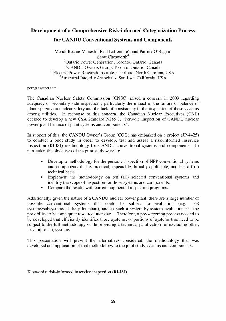
Development of a Comprehensive Risk-informed Categorization Process
for CANDU Conventional Systems and Components
Mehdi Rezaie-Manesh1, Paul Lafreniere
2, and Patrick O’Regan
3
Scott Chesworth4
1Ontario Power Generation, Toronto, Ontario, Canada 2CANDU Owners Group, Toronto, Ontario, Canada
3Electric Power Research Institute, Charlotte, North Carolina, USA
4Structural Integrity Associates, San Jose, California, USA
The Canadian Nuclear Safety Commission (CNSC) raised a concern in 2009 regarding
adequacy of secondary side inspections, particularly the impact of the failure of balance of
plant systems on nuclear safety and the lack of consistency in the inspection of these systems
among utilities. In response to this concern, the Canadian Nuclear Executives (CNE)
decided to develop a new CSA Standard N285.7, “Periodic inspection of CANDU nuclear
power plant balance of plant systems and components”.
In support of this, the CANDU Owner’s Group (COG) has embarked on a project (JP-4425)
to conduct a pilot study in order to develop, test and assess a risk-informed inservice
inspection (RI-ISI) methodology for CANDU conventional systems and components. In
particular, the objectives of the pilot study were to:
• Develop a methodology for the periodic inspection of NPP conventional systems
and components that is practical, repeatable, broadly-applicable, and has a firm
technical basis.
• Implement the methodology on ten (10) selected conventional systems and
identify the scope of inspection for those systems and components.
• Compare the results with current augmented inspection programs.
Additionally, given the nature of a CANDU nuclear power plant, there are a large number of
possible conventional systems that could be subject to evaluation (e.g., 168
systems/subsystems at the pilot plant), and as such a system-by-system evaluation has the
possibility to become quite resource intensive. Therefore, a pre-screening process needed to
be developed that efficiently identifies those systems, or portions of systems that need to be
subject to the full methodology while providing a technical justification for excluding other,
less important, systems.
This presentation will present the alternatives considered, the methodology that was
developed and application of that methodology to the pilot study systems and components.
Keywords: risk-informed inservice inspection (RI-ISI)
69

Development of ultrasonic techniques for the examination of ITER VV T-joint
welds
P.I. Resa1, F. Fernández
1, C.M. Pérez
1, R. Martínez-Oña
1, P. Vessio
2, A. Dans
3, A. Bayón
3
1 Tecnatom Group, Avda. de Montes de Oca 1, 28703 San Sebastián de los Reyes, Spain
2Ansaldo Nucleare, C.so F.M. Perrone 25,16152 Genova, Italy
3Fusion for Energy, c/ Josep Pla 2, 08019 Barcelona, Spain
Abstract
The vacuum vessel of International Thermonuclear Experimental Reactor (ITER) is a double wall torus made of
austenitic stainless steel that houses the fusion reaction and acts as a first safety containment barrier. A consortium led
by Ansaldo Nucleare (including Mangiarotti and Walter Tosto) is in charge of manufacturing seven out of its nine
sectors. Tecnatom is responsible for developing the ultrasonic inspection techniques (UT) for the examination of one
and two-side access welds.
Two-side access welds –to be examined by UT– consist of full penetration welded T-joints with two different
chamfer geometries: (i) Form B, with rib thicknesses between 20 and 80 mm and plate thicknesses between 40 and 60
mm; and (ii) Form C, with rib thickness of 40 mm and plate thickness of 60 mm.
Demonstration of the non-destructive inspection procedures for thick austenitic welds is required by RCC-MR Code.
Detection and characterization capabilities have to be shown in representative test pieces with a wide range of
postulated defects, simulated by side drilled holes and notches (parallel and transverse to the weld).
Tecnatom has developed a fully comprehensive set of ultrasonic techniques, based on phased-array (PA) technology,
including multiple beam angles and different wave modes. Normal incidence, sectorial longitudinal and sectorial shear
wave techniques are simultaneously applied using one single linear PA probe. Space limitations and accessibility
interferences have been overcome by the generation of delay laws without the use of refraction wedges, shear mode
included.
Tecnatom’s approach significantly increases the capabilities of the ultrasonic method in terms of detection and
characterization, at the same time as inspection, calibration and verification activities are notably simplified.
Keywords: ITER, ultrasonic, phased-array, austenitic steel, T-joint.
1. Introduction
The Vacuum Vessel (VV) is the largest component of the International Thermonuclear Experimental Reactor (ITER)
machine. It is composed of nine sectors made of thick austenitic stainless steel 316L (N) – IG ITER Grade. All of the
sectors are similar in shape and are built with double-walls containing shielded plates. Forty four additional ports
allow access and instrumentation during fabrication and further vacuum vessel maintenance (Figure 1).
Both the design and manufacturing of ITER VV and the corresponding non-destructive examinations must be
compliant with the requirements of the 2007 edition of RCC-MR Code [1]. This Code requires radiographic testing
(RT) of all category 1 and 2 welds of the component. Most welded joints have conventional configurations and can be
inspected by RT to ensure their integrity. However, given the geometric characteristics and the construction sequence,
a significant number of welds are not accessible from both sides. The alternative consists of using ultrasonic
techniques (UT), being their qualification required according to CEN/TR 14748:2004 code [2]. Main types of welds to
be examined by ultrasonic testing are: (1) longitudinal and circular (Flexible Housing) welds with access only from
one-side, and (2) T-joint and cruciform welds with access from at least two surfaces.
70

Seven out of the nine sectors of the ITER VV are being manufactured by the European consortium of AMW
(Ansaldo Nucleare S.p.A, Mangiarotti S.p.A and Walter Tosto S.p.A) and Tecnatom is responsible for developing and
qualifying the inspection system and non-destructive techniques [3,4].
Figure 1. ITER VV sector (courtesy of Fusion for Energy)
Due to the access limitations, the geometrical constraints, the diversity of configurations, the challenging postulated
defects in terms of sizes and orientations and the difficulties on UT of austenitic material, the need for advanced UT
techniques is evident.
The present paper focuses on the advances in the development of ultrasonic techniques for the non-destructive
inspection of ITER VV T-joint welds.
2. Material and methods
2.1 Test pieces
Test pieces, reproducing the geometry and characteristics of two-side access joints of ITER VV and containing
representative artificial defects, are required by RCC-MR Code [1] to demonstrate that the ultrasonic inspection
procedures are able to identify and characterize the postulated defects. These welds have different bevel forms (B, C,
CA) and are filled by different welding processes (GTAW and SMAW). The required examination volume includes
100% of the fused material plus 10 mm of base metal corresponding to the heat affected zone adjacent to the weld
(Figure 2).
Equatorial port
Upper port
Lower port
Flexible housing
Outer shell
Inner shell
Poloidal rib
Toroidal rib
71

Form B Form C
Figure 2. Weld forms, thicknesses and examination volumes of ITER VV T-joint welds (UT).
2.2 Postulated defects
Postulated defects are volumetric and planar (open and embedded), and with orientations longitudinal and transversal
to the weld. These reflectors have been reproduced in the test pieces by:
- Side-drilled holes (SDH), 2 mm in diameter
- Open and embedded notches of different heights (open notches: 1.0, 1.3, 2.0 and 2.7 mm; and embedded notches:
1.3, 2.7 and 5.3 mm), depending on the thickness of the rib.
According to RCC-MR code [1]:
- Any planar defect is unacceptable.
- For volumetric defects, criteria based on amplitude and length must be applied.
2.3 Ultrasonic techniques
RCC-MR code [1] recommends the use of two refraction angles, between 35º and 70º, using shear waves, with a
difference of 15º at least, that are selected based on the weld geometry and perpendicular to the bevel. Besides, weld
volume must be examined at least in two directions.
For the ITER VV T-joint welds, in addition to code recommendations, a more comprehensive set of ultrasonic
techniques has been developed including multiple beam angles and different wave modes. Normal incidence, sectorial
longitudinal, sectorial shear and Creep wave techniques have been proposed, which can be simultaneously applied
using one single linear PA probe. Space limitations and accessibility interferences have been overcome by the
generation of delay laws without the use of refraction wedges, shear mode included (Table 1). This approach
significantly increases the capabilities of the ultrasonic method in terms of detection and characterization, at the same
time as inspection, calibration and verification activities are notably simplified.
In order to adequately detect, characterize and size flaws, examinations from three different surfaces and with
different probe skews have been devised (Figure 3).
72

Table 1. UT techniques defined for T-joint welds.
Postulated defect Position Main UT technique
Defects open to surface HAZ or interface, inspection surface Creeping waves or sectorial scan using shear
waves
HAZ or interface, opposite surface Sectorial scan using shear waves
Fused area, in opposite surface Sectorial scan using shear or longitudinal waves
Volumetric embedded defects Base material or fused material Sectorial scan using longitudinal waves
Planar embedded defects HAZ or interface Sectorial scan using shear or longitudinal waves
Fused material Sectorial scan using longitudinal waves
Figure 3. Inspection of T-joint welds.
2.4 Mechanical scanner
A semi-automatic mechanical scanner has been designed for the ultrasonic inspection of ITER VV T-weld joints
(Figure 3). The device is divided into two main assemblies, the encoded guide system and the guiding probe assembly.
All the parts are manufactured in light resistant materials, with the appropriate surface finishing being corrosion
protected, and complying with the given material restrictions of ITER VV.
73

Figure 4. General overview of the semi-automatic scanning system.
3. Results and discussion
3.1 Ultrasonic radiated beam
Ultrasonic probes have been selected taking into account geometrical considerations and the performance in thick
austenitic specimens. Probe characteristics (aperture, frequency, pitch, etc.) have been evaluated by simulating the
ultrasonic beams in complex structural specimens, so as to assess steering capabilities, focal range, resolutions,
grating and side lobes. In a first approach, austenitic steel has been simulated as an oriented polycrystalline aggregate
of cubic crystals. Ultrasonic beam simulations are illustrated in Figure 5 for two delay laws proposed for the
inspection of ITER VV T-welds.
0ºL 35ºT
Figure 5. Simulation of ultrasonic beam in an 80 mm plate using PA in direct contact (not normalized).
3.2 Results on test pieces
Besides the difficulties on account of the intrinsic properties of the material (granular noise and anisotropy), ITER
VV T-joints present very diverse configurations: weld forms, plate and rib thicknesses, etc. In order to cover all the
possibilities, a comprehensive number of test pieces are being inspected and completed with inspection simulations.
Figure 6 shows the inspection simulation parallel to the weld with a PA probe skewed 90º for the detection of a side-
drilled hole, 2 mm in diameter, located in fused material, using a sectorial longitudinal wave technique focused at 40
mm.
74

Figure 6. Illustration of inspection simulation: weld form C, 2 mm diameter SDH.
Figure 7 presents the experimental results obtained in a validation block with planar (open to inspection surfaces)
and volumetric defects (embedded).
Embedded SDHs, 2 mm in diameter, in fused metal (longitudinal
wave) EDM notch, 2 mm in height, open to opposite surface in HAZ
(shear wave)
EDM notch, 2 mm in height, open to the inspection surface in HAZ
(Creeping wave).
EDM notch, 2 mm in height, open to the opposite surface in fused
metal (shear wave).
Figure 7. Ultrasonic acquisition results on test piece.
Hitherto, all the postulated defects have been clearly detected using the ultrasonic techniques developed. In next
steps, the effect of access limitations in cruciform geometries, the interference by weld fillets and potential obstacles
at the inspection stage has to be assessed.
75

Acknowledgements
This paper has been written in the frame of the contract between the consortium composed by Ansaldo Nucleare-
Walter Tosto-Mangiarotti (AMW) and Fusion For Energy (F4E), for the manufacture of 7 out of 9 sectors of ITER
Vacuum Vessel, and thanks to an efficient collaboration among Tecnatom, AMW, F4E, ITER Organization and ANB
(Authorized Notified Body).
References
[1] “Design and Construction Rules for Mechanical Components of Nuclear Installations, Section 3: Examination
Methods and Section 4: Welding”, RCC-MR Code (2007).
[2] “Non-destructive testing – Methodology for qualification of non-destructive tests”, CEN/TR 14748 (2004).
[3] R. Martínez-Oña, A. García, C. Pérez, G. Pirola, “Qualification of ultrasonic inspections in the ITER vacuum
vessel manufacturing project”, Proceedings of the 9th International Conference on NDE in Relation to Structural
Integrity for Nuclear and Pressurised Components (22 – 24 May, Seattle, 2012).
[4] A. García, F.J. Fernández, M.C. Pérez, R. Martínez-Oña, G. Pirola, “Inspection of austenitic welds in ITER
vacuum vessel welds with ultrasonic phased-array technology”, Proceedings of the 9th International Conference
on NDE in Relation to Structural Integrity for Nuclear and Pressurised Components (22 – 24 May, Seattle, 2012).
76

Quantitative Evaluation Program of the Wall Thinning Pipe
Using Infrared Thermography
Koo-Ahn Kwon1, Man-Yong Choi
1, Jung-Hak Park
1, Won-Jae Choi
1,Hee-Sang Park
2, Won-Tae Kim
3
1Korea Research Institute of Standards and science, Daejeon, Korea
2Korea Research Institute of Smart Material and Structures System Association, Korea
3Kongju National University, Chungnam, Korea
Abstract
For the diagnosis of defects in pipes used in nuclear power plants that currently produce the majority of domestic
electricity, a variety of non-destructive test methods such as ultrasonic testing (UT) and radiographic testing (RT) have
been conducted. However, there is still a lack of studies on the quantification of defects and inspection standards for
pipes with a thickness of less than 4 inches. In this regard, this study sought to quantify wall thinning defects that
occur in pipes of less than 4 inches using infrared thermography. After fabricating an artificial defect specimen for
development of programs to quantify defects and performance evaluation, defect quantification was performed using a
calibration reflective tape. Experimental results confirmed that the measurement accuracy of the defect quantification
program ranged from about 80% up to 90%, and the error of quantification was greater in smaller defects.
Keywords :Quantitative Evaluation Program, Wall Thinning Pipe, Infrared Thermography, Lock-in Method,
Calibration Reflection Tape.
1. Introduction
Among problems that occur in nuclear power plant, the problem related to piping accounts for a large portion, with exception
of the problem arising from electric power systems. At present, pipes of various materials and shapes are used, and various
methods are applied to diagnose the defects of the pipes. In the case of pipes used in nuclear power plants, the type of defects is
divided into wall thinning defect and micro-crack defect. As methods to detect these defects, ultrasonic testing (UT), radiographic
testing (RT) and eddy current testing (ECT) have been used. However, test standards for the pipes of less than 4 inches in
diameter have not yet been established.[1,2] In this regard, this study was conducted to quantify defects using infrared
thermography with respect to wall thinning defects that occur in pipes of less than 4 inches in diameter.[3,4]
2. Specimen and experiment configuration
2.1 Specimen
A pipe specimen with a diameter of 89.3mm was produced to quantify defects. A black matt radiation tape was
applied to maintain a constant emissivity of more than 0.95. In addition, a calcification reflective tape (40.0 mm X
30.0 mm, 10.0 mm X 10.0 mm) was produced and attached to the outside of the pipe for quantification of defects in
the pipe. This is what uses the principle that the defective image is formed on the pipe surface because thermal
behavior generated in the inside is delivered to the outside of the pipe, resulting in the radiation of thermal energy. The
large reflective tape is 40±0.5 mm wide and 30±0.5 mm long, and the small reflective tape is 10±0.5 mm in length and
width. The experiment was performed to detect defects in the angle of the front direction and eccentric direction..
77

Figure 1. Specimen
2.2 Experiment configuration
A experimental configuration are shown in Figure 2. Digital lock-in method was used to improve the detection
sensitivity and minimize the defect detection error. Excitation is Halogen lamp(1kW Χ 2).[5,6]
Figure 2. Active IR Thermography
3. Quantitative evaluation program
3.1 Quantifying defects
Figure 3 Quantifying wall thinning defects(centric direction)
In this study, a program for quantifying defects in pipes was developed. The diameter of the pipe is 89.30 mm. The
number of measured pixels is 97, and the length of a pixel is 0.92 mm. This means that an error of 0.92 mm occurs
each time a measurement error of one pixel occurs. The results of being measured by using a defect quantification
program are shown in Figure 3. The measurements of the large defect tape were 40.51 mm in width and 30.22 mm in
length, which shows that the measurement results are close to the error margin (±0.5 mm) of the defect tape. The
small defect tape was measured at 10.13 mm in an axial direction and 10.51 mm in a curvature direction, which can be
also said to be an excellent measurement result as it is close to the error margin of the tape.
78

Fig. 4 shows the measurement results of defects obtained by adjusting the angle of the same specimen in the
eccentric direction. As in the results of the front direction, the large defect tape was measured at 40.09 mm in length of
axial direction and 30.37 mm in length of circumferential direction, which shows an exact measurement result within
a dimensional error of the tape.
Figure 4. Quantifying wall thinning defects(eccentric direction)
3.2 Infrared Thermography
Figure 5. Infrared thermography of 4 inch pipe
Fig. 5 shows the actual pipe with a full length of 500.00 mm, into which a wall thinning defect is inserted. It
was produced through welding after inserting the defect that has a rectangular shape without a slope into the
inside of the pipe. It was measured at 4.00 inches in diameter and 7.50 mm in thickness, and the depth of the
defect was located at 50% of the pipe thickness.
Table 2. Measurement comparison of defect length
Measurements Location
Length (mm)
defect 1 defect 2 defect 3
Vertical real value 85.8 21.4 42.9
Vertical measurements 77.3 24.4 41.7
Horizontal real value 56.5 56.5 56.5
Horizontal measurements 57.3 58.6 58.6
79

A comparison between the actual defect and defect in the infrared thermal image revealed that the error of the
vertical measurement value of defect 2, which is smallest in size, was most significant with 2.98mm (13.90 %)
as shown in Table 1. This means that there was a difficulty in selection of thermal boundary since less thermal
variation occurs as the size of the defect is smaller. In addition, it seems that it is most important to detect defect
images at the optimum time in the process of heat diffusion in the quantification of defects.
4. Conclusion
In this study, an experiment was conducted to quantify wall thinning defects of nuclear power plant pipes using
infrared thermography. To this end, a program for defect quantitative evaluation through a spatial resolution was
applied to measurement. According to the results of the measurement, the defect 2 of the smallest size showed
an accuracy of at least 86%, and the largest defect 1 an accuracy of up to 98.6%, indicating a high accuracy of
more than 94% on average. This suggests that due to the limit of the spatial resolution, the error of defect
quantification is greater as the size of the defect is smaller.
Acknowledgements
This work was supported by Radiation Technology R&D program through the National Research Foundation of
Korea funded by the Ministry of Science, ICT & Future Planning(2013M2A2A9043706) This work was supported
by the Nuclear Power Core Technology Development Program of the Korea Institute of Energy Technology
Evaluation and Planning(KETEP) granted financial resource from the Ministry of Trade, Industry & Energy, Republic
of Korea (No. 20121620100020)
References
[1] M. Y. Choi, K. A. Kwon, H. S. Park, J. H. Park, Y. H. Huh, W. J. Choi, “Quantitative Defects Detection in Wind
Turbine Blade Using Optical Infrared Thermography”, Journal of the Korean Society for Nondestructive Testing,
Vol. 35, No. 1: 25-30, 2015
[2] K.W. Yun, G. U. Go, J. W. Kim, H. C. Jung, K. S. Kim, “Application Angle of Defects Detection in the Pipe
Using Lock-in Infrared Thermography.”, Journal of the Korean Society for Nondestructive Testing, Vol. 33,
No.4: 323-329, 2013.
[3] K. J. Lee, H. S. Jang, H. C. Jung and K. S.Kim, "Quantitative out-of-plane deformation measurement of pressure
vessel with the defect using shearography," Journal of the Korean Society for Precision Engineering, Vol. 23, No.
10, pp. 36-42, 2006
[4] X. P. V. Maldague, "Trends in Optical Nondestructive Testing and Inspection," P. K.Rastogi, D. Ibaudi, Editors
Elsevier Science,Switzerland , 2000
[5] K. S. Kim, H. C. Chang, D. P. Hong, C. J. Park, S. W. Na, K. S. Kim, H. C. Jung, “Defect Detection of the Wall
Thinning Pipe of the Nuclear Power Plant Using Infrared Thermography”, Journal of the Korean Society for
Nondestructive Testing, Vol. 30, No. 2, 2010
[6] K. W. Yun, D. L. Kim, H. C. Jung, D. P. Hong, K. S. Kim, “Application Defects Detection in the Small-Bore Pipe
Using Infrared Thermography Technique”, Journal of the Korean Society for Nondestructive Testing, Vol. 33, No.
1: 34-39, 2013
80

Conceptual Optimization of Sample Size for POD Determination for Cast
Austenitic Stainless Steel Components
Owen Malinowski ([email protected])1, Jason Van Velsor
1, Timothy Griesbach
1,
David Harris1, and Nat Cofie
1
1Structural Integrity Associates, Inc., 1951 Pine Hall Road, Suite 100, State College,
Pennsylvania, 16801, USA
Inspection of cast austenitic stainless steel (CASS) components is very challenging due the
coarse grain structure present in the microstructure. Inspections, together with flaw tolerance
evaluations, are needed to demonstrate piping reliability. In order to meet piping reliability
targets, a certain level of probability of detection (POD) is required that can be demonstrated
by a qualification process. Traditionally, NDE qualification to determine the POD curve
requires a relatively large number of samples and trials. This could be very challenging for
CASS piping components where the sample sizes and number of flawed components is
limited by the availability of flawed specimens. As such, methods have to be sought to reduce
the sample size in determining the POD curve without loss of accuracy while retaining high
confidence. This paper presents a summary of statistical POD modeling methods and
discusses the potential of these techniques to minimize the required number of test samples
needed to produce adequate POD curves for future inspections of CASS piping in nuclear
plant applications.
Keywords: Nondestructive Evaluation, NDE, Cast Austenitic Stainless Steel, CASS,
Probability of Detection, POD, Statistical POD
81
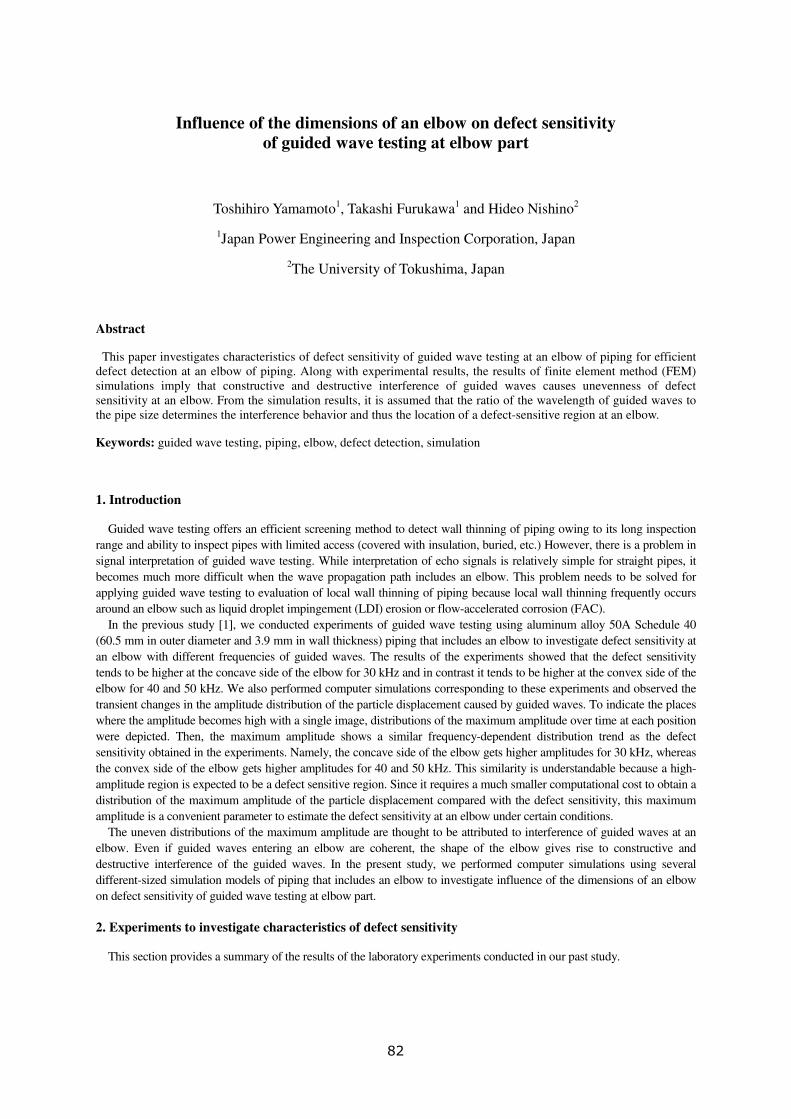
Influence of the dimensions of an elbow on defect sensitivity
of guided wave testing at elbow part
Toshihiro Yamamoto1, Takashi Furukawa
1 and Hideo Nishino
2
1Japan Power Engineering and Inspection Corporation, Japan
2The University of Tokushima, Japan
Abstract
This paper investigates characteristics of defect sensitivity of guided wave testing at an elbow of piping for efficient
defect detection at an elbow of piping. Along with experimental results, the results of finite element method (FEM)
simulations imply that constructive and destructive interference of guided waves causes unevenness of defect
sensitivity at an elbow. From the simulation results, it is assumed that the ratio of the wavelength of guided waves to
the pipe size determines the interference behavior and thus the location of a defect-sensitive region at an elbow.
Keywords: guided wave testing, piping, elbow, defect detection, simulation
1. Introduction
Guided wave testing offers an efficient screening method to detect wall thinning of piping owing to its long inspection
range and ability to inspect pipes with limited access (covered with insulation, buried, etc.) However, there is a problem in
signal interpretation of guided wave testing. While interpretation of echo signals is relatively simple for straight pipes, it
becomes much more difficult when the wave propagation path includes an elbow. This problem needs to be solved for
applying guided wave testing to evaluation of local wall thinning of piping because local wall thinning frequently occurs
around an elbow such as liquid droplet impingement (LDI) erosion or flow-accelerated corrosion (FAC).
In the previous study [1], we conducted experiments of guided wave testing using aluminum alloy 50A Schedule 40
(60.5 mm in outer diameter and 3.9 mm in wall thickness) piping that includes an elbow to investigate defect sensitivity at
an elbow with different frequencies of guided waves. The results of the experiments showed that the defect sensitivity
tends to be higher at the concave side of the elbow for 30 kHz and in contrast it tends to be higher at the convex side of the
elbow for 40 and 50 kHz. We also performed computer simulations corresponding to these experiments and observed the
transient changes in the amplitude distribution of the particle displacement caused by guided waves. To indicate the places
where the amplitude becomes high with a single image, distributions of the maximum amplitude over time at each position
were depicted. Then, the maximum amplitude shows a similar frequency-dependent distribution trend as the defect
sensitivity obtained in the experiments. Namely, the concave side of the elbow gets higher amplitudes for 30 kHz, whereas
the convex side of the elbow gets higher amplitudes for 40 and 50 kHz. This similarity is understandable because a high-
amplitude region is expected to be a defect sensitive region. Since it requires a much smaller computational cost to obtain a
distribution of the maximum amplitude of the particle displacement compared with the defect sensitivity, this maximum
amplitude is a convenient parameter to estimate the defect sensitivity at an elbow under certain conditions.
The uneven distributions of the maximum amplitude are thought to be attributed to interference of guided waves at an
elbow. Even if guided waves entering an elbow are coherent, the shape of the elbow gives rise to constructive and
destructive interference of the guided waves. In the present study, we performed computer simulations using several
different-sized simulation models of piping that includes an elbow to investigate influence of the dimensions of an elbow
on defect sensitivity of guided wave testing at elbow part.
2. Experiments to investigate characteristics of defect sensitivity
This section provides a summary of the results of the laboratory experiments conducted in our past study.
82

2.1 Experimental setup
Figure 1 shows a schematic illustration of the piping specimen used in our experiments. This piping specimen is made of
aluminum alloy, and it consists of two straight pipes and an elbow connecting these two pipes. The pipes are 50A Schedule
40 (60.5 mm in outer diameter and 3.9 mm in wall thickness). The elbow is a long radius elbow complying with JIS B2313
(comparable to ASME B16.9). Either end of the elbow was welded to one of the straight pipes. The dry-coupled
piezoelectric ring-shaped sensor system already presented in the past studies [2, 3] was used to transmit and receive guided
waves in the experiments. The sensor system consists of two sets of eight transducer elements aligned to be placed at equal
intervals in the circumferential direction of the outer surface of the pipe. These transducer elements are oriented to vibrate
in the circumferential direction of the pipe to transmit and receive the fundamental torsional guided wave mode T(0,1)
preferentially. One set of eight transducer elements is used as a transmitter, and the other is used as a receiver. The
transmitter was placed 485 mm before the inlet of the elbow, and the receiver was placed 30 mm before the transmitter.
To find out how the observed signals vary according to the position of a defect at the elbow, 12 piping specimens of the
same configuration as shown in Fig. 1 were prepared. On the outer surface of each specimen, a single defect was made by
a carbide cutting bit at one of the 12 positions indicated in Fig. 2. The diameter of the carbide cutting bit is 9.5 mm. The
depth of each defect was gradually increased up to 2.0 mm with 0.25 mm increments. The observed signals were stored for
each step of the defect depth on the 12 piping specimens.
In the measurements on each specimen, the three frequencies 30, 40 and 50 kHz were used as the center frequency of the
excitation signal for the transmitter to find out how the characteristics of the observed signals are changed according to the
frequency of guided waves.
4852485
Receiver Transmitter
Welds
30
Piezoelectric
sensor systemfor the T(0,1) mode
Figure 1. Piping specimen with piezoelectric sensor system
10˚
10˚
35˚
35˚
20 mm
① ② ③④⑤ ⑥ ⑦⑧⑨ ⑩ ⑪⑫
Carbide cutting bit
Sensor side
The defect depth was
increased up to 2 mm.
Figure 2. 12 positions of artificial defects
83

2.2 Observation of defect signals
Figure 3 shows a typical waveform obtained from the measurements on the piping specimens before the defect was
made at the elbow. The signal labeled represents the guided waves that propagate directly from the transmitter to the
receiver. The signal labeled is formed by several wave packets reflected around the elbow. This group of wave packets
mainly consists of the two wave packets reflected from the two butt welds at both ends of the elbow, respectively. The
signal labeled arises from the waves reflected by the lower right end of the piping specimen shown in Fig. 1.
Figure 4 shows the waveforms of the observed signals with the increasing depth of the defect when the frequency of the
excitation signal is 50 kHz and the defect position is . To focus on the signal variations according to the defect depth,
only the range from 350 µs to 600 µs is displayed. The signal amplitudes are normalized such that the maximum amplitude
of the signal that corresponds to the signal labeled in Fig. 3 is unity. The normalized amplitudes are expressed in permil
(‰). Because the signal variations due to the defect depth are relatively small compared with the original signal, the
baseline subtraction was adopted to clarify the signal variations. The lower graph in Fig. 4 shows the resulting signals that
were obtained by subtracting the baseline signal (the signal when the defect depth is 0 mm) from all the signals in the
upper graph in Fig. 4. Then, only the defect signals were extracted by this subtraction.
2.3 Defect sensitivity
To quantify the increasing rate of the amplitude of the defect signal with respect to the defect depth, Fig. 5 shows the
correlation between the cross-sectional loss caused by the defect and the maximum amplitude of the defect signal for 50
kHz of the guided wave frequency and the defect position . In this graph, the cross-sectional loss is represented as the
proportion (%) of the maximum cross-sectional area of the defect to the cross-sectional area of the intact pipe wall. The
filled circles indicate the data obtained from the experiments. The solid line is the least squares regression line derived
from the data. In this study, the defect sensitivity is defined as the slope of this least squares regression line at each defect
position for each guided wave frequency.
The measurements on the 12 piping specimens provide the defect sensitivity values at the 12 positions presented in Fig.
2. Figure 6 shows the defect sensitivity values at these 12 positions for the three frequencies 30, 40 and 50 kHz. From the
figure, it is observed that the defect sensitivity depends on both the position and the frequency. For 30 kHz higher
sensitivity values are presented at the concave side of the elbow, whereas for 40 and 50 kHz higher sensitivity values are
presented at the convex side of the elbow.
Figure 3. Typical waveform obtained from measurement on piping specimen
84

Baseline subtraction
Defe
ct d
ep
th in
cre
ase
sVariations due to defect depth
Defect signals
Figure 4. Signal variations due to defect depth (frequency 50 kHz, defect position )
0
5
10
15
20
25
30
35
0 1 2 3 4
Rela
tiv
e n
orm
ali
zed
am
pli
tud
e (
‰)
Cross-sectional loss (%)
experimental value
least squares regression line
Sensitivity
7.4 ‰/%
Figure 5. Increasing rate of signal variation (frequency 50 kHz, defect position )
85
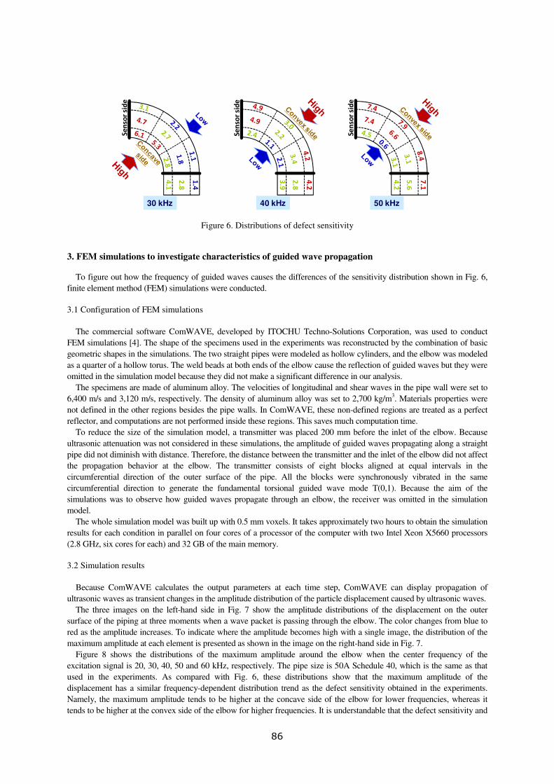
Se
nso
r sid
e
2.8
4.1
1.4
Se
nso
r sid
e
2.8
3.9
4.2
Se
nso
r sid
e
5.6
4.2
7.1
30 kHz 40 kHz 50 kHz
Figure 6. Distributions of defect sensitivity
3. FEM simulations to investigate characteristics of guided wave propagation
To figure out how the frequency of guided waves causes the differences of the sensitivity distribution shown in Fig. 6,
finite element method (FEM) simulations were conducted.
3.1 Configuration of FEM simulations
The commercial software ComWAVE, developed by ITOCHU Techno-Solutions Corporation, was used to conduct
FEM simulations [4]. The shape of the specimens used in the experiments was reconstructed by the combination of basic
geometric shapes in the simulations. The two straight pipes were modeled as hollow cylinders, and the elbow was modeled
as a quarter of a hollow torus. The weld beads at both ends of the elbow cause the reflection of guided waves but they were
omitted in the simulation model because they did not make a significant difference in our analysis.
The specimens are made of aluminum alloy. The velocities of longitudinal and shear waves in the pipe wall were set to
6,400 m/s and 3,120 m/s, respectively. The density of aluminum alloy was set to 2,700 kg/m3. Materials properties were
not defined in the other regions besides the pipe walls. In ComWAVE, these non-defined regions are treated as a perfect
reflector, and computations are not performed inside these regions. This saves much computation time.
To reduce the size of the simulation model, a transmitter was placed 200 mm before the inlet of the elbow. Because
ultrasonic attenuation was not considered in these simulations, the amplitude of guided waves propagating along a straight
pipe did not diminish with distance. Therefore, the distance between the transmitter and the inlet of the elbow did not affect
the propagation behavior at the elbow. The transmitter consists of eight blocks aligned at equal intervals in the
circumferential direction of the outer surface of the pipe. All the blocks were synchronously vibrated in the same
circumferential direction to generate the fundamental torsional guided wave mode T(0,1). Because the aim of the
simulations was to observe how guided waves propagate through an elbow, the receiver was omitted in the simulation
model.
The whole simulation model was built up with 0.5 mm voxels. It takes approximately two hours to obtain the simulation
results for each condition in parallel on four cores of a processor of the computer with two Intel Xeon X5660 processors
(2.8 GHz, six cores for each) and 32 GB of the main memory.
3.2 Simulation results
Because ComWAVE calculates the output parameters at each time step, ComWAVE can display propagation of
ultrasonic waves as transient changes in the amplitude distribution of the particle displacement caused by ultrasonic waves.
The three images on the left-hand side in Fig. 7 show the amplitude distributions of the displacement on the outer
surface of the piping at three moments when a wave packet is passing through the elbow. The color changes from blue to
red as the amplitude increases. To indicate where the amplitude becomes high with a single image, the distribution of the
maximum amplitude at each element is presented as shown in the image on the right-hand side in Fig. 7.
Figure 8 shows the distributions of the maximum amplitude around the elbow when the center frequency of the
excitation signal is 20, 30, 40, 50 and 60 kHz, respectively. The pipe size is 50A Schedule 40, which is the same as that
used in the experiments. As compared with Fig. 6, these distributions show that the maximum amplitude of the
displacement has a similar frequency-dependent distribution trend as the defect sensitivity obtained in the experiments.
Namely, the maximum amplitude tends to be higher at the concave side of the elbow for lower frequencies, whereas it
tends to be higher at the convex side of the elbow for higher frequencies. It is understandable that the defect sensitivity and
86

the maximum amplitude of the displacement have similar distribution trends because a high-amplitude region is expected
to be a defect-sensitive region for guided wave testing.
Figure 7. Amplitude distribution of displacement on outer surface of piping
20 kHz 30 kHz 40 kHz 50 kHz 60 kHz
50A Sch40
Figure 8. Distributions of maximum amplitude (50A Sch. 40) The uneven distributions of the maximum amplitude shown in Fig. 8 are thought to be attributed to interference of
guided waves at an elbow. Even if guided waves entering an elbow are coherent, the shape of the elbow gives rise to
constructive and destructive interference of the guided waves as shown in Fig. 7. In this process, the relation between the
pipe size and the wavelength of the guided waves should determine the interference behavior.
To investigate the effect of the pipe size on the distribution of the maximum amplitude, the simulation results obtained
with different pipe sizes were compared. Table 1 shows the pipe sizes used for the simulations. Because the finite element
used in the simulations is a 0.5 mm voxel, these values are rounded. Figure 9 shows the distributions of the maximum
amplitude around the elbow when the pipe size is 100A Schedule 10S, which has twice the outer diameter and the same
wall thickness compared with 50A Schedule 40. To keep the same ratio between the wavelength of the guided waves and
the pipe size, the frequencies of the guided waves were reduced to half of those used for 50A Schedule 40. Then, a
variation trend observed in these distributions is similar to that found in Fig. 8. This supports that the uneven distributions
of the maximum amplitude are caused by constructive and destructive interference of guided waves.
Table 1. Pipe sizes used in FEM simulations Nominal Size Outer Diameter
Wall Thickness
10S 20S 40
15A 22.0 2.0 2.5 3.0
20A 27.0 2.0 2.5 3.0
50A 61.0 3.0 3.5 4.0
100A 114.0 3.0 4.0 6.0
87

10 kHz 15 kHz 20 kHz 25 kHz 30 kHz
100A Sch10S
Figure 9. Distributions of maximum amplitude (100A Sch. 10S) Figure 10 compares the distributions of the maximum amplitude around the elbow when the pipe size is 50A Schedule
10S, 50A Schedule 20S and 50A Schedule 40. The outer diameter is 61.0 mm for all the cases but the wall thickness is 3.0,
3.5 and 4.0 mm, respectively. The comparison shows that the wall thickness has little influence on whether constructive
interference occurs at the concave or convex side of the elbow.
To confirm that the same ratio between the wavelength of guided waves and the pipe size provide a similar distribution
of the maximum amplitude, the highest frequency with high amplitudes at the concave side of the elbow is marked for
each pipe size in Fig. 11 (The wall thickness is 10S for all the pipe sizes). For example, both the third and forth images
from the left in the row of 15A in Fig. 11 show high amplitudes at the concave side of the elbow but the view given on the
top left corner of each image exhibits that the high-amplitude region is split in the middle of the concave side of the elbow
for 60 kHz. Therefore, 50 kHz was determined to be the highest frequency with high amplitudes at the concave side of the
elbow for the pipe size 15A. In a similar manner, such frequencies were determined to be 40, 20 and 10 kHz for the pipe
sizes 20A, 50A and 100A, respectively. Figure 12 shows that there is an almost linear correlation between the outer
diameter of the pipe and the highest frequency with high amplitudes at the concave side of the elbow. It is plausible that the
ratio of the wavelength of guided waves to the pipe size determines the interference behavior of the guided waves and thus
the locations of high-amplitude regions at the elbow.
20 kHz
20 kHz
20 kHz
30 kHz 40 kHz 50 kHz 60 kHz
30 kHz 40 kHz 50 kHz 60 kHz
30 kHz 40 kHz 50 kHz 60 kHz
(Outer diameter: 61, Thickness: 3.0)
(Outer diameter: 61, Thickness: 3.5)
(Outer diameter: 61, Thickness: 4.0)50A Sch40
50A Sch10S
50A Sch20S
Figure 10. Distributions of maximum amplitude (50A with different wall thicknesses)
88
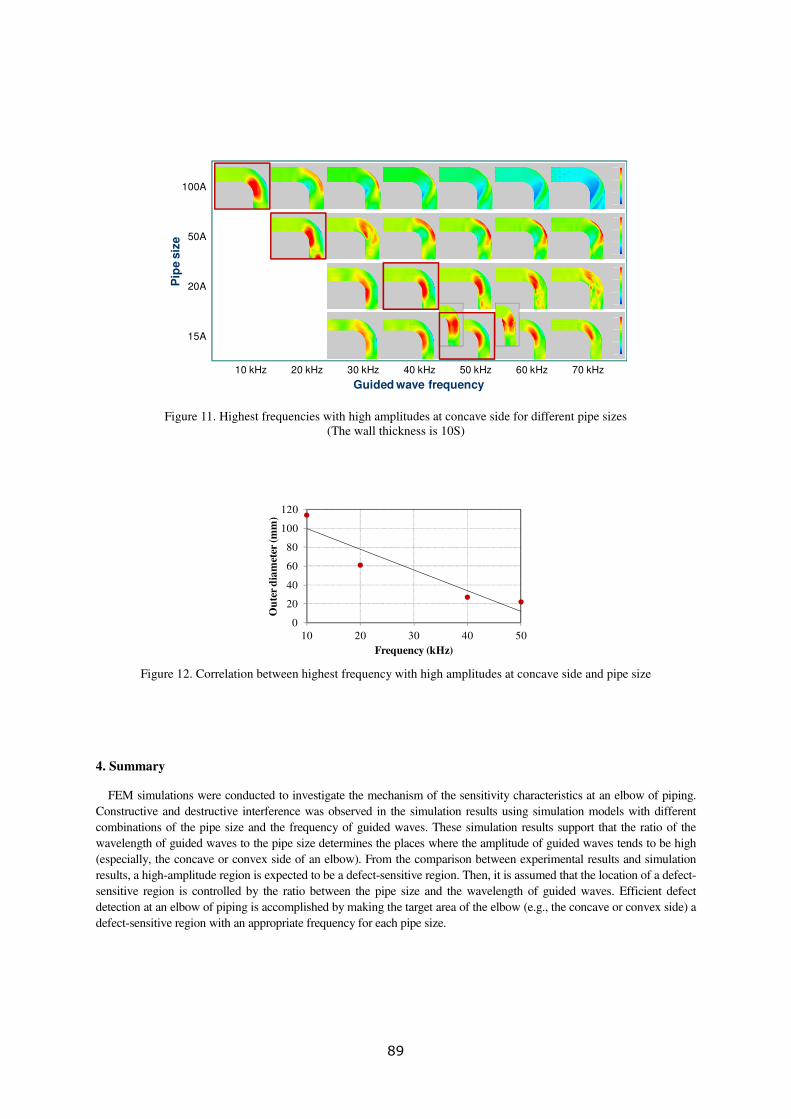
100A
20A
50A
10 kHz 20 kHz 30 kHz 40 kHz 50 kHz 60 kHz 70 kHz
Guided wave frequency
Pip
e s
ize
split
15A
Figure 11. Highest frequencies with high amplitudes at concave side for different pipe sizes
(The wall thickness is 10S)
0
20
40
60
80
100
120
10 20 30 40 50
Ou
ter
dia
met
er (
mm
)
Frequency (kHz)
Figure 12. Correlation between highest frequency with high amplitudes at concave side and pipe size
4. Summary
FEM simulations were conducted to investigate the mechanism of the sensitivity characteristics at an elbow of piping.
Constructive and destructive interference was observed in the simulation results using simulation models with different
combinations of the pipe size and the frequency of guided waves. These simulation results support that the ratio of the
wavelength of guided waves to the pipe size determines the places where the amplitude of guided waves tends to be high
(especially, the concave or convex side of an elbow). From the comparison between experimental results and simulation
results, a high-amplitude region is expected to be a defect-sensitive region. Then, it is assumed that the location of a defect-
sensitive region is controlled by the ratio between the pipe size and the wavelength of guided waves. Efficient defect
detection at an elbow of piping is accomplished by making the target area of the elbow (e.g., the concave or convex side) a
defect-sensitive region with an appropriate frequency for each pipe size.
89

References
[1] T. Yamamoto, T. Furukawa and H. Nishino, “Efficient defect detections of elbow pipes using propagation
characteristics of guided waves,” 40th Annual Review of Progress in Quantitative Nondestructive Evaluation, Vol.
33A, D. E. Chimenti, L. J. Bond and D. O. Thompson (Eds.), AIP Conference Proceedings, Vol. 1581, pp. 373–379,
AIP Publishing LLC (2014)
[2] H. Nishino, S. Masuda, Y. Mizobuchi, T. Asano and K. Yoshida, “Long-range testing of welded elbow pipe using
the T(0, 1) mode ultrasonic guided wave,” Jpn. J. Appl. Phys. 49 (2010), pp. 116602-1–6
[3] H. Nishino, T. Tanaka, S. Katashima and K. Yoshida, “Experimental investigation of mode conversions of the T(0,
1) mode guided wave propagating in an elbow pipe,” Jpn. J. Appl. Phys. 50 (2011), pp. 046601-1–7
[4] Y. Ikegam, Y. Sakai and H. Nakamura, “A highly accurate ultrasonic simulator capable of over one billion
elements for non-destructive evaluations,” Proceedings of the 7th International Conference on NDE in Relation to
Structural Integrity for Nuclear and Pressurised Components, M. Bieth (Eds.), pp. 177–190, European Communities
(2009)
90

Guided Wave Signals for Monitoring of Buried Pipe Mockup using a
Magnetostrictive Sensor Method
Yong-Moo Cheong 1, and Duck-Hyun Lee
1
1Korea Atomic Energy Research Institute, 111, Daedeok-daero, 989-beon-gil, Yuseong-gu,
Daejeon, 305-353, Korea
E-mail address(corresponding author) : [email protected]
When a pipe is buried in the ground, it is difficult to detect a defect until the defect grows
even to the point of leakage. To prevent the leakage of a buried pipe, a guided wave method
can be a promising technique. Among the various vibration modes, the torsional guided wave
T(0,1) mode has many advantages, such as no dispersion, no radial displacement, and a low
attenuation.
Because the torsional guided wave T(0,1) mode has many advantages for long-range guided
wave examination, such as no dispersion, no radial displacement, and a low attenuation, it
can be a promising tool for an evaluation of flaws from a buried pipe as well as the structural
health monitoring of pipes for a long period. A guided wave method with a magnetosrictive
sensor was studied for practical application to an examination of a buried pipe. The signal
amplitude from various reflectors is compared with two different sensor techniques, one by a
variation of DC bias and the other by a remnant magnetic bias technique. Based on the
signal amplitude, attenuation owing to the surrounding sand and soil on the buried pipe
mockup was estimated. The guided wave signals from various reflectors were also compared
with two different sensor techniques, one through a variation of DC bias and the other using a
remnant magnetic bias technique.
Keywords: Torsional guided wave, magnetostrictive sensor, buried pipe monitoring.
91

Human errors of reactor pressure vessel
Examinations in Korean nuclear plants
Euisoon DOH, Chang-hun LEE, Jae-yoon KIM, Wi-hyun KIM
KEPCO KPS, Busan, Korea
E-mail : [email protected]
More than 20 PWR units are under commercial operations in Korea. Every nuclear plant shall
be examined periodically in accordance with regulatory guides and codes in Korea and in the
world. 40 Month examination of reactor pressure vessel is performed in the second outage,
and 10 Year RPV ISI is performed in the sixth outage of the interval in Korea.
Welds, components and structures in the nuclear plants shall be examined very accurately per
regulatory guides, code and fabrication drawings. Reactor pressure vessel is the most
important component among the examination parts.
However, some critical mistakes of reactor pressure vessel examination have been reported
in Korean nuclear plants.
The first error in the examination of reactor pressure vessel was occurred at Yonggwang
(Hanbit) unit 5 in 2001. A weld location of Yonggwang unit 5 and 6 was changed from that of
the previous units of KSNP(Korean Standard Nuclear Plant) to get more examination
coverage. However, an American inspection company which is no more existence now did
not use the right drawings of Yonggwang unit 5. They used another drawing from the
previous plant. Fortunately, they got to know their mistake before getting a fuel load approval
from authority while they were preparing PSI of unit 6.
The next error was revealed at Kori unit 4 in 2014. The same American company with
Yonggwang unit 5 has performed the PSI of Kori unit 4 about 30 years ago, they has used
wrong drawings, and examined 2 wrong welds for Kori unit 4. They have used drawings for
Kori unit 3 to establish the Examination Scan Plan for Kori unit 4. They might have thought
that Kori unit 3 and 4 should have been same fabrications, but they have been wrong. These
drawings and fabrication of Kori unit 4 have been different from Kori unit 3. No body after
the PSI has found the error for 30 years. Wrong welds have been examined after the PSI
before verification of the error by KPS in 2014 during the preparation of the examination for
the 3rd
interval. Korean the only nuclear utility, KHNP investigated all nuclear plants after
revelation of error at Kori unit 4 to check their integrity of examinations for major
components. Unfortunately, KHNP found another fatal error of RPV examination at Hanbit
unit 2. The cause of the error was same as Kori unit 4.
KPS carried out inspections for both units of errors in 2014, and reported their keeping
integrity of their original welds which must have been examined.
The learned lesson from these errors in the examination is the importance of using right and
accurate drawings and the mental concentration of examiners not to make mistake in the PSI.
Otherwise, it would be very difficult to find the any error in the successive examination after
PSI.
Keywords: Reactor vessel, Reactor vessel Examination, RPV Examination, RPV Inspection,
RPV, PSI
92

Understanding of Sub-cooled Nucleate Boiling on the Nuclear Fuel Cladding
Surface Using Acoustic Emission Energy Parameter
Kaige Wu, Seung-HeonBaek, Hee-Sang Shim, DoHaengHur, Deok Hyun Lee*
Korea Atomic Energy Research Institute, 989-111 Daedeok-daero,Yuseong-gu, Daejeon, Republic of
Korea
Abstract
In the primary coolant system of a pressurized water reactor, it has been known that CRUD deposition on the fuel
cladding surfaces is accelerated under sub-cooled nucleate boiling (SNB) conditions. Anomalous neutron absorption
from accumulated boron in the CRUD can lead to an axial offset anomaly (AOA). Thus, the detection and monitoring
of SNB in terms of a non-destructive evaluation is of great importance for analyzing the behavior of CRUD deposition
and AOA. In this work, an acoustic emission (AE) method is proposed to investigate and understand the SNB
phenomenon.
An internal electric heater was inserted within a Zirlo cladding tube to control the boiling process. A high
sensitivityAE sensor was connected to the upper end of thecladding tube, which acted as a waveguide. The internal
heater temperature was controlled from 120 to 260 °C in the simulated primary watercontaining 3.5 ppm Li and 1500
ppm B under atmospheric pressure. The tests were conducted in a cylindrical glass cell whereby the boiling
occurrence could be visibly checked. The AE data were collected and photographic observations were also made
during the boiling process.
When the heater temperature was low, no bubbles were generated and the AE signals obtained should be
background owing to heating and other electrical noises. As the water was heated to the temperature under saturation,
bubbles began to form on the cladding surface but immediately collapsed nearby. The detected AE signals might be
associated with the bubble growth and collapse. After the water temperature reached the saturation temperature, the
bubbles grew, departed from the cladding surface,then rose up and burst at the water/air interface.The AE signals were
distinguished as four groups in the AE energy criterion, which might be associated with the bubble growth, bubbles
departure, bubbles collapse, and bubbles burst, respectively. The results indicate that the SNB phenomenon can be
understood through the characteristics of the AE signals, and AE NDT can be proposed as an effective tool for
monitoring the evolution of nucleate boiling on the fuel cladding surface.
Keywords:Fuel cladding, CRUD, Sub-cooled nucleate boiling, Boling process, Acoustic emission.
1.Introduction
The axial offset anomaly (AOA), which is also known as crud-induced power shift (CIPS), refers to a neutron flux
depression in upper region of a pressurized water reactor core, which can lead to operational issue of the plants with
long-period cycle operation [1-3].It is well known that AOA is caused by anomalous neutron absorption due to
accumulated boron hide out in porous crud deposited on the cladding. Furthermore, large scale laboratory experiments
elaborated and confirmed the mechanism of boiling assisted deposition that porous crud layer on the cladding was
accelerated under sub-cooled nucleate boiling (SNB) condition [4-10].Obviously, the degree of SNB is interrelated to
the crud deposition on the cladding surface. Accordingly, evaluation of the SNB and crud deposition is an important
approach to understand the occurrence of AOA. Indeed, a great many attempts have been made with such
consideration by various methods, such as thermal-hydraulic analysis [4], model analysis of particle transportation [5-
6], micro-layer evaporation and dry-out (MED) model calculation [7], post-morphological analysis [8-9], and high
fidelity digital imaging apparatus [10].Unfortunately, despite much effort focusing on this topic, much still remains to
be investigated for the realization of a comprehensive understanding. Moreover, these methods have their own
disadvantages like that most of these methods are usually off-line and must be performed during plant outage.
Therefore, we are encouraged to get a better understanding of SNB on the cladding surface and the behavior of the
bubbles formed in SNB from the dynamic point of view, using an in-situ nondestructive evaluation (NDE)technique.
93

Acoustic emission method (AE) is an in situNDE method that senses transient elastic waves resulting from a rapid
release of energy within a dynamic process [11], such as corrosion process [12-14], cracks evolution [15-16]
andvarious chemical engineering processes concluding bubbles dynamic [17]. Of many methods proposed for
evaluation of the crud deposition and AOA phenomenon, monitoring and detection of AE signals generated along with
boiling process is considered to be one of the most promising techniques because of its high sensitivity of detection,
real time monitoring and in-situ full body scanning of research target.Up to now, many attentions has been paid to AE
investigation on the boiling process, such as SNB, nucleate boiling (NB) and transition boiling [18-27]. It has been
well acceptedthatthe bubble dynamic is critical for the generation of acoustic emission along with the boiling process.
Nishihara et al. [18] and Zhang et al. [19] investigated the boiling behavior on the surface of a horizontal metal wire
under atmospheric pressure. The AE in boiling was reported to have frequency components up to 50 kHz.
At the beginning of the bubble growth, a significant pressure pulse was found by Robinson and Schmidt [20].
Moreover, the mechanism of the pressure wave generation in bubble growth is shown to follow the Young-Laplace
equation [21-23]. The amplitude increase of AE was thought to be directly proportional to the overheating of the
liquid and indirectly proportional to the critical radius of the bubble.
In the departure or detachment of bubbles from the surface, AE was reported to be generated dependent on the
distribution of surface temperature in the vicinity of the boiling nucleus [22-25]. The detailed source in bubble
departure was believed to be the swirl and turbulence induced by the pulsing vapor nucleus.
Bubble collapsein SNB, or called as bubble implosion, were frequently reported to generate AE signals with larger
amplitude, higher energy comparing with the bubble growth and bubble departure [20, 24]. Bubble collapse due to
heat transfer from the subcooled liquid was assumed to be very fast and the generated acoustic pulses were directly
proportional to sub-cooling and practically independent on the diameter of the collapsing bubbles [24].
In NB, the bubbles rise and burst at the free surface of liquid. Husin and Mba [26], and Divoux et al. [27] found that
bubble rising does not produce AE, while the bubble burst caused AE with large amplitude and high energy which
have a correlation with bubble length. They also observed that the duration of AE increases with the bubble length
[27].
Motivated both by the will to understand the dynamic of SNB on the nuclear fuel cladding surface, and the hope to
use AE NDT as a tool to predict the crud deposition and AOA phenomenon, we carried out an experimental work with
AE sensor directly coupled to the surface of a simulated cladding tube, to investigatethe dynamic of bubbles formed
inSNB under atmospheric pressure by AE method.
2. Experimental procedure
Figure 1 shows a series of schematic drawings of the test section in the present work. A Zirlo cladding tube with an
internal electric heater inserted was placed vertically to provide the surface for boiling process. The internal heater
temperature was controlled from 120 to 260 °C in the simulated primary water containing 3.5 ppm Li and 1500 ppm B
under atmospheric pressure. 500 seconds was held on at each temperature for observation of the boiling behavior and
collection of the AE signals.The test was conducted in a cylindrical glass cell whereby the boiling occurrence could be
visibly checked. The photographic and video observations were made during the boiling process.The video was taken
with a common camera by 30 frames / s. After the test, all the videos taken in each temperature were analyzed by
frames comparison.
Figure 1. (a) A schematic illustration of experimental apparatus used in the present research; (b) and (c)
Theschematics of the detailed structure of internal heater. (d) A real photo showing the experimental setup.
As shown in Fig. 1, a high sensitivity AE sensor (Type R15, MISTRAS from Physical Acoustic Corporation, USA)
was directly coupled with an ultrasonic couplantto the upper end of the cladding tube which also acted as a waveguide.
94

The other end of AE sensor was connected to a pre-amplifier (2/4/6 Preamplifier, Physical Acoustic Corporation,
USA), the other end of which was connected to the AE system. The AE signals and various parameters were collected
by an acquisition device (Model: PCI-2, Physical Acoustic Corporation, USA). The background noises from the
surrounding were tried to be minimized and the threshold value was carefully to determine as 40 dB and the
preamplifier was set to 40 dB, respectively. For detected AE signals, following AE parameters are studied:
(i) Counts: The number of times the AE signal excursions over the AE threshold;
(ii) Amplitude: the maximum AE signal excursion during an AE hit;
(iii) Energy: the parameter derived from the integral of the rectified voltage signal over the duration of the AE
hit;
(iv) Rise Time: the time between the AE Hit start and the peak amplitude of the AE Hit;
(v) Duration: the time from the first threshold crossing to the end of the last threshold crossing of the AE signal
from the AE Threshold.
(vi) Average Frequency: the parameter derived from AE Counts and Duration determines an average frequency
over the entire AE hit.
3. Results and discussion
Figure 2. Evolution of raw AE data obtained during process of boiling test with controlling the temperature
of internal heater from 120 to 260°C: (a) AE signals in energy parameter; (b) AE signals in average frequenc
y parameter.
95
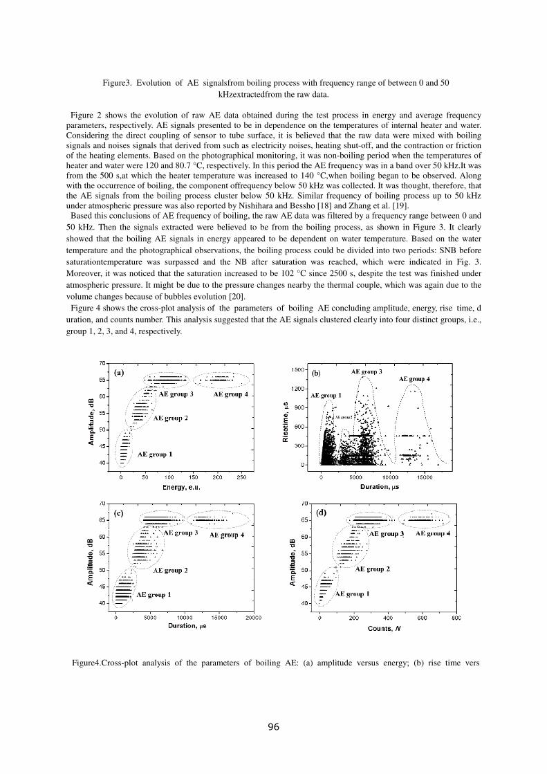
Figure3. Evolution of AE signalsfrom boiling process with frequency range of between 0 and 50
kHzextractedfrom the raw data.
Figure 2 shows the evolution of raw AE data obtained during the test process in energy and average frequency
parameters, respectively. AE signals presented to be in dependence on the temperatures of internal heater and water.
Considering the direct coupling of sensor to tube surface, it is believed that the raw data were mixed with boiling
signals and noises signals that derived from such as electricity noises, heating shut-off, and the contraction or friction
of the heating elements. Based on the photographical monitoring, it was non-boiling period when the temperatures of
heater and water were 120 and 80.7 °C, respectively. In this period the AE frequency was in a band over 50 kHz.It was
from the 500 s,at which the heater temperature was increased to 140 °C,when boiling began to be observed. Along
with the occurrence of boiling, the component offrequency below 50 kHz was collected. It was thought, therefore, that
the AE signals from the boiling process cluster below 50 kHz. Similar frequency of boiling process up to 50 kHz
under atmospheric pressure was also reported by Nishihara and Bessho [18] and Zhang et al. [19].
Based this conclusions of AE frequency of boiling, the raw AE data was filtered by a frequency range between 0 and
50 kHz. Then the signals extracted were believed to be from the boiling process, as shown in Figure 3. It clearly
showed that the boiling AE signals in energy appeared to be dependent on water temperature. Based on the water
temperature and the photographical observations, the boiling process could be divided into two periods: SNB before
saturationtemperature was surpassed and the NB after saturation was reached, which were indicated in Fig. 3.
Moreover, it was noticed that the saturation increased to be 102 °C since 2500 s, despite the test was finished under
atmospheric pressure. It might be due to the pressure changes nearby the thermal couple, which was again due to the
volume changes because of bubbles evolution [20].
Figure 4 shows the cross-plot analysis of the parameters of boiling AE concluding amplitude, energy, rise time, d
uration, and counts number. This analysis suggested that the AE signals clustered clearly into four distinct groups, i.e.,
group 1, 2, 3, and 4, respectively.
Figure4.Cross-plot analysis of the parameters of boiling AE: (a) amplitude versus energy; (b) rise time vers
96

us duration; (c) amplitude versus duration; (d) amplitude versus counts.
Figure 5. (a) Photographical analysis and (b) the corresponding AE data in the condition of TInternal heater = 160°C, Twater
= 92°C.
Figure 6. (a) Photographical analysis and (b) the corresponding AE data in the condition of TInternal heater = 180°C, Twater
= 96°C.
In attempting to uncover the physical mechanism between the AE groups and the dynamic of bubbles formed
during boiling, photographical analysis was carried out based on frame comparison of the video taken during boiling
process.
Figure 5(a) shows a series of frames extracted from the video taken in the condition of T Internal heater was 160°C, T
water was 92°C. When t = 66ms, a bubble was captured to grow on the cladding surface, and collapsed immediately at
the surface after 33ms. The main physical changes during this process were bubble growth and bubble collapseon
thecladding surface, which clearly suggested the occurrence of SNB. Figure 5(b) shows the AE signal in cross-plot
analysis of amplitude and energy, which indicated the appearance of AE signals located in group 1 and 3 in
comparison with the all-process signals in Fig. 4. It has been well known that the bubble collapse produced AE signals
with higher energy and larger amplitude than bubble growth [20-24]. Consequently, it was concluded that AE group 1
and 2 were contributed to the bubble growth and bubble collapse, respectively, as marked in Fig. 5(b).
97

Figure 6(a) shows a series of frames extracted from the video taken in the condition of T Internal heater was 180°C, T water
was 96°C. When t = 33ms, a bubble was observed to grow on the claddingtube surface, subsequently the bubble
departed from the surface. Then it rose upwardly and collapsed nearby the tube surface after 264ms. In this SNB
process, the physical evolutions were bubble growth, bubble departure, bubble rising and bubble collapse. Figure 6(b)
shows the AE signal in this period. It clearly indicated that AE signals appeared to be with three groups, which were
corresponding to the AE groups 1, 2, 3, respectivelycomparing with the total signals in Fig. 4. According to the report
by Husin and Mba [26], bubble rising does not produce AE. Considering that AE groups 1 and 3 were associated with
bubble growth and bubble collapse, the AE group 2 was therefore believed to be the results of bubble departure. This
conclusion shows that the AE signals from bubble collapse are with larger amplitude and higher energy than bubble
growth and bubble departure, which is in good consistent with previous reports [22-24].
Figure 7. (a) Photographical analysis and (b) the corresponding AE data in the condition of TInternal heater = 20
0°C, Twater = 100°C.
Figure 7(a) shows another series of frames extracted from the video taken in the condition of T Internal heater was 200°C,
T water was 100 °C. First, this period was featured by the bubbles burst at the free surface of water after rising to the
free surface, which suggested the beginning of NB. In the bottom of cladding tube, it was observed that the bubble
grew, subsequently departed from the cladding surface, and finally collapsed nearby the cladding surface. While in the
upper of tube, the bubbles rose to the water surface and burst.This phenomenon could be explained that the
temperature of water near the bottom of tube was below saturation, and the surface temperature was very high.
However, the saturation of water near the upper of tube was reached and NB started to be generated. Figure 7(b)
shows the AE signals in this period. AE signals clearly clustered into four groups which were corresponding to the AE
groups 1-4 in comparison with the total signals in Fig. 4. According to the photographic analysis, bubble burst was
first found in this period in comparison with the bubbling in SNB. As a result, bubble burst were proposed to be
responsible for the AE group 4.
Based on analysis above, two proposed schematic diagrams for SNB and the transition from SNB to NB were shown
in Figure 8. Moreover, AE characteristics and detectabilityof the dynamic of bubbles formed during the boiling were
given in Table 1. The AE groups 1-4 were associated with the bubble growth, bubble departure, bubble collapse in
sub-cooled water, and bubble burst in NB process, respectively. This conclusions show the most powerful source for
AE signals during NB are bubble burst at the free surface, while the AE with largest amplitude and highest energy are
contributed to the bubble collapse in sub-cooled liquid. It could be concluded that the AE group 3 from bubble
98

collapse and AE group 4 from bubble burst could be used as the featured indicator for the occurrence of SNB and NB,
respectively. Moreover, the transition from SNB to NB could be distinguished by AE signal monitoring.
Figure 8.The proposed schematic diagrams for SNB (a) and the transition from SNB to NB (b).
Table1. Summary of AE characteristics and detectabilityof the dynamic of bubbles formed during the boiling.
AE
groups
Characteristics of the corresponding AE groups
Physical
mechanismEnergy
(e.u.)
Amplitude
(dB) Duration
(µs)
Rise time
(µs)
Counts
(N)
Group 1 0-9 40-49 0-2178 0-903 0-65 Bubble growth
Group 2 19-73 51-65 2173-6313 0-487 90-282 Bubble departure
Group 3 57-134 64-66 4004-9706 0-1210 201-437 Bubble collapse
Group 4 163-233 64-67 11283-16942 0-460 520-655 Bubble burst
4. Conclusions
99

In this work, AE method was employed to investigate the dynamic of bubbles formed in SNB at atmospheric
pressure in the perspective of in-situ NDE monitoring. Some conclusions can be drawn based on the present work as
follows:
1). AE in-situ monitoring was confirmed to with good feasibility in investigating the dynamic of bubbles formed in
SNB and NB;
2). The frequency of boiling AE was confirmed to be lower than 50 kHz, and the boiling AE could be divided into
four distinct groups based on cross-plot analysis of AE parameters;
3). Based on analysis of boiling AE and the corresponding photographic observations, AE groups 1-4 could be
contributed to the dynamic of bubble growth, bubble departure, bubble collapse in subcooled water, and bubble
burst at water surface, respectively.
4). The AE group 3 from bubble collapse and AE group 4 from bubble burst could be used as the featured indicator
for the occurrence of SNB and NB, respectively.
5). AE energy and amplitude could contribute to monitor the dynamic process of SNB well.The transition from
SNB to NB could be clearly distinguished by AE signals.
6). The obtained AE characteristics of boiling dynamic could provide a good basis for the following experiments in
high temperature and high pressure.
Acknowledgements
This work was supported by the National Research Foundation of Korea (NRF) grant funded by the Korea
government (MSIP).
References
[1] J. Deshon, D. Hussey, B. Kendrick, J. McGurk, J. Secker and M. Short, “Pressurized water reactor fuel crud and
corrosion modeling”, JOM J. Miner. Met.Mater. Soc., Vol.63, No. 8, pp. 64-72 (2011)
[2] E. Decossion and O. Bremnes, “Axial offset anomaly modeling studies on EDF cores” In: Proc. Int. Conf. on
Nuclear Engineering, Orlando, Florida, USA., May 11-25, p.271, 2008
[3] W. Byers and J. Deshon, “Structure and chemistry of PWR crud” In: Proc. Int. Conf. on Water Chemistry of
Nuclear Reactor Systems, San Francisco, USA, p.1722, 2004
[4] M.H. Kim, U.C. Kim, C.W. Won and W.Y. Maeng, “Experimental evaluation of primary water chemistry for
prevention of axial offset anomaly”, Thermochim. Acta, Vol. 542, No. 20, pp. 80-88 (2012)
[5] H. Bindra and B.G. Jones, “Deposition of metallic colloids under sub-cooled nucleate boiling”, Colloids and
Surfaces A: Physicochemical and Engineering Aspects, Vol. 397, No. 5, pp. 85-91 (2012)
[6] H. Bindra, “Effect of boiling in deposition of metallic colloids”, PhD Thesis, University of Illinois, 2010
[7] S. Uchida, Y. Asakura and H. Suzuki, “Deposition of boron on fuel rod surface under sub-cooled boiling
conditions-An approach toward understanding AOA occurrence”,Nucl. Eng. Des., Vol. 241, No. 7, pp. 2398-2410
(2011)
[8] S.H. Baek, H.S. Shim, C.H. Won, D.H. Hur and U.C. Kim, “Effects of Ni, Fe chemicals and hydrogen on deposits
formed on Zirlo fuel cladding material in nuclear primary water chemistry conditions at 325 °C”, Ann.Nucl. Energy,
Vol. 70, pp. 233-239 (2014)
[9] T. Iwahori, T. Mizuno, and H. Koyama, “Role of surface chemistry in crud deposition on heat transfer surface”,
Corros., Vol. 35, No. 8, pp. 345-350, (1979)
[10] W. Wu, P. Chen, B. Jones, and T. Newell, “Measurement and analysis of bubble behavior in sub-cooled boiling
100

flows”, In: Proc. 13th Int. Conf. on Nuclear Engineering, Beijing, China, May 16-20, p.545, (2005)
[11] ASTM E1316, “Standard Terminology for Nondestructive Examinations”, American Society for Testing and
Materials, (2011)
[12] J.W. Byeon, K. Wu and H. Y. Kim, Korean Patent No. 10-1477962, (2014)
[13] K. Wu, W.S. Jung and J.W. Byeon, “Evaluation of corrosion critical variables of 304 stainless steel by delay time
of acoustic emission”, Mater. Trans., Vol. 56, No. 3, pp. 398-403, (2015)
[14] K. Wu, W.S. Jung and J.W. Byeon, “Acoustic emission of hydrogen bubbles on the counter electrode during
pitting corrosion of 304 stainless steel”, Mater. Trans., Vol. 56, No. 4, pp. 587-592, (2015)
[15] M. Huang, L. Jiang, P.K. Liaw, C.R. Brooks, R. Seeley, and D.L. Klarstrom, “Using acoustic emission in fatigue
and fracture materials research”, JOM Nondestructive Evaluation, Vol. 50, No. 11, Presented as JOM-e, (1998)
[16] J.H. Han, D.H.Hur, K.M. Kim, M.S. Choi, D.H. Lee, “Analysis on the Acoustic Emission Signals in the Crack
Evolution of Steam Generator Tube”, Transactions of the Korean Nuclear Society Autumn Meeting, PyeongChang,
Korea, October 25-26, pp. 321-322, (2007)
[17] J.W.R. Boyd, and J. Varley,“The use of passive measurement of acoustic emissions from chemical engineering
processes”, Chem. Eng. Sci., Vol. 56, No. 5, pp. 1749-1767, (2001)
[18] H. Nishihara and Y. Bessho, “Acoustic emission in subcooled nucleate pool boiling”, J.Nucl. Sci.Technol., Vol.
14, No. 6, pp. 407-415, (1977)
[19] Q. Zhang,K. Dong, Z. Huang, J. Wang and Y. Yang, “Mode identification of pool boiling of water by acoustic
emission”, CIESC Journal, Vol. 64, No. 10, pp. 3527-3533, (2013)
[20] G.E. Robinson, F.W. Schmidt, H.R. Block, and G. Green, “An experimental determination of isolated bubble
acoustics in nucleate boiling system”, in: Proc. 5th Int. Heat Transfer Conf., Tokyo, September 3-7, Vol. 4, pp. 75-79,
(1974)
[21] P. Benes and M. Uher, “Identification of liquid boiling by acoustic emission”, In: Proceedings of XIX IMEKO
World Congress Fundamental and Applied Metrology, September 6-11, Lisbon, Portugal, pp. 1396-1401, (2009)
[22] V. P. Carey, Liquid Vapor Phase Change Phenomena: An Introduction to the Thermophysics of Vaporization and
Condensation Processes in Heat Transfer Equipment. New York: Hemisphere Publishing Corporation, ISBN: 0-89116-
836-2, (1992)
[23] G.F. Hewitt, “Boiling”, In: W.M. Rohsenow, J.P. Hartnett, Y.I. Cho, ed., Handbook of Heat Transfer. 3rd
ed. New
York: McGraw-Hill, Chapter 15, pp. 15.1-15.167, ISBN: 978-0-07-053555-8, (1998)
[24] A.F. Mills, Basic Heat and Mass Transfer, 2nd
Ed., New Jersey: Prentice-Hall, ISBN: 978-0-13-096247-3, (1999)
[25] T.G. Leighton, The Acoustic Bubble, Academic Press, London, 1997.
[26] S. Husin and D. Mba, “Acoustic emission of a single bubble activities”, in: Proceedings of the World Congress
on Engineering 2010 Vol II, WCE 2010, June 30-July 2, London, U.K.
[27] T. Divoux, V. Vidal, F. Melo, and J.C. Geminard, “Acoustic emission associated with the bursting of a gas bubble
at the free surface of a non-Newtonian fluid”, Phys. Rev. E, Vol. 77, 056310, pp. 1-7, (2008)
101

Implementation of Special PA UT Techniques
for Manufacturing Inspection of Welds in Thick Wall Components
Dirk Verspeelt 1, Dominic Marois
1, Guy Maes
1,
Jean Marc Crauland 2, Michel Jambon
2, Frédéric Lasserre
3
1 Zetec, zNDT Solutions, Québec, Canada
2 AREVA Nuclear Power, Chalon / St Marcel, France, 3 AREVA Nuclear Power; Paris, France
Abstract
The AREVA-NP/EFF/SAINT-MARCEL factory have selected advanced automated UT based on phased
array and TOFD techniques, in view of replacing manual UT and radiographic testing, for circular welds in
thick-wall components. The principles of the applied phased array and TOFD examination techniques, and the
on-site implementation will be briefly reviewed.
This paper will then address how special UT examination techniques are implemented using phased array
technology, to complement the generic techniques.
Tandem configurations, using the LLT technique, are used to obtain enhanced detection capability on
planar flaws perpendicular to the inspection surface. Both single probe and two-probe configurations are used to
cover the complete wall thickness.
Asymmetric TOFD configurations (Delta technique), generated with phased array probes, are used to
maximize TOFD coverage in areas where access is limited to one side of the weld.
For both techniques, theoretical considerations on probe design will be presented, as well as the practical
implementation of the focal laws using the UltraVision® phased array calculator.
The performance of the special techniques will be illustrated with ultrasonic data from practical trials on
representative specimens with artificial and realistic flaws. It will be shown how the UltraVision software
supports comprehensive visualization of the data generated by the special techniques, and how the advanced
tools allow for efficient data analysis.
Keywords: phased array, TOFD, weld inspection, reactor vessel
Manufacturing of Steam Generators (SG) and Pressurizers (PZR) involves non-destructive testing of the
circumferential welds according to the French Design and Construction Rules for Mechanical Components of
PWR Nuclear Islands (RCC-M) code. This includes surface and volumetric NDT methods.
The low alloy steel pieces of PZR and SG (
Figure 1: Pressurizer (PZR) and Steam Generator (SG) weld outline
) are assembled by means of narrow gap submerged arc welds. The weld thickness range varies between
100 mm and 180 mm. Shell diameters varying between 3.077 m and 5.165 m yield weld lengths up to more than
16 m.
Historically, Radiographic Testing (RT) was applied before heat treatment while manual UT was used in
complement for examination of the welds before and after heat treatment.
For productivity and environment reasons, the AREVA-NP/EFF/SAINT-MARCEL have decided to
replace manual UT and RT by advanced automated phased array pulse-echo (PE) and TOFD techniques.
1. Introduction
102

Figure 1: Pressurizer (PZR) and Steam Generator (SG) weld outline
2.1. Generic Inspection Techniques
In order to demonstrate the best possible equivalence between the current methods (RT and manual UT)
and the proposed alternative UT techniques (PE and TOFD), and instead of a qualification (very time
consuming), the development of the new UT phased array PE technique was at the start based as much as
possible on the existing manual UT characteristics [1],[2]. Figure 2 shows a schematic representation of the
pulse-echo examination techniques that were selected. The phased array beam steering capability is used for
reproducing the refracted angles required by the code (0ºLW, 45ºSW, 60ºSW and 70ºSW) while reducing the
number of probes. In order to optimize the response for various defects orientations, the beam skewing
capability is used to replace manual optimization (turning the probe) in conventional UT.
Figure 2: Weld coverage using beam steering and skewing with phased array pulse-echo techniques
A typical inspection result from the pulse-echo techniques is shown on Figure 3. Since more than 90
pulse-echo beams are used (different beam orientations, refracted angles and skew angles), analysing the weld
data beam by beam would require too much time. Therefore, the merge tool in the UltraVision software is used
to calculate and visualize, considering all beams, the maximum amplitude found for each unitary volume of the
inspected weld zone. The left view (VC-Side) shows a cross section of the weld with all indications found along
the weld seam. The top right view (VC-End) shows a “front” view of the weld, whereas the lower right view
(VC-Top) shows the top view of the weld.
2. Dedicated Advanced Automated UT System
103

Figure 3: Typical inspection result from pulse-echo techniques, using Merged Data from all beams
The TOFD technique is implemented using a combination of conventional and phased array probes (see
Figure 4. The near-surface depth range is covered by two conventional configurations. The phased array probe
set covers the deeper range. Besides a reduction of the number of probes, this allows for flexible adaptation of
zone division to fit various weld thicknesses, and a good control of the beam spread for a given depth range
resulting in a high signal-to-noise ratio (SNR) and reduced back-wall dead zone.
Figure 4: Depth zone coverage for TOFD inspection techniques
The excellent SNR obtained with the phased array TOFD configuration is shown in Figure 5. The left
image shows the signals from an alumina insert, known to yield low diffraction amplitudes: the quality of the
signal is very good and the obtained SNR is about 16 dB. The right image shows a 2 mm deep far-surface
breaking notch in a 165mm test block. The back-wall dead zone is reduced to a minimum.
104

Figure 5: PA-TOFD images from an embedded 4 mm height Alumina insert (left),
and a 2 mm height far-surface EDM notch (right)
2.2. On-Site Implementation
A dedicated industrial system for the UT inspection during manufacturing of large narrow gap submerged
welds has been developed, and the manufacturing was finalized end 2013. It was commissioned in the factory in
France in the spring of 2014 (see Error! Reference source not found.). This system is used to deploy all
inspection techniques discussed in the previous paragraph.
Figure 6: Dedicated automated UT system during commissioning in factory
The system includes a dedicated 2 axis-scanner system with magnetic wheels, shown on the left image of
Figure 7. A detector on the scanner allows for the steering of 2 circumferential motors, to follow the trajectory
projected by a laser tracking device onto the component. The axial movement is performed by a linear arm that
carries the probe holder. The height of the linear movement allows travel over obstacles (nozzles), and the
position of the legs can be adapted to move between obstacles.
The phased array UT & TOFD probe sets are mounted in several probe holders, as shown on the right
image of Figure 7.
105

The system is controlled by the Zetec DYNARAY® 256/256PR phased array UT system and the
UltraVision 3 software. A dedicated calibration table, with calibration blocks and an encoded manually driven
2-axis mechanism has been developed to allow for an efficient and reliable calibration process, without removing
the individual probes from their respective probe holders.
Figure 7: Dedicated scanning mechanism (left) and example of probe holder (right)
In order to obtain enhanced detection capability on planar flaws perpendicular to the inspection surface,
the LLT technique has been selected to complement the pulse-echo techniques discussed in § 2. The principle of
this technique, and the reason for its high sensitivity is shown in Figure 8 : the transmitter generates a
longitudinal wave (shown in blue) with a refracted angle between 5º and 45º. This longitudinal wave is reflected
at the back wall and impinges on the planar reflector with an angle between 45º and 85º. Here, most of the energy
is converted to a shear wave (shown in orange), which travels to the receiver with a beam angle around 60º
Error! Reference source not found..
Implementing the LLT technique with phased array technology offers a drastic improvement in flexibility
for the selection of the beam angles. To cover the complete wall thickness of the component, one single phased
array probe (self-tandem) and one two-probe (tandem) phased array configuration have been implemented. The
single probe configuration covers the upper depth range, down to 2/3 of the wall-thickness, whereas the last 1/3
near the far-surface is covered by the two-probe configuration (see Figure 8). The probe frequency was set at 2
MHz, similar to the shear wave probes used for the pulse-echo inspection techniques.
The UltraVision software includes a dedicated tool to generate the focal law groups for tandem
configurations with phased array probes. It allows selecting the size of transmitting and receiving apertures, and
the probe separation in case of a two-probe configuration. After computation, the beam forming of each focal law
can be visualized (blue for LW beams, orange for SW beams). Each focal law covers a depth range of
approximately 5 mm. The black “trace” in the focal law calculator, the “L-T conversion point locus”, shows the
total depth range covered by a group of focal laws, and the scanning extent required to cover the complete weld
and heat-affected zone volume in the given depth range (see Figure 8 and Figure 9). A single scanning sequence,
using the two configurations provides complete coverage of the volume to be examined. Since the back-wall
reflection is used in the beam path, the focal law groups are specific for a given wall-thickness.
The mechanical setup of the two-probe configuration for the LLT technique is shown on Error!
Reference source not found.. The probe holder allows to adapt the probe separation for various weld
thicknesses.
Sensitivity calibration of the individual focal laws is performed using a calibration block with the same
wall-thickness as the weld to inspect, and containing a set of flat bottom holes (FBH). Around 30 focal laws are
3. LLT Technique
106

required to cover a wall-thickness of 150 mm, therefore, the automated calibration tool in UltraVision 3 is used
to perform this operation efficiently.
Figure 8 : Depth coverage for LLT techniques, with single probe configuration (left)
and two-probe configuration (right)
Figure 9 : Scanning extent for single probe LLT technique
2/3 T
2/3 T
1/3 T
1/3 T
107

Figure 10 : Mechanical setup of two-probe configuration for LLT technique
Specific consideration was given to the analysis of LLT technique data. A large number of focal laws are
used, but for each law only a ± 5 mm depth range around the “L-T conversion point” is considered, to avoid
“double” indications from other mode conversions. The volumetric merge feature in UltraVision is an essential
tool for this analysis: a merge is generated for each focal law in the appropriate depth range, and afterwards the
resulting data are merged together to generate a single data group for each LLT configuration (see Figure 11).
Figure 11 : Final merged data group from LLT technique, showing indications from realistic flaws
In some zones of the circumferential welds to be inspected, access is restricted to one side of the weld.
One example is the region of the weld close to a nozzle, as shown in Figure 12. Except for the near-surface zone,
the standard TOFD technique cannot be applied for detection, sizing and characterization of embedded flaws.
To ensure adequate TOFD coverage, an asymmetric TOFD technique was developed, using a longitudinal
wave angle beam from the transmitter probe to insonify the flaw, and a straight beam from the receiver probe to
detect the signals diffracted from the flaw edges (see Figure 13). This type of configuration is also known as the
“delta technique”.
Figure 12 : Nozzle in the region of the conical shell to high shell weld of a steam generator
4. Asymmetric TOFD Technique
108

Figure 13 : Principle of asymmetric TOFD: angle beam transmitter, straight beam receiver
A large depth range (from 8 to 160 mm) needs to be covered with the asymmetric TOFD technique,
therefore it was appropriate to divide the range in several depth zones and set up appropriate transmit-receive
configurations for each zone. It was decided to use phased array probes for more flexibility, and to allow for
focusing of the receiving beam in order to optimize the detection capability at various depths. Based on previous
experiments, a probe frequency of 5 MHz was selected, and acoustic beam simulations in UltraVision were used
to optimize the active aperture of the probes, the refracted angle of the transmitter beam (between 45ºLW and
60ºLW) and the probe center separation (PCS) of the configurations. Examples for 2 depth zones are shown in
Figure 14.
Figure 14 : Sensitivity of asymmetric TOFD configurations for depth zone 18 mm to 32 mm (left)
and depth zone 115 mm to 147 mm (right)
Initial validation work has shown very promising results. A test specimen with various types of realistic
flaws was scanned with both standard PA TOFD and asymmetric PA TOFD configurations, parallel to the weld.
Figure 15, shows that the flaws are detected with good signal-to-noise ratio (SNR) by both techniques, although
the flaw signature is slightly different. It can also be seen that the data analysis for the asymmetric TOFD data is
relatively simple and very similar to the standard TOFD technique. The final validation of the asymmetric TOFD
technique is on-going.
109

Figure 15 : Data from asymmetric PA TOFD technique (above) and standard PA TOFD technique (below) on
realistic flaws in depth range 110 mm to 130 mm
A dedicated system for the UT inspection during manufacturing of large narrow gap submerged welds
has been developed and commissioned on site. The system allows to efficiently deploy phased array pulse-echo
and TOFD techniques, with an inspection speed of 2 m per hour.
The standard phased array pulse-echo and TOFD techniques have been complemented with additional
phased array techniques to improve specific aspects of the inspection capability. The LLT technique is used as a
complementary inspection technique to obtain enhanced detection capability on planar flaws perpendicular to the
inspection surface, and asymmetric TOFD configurations are used to maximize TOFD coverage in areas where
access is limited to one side of the weld.
All the characteristics and capabilities of the final system have been implemented and studied in the
equivalency file. This study will allow for using the system as an alternative to conventional UT and RT.
[1] F. Lasserre, J.Y. Gourdin, J.M. Crauland, M. Jambon, D. Verspeelt, D. Marois, “Use of Combined UT
Advanced Techniques in Lieu of Conventional UT Associated to Radiography for End of Manufacturing of
Primary Component Circumferential Welds”, 10th Int. Conf. on NDE in Relation to Structural Integrity for
Nuclear and Pressurized Components, Cannes, September 2013
[2] D. Verspeelt, D. Marois, B. Cliché, J.M. Crauland, M. Jambon, F. Lasserre, “Development and
Implementation of Advanced UT Techniques in Lieu of Manual UT and RT for the Inspection of Narrow
Gap Welds during Manufacturing of Primary Component Circumferential Welds”, 10th Int. Conf. on NDE
in Relation to Structural Integrity for Nuclear and Pressurized Components, Cannes, September 2013
5. Conclusions
References
[3] W. Gebhardt, F. Walte, “Crack Detection and Defect Classification using the LLT-Technique”, Annual
Review of Progress in Quantitative Nondestructive Evaluation, La Jolla (CA) USA, 1989 .
110

Energy Contour Map Based Acoustic Emission Source Location for
Pressurized Vessel
Byeong-Hee Han1,2
, Il-Sik Kim1,3
, Choon-Su Park1 and Dong-Jin Yoon
*1
1Center for Safety Measurement, Korea Research Institute of Standards and Science
267 Gajeong-ro, Yuseong-gu, Daejeon, 305-340, Republic of Korea 2Department of Mechanical Engineering, Chungnam National University
99 Daehak-ro, Yusung-gu Daejeon 305-764, Republic of Korea 3KRISS Campus, Korea University of Science and Technology
217 Gajeong-ro, Yuseong-gu, Daejeon, 305-350, Republic of Korea
E-mail address (corresponding author) : [email protected]
Nuclear power plant consists of many kinds of pressurized component such as pressurized
vessel and pipeline system. Recently, in-situ monitoring and maintenance for these kinds of
high pressurized system is one of the issues for prevention of catastrophic failure. So, the
structural health monitoring technique is necessary for real time monitoring of these
components. Acoustic emission (AE) technology is one of the powerful techniques for real
time monitoring in the large and complex structures. However conventional acoustic
emission technique is not suitable sometimes for damage location that is applied to
complicated structures. So, we developed a new source location method, which uses the
propagation energy of elastic wave instead of time arrival difference in the tested structures.
This new source location algorithm is very useful for the structures which consist of
inhomogeneous material or complex geometry, and also good for materials affected by the
speed of wave propagation.
In this study, we have prepared commercial pressurized storage vessel. The new source
location algorithm which is self-developed technique based on AE energy contour map was
applied to these vessels. And also the activities of AE signals obtained from artificial impact
damage sources were used for assessing the degree of damages as well as for locating the
damage source in the tested vessel. From this experimental study, the new source location
method shows much better performance compared to conventional AE source location which
is based on arrival time difference. And we also suggested the methodology for assessing
impact damages based on damage indexing algorithm.
Keywords: acoustic emission, source location, pressurized vessel, energy contour map
111

Defect Sizing using Ultrasonic Phased Array Techniques and SAFT
A. Erhard, Th. Heckel, R. Boehm, J. Kitze
Bundesanstalt für Materialforschung und –prüfung (BAM)
Unter den Eichen 87, 12205 Berlin, Germany
Abstract
In-service inspection at the safety components of the primary circuit of pressurized water reactors are
an essential for the evaluation of the component integrity. One of the assumptions for integrity as-
sessment is the properties of the material, the stresses and the defect size. The information about the
defect size is provided through nondestructive testing methods. In the present contribution nondestruc-
tive testing methods based on ultrasonic phased array technique are employed to find material imper-
fections, i.e. in the particular case cracks in the surfaces areas. Such cracks are generated due to mate-
rial fatigue during operation. The measured data processing using Synthetic Aperture Focusing Tech-
nique (SAFT) is carried out for crack depth estimation. Examples measured at a mock-up pressure
vessel with a base metal wall thickness of 180 mm and 6 mm austenitic cladding are presented. For
this example the phased array probe was coupled at the outer surface. Inspection from the outside is
normally carried out for the BWR pressure vessel examination. A further example is demonstrates the
examination of a nozzle in the thermos-sleeve area is. The aims of these investigations were, to find
out the potential of the SAFT method for the depth evaluation of surface breaking cracks realized due
to notches.
Another degradation mechanism for crack generation is stress corrosion cracking which requires ten-
sile stress and a corrosive environment based on chlorides or sulfides containing substances. The
shape of such cracks came often along with branching’s, which means the surface of stress corrosion
cracks are irregular shaped. Only a multitude of different beam angles, like the application of the
phased array technique, produces enough reflections at the different crack surfaces to reconstruct the
complete defect shape from measured ultrasonic data. In the presentation examples are described.
Keywords: In-service inspection, pressure vessel, surface breaking cracks, phased array technique,
synthetic aperture focusing technique (SAFT)
112

“Qualification pursuant to EPRI PDI methodology of Phased Array UT techniques
for the inspection of PWR reactor vessels using advanced robot equipment”
José R. Gadea, Francisco Fernández, Pablo González, Pedro Gómez
Tecnatom, S.A., Avda. Montes de Oca, 1, 28703 San Sebastián de los Reyes (Madrid), Spain
Abstract
Within the framework of the overall qualification project forming part of the PDI Programme for ultrasonic techniques
for the inspection of PWR type vessel welds, Tecnatom decided to address Supplements 4, 6 and 7 of ASME XI
Appendix VIII, which corresponds to the reactor vessel wall welds (4 and 6) and the welds between the nozzles and
the vessel (7). This constitutes the stage following the qualification of Supplement 14 –PWR piping bimetal welds,
culminated in early 2013, and carried out at the EPRI facilities in Charlotte (USA).
For this case phased array technology has been used, implemented in the SONIA-F1 Compact PA ultrasonic system
and managed in both data acquisition and analysis by means of the InspectView, software, both developed by
Tecnatom and reflecting the state-of-the-art in this type of systems. A novelty aspect in this project is the use of an
industrial robot for qualification, integrated into the data acquisition system. The programming of the inspection
trajectories executed by the robot is accomplished by means of the Gentray software, also developed by Tecnatom, on
the basis of 3D models of the mock-ups to be examined.
The techniques and procedures qualified in the EPRI PDI programme are directly applicable at plants having ASME
XI – specifically Appendix VIII – as their reference code, mainly plants in the USA and in countries in which the
American PWR technology is implemented. Although in countries having ABB technology reactors (Sweden) or
VVER type reactors (Finland and Eastern countries) in operation a specific ENIQ technique qualification is required,
the PDI qualification is a valuable reference since it allows this specific qualification to be addressed with guarantees.
Keywords: Qualification, ultrasonic techniques, robot equipment
1. Introduction
The use of phased array (from here on PA) techniques for the inspection of vessel wall welds and nozzle to shell
welds constitutes an update of the inspection process performed using conventional UT techniques, with advantage
taken of the progress made in the field of PA and data acquisition systems, the electronic management capacity of
which is increasingly high, in parallel with the increasing capacity of the software equipment associated with the
aforementioned acquisition systems.
Tecnatom habitually uses a conventional ultrasonic technique for the inspection of vessel wall and nozzle welds, this
having been qualified within the framework of the 1998 EPRI PDI programme for wall welds. Furthermore, the need
to revise the technique with a view to achieving a PDI qualification that will remain unchanged for several years
makes it advisable to apply the most modern or updated technique available, within the framework of effectiveness
and reliability required by the in-service inspections to which these qualified techniques will be applied.
The ultimate objective of the PA, beyond maintaining the quality of the data acquired using conventional probes, is
to attempt to reduce PWR vessel inspection times by optimising scan plans. In this case, reducing the radiological
component is not such a determining factor as with BWR vessels, but does reduce the number of interventions on the
mechanical equipment since it is not necessary to replace one detection module with another to dimension flaws, for
example.
The choice of an industrial robot as the ultrasonic technique manipulating system was the result of Tecnatom’s wide
experience of working on this type of systems in the aeronautical inspection sector, and implied the pioneering
application of these robots to inspection in a nuclear environment, with its different technical demands, with a view to
application in the pre-service inspection of nuclear components in the factory.
113

2. Main stages of the process
The process of preparing the qualification of Supplements 4 and 6 begins with the specification of a mechanical
system suitable for the application of ultrasonic techniques. With a view to addressing the qualification of these
Supplements, and subsequently Supplement 7 (nozzle-vessel weld), the decision was taken to use a system capable of
providing the simple trajectories involved in scanning of the wall and also the complex trajectories necessary for
scanning of the nozzle-vessel weld, as a result of which the project team opted for an industrial robot. Given
Tecnatom’s experience in the application of these systems in the aeronautical sector, and the possibilities they offer,
industrial robots are a useful mechanical tool not only for qualification activities, but also for pre-service inspections
in the factory. In this case the industrial robot is simply a tool for qualification, as the techniques are to be
implemented on the actual inspection machine (currently the TIME equipment).
As regards the ultrasonic technique proposed, prior to the decision to use PA as the UT technique for qualification, a
study was performed on improvement of the conventional ultrasonic techniques used up until that time, supported
both by simulations using CIVA (ultrasonic simulation software) and data acquisitions on wall mock-ups. The
objective of the study focused on reducing the number of probes and angles used up to that time, fundamentally the
large focused probes used for the dimensioning of defects or flaws located further along the sound path in the
material. From the tests performed it was concluded that it could be done without these sizing probes, and furthermore
the number of detection techniques was simplified, as a result of which the suite of probes to be used was reduced.
One consequence of the switch to the PA technique was the need to update an inspection activity that Tecnatom had
been using for years with conventional probes, and the qualification was a perfect opportunity to do this. Furthermore,
there was the demand from the overseas market that in a sense boosted the use of this technology by including it as a
requirement in calls for bids for inspection services.
The next stage was the integration of the mechanical system – KUKA industrial robot – with Tecnatom’s
InspectView data acquisition software, initially designed for operation with ordinary coordinates from machines,
normally using two encoders (X-Y), which in the case of the KUKA robot now includes six axes operating with a
reference system different from that habitually used. This integration has been particularly laborious since it has been
linked to development of the PA application itself in the InspectView data acquisition system.
The UT technique preparation stage has been carried out using a wall mock-up belonging to Tecnatom and another
provided by EPRI for practical exercises, both with induced flaws having the characteristics indicated in Supplements
4 and 6 of ASME XI. For Supplement 7 – nozzle to vessel welds – a full-scale PWR nozzle mock-up belonging to
Tecnatom, also with induced flaws, was used.
The main project team is made up of a Level III UT Project Manager, four Data Analysts, 1 UT Data Acquisition
Operator and 1 Robot Operator, in addition to the necessary mechanical and electrical maintenance and software
support. Also involved in the project are Mechanical Design/Development and Manufacturing personnel.
3. Ultrasonic equipment and data acquisition system
The two most important elements for data acquisition are the ultrasonic equipment and the software for the
management of the electronics of this equipment and for data acquisition.
The ultrasonic system that generates the electrical pulses required by the probe consists of the SONIA-F1 Compact
PA equipment and the FPA128M PA connection module, both developed by Tecnatom. The overall assembly has a
multi-channel electronic management capacity, such that up to four 32-crystal array probes or other configurations
may be connected to each FPA128M module (figure 1), until the 128 channels of this module are occupied. In turn,
each SONIA-F1 Compact PA rack may have two (2) FPA128M modules connected. The FPA128M modules are
connected to the main rack by an optical fibre, which opens up enormous possibilities as regards the distance at which
the modules may be placed from the feed source, since optical fibre does not suffer any appreciable losses and in this
way the ultrasonic cable connecting the PA probe to the module may be very short, this benefitting signal amplitude.
114

Figure 1. FPA128M array probe management module and connection to SONIA-F1 rack
InspecView-ACQ is the software that manages the aforementioned electronics and ultrasonic data acquisition,
maintaining the required conditions (resolution, sample frequency, channel triggering order, etc.). This programme
module is part of the general InspectView inspections suite, which is made up of InspectView-ACQ (data acquisition)
and InspectView-EVA (data analysis).
Figure 2. InspectView-ACQ data acquisition programme screens
4. Mechanical equipment
The mechanical equipment used for the validation of PWR wall weld and nozzle-vessel weld areas consists of a
KUKA industrial robot that, in addition to its own robot control software (Robomove), includes a trajectory generation
software (Gentray 3), originally developed by Tecnatom for the aeronautical sector and applied for the first time on
this occasion in the industrial nuclear environment.
The choice of an industrial robot for this application springs on the one hand from Tecnatom’s experience in the
115

aeronautical field, applying these robots integrated in inspection systems, and on the other from the possibilities
offered as regards versatility of use, the tracking of complex trajectories, precision of movements, etc. Finally, also
positive is the motivation of applying robotics in the field of nuclear inspection, both for the validation of processes
and for the pre-service inspection of components in the factory.
The mechanical equipment is in charge of executing the necessary trajectories with the speed and accuracy required
and of transmitting the position coordinates to the InspectView data acquisition system at each moment in time, in
addition to generating the ultrasonic equipment triggering order, with the separation between triggers indicated by the
procedure.
The part to be inspected is first modelled in 3D in the Gentray 3 programme, which also designs the trajectories with
the separation between runs required by procedure. Subsequently, the 3D model is passed to the robot control system
(Robomove), where the scan is simulated with all its parameters and possible problems or interferences are detected
before the trajectory is physically executed with the robot. Finally, the scan is launched via the InspectView screens,
from where all the ultrasonic parameters are prepared. Figure 3 shows a general Gentray 3 screen.
Figure 3. Gentray 3 trajectory modelling screen and Robomove robot simulation screen
5. Inspection techniques
5.1 Supplements 4 and 6 (Vessel wall welds)
The design of the inspection techniques aims to achieve a compromise between the capacity to detect flaws with the
required characteristics and inspection time, an important parameter since inspection of the vessel is performed on the
critical path of refuelling outages. In this respect, optimisation of the scan plans is very important to reduce inspection
time in each of the areas. It should be remembered that examination of the reactor vessel wall welds constitutes
approximately 60%-70% of the scanning activity of the mechanical equipment, and improving the times required
without reducing the effectiveness of the inspection is a key objective in the application of UT techniques.
With this objective in mind, two types of probes were finally defined for the qualification of the wall (Supplements 4
and 6): one dual 2 x 16-element PA probe for scanning to an approximate depth of 25% of material thickness
(Supplement 4), and a linear 32-element PA probe for scanning of the rest of the material thickness (Supplement 6).
The probe-holder module carries three (3) PA units: 2 dual linear PA’s with shoe, one oriented in the positive
direction and the other in the negative direction, and a linear PA without shoe, which performs sequential scans in the
positive and negative directions by programming adequate focal laws. Figure 4 shows the module with PA probes.
The ASME XI code establishes the need to perform weld scans in four perpendicular directions, Y+, Y-, X+ and X-,
to an extent covering the width of the weld extended on either side to a distance equivalent to half the thickness of the
wall. Consequently, scanning is required from both sides of the weld if access is available in both cases. The
116

positioning and orientation of the PA probes in the module have been accomplished such that the required scans are
covered with two sweeps of the mechanical equipment, one perpendicular to the other, by rotating the module 90°. In
the case of vessel welds that cannot be examined in four opposing directions due to the inevitable physical
interferences to access on either of the two sides of the weld – for example in the case of the weld between the vessel
flange and the first shell course – qualification pursuant to Appendix VIII of ASME XI includes a method known as
“single side”, in accordance with which the procedure to be validated must demonstrate the capacity to detect
unfavourably oriented flaws by scanning from only one of the two sides of the weld. This demonstration is performed
on a special open block containing flaws with a tilt of up to 45°, which must be detected from the side implying less
reflectivity to ultrasounds. In this case, the PA probe is seen to be more advantageous than a conventional one, due to
its capacity to perform the scan with various focal laws covering a range of angles offering a higher possibility of
impinging on the faces of the flaw in an unfavourable orientation.
Figure 4. PA probe holder module for RPV wall scanning (Supplements 4 and 6)
Going into greater detail as regards the PA elements that make up the module, the dual PA probes with shoes for the
scanning of Supplement 4 have been programmed with scanning focal laws at angles of 60°, 65° and 70°, although
their total design range covers from 0° to 70°, with longitudinal waves. This type of PA probes is made up of two
parallel lines of 16 crystals with an angle of tilt towards the interior (known as the “roof angle” in probe parameter
terminology), which allows for focusing of the ultrasonic beam at short distances, such that the maximum energy of
this beam is concentrated in an area close to the examination surface (figure 5).
Figure 5. Main dual PA probe parameters and scanning capacity
4.00
23.7
5
1.5
0
2 x 16 elements
f = 2.0 MHz
2 (12.00 x 28.00) mm
FS25mm
=2.96mm
Wedge angle = 16.3°, roof angle = 6.0°
refracted angles = 45.0° LW; 22.8° SW
40
40 40
28.00
12.00
23.7512.001
6.3
° 0°LW
Foco=
25m
m
40
45.0
°
45°LW
70°LW
70.0°
0°LW
cladding (stainless steel)carbon steel
VL = 5920m/s
VT = 3250m/s
water
117

Figure 6. KUKA robot performing a scan on a wall mock-up
The linear probe without shoe for the scanning of Supplement 6 (intermediate zones and depth of material) has been
programmed with focal laws of 45° to 55°, with increases of 5°, with sequential emission of the UT beams in the
positive and negative scan directions, as a result of which examination is performed in two opposing directions
simultaneously with a single forward or reverse movement (figure 6).
The overlapping between scan lines in flaw detection has been established in such a way as to achieve a compromise
between detection capacity and a rational inspection time, which as has been pointed out above is a key objective. The
inspection time depends on the number of runs to be performed to cover the entire area of interest and on the scan
speed of the mechanical equipment. However, it should be remembered in this respect that the speed should be
suitable for the data acquisition system to acquire the data (perform triggering) at the rhythm or frequency established,
as a result of which the scan speed and triggering frequency parameters of the ultrasonic system are closely linked.
Management of the focal laws is accomplished by the FocalSIM programme, which is integrated in the InspectView
data acquisition and evaluation system. This is the programme module that plans and simulates previously the focal
laws to be applied with the corresponding scans, verifying their feasibility and detecting planning errors where
appropriate. Once the focal laws are correct and in keeping with the probe required and specific part and material
conditions, they are incorporated in the InspectView data acquisition programme. Figure 7 presents a general view of
the FocalSIM screen.
Figure 7. General view of the FocalSIM programme screen for the verification of phased array
focal laws
The dimensioning of flaws is performed using the same PA probes, optimising focusing to the suitable distance to
the flaw to be measured by displacing the probe perpendicular to the flaw.
118

5.2 Supplement 7 (Nozzle-vessel welds)
The validation of Supplement 7 – weld between nozzle and vessel – is planned to be performed using a single PA
probe emitting ultrasounds with focal laws of 0°, 35° and 45° forwards and in reverse. This probe also has 32 crystals
and replaces the conventional technique used to date with the same sound angles but issued by independent probes.
Dimensioning of flaws is performed using the PA probe, focussing at the depth required to optimise the impingement
of the energy on the area containing the flaw detected. During the inspection for detection, the nozzle is examined
from the bore by rotating the module circumferentially, while the ultrasonic beam is kept oriented axially. For the
dimensioning of each flaw, however, the movement is performed perpendicular to the flaw.
The tests have been performed on a full-scale mock-up of the inlet nozzle of a PWR vessel, containing induced
flaws located in the areas of interest of Supplement 7.
The validation of Supplement 7 is linked to Supplements 4 and 6 in the sense that successful completion of the latter
is a pre-requisite for the former to be addressed.
Figure 8 shows the configuration of the probe in preparation for a nozzle inspection, using a type scan plan.
Figure 8. Configuration of the robot for nozzle inspection (Supplement 7)
6. Conclusions and results of the tests performed
The tests performed using the PA probes on open mock-ups show similar results to conventional techniques as
regards detection capacity, although the PA is more versatile due to its capacity for various focusing arrangements
from one same probe and to optimisation of the trajectory of the probes in the scan plans. The population of flaws
provided is sufficient to appreciate the sensitivity of the system to different working depths in the material. The
evaluation of the results of the acquisitions has been blind, with two chief analysts analysing the data separately, such
that conclusions might be drawn regarding the effectiveness of the procedure.
Validation of the techniques proposed, which are set out in two procedures, were carried out at EPRI (facilities in
Charlotte, USA) during the last quarter of 2014, using blind mock-ups. As a result of this demonstration, the
inspection procedures and analyst were qualified.
119

Assessment of reliability of NDE for CSS and DMW components
Lili DUCOUSSO-GANJEHI1, Damien GASTEAU
1,3, Fréderic JENSON
1, Gérard CATTIAUX
2,
Thierry SOLLIER2
1CEA, LIST, DigitéoLabs, Bât. 565, PC 120, F-91191 Gif-sur-Yvette, France
2Institut de Radioprotection et de Sûreté Nucléaire, B.P. 17 92262 Fontenay-Aux-Roses, France
3LAUM, UMR-CNRS 6613, Université du Maine, Av. Olivier Messiaen, 72085 Le Mans, France
Abstract
Cast stainless steel material (CSS) are used in the primary pressure boundary of U.S. and French pressurized water
reactors due to its relatively low cost and resistance to corrosion. However, potential damage is difficult to detect with
in-service ultrasound inspection systems because of the complex metallurgical structure of these components. The
coarse-grained and anisotropic microstructure of CSS materials makes them difficult to inspect. Similar inspection
problems may occur for dissimilar metal welds for U.S. and French nuclear power plants. In 2012 during the in-service
ultrasonic inspection of DMW in an inlet steam generator nozzle at North Anna Power Station Unit 1, several axially
oriented flaws in varied locations around the weld circumference went undetected. These flaws were then classified as
primary water stress corrosion cracking (PWSCC). In France, almost all of the dissimilar metal welds are made of
austenitic stainless steel, only a few of them are made of nickel based alloys, therefore the solving of the issue is an
important challenge in all cases.
The U.S. Nuclear Regulatory Commission (NRC) and the Institute for Radiological Protection and Nuclear Safety
(IRSN) have each initiated research programs with the objective of assessing the ability of advanced ultrasonic
methods to detect and size defects in CSS and DMW specimens. The overall objectives of the program are to enhance
NDE simulation and modeling to better understand the effects of the parameters such as the microstructure on
ultrasonic inspection performances, to enhance transducers and signal processing for the inspection of components
with complex geometries and material properties, and to improve the reliability of the inspections.
At CEA, the challenge is to identify the most effective ultrasound technologies by using simulation to assess the
microstructure impact on the inspection performances. The simulation depends strongly on the material input data.
Here, the first results on the investigation of an opto-acoustic method to characterize the elastic properties of CSS and
DMW specimens are presented.
Keywords : Ultrasonic Testing, CASS, DMW, Opto-acoustic
1. Introduction
Cast austenitic stainless steel (CASS) material is known to be very ductile, flaw tolerant, and resistant to stress corrosion
cracking. That’s why CASS materials are present in many safety-related nuclear power plant (NPP) components in France
and in the U.S.. Unfortunately, CASS materials are also difficult to inspect with conventional UT. UT inspections do not
provide useful information and, currently, cannot be qualified. The challenge of CASS materials UT inspection is to
develop new UT inspection methods to limit the influence of the metallurgical structure on the reliability of the inspection
methods. Similar inspection problems may occur for dissimilar metal welds (DMW) for U.S. and French NPP. In 2012
during the in-service ultrasonic inspection of DMW in an inlet steam generator nozzle at North Anna Power Station Unit 1,
several axially oriented flaws in varied locations around the weld circumference went undetected. These flaws were
classified as primary water stress corrosion cracking (PWSCC) [1]. NRC continues to assess the event and its causes. It
must however be emphasized that the problem of stress corrosion cracking of bimetallic welds is more important to the
United States because many dissimilar metal welds are made of an alloy sensitive to stress corrosion cracking (alloy
82/182). The solving of the issue is therefore an important challenge.
NRC and IRSN signed an agreement in 2008 to conduct cooperative research to assess the reliability and effectiveness of
NDE for CASS components. The results and findings from the cooperative research have proved very useful to both
organizations. Additional research is required to improve the reliability and effectiveness of the inspection methods. One of
the identified remaining challenges is the assessment of UT inspection reliability of CSS and DMW specimens by using
simulation studies. The CIVA software [2] allows to simulate the impact of the metallurgical structure on UT inspection
performances. To do that, user has to enter the input material data in CIVA summarized in Table 1.
The material characterization essentially includes the evaluation of material microstructure, elastic and morphologic
properties.
120

Table 1. Input data materials in CIVA software for CSS and DMW specimen
Part of the required input data is given by metallographic analysis or EBSD, which give access to information such as the
macrograin sizes and shapes and the texture. The determination of the elastic properties at the grain scale remains very
difficult to date. In this context, the investigation of reliable and easy-to-use techniques to characterize the elastic properties
of complex materials is very important. In our project, the task dedicated to the evaluation of the opto-acoustic method for
material characterization has started in July 2013 with the academic laboratory LAUM (Laboratoire d’Acoustique de
l’Université du Maine) located at Le Mans in France. It deals with the evaluation of an opto-acoustic method to determine
elastic properties without prior knowledge of crystallographic orientation.
2. Opto-acoustic method
The objective is to determine the elastic properties of a polycrystalline material by means of a noncontact experimental
device that includes laser generation and detection of acoustic waves. One of the difficulties is to determine the elastic
properties without prior knowledge on the metallurgical structure.
The so-called laser ultrasonic techniques or opto-acoustic techniques have several advantages for material
characterization which are: contactless ultrasonic measurements on the sample, broadband system providing information
from the kHz to the GHz range, operating on curved and rough surfaces and at hard-to-access locations and providing a
high spatial resolution because of the possibility to focus the beam down to tens of micrometers. These advantages show
that opto-acoustic methods are very attractive for material characterization studies.
2.1. Principles of laser-based generation and detection of ultrasound
The generation of an acoustic wave in a solid can be achieved with a laser excitation. The material itself acts as an elastic
wave source: the thermal induced dilatation acts as a source of compression, shear and Rayleigh surface waves in the
sample. At high energy density, a thin layer located on the component surface melts. This leads to an ablation process
where particles are emitted from the surface, thus giving rise to forces which generate the ultrasonic waves. As opposed to
generation in the ablation range, laser generation of ultrasound in the thermoelastic range does not damage the surface of
the material.
The main parameters of the laser are the wavelength, pulse duration, energy, and repetition rate. The repetition rate is a
limiting factor for the overall speed of inspection.The pulse duration impacts on the frequency content of the
ultrasound generated. Laser pulses of 10 ns are used to generate ultrasounds in the order of 10-MHz frequency range.
For higher frequencies, pulse widths of 100ps (ultrasounds in the order of 100-MHz frequency range) or femtoseconde
(for GHz range) laser systems may be used. The optical power depends on the material to be tested and whether laser
damage is acceptable or not. Power ranging from nanojoules to microjoules to several hundred millijoules have been
used. Finally, the choice of laser wavelength depends on the material absorption. Wavelength ranging from the
ultraviolet to the infrared have been used for laser generation of ultrasound.
Ultrasound waves can be detected using piezoelectric, EMAT or a laser interferometer. Laser detection of ultrasound is
attractive because it is non-contact, with high detection bandwidth and it can provide absolute measurement of the
material displacement or velocity fields. To measure ultrasound using an optical interferometer, a laser beam is
directed on the object surface. The intensity of the light beam reflected by the surface can change due to ultrasound
induced modifications. For instance, modifications can occur in the refractive index of the medium due to the
ultrasound. These changes are typically very small for most materials. Another technique utilizes the surface tilt
associated with ultrasonic motion. The probe light beam is focused onto the specimen surface. The reflected light beam
121

will undergo a slight tilt because of the ultrasonic displacement. This action will cause an intensity change at the
photodetector.
2.2. Experimental setup
The pump-probe experimental setup developed by LAUM [3] has been used by CEA to determine the elastic
properties of different polycrystalline samples such as austenitic, CASS and DMW specimens.
The pump beam is created by laser at 1064 nm at a pulse rate of 1kHz with a pulse duration of around half a
nanosecond. The pump beam excites local deformation on the surface of the sample. Afterwards an optically delayed
probe pulse reflects from the area of the deformation to provide the information about displacement or strain. The
method is based on the measurement of an intensity change at the photodetector. Figure 1 (left part) shows the
simplified version of the experimental setup without the set of mirrors and lenses to understand the principle of the
experimental method. The detailed version is represented in Figure 1(right part).
Pump
laser
Probe
laser
Knife-edge
Specimen
Wave
Photo-
detector
Photo-
detector
Probe
laserPump
laser
Oscillo-
scope
Specimen
Objective
Figure 1. The pump-probe experimental setup – Simplified version (left part) and detailed version (right part)
Figure 2 presents a typical time signal recorded by the pump-probe setup. One can see the clear contribution of the
surface wave and in a lower order the contribution of the longitudinal wave. Figure 2 shows that the setup is mainly
sensitive to the deformations normal to the surface, in this way, the Surface Acoustic Wave (SAW). The determination
of elastic properties is based on the analysis of the velocities measured through the material and their probability of
apparition which is detailed just below.
Figure 2. Typical time signal measured by a pump-probe setup.
3. Determination of elastic parameters
3.1 Test samples
The first samples studied are austenitic steels. The crystal grain or grain size is heterogeneous, but following the NF A
04-102 norm, the mean size of the crystals of three samples has been analyzed on different cut plans and the results are
presented in Table Error! Reference source not found. and Figure 3 .
122

Table 2. Crystal samples sizes
Figure 3. Grain structure observed using light microscope technique: P1 (left part), N1 (middle part), S1 (right part).
3.2 Statistical method
The anisotropic behavior of the medium modifies the existence and the properties of the waves that propagate at the surface
of the medium. A surface wave theory was developed to link the measurement of SAW velocities to the elastic properties
of materials. For instance, the speeds of the SAW are related to the crystal lattice orientation in the vicinity of the surface
and by the direction of propagation. First, a numerical estimation of the SAW velocities and their frequency of apparition
are obtained through N grains of P1 sample. This step allows to obtain a theoretical histogram. In parallel, the pump-probe
experimental setup is used to determine the time of flight of SAW wave through N grains of austenitic sample. The
measurement of time of flight is related to the measurement of SAW speed of sound. A thousand of measurements have
been done by scanning the surface along 20 different lines of 50 different positions. The representation is an histogram in
which the velocity space [1500:4500] is divided in bins of 50m/s width. Finally, an inversion procedure optimizes the
elastic parameters to minimize the difference between the experimental histogram and the numerical one (Fig. 4). Thanks to
this statistical method, Table 1 gives the values of elastic constants of the P1 sample. SEED values correspond to the initial
parameters of the inversion procedure. As written previously, the determination of elastic constants should be calculated
without prior knowledge on the crystallographic orientation. Because of these constraints, the calculation time of the
inversion procedure could be long. Therefore, the procedure must be optimized to minimize the computation time. To do
that, several optimization tests (OPTIM1, OPTIM2, OPTIM3, OPTIM4 and OPTIM5) were performed with different
number of propagation direction (200, 400 and 800). Then, the average values are calculated. These values are closed to the
literature values (c11 = 200.4 GPa, c12 = 129.3 GPa, c44 = 125.8 GPa) [4].
Figure 4. Histogram measured with pump-probe setup (red) and obtained by numerical inversion (blue)
123

Table 1. Optimized elastic parameters of P1 sample
3.3 Estimation of errors
The first source of error on the evaluation of the SAW velocities comes from the metallurgical structure of the material.
As shown on Figure 5 the probability that the surface wave crosses a grain boundary can be very high and depends on
the ratio between the size of the crystal and the propagation distance. One can easily predict that the smaller the
propagation distance is, the smaller the probability of crossing boundary is.
Figure 5. Surface sample representation. Pump focusing is represented in red and probe focusing is represented in
green.
Moreover, as the velocity is inversely proportional to the time of flight, the impact of an error on the time detection of
the wave can be also important. This induces to be careful about the data processing of the time signal acquired
experimentally. In this way, the surface wave time of flight is measured by the zero amplitude crossing of its dipolar
profile. Because of the sampling of the time axis, the error is estimated around 1%.
4. First applications on CSS and DMW specimens
Experimental results were obtained on CSS specimens manufactured by MANOIR and DMW specimens (Fig. 6).
Weld
Buttering Buttering
Ferritic
steelStainless
steel
Cladding
Figure 6. Macrographic representations of DMW (left part) and CASS components (right part)
On CSS specimens, the photoacoustic signals are represented in Figure 7. The measurements were performed for two
124

distances between probe-pump: d= 65 µm and d = 156 µm. For both distances, the SAW is well characterized by a
bipolar signal and the L-wave by a monopolar signal. The measurements were performed at different positions on the
specimen surface and show important signal variations. These variations reflect the complexity and the heterogeneity
of the medium. For several scanning positions, the main difficulty is to extract the SAW signals with a level of signal
to noise ratio sufficient to determine the time of flight. .work is performed on the improvement of the experimental
setup to improve the signal to noise ratio.
Figure 7. Photoacoustic signals measured on MANOIR specimen for d = 156 µm (right part) and d = 65 µm (left part)
at different positions of the specimen surface.
Another result obtained on CSS specimens shows that the opto-acoustic method may be very useful to characterize the
metallurgical structure. Figure 8 shows the measurements of SAW time of flight for different positions of the CSS
specimen. The length of scanning is 5 mm. We observe clearly the variation of time of flight located at the boundary
between two different macrograins (designated by a yellow line on Figure 8). Figure 9 gives the values of SAW speed
measured along the 5mm scanning. This result shows clearly two different values of SAW speed of sound
corresponding to the presence of two different macrograins and the fluctuation of speed around the mean values due to
the biphasic structure of CSS specimens (the measurements through test samples in austenitic material don’t show
these fluctuations). Figure 10 shows the measurements of SAW time of flight on another area of CSS specimen. This
result shows the variations of SAW time of flight through different macrograins and confirm that the setup is sensitive
to the modification of elastic properties from a macrograin to the other.
Figure 8. Measurement of SAW time of flight along the 5mm scanning. Macrography of CSS specimen.
125

Figure 9. Measurement of SAW speed of sound along the 5 mm scanning on CSS specimen
Figure 10. Measurement of SAW time of flight along the 5mm scanning (left part). Macrography of CSS specimen
(right part).
This experimental method was performed on DMW specimens. This specimen is much more complex because of the
crystallographic texture of DMW specimens. For instance, Figure 11 shows the structure of an austenitic sample and a
DMW sample. The first one is characterized by an equiaxed and single grain structure and the second one is
characterized by an elongated and complex structure. The rectangular box shows the surface of DMW sample after a
polishing processing.
Figure 11. Macrographic representations of austenitic sample (left part) and DMW components (right part)
Figure 12 shows the photoacoustic signals measured on DMW specimen for a propagation distance equal to 5 mm at
different positions separated by 200 µm. The shapes of signals are much more complex than the ones measured in
austenitic samples and the signal to noise ratio is too low to detect the SAW time of flight.
126

Figure 12. Photoacoustic signals measured on DMW specimen for d = 5 mm at different positions of the specimen
surface (step = 200 µm between each measurement).
5. Conclusion
This paper presents the experimental setup selected by CEA to evaluate a nondestructive method to characterize the
elastic properties of CSS and DMW specimens. The experimental setup has been performed on three different types of
specimens: austenitic, CSS and DMW specimens. The measurements were performed on polycrystalline, monophasic
and equiaxed samples such as austenitic samples. The determination of elastic parameters is in good comparison with
the literature. The measurements on CSS specimens give quantitative informations on the positions of macrograins and
anisotropic characteristics. Work is currently performed to extract the elastic constants of CSS specimens from these
measurements and to estimate the size of colony (which is a very challenging objective). Unfortunately, measurements
on DMW specimens don’t give quantitative informations on materials. However, the samples were not enough
polished to obtain a mirror surface which will be the next step.
References
[1] M.T. Anderson et al., “Evaluation of manual ultrasonic examinations applied to detect flaws in primary system
dissimilar metal welds at North Anna Power Station”, Technical report, PNNL-21546,(2012)
[2] CIVA website http://www-civa.cea.fr
[3] N. Chigarev et al., “All-optical monitoring of acoustic waves guided by confined micro-fluidic layers”, Applied
physics letters, Vol. 100, 144102, doi 10.1063/1.3701576 (2012).
[4] K. Benyelloul et al., “Elastic constants of austenitic stainless steel: Investigation by the first-principles calculations
and the artificial neural network approach”, Computational Materials Science, Vol. 67, 353-358 (2013)
127

Safety Improvements and Burden Reductions Using a Streamlined, Risk-
informed, Approach to Inspection Program Development
James Agold1, Kimberly Herman
2, and Patrick O’Regan
3
1Southern Nuclear Company, Birmingham, Alabama, USA
2Dominoin Generation, Richmond, Virginia, USA
3Electric Power Research Institute, Charlotte, North Carolina, USA
The US Nuclear Regulatory Commission (USNRC) recently issued revision 17 to Regulatory
Guide 1.147 “Inservice Inspection Code Case Acceptability, ASME Section XI, Division 1.”
In this document, the USNRC identifies those ASME Code Cases that can be used by
licensees (plant operators) without requiring USNRC review and approval. One of the code
cases endorsed in RG1.147 is code case N716-1 which contains what is known as the EPRI
streamlined risk-informed inservice inspection (RI-ISI) methodology.
This streamlined RI-ISI methodology provides an alternative to existing deterministic and
traditional risk-informed inservice inspection (RI-ISI) methodologies. A main advantage of
this new approach is that it is more cost-effective to implement and maintain as compared to
traditional RI-ISI approaches. Benefits to this new approach consist of not only reductions
in reactor coolant pressure boundary piping inspections but cost-effectively extending the
scope of application to other systems such as those that perform a mitigative function. As
importantly, this streamlined approach has been demonstrated to efficiently identify safety
significant piping that may lie outside the traditional deterministic inspection scope thereby
providing safety benefits beyond that typically identified by other risk-informed methods.
These safety benefits consist of a better understanding of risk (e.g. more realistic analyses) as
well as concrete actions (e.g. new or revised operating procedures, plant hardware
modifications) to eliminate risk significant scenarios.
While previous RI-ISI methodologies have been limited to examination of piping welds, the
updated streamlined RI-ISI methodology (N716-1) has been expended to address additional
pressure boundary components (e.g. a number of tanks, vessels, heat exchangers, pump/valve
bodies).
The presentation will provide a description of the RI-ISI process and results of its application
to two pilot plants (a BWR and PWR plant) to demonstrate the application of the revised
streamlined RI-ISI methodology on real plant ISI programs and systems as well as identify
lessons learned that could be used by future applicants.
Keywords: risk-informed inservice inspection (RI-ISI)
128

Assessing Reliability of Remote Visual Testing – Status of Round Robin
Exercise
Authors
John Lindberg, Jeff Landrum, Chris Joffe; Electric Power Research Institute
Pradeep Ramuhalli, Michael Anderson, Aaron Diaz; Pacific Northwest National Laboratory
Abstract
The nuclear industry relies heavily on the use of remote visual examination (VT) for assessing
reactor pressure vessel internals and related components. Because of variability in the
implementation of remote VT, global regulators have challenged the reliability and capabilities
of remote visual examinations for reactor internals inspections. In the United States, the Electric
Power Research Institute (EPRI) has been collaborating with the U.S. Nuclear Regulatory
Commission (NRC) - Research Branch, and their contractor, Pacific Northwest National
Laboratories (PNNL)1 to determine the capabilities and reliability of remote visual examination.
This project is currently in progress, and consists of a complex multi-year, three phase industry
round robin program that began in 2010.
The focus of this round robin program is to quantify the current capabilities of remote visual
examination technology, including equipment, procedures, and personnel; to determine the
reliability of remote visual examination for detection of stress corrosion cracking type flaws in
austenitic stainless steel reactor internals components; and to identify potential improvements in
remote visual examination technology, if necessary. The first two phases of the round robin
testing and data analysis have been completed, and the final testing phase began in 2015. This
paper will discuss the phased testing approach, the key attributes being tested, the testing
methodology, and provide a current status of the industry round robin.
Keywords: Remote visual examination, round robin test, NDE reliability, visual examination,
reactor internals, vessel internal examinations
1 The work was sponsored by the U.S. Nuclear Regulatory Commission under U.S. Department
of Energy Contract DE-AC05-76RL01830; NRC JCN N6398 and V6323; Mr. Wallace Norris,
Program Monitor
129

SEPARATOR REHEATER TUBES:
38 YEARS OF EXPERIENCE IN NON DESTRUCTIVE EXAMINATION
Mathieu Lheureux1
1Vallourec Heat Exchanger Tubes, ZI Rue Marthe Paris, 21150 Venarey-Les-Laumes, France
E-mail address:
A Moisture Separator Reheater (MSR) is a key component in the steam cycle of nuclear
power plants. By drying the exhaust steam leaving the high pressure turbine and reheating the
dry steam before entering the low pressure turbine, it increases the overall efficiency of the
nuclear steam supply system and protects the low pressure turbine from damage.
Subject to stringent operating conditions, any potential residual defect on a tube can
possibly lead to failure. For this reason, it is particularly critical to select high quality tubes
when building or revamping MSR equipment. Although ferritic stainless steels have been
around for a long time, their use for MSR tubes was thwarted by toughness and weldability
limitations. Today, finned welded tubes in material TP439 have been chosen as the industry-
wide new standard material and design.
Along with optimization of the 439 chemical composition, good control of the welding
process and strong non-destructive tests (NDT) are necessary to produce high quality tube for
critical MSR applications. Vallourec Heat Exchanger Tubes has acquired expert know-how in
this matter with its over 38 years of experience and is fully aware of TP439 potential welding
risks and how to avoid them. This paper will review potential defects that can be generated
during the manufacturing process of MSR tubes and the non-destructive examinations needed
to detect them.
The objective of this paper is to share Vallourec Heat Exchanger Tube’s 38 years of
experience in the detection, analysis and prevention of tubes defects and to contribute to
nuclear reliability.
Keywords: Moisture Separator Reheater Tubes, Return of Experience, Welding
130

Evaluation of Thinning Pipe Wall Having Complicated Surface by EMAR
Tetsuya Uchimoto1, Toshiyuki Takagi
1, Ryoichi Urayama
1,
Shoichiroh Hara1, and Kazuhiro Tanji2
1 Institute of Fluid Science, Tohoku University, 2-1-1Katahira, Aoba, Sendai 980-8577, Japan 2Thermal & Nuclear Power Division, Tohoku Electric Power Co., Inc. Japan
E-mail address (corresponding author): [email protected]
Keywords: Pipe wall thinning, EMAT, Resonance Method.
Electromagnetic acoustic resonance method (EMAR) has a high capability of
evaluating thickness or ultrasonic velocity, and it is applied to measurement of thickness,
elastic constants, damping properties and so on [1]. Since the principle of the method is based
on the through-thickness resonances of bulk waves, that is, thickness oscillations, targets are
usually limited to ones with simple geometry such as plates. Authors have proposed the
signal processing method, Superposition of nth compression method (SNC) to extract
thickness information of piping from EMR spectral response, and thickness of a pipe cut
from a mock-up corrosion test loop was accurately evaluated by the signal processing [2].
In this study, EMAR with the signal processing method of SNC is investigated aiming
at application of monitoring pipe wall thickness in a nuclear power plants. For the pipes
having long-term services, the thinning may have scale-like surfaces, and complicated
geometry. To evaluate the wall thickness of complicated surface, the structure of EMAT
probes and test conditions such as excitation and signal processing are discussed and
optimized.
Figure 1 (left) shows an example of SNC spectrum of EMAR together with three
parameters discussed in this study: the peak value, full width half maximum (FWHM) and
fundamental frequency. The right side of Fig. 1 shows the evaluated thickness of a 10 mm-
thick carbon steel plate with a dent having the length of 70 mm and the curvature radius of
300 mm. Thickness of plate with curved surface is evaluated by EMAR with high accuracy.
In addition, the peak value and FWHM may work as the parameters showing the reliability of
evaluation.
Figure 1: An example of SNC spectrum of EMAR (left) and evaluated thickness of a carbon
steel plate having curved dent (right).
References
1. M. Hirao and H. Ogi, EMAT for Science and Industry, Kluwer Academic Publishers, (2003), pp.83-102.
2. R. Urayama, T. Uchimoto, T. Takagi, S. Kanemoto, Quantitative Evaluation of Pipe Wall Thinning by Electromagnetic
Acoustic Resonance, E-Journal of Advanced Maintenance, 2, (2010), pp.25-33.
131

DETECTION OF INCIPICIENT SCC DAMAGE IN PRIMARY LOOP
PIPING USING ACOUSTIC EMISSION & FIBER OPTIC STRAIN
GAGES
Dr. Benjamin K. Jackson1, Dr. Jonnathan L. W. Warwick
1 and Dr. James J. Wall
3
1Intertek AIM, 601 W. California Ave., Sunnyvale, CA 94086, USA
2Electric Power Research Institute, 1300 W.T. Harris Blvd., Charlotte, NC 28221, USA
E-mail address: [email protected]
Stress corrosion cracking (SCC) of austenitic stainless steel components is a materials
degradation issue that the nuclear industry has been addressing to ensure safe, long term
operation of operating plants. Utilities are required to devote a significant quantity of
resources and time to the characterization and mitigation of SCC in primary loop piping.
Current nondestructive examination (NDE) technology detection capabilities limit our ability
to detect SCC damage until it has progressed significantly. This work describes the continued
development of an in-situ monitoring technique to detect and characterize mechanical
damage caused by SCC, allowing the detection of the incipient stages of damage to
components/piping. The application of this study is to prevent failures in the primary cooling
loop piping in nuclear plants. The main benefit to the industry will be improved safety and
component lifetime assessment with fewer and more efficient inspections.
This research focuses on the use of acoustic emission (AE) to detect the initiation and
subsequent growth of SCC cracks using AE sensors mounted to the outer diameter (OD) of a
pipe mock up. Previous work related to this study has resulted in a methodology to create
accelerated realistic SCC in laboratory scale pipe mock-ups using boiling magnesium
chloride (MgCl2). Acoustic events were monitored and recorded over a 2-month period
during the course of an accelerated SCC experiment. The results of this study are presented
here, and the effectiveness of AE as a detection method for this type of damage is discussed.
The paper also describes a summary of the initial work performed in the study that utilized
high-resolution fiber optic strain gages mounted on the pipe OD. The strain gage technique
has successfully detected changes in the residual stress profile caused by cracks propagating
from the pipe inside diameter (ID). The results of two accelerated tests, one run for 12 days,
and the other for 2 months are discussed, and the suitability for strain gage monitoring
compared to AE is also presented.
Keywords: Stress corrosion cracking (SCC), acoustic emission (AE), fiber optic strain gages,
primary loop piping, 304L stainless steel, in-situ monitoring, accelerated SCC simulation.
132

This document, including any attachments and enclosures, is proprietary to IHI Southwest Technologies, Inc.
An Innovative Steam Generator Dissimilar Metal Weld Inspection System
Using Phased Array Ultrasonic and Eddy Current Techniques
Steven J. Todd, Ramon Villagomez, and Carlos M. Barrera
IHI Southwest Technologies, Inc. 6766 Culebra Rd. San Antonio, TX 78238, USA
Abstract
Due to recent issues concerning primary water stress corrosion cracking (PWSCC) in
dissimilar metal welds (DMW) in pressurized water reactors, the American Society of
Mechanical Engineers issued Code Case N-770-1, “Alternative Requirements and
Acceptance Standards for Class 1 PWR Piping and Vessel Nozzle Butt Welds Fabricated
with UNS N06082 or UNS W86182 Weld Filler Material With or Without Application of
Listed Mitigation Activities”. At the time of the issuance, the only approved method for
performing Steam Generator (SG) Nozzle DMW was ultrasonic examinations (UT) from the
outside surface (OD). Additionally examinations had not been established for the
corresponding (S/G) inlet/outlet nozzle-to-reactor coolant piping welds.
As a result, IHI developed the SG Nozzle Examination Tool (SG-NExT), the first of a kind
SG Examination Delivery System that allows the application of a phased array ultrasonic
(PAUT) and Eddy Current (ECT) examination that was previously qualified for examination
of RPV nozzle DMWs to meet the requirements of examination of DMWs at the SG nozzle
from the nozzle interior (ID). The SG-NExT is a remotely operated automated delivery
system capable of performing automated PAUT and ECT ID examinations on Alloy 82/182
SG DMWs.
The performance of conventional OD UT examinations of these welds encounters many
challenges, such as high radiation exposure, significant grinding of tapered areas, less
effective coverage, and in most cases, inability to obtain encoded data. The SG-NExT not
only overcomes these problems, but also provides many additional benefits. The compact
SG-NExT is remotely deployed from the outside of the SG manway to minimize human
exposure to high radiation doses. Applying this technology also allows utilities to
drastically reduce the inspection frequency of Hot and Cold leg DMWs. The reduction in ISI
scope will result in significant dose and dollar savings.
133

Comparison of Conventional and Phased Array TRL Ultrasonic Testing for
Case Austenite Stainless Steel in Nuclear Power Plant
Byungsik Yoon1, Yongsik Kim
1 and Chanhee Cho
1
1KHNP Central Research Institute, 70, 1312-Gil, Yuseung-Daero Yuseung-Gu Daejeon
305-343, Korea
E-mail address(Byungsik Yoon) : [email protected]
Cast austenitic stainless steel(CASS) is used in the primary cooling piping system of
Westinghouse designed nuclear power plant for its relative low cost, corrosion resistance and
easy of welding. However, the coarse-grain structure of cast austenitic stainless steel can
strongly affect the inspectability of ultrasonic testing. The major problems encountered
during inspection are beam skewing, high attenuation and high background noise of CASS
component. So far, the best inspection performance involving CASS components have been
known using low frequency TRL(Transmitter/Receiver side-by-side L wave) angle beam
probe. But TRL technique could not detect shallow defect and it contains an uncertainty for
sizing capability. Currently, most researchers are studying to overcome these challenging
issues.
In this study, we compared conventional TRL ultrasonic testing with phased array TRL
ultrasonic testing technique using plant ultrasonic testing reference block that was
manufactured when the nuclear power plant built. The reference block represents same
metallographic characteristics of RCS piping because the block was made by same heat
number and same heat treatment. The reference blocks contain side drilled holes and
mechanical grooves. We acquired four reference blocks from Korean nuclear power plants.
We assessed the detectability and sizing accuracy by changing ultrasonic probe frequency
from 0.5 MHz to 1.25 MHz. The inspection angle in conventional TRL method is 35˚, 45˚
and 60˚ and the phased array TRL focal law is generated from 20˚ to 60˚ by 1.5 ˚step. Each
reference block is compared by macro metallographic scale with chemical etching. There is a
correlation between grain structure and detectability.
As a conclusion, the phased array TRL ultrasonic testing technique shows higher
detectability and accuracy compared with conventional TRL ultrasonic testing technique. And
the detectability is affected by metallographic characteristic of reference blocks.
Fig. 1 Conventional UT probes Fig. 2 PA UT probes Fig. 3 PA experimental results
Keywords: Cast austenitic stainless steel, Phased Array Ultrasonic Testing, Nuclear power
plant.
SpecimenKORI YK UJ32 UJ33
Dete
ction
(%)
0
10
20
30
40
50
60
70
80
90
100
0.5MHz
0.8MHz
1.0MHz
1.25MHz
134
On-line Monitoring of Pipe Wall Thinning for Flow Accelerated Corrosion
in a Piping at High Temperature
Yong-Moo Cheong 1, Dong-Jin Kim,
1 and Duck-Hyun Lee
1
1Korea Atomic Energy Research Institute, 111, Daedeok-daero, 989-beon-gil, Yuseong-gu,
Daejeon, 305-353, Korea
E-mail address(corresponding author) : [email protected]
An accurate ultrasonic thickness measurement technique at high temperature for monitoring
the FAC (Flow Accelerated Corrosion) in a pipe was developed. Currently, a manual
ultrasonic thickness measurement was carried out during the shutdown period in a nuclear
power plant. Based on the accumulated thickness data of several hundred points for many
years, the FAC of the curved region of the secondary piping are analyzed for the FAC
phenomena occurring in the piping. There are some uncertainties in the measurement
accuracy because the thickness variation is quite small, such as a few tens of micrometers
after a year of operation, and errors might be introduced by manual ultrasonic measurements.
In addition, conventional ultrasonic methods cannot be applied to the pipe at an elevated
temperature because of the depolarization of piezoelectric-ceramic at temperatures above the
Curie temperature, the differential thermal expansion of the substrate, inappropriate contact
between the transducer and test piece, etc. To monitor the FAC phenomena in the pipe, we
developed a high-temperature pipe thickness monitoring system. A couple of strip
waveguides with optimized ultrasonic energy transfer at high temperature are fabricated. Also,
a clamping device was designed and fabricated for stable contact between the waveguides
and high-temperature pipe. This on-line pipe thickness monitoring system shows a very stable
operation in a robust environment, such as a frequent temperature variation of RT to 300°C
for several months of operation.
Keywords: FAC monitoring, pipe wall thickness monitoring, ultrasonic waveguide, high
temperature ultrasound.
135

Sizing of Pipe Wall Thinning using Pulsed Eddy Current Signals
Shejuan Xie1, Zhenmao Chen
1, Toshiyuki Takagi
2, Tetsuya Uchimoto
2
1State Key Lab. for Strength and Vibration of Mechanical Structures, Xi'an Jiaotong
University, Xi'an 710049, China 2Institute of Fluid Science, Tohoku University, Katahira 2-1-1, Aoba-ku, Sendai, Japan
E-mail address(corresponding author): Zhenmao Chen, [email protected]
In nuclear power plants (NPPs), periodical quantitative nondestructive testing (QNDT) to
evaluate the wall thinning caused by the flow accelerated corrosion and/or liquid droplet
impingement in the inner side of the coolant pipes is very important to guarantee the integrity
of NPPs. Pulsed eddy current testing (PECT), due to its rich frequency components and
applicability of large excitation, is considered as a powerful candidate for the QNDT of wall
thinning. In this study, an inverse analysis scheme has been proposed and validated based on
a fast PECT signal simulator developed by authors and a deterministic optimization strategy.
In PECT, the transient response due to the pulsed excitation can be obtained through a
summation of response signals due to excitations of a series of single harmonic frequency.
Hence, to simulate PECT signal, the response of single frequency excitation has to be
obtained in advance. In this work, the database approach for fast simulation of ECT signals
has been imported for the simulation of the single frequency signals. In order to deal with
wall thinning of 3 dimension geometry, the conventional fast simulator for 2D defect has
been upgraded with help of an interpolation strategy. The comparison results show that the
proposed fast simulation scheme is of high accuracy and over 100 times faster.
Sizing of wall thinning is conducted based on the inverse analysis strategy, which converts
the sizing process to an optimization problem of minimizing the objective function. The local
wall thinning is modelled as a group of planar slit defects of given width but with different
length and depth, which are the defect shape parameters to be reconstructed. 2D PECT signals
scanned over the wall thinning are used for the reconstruction. In case that the defect length
and depth are close to 0 in some layers after reconstruction, this layer will be treated as
unflaw region. In this way, the width information of the wall thinning can also be properly
reconstructed.
The conjugate gradient based reconstruction scheme is employed to predict the lengths and
depths of each layer. In this study, Eq. (1) is adopted for the direct calculation of gradient
vector from the calculated electric fields for the TR type PECT probe.
0
1, ,
( , )( , )( ) n
Nj tu u f w
n p e eS
nw i w i
s
c
B tF d e
csσ α
ω
=
∂∂= − ⋅ +
∂ ∂ ∑ ∫
c rrE E E , (1)
where, σ0 is the conductivity of specimen in unflaw region, u
pE is the unflawed electric field
generated by unit current in the pickup coil, u f
e e+E E is the flawed electric field generated
by excitation coil (including unflawed and perturbed field), is a coefficient to correspond the
output of pickup coil and the PECT signal, ,w ic is the i-th wall thinning shape parameter at
the w-th planar layer in width direction and ( , ) 0w
s =c r is the equation of the defect
boundary surface in w-th layer.
According to above theory, a reconstruction program has been developed. The detailed
reconstruction results will be presented in the presentation.
The authors would like to thank the China ITER Program (2013GB113005), NSFC
(51277139, 11321062, 51407132) and the 973 Program of China (2011CB610303).
Keywords: Quantitative NDT, Pipe wall thinning, Pulsed ECT, Inversion sizing
136

Model based simulation of Liquid Level Measurement using Ultrasonic
Lamb wave
Ziqiao Tang, Maodan Yuan, Hakjoon Kim and Sungjin Song*
School of Mechanical Engineering, Sungkyunkwan University, Suwon 440-746, Korea E-mail address(corresponding author) : [email protected]
The paper examines the possibility of using an ultrasonic guided wave system for liquid
level sensing. The system consists of an Aluminum plate which is partly immersed in
water whose level is to be determined. When a wave guide is immersed in water, guided
wave in the waveguide will be attenuated due to the leakage of waves into surrounding
water. The rate of leakage depends on the material properties of Aluminum waveguide and
that of water. The propagation characteristics of waves can be predicted using software
like ABAQUS 6.12. With these predictions it is possible to relate measured characteristics
to liquid level. Previous research shows that the various modes of Lamb waves are
influenced by the presence of liquids. Thereby, the change in the characteristic of the lamb
waves can be used as a function of liquid level. This effect has been investigated using
Finite Element (FE) modelling. Finite Element Analysis is carried out using ABAQUS
6.12 to analysis the behavior of lamb waves in isotropic Aluminum plate immersed in
water.
Keywords: liquid level sensor, ultrasonic lamb wave, waveguide, Finite Element Analysis
137

Evaluations of various scan-images with ultrasonic NDE simulator.
Yasushi Ikegami and Yukihiro Sakai
ITOCHU Techno-Solutions Corporation, Japan
Abstract
We have added two functions to ComWAVE[1-13], which is developed by ITOCHU Techno Solutions Corporation
as below. These functions are effective to evaluate the various scan-images for array testing. ・Function of high-speed imaging with array testing.
This function is for B-scan and aperture synthesis method using phased-array or matrix-array testing. ・Function of automatic report creation.
This function is for generating images and movies from a result calculated by simulation automatically, and
outputting a report in an HTML form to a database.
In this paper, we show the simulation results of various images (a slit or side-drill hole etc.) by B-scan and aperture
synthesis method, and the characteristics of image evaluation for array testing. In addition, we show that the real
inspection with a highly precise scan-image is enabled by building the database of the various scan-images using a
simulation result.
Keywords : scan-images, linear-scan, sector-scan, aperture synthesis, simulator, phased array, matrix array.
1. Introduction
The array testing can inspect various directions from the small accessible region because it can change an incident angle
and a transmission and reception position electronically.
In addition, an array testing can inspect a wide area in a short time in order to evaluate a defect with scan-image.
However, the evaluation of scan images may be difficult because scan-images are changed widely depending on the
conditions of angle or testing direction of a defect.
The simulator can create various inspection bodies and defects with easily and precisely. We believe that I can evaluate
the validity of scan-images at the real inspection by comparing it with the simulation scan-images that was calculated
various inspections bodies and assumed defects beforehand[14-15].
138

2. Hight speed method for array imaging
In this section, we explain the function of high-speed imaging for ComWAVE new feature. We show the procedure of
high-speed imaging technique of array testing as below and figure 1.
1. Repeating FEM calculation of 1 element transmission and all elements reception till N times of total element numbers.
2. Calculating a high-speed imaging of B-scan and aperture synthesis method for various inspection conditions (a focus
position and scan method etc.) by only post-processing with results of FEM.
Figure 1. The calculation method for B-scan and Aperture synthesis images. 3. Evaluations
In this section, we show the simulation result of B-scan imaging using a high-speed imaging function of array
testing. Here, we explain the influence that a defect angle and a testing surface shape give to scan-images. In addition,
we explain the simulation of a three-dimensional image of aperture synthesis method using matrix array whose
calculation load is high. Also, we evaluate an effect of the function of high-speed imaging with array testing.
Furthermore, we introduce the function of automatic report creation and explain the characteristic.
3.1 The imaging simulation of array testing:
We show the model of simulation in figure 2[16]. Here, we evaluate the influence that a defect angle and a testing
surface shape give to a scan-images (linear scan, aperture synthesis method) using the array probe for submersion.
139

Figure 2. The model of scan-image analysis with phased-array.
We show various scan-images calculated by simulation in figure 3. Here, figure 3(a) is the B-scan image for flatted
testing surface. Figure 3(b) is the B-scan image for a curved testing surface. Here, the echo of defect that is
perpendicular to the scan direction becomes strong. Therefore, each scan-image of normal beam and angle beam
testing relatively makes a great difference. On the other hand, there is little difference of images whether testing
surface is flat or not. This phenomenon shows an inspection of a specimen with a complicated testing surface becomes
possible using an array-scan testing.
In addition, figure 3(c) shows the result of an aperture synthesis method. The image of not only horizontal defect
but also declined defect shows relatively clear in comparison with B-scan images. Even if the form of the testing
surface varies, this tendency is similar. However, the echo strength by the aperture synthesis method was weaker than
B-scan. We summarized the characteristics of these scan-images simulation in Table 1.
140

Figure 3. Image examples for several scan methods and testing surface(Flatted and curved).
Table 2. Characteristics of scan-images simulation.
B-scan image with incident
angle 0 degree.
B-scan image with incident
angle 40 degree.
Aperture synthesis image
Flatted scan-
surface
Defect echo with declined
angle 0 and 10 degree
(about perpendicular to the
scan direction) becomes
strong.
Defect echo with declined
angle 20 degree (about
perpendicular to the scan
direction) becomes strong.
The image from declined
defect shows relatively
clear in comparison with
B-scan images.
However, the echo
strength by the aperture
synthesis method was
weaker than B-scan.
Curved scan-
surface
The tendency is similar as
flatted scan-surface.
The tendency is similar as
flatted scan-surface.
The tendency is similar as
flatted scan-surface.
141

Then, we explain the simulation of three-dimensional aperture synthesis image using the matrix array that needs
high calculation load. Figure 4 shows calculation model. Here, The specimen has Φ3mm side drill hole. That is
inspected by ultrasonic matrix array probe of 4x8ch with transmit/receive separation type.
Figure 4. FEM model of aperture synthesis method using matrix array.
First, we repeat FEM calculation of 1 element transmission and all elements reception till N times of total element
numbers, then using the result of waveforms, we calculated aperture synthesis image by post-processing afterward.
Figure 5(a) shows the three-dimensional aperture synthesis image. Figure 5(b) shows the ultrasonic wave propagation.
In addition, we show the calculation time for 2D and 3D aperture synthesis image analysis in Table 2. We also show
the analysis time for the three-dimensional aperture synthesis image by FEM calculation about all focus points. The
image by all FEM and the image by post-processing become same image basically. However, we can see the
calculation time by post-processing are 2,133 times for 2D and 280,000 times for 3D faster than calculated by all
FEM.
Figure 5. Three-dimensional aperture synthesis image (left) and snapshot of ultrasonic propagation (right).
142

Table 2. Simulation time of 2D and 3D aperture synthesis image.
Calculated the images by post-processing. Calculated the images by all FEM.
2D aperture
synthesis
image
4,200sec. This is 2,133 times faster than calculated by all FEM.
(FEM+ Aperture synthesis image cal.)
FEM:2,048×32ch/16jobs=4,096sec.
Aperture synthesis image calculation:
(pitch:0.2mm, focus points:70thousands)
20sec.(flatted testing surface)
93sec.(curved testing surface)
8,960,000sec. (FEM×focus points)
FEM:2,048×70,000ch/16jobs
3D aperture
synthesis
image
112,172sec. This is 280,000 times faster than calculated by all FEM.
(FEM+ Aperture synthesis image cal.)
32 times(32ch) FEM calculation:
(225million element, 5,162steps)
13,860sec.×32ch/4jobs=110,880sec.
Aperture synthesis image calculation:
(pitch:0.2mm, focus points:9millions )
1,292sec.
3.12×10¹⁰
sec. (FEM×focus points)
13,860sec.×9 millions/4jobs
3.2 Function of automatic report creation:
We can generate an image and a movie automatically according to the procedure that we executed in the
past by using this function. We showed the example of creating the movie of the three-dimensional aperture
synthesis analysis with the procedure we executed in the past automatically. The merits of this function are
as follows.
① The same procedure of post-process could be used again if you recorded its procedures.
When there are many models, that should be made images and movies by using the same procedure, the
time of post-processing can much decrease. ② We can prevent a mistake of input parameters because we can record correct parameters.
Figure 6. Function of operation recorded and reproduced at post-processer screen.
143

In addition, we introduce the function of output report in an HTML form to a database. Figure 7 shows a report
creation window and example of output image for an HTML form. The merits of this function are as follows.
① The time to make a report becomes short by using wizard.
① It is easy to confirm the parameters errors with a report that writes automatically.
① We can confirm simulation results with web browser instantly if you have some mobile device.
Figure 7. HTML report creation screen and examples of HTML reports.
4. Summary
We have added two functions to ComWAVE, which is developed by ITOCHU Techno Solutions Corporation. One
is “high-speed imaging function of array testing”, another is “automatic report creation function”. These functions are
effective to evaluate the various scan-images for array testing.
Using this function, we carried out the scan-image simulation of the array testing. As a result, this showed when we
use array-scan, an inspection of a specimen with a complicated testing surface becomes possible. On the other hand,
the difference of scan angle or scan methods relatively makes a great difference of scan-images. From these, the array
testing was shown to need high know-how for the evaluation of the scan images even if the applicability to a
complicated testing surface is high.
We can evaluate the result obtained from the array testing equipment by the function of high-speed imaging of
simulation immediately. It becomes very important to highly precise inspection in future.
In addition, we can refer the database of simulation results at the real inspection immediately by using the function
of automatic report creation. It can easy build the database of simulation results as shown in figure 8. Especially, we
showed that the real inspection with a highly precise scan-image is enabled by building the database of the various
scan-images using a simulation result.
144

Figure 8. Effective utilization of simulation results database.
References
[1] Ikegami Y, Sakai Y, and Nakamura H, “Development of ultrasonic simulation software with FEM”, Proceedings of
the 14th Symposium on Ultrasonic Testing, 2007.
[2] Ikegami Y, Sakai Y, and Nakamura H, “Large scale simulation of 3-D wave propagation”, Proceedings of the 12th
Japan society for computational engineering and society, 2007.
[3] Tezuka K, Mori M, Wada S, Aritomi M, Kikura H and Sakai Y, ”Analysis of Ultrasound Propagation in High-
Temperature Nuclear Reactor Feedwater to Investigate a Clamp-on Ultrasonic Pulse Doppler Flowmeter”, Journal of
NUCLEAR SCIENCE and TECHNOLOGY, Vol.45,No.8,pp.752-762,2008.
[4] Ikegami Y, Sakai Y, and Nakamura H, "A Highly Accurate Ultrasonic Simulator Capable of Over One Billion
Elements for Non-Destructive Evaluations”, 7th Int. Conf on NDE in Relation on Structural Integrity for Nuclear and
Pressurized Components.
[5] Sakai Y and Ikegami Y, “Reducing the Computation Time of FEM Simulator for Ultrasonic Testing Using
GPGPU”, 8th Int. Conf on NDE in Relation on Structural Integrity for Nuclear and Pressurized Components.
[ 6 ] Yoshiyasu Hirose, Miki Nagano, Yukihiro Sakai, Yoshikazu Iriya, and Yasushi Ikegami,“Accelerating
Calculation for NDE Simulator of FEM by Using Multi-GPGPUs and its Procedures for Evaluation”, 38th Review of
Progress in Quantitative Nondestructive Evaluation 2011.
[7] T. Mihara,Y. Ikegami and T. Furukawa,Subharmonic Wave Analysis in Cracks Using Developed FEM. QNDE
2011.
[8] Nagano, Hirose and Ikegami, High-accuracy analytical function for NDE simulation of FEM.,USE2011.
[9] Iriya, Sakai and Ikegami, Accelerating Calculation for Supersonic Vibration Analysis by Using MULTI-GPGPUs.,
Deformation processing and forming 53(618), 636-640, 2012.
[10] Hirose, Nagano and Ikegami, High-accuracy of ultrasonic propagation analysis with FEM., Ultrasonic Techno.
24(4),84-89,2012.
[11] Yasushi Ikegami, Ultrasonic propagation analysis in flow field using Finite Element Method.,USE2013.
[12] Ikegami, Sakai, Iriya and Hirose, The advice of the ultrasonic wave simulation., Piping engineering 56(4), 65-70,
145

2014.
[13] Yasushi Ikegami, Ultrasonic propagation analysis in flow field using Finite Element Method., Ultrasonic
Techno.2014.
[14] Kimura, Hirose, Obara, Matsui, Kamiyama, Ikegami and Sakai, Study on characteristics of array angle probe for
transverse wave using numerical simulation. Ultrasonic NDE sympo.2013.
[15] Furukawa etc., A study of phased array UT for austenitic stainless steel weld metal, Review of JAPEIC Vol.8,
2012.
[16] Dao Gavin, Braconnier Dominique and Gruber Matt, Full-matrix capture with a customizable phased array
instrument, AIP Conference Proceedings, Volume 1650, Issue 1, p.1001-1006 03/2015.
146

Validation of an EMAT Code based on a
Two-Dimensional FEM Coupled Electromechanical Formulation
D. Garcia Rodriguez1, O. Mihalache
1, T. Yamamoto
2, W. Cheng
2
1 Japan Atomic Energy Agency (JAEA), Japan
2 Japan Power Engineering and Inspection Corporation (JAPEIC), Japan
Abstract
This paper presents the validation of a previously introduced EMAT (Electro-Magnetic Acoustic Transducer) simulation
code developed in-house at JAEA. The 2D (two dimensional) plane-parallel finite element code is based on a single
coupled system including both the eddy currents and the wave propagation inside the metallic material. Validations are
performed using both experimental measurements and 3D (three dimensional) numerical simulations done by JAPEIC.
The experimental setup visualizes wave propagations along the vertical surface of a stainless steel plate using a
piezoelectric sensor, while the 3D simulations were performed using an un-coupled model of EMAT based on two
commercial codes: EMSolution for the eddy currents and COMWAVE for the wave propagation.
Keywords: EMAT, Ultrasonics, Finite Element, Eddy Currents, Electro-Magnetic Acoustic Transducer
1. Introduction
In previous work we had presented a novel JAEA developed Finite Element Method (FEM) approach to Electro-
Magnetic Acoustic Transducer (EMAT) simulation in a two-dimensional (2D) plane-parallel approximation, in which for
the first time both electromagnetic and mechanical phenomena are coupled in a single FEM equation system [1]. For
comparison purposes, another code following the traditional uncoupled approach in three steps was also developed, in
which the first step obtains the Lorentz forces in the test material, the second one calculates the resulting wave propagation,
and the final one simulates the induced voltage in the pick-up coil. The uncoupled code is based on the same FEM
architecture as the coupled one, but at that time no experimental validation was offered for either code.
In this paper we therefore compare the results obtained with both the coupled and uncoupled JAEA codes with
experimental wave propagation measurements made by JAPEIC [2]. These measurements were carried on by scanning the
free surface of a SUS316 austenitic stainless steel plate with a piezoelectric transducer, which allows visualization of the
EMAT wave propagation along this surface. In the simulation, we start from the previous reference EMAT setup, and
progress towards the JAPEIC experiment step by step, focusing on the effect of several approximations including, but not
limited to, the magnet configuration, the coil type and positioning, and the EMAT lift-off distance. Finally, the JAEA
simulation results are also compared with those from 2D and three-dimensional (3D) simulations performed by JAPEIC
using a combination of two commercial simulations software in an uncoupled way.
For reference, additional details about EMAT theory/description and practical applications are described in [3].
2. Experimental visualization setup
The EMAT experimental setup was previously described in detail in [2], and is briefly summarized in Figure 1, where
the sample and transmitter dimensions, measurement configuration, and the respective materials are shown. In comparison
with the choices made during previous coupled EMAT work [1], the main differences are:
b) a single EMAT is used, and its elements are mounted without any additional shielding metal cage;
a) a double magnet structure is used vs. the previous single magnet design, and a circular coil is used vs. the previous
meander coil with 5 turns;
c) the input signal is different, with less peaks/valleys and uses a higher main frequency (2GHz vs. 1GHz). Both are
detailed later in paragraph 3.4 (see
Figure 6);
d) the test sample is made from stainless steel SUS316, which is similar to the ANSI316, and different from the
147

previous aluminum plate.
Figure 1. Description of the experimental EMAT visualization setup [2].
In the present paper, we analyze the effect of each of these differences individually, before heading to the ultimate goal
of this study, the comparison between simulation results and experimental measurements shown in section 5.
It is also worth noting that in the original experiment done by JAPEIC [2] two sides (XY-plane and XZ-plane) of the
sample were investigated, and the results were compared with simulations based on a combination of commercial 3D
codes. Because of the 2D geometry limitations of the JAEA-developed coupled EMAT code, in this work we will only
consider experimental data measured on the XY-plane to validate the numerical simulations, as detailed in Figure 1.
3. Simulations fundamentals
We describe below the fundamentals of the EMAT simulations carried out, from the domain and mesh considered to a
brief introduction of the two different JAEA codes.
3.1. Simulation Codes
Three different approaches (four codes) are used in the present work to solve the time transient EMAT problem:
a) two EMAT-specific codes developed in-house by JAEA, 2DEMATc and 2DEMATu, which were previously
presented in [1] and directly solve the EMAT coupled and uncoupled equations, respectively.
b) a combination of two commercially available software, which was previously used by JAPEIC to analyze their
experimental results [2]: EMSolution [4], to simulate the eddy currents, and COMWAVE [5], to simulate the sound wave
propagation inside the test material.
The uncoupled JAEA code, 2DEMATu, uses the conventional approach to solve the EMAT problem, by separating the
electromagnetic and mechanical interactions in three distinct steps. From a physical point of view, the two first steps are
therefore the same as those addressed by the commercial codes above:
a) Evaluation of the eddy currents induced in the test material, which are used to compute the Lorenz forces arising
from its interaction with the permanent magnet field;
b) Propagation of the elastic sound-wave inside the test material and, also along the boundary air-material.
148
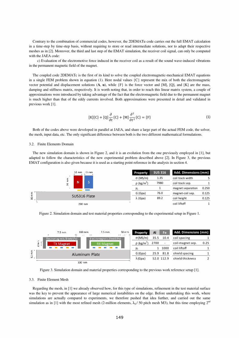
Contrary to the combination of commercial codes, however, the 2DEMATu code carries out the full EMAT calculation
in a time-step by time-step basis, without requiring to store or read intermediate solutions, nor to adapt their respective
meshes as in [2]. Moreover, the third and last step of the EMAT simulation, the receiver coil signal, can only be computed
with the JAEA code:
c) Evaluation of the electromotive force induced in the receiver coil as a result of the sound wave-induced vibrations
in the permanent magnetic field of the magnet.
The coupled code 2DEMATc is the first of its kind to solve the coupled electromagnetic-mechanical EMAT equations
in a single FEM problem shown in equation (1). Here nodal values C represent the mix of both the electromagnetic
vector potential and displacement solutions (A, u), while F is the force vector and [M], [Q], and [K] are the mass,
damping and stiffness matrix, respectively. It is worth noting that, in order to reach this linear matrix system, a couple of
approximations were introduced by taking advantage of the fact that the electromagnetic field due to the permanent magnet
is much higher than that of the eddy currents involved. Both approximations were presented in detail and validated in
previous work [1].
KC + Q
C + M
C = F (1)
Both of the codes above were developed in parallel at JAEA, and share a large part of the actual FEM code, the solver,
the mesh, input data, etc. The only significant difference between both is the two different mathematical formulations.
3.2. Finite Elements Domain
The new simulation domain is shown in Figure 2, and it is an evolution from the one previously employed in [1], but
adapted to follow the characteristics of the new experimental problem described above [2]. In Figure 3, the previous
EMAT configuration is also given because it is used as a starting point reference in the analysis in section 4.
Figure 2. Simulation domain and test material properties corresponding to the experimental setup in Figure 1.
Figure 3. Simulation domain and material properties corresponding to the previous work reference setup [1].
3.3. Finite Element Mesh
Regarding the mesh, in [1] we already observed how, for this type of simulations, refinement in the test material surface
was the key to prevent the appearance of large numerical instabilities on the edge. Before undertaking this work, where
simulations are actually compared to experiments, we therefore pushed that idea further, and carried out the same
simulation as in [1] with the most refined mesh (2-million elements, λS / 50 pitch mesh M3), but this time employing 2nd
Property Al Fe
σ (MS/m) 35.5 10.4
ρ (kg/m3) 2700 -
µr 1 1000
G (Gpa) 25.9 81.8
λ (Gpa) 52.0 112.9
coil spacing 1
coil-magnet sep. 0.25
coil liftoff 1
shield spacing 1
shield thickness 2
Add. Dimensions (mm)
Property
σ (MS/m)
ρ (kg/m3)
µr
G (Gpa)
λ (Gpa)
SUS 316
1.35
7980
1
76.0
89.2
coil track width 5
coil track sep. 1
magnet separation 0.250
magnet-coil sep. 0.125
coil height 0.125
coil liftoff 1
Add. Dimensions (mm)
149

order triangular elements instead of 1st order ones. Those results are not directly showed here, but confirmed the hypothesis
that the edge instabilities were due to the lack of edge mesh refinement.
Figure 4. Effect of mesh refinement in the vicinity of the EMAT emitter. Using a uniform mesh large perturbations arise
on the edge of the test material (right) [1], which totally disappear once the mesh is fine enough (left).
150

Figure 5. Schematic of the FEM mesh used for the simulation domain in Figure 2.
The 2-million 2nd
order element mesh was however too large to be practical for running in a standard workstation, and
further analysis was done to achieve similar results with a 1st order mesh. Focusing in the idea of refining the area in the
vicinity of the EMAT coils, the maximum pitch resolution was increased to 7 µm, which for a 1MHz input EMAT signal
corresponds to roughly λS / 800. Unsurprisingly, this spatial definition is of the same order of magnitude as the time
discretization one we found to be good enough to reproduce all signal features during previous work [1]. A comparison
with mesh M2, which has the same pitch inside the test material (λS / 50) but lacks the edge refinement, is shown in Figure
5 for the reference simulation in Figure 3 [1].
The same approach was therefore employed for the new experimental problem in Figure 2, with the final mesh using
either 1.2 million (standard definition) or 1.8 million (high definition) 1st order triangles. The difference between both lies
in the pitch inside the test material, which varies between 0.250mm (λS / 12.5) and 0.125mm (λS / 25), respectively. Both
meshes are too dense to be represented directly, but a schematic of the different areas involved is shown in Figure 5. In the
figure, for each area, both the X and Y ranges are indicated together with their respective base mesh pitches. The actual
meshes are obtained by triangularization of the whole simulation domain while respecting these constraints, and using a
minimum angle of 33 degrees to ensure adequate element geometrical quality.
151

3.4. Input Currents
Both, the newly adopted input current pulse [2] and that previously used in [1] are given in
Figure 6 left and right, respectively. As an example, here both are given when using the central frequency fc of 1MHz,
but several fundamental differences arise from their respective mathematical expressions:
a) While the new pulse becomes zero after the number of periods defined by the parameter n, the previous one has an
infinite queue, slowly tending towards zero together with the exponential pre-factor.
b) While the central frequency effectively affects the duration of the new pulse (in the example 3µs because n = 3 and
fc = 1MHz), it controls the number of periods in the previous one (the duration of the pulse being fixed by the attenuation
factor α in the pre-exponential term).
Figure 6. Newly adopted (left) and previously used (right) input current density pulses.
152

4. Analysis
4.1. Overview
One of the most noticeable differences between the new experimental setup and the previous one was the asymmetry of
the EMAT-generated sound wave in the material [2]. At first, several hypotheses were made, but ultimately it was decided
to follow a step by step approach, in which each of the configuration changes made when going from the previous model
in Figure 3 to that in Figure 2 could be analyzed individually. The resulting full test matrix is presented in Figure 7, and
includes a total of nine variables, four of which were tested using the previous setup configuration (Figure 3), and five
others using the new setup (Figure 2). In the following, only the most relevant changes on each setup are detailed and
compared qualitatively, since the experimental results only contain the displacement wave propagation figures.
Unless otherwise specified:
a) all the following 2D simulations were performed using the 2DEMATc coupled code, and display + .
.
b) comparisons in paragraphs 4.2 to 4.4 are based in the ISEM’13 configuration in Figure 3, including the input signal
from [1] in
Figure 6 with a frequency of 1MHz.
c) comparisons in paragraphs 4.5 to 4.8 are based on the new JAPEIC configuration Figure 2, including the new input
signal from [2] in
Figure 6, and except that the EMAT was enclosed in a metallic box similar to those in Figure 3.
Figure 7. Analysis test matrix representing all the case-studies considered in the present work.
4.2. Magnet configuration effect
As seen in Figure 2, the magnet configuration was changed from a single magnet element to a couple of magnets with
opposite polarization. The results are shown in Figure 8, where it is made clear that this was the change originating the
asymmetry of the wave, arising from the magnetic field asymmetry of the EMAT in the vicinity of the test sample surface.
153

Figure 8. Sound wave comparison between the single magnet (left) and double magnet (right) configurations.
4.3. Input signal effect
Figure 9 shows how the differences between both input signals in
Figure 6 are well translated into the simulated sound-wave. In this particular single pulse configuration, the shorter new
pulse (right) allows to clearly discern between the longitudinal (P) and shear (S) waves from the very beginning of the
propagation, while the previous pulse is long enough for both to get mixed up in the early stages (left). Also, the new pulse
seems to go ahead of the previous one, but that is only because its amplitude rises much faster as seen in
Figure 6. Comparing both of the time steps provided (top and down), it can be seen however that, after the initial rise,
the wave propagation is identical in both cases, as one would expect since the input signal is the only difference between
both simulations. This case was carried out starting with the overall ISEM’13 configuration in Figure 3, but using the
circular coil from [2] (Figure 1) instead of the meander one [1].
Figure 9. Sound wave comparison between the previous (left) and newly (right) adopted input density currents in
Figure 6.
4.4. Coil shape effect
Another one of the considerable changes between the two experimental configurations was going from a meander coil to a
circular coil. The first direct effect was that of a much larger amplitude, due to the considerably larger section of the coil
elements, so in Figure 10 below signals are actually scaled in order to better appreciate the other differences. As it can be
seen, the overall propagation is very similar, but the shapes of both the shear-S and longitudinal-P waves are considerably
altered, reflecting the coil setup geometry. Indeed, the asymmetry introduced by the double magnet configuration is
considerably enhanced by the meander coil setup when compared with the perfectly symmetrical circular coil case. This
154

comparison was carried out starting with the overall ISEM’13 configuration in Figure 3 [1], but using the new pulse from
[2] in
Figure 6.
Figure 10. Sound wave comparison between the meander (left) and the circular (right) coil configurations.
4.5. FEM code effect
We had seen in previous work that the most noticeable difference between the coupled and uncoupled formulations of
the EMAT problem was the decreased amplitude in the receiver-coil signal [1]. When looking at the propagated sound-
wave in this new configuration, however, the differences are considerably smaller. Altogether, the most significant change
in Figure 11 is the amplitude of the excited S-wave, which almost disappears when using the uncoupled code. It is worth
noting here that in real life there is not such large amplitude difference between both, but our 2D setup can only properly
reproduce the P-wave, as will be discussed later (section 5). This comparison was carried out with the new configuration
from [2] in Figure 2, except that the EMAT was enclosed in a metallic box similar to those in Figure 3.
Figure 11. Sound wave comparison between the uncoupled (left) and the coupled (right) 2DECT codes.
4.6. Mesh refinement effect
As previously discussed (cf. 3.2), two meshes were tested with two different levels of refinement inside the test material
bulk. As seen in Figure 12, the smaller mesh carries considerably more noise and some visible artifacts in the smallest
details, for which the high-quality mesh is needed. If one is interested only in the main signal, however, the standard mesh
with 1.2M elements remains reasonably good. This comparison was also carried out with the new configuration from [2] in
Figure 2, except that the EMAT was enclosed in a metallic box similar to those in Figure 3.
155

Figure 12. Sound wave comparison between the standard (left) and the high quality (right) meshes (cf. Figure 5).
156

4.7. Test material
As far as the test material is concerned, the main differences observed in Figure 13 correspond to the different wave
velocities arising from the change in the material properties given in Figure 2 and Figure 3. Indeed, while the S-wave
velocity is almost identical in both cases (~ 3.1 mm/µs), the P-wave is considerably slower in the SUS316 steel (5.5
mm/µs) vs. the Aluminum (6.2 mm/µs). Again, both of such changes are well rendered by the 2DEMATc coupled code.
This comparison was also carried out with the new configuration from [2] in Figure 2, except that the EMAT was enclosed
in a metallic box similar to those in Figure 3.
Figure 13. Sound wave comparison between the aluminum (left) and the SUS316 (right) test samples.
4.8. Coil misplacement effect
When considering the wave asymmetry observed in the experimental signal [2], an unnoticed shift in the coil position
was among the possible causes. As seen in Figure 14 and Figure 15, however, this effect is noticeable when shifting the
coils to the left (towards the N magnet), but only minor when shifting to the right (towards the S magnet). When
comparing both the left and right shifts, however, it can be seen that differences remain relatively small up to 0.5mm
[Figure 14], and only become truly significant if shifting 1mm [Figure 15], when a considerably loss of symmetry and
signal amplitude can occur. This comparison was also carried out with the new configuration from [2] in Figure 2, except
that the EMAT was enclosed in a metallic box similar to those in Figure 3.
Figure 14. Sound wave comparison between the 0.5mm laterally shifted coils, towards N-magnet (left) or S-magnet (right).
Figure 15. Sound wave comparison between the 1.0mm laterally shifted coils, towards N-magnet (left) or S-magnet (right).
157

5. Comparison between simulations and experimental data
The comparison between simulation and experimental results at three different time instants is shown in Figure 16. As
seen in the figure, the initial longitudinal P-wave is well reproduced by the JAEA 2DEMATc code, both in amplitude and
velocity, resulting in considerably similar figures. Other characteristic features such as the asymmetry of the experiment
visualization could be also reproduced in the numerical simulation, which was confirmed to appear because of the
asymmetry of the permanent magnets sources, creating an asymmetry in the Lorenz force inside the test material (cf. 4.2).
In this case, the asymmetry is inverted left-right because the simulations were inadvertently run with the inverse polarity of
the magnets. Other than that, there are some noticeable detail differences, which are thought to arise from the different
magnitudes plotted. Indeed, while the computational plots are vector based (ux + uy) for the X and Y in-plane components
together, the piezoelectric sensor experimental measurements might include also parts of the Z-perpendicular-plane
component, as well as other 3D effects.
A cut-view for the 3D computational signal obtained by JAPEIC, and representing the amplitude of the displacement
taking into account X, Y and Z components, is shown in Figure 17. It can be seen that, because of the 3D geometry, there
is not only the main shear S-wave propagating in the volume of the material, but also additional waves that seem to result
from other 3D effects in the simulation domain. None of them can be taken into account in the 2D geometry.
All in all, the results above highlight the limitations of the 2D plane-parallel code, into that only the longitudinal P-wave
is excited. Indeed, the shear S-wave, which represents vibrations in the Z direction, perpendicular to the XY simulation
domain, cannot be properly reproduced, because the Z-displacement component is ignored in the 2D approximation. This
is even more clearly visible when comparing JAEA 2D coupled code (2DEMATc) results with those previously obtained
by JAPEIC using a 3D version of COMWAVE, as seen in Figure 18 and Figure 19. The computational plot displays the
absolute values of X and Y component with both FEM approaches.
Finally, as one could have expected from the analysis in paragraph 4.5, results obtained with JAEA 2D uncoupled code
(2DEMATu) in Figure 20 show slightly smaller S-wave amplitude when compared with those obtained with 2DEMATc in
Figure 18 and Figure 19.
Figure 16. Comparison between experimental sound-wave measurements and JAEA’s 2DEMATc simulations.
158

time = 7.15µs
time = 10.83µs
Figure 17. 3D cut-view at for positions at two time steps of the wave amplitude using 3D
numerical simulations (JAPEIC)
159

Figure 18. Sound-wave comparison for X-component between JAEA’s 2DEMATc code and EMsolution/COMWAVE
results.
Figure 19. Sound-wave comparison for Y-component between JAEA’s 2DEMATc code and EMsolution/COMWAVE
results.
160

Figure 20. Sound-wave for X and Y-components computed with uncoupled JAEA’s 2DEMATu code.
6. Conclusion
It was shown that the JAEA developed 2DEMAT codes accurately reproduce the EMAT sound-wave propagation
characteristics, both in terms of overall wave-figures and velocities. Simulation results were shown to be in good
agreement with the experimentally observed waves, but only within the 2D approximation limitations. Indeed, because the
plane-parallel configuration assumes no field variations in the direction perpendicular to the plane, the shear wave cannot
be adequately reproduced. Similarly, Rayleigh waves propagating along the surface of the material cannot be simulated in
this 2D configuration. Finally, for the present EMAT configuration, it is seen that the wave propagation in the coupled and
uncoupled approaches to EMAT result in relatively small differences. The main advantage of the coupled code thus
remains its reduced computational time, which in practical applications is several times faster than the uncoupled code.
That is not only because it is inherently simpler (we solve a single FEM problem instead of 3 consecutive ones in the
uncoupled code), but also because it offers better scalability when parallelized on multi-core CPUs. This advantage is even
greater when compared with the concatenation of several commercial codes, but the latter approach already allows for
simulations of actual 3D configurations, which are required for many practical applications.
References
[1] Daniel Garcia-Rodriguez, Ovidiu Mihalache, Masashi Ueda, "EMAT Simulations based on a Two-Dimensional FEM
Coupled Electro-Mechanical Formulation", International Journal of Applied Electromagnetism and Mechanics, Vol 45, pp.
543-549,2014.
[2] T. Yamamoto, T. Furukawa, I. Komura, R. Urayama, T. Uchimoto and T. Takagi, “Property study on EMATs with
visualization of ultrasonic propagation”, M. Bieth (Ed.), Proceedings of the 10th International Conference on NDE in
Relation to Structural Integrity for Nuclear and Pressurized Components, pp. 902-909, European Union (2014).
[3] Hirao M and Ogi H, “EMATs for science and industry: Non-contacting ultrasonic measurements”, Boston / Dordrecht /
London, Kluwer Academic Publishers, 2003.
[4] EMSolution software ( http://www.ssil.co.jp/em/EMSolution/ja/index.html), 2015.
[5] Y. Ikegami, Y. Sakai and H. Nakamura, “A Highly Accurate Ultrasonic Simulator Capable of Over One Billion
Elements for Non-destructive Evaluations,” Proceedings of the 7th International Conference on NDE in Relation to
Structural Integrity for Nuclear and Pressurized Components, 177-190, (2009).
161

Conventional x-ray radiography versus image plates: a simulation and experimental performance
comparison D. Tisseur
1, B. Rattoni
1,G. Cattiaux
2, T. Sollier
2
1CEA LIST, CEA Saclay 91191 Gif sur Yvette Cedex, France
2Institut de Radioprotection et de Sûreté Nucléaire, B.P.17 92262 Fontenay-Aux-
Roses, France
ABSTRACT.X-ray/gamma ray radiography is a commonly used non-destructive evaluation method. For several
years, a research program funded by the French Institute for Radioprotection and Nuclear Safety (IRSN), in
partnership with CEA, studies gamma/X-ray simulation tools for evaluating NDE methods in the nuclear domain.
In this context, IRSN has started in 2010 a program over several years for the validation of CIVA RT module. The
aim of this paper is to present results of CIVA RT tools validation. The study consists in a cross comparison
between classical X-ray films and image plates on experimental and simulation results. These have been carried
out on very small openings (20 microns to 80 microns) notches. The study focuses on the case of homogeneous
tube-tube and tube-elbow welds for iridium 192, selenium 75 and X-rays sources. Keywords: Radiography, computed radiography, gamma source, validation, Monte Carlo simulation, CIVA
PACS: 28.41.Ak
INTRODUCTION X-ray/gamma ray radiography is a commonly used non-destructive evaluation method. For several
years, a research program funded by the French Institute for Radioprotection and Nuclear Safety
(IRSN), in partnership with CEA, studies gamma/X-ray simulation tools for evaluating NDE methods in
the nuclear domain. In this context, IRSN has started in 2010 a program over several years for the
validation of CIVA RT module[1-3]. The aim of this paper is to present results of CIVA RT tools
validation. The study consists in a cross comparison between classical X-ray films and computed
radiography on experimental and simulation results. These have been carried out on very small openings
notches (20 microns to 80 microns). The study focuses on the case of homogeneous tube-tube and tube-
elbow welds for 192Ir, 75Se and X-rays sources.
MATERIALS AND METHODS
For this study, we used CIVA 11 version. Given the context of thick components, we usedthe fusion
approach of scattered and transmitted images respectively fromMonte Carlo and analytical
computations to simulate the final images [3,4,5]. For conventional radiography, we used the detector
model (Gray model [8]) developed by EDF [7,9]. This model is based on the European standard EN
584-1 [6] and converts the incident dose into an optical density value.For computed radiography, we
used the detector model named “generic detector” based on the transfer function between measured
incident dose and grey level. For each incident dose, mean grey level and standard deviation is
computed in a region of interest. The model converts the simulated incident dose into grey level via this
transfer function. A Gaussian noise is added based on the standard deviation evaluated on experimental
images.
Figure 1 presents the set up for dose versus grey level measurement. Figure 2 presents an example of
“generic detector” transfer function for 192
Ir. These measures were performed for192
Ir, 75
Se and X-rays
sources.
162

Figure 1: On the left, the experimental set up for dose measurement. On the middle, example of mean grey level
and standard deviation in a region of interest.In the right, example of grey level histogram obtained with ImageJ
[14].
Figure 2: Example of transfer function.
In order to validate our detector modelling, we use 192
Ir source associate with Kodak HR and a step
wedge:
- 7 steps between 4 and 18 mm thicknesses
- Ferritic steel
- Total length 272 mm (6*40 mm + 1*32 mm)
The following figure presents a cross comparison between CIVA and experimental results.
Grey level
Incident dose in mGy
163

Figure 3: On the left, simulation and experimental image of the step wedge obtained with
192Ir gamma source. On
the right, grey level profiles (extracted along the step wedge) comparison between simulation and experimental
data.
The X-ray source spectrum was measured experimentally by the National Laboratory Henri Becquerel
(LNHB) using a highly collimated CdTe spectrometer. The following figure shows the spectrum
measured at 1 m in the axis of the X-ray tube window.
Figure 4: X-ray tube spectrum measurement at 200kV.
We used a homogeneous weld mock-up representative of auxiliary piping of main primary
system. This mock-up is composed on one side of a straight part with a tube-tube weldand on the other
side of anelbow part with tube-elbow weld (see figure 5). Pipe thickness is 8.56 mm, inside weld bead is
0.75 mm and outside weld bead is 2 mm.
Figure 5: Schema of the piping mockup.
Simulation
Experience
164

Four notches with several sizes (a height of 2.5 mm and an opening from 20 µm to 80 µm),
orientations (axial or circumferential) and positions have been superimposed to the weld thanks to a
manufactured insert (see figure 6 and table 1).
Figure 6: Schema of the insert with the four notches.
Reference Name Length
(mm) Heigth (mm) Opening(mm)
Notch 1 EN-20 15 2.5 0.020
Notch 2 EN-40 15 2.5 0.040
Notch 3 EN-60 15 2.5 0.060
Notch 4 EN-80 15 2.5 0.080
Table 1:Description of the four notches.
For this validation, the notches are positioned in a circumferential and a longitudinal configurationin
the middle of the weld (see figure 7 for straight part and figure 8 for elbow part) and the sources are
axed on the weld.The distance from the source to the mock-up is 0.725 m.
Figure 7: On the left, straight part experimental set-up. On the right, straight part simulation set-up with axial and
circumferential notch configuration.
192Ir
Source
Insertwith the
4notches
Pipe mock-up
Detector
Source
Insert with4notches
Pipe mock-up
165

Figure 8: On the left, elbow part simulation (side view). In the right, elbow part simulation (top view).
We used a 192
Irand 75
Segamma source with a diameterof 3 mm and a height of 3 mm and an
YXLON 225 kV X-ray tube at 200 kV (spot size 1 mm diameter). For conventional radiography, we
used M100 Kodak X-ray films, manually developed in accordance with Kodak recommendations.
Filters and reinforced used screens are in conformity with the Rules for Design and Fabrication of NPP
Mechanical Components (RCC-M) and European standard [10,11,12]. For computed radiography, we
used Kodak HR image plate associated with a HD CR35 DURR NDT scanner.Computed radiography
cassette composition is in conformity with ISO17636 standard [13]. Image plates were scanned with 50
µm pixel size.
RESULTS AND DISCUSSIONS
Example of validation with
192Ir gamma source with computed radiography on the straight
part
Due to limited size of the paper, we only show a part of the results obtained for computed
radiography with 192
Ir gamma source on the straight part.Grey level profiles have been extracted
from the several images on the different notches (see figure 9). Amplitude and width at middle
height have been measured on each notch on experimental and simulated images.
Figure 9: On the left, grey level profile extraction along the red line on axial notch. In the middle, grey level
profile extractionalong the red line on circumferential notch. On the right, amplitude and width at middle height
measurement example.
Amplitude
Widthat middle height
166

Figure 10 presents grey profiles comparison between CIVA and experimental film perpendicularly
to the weld. The simulated data agrees with the experimental data.
Figure 10: On the left, grey level profile extraction along the red line on a simulated image.In the middle,
grey level profile comparison between CIVA and experimental data. On the right, relative error between
CIVA and experimental data
Figure 11 presents grey level profiles comparison between CIVA and experimental data with
circumferential notch.
Figure 11: On the top left, grey level profile comparison between CIVA and the experimental image for
EN20 notch. On the top right, grey level profile comparison between CIVA and the experimental image for
EN40 notch. On the bottom left, grey level profile comparison between CIVA and the experimental image
for EN60 notch. On the bottom right, grey level profile comparison between CIVA and the experimental
image for EN80 notch.
167

The following table shows the results (note that ND= none detected) for 192
Ir gamma source with
computed radiography for circumferential and axial flaw.
Flaw
Measured
amplitude
Simulated
amplitude
Measured width at
middle height in
mm
Simulated
width at
middle height
in mm
circumferentialfl
aw
EN80 321 397 0,38 0,43
EN60 302 395 0,41 0,39
EN40 188 180 0,39 0,44
EN20 ND ND ND ND
axial flaw
EN80 424 474 0,6 0,54
EN60 406 452 0,46 0,48
EN40 292 263 0,31 0,34
EN20 ND ND ND ND
Table 2:Amplitude and width comparison between CIVA and experimental data on the four notches for
circumferential and longitudinal positionsfor computed radiography with 192
Ir gamma source.
The comparisons between CIVA and experimental data show a good adequacy. EN20 notch is
never detected on the simulation and on the experimental data.
These comparisons have been performed for the 3 sources on the straight and elbow. The following
tables show a result synthesis.
Table 3: Amplitude and width comparison between CIVA and experimental data on the four notches for
circumferential positions for the straight part for computed radiography with 192
Ir and 75
Se gamma source
and X-ray source.
168

Table 4: Amplitude and width comparison between CIVA and experimental data on the four notches for
axial positions for the straight part for computed radiography with 192
Ir and 75
Se gamma source and X-ray
source.
Table 5: Amplitude and width comparison between CIVA and experimental data on the four notches for
circumferential positions for the elbow part for computed radiography with 192Ir and 75Se gamma source and
X-ray source.
Table 6: Amplitude and width comparison between CIVA and experimental data on the four notches for
axial positions for the elbow part for computed radiography with 192
Ir and 75
Se gamma source and X-ray
source.
169

Same procedures have been applied for conventional radiography on the same setup with the three
sources. Comparisons show a good agreement between simulation and experimental data for
computed and conventional radiography.Due to the limited size of the paper, we only show a
synthetic detection comparison between conventional and computed radiography in table 7.
Table 7: Detection comparison between conventional and computed radiography on the straight and elbow
part for the three different sources.
CONCLUSIONS AND PERSPECTIVES
In terms of performance, testing on the straight and elbow part show a lower level of detectability
with computed radiography (EN20 is never seen with computed radiography). Conventional
radiography is able to detect EN20 notch in all scenarios tested with an X-ray source. Conventional
radiography is able to detect EN20 notch in the straight part with a Se75 source.
If we take into account the signal amplitude of the defect (the results synthesis with conventional
radiography are not presented due to the limited size of the paper). For the straight and elbow part,
the 75
Se source and X-ray tube provides no gain in sensitivity with respect to the source 192
Irwith
computed radiography contrary to what has been demonstrated with conventional radiography. The
interpretation of the image is much easy with conventional radiography.
These first tries for computed radiography have been performed with respect to the ISO17636
standard but the cassette composition can be improved to enhance image quality.
170

REFERENCES
1. http://www-civa.cea.fr
2. R. Fernandez, A. Schumm, J. Tabary, P. Hugonnard, “Simulation studies of radiographic
inspections with CIVA”, in 17th WCNDT, Shanghai (2008).
3. J. Tabary, P. Hugonnard, A. Schumm, R. Fernandez “Simulation studies of radiographic
inspections with Civa", in COFREND 2008
4. R. Guillemaud, J. Tabary, P. Hugonnard, F. Mathy, A. Koenig, A. Glière, "SINDBAD: a
multipurpose and scalable X-Ray simulation tool for NDE and medical imaging", in PSIP
2003, Grenoble, France(2003).
5. J. Tabary, F. Mathy, P. Hugonnard "New Functionalities in “SINDBAD” Software for
Realistic X-Ray Simulation Devoted to Complex Parts Inspection" , in ECNDT 2006
6. EN 584-1:2006, "Non-destructive testing – Industrial radiographic film – Part 1: Classification
of film systems for industrial radiography", European standard for non-destructive evaluation
7. A. Schumm, U. Zscherpel, “The EN584 standard for the classification of industrial
radiography films and its use in radiographic modeling”, in Proceedings of the Sixth
International Conference on NDE in relation to structural integrity for nuclear and pressurized
components (2007).
8. T.Jensen, T.Aljundi, J.N.Gray, and R.Wallingford, “A model of X-ray film response”, in
Review of progress in Quantitative Nondestructive Evaluation, edited by D. O. Thompson and
D. E. Chimenti, AIP Conference Proceedings, American Institute of Physics, Melville, NY Vol
15, pp441-448(1996).
9. A. Schumm, U. Zscherpel, “Radiographic film modeling according to EN584”, in COFREND
2008
10. EN 444:1994, “Non-destructive testing — General principles for Radiographic examination of
metallic materials by X- and gamma-rays”, European standard for non-destructive evaluation
11. RCC-M:2007, “Regulatory requirements and design code”, AFCEN publication
12. NF EN 13068-1:2000, “Radioscopic testing - Part 1 : quantitative measurement of imaging
properties.”, European standard for non-destructive testing
13. ISO 17636, “Non-destructive testing of welds. Radiographic testing. X- and gamma-ray
techniques with film” ISO standard, 2013.
14. W.S Rasband, ImageJ, U. S. National Institutes of Health, Bethesda, Maryland, USA,
http://imagej.nih.gov/ij/, 1997-2014.
15. J. Plagnard, “Comparison of measured and calculated spectra emitted by the X-ray tube used at the
Gustave Roussy radiobiological service”, X-ray spectrometry,volume 43, pp 298–304, 2014.
171

Simulation based design of Eddy Current sensor for thickness change
measurement of Multi-layer
Seul-Gi Lee1, Hak-Joon Kim
1, Sung-Jin Song
1 and Chang-Sung Seok
2
1, 2 Department of Mechanical Eng., Sungkyunkwan University, 300 Chunchon-dong, Changan-gu,
Suwon, Kyunggi-do 440-746, Korea
Corresponding Author Sung-Jin Song / E-mail: [email protected], TEL: +82-31-290-7451, FAX: +82-31-290-
5276
Abstract
In case of gas turbine engine, it usually works on extreme environment like ultra-high temperature and pressure. So,
multi-layer spray coating method is applied in order to prevent failure of turbine components such as turbine blade. This
micro failure could be propagated in multi-layer coating and finally these micro cracks changed into possibility of
delamination. Thus, it is important to detect the micro failure crack before turns into the delamination. To detect these,
NDE methods like Ultrasonic Testing (UT) and Eddy Current Testing (ECT) can be applied. But, UT can detect
delamination but is hard to detect micro failure of surface because top coat of multi-layer coating is ceramic. Therefore, it
is recommended that ECT is more effective to evaluate inside failure because ECT is useful to detect the micro failure of
surface and delamination. In order to inspection of damaged multi-layer coating, magnetic shield eddy current probe to
measure thickness of damaged layer are used since it shows focusing magnetic flux density on the coats. We have
investigate relation between Eddy current signal (impedance, phase angle) and thickness of damaged layer using FEM
simulation and by experiments results. In this presentation, we will discussed designed eddy current sensor and analytical
and experimental results.
Keywords : multi-layer coating, micro failure, eddy current testing, FEM simulation
1. Introduction
Gas turbine power generation occupied approximately 30% of domestic power plant has increased steadily because it’s
useful to energy efficiency ratio, environmental affinity and power load control since 1990s[1]. So, to satisfy its
performance and service life of key components under extreme environment, it is important to overcome its limitations of
heat resistance, corrosion resistant anti-oxidation. There are some methods to solve this problem, TBC (Thermal Barrier
Coating) technic attracts attention because TBC technic can get large effect with relatively low investment [2, 3].
TBC is composed by top coat and bond coat so those protect the substrate from environment of high temperature. TBC
can be failure by repetitive thermal stress during operating gas turbine [4]. Failure of turbine Blade is generated from
damage of TBC such as top coat delamination and difference of coefficient thermal conductivity therefore it’s important to
diagnosis the damage and predict remaining service life before generating safety problem. When between top coat and
bond coat is exposed at high temperature, TGO (Thermally Grown Oxide) can be grown in two layers. Thermal stress is
one of main reason of top coat delamination and changed because of TGO growth so this effects TBC durability [5]. In this
study, used structure of TBC specimen and problems of each layer are shown in Fig. 1.
To detect this, non-destructive evaluation methods like Ultrasonic Testing (UT), Thermography, Impedance
Spectroscopy, Eddy Current Testing (ECT) and Pulsed Eddy Current Testing (PECT) can be applied each suitable layer.
When measuring TGO layer, ECT is used, existing research was applied coil with air core. Experiment results were not
that clear and stable at each degradation hour of TBC specimen [6]. In this research, therefore ferrite core and magnetic
shield are used to focus magnetic flux density into TBC specimen. Eddy current signal (impedance, phase angle) and
thickness of damaged layer are investigated using FEM simulation and by experiments results. Finally, decided designed
eddy current sensor through discussion of the results of both FEM simulation and experiments.
172

Figure 1. Structure and problems of TBC with suitable NDE methods[7]
2. Used TBC Specimens
There are two kinds of main TBC coating system, APS and EDC. Both coating system are shown as Fig. 2 (a), (b). APS
has bulking when it is degraded but EDC shows less bulking and residual stress because of inserted vertical cracks even
though EDC has thicker TGO layer. In this study, so we used EDC specimen. Micro-structure analysis results of used TBC
specimens are shown as Table 1. TBC specimen was degraded at each temperature and degradation hours. Specific point is
top coat was totally delaminated at 1100 both 200 hours and 400 hours. From those micro-structure analysis results,
TGO thickness was adopted to the simulation.
(a) APS (b) EDC (c) Micro-structure analysis of TBC specimen
Figure 2. (a), (b) Structure of APS & EDC[8], (c) Micro-structure analysis of APS & EDC
Table 1. Micro-structure analysis results
3. Simulation of ECT
3.1 Simulation setup of ECT
Used simulation commercial program is COMSOL Multiphysics 4.4. Two kinds of simulation setup are about ECT
probe for ‘with magnetic shield’ and ‘without (W/O) magnetic shield’. Ferrite core was used both setup and probe is placed
173

in the center of TBC specimen. Those are shown in Fig. 3 and minimum lift off was 0.5mm. Thickness of TGO layer is
applied differently according to each degradation hour and temperature as shown in Table. 1. Operating Frequency range is
0Hz to 15MHz and coil impedance was measured in air for reference value.
(a) APS (b) EDC (c) Micro-structure analysis of TBC specimen
Figure 2. (a),(b) Structure of APS & EDC, (c) Micro-structure analysis of APS & EDC
3.2 Simulation results
Obtained simulation results are coil resistance and reactance for coil impedance finally. The coil impedance of lift-off
change can be adopted to measure the bond coat thickness, because the electrical properties of the top coat are same as
those of air. The design lift-of the coil is constant, so the coil impedance of lift-off change can be adopted to measure the
bond coat thickness. Normalized each part of coil impedance change and the results show at 9.3MHz were changed bigger
when increasing degradation hour of TBC system. Simulation results of W/O magnetic shield are as shown in figure 3. In
these results, both were changed bigger when degradation hour of TBC system is increased. 1100 shows the biggest
change than other two temperature. In Figure 3. (a), resistance changes almost 0.3 and in Figure 3. (b), reactance changes
as 2.5. Simulation results of with magnetic shield are also as shown in Figure 4. Both resistance and reactance change have
similar trend with W/O magnetic shield. Therefore 1100 shows the biggest change, therefore resistance as shown in Fig
4. (a), changes approximately 0.4 and reactance as shown in Figure 4. (b), changes as 3.1.
(a) resistance change (b) reactance change
Figure 3. Simulation results of W/O magnetic shield
(a) resistance change (b) reactance change
Figure 4. Simulation results of with magnetic shield
174

So from those results, comparison of simulation result of W/O magnetic shield and with magnetic shield is as follow
Figure 5. As shown in magnetic flux density, magnetic flux density can be compared with ‘W/O magnetic shield’ and
‘with magnetic shield’. Magnetic flux density does not spread out more around because of magnetic shield. So magnetic
flux density can be more focused to multi-layer and penetrated more deeply. By comparison with impedance change, with
magnetic shield shows slightly bigger than which is not.
(a) Magnetic flux density (T) (b) Comparison with impedance change
Figure 5. Comparison with simulation results
4. Experiments of ECT
4.1 Experimental setup of ECT
Eddy current testing system for bond coat thickness measurement is as shown in Figure 6. Impedance analyzer is used
for measuring impedance of eddy current probe. It can be used for finding resonance frequency of ECT probe and applied
the frequency under resonance frequency when measuring the impedance. For the experiments, coil size and magnetic
shield case size are same with simulation geometry size. Probe is placed in the center of TBC specimens as simulation did.
Thickness of magnetic shield case is designed as same as simulation results and this is enough to shield magnetic flux.
(a) Experimental setup of eddy current testing (b) Probe W/O magnetic shield (left),
Probe with magnetic shield (right)
Figure 6. Experimental setup and used two types of ECT probe
4.2 Experiments results of ECT
Using impedance analyzer, coil impedance can get directly. When operating frequency is 9.3MHz, ‘W/O magnetic
175

shield’ and ‘with magnetic shield’ are also conducted 900, 1000, and 1100 degraded TBC specimens for every
degradation hours. When compared at each degradation temperature and hours for W/O magnetic shield as shown in
Figure. 7 (a), difference of impedance change at 1100 shows much bigger than others. Results of 900 and 1000are not stable and show steady trend. As shown in Figure. 7 (b), difference of impedance changes steadily at each
temperature and its value is getting bigger according to thermal degradation hours. This result is more easy to assort
degradation temperature and hours relatively.
5. Summary
1) By simulation results, resistance and reactance of coil parameter change the difference of each degradation
temperature and hours. When degradation temperature and hours are getting higher, each impedance change is also higher.
So ‘with magnetic shield’ shows slightly higher than ‘W/O magnetic shield’.
2) By experiment results, impedance change is getting bigger as simulation results did. From both simulation and
experiment results, comparison of impedance change when magnetic shield case is applied or not.
3) Impedance change has been much bigger when TBC thermal degradation temperature is at 1100 and hours are
higher.
4) Simulation and experiment results both show same trend when ‘with magnetic shield’ has been changed bigger than
‘W/O magnetic shield’.
Acknowledgements
This paper was supported by Basic Science Research Program through the National Research Foundation of Korea
(NRF) funded by the Ministry of Science, ICT & Future Planning (No. 2011-002024).
References
[1] Moon Young Kim et al., “Analysis of Damage Trend for Gas Turbine 1st Bucket Related to the Change of
Models”, Korean Soc. Mech. Eng. A, Vol. 31, No. 6, pp. 718~724 (2007)
[2] H. I. Kim et al., “Study on the Integrity Recovery according to Manual Overlay and Pre- & Post- welding
Treatment of Nickel-based Superalloy for Gas Turbine Blade”, Korean Soc. Precis. Eng., Vol. 26, No. 3, pp. 11~18
(2009)
[3] D. J. Kim, “Thermal Fatigue Test Methods for Thermal Barrier Coatings of Gas Turbine Blade”, Korean Soc.
Precis. Eng., Vol. 26, No. 2, pp. 7~15 (2009)
[4] Quadakkers, W.J., Shemet, V., Sebold, D., Anton, R., Wessel, E. and Singhesier, L., “Oxidation Characteristics of
a plainized MCrAlY Bond Coat for TBC Systems During Cyclic Oxidation at 1000”, Surface & Coatings Technology,
Vol. 199, pp. 77~82 (2005)
[5] Hyun Woo Song, Byung Woo Moon, Jae Gu Choi, Won Suk Choi, Dongju Song, Jae-Mean Koo and Chang-Sung
Seok, “Durability Evaluation of Thermal Barrier Coating (TBC) According to Growth of Thermally Grown Oxide
(TGO)”, Korean Soc. Mech. Eng. A, Vol. 38, No. 12, pp. 1431~1434 (2014)
[6] Zhang Jianhai, “Electrical impedance based nondestructive evaluation of thermal barrier coating system”,
Thesis(PH.D.), Sungkwunkwan university : Department of Mechanical Eng., (2015)
[7] David R. Clarke, Matthias Oechsner and Nitin P. padture, “Thermal-barrier coatings for more efficient gas-
turbine engines”, MRS Bulletin, Cambridge univ., Vol. 37, (2012)
[8] Abdullah Cahit Karaoglanli, Kazuhiro Ogawa, Ahmet Turk and Ismail Ozdemir, “Thermal Shock and Cycling
Behavior of Thermal Barrier Coatings (TBCs) Used in Gas Turbines”, Ernesto Benini, ISBN 978-953-51-1166-5
(2013)
176

Technical Support Developing
Performance Demonstration Programs in Japan
P. Ashwin, C. Latiolais, L. Esp, R.Grizzi, J. Langevin
Electric Power Research Institute (EPRI), Charlotte NC, USA
E-mail address: [email protected]
Following the discovery of intergranular stress corrosion cracks (IGSCC) in the 316L low-
carbon stainless steel primary loop recirculation piping of a Japanese boiling water reactor
(BWR), it was determined the ultrasonic technique to measure the through-wall depth of
these cracks was unreliable.
The Japanese utilities responded and set about improving the reliability of the ultrasonic
depth sizing techniques used for IGSCC. A key element was the development of their own
performance demonstration (PD) program for depth sizing of IGSCC. By 2005, the 10
Japanese utilities with operating nuclear plants had joined EPRI’s Nondestructive Evaluation
(NDE) Program and had begun meeting with EPRI and other stakeholders to develop the
Japanese Performance Demonstration (JPD) program. The first JPD qualification
examination was carried out during 2006. Since then there have been many qualifications and
the ultrasonic techniques now used in Japan to measure the through-wall depth of IGSCC
have been demonstrated to meet the acceptance criteria.
Building on the success of the IGSCC depth sizing PD program, the Japanese utilities have
set about introducing performance demonstration requirements for additional applications
into National codes and standards. These applications include weld overlay and dissimilar
metal weld examinations. The EPRI NDE Program continues to work closely with the
Japanese team responsible for these actions and this paper will summarize the technical
support provided by EPRI, this includes:
• Benchmarking Japanese PD requirements against U.S. requirements
• Participating in two pilot studies to improve the understanding of information readily
available for typical dissimilar metal weld configurations in BWR and pressurized
water reactor (PWR) plants
• Jointly developing a technical basis to use alternative flaw types for PD
• Fabricating additional test specimens to address differences in Japan and U.S.
configurations
• Aligning Japanese PD instructions and U.S. instructions
Moving forward, the Japanese Utilities are now evaluating various technologies to support
performance demonstration. Again EPRI are working closely with the Japanese utilities and
other stakeholders. This joint research work includes developing training programs for NDE
technicians and introducing the use of simulation technology to training, maintaining NDE
technician proficiency and qualification.
Keywords: Performance Demonstration; Reliability; Qualification; Ultrasonic
177

The Progressive Statistical Analysis Results of Performance Demonstration
for Piping Welds
Hung-Fa Shyu
Institute of Nuclear Energy Research, 1000 Wenhua Rd., Longtan, Taoyuan City,
Taiwan ROC
E-mail Address: [email protected]
A performance demonstration program has been implemented by the Institute of Nuclear
Energy Research since 2002. This program followed the criteria of ASME Boiler and Pressure
Vessel Code Section XI, Appendix VIII to prepare demonstration sessions in Taiwan and
gained meaningful data during the past twelve years. In this paper, historical demonstration
results on the similar metal pipe welds were analyzed and the statistical data showed the
overall qualification rate, accuracy rate, and detection rate were about 59%, 93%, and 92%
respectively. The length sizing errors depended on the piping material and flaw orientation,
and the average relative error of qualified examinees was 59.1%±4.3%. This program can
provide a good screening function for ultrasonic inspection personnel, and the statistical
results can also provide both regulatory authorities and utilities with a conservative evaluation
of the confidence level of realistic ultrasonic testing results in nuclear power plants.
Keywords: Performance Demonstration, Ultrasonic Testing, Piping Welds
178

Current Status of Japanese Performance Demonstration in FY 2014
Keiji WATANABE1, Hajime SHOHJI
1, Koichiro HIDE
1, and Joji OHTA
1
1PD center, Central Research Institute of Electric Power Industry, Japan
Abstract
The Performance Demonstration (PD) Center of the Central Research Institute of the Electric Power Industry
(CRIEPI) commenced PD examinations for the depth sizing of intergranular stress corrosion cracking (IGSCC) in
austenitic stainless steel pipes in March 2006. By the end of the 2014 fiscal year, 42 examination sessions had been
completed, and 53 candidates had passed the examination. A total of 99 candidates had been administered exams,
including re-tests and re-certification. Candidates who passed the examination can perform depth sizing of IGSCC
flaws with a high level of accuracy. For the final determination of IGSCC crack depths in Japanese PD examinations,
phased-array ultrasonic testing technology is used more often than conventional ultrasonic testing or other
technologies. A statistical analysis shows that the average depth sizing error is 0.32 mm with a standard deviation of
1.87 mm for the successful applicant. From the PD examination results, the correct answer rate will decrease when
the ultrasonic testing time concerning a test answer requires 2.5 hours or more.
Keywords: PD qualification examination, Ultrasonic testing, Nuclear power plant, Inservice inspection, PLR piping,
Intergranular stress corrosion cracking
1. Introduction
The Japan Society of Mechanical Engineers (JSME) issued the first edition of a fitness-for-service code (FFS code) for
nuclear power plants in 2000 [1]. The FFS code was endorsed by the Nuclear and Industrial Safety Agency (NISA) and
has been in effect since October 2003 [1]. The Japanese performance demonstration (PD) standard, NDIS 0603,
“Qualification and certification of personnel for performance demonstration of ultrasonic testing systems,” was issued in
2005 [2]. The NDIS 0603 standard is essentially the same as Appendix VIII and Section XI of the American Society of
Mechanical Engineers (ASME) Code, having the same fundamental content with some modifications reflecting Japanese
technical expertise on IGSCC in austenitic stainless steel welds. The first Japanese PD qualification examination for the
depth sizing of IGSCC flaws was administered in March 2006 [3], and as of January, 2015, 42 examinations have been
conducted. In December 2010, the first PD recertification candidate took an examination. As of the end of the 2014 fiscal
year (FY), 53 out of a total of 99 candidates passed the examination.
2. PD Certification System in Japan
2.1 Operating organization
Figure 1 shows the organizations involved in the Japanese PD qualification examination for crack depth sizing in
austenitic stainless steel pipe welds in nuclear power plants [5]. The PD advisory committee oversees the PD
qualification system. The PD advisory committee reviews the activities of the PD-related organizations (PD
qualification activities, PD examination center, and PD training center) and makes recommendations. The Japanese
Society for Non-destructive Inspection (JSNDI) certifies PD-related organizations. The PD qualification body of
JSNDI consists of two committees: a PD certification committee to manage the PD certification system and a PD
scheme committee to design future PD systems. The PD qualification body organizes the qualification examinations,
preparing and maintaining the test specimens, test facility, and quality control documents. The PD examination center
conducts PD qualification examinations under the direction of the PD qualification body. In particular, the PD Center
of CRIEPI serves as both the authorized PD qualification body and the PD examination center. Finally, the PD
training center serves two functions in the PD system: (1) the training of personnel who fail their first PD examination
and desire to take a re-examination within 30 days and (2) annual training for license renewal. Both the Japan Power
179

Engineering and Inspection Corporation (JAPEIC) and the Electron Science Institute (ESI) have been qualified as PD
training centers.
2.2 Outline of qualification examination
Although the Japanese PD standard NDIS 0603 is similar to the ASME Code Section XI and Appendix VIII, some
adaptations have been incorporated to reflect our findings on IGSCC in austenitic stainless steel welds [4]. The
following adaptations have been incorporated:
(1) All cracks in the test sample should be IGSCC.
(2) At least one IGSCC should be deeper than 15 mm.
(3) At least one IGSCC should penetrate into the weld material.
(4) No undervalue of more than -4.4 mm should be permitted
The Japanese PD qualification test specimens are butt-welded austenitic stainless steel pipes with artificially introduced
IGSCC. The weld crowns are ground flush. Ten IGSCC must be tested in pipes of the following three sizes:
Nominal diameter of 600 mm with 35 mm wall thickness.
Nominal diameter of 350 mm with 25 mm wall thickness.
Nominal diameter of 150 mm with 10 mm wall thickness.
The distribution of the IGSCC crack depth introduced into the Japanese PD qualification test specimens is given in Table 1.
Table 1. Distribution of crack depth
Crack depth h (% wall thickness) Minimum number of IGSCC (Test specimen)
0 < h ≤ 30% 2
30 < h ≤ 60% 2
60 < h < 100% 2
For each candidate, the allowable examination time is five days for 10 samples with up to 8 h per specimen. One test
specimen is examined at a time, and the examinee is not permitted to carryover a specimen to the following day. The
acceptance criteria are as given follows:
A) Root-mean-square error (RMSE) must be less than 3.2 mm.
B) Critical mistake must be less than -4.4 mm.
JSNDI: The Japanese Society for Non-Destructive Inspection
JAPEIC: JAPAN Power Engineering and Inspection Corporation ESI: Electron Science Institute
Figure 1 Organizations involved in Japanese PD qualification examinations
180

The RMSE is derived from the following formula:
RMSE =
where mi is the measured IGSCC depth, ti is the true IGSCC depth, and n is the number of test specimens.
The PD certification is valid for one year and can be extended for up to five years if the qualified personnel receive
PD training at a PD training center.
3. PD Qualification Examination Results
The first PD qualification examination was conducted in March 2006. Over the next nine years, 53 candidates
applied for the examination, and 49 candidates were qualified. The total number of examinees during that nine-year
period, including those who took the recertification test, was 99. Figure 2 shows the change in the number of
candidates as well as the successful applicants from March 2006 to the end of FY 2014. The number of candidates in
each period has decreased gradually over the past eight years. However, looking at the results from a different point of
view, the required number of qualified personnel to support the Japanese nuclear industry was almost satisfied within
the first three years of the PD qualification examination process. After this period, the number of candidates
performing the qualification examination during each period stabilized as candidates was primarily performing the
examinations to support future activities within their organizations. Since then, the number of candidates in each
period has been stable. The PD-qualified persons took the examination considering their futures in their organizations.
Although the pass rate has fluctuated, the overall pass rate has gradually improved. Information obtained though
candidate interviews suggests that this improvement is the result of education and training at independent companies.
3.1 Variation in Candidate Performance
To clarify the depth sizing reliability, the PD Center conducted a statistical analysis of all accumulated test data.
Table 2 shows the statistical results of the IGSCC depth sizing errors. The mean error and standard deviation for
successful candidates were 0.32 mm and 1.87 mm, respectively, whereas the mean error and standard deviation for
Table 2 Statistical analysis of PD result candidates
Candidate group Mean Error (mm) Standard Deviation (mm)
Successful 0.32 1.87
Unsuccessful 1.02 4.84
0
5
10
15
20
0
10
20
30
40
2005 2006 2007 2008 2009 2010 2011 2012 2013 2014
Num
ber
of
exam
inat
ion s
essi
ona
Num
ber
of
candid
ates
Examination period (FY)
Successful(New)Successful(Re-certification)Successful(Re-examination)Unsuccessful
Number of examination sessions
Figure 2 Number of candidates and successful applicants per year
181

unsuccessful candidates were 1.02 mm and 4.84 mm,
respectively.
Figure 3 shows the relationship between the RMSE
and the average measurement errors of the successful
and unsuccessful candidates. The majority of
successful candidates performed IGSCC depth
measurements with average errors of 1 mm or less.
This shows that depth sizing of IGSCC flaws can be
performed with a high level of accuracy.
Figure 4 shows the change in the standard deviation
and average error for candidates who successfully
passed the PD certification examination. The mean
error lies below 1 mm, while the standard deviation
fluctuates between 1.5 to 2 mm. Thus, the candidates
who pass the Japanese PD certification examination
have the skill to determine crack depth sizing with
high accuracy.
3.2 Sizing Procedure
Figure 5 shows the number of candidates utilizing
various crack depth sizing procedures in PD
qualification examinations. In the figure, “PA” refers
to a phased-array examination using either linear or
matrix phased-array transducers with encoded or
automated scanning systems. As shown in Figure 5,
the combination of PA with conventional ultrasonic
testing (UT) (“PA + conventional UT”) is the most
successful procedure. The number of PD candidates
using only “PA” is almost the same as those using
only “Conventional UT”; however, the number of
successful candidates using PA is higher than those
using conventional UT.
Figure 6 shows the number of measurements for
various crack depth sizing procedures used in PD
Figure 4 Change in standard deviation and mean
error for the PD certification examination
0
0.5
1
1.5
2
2.5
2005-2006 2007-2008 2009-2010 2011-2012 2013-2014
Sta
nd
ard
dev
iati
on
, M
ean e
rro
r (m
m)
Examination year (FY)
Standard deviation
Mean error
0
2
4
6
8
10
12
-7 -6 -5 -4 -3 -2 -1 0 +1 +2 +3 +4 +5 +6 +7
RM
SE
(mm
)
Avarage error (mm)
Successful
Unsuccessful
Figure 3 The RMSE vs. average measurement errors for successful and unsuccessful candidates.
182

certification examinations. In this figure, “Others”
refers to normal beam method and tandem probe
technique. The results shown in Figure 6 indicate that
more successful candidates use PA for the final
specification of IGSCC depth than unsuccessful
candidates. On the other hand, when conventional UT
or other technologies are used for the final specification
of a crack depth, there are more unsuccessful
candidates than successful candidates.
Figure 7 shows the rate of the errors for various crack
depth sizing procedures used in PD certification
examinations. The error criterion adopted here is
whether the difference between the true and measured
value was less than ±3.2 mm. The results shown in
Figure 4 indicate that the PA technique, which yielded
the lowest error percentage, was the most successful
technique. The error rate associated with the PA
technology was slightly lower than that associated with
the conventional UT technology and other
technologies. The results suggest that the highest
percentage of correct answers is associated with
skillful utilization of the PA technology, and the second
highest percentage is associated with the use of
conventional UT technologies.
Figure 8 shows the relationship between the rate of
errors and the average UT time for all candidates.
When the inspection time for one test specimen is less
than 2 hours, there are a high percentage of correct
answers. In contrast, when the UT time for one test
specimen exceeds 2.5 hours, the percentage of correct
answers decreases. This trend suggests that longer UT
times result in a higher percentage of errors, possibly
due to hesitation by the examinee.
Figure 6 Final specific techniques for depth sizing of
IGSCC
Figure 7 Rate of errors for each UT technique
Figure 8 Relationship between the average UT time and the percentage of correct answers
183

3.3 Trends for PD Certification Examinees
Figure 9 shows the PD examination results
(numbers of successful and unsuccessful
candidates and pass rates) with respect to
candidate age. Although many candidates were
between 30–40 years of age, there was no
substantial difference in the examination pass
rates among the different age groups.
4. Conclusion
The CRIEPI PD center has been conducting
Japanese PD certification examinations since
March 2006. The results of the Japanese PD
examinations through FY 2014 can be
summarized as follows:
1. Successful candidates for the Japanese
PD certification examination have a high
level of proficiency in measuring crack depth sizing.
2. Successful candidates are capable of skillfully applying phased-array technologies as well as the supplemental
utilization of conventional UT or other technologies for identifying IGSCC.
3. Based on the RMSE, standard deviation, and mean error, the reason for the rejection of PD certification
examinations should be identified to successfully clear the re-examination.
4. When the UT time for one test specimen exceeds 2.5 hours, the percentage of correct answers decreases, suggesting that longer UT times result in a higher percentage of errors.
References
[1] K. Kashima, T. Nomura, and K. Koyama, “Current status of Japanese Code on Fitness-for-Service for Nuclear
Power Plants,” Pressure Vessel and Piping Codes and Standards, PVP-Vol. 480 (2004).
[2] T. Sasahara, T. Yamashita, and T. Nomura, “UT Performance Demonstration in Japan,” Fifth Int. Conf. on NDE
in Relation to Structural Integrity for Nuclear and Pressurized Components (2006).
[3] H. Shohji, K. Hide, and K. Watanabe, “Trends Identified Between Successful and Unsuccessful Candidates that
have Participated in the Japanese Stress Corrosion Cracking (SCC) Depth Sizing Performance Demonstration (PD)
Program,” E-Journal of Advanced Maintenance, Vol. 4, p. 125–132 (2013).
[4] T. Sasahara, T. Jikimoto, K. Hide, and H. Inoue, “Evaluation of SCC Depth Sizing Candidate and Performance,”
Maintenology, Vol. 9, No. 1, p. 44 (2010).
[5] H. Shohji, K. Hide, and K. Watanabe, “Current Status of Japanese Performance Demonstration in FY 2012,”
Proceedings of Twelfth International Conference on NDE in Relation to Structural Integrity for Nuclear and
Pressurized Components, Cannes, p. 436–441 (2013)
Figure 9 Number of candidates, successful candidates,
and examination pass rate by age
184

Development of Virtual Ultrasonic Testing System
Hajime SHOHJI 1 and Koichiro HIDE
1 1 Central Research Institute of Electric Power Industry, JAPAN
Abstract
The reliability of inspection results is affected by the skill of examination personnel, in particular with regard to
manual ultrasonic testing (UT). The number and design of test specimens are among the most important points to be
considered during training or assessing the qualification of UT examination personnel. For training, a simulated UT
system using a computer mouse or touch sensor was proposed. However, this system proved to be inadequate as a
replacement for actual UT work. In this study, we have developed a novel virtual UT system that simulates actual UT
work for piping welds.
This system (the Tool for Realistic UltraSound Testing) comprises a dummy UT probe, dummy piping, a computer
system, and a 3D position detection system. It can detect the state of the dummy probe (3D position and skewing
angle) and displays recorded A-scan data corresponding to the dummy probe status with random noise. Furthermore, it
does not display A-scan data if the dummy probe is not in contact with the pipe. In this way, the system simulates
actual UT work. Using this system, it is possible to significantly reduce the number of test specimens utilized for
training or assessing the qualification of UT examination personnel. In addition, highly efficient training and
certification will be achieved through this system.
Keywords: Ultrasonic, Virtual System, Training, Qualification, Simulator, Piping
1. Introduction
In Japan, ultrasonic testing (UT) for in-service inspection (ISI) has been performed by UT engineers with a great deal of
experience. However, most Japanese nuclear power plants (NPP) have ceased operation, and periodic ISI is not performed
regularly. Most UT engineers are now working in nonnuclear fields. Moreover, after the NPPs are restarted, most of these
highly skilled UT engineers will not return to nuclear field. Conversely, performance demonstration systems such as PDI
programs are currently only being applied to crack depth sizing and Weld Overlay (WOL) inspection, rather than crack
detection in Japan. This is based on a national research project [1] that reports that good inspection results and reliability
are achieved with general examination procedures and highly skilled UT engineers. In addition, Japanese inspection
companies have been operating their own training programs. For these reasons, a highly efficient, highly effective training
program is needed for high reliability UT examination.
However, this training program needs to use test specimens, which should be fabricated by the same process as used on
parts of actual plants, and have realistic defects. But these realistic test specimens are very expensive and take much time to
fabricate. Thus, one idea is to use virtual UT system as a part of training or PD examination.
In this study, we fabricate a prototype realistic virtual UT examination system (the Tool for Realistic UltraSound
Testing) and confirm the viability of this system for training UT engineers.
2. Feasibility Study In Japan, ISI-UT procedure is based on the standard JEAC4207 code[2]. This code is based on the previous ASME
Code in terms of its use of DAC evaluation and conventional UT techniques. Japanese inspection companies use their own
examination procedure, but these are based on JEAC4207 closely enough that there is no noticeable difference. The
reliability of these procedures was confirmed through a national research project [1]. Therefore, the key to the reliability of
examination results is the skill of the UT engineers involved.
UT examination for ISI is performed using automated scanning tools, especially for vessel inspection. However, some
piping inspection is still performed manually, especially at old plants. In addition, IGSCC has been detected at piping
welds. Therefore, the priority of training and/or PD testing for piping inspection for UT engineers is high. Thus, this virtual
system is focused on manual inspection of piping welds.
Generally, commercially available UT simulation systems use a computer mouse as a dummy UT probe. This kind of
185

system is useful for determining wave characteristics. However, it is insufficient for training engineers totally for the
inspection process. We extract the points simulating a realistic UT examination process as follows:
Realistic shape, Piping shape
The waveform should be displayed, and it should
depend on the absolute position of the dummy probe.
depend on the skew angle of the dummy probe
have a real-time response
be accompanied by random noise
Record scanning tracks for feedback training
3. System Design
3.1 Waveform data
It is possible to calculate the ultrasonic waveform using an FEM code or lay trace calculation. However, its calculation
time is generally too long for “real-time response” [3]. Conversely, human perception should be within a time lag no
greater than 40–50 ms [4]. Therefore, this system uses data from pre-recorded or pre-calculated waveforms.
3.2 Position detection system
This system should detect the absolute position and skew angle of a dummy probe with a “real-time response.” To
simulate realistic flaw detection, the dummy probe should require no wires or special equipment having cables. We
examined various position detection systems, including CCD cameras, pressure sensors, touch sensors, and lasers.
Ultimately, a 3D electromagnetic position detection system was selected for this purpose. This 3D system can detect sensor
position and angle with high accuracy, and the slave sensor is as small as a UT probe. However, this system cannot detect
whether the dummy probe is in contact with the dummy pipe surface or not. Thus, a small pressure sensor needs to be
added to this system.
3.3 System Design
Figure 1 shows the basic system design for the Virtual UT system. The master sensor of the 3D position system is set on
the dummy pipe, and a UT engineer moves the dummy UT probe, which includes a slave sensor and a small pressure
sensor. The 3D position system detects the position and skew angle of dummy probe, whereas its touching power is
detected through the pressure sensor.
Figure 1 Virtual UT system
3D Position detector
Pressure sensor I/O
Waveform data
Control PC for Trainer/Administrator Sub monitor
(Dummy UT Instrument)
Master Sensor
Slave Sensor with Pressure sensor
(Dummy Probe)
Dummy Pipe
186

Pressure sensor output and dummy probe 3D position and skew angle are sent to a control PC via the USB port. When
one starts up the software and loads the waveform data, they move to the cash memory of the PC. The control PC displays
the waveform depending on the dummy probe position, angle, and contact with the dummy pipe. The same waveform is
displayed on the sub monitor (Dummy UT instrument).
3.4 Waveform data
We collect UT data from small segmented test specimens (Figure 2). One segment includes a shallow IGSCC on the
butt weld line and the other does not include IGSCC. We use an automated scanner and special probe holder. The special
probe holder can be used to adjust control the skew angle of the conventional probe. We collect UT data from the upstream
and downstream sides at various skewing angles. In this case, the skewing angle is set between −10° to +10° and 170° to
190° with 2° pitch.
We copy the data several times and merge these data, in the form: “"Blank data"+"Blank data"+"IGSCC data"+"Blank
data"+"IGSCC data"+ *+*+*+. Then we generate waveform data for a whole pipe with data from several IGSCC-bearing
specimens.
In addition, we calculate sample waveform data using an FEM code.
Butt WeldUpstreamDownstreamIGSCCSkew +/-10deg.
Figure 2 IGSCC specimens and special probe holder
Figure 3. C-scan display of merged sample data
5. Prototype Model 5.1 Prototype Model
Figure 4 shows the prototype model of the Virtual UT system (Tool for Realistic UltraSound testing). The specifications
of the prototype model are as follows:
Blank data
IGSCC data
Blank data
Blank data
IGSCC data
Blank data
Blank data
Blank data
Blank data
Blank data
IGSCC data
Blank data
Blank data
Weld root echo
IGSCC echo
187

- Waveform display function depending on the position and skew angle of the dummy probe without time lag
- Measurement of position and skew angle of the dummy probe within +/− 1 mm or +/− 2°.
- Functionality for detecting contact status; if no contact with the dummy pipe surface, do not display waveform
- Functionality for adding random noise to the displayed waveform
- Gain control of the displayed waveform (for both main control monitor and sub monitor with pressure sensor)
- Display DAC curve on the waveform display
- Accept 8-bit and 16-bit waveform data
- Maximum waveform data: approximately 7 GB (extending the memory is allowable if necessary)
- Functionality for creating a scanning log (record of scanning trajectory and skew angle)
- Piping diameter of 350 mm (9 in)
Figure 4. Virtual UT system prototype
5.2 Verification of the Prototype Model
We verify the virtual UT system and confirm that the prototype model has a sufficiently high performance. The system
has the following properties:
- Positioning error: less than +/− 1 mm (with position calibration)
- Skew angle error: less than +/− 1.5°
- Can record a scanning log, as in Figure 5.
- Verification by UT engineers certified as level 2 or more (Figure 6)
+Cannot feel waveform display time lag
+Can perform in a manner similar to the actual work
+Same difficulties as in field UT examination
Control PC for Trainer/Administer
Sub monitor for trainee
(Dummy UT instrument)
Main window
Dummy Pipe
(Master sensor include)
Dummy probe
3D Position system
Pressure sensor
188

-100
-80
-60
-40
-20
0
20
40
650 700 750 800 850 900 950 1000 1050 1100
Figure 5 Sample of the scanning log result
(a) UT work with specimen (b) UT work using virtual UT system
Figure 6 Virtual UT system prototype 6. Conclusion and Future plan
We have clarified the required functionality of the virtual UT system for training or qualification purposes. We have
fabricated a prototype of the virtual UT system based on the required specifications. Its prototype was confirmed to have
sufficiently high performance for use in actual inspection training.
We are now fabricating the first complete, commercial system based on this prototype, including large and small
diameter piping, and we are still improving sample data. We plan to perform the training or qualification tests using this
system to confirm the difference between actual and virtual training. In the future, the training program can be enhanced
especially for rare defects and can reduce the number of actual specimens by replacing part of the training or qualification
tests with this system.
Acknowledgment
The authors wish to thank to Japanese utilities for their assistance.
References
[1] Japan Nuclear Energy Safety Organization, “Report of on Development Standards and Guides for Formati
on of Upgraded Inspection System on NPP (Ultrasonic Test & Evaluation for Maintenance Standards,” 20
05. (in Japanese)
[2] Japan Electric Association, “JEAC 4207 Ultrasonic examination for in-service inspection of light water cooled
nuclear power plant components”, 2008. (in Japanese)
[3] S.Lin, H.Yamada, H.Fukutomi, T.Ogata, “Development of Simulation Tools for Improvement of Measurement
Accuracy and Efficiency in Ultrasonic Testing Part 1: Development of Hybrid Approach for Accurate Simulation
Based on the Combination of Analytic Solution and Finite Element Method,” CRIEPI report Q07004 (2007)
[4] S.Okamoto, M.Konyo, S.Saga, S.Tadokoro, “Identification of Cutaneous Detection Thresholds against Time-
Delay and its Effects on Subjective Feelings,” proceedings of 13th Robotics Symposia, pp.153-158 (2008)
189

Austenitic Weld Inspection for Long-Term Fuel Storage Canisters
A Brockett1, J M Dagen
2 and R Hague
3
1,2,3 Doosan Babcock Ltd, Renfrew, PA4 8DJ, Scotland
E-mail address (corresponding author): [email protected]
As part of the long term strategy to manage spent irradiated fuel from UK reactors, a
dedicated facility has been constructed housing modular storage units. Central to these
modules is a stainless steel canister, designed specifically to accommodate spent fuel for a
period of up to 100 years. These canisters comprise a rolled shell and a forged lid which are
welded to form closure of the canister.
Qualified inspection of the austenitic lid to shell weld is required. The inspection is
performed immediately after the spent fuel has been seal welded into the canister.
Doosan Babcock has designed, and is in the process of qualifying, a unique, 3 probe phased-
array inspection with a bespoke automated scanning system to meet the rigorous inspection
requirements.
The project presents a number of technical challenges, for example, ENIQ qualification,
highly reliable defect detection and characterization, remote operation, high temperature
operation and variable surface condition.
This paper examines the technical challenges, and how they were overcome through design
studies, modelling, technical justification, practical trials to deliver a complete solution for
the ongoing inspection needs.
Keywords: Austenitic, Ultrasonic, Weld, Storage, Fuel
190

Ultrasonic phased array technique for check valve evaluation in comparison with
magnetic flux and acoustic method
H. Calás, B. de la Fuente, V. Barcenilla, R. Martínez-Oña and F. Fernández
Tecnatom Group, Avda. de Montes de Oca 1, 28703 San Sebastián de los Reyes, Spain
Abstract
The non destructive evaluation of check valves has received a considerable attention by the nuclear power industry
because these devices are used extensively in nuclear plant safety systems. The most common technique for check
valve inspection includes radiography, acoustic and magnetic flux.
Tecnatom has the VITER-2.0 system with magnetic and acoustic sensors for the non destructive evaluation of check
valves. On the other hand, Tecnatom has developed a new ultrasonic technique for diagnosis of check valves using the
phased array hardware FPA-128M. This technique provides qualitative information on the operation of the valve, the
state of the internal components and can be considered an important complement to the VITER-2.0 system.
In the present work the results obtained for check valve diagnosis with the new integrated system VITER-2.0 + FPA-
128M are presented and analyzed considering different internal components problems.
Keywords: Ultrasonic technique, Check valves, nuclear industry
1. Introduction
Check valves plays as security elements allowing flow path on one direction preventing the opposite direction. These
valves are on work by the flow passing through them. Their main functionalities are: as an isolation of the
containment building at Nuclear power plant, to separate systems that work under different pressures and to preserve
turbo pumps or motor pumps at industrial facilities. Due to the inherent features of its performance, failures or
malfunction can be hidden during the plants operation, affecting to Security, so they have to be regularly inspected.
Most common techniques used so far, are magnetic flow and Sound emission.
For the check valves diagnosis it is desirable to determine: fixing conditions, movement and status of the joint, disc,
hinge ping, and hinge arm (internals of the check valves from now on).
This has motivated the implementation of Phased Array ultrasonic techniques (PAUT) [2] for the diagnosis of check
valves, due to their ability to provide direct information about the location and movement status of the internals.
Figure 1 shows the pattern for internals movement in the standard check valve.
Figure 1. a) Stainless Steel Valve, b) Pattern of closed disc, c) Pattern of 50% opened disc, and d) Pattern of
100% opened disc.
191

Tecnatom has developed a new technique for check valves diagnosis, based in Ultrasonic phased array. On it, the
ultrasounds are expanded inside the valve, sweeping up all the internals position and the trajectory where the valves
once, activated must run. The PAUT technique, provides main information about the productivity of the valve and
about the status of the internals. Its implementation can be considered a main complement to the current system VITE-
R 2.0.
VITE-R 2.0. System of check valves diagnosis, developed by Tecnatom, enables to analyze 2 valves at the same time,
for that, it has 5 channels per valve: 3 channels of accelerometer, one magnetic sensor channel and a subsidiary
channel that can be used to fix the system to a displacement sensor. Thanks to modularity, adaptability and flexibility
of the Electronics of Tecnatom SONIA + FPA-128M, integration of the new technique Phased Array into the system
VITE-R 2.0 is achieved.
Fixing and status of internals within the valve can be or not the adequate, due to the running erosion and/or poor
maintenance and this can generate strange signals that will be difficult to read if they are not duly studied. For this it’s
been realized and study of the PAUT Technique behavior faced to the different anomalies in fixing and the internals
statement.
The current work shows the results obtained for the diagnosis of check valves with the integrated system VITER-2.0
+ FPA128M. Different types of problems on the internal components are been considered and there has been analyzed
the ultrasonic response in comparison with the rest of the sensors of the system.
2. VITE-R 2.0 System + PAUT
New system integrates accelerometer, magnetic sensors and PAUT probe, is being controlled by a computer
connected via Ethernet to the equipment VITE-R 2.0 (accelerometer, magnetic sensor and displacement sensor) and to
the SONIA COMPACT equipment. Cables for this connection will be 50 meters large as maximum. For each valve to
be analyzed one FPA-128M (PAUT) will be used, which is connected to the SONIA COMPACT system via optical
fibre, being approximately 10 meters length. PA Probes are connected to the FPA-128M modules with a cable of 5
meters (see Figure 2). With this configuration valves to be inspected can be separated by 20 meters maximum to each
other.
Figure 2. Scheme of the electronic configuration of valve diagnosis system
Acquisition Software VITE-R + PAUT, developed by Tecnatom, offer the possibility to realize the inspection of two
valves simultaneously and manage the diagnosis for accelerometers, magnetic sensors and with ultrasounds. In this
work, we are focused on the ultrasonic part of the inspection and will use the rest of the sensors as a reference only.
Figures 3 & 4 show the acquisition interfaces and the evaluation respectively for the ultrasonic part of the developed
software.
192

Figure 3. Acquisition software
Figure 4. Evaluation Software
Ultrasonic technique is based on pulse-echo with a phased array transducer. The transducer is located directly on the
valve surface and the focal rules are defined to obtain a sector scan with the appropriate aperture according to the size
of the valve to be inspected. Beams generated for the focal laws have to cover the position of the internals and the
path where they have to move. Figure 5 shows CIVA Simulation of the acoustic field generated within the check valve
for three focal laws.
Figure 5. Focal laws modelling
Focal laws and the inspection area must be defined according to the geometry and the size of the valve to be
inspected. As higher will be the number of focal laws, and higher will be the inspection area, the optimal PRF will be
lower. This creates a compromise between accuracy that will be in depth and the accuracy that will be in time to
determine the position of the internals. When activated the valve, echoes coming from the internals will be moved
through the focal law or from one focal to the other. Figure 6 shows the trail left by internals in a Scroll View for a
focal law and its corresponding position in a S-Scan view non corrected.
193

Figure 6. Evaluation View: a) S-Scan before activation, b) S Scan with opened disc, and c) Scroll View of the focal
law where it is appreciated the temporal evolution of the internals.
Configuration of focal laws must be done according to the following factors:
Size of Valve
Geometry of valve
Access point for ultrasound sensor (effective area for probe position)
Potential points of access will be the following:
Bottom side
Inclined bottom side
Perpendicular side
Figure 7 shows these points, in the access to the lateral, parallel and perpendicular positions; they are referred to the
relative position between the scanning direction and the initial position of the disc
Technique was approved with satisfactory results in the testing loop of Tecnatom, in 3 inch valves, and field tests
were made in operative valves.
Figure 7. Access points to position the ultrasonic probe on valve.
2. Testing made
Testing made had an objective of verifying the effects on the PAUT views of some anomalies in the placement of
the internals of the valve. Internal Parts that can generate reflections are the following (see figure 8): disc, hinge ping,
hinge ping caps, hinge arm, disc stud.
194

Figure 8. Internals in valve.
Some issues that can be found while carrying out a valve diagnosis are the following:
-Non appropriate placement or lack of caps of the turning hinge ping that can induce to a continuous clap along the
flow path and a henceforth wear of the internal of the valve, driving failures of action and the possibility of excessive
leaks, so the valve could not fulfil its functionality.
- Clearance at the hinge ping.
- Shaft hinge ping break, so the disc will be lost within the body of the valve and this valve will not fulfil its
functionality.
- Shaft hinge arm break, so the part of internals will be lost in the body of the valve, with random movements during
the path flow, so the valve will not fulfil its functionality.
- Fixing clearance of the disc to the hinge arm can induce to twist and swing movements of the disc.
In this work, we are limited to compare the response of the internals duly located with the response of the internals
out of seat, which is equivalent to the hinge arm break (Figure 9).
Figure 9. Internals location: a) Internals duly placed, and b) internals out of seat.
4. Results
For the case of the internal well placed the response obtained is shown on figure 9. On this it can be appreciated
clearly the different status of the disc, closed and opened, timing for opening-closing, and the recovery of the echoes
had before auctioning the valve, what implies that the internals have come back to their original position. As well as it
can be appreciated the coincidence on the closing and opening moments with the indications of the rest of sensors.
195
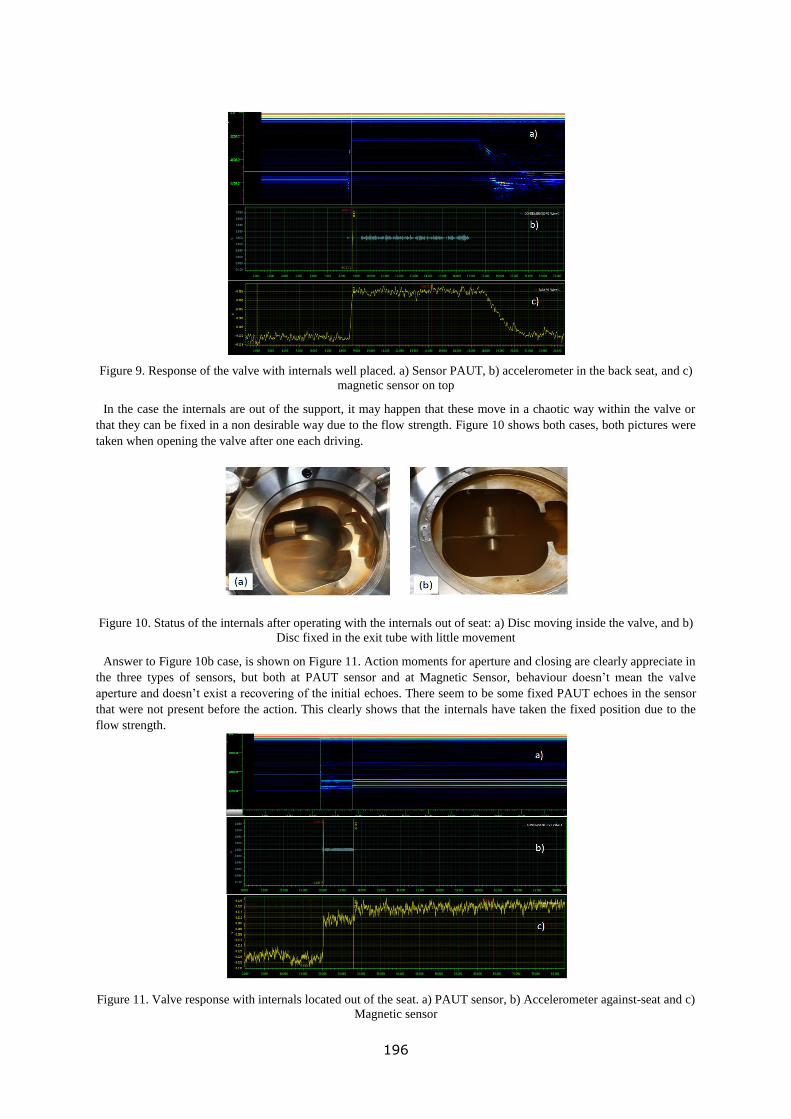
Figure 9. Response of the valve with internals well placed. a) Sensor PAUT, b) accelerometer in the back seat, and c)
magnetic sensor on top
In the case the internals are out of the support, it may happen that these move in a chaotic way within the valve or
that they can be fixed in a non desirable way due to the flow strength. Figure 10 shows both cases, both pictures were
taken when opening the valve after one each driving.
Figure 10. Status of the internals after operating with the internals out of seat: a) Disc moving inside the valve, and b)
Disc fixed in the exit tube with little movement
Answer to Figure 10b case, is shown on Figure 11. Action moments for aperture and closing are clearly appreciate in
the three types of sensors, but both at PAUT sensor and at Magnetic Sensor, behaviour doesn’t mean the valve
aperture and doesn’t exist a recovering of the initial echoes. There seem to be some fixed PAUT echoes in the sensor
that were not present before the action. This clearly shows that the internals have taken the fixed position due to the
flow strength.
Figure 11. Valve response with internals located out of the seat. a) PAUT sensor, b) Accelerometer against-seat and c)
Magnetic sensor
196

5. Conclusions
Tecnatom has developed a PAUT technique for the diagnosis of check valves. The same has been integrated into the
VITE-R 2.0 System, using the electronics Phased Array of Tecnatom (FPA-128M). Through a software development
that controls both electronics at the same time it is able to synchronize on time all the sensors. This new technique has
the advantage to give a direct reference of the position of the internals in every moment through the reflection of the
ultrasonic beams and it constitutes a high value complement to the diagnosis system of valves based in accelerometers
and magnetic sensors. Diagnosis of operative valves has been done in plants that ratify the performance of the
presented technique.
References
[1] H. D. Haynes, “Aging and service Wear of Check Valves Used in Engineered Safety-Feature Systems of Nuclear
Power Plants”, NUREG/CR-4302, ORNL-6193. Vol. 2. 1991
[2] EPRI Project Manager D. Kull, “Nondestructive Evaluation: Check Valve Evaluation Using Phased Array
Ultrasonics”. Final Report, December 2014
197

Detection of Artificial Defects at Storage Vessels for Liquefied Hydrogen by
Ultrasonic Guided Wave
Mu-Kyung Seo1,2
, Ki-Bok Kim2*
, Geonwoo Kim2,3
, Hak-Joon Kim1, Chi-Hwan Oh
4, Sung-
Jin Song1, Minsu Park
5 and Yong Sang Cho
6
1Dept. of Mechanical Engineering, Sungkyunkwan Univ., 2066, Seobu-ro, Jangan-gu,
Suwon-si, Gyeonggi-do, Republic of Korea 2Center for Safety Measurement, Korea Research Institute of Science and Technology, 267,
Gajeong-ro, Yuseong-gu, Daejeon, Republic of Korea 3 Dept. of Science of Measurement, University of Science and Technology, 217, Gajeong-ro,
Yuseong-gu, Daejeon, Republic of Korea
4 Daum Energy Co., Ltd, 830, Yeonsam-ro, Jeju-si, JeJu-do, Republic of Korea
5 Technology Research & Development Institute Robotics Lab, KEPCO plant service &
Engineering Co., LTD, 211, Munhwa-ro, Jeollanam-do, Republic of Korea 6 Mechanical Engineering Group, Korea Electric Power Corporation Research Institute, 105,
Munji-ro, Yuseong-gu, Daejeon, Republic of Korea
E-mail address(*corresponding author) : [email protected]
Recently, many researches on hydrogen have been carried out as one of the alternative energy
sources. The hydrogen is stored at a storage vessel in liquefied state for maximum efficiency
of its storage. The safety of pressurized hydrogen storage vessel is very important because of
explosive characteristics of liquefied hydrogen. As a material for the storage vessel, the
stainless steel 304 (SUS304) has been used. At the former research to apply the ultrasonic
guided wave (UGW) technique to the storage vessel for liquefied hydrogen, we presented the
STFT technique to detect defects at the metal plate (SUS304) for the storage vessel. In this
paper, based on the former research results, we tried to detect the artificial defects at the
storage vessels and hence the artificial defects could be detected by combination of STFT and
UGW techniques.
Keywords: Pressurized hydrogen storage vessel, Ultrasonic guided wave (UGW), Short time
Fourier transform (STFT), Artificial defects
198

Development of sizing techniques of SCC height in dissimilar metal welds of
vessel nozzle safe-end by means of Phased Array TOFD technique with
asymmetrical ultrasonic beams and Multi-Angle Synthesis technique
K. Endoh1, J. Kitasaka1 and H. Ishida2
1 Non-Destructive Inspection Co., Ltd., Japan
2 Institute of Nuclear Safety System, Inc., Japan
Abstract
TOFD technique with asymmetric ultrasonic beams between a transmitter and a receiver, and the multi-angle synthesis
technique which synthesizes test results with different conditions have been developed. Ni base alloy is included in a
dissimilar metal weld of an outlet nozzle of a reactor vessel in a nuclear power plant. The measurement for defect
height of SCC in a direction perpendicular to a Ni base alloy weld line was difficult due to an acoustic anisotropy and
high attenuation. Therefore, examinations of mock-up test specimens using this technique were carried out. As a result
of this study, developed techniques were applicable to height measurement method of SCC on the inner surface by
examining from the inner surface or outer surface of the vessel nozzle.
Keywords: Phased array technique, TOFD technique, Ni based alloy weldment, SCC, Image processing
1. Introduction
A stress corrosion cracking (SCC) was found on an inner surface of a dissimilar metal weld of an outlet nozzle of a
reactor vessel in Japan in 2008. Dimensions of this SCC measured by cross-sectional observation were 13mm in
length and 21mm in depth. Flaw height of SCC is conventionally measured by tip echo technique and/or Time of
Flight Diffraction (TOFD) technique of ultrasonic testing. However, the dissimilar metal weld of the outlet nozzle of
the reactor vessel had coarse-grained structures, thus it was difficult to distinguish tip echoes from scattering noises
due to an acoustic anisotropy and high attenuation caused by coarse grain.
The following techniques which were conventionally based on phased array TOFD have been developed.
(1)To measure the height of SCC with different conditions of refraction angles and focal depth, TOFD
technique using asymmetrical ultrasonic beams by means of a phased array probe (hereafter the phased array
asymmetric TOFD technique) was developed. In this technique, a transmitter emits ultrasound with various refraction
angles to a receiver which handles different beam paths from each refraction angle.
(2)To improve the signal-to-noise ratio, the image processing synthesized scanning data of (1) with different
refraction angles and beam paths (hereafter the multi-angle synthesis technique) was developed.
By combining techniques (1) and (2), examinations of plate specimens were carried out. [1] Examinations of pipe
specimens were also carried out by these techniques from aperture side of crack or the other side.
This study presents evaluation results of crack depth measurement using these techniques from inner and outer
side of pipe specimen.
2. Measurement techniques
2.1 Phased array asymmetric TOFD technique
Figure 1 (a) shows a schematic drawing of a conventional phased array TOFD technique with symmetrical ultrasonic
beams between a transmitter and a receiver. On the other hand, in the figure using phased array asymmetric TOFD
technique, refraction angles from a transmitter are different from those of a receiver. Both transmitter and receiver are
focused on the intersection (figure 1 (b)). Matrix phased array probes for a transmitter and a receiver were moved in a
constant distance.
“Steering angle” is defined as the angle formed by the line from the center of transmitter and receiver to the
199

focal point and a normal to the surface of test specimen, because refraction angles of transmitted wave is different
from those of received wave.
Upper view
Focus point
Transmitter Receiver
Crack
Angle of refractionAngle of refraction
Beam paths
Scanning directionElement
Side view
Upper view
β:Steering angle
TransmitterElement
Crack
Receiver
Focus point
Beam paths
Angle of refraction Angle of refraction
Side view
β
Scanning direction
(a) Phased array TOFD technique (b) Phased array asymmetric TOFD technique
Figure1.Schematic drawing of phased array TOFD technique
2.2 Multi-angle synthesis technique
This technique is a method of synthesizing results from the different steering angles. Received signal of ultrasonic
testing consists of not only signals from a defect but also scattering noise from microstructure of steel.
This Multi-angle synthesis technique is used to average some signals which refraction angles and beam paths are
different from each other. After the signals averaging, the tip echoes from a defect appear clearly, and structural noises
are reduced.
Figure2 shows schematic drawing of Multi-angle synthesis technique. Some tip echoes from a defect can be
obtained from different steering angle at the same focus depth. These echoes which also include some structural
noises randomly are averaged to clarify the tip echoes and reduce the structural noise. In this case, the tip echoes
which refract around the focal depth are emphasized. The tip echoes from different focal depths are synthesized to
make the cross sectional image of test specimen as a result of the examination.
Condition A
Condition B
Condition C
synthesizing of measurement data
Condition A+B+C
Figure2.Multi-angle synthesis method
200

3. Testing method
3.1 Test Specimen
Figure 3 shows a test specimen. The vessel nozzles and the safe-ends are fabricated from carbon steel and stainless
steel respectively. INCONEL 600 was used for a dissimilar metal welded joint connected the safe-end to the vessel
nozzle by butt welding method. SCC and an electric discharge machining slit (hereafter EDM slit) were fabricated at
right angle to the weld line. First, high carbon INCONEL 600 filler metal was used for welding overlay. Then EDM
slit was fabricated. Finally SCC was grown by tensile testing with immersing the test specimen in solution of
tetrathionic acid.
The vessel nozzle
(carbon steel )
The Safe-end
(stainless steel)
Weldment
(INCONEL 600)
EDM slit
SCC
46
150
60゚
195
φ390φ298
軸方向SCC16
20
22
10形状:半楕円、電極厚さ0.4mm
SCC
The vessel nozzle
(carbon steel )The Safe-end
(stainless steel)
Weldment
(INCONEL 600)
EDM slit
Figure3. Test specimen
3.2 Test system
Table 1 shows the specification of the phased array probes. Figure 4 shows pictures of the phased array probes and the
wedges. Array probes used for examinations from inner side or outer side consist of 8x4(32) elements or 32x8 (256)
elements respectively. Each probe is installed on a transmitter or a receiver, and both of them are attached to the
wedge for measuring the defect on the test specimen. Wedges surfaces are machined to add curve based on the surface
shape of the test specimen. ‘Dynaray’ and ’Ultra Vision’ made by Zetec, Inc. are used for phased array system.
Table1. Specification of the phased array probes
inner outer
Frequency(MHz) 2.25 1
Number of elements 32 256
Element array(length×width) 8×4 32×8
Aperture dimension(mm×mm) 15.8×15.8 71.8×25.0
201

(a) 8x4 matrix probes and wedge (b) 32x8 matrix probes and wedge
Figure 4.Phased array probes and the wedges
3.3 Testing conditions
In case of examination from inside, focus depth are from 4mm to 24mm with a pitch of 4mm, steering angles are from
-42 degree to 42 degree with a pitch of 1 degree. On the other hand, in case of examination from outside focus depth
are from 30mm to 46mm with a pitch of 4mm, steering angles are from -26 degree to 26 degree with a pitch of 1
degree.
4. Result
4.1 Examination from inner side
Figure 5 shows result of the examination from inner side to EDM slit and SCC by phased array asymmetric TOFD
technique. B-scope displays with focus depth of 4mm, 8mm and 12mm and steering angle of - 31, -15, 0, 15 and 31
degree are shown in the figure. Tip echoes from EDM slit with 10mm in depth were detected clearly when focus depth
was 8mm or 12mm. Tip echoes from SCC were also detected when focus depth was 8mm or 12mm. However, signal-
to-noise ratio of tip echoes from SCC was lower than those from EDM slit. This result was influenced by
characteristics of weld because SCC was grown into the INCONEL weld but EDM slit was machined into the
stainless steel base metal.
Figure 6 shows an example of the result of synthesized data of different steering angle condition of 8, 12, 16, 20
or 24mm in focus depth. In case of 8mm and 12mm in focus depth, tip echoes from EDM appears clearly by
synthesizing data. However, the phased array asymmetric TOFD technique can be influenced by scattering noises
from the weld; tip echoes from SCC appear in synthesized data when focus depth is 8mm or 12mm.
Figure 7 shows the result of synthesized data of different focus depth. An examination result can be seen in a
cross-sectional image. The height of EDM slit and SCC measured 14mm and 6mm respectively. The multi-angle
synthesis technique was confirmed to be applicable to examine pipes in a nuclear power plant.
202

0°-15°-31° 31°15°Steering angle
focus depth
4mm
8mm
12mm
dep
th
Scanning direction
(a) EDM slit
0°-15°-31° 31°15°Steering angle
focus depth
4mm
8mm
12mm
dep
th
Scanning direction
(b) SCC
Figure 5. Result of the examination from inner side by the phased array asymmetric TOFD technique
203

16mm
12mm
20mm
24mm
Dep
th(m
m)
Scanning direction (mm)
Focus depth
8mm
Dep
th(m
m)
Dep
th(m
m)
Dep
th(m
m)
Dep
th(m
m)
Scanning direction (mm)
Dep
th(m
m)
Dep
th(m
m)
Dep
th(m
m)
Dep
th(m
m)
Dep
th(m
m)
(a) EDM slit (b) SCC
Figure 6. The result of synthesizing data of different steering angle condition
A tip echo from EDM slit A tip echo from SCC
Scanning direction (mm)
Dep
th(m
m)
Scanning direction (mm)
Dep
th(m
m)
(a) EDM slit (b) SCC
Figure 7. The result of synthesizing data of different focus depth condition
4.2 Examination from outer side
Figure 8 shows result of the examination from outer side to EDM slit and SCC by the phased array asymmetric TOFD
technique. B-scope displays with focus depth of 30mm, 34mm and 38mm and steering angle of -24, -12, 0, 12 and 24
degree are shown in the figure. Tip echoes from EDM slit with 10mm in depth were detected clearly when focus depth
was 34mm or 38mm. Tip echoes from SCC were also detected when focus depth was 30mm. However, signal-to-
noise ratio of tip echoes from SCC was lower than that from EDM slit. This result was also influenced by
characteristics of weld because SCC was grown into the INCONEL weld but EDM slit was machined into the
stainless steel base metal.
Figure 9 shows an example of the result of synthesized data of different steering angle condition of 30, 34, 38,
42 or 46mm in focus depth. In case of 34mm or 38mm in focus depth, tip echoes from EDM appears clearly by
synthesizing data. However, the phased array asymmetric TOFD technique can be influenced by scattering noises
204

from the weld; tip echoes from SCC appears in synthesized data when focus depth is 30mm.
Figure 10 shows the result of synthesized data of different focus depth. An examination result can also be
seen in a cross-sectional image. The height of EDM slit and SCC measured 6mm and 16mm respectively. The multi-
angle synthesis technique was confirmed to be applicable to examination from outside of pipe.
0°-12°-24° 24°12°Steering angle
focus depth
30mm
34mm
38mm
dep
th
Scanning direction
(a) EDM slit
0°-12°-24° 24°12°Steering angle
focus depth
30mm
34mm
38mm
dep
th
Scanning direction
(b) SCC
Figure 8. Result of the examination from outer side by the phased array asymmetric TOFD technique
205

38mm
34mm
42mm
46mm
Dep
th(m
m)
Scanning direction (mm)
Focus depth
30mm
Dep
th(m
m)
Dep
th(m
m)
Dep
th(m
m)
Dep
th(m
m)
Dep
th(m
m)
Dep
th(m
m)
Dep
th(m
m)
Dep
th(m
m)
Dep
th(m
m)
Scanning direction (mm)
(a) EDM slit (b) SCC
Figure 9. The result of synthesizing data of different steering angle condition
A tip echo from EDM slitA tip echo from SCC
Dep
th(m
m)
Scanning direction (mm)
Dep
th(m
m)
Scanning direction (mm)
(a) EDM slit (b) SCC
Figure 10. The result of synthesizing data of different focus depth condition
206

5. Conclusion
In this study, with phased array asymmetric TOFD technique, Multi-angle synthesis technique and combined those
techniques, examination was carried out from an aperture side of crack and an opposite side of pipe.
As a result, these techniques were confirmed to be applicable to measurement of the height of SCC on inner
surface by examining from the inner surface or outer surface of the vessel nozzle.
These below are the points that we set as the next goals.
(1)Improve to optimize conditions for detecting defect and measure its depth more accuracy.
(2) Collect many other measurement data.
(3) Evaluate by the Multi-angle synthesis technique in different cross-sections.
References
[1]H.Ishida, J. Kitasaka, “Development of a Phased Array TOFD UT Method to Measure Depth of SCCs in Dissimilar
Welds”, 9th International Conference on NDE in Relation to Structural Integrity for Nuclear and Pressurized
Components, pp.754-762 (2012)
207

Development of the improved PECT system to evaluate thermal
degradation of thermal barrier coatings
Zhang Jianhai1, Hak-Joon Kim
1, Sung-Jin Song
1 and Chang-Sung Seok
1
1Sungkyunkwan University, Korea
E-mail address([email protected]) :
Thermal barrier coatings (TBCs) are applied to protect hot section components, such as gas
turbines for aircraft propulsion and power generation, from high temperature. Major failure
mechanisms of the TBCs include thermal stress developed by the mismatch of the thermal
expansion coefficients between each of the coating layers. The thermal grown oxide (TGO)
layer formation resulting from bond coating (BC) oxidation is known as the most influential
cause of failure in the TBCs. To evaluate the phase degradation of BC layer due to thermal
oxidation, a pulsed eddy current testing (PECT) using a differential probe is proposed. Firstly,
an improved PECT experimental system are developed and verified. Then, PECT technique is
utilized to measure the remaining life of TBCs. Secondly, the basic theory of finite element
model of PECT using a differential probe is presented. Then, the phenomena of phase
degradation of BC are theoretical studied. The PECT experimental results are analyzed by the
proposed model. Finally, the rates of β-NiAl depletion zone and β-NiAl zone of BC are
analyzed through the experimental results and simulation results.
Keywords: Pulsed eddy current testing, thermal barrier coating, phase degradation, finite
element modelling.
208

Effects of Metallic Diaphragm on Sensitivity Characteristics of
Optical Ultrasonic Sensor for Under-Sodium Inspection
Koichi Saruta, Toshihiko Yamaguchi, and Masashi Ueda
Japan Atomic Energy Agency, Japan
Abstract
The paper evaluates experimentally the effects of the metallic diaphragm on the sensitivity characteristics of an optical
ultrasonic sensor used in the under-sodium inspection. The diaphragm is set in a water tank to have direct contact with
water on one side and air on the other side. Ultrasonic pulse propagating through water impinges on the diaphragm, on
which vibration induced by the ultrasonic pulse is detected by a heterodyne interferometer. The sensitivity of the
diaphragm is then evaluated based on the detected amplitude. On the diaphragm two waves are generated. The first
wave is initiated by the ultrasonic pulse that impinges directly on the diaphragm. The second wave, on the other hand,
results from the interference of lamb waves that propagates from the edge of the diaphragm. We have found that the
amplitudes of both waves increase with decreasing thickness of the diaphragm. Thus, the sensitivity can be improved
by using a thinner diaphragm. Moreover, the second wave has larger amplitude than the first wave because the lamb
waves meet in phase, resulting in constructive interference at the center of the diaphragm. The experimental results
show that the sensitivity for the second wave is by a factor of 5 to 6 higher than that for the first wave. This suggests
that the weak ultrasonic wave can be amplified and detected with a higher sensitivity by using the second wave.
Keywords : Optical ultrasonic sensor, Optical pressure sensor, Under-sodium inspection, Fast reactor
1. Introduction
In a fast reactor power plant, visual inspection is being planned to be introduced in order to further enhance the safety
and reliability. Standard optical instruments such as an optical fiber scope and a charge-couple device camera have been
commonly used in a light water reactor for this purpose, while ultrasonic imaging devices are employed in a sodium-
cooled fast reactor on account of the liquid metal coolant [1, 2]. Piezoelectric sensors have been widely used as the sensor
to detect ultrasonic wave, though optical ultrasonic sensors are considered as an attractive alternative because they offer
unique advantages such as small dimensions, multiplexing capability, and immunity to electromagnetic interference,
thereby enabling us to develop a compact sensor array with a high spatial resolution and to realize long-haul signal
transmission without additional signal conditioning devices. The acoustic pressure sensitivity of the optical probe,
however, is lower than that of the piezoelectric probe. The optical ultrasonic sensor employed in under-sodium inspection
consists of a metallic diaphragm and a laser interferometer [3, 4], where mechanical vibration is induced on the diaphragm
as a result of the incidence of ultrasonic wave, which is then detected by the interferometer. Among the key factors that
determine the sensitivity are the properties of the diaphragm.
In this paper we report the effects of the metallic diaphragm on the sensitivity characteristics of the optical ultrasonic
sensor for under-sodium inspection. The diameter and thickness of the diaphragm are used as parameters in order to
evaluate the sensitivity. The diaphragm is set in a tank filled with water instead of liquid sodium so that one side has direct
contact with water and the other side with air. A heterodyne interferometer is employed to detect the wave induced on the
diaphragm as a result of the incidence of ultrasonic wave, which is emitted from a piezoelectric transducer placed in the
water tank. In addition to experimental evaluation of the sensitivity, we also describe the mechanism of the wave observed
on the diaphragm.
2. Experimental setup
Shown in Fig. 1 is the diaphragm used in the experiment, which is fabricated by bonding a sheet of metallic foil on one
side of a substrate with circular apertures by means of diffusion bonding technique. The metallic foil and the substrate are
made of stainless steel (SUS304). The thicknesses of the foil are 5, 10, and 20 µm. The aperture sizes are 3, 5, 7, and 10
209

Figure 1. Diaphragm.
Figure 2. Experimental setup to evaluate the sensitivity of the diaphragm. ECLD, external cavity laser diode; HWP, half-
wave plate; PBS, polarization maintaining beam splitter; AOM, acousto-optic modulator; FG, function generator; M,
mirror; BS, beam splitter; CL, coupling lens; PMF, polarization maintaining fiber; QWP, quarter-wave plate; FL, focusing
lens; PD, photodiode.
mm in diameter, which in turn define the diameter of the diaphragm. The experimental setup to evaluate the sensitivity is
illustrated in Fig. 2. In the laboratory experiments water is used in place of liquid sodium. The diaphragm is set on the
sidewall of a water tank and receives the ultrasonic pulse emitted from a piezoelectric transducer with a center frequency of
5 MHz. The center of the transducer is adjusted to a line that perpendicularly passes through the center of the diaphragm,
and the distance between the transducer and the diaphragm is set at z = 30 cm. A heterodyne interferometer configured in
Mach-Zehnder arrangement is employed to measure the displacement of the diaphragm. The light source is an external
cavity laser diode (ECLD), the lasing wavelength of which is stabilized at λ = 780 nm. The output beam is divided into
two orthogonally polarized beams by a polarizing beam splitter (PBS), where the reflected beam is vertically polarized and
the transmitted beam is horizontally polarized. The splitting ratio is adjusted by rotating a half- wave plate (HWP) in order
to obtain the maximum visibility in the interference signal. In the reference path the beam is given a frequency shift fb by
passage through an acousto-optic modulator (AOM). In the measurement path the beam is launched into a polarization
maintaining fiber (PMF), transmitted through a quarter-wave plate (QWP), and then focused onto the diaphragm with a
focusing lens (FL). The use of the PMF in measurement path allows us to scan the measurement beam over the diaphragm
and to produce a diffraction limited beam spot owing to spatial filtering effect of the narrow mode field diameter of the
PMF. A spot size of approximately 5 µm can be obtained on the diaphragm. A part of the measurement beam reflected by
the diaphragm is coupled into the PMF and travels back the same path as the forward propagation. Since the polarization of
the measurement beam emerging from the PMF is flipped to vertical as a result of passing twice through the QWP, the
measurement beam is reflected at the PBS and goes toward the beam splitter (BS). The measurement and the reference
beam are recombined at the BS, and the resulting interference signal is then converted into electrical signal by a
photodiode (PD). This interference signal is a sinusoid oscillating at a frequency fb with a time varying phase term, which
is proportional to the displacement of the diaphragm. The displacement of the diaphragm is in turn obtained by means of
in-phase/quadrature measurement of the interference signal using a phase demodulator.
3. Results and discussions
In order to compare the waveform detected on the diaphragm, the ultrasonic pulse excited by the transducer is measured
with the use of a needle hydrophone, which is placed in the same plane as the diaphragm. The result is shown in Fig. 3,
where the time is referenced to the trigger signal generated by the pulser. Several cycles of 5 MHz waves with decreasing
amplitude compose the whole ultrasonic pulse, the duration of which is roughly 1.5 µs. The first cycle of the ultrasonic
pulse appears around 200 µs, which is consistent with the propagation time of the acoustic wave from the transducer to the
210

hydrophone in water at room temperature. The peak-to-peak output voltage is approximately 3.77 mV, which can be
converted into an acoustic pressure of 94.3 kPa using the conversion factor of 40 nV/Pa at 5 MHz.
The effect of the thickness of the diaphragm on the detection of ultrasonic pulse is examined using the 10-mm-diameter
diaphragm with thicknesses t of 5, 10, and 20 µm. Figure 4 shows the response of each diaphragm to the incidence of the
ultrasonic pulse shown in Fig. 3, when the measurement beam is adjusted on the center of the diaphragm by means of a
translation stage. One can see that there are two distinct waves that are separated in time. The first wave is similar in both
shape and duration to the ultrasonic pulse measured by the hydrophone and appears around 200 µs. We confirmed that the
waveform does not change and the amplitude is maintained almost constant over the diaphragm except for the region close
to the edge. It follows from these facts that the first wave results from the translational motion of the diaphragm, which is
induced by the ultrasonic pulse that impinges directly on it. In contrast, the shape of the second wave is different from that
of the incident ultrasonic pulse and appears behind the first wave with a delay that depends on the thickness of the
diaphragm. In other words, the group velocity of the second wave increases with increasing thickness of the diaphragm,
indicating that the second wave is a lamb wave propagating over the diaphragm. For both the first and the second wave, the
amplitude increases as the thickness of the diaphragm is reduced. This can be explained as follows. Because of the same
aperture size D = 10 mm, the diaphragms receive the same amount of energy from the ultrasonic pulse while the weight
becomes lighter for the thinner diaphragms. As a result the amplitude of the first wave increases with decreasing thickness
of the diaphragm. The decrease in the thickness also causes a reduction of the flexural rigidity, leading to an increase in the
amplitude of the second wave.
Shown in Fig. 5 are the waveforms detected on the 5-µm-thickness diaphragms with diameters D of 3, 5, 7, and 10 mm.
As with the waveforms shown in Fig. 4, the first wave is followed by the second wave with a delay, but which is
proportional to the diameter D. This implies that the second wave propagates from the edge of the diaphragm; that is, it can
be considered that the boundary of the metallic film and the substrate serves as the source of the lamb wave. Notice that the
amplitude of the first wave is independent of the diameter, whereas the second wave increases in amplitude with
Figure 3. Ultrasonic pulse measured by a needle hydrophone in the plane of the diaphragm.
Figure 4. Waveforms detected on the diaphragm with the diameter of 10 mm. The delay between the first and the second
wave depends on the thickness t of the diaphragm.
211

decreasing diameter. To account for the difference in behavior of two waves, the lateral profile of the acoustic pressure
filed measured in the plane of the diaphragm is plotted in Fig. 6, where the output voltage of the hydrophone is normalized
to the maximum value. The deviation of the acoustic pressure is expected over the diaphragm, ranging from 2 to 10%,
depending on the diameter. However, as far as the first wave is concerned, a uniform pressure field p may be assumed over
the diaphragm except for the vicinity of the edge because we observed the almost constant amplitude when the
measurement beam was swept over the diaphragm, in which case the force applied on the diaphragm is given by
( )2
2Dpπ . The weight of the diaphragm m is given by ( )2
2Dtπσ , where σ and t are the density and the thickness of
the diaphragm, respectively. To calculate the force exerted on the diaphragm of a unit area per unit weight, we have
tp σ . Thus, the amplitude of the first wave becomes independent of the diameter. On the other hand, the acoustic
pressure at the edge of the diaphragm is likely to play a critical role in the generation of the second wave because the lamb
waves appear to emerge at the boundary between the metallic film and the substrate. As can be expected from Fig. 6, the
diaphragm with smaller diameter can receive higher pressure at the edge; therefore, it is considered that the amplitude
increases as the diameter is decreased. It is also important to mention here that as opposed to the first wave, the second
wave drastically changes shape and the amplitude alternates between local extrema before reaching the maximum value at
the center of the diaphragm when the measurement beam is scanned along the diameter. Such behavior of the second wave
can be attributed to the interference of lamb waves. At the center of the diaphragm, constructive interference takes place
because all lamb waves propagating from the circumference meet in phase due to the circular aperture. Therefore, we
consider that the second wave has a larger amplitude compared with the first wave. In fact, the amplitude of the second
Figure 5. Waveforms detected on the diaphragm with the thickness of 5 µm. The delay between the first and the second
wave depends on the diameter D of the diaphragm.
Figure 6. Lateral profile of the acoustic pressure field in the plane of the diaphragm.
212

wave becomes significantly larger than that for the first wave for the case of D = 3 mm, even though the pressure field is
almost flat over the aperture (see Fig. 6).
Figure 7 shows the amplitude of the first wave as a function of acoustic pressure applied on the diaphragm. As described
above, the first wave depends solely on the thickness of the diaphragm. The amplitude linearly increases with increasing
applied pressure with slopes of 0.050, 0.036, and 0.021 nm/kPa for the thicknesses t of 5, 10, and 20 µm, respectively. A
comparison between these slopes indicates that the pressure sensitivity can be improved by reducing the thickness of the
diaphragm. The second wave, however, depends not only on the thickness but also on the diameter of the diaphragm as
shown in Fig. 8, where the data taken from the 5-µm-thickness diaphragm is plotted as a function of applied acoustic
pressure. As the diameter is decreased the slope of the curve becomes steeper; that is, the pressure sensitivity is improved.
The pressure sensitivities obtained from the first and the second wave are summarized in Table 1. One can see that the
sensitivities for the second wave are by a factor of 5 to 6 higher than those for the first wave when the diaphragm with the
diameter of 3 mm is employed regardless of the thickness. It follows from these results that in addition to reducing the
thickness of the diaphragm, the use of the second wave can more effectively improve the sensitivity.
Figure 7. Amplitude of the first wave as a function of applied acoustic pressure.
Figure 8. Amplitude of the second wave as a function of applied acoustic pressure. Data taken from the diaphragm with the
thickness of 5 µm are shown.
Table 1. Sensitivity of the diaphragms for the first and the second wave.
213

4. Summary
We have experimentally evaluated the effects of the metallic diaphragm on the sensitivity characteristics of the optical
ultrasonic sensor for under-sodium inspection. Incident ultrasonic pulse produces two distinct waves on the diaphragm: the
first wave and the second wave. The former is initiated by the ultrasonic pulse that impinges directly on the diaphragm, and
depends only on the thickness, while the latter results from the interference of lamb waves that propagates from the edge of
the diaphragm, and depends both on the thickness and on the diameter. We have found that the amplitudes of both waves
increase with decreasing the thickness of the diaphragm. Thus, the sensitivity can be improved by use of a thinner
diaphragm. Moreover the second wave has larger amplitude than the first wave due to constructive interference at the
center of the diaphragm. The experimental results show that the sensitivity for the second wave is by a factor of 5 to 6
higher than that for the first wave. This suggests that the weak ultrasonic wave can be amplified and detected with a higher
sensitivity by using the second wave.
References
[1] H. Kawahara, M. Izumi, T. Suzuki, S. Nagai, M. Tamura, and S. Fujimori, “Development of Under-so
dium Three-dimensional Visual Inspection Technique Using Matrix-arrayed Ultrasonic Transducer,” J. N
ucl. Sci. Technol., Vol. 37, No. 9, pp. 769-779 (2000).
[2] A. Tagawa and T. Yamashita, “Development of Real Time Sensor for Under Sodium Viewer,” Proc. 1
9th Int. Conf. on Nuclear Engineering, ICONE19-43187 (2011).
[3] R. Mezrich, D. Vilkomerson, and K. Etzold, “Ultrasonic waves; their interferometric measurement and
display,” Appl. Opt. Vol. 15, No. 6, pp. 1499-1505 (1976).
[4] M. Takeishi, F. Tsuri, Y. Koketsu, T. Kobayashi, H. Ito, H. Nishikawa, S. Sasaki, and J. Uchi, “Devel
opment of Multiple Ultrasonic Transducer for Under Sodium Visual Observation,” Proc. 5th Int. Conf.
Nuclear Engineering, ICONE5-2334 (1997).
214

Liquid sodium test results of an 8 element phased array EMAT probe for
nuclear applications
Florian LE BOURDAIS1, Thierry LE POLLÈS
1
1CEA non destructive testing department, CEA LIST, Digiteo Labs, Bât. 565, PC 120, F-
91191 Gif-sur-Yvette, France
E-mail address (corresponding author): [email protected]
Sodium fast reactors pose a significant challenge to conventional non-destructive testing
means. The high temperature, the liquid metal environment and the opacity of liquid sodium
prevent inspections by optical means and make it necessary to design inspection devices and
methods specifically for these conditions. During the last years, CEA LIST has been
developing EMAT probes to close the gap with conventional ultrasonic probe performance
dedicated to under-sodium ultrasound applications, thanks to the advantages of EMAT wave
generation. The potential applications include: telemetry, defect detection in sodium
immersed welds, defect sizing, and more recently using phased array probes, beam forming
images and synthetic focusing.
In this paper we will present an 8 element phased array probe that was developed for use in
liquid sodium. The design process for this probe will be presented, along with laboratory tests
showing the probe’s performances on aluminium blocks. Liquid sodium test results will also
be presented, including beam steering imaging results. These results are compared to
simulation results obtained with the dedicated EMAT computation module included in the
CIVA software.
Keywords: Sodium fast reactors, ultrasonic testing, electromagnetic acoustic transducers,
phased array, liquid sodium testing
215
Open Phased Array Ultrasonic Instrument for Advanced
Applications and Full-Matrix Capture
Gavin Dao1
1Advanced OEM Solutions, Cincinnati, USA
Dominique Braconnier2
1The Phased Array Company, West Chester, USA
Abstract: Full-Matrix Capture (FMC) is a data acquisition technique used to collect valuable ultrasonic in-
formation that can be processed real-time using a popular method like Total Focus Method (TFM). Further-
more, combining such advanced techniques with a small and open platform phased array (PA) ultrasonic
module provides new opportunities for both industry and research. Industrial applications benefit by creating
custom solutions. A small form factor advanced PA module allows mounting the instrument on a scanner or
robotic arm, shortening the transducer cable, which provides better signal quality, better integration, avoids
cable failures and reduces cost. An open instrument allows customization of the software to create a dedicated
software that can simplify user operation. Researchers benefit with an instrument that allows access to low-
level parameters, raw waveforms and the freedom to control and interface to instrumentation with their choice
software language.
Keywords: Non Destructive Testing; Phased Array; Ultrasound; Full –Matrix Caputre
216

High performance Equipment for the Steam Generator Tubes Inspections
Hervé GAC, and Rock Samson,
SG NDT Sarl
190 Route de la croix d’évieu
38110 St Clair de la tour
FRANCE
• Steam generator tubes of pressurized water reactors are designed as a pressure
boundary between the Nuclear Power Plant Primary and Secondary sides.
Unanticipated tubes degradations can cause some tubes leakages during the plant
operation with the consequences of the plant shutdown.
• It’s therefore mandatory to perform the steam generator tubes inspection in a regular
basis with a reliable and high performances inspection equipment. • In the last years the French Canadian Company SG NDT has developed a
sophisticated equipment which allow the tubes inspection with high reliability. • SG NDT is specialized in the development of Eddy Current Instrument, software and
probes. • SG NDT’s innovative solutions have been used in a variety of applications such as
steam generators and standard tubes inspections; • The technical staff at SG NDT pioneered the development of digital Eddy Current
equipment. The heart of the product range are the Eddy Current equipment, the
software and both standards and multicoils probes. The high probes sensitivity allows
the detection and the follow up of all kind of tube degradations. • The innovative probe design leads to a high life time which consequently leads to a
reduction of the total occupation time of the Steam Generators during the outage. • The first aim of this report is to describe a new Eddy Current method applied for the
Steam generator tubes inspection. • The second is to describe the equipment and probes technical features and to
summarize their high performances.
Keywords: Eddy Current inspection, quality insurance, maintenance, nuclear safety.
217

Effect of NDE Signal Variation by Chemical Cleaning on the Steam Generator Tube Integrity for Axial Cracks
Yong Seok Kang1, In Chul Kim1 and Jai Hak Park2
1,2KHNP Central Research Institute, Daejeon, Korea
3Chung Buk National University, Cheongju, Korea
Abstract
Axial out diameter stress corrosion cracking (ODSCC) is one of the main degradation mechanisms in Korean nuclear steam generators. Eddy current testing is the most common non-destructive examination (NDE) technique used to inspect steam generator tubes. An extensive number of stress corrosion cracking was detected by the eddy current testing after chemical cleaning with alloy 600 mill annealed steam generator tubes. In the process of root cause analysis for the increased number of cracking, NDE signal variation of bobbin coil and rotating pancake coil signal are observed. It was found out that voltage amplitude and phase angle are slightly changed after chemical cleaning. Bobbin coil probability of detection is improved. Crack depth and length are became deepen and shorter but their change is not noticeable. Therefore, it seems reasonable to conclude that eddy current signal variation by the chemical cleaning is not affects directly to the structural integrity of steam generator tubes but affects to probability of detection of NDE technique.
Keywords: Axial ODSCC, Chemical cleaning, Eddy current testing, Probability of detection, Steam generator tube integrity
1. Introduction
The thin-walled steam generator tubing is an important part of a major barrier of the pressure boundary of reactor coolant system. Failure of steam generator tubes, which can be caused by cracking, will release radioactive materials to the secondary coolant system [1]. An axial out diameter stress corrosion cracking (ODSCC) is one of the main degradation mechanisms in steam generator tubes of Korean nuclear fleets. Hard chemical cleaning technique was performed to prevent progression of ODSCC by removing tube support plate deposit to one of the CE type steam generators with alloy 600 mill annealed tubes. After an application of steam generator chemical cleaning (SGCC), extensive number of axial ODSCC was observed at the tube support plate contact area. In the process of investigation for the root cause of the increased number of the ODSCC, NDE signal variation was observed. This paper discussed the effect of NDE signal variation by chemical cleaning on the steam generator tube integrity for axial out diameter stress corrosion cracking.
2. NDE Signal Variation Analysis
2.1 NDE system performance
Eddy current testing (ECT) is the most widely utilized NDE technique for determining the extent and location of steam generator tube defects and it has provided valuable information on tube defects. An electrically conducting nature of the inspected Alloy 600 tube will influence the voltage and current relationships in the coil. If some anomaly occurs in the tube then the electrical parameters will change in a characteristic manner [2]. Total system NDE performance uncertainties include technique and analyst variability and shall be established for detection and sizing. A probability of detection (POD) is a functional measure of the ability of an NDE system to detect degradation remaining in-service after an eddy current examination of the tube bundle. Various structural parameters such as maximum depth, average depth, length, voltage can be used as the independent variable depending on the needs of the tube integrity engineer [3].
218

2.2 Bobbin Coil Signal Variation
In order to compare the POD performance between before and after SGCC to axial ODSCC data sample of more than 500 tubes were obtained during in-service inspection to one of CE type steam generators with alloy 600 mill annealed tubes. From the comparison results of the bobbin coil inspection signals to axial ODSCC at tube support plates, variation of voltage amplitude and phase angle are observed. Fig.1 shows comparison results of bobbin voltage amplitude between before and after SGCC. After chemical cleaning bobbin peak to peak voltage amplitude, Vpp, is increased from 0.29 volts to 0.37 volts and maximum voltage amplitude, Vmax, also increased from 0.15 volts to 0.23 volts. Phase angle signals which were located within 0~20 degree and 140~180 degree are moved to 40~100 degree. Therefore the signal is change from horizontal to vertical direction. Both changes are influenced to improve bobbin POD.
Figure 1 Bobbin voltage amplitude between before and after SGCC to axial cracks
2.3 RPC Signal Variation
Some sample of rotating pancake coils (RPC) data, which confirmed as an axial crack, was analyzed correlation phase angle and amplitude between before and after SGCC. Comparison result is shown in figure 2. Phase angle and amplitude shows subtle changes. Amplitude median increased from 0.19 volts to 0.21 volts. RPC amplitude is connected to crack depth. Figure 3 shows measure NDE maximum depth and length distribution of the axial ODSCC. After chemical cleaning, NDE measured maximum depth is increased about 2.1% of tube through wall. In the other hand, the maximum length is decreased. The extent reduction is just 0.28mm (0.011 inch). Even though the shape of crack became deeper and shorter after chemical cleaning, the extent change is negligible.
0 20 40 60 80 100 120 140 160 1800
20
40
60
80
100
120
140
160
180
Phase Angle
Phas
e An
gle_
ACC,
Deg
ree
Phase Angle_BCC, Degree0.00 0.05 0.10 0.15 0.20 0.25 0.30 0.35 0.40 0.45 0.50
0.00
0.05
0.10
0.15
0.20
0.25
0.30
0.35
0.40
0.45
0.50
Amplitude
Ampl
itude
_Vpp
_ACC
, Vol
ts
Ampletude_Vpp_BCC, Volts
Figure 2 RPC phase angle and voltage amplitude between before and after SGCC to axial cracks
219

Figure 3 Maximum depth and length distribution between before and after SGCC to axial cracks
3. Discussion
From the investigation on bobbin and RPC signals for both of before and after chemical cleaning to axial ODSCC, variation of amplitude and phase angle was observed. It is well known that bobbin voltage amplitude and phase angle variation influence on probability of detection (POD). The POD provides an estimate of undetected tube degradation left in-service after steam generator examination and is used as an input to deterministic or probabilistic tube bundle integrity models to establish tube bundle burst probabilities and leak rate [4]. The flaw sizing is also used as an input to steam generator tube bundle integrity models for quantitative tube burst and leakage assessments. Even though crack shape became shorter and deeper by the NDE signal variation, their extent change is not noticeable. It seems reasonable to conclude that eddy current signal variation by SGCC is not directly affected to structural integrity performance criteria but it is influenced to improve POD. The increased detectability of cracks reduces the potential for ODSCC to lead to failure of structural performance criteria. Therefore it will be helpful to ensure condition monitoring structural performance criteria will not be affected from signal variation with the chemical cleaning but it will be affect to the over the length of the upcoming operating interval due to the improvement of POD.
4. Conclusion
Hard chemical cleaning technique is performed to one of CE type steam generators with alloy 600 MA tubing in Korean nuclear fleet. Variation of eddy current signal was observed from the comparison of both before and after chemical cleaning to the sample tubes. Increase of bobbin voltage amplitude and erection of phase angle were observed and it is influenced to improve POD. Crack shape such as maximum depth and length became deepen and shorter after chemical cleaning but their extent change is negligible. This goes to the conclusion that the variation of NDE signal by steam generator chemical cleaning affects to the system POD but may not have a strong correlation with the structural integrity margin requirements.
References
[1] US NRC Regulatory Guide 1.83,”Inservice inspection of pressurized water reactor steam generator tubes”,(1975)
[2] E.E. Chick, “NDE and Mechanical removal of sludge in PWR steam generators”, Vol. 1, EPRI NP-5563, pp.2-10~2-11 (1988)
[3] H. Cothron,”Steam generator integrity assessment guidelines”, EPRI 1019038, pp.4-1 (2009)
[4] S. Swilley, “Pressurized Water Reactor Steam Generator Examination Guidelines”, EPRI 1013706, pp.I-9 (2007)
220

Advanced Inspection Technique for Tube Seal Welds of Steam Generators
H. Yonemura, N. Kawai, M. Morikawa, H. Murakami, T. Hanaoka, T. Tsuruta, K. Kawata,
M. Kurokawa
Mitsubishi Heavy Industries, Ltd., 1-1, Wadasaki-cho 1-chome, Hyogo-ku, Kobe JAPAN
E-mail address: [email protected]
Keywords: Eddy Current Testing, Radiography, Steam Generator, Tube Seal Weld
Mitsubishi Heavy Industries (MHI) has total inspection techniques for Steam Generators
(SG) during SG fabrication process and each of them is optimized according to
characteristics of applicable objective based on careful consideration and broad experience.
In this presentation, MHI proposes our new solution for inspection of SG tube seal welds
which is consist of the important boundary between primary and secondary sides in
Pressurized Water Reactor (PWR) with advanced inspection technique.
In general, Penetrant Testing (PT) and Helium Leak Testing (HLT) are applied for SG tube
seal welds during SG fabrication process. These techniques are effective to detect surface
breaking defects or leak pass, but not effective to detect sub-surface defects in seal welds.
Therefore, MHI has developed Advanced Inspection Technique combined with Eddy Current
Testing (ECT) and Radiography (RT) in order to achieve higher quality of SG tube seal
welds.
ECT Technique makes it possible to examine many seal welds in a short time and to detect
not only surface breaking defects but also sub-surface volumetric defects. Actually, some
noise caused by geometry change of SG tube seal welds is observed. The configuration of
ECT coils was optimized and The state-of-art filtering technique was developed in order to
reduce noise signals and improve Signal to Noise Ratio. In addition, MHI has developed
accurate RT technique to detect volumetric defects and support ECT evaluation. After careful
consideration, MHI decided to adopt X-Ray technique because of more suitable image and
more simple operation compared with gamma ray technique. MHI also considered
possibility of applying Digital Radiography Technique.
As mentioned above, MHI has developed Advanced Total Imaging System for SG tube seal
welds by combination of ECT and RT. MHI has already applied this state –of-art technique
to actual inspection during SG fabrication process and MHI achieved higher quality of SG
seal weld. This technique can be applicable to In-Service Inspection (ISI) and contributes
safety operation of nuclear power plants.
221

AUTOMATED CORRELATION OF HISTORICAL WITH PRESENT
EDDY CURRENT INSPECTION DATA USING HDC® FOR
UNDERSTANDING CHANGE IN STEAM GENERATOR TUBING
CONDITIONS AND VISUAL FLAW MORPHOLOGY
Tom O’Dell1, Tom Bipes
1, Kevin Newell
1
1Zetec Inc. , Snoqualmie Wa, USA
E-mail address: [email protected]
In nuclear power plant primary loop steam generator tubing inspections current data is
compared with historical data to understand change in signals. This historical comparison
process has been a manual effort requiring the analysis to independently recall both sets of
data and compare results. Due to the time consuming effort required to manually compare,
this action could only be partially performed on the data and the analysis of the change
limited to measurement values only.
A new technology called HDC has been developed where three independent data files
acquired during different inspections can be automatically correlated, displayed and
compared for change analysis. This correlation is applied to all active frequency channels of
bobbin data allowing analysis of change to be performed on any available frequencies as well
as process channels. Typically the data files represent the current inspection, prior inspection,
and baseline inspection data. All three data files are overlaid in a commonly calibrated to
provide the analyst a visual to see morphology of change and make comparative
measurements.
In addition, HDC can process a “delta channel” of change for each of the reference
inspections compared to the current inspection. This delta channel provides a strong visual of
change, suppressing common signals and allowing the analyst to focus on change signals only.
This approach does not depend on applying different analysis methodologies based on
regions of interest as the correlation process is only concerned in the basic signals in the
available channels used in the comparison. This delta channels can also be used in an
automated process for analysis such as RevospECT®
where the delta signals can be
automatically analysis and reported on.
The HDC technology can provide value to the inspection at multiple levels. In Manual
Production HDC provides the analyst with additional tools to understand change and
morphology of signals. In Automated Production, the delta channel can be used for detection
and reporting of change, including new anomalies. In the Resolution process, the analysts can
use the correlated overlaid signals to address history and/or determine the resolution of
signals based on morphology. In the Independent Review process, the analyst can use the
correlated overlaid data channels to confirm the reporting and/or use the delta channel to scan
for potentially missed indications.
This paper will provide greater detail on these topics as well as examples of field data
showing the strong visual perspective available.
Keywords: Eddy Current, Steam Generator, Inspection, Analysis, Automated Analysis.
222

Effect of vibration reflection on vibrothermography
Wonjae Choi1*
, Manyong Choi1 and Jeounghak Park1
1Center for Safety Measurement, KRISS, 267 Gajeong-Ro, Yuseong-Gu, Daejeon 305-340,
Rep. of Korea
* E-mail address(corresponding author) : [email protected]
Vibrothermography has been increasingly studied for Non-Destructive Evaluation. In this
method, vibration energy is given to a structure, which is transferred into heat energy at
defects, and infra-red camera is used for detecting the heat from the defects. Laboratory
experiments are often conducted with samples sizing a few times input wavelength, and then
the wave reflection from the sample boundaries inevitably influences the heat generation
mechanism. However, what is inspected in a real industrial field is often a large structure
sizing in the order of ten times the wavelength or more, and then the inspection results will be
different from the experimental ones in laboratory. This paper studies the effect of sample
size on vibrothermography. Numerical simulations are conducted with a group of sample
sizes and their differences are discussed.
Keywords: Vibrothermography, sample size, numerical simulation.
223

Comparison of PZT and PMN-PT based sensors for detection of partial
discharge at electric transformer
Geonwoo Kim1,2
, Mu-Kyung Seo3, Namkyoung Choi
1,2,Ki-Bok Kim
1*, Jae-Ki Jeong
4,
Hong-Sung Kim4 and Minsu Park
5
1Korea Research Institute of Science and Standards, 267 Gajeong-ro, Yuseong-gu, Daejeon
305-340, Republic of Korea 2Dept. of Science of Measurement, University of Science & Technology, 217 Gajeong-ro,
Yuseong-gu, Daejeon, 305-350, Republic of Korea 3Dept. of Mechanical Engineering,Sungkyunkwan Univ., 2066, Seobu-ro, Jangan-gu,
Suwon-si, Gyeonggi-do, Republic of Korea 4Hanbit EDS. CO., Ltd , 44-10, Techno 10-ro, yuseong-gu, DaeJeon, Republic of Korea
5Kepco plant service & Engineering Co.,Ltd, 211, Munhwa-ro, Naju-si,
Jeollanam-do, Republic of Korea
E-mail address(corresponding author) : [email protected]
This paper describes the fabrication and comparison of PZT and PMN-PT basedsensors to
detectPD (partial discharge)signalatelectric transformer. As a front matching material for
ultrasonic PD detecting sensor between a surface of external metal wall ofelectrictransformer
and piezoelectric materials (PZT and PMN-PT), the alumina ceramic (Al2CO3) was selected.
Because ofthe wideband characteristics of PD, optimal back acoustic materials of both
sensors were fabricated. To compare the performance of the developed both PD sensors,
experimental setup consisted of the developed sensors, high voltage supplier generating the
PD within test block and oscilloscope. From the experimental results, PMN-PT based sensor
showed better performance than PZT based sensor.
Keywords:Partial discharge, PZT, PMN-PT, Electric transformer
224

New improved piezoelectric detection method to measure ultrasonic
nonlinearity parameters for incipient damages in nuclear engineering
materials
To Kang1,2
, Jeong K. Na3, Sung-Jin Song
2, and Jin-Ho Park
1
1Korea Atomic Energy Research Institute, 111, Daedeok-daero 989beon-gil, Yuseong-gu,
Daejeon, 305-353 Rep. of Korea; 2Dept. of Mechanical Engineering, Sungkyunkwan Univ.,
2066, Seobu-ro, Jangan-gu, Suwon-si, Gyoenggi-do, 440-746, Rep. of Korea; 3Wyle
Laboratories Inc., 2700 Indian Ripple Road, Beavercreek, OH 45440, USA
E-mail address (corresponding author): [email protected]
When ultrasonic nonlinearity parameter values are measured to determine incipient damage
levels in an engineering metal alloy, a conventional piezoelectric detection method is
commonly used. Piezoelectric detection methods are simple and can be adopted for an
industrial field measurement during which data needs to be collected at a high rate of speed
due to restrictions on accessibility and availability of components or structures at sites.
Despite of the simplicity with the measurement procedure, one of the biggest drawbacks of
conventional piezoelectric detection methods is the possibility of getting a high level of
measurement uncertainty caused by receiving transducer’s low sensitivity to the second
harmonic component of received signals. In this paper, a newly developed piezoelectric
detection method is introduced to overcome the intrinsic weakness of conventional
piezoelectric detection methods. This improved system employing a couple of additional high
Q-value band-pass filters and low-noise preamplifiers is demonstrated to show a significantly
lower uncertainty in the nonlinearity parameter measurement. It is also demonstrated that
absolute nonlinearity parameter values can be determined without having a tedious
calibration procedure otherwise required with the capacitive detection or laser interferometry
method. In order to validate the effectiveness of new improved piezoelectric detection
method, nonlinearity parameter measurements have been made on a titanium alloy that is
widely used for components of nuclear power plant condenser tubes and heat exchangers due
to its high corrosion resistance and light weight.
Keywords: Nonlinearity parameter, Second harmonic signals, Improved piezoelectric
detection, Titanium alloy
225

Application of Fiber-optic Sensors to CFRP Pressure Tanks for Internal Strain
Monitoring
Donghoon Kang1
1Advanced Materials Research Team, Korea Railroad Research Institute, 176, Cheoldo
Bangmulgwan-ro, Uiwang-si, Gyeonggi-do, 437-757, Republic of Korea
Abstract
There are growing concerns on carbon fiber reinforced plastics (CFRP) due to their high specific strength and light
weight for applications on many kinds of structures including aerospace structures like satellites, infrastructures like
bridges, and special purpose structures requesting high level of engineering performances. Among those structures,
CFRP pressure tanks are recently promising as an alternative of metal based pressure tanks that are being widely
applied to many types of gas tanks for decades. In this paper, fiber-optic sensors, fiber Bragg grating (FBG) sensors in
particular, are applied to a CFRP pressure tank with embedment in order to measure internal strains during its in-situ
operation. The tank is fabricated using filament winding processes and the pressurizing test is conducted with water
up to 1,000 psi. All data from embedded FBG sensors and attached electric strain gauges (ESGs) are acquired to a
laptop computer in real-time. Through the test, the applicability and validity of FBG sensors on CFRP pressure tanks
are evaluated by comparing the experimental results from FBG sensors with those from both ESGs and FEM analysis.
In conclusion, FBG sensors embedded into CFRP pressure tanks can successfully measure internal strains at both
domes and cylinders and the results show good agreements with those from FEM analysis as well as ESGs. This
means that FBG sensors can be one of good solutions to monitor internal strains of many kinds of pressure tanks,
which are generally under severe environmental conditions like very high internal pressures and ultra-low
temperatures, including CFRP pressure tanks by embedment.
Keywords : Pressure tanks, CFRP, Fiber-optic sensors, FBG, Internal strain
1. Introduction
Recently, the use of filament wound pressure tanks is increasingly prevalent because of high specific strength and
specific stiffness over their metal counterparts, as well as excellent corrosion and fatigue resistance. The main applications
of filament wound pressure tanks are fuel tanks that are a kind of composite structures and so have the complexity in
damage mechanisms and failure modes. Most of the conventional damage assessment and nondestructive inspection
methods are time-consuming and are often difficult to implement on hard-to-reach parts of the structure. For these reasons,
a built-in assessment system must be developed to monitor the structural integrity of critical components constantly.
Fiber optic sensors (FOSs) have shown a potential to serve as real time health monitoring of the structures. They can be
easily embedded or attached to the structures and are not affected by the electro-magnetic field. Also, they have not only
the flexibility in the selection of the sensor size but also high sensitiveness. Recently, fiber optic sensors have been
introduced to composite structures (Kang et al. 2000, Park et al. 2000). Among many fiber optic sensors, FBG sensors
based on wavelength-division-multiplexing technology are attracting considerable research interest and appear to be
ideally suitable for structural health monitoring of smart composite structures. FBG sensors are easily multiplexed and
have many advantages such as linear response, absolute measurement, and etc. Among many researches on filament
wound pressure tanks, only a few were performed using FBG sensors.
The temperature and strains were measured during the cure and ingress/egress methods for a standard testing and
evaluation bottle (STEB) were investigated using FBG sensors. Through a water-pressurizing test, experimental data were
compared with the results of ESGs and finite element analysis results (Foedinger et al. 1999). The unbalanced strain was
calculated from the wavelength difference of a pair of FBG sensors during a water-pressurizing test (Lo et al. 2000).
However, it was impossible to measure absolute strains at each sensor position. An FBG sensor was embedded between
the hoop layers and used for measuring the internal pressure of the tank through a water-pressurizing test form the
wavelength shift of an FBG sensor (Degrieck et al. 2001). The lack of sensors limited strain measurements onto local
positions. In addition, they conducted a 3-point bending test of carbon/epoxy composite laminate. Using attached 32 FBG
sensors on the filament wound pressure tank as 4 channels, the strains of a filament wound pressure tank were measured
through a water-pressurizing test (Kang et al. 2002). From the above literatures, it can be found out that only a few FBG
sensors were used when embedding sensors into the pressure tank and relatively a large number of FBG sensors were used
when attaching sensors on the surface. Moreover, problems on FBG sensor signals, especially peak split induced by
226

birefringence and strain gradients occurred in a dome part during a water-pressurizing test. Therefore, it is necessary to
monitor the strains of a filament wound pressure tank using a number of embedded FBG sensors in real time without peak
split problems.
In this paper, the strains of a filament wound pressure tank were monitored using a number of embedded FBG
sensors in real time during the water-pressurizing test and the strain results measured by FBG sensors were compared
with those by ESGs and FEM analyses.
2. Fabrication of filament wound pressure tanks
2.1 Fabrication of FBG sensor lines
Among several fabrications of FBG sensors, fabrication using a phase mask, devised by (Hill et al. 1993), is currently
the most prevalently employed approach because it is suitable for mass production and is simple to handle. However, the
grating parts of an FBG sensor can be easily broken by transverse stress applied on the optical fiber. Due to the reason,
FBG sensors embedded into a filament wound pressure tank are easy to fail because of the applied tension in reinforcing
fibers. In this paper, a revised fabrication process of FBG sensors that is focused on the improvement of sensor
survivability during the embedment of FBG sensors is introduced. For this purpose, several processes concerning the
fabrication and the embedment are revised.
First, an optical fiber used for fabricating an FBG was substituted to a photosensitive optical fiber (PS1250/1500,
Fibercore) because the hydrogen loading process of optical fibers decreased the mechanical strength of them. Second,
a sensor line with multiple sensors was fabricated not by the splicing between FBG sensors, but by a simultaneous
fabrication of FBG sensors in single optical fiber. Generally, optical fibers connected by arc-fusion splicing showed
strength degradation to the transverse stress. Third, as a reinforcement of FBG sensors during the embedment, the
protection with an adhesive film was conducted as a 2nd
protection process after recoating with acrylate. Lastly, optical
fibers were extracted from a filament wound pressure tank towards both directions of a sensor line. It was because
optical fiber lines were the weakest at the ingress/egress point after the end of curing process. Figure 1 shows an FBG
sensor line fabricated by a revised fabrication process mentioned in the above paragraph.
Figure 1. An FBG sensor line protected with a revised process
2.2 Filament wound pressure tank with embedded FBG sensor lines
A filament wound pressure tank consists of a forward dome, an aft dome, a cylinder, and a skirt for joining with other
structures. In this paper, a tank is fabricated by the wet winding process using a 4-axis filament winding machine
controlled by a computer. The winding tension was 1.5kg/end and the bandwidth of hoop and helical layer was 10.0,
10.5(mm) for 5-ends, respectively. The cylinder part includes a 3-body helical layers and 7-body hoop layers so that the
sequence is [(±27.5)3]T for helical layers and [902/(±45)2/903]T for hoop layers denoting from inner to outer layers. Figure 2
shows the embedded sensor lines during the fabrication process.
Seven channels of FBG sensors were embedded into a tank. The channel 1(Ch1) and channel 2(Ch2), each has 3 FBG
sensors, were embedded between the layer 1 and 2 at aft dome and the layer 2 and 3 at forward dome, respectively. The
channel 3(Ch3), which has 3 FBG sensors, was embedded into axis direction of a cylinder part and 3 more lines were used
as spare channels (Ch5, 6, 7) because FBG sensors are the weakest when they are embedded perpendicular to the
reinforcing fiber like the case of a Ch3. The channel 4(Ch4), which has 4 FBG sensors, was embedded into hoop direction
of a cylinder part.
After embedding each sensor line, embedded positions of FBG sensors were measured accurately using a laser pointer.
The filament wound pressure tank with embedded FBG sensor lines were cured under rotating condition in the curing
cycle ; 80°C(1hr)→120°C(1hr)→150°C(3hrs) in an oven.
Figure 3 shows the configurations of a tank including sensor positions. From the Fig. 3, ‘F’ denotes FBG sensor and ‘E’
denotes ESG. And, the figure following ‘F’ means the channel number.
227

(a) aft dome – Ch1 (b) forward dome – Ch2
(c) cylinder : axis dir. – Ch3, 5, 6, 7 (d) cylinder : hoop dir. – Ch4
Figure 2. Embedded FBG sensor lines during the fabrication
Unit : [mm]
Figure 3. Configurations and sensor positions
When embedding FBG sensors into a filament wound pressure tank, especially a dome part, the signal stability of FBG
sensors is very important for the strain measurement because there exists a strain gradient in a dome part due to its
geometric shape during the water-pressurizing. However, the effects of strain gradient decrease as the grating length of an
FBG sensor decreases (Kang et al. 2005). In addition, FBG sensors with shorter grating lengths are more effective when
they are embedded perpendicular to the reinforcing fibers. For the reason, two kinds of grating lengths were used such as
10mm and 5mm. All sensors except those of a Ch4 were fabricated as FBG sensors with gage length of 5mm.
When the STEB was completely fabricated, 100% (22 of 22) of sensors survived through the whole fabrication
processes such as embedding, curing, and mandrel separation.
3. Water-pressurizing test
After fabricating a pressure tank, a water pressurizing test of STEB was performed to verify the tank itself. Figure 4
depicts the experimental setup for the strain monitoring of a filament wound pressure tank during hydrostatic
pressurization. The tank was pressurized at intervals of 100 psi up to 1,000 psi using a rotary pump. The strain data from
the FBG sensors, ESGs, and a pressure transducer were acquired and processed by a laptop computer in real time.
As shown in Fig. 3, 4 ESGs were attached on the dome surfaces at the same locations of embedded FBG sensors,
aligned to the helical winding direction. On the cylinder, only 1 ESG (E3) was attached in the hoop winding direction, i.e.,
the circumferential direction of cylinder. The signals of the FBG sensors, strain gauges, and a pressure transducer were
F6-1
F6-3
F4-3
F6-2
F3-3
F4-1
F3-1
F3-2
F7-1
F4-4
F7-2
F7-3
F5-1
F4-2
F5-2
F5-3
F6-1
F6-3
F4-3
F6-2
F3-3
F4-1
F3-1
F3-2
F7-1
F4-4
F7-2
F7-3
F5-1
F4-2
F5-2
F5-344.8 127.0 70.5F1-1
F1-3F2-1
F2-2
F1-282.069.013.067.0 10.0F3-1F3-2F3-3 64.0242.040.0
F2-3
F4-1
F4-2
F4-3
F4-4
84.0 F5-3
F6-3
F7-3
F5-1
F6-1
F7-1
F5-2
F6-2
F7-2
E4
E5
E1
E2
E3
44.8 127.0 70.5F1-1
F1-3F2-1
F2-2
F1-282.069.013.067.0 10.0F3-1F3-2F3-3 64.0242.040.0
F2-3
F4-1
F4-2
F4-3
F4-4
84.0 F5-3
F6-3
F7-3
F5-1
F6-1
F7-1
F5-2
F6-2
F7-2
E4
E5
E1
E2
E3
228

acquired simultaneously by computers, processed and displayed by a signal-processing program written in LabVIEW
software. The specifications of used FBG sensor systems are shown in Table 1.
Figure 4. Experimental setup of water-pressurizing test
Table 2. Specifications of an FBG interrogator
LS-7000 FBG Interrogator (FiberPro Co.)
Wavelength range 35 nm (1530 ∼ 1565 nm)
Average output power 3 mW
Resolution < 2 pm
Measurement speed 200 Hz
# of channels 8
Temperature range 10 ∼ 40 oC
4. Finite element modeling
To compare the strain results measured by FBG sensors and ESGs, finite element analyses on STEB were done by a
commercial code, ABAQUS. In this research, the 3-D layered solid element was utilized and the boundary condition
was considered as cyclic symmetric. Figure 5 shows the detailed FEA model of STEB realized by a commercial code,
PATRAN, and the material properties of T700/Epoxy used in the analysis are as follows.
E1 = 134.6 GPa, E2 = 7.65 GPa, G12 = 3.68 GPa, ν12 = 0.3, σf = 2290 MPa, σt = 31.8 MPa, S = 75.8 MPa
The modified Hashin’s failure criterion was selected and applied to progressive failure analysis. For the purpose of
failure analysis, a subroutine, USDFLD of ABAQUS ver 6.3 was coded to define the change of mechanical properties due
to failure.
229

ZZZZ----axis axis axis axis ssssymmetryymmetryymmetryymmetry Cyclic symmetryCyclic symmetryCyclic symmetryCyclic symmetry
Displacement Fixed in X and Y directionsDisplacement Fixed in X and Y directionsDisplacement Fixed in X and Y directionsDisplacement Fixed in X and Y directions
10 10 10 10 elements in the cylinder partelements in the cylinder partelements in the cylinder partelements in the cylinder part30 30 30 30 elementselementselementselementsin the dome partin the dome partin the dome partin the dome part6 6 6 6 elementselementselementselementsthrough the thicknessthrough the thicknessthrough the thicknessthrough the thickness
Figure 5. The FEA model of STEB
5. Results and discussions
Figure 6 shows strain results measured by FBGs and ESGs in an aft dome. Strains measured by two FBG sensors
showed a good agreement with those by ESGs and the strain measured by each FBG sensor showed a good linearity with
the increase of pressure.
In case of a forward dome, as shown in Fig 7, strains measured by two sensors showed a little higher difference than the
case of an aft dome. The differences in strains measured by FBG sensors and ESGs may be occurred by a mismatch of
attaching angles and locations between them. Also, these differences may be caused by the slippage of an embedded FBG
sensor line during the curing process due to resin flow. This can be occurred more easily in a forward dome than in an aft
dome because the gradient of a forward dome is steeper.
Figure 8 shows the strain results of FBGs and an ESG (E3) in a cylinder part. Compared with an ESG, two FBG
sensors showed a little higher strains and the others lower strains though all sensors showed a good linearity. The
reason seems that there occurred a small angle between optical fiber and reinforcing fiber during embedding the Ch4.
Forward dome Aft dome
Epoxy filler
1st skirt
2nd skirt
Metal boss
Forward dome Aft dome
Epoxy filler
1st skirt
2nd skirt
Metal boss
230

0 200 400 600 800 1000 12000.00
0.05
0.10
0.15
0.20
0.25
0.30
0.35
0.40S
train
(%
)
Pressure (psi)
ESG_No_1
FBG_Ch1_1
0 200 400 600 800 1000 12000.00
0.05
0.10
0.15
0.20
0.25
0.30
0.35
0.40
Str
ain
(%
)
Pressure (psi)
ESG_No_2
FBG_Ch1_2
Figure 6. Strain results of FBG and ESG – aft dome
0 200 400 600 800 1000 12000.0
0.1
0.2
0.3
0.4
0.5
Str
ain
(%
)
Pressure (psi)
ESG_No_4
FBG_Ch2_2
0 200 400 600 800 1000 12000.0
0.1
0.2
0.3
0.4
0.5S
tra
in (
%)
Pressure (psi)
ESG_No_5
FBG_Ch2_3
Figure 7. Strain results of FBG and ESG – forward dome
0 200 400 600 800 1000 12000.0
0.1
0.2
0.3
0.4
0.5
0.6
Str
ain
(%
)
Pressure (psi)
ESG_No_3
FBG_Ch4_1
FBG_Ch4_2
FBG_Ch4_3
FBG_Ch4_4
-400 -300 -200 -100 0 100 200 300 4000.00
0.05
0.10
0.15
0.20
0.25
0.30
0.35
0.40
0.45
0.50
Analysis(Helical_between ply 1 & ply 2)
Experiment(FBG_Ch1)
Analysis(Helical_between ply 2 & ply 3)
Experiment(FBG_Ch2)
Analysis(Helical_Top)
Experiment(ESG)
Analysis(Hoop_under ply 3)
Experiment(FBG_Ch3)
Analysis(Hoop_Top)
Fib
er
str
ain
(%
)
Central axis (mm)
Figure 8. Strain results of FBG and ESG – cylinder part Figure 9. Strain results of FBGs, ESGs and FEA at 1,000 psi
231

Figure 9 shows the strain results measured FBGs, ESGs, and FEA simultaneously at 1,000 psi. The results from FBG
sensors were compared with those from ESGs that were attached at the same longitudinal locations with FBG sensors.
Both strain results were also compared with those of FEM analyses, which were indicated as lines in Figure 9.
Considering only the FEA results, helical layers of forward dome and aft dome showed a large difference in strains
between inner and outer layers. However, there was little difference in strains between inner and outer layers at cylinder
part.
In Figure 9, the strains measured by FBGs and ESGs were similar at hoop layers of cylinder part and also showed a
good agreement with the FEA results, while the results from FBGs and ESGs at both domes showed a little large
difference with each other. As shown in Figure 9, strain changes in both dome parts are very steep in axis direction. Thus, a
small error in sensor position can cause large difference in strain results. Nevertheless, the tendency of strain results seems
to be agreeable. The errors occurred in this research can be decreased if FBG sensors can be embedded more accurately
without any slippage.
Nevertheless, in Figure 9, it is very noticeable that FBG sensors can measure the strain at the positions where the
measurement is impossible with ESGs, for example, between the layers of dome and cylinder, the junction part. And,
this is very important advantage of FBG sensors, especially in a filament wound pressure tank because it has a severe
change in strains between layers of dome part.
6. Conclusions
FBG sensors totaled 22 in 7 channels were embedded into the domes and cylinder parts of a filament wound
pressure tank in order to measure the strains in real time during hydrostatic pressurization. When embedding
multiplexed FBG sensor lines into a filament wound pressure tank, some fabrication steps with sensor line protection
were introduced to increase the survivability of FBG sensors.
From the experiment, the strain data from FBGs showed close agreement with the data from ESGs and the results
were also verified by the finite element analyses. Through the results, it was successfully demonstrated that the FBG
sensors could be useful for the internal strain monitoring of filament wound structures that require a large number of
sensor arrays.
References
[1] H. K. Kang, J. W. Park, C. Y. Ryu, C. S. Hong, and C. G. Kim, “Development of fibre optic ingress/egress methods for
smart composite structures,” Smart Materials and Structures, 9(2): 149-156 (2000)
[2] J. W. Park, C. Y. Ryu, H. K. Kang, and C. S. Hong, “Detection of buckling and crack growth in the delaminated
composites using fiber optic sensor,” Journal of Composite Materials, 34(19): 1602-1623 (2000)
[3] R. C. Foedinger, D. L. Rea, J. S. Sirkis, C. S. Baldwin, J. R. Troll, R. Grande, C. S. Davis, and T. L. VanDiver,
“Embedded fiber optic sensor arrays for structural health monitoring of filament wound composite pressure vessels,”
Proc. Of SPIE, 3670: 289-301 (1999)
[4] Y. L. Lo, P. H. Sung, H. J. Wang, and L. W. Chen, “Pressure vessel wall thinning detection using multiple pairs of
fiber Bragg gratings for unbalanced strain measurements,” Journal of Nondestructive Evaluation, 19(3): 105-113
(2000)
[5] J. Degrieck, W. De Waele, P. Verleysen, “Monitoring of fibre reinforced composites with embedded optical fibre
Bragg sensors, with application to filament wound pressure vessels,” NDT&E International, 34: 289-296 (2001)
[6] H. K. Kang, J. S. Park, D. H. Kang, C. U. Kim, C. S. Hong, and C. G. Kim, “Strain Monitoring of Filament Wound
Composite Tank Using Fiber Bragg Grating Sensors,” Smart Materials and Structures, 11(6): 848-853 (2002)
[7] K. O. Hill, “Bragg gratings fabricated in monomode photosensitive optical fiber by UV exposure through a phase
mask,” Applied Physics Letters, 62(10): 1035-1037 (1993)
[8] D. H. Kang, S. O. Park, C. S. Hong, and C. G. Kim, “The signal characteristics of reflected spectra of fiber Bragg
grating sensors with strain gradients and grating lengths,” NDT&E International 38(8): 712-718 (2005)
232

Computation of inspection parameters for complex component using CIVA
simulation tools
Arnaud VANHOYE1, Sébastien BEY
1,Séverine PAILLARD
1 and Stéphane LE BERRE
1
1Commissariat à l’Energie Atomique,Saclay, France
Phone: +331 69 08 19 30, Fax: +33 1 69 08 75 97; e-mail: [email protected]
Abstract
The inspection of complex component assumes the choice of an adapted transducer, and its supervision along an
adequate trajectory. Flexible probes are generally the most suited probes for this application, since they can fit the
wavy surface of the component and perform an electronic drive of the acoustic beam. However, their supervision
requires the computation of proper delay laws that directly arise from the trajectory and focusing parameters. In case of
complex component, this number of delay laws can considerably increase and become difficult to manage, especially
for data analysis.
The CEA has developed several inspection tools that take advantage of CIVA modeling capacity to determine the most
suited trajectory for a given transducer, and minimize the number of delay laws to embed. On one hand, probe
positioning maps and sensitivity maps can be computed to help in determining the best probe location on the surface,
in regards to the resulting sensitivity to the researched flaw and positioning constraints. On the other hand, the tools
enable the computation of delays laws validity and coverage domain onto a probe positioning area. A trajectory can
then be set with the minimal combination of delay laws and scans that ensures the entire zone coverage.
Considering the example of a nozzle inspection for ortho-radially oriented flaw detection, the article presents the use
of the tools described.
Keywords:Inspection, Optimization, Flexible Phased Array, Trajectory, Nozzle
1. Introduction
The inspection of complex component requires the use of an adapted transducer in order to overcome the coupling
problematic caused by the surface geometry. Good results can be achieved locally with conventional TRL wedge, but
as long as a trajectory is needed, the use of a flexible transducer becomes necessary. Indeed, such transducers allow
proper fitting of the component surface and enable an electronic drive of the acoustic beam.
However, unlike TRL wedge, the relative position of the flexible probe elements depends on the deformation
undergone by the transducer. Therefore, for a given set of acoustic parameters, the corresponding delay laws will
directly be function of the probe positioning on component surface. This may imply to compute and manage a large
number of delay laws in order to cover an entire inspection trajectory, which can quickly become tedious, especially
for data analyzing. Indeed, it is impossible for most acquisition devices to trigger a delay law considering the current
probe position: All delay laws must be fired on each position, and then sorted during the data processing. The CEA has
thus developed several tools that enable to plan an inspection with the minimum set of delay laws, and provide the
proper way to analyze acquired data.
At first, the tools consider the component geometry to help in determining the best probe positioning area in regards of
accessibility constraints and sensitivity to the researched flaw. Probe positioning map and probe sensitivity map are
computed for several inspection configurations, for the user to be likely to decide the most adequate one.
On this basis, the tools evaluate the delays laws validity and coverage domain and a trajectory is subsequently set with
the minimal combination of delay laws that ensures the entire zone coverage. The data acquiredusing the computed
delay laws can then be treated and sorted according to the model.
Considering the robotized inspection of a nozzle weld,the study presents the methodology of the developedinspection
planning tools in order to compute an inspection trajectory and its associated delay laws.
233

2. Probe optimal positioning area
The computation of needed delay lawsarises from the use ofthe developed probe positioning tool, which first helps in
defining the optimalconfiguration in regards of component accessibility and sensitivity to the researched flaw. Its
operation is detailed here.
2.1 Geometric definitions
The tool first requires a geometric definition of the component, researched flaw and region of interest.A parametric
definition was used to depict the nozzle of our study,its characteristics are describedinFigure 1. The researched flaw
consists in a 10x60mm (h x l) radially oriented notch around the secondary nozzle cylinder. The cylindrical coordinate
system centered on the secondary cylinder axis was retained in order to describe transducer or flaw position. All
following results will be presented within this coordinate system.
Figure 1. Geometrical characteristics of the nozzle and coordinate system definition
The study will consider a region of interest which spreads from -10° to +10° around the secondary cylinder with an
extension of 60mm, that is to say the extension of the researched flaw.
2.2 Determination of probe optimal positioning area
The researched flaw and region of interest specified geometries can lead to several probe positioning areas on the
component surface, depending on the manner in which the flaw is hit. Generally, the optimum of detection is obtained
when the acoustic beam hits specularly the bottom of the flaw with an angle of 45° (Figure 2.a).
Figure 2. Optimal flaw attack configuration resulting in favorable probe positioning (a), Optimal flaw attack
configuration resulting in unfavorable probe positioning (b)
However, due to complex surface geometry, such configuration can lead to unfavorable probe positioning (Figure 2.b).
Indeed, positioning the probe within the saddle or cone may be incompatible with the robotized probe positioning
device. Furthermore, such positioning might be less effective for proper acoustic wave generation, resulting in a loss of
sensitivity.
In order to evaluate these two aspects, the probe positioning tool generates, for different attack angles, a probe
positioning map and its associated sensitivity map.
Nozzle geometrical characteristics
Primary cylinder ext. diameter 820.4 mm
Primary cylinder thickness 61 mm
Secondary cylinder ext. diameter 88.9 mm
Saddle curvature radius 33 mm
234

2.2.1 Probe positioning map
The probe positioning information is obtained by firing a ray oriented with the considered attack angle, from the
bottom of the flaw to the component surface. Depending from where the ray is fired within the region of interest, the
probe can be positioned in different areas on the nozzle surface: primary cylinder, nozzle saddle, cone, etc...
Two positioning map can be obtained for a given attack angle, whether the flaw is hit on one side or the other. The
user can also choose to consider the bottom or the top of the notch, whether a corner or a diffraction echo is more
suited to its application.
CIVA positioning tool associates a specific color for each area in order to easily differentiate favorable from
unfavorable configurations (Figure 4).
Figure 3. Colormap for the different nozzle surface areas
On our application, the two sides of the flaw are equivalent since the problem is symmetrical. Only one side will be
considered. We used the bottom of the notch for the generation of probe positioning maps, for this application targets
the maximization of corner echoes.
The probe positioning tool was used to generate the positioning maps for a 25°, 30°, 35°, 40°, and 45° attack angle.
Figure 4below illustrates the results obtained and an example, within the 3D view.
Figure 4. Example of probe positioning map generated by the tool, displayed within the region of interest on the
internal surface of the nozzle (a). Probe positioning maps obtained for various attack angles (b).
Since the nozzle saddle is considered as an unfavorable positioning area, the positioning map reveals a more favorable
positioning configuration for small attack angles. Indeed, inspecting the region of interest with a 25° attack angle
hardly require to impinge the saddle while a 45° attack angle always require to position the probe on the saddle.
However, this result is obtained without any acoustical consideration and attack angles which deviate from the
optimum 45° may lead to less effective sensitivity. In order to determine the best compromise, the probe sensitivity
mapsmust be computed.
235

2.2.2 Probe sensitivity map
The probe sensitivity map renders the manner in which a considered probe will be sensitive to a flaw located in the
region of interest, in regards of its position. Depending on the probe and its focusing parameters used for the
inspection, it can reveal low sensitive area where the detection of the researched flaw might be uneasy.
For the sensitivity map to be computed, the region of interest is divided into a high number of points. At each point, a
modelling is performed thanks to CIVA modelling tool:
A flaw with characteristics identical to researched flaw is positioned atthe point.
Then, the considered probe is positioned on the surface in regards of the focusing parameters to assess.
CIVA performs a flaw response modelling in this configuration
From each single flaw response, the maximum Ascan response amplitude is extracted and plotted to form the
sensitivity map on the considered region of interest.
In order to evaluate the best fitted attack angle for our application, the sensitivity maps were computed for the 25°,
30°, 35°, 40° and 45° angles. The considered probe is a 84 (12x7)elements transducer, working at 2MHz with a global
aperture of 32.6x26.5mm². The resultsof the sensitivity map computing are presented in Figure 5below:
Figure 5. Sensitivity map obtained for various attack angles. Reference (0 dB) is defined as the maximum of all
combined map
The results show an enhancement of the sensitivity with higher attack angle, even if an area remains less sensitive
whatever considered angle. This reveals an unfavorablezone within the region of interest where inspection might be
difficult to achieve anyhow, independently of the attack angle.
Furthermore, 45° does not appear to be the optimum since an attack angle of 40° givesa more homogeneous sensitivity
on the region of interest. This assumes unfavorable positioning configurations for proper acoustic wave emission
arising from the 45° attack angle.
The comparison of the probe positioning maps and probe sensitivity maps highlights the 40° attack angle as the best
compromise between unfavorable probe positioning and best acoustical performance. This angle was thus retained for
the computation of the inspection trajectory.
3. Trajectory and delay laws computation
The sensitivity maps computed previously gives thetheoretical ideal sensitivityfor an inspection performed within our
region of interest. It assumes that the inspection is performed at each point of the probe positioning surface and that
perfectly adapted delays laws are always used. This is obviously not the case in practice.
The purpose of CIVA trajectory computation tool is to determine a trajectory with the minimum number of scans and
minimum number of delay lawswhich sensitivity to the flaw is as close as possible to the theoretical ideal sensitivity
maps. CIVA thus introduces the notion of sensitivity loss tolerance, which defines the maximum loss of sensitivity to
the ideal acceptable for the application. On this basis, the trajectory computation process begins.
236

3.1 Computation of trajectory potential scanning paths
The ideal sensitivity is obtained with a trajectory made of an infinite number of scans, which is not realistic. The user
is thus first asked to define the maximum number of scans the trajectory should consist of. Obviously, the computing
time depends on this parameter.
The region of interest is then divided in as many regularly spaced scans as specified by the user. In fact, this amounts
to consider regularly spaced flaws within the region of interest, and an optimal inspection pathfor each of them,
according to the specified attack angle (here, 40°).Figure 6illustrates the principle with a maximum of 5 scans
trajectory.
Figure 6. Illustration of the computation principle of final trajectory potential scanning paths
The purpose of the tool is to determine which of theses potentials paths are mandatory to ensure the entire coverage
and which aren’t. The combination of the kept paths forms the final inspection trajectory.
The assessment of a path consists in evaluating its resulting coverage onto the region of interest. However, this
operation cannot be achieved without considering the delay laws used along it. In the case of the ideal sensitivity map,
perfectly adapted delays laws are used at each point. Since our purpose is also to minimize the number of delay laws to
embed, a selection operation must be performed.
3.2 Delay laws selection along a potential scanning path
To select which delay laws to keep, the potential path is first divided into a high number of test points. On each of
theses test points, the considered probe (cf. 2.2.2) is positioned and proper delay laws are computed. The purpose is
then to evaluate the domain along which the delay laws are still valid for flaw detection, with a reasonable loss of
performance (equal to the sensitivity loss tolerance specified previously).
3.2.1 Delays laws validity and coverage domain computation
For each delay laws computed, the probe is moved along the scanning path and a flaw response simulation is
performed without re-computing the delays law. The loss of performance compared to flaw response obtained with the
perfectly adapted delays law is evaluated and the limit of validity established, according to the acceptable loss of
sensitivity.Figure 7 below illustrates the principle.
At this point, the flaw considered in the simulation is located at the exact angular position from where the scanning
path was determined (cf.Figure 6). Though, in order to evaluate the capacity of the delay laws to detect a flaw located
slightly apart, the same simulations are performed with the flaw moved to different angular positions.This enables to
get a 2D coverage domain for the delay laws, which refers to the area covered on the region of interest when the
transducer evolves on the delays law validity domain. The principle is illustrated in Figure 8.
237

Figure 7. Illustration of a delay law validity domain computation. The delay law is computed at its nominal position,
and the sensitivity loss evaluated while moving the transducer along the scan without changing the laws. The validity
domain refers to the part of the scan within which the transducer can evolve without changing its delays law.
Figure 8. Illustration of a delays law coverage domain computation. The delays law coverage domain refers to the area
covered on the region of interest when the transducer evolves on the delays law validity domain.
3.2.2 Delays laws sorting
Delays laws coverage computation is performed for eachtest point constituting the scanning path, providing a set of
domains. The high number of test points leads to an overlap of successive domains, that enables the sorting
process.This process consists in removing the domains, thus the delays laws, that aren’t needed to ensure the overall
coverage of the scanning path.The remaining delays laws form the minimal set needed for the inspection along the
considered scanning path, according to the specified loss tolerance. The results of the process for the middle scanning
path are presentedinthe figure below.
238

Figure 9. Illustration of a delays law selection for the middle path and its results in terms of sensitivity. The loss
tolerance was set at 6dB.
3.3 Scanning path selection and trajectory parameters computation
The previous step enables the determination of the minimal set of delays laws to perform an inspection with the target
sensitivity. Concurrently, the coverage in sensitivity provided by each scanning path is computed. The objective of
selecting a scanning path among all those considered can then be fulfilled using the same methodology as laws
selection.Indeed, the coverage in sensitivity of successive scans can also overlap and some of them become useless.
Figure 10 below presents the results of the scanning path filtering onto our region of interest. It indicates that a loss
tolerance of 6dB on sensitivity enables to consider a trajectory of only three scans, and a total of 57 delays laws.
Figure 10. Results of scan filtering process with a loss tolerance set at 6dB. Sensitivity coverage map and deducted
inspection trajectory are presented.
The resulting inspection trajectory can directly be exported by CIVA to a robot interpretable file, as well as delays
laws to an acquisition device. CIVA also enables to perform further simulation on this computed trajectory and delay
laws. Thesesimulations can help in corroborate the validity of the inspection parameters in some specific
configurations.
Moreover, the user is able to add an angular sweep to each delays laws, in order to perform flaw characterization. The
study of the corner echoes and diffraction echoes on these simulations will enable to evaluate the characterization
performance of the trajectory.
Below is an example of such a simulation, performed on our application case with the flaw located at 0° within our
region of interest.
239

Figure 11. Results of a simulation performed on the trajectory for a flaw located at 0°. The figure illustrates the
degradation induced by the laws selection process on the corner echoes and diffraction echoes dynamics. The resulting
detection and characterization performance can then be evaluated.
The results of the simulation presented above give good confidence in the selection process performance. The loss of
sensitivity induced by the laws selection remains limited and still enables to properly detect the flaw and characterize
it.
5. Conclusion
Considering the example of a nozzle, this study presented the use of CIVA tools in order to properly define an
optimized inspection trajectory, with the minimum number of scans and minimum number of delays laws to embed.
The first steptakes advantage of CIVA probe positioning tool in order to determine the optimal inspection settings. The
computation of probe positioning maps depicts the different possible probe configurations on the component and are
useful to identify unfavorable conformation in respect of robotized positioning device. On the other hand, the
computation of sensitivity maps informs the manner in which a given configuration will be sensitive or not to the
researched flaw. The comparison of the two maps gives the best compromise and thus the optimal inspection settings
to use.
The second step aims at determining an optimized trajectory according to the inspection settingsset previously. It first
computes a panel of potential scanning path and then performs acoustic simulations in order to evaluate the coverage
in sensitivity they provide.The strategy is to build a trajectory with the minimum number of scanning paths that ensure
an entire coverage of the region of interest. This coverage is meant to ensure a target sensitivity, according to a loss
tolerance compared to the optimal coverage obtained with an infinite number of scans.
This loss tolerance is also an input criteria for the delays laws selection. For each potential scans, divided into test
points, the adapted delays laws are determined and their coverage computed. The overlapping of the different domains
obtained enables to remove a considerable number of delays laws and to come out with the minimal set that ensure the
zone coverage. The same methodology is used for the scanning paths selection.
The combination of the two processes gives the optimal trajectory parameters: scanning path, delays laws and their
domain of validity, which are directly exportable to a robot and acquisition device. CIVA also enables to add an
angular sweep to the computed delays laws in order to perform flaw characterization. The performance of the
methodology can be assessed by simulation, to confirm the validity of the parameters in specific configurations. The
results obtained for our case of application gives good confidence in the obtained inspection parameters, which
remains to be experimentally validated.
240

References [1] A Vanhoye, SBey, TDesrez, ‘Phased Array Transducer Instrumentation for Complex Geometry Component
Inspection’, ECNDT, Prague, 2014.
[2] A Vanhoye, O Casula, D Moussebois, ‘Phased array transducer optimization for complex nuclear component
inspection’, ICNDT, Cannes, 2013.
[3] A Vanhoye, O Casula, D Moussebois, ‘Design by simulation of the UT array inspection of a nozzle with a flexible
probe: Definition of 3D trajectories and focusing parameters’, QNDE, Denver, 2012.
[4] O Casula, G Toullelan, L Doudet, A Le Brun, N Etchegaray, ‘Flexible multi-elements transducers, new
applications in NDT’, SFEN-COFREND, Paris, 2009.
[5] G Maes, S Turgeon, D Reilly, ‘Advanced phased array UT inspection through complex surfaces’, 7th Int. Conf. on
NDE in relation to Structural Integrity for Nuclear and Pressurized Components, Yokohama, 2009.
[6] D Richard, G Maes, D Reilly, J Berlanger, ‘Advanced software tools for design and implementation of phased
array UT inspection techniques on complex components’, 8th Int. Conf. on NDE in relation to Structural Integrity for
Nuclear and Pressurized Components, Berlin, 2010.
241

Numerical Study of Ultrasonic Nonlinearity Parameter in Solids with Rough
Surfaces
Maodan Yuan1, Jianhai Zhang
1, Sung-Jin Song
1 and Hak-Joon Kim
1
1School of Mechanical Engineering, Sungkyunkwan University, Suwon, 440-746, Korea
Abstract
In nonlinear ultrasonic methods, the surface preparation of specimen is of great concern to provide an accurate value
of nonlinearity parameter. To investigate the influence of the rough surface on the nonlinearity parameter and give a
correction to the practical measurement for arbitrary surfaces, an effective FE model is desirable to model the higher
harmonic generation and recover the nonlinearity parameter. At first, a verification model using plane wave is built
and the calculated nonlinearity parameter agrees with analytical result. Then solids with rough surfaces of sinusoidal
profile are studied and different roughness values are taken into consideration. Transmission coefficients and
nonlinearity parameters generally decrease with surface roughness, while the nonlinearity parameter shows much
higher sensitivity than transmission coefficient. The FE model can provide a good guidance and give corrections for
the nonlinear ultrasonic measurement for practical specimens.
Keywords : Higher Harmonic Generation; Nonlinearity Parameter; FE Model; Surface Roughness.
1. Introduction
It becomes of greater significance and more urgent demand to track the onset of early-stage damage in the
safety-critical fields, such as the nuclear industry. In the early stage, the formation and accumulation of dislocations or the
microcrack initiation lead to tiny and ignorable changes in the bulk properties of the material, before the materialization of
macrocracks or voids [1]. The new challenge to acquire quantitative early-stage information about inspected materials is
thus presented as a difficult task to the NDT community. Therefore, it is required to determine microstructural properties
such as grain size, texture and porosity and characterize failure mechanisms including fatigue, creep, and fracture.
However, the material properties variations at early stage have subtle influence on the linear parameters, making the
conventional ultrasonic methods insensitive to indicate the early-stage damage. Based on the nonlinear response due to the
nonlinear interaction between the elastic wave and the specimen under test, nonlinear ultrasonic is proposed and developed
to evaluate early damage. The nonlinear interaction can distort the incident wave form and generate higher harmonics. An
example of the nonlinear effects of wave distortion is shown in Fig.1. Comparing a nonlinear and a linear solution, the
time-varying waveform distortion from sine harmonic wave into sawtooth-like wave is apparently shown as Fig.1 (a). The
physical background lies in that the peaks of the wave travel faster than the valleys, due to the dependence of local wave
speed on the pressure or particle velocity [2]. Morever, the higher harmonics generation of incident fundamental frequency
along with waveform distortion is shown in Fig.1 (b). The further the ultrasonic wave propagates away from the source
position, the severer waveform is distorted and the more energy of higher harmonic is generated.
The physical nonlinearity resulting from the nonlinear stress-strain relationship is a global and homogenous effect in
the material. In 1963, Breazeale et al. firstly provided second order harmonic generation from anharmonic lattices in solids
using polycrystalline aluminum [3]. Later the experimental evidences of the contributions of dislocation monopoles and
diopoles under plastic deformation were reported by Hikata et al. [4] and Cantrell et al. [5] for the first time. Cantrell et al.
also investigated the influence of the crystalline structure and precipitates to the acoustic nonlinearity [6]. Commonly, the
242

second-order nonlinearity parameter is calculated using the following expression based on the plane-wave theory [7]
2
2 2
1
8 A
xk Aβ
=
(1)
where x is the propagation distance or the specimen length in the experiment; 2 /k π λ= and λ is the wave
length of the specimen. Therefore, once the amplitudes of fundamental 1A and second harmonic 2A are obtained,
the nonlinearity parameter β can be calculated as a material property indicator. This is a simplified way to calculate
the nonlinearity parameter and does not fully take the real behavior of the ultrasonic propagation in solids. Numerical
models are the effective way to handle the complex combined boundary effects and compare with various
experimental conditions. Drewry et al. [8] developed one-dimensional time-domain finite element (FE) model
achieves accurate quantitative modeling of ultrasonic wave propagation and provide modeling guidelines concerning
various model parameters. Based on a quasi-linear assumption, Best et al. [9] described a three-dimensional numerical
model designed to accurately predict the axial variation of nonlinearity parameter and compared with experiments as
well. Therefore, it is a good choice to account for the real ultrasonic wave propagation using such numerical methods
as FE method in the accurate calculation of ultrasonic nonlinearity parameter.
(a)
Linear model
Nonlinear model
(b)
Fig. 1. Nonlinear effects in ultrasonic wave propagation: (a) wave distortion and (b) high harmonics generation.
In the nonlinear ultrasonic measurement, surface treatment of the specimen is usually strict to ensure the measurement
accurate. Therefore, a lot of efforts should be done on the surface treatment prior to the experiment. This kind of stringent
requirement limits the in-situ application of the nonlinear ultrasonic method, since the actual surfaces usually appear with
various features such as curvature and roughness. When ultrasonic wave is incident on these kinds of surfaces, part of the
wave will be scattered at these surface irregularities. This kind of scattering phenomenon results in serious energy losses
which can render an internal defect undetectable and especially changes the sensitive nonlinearity parameter unpredictable,
since the nonlinearity parameter measurement relies on the measuring amplitudes of the fundamental and second harmonic
signals, which can be affected by scattering and phase cancellations due to rough and nonparallel surfaces [10]. Therefore,
a thorough study on the surface irregularity is desirable, which not only proposes a new method for the characterization of
irregular surface, but also provides the correction term for the absolute nonlinearity parameter measurements. In this study,
a unit cell FE model will be built to simulate the higher harmonic generation in solid and extended to investigate the
influence of the rough surface with different roughness value.
2. FE Model for Rough Surface
2.1 Unit Cell FE Model
A FE model of plane wave is firstly built and validated by comparing with the analytical values. The hyperelastic
materials models calculate stresses based on a strain energy density function and are often used to simulate materials
243

like rubber, but also used in acoustic. The Murnaghan model is adopted to simulate the hyperelastic material. The
specimen is Al-1200 and its material properties are shown in Table 1. The third-order elastic constants come from the
experiment data of Smith et al.[11].
Table 1. The material property of Al-1200 [11].
Density Lame Coefficients Murnaghan Constants
ρ λ µ l m n
2737 kg/m3 57.0 GPa 27.6 GPa -311 GPa -401 GPa -408 GPa
To avoid the scattering from the side boundaries, large geometry size with non-reflecting boundaries in the
irrelevant directions is usually used to simulate the wave scattering from rough surfaces. However, the non-reflection
element may also produce unpredictable numerical errors and make the model complicated. Unit cell models,
calculating only a represent domain, have been proposed and proved to be effective to model the wave propagation in
infinite periodic boundaries [12]. The size of the unit cell size is usually set as one period of the surface and proper
boundary conditions 0⋅ =n u are given to both sides to model the periodic boundaries. The geometry model is
shown as Fig. 2 and the incident wave is (sin 2 )cp A f tπ= . Wave propagation from the FE simulation is obtained at a
certain time and an example of wave scattering from the rough surface can be seen, shown as in Fig. 3.
Fig. 2. Unit cell FE model for ultrasonic wave interaction with rough surfaces.
The corresponding A-scan signals for transmitted waves and their FFT results are shown in Fig. 3. Although the
time-varying signal seems to be not distorted, higher harmonics, especially the second harmonic, are clearly generated
in the spectrum, which demonstrates it is possible to simulate generate higher harmonics effectively using the
Murnaghan hyperelastic material model.
244

0 0.5 1 1.5 2 2.5 3 3.5 4 4.5-8
-6
-4
-2
0
2
4
6
8
Time (µµµµs)
Pres
sure
(M
Pa)
(a)
0 5 10 15 20 25 30-80
-70
-60
-50
-40
-30
-20
-10
0
Frequency (MHz)
dB
(b)
Fig. 3. The received signals of plane wave model: (a) A-scan signal and (b) its FFT result.
Using Eqn. (1), the convergence value of ultrasonic nonlinearity can be calculated to be =17.16β . Also the
explicit expression for the nonlinearity parameter can be calculated with Murnaghan constants [13].
( ) ( )3 2 2 2=16.84
2
l mλ µ
β
λ µ
+ + +
= −
+
(2)
Although there is a little difference from both values (relative error is 1.9%) due to the FE numerical error and
also the input sinusoid signal with finite cycles, the nonlinearity parameters calculated from FE simulation and
analytical solution are considered to be agreed very well. Therefore, this FE model is effective for modeling harmonic
generation in a Murnaghan material.
2.2 Rough Surface Profiles
Easy-to-implement regular surfaces are introduced and corresponding unit cell FE model is shown in Fig. 3. The
simplest sinusoidal surface with the same peak height p
R is investigated here. The periodic length of the surface is
kept the same and roughness value p
R varies from 0 to 200 µm. The nonlinearity parameters are calculated as Eqn.
(1), as well as the transmission coefficient for different surface roughness p
R , shown as Fig. 4. From the results,
generally, transmission coefficient and nonlinearity parameter decrease in an exponential fashion with the increasing
surface roughness p
R for the sinusoidal surface profiles. With this result, the nonlinearity parameter can be
recovered with a proper correction term using FE model. Moreover, with increasing roughness value, the change rate
of nonlinearity parameter is much larger than that of transmission coefficient. Therefore, the nonlinearity parameter is
much more sensitive to the surface roughness than transmission coefficient and can be adopted as an effective
indicator to evaluate the surface roughness.
245

0 20 40 60 80 100 120 140 160 180 2000.75
0.8
0.85
0.9
0.95
1
Rp (µµµµm)
Tran
smis
sion
Coeff
icie
nt
(a)
0 20 40 60 80 100 120 140 160 180 2009
10
11
12
13
14
15
16
17
18
Rp (µµµµm)
Non
lin
eari
ty P
ara
met
er ββ ββ
(b)
Fig. 4. Variations with roughness values p
R for sine profile: (a) transmission coefficient and (b) nonlinearity
parameter.
3. Conclusion Remarks
Unit cell FE model is built to simulate the higher harmonic generation in solids based on Murnaghan hyperelastic
material model and calculate the absolute nonlinearity parameter. The nonlinearity parameter from FE simulation
agrees with the analytical calculation, providing a effective tool to analyze the nonlinear ultrasonic wave propagation
with complicated geometries including rough surfaces. Sine surface profile decreases transmission coefficient and the
nonlinearity parameter monotonically. Moreover, a higher decreasing rate of the nonlinearity parameter as a function
with the roughness demonstrates that the nonlinear ultrasonic is much more sensitive and nonlinearity parameter can
be proposed as an effective indicator to the surface roughness measurement.
Acknowledgements
This work was supported by Basic Science Research Program through the National Research Foundation of Korea
(NRF) funded by the Ministry of Science, ICT and Future Planning (No. 2011-0020024).
References
[1] S. I. Rokhlin, and J. Y. Kim, “In situ ultrasonic monitoring of surface fatigue crack initiation and growth from
surface cavity,” International journal of fatigue, Vol. 25, No. 1, pp. 41-49, (2003).
[2] M. F. Hamilton, and D. T. Blackstock, Nonlinear acoustics: Academic press San Diego, (1998).
[3] M. Breazeale, and D. Thompson, “Finite-Amplitude Ultrasonic Waves in Aluminum,” Applied Physics Letters, Vol.
3, No. 5, pp. 77-78, (1963).
[4] A. Hikata, B. B. Chick, and C. Elbaum, “Dislocation Contribution to the Second Harmonic Generation of
Ultrasonic Waves,” Journal of Applied Physics, Vol. 36, No. 1, pp. 229, (1965).
[5] J. H. Cantrell, and W. T. Yost, “Acoustic harmonic generation from fatigue-induced dislocation dipoles,”
246

Philosophical magazine A, Vol. 69, No. 2, pp. 315-326, (1994).
[6] J. H. Cantrell, “Crystalline structure and symmetry dependence of acoustic nonlinearity parameters,” Journal of
Applied Physics, Vol. 76, No. 6, pp. 3372-3380, (1994).
[7] J. K. Na, “Ultrasonic measurement of the linear and the nonlinear elastic properties of PZT ceramics,” The
Univeristy of Tennessee, 1994.
[8] M. A. Drewry, and P. D. Wilcox, “One-dimensional time-domain finite-element modelling of nonlinear wave
propagation for non-destructive evaluation,” NDT & E International, Vol. 61, pp. 45-52, (2014).
[9] S. R. Best, A. J. Croxford, and S. A. Neild, “Modelling harmonic generation measurements in solids,” Ultrasonics,
Vol. 54, No. 2, pp. 442-50, Feb, (2014).
[10] J. K. Na, W. T. Yost, J. H. Cantrell et al., “Effects of Surface Roughness and Nonparallelism on the Measurement
of the Acoustic Nonlinearity Parameter in Steam Turbine Blades,” in Review of Progress in Quantitative
Nondestructive Evaluation(2000).
[11] R. Smith, R. Stern, and R. Stephens, “Third‐Order Elastic Moduli of Polycrystalline Metals from Ultrasonic
Velocity Measurements,” The Journal of the Acoustical Society of America, Vol. 40, No. 5, pp. 1002-1008, (1966).
[12] W. Choi, E. Skelton, M. Lowe et al., "Unit cell finite element modelling for ultrasonic scattering from periodic
surfaces." pp. 83-90, (2013).
[13] F. D. Murnaghan, “Finite deformations of an elastic solid,” American Journal of Mathematics, Vol. 59, No. 2, pp.
235-260, (1937).
247

Eddy-current non destructive testing with the finite element tool
Code_Carmel3D
P. Thomas 1, B. Goursaud
1, L. Maurice
2 and S. Cordeiro
2
(1) EDF R&D / THEMIS, 1, avenue du Général de Gaulle, 92141 Clamart Cedex, France.
(2) EDF CEIDRE, 2 rue Ampère, 93206 Saint Denis, France.
Abstract
The numerical modeling is increasingly involved in the performance demonstration of NDT processes of French
PWR. In that context, EDF commonly uses simulation tools dedicated to eddy currents testing (ET), ultrasonic testing
(UT) and radiographic testing (RT). All of them include realistic models of probes and flaws, but the rest of the
domain is somewhat simplified. For its part, the tri-dimensional finite element method (3D-FEM) allows any complex
configuration but it is sometimes very expensive to operate. However, since the computational resources have
dramatically increased, the 3D-FEM today proves to be effective in many NDT configurations. To illustrate, we
present the enhancements carried out in Code_Carmel3D, a finite element tool developed by EDF and L2EP for
electrotechnics, to simulate EC NDT for steam generators tubes of french PWR. We detail the fundamental pros and
cons of the 3D-FEM when applied to electromagnetism, and through experiences with Code_Carmel3D, we give
limitations and cost of EC NDT simulation by 3D-FEM.
Keywords : eddy current, finite element method, numerical simulation
1. Introduction
The use of numerical simulation is more and more important in the framework of the non destructive testing [1].
More precisely, the numerical modeling helps the demonstration of performance of NDT applications for the purpose
of their qualification, and particularly, it allows an efficient analysis of the influence of any environmental parameter
likely to degrade the performance of the control. These parameters often are tri-dimensionnal and bring a numerical
challenge. Occasionally, the simulation can aid the interpretation of unusual signals or contribute to the design of
innovating probes.
Since the mid 1970's, EDF-R&D has developed powerful simulation codes for solving the tri-dimensional (3D)
problems in thermal-hydraulics (Saturn/Syrthes), thermal-mechanics (Aster) and electromagnetism (Trifou). In
addition to these 3D codes, EDF more recently have developed with the CEA (Comissariat à l'Energie Atomique) a
common graphical user interface (GUI) platform SALOME providing all the computer aided design (CAD) resources
for the meshing and the visualization as well as some multi-physic inter-operability for these 3D codes. All these
developments profit of an high power computing (HPC) environment which is increasing every year.
In that favourable numerical context, EDF-R&D has developed during the last ten years, in partnership with the
L2EP (Laboratoire d'Electronique et d'Electrotechnique de Lille), a research finite element 3D tool named
"code_Carmel", in order to address the electrotechnic problems. More recently, EDF decided to derive a new branch
from that academic code in order to fulfil the two main requirements of the simulation for NDT: accuracy and
robustness. We present here this new version named "Code_Carmel3D" (C3D). We first present the fundamentals,
then the main difficulties to face with when modelling NDT problems with the finite element method. We give some
examples on the validation and the quality of the results, to finish with few computational skills of the software.
2. The fundamentals of Code_Carmel3D
2.1 The Physics
Most of the finite element codes are based on a physical power balance. For C3D this balance is written in time
harmonic with the two equivalent following forms:
- the "ELECTRIC" form: 2 2
B,Ε
1 1( , ) 2
I
I Ii d d d d
µ σ µ
µ σ µω σ
µ µ
= + + ⋅ + × ⋅∫ ∫ ∫ ∫B E B E E J E B n
V V V S
P V V V S
- the "MAGNETIC" form: 2 2
H,J
1 1( , ) 2
I
I Ii d d i d d
µ σ µ
µ σ µω µ ω µ
σ σ
= + + ⋅ + × ⋅∫ ∫ ∫ ∫V V V S
P V V V SH J H J H H J H n
248

The first integral is the magnetic power in µ
V (the whole domain), the second one is the electric losses in the
conductor σ
V (included inµ
V ), the third one is the source imposed in the inductorsI
V : the current I
J in ELECTRIC
form and the equivalent magnetic field I
H such as ( )I I
curl=J H in MAGNETIC form. The last term (Poynting
vector) imposes on the surface µ
S one of the two following boundary conditions: the "wall" condition: 0× =H n or
0× =E n , and the "impedance" condition: σλ× ⋅2
E H n = E in ELECTRIC form and iωµλ× ⋅2
E H n = H in
MAGNETIC form. All these boundary conditions reduce the surface integrals.
We perform the resolution in minimizing each form with respect to an appropriate couple of potentials unknowns
(one vector and one scalar). These new unknowns are chosen to exactly satisfy two of the Maxwell equations, the
other two are satisfied approximately after resolution, following the scheme:
Choice of the potential: exactly satisfy: and by minimization of: weakly satisfy:
( , ) :such ascurl
iϕ
ω ϕ
=
= − −
B AA
E A grad
( ) 0
' .
div
Faraday s Eq
=
B
Ε,B( , )ϕAP
( ) 0
' .
div
Ampere s Eq
=
J
( , ) :such ascurl=
Ω
= − Ω
J TT
H T grad
( ) 0
' .
div
Ampere s Eq
=
J
H,J( , )ΩTP
( ) 0
' .
div
Faraday s Eq
=
B
So, for one given physical problem, C3D provides two sets of equations which have a “dual” structure, that is to say,
what is strongly satisfied in one set of equations, is weakly satisfied in the other.
2.1 The Numerics
The finite element interpolation of the two above forms is performed with linear volume elements, based on edge
degrees of freedom (DoF) for the vector potential (Whitney elements) and on node DoF for the scalar potential. The
consequence is a space linear variation in each volume for E in ELECTRIC form and for H in MAGNETIC form
(other fields are constant). Another consequence is that unfortunately, the required physical continuities at interfaces,
which are tangent E , H and normal B , J are not all satisfied: for example, in ELECTRIC form, we have the only
continuity of tangent E and normal B , and in MAGNETIC form, we have the only continuity of tangent H and
normal J . The respect of the other two conditions, because they are obtained by the resolution, depends on the quality
of the mesh.
So, we actually get two different solutions for one given problem. For example, in NDT problems, one should
choose the ELECTRIC form for best accounting the reluctance in modelling the ferrite core of probes, and on the
contrary, the MAGNETIC form for the best accounting of defects in the tubes. Since the difference between the both
forms decreases with mesh refinement, we shall use that difference as a mesh quality criterion.
3. EC-NDT finite element modelling issues
3-1. Probe modelling
Thanks to the finite element method, there is no principled limitation in modelling any probe, neither in the
geometry nor in the electrical or magnetic properties of its components. The only problem is the availability of the
data, and when we have to assume any missing parameter, we first must evaluate its sensitivity (accounting the signal
calibration process).
The four models of probe already available in C3D are [4], [5], [6] and [7]:
- Two axial probes, with a couple of coils ("AXP") or with two rings of transverse coils ("MXP"),
Figure 1. Axial probes: AXP (left) and MXP (right)
249

- Two rotating probes, much more difficult to modelize because of the magnetic core of the "LRP" (long
rotating probe or the a copper ring around the ferrite pot of the "TRP" (transverse rotating probe).
Figure 2. Rotating probes: LRP (left) and TRP (right)
Since the finite element domain has finite dimensions, the field emitted by the probe must be compatible with the
size of that domain. There are two options for that:
- Option 1: put on the boundary an appropriate non-reflecting model, such as the “infinite box” model or
“perfectly matched” layer,
- Option 2: extend the mesh of the box far from the probe, so that the emitting field is negligible on its
boundary, then apply the wall condition seen above.
In C3D, we adopt the second option because it is more simple and also we have a good meshing tool with Salome.
Furthermore, the probe signal is obtained by summing the solution field over the volume of the coils. As probes often
operate in differential mode, the two coil integrals may be very close in value for small defects, so the coil meshes
have to be as symmetric as possible and the computation must be accurate. Moreover, in case of small lift-of or in
presence of a ferrite core, the gradient of the solution field may be strong at the end of the coil, so the mesh must be
fine enough to catch this gradient.
Finally, the key words for the probe model are: realism of geometry and properties, fineness and symmetry of mesh.
3-2. Eddy current modelling
The first question arising in modelling the eddy current by the finite element method is the discretization of the skin
depth. In C3D, we adopted the rule of about 5 elements in the Conventional Penetration Depth (CPD). If that is not
possible because the CPD is too small (high frequency of permeability), we can use the surface impedance elements,
allowing to limit the meshing to the surface of conductors, but without exempting to refine that surface mesh in the
corners. The simplified case of the figure 3 illustrates the current in the volume of a tube (CPD = 1mm), and on the
surface of the surrounding support plate (CPD = 70µm).
Figure 3. eddy currents in tube volume and on plate surface
The second question is the meshing of the thin layers without producing distorted elements. A thin layer is a flat
volume with thickness small before the CPD. We verified that in that case, we can mesh the layer with only one
volume in the thickness (pentaedron or hexahedron is recommended). If the layer is very thin (less than 1µm), we can
arbitrarily thicken it in keeping the same effective conductance (it is the product of the conductance by the thickness).
The left figure 4 left shows the eddy currents in a tube volume and in the 20 µm thick chromium coating of an anti-
vibration bar (AVB). We note a slight shielding effect and a concentration of current at the corners of the AVB, that
both have a strong effect on the signal (they produce secondary loops). The figure 4 right shows the eddy current in
the volume of a tube and on the surface of a 20 µm thick copper outer square deposit, showing that the deposit diverts
the current from the tube, thus clearly degrading the detection of a potential outer flaw located under the deposit.
250

Figure 4. eddy currents in an AVB coating (left) and in a copper deposit (right)
3-3. Notch modelling
In C3D, we can modelize a fine notch with a "null normal current" surface condition or with a thin volume of air
that we can mesh like the above thin layer. The figure 5 illustrates the current lines transversally impacting a through-
the-wall notch. We note that with ELECTRIC form (figure 5 left), a part of current crosses the notch end, which
results in a small error on the flaw signal, so we should refine the conductor at the surface of the notch to ensure a
good insulating effect (despite the wall condition is weak in ELECTRIC form). For MAGNETIC form, all the lines
by-pass the end of the notch (figure 5 right), producing a higher current concentration, which is physically relevant.
Figure 5. current lines around the end of a notch
Since the two refined faces of the notch have roughly the same fineness, we can put only one element in the
thickness as said for the thin layers (figure 6 left). But we still need to refine the mesh in the surrounding volume of
the conductor, because of the concentration of the current at the ends and corners of the notch (figure 6 right).
Figure 6. meshing refinement and current concentration around a notch
3-4. Moving the probe
In C3D, we have two techniques to move the probe for the simulation of a scan, based on two pre-meshed parts of the
global domain: the "static mesh" and the "moving mesh".
The “sliding mesh” technique: in this technique, the mobile mesh contains the probe and the static mesh contains
the tube and defect, the external air and potential components. Both are connected via a "sliding grid" (cylindrical or
plane), composed with identical quadrangles (distorted if the scan is helical). To move the probe, we just have to shift
the mobile mesh in translation and/or rotation with a round number of quadrangles. The advantage of this technique is
its robustness (no numerical noise) and simplicity of implementation, the drawback is its lack of generality in
movement and its heavy numerical cost when the sliding grid is fine (that is the red surface of the figure 7).
251

Figure 7: box, tube and sliding grid of the “sliding mesh” technique
The “re-meshing” technique: in this technique, the mobile mesh is reduced to the only probe, which releases the
regular surface contact between the mobile mesh and the static mesh so that the meshing of the probe and that of the
defect become totally independent. That provides a very low cost because the two meshes are refined separately only
where it is useful. The drawback is that when moving the probe, the air volume between the probe and the tube must
be totally re-meshed for each position of the probe. That is quite easy with the free-meshing tool of Salome, but the
random-like dependence of the free-meshed zone to the probe displacement induces a so-called “mesh noise” in the
signal. Two improvements have been implemented in C3D to solve that:
1- Include the probe mesh in a pre-meshed “probe box” such as on figure 8 left, in order to drive away the free-
meshed zone, thus preserving a clean symmetric air mesh in the vicinity of the coils. The benefic effect on
the signal is tremendous : on figure 8 right, the red signal is without the box, the black one is with the box.
-7.E-08
-5.E-08
-3.E-08
-1.E-08
1.E-08
3.E-08
5.E-08
7.E-08
-7.E-08 -5.E-08 -3.E-08 -1.E-08 1.E-08 3.E-08 5.E-08 7.E-08
Figure 8. The LRP probe box and signal with (black) and without (red) the probe box
2- Add a so-called “refinement box” (read boundary on the figure 9 left), attached to the probe box (black on
the figure 10 left), and refine the static mesh only included in it. The consequence is that the probe box and
the static mesh facing it have always the same fineness (figure 9 right), and we verified that this property
strongly reduces the mesh noise.
probe box refinement boxprobe box refinement box
Figure 9. The LRP probe box (red), the refinement box (black) and the refined static mesh (right)
4. Validation and quality
4-1 Three levels of validation test
-1: the verification tests consist in checking individually any elementary function of the code. It implies the
availability of theoretical documentation and a good software mastering. The figure 10 shows the 3D mesh (left) used
to test the 1D problem of the skin effect. Indeed on this simple test, the agreement of the two C3D forms with the
analytic solution is excellent (figure 10 right), what is normally the case if there is no bug in the coding of the
function.
Figure 10. 3D simple mesh to verify the 1D skin effect, and corresponding results
252

-2: the benchmarking tests consist in comparing several numerical models with each other and with experimental
data, in order to evaluate the relevance of the hypothesis assumed in each model. We show below the case#1 of the
Benchmark B#9 of the COFREND Working Group « EC–NDT modelling » [2]. The case#1 deals with a coil in
emitting-receiving mode (1 kHz) moving along the axis of a thin plate with a hole and an axial notch (figure 11 left).
The scan is performed by C3D with the “sliding mesh” technique (figure 11 right).
Figure 11. the Cofrend B#9 case#1 (left), and the corresponding "sliding mesh" (right)
We see on figure 12 left that the two C3D forms are in very good agreement except near the boundary of the static
mesh, which is predictable. On figure 12 right, the comparison of the MAGNETIC form with the experiment is
satisfying for the notch signal (the thickness of the large loop) and for the hole signal (the angle of the small loop).
0
10
20
30
-25 -15 -5 5
0
10
20
30
-25 -15 -5 5
Figure 12. the two C3D forms compared (left) and the hole and notch signals compared to measure (right)
-3: the full-scale tests check the capability of the entire simulation process to account a complex phenomena. In the
example illustrated of figure 13, we validate the re-meshing technique for the TRP scanning of the expansion zone
(EZ) of a tube. In that case, the displacement of the TRP is driven by a 2 parameters tilting model (figure 13 left)
taking the inner tube radius in input. We compare the C3D signal with measurements (figure 13 right) for the absolute
real channel generated by a simple axial scan. That test proves that the TRP model properly « see » the EZ.
-40
-20
0
20
40
60
80
100
147 148 149 150 151 152 153 154 155 156 157 158 159 160 161 162 163 164 165 166 167 168 169 170 171 172 173 174 175 176
Figure 13. tilting parameters and comparison of C3D re-meshing computed signal (red) with measurements (yellow)
4-2 Quality
We have seen that the agreement of the two forms of C3D is obtained by the mesh refinement. We verified that in the
case of an external 50% 40 mm longitudinal flaw, with the long rotating probe (LRP). For that purpose, we considered
2 meshes of the ferrite (coarse and fine) and 3 tunings of the refinement box: X1, X2, X4. We see on the figure 14 that
the effect of the refinement differs with the refined component: on the left, the refining of the magnetic core of the
probe only improves the offset of the signal, since the refinement of the tube (and defect) only improves its amplitude.
253

-6.00E-08
-4.00E-08
-2.00E-08
0.00E+00
2.00E-08
4.00E-08
6.00E-08
-6.E-08 -4.E-08 -2.E-08 0.E+00 2.E-08 4.E-08 6.E-08
MAGNETIC
ELECTRIC
-6.00E-08
-4.00E-08
-2.00E-08
0.00E+00
2.00E-08
4.00E-08
6.00E-08
-6.E-08 -4.E-08 -2.E-08 0.E+00 2.E-08 4.E-08 6.E-08
MAGNETIC
ELECTRIC
0.E+00
1.E-08
2.E-08
3.E-08
4.E-08
5.E-08
6.E-08
-6.E-08 -5.E-08 -4.E-08 -3.E-08 -2.E-08 -1.E-08 0.E+00
MAGNETIC
ELECTRIC
0.E+00
1.E-08
2.E-08
3.E-08
4.E-08
5.E-08
6.E-08
-6.E-08 -5.E-08 -4.E-08 -3.E-08 -2.E-08 -1.E-08 0.E+00
MAGNETIC
ELECTRIC
Figure 14. refinement of the probe (left) and of the tube (right)
The conclusion is that to better fit the two C3D forms, one should have to refine everywhere, but that is very
expensive. A solution is the use of a local error estimator, such as that developed by the L2EP in code_Carmel, wich
is reliable (it majorates the global error) and efficient (it minorates the local error). This estimator already has been
validated in magneto-harmonics [3], and it is easily implementable in C3D. The global error is derived from the
results B,E B,E
B , E of the ELECTRIC form and H,J H,J
H , J of the MAGNETIC form via the following formula: 2 2
21 1
d d
µ σ
µ ση ω µ σ
µ σ
= − + −
∫ ∫H,J B,E B,E H,JH B E J
V V
V V
which clearly discriminates two local error maps, magnetic and electric. So, the simple example of figure 15 illustrates
the region to be refined to improve the coil meshing (middle) and to improve the defect meshing (right).
Figure 15: the test-case of a coil above a plate (left), and magnetic (middle) and electric (right) error maps
5. Software features
5.1. NDT oriented interface
Following all the precautions seen above, the meshes are developed thanks to the CAD resources of the Salome
platform and once finalized are stored as Python scripts. Salome is supplemented by dedicated windows to:
- assign physical properties to the mesh components (figure 16 left),
- choose the scan technique and define the probe trajectory,
- launch the computation of the entire scan (on a cluster generally),
- repatriate and display the results (coil fluxes).
The post-processing of the coils fluxes are performed with a specific tool dedicated to the NDT indicators, which
provides the Y Channel, C-Scan (figure 16 middle) and the Amplitude and Phase of the defect (figure 16 right).
Figure 16. pre-processing window (left), Cscan of the signal (middle) and defect indicators in the phase plane (right)
5.2. Some computational skills
254

The HPC resources of EDF-R&D grows every year, for example, the cumulated power was around 1200 Tflops in
2012, 1600 Tflops in 2013 and 2200 Tflops in 2014. The last cluster entered in 2015, named PORTHOS, provides us
14532 Haswell cores.
Given that the both scanning techniques of C3D allow the distributed computing (one position of the probe for one
core of the cluster), and because the total number of available cores is huge for our needs, we can say that the total
time of the simulation of a complete scan never will exceed that of one resolution for one position.
In Table 1, we compare the computational parameters for the simulation of one position of a standard configuration,
obtained with the two forms and the two scanning techniques (with the same result accuracy required for all options).
We note that the "re-meshing" technique is 5 times faster than the "sliding mesh" technique, and we suppose that this
ratio could be improved with the future scanning methods, since the ratio of 2 between both forms probably will not
change. Finally, for a standard study, because we need for both forms to check the quality of the mesh, we can state
today that the total time is about 20 min for any scan, using a cluster.
Table 17: Computational figures for one position of the probe
« Sliding mesh » technique « Re-meshing » technique
ELECTRIC MAGNETIC ELECTRIC MAGNETIC
total number of DoF 6.8 millions 3.8 millions 3.4 millions 0.62 millions
CPU time for FE tasks 1min 50 sec 1min 30 sec 35 sec 1 min 8 sec
RAM needed (store the system) 3.2 GO 2.7 GO 2.2 GO 1.9 GO
CPU time per step of resolution 1.3 sec 0.75 sec 0.41 sec 0.17 sec
number of steps (error < 10-9) 3011 2896 1446 1563
total time 65 min 37 min 13 min 6 min
Note that the Table 1 only deals with the standard case, but we happened to solve with C3D exceptional cases about
10 times bigger in memory and time.
6. Conclusion
The finite element method (FEM) can account, without any limitation, a large panel of realistic 3D geometry
(probes, flaws, influential parameters…), or electromagnetic properties (ferrites, plates and bars, deposit...) at least in
the linear domain, but it involves a significant effort in meshing the skin effect, the thin layers and the defects, and
particularly, the probe displacement in avoiding numerical noise. These problems often lead to refine the finite
element meshes and consequently, they imply a high numerical cost.
To cope with that, Code_Carmel3D profits of advantages: a powerful CAD platform Salome, allowing the fine
meshing of complex configurations, the ability to control the quality of the mesh, thanks to the specific dual
formulations implemented in the code, and a high performance computing environment (clusters) available for EDF.
Thanks these resources, the numerical simulation of various EC-NDT configurations today seems to be ready-to-hand.
The main potential future improvement of Code_Carmel3D is the increasing of the ratio accuracy/cost.
References
[1] ENIQ, ENIQ Recommended Practice 6: the Use of Modeling in Inspection Qualification, ENIQ report No. 45,
vol. 6, 2nd issue, 2011A
[2] Foucher, F., Maurice, L., Sollier, T. Reboud, C., Deneuville, F., Trillon, A., Thomas, P., “Working Group
COFREND « Eddy Current NDT modeling »: Benchmarks for validating and improving simulation codes
acceptation”, 11th ECNDT, 2014
[3] E. Creuse, S. Nicaise, R. Tittarelli, A guaranteed equilibrated error estimator for the A - j and T - W
magnetodynamic harmonic formulations of the Maxwell system, https://hal.archives-ouvertes.fr/hal-01110258,
[4] C. Gilles-Pascaud, A. Skarlatos, G. Pichenot, G. Cattiaux, T. Sollier, "Modelling of Steam Generator Tubes
Inspection in the Proximity of Support Plates Area via a Coupled Finite Elements – Volume Integral Method
Approach", Proceedings of the 7th ICNDE, Yokohama, 2009, May 12-14.
[5] Mistral, Q., Charret, T., “Array probe implementation (SMX) on EDF Steam Generator tubes”, 10th ICNDE,
Cannes, 2013, October 1-3.
[6] Ducreux, J.-P., Lepaul, S., Vérité, J.-C. , “Modelling of NDT in tubes of heat exchanger", 9th ICEM, San
Fransisco, 2005, September 3-8.
255

[7] Moreau, O., Reboud, C., Buvat, F., Gilles-Pascaud, C., and Pichenot, G., “Experimental validations of eddy
current testing models: case of multiple flaws affecting a steam generator tube”, 10th ECNDT, Moscow, 2010, June 7-
11.
256

Modelling Ultrasonic Image Degradation due to Beam-Steering Effects in
Austenitic Steel Welds
O. Nowers1,2
, D. J. Duxbury1 and B. W. Drinkwater
2
1NDE Research, Rolls-Royce, Derby, PO BOX 2000, DE21 7XX, UK
2Dept. of Mechanical Engineering, University Walk, University of Bristol, Bristol, BS8 1TR, UK
Abstract
Ultrasonic inspection of austenitic welds is challenging due to their highly anisotropic and heterogeneous structure.
Epitaxial growth of grains across adjacent weld beads drives the formation of elongated and preferentially oriented
grains within the weld region. The anisotropy causes a steering of the ultrasonic beam and the heterogeneity causes
highback-scatter of energy due to the macroscopic granular structure of the weld. However, the specific impact and
dependencies of these phenomena on ultrasonic imaging is not well understood.A semi-analytical simulation
frameworkis developed to allow the analysis and evaluation of beam-steering effects in austenitic welds. Ray-tracing
is performed using an efficient path-finding algorithm and coupled with a beam simulation and imaging routineto
observe the impact of weld anisotropy on ultrasonic imaging. Representative anisotropy weld-maps are supplied by a
model of the welding process. To provide an example of the operation of the model, the magnitude and behaviour of
defect mislocation and amplitude as a function of the weld anisotropy is presented.
Keywords : Ultrasonics, austenitics, ray-tracing, inspections, welds
1.Introduction
Within the UK nuclear power generation industry, ultrasonic Non-Destructive Evaluation (NDE) is employed as a
means to verify the structural integrity of a given component at the manufacturing stage and at various points throughout
its operational life. Due to the safety-critical nature of the industry, the ability to accurately detect, characterize and size
defects is of paramount importance. Ultrasonic NDE of austenitic welds is particularly challenging due to the highly
anisotropic and heterogeneous microstructures exhibited. This is due to a number of mechanisms. Firstly, austenitic steel
does not undergo a change in crystal structure during the weld solidification process leading to the formation of large
grains [1]. With the majority of other metals, a change in crystal structure during solidification would help to ‘break-up’
the grain structure leading to a more refined microstructure. Secondly, re-melting of previous weld passes by the current
weld pass leads to the epitaxial growth of grains along the local temperature gradient, in turn leading to an elongated grain
morphology. Furthermore, favorably oriented grains i.e. grains with a <100> crystallographic direction parallel to the heat
flow direction, dominate the crystal structure during solidification in a process known as selective growth. As a result, a
typical austenitic weld microstructure is composed of large, preferentially oriented grains and exhibits a high degree of
anisotropy.
Due to the highly anisotropic and heterogeneous microstructure exhibited by typical austenitic welds, ultrasound passing
through a weld is ‘bent’ in a process known as ‘beam-steering’. This causes a variety of problems during ultrasonic
inspection, including the mislocation of defects and aberration of the ultrasonic beam. This leads to a reduced Probability
of Detection (POD) and an increased Probability of False Alarm (PFA), impacting upon both the quality of the inspection
and the confidence placed in its results. The ability to model this beam-steering and its impact upon ultrasonic imaging
allows a qualitative and quantitative assessment of the severity of anisotropy of a particular weld, and more importantly,
the potential to optimize an inspection through parametric analysis.
Fundamental to the ability to model beam-steering is the use of a ray-tracing algorithm. A ray-tracing algorithm, as
applied to ultrasonic NDE, is designed to predict the path of a wave during propagation through an arbitrary medium. Ray-
tracing algorithms are particularly useful for the prediction of wave propagation in inhomogeneous and anisotropic
materials, where the path of a ray is ‘steered’ due to the characteristic directional dependence of the wave velocity.
Typically, the wave is ‘traced’ in the direction of maximum group velocity i.e. the energy flow. Historically, ray-tracing
algorithms as applied to austenitic weld inspection have fulfilled a number of applications, including the modelling of
257

wave paths to determine weld inspection coverage [2,3,4,5], analysis of reflection properties of defects within welds [6],
and the correction of degraded images due to wave propagation through austenitic welds [7,8]. This paper, however,
concerns the novel use of ray-tracing algorithms to simulate degraded ultrasonic images due to propagation through
austenitic weld material, and analysis of the characteristics of the degradation when key inspection parameters are varied
through parametric analysis.
There are generally two types of ray-tracing algorithm as applied to ultrasonic NDE: ‘marching’ algorithms and
‘minimisation’ algorithms. The former generally relies upon the principle of ‘stepping’ a ray a through a fixed time or
distance interval coupled with iterative solution of the wave properties at each increment. If Ψ(t) is the ray-state at time, t,
and Ψ(t+dt) is the ray state at a later time, t + dt, then:
whereF is a necessary operation on the current ray state to calculate the next ray state. For example, this may include the
creation of an imaginary interface and consideration of refractive properties such that the on-going ray may be calculated.
One of the principal marching methods was developed by Ogilvy [2]and packaged into softwarecalled RAYTRAIM. A
ray is launched at a specific angle and discrete distance steps are taken along the ray trajectory. At each step, an imaginary
interface is created and the local material properties are analyzed to solve for the on-going ray. Both the wave amplitude
and direction are predicted, however this can lead to lengthy computation times should a ray be required to propagate a
long distance or to a specific termination point. The latter limitation was addressed by Connolly et al. who implemented a
procedure to iteratively adjust the ‘launch’ angle of a ray until the ray terminates at the desired point in a trial-and-error
approach [5]. This is particularly useful for imaging where a specific ray creation and ray termination point are required.
However, the algorithm can suffer from extended computation times due to the potential need for hundreds of trial
solutions before the correct termination point is achieved to a given accuracy.
Minimisation algorithms operate through the minimization of a particular function descriptive of the material
heterogeneity and anisotropy. Their operation is founded upon Fermat’s principle of minimum time stating that a wave will
propagate between two arbitrary points in space such that the time of propagation between the two is a minimum. A
common example is the beam-bending method [9], which relies upon the iterative ‘bending’ of a spline curve between two
points such that the total time-of-flight along the spline is minimized. The algorithm does not explicitly involve the
calculation of wave properties (e.g. amplitude, polarization e.t.c.), however this allows a dramatically reduced computation
time as compared to typical marching methods. Another class of minimization algorithms is the field of path-finding
algorithms, predominantly used within computer science applications but which have seen increased uptake into the field
of NDE in recent years [8,10]. The A* algorithm is a rapid nodal-based path-finding algorithm and enables ray-tracing
between two specified points. Unique to its operation is the use of ‘heuristics’, whereby knowledge of the termination point
is used to inform the progression of the algorithm. This may be exploited to yield a solution for a given ray-trace in a very
short amount of time, making the algorithm ideal for the current array modelling requirements, where many thousands of
ray-traces may be required for a parametric study or optimization attempt. The algorithm does, however, assume a ray-
trace will always exist between the specified creation and termination points and therefore does not account for the
potential existence of dead-zones i.e. regions where ultrasound does not propagate. The operation of the A* algorithm is
discussed in further detail in Section 2.2.
This paper details the development of a beam-steering simulation framework that draws upon an efficient ray-tracing
algorithm, the A* algorithm, to simulate both the propagation of ultrasound through anisotropic and heterogeneous
austenitic welds, and to analyse the subsequent impact upon ultrasonic imaging. Crucial to the model is the ability to
rapidly and accurately simulate propagation through anisotropic weld material such that parametric analysis or
optimization methods may be undertaken, where many thousands of ray-traces may be required.
2. Methodology
The beam-steering modelling framework consists of four major parts: (1) weld simulation, (2) ray-tracing, (3) defect
simulation and (4) beam-simulation and imaging. The weld simulation step concerns the specification of the weld
anisotropy, and its material parameters such that the velocity of propagation may be calculated. Ray-tracing is performed
using the A* algorithm [11] as detailed in Section 2.2, to obtain the time-of-flight for each array element combination to
and from the defect. The scattering behaviour of the defect is encapsulated through use of the scattering matrix (or S-
matrix) associated with the defect, describing the far-field scattering amplitude as a function of the incident and scattered
angles, and the ultrasonic wavelength [12]. Finally, the full matrix of transmit-receive data is created in the beam
simulation step, and an imaging algorithm applied to allow analysis of defect mislocation and aberration due to weld
anisotropy.
[1]
258

2.1 Weld simulation
The beam-steering simulation framework relies upon the initial specification of the weld anisotropy, such that the
velocity of wave propagation may be calculated and ray-tracing performed. A ‘weld-map’ is a useful descriptor of material
anisotropy, and indicates the local anisotropic orientation as a function of position in the weld. A number of models exist
for the description of anisotropy in austenitic welds [2, 6, 13, 14, 15]. The MINA model (Modelling anIsotropy through the
Notebook of Arc-welding) described by Moysan et al. [15]can be tailored towards a specific weld and draws upon
measurements made from a macrograph of the weld and knowledge of welding parameters to predict the weld anisotropy.
As such, the model is able to account for anisotropy variation on a weld-by-weld basis. There are five key inputs to the
MINA model. The re-melting rates govern the extent to which one weld-pass re-melts a previous weld-pass and includes
the lateral re-melting rate, RL, defined as the ratio of the re-melted width of the current weld-pass due to deposition of the
next weld-pass and its total width, and the vertical re-melting rate, RV, defined as the ratio of the re-melted height of the
current weld-pass due to deposition of the weld-pass above, and its total height. The inclination angles govern the tilt of
each weld-pass with respect to a given parameter, and include the chamfer inclination, θB, and the weld-pass inclination, θC,
defined as the angles of inclination of the symmetry axis of the weld-pass to the vertical when the weld-pass is against the
edge of the chamfer, or another weld-pass, respectively. Finally, the sequencing order of weld-passes must be included to
account for variation induced by differing welding procedures. In this way the MINA model can be used to predict the
weld anisotropy on a case-by-case basis.
Since ray-tracing is performed using a time-minimisation approach, knowledge of the associated propagation velocities
of each section of the weld is crucial to the accuracy of the final ray-trace. As such, once the weld anisotropy has been
specified, the Christoffel equations may be used to calculate the velocity variation associated with the particular anisotropic
orientation and incident angle of the wave [16].Ray-tracing may then be performed as detailed in Section 2.2.
2.2 Ray-tracing algorithms
The A* algorithm is chosen to perform ray-tracing for the given weld anisotropy input. The A* algorithm [11] is a
modified version of Dijkstra’s algorithm [17], which was originally conceived in 1958 as a solution to the ‘Travelling
Salesman Problem’ [18].Dijkstra’s algorithm operates on a nodal basis, whereby a ray-trace is calculated through the
connection of a number of nodes that form the shape of the ray, with the properties of each node dependent upon its
location within the anisotropic region. The algorithm performs a ‘weighted’ breadth-first search and obeys the general
search rules as follows to determine the minimum propagation time from a given start node to every node in the system.
1) Assign every node an infinite propagation time except start node
(zero propagation time).
2) Mark all nodes unvisited and allocate all to the unvisited set.
3) Consider all neighbor nodes to current node and update propagation
time dependent on local propagation velocity and distance from current node, overwriting previous propagation
time if less.
4) Save minimum propagation time taken to node under consideration.
5) Once all neighbor nodes considered, remove current node from
unvisited set.
6) Set current node as the unvisited node with the minimum
propagation time and repeat steps 3-5.
7) Repeat until unvisited set is empty at which point terminate
algorithm.
Nodes may be allocated to an imaging area in a regular arrangement or randomly distributed. Previous work by the
authors[10] recommends the use of a random nodal distribution, and includes the optimization of various parameters
associated with the accurate operation of the Dijkstra and A* algorithms.
Fundamental to the concept of the A* algorithm, is the concept of the ‘weighted time’, T(n), defined as:
where n is the node under consideration, g(n) is the nodal cost and h(n) is the heuristic cost. The nodal cost describes the
propagation time between the current node and the desired propagation node. The heuristic cost is composed of two parts:
[2] 259

the heuristic time, th, and the heuristic weight, η, and is given as:
The heuristic time describes the propagation time from the node under consideration to the finish node and is given as
the Euclidean distance divided by a reference velocity, c, as:
where x, z are the co-ordinates of the node under consideration, and xg, zg are the co-ordinates of the finish node. The
reference velocity may either be chosen as the base material velocity or an average velocity attributed to all propagation
directions within the weld. The heuristic weight is able to strengthen or weaken the influence of the heuristic calculation on
the progression of the algorithm and varies from 0 i.e. nodal-dominated with no consideration of heuristic costs (i.e.
Dijkstra’s algorithm), to infinity i.e. heuristic-dominated with no consideration of nodal costs (i.e. a weighted depth-first
search). Contrary to Dijkstra’s algorithm, the A* algorithm can terminate before all nodes have been visited, and therefore
a globally optimal solution cannot be guaranteed unless the choice of heuristic is admissible i.e. it never over-estimates the
cost of reaching the finish node. With the correct choice of heuristic and a carefully chosen weight to ensure its
admissibility, the literature indicates that the A* algorithm can reduce computational time with no impact upon accuracy as
compared to Dijkstra’s algorithm [10,19].
2.3 Defect simulation
To simulate defect scattering events, the beam-steering simulation framework uses Finite-Element Method (FEM)
generated Scattering matrices (or S-matrices). This has been developed by Velichko et al. [20, 21, 22] and allows the
computation of the scattered amplitude and phase for a given incident and scattered angle, from a scatterer of arbitrary size
and shape at a given frequency. The method draws upon a numerical implementation of the integral representation formula
for an elastic solid along a surface that bounds the scatterer and can be implemented in both 2D and 3D domains. As such,
S-matrices provide a robust and efficient method to obtain the complete scattering behaviour of an arbitrary scatterer.
2.4 Beam-simulation and imaging
The beam-steering simulation framework is built in a semi-analytical environment [23] and thus benefits from a high
degree of flexibility with regards to both the type and geometry of the component to be inspected, and the probe to be used
(e.g. single-element or contact/wedge-mounted phased array). Considering the phased array inspection of a weld and
accounting for the interaction of longitudinal waves only, the frequency domain response for an arbitrary scatterer, F(ω), is
given as:
where λ is the wavelength, rtx and rrx are the propagation distances from the transmitting and receiving element to the
defect, respectively,ttx and trx are the times-of-flight from the transmitting and receiving element to the defect, respectively,
ω is the angular frequency, D is the directivity function of the array element, θtx and θrx are the ray angles as taken from the
normal to the transmitting and receiving elements, respectively, I(ω) is the impulse response function of the element, ALL is
the longitudinal-longitudinal far-field defect scattered amplitude component as given by the corresponding S-matrix and
θinc and θscat are the incident and scattering angles from the defect, respectively.
The beam-steering simulation framework collects the full FMC of data for a given inspection scenario and can therefore
support any imaging algorithm in a post-processing environment. For all scenarios considered in this paper, the Total
Focusing Method (TFM) is used for imaging as developed by Holmes et al. [24]due to its ability to produce a fully focused
image. To calculate the mislocation and amplitude decrease of the defect response, firstly the isotropic equivalent
simulation is run and then the anisotropic ray-tracing simulation is run. The defect mislocation is equivalent to the distance
between the locations of the maxima of each simulation, while the defect amplitude decrease is equivalent to the difference
between the peak amplitudes of each simulation (in dB).
[3] [4]
[5]
260

3. Validation
Previous work by the author has involved the validation of the Dijkstra and A* algorithms against the beam-bending
method [10]. To provide validation of the entire beam-steering simulation framework, a methodology was used whereby
perturbation of an array-generated focal spot was measured in experiment, and then recreated in simulation and compared.
Figure 1 details the validation experimental arrangement indicating two linear contact 64 element 2 MHzultrasonic phased
arrays; array A and array B. Both arrays were held a fixed lateral distance apart, xsep = 90 mm, and placed firstly over 55
mm thick isotropic 304 stainless steel parent material (position 1) and then asymmetrically over a 55 mm thick anisotropic
308 stainless steel V-weld (position 2) so as to maximise the distance of propagation through the weld. Note that the test-
piece in Figure 1 has been ‘split’ into separate sections for illustrative purposes. FMC data was captured at both positions
and array A focused onto the surface of array B at each element location in post-processing for both data-sets. For each
focal spot position, the absolute amplitude across array B was measured at each element such that the position of the focal
maxima could be extracted. The difference between the position of the focal maxima during isotropic propagation and that
obtained for anisotropic weld propagation was then calculated to give the ‘focal-spot shift’, S, due to the presence of weld
anisotropy. Note that S can be either positive or negative dependent on whether the focal-spot movement was to the right
or to the left, respectively. This procedure was conducted in experiment, and an equivalent arrangement built in the beam-
steering simulation framework.
Figure 1. Schematic showing the positioning of the rig so as to allow measurement of the focal spot perturbation due to
weld anisotropy.
Fundamental to the accuracy of the validation was the recreation of the experimental weld in simulation. With
knowledge of the welding parameters, and analysis of a macrograph of the weld, the MINA weld-map was produced and
used to describe the anisotropy of the weld as given in Table 1. An anisotropy sub-region size of 1 mm2 was used to
approximate to the typical grain sizes observed within the weld.
261

MINA Parameter Value
RL 0.165
RV 0.311
θB 17.08°
θC 0.82°
Table 1.MINA parameters for the validation weld test-piece
Figure 2 details the focal spot movement as a function of the focal element position on array B. Both simulated and
experimentaldata show excellent trend agreement as the focal element is adjusted, with a negative S shift at lower focal
elements and a positive S shift at higher focal elements. For example, at a focal element of 27, a 3 mm positive S shift is
recorded in both simulation and experiment. Results do, however, observe a degree of fluctuation that can be attributed to
the inherent variation of the weld microstructure and the errors associated with weld recreation in simulation using the
MINA model. Larger discrepancy between results above a focal element of 28 may be attributed to the reduced ability of
the array to focus at higher beam angles. Results below a focal element of 15 have been excluded such that a sufficiently
large amplitude profile across array B could be analyzed and a focal spot maximum extracted.
Figure 2. Focal spot movement as a function of the focal element on array B for simulated and experimental data.
4. Parametric studies
To provide an example of the operation of the beam-steering simulation framework, aparametric study is described. This
was chosen to reflect the flexibility of the individual components of the model, with particular reference given to the
corresponding computation time and the ability to conduct parametric studies on a reasonable timescale. The primary
purpose of the model is to allow optimization of a given austenitic weld inspection. For this reason, there is significant
future potential to encapsulate the model within an inversion framework.
4.1Variation of anisotropy distribution
Due to the fact that grain formation is an inherently random process during weld solidification (albeit subject to
mechanisms that influence the size, shape and orientation of the grains), the grain structure at different circumferential
positions along a weld cannot be assumed to be identical. Moreover, due to the variation in weld microstructure, the
262

subsequent impact upon ultrasonic imaging cannot be assumed to remain constant. As such, it is useful to perform
statistical analysis of variation in the weld microstructure and the associated impact upon mislocation and aberration of a
defect response as compared to an equivalent isotropic inspection. Averaging metrics may then be produced, such as the
mean mislocation or mean amplitude decrease, and used to inform an inspection development process. Furthermore, worst-
case scenarios may be extracted should a statistically sufficient number of weld-map variations be run.
Figure 3 details the simulated inspection setup for analysis of the impact of anisotropy distribution upon imaging. All
simulations were performed using a 32 element 0.78 mm pitch 2 MHz phased array mounted on a rexolite wedge with a
wedge angle of 16°. A 4 mm planar smooth lack of fusion crack is located on the right-hand fusion-face of a 308 austenitic
steel weld at (x,z) = (10.88,27.5)mm. Table 2 details the bounds of variation of the MINA parameters to simulate variation
of the weld anisotropy due to the inherently random grain formation process.Note that variation in the weld microstructure
due to gravitational effects, for example, if the welding head is moved around a fixed pipe, has not been considered.
Instead, the welding head is considered to be fixed while the pipe is rotated. The chosen weld is intended to simulate the
experimental weld used for validation in Section 3 due to its industrial applicability.
Figure 3. Simulated inspection setup for the anisotropy distribution parametric study.
MINA
Parameter
± Variation Minimum Value Actual Value Maximum Value
RL 0.15 0.015 0.165 0.315
RV 0.15 0.161 0.311 0.461
θB 10° 7.08° 17.08° 27.08°
θC 10° 0° 0.82° 10.82°
Table 2.Variation of MINA parameters for the anisotropy distribution parametric study.
Figure 4 illustrates one iteration of the beam-steering simulation framework indicating both the isotropic material case
(Figure 4a) and the anisotropic material case (Figure 4b). For isotropic material, the lack of fusion crack is easily
located and exhibits a smooth response from the crack face. The anisotropic material image is normalized against the
peak amplitude of the isotropic image and exhibits an amplitude decrease of around -3 dB, including a mislocation of
around 5 mm. The direction of mislocation towards the upper part of the weld would be of particular concern in a real
263

inspection, as the defect to inner-diameter measurement is of critical importance from a structural integrity point of
view.
Figure 4. Example TFM images (in dB) assuming material isotropy for (a) isotropic material and (b) anisotropic
material, indicating the corresponding defect mislocation and degradation.
Figure 5 details the corresponding histograms for defect mislocation (Figure 5a) and defect peak amplitude decrease
(Figure 5b) for 200 iterations of the beam-steering simulation framework. Each iteration of the model (i.e. collection
of 32x32 FMC data and imaging) took a total of 3 minutes to run. A mean defect mislocation of (3.7 ± 1.2) mm was
obtained, where the error is equal to the standard deviation of the results. Analysis of Figure 5a indicates a distribution
skewed to a lower mislocation and the presence of ‘gaps’ in the histogram, for example at a mislocation of 5.75 mm.
This may be due to the presence of preferential ray-traces for the set of MINA parameter distributions leading to
highly unlikely mis-located defect positions. A mean defect peak amplitude decrease (Figure 5b) of (-4.4 ± 1.8) dB
was obtained, where the error is equal to the standard deviation of the results. However, analysis of Figure 5b
indicates a bimodal distributionwith two distinct peaks at -2 and -6 dB, respectively. Such a result highlights the
importance of a model of this nature, and the added insight that can be provided with regards to potential defect
degradation during inspection of a weld.
Figure 5. (a) Mislocation and (b) amplitude decrease histograms for 200 iterations of the beam-steering simulation
framework
(a) (b)
(a) (b)
264

4. Conclusions
This paper has detailed the development and operation of a semi-analytical beam-steering simulation framework for the
analysis of defect mislocation and aberration due to anisotropic austenitic weld material. The model draws upon a rapid
ray-tracing algorithm, the A* algorithm to calculate the path of ultrasound through a predetermined weld anisotropy
distribution and calculates the scattered response from a given defect using an efficient FEM method. This is then
compared to the isotropic equivalent and metrics such as defect mis-location and aberration due to the presence of weld
anisotropy extracted. An example parametricstudy was presented to simulate the ultrasonic inspection of a typical
austenitic weld, and to exhibit the potential for use of such an algorithm in an industrial environment. Crucial to this was
the speed of execution of the model, requiring only 3 minutes to collect and image a 32x32 FMC data-set.
Acknowledgements
This work was jointly funded by the Engineering and Physical Sciences Research Council (EPSRC) and the Research
Centre in Non-Destructive Evaluation (RCNDE).
References
[1] R. J. Hudgell and B. S. Gray, “The ultrasonic inspection of austenitic materials – State of the Art Report”,
Technical Report, Risley Nuclear Power Development Laboratories, pp.1-29 (1985)
[2] J. A. Ogilvy, “Computerized ultrasonic ray-tracing in austenitic steel”, NDT International, Vol.18, pp67-77
(1985)
[3]J. A. Ogilvy, “Ultrasonic beam profiles and beam propagation in an austenitic weld using a theoretical ray-tracing
model”, Ultrasonics, Vol.24, pp337-347 (1986)
[4]A. Harker, J. A. Ogilvy and J. A. G. Temple, “Modelling ultrasonic inspection of austenitic welds”, Journal of
Non-Destructive Evaluation, Vol.9, pp155-165 (1990)
[5]G. D. Connolly, “Modelling of the propagation of ultrasound through austenitic steel welds”, PhD thesis, Imperial
College London (2009)
[6]J. A. Ogilvy, “The ultrasonic reflection properties of planar defects within austenitic welds”, Ultrasonics, Vol.26,
pp318-327 (1986)
[7]G. D. Connolly, M. J. S. Lowe, J. A. G. Temple and S. I. Rokhlin, “Correction of ultrasonic array images to
improve reflector sizing and location in inhomogeneous materials using a ray-tracing model”, Acoustical Society of
America, Vol.127, pp2802-2812 (2010)
[8]J. Zhang, B. W. Drinkwater and P. Wilcox, “Monte-Carlo inversion of ultrasonic array data to map anisotropic
weld properties”, IEEE Transactions on Ultrasonics, Ferroelectrics and Frequency Control, Vol.59, pp2487-2497
(2012)
[9]B. R. Julian and D. Gubbins, “Three-dimensional seismic ray-tracing”, Journal of Geophysics, Vol.43, pp95-114
(1977)
[10]O. Nowers, D. J. Duxbury, J. Zhang and B. W. Drinkwater, “Novel ray-tracing algorithms in NDE: Application
of Dijkstra and A* algorithms to the inspection of an anisotropic austenitic steel weld”,NDT&E International, Vol.61,
pp58-66 (2014)
[11]P. E. Hart, N. J. Nilsson and B. Raphael, “A formal basis for the heuristic determination of minimum cost paths”,
IEEE Transactions on Systems Science and Cybernetics, Vol.4, pp100-107 (1968)
265

[12]A. Velichko and P. Wilcox, “A generalized approach for efficient finite element modelling of elastodynamic
scattering in two and three dimensions”, Journal of the Acoustical Society of America, Vol.128, pp1004-1014 (2010)
[13]M. G. Silk, “Computer model for ultrasonic propagation in complex orthotropic structures”, Ultrasonics, Vol.19,
pp208-212 (1981)
[14] V. Schmitz, F. Walte and S. V. Chakhlov, “3D ray-tracing in austenite materials”, NDT&E International, Vol.32,
pp201-213 (1999)
[15] J. Moysan, A. Apfel, G. Corneloup and B. Chassignole, “Modelling the grain orientation of austenitic stainless
steel multipass welds to improve ultrasonic assessment of structural integrity”, International Journal of Pressure
Vessels and Piping, Vol.80, pp77-85 (2003)
[16] B. A. Auld, “Acoustic fields and waves in solids”, Wiley (1973)
[17]E. Dijkstra, “A note on two problems in connexion with graphs”, Numerische Mathematik, Vol.1, pp269-271
(1959)
[18]G. Gutin and A. P. Punnen, “The travelling salesman problem and its variations”, Springer (2006)
[19]I. Chabini and S. Lan, “Adaptations of the A* algorithm for the computation of fastest paths in deterministic
discrete-time dynamic networks”, IEEE Transactions on Intelligent Transportation Systems, Vol.3, pp60-74 (2002)
[20] A. Velichko and P. Wilcox, “A generalized approach for efficient finite element modeling of elastodynamic
scattering in two and three dimensions”, Journal of the Acoustical Society of America, Vol.128, pp1004-1014 (2010)
[21] P. Wilcox and A. Velichko, “Efficient frequency-domain finite element modeling of two-dimensional
elastodynamic scattering”, Journal of the Acoustical Society of America, Vol.127, pp155-165 (2010)
[22] A. Velichko and P. Wilcox, “Efficient finite element modeling of elastodynamic scattering with non-reflecting
boundary conditions”, Review of Progress in Quantitative Nondestructive Evaluation Proceedings, Vol.1430, pp142-
149 (2012)
[23] MatLab R2012a, The Mathworks Inc.
[24] C. Holmes, B. W. Drinkwater and P. Wilcox, “Post-processing of the full matrix of ultrasonic transmit-receive
array data for non-destructive evaluation”, NDT&E International, Vol.38, pp701-711 (2005)
266

Overview and Status of the International Program to Assess the Reliability of
Emerging Nondestructive Techniques
Ryan M. Meyer1, Ichiro Komura
2, Kyung-cho Kim
3, Tommy Zetterwall
4, Stephen E. Cumblidge
5, and
Iouri Prokofiev5
1Pacific Northwest National Laboratory, Richland, WA, USA
2Japan Power Engineering and Inspection Corporation, Yokohama, Japan
3Korea Institute of Nuclear Safety, Daejeon, South Korea
4Swedish Qualification Center, Täby, Sweden
5Nuclear Regulatory Commission, Washington D.C., USA
Abstract
The Program to Assess the Reliability of Emerging Nondestructive Techniques (PARENT) was established to follow
on from the international Program for the Inspection of Nickel alloy Components (PINC). The goals of PARENT are
to conduct a confirmatory assessment of the reliability of nondestructive evaluation (NDE) techniques for detecting
and sizing primary water stress corrosion cracks and apply the lessons learned from PINC to a series of round-robin
tests. Testing was performed on a set of typical pressure boundary components including dissimilar metal welds
(DMWs), bottom-mounted instrumentation (BMI) penetrations, and weld over-lay (WOL) components. Testing is
split into blind and open tests with the aim of blind testing to assess the performance of more established technologies
and procedures applied by qualified teams. Open testing engaged participants from industry, academia, and national
research laboratories in participating countries with the goal of assessing the capability of emerging and less mature
technologies. This paper provides an overview of the PARENT program including some results obtained from DMW
test blocks in blind testing and a brief description of the Atlas information tool under development for open test data.
Keywords:Nondestructive Examination, Dissimilar Metal Weld, Bottom-Mounted Instrumentation, Stress Corrosion
Cracking, Round Robin Test
1.Introduction
The U.S. Nuclear Regulatory Commission (NRC) has established the Program to Assess the Reliability of Emerging
Nondestructive Techniques (PARENT) whose goal is to investigate the effectiveness of current emerging and perspective
novel nondestructive examination (NDE) procedures and techniques to find flaws in nickel-alloy welds and base materials.
This is done by conducting a series of open and blind international round-robin tests on a set of piping components that
include large-bore dissimilar metal welds (LBDMW), small-bore dissimilar metal welds (SBDMW), and bottom-mounted
instrumentation (BMI) penetration welds.
The PARENT is a follow-on to the Program for Inspection of Nickel Allow Components (PINC) [1] based on the
Bilateral International Agreements with participants and the in-kind contribution of resources from organizations of
Finland, Japan, Republic of Korea, Sweden, and the United States of America to evaluate several nondestructive
techniques for detection and characterization of primary water stress corrosion cracking (PWSCC) in SBDMW and BMI
components. In February 2012, the NRC executed new agreements with VTT Technical Research Centre of Finland,
Nuclear Regulatory Authority of Japan (NRA, former JNES), Korea Institute of Nuclear Safety (KINS), Swedish
Radiation Safety Authority (SSM), and Swiss Federal Nuclear Safety Inspectorate (ENSI) to establish PARENT to
conduct a series of round-robin tests on SBDMWs, BMIs, and LBDMWs.
The PARENT was divided into blind and open testing portions, whose objectives are described below:
(1) Blind Round-Robin Testing: The objective of the blind testing is to evaluate the latest commercially employed
NDE inspection techniques to determine the effectiveness for reliably detecting and accurately sizing PWSCC in
SBDMWs, LBDMWs, and BMIs. Only qualified inspectors and qualified procedures participated in blind testing.
(2) Open Round-Robin Testing: The objective of the open testing is to evaluate novel and emerging NDE inspection
techniques to determine which ones show the most promise for inspecting SBDMWs, LBDMWs, and BMIs. The
267

tests are designed to learn how a variety of advanced techniques being developed by universities and new
techniques being developed by industry respond to realistically simulated PWSCC in components that have
realistic geometries.
Final reports for PARENT blind and open testing are anticipated to be published in the final quarter of 2015. This paper
will provide an overview of the blind and open testing portions of PARENT including a presentation of current status of
both efforts. For the blind testing, substantial data analysis has been completed and results obtained from this data analysis
will be presented. For the open testing effort, data analysis is in a much earlier phase. Therefore, a description of the status
of open testing will focus more on the description of the Atlas information tool, which is an electronic database for
organizing open test data.
During the course of planning for the PARENT blind testing, the opportunity arose to inspect some LBDMW test blocks
with laboratory-grown stress corrosion cracking (SCC) flaws, contributed by Japan. However, the test blocks were
scheduled to undergo a destructive evaluation before most of the blind testing could be completed so a decision was made
to conduct a “Quick” blind (referred to hereafter as “Quickblind”) study on these test blocks on a separate schedule than
the rest of the blind testing. The Quickblind test results have been analyzed and are documented in a report [2]. In Section 3,
results from the Quickblind portion of testing are presented separately from the rest of the blind testing results.
The next section (Section 2) will provide a general overview of the blind and open testing methodologies. This is
followed by a presentation of some results from blind testing and a discussion of those results in Section 3. The next
section will present the status of open testing, which includes a discussion of the development of the Atlas information tool.
Finally, the paper will conclude with a discussion on future efforts and some conclusions from PARENT.
2. Testing Overview
Both the blind and open testing portions of PARENT include BMI nozzle test blocks and dissimilar metal weld (DMW)
test blocks. The DMW specimens could be further classified as small bore (SBDMW) and large bore (LBDMW) test
blocks. In addition, one weld overlay (WOL) test block was included in blind testing. Test blocks contained a variety of
simulated flaws including laboratory-grown stress corrosion cracking (SCC), thermal fatigue cracks, weld solidification
cracks, welding defects, and electrical discharge machining (EDM) notches. An overview of blind and open test blocks and
the techniques applied in blind and open testing has been presented by Prokofiev et al. [3]. Information on flaw true states
for each test block were documented on test block drawings based on information documented in the flaw fabrication
process, by fingerprinting of test blocks, and by destructive analysis of a few test blocks. A total of 15 test blocks were
contributed for the blind testing, while 19 test blocks were contributed to the open testing. Four of the test blocks
contributed to the blind testing portion of PARENT were inspected as part of the Quickblind testing. A breakdown of test
blocks by category included in the blind and open tests is provided in Table 1.
Table 1.Number of Test Blocks for Each Category in Open and Blind Testing
Category All Blind Testing Quickblind Testing Open Testing
BMI 5 0 4
SBDMW 2 0 11
LBDMW 6 4 4
WOL 1 0 0
Results from individual examinations were recorded on datasheets, which included entries for coordinates of cuboids
bounding each indication. This information was input to a database that also included flaw true-state information for the
purpose of evaluating “hits” (an indication volume that intersects a flaw true-state volume), “false calls” (an indication
volume that does not intersect any flaw true-state volumes), and “misses” (flaw true-state volumes that are not intersected
by any indication volumes). A tolerance of 10 mm was provided on all sides of the flaw true-state bounding rectangle to
avoid penalizing minor positioning errors. The data can be represented visually by mapping the coordinates for bounding
indication and flaw cuboids onto two-dimensional indication plots. Two such plots are used to represent the data in two
separate views. Following a Cartesian coordinate system definition, these views include an X-Y view (seeFigure 1) and
Y-Z view (seeFigure 2). Figure 1provides an illustration of a “miss,” “false call,” and “hits” while Figure 2illustrates how
flaw heights and recorded indication heights can be used to quantify depth-sizing accuracy. Length-sizing accuracy can be
quantified based on similar data in the X or Y dimension. It should be noted that the 10-mm tolerance is not represented in
Figures 1and2.
268

Figure 1. Example of a 2-D indication plot (X-Y view) illustrating a miss, false call, and hits. Blue rectangles
represent true state (flaws) while the transparent rectangles represent recorded indications. The yellow shaded region
is the reported region of examination.
Figure 2. Example of a 2-D indication plot (X-Z view) illustrating flaw height and indication height.Blue rectangles
represent true state (flaws) while the transparent rectangles represent recorded indications. The yellow shaded region
is the reported region of examination.
Detection performance can be evaluated through probability-of-detection (POD) and false-call-probability (FCP)
metrics. Because POD is significantly influenced by flaw dimensions, POD is often expressed as a curve with respect to
flaw dimension of interest (i.e., depth or length). For open test data, however, this traditional approach to performance
assessment is not suitable as teams are provided with the flaw information prior to inspection, significantly biasing the
results. Further, open inspections were approached in different ways, with some teams intending only to evaluate sizing
capability of a particular technique, while other teams approached open testing similarly to the way they would approach a
blind inspection. Sizing performance analysis for blind and open testing can be performed in a similar fashion—by
applying regression analysis to fit a curve to sizing data and computing the root mean squared error (RMSE) of estimated
indication depths relative to flaw depths.
The NDE techniques applied in blind testing could be classified as conventional UT (UT), phased-array UT (PAUT),
time-of-flight diffraction UT (TOFD), or eddy current testing (ECT). Test procedures could include one or more of these
techniques and a unique procedure identifier can be constructed by concatenation of techniques applied and the team
identifier. A total of 23procedures were applied in the blind testing by a total of 14 teams. In all, 71 inspections were
performed in blind testing for a total of 421 flaw observations on DMWs, 77 flaw observations on BMIs, and 20 flaw
observations on WOLs. In the Quickblind portion of testing, a total of 6 procedures were applied by 6 teams for a total of
24 inspections and 18 flaw observations (one test block was blank). A summary of Quickblind test procedures and
inspections performed is included inTable 2, while a summary of test procedures and inspections performed in “Normal”
blind testing is included in Table 3.
269

Table 2.Number of Inspections Performed for Each Procedure in PARENT Quickblind Testing
Procedure BMI DMW WOL
PAUT.132 0 4 0
UT.134.1 0 4 0
UT.ECT.106 0 4 0
UT.PAUT.108 0 4 0
UT.PAUT.113 0 4 0
UT.PAUT.126 0 4 0
TOTAL 0 24 0
Table 3.Number of Inspections Performed for Each Procedure in PARENT “Normal” Blind Testing
Procedure BMI DMW WOL
ECT.108 5 0 0
ECT.124 5 0 0
ECT.135 0 1 0
PAUT.108.1 0 4 0
PAUT.108.2 0 0 1
PAUT.115 0 2 0
PAUT.126.1 0 4 0
PAUT.126.2 0 0 1
PAUT.128 0 2 0
TOFD.ECT.126 2 0 0
UT.108 0 4 0
UT.126 0 4 0
UT.134.2 0 4 0
UT.25 0 1 0
UT.ECT.144 0 2 0
UT.PAUT.113 0 1 0
UT.TOFD.117 0 2 0
UT.TOFD.ECT.101 0 2 0
TOTAL 12 33 2
Open testing included inspections by unqualified teams and unqualified procedures. A greater diversity of techniques
was employed in terms of type, maturity, and capability in the open testing. A detailed summary of techniques employed in
open testing will be provided in the final open testing report.Motivations for exploring many of the NDE techniques in
open testing can be characterized as addressing one or more of the following challenges: (1) to more accurately
characterize large defects, (2) to enable inspections of difficult-to-access regions, and (3) to improve detectability of small
defects. Moreover, the techniques employed in open testing can largely be associated with one of two categories: i)
established techniques or novel techniques that represent an incremental advancement of established techniques currently
deployed in the field, and ii) novel techniques that are significantly different than any technique that has been field-
deployed. One can expect that techniques in the former category should provide data with a high degree of fidelity. With
the latter category, however, greater uncertainty is associated with anticipated performance. Examples of techniques that
would fall in the former category include PAUT, ECT, and UT. Examples that would fall into the latter category include
some techniques based on nonlinear acoustic phenomena such as higher harmonic UT (HHUT) and nonlinear resonant
ultrasound spectroscopy (NRUS). A summary of procedures implemented in open testing and number of inspection
records collected for each procedure is included inTable 4.
270

Table 4.Number of Inspections Performed for EachProcedure in PARENT Open Testing
Procedure BMI DMW
CEECT.5.1 1 2
CEECT.5.2 0 1
ECT.7 4 0
PECT.11 0 3
ECT.16 2 11
AECT.33 2 11
PAUT.114 0 10
PAUT.122.1 0 7
PAUT.122.2 0 7
PAUT.131.1 0 7
PAUT.131.2 0 3
PAUT.131.4 0 1
PAUT.150 0 2
PAUT.20 0 7
PAUT.7 0 2
PAATOFD.29.0 0 6
PATP.29 0 6
PAATOFD.29.1 0 20
PAATOFD.29.2 0 17
SAFT.17 0 14
PATRT.22 0 1
UT.104 0 9
SHPA.6.1 0 2
SHPA.6.2 0 1
SHPA.6.3 0 4
NRUS.11 0 3
HHUT.30 0 3
LASH.18 0 7
HHUT.27.1 0 2
HHUT.27.2 0 8
MM.28.1 1 6
MM.28.2 0 5
RT.109 0 6
RT.112 0 4
UIR.20 0 6
GW.21 1 1
LUV.170 6 4
TOTAL 17 209
3. Blind Testing Results
This section presents some of the blind testing results including results from the Quickblind testing and results obtained
from DMW test blocks in the “Normal” blind testing. The results from Quickblind testing are presented next, including
results of the detection performance analysis by procedure, flaw depth, and flaw length, expressed as overall POD values
and POD curves. Depth and length sizing results are also included and expressed as root-mean-squared-error (RMSE) by
procedure.
3.1 Quickblind Testing Results
Figures 3 and 4provide POD curves as a function of flaw depth and length, respectively. These were developed from the
combined detection and false call data of the six test teams. The dashed red lines represent the 95% confidence bounds.
The wide confidence interval is a result of the limited number of data points available. The black circles near the origin of
271

both figures are representative of the false call probability. The black circles at the top of Figures 3and 4represent the POD
data for each of the flaws. Three flaws were included in Quickblind testing (one in each test block), and all flaws were
inspected by each team (total of six teams). All the teams detected all flaws in all test blocks.
Figure 3. Probability of detection versus flaw depth
Figure 4. Probability of detection versus flaw length
Table 5 shows the depth sizing error by test team and by ID or OD access for combined data taken on Quickblind test
blocks. Teams 113 and 106 had the lowest RMSE, both having accessed the test block from the ID. Table 6 provides a
summary of the depth sizing errors for all of the Quickblind inspections. Based on the −4.3-mm sizing error for flaw depth,
it can be concluded that overall, teams tended to undersize the depth.
272

Table 5. Flaw Depth Sizing Error by Procedure
Procedure Access Bias (mm) RMSE (mm)
UT.134.1 OD −6.5 11.3
PAUT.132 ID −7.5 9.4
UT.PAUT.108 OD −9.1 12.4
UT.PAUT.126 OD −3.5 7.1
UT.PAUT.113 ID 0.9 1.3
UT.ECT.106 ID 0.0 4.1
Table 6. Flaw Depth Sizing Error Summary
Flaw Dimension Bias (mm) RMSE (mm)
Depth (mm) −4.3 7.9
Table 7 shows how the depth sizing error differs for ID and OD access. The RMSE values indicate that those procedures
that accessed the test block from the ID outperformed procedures that accessed from the OD.Table 8 shows the length
sizing error by test team for data collected from Quickblind test blocks.
Table 9 provides a summary of the length sizing errors for all of the inspections performed on Quickblind test blocks.
Table 7. Flaw Depth Sizing Error by ID/OD Access
Access Bias RMSE
ID −2.2 5.8
OD −6.4 28.4
Table 8. Flaw Axial Length Sizing Error by Procedure
Procedure Bias RMSE
UT.134.1 −5.0 8.2
PAUT.132 26.4 26.9
UT.PAUT.108 −5.0 7.3
UT.PAUT.126 4.7 8.1
UT.PAUT.113 −8.0 9.4
UT.ECT.106 −10.7 11.4
Table 9. Flaw Axial Length Sizing Error Summary
Flaw Dimension Bias RMSE
Length (mm) 0.4 13.7
3.2 “Regular” Blind Testing Results
This section presents the results of the regular portion of Blind testing. The POD, as a function of depth, is tabulated for
procedures applied to LBDMWs in Table 10 and for procedure types for LBDMWs in Table 11. For SBDMWs, the POD
as a function of depth is tabulated for procedures in Table 12 and procedure types in Table 13. A review of Tables 11 and
13indicates that PAUT procedure types performed better than UT procedure types for both LBDMW and SBDMW test
blocks, although the difference is smaller for LBDMWs. As expected, PAUT procedure types and UT procedure types
exhibit better performance for a given flaw size in SBDMW test blocks. For LBDMW test blocks, in particular, several
multi-technique procedures have been applied. The multi-technique procedures were applied to the inner diameter (ID)
surface as opposed to the outer diameter (OD) surface.Comparison of the detection performances of PAUT and UT
273

procedure types in Tables 11 and 13indicates significantly greater PODs on SBDMWs versus LBDMWs, as expected.
Tables 10 and 11 also indicate that ID procedures perform better than OD procedures, overall, as expected. However,
many of the ID procedures are also multiple technique procedures, making it difficult to separate the effects of access and
combination of techniques.
Table 10. Summary of POD versus Depth for Procedures Applied to LBDMWs
# Obs. 5mm 10mm 15mm 30mm FCP Access
ECT.135 16 22 72 96 100 3 ID
PAUT.108.1 19 8 15 29 82 4 OD
PAUT.126.1 19 14 25 39 83 8 OD
UT.108 19 8 15 29 82 4 OD
UT.126 19 11 15 20 42 8 OD
UT.134.2 19 14 27 47 92 6 OD
UT.ECT.144 19 17 29 45 86 9 ID
UT.PAUT.113 18 37 91 99 100 3 ID
UT.TOFD.ECT.101 19 21 46 74 99 8 ID
Table 11.Summary of POD versus Depth for Procedure Typesfor LBDMWs
# Obs. 5mm 10mm 15mm 30mm FCP Access
ECT 16 22 72 96 100 3 ID
PAUT 38 11 21 36 85 5 OD
UT 57 11 19 32 78 6 OD
UT.ECT 19 17 29 45 86 9 ID
UT.PAUT 18 37 91 99 100 3 ID
UT.TOFD.ECT 19 21 46 74 99 8 ID
Table 12. Summary of POD versus Depth for Procedures Applied to SBDMWs
# Obs. 5mm 10mm 15mm 30mm FCP Access
PAUT.108.1 28 35 84 98 100 5 OD
PAUT.115 28 58 97 100 100 6 OD
PAUT.126.1 28 12 33 65 99 3 OD
PAUT.128 28 51 89 99 100 11 OD
UT.108 28 33 81 97 100 6 OD
UT.126 28 14 23 35 76 8 OD
UT.134.2 28 28 59 84 100 9 OD
UT.25 12 17 26 37 74 11 OD
UT.TOFD.117 28 37 90 99 100 4 OD
Table 13. Summary of POD versus Depth for Procedure Types for SBDMWs
# Obs. 5mm 10mm 15mm 30mm FCP Access
PAUT 112 39 87 99 100 6 OD
UT 96 20 43 69 98 8 OD
UT.TOFD 28 37 90 99 100 4 OD
Summaries of sizing errors including depth sizing errors for LBDMWs and SBDMWs and length sizing errors for all
test blocks are included in Tables 14 through20.Depth sizing performance is tabulated for procedures and procedure types
in Tables 14 and 15 for LBDMWs and for procedures and procedure types applied to SBDMWs in Tables 16 and 17.
Length sizing performance is tabulated for all procedures in Table 18 and for procedure types in Tables 19 and 20 for
LBDMWs and SBDMWs, respectively.Table 15 seems to clearly indicate that ID procedures exhibit much better depth
sizing performance than OD procedures. However, the ID procedures are also multiple technique procedures, so it is not
clear the extent to which each factor may be contributing to the improved depth sizing performance on LBDMWs. A
review of Tables 15 and 17indicates that PAUT and UT procedures exhibit better depth sizing performance on SBDMWs
274

compared to LBDMWs. In the case of LBDMWs, the depth sizing RMSEs of PAUT and UT procedure types are
equivalent. For SBDMWs, The depth sizing RMSE for PAUT procedure types is smaller than the depth sizing RMSE for
UT procedure types. A review of the “Bias” columns in Tables 15 and 17indicate an overall tendency of UT procedure
types to undersize flaws while PAUT procedure types exhibit a slight overall oversizing tendency.
Tables 19 and 20indicate it is difficult to draw strong conclusions regarding length sizing trends. While it appears that
better length sizing performance is observed for PAUT procedure types applied to LBDMWs relative to SBDMWs, this is
not true for UT procedure types. Also, several of the ID procedure types exhibit better length sizing performance than OD
procedure types, with the exception of procedure type UT.PAUT.
Table 14. Summary of Depth Sizing Errors for Procedures on LBDMWs
# Obs. Bias RMSE Access
PAUT.108.1 7 −2.8 5.3 OD
PAUT.126.1 8 2.6 13.3 OD
UT.108 4 −0.3 10.3 OD
UT.126 4 0.6 7.8 OD
UT.134.2 8 −8.9 11.7 OD
UT.ECT.144 9 0.7 2.3 ID
UT.PAUT.113 15 2.0 3.0 ID
UT.TOFD.ECT.101 15 −1.0 3.5 ID
Table 15. Summary of Depth Sizing Errors for Procedures Types on LBDMWs
# Obs. Bias RMSE Access
PAUT 15 0.1 10.1 OD
UT 16 −4.4 10.1 OD
UT.ECT 9 0.7 2.3 ID
UT.PAUT 15 2.0 3.0 ID
UT.TOFD.ECT 15 −1.0 3.5 ID
Table 16. Summary of Depth Sizing Errors for Procedures on SBDMWs
# Obs. Bias RMSE Access
PAUT.108.1 23 −0.3 5.2 OD
PAUT.115 27 1.0 5.1 OD
PAUT.126.1 16 −2.5 8.0 OD
PAUT.128 26 3.0 7.6 OD
UT.108 22 0.5 6.6 OD
UT.126 12 −0.5 10.3 OD
UT.134.2 23 −3.5 10.0 OD
UT25 3 −8.8 15.9 OD
UT.TOFD.117 18 0.6 4.4 OD
Table 17. Summary of Depth Sizing Errors for Procedures Types on SBDMWs
# Obs. Bias RMSE Access
PAUT 92 0.6 6.4 OD
UT 60 −1.7 9.1 OD
UT.TOFD 18 0.6 4.4 OD
275
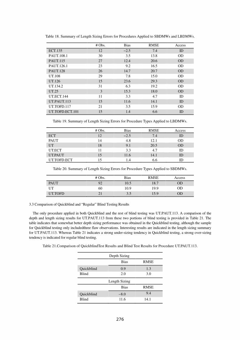
Table 18. Summary of Length Sizing Errors for Procedures Applied to SBDMWs and LBDMWs.
# Obs. Bias RMSE Access
ECT.135 12 −2.5 7.4 ID
PAUT.108.1 30 3.5 13.8 OD
PAUT.115 27 12.4 20.6 OD
PAUT.126.1 23 9.2 16.5 OD
PAUT.128 26 14.7 20.7 OD
UT.108 29 7.8 15.0 OD
UT.126 15 23.6 29.3 OD
UT.134.2 31 6.3 19.2 OD
UT.25 3 15.3 18.0 OD
UT.ECT.144 11 3.3 4.7 ID
UT.PAUT.113 15 11.6 14.1 ID
UT.TOFD.117 21 3.5 15.9 OD
UT.TOFD.ECT.101 15 1.4 6.6 ID
Table 19. Summary of Length Sizing Errors for Procedure Types Applied to LBDMWs.
# Obs. Bias RMSE Access
ECT 12 −2.5 7.4 ID
PAUT 14 4.8 12.1 OD
UT 18 9.1 20.5 OD
UT.ECT 11 3.3 4.7 ID
UT.PAUT 15 11.6 14.1 ID
UT.TOFD.ECT 15 1.4 6.6 ID
Table 20. Summary of Length Sizing Errors for Procedure Types Applied to SBDMWs.
# Obs. Bias RMSE Access
PAUT 92 10.5 18.7 OD
UT 60 10.9 19.9 OD
UT.TOFD 21 3.5 15.9 OD
3.3 Comparison of Quickblind and “Regular” Blind Testing Results
The only procedure applied in both Quickblind and the rest of blind testing was UT.PAUT.113. A comparison of the
depth and length sizing results for UT.PAUT.113 from these two portions of blind testing is provided in Table 21. The
table indicates that somewhat better depth sizing performance was obtained in the Quickblind testing, although the sample
for Quickblind testing only includedthree flaw observations. Interesting results are indicated in the length sizing summary
for UT.PAUT.113. Whereas Table 21 indicates a strong under-sizing tendency in Quickblind testing, a strong over-sizing
tendency is indicated for regular blind testing.
Table 21.Comparison of QuickblindTest Results and Blind Test Results for Procedure UT.PAUT.113.
Depth Sizing
Bias RMSE
Quickblind 0.9 1.3
Blind 2.0 3.0
Length Sizing
Bias RMSE
Quickblind −8.0 9.4
Blind 11.6 14.1
276

4. The PARENT Atlas Information Tool
The PARENT Atlas information tool is under development to document the open testing data and results as well as
relevant data from field experience. The main tab for the open data is shown inFigure 5 and allows users to filter through
data by technique, team, or test block. Multiple selections can be made so that the results of multiple inspections can be
compared. The selections appear on the right-hand side of the main Open Data interface where data regarding the selected
inspections can be accessed. An expanded view of one of the menu items from the right-hand side is shown in Figure 6and
shows that the information that may be accessed for an inspection includes procedure information, data images, inspection
record sheets, and flaw information for the flaws in the inspected test blocks.
Efforts are currently underway to develop hitograms in the PARENT Atlas tool and to incorporate field experience into
the PARENT Atlas. The hitograms allow simultaneous display of hits, misses, and false calls for multiple selected
inspections relative to true flaw state for the inspections.
Figure 5. Screenshot of the PARENT Atlas information tool Open Data tab display
277

Figure 6. Expanded view of the right-hand side of the Open Data interface illustrating information accessible for each
selected inspection
5. Conclusions
This paper presents some of the blind data results for DMW test blocks from the PARENT program and status of the
PARENT Atlas information tool for open testing. Final reports for PARENT blind and open testing are anticipated to be
published in the final quarter of 2015. Although not all of the blind testing analysis and results could be included in this
paper, the results that are provided illustrate some significant trends. For instance, the detection and depth sizing
performances of PAUT and UT procedure types are better for SBDMW test blocks than LBDMW test blocks. Also, the
performance of PAUT procedure types is generally better than the performance of UT procedure types, but the difference
in performance appears to be somewhat diminished for LBDMW test blocks. Further, whereas the sizing performances of
PAUT procedure types appears to be significantly different between LBDMW and SBDMW test blocks, the sizing
performances of UT procedure types are consistent between block types. Finally, several of the ID procedures applied to
LBDMW test blocks were also multiple technique procedures. The ID procedure exhibited much better depth sizing
performance than the OD procedures and the detection and length sizing performances of ID procedures were better than
OD procedures, as well. Only OD procedures were applied to SBDMW test blocks in PARENT.
Acknowledgements
This work is being conducted by U.S. Nuclear Regulatory Commission and Pacific Northwest National Laboratory in
partnership with ; IHI Southwest Technologies; AlphaSense; Nuclear Regulatory Authority of Japan; Japan Power
Engineering and Inspection Corporation; Tohoku University; Mitsubishi Heavy Industries, Ltd.;Institute of Nuclear Safety
System, Incorporated ; Ultrasonic Materials Diagnosis Laboratory; Nagoya University; Toyama University; Kansai
Electric Power Company; Korea Institute of Nuclear Safety; Korea Atomic Energy Research Institute; Doosan Heavy
Industries; Korea Hydro & Nuclear Power; Korea Plant Service & Engineering;; Korea Research Institute of Standards and
Science; Korea Inservice Inspection; Sungkunkwan University; Hanyunag University; Pusan National University; Swedish
Radiation Safety Authority; Swedish Qualification Centre; VTT Technical Research Centre of Finland; Aalto University;
Swiss Federal Nuclear Safety Inspectorate; Paul Scherrer Institute; Swiss Association for Technical Inspections, Nuclear
Inspectorate; Swiss Federal Laboratories for Materials Science and Technology; Alstom; DEKRA; Chalmers Institute of
Technology, FORCE Technology; and NRG.
278

References
[1] Cumblidge, S.E., et al., Results of the Program for the Inspection of Nickel Alloy Components. 2010, U.S. Nuclear
Regulatory Commission: Washington, D.C.
[2] Braatz, B.G., P.G. Heasler, and R.M. Meyer, PARENT Quick Blind Round-Robin Test Report. 2014, Pacific Northwest
National Laboratory: Richland, Washington.
[3] Prokofiev, I., et al., New International Program to Assess the Reliability of Emerging Nondestructive Techniques
(PARENT), in Review of Progress in Quantitative Nondestructive Evaluation, Vol. 32, AIP Conference Proceedings Vol.
1511, D.O. Thompson and D.E. Chimenti, Editors. 2013, American Institute of Physics, Melville, New York: Denver,
Colorado. p. 1097-1103.
279

Challenge for the Detection of Crack in Dissimilar Weld Region Using
PECT (Pulsed Eddy Current Technology)
Duck-Gun Park1, M.B Kishore
Nuclear Materials Safety Research Division , Korea Atomic Energy Research Institute, Daejeon,
South Korea -305-353,
Abstract
Pulsed Eddy Current (PEC) technique uses multiple frequency current pulse to drive the
excitation coil of PEC probes unlike conventional single frequency eddy current methods. In
the present study, we make an effort to detect the crack in dissimilar weld region using PEC
technique. The test samples were prepared by welding two base metals, the composition of
base metal is SA508 cl.2 and that of welding metal is alloy 182. The defect region was
positioned in the weld metal, and the types of defect are stress corrosion cracking, fatigue
cracks having the width of several micrometers. A rectangular pulse having 10ms pulse width
and 15A current is applied to the exciting coil of PEC probe to inspect the sample cracks. The
peak amplitude of the detected PEC pulse was chosen as a measure to estimate the cracks
under the sample surface. The PEC signal amplitude detected in the defect region (welded
part) showed lower value than that of base material. The crack is positioned in the middle of
dissimilar weld region, which shows the minimum PEC signal amplitude. In time domain
analysis, the peak amplitude of the detected pulse is decreased, with an increase in the crack
depth. The experimental results indicated that the proposed system using PEC technique has
the potential to detect the sub surface cracks in dissimilar weld region.
Keywords— pulsed eddy current, dissimilar weld, crack, PEC probe, hall sensor, peak
amplitude
1. Introduction
Eddy current testing is a non destructive testing (NDT) method used for metals and includes the detecting and sizing of defects, identifying composition, structure and measuring thicknesses. Among the available conventional NDT methods, eddy current testing (ECT) is the most promising technique to detect flaws in conductive materials. The conventional ECT uses a single-frequency sinusoidal excitation for the detection of defects or flaws as a function of changes in voltage, impedance, or phase. Because of limited depths of penetration and complexity in signal analysis ECT was confined to limited applications [1]. Unlike a conventional ECT, PEC uses a multiple frequency sinusoidal excitation of the electric current resulting from the broad band nature of the pulse; hence it has the ability to penetrate different depths in a conductive material and provides the depth information of the defects [2, 3] located at different depths. PEC testing has been demonstrated to be one of the most effective methods, and is capable of performing different inspection tasks, such as sub-surface defect detection in complex structures, wall thinning detection, crack detection, coating thickness detection etc. [4,5]. Moreover, PEC is more economical than other NDT methods such as low power consumption owing to short pulse excitation and it doesn’t need any complex electronic circuitry. Even though the use of PEC has long been considered for the testing of materials, in recent decades, PEC testing has become the subject of wide spread interests in NDT because of its advancement in technologies such as computer data acquisition and digital signal processing. Because of the potential advantages of the PEC, prevalent investigations on this technique have been made, such as for detection of wall thinning and corrosion in aircraft multilayer structures [9, 10]. Especially, it is efficient to detect the subsurface crack of thick
280

plate often used in the nuclear industry. The thickness of tubes and nozzle used in the nuclear power plant is up to several tenth of millimeter, which is made of stainless steel and/or Inconel alloy to protect the corrosion. The crack detecting sensitivity using PEC probes depends on several parameters such as pulse width, coil size, coil diameter. To achieve this, it is necessary to increase the flux through the circular coil, which can be described by the following equation.
∅ = Bπr
Where B is the magnitude of the magnetic flux density perpendicular to the surface defined by the coil of radius (r). Therefore, if larger size coil is used for the detection purposes, a low resolution and sensitivity would be achieved. The reason is that they respond to all magnetic flux line passing through the coil winding, regardless of their spatial direction and orientation. This characteristic together with the size of the coil can impact the sensitivity of this sensor. Using smaller coil would provide a better sensitivity but would limit eddy current penetration within the test object. Therefore, in order to detect the deep crack buried under thick sample, we have to design PEC probe considering many parameters such as skin depth, coil inductance, and detection sensor. In the present study, a new PEC probe to detect a very thin cracks made by stress corrosion cracking phenomena in the dissimilar weld region was made by considering special resolution and sensitivity of detecting element. For this purpose, specially designed probe was used, and the performance of the new designed probe was tested with a PEC system designed and developed for this purpose
2. Experimental Setup
The block diagram of the PEC system design is shown in Figure 1. The system consists of a
rectangular waveform generator, a probe integrated with an excitation coil and a pickup Hall-
sensor to detect the induced field from test specimen, an amplifier to process the signal
obtained from Hall-sensor for further steps as the sensor output is too low in magnitude, a
data acquisition card connected to PC using signal processing software to digitize the
obtained data and to record the PEC data. The operational flow of the PEC system is as
follows; the waveform generator produces a rectangular pulse with variable frequency and
duty cycle. The pulse is fed to a coil driver circuit which excites the driving coil of the PEC
probe. When the probe is mounted on the metal structure, the pick-up hall sensor will
measure the vertical resultant magnetic field, which is the vector sum of the field generated
by the excitation coil and the opposing magnetic field generated by the induced eddy currents
in the test sample (Primary flux Φ1 created by driving coil induces EC in the conducting
medium, induced EC produces counter flux Φ2. Now pick-up sensor measures total flux Φ =
Φ1 + Φ2.). The signal obtained from the pick-up sensor is amplified by a voltage amplifier
with variable gain. The A/D card will convert the analog input signal into digital data which
can be used for further signal analysis by the end user. A software program is used to Signal
pre-processing, feature extraction, defect categorization, and the presentation of the results on
the PC monitor.
281

Figure 1.The block diagram of the PEC system.
The pulse amplifier supplies a high current pulse to the Driving Coil or exciting coil. The
pulse width, pulse amplitude and duty cycle can be controlled and selected by considering the
skin depth of sample. The excitation coil is a 1x3 mm rectangular cross sectional copper wire
wound on the cylindrical ferrite core, the number of turns are made to be 132 turns having
total resistance 0.192 Ω . To obtain good special resolution, the probe has a 60mm height and
9mm inner diameter, and the Hall-sensor was positioned in the center of probe to detect the
induced signal from defects. The cylindrical type ferrite core not only reduces the magnetic
leakage but also improves the detection sensitivity by sustaining adequate excitation intensity.
The Hall-sensor gives the frequency independent sensitivity from DC to 100 KHz, high
spatial resolution, less power consumption with increased sensitivity and simple readout
circuitry. When the probe was placed in close proximity to the conducting plate, the steep
exciting pulse induces eddy currents and its associated magnetic field dissipates
exponentially to approach its steady state. The induced eddy current field flow is in the
opposite direction to primary exciting field, hence when the probe is placed on the
conducting plate, the detected field rises slowly to the maximum peak value.
3. PEC signal measurement and Tested Sample
A 10ms pulse width and 15A excitation current is applied to exciting coil of the probe to test
the sample. figure 2(a) shows the experimental setup, The PEC probe is fixed to the X-Y
scanner to perform the manual scanning on the defect free side of the tested sample. Initially
the probe is placed on the sample such that the hall sensor positions at the center in vertical
direction i.e. about x axis and continued to be at its center position as the scanning process
continues along the y axis i.e. along the length of the test sample, the probe used in this
experiment and the test specimen can be observed in figure 2(b) . A LabView based data
acquisition program shown in figure 2(c) was developed to continuously monitor the
variation in the thickness of the sample and is observed on the computer screen. The time
domain feature, peak amplitude of the detected pulse is used to detect the sub-surface cracks
282

in the tested sample. in order to reduce the experimental error, average of 5 pulses is
considered as the resultant PEC pulse. The three kinds of test blocks with ID 28, 29, and 30
provided by ENSI were tested. the flaw types of these test blocks are BWR/NWC SCC Crack,
Fatigue Crack, and PWR SCC crack, respectively. The samples were composed by the
welding of two base metals, and the composition of base metal is SA508 cl.2, and the
welding metal is alloy 182 as shown in the figure 2(d).
Figure 2(a).Experimental Setup. (b) closed view of Probe and Test specimen. (c) Lab VIEW based
application to read and process PEC data. (d) Schematic of PARENT Test Specimen, PECT probe is
located on the opposite side of crack surface
5. Experimental results and feature extraction
when the probe is placed on the test specimen, the excitation pulse will generate a primary
magnetic field which can penetrate into the test sample resulting into eddy currents to
generate and pass through the sample, these small eddy currents will generate secondary
magnetic field which can oppose the primary magnetic field will be detected by the hall
element. since the secondary field is opposite to the primary magnetic field, the detected
pulse tends to change depending on the test specimen and portrayed as the defect information.
A typical response signal from PEC probe when placed on the test sample in such a position
is shown in Fig. 3. Calibration of PEC signal with standard specimen is essential to obtain a
reliable experimental result. Because of no calibration sample is prepared, the validity of
experiment was verified using the difference of the PEC peak amplitude obtained in the crack
and opposite side (Fig. 4). The base metal of sample block SA508 Cl.2 is ferromagnetic and
283

welding material alloy 182 which is nonmagnetic material. Therefore, the PEC amplitude
measured in the ferromagnetic part is higher than that of the nonmagnetic part. The y
coordinate 10 and 12 cm neighborhood is the interface region between ferromagnetic and
nonmagnetic material. The crack is positioned in the neighborhood of y coordinate 11 cm,
which shows the minimum PEC signal amplitude.
Figure 3. Typical PEC signal induced in the Hall-sensor from the test block.
The important characteristic of detected signal to interpret the results is the peak value of the
pulse. The measuring points were selected as a x-y coordinate, the x points were fixed at the
center of transverse direction and y points were selected along the longitudinal direction.
Fig. 5 show the change of PEC peak amplitude along the coordinate and shows minimum
value at the defect position.
284
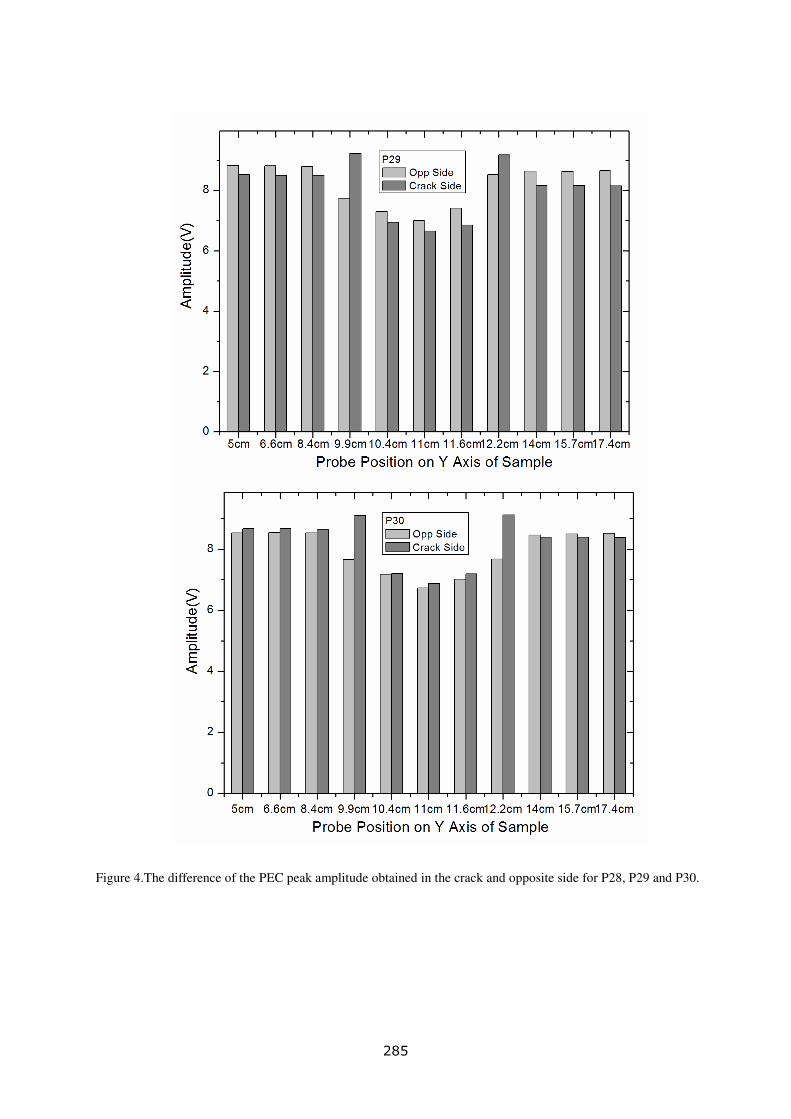
Figure 4.The difference of the PEC peak amplitude obtained in the crack and opposite side for P28, P29 and P30.
285

Figure 7.The difference of the PEC peak amplitude obtained in the crack and opposite side for P28, P29 and P30
286

6. Summary
1) The nondestructive evaluation (NDE) using PECT to detect the sub surface crack under the
thick plate has been performed on the PARENT round robin sample. Three classes of round
robin sample for P28, P29 and P30 have been tested, each class has dissmilar weld region
between two ferromagnetic base materials.
2The PEC amplitude detected in the defect region (welded part) showed lower value than that
of base material. The y coordinate 10 and 12 cm neighborhood is the interface region
between ferromagnetic and nonmagnetic material. The crack is positioned in the
neighborhood of y coordinate 11 cm, which shows the minimum PEC signal amplitude.
3) The base material is made of ferromagnetic materials, and dissimilar weld region is made
of nonmagnetic materials. Considering the ferromagnetic materials induce a high magnetic
signal, it is not certain that the decrements of amplitude are attributed to the defects or
nonmagnetic part.
4) The PEC technology showed potential possibility detecting the subsurface crack in the
nonmagnetic stainless steel plate, but the signals are largely depend on the appearance of
ferromagnetic substance. Therefore the PECT technique requires further assessment and
improvement in order to apply in the dissimilar weld region.
References
[1] G. Y. Tian, Z. X. Zhao, and R. W. Baines, “The research of inhomogeneity in eddy
current sensors”, Sens. Act. A., vol. 69, pp 148–151, 1998.
[2] E. E. Kriezis, Theodoros D. Tsiboukis, Stavros M. Panas and John A. Tegopoulos, “Eddy
currents: Theory and applications”, Proceedings of IEEE, Vol. 80, No. 10, pp 1559- 1589,
Oct 1992.
[3] B.P.C. Rao, B. Raj, T. Jayakumar and P. Kalyanasundaram, “An Artificial neural network
for eddy current testing of austenitic stainless steel welds”, NDT&E Internationl, Vol.
35,pp 393-398, 2002.
[4] Y. He, F. Luo, M. Pan, “Defect characterisation based on pulsed eddy current imaging
technique”, Sensors and Actuators A, Vol 164, pp 1-7, 2010.
[5] J.C. Moulder, J.A. Bieber, W.W. Ward III, J.H. Rose, “Scanned pulsed eddy current
instrument for non-destructive inspection of aging aircraft”, SPIE 2945, pp 2–13,1996.
[6] B.P.C. Rao, B. Raj, T. Jayakumar and P. Kalyanasundaram, “An Artificial neural network
for eddy current testing of austenitic stainless steel welds”, NDT&E Internationl, Vol.
35,pp 393-398, 2002.
[7] Y. He, M. Pan, F. Luo, G.Ti, “Pulsed eddy current imaging and frequency spectrum
analysis for hidden defect nondestructive testing and evaluation”, NDT& Int., Vol 44,
pp 344-352, 2011.
[8] H. C. Yang, C.C. Tai, “Pulsed eddy current measurement of a conducting coating on a
magnetic metal plate”, Meas Sci Techno.l, Vol 13, pp 1259-1265, 2002.
287

[9] M. A. Robers, R. Scottini, "Pulsed eddy current in corrosion detection", NDT.net The e-
Journal of Nondestructive Testing, Vol.7, Oct. 2002.
[10] A. Smith, G. R. Hugo, "Transient Eddy-current NDE for aging aircraft capabilities and
limitations", Insight: Non-Des. Testing and Condition Monitoring, Vol.43, pp. 14-25, Jan.
2001.
288

TOFD Technique and field application in Korean nuclear plants
Euisoon DOH, Jae-yoon KIM, Chang-ho Song, Tack-su LEE
KEPCO KPS, Busan, Korea
E-mail :[email protected]
TOFD(Time of Flight Diffraction) technique is a very useful method to detect a very tight
crack caused by PWSCC(Primary Water Stress Corrosion Crack) in nuclear power plant. A
Lateral wave and Tip signals are used to detect and size a flaw in TOFD technique. And one
of the most important factor for TOFD technique is a proper spacing between two paired
probes to maximize the detect ability and accuracy of sizing flaw considering the thickness of
examined material.
We are applying this TOFD technique to Reactor vessel upper and bottom head penetration
inspection in Korean plants. We also have participated in the Blind Round Robin test for the
PARENT to detect flaws at BMI(Bottom Mounted Instrumentation Nozzle) mock up
specimens.
We have found the first several PWSCC flaws at upper Reactor vessel head penetrations in
Korean nuclear plants. And this event has played a main role in reducing the inspection
interval of Reactor upper head penetration inspection, which designed with alloy 600
materials in Korean nuclear plants.
I will describe the characteristics of TOFD technique and the detection of PWSCC flaws in
the field examination in Korean nuclear plants in this paper.
Keywords: Reactor vessel, Reactor vessel Head Penetration Examination, RVHP Inspection,
RVHPI, ISI.
289

Nonlinear Ultrasonic Technique for Assessment of Thermal Aging
Jongbeom Kim1 and Kyung-Young Jhang
2†
1Department of Mechanical Convergence Engineering, Hanyang University, 222 Wangsimni-ro, Seongdong-gu,
Seoul, Republic of Korea 133-791
2School of Mechanical Engineering, Hanyang University, 222 Wangsimni-ro, Seongdong-gu, Seoul, Republic
of Korea 133-791
†Corresponding Author/ E-mail: [email protected],
TEL: +82-2220-0434, FAX: +82 -2299-7207
Abstract:
The second-order ultrasonic nonlinear parameter has been studied for the evaluation of material
degradation. However, there are some limits to the assessment of thermal aging in aluminum alloys
due to the fluctuation in the nonlinear parameter with the aging time. This is because the nonlinear
parameter strongly depends on the behavior of the precipitate when exposed to high temperatures.
That is, the nonlinear parameter does not one-sidedly increase with the thermal aging. In such cases, it
is difficult to evaluate the damage level from the nonlinear parameter. In order to overcome such
limitations, we propose a cumulative nonlinear parameter defined by the accumulation of
variation in the nonlinear parameter over the aging time. In order to verify the usefulness of the
proposed parameter, the nonlinear parameters were measured in aluminum alloy specimens heat-
treated with different aging temperatures and aging times, and accumulated values of their variation
were obtained as a function of the aging time. Tensile tests were conducted to estimate the altered
strength of the Al alloy specimens due to thermal aging from the stress–strain curves. Results showed
that the nonlinear parameter varied in directions of both increase and decrease, but the strength
decreased one-sidedly with aging. Thus, the parameter could not be used as a direct index of
strength degradation. On the other hand, the proposed parameter one-sidedly increased and
agreed well with the reduction in the strength.
Key words: Cumulative ultrasonic nonlinear parameter; Ultrasonic nonlinear parameter; Thermal
aging; Aluminum Alloy; Precipitation 290

A Feasibility Study on Detection and Sizing of Defects in the Reference
Block Specimen by Using Ultrasonic Infrared Thermography
Hee-Sang Park2, Jeong-Hak Park
1, Dong-Jin Yoon
1*, Kyung-cho Kim
3, Won-Tae Kim
4 and
Man-Yong Choi1
1 Center for Safety Measurement, Korea Research Institute of Standards and Science, Korea,
2 Korea Research Institute of Smart Material and Structures System Association, Korea
3 Dept. of Mechanical & Materials Engineering, Korea Institute of Nuclear Safety, Korea
4 Dept. of Mechanical Engineering, Kongju National University, Cheonan, Korea
Ultrasonic infrared thermography (UIRT) is based on the detection of thermal energy
generated when elastic energy is absorbed by a defect and converted to thermal energy
through thermos-elastic effects. The advantage of UIRT is that it potentially enables more
rapid examination of large areas based on camera images in contrast to other techniques that
would require a point-by-point raster scan. Especially, with lock-in phased method, the
amplitude and phase information about the thermal waves emitted from the specimen is
preserved for several frequencies. Therefore it enables characterizing the depth of a source of
thermal emissions in the test component inside.
This study describes a part of the results of open round robin test for PARENT by using
ultrasonic infrared thermography technology. We used several types of specimen which is
fabricated as reference block including several kinds of defects inside. In this preliminary
study, all indications produced by infrared thermal image and lock-in phase image with
temperature difference within the volume to be examined shall be considered as defect
indications. This procedure was conducted after exciting the basic material near the welds by
using ultrasonic guided horn for a certain amount of time. And also, a defect indication was
discriminated by a healthy image to show temperature difference (< 0.15°C) along the
position of component. In case of the evaluation of length sizing, defect size was correlated
with the spatial resolution of pixel image. And the lock-in phase images was used for
evaluating the temperature distribution through the temperature difference. Finally hot spot
image indications produced by infrared thermal image and lock-in phase image were
evaluated by comparing with defect size.
Keywords: Detection of defects, Ultrasonic infrared thermography, Dissimillar metal weld,
PWSCC, NDE
291

Experimental Visualization of Ultrasonic Wave Propagation in Dissimilar Metal
Welds
Masaki NAGAI1, Shan LIN
1, Audrey GARDAHAUT
2, Hugues LOURME
2 and Frédéric JENSON
2
1Central Research Institute of Electric Power Industry, Japan
2CEA, LIST, France
Abstract
In nuclear power plants, a number of surface cracks attributed to stress corrosion cracking (SCC) have been
detected in dissimilar metal welds (DMWs) between austenitic stainless and low alloy steels. When a crack is
detected in a component of a nuclear power plant during an in-service inspection, fitness-for-service codes require that
a flaw evaluation has to be conducted. Detection and sizing of such cracks with high accuracy are necessary for
accurate flaw evaluation. Although ultrasonic testing (UT) is widely used in nondestructive inspection techniques
for components in nuclear power plants, it is difficult to be applied to DMWs because coarse grains in DMWs scatter
and attenuate ultrasonic waves severely. Moreover, anisotropic and heterogeneous properties in DMWs result in
beam splitting and skewing, which reduce the detection capability and the sizing accuracy of UT. For improvement
of UT capability, CEA and CRIEPI both agree to have a collaborative research program focusing on deep
understanding of wave propagation within DMWs. In this program, CEA performed a simulation of wave
propagation and defect response regarding DMWs by using CIVA software. And CRIEPI conducted experimental
visualization of wave propagation in DMWs and ultrasonic examination by phased array technology, which is the
content of this paper.
Keywords: Ultrasonic Testing, Dissimilar Metal Welds, Phased Array Technology, Wave Visualization
1. Introduction
In nuclear power plants, nickel alloys have been used for dissimilar metal welds (DMWs) between austenitic stainless
and low alloy ferritic steels. In recent years, a number of surface cracks attributed to stress corrosion cracking (SCC)
have been detected in DMWs. In Japan, for instance, a crack was found in a weld in a reactor pressure vessel nozzle at
the Ohi-3 pressurized water reactor (PWR) power plant [1], and cracks were detected in a shroud support weld at the
Tsuruga-1 boiling water reactor (BWR) power plant [2]. When a crack is detected in a component of a nuclear power
plant during an in-service inspection, fitness-for-service codes require that a flaw evaluation be conducted. Detection and
sizing of such cracks with high accuracy are necessary for accurate flaw evaluation. Although ultrasonic testing (UT) is
widely used to detect components of nuclear power plants, it is difficult to be applied to DMWs due to (1) ultrasonic waves
are scattered and attenuated by coarse grains in DMWs, and (2) anisotropic and heterogeneous properties in DMWs result
in beam splitting and skewing. These reasons reduce the detection capability and the sizing accuracy of UT.
In order to improve UT capability, experimental investigation by means of mock-up is useful, but it is time-consuming
and costly. Instead of experiments, the CIVA developed by CEA/LIST is a proven software that it is effective for the
optimization of inspection conditions. Nevertheless, it is necessary to ascertain whether the CIVA software can be used
to model UT inspections in DMWs with severe anisotropic and heterogeneous properties. Therefore, CEA and CRIEPI
both agree to have a collaborative research program focusing on (1) deep understanding of wave propagation within
DMWs by means of simulation and experiment, (2) the evaluation of applicability of CIVA to DMWs with anisotropic and
heterogeneous properties. In this paper, experimental visualization of wave propagation in DMWs and UT results using
phased array method are shown.
2. Overview of collaborative research program
In this research, as shown in figure 1, a specimen made of austenitic stainless and ferritic steels with a nickel ally weld
has been prepared and its crystallographic orientation of grains in weld is observed by macrograph. Three electrical
discharge machining (EDM) notches with the same dimensions and shape are introduced into buttering, weld and stainless
292

steel base metal, respectively. In order to deeply understand how waves propagate within DMWs, the propagation of
waves which are excited on surfaces of ferritic steel, buttering, weld metal and stainless steel, are visualized experimentally.
Several linear array transducers with different frequencies are used to detect notches by pulse-echo and pitch-catch
techniques. UT results predicted by the CIVA are compared to experimental results to evaluate the applicability of the
model developed in the software. This collaborative research program started in April 2012 and ended in March 2014.
Figure 1 Specimen with dissimilar metal weld
3. Experimental visualization of wave propagation
3.1 Measurement method
Figure 2 shows the system used for measuring wave propagation. This system consists of a pulser / receiver, an
oscilloscope, a transmitter, a receiver, a computer and a scanner. A voltage pulse is sent to the transmitter, which is
an angle beam transducer, and is located on the top surface. The transmitter generates waves propagating within a
specimen. As the waves propagate within the specimen, they are probed by the receiver which is a normal incidence
transducer. The diameter of vibrator in the receiver is 1 mm. Received waves are digitized by the oscilloscope and are
inputted to the computer. The measurement is performed on an area so that wave propagation is not disturbed by
notches introduced. The scanner moves the normal incidence transducer over 80 mm in x-direction and 35 mm in
y-direction with a resolution of 0.2 mm on the side surface. The computer acquires data sent by the oscilloscope,
controls the scanner and processes acquired data to view wave propagation. The transmitter and the receiver have the
same nominate frequency of 2 MHz. A longitudinal angle beam transducer with a refraction angle of 49 degrees is
used.
Figure 2 System for wave propagation visualization
Transmitter
( Angle )
Receiver ( Normal )
Measurement area
(35 mm x 80 mm)
Data acquisition
Scanner control
Wave viewer
Scanning pitch: 0.2mm
Frequency: 2MHz
Diameter of receiver: 1mm
Receiver: Longitudinal
Refraction angle:
49 degrees (Long.)
45 degrees (Trans.)
Ferritic steel Stainless steel
Buttering Weld
Notch in buttering
Notch in weld92.8
50
40
85Notch in
stainless steel
(for reference)
293

3.2 Visualization results and discussion
Figure 3 shows waves excited by a longitudinal angle beam transducer on the ferritic steel, where L and T represent
longitudinal and transverse waves, respectively. Color code represents the amplitude of waves. As shown in this
figure, longitudinal and transverse waves are excited at the same time. Longitudinal waves are scattered in the
buttering, but this scattering is so weak that it does not prevent longitudinal waves from traveling through the
buttering. Figure 4 depicts longitudinal and transverse waves excited on the buttering. As shown in this figure,
longitudinal waves can travel through the buttering and the weld while it is difficult for transverse waves to do so
because they are severely scattered. Figure 5 and 6 are results of wave propagation observed on the opposite side of
those shown in Figures 3 and 4. As shown in Figure 5, the weld scatters and attenuates longitudinal waves to some
degree, but longitudinal waves propagate through it. Moreover, as shown in Figure 6, for longitudinal and transverse
waves excited on the weld, longitudinal waves propagate through the buttering and the weld without difficulty. On the
other hand, the weld scatters and attenuates transverse waves much more seriously than longitudinal waves, which
implies that transverse waves propagate difficulty through the weld and the buttering. However, as shown in Figure 6,
the wave front of transverse waves can be observed in some degree in the weld, but not in the buttering in figure 4.
This is probably because the angle between grain axis and incident direction of ultrasonic waves in the buttering is
much larger than that in the weld. This fact suggests that the buttering affects the propagation of transverse waves
more than the weld. From results shown in figures 3-6, longitudinal waves have sufficient capability to travel
through DMWs.
4. Ultrasonic examination by phased array technology
4.1 Examination conditions
Four kinds of ultrasonic examinations are performed using three different types of linear array transducers.
Nominal frequency, the number of elements, pitch, length and width of respective transducer are shown in Table 1.
Main examination conditions corresponding to respective examination are shown in Table 2, where PE and P/C mean
pulse-echo and pitch-catch techniques, respectively. All examinations are carried out under longitudinal mode by
raster scan.
4.2 Examination results and discussion
In this paper, only results of Examination 3, in which pulse-echo technique was applied with 1 MHz, are presented
due to limitations of space. Figures 7 and 8 show results corresponding to the refraction angle of 45 degrees. T1
and C1 are indications in regard to tip and corner echoes of notch in weld metal, respectively. T2 and C2 mean tip
and corner echoes of notch in buttering, respectively. WB is the indication of echo from the boundary between the
weld and the buttering. Values shown in dB are echo intensities of notches introduced in the weld and the buttering
normalized with respect to that of notch in stainless steel. Except for notch in the weld when waves are emitted from
the stainless steel side, the decrease level for corner echoes is much larger than that for tip echoes. This is probably
resulted from anisotropic and heterogeneous properties in the weld and buttering.
As shown in Figures 7 and 8, noise echoes resulting from scattering in the weld and buttering are observed. It is
easy to detect notches introduced in weld and buttering when waves are emitted from the ferritic steel side.
However, it is not easy to identify echoes associated to notches, especially for a notch in buttering, because of strong
boundary echoes when waves are emitted from the stainless steel side.
5. Conclusions
In order to improve UT capability regarding DMWs, the specimen made of austenitic stainless and ferritic steels
with a nickel alloy weld was prepared. Wave propagation in DMWs was visualized experimentally to understand how
waves propagate within DMWs. Longitudinal waves have sufficient capability to travel through DMWs.
Moreover, UT inspections were performed using several linear array transducers. Due to strong boundary echoes
between weld and buttering, it is difficult to identify echoes associated to a notch in the buttering when waves are
emitted from the stainless steel side.
294

Incident point (60, 40)
X
Y
40
0.0 0.033 0.067 0.10
(a)16µs (b)19µs (c)21µs L
L
L
TT
T
Figure 3 Waves excited by a longitudinal angle transducer located on ferritic steel
Incident point (80, 40)
X
Y
55
(a)8µs (b)12µs (c)17µs
0.0 0.033 0.067 0.10
L
TL
T
Figure 4 Waves excited by a longitudinal angle transducer located on buttering
Incident point (55, 40)
X
Y
40
(a)9µs (b)13µs (c)16µs
0.0 0.013 0.027 0.40
L
L
L T
T
T
Figure 5 Waves excited by a longitudinal angle transducer located on austenitic stainless steel
Incident point (80, 40)
XY
60
(a)9µs (b)12µs (c)15µs
0.0 0.013 0.027 0.040
L
T
L
LT
Figure 6 Waves excited by a longitudinal angle transducer located on weld metal
295

Table 1 Main specifications of transducer
Nominal frequency
(MHz)
Num. of elements Pitch
(mm)
Length
(mm)
Width
(mm)
Transducer 1 2 32 0.8 0.7 10
Transducer 2 2 64 0.6 0.5 20
Transducer 3 1 64 0.6 0.5 20
Table 2 Main examination conditions
Technique Transducer Wave type Num. of active
elements
Emission depth
(mm)
Examination 1 PE Transducer 1 Longitudinal 32 20
Examination 2 PE Transducer 2 Longitudinal 64 20
Examination 3 PE Transducer 3 Longitudinal 64 20
Examination 4 P/C Transducer 1 Longitudinal 32 32
Notch
in buttering
Notch
in weld
T2=-5.6dB
C2=-12.2dB
Notch
in buttering
T1=-2.4dB
C1=-6.3dB
Notch
in weld
Notch
in buttering
Notch
in weld
Figure 7 Results performed from ferritic steel side for examination 3
T2=-8.9dB
C2=-12.2dB
T1=-5.1dB
C1=-7.0dB
Notch
in buttering
Notch
in weld
Notch
in buttering
Notch
in weld
Notch
in buttering
Notch
in weld
+6dB
+6dB
+6dB
+6dB
Boundary
echoes
Boundary
echoes
Figure 8 Results performed from stainless steel side for examination 3
296

References
[1] Nakamura T., Taniguchi, K., Hirano, S., Narita M., Sato T., “Stress Corrosion Cracking in Welds of Reactor Vessel
Nozzle at Ohi-3 and of Other Vessel’s Nozzle at Japan’s PWR Plants”, PVP2009-77344, pp. 1-9 (2009)
[2] Aoki T., Shimizu S., Miyazaki K., Hayashi M., Kobayashi, H., “Evaluation on Crack Growth Analysis Model
based on the Knowledge obtained from Stress Corrosion Cracking in Ni-Based Alloy used for a Long Time in a
BWR”, Maintenology, 5, pp. 46-53. (2006)
297

Application of a 3D ray tracing model to the study of ultrasonic wave
propagation in Dissimilar Metal Welds
Audrey GARDAHAUT1, Hugues LOURME
1, Frédéric JENSON
1, Shan LIN
2 and Masaki NAGAI
2
1CEA, LIST, Bât. 565, PC 120, F-91191 Gif-sur-Yvette, France
2Materials Science Research Laboratory, Central Research Institute of Electric Power Industry,
2-6-1 Nagasaka, Yokohama-Shi, Kanagawa-ken 240-0196, Japan
Abstract
The primary circuit of Nuclear Power Plants (NPP) is inspected using Ultrasonic NonDestructive Testing (NDT)
techniques in order to maintain the integrity of its structure and detect eventual defects such as Stress Corrosion
Cracking (SCC). Nevertheless in some components as Dissimilar Metal Welds (DMW), the interpretation of
inspection results is difficult due to the appearance of beam disturbances as well as splitting and skewing. Those
physical phenomena, occurring due to the anisotropic and inhomogeneous properties of the media, affect the detection
and the characterization of possible discontinuities located inside or in the vicinity of the welds. In this context,
numerical simulation tools are really useful to understand these disruptions and optimize the ultrasonic NTD methods.
An analytical model, based on a ray theory, has been recently developed by CEA-LIST and implemented in the CIVA
software to evaluate the propagation of elastic waves in anisotropic and inhomogeneous media. It allows the
evaluation of the ray trajectories and travel-time and the computation of the amplitude along the ray tube in a medium
described thanks to a continuously varying description of its physical properties. This paper presents the work made as
a part of a collaborative program between CRIEPI and CEA. The ray-based model has been applied to the study of a
DMW described by a smooth representation of the crystallographic orientation. Comparisons of the transmitted beam
and the detection of notches, located in the weld and the buttering, obtained by simulations and experiments
performed on this mock-up have been presented.
Keywords: Ultrasonic Testing, Ray-based Model, Dissimilar Metal Weld.
1. Introduction
Nickel-based alloys have been widely used in Nuclear Power Plants (NPP) to facilitate the welding of stainless steel
cooling line pipes and instrumentation components to the ferritic steel vessels. Leaks have appeared in Dissimilar Metal
Welds (DMW) of the primary circuit of NPPs [1-6] due to the formation and the growth of Stress Corrosion Cracking
(SCC). Accurate detection and depth sizing of such cracks is a serious issue regarding the reliability and the safety of NPPs.
Ultrasonic Testing (UT) techniques are commonly apply for DMWs inspection and difficult to interpret due to
disturbances of the ultrasonic beam. Splitting and skewing [7], resulting from the anisotropy and heterogeneity of the
materials [8], and scattering and attenuation, due to the coarse grain structure, may indeed affect the detection capabilities
and sizing accuracy of UT. In this context, simulation tools are quite useful to understand those complex phenomena
observed on inspection results.
Finite differences [9], finite elements [10-11] and ray tracing [12] models have been used to simulate the propagation of
ultrasonic wave. Semi-analytical propagation models [13], based on a ray theory, have been implemented in the CIVA
software [14-15], developed by CEA-LIST, and applied to the inspection of weld. The welds are described as a set of
several anisotropic and homogeneous domains with a given crystallographic orientation. However, for domains with small
dimensions compared to the wavelength, the simulated results are valid only if the contrast of impedance is small between
two neighbouring domains [16]. A new approach has been considered to take into account the inhomogeneity in such
anisotropic media. Based on the Dynamic Ray Tracing (DRT) model, it is applied to a weld described as a continuously
variable description of the crystallographic orientation [17].
A collaborative research program has been set up between CRIEPI and CEA-LIST to understand the propagation of
ultrasonic wave in DMWs. It focuses on the realization of simulations and experiments, the evaluation of applicability of
CIVA for the study of material with complex structures and the evaluation of phased array techniques for DMWs
inspections.
298

2. Dynamic Ray Tracing model for the simulation of ultrasonic propagation
Usually applied in Geophysics [18], the Dynamic Ray Tracing (DRT) model is based on the solving of two equations
in anisotropic and inhomogeneous media [17].
The solving of the first equation, the eikonal equation, gives the following system called axial ray system [18]:
Composed of two coupled ordinary differential equations, this system describes the variations of the position xi and
the slowness pi with respect to the travel-time T(x). It is expressed in function of the elastic constants of the material
aijkl, the density ρ and the components of the slowness vector pi. gj(m)
are the eigenvectors of the Christoffel tensor
corresponding to the polarization vectors and Vie(m)
is the energy velocity for the m-mode. The solutions of this system
give the ray trajectories and the travel-time in the weld.
A second system called the paraxial ray system is obtained by solving the transport equation. Composed of ordinary
linear differential equations of the first order of the paraxial quantities Qi and Pi, it expresses the variations of the
position xi and the slowness pi in function of the travel-time T(x) and the parameter γ:
.2
1
,2
1
2)(
)(
2
i
ix
i
xi
ii
x
G
dT
dP
d
dp
dT
d
p
G
dT
dQ
d
dx
dT
d
(2)
γ is any parameter of a ray Ω and is chosen as a take-off angle between a reference axis and the initial slowness vector
and Gm, expressed as )()( mk
miljijklm ggppaG , are the normalized eigenvalues of the Christoffel tensor. Through the
solving of this system, the evolution of the ray tube during the propagation is obtained and its amplitude, assuming the
conservation of the energy across a ray tube section, is evaluated.
These two systems are solved simultaneously by using numerical techniques such as the Euler method in this example.
3. Description of the physical properties of a dissimilar metal weld
The mock-up considered in this study (cf. Figure 1) connects a SM490 ferritic steel pipe to a SUS316L stainless steel
pipe. This dissimilar V-butt weld and the buttering are made with alloy 600.
Figure 1. Macrograph of a V-butt DMW.
This weld is characterized by an anisotropic and inhomogeneous structure and a strong attenuation. Responsible for
the splitting and skewing of the ultrasonic beam along the propagation, these characteristics have to be known and
used as input data in the simulations.
The anisotropy of the material, expressed through the elastic constants, results of the dependence of the ultrasonic
velocity to the direction of propagation. The chosen set of parameters is presented in Table 1. These properties of alloy
182 are representative of the anisotropy of the studied V-butt weld made of alloy 600.
.2
1
,
)()(
)()()(
ml
mjnk
i
ijkli
mei
mk
mjlijkl
i
ggppx
a
dT
dp
VggpadT
dx
(1)
299

C11 C22 C33 C23 C13 C12 C44 C55 C66 ρ
Alloy 182
[19] 255.8 255.8 236 135.4 137.9 130.5 111.4 111.9 81.4 8260
Table 1. Input parameters in CIVA for alloy 182. Elastic constants in GPa and density in kg.m-3
.
The ultrasonic attenuation during the propagation is caused by two phenomena: the wave scattering on the constitutive
macroscopic grains and the absorption linked to the material viscosity. This energy loss has been evaluated at 2 MHz
for a 316L sample in function of the orientation between the ultrasonic beam and the grain [19]. It is given in Table 2.
0° 15° 30° 45° 60° 75° 90°
Attenuation coefficient
(in dB.mm-1
) [19] 0.037 0.036 0.048 0.068 0.087 0.115 0.175
Table 2. Attenuation coefficient for a L-wave at 2 MHz in 316L material.
These values are used in the CIVA software to express the attenuation law of the longitudinal wave in function of the
angle between the incident beam and the grain.
As the DRT model relies on a high frequency approximation, the weld has to be described as a continuously varying
description of the grain orientation. This representation of the inhomogeneity of the medium can be made through an
analytical law [12] expressed as:
.0),)(
)tan(arctan(
,0,2/
,0),)tan(
arctan(
xforx
zDT
xfor
xforx
zDT
(3)
T and η represent the evolution of the grain orientation and D and α express the geometry of the V-butt weld. The
macrograph presented previously highlights two distinct domains in the mock-up. The buttering is then considered as
a homogeneous medium with a grain orientation of 78° and the weld is described as symmetrical with the closed-form
expression. This description is presented in Figure 2.
Figure 2. Representation of the weld orientation in the V-butt DMW.
4. Ultrasonic wave propagation
4.1 Experimental set up
The aim of this first experiment is to measure the transmitted beam of longitudinal wave through the mock-up (cf.
Figure 3). A first transducer emits a longitudinal wave at 2 MHz with a refraction angle equal to 49° in the weld. It is
located on the top of the weld while a second 2 MHz normal incidence probe with a 1 mm diameter vibrator is
positioned on a side of the mock-up.
300

Figure 3. Experimental set up for the ultrasonic wave propagation visualization.
4.2 Comparison of simulation and experiments
The first application of the DMW modelling is the simulation of the wave propagation through the weld. Figure 4
presents the simulated and experimental results obtained for an emission in the buttering and propagation from the
ferritic to the stainless steel part across the buttering and the weld.
Figure 4. Experimental and simulated beam of a L49° wave emitted on the top of the buttering.
At this position, the deviation of the ultrasonic beam during its propagation through the buttering and the weld is well
represented in the simulation. Furthermore, the wave front of the longitudinal wave propagating in this mock-up is
observed. The experimental and simulated snapshots are in good agreement at different propagation time. Even so, the
wave field perturbation is not represented as the shear wave has not been taken into account in the simulations. The
scattering of the elastic wave due to the constitutive grains of the DMW is not simulated either.
Figure 5 shows the results obtained for a second position, where the emitting probe is located at the interface of the
stainless steel and the weld and for propagation from the stainless to the ferritic steel part.
301

Figure 5. Experiment and simulation of a L49° wave emitted at the interface of the weld and the stainless steel part.
At this position, the wave propagates in the weld and the buttering, and the simulation shows its deviation. As for the
first direction of propagation, the wave front is well simulated compared to the experiment but the positions of the
maximal amplitude are slightly different.
5. Ultrasonic inspection
As the ultrasonic beam is well evaluated, the simulated and experimental results of a defect response are then
compared.
5.1 Experimental set up
Three 10 mm height notches are considered here. As shown in Figure 6, one is in the buttering (S1), one in the weld
(S2) and another one in the stainless steel (S3). A 1 MHz linear array transducer of 64 elements (length = 0.5 mm,
pitch = 0.6 mm) is used in pulse echo technique and emits a longitudinal wave at 49°. The simulations, performed in a
development version of the CIVA software, are compared to the experimental results.
Figure 6. Location of the three considered 10 mm height notches in the mock-up.
302

In the following section, T and C indicate the tip diffraction and corner echoes of the notches and the S3 defect is
chosen as the reference.
5.2 Simulated and experimental results
Figure 7 shows the simulated and experimental detection of the notches located in the weld and the buttering for an
inspection made from the ferritic steel to the stainless steel part while Figure 8 is the comparison for propagation from
the stainless steel to the ferritic steel.
Figure 7. Simulated and experimental inspection from the ferritic to the stainless steel part of notches located in the
weld and the buttering.
Figure 8. Simulated and experimental inspection from the stainless to the ferritic part of notches located in the
buttering and the weld.
For an inspection from the ferritic to the stainless steel part, the tip diffraction and corner echoes are well detected in
experiments for both notches and well reproduced by simulation. Furthermore, the amplitude of each echo is in good
303

agreement between simulation and experiment. The maximal difference is obtained for the tip diffraction of the S2
notch located in the weld. It corresponds to a wave that propagates across the buttering and the weld zone.
In the second direction of propagation, the tip diffraction and corner echoes are well detected in simulation but not in
experiment. Indeed, the inspection interpretation is difficult due to the noise caused by the internal structure
organization of the weld. Nevertheless, the amplitude evaluated from the simulated and experimental results are in a
very good agreement.
6. Conclusion and perspectives
Simulations and experiments of the ultrasonic propagation and defect response, performed on a V-butt weld, have
been presented in this paper. The aim was to evaluate the applicability of the DRT model developed in CIVA to study
the propagation of ultrasonic wave in anisotropic inhomogeneous media. The weld considered in this study has been
described with a continuously variable representation of the crystallographic orientation obtained thanks to an
analytical law from the observation of the macrograph.
Simulations of the transmitted beam through the mock-up have been compared to experimental studies. The snapshots
made of the wave front are in good agreement at different time. Moreover, the amplitude of defects located in the weld
and the buttering are also well evaluated with the model in comparison to the experimental UT inspection.
Nevertheless, slight differences have been highlighted. A new description of the weld is planned to be used to improve
the evaluation of the defect response. It is considered to represent the entire weld with a continuously variable
description of the crystallographic orientation to avoid the creation of a straight separation between the buttering and
the welded zone. Furthermore, the amplitude is overestimated in simulation. The attenuation used in this work is
maybe lower than the real attenuation of the considered material. The scattering coefficient on the defect is currently
evaluated by considering that the defect is located in a homogeneous media. The variations of physical properties of
the material on its edges are not considered at this point which can explain discrepancies observed for the evaluation
of the amplitude of the notches.
This collaboration has been extended to study the ultrasonic inspection of a real stress corrosion cracking defect
implanted in a dissimilar metal weld whose physical properties are well-known.
References
[1] B. G. Braatz et al., “Primary Water Stress Corrosion Cracks in Nickel Alloy Dissimilar Metal Welds: Detection
and Sizing Using Established and Emerging Nondestructive Examination Techniques”, IAEA-CN-194-025, pp.1-9
(2012)
[2] W. H. Bamford et al., “Integrity Evaluation for Future Operation: Virgil C. Summer Nuclear Power Plant Reactor
Vessel Nozzle to Pipe Weld Regions”, WCAP-15615, Rev. 0, Westinghouse Engineering (2000)
[3] W. H. Bamford et al., “Alloy 182 Crack Growth and its Impact on Service-Induced Cracking in PWR Plant
Piping”, (Proc. 10th International Conference on Environmental Degradation of Materials in Nuclear Power Systems –
Water Reactors, Houston, Texas), NACE , Paper 34 (2002)
[4] A. Jenssen et al., “Assessment of Cracking in Dissimilar Metal Welds”, (Proc. 10th International Conference on
Environmental Degradation of Materials in Nuclear Power Systems – Water Reactors, Houston, Texas), NACE (2002)
[5] A. Jenssen et al., “Structural Assessment of Defected Nozzle to Safe-End Welds in Ringhals-3 and -4”, (Proc.
Fontevraud V International Symposium), SFEN (2000)
[6] S. E. Cumblidge et al., “Nondestructive and Destructive Examination Studies on Removed from-Service Control
Rod Drive Mechanism Penetrations”, NUREG/CR-6996, PNNL-18372, U.S. Nuclear Regulatory Commission,
Washington, D.C. (2009)
[7] B. Chassignole et al., “Ultrasonic Examination of Austenitic Weld: Illustration of the Disturbances of the
Ultrasonic Beam”, 35th Review of Progress in Quantitative Nondestructive Evaluation, Vol. 28, pp. 1886-1893 (2009)
[8] D. S. Kupperman and K. J. Reimann, “Ultrasonic Wave Propagation and Anisotropy in Austenitic Stainless Steel
Weld Metal”, IEEE Transactions on Sonics and Ultrasonics, Vol. SU-27, No. 1, pp. 7-15 (1980)
304
[9] P. Fellinger et al., “Numerical Modeling of Elastic Wave Propagation and Scattering with EFIT – Elastodynamic
Finite Integration Technique”, Wave Motion, Vol. 21, pp. 47-66 (1995)
[10] A. Apfel et al., “Coupling an Ultrasonic Propagation Code with a Model of the Heterogeneity of Multipass
Welds to Simulate Ultrasonic Testing”, Ultrasonics, Vol. 43, pp. 447-456 (2005)
[11] B. Chassignole et al., “Modelling the Attenuation in the ATHENA Finite Elements Code for the Ultrasonic
Testing of Austenitic Stainless Steel Welds”, Ultrasonics, Vol. 49, pp. 653-658 (2009)
[12] J. A. Ogilvy, “Computerized ultrasonic Ray Tracing in Austenitic Steel”, NDT International, Vol. 18, No. 2,
pp. 67-77 (1985)
[13] N. Gengembre and A. Lhémery, “Pencil Method in Elastodynamics: Application to Ultrasonic Field
Computation”, Ultrasonics, Vol. 38, pp. 495-499 (2000)
[14] CIVA software platform for simulating NDT techniques (UT, EC, RT) http://www-civa.cea.fr
[15] A. Lhémery et al., “Modeling Tools for Ultrasonic Inspection of Welds”, NDT&E International, Vol. 37,
pp. 499-513 (2000)
[16] A. Gardahaut et al., “Evaluation of Ray-Based Methods for the Simulation of UT Welds Inspection”, 39th
Review of Progress in Quantitative Nondestructive Evaluation, Vol. 32B, pp. 1073-1080 (2013)
[17] A. Gardahaut et al., “Paraxial Ray-Tracing Approach for the Simulation of Ultrasonic Inspection of Welds”, 40th
Review of Progress in Quantitative Nondestructive Evaluation, Vol. 33A, pp. 529-536 (2014)
[18] V. Červený, “Seismic Ray Theory”, Cambridge: Cambridge University Press (2001)
[19] B. Chassignole et al., “Ultrasonic and Metallurgical Examination of an alloy 182 Welding Mold”, 7th
International Conference on NDE in Relation to Structural Integrity of Nuclear and Pressurized Components, 12-15
May, Yokohama, Japan (2009)
305

Comparison of Artificial flaws in Austenitic Steel Welds with NDE Methods
Ari Koskinen1 and Esa Leskelä
1
1VTT Technical Research Centre of Finland; Kemistintie 3, 02150 Espoo, Finland
Abstract
Qualification of non-destructive examination (NDE) procedures for in-service inspections (ISI) of nuclear power
plant (NPP) components is performed using different types of artificial flaws. The assessment of the reliability of a
procedure requires representative flaws compared to the real service-induced flaws.
Fatigue cracks can nowadays be produced artificially as thermal fatigue or mechanical fatigue cracks. Thermal
fatigue crack production is very well controlled in matter of size and opening. That kind of cracks are very realistic
option compared to the real service-induced cracks. Mechanical fatigue crack production is well known and widely
used method and can produce very realistic cracks as well. The aim of the study is to get a wider perspective to the
differences in similar size of flaws from different manufacturers.
Ultrasonic indications are highly dependent on defect characteristics like roughness, crack opening, tilt and
branching. This work studies the influence of different reflector properties on flaw indications. Two kinds of
artificially produced cracks from different manufactures and one electric discharge machining (EDM) reference notch
were made in two welded austenitic stainless steel test blocks. Flaws were examined using conventional ultrasonic
testing (UT), phased array ultrasonic testing (PAUT) and computed tomography (CT). The flaws were sized with
different techniques and those results are compared to the true state flaw dimensions as determined by destructive
analysis.
This study was made as a part of Finnish national research program on NPP safety 2010-2014 (SAFIR2014),
Monitoring of the structural integrity of materials and components in reactor circuit, MAKOMON project.
Keywords : ultrasonic testing (UT), phased array, computed tomography, mechanical fatigue crack, thermal fatigue
crack, indication, flaw, flaw sizing
1. Introduction
Qualification of non-destructive examination (NDE) procedures for in-service inspections (ISI) of nuclear power plant
(NPP) components is performed using different types of artificial flaws. The assessment of the reliability of a procedure
requires representative flaws compared to the real service-induced flaws.
Fatigue cracks can nowadays be produced artificially as thermal fatigue or mechanical fatigue cracks. Thermal fatigue
crack production is very well controlled in matter of size and opening. That kind of cracks are very realistic option
compared to the real service-induced cracks. Mechanical fatigue crack production is well-known and widely used method
and can produce very realistic cracks as well.
Ultrasonic indications are highly dependent on defect characteristics like roughness, crack opening, tilt and branching as
well as any additional disturbances of the material caused for example by the flaw manufacturing process. This work
studies the influence of different reflector properties on flaw indications. This study was made as a part of Finnish national
research program on NPP safety 2010-2014 (SAFIR2014), Monitoring of the structural integrity of materials and
components in reactor circuit, MAKOMON project. The aim of the study is to get a wider perspective to the differences of
two different types of fatigue cracks from different manufacturers [1]. 2. Goal
The goal of the study was to compare NDE indications of different kinds of artificial flaws. Another objective was to
evaluate the accuracy of various ultrasonic techniques – both conventional ultrasonic testing (UT) and phased array
ultrasonic testing (PAUT) – in flaw sizing. Also the effect of flaw type on sizing accuracy was compared. The crack
characterization and sizing accuracy with computed x-ray tomography (CT) was also studied.
The goal of destructive examination was to measure the dimensions of the flaws, to characterise the fracture surface as
well as the crack path in the materials. Another objective was to evaluate how well the characteristics of the flaws mimic
306

real cracks in NPP primary system piping.
3. Test samples
Two different fatigue samples were studied. Both samples were made of austenitic stainless steel 316L (ASTM) plate
with a thickness of 25 mm. Samples were butt welded of two pieces and both weld face and root sides were ground to
allow full scanning access and to exclude geometrical indications. The cracks were produced on the weld root side along
the fusion line (Figure 1 a) to simulate inside surface breaking service-induced stress corrosion cracks (SCC). One of the
samples contained one thermal fatigue (TF) crack and electric discharge machining (EDM) reference notch and the other
contained two mechanical fatigue (MF) cracks [2].
Liquid penetrant indications of both thermal and mechanical fatigue cracks are shown in Figure 1 b and c. The
branching shape of the TF crack is well visible whereas the shape of the MF crack seems to be rather smooth. The
dimensions of the cracks in both samples were targeted to be 15 mm in length and 5 mm in height. The true dimensions
were determined by destructive investigation as a part of SAFIR2014, Environmental influence on cracking susceptibility
and ageing of nuclear materials, ENVIS project [3].
Figure 1. a) Schematic picture of the sample and liquid penetrant indications of b) thermal fatigue crack and c)
mechanical fatigue crack.
4. Methods
4.1 Destructive examination
The three plate samples, named MF A, MF B and TF were received for destructive examinations after thorough NDE
investigations which are presented in detail in the following chapters. First, the locations of the defects in the plates were
identified and then about 30 x 80 mm sized samples were cut out, containing the defects.
The surfaces with the cracks were investigated using scanning electron microscopy (SEM), and the length was measured
from the SEM-pictures in the two cases, where the cracks were visible on the surfaces. The cracks were then opened and
the sizes (length and height) were measured from stereo microscope pictures. One of each fracture surface was investigated
using SEM, and the typical features were documented.
A cross-section was prepared from each flaw by cutting a slice across the crack. As the crack was opened, the cut was
performed separately from each half at the same location. This will, however, never result in a perfect match of the two
fracture surfaces. If the cutting would have been performed before opening of the flaws, the dimensions would have been
less accurate, and this was considered more important. The cross-sections were investigated in polished and etched
condition using an optical microscope.
4.2 Ultrasonic examination
The ultrasonic inspections were performed on the two test blocks containing flaws. Scanning was performed on the top
surface of the blocks from both sides of the weld. PAUT and conventional UT were both used with multiple setups. With
conventional UT eight different setups and with PAUT six different setups were used for height sizing for each flaw. In
length sizing with conventional UT 12 setups and with PAUT eight setups were used for each flaw. The PAUT TRS
(transmit-receive shear wave) and TRL (transmit-receive longitudinal wave) techniques are included in a procedure
qualified through the Performance Demonstration Initiative (PDI) program administered by Electric Power Research
Institute (EPRI). The procedure which is later referred as ‘PDI technique’ is not qualified for height sizing but only for
length sizing.
a) b) c)
307

4.3 X-ray tomography examination
Digital radiography was used to gather more information on the crack size, tilting, possible branching etc. [4]. Digital
radiography examinations were done at Federal Institute of Material Research and Testing (BAM), Division 8.3,
Radiological Methods in Berlin. The used methods included Vidisco RayzorX flat panel detector and TomoCAR which is
equipment for x-ray tomography. TomoCAR results are included in this article.
The TomoCAR equipment has an ENIQ certification for detecting cracks in the tube with 25 mm wall thickness, the
total penetration thickness 50 mm. The certified crack opening is min. 100 µm and the tolerance in crack height sizing is ±
1 mm. In the equipment the x-ray tube moves along a straight bar over the examined specimen taking 400 images. The
Cadmium telluride detector is made by AJAT Finland. The size of the detector is 100 mm x 25 mm with 0.1 mm pixel size.
Tomographic data was processed and analysed using Analytical RT Inspection Simulation Tool (aRtist) [5]. 4.4 Flaw sizing in ultrasonic examination
Height sizing was primarily based on crack tip diffraction method: height of a flaw is the distance between flaw base and
the maximum amplitude of tip diffraction signal. In the case that this signal was not detected or clearly separated, the
estimation of height was based on 6 dB maximum amplitude drop sizing method: height is the distance between flaw base
and the position where the flaw amplitude decreases 50 % (6 dB drop) of the maximum amplitude of the flaw.
Length sizing was done according to full amplitude drop technique: length of a flaw is the distance between two end
points where the flaw signal drops on the average noise level of the surrounding area.
According to ASME Code, Section XI, Appendix VIII acceptance criterion, to pass a typical weld qualification
examination, the maximum difference between indicated and true state values for flaw height and length is 3.18 mm and
19.05 mm, respectively [6]. 4.5 Evaluation of sizing performance of ultrasonic examination
Some statistical analysis of flaw length and height characterization was done to make conclusions concerning flaw
sizing capability and to compare the flaws and UT techniques. The statistical analysis presented in this article is limited to
calculations of the root mean square error (RMSE). Also measurement error, mean error and standard deviation were
calculated [1], but are not presented in this article.
RMSE is computed according to the formula shown below:
(1)
5. Results
In the destructive analyses the study included the surface examination, dimensioning, fracture surface examination and
3D-profiling (in Figure 2), followed by the results from the microscopical analyses. In this article a short conclusion of the
destructive results is presented. The dimensions of the cracks were determined after opening from stereomicroscope
pictures and the results are presented in Table 1. As can be seen from the table, there is a difference between the length
measurements from the surface and from the fracture surface. The measurements from the fracture surfaces are considered
more accurate. The height measurements are projections, and do not take the inclination into account.
308

Figure 2. 3D-profimetric picture of the fracture surface in samples. From the left MF A, MF B and TF.
Table 1. Summary of dimensions for samples MF A, MF B and TF.
Sample
Length measured
from surface
(mm)
Maximum length
measured from fracture
surface
(mm)
Maximum height
measured from fracture
surface
(mm)
Length/height
MF A (14.5) 13.1 6.2 2.11
MF B - 14.3 5.0 2.86
TF (12.8) 13.5 5.2 2.60 5.1 Height sizing results
It can be seen on the left hand side in Figure 3 that most of the techniques tend to undersize crack MF A except the
conventional UT techniques with longitudinal wave (LW) mode which oversized the crack. The height sizing error was
smallest with shear wave SW55 PAUT technique and the both PDI techniques.
All conventional UT techniques oversized crack MF B. PAUT techniques with lower frequencies (1.5–2.25 MHz)
slightly undersized and PAUT techniques with higher frequency (5 MHz) slightly oversized the crack. The errors were
smallest with MWK45-4 conventional UT and 45 SW PAUT techniques. The both PDI techniques slightly undersized the
crack.
It can also be seen on the right hand side in Figure 3 that most of the conventional UT techniques oversized TF crack but
all the PAUT techniques undersized the crack. Error was smallest with TRL 45-2 technique.
309

Figure 3. Comparison of the ultrasonic measurement height from the near side and destructively measured height.
5.2 Height sizing results
Only PAUT was performed for EDM notch. All the techniques were able to height size the notch both from near side
(sounding from defect side) and far side (sounding through the weld). Half of the techniques undersized the notch when
scanned from near side and all the techniques except TRS technique undersized the flaw when scanned from far side of the
weld. The maximum error was –1.5 mm with 45 SW technique.
Reliable flaw height sizing of mechanical fatigue cracks was not possible from far side. This was due to the strong
structural noise and metallurgical indication on the crack tip area. Half of the techniques were able to height size the
thermal fatigue crack also from far side.
In the study all test techniques fulfilled the RMSE requirement of 3.2 mm in height sizing. The lowest RMSE values
were calculated for MWK 45-4, MWK 55-4, 55 SW, TRL and TRS techniques. The highest RMSE value was calculated
for TRL 60-2 technique.
The highest RMSE value with both conventional UT and PAUT was calculated for crack MF A. The lowest RMSE
value with conventional UT was calculated for TF crack and with PAUT for crack MF B. There was a clear difference
between the two mechanical fatigue cracks with both conventional UT and PAUT. All RMSE values were lower with
PAUT than with conventional UT and unexpectedly the far side RMSE values were lower than the near side RMSE values.
Results showed lower RMSE values for PAUT than with conventional UT and highest RMSE values for crack MF A. It
was also seen that the combined RMSE values were lowest for EDM notch and highest for crack MF A. There was a
difference between the two mechanical fatigue cracks. The combined RMSE value for height sizing in this study was
approximately 1.4 mm. 5.3 Length sizing results
According to results the greatest flaw undersizing for crack MF A occured with conventional UT techniques MWB55-2
and MWK55-2 together with the PAUT TRS technique when scanned from far side as can be seen on the left hand side in
Figure 4. The TRL70-2 undersized the crack both from near and far side. Techniques MWB45-2, MWB70-2, MWK70-2,
Sectorial 2 and 70 SW oversized the crack in near side scanning.
As can be seen in the middle of Figure 4, with crack MF B the TRL70-2, TRS and sectorial 2 techniques undersized the
crack when scanned from far side. Techniques MWB45-2, Sectorial 2, 45 SW and 55 SW oversized the crack in near side
scanning.
Comparison of length measurement results of MF A and MF B indicated the difference between the results of two
similarly targeted mechanical fatigue cracks. The common observation was that all undersizing was done when scanned
from far side with one exception (TRL70-2) and all oversizing was done when scanned from near side.
The results of length sizing of crack TF showed that all PAUT techniques except TRL and MC well oversized the crack
when scanned from far side as can be seen on the right hand side in Figure 4. That was likely a consequence of noise due to
Conventional UT Phased Array
UT
Conventional UT Phased Array
UT Conventional UT Phased Array
UT
310

weld metal causing difficulties to define the actual end points of a flaw indication. Despite of that, only two conventional
techniques, MWK55-2 and MWK55-4, oversized the crack. Several techniques undersized the crack in near side
inspection and TRL technique in both scanning directions. The results differ from those of mechanical fatigue cracks.
Figure 4. Comparison of the ultrasonic measurement length and destructively measured length.
Results showed that all PAUT techniques used in the inspection of EDM notch oversized the flaw except 55 SW and
MC techniques.
It was also seen that the highest RMSE values with conventional UT were calculated for techniques MWK55-2 from far
side and MWK70-2 from near side. All PAUT RMSE values were rather high. The highest values were calculated for TRS
and Sectorial 2 techniques from both scanning directions ranging from 4.0 mm to 5.0 mm. Also the RMSE of 70 SW from
near side and with TRL from far side were among the highest values. A combination of near and far side inspection results
indicated the higher RMSE of PAUT (except MC) compared to those of conventional UT.
Clearly higher RMSE was calculated for crack MF A than for other cracks with conventional UT. With PAUT, the
RMSE for crack TF scanned from far side and EDM notch scanned from near side were clearly higher than the others.
Comparison of conventional UT and PAUT showed that RMSE of TF crack and EDM notch with PAUT were clearly
the highest and there was no difference between the techniques with crack MF A.
The highest length sizing RMSE values were calculated for TF crack when scanned through the weld (4.7 mm) and for
EDM notch in both scanning directions (far side 4.0 mm and near side 5.5 mm). The RMSE of crack MF A was clearly
higher when scanned from near side. Combination of near and far side inspection data showed that there was a difference
between the two mechanical fatigue cracks and the highest RMSE was measured for EDM notch and secondly highest for
TF crack.
Results indicated that the length RMSE values of the studied flaws were higher in far side inspection with PAUT. With
conventional UT, there was only a minor difference between near and far side inspection. The combined RMSE value of
all length sizing data in this study was 3.3 mm. 5.4 X-ray tomography results
The results of tomographic x-ray imaging are presented in more detail in VTT research report VTT-R-05649-14 [1]. The
length and the height measurements of the tomographic imaging are shown in Table 2 and visualisation of the cracks can
be seen in Figure 5. According to these results tomographic imaging seems to be good method for sizing fatigue flaws.
The TF length measure differs more from the destructive results than MF A and MF B lengths. It can be concluded that the
true branching of the both ends of the TF crack is not fully visible in tomographic x-ray imaging and this can affect on the
accuracy of the length measurement done using tomographic results. It seems that tomographic imaging results are
showing the shape of the flaws quite nicely near the surface area. Although the height measurement is relatively accurate,
the shape of the flaw tip does not represent the actual flaw shape described in the destructive results.
Conventional UT Phased Array
UT
Conventional UT Phased Array
UT
Conventional UT Phased Array
UT
311

Table 2. Dimensions measured using x-ray tomography.
Sample
Maximum length
measured from
tomographic x-ray
imaging
(mm)
Difference to length
measured from
fracture surface
(mm)
Maximum height
measured from
tomographic x-ray
imaging
(mm)
Difference to height
measured from
fracture surface
(mm)
MF A 13.0 -0.1 6.3 0.1
MF B 14.5 0.2 5.0 0.0
TF 12.5 -1.0 5.2 0.0
Figure 5. Visualisation of the tomographic x-ray inspection results.
6. Summary and conclusions
In this study two kinds of artificial cracks from different manufactures and one reference notch were made in austenitic
stainless steel test blocks. Flaws were examined using conventional UT, PAUT, computed x-ray tomography and digital
radiography. The flaws were sized with different techniques and those results were compared to the true state flaw
dimensions as determined by destructive analysis.
Typically flaw detection and especially flaw height sizing is considered challenging in ultrasonic inspection done from
far side as the sound beam must penetrate through the weld material distorting and attenuating the sound waves. This study
showed that mechanical fatigue cracks were not possible to reliably height size from far side but in most of the cases both
TF crack and EDM notch could be height sized also from far side. That may be a consequence of the branching shape of
the TF crack and wider opening of both TF crack (surface area) and EDM notch. This indicates the flaw type chosen may
have a significant influence in the evaluation of the performance of the technique in that case. On the other hand, the strong
structural noise and metallurgical indications on the crack tip area affected the results.
To draw some conclusions of the performance of the techniques, RMSE values were compared. According to RMSE,
EDM notch was height sized most accurately. PAUT performed better in height sizing than conventional UT and far side
access was better than near side access. With conventional UT, TF crack was height sized most accurately and with PAUT,
crack MF B was height sized most accurately. This study indicated slight height undersizing for PAUT techniques. Still, all
PAUT techniques fulfilled the requirement of sizing accuracy stated by ASME [6].
Best performing conventional UT techniques for height sizing were techniques utilizing composite probes and angles of
45 and 55 degrees shear wave. The poorest conventional UT techniques for height sizing were the techniques utilizing
longitudinal waves. Best performing PAUT technique for height sizing was 55 SW. This indicates that rather high
frequency can be used for austenitic weld inspection with thickness of at least 25 mm. However, both side access is
required to ensure the detection. The poorest PAUT techniques for height sizing were Sectorial 2 and 45 SW techniques
which both undersized the flaws. Comparison between 45 SW and 55 SW – both utilizing 5 MHz frequency with linear
scanning – indicates that a higher angle performs better in height sizing.
Crack MF B was length sized most accurately. Conventional UT performed better in length sizing than PAUT and near
side access was slightly better than far side access. With conventional UT, both MF B and TF crack were length sized with
smallest error and with PAUT, crack MF B was length sized most accurately.
Conventional UT techniques MWK45-2 and MWK45-4 were both performing best in length sizing. The poorest
312

conventional UT techniques for length sizing were MWB45-2, MWK70-2 and TRL70-2. PAUT technique performing
best in length sizing was MC technique utilizing inside surface creeping wave. The poorest PAUT techniques for length
sizing were 45 SW and 70 SW both oversizing the flaws.
The size of the two mechanical fatigue cracks differed from each other. Also there was a difference in length/height ratio
of the two similarly targeted flaws. All the flaws were reliably detected with all techniques when scanned from near side
and with all techniques with frequency of 4 MHz or lower when scanned from far side.
X-ray tomography seems to be very accurate NDT method for length and height measurements of fatigue cracks with
the setup and samples used in this research. There is some deviation in thermal fatigue crack length measurement but this is
probably due to branching of the thermal fatigue crack is not fully visible with x-ray tomography. As a conclusion, x-ray
tomography is a potential method for NDT inspections of crack like defects in austenitic stainless steels and welds. As seen
in the x-ray tomography results section, the shape of the flaw is not entirely representative, especially the flaw tip area
seems to be more or less incomplete compared to destructive analysis. Verifying the full potential of the method would
need more research with different types and sizes of flaws as well as different materials and material thicknesses. X-ray
tomography is relatively slow inspection method and therefore the use of the method requires careful planning in advance.
The best option for in-service inspections with x-ray tomography would be the use of the method for verification and
sizing the indications detected with other NDT methods.
The destructive investigations revealed that the cracks, in the investigated cross-sections, located in the weld metals,
close to the fusion line. The cracks were unbranched and in two cross-sections, i.e., from samples MF A and MF B, small
weld pores were observed. The cracks resembles fatigue cracks, although typical fatigue (corrosion fatigue and mechanical
fatigue) are even straighter that these flaws. Intergranular stress-corrosion cracks in sensitized austenitic stainless steels are
typically only slightly branched and the resemblance to the flaws is thus good. Also intergranular stress corrosion cracks in
non-sensitized stainless steels are unbranched and resemble those of the flaws. They locate very close to the fusion line,
within the few first grains from the fusion line. Transgranular stress corrosion cracks are, however, typically much more
branched than the flaws.
In the future, more data from flaws of different sizes is needed to extend the knowledge of different reflector properties
and the performance of different techniques. Also real geometries (pipe) shall be used. The presence of weld cap can also
be studied by limiting the scanning area. As flaw manufacturing is expensive, destructive testing cannot be always done so
data and knowledge gathered from this study is very important for future research work.
References
[1] Leskelä, E.; Koskinen, A.; Haapalainen, J.; Ehrnsten, U.; Autio, J.-M. 2014. Comparison of artificial flaws
in austenitic steel welds with NDE methods, VTT. 51 p. Research Report ; VTT-R-05649-14
[2] Jäppinen, T.; Koskinen, A.; Leskelä, E.; Tuhti, A.; Haapalainen, J.; Sandlin, S. 2013. Monitoring of the
structural integrity of materials and components in reactor circuit (MAKOMON). In: SAFIR2014. The
Finnish Research Programme on Nuclear Power Plant Safety 2011-2014. Interim Report. Simola, Kaisa
(ed.). VTT Technology 80. VTT, pp. 292 – 301 http://www.vtt.fi/inf/pdf/technology/2013/T80.pdf
[3] Ehrnsten, U.; Pakarinen, J.; Karlsen, W.; Hänninen, H.; Mouginot, R.; Soinila, E.; Ahonen, M.; Autio, J.-M.,
Aaltonen, P.; Saukkonen, T. 2013. Environmental influence on cracking susceptibility and ageing of nuclear
materials (ENVIS). In: SAFIR2014. The Finnish Research Programme on Nuclear Power Plant Safety 2011-
2014. Interim Report. Simola, Kaisa (ed.). VTT Technology 80. VTT, pp. 268 – 282
http://www.vtt.fi/inf/pdf/technology/2013/T80.pdf
[4] Koskinen, A.; Leskelä, E. 2013. Differences in indications of different artificially produced flaws in non-
destructive examination. The 10th International Conference on NDE in Relation to Structural Integrity for
Nuclear and Pressurized Components, Cannes, France, 1 – 3 October 2013. COFREND (Confédération
Française pour les Essais Non Destructifs)
[5] Leskelä, E. and Koskinen, A. Comparison of mechanical and thermal fatigue cracks by ultrasonic
examination. VTT, Espoo 2014. 65 p. Research Report; VTT-R-00626-14
[6] ASME. 2004. "Rules for Inservice Inspection of Nuclear Power Plant Components, Section XI." In ASME
Boiler and Pressure Vessel Code – An International Code. American Society of Mechanical Engineers, New
York.
313

Manufacturing of a new type of NDE test samples with laboratory-grown
intergranular SCC cracks in a Nickel base weld – Comparison of various
NDE techniques applied to a challenging crack morphology
Klaus GERMERDONK1, Hans-Peter SEIFERT
2, Hardy ERNST
3, Alex FLISCH
4 and
Dominik NUSSBAUM5
1ENSI – Swiss Federal Nuclear Safety Inspectorate, Industriestrasse 19, Brugg, Switzerland
2PSI – Paul Scherrer Institute (PSI), Nuclear Energy and Safety Research Department,
Laboratory for Nuclear Materials, Villigen, Switzerland 3SVTI – Swiss Association for Technical Inspections – Nuclear Inspectorate, Wallisellen; and
QuaNDT GmbH, Switzerland 4EMPA – Swiss Federal Laboratories for Materials Science and Technology, Dübendorf,
Switzerland 5ALSTOM – ALSTOM Power Products, NDT METHODOLOGIES, Baden, Switzerland
E-mail address (corresponding author): [email protected]
In order to produce NDE-test samples with a crack morphology close to PWSCC/IDSCC-
cracks found in the field, a modified fracture mechanic specimen was designed. Several test
samples were produced containing different crack morphologies (PWSCC/IDSCC-cracks as
well as fatigue-cracks and EDM-notches for comparison purposes).
The specimen fit into the autoclave test facilities at PSI. The specimens were loaded under
typical PWR und BWR water chemistry conditions at 290 °C. It took several months until
sufficient IDSCC crack growth was achieved, afterwards the NDE-specimen were machined
to the final geometry for later NDE-testing.
In order to validate the new test samples for further utilization, several organizations in
Switzerland performed evaluations by advanced NDE-techniques on those test samples
including X-ray testing as well as UT-techniques. Furthermore, metallographic analysis of a
laboratory grown IDSCC-crack completed the investigations.
The UT-measurements seem to indicate that the existing tip diffraction technique reaches its
limit for the challenging crack morphology ensuing from the newly developed NDE-test
samples.
Keywords: laboratory-grown SCC, PWSCC/IDSCC, tip diffraction technique
314

Advanced ultrasonic technologies applied to the inspection of HDPE
piping fusion welds
Andre Lamarre
Olympus NDT Canada, Quebec City, Canada
E-mail address(corresponding author) : [email protected]
High-density polyethylene (HDPE) piping is known for its exceptional corrosion and
erosion resistance. Over time, its use has spread to a variety of industries, such as
petrochemical, power generation, and mining.
Drawing on years of experience and expertise in advanced ultrasonic technology (AUT)
for metal weld inspection, Olympus has adapted its AUT tools to ensure full coverage of
HDPE piping fusion joints. An instrument featuring time-of-flight diffraction and
ultrasonic phased array technology equipped with a semi-automated scanner is the
method of choice for performing a reliable inspection.
The main issues to overcome when inspecting HDPE with ultrasound are the low sound
velocity and high attenuation of the material. To benefit from the refraction phenomena,
it is preferable to use a wedge with a lower sound velocity than plastic. As the velocity of
sound in water is much lower than that in HDPE, and the signal attenuation is practically
nonexistent, specially designed water wedges are well suited to resolve these issues.
Keywords: HDPE, ultrasonic phased-array, TOFD
315

New Magnetic Crawler Inspection Manipulators
Mats Wendel, Torbjörn Sjö, David Eriksson
DEKRA Industrial AB, Stockholm, Sweden
E-mail address: [email protected], [email protected],
ABSTRACT
Small, independent and possible for use on different objects has been the key function for the
development of these new magnetic crawler systems for PWR and BWR vessels.
By using magnets as attachment and base for the traction system we have realized the
combined manipulator system for both RPV and Core Shroud in the same lightweight
solution.
This new manipulator concept has been developed mainly for BWRs with their complicated
internal structures and confined spaces. The development have been performed in two steps,
first with a simple but very effective and position accurate crawler manipulator for the RPV
outer surface, where the challenge mainly where the positioning.
The second step was to develop this concept further into a magnetic crawler for submersed
use. Here was the challenge to achieve sufficient attachment through a non-ferrite stainless
steel cladding maintaining the position accuracy.
Our goal was also to minimize the time in the reactor containment with the possibility to
prepare the equipment in only a few hours for a full RPV or CS exam.
Furthermore, the manipulator is neutrally buoyant in water and is intended for parallel
operations together with identical manipulators to minimize the total inspection time. With its
small size and simple functions it is really a “direct out of the box” operating equipment
totally independent of other systems. No pre-installations in the vessel are needed.
The NDE techniques are being qualified according to the ENIQ and respective Swedish rules.
The qualifications are valid for detection, characterization and sizing.
Keywords: Magnetic Crawler Inspection Manipulator, BWR, PWR, Scanner, Submersed
Magnetic Crawler
316

Background
DEKRA Industrial has designed manipulators for several types of nuclear power plants as
well as for conventional plants. This includes development of scanners and manipulators for
the inspection of the RPV Shell Welds, Nozzle Welds and BMI Welds (Bottom Mounted
Instrumentation nozzles) as well as visual testing of internals in PWRs.
Fig. 1 The nozzle tool during set up Fig. 2 Vessel and Nozzle manipulators used in parallel
The new set of manipulators will now address the inspection task of core shroud and vessel in BWR’s.
Development of tooling
Small, independent and possible for use on different objects has been the key function for the
development of these new magnetic crawler systems for PWR and BWR vessels.
By using magnets as attachment and base for the traction system we have realized the
combined manipulator system for both RPV and Core Shroud in the same lightweight
solution. All manipulators have been designed to minimize the time in the reactor vessel and also in
the reactor containment. The equipment can be prepared in only one shift for a full vessel
exam. Furthermore, the equipment will work in parallel totally independent of each other and
with minimum support from the crane and service bridge. No pre-installation in the vessel is
needed.
This new manipulator concept has been developed mainly for BWRs with their complicated
internal structures and confined spaces.
The development has been performed in two steps, first with a simple but very effective and
position accurate crawler manipulator for the RPV outer surface, where the challenge mainly
317

were the positioning.
The second step was to develop this concept further into a magnetic crawler for submersed
use. Here the challenge was to achieve sufficient attachment through a non-ferrite stainless
steel cladding maintaining the position accuracy.
Furthermore, the manipulator is neutrally buoyant in water and is intended for parallel
operations together with other manipulators to minimize the total inspection time. With its
small size and simple functions it is really a “direct out of the box” operating equipment
totally independent of other systems. No pre-installations in the vessel are needed.
The NDE technique has been qualified according to the ENIQ and the Swedish regulations.
The data gathered will be sufficient for detection, characterization and sizing.
The personnel resources cover all needs for development of manipulators and NDT, as well
as probe design. All equipment has been tested in a pool with mock-ups before the first
outage performance.
The Equipment
Several new equipment has been designed with the focus to allow for inspection of the vessel
and core shroud in hard to reach areas with the possibility to perform parallel inspections.
• MJÖLNER, Manipulator for Vessel OD
• RINGHORNE, Manipulator for Vessel ID and Core Shroud OD
• GRISNE, Manipulator for Core Shroud ID
The concept is based on the idea of lightweight and remotely operated vehicles, ROV-
equipment, independent of cranes and platforms. The same type of controllers is used for all
tooling.
318

Fig. 3 The Vessel OD inspection manipulator Mjölner Fig. 4 The Vessel ID manipulator Ringhorne
Fig.5 The Vessel OD inspection manipulator Mjölner sc
anning
Fig. 6 The Vessel ID manipulator Ringhorne scanning
In figures 3-6 the new concept of magnetic wheel crawlers are shown. The crawlers can
position on either inside or outside of reactor vessels. The wheels can be rotated 90 degrees to
be able to scan with high accuracy in both vertical and circumferential direction. The concept
is designed for access in tight spaces including the core shrouds. The Ringhorne manipulator
is designed for gaps of 80 mm.
319

Fig. 7 The manipulator GRISNE, Configuration for Core Shroud
ID scanning
Fig. 8 The manipulator GRISNE, Configuration f
or introduction through the core grid
The Grisne manipulator includes a buoyancy tank to give the function of sinking down to the
scanning area and the floatation force to give a firm fixation force on the core shroud bottom
edge. The manipulator is installed with poles. The manipulator is then clamped under the core
shroud bottom edge.
Scanning is possible on circular and vertical welds. The scanning rail rotates 90 degrees and
has a manual emergency rotation possibility
The manipulator is installed through the core grid
All equipment are tested and the personnel are trained at our test facility which includes a test
pool with demineralized water as well as a hot cell for contaminated manipulators.
320

Fig. 9 The test pool Fig. 10 Handling a nozzle ROV
Performance
The task is to perform a qualified inspection of BWR vessel welds and core shroud welds.
The first inspection was performed on the Oskarshamn 3 vessel OD with a very good result.
With its small size and simple functions it is really a “direct out of the box” operating
equipment totally independent of other systems.
The ability to perform parallel activities results in less impact on critical path.
The next inspection projects with the manipulators will be the vessel, core shroud and nozzles
in BWR’s in Oskarshamn and Ringhals, Sweden and the vessel and nozzles in the PWRs in
Beznau, Switzerland. This includes qualified state-of-the-art phased array technique for
lamination inspection.
321

CRONOS, An Advanced System for RCCA Inspection
A. Sola, F. Fernández
Tecnatom S. A., Avda. Montes de Oca, 1, 28703 San Sebastián de los Reyes (Madrid), Spain
Abstract
CRONOS is a system for the inspection of PWR NPP Rod Cluster Control Assemblies (RCCA) designed and
developed entirely by Tecnatom. This system combines ultrasonic test (UT) and eddy current test (ET) methods to
detect and characterize typical defects affecting the control rods, including wear caused by friction of the rods with the
guide structures and swellings at the tips of the rods induced by the deformation of the irradiated absorbent.
The main components of CRONOS Inspection System (IS) are: a mechanical module with rotary UT transducers
and encircling ET coils; SUMIAD F1 equipment and ETbox8i equipment as UT and ET data acquisition systems
(DAS); INSPECTVIEW and TEDDY as UT and ET data acquisition and analysis Software; UMAC control of
movements system, and SIRINET Data Base system.
Tecnatom currently have available a mechanical system for inspecting RCCA's of 17x17 fuel elements and is
developing another mechanical system for rods assemblies of 16x16 fuel elements. CRONOS IS system has already
made inspections at different NPPs in China and Spain.
1. Introduction
The Rod Cluster Control Assembly (RCCA) is critical for the safe operation of nuclear power plants since its main
function is to control neutron activity inside the core. These assemblies have a spider-shaped structure and are made
up of a set of rods filled with a neutron absorbent. They are usually partially inserted in the fuel assemblies (normally
only the lower part during normal operation) and may be completely inserted when necessary.
Fig. 1 - Rod Cluster Control Assembly
The degradation mechanisms that may typically occur during the operation of the rod cluster control assemblies are
as follows:
322

wear caused by friction of the rods against their guide structures;
increase in the diameter of the tips of the rods caused by irradiation-induced swelling of the absorbent. This
increase in diameter causes deformation of the rod, which may generate cracks in the material of the rod and
eventually hinder its insertion in the fuel assemblies.
The RCCA’s have traditionally been inspected with a view to verifying their correct status and guaranteeing their
operability. Since the 1990’s, Tecnatom has been performing eddy current inspections using systems based on
different techniques (wrap-around, pancake and rotary probes).
The new CRONOS inspection system (IS) developed by Tecnatom combines the eddy current (ET) and ultrasonic
(UT) methods, incorporating the capacity to detect and characterise all the possible degradations that affect the
RCCA’s. At present Tecnatom has a mechanical system applicable to RCCA’s for 17x17 fuel assemblies and is
developing a second unit for 16x16 assemblies.
Fig. 2- CRONOS RCCA Inspection System
Development of the CRONOS IS began in 2011 and the system has been used successfully in three inspections at
Spanish NPP’s (2 at Vandellós 2 and 1 at Ascó 1) and one inspection in China (Ling Ao 2 NPP). The control cluster
rods inspected are made of AISI304 or 316 stainless steel, with a chrome or nitride surface treatment, and have a
nominal outer diameter of 9.68 mm and a thickness of between 0.47 and 0.98 mm.
2. CRONOS RCCA IS
The configuration of the IS contains 24 housings, 12 of them holding eddy current encircling bobbin probes and the
other 12 locating 0º focussed rotary ultrasonic probes. This configuration allows 100% of the rods to be inspected
using both methods in just two positions (it should be pointed out that the inspection is performed by inserting the
RCCA rods through the housings in the IS main box). The system also includes an additional probe that allows for the
instantaneous measurement/monitoring of the speed of the ultrasonic wave in water depending on temperature and the
automatic correction of the calibration. The equipment is also fitted with a circumferential encoder and two axial
resolvers (one redundant) that allow indications detected to be located circumferentially and axially.
Fig. 3- UT&ET probe configurations
Encoder ET Probes
UT Probes
323

The main equipment drive box is fitted with a motor that provides the UT probes with a maximum rotation speed of
700 rpm. The inspection is carried out following a helicoidal trajectory, combining the rotation of the probes with the
axial movement of the control rod imparted by the control rod handling tool. While other inspection systems for these
components require low inspection speeds for acquisition of the UT data, the CRONOS system allows performing the
inspection of the control rods at the normal operating speed of the rod handling tool, with remarkable axial resolution.
As a reference, CRONOS carries out inspections at axial speeds of up to 58 mm/s, acquiring UT data with an
acquisition mesh of 5 mm axial resolution and 1 mm circumferential resolution. These parameters allow the
examination of an RCCA to be completed in approximately 10 minutes.
In the normal acquisition mode, the UT and ET data are registered simultaneously in the same insertion; in other
words, while 12 rods are being inspected by UT, the other 12 are being acquired by ET. Subsequently, the
acquisition of all the rods is completed using both methods in two insertions with an intermediate rotation of 180º.
Besides the mechanical system, the main components of the CRONOS inspection system are: the data acquisition
systems (DAS), the SUMIAD F1 equipment with INSPECTVIEW acquisition and analysis SW for UT inspections
and the ETbox8i equipment with TEDDY ACQ/EVA acquisition/evaluation SW for ET inspections; the SIROCO
mechanical control that is based on UMAC technology and the specific SIRIO NET database application for the
recording and management of the inspection registers obtained. The entire above make up a compact IS based fully on
Tecnatom proprietary technology, covering all the areas of RCCA inspection from data acquisition to the drawing up
of the final report, including registers, lists and tables of inspection results.
Fig. 4 – CRONOS RCCA IS
3. UT Data Acquisition System
The SUMIAD F1 UT data acquisition system is made up of two so-called FPR8 modules providing up to 16
channels. The product has an adequate industrial termination for field applications, with IP54 especially suitable for
contaminated environment. With the current machine configuration, 12 of these channels are used for acquisition with
0º UT rotary probes. An additional channel is used to measure the speed of the ultrasonic wave in water and perform
an automatic correction depending on temperature. Overall 13 channels are in use and three are left as spare. The
acquisition configuration associates each of the UT channels with a given probe, and therefore a specific rod,
depending on the data acquisition position. The UT data acquired via each channel are assigned a rod identification,
which is pre-defined by each of the previously defined and programmed trajectories.
324

Fig. 5 – SUMIAD F1 UT DAS & 2 FR8 modules
A version of the Tecnatom INSPECTVIEW software specific for the inspection of control rods is used for UT data
acquisition and analysis. This SW allows either simultaneous acquisition of the 12 channels or a selection of channels
to be acquired. In all cases the progress of the acquisition may be displayed in real time. The digitalisation mode may
be controlled depending on the configuration selected, registering data in coordination with the axial encoder signals
or in accordance with a fixed frequency (by “pulse repetition frequency” or PRF).
While data acquisition is being performed, the system allows the operator to perform an on-line data quality
verification, showing the “A-Scan” view registers of the 12 channels and the “C-Scan” view of each channel selected
in a separate window. Furthermore, INSPECTVIEW is equipped with an alarms system that notifies the operator of
any signal loss on any channel. The system has sufficient processing capacity to allow the operator to view the data
recorded by each of the UT channels in order to be capable of validating the register before removing the rod
inspected from the CRONOS manipulator.
The INSPECTVIEW analysis SW application has pre-programmed utilities for the control of critical control rod
dimensions. Also incorporated is monitoring of the outer diameter of the rods in areas in which swelling might occur.
It is also possible to measure the remaining wall of the rods following wear arising as a result of fretting against the
plates of the guide tubes, these being of two types depending on the geometry of the plate rubbing against the rod, as
may be appreciated in figure 6. The application uses display and measuring tools based on the fast Fourier transform
(FFT). Additionally, INSPECTVIEW also reports the distance between the probe and the surface of the rod (IG), this
allowing wear measurement to be confirmed by two independent routes.
Fig. 6 Defect types
325

Fig. 7 – INSPECTVIEW TOOL – FFT wear measure
Fig. 8 – INSPECTVIEW TOOL – IG wear measure
Each of the indications detected may be appropriately characterised, specifying the remaining wall thickness in the
case of wear and the outer diameter in the case of swelling, in addition to axial and circumferential location.
INSPECTVIEW is equipped with a utility for the generation of inspection records, which includes the parameters
most representative of the analysis of the indications detected. The analysis SW is capable of generating a file
containing all the indications reported, attaching the main parameters, this being easily exported in database format for
subsequent treatment.
The measurement uncertainties obtained by the CRONOS system applying the UT method are ± 0.03 mm for the
characterisation of wear (measurement of remaining wall thickness) and the measurement of diameters (swelling) and
± 2mm for axial location.
4. ET Data Acquisition System
The ET data acquisition equipment used is the ETbox8i, this multi-channel and multi-frequency equipment
developed by TECNATOM allows working with a wide range of probes (including multi-coil and array probes) and in
reference simulation mode. In its basic configuration this state-of-the-art DAS has 8 inputs, for which reason for the
CRONOS application, which uses 12 ET encircling bobbin probes, a 3x4 multiplexing device is used, allowing the 12
coils to be excited simultaneously when operating in absolute mode. Even when working with the external multiplexor,
the sampling capacity of the ETBox8i equipment allows for high acquisition speeds, with a sampling by mm ratio far
above the habitual sampling frequency for this type of ET tests (1.2 samples per mm).
326

Fig. 9 – TEDDY + ET DAS (change for ETBox 8i)
The ET data acquisition SW used is TEDDY ACQ, the general TECNATOM application for the acquisition of tube
bundles. The ET data mesh includes information on the resolvers that allows detected indications to be located axially.
The ET analysis SW used is TEDDY EVA, which is the specific TECNATOM eddy current analysis SW application
for the analysis of control rods. In RCCA inspections using the CRONOS system, the ET data are used to characterise
wear on the basis of loss of rod cross-section (the system allows a loss of around 1% to be discriminated) and to detect
and characterise axial cracks (capacity for the detection of realistic defects of up to 1mm minimum length).
Fig. 10 – TEDDY EVA analysis windows for RCCA’s
The TEDDY EVA analysis SW incorporates the tools required to generate independent report lines for each
indication detected, identifying the control cluster, rod, axial location, nature of the indication (wear or cracking) and
loss of cross-section due to wear.
5. Database
Based on the SIRIONET tube bundle database, developed by Tecnatom for the management of SG tube bundle
inspections, the CRONOS IS includes a specific database for management of inspections and control of the results.
This application allows for the transfer of the results from UT (INSPECTVIEW) and ET (TEDDY EVA) analysis
applications. After the integration and structuring of all the results obtained, the database application allows for
control and for the programming of queries concerning different inspection parameters (rod UT/ET analysis
performed, rods pending analysis, duplicated indications, etc.). Also, on conclusion of the inspection, it is possible to
perform comparisons on the results, either by comparing UT and ET results or by comparing the results of the current
327

inspection to those for the same rods in previous inspections.
Fig. 11 –RCCA SIRIONET map in core
RCCA UT RESULTS ET RESULTS
ID ROD TP LOC. THIN % DPH. TIP LOC. % L.S. VOLTS PH CHANNEL
R-01 A4 V 149,5 0.931 5% FRE 135 1 0.48 89 A4( 800)
R-01 B6 V 149,5 0.796 18.7% FRE 151 2 1.29 87 B6( 800)
R-01 C1 V 130 0.865 11.7% FRE 133,9 1 0.99 267 C1( 800)
R-01 C1 V 149,5 0.855 12.8% FRE 153,6 1 1.09 269 C1( 800)
R-01 C4 V 3718 0.737 24.8% FRE 3740 3 2.56 66 C4( 800)
R-01 C7 V 2860 0.767 21.7% FRE 2870 1 1.19 264 C7( 800)
R-01 C7 V 3146 0.885 9.7% NBD
R-01 C7 V 3438,5 0.86 12.3% NBD
R-01 D3 V 3393 0.575 41.4% FRE 3420 2 1.38 95 D3( 800)
R-01 E1 V 130 0.802 18.2% FRE 133 2 1.87 90 E1( 800)
R-01 E1 V 149,5 0.776 20.8% FRE 153,5 1 1.23 269 E1( 800)
R-01 E1 V 3406 0.862 12.1% FRE 3409 1 0.85 263 E1( 800)
R-01 G5 V 110,5 0.871 11.1% FRE 122 1 0.76 267 G5( 800)
R-01 G5 V 149,5 0.794 18.9% FRE 160 2 1.51 269 G5( 800)
Fig. 12 – RCCA UT&ET wear results
The CRONOS DB allows all types of statistical calculations to be performed or tables to be presented with the
results obtained from the inspection performed. The table included in Figure 13 shows the maximum diameter value
measured for each of the cluster rods.
RCCA G4 D3 B6 F2 C5 F6 A3 A4 E1 G5 E4 C1 D7 B2 E3 E7 E5 D5 C3 C7 A5 C4 G3 D1
R-01 9,673 9,767 9,727 9,796 9,716 9,709 9,738 9,719 9,693 9,755 9,687 9,738 9,74 9,73 9,727 9,671 9,672 9,699 9,708 9,758 9,686 9,732 9,714 9,743
R-02 9,676 9,69 9,723 9,729 9,687 9,695 9,69 9,688 9,776 9,708 9,724 9,682 9,746 9,677 9,732 9,706 9,738 9,686 9,725 9,701 9,679 9,718 9,674 9,682
R-03 9,728 9,744 9,722 9,741 9,701 9,664 9,729 9,704 9,768 9,683 9,67 9,72 9,753 9,725 9,724 9,688 9,701 9,718 9,707 9,743 9,766 9,721 9,757 9,715
Fig. 13 – RCCA UT results - OD diameters (swelling)
328

The following table shows the maximum loss of thickness value evaluated by UT for cases of wear, related to the
remaining wall thickness of the rod measured.
Fig. 14 – RCCA UT results - % loss of thickness
Generically speaking, the CRONOS DB provides pre-configured consultations in which it is possible to show the
results in map and list form, with outputs in “pdf”, Word or Excel format. These files are subsequently the basis of the
results that make up the inspection reports. In addition, it allows for the creation of specific tables, with the
performance of specific selections and the application of a series of basic statistical and logic filters that are very
simple to use.
6. Conclusions
In summary, TECNATOM possesses a CRONOS IS control rod inspection system whose SW and HW technology
has been developed completely in house and that integrates both eddy current and ultrasonic inspections for the
verification of control rod status.
The effectiveness of this system has been contrasted in three inspections at Spanish NPP’s (2 at Vandellós 2 and 1 at
Ascó 1) and one inspection carried out in China (Ling Ao 2 NPP), validation results of ±0.03mm being obtained, with
inspection times of approximately 10 minutes per RCCA.
329

Nondestructive Testing of Ferromagnetic Heat Exchanger Tube Using
Bobbin-Type Solid-State Hall Sensor Array with Low Exciting Frequency
Jung-Min Kim1, Jong-Hyun Seo
1, Sol-A Kang
1 and Jinyi Lee
1,2
1Departmet of Control and Instrumentation Engineering, Chosun University, Gwangju, Korea
2Departmet of Electronic Engineering, Chosun University, Gwangju, Korea
E-mail address(Jinyi Lee) : [email protected]
More than 70 % of heat exchangers, ferromagnetic tubes are used in the thermal power
station and petrochemical plants. The remote field (RFECT), partial saturation (PSET) and
pulsed eddy current techniques (PEC) are used for inspecting damages in the ferromagnetic
heat exchanger instead of the conventional eddy current testing (ECT) because of high
permeability and magnetic properties of specimen. However, the low sensitivity, complicated
structure and big sensor size have to be improved to apply RFECT, PSET and PEC to inspect
damages in the small bore-piping system with ferromagnetic material. In this paper, an
advanced nondestructive testing (NDT) technology using bobbin coil and bobbin-type Hall
sensor array is proposed. Low frequency alternative current was supplied to the bobbin coil.
The induced current in the specimen was distorted because of fretting wear, and radial-
directional time-varying magnetic field occurs. A solid-state bobbin-type linearly integrated
Hall sensor array (BIHaS) is used to measure the distribution of time-varying magnetic field.
To measure the amplitudes of the time-varying magnetic field, high-pass-filters (HPF), and
amplifiers, root-mean-square circuits (RMSs), and AD converters were connected to output
lines in parallel. By using this system the amplitudes of radial-directional magnetic fields due
to outer diameter fretting wear were measured with high sensitivity, simple structure and
compact size.
Keywords: ferromagnetic tube, heat exchanger, low frequency, Hall sensor array, magnetic
image
330

Development of ROV systems for Narrow Environment Inspection
Satoshi OKADA and Ryosuke KOBAYASHI
Hitachi Research Laboratory, Hitachi, Ltd.
7-2-1 Omika-cho, Hitachi-shi, Ibaraki, 319-1221, Japan E-mail address: [email protected]:
We have developed underwater ROV system for core internal inspections of nuclear power
plants. In this paper, a compact type ROV is proposed to inspect narrow environment. The
inspection area is to depth of the water 30m. Also ROV has to pass through the gap of
0.18m. The ROV has multiple thrusters and a buoyancy adjustment mechanism to move
three-dimensionally. The buoyancy is adjusted by changing a cylinder volume. A pan-tilt
camera unit is also mounted for visual testing. The pan and tilt mechanism can move in the
range of 180 degrees. In addition, an installation launcher is equipped with a localization
system, a stereo camera with wide-angle lens. LEDs mounted to the bottom of ROV are
tracked by the localization system. Region-dividing distortion correction of the images is
developed to improve measurement accuracy. Evaluation experiments of the proposed
systems were implemented at mock-up environment. As a result, it was confirmed that visual
testing was implemented with localizing the ROV position.
and localization method are
Keywords: ROV, narrow environment, visual testing, localization, stereo camera
331
HELIUM LEAK TEST IN-LINE: ENHANCED RELIABILITY FOR
HEAT EXCHANGER TUBES
Mathieu Lheureux1
Pascal Gerard1
1Vallourec Heat Exchanger Tubes, ZI Rue Marthe Paris, 21150 Venarey-Les-Laumes, France
E-mail address:
Non Destructive Testing (NDT) techniques are vital to guarantee the delivery of
dependable shell and tube heat exchangers. They are even more relevant when it comes to
nuclear applications. This is critical not only in the nuclear island to prevent catastrophic
issues, but the conventional island and the balance of plant also call for high quality product..
Among these issues is tube tightness which may be considered a basic quality but which can
become a very challenging topic when the operator and/or the fabricator must choose the leak
test method to be carried out on the tube. The optimal leak test method must be the best
compromise between sensitivity, repeatability in industrial environment, cost evaluation and
possible consequences in case of failure.
The current ASTM standard (A1016/A1016M) specifies pneumatic test using air under water
or the air pressure differential method for welded tubes. This paper reviews these two leak
testing methods and introduces an innovative in-line helium leak test method developed by
Vallourec Heat Exchanger Tubes. The first results obtained by this method demonstrate its
advantage to substitute and improve the current pneumatic tests with lower detection level
and higher reliability. This innovative leak testing method not only reduces the potential of an
undetected leak due to complex defect geometry, but it also closes the gap between the final
testing methods used on assembled heat exchangers and the leak test performed during tube
manufacturing process.
Keywords: Leak Test, Helium Test, Heat Exchangers Tubes
332

Effectiveness Evolution of DMW Inspection Techniques Assessed Through
Three International RRT’s
1Tommy Zettervall,
2Steven R Doctor
1SQC Swedish Qualification Centre,
P.O.Box 519, 183 25 Täby, Sweden 2Pacific Northwest National Laboratory PNNL,
P.O. Box 999, MSIN K5-26, Richland, WA 99352, USA
E-mail address : [email protected]; [email protected];
Nickel-based alloy cracking of reactor pressure boundary components has been a worldwide
concern for about 25 years. Increased inspection frequencies, improved inspection practices,
and increased licensee vigilance continue to identify nickel-based alloy cracking in vessel
penetrations and various components of the primary coolant loop.
To address the issue of quantifying the effectiveness of NDE, a number of international
Round Robin Tests (RRT) have been conducted since 1986.
The first RRT was PISC III Action No. 3 which was initiated in 1986 with the objective to
evaluate the non-destructive examination (NDE) performance capability of in-service
inspection procedures used for structural integrity assessment of safe-end welds in power
plants. A number of test pieces were manufactured with state of the art techniques at that time
for implanting flaws simulating the NDE response expected from service degradation.
The next RRT was the PINC-project initiated in 2005 addressing the problem of primary
water stress corrosion cracking (PWSCC/IDSCC), which is a form of degradation observed
in some reactor piping and pressure vessel components. PINC was designed to understand the
crack morphology and to assess the NDE evaluation of procedures/techniques for the
detection, characterization and sizing of SCC. PINC provided data that enabled a quantitative
assessment of both commercially available and evolving laboratory NDE techniques. Two
types of nickel-alloy components were studied, bottom-mounted instrumentation penetrations
(BMI) and dissimilar metal piping welds (DMWs).
An on-going RRT is PARENT that was initiated in 2010 as a follow-up to the PINC RRT and
is planned to be finished in 2015. The PARENT RRT comprises a study of the efficiency of
NDE techniques for detecting, characterizing and sizing SCC defect types in nickel based
materials. Emerging techniques were demonstrated in open tests and commercial techniques
in blind tests.
The objectives of this paper is to compare results, make conclusions and propose future
activities based upon these three international RRT’s conducted over the past 3 decades. The
paper will also include a comparison of field experience from detected PWSCC/IDSCC at
power plants in the USA and Sweden. One focus is the NDE signal responses versus the
crack morphology that have been simulated in test pieces with respect to real crack
morphologies.
Keywords: Ni-alloys, RRT, NDE
333

Integrity evaluation case subject to replacement & preventive maintenance
for NPP Ni-alloy components
Changkuen Kim1, Jooyoul Hong
1, Dongjin Lee
1
1Doosan Heavy Industries & Construction 22, DoosanVolvo-ro, Changwon, 642-792, Korea
[email protected] ([email protected], [email protected]) :
DHIC has been participated PARENT(Program to Assess the Reliability of Emerging
Nondestructive Techniques) that is an International collaboration to explore the NDE
responses of cracks in nikel-alloy components. The objectives of PARENT participants are to
pool available resources to cooperatively conduct research on emerging nondestructive
evaluation (NDE) technologies to address detection and characterization issues for PWSCC
in DMW.
Especially it shall be investigated that flexible ECT array probe has highly POD(probability
of detection) and best practice form complex surface shape like J-weld of RPV BMI or
penetration, because this probe has excellent resolution for near adjacent resolution.(refer to
Fig.1)
Fig.1 Application of flexible ECT array probe for PARENT round robin Mock-up
Activity of Ni-alloy component inspection being applied advanced techniques. Case of Fig. 2
had replaced from Inconel-6600 to Inconel-690 material for preventing of PWSCC. It
performed semi-immersion UT technique and automated scanning for A-, B- and C-scan
display which allowed image evaluation.
Fig.2 Repair and inspection of Ni-alloy J-weld of RPV Head vent line
Thus, in this article introduce the PARENT Activity of DHIC and component integrity case
including Mock-up, Site-work & results.
Keywords: PARENT, Inconel-690, PAUT, TOFD, Replacement.
334

Simulation of inspection for dissimilar metal welds by phased array UT with
focusing techniques
Young-In Hwang1, Jae-Hyun Bae
,1, Hak-Joon Kim
1, Sung-Jin Song
1, Kyung-Cho Kim
2,
Yong-Buem Kim2 and Hun-Hee Kim
3
1Sungkyunkwan University, Republic of Korea
2Korea Institute of Nuclear Safety, Republic of Korea
3Doosan Heavy Industries & Construction, Republic of Korea
Abstract
Dissimilar metal welds (DMWs) are widely used as nozzles of major components in nuclear power plants, for
example, control rod drive mechanism (CRDM), bottom-mounted instrumentation (BMI) and large bore pipe
connecting reactor vessel and steam generator. These welds have caused significant reliability problem; leakage in the
small bore piping, Primary Water Stress Corrosion Cracking (PWSCC) associated with safe end welds and etc.
Especially, PWSCC is critical to the potential for large loss of coolant inventory or control rod ejection and loss of
coolant accident. Inspection of dissimilar metal welds can be performed with ultrasonic testing. However, ultrasonic
inspection of nickel-based dissimilar metal welds is difficult due to anisotropic and dendrite structure of DMWs and
attenuation phenomena which propagates dendrite structure. So, phased array ultrasound is widely used to inspect
surface break cracks and stress corrosion cracks in DMWs. Nevertheless, the inspection of dissimilar metal weld using
phased array ultrasound has relatively low probability of detection of cracks due to high attenuation and noise caused
by coarse grains and beam skewing due to anisotropy in material properties. Therefore, advanced focusing techniques
of phased array ultrasound are needed for improvement in the probability of detection of flaws in DMWs. In this study,
we had investigated focusing and steering phased array ultrasound in dissimilar metal welds with modeling crystalline
structure and determination of time delays. And, compared focusing techniques to enhance SNR of phased array
ultrasonic signals for optimal inspection setup of testing systems in DMWs.
Keywords : Dissimilar Metal Weld, Phased array ultrasonic testing, Adaptive focusing technique, Time Reversal
Technique
1. Introduction
In nuclear power plants, PWSCC in dissimilar metal welds is critical as there is high potential for a serious loss of
control rod ejection and coolant inventory. By tension residual stress and etc., corrosion damage can occur in nuclear
power plant at BMI Nozzle RCS hot leg and CRDM, especially. Ultrasonic Testing of Dissimilar Metal Welds is a very
difficult task due to grain noise and splitting by anisotropic / inhomogeneous structure and coarse grain. From those figures,
we can see grain noise and splitting effect at austenitic weld area.
Phased array ultrasonic techniques are increasingly adapted as those can focus beams at desired locations. However,
inspection of dissimilar metal welds using phased array ultrasound has relatively low probability of detection of cracks due
to beam skewing in dissimilar metal welds and high attenuation and noise caused by coarse grain. So, advanced focusing
techniques of phased array ultrasound are needed for improvement in the probability of detection of flaws in DMWs.
2. Objectives
Modeling crystalline structures of dissimilar metal welds, Determination of time delays for focusing and/or steering
ultrasonic beams at desired position in the austenitic steel welds, Comparison of focusing techniques such as time reversal
technique, adaptive focusing technique, and conventional focusing techniques to enhance SNR of phased array ultrasonic
signals were performed to investigate a focusing techniques for optimal inspection setup of phased array ultrasonic testing
systems in dissimilar metal welds.
335

3. Modeling of DMWs
Even though Ogilvy’s model [1] is widely used in the austenitic stainless steel welds, it can describe just symmetric
welds. In this study, we adopted the modified Ogilvy’s model [2] that can describe asymmetric weld structures using
Eqs. (1) and (2).
( )( )1 1 1
1
( tan ), tan 0
T D zF y z y
yη
α
θ
+
= = > (1)
( )( )2 2 2
2
( tan ), tan 0
T D zF y z y
yη
α
θ
+
= = < (2)
T1 and T2 are proportional to the tangents of the grain axes at the sloping edges. η is a parameter for determination of
how fast the grain orientation falls with an increase in y. Figure 1. shows result of grain orientation in dissimilar metal
welds based on the modified Ogilvy’s model.
-40 -30 -20 -10 0 10 20 30 40
0
2
4
6
8
10
12
14
16
18
20
Figure 1. Grain orientation in dissimilar metal welds based on the modified Ogilvy’s model
We applied rotation matrix to elastic constant of transversely isotropic austenitic weld metal, then we calculate
applied elastic constant using this matrix. The center frequency of transducer 2.25 MHz and 16 elements of phased
array transducer were used. The width and spacing of phased array transducer are 0.8mm and 1mm and bush shaped
flaw image was extracted [3] and imported for the application of DMWs. Figure 2. shows the simulation setup for
ultrasonic propagation in DMW. The calculations were carried out by a finite element modeling software, COMSOL
Multiphysics.
Figure 2. Simulation setup for ultrasonic propagation in DMW
To investigate the performance of three focusing techniques for phased array ultrasonic testing in dissimilar metal
welds, firstly, we simulate the ultrasonic beam propagation without any time delay. As shown in Figure 3., due to the
336

complexity of grain orientation in weldments, there occurred beam distortion and skewing during ultrasonic beam
propagation. One can see low signal-noise ratio from crack in weldments due to beam distortion and skewing. It is
hard to discriminate flaw from the signals. For that reason, it is necessary to have enhanced focusing techniques to
improve signal-noise ratio. So, we applied focusing techniques such as time reversal technique and adaptive focusing
technique.
Figure 3. Simulation of phased array ultrasonic beam without time delay
4. Comparison of flaw signals with different ultrasonic focusing methods
We compared the performances of three focusing techniques to improve the probability of detection of flaws in the
DMWs; phase matching method, adaptive focusing method and time reversal method.
To focus the phased array ultrasonic beam, time delays should be applied to the array elements. In order to determine
the time delay to be applied, the distances of between individual elements to the focal point should be identified. Then,
the time delay can be determined. For phase matching at focal point, we matched radiated sound pressure. Then, we
matched radiated sound pressure. The adaptive focusing technique is a time delay estimation method based on the
cross correlation. Time delay can be rapidly detected and quantified using a cross-correlation between each received
signals. Time reversal technique was time delay estimation method that can be used in ultrasonic testing to improve
flaw detection through anisotropy and inhomogeneous material such as dissimilar metal weld. Among the techniques,
we applied DORT method.
Figure 4. shows simulation of ultrasonic beam propagation using phase matching method. Using the phase matching
methods, the reflected beam from crack was weak and it still caused beam distortion and skewing during the
ultrasonic beam propagation.
Figure 4. Simulation of phased array ultrasonic beam with time delay
For calculating the cross-correlation between each received signals, the maximum of the cross-correlation function
indicates the point in time where the signals are best aligned[4]. Figure 5. shows the calculated time delay using
adaptive focusing techniques. This figure shows the simulation results using the adaptive focusing method. The
reflected beam from crack using adaptive focusing method was stronger than reflected beam using phase matching
method. And, the beam distortion and skewing during ultrasonic beam propagation noticeably decreased, compared to
phase matching method.
337

Figure 5. Simulation of phased array ultrasonic beam with adaptive focusing technique
For time reversal method, first, Acquired inter-element waveforms from crack without time-delay are measured by
each of the elements. Then, we have converted from time-domain to frequency-domain. We used singular value
decomposition (SVD) of the transfer matrix to obtain eigenvalue and eigenvector of acquired inter-element
waveforms[5]. The number of significant eigenvalues is equal to the number of well resolved scatters. Each
eigenvector provides phase and amplitude information that should be applied to the transducer array in order to focus
on each scatterer. One high eigenvalue means that there is only one scatter exist in the sector. Figure 6. shows
simulation of ultrasonic beam propagation using time reversal techniques. The reflected beam from crack using time
reversal techniques was strongest among the focusing techniques. Using the time reversal technique, the beam
distortion and skewing during the ultrasonic beam propagation noticeably decreased compared to the phase matching
technique and the adaptive focusing technique.
Figure 6. Simulation of phased array ultrasonic beam with time reversal technique
Figure 7. shows the comparison of A-scan signals obtained by using three different focusing techniques. When the time
delay determined by the time reversal techniques, the signal amplitude is the highest, showing higher than that by the phase
matching method. Time reversal techniques enhanced SNR of phased array ultrasonic signals most effectively compared to
other techniques.
Figure 7. Comparison of A-scan signals obtained by using three different focusing techniques
338

5. Conclusion
Modeling crystalline structures of the austenitic steel welds was performed using Ogilvy’s crystalline structure model.
Time delays were calculated for focusing and/or steering ultrasonic beams at desired position in the austenitic steel
welds, for phase matching focusing techniques, adaptive focusing techniques and time reversal technique. Comparison
of focusing techniques such as time reversal technique, adaptive focusing technique, and etc. to enhance SNR of
phased array ultrasonic signals were performed. Time reversal techniques enhanced SNR of phased array ultrasonic
signals more than other techniques. However, in practical field, adaptive focusing techniques could be one of
alternative method to improve SNR.
Acknowledgements
This work was supported by the National Research Foundation of Korea (NRF) grant funded by the Korea
government (MEST) (No. 2012R1A1A2044423)
References
[1] JA Ogilvy, Computerized ultrasonic ray tracing in austenitic steel, NDT international, 18 pp. 66-67 (1985)
[2] J. Ye, H. J. Kim, S. J. Song, S. S. Kang, K. C. Kim, M. H. Song, Model-based simulation of focused beam fields
produced by a phased array ultrasonic transducer in dissimilar metal welds, NDE&E International, 44, 3, pp. 290-296,
2011
[3] Heloisa CunhaFurtado, Iain Le May, High Temperature Degradation in Power Plants and Refineries, Materials
Research, Vol. 7, No. 1, pp. 103-110, 2004
[4] Noor Shafiza Mohd Tamim, Farid Ghani, “Techniques for Optimization in Time Delay Estimation from Cross
Correlation Function”, International Journal of Engineering & Technology IJET-IJENS, Vol. 10, No.02
[5] C. Prada, etc, “Time reversal techniques in ultrasonic nondestructive testing of scattering media”, Inverse
Problems, Vol. 18, pp. 1761-1773, 2002.
339

Higher harmonic imaging of SCC in dissimilar metal weld with Ni-based alloy
and fatigue crack in cast stainless steel
Hitoshi Ishida1, Koichiro Kawashima
,2
1Institute of Nuclear Safety System, Inc., Mihama-cho, Mikata-gun,Fukui, 919-1205, Japan 2Ultrasonic Materials Diagnosis Laboratory Ltd., Showa-ku, Nagoya-shi, Aichi, 466-8555, Japan
1. Introduction
Ultrasonic testing is performed for welds of the reactor vessel and pipes,etc. in nuclear power plants as an
in-service inspection.
Complex configurations and the possible occurrence of acoustic anisotropy in a dissimilar metal weld with
Ni-based alloy in a nozzle of a reactor vessel and the main coolant pipe made of cast stainless steel necessitate
that the inspection techniques be advanced and the inspectors be experienced. Many kinds of techniques have
been developed including those that use a large aperture focused transducer and a phased array1)
.The ultrasonic
testing method applied to an in-service inspection in nuclear plants is a pulse echo technique to detect an
acoustic discontinuity based on the difference of acoustic impedance (product of density and propagation
velocity of material).
On the other hand, the fitness rule requires sizing of flaws(cracks) with high accuracy to evaluate structural
integrity in nuclear power plants.It is difficult to detect a closed crack in an acoustic continuous condition with
contact of crack surfaces despite material discontinuity under the principle of the pulse echo technique.For the
closed crack, the incident ultrasonic wave changes the contact condition of the crack surfaces causing distortion
of the wave form of the ultrasonic wave. This wave form distortion generates a high harmonic wavewith a
frequency that is a multiple of the incident wave frequency.Therefore it is expected that the closed crack, which
cannot be detected by a conventional pulse echo method, can be detected by the high harmonic wave2)
.
In this paper, we report the test results obtained using the high harmonic ultrasonic wave method to detect,
visualize and measure cracks, specifically caused by stress corrosion cracking(SCC) in the Ni-based alloy weld
and fatigue cracks in the cast stainless steel.
2. Test method
2.1 Specimens
Figure 1 shows a Ni-based alloy weld specimen. This specimen simulated the weld on a nozzle (943mmOD,
77.5mmt) of an actual reactor vessel.The nozzle was made of carbon steel as the nozzle and it had stainless
steel as a safe-end. The SCC and electrical discharge machining (EDM) slit were manufactured perpendicular
to the nozzle weld line on the inner surface of the nozzle.The depths of the SCC of 5mm and 10mm were the
target manufacturedsize.
Figure 2 shows a cast stainless steel specimen.The specimen was a block made froma centrifugal cast
stainless steel pipe (65mmt) and the fatigue crack was manufactured on the inner surface of the pipe.The target
depths of the fatigue cracks were 10, 20, 30, and 50% of the specimen thickness2.
340

炭素鋼 SUS31677 .5
300(36.46°)5050 φ943φ788EDMスリットSCC 5mm
75 75150 77.5SCC 10mm
Ni基合金溶接部
Carbon steel
EDM slit
Ni-based alloy weld200
65
80
疲労き裂100
Fatigue crack
Fig.1 Ni-Based alloy weld specimen Fig.2 Cast stainless steel specimen
2.2 Measurement method
We visualized the cracks by normal incidence from the specimen inner surface and the angle beam incidence
from the specimen outer surface using the immersion technique.
Figure 3 shows a schematic diagram of the testing system.We useda large amplitude continuous sine wave
signal generator(RPR-4000,RITEC).We could sample a high harmonic wave arbitrarily by selection of a
suitable cut-off frequency on the high-pass filter for the signal received by the transducer.
Large amplitude
signal generator
Scanner
controller
High-pass filter
Signal
processing /
Amplifier /
Recorder
Imaging Unit
Test
Specimen
Focused
probe
Scanner
Water
(a) Normal beam technique (b) Angle beam technique
Fig.3 Immersion higher harmonic imaging system
341

3. Test results
3.1 Ni-based alloy weld specimen
Figure 4 shows examples of images from the crack side (vessel nozzle inner surface) for the SCC of 5mm
depth.We used the following conditions: 5MHz frequency, 9.6mm diameter element, 51mm focus length
transducer with 194V applied voltage, 5MHz-2cycle sine wave by normal incidence, and the received echo with
10MHz high-pass filter.We could detect the SCC on the C-scope image clearly and we also recognized the
surface of the SCC in the direction of the depth clearly on the B-scope images.We measured a depth of 4.2mm
from the B-scope image for the 5mm depth of the manufactured SCC.
SCC 小SCC 小SCC 小
C-scope
B-scope
Fig.4 Scan image of SCC 5mm in the Ni-based alloy weld specimen
3.2 Cast stainless steel specimen
Figure 5 shows examples of images from the crack side (pipe inner surface) for the fatigue crack of 50%
thickness depth.We used the following conditions: 2.25MHz frequency, 25mm diameter element, 152mm focus
length transducer with 240V applied voltage, 2MHz-3cycle sine wave by angle incidence of 10 degrees, and the
received echo with 4MHz high-pass filter.On the B-scope image, the surface (thickness direction) was drawn
with an angle due to drawing the vertical direction in the direction of the angle beam path.We could detect the
fatigue crack on the C-scope image clearly and we could also recognize the surface of the SCC in the direction
of the depth clearly on the B-scope images.We measured a depth of 31mm from the B-scope image for the for
the fatigue crack of 50%thickness depth.
342

3131
C-scope
B-scope
Fig.5 Scan image of fatigue crack 50%t in the cast stainless steel specimen
4. Conclusion
We visualized the flaws (cracks) in the Ni-based alloy weld and cast stainless steel specimens by a high
harmonic ultrasonic method. We could detect the flaws on the images and measure their depth with good
accuracy. In particular, recognition of the flaw and its surface on the image is a distinctive feature of the high
harmonic method, and something thatthe pulse echo method does not have.
Next, we are going to evaluate testing conditions and the procedure to apply the high harmonic ultrasonic
method in the field.
References
1) H. Ishida, J. Kitasaka, “Development of a Phased Array TOFD UT Method to measure the Depth of SCCs in
Dissimilar Metal Weld,”the 9th International conference on NDE in Relation to Structural Integrity for Nuclear
and Pressurized Components, pp. 754-762, (2012).
2) K.Kawashima, R. Imanishi, “Harmonic Imaging of Inter-Granular Stress Corrosion Cracking in Ni-Based
Alloy Welds,” Journal of JSNDI,60(12), pp.713-719,(2011).(in Japanese)
343

Automated Ultrasonic Nondestructive Evaluation of High Density Polyethylene Mitered Joints and Butt Fusion Welds
Jeff Milligan1, Cliff Searfass
2, and Joseph Agnew
1
1Structural Integrity Associates, 11515 Vanstory Drive, Huntersville, NC, USA 2Structural Integrity Associates, 1951 Pine Hall Rd, State College, PA, USA
[email protected] (Joseph Agnew):
High density polyethylene (HDPE) is being increasingly used for buried and aboveground piping in
the marine, septic, highway, and nuclear energy industries due to its low cost, lightweight, and
corrosion resistant properties. Traditional ultrasonic nondestructive evaluation (NDE) techniques
that are commonly applied to metallic structures cannot be directly applied to HDPE materials due
to their viscoelastic material properties and new or modified inspection techniques are needed. The
paper will review the review the special consideration that must be made when applying ultrasonic
(UT) inspection techniques to HDPE materials and will present several Phased Array UT (PAUT)
inspection techniques for the inspection of butt fusion and mitered joints. Numerical modeling
results will also be presented that justify the inspection methods employed and experimental results
will be presented for several HDPE joint configurations and flaw types and geometries.
Keywords: HDPE; high density polyethylene; fusion joints; PAUT; Phased Array UT.
344

Developments of Portable Pulsed Eddy Current Equipment for the Detection
of Wall Thinning in the Insulated Carbon Steel Pipe
Duck-Gun Park a, M.B. Kishore
a, D.H. Lee
a.
a Nuclear Materials Development Division, Korea Atomic Energy Research Institute, Daejeon, South
Korea -305-353.
Abstract Non Destructive Technique (NDT) methods that are capable of detecting the wall thinning and
defects without removing the insulation are necessary. In this study we developed a Pulsed Eddy Current
(PEC) technique to detect wall thinning of Ferro magnetic steel pipes covered with fiber glass thermal
insulator and shielded with Aluminum plate. The developed system is capable of detecting the wall
thickness change through an insulation of thickness 9.5cm and 0.4mm Aluminum (Al) shielding. In order
to confirm the thickness change due to wall thinning, two different sensors, a hall sensor and a coil sensor
were used as a detecting element. In both the cases, results show a very good change corresponding to the
sample thickness variation. To simulate the wall thinning, two kinds of tube samples are tested with
different defects configurations and depth using experimental setup portable equipment.
Keywords: wall thinning, Eddy Currents, Carbon steel, portable PEC equipment, hall sensor and Coil
1. Introduction
The pipelines of power plants and heat exchangers are covered with a thermal insulator to decrease the
heat loss. During the long-term services, corrosion might occur on the outer side of the pipe as corrosion
under insulation (CUI), or on the inner side of a pipe as flow accelerated corrosion (FAC) and develops
into wall thinning of the pipelines is a real threat for the reliability of carbon steel equipment, which may
finally results into a catastrophic failure. Therefore, local wall thinning is a point of concern in almost all
steel structures. Usually, thermal insulators used for the purpose of covering the pipelines is made up of
materials with low thermal conductivity (fiberglass or mineral wool); hence, NDT methods that are
capable of detecting the wall thinning and defects without removing the insulation or through this
insulation are necessary. PEC nondestructive testing is widely used for the characterization of deep flaw in
ferromagnetic materials. The conventional ECT which operates with a single frequency sinusoidal
excitation has gained wide acceptance in the field of NDT [1]; yet, this technique suffers from a limitation,
i.e., penetration depth or skin depth. The penetration depth δ depends on excitation frequency f [2]. In
contrast to the traditional ECT, the PEC employs a non sinusoidal excitation, such as a pulse or square
wave, instead of a single frequency sinusoidal excitation Because the Fourier transform of a pulse contains
multiple frequency components [3, 4], a rectangular pulse can provide the depth profile of a material
under test [5, 6]. The usage of short current pulse excitation reduces the power consumption, which is the
most desired specification for the development of portable instruments. Due to the potential advantages of
the PEC, prevalent investigations on this technique have been conducted, such as detection of wall
thinning and corrosion in aircraft multilayer structures [7, 8].The developed PEC system is optimized for
the detection of thickness change as well as sub surface crack detection on the Ferro magnetic samples. A
LabView based program is used to record the data and to analyze the recorded data. We developed two
kinds of PEC equipment, one is laboratory setup and another is portable equipment. Both the results give
a concrete change in the thickness of the sample
2. System Designing
345

The PEC system consists of a pulse amplifier, a probe with a driving coil and a magnetic field detecting
sensor, a sensitive PEC differential amplifier with variable gain to amplify the output voltage from the
magnetic field detection sensor, a A/D converter, and a computer with signal processing software. A
schematic of the PEC system is shown in Fig. 1(a). From this figure it is clear that the pulse amplifier
drives the excitation coil and the sensor electronic reads the output from magnetic sensor used in probe
and conditions the detected signal, the proper conditioned signal is recorded in computer using some
software application. The PEC probe characteristics are determined by a combination of measuring
environments and a PEC probe consisting of an exciting coil and a field detection sensor. The excitation
coil is made by wounding a copper wire, and detection coil is wounded around the excitation coil. A
commercially available hall sensor with proper connections was placed in the middle of the excited coil to
detect the response from eddy currents. A real-time LabView program was developed for the data
acquisition and for scanning the probe on the insulated and shielded sample. The scanning and analyzed
results were displayed on the computer monitor.
Fig 1 Schematic Diagram of the PEC System
3. Experimental Setup
The PEC system to simulate the wall thinning of a steel pipe, a mock-up of During these
experiments a Ferro magnetic steel tube of diameter 210mm and a length of 620mm, which is covered
with insulator of 95mm thickness was used a wall thinned pipe with various thickness regions 2.5mm,
5mm and 8mm respectively was shown in Fig. 1 (a, b, c). A 95mm thick insulator with galvanized
cladding of 0.4 mm thickness covers the pipeline to simulate real time environment as shown in the Fig.
2(b). The test specimen also consists of three similar cracks of 5mm width, 1mm depth on 2.5mm thick
region and same quantity of 5mm width, 2mm deeper cracks on 5mm thick region. Fig. 2(c) clearly
depicts the inner cross section of the tube covered with insulation and shielded with Al plate, three similar
cracks also can be observed on 2.5mm and 5mm thick regions. A bipolar rectangular current pulse
generated from Pulse Amplifier was used to excite the driving coil and the detected sensor output is fed to
the PEC amplifier for signal conditioning and then connected to a computer through DAQ equipment as
shown in the Fig. 2(a). While placing the probe great care was taken to avoid the cracked region not to
come under the probe area in order to avoid the ambiguity in the results of thickness change. The probe
was scanned along the different thickness step of pipe, and the excited pulse is repeated for five times and
the average of the response is recorded as the resultant detected pulse corresponding to a thickness of the
346

test sample which leads to reduce the percentage of error as less as possible. After finishing the
measurement, the probe is moved to 5 mm thick region of the sample and repeated the same process to
record the detected signal corresponding to 5mm thickness. Finally, the probe is moved to 8mm thickness
region and its corresponding detected pulse is recorded in same fashion. All the data recording process has
been developed in Lab VIEW environment also the data analysis and processing can be done by using this
program. Once after completing the data recording process all the data is analyzed and displayed on the
computer. The system applied in the mock-up can distinguish a wall thickness of 2.5, 5, and 8 mm under
95 mm insulation covered with 0.4 mm of stainless cladding.
Fig 2.a) Experimental Setup of PEC system b) Test Specimen c) Inner Cross sectional view of the test
specimen
4. Results and Analysis
When a high-level current is applied to the exciting coil, the coil makes a static magnetic field (primary
magnetic field) into the sample; when there is a sudden transition in the exciting current, eddy currents are
induced into the sample. The time-varying magnetic fields (secondary magnetic field) generated by the
decaying eddy currents are captured by the Hall-sensor as a voltage signal. The strength and duration of
induced pulse signal resembles the average wall thickness that can be measured. The duration of the eddy
currents will have an effect on the transition period of the detected pulse. Form the Fig. 2(a) it is clearly
observed that the transition time gradually increases as the thickness of the sample increases during the
rising of the detected pulse. In other words the rising edge of the detected pulse is delayed more as the
thickness of the sample increases, during its falling edge the delay is decreasing as the thickness increases
also the magnitude of the detected pulse gradually decreases with increasing sample thickness. When the
insulation over the test specimen is covered with 0.4mm Aluminum plate, same phenomenon is observed
i.e. the transition period gradually increases as the thickness of the sample increases during the rising of
the detected pulse, also the magnitude of the detected pulse gradually decreases with increasing sample
thickness in the detected pulse. The detected pulse is further reduced compared to the previous case i.e.
without aluminum plate on the insulation as shown in Fig 2(b). The slope of rising pulse in the Al shielded
347

one increased compared to that of unshielded one, which is attributed to the damping of the eddy current
by Al shield.
Fig 3. a) Hall Sensor output with 95mm Insulation and not Aluminum shielding b) Hall Sensor output
when the sample insulated with 95mm Insulation and shielded with 0.4mm Aluminum plate
When the insulation on the sample is shielded with Aluminum plate the magnitude of the detected pulse
considerably decreased since the penetration of the excited magnetic fields are limited by the aluminum
shielding as shown in Fig. 4(b). For conformations of the experiments, the coil sensor results are also
analyzed which concludes the same as that of hall sensor detection method. Since both the experiments are
conducted in a single instant all the experimental conditions are exactly same as the prior experiment
which is clearly shown in Fig 4(a). From this figure it is clear that the peak of the sensing signal gradually
increases as the thickness of the tube decreases, it is observed that the decaying of the eddy currents
increases as the thickness decreases which is a clear identification of the change in the sample thickness.
When the insulation on the sample is shielded with Aluminium plate the magnitude of the detected pulse
considerably decreases since the penetration of the excited magnetic fields are limited by the aluminium
shielding.
Fig 4. a) Coil Sensor output with 95mm Insulation and not Aluminum shielding b) Coil Sensor output
when the sample insulated with 95mm Insulation and shielded with 0.4mm Aluminum plate
348

Fig. 5(a) and (b) shows the portable PEC equipment and tested tube sample. The portable equipment was
manufactured in order to apply for the field test, and the constructions are same as the laboratory setup.
The sample in Fig 5(b) sample was machined considering the defects created in the pipe of oil refining
company. The tube was covered with silica insulation with 60mm thickness, and the insulation was
protected with 0.5mm thickness Al shield, which is the same environment of the pipe in oil industry.
Four different kinds of defects are machined in the tube wall with the angle of 0, 90, 270, and 360degree.
The depth of defects are 20%, 40%, 60%, of the tube wall thickness, and the widths are 20x20, 40x40, and
60x60mm, respectively, which are positioned in the 0, 90, and 270 degree from the arbitrary reference line
in the axial direction. Last one defect in the 360 degree direction is the combination of three defects
configuration having same width, but the depth is 100, 40, and 20% of the wall thickness. The defects
configurations and tested results are shown in Fig. 6(a), (b), and (c).
Fig. 6(a) defect sizes and configuration, (b) induced Hall sensor signal at each defect, (c) differential peak
amplitude with defect depth.
Fig. 6(b) shows the induced signal by differential Hall sensor at each defect. The upper convex part of
induced signal is come from the decreasing transition region of driving pulse, and lower concave part is
that of increasing transition region of the negative to positive pulse. As shown in Fig.6(c) the peak
amplitude of induced differential pulse signal decrease with increasing defects depth, which attributed to
the decaying of eddy current with increasing depth. Fig. 7 shows the signal variation obtained from step
(a) (b) Fig. 5. The portable PEC equipment (a) and tested tube sample (b).
349

like defects positioned at 360 degree from the reference line. The measurements were conducted at each
probe position on the Al shielding corresponding to the defect position. The peak amplitude decreases
with increasing defect depth as shown in Fig. 7(c).
Fig. 7(a) defect sizes and configuration, (b) induced coil sensor signal at each defect step, (c) differential
peak amplitude with defect step. The number in Fig. 7(a) represent the sensor positions (points 0_0 and
0_2 are the without defect positions in the base of tube sample, points 0_3 and 0_4 are the position of 20%
defect with size of 60x60mm, point 0_5 is the position of 40% defect with size of 40x40mm, point 0_6 is
the position of through hole defect with size of 20x20mm. (b) signal induced at each defects position, and
(c) represent the variation of peak amplitude at each sensor position.
5. Conclusion
The PEC technique which can detects wall thinning of pipelines covered with thick insulation and
shielded with thick metal sheets was developed using a Hall sensor and coil sensor. The probe
performance was tested using the wall thinning pipe covered with95 mm insulation covered with 0.4 mm
of Aluminum cladding. The results obtained from Hall-sensor show better resolution than that of coil
sensor. The detected pulse is further reduced compared without aluminum plate on the insulation. The
slope of rising pulse in the Al shielded one increased compared to that of unshielded one, which is
attributed to the damping of the eddy current by Al shield. The results obtained from portable equipment
also showed are well accorded with that measured at laboratory equipment. The eddy currents decays at a
faster rate as the thickness increases, which means that the energy of the detected pulse for higher
thickness region is small compared to that of lower thickness regions.
REFERENCES
[1] N.Nair, V.Melapudi, J. Hector, X. Liu, Y. Deng, Z. Zang, L. Udpa, J. M. Thomas and S. Udpa, A
GMR based eddy current system for NDE of aircraft structures, IEEE Trans. Magn.42, 3312 (2006).
[2] R. Griberg, L. Udpa, A. Savin, R. Steigmann, V. Palihovic and S. S. Udpa, “2D eddy current sensor
array”, NDT&E Int. 39, 264 (2006).
[3] Sophian, G. Y.Tian, D.Taylor, J. Rudlin, A feature extraction technique based on the principal
component analysis for pulsed eddy current NDT, NDT & E int., Vol. 36, 37, (2003).
[4] Zhang Gang, Zhao Liang, Research on thickness of metallic layers from pulsed eddy current
nondestructive measurements, Transducer and Microsystems Technologies, 25(4), 35 (2006).
[5] C.J.Renken. The use of personal computer to extract information from Pulsed eddy currents,
Materials Evaluation, 59(3), 356 (2001).
350

[6] J. Blitz, Electrical and magnetic Methods of nondestructive testing, Chapman & Hall (London). 1997.
[7] M. A. Robers, R. S. Scottini, Proc. of 8th ECNDT conf, ndt.net, 7(10), Barcelona, June (2002).
[8] R. A. Smith, G.R. Hugo, Transient Eddy-current NDE for aging aircraft capabilities and limitations,
Insight, 43(1), 14 (2001).
351

New developments in the use of flexible PCB-based eddy current array
probes for the surface inspection of welds and pipes
Andre Lamarre1, Tommy Bourgelas
1 and Benoit Lepage
1
1Olympus NDT Canada, Quebec City, Canada
E-mail address(corresponding author) : [email protected]
The use of eddy current arrays (ECA) is already known to increase the inspection speed and
the reliability of the inspection process. One practical limitation of the ECA technology is
each ECA probes have to conform to the shape of the inspected components making its use
expensive and limited. Recently, Olympus NDT has overcome these limitations by
introducing the flexible PCB-based ECA probe technology. This paper will present the
contribution of this technology for the surface inspection of weld. Detection and sizing of
stress corrosion cracking (SCC) on pipes will also be presented.
Keywords: eddy current array, flexible, pipe
352

A Study on Development of RFECT System for Inspection of Ferromagnetic
Pipelines
Jae-Ha Park1, Hak-Joon Kim
1, Sung-Jin Song
1, Dae-Kwang Kim
2, Hui-Ryong Yoo
2, Sung-Ho Cho
2
1School of Mechanical Engineering, Sungkyunkwan university, South Korea
2R&D Division, Korea Gas Coporation, South Korea
Abstract
The RFECT(Remote-field Eddy Current Testing) is one of the non-contact and non-destructive testing method
inspects both external and internal flaws of pipelines. Also it does not require a great traction force. Due to these
advantages some countries have tried the RFECT in pipeline inspection. However, there are lack of discussion about
optimal exciting and pick-up coil design and accurate understanding of measurement signal depend on variation of
parameters for the evaluation of flaw. In this work, discussion about acquired signal focusing on parameters such as
dipole magnetic moment, induced electromotive force, lift-off and orientation was presented. The 3-bed RFECT
system was fabricated to verify performance of RFECT system. Also experimental results showed detectability to flaw
in 8 inch ferromagnetic pipeline.
Keywords : Remote-field, Eddy current, In-line inspection, RFECT
1. Introduction
The RFECT is based on a phenomenon that takes place in the vicinity of a solenoid exciting coil in a conductive
material. There exists the direct field and remote field in conductive material. Measurements are made in the remote
field region of the magnetic circuit, some distance away from the exciting coil where the induced eddy current fields
are decaying inwards from the outside wall [1]. RFECT phenomenon is based on skin depth of ECT. While
conventional reflected impedance eddy current testing techniques are limited by skin depth, RFECT technique is a
through-wall inspection because RFECT operates below the cut-off frequency to pass through double-wall of pipe[2-
3]. The electromagnetic waves by eddy current can travel inside and outside of the pipe. Inside of the pipe, direct
electromagnetic waves in the vicinity of exciting coil are rapidly attenuated because of permeability of ferromagnetic
material. This section is called the direct coupled field. Outside of pipe, indirect electromagnetic waves flow from
backward to inside of pipe. These two direct and indirect waves are coupled at some distance away from exciting coil
along the pipe, then transition zone occurs and then indirect electromagnetic waves are stronger than direct wave. This
section is called remote eddy current field. In the remote-field, electromagnetic waves are gradually attenuated.
Generally remote field in the pipeline is formed in 2 diameter or over. So a sensor placed in this remote-field, is able
to be pick up magnetic flux from currents through the pipe wall. The magnitude and phase of sensed voltage
depending on the wall thickness is presented for evaluation of discontinuity.
RFECT has advantage that can detect the flaws on the interior and exterior of the pipe wall with approximately equal
sensitivity[4]. Also the RFECT can inspect both ferromagnetic conducting pipelines. RFECT has low traction force
compared to Conventional in-line inspection tools such as MFL(Magnetic Flux Leakage), EMAT(Electromagnetic-
acoustic Transducer). So it is advantageous to configure integrating any other tracking system. Despite these
advantages, RFECT has not been applied much in industrial application. Because there is lack of accurate
understanding and discussion about RFECT phenomenon. So in this work, to develop an applicable RFECT in
ferromagnetic pipeline for in-line inspection, we studied on the optimization of exciting and pick-up coil for efficient
transmission and receiving. And sensitivity of coils was considered in order to improve the efficiency. Also 3-bed
RFECT system is developed in order to verify the performance of RFECT system. Detectability of flaws was
353

confirmed in 8 inch ferromagnetic pipeline.
2. Design for RFECT
To develop the applicable RFECT system for in-line inspection of ferromagnetic pipeline it is important to design
optimal exciting and pick-up coil suitable to use in the measurement target. RFECT using the electromagnetic wave
with solenoid coils could estimate the sensitivity of coils. So, to increase the receiving sensitivity we have considered
configuration of high resolution type pick-up coil. And exciting coil was designed to maximize the dipole magnetic
moment. Operational frequency for exciting in 8 inch pipe is 50 Hz that can be applied with skin depth equation. To
confirm the sensitivity, we decided to look at the signal one might get from a typical defect by carrying out the pull-
out test.
2.1 Exciting coil design
To optimize the exciting coil in 8inch pipe, we considered the performance of coil which can have higher magnetic
moment contrast with lower power consumption. So calculation model considering the coil parameters was applied to
performance evaluation. And dissipating transient current was set to 1 A per hour. Maximum outer diameter of
exciting coil is 92 mm approximately 50% of pipe inner diameter and input voltage is 12. So some cases are
selected by considering the geometric condition. Also space factor of winding coil was considered to be 75%.
Parameters and equations for calculation are presented in table 1. Where R is resistance and L is inductance,
respectively. I and J are current and current density. Also P and M are power consumption and magnetic moment. To
increase the excitation efficiency, an impedance dominated by resistance and inductance could be key parameters
determining the performance of the coil. Allowable currents to coil diameter can differ by cross-sectional area of each
coil. So Increased allowable power consumption for system will compensate the decrease in coil diameter. Thus, three
models are selected and fabricated by calculation of parameters near the targeted applied current 1A. Amplitude and
phase angle are measured by pull-out test and imperfection sensitivity was evaluated for same defect. As a result,
exciter number 3 showed a highest sensitivity among three cases. The measurement results of current applied to the
coil are similar to calculation results. As shown table 2, dipole magnetic moment of number 3 is largest because the
current applied to the coil is proportional to magnetic moment. On the other hand, power consumption is smallest. The
more current is applied to the coil, the larger magnetic moment can be generated. However we always consider a
compromise between geometrical design and system capacity. The acquired signal of the selected models is shown in
figure 1. Figure 1(c) shows the sensitivity of each coils. The magnitude variation from base line to peak point of
amplitude and phase shown in figure 1(a) and 1(b) is largest in exciter 3. So exciting efficiency is well evaluated by
increasing magnetic moment contrast with lower power consumption.
Parameter Turns [Times] R [Ω] L [H] I [A] J [A/] P [W] M [A]
Equation × ×
.××
×
. ×
! "# "$
%
&
'
() μNI-./0
Table. 1 Parameters and equation for calculation model
Parameter
Coil
Diameter
[mm]
Turns [Times] I [A] P
[W] M
[A] Calculation Measurement Calculation Measurement
Exciter #1 0.75 611 607 0.850 0.694 4.502 2.733
Exciter #2 0.85 657 651 0.803 0.709 3.455 2.814
Exciter #3 1.1 726 715 0.995 0.994 3.299 3.677
Table. 2 Comparison with calculation and measurement model
354

(a) (b) (c)
Figure. 1 The acquired (a) amplitude and (b) phase variation with exciting coils and it’s (c) sensitivities comparison
2.2 Pick-up coil design
To increase the receiving efficiency, we considered following points: The first is coil turns and size, second is
orientation of sensor on the pipe and third is lift-off. Performance of pick-up coil is proportional to magnetic flux
through unit area and number of turns of coil. This relation is represented by Maxwell-Faraday’ law as equation 2. So,
to increase the induced electromotive force of pick-up coil, it is good to wind the coil as many times as possible.
However sensor size of high resolution type for full coverage of pipe is limited by number of sensors. In this study,
arrangement of pick-up coils is 36 channel for 8 inch ferromagnetic pipeline. We wound the coil to 40000 turns with
0.02mm coil diameter and maximum diameter is 16∅.
ε = −N∅
5 (2)
To investigate the effect of orientation of pick-up coil on the pipe, experiment with 2 configuration of pick-up coil by
radial and axial direction was performed. Amplitude and phase angle were measured by pull-out test and imperfection
sensitivity was evaluated for same defect. Signal pattern and sensitivity are different by orientation of pick-up coil.
Assuming that the pattern of signal with 6 and 67 component of magnetic field leaking in the vicinity of flaw,
signal pattern has a mono-peak by axial direction and bipole-peak by radial direction. So to verify the signal pattern
and it’s sensitivity, pull-out test was carried out on the test pipe as shown figure 2. Acquired signals have a same
pattern as shown figure 3. And the variation of peak magnitude with radial direction is larger than axial direction.
Amplitude variation is 4.7 times greater and phase angle variation is 2.6 times greater in radial direction. Also radial
scan signal has better stability than the axial scan. In figure 3(a), radial amplitude has presented as positive bipole-
peak unlike assumption because the amplitude is represented square root of in-phase and quadrature component. So
orientation of pick-up coil with radial direction is good for sensitivity.
Figure. 2 Configuration of sensor orientation
355

(a) (b)
Figure. 3 Acquired signals depending on the orientation of pick-up coil; (a) amplitude and (b) phase
Figure. 4 Acquired signals depending on lift-off between pick-up coil and pipe wall
Generally in non-contact method, the lift-off has significant effect on receiving efficiency. The contact condition
between pick-up coil and pipe wall is unstable because pipe wall is not smooth and including any local irregularity.
Also stability of sensor in dynamic environment such as in-line inspection is more unstable. Attenuation of acquired
signal could be severed even a little off the pipe wall. So, to investigate the sensitivity depending on the lift-off of
pick-up coil on the pipe, we test the effect of lift-off by increasing the distance of 0.5mm. The orientation of pick-up
coil was placed in radial direction. Figure 4 shows acquired signal by increasing lift-off. The amplitude of base-line
has decrease by increasing lift-off. However variation of amplitude by flaw are similar to each of them. The sensitivity
is best of the 1mm lift-off. So, lift-off does not affect significantly to 1mm.
3. 3-bed RFECT system
To verify the performance of fabricated exciting and pick-up coils, 3-bed RFECT system which can drive inside the
pipe by pull-rig test was fabricated for in-line inspection. Test specimen was 8 inch pipeline. And distance between
exciting and pick-up coils is 480mm for remote zone in 8inch pipeline. The chosen exciting coil was model number 3,
which has wound 715 turns with 1.1mm copper wire on 80mm wide of 700mm diameter spool. Pick-up coil has
wound 40000 turns with 0.02mm copper wire on 6mm wide of 4mm diameter spool. And pick-up coil was placed in
radial direction. Lift-off was considered 1mm. Function generator(Agilent 33220A) was used for excitation of 50Hz
continuous sine wave, and amplify the excitation signal using amplifier(Kepco BOP 36-6D). Lock-in amplifier(Femto
LIA-MV-200D) receives the signal by pick-up coil for real time acquisition. An odometer which has 1.5mm pitch is
applied for data sampling. Figure 5 shows the fabricated 3-bed RFECT system. It designed to enable running in one
direction. Flaw can be detected by pull-rig test as shown figure 4.
356

Figure. 5 The fabricated 3-bed RFECT system and pull-rig test
4. Flaw detection and evaluation
The main purpose of in-line inspection is the characterization of external flaws. For this work, data analysis method
is important. The available data using lock-in amplifier are in-phase(X) and quadrature(Y) component. The relation of
this two components is represented the amplitude and phase angle. The variation of magnetic field leaking in the
vicinity of flaw present variation of amplitude and phase. So we can estimate the size of flaw using variation of
amplitude and phase. Equation 3 and 4 are calculation of amplitude and phase.
AmplitudeARC = √E F G (3)
PhaseAθC = MNOP$Q
R (4)
To verify the detectability of flaw, we has machined the artificial flaws which has length of 17.55mm and depth of
20~80% thickness of 8 inch pipeline. Thickness of 8 inch pipe wall is 5.8mm. The pull-rig test has performed in test
pipe. Figure 6 show the scan data in the vicinity of the flaw. The amplitude and phase angle have increased depending
on increasing depth. The distance between peaks represents length. And phase angle represents depth. This results
show that depth are affected in both amplitude and phase angle. Figure 7 shows the relation of amplitude and phase
angle depending on depth variation. The relations have a tendency with linearly increasing depending on increasing
depth. The 20 % and 80% depth of flaw has evaluated in each of 33.46 degree and 71.48 degree. The phase angle is a
difference of 6.33degree when the depth is increased 10%. So we can estimate the flaw size using a variation of
amplitude and phase.
Figure. 6 Acquired signals of (a) amplitude and (b) phase depending on depth variation
357

Figure. 7 The relation between (a) amplitude and (b) phase depending on depth variation
5. Conclusion
In this work, we focused on parameter study to develop the RFECT for inspection of ferromagnetic pipeline, to
optimize the exciting and pick-up coils applied in 8 inch pipe. The exciting coil which can have higher magnetic
moment contrast with lower power consumption was designed. Also pick-up coil was considered as high resolution
type sensor and designed by increasing the induced electromotive force. The signal pattern and sensitivity depending
on pick-up coil orientation was confirmed by pull-out test. Consequently detectability of flaw was verified using
fabricated 3-bed system. Also characterization of the flaw by applying the relation between amplitude and phase angle
was presented.
Acknowledgements
Research supported by ministry of knowledge economy in 2014 as South Korea’s economic resources.
References
[1] W. Lord, S. Sun, S.S. Udpa, S. Nath, “A finite element study of the remote field eddy current phenomenon,” IEEE Transactions on Magnetics, Vol. 24, No. 1, pp. 435-438, 1988.
[2] David D. Mackintosh, David L. Atherton, and Sean P. Sullivan, “Remote-field Eddy Current Signal Analysis
in Small-bore Ferromagnetic tubes,” Materials Evaluation, vol. 51, No. 4, pp. 492-495, 1993.
[3] Atherton, D. L, “Remote Field Eddy Current Inspection,” IEEE Transactions on Magnetics, vol. 31, pp.
4142-4147, 1995.
[4] David Atherton, David Mackintosh, Sean Sullivan, J. M. S. Dobois, and Thomas Schmidt, “Remote-field
Eddy Current Signal Representation,” Materials Evaluation, vol. 51, No. 7, pp. 782-789, 1993.
358

Evaluation of Effect of the magnetic field on the Exciter tilting of RFECT
System Module in pipeline.
Jeong-won Park1, Jae-ha park
1 , Sung-jin Song
1 Hak-joon Kim
1
School of Mechanical Engineering, Sungkyunkwan Univ., 300 chunchun-dong,
Jangan-gu Suwon 440-746, Requblic of Korea
E-mail address (corresponding author): [email protected]
In order to ensure structural integrity in domestic industrial facilities, various researches
have been performed actively. Especially in storage tank or gas pipe, thinning and corrosion
occurred by external environmental factors may one of major defect affect those structural
integrity. In General, defect inspection methods of thinning and corrosion are
Ultrasonic(include EMAT), Eddy Current (include Pulsed ECT and RFECT) and etc.
Among them, Eddy Current methods have great potential to rapid inspection of gas pipe or
gas storage tank. These methods do not require coupling materials and, especially, RFECT
used for inspection of pipe with ferromagnetic.
Thus, in this study, we studied tilting, misalign, distance between exciter and receiver,
receiver shape and orientation to RFECT signal when driving the pipeline based on FEM
simulation and experiment. Keywords: RFECT, Exciter tilting, Receiver.
359

Improvements to Surface Detection Algorithm for the TFM Beam Former
R.L. ten Grotenhuis1, R. Fernandez-Gonzalez
2, N. Saeed
1, 3, M. Wang
2, T. Zulueta
2, A. Hong
1, and Y.
Verma1
1Ontario Power Generation, Inspection & Maintenance Division, 800 Kipling Ave. Toronto,
Canada; E-mail (corresponding author): [email protected]
2University of Toronto, Institute of Biomaterials and Biomedical Engineering, Canada
3University of Toronto, Division of Engineering Science, Canada
Abstract
Ontario Power Generation’s (OPG) Matrix Inspection Technique (MIT) is based upon the combination of the Full
Matrix Capture (FMC) UT acquisition technique with the Total Focusing Method (TFM) beamformer. This recent
development has yielded outstanding results in several CANDU field inspection campaigns from 2010 to present. The
inspection coverage and resolution of pressure boundary fitting to fitting weld geometries is unsurpassed in the TFM
derived intensity images. Current work directed towards the Inspection Qualification of the MIT system has provided
an opportunity to re-examine the surface detection strategy applied to the TFM images. Previous versions of the TFM
beamformer employed the Canny edge detector. The Canny detector is acknowledged as an excellent general-purpose
algorithm however requires judicious selection of operating parameters as well as carefully constructed ‘wrapper’
logic to provide stable results in the MIT application. Unique characteristics and specific features are typically
observed in high quality TFM images. It is believed these characteristics could be exploited by a bespoke edge
detector in a way that affords greater robustness in the final result. The new strategy was implemented to address
several challenging scenarios highlighted in field based OPEX. Rejection of grating lobe artefacts, suppression of
ring-down noise and identification of isolated discontinuities are issues specifically addressed by the new edge
detector. Modification of the wrapper logic also permitted isolation of features of the weld pool ripple, the constituent
data provided by contributions across the elevation direction of the transducer. Isolation of these features in turn
enables superior imaging of the weld volume. This paper describes the development of an enhanced edge detector and
the resultant performance on data sets obtained from the field.
Keywords : Total Focus Method (TFM), Beam Former, Surface Detection, Edge Detection, Image Analysis
1. Introduction
The CANDU nuclear units operated by Ontario Power Generation (OPG) have experienced Flow Accelerated
Corrosion (FAC) in carbon steel piping of the Primary Heat Transport (PHT) system (Figure 1). Areas located at the
weld root and immediately downstream are particularly prone to highly localized FAC. These locations are
particularly challenging to inspect due to the confluence of complicating factors. The factors include: constrained
access, small diameter pipes, fitting to fitting configurations, presence of unground weld caps, and a demanding
inspection specification.
NDE Projects Department devised a novel inspection system in response to this inspection challenge, called the
Matrix Inspection Technique or MIT. The system developed employs the Full Matrix Capture (FMC) data acquisition
method in combination with a proprietary version of a two media Total Focussing Method (TFM) beam former [1]. It
was first deployed in 2010 and since that time has been used in four inspection campaigns.
MIT has evolved and several changes have been made to address deficiencies, enhance productivity and improve
overall capabilities. A sufficient body of inspection Operating Experience (OPEX) has been established to facilitate an
Inspection Qualification (IQ) exercise. At OPG the IQ of the MIT system is proceeding on facets of the system that
are accepted as appropriate and hence not subject to change. The schedule for the IQ activity has given impetus to
360

assess the MIT system for potential modifications prior to completion of the IQ exercise. One of the areas identified as
a candidate for improvement is the TFM beam former algorithm.
Figure 1. CANDU PHT General Configuration
2. TFM Beamforming and Imaging
2.1 TFM Overview
A description of the TFM beam former follows from Figure 2. First, pre-processing is applied to the raw data,
including zero-phase bandpass filtering, up-sampling and formation of the analytic waveform. The outside diameter
(OD) or exterior surface of the inspection sample is imaged using a series of sub-apertures, calculating the flight times
for transducer element pairs within the aperture to each point in the region imaged. The size of the sub-aperture is
optimized based on the distance to the focal point. The arrival time of the interface signal in the linear electronic B
scan is used to set the centre of the zone to be imaged. An intensity image is rendered as the signal envelopes of the
analytic waveforms are summed for the collection of points in the image zone. Once the OD intensity image is
successfully formed, coordinates of the OD surface are obtained by applying an edge detection algorithm.
Imaging of the interior volume essentially follows the same algorithm as defined for the OD however has the added
complication of solving for the correct flight time from the transducer element to the desired focal point through the
edge-detected OD surface. This is accomplished by sequentially evaluating the flight times through the OD to isolate
the path of least time, otherwise known as the Fermat’s principle. The coordinates of the inside diameter (ID) or
interior surface are obtained by again applying an edge detection algorithm. OD and ID surfaces are created for FMC
data acquired at each specific, circumferential location on the specimen, called a frame. These are evaluated for the
minimum distance between the two surfaces, and finally compiled into a 3D rendering of the inspected specimen.
2.2 Canny Edge Detector
Edge detection plays a central role in the overall performance of the MIT imaging method. The edge detector
chosen for this application is the Canny operator, which is a member of operators known as first order or gradient
edge detectors. Other members of this category include Prewitt, Sobel, and Phase Congruency. Canny is widely
acknowledged as an optimal, general purpose, first order edge detector, defined by a series of steps [2]:
1. Image smoothing using a Gaussian filter to reduce noise that gives rise to spurious gradients. Key parameters
include the standard deviation, σ, which determines the degree of smoothing and the size of the Gaussian
kernel which specifies the number of pixels to sample while filtering (Figure 3).
2. Finding gradient magnitudes (or edge strength) and directions to mark pixels that meet the gradient criteria
361

as possible edge points.
3. Non-maximum suppression to ‘thin’ the edges, preserving only the local maximum gradients.
4. Edge tracking by hysteresis to connect maximum gradient points with weaker maxima in adjacent regions to
form segments of a detected edge.
5. Geometric dilation and erosion to link segments into a continuous surface where possible.
The OPG implementation of the edge detector includes additional logic to reject non-relevant edges, address
aberrations, and interpolate in regions of weak image intensity where no edges were detected. Since only the
leading OD and ID surfaces are desired, the trailing or lower sides of closed edges are non-relevant and
aberrations include curved edges wrapping around the ends of the imaged region.
Figure 2. High level functions within the dual media TFM imaging method.
Figure 3. (Left) The 'LENA' benchmark image. (Centre) Canny edge detection with σ = 0.15. (Right) Canny
edge detection with σ = 0.28.
362

3. Field Images
Parameters associated with the TFM beamformer and the Canny algorithm were established through trials on
reference samples and spool pieces, for which the performance yielded accurate, consistent results. When
applied in the field, similar performance was obtained in the majority of cases. These inspection campaigns
presented some cases where the performance of the edge detection method was observed to be degraded.
These conditions, discussed in detail in this section, briefly included:
• False detection of non-relevant surfaces on the OD, including grating lobe artefacts and the crest of air
bubbles
• Inaccurate interpolation of missing surface regions
• Inappropriate detection of interior volume pulse ring-down artefacts
• Over-smoothing of ID in presence of rapid contour changes or attenuated (weak intensity) regions
3.1 Outer Surface Edge Detection
OD images compose of 2 main regions, the parent material and the weld cap. These can be further subdivided into
local features with unique properties (Figure 4A):
Parent Material
Canny generally performs reasonably well detecting smooth edges of the OD parent material. However, parent
material can have texture (variations in the vertical direction with short duration in the circumferential direction)
which is currently undetected.
Weld Cap
The single, continuous surface assumption used for a parent material cannot be applied to the weld cap. This is
because surfaces of the weld cap consist of fine ripples, overlaps, ridges and valleys all of which become manifest in
the TFM intensity images (Figure 4B). The peaks and troughs of the weld pool ripples may segment the weld into
individual entities/bodies or multiple surfaces lying on top of one another. These features can be easily delineated
visually by observing the intensity patterns on the images. Observations of adjacent frames show that as one surface
builds in, the other fades out with steps in the circumferential direction (Figure 4C).
Weld Toe
A third critical feature of the weld is the weld toe, defined as the junction between the weld and the parent material.
In some cases, the weld cap is flat enough that the contour between the parent material and the cap will be continuous.
In cases of a higher weld cap, the image will have a discontinuity due to the directivity of the transducer elements
restricting the transducer from ‘seeing’ surfaces at large angles. Currently, linear interpolation is applied but results in
a poor approximation of the missing surface (Figure 4C).
3.2 Inner Surface Edge Detection
ID images consist primarily of horizontal surfaces, but can vary in intensity considerably through the regions of the
parent material, under the weld cap to the parent material on the remaining side. Highly localized wall loss may result
in rapid contour changes in the circumferential direction which the edge detector must accurately delineate. Noisy
features of the ID volume, including speckles and anomalous ring-down artefacts from decaying pulses of the
transducer interrupt the current edge detector.
3.3 Effects of Gaussian Smoothing
Canny performs reasonably well outlining the overall OD and ID surfaces at the expense of local features due to the
Gaussian blurring. Mathematically, applying a Gaussian filter reduces the image’s high frequency components which
removes noise and makes the edges smoother. However, besides noise, details such as fine contours and underlying
weld surfaces are also smoothed out (Figure 5).
363

Figure 4. (A) Features of OD Images. (B) Weld cap ripples on a piece of pipe. (C) OD Intensity Images
showing building in and fading out of peaks and troughs of a ripple pool in adjacent frames. Canny edge
detection and linear interpolation at the weld toe are shown.
Figure 5. Effect of Gaussian Smoothing. (A) Loss of OD features (B) Improper ID contour following.
Use of conventional edge detection strategies is challenged by the results of TFM imaging. Underlying reasons for
reduced performance are:
• Inherently wide dynamic intensity range of relevant features in the image
• Variable signal to noise ratio from image to image
• Resolution mismatch arising from fine resolution available in the time-denoted direction in contrast to the
pixel resolution limit imposed by element geometry
364

Some of the above issues could be addressed by applying even more sophisticated wrapper logic to the Canny
algorithm; however, a re-evaluation of the edge detection approach was undertaken instead.
3. Improved Algorithm
The proposed algorithm comprises of comprehensive techniques implemented in MATLAB 2012 [3], described as
follows:
Step 1: Triangle Thresholding
The intensity image is binarized using a Triangle Threshold to separate foreground and background pixels [4].
Thresholding is a simple technique where intensity values greater than a threshold are set as foreground (objects of
interest) and all other pixels are voided as background. Unlike conventional fixed thresholding, triangle method
investigates the histogram (or intensity range) of each image to automatically determine the optimum threshold value
(Figure 6A). Since OD and ID features can have relatively weak intensities in the histogram, this method is
particularly effective.
Step 2: Morphological Opening
A morphological opening is applied to erode the binary image in order to separate objects in close proximity to each
other. The technique facilitates the identification of multiple weld surfaces which sometimes blend into each other and
hence can be difficult to distinguish.
Step 3: Connected Component Labeling
The binary image from Step 1 is ‘grouped’ into connected components based on pixel connectivity. The process
enables extraction and labeling of various features such as the parent material, individual weld cap entities, and
objects representing noise.
Step 4: Identification of Valid Objects
Conditions related to object size, long-to-short axis ratio, and angle with respect to horizontal are tested for each
labeled object to identify valid objects and eliminate specific artifacts including grating lobes, ring down, and interior
volume noise.
Step 5: Surface Detection
The labeled image containing only valid objects is scanned column-by-column to detect the upper surfaces. For every
column, the position of the surface is determined as the first non-zero (non-background) pixel. Scanning continues
beyond the surface, and subsequent non-zero pixels encountered after a background pixel are determined to be
underlying surfaces.
Step 6: Upper Surface Interpolation
Missing surface segments are then connected using Piecewise Cubic Hermite Interpolating Polynomials (PCHIP),
which are piecewise cubic polynomial functions [5]. PCHIP interpolation connects a number of predefined points
ensuring that their first derivatives are continuous, and that monotonicity of the data is preserved. PCHIP-based
interpolation creates smooth edges in regions where edge detection had failed, particularly the weld toe and weak ID
regions beneath the weld cap.
Step 7: Multiple Surfaces Interpolation
Underlying surface pixels are connected using Dijkstra’s minimum cost path search algorithm [6]. The blending and
spatial proximity of weld features make polynomial interpolation ineffective here. Dijkstra’s algorithm identifies the
“cheapest” path based on intensity values between the ends of disconnected surface segments, such that the
reconstructed boundary would follow the most intense set of pixels between both segments (Figure 6B).
365

Step 8: Smoothing
Edges are filtered and smoothed using local regression methods in MATLAB to decrease influence of outliers as well
as jaggedness of final surfaces.
Figure 6. (A) Triangle Thresholding. Line L is constructed between the histogram maximum, h(m) and
minimum, h(n). Pixel value IV at which distance d(IV) normal to L is maximized is located, and then a fixed
constant is added to determine threshold value, T. (B) Dijkstra’s Search Algorithm. A bidirectional, weighted
graph is built to find the ‘cheapest’ path between pixels based on intensity values.
4. Results
Improved results from the proposed edge detection algorithm are shown in Figures 7-10.
Figure 7. Artifacts Removal from Intensity Images. (A) Grating lobes being picked up by Canny gradient-
based edge detector. (B) Thresholding and labeling of binary image. (C) Valid objects retained based on
morphology, size, and orientation. (D) Edge detection result without multiple surfaces and interpolation.
366

Figure 8. OD Feature Detection. (A) Individual entities of weld cap. (B) Thresholding, object labeling and
morphological opening to distinguish between multiple surfaces. (C-D) Detection of multiple OD surfaces.
Figure 9. Weld Toe. Piecewise Cubic Hermite (white) versus Linear Interpolation (red).
Figure 10. ID Edge Detection. (A-C) Improved texture and contour following. (D) Improved detection of weak
surfaces. (E) Rejection of ring-down artifacts.
367

5. Quality Metric
The proposed algorithm detects surfaces scanning a binary image column-by-column. Ultrasonically, TFM beam
forming and image formation occurs in a direction approximately normal to the surface. One way to assess the quality
of surface detection is to ‘walk along’ the detected edge points, and evaluate the intensity profile normal
(perpendicular) to the surface point based on a fit to a desired profile using Gaussian fitting. The normal intensity
profile is fitted by a single Gaussian function (Figure 11A) or in case of multiple surfaces, the profile has two maxima
and is fitted using a sum of Gaussians instead (Figure 11B). To perform the fitting, a Gaussian curve is defined as:
............................................................... (1)
where µ is the mean of the Gaussian, σ is the standard deviation, s is the amplitude, and z are the coordinates of the
intensity profile along the line perpendicular to the edge. To evaluate the goodness-of-fit, a correlation coefficient, ρ,
between the line intensity profile and the fitted function is calculated as:
Figure 11. Surface Detection Quality Measure. (A-B) Normal line (yellow) to the detected edge (white) at
different points along the surface. Fitting the normal intensity profile with a Gaussian function (AI) or a sum
of Gaussians (BI). (C-C
I) Goodness of fit for upper (red) and second (blue) OD surfaces along the image
horizontal. Missing image regions such as the weld toe cause a sharp drop in detection reliability.
A
E
368

......................................................................(2)
where is the covariance between the intensity profile values, Y, and the Gaussian function, G, and
and are the respective standard deviations.
The correlation coefficient measures the dependence between the functions that are being evaluated, and varies
from 1 to -1, with 1 indicating a perfect correlation, -1 a perfect anti-correlation, and 0 no correlation. In most cases,
the goodness-of-fit is very close to 1 but provides a useful relative measure of surface detection reliability (Figure
11C). Regions of low fit relative to other regions of the image will suggest where edges may be less reliable.
6. Conclusions
A UT inspection system has been developed incorporating FMC data acquisition with a two media TFM
beamforming and imaging strategy. Accurate, robust surface detection is central to the beamforming function. The
Canny edge detector was originally selected for this application and has been proven to be suitable under most
conditions encountered on the field. Performance of the edge detector is diminished as inspection conditions
deteriorate or as surfaces present rapid changes in profile.
A revised edge detection strategy has been developed to address these shortcomings. The edge detection problem
has been divided into unique regions that can be treated separately. Triangle thresholding has been introduced to
accommodate changes in signal to noise ratio with morphological operators applied to the resulting binary image.
Potential objects are filtered using a series of rules to reject non-relevant indications and isolate features of interest.
The new edge detection strategy has been applied to a series of test images representing weld pool ripple, weld toe
area interpolation and rapid changes in interior contour. In all cases the new approach has outperformed the previous
method based on the Canny detector.
A quality of fit metric was developed to evaluate the success of the edge detection process. This same metric can
be leveraged to provide an overall confidence level for the surfaces detected in the different regions of the TFM image
and hence the final results.
Acknowledgements
This study was funded by an engage grant from Natural Sciences and Engineering Research Council of Canada
(NSERC).
References
[1] R. Ten Grotenhuis and A. Hong, “Imaging the Weld Volume Via the Total Focus Method”, 4th International;
CANDU In-service Inspection Workshop and NDT in Canada Conference, Toronto ( 2012)
[2] M. S. Nixon and A.S. Aguado, Feature Extraction and Image Processing, 3rd ed. London, UK: Elsevier, ch. 4,
pp. 140-173 ( 2012)
[3] MathWorks – MATLAB and Simulink for Technical Computing. Available: http://www.mathworks.com/
[4] G. Zack, W. Rogers, and S. Latt, “Automatic measurement of sister chromatid exchange frequency” , Journal of
Histochemistry & Cytochemistry,Vol. 25, No. 7, pp. 741-753 (1977)
[5] F. N. Fritsch and R. E. Carlson, “Monotone Piecewise Cubic Interpolation”, SIAM J. Numerical Analysis, Vol.
17, No. 2, pp. 238-246 (1980)
[6] E. W. Dijkstra, “A note on two problems in connexion with graphs”, Numerische mathematik, Vol. 1, No. 1, pp.
269-271 (1959)
369

Evaluation of Interface Property for Thin Film by Laser Interferometer
Hae-Sung Park1, Sanichiro Yoshida
2, David Didie
2 and Ik-Keun Park
1
1Department of Mechanical & Automotive Engineering, Seoultech
232 Gongneung-ro, Nowon-gu, Seoul 139-743, Korea 2Department of Chemistry and Physics, Southeastern Louisiana University
SLU 10878, Hammond, LA 70402, USA
E-mail address(corresponding author) : [email protected]
Thin Film systems are used in a variety of area such as fuel cell, semi-conductor, prosthetic
joints, LED display…etc. Since the thin film is composed of dissimilar materials, the residual
stress can be induced at the interface and it can significantly affect the life of thin film.
Therefore it is important to evaluate the interface property for the thin film.
In this paper, we proposed optical method using laser interferometer which combined with
acoustic method. In order to form the interference by specimens, these are replaced with end-
mirror in conventional Michelson interferometer and oscillated from acoustic transducer
which attached on backside of substrate. The contrast of fringe pattern depends on oscillation
amplitude at the interface of thin film. Thus we can evaluate the behavior of interface by
Fourier spectrum analysis on the fringe pattern.
Two kinds of platinum specimens which fabricated from different method were tested. The
one was treated by pre-surface O2-plasma before the deposition (treated Pt) and the other one
was deposited on the substrate without treatment (untreated Pt). It is generally known that
treated case has better interface property. Interestingly, however, the spectrum peak by
Fourier spectrum analysis for the treat Pt was lower than those of the untreated Pt at the
certain frequency. The result shows that the pre-surface O2-plasma treatment not always
makes the better performance.
Keywords: Thin Film, Acousto-optic system, Michelson Interferometer, Nondestructive
Evaluation, Adhesion strength
370

Development of ultrasonic inspection techniques
using a matrix array transducer for acoustical anisotropic media
Naoyuki Kono and So Kitazawa
Hitachi Research Laboratory, Hitachi, Ltd.
7-2-1 Omika-cho, Hitachi-shi, Ibaraki, 319-1221, Japan
E-mail address : [email protected]
Ultrasonic inspection techniques utilizing a matrix array transducer have been developed for
non-destructive evaluation of anisotropic media. In the ultrasonic phased array techniques,
point focusing beams are transmitted and received by appropriate setting of delay laws
applied to each transducer element. The delay laws in anisotropic media are derived by
propagation paths calculation based on ray tracing method. From the ray tracing calculation,
efficient insonification angles are also evaluated by density of propagating rays in the media.
Inspection results are represented as cross section images, and image distortion due to beam
skewing in anisotropic media is compensated by ray tracing for each beam of sector scanning.
In this study, capability of the ultrasonic inspection techniques assisted ray tracing in
anisotropic media are evaluated by sizing of artificial notches prepared in test pieces with
homogeneous anisotropy, as the first step of development for anisotropic media, e.g. a weld
metal. The test pieces are made of built-up welded austenitic stainless steel. Sizing accuracy
for anisotropic material is improved with a combination of selecting appropriate
insonification angles and distortion compensation of cross section images, derived from ray
tracing calculation.
Keywords: phased array, anisotropy, ray tracing, matrix array
371

A Study of Laser Generated Guided Ultrasonic Waves for Measuring
Elastic Modulus of Metal Thin Film Layers on Silicon Substrate
Taehoon Heo1,2
, Bonggyu Ji1,2
, Bongyoung Ahn1, Gang-Won Jang
3 and Seung Hyun Cho
1
1Korea Research Institute of Standards and Science, Center for Safety Measurement, 267
Gajeong-ro, Yuseong-gu, Daejeon 305-340, Republic of Korea 2University of Science and Technology, 217 Gajeong-ro, Yuseong-gu, Daejeon 305-350,
Republic of Korea 3Sejong University, 209, Neungdong-ro, Gwangjin-gu, Seoul 143-747, Republic of Korea
E-mail address(corresponding author) : [email protected]
The accurate measurement of mechanical properties of thin films in MEMS/NEMS structures
is very necessary to improve the reliability of their design and manufacturing. However,
existing methods to measure them, such as a tensile test or a resonance test, cannot be applied
to thin films because of its quite small thickness. In this work, the method of elastic modulus
measurement using laser generated guided ultrasonic waves, which propagating through
constant geometric boundaries, is concerns for noncontact and nondestructive measurement
so guided wave excitation and detection system using a pulsed laser and a laser
interferometry has been established. Also an elastic modulus extraction algorithm from the
measured guided wave signal was developed to build dispersion relations between wave
speed and frequency. Finally, it was applied to actual metal thin film structures of Al-Si and
Ni-Si multilayers. From experimental results, we confirm that the proposed method has
considerable feasibility to assess elastic properties of metal thin films on silicon substrate.
Keywords: Laser based ultrasonic, Guided wave, Thin films, Elastic modulus
372

Real-time Adaptive Imaging for Ultrasonic Nondestructive Testing of
Structures with Irregular Shapes
Sébastien Robert1, Léonard Le Jeune
1, Vincent Saint-Martin
1 and Olivier Roy
2
1CEA-LIST, Centre de Saclay, 91191, Gif-sur-Yvette Cedex, France
2M2M, 1 rue de Terre-Neuve, 91940, Les Ulis, France
E-mail address: [email protected]
Immersion ultrasonic testing of structures with irregular geometries may be significantly
enhanced by using phased-arrays and specific adaptive algorithms that allow to image flaws
under a complex and unknown interface. The common principle of all immersion methods
adaptive can be summarized in two key-steps: first, the surface is determined by recording
and processing the interface echoes; second, the ultrasonic ray paths through the measured
surface are calculated to update the focusing laws and to preserve the image quality inside the
structure.
In the first part of this communication, we present an adaptive imaging method based on the
Synthetic Transmit Aperture (STA) technique, also called Total Focusing Method (TFM). The
acquisition scheme consists in transmitting a large number of cylindrical waves by firing the
array elements one by one. For each transmission, the backscattered waves are recorded with
the whole array. In the proposed method, the recorded signals are processed a first time to
image the surface of the test specimen and to extract its geometry. Once the surface geometry
has been measured, a second TFM image can be displayed in the material by processing the
same acquisition with focusing laws adapted to the surface. This processing is implemented
in the portable M2M systems (developed in partnership with the CEA-LIST) to perform real-
time adaptive imaging, and several results are presented and discussed in this paper.
In the second part, a new approach is proposed in order to accelerate imaging frame-rates and
to reduce both the noise and the attenuation effects. In this approach, all the array elements
are excited simultaneously to transmit planes waves in the specimen (instead of cylindrical
waves characterized by lower amplitudes). Because the plane waves are less sensitive to
noise and attenuation, we demonstrate that it is possible to obtain high quality images in
complex specimens with a very small number of transmissions.
373

Improved Inspection Technique for Large Rotor Shafts,
Using a Semi-Flexible Phased Array UT Probe
Guy Maes 1, Dany Devos
1, Patrick Tremblay
1
Nobuyuki Hoshi 2, Hiroki Nimura
2, Hideaki Narigasawa
2
1 Zetec, zNDT Solutions, Québec, Canada
2 The Japan Steel Works, Ltd., Hokkaido, Japan
Abstract
A new generation of nuclear power plants is being deployed worldwide. These new designs require large
rotor shaft forgings with dimensions never seen before. Such heavy components present new challenges for non-
destructive testing.
Due to the long sound path, conventional UT techniques cannot provide adequate detectability of the
reference reflectors required by the existing codes. Also, some standards (e.g. VGB) require multiple angle
beams to be applied in addition to the straight beam inspection, and this leads to long inspection times.
This paper will address the implementation and validation of phased array UT techniques, using a semi-
flexible 2D array probe, for the inspection of large mono-block rotor shaft forgings. It will be shown how
“Depth-Zone Focusing” and “Beam Steering” can be used to overcome the issues occurring with conventional
UT probes.
Results of detectability measurements and data acquisitions on representative test specimens will be
presented, and compared with conventional UT performance.
Various aspects of the hardware and software specification will be addressed, as well as the considerable
reduction of the total inspection time.
Keywords: phased array probe, large forging inspection, rotor inspection
Generation III+ nuclear power plants, especially those with more than 1100 MWe, require forged
components which are a lot larger than those of previous plant designs. For instance, the size of mono-block
rotor shaft forgings, as manufactured by The Japan Steel Works, Ltd. (JSW) is increasing: the maximum
diameter of these forgings is reaching 3200 mm.
The acceptance criteria for rotor inspections during manufacturing are based upon the equivalent flat-
bottom hole (FBH) size. Reflectors equivalent with a FBH of 0.9 mm diameter should be detected by ultrasonic
testing in order to assure the quality of the component.
This is a very challenging requirement, and with increasing rotor shaft diameters, these small indications
at the center of rotor shaft forgings could not be reliably detected with conventional UT probes. Due to the long
sound path and the corresponding acoustic beam spread, the small indications cannot be discriminated from the
grain noise.
In addition, the inspection of large mono-block forgings is very time-consuming. Some inspection
specifications require the application of several angle beam techniques in addition to the straight beam technique.
For example, the European VGB standard requires the use of angle beams at ±7°, ±14°, ±21° and ±28°. When
using conventional UT (C-UT) on mono-block rotor shaft forgings with a diameter of 2800 mm, it would take
approximately one month to complete scanning with all beam angles required by the European specification.
Obviously, this has a big influence on the manufacturing process, and might decrease productivity.
1. Introduction
374

This paper will show that phased array UT (PA-UT) technology can overcome the challenges related to
the inspection of large mono-block rotor shaft forgings, due to the following characteristics:
• The active aperture of the UT probe should be increased, to yield more acoustic energy on the reflector by a
smaller divergence of the UT beam; this could be done using a larger conventional UT probe, but it will be
better addressed by the PA technology: the use of multiple pulse generators and multiple smaller elements
leads to a better pulse energy transfer as compared to a single generator and a large active surface of a
conventional probe
• The capability to focus acoustic energy at various depths is another advantage of PA-UT technology; a
single PA-UT probe can be used for the whole rotor and the focal depth can be optimized for each section,
thus improving the signal-to-noise ratio of the small reflectors compared to the grain noise (see Figure 1:
Depth focusing with PA-UT probe to improve SNR on small reflectorsFigure 1); in addition, being able to
change the focal depth gives more flexibility in terms of specimen dimensions on which the probe can be
used
• PA-UT probes can be used to generate multiple acoustic beams within the same scanning sequence, and
therefore the total scanning time is expected to be drastically decreased (see Figure 2)
Figure 1: Depth focusing with PA-UT probe to improve SNR on small reflectors
Figure 2: Example of beam steering with PA-UT probe on 2000 mm diameter rotor
375

Zetec has designed an innovative new PA UT probe, which consists of 4 individual matrix arrays of 8 x 8
elements and aperture of 16 mm x 64 mm [1]. The 4 matrices are mechanically linked and are used as a single
array (see Figure 3). Due to the mechanical linking, the 2M8x8E16-64-QUAD probe assembly allows an
adequate direct coupling on diameters of 250 mm and up, thus allowing for conducting efficient inspection of a
complete rotor with multiple stages. It also provides the benefit to mechanically focus the acoustic energy
towards the center of curvature of the inspected specimens.
Figure 3: 2M8x8E16-64-QUAD Probe Assembly
The total active aperture of the PA-UT probe, 64 mm x 64 mm, has been determined by considering
conflicting requirements: the long sound path required for rotor inspection requires high energy and thus large
aperture, whereas the need for steering capabilities requires small individual elements. Another parameter that
has been considered is the maximum number of elements that can be simultaneously managed by commercially
available PA hardware and software (256).
The active surface of the QUAD probe is approximately 9 times larger than the typical C-UT probe used
for this application. Figure 4 shows the effect on the beam diameter at 2000 mm sound path. The slightly
elliptical cross section for the QUAD probe is due to the inter-array spacing.
Figure 4 : Cross section of acoustic beam for QUAD probe (left), rigid PA-UT probe (middle)
and typical C-UT probe (right)
2. Semi-Flexible Phased Array Probe Design
376

Even with its large active aperture, the element size of the 2M8x8E16-64-QUAD still allows for steering
the acoustic beam from 0°LW to ±35° on specimens from 250-mm OD up to flat, as can be seen on Figure 2 and
Figure 5. For detection of indications at intermediate depths, a reduced aperture can be used. Finally, the design
of the 2M8x8E16-64-QUAD probe assembly also provides the benefit of allowing the use of inter-array transmit-
receive configurations for the detection of near surface indications.
Figure 5 : QUAD probe steering capability from 0° to 35°LW for various diameters
To conduct the challenging inspections of large mono-block rotors efficiently, a high-performance UT PA
system is required. The DYNARAY® system allows using up to 256 beam-forming channels simultaneously,
and can efficiently drive large 2D matrix probes. This system can deliver an excitation pulse of up to 200V
(loaded on 50 Ω) to every individual element of the probe in order to assure maximum energy transmission. The
capability to record up to 256,000 points per A-Scan with an amplitude resolution of 16 bits at a rate of 30 MB/s
really allows the DYNARAY to run efficient inspections through long sound paths.
The DYNARAY is controlled by UltraVision® 3. This software suite manages ultrasonic signal
acquisition, displays real-time imaging of these signals, and provides online as well as offline data analysis and
reporting. UltraVision 3 offers many advanced features and tools that improve the efficiency of UT inspections.
In particular, it allows the control of custom arrays such as the 2M8x8E16-64-QUAD probe assembly which has
multiple pitches [2].
Given the amount of data recorded when conducting inspections on large rotors and disks, the fact that
UltraVision 3 can handle data files of more than 20 GB makes it a perfect fit for this type of work.
4.1. Inspection Objectives
The objective was to develop an automated inspection methodology for large 2800 mm diameter mono-
block rotors, satisfying the following requirements [3]:
• Indications with a size equivalent to a 0.9 mm diameter Flat Bottom Hole (FBH), and located between the
near-surface and the center of the rotor shaft forging, can be reliably detected
• Indications with a size equivalent to a 1.6 mm diameter Flat Bottom Hole (FBH), and located between the
center of the rotor shaft forging and the back-wall of the rotor, can be reliably detected
• Angle beam examination with refracted angles of 7°LW, 14°LW, 21°LW and 28°LW, in both CW and
CCW orientations, can be performed using the same PA-UT probe, and simultaneously with the straight
beam examination.
3. Hardware and Software Innovations
4. Development and Validation of Inspection Technique
377

4.2. Straight Beam Inspection Technique
In order to achieve reliable detection of the target reflector over the complete sound path range, from the
near surface to the back-wall, various straight beams (focal laws), focusing at different depths, have to be
generated for the PA-UT probe. In order to allow the use of DAC curves for sizing of indications, the various
beams (focal laws) should not be used in the near-field. Finally, 3 focal laws were selected to cover the complete
depth range up 2800 mm.
A number of test blocks (see Figure 6), with 1.6 mm diameter FBH at depths from 5 mm to 2713 mm,
were used to investigate the detection capability of the selected focal laws.
Figure 6 : Various curved and flat test specimens with 1.6 mm FBH
Typical UT responses obtained with the 3 focal laws at 0ºLW from the QUAD probe on FBH reflectors at
various depths show excellent signal-to-noise ratio (SNR) (see Figure 7).
Figure 7 : A-Scan UT signals at 0°LW obtained from 1.6 mm diameter FBH at various depths
378

Based on the SNR obtained on the 1.6 mm diameter FBH reflectors, the minimum flaw size to generate a
6 dB SNR was calculated. Figure 8 shows a comparison of this minimum detectable flaw size for conventional
UT and phased array UT at various depths. The conclusion is that a 0.9 mm diameter FBH located between the
near surface (starting at 25 mm depth) and the center of rotor shaft forging (depth 1400 mm) can be clearly
detected. In addition, it is obvious that a 1.6 mm diameter FBH located between the center of rotor shaft forging
and back wall (depth 2800 mm) can be clearly detected.
Figure 8 : Minimum detectable flaw size (SNR > 6 dB)
4.3. Angle Beam Inspection Techniques
Angle beams with refracted angles of 7°LW, 14°LW, 21°LW and 28°LW were generated using the
QUAD probe, and were tested on 4.0 mm diameter SDH, at beam paths of 50 mm, 500 mm and 1000 mm, to
compare the detection capability of angle beam examination with the straight beam examination. The UT
responses in Figure 9 again show excellent SNR for all angles. The table in Figure 10 shows the complete results
of the experimental comparison: the maximum decrease in sensitivity is 5 dB between the 0°LW and the 28°LW
beams, generated with the QUAD probe.
In order to assess the detectability of the target reflector for angle beam examination, the SNR for the
angle beams on a 1.6 mm diameter FBH was calculated. For this purpose, a correction factor was applied on the
measured SNR on the 4.0 mm SDH, based on the theoretically calculated reflectivity difference between SDH
4.0 mm and FBH 1.6 mm (*), and the results of Figure 10 (**). From the results in the table of Figure 11, it can
be observed that 1.6 mm diameter FBH at various depths between 50 mm and the back-wall of the rotor can be
detected with a high SNR, using angle beam examinations up to 28°LW.
379

Figure 9 : A-Scan UT signals at 0°LW and 28°LW obtained from 4.0 mm diameter SDH at various depths
Figure 10 : Experimental comparison of sensitivity between straight beam and angle beams
Figure 11: Detection capability of angle beam examination at various depths
Refracted Angle Soundpath 50 mm Soundpath 500 mm Soundpath 1000 mm
0 deg 0.0 dB 0.0 dB 0.0 dB
7 deg -0.8 dB -0.3 dB -1.4 dB
14 deg -1.9 dB -1.8 dB -0.9 dB
21 deg -2.6 dB -3.3 dB -1.3 dB
28 deg -5.0 dB -3.0 dB -3.0 dB
Relative Sensitivity
Soundpath 50 mm Soundpath 500 mm Soundpath 1000 mm
SNR for SDH 4.0 mm 48.0 dB 54.0 dB 54.0 dB
Correction Factor 17.1 dB (*) + 5.0 dB (**) 27.3 dB (*) + 3.3 dB (**) 30.3 dB (*) + 3.0 dB (**)
SNR for FBH 1.6 mm 25.9 dB 23.4 dB 20.7 dB
380

4.4. Considerations for Automated Scanning
In order to perform automated UT scanning, the appropriate scanning resolution in axial and
circumferential directions needed to be determined. Typically, the largest allowed scanning resolution is defined
as 50% of the -6 dB beam spread of the narrowest acoustic beam in each direction, amongst the various applied
focal laws. After experimental measurement of the beam spread of the applied beams using 1.6 mm FBH, the
scanning resolution was set at 3.75 mm in the axial direction and 3.5 mm in the circumferential direction.
The automated UT scanning was set up as follows:
• Outer diameter of rotor shaft forging : 2811 mm diameter
• Number of PA-UT channels : a total of 11 channels, straight beam technique 3 channels, angle beam
technique 8 channels (7°LW, 14°LW, 21°LW and 28°LW, CW and CCW)
• Scan Resolution : axial direction 3.5 mm; circumferential direction 0.12 deg
• Scanning speed : 50 mm/sec
• Mechanical scanning system : TUROMAN5, manufactured by Actemium Cegelec (see Figure 12)
It was confirmed that straight beam examinations and angle beam examination as mentioned above can be
performed simultaneously using the DYNARAY phased array system, without loss of data. Although the
scanning speed is only 50% of the speed of the typical conventional automated UT, the total scanning time can
be reduced by 90%, because of the number of scanning sequences is drastically reduced.
Figure 12 : Mechanical scanning system (TUROMAN5)
381

From the work presented in this paper, the following conclusions can be drawn:
• The use of a large semi-flexible PA-UT probe for the inspection of large mono-block rotors provides
improved detection performance compared to a standard conventional UT probe, due to the higher acoustic
energy transmitted through the specimen and the smaller beam spread
• It was experimentally validated that a single PA-UT probe can be set up to meet the detectability
requirements of the applicable codes, for both straight beam examination and angle beam examination
• Commercially available state-of-the-art phased array hardware and software allows for efficient application
of this improved inspection technique in industrial conditions, resulting in a drastic reduction of the total
inspection time
[1] P. Tremblay, D. Verspeelt, “Design and Validation of a Semi-Flexible Phased Array UT Probe for the
Inspection of Large Forged Rotors”, 9th Int. Conf. on NDE in Relation to Structural Integrity for Nuclear
and Pressurized Components, Seattle, May 2012
[2] J. Berlanger, D. Reilly, D. Richard, G. Maes, “Advanced 3D Visualization and Analysis of Phased Array
UT Inspection Data”, 10th Int. Conf. on NDE in Relation to Structural Integrity for Nuclear and
Pressurized Components, Cannes, September 2013
[3] N. Hoshi, H. Yoshida, H. Nimura, H. Narigasawa, R. Falsetti, F. Gatazka, “Establishment of Quality
Evaluation Technique by PA UT for large Monoblock Rotor Shaft”, 19th International Forgemasters
Meeting, Tokyo, October 2014
5. Conclusions
References
382

Evaluation of dispersion characteristics for leaky surface acoustic wave on
aluminum thin film with scanning acoustic microscopy
Byung-seok Jo1, Tae-sung Park
1, Seung-bum Cho
1 and Ik-keun Park
1
1Department of Automotive and Mechanical Engineering, Seoul National University of
Science and Technology, 172, Gongreung-dong, Nowon-gu, Seoul, South Korea
E-mail address(corresponding author) : [email protected]
Leaky surface acoustic waves (LSAW) are generated in measurement process for V(z) curve
technique of scanning acoustic microscopy (SAM) and have dispersion characteristics in
multilayered thin film structure. The dispersion characteristics is used to evaluate the
aluminum thin films which have a different thickness. To verify this relation, aluminum thin
film with different thickness was deposited on the silicon (100) substrate by DC magnetron
sputtering and scanning electron microscopy (SEM) is used to confirm the thickness of
deposited thin film. Then the LSAW velocity of the thin films was measured using V(z) curve
technique of scanning acoustic microscopy. The Rayleigh wave dispersion curves of
multilayered structure (Al-Si) were also theoretically calculated to confirm the dispersion
characteristics of measured LSAW velocities. As the thickness of aluminum thin film
increased, the velocity of LSAW was decreased and this trend was similar to that of
calculated dispersion curve. Consequently, we confirm the relation between the thickness of
thin film and LSAW velocity and the similarity of dispersion characteristics between
theoretical results and experimental results.
Keywords: Scanning Acoustic Microscopy, Leaky Surface Acoustic Wave, Dispersion
Characteristics, Thin Film.
383

Study for Microcrack of steel wire rods using EMAR Method
Seung Wan Cho1,2
, Taehoon Heo1,3
, Seung Hyun Cho1
and Zhong Soo Lim4
1Korea Research Institute of Standards and Science, Center for safety measurement, 267
Gajeong-ro, Yuseong-gu, Daejeon, Korea 2Sungkyunkwan Univ., 2066, Seobu-ro, Jangan-gu, Suwon-si, Gyeong gi-do, Korea
3University of Science and Technology, 217 Gajeong-ro, Yuseong-gu, Daejeon, Korea
4Research Institute of Industrial Science &Technology, 67, Cheongam-ro, Nam-gu, Pohang-si,
Gyeongsangbuk-do, Korea
In a manufacturing process of a steel wire rod, lots of micro scale axial cracks usually occur
on surface. Cracks over 30 micrometer of its depth may bring about severe problems, so it is
very necessary to evaluate the depth of surface microcracks. Traditional UT Methods had a
some difficulties to detect a micro crack because of its accuracy, this work concerns a
nondestructive method to defect micro surface cracks in a steel wire rod using an
electromagnetic acoustic resonance (EMAR) technique, which generates SH waves
circumferentially in a cylinderical rod and measure the in-lane resonance of its cross section.
The resonance frequency and attenuation coefficient were analyzed about healthy and
damaged specimens. The results clearly showed the present method can detect surface cracks
of a few tens of micrometers.
Keywords: EMAR, Resonance, Wire rod, micro crack.
384

Surface property measurement of the cylinder liner using the Honing
polishing
Ho-Girl Lee1, Taek-Gyu Lee
1, Hak-Joon Kim
1, Sung-Jin Song
1, Seung-Mok Kim
1, and
Yeong-Jae Lee1
1Sungkyunkwan Univ. Natural Sciences Campus, Cheoncheon-dong, Jangan-gu, Suwon-si,
Gyeonggi-do, Korea
E-mail address(corresponding author) : [email protected]
Melting phenomenon of the inner wall of piston in or pump automatic engine has occur due to the friction and
wear by high-speed reciprocating motion. As one of alternatives, the inner surface of a cylinder has been
protected using cylinder liner. For the main material of the cylinder liner, casting and gray cast iron have been
used as consideration of the economical efficiency and easy workability. And, honing polishing has been used to
control the roughness of the cylinder liner. Honing polishing was observed to evaluate a difference in the
surface with a change of roughness of the inner cylinder liners using a change in reciprocation. Thus, in this
presentation, we will present measurement method and microstructure analysis results and relation between
Rayleigh wave and surface properties. Using a Rayleigh wave, changes in physical properties of the specimen
surface and the progress of the wear surface have been measured.
Keywords : ultrasound, Rayleigh wave, C-Scan
385

Study on ultrasonic method for detection of micro-defects in pipeline using
the Rayleigh wave
Yun-Taek Yeom1, Hak-Joon Kim
1*, Sung-Jin Song1, Sung-Duk Kwon
2, Ki-Bok Kim
3
1Dept. of Mechanical Engineering, Sungkyunkwan Univ., 2066, Seobu-ro, Jangan-gu,
Suwon-si, Gyeonggi-do, Republic of Korea
2Department of Physics, Andong National Univ., Songcheon-dong, Andong-si,
Gyeongsangbuk-do, Republic of Korea 3
Center for Safety Measurement, Korea Research Institute of Science and Technology, 267,
Gajeong-ro, Yuseong-gu, Daejeon, Republic of Korea
E-mail address(*corresponding author) : [email protected]
Rayleigh surface waves is applied to detect defects on the surface area of the materials.
Rayleigh wave propagate the surface of liquid-solid interface generating directional leaky
wave. In the study, to measure the defects using the Rayleigh wave, we made SAW
measurement system that generate and measure the leaky Rayleigh wave. SM45C specimens
with artificial micro-surface defects were prepared. The incidence angle of the ultrasonic
beam is fixed at Rayleigh angle. Signals reflected by surface defects were measured by pulse-
echo technique and transmitted signals were measured by pitch-catch technique. We evaluate
the size and depth of micro-surface defect (by reflection signals and transmission signal over
defects of the surface wave.) The Correlation between surface defects and reflection and
transmission signals showed the usefulness of leaky Rayleigh wave.
Key words : ultrasound, Rayleigh wave, surface defect, reflection, transmission
386

Accelerations of total focusing method for ultrasonic imaging
Ewen Carcreff1 and Dominique Braconnier
1
1The Phased Array Company, 9078 Union Center Blvd. #350 West Chester, Ohio, USA
E-mail address (corresponding author): [email protected]
The total focusing method (TFM) has become a popular tool for the imaging of objects under
ultrasonic testing. Compared to conventional imaging techniques, the benefits of TFM are
optimal focusing and the possibility to reconstruct images of variable size with fine precision.
Moreover, the process enables the use of arbitrary array geometries. The method requires the
capture of time signals from every transmitter-receiver pair of an array transducer. The TFM
algorithm is then applied to reconstruct an image by coherent summations over all elements.
This procedure requires a large number of delay computations and summations according to
the output image size. In a real-time imaging context, the computation of a single image
needs to be as short as possible. For this purpose, implementations using multi-core and
Graphics Processing Unit (GPU) have been developed. In this paper, we give an overview of
such implementations and compare the computation times on real ultrasonic data. Reducing
the number of operations can also shorten computation speed. This is achieved by using the
array symmetry and by applying limited apertures. This paper also presents experimental
results with those accelerations.
Keywords: Total focusing method, parallelization, multi-threading, graphics processing unit.
387
Experimental Visualization of Ultrasonic Pulse Waves
Using Piezoelectric Films
Yoshinori Kamiyama1 and Takashi Furukawa
1
1Japan Power Engineering and Inspection Corporation, Japan
Abstract
The ability to predict the propagation path of ultrasonic waves is necessary for ultrasonic testing technicians who
must be able to discriminate defect signals from noise. The visualization of ultrasonic propagation enhances
understanding and prediction ability. Previously, we had developed a method to visualize ultrasonic propagation by
mechanically scanning the surface of a test object with a piezoelectric ceramic transducer used as a receiver. This
method did not lend itself to the measurement of transverse waves with isotropic sensitivity, and the spatial resolution
of the method was limited. We have now developed a new visualization method that has uniform sensitivity to
transverse waves and uses piezoelectric films in conjunction with a computer-controlled, mechanically scanned,
miniature voltage probe to achieve high spatial resolution. In this paper, we explain the new method, compare our
results with those obtained from photo-elastic measurements, and present the results of ultrasonic visualization in
welded stainless steel.
Keywords : Piezoelectric film, Ultrasonic wave propagation, Visualization, PVDF, nondestructive testing
1. Introduction
In ultrasonic testing, it is important to track the propagation paths of ultrasonic waves emitted into a test object to
perform an evaluation from the observed ultrasonic echoes. Thus, an improved understanding of ultrasonic propagation in
actual test objects is important. The visualization of ultrasonic waves provides effective information for better
understanding. In past studies, we developed a method to visualize ultrasonic propagation by scanning a two-dimensional
area on the surface of a test object with a piezoelectric ceramic transducer used as a receiver [1]. A scanning mechanism
holding the transducer was mounted on a surface parallel to the direction of travel of the ultrasonic waves propagating in
the test object. Then, the ultrasonic propagation on this surface was visualized by means of the images created from the
scanning results. However, this method had some inherent problems when detailed information about the ultrasonic
propagation was required. Because the sensitivity of piezoelectric ceramics depends on the direction of shear strain in the
transverse waves and the direction of shear strain varies according to the direction of wave propagation, this method could
not observe transverse waves with uniform sensitivity. Furthermore, the spatial resolution of visualization images made by
this method was limited because the resolution was restricted by the size of the piezoelectric ceramic element used as a
receiver, and tiny piezoelectric ceramics are difficult to make. To solve these problems, we have developed a new
visualization method using piezoelectric film that has uniform sensitivity to transverse waves and offers the possibility of
higher spatial resolution. In this paper, we explain this new visualization method, compare its results to those of a photo-
elastic measurement, and show a visualization of ultrasonic propagation in a welded stainless steel specimen.
2. The problems of the previous method and the solutions by the new method
Figure 1(a) shows the architecture of our previous visualization system. The strain is excited on the receiving surface of
a test object by ultrasonic waves from a transmitter. In the previous method, the strain was received by a piezoelectric
ceramic transducer, and visualized images of the propagating ultrasonic waves were obtained by scanning a two-
dimensional area on the receiving surface with the transducer. Even though our method needs a surface that is orthogonal
to the transmitting surface to serve as a receiving surface, it can visualize the ultrasonic propagation in actual metal
materials. For example, an ultrasonic propagation path that curves because of anisotropic properties of materials and/or a
scattering of ultrasonic waves caused by a discontinuity in the metal structure can be visualized by our previous method.
However, the previous method had some inherent problems. The first problem was anisotropic sensitivity. To visualize a
388

transverse wave, we used a shear horizontal (SH) wave transducer as a receiver. The sensitivity of SH wave transducers
depends on the direction of shear strain of the transverse waves and this direction will vary as a result of reflection or
refraction. For example, when we evaluate the angled transverse ultrasonic wave before and after reflection from the
bottom surface of a test object, we needed at least two separate measurement in order to evaluate each part of the wave
with the same sensitivity. The second problem was limited spatial resolution. The resolution of the previous method was
restricted by the size of the piezoelectric ceramic in the receiving transducer, and tiny piezoelectric ceramics are difficult to
fabricate. The third problem was stability of transverse wave sensitivity. To visualize a transverse wave, we need an SH
transducer as a receiver. The sensitivity of an SH transducer is a function of the contact conditions, which can easily
become unstable unless slow mechanical scanning is employed.
Figure 1(b) shows the new visualization system. A piezoelectric film is mounted on the receiving surface of the test
object with couplant or an adhesive. The ultrasonic wave is detected by an electrode scanning the surface of the
piezoelectric film. In this study, we used PVDF (Polyvinylidene Difluoride) as the piezoelectric film. A PVDF film passed
between rollers and polarized across the thickness direction has anisotropic sensitivity. However, a two-layer PVDF film,
as shown in Figure 2, has uniform sensitivity [2]. To observe transverse waves, we laminated two films together with
opposing directions of polarization and orthogonal anisotropic axes [2]. Such a two-layer PVDF structure solves the
sensitivity problem of our previous method.
The spatial resolution of the new method depends on the nose shape of the electrode and the pitch of the mechanical
scanning. Thus, the spatial resolution is improved by the new method from that of the previous method that was restricted
by the size of the piezoelectric ceramic. Moreover, the stability and reproducibility of the measurement is improved for two
reasons: (a) the electrode is now used as a receiver instead of the piezoelectric transducer whose sensitivity was strongly
dependent on the contact conditions, and (b) couplant is not required between the PVDF and the electrode.
3. Equipment for the new visualization method using PVDF
Figure 3(a) shows the block diagram of the equipment for the new method and Figure 3(b) is an actual photograph. An
electrode used as a receiver is connected to a pre-amplifier (fixed 20dB gain, LNA130WS, COSMOWAVE Co., Ltd.) that
is grounded to an electrode layer on the laminated PVDF. An ultrasonic test instrument (USIP12, KRAUTKRAMER) is
connected to an ultrasonic transmitter and the output of the pre-amplifier. The ultrasonic test instrument generates a single-
pulse voltage waveform, and it excites an ultrasonic wave into the test object from the transmitter. After going through a
bandpass filter and a variable amplifier in the ultrasonic test instrument, the received signal is sent to an A/D converter (16
(a) Previous method using piezoelectric ceramics. (b) New method using piezoelectric films.
Figure 1. Previous and new methods of ultrasonic wave visualization.
Figure 2. Laminated PVDF film for transverse wave measurement.
389

bit, 25 MHz sampling, Turtle Industry Co., Ltd.). In the ultrasonic test instrument, a 2.25 MHz or 5 MHz narrow bandpass
filter was employed in each experiment, and 80 dB gain was selected for the variable amplifier. A PC receives the outputs
of the A/D converter and controls the drive motors of a two-dimensional mechanical scanner. The recorded data of
positions and the A/D converted waves are reconstructed by software in the PC to form images of the ultrasonic wave
patterns. The PVDF laminated film was attached to the receiving surface with soluble couplant (SHN-A5, TAIYO
NIPPON SANSO CORPORATION). The laminated PVDF film consists of two PVDF films bonded with an epoxy
adhesive, as shown in Figure 2; each layer is 110 µm thick, and there is also a thin Ag grounding electrode layer on the
bottom side that is connected to the pre-amplifier and the test object. The strain caused by ultrasonic waves through the
electrode layer excites electric signals in the PVDF layers. The receiving electrode that scans over the laminated PVDF
film is 1 mm in diameter and has a hemispherical nose figure; it is internally spring-loaded to maintain constant contact
pressure. In these experiments the ultrasonic wave was measured eight times at each point, the software recorded the
averaged wave, and then the receiving electrode was moved to the next point. The interval between the recording points
was 0.2 mm.
4. Comparing to photo-elastic visualization
We compared the result of the new method to that of a photo-elastic visualization method. Our method detects ultrasonic
waves at the surface of a test object, whereas the photo-elastic visualization method observes inside of the test object.
In this experiment, we used a 2 MHz, 45 degree refracted transverse wave transducer (MWB45-2, KRAUTKRAMER).
The photo-elastic method needs a transparent test object, therefore glass was used. The glass was 50 mm high, 15 mm
thick and 300 mm long, and had a 3 mm diameter drilled hole placed about 15 mm from the top. In this experiment, the
photo-elastic method used a pulsed strobe lamp (approximately 100 ns) and recorded the ultrasonic waveform at 40 ns
intervals, using a CCD camera; this is nearly equivalent to sampling waves at each pixel at a 25 MHz rate.
Figure 4 shows the results of the two methods. Figure 4(a) is a result of the photo-elastic visualization. Figure 4(b) is a
result of the new method using PVDF. Both results were obtained by a peak-hold procedure after an ultrasonic wave was
reflected at the drilled hole. The peak-hold procedure involves searching for, and recording, the maximum value within a
specified time period. Each of the visualization methods can be considered as an aggregate of time based waves in each
pixel, thus we applied the same procedure to create the images in Figure 4.The photo-elastic visualization detects pressure
as a brightness value proportional to the square of the pressure [3]. Thus, we show the square root of the obtained
brightness value in Figure 4(a). Both results show reflected waves returning to a transmitter and fringe patterns caused by
interference between the non-scattered portion of the incident waves around the drilled hole and the reflected waves.
Comparing Figure 4(a) and Figure 4(b), confirms that the results of the new visualization method with PVDF correspond
to the ultrasonic wave propagation inside the test object.
(a) Block Diagram (b) Equipment layout
Figure 3. Equipment configuration of the ultrasonic visualization system.
390

5. Visualization results of a welded stainless steel
Figure 5 is a visualization, by our new PVDF method, of ultrasonic wave propagation in a 16 mm thick stainless steel
test object with a TIG weld. In Figure 5, the TIG welding area is indicated by a broken red line. A 5 MHz and 45 degree
refracted transverse wave transducer (5C10x10A45, KGK) was used as the transmitter. Figure 5(a) shows the waveform
shortly after the transmission into the base metal of the test object. Figure 5(b) shows the wave propagating in the welding
metal. Compared with the waves in the base metal shown by Figure 5(a), the waves in the welding metal shown by Figure
5(b) denote relatively strong scattering caused by a metal structure. In Figure 5(c), an ultrasonic wave that passed through
the welding metal and reflected at the bottom of the test object is observed. Because of attenuation in a metal structure, it is
generally difficult to visualize waves that have passed a weld, but our new method has a high enough S/N ratio to observe
the waves passing the weld. Figure 5(c) also shows an ultrasonic wave reflected at the bottom. When a vibration direction
is varied as with Figure 5(b) to (c), the previous method required at least two separate measurements aiming to the each
direction, but with the new method, the data can be obtained in a single measurement. Figure 5 confirms that the new
visualization method using PVDF can be applied around a weld metal and offers the possibility of quantitative evaluation
of ultrasonic wave propagation.
6. Conclusions
In previous studies, we developed an ultrasonic visualization method using piezoelectric ceramics. However, it had
problems with anisotropic sensitivity, limited spatial resolution, and stability of transverse wave sensitivity. In this paper,
we have presented a new visualization method using PVDF which offers the possibility of resolving those three problems,
and we have shown the result of ultrasonic propagation in a stainless steel test object with a TIG weld. We intend to
continue improvement of this visualization method to obtain quantitative evaluation of directional characteristics and
attenuation, along with high spatial resolution.
(a) Photo-elastic measurement (b) PVDF visualization system
Figure 4. The peak-hold results of the two methods after reflection by the drilled hole.
391

References
[1] K. Furukawa, H. Yoneyama, Y. Horii and N. Uesugi, “Measurement of ultrasonic wave propagation in austenitic
stainless steel welds-(I)”, Proceedings of the Second International Conference on NDE in Relation to Structural
Integrity for Nuclear and Pressurized Components, pp. B195-201 (2000).
[2] Y. Tanaka, T. Ikeda, K. Toiyama, S. Kuwako, Y. Fujimoto, “Basic Study on Measurement of Guided Wave Using
Piezoelectric Film”, Transactions of the Japan Society of Mechanical Engineers. A, Vol.72, No.718, pp.951-956
(2006).
[3] H. Aizawa et al., “Shin Hihakaikensa Binran (New Handbook of Nondestructive Inspection)” (in Japanese), Nikkan
Kogyo Shimbun Ltd., pp.732-736 (1992).
(a) About 5.8 µs after the triggering of the ultrasonic pulse.
(b) About 8.2 µs after the triggering of the ultrasonic pulse.
(c) About 14.1 µs after the triggering of the ultrasonic pulse.
Figure 5. Results of ultrasonic wave visualization using piezoelectric film. The dashed red lines denote the welded
zone and the black ovals denote the transverse ultrasonic waveforms.
392

Monitoring of pipe wall thinning using high-temperature thin-film UT
sensor
Takeshi KODAIRA , Isao SEKI, Naoto KAWASE, Takayuki MATSUURA,
Yuko YAMAMOTO and Seiichi KAWANAMI
Mitsubishi Heavy Industries, Ltd.
1. Abstract
Periodical measurement of pipe wall thinning for nuclear power plant is performed manually and it
is performed based on JSME code which is Japanese rules on pipe wall thinning management.
However, there are following concerns.
i. Measured values may vary depending on the stability of measurement position and condition
of contact.
ii. The additional work for installation and removal of heat insulating material and a scaffold is
required at every measurement.
iii. The stable measurement is difficult on complex geometry, such as T-jointing of small pipe,
because of the curvature.
iv. The continuous wall thinning monitoring in plant operating is impossible because of
high-temperature.
Therefore, we developed the thin-film UT sensor for high-temperature use. Since the thickness of
the sensor is thin (less than 1.0mm), it can be installed under the heat insulator of pipe. And its
flexibility enables to measure the thickness on complex shape, such as T-jointing of small pipe.
Moreover, it has the high-temperature durability and it can be continuously attached during plant
operation.
We performed verification tests of measurement accuracy and load test of heat and irradiation
durability. Furthermore, field trial was performed at actual nuclear power plant.
In this paper, we introduce features of the thin-film UT sensor, results of the verification tests and
field trial.
2. Summary of thin-film UT sensor and measurement system
The thin-film UT sensor is shown in Fig.1. The thin-film UT sensor consists of top electrode,
piezoceramic film and bottom electrode. Since the thickness of the sensor is less than 1.0mm and it is
flexible, it can be installed under the heat insulator of pipe. It is also possible to measure complex
shape, such as T-jointing of small pipe. Moreover, it has the high-temperature durability and it is
applicable to the location of the maximum temperature 200 degrees C or higher by selecting material
of piezoceramic film.
The measurement configuration using the thin-film UT sensor is shown in Fig.2. The thin-film UT
sensor is fixed using adhesive material under heat insulator. Each sensor is connected to the relay box
placed outside of heat insulator in order to bundle signal wires. In case of periodical wall thinning
measurement, portable measurement equipment is connected to the relay box. Therefore, it is possible
to measure wall thickness without removing heat insulator. Moreover, in case of wall thinning
monitoring, data acquisition station is connected to the relay box and collects the wall thickness data
continuously with appropriate interval.
393

Fig.1 Thin-film UT sensor
Fig.2 Measurement system
3. Verification test
3.1. Measurement accuracy of thickness
In order to confirm measurement accuracy of thin-film UT sensor, thickness is continuously
measured on plate which is ground by 10μm unit using milling machine as shown in Fig.3. As shown
in Fig.4, root mean square error between grinding value and measurement value was less than 2.3μm
on the plate of approximately 10mm of thickness. Therefore, it is considered that thin-film UT sensor
has enough accuracy to perform periodical measurement of pipe wall thinning.
System for periodical wall thinning measurement System for wall thinning monitoring
Fig.3 Measurement configuration on plate
Pulser/
Receiver
Acquisition
computerThin film UT sensor
Pulser / Receiver
Thin-film UT sensor
Acquisition computer
Milling machine
394

Moreover, in order to confirm measurement accuracy of thin-film UT sensor on complex shape, we
measured wall thickness of T-joint piping and elbow piping by using both thin-film UT sensor and
small size UT sensor as shown in Fig.5. The specification of mockup is shown in Table1.
As shown in Fig.7, maximum difference between both sensors was less than 0.1mm and it is
considered that thin-film UT sensor has same measurement accuracy as small size UT sensor. On the
other hand, although the stable measurement using small size UT sensor had a difficulty because of
point contact. Thin-film UT sensor had an advantage of stable measurement because it could fit the
surface of complex geometry because of its flexibility.
Table1 Specification of complex shape mockup
No. Type Nominal Diameter Pipe Schedule
A Elbow 3/4 inch Sch80
B T-joint 3/4 inch Sch40
C T-joint 1 inch Sch40
D T-joint 3/4 inch Sch80
E T-joint 1 inch Sch80
F T-joint 2 inch Sch160
Fig.4 Measurement accuracy on plate Thickness from milling machine (mm)T
hic
kn
es
s f
rom
UT
se
ns
or
(mm
)
Thickness from milling machine (mm)
Th
ick
nes
s fr
om
UT
sen
sor
(mm
)
Fig.5 Measurement image of T-joint Fig.6 Small size UT sensor
395

3.2. Verification of high-temperature durability
In order to confirm high-temperature durability of the thin-film UT sensor, the thermal cycle test
and the continuous thermal test were carried out.
The thermal cycling test was carried out between room temperature and 200 degrees C by turns.
The test condition of thermal cycle test is shown in Table2. As shown in Fig.8, the sensor could work
after ten heat cycles without the indication of sensor flaking caused by heat expansion.
The continuous thermal test was carried out at 200 degrees C and the measurement is still ongoing.
As shown in Fig.9, there were not remarkable signal distortion, noise and remarkable attenuation of
signal amplitude after two years heating. Based on these results, it is considered that thin-film UT
sensor has good high-temperature durability.
Table2 Test condition of thermal cycle test
Items Condition
Number of thermal cycles 10 times
Heat temperature approximately 200 degrees C
Fig.7 Measurement accuracy on complex shaped mockup
Small size UT sensor
Thin-film UT sensor
RoomTemperature
#1 #10
200
#1 #10
CRT80%Gain
37.7dB
t=4.99mm
CRT80%Gain
39.7dB
CRT80%Gain
45.2dB
CRT80%Gain
45.3dB
t=4.96mm
t=5.05mm t=5.05mm
Fig.8 UT waveform of thermal cycle test
CRT80% Gain 37.7dB
CRT80% Gain 39.7dB
#1 #10
t=4.99mm t=4.96mm
after 597 days after 803 days after 35 days
t=5.68mm t=5.65mm t=5.68mm
CRT80% Gain 32.2dB
CRT80% Gain 34.3dB
CRT80% Gain 34.8dB
Fig.9 UT waveform of continuous thermal test
396

3.3. Verification of irradiation durability
In order to confirm irradiation durability of thin-film UT sensor, irradiation durability test was
carried out. The test condition of irradiation is shown in Table3.
As shown in Fig.10, there were not remarkable signal distortion, noise and remarkable
attenuation of signal amplitude after the irradiation test. 3300Gy is equivalent to the amount of
irradiation for approximately 30 to 40 years on the surface of Main Coolant Pipes in nuclear power
plant. Therefore, it is considered that thin-film UT sensor has long term applicability in nuclear power
plant.
Table3 Test condition of irradiation
Irradiation source cobalt 60 Irradiation time 11 hours
Dose rate No.1 Location : 300Gy/H
No.2 Location : 200Gy/H
Total irradiation No.1 Location : 3300Gy
No.2 Location : 2200Gy
Fig.10 Irradiation layout
Fig.11 UT waveform of verification of irradiation durability
Sensor of No.1 Location
Gain:57.3dB
B1:5.9mm
B2:12.0mm Before Irradiation
Gain:57.7dB
B1:5.9mm
B2:12.0mm
After Irradiation
B1:5.9mm
B2:12.1mm Before Irradiation
Gain:51.9dB Gain:51.9dB
B1:5.9mm
B2:12.1mm After Irradiation
Sensor of No.2 Location
No.2 Location (200Gy/H)
No.1 Location (300Gy/H)
Irradiation source
397

4. Field trial
In order to confirm applicability to actual plant of the thin-film UT sensor, we carried out the
field trial at nuclear power plant as shown in Table 4. We installed thin-film UT sensors (Fig.12) to
the pipe of actual nuclear power plant. It is planned that the measurement duration is 3 years and
measurement frequency is shown in Table5.
An example of waveform is shown in Fig.13. There were not remarkable signal distortion and
noise after test period of 4 months. As for two sensors, it is observed slightly attenuation. We consider
that there is no issue in thin-film UT sensors and it was caused by changing of contact condition.
There is an issue of install process and it needs to be modified for more stable measurement.
Table 4 Field trial condition
Items Condition
Sensor numbers 4 sensors
Pipe wall thickness approximately 6.0mm
Pipe temperature Approximately 150 degrees C
Fig.12 Thin-film UT sensor for field trial
Table 5 Measurement frequency of field trial
Period Measurement frequency
from installation to 7 days every day
from 8 days to 1 month every two days
from 1 month to 1 year every two weeks
after 1 year every two months
Fig.13 Waveform of field trial
Connector
Thin-film UT sensor
CRT80%Gain 60.0dB
t=5.75mm
CRT80%Gain 56.8dB
t=5.75mm
after 10 days after 132 days
398

5. Thin-film phased array UT sensor
In order to expand application of thin film UT technology, we developed a prototype of thin-film
phased array UT sensor. Fig.14 shows the prototype. It is linear configuration phased array probe
which has 8 elements. As it is known, this enables angle-beam examination by controlling oscillation
timing as shown in Fig.15. Mockup test results are shown in Fig.16. This mockup is plate mockup of
22mm thickness and has several fatigue cracks. Tip echo of 3.7mm depth crack is clearly observed
and the difference of crack depth is also clearly observed. These results suggest the possibility of
continuous crack growth monitoring during plant operation.
Fig.14 Thin-film phased array UT sensor
Fig.15 Concept of thin-film phased array UT sensor
Fig.16 B-scope data of thin-film phased array UT sensor
22
.0m
m
bottom
Corner echo
Tip echo Tip echo
Tip echo
Flaw Depth=1.0mm Flaw Depth=3.7mm Flaw Depth=8.9mm Flaw Depth=10.2mm
399

6. Conclusion
We developed the thin-film UT sensor which is flexible and high temperature tolerant. We
verified that thin-film UT sensor have high-measurement accuracy, high-temperature tolerant and
irradiation durability. This thin-film UT sensor produces following advantage for pipe wall thinning
management of nuclear power plant.
i. Measurement becomes stable because of continuous attachment.
ii. Additional work for installation and removal becomes unnecessary because of
continuous attachment.
iii. Measurement on complex geometry becomes possible because of the flexibility.
iv. The continuous wall thinning monitoring during plant operating becomes possible.
Furthermore, we confirmed that thin-film UT sensor has possibility of continuous crack growth
monitoring during plant operation.
We will investigate the suitability to Japanese standard and would like to replace all manual
thickness measurement to continuous monitoring using thin-film UT sensor in the future.
References
[1] N. Fujita, I. Seki, T. Matsuura, Y. Yamamoto, M. Kurokawa, “Development of thickness measurement and
thickness trend monitoring technology using high-temperature thin-film UT sensor”, Japan Society of
Maintenology, Vol.10, July 2013.
[2] M. Kobayashi, Cheng-Kuei Jen, Daniel Levesque, “Flexible Ultrasonic Transducers”, IEEE Transactions
on ultrasonics, and frequency control, Vol.52, No.8, August 2006.
[3] K. T. Wu, C. K. Jen, M. Kobayashi, A. Blouin, “Integrated Piezoelectric Ultrasonic Receivers for Laser
Ultrasound in Non-destructive Testing of Metals”, Journal of Nondestructive Evaluation (2011) 30:1-8
400

Residual stress evaluation of an IN 600 shot peening specimen by using the
minimum reflection
Taek-Gyu Lee1, Hak-Joon Kim
1, Sung-Jin Song
1, and Sung-Duk Kwon
2, Sung-Sik Kang
3,
1Sungkyunkwan Univ. Natural Sciences Campus, Cheoncheon-dong, Jangan-gu, Suwon-si,
Gyeonggi-do, Korea 2Andong Univ., Songcheon-dong, Andong-si, Gyeongsangbuk-do, Korea
3Korea Institute of Nuclear Safety, 62 Gwahak-ro, Yuseong-gu, Daejeon 305-338, Korea
E-mail address(corresponding author) : [email protected]
Inconel alloy is suitable for parts or system used in extreme environments like jet engine and
nuclear reactor because it has high heat resistant and strong tensile strength. Especially,
components made by IN 600, have applied ware shot peening process to produce residual
stress. On the surface load in order to increase fatigue limit. So measurement of shot peening
condition nondestructively is one of major issue in structure internally of the components. In
this study, we applied minimum reflection method for measuring shot peening condition
minimum reflected made based on reflection phenomena of generated Rayleigh waves. In
this paper we will introduce minimum reflect method and measured results of shot peening at
IN600 surface
Keywords: Inconel, shot peening, C-Scan, Rayleigh wave
401

Monitoring Microstructural Evolution in Steel Components with
Nonlinear Ultrasound
James J. Wall1,2,*, Kathryn Matlack2,3, Jin-Yeon Kim4, Jianmin Qu5, Laurence J. Jacobs2,4
1Electric Power Research Institute, Charlotte, NC 28262 2G. W. Woodruff School of Mechanical Engineering, Georgia Institute of Technology,
Atlanta, GA 30332 3Eidgenössische Technische Hochschule (ETH), Zurich, Switzerland
4School of Civil and Environmental Engineering, Georgia Institute of Technology,
Atlanta, GA 30332 5Department of Civil and Environmental Engineering, Northwestern University,
Evanston, IL 60208
*Corresponding Author ([email protected])
Material damage in structural components is driven by microstructural evolution that
occurs at small length scales and begins early in component life. In metallic materials,
these microstructural features associated with material damage are known to cause
measurable changes in the acoustic nonlinearity parameter. Physically, the interaction of
a monochromatic ultrasonic wave with microstructural features such as dislocations,
precipitates, and vacancies generates a second harmonic wave with an amplitude that is
proportional to the acoustic nonlinearity parameter. These nonlinear ultrasonic
techniques thus have the capability to evaluate initial material damage, particularly before
macroscale crack initiation and propagation occur. This talk will discuss how the
nonlinear ultrasonic technique of second harmonic generation can be used as a
nondestructive evaluation tool to monitor microstructural changes in steel, with a focus
on characterizing neutron radiation- and thermally-induced embrittlement in nuclear
reactor steels and model components. Experimental evidence in thermally and radiation
damaged steels will be presented.
402

Corrosion Behavior of 304L stainless steel using confocal laser scanning
microscopy (CLSM) and atomic force microscopy (AFM)
Joe-Ming Chang*, Tai-Cheng Chen, Hsiao-Ming Tung
Institute of Nuclear Energy Research Atomic Energy Council, No. 1000, Wenhua Rd., Jiaan
Village, Longtan Dist, Taoyuan County 32546, Taiwan (R.O.C)
E-mail address(corresponding author) : [email protected]
Dry Cask Storage System (DCSS) designs in Taiwan utilize a 304L stainless steel
canister to confine spent nuclear fuel (SNF). These canisters were subjected to cold rolling
and then welding during the fabrication process. Since these canisters are planned to be
placed near the seacoast, chloride salts may deposit on the canister surface. The salts can
deliquesce in specific environments, which may result in the aqueous solution necessary to
initiate surface corrosion of the canister.
The purpose of this study was to investigate the effects of cold work on the corrosion
behavior of 304L stainless steels. As-received and 20% cold-worked 304L stainless steels
were used in the study. Corrosion tests were carried out in a salt spray system with a solution
of 3.5% simulated seawater. The exposure time ranged from 0 to 12 h. Weight change and
hardness were measured using a microbalance and a micro-hardness tester, respectively.
Atomic Force Microscope (AFM) and Confocal Laser Scanning Microscope (CLSM) were
employed to examine the surface morphology and surface roughness. In addition, the features
of pitting corrosion, such as pitting area, width, length, depth and volume were characterized
using OLS 4000 software.
The measurements of surface hardness exhibited no significant change before and after
corrosion tests for both as-received and 20% cold-worked specimens. Surface morphology
analyses revealed that corrosion products of the as-received specimen were observed after 2 h
exposure. The degree of corrosion is more severe in the as-received specimen than that in the
20% cold-worked specimen.
Keywords: Corrosion, 304L stainless steel, Atomic Force Microscope, Confocal Laser
Scanning Microscope
403

Water content distribution in concrete using the FDR method
Denis Vautrin1, T. Clauzon
2, A. Courtois
2, F. Taillade
1
1EDF R&D STEP, 6 quai Watier, BP 49, 78401 Chatou, France
2 EDF DPIH DTG, Lyon, France
Abstract
This paper presents a diagnostic method for the estimation of the water content profile based on frequency domain
reflectometry (FDR) measurements. The inversion algorithm allows estimating the inhomogeneous spatial profile of
the water content into an electromagnetic dispersive material such as clay rock, concrete, etc. The principle of this
method is validated on a synthetic data set corresponding to an inhomogeneous spatial water content profile and
computed with a dispersive material model. Two experimental tests with sand have also been performed. The results
show a good performance of the algorithm on the condition that different constraints are taken into account. The
inversion algorithm requires a minimum of knowledge on the TDR sensor (no need for electromagnetic calibration of
the TDR sensor head).
Keywords: water content, concrete, Frequency domain reflectometry, TDR sensors, inverse problem
1. Introduction
Electricité de France (EDF) operates 58 nuclear power plants in France, including a lot of concrete buildings, such as
containment vessels and reinforced concrete natural draft cooling towers. These facilities have been in service for about 25
years and they are expected to provide electricity for the next 15 to 35 years. In order to support such long term operation
project in high safety conditions, a specific Structural Health Monitoring (SHM) program has been established for each
structure [1].
For nuclear structures, water content estimation is a major topic to understand and predict their behaviour at the end of
the operating period. That is the reason why EDF is involved in research programs dedicated to concrete Thermo-Hydro-
Mechanical (THM) modeling and to in-situ water content assessment technologies. It is well known that concrete delayed
behaviour (shrinkage, creep…) is closely linked to the drying and moisture transfers within it. These phenomena are
basically involved in the design of prestressed concrete civil structures, such as bridges, large LNG tanks, or nuclear power
plant containments.
In order to get a better assessment of the delayed deformation for long term operation, EDF aims at enhancing the
standard surveillance system provided for acceptance tests and in-service inspection (extensometer, displacement sensors,
temperature probes, dynamometers). It turned out that the follow up of concrete water content over time could be a
relevant method to reduce the uncertainties of the containment long term behaviour prediction. Among the sensing
techniques able to measure water content in porous media, the Time Domain Reflectometry (TDR) probes appeared as a
possible suitable monitoring tool for concrete moisture measurement. The TDR probes, interrogated by a method based on
the Frequency Domain Reflectometry (FDR), enable to retrieve the water content distribution along the antennas (called
also electrodes) of a TDR probe [2-4].
We present in this paper, a new formulation of the inverse problem taking the dispersive material (as concrete) and the
water content distribution account in the telegrapher’s equations. The new inversion algorithm is evaluated on numerical
signals and tested on experimental measurements.
404

2. Theorical Background
2.1 Overview of some measurement technologies
Concrete is a porous material, made of cement, aggregates, sand, water, and sometimes other cement additive (Figure 1).
Figure 1. Porous network of concrete
The porous network resulting from the hydration of cement is characterized by its porosity Φ which corresponds to the
fraction of void space in the material. Then we can define the saturation Sw (from 0 to 1) as the rate of full-water porosity
volume versus the total porosity volume. At last, directly linked to the saturation, we can define the mass water content w:
c
wwSw
ρ
ρ Φ⋅⋅=
with ρw the water density (kg/m3) and ρc (kg/m
3) the dry concrete density. In theory, saturation and concrete moisture are
volumetric parameters, an average over an apparent and representative volume. The volumetric water content θ defined
will be considered in the following:
w
c w
ρ
ρθ
⋅=
Capacitive sensors, Time Domain Reflectometry (TDR) sensors, tensiometric suction probes and neutron probes are
sensors based on different physical phenomena able to provide a water content measurement. Ecole Centrale de Lille,
ANDRA and EDF have launched a benchmark in order to compare the performance of these techniques and to collect data
on the possible long term drifts. The tested technologies are presented in [5]. One of the outcomes of theses tests was the
selection of two sensors suitable for structural monitoring: TDR and gas permeability “pulse” probes. Thanks to the high
relative electric permittivity ε of the water (about 80) compared to the other concrete components (1 for air and about 5 for
dry aggregates or cement paste), the electromagnetic methods are an attractive way to measure the water content.
Moreover, the TDR sensors are especially robust for a use in industrial environment.
TDR is a well-known electromagnetic technique that has been used to determine the spatial location of cable faults.
In the 1970's, the TDR technology has begun to be applied to geo-materials, in particular to evaluate soil water
content [6-7]. The TDR sensors are constituted of two parallel rods placed into the probed material. The TDR method
consists in recording the reflected voltage resulting from the emission and the propagation of a step pulse along the
probe and in measuring the travel time and magnitude of all the echoes on the recorded signal (Figure 2). The
relationship between the travel time τ and the material relative permittivity ε can be written as: ε = c.τ / (2.l)2 (where
c ≈ 3 × 10⁸ m/s is the velocity of light in vacuum and l is the electrode length).
Standard TDR devices (such as Campbell TDR100) make use of a broadband step voltage pulse, the frequency
content of the measured TDR wave form extends from about 20 kHz to roughly 1.5 GHz [8]. However, this technique
does not take into account the dispersive phenomenon: the relative permittivity of the concrete versus frequency is not
a constant [9], called dispersive phenomenon. Moreover, it only provides a mean value of the water content and not an
inhomogeneous distribution of the water content along the electrodes. For these reasons, we have preferred to use the
FDR method.
Water
Gas
Solid
(cement aggregate, sand, cement)
405

Figure 2. TDR device: measurement principle and picture of a TDR probe
2.2 FDR method & Electric model of the transmission line
The proposed technique is based on examining the concrete walls with the FDR method. The probe is connected to a
calibrated vector network analyzer (VNA) using a coaxial cable (Figure 2). It measures the reflection coefficient S11(ω) for
different pulsations ω (ω=2πf where f is the frequency).
To model the propagation of an electric signal, the probe is considered as an electric line [10]. Generally, the electric
signal transmission is modeled using the "telegrapher's equation" and characterized by the line parameters R, L, C and G,
representing, respectively, the resistance, the inductance, the capacitance and the shunt conductance, per unit length (Figure
3). In the harmonic regime, telegrapher's equations are written as follow:
with the intensity I(ω,z) and the voltage V(ω,z) depend on the space position z and the pulsation ω=2πf where f is
the frequency. The following boundary conditions are verified at both ends at z=0 and z=l
V(ω,0) + Zsrce(ω) I(ω,0) = Vsrce(ω)
V(ω,l) - Zextr(ω) I(ω,l) = 0
where Zsrce(ω) is the internal source impedance of the VNA connected at z=0 (Zsrce(ω)=50Ω) and Zextr(ω) is the
terminal impedance connected at z=l with Zextr(ω) = 1 / (iχω ε'(ω)) where χ is determined by finite element simulation
and it depends on geometries of the TDR sensors (for a typical TDR sensors: 2a = 6 mm and D = 40 mm,
χ = 2.4 × 10⁻³
m). Vsrce(ω) represents the harmonic source generator
The transmission parameters along the line (as velocity and attenuation) depend on the complex permittivity of the
material that is placed between the wires of the electric line (the TDR’s electrodes). For two parallel rods, the electrical
parameters depends on the permittivity as written below:
L(z) = µ0 η with η = 1/π acos(D/2a)
C(ω,z) = ε0 ε'(ω) η
G(ω,z) = ω C(ω,z) ε''(ω, z) / ε'(ω, z) where ε(ω, z) = ε'(ω, z) – i ε''(ω, z) = g(ω, θ(z)) and i=√(-1)
R(ω,z) = 1 / (σ π a δr) with δr = 1/√µσπf and σ the electric conductivity of electrodes
The water content profile along the electrodes is introduced by a function g(ω, θ(z)) in the relative electric
permittivity parameter ε which takes into account the dispersive phenomenon.
TDR acquisition
device or VNA
406

Figure 3. Transmission line model
For a given water content profile, the previous equations enable one to compute the voltage V(ω,x) and the electric
current I(ω,x) for each spatial points of the electric line and each frequency. Taking the condition boundary at z=0 into
account, the modeled reflection coefficient S11cal
(ω, θ) which depends on a water content profile θ as follows:
S11cal
(ω, θ) = 2 V(ω,0) – 1
2.3 Inversion method
The inversion method is based on the minimization of a regularized least-squares criterion:
C(θ) = ∑(S11mes
(ω) - S11cal
(ω, θ))2 + ϕ(θ)
where ϕ is a regularization term.
In order to speed up the inversion, the reflection coefficient are computed using a matrix formulation of the model based
on sparse matrices. The criterion is minimized by means of the L-BFGS algorithm [11]. This quasi-Newton method only
requires criterion and gradient computations. It is well suited to our problem since it enables to approximate the Hessian of
the criterion with a small amount of storage. A similar approach was proposed in [12].
3. Simulations and validations
3.1 Result on synthetic data
In order to validate the proposed inversion method, results on a numerical simulation is presented in this section.
Synthetic reflectometry measurements are computed by solving the forward problem presented in the previous section on a
frequency range from 1 MHz to 1 GHz with a frequency sampling ∆f = 1 MHz. To avoid the inverse crime problem, we
add a white Gaussian noise sequence with a standard deviation such that the signal to noise ratio is 40 dB. The following
water content profile is used: θ(z)=8%.(1-e10z
) )+3%.
A model of the relative electric permittivity of the clay rock based on [13] is used so as to introduce a dispersive
frequency dependence. In the first simulation, we have considered only the two parallel electrodes of the 600 mm of length
as an electric line i.e. TDR sensors without head (junction between coaxial cable and two electrodes). A first-order
Tikhonov regularization function is used to regularize the problem: ϕ corresponds to a quadratic penalty term applied to the
differences in water content between all pairs of neighboring points. The first result is shown on the figure 4. The algorithm
converges to a water content profile close to the exact solution. The solution found is relatively independent of the
initialization of the inverse algorithm.
3.2 Results on experimental data
Experiments were carried out to check the validity of the numerical simulations. A TDR sensors with the electrodes of a
6 mm diameter, 40 mm inter-axis and 600 mm of length is used; the TDR is buried in a sand tank (Figure 5). The sand is a
non-dispersive material but it allows us to test rapidly the inversion algorithm on experimental data. In a first test, the sand
is considered as “dry” i. e. with the low relative humidity (HR). In the second test, a part of sand (between 240 and 600
mm) is moist and the HR is increased of few percent. The measurements S11mes
(ω) are performed using a VNA of Anritsu
MS2026 (Figure 6a). The TDR sensors is connected to the VNA through a coaxial cable of 2 m length. The measurements
are performed on a frequency range of 1 MHz to 1 GHz with a frequency sampling of 1 MHz (1000 points).
407

Figure 4. Water content profile: in dotted line the exact solution and in blue line the fitted solution
Figure 5. Mockup for a water content profile
We have considered a Topp [14] model to describe the relation between the relative electric permittivity and the
volumetric water content of the sand. The inversion algorithm is performed on the experimental measurements.
Unfortunately, the lack of knowledge of the TDR sensor head has introduced some perturbations in the inversion which
does not allow to determine the water content profiles with a good accuracy. To compensate the lack of knowledge about
the sensor head, additional prior information have been taken into account in the inversion algorithm. The results are
presented in Figure 6b. In the first test (dry sand), the volumetric water content profile is relatively constant (of the order of
2%) along the electrodes. In the second test (dry + moist sand), the volumetric water content profile is close to the previous
profile on the spatial range of 0 to 210 mm corresponding to a dry sand zone. On the spatial range of 210 mm to 600 mm,
the volumetric water content profile is increased as expected qualitatively.
0 0.1 0.2 0.3 0.4 0.5 0.60
1
2
3
4
5
6
7
8
9
10
z (m)
θ (
%)
dry sand
dry + moist sand
Figure 6. a) S11mes
(ω) measurements, b) water content profile estimated
0 200 400 600 800 10000
0.2
0.4
0.6
0.8
1
Ab
s
S11
sable sec
sable sec(24cm) + humide 15%
0 200 400 600 800 1000-4
-2
0
2
4
f (MHz)
Ph
ase
dry sand dry + moist sand
408

4. Conclusion
In this paper, we have presented an inversion algorithm for the water content estimation based on FDR measurements.
The principle of this method is validated on a synthetic inhomogeneous spatial water content profile and using a dispersive
material model. Two experimental tests where the probe is buried in a sand tank show that the proposed method is able to
distinguish a homogeneous and inhomogeneous water content profile, on the condition that different constraints are taken
into account. The inverse algorithm requires a minimum of knowledge on the TDR sensor (no need for electromagnetic
calibration of the TDR sensor head).
Further research is needed to estimate the profile of the water content along the TDR sensor electrodes with a better
accuracy. Another improvement relates to the design of the TDR probe itself and in particular the junction between the
coaxial cable and two parallel electrodes, i.e. the TDR sensor head.
References
[1] P. Stephan, J. Salin, Ageing management of concrete structure: Assessment of EDF methodology in comparison
with SHM and AIEA guides, Constr. And Build Mat., 37 924-933 (2012).
[2] H. Tang and Q. Zhang, Inverse scattering for lossy electric transmission line soft fault diagnosis, Antennas and
Propagation Society International Symposium (APSURSI), (2010)
[3] Q. Zhang, M. Sorine, and M. Admane, Inverse Scattering for Soft Fault Diagnosis in Electric Transmission Lines,
In 48th IEEE Conference on decision and Control, Shanghai, China, (2009).
[4] F. Visco-Comandini, T. Bore, G. Six, F. Sagnard, S. Delepine-Lesoille, G. Moreau, D. Placko and F. Taillade, FDR
for non destructive evaluation: inspection of external post-tensioned ducts and measurement of water content in
concrete, In 10th International Conference on Nondestructive Evaluation (NDE) in relation to Structure Safety for
Nuclear and Pressurized Components, Cannes, France, (2009).
[5] Moreau G., Dubois J.-P., Agostini F., Salin J., Masson B., and Skoczylas F. (2010). “Survey of the future concrete
structures lifetime measuring the water content: four types of embedded sensor under checking”, International
Symposium Fontevraud 7 - Contribution of materials investigations to improve the safety and performance of LWRs,
Avignon, France, (2010)
[6] Davis J.L. and Chudobiak J.W. “In-situ Meter for Measuring Relative Permittivity of Soils”, Geol. Surv. Can.,
Ottawa, Pap 75-1A, 75-79, (1975)
[7] Noborio K. “Measurement of soil water content and electrical conductivity by time domain reflectometry: a
review”, Comput. Electr. Agricult., 31, 213-237, (2001)
[8] Heimovaara, T., W. Bouten, and J. Verstraten (1994), “Frequency domain analysis of time domain reflectometry
waveforms, A four-component complex dielectric mixing model for soils”, Water Resour. Res., 30(2), 201-209.
[9] Al-Qadi I. L., Riad S. M., Mostaf R. and Su W. (1997). “Design and evaluation of a coaxial transmission line
fixture to characterize Portland Cement Concrete”, Constr. and Build. Mat. 11(3), 163-113
[10] D. M. Pozar, Microwave engineering, Wiley, New York, 3rd ed. edition, (2005)
[11] Hu, J.-L., Wu, Z., McCann, H., Davis, L., and Xie, C.-G., “BFGS quasi-Newton method for solving electro-
magnetic inverse problems,” IEE Proceedings Microwaves, Antennas and Propagation 153, 199–204 (2006).
[12] D. Vautrin, M. Voorons, J. Idier, Y. Goussard, S. Kerzal et N. Paul, Seismic imaging of transmission overhead
line structure foundations, in Computational Imaging IX (IS&T/SPIE Symposium on Electronic Imaging), San
Francisco Airport, CA, USA, jan. (2011).
[13] N. Wagner, T. Bore, J.-C. Robinet, D. Coelho, F. Taillade and S. Delepine‐Lesoille, Dielectric relaxation
behavior of Callovo‐Oxfordian clay rock: A hydraulic‐mechanical‐electromagnetic coupling approach, Journal of
Geophysical Research: Solid Earth 118 (9), 4729-4744, (2013)
[14] Topp G.C., Davis J.L., Annan P., Electromagnetic determination of soil water content: measurement in coaxial
transmission lines. Water Resour. Res., 16(3), 574-582, (1980)
409

Two dimensional FEM simulation of ultrasonic guided wave propagation in
multilayered pipe with delamination
Vu Anh Hoang1, Hak-Joon Kim
1, Sung-Jin Song
1
1Sungkyunkwan University, School of Mechanical Engineering, 300 Chunchun-dong, Jangan-gu,
Suwon 440-746, South Korea
E-mail address : [email protected]
Abtract: Ultrasonic guided wave propagation in multilayered pipes can be modeled using Finite Element Method (FEM). The
FEM uses various parameters which need to be optimized properly to obtain the solutions closer to the exact one. A
two dimensional FEM model has been designed in COMSOL Multiphysics and has been simulated for having a better
understanding of propagation and interference phenomena by creating a window of observation in the multi-layered
pipe. A COMSOL simulation has been set up with the ultrasonic guided wave generated in the complete multilayered
pipe without any defect. Then a delamination between two layers of the pipe has been created and again simulated for
guided wave propagation with the presence of the delamination. The different modes of ultrasonic vibration were
observed due to the presence of the delamination in the pipes.
Keywords: Ultrasonic, Guided wave propagation, FEM, Delamination, COMSOL
1. Introduction
The ultrasonic guided wave method has become successful in Non-Destructive Evaluation (NDE) because of its
versatility and long-ranger inspection possibility in thin-wall structures. Understanding of ultrasonic guided wave
propagation and its capability of flaw defection is an important aspect for proper evaluation of wave characteristics for
nondestructive evaluation of material or defection of flaws [1]. Ultrasonic guided waves are suitable for long-range
inspection and online monitoring of pipe [2-3]. Guided wave in piping are combination of various wave modes, each
wave mode has a different sound velocity that depends on frequency. Therefore, guided wave inspection results are
difficult to interpret so theoretical analyses tools, such as model analyses, mathematical calculation [4] and semi-
analytic numerical calculation [5] help for optimization of the inspection setup as well as interpretation of the
inspection results for simple situation. However, the ultrasonic guided wave propagation can be simulated using Finite
Element Method (FEM) [6]. The simulation parameters used in FEM plays very important role for the usefulness of
the obtained data. This paper presents Finite Element Method (FEM) simulation of ultrasonic guided wave
propagation in delaminated multilayered pipes using COMSOL.
2. Two Dimensional FEM Model of ultrasonic guided wave propagation A two-dimensional finite element method model for propagation of ultrasonic wave in the delaminated multilayered
pipes has been studied with COMSOL.
2.1 Material and Ultrasonic guided wave properties
The materials chosen were Stainless steel, Teflon and Acrylic plastic with following properties as table 1.
Table 1. Materials and Ultrasonic guided wave properties
2.2 Incident ultrasonic guided wave
A 2 mHz frequency ultrasound has been transmitted to the pipes. The disturbance as the input signal is applied to a
line of length 2.54cm which means the transducer has been modeled as the disturbances on a line. The initial
disturbance is given as the displacements in perpendicular direction to the wedge surface only for modeling the
normal incidence of ultrasonic wave. The input signal is provided from a date file and the linear interpolation is
considered for the value of displacement at the undefined time in the data file.
The time domain representation of input displacement pulse used in the model is shown in the figure 1. The
frequency content of the input signal was evaluated as the Fourier transform of the time domain signal and is as shown
in figure 2.
410

Figure 1. Input pulse as source excitation
Figure 2. Input signal in frequency domain
2.3 Model Geometry
A circular geometry has been chosen as shown in figure 3 where the essential free boundary conditions were
applied at the inner and outer diameters of the pipe wall. The initial disturbance was applied on a line of length 2.54
cm located at the top line of the designed wedge. As all the observation were made for the longitudinal wave only the
signal was observed on the perpendicular line that passes through the middle of the source.
Figure 3. 2 dimensional multilayered sample pipe with delaminated area
2.4 Meshing
The mesh was generated automatically with the triangular elements. Free meshing provided in COMSOL was used
for the generation of mesh. The elements were chosen as uniform throughout the domain. The mesh has been refined
at the region below the excitation source. Minimum mesh quality that has been ensured for each of the model that has
been solved is 0.1 with an element area ratio of about 0.03.
2.5 Application mode
For modeling of the two dimensional geometry, the plane wave radiation was applied. Time dependent analysis, free
triangular type of element and time dependent solver was used for the solution. The duration of time span for the
solution was chosen such that defect reflected signal appeared or from where excitation started.
3. Simulation result for ultrasonic guided wave propagation in Time domain In this study, the maximum element size was chosen of /12 and the model was simulated for the ultrasonic
guided wave propagation, is the wave length of longitudinal ultrasonic wave propagated in the direction of
incidence. The time step chosen initially for simulation is 0.1 × 10. The calculation for the chosen time steps is as
follows.
411

As per CFL criteria the time step should be less than ∆/ , in this case, for the maximum element length of /12
the time step should be ≤ /12 × that means if ∆ =
⇒ Δ ≤
∆
=
× . Corresponding the critical
value of Δ was calculated to be
Δ =∆
=
0.2
5850 /= 0.3 × 10
The value of Δ used in the simulation was 0.1 × 10 which was less than the critical time step calculated above.
The ultrasonic signals were plotted in time domain at different sizes of the delaminated area in different specimens for
the same value of
∆ at t = 3 × 10$. A cross sectional plot (a cut line in the middle of the delaminated area) was
also plotted at t = 3 × 10$. The time t = 3 × 10$ is chosen by the time the signal reaches to the defect. The
above plots were used to evaluate the appearance of the delamination in pipes by comparing the arrival time and
amplitude of the reflected and transmitted waves between different cases.
The signal at a various sizes of delaminated area in separated specimens was plotted for same size of element as
shown below. The following plots ( figure 4) show the onward propagating signal at a time of 3 × 10$ plotted
along the perpendicular line passing through the center of the line source.
(a)
(b)
(c)
(d)
(e)
(f)
Figure 4. Onward propagating waves signal at various sizes of delaminated area in time domain corresponding to (a)
D = 0, (b) D =3.75cm, (c) D = 5cm, (d) D = 7.5cm, (e) D = 12.5cm, (f) D = 15cm.
412

4. Frequency content of the forward propagated signal The frequency content of the propagating wave has been evaluated by Fast Fourier transform of the onward
propagating wave. The figure 5 shows the onward propagating waves in frequency domain for six cases of different
sizes of delamination for ∆ = 0.1 × 10
(a)
(b)
(c)
(d)
(e)
(f)
Figure 5. Frequency domain signal for on ward propagating wave corresponding to (a) D = 0, (b) D =3.75cm, (c) D
= 5cm, (d) D = 7.5cm, (e) D = 12.5cm, (f) D = 15cm.
5. Discussion All results shown in figure 4 were obtained for the time step of0.1 × 10 which is well below the value
calculated using CFL criteria. The time domain signal shown in figure 4 (a) that in the case that is no defect, signal
acquired will show the high value of maximum amplitude, and the time arrival of reflected waves is around 15 ×
10% . For the following case in Figure 3 (b), (c), (d), (e), (f), when the wave encounters the delaminated area across
it path, part of the wave gets reflected and travels in the opposite direction, and reflected wave reaches the transducer
around the time of arrival of 10 × 10%. Thus, the presence of the delaminated area will be indicated by a sudden
decrease in the maximum amplitude of the signal between the initial and the delamination signal group that can be
shown in figure 6.
413

Figure 6. Maximum amplitude for different sized delamination in time domain
Figure 5 shows it is clear that the delaminated area can be determined by observing the change in the frequency
domain signal for the onward propagating for various sizes of delaminated area in the final converged solution.
Although there is no substantial change between the initial and the case with smallest sizes of delaminated area but
when increasing the sizes of delaminated area difference can be observed as shown in Figure 7.
Figure 7. Maximum amplitude for different sized delamination at 1mHz
6. Conclusion Ultrasonic Guided wave propagation can well be modeled using two dimensional Finite Element method with
excitation on line segment as transducer. The free triangular element meshing can be used for the simulation of
Ultrasonic Guided wave propagation for a value of
∆= 12. Delaminated area can be determined by comparing
the arrival time and amplitude of the reflected and transmitted waves between specimens with and without
delamination in time domain also frequency domain. No substantial difference of the maximum amplitude in the
frequency content of the onward solution between the initial and delaminated specimen with small size but if we keep
increasing the size of delaminated area the difference becoming clearly.
References [1] M.J.S Lowe, D.N. Alleyne , P. Cawley, “Defect Detection in Pipes using Guided Waves”, Ultrasonic, Vol. 36,
pp.147-154 (1998)
[2] Joseph L. Rose, “Ultrasonic Guided Waves: An Introduction to the Technical Focus Issues”, Materials Evaluation,
Vol. 61, pp.65(2003)
[3] P. Cawley, M.J.S. Lowe, P.N. Alleyne, B. Pavlakovic and P. Wilcox, “Practical Long Range Guided Wave Testing:
Applications to Pipes and Rails”, Materials Evaluation, Vol.61a, pp.80-84(2003)
[4] Joseph L. Rose, Jing MU, Younho CHO, “Recent Advances on Guided Waves in Pipe Inspection”, 17th WCNDT,
pp.25-28(2008)
[5] Takahiro, Hayashi and Joseph L. Rose, “Guided Wave simulation and visualization by a semi-analytical Finite
Element Method”, Materials Evaluation, Vol.61, pp.75-79(2003)
[6] Friedrich Moser, Laurence J. Jacobs, Jianmin Qu, “Modeling Elastic Wave Propagation in Waveguideds with
Finite Element Method”, NDT&E International, Vol.32, pp.225-234(1999)
414

Advanced Tools based on Simulation for Analysis of Ultrasonic Data
Souad BANNOUF
1, Sébastien LONNE
1, Florence GRASSIN
2, Stéphane LE BERRE
2 , David ROUE
2
1EXTENDE, 15 Avenue Emile Baudot, 91300 MASSY, France
2CEA-LIST, Centre de Saclay, 91191, Gif-sur-Yvette Cedex, France
Abstract
The analysis of ultrasonic data occurs at the final step of nondestructive testing process, and is a critical element for its
performance. Phased array technologies add an additional level of complexity, by their ability to combine several
modes and several exploration areas. The use of simulation in order to facilitate the interpretation of data acquisition is
a relatively untapped area, and opens the way for advanced characterization and automatic inversion.
The first part of this paper presents the module "CIVA Analysis" for ultrasonic NDT data. It includes imaging and
reconstruction tools to identify the indications of an inspection. As an example, the segmentation will be described.
This feature allows an automatic identification and characterization of indications in a large area of interest.
The second part of this communication will present the "Simulation on Acquisition" feature: from his first diagnosis,
the analyst is able to quickly launch a simulation process to understand and interpret certain complex phenomena.
Keywords: CIVA, Analysis, Simulation, Acquisition, Characterization, Segmentation
1. Introduction: A software platform for UT data analysis and simulation
CIVA is a well-known versatile software for the modelling of NDT process that includes different simulation
modules for various inspection methods: Ultrasound testing (UT), Guided-wave Testing (GWT), Eddy-Current Testing
(ET), Radiographic Testing (RT) and Computed Tomography (CT). Along with its latest version CIVA 2015, this
platform also includes now an analysis module for UT acquisition data. The main objectives of this analysis software
are to display acquisition data in an easy and understandable way, to extract advanced information in an efficient
manner, to put this data into a dynamic report and to avoid repeatable and time consuming operations. In addition to
these essential tools for the analysis work, this module benefits from the long experience capitalized in CIVA in
modelling innovative UT inspection methods in order to provide the users with advanced and easy to use tools. One
example is the segmentation algorithm (now enhanced and automated) that has been used for years and has been
qualified for the analysis of inspection data on French nuclear vessels. Innovative reconstruction methods associated to
Phased-Array technologies such as the “Total focusing Method” is also available to process UT data, often acquired
with the Full Matrix Capture mode. Signal processing tools are other features available to help for Signal to Noise ratio
enhancement. Finally, the connection with the simulation part of CIVA provides to the user the possibility to compare
easily real data and simulated trials. This helps to understand some phenomena or to highlight the need for an
improvement in detection and characterization methods especially when the current results are ambiguous or lead to
imprecise diagnosis. Some simplified simulation tools (“Simulation on Acquisition”) are even directly available in the
CIVA Analysis module itself.
In this paper, after a description of the general process followed during a data analysis, some features of this new
analysis software are described, such as the segmentation principle or the “Simulation on Acquisition” tool.
Application examples are described to illustrate their use.
2. The process of UT data of analysis
The analysis of ultrasonic data obtained by automated or at least geo-localized acquisitions is usually performed
according to one or several procedures and with the use of dedicated software. The analysis objective is to obtain an
examination report that lists the operating conditions and the indications present in the inspected component.
415

The first step in the analysis process is to validate the acquisition, that is to say, to ensure that it is conform to the
expected one. The acquisition parameters, its quality and the probes calibration are checked. Then, the analysis
procedure may include some preliminary signal processing such as amplitude thresholding, application of Distance
Amplitude Curve correction or reconstruction of the data in the accurate frame. For example, let’s consider cracks
analysis using angular scanning with a linear probe . The challenge is to optimize the visualization of the diffraction
echo for an optimal characterization of the defect. In CIVA Analysis, the "limitation" tool allows to select data
acquired at different angles. Figure 1 presents an analysis page where the top view (left) and section view (right) for
each studied angle are displayed. This provides an overview of the acquired data.
Figure 1: Overview of the data at different angles (35°, 45° and 55° from top to bottom). Images at left are top views
and images at right are section views.
Synchronized cursors allow to optimize the limitation of the data (Figure 2) so the user may select the “best” angle
to use for side view display. This allows to improve analysis.
Figure 2: Optimization of the limitation to enhance the diffraction echo detection for the “best” inspection angle
This first step may take time but it needs to be realized only once. Indeed, all the actions described above
(limitation, display of specific views,…) can be recorded thanks to the "template" tool and be reapplied to files
corresponding to similar controls. Thus, the "template" automates this preliminary step, allowing the user to save time
and to focus on the analysis itself.
Once it is done, the procedure imposes detection and characterization thresholds, most of the time defined by
standards or codes. The goal is to eliminate false calls or small defects which do not fall within the search criteria.
Clustering and segmentation algorithms help quickly determining the echoes of interest which are then studied more
finely. The signals evolution according to the probe position, the shape and the position of the echoes, distance
416

measurement and so on are analyzed and noted in an indication table that is resumed in the final examination report.
Figure 3 shows the results of application of the segementation tool to the previously studied angular scanning of a
crack. The algorithm will be described more precisely in section 3.
Figure 3: Segmentation result for the defect
Some inspection cases need particular process for both acquisition and analysis. Systems including analysis software
were developed and dedicated to these particular cases such as pipe inspection with “zonal discrimination” method.
Several suppliers propose solutions. However, these solutions have to be adapted to each case and vigilance is required
in order to make sure that influent parameters are under control. In the French nuclear industry, qualification is based
on the RSEM code. CIVA simulation software and its associated analysis tools are dedicated for the analysis of
inspection data.
3. Segmentation: A powerful algorithm for indications grouping
The goal of the segmentation algorithm is to group signals that come from the same defect or part of a defect. This
grouping is based on an algorithm that ensures a more efficient association than a geometrical one (only based on
geometrical proximity). This algorithm assumes that locally, the wave front is planar. Thus, the grouping is based on a
physical behavior of the ultrasound wave and reduces drastically grouping of false calls such as noise.
The parameters used to set segmentation can also be determined by a physical approach that increases the
confidence level of grouping (based on the frequency, the bandwidth and other essential parameters of the transducer).
Segmentation is a process that uses experimental or simulated data to compute segments that represent the various
echoes. Segmentation can be 2D (applied to a single scan line) or 3D (applied to several consecutive scan lines).
Once the grouping is done, the groups and all relevant information (various possibilities depending on the
procedure) can be managed to create the data for the examination report in the way they are required by most codes
and norms. Multiple indications can also be grouped as one indication (tip diffraction echoes from a crack for
example). One example of segmentation analysis performed in the CIVA UT analysis software is presented below.
5. Analysis of a UT acquisition on a given component
Hereafter, an acquisition performed with M2M systems will be used to illustrate the Smart Segmentation tool of
CIVA Analysis and other functionalities. This acquisition corresponds to the inspection in immersion of a composite
plate with a 5 MHz phased-array probe of 64 elements. An electronic scanning of 16 elements with null delay law and
1 element step is associated with a Cscan displacement of the probe.
The first thing to do before using the analysis tools of CIVA Analysis when dealing with such acquisition mixing
electronic scanning and mechanical scanning is to concatenate the data. This allows to visualize the data coming from
these two collinear axes of scanning (electronic and mechanical) on the same view. This also eases the reading and
417

understanding of the recorded signals. Figure 4 shows the differences in the Cscan view after application of the
concatenation tool.
(a) (b)
Figure 4. Modification of the Cscan view after application of the concatenation tool – (a) before concatenation, (b)
after concatenation.
Figure 5(a) shows the Bscan view for a specific increment index of the probe. The defects to be identified are
located between the surface and backwall echo. The use of temporal gates will allow to isolate the flaw’s responses in
CIVA Analysis. As it can be seen, the surface echo is not perfectly horizontal. This is due to a slight mismatch in
parallelism between the probe and the specimen. Therefore, a simple gate between the 2 geometry echoes is not
sufficient since it will not be defined with the same time bounds for all probe positions. In CIVA Analysis, it is
possible to define several gates and synchronize them in order to display only the different views in the desired
temporal gate. For this particular case, two additional temporal windows will be used. The first one is associated with
the entry echo (pink gate on Figure 5(b)) and the last one (blue gate) and includes the signals between the geometry
echoes. This one is synchronized with the maximum echo of the entry echo in order to overcome with the change in
time of flight of the entry echo.
(a) (b)
Figure 5. Use of temporal gates in CIVA Analysis.
The result of the application of the temporal gates is presented on Figure 6 where several indications, certainly flaw
echoes can be observed.
Figure 6. Cscan after application of temporal gates.
Then, the “Smart Segmentation” is a tool to assist in analysis. It allows the user to detect, in a Region Of Interest
(ROI), indications that correspond to a predefined set of criteria.
First, the user defines a ROI containing the data to be segmented with the “selection” tool. Then, clicking on the
segmentation button makes Segmentation (parameters) and Segmentation results toolboxes (Figure 7) appear. The user
can adjust the “threshold” on the amplitude, the spatial and temporal resolution defining the grouping parameters, and
the “tempo” parameter. The threshold corresponds to an amplitude level above which the signal will be taken into
418

account during the analysis. The spatial resolution is the number of successive shots considered to group information.
The temporal resolution is the time window in which the processing will join two points of consecutive shots by a
segment. Finally, the “tempo” parameter is the time window in each Ascan in which we keep only one echo. This must
be in correspondence with the width of the signal (and the bandwidth). Note that all these parameters are set to
pertinent values by default and should give an interesting result by a simple click with no adjustment except the
threshold that has to be in accordance with the procedure and the noise level.
Figure 7. Segmentation toolboxes.
The results of the segmentation are displayed on the views in the layout (Figure 8). Twelve indications were found,
corresponding to 12 possible defects.
(a) (b)
Figure 8. Display of the groups after segmentation (a) on the Cscan, (b) on the 3D view.
Relevant information (amplitude, position, size…) is included in an indication table in one click: images, distances,
type of indication or other comments can be added. Multiple indications can be grouped as one indication. Columns of
this indication table can be selected, sorted among a long list of available data. This indication table can be exported in
CSV format or an HTML report can be generated in one click.
Figure 9. Indication table.
In parallel, to help with the diagnosis, multiple functionalities are available: a wide range of signal processing
methods, some are classical (filters, etc.), others are more sophisticated (wavelet transforms, deconvolution methods,
Split Spectrum).
5. Simulation on Acquisition: To help the diagnosis
The stand-alone version of CIVA UT Analysis module also proposes to perform a simulation in a ROI of the
acquisition in order to enhance diagnosis.
419

To illustrate the usefulness of the “simulation-acquisition” tool, let’s consider the following acquisition
corresponding to the inspection of a mock-up representative of a NDT configuration. The component is made of
homogeneous stainless steel; the surface is disturbed by a butt weld while the backwall is made up of two slopes of
±10° linked by a bead weld. The control is performed with a 2 MHz phased-array probe of 48 elements. A focused
angular scanning is applied to cover the region of the welding (Figure 10).
Figure 10. Configuration of the inspection.
Figure 11 shows the S-scan obtained after acquisition. Three echoes can be distinguished. There is no uncertainty on
the origin of echoes n°1 and n°2 which correspond to geometry echoes from the backwall (respectively direct echo and
conversion mode echo). On the other hand, the origin of echo n°3 is less clear. This echo may be a geometry echo from
the bead weld or the echo from a flaw, probably from a tilted planar defect.
Figure 11. Result from the acquisition.
Because such uncertainty may not be acceptable for safety reason, CIVA Analysis users may remove doubt with the
“simulation on acquisition” tool. To access this option, a ROI must be selected then the user activates the “Simulation
on acquisition” tool.
A new page opens and offers to choose the options for simulation (Figure 12).
Figure 12. Simulation on acquisition panel.
The simulation is performed in the ROI where specimen echoes and flaws (planar defects and side drilled holes
only) responses may be calculated. As a first step, let’s consider that echo n°3 is a geometrical echo. Thus, no defects
420

will be simulated. The calculation result is shown on Figure 13 (image on the right) where it can be seen that the
echoes n°1 and n°2 are well simulated whereas echo n°3 is absent.
Note that, the user has the choice between automatic and manual calibration of the amplitude of the simulated data.
With automatic calibration, the maximum of amplitude in the simulated area is calibrated with the maximum one of
the acquisition in the same zone. However, it is possible to adjust the dynamic afterwards.
Figure 13. Comparison of the experimental S-scan (on the left) and the simulated one (on the right) without flaw.
The comparison of Figure 13 allows to confirm that echo n°3 is not a geometrical echo from the bead weld. The
“simulation on acquisition” is then used with flaw response to check that the echo of interest comes from a planar flaw.
This time, the ROI where will be applied the simulation is located around the zone of echo n°1 (Figure 14)
Figure 14. Flaw panel of the simulation on acquisition tool.
In the flaw tab of the simulation on acquisition panel, one rectangular defect is added which position and
characteristics (height, tilt…) were based on the position of the echo (Figure 15). The defect location in the specimen
can be adjusted with the mouse directly in the True image (e.g. True Bscan or True Sscan) where is shown the ROI. It
is also possible in the 3D view where the S-scan can be dropped. This allows better fitting of the flaw position and
orientation according to the one of the echo.
Figure 15. 3D view of the specimen and flaw with the S-scan.
Figure 16 show the result of the simulation in the ROI on the S-scan.
421

Figure 16. Comparison of the experimental S-scan (on the left) and the simulated one (on the right) with flaw.
An echo close to the experimental one has been obtained by simulation. This confirms that the echo n°3 belongs to a
notch. The Ascans and echodynamic curves of the simulated data can be superimposed to experimental ones in order
to compare the result (Figure 17). There is a good agreement between experiment and simulation. Simulations may be
computed in 2D or 3D. In a first approach, 2D computation can be used. It presents the advantage of fast computation
(in this example 2D simulation takes 3 seconds). Then, 3D computation which requires more computation time (1
minute 20s) may be considered especially when dealing with 3D cases and phenomena. The result will be thus more
accurate for complex configurations.
Note that only planar defects and side drilled holes may be simulated in the CIVA Analysis module. Simulations
with many more complex flaws may be performed in the full simulation software “CIVA 2015”.
Figure 17. Comparison of experimental and simulated Ascans and echodynamic curves. In red, the result of
simulation, in black the experimental data.
This example and the associated results show that the “simulation on acquisition” tool may help to better diagnosis
of experimental acquisitions.
6. Conclusion
This article has introduced some of the tools available in the new UT analysis software, available with the CIVA
platform. Among them, the principle and application of the segmentation algorithm have been detailed, this one being
now available as an automatic tool. The interest of the “Simulation on Acquisition” feature has also been illustrated on
an example where it can help to confirm or disprove a given diagnosis, especially when the acquisition data involves
complex signals. Thus, CIVA Analysis module is a tool providing manual data inversion assisted by simulation.
Ongoing developments at CEA aim to develop increasingly automated tools in order to improve and ease the detection
and characterization of the flaws. Today, this software can be used to process acquisition data from various formats
(M2M systems, Gekko, Olympus Data). As an option, full simulation modules can be used along with the analysis part
to help in expertise or design works.
422

Westinghouse Non-Proprietary Class 3
Model-aided Design of Purpose Built Ultrasonic Probes
Lars Skoglund,
WesDyne Sweden AB
Kemistvägen 5
18379 Täby
Sweden
E-mail address: [email protected]
Abstract
For In-Service-Inspections (ISI) of components in a nuclear environment, limited access is
often one of the challenges. The restrictions can be of several types, narrow gaps, varying
geometries, obstacles etc. Aging of the nuclear fleet is causing an extended need for
inspection, possibly at areas considered as non-inspectable before. To access these hard-to-
reach areas, a purpose built ultrasonic probe is often the solution.
An unexpected inspection often requires a quick response which in turn means rapid
development of a special purpose probe with no room for trial-and-error, the first design must
deliver the quality required for the job.
Classical “standard” probe design is often a simplified model using ray-tracing, Snell’s law
and assuming the sound beam to be a line or a cone. This gives acceptable results for plane
geometries and crystal sizes relatively big, but when the probe size is restricted (and thus the
crystal size), for curved geometries or higher refracted angles, this simplified design is often
not sufficient. The focal depth can end up at an unexpected depth, the beam shape can be
non-symmetric, surface waves can affect the sound pressure maxima etc.
As an aid for improved designing of ultrasonic probes, there are a number of modelling
softwares available on the market. However, modelling softwares can have limitations that
can cause unexpected results if not considered.
This paper will discuss some of the main benefits of simulated probe design including a few
examples of modelling pitfalls. A reference case is the Heysham Boiler Spine inspections
2014 where the weld area was only accessible ca 1500mm down an 8mm gap.
Keywords: Ultrasonic, NDE Probes, Purpose built, Probe design, Modelling, Simulation,
423

Westinghouse Non-Proprietary Class 3
Electronically approved records are authenticated in the Electronic Document Management System.
©2015 Westinghouse Electric Company LLC All Rights Reserved
Inspection of inaccessible areas
The Heysham Case
Martin Bolander
WesDyne International
Abstract
Most utility owner’s fear to have a call from their Non-Destructive Examination (NDE) group stating that “we have an
indication we can’t explain”. In the Heysham case this is what happened late 2013. During normal in-service inspection
of the Heysham boiler spines one of the eight boilers indicated an anomaly placed in an inaccessible location.
During the first half of 2014 the EDF-Energy team and a number of Nuclear Service companies, Westinghouse and
WesDyne included, developed procedures and methods to enable WesDyne to inspect the area in question using
ultrasonic and eddy current techniques. In parallel a backup solution was developed by Phoenix Ltd and an X-ray
approach using a second entry point was developed by AMEC.
The essence of the inspection challenge was to inspect a 360 degree weld. The weld area was only accessible via an 8
mm gap and located ~2000 mm down the said gap. The deployment was to be executed in a 60 C° environment of inside
a gas cooled reactor. The inspection solution including factory acceptance tests needed to be developed and completed
within six months.
This paper is primarily focused on presenting the rapid development process of the inspection solutions chosen and the
associated lessons learned of this project.
Keywords : Boiler spine, Ultrasonic, Eddy Current, Unapproachable, Accessibility
Background
At the end of 2013 EDF Energy (EDF-E) identified an anomalous result during routine Teletesting using guided waves
which was carried out at Heysham unit 1 power station at the routine maintenance shutdown. This result was found on
the central support column (spine) of one of the eight boilers (1D1) attached to Reactor 1. Heysham needed to
understand more about the nature of the anomalous results and its possible cause and initiated and investigation project.
This project soon became EDF Energy’s number one risk and highest profile project during 2014. The two main
reasons for the high focus were:
• The extended shut down created a significant loss of generation
• If the anomalous test results weren’t properly understood and corrected lifetime production of 2.4 G Watt (until
2019) was at risk.
Customer Request
Westinghouse and WesDyne were approached by EDF-E in early 2014 and asked to develop bespoke inspection
tooling and inspection technique to access the space where the anomalous reading was indicating.
More specifically the challenge given was to develop remotely operated tooling that would fit into a 20mm wide and
2m deep gap. This narrow slot formed an annular space between a thermal shroud and the boiler spine itself. To make
the situation even more challenging the temperature of the boiler during the requested inspection was expected to be i
n the excess of 50 degrees C and the radiation rates also expected to be high.
424

Westinghouse Non-Proprietary Class 3
Electronically approved records are authenticated in the Electronic Document Management System.
©2015 Westinghouse Electric Company LLC All Rights Reserved
Figure 1 Inspection area (encircled)
The inspection task as initially described was to detect, characterize and size the anomaly. Actual inspection and
acceptance criteria were to be developed during the course of the project but the true undertaking was to develop probes
that would fit into the gap and survive the radiation and temperature levels.
Site execution was requested to mid-June. Hence we were given a six months window to develop tooling and technique,
build test blocks, validate tooling and techniques, train personnel to install and service equipment in the full scale
mock-up and execute on site.
Functional Requirements
Based on limited condition information WesDyne started to develop an inspection concept. The key initial
specifications are presented below.
Component Access Specification
• V weld without cap
• Stainless steel parent material and weld material
• All couplant used to be retrieved
• Narrow gap
(initially 20mm, in the end design criteria 8mm
used)
• Component ~60°C
• Radiation level ~2mSv/h at 1m
Inspection Requirements
• Inspection area weld center line +/- 200mm
• Detection of surface breaking defects (ID and OD)
• Sizing of detected defects
• Positioning of detected defects
Equipment Requirements
• Able to be installed in reactor by trained “Divers”
• Robust to manage transport inside reactor
• Foreign Material protocol
• NDE instrumentation to be positioned in “cool” area
Personnel Requirements
• Project manager with high communication skills
• NDE UT & ET Level III to lead development
• Experienced in first of a kind project development
• Mechanical and Electrical designers experienced
with remote NDE
425

Westinghouse Non-Proprietary Class 3
Electronically approved records are authenticated in the Electronic Document Management System. ©2015 Westinghouse Electric Company LLC All Rights Reserved
Challenges
Besides the restricted time to develop an inspection solution there was three key challenges.
Unknown inspection targets
All data and in depth analysis on mock-ups indicated that the indication was circumferential and covering 360 degrees.
If it was a real defect it had to be in-service induced and would consequently be initiated from either outer or inner
surface.
Unknown defect location
As the guided waves was penetrating down the center column and the geometries keeps changing the accuracy of the
location was initially given with +/- 200 mm from the theoretical weld center line of the 12.3 weld. This uncertainty in
turn created some challenges for the detection technique.
Unknown object dimensions
As the object dimensions wasn’t completely understood at the start of the project but the time pressure forced us to
initiate development prior to have a complete picture. The major challenge was the continuously changing requirements
related to the available gap. During our initial meeting in January 2014 the gap was presented as 20mm at the end of the
development it had shrunk to “8 mm – can be less at some points”.
Figure 2: Reduction of estimated gap over time
Creating the solution or How to design a Swiss watch
Basically the development concept was divided into Inspection and Mechanical delivery. However, as the time
constraints was quite aggressive all development was done in parallel communication and understanding of all work
streams were essential.
For example, if the probe width needed to be adjusted the mechanical team was immediately notified in order to
evaluate if this was acceptable or if a new inspection solution should be pursued as an alternative. This iterative process
was continuously ongoing between the work streams and was enabled by in-house production of all of the essential
parts.
Inspection concept
The team decided to focus on detection of inner (ID) and outer (OD) surface defects. As the extent was expected to be
360 degrees but not confirmed. The customer and the NDE companies decided that a detection target of 10mm*5mm
surface breaking defect needed to be justified.
The as the initial inspection area was quite wide the selected solution needed to be very flexible. Inspection was to be
performed from above the heat affected zone to below the thermal shield.
426

Westinghouse Non-Proprietary Class 3
Electronically approved records are authenticated in the Electronic Document Management System. ©2015 Westinghouse Electric Company LLC All Rights Reserved
Standard inspection through weld
Outside surface of slope a challenge
Stainless parent material and weld
Figure 3: Inspection volume
The solution selected was to use Eddy Current for detection of OD surface breaking defects and for weld positioning
along the spine axis. For defects originating from the ID and defects below the thermal shield various bespoke UT pulse
echo probes was developed. The inspection area below the thermal shield areas however unlikely still needed to be
covered as the inspection solution. The challenge given was to cover all areas.
On a high level the ultrasonic solution relied on low frequency 60°TRL, 70°TRL and 45°S with various focal depths.
This is not an unconventional inspection solution but the height restriction of the probe posed the challenge to the probe
design. The limitation in probe height, temperature and schedule drove the development team to abandon the phased
array solution that from a pure NDE perspective was a most attractive route forward.
Mechanical Concept 360 Scanner
Access to the gap was given via a cut in the thermal shield ~2m above the area to be inspected. There is access to
approximately 90 degrees of the spine circumference at this level and the opening is approximately 45 degrees. These
restraints give the need to do a raster scan 2000 mm down an 8 mm gap 180 degrees from your access point!
Initially there were a number of design ideas but the selected one basically consists of three parts:
• Frame and motor drive.
A frame is fitted in the opening of the thermal shield and this frame holds the vertical and rotational movements.
• Hinged ring
A hinged ring is fitted into the gap and locked to create 360 degrees and then connected to the rotational motor.
Three different rings was produced to compensate for the uncertainties related to the spine dimensions.
• Probe sword
A curved 2 m long hinged sword is fitted down the gap and connected to the ring. In the end of the blade three
probes, water spray, two cameras and lights are fitted. (refer figure 4)
427

Westinghouse Non-Proprietary Class 3
Electronically approved records are authenticated in the Electronic Document Management System. ©2015 Westinghouse Electric Company LLC All Rights Reserved
Figure 4 Probe head of 360 scanner
Figure 5: 360 scanner installed in thermal shield opening
428

Westinghouse Non-Proprietary Class 3
Electronically approved records are authenticated in the Electronic Document Management System. ©2015 Westinghouse Electric Company LLC All Rights Reserved
Mechanical Concept Helical Scanner
In April 2014 the project was informed by the customer that they had indications that the gap could be less than 8mm at
some areas. If this was the case the 360 scanner concept would not work as the ring and the blade both had their design
criteria of 8mm and needed an 8mm gap 360 degrees the full length of the gap. Given this new challenge WesDyne
presented a “best effort” concept to the customer named the Helical Scanner.
The basis of the concept was that “any inspection is better than none”. If we could find areas with 8 mm gap we would
be able to push the probes down to the inspection area and still validate the nature of the anomaly although we might not
be able to cover the whole 360 degrees. The Helical scanner was created around three major parts
• Frame fixture
A small frame is fitted in to the opening.
• Probe pusher and circumferential movement
The vertical movement is performed by a probe pusher and the circumferential movement is done by moving the
probe pusher outside the shroud. The circumferential movement is approximately 30 degrees and full
circumferential coverage is achieved by entering the probe in 5 different angles.
• Flexible blade and turtle probe head
A 2m and 1mm thick blade with a probe head holding one UT and ET probe under a “turtle back” to secure the
probes from getting caught in obstacles.
Figure 6: Helical scanner installed in the thermal shield opening
Helical scanner was developed and manufactured within three months during the final stages of the project and was the
first ultrasonic tool to go into the gap!
429

Westinghouse Non-Proprietary Class 3
Electronically approved records are authenticated in the Electronic Document Management System. ©2015 Westinghouse Electric Company LLC All Rights Reserved
Schedule
Figure 7: Milestones delivered during the 6 months
On-site execution
Due to Helical scanner quick installation and flexibility EDF-E choose to start with this as the defect was expected to
be present 360°. The inspection went flawless in term of execution but there was no flaw detected in the space below the
thermal shield opening.
The 360 scanner was deployed to scan the “dark side of the spine”. The scanner performed a 360° scan with a perfect
result and the defects was found and sized. This too was a stellar performance and the customer applauded the crew and
the tool as they executed with the “accuracy of a Swiss watch”.
Conclusions
The fact that WesDyne and Westinghouse were able to support EDF-E in this urgent predicament comes down to a
number of key points.
• Our long history of bespoke mechanized remote NDE equipment for complex environments
• Our understanding of development and qualification processes in various countries
• Our ability to do probe development in parallel with conceptual design of inspection solutions
• Our capability to build everything from probe to manipulator in house in order to shorten lead times and re-work.
• Our ability to quickly mobilize resources globally with nuclear experience and understanding to support the
challenge ahead.
430

Westinghouse Non-Proprietary Class 3
Electronically approved records are authenticated in the Electronic Document Management System. ©2015 Westinghouse Electric Company LLC All Rights Reserved
However, the WesDyne and Westinghouse delivery had not been possible had EDF-E not taken the approach to the
challenge they did. Without the following we would not have been able to be successful.
• EDF-E quickly built a team of key Nuclear Service providers and pursued parallel solutions for vital areas as
redundancy (NDE being one of them)
• EDF-E also created a non-hostile environment where companies normally being competitors work together for
the same goal and a feeling that we all succeed together.
• Although specifications were “floating” in the beginning of the project EDF-E made sure that the suppliers had
access to the information as soon as EDF-E themselves had it.
• EDF-E’s ability to establish a creative and trusting environment.
As to further highlight the successful collaboration Westinghouse, Doosan AMEC and RR was given EDF-E
collaboration award 2014.
Figure 8: Westinghouse, Doosan, AMEC, Atkins and RR receives the EDF-E collaboration award
Thanks
WesDyne and Westinghouse would never have been able to perform and support EDF-E had it not been for the support
from:
• James Wenham, Project manager EDF-Energy
• Adrian Smith, Technical Lead – EDF-Energy
• Kim Sharp, NDE Level III – EDF-Energy
WesDyne
WesDyne Int.is the Non Destructive Inspection branch of Westinghouse Electric Company and is a leading supplier of
mechanized Non-Destructive Examination products for all inspection needs worldwide. WesDyne provides turn-key
and one-off type solutions with focus on the nuclear market. The expertise spans all aspects of remote and mechanized
inspections, from problem analysis & solutions generation, development and manufacturing to field deployment of
personnel & equipment. Inspection capabilities cover all key NDE areas such as Ultrasonic, Visual, Eddy Current,
Magnetic Particle, Dye Penetrant and X-ray.
431

Short-Range Guided Wave Testing of Dry Cask Storage Systems Using
EMATs
Matthew S. Lindsey1, Jason K. Van Velsor
,1 and Owen M. Malinowski
1
Jeremy Renshaw2 and Nathan Muthu
2
1Structural Integrity Associates, Inc.
1951 Pine Hall Road, Suite 100
State College, Pennsylvania 16801
United States of America
2Electric Power Research Institute
1300 West W.T. Harris Boulevard
Charlotte, North Carolina 28262
United States of America
E-mail address (corresponding author): [email protected]
With the defunding of the Yucca Mountain Nuclear Waste Repository, the U.S. nuclear power
industry is without a remote long-term storage option for spent nuclear fuel. As a result,
individual nuclear power generation facilities have turned to storing spent nuclear fuel on-site
in Dry Cask Storage Systems (DCSSs). With many of these DCSSs having resided near
saltwater for nearly 20 years now, the NRC has expressed concern over the potential of
Chloride Induced Stress Corrosion Cracking (CISCC) damage occurring in the stainless steel
storage canisters and has encouraged the industry to proactively address this issue. This paper
will review the development of a volumetric inspection approach that utilizes high-frequency
ultrasonic guided waves excited by low-profile Electromagnetic Acoustic Transducers
(EMATs). This technique enables relatively significant portions of the canisters to be
inspected for CISCC from the limited space available between the stainless steel canister and
the concrete overpack. Furthermore, EMATs can operate without liquid couplant, at elevated
temperatures, and within high radiation environments. Experimental results will be presented
that demonstrate the ability of the short-range guided wave testing (SR-GWT) EMAT
technique to detect the flaw geometries and sizes of interest for this application.
Keywords: EMAT, short-range guided wave testing, dry canister storage system, volumetric
inspection, chloride induced stress corrosion cracking, spent fuel
432

Detection of corrosion on non-accessible areas using Rayleigh-like waves
Laura TAUPIN1, Frederic JENSON
1, Sylvain MURGIER
2 and Pierre-Emile LHUILLIER
3
1CEA, LIST, Digiteo Labs, Bât. 565, PC 120, F-91191 Gif-sur-Yvette, France
2EDF CEIDRE, 93206 Saint-Denis Cedex, France
3EDF R&D, EDF Lab Les Renardières, 77818 Moret sur Loing, France
E-mail address (corresponding author) : [email protected]
Nuclear plants contain pipes which are maintained by supports or concrete walls. These
components might experience corrosion which may induce loss of thickness. Due to the
presence of metallic or concrete supports, some region of those pipes are non accessible. Bulk
wave ultrasonic testing has a proven good sensitivity for the detection of corrosion defect.
However this method requires to have a local access to the inspected part. Consequently no
conventional non-destructive methods are available to inspect pipes under supports or
concrete walls.
To control these non-accessible areas, EDF and CEA have started a collaborative work
aiming at exploring the potentialities of an innovative inspection method based on the use of
Rayleigh-like waves.
Rayleigh-like waves can be interpreted as the superposition of the first anti-symmetric and
the first symmetric guided wave modes. Their propagation is characterized by beating
phenomenon showing a periodic transfer of energy between both sides of the plate with a
characteristic distance called the beatlenght. As a consequence, unwanted reflections and
mode conversions at pipe supports can be avoided. It might also increase the detection
performances of defects located under supports. To match the support dimension, the
beatlenght can be adjusted by selecting the probe frequency. As a first step, this method has been investigated on flat structures. Corrosion-induced losses
of thickness have been modeled by rectangular notches. Simulations, using the NDT platform
CIVA, and experimental works were compared. During the first experiments, it has been
shown that an appropriate choice of the beatlenght and probe position allows to avoid support
effect on the transmitted wave echoes.
Keywords: Rayleigh like waves, pipes support, corrosion defect.
433

Use of creeping wave/head wave ultrasonic method for inspection of a
carbon steel pipe hidden areas under bedplate
S. MURGIER1, C. HERAULT
1, P. BERGALONNE
2
1 EDF CEIDRE, 93206 Saint-Denis Cedex, France
2 COMEX Nucléaire, 13276 Marseille, France
E-mail address(corresponding author) : [email protected]
Non-destructive examinations are an important part of the preventive maintenance strategy of
the EDF Group nuclear power plants. Some inaccessible components, such as buried pipes or
covered areas under pipe bedplates for example, have not been designed to be serviced
inspected. Despite the several examinations techniques used by EDF, there were no NDT
methods available to inspect these areas.
Nevertheless, in the context of preventive maintenance and in order to extend the operating
life of these power plants, EDF wished to have a detailed thickness mapping of these types of
components, in order to support the establishment an industrial maintenance strategy.
In partnership with COMEX Nucléaire, a methodology for the inspection of unreachable
areas in carbon steel pipes lines was developed by adapting an ultra-sonic transmission
approach based on generated creeping wave/head wave type all-around the pipe diameter,
using a robotic carrier to insure the coupling between the transmitter and receiver probe.
This new method has been successfully implemented on large diameter carbon steel pipes (24
inches) of the raw water system and allowed to carry out a detailed mapping of the remained
steel thickness of the four areas under pipe bedplate for each section of the pipe.
This technique can be implemented outside of unit outages and thereby provide information
for any necessary maintenance of the line. The results obtained in this examination campaign
gave EDF the first elements to establish an industrially relevant maintenance strategy.
Keywords: corrosion mapping, pipes support, creeping wave, head wave.
434

A new State of the Art portable Phased Array equipment dedicated to defect characterization Philippe Benoist (M2M), Olivier Roy (M2M), François Cartier (CEA)
Phased-Array Ultrasonic Testing brings efficiency and flexibility for testing of various components in the nuclear industry. Function of the applications, new ways to use Phased Arrays are developed: powerful systems for the manufacturing sectors as well as portable instrumentation during in service inspection. Now portable industrial equipment allows handling full parallel systems, matrix probes, 3D imaging and advanced techniques for optimal focusing. Associated to an intuitive user interface, the new system permits an optimal use of ultrasonic phased arrays in order to achieve rapid and reliable inspections. Among the new features, a new real-time inspection method is presented: Image reconstruction using Total Focusing Method permits a better characterization of the defects during inspections. Associated to Phased Array portable equipment and to matrix probes, this technique will be able to improve the results of an examination: this method includes different type of reconstruction (Direct, corner, mode converted). Moreover, it becomes possible to obtain, associated to Total Focusing Method, real time adaptive inspection taking into account of the variability of the examination surface. During the presentation, examples providing of different industrial sectors will be shown.
435

Detection and sizing of cracks in bolts based on
ultrasonic phased array technology
Shan LIN1
1Cental Research Institute of Electric Power Industry, Japan
Abstract
It is necessary to check for any cracks that may be present in anchor bolts used in nuclear power plants after a massive
earthquake. Moreover, there have also been reports of cracks in bolts in aging nuclear and thermal power plants. Phased
array ultrasonic testing is an effective technology for detecting such cracks. In this study, linear-array probes with different
frequencies are used to investigate the detectability of cracks, investigations show that 1-mm- deep crack can easily be
detected using 10-MHz frequency, which is more appropriate than 2- and 5-MHz frequencies for detecting small cracks.
Moreover, a new method for the depth sizing of cracks in bolts using ultrasonic phased array technology is addressed.
More specifically, the finite element method (FEM) is used to predict sectorial views of various crack depths when a
linear-array probe is used to inspect the bolts. Numerical results show that a peak associated with the vicinity of a crack’s
tip can be observed in the curve of echo intensity versus refraction angle for deep cracks. The refraction angle with respect
to this peak decreases as crack depth increases. To verify the numerical results, experiments are performed on bolt
specimens in which electrical discharge machining slits with different depths are introduced. The experimental and
numerical results are in good agreement with each other. Therefore, based on the refraction angle associated with the peak,
a new method for the depth sizing of cracks in bolts is proposed. Comparisons between determined and actual depths show
that accurately determining a crack’s depth from the inspection results by the proposed method is possible.
Keywords : Ultrasonic testing, Ultrasonic phased array technology, Bolts, Cracks, Detectability, Depth sizing
1. Introduction
Massive earthquakes may cause cracks in anchor bolts that are used to fix components to foundations in nuclear
power plants. Moreover, numerous fatigue cracks have previously been found in aging nuclear and thermal power
plants [1-2]. To assess the integrity of anchor bolts, cracks must be reliably detected and their respective depths must
be determined. Currently, hammering and visual tests are used to detect cracks in bolts; however, detecting
underground defects is impossible via a visual test. Further, results of a hammering test are strongly influenced by
environmental and human factors; however, in contrast with hammering and visual tests, ultrasonic tests offer a more
effective technique for detecting such cracks [3].
Because a crack tip echo is overwhelmed by a reflection echo, determining the crack depth via a conventional tip
echo technique is difficult. In a previous study, we showed that (1) phased array ultrasonic testing (PAUT) is a
promising candidate for detect such cracks and (2) the concrete surrounding anchor bolts and engraved number marks
on bolt ends cause the intensity of crack echoes to decrease slightly, but they scarcely affect the detectability of cracks
in anchor bolts [4]. Nonetheless, there remain two unsolved problems in the application of PAUT to bolts. First, how
can small cracks be detected? Second, how can crack depths be determined from measured results?
In the present study, bolt specimens with different slits and fatigue cracks were prepared. These specimens were
measured by three linear-array probes with respective frequency of 2, 5, and 10 MHz. To find a method for determining
crack depth from measured results via PAUT, wave propagation in the specimens was performed. On the basis of this
study’s numerical results, a procedure to determine crack depth was proposed and applied to the specimens, and the
determined crack depths were compared with actual values.
2. Detecting fatigue cracks in bolts via PAUT
2.1 Specimens
For convenience, the parameters related to the definition of a crack are shown in Figure 1. The geometry of the bolt
specimens made of SS400 is shown in Figure 2. The length of the specimens was 300 mm for those in which a slit was
introduced and 150 mm for those with a fatigue crack. The thread length is the same as the bolt length. Considering the
436

dimensions of a base plate and nut, the axial position of a slit or fatigue crack was determined to be 100 or 50 mm. Fatigue
cracks were introduced to M30 and M24 bolts via the bending fatigue test. Slit depths ranged from 0.5 to 10 mm, whereas
the targeted fatigue crack depths were 0.5, 1, 2, 4, 6, and 8 mm. After ultrasonic testing had been performed, fracture
surface was observed and actual fatigue crack depths were measured. As such, depths corresponding to fatigue cracks are
hereafter actual values.
2.2 Measurement setup
Figure 3 shows the system used to detect cracks in the specimens; the system comprised a jig, a probe, a controller,
a phased array instrument, and a computer. Different adapters were used for bolts with different diameters. In this
study, three 64-element probes with respective frequencies of 2, 5 and 10 MHz were used. The active aperture was set
as 32 and the refraction angle ranged −20° to 20°. The focusing depth for transmission was 60 mm, but it ranged from
10 to 150 mm for reception in the dynamic depth focusing mode.
To determine an appropriate frequency, three linear-array probes are used to measure a bolt specimen in which a
slit was introduced. The slit had a depth of 0.5 mm and an axial position of 100 mm. Measurement results showed that
this slit could be easily detected via the 10-MHz probe and difficult to be detected via the 2-MHz probe. Therefore,
10-MHz frequency was considered to be suitable for the detection of cracks in bolts.
2.3 Detectability of fatigue cracks
Figure 4 shows measurement results for two M30 bolt specimens with cracks. The axial position of the cracks was
50 mm, and crack depths were 0.48 and 1.39 mm, respectively. As shown in the figure, there was no echo observed
for the 0.48-mm-deep crack, but the crack echo from the 1.39-mm-deep crack was obvious; the signal-to-noise ratio of
the crack echo was 3.1 dB. In another study, a 1.03-mm-deep crack in an M24 bolt specimen was easily detected [5];
the axial position of the crack was 90 mm. From these facts, it can be concluded that detecting 1-mm-deep cracks in
bolts is possible.
(a) P = 50 mm, D = 0.48 mm
Thread echo
3D view
Section view
(b) P = 50 mm, D = 1.39 mm
Thread echo
Crack echo S/N=3.1
3D view
Section view
Figure 3 Measurement setup
Specimen
Jig
Motor
Probe
Controller
Computer
Dynaray
ScrewSpring
Adapter
Figure 4 Measurement results for different cracks
Fatigue crack
Length
L
Axial position
P Dep
th
D
Figure 1 Definition of fatigue crack parameters Figure 2 Geometry of bolt specimen
c2x4
Slit or Fatigue crack
M30 x 3.5 or M24 x 3
150 or 300
P
Unit: mm
437

3. Proposal for determining crack depth by FEM
3.1 Predicted measurement results with FEM
To develop a method for determining crack depth, wave propagation in bolts was performed via FEM. Figure 5
illustrates the numerical model used. In this model, a slit is introduced to a bolt whose diameter is 30 mm. The axial
position of the slit is 50 or 100 mm, and slit depth varies from 0.5 to 10 mm. A 32-element linear-array probe was used to
detect this slit. The pitch, width, and length of the element in the linear array are 0.6, 0.5, and 10 mm, respectively.
For this computation, wave mode was set to be longitudinal, and the central frequency of an incident wave was 5
MHz, which is different from the frequency used in experiment to reduce computation time. The refraction angle
ranged from -5° to 20° with a step of 1°, and the focus depth was 60 mm.
Figure 6 shows the sectorial scan for a slit with a depth of 6 mm. As shown in the figure, thread echo (SE), slit
echo (DE), echo that resulted from the second reflection at the slit (MDE), and back echo (BW) were all observed.
The slit echo had two parts with a large intensity. Figure 7 depicts the dependence of echo intensity on reflection
angle with a varying slit depth. As shown in the figure, when slit depth was a minimum of 2 mm, two separate peaks
could be observed. The reflection angle corresponding to Peak 1 in the figure was constant, whereas that of Peak 2
decreased as slit depth increased. This indicates that the reflection angle of Peak 2 has a strong correlation with slit
depth, i.e., determining slit depth based on Peak 2 it is possible.
Figure 5 Simulation model for propagation of waves
excited by linear array probe
120-P P=50 or 100
200
D=0.5, 1.0, 2.0, 2.5 4.0, 6.0,
7.5, or 12.5
30
……
Lin
ear array p
rob
e
Sli
t
α
Unit: mm
BW
NE
MNE
SE
NE
100
-100
-33.3
33.3
Probe
-5° 20°0°M
agn
ific
atio
n
Figure 6 Predicted sectorial view by FEM
0.5
1.0
2.0
2.5
4.0
6.0
7.5
12.5
-5 0 5 10 15 20 25
Refraction angle (Degree)
No
rmal
ized
ech
o i
nte
nsi
ty (
a.u
.)
5
0
Peak 1
Peak 2
Slit depth(mm)
1
2
3
4
Figure 7 Dependence of echo intensity on refraction angle
438

3.2 Determination of crack depth
To determine slit depth based on Peak 2 from the previous subsection, making clear how Peak 2 occurs is necessary.
Figure 8 illustrates how waves propagate in bolts when the central beam impinges the slit tip. In the figure, L, S, RL, DL,
and DS indicate longitudinal, shear,
reflected longitudinal, diffracted longitudinal, and diffracted shear waves, respectively. As shown in the figure,
longitudinal waves excited by the linear-array probe propagated toward the slit tip and reached the tip before 9.5 µs.
Diffracted longitudinal and shear waves were generated while longitudinal waves impinged the tip. These diffracted
waves propagated in all directions with circular wave fronts and were scattered by the thread, which resulted in the
intensity of diffracted longitudinal waves becoming weaker with such propagation. In contrast, reflected longitudinal
waves propagated toward the probe with a much larger intensity than that of diffracted longitudinal waves, which
were received by the probe and therefore showed up as Peak 2.
As described in Section 3.1, determining crack depth using Peak 2 is possible. Figure 8 depicts the study’s
proposed procedure for determining crack depth from measurement results via ultrasonic phased array technology.
(a) 8.0 µs (b) 9.5 µs (c) 11.0 µs (d) 13.0 µs (e) 15.0 µs
L
S
L
RL
S
S
S
S
RL
DL
RL
DL
DL
DS
L
L
L
DS DS
DS
L: Longitudinal wave S: Shear wave
RL: Reflected longitudinal wave
DL: Diffracted longitudinal wave DS: Diffracted shear wave
Figure 8 Wave propagation in bolts
Slit
(1) Inspect a bolt
(2) Analyze inspection result
(3) A crack exists?
(4) Obtain a sectorial view with
maximum crack echo
(6) Two peaks?
(7) Calculate the refraction angle,
α, corresponding to half echo
intensity of Peak 2
(8) Calculate the refraction angle,
α, corresponding to half echo
intensity of Peak 1
(9) Calculate crack depth, D END
(5) Obtain axial position, P
No
No
Yes
Yes
Figure 9 Procedure for determination of crack depth
439

Refraction angle (Degree)
0 5 10 15 20
4
No
rmal
ized
ech
o i
nte
nsi
ty (
a.u
.)
3
2
1
0
5
0.5
1.0
2.0
4.0
6.0
8.0
Peak 1
Peak 2
Peak 2
Peak 1
Figure 10 Section view of echo of 6-mm-
deep slit at axial position of 50 mm in M30
bolt
Figure 11 Dependence of echo intensity on
refraction angle for slit at axial position of 50 mm.
0 5 10 15
Simulation (M30,P=50,Slit) Simulation (M30,P=100,Slit)
Experiment(M24,P=50,Slit) Experiment(M30,P=50,Slit)
Experiment(M24,P=50,Slit) Experiment(M24,P=100,Slit)
Experiment(M30,P=50,Slit) Experiment(M30,P=100,Slit)
Experiment(M24,P=50,Crack) Experiment(M24,P=100,Crack)
Experiment(M30,P=50,Crack) Experiment(M30,P=100,Crack)
0 5 10 15
10
Actual depth (mm)
Det
erm
ined
dep
th (
mm
)
5
0
15
Figure 12 Comparison between actual depths and depths
determined by experimental results.
Crack depth, D, can be obtained via D = d – P * tan(α), where d, P, and α are the minor diameter, axial position, and
refraction angle, respectively, obtained from the procedure. If Peak 2 exists, then α is the smaller one of two refraction
angles corresponding to the half echo intensity of Peak 2. Otherwise, Peak 1 is used to calculate α instead of Peak 2.
4 Experimental verification
4.1 Experimental results
Figures 10 and 11 show this study’s measurement results for the specimens with a slit at an axial position of 50 mm.
Figure 10 shows section views, and Figure 11 shows curves of echo intensity versus refraction angle. These curves
were normalized by the maximum echo intensity of a 0.5-mm-deep slit. As observed in these simulation results, the
slit echo in the section view had two obvious parts with a large intensity, and two separate peaks appear in the curves
of echo intensity when slit depth was minimum of 2 mm.
440

4.2 Crack depth
The procedure proposed in Section 3.1 was applied to the specimens to determine slit and fatigue crack depths.
Figure 12 shows a comparison between actual depths and depths determined from measurement results via ultrasonic
phased array technology. As shown in the figure, there is no problem in determining crack depth with a maximum
error less than 2 mm for M30 bolts when P ≦ 100 mm, and M24 bolts when P ≦ 50 mm.
5. Conclusion
In this study, three linear-array probes with respective frequency of 2, 5 and 10 MHz were used to detect different
fatigue cracks in bolt specimens. Measurement results showed that the 10-MHz probe was more appropriate for
detecting cracks as compared to the 2-MHz and 5-MHz probes; further, the study showed that detecting 1-mm-deep
cracks via this probe was possible.
Numerical computations were performed via FEM to discover a method for determining crack depth. The predicted
intensity of crack echo showed that the reflection at the vicinity of the crack tip formed a peak in the curve of echo
intensity versus refraction angle, and this phenomenon was verified via an experiment. On the basis of this
phenomenon, a procedure to determine crack depths in bolts was proposed. For cracks at axial positions less than 100
mm in M30 bolts, determining crack depths via this procedure within an error of less than 2 mm is possible.
References
[1] Yi-Bin Chen, Shen-Yu Lai, Ta-Kang Hsiung and Ting Chow, “Degradation and Failure of RPV Support Skirt
Anchor Bolts at Taipower’s Kuosheng Nuclear Power Station,” 1st ICMST Conference 2012, 2012, pp.63-64.
[2] Resolution of Generic Safety Issue: Issue 29: Bolting Degradation or Failure in Nuclear Power Plants (Rev.2)
(NUREG-0933, Main Report with Supplements 1-34), http://www.nrc.gov/reading-rm/doc-
collections/nuregs/staff/sr0933/sec3/029r2.html.
[3] Dong M. Suh and Whan W. Kim, Journal of Nondestructive Evaluation, Vol. 14, No. 4, 1995, pp. 201-206.
[4] Shan Lin and Hiroyuki Fukutomi, “Investigation of detectability of cracks in anchor bolts for application
of phased array ultrasonic testing”, Proceedings of the 10th International Conference on NDE in Relation
to Structural Integrity for Nuclear and Pressurized Components, pp.1001-1007(2013)
[5]Shan Lin, Hiroyuki Fukutomi and Katsumi Shimomura, “Development of Ultrasonic Testing Technique for
Anchor Bolt - Part 1: Basic Investigation of Evaluation of Fatigue Cracks by Phased Array Ultrasonics”,
CRIEPI Report, Q12009 (2013)
441

Ultrasonic Phased Array Inspection of Small Bore Tubing
- a Replacement for Radiography
Toufik Cherraben1 ; Francis Hancock
1, Jérôme Delemontez
2, Thierry Le Guevel
3,
Philippe Cornaton3
1Doosan Babcock, NDT Department, Porterfield Road, Renfrew, PA4 8DJ, UK
2EDF, Division Technique Générale, Service Contrôle Matériaux Mécanisme, 21
Avenue de l’Europe, Grenoble, France 3EDF, Centre d’Ingénierie Thermique, 7 allée de l’Arche, Paris La Défense, France
E-mail address(corresponding author) : [email protected]
As part of the follow-up monitoring of welds in heat exchangers, EDF wished to
implement an alternative to radiographic examination (to eliminate the use of ionizing
radiation). Any replacement system would have to undergo formal qualification.
To meet this requirement, Doosan Babcock has qualified an ultrasonic phased-array
system for inspection of butt welds in small diameter (21mm to 80mm), thin-walled
(2.8mm to 9mm) tubing.
The inspection system had to meet the requirements defined by the French decree
AM1978. A qualification exercise, based on the european standard FD CEN/TR
14748 methodology, was undertaken to demonstrate that the phased-array equipment
and techniques applied meet those requirements (which were conceived for
radiographic examination); indeed, regarding planar defects, the requirements are
exceeded.
This qualification was based on a combination of open and blind trials on
representative tests pieces with artificial and real defects supported by the FD
CEN/TR 14748 based technical justification.
This paper describes the process put in place to achieve this qualification and the
results obtained in terms of performance in comparison with radiography.
Keywords: Qualification, Phased array, Small bore
442

Development of alternatives to radiographic testing at AREVA.
Comparison and challenges
Frédéric LASSERRE1, Sophie HEM
2, Bruno BADER
3 and Jean-Marc CRAULAND
4
1, 2« Engineering & Project » department, AREVA Nuclear Power ; Paris, France
3«Reactors & Services» BG, installed base BU, AREVA Nuclear Power, Chalon France 4«Reactors & Services» BG, equipment BU, AREVA NP, Chalon / St Marcel France
E-mail address (corresponding author): [email protected]
For productivity reason and with a view of optimization of Non Destructive Testing (NDT) at
the end of manufacturing or site installation, several departments of AREVA NP came within
a common generic process for the development of alternatives to Radiography Testing (RT).
Some developments have thus been launched, for the examination of thick ferritic welds in
heavy components (steam generator “SG”, pressurizer “PZR” and reactor pressure vessel
“RPV”), ferritic welds in piping (e. g. steam line) and thin ferritic welds in containment liner.
The implementation of alternatives to RT will at the end be acceptable provided that the
quality guaranteed by the new techniques is demonstrated as at least as stringent as the
quality insured (according to RCC-M) by the former NDT.
The NDT involved is RT, plus eventually Ultrasonic Testing (UT) as a complement (1 or 2
methods to replace). The replacing method is UT using different advanced techniques, mainly
Pulse-Echo (PE) technique with Phased Array (PA) equipment and Time of Flight Diffraction
(ToFD) technique with or without PA equipment. Alternatives are systematically proposed
through automation of the NDT.
For replacement of conventional RT plus conventional manual UT required by RCC-M code
for the examination at the end of manufacturing of the SG and PZR circumferential ferritic
welds with large thickness, the foreseen techniques are automated UT/PE with PA and ToFD.
For replacement of RT in the examination of steam line ferritic piping welds (approximately
40 mm thick) as required by RCC-M code for level 2 welds, the foreseen technique is
automated UT pulse-echo technique only, using phased array.
For replacement of RT in the examination of the containment liner welds (6 mm thick) as
required by ETC-C (EPRTM
Technical Code for Civil works) code, automated UT/PE with PA
is foreseen.
For all these projects, the main issues are the shift between two methods (RT and UT) which
deal with different physical principles and defect representations, and the necessary set up of
new acceptance criteria (PA and ToFD not permitted so far in the applicable codes).
The present paper aims at presenting a step by step comparison of the replaced and replacing
methods and techniques for each project of interest, also highlights how the emerging
challenges are solved or overcame and shows how the improvements could finally be
accepted through the same generic principles and process.
Keywords: ultrasonic testing, radiographic testing, alternatives, weld inspection.
443

444
6. List of participants and exhibitors
No. Country Participants &
Exhibitors
E-mail Affiliation
1 Austria Harri Varjonen [email protected] IAEA
2 Canada Evan Choi [email protected] CANDU Owners
Group
3 Canada Guy Maes [email protected] Zetec, Inc.
4 Canada Ray ten
Grotenhuis
[email protected] Ontario Power
Generation Inc.
5 Canada Colombe Dalpe [email protected] EDDYFI
6 Canada Michael Sirois [email protected] EDDYFI
7 China Jianhai Zhang [email protected] Sungkyunkwan Univ.
8 China Maodan Yuan [email protected] Sungkyunkwan Univ.
9 China Ziqiao Tang [email protected] Sungkyunkwan Univ.
10 China Li Ying [email protected] Granpect Company
Limited
11 China Tang Liang [email protected] Granpect Company
Limited
12 China Bai Xiaobao [email protected] MATRIX U/E
TECHNOLOGIES
LIMITED
13 China Zhou Ping [email protected] MATRIX U/E
TECHNOLOGIES
LIMITED
14 Croatia Sergio Galosic [email protected] INETEC-INSTITUTE
For Nuclear
Technology
15 Croatia Zrinka Corak [email protected] INETEC-INSTITUTE
For Nuclear
Technology
16 Czech Pavel Kopcil [email protected] CEZ, a.s.

445
17 Denmark Anne Marie
Thommesen
[email protected] NDT engineer
18 Finland Ari Koskinen [email protected] VTT Technical
Research Centre of
Finland Ltd
19 Finland Jorma Ahonen [email protected] Fortum
20 Finland Jukka Härkola [email protected] STUK
21 Finland Petri Luostarinen [email protected] Fortum
22 Finland Tapani Packalén [email protected] Inspecta Sertifiointi
Oy
23 France Arnaud Vanhoye [email protected] CEA Saclay
24 France David Tisseur [email protected] CEA
25 France Duprat Joel [email protected] Vallourec Heat
Exchanger Tubes
26 France Frederic Jenson [email protected] CEA LIST
27 France Frederic Taillade [email protected] EDF R&D
28 France Hervé Gac [email protected] SGNDT
29 France Laura Taupin [email protected] CEA
30 France Patrice Jardet [email protected] EDF
31 France Philippe Benoist [email protected] M2M
32 France Pierre Thomas [email protected] EDF
33 France Pierre-Emile
Lhuillier
34 France Steve Mahaut [email protected] CEA-LIST
35 France Sylvain Murgier [email protected] EDF
36 France Vincent Massol [email protected] Safran - Snecma
37 France Yann Gelebart [email protected] EDF
38 France Audrey
Gardahaut

446
39 France Roman
Fernandez
[email protected] EXTENDE
40 France Sébastien Lonné [email protected] EXTENDE
41 France Jérôme Poguet [email protected] IMASONIC
42 France Stéphane Oster [email protected] IMASONIC
43 France Laurent Le Ber [email protected] M2M
44 France Olivier Roy [email protected] M2M
45 Germany Martin Bolander [email protected] Westinghouse
46 Germany Erhard Anton [email protected] 19th WCNDT
2016/German Society
for NDT
47 Germany Purschke
Matthias
[email protected] 19th WCNDT
2016/German Society
for NDT
48 Hungary Peter Trampus [email protected] Trampus Consulting
& Engineering
49 Japan Toshiyuki Takagi [email protected] Tohoku University
50 Japan Hajime Shohji [email protected] Central Research
Institute of Electric
Power
Industry(CRIEPI)
51 Japan Haruo Miyadera [email protected] Toshiba Corporation
52 Japan Hitoshi Ishida [email protected] Institute of Nuclear
Safety System,
Incorporated
53 Japan Keiji Watanabe [email protected] Central Research
Institute of Electric
Power Industry
54 Japan Ken Endoh [email protected] Non-Destructive
Inspection Co., Ltd
55 Japan Koichi Saruta [email protected] Japan Atomic Energy
Agency

447
56 Japan Masaki Nagai [email protected] Central Research
Institute of Electric
Power Industry
57 Japan Miho Morikawa [email protected] MITSUBISHI HEAVY
INDUSTRIES, LTD.
58 Japan Naoyuki Kono [email protected] Hitachi, Ltd.
59 Japan Ovidiu Mihalache [email protected] Japan Atomic Energy
Agency
60 Japan Ryosuke
Kobayashi
[email protected] Hitachi, Ltd.
61 Japan Shan Lin [email protected] Central Research
Institute of Electric
Power Industry
62 Japan Shuji Tanioka [email protected] E-Techno Ltd.
63 Japan Takashi Yatoh [email protected] NUCLEAR
ENGINEERING, Ltd.
64 Japan Takeshi Kodaira [email protected] Mitsubishi Heavy
Industries, LTD.
65 Japan Tetsuya
Uchimoto
[email protected] Tohoku University
66 Japan Toshihiro
Yamamoto
[email protected] Japan Power
Engineering and
Inspection
Corporation
67 Japan Yasushi Ikegami [email protected] ITOCHU Techno-
Solutions Corporation
68 Japan Yoshinori
Kamiyama
[email protected] Japan Power
Engineering and
Inspection
Corporation
69 Korea Byungsik Yoon [email protected] KHNP-CRI
70 Korea Hakjoon Kim [email protected] Sungkynkwan
University

448
71 Korea Hogirl Lee [email protected] Sungkyunkwan Univ.
72 Korea Jaeha Park [email protected] Sungkyunkwan Univ.
73 Korea Jungwon Park [email protected] Sungkyunkwan Univ.
74 Korea Seulgi Lee [email protected] Sungkyunkwan Univ.
75 Korea Sungjin Song [email protected] Sungkynkwan
University
76 Korea To Kang [email protected] Korea Atomic Energy
Research Institute
77 Korea Yong Seok Kang [email protected] KHNP CRI
78 Korea Yongsik Kim [email protected] Central Research
Institute, KHNP
79 Korea Koo Kab Chung [email protected] KINS
80 Korea Seung Seok Lee [email protected] KRISS
81 Korea Inchul Kim [email protected] KHNP(Korea Hydro &
Nuclear Power Co.
LTD)
82 Korea Bongjae Sheen [email protected] KHNP(KOREA HYDRO
$ NUCLEAR POWER
CO.,LTD)
83 Korea Byeong-Hee Han [email protected] Korea Research
Institute of Standards
and Science
84 Korea Byeongkwan Lee [email protected] KHNP(Korea Hydro &
Nuclear Power Co.
LTD)
85 Korea Byung-Seok Jo [email protected] Seoul National
University of Science
and Technology
86 Korea Changkuen Kim [email protected] Doosan Heavy
Industries &
Construction
87 Korea Donghoon Kang [email protected] Korea Railroad
Research Institute

449
88 Korea Dong-Jin Yoon [email protected] Korea Research
Institute of Standards
and Science (KRISS)
89 Korea Dong-Yeol Kim [email protected] DSME(Daewoo
Shipbuilding&Marine
Engineering)
90 Korea Duck-Gun Park [email protected] KAERI
91 Korea Euisoon Doh [email protected] KEPCO KPS
92 Korea Geonwoo Kim [email protected] Korea Research
Institute of Science
and Standards
93 Korea Hae Sung Park [email protected] Seoultech
94 Korea Hunhee Kim [email protected] Doosan Heavy
Industries
95 Korea Hwan-Sik Yoon [email protected] KHNP(KOREA HYDRO
& NUCLEAR POWER
CO.,LTD)
96 Korea Hyucksik Jang [email protected] KHNP(Korea Hydro &
Nuclear Power Co.
LTD)
97 Korea Hyunjoon Cho [email protected];
ISAQ
98 Korea Ik-Keun Park [email protected] Seoul National
University of Science
and Technology
99 Korea Il-Sik Kim [email protected] Korea Research
Institute of Standards
and Science (KRISS)
100 Korea Jaehyun Bae [email protected] Sungkyunkwan Univ.
101 Korea Jaeseok Park [email protected] Doosan Heavy
Industries
102 Korea Jaesun Lee [email protected] Pusan National
University
450
103 Korea Jin Ki Hong [email protected] Korea Institute of
Nuclear Safety
104 Korea Jinyi Lee [email protected] Chosun University
105 Korea Jonmin Park [email protected] KHNP(Korea Hydro &
Nuclear Power Co.
LTD)
106 Korea Jungil Song [email protected] KHNP(Korea Hydro &
Nuclear Power Co.
LTD)
107 Korea Junsoo Park [email protected] Doosan Heavy
Industries
108 Korea Junyoung Park [email protected] KHNP(KOREA HYDRO
$ NUCLEAR POWER
CO.,LTD)
109 Korea Kaige Wu [email protected] Korea Atomic Energy
Research Institute
110 Korea Ki Bok Kim [email protected] Korea Research
Institute of Stndards
and Science
111 Korea Ki-Hyoung Lee [email protected] KINS
112 Korea Kim Chi Yup [email protected] KRISS
113 Korea Koo Ahn Kwon [email protected] KRISS
114 Korea Kyeongmin Lee [email protected] KHNP(Korea Hydro &
Nuclear Power Co.
LTD)
115 Korea Kyungcho Kim [email protected] KINS
116 Korea Kyung-Young
Jhang
[email protected] Hanyang University
117 Korea Man Yong Choi [email protected] KRISS
118 Korea Mingeun Song [email protected] EPRI(Electric Power
Research Institute)

451
119 Korea Moo-Song Shin [email protected] KHNP(KOREA HYDRO
$ NUCLEAR POWER
CO.,LTD)
120 Korea Seungwan Cho [email protected] Korea Research
Institute of Standards
and Science
121 Korea Sung-Sik Kang [email protected] Korea Institute of
Nuclear Safety
122 Korea Taehoon Heo [email protected] Korea Research
Institute of Standards
and Science
123 Korea Taek-Gyu Lee [email protected] Sungkynkwan
University
124 Korea Wonjae Choi [email protected] KRISS
125 Korea Yong Sang Cho [email protected] KEPCO KPS
126 Korea Yong-Moo
Cheong
[email protected] Korea Atomic Energy
Research Institute
127 Korea Yongtae Lee [email protected] ISAQ
128 Korea Yoonsang Lee [email protected] KEPCO KPS
129 Korea Young-Gil Kim [email protected] Korea Research
Institute of Standards
and Science
130 Korea Youngin Hwang [email protected] Sungkyunkwan Univ.
131 Korea Young-Joo Kim [email protected] Korea Research
Institute of Standards
and Science (KRISS)
132 Korea Youngwon Kim [email protected] KHNP
133 Korea Yuntaek Yeom [email protected] Sungkyunkwan Univ.
134 Korea Young-Ho Son [email protected] KIMS
135 Korea Sang-Hoon Lee [email protected] KIMS
136 Korea Keun-Bong Yoo [email protected] KEPCO KPS

452
137 Korea Kwang-Hee Im [email protected] Woosuk Univ.
138 Korea Byung Kook Lee [email protected] Hanbit EDS.CO.,Ltd
139 Korea Cha Sanggyeong [email protected] OMP CO., LTD
140 Korea Sung-Sik Lee [email protected] OMP CO., LTD
141 Korea Hong Joo Chung [email protected] The Korea Society for
NDT
142 Korea Hyunmin Cho [email protected] The Korea Society for
NDT
143 Korea Hyun Sun Jung [email protected] Zetec, Inc
144 Korea Ki Hang Choi [email protected] Zetec, Inc
145 Singapore Dennis Chai [email protected] Olympus Singapore
146 Spain Rafael Martínez-
Oña
[email protected] Tecnatom, S.A.
147 Sweden Erik Strindö [email protected] Swedish Radiation
Safety Authority
148 Sweden Giselle García
Roldán
[email protected] Swedish Radiation
Safety Authority
149 Sweden Jonas Jinnestrand [email protected] TÜV NORD
150 Sweden Lars Skoglund [email protected] Wesdyne Sweden
151 Sweden Peter Alzén [email protected] Swedish Qualification
Centre
152 Sweden Tommy Zettervall [email protected];
SQC Swedish
Qualification Centre
153 Sweden Peter Merck [email protected] DEKRA Industrial AB
154 Sweden Torbjorn Sjo [email protected] DEKRA Industrial AB
155 Switzerland Patrick Graedel [email protected] BKW Energie AG
156 Switzerland Jens Beyer [email protected] Switzerland Federal
Nuclear Safety
Inspectorate ENSI

453
157 Switzerland Klaus
Germerdonk
[email protected] ENSI
158 UK Andrew Brockett [email protected] Doosan Babcock Ltd
159 UK Christopher
Greener
[email protected] Rolls-Royce
160 UK David Duxbury [email protected] Rolls-Royce
161 UK Fraser Hardie [email protected] Doosan Babcock
162 UK Oliver Nowers [email protected] Rolls-Royce plc /
University of Bristol
163 UK Neil Hankinson [email protected] PHOENIX INSPECTION
SYSTEMS LTD
164 USA Erica Schumacher [email protected] EXTENDE INC.
165 USA Benjamin Jackson [email protected] Intertek AIM
166 USA Greg Selby [email protected] EPRI
167 USA Myles Dunlap [email protected] EPRI
168 USA Nicholas Cardillo [email protected] Zetec, Inc
169 USA Philip Ashwin [email protected] EPRI
170 USA Ryan Meyer [email protected] Pacific Northwest
National Laboratory
171 USA Jason Van Velsor [email protected] Structural Integrity
Associates
172 USA Joe Agnew [email protected] Structural Integrity
Associates
173 USA Dominique
Braconnier
[email protected] The Phased Array
Company
174 USA Gavin Dao contact@thephasedarraycompany.
com
The Phased Array
Company
175 Vietnam Anh Hoang Vu [email protected] Sungkyunkwan Univ.

454
How to obtain EU publications
Our publications are available from EU Bookshop (http://bookshop.europa.eu),
where you can place an order with the sales agent of your choice.
The Publications Office has a worldwide network of sales agents.
You can obtain their contact details by sending a fax to (352) 29 29-42758.
Europe Direct is a service to help you find answers to your questions about the European Union
Free phone number (*): 00 800 6 7 8 9 10 11
(*) Certain mobile telephone operators do not allow access to 00 800 numbers or these calls may be billed.
A great deal of additional information on the European Union is available on the Internet.
It can be accessed through the Europa server http://europa.eu

455
doi:10.2790/13215
ISBN 978-92-79-57266-1
LD
-NA-2
7790-E
N-N
JRC Mission
As the Commission’s
in-house science service,
the Joint Research Centre’s
mission is to provide EU
policies with independent,
evidence-based scientific
and technical support
throughout the whole
policy cycle.
Working in close
cooperation with policy
Directorates-General,
the JRC addresses key
societal challenges while
stimulating innovation
through developing
new methods, tools
and standards, and sharing
its know-how with
the Member States,
the scientific community
and international partners.
Serving society Stimulating innovation Supporting legislation