
NDE Technology Development Program for Non-Visual ...
378
PNNL-26603 Prepared for the U.S. Department of Energy under Contract DE-AC05-76RL01830 NDE Technology Development Program for Non-Visual Volumetric Inspection Technology Sensor Effectiveness Testing Report August 2017 TL Moran KM Denslow MR Larche SW Glass
-
Upload
khangminh22 -
Category
Documents
-
view
0 -
download
0
Transcript of NDE Technology Development Program for Non-Visual ...

PNNL-26603
Prepared for the U.S. Department of Energy under Contract DE-AC05-76RL01830
NDE Technology Development Program for Non-Visual Volumetric Inspection Technology Sensor Effectiveness Testing Report
August 2017
TL Moran KM Denslow MR Larche SW Glass


PNNL-26603
NDE Technology Development Program for Non-Visual Volumetric Inspection Technology Sensor Effectiveness Testing Report TL Moran KM Denslow MR Larche SW Glass August 2017 Prepared for the U.S. Department of Energy under Contract DE-AC05-76RL01830 Pacific Northwest National Laboratory Richland, Washington 99352

iii
Summary
The U.S. Department of Energy (DOE) and the Hanford Site Tank Operations Contractor Washington River Protection Solutions, LLC (WRPS) are sponsoring a non-destructive evaluation (NDE) technology development program to identify and mature volumetric (non-visual) NDE technology that will enable the examination of Hanford double-shell tank bottoms. NDE technology for Hanford under-tank inspection will be made possible through testing and evaluation of suitable volumetric NDE methods, adaptation of NDE technology to overcome access challenges presented by tank risers and refractory pad air-slots, integration with robotic delivery systems, and finally deployment in the annular region of the tanks.
This report describes testing and evaluation that was performed at Pacific Northwest National Laboratory to baseline the flaw detection performance of current or emerging ultrasonic volumetric NDE technologies against the flaw detection requirements established for high-level waste tanks at the Hanford and Savannah River Sites. NDE system attributes and trade-offs that will impact time to deployment and suitability for deployment were also evaluated, such as the degree of NDE sensor adaptation necessary to overcome access challenges and sensor coupling and translation requirements.
The flaw detection performance of four ultrasonic guided-wave NDE volumetric inspection technologies was tested using two full-scale swaths of Hanford primary tanks. The mock-ups were constructed with representative carbon steel materials, bottom plate geometries, weld types/patterns and surface conditions. Surrogate flaws that represent three flaw types of highest concern in the tanks (pitting corrosion, wall thinning and weld seam openings) were inserted in the mock-up welds and bottom plates at depths that bounded the reportable level and actionable level flaw sizes established for high-level waste tanks.
NDE Technologies
The four ultrasonic guided-wave NDE technologies that were tested and evaluated fall into two employment categories: (1) employment on the primary tank wall to transmit energy around the tank knuckle for remote examination of the primary tank bottom and (2) employment on the primary tank bottom in the air-slots where sensors have direct contact with the primary tank bottom plates. One of the four technologies that were tested and evaluated during Sensor Effectiveness Testing is designed for employment on the primary tank wall. Three of the four technologies are designed for employment on the primary tank bottom in the refractory pad air-slots.
Southwest Research Institute (SwRI) demonstrated a low-frequency (42-72 kHz) electromagnetic acoustic transducer (EMAT) system that transmits horizontally polarized shear waves from the mock-up walls around the knuckle and into the tank bottom plates. The EMAT system was positioned at a single height above the mock-up knuckles during testing and translated along the width of the mock-up walls to generate C-scan image of the entire knuckle and tank bottom plates.
The technology demonstrated by Guidedwave consisted of a single phased-array sensor containing 30 piezoelectric elements that are used to generate a beam of mid-frequency (160-225 kHz) horizontally polarized ultrasonic shear waves that are electronically steered 360 degrees around the sensor while the sensor is held stationary. The sensor was placed in a variety of locations along the virtual air-slots on the mock-ups to transmit and receive ultrasonic energy. Data from each location was combined to produce a composite C-scan image of the entire bottom of the mock-ups.
The EMAT approach demonstrated by Innerspec consisted of a single sensor that generates bi-directional, high-frequency (2.25 MHz) vertically polarized ultrasonic shear waves. The sensor was placed along the

iv
virtual air-slots on the mock-ups to transmit and receive ultrasonic energy. The sensor was rotated at each measurement location to optimize signals from the flaws, which was often critical to flaw detection. A-scans (signal amplitude vs. time signals) from discrete measurement locations were collected and analyzed.
A permanent-magnet Lorentz EMAT approach demonstrated by Penn State consists of pair of sensors that generate bi-directional, mid-frequency (250 kHz) horizontally polarized ultrasonic shear waves. The sensor pair was placed in the same or adjacent air-slots on the mock-ups to satisfy the three combinations of configurations required for detection of different flaw types. Coordinated positioning of the sensor pair is required. Signals collected over discrete regions of the mock-up bottoms were processed using a synthetic aperture focusing technique to generate C-scan images of the scanned regions.
Grading, Performance and Technology Selection
The testing and evaluation scores for each of the four NDE technologies are provided in the table below.
Vendor
Total Score
(of 174)
Flaw Detection Subtotal (of 83)
Sensor Attribute Subtotal (of 50)
Deployment Trade-off Subtotal (of 41) Key benefits Key trade-offs
A
ir-s
lot
Guided-wave 150 78 42 30
•Single slot deployment •Simple image-based analysis •High signal-to-noise
•Requires liquid couplant •Low sensitivity to wall thinning •Moderate sensor modification required
Inner-spec 145 75 42 28 •Single slot deployment
•No couplant required •Significant sensor modification •Analysis is more difficult (A-scan based)
Penn State 143 73 44 26
•Sensor size deployment ready •No couplant required
•More intensive deployment; requires two open and adjacent air-slots plus coordinated sensor rotation
R
emot
e
SwRI 126 59 41 26
•No under tank access required •No couplant required
•Less sensitive to weld defects and wall thinning •Significant sensor modification to reduce size and weight
The scores are good indicators of individual performance; however, none of the technologies alone would provide an effective or efficient solution for under-tank inspection. The remote examination technology with at least one of the three air-slot deployed NDE technologies would serve as a strategic combination of complementary technologies that can satisfy a proposed examination strategy that would provide a reliable and efficient under-tank inspection approach. The approach includes:
1. Initially employing remote NDE technology to rapidly screen the primary tank bottom from the primary tank wall. The data would be used to identify potentially flawed tank bottom regions and the air-slots that correspond with these regions.
2. Subsequently employing NDE sensors on the primary tank bottom in air-slots beneath the potentially flawed tank regions indicated during screening to obtain higher-resolution data.
Using remote screening results to direct the selection of air-slots into which to deploy NDE sensors has the potential to provide more valuable inspection data and reduce the number of air-slots used for tank examination, thereby reducing the time, complexity and equipment risks associated with air-slot sensor deployments. All three of the air-slot sensors would serve as suitable complements to the remote screening technology, starting with the highest-scoring piezoelectric phased-array sensor, followed by one of the equally scored EMAT sensors. The key benefits and trade-offs of these air-slot sensors listed in the table above will be major factors in the decision. Sensor attributes and deployment trade-offs will be discussed further in this report.

v
Acronyms and Abbreviations
COTS Commercial off-the-shelf DOE U.S. Department of Energy DST double-shell tank EMAT electromagnetic acoustic transducer EOI expression of interest GWPA Guidedwave Phased-Array ID inner diameter or identification (context-specific) NDE non-destructive examination OD outer diameter PC pitch-catch PE pulse-echo PNNL Pacific Northwest National Laboratory QAP Quality Assurance Program SAFT synthetic aperture focusing technique SH shear horizontal SNR signal-to-noise ratio SV shear vertical SwRI Southwest Research Institute UT ultrasonic testing WRPS Washington River Protection Solutions, LLC


vii
Contents
Summary ...................................................................................................................................................... iii NDE Technologies .............................................................................................................................. iii Grading, Performance and Technology Selection ............................................................................... iv
Acronyms and Abbreviations ....................................................................................................................... v 1.0 Introduction ....................................................................................................................................... 1.1 2.0 Background ........................................................................................................................................ 2.1 3.0 Purpose/Objective .............................................................................................................................. 3.1
3.1 Purpose ..................................................................................................................................... 3.1 3.2 Test Objectives ......................................................................................................................... 3.2
4.0 Scope ................................................................................................................................................. 4.1 4.1 Mock-ups ................................................................................................................................. 4.1 4.2 Surrogate Flaws ....................................................................................................................... 4.2 4.3 Test Conditions ........................................................................................................................ 4.3
5.0 Quality Assurance .............................................................................................................................. 5.1 6.0 Methods ............................................................................................................................................. 6.1
6.1 Guidedwave ............................................................................................................................. 6.1 6.2 Innerspec .................................................................................................................................. 6.2 6.3 Penn State ................................................................................................................................. 6.4 6.4 Southwest Research Institute ................................................................................................... 6.6
7.0 Results ............................................................................................................................................... 7.1 7.1 Overall Flaw Detection Summary ............................................................................................ 7.1 7.2 Flaw Type – Pit (P4) ................................................................................................................ 7.3
7.2.1 Guidedwave ................................................................................................................ 7.4 7.2.2 Innerspec ..................................................................................................................... 7.5 7.2.3 Penn State.................................................................................................................... 7.6 7.2.4 SwRI ........................................................................................................................... 7.6
7.3 Flaw Type – Notch (N2) .......................................................................................................... 7.7 7.3.1 Guidedwave ................................................................................................................ 7.8 7.3.2 Innerspec ..................................................................................................................... 7.9 7.3.3 Penn State.................................................................................................................... 7.9 7.3.4 SwRI ......................................................................................................................... 7.10
7.4 Flaw Type – Wall Thinning ................................................................................................... 7.11 7.4.1 Guidedwave .............................................................................................................. 7.12 7.4.2 Innerspec ................................................................................................................... 7.13 7.4.3 Penn State.................................................................................................................. 7.14 7.4.4 SwRI ......................................................................................................................... 7.14
7.5 Measurement Robustness ....................................................................................................... 7.14

viii
7.5.1 Rust Test ................................................................................................................... 7.15 7.5.2 Dirt Test .................................................................................................................... 7.16
7.6 Blind Flaws ............................................................................................................................ 7.17 7.6.1 Guidedwave .............................................................................................................. 7.18 7.6.2 Innerspec ................................................................................................................... 7.18 7.6.3 Penn State.................................................................................................................. 7.18 7.6.4 SwRI ......................................................................................................................... 7.19
7.7 Other Notable Features from Mock-up .................................................................................. 7.19 8.0 Analysis ............................................................................................................................................. 8.1 9.0 Discussion .......................................................................................................................................... 9.1
9.1 Overall Performance Comparison of All Demonstrated Technologies ................................... 9.1 9.2 Performance Trade-offs for Localized Inspection Technology ............................................... 9.2 9.3 Sensor Attribute Trade-offs for Localized Inspection Technologies ....................................... 9.3
9.3.1 Data Quality ................................................................................................................ 9.3 9.3.2 Vulnerability ............................................................................................................... 9.3 9.3.3 Robotic Delivery System Complexity and Practicality .............................................. 9.4 9.3.4 Adaptation Risk .......................................................................................................... 9.4 9.3.5 Maturity and Time-to-Commercial Grade .................................................................. 9.4 9.3.6 Lessons Learned and Deployment Considerations ..................................................... 9.5
9.4 Comparison of Technology Advantages and Trade-offs ......................................................... 9.6 10.0 Conclusions ..................................................................................................................................... 10.1 11.0 References ....................................................................................................................................... 11.1 Appendix A – Guidedwave ....................................................................................................................... A.1 Appendix B – Innerspec .............................................................................................................................B.1 Appendix C – Penn State ...........................................................................................................................C.1 Appendix D – SwRI .................................................................................................................................. D.1

ix
Figures
2.1. Hanford Double-Shell Tank Basic Design Detail .............................................................................. 2.2 2.2. Double-Shell Tank Annulus Riser Access ......................................................................................... 2.2 2.3. Example of a Refractory Pad beneath a Primary Tank ...................................................................... 2.3 2.4. AY Farm Refractory Pad Air-Slot Pattern and Cross Sections .......................................................... 2.3 2.5. AZ, SY, AW, AN, and AP Farm Refractory Pad Air-Slot Pattern and Cross Sections ..................... 2.4 3.1. Summary of NDE Technology Development Program ..................................................................... 3.1 4.1. Top View Drawings of the Modified Technology Screening Mock-up in Support of Sensor
Effectiveness Testing Including Representations of Air-Slots ......................................................... 4.4 4.2. Top and Side View Drawings of the New Sensor Effectiveness Testing Mock-up in Support
of Sensor Effectiveness Testing Including Representations of Air-Slots But Not Including the Blind Flaw Locations ................................................................................................................. 4.5
4.3. Isometric View of the Mock-ups for Sensor Effectiveness Testing. Modified Technology Screening Mock-up (top); New Sensor Effectiveness Testing Mock-up (bottom) Not Including Blind Flaws ...................................................................................................................... 4.6
4.4. Rust Test using 7/8-inch Plates from Three Mock-ups with (a) Clean, (b) Mild, and (c) Field-Representative Rust/Oxide Layers ......................................................................................... 4.8
4.5. Dirt Test Using Pit “C” as Reflector with (a) Clean and (b) Minimal Layer of Dirt Surface Conditions 4.8
6.1. Guidedwave Sensor ........................................................................................................................... 6.1 6.2. Inspection Locations on the 1/2-inch Bottom Plate ........................................................................... 6.2 6.3. EMAT Technique Using Magnetostrictive Strip during Technology Screening (left) and
Sensor Effectiveness Testing (right) ................................................................................................. 6.3 6.4. EMAT Technique Using Shear Vertical Sensor ................................................................................ 6.3 6.5. Through-Transmission Configuration in Two Separate Air-slots...................................................... 6.4 6.6. Pitch Catch Configuration .................................................................................................................. 6.5 6.7. Pulse-Echo Configuration .................................................................................................................. 6.5 6.8. Side View of the Sensor in Place above the Knuckle for Examining the Surrogate Flaws
Remotely 6.7 6.9. Sensor at the Starting Position of an Examination ............................................................................. 6.7 6.10. Meander Coil Being Replaced Between Examinations ................................................................... 6.8 6.11. EMAT Sensor Rotated Using Pedestal Fixture ................................................................................ 6.8 7.1. Image of the Modified Technology Screening Mock-up with Detection Calls for Each
Participant 7.2 7.2. Image of the Sensor Effectiveness Testing Mock-up with Detection Calls for Each
Participant 7.3 7.3. Photograph of Pit “P4” ....................................................................................................................... 7.3 7.4. Guidedwave Phased-Array (GWPA) Scan on the Sensor Effectiveness Testing Mock-up at
Location C Pulsed at 160 kHz (image from Figure 40 of Appendix A) .......................................... 7.4

x
7.5. Composite Image from the Sensor Effectiveness Testing Mock-up Using 13 Scan Locations (Figure 26 in Appendix A) ............................................................................................................... 7.5
7.6. Manual A-scan Pit “P4” with the Shear Vertical Technique ............................................................. 7.5 7.7. SAFT Reconstructed Image (left), and PC Configuration (right) for Pit “P4” .................................. 7.6 7.8. Sensor Effectiveness Testing Mock-up – 57 kHz Data (high bandwidth filters) – Set 71
(straight down) ................................................................................................................................. 7.7 7.9. Photograph of Notch “N2” ................................................................................................................. 7.8 7.10. Composite Image from Technology Screening Mock-up Using Six Different Locations ............... 7.8 7.11. Manual A-scan from Notch “N2”from a Distance of 30 Inches with the SV Technique ................ 7.9 7.12. SAFT-Processed Image with the End Wall Reflections Gated to Provide a Better Signal
Response for the Notches ............................................................................................................... 7.10 7.13. Modified Technology Screening Mock-up – 57 kHz Data (Low Bandwidth Filters) – Set 88
(Straight Down).............................................................................................................................. 7.11 7.14. Photograph of Wall Thinning “T3” ................................................................................................ 7.12 7.15. GWPA Scan on the Sensor Effectiveness Testing Mock-up at Location II Pulsed at 225 kHz
(image from Figure 64 of Appendix A) ......................................................................................... 7.13 7.16. Manual A-scan from Wall Thinning “T3” from a Distance of 7 Inches with the SV
Technique 7.13 7.17. SAFT-Reconstructed Image of the Response from T3 and Transducer Orientation on
Mock-up 7.14 7.18. Rust Test Using 7/8-inch Plates from Three Mock-ups with (a) Clean with Guidedwave
Sensor, (b) Mild with Innerspec Sensor, and (c) Field-Representative Rust/Oxide with Penn State Sensors .................................................................................................................................. 7.15
7.19. Dirt Test Using Pit “C” as Reflector with Minimal Layer of Dirt: c (a) Guidedwave Sensor, (b) Innerspec Sensor, and (c) Penn State Sensor Locations ........................................................... 7.16
7.20. Blind Flaw Locations on the Sensor Effectiveness Mock-up ........................................................ 7.17 7.21. Schematic of the Sensor Effectiveness Testing Mock-up with the Blind Flaws Shown in
RED, Possible Weld Defect Indicated in the Transition Weld, and Inspection Locations Shown in Yellow ............................................................................................................................ 7.18
7.22. SAFT Reconstructed Image (left), and PC Configuration (right) for Flaw “B2” .......................... 7.19

xi
Tables
4.1. Sensor Effectiveness Testing Summary Flaw Matrix ......................................................................... 4.3 4.2. Surrogate Flaw Matrix to Support Sensor Effectiveness Testing ....................................................... 4.7 7.1. Summary Flaw Detection Table for Sensor Effectiveness Testing .................................................... 7.1 7.2. Sensor Effectiveness Testing SNR for Measurement Robustness – Rust Test ................................ 7.16 7.3. Sensor Effectiveness Testing SNR for Measurement Robustness – Dirt Test ................................. 7.17 8.1. Sensor Effectiveness Flaw Detection Scoring .................................................................................... 8.1 8.2. Technology Screening Attribute Scoring Criteria for Potential/Plan to Overcome Access
Challenges ........................................................................................................................................ 8.3 8.3. Sensor Effectiveness Testing Scoring for Localized Sensor Attributes and Measurement
Robustness ....................................................................................................................................... 8.4 8.4. Sensor Effectiveness Testing Flaw Detection Scores ......................................................................... 8.6 8.5. Sensor Effectiveness Testing Scoring for Sensor Attributes and Measurement Robustness .............. 8.7 9.1. Advantages and Trade-offs for Each of the Four Technologies ........................................................ 9.7 9.2. NDE Sensor System Deployment Considerations ............................................................................. 9.9 9.3. Scores for Deployment Considerations ............................................................................................ 9.10 9.4. Overall Scoring, Key Benefits, and Trade-offs for the Four Technologies ..................................... 9.11


1.1
1.0 Introduction
In September 2016, a Washington River Protection Solutions, LLC (WRPS) Request for Expression of Interest (EOI) was issued as a means of conducting market research to identify parties having an interest in and the resources to provide a non-destructive examination (NDE) system to meet the Hanford double-shell tank (DST) primary tank bottom inspection challenge. The EOI described the tank construction and physical layout, available access and access limitations, the history of tank inspections, relevant aspects of the apparent primary tank leak of DST AY-102, and other information pertinent to primary tank bottom inspection.
The Pacific Northwest National Laboratory (PNNL) located in Richland, Washington, hosted and administered Sensor Effectiveness Testing that allowed four different participants to demonstrate the NDE volumetric inspection technologies that were previously demonstrated during the Technology Screening session. This document provides a Sensor Effectiveness Testing report for the final part of Phase I of a three-phase NDE Technology Development Program designed to identify and mature a system or set of non-visual volumetric NDE technologies for Hanford DST primary tank bottom inspection. Phase I of the program will baseline the performance of current or emerging non-visual volumetric NDE technologies for their ability to detect and characterize primary tank bottom flaws, and identify candidate technologies for adaptation and maturation for Phase II of the program.
This test report is organized with Section 2.0 containing the background on the DST Inspection Program, while Sections 3.0 and 4.0 outline the purpose and scope of the three-phase NDE Technology Development Program. Section 5.0 details the quality assurance program used at PNNL. The Sensor Effectiveness Testing methods, test results, and analysis are presented in Sections 6.0, 7.0, and 8.0. Section 9.0 will discuss the overall inspection strategy and discussion of the analysis and trade-offs for each of the different technologies. Finally, Section 10.0 draws conclusion from the results presented from each of the four teams that participated. Appendix A through Appendix D contain each of the participant’s test reports and presentations.


2.1
2.0 Background
The first leak in a Hanford DST was discovered in 2012 in the first DST constructed at Hanford in 1968—Tank AY-102 (241-AY tank farm). The failure in AY-102 was determined to be in the bottom of its primary tank based on the presence of residual material in the secondary liner and the effects of sluicing during subsequent tank waste retrieval. The exact failure location(s) and degradation mechanism(s) are still undetermined because, up to this point, volumetric inspections of DST primary tanks to assess their integrity have been limited to the side walls. The rationale behind this approach was that the condition of the side walls was expected to provide an indication of the condition of the primary tank bottoms and yield early warnings of potential primary tank bottom failures. This was based on expected low mechanical stresses in the tank bottom and the tank bottom waste sludge environment not being conducive to corrosion because of the lack of oxygen transport from the waste surface to the stagnant bottom layers.
The failure of the AY-102 primary tank bottom in 2012 called into question for the remaining 27 operating DSTs. The U.S. Department of Energy (DOE) and the Hanford Site Tank Operations Contractor, WRPS, recognize the need to expand the scope of DST primary tank volumetric inspections to include the primary tank bottoms. However, the expansion in coverage will require an expansion of volumetric inspection technology beyond that used for side-wall inspections in order to overcome access challenges associated with the primary tank bottom.
The DST primary tank side walls are currently inspected with ultrasonic NDE technology primarily based on conventional normal-beam ultrasonic testing (UT) transducers. The ultrasonic NDE transducers are deployed in the annular space between the secondary liner and primary tank on robotic crawler delivery systems that enter the annulus via the risers in the secondary liner. Figure 2.1 depicts the secondary liner and primary tank and Figure 2.2 depicts the risers.
The ultrasonic NDE technologies used for the primary tank side-wall inspections would be effective for the primary tank bottoms also, if access to the exterior surface of the primary tank bottoms was not obstructed by the refractory pad upon which the primary tanks rest, as shown in Figure 2.3.
Direct access to the exterior surface of the primary tank bottoms is limited to channels (air-slots) in the refractory pad that collectively expose approximately ~8% of the primary tank bottom surface area. The two primary air-slot layouts used in the DST concrete refractory pads are provided in Figures 2.4 and 2.5. The two tanks in the 241-AY tank farm (Tanks AY-102 and AY-101) share a different refractory pattern from the remaining 26 operating DSTs. As depicted, the cross-sectional dimensions for these air-slots vary within each pattern. The smallest and most limiting case is 1.5 inch × 1.5 inch on the outer most perimeter air-slots of the AY Tank Farm.
Prior attempts have been made to utilize the air-slots as access points to the primary bottom for volumetric inspection (Berman 2005). During this initial attempt, air-slots in four of the six DSTs selected were found to be difficult to access due to obstructions presented by previously installed thermocouples and debris from deteriorating refractory pad material. Some of these limitations were due to the floor access approach. Use of a side-wall approach robotic technique should mitigate air-slot access issues but it is still a concern. Although these air-slot obstructions do not completely preclude the use of the air-slots for primary tank bottom inspection, it highlights the need for a well-rounded set of NDE technologies that are not completely dependent on air-slot access for primary tank bottom inspection.

2.2
Figure 2.1. Hanford Double-Shell Tank Basic Design Detail
Figure 2.2. Double-Shell Tank Annulus Riser Access
Secondary Liner
Primary Tank
Annulus Floor
Concrete Foundation
Refractory Pad
Concrete Shell

2.3
Figure 2.3. Example of a Refractory Pad beneath a Primary Tank
Figure 2.4. AY Farm Refractory Pad Air-Slot Pattern and Cross Sections
Historic Construction Photo

2.4
Figure 2.5. AZ, SY, AW, AN, and AP Farm Refractory Pad Air-Slot Pattern and Cross Sections
Historic Construction Photo

3.1
3.0 Purpose/Objective
3.1 Purpose
In FY16, WRPS began leading an NDE Technology Development Program designed to address the need for non-visual volumetric NDE technologies for DST primary tank bottom inspection. The goal of the program is to identify and mature one or more volumetric NDE technologies that can be transitioned to the DST Integrity Program to enable that program to address non-visual volumetric inspection needs for primary tank bottoms identified in the 2015 DST Integrity Improvement Plan (Garfield et al. 2015).
The NDE Technology Development Program consists of three phases that will:
1. Perform baseline evaluations of current or emerging NDE volumetric inspection technologies to identify the strongest candidates for flaw detection and flaw characterization in a mock-up of a primary tank; then
2. Mature the strongest candidate NDE volumetric inspection technologies by adapting transducer hardware and robotic delivery systems to overcome primary tank bottom access challenges; and finally
3. Culminate in a system or set of integrated NDE volumetric inspection technologies for demonstration in a full-scale DST cold test platform, where both the ability to detect/characterize flaws and overcome primary tank access challenges will be attempted.
This planned three-phased approach is summarized in Figure 3.1.
Figure 3.1. Summary of NDE Technology Development Program
The NDE Technology Development Program will start with Phase I and be carried out in series. The program is currently in Phase I. The purpose of Phase I is to evaluate and down-select NDE volumetric inspection technologies before advancing one or more to the prototype stage under Phase II and conducting the integrated NDE system demonstration under Phase III.
Phas
e I NDE Capability
Testing: Identify and down-select NDE technologies based on flaw detection and characterization abilities only
Phas
e II
NDE Delivery System Testing: Mature promising NDE technologies to adapt transducer hardware and robotic delivery system to address access challenges
Phas
e II
I Full-scale Demonstration of Integrated NDE System: Demonstrate adapted NDE technologies in a cold test platform to challenge flaw detection and navigation abilities

3.2
3.2 Test Objectives
To support the programmatic objective of Phase I, emerging or currently available NDE volumetric inspection technologies will be evaluated under two tests to baseline their abilities to detect flaws in a primary tank mock-up against a set of flaw detection and characterization criteria. The test results will be used to identify specific NDE volumetric inspection technologies that are strong candidates for adaptation and maturation under Phase II. Ideally, the technologies identified under Phase I would have the potential to be adapted in a 6-month time period or less under Phase II to overcome primary tank bottom access challenges so they could be adaptable to a robotic delivery system, such as the system currently being developed for visual inspections, that would be deployable through DST access risers shown in Figure 2.2.
Specific Phase I test objectives are the following:
1. Conduct preliminary Technology Screening tests. This will entail providing an opportunity for interested NDE vendors to conduct a preliminary demonstration of their volumetric inspection technology on a mock-up of a primary tank that contains surrogate flaws. This opportunity will be open to all interested vendors. Technology Screening criteria will be used to identify a qualified set of NDE volumetric inspection technologies based on the abilities of the technologies to detect relatively large flaws in the mock-up as well as demonstration or communication of a realistic potential for timely transducer hardware adaptation. Participants that pass the Technology Screening tests will be invited to return for Sensor Effectiveness Testing, where the ability of their technology to detect and characterize more challenging surrogate flaws in the primary tank mock-up will be evaluated more thoroughly.
2. Conduct Phase I Sensor Effectiveness Testing. This will entail conducting a more thorough evaluation of each NDE volumetric inspection technology that was qualified during Technology Screening tests using a similar primary tank mock-up and an augmented set of surrogate flaws. NDE vendors will have approximately three months after Technology Screening to make any minor adjustments to their NDE volumetric inspection technologies before returning for Sensor Effectiveness Testing. More rigorous criteria will be used to determine the extent to which each down-selected technology can address the program’s flaw detection and characterization requirements.
3. Use the outcomes of Sensor Effectiveness Testing to baseline the abilities of selected NDE volumetric inspection technologies against the flaw detection and characterization requirements established for the program. This will identify one or more candidate NDE volumetric inspection technologies that can both detect and characterize flaws of interest and have the potential to be adapted to overcome access challenges posed by the primary tank refractory pad and the DST risers.
The results and recommendations from the Phase I Sensor Effectiveness Testing are the subject of this report.

4.1
4.0 Scope
Sensor Effectiveness Testing provided an opportunity for four NDE participants to demonstrate the flaw detection abilities of their NDE volumetric inspection technology and communicate the adaptation potential of their NDE sensors for Hanford under-tank inspection. Each participant was invited to bring their NDE volumetric inspection technology to demonstrate its flaw detection and characterization performance on two primary tank mock-ups that represent a vertical “swath” or strip of a DST primary tank wall, knuckle, and bottom. One mock-up is the modified version of the mock-up used in Technology Screening with additional surrogate flaws, and the second mock-up is a newly fabricated mock-up with additional surrogate flaw types and sizes for the purpose of assessing any gaps presented by the proposed inspection technologies. The Sensor Effectiveness tests were conducted June 6 through June 22, 2017.
4.1 Mock-ups
Drawings of the two primary tank mock-ups that supported Sensor Effectiveness Testing are provided in Figures 4.1 through 4.3 (modified Technology Screening mock-up and Sensor Effectiveness Testing mock-up). The plate thicknesses of both mock-ups are representative of those found in a majority of the DSTs. The knuckle (curved plate) length and radius are also representative of those found in DST primary tanks. Using representative plate geometries for testing was necessary to host flaw sizes required for detection and to assess NDE sensitivity to the flaws the frequencies selected for the plate thicknesses.
The Technology Screening mock-up was modified to support Sensor Effectiveness Testing by welding in the mid-bottom plate cut-out that was reserved for re-integration after Technology Screening. The corner plate weld created two 1/2-to-1/2 inch welds located near the middle/end region of the mock-up. One weld is axially oriented (i.e., perpendicular relative to the 7/8-to-1/2 inch transition weld) and one is at a 30-degree angle to represent weld angles encountered in air-slots. The modified Technology Screening mock-up is 4-feet wide and constructed with A-516 Grade 70 carbon steel to represent the A-516 and A-515 carbon steel used in the construction of three of the six tank farms. Eight feed were dedicated to the 1/2-1/2 inch thick mid-floor bottom plate. The overall 12-foot length of the mock-up is approximately 70% of the distance from the outside knuckle of a DST to the first air-slot transition in the refractory pads upon which primary tanks rest. Reaching this first air-slot transition is the first navigation goal for NDE volumetric inspection technologies that require direct contact with the exterior surface of the primary tank bottom and will require deployment of sensors under the primary tank.
The new Sensor Effectiveness Testing mock-up has a width of 6 feet and a total length of 14 feet (~80% of the distance from the outside knuckle to the first air-slot transition). Ten feet were dedicated to the 1/2-inch thick mid-floor bottom plate. The width and length of the new mock-up were selected to provide ample usable area in the mid-floor bottom plate to accommodate flaws with conservative 12-inch flaw spacing, and to accommodate a 1/2-to-1/2 inch weld pattern that may represent a high-risk area for flaw development—a 90-degree weld confluence found in the primary liner bottoms (and the secondary liner bottoms) in the AY, AZ, and SY tank farms. The mock-up was constructed A-516 Grade 70 carbon steel.
Both primary tank mock-ups were oriented in the representative upright position as shown in Figure 4.3 to accommodate testing of the four different NDE methods.

4.2
4.2 Surrogate Flaws
To facilitate the flaw detection portion of Sensor Effectiveness Testing, 25 surrogate flaws were used that represent corrosion-type pitting, wall thinning and weld seam openings/cracks. The surrogate flaws were placed away from, near, and within welds in the mock-ups to represent potential flaw scenarios and to test the NDE technologies on their ability to distinguish between weld reflections and flaw reflections.
Simple-geometry, machined surrogate flaws were selected to represent the three flaw types instead of complex “real” flaws for Phase I testing for two main reasons:
1. simple-geometry flaws are typically easier to detect than complex, real flaws and the detection of simple-geometry flaws should be demonstrated with the NDE volumetric inspection technologies before graduating to advanced testing using complex flaws; and
2. complex flaws require more time to implant in test specimens because they are “grown” in a laboratory through exposure of the mock-up plates to corrosive chemicals (e.g., pitting) or conditions to accelerate the growth of an incipient flaw (e.g., notch). Given the Phase I timeline, it was only possible for complex flaws to be used if they are in existing mock-ups. Implantation of complex flaws in new mock-ups will be reserved for future test phases, such as the full-scale integrated NDE systems demonstration in Phase III.
All pits inserted in the mock-ups were machined with a diameter-to-depth ratio of 3:1, which was selected based on a confirmed case of pitting corrosion in the primary liner wall of Hanford DST AY-101 in 2003 (Deibler et al. 2007). The machined notches that served as surrogate weld separation/cracks are straight with lengths of 2-2.5 in, widths of 1/8 in, and radius ends. Surrogate wall thinning was represented by a 4-inch diameter thin-wall area with an ellipsoidal bottom with a maximum depth that matched the target flaw depth.
Flaw sizes for each of the three surrogate flaw types were selected to bound the conservative reportable level values used by WRPS and the actionable level values established for DOE high-level waste tanks (Bandyopadhyay et al. 1997). The Sensor Effectiveness Testing flaw set included the flaw types and sizes indicated by yellow highlighted cells in the summary flaw matrix in Table 4.1. For reference, the reportable level and actionable level flaw detection requirements are noted in the table.
The detailed matrix of 25 surrogate flaws is provided in Table 4.2. The flaw identifications (IDs) provided in the matrix correspond with those in the mock-up drawings. The new and re-purposed flaws used for Sensor Effectiveness Testing were positioned in the 1/2-inch thick plate and the welds that join the 1/2- to 1/2-inch bottom plates for the modified Technology Screening mock-up, and in the 1/2-inch thick plates, the welds that join the 1/2- to 1/2-inch bottom plates, and the transition weld that joins the 7/8- to 1/2-inch bottom plates for the new Sensor Effectiveness Testing mock-up. Two of the 25 two flaws were connected to the OD of the Sensor Effectiveness Testing mock-up, which were designated as blind flaws.

4.3
Table 4.1. Sensor Effectiveness Testing Summary Flaw Matrix
Flaw Type Depth Pit Crack(a) Wall Thinning
10% plate thickness Reportable Level 20% plate thickness Reportable Level(b) Actionable Level 25% plate thickness Reportable Level 50% plate thickness Actionable Level Actionable Level 75% plate thickness (a) Criteria for cracks were also applied to weld seam openings. (b) A 20% through-wall crack specified for the actionable level value is equivalent to the 0.1 in. through-
wall depth specified for the reportable level value when flaw length is not a factor.
4.3 Test Conditions
Sensor Effectiveness Testing was performed in a non-nuclear research laboratory test environment at PNNL in Richland, Washington. NDE volumetric inspection technology demonstrations were performed by each of the four participants under an open format in a laboratory where all surrogate flaws were viewable during testing except for two blind flaws.
Participants with NDE volumetric inspection technologies that rely on direct contact between transducers and the mid-floor bottom plate were permitted to place their transducers near the surrogate flaws, within the provided air-slot channel indication markings, and propagate energy through and across the bottom plates in a direction that preserves the intended orientation of the surrogate flaws. Transducer proximity to the surrogate flaws was determined by the air-slot channel markings and may represent close proximity inspections or more remote inspections where transducer pairs are separated by an appreciable distance to simulate, for example, a “cross–air-slot” configuration (i.e., transducers straddling the flaw). These participants were also permitted to perform inspections using transducer positioning that renders notches in off-angle orientations (i.e., position the transducers such that a notch intended for a circumferential orientation becomes an axial notch). Simulated air-slot channel markings are indicated in both mock-up drawings in Figures 4.1 and 4.2 and are 20- and 18-inches apart, respectively.
The measurement robustness of each sensor configuration that relies on direct contact of the bottom plate was assessed in addition to the augmented surrogate flaw set. The measurement robustness of the proposed NDE sensors were evaluated in two categories—surface rust and surface debris. The evaluation of tolerance for rust was performed by comparing signal responses of a common reflector (edge of 7/8-inch plate) in three different mock-ups with clean, mild, and field-representative rust/oxide layers, respectively as seen in Figure 4.4. The sensor’s tolerance for surface debris was determined by comparing the signal response from a surrogate flaw (Pit “C” from the modified Technology Screening mock-up) with two surface conditions—clean and a minimal layer of dirt (non-metallic surface debris) between the sensors and mock-up (Figure 4.5).
Participants with NDE volumetric inspection technology that rely on placing transducers on or above the knuckle and propagating energy remotely to the primary tank bottom plates were not tested on the measurement robustness (dirt and rust tests) as the tank walls are already cleaned for UT wall inspections that are currently being performed.

4.4
Figure 4.1. Top View Drawings of the Modified Technology Screening Mock-up in Support of Sensor Effectiveness Testing Including
Representations of Air-Slots

4.5
Figure 4.2. Top and Side View Drawings of the New Sensor Effectiveness Testing Mock-up in Support
of Sensor Effectiveness Testing Including Representations of Air-Slots But Not Including the Blind Flaw Locations

4.6
Figure 4.3. Isometric View of the Mock-ups for Sensor Effectiveness Testing. Modified Technology Screening Mock-up (top); New Sensor Effectiveness Testing Mock-up (bottom) Not Including Blind Flaws

4.7
Table 4.2. Surrogate Flaw Matrix to Support Sensor Effectiveness Testing
Machined Surrogate
Flaw Flaw Depth(a) Length and Width Flaw ID(b) Flaw Location and Orientation in
Mock-up Pit 25% t, 0.125 in. 0.375 in. diameter P1 Base plate (ID) Pit 50% t, 0.25 in. 0.75 in. diameter P4 Base plate (ID) Pit 50% t, 0.25 in. 0.75 in. diameter B1 Base plate (OD) Pit 75% t, 0.375 in. 1.125 in. diameter P5 Base plate (ID) Pit 50% t, 0.25 in. 0.75 in. diameter P6 7/8-to-1/2 in. transition weld (ID) Pit 75% t, 0.375 in. 1.125 in. diameter P7 7/8-to-1/2 in. transition weld (ID) Pit 25% t, 0.125 in. 0.375 in. diameter P2 1/2-to-1/2 in. weld (ID) Pit 50% t, 0.25 in. 0.75 in. diameter P8 1/2-to-1/2 in. weld (ID) Pit 75% t, 0.375 in. 1.125 in. diameter P9 1/2-to-1/2 in. weld (ID) Notch 20% t, 0.10 in. 2 in. long, 0.125 in.
wide N1 1/2-to-1/2 in. weld (ID), axial
orientation, parallel with weld Notch 50% t, 0.25 in. 2 in. long, 0.125 in.
wide N4 1/2-to-1/2 in. weld (ID),
circumferential orientation, parallel with weld
Notch 50% t, 0.25 in. 2 in. long, 0.125 in. wide
N5 7/8-to-1/2 in. transition weld (ID), axial orientation, perpendicular to weld
Notch 50% t, 0.25 in. 2 in. long, 0.125 in. wide
N6 1/2-to-1/2 in. weld (ID), axial orientation, perpendicular to weld
Notch 50% t, 0.25 in. 3 in. long, 0.125 in. wide
B2 1/2-to-1/2 in. weld (OD), circumferential orientation, perpendicular to weld
Wall thinning 10% 5, 0.05 in. 4 in. diameter T1 Base plate (ID) Wall thinning 20% t, 0.10 in. 4 in. diameter T2 Base plate (ID) Wall thinning 50% t, 0.25 in. 4 in. diameter T3 Base plate (ID) Pit 50% t, 0.25 in. 0.75 in. diameter P10 1/2-to-1/2 in. weld (ID), corner of 90°
weld confluence Notch 50% t, 0.25 in. 2.875 in. long, 0.125
in. wide N7 1/2-to-1/2 in. weld (ID), extending
from corner of 90° weld confluence, circumferential orientation, parallel with weld
Pit 50% t, 0.25 in. 2.875 in. long, 0.125 in. wide
P3 1/2-to-1/2 in. weld (ID), within 30° angled weld
Pit 25% t, 0.125 in. 0.375 in. diameter P11 7/8-to-1/2 in. transition weld (ID) Pit 50% t, 0.25 in. 0.75 in. diameter P12 Base plate, located beyond a 1/2-to-
1/2 in. weld (ID) Wall thinning 50% t, 0.25 in. 4 in. diameter T4 Base plate (ID) , located beyond a 1/2-
to-1/2 in. weld (ID) Notch 50% t, 0.25 in. 2 in. long, 0.125 in.
wide N2(i) Base plate perpendicular to 1/2-to-1/2
in. weld (ID) (previously Flaw i from Technology Screening)
Notch 50% t, 0.25 in. 2 in. long, 0.125 in. wide
N3(m) Base plate parallel to 1/2-to-1/2 in. weld (ID) (previously Flaw m from Technology Screening)
(a) t = plate thickness.

4.8
Figure 4.4. Rust Test using 7/8-inch Plates from Three Mock-ups with (a) Clean, (b) Mild, and (c) Field-
Representative Rust/Oxide Layers
Figure 4.5. Dirt Test Using Pit “C” as Reflector with (a) Clean and (b) Minimal Layer of Dirt Surface
Conditions

5.1
5.0 Quality Assurance
The Quality Management M&O Program Description document describes PNNL’s DOE Pacific Northwest Site Office-approved Quality Assurance Program (QAP, also known as the QAPD). The source requirements for this QAP are: 10 CFR 830, Nuclear Safety Management, Subpart A, Quality Assurance Requirements (QA Rule), and DOE O 414.1D, Attachment 1, Contractor Requirements Documents (CRD), Quality Assurance (QA Order). The PNNL QAP uses the following voluntary consensus standards in deployment of the QAP:
• ASME NQA-1-2000, Quality Assurance Requirements for Nuclear Facility Applications, Part I: Requirements for Quality Assurance Programs for Nuclear Facilities (from Former NQA-1).
• ASME NQA-1-2000, Quality Assurance Requirements for Nuclear Facility Applications, as graded using NQA-1-2000 Subpart 4.2, Guidance on Graded Application for Quality Assurance (QA) for Nuclear-Related Research and Development and as appropriate for the level of risk involved.
• ASME NQA-1-2000, Part II, Subpart 2.7, Quality Assurance Requirements for Computer Software for Nuclear Facility Applications. These requirements, in addition to the requirements contained in Part I of NQA-1-2000, are the basis for PNNL’s graded software QA controls including Safety Software.
• Additional standards may be applied to address unique work activities or customer requirements on a project-by-project basis.
This work is designated by WRPS as Quality Level 3, which requires PNNL to operate under its Quality Assurance Program. The quality assurance requirements for this project are provided through PNNL’s standards-based management approach entitled “How Do I?” (HDI). The HDI program allows for a graded QA approach to meet the requirements of individual projects.


6.1
6.0 Methods
Each of the four participants brought different technologies and approaches to solve the problem of performing a non-visual volumetric examination on the two DST bottom mock-ups. Sections 6.1 through 6.4 summarize the different technique, equipment, and inspection approach taken by each of the four participants—Guidedwave, Innerspec, Penn State, and Southwest Research Institute (SwRI). Potential design improvements are included with the vendor test reports in the appendices of this report.
6.1 Guidedwave
The demonstration conducted by Guidedwave consisted of a guided-wave technique where a single sensor containing many elements produced an acoustic guided-wave in the test material. This approach used specific time delays and excitation amplitudes for each element of the array to produce a guided wave in a specific direction. The data acquisition hardware controlled these delays and varied them in such a way to produce a 360° inspection around the single sensor. This approach used a shear couplant to propagate the guided wave into the test material. The two guided-wave sensors brought for Sensor Effectiveness Testing are shown in Figure 6.1, and Guidedwave’s test report is included as Appendix A.
Figure 6.1. Guidedwave Sensor
Guidedwave selected a 165 kHz, 30-element phased-array sensor for their primary interrogation method of the mock-ups. The active element portion of this transducer array, pictured on the right of Figure 6.1, is 2 inches in diameter and 3/8 inch in height and would be small enough to fit into the air-slots of a DST. The secondary probe brought for testing is a 200 kHz, 30-element phased-array sensor with a diameter of 1.5 inches. Guidedwave can work with the manufacturer, Olympus, to redesign and build these probes to easily fit within the air-slot channels of a DST. The sensors were used to make measurements on the 1/2-

6.2
inch thick bottom plate of the mock-ups in a predetermined grid pattern within the simulated air-slot paths to resemble a field inspection. Multiple inspection locations on each plate allowed for post-processing of the data into a composite image. Some measurements were also made on the 7/8-inch bottom plate for the rust tests. Figure 6.2 shows the Guidedwave participants and the equipment at an inspection location on the Sensor Effectiveness mock-up.
Figure 6.2. Inspection Locations on the 1/2-inch Bottom Plate
6.2 Innerspec
Two EMAT approaches were demonstrated by Innerspec for detecting the surrogate flaws in the DST mock-up during Sensor Effectiveness Testing. The first EMAT technique used a magnetostrictive strip that was attached to the probe for generating shear horizontal guided waves (Figure 6.3 right side) in the mock-up. A weight was used to apply uniform pressure on the strip for adequate coupling. This approach is a modified version of the approach that was demonstrated during Technology Screening, which required the magnetostrictive strip, shown in the left side of Figure 6.3, to be adhesively backed and attached to the mock-up for generating shear horizontal acoustic waves in the mock-up.
The other EMAT technique demonstrated did not require the use of the magnetostrictive strip or couplant and used shear vertical waves in pulse-echo mode, where one sensor was operated as both the transmitter and receiver (Figure 6.4). This EMAT approach used an electromagnet that was pulsed for generating the necessary magnetic field to incite the shear vertical wave mode. A similar approach was demonstrated by Innerspec during Technology Screening, but the previous demonstration used permanent magnets that made translation of the sensor on the surface more difficult.

6.3
Figure 6.3. EMAT Technique Using Magnetostrictive Strip during Technology Screening (left) and
Sensor Effectiveness Testing (right)
Figure 6.4. EMAT Technique Using Shear Vertical Sensor
Documentation by Innerspec (included as Appendix B) indicated the shear horizontal approach performed well at flaw detection, but was very sensitive to surface debris, roughness, and uneven contact points. Due to these considerations, the evaluation of this vendor is focused on the pulse-echo EMAT approach using a pulsed electromagnet to generate shear vertical waves. The shear vertical EMAT sensor consisted of a meander coil circuit in a short flexible strip that was placed over the electromagnet. This configuration induced guided waves that traversed across the mock-ups and measured reflections from welds and the surrogate flaws. The shear vertical magnetostrictive EMATs were Innerspec’s main technology that was demonstrated for the Sensor Effectiveness testing; therefore, the analysis was conducted on this technique. This EMAT would require modification and down-sizing to fit within the air-slots of a DST.

6.4
6.3 Penn State
The demonstration conducted by Penn State used a permanent magnet EMAT approach where Lorentz force transduction was used to generate acoustic guided waves (shear horizontal waves) in the mock-up. Their test report is included as Appendix C. The technique required access directly on the bottom section of the mock-up. No couplant was required for this approach. Removing the magnetically attached EMAT from the tank bottom required a force of several pounds during Technology Screening; however, it was demonstrated during Sensor Effectiveness Testing that the transducers could slide along the plates with minimal force with the addition of ball bearing to create a slight separation between the transducer and the steel bottom. The equipment used in Sensor Effectiveness Testing was designed specifically for this testing and is different than the equipment used for Technology Screening.
The system demonstrated used two EMAT sensors that were contained in a 2-inch diameter housing and used a four × four array of permanent magnets with an electrical coil for the necessary magnetic field. Data were acquired by generating shear horizontal (SH) waves at 250 kHz in SH0, SH1, and SH2 modes. One sensor was used as the transmitter and the other as the receiver. The transmitter-receiver pair were used on the 1/2-inch thick plate in three configurations—through-transmission, pitch-catch, and pulse-echo.
The through-transmission configuration used a transmitter and receiver separated by some distance either one or two air-slots away (~18–40 inches) depending on the mock-up and geometry constraints. Through-transmission configuration requires the use of more than one air-slot and is the main configuration used to detect wall thinning. The sensor pair was kept in alignment as shown below in Figure 6.5. Data were collected by moving the EMAT sensor pair in 1-inch increments over regions of the mock-ups away from the welds.
Figure 6.5. Through-Transmission Configuration in Two Separate Air-slots
The pitch-catch (PC) configuration consisted of placing the transmitter and receiver at a 45° orientation relative to the air-slot direction as shown in Figure 6.6. In this configuration, measurements were made by placing the transmitter in either a fixed location and acquiring data with the receiver in 1-inch steps moving along the air-slot path or having the transmitter and receiver both incrementing in 1-inch steps along the air-slot path. PC was used to inspect flaws along the weld and also in the volume of the base plate. This technique in some cases only required the sensor to be in the same air-slot and in other cases the use of two separate air-slots. The data from these positions were then combined to produce a composite image using synthetic aperture focusing technique (SAFT) processing algorithms.

6.5
Figure 6.6. Pitch Catch Configuration
For the pulse-echo (PE) configuration, shown in Figure 6.7, the transmitter and receiver were used side-by-side with the active areas of the sensors in alignment. During Technology Screening this setup required an electromagnetic shield to be placed between the transmitter and the receiver; however, the shield was not used during Sensor Effectiveness Testing and additional separation between the sensors was required. SAFT processing was performed to reconstruct the raw data into an image. The data collected using this approach was intended to supplement and validate data collected from the PC configuration during weld inspection as appropriate.
Figure 6.7. Pulse-Echo Configuration
The EMAT sensor size is nearly compatible with the range of air-slot sizes found in a DST, but will require modest modifications to the sensor housing to accommodate different air-slot cross-section geometries. A gated amplifier (Ritec GA-10K) pulser was used to operate the sensors for Sensor Effectiveness Testing, which has been shown to be more effective than the Ultratek used during Technology Screening. The performance differences between these amplifiers are noted in Penn State’s report in Appendix C.

6.6
6.4 Southwest Research Institute
Southwest Research Institute’s (SwRI) test report is provided in Appendix D. They demonstrated a guided wave approach for remotely detecting surrogate flaws in the DST mock-up. This magnetostrictive approach employed the use of a magnetically coupled EMAT to generate guided acoustic waves in the test material. The system used a biasing electromagnet that was pulsed with transmit and receive meander coils. The coil spacing determined the inspection frequency. This EMAT approach did not require the use of a couplant or direct access to the primary tank floor.
The sensor system demonstrated for the Technology Screening effort was specifically designed to inspect reactor containment vessels, although additional meander coil configurations, producing higher frequencies, were assembled specifically for this demonstration. The demonstrated system was rather large (~ 1 ft3) and heavy (> 200 lbs.) but SwRI assured that the sensor could be reduced in size and weight to accommodate deployment through a 24-inch riser into the annulus space of a DST. The system was placed on the primary wall section of the mock-ups just above the upper knuckle weld. The meander coils, electromagnets, and some circuitry were positioned at the inspection site, and this equipment was connected to the power supply and data acquisition equipment through a long umbilical cable. A side view of the sensor equipment at the examination site is shown in Figure 6.8.
Data were collected by performing line scans across the wall portion of the mock-up with the sensor located above the upper knuckle weld. Figure 6.9 shows the sensor at the starting location of an examination on the modified Technology Screening mock-up. Data were acquired in 1-inch steps with the sensor being moved to the right as shown in this figure. At each location, an A-scan display was visible but the data did not become meaningful until the entire set was collected and post-processed with a SAFT technique to produce a composite image of the inspection region. Multiple inspection frequencies—42, 49, 57, and 72 kHz—were used along with hardware filters to acquire data on the surrogate flaws in the mock-up. A higher inspection frequency is generally more sensitive to smaller discontinuities, but at the expense of propagation distance and signal amplitude. Because the meander coil determines the inspection frequency, multiple examinations were conducted with varying coils and filter settings. Figure 6.10 shows the meander coil being replaced between examinations. Additionally, a pedestal fixture was used for some of the data acquisition that rotated the electromagnet, shown in Figure 6.11, and consequently changed the angle of propagation through the mock-up. The pedestal was used for rotating the sensor 20° clockwise and counterclockwise. The fixture allowed the angle of the welds relative to the sensor to change, making the system more sensitive to surrogate flaws in and near the welds.

6.7
Figure 6.8. Side View of the Sensor in Place above the Knuckle for Examining the Surrogate Flaws
Remotely
Figure 6.9. Sensor at the Starting Position of an Examination

6.8
Figure 6.10. Meander Coil Being Replaced Between Examinations
Figure 6.11. EMAT Sensor Rotated Using Pedestal Fixture

7.1
7.0 Results
Section 7.1 provides a summary table and figures for the four participants’ overall results on the detection of each of the 25 flaws. Examples of the three different surrogate flaw types, pits, notches, and wall thinning and images provided by each of the participants for the different flaw types are provided in Sections 7.2 through 7.4. The results from the measurement robustness tests on rust and dirt are shown in Section 7.5. A brief summary on the blind flaws is provided in Section 7.6 and Section 7.7 provides a summary of other noticeable features found by the participants during Sensor Effectiveness Testing. The details for each of the 25 surrogate flaws in this study and results for each of the four participants on the specific flaws and measurement robustness are in the test reports provided by each participant located in Appendices A through D of this report.
7.1 Overall Flaw Detection Summary
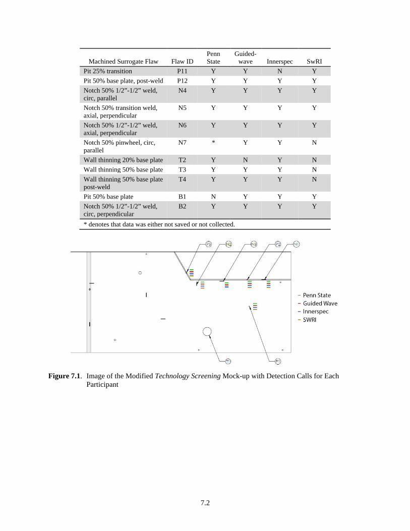
Table 7.1 provides a yes/no detection summary for all four participants (Penn State, Guidedwave, Innerspec, and SwRI) on the 25 surrogate flaws that were included in Sensor Effectiveness Testing. Figures 7.1 and 7.2 provide a visual image representation of the yes/no detection summary for each of the mock-ups. Detections are represented by colored dashed lines: Penn State’s results are represented in green, Guidedwave in red, Innerspec in blue, and SwRI results are shown in brown. Guidedwave missed the 10% and 20% depth wall thinning flaws. Innerspec missed the 10% wall thinning and 0.375-inch diameter pit with a 25% through-wall depth in the transition weld. Penn State did not detect the blind pit located in the base plate and failed to save or collect data on the 10% wall thinning defect and the notch located in the pinwheel weld. SwRI was not sensitive to any of the wall thinning flaws or the pit and notch located in the transition welds. Overall, all technologies performed well although none of the participants found all flaws.
Table 7.1. Summary Flaw Detection Table for Sensor Effectiveness Testing
Machined Surrogate Flaw Flaw ID Penn State
Guided- wave Innerspec SwRI
Pit 25% base plate P1 Y Y Y Y Pit 25% 1/2”-1/2” weld P2 Y Y Y Y Pit 50% 1/2”-1/2” weld P3 Y Y Y Y Notch 20% 1/2”-1/2” weld, axial, parallel
N1 Y Y Y Y
Notch 50% 1/2”-1/2” weld, circ, perpendicular
N2(i) Y Y Y Y
Notch 50% 1/2”-1/2” weld, axial, parallel
N3(m) Y Y Y N
Wall thinning 10% base plate T1 * N N N Pit 50% base plate P4 Y Y Y Y Pit 75% base plate P5 Y Y Y Y Pit 50% transition weld P6 Y Y Y Y Pit 75% transition weld P7 Y Y Y Y Pit 50% 1/2”-1/2” weld P8 Y Y Y Y Pit 75% 1/2”-1/2” weld P9 Y Y Y N Pit 50% Pinwheel P10 Y Y Y N
7.2
Machined Surrogate Flaw Flaw ID Penn State
Guided- wave Innerspec SwRI
Pit 25% transition P11 Y Y N Y Pit 50% base plate, post-weld P12 Y Y Y Y Notch 50% 1/2”-1/2” weld, circ, parallel
N4 Y Y Y Y
Notch 50% transition weld, axial, perpendicular
N5 Y Y Y Y
Notch 50% 1/2”-1/2” weld, axial, perpendicular
N6 Y Y Y Y
Notch 50% pinwheel, circ, parallel
N7 * Y Y N
Wall thinning 20% base plate T2 Y N Y N Wall thinning 50% base plate T3 Y Y Y N Wall thinning 50% base plate post-weld
T4 Y Y Y N
Pit 50% base plate B1 N Y Y Y Notch 50% 1/2”-1/2” weld, circ, perpendicular
B2 Y Y Y Y
* denotes that data was either not saved or not collected.
Figure 7.1. Image of the Modified Technology Screening Mock-up with Detection Calls for Each
Participant

7.3
Figure 7.2. Image of the Sensor Effectiveness Testing Mock-up with Detection Calls for Each Participant
7.2 Flaw Type – Pit (P4)
Flaw “P4” is a 0.750-inch diameter pit with a depth of 50% of the plate thickness (0.250 in.) located in the base plate of the Sensor Effectiveness Testing mock-up 12 inches from the 7/8- to 1/2-inch transition weld. A photograph of P4 is shown in Figure 7.3.
Figure 7.3. Photograph of Pit “P4”

7.4
7.2.1 Guidedwave
Pit “P4” was detected by Guidedwave from four different transducer locations at an excitation frequency of 160 kHz. Transducer Location C was the farthest from Pit “P4” at 46 inches (Figure 7.4). Pit “P4” was also clearly identified in the composite images derived from 13 different inspection locations at 160 kHz excitation frequency (Figure 7.5). The signal-to-noise ratio (SNR) for Pit “P4” ranged from 8.1 to 29 dB. Guidedwave reliably detected all of the pits in both mock-ups as seen in Table 7.1 and Figures 7.1 and 7.2.
Figure 7.4. Guidedwave Phased-Array (GWPA) Scan on the Sensor Effectiveness Testing Mock-up at
Location C Pulsed at 160 kHz (image from Figure 40 of Appendix A)

7.5
Figure 7.5. Composite Image from the Sensor Effectiveness Testing Mock-up Using 13 Scan Locations
(Figure 26 in Appendix A)
7.2.2 Innerspec
Innerspec detected Pit “P4” with the shear vertical (SV) sensor pulsed at 2.25 MHz frequency from the closest air-slot, 5 inches away from the flaw. The transducer was slightly angled to avoid any reflections from the weld and plate edges. The SNR calculated for Pit “P4” was approximately 24 dB (Figure 7.6). Innerspec reliably detected all but one of the pits in both mock-ups as seen in Table 7.1 and Figures 7.1 and 7.2. Pit “P11” located near the edge in the transition weld in the Sensor Effectiveness Testing mock-up was the only pit not detected.
Figure 7.6. Manual A-scan Pit “P4” with the Shear Vertical Technique

7.6
7.2.3 Penn State
Penn State detected Pit “P4” using pitch-catch (PC) test configuration with the transmitter and receiver angled at a 45 degrees, separated by a fixed distance of 10 inches apart in the same air-slot perpendicular to the transition weld. In this case the transducers were moved together while maintaining the 10 inch spacing. All pits in both mock-ups were detected using some version of PC test configuration, either keeping the transducer fixed and moving the receiver or keeping a fixed distance between the transducers and moving along the air-slot together as in this case. The pitch-catch technique only required the sensor to be in the same air-slot in certain cases like the example shown here, and in other cases the use of two separate air-slots were needed. The SNR for Pit “P4” was 21.9 dB (Figure 7.7). Penn State reliably detected all of the pits in both mock-ups except for the blind flaw, B1, as seen in Table 7.1 and Figures 7.1 and 7.2. The missed detection of B1 will be discussed in Section 7.6.
Figure 7.7. SAFT Reconstructed Image (left), and PC Configuration (right) for Pit “P4”
7.2.4 SwRI
Pit “P4” was clearly detected by SwRI from seven different data sets at excitation frequencies of 42, 49, 57, and 72 kHz. The EMAT sensor location was 63 inches from Pit “P4.” Figure 7.8 shows the 57 kHz down data with high bandwidth filters. The SNR for Pit “P4” ranged from 10.6 to 59.3 dB. The location of the signal from the SAFT-processed image closely agreed with the actual flaw location. SwRI reliably detected all pits in both mock-ups except for two pits as seen in Table 7.1 and Figures 7.1 and 7.2. Pit “P10” is located on the Sensor Effectiveness Testing mock-up in the critical section of the pin-wheel weld pattern and P9 which is in the same 1/2-to-1/2 inch weld.

7.7
Figure 7.8. Sensor Effectiveness Testing Mock-up – 57 kHz Data (high bandwidth filters) – Set 71
(straight down)
7.3 Flaw Type – Notch (N2)
Notch “N2” was a 2-inch long, 0.125-inch wide machined notch with a depth of 50% of the plate thickness (0.25 in.). Notch “N2” was located in the base plate of the modified Technology Screening mock-up near the edge of the 1/2-to-1/2 inch weld and oriented perpendicular to the weld direction as seen in Figure 7.9.

7.8
Figure 7.9. Photograph of Notch “N2”
7.3.1 Guidedwave
Notch “N2” was detected by Guidedwave from eight different transducer locations using an excitation frequency of 160 kHz. The farthest position Notch “N2” was detected from was 27 inches. Notch “N2” was also detected in the composite images as seen in Figure 7.10. The SNR for Notch “N2” ranged from 42.8 to 45 dB. Guidedwave reliably detected all notches in both mock-up as seen in Table 7.1 and Figures 7.1 and 7.2.
Figure 7.10. Composite Image from Technology Screening Mock-up Using Six Different Locations

7.9
7.3.2 Innerspec
Innerspec detected Notch “N2” using the SV sensor pulsed at 2.25 MHz frequency from about 36 inches away. The SNR reported for N2 was 19 dB (Figure 7.6). Innerspec reliably detected all notches in both mock-ups during testing as shown in Table 7.1 and Figures 7.1 and 7.2.
Figure 7.11. Manual A-scan from Notch “N2”from a Distance of 30 Inches with the SV Technique
7.3.3 Penn State
Penn State detected Notch “N2” using the pulse-echo mode with the transmitter and receiver separated by a fixed distance of 3 inches and incrementally moved together within the air-slot along the weld. The SNR for Notch “N2” was conservatively calculated to be 2 dB (Figure 7.17). The SNR is calculated from the data shown in Figure 7.17 using the noise floor computed from the weld echo at a location away from the defects which leads to a low SNR. Penn State reliably detected all notches in both mock-ups except for N7 due an error in not acquiring the data for this particular flaw.

7.10
Figure 7.12. SAFT-Processed Image with the End Wall Reflections Gated to Provide a Better Signal
Response for the Notches
7.3.4 SwRI
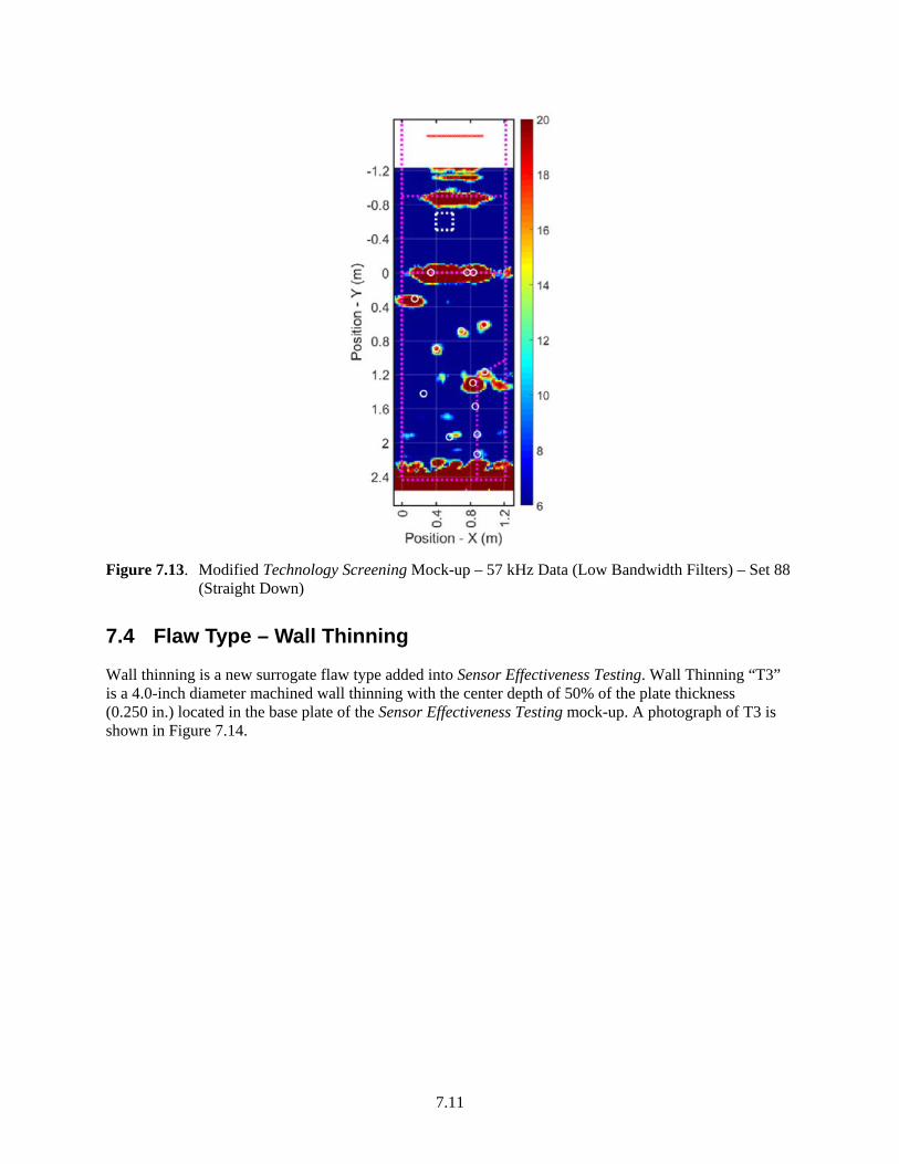
Notch “N2” was detected by SwRI from three different frequencies and orientations of straight down and at an angle with SNR values ranging from 27.4 to 40.8 dB. The EMAT instrument was positioned approximately 98 inches from Notch “N2” (Figure 7.13). SwRI detected all notches except for two—N3 from the modified Technology Screening mock-up and N7 from the Sensor Effectiveness mock-up. These notches were either in or within a few inches of a weld.
7.11
Figure 7.13. Modified Technology Screening Mock-up – 57 kHz Data (Low Bandwidth Filters) – Set 88
(Straight Down)
7.4 Flaw Type – Wall Thinning
Wall thinning is a new surrogate flaw type added into Sensor Effectiveness Testing. Wall Thinning “T3” is a 4.0-inch diameter machined wall thinning with the center depth of 50% of the plate thickness (0.250 in.) located in the base plate of the Sensor Effectiveness Testing mock-up. A photograph of T3 is shown in Figure 7.14.

7.12
Figure 7.14. Photograph of Wall Thinning “T3”
7.4.1 Guidedwave
Guidedwave detected Wall Thinning “T3” using the higher frequency probe pulsed at 225 kHz. T3 was detected from two different locations on the 1/2-inch thick base plate of the Sensor Effectiveness Testing mock-up but not able to be seen in any of the composite images using the lower frequency probe. Transducer Location II was the farthest from Wall Thinning “T3” at 21 inches (Figure 7.15). The best SNR for T3 was 40 dB. Guidedwave detected all of the 50% through-wall thinning but was not able to detect the 10% or 20% as seen in in Table 7.1 and Figures 7.1 and 7.2.

7.13
Figure 7.15. GWPA Scan on the Sensor Effectiveness Testing Mock-up at Location II Pulsed at 225 kHz
(image from Figure 64 of Appendix A)
7.4.2 Innerspec
Wall Thinning “T3” was detected by Innerspec with a SNR of approximately 20 dB from a distance of 7 inches from the thinning as seen in Figure 7.16. Innerspec reliably detected all but the smallest thinning, T1 which was 10% of the thickness at the center.
Figure 7.16. Manual A-scan from Wall Thinning “T3” from a Distance of 7 Inches with the SV
Technique

7.14
7.4.3 Penn State
Penn State detected Wall Thinning “T3” using the through-transmission technique with the transmitter and receiver separated by 36 inches. Through-transmission configuration requires the use of more than one air-slot. All thinning flaws were detected using this technique due to the noticeable reduction in sound from the SH1 wave packet. The SNR for T3”was calculated as 11.9 dB (Figure 7.17). Penn State was able to reliably detect all wall thinning flaws; however, Penn State failed to save the data that was collected on T1, the smallest thinning, so Penn State was not given credit for this detection as seen in Table 7.1 and Figure 7.1.
Figure 7.17. SAFT-Reconstructed Image of the Response from T3 and Transducer Orientation on
Mock-up
7.4.4 SwRI
SwRI did not detect any of the wall thinning surrogate flaws in either of the mock-ups. These flaws had a very gradual change over 2 inches along the surface to their maximum depth, which is difficult to detect using guided waves at the test frequencies and inspection distances used by this technology. T4 was the only flaw that had some marginal detection but was below the 10 dB SNR threshold set by SwRI for calling defects.
7.5 Measurement Robustness
The measurement robustness of each sensor configuration that relies on direct contact with the bottom plate was assessed in addition to the augmented surrogate flaw set. The measurement robustness of the proposed NDE sensors were evaluated in two categories—surface rust and surface debris. The purpose of these two tests was to determine what level of cleaning would need to be done to the surface prior to inspection. The three participants that were tested on measurement robustness are Guidedwave, Innerspec, and Penn State.
Participants with NDE volumetric inspection technologies that rely on placing transducers on or above the knuckle and propagating energy remotely to the primary tank bottom plates were not tested on the measurement robustness (dirt and rust tests) as the tank walls are already cleaned for UT wall inspections that are currently being performed. During this testing the only participant that falls into this category is SwRI.

7.15
7.5.1 Rust Test
The evaluation of tolerance for rust was performed by comparing signal responses of a common reflector (edge of 7/8-inch plate) in three different mock-ups with clean, mild, and field-representative rust/oxide layers, respectively as seen in Figure 7.18 with each of the participant’s technology.
Figure 7.18. Rust Test Using 7/8-inch Plates from Three Mock-ups with (a) Clean with Guidedwave
Sensor, (b) Mild with Innerspec Sensor, and (c) Field-Representative Rust/Oxide with Penn State Sensors
Guidedwave collected three different responses from 12 inches away on each mock-up and then averaged the three signals for the SNR values reported in Table 7.2. Innerspec collected one measurement per mock-up at a distance of 15 inches from the mock-up edge. Penn State used the pulse-echo technique and collected one measurement per mock-up at a distance of 12 inches away from the edge. Looking at the results in Table 7.2, the presence of uniform surface rust of varying levels did not affect responses of the methods tested by the three participants.

7.16
Table 7.2. Sensor Effectiveness Testing SNR for Measurement Robustness – Rust Test
SNR (dB)
Surface Condition Guidedwave Innerspec Penn State Near pristine (modified Technology Screening mock-up) 70.7 21.6 33 Mild rust/oxide (Sensor Effectiveness Testing mock-up) 66 26 31 Field representative rust/oxide (APEL mock-up) 69 26 31
7.5.2 Dirt Test
The sensor’s tolerance for surface debris was determined by comparing the signal response from a surrogate flaw (Pit “C” from Technology Screening mock-up) with two surface conditions—clean and a minimal layer of dirt (non-metallic surface debris) between the sensors and mock-up. Figure 7.19 shows each of the participant’s location with respect to Pit “C” on the surface contain a minimal layer of dirt.
Figure 7.19. Dirt Test Using Pit “C” as Reflector with Minimal Layer of Dirt: c (a) Guidedwave Sensor,
(b) Innerspec Sensor, and (c) Penn State Sensor Locations

7.17
Guidedwave collected six different responses of Pit “C” on a clean surface and six responses from a dirty surface from 12 inches away. The SNRs were then averaged reported in Table 7.3. Innerspec collected one measurement on a clean and one measurement on a dirty surface at a distance of 8 inches from Pit “C”. Penn State used the pulse-echo technique and collected one data set per each surface (clean/dirty) at a distance of 8 inches away from Pit “C”. Looking at the results in Table 7.3, the presence of a thin layer of dirt did not affect signal responses significantly for any of the methods tested by the three participants.
Table 7.3. Sensor Effectiveness Testing SNR for Measurement Robustness – Dirt Test
SNR (dB)
Surface Condition Guidedwave Innerspec Penn State No debris 35.3 19 9.2 Minimal debris 34 19 6.8
7.6 Blind Flaws
Flaw “B1” is a 0.750-inch diameter pit with a depth of 50% of the plate thickness (0.250 in.) located in the base plate of the Sensor Effectiveness Testing mock-up with x and y coordinates of (48,48). Flaw “B2” is a 3-inch long, 0.125-inch wide machined notch with a depth of 50% of the plate thickness (0.250 in.). B2 is located perpendicular to the 1/2-to-1/2 inch weld on the Sensor Effectiveness mock-up with x and y coordinates of (60,21) and (60,24). A schematic of the Blind flaw location is shown in Figure 7.20. Both blind flaws are on the OD surface of the mock-up.
Figure 7.20. Blind Flaw Locations on the Sensor Effectiveness Mock-up

7.18
7.6.1 Guidedwave
Guidedwave easily detected both B1 and B2 from eight or more locations on the 1/2-inch thick base plate. For B1, Guidedwave called this a pit located at (48,48) and had an SNR ranging from 11.7 to 37 dB. B1 was even detected from a maximum distance of 43 inches. For B2, Guidedwave called this a notch extending from (61,20) to (61,24) perpendicular to the 1/2-to-1/2 inch weld. B2 was detected from a maximum distance of 55 inches. The blind flaws are clearly visible in the composite image seen in Figure 7.5.
7.6.2 Innerspec
Innerspec’s SV technique was able to detect both blind flaws in the Sensor Effectiveness Testing mock-up. Flaw “B1” was identified as a pit with a rough location of (47,44) from Figure 7.21. The pit was detected from 9 inches away and has an SNR of approximately 19 dB. B2 was detected and identified to be a notch at least 2 inches long. The approximate location is (59,22) and (59,24) and had an SNR of 26 dB from 5 inches from the flaw.
Figure 7.21. Schematic of the Sensor Effectiveness Testing Mock-up with the Blind Flaws Shown in RED,
Possible Weld Defect Indicated in the Transition Weld, and Inspection Locations Shown in Yellow
7.6.3 Penn State
Penn State reliably detected only one of the blind flaws. Flaw “B2” was detected and identified to be a 4-inch long notch. The x and y coordinates provided are (56,24) and (59,24) putting the orientation parallel to the weld. Although the notch is perpendicular to the weld, this technique did detect this notch and was given credit for detection (Figure 7.22). Penn State called a second blind flaw, but it was not identified in the correct location. The location for the pit-like indication was given as (37,64). During testing, however, PNNL witnessed the EMAT technology brought by Penn State being sensitive to B1 although it was not recognized at the time by the participant and the data were not recorded.

7.19
Figure 7.22. SAFT Reconstructed Image (left), and PC Configuration (right) for Flaw “B2”
7.6.4 SwRI
Both blind flaws B1 and B2 were detected by SwRI with at three different frequencies. Flaw “B1” was detected at an x and y location of (48,49) and classified as a pit-like defect that is similar in size to P4 (0.75 inch in diameter and 50% depth). The range of SNR for this defect is 14.8 to 50.8 dB. B2 was located at x and y coordinates of (60,23) and is expected to be a large flaw of 50% or more in through wall depth. The SNR for B1 ranged from 35 to 61 dB. The blind flaws are indicated by the white diamonds in Figure 7.8 above.
7.7 Other Notable Features from Mock-up
During Sensor Effectiveness Testing, some of the participants noticed “other” features in the new mock-up particularly near some heavy weld repair regions. Guidedwave and Penn State both identified a large weld repair in the transition weld between the 1/2-to-1/2 inch weld and P6. Innerspec noticed another weld repair in the transition weld between P6 and P11. Penn State also noted responses from weld repairs along the 1/2-to-1/2 inch weld and other feature in the 1/2-inch base plate material. These indications have not been verified by PNNL at this time but are worthy of noting the sensitivity of the different guided-wave techniques.
In the modified Technology Screening mock-up, SwRI was able to detect the three flaws located in the transition weld (g, a, and k). The responses from Flaws “a” and “k” were not resolved and detected as one flaw. These flaws were not part of the Sensor Effectiveness Testing but worthy to note as SwRI was unable to detect these flaws during Technology Screening. The improvement in detection is due to rotation of the sensor and improved filtering on the high frequencies.


8.1
8.0 Analysis
Grading of each sensor approach was performed against criteria and a scoring system that factored in the detection of each surrogate flaw in the mock-ups, and accounted for multiple attributes consisting of measurement robustness, delivery requirements, adaption for access limitations, and overall data quality. Scoring values were awarded for each flaw that was detected and partial points were not awarded. The available point values, shown in Table 8.1, were determined by size, flaw orientation, and relative position to an edge or weld in the mock-ups. Each sensor attribute scoring category had five available points and partial points were awarded. Details on the attribute scoring criteria are shown below in Tables 8.2 and 8.3. A total of 83 points were available for flaw detection, and attributes were worth a total 50 points. A total of 133 points were available.
Table 8.1. Sensor Effectiveness Flaw Detection Scoring
Machined Surrogate
Flaw Flaw
Depth(a) Length and
Width Flaw ID Flaw Location and Orientation in
Mock-up Total Points Score Pit 25% t,
0.125 in. 0.375 in. diameter
P1 Base plate (ID) 3
Pit 25% t, 0.125 in.
0.375 in. diameter
P2 1/2-to-1/2 in. weld (ID) 5
Pit 50% t, 0.25 in.
0.75 in. diameter
P3 1/2-to-1/2 in. weld (ID), within 30° angled weld
4
Notch 20% t, 0.10 in.
2 in. long, 0.125 in. wide
N1 1/2-to-1/2 in. weld (ID), axial orientation, parallel with weld
4
Notch 50% t, 0.25 in.
2 in. long, 0.125 in wide
N2(i) Base plate perpendicular to 1/2-to-1/2 in. weld (ID) (previously Flaw i from Technology Screening)
3
Notch 50% t, 0.25 in.
2 in. long, 0125 in wide
N3(m) Base plate parallel to 1/2-to-1/2 in. weld (ID) (previously Flaw m from Technology Screening)
3
Wall thinning
10% t, 0.05 in.
4 in. diameter T1 Base plate (ID) 3
Pit 50% t, 0.25 in.
0.75 in. diameter
P4 Base plate (ID) 2
Pit 75% t, 0.375 in.
1.125 in. diameter
P5 Base plate (ID) 1
Pit 50% t, 0.25 in.
0.75 in. diameter
P6 7/8-to-1/2 in. transition weld (ID) 4
Pit 75% t, 0.375 in.
1.125 in. diameter
P7 7/8-to-1/2 in. transition weld (ID) 3
Pit 50% t, 0.25 in.
0.75 in. diameter
P8 1/2-to-1/2 in. weld (ID) 4
Pit 75% t, 0.375 in.
1.125 in. diameter
P9 1/2-to-1/2 in. weld (ID) 3
Pit 50% t, 0.25 in.
0.75 in. diameter
P10 1/2-to-1/2 in. weld (ID), corner of 90° weld confluence
4
Pit 25% t, 0.125 in.
0.375 in. diameter
P11 7/8-to-1/2 in. transition weld (ID) 5
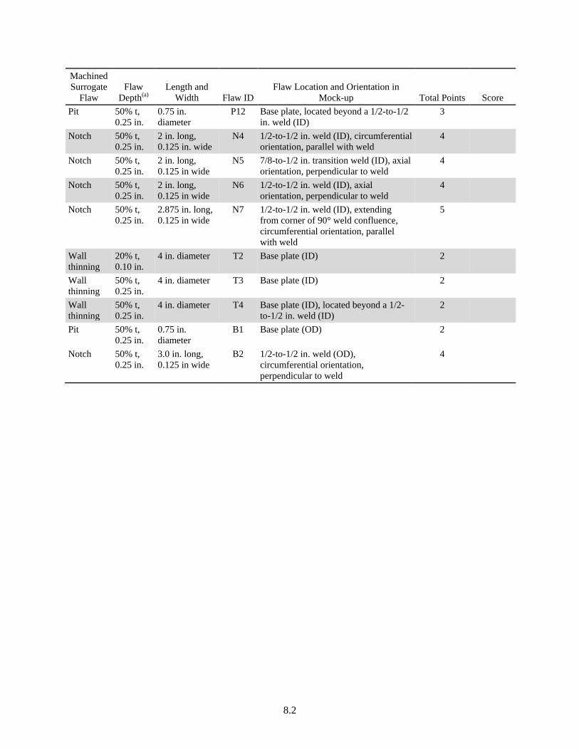
8.2
Machined Surrogate
Flaw Flaw
Depth(a) Length and
Width Flaw ID Flaw Location and Orientation in
Mock-up Total Points Score Pit 50% t,
0.25 in. 0.75 in. diameter
P12 Base plate, located beyond a 1/2-to-1/2 in. weld (ID)
3
Notch 50% t, 0.25 in.
2 in. long, 0.125 in. wide
N4 1/2-to-1/2 in. weld (ID), circumferential orientation, parallel with weld
4
Notch 50% t, 0.25 in.
2 in. long, 0.125 in wide
N5 7/8-to-1/2 in. transition weld (ID), axial orientation, perpendicular to weld
4
Notch 50% t, 0.25 in.
2 in. long, 0.125 in wide
N6 1/2-to-1/2 in. weld (ID), axial orientation, perpendicular to weld
4
Notch 50% t, 0.25 in.
2.875 in. long, 0.125 in wide
N7 1/2-to-1/2 in. weld (ID), extending from corner of 90° weld confluence, circumferential orientation, parallel with weld
5
Wall thinning
20% t, 0.10 in.
4 in. diameter T2 Base plate (ID) 2
Wall thinning
50% t, 0.25 in.
4 in. diameter T3 Base plate (ID) 2
Wall thinning
50% t, 0.25 in.
4 in. diameter T4 Base plate (ID), located beyond a 1/2-to-1/2 in. weld (ID)
2
Pit 50% t, 0.25 in.
0.75 in. diameter
B1 Base plate (OD) 2
Notch 50% t, 0.25 in.
3.0 in. long, 0.125 in wide
B2 1/2-to-1/2 in. weld (OD), circumferential orientation, perpendicular to weld
4
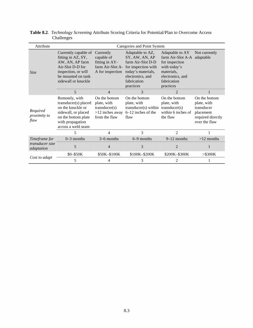
8.3
Table 8.2. Technology Screening Attribute Scoring Criteria for Potential/Plan to Overcome Access Challenges
Attribute Categories and Point System
Size
Currently capable of fitting in AZ, SY, AW, AN, AP farm Air-Slot D-D for inspection, or will be mounted on tank sidewall or knuckle
Currently capable of fitting in AY-farm Air-Slot A-A for inspection
Adaptable to AZ, SY, AW, AN, AP farm Air-Slot D-D for inspection with today’s materials, electronics, and fabrication practices
Adaptable to AY farm Air-Slot A-A for inspection with today’s materials, electronics, and fabrication practices
Not currently adaptable
5 4 3 2 1
Required proximity to flaw
Remotely, with transducer(s) placed on the knuckle or sidewall, or placed on the bottom plate with propagation across a weld seam
On the bottom plate, with transducer(s) >12 inches away from the flaw
On the bottom plate, with transducer(s) within 6–12 inches of the flaw
On the bottom plate, with transducer(s) within 6 inches of the flaw
On the bottom plate, with transducer placement required directly over the flaw
5 4 3 2 1 Timeframe for transducer size adaptation
0–3 months 3–6 months 6–9 months 9–12 months >12 months
5 4 3 2 1
Cost to adapt $0–$50K $50K–$100K $100K–$200K $200K–$300K >$300K
5 4 3 2 1

8.4
Table 8.3. Sensor Effectiveness Testing Scoring for Localized Sensor Attributes and Measurement Robustness
Attribute Categories and Point System Score Surface prep requirements
No surface prep required. Examination conducted on as-is surface.
Minimal surface prep required (removal of dust/dirt). Can be done with passive system (i.e., brush).
Surface prep required. Per-formed using active system.
Pristine surface required. Done using separate deployment with surface cleaning equipment. Removal of dirt and rust required.
Surface requires sanding/ buffing.
5 4 3 2 1 Couplant requirements
No couplant required
Couplant applied/ removed during examination (applied and wiped off while scanning using passive system)
Couplant applied/ removed during examination using active system (brush/ scrubber or sep-arate mechani-cal system)
Separate deploy-ment/tooling is required to apply/remove couplant
Couplant permanently attached to inspection surface
5 4 3 2 1 Measurement robustness (toler-ance for loose surface material)
Signal unaffected by dirt/rust layer
Signal reduced by 50% or less
Signal reduced by more than 50% but still see a signal
No signal detected
5 4 3 2 1 Motion requirements
No additional degree of free-dom is needed
Sensor requires rotation in air-slot
Coordinated motion in adja-cent air-slots is required
Sensor requires removal from deployment to adjust orientation
5 4 3 2 1 Delivery require-ments (application and removal force)
<10 lbs. 10–25 lbs. 25–50 lbs. >50 lbs.
5 4 3 2 1 Data quality – SNR >20 dB 10 to 19 dB 5 to 9 dB <5 dB 5 4 3 2 1 TOTAL:
The timeframe and cost criteria in Table 8.2 are applicable only to the sensor attributes that affect access to the desired inspection area. The time and cost for a robotic deployment system is not factored in for these two Technology Screening criteria because they will be addressed during Phase II of the NDE technology development program.
The Sensor Effectiveness Testing scores provided in Tables 8.4 and 8.5 are measures of:
1. The extent to which a technique can detect the most likely types of tank bottom flaws (pits, wall thinning, and weld seam openings) of sizes/depths below, at, and above the actionable level values in

8.5
plates and welds of representative geometries, types, and orientations/patterns. The purpose of including representative welds and plate thicknesses is these factors influence the level of difficulty for detection.
2. Pre-requisites that must be satisfied by a technique to permit successful measurements on a test surface (e.g., coupling or surface preparation). These were captured under the Measurement Robustness categories under Sensor Attributes.
3. Requirements for sensor translation and motion to examine a given area, which will impact the complexity of a robotic delivery system (e.g., force to slide/push or remove/step the sensor, sensor rotation needs, number of sensors and air-slots required simultaneously). This also reflects the number of air-slots that would need to be accessed to examine a given tank region, which determines risk level of getting stuck in an air-slot and the intensity of work that must be performed (time, cost) to cover that tank region. These were captured under Delivery Requirements under Sensor Attributes.
4. Signal-to-noise ratio and integrity of its calculation, which impact downstream analysis activities (subjectivity of data interpretation by operators) and confidence in inspection results (e.g., false call rate). This was captured in the Data Quality category under Sensor Attributes.
5. Time and cost to adapt the sensor (i.e., downsize) to fit inside the air-slots. This was captured in its own category under Sensor Attributes. These scores remained the same as those provided during the Technology Screening phase. They are provided again here to provide validation of their applicability.
The purpose of the score for item 1 listed above is to provide an indication of the extent to which a technology can satisfy detection of the variety of different flaw types and scenarios. The purpose of the score that covers items 2–5 listed above is to uncover key weaknesses and key strengths that need to be considered and balanced with flaw detection performance because the impact of the weaknesses for a given technology would either be a “non-starter”—an attribute that cannot be overcome—or mitigated/ addressed by using it in tandem with a complementary technology that can offset the weakness.
The scores for each of the technologies are compared in Tables 8.4 and 8.5. Guidedwave scored the highest in the flaw detection category for the localized technology approach with 78 total points. Innerspec scored 75 points, and Penn State scored 73 total points, although Penn State would have had the most points had they not failed to record data sets for T1, the smallest thinning, and N7, the notch in the pinwheel weld. SwRI was the only participant in the remote technology category and scored a total of 59 points for flaw detection. For the attribute scores in Table 8.5, Penn State scored the highest with 44 points. Innerspec and Guidedwave both had 42 points, and SwRI had 41 points.

8.6
Table 8.4. Sensor Effectiveness Testing Flaw Detection Scores
Localized Technology
Remote Technology
Machined Surrogate Flaw Flaw ID
Total Points Available Penn State Guidedwave Innerspec SwRI
Pit P1 3 3 3 3 3 Pit P2 5 5 5 5 5 Pit P3 4 4 4 4 4 Notch N1 4 4 4 4 4 Notch N2(i) 3 3 3 3 3 Notch N3(m) 3 3 3 3 --- Wall thinning T1 3 --- --- --- --- Pit P4 2 2 2 2 2 Pit P5 1 1 1 1 1 Pit P6 4 4 4 4 4 Pit P7 3 3 3 3 3 Pit P8 4 4 4 4 4 Pit P9 3 3 3 3 --- Pit P10 4 4 4 4 --- Pit P11 5 5 5 --- 5 Pit P12 3 3 3 3 3 Notch N4 4 4 4 4 4 Notch N5 4 4 4 4 4 Notch N6 4 4 4 4 4 Notch N7 5 --- 5 5 --- Wall thinning T2 2 2 --- 2 --- Wall thinning T3 2 2 2 2 --- Wall thinning T4 2 2 2 2 --- Pit B1 2 --- 2 2 2 Notch B2 4 4 4 4 4 Total Points 83 73 78 75 59 Percent Detected 88% 94% 90% 71%
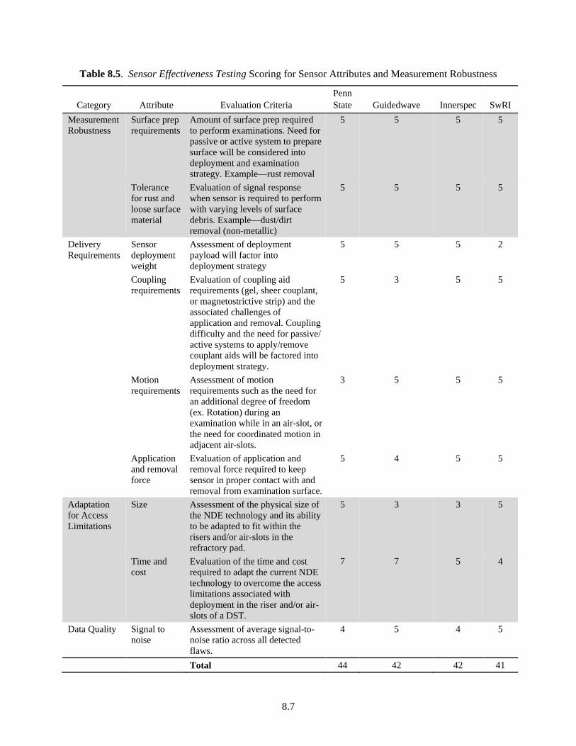
8.7
Table 8.5. Sensor Effectiveness Testing Scoring for Sensor Attributes and Measurement Robustness
Category Attribute Evaluation Criteria Penn State Guidedwave Innerspec SwRI
Measurement Robustness
Surface prep requirements
Amount of surface prep required to perform examinations. Need for passive or active system to prepare surface will be considered into deployment and examination strategy. Example—rust removal
5 5 5 5
Tolerance for rust and loose surface material
Evaluation of signal response when sensor is required to perform with varying levels of surface debris. Example—dust/dirt removal (non-metallic)
5 5 5 5
Delivery Requirements
Sensor deployment weight
Assessment of deployment payload will factor into deployment strategy
5 5 5 2
Coupling requirements
Evaluation of coupling aid requirements (gel, sheer couplant, or magnetostrictive strip) and the associated challenges of application and removal. Coupling difficulty and the need for passive/ active systems to apply/remove couplant aids will be factored into deployment strategy.
5 3 5 5
Motion requirements
Assessment of motion requirements such as the need for an additional degree of freedom (ex. Rotation) during an examination while in an air-slot, or the need for coordinated motion in adjacent air-slots.
3 5 5 5
Application and removal force
Evaluation of application and removal force required to keep sensor in proper contact with and removal from examination surface.
5 4 5 5
Adaptation for Access Limitations
Size Assessment of the physical size of the NDE technology and its ability to be adapted to fit within the risers and/or air-slots in the refractory pad.
5 3 3 5
Time and cost
Evaluation of the time and cost required to adapt the current NDE technology to overcome the access limitations associated with deployment in the riser and/or air-slots of a DST.
7 7 5 4
Data Quality Signal to noise
Assessment of average signal-to-noise ratio across all detected flaws.
4 5 4 5
Total 44 42 42 41


9.1
9.0 Discussion
Performance in the areas of flaw detection and sensor attributes, which were covered in the previous section, should be considered with other critical parameters affecting technology development and ultimately deployment in light of the preferred inspection strategy. The optimized inspection strategy for interrogating the floor of a DST primary tank consists of applying a remote screening technique prior to a local under-tank sensor technique to identify gross degradation and, to the extent possible, direct strategic deployment of air-slot transducers. The combination selected should provide both the best coverage in terms of tank bottom plate regions, with emphasis on the potentially high-risk pinwheel welds, and in terms of the most certain flaw detection for the defect types and sizes of concern.
All techniques performed well at flaw detection and most were able to detect the blind flaws in the mock-up. Each technique presented a unique set of flaw detection and sensor attribute strengths and limitations (dependent on tank region/geometry, flaw type, and flaw size) that need to be considered when selecting techniques and technique pairing in support of the inspection strategy. This section will compare the advantages and limitations of the proposed technologies as they would be applied using the preferred inspection strategy. Comparisons will be made on the basis of overall performance, performance by region of the mock-ups, and performance on flaw types.
9.1 Overall Performance Comparison of All Demonstrated Technologies
The piezoelectric technique presented by Guidedwave provided the best overall flaw detection performance with a score of 78 out of 83 total possible points. Advantages of this technique are that it can detect all flaw types in all locations of the mock-ups, in particular the pinwheel weld which is of high interest. It can detect flaws at the reportable and actionable level for pits and notches (seam openings), flaw detection does not depend on transducer orientation, and only single-slot deployment is required. Disadvantages of this technique include the need for liquid couplant application, a downward force applied to transducer to support efficient coupling, and it has not demonstrated detection of wall thinning at the reportable level (10%) or actionable level (20%), only at T=50%. So, an estimated detection threshold for this flaw type is somewhere between 20% and 50% for the piezoelectric method.
The localized EMAT techniques are comparable in overall performance with Penn State earning 73 points and Innerspec earning 75 points out of 83. Advantages of the EMAT approach are that it can detect all flaw types in all locations of the mock-up, in particular the pinwheel weld which is of high interest. It can detect flaws at the reportable and actionable level for pits and notches (seam openings), EMATs can detect wall thinning at the actionable level, and the sensors couple without liquid and do not require application of a downward force for coupling. Disadvantages of the EMAT approach include lower SNR values and the reliance on preferential transducer orientation to detect flaws. In the current sensor configuration, the sensors require physical rotation but future sensor designs may feature multiple EMAT coils to steer sound fields without physical rotation and address this need. Specifically, the technique demonstrated by Penn State would require coordinated dual air-slot deployment and dependence of available adjacent air-slots to detect wall thinning, a prerequisite that is perceived as a vulnerability, and would also require a more complex robotic delivery system. The method demonstrated by Innerspec would require single air-slot deployment, but considerable sensor down-sizing would be necessary, and the SV wave mode may be impacted, damped, and thus attenuated, by waste inside the tank.
The remote EMAT technique demonstrated by SwRI had the lowest overall detection score of 59 points. Performance advantages of this technique are that it is capable of detecting all pit-type flaws in the base

9.2
plate material and a limited number of pit-type flaws and weld seam openings located in welds from the greatest distance away (inspection from primary tank wall). This technique similar to the localize EMAT techniques do not require couplant. Disadvantages of this technique are that it is the least sensitive to wall thinning and defects located in the pinwheel weld region. There is also a considerable down-sizing in the sensor that is needed in order to fit through the annulus and have a manageable weight for a robotic system.
9.2 Performance Trade-offs for Localized Inspection Technology
The technique currently demonstrated for the remote screening for the general inspection strategy is not capable of detecting gradual wall thinning and detecting flaws in the 90-degree weld confluence, which may represent a high-risk tank region that should be examined frequently.
All three sensor techniques intended for air-slot deployment performed well overall in flaw detection and, based on flaw detection scores alone, they would all be considered suitable candidates for use with the remote screening technique. However, for an air-slot deployed technique to be a strong complement to the remote screening technique, it should be capable of detecting flaws in the 90-degree weld confluence that cannot currently be detected by the remote screening technique, as mentioned above. Two of the three air-slot deployed techniques demonstrated the ability to detect both flaws (pit and seam opening) in this weld confluence during testing—the EMAT technique from Innerspec and the piezoelectric technique from Guidedwave. The pit in this weld confluence was detected by the EMAT technique from Penn State, but data for the seam opening was reported as not collected. For the pit, the SNR values are 8.5, 9.5, and 25 for Penn State, Innerspec, and Guidedwave, respectively. For the weld seam opening, the SNR values are 12 and 41 for Innerspec and Guidedwave, respectively (N/A for Penn State).
A second air-slot deployed sensor technique feature to consider that would complement the remote screening technique is the ability to detect gradual wall thinning at a depth that is at least equal to the actionable level value for this flaw type (20% wall thickness). Wall thinning cannot currently be detected by the remote screening technique (even at a depth that is 2.5x the actionable level value), as mentioned previously. Although this means direction could not be provided to an air-slot deployed technique for this flaw type at this point in time, it would be useful for the air-slot deployed technique(s) to have the ability to detect wall thinning in the event it gets encountered during a follow-up examination of a flaw that is detected by the remote screening technique. This would also be a useful feature to have in the event a remote screening technique is developed in the future that can detect wall thinning remotely and provide direction for air-slot deployed sensors for higher-resolution confirmation/follow-up examinations. Although all three sensor techniques for air-slot deployment are capable of detecting wall thinning, the techniques that are capable of detecting wall thinning at the actionable level value are the two EMAT techniques from Penn State and Innerspec. Wall thinning at the actionable level value cannot be detected by the piezoelectric technique from Guidedwave. Detection of this flaw type with the piezoelectric technique was possible at a depth 2.5 times the actionable level value (with a higher-frequency sensor) and therefore the detection threshold for this technique is between the actionable level value and 2.5 times the actionable level (i.e., between 20% and 50% wall thickness). None of the three air-slot deployed sensor techniques is capable of detecting wall thinning at the reportable level value (10%). The SNR values for actionable level wall thinning are 5 and 12 for Penn State and Innerspec, respectively (N/A for Guidedwave).
If flaws in the 90-degree weld confluence pose more risk to tank leak integrity than general wall thinning or if its occurrence is considered more probable based on available information and data, then more weight should be given to an air-slot deployed sensor technique that has the ability to reliably detect flaws in this weld pattern.

9.3
9.3 Sensor Attribute Trade-offs for Localized Inspection Technologies
Once performance trade-offs are considered, the data quality and vulnerability of sensor function and performance to un-met prerequisite conditions should be considered and weighed along with practicality of deployment with a robotic delivery system and risk of sensor adaptation negatively impacting performance.
9.3.1 Data Quality
SNR is a measure of signal amplitude of a flaw response relative to the amplitude of background noise from the surrounding material or weld response, with a higher SNR representing better data quality. The noise in a signal or image that gets quantified and used for a SNR calculation can be done conservatively to favorably control the magnitude of the SNR value that is reported. For flaw reporting, a SNR value of at least 2–3 is necessary to distinguish a flaw response from surrounding noise represented by the weld or base plate. Conservatively calculated SNR values typically provide higher confidence in flaw reporting, while favorably calculated SNR values can lead to higher false calls or false positives. The integrity of the SNR calculation and value therefore impact downstream analysis activities (subjectivity required for data interpretation by operators) and confidence in inspection results (e.g., false call rate). The most conservative SNR calculations were performed for the EMAT technique used by Penn State. The noise level quantified in their processed images was base plate noise if the flaw was located in a base plate and weld noise level if the flaw was located in a weld. Moderately conservative SNR calculations were performed for the piezoelectric technique used by Guidedwave using noise levels in their processed composite images. The processing and filtering provides for lower noise levels; however, side-lobe or edge reflection noise were quantified if they encroached on the flaw response. The least conservative SNR calculations were performed for the EMAT technique used by Innerspec. The electronic noise level in unprocessed A-scans was used whether the signal was for a flaw located in the base plate or a weld. Further detail on the participants’ approaches for computing SNR can be found in Appendix A through Appendix D.
9.3.2 Vulnerability
All three of the sensor techniques intended for air-slot deployment will struggle to different degrees if air-slots are not available for deployment due to debris or obstruction that cannot be removed or would be overly labor-intensive or unsafe to remove. There are several considerations to be made on impact of air-slot blockage:
1. Two of the three techniques would have an inherently lower chance of becoming stuck because they are single-sensor arrangements and require one air-slot for deployment—the EMAT technique from Innerspec and the piezoelectric technique from Guidedwave. The dual-sensor EMAT technique from Penn State would either require deployment of both sensors in one air-slot or one transducer each into two adjacent air-slots. The double sensor and double air-slot arrangements both increase the risk of sensor retrieval issues. The unavailability of open adjacent air-slots for the dual-sensor technique would have the most impact on the ability to detect wall thinning. However, as previously stated, if general wall thinning or if its occurrence is considered low probability based on available information and data, then dual-sensor deployment in one air-slot may be acceptable.
2. Sensor techniques with ranges limited to one half to full distance between adjacent air-slots will be unable to inspect tank regions above blocked air-slots. This will only be an issue if many air-slots are blocked, especially those beneath and near the 90-degree weld confluence. Of the three sensor

9.4
techniques, the EMAT sensor technique from Innerspec has the shortest inspection range due to its greater than 1 MHz inspection frequency; the EMAT sensor technique from Penn State, operating at 250 kHz, has enough range to potentially cross two air-slots.
An environmental factor that may impact the EMAT technique is naturally occurring mill scale on the tank plates that influence the signal amplitude. This would impact the certainty of measurements that rely on signal amplitude (i.e., signal reduction) alone as an indicator of flaw presence, namely through-transmission sensor arrangement used by Penn State for detection of wall thinning. Further, the shear-vertical wave mode employed by the EMAT sensor used by Innerspec may suffer signal amplitude loss due to1) mode conversion and 2) loss of energy due to coupling to the waste on the inside of the primary tank.
9.3.3 Robotic Delivery System Complexity and Practicality
All three of the sensor techniques intended for air-slot deployment would require a robotic delivery system. Sensor translation and rotation motion within the air-slots will be required by both EMAT techniques although Innerspec suggested that they could achieve the directional rotation with a multi-channel multi-layer coil thereby avoiding an additional robot degree of freedom. The dual-sensor EMAT technique used by Penn State will likely require the most robotic complexity to satisfy the arrangement that entails placing one sensor each in adjacent air-slots and coordinating motion during translation. The dual air-slot arrangement is necessary primarily for detection of wall thinning.
The shorter the range, the greater the number of air-slot deployments that would be necessary to inspect a given tank region. High-frequency air-slot deployment results in more time and therefore cost to examine a given tank region, and also increases risk level associated with sensors becoming stuck and damaged. Given the approximate 18-inch range of the EMAT sensor technique used by Innerspec, this technique would require the most frequent air-slot deployment to cover a given range, followed by Penn State. The piezoelectric technique used by Guidedwave would require the fewest air-slot deployments to cover a given range.
9.3.4 Adaptation Risk
Each of the three sensor techniques would require some degree of adaptation to fit inside the air-slots. The EMAT sensors used by Penn State would require minimal change and thus have the lowest risk of adaptation impacting performance in a negative way. The piezoelectric sensor used by Guidedwave would require moderate changes to the housing and perhaps number of piezoelectric elements to fit within the air-slots. The change in number of elements is a perceived risk on performance and thus the risk level of adaptation is considered moderate. The risk is considered moderate to high if couplant dispensers are integrated into the sensor housing. The EMAT sensor from Innerspec would require the most significant changes to downsize the housing and magnet to fit inside an air-slot. Therefore, the risk of adaptation impacting performance is considered the highest.
9.3.5 Maturity and Time-to-Commercial Grade
The phased-array piezoelectric sensor, electronics and analysis software demonstrated by Guidedwave is commercial-grade and the sensor would need to undergo modest re-design to fit inside the air-slots. Therefore, this system would likely be ready for deployment on the shortest timescale.

9.5
The EMAT sensor and electronics demonstrated by Innerspec are also commercial-grade; however, the significant sensor design changes would be the primary factor that delays successful operation and deployment of this system in air-slots.
The EMAT sensor and electronics demonstrated by Penn State is in a laboratory prototype state and of lower technical maturity that the air-slot sensor systems demonstrated by Guidedwave and Innerspec and would require more time to reach a commercial-grade pedigree; however, the pathway to a commercial-grade system could be accelerated through collaboration between the university and a sensor technology company.
The EMAT remote screening system demonstrated by SwRI is also in a prototype state, although its use has been previously demonstrated in operational environments. Although the analysis software is mature, the significant modifications required of the sensor and electronics would likely occur over the longest timescale.
9.3.6 Lessons Learned and Deployment Considerations
In conjunction with the analysis of the several technologies, additional considerations were appreciated as noted below.
9.3.6.1 Cable Management and In-tank Sensor Electronics
The piezoelectric phased-array sensor technology presents the simplest cable management challenge. The high impedance nature of these sensors requires very little current to traverse the cable, so even though the cable includes several wires, they are quite small and the assumed cable length between sensor and an instrument outside the tank is 150-ft.
By contrast, all EMAT technologies require a relatively large diameter cable to carry a significant current between an electronics module and the coil. This is easily managed with the remote screening EMAT technology since all electronics are resident near the sensor. For the single-sensor EMAT sensor, the preference is for cable length to be 10-ft or less and assumes the electronics for this sensor are located in the annulus (e.g., on a delivery robot). Longer cables will be required for the sensor to extend to at least the first air-slot transition. A remote pulser/pre-amplifier would be possible to co-deploy in the air-slots to mitigate performance degradation. Such an electronics package would have to be developed to match the form-factor of the air-slot and would have to be managed either as part of a single train of air-slot cars, or as a separate air-slot train. This will be an issue for both of the air-slot EMAT sensor technologies.
The single sensor/single cable approaches will have the lowest cable management challenge over dual sensor EMAT approach, especially when both sensors must be in the same air-slot. For the dual sensor approach, the sensor and robot carrier that are second into the air-slot must be able to move freely without pinching the cables associated with the first robot. This will probably mandate an independent active cable management reel for each of the two robot and sensor train systems.
9.3.6.2 Slot Entries vs. Examination Coverage
The piezoelectric sensor covered a relatively broad expanse of material and suffered relatively little attenuation as long as the ultrasound did not cross a weld. Thus, a significantly larger coverage of the tank bottom could probably be achieved by entering fewer (e.g., every 2nd or 3rd) air-slot.

9.6
By contrast, the EMAT sensors designed for air-slot deployment require the sensors be relatively close to the flaws. Although the single EMAT air-slot sensor requires only single air-slot access to produce all wave inspection patterns for complete coverage, the preference for the flaws to be 18-in or less from the sensors essentially mandates access to air-slots on both sides of the inspection volume region. The dual EMAT air-slot sensors use a more complex set of send and receive patterns that will require access to adjacent air-slots for complete coverage.
9.3.6.3 Replacement Cost of In-tank Sensors and Electronics
The DST annulus and air-slots are harsh environments and there may be reasonable expectations that sensors and sensor systems may be damaged during deployment and use, or become contaminated, which would require replacement of sensors and components deployed in the annular space and/or air-slots. There are similarities among the four NDE technologies; however there are also some subtle differences that are captured in the table shown below.
In-tank Sensor / Related Components SwRI Innerspec Penn State Guided Wave Key Electronics/Preamplifiers (b),(h) Need Magnetizer/Electromagnet (b) (f),(b) Don’t need Sensor/Coil Assembly (d),(e) 7 Umbilical Cable to Surface (a) (a) Piezoelectric Sensor with Integral Cable (a),(c) Cost of Above Items $12-$14K $35K $9K $10-$15K (a) Assumes 150-ft cable from sensor to outside computer. (b) Highest cost item. (c) Probe height: 0.5-1 in., diameter: 1.25-2 in. (d) Includes 10-15 ft cable from preamp to sensor. Prefer shorter (10 ft). (e) Coils (most fragile part) should be possible to field replace if necessary. (f) Two (2) required. (g) Four (4) required. In this case, assembly includes magnets. (h) Would plan to design a switching card, thereby only using one remote preamplifier.
9.4 Comparison of Technology Advantages and Trade-offs
The above comparisons of the demonstrated technologies serve to identify strengths and gaps of the various technologies in support of the preferred inspection strategy. In addition to flaw detection performance, the development and deployment requirements of each technology will greatly influence the selection of technologies for implementing the preferred inspection strategy. Table 9.1 shows a holistic comparison of each demonstrated technology across a number of categories. In addition to flaw detection capabilities, comparisons of these categories are essential for selecting the appropriate path forward for implementing the preferred inspection strategy. For completeness, the flaw detection and attribute scores for each demonstrated technology are presented with the key benefits and trade-offs of each technology in Table 9.4.

9.7
Table 9.1. Advantages and Trade-offs for Each of the Four Technologies
Category
Localized Inspection Approaches Remote Inspection Approach
Guidedwave (Piezoelectric) Innerspec (EMAT using pulsed
electromagnet) Penn State (EMAT using permanent magnets)
SwRI (EMAT using pulsed electromagnet remotely applied to the
primary tank wall )
Advantages Disadvantages Advantages Disadvantages Advantages Disadvantages Advantages Disadvantages
Robotic deploy-ment intensity (Deployment weight, motion requirements, application and removal force)
•Measurements from a few locations can provide detailed information over a large area of the pri-mary tank using composite data sets. Single point acquisi-tion produces data from 360° around sensor •Technique would use single-slot approach
•Requires access directly on primary tank bottom to per-form inspection •Some active system would be required as part of the deploy-ment robotics for application and removal of couplant
•Technique would use single-slot approach •May be able to use multiple stacked coils to eliminate need for rotation
•Requires access directly on primary tank bottom to per-form inspection • Requirement for close proximity to flaw mandates access through 2 open and adjacent air-slots for full volume coverage •Rotation of sensor or multiple deploy-ments into air-slot are required for acquiring 360° of data
--- •Requires access directly on primary tank bottom to per-form inspection •Through-transmission mode will require simultaneous access to 2 air-slots and coordinated motion •Deployment strategy using two air-slots is vulnerable to blocked air-slots •Rotation of sensor or multiple deployments into air-slot are required for acquiring 360° of data
•Requires access only to primary tank wall •Sufficient sen-sitivity to flaws for guiding deployment of local inspection technologies
•Sensor weight targeted to be around 50 lbs
Coupling Potential to act as corrosion inhibitor (to be verified)
•Requires shear couplant. Concerns include robotic delivery and corrosion
•No couplant is required
--- •No couplant is required
•Minimal removal force is required to move sensors along test surface
•No couplant is required
---
Analysis and Data interpretation
•Analysis is less complicated due to well developed software •Analysis is image based (C-scan) •Data reconstruction is automated and analysis done in near real-time
--- --- •Data analysis is A-scan based and requires more operator skill
--- •Analysis is image based (C-scan)
--- •Real-time data is A-scan based and not useful •Off-line post-processing is required to produce C-scan images

9.8
Category
Localized Inspection Approaches Remote Inspection Approach
Guidedwave (Piezoelectric) Innerspec (EMAT using pulsed
electromagnet) Penn State (EMAT using permanent magnets)
SwRI (EMAT using pulsed electromagnet remotely applied to the
primary tank wall )
Advantages Disadvantages Advantages Disadvantages Advantages Disadvantages Advantages Disadvantages
Adaptation (size, time and cost)
--- •Current sensor configuration will not fit into air-slot and will require down-sizing •Down-sizing of sensor may negatively impact performance
--- •Current sensor configuration will not fit into air-slot and will require down-sizing •Down-sizing of sensor may negatively impact performance
•Current sensor con-figuration will fit into air-slot. •Down-sized sensors used for Sensor Effectiveness Testing have good perfor-mance
--- --- •Current sensor weight is not feasible for deployment through riser into the annulus and will require down-sizing •Down-sizing of sen-sor may negatively impact performance •Cost to adapt sensor is the greatest.
Sensitivity of Flaw Type and Location
--- •Not shown to be sensitive to gradual wall thinning flaws, smaller than 50% through-wall, featured in the mock-ups
•Sensitive to wall thinning surro-gate flaws at or greater than 20% through-wall
•SV wave mode may adversely affect sensitivity to defects in waste-filled tank
•Sensitive to wall thinning surrogate flaws at or greater than 20% through-wall
--- --- •Not sensitive to gradual wall thinning •Not sensitive to flaws in the pin-wheel weld
Signal Quality (Average SNR)
•High SNR without conservative noise calculation
--- --- •Lower SNR without conservative noise calculation
--- •Lower SNR with conserva-tive noise calculation
•High SNR without con-servative noise calculation
---
Stand-off Distance/Required Proximity to Flaw
•Demonstrated relia-ble detection 5–7 feet from sensor and previous experience of up to 10 feet from sensor
--- --- •Demonstrated relia-ble detection 30 inches away for notches and 18 inches for pits
--- •Demonstrated reliable detec-tion 36–48 inches away
•Demonstrated reliable detec-tion 13–14 feet from sensor and potentially up to 10 m from the sensor location
---
Cables/in-tank electronics
Direct integral 150-ft cable from sensor to out-of-tank instrument
Single transducer minimizes cable management
Need electronics ~ 10-ft from sensor (on mother robot)
Separate transmit/receive transducers complicate cable management. Also need electronics ~ 10-ft from sensor
Electronics integral with sensor in tank annulus

9.9
Several of the NDE sensor technology trade-offs discussed in Section 9.0 and summarized in Table 9.1 are reflected in the sensor attributes criteria in Section 8.0. Trade-offs that are discussed in Section 9.0, but not captured under sensor attributes (Table 8.2 and Table 8.3), are captured in Table 9.2. The trade-offs in Table 9.2 are those that were uncovered during the course of testing that are important to consider in the NDE technology selection process. Specific flaw type sensitivities/insensitivities are included in Table 9.2 that are not reflected in the aggregate flaw detection scores in Section 8.0. Each trade-off listed in Table 9.2 is assigned 3-5 categories and a point range that spans 1-3, 1-4 or 1-5 depending on the number of categories. The scores for the four NDE technologies graded against the deployment trade-off categories in Table 9.2 are provided in Table 9.3. For completeness, the flaw detection, sensor attribute and deployment trade-off scores for each demonstrated technology are presented with the key benefits and trade-offs in Table 9.4.
Table 9.2. NDE Sensor System Deployment Considerations
Categories and Point System Deployment Trade-off 5 4 3 2 1 Sensitivity to Wall thinning
- Detected WT at reportable and actionable levels
Detected WT at actionable level
Detected WT only above actionable level
Not shown to be sensitive to WT
Ability to Detect Defects in 90-degree Weld Confluence (“Pinwheel” weld)
- - Detected both defects
Demonstrated detection of one defect
Detection of defects in this region not demonstrated
Performance in Detection of ‘Blind’ Flaws
- - Detected both defects
Detected one defect
Detected no defects
Vulnerability to Obstructed Air-slots
No vulnerability – the inspection technique does not rely on air –slot access
Low vulnerability – the inspection technique requires at least one air-slot to be unblocked 25-50% of the length between the air-slot entrance and the first air-slot transition (up to 9-ft) in order to inspect up to the first air-slot transition (~17-ft).
Moderate vulnerability – the inspection technique requires at least one air-slot to be unblocked 75-100% of the length between the air-slot entrance and the first air- slot transition (>13-ft) in order to inspect a portion of the tank bottom up to the first air-slot transition
High vulnerability –the inspection technique requires two adjacent air-slots that are both unblocked 50-75% of the length between the air-slot entrances and the first air-slot transitions in order to inspect a portion of the tank bottom up to the first air-slot transition
Extreme vulnerability – the inspection technique requires two adjacent air-slots that are both unblocked 75-100% of the length between the air-slot entrances and the first air-slot transitions in order to inspect a portion of the tank bottom up to the first air-slot transition
Potential Vulnerability to mill scale
- - No foreseen vulnerability based on principles of measurements
At least one measurement will be influenced by mill scale
Multiple measurements will be influenced by mill scale
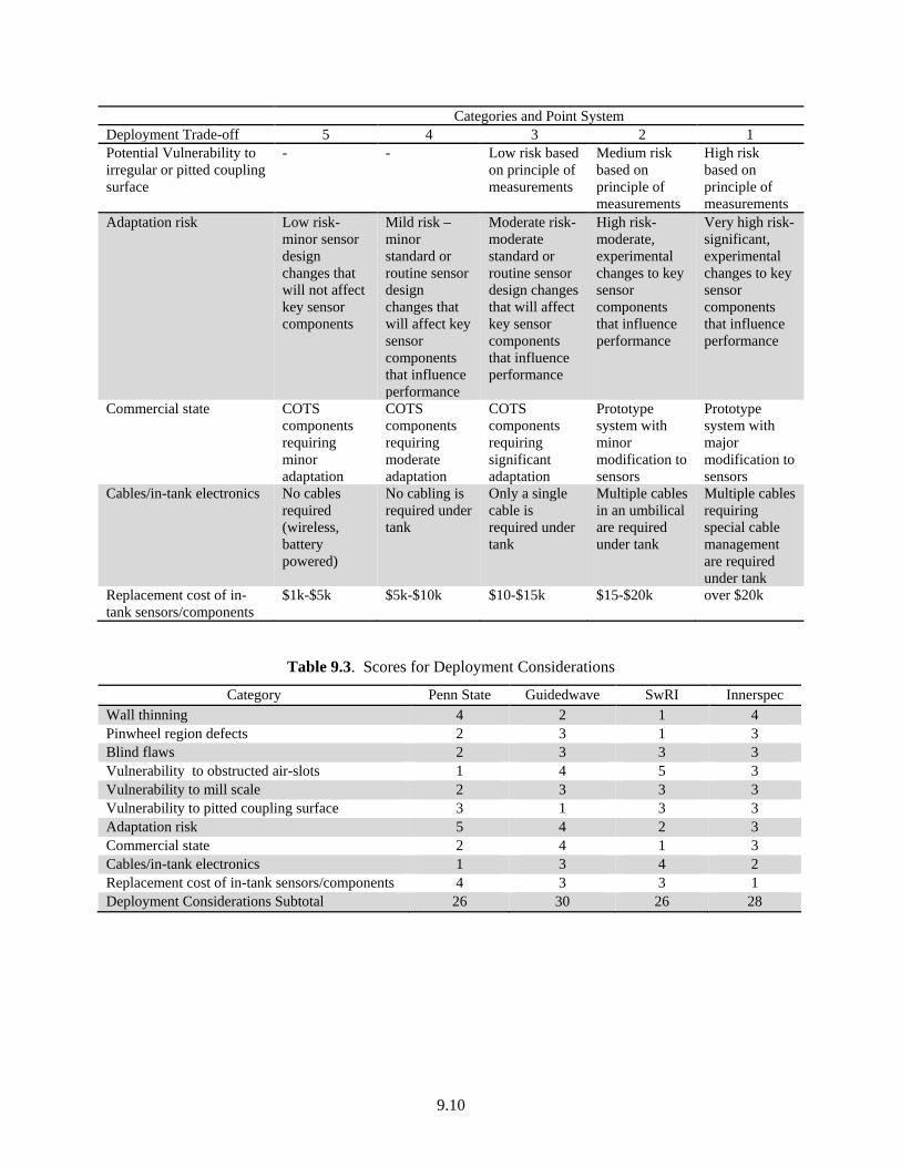
9.10
Categories and Point System Deployment Trade-off 5 4 3 2 1 Potential Vulnerability to irregular or pitted coupling surface
- - Low risk based on principle of measurements
Medium risk based on principle of measurements
High risk based on principle of measurements
Adaptation risk Low risk-minor sensor design changes that will not affect key sensor components
Mild risk – minor standard or routine sensor design changes that will affect key sensor components that influence performance
Moderate risk- moderate standard or routine sensor design changes that will affect key sensor components that influence performance
High risk-moderate, experimental changes to key sensor components that influence performance
Very high risk-significant, experimental changes to key sensor components that influence performance
Commercial state COTS components requiring minor adaptation
COTS components requiring moderate adaptation
COTS components requiring significant adaptation
Prototype system with minor modification to sensors
Prototype system with major modification to sensors
Cables/in-tank electronics No cables required (wireless, battery powered)
No cabling is required under tank
Only a single cable is required under tank
Multiple cables in an umbilical are required under tank
Multiple cables requiring special cable management are required under tank
Replacement cost of in-tank sensors/components
$1k-$5k $5k-$10k $10-$15k $15-$20k over $20k
Table 9.3. Scores for Deployment Considerations
Category Penn State Guidedwave SwRI Innerspec Wall thinning 4 2 1 4 Pinwheel region defects 2 3 1 3 Blind flaws 2 3 3 3 Vulnerability to obstructed air-slots 1 4 5 3 Vulnerability to mill scale 2 3 3 3 Vulnerability to pitted coupling surface 3 1 3 3 Adaptation risk 5 4 2 3 Commercial state 2 4 1 3 Cables/in-tank electronics 1 3 4 2 Replacement cost of in-tank sensors/components 4 3 3 1 Deployment Considerations Subtotal 26 30 26 28

9.11
Table 9.4. Overall Scoring, Key Benefits, and Trade-offs for the Four Technologies
Vendor
Total Score
(of 174)
Flaw Detection Subtotal (of 83)
Sensor Attribute Subtotal (of 50)
Deployment Trade-off Subtotal (of 41) Key benefits Key tradeoffs
Air
-slo
t
Guided-wave
150 78 42 30 •Single slot deployment •Simple image-based analysis •High SNR
•Requires liquid couplant •Sensitivity to wall thinning between 20% and 50% with second sensor •Moderate sensor modification required
Inner-spec
145 75 42 28 •Single slot deployment •No couplant required
•Significant sensor modification required •Analysis is more difficult (A-scan based)
Penn State
143 73 44 26 •Sensor size is deployment ready •No couplant required
•More intensive deployment; requires two open and adjacent air-slots plus coordinated sensor rotation
Rem
ote SwRI 126 59 41 26 •No under tank access
required •No couplant required
•Less sensitive to in-weld defects and wall thinning •Significant sensor modification to reduce size and weight


10.1
10.0 Conclusions
It has been recognized from the start of the NDE Technology Development Program that more than one technique may be required to maximize effectiveness of Hanford under-tank inspection. The general inspection approach recommended for efficient under-tank inspection is to first perform remote screening from the primary tank wall to identify regions that warrant higher-resolution examination with air-slot deployed sensors. This approach will reduce the time and costs associated with tank inspection and minimize risks (failed equipment, air-slot blockage, inability to penetrate air-slot due to debris, longer inspection schedule, etc. ) associated with sending equipment into the air-slots. The approach would use the results from remote screening to identify and prioritize a sub-set of air-slots into which sensor deployment would be warranted for a more detailed examination.
Only one remote screening technology has been demonstrated under Phase I—the EMAT long-range guided-wave technology from SwRI. The method and technology is capable of detecting all pit-type flaws in the base plate material and a limited number of pit-type flaws and weld seam openings located in welds. The technique is not capable of detecting gradual wall thinning and not capable of detecting flaws in the 90-degree weld confluence, which may represent a higher-risk tank region. These deficiencies in performance for remote screening may be acceptable if:
1. it is paired with a second, complementary remote screening technique that can detect gradual wall thinning, which would need to be developed; or
2. gradual wall thinning due to corrosion can be shown to be less likely and thus of less concern than flaw types that provide a sharper change in wall thickness that lends them to detection by this method (pitting-type corrosion and weld seam openings); and
3. air-slots under the tank bottom region that contains the 90-degree weld confluence are accessible and can be examined by air-slot deployed sensors.
Three air-slot deployed higher-resolution screening technologies were demonstrated under Phase I—two EMAT sensor techniques from Penn State and Innerspec and a piezoelectric technique from Guidedwave. The performance and sensor attribute trade-offs that should be considered when selecting techniques to complement the remote screening techniques are discussed below.
All three sensor techniques intended for air-slot deployment performed well overall in flaw detection and, based on flaw detection scores alone, would all be considered suitable candidates for use with the remote screening technique. Making a selection based simply on performance or simply on ease of deployment will result in consequences that will need to be managed during sensor deployment or examination data reduction. This report attempts to capture the trade-offs of each technique for consideration by WRPS to support their decision process.
From purely a flaw detection standpoint, the piezoelectric guided-wave phased-array technique provides the best performance in terms of number of flaws detected and signal quality. The technique also provides the largest range of coverage using a single sensor from a single air-slot. However, the viscous liquid shear-wave couplant application and removal would need to be managed and compatibility with the tank would need to be evaluated. These are obstacles that would need to be overcome to render it applicable and suitable. Further, the lower sensitivity to flaws with gradual wall thickness changes (wall thinning) would need to be considered.
From purely a “deployment readiness” standpoint, the dual-sensor EMAT technique is the closest to being deployment ready. The sensors are small enough to fit inside the air-slots and this sensor technique also has the advantage of being dry coupled. The signal quality was high enough to allow for detection of

10.2
most flaws; however, detection of one of the two flaws (weld seam opening) in the 90-degree weld confluence was not demonstrated and one of the blind flaws (pit in the base plate) was reported as undetected. Further, the robotic delivery of the sensor pair would be the most complex due to the requirement to rotate the sensors in the air-slots and to rotate and translate the pair in a coordinated fashion when they are in separate air-slots.
The single EMAT transducer approach offered the simplest deployment possibility among the no-couplant alternatives. Only a single sensor would be required to deploy and their concept was to incorporate multiple coils with the same magnet to eliminate the need to rotate the sensor. This approach however demonstrated reduced sensitivity as the distance to flaws exceeded 18 inches for pits and 30 inches for notches. In addition, the risk for degraded performance from the sensor modification required to move the design from the demonstrated configuration to a final version is higher than for other technologies.
As a conservative approach to prepare for unknown challenges that may be encountered, more than one air-slot deployed technique could be selected. For example, an EMAT technology would require multiple unobstructed adjacent air-slots to examine a region of a tank bottom due to the estimated 18–36 inches of coverage by this technique. If it is discovered that most air-slots are blocked, then the extent of examination that could be achieved would be limited using either EMAT technique. Some tank bottom regions over blocked air-slots would either go unexamined or action would need to be taken to clear the air-slots to facilitate examination. The potential of encountering blocked air-slots is especially important to consider for potentially high-risk regions of the tank that may need to be included during any inspection, such as the confluence of closely spaced 90-degree welds (pinwheel weld pattern).
To offset the vulnerability and risk associated with the EMAT techniques, the piezoelectric phased-array technology could be used as a primary or back-up technique. The piezoelectric phased-array technique requires single-sensor deployment down one air-slot and is capable of examining a wide region of the tank bottom from a few positions due to its 360-degree beam steering capability and range of coverage (up to a plate weld). Therefore, the extent of examination that could be achieved in partially blocked air-slots would not be as limited with this technique. For example, if the sensor was deployed in an air-slot located near the 90-degree position under the primary tank, it may only need to extend into the first 5-10 feet under the tank to examine the bottom plate, which extends beyond the first air-slot transition (i.e., >17-ft). The primary weakness of this technique is its liquid couplant requirement, as mentioned previously. Corrosion compatibility between the tank and couplant would need to be demonstrated, and the remainder of the challenge would be associated with couplant application and removal. The challenge could be minimized by either limiting deployment of the phased-array sensor to the first 5-10 feet of air-slots or using the technique in the event air-slot conditions preclude the use of an air-slot EMAT sensor.

11.1
11.0 References
Bandyopadhyay K, S Bush, M Kassir, B Mather, P Shewmon, M Streicher, B Thompson, Dv Rooyen and J Weeks. 1997. Guidelines for Development of Structural Integrity Programs for DOE High-Level Waste Storage Tanks. BNL-52527, Brookhaven National Laboratory, Upton, New York.
Berman HS. 2005. Rationale for Requesting Deletion of the Double-Shell Tank Bottom Plate Ultrasonic Inspection Requirement. RPP-25844, Rev. 0, CH2M Hill Hanford Group, Inc., Richland, Washington.
Deibler JE, KI Johnson, NK Karri, SP Pilli and MW Rinker. 2007. Hanford Double-Shell Tank Thermal and Seismic Project – Primary Tank Minimum Wall Thickness Analysis. RPP-RPT-32238, Rev. 0, Pacific Northwest National Laboratory, Richland, Washington.
Garfield JS, BJ Vazquez, JR Gunter, AJ Feero and KD Boomer. 2015. Double-Shell Tank Integrity Improvement Plan. RPP-PLAN-57352, Rev. 1, Washington River Protection Solutions, Richland, Washington.


Appendix A –
Guidedwave


FBS, Inc. DBA Guidedwave © 2017
Report on Guided Wave Phased Array Sensor Effectiveness Testing for Hanford DST Inspection
A summary of findings from guided wave phased array Sensor Effectiveness Testing at PNNL in Richland, Washington on 12-13 June, 2017
Subcontract #: 63295
performed for:
Washington River Protection Solutions, LLC
P.O. Box 850
Richland, WA 99352, USA
provided by:
Cody Borigo, [email protected]
Russell Love, [email protected]
Steven Owens [email protected]
Guidedwave
450 Rolling Ridge Drive
Bellefonte, PA, USA 16823
+1-814-234-3437
28 June, 2017

1 FBS, Inc. DBA Guidedwave © 2017
Guidedwave ◦ The Guided Wave Innovations Company 450 Rolling Ridge Drive ◦ Bellefonte, PA ◦ 16823
(814) 234-3437 ◦ www.gwultrasonics.com
Executive Summary
Guided wave phased array (GWPA) testing was carried out on two primary liner mockups at the Pacific Northwest National Laboratory (PNNL) in Richland, Washington on 12 and 13 June, 2017. These tests were to evaluate the sensitivity of the GWPA technology to various flaws on the primary liner floor mockups and to identify the strengths and weaknesses of the technology for adaptation for inspecting the actual primary liner floor.
The use of bulk wave phased array has revolutionized the way we inspect structures when looking through the thickness of a specimen, by rapidly providing sector scans that are more intuitive than a traditional ultrasonic A-scan. In this same way, Guidedwave has proven it possible to develop probes that could revolutionize guided wave inspection by rapidly scanning large plates from a single probe position. The GWPA system steers and focuses guided wave energy 360° around a plate from a single sensor position to generate a “radar-like” scan of anomalies in the plate. Guidedwave accomplishes this guided wave beam steering by utilizing a small array of guided wave sensor elements packed into a single probe and applying signals with predetermined time delays and amplitude factors using a phased array pulser/receiver system and advanced algorithms. Without the capability of 360° inspection, many defects can be missed due to their geometry and incident angle relative to the probe. This is a common problem with guided wave scanners where the beam is only sent out perpendicular to the scanning direction. 360° scanning gives multiple shots on any defects from multiple angles and distances, increasing the likelihood of detection. The composite imaging tool compiles these scans to further improve detection capabilities and aid the user in data interpretation. The technology does not provide an exact thickness map of the structure, but it does allow the user to rapidly locate and categorize severity of defects.
In summary, Guidedwave approached the Sensor Effectiveness Testing by scanning the mockups in predetermined grids along the air slot channels, similar to the way in which a real inspection would be performed, with great success. In doing so, Guidedwave demonstrated that the GWPA technology is a rapid, accurate, and reliable method of inspecting the DST primary liner floor. Further testing showed that any engineering challenges in deploying the technology can be overcome with a very reasonable degree of effort. The GWPA technology is already very mature and would be deployed on a commercially-available hardware platform with custom-built, easy-to-use software. The two-dimensional C-scan images and composite imaging tools in the GWPA software allow for confident, straightforward data interpretation by a user without the need for extensive training, experience, or intense data interpretation efforts.
All the flaws were identified on both mockups with the exception of the 10% wall thinning (Technology Screening mockup) and the 20% wall thinning (Sensor Effectiveness Testing mockup). Both blind flaws were detected easily, quickly, and accurately, which attests to the power of the GWPA technology for real inspection scenarios. In fact, Guidedwave hopes that PNNL plans to conduct full-blind testing at some point in the near future.

2 FBS, Inc. DBA Guidedwave © 2017
Guidedwave ◦ The Guided Wave Innovations Company 450 Rolling Ridge Drive ◦ Bellefonte, PA ◦ 16823
(814) 234-3437 ◦ www.gwultrasonics.com
Although it was more difficult to detect the wall thinning than the other defects, in reality, true wall thinning defects may be detectable at the levels represented in the mockup, since the geometry of the wall thinning flaws was a major factor leading to the difficulty of the system to detect them. Furthermore, flaw detection was achieved for nearly all defects without changing data collection settings or moving the probe from the predetermined scan grid. The composite images of the plates and the selected composite images of the welds provided excellent, easy-to-interpret images showing nearly all of the detectable flaws.
The general data quality was excellent, and a detection range of up to 5-7 feet in all directions around the probe was demonstrated. The SNR of the defects was typically in the 20-45 dB range for the individual scans and 10-20 dB range for the composite images. Due to the 360° scan capabilities of the GWPA, as well as the composite imaging capabilities, defect orientation and air slot restrictions had minimal effect on the detection capabilities during testing. The greatest challenges with defect detection and noise reduction in either mockup were due to free plate edges, which cause significant additional noise and artifacts, even with the T-tape. Additional challenges were present due to the small edge plates, which led to limited access and additional reverberations that would not be present in the real structures.
The dirt and rust tests demonstrated that the GWPA scan SNR was unaffected by either type of surface contamination. Based on performance during the dirt and rust tests and discussions will PNNL and WRPS personnel regarding surface condition in the air slots, it is very likely that little to no surface preparation will be required for GWPA inspection of the Hanford DSL primary liner floors, barring any significant deviation between the surface conditions present in the field and those anticipated by PNNL and WRPS personnel.
One of the potential challenges with deploying the GWPA technology robotically is coupling the probe. Guidedwave demonstrated, through a series of tests, that a couplant dispenser is practical using only vertical actuation and a couplant dispensing cylinder, with no loss in SNR. It may also be possible to dispense the couplant through ports on the probe between the element faceplates. Further testing demonstrated that very little force is required to couple the probe to the structure. Tests were conducted with no application force, 5 lbs, 10 lbs, 15 lbs, and 20 lbs, and the results were nearly identical.
In the final system configuration, it is envisioned that the probe will be deployed on the robotic crawler with a cable extending to the surface, where the UltraWave data acquisition unit, the control laptop, and all other components will be located. This exposes as little of the system as possible to the elevated radiation levels in the tank annulus. It is envisioned that coupling of the probe will be achieved by dispensing couplant with a pneumatic or electric dispenser through either a separate couplant delivery head or through ports in the probe face. The couplant reservoir can be kept locally on the crawler to minimize the distance over which it must be pumped. It is further envisioned that the probe can be pressed against the underside of the primary tank liner floor using a linear actuator. The probe can be removed from the surface by pressing a second actuator against the primary tank liner floor. No rotation or sliding of the probe would be necessary. Data would be collected this way in approximately 1-2 foot increments, although this could be increased

3 FBS, Inc. DBA Guidedwave © 2017
Guidedwave ◦ The Guided Wave Innovations Company 450 Rolling Ridge Drive ◦ Bellefonte, PA ◦ 16823
(814) 234-3437 ◦ www.gwultrasonics.com
or decreased as needed based on tank floor geometry, critical flaw sizes, and conditions in the real test environment. The technology would be applicable to plates having thicknesses of 1” or less in its current form, and the internal sensor array of the GWPA sensors can be made small enough to meet the space limitations of the primary liner access channels, although the smallest slot design may require further modifications, such as reducing the total number of elements. No transducer power is required other than the ultrasonic pulser signals. The data acquisition unit is powered by two Li-ion OmniScan batteries. The laptop is also battery-powered. No permanent magnets are required as any part of the system. No cable length issues are anticipated based on past experience and the signal amplitude generated by the piezoelectric elements.
Guidedwave believes that the GWPA technology would be an excellent method for DST primary liner floor inspection.

4 FBS, Inc. DBA Guidedwave © 2017
Guidedwave ◦ The Guided Wave Innovations Company 450 Rolling Ridge Drive ◦ Bellefonte, PA ◦ 16823
(814) 234-3437 ◦ www.gwultrasonics.com
Table of Contents
Executive Summary.............................................................................................................................................. 1
1. Introduction ................................................................................................................................................... 6
2. Background .................................................................................................................................................... 7
Ultrasonic Guided Waves .............................................................................................................................. 7
Past Efforts .......................................................................................................................................................... 9
Guided Wave Phased Array ....................................................................................................................... 10
4. Approach for Sensor Effectiveness Testing .................................................................................... 12
Inspection Method ........................................................................................................................................ 12
Inspection Equipment ................................................................................................................................. 12
Coupling ............................................................................................................................................................ 14
Sensor Coverage and Dead Zone ............................................................................................................. 19
Software ............................................................................................................................................................ 19
Surface Preparation ...................................................................................................................................... 21
Data Collection Strategy ............................................................................................................................. 21
Rust Test ........................................................................................................................................................... 23
Dirt Test ............................................................................................................................................................ 25
Signal Processing ........................................................................................................................................... 26
Signal-to-Noise Calculation Technique ................................................................................................. 27
Calculation Used to Asses Impact of Dirt and Rust on Signal Quality ....................................... 28
5. Data ................................................................................................................................................................ 29
Typical Pit, Notch, and Wall Thinning Reflection Images .............................................................. 29
Example Images from Dirt Test ............................................................................................................... 30
Example Images from Dirt Test ............................................................................................................... 31
6. Results........................................................................................................................................................... 32
Composite Images ......................................................................................................................................... 32
Flaw Detection Summary ........................................................................................................................... 36
Blind Flaw Detection .................................................................................................................................... 38
7. Discussion/Conclusions ......................................................................................................................... 40
Flaw Detection and Characterization .................................................................................................... 40
Signal Quality and Noise Levels ............................................................................................................... 40
Surface Preparation ...................................................................................................................................... 41
Transducer Requirements ......................................................................................................................... 41
Vision for the System ................................................................................................................................... 42
Appendix A – Flaw Detection Images ......................................................................................................... 44

5 FBS, Inc. DBA Guidedwave © 2017
Guidedwave ◦ The Guided Wave Innovations Company 450 Rolling Ridge Drive ◦ Bellefonte, PA ◦ 16823
(814) 234-3437 ◦ www.gwultrasonics.com
Composite GWPA Scan Images – Sensor Effectiveness Testing Mockup ................................. 44
Individual GWPA Scan Images – Sensor Effectiveness Testing Mockup .................................. 46
Composite GWPA Scan Images – Technology Screening Mockup .............................................. 69
Individual GWPA Scan Images – Technology Screening Mockup ............................................... 70
Appendix B – Dirt Test Images...................................................................................................................... 74
Clean Surface Condition GWPA Scan Images ...................................................................................... 74
Dirty Surface Condition GWPA Scan Images ...................................................................................... 80
Appendix C – Rust Test Images..................................................................................................................... 86
Level 1 Surface Rust GWPA Scan Images ............................................................................................. 86
Level 2 Surface Rust GWPA Scan Images ............................................................................................. 88
Level 3 Surface Rust GWPA Scan Images ............................................................................................. 90
Additional Surface Rust GWPA Scan Image on Vertical Plate ...................................................... 92
Appendix D – Coupling Force Tests ............................................................................................................ 93
Appendix E – Couplant Dispenser Test ..................................................................................................... 98

6 FBS, Inc. DBA Guidedwave © 2017
Guidedwave ◦ The Guided Wave Innovations Company 450 Rolling Ridge Drive ◦ Bellefonte, PA ◦ 16823
(814) 234-3437 ◦ www.gwultrasonics.com
1. Introduction
Guided wave phased array (GWPA) testing was carried out on two primary liner mockups at the Pacific Northwest National Laboratory (PNNL) in Richland, Washington on 12 and 13 June, 2017. These tests were to evaluate the sensitivity of the GWPA technology to various defects on the primary liner floor mockups and to identify the strengths and weaknesses of the technology for adaptation for inspecting the actual primary liner floor.
Table 1 Inspector and equipment overview
Participant Name and Company: Russell Love (Guidedwave)
Cody Borigo (Guidedwave)
Date of Demonstration: June 12-13, 2017
NDE system model and description (transducer specifications, wave modes):
GWPA Probe C16-10-4O: 30 Element, 160 kHz, SH0 wave)
GWPA Probe C16-10-4O: 30 Element, 200 kHz, SH0 wave)
GWPA Probe C16-10-4S: 30 Element, 225 kHz, SH0 wave)
NDE system serial number (optional): UltraWave (UW00005)
GWPA sensor C16-10-4O (PA100466)
GWPA sensor C16-10-4S (PA100468)

7 FBS, Inc. DBA Guidedwave © 2017
Guidedwave ◦ The Guided Wave Innovations Company 450 Rolling Ridge Drive ◦ Bellefonte, PA ◦ 16823
(814) 234-3437 ◦ www.gwultrasonics.com
2. Background
Ultrasonic Guided Waves
The use of ultrasonic guided waves has been increasing tremendously over the past decade due to a variety of reasons, notably improved understanding and computational efficiency for complex problem solving. Guided waves provide the ability to inspect hidden and inaccessible regions of structures, structures under soil, water, coatings, insulations, and concrete because of the inspection capability from a single remote probe position. The best example of guided wave success is in long-range ultrasonic pipeline inspection, where the technology has been accepted commercially for years. This technology has matured to the point that ASNT (American Society for Nondestructive Testing) is now developing a certification process for guided wave inspectors. Guided wave ultrasound differs substantially from traditional bulk wave ultrasonic testing (UT) and can often succeed where traditional UT techniques have failed.
A comparison of ultrasonic bulk waves and guided waves is made in Figure 1. Traditional bulk wave ultrasonic sensors send sound energy into an area directly below the transducer. They are used for thickness measurements, defect detection, and material characterization. The main disadvantage of bulk wave techniques is that to cover a large region, the probe must mechanically scan the entire area. Furthermore, it is difficult to inspect hidden or inaccessible structures, such as those under coatings or soil, using UT techniques.
Figure 1 Comparison of bulk wave excitation (top), and guided wave excitation (bottom) in a plate. The guided wave is capable of detecting reflections from the corrosion patch and the weld that are distant from the transducer location, which is not possible with traditional UT.

8 FBS, Inc. DBA Guidedwave © 2017
Guidedwave ◦ The Guided Wave Innovations Company 450 Rolling Ridge Drive ◦ Bellefonte, PA ◦ 16823
(814) 234-3437 ◦ www.gwultrasonics.com
Guided waves travel along or between two physical boundaries of a waveguide; two examples of such waveguides are a plate and a pipe. Other examples include rails, beams, composite materials, and any other structures that have physical boundaries. Guided waves take advantage of these boundaries to inspect over great distances by creating a resonance condition between the structural boundaries, which allows the waves to propagate much farther than bulk ultrasonic waves. A comparison between bulk wave and guided wave activation can be seen in Figure 1. It is possible to generate guided waves with different types of vibration and energy distributions through the cross-section of a structure. Exploiting these characteristics gives a skilled engineer the ability to create waves that are more or less sensitive to different types of defects and loading conditions. Different guided wave modes also have different velocity characteristics as a function of frequency. These are all considerations that can affect the performance of a guided wave system, and Guidedwave has the skills, knowledge, and tools to understand and exploit these nuances.
The generation of certain guided wave modes at particular frequencies to accomplish special tasks is scientifically-founded and physically-based. Advanced understanding and utilization is possible because of the tremendous advances in computational power and analysis available today. For a given structure, a dispersion curve, such as the one presented for a ½ inch carbon steel plate in Figure 2, can be generated and wave structure profiles subsequently produced. A dispersion curve shows all of the possible guided wave modes that can be excited in a particular structure and the relationship between wave mode, frequency, and velocity. From the dispersion curves, wave structure profiles can be created. The wave structure profiles show how different types of energy are distributed throughout the thickness of that structure. For example, all of the energy can be concentrated at the surface or it can be evenly distributed throughout the thickness.
Figure 2 A guided wave dispersion curve of a ½-inch carbon steel plate, which describes the relationship between wave velocity and frequency for all of the possible guided wave modes in the plate. The SH0 mode that Guidedwave is utilizing for the GWPA inspection is highlighted.

9 FBS, Inc. DBA Guidedwave © 2017
Guidedwave ◦ The Guided Wave Innovations Company 450 Rolling Ridge Drive ◦ Bellefonte, PA ◦ 16823
(814) 234-3437 ◦ www.gwultrasonics.com
The wave vibration components can also be predominantly compressional, flexural, shear, or some combination of these. Guidedwave has a wealth of experience using this type of analysis to solve a variety of problems. In the case of the current application, it was determined that the shear horizontal, SH0 mode, indicated on the dispersion curve in Figure 2, is the best candidate due to its non-dispersive nature, insensitivity to liquids on the surface of the structure, and even energy distribution throughout the cross-section of the pipe wall. The SH0 mode propagates as a pure in plane vibration distributed uniformly through the plate thickness. This characteristic means it is unaffected by inviscid fluids on the surface or the interior due to the lack of shear coupling to liquids. The uniformity of the wave energy through the thickness of the structure also ensures a linear relationship between guided wave reflection amplitude and reflector cross-section.
Principal benefits of the shear horizontal guided wave mode include:
1. Zero out-of-plane displacement through the thickness of the plate – No sensitivity to fluids on either side of plate, which can be a serious problem
with other guided wave modes. 2. Fundamental mode phase and group velocity are constant
– Technology is readily adaptable to wide range of structures, less complex calculations and less knowledge required by user
3. Wave always travels at bulk shear wave speed – User only needs traditional UT wave velocity table – No need to calculate complex dispersion curves
4. Purely non-dispersive – No spreading of wave packet as with many other guided wave modes – Probe frequency can be changed without negative effects on focusing
5. Fundamental mode is independent of plate thickness – Technology is readily adaptable to wide range of structures, less complex
calculations and less knowledge required by user
Past Efforts
Guidedwave originally developed the GWPA technology as part of a Navy SBIR effort for efficient inspection of ship hulls below the waterline. Guidedwave has tested the technology on several Navy ships, including the USS Antietam in Yokosuka, Japan, the USTS Kennedy in Buzzards Bay, MA, the USS Tornado in Jacksonville, FL, and the USS Detroit in Jacksonville, FL. Guidedwave is also working with the Air Force to adapt the GWPA technology for rapid, large-area inspection of aircraft structures. Furthermore, Guidedwave views storage tanks, pressure vessels, and similar structures as excellent opportunities for extending the applications portfolio of the GWPA technology.

10 FBS, Inc. DBA Guidedwave © 2017
Guidedwave ◦ The Guided Wave Innovations Company 450 Rolling Ridge Drive ◦ Bellefonte, PA ◦ 16823
(814) 234-3437 ◦ www.gwultrasonics.com
Guided Wave Phased Array
The use of bulk wave phased array has revolutionized the way we inspect structures when looking through the thickness of a specimen, by rapidly providing sector scans that are more intuitive than a traditional ultrasonic A-scan. In this same way, Guidedwave has proven it possible to develop probes that could revolutionize guided wave inspection by rapidly scanning large plates from a single probe position. Over the past several years, Guidedwave has been developing guided wave phased array technology for the rapid inspection of large areas of steel and aluminum ship hulls for the Navy, as illustrated in Figure 3. Guidedwave has two patents pending on GWPA technologies.
Figure 3 Guided wave phased array technology uses a compact phased array probe to electronically steer and focus a guided wave beam around a plate-like structure; corrosion, cracks, and other anomalies can be detected. This technique resembles a radar or sonar scan and is the guided wave analogue of traditional ultrasonic bulk wave phased array, which revolutionized the UT field.
The guided wave phased array technology performs in a manner akin to sonar, in which sound is electronically focused and swept in different directions to detect the location and distance of other ships, or radar, in which radio waves are steered to detect aircraft. Similarly, the guided wave phased array system steers and focuses guided wave energy 360° around a plate from a single sensor position to generate a “radar-like” scan of anomalies in the plate. Guidedwave accomplishes this guided wave beam steering by
Phased array probe
Plate or shell structure
Guided wave phased array scan
image
Focused guided wave beam
Defects reflections
UltraWave LRT guided wave phased array system,
marketed by Olympus NDT
Defects reflections

11 FBS, Inc. DBA Guidedwave © 2017
Guidedwave ◦ The Guided Wave Innovations Company 450 Rolling Ridge Drive ◦ Bellefonte, PA ◦ 16823
(814) 234-3437 ◦ www.gwultrasonics.com
utilizing a small array of guided wave sensor elements packed into a single probe and applying signals with predetermined time delays and amplitude factors using a phased array pulser/receiver system and advanced algorithms. This beam steering allows the sensor to detect the presence of defects at distances of up to 10 feet in all directions around the probe. Guidedwave has performed guided wave phased array scans of ship hull mockups with an area of 50 ft2 in less than 15 seconds. The damage image can be obtained either directly from the scan signals as a non-destructive evaluation (NDE) approach or by comparison with baseline signals as a structural health monitoring (SHM) method. The SHM approach can be useful in structures with complex geometry by taking advantage of baseline signal comparison. The technology does not provide an exact thickness map of the structure, but it does allow the user to rapidly locate and categorize severity of defects.

12 FBS, Inc. DBA Guidedwave © 2017
Guidedwave ◦ The Guided Wave Innovations Company 450 Rolling Ridge Drive ◦ Bellefonte, PA ◦ 16823
(814) 234-3437 ◦ www.gwultrasonics.com
4. Approach for Sensor Effectiveness Testing
Inspection Method
Guidedwave employed patented guided wave phased array (GWPA) technology using the SH0 wave mode during Sensor Effectiveness Testing. The technology is largely identical to that used during the Technology Screening Testing earlier in the year. Data analysis was performed on the two-dimensional phased array NDT scan images and the two-dimensional composite scan images.
Inspection Equipment
The GWPA inspection system is comprised of an UltraWave LRT multi-channel pulser-receiver unit, a handheld GWPA sensor, a laptop loaded with purpose-built data collection and analysis software, and the associated cabling and accessories.
The UltraWave LRT unit, shown in Figure 4, is a multi-channel guided wave pulser-receiver platform sold and serviced through Olympus Scientific Solutions Americas (OSSA) that is currently used with the UltraWave long-range guided wave pipe inspection system, also offered by OSSA. This unit is a powerful, flexible platform for a variety of guided wave technologies, and can be utilized for GWPA applications.
Figure 4 The UltraWave LRT guided wave pulser-receiver system sold and serviced by Olympus.

13 FBS, Inc. DBA Guidedwave © 2017
Guidedwave ◦ The Guided Wave Innovations Company 450 Rolling Ridge Drive ◦ Bellefonte, PA ◦ 16823
(814) 234-3437 ◦ www.gwultrasonics.com
Currently, Guidedwave has designed and manufactured multiple GWPA sensors for a multitude of applications. For the primary wall mock-up, Guidedwave has selected the 165 kHz 30-element GWPA sensor PA100466 (Figure 5). This sensor offers the optimal frequency bandwidth for the given plate thickness and defect sizes expected. However, with this sensor, the resolution is slightly reduced to minimize the side lobes produced. This is necessary when there are many features in the plates or cut ends, like in a mock-up, which will produce artifacts in the final GWPA image.
Figure 5 Photograph of a GWPA sensor that was used during the primary liner mockup inspection feasibility study
The existing GWPA sensors have been designed to be handheld and ergonomic. The height and diameter of the 165 kHz 30-element GWPA sensor are 1.7 and 2.7 inches, respectively. However, the actual sensor array diameter is only 2 inches and the active element height is 3/8 inches. Guidedwave has fabricated sensors with diameters as small as 1.5 inches, and one of these was brought along during testing to demonstrate. Guidedwave is also in the process of building a probe with elements half the size of the smallest yet developed, which could possibly reduce the dimensions even further, if necessary. Therefore, a smaller diameter GWPA probe is absolutely possible for this application. We work with Olympus NDT to produce the GWPA probes, based on our specifications, so it is quite reasonable to redesign the probe for the limited-access channel geometry.

14 FBS, Inc. DBA Guidedwave © 2017
Guidedwave ◦ The Guided Wave Innovations Company 450 Rolling Ridge Drive ◦ Bellefonte, PA ◦ 16823
(814) 234-3437 ◦ www.gwultrasonics.com
Figure 6 Photograph of several GWPA probes produced to date, including the C16-10-4O probe (second from left) utilized for the Technology Screening and almost all of the Sensor Effectiveness Testing and the smaller C16-10-4S probe (far right) that demonstrates the possibility of reducing the probe size.
Coupling
The sensor is applied to the structure with ultrasonic shear couplant. This couplant has a high viscosity to support the shear vibration. It can be purchased from commercial vendors or produced in-house, which offers increased control on the final viscosity for optimizing its performance for different temperature ranges. Guidedwave dispensed the shear couplant with a handheld plunger system during testing, and automating that process is very feasible. A small, prototype dispenser head was fabricated and brought to testing for demonstration, however the grease gun that was used to deliver the couplant through the dispenser wasn’t functioning properly during the visit. Using a similar couplant dispensing mechanism, the couplant can be applied to the probe or directly to the surface (including inverted surfaces). Figure 7 and Figure 8 are series of photographs showing the application of shear couplant with a dispenser head, as well as a scan showing data collected using this

15 FBS, Inc. DBA Guidedwave © 2017
Guidedwave ◦ The Guided Wave Innovations Company 450 Rolling Ridge Drive ◦ Bellefonte, PA ◦ 16823
(814) 234-3437 ◦ www.gwultrasonics.com
method. It may also be possible to design a GWPA probe with port holes on the front face (between elements) that can secrete couplant directly onto the plate, instead of using a separate dispenser head.
Figure 7 Photographs showing the dispensing of couplant through a perforated faceplate. A similar device could be utilized to dispense couplant robotically for GWPA scanning of the DST primary liner.
Figure 8 Photographs showing the process of applying the couplant with the dispenser, removing it, and placing the probe over the couplant prior to scanning. This process can be adapted for robotic implementation. The couplant dispensing mechanism could also possibly be incorporated into the probe.
The scan comparisons in Figure 9 show that the signals are comparable with the dispensed couplant (left) and the manually applied couplant (right). The SNR of the holes and the edges are also comparable, as shown in Figure 10.

16 FBS, Inc. DBA Guidedwave © 2017
Guidedwave ◦ The Guided Wave Innovations Company 450 Rolling Ridge Drive ◦ Bellefonte, PA ◦ 16823
(814) 234-3437 ◦ www.gwultrasonics.com
Figure 9 Comparison of the GWPA scans with remotely dispensed couplant (left) and manually applied couplant (right). There is a negligible difference.
Figure 10 Comparison of the average SNR of three holes and four plate edges using remotely dispensed couplant (left) and manually applied couplant (right). There is a negligible difference.
0.0
10.0
20.0
30.0
40.0
50.0
60.0
70.0
80.0
Dispensed Manual
SNR
(d
B)
Edge SNR
Hole SNR

17 FBS, Inc. DBA Guidedwave © 2017
Guidedwave ◦ The Guided Wave Innovations Company 450 Rolling Ridge Drive ◦ Bellefonte, PA ◦ 16823
(814) 234-3437 ◦ www.gwultrasonics.com
After dispensing the couplant, the probe can be pressed in place onto the couplant with a linear actuator and subsequently removed by pushing it away from the liner surface or driving a small wedge between the probe and the liner. Tests have shown that very little force is necessary to achieve sufficient coupling, as long as the original couplant layer is reasonably thin. Guidedwave conducted tests on a 30” x 30” demo plate with three partial-through-wall flat-bottom holes, shown in Figure 11.
Figure 11 Photograph of the aluminum demo plate used for the application force tests; the plate is 30" x 30" x 0.080" thick and has three 1/4"-diameter, 80% deep flat-bottom holes.
The probe was applied with varying amounts of force, from 0 lbs to 20 lbs in 5-lb increments. The probe was given 60 seconds after the force was applied before data was collected. Figure 12 provides examples of several scans with varying degrees of application force.
¼” flat-bottom holes, 80% deep
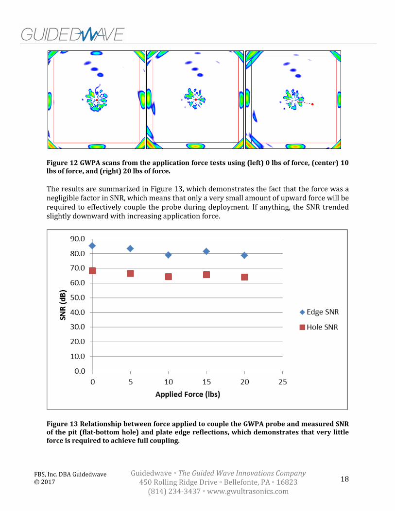
18 FBS, Inc. DBA Guidedwave © 2017
Guidedwave ◦ The Guided Wave Innovations Company 450 Rolling Ridge Drive ◦ Bellefonte, PA ◦ 16823
(814) 234-3437 ◦ www.gwultrasonics.com
Figure 12 GWPA scans from the application force tests using (left) 0 lbs of force, (center) 10 lbs of force, and (right) 20 lbs of force.
The results are summarized in Figure 13, which demonstrates the fact that the force was a negligible factor in SNR, which means that only a very small amount of upward force will be required to effectively couple the probe during deployment. If anything, the SNR trended slightly downward with increasing application force.
Figure 13 Relationship between force applied to couple the GWPA probe and measured SNR of the pit (flat-bottom hole) and plate edge reflections, which demonstrates that very little force is required to achieve full coupling.

19 FBS, Inc. DBA Guidedwave © 2017
Guidedwave ◦ The Guided Wave Innovations Company 450 Rolling Ridge Drive ◦ Bellefonte, PA ◦ 16823
(814) 234-3437 ◦ www.gwultrasonics.com
Sensor Coverage and Dead Zone
Based on previous experience, lab tests, and the results from the Sensor Effectiveness Testing, reliable flaw detection can be achieved over distances of 5-7 feet omni-directionally, with this range depending on the plate geometry and the critical defect size. The GWPA probe automatically collects data in 360° for each scan, which can yield a coverage area of 80-150 ft2 from a single shot. Note that the collection of data in 360° is performed with no physical rotation/movement of the probe. Of course, multiple overlapping shots will yield much greater probability of detection and higher confidence, and the inspection range will be affected by the presence of welds or elevated attenuation.
The dead zone around the transducer is primarily affected by the data collection settings (frequency, pulse cycles, and gain) as well as the coupling. Poor coupling will lead to an increased dead zone due to inefficient transfer of the ultrasonic energy into the plate. Typical dead zone sizes observed in the Sensor Effectiveness Testing were approximately 7-10 inch radius.
Software
Guidedwave has created specifically-designed software for GWPA applications. Several screen captures of the GWPA software are provided in Figure 14 and Figure 15. The software and electronics record any reflected ultrasonic energy from the incident waves and display the waveforms on a radar type graph on the laptop screen. The user can then analyze the image to identify the known features and any anomalies that may be present. The software contains all necessary algorithms for completing a scan including: focusing calculations, data acquisition, data display, data analysis tools, and data saving and loading. This software has been created for use on a handheld device for rapid screening of plates, and can be adapted for robotic deployment. All of our software development is done in-house and we have produced specialty versions for unique applications such as this in the past.

20 FBS, Inc. DBA Guidedwave © 2017
Guidedwave ◦ The Guided Wave Innovations Company 450 Rolling Ridge Drive ◦ Bellefonte, PA ◦ 16823
(814) 234-3437 ◦ www.gwultrasonics.com
Figure 14 Screen capture of the specially-designed software for collecting and analyzing GWPA data (phased array image screen).
Figure 15 Screen capture of the specially-designed software for collecting and analyzing GWPA data (composite image screen).

21 FBS, Inc. DBA Guidedwave © 2017
Guidedwave ◦ The Guided Wave Innovations Company 450 Rolling Ridge Drive ◦ Bellefonte, PA ◦ 16823
(814) 234-3437 ◦ www.gwultrasonics.com
Surface Preparation
No surface preparation was performed during Sensor Effectiveness Testing. Excessive surface dirt, loose rust, or other contaminants can impact the coupling, as with any ultrasonic method, but none of the conditions present on the mockups, including those during the Rust Test or Dirt Test had any negative impact on the GWPA signal quality. Guidedwave has done lab and field testing with this technology on plates in far worse condition than those observed during this testing.
Data Collection Strategy
It was our intent to collect data during Sensor Effectiveness Testing in a manner that was as close a real field inspection as possible, in which the location and characteristics of defects would be generally unknown. Therefore we mapped out a grid of points in several air slots that would allow us to achieve general coverage across all of the plates of interest in the two mockups. On the second day, we did take a few additional shots to attempt to have better sensitivity to the “wall thinning” defects. Along the same line of thinking, we attempted to keep the data collection settings unchanged throughout testing. Even with this approach, we were able to clearly detect almost all of the defects without optimizing the sensor position and settings for each individual flaw. This data collection strategy also proved to very easily detect the two blind flaws, and thus also demonstrates how effective the GWPA technology could be in real-world blind inspection scenarios. In fact, Guidedwave hopes that PNNL will conduct full-blind testing as part of their technology selection effort in the near future.
Table 2 provides a list of the locations at which GWPA data was collected on both mockups. If not for the small plates attached to the edges, far fewer data collection locations would be necessary. Furthermore, composite image analysis showed that half the number of shots on the Sensor Effectiveness Testing mockup could be collected while still maintaining a high level of detectability for most of the defects.
A complete summary of the data collection settings and probe locations corresponding to detection of each of the individual defects are provided in the Results section.

22 FBS, Inc. DBA Guidedwave © 2017
Guidedwave ◦ The Guided Wave Innovations Company 450 Rolling Ridge Drive ◦ Bellefonte, PA ◦ 16823
(814) 234-3437 ◦ www.gwultrasonics.com
Table 2 List of GWPA data collection locations on both mockups
Sensor Effectiveness Testing Mockup
Technology Screening Mockup Location X (in) Y (in)
Location X (in) Y (in)
A 21 55
EE 12 38
AA 21 19
T 42 26
B 38 55
U 62 26
BB 21 3
V 82 26
C 56 55
W 32 16
CC 74 19
X 52 16
D 74 55
Y 72 16
DD 74 3
Z 72 41
E 21 37 F 38 37 G 56 37 H 74 37 I 11 11 J 29 11 K 47 11 L 65 11 M 83 11 N 101 28 P 114 19 R 101 46 S 114 55

23 FBS, Inc. DBA Guidedwave © 2017
Guidedwave ◦ The Guided Wave Innovations Company 450 Rolling Ridge Drive ◦ Bellefonte, PA ◦ 16823
(814) 234-3437 ◦ www.gwultrasonics.com
Rust Test
The rust test consisted of collecting data on a free edge reflection on the 7/8” parts of the mockups with the probe placed 12” from the edge. Data was collected in this manner on three mockups with varying degrees of surface rust. Three shots were collected for each rust condition to provide a better statistical measure of the effect of the surface rust on the GWPA scans. The results, as summarized in Table 3 and Figure 16, demonstrate that the surface rust had no discernible effect on the signal-to-noise. Guidedwave also tested the probe on the vertical plate of the mockup with the level 3 corrosion, which had even more surface corrosion and roughness than the level 3 test surface; the SNR on this shot was 74 dB. Figure 10 provides photographs of the probe on the Rust Test surfaces.
Table 3 Summary of Rust Test shots and edge amplitudes above noise floor
Rust Level
L1 SNR (dB) L2 SNR (dB) L3 SNR (dB)
Shot 1 73 65 69
Shot 2 70 66 69
Shot 3 69 67 70
Average SNR (dB) 70.7 66.0 69
Standard Deviation (dB) 1.70 0.82 0.47
Figure 16 Summary of Rust Test results, showing no discernible effect of signal to noise.
0
10
20
30
40
50
60
70
80
0 1 2 3 4
SNR
(d
B)
Rust Level
C-Filtered Data
L1
Average L1
L2
Average L2
L3
Average L3

24 FBS, Inc. DBA Guidedwave © 2017
Guidedwave ◦ The Guided Wave Innovations Company 450 Rolling Ridge Drive ◦ Bellefonte, PA ◦ 16823
(814) 234-3437 ◦ www.gwultrasonics.com
Figure 17 Photographs of the probe on the three rust specimens, from left to right: Level 1, Level 2, and Level 3; none of the surface conditions had any effect on the SNR of the GWPA data.
Figure 18 Photographs of the probe (left) and close-up of the surface condition on the vertical plate of the Level 3 rust mockup, which has even more surface roughness than the Level 3 rust plate; this surface also had no effect on the SNR of the GWPA data.

25 FBS, Inc. DBA Guidedwave © 2017
Guidedwave ◦ The Guided Wave Innovations Company 450 Rolling Ridge Drive ◦ Bellefonte, PA ◦ 16823
(814) 234-3437 ◦ www.gwultrasonics.com
Dirt Test
The dirt test consisted of collecting data on flaw C of the Technology Screening mockup.
Shots were collected under two separate rounds of “dirty” conditions and two separate
rounds of “clean” conditions, with shots being collected from three locations: (12,35), (12,
38), and (12, 41) during each test to provide a better statistical measure of the effect of the
dirt contamination on the GWPA scans. During the tests, the transducer was coupled and
seated normally, followed by data collection, so no adjustments or optimization was
required to achieve excellent signal quality. The results, as summarized in Table 4 and
Figure 19, demonstrate that the surface dirt had no discernible effect on the signal-to-noise,
although the standard deviation was greater, which could mean there is more variability
possible in coupling.
Table 4 Summary of the results of the Dirt Test, demonstrating that the dirt had no discernible effect on the SNR of the GWPA data.
Clean SNR (dB) Dirty SNR (dB)
Shot 1 36 28
Shot 2 33 38
Shot 3 42 25
Shot 4 34 30
Shot 5 35 44
Shot 6 32 36
Average SNR (dB) 35.3 34
Standard Deviation (dB) 3.25 6.47
Figure 19 Summary of the results of the Dirt Test, demonstrating that the dirt had no discernible effect on the SNR of the GWPA data.
0
5
10
15
20
25
30
35
40
45
50
SNR
(d
B)
C-Filtered Data
Clean
Average Clean
Dirty
Average Dirty

26 FBS, Inc. DBA Guidedwave © 2017
Guidedwave ◦ The Guided Wave Innovations Company 450 Rolling Ridge Drive ◦ Bellefonte, PA ◦ 16823
(814) 234-3437 ◦ www.gwultrasonics.com
Signal Processing
The GWPA technology uses extensive data processing to generate the two-dimensional scan images from the individual raw signals. The data collection routine can vary, depending on the specific circumstances, but for the Sensor Effectiveness Testing (as well as the Technology Screening testing), the following general processing is performed:
1. Guided waves are generated by pulsing all active 16 active elements in the array with pre-determined time delays in order to focus the guided wave beam in the specified steering direction (0° to start).
2. Reflected guided wave signals are detected by all 30 active and passive elements in the array; these raw signals are stored for each beam steering direction.
3. Software-based bandpass filtering is applied to all 30 time-domain waveforms.
4. Phase shifting is applied to the 30 received waveforms in the frequency domain in order to further enhance the guided wave focusing.
5. The focused waveforms for each direction are enveloped using a Hilbert transform and plotted in the appropriate direction on the display screen.
6. Steps 1-3 are repeated for each beam steering direction through 360°.
7. (Optional) C-filtering can be applied to the 360° scan data after data collection. This entails utilizing the known reflected field and cross-correlating with the expected beam profile in order to identify and suppress imaging artifacts due to side lobes and grating lobes.
8. (Optional) Composite imaging can be performed on multiple GWPA scans (with or without C-filtering). This entails combining the GWPA scans from multiple scans with known relative locations, in which “real indications” are reinforced and noise and “phantom indications” are suppressed.
The C-filtering and composite imaging are very useful tools that can be performed in post-processing to enhance the GWPA scan images and aid the user in distinguishing real indications from phantom indications. Furthermore, the composite imaging tool provides a single, very easy-to-interpret scan result that precludes the need for the user to sift through dozens or even hundreds of individual shots. By using the composite imaging tool in the software, not only does the user not need to look at A-scans, but the user doesn’t even need to analyze individual C-scans. Once indications are identified, the user may go back to individual data files for further analysis, but the upfront inspection time is greatly reduced and the user confidence in the data interpretation is greatly improved by using the composite imaging.
Note that the signal processing was applied to all data in the same manner throughout
Sensor Effectiveness Testing. Results were not fine-tuned to optimize individual flaws.

27 FBS, Inc. DBA Guidedwave © 2017
Guidedwave ◦ The Guided Wave Innovations Company 450 Rolling Ridge Drive ◦ Bellefonte, PA ◦ 16823
(814) 234-3437 ◦ www.gwultrasonics.com
Signal-to-Noise Calculation Technique
Signal-to-noise ratio (SNR) was calculated from the C-filtered GWPA scans, and not from individual A-scans. This is the most accurate method of SNR analysis, since this is the form of the data that would most likely be analyzed by a user. Note that a separate SNR analysis was performed for each defect based on the composite image(s). The precise “noise” level is difficult to characterize in a GWPA scan because of the presence of artifacts from side lobes. Typically, the C-filter removes most sidelobe artifacts quite effectively, so these are not of concern. However, due to the presence of free edges on the mockup (even with the T-tape), there are some sidelobe artifacts that remain; in real-world inspections, these would not be present. Isolated sidelobe artifacts were generally ignored in the SNR analysis, unless they were present to such a degree that they effectively raise the “noise level” in the scan, such as in some shots near free edges or on the very small edge plates, in which reverberation also contributed to the noise floor. Therefore, the noise floor was generally considered to be the peak of the noise level at a medium distance in the data set. This SNR analysis was applied to all the data in the same manner. Figure 20 illustrates one example of the “noise level” in the GWPA data for Location A at 160 kHz, which was approximated to be at 59.4 dB. In this figure, the colormap threshold is set to 59.4dB such that the peaks of the noise are just barely visible in light blue. The remaining indications are weld or edge reflections, defect indications, dead zone noise, sidelobe artifacts from the free edges, or reverberations from the free edges.
Figure 20 One example of the "noise level" for Location A.

28 FBS, Inc. DBA Guidedwave © 2017
Guidedwave ◦ The Guided Wave Innovations Company 450 Rolling Ridge Drive ◦ Bellefonte, PA ◦ 16823
(814) 234-3437 ◦ www.gwultrasonics.com
Calculation Used to Asses Impact of Dirt and Rust on Signal Quality
The dirt and rust test data was analyzed by comparing the signal-to-noise ratio (SNR) of the selected flaw (for the dirt tests) or edge (for the rust tests) between test conditions. The data was collected multiple times for each test conditions, and the results were plotted as shown in Figure 16 and Figure 19. The average SNR for each test condition was calculated along with error bars set to +/- one standard deviation. The full data is provided in Table 3 and Table 4.

29 FBS, Inc. DBA Guidedwave © 2017
Guidedwave ◦ The Guided Wave Innovations Company 450 Rolling Ridge Drive ◦ Bellefonte, PA ◦ 16823
(814) 234-3437 ◦ www.gwultrasonics.com
5. Data
Typical Pit, Notch, and Wall Thinning Reflection Images
The following images provide typical examples of pit, notch, and wall thinning defect indications from various locations on the Sensor Effectiveness Testing mockup.
Figure 21 GWPA scan from Location H showing typical pit indications at P5 (ID), P8 (ID), and B1 (OD).
Figure 22 GWPA scan from Location J showing typical notch reflections at N4 (ID), N5 (ID), N7 (ID), and B2 (OD).
P5
B1
P8
N5
B2
N4
N7

30 FBS, Inc. DBA Guidedwave © 2017
Guidedwave ◦ The Guided Wave Innovations Company 450 Rolling Ridge Drive ◦ Bellefonte, PA ◦ 16823
(814) 234-3437 ◦ www.gwultrasonics.com
Figure 23 GWPA scan from Location "thinning2" showing a typical wall thinning reflection at T3 (ID).
Example Images from Dirt Test
The following images are examples of these used to analyze the effect of surface dirt on the GWPA scan data SNR. Flaw C on the Technology Screening mockup is highlighted with the cursor.
Figure 24 Comparison of images from shot 5 with a clean surface (left) and shot 5 with a dirty surface (right).

31 FBS, Inc. DBA Guidedwave © 2017
Guidedwave ◦ The Guided Wave Innovations Company 450 Rolling Ridge Drive ◦ Bellefonte, PA ◦ 16823
(814) 234-3437 ◦ www.gwultrasonics.com
Example Images from Rust Test
The following images are examples of these used to analyze the effect of surface rust on the GWPA scan data SNR. The free edge reflection of the mockup is highlighted with the cursor.
Figure 25 Comparison of images from shot 2 of the Rust Test for surface rust level 1 (left), surface rust level 2 (center), and surface rust level 3 (right).

32 FBS, Inc. DBA Guidedwave © 2017
Guidedwave ◦ The Guided Wave Innovations Company 450 Rolling Ridge Drive ◦ Bellefonte, PA ◦ 16823
(814) 234-3437 ◦ www.gwultrasonics.com
6. Results
The scope of testing was fully completed, with time to spare. All defects, with the exception of the 10% and 20% thinning were detected, most from several locations and with no changes in probe settings or position. The hidden flaws were easily detected and characterized by the GWPA data. The surface dirt and rust were shown to have no statistically significant effect on the SNR; see results in Section 4. The composite images compiled from the GWPA scan data clearly indicate almost all of the defects. The major results are provided below, with additional supporting content in the Appendix.
Composite Images
The composite images provided excellent results, showing clear indications of the vast majority of defects in a single image; see Figure 26. This easy-to-interpret image would provide a very straightforward means of inspection for an operator with limited training. The black dots in the composite image correspond to the scan locations used to construct it. Note that in the composite image in Figure 26, one area of heavy weld repair is also visible along the transition weld; this is not noise.
Figure 26 Composite image from Sensor Effectiveness Testing mockup showing detection of defects P4, P5, P6, P7, P8, P9, P10, N4, N6, N7, blind flaw B1, and blind flaw B2. Also note the area of heavy weld repair along the transition weld was also visible in the composite image.
P6
P7
P8
B2
B1
P5
P4
N6
P9
P10
N7
N4
Weld repair

33 FBS, Inc. DBA Guidedwave © 2017
Guidedwave ◦ The Guided Wave Innovations Company 450 Rolling Ridge Drive ◦ Bellefonte, PA ◦ 16823
(814) 234-3437 ◦ www.gwultrasonics.com
It would also be advantageous to try to analyze the welds for defects by considering them
separately from the rest of the plate. Figure 27 provides a composite image showing only
the transition weld (rotated to fit the page), in which all the defects (and the heavily
repaired area, as shown in the photograph in FFF28) are clearly indicated.
Figure 27 Composite image of the transition weld showing detection of flaws N5, P7, P6, P11, and the heavily repaired weld area.
Figure 28 Photograph of the 7/8-to-1/2 inch transition weld including the area of heavy weld repair that was detected in the composite images above.
P6 P7 Weld repair P11 N5
Area of heavy weld repair in 7/8-to-1/2 inch transition weld

34 FBS, Inc. DBA Guidedwave © 2017
Guidedwave ◦ The Guided Wave Innovations Company 450 Rolling Ridge Drive ◦ Bellefonte, PA ◦ 16823
(814) 234-3437 ◦ www.gwultrasonics.com
The same can be done for any of the ½-to-½ inch welds, as shown in Figure 29 for the weld
at X = 96” (rotated to fit the page).
Figure 29 Composite image of the ½-to-½ inch at X = 96” showing detection of flaws N6, P9, P10, N7, and N4.
Further analysis was conducted to determine if fewer scan locations could still provide
high-quality composite images, which would allow for a reduction in the number of shots
necessary to inspect a given area. The composite image in Figure 30 was constructed using
approximately half of the scan locations compared to those used in Figure 26. This image is
still quite good.
Figure 30 Composite image from Sensor Effectiveness Testing mockup using only 7 scan locations, as opposed to the 13 scan locations used for the composite image in Figure 26.
N6 P9 P10 N7 N4

35 FBS, Inc. DBA Guidedwave © 2017
Guidedwave ◦ The Guided Wave Innovations Company 450 Rolling Ridge Drive ◦ Bellefonte, PA ◦ 16823
(814) 234-3437 ◦ www.gwultrasonics.com
Additionally, a composite image for the Technology Screening mockup is provided in
Figure 31. Figure 32 shows the composite image of the ½-to-½ inch weld area of this
mockup.
Figure 31 Composite image from Technology Screening mockup showing detection of flaws P2, P3, N1, N2, and N3, as well as many flaws from the original Technology Screening tests; the scan locations used to compile this composite image are shown as black dots.
Figure 32 Composite image from Technology Screening mockup showing detection of flaws P2, P3, N1, N2, and N3, zoomed in on the weld area.
P3
N2 N3 P2 N1
P3
N2 N3 P2 N1

36 FBS, Inc. DBA Guidedwave © 2017
Guidedwave ◦ The Guided Wave Innovations Company 450 Rolling Ridge Drive ◦ Bellefonte, PA ◦ 16823
(814) 234-3437 ◦ www.gwultrasonics.com
Flaw Detection Summary
Details of the detection of each flaw are provided in the following tables. TT4 summarizes the flaws in the Technology Screening mockup, and TT5 summarizes the flaws in the Sensor Effectiveness Testing mockup. Note that the tables are constructed somewhat differently than the template provided in the Test Protocol in order to more fully present the flaw detection capabilities and limitations.
Table 5 Flaw detection summary on the Technology Screening mockup.
Machined
Surrogate
Flaw
Flaw
ID
Flaw Location and
Orientation
ID or
OD
Flaw
Detection
Indicated?
Best
SNR
(dB)
Transducer
Location for
Best SNR
(inches)
Data File
Date/Time
Stamp
Data Acquisition
Settings
Greatest
Distance
Detected
Locations
Detected
From
SNR in
Composite
Image(s)
Comments
Pit P1 Base plate (ID) ID Yes 23 Z(72, 41)6/12/2017
10:45 AM
Probe: C16-10-4O
Freq: 160 kHz
Gain: 45dB
C-filter: ON
20 inches (1) Z 0.0
Slightly more difficult to detect
due to small size. Did not
appear well in composite
image, but more shots could
remedy this.
Pit P21/2-to-1/2 inch weld
(ID)ID Yes 32 Z(72, 41)
6/12/2017
10:45 AM
Probe: C16-10-4O
Freq: 160 kHz
Gain: 45dB
C-filter: ON
29 inches (2) X, Z 18.3 Very easy to detect.
Pit P31/2-to-1/2 inch 30°
angled weld (ID)ID Yes 29 U(62, 26)
6/12/2017
11:15 AM
Probe: C16-10-4O
Freq: 160 kHz
Gain: 45dB
C-filter: ON
34 inches(4) T, U,
X, EE19.5 Very easy to detect.
Notch N1
1/2-to-1/2 inch weld,
circumferential
orientation, parallel
with weld (ID)
ID Yes 38 Y(72, 16)6/12/2017
11:33 AM
Probe: C16-10-4O
Freq: 160 kHz
Gain: 45dB
C-filter: ON
22 inches (2) Y, Z 22.3 Very easy to detect.
Notch N2
Base plate edge,
circumferential
orientation, parallel to
weld (ID)
ID Yes 45 T(42, 26)6/12/2017
11:06 AM
Probe: C16-10-4O
Freq: 160 kHz
Gain: 45dB
C-filter: ON
27 inches
(8) T, U,
V, W, X, Y,
Z, FF
42.8 Very easy to detect.
Notch N3
Base plate edge, axial
orientation,
perpendicular to weld
(ID)
ID Yes 35 X(52, 16)6/12/2017
11:42 AM
Probe: C16-10-4O
Freq: 160 kHz
Gain: 45dB
C-filter: ON
36 inches(4) V, W,
X, Y28.3 Very easy to detect.
Wall
ThinningT1 Base plate (ID) ID No N/A N/A N/A N/A N/A N/A N/A
Thinning difficult to detect
due to unrealistic geometry;
this flaw was not definitively
detected in any of the shots
collected.
DocumentationSurrogate Flaw Details

37 FBS, Inc. DBA Guidedwave © 2017
Guidedwave ◦ The Guided Wave Innovations Company 450 Rolling Ridge Drive ◦ Bellefonte, PA ◦ 16823
(814) 234-3437 ◦ www.gwultrasonics.com
Table 6 Flaw detection summary from Sensor Effectiveness Testing mockup
(continued on next page)
Machined
Surrogate
Flaw
Flaw
ID
Flaw Location and
Orientation
ID or
OD
Flaw
Detection
Indicated?
Best
SNR
(dB)
Transducer
Location for
Best SNR
(inches)
Data File
Date/Time
Stamp
Data Acquisition
Settings
Greatest
Distance
Detected
Locations
Detected
From
SNR in
Composite
Image(s)
Comments
Pit P4 Base plate (ID) ID Yes 29 A(21, 55) 6/12/2017
1:24 PM
Probe: C16-10-4O
Freq: 160 kHz
Gain: 45dB
C-filter: ON
46 inches(4) A, C, F,
G8.1 Very easy to detect.
Pit P5 Base plate (ID) ID Yes 32 B(38, 55)6/12/2017
1:40 PM
Probe: C16-10-4O
Freq: 160 kHz
Gain: 45dB
C-filter: ON
54 inches
(7) B, C,
E, F, H, J,
K
15.4 Very easy to detect.
Pit P67/8-to-1/2 inch
transition weld (ID)ID Yes 21 A(21, 55)
6/12/2017
1:24 PM
Probe: C16-10-4O
Freq: 160 kHz
Gain: 45dB
C-filter: ON
26 inches (2) A, E 11.9Very easy to detect. Detectable
from axial air slots.
Pit P77/8-to-1/2 inch
transition weld (ID)ID Yes 30 J(29, 11)
6/12/2017
3:53 PM
Probe: C16-10-4O
Freq: 160 kHz
Gain: 45dB
C-filter: ON
44 inches (3) A, E, J 11.2
Slightly more difficult defect to
detect due to location in
narrow plate near free edge.
Pit P81/2-to-1/2 inch weld
(ID)ID Yes 35 I(11, 11)
6/12/2017
4:25 PM
Probe: C16-10-4O
Freq: 160 kHz
Gain: 45dB
C-filter: ON
34 inches(4) B, F, I,
K12.3 Very easy to detect.
Pit P91/2-to-1/2 inch weld
(ID)ID Yes 27 P(114, 19)
6/12/2017
5:54 PM
Probe: C16-10-4O
Freq: 160 kHz
Gain: 45dB
C-filter: ON
50 inches
(6) H, L,
N, P, CC,
DD
9.5 Very easy to detect.
Pit P10
1/2-to-1/2 inch weld
(ID), corner of 90°
weld confluence
ID Yes 25 M(83, 11)6/12/2017
4:59 PM
Probe: C16-10-4O
Freq: 160 kHz
Gain: 45dB
C-filter: ON
56 inches(5) G, K,
M, P, S11.3 Very easy to detect.
Pit P117/8-to-1/2 inch
transition weld (ID)ID Yes 9.6 A(21, 55)
6/12/2017
1:24 PM
Probe: C16-10-4O
Freq: 160 kHz
Gain: 45dB
C-filter: ON
24 inches (1) A 6.3
More difficult to detect than
other pits due to location near
free corner and almost in line
with air slot. Both of these
factors tended to make the pit
reflection indistinguishable
from the weld and corner
reflections.
Pit P12
Base plate, located
beyond a 1/2-to-1/2
inch weld (ID)
ID Yes 13 C(56, 55)6/12/2017
2:07 PM
Probe: C16-10-4O
Freq: 200 kHz
Gain: 45dB
C-filter: ON
52 inches (2) C, M N/A
More difficult to detect than
other pits due to location in
small corner plate with limited
access and close proximity to
free edges.
Notch N4
1/2-to-1/2 inch weld
(ID), circumferential
orientation, parallel
with weld
ID Yes 51 M(83, 11)6/12/2017
4:59 PM
Probe: C16-10-4O
Freq: 160 kHz
Gain: 45dB
C-filter: ON
67 inches
(7) J, K, L,
M, N, S,
CC
17.0Very easy to detect. Detectable
from axial air slots.
Notch N5
7/8-to-1/2 inch
transition weld (ID),
axial orientation,
perpendicular to weld
ID Yes 13 J(21, 3)6/12/2017
3:54 PM
Probe: C16-10-4O
Freq: 160 kHz
Gain: 45dB
C-filter: ON
30 inches(3) J, AA,
BB7.7
Slightly more difficult defect to
detect due to location in
narrow plate near free edge.
Detectable from axial air slots
using 200 kHz setting at (21,
3). Data from this location
(Loc. BB) at 160 kHz was
missing; either shot was not
collected or it was deleted
accidentally. We are confident
that the shot here at 160 kHz
setting would also have
detected the defect.
Notch N6
1/2-to-1/2 inch weld
(ID), axial orientation,
perpendicular with
weld
ID Yes 31 M(83, 11)6/12/2017
4:59 PM
Probe: C16-10-4O
Freq: 160 kHz
Gain: 45dB
C-filter: ON
64 inches
(7) B, D,
F, G, I, M,
N
10.5 Very easy to detect.
DocumentationSurrogate Flaw Details

38 FBS, Inc. DBA Guidedwave © 2017
Guidedwave ◦ The Guided Wave Innovations Company 450 Rolling Ridge Drive ◦ Bellefonte, PA ◦ 16823
(814) 234-3437 ◦ www.gwultrasonics.com
(continued from previous page)
Blind Flaw Detection
Both blind flaws were clearly detected from many locations. From the GWPA data, it can be easily determined that blind flaw 1 is a moderate-size pit located at (48, 48) on the OD and that blind flaw 2 is a large notch extending from (61, 20) to (61, 24) perpendicular to the ½-to-½ inch weld on the OD. These are clearly indicated in Figure 33 and Figure 34 below. These are also clearly visible in the composite image in Figure 26.
It is possible to identify blind flaw B1 as a pit due to its omnidirectional reflectivity. Alternatively, blind flaw B2 was identified as a notch due to the strong dependence of the reflection amplitude on relative orientation to the flaw. The ends of notch B2 are also detectable in many scans and clearly show up in the composite image, which allows for characterization of the notch length.
Notch N7
1/2-to-1/2 inch weld
(ID), extending from
corner of 90° weld
confluence,
circumferential
orientation, parallel
with weld
ID Yes 41 G(56, 37)6/12/2017
2:11 PM
Probe: C16-10-4O
Freq: 160 kHz
Gain: 45dB
C-filter: ON
81 inches
(12) A, B,
C, D, E, F,
G, H, I, J, R,
DD
27.4 Very easy to detect.
Wall
ThinningT2 Base plate (ID) ID No N/A N/A N/A N/A N/A N/A N/A
Thinning difficult to detect
due to unrealistic geometry;
this flaw was not definitively
detected in any of the shots
collected.
Wall
ThinningT3 Base plate (ID) ID Yes 40
thinning2
(70, 47)
6/13/2017
10:04 AM
Probe: C16-10-4S
Freq: 225 kHz
Gain: 45dB
C-filter: ON
21 inches
(2)
thinning2
, II
N/A
Thinning difficult to detect
due to unrealistic geometry.
This flaw was detectable using
a higher-frequency probe, but
true thinning would not have
this geometry and thus may
be more detectable with the
standard 160-kHz settings.
Wall
ThinningT4
Base plate (ID),
located beyond a 1/2-
to-1/2 inch weld (ID)
ID Yes 39HH(111,
34)
6/13/2017
10:40 AM
Probe: C16-10-4S
Freq: 225 kHz
Gain: 45dB
C-filter: ON
32 inches(2) HH,
GGN/A
Thinning difficult to detect
due to unrealistic geometry.
This flaw was detectable using
a higher-frequency probe, but
true thinning would not have
this geometry and thus may
be more detectable with the
standard 160-kHz settings.
Blind Flaw
1B1 Pit @ (48", 48") (OD) ID Yes 37 C(56, 55)
6/12/2017
2:03 PM
Probe: C16-10-4O
Freq: 160 kHz
Gain: 45dB
C-filter: ON
43 inches
(8) A, B,
C, E, F, G,
H, J
11.7
Very easy to detect. Blind flaw
1 is a moderate-size pit located
at (48, 48).
Blind Flaw
2B2
Notch from (61", 20")
to (61", 24"),
perpendicular to 1/2-
to-1/2 inch weld (OD)
ID Yes 46 I(11, 11)6/12/2017
4:25 PM
Probe: C16-10-4O
Freq: 160 kHz
Gain: 45dB
C-filter: ON
55 inches
(13) B, C,
D, E, F, G,
I, J, K, M,
P
21.6
Very easy to detect. Blind flaw
2 is a large-size notch located
extending from (61, 20) to
(61, 24), perpendicular to the
1/2-to-1/2 inch weld.
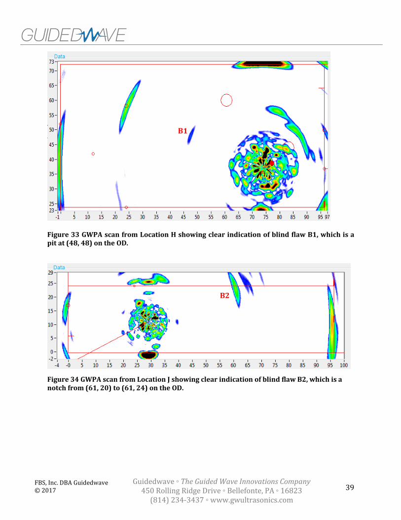
39 FBS, Inc. DBA Guidedwave © 2017
Guidedwave ◦ The Guided Wave Innovations Company 450 Rolling Ridge Drive ◦ Bellefonte, PA ◦ 16823
(814) 234-3437 ◦ www.gwultrasonics.com
Figure 33 GWPA scan from Location H showing clear indication of blind flaw B1, which is a pit at (48, 48) on the OD.
Figure 34 GWPA scan from Location J showing clear indication of blind flaw B2, which is a notch from (61, 20) to (61, 24) on the OD.
B1
B2

40 FBS, Inc. DBA Guidedwave © 2017
Guidedwave ◦ The Guided Wave Innovations Company 450 Rolling Ridge Drive ◦ Bellefonte, PA ◦ 16823
(814) 234-3437 ◦ www.gwultrasonics.com
7. Discussion/Conclusions
Flaw Detection and Characterization
1. The GWPA technology provides a 360° inspection at each location, which is paramount when there is limited access for scanning. Without the capability of 360° inspection, many defects can be missed due to their geometry and incident angle relative to the probe. This is a common problem with guided wave scanners where the beam is only sent out perpendicular to the scanning direction. 360° scanning gives multiple shots on any defects from multiple angles and distances, increasing the likelihood of detection. The composite imaging compiles these scans to further improve detection capabilities and aid the user in data interpretation.
2. All the flaws were identified on both mockups with the exception of the 10% wall thinning (Technology Screening mockup) and the 20% wall thinning (Sensor Effectiveness Testing mockup).
3. In reality, true wall thinning defects may be detectable at these levels, since the geometry of the wall thinning flaws was a major factor leading to the difficulty of the system to detect them.
4. Flaw detection was achieved for nearly all defects without changing data collection settings or moving the probe from the predetermined scan grid.
5. The composite image of the plate and the selected composite images of the welds provided excellent, easy-to-interpret images showing nearly all of the detectable flaws.
6. Both blind flaws were detected easily, quickly, and accurately, which attests to the power of the GWPA technology for real inspection scenarios. In fact, Guidedwave hopes that PNNL plans to conduct full-blind testing at some point in the near future.
7. Flaw sizing was not evaluated during testing, but it should be possible to characterize the extent of the flaws in the X-Y plane by analyzing the composite images, which provide data on the flaws from various angles. Furthermore, the depth of the flaws may likely be characterized to some extent by analyzing the amplitude of the reflections. Guidedwave is currently developing sizing routines for the GWPA technology that utilize weld reflections to apply time-compensated gain (TCG) to the data, which can then be analyzed for flaw sizing purposes.
Signal Quality and Noise Levels
8. The general data quality was excellent, and a detection range of up to 5-7 feet in all directions around the probe was demonstrated. The SNR of the defects was typically in the 20-45 dB range for the individual scans and 10-20 dB range for the composite images.

41 FBS, Inc. DBA Guidedwave © 2017
Guidedwave ◦ The Guided Wave Innovations Company 450 Rolling Ridge Drive ◦ Bellefonte, PA ◦ 16823
(814) 234-3437 ◦ www.gwultrasonics.com
9. Due to the 360° scan capabilities of the GWPA, as well as the composite imaging capabilities, defect orientation and air slot restrictions had minimal effect on the detection capabilities during testing.
10. The greatest challenges with defect detection and noise reduction in either mockup were due to free plate edges, which cause significant additional noise and artifacts, even with the T-tape. Additional challenges were present due to the small edge plates, which led to limited access and additional reverberations that would not be present in the real structures.
Surface Preparation
11. The dirt tests demonstrated that the GWPA scan SNR was unaffected by the surface contamination, although the standard deviation was greater, which could mean there is more variability possible in coupling.
12. The rust tests demonstrated that the GWPA scan SNR was unaffected by the three levels of surface corrosion considered during testing.
13. Based on performance during the dirt and rust tests and discussions will PNNL and WRPS personnel regarding surface condition in the air slots, it is very likely that little to no surface preparation will be required for GWPA inspection of the Hanford DSL primary liner floors, barring any significant deviation between the surface conditions present in the field and those anticipated by PNNL and WRPS personnel.
14. Although not tested here, the selected mode would be insensitive to fluids on either plate surface, whereas non-SH guided wave modes could experience significant attenuation due to fluids. It is also likely feasible to deploy the GWPA technology on the ID of the tank if the liquid level is reduced low enough to allow for couplant dispensing on the surface.
Transducer Requirements
15. The internal sensor array of the GWPA sensors can be made small enough to meet the space limitations of the primary liner access channels. Guidedwave brought a smaller probe as an example of this capability during testing. Guidedwave works with Olympus NDT to fabricate the GWPA probes to spec. The smallest slot design may require further modifications, such as reducing the total number of elements.
16. One of the potential challenges with deploying the GWPA technology robotically is coupling the probe. Guidedwave demonstrated that a couplant dispenser is practical using only vertical actuation and a couplant dispensing cylinder. It may also be possible to dispense the couplant through ports on the probe between the element faceplates.
17. Linear pushing would be required. One linear actuator would be necessary to actuate the probe upward, and a second would be necessary to either push the probe away from the surface or drive a small wedge between the probe and the plate. No rotation or sliding would be necessary.

42 FBS, Inc. DBA Guidedwave © 2017
Guidedwave ◦ The Guided Wave Innovations Company 450 Rolling Ridge Drive ◦ Bellefonte, PA ◦ 16823
(814) 234-3437 ◦ www.gwultrasonics.com
18. Tests have shown that very little force is required to couple the probe to the structure. Tests were conducted with no application force, 5 lbs, 10 lbs, 15 lbs, and 20 lbs, and the results were nearly identical.
19. No transducer power is required other than the ultrasonic pulser signals.
20. The transducer requires neither permanent magnets nor electromagnets.
Vision for the System
21. It is envisioned that the probe will be deployed on the robotic crawler with a cable extending to the surface, where the UltraWave data acquisition unit, the control laptop, and all other components will be located. This exposes as little of the system as possible to the elevated radiation levels in the tank annulus.
22. It is envisioned that coupling of the probe will be achieved by dispensing couplant with a pneumatic or electric dispenser through either a separate couplant delivery head or through ports in the probe face. The couplant reservoir can be kept locally on the crawler to minimize the distance over which it must be pumped.
23. It is envisioned that the probe can be pressed against the underside of the primary tank liner floor using a linear actuator. The probe can be removed from the surface by pressing a second actuator against the primary tank liner floor. No rotation or sliding of the probe would be necessary. Data would be collected this way in approximately 1-2 foot increments, although this could be increased or decreased as needed based on tank floor geometry, critical flaw sizes, and conditions in the real test environment.
24. The UltraWave system and associated hardware components are already commercially-available and are ruggedized for battery-powered field deployment. The UltraWave unit is CE, RoHS, and WEEE certified and is IP54 rated. The probes are produced by Olympus NDT and use their proven OmniScan connector and cabling; they are also water-resistant, although they have not yet undergone IP54 testing.
25. The GWPA software development is on-going. The primary functionality of the software is in place, which is evidenced by the fact that the data was collected and analyzed in this software during the Sensor Effectiveness Testing. However, additional functionality and improvements are still being incorporated.
26. The technology would be applicable to plates having thicknesses of 1” or less in its current form. Optimizing the system for other thicknesses is only a matter of attaching a different probe.
27. The UltraWave LRT data acquisition unit is approximately 9.8 x 6 x 15.7 inches and 16 lbs; this will be located on the surface. The GWPA probe is targeted to weigh less than 10 oz and have dimensions that will allow it to be deployed in any of the Hanford air slots, although the smallest slot design may require further modifications, such as reducing the total number of elements. The target data cable diameter will be less than ¼ inch.

43 FBS, Inc. DBA Guidedwave © 2017
Guidedwave ◦ The Guided Wave Innovations Company 450 Rolling Ridge Drive ◦ Bellefonte, PA ◦ 16823
(814) 234-3437 ◦ www.gwultrasonics.com
28. No transducer power is required other than the ultrasonic pulser signals. The data acquisition unit is powered by two Li-ion OmniScan batteries. The laptop is also battery-powered.
29. No permanent magnets are required as any part of the system.
30. It is envisioned that the UltraWave data acquisition unit and the control laptop would be located on the surface. Based on the signal amplitudes and past experience with piezoelectric-based guided wave inspections, the cable range limitations do not currently pose a concern. If, for some reason, signal amplitude did become an issue, one solution could be to place the UltraWave acquisition unit within the tank annulus instead of on the surface; this would require some radiation hardening, but should be feasible.

44 FBS, Inc. DBA Guidedwave © 2017
Guidedwave ◦ The Guided Wave Innovations Company 450 Rolling Ridge Drive ◦ Bellefonte, PA ◦ 16823
(814) 234-3437 ◦ www.gwultrasonics.com
Appendix A – Flaw Detection Images
Composite GWPA Scan Images – Sensor Effectiveness Testing Mockup
Figure 35 Composite image from Sensor Effectiveness Testing mockup showing detection of defects P4, P5, P6, P7, P8, P9, P10, N4, N6, N7, blind flaw B1, and blind flaw B2.
P6
P7
P8
B2
B1
P5
P4
N6
P9
P10
N7
N4
Weld repair

45 FBS, Inc. DBA Guidedwave © 2017
Guidedwave ◦ The Guided Wave Innovations Company 450 Rolling Ridge Drive ◦ Bellefonte, PA ◦ 16823
(814) 234-3437 ◦ www.gwultrasonics.com
Figure 36 Composite image of the transition weld showing detection of flaws N5, P7, P6, P11, and the heavily repaired weld area.
Figure 37 Composite image of the ½-to-½ inch at X = 96” showing detection of flaws N5, P7, P6, P11, and the heavily repaired weld area.
P6 P7 Weld repair P11 N5
N6 P9 P10 N7 N4

46 FBS, Inc. DBA Guidedwave © 2017
Guidedwave ◦ The Guided Wave Innovations Company 450 Rolling Ridge Drive ◦ Bellefonte, PA ◦ 16823
(814) 234-3437 ◦ www.gwultrasonics.com
Individual GWPA Scan Images – Sensor Effectiveness Testing Mockup
Figure 38 Location A (Probe 1 @ 160 kHz)

47 FBS, Inc. DBA Guidedwave © 2017
Guidedwave ◦ The Guided Wave Innovations Company 450 Rolling Ridge Drive ◦ Bellefonte, PA ◦ 16823
(814) 234-3437 ◦ www.gwultrasonics.com
Figure 39 Location B (Probe 1 @ 160 kHz)

48 FBS, Inc. DBA Guidedwave © 2017
Guidedwave ◦ The Guided Wave Innovations Company 450 Rolling Ridge Drive ◦ Bellefonte, PA ◦ 16823
(814) 234-3437 ◦ www.gwultrasonics.com
Figure 40 Location C (Probe 1 @ 160 kHz)

49 FBS, Inc. DBA Guidedwave © 2017
Guidedwave ◦ The Guided Wave Innovations Company 450 Rolling Ridge Drive ◦ Bellefonte, PA ◦ 16823
(814) 234-3437 ◦ www.gwultrasonics.com
Figure 41 Location D (Probe 1 @ 160 kHz)

50 FBS, Inc. DBA Guidedwave © 2017
Guidedwave ◦ The Guided Wave Innovations Company 450 Rolling Ridge Drive ◦ Bellefonte, PA ◦ 16823
(814) 234-3437 ◦ www.gwultrasonics.com
Figure 42 Location E (Probe 1 @ 160 kHz)

51 FBS, Inc. DBA Guidedwave © 2017
Guidedwave ◦ The Guided Wave Innovations Company 450 Rolling Ridge Drive ◦ Bellefonte, PA ◦ 16823
(814) 234-3437 ◦ www.gwultrasonics.com
Figure 43 Location F (Probe 1 @ 160 kHz)

52 FBS, Inc. DBA Guidedwave © 2017
Guidedwave ◦ The Guided Wave Innovations Company 450 Rolling Ridge Drive ◦ Bellefonte, PA ◦ 16823
(814) 234-3437 ◦ www.gwultrasonics.com
Figure 44 Location G (Probe 1 @ 160 kHz)

53 FBS, Inc. DBA Guidedwave © 2017
Guidedwave ◦ The Guided Wave Innovations Company 450 Rolling Ridge Drive ◦ Bellefonte, PA ◦ 16823
(814) 234-3437 ◦ www.gwultrasonics.com
Figure 45 Location H (Probe 1 @ 160 kHz)

54 FBS, Inc. DBA Guidedwave © 2017
Guidedwave ◦ The Guided Wave Innovations Company 450 Rolling Ridge Drive ◦ Bellefonte, PA ◦ 16823
(814) 234-3437 ◦ www.gwultrasonics.com
Figure 46 Location I (Probe 1 @ 160 kHz)

55 FBS, Inc. DBA Guidedwave © 2017
Guidedwave ◦ The Guided Wave Innovations Company 450 Rolling Ridge Drive ◦ Bellefonte, PA ◦ 16823
(814) 234-3437 ◦ www.gwultrasonics.com
Figure 47 Location J (Probe 1 @ 160 kHz)
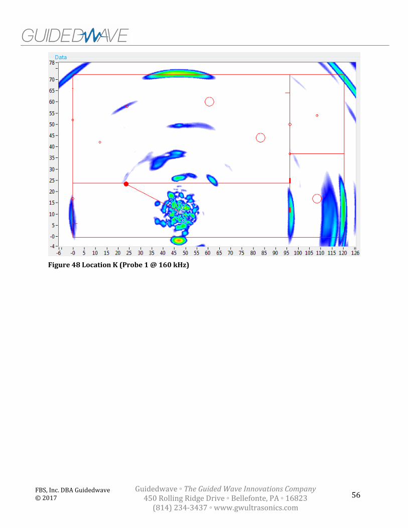
56 FBS, Inc. DBA Guidedwave © 2017
Guidedwave ◦ The Guided Wave Innovations Company 450 Rolling Ridge Drive ◦ Bellefonte, PA ◦ 16823
(814) 234-3437 ◦ www.gwultrasonics.com
Figure 48 Location K (Probe 1 @ 160 kHz)

57 FBS, Inc. DBA Guidedwave © 2017
Guidedwave ◦ The Guided Wave Innovations Company 450 Rolling Ridge Drive ◦ Bellefonte, PA ◦ 16823
(814) 234-3437 ◦ www.gwultrasonics.com
Figure 49 Location L (Probe 1 @ 160 kHz)

58 FBS, Inc. DBA Guidedwave © 2017
Guidedwave ◦ The Guided Wave Innovations Company 450 Rolling Ridge Drive ◦ Bellefonte, PA ◦ 16823
(814) 234-3437 ◦ www.gwultrasonics.com
Figure 50 Location M (Probe 1 @ 160 kHz)

59 FBS, Inc. DBA Guidedwave © 2017
Guidedwave ◦ The Guided Wave Innovations Company 450 Rolling Ridge Drive ◦ Bellefonte, PA ◦ 16823
(814) 234-3437 ◦ www.gwultrasonics.com
Figure 51 Location N (Probe 1 @ 160 kHz)

60 FBS, Inc. DBA Guidedwave © 2017
Guidedwave ◦ The Guided Wave Innovations Company 450 Rolling Ridge Drive ◦ Bellefonte, PA ◦ 16823
(814) 234-3437 ◦ www.gwultrasonics.com
Figure 52 Location P (Probe 1 @ 160 kHz)

61 FBS, Inc. DBA Guidedwave © 2017
Guidedwave ◦ The Guided Wave Innovations Company 450 Rolling Ridge Drive ◦ Bellefonte, PA ◦ 16823
(814) 234-3437 ◦ www.gwultrasonics.com
Figure 53 Location R (Probe 1 @ 160 kHz)

62 FBS, Inc. DBA Guidedwave © 2017
Guidedwave ◦ The Guided Wave Innovations Company 450 Rolling Ridge Drive ◦ Bellefonte, PA ◦ 16823
(814) 234-3437 ◦ www.gwultrasonics.com
Figure 54 Location S (Probe 1 @ 160 kHz)

63 FBS, Inc. DBA Guidedwave © 2017
Guidedwave ◦ The Guided Wave Innovations Company 450 Rolling Ridge Drive ◦ Bellefonte, PA ◦ 16823
(814) 234-3437 ◦ www.gwultrasonics.com
Figure 55 Location C (Probe 1 @ 200 kHz)

64 FBS, Inc. DBA Guidedwave © 2017
Guidedwave ◦ The Guided Wave Innovations Company 450 Rolling Ridge Drive ◦ Bellefonte, PA ◦ 16823
(814) 234-3437 ◦ www.gwultrasonics.com
Figure 56 Location M (Probe 1 @ 200 kHz)

65 FBS, Inc. DBA Guidedwave © 2017
Guidedwave ◦ The Guided Wave Innovations Company 450 Rolling Ridge Drive ◦ Bellefonte, PA ◦ 16823
(814) 234-3437 ◦ www.gwultrasonics.com
Figure 57 Location thinning2 (Probe 2 @ 225 kHz)

66 FBS, Inc. DBA Guidedwave © 2017
Guidedwave ◦ The Guided Wave Innovations Company 450 Rolling Ridge Drive ◦ Bellefonte, PA ◦ 16823
(814) 234-3437 ◦ www.gwultrasonics.com
Figure 58 Location GG (Probe 2 @ 225 kHz)

67 FBS, Inc. DBA Guidedwave © 2017
Guidedwave ◦ The Guided Wave Innovations Company 450 Rolling Ridge Drive ◦ Bellefonte, PA ◦ 16823
(814) 234-3437 ◦ www.gwultrasonics.com
Figure 59 Location HH (Probe 2 @ 225 kHz)

68 FBS, Inc. DBA Guidedwave © 2017
Guidedwave ◦ The Guided Wave Innovations Company 450 Rolling Ridge Drive ◦ Bellefonte, PA ◦ 16823
(814) 234-3437 ◦ www.gwultrasonics.com
Figure 60 Location II (Probe 2 @ 225 kHz)

69 FBS, Inc. DBA Guidedwave © 2017
Guidedwave ◦ The Guided Wave Innovations Company 450 Rolling Ridge Drive ◦ Bellefonte, PA ◦ 16823
(814) 234-3437 ◦ www.gwultrasonics.com
Composite GWPA Scan Images – Technology Screening Mockup
Figure 61 Composite image from Technology Screening mockup showing detection of flaws P2, P3, N1, N2, and N3, as well as many flaws from the original Technology Screening tests; the scan locations used to compile this composite image are shown as black dots.

70 FBS, Inc. DBA Guidedwave © 2017
Guidedwave ◦ The Guided Wave Innovations Company 450 Rolling Ridge Drive ◦ Bellefonte, PA ◦ 16823
(814) 234-3437 ◦ www.gwultrasonics.com
Individual GWPA Scan Images – Technology Screening Mockup
Figure 62 Location T (Probe 1 @ 160 kHz)
Figure 63 Location U (Probe 1 @ 160 kHz)

71 FBS, Inc. DBA Guidedwave © 2017
Guidedwave ◦ The Guided Wave Innovations Company 450 Rolling Ridge Drive ◦ Bellefonte, PA ◦ 16823
(814) 234-3437 ◦ www.gwultrasonics.com
Figure 64 Location V (Probe 1 @ 160 kHz)
Figure 65 Location W (Probe 1 @ 160 kHz)

72 FBS, Inc. DBA Guidedwave © 2017
Guidedwave ◦ The Guided Wave Innovations Company 450 Rolling Ridge Drive ◦ Bellefonte, PA ◦ 16823
(814) 234-3437 ◦ www.gwultrasonics.com
Figure 66 Location X (Probe 1 @ 160 kHz)
Figure 67 Location Y (Probe 1 @ 160 kHz)

73 FBS, Inc. DBA Guidedwave © 2017
Guidedwave ◦ The Guided Wave Innovations Company 450 Rolling Ridge Drive ◦ Bellefonte, PA ◦ 16823
(814) 234-3437 ◦ www.gwultrasonics.com
Figure 68 Location Z (Probe 1 @ 160 kHz)
Figure 69 Location FF (Probe 1 @ 160 kHz)

74 FBS, Inc. DBA Guidedwave © 2017
Guidedwave ◦ The Guided Wave Innovations Company 450 Rolling Ridge Drive ◦ Bellefonte, PA ◦ 16823
(814) 234-3437 ◦ www.gwultrasonics.com
Appendix B – Dirt Test Images
Clean Surface Condition GWPA Scan Images
Figure 70 First clean surface condition scan at Location EE-1 (12, 38) (Probe 1 @ 160 kHz)

75 FBS, Inc. DBA Guidedwave © 2017
Guidedwave ◦ The Guided Wave Innovations Company 450 Rolling Ridge Drive ◦ Bellefonte, PA ◦ 16823
(814) 234-3437 ◦ www.gwultrasonics.com
Figure 71 Second clean surface condition scan at Location EE-1 (12, 38) (Probe 1 @ 160 kHz)

76 FBS, Inc. DBA Guidedwave © 2017
Guidedwave ◦ The Guided Wave Innovations Company 450 Rolling Ridge Drive ◦ Bellefonte, PA ◦ 16823
(814) 234-3437 ◦ www.gwultrasonics.com
Figure 72 First clean surface condition scan at Location EE-2 (12, 35) (Probe 1 @ 160 kHz)

77 FBS, Inc. DBA Guidedwave © 2017
Guidedwave ◦ The Guided Wave Innovations Company 450 Rolling Ridge Drive ◦ Bellefonte, PA ◦ 16823
(814) 234-3437 ◦ www.gwultrasonics.com
Figure 73 Second clean surface condition scan at Location EE-2 (12, 35) (Probe 1 @ 160 kHz)

78 FBS, Inc. DBA Guidedwave © 2017
Guidedwave ◦ The Guided Wave Innovations Company 450 Rolling Ridge Drive ◦ Bellefonte, PA ◦ 16823
(814) 234-3437 ◦ www.gwultrasonics.com
Figure 74 First clean surface condition scan at Location EE-3 (12, 41) (Probe 1 @ 160 kHz)
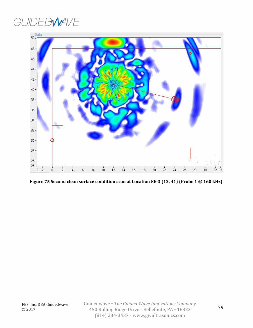
79 FBS, Inc. DBA Guidedwave © 2017
Guidedwave ◦ The Guided Wave Innovations Company 450 Rolling Ridge Drive ◦ Bellefonte, PA ◦ 16823
(814) 234-3437 ◦ www.gwultrasonics.com
Figure 75 Second clean surface condition scan at Location EE-3 (12, 41) (Probe 1 @ 160 kHz)

80 FBS, Inc. DBA Guidedwave © 2017
Guidedwave ◦ The Guided Wave Innovations Company 450 Rolling Ridge Drive ◦ Bellefonte, PA ◦ 16823
(814) 234-3437 ◦ www.gwultrasonics.com
Dirty Surface Condition GWPA Scan Images
Figure 76 First dirty surface condition scan at Location EE-1 (12, 38) (Probe 1 @ 160 kHz)

81 FBS, Inc. DBA Guidedwave © 2017
Guidedwave ◦ The Guided Wave Innovations Company 450 Rolling Ridge Drive ◦ Bellefonte, PA ◦ 16823
(814) 234-3437 ◦ www.gwultrasonics.com
Figure 77 Second dirty surface condition scan at Location EE-1 (12, 38) (Probe 1 @ 160 kHz)

82 FBS, Inc. DBA Guidedwave © 2017
Guidedwave ◦ The Guided Wave Innovations Company 450 Rolling Ridge Drive ◦ Bellefonte, PA ◦ 16823
(814) 234-3437 ◦ www.gwultrasonics.com
Figure 78 First dirty surface condition scan at Location EE-3 (12, 41) (Probe 1 @ 160 kHz)

83 FBS, Inc. DBA Guidedwave © 2017
Guidedwave ◦ The Guided Wave Innovations Company 450 Rolling Ridge Drive ◦ Bellefonte, PA ◦ 16823
(814) 234-3437 ◦ www.gwultrasonics.com
Figure 79 Second dirty surface condition scan at Location EE-3 (12, 41) (Probe 1 @ 160 kHz)

84 FBS, Inc. DBA Guidedwave © 2017
Guidedwave ◦ The Guided Wave Innovations Company 450 Rolling Ridge Drive ◦ Bellefonte, PA ◦ 16823
(814) 234-3437 ◦ www.gwultrasonics.com
Figure 80 First dirty surface condition scan at Location EE-3 (12, 48) (Probe 1 @ 160 kHz)

85 FBS, Inc. DBA Guidedwave © 2017
Guidedwave ◦ The Guided Wave Innovations Company 450 Rolling Ridge Drive ◦ Bellefonte, PA ◦ 16823
(814) 234-3437 ◦ www.gwultrasonics.com
Figure 81 Second dirty surface condition scan at Location EE-3 (12, 48) (Probe 1 @ 160 kHz)

86 FBS, Inc. DBA Guidedwave © 2017
Guidedwave ◦ The Guided Wave Innovations Company 450 Rolling Ridge Drive ◦ Bellefonte, PA ◦ 16823
(814) 234-3437 ◦ www.gwultrasonics.com
Appendix C – Rust Test Images
Level 1 Surface Rust GWPA Scan Images
Figure 82 First surface corrosion Level 1 test 12" from free edge (Probe 1 @ 160 kHz)
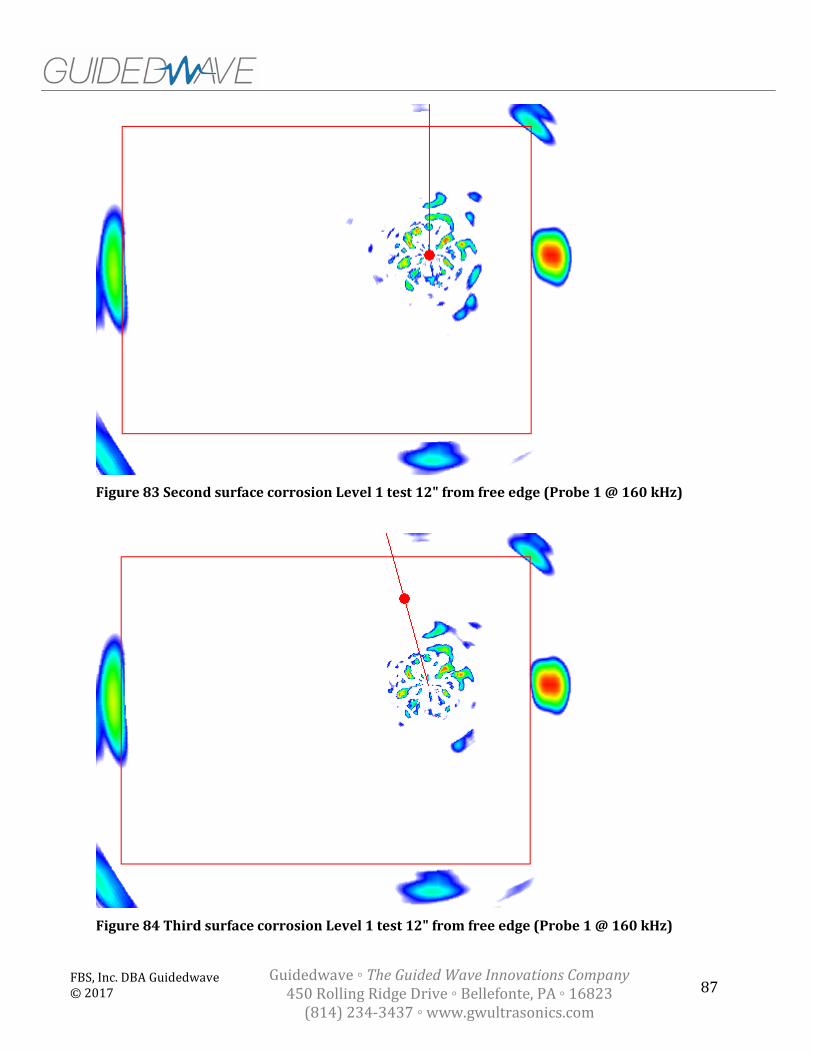
87 FBS, Inc. DBA Guidedwave © 2017
Guidedwave ◦ The Guided Wave Innovations Company 450 Rolling Ridge Drive ◦ Bellefonte, PA ◦ 16823
(814) 234-3437 ◦ www.gwultrasonics.com
Figure 83 Second surface corrosion Level 1 test 12" from free edge (Probe 1 @ 160 kHz)
Figure 84 Third surface corrosion Level 1 test 12" from free edge (Probe 1 @ 160 kHz)
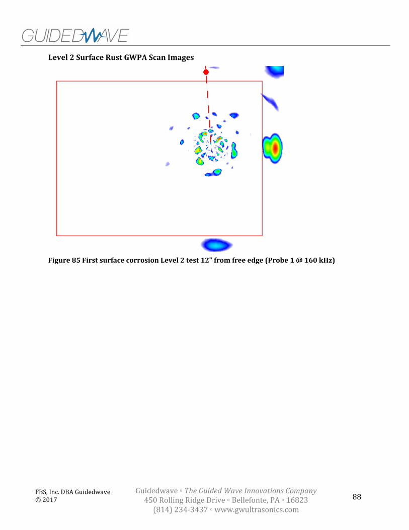
88 FBS, Inc. DBA Guidedwave © 2017
Guidedwave ◦ The Guided Wave Innovations Company 450 Rolling Ridge Drive ◦ Bellefonte, PA ◦ 16823
(814) 234-3437 ◦ www.gwultrasonics.com
Level 2 Surface Rust GWPA Scan Images
Figure 85 First surface corrosion Level 2 test 12" from free edge (Probe 1 @ 160 kHz)

89 FBS, Inc. DBA Guidedwave © 2017
Guidedwave ◦ The Guided Wave Innovations Company 450 Rolling Ridge Drive ◦ Bellefonte, PA ◦ 16823
(814) 234-3437 ◦ www.gwultrasonics.com
Figure 86 Second surface corrosion Level 2 test 12" from free edge (Probe 1 @ 160 kHz)
Figure 87 Third surface corrosion Level 2 test 12" from free edge (Probe 1 @ 160 kHz)
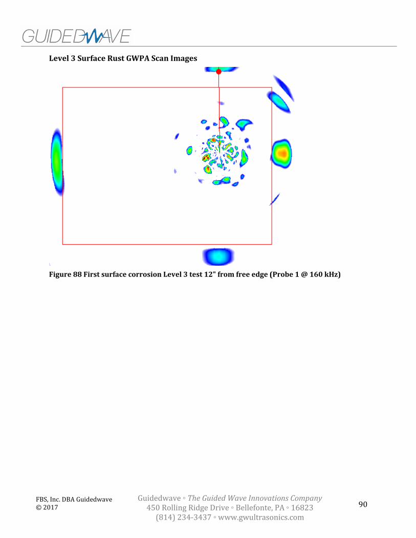
90 FBS, Inc. DBA Guidedwave © 2017
Guidedwave ◦ The Guided Wave Innovations Company 450 Rolling Ridge Drive ◦ Bellefonte, PA ◦ 16823
(814) 234-3437 ◦ www.gwultrasonics.com
Level 3 Surface Rust GWPA Scan Images
Figure 88 First surface corrosion Level 3 test 12" from free edge (Probe 1 @ 160 kHz)
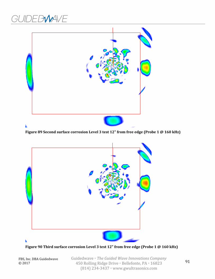
91 FBS, Inc. DBA Guidedwave © 2017
Guidedwave ◦ The Guided Wave Innovations Company 450 Rolling Ridge Drive ◦ Bellefonte, PA ◦ 16823
(814) 234-3437 ◦ www.gwultrasonics.com
Figure 89 Second surface corrosion Level 3 test 12" from free edge (Probe 1 @ 160 kHz)
Figure 90 Third surface corrosion Level 3 test 12" from free edge (Probe 1 @ 160 kHz)

92 FBS, Inc. DBA Guidedwave © 2017
Guidedwave ◦ The Guided Wave Innovations Company 450 Rolling Ridge Drive ◦ Bellefonte, PA ◦ 16823
(814) 234-3437 ◦ www.gwultrasonics.com
Additional Surface Rust GWPA Scan Image on Vertical Plate
Figure 91 Additional surface corrosion test collected on vertical “wall” plate of Level 3 rust test mockup, 12" from free edge (Probe 1 @ 160 kHz)
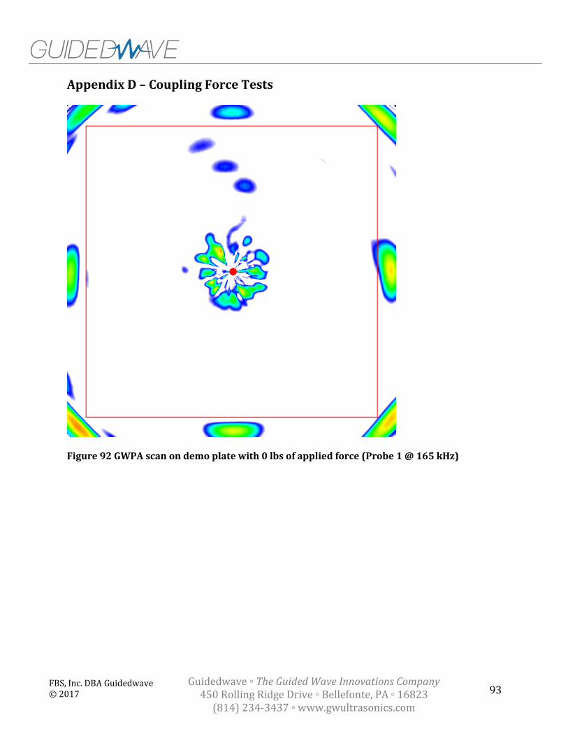
93 FBS, Inc. DBA Guidedwave © 2017
Guidedwave ◦ The Guided Wave Innovations Company 450 Rolling Ridge Drive ◦ Bellefonte, PA ◦ 16823
(814) 234-3437 ◦ www.gwultrasonics.com
Appendix D – Coupling Force Tests
Figure 92 GWPA scan on demo plate with 0 lbs of applied force (Probe 1 @ 165 kHz)

94 FBS, Inc. DBA Guidedwave © 2017
Guidedwave ◦ The Guided Wave Innovations Company 450 Rolling Ridge Drive ◦ Bellefonte, PA ◦ 16823
(814) 234-3437 ◦ www.gwultrasonics.com
Figure 93 GWPA scan on demo plate with 5 lbs of applied force (Probe 1 @ 165 kHz)

95 FBS, Inc. DBA Guidedwave © 2017
Guidedwave ◦ The Guided Wave Innovations Company 450 Rolling Ridge Drive ◦ Bellefonte, PA ◦ 16823
(814) 234-3437 ◦ www.gwultrasonics.com
Figure 94 GWPA scan on demo plate with 10 lbs of applied force (Probe 1 @ 165 kHz)

96 FBS, Inc. DBA Guidedwave © 2017
Guidedwave ◦ The Guided Wave Innovations Company 450 Rolling Ridge Drive ◦ Bellefonte, PA ◦ 16823
(814) 234-3437 ◦ www.gwultrasonics.com
Figure 95 GWPA scan on demo plate with 15 lbs of applied force (Probe 1 @ 165 kHz)
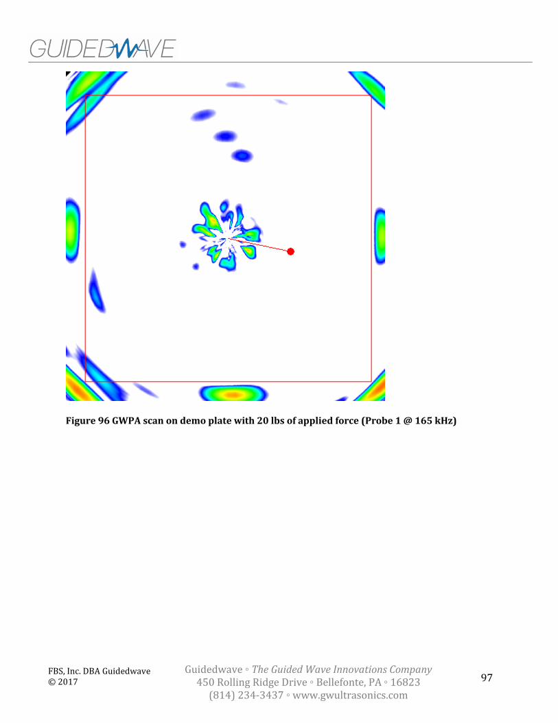
97 FBS, Inc. DBA Guidedwave © 2017
Guidedwave ◦ The Guided Wave Innovations Company 450 Rolling Ridge Drive ◦ Bellefonte, PA ◦ 16823
(814) 234-3437 ◦ www.gwultrasonics.com
Figure 96 GWPA scan on demo plate with 20 lbs of applied force (Probe 1 @ 165 kHz)

98 FBS, Inc. DBA Guidedwave © 2017
Guidedwave ◦ The Guided Wave Innovations Company 450 Rolling Ridge Drive ◦ Bellefonte, PA ◦ 16823
(814) 234-3437 ◦ www.gwultrasonics.com
Appendix E – Couplant Dispenser Test
Figure 97 GWPA scan on three-hole demo plate with remotely dispensed couplant (16-element probe C16O @ 165 kHz)

99 FBS, Inc. DBA Guidedwave © 2017
Guidedwave ◦ The Guided Wave Innovations Company 450 Rolling Ridge Drive ◦ Bellefonte, PA ◦ 16823
(814) 234-3437 ◦ www.gwultrasonics.com
Figure 98 GWPA scan on three-hole demo plate with manually applied couplant (16-element probe C16O @ 165 kHz)
FBS, Inc. DBA Guidedwave © 2016
Dry-Coupling for Guided Wave Phased Array Technology
Addendum to Hanford DST Sensor Effectiveness Testing report to demonstrate dry-coupling method for GWPA technology.
Subcontract #: 63295
performed for:
Washington River Protection Solutions, LLC
P.O. Box 850
Richland, WA 99352, USA
provided by:
Cody Borigo, [email protected]
Russell Love, [email protected]
Steven Owens [email protected]
Guidedwave
450 Rolling Ridge Drive
Bellefonte, PA, USA 16823
+1-814-234-3437
28 July, 2017

FBS, Inc. DBA Guidedwave © 2016 1
Guidedwave ◦ The Guided Wave Innovations Company 450 Rolling Ridge Drive ◦ Bellefonte, PA ◦ 16823
(814) 234-3437 ◦ www.gwultrasonics.com
Introduction
This document is an addendum to the Report on Guided Wave Phased Array Sensor Effectiveness Testing for Hanford DST Inspection, submitted on 28 June, 2017 to PNNL and WRPS. The purpose of this additional material is to demonstrate the capability to dry-couple the guided wave phased array (GWPA) probe, i.e. to collect GWPA data without the challenges associated with the shear couplant used with the technology during prior testing. The shear couplant was a concern for WRPS and PNNL due to the additional challenges associated with dispensing, applying, and cleaning the couplant during remote testing. The development of a dry-coupled solution will circumvent those challenges without reducing the effectiveness of the technology.

FBS, Inc. DBA Guidedwave © 2016 2
Guidedwave ◦ The Guided Wave Innovations Company 450 Rolling Ridge Drive ◦ Bellefonte, PA ◦ 16823
(814) 234-3437 ◦ www.gwultrasonics.com
Dry-Coupling Method
The method for dry-coupling the GWPA probe involves applying a layer of shear couplant to the probe face and then covering it with a sheet of thin aluminum foil (between 0.0005” and 0.0050” thick), as shown in Figure 1. The aluminum foil acts as a barrier between the couplant and the test surface, but still provides excellent coupling efficiency on rough or smooth surfaces when applied with a reasonable application force. Note that Guidedwave already utilizes aluminum foil couplant in a similar configuration (with the shear gel couplant layer) for normal- and high-temperature torsional wave magnetostrictive pipe inspection applications, with great success.
Figure 1 Process for preparing the "dry-coupled" GWPA probe; (left) a small sheet of aluminum foil is prepared; (center) a thin layer of shear couplant is applied to the probe face; and (right) the aluminum foil is placed over the shear couplant.
Despite the use of a shear couplant intermediary layer, this method is, for all intents and purposes, dry-coupling due to the way in which it is implemented. The aluminum foil barrier allows the probe to be used repeatedly without reapplying the couplant or needing any cleanup, since the couplant never touches the test surface. Guidedwave can manufacture easy-to-apply prepared couplant/foil sheets for easy replacement in the field. Also, since the couplant no longer needs to be dispensed or spread manually, a more-viscous formulation can be used that provides improved signal strength over a wider range of temperatures than the standard shear gel couplant.

FBS, Inc. DBA Guidedwave © 2016 3
Guidedwave ◦ The Guided Wave Innovations Company 450 Rolling Ridge Drive ◦ Bellefonte, PA ◦ 16823
(814) 234-3437 ◦ www.gwultrasonics.com
Mockup Test Results
To characterize the performance of the new coupling methods, comparison tests were conducted on the new dry-coupled configuration and the conventional shear gel-coupled configuration that was used during testing at PNNL. The test specimen was a 48” x 48” x 0.080” aluminum panel with three manufactured flaws, as shown in Figure 3. The flaws included a 0.65” x 0.05” notch, a 0.25”-diameter through hole, and a 0.375”-diameter through hole. Data was collected with the probe in the center of the plate and 25 dB of receiver gain; this is approximately 20 dB less than was used during testing at PNNL, due to the smaller size of the test structure.
Figure 2 Drawing of the test panel used for couplant method comparison testing; the panel includes three manufactured flaws: two holes and one notch.
Figure 3 compares the GWPA images for both coupling methods (“shear gel” vs. “dry”) normalized to 12 dB above the edge reflection amplitude. Not only is the signal quality comparable to the conventional gel coupling, but it is actually improved in some respects. The signal-to-noise ratio (SNR) of the notch is 47 dB for both scans and the SNR of the holes is 32.4 dB with shear gel vs. 33.7 with dry coupling. The dead zone radius is slightly larger with the dry coupling, at 5.5” vs. 5.2”, but the sidelobe artifacts caused by the notch defect,

FBS, Inc. DBA Guidedwave © 2016 4
Guidedwave ◦ The Guided Wave Innovations Company 450 Rolling Ridge Drive ◦ Bellefonte, PA ◦ 16823
(814) 234-3437 ◦ www.gwultrasonics.com
which appear as additional indications between the two hole defects and the probe, are reduced substantially. Figure 4 compares the same two scans with the C-filter applied.
Figure 3 Comparison of the GWPA scan using the conventional shear couplant method (left) and the new dry-coupled method (right).
Shear Couplant Dry-Coupled

FBS, Inc. DBA Guidedwave © 2016 5
Guidedwave ◦ The Guided Wave Innovations Company 450 Rolling Ridge Drive ◦ Bellefonte, PA ◦ 16823
(814) 234-3437 ◦ www.gwultrasonics.com
Figure 4 Comparison of the GWPA scan using the conventional shear couplant method (left) and the new dry-coupled method (right).
Guidedwave is going to conduct further testing to optimize the foil thickness, comparison test on various surfaces, and designing an easy-to-apply prepared foil/couplant system for even easier field use.
Dry-Coupled, C-Filtered Shear Couplant, C-Filtered

FBS, Inc. DBA Guidedwave © 2016 6
Guidedwave ◦ The Guided Wave Innovations Company 450 Rolling Ridge Drive ◦ Bellefonte, PA ◦ 16823
(814) 234-3437 ◦ www.gwultrasonics.com
Force Requirements
Tests were conducted with the dry-coupling mechanism using varying static loads applied to the back of the probe. Loads of from 5 to 50 lbs were applied 5 lb increments, and the signal attributes were compared to each other and those of a probe coupled directly with shear gel couplant. Figure 5 compares the plate edge and notch defect SNR for the two coupling mechanisms versus load. For this measurement, a higher value is better. The shear gel-coupled probe SNR was generally independent of applied load, while the dry-coupled probe SNR increased with load, but leveled off near the values for the gel-coupled probe near 40 lbs.
Figure 5 Edge and notch SNR values (in dB) for both coupling mechanisms versus load.
20
25
30
35
40
45
50
55
60
0 10 20 30 40 50 60
Re
fle
ctio
n S
NR
(d
B)
Applied Load (lbs)
Edge and Notch SNR
Dry Coupling - Edge SNR
Shear Couplant - Edge SNR
Dry Coupling - Notch SNR
Shear Couplant - Notch SNR

FBS, Inc. DBA Guidedwave © 2016 7
Guidedwave ◦ The Guided Wave Innovations Company 450 Rolling Ridge Drive ◦ Bellefonte, PA ◦ 16823
(814) 234-3437 ◦ www.gwultrasonics.com
Figure 6 compares the maximum raw signal amplitude from the notch reflection (in mV), measured prior to phased array post-processing, for the two coupling mechanisms versus load. For this measurement, a higher value is better. The shear gel-coupled probe signal amplitude gradually decreased with load, but started at a high level, while the dry-coupled probe signal amplitude increased monotonically with load.
Figure 6 Max raw signal amplitude from the notch reflection for both coupling mechanisms versus load.
0
50
100
150
200
250
300
350
0 10 20 30 40 50 60
Raw
No
tch
Re
fle
ctio
n A
mp
litu
de
(m
V)
Applied Load (lbs)
Raw Notch Signal Amplitude
Dry Coupling - Notch SignalAmplitude
Shear Couplant - Notch SignalAmplitude

FBS, Inc. DBA Guidedwave © 2016 8
Guidedwave ◦ The Guided Wave Innovations Company 450 Rolling Ridge Drive ◦ Bellefonte, PA ◦ 16823
(814) 234-3437 ◦ www.gwultrasonics.com
Figure 7 compares the sidelobe amplitude from the notch reflection for the two coupling mechanisms versus load. For this measurement, a lower value is better. The shear gel-coupled probe sidelobes were stronger and got worse with load, while the dry-coupled probe sidelobes were weaker and generally improved with load.
Figure 7 Sidelobe amplitude for both coupling conditions versus load.
-25
-20
-15
-10
-5
0
0 10 20 30 40 50 60
Sid
elo
be
Am
plit
ud
e (
dB
)
Applied Load (lbs)
Sidelobe Amplitude
Dry Coupling - SidelobeAmplitude
Shear Couplant - SidelobeAmplitude

FBS, Inc. DBA Guidedwave © 2016 9
Guidedwave ◦ The Guided Wave Innovations Company 450 Rolling Ridge Drive ◦ Bellefonte, PA ◦ 16823
(814) 234-3437 ◦ www.gwultrasonics.com
Figure 8 compares the dead zone radius for the two coupling mechanisms versus load. For this measurement, a lower value is better. The shear gel-coupled probe dead zone was small and constant with load, while the dry-coupled probe dead zone was larger and rapidly decreased with load, approaching the value for the gel-coupled probe around 50 lbs.
Figure 8 Dead zone radius for both coupling mechanisms versus load.
0
2
4
6
8
10
12
14
0 10 20 30 40 50 60
De
ad Z
on
e R
adiu
s (i
nch
es)
Applied Load (lbs)
Dead Zone Radius
Dry Coupling - Dead Zone
Shear Couplant - Dead Zone

FBS, Inc. DBA Guidedwave © 2016 10
Guidedwave ◦ The Guided Wave Innovations Company 450 Rolling Ridge Drive ◦ Bellefonte, PA ◦ 16823
(814) 234-3437 ◦ www.gwultrasonics.com
Shear Couplant Corrosion Effects
While we are still waiting to receive a response from the manufacturer of a commercially-available shear gel couplant regarding corrosion-causing compounds, we did find some general information that appears to demonstrate that there should be no corrosion concerns from the couplant, if any were to contact the surface. The manufacturer’s data sheet claims that the shear gel couplant features “very good corrosion inhibition”. Further study revealed a general consensus that honey is actually an excellent corrosion inhibitor for many metals; remember that the shear gel couplant is simply processed honey. For instance, see A.Y. El-Etre and M. Abdallah, “Natural honey as corrosion inhibitor for metals and alloys. II. C-steel in high saline water”, Corrosion Science, 42(4), 2000, pp. 731-738.

FBS, Inc. DBA Guidedwave © 2016 11
Guidedwave ◦ The Guided Wave Innovations Company 450 Rolling Ridge Drive ◦ Bellefonte, PA ◦ 16823
(814) 234-3437 ◦ www.gwultrasonics.com
Summary
The new dry coupling method for the GWPA technology further improves an already excellent NDT technique and eliminates the need for remote couplant dispensing, application, or cleanup during remote testing on the Hanford DST primary liner floors. The couplant and foil sheet can be easily applied on the surface prior to probe deployment, and the prepared probe can be used repeatedly without reapplying any couplant by simply pressing the probe against the test surface with minimal force. There is no cleanup involved since the couplant never touches the test surface, and if the coupling needs to be reapplied after a series of tests, it’s as simple as peeling off the old couplant sheet and applying a new one. If any couplant does get onto the steel test surface, the residual couplant can be left in place since it is a corrosion inhibitor. The performance of the probe with the dry coupling versus gel coupling generally improves with applied load, nearing the values for the gel-coupled probe at 40-50 lbs of force for the key signal characteristics. This is a major improvement in the GWPA technology and allows it to be remotely deployed for primary liner floor inspection with great ease.

Appendix B –
Innerspec

Page 1 of 51 ISO 9001:2008 Registered
June 30, 2017
Ms. Kayte Denslow Mr. Bill Glass PNNL
NDE Technology Development Program for Hanford DST Non-Visual Volumetric Inspection Technology: Sensor Effectiveness Testing Report from Innerspec Technologies
Dear Ms. Denslow and Mr. Glass, Thank you for your invitation to demonstrate our technology and capabilities on the DST mockups during Sensor Effectiveness Testing Phase. This document provides additional information and details of the results. Both mockups were tested using two different techniques which were initially screened in the phase-I of the project which including EMAT-generated Shear Horizontal waves (SH0) using a magnetostrictive strip and EMAT-generated Shear Vertical waves (SV) in pulse-echo configuration. The generation of SH0 waves using magnetostrictive patch was tested in a more practical manner by using a 50 lbs. weight as a coupling mechanism instead of using a double-stick tape to adhere the strip to the metal. The weight can be substituted with air-filled bladder to provide an equivalent force of 50 pounds in the real inspection. We also tested EMAT-generated Shear Vertical waves (SV) in pulse-echo configuration using a pulsed-dc electromagnet which facilitates scanning and provides better signal to noise. Overall we were able to detect all defects in both mockups using off-the-shelf instrumentation and sensors. The best results were achieved using SV waves, whereas magnetostrictive SH wave technique did not perform well due to the inefficient coupling using weights. Notwithstanding this, there is still significant work to be done to the instrumentation, sensors, and technique to improve detection, and enhance sizing capabilities, plus the development of a deployment mechanism. Thank you again for your invitation to provide this demonstration. We hope that these promising results will warrant additional work to take this project further. Sincerely,
Borja Lopez President & CEO Innerspec Technologies, Inc.

DST Mockup - Sensor Effectiveness Testing Results
Page 2 of 51 ISO 9001:2008 Registered
1. Executive Summary The sensor effectiveness testing was performed using off the shelf EMAT (Electromagnetic Acoustic Transducers) sensors, portable EMAT Ultrasonic Tester (PowerBox® H) and portable EMAT magnet pulser (PowerBox® MP). The two techniques which provided best results during “Technology Screening” were selected for the “Sensor Effectiveness Testing”. The first of the two techniques tested in this phase used EMAT generated “Shear Horizontal” (SH0) waves using a magnetostrictive strip. However, instead of adhering the magnetostrictive strip with the material using double-sided tape as during the “Technology Screening” phase, a more practical approach was tested in which weights or pressure was used on top of the sensor to push it against the metal plate to get the best possible coupling to transfer ultrasonic vibrations from the strip into the material. The weights producing pressure on the sensor can be easily substituted using an air bladder for inspection in the field. A second technique tested in ‘Sensor Effectiveness” phase used EMAT generated “Shear Vertical” (SV) waves. In this technique also a more practical approach was used as compare to the first phase of “Technology Screening” where permanent magnets were used to generate “SV” waves. In this case the “SV” waves were generated using a small sized pulsed-dc electromagnet, which is pulsed several times per second. This provides advantage of easy scanning as magnet is not attracted to the part, it avoids collecting magnetic dust (rust), performs relatively well on rusty, rough, and oxidized magnetic surfaces, and it typically provides signals with better signal to noise. After testing both techniques, we found that first approach of generating SH waves using magnetostrictive strip is too sensitive to the surface condition and needs extensive surface preparations for achieving good coupling for best results. In situations where the surface was not perfectly levelled causing uneven pressure on the strip or if the surface was mildly rusty the sensor generated more noise with longer dead zone. In some cases we observed that this dead zone extended beyond 12 inches. We determined that this technique was not reliable with pressure coupling for this application. After spending sometime on the first mockup with mixed results the technique was discarded. However, the second technique of using SV waves using an electromagnet proved to be extremely successful. We were able to detect all defects in both mock-ups with excellent signal to noise ratio. The use of electromagnet also provided good results on rough, rusty and dirty surfaces without any degradation of ultrasonic signal. The techniques demonstrated good sensitivity to all sizes and depths of defects machined in the mock-ups. We are excited with these results and feel that this technique can be one of the best options for the inspection of “Double Shell Tanks”. We can easily customize and optimize the size of the electromagnet further considering the smallest access available in the air slots. The EMAT coils can also be optimized to be unidirectional for ease of signal interpretation and multi-layer EMAT coils can be designed to be deployed on a single magnet shooting energy straight and at an angle to enhance the detectability of the system.

DST Mockup - Sensor Effectiveness Testing Results
Page 3 of 51 ISO 9001:2008 Registered
1. Executive Summary .................................................................................................................................. 2
1. Introduction to EMAT Technology ............................................................................................................ 5
2. Background and Previous Work ............................................................................................................... 5
3. Approach for Sensor Effectiveness Testing ............................................................................................. 6
3.1. Details of Techniques or Methods Employed for Testing ................................................................ 6
3.1.1. Generation of SV Waves .......................................................................................................... 6
3.1.1.1. SV Wave – Maximum Range and Dead Zone. .................................................................... 7
3.1.2. Generating SH0 Wave - Magnetostrictive Mechanism ............................................................. 7
3.1.2.1. SH Wave – Maximum Rang and Dead Zone. ...................................................................... 9
3.2. Equipment Used for Testing ........................................................................................................... 10
3.3. Surface Preparation ....................................................................................................................... 11
3.4. Data Collection Strategy/Scan Plan ............................................................................................... 11
3.4.1. Flaw Detection - Position on Mockup (Air Slot or Location) ................................................... 11
3.4.1.1. Mock Up-1 .......................................................................................................................... 11
3.4.1.2. Mock Up-2 .......................................................................................................................... 12
3.4.2. SV Wave Test Parameters ..................................................................................................... 13
3.4.3. Calculations of Signal to Noise Ratio ..................................................................................... 13
3.4.4. Measurement Robustness Test ............................................................................................. 13
3.4.5. Rust Test ................................................................................................................................ 14
3.4.5.1. Clean Surface ..................................................................................................................... 14
3.4.5.2. Mild Rust ............................................................................................................................ 15
3.4.5.3. Heavy Rust (Hot) ................................................................................................................ 16
3.4.6. Dirt Test .................................................................................................................................. 17
3.4.6.1. Clean Area ......................................................................................................................... 17
3.4.6.2. Area with Dirt ...................................................................................................................... 18
3.4.7. Signal Post-Processing .......................................................................................................... 18
3.4.8. Impact of Rust and Dirt on Signal Quality .............................................................................. 18
3.4.9. Range Test ............................................................................................................................. 19
3.4.9.1. Notch-N2 in Mockup-1 – Distance 30 inches ..................................................................... 19
3.4.9.2. Pit-P5 in Mockup-2 – Distance 12 inches .......................................................................... 20
3.4.9.3. Pit-P5 in Mockup-2 – Distance 15 inches .......................................................................... 21
3.4.9.4. Pit-P5 in Mockup-2 – Distance 18 inches .......................................................................... 22
4. Data – Test Results ................................................................................................................................ 23
4.1. Mock up 1 – SV Waves .................................................................................................................. 23
4.1.1. Defect Pit – P1 ....................................................................................................................... 24
4.1.2. Defect Pit – P2 ....................................................................................................................... 25
4.1.3. Defect Pit – P3 ....................................................................................................................... 26
4.1.4. Defect Notch – N1 .................................................................................................................. 27
4.1.5. Defect Notch – N2 .................................................................................................................. 28
4.1.6. Defect Notch – N3 .................................................................................................................. 29
4.1.7. Defect Wall Thinning – T1 ...................................................................................................... 30

DST Mockup - Sensor Effectiveness Testing Results
Page 4 of 51 ISO 9001:2008 Registered
4.2. Mock up 2 – SV Waves .................................................................................................................. 30
4.2.1. Defect Pit – P4 ....................................................................................................................... 32
4.2.2. Defect Pit – P5 ....................................................................................................................... 33
4.2.3. Defect Pit – P6 ....................................................................................................................... 34
4.2.4. Defect Pit – P7 ....................................................................................................................... 35
4.2.5. Defect Pit – P8 ....................................................................................................................... 36
4.2.6. Defect Pit – P9 ....................................................................................................................... 37
4.2.7. Defect Pit – P10 ..................................................................................................................... 38
4.2.8. Defect Pit – P11 ..................................................................................................................... 39
4.2.9. Defect Pit – P12 ..................................................................................................................... 40
4.2.10. Defect Notch – N4 .................................................................................................................. 41
4.2.11. Defect Notch – N5 .................................................................................................................. 42
4.2.12. Defect Notch – N6 .................................................................................................................. 43
4.2.13. Defect Notch – N7 .................................................................................................................. 44
4.2.14. Defect Wall Thinning – T2 ...................................................................................................... 45
4.2.15. Defect Wall Thinning – T3 ...................................................................................................... 46
4.2.16. Defect Wall Thinning – T4 ...................................................................................................... 47
4.2.17. Natural Weld Flaw – BD1 ....................................................................................................... 48
4.2.18. Blind Defect – BD2 ................................................................................................................. 49
4.2.19. Blind Defect – BD3 ................................................................................................................. 50
5. Technique Options - Conclusions ........................................................................................................... 51
5.1. Guided Waves ................................................................................................................................ 51
5.2. EMAT generated SV Waves .......................................................................................................... 51
5.2.1. Advantages and Limitations ................................................................................................... 51

DST Mockup - Sensor Effectiveness Testing Results
Page 5 of 51 ISO 9001:2008 Registered
1. Introduction to EMAT Technology EMAT or Electro Magnetic Acoustic Transducer is an Ultrasonic Testing (UT) technique that generates the sound in the part inspected instead of the transducer, therefore no couplant is needed. An EMAT induces ultrasonic waves into a test object with two interacting magnetic fields. A relatively high frequency (RF) field generated by electrical coils interacts with a low frequency or static field generated by magnets to generate a Lorentz force in a manner similar to an electric motor. This disturbance is transferred to the lattice of the material, producing an elastic wave. In a reciprocal process, the interaction of elastic waves in the presence of a magnetic field induces voltage in the receiving EMAT coil circuit. For ferromagnetic conductors, magnetostriction produces additional stresses that enhance the signals to much higher levels than could be obtained by the Lorentz force alone. Various types of waves can be generated using different combinations of RF Coils and Magnets. EMATs are the only practical means for generating shear waves with horizontal polarization (SH waves), which do not travel through low-density couplants. The ability to easily produce SV waves, Guided SH waves and lamb waves make EMAT ideal for generation of guided waves, used in the inspection of plates, tubes and round products.
Figure 1. Principle of EMAT and Comparison with Piezo Transducer
2. Background and Previous Work During the technology screening phase we evaluated different techniques including EMAT-generated Shear Horizontal waves (SH0) using a magnetostrictive strip that had to be attached to the part using tape. We also tested EMAT-generated Shear Vertical waves (SV) using permanent magnets, and Lamb waves (A0 mode) in both pitch-catch and pulse-echo configurations also using permanent magnets. In this earlier work we found EMAT generated SV wave providing good results but permanent magnets were very difficult to manipulate on the plate. We took some data with SV waves which was encouraging but the best results were achieved with EMAT generated SH0 waves using magnetostrictive strip when strip was adhered with the plate using a tape. Most of the data collected in this phase was with SH0 waves. Whereas, Lamb waves using A0 mode provided marginal results. The details of all wave modes used are provided in the first test report.

DST Mockup - Sensor Effectiveness Testing Results
Page 6 of 51 ISO 9001:2008 Registered
3. Approach for Sensor Effectiveness Testing Considering the deployment difficulties and disadvantages of these approaches a more practical approach was used for the best possible techniques in the next phase. In “Sensor Effectiveness” testing phase we implemented two of the best techniques of SH0 and SV waves. The SV waves were implemented using a pulsed-dc electromagnet which eliminates the hard pull of the permanent magnet and makes scanning extremely easy. Whereas, the SH0 wave were also tried out using pressure coupling using weights on the sensor as adhering magnetostriction strip under the air slot with double-sided tape was not considered practical. Both techniques were used in pulse-echo configuration using single transducer acting both as transmitter and receiver considering the limited space of the air-slots. 3.1. Details of Techniques or Methods Employed for Testing The theoretical generation mechanism for the generation of both wave modes is explained below. 3.1.1. Generation of SV Waves An EMAT can induce Shear Vertical (SV) wave in the test object using the same principle of two interacting magnetic fields as discussed above. In the case of SV wave generation a meander shaped coil is used along with a permanent magnet. An EMAT meander coil is excited with a high frequency RF field which interacts with the static field generated by permanent magnet to produce Lorentz forces. This disturbance is transferred to the atomic lattice of the material producing elastic wave. In a reciprocal process, the interaction of elastic waves in the presence of a magnetic field induces currents in the receiving EMAT coil circuit. For ferromagnetic conductors, magnetostriction produces additional stresses that enhance the signals to much higher levels than could be obtained by the Lorentz force alone. Error! Reference source not found.2 illustrates the physical principle of SV wave excitation using a meander coil and a permanent magnet. The meander coils produces a meander shaped eddy current, which in turn generates a periodic pattern of excitation force on the surface of the material. This results in the generation of SV wave in the test sample. In case of EMAT the strongest SV wave is generated at 35 degrees which propagates by bouncing within the top and bottom surfaces of the structure. The excitation frequency of SV wave at 35 degrees is dependent upon the wavelength “λ” (separation between two alternate wires of an emat coil) of the meander coil and the velocity of shear wave in the material, and can be calculated as:
𝑓𝑆𝑉 =𝑉𝑒𝑙𝑆ℎ𝑒𝑎𝑟
𝜆 𝑆𝑖𝑛(35)

DST Mockup - Sensor Effectiveness Testing Results
Page 7 of 51 ISO 9001:2008 Registered
Figure 3. Magnetostrictive Strip and EMAT Coil
Figure 2. Principle of SV Wave Excitation using EMATs
3.1.1.1. SV Wave – Maximum Range and Dead Zone. The SV wave technique presents a dead zone of maximum 1” to 1.5” maximum with no additional requirements for surface preparation with excellent signal to noise ratio. It provided a good detection rage of about 18” on pit shaped defects and about 30” on straight notches or planar type defects. The sensor can be designed for bi-directional (single channel) or uni-directional (two channels) transmission in straight line normal to the sensor or at an angle to the surface to enhance coverage. The existing sensor used for these tests was bi-directional using a single ultrasonic channel.
Figure 6: SV Wave Response on MockUp-1, Slot-D from defect C (Pit) 3.1.2. Generating SH0 Wave - Magnetostrictive Mechanism
Magnetostriction is a phenomenon which causes changes in the material dimensions when under the influence of a magnetic field. It was first discovered and described by James Joule and was called

DST Mockup - Sensor Effectiveness Testing Results
Page 8 of 51 ISO 9001:2008 Registered
Joule magnetostriction (Joule, 1842). The principle of magnetostriction is based on the domain oscillation or rotation due to the applied magnetic fields. Typically, a permanent magnetic field is used to give the domains a preferred orientation and then variable magnetic fields are applied to initiate the rotation of the domains, causing the dimensional changes. Depending on the mutual orientation of magnetic fields (in plane or out of plane), oscillation of domains can produce longitudinal or transverse vibrations. For practical guided wave testing, the fundamental transverse vibration mode (SH0) was found to be best because of its low dispersive nature. Low dispersion implies that the group and phase velocities of guided waves are not frequency-dependent. This feature of the fundamental mode on shear guided waves significantly simplifies the interpretation of signals. Also, unlike other wave modes, shear horizontal waves show no out-of-plane particle displacement, thus they do not couple easily and lose energy onto adjacent liquids or structures (e.g. refractory material or waste sludge). For these reasons, magnetostrictive EMAT that produce transverse and horizontally polarized vibrations will be preferred for this application. Dispersion Curves for Shear Horizontal waves are presented in the following Figure.
Figure 4. SH Wave Dispersion Curves for 0.5” and 0.75” Thick Steel Plates.
In order to enhance the magnetostrictive properties of the material, a metallic strip is normally adhered to the plate, however, in this case we tested placing a 50 pounds weight on the sensor to couple sound into the part for practical reasons. This metallic strip has been treated on a special oven using Innerspec’s proprietary process to maximize its magnetostrictive properties and help retain the bias magnetic field in the intended orientation. Once properly coupled, the vibrations generated in the strip will be transferred to the material being inspected in the form of shear horizontal waves. The sensor used for this inspection was an off-the-shelf coil designed to produce SH0 wave mode at 128 kHz in pulse-echo (PE) configuration. For deployment in the field, pressure coupling was suggested in Phase-I of “Technology Screening Phase” by means of air bladders or other, and compared with standard adhesives (epoxy and double stick tape). A conceptual diagram of a pressure-coupled sensor is also shown on Figure 5 below. In Phase-II (Sensor Effective Testing) of the testing we use weights as alternate to test pressure coupling efficiency as shown in Figure 3.

DST Mockup - Sensor Effectiveness Testing Results
Page 9 of 51 ISO 9001:2008 Registered
3.1.2.1. SH Wave – Maximum Range and Dead Zone. Generally the SH waves generated with magnetostrictive strip when coupled extremely well (glued with epoxy) provides excellent range up to 3 feet to 6 feet with dead zone normally extending up to 6 inches. However, the pressure coupling mechanism using weights unfortunately did not work too well. It enhanced our dead zone in some cases to more than 12 inches with enhanced noise levels resulting in poor signal to noise ratio. This also reduced the effective detection range to some extent.
Figure 6: SH Wave Response on MockUp-1, Slot-E from defect Pit-P1
Figure 5: Conceptual Diagram of Custom Sensor

DST Mockup - Sensor Effectiveness Testing Results
Page 10 of 51 ISO 9001:2008 Registered
3.2. Equipment Used for Testing The equipment used in this testing was our standard off the shelf portable system which included an EMAT UT Tester branded as “PowerBox® H” and a pulsed-dc electromagnet also known as “PowerBox® MP”.
The PowerBox® H equipment has limited capabilities due to its smaller size and being battery operated portable EMAT UT tester. For automated inspections we normally use our rack mounted systems capable of performing inspections at high speeds and high repetition rates with abilities to automatically save all data for post processing. The sensor attached with this portable equipment cannot be extended beyond 6 feet. However, the rack mounted industrial system can allow us to extend sensors to several hundred feet. The sensors used for this test included an Electromagnet mounted with an EMAT meander coil to generate SV waves at 2.25MHz and a second EMAT sensor including a meander coil glued with a tape to the magnetostriction strip along with weights applied through a wooden block for even pressure. The sensors used in these tests are shown in the following figure.
Figure 6: SH Wave Magnetostrictive Sensor with Weights
and SV Wave Sensor with Electromagnet
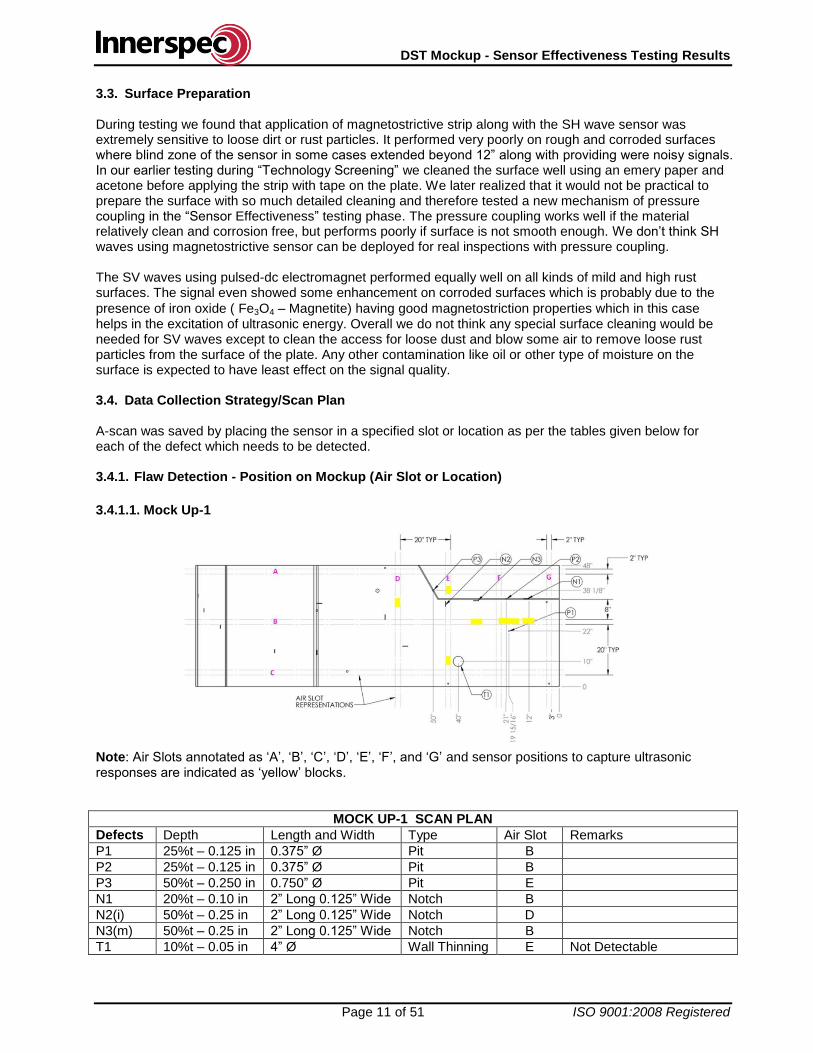
DST Mockup - Sensor Effectiveness Testing Results
Page 11 of 51 ISO 9001:2008 Registered
3.3. Surface Preparation During testing we found that application of magnetostrictive strip along with the SH wave sensor was extremely sensitive to loose dirt or rust particles. It performed very poorly on rough and corroded surfaces where blind zone of the sensor in some cases extended beyond 12” along with providing were noisy signals. In our earlier testing during “Technology Screening” we cleaned the surface well using an emery paper and acetone before applying the strip with tape on the plate. We later realized that it would not be practical to prepare the surface with so much detailed cleaning and therefore tested a new mechanism of pressure coupling in the “Sensor Effectiveness” testing phase. The pressure coupling works well if the material relatively clean and corrosion free, but performs poorly if surface is not smooth enough. We don’t think SH waves using magnetostrictive sensor can be deployed for real inspections with pressure coupling. The SV waves using pulsed-dc electromagnet performed equally well on all kinds of mild and high rust surfaces. The signal even showed some enhancement on corroded surfaces which is probably due to the
presence of iron oxide ( Fe3O4 – Magnetite) having good magnetostriction properties which in this case helps in the excitation of ultrasonic energy. Overall we do not think any special surface cleaning would be needed for SV waves except to clean the access for loose dust and blow some air to remove loose rust particles from the surface of the plate. Any other contamination like oil or other type of moisture on the surface is expected to have least effect on the signal quality. 3.4. Data Collection Strategy/Scan Plan A-scan was saved by placing the sensor in a specified slot or location as per the tables given below for each of the defect which needs to be detected. 3.4.1. Flaw Detection - Position on Mockup (Air Slot or Location)
3.4.1.1. Mock Up-1
Note: Air Slots annotated as ‘A’, ‘B’, ‘C’, ‘D’, ‘E’, ‘F’, and ‘G’ and sensor positions to capture ultrasonic responses are indicated as ‘yellow’ blocks.
MOCK UP-1 SCAN PLAN
Defects Depth Length and Width Type Air Slot Remarks
P1 25%t – 0.125 in 0.375” Ø Pit B
P2 25%t – 0.125 in 0.375” Ø Pit B
P3 50%t – 0.250 in 0.750” Ø Pit E
N1 20%t – 0.10 in 2” Long 0.125” Wide Notch B
N2(i) 50%t – 0.25 in 2” Long 0.125” Wide Notch D
N3(m) 50%t – 0.25 in 2” Long 0.125” Wide Notch B
T1 10%t – 0.05 in 4” Ø Wall Thinning E Not Detectable

DST Mockup - Sensor Effectiveness Testing Results
Page 12 of 51 ISO 9001:2008 Registered
3.4.1.2. Mock Up-2
Note: Air Slots annotated as ‘A’, ‘B’, ‘C’, ‘D’, ‘E’, ‘F’, ‘G’, ‘H’, ‘J’, ‘K’, ‘L’ and ‘M’, and sensor positions to capture ultrasonic responses are indicated as ‘yellow’ blocks. The blind defects are shown as RED, whereas a possible natural weld defect also indicated on the map in red as ‘weld defect’.
MOCK UP-2 SCAN PLAN
Defects Depth Length and Width Type Air Slot Remarks
P4 50%t – 0.250 in 0.75” Ø Pit B
P5 75%t – 0.375 in 1.125” Ø Pit A
P6 50%t – 0.250 in 0.750” Ø Pit A
P7 75%t – 0.375 in 1.125” Ø Pit D
P8 50%t – 0.25 in 0.75” Ø Pit C
P9 75%t – 0.375 in 1.125” Ø Pit A
P10 50%t – 0.25 in 0.75” Ø Pit
P11 25%t – 0.125 in 0.375” Ø Pit A
P12 50%t – 0.250 in 0.750” Ø Pit L
N4 50%t – 0.25 in 2” Long 0.125” Wide Notch L We should have Captured from Slot-C - Error
N5 50%t – 0.25 in 2” Long 0.125” Wide Notch D
N6 50%t – 0.25 in 2” Long 0.125” Wide Notch A
N7 50%t – 0.25 in 2.875” Long 0.125” Wide
Notch C
T2 20%t – 0.10 in 4” Ø Wall Thinning A
T3 50%t – 0.25 in 4” Ø Wall Thinning B
T4 50%t – 0.25 in 4” Ø Wall Thinning L
B1 Pit A
B2 Notch J

DST Mockup - Sensor Effectiveness Testing Results
Page 13 of 51 ISO 9001:2008 Registered
3.4.2. SV Wave Test Parameters
Test Parameter Value
Frequency 2266 kHz
Cycles 5
Gain 18dB
Wavelength 0.10 in
Digital Band Pass Filter 1 MHz to 3 MHz
Averaging 4
Magnet Pulse Width 800 us
Magnet Pulse Delay 200 us
Data Window 600 us
Wave Mode SV at 35 Degrees
3.4.3. Calculations of Signal to Noise Ratio To calculate signal to noise ratio the noise measurement was based from the a-scan in a clean defect free area of the plate by observing the average noise level (typically 5%) and the signal level was recorded as the highest absolute peak in the amplitude response. The dB levels were calculated using:
𝑆𝑁𝑅 = 20 log10
𝑀𝑎𝑥 𝑆𝑖𝑔𝑛𝑎𝑙 𝐴𝑚𝑝𝑙𝑖𝑡𝑢𝑑𝑒
𝐵𝑎𝑠𝑒𝑙𝑖𝑛𝑒 𝑁𝑜𝑖𝑠𝑒 𝐴𝑚𝑝𝑙𝑖𝑡𝑢𝑑𝑒
3.4.4. Measurement Robustness Test This test included testing a fixed defect without any dirt and then examining it again with dirt or debris applied to observe any signal variations. The second part of the test included testing plate edge as a fixed reflector on three different sample plates with almost no rust, mild rust and heavy rust to observe the signal variations. The following table provides summary of this test followed by results displaying data captured during the tests.
Sensor Effectiveness Testing Data Sheet for Measurement Robustness Testing

DST Mockup - Sensor Effectiveness Testing Results
Page 14 of 51 ISO 9001:2008 Registered
3.4.5. Rust Test The rust test was performed on Mockup-1(Clean), Mockup-2 (Medium Rust) and a Corroded Plate (Heavy Rust) capturing edge response from a fixed distance of 16 inches for all cases.
3.4.5.1. Clean Surface
Snapshot on Clean Surface (Mock Up-1) – Edge Reflections Taken from 16 inches Remarks:
SNR – 21.58 dBs
Distance – 16 inches
Defect – Plate Edge
Condition – No Rust
Sensor – Straight

DST Mockup - Sensor Effectiveness Testing Results
Page 15 of 51 ISO 9001:2008 Registered
3.4.5.2. Mild Rust
Snapshot on Mildly Corroded Surface (Mock Up-2) – Edge Reflections Taken from 16 inches
Remarks:
SNR – 26.02 dBs
Distance – 16 inches
Defect – Plate Edge
Condition – Mild Rust
Sensor – Straight

DST Mockup - Sensor Effectiveness Testing Results
Page 16 of 51 ISO 9001:2008 Registered
3.4.5.3. Heavy Rust
Snapshot on Heavily Corroded Surface (Corroded Plate) – Edge Reflections Taken from 16 inches Remarks:
SNR – 26.02 dBs
Distance – 16 inches
Defect – Plate Edge
Condition – Heavy Rust
Sensor – Straight
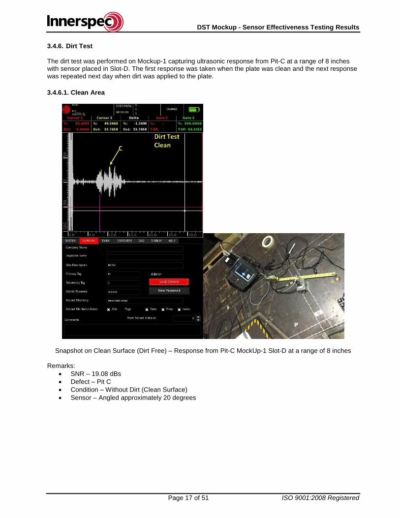
DST Mockup - Sensor Effectiveness Testing Results
Page 17 of 51 ISO 9001:2008 Registered
3.4.6. Dirt Test The dirt test was performed on Mockup-1 capturing ultrasonic response from Pit-C at a range of 8 inches with sensor placed in Slot-D. The first response was taken when the plate was clean and the next response was repeated next day when dirt was applied to the plate.
3.4.6.1. Clean Area
Snapshot on Clean Surface (Dirt Free) – Response from Pit-C MockUp-1 Slot-D at a range of 8 inches Remarks:
SNR – 19.08 dBs
Defect – Pit C
Condition – Without Dirt (Clean Surface)
Sensor – Angled approximately 20 degrees

DST Mockup - Sensor Effectiveness Testing Results
Page 18 of 51 ISO 9001:2008 Registered
3.4.6.2. Area with Dirt
Snapshot on Dirty Surface (Dirt Applied) – Response from Pit-C MockUp-1 Slot-D at a range of 8 inches Remarks:
SNR – 19.08 dBs
Defect – Pit C
Condition – With Dirt Applied
Sensor – Angled approximately 20 degrees 3.4.7. Signal Post-Processing No post signal processing has been performed for all the results presented. The only signal processing done was before the final results were captured on the instrument which included a built-in digital Band-Pass Filter (FIR) with a pass band of 1Mhz to 3 MHz along with a signal averaging of four (4) waveforms to smooth out the random noise. 3.4.8. Impact of Rust and Dirt on Signal Quality No significant degradation was observed due to the dirt or rusty surfaces as shown in para 3.4.4. In fact, we observed slightly higher response in case of rusty surface. This can be attributed to the presence of tightly adhered magnetite (Fe3O4 iron oxides), which enhances the magnetostriction properties of the material and helps in emat signal generation process. However, loose rust may possibly create signal variations and it is recommended that all loosely coupled rust may be removed as much as possible during the preparation phase to get the best possible results.

DST Mockup - Sensor Effectiveness Testing Results
Page 19 of 51 ISO 9001:2008 Registered
3.4.9. Range Test
3.4.9.1. Notch-N2 in Mockup-1 – Distance 30 inches
Response on MockUp-1 from Notch-N2 at a range of 30 inches Remarks:
SNR – 19.08 dBs
Defect – N2
Distance – 30 inches
Sensor – Straight

DST Mockup - Sensor Effectiveness Testing Results
Page 20 of 51 ISO 9001:2008 Registered
3.4.9.2. Pit-P5 in Mockup-2 – Distance 12 inches
Response on MockUp-2 from Pit-P5 at a range of 12 inches Remarks:
SNR – 15.56 dBs
Defect – P5
Distance – 12 inches
Sensor – Straight

DST Mockup - Sensor Effectiveness Testing Results
Page 21 of 51 ISO 9001:2008 Registered
3.4.9.3. Pit-P5 in Mockup-2 – Distance 15 inches
Response on MockUp-2 from Pit-P5 at a range of 15 inches Remarks:
SNR – 11.12 dBs
Defect – P5
Distance – 15 inches
Sensor – Straight

DST Mockup - Sensor Effectiveness Testing Results
Page 22 of 51 ISO 9001:2008 Registered
3.4.9.4. Pit-P5 in Mockup-2 – Distance 18 inches
Response on MockUp-2 from Pit-P5 at a range of 18 inches Remarks:
SNR – 11.12 dBs
Defect – P5
Distance – 18 inches
Sensor – Straight

DST Mockup - Sensor Effectiveness Testing Results
Page 23 of 51 ISO 9001:2008 Registered
4. Data – Test Results 4.1. Mock up 1 – SV Waves
Sensor Effectiveness Testing Data Sheet for Sensor Effectiveness Testing Mock-up-1

DST Mockup - Sensor Effectiveness Testing Results
Page 24 of 51 ISO 9001:2008 Registered
4.1.1. Defect Pit – P1
Data and Snapshot of Defect Pit-P1
Remarks:
SNR – 16.90 dBs
Location – Slot-B
Range – 4 inches
Sensor – Angled approximately 20 degrees

DST Mockup - Sensor Effectiveness Testing Results
Page 25 of 51 ISO 9001:2008 Registered
4.1.2. Defect Pit – P2
Data and Snapshot of Defect Pit-P2
Remarks:
SNR – 12.04 dBs
Location – Slot-B
Range – 9 inches
Sensor – Angled approximately 20 degrees

DST Mockup - Sensor Effectiveness Testing Results
Page 26 of 51 ISO 9001:2008 Registered
4.1.3. Defect Pit – P3
Data and Snapshot of Defect Pit-P3
Remarks:
SNR – 21.58 dBs
Location – Slot-E
Range – 7 inches
Sensor – Straight

DST Mockup - Sensor Effectiveness Testing Results
Page 27 of 51 ISO 9001:2008 Registered
4.1.4. Defect Notch – N1
Data and Snapshot of Defect Notch-N1
Remarks:
SNR – 21.58 dBs
Location – Slot-B
Range – 7 inches
Sensor – Straight
Trace is bit noisy around 30 in away possibly due to the edge reflections, which cannot be considered general noise.

DST Mockup - Sensor Effectiveness Testing Results
Page 28 of 51 ISO 9001:2008 Registered
4.1.5. Defect Notch – N2
Data and Snapshot of Defect Notch-N2
Remarks:
SNR – 24.60 dBs
Location – Slot-D
Range – 19 inches
Sensor – Straight

DST Mockup - Sensor Effectiveness Testing Results
Page 29 of 51 ISO 9001:2008 Registered
4.1.6. Defect Notch – N3
Data and Snapshot of Defect Notch-N3
Remarks:
SNR – 26.0 dBs
Location – Slot-B
Range – 8 inches
Sensor – Straight
Trace is bit noisy around 30 in away possibly due to the edge reflections, which cannot be considered general noise.

DST Mockup - Sensor Effectiveness Testing Results
Page 30 of 51 ISO 9001:2008 Registered
4.1.7. Defect Wall Thinning – T1 This defect of wall thinning 4in in diameter could not be detected possibly due to the very shallow depth (10%t or 0.05 in) and extremely smooth edges of the defect. 4.2. Mock up 2 – SV Waves
Sensor Effectiveness Testing Data Sheet for Sensor Effectiveness Testing Mock-up-2 (1/2)

DST Mockup - Sensor Effectiveness Testing Results
Page 31 of 51 ISO 9001:2008 Registered
Sensor Effectiveness Testing Data Sheet for Sensor Effectiveness Testing Mock-up-2 (2/2)

DST Mockup - Sensor Effectiveness Testing Results
Page 32 of 51 ISO 9001:2008 Registered
4.2.1. Defect Pit – P4
Data and Snapshot of Defect Pit-P4
Remarks:
SNR – 24.08 dBs
Location – Slot-B
Range – 5 inches
Sensor – Slightly Angled to avoid reflections from the back and front edges of the mockup.

DST Mockup - Sensor Effectiveness Testing Results
Page 33 of 51 ISO 9001:2008 Registered
4.2.2. Defect Pit – P5
Data and Snapshot of Defect Pit-P5
Remarks:
SNR – 24.60 dBs
Location – Slot-A
Range – 4 inches
Sensor – Angled approximately 20 degrees to avoid reflections from the back and front edges of the mockup.

DST Mockup - Sensor Effectiveness Testing Results
Page 34 of 51 ISO 9001:2008 Registered
4.2.3. Defect Pit – P6
Data and Snapshot of Defect Pit-P6
Remarks:
SNR – 22.28 dBs
Location – Slot-A
Range – 4 inches
Sensor – Angled approximately 20 degrees to avoid reflections from the weld.

DST Mockup - Sensor Effectiveness Testing Results
Page 35 of 51 ISO 9001:2008 Registered
4.2.4. Defect Pit – P7
Data and Snapshot of Defect Pit-P7
Remarks:
SNR – 12.04 dBs
Location – Slot-D
Range – 16 inches
Sensor – Angled approximately 20 degrees to avoid reflections from the weld and back edge of the plate.

DST Mockup - Sensor Effectiveness Testing Results
Page 36 of 51 ISO 9001:2008 Registered
4.2.5. Defect Pit – P8
Data and Snapshot of Defect Pit-P8
Remarks:
SNR – 22.92 dBs
Location – Slot-C
Range – 6 inches
Sensor – Angled approximately 20 degrees to avoid reflections from the weld and back edge of the plate.

DST Mockup - Sensor Effectiveness Testing Results
Page 37 of 51 ISO 9001:2008 Registered
4.2.6. Defect Pit – P9
Data and Snapshot of Defect Pit-P9
Remarks:
SNR – 18.06 dBs
Location – Slot-A
Range – 6 inches
Sensor – Angled approximately 20 degrees.

DST Mockup - Sensor Effectiveness Testing Results
Page 38 of 51 ISO 9001:2008 Registered
4.2.7. Defect Pit – P10
Data and Snapshot of Defect Pit-P10
Remarks:
SNR – 9.54 dBs
Location – Slot-A
Range – 17 inches
Sensor – Angled approximately 20 degrees.

DST Mockup - Sensor Effectiveness Testing Results
Page 39 of 51 ISO 9001:2008 Registered
4.2.8. Defect Pit – P11
Data and Snapshot of Defect Pit-P11
Remarks:
SNR – 4.08 dBs
Location – Slot-A
Range – 13 inches
Sensor – Angled approximately 20 degrees.
Marginal or weak response probably due to the size (0.375 in Ø) and very shallow depth (25%t or 0.125 in) of this defect.

DST Mockup - Sensor Effectiveness Testing Results
Page 40 of 51 ISO 9001:2008 Registered
4.2.9. Defect Pit – P12
Data and Snapshot of Defect Pit-P12
Remarks:
SNR – 15.56 dBs
Location – Slot-L
Range – 9 inches
Sensor – Angled approximately 20 degrees

DST Mockup - Sensor Effectiveness Testing Results
Page 41 of 51 ISO 9001:2008 Registered
4.2.10. Defect Notch – N4
Data and Snapshot of Defect Notch-N4
Remarks:
SNR – 21.58 dBs
Location – Slot-L
Range – 6 inches
Sensor – Straight

DST Mockup - Sensor Effectiveness Testing Results
Page 42 of 51 ISO 9001:2008 Registered
4.2.11. Defect Notch – N5
Data and Snapshot of Defect Notch-N5
Remarks:
SNR – 18.06 dBs
Location – Slot-D
Range – 4 inches
Sensor – Angled approximately 20 degrees

DST Mockup - Sensor Effectiveness Testing Results
Page 43 of 51 ISO 9001:2008 Registered
4.2.12. Defect Notch – N6
Data and Snapshot of Defect Notch-N6
Remarks:
SNR – 26.02 dBs
Location – Slot-A
Range – 9 inches
Sensor – Straight

DST Mockup - Sensor Effectiveness Testing Results
Page 44 of 51 ISO 9001:2008 Registered
4.2.13. Defect Notch – N7
Data and Snapshot of Defect Notch-N7
Remarks:
SNR – 12.04 dBs
Location – Slot-C
Range – 5 inches
Sensor – Angled approximately 20 degrees
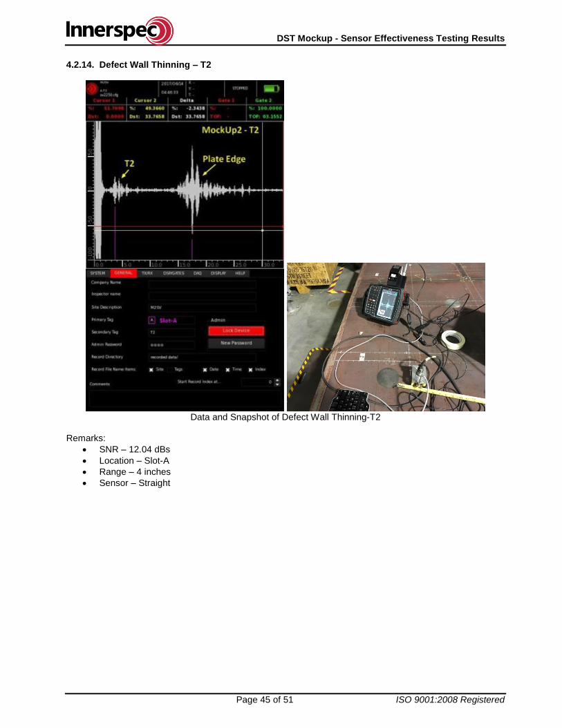
DST Mockup - Sensor Effectiveness Testing Results
Page 45 of 51 ISO 9001:2008 Registered
4.2.14. Defect Wall Thinning – T2
Data and Snapshot of Defect Wall Thinning-T2
Remarks:
SNR – 12.04 dBs
Location – Slot-A
Range – 4 inches
Sensor – Straight

DST Mockup - Sensor Effectiveness Testing Results
Page 46 of 51 ISO 9001:2008 Registered
4.2.15. Defect Wall Thinning – T3
Data and Snapshot of Defect Wall Thinning-T3
Remarks:
SNR – 20.00 dBs
Location – Slot-B
Range – 7 inches
Sensor – Straight

DST Mockup - Sensor Effectiveness Testing Results
Page 47 of 51 ISO 9001:2008 Registered
4.2.16. Defect Wall Thinning – T4
Data and Snapshot of Defect Wall Thinning-T4
Remarks:
SNR – 20.82 dBs
Location – Slot-L
Range – 7 inches
Sensor – Angled approximately 20 degrees to avoid edge reflections

DST Mockup - Sensor Effectiveness Testing Results
Page 48 of 51 ISO 9001:2008 Registered
4.2.17. Natural Weld Flaw – BD1 We suspect a natural flaw in the weld as shown in the picture. This may not be the intended blind defect purposely machined for this test but possibly a natural weld flaw and designated as ‘BD1”.
Data and Snapshot of Natural Weld Defect – BD1
Remarks:
SNR – 16.90 dBs
Location – Slot-F
Range – 12 inches
Sensor – Straight

DST Mockup - Sensor Effectiveness Testing Results
Page 49 of 51 ISO 9001:2008 Registered
4.2.18. Blind Defect – BD2 This flaw is possibly of a round shape like a pit and hidden on the ID side of the plate close to slot-H and slot-B.
Data and Snapshot of Blind Defect – BD2
Remarks:
SNR – 19.08 dBs
Location – Slot-A
Range – 9 inches
Sensor – Angled approximately 20 degrees to avoid edge reflections
Shape – Probably Circular Pit

DST Mockup - Sensor Effectiveness Testing Results
Page 50 of 51 ISO 9001:2008 Registered
4.2.19. Blind Defect – BD3 This blind defect is a planar defect like a notch of at least 2” long located close to slot-J and slot-C and connected with the weld at 90 degrees.
Data and Snapshot of Blind Defect – BD3
Remarks:
SNR – 26.02 dBs
Location – Slot-J
Range – 5 inches
Sensor – Straight
Shape – Probably a Notch

DST Mockup - Sensor Effectiveness Testing Results
Page 51 of 51 ISO 9001:2008 Registered
5. Technique Options - Conclusions 5.1. Guided Waves In the earlier test during Technology Screening, the magnetostrictive guided wave technique had shown greater sensitivity, reach, and resolution than any other technique. However, adhering the magnetostrictive strip inside the refractory channels was not a practical option and therefore a weight coupling technique was tested, which unfortunately did not provided good signal to noise ratio and resulted in very large dead zone in rusty and corroded surfaces. The technique was very sensitive to lift-off and provided poor signal to noise ratio. After conducting few tests on both Mockups we decided not to proceed with this technique.
5.2. EMAT generated SV Waves SV waves can provide strong reflections on almost all the defects in both Mockups. We were also been able to detect both “Blind Defects” on the bottom surface (OD) which was not accessible or visible during the tests. We were also able to detect a possible weld defect which was not indicated on the flaw map. The existing air slots on the refractory pad are large enough to fit SV sensors and if needed can easily be customized further. In some cases we have to angle the sensor in order to avoid weld reflections where defects were buried in the weld. This technique of shooting wave at an angle can be implemented in the final system by designing special multilayer and multi-channel emat coils which can provide us ability to send energy straight, at a fixed angle and also in a single direction to avoid ambiguities due to reflections from the back side of the sensor. A single sensor was used in pulse-echo mode looking for the reflections from possible defects. Reflection mode would be the preferred choice in the final system as well, since it is a “positive” inspection technique that should not generate false positives. 5.2.1. Advantages and Limitations
EMAT SV waves using electromagnets is a couplant free technique providing ease of handling and high speed of scanning.
The existing refractory air slot is large enough for SV wave emat sensor in reflection mode. However, the sensor design still needs to be optimized in an even a smaller package with cable connectors position changed to the side of the sensor instead of being in the vertical direction. The probe/s can be packaged in a 2” x 1” size housing with a built-in encoder to be pushed through the channels by the inspection robot.
The EMATs can be applied to a relatively rough surface. Surface preparation is not as demanding with Shear Vertical Wave (SV Wave) technique.
No couplant or strip is needed for the generation of ultrasonic energy.
This technique permits covering large areas for detecting flaws, defects and corroded areas but may not be able to provide an accurate measurement of wall thickness in corroded areas. More work and calibration will be required in this area.
It could be very effective for detection of shallow cracks.
The use of electromagnets makes the scanning extremely easy and would inhibit any metallic dust getting attached to the sensors.
The technique demonstrated little effect to moderate dust and debris and performed equally well in all pristine and heavily corroded surfaces. However, it would help if loose rust can be cleaned to avoid getting ant interference to ultrasonic signals.
The same sensor is expected to perform well in plate thickness ranging from 0.5” to 1.0”, without making any additional changes or adjustments.
Using an array of probes could significantly improve detection of defects, reduce influence of weld reflections, and create opportunities for sizing. A prototype probe and scanning software would need to be developed. The multiple channels in the array can be excited individually or phased to sweep the combined beam area. Multiple channels will also enhance signal to noise and permit reception of scattered signals.


Appendix C –
Penn State


NDE Technology Development Program for Hanford DST Non-‐Visual Volumetric Inspection Technology: Sensor Effectiveness Testing Report From Penn State The Pennsylvania State University University Park, PA 16802 Cliff J Lissenden, [email protected] Parisa Shokouhi, [email protected] 21 June 2017

Sensor Effectiveness Testing 2
1. Executive Summary Ultrasonic nondestructive testing was performed on DST primary tank bottom mockups at PNNL using electromagnetic acoustic transducers (EMATs). Pitch-catch, pulse-echo, and through-transmission modes of inspection provided documented indications of all visible defects for which we had data. We believe that two hidden flaws have been located as well. Unfortunately, there are two defects for which data were not acquired by our mistake (T1 and N7). The EMATs require no surface preparation or coupling and were shown to be insensitive to rust and ‘dirt’. The new EMATs were much easier to use than the ones we used for the Technology Screening and a large amount of data was acquired and analyzed. Often the EMATs were located 36” apart, and they were always located in ‘air slot’ pathways. A very preliminary outline for development of a robotic inspection system is provided. 2. Introduction On June 6-7 Cliff Lissenden and Parisa Shokouhi performed Sensor Evaluation Testing on two mockups of Hanford DST primary tank bottoms. One mockup is modified from the Technology Screening Testing conducted in February, and will be called the modified mockup (see Fig. 1). In addition to the original flaws, there are 3 pits, 3 notches, and 1 wall thinning flaw that are visible. These seven flaws are to be detected. A new mockup (shown in Fig. 2) containing 9 pits, 4 notches, and 3 wall thinning flaws was also prepared. In addition to these 16 visible flaws, there are 2 hidden flaws to be detected. Descriptions of the flaws copied from the Sensor Evaluation Testing Protocol are provided for the modified and new mockups in Tables 1 and 2 respectively. Electromagnetic acoustic transducers (EMATs) were deployed in the ‘air slots’ to acquire ultrasonic signals after the waves interact with flaws. The modes of nondestructive inspection included pitch-catch, pulse-echo, and through-transmission. With the EMATs confined to the air slots the shear horizontal (SH) waves propagated roughly 1-4 feet before being received. This is realistic for the air slot pattern under DSTs.

Sensor Effectiveness Testing 3
Fig. 1. Modified mockup with flaws P1-P3, N1-N3, and T1.

Sensor Effectiveness Testing 4
Fig. 2. New mockup with flaws P4-P12, N4-N7, T2-T4, and 2 hidden flaws.

Sensor Effectiveness Testing 5
Table 1. Description of flaws in Modified Mockup [from SET Protocol, PNNL-26478]

Sensor Effectiveness Testing 6
Table 2. Description of flaws in New Mockup [from SET Protocol, PNNL-26478]

Sensor Effectiveness Testing 7
3. Background 3.a. Relevant Experience Cliff Lissenden is currently the PI on a Nuclear Energy University Program Integrated Research Project on multi-‐sensor inspection and robotic systems for dry storage casks (NEUP IRP 14-‐7356). This section provides a brief summary of pertinent aspects of that project. The extended use of dry storage for spent nuclear fuel from U.S. nuclear power plants makes it desirable to confirm the structural integrity of the storage canisters through inspections. The Nuclear Regulatory Commission (NRC) requires independent spent fuel storage installations (ISFSIs) to submit an aging management program (AMP) as part of the re-‐licensure process. The technology developed in this project could become part of an AMP. Stress corrosion cracking (SCC) is a potential mode of canister degradation that requires the simultaneous presence of three elements: a susceptible material, a driving force, and a corrosive environment. Austenitic stainless steel can be susceptible to SCC when it is heated such that grain boundaries become chromium-‐depleted, as can happen during welding. Additionally, welding can result in high thermal residual tensile stresses that could act as a driving force. Finally, ISFSIs located in environments in which airborne chloride salts are present (such as in coastal regions) that could deliquesce on the canister surface, providing a corrosive environment for SCC. Since the heat affected zone (HAZ) of full penetration welds contains both susceptible material and a tensile driving force it is important to assess whether the environment is corrosive. Chloride bearing salts in solution on the surface of the stainless steel canister represent a corrosive environment and thus their detection could provide an early indication of the degradation in the structural integrity of the canister. Laser induced breakdown spectroscopy (LIBS) is being researched and developed to provide an in-‐situ characterization of the surface composition of the canister. The absence of chlorides would indicate that chloride-‐induced SCC could not occur. Additionally, it is important to conduct nondestructive inspection (NDI) for cracks in the HAZ of canister welds. Ultrasonic shear-‐horizontal waves generated by electromagnetic acoustic transducers (EMATs) interact with SCC, thereby enabling its detection and characterization. Both the LIBS and EMAT systems need to be delivered robotically because the dry storage cask environment is harsh in terms of high temperature and gamma radiation dose. Additionally, the canister is also shielded by its overpack, which is a steel and concrete structure that prevents access to the canister except through the ventilation system (or by opening the lid, which is undesirable). The fundamental considerations of the robotic inspection systems for dry storage casks are:
• Delivery of the sensors to appropriate locations on the canister, positional awareness, and an ability to return to positions of interest at a later time;
• That the robotic inspection system in no way accelerates degradation of the cask or provides a safety hazard; thus it should not leave potentially damaging marks or scratches, generate corrosive gases, nor should any component of the robot be left behind.

Sensor Effectiveness Testing 8
While the various canister models have different internal basket structures to hold the spent fuel rod assemblies, the confinement boundary is a thin-‐walled cylindrical shell fabricated with full penetration welds. Thus, the surface composition and NDI sensing systems being developed apply to all stainless steel canister designs. However, the development of the robotic inspection system is challenged by the diverse geometric configurations of the overpack structures currently in use. All overpack structures contain a passive convective cooling system with inlet and outlet vents that enable access for robotic inspection systems, but the specific features of the overpack structures are dissimilar. Different overpack structures support the canister with its axis either vertical or horizontal. Horizontal axis systems typically have a large air plenum while vertical access systems have a relatively tight fit between the canister and the overpack. The cooling air pathways have numerous bends to maximize shielding of the gamma rays, but each overpack model has different vent geometries. Therefore, it was necessary to design a robotic system for one particular type of cask and make it as applicable to the other cask models as possible. The Holtec HI-‐STORM 100S overpack was selected because:
• It provides a rigorous test for the robotic inspection system due to the constrained geometry (guide channels around the inside liner of the overpack severely limit maneuverability inside the ventilation system);
• The gap between the multipurpose canister (MPC) lid and the overpack lid enables the MPC lid to be used to stage delivery of sensor cars over the edge and down the side of the MPC;
• The overall geometry of the canister is similar to a large number of other dry storage systems; and
• Holtec is a collaborating partner. The robotic delivery system is a marsupial system comprised of a winch mechanism placed outside an inlet vent, a delivery arm that is inserted into an inlet vent, and a sensor train that is parked on the delivery arm until it gets deployed over the edge of the canister. The sensing systems are contained within the cargo bays of the individual sensor cars. The entire operation is controlled from a remote site outside the cask. 3.b. Technology Screening Testing On February 2, 2017 Cliff Lissenden and Parisa Shokouhi conducted a series of tests on the ‘Hanford DST primary liner test mock-up’. In all tests two electromagnetic acoustic transducers (EMATs) were used: one to transmit an ultrasonic signal into the steel plate and the other to receive the signal. Unless noted otherwise all EMAT positions on the plate were consistent with air slot locations in the double shell tank (DST). All ultrasonic waves analyzed herein are guided waves known as shear horizontal (SH) waves. Multiple SH modes propagate in plates at a given frequency. The EMATs were placed only on the 0.5” thick steel plate portion of the mockup and actuated at 250 kHz, where 3 SH modes exist. The group velocities of these modes were predicted to be: 3200, 2800, and ~0 m/s for the SH0, SH1, and SH2 modes respectively. The SH2 mode is highly dispersive at this frequency, resulting in a very slow group velocity, thus our data include only the SH0 and SH1 modes. Typically, the distance between transmitter and receiver was sufficiently large for the SH0 and SH1 modes to separate, such that they are received as separate wave packets.

Sensor Effectiveness Testing 9
EMATs were selected for this application because they are noncontact transducers, which is very beneficial for remote inspections with robotic devices. However, the amplitude of the wave signal decreases as the liftoff (i.e., gap between the electric coil and plate surface) increases; and so does the magnetic force. The tests on the mockup were conducted by manual positioning of the EMATs on the plate, so the liftoff was set as a compromise between sufficient signal strength and ease of manual positioning. Preliminary tests at Penn State showed the signal decrease of 3.5 to 1.8 to 1.1 mV for liftoffs of 0.3, 0.6, and 0.9 mm as set by 0.3 mm thick wear strips. For the actual robotic inspection of a DST we plan to use ‘transfer balls’ to enable the EMATs to be easily moved along the air slot in close proximity to the steel primary tank bottom. We used a liftoff of 0.6 mm for all tests on the mockup, thereby sacrificing signal amplitude for ease of EMAT positioning, but ‘transfer balls’ are likely to allow a smaller liftoff, and would thus provide a larger ultrasonic signal. EMATs based on Lorentz force transduction generally have lower coupling than piezoelectric or magnetostrictive transduction, thus high power instrumentation is typically employed. Our laboratory at Penn State is equipped with a Ritec RAM-5000 SNAP system (Warwick, RI), but this is a sensitive instrument that we did not want to transport across the country. We brought instead a simple low power Ultratek system for the mockup testing at PNNL. SH waves sent and received by EMATs that were placed at locations on the mockup representative of air slots in the refractory pad of DSTs at Hanford. The center-to-center distance between transmitting and receiving EMATs was 26”-35” (except in the pulse-echo experiment) to simulate the spacing between adjacent air slots in the DST. EMATs were selected for this application primarily because they are noncontact transducers that are well suited for robotic delivery to remote locations, and they are sufficiently small to fit through the air slots in all DST farms at Hanford. Due to restrictions associated with the equipment transport, we utilized a relatively low power acquisition system for data collection. While the signal amplitudes were reasonably large, SNRs would have been an order of magnitude higher by using the high power instrumentation intended for EMATs. As summarized below, all defects identified as high priority (a, b, c, g, and k) were identified. Through-transmission mode was used to identify defects L, c, b, and h, which are located on the ½” thick plate. Only detection of defect h (20% through wall) was questionable. The sensitivity to defect h could be improved by acquiring more data to enable SAFT or tomography reconstruction algorithms to be implemented. The pitch-catch mode and SAFT reconstruction effectively identified defects g, a, and k, which are located along the weld between the 1/2” thick plate and the 7/8” thick plate. There were localization errors due to the manual placement of EMATs that could be improved by using an encoder. Finally, we did not have time to attempt to detect defects ‘i’ and ‘m’, which are located along an edge of the plate. Time permitting, we would have used a pitch-catch method that would have distinguished defect reflection from edge reflection.

Sensor Effectiveness Testing 10
4. Approach for Sensor Effectiveness Testing 4.a. Method Ultrasonic guided waves, specifically shear-horizontal (SH) waves, are used for nondestructive inspection (NDI) of flaws in the mockups provided. The EMATs are located in ‘air slots’ on the top surface of the mockup that simulate the air slots below the primary tank bottom. In general, three modes of ultrasonic NDI are used: Pitch-Catch (PC) – The EMATs are oriented at 45 degree angles to the air slots and located such that the receiver will capture waves that are scattered by flaws. The received waves do not travel in a straight line from transmitter (T) to receiver (R). Pulse-Echo (PE) – The transmit and receive EMATs are positioned in an air slot adjacent to each other and aligned. The receiver captures reflections from flaws and other reflectors. Through-Transmission (TT) – The transmit and receive EMATs are positioned some distance apart and aligned. The receiver captures the incident wave actuated by the transmitter unless there is a flaw between the transmit and reeive EMATs that scatters the wave. Upon arrival at PNNL and seeing the two mockups and visible flaws we planned how to best apply the 3 NDI modes to obtain indications of the flaws. We decided to detect flaws along weld lines primarily with PC, but also using PE where appropriate given the air slot locations. We then used the TT and PC modes to indicate flaws within the volume of the plate (away from the welds). After getting indications from the visible defects we then inspected regions for hidden defects where measurements had not yet been made. 4.b. Equipment The equipment used is listed below and is essentially completely different than what was used for the Technology Screening work.
• Two identical EMATs, one is the transmitter and one is the receiver (detailed description will be provided);
• Two RG-58 coaxial cables 50 ft long; • Transmitter matching network (12 nF and 2.6 µH); • Receiver matching network (22 nF and 2.7 µH) with 20 dB preamp; • Ritec GA-10000 gated amplifier (output power = 7.0); • National Instruments PXIe-1062Q (used to send 5 cycle toneburst with 250 kHz central
frequency and to digitize the received signal) controlled by Labview (all saved data are the result of 100 averages);
• Olympus Preamp 5660B (40 dB); • Dell laptop computer.
The parameters/settings identified above are used in all tests. The comparison between the gated amplifier (GA-10K) and the Ultratek system that was used for the Technology Screening is shown in Fig. 3 for a ¼” steel plate at Penn State. The Ritec RAM 5000 system that we use in the laboratory is also shown for reference. The peak amplitudes are 21.0, 15.9, 2.3 mV for RAM-5K, GA-10K, and Ultratek respectively.

Sensor Effectiveness Testing 11
Fig. 3. Comparison of signals from different instruments (GA-10K used in this work). Custom EMATs were designed and fabricated for the Sensor Effectiveness Testing (SET). As for the Technology Screening a 4 by 4 array of magnets was used with an electrical coil. The electrical coil is a flexible printed circuit board designed for attachment to the 3D printed EMAT housing geometry. A 50 µm thick PEEK wear strip tape protects the coil. The housing is comprised of four pieces. Four transfer balls are used to fix the liftoff and promote easy EMAT positioning. The liftoff was optimized for a strong signal and a weak magnetic force. The housing has a 2” diameter, capability to rotate the EMAT in any direction, and the ability to be fitted with an encoder wheel or mounted on a robotic device. During SET the EMAT orientations were always 0, ±45, or 90 degrees relative to the air slot. Figure 4 shows the EMATs. EMATs are noncontact transducers coupled by the Lorentz force, so no couplant is needed. Based on our experience with the technology screening and SET tests we expect reliable flaw detection for distances of 3-4 feet. The EMAT dead zone is associated with the electromagnetic interference and is roughly 6”. The beam divergence from the EMAT is substantial as shown in Fig. 5, which is very helpful for flaw detection.
Fig. 4. EMAT components and assembly.

Sensor Effectiveness Testing 12
Fig. 5. Ultrasonic beam divergence from EMATs. 4.c. Surface Preparation There was no surface preparation. 4.d. Data Collection Initially, data were collected that enabled the beam divergence shown in Fig. 5 to be determined. The group velocities for the SH0 and SH1 modes were computed to be 3060 and 2760 m/s respectively, for the ½” thick mild steel (A36) plate. Mixing of units is unfortunate, but fairly common for ultrasonic NDI because structural dimensions are typically given in English units, while material properties and wave speeds are more often given in SI units. 4.d.i. Flaw Detection As mentioned earlier, three modes of NDI were employed: pitch-catch (PC), pulse-echo (PE), and through-transmission (TT). Each mode can be used for both weld line and volumetric inspection, but generally PC was used for weld line inspections and TT was reserved for volumetric inspections. With a few exceptions, the EMATs were located in the air slots running in the y-direction (would be the radial direction for a DST), and in most cases adjacent air slots were not used, rather one slot was skipped such that the slots in which EMATs were positioned are nominally 36” apart. This is representative of air slot spacing for DSTs. We reiterate that the same equipment parameters were used throughout the testing, only the EMAT positions changed from test to test. Schematics showing EMAT positions in air slots, orientations, and scan directions are provided on the following pages.

Sensor Effectiveness Testing 13
Modified mockup
48”
1/2” plate
weld
air slots
x
y
scan y-‐dir in 1” incs
x=6” x=26” x=46” Mode: PE EMAT Orientation: 0o T = (26,37)S, R = (26,40)S Flaws assessed: P3, N2, N3, P2, N1
T
R
48”
1/2” plate
weld
air slots
x
y
scan y-‐dir in 1” incs
x=6” x=26” x=46” Mode: PC EMAT Orientation: ±45o T = (26,34)S, R = (26,52)S Flaws assessed: P3, N2, N3, P2, N1
T
R
48”
1/2” plate
weld
air slots
x
y
scan y-‐dir in 1” incs
x=6” x=26” x=46” Mode: PC EMAT Orientation: ±45o T = (46,34)S, R = (46,52)S Flaw assessed: P3
T
R
48”
1/2” plate
weld
air slots
x
y
scan y-‐dir in 1” incs
x=6” x=26” x=46” Mode: PC EMAT Orientation: ±45o T = (26,34)F, R = (26,52)S Flaw assessed: P3
T
R

Sensor Effectiveness Testing 14
48”
1/2” plate
weld
air slots
x
y
scan y-‐dir in 1” incs
x=6” x=26” x=46” Mode: TT EMAT Orientation: 0o T = (6,74)S, R = (26,74)S Flaw assessed: P1
T
R
48”
1/2” plate
weld
air slots
x
y
scan y-‐dir in 1” incs
x=6” x=26” x=46” Mode: PC EMAT Orientation: ±45o T = (26,71)S, R = (26,79)S T = (26,72)F, R = (26,76)S Flaw assessed: P1
T
R
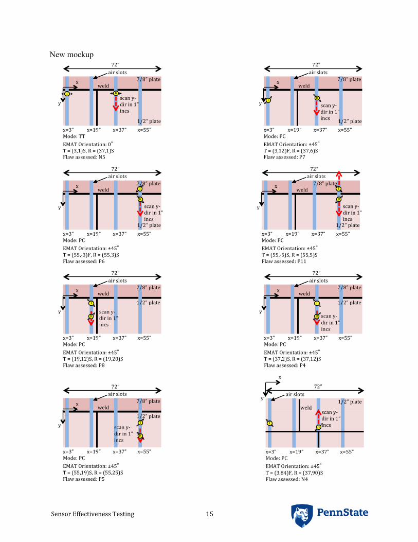
Sensor Effectiveness Testing 15
New mockup
72”
7/8” plate
1/2” plate
weld
air slots x
y scan y-‐dir in 1” incs
x=3” x=19” x=37” x=55” Mode: TT EMAT Orientation: 0o T = (3,1)S, R = (37,1)S Flaw assessed: N5
T
R
72”
7/8” plate
1/2” plate
weld
air slots x
y scan y-‐dir in 1” incs
x=3” x=19” x=37” x=55” Mode: PC EMAT Orientation: ±45o T = (3,12)F, R = (37,6)S Flaw assessed: P7
T
R
72”
7/8” plate
1/2” plate
weld
air slots x
y scan y-‐dir in 1” incs
x=3” x=19” x=37” x=55” Mode: PC EMAT Orientation: ±45o T = (55,-‐3)F, R = (55,3)S Flaw assessed: P6
T
R
72”
7/8” plate
1/2” plate
weld
air slots x
y scan y-‐dir in 1” incs
x=3” x=19” x=37” x=55” Mode: PC EMAT Orientation: ±45o T = (55,-‐5)S, R = (55,5)S Flaw assessed: P11
T
R
72”
7/8” plate
1/2” plate weld
air slots x
y scan y-‐dir in 1” incs
x=3” x=19” x=37” x=55” Mode: PC EMAT Orientation: ±45o T = (19,12)S, R = (19,20)S Flaw assessed: P8
T
R
72”
7/8” plate
1/2” plate weld
air slots x
y scan y-‐dir in 1” incs
x=3” x=19” x=37” x=55” Mode: PC EMAT Orientation: ±45o T = (37,2)S, R = (37,12)S Flaw assessed: P4
T
R
72”
7/8” plate
1/2” plate weld
air slots x
y scan y-‐dir in 1” incs
x=3” x=19” x=37” x=55” Mode: PC EMAT Orientation: ±45o T = (55,19)S, R = (55,25)S Flaw assessed: P5
T
R
72”
1/2” plate weld
air slots
x
y
scan y-‐dir in 1” incs
x=3” x=19” x=37” x=55” Mode: PC EMAT Orientation: ±45o T = (3,84)F, R = (37,90)S Flaw assessed: N4
T
R

Sensor Effectiveness Testing 16
x=3” x=19” x=37” x=55” Mode: PC EMAT Orientation: ±45o T = (19,78)F, R = (55,84)S Flaw assessed: P10
72”
1/2” plate weld
air slots
x
y
scan y-‐dir in 1” incs
T
R
x=3” x=19” x=37” x=55” Mode: PC EMAT Orientation: ±45o T = (19,72)F, R = (55,93)S Flaw assessed: P9
72”
1/2” plate weld
air slots
x
y
scan y-‐dir in 1” incs
T
R
x=3” x=19” x=37” x=55” Mode: PC EMAT Orientation: ±45o T = (55,106)S, R = (55,88)S Flaw assessed: N6
72”
1/2” plate
weld
air slots
x
y
scan y-‐dir in 1” incs
T
R
72”
weld
air slots
x
y
x=3” x=19” x=37” x=55” Mode: PC EMAT Orientation: ±45o T = (42,101)S, R = (56,101)S Flaw assessed: P12
1/2” plate
T
R
scan x-‐dir in 1” incs
72”
weld
air slots
x
y scan x-‐dir in 1” incs
x=3” x=19” x=37” x=55” Mode: TT EMAT Orientation: 0o T = (66,47)S, R = (66,83)S Flaw assessed: T2
1/2” plate
T
R
36”
x=3” x=19” x=37” x=55” Mode: TT EMAT Orientation: 0o T = (19,76)S, R = (55,76)S Flaw assessed: T3
72”
1/2” plate weld
air slots
x
y
scan y-‐dir in 1” incs
T
R

Sensor Effectiveness Testing 17
4.d.ii. Rust Test The effect of rust was investigated by comparing the strength of pulse-echo (PE) reflections from the edge of the 7/8” thick plates with three conditions: clean (modified mockup), moderately corroded (new mockup), and severely corroded (new mockup). The orientation of the transducers with respect to the edge of the plate is shown in the picture below.
1. The standoff distance between the center of the EMATs and the edge was 12”. 2. No adjustment was needed for placing the EMATs on the rusty plates. 3. One measurement per plate was made. The results are compared in terms of the
amplitude of the reflected SH0 and SH1 wave packets: 4.d.iii. Dirt Test We present PE test results to demonstrate the effect of dirt on the SNR and detectability of Flaw “C” in the modified mockup (PC and TT tests were also conducted). As shown in Fig. 6, in both tests, the T-R EMAT pair (center-to-center spacing of 3”) is placed in an air slot and moved in 1” increments starting at y=32”. The air slot is about 8” from Flaw “C”. No adjustments were needed for placing the transducers on the dirty plate.
72”
1/2” plate weld
air slots
x
y
scan y-‐dir in 1” incs x=3” x=19” x=37” x=55”
Mode: TT EMAT Orientation: 0o T = (3,103)S, R = (37,103)S Flaw assessed: T4
T
R
x=3” x=19” x=37” x=55” Mode: PC EMAT Orientation: ±45o T = (37,2)S, R = (37,28)S Flaw assessed: B1
72”
1/2” plate weld
air slots
x
y
scan y-‐dir in 1” incs
T
R
x=3” x=19” x=37” x=55” Mode: TT EMAT Orientation: 0o T = (37,49)S, R = (19,49)S Flaw assessed: B1
72”
1/2” plate weld
air slots
x
y
scan y-‐dir in 1” incs
T
R
72”
weld
air slots
x
y scan x-‐dir in 1” incs
x=3” x=19” x=37” x=55” Mode: PE EMAT Orientation: 0o T = (60,47)S, R = (63,47)S T = (60,29)S, R = (63,29)S Flaw assessed: B2
1/2” plate
T
R
36”

Sensor Effectiveness Testing 18
clean with dirt
Fig. 6. EMATs positioned in an air slot prepared for scanning to the right for PE mode detection of flaw C on the modified mockup: clean and with dirt. 4.e. Signal Processing Depending on the data collection configuration, different post-processing procedures were used to analyze the data: • For through-transmission (TT), B-scans of the envelope (Hilbert transform) of the recorded
A-scan signals were analyzed. • For the other two data collection configurations (PE, PC), the signals collected at multiple
locations were used to reconstruct an image of the inspected volume based on the principles of SAFT and taking into account the divergence properties of the transducers.
SAFT is an algebraic reconstruction algorithm that exploits the constructive and destructive interferences among the reflected waves to image the positions of the reflectors across the test area. To perform SAFT, the test area is divided into a large number of small pixels (here, 1/5” x 1/5”). Next, for each pair of T and R, the time instance and amplitude corresponding to the reflection from the center of each pixel is calculated. This process is repeated for all T-R combinations taking into account the divergence angels of the transducers. If the pixels coincide with the position of a reflector, the amplitudes are constructive whereas if no reflector is present, the amplitudes are destructive. As a result, the signal amplitude increases at the location of the reflectors and diminishes elsewhere. SAFT images provide improved localization and higher SNR than the corresponding B-scans. 4.f. Signal-to-Noise (SNR) Calculation SNR is generally calculated based on the Mean-Mean amplitude ratio for TT tests and based on the Peak-Mean amplitude ratio for PE and PC tests. Details on the calculation of SNR for different test configurations are given in Section 5 (Data). To report SNR in dB the log10 of the SNR is multiplied by 20.
R
T

Sensor Effectiveness Testing 19
4.g. Impact of Dirt and Rust on Signal Quality Please see sections 4.d.ii and 4.d.iii above for details on the methodology used to assess the impact of dirt and rust on the measurements. 5. Data 5.a. Example Signals/Images – Pits, Notches, Thinning Wall thinning (Example: T3): Through-transmission (TT) test configuration was used to detect this class of defects. The SH1 wave packet weakens at the location of the defect as shown in the image below. The reported SNRs for wall thinning defects are calculated as:
𝑆𝑁𝑅 (𝑑𝐵) =𝑎𝑣𝑒𝑟𝑎𝑔𝑒 𝑆𝐻1 𝑎𝑚𝑝𝑙𝑖𝑡𝑢𝑑𝑒 𝑜𝑢𝑡𝑠𝑖𝑑𝑒 𝑡ℎ𝑒 𝑑𝑒𝑓𝑒𝑐𝑡
𝑎𝑣𝑒𝑟𝑎𝑔𝑒 𝑆𝐻1 𝑎𝑚𝑝𝑙𝑖𝑡𝑢𝑑𝑒 𝑜𝑣𝑒𝑟 𝑡ℎ𝑒 𝑙𝑜𝑐𝑎𝑡𝑖𝑜𝑛 𝑜𝑓 𝑡ℎ𝑒 𝑑𝑒𝑓𝑒𝑐𝑡
Pits (Example: P4): Several different Pitch-Catch (PC) test configurations were used to detect pits based on the reflections from the pit in the SAFT-reconstructed image. The T-R transducer pair was placed in the air slots parallel to the y-axis. For example, to detect P4 (image shown below), the T and R were placed in the air slot at x = 37”, 10 inches apart. In this case, the transducer pair was moved together while maintaining the 10” spacing. In other variations of PC inspections, the transducer was stationary while the receiver was moved at 1” intervals (TF – PC). In one case (P11), T and R were moved away from each other at 1” intervals.

Sensor Effectiveness Testing 20
The reported SNR was calculated based on the SAFT-reconstructed image (without smoothing) using the following expression:
𝑆𝑁𝑅 (𝑑𝐵) =𝑚𝑎𝑥𝑖𝑚𝑢𝑚 𝑎𝑚𝑝𝑙𝑖𝑡𝑢𝑑𝑒 𝑎𝑡 𝑡ℎ𝑒 𝑙𝑜𝑐𝑎𝑡𝑖𝑜𝑛 𝑜𝑓 𝑡ℎ𝑒 𝑑𝑒𝑓𝑒𝑐𝑡
𝑎𝑝𝑝𝑟𝑜𝑥𝑖𝑚𝑎𝑡𝑒 𝑎𝑣𝑒𝑟𝑎𝑔𝑒 𝑖𝑚𝑎𝑔𝑒 𝑎𝑚𝑝𝑙𝑖𝑡𝑢𝑑𝑒 𝑜𝑢𝑡𝑠𝑖𝑑𝑒 𝑡ℎ𝑒 𝑑𝑒𝑓𝑒𝑐𝑡
The denominator is calculated by manually picking three to five points in the sensor coverage area outside the defect and averaging their amplitudes. Notches (Example: N4): Similar to pits, several different Pitch-Catch (PC) test configurations were used to detect notches based on the reflections and scattering from the notch in the SAFT-reconstructed image. The T-R transducer pair was generally placed in the radial air slots. For example, to detect N4 (image shown below), the T was placed in the air slot at x=3” (fixed position at y = 84”) while R was moved at 1” intervals within the air slot at x = 37”. In other cases (e.g., to detect N6), the transducer pair was moved together at 1” intervals (PC).

Sensor Effectiveness Testing 21
The reported SNR was calculated based on the SAFT-reconstructed image (without smoothing) using the following expression:
𝑆𝑁𝑅 (𝑑𝐵) =𝑚𝑎𝑥𝑖𝑚𝑢𝑚 𝑎𝑚𝑝𝑙𝑖𝑡𝑢𝑑𝑒 𝑎𝑡 𝑡ℎ𝑒 𝑙𝑜𝑐𝑎𝑡𝑖𝑜𝑛 𝑜𝑓 𝑡ℎ𝑒 𝑑𝑒𝑓𝑒𝑐𝑡
𝑎𝑝𝑝𝑟𝑜𝑥𝑖𝑚𝑎𝑡𝑒 𝑎𝑣𝑒𝑟𝑎𝑔𝑒 𝑖𝑚𝑎𝑔𝑒 𝑎𝑚𝑝𝑙𝑖𝑡𝑢𝑑𝑒 𝑜𝑢𝑡𝑠𝑖𝑑𝑒 𝑡ℎ𝑒 𝑑𝑒𝑓𝑒𝑐𝑡
TT was used to detect N5. T and R were placed in the air slots at x=3” and 37”, respectively. In that case, SNR was calculated similarly to what was previously explained for wall thinning defects T2, T3, and T4.

Sensor Effectiveness Testing 22
Blind flaw 1 (B1): A 4” long blind flaw along the weld at x = 24” between y = 56” and y = 59” is suspected. Large amplitude reflections are present in the PC scans of the weld from the radial air slot at x=37”. A reduction in the transmitted energy was also observed in TT signals when sliding a T-R transducer pair in two parallel air slots at x = 19” and 37”. Based on the size and location of this indication we suspect that it is a notch parallel to the weld.
The reported SNR is calculated based on the reduction of SH1 wave packet amplitude: 𝑆𝑁𝑅 (𝑑𝐵) = !"#$!%# !"! !"#$%&'() !"#$%&' !!! !"#"$%
!"#$!%# !"! !"#$%&'() !"#$ !!! !"#$%!"# !" !!! !"#"$%

Sensor Effectiveness Testing 23
Blind flaw 2 (B2): A second defect-like indication was found at x ~ 63-64” and y ~ 36-37”. Reflections were observed in two pulse-echo measurements from the air slots at y = 29” and y = 47”. The PC indications are consistent with scattering from a pit. The TT shows shadowing from from a pit-like defect relatively near the transmitter.
A slight reduction in transmitted energy was also observed in TT from the air slots at y=11” and y=47”.
The reported SNR is calculated based on the SAFT-reconstructed images for PE measurements using the following equation:
𝑆𝑁𝑅 (𝑑𝐵) =𝑚𝑎𝑥𝑖𝑚𝑢𝑚 𝑎𝑚𝑝𝑙𝑖𝑡𝑢𝑑𝑒 𝑎𝑡 𝑡ℎ𝑒 𝑙𝑜𝑐𝑎𝑡𝑖𝑜𝑛 𝑜𝑓 𝑡ℎ𝑒 𝑑𝑒𝑓𝑒𝑐𝑡
𝑎𝑝𝑝𝑟𝑜𝑥𝑖𝑚𝑎𝑡𝑒 𝑎𝑣𝑒𝑟𝑎𝑔𝑒 𝑖𝑚𝑎𝑔𝑒 𝑎𝑚𝑝𝑙𝑖𝑡𝑢𝑑𝑒 𝑜𝑢𝑡𝑠𝑖𝑑𝑒 𝑡ℎ𝑒 𝑑𝑒𝑓𝑒𝑐𝑡
cliff
Sticky Note
PE

Sensor Effectiveness Testing 24
Unknown Reflector at x ~ 33” and y ~ 90” (New Mockup Coordinate System) An unknown reflector (marked with a data tip in the image below) was found in SAFT-reconstructed images corresponding to PC tests with a stationary T at (19,78) and a R moving in the air slot at x=55” starting from (55,84) at 1” intervals. The recorded reflections do not correspond to any of the known defects (SNR ~ 4 dB). The more pronounced reflections in this image (warmer colors) are from defect P10.
Potential reflector at x ~ 8-13” between air slots at y = 11” and y = 47” (New Mockup Coordinate System) A loss of amplitude is detected in TT results corresponding to the T-R pair moving within the air slots at y = 11” and y = 47” starting from T(3,47) and R(3,11). The loss of amplitude for x ~ 8- 13”. The corresponding SNR is about 1.8 dB.

Sensor Effectiveness Testing 25
Weld reflections The reflections from the different welds in the mockups are not negligible. However, the reflections from flaws in a weld clearly stand out. For example, the image on the top shows the scattering from the weld (new mockup at y=0”) and the image on the bottom shows how the weld scattering compares to the scattering from flaw P6. Similar observations were made for the other welds. For example, the reflections from the Blind Defect B1 and the visible weld repair are of much higher amplitude than the reflection from the weld itself (at x=24”). It should be noted that for defects within a weld, the SNR is calculated with respect to the reflected amplitude from the weld. This results in a markedly lower SNR. 𝑆𝑁𝑅 (𝑑𝐵)
=𝑚𝑎𝑥𝑖𝑚𝑢𝑚 𝑎𝑚𝑝𝑙𝑖𝑡𝑢𝑑𝑒 𝑎𝑡 𝑡ℎ𝑒 𝑙𝑜𝑐𝑎𝑡𝑖𝑜𝑛 𝑜𝑓 𝑡ℎ𝑒 𝑑𝑒𝑓𝑒𝑐𝑡
𝑎𝑝𝑝𝑟𝑜𝑥𝑖𝑚𝑎𝑡𝑒 𝑎𝑣𝑒𝑟𝑎𝑔𝑒 𝑎𝑚𝑝𝑙𝑖𝑡𝑢𝑑𝑒 𝑜𝑓 𝑟𝑒𝑓𝑙𝑒𝑐𝑡𝑖𝑜𝑛𝑠 𝑓𝑟𝑜𝑚 𝑡ℎ𝑒 𝑤𝑒𝑙𝑑 𝑜𝑢𝑡𝑠𝑖𝑑𝑒 𝑡ℎ𝑒 𝑑𝑒𝑓𝑒𝑐𝑡 𝑙𝑜𝑐𝑎𝑡𝑖𝑜𝑛

Sensor Effectiveness Testing 26
Reflections from weld
Reflections from weld

Sensor Effectiveness Testing 27
B1 Reflections from weld
Visible weld repair

Sensor Effectiveness Testing 28
Photo showing what we called a ‘weld repair’ along the weld line x=24” on new mockup. These anomalies are periodic and indicated in the previous SAFT image. Note that this is not the same region as shown in the SAFT image. 5.b. Example Signals/Images – Dirt Test Seven PE signals were collected in each case and processed using a time-domain SAFT algorithm. The defect indication in each case is shown in Fig. 7. The second row of images is the “smoothed” version of the first row. The SNRs are estimated as: SNRclean=0.002568/0.0008891=2.9 and SNRdirty=0.002435/0.001105= 2.2.

Sensor Effectiveness Testing 29
Fig. 7. Intensity maps showing the location of flaw C from PE signals on clean mockup (left) and mockup with dirt (right). Bottom images are simply smoothed versions of the top images. 5.c. Example Signals/Images – Rust Test
Condition SH0 Amp (mV) / SNR
SH1 Amp (mV) / SNR
Clean (modified mockup)
5.4 / 46.5 (33 dB)
3.3 / 28.4 (29 dB)
Moderately corroded (new mockup)
5.1 (-5.5%) / 33.8 (31 dB)
3.6 (+9.1%) / 23.8 (27 dB)
Severely corroded (new mockup)
4.3 (-20.4%) / 34.7 (31 dB)
2.9 (-12.1%) / 23.4 (27 dB)
*SNR is calculated as the ratio of the reflected SH0 or SH1 wave and the average noise amplitude ahead of the defect indications, 0.116, 0.151, 0.124 mV, respectively.

Sensor Effectiveness Testing 30

Sensor Effectiveness Testing 31
6. Results 6.a. Completion of Testing The scope of testing was not 100% completed. We documented indications of 21 visible flaws and 2 possible hidden flaws. Although we collected TT data, we neglected to save the data corresponding to the wall-thinning defect T1. This is unfortunate because this is the smallest wall-thinning flaw and we easily detected the larger flaws T2-T4, so it would have been informative to know how well T1 is detected. In addition, we did not collect data to detect flaw N7. This was a bookkeeping error in that it was erroneously checked off the sheet as detected during testing. This is distressing because it is in the region where we were asked to pay particular attention to flaws (because DST leakage is suspected to occur in this ‘pinwheel’ region). N7 is a 50% through-thickness notch almost 3” long; it should have been relatively easy to detect it using the PC mode with EMAT T in air slot x=37” and EMAT R in air slot x=19” or with EMAT T in air slot x=19” and EMAT R in air slot x=37”. We could have also used the PE mode from the air slot y=83”. The PC data that we acquired in this area was from EMAT T in air slot x=19” and EMAT R in air slot x=55” and we simply did not move EMAT R far enough away from the weld to receive the reflection from the notch. Since Cliff Lissenden is scheduled to be at PNNL July 31-August 1 to conduct EMAT testing for a different project, we will offer to examine defects T1 and N7 at that time. 6.b. Flaw Detection Summary The flaw detection summary is given in the following tables taken from Appendix VI of the SET Protocol. 6.c. Hidden Flaw Locations The locations and other details pertaining to the detected hidden flaws are given in the previous section 5. 6.d. Rust Test The signals used for the dirt test are provided in section 5.b. The equipment settings were the same for the two measurements. 6.e. Dirt Test The images used for the rust test are provided in section 5.c. The equipment settings were the same for the three measurements.

17
Appendix VI: Data Collection and Documentation Guide and Test Report Data Sheets
Participate Name and Company: Date of Demonstration: NDE system model and description (transducer specifications, wave modes):
NDE system serial number (optional): Pre-Demonstration Checklist: □ Synchronize clock of data acquisition system with master clock. □ Complete functional checks (e.g., verify detection of large reflector, such as a weld or plate edge). □ If encoded scanners are used, calibrate encoders and assign scan/index directions.
Table VI-a. Sensor Effectiveness Testing Data Sheet for Modified Sensor Technology Screening Mock-up
Surrogate Flaw Details Documentation
Machined Surrogate
Flaw* Flaw ID in Mock-up
Flaw Location and Orientation in Mock-up
Mock-up Side Used
for Inspection (ID or OD)
Flaw Detection
Indicated?
Transducer Location and Orientation in
Mock-up Coordinate
System
Signal-to-Noise Ratio (dB)
Data File Date/Time
Stamp
Data Acquisition
Settings (Gain,
Filters, etc.) Comments/Notes Pit P1 Base plate (ID)
Pit P2 ½-to-½ inch weld (ID)
Pit P3 ½-to-½ inch weld (ID), within 30° angled weld
Notch N1 ½-to-½ inch weld (ID), circumferential orientation, parallel with weld
Notch N2 Base plate edge, circumferential orientation (i.e., parallel to weld)
Notch N3 Base plate edge, axial orientation (i.e., perpendicular to weld)
Wall thinning
T1 Base plate (ID)
parisashokouhi
Typewritten Text
Cliff J. Lissenden and Parisa Shokouhi - The Pennsylvania State University
parisashokouhi
Typewritten Text
June 6 and 7, 2017
parisashokouhi
Typewritten Text
parisashokouhi
Typewritten Text
parisashokouhi
Typewritten Text
parisashokouhi
Typewritten Text
parisashokouhi
Typewritten Text
parisashokouhi
Typewritten Text
parisashokouhi
Typewritten Text
EMAT transducers, guided wave testing (SH0 and SH1 modes)
parisashokouhi
Typewritten Text
parisashokouhi
Typewritten Text
parisashokouhi
Typewritten Text
parisashokouhi
Typewritten Text
parisashokouhi
Typewritten Text
parisashokouhi
Typewritten Text
parisashokouhi
Typewritten Text
parisashokouhi
Typewritten Text
parisashokouhi
Typewritten Text
ID
parisashokouhi
Typewritten Text
ID
parisashokouhi
Typewritten Text
ID
parisashokouhi
Typewritten Text
ID
parisashokouhi
Typewritten Text
ID
parisashokouhi
Typewritten Text
NA
parisashokouhi
Typewritten Text
parisashokouhi
Typewritten Text
Data were not saved!
parisashokouhi
Typewritten Text
-
parisashokouhi
Typewritten Text
parisashokouhi
Typewritten Text
parisashokouhi
Typewritten Text
parisashokouhi
Typewritten Text
parisashokouhi
Typewritten Text
-
parisashokouhi
Typewritten Text
-
parisashokouhi
Typewritten Text
-
parisashokouhi
Typewritten Text
ID
parisashokouhi
Typewritten Text
ID
parisashokouhi
Typewritten Text
Y
parisashokouhi
Typewritten Text
Y
parisashokouhi
Typewritten Text
Y
parisashokouhi
Typewritten Text
Y
parisashokouhi
Typewritten Text
Y
parisashokouhi
Typewritten Text
Y
parisashokouhi
Typewritten Text
parisashokouhi
Typewritten Text
parisashokouhi
Typewritten Text
parisashokouhi
Typewritten Text
10 dB
parisashokouhi
Typewritten Text
T(26,71)-R(26,79)
parisashokouhi
Typewritten Text
parisashokouhi
Typewritten Text
parisashokouhi
Typewritten Text
PC (and TT)
parisashokouhi
Typewritten Text
parisashokouhi
Typewritten Text
parisashokouhi
Typewritten Text
T(26,34)-R(26,52)
parisashokouhi
Typewritten Text
parisashokouhi
Typewritten Text
parisashokouhi
Typewritten Text
T(26,34)-R(26,52)
parisashokouhi
Typewritten Text
PC
parisashokouhi
Typewritten Text
PC
parisashokouhi
Typewritten Text
parisashokouhi
Typewritten Text
6.5 dB
parisashokouhi
Typewritten Text
6.5 dB
parisashokouhi
Typewritten Text
parisashokouhi
Typewritten Text
PC
parisashokouhi
Typewritten Text
7.5 dB
parisashokouhi
Typewritten Text
T(46,48)-R(46,32)
parisashokouhi
Typewritten Text
parisashokouhi
Typewritten Text
parisashokouhi
Typewritten Text
T(26,37)-R(26,72)
parisashokouhi
Typewritten Text
T(26,37)-R(26,72)
parisashokouhi
Typewritten Text
parisashokouhi
Typewritten Text
parisashokouhi
Typewritten Text
4 dB
parisashokouhi
Typewritten Text
PE
parisashokouhi
Typewritten Text
parisashokouhi
Typewritten Text
parisashokouhi
Typewritten Text
2 dB
parisashokouhi
Typewritten Text
PE
parisashokouhi
Typewritten Text
cliff
Sticky Note
corrected from PC
cliff
Sticky Note
corrected from PC
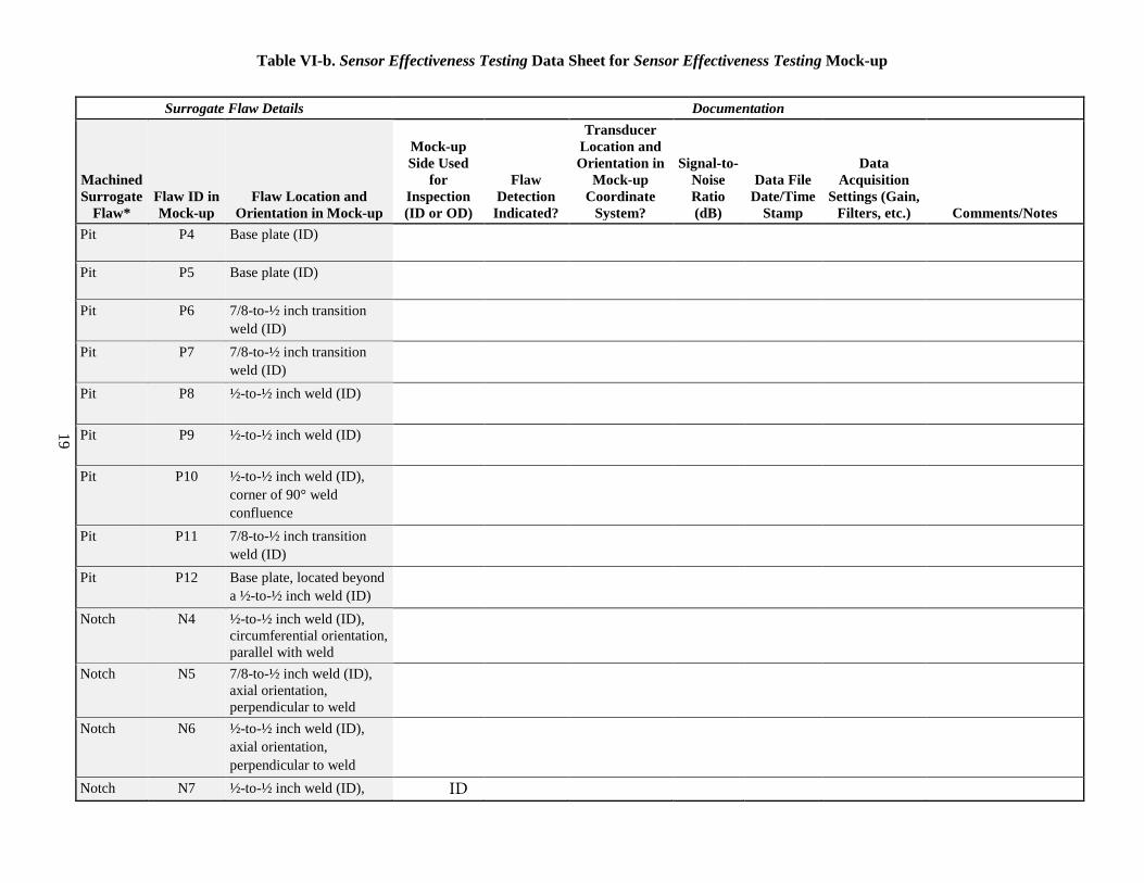
19
Table VI-b. Sensor Effectiveness Testing Data Sheet for Sensor Effectiveness Testing Mock-up
Surrogate Flaw Details Documentation
Machined Surrogate
Flaw* Flaw ID in Mock-up
Flaw Location and Orientation in Mock-up
Mock-up Side Used
for Inspection (ID or OD)
Flaw Detection
Indicated?
Transducer Location and Orientation in
Mock-up Coordinate
System?
Signal-to-Noise Ratio (dB)
Data File Date/Time
Stamp
Data Acquisition
Settings (Gain, Filters, etc.) Comments/Notes
Pit P4 Base plate (ID)
Pit P5 Base plate (ID)
Pit P6 7/8-to-½ inch transition weld (ID)
Pit P7 7/8-to-½ inch transition weld (ID)
Pit P8 ½-to-½ inch weld (ID)
Pit P9 ½-to-½ inch weld (ID)
Pit P10 ½-to-½ inch weld (ID), corner of 90° weld confluence
Pit P11 7/8-to-½ inch transition weld (ID)
Pit P12 Base plate, located beyond a ½-to-½ inch weld (ID)
Notch N4 ½-to-½ inch weld (ID), circumferential orientation, parallel with weld
Notch N5 7/8-to-½ inch weld (ID), axial orientation, perpendicular to weld
Notch N6 ½-to-½ inch weld (ID), axial orientation, perpendicular to weld
Notch N7 ½-to-½ inch weld (ID), ID
parisashokouhi
Typewritten Text
parisashokouhi
Typewritten Text
parisashokouhi
Typewritten Text
T(42,101)-R(56,101)
parisashokouhi
Typewritten Text
parisashokouhi
Typewritten Text
parisashokouhi
Typewritten Text
parisashokouhi
Typewritten Text
ID
parisashokouhi
Typewritten Text
Y
parisashokouhi
Typewritten Text
T(37,2)-R(37,12)
parisashokouhi
Typewritten Text
parisashokouhi
Typewritten Text
parisashokouhi
Typewritten Text
parisashokouhi
Typewritten Text
parisashokouhi
Typewritten Text
21.9 dB
parisashokouhi
Typewritten Text
Pitch-catch (PC)
parisashokouhi
Typewritten Text
parisashokouhi
Typewritten Text
parisashokouhi
Typewritten Text
parisashokouhi
Typewritten Text
ID
parisashokouhi
Typewritten Text
Y
parisashokouhi
Typewritten Text
parisashokouhi
Typewritten Text
25.7 dB
parisashokouhi
Typewritten Text
parisashokouhi
Typewritten Text
parisashokouhi
Typewritten Text
T(55,19)-R(55,25)
parisashokouhi
Typewritten Text
PC
parisashokouhi
Typewritten Text
parisashokouhi
Typewritten Text
ID
parisashokouhi
Typewritten Text
Y
parisashokouhi
Typewritten Text
T(55,-3)-R(55,+3)
parisashokouhi
Typewritten Text
parisashokouhi
Typewritten Text
parisashokouhi
Typewritten Text
parisashokouhi
Typewritten Text
14 dB
parisashokouhi
Typewritten Text
PC
parisashokouhi
Typewritten Text
parisashokouhi
Typewritten Text
parisashokouhi
Typewritten Text
- TF
parisashokouhi
Typewritten Text
parisashokouhi
Typewritten Text
ID
parisashokouhi
Typewritten Text
PC - TF
parisashokouhi
Typewritten Text
Y
parisashokouhi
Typewritten Text
T(3,12)-R(37,6)
parisashokouhi
Typewritten Text
parisashokouhi
Typewritten Text
parisashokouhi
Typewritten Text
parisashokouhi
Typewritten Text
parisashokouhi
Typewritten Text
parisashokouhi
Typewritten Text
parisashokouhi
Typewritten Text
19 dB
parisashokouhi
Typewritten Text
ID
parisashokouhi
Typewritten Text
parisashokouhi
Typewritten Text
parisashokouhi
Typewritten Text
parisashokouhi
Typewritten Text
Y
parisashokouhi
Typewritten Text
parisashokouhi
Typewritten Text
parisashokouhi
Typewritten Text
T(19,12)-R(19,20)
parisashokouhi
Typewritten Text
parisashokouhi
Typewritten Text
15.6 dB
parisashokouhi
Typewritten Text
PC
parisashokouhi
Typewritten Text
parisashokouhi
Typewritten Text
T(19,72)-R(55,93)
parisashokouhi
Typewritten Text
parisashokouhi
Typewritten Text
parisashokouhi
Typewritten Text
parisashokouhi
Typewritten Text
parisashokouhi
Typewritten Text
parisashokouhi
Typewritten Text
ID
parisashokouhi
Typewritten Text
parisashokouhi
Typewritten Text
Y
parisashokouhi
Typewritten Text
~ 8 dB
parisashokouhi
Typewritten Text
PC-TF
parisashokouhi
Typewritten Text
*
parisashokouhi
Typewritten Text
* TF = fixed transmitting transducer
parisashokouhi
Typewritten Text
parisashokouhi
Typewritten Text
ID
parisashokouhi
Typewritten Text
8.5 dB
parisashokouhi
Typewritten Text
Y
parisashokouhi
Typewritten Text
parisashokouhi
Typewritten Text
T(19,78)-R(55,84)
parisashokouhi
Typewritten Text
PC-TF
parisashokouhi
Typewritten Text
parisashokouhi
Typewritten Text
parisashokouhi
Typewritten Text
parisashokouhi
Typewritten Text
ID
parisashokouhi
Typewritten Text
Y
parisashokouhi
Typewritten Text
10 dB
parisashokouhi
Typewritten Text
T(55, -5)-R(55,+5)
parisashokouhi
Typewritten Text
5
parisashokouhi
Typewritten Text
parisashokouhi
Typewritten Text
parisashokouhi
Typewritten Text
parisashokouhi
Typewritten Text
parisashokouhi
Typewritten Text
from each other at 1"
parisashokouhi
Typewritten Text
PC - T and R move away
parisashokouhi
Typewritten Text
parisashokouhi
Typewritten Text
13.5 dB
parisashokouhi
Typewritten Text
ID
parisashokouhi
Typewritten Text
Y
parisashokouhi
Typewritten Text
parisashokouhi
Typewritten Text
parisashokouhi
Typewritten Text
PC
parisashokouhi
Typewritten Text
parisashokouhi
Typewritten Text
parisashokouhi
Typewritten Text
parisashokouhi
Typewritten Text
parisashokouhi
Typewritten Text
16 dB
parisashokouhi
Typewritten Text
PC-TF
parisashokouhi
Typewritten Text
ID
parisashokouhi
Typewritten Text
Y
parisashokouhi
Typewritten Text
T(3,84)-R(37,90)
parisashokouhi
Typewritten Text
parisashokouhi
Typewritten Text
parisashokouhi
Typewritten Text
parisashokouhi
Typewritten Text
parisashokouhi
Typewritten Text
ID
parisashokouhi
Typewritten Text
Y
parisashokouhi
Typewritten Text
TT
parisashokouhi
Typewritten Text
parisashokouhi
Typewritten Text
T(3,1)-R(37,1)
parisashokouhi
Typewritten Text
8 dB
parisashokouhi
Typewritten Text
parisashokouhi
Typewritten Text
parisashokouhi
Typewritten Text
parisashokouhi
Typewritten Text
parisashokouhi
Typewritten Text
15 dB
parisashokouhi
Typewritten Text
TC
parisashokouhi
Typewritten Text
parisashokouhi
Typewritten Text
ID
parisashokouhi
Typewritten Text
Y
parisashokouhi
Typewritten Text
T(55,106)-R(55,88)
parisashokouhi
Typewritten Text
parisashokouhi
Typewritten Text
parisashokouhi
Typewritten Text
parisashokouhi
Typewritten Text
parisashokouhi
Typewritten Text
parisashokouhi
Typewritten Text
parisashokouhi
Typewritten Text
parisashokouhi
Typewritten Text
parisashokouhi
Typewritten Text
parisashokouhi
Typewritten Text
parisashokouhi
Typewritten Text
parisashokouhi
Typewritten Text
parisashokouhi
Typewritten Text
parisashokouhi
Typewritten Text
parisashokouhi
Typewritten Text
parisashokouhi
Typewritten Text
parisashokouhi
Typewritten Text
parisashokouhi
Typewritten Text
parisashokouhi
Typewritten Text
parisashokouhi
Typewritten Text
parisashokouhi
Typewritten Text
parisashokouhi
Typewritten Text
parisashokouhi
Typewritten Text
?
parisashokouhi
Typewritten Text
parisashokouhi
Typewritten Text

20
Surrogate Flaw Details Documentation
Machined Surrogate
Flaw* Flaw ID in Mock-up
Flaw Location and Orientation in Mock-up
Mock-up Side Used
for Inspection (ID or OD)
Flaw Detection
Indicated?
Transducer Location and Orientation in
Mock-up Coordinate
System?
Signal-to-Noise Ratio (dB)
Data File Date/Time
Stamp
Data Acquisition
Settings (Gain, Filters, etc.) Comments/Notes
extending from corner of 90° weld confluence, circumferential orientation, parallel with weld
Wall thinning
T2 Base plate (ID)
Wall thinning
T3 Base plate (ID)
Wall thinning
T4 Base plate (ID), located beyond a ½-to-½ inch weld (ID)
Blind Flaw 1
B1 ---
Blind Flaw 2
B2 ---
Comments/Notes:
parisashokouhi
Typewritten Text
parisashokouhi
Typewritten Text
parisashokouhi
Typewritten Text
parisashokouhi
Typewritten Text
parisashokouhi
Typewritten Text
parisashokouhi
Typewritten Text
ID
parisashokouhi
Typewritten Text
ID
parisashokouhi
Typewritten Text
ID
parisashokouhi
Typewritten Text
Y
parisashokouhi
Typewritten Text
parisashokouhi
Typewritten Text
Y
parisashokouhi
Typewritten Text
Y
parisashokouhi
Typewritten Text
parisashokouhi
Typewritten Text
parisashokouhi
Typewritten Text
parisashokouhi
Typewritten Text
parisashokouhi
Typewritten Text
parisashokouhi
Typewritten Text
parisashokouhi
Typewritten Text
parisashokouhi
Typewritten Text
T(19,76)-R(55,76)
parisashokouhi
Typewritten Text
parisashokouhi
Typewritten Text
T(3,103)-R(37,103)
parisashokouhi
Typewritten Text
T(66,47)-R(66,83)
parisashokouhi
Typewritten Text
parisashokouhi
Typewritten Text
parisashokouhi
Typewritten Text
parisashokouhi
Typewritten Text
5.3 dB
parisashokouhi
Typewritten Text
parisashokouhi
Typewritten Text
parisashokouhi
Typewritten Text
parisashokouhi
Typewritten Text
parisashokouhi
Typewritten Text
parisashokouhi
Typewritten Text
12 : y=76:+1:87
parisashokouhi
Typewritten Text
parisashokouhi
Typewritten Text
parisashokouhi
Typewritten Text
parisashokouhi
Typewritten Text
parisashokouhi
Typewritten Text
parisashokouhi
Typewritten Text
parisashokouhi
Typewritten Text
parisashokouhi
Typewritten Text
11.9 dB
parisashokouhi
Typewritten Text
parisashokouhi
Typewritten Text
parisashokouhi
Typewritten Text
The same data acquisition settings were used for detecting all defects.
parisashokouhi
Typewritten Text
parisashokouhi
Typewritten Text
10:
parisashokouhi
Typewritten Text
x=66:-1:57
parisashokouhi
Typewritten Text
parisashokouhi
Typewritten Text
parisashokouhi
Typewritten Text
parisashokouhi
Typewritten Text
parisashokouhi
Typewritten Text
parisashokouhi
Typewritten Text
11: y=103:+1:113
parisashokouhi
Typewritten Text
parisashokouhi
Typewritten Text
parisashokouhi
Typewritten Text
parisashokouhi
Typewritten Text
7.1 dB
parisashokouhi
Typewritten Text
parisashokouhi
Typewritten Text
parisashokouhi
Typewritten Text
parisashokouhi
Typewritten Text
parisashokouhi
Typewritten Text
parisashokouhi
Typewritten Text
parisashokouhi
Typewritten Text
parisashokouhi
Typewritten Text
parisashokouhi
Typewritten Text
parisashokouhi
Typewritten Text
parisashokouhi
Typewritten Text
parisashokouhi
Typewritten Text
parisashokouhi
Typewritten Text
parisashokouhi
Typewritten Text
parisashokouhi
Typewritten Text
parisashokouhi
Typewritten Text
parisashokouhi
Typewritten Text
parisashokouhi
Typewritten Text
parisashokouhi
Typewritten Text
parisashokouhi
Typewritten Text
Y
parisashokouhi
Typewritten Text
parisashokouhi
Typewritten Text
3.7 dB
parisashokouhi
Typewritten Text
ID
parisashokouhi
Typewritten Text
16:
parisashokouhi
Typewritten Text
parisashokouhi
Typewritten Text
parisashokouhi
Typewritten Text
y=49:+1:65
parisashokouhi
Typewritten Text
T(37,49)-R(19,49)
parisashokouhi
Typewritten Text
37,49
parisashokouhi
Typewritten Text
parisashokouhi
Typewritten Text
parisashokouhi
Typewritten Text
parisashokouhi
Typewritten Text
notch along the weld
parisashokouhi
Typewritten Text
pit
parisashokouhi
Typewritten Text
ID
parisashokouhi
Typewritten Text
Y
parisashokouhi
Typewritten Text
parisashokouhi
Typewritten Text
parisashokouhi
Typewritten Text
7.5 dB
parisashokouhi
Typewritten Text
PE air slot y=29"
parisashokouhi
Typewritten Text
T(60,29)-R(63,29)
parisashokouhi
Typewritten Text
5 scans
parisashokouhi
Typewritten Text
parisashokouhi
Typewritten Text

21
Table VI-c. Sensor Effectiveness Testing Data Sheet for Measurement Robustness Testing
Surface Condition
Targeted Reflector Detected
(Y/N) SNR (dB)
Sensor Location on
Mock-up File Date/
Time Stamp Comments/notes
Non-metallic Debris
No debris
Minimal debris
Oxides
Near pristine (Modified
Technology Screening Mock-up)
Mild Rust/Oxide
(Sensor Effectiveness Testing Mock-up)
Field Representative Rust/Oxide (APEL
Mock-up)
parisashokouhi
Typewritten Text
Y
parisashokouhi
Typewritten Text
Y
parisashokouhi
Typewritten Text
parisashokouhi
Typewritten Text
parisashokouhi
Typewritten Text
9.2
parisashokouhi
Typewritten Text
parisashokouhi
Typewritten Text
parisashokouhi
Typewritten Text
parisashokouhi
Typewritten Text
6.8
parisashokouhi
Typewritten Text
parisashokouhi
Typewritten Text
parisashokouhi
Typewritten Text
parisashokouhi
Typewritten Text
parisashokouhi
Typewritten Text
Y
parisashokouhi
Typewritten Text
Y
parisashokouhi
Typewritten Text
Y
parisashokouhi
Typewritten Text
parisashokouhi
Typewritten Text
parisashokouhi
Typewritten Text
parisashokouhi
Typewritten Text
parisashokouhi
Typewritten Text
parisashokouhi
Typewritten Text
@12" edge
parisashokouhi
Typewritten Text
@ 12" edge
parisashokouhi
Typewritten Text
@ 12" edge
parisashokouhi
Typewritten Text
parisashokouhi
Typewritten Text
33
parisashokouhi
Typewritten Text
31
parisashokouhi
Typewritten Text
31
parisashokouhi
Typewritten Text
parisashokouhi
Typewritten Text
parisashokouhi
Typewritten Text
parisashokouhi
Typewritten Text
parisashokouhi
Typewritten Text
parisashokouhi
Typewritten Text
parisashokouhi
Typewritten Text
parisashokouhi
Typewritten Text
parisashokouhi
Typewritten Text
parisashokouhi
Typewritten Text
T(43,32)
parisashokouhi
Typewritten Text
parisashokouhi
Typewritten Text
parisashokouhi
Typewritten Text
parisashokouhi
Typewritten Text
parisashokouhi
Typewritten Text
parisashokouhi
Typewritten Text
T(43,32)
parisashokouhi
Typewritten Text
R(40,32)
parisashokouhi
Typewritten Text
parisashokouhi
Typewritten Text
PE - 7 @1"
parisashokouhi
Typewritten Text
parisashokouhi
Typewritten Text
parisashokouhi
Typewritten Text
parisashokouhi
Typewritten Text
parisashokouhi
Typewritten Text
parisashokouhi
Typewritten Text
parisashokouhi
Typewritten Text
parisashokouhi
Typewritten Text
parisashokouhi
Typewritten Text
parisashokouhi
Typewritten Text
parisashokouhi
Typewritten Text
R(40,32)
parisashokouhi
Typewritten Text
parisashokouhi
Typewritten Text
PE - 7@1"
parisashokouhi
Typewritten Text
PE - 1
parisashokouhi
Typewritten Text
PE - 1
parisashokouhi
Typewritten Text
parisashokouhi
Typewritten Text
parisashokouhi
Typewritten Text
PE - 1
parisashokouhi
Typewritten Text
parisashokouhi
Typewritten Text
PE = Pulse - Echo (moving T and R together) PE - 7 @1" = Pulse - Echo, 7 locations, 1" spacing
parisashokouhi
Typewritten Text
parisashokouhi
Typewritten Text
(Tx=43, 42, ... y=32 & Ry=40, 39, ... y=32)
parisashokouhi
Typewritten Text
parisashokouhi
Typewritten Text
parisashokouhi
Typewritten Text
parisashokouhi
Typewritten Text
parisashokouhi
Typewritten Text
PE - 1 = a single pulse-echo measurement
parisashokouhi
Typewritten Text

Sensor Effectiveness Testing 35
7. Discussion / Conclusions 7.a. Dependence of flaw detection on transducer orientation The pit and thinning flaws are axisymmetric and therefore it does not matter from which direction the wave impings upon the flaw; what does matter for the axisymmetric flaws is their size and distance from the air slots. The notch flaws are more readily detected by waves that have a significant projection onto the notch face; both PC and PE modes are observed to work well. 7.b. Impact of air slot restrictions on flaw detection ability The restriction that the EMATs be located within air slots did not present problems because the whole system (EMATs, instrumentation, and methods) was developed with this restriction in mind. We were initially concerned that the weld pattern in the DST bottom could create complications due to weld echoes. Fortunately, the energy transmitted across a weld is significantly higher than that reflected. 7.c. General signal quality and data quality The EMATs were configured to send and receive strong SH waves by the liftoff and the position of the magnet array. Relative to the technology screening tests, where an Ultratek system was used, the gated amplified provided high power excitation more appropriate for the EMAT transmitter. The signal quality was high and the EMATs were easy to position because the magnetic force was relatively low (for an EMAT on steel). The alignment marks on the EMAT housing made it quite simple to position it with relatively good accuracy. 7.d. Ability to locate and size flaws The NDI pitch-catch (PC) and pulse-echo (PE) modes lend themselves to reliable flaw detection as long as the received scattering or reflection signal is above the noise floor because there are no other signals. However, the presence of other reflectors complicates locating defects. The TT mode is based on flaws scattering waves and therefore the receiving EMAT captures a smaller signal. Thus, the received signals are larger, but often there is deviation in the incident wave amplitude due to variations in material and boundary conditions. Our method to detect wall-thinning is based upon the cutoff of the SH1 mode due to thickness change and on scattering. The tests that we have conducted to date have been to detect and locate flaws, but characterization of flaw type and size range should be possible given a sufficient database of flaws, such as provided by the two existing mockups. 7.e. Tolerance for rust The presence of uniform surface rust did not affect operation of the EMATs at all. Absolutely no changes in procedures were implemented. The rust did result in an amplitude decrease of as much as 20% for the SH0 wave packet. If the rust is uniform then there would be no affect on flaw detection. The amplitude decrease is probably due to the combined affects of increased EMAT liftoff and increased material attenuation. We conjecture that the biggest affect of rust on flaw detection would be if the rust was very localized rather than uniform, resulting in larger amplitude variations in TT mode. 7.f. Tolerance for dirt The tolerance for dirt was excellent. No procedural changes were made to detect flaw C after the

Sensor Effectiveness Testing 36
dirt was added. The flaw images were essentially the same for clean and dirty surfaces. 7.g. Transducer requirements The EMATs require no applied force or couplant. The transfer balls enable the EMATs to roll smoothly over the plate surface under the action of a small lateral force (this force was not measured, but is roughly 1 lb). The EMAT housings are designed with robotic delivery in mind. The force required to remove the EMAT from the plate is slightly higher (but still less than 5 lb). For convenience the EMATs were placed on the top surface of the mockup, but the same results would be obtained if they were on the bottom surface. Because of this, it is not possible to determine whether the defects are connected to the top or bottom surface, which is true for almost all guided wave methods. That is why we also plan to use a giant magneto resistance (GMR) probe in combination with EMATS. Because this probe only assesses the nearby surface, it can identify surface connectivity of defects located at the air slots. 7.h. Vision for what the system would look like for actual testing We envision continued development of the EMAT-based nondestructive inspection system to entail the following tasks: 1. Remote deployment of EMATs in realistic ‘air slot’-like channels below the two mockups at
PNNL; 2. Development of a systematic inspection methodology for weld lines and volumetric plate
material in the mockups based on pitch-catch, pulse-echo, and through-transmission modes; 3. Creation of a library of signal features correlated to defect type and size for characterization
of hidden flaws; 4. Integration of the EMAT inspection system with a robotic delivery system and evaluation of
the robotic inspection system. Based on the SET results we envision an EMAT-based DST NDI system using a marsupial robotic delivery system. The mother system would be positioned in the annulus and would extend a wand/probe/crawler into an air slot. There would actually be two systems operating in adjacent air slots. Each wand/probe/crawler would deliver two EMATs with variable orientations of 0, ±45, and 90 degrees. EMAT orientation would be set by a pneumatic or servomotor controlled spline. In addition, the distance between the two EMATs in the same air slot would vary between 0-48”. This system would provide great flexibility for PC, PE, and TT modes of flaw detection and localization. A systematic NDI methodology would be developed to provide optimal coverage, with as much redundancy as practical, of the accessible region of the primary tank bottom. Modifications to the system used for SET would be primarily to the EMAT housing to adapt it to the robotic delivery system. The inspection functionality of the system would be based on 4 EMATs, with 2 EMATs being located in 2 different air slots. The distance between EMATs in each air slot would be ~ 6-48”. Each EMAT needs two modes of actuation, one to move along the air slot and one to set its orientation. Both of these degrees of freedom need to be encoded to track the current position and orientation of the EMAT. Furthermore, the encoded position and orientation need to be related to the DST coordinate system in order to obtain meaningful data. Since the system uses 4 EMATs, any of which could be the transmitter, a switching board

Sensor Effectiveness Testing 37
capable of high power signals will need to be added. As a university, Penn State is accustomed to research and development, which is how we envision tasks 1-4 (above). The project will eventually reach a point where the prototype robotic inspection system (e.g., sensors, equipment, and software) needs to become rugged and fool-proof. At that point we will partner with a company (e.g., Structural Integrity, Guidedwave, Innerspec) to build a production system and train operators on its use. Currently, our best guesses for task durations and budgets are: (1) 6 months and $50K, (2) 6 months and $50K, (3) 12 months and $100K, (4) 6-12 months and $50-100K. Better estimates can be provided after the scope of work has been refined.

Sensor Effectiveness Testing 1
Appendix The appendix is organized by mockup (modified and new) and then by flaw type (pits, notches, thinning, and blind). The information provided about the image is type (SAFT, Bscan), method (PC, PE, TT), EMAT coordinates for both transmitter and receiver, and time and date (to link with photographs). When an EMAT is scanned a range of coordinates is given. Multiple images are provided for some flaws. Time and date is provided to correlate images with photographs taken by PNNL. Results from Dirt and Rust tests are given in the body of the report and therefore are not repeated here.

Sensor Effectiveness Testing 2
1. Modified Mockup 1.1 Pits P1 (22,76), SAFT, PC, T(26,71-‐76), R(26,79-‐84), 5:01 6/6 0.375” diam, 0.125” deep

Sensor Effectiveness Testing 3
P1, SAFT, PC, T(26,72), R(26,76-‐84), 5:07 6/6

Sensor Effectiveness Testing 4
P2 (weld,75), SAFT, PC, T(26,34-‐74), R(26,52-‐92), 3:37 6/6 [contains N3 too] 0.375” diam, 0.125” deep

Sensor Effectiveness Testing 5
P2, SAFT, PC, T(26,67), R(26,76-‐91), 4:45 6/6

Sensor Effectiveness Testing 6
P3 (38.125,46.06), SAFT, PC, T(46,48-‐57), R(46,32-‐41), 4:37 6/6 0.75” diam, 0.25” deep

Sensor Effectiveness Testing 7
P3, SAFT, PC, T(26,34), R(26,52-‐64), 4:25 6/6

Sensor Effectiveness Testing 8
1.2 Notches N1-‐N3, PE, SAFT, T(26,37-‐87), R(26,40-‐90), 2:11 6/6 N1 (weld, 82) 2” long, 0.1” deep, along weld N2 (before weld, ~50) 2” long, 0.25” deep, transverse to weld N3 (before weld, ~60) 2” long, 0.25” deep, parallel to weld
This images are dominated by the end wall reflections of the plate. However, the reflections at 15” from the edge are the notch defects N1, N3, and N2 from left to right.

Sensor Effectiveness Testing 9
By analyzing just the first 15” from the EMATs we can eliminate the end wall reflections and the notch defects become clearer. Below, the notch defects from left to right are N2, N3, and N1. The y-‐axis indicates the y-‐coordinate. The SNR was calculated from the preceding images where the noise floor was computed from the weld echo at locations away from the defects. This is somewhat arbitrary and leads to a low SNR. Even though a case could be made for computing the SNR in a less conservative way, we have not.

Sensor Effectiveness Testing 10
N3, SAFT, PC, T(26,34-‐74), R(26,52-‐92), 3:37 6/6 (contains P2 too)

Sensor Effectiveness Testing 11
1.3 Thinning T1 (10,56), TT, T(14-‐4,32), R(14-‐4,72) data not saved 4” diam, 0.05” deep We ran the test but neglected to save the data, therefore we could analyze T1.

Sensor Effectiveness Testing 12
2. New Mockup 2.1 Pits P4 (42,12), SAFT, PC, T(37,2-‐11), R(37,12-‐21), 2:46 6/7 0.75” diam, 0.25” deep

Sensor Effectiveness Testing 13
P5 (58,24), SAFT, PC, T(55,19-‐25), R(55,25-‐31), 2:51 6/7 1.125” diam, 0.375” deep

Sensor Effectiveness Testing 14
P6 (52,0), SAFT, PC, T(55,-‐3), R(55,3-‐11), 8:24 6/7 0.75” diam, 0.25” deep, in weld

Sensor Effectiveness Testing 15
P7 (17,0), SAFT, PC, T(3,12), R(37,6-‐26), 6:10 6/6 1.125” diam, 0.375” deep, in weld

Sensor Effectiveness Testing 16
P8 (24,24), SAFT, PC, T(19,12-‐23), R(19,20-‐31), 2:03 6/7 0.75” diam, 0.25” deep, in weld

Sensor Effectiveness Testing 17
P9 (50,96), SAFT, PC, T(19,72), R(55,93-‐71), 10:24 6/7 1.125” diam, 0.375” deep, in weld
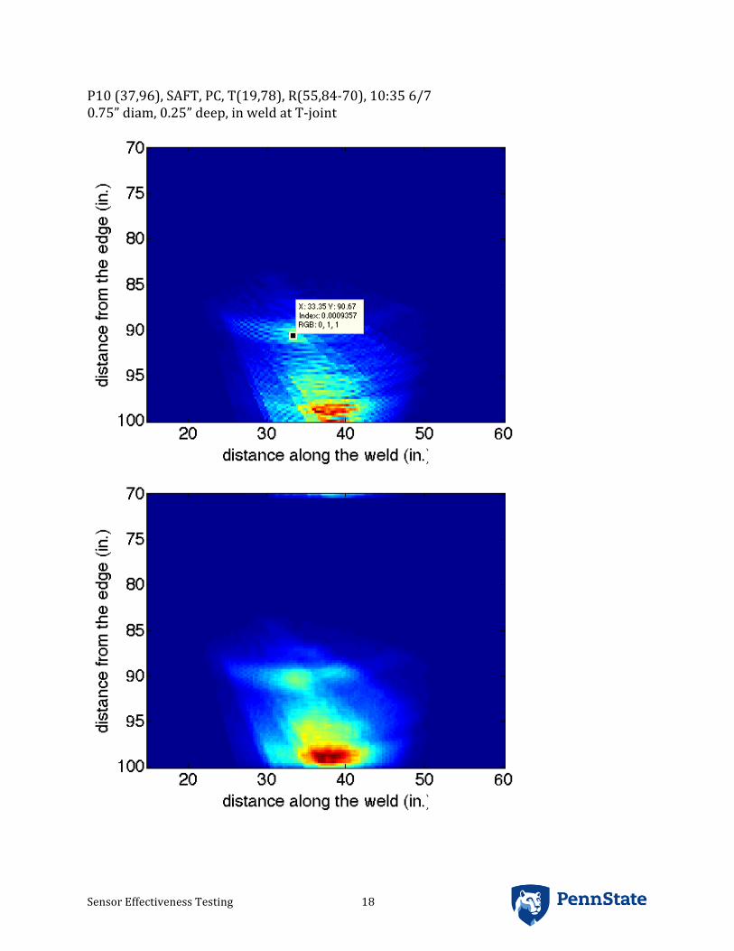
Sensor Effectiveness Testing 18
P10 (37,96), SAFT, PC, T(19,78), R(55,84-‐70), 10:35 6/7 0.75” diam, 0.25” deep, in weld at T-‐joint

Sensor Effectiveness Testing 19
P11 (66,0), SAFT, PC, T(55,-‐5-‐(-‐18)), R(55,5-‐18), 8:52 6/7 0.375 diam, 0.125” deep, in weld

Sensor Effectiveness Testing 20
P12 (54, 108), SAFT, PC, T(42-‐52,101), R(56-‐66,101), 11:26 6/7 0.75” diam, 0.25” deep
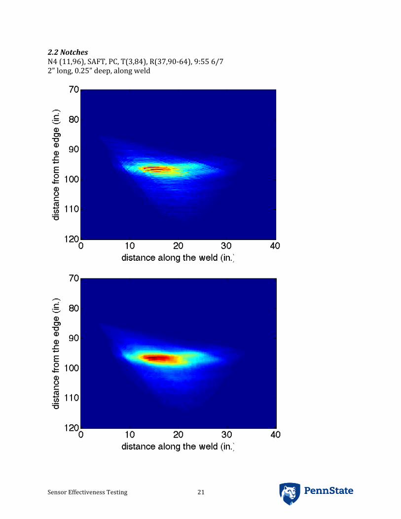
Sensor Effectiveness Testing 21
2.2 Notches N4 (11,96), SAFT, PC, T(3,84), R(37,90-‐64), 9:55 6/7 2” long, 0.25” deep, along weld

Sensor Effectiveness Testing 22
N5 (6,0), SAFT based on SH1 speed, TT, T(3,1-‐6), R(37,1-‐6), 5:55 6/6 2” long, 0.25” deep, transverse to weld Note that incident wave is followed quickly by an end wall echo

Sensor Effectiveness Testing 23
N6 (66,96), SAFT, PC, T(55,106-‐97), R(55,88-‐79), 10:53 6/7 2” long, 0.25” deep, transverse to weld P12 limited positioning of T

Sensor Effectiveness Testing 24
N7 (25, 96) should have used PC with T(19,90), R(37,90-‐75) 2.875” long, 0.25” deep, along weld We mistakenly marked N7 off the list of found defects, thus we did not acquire to necessary data.

Sensor Effectiveness Testing 25
2.3 Thinning T2 (60,60.5), SAFT based on SH1 speed, TT, T(66-‐76,47), R(66-‐76,83), 3:28 6/7 4” diam, 0.1” deep

Sensor Effectiveness Testing 26
T3 (44,83), SAFT based on SH1 speed, TT, T(19,76-‐88), R(55,76-‐88), 3:20 6/7 4” diam, 0.25” deep

Sensor Effectiveness Testing 27
T4 (17,108), SAFT based on SH1 speed, TT, T(3,103-‐114), R(37,103-‐114), 3:10 6/7 4” diam, 0.25” deep End wall echo follows right behind the incident wave The receiver was located right on the weld cap at x=37” resulting in a lower amplitude and more variability, but generally it was ok

Sensor Effectiveness Testing 28
2.4 Blind Defects B1, SAFT, PC, T(37,2-‐69), R(37,28-‐95), 1:08 6/7 Probable notch along weld x=24” between 56-‐59”
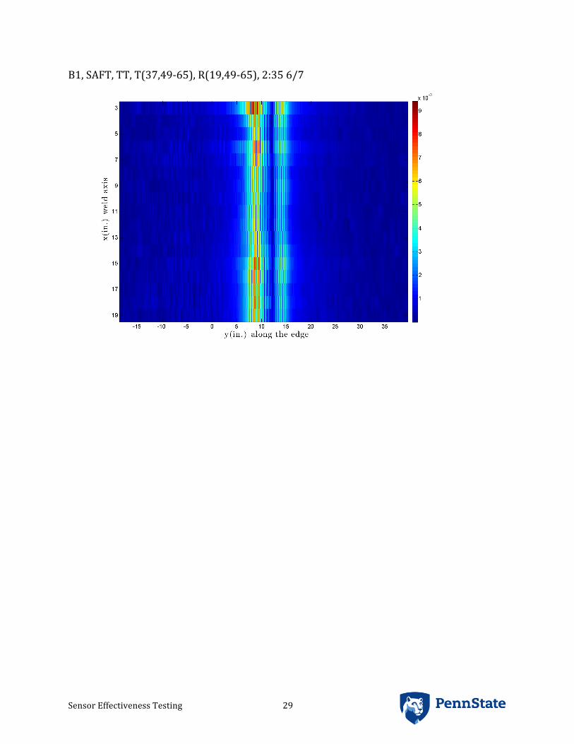
Sensor Effectiveness Testing 29
B1, SAFT, TT, T(37,49-‐65), R(19,49-‐65), 2:35 6/7

Sensor Effectiveness Testing 30
B2, SAFT, PE, T(60-‐65,47), R(63-‐68,47), 6:21 6/7 Possible pit located in the plate at (63-‐64,36-‐37)

Sensor Effectiveness Testing 31
B2, SAFT, PE, T(60-‐65,29), R(63-‐68,29), 6:27 6/7

Sensor Effectiveness Testing 32
B2, SAFT, TT, T(55-‐70,47), R(55-‐70,11), 6:14 6/7

Appendix D –
SwRI


SwRI Project 18.22929 August 2, 2017
S O U T H W E S T R E S E A R C H I N S T I T U T E®
SENSOR EFFECTIVENESS TESTING TEST REPORT
Prepared for: Prepared by:
Pacific Northwest National Laboratory Sensor Systems and NDE Sect. 902 Battelle Boulevard Southwest Research Institute Richland, Washington 99352 6220 Culebra Road San Antonio, TX 78238-5166

SwRI Project 18.22929 August 2, 2017
S O U T H W E S T R E S E A R C H I N S T I T U T E®
SENSOR EFFECTIVENESS TESTING TEST REPORT Prepared for
Pacific Northwest National Laboratory 902 Battelle Boulevard Richland, Washington 99352 Prepared by
Adam C. Cobb, Ph.D., Principal Engineer Sensor Systems & NDE Technology Section Approved:
Clinton Thwing, Manager Sensor Systems & NDE Technology Section
Project 18.22929 ii August 2, 2017
EXECUTIVE SUMMARY
Southwest Research Institute® (SwRI®) was contracted by Washington River Protection
Solutions (WRPS) to perform sensor effectiveness testing of an SwRI-developed inspection
approach on two mockups of the double-shell tanks (DSTs) located at the Hanford site. This
testing was performed in late June, 2017 at the Pacific Northwest National Laboratory (PNNL).
The proposed inspection approach for the tanks uses a guided wave sensor positioned on the
vertical wall of the DST primary vessel. The acoustic waves generated on the wall would
propagate to the primary tank bottom; any corrosion or cracks in the acoustic path would cause
waves to be reflected back to the sensor for detection. The sensor would be scanned robotically
around the circumference of the vessel and data would be acquired at regular intervals. All of the
data would be combined together using special signal processing algorithms to create an easy to
interpret, color image of the vessel condition. Key features of this inspection approach are that:
• Low risk of getting stuck: The system does not require direct access to the tank
bottom through the available air slots between the primary and secondary tanks,
• Simplified robotic delivery: The sensor does not need any fluid couplants or
excessive pressing of the sensor to the vessel, and the sensor does not need to be
transported into the air slots
• Can inspect a large percentage of the tank: The guided waves can propagate long
distances, potentially up to 10 m from the sensor location
The purpose of the sensor effectiveness testing discussed in this report was to assess the
performance of the inspection approach using artificial flaws that were known to be difficult to
detect based on the results of a prior screening demonstration held in February, 2017. The same
inspection system designed and manufactured by SwRI was used at both demonstrations. The
original application of this field-deployed system was the inspection of nuclear power plant
containment vessels. Key modifications were made to the system to improve the performance for
DSTs based on lessons learned during the screening demonstration.
During the two days of testing, each of the two mockups provided was inspected using this
system numerous times, to evaluate different possible configurations. The quality of the data
acquired was excellent and the evaluation of the mockups was completed successfully. Across the

Project 18.22929 iii August 2, 2017
two mockups there were a total of 32 defects located in either the 1/2-inch bottom plates or in the
thickness transition welds joining the 7/8-inch to 1/2-inch plates; at least 24 were detected,
including every defect in the thickness transition weld, all but two pit-shaped flaws, and the
majority of the crack-like flaws in the mockups. This included two blind defects located in the
sensor effectiveness testing mockup that was designed for this sensor evaluation. This
performance was achieved in spite of the guided waves being required to propagate through
multiple welds and having a sensor-to-flaw separation of over 14 feet. The only flaw type that
presented significant challenges to the inspection approach was a wall thinning feature. These
flaws had a very gradual change over a couple of inches along the surface to their maximum depth,
which is difficult to detect using guided waves at the test frequencies and inspection distances used
here.
Based on these results, it is the conclusion of SwRI that the technology demonstrated could
screen the DST primary bottom for damage from the side wall without needing any portion of the
system to be inserted into the air slots. Moreover, the system should be readily miniaturized for
pairing with a robotic delivery vehicle to work in the harsh environment at Hanford. Finally, the
finalized inspection system developed for this current inspection challenge could potentially be
adapted for other inspection targets at the facility, including the secondary tank bottom as well as
the primary and secondary tank vertical walls.

Project 18.22929 iv August 2, 2017
TABLE OF CONTENTS
Section Page
1. INTRODUCTION .................................................................................................. 1
2. BACKGROUND .................................................................................................... 2
3. APPROACH FOR SENSOR EFFECTIVENESS TESTING ............................................... 7
4. DATA SUMMARY .............................................................................................. 11
5. INSPECTION RESULTS ........................................................................................ 17
5.1 Technology Screening Mockup Results ................................................................. 18
5.2 Sensor Effectiveness Testing Mockup Results........................................................ 20
6. CONCLUSIONS AND DISCUSSIONS ..................................................................... 22
7. APPENDIX A – SAFT IMAGES OF MOCKUPS ....................................................... A-1
Technology Screening Mockup Images............................................................................ A-1
Sensor Effectiveness Testing Mockup Images .................................................................. A-4
8. APPENDIX B – INSPECTION RESULTS ................................................................. B-1
9. APPENDIX C – SAFT IMAGES OF FLAWS ............................................................ C-1
10. APPENDIX D – POTENTIAL SYSTEM IMPROVEMENTS ..................................... D-1

Project 18.22929 v August 2, 2017
LIST OF FIGURES
Figure Page
Figure 1. Conceptual illustration of EMAT in inspection system ...................................... 3
Figure 2. Cart in final assembled condition, with electromagnet, sensor assembly,
and pulser/receiver electronics. The view is as seen from the vessel
wall. .............................................................................................................. 4
Figure 3. Photograph of umbilical cable (red cable) connected to the power supply
enclosure (left-most box) and data acquisition computer with a LabVIEW
application running. The laptop on the right is used for processing the
data following the data acquisition process, but the processing could
occur on the data acquisition computer if necessary. ................................... 5
Figure 4. Overall description of the beam forming approach for looking at a single
location, (x, y). For each sensor location, p, the associated angle θpx, y
and propagation distance dpx, y must be calculated. .................................... 6
Figure 5. Flaw description on an SwRI containment vessel mockup (left). The
numbered artificial defects were various notches (lines), circular-shaped
flaws (circles) and drilled holes (“x” markers) between 10% and 50% of
wall thickness in depth. SAFT beam forming data with corresponding
flaws marked (right). ..................................................................................... 7
Figure 6. Photograph of the EMAT holder before (left) and after (right) installed on
the sensor cart ............................................................................................ 11
Figure 7. Example waveform collected using the EMAT system .................................. 14
Figure 8. SAFT images produced using the 57 kHz sensor coil on the effectiveness
testing mockup (data sets 77, 83, and 87). The left and right plots are
the “high” and “low” sensor configurations, respectively, while the center
plot is the original straight down configuration. The color scale for each
image is shown to the right of that image. The white markers (circles

Project 18.22929 vi August 2, 2017
and diamonds) denote flaw locations, the dashed magenta lines denote
mockup edges and welds, the dashed white box denotes the noise
region, and the red “x” markers near the top of each image are where
data was collected. ..................................................................................... 15
Figure 9. Graphical representation of the detection performance in the technology
screening mockup. Green circles highlight detected defects whereas
red circles denote undetected defects. ....................................................... 20
Figure 10. Graphical representation of the detection performance in the technology
screening mockup. Green circles highlight detected defects, red circles
denote undetected defects and the purple circles denote locations
where suspected blind defects are located. ................................................ 22
Figure 11. Conceptual illustration of the DST inspection system showing a robotic
delivery vehicle close-up (left) and on the DST wall (right). ........................ 25
LIST OF TABLES
Table Page
Table 1. Summary of the parameters of the data sets acquired during sensor
effectiveness testing. Abbreviations BP, HP, and LP stand for band
pass, high pass and low pass, respectively. ............................................... 12
Table 2. Summary of transducer heights relative to the weld immediately below the
EMAT ......................................................................................................... 13

Project 18.22929 Page 1 “Sensor Effectiveness Testing Test Report” August 2, 2017
1. INTRODUCTION
Southwest Research Institute® (SwRI®) was invited by Washington River Protection
Solutions (WRPS) to perform sensor effectiveness testing of an SwRI-developed inspection
approach on two mockups of a thick-walled vessel. The testing was performed at Pacific
Northwest National Laboratory (PNNL). The inspection technology utilizes an electromagnetic
acoustic transducer (EMAT) to generate and receive guided ultrasonic waves. The inspection
process involves moving the custom transducer around the circumference of the vessel and
collecting data at regular intervals. The collected data are processed to form a color-mapped image
of the structure condition. This technology was developed over several years to assess the integrity
of nuclear power plant containment vessels; it has recently been used to assess vessel conditions
at two nuclear plant sites.
SwRI previously demonstrated this system during a technology demonstration test in
February, 2017 (“Technology Demonstration Report” dated February 24, 2017 / Project
18.R8720). This demonstration was performed on a single mockup of the double-shell tanks
(DSTs) located at the Hanford site. The mockup represented a portion of the bottom of the DST
primary/inner tank that rests on a concrete pad with an attached vertical wall and transition plates.
As would be done in an actual inspection of a DST, the sensor system was scanned along the
vertical wall of the mockup and guided waves were propagated into the mockup floor. This
mockup had artificial flaws introduced that were large enough to warrant remedy if found in the
actual DSTs. The demonstration test results were that most of the defects located away from the
weld were detectible, but detection of defects located within the weld was problematic due to the
large reflection from the weld itself.
The purpose of this second round of testing was to evaluate the effectiveness of the
sensors/systems using more challenging flaw shapes and sizes. Some of these flaws would be of
interest if found in the actual DSTs but not necessarily require immediate repair, based on
discussion with PNNL. Both the original mockup, with additional flaws added, and a second
mockup, were used in the evaluations. The system used previously was modified for this
demonstration to improve performance based on lessons learned during the first technology
demonstration. Note that the test protocol included measurements related to the sensitivity of the

Project 18.22929 Page 2 “Sensor Effectiveness Testing Test Report” August 2, 2017
system to surface contaminants such as rust, but these tests were not necessary and not performed
here as contamination is not a concern for the DST wall. Following this demonstration, it is
anticipated that the most successful sensing technology(ies) would be transitioned into a field-
deployable system in future project phases.
This document is the final test report of the sensor effectiveness testing held during in June
2017. Included in this report are descriptions of the inspection system and data analysis approach,
summary of system changes from the prior demonstration, data collection summary, complete
inspection results, and discussions and conclusions from these results.
2. BACKGROUND
The inspection system combines a custom-built guided wave EMAT with array signal
processing techniques to allow for the inspection of large areas of a vessel. Rather than build a
physical array of sensors, a single sensor is translated around the circumference of the vessel, and
waveforms are acquired at regular intervals. The signals acquired from each of the transducer
locations are then processed using a synthetic aperture focusing technique (SAFT), which produces
a color image of the structure that shows where indications are located.
The demonstration system sensor is an EMAT that operates using the magnetostrictive
effect for the generation and reception of guided waves. This style of EMAT was chosen for the
original application given requirements on test frequency and aperture, but other EMAT
implementations, e.g., periodic permanent magnet (PPM) EMATs, would be appropriate for
different applications. The biasing magnet in the demonstration system is an electromagnet, and
the coil is arranged in a meander configuration, as shown in Figure 1. In operation, the coil is
pulsed with a short tone burst at the test frequency. Guided waves are produced by the interaction
of the biasing and pulsed magnetic fields with the magnetostrictive structure under test.

Project 18.22929 Page 3 “Sensor Effectiveness Testing Test Report” August 2, 2017
Figure 1. Conceptual illustration of EMAT in inspection system
For the previous technology demonstration, multiple EMAT coils were fabricated using a
flexible printed circuit technique. Each sensor coil assembly combines two transmitter and two
receiver coils. Transmitter coils are designed to maximize transmit current, whereas receive coils
are designed to maximize received signal voltages. All coils were designed to generate the
fundamental shear horizontal guided wave mode (SH0). This specific wave mode was chosen
because (1) it is nondispersive (the wave speed is independent of frequency), which simplifies
analysis, and (2) it has no out-of-plane strain (to reduce the effect of any fluids in the DST). For
this mode, the meander line spacing on each coil is equal to half of the guided wave wavelength
being used. Furthermore, the two transmit coils are precisely offset from one another in the wave
propagation direction. The offset, when combined with the custom two channel pulser circuit,
allows for the generated guided wave to be reinforced in one direction and cancelled in the other.
This means that the guided wave propagates primarily in one direction. The receive coil spacing
and two channel receiver electronics produces similar functionality. For the technology
demonstration, four EMAT coils were tested with the following meander spacing and associated
test frequencies:
• 76 mm wavelength (42 kHz test frequency)
• 66 mm wavelength (49 kHz test frequency)
• 56 mm wavelength (57 kHz test frequency)
• 44 mm wavelength (72 kHz test frequency)
The coil wavelength and test frequencies were chosen to produce the lowest order shear
horizontal guided waves in appropriate thickness steel wall that would avoid exciting higher order
modes. The lowest two frequency coils were designed for testing thicker (>30 mm) vessels;
whereas, the two highest frequency coils were fabricated for the 22.2 mm wall for this technology

Project 18.22929 Page 4 “Sensor Effectiveness Testing Test Report” August 2, 2017
demonstration. All of these sensor coils had the same aperture (width) to wavelength ratio of
approximately three.
Figure 2 is a picture of the field-deployable EMAT. The transducer is attached to a cart
along with a custom pulser and receiver circuit. The EMAT sensor is lifted vertically into place
by the rolling lift cart, and the EMAT is attached and removed from the wall surface by energizing
and de-energizing the electromagnet, respectively. The sensor coil is visible between the two
magnet pole tips; the individual traces are not visible as they are covered by a thin titanium sheet
that is used to protect the flexible printed circuitry. An SwRI-designed custom pulser/receiver
circuit is also resident on the scanner cart electronics enclosure; the pulser/receiver is connected
to the sensor coil with four cables. The primary functions of the pulser/receiver system are
twofold: the pulser circuit provides the high power tone burst into the low impedance EMAT
sensor coil, and the received signal is amplified and bandpass filtered by the receiver circuitry.
Figure 2. Cart in final assembled condition, with electromagnet, sensor assembly, and pulser/receiver electronics. The view is as seen from the vessel wall.
The amplified and filtered signals are connected to an external LabVIEW-based data
acquisition subsystem through an umbilical cable. This subsystem is shown in Figure 3; it is
comprised of a portable computer workstation with an internal waveform digitizer and a separate

Project 18.22929 Page 5 “Sensor Effectiveness Testing Test Report” August 2, 2017
power supply system that supplies power to the electronics and electromagnet on the cart. The
LabVIEW data acquisition program runs on a computer to control the acquisition process. At the
start of an inspection, the operator specifies the inspection parameters such as sensor height, test
frequencies, inspection interval, etc. During the inspection process, the data acquisition program
prompts the operator to move the sensor cart to an incremental position. Once the operator
indicates that the sensor cart has reached the desired position, the sensor electromagnet is engaged,
data is acquired, and the electromagnet is disabled. This process is repeated until the scan is
completed.
Figure 3. Photograph of umbilical cable (red cable) connected to the power supply enclosure (left-most box) and data acquisition computer with a LabVIEW application running. The laptop on the right is used for processing the data following the data acquisition process, but the processing
could occur on the data acquisition computer if necessary.
The data analysis approach combines the waveforms collected using a signal processing
strategy known as SAFT. As an overview of the SAFT procedure, the approach combines the
acquired waveforms from all of the sensor positions to produce an image. First, the structure is
divided into a virtual grid of locations for computing the SAFT response. For a given imaging
location (i.e., a pixel), as illustrated in Figure 4, two parameters are computed from each of the m
sensor locations: propagation distance (d) and theoretical signal amplitude (a). The propagation
distance defines the portion of the waveform that corresponds to the given location and is
computed using geometry. The theoretical signal amplitude at each location is computed using

Project 18.22929 Page 6 “Sensor Effectiveness Testing Test Report” August 2, 2017
the known radiation pattern of the sensor and the angle (θ) between the dominant propagation
direction and the target image location. The SAFT response at a specific pixel in the image is
found by adding together the portion of each signal defined by the distance d after scaling using
the signal amplitude a. This SAFT calculation is repeated for each pixel in the image. Finally, a
region with no obvious indications or where the structure is known to be free of any features is
used to define the noise level of the data set. All of the SAFT data is then plotted as the ratio of
the SAFT response to the mean SAFT value in this noise region. Figure 5 shows the results of
SAFT beam forming performed on data collected on an SwRI developed containment vessel
mockup, where the color scale denotes the signal-to-noise ratio (SNR).
Figure 4. Overall description of the beam forming approach for looking at a single location, (x, y). For each sensor location, p, the associated angle 𝜽𝜽𝒑𝒑
𝒙𝒙,𝒚𝒚 and propagation distance 𝒅𝒅𝒑𝒑𝒙𝒙,𝒚𝒚 must be
calculated.
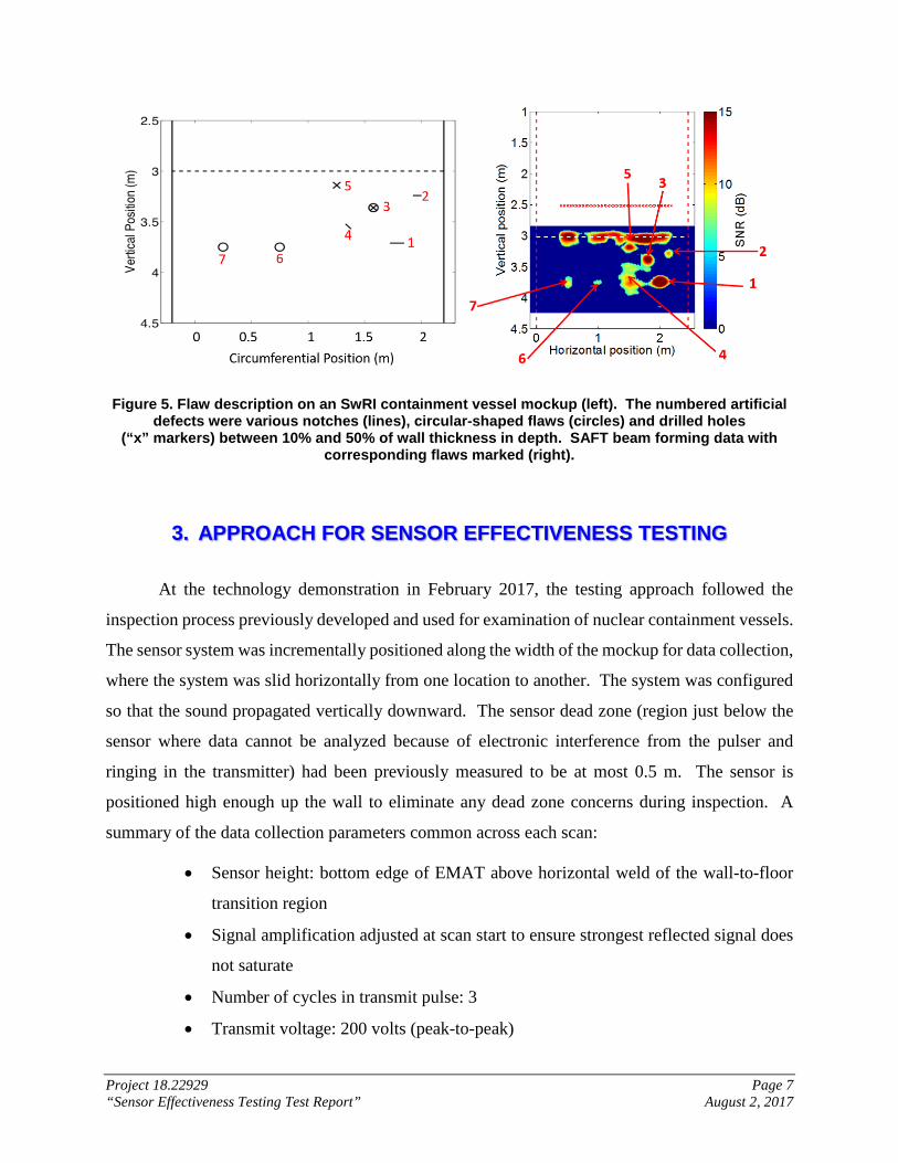
Project 18.22929 Page 7 “Sensor Effectiveness Testing Test Report” August 2, 2017
Figure 5. Flaw description on an SwRI containment vessel mockup (left). The numbered artificial defects were various notches (lines), circular-shaped flaws (circles) and drilled holes
(“x” markers) between 10% and 50% of wall thickness in depth. SAFT beam forming data with corresponding flaws marked (right).
3. APPROACH FOR SENSOR EFFECTIVENESS TESTING
At the technology demonstration in February 2017, the testing approach followed the
inspection process previously developed and used for examination of nuclear containment vessels.
The sensor system was incrementally positioned along the width of the mockup for data collection,
where the system was slid horizontally from one location to another. The system was configured
so that the sound propagated vertically downward. The sensor dead zone (region just below the
sensor where data cannot be analyzed because of electronic interference from the pulser and
ringing in the transmitter) had been previously measured to be at most 0.5 m. The sensor is
positioned high enough up the wall to eliminate any dead zone concerns during inspection. A
summary of the data collection parameters common across each scan:
• Sensor height: bottom edge of EMAT above horizontal weld of the wall-to-floor
transition region
• Signal amplification adjusted at scan start to ensure strongest reflected signal does
not saturate
• Number of cycles in transmit pulse: 3
• Transmit voltage: 200 volts (peak-to-peak)

Project 18.22929 Page 8 “Sensor Effectiveness Testing Test Report” August 2, 2017
• Transmit signal: square wave
• Data collection interval: 25.4 mm
• Sample rate: 5 mega samples per second
• Record length: 40,960 samples
• Electromagnet voltage: 8 volts
• Signal averages: 15
• Surface Preparation Required: None
• Guided wave mode: Lowest order shear horizontal plate mode (SH0)
Data collection parameters and any signal processing parameters that varied between the
inspections will be summarized in a later section.
There are several major features of this system that help differentiate it from other
inspection approaches for looking at large plate-like structures such as the DSTs:
• There is no requirement for surface preparation (i.e., sanding) or acoustic couplants.
• The sensor can be electronically configured to reverse the direction of wave
propagation to allow inspection above the sensor rather than below, if necessary.
• The system setup (e.g., gain, sensor position, etc.) is based on reflections from
known geometric features of the structure, such as a weld, at the start of an
inspection, without regard for optimizing the response from any defects in a
separate calibration or reference block.
• Beyond using a geometric feature for system setup, no information about the
structure being inspected is required for the computation of the SAFT images.
• The sensor test frequency/wavelength can be easily adjusted by changing the sensor
coil located below the electromagnet. This feature was exploited during both visits
to PNNL by testing at multiple frequencies.
There were two types of observations from the February demonstration test results (see the
prior technology screening report for a description of the flaws associated with the labels):
• Data Quality Observations:
o Data was collected and analyzed successfully on all but the highest
frequency (72 kHz) sensor configuration.

Project 18.22929 Page 9 “Sensor Effectiveness Testing Test Report” August 2, 2017
o The best performing test frequency was with the second highest frequency
sensor coil (57 kHz).
o The direction control performance was not as good as expected based on
past experience.
• Detection Performance Observations:
o Five of the six defects located away from the weld were detected (five of
nine overall).
o Three defects (“a”, “g,” and “k”) located in the 7/8-inch to 1/2-inch
transition weld were not detected because of the large amplitude signal
reflected from the weld itself.
o All four defects (“b”, “c,” “h,” and “L”) located away from the welds and
mockup edges were detected with signal-to-noise ratios (SNRs) in excess
of 10 dB.
o One of two defects (“i” and “m”) located near the mockup edge were
detected; the detected flaw was favorably oriented perpendicular to the
wave propagation direction while the undetected flaw was parallel to the
propagation direction.
Based on these observations, several changes were made to the system setup with the goal
of improving data quality and detection performance. The particular goal was to improve the
performance at detecting defects in the welds. A summary of the changes and their rationale are
as follows:
• Generally improved instrumentation setup: Upon return of the system to SwRI, a
careful review of the system was performed based on the data quality observations
detailed above. The particular concerns were the poorer-than-expected direction
control and inability to use the highest-frequency sensor coil. Several configuration
discrepancies were discovered and corrected in the data collection process in
preparation for the sensor effectiveness testing:
o The two highest frequency sensor coils had two transmitter coils
inadvertently flipped (e.g., the transmitter circuit expected to be higher up
the wall was actually the lower circuit).

Project 18.22929 Page 10 “Sensor Effectiveness Testing Test Report” August 2, 2017
o The 49 kHz and 57 kHz pulser settings were reversed, meaning tests at these
frequencies used the wrong input excitation signals.
o There was a minor software error in the algorithm for combining the two
receiver signals into a signal waveform for SAFT processing, which
reduced the efficacy of the sensor’s direction control.
By remedying these configuration issues, the performance at detecting defects
away from the welds should be improved.
• Angled EMAT inspection: The key observation from the first test results was that
the detection performance away from the welds was good, but no defects were
detected in welds. The cause was that the weld with defects in the first mockup
was perpendicular to the guided wave propagation direction, which produced a
strong reflected signal from the weld that masked any defect responses. This
limitation was problematic as defects in the DST could occur near the welds.
It was suggested that SwRI make any possible changes to the inspection
process to improve the detection performance near the welds for the second round
of testing at PNNL. The approach was to adjust the sensor so that the weld was no
longer perpendicular to the guided wave direction. The result is that any reflection
from the weld would be reflected away from the sensor because the weld is much
larger than the acoustic wavelength; therefore, the weld acts as a pure specular
reflector. Any defects in the weld, which are typically of a size similar to the
acoustic wavelength, will scatter the acoustic wave in many directions and ideally
back to the transmitting transducer. Thus, the reflection from the weld will be lost,
whereas, the response from any defects will be received and allow detection.
To accomplish this approach, a simple modification was made to the test
system, to hold the sensor at an angle of 20 degrees relative to the original, 0-degree
(straight-down) propagation configuration. This angle was selected based on a
simple experiment performed at SwRI: using an EMAT with a similar width to
wavelength ratio as the ones used on this program, it was found that a 20-degree
rotation eliminated most of the reflected energy from a plate boundary at
propagation distances equivalent to those expected during the sensor effectiveness
testing. A sensor holder was manufactured and is shown in Figure 6. This

Project 18.22929 Page 11 “Sensor Effectiveness Testing Test Report” August 2, 2017
mounting device is installed between the EMAT and sensor cart, which is also
shown in Figure 6. This mounting device was reversible to allow scanning with
the sensor in either 20-degree direction. In addition to this mechanical change, the
SAFT algorithm had to be modified to account for the different wave propagation
direction. All other data collection and analysis processes were unchanged.
Figure 6. Photograph of the EMAT holder before (left) and after (right) installed on the sensor cart
4. DATA SUMMARY
At total of twenty-two data sets were acquired during the two-day sensor effectiveness
testing held on June 21st and 22nd, 2017. Eleven data sets were acquired on each of the two
mockups. Five data sets were collected on each mockup using the original, straight down 0-degree
configuration; one at each test frequency and a final data set with the 57 kHz sensor coil paired
with a lower frequency band hardware filter. The additional 57 kHz test was done to eliminate
noise found during analysis from higher frequency wave modes being generated that complicated
the SAFT images. Data sets were also collected at each of the two angled sensor configurations
at 49 kHz, 57 kHz and 72 kHz. Data was not acquired with the lowest frequency (42 kHz) sensor
coil at an angle because field analysis revealed it did not provide significantly different results at
0 degrees compared to the 49 kHz sensor coil. The convention for discriminating between the two
angled configurations was based on the location of the side of the EMAT near the system push
handle. For instance, the setup shown in Figure 6 is denoted the “low” configuration.

Project 18.22929 Page 12 “Sensor Effectiveness Testing Test Report” August 2, 2017
Table 1 summarizes the system parameters for each data set acquired using the system, as
well as the digital filter bandwidth applied to the data prior to using the SAFT algorithm. Note
that the first data set number is 67. Also, data sets 83 and 84 were unintentionally collected with
the two receiver cables reversed. This was identified during analysis, but since the data acquisition
process records the data from both channels, this error was corrected during analysis. The only
parameter not included in this table is the EMAT height, which was measured relative to the top
weld above the wall-to-floor transition. Table 2 summarizes the approximate height of the EMAT
for each configuration for both mockups: the technology screening mockup (“Screening”) and the
sensor effectiveness testing mockup (“Effectiveness”). Note that these heights were chosen such
that the entirety of the mockup floors in the beam direction below the weld could be inspected:
the center of the sensor is above the listed height, which is for the lower corner of the sensor.
Table 1. Summary of the parameters of the data sets acquired during sensor effectiveness testing. Abbreviations BP, HP, and LP stand for band pass, high pass and low pass, respectively.
Data Set
Frequency (kHz) Mockup
Sensor Configuration Analog Filters
Digital Filter
Bandwidth Additional Gain (dB)
67 42 Effectiveness Straight Down 30 kHz HP / 70 kHz LP 26-61 kHz +0
68 42 Screening Straight Down 30 kHz HP / 70 kHz LP 26-61 kHz +0
69 49 Effectiveness Straight Down 45 kHz BP 26-61 kHz +0
70 49 Screening Straight Down 45 kHz BP 26-61 kHz +0
71 57 Effectiveness Straight Down 64 kHz BP 26-61 kHz +0
72 57 Screening Straight Down 64 kHz BP 26-61 kHz +0
73 72 Effectiveness Straight Down 64 kHz BP 37-93 kHz +0
74 72 Screening Straight Down 64 kHz BP 37-93 kHz +0
75 72 Effectiveness Angled (Low) 64 kHz BP 37-93 kHz +0
76 72 Screening Angled (Low) 64 kHz BP 37-93 kHz +0
77 57 Effectiveness Angled (Low) 64 kHz BP 26-61 kHz +20
78 57 Screening Angled (Low) 64 kHz BP 26-61 kHz +20
79 49 Effectiveness Angled (Low) 45 kHz BP 26-61 kHz +20
80 49 Screening Angled (Low) 45 kHz BP 26-61 kHz +20
81 49 Effectiveness Angled (High) 45 kHz BP 26-61 kHz +20
82 49 Screening Angled (High) 45 kHz BP 26-61 kHz +20
83 57 Effectiveness Angled (High) 64 kHz BP 26-61 kHz +20
84 57 Screening Angled (High) 64 kHz BP 26-61 kHz +20
85 72 Effectiveness Angled (High) 64 kHz BP 37-93 kHz +20
86 72 Screening Angled (High) 64 kHz BP 37-93 kHz +20
87 57 Effectiveness Straight Down 45 kHz BP 26-61 kHz +0
88 57 Screening Straight Down 45 kHz BP 26-61 kHz +0

Project 18.22929 Page 13 “Sensor Effectiveness Testing Test Report” August 2, 2017
Table 2. Summary of transducer heights relative to the weld immediately below the EMAT
Configuration Mockup Height (mm) Straight Down Effectiveness 150
Straight Down Screening 100
Angled, Low Effectiveness 50
Angled, Low Screening 0
Angled, High Effectiveness 75
Angled, High Screening 25
An example waveform collected using the system is shown in Figure 7. This data was
collected on the effectiveness testing mockup using the 57 kHz sensor coil oriented to propagate
vertically downward. The x-axis in the figure has been adjusted to indicate the distance propagated
by the signals from the EMAT. The large signal at approximately 4.7 m is the response from the
far edge of the mockup after propagating from the wall through the mockup bottom. All of the
other indications are resulting from either welds or defects in the mockup. The dead zone of the
system can also be seen in this waveform; the initial pulse ends and meaningful data can be
recorded from reflectors as close as approximately 0.44 m from the sensor. Finally, coverage from
a sensor is difficult to quantify using this waveform, but there are significant amplitude arrivals
that are over 10 m from the EMAT. Since the mockup is not 10 m in any dimension, these far
arrivals are a result of the wave bouncing around within the plate. These later arrivals provide an
indication of how far the guided wave can be successfully propagated; it may be possible to inspect
as far as 10 m from the sensor successfully, allowing the vast majority of the tank floor to be
inspected. Detection performance will be degraded, however, at such long inspection ranges.

Project 18.22929 Page 14 “Sensor Effectiveness Testing Test Report” August 2, 2017
Figure 7. Example waveform collected using the EMAT system
Each data set was processed using a SAFT algorithm developed by SwRI for use with this
system. The same algorithm and associated configuration parameters were used to process each
data after accounting for the differences documented in Table 1 and Table 2. The raw images were
normalized based on the average SAFT response in a small region selected and replotted as SNR
in decibels (dBs). The noise region was restricted to be between the wall-to-floor transition piece
and the 7/8-inch to 1/2-inch transition weld.
All of the SAFT images produced are provided in Appendix A. Figure 8 shows example
SAFT images collected on the technology screening mockup at 57 kHz at three inspection
configurations (data sets 77, 83, and 87) and the lower frequency filters where applicable. The
SAFT processing was performed on a Cartesian grid with 19 mm spacing in X and Y directions.
The “X” axis is parallel to the thickness transition weld and the “Y” axis convention is such that
the data collection locations were located on the negative side of the thickness transition weld.
The origin of the grid was defined to be at the thickness transition weld on one edge of the mockup.
Welds and plate edges are denoted by the dashed magenta lines. Data collection locations are
shown by the closely-spaced red “x” markers, the white circles denote the known defect locations,
the white diamonds denote the suspected blind defect locations, and the dashed white rectangle
denotes the noise region used to calculate SNR of observed indications.
0 2 4 6 8 10 12
Distance from EMAT (m)
-2
-1
0
1
2
Ampl
itude
(V)

Project 18.22929 Page 15 “Sensor Effectiveness Testing Test Report” August 2, 2017
Figure 8. SAFT images produced using the 57 kHz sensor coil on the effectiveness testing mockup (data sets 77, 83, and 87). The left and right plots are the “high” and “low” sensor
configurations, respectively, while the center plot is the original straight down configuration. The color scale for each image is shown to the right of that image. The white markers (circles and
diamonds) denote flaw locations, the dashed magenta lines denote mockup edges and welds, the dashed white box denotes the noise region, and the red “x” markers near the top of each image
are where data was collected.
A major difference between the straight down and angled inspection results was that the
signal amplitudes from flaws in the majority of the angled inspections had significantly higher
SNR values compared to those found in the straight down configurations. This is because for
almost all of the angled inspections, the system gain was increased by 20 dB (see Table 1). The
system gain in the straight down configuration was set so that the large reflection from the far end
of the mockups would not saturate the receiver/data acquisition system. This large reflector did
not exist in the angled inspections, and therefore more gain could be used. This increased gain
allowed for acoustic noise in the structure (e.g., the effects of sound wave interacting with the
mockup edges) to be observed that was largely undetectable at lower gain settings. In other words,
this noise measured in the low-gain SAFT images was likely caused by the electronic noise in the
system, whereas, the noise measured in the high-gain SAFT angled images was probably due to

Project 18.22929 Page 16 “Sensor Effectiveness Testing Test Report” August 2, 2017
acoustic noise in the structure. The major implication of this difference is that the analysis of the
low-gain SAFT images was performed using a 10 dB detection threshold, whereas the detection
threshold for the high-gain SAFT images was done using a 30 dB detection threshold. The color
scales for the SAFT images were adjusted to be appropriate for their respective detection
thresholds.
In addition to this signal range difference based on the gain settings, there are many general
observations that can be made about the data:
• Direction control performance was significantly improved compared to the
previous results acquired using this system. There were significantly fewer
indications from the guided waves propagating in the wrong direction (vertically
upward). This is attributed to the improved instrument parameters used.
• The SNR values from the defects were improved relative to the first technology
screening demonstration results. This is attributed to the improved instrument
parameters used.
• The angled inspection almost eliminated the weld reflection, allowing for detection
of defects within the welds.
• During angled inspection, secondary defect indications could be observed from
defects near the center of the mockup. These indications were the result of sound
bouncing off the mockup edges, reflecting from the indication and returning to the
EMAT. These secondary indications will not exist when inspecting the DSTs.
• The intersection between the perpendicular welds and the mockup caused
indications in the angled inspections because of the “corner” shape. These
indications will not exist when inspecting the DSTs.
• As before, the straight down sensor configuration provided meaningful information
for the middle 75% of the mockup in the X direction. This was because the physical
size of the EMAT does not allow scanning to the edge. Again, this should not be a
problem for the DSTs.
• Angled inspections only allowed a portion (~33%) of the mockup to be inspected
but each mockup was scanning in both angled direction, so the majority of the

Project 18.22929 Page 17 “Sensor Effectiveness Testing Test Report” August 2, 2017
mockup was investigated using the angled configurations. Again, this should not
be a problem for the DSTs.
• Welds oriented parallel to the wave propagation direction were not visible, but
defects in these welds were detectable.
• It was occasionally possible to detect defects in welds oriented perpendicular to the
propagation direction with the straight down configuration by noting a loss of signal
from the weld.
• All welds that were perpendicular to the beam direction were detected in the straight
down sensor configuration with one exception. For the 72 kHz straight down test
(data set 73), the thickness transition weld was not observed. The theorized cause
was because the wavelength of the guided wave was close to an integer multiple of
the weld width in the propagation direction. Reflections from the near and far edges
of the weld would be out of phase with one another and cancel.
• As the sensor coil frequency increased and wavelength decreased, the size of an
indication in the X and Y directions was reduced and, thus, localization
performance was improved.
• The single best performing sensor coil remained as 57 kHz. The highest frequency
(72 kHz) sensor coil had the best localization performance but also had unwanted
higher-order mode signals that complicated SAFT image interpretation.
• The best possible results are achieved if multiple sensor coil frequencies and angles
are used together to image an area.
• All data sets were processed independently. Even better performance would likely
be possible if the angled and straight down data sets at a common frequency were
combined together during SAFT calculations.
5. INSPECTION RESULTS
Testing was performed over two days (June 21-22, 2017); the scope of testing required by
the effectiveness testing protocol was completed in its entirety. The SAFT images (Appendix A)
were analyzed visually with an SNR threshold to detect defects. As discussed before, the detection

Project 18.22929 Page 18 “Sensor Effectiveness Testing Test Report” August 2, 2017
threshold for low-gain setups (predominately straight down scans) was 10 dB, whereas, the
detection threshold for high gain setups (mainly angled scans) was 30 dB. Also, a defect was only
classified as detected if the SAFT indication was recognized as being unambiguously from the
defect; some SAFT images had spurious indications that lowered the confidence that the
indications in the image was from defect even if it was at the correction location. Finally, no
attempt was made to detect defects located in welds that were perpendicular to the beam
propagation direction. This was done because it was known that performance is unreliable in these
regions given the prior results from the technology screening demonstration as well as experience
with the system in other environments.
The analysis results from both mockups are presented in Appendix B in tabular format.
Additionally, zoomed in views of each SAFT image with defect indications identified are shown
in Appendix C. The inspection results from each mockup are discussed in the following
subsections. Note that 42 kHz data was not included in this analysis, as the other test frequencies
were clearly better.
5.1 TECHNOLOGY SCREENING MOCKUP RESULTS
This mockup was modified after the original technology demonstration testing performed
in February, 2017. A total of fourteen defects were introduced into this mockup in the thickness
transition weld and 1/2-inch base plate. Seven of the defects (P1, P2, P3, N1, N2, N3 and T1)
were the target flaws for the investigation during the sensor effectiveness testing. The other seven
flaws (a, b, c, g, h, k, and L) existed previously in this mockup; a description of these defects can
be found in the testing protocol for the prior demonstration efforts. There were no blind defects
added to this mockup. Because of the improvements made to the test process, the performance at
detecting the all fourteen flaws was documented. Refer to Figure 9 for a graphical summary of
the detection performance on this mockup. The following observations can be made based on this
analysis:
• Twelve of the 14 defects were detected with SNR values greater than the
appropriate threshold for the system configuration used to collect the data.
• Two defects (a and k) were close together and unable to be identified as two
separate indications. All other defects could be identified separately.

Project 18.22929 Page 19 “Sensor Effectiveness Testing Test Report” August 2, 2017
• The best performing straight down configuration was the same configuration
identified during the technology demonstration: 57 kHz sensor coil with 45 kHz
band pass hardware filters.
• Compared to the technology demonstration results, this best performing
configuration was improved in two significant ways: no evidence of poor direction
control and the SNRs of the same five detected defects were higher by
approximately 6 dB.
• Angled investigations allowed for the three previously undetected defects in the
thickness transition weld to be detected with SNRs of at least 40 dB. Note that
SNR-based comparison between the different test configurations is difficult at this
time.
• The undetected defects (N3 and T1) were not detected because of the following
reasons:
o N3: This defect is oriented parallel to the beam direction in the straight
down configuration. Also, it is located “behind” at least five other defects
(c, P3, N2, N1, and P2) which reduces performance. Finally, the defect
located a weld. This difference may explain why defect N1, which was
smaller than N3 and similarly oriented, was detected since it was near the
weld but not inside it.
o T1: This defect had a depth of 10% of the total wall thickness and a gradual
transition to the maximum depth, which is difficult to detect using this
inspection strategy.

Project 18.22929 Page 20 “Sensor Effectiveness Testing Test Report” August 2, 2017
Figure 9. Graphical representation of the detection performance in the technology screening mockup. Green circles highlight detected defects, whereas, red circles denote undetected
defects.
5.2 SENSOR EFFECTIVENESS TESTING MOCKUP RESULTS
This mockup had not been previously investigated using the inspection system developed
at SwRI. A total of 18 defects were introduced into this mockup in the thickness transition weld
and 1/2-inch base plate. Sixteen of these defects were known prior to performing the inspection
and two defects were known to exist but their location and characteristics were not provided. Refer
to Figure 10 for a graphical summary of the detection performance on this mockup. The following
observations can be made based on this analysis:
• Twelve of the 18 defects were detected with SNR values greater than the
appropriate threshold for the system configuration used to collect the data. .
• Two of these 12 defects were attributed to the blind-test defects (B1 and B2).
o B1 was defined as approximately 60 inches from the thickness transition
weld and close or in the weld that parallels the long dimension of the
mockup. That defect coordinates are (0.58 m, 1.52 m). Based on the
amplitude of the indication associated with this defect, it is expected that
this is a large flaw, potentially 50% or more of the wall thickness in depth.

Project 18.22929 Page 21 “Sensor Effectiveness Testing Test Report” August 2, 2017
o B2 was defined as being in the base plate away from other features such as
welds or defects. That defect coordinates are (1.22 m, 1.26 m). Based on
the amplitude of this defect, it is expected that this flaw is similar in size to
P4 (0.75 in. diameter pit 50% through the wall thickness).
• While no defects were defined as detected in this fashion, there were numerous
examples of signal loss being caused by a defect in the weld. This effect could be
exploited to further enhance defect detection performance.
• The welds parallel to the long dimension of the mockup were not apparent in the
data but defects were detected within these welds.
• It was possible to detect defect P12, a pit-like flaw located on the far end of the
plate, after propagation through four welds, one of which was a thickness transition
weld.
• There was not a clear best performing straight down configuration. One
configuration (57 kHz, high frequency band filters) had the best SNRs for the
defect, but another configuration (57 kHz, low frequency band filters) detected the
most defects.
• The undetected defects (P9, P10, N7, T2, T3, and T4) were not detected because of
the following reasons:
o The wall thinning defects (T2, T3, and T4) are a difficult geometry for the
inspection system to detect, because the scale of the thickness change is
comparable to the wavelength.
o P9: This pit was larger than other pit-like flaws detected, but positioned in
a weld perpendicular to the long edge of the mockup. Based on the ability
to detect defect “a” in the thickness transition weld of the screening mockup,
flaw P9 should be detectable. The likely reason for the lack of detection is
the increased range (over 4 m from the sensor locations) and multiple
defects between the sensor locations and P9.
o P10: This defect, which is in a weld perpendicular to the long edge of the
mockup, is located very close to the middle in the X-direction but close to
the far edge of the mockup. Detection of defects this size in welds (P6) was
shown to be possible, but the angled inspection was necessary.

Project 18.22929 Page 22 “Sensor Effectiveness Testing Test Report” August 2, 2017
Unfortunately, P10 was positioned in the mockup where no angled
inspection had coverage. It is expected that this defect would be detected if
it were at a slightly different location.
o N7: This notch was located in a weld but oriented favorably for the guided
wave inspection. The angled inspection should be able to detect this defect
size and orientation. The defect, however, was positioned near the
intersection of two welds, which creates a corner and potentially large
indication. There is an indication in the SAFT images produced at 49 kHz
(data set 79) and 57 kHz (data set 77) when inspecting at an angle, but it is
not known if this response is due to the weld or the defect. Based on this
ambiguity, it was not possible to ensure that this indication was from the
defect.
Figure 10. Graphical representation of the detection performance in the technology screening mockup. Green circles highlight detected defects, red circles denote undetected defects and the
purple circles denote locations where suspected blind defects are located.
6. CONCLUSIONS AND DISCUSSIONS
This report summarizes the operating principles and performance characteristics of an
inspection system developed by SwRI for assessing thick-walled vessels in areas where access is

Project 18.22929 Page 23 “Sensor Effectiveness Testing Test Report” August 2, 2017
extremely limited. This system works by sliding a sensor across the width of the mockup and
collecting data periodically with no need for coupling fluid or coupling pressure/force. The data
from the multiple inspection locations is combined together using a signal processing algorithm to
produce a color image that highlights where indications exist in the data. Localization performance
is typically good (i.e., commonly accurate to within 25 mm of the true location), but accurate sizing
of flaws from the data is challenging.
The performance of the system was evaluated using two mockups with artificial flaws.
Generally, the signal and data quality were excellent, especially when compared to the prior
technology demonstration results. There were thirty-two defects spread across both mockups; at
least twenty-four were detected. This includes both blind defects located in the sensor
effectiveness testing mockup. This performance was achieved in spite of the guided waves being
required to propagate through multiple welds, including a thickness transition weld, and having a
sensor-to-flaw separation of up to approximately 4.4 m (14.5 feet). No effort was made to size the
flaws based on the amplitude of the signals, but the estimated defect location was generally within
25-50 mm of the true position value.
There were three types of flaws (pits, notches and wall thinning regions) in the mockups.
Based on the detection performance across the two mockups, the following flaw-specific
conclusions can be drawn about detection:
• Pit-like flaws were generally detected successfully regardless of their location in
the mockup. For example, it was possible to detect the small diameter pit (25% of
wall thickness) even when located within the thickness transition weld. The only
pit-like flaws not detected were located where the angled inspections had no
coverage (P10) or behind other defects in the mockup (P9).
• Notch-like flaws were detectible regardless of their orientation relative to the sensor
when located in the base material (i.e., away from the welds). Notch-like flaws
could be detected when within the welds, but detection performance was reduced.
Three flaws oriented parallel to the long dimension of the mockup and within or
near a weld were detected (N1, N5, and N6). A similar flaw (N3) was not detected;
this may have been due to the large number of flaws around this defect. Only one

Project 18.22929 Page 24 “Sensor Effectiveness Testing Test Report” August 2, 2017
favorably oriented flaw (N7) was not detected conclusively, but it was located near
the intersection of two welds.
• Wall-thinning flaws were very challenging to detect given their gradual depth
profile changes. Prior experience has shown the ability to detect similar flaws (10-
20% of wall thickness in depth and 100 mm [4 inches] in diameter), but the flaw
surface was typically less smooth, which could have aided detection.
One major point of discussion moving forward is establishing appropriate detection
thresholds regardless of the system amplifier gain. The detection threshold used during this
effectiveness testing effort was based on both the measured SAFT image noise and amplifier gain.
The signal noise was measured in the SAFT images near the sensor locations in regions with no
obvious localized defect responses. For the low-gain (straight down) system configuration, the
amplifier gain was low enough that acoustic noise, likely caused by sound interacting with the
mockup edges at long range, was not resolvable. As a result, the noise measured near the sensor
caused by the system electronic noise was appropriate for setting a detection threshold for the
entire image. For the high-gain configuration, however, acoustic noise was detectible in the SAFT
images especially at large distances from the sensor locations. Thus, the noise level computed
near the sensor locations did not appropriately capture the noise level for the entire SAFT image.
Going forward, a better solution may be to compute the noise level in the images at further
distances from the sensor, so any acoustic noise will be present in the calculation. Another solution
may be to use a geometric reflector, such as a weld, to calibration the amplitude response. More
work is necessary to determine which detection threshold strategy is best for the DST inspection
application.
Based on these results, it is the conclusion of SwRI that the technology demonstrated would
be able to screen the DST bottom for damage without requiring insertion of equipment underneath
the DST via the air channels. The vision is a miniaturized EMAT that is delivered to the DST wall
using a robotic vehicle. The EMAT would be connected to a remote base station for control and
data storage using a long umbilical cable. The analog electronics, as well as the digitizers, would
be miniaturized so they could be collocated with the sensor; this would eliminate the concerns
associated with cable length impacting the signal quality. Figure 11 shows a computer rendering
of one possible implementation of this inspection system.

Project 18.22929 Page 25 “Sensor Effectiveness Testing Test Report” August 2, 2017
Figure 11. Conceptual illustration of the DST inspection system showing a robotic delivery vehicle close-up (left) and on the DST wall (right).
To accomplish this vision, it is expected that SwRI would need to significantly reduce the
size and weight of the EMAT, which would be based primarily on reducing the dimensions of the
electromagnet. This should be realizable because of three design criteria changes:
• The existing electromagnet was originally designed for inspection of 38 mm thick
containment vessels, which necessitated having a magnetic circuit thickness of
close to 175 mm. A much thinner magnetic circuit would be practical for the
22 mm (7/8-inch) thick DST wall. This should allow the electromagnet to be about
half the current 250 kg (550 lbs.) weight. The height would also be reduced slightly
to be less the current electromagnet.
• The electromagnet was designed to be paired with a 42 kHz sensor coil that was
200 mm in length (perpendicular to the beam direction). This length defines the
pole tip internal spacing for the electromagnet. The best performing coil had a
length of approximate 120 mm. This one change should allow the electromagnet
to be approximately 60% as long as the current design, which should reduce the
length by about 40%. This would cause a significant reduction in the weight.
• The original 42 kHz sensor coil was also almost 200 mm wide based on the
wavelength of the guided wave. The best performing coil had a smaller wavelength
and, thus, narrow coil width. This change will allow for a narrower electromagnet
to be used, which also reduces the weight of the sensor.
• The original electromagnet was very conservatively designed; in practice it was
operated below capacity on even the 38-mm thick wall. The experience with this

Project 18.22929 Page 26 “Sensor Effectiveness Testing Test Report” August 2, 2017
magnet and improved modeling capability will allow the design to be further
optimized.
These differences should allow for an electromagnet that is much less than 50 kg (110 lbs. in
weight and less than 400 mm (15 inches) long, 150 mm (6 inches) wide and 150 mm (6 inches)
tall. Further weight and size savings should also be possible by allowing the sensor to operate at
higher temperature and, if necessary, using higher permeability magnetic materials, such as
Permandur or other cobalt alloys instead of carbon steel. This electromagnet would be suitable for
use on the DST side walls up to approximately 25 mm (1 inch) in thickness; the thickness of the
DST floor would not affect the performance of the electromagnet. Note that this reduction in size
and weight would not materially affect the inspection range of the sensor.
The cost and schedule for achieving this miniaturized EMAT is difficult to quantify without
better definition regarding the final form of the inspection system. As a rough estimate, it is
expected that this custom sensor and electronics miniaturization would cost in the range of $200-
300k and take approximately 9-12 months. The output of this development effort is a sensor
system that would be suitable for test and evaluation with a robotic delivery system. This estimate
does not include development of a robotic delivery system, integration of the sensor with the robot,
or the test and evaluation. This is an admittedly conservative estimate given the current
understanding of the future scope of work. Please note that this estimate is provided as a guide
and does not constitute an offer for services.
Beyond the system changes described above to transition the current design to one that
would be practical for field use, other design changes could be made to potentially improve the
performance beyond what was demonstrated. These potential changes include but are not limited
to refining the inspection frequencies, adjusting the propagation angle, and utilizing different wave
modes. Implementation of these improvements was not performed prior to the sensor effectiveness
testing given the time limits of the project schedule. Since discussion of system improvements
was not included in the provided final report outline, a summary of these candidate design changes
is provided in Appendix D.

Project 18.22929 Page A-1 “Sensor Effectiveness Testing Test Report” August 2, 2017
7. APPENDIX A – SAFT IMAGES OF MOCKUPS
This appendix presents the SAFT images collected on the technology screening mockup at
each configuration. Where possible, SAFT images from all three configurations (“high” angle,
“low” angle, and straight down) at a single instrument setup were presented together. The SAFT
processing was performed on a Cartesian grid with 19 mm spacing in X and Y directions. The
“X” axis is parallel to the thickness transition weld and the “Y” axis convention is such that the
data collection locations were located on the negative side of the thickness transition weld. The
origin of the grid was defined to be at the thickness transition weld on one edge of the mockup.
Welds and plate edges are denoted by the dashed magenta lines, data collection locations are shown
by the red “x” markers, the white circles denote the known defect locations, the white diamonds
denote the suspected blind defect locations, and the dashed white rectangle denotes the noise
region. The images are in terms of SNR in decibels and the color bar next to each image shows
the range.
TECHNOLOGY SCREENING MOCKUP IMAGES
42 kHz Data – Set 68 (Straight Down)

Project 18.22929 Page A-2 “Sensor Effectiveness Testing Test Report” August 2, 2017
49 kHz Data – Sets 80 (Low Angle), 70 (Straight Down), and 82 (High Angle)
57 kHz Data (Low Bandwidth Filters) – Set 88 (Straight Down)

Project 18.22929 Page A-3 “Sensor Effectiveness Testing Test Report” August 2, 2017
57 kHz Data (High Bandwidth Filters) – Sets 78 (Low Angle), 72 (Straight Down),
and 84 (High Angle)

Project 18.22929 Page A-4 “Sensor Effectiveness Testing Test Report” August 2, 2017
72 kHz Data – Sets 76 (Low Angle), 74 (Straight Down), and 86 (High Angle)
SENSOR EFFECTIVENESS TESTING MOCKUP IMAGES
42 kHz Data – Set 67 (Straight Down)

Project 18.22929 Page A-5 “Sensor Effectiveness Testing Test Report” August 2, 2017
49 kHz Data – Sets 79 (Low Angle), 69 (Straight Down), and 81 (High Angle)
57 kHz Data (Low Bandwidth Filters) – Set 87 (Straight Down)

Project 18.22929 Page A-6 “Sensor Effectiveness Testing Test Report” August 2, 2017
57 kHz Data (High Bandwidth Filters) – Sets 77 (Low Angle), 71 (Straight Down),
and 83 (High Angle)

Project 18.22929 Page A-7 “Sensor Effectiveness Testing Test Report” August 2, 2017
72 kHz Data – Sets 75 (Low Angle), 73 (Straight Down), and 85 (High Angle)
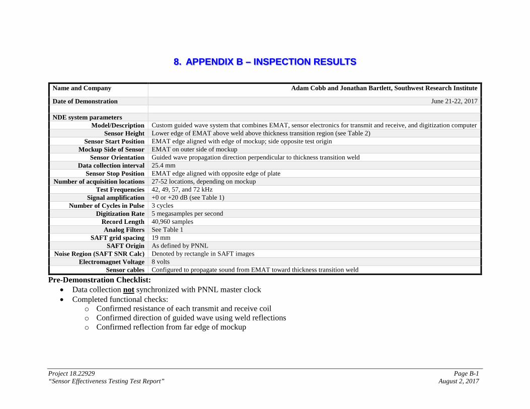
Project 18.22929 Page B-1 “Sensor Effectiveness Testing Test Report” August 2, 2017
8. APPENDIX B – INSPECTION RESULTS
Name and Company Adam Cobb and Jonathan Bartlett, Southwest Research Institute
Date of Demonstration June 21-22, 2017 NDE system parameters
Model/Description Custom guided wave system that combines EMAT, sensor electronics for transmit and receive, and digitization computer Sensor Height Lower edge of EMAT above weld above thickness transition region (see Table 2)
Sensor Start Position EMAT edge aligned with edge of mockup; side opposite test origin Mockup Side of Sensor EMAT on outer side of mockup
Sensor Orientation Guided wave propagation direction perpendicular to thickness transition weld Data collection interval 25.4 mm
Sensor Stop Position EMAT edge aligned with opposite edge of plate Number of acquisition locations 27-52 locations, depending on mockup
Test Frequencies 42, 49, 57, and 72 kHz Signal amplification +0 or +20 dB (see Table 1)
Number of Cycles in Pulse 3 cycles Digitization Rate 5 megasamples per second
Record Length 40,960 samples Analog Filters See Table 1
SAFT grid spacing 19 mm SAFT Origin As defined by PNNL
Noise Region (SAFT SNR Calc) Denoted by rectangle in SAFT images Electromagnet Voltage 8 volts
Sensor cables Configured to propagate sound from EMAT toward thickness transition weld Pre-Demonstration Checklist:
• Data collection not synchronized with PNNL master clock • Completed functional checks:
o Confirmed resistance of each transmit and receive coil o Confirmed direction of guided wave using weld reflections o Confirmed reflection from far edge of mockup

Project 18.22929 Page B-2 “Sensor Effectiveness Testing Test Report” August 2, 2017
Screening Mockup Inspection Results
SNR for Each Inspection Case Flaw
ID Flaw
Detected? (Y/N)
Configuration 49 kHz Down
49 kHz Low
Angle
49 kHz High
Angle
57 kHz Down (Lower
Frequency Filtered)
57 kHz Down
(Higher Frequency Filtered)
57 kHz Low
Angle
57 kHz High
Angle
72 kHz Down
72 kHz Low
Angle
72 kHz High
Angle
Data Set Number
70 80 82 88 72 78 84 74 76 86
P1 Y
12 n/a n/a 16.4 - n/a n/a - n/a n/a P2 Y - n/a - 11.67 - n/a - - n/a - P3 Y
10.9 n/a - 20.4 - n/a - - n/a -
N1 Y
- n/a - 11.7 - n/a - - n/a - N2 Y
27.7 n/a - 34.7 40.8 n/a - 27.4 n/a -
N3 N
- n/a - - - n/a - - n/a - T1 N
- - n/a - - - n/a - - n/a
a
Y
- n/a
52.1 Merged with k - - n/a
58.9- Merged with k - n/a
35.07 Merged with k
b Y
30.3 41.5 n/a 26 32.1 53.6 n/a - 45.9 n/a c Y
13.4 n/a 56.2 19.9 19.8 n/a 53.8 - n/a 31.8
g Y
- 44.9 n/a - - 63.8 n/a - 44.6 n/a h Y
12.4 n/a n/a 18.1 26.8 n/a n/a - n/a n/a
k
Y
- n/a
52.1 - Merged with a - - n/a
58.9 - Merged with a - n/a
35.07 Merged with a
L Y 21.8 n/a n/a 19.5 22.8 n/a n/a - n/a n/a
• - Not detected
• n/a Not applicable for this test configuration
• ?? Possible indication but not clear because of other arrivals in the region of interest
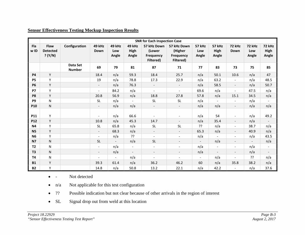
Project 18.22929 Page B-3 “Sensor Effectiveness Testing Test Report” August 2, 2017
Sensor Effectiveness Testing Mockup Inspection Results
SNR for Each Inspection Case Fla
w ID Flaw
Detected? (Y/N)
Configuration 49 kHz Down
49 kHz Low
Angle
49 kHz High
Angle
57 kHz Down (Lower
Frequency Filtered)
57 kHz Down (Higher
Frequency Filtered)
57 kHz Low
Angle
57 kHz High
Angle
72 kHz Down
72 kHz Low
Angle
72 kHz High
Angle
Data Set Number 69 79 81 87 71 77 83 73 75 85
P4 Y 18.4 n/a 59.3 18.4 25.7 n/a 50.1 10.6 n/a 47 P5 Y 19 n/a 78.8 17.3 22.9 n/a 63.2 - n/a 48.5 P6 Y - n/a 76.3 - - n/a 58.5 - n/a 50.7 P7 Y - 84.2 n/a - - 69.6 n/a - 47.5 n/a P8 Y 20.8 56.9 n/a 18.8 27.8 57.8 n/a 15.1 34.5 n/a P9 N SL n/a - SL SL n/a - - n/a -
P10 N - n/a n/a - - n/a n/a - n/a n/a
P11 Y - n/a 66.6 - - n/a 54 - n/a 49.2 P12 Y 10.8 n/a 45.3 14.7 - n/a 35.4 - n/a - N4 Y SL 65.8 n/a SL SL ?? n/a - 38.7 n/a N5 Y - 68.3 n/a - - 65.3 n/a - 40.9 n/a N6 Y - n/a ?? - - n/a - - n/a 43.5 N7 N SL - n/a SL - - n/a - - n/a T2 N - n/a - - - n/a - - n/a - T3 N - n/a - - - n/a - - n/a - T4 N - - n/a - - - n/a - ?? n/a B1 Y 39.3 61.4 n/a 36.2 46.2 60 n/a 35.8 38.2 n/a B2 Y 14.8 n/a 50.8 13.2 22.1 n/a 42.2 - n/a 37.6
• - Not detected
• n/a Not applicable for this test configuration
• ?? Possible indication but not clear because of other arrivals in the region of interest
• SL Signal drop out from weld at this location

Project 18.22929 Page C-1 “Sensor Effectiveness Testing Test Report” August 2, 2017
9. APPENDIX C – SAFT IMAGES OF FLAWS
This appendix presents the focused-view SAFT images the two mockups from each test
configuration. The data is the same as what is presented in Appendix A. The only difference is
the field of view is restricted to allow a better view of the indications. Additionally, where a defect
was identified as detected (see Appendix B), a defect label was added to the SAFT image near the
indication. All markers and annotations are consistent with Appendix A
.

Project 18.22929 Page C-2 “Sensor Effectiveness Testing Test Report” August 2, 2017
Screening Mockup Flaw Images – Top Half of Mockup
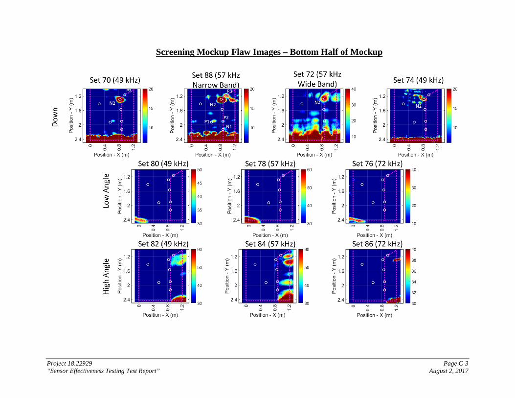
Project 18.22929 Page C-3 “Sensor Effectiveness Testing Test Report” August 2, 2017
Screening Mockup Flaw Images – Bottom Half of Mockup

Project 18.22929 Page C-4 “Sensor Effectiveness Testing Test Report” August 2, 2017
Sensor Effectiveness Testing Mockup Flaw Images – Top Half of Mockup
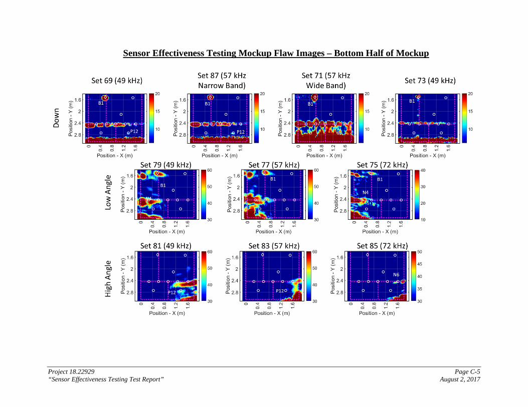
Project 18.22929 Page C-5 “Sensor Effectiveness Testing Test Report” August 2, 2017
Sensor Effectiveness Testing Mockup Flaw Images – Bottom Half of Mockup

Project 18.22929 Page D-1 “Sensor Effectiveness Testing Test Report” August 2, 2017
10. APPENDIX D – POTENTIAL SYSTEM IMPROVEMENTS
As discussed in the final report, the system demonstrated at the Sensor Effectiveness
Testing demonstration is an existing SwRI system originally designed for nuclear power plant
containment vessel inspections. While the system itself was modified in some basic ways (e.g.,
increasing the test frequencies) to accommodate the Hanford DST inspection challenges, the
modifications performed should not be considered as optimal; there was not sufficient time
available to allow potentially better system improvements to be researched and implemented.
This appendix is added to the report to summarize the key design variables or changes that
could be implemented to improve system performance at detecting the required defects. Note that
other changes could be made to improve system usability and data collection speed, but those
design changes are not presented. The list of potential improvements paths is presented as a
bulleted list here:
• Each of the test configurations (i.e., guided wave frequency and wave propagation
direction) were generated and analyzed independently without any attempt to
aggregate the data to improve the performance. Better performance could
potentially be achieved by combining the data collected from multiple test
configurations together. For example, the data taken at the same frequency but
different wave propagation directions could be combined together using the SAFT
algorithm with little change to the analysis process. The likely result would be
better signal amplitudes and a reduction in the acoustic noise present in the data,
further increasing the SNR measured from the defects.
• All of the sensor configurations used had a single test frequency. This was because
the original system was designed for detecting a single type of damage, namely
localized corrosion. One difference introduced by the Hanford DST challenge is
the need to detect multiple defect types and the results here indicate that multiple
test frequencies are useful for improving detection performance overall. Given this
difference, it may be prudent to modify the sensor coil and associated electronics
so that multiple sensor frequencies could be generated and received using a given
sensor coil. This would be done by basically incorporating multiple sensor coil

Project 18.22929 Page D-2 “Sensor Effectiveness Testing Test Report” August 2, 2017
designs into a single physical printed circuit in the sensor. The result would be
faster system operation and simpler data collection in the field.
• For this demonstration, two different wave propagation directions were considered;
a conventional straight-down configuration and a 20-degree angled configuration
to eliminate the influence of weld signals. The choice of 20-degrees of rotation
ensured that any reflection from the weld would be eliminated completely. This
sensor rotation, however, could reduce the signal amplitudes received from some
defects based on their geometry. It should be possible, however, to use different
rotation angles and improve the signal amplitudes received from a defect while still
eliminating the response from the weld. Furthermore, as mentioned above in the
first bullet, improvements would likely be possible if data from multiple angles is
combined together using the SAFT analysis process.
• While multiple sensor test frequencies were considered, all of the sensors evaluated
had the same width relative to their respective wavelengths. The implication of this
is that all of the sensors had the same beam divergence characteristics; in other
words, how the guided wave widened as it propagated away from the sensor was
the same for each test frequency used. The beam divergence characteristics were
the same as those of the original containment vessel inspection system, which was
only required to investigate approximately 2 – 2.5 m from the sensor. Since the
Hanford DST challenge requires detecting damage further from the sensor,
increasing the sensor width would improve performance at longer distances.
• The one type of defect where performance was poor was the gradual wall-thinning
style flaws. Based on past experience, the best approach for improving detection
performance for this type of flaw is to reduce the test frequency as much as possible
to make the wavelength as large or larger than the flaw dimensions. If this type of
flaw is critical to detect, modifications could be made to improve performance.
• All of the testing done here used the lowest order shear-horizontal plate mode
(SH0). This mode is characterized by its non-dispersive (i.e., all wave frequencies
move at the same speed) nature as well as uniform energy profile across the entire
plate thickness. The next higher order wave mode (SH1) is dispersive, which
complicates the analysis, but most of the wave energy is concentrated on the plate

Project 18.22929 Page D-3 “Sensor Effectiveness Testing Test Report” August 2, 2017
surfaces. SwRI and others have shown previously that this concentration of the
energy on the surfaces allows for improved detection sensitivity for defects that
originate on the surface. This wave mode could be considered as a way to improve
performance of the test system.