
Proceedings of The IEEE 18th International Conference on ...
358
Proceedings of The IEEE 18 th International Conference on Computer Applications 2020 27 th – 28 th February, 2020 Novotel Hotel Organized by University of Computer Studies, Yangon Ministry of Education, Myanmar Proceedings of The IEEE 18th International Conference on Computer Applications 2020
-
Upload
khangminh22 -
Category
Documents
-
view
2 -
download
0
Transcript of Proceedings of The IEEE 18th International Conference on ...

Proceedings of
The IEEE 18th International Conference on
Computer Applications 2020
27th – 28th February, 2020
Novotel Hotel
Organized by
University of Computer Studies, Yangon
Ministry of Education, Myanmar
Proceedings of The IEEE 18th International Conference on Computer Applications 2020

Proceedings of The IEEE 18th International Conference on Computer Applications 2020

Conference Chair
Prof. Mie Mie Thet Thwin, Rector, University of Computer Studies, Yangon, Myanmar
Conference Co-Chairs
Prof. Pyke Tin, University of Miyazaki, Japan
Prof. Moe Pwint, Rector, University of Computer Studies, Mandalay, Myanmar
Conference Organizing Committee Members
Prof. Myint Myint Sein, University of Computer Studies, Yangon, Myanmar
Prof. Mu Mu Myint, University of Computer Studies, Yangon, Myanmar
Prof. Khin Mar Soe, University of Computer Studies, Yangon, Myanmar
Prof. Thi Thi Soe Nyunt, University of Computer Studies, Yangon, Myanmar
Prof. Nang Saing Moon Kham, University of Computer Studies, Yangon, Myanmar
Prof. Khin Than Mya, University of Computer Studies, Yangon, Myanmar
Prof. May Aye Khine, University of Computer Studies, Yangon, Myanmar
Prof. Yadanar Thein, University of Computer Studies, Yangon, Myanmar
Prof. Khaing Moe Nwe, University of Computer Studies, Yangon, Myanmar
Prof. Khine Khine Oo, University of Computer Studies, Yangon, Myanmar
Prof. Sabai Phyu, University of Computer Studies, Yangon, Myanmar
Prof. Mie Mie Su Thwin, University of Computer Studies, Yangon, Myanmar
Prof. Win Pa Pa, University of Computer Studies, Yangon, Myanmar
Asso.Prof. Aye Aye Khine, University of Computer Studies, Yangon, Myanmar
ICCA 2020 Conference Organizing Committee
Proceedings of The IEEE 18th International Conference on Computer Applications 2020

Technical Program Committee Chair
Prof. Khin Mar Soe, University of Computer Studies, Yangon, Myanmar
Technical Program Committee Co-Chairs
Prof. Yutaka Ishibashi, Nagoya Institute of Technology, Japan
Prof. Khin Than Mya, University of Computer Studies, Yangon, Myanmar
Local Chair
Prof. Nang Saing Moon Kham, University of Computer Studies, Yangon, Myanmar
Technical Program Committee Members
ICCA 2020 Technical Program Committee
Proceedings of The IEEE 18th International Conference on Computer Applications 2020
Prof. Pyke Tin, University of Miyazaki, Japan
Prof. Maung Maung Htay, Radford University, Virginia, US
Prof. Mie Mie Thet Thwin, University of Computer Studies, Yangon, Myanmar
Prof. Kyaw Zwa Soe, Computer University (Mandalay), Mandalay
Prof. Moe Pwint, University of Computer Studies, Mandalay, Myanmar
Prof. Saw Sanda Aye, University of Information Technology, Yangon, Myanmar
Prof. Thinn Thu Naing, University of Computer Studies (Taunggyi), Myanmar
Prof. Thandar Thein, University of Computer Studies (Maubin), Myanmar
Prof. Win Aye, Myanmar Institute of Information Technology, Myanmar
Prof. Khin Mar Lar Tun, University of Computer Studies (Pathein), Myanmar
Prof. May Aye Khine, University of Computer Studies, Yangon, Myanmar
Prof. Yadanar Thein, University of Computer Studies, Yangon, Myanmar
Prof. Thi Thi Soe Nyunt, University of Computer Studies, Yangon, Myanmar
Prof. Yoshinori Sagisaka,Waseda University,Japan
Prof. Yutaka Ishibashi, Nagoya Institute of Technology, Japan
Prof. Yutaka Ohsawa, Saitama University, Japan
Prof. Saw Wai Hla, Ohio University, USA

Prof. Tang Enya Kong, Universiti Sains Malaysia, Malaysia
Prof. Jeng-Shyang Pan, Fujian University of Technology, Taiwan
Prof. Jong Sou Park, Korean Aerospace University, Korea
Prof. Khaing Moe Nwe, University of Computer Studies, Yangon, Myanmar
Prof. Keum-Young Sung, Handong Global University, Korea
Prof. Kun Lee Handong, Global University, Korea
Prof. Sang-Mo JeongHandong Global University, Korea
Prof. Dong Seong Kim, University of Canterbury, New Zealand
Prof. Myint Myint Sein, University of Computer Studies, Yangon, Myanmar
Prof. Andrew Lewis, Griffith University, Queensland, Australia
Prof. Nang Saing Moon Kham, University of Computer Studies, Yangon, Myanmar
Prof. Kun Lee, Handong Global University, South Korea
Prof. Takashi Komuro, Saitama University, Japan
Prof. Yutaka Ohsawa, Saitama University, Japan
Prof. Wen-Chung Kao, National Taiwan Normal University, Taiwan
Prof. Hiroshi Fujinoki, Southern Illinois University Edwardsville, USA
Prof. Chih-Peng Fan, National Chung Hsing University, Taiwan
Prof. Yu-Cheng Fan, National Taipei University of Technology, Taiwan
Dr. Pingguo Huang, Seijoh University, Japan
Prof. Takanori Miyoshi, Nagaoka University of Technology, Japan
Prof. Hitoshi Ohnishi, The Open University of Japan
Prof. Takashi Okuda, Aichi Prefectural University, Japan
Prof. Hitoshi Watanabe, Tokyo University of Science, Japan
Prof. Tatsuya Yamazaki, Niigata University, Japan
Asso. Prof. Yasunori Kawai, National Institute of Technology, Ishikawa College, Japan
Asst. Prof. Yosuke Sugiura, Saitama University, Japan
Prof. Teck Chaw Ling, University of Malaya, Malaysia
Prof. Sabai Phyu, University of Computer Studies, Yangon, Myanmar
Prof. Win Pa Pa, University of Computer Studies, Yangon, Myanmar
Assoc. Prof. Ang Tanf Fong, University of Malaya, Malaysia
ICCA 2020 Technical Program Committee
Proceedings of The IEEE 18th International Conference on Computer Applications 2020

Dr. Ye Kyaw Thu, National Electronics and Computer Technology Center, Thailand
Dr. Chen Chen Ding, National Institute of Information and Communication Technology,
Japan
Asst. Prof.Htoo Htoo, Saitama University, Japan
Prof. Mie Mie Su Thwin, University of Computer Studies, Yangon, Myanmar
Prof. Abhishek Vaish, Indian Institute of Information Technology, Allahabad, India
Prof. Nobuo Funabiki, Okayama University, Japan
Dr. Utiyama Masao, Universal Communication Research Institute, Japan
Asso. Prof. Toshiro Nunome, Nagoya Institute of Technology, Japan
Prof. Win Zaw, Yangon Technological University, Myanmar
Prof. Sunyoung Han, KONKUK University, Korea
Prof. Khine Khine Oo, University of Computer Studies, Yangon, Myanmar
Prof. Khin Than Mya, University of Computer Studies, Yangon, Myanmar r
Prof. Shinji Sugawara, Chiba Institute of Technology, Japan
Asst. Prof. Yuichiro Tateiwa, Nagoya Institute of Technology, Japan
Prof. Twe Ta Oo, University of Computer Studies, Yangon, Myanmar
Prof. Tammam Tillo, Libera Universita di Bolzano-Bozen, Italy
Dr. Khin Mar Soe, University of Computer Studies, Yangon, Myanmar
Dr. Khin New Ni Tun, University of Information Technology, Yangon, Myanmar
Dr. Zin May Aye, University of Computer Studies, Yangon, Myanmar
Dr. Khin Thida Lynn, University of Computer Studies, Mandalay, Myanmar
Dr. Kyaw May Oo, University of Information Technology, Yangon, Myanmar
Dr. Aye Thida, University of Computer Studies, Mandalay, Myanmar
Dr. Than Naing Soe, University of Computer Studies, Myitkyina, Myanmar
Dr. Win Htay, Japan IT & Business College, Myanmar
Dr. Kalyar Myo San, University of Computer Studies, Mandalay, Myanmar
Dr. Su Thawda Win, University of Computer Studies, Mandalay, Myanmar
Dr. Aung Htein Maw, University of Information Technology, Yangon, Myanmar
Dr. Thin Lai Lai Thein, University of Computer Studies, Yangon, Myanmar
ICCA 2020 Technical Program Committee
Proceedings of The IEEE 18th International Conference on Computer Applications 2020

Dr. Tin Htar New, University of Information Technology, Yangon, Myanmar
Dr. Hnin Aye Thant, University of Technology, Yadanabon Cyber City, Myanmar
Dr. Tin Myat Htwe, University of Computer Studies, Kyaing Tone, Myanmar
Dr. Myat Thida Moon, University of Information Technology, Yangon, Myanmar
Dr. Ei Chaw Htoon, University of Information Technology, Yangon, Myanmar
Dr. Swe Zin Hlaing, University of Information Technology, Yangon, Myanmar
Dr. Khin Mo Mo Htun, University of Computer Studies, Yangon, Myanmar
Dr. Win Lei Lei Phyu, University of Computer Studies, Yangon, Myanmar
Dr. Aung Nway Oo, University of Information Technology, Yangon, Myanmar
Dr. Thein Than Thwin, University of Computer Studies, Hpa-an, Myanmar
Dr. Ahnge Htwe, University of Computer Studies, Yangon, Myanmar
Dr. Thet Thet Khin, University of Computer Studies, Yangon, Myanmar
Dr. Phyu Hnin Myint,University of Computer Studies, Yangon, Myanmar
Dr. Kyar Nyo Aye, University of Computer Studies, Yangon, Myanmar
Dr. Zon Nyein Nway, University of Computer Studies, Yangon, Myanmar
ICCA 2020 Technical Program Committee
Proceedings of The IEEE 18th International Conference on Computer Applications 2020

Proceedings of The IEEE 18th International Conference on Computer Applications 2020

Proceedings of
The IEEE 18th International Conference on Computer Applications
February, 2020
Contents
Big Data and Cloud Computing
An Improved Differential Evolution Algorithm with Opposition-Based 17-23
Learning for Clustering Problems Pyae Pyae Win Cho, Thi Thi Soe Nyunt
An Improvement of FP-Growth Mining Algorithm Using Linked List 24-28
San San Maw
Community Detection in Scientific Co-Authorship Networks using Neo4j 29-35
Thet Thet Aung, Thi Thi Soe Nyunt
Effective Analytics on Healthcare Big Data Using Ensemble Learning 36-40
Pau Suan Mung, Sabai Phyu
Efficient Mapping for VM Allocation Scheme in Cloud Data Center 41-44
Khine Moe New, Yu Mon Zaw
Energy-Saving Resource Allocation in Cloud Data Centers 45-51
Moh Moh Than, Thandar Thein
Ensemble Framework for Big Data Stream Mining 52-57
Phyo Thu Thu Khine, Htwe Pa Pa Win
Improving the Performance of Hadoop MapReduce Applications via 58-63
Optimization of Concurrent Containers per Node
Than Than Htay, Sabai Phyu
Mongodb on Cloud for Weather Data (Temperature and Humidity) in Sittway 64-70
San Nyein Khine, Dr. Zaw Tun
Preserving the Privacy for University Data Using Blockchain and 71-77
Attribute-based Encryption
Soe Myint Myat, Than Naing Soe
Scheduling Methods in HPC System: Review 78-86
Lett Yi Kyaw, Sabai Phyu
Proceedings of The IEEE 18th International Conference on Computer Applications 2020

Cyber Security and Digital Forensics
Comparative Analysis of Site-to-Site Layer 2 Virtual Private Networks 89-94
Si Thu Aung, Thandar Thein
Effect of Stabilization Control for Cooperation between Tele-Robot Systems 95-100
with Force Feedback by Using Master-Slave Relation
Kazuya Kanaishi, Yutaka Ishibashi, Pingguo Huang, Yuichiro Tateiwa
Experimental Design and Analysis of Vehicle Mobility in WiFi Network 101-105
Khin Kyu Kyu Win, Thet Nwe Win, Kaung Waiyan Kyaw
Information Security Risk Management in Electronic Banking System 106-113
U Sai Saw Han
Data Mining
Data Mining to Solve Oil Well Problems 117-122
Zayar Aung, Mihailov Ilya Sergeevich, Ye Thu Aung
Defining News Authenticity on Social Media Using Machine Learning 123-129
Approach
May Me Me Hlaing, Nang Saing Moon Kham
ETL Preprocessing with Multiple Data Sources for Academic Data Analysis 130-135
Gant Gaw Wutt Mhon, Nang Saing Moon Kham
The Implementation of Support Vector Machines For Solving in Oil Wells 136-141
Zayar Aung, Ye Thu Aung, Mihaylov Ilya Sergeevich, Phyo Wai Linn
Geographic Information Systems and Image Processing
An Efficient Tumor Segmentation of MRI Brain Images Using 145-150
Thresholding and Morphology Operation
Hla Hla Myint, Soe Lin Aung
Real-Time Human Motion Detection, Tracking and Activity Recognition 151-156
with Skeletal Model
Sandar Win, Thin Lai Lai Thein
Vehicle Accident Detection on Highway and Communication 157-164
to the Closest Rescue Service
Nay Win Aung, Thin Lai Lai Thein
Proceedings of The IEEE 18th International Conference on Computer Applications 2020

Natural Language and Speech Processing
A Study on a Joint Deep Learning Model for Myanmar Text 167-172
Classification
Myat Sapal Phyu, Khin Thandar Nwet
Analysis of Word Vector Representation Techniques with Machine- 173-181
Learning Classifiers for Sentiment Analysis of Public Facebook Page’s
Comments in Myanmar Text
Hay Mar Su Aung, Win Pa Pa
Building Speaker Identification Dataset for Noisy Conditions 182-188
Win Lai Lai Phyu, Win Pa Pa
English-Myanmar (Burmese) Phrase-Based SMT with One-to-One 189-198
and One-to-Multiple Translations Corpora
Honey Htun, Ye Kyaw Thu, Nyein Nyein Oo, Thepchai Supnithi
Generating Myanmar News Headlines using Recursive Neural Network 199-205
Yamin Thu, Win Pa Pa
Myanmar Dialogue Act Recognition (MDAR) 206-213
Sann Su Su Yee, Khin Mar Soe, Ye Kyaw Thu
Myanmar News Retrieval in Vector Space Model using Cosine 214-218
Similarity Measure
Hay Man Oo, Win Pa Pa
Neural Machine Translation between Myanmar (Burmese) 219-227
and Dawei (Tavoyan)
Thazin Myint Oo, Ye Kyaw Thu, Khin Mar Soe, Thepchai Supnithi
Preprocessing of YouTube Myanmar Music Comments for 228-234
Sentiment Analysis
Win Win Thant, Sandar Khaing, Ei Ei Mon
Sentence-Final Prosody Analysis of Japanese Communicative 235-239
Speech Based on the Command-Response Model
Kazuma Takada, Hideharu Nakajima, Yoshinori Sagisaks
Sentiment Polarity in Translation 240-247
Thet Thet Zin
Time Delay Neural Network for Myanmar Automatic 248-252
Speech Recognition
Myat Aye Aye Aung, Win Pa Pa
University Chatbot using Artificial Intelligence Markup Language 253-258
Naing Naing Khin, Khin Mar Soe
Proceedings of The IEEE 18th International Conference on Computer Applications 2020

Security and Safety Management
A Detection and Prevention Technique on SQL Injection Attacks 261-267
Zar Chi Su Su Hlaing, Myo Khaing
A Hybrid Solution for Confidential Data Transfer Using PKI, 268-272
Modified AES Algorithm and Image as a Secret Key
Aye Aye Thinn, Mie Mie Su Thwin
Comparative Analysis of Android Mobile Forensics Tools 273-279
Htar Htar Lwin, Wai Phyo Aung, Kyaw Kyaw Lin
Credit Card Fraud Detection Using Online Boosting with 280-284
Extremely Fast Decision Tree
Aye Aye Khine, Hint Wint Khin
Developing and Analysis of Cyber Security Models for 285-291
Security Operation Center in Myanmar
Wai Phyo Aung, Htar Htar Lwin, Kyaw Kyaw Lin
Influence of Voice Delay on Human Perception of Group 292-297
Synchronization Error for Remote Learning
Hay Mar Mo Mo Lwin, Yutaka Ishibashi, Khin Than Mya
IoT Botnet Detection Mechanism Based on UDP Protocol 298-306
Myint Soe Khaing, Yee Mon Thant, Thazin Tun,
Chaw Su Htwe, Mie Mie Su Thwin
Software Define Network
Analysis of Availability Model Based on Software Aging in SDN 309-317
Controllers with Rejuvenation
Aye Myat Myat Paing
Flow Collision Avoiding in Software Defined Networking 318-322
Myat Thida Mon
Market Intelligence Analysis on Age Estimation and 323-328
Gender Classification on Events with deep learning
hyperparameters optimization and SDN Controllers
Khaing Suu Htet, Myint Myint Sein
Proceedings of The IEEE 18th International Conference on Computer Applications 2020

Software Engineering and Modeling
Consequences of Dependent and Independent Variables based on 331-336
Acceptance Test Suite Metric Using Test Driven
Development Approach
Myint Myint Moe, Khine Khine Oo
Determining Spatial and Temporal Changes of Water Quality in 337-344
Hlaing River using Principal Component Analysis
Mu Mu Than, Khin Mar Yee, Kyi Lint, Marlar Han, Thet Wai Hnin
Process Provenance-based Trust Management in Collaborative 345-351
Fog Environment
Aye Thida, Thanda Shwe
Software Quality Metrics Calculations for Java Programming 352-358
Learning Assistant System
Khin Khin Zaw, Hsu Wai Hnin, Nobuo Funabiki, Khin Yadanar Kyaw
Proceedings of The IEEE 18th International Conference on Computer Applications 2020

Proceedings of The IEEE 18th International Conference on Computer Applications 2020

Big Data and Cloud Computing
Proceedings of The IEEE 18th International Conference on Computer Applications 2020

Proceedings of The IEEE 18th International Conference on Computer Applications 2020

Pyae Pyae Win Cho
University of Computer Studies, Yangon
Thi Thi Soe Nyunt
University of Computer Studies, Yangon
Abstract
Differential Evolution (DE) is a popular
efficient population-based stochastic optimization
technique for solving real-world optimization
problems in various domains. In knowledge discovery
and data mining, optimization-based pattern
recognition has become an important field, and
optimization approaches have been exploited to
enhance the efficiency and accuracy of classification,
clustering and association rule mining. Like other
population-based approaches, the performance of DE
relies on the positions of initial population which may
lead to the situation of stagnation and premature
convergence. This paper describes a differential
evolution algorithm for solving clustering problems,
in which opposition-based learning (OBL) is utilized
to create high-quality solutions for initial population,
and enhance the performance of clustering. The
experimental test has been carried out on some UCI
standard datasets that are mostly used for
optimization-based clustering. According to the
results, the proposed algorithm is more efficient and
robust than classical DE based clustering.
Keywords: differential evolution algorithm,
clustering, opposition-based learning
I. INTRODUCTION
The rapid progress in technologies for data
storage and the remarkable increase in internet
applications have made a huge amount of different
types of data. Undoubtedly, these data involve a lot of
useful information and knowledge. Data mining is an
efficient way to extract valuable hidden patterns from
these large data sets. Clustering, often called
unsupervised learning, is one technique for finding
intrinsic structures from data with no class labels. It
partitions a given dataset into different sets called
clusters such that members of a cluster are more
similar to each other and these are dissimilar from
members in other clusters. Cluster analysis has been
DE is a simple, efficient and robust optimizer
for many real-world global optimization problems in
various domains. It has been successfully utilized as
an effective alternative way to solve clustering
problems [6] [7]. DE, however, sometimes fails to
meet the global optimum. It may suffer from the
situation of stagnation in which DE may stop
searching the global optimal solution even though it
has not caught the local optima. DE is vulnerable to
premature convergence which may take place due to
the loss of diversity in population. Besides, DE’s
performance relies on control parameter settings and
the positions of initial population. If the initial
population is composed of high-quality individuals, it
is more likely to give rise to higher quality or
acceptable solution. Many research works have been
recently introduced to boost the efficiency of standard
differential evolution algorithm [8] [9]. This paper
aims to employ the DE algorithm for clustering
problems. In order to boost the clustering effectiveness
of DE based algorithm, a two-step population
An Improved Differential Evolution Algorithm with Opposition-Based
Learning for Clustering Problems
successfully used in various domains such as image
processing, web mining, market segmentation,
medical diagnosis, etc. The various kinds of clustering
approaches have been proposed and used in different
research communities [1]. Partition-based and
hierarchy-based clustering are the two most important
approaches [2]. In partition-based clustering, the data
instances are divided into a given number of different
partitions based on their similarities. In hierarchy-
based clustering, a nested sequence of partitions is
produced by representing as a dendrogram. This paper
emphasizes on the partition-based clustering. The
most well-known and widely used partition-based
clustering approach is K-means [3]. Nevertheless, it is
sensitive to initial settings and may trap to local
optima. In recent times, optimization-based clustering
approaches have become an attractive way in solving
cluster analysis problems [4] [5] due to their
population-based, self-organized and decentralized
search behavior and their ability of discovering
superior results.
Proceedings of The IEEE 18th International Conference on Computer Applications 2020
17

initialization method (OBL) is utilized to create the
high-quality initial population.
The rest sections are structured as follows: In
section 2, a background about the basic concepts
related to the canonical DE algorithm and OBL
approach, and existing works related to cluster
analysis utilizing DE are presented. The proposed
approach is introduced in Section 3 and the conducted
experimentations for evaluating the clustering
performance of the DE variants are presented in
Section 4. Lastly, Section 5 describes the conclusion
of this paper.
II. BACKGROUND
In this section, the brief description of DE
algorithm and OBL scheme, and then the related works
to cluster analysis based on DE are described.
A. Differential Evolution Algorithm
Differential evolution (DE) algorithm, proposed
by R. Storn and K. Price in 1995, is a simple and
dominant population-based nature-inspired approach
to solve global optimization problems [10]. Several
variations of the DE algorithm have been recently
introduced and employed to resolve optimization
problems in several domains. DE, like other
population-based algorithms, evolves the population of
solutions at each generation by reproduction processes
to deliver a better solution. The procedure of standard
DE algorithm involves four successive steps such as
initialization of a population, mutation, crossover, and
selection. As soon as the first step is performed by
generating an initial population, DE performs three
remaining steps iteratively until a stopping situation. A
brief description of all these steps based on the
traditional DE [11] is presented in the followings.
1) Population Initialization
DE generally constructs the initial population
with a set of candidate solution vectors (also called as
chromosomes or individuals) that are randomly
selected from the search space. Each solution vector Xi
in the population, P=X1, X2, .., XNP at the tth
iteration is denoted as Xi,g=xi,t1 ,xi,t
2 , …, xi,td where NP
represents the number of population and d refers to the
number of solution dimensions.
2) Mutation
Once the population is initialized, a mutant
vector 𝑉𝑖 is created for each parent vector Xi by
perturbing a target vector with a weighted difference of
two random solution vectors from the current
population as stated by the following equation:
Vi=Xa+f(Xb-Xc) (1)
where Xa, Xband Xc are three randomly selected
vectors such that a, b, c [1, NP] and i ≠ a ≠ b ≠ c,
and then f is the scaled factor within (0, ).
3) Crossover
In crossover step, an offspring vector Ui is
created by recombining the parent Xi and the
mutant Vi. Crossover is implemented as follows:
ui,t
j=
vi,tj
if rand(j)≤CR
xi,tj
otherwise (2)
where rand(j) U(0,1), i[1,NP], j[1,d], and CR is
the crossover rate within (0,1).
4) Selection
The selection phase determines the survival
solution among the parent and offspring vectors
according to the value of fitness function. For a
maximization problem, the solution with the larger
value of fitness will survive in the iteration as follows:
Xi,t+1= Ui,t if f(Ui,t)>f(Xi,t)
Xi,t otherwise (3)
where f(.) indicates the value of fitness function.
There are numerous variants that were extended
from basic DE. These variants are denoted by DE/x/y/z
notation where x indicates the way of choosing a target
vector; y specifies the number of pairs of vectors to
compute difference vectors, and the last symbol, z
indicates the recombination scheme for the crossover
operator [11]. Normally, the DE algorithm’s
performance highly relies on control parameters,
adopted mutation strategy, and population size and
positions.
B. Opposition-Based Learning
An innovative scheme for machine intelligence
algorithms, Opposition-based learning (OBL) has been
proposed by Tizhoosh and utilized to accelerate genetic
algorithm (GA), artificial neural networks (ANN),
reinforcement learning [12] [13], and differential
evolution algorithm [14] [15]. Numerous researches
have carried out the integration of population-based
optimization approaches with the OBL scheme to
enhance their search behaviors. The key idea of OBL
is searching for a superior estimation of the current
candidate solution by considering estimates and their
Proceedings of The IEEE 18th International Conference on Computer Applications 2020
18

respective opposite estimates together. Definition 1
and 2 are the concept of OBL described in [12].
Definition 1- If x be a real number in a range of
[xmin ,xmax], then the opposite number of x, x can be
defined as follows:
x=xmin+xmax-x (4)
Definition 2- If P(x1, x2,…, xn) is a point in n-
dimensional space such that (x1, x2,…, xn)∈R and
xi∈[xi,min,xi,max], then the opposite point of P, P(x1,
x2,…,xn) can be defined by its elements as follows:
xi=xi,min+xi,max-xi (5)
Opposition-based optimization generates an
opposite solution for each candidate solution. After
calculating their fitness values, the fitter one among the
candidate and its opposite will survive in the evolution
process. This paper uses this concept to find initial
cluster solution for DE.
C. Related Works
The application of differential evolution to the
cluster analysis has been an interesting research topic
for a long time. The work proposed by S. Paterlini and
T. Krimk [6] can be regarded as innovative effort in this
field. The authors investigated the clustering
performance of DE, GA, and particle swarm
optimization (PSO) by employing medoid-based
representation. Finally, they concluded that DE is
superior compared to the other approaches and more
suitable rather than GA for clustering analysis. In [16],
the authors proposed a dynamic shuffled differential
evolution algorithm for data clustering (DSDE) to
enhance the speed of clustering convergence. This
work proposed a random multi-step sampling as an
initialization method due to most of clustering
algorithms are sensitive to the chosen initial centroids,
which can lead to premature convergence. They also
applied a sorting and shuffled scheme to divide the
whole population into two subpopulations in order to
enhance the diversity of population. In this proposed
approach, DE/best/1 mutation strategy is employed for
both subpopulations during the process of evolution to
exchange the direction information among the
populations effectively and to balance the exploitation
ability of this mutation strategy. According to the
results, DSDE is superior to the classical DE and other
well-known evolutionary algorithms in term of total
intra-cluster distances.
The differential evolution based clustering
approach with K-mean algorithm (DE-KM) [17] was
proposed to catch high quality clustering solutions in
term of sum of squared errors (SSE). In this work, the
K-mean algorithm was incorporated into the process of
DE to create the initial population and optimize the
offspring solution. Their reported experimental results
described that the incorporation of DE with a local
search algorithm is superior to the DE only. In [18], an
efficient data clustering approach based on DE was
presented to manage the weaknesses of k-means
algorithm. The proposed work utilized the classical DE
with the within-cluster and between-cluster distances
as objective functions. They concluded that their
presented approach was comparable to the K-means
and achieved better solutions. In [19], the author
proposed a differential evolution algorithm with
macromutations (DEMM) to enhance the exploration
ability of the classical DE for clustering. In DEMM, the
macromuation scheme was applied with the application
probability and macromutation intensity that are
dynamically changed during the evolution process. The
application probability was used to shift between the
common mutation and crossover and macromutaions.
The intensity (crossover rate) of the macromutations
was exponentially decreased in order to get wider
exploration at the initial stage and then gradually turn
into better exploitation at the later stage. As the
performance of the DE algorithm depends on the
adopted mutation strategies, a new DE variant, Forced
Strategy Differential Evolution (FSDE) was proposed
and applied it for data clustering in [20]. In FSDE, a
new mutation strategy was presented, which applied
two difference vectors based on the best solution
vector. Besides a constant traditional scaling factor,
this strategy used an additional variable control
parameter. FSDE applied the result from K-means as
one member of the initial population and then chose the
rest of the population randomly. According to the
stated results, the FSED delivered fine cluster solutions
based on different cluster validity measures.
The main intention of this paper is to boost the
clustering performance of the DE algorithm by
adapting a two-steps initialization method.
Opposition-based learning proposed to accelerate the
machine intelligence algorithms will be used as an
initialization method.
Proceedings of The IEEE 18th International Conference on Computer Applications 2020
19

III. A DIFFERENTIAL EVOLUTION BASED
CLUSTERING ALGORITHM WITH
OPPOSITION-BASED LEARNING
For applying the DE algorithm to the clustering
problem, a chromosome encodes a cluster solution that
is represented by vectors of real numbers. Hence, the
length of each chromosome depends on the dimension
of the given dataset and the number of clusters in the
dataset. If K is the number of clusters and d is the
number of dimensions of the dataset, K*d will be the
length of the chromosome , where the first d-genes of
the chromosome represents the first cluster solution,
the next d- genes encodes the second solution, and the
last d-genes is the Kth cluster solution as shown in
Fig.1.
In the optimization based clustering problem,
cluster validity measures are used as objective
functions. In this paper the fitness of every
chromosome is calculated by using the total intra-
cluster distance (IntraD) which is formulated as
follows:
IntraD = ∑ ∑ d(p,cj)p∈Cj
kj=1 (6)
where k is the number of clusters, p is a data point in
the jth cluster Cj, cj is the cluster center of Cj and then
d(p, cj) denotes the Euclidean distance between data
point and cluster center of Cj. In this work, a two-step
initialization technique is adopted in order to get better
positions of the initial population. The opposite-based
learning is exploited to enhance the quality and
diversity of initial population. To generate the initial
population, each solution vector Xi=xi1,…, xi
d, …,
xi
(k-1)d+1, …, xi
kd is firstly initialized with randomly
selected k data point from the given dataset. And then
its opposite vector Xi=xi1, …, xi
d, …, xi
(k-1)d+1, …,
xikd
Figure 1. Chromosome Encoding for a Cluster
Solution
is calculated according to the equation (5). The fitness
of each solution vector and its opposite vector are
evaluated and then, the fitter vector is selected as an
initial solution. Once the initial population is
constructed, the evolution processes are accomplished
until a stopping condition is met. In Fig. 2, the proposed
DE based clustering algorithm, DEC-OBL is given.
Figure 2. Differential Evolution based Clustering
Algorithm with Opposition-Based Learning
IV. EXPERIMENTATION
This section provides the computational results
of the proposed approach. The aim is to study the
impact of population initialization technique on the
clustering performance of the DE based approaches.
The proposed algorithm and the traditional DE based
clustering algorithm (with random initialization
method) were evaluated on two mutation strategies,
DE/best/1and DE/rand/1. These algorithms were
implemented on Core i7 processor, 8GB RAM, and 64-
bit operating system using the java programming
language (NetBean IDE 8.2).
The experimental test was conducted on a
number of the mostly used UCI benchmark data sets
for optimization-based clustering [5]. The summary of
the used datasets is presented in Table I. The control
parameters were set as follows: the size of the
population = 100, the number of maximum iterations =
100, the scaling factor, F = 0.9, and the crossover rate,
Cr = 0.5. Each approach was independently run 30
times on each dataset.
In Table II, the obtained results are given in
terms of maximum, minimum, mean and standard
deviation. As reported in Table II, DEC-OBL is
superior to DE on both mutation strategies. The
Proceedings of The IEEE 18th International Conference on Computer Applications 2020
20

adaptation of the OBL based initialization method can
enhance the quality of cluster solutions. Moreover,
DEC-OBL achieved the smaller values of the standard
deviation on all data sets. Thus, the proposed approach
is more effective and robust than DE.
The convergence rate of DE and DEC-OBL
with the DE/best/1 mutation strategy is shown in Fig.
3. As may be noticed from figure 3, the convergence
rate of DEC-OBL is slightly faster than DE, and DEC-
OBL achieves a better exploration of the search space
at the early stage of the searching.
TABLE I. THE DESCRIPTION OF DATASETS
Dataset
s
No. of
features
No. of data
instances
No. of
Clusters
Iris 4 150 3
Wine 13 178 3
Glass 9 214 6
Cancer 9 683 2
Thyroid 5 215 3
TABLE II. COMPARISON FOR SUM OF INTRA-CLUSTER DISTANCE OF DE AND DEC-OBL WITH TWO
MUTATION STRATEGIES
Datasets Mutation
Strategies Algorithms Maximum Minimum Mean Std.
Iris
DE/rand/1 DE 102.1521 101.475162 99.4258 0.794783153
DEC-OBL 100.2946 97.875 99.70693 0.018106804
DE/best/1 DE 97.4226 96.84346 96.6578 0.273315338
DEC-OBL 96.6578 96.65593 96.6554 0.00071655
Wine
DE/rand/1 DE 16342.188 16311.866 16319.52917 9.278565097
DEC-OBL 16312.8125 16300.004 16306.56595 4.709555761
DE/best/1 DE 16313.771 16295.3475 16298.85414 5.527263155
DEC-OBL 16295.817 16292.639 16294.61315 1.221286072
Glass
DE/rand/1 DE 248.6747 239.069 243.760621 3.651353923
DEC-OBL 242.1051 235.286 239.78097 2.258780807
DE/best/1 DE 223.29367 218.3881 220.372695 1.823091664
DEC-OBL 217.4788 213.3792 215.410262 1.196080611
Cancer
DE/rand/1 DE 3008.2185 2989.3984 2998.99096 8.07684039
DEC-OBL 2988.9023 2977.8376 2983.9711 3.59454961
DE/best/1 DE 2984.6045 2965.6616 2968.92243 5.64962512
DEC-OBL 2965.309 2964.4873 2964.72553 0.30670541
Thyroid
DE/rand/1 DE 1898.324 1892.0066 1895.27901 2.39391237
DEC-OBL 1882.9974 1878.0023 1881.18675 1.54906751
DE/best/1 DE 1897.0674 1869.5518 1887.54791 9.17279202
DEC-OBL 1869.4032 1866.5364 1867.16008 1.10661843
(a)
(b)
95
97
99
101
103
105
107
109
111
113
Solu
tion
Qu
ali
ty
Number of fitness function evaluations
Iris
DEC-OBLDE
16200
16300
16400
16500
16600
16700
16800
16900
Solu
tion
Qu
ali
ty
Number of fitness function evaluations
Wine
DEC-OBL
DE
Proceedings of The IEEE 18th International Conference on Computer Applications 2020
21

(c)
(d)
(e)
Figure 3. Convergence Performance of DE and
DEC-OBL with DE/best/1 Mutation Strategy on
Datasets: (a) Iris, (b) Wine, (c) Glass, (d) Cancer,
(e) Thyroid
V. CONCLUSION
In this paper, a DE based clustering algorithm is
presented. The idea of OBL has been exploited to
enhance the clustering performance of DE. OBL is
used for generating the initial solutions instead of
selecting randomly. According to the obtained results,
the proposed algorithm achieves the better cluster
solutions and it is more robust than classical DE based
clustering. As future works, the convergence speed of
the proposed algorithm will be enhance by dynamically
adjusting the scaling factor and crossover rate, and
different cluster validity measures will be considered
as fitness function. Moreover, the effect of population
size on the cluster results will be investigated.
REFERENCES
[1] A. K. Jain, “Data clustering: 50 years beyond K-
means”, Pattern recognition letters, vol. 3(8), June
2010, pp. 651–666.
[2] B. Liu, Web Data Mining: Exploring Hyperlinks,
Contents, and Usage Data, Springer Science &
Business Media, 2007.
[3] J. MacQueen, “Some methods for classification
and analysis of multivariate observations”,
Proceedings of the Fifth Berkeley Symposium on
Mathematical Statistics and Probability, 1967,
vol. 1(14), pp. 281–297.
[4] E. R. Hruschka, R. J. G. B. Campello, A. A.
Freitas, and A. C. P. L. F. de Carvalho, “A Survey
of Evolutionary Algorithms for Clustering”, IEEE
Transactions on Systems, Man, and Cybernetics,
2009, vol. 39(2), February 2009, pp. 133-155.
[5] S.J. Nanda, G. Panda, “A survey on nature
inspired metaheuristic algorithms for partitional
clustering”, Swarm and Evolutionary
Computation, vol. 16, June 2014, pp. 1-18.
[6] S. Paterlini, T. Krink, “High performance
clustering with differential evolution”,
Proceedings of the 2004 Congress on
Evolutionary Computation, June 2004.
[7] S. Paterlini, T. Krink, “Differential evolution and
particle swarm optimisation in partitional
clustering”, Computational Statistics & Data
Analysis, 2006, 50(5), pp. 1220–1247.
[8] S. Das, P. N. Suganthan, “Differential Evolution:
A Survey of the State-of-the-Art”, IEEE
Transactions on Evolutionary Computation, vol.
15(1), October 2010, pp. 4-31.
[9] S. Das, S.S. Mullick, P.N. Suganthan, “Recent
advances in differential evolution – An updated
survey”, Swarm and Evolutionary Computation,
vol. 27, April 2016, pp. 1-30.
[10] R. Storn, K. Price, “Differential evolution—a
simple and efficient heuristic for global
optimization over continuous spaces”, Journal of
Global Optimization, vol. 11(4), December 1997,
pp. 341–359.
[11] A. P. Engelbrecht, Computational Intelligence-
An Introduction, Second Edition, John Wiley &
Sons Ltd, England, 2007.
[12] H.R.Tizhoosh. “Opposition-Based Learning: A
New Scheme for Machine Intelligence”,
International Conference on Computational
Intelligence for Modeling Control and
210
215
220
225
230
235
240
245
250S
luti
on
Qu
ali
ty
Number of fitness function evaluations
Glass
DEC-OBL
DE
2950
3000
3050
3100
3150
3200
3250
3300
3350
3400
3450
3500
Solu
tio
n Q
ua
lity
Number of fitness function evaluations
Cancer
DEC-OBL
DE
1850
1870
1890
1910
1930
1950
1970
1990
Solu
tion
Qu
ali
ty
Number of fitness function evaluations
Thyroid
DEC-OBL
DE
Proceedings of The IEEE 18th International Conference on Computer Applications 2020
22

Automation -MCA'2005, Vienna, Austria, vol. I,
2005, pp. 695-701.
[13] H. R. Tizhoosh, “Opposition-Based
Reinforcement Learning”, Journal of Advanced
Computational Intelligence and Intelligent
Informatics, vol.10 (4), 2006, pp. 578-585.
[14] S. Rahnamayan, H. R. Tizhoosh, M. M. A.
Salama, “Opposition-Based Differential
Evolution”, IEEE Transactions on Evolutionary
Computation, vol. 12(1), February 2008, pp. 64-
79.
[15] S. Rahnamayan, H.R. Tizhoosh, M.M.A.
Salama,“Opposition-Based Differential
Evolution (ODE) with Variable Jumping Rate,”
IEEE Symposium on Foundations of
Computational Intelligence, April 2007.
[16] W.-l. Xiang, N. Zhu, S.-f. Ma, X.-l. Meng, M.-q.
An, “A dynamic shuffled differential evolution
algorithm for data clustering”, Neurocomputing,
vol. 158, June 2015, pp. 144-154.
[17] W. Kwedlo, “A clustering method combining
differential evolution with the K-means
algorithm”, Pattern Recognition Letters, vol. 32
(12), September 2011, pp. 1613-1621.
[18] M. Hosseini, M. Sadeghzade, R. Nourmandi-
Pour, “An efficient approach based on differential
evolution algorithm for data clustering, Decision
Science Letters, vol. 3 (3), June 2014, pp. 319-
324.
[19] G. Martinović, D. Bajer, “Data Clustering with
Differential Evolution Incorporating
Macromutations”, Swarm, Evolutionary, and
Memetic Computing - 4th International
Conference, SEMCCO 2013, Chennai, India,
December 2013, Proceedings, Part I, Springer
International Publishing, Cham, pp. 158-169.
[20] M. Ramadas, A. Abraham, S. Kumar, “FSDE-
Forced Strategy Differential Evolution used for
data clustering”, Journal of King Saud University-
Computer and Information Sciences, vol.31 (1),
January 2019, pp. 52-61.
Proceedings of The IEEE 18th International Conference on Computer Applications 2020
23

An Improvement of FP-Growth Mining Algorithm Using Linked List
San San Maw
Faculty of Computing, University of Computer Studies, Mandalay
Mandalay, Myanmar
Abstract
Frequent pattern mining such as association
rules, clustering, and classification is one of the most
central areas in the data mining research. One of the
foremost processes in association rule mining is the
discovering of the frequent pattern. To draw on all
substantial frequent patterns from the sizable amount
of transaction data, various algorithms have been
proposed. The proposed research aims to mine
frequent patterns from the sizable amount of
transaction database by using linked list. In this
method, first scanning the database, the count of
frequent 1-itemsets is searched using the hash map
and for next itemsets, it is stored in the linked list,
second scanning the database. The frequent 2-
itemsets is generated using hash table and so on. So,
the proposed research needs only two scans and this
proposed method requires shorter processing time
and smaller memory space.
Keywords: frequent pattern mining, data mining,
linked list, hash table
I. INTRODUCTION
Data mining is to draw forth the applicable
information from the sizable database. The
association rule mining is one of the substantial
matters in the field of data mining. The frequent
pattern mining is the core process of association rule
mining. The frequent pattern mining, which searches
the relationship in a given data set, has been widely
employed in various data mining techniques. The
mined information should be wide-ranging that is
hidden in the data and provides some facts and
information that can further be used for management
decision making and process control. Several
algorithms have been developed for mining frequent
patterns that are significant and can provide important
information of planning and control.
In frequent pattern mining, it is necessary to
consider a dataset, D T1, T2, T3, …., Tn and so, it
consists of “n” transactions. Each transaction T
encloses a number of items of the itemsets I = i1, i2,
i3, …., im. Each transaction (TID, I) is combined
together with an identifier, called TID. The minimum
support count, “min-sup”, the percentage of
transactions in D. Assume A be a set of items. If A
T, a transaction T is said to contain A. In the
transaction set D with support s, the rule
A B holds it contains A B.
Support (A B) = P (A B )
The rule A B has confidence “c” in the
transaction set D, where “c” is the percentage of
transaction in D containing A that also contain B.
Confidence (A B) = P(B A)
Association rule mining is essential in data
analysis method and data mining technology. R.
Srikant proposed the Apriori algorithm, which
employs iterative approach and the candidate itemsets
generation. If the frequent k-itemsets exist, then it
scans the k times fully database. This result is more
time consuming and takes more memory space.
FP-Growth algorithm was proposed by Han et
al. The set of frequent 1-itemset are collected by
scanning the database. And then, FP-Tree, whose
structure has only frequent 1-items as nodes, is
constructed. And then it stored information about the
frequent patterns. This method mines frequent
patterns without using the generation of candidate
itemsets and the database scans twice. A set of item-
prefix subtrees has in the FP-Tree. Each node in the
item-prefix subtree contains three fields - item node,
count, node-link.
II. RELATED WORK
The various improvements in FP-Growth
algorithm have been made by the researchers. Some
algorithms are discussed.
In [2], frequent pattern mining using linked
list(PML) was presented. Horizontal and vertical data
layout are used. For frequent 1-itemset, horizontal
data layout is employed. For frequent 2-itemsets and
more, vertical data layout is used. Using intersection
Proceedings of The IEEE 18th International Conference on Computer Applications 2020
24

operations, transaction ids are speedy counted. This is
the significant highlight of vertical data layout. When
the frequent itemsets are large, the PML method runs
faster than other methods (Apriori, FP-Growth and
Eclat algorithms).
In [3], the frequent itemset mining using the
N-list and subsume concepts (NSFI) was introduced
by Vo, B., Le, T., Coenen, F. and Hong, T.P. The
procedure of creating the N-list associated with 1-
itemsets is modified and N-list intersection algorithm
is improved by using hash table. Moreover, the
subsume index of frequent 1-itemset based on N-list
concept is determined. This method suggested two
theorems. In the light dataset, NSFI did not improve
over PrePost method. In the compact dataset, NSFI
method is speedier than Prepost method and dEclat
method.
In [4], “an improvement of FP-Growth
association rule mining algorithm based on adjacency
table” was proposed by Yin, M., Wang, W., Liu, Y.
and Jiang, D. The items in the adjacency table were
stored using hash table. In this algorithm, only one
scan is needed for the transaction database, to make
the input/output jobs smaller to a certain degree.
Particularly, this method proves to have the high
performance in the dense transaction.
In the finding of Nadi, F., Hormozi, S.G.,
Foroozandeh, A. and Shahraki, M.H.N., the
transactions elements of database are translated into a
square matrix [1]. Then, this matrix is considered as
the complete graph: one-to-one correspondence, and
maximum complete subgraphs are pulled out as
maximal frequent itemsets. This method has fit
performance in the sizable database which has
particularly small number of unique items compared
to the complete number of transactions.
In [5], Zhang, R., Chen, W., Hsu, T.C., Yang,
H. and Chung, Y.C presented “A combination of
Apriori and graph computing techniques for
frequent itemsets mining: ANG”. In this method,
Apriori method is very efficient when frequent
small-itemsets are searched. When frequent large-
itemsets are searched, the graph computing method
is used. So, using the advantages of two methods,
hybrid method was proposed. But, in this method,
the accurate switching point is essential.
III. METHODOLOGY
A. The steps of frequent pattern mining using
linked list
The proposed method only needs twice to scan
the database.
Firstly, the frequency of 1-itemsets is counted
scanning the database and removed this 1-itemsets
that the support count(Sup-count) is less than
minimum support count(min-sup).
Secondly, each of frequent 1-itemsets is stored
in hash table as the key.
Thirdly, each of transaction is sorted
decreasing order over frequent 1-itemsets and for the
next itemsets, it is stored in the linked list.
Finally, the 1-itemsets related the key are
counted with sup-count and removed this 1-itemsets
whose frequency is less than min-sup and so on.
B. The algorithm for frequent itemsets
generation
Algorithm: Find frequent itemsets using linked list
Input:
D, a database of transactions;
min-sup, the minimum support count
threshold.
Output: frequent itemsets in D.
Method:
(1) Count the number of 1-itemsets from the
transaction by scanning the database.
(2) Find the frequent 1-itemsets that satisfy min-sup.
(3) if (frequent 1-itemsets exists),
Set frequency = true.
Output frequent 1-itemsets.
Go to step 4.
else
Set frequency = false.
Output “No frequent 1-itemsets”.
Break.
(4) Create Transaction Linked List hash table with
items found in step-2 as hash table key.
(5) For each transaction of the database (//Scan D)
-Sort the decreasing order with the items found
in step-2.
Search the node related Transaction Linked List
hash table key for the following itemsets in the
database.
If exists, the frequency of this itemsets
increases by one.
Else, create the node of this itemsets and the
frequency sets one.
(6) Initialize k = 2.
(7) While (frequency)
If (k = = 2), then
Proceedings of The IEEE 18th International Conference on Computer Applications 2020
25

Create 2-Itemsets Linked List hash table using
the key in the Transaction Linked List hash
table.
Count the frequency of 1-itemsets related the
key using Transaction Linked List hash table.
Prune the 1-itemsets whose frequency is less
than min-sup and update 2-Itemsets Linked
List hash table
Else
Create k-Itemsets Linked List hash table using
the key of k-1 Itemsets Linked List hash table.
Create the node of k-1 itemsets related the key
using k-1 Itemsets Linked List hash table and
then count the frequency of this node using
Transaction Linked List hash table.
Prune the node of k-1 itemsets that the
frequency is less than min-sup and update k-
Itemsets Linked List hash table.
-if (frequent k-itemsets exists), =
Set frequency = true.
Output frequent k-itemsets.
else
Set frequency = false.
Output “No frequent k-itemsets.”
Increases k;
As an example, the database shown in table 1
is explained and predefined minimum support
count(min-sup) is 3.
Table 1: Transaction Database
Transaction Items
T1 a, d. f
T2 a, c, d, e
T3 b, d
T4 b, c, d
T5 b, c
T6 a, b, d
T7 b, d, e
T8 b, c, e, g
T9 c, d, f
T10 a, b, d
Firstly, the frequency of each item is counted
with the support count(Sup-count) by scanning the
database shown in table 2.
Table 2: frequency of each item
1-itemset Sup-count
a 4
b 7
c 5
d 8
e 3
f 2
g 1
And then, the frequent 1-itemset are collected
by pruning the 1-itemset whose frequency is less than
minimum support count that are shown in table 3.
Table 3: frequent 1-itemset
Frequent 1-itemset Sup-count
a 4
b 7
c 5
d 8
e 3
Each of frequent 1-itemset is stored as the key
in the Transaction Linked List hash table shown in
figure:1 and by scanning the database, each
transaction of the database is sorted in decreasing
order based on frequent 1-itemset shown in table 4
and the count of the next itemsets that are related with
the hash table key are stored in the Transaction
Linked List hash table.
Table 4: sorted transaction
Transaction Items
T1 d, a
T2 e, d, c, a
T3 d, b
T4 d, c, b
T5 c, b
T6 d, b, a
T7 e, d, b
T8 e, c, b
T9 d, c
T10 d, b, a
Proceedings of The IEEE 18th International Conference on Computer Applications 2020
26

Figure:1 Transaction Linked List hash table
In addition, the 2-Itemsets Linked List is
created using the key of the Transaction Linked List
and then one itemsets that are related the key are
counted shown in figure:2.
Figure 2: 2-Itemsets Linked List hash table
In accord with this min-sup count, it is
necessary to get rid of infrequent items and update 2-
Itemsets Linked List shown in figure:3.
Figure 3: Updated 2-Itemsets Linked List hash
table
Table 5: frequent 2-itemsets
Frequent 2-itemset Sup-count
b, c 3
a, d 4
b, d 5
c, d 3
The frequent 2-itemsets are b, c: 3, a, d: 4, b,
d: 5, c, d: 3.
And then, it is to create 3-Itemsets Linked List
hash table shown in figure:4 using the key of 2-
Itemsets Linked List and the two itemsets related the
key are counted in the Transaction Linked List and
pruned the itemsets whose frequency is less than min-
sup count. Similarly, three itemsets are counted in the
4-Itemsets Linked List and pruned and so on.
Figure 4: 3-Itemsets Linked List hash table
If there is no frequent itemsets, the process
has stopped. In this example, frequent 3-itemsets does
not occur because the frequency of next two itemsets
is less than min-sup. So, the processing has stopped
and frequent 1-itemsets and 2-iemsets are generated
as the output.
IV. CONCLUSION
After having studied the mining process of
frequent patterns algorithm, this paper proposes an
improved FP-Growth method based on linked list. In
the proposed algorithm, the database is scanned only
twice and this tremendously reduces the input/output
operations. The hash table is adopted in this
algorithm for the speedy lookup. The proposed
method has considerably reduced the running time
and used up less memory space. The future work will
be able to perform the comparison of the improved
FP-Growth method employing linked list and FP-
Growth.
ACKNOWLEDGMENT
First and foremost, I would like to thank Dr.
Kay Thi Win and Dr. Ingyin Oo for giving me kind
supports in doing my research. Then, I would also
like to thank the organizers of the ICCA conference
and the reviewers for providing me valuable and
effective feedback comments in revising my paper.
a
e
d
c
b
2 b
3 c
3 b
2 a
1 a
4 a
1 a
5 b
2 d
2 c
c
d
b 3
b 5 c 3 a 4
d a, b 2 b, c 1 a, c 1
Proceedings of The IEEE 18th International Conference on Computer Applications 2020
27

REFERENCES
[1] Nadi, F., Hormozi, S.G., Foroozandeh, A. and
Shahraki, M.H.N., 2014, October. A new method
for mining maximal frequent itemsets based on
graph theory. In 2014 4th International
Conference on Computer and Knowledge
Engineering (IEEE) (pp. 183-188)..
[2] Sandpit, B.S. and Apurva, A.D., 2017, July.
Pattern mining using Linked list (PML) mine the
frequent patterns from transaction dataset using
Linked list data structure. In 2017 8th
International Conference on Computing,
Communication and Networking Technologies
(ICCCNT) (pp. 1-6). IEEE.
[3] Vo, B., Le, T., Coenen, F. and Hong, T.P., 2016.
Mining frequent itemsets using the N-list and
subsume concepts. International Journal of
Machine Learning and Cybernetics, 7(2),
pp.253-265. Springer
[4] Yin, M., Wang, W., Liu, Y. and Jiang, D., 2018.
An improvement of FP-Growth association rule
mining algorithm based on adjacency table. In
MATEC Web of Conferences (Vol. 189, p.
10012). EDP Sciences.
[5] Zhang, R., Chen, W., Hsu, T.C., Yang, H. and
Chung, Y.C., 2019. ANG: a combination of
Apriori and graph computing techniques for
frequent itemsets mining. The Journal of
Supercomputing, 75(2), pp.646-661.
Proceedings of The IEEE 18th International Conference on Computer Applications 2020
28

Thet Thet Aung
Faculty of Computer Science
University of Computer Studies, Yangon
Yangon, Myanmar
Thi Thi Soe Nyunt
Faculty of Computer Science
University of Computer Studies, Yangon
Yangon, Mynmar
Abstract
Community structure in scientific collaboration
network has become an important research area. Co-
author of a paper can be thought of as a collaborative
document between more than one authors. Community
detection in co-authorship network reveals characteristic
patterns of scientific collaboration in computer science
research and help to understand the identity-organization
of the author community. Louvain algorithm is a simple,
easy to implement and efficient to recognize community in
huge networks. In this paper, it is used to examine the
structure of community in Computer University’s coauthor
network in Myanmar. Neo4j is also used to visualize the co-
authorship network analysis results. Modularity is used to
measure the quality of the cluster structure found by
community discovery algorithms. In experiment, Louvain
algorithm gives more effective qualitative community
structures than other algorithms in co-authorship network.
Keyword: co-authorship network, community
detection, modularity, Neo4j
I. INTRODUCTION
Co-authorship relationship is well documented
form and one of the most visible of scientific
collaboration. Co-authorship networks analysis is
used to rank most influential authors in a co-author
network, or to estimate future research collaboration,
to determine the most appropriate reviewers for a
manuscript. [1]. Research collaboration and co-
authorship is science in an interesting multi-faced
phenomenon. In co-authorship network, nodes
represent paper’s authors, and two authors are
connected by a relationship in which they published at
least one research paper.
Co-authorship social network is one kind of the
social relationship network. A community is a cluster
of a network where internal nodes connections are
closer than external nodes. Detection community in
social relationship network help to understand the
network structure, to identify subgroup and to
visualize the result communities. Community
detection in social networks are limited and no ground
truth solution to compare and it may have more than
one solution to the problem. Researcher have been
developed many kinds of community detection
algorithms to detect community in social networks.
Bibliographical record of University of
Computer Studies, Mandalay are collected from
UCSM research repository [2]. The UCSM research
repository is an open access institutional repository
that provides search access to research publication
written by UCSM staff and students. Community
detection in UCSM co-authorship network reveals
type of scientific collaboration in the university. It
also helps us to understand the own-community of
UCSM community authors. Next several years,
UCSM co-authorship will emerge. At this time,
current time community form can be compared with
overtime community form. Co-authorship community
structure can get many advantages such as
collaborative work among research increases research
productivity both in terms of quality and quantity of
publication. Sometime, two or more researchers who
have different community should collaborate to
emerge new trend or technology. The purpose of this
paper is to provide overview of growing research on
co-author network approach to research collaboration,
identifying gaps for future research.
Neo4j Desktop is a convenient way for
developers to work with local Neo4j database. Graph
algorithm in Neo4j library is installed as plug-in and
launched the Neo4j Desktop. Louvain algorithm in
Neo4j’s graph algorithms is used to detect graph
community structure. It is one kind of community
detection algorithm that relies upon a heuristic for
maximizing the modularity [3]. In this paper, the
communities structure of UCSM co-authorship
network is detected by using Louvain community
detection algorithm in Neo4j. According to the
previous research findings, it has been used with
success for many kind of networks and it is suitable
for more than hundred million node and billions of
edges. It has been the most widely used method for
detecting communities in large networks [4].
The next parts of the paper are described as
follow. The theory background of network
Community Detection in Scientific Co-Authorship Networks using Neo4j
Proceedings of The IEEE 18th International Conference on Computer Applications 2020
29

community detection algorithms is described in
section II. In the next sections, section III explores the
literature reviews and section IV presents the dataset
collection. Section V is the experimental results and
section VI gives conclusion.
II. BACKGROUND THEORY
In this section, the necessary background
knowledge of network community detection,
modularity structure, co-authorship network,
community detection algorithm and about Neo4j are
presented.
A. Community Detection
Formation of communities is common in all
types of networks and identifying them is essential for
evaluating group behaviour and emergent phenomena.
This information helps to infer the behaviour or
similar preferences of peer groups, assess flexibility,
find nested relationships, and provide information for
other analysis. Community detection algorithms are
also commonly used to produce network visualization
for general exploration [5]. A community is a
subgroup of a network where internal connections are
part of a denser network than external connections.
Detecting communities helps to understand network
structure, to identify cohesive sub-cluster, and to draw
a readable network’s map.
The method of detecting by the community is
to partitions which maximize connection density
within a group by taking into account the connection
density between groups and finding dense optimal
sub-graphs in large graphs. Many community
detection algorithms have been developed to find
optimal communities in reasonable fast time.
B. Modularity
There are many kind of evaluation metrics to
measure the quality of result community. Evaluation
metrics are based on internal connectivity, external
connectivity, consider on both internal and external
connections and model of network.
Modularity Q is a model of network based
quality metric. It is used to measure the quality of
partitioning the network into cluster detected by the
proposed algorithm. It is the measure of the density of
intra-community relationship as compared to inter-
community relationship [6]. Modularity Q can be
calculated by using equation 1.
),(][1
ji
ji
ijij cc
M
ddA
MQ −= (1)
where M=2e, e is the number of edges, Aij is 1
if there exists the actual number of edge between i and
j else it is 0, di is the degree of node i, dj is the degree
of node j, ci is the cluster of i, cj that of j and δ
function is 1 if i and j reach in same cluster and 0
otherwise.
Step by step calculation of modularity are
described as followed. Input of given network is edges
list text file. Example network structure’s edge lists
are (1—2, 1—3, 2—3, 3—4, 4—5, 4—6, 5—6).
Louvain method detects two community structure for
the example network. One community contains node
1, node 2 and node 3 (C1= 1,2,3) and next
community contains nodes 4,5 and 6 (C2=4,5,6).
To calculate modularity Q, M=2*7, Aij is the
adjacency matrix of each node ( nodes defined by the
row and the column have different element values)
and ),( ji cc is 1 if node i and node j are in the
same community. Delta function use the result
community structures C1=1,2,3 and C2=4,5,6.
After replacing the corresponding values in equation
1, modularity Q will be produced. In this example, Q
is 0.3571429.
Q’s value lies in the range [−1, 1]. For most
real-networks’ result community structures, the value
of Q is above 0.3. Higher modularity values imply
strong community structure. Most of the traditional
and proposed community detection algorithms aim to
optimize modularity value.
C. Co-Authorship Network
Co-authorship network is two authors have a
connection if they write together at least one paper.
Node in a co-authorship network represents author in
which author published at least one paper. The
network of co-author is one of the most tangible and
well documented forms of scientific collaboration.
Co-authorship network analysis is useful in
understanding the structure of scientific collaborations
and individual author’s status.
The co-authorship network is represented as a
graph G= (V, E). In which, the V is the set of
researcher and E is the set of relationships if two
researchers have co-authored a paper together. The
primary application of co-authorship networks is to
study the structure and evolution of scientific
collaboration. Figure 1 shows the sample visualization
of co-authorship network using Neo4j. In this
network, author Aye Aye and author Mya Mya wrote
a paper together and Soe Soe and Aye Aye also wrote
a paper together. Analysis of the co-author network
reveals characteristics of the academic community
Proceedings of The IEEE 18th International Conference on Computer Applications 2020
30

that can help us to understand the collaboration
research works and to identify prominent researchers
[7].
Figure 1. The sample co-authorship network(S)
D. Neo4j
Neo4j is world’s learning graph database
management system developed by Neo technology,
Inc. It is designed to optimize fast management,
storage and traversal of nodes and relationships.
Graph visualization takes the understandable features
one step further by drawing the graph in variety of
formats, making it easier for users to work with the
data. Neo4j has two visualization tools called Neo4j
Browser and Neo4j Bloom that are built and designed
to work with data in Neo4j’s graph database. In this
paper, Neo4j Browser is used for graph visualization
[8].
Cypher is Neo4j’s graph language and it can
easily express graph structure. Graph algorithm
library is installed in Neo4j Desktop. Neo4j graph
algorithms help in several areas such as a route search
to find the shortest route or evaluate the availability
and quality of routes; determine the centrality about
the importance of separate nodes and uncovering
community that evaluates how groups are clustered or
determines the importance of separate nodes in the
network. In this paper, Louvain algorithm is used to
detect community structures for co-author networks.
E. Community Detection Algorithms
There are many conventional community
detection algorithms. Most of the algorithms get
effective results in small and middle scale networks.
For large scale networks, researcher have proposed
various kind of effective community detection
algorithm. They purposed to solve the scalable and
time complexity challenges.Among them, some
community detection algorithms are discussed in this
section.
Edge-betweenness algorithm [9] finds edges
connection separate modules have high edge
betweenness as all the shortest paths from one module
to another must pass through them. It performs by
calculating the edge betweenness of the graph,
removing the edge with the highest edge betweenness
score, then recalculating edge betweenness of the
edges and again removing the highest score edge. It
returns a community object.
Infomap algorithm [10] uses random walks to
analyses the information flow through a network. It is
assumed that a random walker will enter the
community if he spends some time traveling through
the nodes of the community.
Label propagation algorithm [11] uses the
information of the neighborhood node to identify
community structure. Every node is labeled with their
own value. Then the label of each node are replaced
with the most spread in its neighborhood. This process
is repeated until one of several conditions is met or no
label change. The last label value is the result
communities or size of communities.
Leading eigenvector algorithm [12] applies the
eigenvalues and eigenvector of modularity matrix.
Firstly, it calculates the leading eigenvector of
modularity matrix then the graph is divided into two
group. Modularity improvement is maximized depend
on the leading eigenvector. In each sub division of a
network, modularity is calculated. This process is
repeated until the satisfy modularity result.
Louvain algorithm adopts one kind of
hierarchical method called agglomerative. Each node
owns a unique community. Then nodes are assigned
to the community which achieve the higher
modularity result and merge the communities. This
process terminates when there exists only node or
modularity value can’t improve. Louvain algorithm is
one of the fastest community detection algorithm and
works well with large graphs. The advantage of
Louvain is to minimize the time of computation. This
mathematical method has become quite popular and
consists in calculating a number of each partition
which quantifies the quality of the partition and then
finding the maximal modularity partition. Louvain
algorithm can be called in Neo4j Desktop software
when installing Neo4j’s graph algorithm library.
III. LITERATURE REVIEWS
Communities in social graphs may indicate
groups of people with common interest. Most
conventional community detection techniques are
based graph partitioning, hierarchical clustering and
modularity optimization algorithm [13]. Graph
partitioning algorithm divides the graph into
Proceedings of The IEEE 18th International Conference on Computer Applications 2020
31

predefined size. So graph partitioning based algorithm
need to know the number of community. Hierarchical
clustering techniques are based on the vertex
similarity measure. These techniques don’t need a
predefined size and number of communities.
There are two types of categories:
agglomerative and divisive algorithms.
Agglomerative algorithm is bottom up approach. It
starts with each node as a separate cluster and
iteratively merged them based on high similarity.
Divisive algorithm is top down techniques. It starts
with the entire network as a single cluster and
iteratively splits it by eliminating links joining nodes
with low similarity and ends up with unique
communities. Modularity optimization techniques is
based on the modularity value to get quantitative
community structure. The larger the modularity value,
the better the partition.
IV. DATASET COLLECTION
Co-authorship network has been constructed
from the publication list of UCSM research repository
in “https://www.ucsm.edu.mm/ucsm/”. These data are
crawled by web crawler and then collect coauthors
information. Coauthor information can be gotten from
their publication lists. Figure 2 is the publication
information on the UCSM webpage. This data is
collected at November, 2019 from UCSM webpage.
When creating UCSM co-authorship network, it
contains 80 authors and 189 relationships between
authors. In this network, if a paper is write only one
author, this publication will be ignored. If one
publication has three author a, b and c, its
relationships will be a-b and a-c [14]. Co-authorship
network is constructed based on UCSM research
repository’s publication, and then visualize and
analysed with Neo4j.
Figure 2. UCSM’s research repository page
V. EXPERIMENTAL ANALYSIS
The experiments are implemented on a
laptop with Core i7, 8GB of RAM, 64-bit Window
operating system and using neo4j-desktop-offline-
1.2.3-setup. Neo4j is used for the co-authorship
network analysis. Sample co-authorship network (S)
that are shown in figure 1, is used as the example to
detect the community. It contains six nodes and seven
edges. Firstly, create six nodes and edges using the
following cypher language.
Create Node:
MERGE (ThetThet:Authorid:"Thet Thet");
MERGE (Lynn:Authorid:"Lynn");
Create Edge:
MATCH (a:Author), (b:Author)
WHERE a.id = "Thet Thet" AND b.id = "Lynn"
CREATE (a)-[: CoAuthor]->(b)
RETURN a,b;
After creating graph structure, detect the
community structure of network by using Louvain
algorithm in Neo4j graph library. The cypher query
for detecting community is described as follow.
CALL algo.louvain.stream("Author", "CoAuthor", )
YIELD nodeId, community
MATCH (user:Author) WHERE id(user) = nodeId
RETURN user.id AS user, community
ORDER BY community;
Louvain community detection algorithm
produces two community structures for sample
network S that are shown in Table I. According to
result table, Thet Thet, Aung Aung, Lynn are in the
same group and Aye Aye, Mya Mya, Soe Soe are in
the same group. Then, the quality of result
communities is measured using the modularity Q.
Modularity value gets 0.3571429.
Proceedings of The IEEE 18th International Conference on Computer Applications 2020
32

From UCSM’s co-authorship network, not only
network’s community information but also other co-
author information can also be extracted. Author and
his or her co-author information are extracted from
graph database. Table II shows the query result about
the co-authors who worked together. In this table,
Author Thet Thet wrote publication papers together
with Soe Soe, Lynn and Aung Aung. If the paper is
written with co-author, it will provide more value,
wisdom, and improve research efficiency. Figure 3
shows the graph based structure for the author Thet
Thet and her coauthors using cypher query language.
TABLE I. COMMUNITY STRUCTURE OF SAMPLE CO-AUTHORSHIP NETWORK
“User” “Community”
“Thet Thet” 0
“Lynn”
0
“Aung Aunt” 0
“Soe Soe” 1
“Aye Aye” 1
“Mya Mya” 1
TABLE II. CO-AUTHORS’ INFORMATION OF
SAMPLE CO-AUTHORSHIP NETWORK
“Author” “Coauthor”
“Thet Thet” [“Soe Soe”, “Lynn”,
“Aung Aung”]
“Aye Aye”
[Mya Mya]
“Lynn” [“Aung Aung”]
“Soe Soe” [“Mya Mya”, “Aye Aye”]
Figure 3. Specific author “Thet Thet”
and her relationship
By using sample co-authorship network S,
various type of co-authorship network analysis is
described. In Table III, each author’s publication
information is extracted in Neo4j graph databased and
shows with table structure. Next experiment is tested
on UCSM’s co-authorship network. Firstly; this graph
is created and stored in Neo4j graph database. The
graph structure of the UCSM co-authorship network
is shown in figure 4. Current time, this network is a
disconnected network between some authors and the
network will emerge as large scale network at the
coming years. Louvain method in neo4j graph library
is used to detect the community structure in that co-
authorship network.
TABLE III. EACH AUTHOR’S PUBLICATION
INFORMATION
“Name”
“First Author
Publication Count”
“Second Author
PublicationCount
”
“Thet Thet” 3 0
“Aunt Aung” 0 2
“Aye Aye” 1 1
“Mya Mya” 0 2
“Lynn” 1 1
“Soe Soe” 2 1
Figure 4. UCSM co-authorship network
Table IV is the result community structures of
UCSM co-author network. In table IV, “Author”
column is the group of member name in each
community and “Community” column is only the
identify group label for each group. The table
describes the coauthor community structure of
UCSM’s co-authorship network. When learning the
result communities, members in same community
have similar research field and they interest in the
Proceedings of The IEEE 18th International Conference on Computer Applications 2020
33

same area. Most influence member in each
community is the supervisor or head of its research
area. He or she have many relationships to other
members in the same community. If authors in same
community collaborate the new research, these
finding can improve. When two different
communities work together, new technology trend
will be emerged. Carlos Medicia Morel et.al presented
that co-authorship network analysis could help
address, providing a substantial contribution to global
health [15]. After getting community results found by
the proposed community detection algorithm, the
result community’s quality is measured by using
Modularity Q in equation 1.
TABLE IV. Result community structures of
UCSM’s co-authorship network
“Author” “Community”
["Than Nwe Aung", "Yi Yi Aung", "Nwe
Nwe", "Phyu Phyu Khaing", "Ei Ei
Thu", "Khaing Phyo Wai", "Tin Tin
Yu", "Pyae Phyo Thu", "Khine Zar
Thwe", "Mie Mie Thaw"]
0
["Myat Myat Min", "Aye Aye
Myint", "Thin Thin Soe", "Kaing Sabai
Phyu"]
1
["Aye Thida", "Nway Nway Han", "Chaw
Su Hlaing", "Sheinn Thawtar Oo"]
2
["Zin Mar Kyu (2)", "Nu War", "Kyi Pyar
Zaw", "Nay Chi Lynn", "Su Su
Aung", "Aye Min", "Khin Myat Myat
Moe", "Thi Thi Zin", "Ikuo
Kobayashi", "Thein Htay Zaw"]
3
["Sai Maung Maung Zaw", "Si Si Mar
Win", "Sint Sint Aung", "Hnin Mya
Aye", "Chit Su Hlaing", "Myat Su
Wai", "Yu Mon Aye", "Kathy
Khaing", "Nyein Aye", "Khaing Zarchi
Htun", "May Aye Chan Aung"]
4
["Nyein Nyein Myo", "Khin Zezawar
Aung", "Myo Myo Swe"]
5
["Kay Thi Win", "Tin Tin San", "Htet Htet
Lin", "Myint Myitzu Aung"]
6
["Phyu Hninn Myint", "May The`
Yu", "Thinzar Saw", "Myat Su Oo", "Yin
Min Tun", "Zan Mo Mo Aung", "Phyu Myo
Thwe", "Thiri Marlar Swe", "Kyu Kyu
Win"]
7
["Lwin Lwin Oo", "Kay Thinzar Phu", "Mie
Mie Oo"]
8
["Thein Thein", "Kalyar Myo San"] 9
["Hnin Min Oo", "Kyaw Ei Ei Swe", "Thae
Hsu Hsu Mon", "Cherry Oo"]
10
["Htwe Nu Win", "Mar Mar Nwe"] 11
["Nyein Pyae Pyae Khin"], ["Khin Thida
Lynn"]
12
["Naw Lay Wah", "Zin Mar Kyu
(1)", "Khin Cho Win"]
13
["Zin Mar Win", "Aye Aye Aung", "Moe 14
Moe Htay"]
["May Thu Lwin", "Myat Mon Oo", "Su
Mon Linn"]
15
["Myint Myint Maw", "Renu"] 16
Most of data mining and machine learning
tasks contain training data and testing data
information. Social network analysis task does not
have ground truth solution to the problem. So, the
quality of result is tested using quality metrics. If the
given network has ground truth result, Normalize
Mutual Information can be used [16]. It compares the
similarity between the detected community and
ground true community of the same network. In this
paper, there is no ground truth community result for
UCSM co-author network. So, modularity is used to
test the quality of result community.
To compare the quality of Louvain algorithm
in Neo4j’s graph library, four kinds of community
detection algorithm such as Edge-betweenness
algorithm, Infomap algorithm, Label-propagation
algorithm, Leading-eigen algorithm are used. Table V
shows comparison of quality metric, modularity for
five algorithms on UCSM’s co-authorship network. In
table V, modularity Q column is modularity value of
the result community structures of each algorithm and
Number of Community (NC) column is the number of
cluster for given network that is just knowledge about
the cluster information.
According to the Table V, all of the algorithm
get suitable modularity result. Among them, Louvain
algorithm get highest modularity value than other
algorithms. This means that the quality of result
community structure using Louvain algorithm is
better than the other algorithms.
TABLE V. COMPARISON OF FIVE COMMUNITY
DETECTION ALGORITHMS BASED ON MODULARITY
VALUE
Algorithm Modularity (Q) Number of
Community(NC)
Edge_Betweenness 0.7862182 19
Infomap 0.6067019 26
Label_prop 0.7725848 20
Leading_eigen 0.7532404 16
Louvain (Neo4j) 0.7912292 17
Researcher comprise as a community that
entrance to success in this research field. Paper
publication information of researchers are also
visualized using Neo4j. Ten author’s publication
information in the co-authorship network is described
in Table VI.
Proceedings of The IEEE 18th International Conference on Computer Applications 2020
34

TABLE VI. SAMPLE TEN AUTHORS’
PUBLICATION INFORMATION
“Name”
“First Author
Publication
Count”
“Second Author
Publication
Count”
"Nay Chi Lynn" 6 0 "Nway Nway Han" 4 2
"Tin Tin Yu" 4 2 "Si Si Mar Win" 6 0 "Pyae Phyo Thu" 6 0 "Khine Zar Thwe" 4 2
"May The` Yu" 0 6 "Chaw Su Hlaing" 6 0
"Khin Zezawar
Aung" 4 0
"Myo Myo Swe" 5 0
Visualization is a main component for social
network analysis. It gives meaning to the analysis and
both complement each other. Today, Neo4j Browser
is being increasingly used to visualize co-authorship
network. Neo4j can be used to run complex queries.
According to the above experiment, when using
Neo4j user can find most influential member in this
community, automatically determine the most
appropriate reviewer for manuscript or to predict
future research collaboration and can understand
structure and evolution of the related academic
society.
VI. CONCLUSION
Community detection in social relationship
network has become important research area in social
network analysis. Co-authorship social network is
used to detect the community in co-author network.
The main contribution of this paper is that the strongly
connected component of co-authorship graph own
clear community structure. Author belonging to the
strongest connected components are grouped into no-
overlapping cohesive subgroup. One of the useful
tools for graph clustering and visualization, Neo4j is
used for co-authorship network analysis. Neo4j is
suitable if data is represented using the graph model
such as network and can run complex queries. In
experiment, Louvain algorithm in Neo4j’s graph
library can detect more effective qualitative
community structures than other algorithms.
The main drawback of Louvain algorithm is
resolution limit. Resolution limit is a phenomenon in
which communities that are smaller than a scale, are
not specified. So, future research direction aims to
propose effective and efficient improve Louvain
algorithm for finding community structures on large
co-authorship networks. Not only modularity but also
other kind of quality metrics will be used to evaluate
the community structure results. It will be
implemented using Spark framework and Neo4j.
ACKNOWLEDGMENT
I would like to think all of my friends and teachers who give me many suggestions for my research. Dr. Thi Thi Soe Nyunt, my supervisor’s instruction, kindness and helpful become many force for me. I also wish to thank my family members for their support, kindness and helpful.
REFERENCES
[1] M Savić, M Ivanović, M Radovanović, Z Ognjanović, A Pejović, TJ Krüger, " Exploratory Analysis of Communities in Coauthorship Networks: A Case Study", International Conference on ICT Innovations, Springer, 2015, pp. 55-64
[2] https://www.ucsm.edu.mm/ucsm/publicationsrepository.jsp
[3] V. D. Blondel, J-L. Guillaume, R. Lambiotte, E. Lefebvre, “Fast unfolding of communities in large networks”, Journal of Statistical Mechanics: Theory and Experiment (10), P10008, 2008.
[4] M. Needham, A E. Hodler, "Graph Algorithms: Practical Examples in Apache Spark and Neo4j", O’Reilly, May 2019, First Edition
[5] A. Karates, S. Sahin, " Community Detection Methods for Online Social Networks", CEUR-WS.org/vol-22201/UYMS_2018_Paper_68.pdf
[6] S. Bilal, M. Abdelouahab, “Evolutionary algorithm and modularity for detecting communities in networks”, Physica A (2017), http://dx.doi.org/10.1016/j.physa.2017.01.018
[7] V. Umadevi, "Community Mining in Co-authorshio Netowrk", ICICES2014, S.A.Engineering College, Chennai,Tamil Nadu, India.
[8] https://dzone.com/articles/graph-algorithms-in-neo4j-the-neo4j-graph-algorithm.
[9] M. Girvan and M. E. J. Newman. “Community structure in social and biological networks.” Proceedings of the National Academy of Sciences , June 11, 2002 99 (12) 7821-7826
[10] Rosvall, M., Axelsson, D.& Bergstrom, C. T. “The map equation.”, The European Physical Journal Special Topics 178,13–23 (2010).
[11] Raghavan, U. N., Albert, R. & Kumara, S. “Near linear time algorithm to detect community structures in large-scale networks”. Physical Review E 76, 036106 (2007).
[12] M E. Newman, “Finding community structure in networks using the eigenvectors of matrices”. Physical Review E 74, 036104 (2006)
[13] S. Fortunato, “Community Detection in Graphs”, Physics Reports 486(3-5) · June 2009
[14] X. Liu, J. Bollen, M. L. Nelson, “Co-authorship networks in the digital library research community”, 2005 Elsevier Ltd, 13 June 2005
[15] C. M. Morel , S. J. Serruya, G.O. Penna, R. Guimarães , “ Co-authorship Network Analysis: A Powerful Tool for Strategic Planning of Research, Development and Capacity Building Programs on Neglected Diseases”, August 18, 2009, https://doi.org/10.1371/journal.pntd.0000501
[16] L. Danon, A.D.Guilera , J.Duch , A. Arenas. “Comparing community structure identification.” Journal of Statistical Mechanics: Theory and Experiment, 26 september 2005; 09: P09008.
Proceedings of The IEEE 18th International Conference on Computer Applications 2020
35

Effective Analytics on Healthcare Big Data Using Ensemble Learning
Pau Suan Mung
University of Computer Studies, Yangon
Yangon, Myanmar
Sabai Phyu
University of Computer Studies, Yangon
Yangon, Myanmar
Abstract
Healthcare big data is a collection of record
of patient, hospital, doctors and medical treatment
and it is so large, complex, distributed and growing
so fast that this data is difficult to maintain and
analyze using some traditional data analytics tools.
To solve this difficulties, some machine learning tools
are applied on such big amount of data using big
data analytics framework. In recent years, many
researchers have proposed some machine learning
approaches on healthcare data to improve the
accuracy of analytics. These techniques were applied
individually and compared their results. To get better
accuracy, this paper proposes one machine learning
approach called ensemble learning, in which the
results of three machine learning algorithms are
combined. Soft voting method is used for combining
accuracies. From these results, it is observed that
ensemble learning can obtain maximum accuracy.
Keywords: Ensemble learning, big data analytics,
soft voting
I. INTRODUCTION
Historically, healthcare industry is highly data
intensive and large amount of data generated by
healthcare industry is driven by record keeping and
regulatory requirements for caring patient. Most of
these healthcare data are in the form of hard copy and
they are required to be digitized rapidly into digital
format. These big amount of healthcare data can be
used to improve the quality of healthcare and also to
reduce the costs. These data can be used in wide area
of medical fields and healthcare functions, health
management and also disease surveillance.
One of the main purpose of healthcare services
is to get the best cares or services to patients.
Nowadays many organizations of healthcare services
proposed many models of information system.
Electronic health records (EHRs) and large amount of
complex biomedical data are used to get personalized,
predictive and preventive medicine. Genomics and
post-genomics technologies can produce large size of
raw data in the process of complex biochemical
regulatory for the living creatures [4]. Since these
EHRs data are heterogeneous, they must be stored in
different data forms, different styles and different
storage types. Such data can be unstructured, semi-
structured or structured. They may also be discrete or
continuous.
Healthcare sector needs to be modified and
modernized with the big data analytics because big
data techniques is new emerging technology. Careful
analyzing of healthcare big data is required to be used
big data techniques in healthcare inductor. Big data
are difficult to analyze and manage with traditional
computations. There are huge amount of data in
healthcare such as list of patients, doctors and
medicine, history of patient records. Big data analytics
can be used for integration of heterogeneous data and
data quality control. It can also be applied in analysis,
modeling, integration and validation [5].
Comprehensive knowledge discovery from large
amount of data can be provided in big data analytics
application. Big data analytics will discover new
knowledge and it can be provided for benefit to the
patients, health workers and healthcare policy makers
[7].
Big data analytics for healthcare and medical
field can enable analysis of large amount of datasets
of thousands of patients and correlation between these
datasets. This analytics can also integrate the results of
analysis of many scientific areas such as
bioinformatics, medical imaging, health informatics
and sensor informatics.
Using machine learning techniques on big data
analytics tools can enhance the performance of the
techniques. Many researchers have proved these
techniques individually and then compared such
results with other methods. This paper proposes an
ensemble learning techniques for better accuracy on
healthcare big data. A big data analytics tool, Spark, is
used in this proposed system. With Spark MLlib,
different machine learning tools such as Naïve
Bayesian, Decision Tree and K-NN are used as base
learners to get particular accuracy of each method and
Proceedings of The IEEE 18th International Conference on Computer Applications 2020
36

ensemble learning method is applied on the same
dataset to get more accuracy than particular methods.
This paper is organized as follows: Section 2
describes the related research works. Characteristics
of big data and some of big data analysis techniques
are described in Section 3. Ensemble learning
proposed in this paper is also included in this section.
The next section, Section 4, includes the experimental
results of this research work. Section 5 is the last
section and it concludes the paper with conclusion and
future works.
II. RELATED WORKS
Many machine learning algorithms have been
applied in big data analysis and also healthcare big
data. The authors in [7] proposed a framework for
analysis of stock markets with machine learning
algorithms. In this paper, forecasting on decision of
stock trading was proposed using ANN and decision
support model. Such decision was compared with
other methods such as Naïve Bayes, SVM, K-Nearest
Neighbor and Decision Tree Model.
In the paper [9], the authors proposed an
algorithm called Ensemble Random Forest Algorithm
to be analyzed on big data. It presented the difficulties
of modelling the insurance business data with
classification because of imbalanced of business data
that was missing by user features and many other
reasons. Heuristic bootstrap sampling approach was
combined with the ensemble learning algorithm for
mining on insurance business data with large-scale.
Ensemble random forest algorithm was also proposed
and it can be applied in the parallel computing process
and Spark tool was used to optimize memory-cache
mechanism. The performance of the proposed
algorithm was evaluated by F-Measure and G-Mean.
Its experimental results of this proposed system
showed that it outperformed in both performance and
accuracy with imbalanced data than other
classification algorithms.
In the paper [2], the authors proposed
efficiency and reliability classification approach for
diabetes. The real data was collected from
Sawanpracharak Regional Hospital, Thailand and this
data was analyzed with gain-ratio feature selection.
Naïve Bayesian, K-nearest neighbors and decision tree
classification were used as base learners on the
selected features. To apply the ensemble learning on
these three algorithms, bagging and boosting were
combined. Comparison of results of base learners and
ensemble learnings were presented. Then the results
of each ensemble learning with respective base learner
were collected and compared to find the best method
for its research work.
The EC3 ensemble learning was proposed in
the paper [8]. In which, step by step processing of a
novel algorithm named EC3, Combining Clustering
and Classification for Ensemble Learning, was
presented. Classification and clustering have been
successful individually but they had their own
advantages and limitations. The author proposed
systematic utilization of both of these types of
algorithms together to get better prediction results. Its
proposed algorithm can also handle imbalanced
datasets. 13 datasets from UCI machine learning
repository were used and 60% was for training, 20%
for testing and other 20% for validation. Six
algorithms were used as base classifiers namely
Decision Tree, Naïve Bayes, K-nearest neighbors,
Logistic Regression, SVM and Stochastic Gradient
Descent Classifier. Base clustering methods were
DBSCAN, Hierarchical, Affinity, K-Means and
MeanShift.
Big data tool applied on healthcare analytics
was presented in the paper [5]. K-means clustering
techniques was applied on healthcare big data and
MongoDB was used as data storage. History data of
patient’s medical treatment were clustered according
to their attribute values. This paper proved that using
machine learning tools on big amount of healthcare
data is efficient for patients, doctors and medical
treatment.
III. ENSEMBLE MODEL FOR BIG DATA
ANALYTICS ON HEALTHCARE DATA
Data mining has many specialized forms and
machine learning is one of such specialized forms. In
machine learning, models are learnt by supervised or
unsupervised learning. A mathematical model is
generated from a set of data in supervised learning and
it includes both the inputs and the respective outputs.
Classification and regression algorithms are the type
of supervised learning. Classification algorithms can
be used for the outputs that are restricted to a limited
set of values. Regression can be used for the
continuous outputs such as length and temperature. In
unsupervised learning, a mathematical model is
generated from a set of data. This model has only
inputs and no desired output labels. It can be used to
search structure in data, such as data points clustering.
This type of learning can find patterns in data, and the
input can be grouped into clusters or categories, as in
feature learning. The process of reducing the number
Proceedings of The IEEE 18th International Conference on Computer Applications 2020
37

of features and dimensionality reduction can be
applied on input data sets.
Ensemble learning method is used for finding
better performance and it integrates multiple learning
algorithms and produces more performance than the
individual algorithm. This type of learning has two
main categories namely serialization and
parallelization. Serialization refers to the existence of
strong dependency between some individual learners
that generate result serially and including boosting.
Parallelization has no dependence with other learners
and therefore the learners can be trained concurrently,
including random forest and bagging [6].
Figure 1. Voting for Accuracy
The basic idea of ensemble learning apply
different learning models to get better classification or
results [6]. The results from different classification
models can be combined in two different ways, that
are voting and averaging. Voting method is mainly
used in classification and averaging method is
commonly used in regression model. There are two
common types of voting, hard and soft voting. Hard
voting is also known as majority voting and in which
each classifier votes individually and the majority of
these votes is accepted. In soft voting, each classifier
defines the probability values for a particular target
class on each data point. By averaging these
probabilities, the target label with the greatest average
provides the vote [11].
Ensemble learning is also consolidation of
some base models of machine learning methods to get
one ideal model. Ensemble model can improve
accuracy and robustness on single learning methods
and also can overcome the constraints of a single
method. Therefore it has some different learners called
base learners. Base learners are known as powerless
learners and their results are combined to get superior
to strong learners [6]. Healthcare analytics is a
supervised classification problem. Ensemble learning
model proposed in this paper combines the results of
three algorithms namely, Naïve Bayesian, Decision
Tree and K-NN. The method for building ensemble
learning and the algorithms used in ensemble learning
are presented in the next subsection.
A. Ensemble Learning
Ensemble learning is a method that combines
some machine learning algorithms to get better
performance. The ensemble learning model is built in
two steps. In the first step, all the base learners are
used in parallel where the generation from a learner
has an impact to the other learners. In the next step,
the decisions or results of all base learners are
combined in two different way namely, majority
voting and weighted averaging. Result combination
with majority voting is popular for classification and
weighted averaging is popular for regression [6].
B. Machine Learning Algorithms Used
Ensemble learning is a method that combines
some machine learning algorithms to get better
performance. The ensemble learning model is built in
two steps. In the first step, all the base learners are
used in parallel where the generation from a learner
has an impact to the other learners. In the next step,
the decisions or results of all base learners are
combined in two different way namely, majority
voting and weighted averaging. Result combination
with majority voting is popular for classification and
weighted averaging is popular for regression [6].
i. Naïve Bayesian
Naïve Bayesian classifier is probabilistic
classifier and that is based on Bayes theorem. This
classifier is highly scalable and requires a number of
parameters (features/predictors). Naïve Bayes is a
simple method for building classification model. Class
labels are assigned to problem instances and the class
labels are drawn from some finite set. This classifiers
can be trained in a supervised learning efficiently. It
can be used in many complex situations in real-world
environment. This method is outperformed by other
approaches such as boosted trees or random forests.
Naïve Bayesian classifier is used in application with
automatic medical diagnosis. [9]. The advantage of
Naïve Bayesian classifiers is that small number of
training data is required to estimate for classification.
The process of Bayes theorem is mathematical and to
find the probability for a condition, that is mostly
Proceedings of The IEEE 18th International Conference on Computer Applications 2020
38

related with a condition already taken. Bayes’ theorem
is based on the following equation:
(1)
ii. Decision Tree
Decision tree is the form of tree structure and is
used for classification or regression models. The data
set is broken down into smaller and smaller subsets
and therefore an associated decision tree is
incrementally developed. Decision tree produces
decision nodes and leaf nodes at its final result. Each
decision node has two or more branches. The leaf
node represents a decision or final result. The topmost
decision node in a tree is root node. The root node is
best predictor. A decision tree is also a top-down
structure and the topmost is the root node. The data is
partitioned into subsets that have similar values
(homogenous). Entropy value is used in decision tree
algorithm to get the homogeneity of a subset. The
entropy is zero for the sample with completely
homogeneous. If the sample is an equally divided, the
entropy is one [5]. The entropy is calculated as:
H(x) = - (2)
iii. K-NN
K-NN or K-Nearest Neighbors is a simple
algorithm and it can be used for both classification
and regression. In both cases, the input contains the k
closest training examples for the feature space and the
output depends on whether k-NN is used for
classification or regression. All available cases are
stored and new cases is classified using a similarity
measure or distance function. The case is assigned to
class of its nearest neighbor when K is 1. Weights can
be assigned to the contributions for the neighbors and
therefore the neighbors nearer can contribute more on
average than the more distinct ones. Let d is the
distinct to neighbor, a common weighting scheme
contains each neighbor a weight of 1/d to each
neighbor. The neighbors are in the set of objects. For
the neighbors, the class is for K-NN classification and
the object property value is for K-NN regression.
C. Proposed Model of Ensemble Learning
This paper proposed an ensemble learning
model based on soft voting method. Compared to hard
voting method, the class labels can be predicted based
on the predicted probabilities p for classifier. Firstly,
healthcare data are analyzed using base learners. Big
data analytics framework, Spark, and its MLlib
(Machine Learning Library) are used for these base
learners: Naïve Bayesian, Decision Tree and K-NN.
Then accuracies from these base learners on each data
object are obtained and soft voting is applied on the
average of these accuracies. The result of soft voting
is used as prediction value of ensemble learning. Let
A has the probabilities, 0.9 for positive and 0.1 for
negative on class label, B has 0.8 for positive and 0.2
for negative, and C has 0.4 for positive and 0.6 for
negative. Then the soft voting method produces
positive as its prediction as it has the average value
0.7 greater than those of negative. The prediction
value for the soft voting is calculated as:
y = (3)
IV. EXPERIMENTAL RESULTS AND
ANALYSIS
In this experiment, three base learners or
machine learning algorithms: Naïve Bayesian,
Decision Tree and K-NN are used individually and
their accuracy results are compared with those of
proposed ensemble learning model. Experiments are
done with Spark MLlib with Java. All techniques are
implemented on a computer system with 8GB RAM,
Intel Core i5 processor and Spark 2.4.4 framework on
Mojave MacOS. The different datasets on healthcare
are taken from UCI machine learning repository [12].
TABLE I. DATASET DESCRIPTION
Data
set
No.
Data sets
Name
No. of
Instances
No. of
Attributes
1 Lung-cancer 598 57
2 Heart-disease 370 14
3 Diabetes-disease 100000 55
4 Cervical-cancer 858 36
TABLE II. ACCURACY COMPARISON
Data
set
No.
Classification Accuracy (%)
Naïve
Bayes
Decision
Tree
K-NN Ensemble
Learning
1 88.32 98.65 96.24 99.93
2 87.19 91.48 86.32 93.56
3 80.22 96.50 87.68 98.06
4 89.51 96.85 96.15 98.82
Each of base learners is trained with the
training dataset and then testing datasets is applied to
get the accuracy of each learner. For each of class
label obtained by each data object with each base
learner is recorded. According to soft voting method,
these class label values are averaged to get the value
for class label of ensemble learner. Then testing
dataset is applied on each base learner and ensemble
Proceedings of The IEEE 18th International Conference on Computer Applications 2020
39

learner. The accuracy of each base learner is recorded
and are shown in table 2.
In this experiment, four healthcare datasets from UCI machine learning repository, namely Lung Cancer, Heart Disease, Diabetes and Cervical Cancer, are used. As shown in table 2, the accuracy of Naïve Bayesian classifier is minimum for all datasets whereas those accuracies of Decision Tree and K-NN classifiers fluctuate for all datasets. Nevertheless, proposed ensemble learning has the highest accuracy rate. The most attractive reason of using ensemble learning is to get more accuracy. This experience also shows that the ensemble method gets more accuracy than any single method
Figure 2. Accuracy Comparison
V. CONCLUSION AND FUTURE EXTENSION
This paper proposed an ensemble learning
model that is based on the accuracy values of base
learners: Naïve Bayesian, Decision Tree and K-NN
classification algorithms. Soft voting method is used
for combining accuracies of the base learners. By
using this method, the proposed ensemble learning
method has the highest accuracy than those of
individual classifiers. There are many classification
algorithms and many combining methods. Ensemble
learning can also be applied with other classifiers and
combining methods. Comparing the accuracies on
these ensemble learnings are future works of the
paper.
REFERENCES
[1] Junhai Zhai, Sufang Zhang and Chenxi Wang,
“The Classification of Imbalanced Large Data
Sets based on MapReduce and Ensemble of ELM
Classifiers”, Springer-Verlag Berlin Heidelberg,
Springer 2015
[2] Nongyao Nai-arun and Punnee Sittidech,
“Ensemble Learning Model for Diabetes
Classificaion”, Faculty of Science, Naresuan
University, Phitsanulok, Thailand, Advanced
Materials Research Vols. 931-932 pp. 1427-
1431, Trans Tech Publications, Switzerland,
2014
[3] Ping Deng, Honghun Wang, Shi-Jinn Horng,
Dexian Wang, Ji Zhang and Hengxue Zhou,
“Softmax Regression by Using Unsupervised
Ensemble Learning”, 2018 9th International
Symposium on Parallel Architectures,
Algorithms and Programming (PAAP), IEEE
2018
[4] Prashant Dhotre, Sayali Shimpi, Pooja
Suryawanshi, Maya Sanghati, “Health Care
Analysis Using Hadoop”, Department of
Computer Engineering, SITS, Narhe, IJSTR
2015
[5] Priyanka Dhaka, Rahul Johari, “HCAB:
HealthCare Analysis and Data Archival using
Big Data Tool”, Indraprastha University, New
Delhi, India, IEEE 2016
[6] Shikha Mehta, Priyanka Rana, Shivam Singh,
Ankita Aharma, Parul Agarwal, “Ensemble
Learning Approach for Enhanced Stock
Prediction”, Department of Computer Science
and Engineering, Jaypee Institute of Information
Technology, Noida, India, IEEE 2019
[7] Shuaichao Gao, Jianhua Dai, Hong Shi,
“Discernibility Matrix-Based Ensemble
Learning”, 2018 24th International Conference on
Pattern Recognition (ICPR), Beijing, China,
IEEE 2018
[8] Tanmoy Chakraborty, “EC3: Combining
Clustering and Classification for Ensemble
Learning”, Dept of CSE, IIIT Delhi, India, 2017
IEEE International Conference on Data Mining,
IEEE 2017
[9] Weiwei Lin, Ziming Wu, Longxin Lin, Angzhan
Wen and Jin Li, “An Ensemble Random Forest
Algorithm for Insurance Big Data Analysis”,
School of Computer Science, Guanzhou
University, China, IEEE 2017
[10] Yong Liu, Qiangfu Zhao and Yan Pei,
“Ensemble Learning with Correlation-Based
Penalty”, School of Computer Science and
Engineering, The University of Aizu, Japan,
2014 IEEE 12th International Conference on
Dependable, Autonomic and Secure Computing,
IEEE 2014
[11] http://rasbt.github.io/mlxtend/user_guide/classifi
er/ Ensemble VoteClassifier/#methods,
“Ensemble Vote Classifier”, 2014-2019.
[12] https://archive.ics.uci.edu/ml/index.php, “UCI
Machine Lerning Repository”
Proceedings of The IEEE 18th International Conference on Computer Applications 2020
40
Efficient Mapping for VM Allocation Scheme in Cloud Data Center
Khine Moe Nwe
University of Computer Studies, Yangon
Yu Mon Zaw
University of Computer Studies, Yangon
Yangon, Myanmar
Abstract
Keywords— Bin-packing, BestFit, Binary Search, Cloud
Data Center, Virtual Machine allocation, mapping scheme,
CloudSim
I. INTRODUCTION
The advent of cloud computing technology has
turned the IT industry into a part of the modernized world,
and large cloud data centers are serving the millions of on
demand services for computing resources, storage, networks
and applications based on a pay-per-use model. The
virtualization technique enables the sharing of physical
resources by allowing the number of virtual machines to be
allocated to the sets of physical machines (PMs) in Data
Center. The effectively utilize the resources of PMs become
an important issue in IaaS. The proper VM allocation
algorithms play as an important role in order to achieve a
better utilization of PMs’ resources in cloud data center.
The Bin-packing model is an effective model to solve the
virtual machine allocation problem. It enables to reduce the
number of used PMs due to its packing techniques. There
are recent studies [1, 2, 6, 7, 8] to resolve the VMs
allocation problem in Data Center by applying Bin-packing
model with FirstFit or BestFit scheme.
The rest of the paper is organized as follows. Section
II describes about the related work. Section III presents the
proposed VMs allocation model and proposed VMs
algorithm. Section IV explores the experiments and
comparative analysis which verify our contribution. Section
V conclude this paper and describes our future work.
II. RELATED WORKS
The efficient VMs allocation becomes a key factor
and it is still a problem in cloud data center. The improper
VMs allocation causes the underutilization of resources of
PMs in data center. In [4], their proposed algorithm (RVMP)
is able to scale down the active PMs in order to minimize the
power consumption of IaaS cloud. In their study, the
resource usage factor is contributed in their resource usage
model in order to efficiently utilize the resources of the
active PMs. In [1], Dynamic Resource Management
Algorithm (DRMA) was proposed, and it can solve the
resource utilization problem in a certain period of time, and
the bin-packing and best fit method is used to solve resource
allocation problem. For their simulation, two resources- CPU
and RAM are used as configuration parameters. In [6], a
virtual machine dynamic forecast scheduling (VM-DFS) is
proposed in order to optimize the VMs allocation according
to the forecast of future consumption in a cloud computing
environment. VM-DFS analyzed historical memory
consumption and predicted future memory consumption and
allocated VMs to the most proper PM in the cloud
datacenters. The problem of VMs allocation is formed as the
The allocation of virtual machines in the cloud data
center has been a challenge in recent years. The needed
resources for virtual machine (VMs) allocation map to the
available resources of physical machines (PMs). The
efficient allocation of the virtual machines is one of the
optimization problems in order to resolve the
underutilization of resources in cloud data center. The
recently studies emphasized this optimization problem. This
paper presents the proposed efficient mapping scheme of
virtual machines (VMs) allocation in the cloud data center
and then evaluates the efficiency of the proposed allocation
scheme. In the presented mapping scheme, the VM
allocation problem solved as Bin-packing with BestFit
algorithm (BF) and the binary search concept is integrated.
The efficiency of the proposed mapping scheme of VMs
allocation is verified through the CloudSim simulator.
According to the experiment results, the proposed binary
search based VMs allocation requires less processing time
than the existing one.
Yangon, Myanmar
[email protected] [email protected]
We proposed the resource management model and
efficient VMs allocation algorithm in [3]. In which, the VM
allocation algorithm applied the Bin-packing and BestFit
Descending concepts to solve the utilization problem. The
proposed algorithm considers not only the utilization of
resources of PMS but also the reduction of mapping to
suitable PMs for VMs allocation. In order to reduce the
mapping and allocation time, the binary search mechanism
is used in the proposed algorithm. Two resources- CPU and
memory are used as configuration parameters for VMs
allocation. The simulation result verifies that the proposed
VMs allocation is an efficient mapping of VMs allocation.
Proceedings of The IEEE 18th International Conference on Computer Applications 2020
41

problem of bin-packing and used first-fit decreasing method.
VM-DFS was based on dynamic deployment, time series
forecasting theory, and binary packaging models. According
to the experimental result, it can reduce the number of active
PMs relatively. In [7], author explored two works- mapping
of VMs to PMs and mapping of tasks to VMs and examined
how these two works influence in each other. In [8], the
author explored two heuristic algorithms–Modified BestFit
Descending (MBFD) method’s performance and
contribution of Migration Minimization (MM) to consolidate
VMs in a cloud data center. According to their study, these
algorithms are practically useful for the issue of
consolidating VMs. Our study focuses on modifications to
existing models with an optimized VMs allocation algorithm
based on binary search contribution [3] and verify the
efficiency of mapping for VMs allocations by CloudSim
simulator in this paper.
III. PROPOSED VIRTUAL MACHINES
ALLOCATION MODEL
In cloud computing environment, Data Center is a specialized IT infrastructure that houses the number of physical machines. In our proposed model, Data center includes the number of physical machines (PMs) and that can host the number of virtual machines (VMs). There are two modules- VM manager and allocation manager in the cloud data center as shown in Fig.1. The VMs manager keeps tracks the resources of PMs in the cloud data center and the incoming VMs requests as well. Before allocation of VMs, the VM manager sorts the requested VMs and PMs in descending order according to their resources. The allocation manager allocates the VMs to the most proper PMs through the proposed Efficient VMs Allocation Algorithm. Here, we consider two resources-CPU and RAM for allocation problem. Initially, all PMs in the cloud data center are active.
Figure 1. The proposed VMs allocation model
The CloudSim simulator enables to implement the
cloud computing environment. The proposed VMs
allocation model that describe in Fig. 1, is simulated by
using the CloudSim 3.0. The CloudSim simulator provides
DataCenter class, vm class, Cloudlet class. The DataCenter
class is used for creating a Datacenter with a number of
PMs and the vm class is used for creating virtual machines
(VMs). The Cloudlet class is used for creating the tasks run
on the virtual machines. In our proposed model, we consider
the part of VMs allocation to suitable PMs in Data Center
and not consider the part of task allocation to suitable VMs.
To simulate the proposed model, the number of PMs and the
number of VMs are created by DatacenterBroker class and
then Datacenter class is created with those PMs. These VMs
and PMs are keeping in sorted list before mapping and
allocation. The BinaryVmAllocationPolicy class is created
to maintain the Data Center allocation policy. The proposed
model simulation handles with a SimulationStartingPoint
main class.
A. Proposed VMs Allocation Algorithm
The efficient VMs allocation algorithm was proposed
in our previous work [3].
Figure 2. The proposed VMs allocation algorithm
Proceedings of The IEEE 18th International Conference on Computer Applications 2020
42

In this proposed algorithm, we consider the resource
utilization of PMs and mapping to suitable PMs for VMs
allocation. It is important that, the PM needs to be host the
more number of virtual machine for better resource
utilization. Bin-packing model can handle the resource
utilization issue. The proposed algorithm uses the Bin-
packing with BestFit Descending method to handle resource
utilization. Moreover, we consider the VMs allocation in
linear fashion is time consuming task while mapping and
allocating to the proper PMs. In this algorithm, the
contribution of binary search based mapping can handle this
time consuming issue and can reduce the allocation time
efficiently.
In the proposed algorithm, the list of PMs and VMs
need to be sorted in descending due to binary search method.
The detail steps of the VMs allocation algorithm is described
in Fig. 2.
IV. EVALUATION
The proposed VMs allocation algorithm is
evaluated with complexity analysis and running time
analysis. And then compare with the ordinary linear
allocation algorithm.
A. Complexity Analysis
The Bin-packing heuristics with BestFit decreasing
approach can be adapted to the proposed allocation
problem. The complexity of algorithm is O(log n) and it is
faster than the ordinary sequential based mapping. The
allocation time would not too much increase even there are
more PMs exist for mapping to allocate.
B. Run Time Analysis
The proposed model is evaluated with the average
time taken parameters that is measured while mapping to
find out the closest match PM with the needs of VMs’
allocation. The experiment is carried out by deploying
CloudSim 3.0 with Window 7 OS, RAM 4.0 GB, processor
core i5 and Eclipse IDE Oxygen version. The proposed
binary search based VMs allocation is simulated with seven
experiments. We setup four types of VMs and PMs as
shown in Table 1 and Table 2.
TABLE1. VMs Specification Type RAM
(MB)
CPU (core)
Small 128 2
Medium 512 4
Large 512 8
Ex-Large 1024 16
TABLE 2. PMs Specification
Type RAM (GB)
CPU (core)
Small 128 2
Medium 512 4
Large 512 8
Ex-Large 1024 16
TABLE 3. Experiment Setup of Four Types of PMs #Experiment #
PMs
Small Medium Large Ex-
Large
1 5 1 1 1 2
2 10 2 2 2 4
3 20 4 4 4 8
4 50 12 12 12 14
5 70 17 17 17 19
6 100 25 25 25 25
7 150 35 35 35 45
For each experiment, we create four types of 20
VMs including 5 Ex-Large, 5 Large, 5 Medium, and 5
Small and four types of PMs 5, 10,20, 50, 70, 100 and 150
respectively. We setup four types of PMs for seven
experiments are described in Table 3.The experiments do 20
times repeatedly in order to get the correctness of simulation
result and find the average time taken of mapping for VMs
allocations are recorded as shown in Table 4.
TABLE 4. Average Time Taken of Mapping the
Requested VMs with PM
Number of Hosts
(PMs)
Number of VMs
Average Time
Taken
(mili seconds)
5 20 146.3
10 20 155.15
20 20 158.33
50 20 160.82
70 20 167.6
100 20 188.8
150 20 191.9
According to the experimental results, the average
time processing of the proposed binary search based
mapping does not becomes too large even increasing the
number of PMs. This shows that the proposed VMs
allocation is more efficient in processing time while mapping
to find out the most suitable PMs.
C. Comparative Analysis
In this paper, the experiments are done for VMs
allocation algorithm based on ordinary sequential based
mapping and the proposed binary search based mapping and
then compare their average time taken of VMs allocation.
For experiments for both linear and binary based allocation,
Proceedings of The IEEE 18th International Conference on Computer Applications 2020
43

the setup configuration of VMs and PMs are the same with
Table1,Table2 and Table 3. The average time taken of both
VMs allocations are as shown in Table 5. According to the
average time taken in mapping for VMs allocation, the
proposed allocation algorithm can reduce in mapping time.
TABLE 5. Ordinary Sequential Mapping vs Binary
Mapping
Number
of PMs
Number
of VMs
Average Time
processing Sequential Based
Mapping
(mili seconds)
Average Time processing
Proposed
Binary search based Mapping
(mili seconds)
5 20 146.9 146.3
10 20 157.17 155.15
20 20 160.34 158.33
50 20 162.85 160.82
70 20 173.6 167.6
100 20 195.8 188.8
150 20 201.9 191.9
As shown in Fig.3, the proposed binary search based
mapping is faster than that of ordinary sequential one.
Figure 3. Average Time Processing Comparison
It is the contribution of the binary search during the
mapping for VMs allocation. There is no doubt that the
proposed VMs allocation is more efficient in mapping
compare with the existing one.
V. CONCLUSION AND FUTURE WORK
In this paper, the efficient VMs allocation algorithm
is presented and evaluates the efficiency of the proposed
VMs allocation algorithm through CloudSim. For
experiment of VMs allocation, two resources i.e memory
and CPU are configured as resources’ parameters. The
comparative analysis shows that the average time taken of
the proposed VMs allocation algorithm is faster than the
existing one due to the contribution of binary search based
mapping. In order to be an efficient the VMs allocation in
Cloud Data center, the optimization problems- resource
utilization and energy reduction are important. In the future,
the effective policies and efficient algorithm would be
integrated in the proposed VMs allocation model for
resolving these optimization issues.
REFERENCES
[1] Alexander Ngenzi, R.Selvarani Rangasamy, Suchithra R. Nair, “Dynamic Resource Management in Cloud Data Centers For Server Consolidation”, International Conference on Information Science & Technology for Sustainability & Innovation (ICISTSI’15), 22-23 May 2015, Bangalore, Idia.
[2] Coffman EG Jr, Garey MR, Johnson DS (1996) “Approximation algorithms for bin packing: a survey. Approximation algorithms for NP-hard problems”, pp 46–93.
[3] Khine Moe Nwe, Mi Khine Oo, Maung Maung Htay, “Efficient Resource Management for Virtual Machine Allocation in Cloud Data Centers” 2018 IEEE 7th Global Conference on Consumer Electronics (GCCE), Oct 9-12, 2018, Nara, Japan.
[4] Madnesh K. Gupta, Tarachand Amgoth , “Resource-aware virtual machine placement algorithm for IaaS cloud”, The Journal of Supercomputing, July 2017, DOI: 10.1007/s11227-017-2112-9.
[5] Padala P, Zhu X, Wang Z, Singhal S, Shin KG et al (2007) “Performance evaluation of virtualization technologies for server consolidation”,HP Labs Tec. Report, Palo Alto.
[6] Zhuo Tang, Yanqing Mo, Kenli Li, Keqin Li, “Dynamic forecast scheduling algorithm for virtual machine placement in cloud computing environment”, The Journal of Supercomputing, December 2014. DOI: 10.1007/s11227-014-1227-5.
[7] Zoltán Ádám Mann, “Interplay of Virtual Machine Selection and Virtual Machine Placement”, Published in Proceedings of the 5th European Conference on Service-Oriented and Cloud Computing, pages 137-151, Springer, 2016.
[8] ZoltánÁdám Mann, Rigorous results on the effectiveness of some heuristics for the consolidation of virtual machines in a cloud data center, Future Generation Computer Systems, April 2015, DOI: 10.1016/j.future.2015.04.004.
140
150
160
170
180
190
200
210
5 10 20 50 70 100 150
Process
ing T
ime (
mili
sec)
Number of PMs
Ordinary SequentialBased VM Allocation
Binary SearchBased VM Allocation
Proceedings of The IEEE 18th International Conference on Computer Applications 2020
44

Energy-Saving Resource Allocation in Cloud Data Centers
Moh Moh Than1
University of Computer Studies, Yangon1
Thandar Thein2
University of Computer Studies (Maubin)2
Abstract
As the demands of cloud computing intensify,
more facilities running power-intensive servers are
necessary for cloud data centers. Such data center
servers consume a large amount of energy, resulting
in high operating costs. Therefore, high energy
consumption has become a growing problem for cloud
data centers. This paper proposes two energy-saving
resource allocation algorithms that take into account
several energy efficiency factors: resource allocation
policies, power management techniques, and power
models for better energy management in cloud data
centers. These two algorithms are implemented on
CloudSim toolkit and evaluated with real-world
workload data. By the experimental evaluation of
these algorithms for competitive analysis of energy
consumption, we found that this work contributes to
save the energy consumption in cloud data centers.
Keywords: Cloud data centers, CloudSim, Energy
consumption, Power management technique,
Resource allocation
1. Introduction
Cloud computing has become an essential
aspect of the modern IT world, and cloud data centers
become growing exponentially. Data centers' power
consumption has increased in recent years due to an
increase in size and number of data centers. The
datacenter that delivers cloud services contains tens of
thousands of servers. Data centers take advantage of
virtualization technology [1] to host multiple virtual
machines (VMs) on a single physical server.
Electricity cost for powering servers forms a
significant portion of the operational cost of data
centers.
It is expected that the electricity demand for
data centers to rise more than 66% over the period
2011–2035 [2]. It is estimated that energy costs may
contribute even more than the cost of IT in the near
future. Cloud service providers need to implement
energy efficient management of data center resources
to meet the increasing demand for cloud computing
services and ensure low costs. Hence, there is a
growing interest in saving energy consumption of
cloud data centers.
Due to massive power consumption levels of
data centers, energy-saving techniques have become
essential to maintain both energy and cost-efficiency.
Resource allocation is the most critical tasks in cloud
computing. It involves identifying and allocating
resources to every user request in such a manner that
user requirements are met, and the goals of the cloud
service providers are satisfied. These goals are
primarily related to energy consumption or cost-
saving.
Power management is also important since
effective power management improves energy
efficiency. As servers are the primary consumers of
power in a data center, power management techniques
are used to minimize power consumption by shutting
temporarily down servers when they are not utilized.
This research work also focuses on four energy-aware
power models on cloud infrastructure environment.
CloudSim [3] is a generalized and extensible
simulation toolkit that facilitates cloud infrastructures
to be experimented and modeled. It supports for user-
defined policies to allocate virtual machines to hosts.
It is written in Java programming language and
supports built-in classes to simulate the cloud
environment on a single computing node. As a cloud
environment consists of a large number of nodes,
creating a real cloud and testing our proposed
algorithms on it is impossible. So CloudSim offers a
very suitable simulation environment to experiment
our proposed energy-saving resource allocation
algorithms.
This paper aims to manage data center power
consumption and energy usage. In this paper, three
different power management techniques and four
energy-aware power models for two allocation
policies are compared and analyzed to choose the most
energy-efficient one. Based on these energy
consumption comparisons, two energy-saving
resource allocation algorithms are proposed and
compared to gain higher energy efficiency. Cloud
computing environments are simulated on the
Cloudsim toolkit.
Proceedings of The IEEE 18th International Conference on Computer Applications 2020
45

The remaining part of the paper is arranged as
follows. Section 2 presents the literature review,
section 3 discusses heuristics for energy efficient
management, section 4 presents simulation setup,
section 5 describes analysis for energy consumption of
two allocation policies, section 6 presents proposed
energy-saving resource allocation algorithms, and
finally section 7 provides conclusion.
2. Literature Review
This section discusses state-of-the-art
researches and technologies related to energy-saving
resource allocation that eliminates a large portion of
energy consumption in cloud data centers.
Ali et al. [4] proposed Energy Efficient VM
allocation algorithm for data centers by selecting the
most energy efficient host first. To reduce the power
consumption in data centers, they applied three power
management techniques: non power aware (NPA),
power aware (PA) and dynamic voltage frequency
scaling (DVFS) to their algorithms. Their algorithm
achieved 23%, 23% and 9% more power efficiency
than Best Resource selection (BRS), Round Robin
(RR) and Minimum Power Difference (MPD)
algorithms.
In [5], the researchers enhanced Round Robin
(RR) algorithm by reintegrating Round Robin with
shortest job first (SJF) algorithm that are selected for
processing according to shortest task firstly in RR
fashion then select the optimal job. This Scheduling
algorithm gives a better result compared to RR.
Beloglazov et al. [6] proposed an energy-aware
VM allocation algorithm that provision and schedule
cloud data center resources to the user’s tasks in an
efficient manner. They demonstrated that their
proposed algorithm reduces the level of data center’s
energy consumption.
An interior search based VM allocation
algorithm: Energy-Efficient Interior Search (EE-IS) is
proposed by the authors [7] for saving energy
consumption and proper resource utilization. The
proposed algorithm is implemented and tested on
CloudSim and compared the amount of energy
consumption with Genetic Algorithm (GA) and Best-
fit Decreasing (BFD) algorithm. They showed that
average 30% of energy has been saved using their
proposed EE-IS as compare to the energy consumption
of GA and BFD.
The research paper [8] evaluated the
performance of four different power models: square
root, linear, square and cubic models over IaaS Cloud
infrastructure. They verified that cubic power model
consumes less power than other three models.
This paper proposes two energy-saving
resource allocation algorithms: DVFS enabled first
come first serve (DFCFS) and DVFS enabled shortest
job first (DSJF) considering energy efficiency factors:
allocation policies, power management techniques and
power models. We extend CloudSim to enable energy-
saving resource allocation for data centers and to
evaluate the performances of the proposed algorithms.
3. Heuristics for Energy Efficient
Management
The total energy consumption is calculated by
multiplying the power and time needed to turn on the
servers. The energy efficiency objective aims to
minimize the power consumption of servers in cloud
data centers. Several energy-saving techniques can be
used to monitor and control energy consumption.
3.1 Resource Allocation Policies
Resource allocation is the process of creating
VM instances that match with the incoming requests
onto hosts (servers). This paper emphasizes the
following two allocation policies.
First Come First Serve (FCFS) – It is the
simple allocation strategy. The request which comes
first to the data center is allocated to the VM first. The
only data required by allocator to make allocating
decision is the arrival time of the request.
Shortest Job First (SJF) - The request is
allocated to the VM with least run time among the
requests in the ready queue. The request is always
assigned to the process with least run time requirement.
If the two requests having the same length, next
request to be allocated, FCFS scheduling is used i.e.
one which arrives first, will be allocated first to VM.
3.2 Power Management Techniques
Several techniques have been proposed for
managing power consumption of data centers. The
following are the existing techniques used for reducing
power consumption without degrading the
performance of servers in data centers:
Non Power Aware (NPA) - It calculates the
server's energy usage without using any energy-saving
method. Since there is no energy-saving mechanism,
the total energy is dependent on the power
consumption of the switched on servers and is
independent of the CPU utilization. The servers use
Proceedings of The IEEE 18th International Conference on Computer Applications 2020
46

the same amount of maximum power for both levels
of extremely low and high CPU usage.
Power Aware (PA) - It calculates the energy
consumption of servers independent of the CPU
utilization as NPA and the utilized servers consume
the same amount of maximum power for both
extremes of too low and too high CPU utilization. It
supports to shut down unused machines in the data
center.
Dynamic Voltage and Frequency Scaling
(DVFS) - It is able to save power consumption of a
CMOS integrated circuit, a modern computer
processor. The most of power consumption in CMOS
circuits is composed of static and dynamic power. The
dynamic power consumption is defined by multiplying
the voltage square with system frequency as in (1). It
scales the power of the system varying both CPU
frequency and voltage. System voltage and frequency
of a server can be adjusted by DVFS technology [9]
without restart the power.
Pd = a * c * v2 * f
where Pd is dynamic power consumption, a is
switching activity, c is capacitance, v is voltage, and f
is frequency.
Fan et al. [10] have found a strong relation
between the total power consumption of a server and
CPU utilization that power consumption of a server
grows linearly with the growth of CPU utilization.
DVFS is the dynamic power management technique
[11] which reduces the dynamic power consumed by
dynamically changing the frequency and the voltage
of the processor during execution depending on the
CPU utilization. By the time CPU voltage is decreased
depending on the CPU utilization, a huge amount of
energy is saved. Therefore, the cloud service providers
can increase their profit by reducing the dynamic
power consumed.
3.3 Power Models
By using the utilization of the CPU server and
its power consumption in idle and maximum states, the
power consumption of CPU servers can be estimated
by power models. CloudSim provides an abstract
"Power Model" implementation that can be extended
to support various power models [12]. In recent
releases of CloudSim, the provided power models are
as follow:
Linear model: P(u) = Pidle + (Pmax − Pidle) * u
Square model: P(u) = Pidle + (Pmax − Pidle) * u2
Cubic model: P(u) = Pidle + (Pmax − Pidle) * u3
Square root model:P(u) = Pidle + (Pmax − Pidle) * ξ𝑢
where current CPU utilization u, the maximum
power value Pmax and the idle power value Pidle of the
CPU server.
4. Simulation Setup
CloudSim toolkit [3] is used to simulate the
virtualized cloud computing environment. We extend
CloudSim to allow energy-saving resource allocation
for cloud data centers.
The real-world workload traces chosen for the
experimentation is the RICC dataset (RIKEN
Integrated Cluster of Clusters), publicly available at
Parallel Workload Archive [13]. There are enormous
collections of workload traces (dataset) of a variety of
High Performance Computing. It contains trace of
several thousands of submitted job requests over a
period of five months; each has arrival time, run time
(length), amount of requested CPU and memory.
To evaluate the proposed algorithms, we
consider a cloud infrastructure provider with 3 data
centers and, each data center has 45 heterogeneous
physical servers with five different configurations
shown in Table 1.
Table I. Server types characteristics Server
Type
Number of
Core Power
Number of
Servers
Type 1 64 1100 W 9
Type 2 64 750 W 9
Type 3 32 750 W 9
Type 4 28 800 W 9
Type 5 16 750 W 9
In this work, we modify CloudSim to enable the
simulation of High Performance Computing jobs from
the logs of workloads on parallel machines [13]. At the
start of simulation, VMs are created, and jobs
(cloudlets) are submitted to data center broker which
maps a job to a VM. Since we focus on allocation of
VMs to physical hosts, we create a one-to-one
mapping between cloudlets and VMs. Moreover, we
implement VM termination during simulation to
ensure complete simulation. The allocation of VMs to
hosts utilizes our proposed algorithms. Space shared
policy is used to assign the cloudlets to VMs, so that
the jobs are sequentially executed in each VM. Using
this policy, each job unit has its own dedicated core,
and thus number of incoming jobs or queue size did
not affect the execution time of individual job units
since the proposed algorithms use non-preemptive
method. Power management techniques and power
models are implemented using the class PowerModel.
This class offers getPower() function, that, returns the (5)
(1)
(2)
(3)
(4)
Proceedings of The IEEE 18th International Conference on Computer Applications 2020
47

power consumption of hosts depending on power
management techniques and power models.
CloudSim's inner code is modified to evaluate our
proposed algorithms and to compare them. Then our
own allocation classes are specified to extend the basic
CloudSim classes.
5. Analysis for Energy Consumption of
Two Allocation Policies
Three power management techniques: NPA,
PA and DVFS, and four energy-aware power models:
square root, linear, square and cubic are applied in two
allocation policies: FCFS and SJF. Energy
consumptions are compared and analyzed in each
allocation policy to choose the most efficient one for
better energy management in cloud data centers.
5.1 Energy Consumption Comparison in
FCFS Resource Allocation
The comparison of energy consumption with
NPA, PA and DVFS techniques in FCFS allocation
policy for different number of requests are shown in
Figure 1. DVFS has lower power consumption in
comparison with PA and NPA because these two
mechanisms use maximum power for all servers
although PA supports to shut down the servers which
are not used and NPA does not support to shut down
the unused servers. DVFS consumes power depending
on the CPU utilization of the utilized servers.
Table 2. provides energy consumption (kWh)
with various power models of DVFS in FCFS
allocation policy for the different number of requests.
It can be seen that the cubic power model is the most
effective one compared to the other three models for
every number of requests. This model can, therefore,
be used to save energy in data centers.
Table II. Energy consumption comparison of
DVFS with four power models in FCFS resource
allocation policy
Number of
requests
Square
root Linear Square Cubic
200 0.05716 0.05716 0.05666 0.05659
400 0.10476 0.10361 0.10275 0.10254
600 0.14685 0.14611 0.14538 0.14510
800 0.17843 0.17778 0.17700 0.17661
1000 0.81771 0.81339 0.80895 0.80704
1200 1.05271 1.04889 1.04533 1.04371
1400 1.97530 1.97027 1.96196 1.95536
1600 2.77189 2.77059 2.77025 2.77023
1800 2.84846 2.84661 2.84552 2.84533
2000 2.95514 2.95378 2.95194 2.95084
5.2 Energy Consumption Comparison in SJF
Resource Allocation
The comparison of energy consumption with
NPA, PA and DVFS techniques in SJF allocation
policy for different number of requests are presented
in Figure 2. It can be clearly seen that DVFS consumes
less power than other two techniques NPA and PA
because these two techniques use maximum power for
all servers when the servers are on while DVFS
consumes power depending on the CPU utilization,
and shuts down the servers that are not used. Thus, a
huge amount of energy is saved with DVFS.
Table 3. presents energy consumption (kWh)
with different power models of DVFS in SJF
allocation policy for different number of requests. It
can be found that energy consumption with the cubic
power model is less than the other three models. Hence
this model is applied in the proposed algorithms for
better energy efficiency in the cloud data centers.
Figure 1. Comparison of energy consumption with
different power management techniques in FCFS
resource allocation policy
0.0
1.0
2.0
3.0
4.0
5.0
0
200
400
600
800
100
0
120
0
140
0
160
0
180
0
200
0
En
ergy C
on
sum
pti
on
(kW
h)
Number of requests
DVFS
PA
NPA
Figure 2. Energy consumption comparison of
different power management techniques in SJF
resource allocation policy
0.0
0.5
1.0
1.5
2.0
2.5
3.0
3.5
0
20
0
40
0
60
0
80
0
10
00
12
00
14
00
16
00
18
00
20
00
En
ergy C
on
sum
pti
on
(kW
h)
Number of requests
DVFS
PA
NPA
Proceedings of The IEEE 18th International Conference on Computer Applications 2020
48

Table III. Energy consumption comparison of
DVFS with four power models in SJF resource
allocation policy
Number of
requests
Square
root Linear Square Cubic
200 0.05821 0.05716 0.05666 0.05659
400 0.10476 0.10361 0.10275 0.10254
600 0.14685 0.14611 0.14538 0.14510
800 0.17843 0.17778 0.17700 0.17661
1000 0.37145 0.37133 0.37110 0.37090
1200 0.43174 0.43095 0.42990 0.42927
1400 0.89015 0.88819 0.88470 0.88168
1600 1.22865 1.22711 1.22519 1.22418
1800 1.26036 1.25903 1.25724 1.25616
2000 1.30356 1.30326 1.30276 1.30235
6. Proposed Energy-Saving Resource
Allocation Algorithms
In this paper, two energy-saving resource
allocation algorithms: DFCFS and DSJF algorithms
are proposed based on the results of the above
experiments. The energy consumptions of these two
algorithms are compared to choose the better energy
efficient one.
6. 1 Proposed DFCFS Algorithm
Energy-saving resource allocation DFCFS
algorithm shown in Figurer 3. is proposed based on
FCFS scheduling tasks and DVFS power management
technique with cubic power model.
Algorithm1: DFCFS Algorithm
1. procedure Resource Allocation (VMj, Hosti)
2. Add user request to VM based on matching
configuration
3. for all VM from j to n do
4. for all Host from i to m do
5. if VMj fits in Hosti then
6. Calculate the remaining CPU capacity of
Host after VM has been added
7. end if
8. end for
9. Start a new Host in the data center, and
allocate remaining VM into a new Host
10. end for
11. Calculate total energy consumption of servers
with DVFS and cubic power model
12. end procedure
6.2 Proposed DSJF Algorithm
In DSJF algorithm shown in Figure 4, the
resource allocation policy SJF is applied and the
energy consumption of the servers are calculated by
using DVFS with cubic power model chosen
according to the above comparative and analysis
results.
Algorithm2: DSJF Algorithm
1. procedure Resource Allocation (VMj, Hosti)
2. Sort the request list in ascending order according
to their length
3. for all requests in the sorted List do
4. Add user request to VM based on matching
configuration
5. if the current request length = next request
length then
6. Sort the request according to their arrival
time
7. end if
8. end for
9. for all VM from j to n do
10. for all Host from i to m do
11. if VMj fits in Hosti then
12. Calculate the remaining CPU capacity of
Host after VM has been added
13. endif
14. end for 15. Start a new Host in the data center, and
allocate remaining VM into a new Host
16. end for
17. Calculate total energy consumption of servers
with DVFS and cubic power model
18. end procedure
6.3 Energy Consumption Comparison of
DFCFS and DSJF
Figure 5. shows comparison of energy
consumption with DFCFS and DSJF algorithms for
different number of requests. The energy
consumptions for DFCFS and DSJF from 200 to 800
numbers of requests are almost indistinguishable. The
reason behind is that the run time of those requests are
similar in spite of sorting ascending order as DSJF
algorithm. As the algorithms mentioned above, DSJF
sorts ascending order for the run time (length) of
requests before execution, while DFCFS does not.
There is no impact of DSJF algorithm for the requests
having almost equal run time. When the requests over
800 having different run time, it can be seen the impact
Figure 3. DFCFS Algorithm
Figure 4. DSJF Algorithm
Proceedings of The IEEE 18th International Conference on Computer Applications 2020
49

of DSJF algorithm that can save energy consumption
compared to DFCFS algorithm. DSJF takes minimum
turnaround time because the shortest length task gets
finish in shortest possible time. Then the VM that has
now become idle after executing the current task can
take up next selected task. This will minimize the
number of active VMs as well as active servers so that
power consumption is less. In this way, DSJF resource
allocation can greatly reduce power consumption.
DSJF algorithm gains higher energy efficiency for the
case where run time of incoming requests are different
from each other and it can save up to 55% of energy
consumption compared to DFCFS algorithm.
7. Conclusion
Cloud data centers are the digital age factories,
and data center power consumption becomes a global
issue. The proposed algorithms are intended to save
cloud data center energy consumption. To achieve this
goal, under FCFS and SJF allocation policies, different
power management techniques and different power
models are compared and analyzed. The results proved
that DVFS is saving more power than the other two
power management techniques. The findings of the
analysis showed that the cubic power model achieves
greater energy efficiency and consumes less power
than the other three power models. The evaluations for
the proposed algorithms: DFCFS and DSJF are
experimented using real workload traces of virtualized
environment on Cloudsim simulator. The
combination of SJF resource allocation algorithm and
DVFS power management techniques with Cubic
power model, called DSJF is very suitable for the case
where run times of incoming requests are different
from each other. The experimental results show DSJF
algorithm gains higher energy efficiency and it can
save up to 55% of energy consumption compared to
DFCFS algorithm.
References
[1] T. Brey, L. Lamers, “Using virtualization to
improve data center efficiency”, The Green Grid,
Whitepaper, 2009.
[2] A. Varasteh, M. Goudarzi, “Server consolidation
techniques in virtualized data centers: a survey”,
IEEE Systems Journal, 11 (2), 2017, pp. 772-783.
[3] R. N. Calheiros, R. Ranjan, A. Beloglazov, C. A.
De Rose, R. Buyya, “Cloudsim: a toolkit for
modeling and simulation of cloud computing
environments and evaluation of resource
provisioning algorithms”, Software: Practice and
Experience, 2011, pp. 23–50.
[4] A. Ali, L. Lu, Y. Zhu, J. Yu, “An energy efficient
algorithm for virtual machine allocation in cloud
data centers”, Springer Science and Business
Media Singapore, J. Wu and L. Li (Eds.): ACA
2016, pp. 61–72.
[5] T. Yeboah, I. Odabi, K. K. Hiran, "An Integration
of Round Robin with Shortest Job First Algorithm
for Cloud Computing Environment",
International Conference On Management,
Communication and Technology, III.1, 2015, pp.
1–5.
[6] A. Beloglazov, J. Abawajy, R. Buyya, “Energy-
aware resource allocation heuristics for efficient
management of data centers for cloud computing”,
Future generation computer systems, 28(5), 2012,
pp. 755-768.
[7] M. J. Usman, A. Samad, H. Chizari, & A. Aliyu,
“Energy-Efficient virtual machine allocation
technique using interior search algorithm for
cloud datacenter”, 6th IEEE ICT International
Student Project Conference (ICT-ISPC), 2017, pp.
1-4.
[8] S. R. Jena, V. Vijayaraja, A. K. Sahu,
"Performance Evaluation of Energy Efficient
Power Models for Digital Cloud", Indian Journal
of Science and Technology, 9(48), 2016, pp. 1-7.
[9] L. Lee, K. Liu, H. Huang, C. Tseng, “A dynamic
resource management with energy saving
mechanism for supporting cloud computing”, Int.
J. Grid Distrib. Comput. 6 (1), 2013, pp. 67–76.
[10] X. Fan, W. D. Weber, L. A. Barroso, “Power
provisioning for a warehouse-sized computer”,
Proc. 34th Annual Int. Sympo. Comput. Archit.
(ISCA), ACM New York, USA, 2007, pp. 13–23.
[11] Kliazovich, D. Bouvry, P. Audzevich, Y. Khan,
“Greencloud: A packet-level simulator of energy-
aware cloud computing data centers”, IEEE
International Global Telecommunications
Conference, 2010, pp. 1–5.
Proceedings of The IEEE 18th International Conference on Computer Applications 2020
50

[12] A. T. Makaratzis, K. M. Giannoutakis, D.
Tzovaras, “Energy modeling in cloud simulation
frameworks”, J. Futu. Gen. Comput. Syst., 79 ,
2017, pp. 715–725.
[13] Parallel Workloads Archive. [Online]. Available:
http://www.cs.huji.ac.il/labs/parallel/workload/
Proceedings of The IEEE 18th International Conference on Computer Applications 2020
51

Ensemble Framework for Big Data Stream Mining
Phyo Thu Thu Khine University of Computer Studies, Hpa-an
Hpa-an, Myanmar [email protected]
Htwe Pa Pa Win University of Computer Studies, Hpa-an
Hpa-an, Myanmar [email protected]
Abstract
The rapid development of industry enterprises, the large amount of data generated by these originalities and the exponential growth of industrial business website are the causes that lead to different types of big data and data stream problem. There are many stream data mining algorithms for classification and clustering with their specific properties and significance key features. Ensemble classifiers help to improve the best predictive performance results among these up-to-date algorithms. In ensemble methods, different kinds of classifiers and clusters are trained rather than training single classifier. Their prediction machine learning results are combined to a voting schedule. This paper presented a framework for stream data mining by taking the benefits of assembling technology based on miss classification stream data. Experiments are carried out with real world data streams. The experimental performance results are compared with the modern popular ensemble techniques such as Boosting and Bagging. The increasing in accuracy rate and the reducing in classification time can be seen from the test results.
Keywords: Big Data, Bagging, Boosting, Data Stream Mining, Ensemble Classifiers, Misclassification Stream Data
I. INTRODUCTION
In the strong-growing of big data era, all the internet application significantly needs to process large amount and varieties of data. This growing is quickly rapid up and affecting to all technology and businesses environments for organizations and individuals benefits respectively. Furthermore, big data analysis intend to extract the statistical information using data mining algorithms in instantaneously way that assist in making likelihoods, finding the hidden information, classifying recent developments and defining decisions. Though, the rise in classification speed comes at what cost, difference in estimation with the original, and mis-assigning in relative classes whatever machine learning algorithms used [1-3].
To overcome this problem, this paper focuses on finding a way to speed up the mining of streaming in high accuracy rate based on miss classification data streams.
Section 2 deals with the nature of big data and how it is associated in real-world applications. Section 3 describes about the data stream mining, and briefly describes modern data stream mining methods. Section 4 provides the previous research for data stream classification. Section 5 proposes the classification framework. Experimental setups and results are depicted in Section 6. Finally, conclusions are presented in section 7 to summarize outcomes.
II. BIG DATA
The meaning of “Big Data” can be classified into many ways: someone defines that big data is the large amount of data over a certain threshold. Others defined as data that cannot handle by the conventional analytical suits such as Microsoft Excel. More popular mechanisms identified big data as data that has the Variety, Velocity, and Volume features. Big data analytics is an innovative approach including of various mechanisms and procedures to extract treasured insights from raw data that does not suitable for the traditional database system due to any reasons.
Big data applications can be found in several fields such as financial area, technological area, electronic governmental area, business and health care processes, etc. Furthermore, in other specific cases, energy control used big data, anomaly detection, crime prediction, and risk management. Big data are having a strong control for every kinds of business.
Information data can be defined as a new form of investment, a different type of currency, and an original resource of valuable things. It has been revealed about the power of big data that has the efficient strategies to become successful business. But it can’t be argued that all the strategies of big data may not be used for all business types. However, it is the universal truth that a data information strategy is still valuable, whatever the size of data. This enormous
Proceedings of The IEEE 18th International Conference on Computer Applications 2020
52

amount of data in application opens new challenging detection tasks and lead to Data Stream Mining [4].
III. DATA STREAM MINING
In computer science, data stream mining is associated with two fields: data mining and data streams. It turns out to be essential areas of computer science applications such as industrial engineering processes, transaction flows of credit card, robotics, e-commerce business, spam filtering, sensor networks, etc.
The data stream mining task quite different traditional data mining task regarding processing or executing the mining task, but the objectives are the same. The normal algorithms of data mining methods cannot be used directly for data streams because of the following factors:
-Data Streams may be large amount of data and these are actually unlimited number of elements.
-Data Streams can be arrived to the system in a short period of time.
-Data Streams may be changed to different manners during the distribution times of processing.
Therefore, the algorithms for data stream need to store previous information in a condensed format structures. The most widespread methods for the data stream classification are categorized into the following groups;
• Instance-Based Learning Methods • Bayesian Learning Methods • Artificial Neural Networks Learning
Methods • Decision Trees Learning Methods • Ensemble Learning Methods • Clustering Methods
A. Instance-Based Learning Methods
Instance-based learning classifiers are also called k-nearest neighbors learners. As these instance classifiers can process incremental learning method, there is a necessary to store all the previous data elements in the memory. Therefore, these normal learning methods can’t be directly used for data streams [5]. All the series of instance-based classification algorithms were presented in [7].
B. Bayesian Learning Methods
Bayesian learning classification methods are based on the standard Bayesian theorem. The aim of Bayesian learning is to evaluate the essential likelihoods using the existing training dataset. Then, a
learning algorithm is used to categorize new data—the group which maximizes the next probability is allocated to an uncategorized or unlabeled element. Naive Bayes learning method is done in an incremental fashion. However, they need to have a fix size of memory. These Naive Bayes learning features possibly appropriate in the mining process of data stream [5].
C. Artificial Neural Networks Learning Methods
Artificial Neural Networks learning methods are likely the nervous system of the animals. Multi-Layer Perceptron is the most common learning classification method. When the number of data streams training elements is large, neural network learning can be transformed to single-pass incremental way. If input neurons and synapses number is kept unaltered during the learning process then the memory requirement is kept constant. The above properties of neural networks can be appropriate for data streams [5, 8].
D. Decision Trees Learning Methods
The state-of-the-art Decision Tree algorithms can be used for classification of data stream. The algorithms in this type are based on Hoeffding trees method. For the static data, Hoeffding tree chooses an attribute that is appropriate to split tree nodes. Because of the infinite size of the data streams, all the data elements of the node can’t be kept in memory. Therefore, evolutionary learning algorithms are used for data streams. The most noticeable method of this type of learning is the VFDT algorithm [10].
E. Ensemble Learning Methods
Other learning techniques which can be applied for data stream mining are ensemble ways. Various approaches are suggested to combine many single algorithms into a group to form ensemble classifiers. Among the state-of-the-art classifiers available in many data mining environment, including the stream data mining, assembling of classifiers provides the best performance [5, 11-13]. The most common and effective approaches of ensemble methodologies are Bagging and Boosting. These popular methods have been discovered in the data stream scenario and are firstly presented by Oza and Russell [14, 15].
F. Clustering Methods
Clustering can be used for the unsigned instances that have homogeneous clusters relating with
Proceedings of The IEEE 18th International Conference on Computer Applications 2020
53
their similarities. Streaming methods for clustering can be done with two levels, online and to eliminate similar data which in offline. At the online level, a set of extremely small clusters is computed and updated from the stream efficiently; in the offline phase, a classical batch clustering method, for example, k-means is performed on the micro clusters. Although the offline level clustering carries out for several amount of processing phase, the online level clustering only done with a single pass phase for the input data. Because the offline processing can be separated to a set of small clusters and can be invoked when the stream ends. Furthermore, they can update the group of separated clusters periodically according to the stream flows they need.
The k -means clustering method is one of the most used methods in clustering, due to its simplicity. To initiate the clustering process, the value of k is chosen in a random way, but most popular developed algorithms begins with 1, and some starts with 5 or 10. Then, according to that centroid value, each instance is assigned to the nearest centroid. The cluster centroids are computed again with the center of mass of the assigned instance. This process is computed repeatedly until the desired criterion is encountered or the assignments cannot be changed. This routine cannot be used for data streams mining process because the streams require many passes to be clustered [16].
However, this paper focuses on Bayesian Classifiers and Ensemble Classifiers and Decision Trees and Cluster.
IV. LITERATURE REVIEW
Hundreds of academic papers have been presented based on research done for big data classification on the standard dataset of data stream mining. These works done are described according to categorization of the above state-of-the-art classification groups.
The author in paper [6] illustrates the developed numerous streaming data computation platforms and discuss their major abilities. They clearly specify the prospective research directions for high-speed large-scale mining methods for data stream from different point of views such as procedures, implementation nature and performance evaluation analysis. They clearly described that Instance-Based Classifiers get more accuracy among the other classifiers but the time taken for that is extremely large. Therefore, in order to perform faster changes, the authors in [17] took the distributed computing advantages and then proposed the nearest neighbor incremental classifier.
In [18], an operational pattern-based Bayesian learning classifier was proposed to handle data streams. The researchers in [19] implemented highly efficient and popular algorithm “Naïve Bayes Algorithm” on huge complex data to acquire knowledge. They proposed reduction technique to remove similar data which in sequence reduces the time of computation, the amount of memory space requirement, and enhances the performance of Naïve Bayes Algorithm. Their research work indicates highly efficient Naive Bayes Algorithm solution or huge data streams.
Many authors proposed to apply Neural Network Deep Learning methods for data stream processing in many ways. Neural Network deep learning architectures can be capable for complex tasks and sometimes it can outperform human’s beings in some application areas. Although the remarkable advancements for this area can be seen clearly, there is an ill-posed optimization problem for training deep architectures that has a very large number of hyper-parameters. For this reason, modification of Neural Network integrated framework has been presented to get online calculation capabilities of highly scalable solution for mining data streams in [20].
Extensive surveys research on assembling for classification of data stream and also regression tasks have been done by [13]. They surveyed wide ranges of data streams ensemble techniques and introduces the innovated learning methods for imbalance data streams processing including complex representation of data, semi-supervised learning, the structured outputs and the detection method. The authors in [16] propose a new ensemble learning method, called Iterative Boosting Streaming ensemble (IBS) that can be able to classify streaming data. The authors in [21] introduce the new distributed training model for ensemble classifiers to avoid the dangers of the vote-based separated ensembles. This model is named as “LADEL”.
V. PROPOSED FRAMEWORK
Let a data stream input as a sequence of batches DS = S1, S2 . . ., St,, where St = S1…, SN be an unlabeled batch. Assume the real class label Li of instance Si, for i = 1. . . N, and the equivalent labeled set, defined as ˆSt = (S1, L1) . . ., (SN, LN), that can be used at the training stages. The class labels are necessary to be predicted manually for incoming unlabeled data of real-world data. The standard stream dataset no need to do this state. An automatic mining system of data streams, that has acceptable and
Proceedings of The IEEE 18th International Conference on Computer Applications 2020
54

constant performance at classification accuracy, computation procedure and memory usage.
Figure 1. Ensemble Framework for Data Streams
After labeling batches, St, is presented, the simple classifier categorizes its instances. There is an assumption that the name of the labels will be known immediately after the classification process took place, so the miss classification error of this batch can be predicted and clearly know the correct instance stream. The uncertain, ambiguous, incomplete, and subjective data can reduce the performance of the classifier and not all the techniques are suitable for all data streams. Therefore, the misclassification data streams are filtering out after the classification process. After the filtering process is created, assembling method is designed by using the simple cluster to improve the model to focus on data stream that is not easy to classify. The miss classified data streams, MDS = S1, S2… St are separated from correctly labeled streams, clean data streams CDS= S1, S2…, St from DS. Then the clustering is ensemble to label the left incorrect data streams, MDS.
After grouping batches of MDS, the accuracy for that clusters is calculated, and the overall accuracy of the DS can also be calculated as illustrated in Fig. 1.
The well-known data set of streams, real world Electricity [22] data is used to test the ensemble effect. The Electricity data was accumulated from the New South Wales’ electricity market, Australian State. Prices are unstable and depends on the demand and supply in this market. It contains the real data collected at every 30 minutes for 2 years and 7 months. This dataset consists of 45,312 instances with five attributes for the time, day, period and price. The class label defines the alteration of the price corresponding to moving average (MA) of the past 24 hours.
The experiments are conducted on the tasks of data stream classification. The experiment design is implemented with the use of EvaluatePrequential approach because the system needs to know the label of the class and to filter out the mis-classified data. Firstly, the classification is done with the well-known classifier Naïve Bayes and VFDT and the results are shown in Table I.
TABLE I. PERFORMANCE MEASUREMENT COMPARISON FOR SINGLE STANDARD DATA
STREAM CLASSIFIERS Name of Data
Stream Algorithm
Classification Accuracy
(%)
Kappa Statistic
Kappa Temporal Statistic
Elapsed Time (s)
Naive Bayes 73.07 40.89 -83.57 0.67 VFDT 72.23 43.59 -89.30 0.52
The data streams are tested with the standard
ensemble methods of Leveraging and Boosting. The results from the experiments are summarized in Table II.
TABLE II. PERFORMANCE MEASUREMENT COMPARISON FOR ENSEMBLE DATA STREAM
CLASSIFIERS Name of Data
Stream Algorithms
Classification Accuracy
(%)
Kappa Statistic
Kappa Temporal Statistic
Elapsed Time
(s) LeveragingNB 52.82 12.95 -221.62 1.58
LeveragingVFDT 75.497 48.38 -67.04 4.25 OZOBoostNB 74.322 44.38 -75.04 1.02
OZOBOOSTVFDT 69.352 39.70 -108.92 1.72
Then experiments are carried out for the part of
the proposed framework by using the simple KMeans clustering method. The data and results are shown in Table III and this addition tasks can enforce the
Data Stream Sets
Filtering
Clean Data Streams
Ensemble Framework
Classification Clustering
Accuracy
Result
Misclassification Data Streams
Data Stream Classification
VI. EXPERIMENT RESULTS
Proceedings of The IEEE 18th International Conference on Computer Applications 2020
55

classification accuracy but need to care for elapsed time. The overall performance for the proposed ensemble method is illustrated in Table IV.
TABLE III. PERFORMANCE MEASUREMENT COMPARISON FOR CLUSTERING FOR MISS DATA Data Stream Classification
Accuracy (%) Data Count Elapsed Time (s)
Miss data for NB 45.57 12202 0.03 Miss data for VFDT 59.29 12583 0.08
TABLE IV. PERFORMANCE MEASUREMENT COMPARISON FOR PROPOSED ENSEMBLE DATA
STREAM CLASSIFIERS Name of Data
Stream Algorithms Classification Accuracy (%)
Elapsed Time (s)
Improved Accuracy
(%) NB + KMeans 88.04 0.7 14.97
VFDT + KMeans 88.69 0.6 16.46
Figure 2. Measurement Comparison for proposed Ensemble Data Stream Classifiers and Standard
Ensemble Classifier
Then the comparison is carried out the proposed ensemble method and the state-of-the-art ensemble methods and results are shown in Fig. 2 and Fig. 3. From these results, it can be seen clearly that the proposed framework not only can increase the classification accuracy but also less than in elapsed time.
Figure 3. Time Consume comparison for proposed Ensemble Data Stream Classifiers and Standard
Ensemble Classifier
REFERENCES
[1] N. Sun, B. Sun, J. Lin and M. Yu-Chi Wu, “Lossless Pruned Naive Bayes for Big Data Classifications,” Big Data Research, vol.14, pp. 27-36, December 2018. https://doi.org/10.1016/j.bdr.2018.05.007.
[2] C. Tsai, C. Lai, H. Chao and A. V. Vasilakos, “Big Data Analytics: A Survey,” Journal of Big Data, vol.2, A21, pp. 1-32, December 2015. https://doi.org/10.1186/s40537-015-0030-3.
0
10
20
30
40
50
60
70
80
90
100
NB+Kmeans
VFDT+Kmeans
Levera
gingN
B
Levera
gingV
FDT
OZOBoostN
B
OZOBOOSTVFDT
Classification Accuracy (%)
0
0.5
1
1.5
2
2.5
3
3.5
4
4.5
NB+KMeans
VFDT+KMeans
Levera
gingN
B
Levera
gingV
FDT
OZOBoostN
B
OZOBOOSTVFDT
Elapsed Time (s)
In this paper, the ensemble framework constructed from the data streams classifiers and simple K-Means clustering is proposed for mining data streams. The proposed framework of the ensemble learning classifiers, the combination of Naïve Bayes and K-Means, and VFDT and K-Means, has been evaluated. Furthermore, the comparison of the proposed framework against state-of-the-art ensembles, Leveraging and Boosting using standard data stream set. The results clearly show that the proposed framework not only can improve the classification accuracy based on mis-classification data, but also can reduce the time taken than the above standard ensemble techniques. Future research will concentrate on learning the influence of the size of stream data and more effective ensemble mechanisms on accuracy of the ensemble classifier.
VII. CONCLUSION
Proceedings of The IEEE 18th International Conference on Computer Applications 2020
56

[3] M. Marjani, F. Nasaruddin, A. Gani, A. Karim, A., I. Abaker Targio Hashem, A. Siddiqa, and I. Yaqoob, “Big IoT Data Analytics: Architecture, Opportunities, and Open Research Challenges,” IEEE Access, vol.5, pp. 5247-5261, May 2017. https://doi.org/10.1109/ACCESS.2017.2689040
[4] F. Corea, An Introduction to Data Everything You Need to Know About AI, Big Data and Data Science. ISBN 978-3-030-04467-1, Springer Nature Switzerland AG, 2019. https://doi.org/10.1007/978-3-030-04468-8.
[5] L. Rutkowski, M. Jaworski and P. Duda, Stream Data Mining: Algorithms and Their Probabilistic Properties, Studies in Big Data, Volume 56, ISSN 2197-6503, Springer Nature Switzerland AG: Springer International Publishing, 2020.
[6] B. Rohit Prasad and S. Agarwal, “Stream Data Mining: Platforms, Algorithms, Performance Evaluators and Research Trends,” International Journal of Database Theory and Application, vol. 9, No. 9, pp. 201-218, 2016. http://dx.doi.org/10.14257/ijdta.2016.9.9.19.
[7] D.W. Aha, D. Kibler and M.K. Albert, “Instance-Based Learning Algorithms,” Machine Learning, vol. 6, No. 1, pp. 37-66, 1991. https://doi.org/10.1007/BF00153759.
[8] J. Gama, P. Pereira Rodrigues, “Stream-Based Electricity Load Forecast,” Knowledge Discovery in Databases: PKDD 2007, Lecture Notes in Computer Science, vol. 4702, pp. 446-453, 2007, Springer, Berlin. https://doi.org/10.1007/978-3-540-74976-9_45.
[9] D. Jankowski, K. Jackowski and B. Cyganek, “Learning Decision Trees from Data Streams with Concept Drift,” International Conference on Computational Science 2016, ICCS 2016, San Diego, California, USA, 6–8 June 2016. Procedia Computer Science vol. 80, pp. 1682-1691, 2016. https://doi.org/10.1016/j.procs.2016.05.508.
[10] P. Domingos and G. Hulten, “Mining High-Speed Data Streams,” In Proceedings of the 6th ACM SIGKDD International Conference on Knowledge Discovery and Data Mining, Boston, Massachusetts, USA, pp. 71-80, 2000. https://doi.org/10.1145/347090.347107.
[11] J. N. van Rijn, G. Holmes, B. Pfahringer and J. Vanschoren, “The Online Performance Estimation Framework: Heterogeneous Ensemble Learning for Data Streams,” Machine Learning, vol. 107, No. 1, pp. 149-176, 2018. https://doi.org/10.1007/s10994-017-5686-9.
[12] L. I. Kuncheva, “Classifier Ensembles for Detecting Concept Change in Streaming Data: Overview and Perspectives,” In Proceedings of
the 2nd Workshop SUEMA, ECAI, Patras, Greece, pp. 5-9, July 2008.
[13] B. Krawczyk, L. L. Minku, J. Gama, J. Stefanowski and M. Wo´zniak, “Ensemble Learning for Data Stream Analysis: A Survey,” Information Fusion, vol. 37, pp. 132-156, 2017. https://doi.org/10.1016/j.inffus.2017.02.004.
[14] N. C. Oza and R. Russell, “Online Bagging and Boosting,” In Eighth International Workshop on Artificial Intelligence and Statistics, pp. 105-112, January 2001, Morgan Kaufmann, Key West, Florida, USA.
[15] J. Roberto Bertini Junior and M. Carmo Nicoletti, “An Iterative Boosting-Based Ensemble for Streaming Data Classification,” Information Fusion, vol. 45, pp. 66-78, 2018. https://doi.org/10.1016/j.inffus.2018.01.003.
[16] A. Bifet, R. Gavaldà, G. Holmes and B. Pfahringer, Machine Learning for Data Streams: with Practical Examples in MOA. ISBN: 9780262037792. The MIT Press, 2018.
[17] S. Ram´ırez-Gallego, B. Krawczyk, S. Garc´ıa, M. Wo´zniak, J. Manuel Ben´ıtez and F. Herrera, “Nearest Neighbor Classification for High-Speed Big Data Streams Using Spark,” IEEE Transactions on Systems, Man, and Cybernetics: Systems, vol. 47, issue. 10, pp. 2727-2739, 2017. https://doi.org/10.1109/TSMC.2017.2700889.
[18] J. Yuan, Z. Wang, Y. Sun, W. Zhang, and J. Jiang, “An Effective Pattern-based Bayesian Classifier for Evolving Data Stream,” Neurocomputing, pp. 1-12, 2018. https://doi.org/10.1016/j.neucom.2018.01.016.
[19] S. David, K. Ranjithkumar, S. Rao, S. Baradwaj, and D. Sudhakar, “Classification of Massive Data Streams Using Naïve Bayes,” IAETSD Journal for Advanced Research in Applied Sciences, vol. 5, issue 4, pp. 208-215, 2018.
[20] M. Pratama, P. Angelov, J. Lu, E. Lughofer, M. Seera and C. P. Lim, “A Randomized Neural Network for Data Streams,” International Joint Conference on Neural Networks (IJCNN), Anchorage, AK, USA, May 2017, pp. 14-19. https://doi.org/10.1109/IJCNN.2017.7966286.
[21] S. Khalifa, P. Martin, and R. Young, “Label-Aware Distributed Ensemble Learning: A Simplified Distributed Classifier Training Model for Big Data,” Big Data Research, vol. 15, pp. 1-11,2019. https://doi.org/10.1016/j.bdr.2018.11.001.
[22] M. Harries, “Splice-2 Comparative Evaluation: Electricity Pricing,” Technical Report 9905, School of Computer Science and Engineering, University of New South Wales, Australia, 1999.
Proceedings of The IEEE 18th International Conference on Computer Applications 2020
57

Than Than Htay
University of Computer Studies, Yangon
Yangon, Myanmar
Sabai Phyu
University of Computer Studies, Yangon
Yangon, Myanmar
Abstract
Apache Hadoop is a distributed platform for
storing, processing and analyzing of big data on
commodity machines. Hadoop has tunable parameters
and they affect the performance of MapReduce
applications significantly. In order to improve the
performance, tuning the Hadoop configuration
parameters is an effective approach. Performance
optimization is usually based on memory utilization,
disk I/O rate, CPU utilization and network traffic. In
this paper, the effect of MapReduce performance is
experimented and analyzed by varying the number of
concurrent containers (cc) per machine on yarn-based
pseudo-distributed mode. In this experiment, we also
measure the impact of performance by using different
suitable Hadoop Distributed File System (HDFS)
block size. From our experiment, we found that tuning
cc per node improve performance compared to default
parameter setting. We also observed the further
performance improvement via optimizing cc along
with different HDFS block size.
Keywords: MapReduce, parameter tuning, concurrent
containers, block size
I. INTRODUCTION
Apache Hadoop is an open-source distributed
software framework for large scale data storage and
processing of data-sets on clusters of commodity
hardware. Apache Hadoop architecture consists of the
three main components: YARN (Yet Another
Resource Negotiator), HDFS (Hadoop Distributed File
System) and MapReduce. HDFS is used as a big data
storage layer (for structured and unstructured data) in a
distributed fashion with high throughput access to
application data in a reliable manner and Hadoop
MapReduce is the software layer implementing the
MapReduce paradigm (only one of many possible
framework which runs on top of YARN) and provides
YARN based parallel processing of large data sets [5,
6]. YARN is an improved architecture of Hadoop that
separates resource management from application logic
[1]. The generalization of resource management makes
it easier to deploy not only MapReduce applications,
but also other applications such as Spark and Tez [1].
Despite the improvement in architecture of
Hadoop in YARN and its wide adoption, performance
optimization for MapReduce applications remains
challenge because it uses static resource management
based on pre-defined resource units (a unit could
represent to 1GB memory and 1 CPU core) called
containers that are assigned to the map tasks and reduce
tasks of MapReduce application. Therefore, the size of
a unit and the total number of available containers per
node are static in nature, i.e., we need to determine it
before creating the cluster and/or prior to executing the
application and it cannot be changed after start up the
cluster [4, 11]. This form of static resource
management has a limited ability to address with
diverse MapReduce application resulting in poor
performance. Therefore, the performance limitation of
Hadoop yarn framework are tested and measured by
running representative MapReduce applications on
pseudo-distributed mode with YARN. In MapReduce
framework, the reduce stage depend on output from the
map tasks and they can start as soon as any map task
finishes. Therefore, map tasks are important to finish
as quickly as possible. In this work, map tasks are
selected to optimize the map elapsed time of
MapReduce applications along with optimal cc. In
other word, finding optimal cc per node is determining
the optimal number of concurrent map tasks per node.
The experimental result shows that optimal cc yields
significant performance improvement over Hadoop-
default configurations. The number of map tasks for a
job depends on HDFS block size. For example, if the
input file size is 1024MB, the number of map tasks is
8 and 4 for HDFS block sizes with 128MB and 256MB,
respectively. Where, additional time of map tasks (such
as creating/destroying JVM, setting up/cleaning up at
task level, etc.,) can be reduced by reducing the number
of map tasks, Therefore, we also analyzed the impact
of performance by running on different suitable HDFS
block sizes. Optimizing cc along with different HDFS
Improving the Performance of Hadoop MapReduce Applications via
Optimization of Concurrent Containers per Node
Proceedings of The IEEE 18th International Conference on Computer Applications 2020
58

block size can achieve the further performance
improvement over the default parameter setting.
In the following sections of the paper, we
present background theory, determining the number of
cc and why cc is selected for performance tuning,
describe the performance evaluation on pseudo-
distributed mode with Hadoop-2.7.2 and finally
conclude the proposed system.
II. BACKGROUND THEORY
A. Hadoop MapReduce Framework
Figure 1. Overview of MapReduce Architecture
In Hadoop, the input files reside in HDFS
(e.g., HDFS://user/frank/data1.txt) by dividing it into
blocks with block size of 128MB. Hadoop InputFormat
divides the input data into logical input splits in
Hadoop. They just refer to the data which is stored as
blocks in HDFS. In map stage, Hadoop creates one
map task per input split and process records in that
input split [13]. That is how parallelism is achieved in
Hadoop framework. When a MapReduce application
(JAR) is run, mappers start producing intermediate
output internally; shuffling and sorting is done by the
Hadoop framework before the reducers get their input.
In reduce stage, once the reducer has got its respective
portion of intermediate data from all the mappers, it
performs user specified reduce function. The final
reduce output is written on HDFS (e.g.,
HDFS://user/frank/wc_data1_output) as shown in
figure 1.
B. YARN
YARN is essentially a distributed operating
system that provides computational resources in the
Hadoop cluster needed for running distributed
applications. Apache Hadoop YARN Architecture
consists of three main components: Resource Manager
RM (one per cluster), Node Manager NM (one per
node) and Application Master AM (one per
application).
Figure 2. Overview of YARN Architecture
RM is the master of the YARN framework. It
knows where the slaves (NM) are located and how
many resources they have. RM has two main
components: Scheduler and Applications Manager.
Scheduler is responsible for allocating resources to the
various running applications based on resource
availability and the configured sharing policy. It also
performs its scheduling function based on the resource
requirements of the applications. Application Manager
manages running the Application Masters in a cluster.
It is responsible for accepting job submissions from the
client, negotiating the first container from the Resource
Manager to execute the application specific AM [14].
NM is the slave and offers some resources to the
cluster. Its resource capacity is the amount of memory
and the number of virtual cores (vcores). It takes care
of individual nodes in a Hadoop cluster and manages
application containers assigned to it by the RM.
Container is a specified resource fraction (memory,
CPU etc.) of the NM capacity on a host machine and
many containers can reside on it [4]. How many
number of cc can be run on a node, it depends on
default resource calculator of capacity scheduler
(default yarn scheduler). The
DefaultResourceCalculator only checks memory
amount specified by requests and the available memory
of the node. By default, processing CPU resource is not
considered.
AM is responsible for the execution of a single
application. It asks for containers from the scheduler
and executes specific programs on the obtained
containers. It works along with the NM and monitors
the execution status of tasks and progress for the
application. Where, an application is a single job
submitted to the framework. Each application has a
unique Application Master associated with it which is
a framework specific entity [14].
Proceedings of The IEEE 18th International Conference on Computer Applications 2020
59

III. DETERMINING THE NUMBER OF
AND WHY CC IS SELECTED FOR
PERFORMANCE TUNING
TABLE I. MEMORY RELATED
PARAMETERS THAT CONTROL THE
NUMBER OF CC
The table 1 describes some important memory-
related parameters and their corresponding default
values based on the machine specifications for
determining the maximum number of cc per node in a
cluster. According to the default settings in table 1, the
maximum number of cc is 6 (available RAM for tasks
=p1-p4=8192MB-2048MB=6144MB, cc=
6144MB/1024MB based on p5, where p4 is set based
on increment of p2 if the p4 is greater than p2).
Therefore, the number of concurrent container per
node is within the range of 1 to 6. Where, we need to
select how many number of cc per node should be run
for improving the performance of Hadoop. Therefore,
we experimented on cc per node. According to
experimental result, tuning cc choice can improve
performance of map stage significantly. In other
word, tuning cc allow to take advantage of node
performance leading to faster execution time of
MapReduce applications. Therefore, other
performance impact parameters relating to Hadoop 2.x
(such as the parameters in [12] collected from many
research papers) can be tuned to achieve better
performance improvement based on proposed system.
IV. EXPERIMENTAL EVALUATION
This section presents the experimental
environment and the experimental results obtained for
various workloads.
Our motivation for this experiment is two-fold:
to measure the execution time difference of various cc
(on the same HDFS block size) per machine instance
and to measure the performance impact of HDFS block
size for possible cc per node, where possible cc is
within the range of 1 to 6.
A. Experimental Setup
In our experiment, Hadoop-2.7.2 is used and is
deployed on virtual machine (vm) using VMware
Workstation 12 Pro. This machine is setup with 8G
RAM and 4vcores and 200GB disk space. On this vm,
pseudo-distributed mode with YARN is setup. This
mode is a single-node cluster where all the Hadoop
components will run on a single machine and is mainly
used for testing purpose.
In this paper, we use a single machine instance
and run only one MapReduce application (i.e.,
concurrently running application is one) at each test
run. Thus, cc is calculated for running map tasks per
application.
B. Experimental Benchmark
TABLE II. EXPERIMENTAL BENCHMARK
USED IN THE EXPERIMENT
Benchmark
MapReduce
Program
Map
Task
s or
cc
Benchmark Dataset(MB)
TeraSort
1, 2, 3, 4,
5, 6
Data
Generator
BS=128 BS=256
TeraGen
128,
256,
384,
512,
640, 768
256,
512,
768,
1024,
1280, 1536
Sort
1, 2,
3, 4, 5, 6
Random
Writer
128,
256,
384, 512,
640, 768
256,
512,
768, 1024,
1280, 1536
Wordcount
1, 2,
3, 4, 5, 6
RandomText
Writer
128,
256,
384, 512,
640,
768
256,
512,
768, 1024,
1280,
1536
Table II lists the selected representative
MapReduce programs and benchmark datasets
generated by data generators used in our evaluation. In
benchmark programs, different MapReduce
applications with a variety of typical Hadoop workload
characteristics are considered: WordCount (CPU-
bound), Sort and TeraSort (I/O bound) [3]. These
programs are taken from the Hadoop distribution and
serve as standard benchmarks and they are commonly
Proceedings of The IEEE 18th International Conference on Computer Applications 2020
60

used to measure MapReduce performance of an
Apache Hadoop cluster [7, 8, 2].
For each MapReduce program, we use 128 MB
(default) and 256MB to evaluate the block size effect.
Therefore, for each MapReduce program, the
corresponding data generators are used to generate six
input datasets (in Table 2) for each block size that
produce required number of map task based on the
number of cc. That is, cc is set to 1, we run 1 map task
on 1 data block.
C. Analyzing the Effect of Map Stage Elapsed
Time (MSET) Based on cc and BS for
Experimented Applications
TABLE III. MAP TASK ELAPSED TIME
BASED ON CC AND BS
Table III shows the map task elapsed time of
each MapReduce program (TeraSort, Sort and
WordCount) based on possible concurrent containers
for the experimental cluster. Each program is run on
both HDFS block sizes: 128MB (default) and 256MB;
and collect Map elapsed time on the corresponding
input data sizes for three workloads. For each test run,
we run three times in order to consider the execution
time variances and for each test run, we choose the
median values for better performance measurement
TABLE IV. PERFORMANCE IMPROVEMENT
% BASED ON OPTIMAL CC FOR EACH
PROGRAM AND BS Map
Reduce
Program
Optimal
cc
Improvement % for Input
Data=15G
BS=128MB BS=256MB
TeraSort 1 52.3322 59.15813
Sort 1 47.90419 64.23517
WordCount 4 4.076878 18.05475
Table IV shows the performance of map stage
for all three MapReduce applications in terms of map
stage elapsed time. In order to compare the
performance difference between optimal cc based on
BS and Hadoop’s default cc. It is complex to
explicitly/directly compare the differences because
different cc run on different data size. (e.g. map task
elapsed time on cc of 4 is longer than that of 2, however
cc of 4 can run two times of input data size on cc of 2).
To clearly compare the map elapsed time differences,
the case of input data with 15GB is considered and the
map stage elapsed time is computed based on the
relation of map elapsed time on the number of cc along
with block sizes in table 3 without running the
workloads. The optimal number of concurrent
containers per node is 1 for both TeraSort and Sort and
4 for WordCount.
Figure 3. MSET Comparisons Between Hadoop
Default cc and Observed Optimal Number of cc
This figure briefly describes the Map stage
elapsed times for performance comparisons between
observed optimal cc based on two block sizes(one is
Hadoop default and other is suitable block size based
on rule-of –thumb) over default cc. For all three
workloads, optimal number of cc with block size of
256MB for each map task result in optimal
performance with minimum the Map stage elapsed
time, while default block size of 128MB is suboptimal.
D. Result and Discussion
Based on the computed results based on input
data size of 15GB, the optimal number of concurrent
containers per node is 1 for both TeraSort and Sort and
4 for WordCount. Where, sort and terasort require
more disk other than CPU as these resources are shared
among tasks. Consequently, the default based cc of 6
per disk on a single node cluster results in poor
performance. Therefore, the optimal performance on
Map stage can be obtained when the number of cc is
one per disk. TeraSort program with optimal cc of 1
improve the performance of map stage by 52.3322%
and 59.15813 with HDFS block size of 128MB and
256MB , respectively. Sort program with optimal cc of
1 improve the performance of map stage by 47.90419
Proceedings of The IEEE 18th International Conference on Computer Applications 2020
61

% and 64.23517 % with HDFS block size of 128MB
and 256MB, respectively.
However, in the case of WordCount, the optimal
performance on map stage can be reached when the
number of cc is 4 containers per node because the
workcount is mostly CPU bound and the experimented
machine instance has 4 vcores. For CPU bound job,
using one map task per CPU can achieve optimal
performance and for heavy disk or I/O, running only
one map task per disk results in optimal performance
in terms of map stage elapsed time. WordCount
program with optimal cc of 4 improves the
performance of map stage by 4.076878% and
18.05475% with HDFS block size of 128MB and
256MB, respectively. The optimal number of
concurrent containers per node varies depending on the
applications characteristics, such as heavy I/O and
heavy CPU. Hence, prior to running MapReduce jobs,
the cluster performance can be optimized via
improving the node performance on map tasks by
tuning the number of map tasks or cc per node along
with suitable HDFS block sizes.
V. CONCLUSION
Performance optimization of MapReduce
applications via Apache Hadoop Parameter
configuration is still an open issue for researcher. This
work investigates the performance limitation of
Hadoop framework depending on container based
static resource management and analyzes the
performance improvement. The experimental results
showed that different settings of concurrent containers
running map tasks on the same default HDFS block
size lead to different performance. In addition, we also
observed that the performance can be further improved
by tuning CC along with suitable HDFS block size. To
show the performance differences among cc (along
with two HDFS block sizes) per node, we measure the
performance in terms of map stage elapsed time with
example input data of 15GB for three MapReduce
applications. This work achieves improvement of
59.15813, 64.23517 and 18.05475 in map stage elapsed
time for the MapReduce applications: TeraSort, Sort
and WordCount, respectively when compared to
running them with Hadoop-default settings. In the
future, the dynamic optimization on cc is performed by
classifying the job types on fully-distributed mode by
running multiple jobs concurrently.
REFERENCES
[1] Kc, Kamal, and Vincent W. Freeh, "Dynamically
controlling node-level parallelism in Hadoop", In
Proceedings of the 2015 IEEE 8th International
Conference on Cloud Computing (CLOUD’15),
IEEE, 309–316.
[2] J. Dean and S. Ghemawat, “MapReduce:
Simplified Data Processing on Large Clusters”,
Communications of the ACM, 51(1), 2008,
pp.107-113.
[3] Huang, Shengsheng, Jie Huang, Jinquan Dai, Tao
Xie, and Bo Huang, "The HiBench benchmark
suite: Characterization of the MapReduce-based
data analysis", In 2010 IEEE 26th International
Conference on Data Engineering Workshops
(ICDEW 2010), IEEE, 2010, pp. 41-51.
[4] Lee GJ, Fortes JA, “Improving Data-Analytics
Performance Via Autonomic Control of
Concurrency and Resource Units”, ACM
Transactions on Autonomous and Adaptive
Systems (TAAS), 13(3), 2019, pp.1-25.
[5] Zhang, Zhuoyao, Ludmila Cherkasova, and Boon
Thau Loo, "Parameterizable benchmarking
framework for designing a MapReduce
performance model", Concurrency and
Computation: Practice and Experience, 26(12),
2014, pp.2005-2026.
[6] Xueyuan, Brian, Yuansong, "Experimental
evaluation of memory configurations of Hadoop
in Docker environments", In 2016 27th Irish
Signals and Systems Conference. ISSC 2016”,
No.1, 2016.
[7] O. O’Malley and A. C. Murthy, “Winning a 60
Second Dash with a Yellow Elephant”, Available:
http://sortbenchmark.org/Yahoo2009.pdf.
[8] Grzegorz Czajkowski, “Sorting 1PB with
MapReduce”, Available:
http://googleblog.blogspot.com/2008/11/sorting-
1pb-with-mapreduce.html.
[9] Yanfei Guo, Jia Rao, Dazhao Cheng, Xiaobo
Zhou, "iShuffle: Improving Hadoop Performance
with Shuffle-on-Write", IEEE Transactions on
Parallel and Distributed Systems, 2017.
[10] Hoo Young Ahn, Hyunjae Kim, WoongShik You,
"Performance Study of Distributed Big Data
Analysis in YARN Cluster", In 2018 International
Conference on Information and Communication
Technology Convergence (ICTC), 2018.
[11] Gil Jae Lee, Jose A. B. Fortes, "Hierarchical Self-
Tuning of Concurrency and Resource Units in
Data-Analytics Frameworks", In 2017 IEEE
Proceedings of The IEEE 18th International Conference on Computer Applications 2020
62

International Conference on Autonomic
Computing (ICAC), 2017.
[12] Bonifacio AS, Menolli A, Silva F., “Hadoop
mapreduce configuration parameters and system
performance: a systematic review”, In
Proceedings of the International Conference on
Parallel and Distributed Processing Techniques
and Applications (PDPTA), 2014.
[13] DataFlair Team, “Hadoop InputFormat, Types of
InputFormat in MapReduce”,
Available:https://data-
flair.training/blogs/hadoop-inputformat.
[14] Edureka, “Big Data and Hadoop”,
Available:https://www.edureka.co/blog/introduct
ion-to-hadoop-2-0-and-advantages-of-hadoop-2-
0.
Proceedings of The IEEE 18th International Conference on Computer Applications 2020
63

Mongodb on Cloud for Weather Data (Temperature and Humidity) in
Sittway
San Nyein Khine
Faculty of Computer Systems and Technologies
University of Computer Studies (Sittway)
Dr. Zaw Tun
University of Computer Studies (Sittway)
Sittway, Myanmar
Abstract
The environmental conditions play the major
effects on human beings and the weather parameters
are very important roles in our daily life. Many
research efforts have paid to solve the environmental
problems. So the collecting of data about different
parameters of the weather is necessary for planning
in home and environment, and the database of
weather parameters become more important for
living things. In this work, two weather parameters:
temperature and relative humidity in Sittway
township, Rakhine state have been measured by
Raspberry Pi 4 with DHT22 sensor for solving the
environmental problems. The collected data from the
system have been stored and transmitted to the cloud
by MONGODB with Java Script programming
language and then the comparison of the data
collected from the sensor and the Mongo database on
cloud has been made for the accuracy of the project.
Keyword ¼¼ DHT 22, IoT, Momgodb,
I. INTRODUCTION
Weather condition plays an important role in
our daily life as weather and climate are the most
ubiquitous factors for home and environment
planning. Moreover, the tremendous development of
Internet nowadays made possible to monitor weather
conditions and collect the respective data in-situ. All
the objects, sensors and devices can be linked through
Internet to share and analyze the data collected at
various locations.
Most Internet applications focus on providing
information for human beings. IoT is Internet of
Things, known as M2M between smart devices that
collect data, relay information to the others, process
the information collaboratively, and take action
automatically. IoT can be much more extensive in
predicting and knowing the weather conditions in
particular place by connecting the weather station to
the Internet. IoT is a system consists of things
attached with sensors, connected to the internet via
wire or wireless network. In this paper, the attempt to
support the solving the environmental problems and
the real time weather conditions have been made to
get the smart
system for human beings and, living things or non-
living things[1][6].
DHT22 is a digital sensor with built-in analog-
to-digital converter. It consists of both temperature
sensor with negative temperature coefficient and
humidity sensor. So, it has been used to detect the
temperature and relative humidity of the desired
environment. Raspberry Pi 4 reads the output from
DHT22 first. And then the data collected are
continuously stored in SD card of the Pi-board. By
using MONGODB, these data are transmitted to the
cloud to make the sharing data with the others, and
the predicting the weather condition of specific
area[2][8].
II. RELATED WORK
S. Adnan et.al proposed “Low Cost Embedded
Weather Station with Intelligent System” using
reflective optical sensor, 1-turn continuous
potentiometer, low-power linear active thermistor.
All sensors being used were basic type sensors, so the
cost of the system was reduced. And “Design of
Weather Monitoring System using Arduino Based
Database Implementation” to measure and store
temperature, humidity and wind speed was made by
N. M. Sarmad and F. H. Forat. And then N. Ahmad
et.al proposed “Design and Construction of Digital
Anemometer”. A three-cup anemometer was
designed to reduce the measurement errors in this
work and microcontroller was used to make it
digitalized.
III. BACKGROUND THEORY
Weather forecasting normally tells people the
weather conditions for a certain place and a certain
period of time. However, the forecasting sometimes
Proceedings of The IEEE 18th International Conference on Computer Applications 2020
64

cannot predict precisely, especially in a particular
case. For example, strong wind during winter would
make the actual feel temperature much lower than
what it is. To support the solving these problems, the
weather forecasting station has been built and tested.
Control system, embedded system and wireless
communication are essential parts in weather
station[9][11].
A. Control System
Measuring, comparing, computing and
correcting are four functions in control system. The
measuring is completed by detector, transducer and
transmitter. Comparing and computing are within the
controller and the correcting is with final control
element.
B. Embedded System
Embedded system consists of hardware,
software and other parts to perform specific function.
Personal computer has general purpose and is able to
do many different things. The embedded system is
the system within a larger system. Modern cars and
trucks contain many embedded systems. One
embedded system controls anti-lock brakes, another
monitors and controls vehicle’s emission and a third
displays information on the dashboard.
C. Wireless Communication
The transfer of information between two or
more points is called wireless communication by
electromagnetic waves. Wireless sensor networks are
responsible for sensing noise, interference and
activity in data collection networks. This allows us to
detect relevant quantities in monitor and collect data,
and to perform decision-making functions.
Wireless data communications are used to spin
a distance beyond the capabilities of typical cabling
in point-to-point or point-to-multipoint
communication, to provide a backup communication
link in case of normal network failure, to link
portable or temporary workstations, to overcome
situations where normal cabling is difficult or
financially impractical, or to remotely connect mobile
users or networks[5][10].
IV. EXPERIMENTAL DETAIL
The proposed system consists of (i)
temperature sensor, (ii) humidity sensor, (iii) data
input from hardware sensors and (iv) data output to
storage SD card and to the cloud for sharing with the
others.
In this proposed weather data collected system,
DHT22 has been used for temperature and humidity
of the environment. It is a digital sensor with an
inbuilt analog-to-digital converter (ADC) and the data
can be transmitted through wire up to 20 m away
from Raspberry pi. It consists of a humidity sensing
component, a NTC (negative temperature coefficient)
temperature sensor and an IC on the back side of the
sensor. It is necessary to put on 10 kΩ resistor
between pin-1 and pin-2 of DHT22.
Figure 1. DHT22
Figure 2. Raspberry pi 4
Figure 3. Proposed system
Proceedings of The IEEE 18th International Conference on Computer Applications 2020
65

The weather data such as temperature and
humidity in Sittway, have been collected by using
DHT22 with the aid of Raspberry Pi 4 by Java Script.
The first part creates the database (“test”) and the
collection (“dht”) which apply the connection to the
cloud. For the data sorting on CLOUD, the first
creates the variable “insert” for temperature and
humidity. When the term “data inserted” appears, the
data value can be inserted, and it is necessary to
create ID on cloud. The duration time between one-
data and another is 10 s[3][7].
MongoDB is a cross-platform, document
oriented database that provides, high performance,
high availability, and easy scalability. It works on
concept of collection and document. MongoDB is
also a NoSQL type database. NoSQL is not a
relational database. It provides more flexibility, since
all records are not restricted by the same column
names and types defined across the entire table.
Fig. 5 shows email address of MongoDB
“[email protected]” and its password
“005350soe”.
Database is a physical container for collections.
Each database gets its own set of files on the file
system. A single MongoDB server typically has
multiple database. To store the weather data, “test”
database must be created on cloud. Collection is a
group of MongoDB documents. It is the equivalent of
an RDBMS table. A collection exists within a single
database. In this work, “dht” collection has been
made under “test” database.
In the proposed work, “dht” collection of “test
database” has been created for temperature and
humidity data in Sittway. MongoDB can be used for
“BIG DATA” in its collection of respective database.
It is a document database in which one collection
holds different documents. Number of fields, content
and size of the document can differ from one
document to another, and then data is stored in the
form of JSON style documents.
Figure 4. Internal configuration of DHT22
Figure 5. Email address of MongoDB to Cloud
Figure 7. “dht” collection of “test” database
Figure 6. Create “test” database on cloud
Proceedings of The IEEE 18th International Conference on Computer Applications 2020
66

For the running program of node.js, it is
necessary to make the command “node
nodemongodht.js”. In this work, there are three
programs such as “nodemongodht.js, “package.json”
and “package-lock.json” in “projectTest” directory.
As shown in Fig. 9, the first data output of
temperature is 24.4oC and its humidity is 57.8%. The
second data will be produced within 10 s after the
first output. The temperature and the humidity data of
the desired environment for specific duration time are
continuously collected by the proposed system.
It is now seen that each document is printed in
JSON style. The temperature and humidity data in
Sittway, Rakhine state, transmitted into the cloud are
shown in Fig. 10.
Fig. 11 shows the comparison of DHT22
sensor outputs and data on cloud for the accuracy of
the project.
Sensor Data
data inserted connected
temp: 26.2oC, humidity: 48.1% (*)
data inserted connected
temp: 26.1oC, humidity: 48.0%
data inserted connected
temp: 26.2oC, humidity: 47.9%
Figure 9. Output data of the system
Figure 10. Comparison of sensor outputs and
data on Cloud
Figure 8. nodemongodht.js
Figure 10. Temperatures & Humidities on
Cloud
Proceedings of The IEEE 18th International Conference on Computer Applications 2020
67
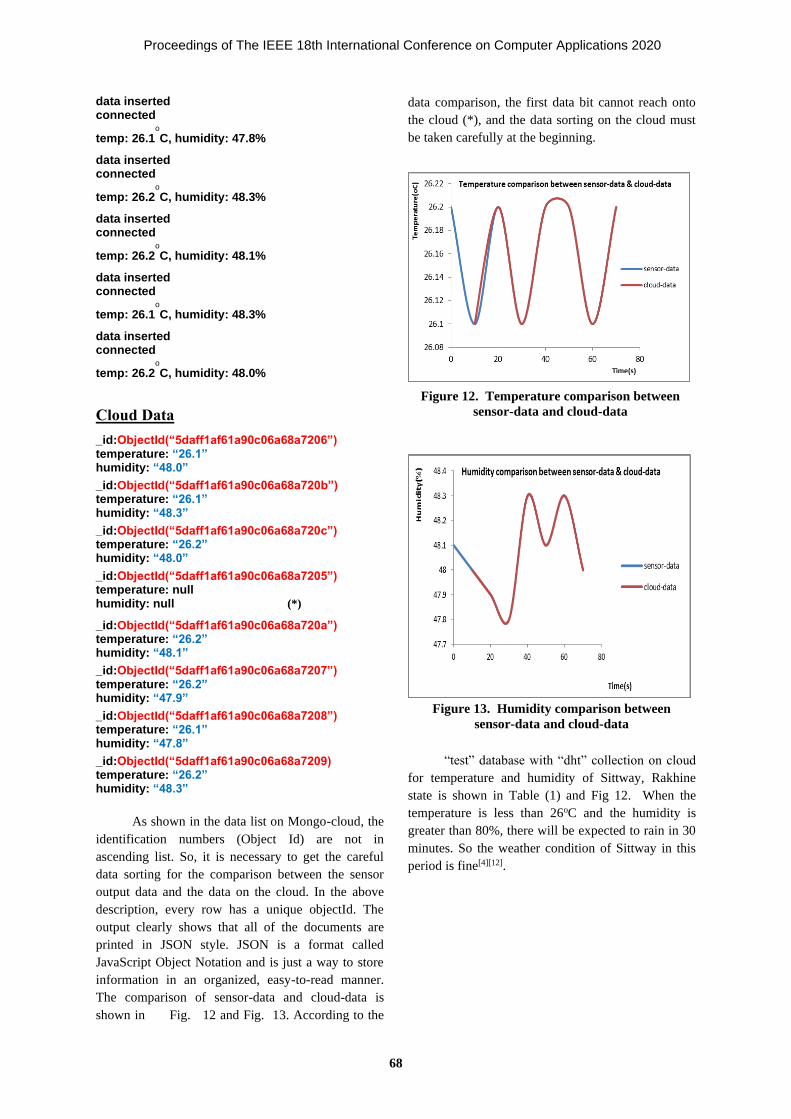
data inserted connected
temp: 26.1oC, humidity: 47.8%
data inserted connected
temp: 26.2oC, humidity: 48.3%
data inserted connected
temp: 26.2oC, humidity: 48.1%
data inserted connected
temp: 26.1oC, humidity: 48.3%
data inserted connected
temp: 26.2oC, humidity: 48.0%
Cloud Data
_id:ObjectId(“5daff1af61a90c06a68a7206”) temperature: “26.1” humidity: “48.0” _id:ObjectId(“5daff1af61a90c06a68a720b”) temperature: “26.1” humidity: “48.3” _id:ObjectId(“5daff1af61a90c06a68a720c”) temperature: “26.2” humidity: “48.0” _id:ObjectId(“5daff1af61a90c06a68a7205”) temperature: null humidity: null (*)
_id:ObjectId(“5daff1af61a90c06a68a720a”) temperature: “26.2” humidity: “48.1” _id:ObjectId(“5daff1af61a90c06a68a7207”) temperature: “26.2” humidity: “47.9” _id:ObjectId(“5daff1af61a90c06a68a7208”) temperature: “26.1” humidity: “47.8” _id:ObjectId(“5daff1af61a90c06a68a7209) temperature: “26.2” humidity: “48.3”
As shown in the data list on Mongo-cloud, the
identification numbers (Object Id) are not in
ascending list. So, it is necessary to get the careful
data sorting for the comparison between the sensor
output data and the data on the cloud. In the above
description, every row has a unique objectId. The
output clearly shows that all of the documents are
printed in JSON style. JSON is a format called
JavaScript Object Notation and is just a way to store
information in an organized, easy-to-read manner.
The comparison of sensor-data and cloud-data is
shown in Fig. 12 and Fig. 13. According to the
data comparison, the first data bit cannot reach onto
the cloud (*), and the data sorting on the cloud must
be taken carefully at the beginning.
“test” database with “dht” collection on cloud
for temperature and humidity of Sittway, Rakhine
state is shown in Table (1) and Fig 12. When the
temperature is less than 26oC and the humidity is
greater than 80%, there will be expected to rain in 30
minutes. So the weather condition of Sittway in this
period is fine[4][12].
Figure 12. Temperature comparison between
sensor-data and cloud-data
Figure 13. Humidity comparison between
sensor-data and cloud-data
Proceedings of The IEEE 18th International Conference on Computer Applications 2020
68

V. CONTRIBUTION
The proposed system has been designed to
create the low cost weather station to get the
information of real time weather condition and easy
to install to achieve the weather data of a specific area.
And then the data can be used to share to the others
by using MONGODB with node.js.
VI. CONCLUSION
Weather prediction is a very important factor,
which forecasts the climate in a region based upon
the values of weather parameters. So the calculated
results from this system can be used in forecasting the
weather of that locality for a period of time. This
research makes the understanding concepts of
humidity sensor and temperature sensor of DHT22
according to the construction of them, and then how
to create the MONGO database on cloud of the
weather parameters of the specific area. The data
from sensor are transmitted to sever where they can
be viewed globally which will be easily accessible to
everyone. All the weather parameters were
successfully displayed via MONGO database which
are accessible by both administrator and users.
Because there is no concept of relationship in
MongoDB, a document database, in which one
collection holds different documents and it can deal
with big data. The comparison between sensor data
and cloud data has been made for the determination
of the accuracy of mongo-node.js on private-cloud.
The system can make to solve the environmental
problems due to the weather condition for living-
things and non-living things.
REFERENCES
[1] Adnan S, Yulong L, Mohan Z, Selim A, 2014,
“Low Cost Embedded Weather Station with
Intelligent System” (USA: Michigan)
[2] Aguado E & Burt J, Understanding Weather and
Climate, 6th ed. Boston [Mass.]: Pearson
Education, Inc., (2013).
[3] Avid Kopec, 2019, “Classic Computer Science
Problems in Python” (New York: Manning
Publications Company)
[4] Hamid F, Rahman W, Mohd Nizar H, “Humidity
Sensors Principle, Mechanism, and Fabrication
Technologies”, IJIRCCE, March 2015
[5] Kodali R & Mandal S, “IoT based weather
station”, 2016 Interna-tional Conference on
Control, Instrumentation, Communication and
Computational Technologies (ICCICCT),
Kumaracoil, India, pp. 680-683, (2016).
[6] Narasimha Karumanchi, 2016, “Data Structure
and Algorithmic Thinking with Python”,
(Bombay: CareeMonk Publications)
[7] Peter Farrell, 2019, “Math Adventures with
Python”, (San Francisco: no statch Press)
[8] Ruano AE, Mestre G, Duarte H & Silva S, “A
neural network based intelligent weather
station”, 2015 IEEE 9th International Symposi-
um on Intelligent Signal Processing (WISP),
Siena, Italy, pp. 1-6, (2015).
[9] Sarmad Nozad M, “Design od Weather
Monitoring System Using Arduino Based
Database Implementation”, Journal of
TABLE I. TEMPERATURE AND
HUMIDITY IN SITTWAY
Figure 14. Temperature and humidity on cloud
Proceedings of The IEEE 18th International Conference on Computer Applications 2020
69

MultidisciplinaryEngineering Science and
Technology, Vol.4, Issue 4, April-2017
[10] Satyanarayana KNV, Reddy SRN, Sai Teja
PVYN & Habibuddin B, “IOT Based Smart
Weather Station Using Raspberry-PI3”, Journal
of Chemical and Pharmaceutical Sciences, Vol.
2016, No. 10, pp. 1-6, (2016).
[11] Stefano Z, 2018, “Wind Direction Extraction
from SAR in Coastal Areas” (Italy: Padova)
[12] Yash M, Anshika M & Bhateja D, “Correlation
among environ-mental parameters using an
online smart weather station system”, India
Conference (INDICON), 2015 Annual IEEE,
New Delhi, In-dia, pp. 1-6, (2015).
Proceedings of The IEEE 18th International Conference on Computer Applications 2020
70

Preserving the Privacy for University Data Using Blockchain and
Attribute-based Encryption
Soe Myint Myat
Computer Science Department
Myanmar Aerospace Engineering University
Meiktila, Myanmar
Than Naing Soe
University of Computer Studies, Myitkyina
Myanmar
Abstract
An effective IT solution is required for the
administrative processes which is the core of
university. The tamper resistance, transparency and
auditability for university management data are very
important to avoid the corruption. Blockchain
occupies the immutability and irreversibility
properties thus, it becomes a potential solution.
Regrettably, there are some challenges such as
privacy concern and limited storage exists in
blockchain technology. In this work, a blockchain-
based university data storage model is proposed and
such barriers of blockchain are handled. The
proposed model achieves the tamper resistance,
transparency and auditability feature by using
blockchain technology. CP-ABE and other
cryptographic techniques are used to provide the fine-
grained access and privacy preserving facilities. The
security analysis is performed and shows that our
approach is tamper resistant and provably secure for
privacy.
Keywords—data security, tamper resistance,
blockchain, privacy, fine-grained access
I. INTRODUCTION
In the premise of industrial 4.0 revolutions [1],
human society will be stimulated with the higher
education which is an essential factor for human
development. Thus, a large number of information
systems such as office automation system, teaching
system, administrative system, personnel system and
asset system are built in universities to improve the
efficiency of staffs [1]. This work will make dialectical,
complicated an interesting prospects of human centric
characteristic. The research, services and teaching will
be changed to different ways and new forms of
universities will be emerged in the fourth industrial
revolution. Thus, the tamper resistance, transparency
and auditability for university management data are
very important to avoid the corruption. Then again, the
industrial 4.0 also takes the popular technology,
blockchain which occupies the transparency,
immutability and cryptographic verifiability
properties. Thus, blockchain become a candidate
solution for university data.
Contrary to the expectation, the blockchain
technology also contains some obstacles in using for
university data. One of the obvious requirements for
university data is fine grained access that allows the
only authorized user to access the certain data. For
instance, if the university data of all departments are
transparently stored on blockchain, any faculty or
everybody who can access the blockchain can access
any document. However, the blockchain stores
cryptographically verified data; it does not encrypt the
data at all [2]. In some private blockchain system like
Hyperledger Fabric [3], the participation in network
can be regulated, however, the university data still
needs to allow only certain users to access a specific
data. Consequently, the privacy issue has to be handled.
The append-only property of blockchain becomes a
barrier for a user revocation feature which allows
eliminating permission of the access on the university
data for specified individuals. The explosive growth of
the university data causes the available issue for the
limited blockchain storage. Thus, how to use
blockchain technology for university data as an
underlying mechanism is still an issue.
To provide the confidentiality and to preserve
the privacy, encryption is a promising way. However,
there exist some traditional technology such as
password based and classical public key encryption
based approaches, the individual user needs to maintain
too much secret information (decryption keys or
passwords) for accessing the multiple files. The
attribute-based encryption (ABE) [4] uses the user
attribute set as the public key instead of using random
string as the public key. The further development of
ABE encrypts the message with an access policy and it
is called Ciphertext Policy Attribute-based Encryption
(CP-ABE) [5]. In CP-ABE scheme, only the user who
Proceedings of The IEEE 18th International Conference on Computer Applications 2020
71

has the attributes that meet the access policy
requirement can decrypt the encrypted message thus,
CP-ABE can support more efficient access control
mechanism.
In this work, the blockchain technology, cloud
storage and CP-ABE encryption technique are used to
preserve the privacy for the university data. The
blockchain technology is used to support the tamper
resistance, auditability and transparency of university
data. The cloud storage is used to overcome the
availability issue of blockchain and CP-ABE is used to
support the fine grained access on university data.
Thus, our approach requires only one secret key per
user while other systems such as password based
systems require multiple passwords for multiple files.
Similarly, our approach requires encrypting the data
only one time while public key crypto systems require
multiple times for encryption for a document for
multiple users. At the same time, our approach can
support tamper resistant, auditability and transparent
property for university management data.
The followings are the rest of the paper. Section
2 discusses about some existing related works. Section
3 discusses some technology and knowledge that
support in developing our system such as blockchain
technology, CP-ABE encryption and other
cryptographic primitives. The detailed of our proposed
approach is discussed in section 4 and security analysis
is performed in section 5. Finally, the paper is
concluded in section 6.
II. RELATED WORKS
Blockchain is used as the storage for diverse
items such as academic work, attendance, certificates
and awarding of a university degree in the education
purpose [6], [7]. The distributed and transparent
properties of blockchain are used to reduce the fraud in
academic items such as certificates and informal
context such as misrepresentation of knowledge,
background and skill [8]. Most of these existing works
are trying to use some properties of blockchain such as
transparency and there are some challenges such as
confidentiality, privacy and availability for using
blockchain.
In [9] the fine grained access control for
encrypted data is firstly developed with a variant of
ABE. However, this approach cannot support complex
policies require for university data. To support such
sophisticated policies, CP-ABE which describe the
users with various attributes is more suitable. The CP-
ABE algorithm is firstly introduced by Bethencourt et
al. in [6]. They used access tree in encrypting the
message and “Lagrange Interpolation” is used in
decryption. Then, a comparative attribute-based
encryption is proposed in [10] and the proposed
method is illustrated with an example of telemedicine.
Moreover, an implementation of Functional
Encryption is proposed in [11]. Most of the existing
works tried to use attribute-based encryption for
healthcare data.
There is no universally accepted standard
definition for the term “privacy”. Privacy encompasses
with several concepts such as anonymity, pseudonymi
ty, unlinkability, unobservability and revocability of
consent. The blockchain support most of these
concepts, thus, we try to use the benefits of blockchain
technology for university data and the cloud
technology and CP-ABE technology is used to handle
some blockchain issue for using in university data
storage.
III. PRELIMINARIES
A. Blockchain
The blockchain technology is introduced by
Satoshi Nakamoto with the crypto-currency called
Bitcoin [2]. Actually, the blockchain is a distributed
database and each data storage structure called block
links each other as a chain [12]. A block is a special
storage structure of blockchain and it maintains the
hash value of the previous block to form a chain. By
forming a chain, the block is immutable to
modification [13]. The block also maintains other
items such as payload, timestamp and signature of the
contributor. Payload of the block may vary according
to the various applications. The payload can be any
asset or item such as the content of the transaction, an
address pointer of the original data or some other
information. The timestamp is used to order the blocks
in chronological fashion. The signature of contributor
shows the generator of the block. Generally,
blockchain network includes two main entities, miners
who produce new blocks and verifiers who verify the
new blocks. In generating the new block, consensus
mechanism is usually used. In this work the metadata
will be stored on blockchain as verified data.
There are three categories of blockchain in
general. They are permission-less blockchain also
called public blockchain, permission blockchain also
called private blockchain and consortium blockchain.
The permission-less blockchain is public in nature and
everyone can participate in the blockchain system.
Bitcoin is a good example for permission-less
blockchain system. In the group of permission
blockchains, the access right and participation on
Proceedings of The IEEE 18th International Conference on Computer Applications 2020
72

blockchain network is controlled by an organization in
private blockchain while several organizations manage
the consortium blockchain. The permission blockchain
(private blockchain or consortium blockchain) is
suitable to store and manage the university data
according to the architecture of our work.
B. Ciphertext-policy Attribute-based
Encryption
The ciphertext-policy attribute-based
encryption (CP-ABE) [5] is a one-to-many encryption
scheme. CP-ABE allows the multiple users to access
the encrypted data. CP-ABE use a set of attribute in
identifying the user with the decrypting key called CP-
ABE private key. By using a list of attribute which
correspond to the authorized users, the data owner can
specify various access policy. The policy is then
embedded into the encrypted data. For example, the
policy can be expressed as follow.
Policy P = “(Rector) OR (Head_of_Department)
AND (Department_1)”
If the user processes the attributes ‘Rector’ or
‘Head of Department from Department 1’, the
ciphertext can be decrypted. Otherwise, the data cannot
be decrypted. Generally, there are four main steps in
CP-ABE scheme. In the first step, a master
secret key MSK and a public parameter PK are
generated and this step is called setup phase. The public
parameter PK contains the generator g, gβ , and an
efficiently computable symmetric bilinear
mape (g, g)α. The master secret key MSK contains the
value β and gα. The PK can be reveal publicly, and the
MSK must be kept secret.
In second phase, the encrypting process is
performed. The cipher text CT is output from the set of
input which includes plaintext message M, public
parameters PK and an access policy T in encryption
phase. A set of Boolean formulas is used to create an
access policy tree. The figure 1 illustrates the creating
the access policy tree from the policy P.
Figure 1. Sample access policy tree
The third step is the key-generation phase. The
private key SK which associate to the set of user
attributes set S is generated in this phase. The master
secret key MSK, the public parameters PK and a set of
user attributes S are taken by this process as input. That
is why, the attributes are mathematically incorporated
into the key.
The fourth step is the decryption phase. The
ciphertext CT will be decrypted in the decryption
phase, if and only if the access policy tree T is satisfied
by theset of attributes associated with the private key
SK.
C. Access Structure
Let a set of n ∈ N+ be a set of participants
P1, P2, … , Pn and a collection A ⊆ 2P1,P2,…,Pn is
monotone for ∀B and C, and if B ∈ A, B ⊆ C, then C ∈
A. Then, an access structure is a collection A of non-
empty subsets of P1, P2, … , Pn , i.e, A ∈ 2P1,P2,⋯,Pn\
∅ [5].
The sets which are included in A are called as
the authorized sets. However, the sets which are not
included in A are called unauthorized sets. Attributes
take the role of parties in our context. Thus, the access
structure A will contain the authorized sets of
attributes.
D. Bilinear Map
Let G and GTas two cyclic groups of order p for
some large primep. G is a group of points on an elliptic
curve over FP (namely the finite field mod p) is G and
a subgroup of a finite field Fp2∗ (namely the finite field
mod p2) is GT.
Then, a map e ∶ G × G → GT is called to be a
bilinear map if it satisfies the following properties.
1) Bilinear ( (aP , bQ) = e(P , Q)ab for all P, Q ∈
G and a, b ∈ Zp).
2) Non-Degenerate (the map does not send all pairs
in G × G to the identity in GT and observe that
since G and GT are groups of prime order, this
implies that if P is a generator of G, then e (P, P)
is a generator of GT )
3) Computable (there is an efficient algorithm to
compute e(P, Q) for any P, Q ∈ G)
Head_of_Department
OR
AND
OR
Rector
Department_1 Department_2
Proceedings of The IEEE 18th International Conference on Computer Applications 2020
73

IV. METHODOLOGY
This section provides the problem scenario of
our work and the detailed description about our
proposed model.
A. Problem Scenario
Generally, in a university, the role hierarchy of
the employees may be in the form which is illustrated
in Figure 2. If the data are stored in the same location
or storage, everyone in the university (all faculties or
departments or all participants) can access these data.
In reality, there may be various attributes of employees
in university environment; however, the Table 1
illustrates some sample attribute list for employees in
university.
To support data privacy (authorized access),
data protection mechanism which allows only the
authorized employees to access the data is required.
The authorized employees must occupy the attributes
values which can satisfy the access conditions. Thus,
the attribute values which are shown in Table 1 are
used to generate the decryption keys (private keys) for
each group of users.
Figure 2. Sample hierarchy of employees in
university
For instance, an examination data, S2_D3_
B5_Sem2_Lab_Marks_2016.doc is stored in the
system. In this data the subject is S2, the department is
D3, and the batch is B5, and the semester is the second
semester Sem2. The employees associated with this
batch should access it is confidential by this marks
data.
Everyone can access this data if the data is
stored in common storage. Password-based usage has
operational difficulties such as maintaining many
passwords although some password protection can be
employed for protection. Thus, a new approach is
required to store the data in the manner that the data is
encrypted; the data is tamper resistant and the data must
be accessible by only authorized users.
TABLE I. SAMPLE ATTRIBUTE LIST OF UNIVERSITY EMPLOYEES
Faculty F1 F2 F3 F4 F5 F6 F7 F8
Department D1 D1 D3 D1 D2 D1 D1 D1
Designation Associate Professor
Assistant Professor
Assistant Professor
Professor Professor Associate Professor
Assistant Professor
Professor
Role Lecture Tutorial Lab Coordinator
Theory Lecture
In-charge D1
2018
In-charge D1
2Sem 2019
In-charge
D1 2Sem 2018
ID 'ID = 1764' 'ID = 1760' 'ID = 1543' 'ID = 1729' 'ID = 1271' 'ID = 1270' 'ID = 1290' 'ID = 1250'
Batch B1 B6 B5 B3 B2 B7 B4 B5
Subject S1 S1 S2 S1 S3 S4 S5 S3
Semester Sem2 Sem2 Sem2 Sem2 Sem1 Sem2 Sem1 Sem2
Year 2016 2017 2016 2017 2018 2018 2019 2018
Proceedings of The IEEE 18th International Conference on Computer Applications 2020
74

B. Proposed method
Attribute-based encryption technique and
blockchain propose a privacy preserving so as to
support the data owner with the fined grained access
control and tamper resistant storage. CP-ABE
algorithm encrypts the actual data to support
confidentiality. The encrypted data is stored on the
cloud storage which can guarantee the availability. The
metadata which represents the university data is
permanently stored on the blockchain to provide a
search and to obtain the tamper resistance property.
Figure 3 represents the overall architecture.
Figure 3. Architecture of the proposed model
There are five main entities that include in
proposed model. The first entity is the data owner
(DO). DO will access or store the university data. DO
has full right to control the over the data, thus, DO will
define the access policy to allow or disallow some
accesses on data. The second entity is the data user
(DU) and DU can access the data with the permission
of corresponding DO. Typically, DU can be an entity
from several sections. DU can search the information
about data on blockchain via the metadata. Then, DU
can download the encrypted data from cloud storage
(CS). The third entity is the attribute authority (AA)
and it is responsible for verifying the attribute of each
user and issuing the corresponding key. The other
entities are cloud storage (CS) which stores the
encrypted data and blockchain (BC) which stores the
metadata.
1) Setting the system
All participants in the system must register with
the attribute authority to setup the system and perform
the initial agreement to support the operations in the
model. To start the agreement, AA performs the setup
algorithm. The setup algorithm uses the implicit
security parameter as an input and it produces a master
key MK and the public parameter PK. Then, AA
performs the key generation algorithm for each user
with their attributes set S and master key MK. At the
end of setting the system, AA distributes an appropriate
private key SK to corresponding user.
2) Storing Data
The data owner (DO) starts the store operation
by performing the encrypt algorithm with an access
structure A over the universe of attributes and the
sensitive information or message M. Therefore, users
who occupy the required attributes set which can
satisfy the access structure can decrypt the resulted
ciphertext CT. On the other hand, the the access policy
which is embedded in the ciphertext CT or CT
implicitly maintains the authorized attributes A. Then,
the hash code is generated from CT for integrity
checking. CT is stored on cloud storage and the link to
CT is received. The DO extracts the metadata and
includes the hash code and link for search purpose
within the system. Finally, DO stores the metadata and
other required information about the encrypted data on
the blockchain.
3) Retrieving Data
The DU starts the retrieve operation by
searching the required information of encrypted data
on the blockchain. DU uses the link from metadata to
get the encrypted data from CS. DU checks the
integrity of encrypted data with hash code obtained
from metadata set. DU runs the decryption algorithm
with his/her private key SK, the public parameters PK
and the ciphertext CT.
If the attribute set S of DU satisfies the access
structure A which is embedded in the ciphertext CT,
then the algorithm can decrypt the CT and DU get the
original message M.
V. SECURITY ANALYSIS
In this section, the security of proposed model is
proven through the following cases of adversaries’
attempts.
Case 1: Supposing that the data stored by some
users in the cloud can be access by the adversaries,
however the adversaries cannot alter or modify the data
as well as cannot view the stored data. Even if the data
Proceedings of The IEEE 18th International Conference on Computer Applications 2020
75

is altered, all the users can know such action. Thus, the
data is tamper resistant and can be safely preserved.
Proof: The blockchain actually maintain the hash
code of all uploaded data and the characteristics of
blockchain ensure that the stored data cannot be
modified. The data stored on blockchain cannot be
altered or delete once confirmed. If the metadata in the
blockchain is wanted to modify by the adversaries, they
must try the extensive work to construct a new main
chain. Such kind of action is neraly impossible.
Moreover, if the data is tampered, it can be verified by
comparison with the hash code preserved in the
blockchain.
Case 2: Supposing that the adversaries attempt to
cover the real content by preserving some piece of
metadata which is different from the existing metadata,
however, the early metadata which is stored on
blockchain always exist and it is more legally effective,
thus, the adversaries cannot defraud with the false
metadata.
Proof: Generally, a judicial system will be needed
to adjudicate with some evidence when two different
metadata exist. However, no judicial evidence will be
needed in our approach because each metadata has a
timestamp that shows the time of preservation in the
blockchain.
Case 3: Suppose adversaries can pinpoint all
blockchain transactions and read the data. If he/she
cannot understand the encrypted data, the adversaries
will not be able to steal the sensitive information.
Proof: As all data are encrypted and then
stored, and thus no one can see the real contents of the
preservation as long as the private key is not
compromised.
VI. CONCLUSION
In this paper, the CP-ABE is applied to
efficiently control access right to achieve the benefits
of blockchain technology for university data. All
metadata that represent the university data are saved on
an immutable and distributed data storage called
blockchain. A user who doesn’t have access right will
not be able to view the data, and the stored data can
verify that it had been modified. Thus, it provides a
data integrity, authentication and reliable system. A
CP-ABE based fine grained access control of data has
also been presented in a university scenario. The
university data can be stored at cloud storage and still
accessible to only those users whose attribute values
satisfy the access policy. The proposed model is part of
our ongoing research thus, an experimental study will
be conducted on the proposed model and evaluate the
empirical result to improve the model in the future.
REFERENCES
[1] Q. Liu, Q. Guan, X. Yang, H. Zhu, G. Green, and
S. Yin, “Education-Industry Cooperative System
Based on Blockchain,” in 2018 1st IEEE
International Conference on Hot Information-
Centric Networking (HotICN), Shenzhen, 2018,
pp. 207–211, doi:
10.1109/HOTICN.2018.8606036.
[2] S. Nakamoto, “Bitcoin: A peer-to-peer electronic
cash system,” 2008.
[3] Hyperledger, “Hyperledger-fabricdocs Master
documentation.” [Online]. Available:
http://hyperledger- fabric. readthedocs.io/ en/
release/ prereqs.html.
[4] A. Sahai and B. Waters, “Fuzzy identity-based
encryption,” Springer, vol. 3494, pp. 457–473,
2005.
[5] J. Bethencourt, A. Sahai, and B. Waters,
“Ciphertext-Policy Attribute-Based Encryption,”
in 2007 IEEE Symposium on Security and
Privacy (SP ’07), 2007, pp. 321–334, doi:
10.1109/SP.2007.11.
[6] M. Sharples and J. Domingue, “The Blockchain
and Kudos: A Distributed System for Educational
Record, Reputation and Reward,” in Adaptive and
Adaptable Learning, 2016, pp. 490–496.
[7] D. J. Skiba, “The Potential of Blockchain in
Education and Health Care,” Nursing Education
Perspectives, vol. 38, no. 4, p. 220, Aug. 2017,
doi: 10.1097/01.NEP.0000000000000190.
[8] A. Grech and A. F. Camilleri, “Blockchain in
education,” Luxembourg: Publications Office of
the European Union 2017, no. 132 S. (JRC
Science for Policy Report), pp. 1–125, 2017.
[9] R. Gavriloaie, W. Nejdl, D. Olmedilla, K. E.
Seamons, and M. Winslett, “No Registration
Needed: How to Use Declarative Policies and
Negotiation to Access Sensitive Resources on the
Semantic Web,” in The Semantic Web: Research
and Applications, 2004, pp. 342–356.
[10] Ting Yu and M. Winslett, “A unified scheme for
resource protection in automated trust
negotiation,” in 2003 Symposium on Security and
Privacy, 2003., 2003, pp. 110–122, doi:
10.1109/SECPRI.2003.1199331.
Proceedings of The IEEE 18th International Conference on Computer Applications 2020
76

[11] J. Li, N. Li, and W. H. Winsborough, “Automated
Trust Negotiation Using Cryptographic
Credentials,” in Proceedings of the 12th ACM
Conference on Computer and Communications
Security, New York, NY, USA, 2005, pp. 46–57,
doi: 10.1145/1102120.1102129.
[12] T. T. Thwin and S. Vasupongayya, “Blockchain-
Based Access Control Model to Preserve Privacy
for Personal Health Record Systems,” Security
and Communication Networks, 2019. doi:
10.1155/2019/8315614
[13] T. T. Thwin and S. Vasupongayya, “Blockchain
Based Secret-Data Sharing Model for Personal
Health Record System,” in 2018 5th International
Conference on Advanced Informatics: Concept
Theory and Applications (ICAICTA), 2018, pp.
196–201, doi: 10.1109/ICAICTA.2018.8541296.
Proceedings of The IEEE 18th International Conference on Computer Applications 2020
77

Scheduling Methods in HPC System: Review
Lett Yi Kyaw
Cloud Computing Lab, UCSY
University of Computer Studies, Yangon
(UCSY)
Yangon, Myanmar
Sabai Phyu
Cloud Computing Lab, UCSY
University of Computer Studies, Yangon
(UCSY)
Yangon, Myanmar
Abstract
Parallel and distributed computing is a
research area that is complex and rapidly evolving.
Researchers are trying to get more and more
methods and technologies in parallel and distributed
computing. Most users who use Pay as you do go
design, elasticity, and virtualization mobility and
automation make cloud computing an attractive
option to meet the development needs of some HPC
users. Over the years, the research algorithm has
also changed accordingly. The basic principles of
parallel computing, however, remain the same, such
as inter - process and inter - processor
communication schemes, parallelism methods and
performance model. In this paper, HPC system,
scheduling methods and challenges are discussed
and given some potential solutions.
Keywords: parallel and distributed computing, high
performance computing, methods, challenges
I. INTRODUCTION
Scheduling technology is very important role
in Information Era. Data input is processing in
various ways and displaying. High Performance
Computing (HPC) performs and demands many
computers to work multiple tasks concurrently and
efficiently. For a long time, the preparation of work
for parallel computers has been subject to study. For
a long time, the preparation of jobs since parallel
computers has been subject to study. Job execution
time is defined as the amount of processors allocated
to it or requires users to provide estimated time for
execution of jobs. The simulation software produces
the estimation runtime attribute based on the
specified range of estimation errors. The proposed
method is to estimate and reduce execution time in a
system.
Today, a super computer is and will always be
a one-of - a-kind framework. Only a small number of
users can use it. The operating mode can be
compared to an experimental facility's exclusive use.
A supercomputer does not usually have free
resources. Typically the client has to wait, not the
other way, to use a supercomputer program. During
the past few years, supercomputers have been widely
used in scientific research and industrial
development. The architectures of such systems have
varied during time. Today, to construct a real
scientific grid, the main building blocks are mostly in
place. The requisite communication quality is given
by high speed wide area networks.
HPC system such as Grid computing [11], grid
computing is a distributed network of large numbers
of connected computers to solve a difficult problem.
Servers and personal computers perform different
functions in the grid computing model and are
loosely connected to the internet and low-speed
networks. Computers may connect through
scheduling systems or directly. Grid computing
involves dynamic digital organization (doctors,
scientists and physicists), sharing of resources
(reliable and unreliable collection of resources) and
peer-to-peer computing. The grid also aims to
provide access to computing power, scientific data
resources and analytical facilities and is a grid
computing challenge.
The key issue for high-performance computing
is executing computational processes on a specific set
of processors. Although the literature has also
proposed a large number of schedules for heuristics,
most of them target only homogeneous resources
[19]. Future computing systems are most likely as the
computational grid to be widespread and highly
heterogeneous.
To achieve their performance goals, the
development of research applications running on
these systems has typically complicated new
structural changes and new technology capabilities.
Growing demand for new resources generation of
HPC systems (computing nodes, memory, power,
etc.) need to be supported by the ability to run more
and larger applications with increased resource
Proceedings of The IEEE 18th International Conference on Computer Applications 2020
78

utilization as well as HPC system job turnaround
time.
The traditional purpose of scheduling
algorithms is as follows: find a mapping of processor
tasks and order tasks to fulfill a task graph and a set
of computer resources: (i) task precedence constraints
are met; (ii) resource constraints are met; (iii) a
minimum schedule is established. A divisible job is a
job that randomly divides the cab into any number of
processors in a linear fashion. It applies to a parallel
job perfectly: every sub-task can be performed in
parallel on any number of processors.
II. BACKGROUND
Parallel systems are valuable resources, such
as supercomputers, which are widely shared by user
groups.
A. Parallel Computing
The early standardization on a single machine
device, the von Neumann computer, gave a lot to the
rapid penetration of computer systems into commerce,
research, and education. A von Neumann pc
incorporates a principal processing unit (CPU)
connected to a storage unit (memory). The CPU
executes a saved application that specifies a chain of
study and writes operations at the memory. This easy
model has proved remarkably robust. Its endurance
over more than forty years has allowed the look at of
such important subjects as algorithms and
programming languages to proceed to a big volume
independently of developments in laptop architecture.
High performance computing investigates the
parallel algorithm and strengthens the parallel
computing architecture. Parallel computation could be
a kind of calculation in which at one time different
enlightenment is performed. The goal is to extend
computation speed to possibly understand complex
assignments of computing. There are two different
loads and loads of parallelism refers to pipeline,
whereas space parallelism involves numerous
synchronous computing processors.
B. Scheduler
Scheduling is defined as a method through
which a task, specified by some means, is assigned to
resources required to carry out the specified task. The
research can be virtual computing components such
as threads, processes or data streams, which in turn
are built on hardware resources such as processors,
network connections or expansion cards. The
scheduling in CPU is difficult to control others.
Multiple processors have to be scheduled in parallel
computing and to manage the resources for all
processors any overlapping of the resources to
produce any conflicting results are needed. So the
scheduling in multiprocessors is more complex than
scheduling in a single processor unit. In HPC system,
parallel computing is using to get high performance.
In scheduling of multiple processors it should be
ensured that any processor should not be overloaded
and any processor should not be under loaded. There
will be multiple processors; there will be multiple
queues, so there is need of scheduling multiple
queues simultaneously.
TABLE I. TYPES OF HPC SCHEDULER
Scheduler
Name
Description
Slurm[9] One of the HPC scheduler, a highly scalable,
fault-tolerant resource cluster manager and massive computer systems job scheduler. A
commonly used plugin-based job scheduler that
provides several optimization options, either by adjusting the configuration parameters or by
implementing new plugins and new scheduling
and policy collection.
LSF[3] It is a tool for task management, a job scheduler for high-performance distributed computing. It
also allows users to access vast amounts of
computing resources distributed around the network in large, heterogeneous distributed
systems and can provide major performance
upgrades to applications.
Loadlever It schedules jobs and offers functions for the
faster and more efficient production, submission
and processing the jobs in a dynamic environment [21].
Moab [22] A method of task planning and management for
use on clusters, supercomputers, and grids. It
can support a wide range of policy planning and fairness dynamic priorities, and substantial
reservations.
Torque It is an open source resource manager [23] that enables batch job control and distributed
compute nodes.
The primary purpose of the job scheduler is to
assign resources to work for users and ensure that
jobs are operating at their highest performance. It
prevents the overloading of a given compute node
and puts jobs on hold before resources are available.
The scheduler’s secondary purpose is to
monitor usage to ensure fair distribution of HPC
resources over time. To run multiple applications
concurrently, HPC schedulers order to execution of
batch jobs to achieve high utilization while
controlling their turnaround times. In HPC
schedulers, the balance between utilization and
turnaround time is controlled by the scheduler
prioritization system and the scheduling algorithms.
Proceedings of The IEEE 18th International Conference on Computer Applications 2020
79

Turnaround Time: Time from submission to
completion of process
Production HPC system uses different
workload manager that combine scheduling and
resource management. The following table 1 is most
popular schedulers.
Modern HPC tools usually consist of a cluster
of computing nodes that provide the user with the
ability to coordinate tasks and substantially reduce
the time it takes for complex operations to be
performed. Usually, a node is defined as a discrete
unit of a computer system running its own operating
system case. Modern nodes have several processors,
also referred to as Central Processing Units or CPUs,
each of which contains multiple cores that can
process a separate instruction stream.
All things considered, in spite of which
strategy is used, the idea of a high-performance
system is stable. The management of a high-
performance system (referred to as part of a single
gadget or multi-computer cluster by multiple
processors) is treated as a single computing
commodity, placing demands on unmistakable hubs.
The HPC framework could be a partitioned unit
created and actualized unequivocally as an effective
computing device.
C. Time-sharing and Space-sharing
Time sharing refers to any scheduling
approach that allows others to preempt and restart
threads later during execution. The amount of jobs
that each processor can perform at the equal time is
defining as the level of multi-programming. Future
HPC systems will be much noisier, with much greater
competition and heterogeneity, requiring the use of
new, asynchronous programming models [5].
Space-sharing procedures only offer a string
that uses a processor until its execution is complete or
the most extreme period of time has been reached and
the string is done. Space sharing techniques [14]
control time by putting that work in a line and at the
same time running all its strings when discharged
from that line.
D. HPC Scheduling
Parallel computing has become most
important issue right this time but because of the high
cost of computer it is not accessible for everyone.
Cluster is only technique that provides parallel
computing, scalability and high availability at low
cost, in fig 1. Cluster collection provides high-
performance computing, while individual computers
work to solve a problem at the same time. Clusters
are designed as they provide computation and
availability of high performance over a single
computer. A cluster is a group of connected devices,
such as computers and switches that function as a
single system together. Each and every node of a
cluster is associated with a single system. Each and
every cluster node is either connected by wire
(Ethernet) or wireless that transfers data between
nodes. A strong cluster provides distributed
computing consisting of standard desktop computers
linked through a network like Ethernet. Linux
operating system can be used to control the cluster. In
this way, we can build high performance computing
(HPC) at low-cost price.
Scheduling method is mainly divided into two
types: static and dynamic. With static scheduling, the
consideration concerning processor placement and
task assignment is made at the onset of the job
execution. Static policies have low run-time overhead
and the scheduling costs are paid only once, during
the compilation time, for instance. As a consequence,
static scheduling policies can afford to be based on
sophisticated heuristics that lead to efficient
allocations. Parallelism can be well exploited by
spreading different tasks over different processors
statically. Static scheduling needs to know in advance
detailed information about the job's run-time profile
which is relied on the input data, static scheduling
carries some degree of unsure. The consequence may
be an unbalanced load resulting in longer parallel
execution time and low utilization of the network.
Dynamic scheduling, during execution, the
number of processors assigned to a job can vary. The
allocated processors are also assigned tasks during
the execution of a job. In both their advantages and
disadvantages, dynamic scheduling policies
complement static policies. Typically, complex
policies generate high overhead run-time, which can
lead to performance degradation. But there are
dynamic scheduling processes and adaptive behavior,
which results in a high degree of load balancing.
HPC scheduling research [7] relates to how
such research should be performed, because such
research requires information, methodology, and
resources that are not always available. Some of three
basic methods for job scheduling research:
• Theoretical analysis
• Real system experiments
• Simulation
Proceedings of The IEEE 18th International Conference on Computer Applications 2020
80

Theoretical Analysis
By defining boundary cases reflecting the
best and worst-case results, algorithm behavior is
analyzed. This approach may provide insight into the
actions of the algorithm, but may not reflect the
performance anticipated when performing a real
workload. In HPC method, percentage of execution
time spent in inter-process communication,
congestion of memory bandwidth and performance of
FLOPs are evaluating various ways to determine the
degree of performance degradation when running
practical HPC workloads.
Real System Experiments
Simple measurements of the behavior of the
algorithm with a real system and workload still
involve several different experiments [3] to be
performed, which can be difficult for several reasons.
However, a single experiment only produces evidence
for one workload and process state, which is usually
not enough to rationalize the general case or test a
general hypothesis. Eventually, the conditions of
workload are difficult to control, so evaluating
specific scenarios can be challenging.
Simulation
A process is emulated, the emulated system
runs a batch scheduler, and the scheduler receives a
synthetic workload. This method allows the
development of various experimental scenarios and
the execution of large-scale experiments to produce
information that enable general conclusions to be
induced. Nevertheless, their findings are only true if
they are indicative of the recreated workloads,
processes and scheduling behaviors.
Figure 1. A cluster used to run a parallel program
No interaction with the administrator is
needed through the usage of HPC program, jobs are
completed sequentially without delays created by
human interaction, which saves processing time this
is generally wasted with human interaction. An
application usually uses a parallel algorithm to run on
a high performance cluster. A big task can be divided
into several sub-duties, running on cluster-based
exclusive nodes. The knowledge collected, resulting
from the sub-duties, is translated into the special
challenge's quit end result.
E. Need of Job Scheduling
Through a planning system responsible for
defining available resources, a task is allocated to
tools: matching job requirements with resources,
making work ordering decisions and goals. Usually,
the use of HPC resources is strong. In this manner,
assets are not quickly accessible and employments are
lined for future execution time until execution is
regularly very long (numerous generation frameworks
have and normal delay until execution of >1h),
employments may run for a long time (a few hours,
days or weeks).
Job Steps
A user job enters a job queue, the scheduler
(its technique) chooses on begin time and asset
properties of the work. The occupations can come at
the shape of batch or interactive type.
• A batch job is a script is used to submit the
job. A shell script may be a given list of shell
commands to be executed in a given arrange.
• Today's shells are so modern simply can
make scripts that are genuine programs with
a few factors, control structures, circles.
• An interactive job is typically an assignment
of one or more nodes where one of the
cluster nodes receives a shell from the user.
Job scheduling is a mapping mechanism from
the tasks of users to the proper selection and execution
of resources [1].A scheduler may aim at one or more
goals, for example: minimizing throughput,
minimizing wait time, minimizing latency or response
time or maximizing fairness [2].The following job
scheduling algorithms are: First come first serve
(FCFS), Shortest first job (SJF), Round - robin (RR),
Priority scheduling, Min - min, Max - min, Genetic
algorithm (GA) and so on which are using for job
management.
A good scheduling algorithm allocates suitable
resources to workflow tasks in order to complete the
application and at the same time satisfy user
requirements.
One Parallel Program
Cluster
Result
Proceedings of The IEEE 18th International Conference on Computer Applications 2020
81

Job Scheduling Algorithms
Genetic Algorithm: A method for solving
constrained and unconstrained problems of
optimization foundation on natural selection, the
mechanism that evolved biological process. A
population of individual solutions is repeatedly
updated by the genetic algorithm. The genetic
algorithm selects individuals from the current
population at random to be parents at each stage and
uses them to produce the babies for the next
generation. The genetic algorithm can be used to
solve a variety of optimization issues that are not
suitable for conventional optimization algorithms
where objective function is discontinuous, non-
differentiable, stochastic, or highly nonlinear. By
using GA, each iteration generates a population of
points and selects an optimal solution for the best
point in the population. And then, by calculation,
select the next population using random number
generators.
GA is used in a number of different fields of usage.
Hence, by providing arrays of bits or characters to
represent the chromosomes, most researchers can
introduce this genetic model of computation. Simple
operations of bit manipulation allow crossover,
mutation and other operations to be performed.
First come first serve (FCFS): FCFS is similar
to the data structure of the FIFO (First in First out)
queue, where the first data element added to the
queue is the first element to exit the queue. In Batch
Systems, this is used. Using a queue data structure,
where a new process works through the queue's tail,
it is easy to programmatically understand and
execute, and the scheduler selects the process from
the queue end. Purchasing tickets at the ticket counter
is a perfect example of FCFS planning in real life.
But there is an issue with FCFS, system priority is
not taken into account. Parallel use of resources is not
feasible and use of bad resources (CPU, I / O, etc.).
Shortest Job First (SJF): A scheduling strategy
that chooses the process of waiting to execute next
with the smallest execution time. Second, the system
is completed, which takes the shortest time to
complete the execution. Using ordered FIFO queue,
this rule can be enforced. All processes in a queue are
sorted on the basis of their CPU bursts. When the
CPU is available, a system will be selected to run
from the first position in a queue [16].
Round - robin (RR): When the process can be
executed, procedures are given an equal slice of time.
The execution is carried out one after another on a
circular order. So every work has a quantity when it
can be done. If this quantity is not sufficient to
complete the execution of the process, it will be
stopped and the next process will be performed.
Upon completing a full round, its turn will come
again and so on. If a process is completed, it will go
off the list and if another arrives, it will be put at the
end of the list waiting for its turn.
There is no hunger in this algorithm, but it can
often be too long. This is a typical and conventional
load balancing algorithm, but the challenge in round
robin is setting the time quantity. To calculate the
dynamic quantity of time, various optimization
algorithms can be combined with RR [4].
Priority scheduling: It gives a well-defined
priority to each system. This way, each process has
its own priority, depending on whether it will be run
or wait. The first to run is going to be the highest
priority operation, while others are going to wait for
their turn. First will be handled high-priority
activities [20]. Therefore, the low priority tasks
would have to wait a long time in the queue. If the
system crashes, all non-performing low-priority tasks
will be lost.
Min – Min: This algorithm is based on the resource
assignment principle that has the shortest completion
time (fastest resource), a minimum completion time
(MCT) functioned [8]. It is a sample algorithm but it
gives the quick result when the size of the task in the
task group that deals with other tasks is small
compared to the large size task, on the other hand,
when large size tasks are performed, it gives poor use
of the resource and large maximum completion time
of the task since larger tasks have to wait for smaller
tasks to be completed. For all tasks to be performed,
the Min - Min algorithm first finds the minimum
time. Then, it selects the task with the least execution
time among all tasks. The algorithm proceeds by
assigning the task to the resource generating the
minimum completion time. Min - Min repeats the
same procedure until all tasks are planned. Min - Min
algorithm's limitation is that it first selects smaller
tasks that make use of high computational power
resource. As a result, when the number of smaller
tasks exceeds the large ones, Min-Min's schedule is
not optimal.
Max – Min: This algorithm is bottomed on the
concept of assigning to the asset, which has the
maximum completion time (fastest resource), a task
with maximum completion time (MCT). It is a test
algorithm but it gives the fast result when the size of
the task in the metatask is big compared to the small
Proceedings of The IEEE 18th International Conference on Computer Applications 2020
82

size task. On the other hand, if small size tasks are
performed, it gives poor use of the resource and a
large maximum completion time of the task as
smaller tasks have to wait for larger tasks to be
completed. The purpose of this algorithm is to
prioritize tasks with optimum completion time by
executing them first before assigning other tasks with
minimum completion time [13].
F. Components of HPC Scheduling
High-performance computing has five
components: CPUs, memory, nodes, internodes in the
network, and storage (disks, tape). Single-core CPU
(processors) is no longer being used today. To date,
all CPUs (processors) consist of the configuration
used on the motherboard (multiple' cores' on a single'
chip'). For a number of reasons, the trend of even
more ' core ' per unit will rise. The node plays a
major role in linking CPUs, memory, interfaces,
computers and other nodes in a physical way. For a
high-performance computing system, shared memory
is often necessary.
There are five different node types: user
node, control node, node of management, node of
processing and node of computation, in Fig 2. The
client node is the only portal to reach the cluster
network for outsiders. Users typically have to log in
to compile and run the tasks from the node. Fault-
tolerant architecture is accomplished with hardware
redundancy to be built in the system to ensure the
client node is highly accessible. Control node is
mainly responsible for delivering computer node to
basic network services such as DHCP (Dynamic Host
Control Protocol), DNS (Domain Name Service),
NFS (Network File Service) and the distribution of
computer node tasks.
Figure 2. A High Performance Computing Cluster
III. CHALLENGES
In recent study, as the chosen platform for
execution as the optimal medium for a wide range of
workloads to be performed, there are four major
challenges for heterogeneous computing clusters to
address.
First, the majority of business applications
currently in use were not designed to run on such
large, open and heterogeneous computing clusters.
To move these applications to heterogeneous
computer clusters, particularly with significant
performance improvements or improvements in
energy efficiency, is a quest and attempt to solve
problem. Second, it is also overwhelming to generate
new, ground-up enterprise applications to run on the
different, heterogeneous computing framework. It is
extremely challenging to write high-performance,
energy-efficient programs [12]for these architectures
to die on an unprecedented scale of parallelism, as
well as difficulty in scheduling, interconnecting and
sorting. Third, cost savings for utilization and
distribution of IT services from the new shared
network architecture are only feasible if multiple
business applications can share resources in the
heterogeneous computing cluster. Nonetheless,
allowing multi-tenancy without adversely affecting
that application's stringent performance service
metrics needs complex scalability and virtualization
of a wide variety of different computing, processing
and interconnect devices, and this is yet another
unresolved issue. Fourth, enterprise systems with
unusually heavy load spikes experience greatly
variable user loads. Meeting service metrics quality
across multiple loads includes the use of an
application's elastic computing resources in response
to increasing user demand. There are no good
solutions to this problem at the moment. There are no
good solutions to this obstacle at the moment. The
resource management dynamics in HPC are evolving.
New application innovations and technical transitions
introduce the scheduling models and process
architecture with new concepts and specifications.
Another problem is that multicore chips are
relatively simple processor core and will be
underused if user programs are unable to provide
enough parallel thread speed. It is the responsible of
the programmer to write parallel high-performance
software to make maximum use of the processor
core. The new parallel multicore technology should
have two characteristics to achieve high performance:
Fine grain thread: a high degree of parallelism
is needed to keep each core processor busy. Another
Proceedings of The IEEE 18th International Conference on Computer Applications 2020
83

factor is that a core often has to operate on a small-
size cache or scratch buffer that allows developers to
break down a task into smaller tasks.
Asynchronous program execution: The
existence of a synchronization point can seriously
affect the performance of the program when there are
many processor cores. And reducing unnecessary
points of synchronization can subsequently increase
the degree of parallelism.
IV. CONCLUSION
We present HPC framework, its scheduling
and research challenges in this paper as express in
table 2. Task scheduling on parallel machines is a
research field that has been well explored and has led
to widespread use and there are several methods,
including automatic calculations of runtime, partial
executions, and smarter allocation schemes for
processors. Parallel processing builds on existing
technologies implemented in new scenarios and
serving diverse users and priorities. Max-min
algorithms is the execution of tasks with maximum
completion time may first increase the total response
time of the system and thus make it inefficient and it
has these drawbacks so that researchers may consider
the different methods to implement this algorithm.
Min-min algorithm is first considered to be the
shortest jobs, so it fails to efficiently leverage the
resources that lead to a load imbalance, so efficient
methods are needed to solve this problem. FCFS
which can be a long waiting time if the short request
is waiting for the long process [15]. It is not ideal for
a system of time sharing where it is critical that each
user receives the CPU for the same time interval.
The through in round robin largely depends on
the selection of the size of the time quantum. If time
quantum is too large it behaves as FCFS. If time
quantum is too short much of the time is spent in
process switching and hence low throughput and one
cannot assign priority to any process which can be a
drawback. Priority scheduling will have to consider
which parameters are set to high priority within
system.
Genetic algorithm has different parameters
(size of population, times, rates of mutation, etc.) and
there are many problems not well defined
(parameters are not well defined or not
known).Researchers are need to decide which
optimization method to use for research environment
to solve problem. Longer processes in shortest job
first algorithm have more waiting time, so starvation
occurred and need to solve this issue. Some are used
average waiting time to reduce long waiting time. We
agree that several areas of HPC still need the
attention of the researcher. We will have a detailed
study of HPC problems and challenges in the future.
TABLE II. COMPARISON OF EACH METHOD
Algorithm Comparison Advantages Disadvantages
Genetic
Algorithm
(GA)[18]
It is
necessary to
use as a tool to solve the
problems of
optimization and search.
GA includes
several operations to
execute the
algorithm
with several
techniques.
This
combines
good solutions
and
optimizes towards a
goal over
time.
Without
through too
much time for GA to check
for optimum
results, some new genetic
values should
be incorporated
into the
population.
First Come First Serve
(FCFS)[15]
FCFS starts imply the
first task to
be done.
For long process,
FCFS is
suitable than others and
one of the
easiest methods.
Each and every small process
should wait for
its turn to utilize the CPU
also,
throughput is not
emphasized.
Shortest Job First
(SJF)[16]
Shortest job starts to be
process.
It is optimized
for average
waiting time.
There is more number of
short jobs in a
system, the long jobs will
be starvation.
Round-
Robin (RR) [10]
Time is to be
allocated to resources in a
time slice
manner in this
scheduling
algorithm.
In a general-
purpose, time-sharing
or
transaction processing
system, RR
is successful.
There is also
a small overhead on
the
processor.
Care must be
taken when determining
the quantity
value, and if the quantity
time is too
high, the result is also weak.
Priority
scheduling
A well-
defined
priority to each system.
A handled
high-priority
activity, so user defines
process is
more suitable.
The low
priority tasks
would have to wait a long
time in the
queue of the system.
Min-min
[6]
Chooses
smaller tasks first to be
done.
One
resource can execute only
one at a time
and resources
are known
in prior.
This is caused
load imbalance between large
task and small
task to execute in the system.
Max-min [6]
Chooses bigger tasks
to be
completed first.
Prioritize tasks with
optimum
completion time by
executing
them first
Execution of task with
maximum
completion time first
might increase
the total
Proceedings of The IEEE 18th International Conference on Computer Applications 2020
84

before
assigning
other tasks
with minimum
completion
time.
response time
of the system
thus making it
inefficient.
REFERENCES
[1] W. Bradley, S. Ramaswamy, R.B.Lenin and D.
Hoffman, “Modelling and Simulation of HPC
Systems Through Job Scheduling Analysis”,
January 2011.
[2] M. A. Obaida, J. Liu, “Simulation of HPC Job
Scheduling And Large-Scale Parallel
Workloads”, 978-1-5386-3428-8,IEEE,2017.
[3] IBM LSF & HPC User Group @SC18,
LSF&HPC User Group/SC18/@2018 IBM
Corporation .
[4] N. K.C Das, M. S. George and P. Jaya,
“Incorporating weighed Round Robin in
Honeybee Algorithm for Enhanced Load
Balancing in Cloud Environment”, 978-1-5090-
3800-8, IEEE,2017.
[5] S. Hofmeyr,C. Iancu, J. A. Colmenares, E.
Roman and B. Austin,” Time-Sharing Redux for
Large-scale HPC systems”, 978-1-5090-4297-5,
IEEE,2016.
[6] N. Thakkar,.R. Nath,”Performance Analysis of
Min-Min, Max-Min and Artificial Bee Colony
Load Balancing Algorithm in Cloud
Computing”, IJACS,ISSN 2347-8616, Volume7,
Issue 4, April 2018.
[7] G. P.R. Alvarez, P. Ostberg, E. Elmroth, K.
Antypas, R. Gerber, and L.Ramakrishnan,
“Towards Understanding Job Heterogeneity in
HPC: A NERSC Case Study”, In Proceeding of
the 16th IEEE/ACM International Symposium on
Cluster, Cloud and Grid Computing
(CCGrid’16), IEEE/ACM 2016.
[8] G. Sharma, P. Bansal,”Min-Min Approach for
Scheduling in Grid Environment”, IJLTET,
ISSN: 2278-621X, Vol.1, Issue 1, May 2012.
[9] A. Jokanovic,M. D’Amico,J.
Corbalan,”Evaluating SLUM Simulator with
real-machine SLUM and vice
versa”,https://www.researchgate.net/publication/
328886964, November 2018.
[10] B. Mohamed, N. E.AL-Attar, W. Awad, F. A.
Omara, “Dynamic Job Scheduling Algorithms
Based on Round Robin for Cloud Environment”,
Research Journal of Applied Sciences,
Engineering and Technology 14(3): 124-131,
2017.
[11] F. Xhafa, A. Abraham,"Computational models
and heuristic methods for Grid scheduling
problems", Future Generation Computer Systems
26 (2010) 608_621,
doi:10.1016/j.future.2009.11.005, Elsevier, 2009.
[12] S. Wallace, X.Yang, V. Vishwanath, W. E.
Allcock, S. Coghlan, M. E. Papka, Z. Lan,"A
Data Driven Scheduling Approach for Power
Management on HPC Systems", 978-1-4673-
8815-3,IEEE,2016.
[13] C. Diaz, J. E. Pecero, P. Bouvry, “Scalable, low
complexity, and fast greedy scheduling heuristics
for highly heterogeneous distributed computing
systems”, Journal of Supercomputing 67(3),
837–853(2014),2014.
[14] T. Li, V. K.Narayana, T. EI-Ghazawi,”Exploring
Graphics Processing Unit(GPU) Resource
Sharing Efficiency for High Performance
Computing”,
https://www.researchgate.net/publication/260422
348,November,2013.
[15] A. P. U. Siahaan,"Comparison Analysis of CPU
Scheduling: FCFS, SJF and Round Robin",
IJEDR,Volume 4,Issue 3, ISSN: 2321-
9939,2016.
[16] M. A.Alworafi, A. Dhari, A. A. Al-Hashmi, "An
Improved SJF Scheduling Algorithm in Cloud
Computing Environment", ,International
Conference on Electrical, Electronics,
Communication, Computer and Optimization
Techniques (ICEECCOT), , 978-1-5090-4697-
3,IEEE,2016.
[17] L. Kishor, D. Goyal, "Comparative Analysis of
Various Scheduling Algorithms", International
Journal of Advanced Research in Computer
Engineering& Technology (IJARCET), Volume
2, Issue4,April 2013.
[18] S. P. Lim, H. Haron,"Performance Comparison
of Genetic Algorithm, Differential Evolution and
Particle Swarm Optimization Towards
Benchmark Functions", Conference on Open
Systems (ICOS), 978-1-4799-0285-
9,IEEE,December2-3,2014.
[19] S. Razzaq, A. Wahid, F. Khan, N. u. Amin, M.
A. Shah, A. Akhunzada, I. Ali ,"Scheduling
Algorithms for High-Performance Computing:
An Application Perspective of Fog Computing" ,
https://doi.org/10.1007/978-3-319-99966-
1_10,Springer,2019.
Proceedings of The IEEE 18th International Conference on Computer Applications 2020
85

[20] https://en.wikipedia.org/wiki/Scheduling_(c
omputing)#Scheduling_disciplines .
[21] https://www.ibm.com/support/knowledgece
nter/en/SSFJTW_5.1.0/com.ibm.cluster.loa
dl.v5r1.load100.doc/am2ug_ch1.htm
[22] https://computing.llnl.gov/tutorials/moab/,
https://computing.llnl.gov/tutorials/datahero
es/moab/
[23] https://en.wikipedia.org/wiki/TORQUE,http
s://hpc-wiki.info/hpc/Torque
Proceedings of The IEEE 18th International Conference on Computer Applications 2020
86

Cyber Security and Digital Forensics
Proceedings of The IEEE 18th International Conference on Computer Applications 2020

Proceedings of The IEEE 18th International Conference on Computer Applications 2020

Comparative Analysis of Site-to-Site Layer 2 Virtual Private Networks
Si Thu Aung
University of Computer Studies, Yangon
Thandar Thein
University of Computer Studies (Maubin)
Abstract
Nowadays, many companies have branch
offices and connect those offices to the main office over
the Internet using a site-to-site Virtual Private Network
connection. Most of these connections have always
operated at Layer 3 of the OSI network model. In recent
years, there has been a growing requirement to extend
links at Layer 2, which allows broadcast traffic to be
forwarded between sites. Depending on inter-site
connection medium, different technologies are utilized.
This paper compares and analyses site-to-site Layer 2
VPN technologies, which include layer 2 tunneling
protocol (L2TP), and point to point tunneling protocol
(PPTP), OpenVPN, Ethernet over IP (EoIP), and
MPLS/VPLS to choose the right VPN for the
organization. This is done by means of performance
measurement and packet analysis. In order to provide
fair comparable results, all technologies are tested in
the same manner.
Keyword: PPTP, L2TP, OpenVPN, EoIP, VPLS,
Virtual Private Network
I. INTRODUCTION
While VPNs were commonly planned for
individual clients, demand is likewise expanding in
business. Organizations presently use VPNs to verify
their office systems, business PCs, and Internet
connection while others use VPNs to remotely access
network resources that are not near them geologically.
In the course of the most recent couple of years, VPNs
have turned strongly to be one of the most well-known
and irreplaceable tools for every privacy-conscious
consumer. Globally, the Internet handles around
71,131 GB of traffic for each second, including
2,790,265 emails and 73,849 Google searches for every
second [1]. All the company’s communications and
employees searching for business-related information
help to make up those numbers. Furthermore, a breach
or leak of the business’s data transmitted over the
Internet could cost people millions. This raises alarms
because, according to a Ponemon Institute survey [2],
67% of SMBs admitted to being attacked in 2018.
Large businesses with massive investment may be in a
better position to deploy a range of IT security
solutions; small businesses need to be more vigilant.
The most effective way to prevent the data from
reaching the wrong hands is through the use of a VPN
service that makes the Internet usage fully private and
secure. Businesses may also find different reasons for
using a VPN. To fill this gap, there are many kinds of
VPN technologies such as IPSec, GRE and SSL. Most
of them are Layer 3 VPNs, and it fulfills most of the
business requirements. With Layer 3 VPNs, exchange
emails and accessing internal servers are easy to use
and secure. However, it is not possible to use some
software for LAN between two sites, although they are
connected by Layer 3 VPN, for example, printer
sharing, some database protocols, CRMs, and other
applications that are developed for LAN specified
purpose. If people want to use LAN applications, a
single Ethernet segment needs to be constructed.
Imagine the situation of three remote sites;
Yangon, Mandalay and MauBin, and every site have an
Ethernet switch. It is a big challenge to connect
Ethernet network cables between them. To lay the
cable between different offices in different cities is
expensive as well as time-consuming. The Internet
cannot become an alternative to Ethernet because even
if both sites are connected to the Internet, two sites do
not construct the single Ethernet segment at all. Layer
2 “Site-to-Site VPN” tunnels the Internet and establish
a VPN Session between remote sites with full
capabilities to transmit any Ethernet frames. Layer 2
VPN has unlimited protocol transparency, which is
identical to physical Ethernet segments. Many
protocols such as IPv4 (TCP, UDP, ICMP, ESP, GRE),
IPv6, PPPoE, RIP, STP, and others can be used on
Ethernet. Any legacy and latest protocols can be used
within the Layer 2 VPN sessions. Although provider
provisioned Layer 2 VPN solutions such as
MPLS/VPLS can be purchased from ISPs, most of
these services are monthly payment basis, and the price
is not cost-effective.
Proceedings of The IEEE 18th International Conference on Computer Applications 2020
89

Not only are these restrictions, but also different
IP subnets on each site need to be built. A site's IP
subnet cannot overlap with other sites. Moreover, a
number of subnets have to be managed in order to
prevent any other subnets from colliding. Adopting the
Layer 3 VPN for creating site-to-site VPN requires
special pain to satisfy the demands of legacy VPNs.
However, when we use Layer 2 VPN to link up the site-
to-site VPN, it is very straightforward and reduces the
effort to coop against several troublesome errors which
might occur when Layer 3 VPNs are used. Designing
and architecting networks with layer 2 VPNs can be as
simple as designing traditional Ethernet network
topology with hub-and-spoke mode. Connecting VPN
Sessions between sites is possible instead of using
physical Ethernet network cables.
All kinds of server and inter-client-PC-
communication applications will work well, with no
difference between inside the same site and beyond the
distance. It is the main reason that the decision to carry
out a performance comparison of Layer 2 VPNs is
made.
In this paper, the impact of Layer 2 VPNs and
performance analysis of five different VPNs, namely,
PPTP, L2TP, OpenVPN with BCP, EoIP and
MPLS/VPLS are discussed and presented. However,
this paper does not provide explicit suggestion on
which technology is to be preferred. The rest of this
paper is organized as follows: Section II presents
related work. Section III explains the characteristic of
VPN, and Section IV provides the testbed setup. The
experiment results are discussed in section V and draw
conclusions in section VI.
II. RELATED WORK
Singh and Gupta [3] proposed Multi-phase
encryption and payload encryption; it was applied to
the data inside the IP packet of the encapsulated tunnel
packet. They discussed the traditional security
measures of VPN and a whole new approach for VPN
security by using a multi-phase encryption technique.
I. Kotuliak, P. Rybár, and P. Trúchly [4] analyzed
OpenVPN and IPSec based VPN; they compared those
technologies based on parameters such as throughput,
the response time of each protocol. They chose
OpenVPN due to its simplicity and fast and
straightforward implementation.
Chawla et al. [5] explained the architecture and
protocols of IPSec and SSL VPN technologies,
including their advantages and disadvantages for real
kinds of applications. Qin et al. [6] studied IPSec and
SSL VPN in detail, and the scope of application,
security, scalability, and other aspects are analyzed and
compared, advantages and inadequacy are
summarized. Zhang Zhipeng et al. [7] presented three
types of common VPNs and explained a comparative
study of their features, performance, security, and cost-
efficient.
None of the related works compared to the
performance of Layer 2 VPNs. In this paper, we
concentrate on the performance of Layer 2 VPNs.
III. Characteristics and Models of VPNs
A plethora of methods is used to model and
characterize VPNs. The purpose of this section is to
introduce and explain each of these models and
characterizations.
A. Service Provider and Customer
Provisioned VPNs
VPNs that are configured and managed by a
service provider are service provider provisioned
VPNs. VPNs that are configured and managed by the
customer itself are called customer provisioned VPNs.
Examples of service provider provisioned, and
customer provisioned VPNs are shown in Table 1.
TABLE 1. Service Provider and Customer
Provisioned VPNs
Provider Provisioned Customer Provisioned
VPWS, VPLS, IPLS PPTP, L2TP, OpenVPN
BGP/MPLS, IPSec, GRE, IP-in-IP
IPSec, GRE, EoIP
B. Site-To-Site and Remote Access VPNs
Whether provider or customer provisioned,
VPNs fall into one of two broad categories: site to site
or remote access. Site-to-site VPNs allow connectivity
between an organization’s geographically dispersed
sites (such as a head office and branch offices). Fig 1
illustrates a typical site-to-site VPN.
Remote access VPNs allow mobile or home-
based users to access an organization’s resources
remotely. Fig. 2 illustrates typical remote access VPNs.
C. Protocol Background
This section presents protocols used in Layer 2
VPN technologies.
1) PPTP: The Point to Point Tunneling Protocol
(PPTP) is one of the oldest protocol. PPTP uses the
TCP port 1723 for remote access over the Internet. The
data packets transmitted through the tunnel are
Proceedings of The IEEE 18th International Conference on Computer Applications 2020
90

encapsulated. It is suitable for applications where speed
is important, such as streaming and gaming.
Figure 1. Typical site-to-site VPN
Figure 2. Remote Access VPNs
2) L2TP with IPSec: L2TP stands for Layer 2
Tunneling Protocol and does not provide any
encryption on its own. L2TP usually uses IPSec
(Internet Protocol Security) authentication protocol.
The data transmitted through the L2TP / IPSec
protocol is usually authenticated twice. Each data
packet transmitted through the tunnel includes L2TP
headers. One of the many reasons why L2TP is a
common protocol is that there are no known
vulnerabilities.
3) OpenVPN: OpenVPN is often referred to as
an SSL-based VPN because it uses the SSL/TLS
protocol for secure communication. The control
channel is encrypted and protected using SSL/TLS
while the data channel is encrypted using a custom
encryption protocol. OpenVPN's default protocol and
port are UDP and port 1194.
4) PPP Bridging Control Protocol: BCP allows
bridging the Ethernet frame through the PPP link.
Established BCP is an integral part of the PPP tunnel.
The Bridging Control Protocol (BCP) is responsible
for configuring, activating and disabling the bridge
protocol modules at both ends of the point-to-point
link. PPTP, L2TP, and OpenVPN protocols can carry
only the upper layer of Layer 3 and more. However,
with the support of BCP, they can work as Layer 2.
5) EoIP with IPSec: IP protocol 47/GRE allows
tunnel creation by encapsulating Ethernet frames in IP
packets and forwarding them to another router.
Ethernet over IP (EoIP) establishes an Ethernet tunnel
on top of an IP connection between two routers. All
Ethernet traffic will be bridged, just as if there is a
physical interface.
6) MPLS VPLS: Virtual Private LAN Service
(VPLS) offers multipoint Ethernet-based connectivity
over IP or MPLS networks. It enables geographically
dispersed sites to share an Ethernet broadcast domain
by linking sites through pseudowires. It is often used
for extending LAN services over a network given by
a service provider.
IV. TESTBED SETUP AND PERFORMANCE
PARAMETERS
This section describes how to setup testbed to
measure performance and to analyze security.
A. Testbed Setup
There are two laptop computers and three
desktop computers in this setup. WAN Emulator [8] is
running on a desktop computer. RouterOS [9] is
running on two computers to create a tunnel between
these two desktop computers. Two laptops are running
iPerf software to test throughput. In testbed example,
the iPerf client send the 100MB of data to the iPerf
server, and the output are saved in CSV file. Our
testbed setup is as shown in Fig. 3 and their hardware
and software specifications are shown in Table 2.
WAN Emulator
12.0.0.1/24 34.0.0.4/24
192.168.4.3/24 192.168.4.2/24
R1 R2
Figure 3. Testbed setup
Proceedings of The IEEE 18th International Conference on Computer Applications 2020
91

TABLE 2. Hardware and Software Specification
Type Description
Laptop x 2 Intel(R) Core(TM) i5-7200 CPU @ 2.50GHz(4CPUs), ~2.7GHz, 8GB
memory
Desktop x 3 Intel(R) Core(TM) i3-2100 CPU @
3.10GHz(4CPUs)
WANem Wide Area Network Emulator v3.0 Beta
2 released
VirtualBox [10] Oracle VirtualBox 6.0 hypervisor
software
RouterOS 6.46.1 (Stable) release
In this paper, WANEM is used to emulate to
define QoS parameters such as packet loss, jitter, and
delay. Packet loss has a direct impact on the stability of
the VPN. Packet loss occurs when the network is
congested.
TABLE 3. QoS Parameters
Parameters Value
Bandwidth Limit 50 Mbps
Delay 20ms, 40ms, 60ms
Jitter 2ms
Packet Loss 0.1%
Delay is the amount of time a packet travels
from its source to destination. Jitter is the changing rate
of delay across a network, and is measured in
milliseconds and it has a great impact on live streaming
application such as video and VoIP. To be similar with
real network, QoS values are defined as shown in Table
3.
B. Measurement Tools
Assessing the performance of Layer 2 VPN
requires the use of several measurement tools for
generating, measuring, and monitoring network traffic.
The tools used in this work are Wireshark [11] and
iPerf3 [12]. Wireshark is a network protocol analyzer
with a rich feature set for capturing and analyzing
network traffic. iPerf3 is a network testing tool for
active measurements of the maximum achievable
bandwidth on IP networks.
V. EXPERIMENTAL RESULTS AND
DISCUSSION
Experimental results are based on the different
parameters for the different VPN technologies. This
section shows the performance of seven different
methods of Layer 2 VPNs in terms of throughput and
protocol analysis.
A. Throughput
Throughput is measured in bits per second. By
analyzing the results, throughput varies depending on
protocol nature and encryption method. For throughput
measurement, iPerf3 is used to exchange traffic
between two laptops. For all VPN technologies, the
same amount of traffic (100MB) is exchanged and
tested three times with three different delays; 20
milliseconds (ms), 40 ms, and 60 ms. The results are
documented in Table 4, and Fig. 4 shows the
throughput comparisons.
TABLE 4. Throughput Comparison with
Different Delays
VPN Delay 20
ms Delay 40 ms
Delay 60
ms
PPTP-BCP 45.1 Mbps 31.4 Mbps 22.2 Mbps
L2TP-BCP 45.2 Mbps 31.4 Mbps 22.6 Mbps
L2TP-BCP-
IPSec 44 Mbps 30.8 Mbps 22.7 Mbps
OpenVPN 9.6 Mbps 4.16 Mbps 2.6 Mbps
EoIP 46 Mbps 30.4 Mbps 21.2 Mbps
EoIP_IPSec 45.1 Mbps 31.8 Mbps 23.1 Mbps
MPLS VPLS 48.1 Mbps 29.4 Mbps 21.3 Mbps
TABLE 5. Throughput and Loss Comparison
between Non-VPN Traffic and VPN Traffic at
20ms delay
VPN Non-VPN
Throughput
VPN
Throughput % of Loss
PPTP-BCP 50 Mbps 45.1 Mbps 9.8%
L2TP-BCP 50 Mbps 45.2 Mbps 9.6%
L2TP-BCP-
IPSec 50 Mbps 44 Mbps 12.0%
OpenVPN 50 Mbps 9.6 Mbps 80.8%
EoIP 50 Mbps 46 Mbps 8.0%
EoIP_IPSec 50 Mbps 45.1 Mbps 9.8%
MPLS VPLS 50 Mbps 48.1 Mbps 3.8%
Figure 4. Throughput comparison
Proceedings of The IEEE 18th International Conference on Computer Applications 2020
92

All VPN tunnels can degrade performance
because of the overhead and encryption methods they
use. The amount of throughput loss is due to the trade-
off between network performance and security.
Generally, the more secure tunnel may result in poor
throughput, while less secure tunnel may have better
throughput. Table 5 shows the loss of throughput when
traversing a tunnel.
B. Packet Analysis
Wireshark protocol analyzer captures the traffic
and analyze while two computers ping each other
inside Layer 2 VPN tunnels.
1) PPTP with BCP: Fig. 5 shows the packet
analysis for the PPTP with BCP, and it can be seen
clearly that two computers ping each other since there
is no encryption with PPTP.
2) L2TP with BCP: When analyzing the packets
transmitted through L2TP with BCP tunnel, it is
observed that which protocols, along with which
source addresses and destination addresses that are
being used can be sniffed.
3) L2TP with IPSec with BCP: When analyzing
the packets transmitted through L2TP with BCP
tunnel with IPSec encryption, only the information of
encapsulated payload can be sniffed.
4) OpenVPN: Due to its secure encryption methods used, packets that are transmitted through OpenVPN display only the OpenVPN protocol with no other additional information.
5) EoIP: Similar to unencrypted L2TP and
PPTP tunnels, EoIP also shows protocol and addresses
of both source and destination when analyzed by a
packet sniffer.
6) EoIP with IPSec: EoIP with IPSec no longer
displays which protocols along with source and
destination addresses accessed in packet analysis if it is
properly encrypted by IPSec.
7) MPLS VPLS: When examine the packets
transmitted with MPLS VPLS, it is observed which
protocols can be sniffed along with the source
addresses and destination addresses used.
TABLE 6. Comparison Matrix of Authentication
and Encryption
VPN
Type Encryption Authentication
Can be
bridge
PPTP MPPE128 Username
Password
With BCP
L2TP IPSec Username
Password
With BCP
OpenVP
N
TLS
(AES/BF)
TLS With BCP
EoIP IPSec No Yes
MPLS/
VPLS
No No Pseudowires
& Control
Word
C. VPN Selection
This section discusses the use of each VPN
based on the various throughput performance test and
packet analysis conducted in previous sections. Packet
analysis describes that OpenVPN, L2TP IPSec with
Figure 5. PPTP with BCP
›
›
Figure 11. MPLS VPLS
Figure 6. L2TP with BCP
Figure 8. OpenVPN
›
Figure 9. EoIP
Proceedings of The IEEE 18th International Conference on Computer Applications 2020
93

BCP, and EoIP with IPSec are good for security. The
throughput result shows that MPLS VPLS is 48.1
Mbps at 20 ms. EoIP with IPSec is 31.8 Mbps at 40 ms,
and 23.1 Mbps at 60 ms. Although the result of EoIP is
good at 40 ms and 60 ms, it is not widely used in the
industry because it is not mature yet and still vendor
dependent. As mentioned in section III, MPLS/VPLS
is a provider provisioned VPN, and customer cannot
manage themselves. L2TP IPSec with BCP should be
considered in term of performance and security
perspective for enterprise networks which need Layer
2 VPN connections. The pros and cons of each VPN on
various aspects can be observed in Table 7.
TABLE 7. Pros and Cons of Different VPNs
Security QoS Scalability Cost
PPTP-BCP Low No Good Low
L2TP-BCP Low No Good Low
L2TP-BCP-IPSec
High No Good Average
OpenVPN Higher No Good Average
EoIP Low Yes Average High
EoIP_IPSec High Yes Average High
MPLS VPLS
Average Yes Best Higher
VI. CONCLUSION
The main purpose of this paper is to analyze and
compare site-to-site Layer 2 VPNs. The experimental
results are achieved with different throughputs from
five different VPN technologies. They are monitored
and captured by Wireshark network protocol analyzer
so as to see what protocols and overheads are added to
the original frame inside layer 2 tunnel. It is easy to see
that Layer 2 VPN carries Ethernet frame that can raise
the overhead compared to Layer 3 VPN. As a result of
this study, it is not easy to recommend one VPN against
to the other because each one of them has advantages
and disadvantages in term of security and performance.
VPN protocol’s encryption capabilities are paramount
important because it determines the level of privacy
and protection, however, this should not be only one
reason to choose the VPN for organization. Therefore,
organization should consider VPN technology that can
balance performance as well as security.
REFERENCES
[1] Internetlivestats. Accessed: Dec 20, 2019.
[Online]. Available: https://internetlivestats.com
[2] Ponemon-Report. Accesed: Dec 20, 2019.
[Online]. Available:
https://www.keepersecurity.com/assets/pdf/Keep
er-2018-Ponemon-Report.pdf
[3] Kuwar Kuldeep Veer Vikram Singh and
Himanshu Gupta “A New Approach for the
Security of VPN” in Proc. ICTCS 2016,
doi:10.1145/2905055.2905219
[4] I. Kotuliak, P. Rybár and P. Trúchly
“Performance Comparison of IPSec and TLS
Based VPN Technologies,” ICTEA 2011,
Slovakia, Oct 2011, pp. 217-221, doi:
10.1109/ICETA. 2011.6112567
[5] Baljot Kaur Chawla, O.P. Gupta, B. K. Sawhney
“A Review on IPsec and SSL VPN,” International
Journal of Scientific & Engineering Research,
Volume 5, Issue 11, November-2014 pp. 21-24
[6] Huaqing MAO, Li ZHU and Hang Qin “A
comparative research on SSL VPN and IPSec
VPN,” in proc. ICTCS 2012
[7] Zhang Zhipeng Et al “VPN: a Boon or Trap? A
Comparative Study of MPLS, IPSec, and SSL
Virtual Private Networks,” in Proc. ICCMC
2018, pp. 510-515
[8] WANEM, wide area network emulator.
Accessed: Dec 20, 2019 [Online]. Available:
http://wanem.sourceforge.net/
[9] RouterOS, operating system for routerboard.
Accessed: Dec 20, 2019 [Online]. Available:
https://mikrotik.com/software
[10] VirtualBox, open-source hosted hypervisor.
Accessed: Dec 20, 2019, [Online]. Available:
https://www.virtualbox.org/
[11] Wireshark, packet analyzer. Accessed: Dec 20,
2019 [Online]. Available:
https://www.wireshark.org/download.html
[12] iPerf, network measurement tool. Accessed: Dec
20, 2019 [Online]. Available: https://iperf.fr/
Proceedings of The IEEE 18th International Conference on Computer Applications 2020
94

Effect of Stabilization Control for Cooperation between Tele-Robot
Systems with Force Feedback by Using Master-Slave Relation
Kazuya Kanaishi
Nagoya Institute of
Technology,
Nagoya, Japan
ech.ac.jp
Yutaka Ishibashi
Nagoya Institute of
Technology,
Nagoya, Japan
Pingguo Huang
Seijo University
Tokai, Japan
huangpg@seijoh-
u.ac.jp
Yuichiro Tateiwa
Nagoya Institute of
Technology,
Nagoya, Japan
Abstract
By experiment, this paper investigates the
effect of the stabilization control with filters to
suppress instability phenomena for tele-robot systems
with force feedback by using a master-slave relation.
As the quality of service (QoS) control to improve the
quality of experience (QoE), the systems carry out the
adaptive ∆-causality control, which we previously
proposed. In our experiment, we carry a wooden stick
together by gripping the two ends of the stick with the
two robot arms of the systems. Experimental results
illustrate that the stabilization control with filters can
suppress instability phenomena.
Keywords—Tele-Robot System, Remote Control,
Force Feedback, Cooperation, Stabilization Control,
QoS, Experiment
I. INTRODUCTION
By using multiple bilateral tele-robot (i.e.,
remote robot) systems with force feedback [1]-[5], we
can conduct cooperative work among the systems [6],
[7]. This is because a user of such a system can operate
a tele-industrial robot having a force sensor via a
network by employing a haptic interface device while
watching video of the robot motion. By using force
feedback for the robot operation, the user can feel the
reaction force outputted by the haptic interface device,
and he/she can perform more accurate operation.
However, if the information about force is transmitted
via a network without the quality of service (QoS) [8]
guarantee such as the Internet, the quality of experience
(QoE) [9] may seriously be degraded and the instability
phenomena may occur owing to the network delay,
delay jitter, and so on. In order to solve the problems,
we need to perform QoS control [8] and stabilization
control [10] together.
In [6], the authors investigate the influence of
the network delay on cooperative work in which a
single user operates the haptic interface devices of the
two tele-robot systems with his/her both hands, and
carries an object held by the two robot arms. The
systems have an equal relationship in this paper, but a
master-slave relation between the systems is also
important. In [7], thus, the authors conduct the same
work as that in [6] by using the tele-robot systems with
a master-slave relation and apply the adaptive ∆-
causality control [11] to avoid large force applied to the
object. As a result, it is illustrated that the control can
suppress large force even if the network delay becomes
larger. However, to avoid instability phenomena, the
reaction force outputted from the haptic interface
device is set to a small value by multiplying 0.5 to the
force detected by the robot's force sensor. We need to
perceive larger reaction force to conduct the work more
precisely. To solve the problem, we need to perform
the stabilization control with filters [10]. However, the
effect of the control has not been clarified
quantitatively in the systems using the master-slave
relation.
Therefore, in this paper, we perform the
stabilization control with filters for the tele-robot
systems using the master-slave relation with force
feedback in which the adaptive ∆-causality control is
exerted. By experiment, we clarify the effect of the
stabilization control. We also investigate the effect of
the adaptive ∆-causality control under the stabilization
control.
The remainder of this paper is organized as
follows. In Section II, first we give an outline of the
tele-robot systems with force feedback by using the
master-slave relation. Next, we explain the adaptive ∆-
causality control in Section III, the stabilization control
with filters in Section IV, and experiment method in
Section V. Then, Section VI presents experimental
results and discusses them. Finally, Section VII
concludes the paper.
Proceedings of The IEEE 18th International Conference on Computer Applications 2020
95

II. TELE-ROBOT SYSTEMS WITH FORCE
FEEDBACK BY USING MASTER-SLAVE
RELATION
In this section, we outline the tele-robot systems
with force feedback in Subsection II.A and how to
calculate the reaction force in Subsection II.B. We also
describe the tele-robot systems by using the master-
slave relation in Subsection II.C.
A. Tele-Robot Systems with Force Feedback
As shown in Figure 1, each of the two systems
(called systems 1 and 2 here) consists of a master
terminal with a haptic interface device (3D Systems
Touch [12]), and a slave terminal with an industrial
robot and a web camera (made by Microsoft). The
master terminal in system 1 is composed of two PCs;
one is for haptic interface device, and the other is for
video. The two PCs are connected by a switching hub.
One PC called PC for haptic interface device and video
is used in system 2, and the functions of PC are same
as those in system 1. The slave terminal in system 1
also consists of two PCs (called PC for industrial robot
and PC for video) which are connected by a switching
hub. One PC (called PC for haptic interface device and
video) is employed in system 2. PC for industrial robot
(or PC for industrial robot and video) is connected to
the industrial robot directly by a 100BASE-TX cable.
The industrial robot consists of a robot controller
(CR750-Q), a force interface unit (2F-TZ561), and a
robot arm with 6 DoF (Degree of Freedom) (RV-2FB-
Q). The force sensor (1F-FS001-W200) is linked to the
tip of the robot arm. Furthermore, a toggle clamp hand
is attached to the force sensor. We use the toggle clamp
hand to fix an object by a toggle. The reaction force
outputted by the haptic interface device is calculated
from the value obtained by the sensor (the calculation
method will be described in the next subsection).
B. Calculation Method of Reaction Force
The reaction force 𝑭𝑡(m)
outputted by the haptic
interface device at the master terminal at time 𝑡 (≥ 1)
is calculated by the following equation:
𝑭𝑡(m)
= 𝐾scale𝑭𝑡−1(s) (1)
where 𝑭𝑡(s)
is the force obtained from the slave
terminal at time t, and 𝐾scale (> 0) is the scaling
factor applied to 𝑭𝑡−1(s)
. In this paper, we set 𝐾scale =
1.0 (note that 𝐾scale= 0.5 in [7]).
Furthermore, the position vector 𝑺𝑡 of the
industrial robot at time 𝑡 (≥ 2) can be obtained from
the following equation:
𝑺𝑡 =
𝑴𝑡−1 + 𝑽𝑡−1 (if |𝑽𝑡−1| ≥ 𝑉max)
𝑴𝑡−1 + 𝑉max
𝑽𝑡−1
|𝑽𝑡−1| (otherwise)
(2)
where 𝑴𝑡 is the position vector of the haptic
interface device that the slave terminal receives from
the master terminal at time t, and 𝑽𝑡 is the velocity
Figure 1. Configuration of tele-robot systems with force feedback.
Proceedings of The IEEE 18th International Conference on Computer Applications 2020
96

vector of the robot arm at time t. 𝑉max is the maximum
moving velocity, and the moving amount is limited so
that the robot does not move too fast. In this paper, we
set 𝑉max = 5 mm ⁄ s [13].
C. Master-Slave Relation
The two tele-robot systems in Subsection II.A
are used as follows. One system is master, and the other
is slave. The robot of the slave system (called the slave
robot here) works according to the movement of the
robot of the master system (called the master robot).
Position information of the master robot is transmitted
from the slave terminal of the master system to the
slave terminal of the slave system, and the slave robot
is controlled by using the information (i.e., unilateral
control). For simplicity, the position information of the
haptic interface device of the slave system is not
transmitted to the slave terminal. A user of the master
system operates the haptic interface device of the
master system, and another user of the slave system can
feel the reaction force by holding the haptic interface
device of the slave system.
III. ADAPTIVE ∆-CAUSALITY CONTROL
When the network delay between the master and
slave systems is large, the slave robot lags behind the
master robot in the movement of robot arm. Then, the
force applied to an object carried by the two robot arms
becomes larger, and the operability of the haptic
interface device is significantly degraded. We reduce
the force and improve the operability by carrying out
the adaptive ∆-causality control [10], which delays the
output timing of the robot’s position information
dynamically according to the network delay; by this,
because we can delay the master robot’s operation by
the network delay from the slave terminal of the master
system to the slave terminal of the slave system, the
operations at both robots are performed at almost the
same time.
The adaptive ∆-causality control outputs
position information at the generation time (i.e., the
timestamp) + ∆ ( > 0) seconds if the information is
received by the time + ∆. Otherwise, the information
is discarded as old and useless information to keep the
causality. The minimum value ΔL and the maximum
value ΔH (ΔH ≥ Δ L > 0) are set for ∆. Also, since ∆
Figure 2. Block diagram of stabilization control with filter.
(b) Plan view (a) Displayed image of video.
Figure 3. Positional relationships between wooden stick and building blocks.
Proceedings of The IEEE 18th International Conference on Computer Applications 2020
97

changes dynamically according to the network delay,
the value 𝐷𝑡 ( 𝑡 ≥ 0 ) obtained by smoothing the
network delay 𝑑𝑡 measured at time t by the following
equation is used as Δ:
𝐷0 = 𝑑0
𝐷𝑡 = α𝐷𝑡−1 + (1 − 𝛼)𝑑𝑡 (𝑡 ≥ 1)(3)
where α is a smoothing coefficient, and we set α =
0.998 [15] in this paper.
IV. STABILIZATION CONTROL
This section gives an outline of the stabilization
control with filters. Figure 2 shows the block diagram
of the stabilization control. The control employs the
wave filter in combination with the phase control filter
[10], [15]. It can make the tele-robot systems with force
feedback stable for any network delay. The reader is
referred to [10], [15], and [16] for details of the control.
V. EXPERIMENT METHOD
In this paper, for simplicity, the experiment was
performed by one person, and the video was watched
only at the master system. In the experimental system,
the master and slave systems were connected via a
network emulator (NIST Net [17]), and a constant
delay was added to each packet transferred in both
directions between the two slave terminals (the one-
way constant delay is called the additional delay here).
The additional delay between the master and slave
terminals in each system was 0 ms for simplicity.
In the experiment, in order to move the robot
arms in almost the same way always, we carried out
work of pushing the top block piled up front and behind
the initial position of the wooden stick held by the two
toggle clamp hands of the robot arms for about 15
seconds (it took about 5 seconds to drop the front block,
and around 10 seconds to drop the behind block. Note
that the hands change the movement directions after
dropping the front block). Figure 3 shows the positional
relationships between the wooden stick and building
blocks; the position difference between the front and
behind brocks is 80 mm. The height of the behind block
is 50 mm higher than the front block as shown in Figure
3 (a). In order to realize more stable operation, the
motion of the robot arm in the left and right (the y-axis)
direction was stopped, and the motion was performed
only in the front and behind (the x-axis) and up and
down (the z-axis) directions [6].
We changed the additional delay between the
two robots of the master and slave systems to 0 ms and
200 ms with and without the adaptive ∆-causality
control (called control and no control, respectively, in
Section VI). Then, we measured the position and the
force detected by the force sensor.
VI. EXPERIMENTAL RESULTS
We show the position and force of each robot’s
x and z axes as a function of the elapsed time from the
beginning of the work in Figures 4 and 5. We set the
additional delay to 200 ms in the figures.
In Figures 4 and 5, we see that there is no
instability phenomenon in the tele-robot systems even
though the reaction force output from the device is
multiplied by 1.0 to the force detected by the robot's
force sensor ( 𝐾scale = 1.0). However, instability
phenomena (i.e., large vibrations) of the robot arms
occurred and we could not carry out the work when we
did not carry out the stabilization control; even if the
additional delay is 0 ms, the phenomena occurred.
Thus, we do not show the position and force in this
case. On the other hand, we confirmed that there was
no instability phenomenon under the stabilization
control with filters when the additional delay is less
than or equal to at least 400 ms; we obtained almost the
same results as those in Figures 4 and 5. Therefore, we
can say that the instability phenomena of the robot arms
are greatly suppressed by the stabilization control.
We find in Figures 4 and 5 that the position and force
of no control fluctuate greatly, but those of control are
suppressed. In Figures 4 (a) and (c), we observe that the
position of the salve robot is about 200 ms behind that
of the master robot. However, we confirm in Figures 5
(a) and (c) that the two positions are almost the same.
These are the effects of the adaptive ∆-causality control
under the stabilization control.
Furthermore, from Figures 4 and 5, we can
confirm that the movement direction of the robot is
reversed at about 6 second, and the sign of the force is
also reversed. This is because the direction of
movement to drop the behind block after dropping the
front block is changed at about 6 second. Figures 4 and
5 reveal that the force in x-axis is larger than the force
in z-axis under control, but the magnitudes of force in
the x-axis and z-axis directions are almost the same
under control.
VII. CONCLUSION
In this paper, we applied the stabilization control
with filters for cooperative work between the tele-robot
systems with force feedback by using a master-slave
relation. As QoS control, we carried out the adaptive ∆-
causality control, and we also investigated the effect of
Proceedings of The IEEE 18th International Conference on Computer Applications 2020
98

the stabilization control. As a result, we found that the
instability phenomena can greatly be suppressed by the
control in the systems. We also saw that the adaptive ∆-
causality control is effective under the stabilization
control.
As our future work, we will apply the
stabilization control with filters and the adaptive ∆-
causality control to the systems with an equal
relationship and investigate their effects. We will also
switch the master-slave relationship dynamically
according to the network delay in the systems.
ACKNOWLEDGMENT
This work was partly supported by JSPS
KAKENHI Grant Number 18K11261.
REFERENCES
[1] P. Nadrag, L. Temzi, H. Arioui, and P. Hoppenot,
‘‘Remote control of an assistive Robot using force
feedback,’’ Proc. The 15th International
Conference on Advanced Robotics (ICAR),
pp.211-216, June 2011.
[2] T. Miyoshi and K. Terashima, ‘‘stabilizing
method for non-passive force-position
teleoperating system,’’ Proc. The 35th SICE
Symposium on Control Theory, vol. 35, pp. 127-
130, Sep. 2006.
[3] T. Miyoshi, Y. Maeda, Y. Morita, Y. Ishibashi,
and K. Terashima, ‘‘Development of haptic
network game based on multi-lateral tele-control
theory and influence of network delay on QoE,’’
(in Japanese), Trans. the Virtual Reality Society
of Japan (VRSJ), Special Issues on Haptic
Contents, vol. 19, no. 4, pp. 559-569, Dec. 2014.
[4] Y. Ishibashi and P. Huang, ‘‘Improvement of QoS
in haptic communication and its future,’’ IEICE
Trans. Commun. (Japanese Edition), vol. J99-B,
no. 10, pp. 911-925, Oct. 2016.
[5] K. Suzuki, Y. Maeda, Y. Ishibashi, and N.
Fukushima, ‘‘Improvement of operability in
remote robot control with force feedback,’’ Proc.
IEEE Global Conference on Consumer
Electronics (GCCE), pp. 16-20, Oct. 2015.
[6] E. Taguchi, Y. Ishibashi, P. Huang, and Y.
Tateiwa, ‘‘Experiment on collaborative work
between remote robot systems with haptics,’’ (in
Japanese), IEICE General Conference, B-11-17,
Mar. 2018.
[7] K. Kanaishi, Y. Ishibashi, P. Huang, and Y.
Tateiwa, ‘‘Effects of adaptive ∆-causality control
for cooperation between remote robot systems
with Force Feedback by using master-slave
relation,’’ Proc. The 3rd International Conference
on Telecommunications and Communication
Engineering (ICTCE), Nov. 2019.
[8] P. Huang and Y. Ishibashi, ‘‘QoS control in haptic
communications,’’ (in Japanese), Journal of
IEICE, Special Section: Advancement and
Quality Enhancement in Haptic Communications,
vol. 102, no. 1, pp. 42-46, Jan. 2019.
[9] T. Abe, Y. Ishibashi, and H. Yoshino, ‘‘State of
the art of service quality,’’ (in Japanese), Journal
of IEICE, vol. 91, no. 2, pp. 82-86, Feb. 2008.
[10] T. Miyoshi, K. Terashima, and M. Buss, ‘‘A
design method of wave filter for stabilizing non-
passive operating system,’’ Proc. IEEE CCA, pp.
1318-1324, Oct. 2006.
[11] Y. Hara, Y. Ishibashi, N. Fukushima, and S.
Sugawara, ‘‘Adaptive delta-causality control with
prediction in networked real-time game using
haptic media,’’ Proc. The 11th Annual Workshop
on Network and Systems Support for Games
(NetGames), Nov. 2012.
[12] 3D Systems Touch, https://www.3dsystems.com/
haptics-devices/touch.
[13] K. Suzuki, Y. Maeda, Y. Ishibashi, and N.
Fukushima, ‘‘Improvement of operability in
remote robot control with force feedback,’’ Proc.
IEEE Global Conference on Consumer
Electronics (GCCE), pp. 16-20, Oct. 2015.
[14] T. Abe, Y. Ishibashi, and H. Ohnishi, ‘‘QoE
assessment of adaptive viscoelasticity control in
remote control system with haptics: Effect against
speed change of pen stroke,’’ (in Japanese), IEICE
Technical Report, CQ2018-60, Aug. 2018.
[15] M. D. Duong, T. Miyoshi, K. Terashima, and E.
J. Rodriguezseda, ‘‘Analysis and design of
position-force teleoperation with scattering
matrix,’’ Proc. The 17th IFAC World Congress,
pp. 12715-12720, July 2008.
[16] P. Huang, T. Miyoshi, and Y. Ishibashi,
‘‘Enhancement of stabilization control in remote
robot system with force feedback,’’ International
Journal of Communications, Network and System
Sciences (IJCNS), vol. 12, no. 7, pp. 99-111, July
2019.
[17] M. Carson and D. Santay, ‘‘NIST Net - A Linux-
based network emulation tool,’’ ACM
SIGCOMM Computer Communication Review,
vol. 33, no. 3, pp. 111-126, July 2003.
Proceedings of The IEEE 18th International Conference on Computer Applications 2020
99

(a) Position of x-axis
(b) Force of x-axis
(c) Position of z-axis
Figure 5. Robot position and force vs. elapsed
time under control (additional delay: 200
ms).
(d) Force of z-axis
(a) Position of x-axis
(b) Force of x-axis
(c) Position of z-axis
(d) Force of z-axis
Figure 4. Robot position and force vs. elapsed
time under no control (additional delay: 200
ms).
Proceedings of The IEEE 18th International Conference on Computer Applications 2020
100

Experimental Design and Analysis of Vehicle Mobility in WiFi Network
Khin Kyu Kyu Win
Department of Electronic
Enginnering
Yangon Technological University
Yangon, Myanmar
Thet Nwe Win
Department of Electronic
Engineering
Yangon Technological University
Ynagon, Myanmar
Kaung Waiyan Kyaw
Department of Electronic
Engineering
Yangon Technological University
Yangon, Myanmar
kaungwaiyankyaw.96@gmail,com
Abstract
Instead of using static nodes in wireless sensor
network, implementation of hardware and mobile
environment are challenges of mobile wireless sensor
network. Mobile sensor nodes combined with wireless
network is one of research area and mobility is one of
key factors in designing mobile wireless sensor
network. To analyze vehicle mobility, this work
implements a mobile sensor node in WiFi network and
it is equipped with ultrasonic sensor and ESP8266
NodeMCU. The sensor data can be monitored on
ThingSpeak over the internet via wireless LAN and its
measurement can be taken within 10 s delay. MikroTik
(RB931-2nD) router is used as an access point in
system architecture. Experiments are performed to
study mobility effects on network throughput when
mobile sensor node is moving with constant velocity of
10 cm/s. With connectivity in wireless LAN 802.11/n
technology, signal strength and throughput are
measured for vehicle mobility.
Keywords: Vehicle Mobility, WiFi, Mobile Wireless
Sensor Network, ThingSpeak, Throughput Analysis
I. INTRODUCTION
Several mobility patterns can be classified as
follows; pedestrian, vehicles, aerial, robot and others.
Regarding mobility in wireless sensor network with
WiFi connectivity, reducing friction and allowing high
speed can be obtained in wheel based vehicular
mobility. To prevent collisions, all vehicles are planned
to move in paths for bounded in 1D movement. In this
work, assumption on constant speed and linear
movement are made to be bounded in mobility pattern.
A mobile sensor node is implemented as parasitic
mobility. This mobility pattern can present sensor
network performance where sensor node harvests the
mobility from vehicle. To measure mobility pattern in
wireless sensor network, localization of sensor node
can help to analyze the network behavior [1]. In this
paper, measuring vehicle mobility is analyzed by using
range-based localization technique. In this ultrasonic
sensor based for range information, basic principles of
ultrasonic range finder are used to be implemented with
Arduino. Experimental study is done for analysis of
mobility in connectivity of wireless local area network.
The rest of paper is organized as follows: related work
is described in section 2. Definition and assumption in
this paper is mentioned in section 3. Section 4 gives the
results and discussion and section 5 gives the
conclusions of this work.
II. RELATED WORK
The research work on mobility are studied in
literature and presented in sections 2.1, 2.2 and 2.3.
A. Localization in Mobility
Mobility can help to solve the typical problems
such as low node density, obstacles and concave
topologies. In addition, mobile assisted localization can
give better localization accuracy and coverage. Survey
of localization problems and solutions are analyzed for
wireless sensor network in [2]. In wireless sensor
network, range free localization techniques can be used
for moving target nodes. In [3], localization algorithm
was used to demonstrate localization accuracy and
stability. The dynamic aspect of network coverage can
be characterized and identified in [4] on the process of
sensor movement in optimal mobility strategies.
B. Network Topology in Mobility
Due to the mobility of mobile node, network
topology can change significantly for long time scale.
Several researches considered mobility effect in Ad
Hoc network model. In [5], per-session throughout is
kept constant with increasing number of nodes per unit
area when users move independently around the
network. Investigation of node mobility effect in
finding best relay node are proposed in [6] to improve
the throughput in Ad Hoc network model. Ad hoc is
Proceedings of The IEEE 18th International Conference on Computer Applications 2020
101
one of wireless mesh typology. Rapid growth of IoT
applications, mesh typology is attractive for
heterogeneous network in which coverage is one of
factors [7].
C. Mobility in Wireless Sensor Network
Data drive is the main difference between
sensor network and mobile Ad Hoc network. Instead
of using static sensor node in network, mobile sensor
nodes are necessary in real applications. In [8],
mobility, typology and localization are key factors in
designing mobile wireless sensor network. The
mobility and sharing of internet enabled wireless
sensor network are analyzed for specific applications
[9]. Hardware cost is one of design challenges for
implementing mobile sensor node in wireless sensor
network. Nowadays, microcontroller-based sensor
nodes are easily implemented with additional unit of
localization finder to be implemented a mobile sensor
node.
III. DEFINITION AND ASSUMPTIONS
In this section, definition and some models that
used in this paper is introduced.
A. Throughput
Throughput of the network is the sum of per-
node throughput for all nodes in a network. Per-node
throughput of λ(n) bits/s can be defined as the time
average of transmitted bits by each node to its
destination [10]. In this work, destination is gateway
router. In a network, per-node throughput capacity is
of order of f(n) bits per second if a deterministic
constant 0<c1<+∞.
B. Network Model
Assumption in this network is that all n mobile
sensor nodes are independently and randomly
distributed in defined area. To localize parasitic
mobility, generated traffic denoted as λ(n) bits/s at each
sensor node is dependent of vehicle mobility process.
A mobile sensor node sends a packet directly to fixed
router if it is within transmission range of mobile sensor
node.
C. Random Direction Mobility Model
In this mobility model, mobile sensor node must
travel within defined area at a constant speed and
direction. After the nodes pause, a new direction and
velocity is chosen randomly and then the process will
repeat [11]. The parameters for point-to-point segment
i is as random variables with the following uniform
distributions:
• Absolute angle φi = Φ : uniform [0, 2π]
• Distance traveled li = L: uniform[Lmin, Lmax]
• The speed vi = V: uniform[Vmin, Vmax]
• The pause ti = T : uniform[Tmin, Tmax]
IV. TESTS AND RESULTS
To summarize the entire system work in Fig. 1,
the system comprises three portions: wireless mobile
sensor node, fixed router and monitoring server.
Figure 1. Flow chart for system process
Wireless mobile sensor node senses the distance
between it and the facing obstacles by using an
ultrasonic sensor. Fixed router receives the packages
from mobile sensor node and routes them to the
destination. And the ThingSpeak IoT analytic platform
is used as a monitoring service provider in this system.
All the router configuration is managed with the
use of Winbox software. For local network, IP address
of Mikrotik router is set to 172.20.23.17 with a subnet
mask of 255.255.255.240 whose prefix is (/28). DHCP
Proceedings of The IEEE 18th International Conference on Computer Applications 2020
102

server is configured in the router. For WiFi interface,
configuration includes WiFi hotspot creating and
setting authentication features for wireless protocol
IEEE 802.11. For monitoring sensor data on
ThingSpeak, a new channel is created after creating
user account. Unique channel ID 774771 is used in
testing and the feed data of channel can be viewed with
private access or public access. There are two API keys
and feed data is imported as a CSV file format. For
connectivity of ThingSpeak server and NodeMCU,
ThingSpeak library is installed in the Aurdino IDE
software.
A. System Description
The system shown in Fig. 2 is developed to
measure and analyze the throughput of wireless
network, according to measured distance while moving
one mobile node in this network.
Figure 2. System architecture
The vehicle is moved in WiFi network as mobile
sensor node. It is constructed by using ultrasonic sensor
and ESP8266 NodeMCU WiFi module. Ultrasonic
sensor is used to measure the distance when mobile
sensor node is moving. Blynk application is
implemented to control mobile sensor node and it can
also command desired movement of node deployment.
NodeMCU from the mobile sensor node, motor
controlling via phone, two laptops (one is for sensor
data monitoring and the other is for network
performance monitoring) are connected to WiFi via
fixed router. This router is configured by IEEE 802.11n
wireless LAN. The sensor data (distance measured)
from the ultrasonic sensor is sent to ThingSpeak sever.
NodeMCU transmits these sensor data to ThingSpeak
via the router shown in Fig. 3.
And measured distance data is monitored with
one laptop that is connected to WiFi via the router. The
throughput and signal strength of the network is
measured and it is monitored by using WinBox
software shown in Fig. 4. From these data, the mobility
pattern of this network is analyzed according to
measured range information from ultrasonic sensor.
Figure 3. Monitoring moving distance on
ThingSpeak
Figure 4. Monitoring throughput and signal
strength
B. Testing Environment
In this work, 30 feet path from starting point to
end point (at fixed router) distance is specified between
fixed router and mobile sensor node. Testing
environment 1 is less friction than testing environment
2 shown in Fig. 5. For these two testing, constant speed
of vehicle is set as 10 cm/s. Ultrasonic sensor HC-SR04
can be used to measure distance in range of 2 cm-400
cm with accuracy of 3 mm. This sensor module is
needed to trigger for signal transmission by using
NodeMCU. NodeMCU reads arrival time between
triggering and received echo. The speed of sound from
ultrasonic sensor is around 340 m/s. When the system
starts, sensor releases ultrasonic waves and gather
return echo after hitting the obstacle. Based on round
trip time, distance can be calculated.
Proceedings of The IEEE 18th International Conference on Computer Applications 2020
103

Figure 5. Testing in environment 1 and 2
C. Discussions
By analyzing test results within one-minute
data collection, distance 1 from mobility of vehicle on
the floor with less friction cannot be the same as actual
distance. Distance 2 from mobility of vehicle on the
floor with more friction can be approximately the same
as actual distance shown in Fig. 6. In Fig. 7 and Fig. 8,
signal strengths and throughput from two different
testing are plotted with collected data time. Based on
these results, changes in signal strengths and per-node
throughout is approximately the same for two different
testing. It can be seen that changes in signal strength
and throughput are approximately constant in random
direction mobility model. Reason for testing with
constant vehicle speed in this mobility testing is to be
focused on friction and frictionless environment. If
variable speed is used in testing mobility, it is
necessary to consider several parameters for suitable
control technique and stability. Thus, this work was
initially implemented and tested with mobile vehicle
node without variable speed control program.
Figure 6. Results of moving distance in
environment 1 and 2
Figure 7. Results of signal strength in environment
1 and 2
Figure 8. Results of throughput in environment 1
and 2
Based on measured results, per-node
throughput changes gradually with distance except at
initial start and final stop of mobile vehicle shown in
Fig. 9 and Fig.10 in testing of two environments. The
throughput at each distance seem nearly the same
because vehicle mobility is stable in limited small
range. Signal strength is almost stable with time and
distance for two environment shown in Fig. 11 and
Fig. 12. In this case, vehicle control is needed to
consider for stable motion along defined path. It can
be seen that network throughput may be affected by
measuring moving distance collected from ultrasonic
sensor equipped with moving vehicle in WiFi network.
The IEEE 802.11n support a maximum theoretical
throughput of 600 Mbps. But some routers can support
theoretical maximums of 150, 300 or 450 Mbps
depending on their configuration. The measured
throughput from two different testing is in the range of
80 to 120 Mbps. It is lower than maximum theoretical
throughput. This would be occurred when there will be
some factors such as interference, packet delay and
network workload.
0
1
2
3
4
5
6
7
8
9
0 10 20 30 40 50 60 70
Dis
tan
ce
(m
)
Time (s)
Distance 1 Distance 2
-100
-90
-80
-70
-60
-50
-40
-30
-20
-10
0
0 10 20 30 40 50 60 70
Sig
na
l S
tre
ng
th (
dB
m)
Time (s)
signal strength 1 signal strength 2
0
20
40
60
80
100
120
0 10 20 30 40 50 60 70
Th
rou
gh
pu
t (M
bp
s)
Time (s)
Throughput data 1 Throughput data 2
Proceedings of The IEEE 18th International Conference on Computer Applications 2020
104

Figure 9. Plotting throughput versus distance
for environment 1
Figure 10. Plotting throughput versus distance
for environment 2
Figure 11. Plotting signal strength versus distance
for environment 1
Figure 12. Plotting signal strength versus distance
for environment 2
V. CONCLUSIONS
In this paper, range-based localization was used
in measuring vehicle mobility in wireless sensor
network. Measured range distance is obtained from
ultrasonic sensor equipped with vehicle moving in
WiFi network. The mobile sensor node was
constructed with NodeMCU, WiFi module and
ultrasonic sensor as localization finder. In vehicular
mobility, all mobile sensor nodes can move arbitrarily
fast. To maintain network performance for some
constant time, experimental tests are done with
constant speed of mobile sensor node. It is still needed
to consider modifications for realistic vehicle mobility.
Changing behavior of signal strengths and per-node
throughput are presented and discussed on two
different testing environments. Extended study on
wireless mesh network by using many mobile sensor
nodes can be applied on massive wireless IoT.
REFERENCES
[1] Christian Schindelhauer, “Mobility in Wireless Networks,”
International Conference on Current Trends in Theory and
Practice of Computer Science, SOFSEM, pp. 110–116, 2006.
[2] M. Pestana Leão de Brito and M. Rodríguez Peralta, “An
Analysis of Localization Problems and Solutions in Wireless
Sensor Networks,” in Polytechnical Study Review, vol. 6, no.
9, 2008.
[3] Parulpreet Singh, et. al., “A Novel Approach for Localization
of Moving Target Nodes in Wireless Sensor Networks,”
International Journal of Grid and Distributed Computing, vol.
10, no. 10, 2017, pp. 33-44.
[4] Benyuan Liu, et. al., “Mobility Improves Coverage of Sensor
Networks,” MobiHoc’05, May 25–27, 2005, Urbana-
Champaign, Illinois, USA.
[5] Matthias Grossglauser and N. C. Tse, “Mobility Increases the
Capacity of Ad Hoc Wireless Networks,” IEEE/ACM
Transactions on Networking, vol. 10, no. 4, 2002.
[6] Antonio Cilfone, Luca Davoli, Laura Belli and Gianluigi
Ferrari, “Wireless Mesh Networking: An IoT-Oriented
Perspective Survey on Relevant Technologies,” Future
Internet, vol. 11, no. 99, 2019.
[7] Abdorasoul Ghasemi and Mina Fshimi, “A Mobility Based
Cooperative MAC Protocol for Wireless Networks,”
International Journal of Infromation and Communication
Technology Research, vol. 4, no. 5, 2012.
[8] Velmani Ramasamy, “Mobile Wireless Sensor Networks: An
Overview,” Intech Open, 2017.
[9] J. A.Bijwaard, J. M. Havinga, and Henk Eertink, “Analysis of
Mobility and Sharing of WSNs By IP Applications,”
International Journal of Distributed Sensor Networks, 2012.
[10] Pan Li, Yuguang Fang, and Jie Li, “Throughout, Delay and
Mobility in Wireless Ad Hoc Network,” IEEE INFOCOM,
March 17-19, USA, 2010.
Bernd Gloss, Michael Scharf, and Daniel Neubauer, “A More
Realistic Random Direction Mobility Model,” 4th
Management Committee Meeting, W¨urzburg, Germany,
October 13-14, 2005.
0
20
40
60
80
100
120
140
4 4.5 5 5.5 6 6.5 7 7.5 8
Thro
ugh
pu
t (M
bp
s)
Distance (m)
0
20
40
60
80
100
120
4 4.5 5 5.5 6 6.5 7 7.5 8
Th
rou
gh
pu
t (M
bp
s)
Distance (m)
-120
-100
-80
-60
-40
-20
0
4 4.5 5 5.5 6 6.5 7 7.5 8
Sig
na
l S
tre
ng
th (
dB
m)
Distance (m)
-120
-100
-80
-60
-40
-20
0
4 4.5 5 5.5 6 6.5 7 7.5 8
Sign
al S
tren
gth
(d
Bm
)
Distance (m)
Proceedings of The IEEE 18th International Conference on Computer Applications 2020
105

Information Security Risk Management in Electronic Banking System
U Sai Saw Han
Faculty of Information Science
University of Computer Studies (Myeik)
Myeik, Myanmar
[email protected], [email protected]
Abstract
Information and communication technology
stands up as an important and effective part of various
organization in Myanmar. By use of
telecommunication network and internet, the
information security and IT risk management system
become indispensable requirement of organization.
The organization need to maintain their information
from when internal or external threats are incident.
All of threats might control the information security
risks and organizations are managed their own
information environment. So, the organization
required that they maintain and cover with high level
security system. This paper focuses on information
security risk management in the some activity of
electronic banking system (e-banking system). The
electronic banking technology is allowed for a variety
of implementing financial services between
organizations and customers. It allows serving,
business market to improve customer service all the
time [3]. The use of e-banking system is high rate in
developed countries and comparatively lower in less
developed countries. The analysis of the evolution and
existing standard of electronic banking made the
economic opportunity grow for the government [4].
Keywords: E-banking services, security, risk management
I. INTRODUCTION
All organizations must have information
security model and it is a resource or information to
be protected and kept safely. Assets, vulnerabilities,
threats, and controls are the basic requirements of
information security model. E-banking (Electronic
banking) technology is popular in Myanmar banks. It
a means of communication between computer system
and information communication technology to
archive many benefit for customer and bank. There
are a total of twenty eight local banks and thirteen
foreign branched banks in Myanmar. Including five
organizations authorized by the Central Bank of
Myanmar to provide mobile financial services. The
way for customers to interest with banks, E-banking
channel, such as online banking channel, mobile
banking channel self-service terminals, social media
platforms and mobile payments channels are very
interesting. Many banks in Myanmar have long
offered e-banking services for customers to perform
online balance enquiries and fund transfers need to
solve the requirements to assess customers’
compliance [3].
By the increasing use of mobile devices and
social media platforms, banks depend on the
requirements of technical and controls corresponding
e-banking service system platforms have been
enhancing their existing e-banking system platforms
to improving their mobile banking application system
and functional platforms. Professional responsibilities
of information security professionals include a mix of
technical and nontechnical activities. Their technical
responsibilities include planning, implementing,
upgrading, or monitoring security measures for the
protection of computer networks and information. It
is important to identify asset that are need to be
upgrade process in developing technology and
potential risks with e-banking system and so that the
organization can deploy the right controls across the
banks. The challenge is to determine what needs to be
protected. By means of assets manages by IT systems,
which have one or more vulnerabilities. Adversaries
are interested in exploiting these vulnerabilities by
means of threats. Information security professionals
use control to ward off these threats.
In developing mobile technology and the
potential risks associated in present, the system need
to be upgrade process a wider scope of e-banking
process. The new requirements shield of online
banking, mobile banking, self-service terminals, e-
banking services in social media platforms and
contactless mobile payments detail depend on the
technical requirements and controls corresponding to
the provision of e-banking services. Much of new risk
management are required to solve and guide customer
complain. The weakness of the requirements for
Proceedings of The IEEE 18th International Conference on Computer Applications 2020
106

banks has an extended scope of e-banking. Banks will
need to perform an overall review based on the new
to ensure compliance with the extended scope of
requirements. In the technology control standard of
the industry improving technology risk and actively
issued adapt increase regulate on cyber risk and
technological risk. Banks are used this process to
assess the benefits carry by e-banking channels and
improve upcoming technology strategy and way [3].
The other researchers work related in e-
banking system are top point out the risks of e-
banking which both banks and their clients face all the
while placing special attention on examples of risk
management of electronic banking and security
challenges in e-banking. The objectives of this survey
analysis are to understand the impact of e-banking on
the banking performance, to know the various risks
and security challenges in e-banking, to manage the
risk and security aspect of various e-banking services
where customers have high level of concern and to get
knowledge of the e-banking and its impact on
traditional services in less developed countries.
II. E-BAKING AND SERVICES
E-banking is providing to twenty four hours
access available at every time for whom with the
customer contact. It can reduce waste time to visit to
check information of balances or transferring money
to another as in normal bank. Because of low
operating costs of e-banking came into existence in
greater numbers of the usage of e-banking by the
enterprises now. E-banking transaction service is
based on information technology and it can provide
financial transactions electronically fund process
faster services and low cost between banks and
customers. Automatic teller machines are start of
developing banking process and it developed to
internet banking services done in mobile devices
become used of the best financial transactions. It can
use easier and banking process faster between
customers and banks. To perform financial
transactions by use of card, the electronic payments
and where the cardholder pays by using of computer
systems. There are many transaction types such as
deposit, withdrawal and electronic fund transfer to
account. To protect non-financial transactions, the
administrative that including identification number is
needed. During e-banking procedures the electronic
funds transaction need to be activated. TV banking,
short message service banking, mobile banking and
internet banking system are useful types of e-banking
system. For customer to access financial service an
internet connection is required. E-banking remove the
customer personnel activity in e-banking system, the
service transaction to provide the benefit depend on
customer responsibilities. Thus, to fit the process the
customer require knowledge, understanding the
technology of the banking system and interface.
In development of mobile technology, mobile
software is a program that downloaded onto a mobile
device or accessed by a device used of the internet.
The use of mobile device for financial transaction
service need to understand the sequence of
instruction. The knowledge of the risks and
experience of customer are limited. The mobile
banking applications (online shopping systems,
mobile payment systems, mobile banking system,
mobile play store and so on) are applications that can
be used by mobile devices that allow to browsed
complete customer wish and banking transactions
process. Mobile accounting, mobile service fee and
user financial information are the three main parts of
mobile banking system. Administer managed to
operate of the account in mobile accounting services.
Mobile accounting services have account operations
and account administration. Account operations are
services for fund transfers and bill payments.
Account administration manages by blocking lost
cards, update active accounts, and instruction to
check. Mobile service fee are the services that are
required to benefit for an investment account,
including the variety of funds operation and
requirements of information securities. Account
financial information and market target area are the
main part of mobile user financial information
services. Account information includes information
of balance inquires, requests, alerts, location of
branch, and veritable card information. Target area
information provides information played exchange
rates, interest rates, products and services
information. Many banks in Myanmar have mobile
application that allows to taking online banking
application in mobile devices. It more convenient and
quickly checking up to customer account information
and funds transaction.
Every bank has system architecture for
managing the operation and security risks depend on
system design and control processes. Bank also need
to be update and the staff require training to new
system architecture for bank efficient service. The
important critical issue for banking system is
reputation. The common type of risk in e-banking is
transaction risk. Because of incorrect processing, data
integrity compromising and by access of unauthorized
Proceedings of The IEEE 18th International Conference on Computer Applications 2020
107

to system the transaction risk can occur. The missing
authorization vulnerability happens when a software
program allows users access to privileged parts of the
program without verifying the credentials of the user.
This vulnerability is particularly harmful in the
financial industry. Attackers are always trying to find
parts of financial information systems that they can
reach without credentials. For example, according to
the “top 25 dangerous errors” publication, hundreds
of thousands of bank accounts were compromised in
May 2011 at Citigroup as a result of missing
authorization vulnerability [1].
The process of risk management and
implementation of business objectives are important
in information system.
Figure 1. Architecture of Banks’ information
management system
This system structure is included three levels
of organization, which are strategic management
level, analysts’ level and operation level of
organization which can be seen in figure 1. The way
of efficient transferring information between
management level and strategic management level
can be easy to achieve goals and operation process
including the expert’s field of risk management,
analyst state to offer solutions in banking operation.
The middle of management specific set of goals and
recreate the specific issues.
III. SECURITY OF MOBIL-BANKING
Today mobile communication becomes
network connector of the human society. Mobile
banking system is one of the most useful applications
in mobile communication system. The information
security is an important part in mobile banking system
between customer and banks. The information
security in mobile banking system is be as follows:
A. Information distortion and damage
Mobile communication system is used wireless
transmission media the modulation process need to
convert analog data to digital signal modulation
techniques. In mobile communication network
technology provides limited tools to cover the
transmission media. Attacker can modify the
information to distortion or damage the used of
legitimate users the overlapping and installation
acceptable in mobile communication network and
then modify or update data or delete. Confidential
banking information may be weak and distortion
damage in the daily transaction devices [4].
B. Incomplete process information
If a customer use mobile device in poor of
communication network connection it will be become
unwanted data processing and incomplete
communication information. Delay or failure
transaction can occur in interruption by noise or other
signals. It lead to unfinished transaction process could
be easy to incomplete data or loss. Banking
organization need to turn off and make the
information unfinished.
C. Virus attacks control
Target of hackers is the weak of e-banking and
security is one of the risk management problem by
customer in access their account using internet. An
intended as an attack have plan to the system fraud.
Living in digital age, despite the current virus on
mobile operations found mainly destruct mobile
phone function, use of mobile phone application,
restore the battery of charges, log on to using internet
and record other data are all faced with the threat of
exposing private information [2]. The virus designed
to do harm to mobile system, replicated and infected
to operating system and spread to other system. By the
passwords control, firewalls and antivirus software
control are built into the information system itself by
technical controls [1].
D. System and data integrity
E-banking systems are more available than
Traditional banking system. It can provide internet
access for their customers with paper less system. A
customer can print the information by using internet.
It provides the relations and satisfaction able to create.
If a customer does not want to use e-banking system,
the system may be break and cut available services to
Proceedings of The IEEE 18th International Conference on Computer Applications 2020
108

a customer wished in bank. E-banking system allowed
to customer the control and manages in his account.
The integrity process of the system allowed testing
and documentation to complete of banking system.
E. Digital Signature
By means of digital signatures based on
encryption and decryption method technology which
built solution with signed document verified the
authenticity of signed record. It plays a role in the data
authentication and non- repudiation.
IV. CYBER SECURITY RISKS
Cyber security risks in e-banking systems are
corresponding to using of internet. Cyber security in
an organization is used of technical infrastructure to
protect data and information from cyber-attacks on e-
banking system. Source of cyber risk can meet, the
organization reviews to manage the weakness of
issues and IT function cover to multi-level of cyber
risks.
The following resources are the key areas that
organizations should look into when incident of cyber
risks.
1. Leadership and governance
2. People factors
3. Information risk governance
4. Business management
5. Operations and technology and
6. Rule and law
A. Leadership and Governance
Maintenance and development of the e-
banking system depend on the technology and
responsible in department of organization. E-banking
system with build in designed, infrastructure of
process and procedures. That have to be responsibility
in e-banking system to obtain manage the procedures
of reasons in nonfunctional conformance policies.
The departments need to develop and manage the risk
of requirement. If necessary to assistance formulation
and procedures should checks the adequacy existing
controls management.
B. People Factors
All of employees in an organization have the
various knowledge and expert in their job. The
responsibilities of senior management in e-banking
are abide in security and banking strategy. By using
IT to handle not efficient manage to organization
them self. To improve the weakest of cyber security
in people, training the staff to improve knowledge and
understanding help are the effective ways.
C. Information Risk Governance
The requirements of evolution continuous
corresponding to the risk management in organization
depend sample review the procedures and policies of
system. That identified requirements of risk
assessments on e-banking system sample document
and result in the risk. Documentation procedures and
policies performed required activities. In use of
different e-banking frame, the requirements and
industry achieved the good banking policies in time
by time.
D. Bank Management
The process of managing the bank’s activity
refers to bank management. It is financial relations
connect with bank activity and management function
in implementation of banking system. The application
infrastructure support to target areas that are with a
view to get profits and recovery plans should failure
of other technical issues. The operation management
for organization is to manage daily improves all over
the customer.
E. Operations and Technology
The development of internet technologies with
new processing of frame including mobile banking,
online banking and media form submit to web site.
The risks occurrence in banks, it is associated risk
assessment to step by step to design banking frame.
The weakness of cross channel risk assessments is the
one of the common factor in regarding e-banking
system. The impact arising from other banking system
for bank to comprehensive is important for cross
channel to understand on banking system. Mobile
application updates are software updates that fix
activity with components of the application software.
The system directly developed and released by
software and it automatically checks for installing or
updates system administrator intervention.
F. Rule and law
E-banking system determine to perform
normal risk assessments on existing banking system
is required. Compliance departments work in
financial services activity meet for efficient,
transparent and markets are fair. The documentation
is reducing system risk and financial crime. The
Proceedings of The IEEE 18th International Conference on Computer Applications 2020
109
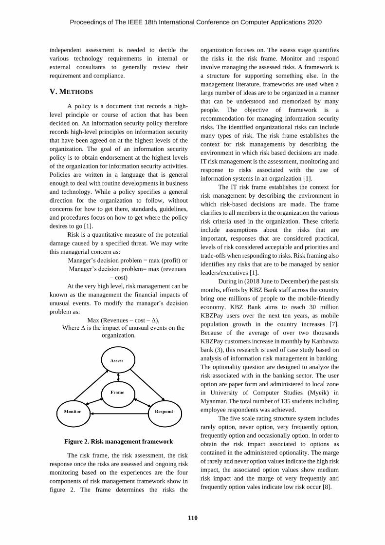
independent assessment is needed to decide the
various technology requirements in internal or
external consultants to generally review their
requirement and compliance.
V. METHODS
A policy is a document that records a high-
level principle or course of action that has been
decided on. An information security policy therefore
records high-level principles on information security
that have been agreed on at the highest levels of the
organization. The goal of an information security
policy is to obtain endorsement at the highest levels
of the organization for information security activities.
Policies are written in a language that is general
enough to deal with routine developments in business
and technology. While a policy specifies a general
direction for the organization to follow, without
concerns for how to get there, standards, guidelines,
and procedures focus on how to get where the policy
desires to go [1].
Risk is a quantitative measure of the potential
damage caused by a specified threat. We may write
this managerial concern as:
Manager’s decision problem = max (profit) or
Manager’s decision problem= max (revenues
– cost)
At the very high level, risk management can be
known as the management the financial impacts of
unusual events. To modify the manager’s decision
problem as:
Max (Revenues – cost – Δ),
Where Δ is the impact of unusual events on the
organization.
Figure 2. Risk management framework
The risk frame, the risk assessment, the risk
response once the risks are assessed and ongoing risk
monitoring based on the experiences are the four
components of risk management framework show in
figure 2. The frame determines the risks the
organization focuses on. The assess stage quantifies
the risks in the risk frame. Monitor and respond
involve managing the assessed risks. A framework is
a structure for supporting something else. In the
management literature, frameworks are used when a
large number of ideas are to be organized in a manner
that can be understood and memorized by many
people. The objective of framework is a
recommendation for managing information security
risks. The identified organizational risks can include
many types of risk. The risk frame establishes the
context for risk managements by describing the
environment in which risk based decisions are made.
IT risk management is the assessment, monitoring and
response to risks associated with the use of
information systems in an organization [1].
The IT risk frame establishes the context for
risk management by describing the environment in
which risk-based decisions are made. The frame
clarifies to all members in the organization the various
risk criteria used in the organization. These criteria
include assumptions about the risks that are
important, responses that are considered practical,
levels of risk considered acceptable and priorities and
trade-offs when responding to risks. Risk framing also
identifies any risks that are to be managed by senior
leaders/executives [1].
During in (2018 June to December) the past six
months, efforts by KBZ Bank staff across the country
bring one millions of people to the mobile-friendly
economy. KBZ Bank aims to reach 30 million
KBZPay users over the next ten years, as mobile
population growth in the country increases [7].
Because of the average of over two thousands
KBZPay customers increase in monthly by Kanbawza
bank (3), this research is used of case study based on
analysis of information risk management in banking.
The optionality question are designed to analyze the
risk associated with in the banking sector. The user
option are paper form and administered to local zone
in University of Computer Studies (Myeik) in
Myanmar. The total number of 135 students including
employee respondents was achieved.
The five scale rating structure system includes
rarely option, never option, very frequently option,
frequently option and occasionally option. In order to
obtain the risk impact associated to options as
contained in the administered optionality. The marge
of rarely and never option values indicate the high risk
impact, the associated option values show medium
risk impact and the marge of very frequently and
frequently option vales indicate low risk occur [8].
Proceedings of The IEEE 18th International Conference on Computer Applications 2020
110

A. Results and Discussion
This research state that 28.15% are male and
71.85% are female respondents. It indicate the most
of respondents banking user of female are more than
male banking user because of female students and
employee more than male show in figure 3 below.
Figure 3. Gender distribution
Figure 4. Age distribution
Figure 5. Banking experience
Figure 5 state the experience in banking
system, 57.8% have under 5 year experience, 14.8%
respondents have 6 to 8 year experience and 27.4%
respondents are with 9 year above. This indicate all
respondents with a good period of time in banking
system.
Figure 6. Confidentiality level frequency of KBZ
pay and ATM
In above figure 6 states the ATM (Automated
Teller Machine) card and KBZ pay account exposed
40% of the rarely live their account, the respondents
occasionally leave 25.2%. The frequently never used
with 4.4% and 23.7% respondents never leave their
account and card. 3.7% of the banking user leave their
account very frequently. 21.48% respondents are
occasionally.
The figure 6 shows the state of seek for
assistance during an online transaction. 62.9% of
respondents no need to seek for online transaction,
17.1% occasionally seek for assistance and 20% of
respondents seek for assistance.
In figure 7 in below showed 31.85%
respondents used their devices in financial process
frequently and 29.63 very frequently. 21.48%
respondents are occasionally and 17.04% respondents
are rarely used their device in financial transaction.
Figure 7. Frequency used of smart devices with
password in financial transaction
Figure 8. Frequency of free wireless access point
used for online transaction
38(28.15%)
97(71.85%)
0
20
40
60
80
100
120
Male Female
55(40.74%
52(38.51%)
28 (20.74%)
0
10
20
30
40
50
60
16-21 22-35 36 above
78(57.8%)
20(14.8%)
37(27.4%)
0
20
40
60
80
100
0 to 5 Years 6 to 8 Years 9 Year above
5(3.7%)
32(23.7%)34(25.2…
54(4o%)
10(4.4%)
0102030405060
43(31.85%)
40(29.63%) 29(21.48
%)23(17.04
%)
01020304050
15(11.11%)
37(27.41%)
26(19.26%)
38(28.15%) 37(27.41%)
0
10
20
30
40
Proceedings of The IEEE 18th International Conference on Computer Applications 2020
111

In figure 8, it shows the use of wireless access
during in online transaction. 28.15% are rarely use
wireless access point, 19.26% used occasionally,
27.41% respondents are never use free wireless access
point in online transaction, 27.41% are frequently
used and 11.11%respondent very frequently use
wireless access point for online transaction.
According to figure 6,7, and 8 in this survey,
that exposing ATM Card or KBZPay will have a high
impact of risk on the customer, while sharing of ATM
Card and PIN with third party also has a high impact
risk on the customer, while the necessary of devices
using password for online transaction and having a
licensed antivirus software with on the devices used
for online transaction indicate a low impact risk,
during online transaction, using a free wireless access
point and been debited without a successful
transaction all have a high impact risk on financial
institution.
B. Suggestions from Survey analysis
1. In e-banking system construct by one of
supervisory policy manual and other monetary
authority hold together with two factor
authentication services, account unity
response services from when the threat is
incident and so on. The customer compliance
of requirement is solved by banks. Banks need
to examine to the e-banking services in
supervisory policy manual.
2. The board of organization and senior managed
to e-banking system when the incident of risk
occurrence and including employee resource.
The requirements of adequate employee skills
are depend on expertise senior management to
manage the risk. Accounting staff manage e-
banking services for specify of banks.
3. Fund transfers to unregistered third parties are
considered high-risk transactions and should
be subject to two-factor authentication. Small
value fund transfers to unregistered third
parties can be performed without two-factor
authentication. Banks should refer to the
requirement stated in the additional guidance
on SPM (Supervisory policy Manual) also
consider the banks’ own risk appetite when
determining the caps for small value fund
transfers [3]. In two factor authentication, the
fund transfers to without accounting person to
performed risk transaction. It can be
performed by banks should supervisory
policy manual to manage the risk, bank also
determining to allowed for few value of fund
transfers.
4. Application forms are not required in online.
Banks are needed to solve to assess the risk
and establish controls the online services
information. The required of service include:
a. The use of password to protect the
confidentiality and integrity of the
information sub-post to online.
b. Manage to cyber attacks through the
documents information.
c. If required, checks to rule identity of the
customer online services information
[3].
5. In mobile banking system, the security and
weakness of mobile application specific risks
and banks also need to assess the detail risk
and management to mobile banking
infrastructure. Many risks can be asses in
attacker attack, risk from virus, structure of
security and devices loss of customer.
6. Including the weakness of credit card
information and transactions process run in
mobile devices, banks need to assess security risks on contactless payments and defined
multilevel security risk. The standards of
security issued depend on banking
associations and mobile payment services are
ensured in banks sector.
7. The notifications system is important part of
the maintaining and solving the process of
system implementation. Banks always need to
promptly customer requirement notify
transactions include card damaged or other.
Banks need to solve immediately by using
automated process after detection notify high
risk transactions occurs.
VI. CONCLUSION
Many organizations use information and
communication technology. For developments of any
organization (such as business, financial, database
record keeping and so on) are needed to manage
information security and risk management system in
organization. Especially, many banks in Myanmar use
information communication technology. Every
banking system to fulfill the needs of the customers in
managing their personal information, data, and
security. The e-banking technology is allowed for a
variety of implementing financial services between
organization and customers. Because of mobile
banking system is attractive and convenient to
Proceedings of The IEEE 18th International Conference on Computer Applications 2020
112

perform remote banking approached, the improving
information security risk management in e-banking
system, it can useful tool of system development and
main issues of mobile telecommunications
technology especially mobile device function
improved [4]. It can integrate the mobile banking and
current service. In banking industry, it make easy use
of the benefits provided by of mobile phones and
develop a unique customer oriented services will be
stand to play more standard role. The main challenges
in e-banking system are it has run and developed for
different operating systems of mobile device and on
security issues which has the risk to the customer who
use mobile banking system.
REFERENCES
[2] Walfried M. Lassar, Chris Manolis, Sharon S.
Lassar (2005), “The relationship between
consumer innovativeness, personal
characteristics, and online banking adoption",
International Journal of Bank Marketing;
Volume: 23 Issue: 2; 2005 Research paper
[3] Henry Shek, Kelvin leung. “Internet Banking
Update, The New Electronic Banking and
Cybersecurity requirements”
[4] Jin Nie, Xianling Hu. “Mobile Banking
Information Security and Protection Methods”
2008 International Conference on Computer
Science and Software Engineering, 2008
[5] https://www.cbm.gov.mm
[6] Dugguh, S.I.,PhD& Diggi, J. (2015). Risk
Management Stategies in Financial Institutions in
Nigeria: the Experience of Commercial
Banks,2(6),77-73
[7] https://www.kbzbank.com/mm/
[8] Noah N. Gana, Shafi’i M. Abdulhamid, Joseph
A. Ojeniyi. "Security Risk Analysis and
Management in Banking Sector: A Case Study of
a Selected Commercial Bank in Nigeria",
International Journal of Information Engineering
and Electronic Business, 2019 Publication
[1] Eric Pierce, Alex Campoe, Manish Agrawal
Information Security and IT Risk Management
Proceedings of The IEEE 18th International Conference on Computer Applications 2020
113

Proceedings of The IEEE 18th International Conference on Computer Applications 2020

Data Mining
Proceedings of The IEEE 18th International Conference on Computer Applications 2020

Proceedings of The IEEE 18th International Conference on Computer Applications 2020

DATA MINING TO SOLVE OIL WELL PROBLEMS
Zayar Aung
Applies Mathematics and In-
formatics
National Research University
Moscow Power Engineering
Institute (MPEI)
Moscow, Russian
Mihailov Ilya Sergeevich
Applies Mathematics and In-
formatics
National Research University
Moscow Power Engineering
Institute (MPEI)
Moscow, Russian
Ye Thu Aung
Applies Mathematics and In-
formatics
National Research University
Moscow Power Engineering
Institute (MPEI)
Moscow, Russian
Abstract
The purpose of this work is to create a learning al-
gorithm which is based on accumulated historical data on
previously drilled wells. Wells will forecast an emergency
accompanied by drilling. Such a decision support system
will help the engineer time to intervene in the drilling pro-
cess and prevent high drilling costs simple and repair
equipment resulting in an accident. The article provides a
brief overview of the most common method of artificial
intelligence — artificial neural networks, as well as the
main areas of their application in the oil and gas sector. In
their work, the authors distinguish three main areas of use
of such technologies: interpretation of geological data,
exploitation of deposits (smart fields) and price forecast-
ing. The use of methods based on artificial intelligence
increases the efficiency of the work carried out both in
exploration and production, makes it possible to achieve
better results with less cost.
Key words: classification oil and gas, drilling complica-
tions, machine learning, neural network, effciency im-
provement, gradient boosting.
I. INTRODUCTION
In the course of the study, work was carried
out on the study of machine learning methods; review
of existing practices for the use of melon models to
improve drilling efficiency. The provided reports on
drilling of wells at the field are analysed. Identified
wells in which there were complications. Calcula-
tions on various machine learning algorithms are
carried out to identify the algorithm that gives the
minimum percentage of error. As a result of the
study, a model based on gradient boosting was calcu-
lated to classify complications in the drilling process.
II. ARTIFICIAL INTELLIGENCE IN
DRILLING
At present, methods of neural programming
networks for solving problems in various fields have
been widely used. An artificial neural network is an
interconnected group of nodes, similar to our brain
system. Figure 1 shows the neural network scheme.
There are three layers, each circle is a neuron, and the
line is a connection between neurons. The first layer
has input neurons that send data through communica-
tion lines to the second layer of neurons, and then
through a large number of link nodes to the third lay-
er of output neurons.
The requirements of the practice of drilling
deep oil and gas wells require a broad range of needs
for the theory. In this case, the theory should explain
the flow of drilling technological processes both in
typical regimes and at the time of the onset of com-
plications and during development, treating compli-
cations as an integral part of such procedures. It is
desirable that a theoretical description of difficulties
allows judging them not only at a qualitative level,
but also quantify the interrelation of their essential
variables. Because of the rather narrow applied na-
ture of modelling tasks and prevention of complica-
tions, their formulation and evaluation of the results
obtained should first of all be guided by the needs
and possibilities of practice. The existing capabilities
of computer technology make it possible to carry out
calculations that several years ago seemed laborious.
Let us briefly review the existing works, which were
aimed at improving the drilling process using neural
networks and machine learning.
Proceedings of The IEEE 18th International Conference on Computer Applications 2020
117

Figure 1. Diagram of the neural network
III. THE ALGORITHM WITH HIGH
ACCURACY OF THE
CLASSIFICATION OF PROBLEM
According to the algorithms of machine train-
ing given in the previous chapter, calculations were
made to classify (forecast) the complications in the
drilling process. For calculations, the Python pro-
gramming language was used. Percentage between
training and test sample 65/35%. The training sample
is a sample based on which the chosen algorithm
adjusts the dependency model. The test sample is the
sample by which the accuracy of the model used is
checked. Metrics were used to assess the quality of
the models used to classify the complications in the
drilling process. For each of the algorithms, precision
(precision), recall (completeness), and F-measure
metrics were introduced.
where,
TP - positive observation, and expected to be posi-
tive;
FN - observation is positive, but it is predicted nega-
tively;
FP - observation is negative, but predicted positively.
Precision is a kind of share of objects, which is
called a positive classifier, and in this case, these
objects are in fact positive. The recall is a metric in-
dicating which fraction of objects of a positive class
from all objects of a positive class found an algo-
rithm (Figure 2). In other words, precision does not
allow you to assign all objects to one class because,
in this situation, the FP level will increase. Recall
shows the possibility of the model to define this type
in principle, and precision - to distinguish the class
from other classes.
Figure 2. Accuracy of the classification of problem
The F-measure is an aggregated quality crite-
rion that combines precision and recall-average har-
monic precision and recall.
where, β is the weight of the accuracy of the
metric (β = 1 is the average harmonic). F-measure for
completeness and accuracy reaches a maximum of
one, and if one of the arguments is close to zero, it
tends to zero. The data loaded into the Python soft-
ware environment was loaded with a single dataset,
with a preliminary classification of the complica-
tions, for the subsequent learning of the model. As
indicated, the training sample is 65% of the total da-
ta, and 35% of the data is used to verify the correct-
ness of the model set. The following drilling parame-
ters were used as input parameters:
• Level of tank 02;
• Input flow;
• Weight on the hook;
• Torque on the rotor;
• Rate of penetration;
• Volume of tank 02;
• Gas content.
As a result of the calculations, the following
metrics were obtained, for the subsequent detection
of the most accurate model.
IV. SUPPORT VECTOR MACHINE
The General idea of an SVM is to solve the
problem of correctly classifying a set of data and
maximizing a geometric field. There can be multiple
separating hyper planes, but there is only one separat-
Proceedings of The IEEE 18th International Conference on Computer Applications 2020
118

ing hyper plane with maximum geometric indenta-
tion. A direct explanation for maximizing the geo-
metric field is that the hyper plane with the maximum
geometric indentation derived from the classification
is equal to classifying the training data by a sufficient
certainty factor [7]. It is necessary not only to classify
correctly, but also to separate the nearest points with
a sufficient coefficient of reliability. This process can
provide certain data with a good predictive ability
called generalization ability.
When solving a nonlinear problem after con-
verting to multidimensional space, it is usually diffi-
cult to find a hyper plane that can completely sepa-
rate the data points, which means that there are some
special points. But after removing these special
points, most of the points become linearly separable.
To solve this problem, we import the sliding variable
into the training sample. In a soft-edged situation, the
SVM learning task will look like:
(1)
s.t. (2)
where C is the penalty parameter. Increasing C also
increases the penalty for classification errors. You
must adjust the target function to minimize the num-
ber of singular points while maximizing the offset
from the hyper plane.
Figure 3. Support Vector Machine
V. LINEAR LOGISTIC REGRESSION
ALGORITHM
WT
X and the sigmoid curve:
(3)
Figure 4. Logistic regression distribution function
and density function
(4)
Likelihood function
(5)
Logarithm likelihood function
(6)
VI. IMPLEMENTATION AND RESULTS OF
THE EXPERIMENT
Table 1. Metrics by model
Table 1 shows that the following algorithms of
machine learning have the highest accuracy: decision
tree; "Casual forest"; Gradient boosting.
Next, we considered the number of correct and
correct assumptions in the calculation of algorithms.
Table 2 presents the case for situations where there
are no complications, and in Table 3 the classifica-
tion of complications is correct. True is the number
of correctly predicted values; false is the number of
The linear logistic regression algorithm is a
classical classification method in the study of statis-
tics related to the linear logarithmic model [8-9]. This
classification model is a conditional probability dis-
tribution P (Y / X), which is a judgment model. It can
be obtained from the linear regression model hw (x)=
Proceedings of The IEEE 18th International Conference on Computer Applications 2020
119

misplaced predictions. From the data presented, it
can be seen that the greatest number of correct and
accurate classifications of situations is obtained using
the machine learning method gradient boosting. Gra-
dient boosting (Appendix B) allowed with a mini-
mum of the error to classify the complication from
the available data set.
Table 2. Accuracy of prediction of a normal situation
Algorithm Situation True False
Logistic regression Normal 3916 1
Naive Bayesian Classifier Normal 2484 1433
Method of k-nearest
neighbors Normal 3911 6
Decision tree Normal 3916 1
Support vector method Normal 3917 0
«Random Forest» Normal 3917 0
Gradient boosting Normal 3917 0
Neural network Normal 3915 2
Then, input parameters were analyzed by sig-
nificance category, weighting criteria for gradient
boosting. The greatest influence on the operation of
the algorithm is "Input pressure", "Torque", "Flow
rate at the input".
• Inlet pressure (0.3115)
• Torque on the rotor (0.2709)
• Inlet flow rate (0.2363)
• The volume of tank 02 (0.0704)
• Gas content (0.0601)
• Weight on the hook (0.0160)
• Rate of penetration (0.0082)
• Level of tank 02 (0.0000)
VII. EXAMPLE OF GRADIENT BOOSTING
IMPLEMENTATION
Figure 5. Example of gradient boosting imple-
mentation
Figure 6. Accuracy of prediction of a normal
situation
Figure 7. Precision of prediction of problems
VIII. CONCLUSION
The most effective methods of machine learn-
ing were used to classify complications in the drilling
process. For the algorithms, drilling parameters were
selected, which will be obtained at the entrance to the
program, for its training and further prediction of
complications. As a result of the calculations, the
most effective method of machine learning-gradient
boosting-was chosen. This method showed the small-
est error in the complication classification test. Of all
the drilling parameters, the inlet pressure exerts the
greatest influence on the classifier.
As a result of this work, it can be argued that
the algorithm was chosen, which with a minimum
error is able to classify complications in the drilling
process on the basis of the parameters recorded on
the rig. Such a program will help the engineer to
intervene in the drilling process in time and prevent
high costs of downtime and equipment repair. It is
recommended for further work on the project to in-
clude more wells with complications to more accu-
rately adjust the program for the classification of
various complications. It is very important for the oil
field technological service to determine the multi-
phase (oil-water-gas) stream flow regime because, for
example, even high liquid flow rate in the not corre-
Proceedings of The IEEE 18th International Conference on Computer Applications 2020
120

sponding regime can lead to feed failure of the pump
and to emergency stop of oil well. However, if this
situation could be classified at the early stage, it can
provide to avoid accident situation and thus to main-
tain oil well operating efficiency.
REFERENCES
[1] Линд Ю. Б., Самсыкин А. В., Галеев С. Р.
Информационно-аналитическая система
предупреждения поглощений буровых
растворов. SPE доклад был подготовлен для
презентации на сессии молодых
специалистов Российской технической
конференции SPE, 26 – 28 октября, 2015,
Москва.
[2] Чучалина К. Ю. Особенности геологического
строения и критерии, и признаки
прогнозирования углеводородов в
низкопроницаемых коллекторах на примере
Новопортовского нефтегазоконденсатного
месторождения: бакалаврская работа /
Томский политехнический университет. –
2017. – 109 л.
[3] Щепетов О.А. Системная классификация
аварий в бурении. –М.:2009. – 7 с.
[4] Ali J. K., British Gas PLC. «Neural Networks: A
New Tool for the Petroleum Industry?», paper
was prepared for presentation at the European
Petroleum Computer Conference held in Ab-
erdean, U.K., 16-17 March, 1994.
[5] Sheng Zhan, Jens Rodiek, Ludger Ewald Heu-
ermann-Kuehn and Joerg Baumann, Prognostics
Health Management for a Directional Drilling
System. Baker Hughes Incorporated, 2011 – 7 p.
[6] Yanfang Wang, Drilling Hydraulics Optimiza-
tion Using Neural Networks. University of Loui-
siana, 2014 – 74 p.
[7] Fatih Camci and Ratna Babu Chinnam. Dynamic
Bayesian Networks for Machine Diagnostics:
Hierarchical Hidden Markov Models vs. Com-
petitive Learning. Wayne State University, De-
troit, 2005 – 6 p.
[8] Yuliya B. Lind, Aigul R. Kabirova. Artificial
Neural Networks in Drilling Troubles Prediction.
SPE paper 171274-MS was prepared for presen-
tation at the SPE Russian Oil and Gas Explora-
tion and Production Technical Conference and
Exhibition held in Moscow, Russia, 14–16 Oc-
tober 2014.
[9] Abdullah Saleh H. Alyami. Using bayesian net-
work to develop drilling expert systems. Texas
A&M University, 2012 – 226 p.
[10] Jahanbakhshi, R. and Keshavarzi, R. Real-time
Prediction of Rate of Penetration during Drilling
Operation in Oil and Gas Wells. ARMA paper
12-244 prepared for presentation at the 46th US
Rock Mechanics / Geomechanics Symposium
held in Chicago, IL, USA, 24-27 June 2012.
[11] Mehran Monazami, Abdonabi Hashemi, Mehdi
Shahbazian. Drilling rate of penetration predic-
tion using artificial neural network: a case study
of one of Iranian southern oil fields. Electronic
scientific journal “Oil and Gas Business”, 2012,
[12] Yashodhan Gidh, Hani Ibrahim. Artificial Neural
Network Drilling Parameter Optimization Sys-
tem Improves ROP by Predicting/Managing Bit
Wear. SPE paper 149801 was prepared for
presentation at the SPE Intelligent Energy Inter-
national held in Utrecht, The Netherlands, 27–29
March 2012.
[13] Rashidi B. and Nygaard R. Real-Time Drill Bit
Wear Prediction by Combining Rock Energy and
Drilling Strength Concepts. SPE paper 117109
was prepared for presentation at the 2008 Abu
Dhabi International Petroleum Exhibition and
Conference held in Abu Dhabi, UAE, and 3–6
November 2008.
[14] Mustafa M. Amer, Dr. Prof. Abdel Sattar DA-
HAB. An ROP Predictive Model in Nile Delta
Area Using Artificial Neural Networks. SPE pa-
per 187969-MS was prepared for presentation at
the SPE Kingdom of Saudi Arabia Annual Tech-
nical Symposium and Exhibition held in
Dammam, Saudi Arabia, 24–27 April 2017.
[15] Валисевич Алексей, Ружников Алексей,
Бебешко Иван, Жентичка Максим. Система
оптимизации буровых долот: Увеличение
механической скорости проходки и
мониторинг износа долота в режиме
реального времени. SPE доклад 176517-RU
был подготовлен для презентации на
Российской нефтегазовой технической
конференции SPE, 26 – 28 октября, 2015,
Москва.
[16] Dashevskiy D., Dubinsky, V. and Macpherson J.
D. Application of Neural Networks for Predic-
tive Control in Drilling Dynamics. SPE paper
56442 was prepared for presentation at the 1999
SPE Annual Technical Conference and Exhibi-
tion held in Houston, Texas, 3–6 October 1999.
[17] GirirajKumar S. M., Deepak Jayaraj,
Anoop.R.Kishan. PSO based Tuning of a PID
Controller for a High Performance Drilling Ma-
Proceedings of The IEEE 18th International Conference on Computer Applications 2020
121

chine. International Journal of Computer Appli-
cations, 2010, Volume 1 – No. 19.
[18] Chiranth Hegde, Scott Wallace, and Ken Gray.
Real Time Prediction and Classification of
Torque and Drag During Drilling Using Statisti-
cal Learning Methods. SPE paper 177313-MS
was prepared for presentation at the SPE Eastern
Regional Meeting held in Morgantown, West
Virginia, USA, 13–15 October 2015.
[19] Okpo E. E., Dosunmu A., and Odagme B. S.
Artificial Neural Network Model for Predicting
Wellbore Instability. SPE paper 184371-MS was
prepared for presentation at the SPE Nigeria An-
nual International Conference and Exhibition
held in Lagos, Nigeria, 2–4 August 2016.
[20] Sean Unrau. Machine Learning Algorithms Ap-
plied to Detection of Well Control Events. SPE
paper was prepared for presentation at the SPE
Kingdom of Saudi Arabia Annual Technical
Symposium and Exhibition held in Dammam,
Saudi Arabia, 24–27 April 2017.
[21] Walt Aldred et al. Managing drilling risk. Oil-
field review, 1999, 18 p.
Proceedings of The IEEE 18th International Conference on Computer Applications 2020
122

Defining News Authenticity on Social Media Using Machine Learning Approach
May Me Me Hlaing Faculty of Information Science
University of Computer Studies,Yangon Yangon, Myanmar
Nang Saing Moon Kham Faculty of Information Science
University of Computer Studies,Yangon Yangon, Myanmar
Abstract
Social network and online news media are becoming popular in today’s era. Due to low cost, easy access and rapid diffusion, social media platform becomes a source to distribute false information. Fake news propagation on social media can cause serious negative effects on human society especially in politic, reputation and finance. So, automatic fake news detection plays a vital role to robust news media platform on social network. Defining news authenticity is insufficient based on news content only. It also needs to analyze social features of news. In this paper, we propose an approach to detect fake news on social media that covers both news content and social context. We use synonym-based feature extraction method and three different classifiers based on multidimensional dataset. Experimental result shows the effective as an accuracy way to define news authenticity on online news media.
Keywords: fake news, news media platform, news content, social context, news authenticity
I. INTRODUCTION
Nowadays, the more people use online news media, the less they spend with traditional news media such as newspaper, journal and television due to advancement of latest technology. Social media becomes a global information network and it provides an easy, fast dissemination and less expensive way to access news than traditional news media. According to recent survey, an estimated 3.484 billion people in the world were using the social media and it predicts that the number of social media users will increase 9.1 % year on year[1] .In particular, dissemination of fake information on social media has been increasing in today’s world. Popular social networking sites such as Facebook, Twitter, YouTube and Google plus are the primary source of diffusion misinformation on online news media[2] .
Fake news refers to news articles which intent to mislead news consumers in order to damage individual or society’s reputation, politics and economic events. Social
media users are often less likely to critically evaluate the information shared by other people or confirm their existing beliefs. Therefore, digital false information is more spreading about politics, finance and economy in recent years. Sufficed to mention that during the 2016 US presidential election, social bots spread misinformation on Twitter to confuse people opinion. One interested fake news is “Pope Francis shocks world, endorses Donald Trump for president” release statement that was very popular among social media users and it caused unexpected impacts on election[3]. The another conspicuous example of fake news is that Steve Job’s company stock share would significantly decline in a short time due to fake news report of CNN’s iReport.com in October 2008 [4].
Detecting misinformation on social media is unique challenges. A news piece on online news media has several characteristics to analyze news authenticity. First, fake news is written to mislead viewers and it mimics real news like topic, writing styles and media platform. Thus, it is insufficient based on only news content to detect fake news. Other auxiliary information including social engagement and stance of news or comments are also useful factors for improving automatic fake news detection. Second, exploiting social engagement and news comments are another critical challenge. Today researchers consider to build multidimensional model by combining news content and social context to detect fake news . News on social media is continuously updating which may not be verified with existing knowledge base because it is lack of corroborative evidence. However, auxiliary information in online news is noisy, big, incomplete and unstructured [5]. Therefore, detecting news authenticity on social media needs further investigation such as defining user authenticity, extracting useful post features and social features. The core motivations of this paper are summarized as follows:
• Automatic fake news detection is an emerging problem on social media and it can cause serious impacts on social, political and economic issues.
Proceedings of The IEEE 18th International Conference on Computer Applications 2020
123

• Exploring effective features from news content and social context to analyze news authenticity is also a technically challenging task.
• The prior researches about this problem lack labeled benchmark datasets that covers news content, social context. To better guide the future direction of this problem, new multidimensional fake news benchmark datasets are necessary.
In this paper, we discuss News Application Programming Interface (News API), Graph Application Programming Interface (Graph API) to collect news stories from social media, synonym based feature extraction method and three different classifiers to define news authenticity on online news media. The objective of this paper is to describe the framework of fake news detection system by exploring the correlations of content of news, stance of news and social engagement. It also aims to analyze which features of news stories are helpful for fake news detection and to know the ideas and process of automatic fake news detection system.
The remainder of this paper is follows. In section II, we review related work of previous research for fake news detection system. In section III, we briefly discuss our proposed model and fake news detection methods. We describe nature of dataset, evaluation metrics and performance result of the proposed system in section IV and conclude and discuss future directions of this paper in section V.
II. RELATED WORK
The propagation of fake news on social media can cause negative effects on human society. Therefore, automatic fake news detection becomes emerging research topic and there were many prior researches about this problem. We can consider that online news includes news content and social context. The previous research based on these factors to detect fake news on social media.
The authors described fake news detection problem in online news articles using semantic features and three machine learning techniques in [6]. In this paper, it used real-or-fake benchmark dataset which includes 6256 news articles from kaggle.com. They compared the performance of recurrent neural network, naïve bayes and random forest classifiers based on various features extraction methods such as term frequency, term frequency-inverse document frequency, bigram, trigram and quadgram to perform binary classification of online news.
In reference [7], the author discussed automatic fake news detection problem in two aspects: fake news characterization and fake news detection. In fake news characterization phase, they presented the key factors related to fake news on online media including psychological and social theories of fake news, news content features and social context features of fake news, fake news distributors on social media and types of fake news and differences of news patterns
between traditional media and social media. In fake news detection phase, they discussed the approaches to detect fake news, available benchmark fake news datasets and challenging issues for fake news detection system on social media.
The author introduced a fake news detection model using hybrid convolutional neural network. It used large dataset “LIAR” which includes over twelve thousands news short statements with meta information from politifact fact checking website in [8]. Then, they evaluated text feature only in this dataset to detect news authenticity by using various classification models and compared the performance with hybrid model which based text and meta data of news.
In reference [9], the authors proposed a model to detect false information on Facebook news pages that covers news content and social context features on three different fake news datasets. In this system, they described content-based methods for news content only and logistic regression and Harmonic Boolean label crowdsourcing methods for social features. These methods are used depending on the social engagement threshold parameter. This paper is also implemented fake news detection model within a Facebook Messenger Chabot to validate the authenticity of real time Facebook’s news.
The authors presented WordNet-based similarity measure to calculate the similarity between sentences by using ontology structure in [10]. They discussed about existing sentence level similarity evaluation approaches, WordNet structure, calculating word similarity, computing sentence similarity based on two example sentences and dataset that includes ground truth for sentence similarity calculation.
In reference [11], the authors discussed different approaches for sentiment analysis and compared the performance of domain adaption using supervised, semi-supervised and unsupervised methods. They also explained how to extract words from social media comments and how to work on sentiment dictionary for opinion target.
III. PROPOSED SYSTEM AND METHODOLOGY
The aim of our system is to define political news authenticity on social media. In this section, we describe the overview flow diagram of proposed system in Fig1.In this system, we collect data from Facebook news posts using Graph API. Each news post includes news content, reactions counts and comments. Before we define the authenticity of Facebook news post, we need to calculate content similarity. Therefore, we fetch political news stories from reliable news websites using News API to check similarity of news content.
The system collects news stories from twelve most reliable websites [12] such as BBC News, The Washington Post etc., to compute content similarity with Facebook news. We use synonym-based (WordNet-based) sentence similarity method to get content similarity score in this system.
Proceedings of The IEEE 18th International Conference on Computer Applications 2020
124

Figure 1. Overview of Proposed System
News comments and reaction counts are also useful factors to classify news as real or not. For instance, when we don’t know a news post is true or not by our existing beliefs, we can get clues by reading the news post’s comments and post’s reactions. To know comments polarity score: positive (news is true), negative (news is false) and neutral, we use VADER: sentiment analysis tool in our system. Then, we define news authenticity by using three different classifiers: Decision Tree, AdaBoost and Random Forest classifiers based on news content similarity score, comment polarity score and reaction counts.
There are four main phases in our proposed system: collecting data, checking semantic similarity between news content, analyzing polarity score from comments and classifying news authenticity. The explanations of each phase are described below.
A. Data Collection
Online news stories can be collected from various social media platforms such as search engine, news websites, Facebook and Twitter. However, it is difficult to know news authenticity manually because there is so much information and it now increased day by day. Thus, building comprehensive large-scale datasets and defining ground truth label of news are challenging task. Generally, determining authenticity of news is based on expert journalists, reliable sources and fact-checking websites. We discuss some available benchmark data repositories below which are focused on fake news detection system.
Vlachos and Riedel firstly proposed a fact-checking dataset for fake news detection system. This data repository includes only 221 news statements. This small dataset includes news content only which does not suitable for machine learning based models [13].
To tackle this problem, William introduced a fake claim benchmark dataset “LIAR” [14]. It is a large scale dataset which comprise 12.8K short statements with annotated ground-truth labels. However, LIAR does not contain the entire news content and it describes only short statement labeled with meta information for each news.
Another dataset called “BuzzFeed” [15] which collected a complete 1627 news articles from nine news agencies over a week in the US election. Every posts and links articles were fact-checked claim-by-claim by five journalists from BuzzFeed news team. The news articles are annotated labels into four categories: mostly true, mostly false, mixture of true and false and no factual content. Nevertheless, it only contained headlines and text with no social features from very few news agencies.
Santa and Williams created a news dataset “BuzzFace”
[16] which extends on BuzzFeed dataset in 2018. The news in this dataset is concerned with politic which happened during 2016 US election. It included rich sets of feature such as Facebook-id, post-id, post-url, published-date, reaction count and comments that covered both news content and social context. It also defined news’ labels into four categories as BuzzFeed news dataset.
Unlike the traditional news media, online news is real time and it can change at any time. Dynamic social features such as number of reaction count and news comments are become useful features to spot fake news on social media. Before “BuzzFace” is launched, there were no existing available datasets that cover both news content and news social features [17].To tackle the disadvantages of available
FB posts
Data Collection (Graph API)
Data Collection (News API)
Social Media
Reaction Counts Comments Content
News Stories
Data Collection Phase
Preprocessing
Feature Extraction
Feature Extraction
Preprocessing
DB
Semantic Similarity
Similarity Score
DB
Check Content Similarity
Modeling (Decision Tree, AdaBoost, Random Forest)
News Authenticity Score
Classify News Authenticity
Sentiment Analysis
Polarity Score
Comments Polarity Score
Proceedings of The IEEE 18th International Conference on Computer Applications 2020
125

existing datasets, we need to build multidimensional dataset which help to develop fake news detection system.
In our proposed system, we use “BuzzFace” news dataset to detect political fake news from Facebook posts. Facebook-id and post-id are useful features which allow crawling news content, comments and reaction of news by using Facebook Graph API. To check content similarity, we use News API to collect political news articles from authentic news sources (websites). By using News API, we get news title, news-url, published-date and content from reliable news websites which are used to check content similarity with Facebook news content.
Graph API: The Graph API is HTTP-based API and it can use to get data into and out of the Facebook platform. It is composed of nodes, edges and fields. We can use nodes to get data about specific object such as Facebook users, photos, Facebook pages or Facebook comments. Edges are used to get connection between objects and fields are used to get data about an object [18].
News API: It is a simple and easy-to-use API for searching and retrieving nearly real time news stories from news sources and blogs all over the world. News content and metadata automatically access via this API using the API key. We fetch news stories from twelve most reliable news sources to check news authenticity. Each news site has own news API to acquire news categories [19].
B. Checking Semantic Similarity between News Article’s Contents
News stories from various news websites and Facebook are unstructured, big and noisy. Therefore, these data need to be preprocessing such as tokenization, stop word removal and stemming before checking semantic similarity of news content.
Tokenization: It is the process of splitting a stream of sentence into words phrases, symbols or other meaningful information. Tokenization aims to explore the words in the sentence. The resulting tokens become useful inputs for text mining and further processing.
Stop Word Removal: Stop words are frequently used or insignificant word in a text corpus that will be noise when these words used in text mining process. Thus, the words like pronouns, articles, conjunction and preposition need to remove from the sentence.
Stemming: After tokenization and stop word removal, we need to transform list of token into a standard form. Stemming is the process of transforming a word into its stem word. For example, the words “Speaking”, “Speak” and “Speaker” transform into “Speak”. Stemming provide classification task more efficient and faster.
After preprocessing steps, we need to calculate similarity between sentences. Similarity between sentences can be measured lexically or semantically. Lexical similarity
approach is also known as string based similarity approach which depends on measuring similarity between sequences of characters. Semantic similarity method based on similar meanings of words between sentences. In our system, we implement semantic similarity approach using WordNet to compute similarity score between sentences. This approach is also called synonym-based similarity.
Word Net is a large repository English words which are grouped into synsets (group of synonyms). These synsets are constructed into a hierarchical structure which has conceptual relation between them. The WordNet pointer describes both lexical and semantic relationships between words. To check semantic similarity between two sentences, we first transform the sentences into bag-of-words form T1, T2 and create superset T = T1 U T2. After creating superset for two semantic vectors T1 and T2, lexical semantic vectors V1 and V2 are derived from the superset T. The entry value in V1 or V2 describes the semantic similarity of any word in V1 or V2 to any word in two sentences. Next, we would calculate semantic similarity score for every word (w1-----wn) using the value of corresponding vector entry. Then, small weight value ẟ (0 < ẟ < 1) is given to words in the sentence due to their prevalence of usage. Finally, we get news content similarity score by computing cosine similarity from (1).
𝑆𝑖𝑚(𝑠𝑒𝑛𝑡𝑒𝑛𝑐𝑒1, 𝑠𝑒𝑛𝑡𝑒𝑛𝑐𝑒2) =𝑉0𝑉1
‖𝑉0‖‖𝑉1‖
=3∑ 𝑉0516
780 3∑ 𝑉1516
780
C. Analyzing Polarity Score from News Comments
New consumers’ opinion or comments from Facebook news posts help to define news authenticity. Defining comments polarity score is generally based on set of lexicons or pre trained classifiers. In our system, we use sentiment analytical tool: VADER to know users opinion within the comments. VADER is a lexicon and rule-based sentimental tool which intend to extract opinion in social media text [20]. It relies on a dictionary which maps lexical features to know emotion intensities called sentiment polarity score. This score of a text obtain by summing the word intensity in the text. VADER defines how positive or negative score of a text comments in the Facebook news post.
D. Classifying News Authenticity
Fake news detection on social media is a complex and difficult task. To solve this issue, we need to consider efficient supervised machine learning techniques to classify online news’ authenticity. In our system, we utilize three different machine learning classifiers namely Decision Tree, AdaBoost and Random Forest classifiers.
Decision Tree: This classifier is a tree-like structure of possible outcomes of a series of related choices. There are three different types of nodes in structure: chance nodes,
(1)
Proceedings of The IEEE 18th International Conference on Computer Applications 2020
126

decision nodes and end nodes. A chance node is a branch in a tree which shows a set of possible outcomes of the decision tree. A decision node is a decision to be made and an end node is the final outcome of decision tree. The tree starts with a single node which branches into possible outcomes. To select the best attributes in decision tree, it uses two measures: Entropy and Information Gain. Entropy is the useful measure which shows the uncertainly in the data values. It is used to determine how a decision tree can split the data. Information Gain is the measure which is used to choose attribute that best splits the data of each node in a decision tree. The tree is constructed top-down manner by using divide-and-conquer approach.
Although decision tree classifier is easy to interpret, visualize and no need to normalize column, it has few weak points. Decision tree can overfit due to noisy data when a tree is particularly deep. To tackle this problem, we use ensemble machine learning approach in fake news detection system. It is a composite model to get higher accuracy than using a single classifier (decision tree). There are two groups of ensemble methods are parallel ensemble methods and sequential ensemble methods. In our propose system, we use Random Forest classifier for parallel approach and AdaBoost classifier for sequential approach to classify news authenticity. We describe work flow between single classifier and ensemble classifiers in Fig 2.
Random Forest classifier: It is a strong modeling technique which operates a multitude of decision trees and thus improves the accuracy than a single decision tree. Their ability is to limit over fitting as well as error due to bias. It needs adjust parameters such as max-depth, min-samples-split, n-estimators and random-state to achieve the best performance; where max-depth is the maximum depth of a decision tree; in-samples-split is the minimum number of samples to split an internal node and n-estimators is the number of decision trees in the random forest.
AdaBoost classifier: It is used to boost the performance of decision trees on binary classification problems. A single classifier may classify the objects poorly. It is iterative ensemble method which combines low accurate classifiers into a high accurate classifier. The basic concept of AdaBoost is that weak models are added sequentially and trained the data sample in each iteration using the weighted training values.
Figure 2. Work flow between single classifier and ensemble classifiers
In this section, we first describe the nature of “BuzzFace” dataset which are used in our proposed model. Next, evaluation metrics are presented for fake news detection system and we compare the performance result of proposed system using three different classifiers.
A. Dataset
We use BuzzFace news dataset to detect fake news in this system. It contains 1780 news articles with social features which are collected from Facebook news posts. It annotates the labels of the news articles into four categories: 77.81% of the 1780 news articles are labeled as mostly true, 12.87% are labeled as mixture of true and false, 3.99% are labeled as no factual content and the remaining as mostly false. Mostly true and mostly false mean that information in the news article is either accurate or inaccurate. Mixture of true and false is used when the information seems to be accurate or when the information is based on unconfirmed news article by authentic sources. No factual content is chosen when the information is opinion, satire or comics. Each news article includes both news content and news’ social features such as reaction and news’ comment with annotated label. According to 5-fold cross validation, we split the dataset 80% for training and 20% of the dataset for testing in this system.
B. Evaluation Metric and Performance
The various evaluation metrics have been used in evaluating performance for fake news detection system. In this paper, we apply the following metric to predict the news is reliable or fake. 𝑃𝑟𝑒𝑐𝑖𝑠𝑖𝑜𝑛 = |>?|
|>?|@|A?|
𝑅𝑒𝑐𝑎𝑙𝑙 = |>?|
|>?|@|AE|
IV. SYSTEM EVALUATION
Proceedings of The IEEE 18th International Conference on Computer Applications 2020
127

𝐹1𝑠𝑐𝑜𝑟𝑒 = 1.?HIJ7K7L6.MIJNOO?HIJ7K7L6@MIJNOO
𝐴𝑐𝑐𝑢𝑟𝑎𝑐𝑦 = |>?|@|>E|
|>?|@|>E|@|A?|@|AE| , where
True Positive (TP) means that predicted fake news pieces are actually annotated as fake news. True Negative (TN) means that predicted true news pieces are actually annotated as true news. False Negative (FN) means that predicted true news pieces are actually annotated as fake news. False Positive (FP) means that predicted fake news pieces are actually annotated as true news.
Precision is a good measure when the false positive is high. The news consumers might lose to know news’ authenticity if the precision is not high for fake news detection model. Precision shows about how our fake news detection model is out of these predicted positive. Recall calculates how many of the actual positive our model capture true positive. F1 is used to combine precision and recall which can provide overall prediction performance for fake news detection. In our evaluating system, the higher accuracy provides the better performance.
C. Performance Result
This section describes the system evaluation using Decision Tree, AdaBoost and Random Forest classifiers. The experimental results show in Fig 3 by using these classifiers. We observe that the accuracy of Random Forest classifier is better than Decision Tree and AdaBoost classifier. In other word, the accuracy of bagging algorithm is better than single classifier and boosting method in our system.
Figure 3. The performance of fake news detection in term of precision, recall and accuracy using Decision
Tree, AdaBoost and Random Forest classifiers
V. CONCLUSION
In this paper, we present a multidimensional fake news data repository that covers news content, social engagement and news stance. We describe how to collect news stories from different news sources using Graph API and News API and how to define annotate label for each news piece. The proposed model in this system is an idea to be more precise and achieve better performance than prior research which based on news content only. Moreover, we perform an exploration study on BuzzFace dataset by applying synonym-based feature extraction method and compare the performance of the system using three different classifiers. In future work, we wish to test hybrid classification methods to get better performance in classifying online news.
REFERENCES
[1] https://www.smartinsights.com/social-media-marketing/social-media-startegy/mew-global-social-media-research
[2] https://journalistsresources.org/studies/society/internet/fake-news-conspiracy-theories-journalism-research/
[3] https://www.cnbc.com/2016/12/30/read-all-about-it-the-biggest-fake-news-stories-of-2016.html
[4] Rubin, Victoria L, “Deception detection and rumor debunking for social media”, The SAGE Handbook of Social Media Research Methods,2017,SAGE.
[5] Jiliang Tang, Yi Chang, and Huan Liu. Mining social media with social theories: a survey. ACM SIGKDD Explorations Newsletter, 15(2):20-29,2014.
[6] Bharadwaj, Pranav, and Zongru Shao. "Fake News Detection with Semantic Features and Text Mining." International Journal on Natural Language Computing (IJNLC) Vol 8 (2019).
[7] Shu, Kai; Sliva, Amy; Wang, Suhang; Tang, Jiliang; Liu, Huan,” Fake news detection on social media: A data mining perspective”, ACM SIGKDD Explorations Newsletter,vol 19,pp. 22-36,2017 ACM.
[8] Wang, William Yang. "" liar, liar pants on fire": A new benchmark dataset for fake news detection." arXiv preprint arXiv:1705.00648 (2017).
[9] Della Vedova, Marco L., Eugenio Tacchini, Stefano Moret, Gabriele Ballarin, Massimo DiPierro, and Luca de Alfaro. "Automatic online fake news detection combining content and social signals." In 2018 22nd Conference of Open Innovations Association (FRUCT), pp. 272-279. IEEE, 2018.
[10] Liu, Hongzhe, and Pengfei Wang. "Assessing Sentence Similarity Using WordNet based Word Similarity." JSW 8.6 (2013): 1451-1458.
[11] Mathapati, Savitha, and S. H. Manjula. "Sentiment analysis and opinion mining from social media: A
Proceedings of The IEEE 18th International Conference on Computer Applications 2020
128

review." Global Journal of Computer Science and Technology (2017).
[12] https://www.makeuseof.com/tag/trust-news-sites [13] Vlachos, Andreas, and Sebastian Riedel. "Fact checking:
Task definition and dataset construction." In Proceedings of the ACL 2014 Workshop on Language Technologies and Computational Social Science, pp. 18-22. 2014.
[14] https://www.cs.ucsb.edu//William/data/liar dataset.zip [15] https://github.com/BuzzFeedNews [16] https://github.com/gsantia/Buzzface [17] Feng, Song, Ritwik Banerjee, and Yejin Choi. "Syntactic
stylometry for deception detection." In Proceedings of the 50th Annual Meeting of the Association for Computational Linguistics: Short Papers-Volume 2, pp. 171-175. Association for Computational Linguistics, 2012.
[18] https://developers.facebook.com/docs/graph-api/overview
[19] Lomborg, Stine, and Anja Bechmann. "Using APIs for data collection on social media." The Information Society 30, no. 4 (2014): 256-265.
[20] Hutto, Clayton J., and Eric Gilbert. "Vader: A parsimonious rule-based model for sentiment analysis of social media text." Eighth international AAAI conference on weblogs and social media. 2014.
Proceedings of The IEEE 18th International Conference on Computer Applications 2020
129

ETL Preprocessing with Multiple Data Sources for Academic Data Analysis
Gant Gaw Wutt Mhon Faculty of Information Science
University of Computer Studies,Yangon Yangon, Myanmar
Nang Saing Moon Kham Faculty of Information Science
University of Computer Studies,Yangon Yangon, Myanmar
Abstract
More and more, the needs of academic data analysis are requiring in educational settings for the purpose of improving student learning and institutional effectiveness. In the education world, testing and data are driving decisions for what knowledge and skills students should be learning and how students’ learning relates to their learning outcomes. On that occasion, a better option for building a machine learning model is to get effective data preprocessing concepts. For these reasons, this paper describes the very first step of the main research work which considers the correlations between students’ academic performance, behavior and personality traits to reveal the presence of an intriguing way. Intuitively, this paper proposes the uses of Extraction-Transformation-Loading (ETL) in the preprocessing stage to collect and analyze of students’ data from multiple data sources. In this system, data is collected from multiple data sources based on the structures which are used as a testbed. Students’ demographic data and assessment results from Student Information System (SIS), logs of their interaction with Moodle are used for data collection. Then aggregating with Web logs also captures student behavior that is represented by daily summaries of student clicks based on courses and by their actions.
Keywords: machine learning, data preprocessing, ETL, multiple data sources, demographic data, assessment results, Moodle logs, Web logs
I. INTRODUCTION
Many new pathways and insights for institutional effectiveness and the learning sciences are opening up due to the growth of information and educational technologies like Learning Management Systems (LMS), SIS. These technologies captured as ‘digital breadcrumbs’ from sources such as personality profiles, learning outcomes and behaviors; hence various analytics systems are emerged for
improvement in institutional decision making, advancements in learning outcomes for at-risk students, significant evolutions in pedagogy more accurately and easily. Over time, their digital records may be augmented with other information, including financial and awards, involvement on campus, disciplinary and criminal reports, and personal health information. This increasing amount of admitted student data available on various data sources, the new technologies for linking data across datasets, and the increasing challenges need to integrate structured and unstructured data are all driving new aspects. Then, data collection and preprocessing are the most important and essential stages to acquire the fine and final data from multiple data sources that can be lead to correct and suitable for further data mining tasks.
By seeing current student data situation, data preprocessing becomes more crucial part and plays as a key concept of a system .There are a number of data preprocessing techniques rely on requirements and features of system’s data model. Since last decade, ETL process became fruitful to flow preprocessing step smoothly. After data preprocessing, consistent data will be pulled from multiple sources and loaded to data warehouse. After retrieving some meaningful and knowledge information, the system needed to do for understanding and identifying the correlation rules between student assessment, behavior and personality traits with machine learning algorithm. There are many aspects to achieve in academic system. But the main idea of the proposed research work is that clustered analysis result are firstly explored based on students’ academic performance and behavior of each student. After that, with their personality results from online survey test are merged to conduct the correlated rules between them.
The introduction of today’s educational technologies situation and advantages, ETL preprocessing with multiple sources are presented in this section. The remainder of this paper has been arranged in different sections. Section 2 describes the related researches in this area. Then section 3 implements terminology of ETL. Implementation and
Proceedings of The IEEE 18th International Conference on Computer Applications 2020
130

Experiments will be presented in section 4. Conclusion is made in the final section.
II. RELATED WORK
In recent past, most of the related works are implementation of predicting academic achievement based on personality model and then focusing on students’ previous marks, other historical data and students’ behavior analysis by using data mining techniques approaches. Due to the development of educational technologies, there are many statistics and evolution settings to provide better academic environment by tracking, aggregating and analyzing student profiles along with all of the digitalized data of students.
Some of the research works with ETL processing in higher education are reviewed in this section. There are various implements in the processing of data in ETL process to suit with the requirements of the system. To qualify for work in academic data analysis model with current data situation, building preprocessing step is one of the challenges and important parts of a model. In [1], the authors evaluated student behavior clustering method based on campus big data with density based clustering method which is parallelized on the Spark platform and applied to subdivide student behavior into different group using historical data are as source in digital campus shared database. This proposed approach is to study for universities to know students well and manage them reasonably and improved algorithm is also effective. And then, the authors proposed ETL as data acquisition and preprocessing by integrating multi-source data before loading to the target system. Because this has been the way to process large volumes of data that it can scale cost effectively.
In [2], the authors explored the framework of the modern data warehouse with big data technology to support decision making process in academic information system. To reduce difficulties associated with traditional data warehouse, they designed a decision support system for big data by involving Hadoop technology. They also discussed ETL architecture based on the characteristics of the traditional data warehouse technology which cannot handle unstructured data and modern data warehouse. In [3], the authors proposed a framework for development of flexible educational data mining application to facilitate self-discovery of rules and trends from educators with little technical skills to various user types. This framework is also demonstrated with utilizing tools which are used for
data mining analysis within a LMS. The authors used ETL stage as preprocessing for extracting the information from the LMS or e-learning system to do analysis much easier.
In [4], the authors implemented the case study in business intelligence framework by using data integration and ETL and then described its significance for better higher education management. They detected the functions of data integration and ETL tools and described how the correlated to each other to develop business intelligence. Because of data integration is one of the important components and ETL is the common steps to integrate data and transform it to targeted system from different academic data sources for higher education. They demonstrated on the Graduate Studies Management System (GSMS) database of University Technologies of Malaysia to store basic information of student. To ensure the data is reliable and could make decision accurately with ETL process, this database must be integrated with various sources which have different platform and format.
III. ETL TERMINOLOGY
There are solutions coming up for better data integration and data warehousing because of data management has been evolving rapidly. ETL is a popular architectural pattern and used for data process with necessary integration from heterogeneous and distributed data sources with different format. ETL procedures is needed to dedicate based on the design and implementation of the system because designed ETL process are expensive to maintain, alter, and upgrade, so it is crucial to make the right choices in terms the best innovation will certainly be used for developing and preserving the ETL procedures.
A. Data Warehouse and ETL
Data Warehouses are used in higher education for decision making to take an action and to predict risk and opportunities of students. It is a process of collecting and managing data from varied sources to achieve reliable, accurate and meaningful information from various data sources. There are three steps to follow before storing data in a data warehouse, which is called ETL. This three-step process takes place when information from one system needs to be moved into a data warehouse environment. Data extraction involves extracting data from homogeneous or heterogeneous sources; data transformation processes data by data cleansing and transforming them into a
Proceedings of The IEEE 18th International Conference on Computer Applications 2020
131

proper storage format/structure for the purposes of querying and analysis; finally, data loading describes the insertion of data into the final target database such as an operational data store, a data mart, data lake or a data warehouse.
B. ETL with Big Data
The need for ETL has increased considerably due to modern data analytics operations often have to process with rise in data volumes as quickly as possible. Therefore traditional ETL approach has to develop to function of more constrained data storage and data availability because it can slow down the process significantly for systems optimization. Apache Hadoop provides a cost-effective and massively scalable platform for ingesting big data and preparing it for analysis [5]. Using Hadoop to offload the traditional ETL processes can reduce time to analysis by hours or even days.
Moreover, ETL on platform like Hadoop and Spark give ETL a new look because it changes the cost structure around harnessing big data and save time too. [6] From their study, they recognized each ETL process instance handles a partition of data source in parallel way to improve further ETL performance facing the big data by using parallel/distributed ETL approach (Big-ETL). The researchers developed ETL functionalities which can be run easily on a cluster of computers with Map Reduce (MR) paradigm. Apparently, by using this approach on very large data integration in a data warehouse to qualify in good performance of ETL process significantly.
IV. IMPLEMENTATION AND EXPERIMENT
In today’s education world, for better or worse, testing and data are driving decision more and more as universities seek to be evidence-driven by using all of student related data. To fulfill their needs and know their weakness in time for their educational life, there are various new trends and aspects in need to collect, analyze, interpret, store, track, aggregate the increasing amount of admitted student data available from various data sources.
Apparently, there need to explore accurate and effective way of data collection and preprocessing for linking data across datasets from multiple data sources. Accurately, the proposed system collects student related data from three different data sources by using ETL as preprocessing stage for the collection analysis of students’ data. Demographic data and assessment results are collected from SIS. It is very
time saving and effective way to observe all students’ related data and many suggestions and ideas can get from these data which are used to investigate the academic growth. Then logs of their interaction with Moodle are also collected which is one of the best data sources to know about students’ behaviors based on their interested course and relevant teachers. To know their academic behavior more accurately, aggregating with Web logs which are represented by daily summaries of student clicks based on courses and by their actions. In above Fig 1, overview of proposed system for academic data analysis with ETL preprocessing is described in details. For research environment, University of Computer Studies Yangon (UCSY) is used for students’ datasets as sample.
Figure 1. Proprosed System of Academic Data
Analysis with ETL Preprocessing
A. Data Collection and Implementation of ETL
As in fact of the data processing of the system, each student represents the portion of data which are correlated and these are from multiple data sources of the university. Therefore, building ETL preprocessing based on the proposed system’s used data scale detect a formal representation model for capturing the ETL
Proceedings of The IEEE 18th International Conference on Computer Applications 2020
132
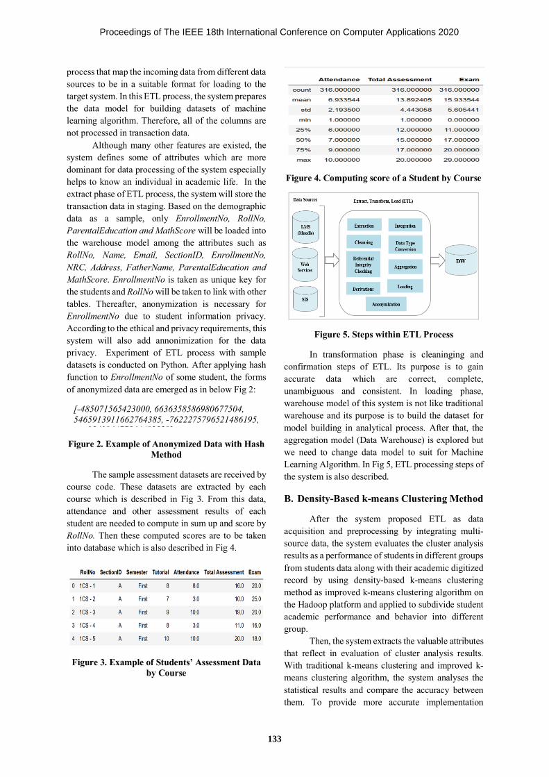
process that map the incoming data from different data sources to be in a suitable format for loading to the target system. In this ETL process, the system prepares the data model for building datasets of machine learning algorithm. Therefore, all of the columns are not processed in transaction data.
Although many other features are existed, the system defines some of attributes which are more dominant for data processing of the system especially helps to know an individual in academic life. In the extract phase of ETL process, the system will store the transaction data in staging. Based on the demographic data as a sample, only EnrollmentNo, RollNo, ParentalEducation and MathScore will be loaded into the warehouse model among the attributes such as RollNo, Name, Email, SectionID, EnrollmentNo, NRC, Address, FatherName, ParentalEducation and MathScore. EnrollmentNo is taken as unique key for the students and RollNo will be taken to link with other tables. Thereafter, anonymization is necessary for EnrollmentNo due to student information privacy. According to the ethical and privacy requirements, this system will also add annonimization for the data privacy. Experiment of ETL process with sample datasets is conducted on Python. After applying hash function to EnrollmentNo of some student, the forms of anonymized data are emerged as in below Fig 2:
Figure 2. Example of Anonymized Data with Hash Method
The sample assessment datasets are received by course code. These datasets are extracted by each course which is described in Fig 3. From this data, attendance and other assessment results of each student are needed to compute in sum up and score by RollNo. Then these computed scores are to be taken into database which is also described in Fig 4.
Figure 3. Example of Students’ Assessment Data by Course
Figure 4. Computing score of a Student by Course
Figure 5. Steps within ETL Process
In transformation phase is cleaninging and confirmation steps of ETL. Its purpose is to gain accurate data which are correct, complete, unambiguous and consistent. In loading phase, warehouse model of this system is not like traditional warehouse and its purpose is to build the dataset for model building in analytical process. After that, the aggregation model (Data Warehouse) is explored but we need to change data model to suit for Machine Learning Algorithm. In Fig 5, ETL processing steps of the system is also described.
B. Density-Based k-means Clustering Method
After the system proposed ETL as data acquisition and preprocessing by integrating multi-source data, the system evaluates the cluster analysis results as a performance of students in different groups from students data along with their academic digitized record by using density-based k-means clustering method as improved k-means clustering algorithm on the Hadoop platform and applied to subdivide student academic performance and behavior into different group.
Then, the system extracts the valuable attributes that reflect in evaluation of cluster analysis results. With traditional k-means clustering and improved k-means clustering algorithm, the system analyses the statistical results and compare the accuracy between them. To provide more accurate implementation
[-485071565423000, 6636358586980677504, 5465913911662764385, -7622275796521486195,
954196477564483528]
Proceedings of The IEEE 18th International Conference on Computer Applications 2020
133

method, k-means algorithm based on density partitioning is needed. In fact, the system construct initial clustering center set based on density not k value. Thereafter improved k-means clustering algorithm is developed by applying the selected initial clustering center. The method first determines a similarity measure method suitable for student data to normalize data and then builds initial clustering center set based on the density.
The density of the data object Xi in the sample set S=X1, X2, … , Xn | Xi € Rt is defined as the number of samples within the Eps neighborhood of Xi. The density reflects the intensity of the sample points in the neighborhood. The density threshold minPts is the specified division of the core and the isolated point of the density range, which can be artificially set. The density parameter NEps(Xi) of the sample is calculated as in 1:
NEps(Xi)=Xj € S|0 ≤ D(Xi, Xj) ≤ Eps, j=1,2,…,n
Where D( Xi,Xj ) represents the distance between two samples in S. Actually, k-means doesn’t allow development of an optimal set of clusters and so for effective results, the need to decide on the clusters before. Then, the statistic of traditional k-means clustering is difficult to predict k-value, different initial partitions can result in different final clusters.
C. The Big-Five Personality Test
Finally, the students’ personality results and the clustered results are merged with their student identification number and then analyze with Apriori association rule algorithm, the most classical and important algorithm for mining frequent item sets, to conduct the correlated rules between them which are firmly and consistently associated. In this system, 50-questions (items) inventory is used to measures as individual on the Big-Five personality dimension that is recreated from the Big-Five Inventory (BFI). To achieve students’ personality results, they need to take online personality survey test from Moodle.
The development of questionnaires measuring the Big-Five personality traits is common in psychology research for different reasons. There are countless personality tests designed with many formats. But the Big-Five personality model is one of the popular models and it also called as the Five-Factor Model (FFM). The personality survey test is designed to assess the Big-Five factors of personality: Extraversion (E), Agreeableness (A), Conscientiousness (C), Neuroticism (N), and
Openness to Experience (O) [7,8]. In the system, the items on the BFI scale were also scored with a Likert-scale (5-point) from “strongly disagree” to “strongly agree” and each factor represents ten questions respectively. Some example phases are:
• I am talkative. (E) • I feel little concern for others. (A) • I am always prepared. (C) • I get stressed out easily. (N) • I am an inventive. (O)
Each personality trait is associated with a set of statements and the score of a trait is calculated for each user on the associated questions. After data collected through the questionnaires, Statistical Package for the Social Sciences (SPSS) is used for statistical analysis. Firstly, the system need to test the reliability and validity of the questionnaire in data collection by reason of the results of research quality. In addition, reliability estimates conduct the amount of measurement error and validity determines the questionnaire compiled it valid or not in a test. In this paper, 30-participants are only participated as sample to test the reliability and validity of system’s personality survey test questionnaires.
Cronbach’s alpha is the most widely used objective measure of reliability or internal consistency and it is a simple way to measure whether or not a score is reliable. But in some questions often contain some items with negative sense which are need to be reversed score before run Cronbach’s alpha in SPSS. Reverse scoring means that the numerical scoring scale runs in the opposite direction and so the system need to reverse-score all negatively-keyed items. For interpreting alpha for Likert-scale question: 0.70 and above is good, 0.80 and above is better, and 0.90 and above is best [9].
In Table 1, the reliability of the questionnaire (30-participants to complete the N= 50-item) in data collection are tested with compare result based on reverse-score are described. After reverse-score the negative worded questions, the scale had an internal consistency is α=.76. However, a high coefficient alpha does not always mean a high degree of internal consistency and it is also affected by the length of the test.
Table 1. Comparison of Reliability Statistics
z Cronbach’s Alpha
Cronbach’s Alpha Based on
Standardized Items
N of Items
Without Reverse -Score .588 .490 50
With Reverse- Score .762 .756 50
(1)
Proceedings of The IEEE 18th International Conference on Computer Applications 2020
134

As pointed out earlier, test the validity of the questionnaire is conducted using Pearson Product Moment Correlation (PPMC) using SPSS. It is the test statistics to measures the statistical relationship, or association, between the continuous variables and based on the method of covariance. This validity test is done by correlating each item questionnaire scores with the totally score. The sign of the correlation coefficient r indicates the direction of the relationship, while the magnitude of the correlation indicates the strength of the relationship in the range -1 to 1 [10]. In Fig 6, the validity of the questionnaire (N=30-participants with sample questions of Extraversion) in data collection are tested.
Figure 6. Pearson’s Correlation among the Items
In fact of above figure, Pearson’s correlation of two questions is (r=0.790) which indicate that the strength of association between the variables is very high. Then Sig(2-tailed) value is 0.000<0.05. This means there is a statistically significant correlations between two variables. After the testing of reliability and validity, with the factor analysis on scale items, each student has five traits which are scored on a continuum from high to low. According to calculated result, score description of each trait is as an example in extraversion, high scores tend to be very social while low scores prefer to work on their projects alone.
Finally, the main idea of the proposed approach is explored by merging based on students’ identification number to find the correlations between the students’ personality results and the clustered results. Then to conduct the correlated rules between them which are firmly and consistently associated by analyzing with Apriori association rule algorithm. Therefore, from the final resulted correlated rules, students’ academic performance and behaviors are correlated or not on their personality results.
V. CONCLUSION
Higher education is working in a more and more complex and there need to explore accurate and
effective way of data collection and preprocessing for linking data across datasets from multiple data sources. This paper described on the ETL preprocessing step for the collection and analysis of student academic digital record from multiple data sources to ensure the data is reliable and could contribute to decision making for work in academic data analysis model. Then, to qualify for the results of research quality in data collection, a part of measuring the personality test questionnaire are also described in this paper.
REFERENCES
[1] Ding, Dong; Li, Junhuai; Wang, Huaijun; Liang, Zhu; "Student Behavior Clustering Method Based on Campus Big Data"; IEEE, 2017.
[2] Santoso, Leo Willyanto; “Data warehouse with big data technology for higher education”; Procedia Computer Science; Elsevier, 124, 93-99, 2017.
[3] DeFreitas, Kyle; Bernard, Margaret; “A framework for flexible educational data mining”; Proceedings of the International Conference on Data Mining (DMIN); 2014.
[4] Rodzi, Nur Alia Hamizah Mohamad; Othman, Mohd Shahizan; Yusuf, Lizawati Mi; “Significance of data integration and ETL in business intelligence framework for higher education”; 2015 International Conference on Science in Information Technology (ICSITech), IEEE, 181-186, 2015.
[5] Big Data Analytics; White Paper - “Extract, Transform, and Load Big Data with Apache Hadoop”; 2013.
[6] Bala, Mahfoud; Boussaid, Omar; Alimazighi, Zaia; “Big-ETL: extracting-transforming-loading approach for Big Data”; Proceedings of the International Conference on Parallel and Distributed Processing Techniques and Applications (PDPTA), 2015.
[7] O’Connor, Melissa C, Paunonen, Sampo V,“Big Five personality predictors of post-secondary academic performance”, Elsevier, 2007.
[8] Gosling, Samuel D; Rentfrow, Peter J; Swann Jr, William B; “A very brief measure of the Big-Five personality domains”; Elsevier, 2003.
[9] Tavakol, Mohsen; Dennick, Reg;” Making sense of Cronbach's alpha”; International journal of medical education, IJME, 2011
[10] Fosse, Thomas Hol; Buch, Robert; Säfvenbom, Reidar; Martinussen, Monica; “The impact of personality and self-efficacy on academic and military performance: The mediating role of self-efficacy”; Journal of Military Studies, 2015.
Proceedings of The IEEE 18th International Conference on Computer Applications 2020
135

Zayar Aung
Applied Mathematics and Artificial Intelligence
National Research University
Moscow Power Engineering Institute (MPEI)
Moscow, Russia
Mihaylov Ilya Sergeevich
Applied Mathematics and Artificial Intelligence
National Research University
Moscow Power Engineering Institute (MPEI)
Moscow, Russia
Ye Thu Aung
Applied Mathematics and Artificial Intelligence
National Research University
Moscow Power Engineering Institute (MPEI)
Moscow, Russia
Phyo Wai Linn
Dept. Applied Mathematics
Moscow State Technical University (Stankin)
Moscow, Russia
Abstract
The article deals with the problem of timely
forecasting and classification of problems that arise
in the process of well construction remains relevant.
It is necessary to create a new methodology that
should help drilling personnel to make timely deci-
sions about possible problems in the drilling process
on the basis of real-time data analysis, which will
increase efficiency and reduce drilling costs accord-
ingly.
Keywords: drilling complications, machine learning,
neural network, efficiency improvement, gradient
boosting, classification
I. INTRODUCTION
With the development of oil well digitization,
both the data source for mass production parameters
and the real-time data collection method support oil
production with an optimized solution [1]. Using
machine learning to improve, combine, modify, im-
prove applications, and optimize oil well data analy-
sis is a new smart scientific method of the oil well
data analysis system. Currently, the parameters of an
oil well used in the data analysis algorithm are rela-
tively simple, in the absence of polyphyletic parame-
ters, a standard for evaluating and terminating data
[2]. In addition, in some oil wells that have entered
the middle or later periods of the high water stage,
features such as low permeability and resistivity of
the complex accumulation layer may cause the Gen-
eral manual analysis and linear analysis to be invalid
[3]. From the perspective of intelligent machine
learning, a nonlinear SVM classification algorithm is
proposed in this paper, the structure of the data de-
velopment system and the pattern recognition model
for polyphyletic parameters are constructed, and the
use of SVM through a high-dimensional spatial fea-
ture map and hyperplane optimized classification
allows solving the problem of analysing nonlinear
parameters of oil wells and pattern recognition.
II. PATTERN RECOGNITION OF OIL WELLS
In the course of oil production, the monitoring
centre collects, transmits, analyses and provides real-
time data on the flow rate of oil and gas for oil pro-
duction, product watering, pressure, temperature,
electrical voltage, electric current and load, as well as
other primary parameters, which helps the adminis-
trator understand the operating conditions of the oil
well and ensure its operation in a high-efficiency and
low operating flow mode [4]. As a rule, these param-
eters also include peak values of electric current and
voltage, pump pressure, back pressure, oil pressure
and pressure in the annular space of the well.
Figure 1. Intelligent systems in oil fields
The Implementation of Support Vector Machines for Solving in Oil Wells
Proceedings of The IEEE 18th International Conference on Computer Applications 2020
136

This data is transmitted to the automated control sys-
tem in real time. After performing a linear approxi-
mation and forecasting of the obtained data, the deci-
sion-maker can assess the state of the well at the
moment and predict its behaviour in the future, and
take appropriate compensating control actions.
III. NONLINEAR SVM
The kernel method allows for solving the
problem of nonlinear classification using a nonlinear
transformation [7]. Provided that the input space is
Euclidean and the feature space is Hilbert, the kernel
method means the product of feature vectors obtained
by converting input data from the input space to the
feature space. Using the kernel method to study non-
linear data in order to obtain a nonlinear SVM. The
entire procedure is the operation of the linear SVM
method in a multidimensional feature space.
The General idea is to use a nonlinear trans-
formation to change the input space into a feature
space, which can transform the hypersurface model
in the source space into a hyperplane in the feature
space. This means that a nonlinear classification
problem in the original space is transformed into a
problem that can be solved b y a linear SVM in the
feature space [5].
Figure 2. Using the kernel method to solve a non-
linear problem
IV. SUPPORT VECTOR MACHINE
The SVM model builds a hyperplane or set of
hyperplanes in a multidimensional space called the
feature space, which can be used for classification or
regression. Its advantages over other machine learn-
ing methods include greater generalization capability,
strong noise immunity, and less learning time (Vap-
nik V. 1995; Ani-fowose and Abdulraheem 2011).
The SVM approach was developed in 1992 by a
company Vanpik in collaboration with the Laborato-
ry of Bell Laboratories. The SVM model is a set of
interrelated managed learning methods used for clas-
sification and regression [6]. The SVM principle is
based on statistical learning theory and structural
minimization, which has shown better performance
than the usual empirical risk minimization used by
many machine learning methods (James Lara 2008).
(1)
(2)
Where C is the penalty parameter. Increasing C also
increases the penalty for classification errors. You
must adjust the target function to minimize the num-
ber of singular points while maximizing the offset
from the hyper plane.
Figure 3. Hyperplanes and Support Vectors
V. LINEAR LOGISTIC REGRESSION
GORITHM
The linear logistic regression algorithm is a
classic classification method for studying statistics
related to the linear logarithmic model [8]. This clas-
sification model is a conditional probability distribu-
tion P (Y / X), which is a judgment model. It can be
obtained from the linear regression model hw (x)=
WT
X and the sigmoid curve:
(3)
Where X is the input, Y is the output, W is the
weighted coefficient, and WX is the internal product.
The logistic regression distribution function and the
density function are shown in Fig. 3. Logistic regres-
sion compares the difference between two condition-
al probabilities and classifies the training example x
Proceedings of The IEEE 18th International Conference on Computer Applications 2020
137

into a large probability group. For the data of the
training set it is possible to use maximum likelihood
to estimate the parameters of the model to obtain the
logistic model. The following assumptions are intro-
duced [9].
(4)
Likelihood function
(5)
Logarithm likelihood function
(6)
Figure 4. Logistic regression distribution func-
tion and density function
VI. IMPLEMENTATION AND RESULTS OF
THE EXPERIMENT
The main purpose of the study is to evaluate
the effectiveness of oil well planning. The efficiency
of the system is the most important factor in the qual-
ity of the production system. The efficiency of a pro-
duction system is the ratio of the useful amount of
liquid produced to the power consumed per unit of
time, which is a significant factor in production. As a
result of the experiment, the efficiency of the system
was chosen as the target factor. It is assumed that the
system efficiency value above 45% is positive, less
than 45% is negative.
In data mining, parameters such as pump load,
temperature, and electrical voltage are suitable for
solving the classification problem in the evaluation
model. When analyzing the efficiency of the pump-
ing system, the factors that affect it listed in the table
are taken into account.1 and table. 2 [10].
Table 1. Oil well parameters
Parameter Unit Parameter Unit
Reactive
power
[KW] Depth [m]
Oil pressure [MPa] Period of
work
[/]
Max pressure [MPa] Max load [KN]
Min pressure [MPa] Min load [KN]
Power factor [1] Production
pressure
[MPa
]
Voltage [V] Active
power
[KW]
Current [A] Max active
power
[KW]
Table 2. Oil well production parameters
Parame-
ter
Unit Parameter Unit
Doppler
velocity
(array)
[Hz] Liquid Con-
sumption
[m3/day]
Gas void
fraction
(array)
[%] Gas Consump-
tion
[m3/day]
Sound
velocity
[m/s] Water cut [%]
Fluid
Pressure
[MPa] Temperature [C]
Primary data were obtained for oil fields in the
Perm region, for oil wells and booster pumping sta-
tions for a long period of their operation [11].
The first block of data presented in table 1 was
relatively easy to obtain, since these parameters are
measured directly by the corresponding sensors. The
data shown in table 2 are the results of measurements
of an innovative ultrasonic multiphase flow meter. It
was installed in oil wells and booster pumping sta-
tions and consists of a vertical measuring tube with
two different calibrated sections, four Doppler sen-
sors, four gas void fraction (GWF) sensors, two
sound velocity sensors, a thermometer, a sensor, and
a computing unit with a multi-layer mathematical
model. This model sets the boundary between the
primary data (Doppler speed, GWF, speed of sound,
temperature, pressure) and the calculated data (liquid
flow, gas flow, and water flow).
Proceedings of The IEEE 18th International Conference on Computer Applications 2020
138

The main parameters of oil production effi-
ciency are the flow rate of liquid, gas and water con-
tent. However, using the primary parameters, you can
determine the flow mode of the mixture. There are
four main types of flow modes: bubble, mucus, dis-
persed ring, and dispersed [12]. The flow mode
shows the stability of the oil well operation, and it
should also be taken into account when evaluating
the efficiency [13].
To reduce the feature space, the integral values
of the Doppler velocity and GWF can be calculated
as the arithmetic mean of the four corresponding pa-
rameters. Parameters are measured at four points of
two different calibrated cross sections of the pipe: in
the center of the small cross section, on the periphery
of the small cross section, in the center of the large
cross section, on the periphery of the large cross sec-
tion [14].
According to the mathematical model of the
flow meter, the flow rate depends on the primary data
of the twelve parameters. However, as an example in
Fig.1 shows the relationship between the fluid flow
rate and the integral Doppler velocity.
Figure 4. Dependence between liquid consumption
and integral Doppler velocity
Figure 4 shows that when the Doppler velocity
increases, the fluid flow increases. However, fluid
flow also correlates with other parameters such as
GVF, water flow, temperature, pressure, and others.
And the main correlation between the flow rate of the
liquid and the integral Doppler velocity is blurred
under the influence of these parameters [15].
For rice. 2 shows the relationship between the
gas flow rate and the integral fraction of gas voids.
Figure 5. Dependence between gas consumption
and integral gas void fraction
It follows from the figure 5, it is shown that
the higher the GWF, the greater the gas consumption.
However, gas consumption also depends on other
parameters, such as fluid velocity, water content,
temperature, pressure, and so on. the main correlation
between gas consumption and GWF is also blurred
by these parameters. Moreover, the greater the abso-
lute value of the GWF, the greater the variation in
gas flow [17].
Therefore, after analyzing cross-correlations in
the training set, it was determined that all parameters
should be used in the study.
To improve the results of the work performed
in accordance with the received data, the following
actions were performed.
1) to improve the efficiency of data collection, all
possible related information was collected.
2) created an evaluation model for solving real prob-
lems.
3) an optimal modular scheme has been developed.
4) results are compared with real data and the model
is updated.
5) the data set was pre-processed using anti-aliasing,
normalization, and noise reduction techniques.
6) the evaluation of the obtained models was carried
out.
VII. Classification Results
As a training set, 2019 examples of data from
oil wells and pumping stations were selected, and 20
examples were selected as a test sample. According
to experience, the penalty parameter C was set to 0.8,
the RBF estimation function and the standard devia-
tion 0.5 for the SVM model; the penalty parameter
C=1 for LR. A comparison of projected and actual
Proceedings of The IEEE 18th International Conference on Computer Applications 2020
139

performance indicators is shown in table 3. The ex-
periment was performed in python on the example of
oil well data using SVM and LR algorithms. Five
years of measurement experience and primary and
calculated data were obtained, where they were sys-
tematized and cleared.
Real values
Forecast LR
Forecast SVM
Real val-ues
Forecast LR
Fore-cast
SVM
1 0 1 0 11 0 0 1
2 0 0 0 12 0 0 0
3 0 0 0 13 0 0 0
4 0 0 0 14 0 0 0
5 0 0 0 15 0 0 0
6 0 1 1 16 1 1 1
7 1 0 1 17 0 1 0
8 1 1 1 18 0 0 0
9 0 1 1 19 0 0 0
10 1 1 1 20 1 1 1
Using the logistics model, 18 correct classifi-
cations were found with 90% accuracy that meet the
forecast conditions. Using the PCA dimension reduc-
tion method, the data dimension was reduced from 17
to 2. The deviation of the result from the graph of
real values is shown in Fig.6. 15 correct classification
results were found, which means that the accuracy
reaches 75%. Within the SVM model.
Figure 6. Results of the SVM and LR experiment
In the subject area of oil wells, data distribu-
tion is complicated by the high dimension of the in-
formation space, which can have a large impact on
the collection of primary data. In this situation, there
may be errors in the collection of one or more data
types, as well as uneven distribution of data. Classic
manual analysis, such as using charts, linear analysis,
or logistic regression, does not provide qualitative
classification. In this case, a support vector machine
using the kernel method is better suited for nonlinear
complex data processing. In this case, the current
operating mode of oil wells is considered automati-
cally based on a set of primary data that leads to low-
er or higher values of liquid and gas flow rates and to
lower or higher efficiency values, without direct clas-
sification of oil wells by this parameter. However, it
would be very useful to develop such a classification
for predicting the behavior of oil wells and prevent-
ing accidents. For figure 6 deviation ratio between
the real value and the forecast of LR is shown by
triangles, and the deviation ratio between the real
value and prediction of SVM are shown by circles.
VIII. CONCLUSION
The article presents a theoretical analysis of
the support vector machine and logistic regression. It
is shown that the nonlinear SVM algorithm works
better than the linear LR algorithm when analyzing
the oil well system and predicting its efficiency. In
future studies based on the current review, it is neces-
sary to develop a method of multiple classifications
based on the support vector machine, which allows
you to classify the original data set into several clas-
ses with the ability to assess the degree of proximity
to each of these classes. For an oil field process ser-
vice, it is very important to determine the multiphase
flow mode (oil-water-gas), since, for example, even a
high flow rate in an inappropriate mode can lead to a
pump failure and an emergency stop of the oil well.
However, if this situation could be classified at an
early stage, it would avoid an emergency situation
and thus preserve the efficiency of oil well operation.
REFERENCES
[1] Bashmakov, A. I., Bashmakov, I. A. Intellectual
information technologies. Benefit // –M.: Pub-
lishing MGTU im. N.Uh. Bauman, 2005.
[2] Вапник В. Н., Статистическая теория
обучения: Нью- Йорк: John Wiley \ & Sons,
1998, 740 С. RRDtool. URL:
Proceedings of The IEEE 18th International Conference on Computer Applications 2020
140

http://oss.oetiker.ch/rrdtool/ (дата обращения:
25.04.2013).
[3] Kaufman L., Rousseeuw P. J., Нахождение
групп в данных введение в кластерный
анализ: NJ, Hoboken, USA: John Wiley \ &
Sons, 2005, 355 p.
[4] Scholkopf Б., С. Платт Дж., Shawe-Тейлор
Дж., Смола А.Дж., Уильямсон К. К.,
Нейронные вычисления, 2001, том. 13,С.
1443-1471.
[5] Лин ХС.- Ти, Линч.- J., Weng R. C.,
Машинное обучение,2007, Vol. 68, PP.
[6] Санчес-Фернандес М., Арен-Гарсия Дж.,
Перес-Крус Ф.,Сделки IEEE по обработке
сигналов, 2004, вып. ХХ, нет. V, PP.
[7] Черкасских В., М. GPE фирмы Intel 2415,
Спрингер-Верлаг, Берлин-Хайдельберг, 2002,
с. 687-693.
[8] Ма Я., С. Перкинс, Тез. Доклад на 9-м
симпозиуме АСМ'03, Вашингтон, округ
Колумбия, США, 2003, с. 613-618.
[9] Yeon Su Kim. Evaluation of the effectiveness of
classification methods: comparative modeling.
Expert systems with applications, 2009, 373 p.
[10] Hanuman Tota, Raghava Miriyala, Shiva Prasad
Akula, K. Mrityunjaya RAO, Chandra Sekhar
Vellanki, etc.. Performance comparison in classi-
fication algorithms using real data sets. Journal
of computer science and systems biology, 2009,
02-01.
[11] honglin AO, Junsheng Cheng, Yu Yan, Dong
HAK Chu-Ong. The method for optimizing the
parameters of support vectors is based on the al-
gorithm for optimizing artificial chemical reac-
tions and its application for diagnosing roller
bearing failures. Journal of vibration and con-
trol.2015 (12).
[12] Agrawal Rimjhim, Tukaram Of Dharbanga.
Identification of the fault location in distribution
networks using multi-class support vector ma-
chines. International journal of developing elec-
tric power systems.2012 (3).
[13] A. Snehal Mulay, P. R. Devale, G. V. Garje.
Intrusion protection system using a support vec-
tor machine and a decision tree. International
journal of computer applications.2010 (3).
[14] Wang Lijun, Lai Huicheng, Zhang Taiyi. Im-
proved least squares support vector machine al-
gorithm. Journal of information technology.2008
(2).
[15] R. Cogdill And P. Dardenne. Least squares sup-
port vectors for Chemometry: an introduction to
andevaluation. Journal of near-infrared spectros-
copy.2004 (2).
[16] Ke Lin, Anirban Basudhar, Sami Missum. Paral-
lel construction of explicit boundaries using sup-
port vector machines. engineering calcula-
tion.2013 (1).
[17] Ashkan Musavian, Hojat Ahmadi, Babak, Sahai,
Reza Labbafi. Support vector machine and K-
nearest neighbor for unbalanced fault detection.
Journal of quality in the field of mainte-
nance.2014 (1).
Proceedings of The IEEE 18th International Conference on Computer Applications 2020
141

Proceedings of The IEEE 18th International Conference on Computer Applications 2020

Image Processing
Geographic Information Systems
and
Proceedings of The IEEE 18th International Conference on Computer Applications 2020

Proceedings of The IEEE 18th International Conference on Computer Applications 2020

An Efficient Tumor Segmentation of MRI Brain Images Using
Thresholding and Morphology Operation
Hla Hla Myint
University of Computer Studies
Pinlon
Myanmar
Soe Lin Aung
University of Computer Studies
Magwe
Myanmar
slinaung @ gmail.com
Abstract
In medical image processing, segmentation of
the internal structure of brain is the fundamental task.
The precise segmentation of brain tumor has great
impact on diagnosis, monitoring, treatment planning
for patients. Various segmentation techniques are
widely used for brain Magnetic Resonance Imaging
(MRI). The aim of this paper presents an efficient
method of brain tumor segmentation. Morphological
operation, pixel extraction threshold based
segmentation and Gaussian high pass filter techniques
are used in this paper. Thresholding is the simplest
approach to separate object from the background, and
it is an efficient technique in medical image
segmentation. Morphology operation can be used to
extract region of brain tumor. This system converts the
RGB image to gray scale image and removes the noise
by using Gaussian high pass filter. Gaussian high pass
filter produced sharpen image and that improves the
contrast between bright and dark pixels. This method
will help physicians to identify the brain tumor before
performing the surgery.
Keywords: Image segmentation,
Thresholding, Morphology operation, Preprocessing
I. INTRODUCTION
Various segmentation techniques are used in
medical images processing for different accuracy and
degree of complexity. Image segmentation is the
method of separating an image into different regions
which is performed to detect, extract and characterize
the anatomical structure of brain. Tumor is one of the
most dangerous diseases in any part of the body, and
has different characteristics and different types. The
tumor occurs in fatal parts of the body in which total
system is dysfunctional, when it is in the brain [1].
Brain tumor is an abnormal mass of tissue in brain and
is classified based on the involved tissue type, tumor
location whether it is benign or malignant, and other
factors. Abnormal tissues will make more mistakes for
brain area. Although many efforts and favorable
results in the medical imaging community, accurate
and performance segmentation and characterization of
abnormalities are still a challenging and difficult task
[2]. MRI segmentation is an imaging technique used to
provide invaluable information about anatomical
structure of brain. This paper presents an efficient
method based on thresholding and morphology
operation for brain tumor segmentation using MRI
images. Medical images have very complex
distribution of intensity so segmentation using
thresholding often fails. However, thresholding
methods are often combined with other segmentation
methods. Thresholding is an efficient method for
image segmentation because it reduce computational
time, and faster than other method. But the spatial
characteristics of an image do not work into account
[3].
Brain tumor segmentation would be difficult to
solve because it usually involves an enormous data.
These facts are the most challenging and difficult in
many medical images. Brain involved many types of
tumor which have various shape and size. In this
paper, accurate segmentation of brain tumors are
identify in MRI images. In first stage is pre-processing
operations. The second stage is brain tumor
segmentation using thresholding. And then extract the
tumor in segmented image using morphology
operation.
Nowadays, many segmentation techniques can
be considered using manual segmentation method.
This method will become an error-prone and time
consuming task for the expert. Brain MRI
segmentation can help the radiologists and clinicians,
who they decide accurately the patient’s condition.
Moreover it can effectively not only physicians but
also patients. In fact, physician can identify the brain
tumor before performing surgeries. Furthermore,
patients can get accurate treatment from physicians by
using segmentation of MRI imaging. The remainder of
the paper is organized as follow. The next section is
the concern of the brain tumor system. In section 3, we
Proceedings of The IEEE 18th International Conference on Computer Applications 2020
145

2
discuss the preprocessing step of the system. In section
4, addresses the metrologies of the system. In section
5, discuss the proposed system. In section 6, addresses
the experimental results of the system. Finally section
7 presents the conclusion.
II. RELATED WORKS
Abnormality, surgical planning and post-
surgery are significant tasks in medical application.
Dey, et al.in [4] addressed robust watershed
segmentation of noisy image using wavelet. This paper
describes that using soft threshold wavelet on the
region based watershed segmentation on noise image
contribute a very effective result.
Alpana, et al.in [5] presented an effective
method based on convolutional neural networks
(CNN). Preprocessing used median filtering to remove
the noise. Finally the CNN is used to identify brain
tumor using MRI images.
Pooja Thakur et al.in [6] discussed brain tumor
segmentation and detection. These methods are based
on watershed segmentation and morphological
operation. This paper described very good
segmentation results, and reduced the computational
time by using watershed segmentation. Furthermore, it
detected the brain tumor. This paper will help the
physician to surgery because watershed segmentation
and morphological operation can calculate the area of
brain tumor.
Ivana Despotovi et al.in [7] discussed image
segmentation in medical application. The important
steps of image segmentation are fundamental concepts
of MRI segmentation of the human brain and basic
concept of MRI segmentation methods. Image
definition involves two dimensions and three
dimensions of image. Furthermore image features and
brain MRI intensity distributions. Then this paper
reviewed preprocessing steps and the most popular
image segmentation methods.
ARCHANA CHAUDHARI et al.in [9]
proposed seed selection method. These method discuss
using region growing algorithm. Automatic seed
selection in segmented tumor is used fuzzy c- mean
algorithm from MR brain images.
Jin Liu et al.in [8] described brain tumor
segmentation in MRI images. Segmenation methods
describe overview. Authors discussed the
preprocessing of MRI images. Furthermore, brain
tumor segmentation methods are discussed. There are
conventional methods, thresholding-based methods,
region- based methods, classification and clustering
methods. In this method, some algorithm used to
implement the development.
Shilpa Kamdi et al.in [9], discussed image
segmentation and region growing algorithm. This
paper described three methods: threshold-based, edge-
based and region- based. Region growing method is
better result over conventional segmentation method.
This algorithm is determine with regard to noise.
III. PRE-PROCESSING
Pre-processing has to be solved before any
segmentation operations which are directly related to
the accuracy of the segmentation results. Pre-
processing operations include many methods such as
de-nosing, skull stripping, intensity normalization etc.
These operations directly impact the results of brain
tumor segmentation.
Image de-noising is an essential pre-processing
stage for MRI images processing. Noise in MRI image
makes it difficult to precisely delineate regions of
interest between brain tumor and normal brain tissues
[9]. Therefore enhancement and noise reduction
techniques are necessary to pre-process MRI image.
There are many de-noising methods for MRI image.
Median filtering is used to remove `salt-and-
pepper´ ´like noise, and could give good results.
Median filtering technique calculates the median
pixels within the median window, and then the
selected median value gets placed at the position
corresponding to the center of the median window in
the output image. High pass filter produced sharpen
image and that improves the contrast between bright
and dark pixels.
Gaussian high pass filter is utilized to enhance
the boundary of the object in the image and will blur
edges and reduce contrast [6].
IV. BRAIN TUMOR SEGMENTATION
METHODS
Usually brain tumor segmentation methods are
classified into three main categories such as manual,
semi- automatic, and fully automatic segmentation
based on the degree of needed human interaction.
Fully automatic brain tumor segmentation method,
determines the segmentation of brain tumor without
any human interaction, may obtain better result than
manual and semi-automatic segmentation. The
proposed system segmented MRI images by using two
methods such as thresholding and morphology
operation.
Proceedings of The IEEE 18th International Conference on Computer Applications 2020
146

3
A. Thresholding
Thresholding an image gth (x, y ) can be
defined;
gth (x,y) = 0 if f (x,y) ≤ thres
1 if f(x,y) > thres ,
Where, thres is threshold. Thresholding
operation, input could be a gray scale image or color
image and its output is a binary image. Thresholding
techniques can be categories into three techniques.
These are global thresholding, local thresholding and
adaptive thresholding.
B. Morphology Operation
Morphology-based image processing can be
performed on image, and it involves many operations.
These methods are driven by operations applied by the
structuring elements (SE’s) on the image matrix,
which use ones and zeros to perform operation based
on the distributions of said ones and zeros [10].
Erosion and dilation operations are fundamental to
morphology processing and these operations are
defined in term of set notation. In morphology erosion,
erosion of E by F, denoted E⊖ 𝐹, “is the set of all
elements y for which (y+c) ∈ 𝐸 for every F. That
erosion shrinks or thins object in binary image.
Dilation of E by the structuring element F is denoted
E⊕ F. E overlaps by at least one element. Dilation
operation causes thickening of foreground areas.
V. PROPOSED SYSTEM
Image segmentation is mostly used for
measuring the brain’s anatomical structure, brain
changes, treatment and surgical planning. Brain tumor
segmentation is the process of separating abnormal
tissue from normal tissue. The normal tissue is White
Matter (WM), Gray Matter (GM), and Cerebrospinal
Fluid (CSF). The accurate segmentation of brain tumor
Magnetic Resonance Imaging (MRI) is still
challenging and difficult task, so it cannot solve all the
way because of the various types of tumor intensity,
shapes, and location. This system is proposed to solve
above the difficulty and challenging.
The proposed system includes preprocessing,
segmentation, morphological operation. In
preprocessing steps, first step converts the RGB
images to gray scale images. Second step used
Gaussian high pass filter. This filter will increase the
contrast between bright and dark pixel to produce a
sharping image. Segmentation is carried out by
thresholding algorithm. In thresholding algorithm, the
proposed` system used Otsu’s thresholding method
and then morphology operation is used to segment the
MRI image. The number of pixels of the brain tumor
segmented area is calculated using Matlab 2018a. The
block diagram of the proposed system is shown in Fig.
1.
Figure 1. Block diagram of proposed system
Performance of each method would be
calculated by using Peak Signal-to –Noise Ratio
(PSNR) and Signal-to –Noise Ratio (SNR).
Peak Signal-to –Noise Ratio (PSNR) measures
the quality of image. This quality based on pixels
different between two images. PSNR is describes as
PSNR= 10 log 𝑃2
𝑀𝑆𝐸
Where P=255 for an 8 bit integer.
MSE= mean square error
MSE=1
𝑀𝑁∑ ∑𝑁
𝑦=1𝑀𝑥=1 [𝐼(𝑥, 𝑦) − Î(𝑥, 𝑦)]2
M and N are the value of row and column. x, y
is current pixels position.
VI. EXPERMENTAL RESULT
The proposed system was tested with images
from Internet by using 100 brain MRI images of
different nature.
Figure 2(a), 3(a), 4(a), 5(a), 6(a) shows the
original image of brain MRI. The original images are
converted to gray scale images using Matlab as shown
in Fig. 2(b), 3(b), 4(b), 5(b), and 6(b). The output of
testing image is preprocessing using Gaussian high
pass filter that is used to make image sharper and
describes fine details in the image in Fig. 2(c),
3(c),4(c),5(c),6(c). The output of the segmentation
stage is shown in Fig. 2(d),3(d),4(d),5(d),6(d). The
output of the morphology operation is shown in figure
Proceedings of The IEEE 18th International Conference on Computer Applications 2020
147

4
2(e), 3(e), 4(e), 5(e), 6(e). The number of white pixels
(i.e., foreground regions), black pixel (i.e., background
regions) and the total number of pixels are shown on
the right of Fig. 2(e), 3(e), 4(e), 5(e) and 6(e).
Fig. 2(a)
Total pixels=65536
White pixels=10606
Black pixels=54930
Total pixels=65536
White pixels=5966
Black pixels=59575
Total pixels=65536
White pixels=961
Black pixels=64575
Total pixels=65536
White pixels=2239
Black pixels=63297
Fig. 2(b)
Fig. 2(c) Fig. 2(d)
Fig. 2(e) Fig. 2(f)
Fig. 3(a) Fig. 3(b)
Fig. 3(c) Fig. 3(d)
Fig. 3(f)
Fig. 4(a) Fig. 4(b)
Fig. 4(c) Fig. 4(d)
Fig. 4(e) Fig. 4(f)
Fig. 5(a) Fig. 5(b)
Fig. 5(c) Fig. 5(d)
Fig. 5(e) Fig. 5(f)
Fig. 6(a) Fig. 6(b)
Fig. 3(e)
Proceedings of The IEEE 18th International Conference on Computer Applications 2020
148

5
The performance of this system is analyzed
using Peak Signal-to-Noise Ratio and Signal -to -
Noise Ratio. PSNR and SNR value of five images
presented in table 1. Otsu’s method and morphological
operation were analyzed for segmentation. Using these
two techniques, performance of difference images
were measured by using PSNR and SNR. Performance
evolution of proposed system analyzed by using
Gaussion high pass filter. Otsu's and morphology
operation do not use the Gaussion high pass filter
method. An image produce better quality and sharer
by using Gaussion high pass filter. Image qualities of
proposed system are higher than Otsu’s and
morphological operation. Performance value of five
images are presented in following table 1.
TABLE I. REPRESENT PSNR AND SNR VALUE OF
FIVE IMAGES
Images Proposed System Otus’s Method Morphology
Operation
PSNR SNR PSNR SNR PSNR SNR
image2 20.3319 5.3941 19.5674 16.6256 20.2710 11.5211
image3 20.1152 5.1174 19.9301 16.7515 20.0156 9.1873
image4 19.8976 0.5580 19.3978 18.2357 19.8810 7.6215
image5 19.5674 4.9032 19.2759 16.7030 19.4284 7.6310
image6 20.1098 -9697 19.8782 17.0575 20.0045 5.7601
VII. CONCLUSION
MRI using segmentation method is an
important for brain tumor. This paper has three steps,
first is preprocessing of given MRI image and second
is tumor segmentation and third step is extract of brain
tumor. Preprocessing used RGB to convert gray scale
image and Gaussian high pass filter is for improving
the segmentation quality. Tumor segmentation
proposes about thresholding for brain MRI and finally,
morphology operation is used to extract of brain tumor.
The number of total pixels, white pixels and black
pixels are also calculated from the extracted brain
tumor image. Brain tumor is extracted from any MRI
images in this system.
Performance of each image is measured by
value of PSNR. Performance of proposed system
analyzed using Gaussion high pass filter, and this filter
produce a sharper image and give better quality of
image.
Furthermore, a large amount of computation
time can be reduced in this system because Otsu’s
thresholding method takes less time of segment the
image. Next, the area and location of extracted brain
tumor will also be calculated in this system. The
proposed system will be analyzed using MATLAB
continuously.
ACKNOWLEDGMENT
I would like to thank Pro-Rector Dr. Soe Lin
Aung , Head of University of Computer Studies
(Magway), for his valuable knowledge and support
and guiding me to get to right path. I would also like
to give my sincere thanks to all the colleagues who
support me during my research work.
REFERENCES
[1] M.Angulakshmi, G.G.Lakshmi Priya,
Automatied Brain Tumor segmentation
technique- A review, International Journal of
Imaging System and Technology/ Volume 27,
Issue 1.
[2] P.narendran, Mr.V.K.narendira kumar ,
Dr.K.Somasundaramet “ 3D Brain Tumors and
Internal Brain Structures Segmentation in MR
images” I.J. Image, Graphics and Signal
Processing, 2012,1,35-43.
[3] Ivana Despotovi, Bart Goossens, and Wilfried
Philips “MRI Segmentation on the Human Brain:
Challenges, Methods, and Application”,
Computational and Mathematics Methods in
Medicine Volume 2015, Article ID 450341, 23
pages.
[4] Pooja Thakur, Dr.Kuldip Pahwa and Dr. Rajat
Gupta, “Brain Tumor Segmentation, Detection
Using Watershed Segmentation And
Morphological Operation”, International Journal
of Advanced Research in Electronics and
Communication Engineering (IJARECE),
volume4,Issue 6, june 2015.
Total pixels=65536
White pixels=406
Black pixels=65130
Fig. 6(c) Fig. 6(d)
Fig. 6(e) Fig. 6(f)
Proceedings of The IEEE 18th International Conference on Computer Applications 2020
149

6
[5] Ivana Despotovi, Bart Goossens, and Wilfried
Philips “MRI Segmentation on the Human Brain:
Challenges, Methods, and Application”,
Computational and Mathematics Methods in
Medicine Volume 2015, Article ID 450341, 23
pages.
[6] Archana Chaudhari, Vaidarbhi Choudhari, Jayant
Kulkarni, “Automatic Brain Mr Image Tumor
Detection Using Region Growing” International
Journal of Industrial Electronic and Electrical
Engineering, Volume-5, Issue-12, Dec.-2017.
[7] Jin Liu, Min Li, Jianxin Wang*, Fangxiang Wu,
Tianming Liu, and Yi Pan “ A survey of MRI-
Based Brain Tumor Segmentation Methods”
Tsinghua Science And Technology Volume 19,
number 6, December 2014.
[8] Shilpa Kamdi, R.K.Krishna, “ImageSegmentation
and Region Growing Algorithm”, International
Journal of Computer Technology and Electronic
Engineering (IJCTEE), vol2, Issue1, ISSN 2249-
6343.
[9] Joshua Michael Lojzim & Marcus Fries, “Brain
Tumor Segmentation Using Morphological
Processing and the Discrete Wavelet
Transform”,Journal Of Young Investigators,
August 19, 2017.
Proceedings of The IEEE 18th International Conference on Computer Applications 2020
150

Real-Time Human Motion Detection, Tracking and Activity Recognition
with Skeletal Model
Sandar Win
Faculty of computing(UCSY)
University of Computer Studies,Yangon
Yangon, Myanmar
Thin Lai Lai Thein
Faculty of Computer Science (UCSY)
University of Computer Studies,Yangon
Yangon, Myanmar
Abstract
Human activity recognition with 3Dskeletal
model has been attracted in a lot of application area.
Representations of human based on 3D perception
have been occurred prevalent problems in activity
recognition. In recent work with RGB-Depth
cameras, expensive wearable sensors and illuminator
array have been used to construct the 3D human
skeleton model in recognition system. But these
systems have been defined specific lightening
condition, limited range. and great constraint in
outdoor applications. To overcome this restriction,
the proposed system is considered on the real-time
video sequences of the human movement to
understand human behavior in indoor and outdoor
environment. The proposed method is constructed
human detection and motion tracking by using
framewise displacement and recognition is based on
skeletal model with deep learning framework. The
result is to become an efficient detection, tracking
and recognition system for real-time human motion.
The performance and accuracy of the system is
analyzed with the various videos to show the results.
Keywords: human recognition, skeletal model, deep
learning
I. INTRODUCTION
Real-Time human motion detection, tracking
and activity recognition is one of the active research
areas in computer vision and has applied in many
application areas. The component of human pose can
interpret visual information from the surrounding
environment to real-world problem. Human activity
recognition system also applies in many fields such as
security, safety and human activity monitoring in
many environments. Human motion analysis in
computer vision system consists of face recognition,
gesture recognition and body recognition. 3D
skeleton-based human representations generally
analyzed into four categories based on raw position,
joint displacement, orientation, and combined
information. Local features and skeleton based
representation are useful for human representation
systems [6].
Although 3D modeling and skeletonization
system have been proposed in past decades, there are
unsatisfied for outdoor application [11]. To get
reliable manner, the proposed system is structured 3D
skeletal model according to the component of human
body parts contain 18 fundamental points defined as
head, neck, shoulders, elbows, wrists, hips, knees and
ankles, etc. to represent human body skeletal structure
and to recognize human activity. 3D skeletal model
performs us to focus hidden human body parts in 2D
images and that can show people interact with each
other, overlapping groups and human activity.
Currently human activity recognition with 3D skeletal
model has limitations in various aspects. Most of the
system require the generation of data for better
performance with development method. Our system is
intended to perform robust 3D human skeleton system
based on deep neural network that is without being
Figure 1. Example result of human detection,
tracking and recognition with 3D skeletal
model
Proceedings of The IEEE 18th International Conference on Computer Applications 2020
151

altered by different situations and environmental
changes. The system is constructed a skeletal model
from the perception of data through joint estimation
and pose recognition. Our goal is a robust and
efficient approach in human recognition system from
training and testing on different data. Fig. 1 shows
input video with detection, tracking and recognition
result of the proposed system. The arrangement of this
paper as follow: Section II concerned with about the
related papers. Section III focus on detection and
tracking process of human movement. Section IV
shows human recognition with skeletal model. In
session V, expresses the experiment and accuracy
results in detail. Finally, Session VI describes the
conclusion and future work.
II. RELATED WORK
Along with several numbers of human
representation approaches, most of the existing of
human recognition system have been proposed with
skeletal model. Hussein et al. [5] proposed human
skeleton by using Covariance of 3D joints (Cov3DJ)
matrix over the sub-sequences frame in a temporal
hierarchy manner. That has fixed length and not
depend on sequence length. They computed random
joint probability distribution variable correspond to
different feature maps in the region. The system
deployed joint location over time and action
classification with Support Vector Machine (SVM).
Du et al. [8] proposed Recurrent Pose Attention
Network (RPAN) that predicts the related features in
human pose. The system used end to end recurrent
network layers for temporal action modeling to
construct a skeleton-based human representation. As
the number of layers increase, the representations
extracted by the subnets are hierarchically fused to
figure a high-level feature to represent human in 3D
space.
Plagemann et al. [1] analyzed human shape
from interest points of salient human body. The
system directly estimated 3D orientation vector from
body part in space and learned the estimated body part
locations with Bayesian network. Luvizon et al. [3]
proposed a multitask framework for 2D joint and 3D
pose estimation from still images and human action
recognition from video sequences. They trained multi
type of dataset to generate 3D predictions from 2D
annotated data and proved an efficient way for action
recognition based on skeleton information. Hou et al.
[4] proposed shadow silhouette-based skeleton
extraction (SSSE) method that analyzed silhouette
information. Skeleton synthesis and 3D joint
estimation is working on extracted 2D joint positions
from shadow area on the ground. Major joint position
is defined and result is compared with RGB-D
skeletonization. Various systems with different
improved methods have been occurred on skeleton
based human representation.
Our system is intended to build more robust
system for human motion with fast and accurate
detection, tracking and activity recognition by using
skeleton based system. The system flow of proposed
system is shown in Fig. 2.
The proposed system proceeds as the following steps:
1) Detect human silhouette information from background for each frame.
2) Extract 2D joint projected positions.
3) Extracted 2D joint positions are categorized as
sequence of body parts.
4) Generate 3D human skeleton using spatial-
temporal integration of 2D joint positions.
5) Define activity recognition according to
skeleton joint position.
III. HUMAN DETECTION
Human detection is to know human shape,
pose, and motion from perception data in a frame. An
efficient and accurate detection method rely on the
application of human attributes. The system detects
silhouette image from the background by using
threshold value and the skeleton feature points is
Figure 2. System flow of the proposed system
Proceedings of The IEEE 18th International Conference on Computer Applications 2020
152

extracted from spatial-temporal evolution of human
body parts. The system finds the location of each
human joint on all the feature maps [7]. And the
feature map with the highest-activated value at the
joint location is selected for the corresponding joint.
The position of the joints is defined by using local
minimum and maximum value of distance
transformation and that value should be greater than
their neighbor’s points. The system uses iterative
method on the human body until a skeleton leftover
with deletion or retaining the value. The arrangement
of points is based on nearest neighbor distance order
according to body parts. Then, define a bounding box
and detect around the human body.
A. Graph Modeling
For spatial-temporal graph modeling, the
system initiates a novel adaptive dependency matrix
and learns it through node embedding on connected
human body parts. Our model can precisely capture
the hidden spatial dependency in the data. As the
number of layers increases, whose receptive field
grows exponentially and handles the very long
sequences for pose estimation.
B. 3D Pose Estimation
Pose estimation is an important class in
action recognition. Partially, previous pose is carried
as the known pose to fit and serves as a preprocessing
step for next processing [2]. The estimation of 3D
human pose from 2D joint locations is central to many
vision problems on the analysis of people in images
and video. Pose estimation can deal with any
composition of rigidly moving parts connected to
each other according to joints. The system identifies
human body parts to estimate the pose, as in:
(1)
where is total time steps, is high visual data for
all joints, is joint attention score which can be
computed, as in:
(2)
The related feature of human body parts is described, as in:
()
is the feature vector of at the spatial
location ( , is the unnormalized
attention score of for each joint , is the
body part. That describes the human figure which has
relative positions of the limbs and generate 3D pose
estimation that contains frontal, lateral, backwards
and forwards displacement. And then tracking
algorithm is applied to track the detected object
across different frame.
C. Frame-wise Displacement
In Frame-wise displacement, Frame-wise
Motion Fields (FMF) and Frame-wise Appearance
Features (FAF) are motion representations that
estimate appearance and contextual information of
the video between two frames. Frame-wise
displacement relative to previous frame and reference
frame is computed, as in:
()
Where , these variable measures the
movement of any given frame. We have to consider
the cross-entropy method to fix uncertain matches in
information. This leads to very fast and reliable
matching among a large number of objects bounding
boxes with the significant achievements made in
object tracking.
D. Human Motion Tracking
The main work of motion tracking is to find
detected object in each frame and search motion path
of the object to track in time sequences. That is
changing location with respect to its background. By
using inference algorithm. To increase reliability and
robustness, analyzing temporal information is good
track for trajectories. The motion sequences move
each target from frame to frame, which is the key of
moving object tracking to locate the search regions of
a target in the next frame. When the next frame, this
distribution has changed due to the new mode and
tracks the object correctly. This system gives a high
precision of detection and tracking for moving object
concerned with variation of appearance such as
presence of noise in foreground image, different
poses, changes of size, shape and scene in indoor or
outdoor environment. Input video and result of
outdoor environment as shown in Fig. 4.
IV. HUMAN MOTION RECOGNITION
In human recognition systems, the input
features have structured in various ways in motion
Proceedings of The IEEE 18th International Conference on Computer Applications 2020
153

sequences. Since human actions are highly dynamic,
partially visible, occluded, or cropped targets and very
closely resemble with ambiguities. For the
understanding and analysis of human behavior,
recognition with skeleton system are robust to
variations of viewpoints, body scales and motion
speeds. It is essential for general shape representation
and that information can be access in real-time. The
system first extracts simple but effective frame-level
features from the skeletal data and build a recognition
system based on deep learning neural network to
obtain the recognition results on defined action
sequence level. Human body parts representation
from spatial-temporal parts as expressed in Fig. 3.
A. Deep Learning Approach
The system applies Deep Neural Network
(DNN) to represent human in 3D space and to
recognize skeleton joint locations. DNN is capable of
capturing the full context of each body joint in the full
image as a signal. Since, skeleton feature points are
scattered in human body and joint coordinates system
has different coordinates due to translation and
rotation and then depend on different body sizes. The
system is learned in neural network for connecting the
skeleton feature points and estimating joints to
increase precision result of joint localization.
Figure 3. Human body parts representation from spatial-temporal parts
B. The Gradient of Distance Transform
Human body is connected by joints and human
action present continuous evolution of spatial
configurations of joints [9]. We normalize the
positions of the joints of each subject using the neck
point and then concatenate (x, y) coordinates into a
feature vector. The system is trained in a deep
network using similar approach to the above shape
context method. To obtain the connected lines, we
may need to explore the local features that is using
with the gradient of distance transform image, as in:
(5)
The norm of gradient vector is obtained in:
(6)
To overcome unmatched point in
skeletonization, the system is defined on constraint
condition when searching the successive feature
points that means , where p is a rigid part
that is joined by joint. It is reliable for any lines
connecting two points must locate on the foreground.
Roughly, the proportions of human body parts are the
same.
C. Skeletonization
Evolving the skeleton feature points in the
body parts is a specific routine of skeletonization. By
capturing spatial-temporal representation of body
parts in one frame as well as movements across a
sequence of frames through graph model [10]. The
graph model captures the geometric and appearance
variations of human at each frame and that represent
the motion of human with 3D skeleton joints. The
structural data is represented by pairwise features,
relative to the position of each pair of joints relate to
each other. The orientation between two joints and
are computed, as in:
()
where is define for the geometry distance
between two joints and in 3D space.
Figure 4. Input walking video and recognition
result in outdoor environment
Proceedings of The IEEE 18th International Conference on Computer Applications 2020
154

V. EXPERIMENTAL RESULTS
The results obtained in the implementation
are shown in this section by using HMDB51 dataset
consists of 6,766 videos. That is collected from
various sources from YouTube, Google videos,
mostly movies and small public database. From that
we experiment on 500 videos with 4 actions. The
frame rate of videos is 30 fps. Testing on dataset with
different conditions are shown in Table I. The
confusion matrix on different activities are described
in Fig. 5. The performance of the system is critical
point in any dataset. The accuracy for human
recognition results on different iterations are
expressed in Fig. 6.
VI. CONCLUSION AND FUTURE WORK
In many application area, real-time information
is very important and require for efficient human
motion detection, tracking and activity recognition
system. That can record useful information and
analyze the environment in many scopes. There are
many challenges that are concerned with different
variation in human pose, shape, illumination changes
and background appearance. In this paper, the system
is implemented by using deep neural network
framework to get high accuracy recognition of human
movement in indoor and outdoor areas. The
experimental results have been concluded that all
method have a big dependency on different
backgrounds, camera calibration and illumination
changes. We trained and tested video data on different
changes that are significantly increased the detection,
tracking and recognition rate of our results.
Future research directions will continue 3D
skeletal model for moving object with various dataset
containing different activities to describe the accurate
result of human motion detection, tracking and
activity recognition system.
TABLE I. TESTING THE SEQUENCES ON HMDB51
DATASET
Activity
Frame Per
Second
Length
of Time
Number
of Track
Box
Conditions
Walking
30
00:00:05
12
sunny
Standing
30
00:00:03
13
indoor
Activity
Frame Per
Second
Length
of Time
Number
of Track
Box
Conditions
Sitting
30
00:00:05
10
cloudy
Running
30
00:00:10
5
outdoor
Figure 5. The result of detection, tracking and
recognition with confusion matrix on different
activities
Proceedings of The IEEE 18th International Conference on Computer Applications 2020
155
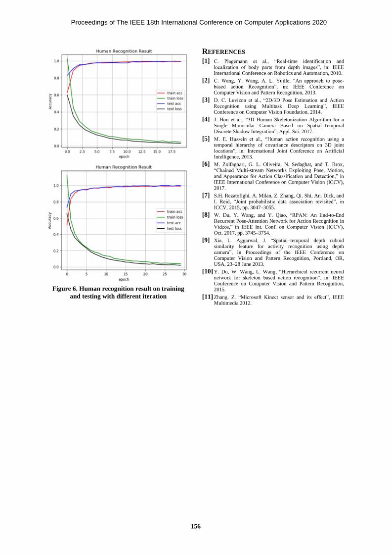
Figure 6. Human recognition result on training
and testing with different iteration
REFERENCES
[1] C. Plagemann et al., “Real-time identification and localization of body parts from depth images”, in: IEEE International Conference on Robotics and Automation, 2010.
[2] C. Wang, Y. Wang, A. L. Yuille, “An approach to pose-based action Recognition”, in: IEEE Conference on Computer Vision and Pattern Recognition, 2013.
[3] D. C. Luvizon et al., “2D/3D Pose Estimation and Action Recognition using Multitask Deep Learning”, IEEE Conference on Computer Vision Foundation, 2014.
[4] J. Hou et al., “3D Human Skeletonization Algorithm for a Single Monocular Camera Based on Spatial-Temporal Discrete Shadow Integration”, Appl. Sci. 2017.
[5] M. E. Hussein et al., “Human action recognition using a temporal hierarchy of covariance descriptors on 3D joint locations”, in: International Joint Conference on Artificial Intelligence, 2013.
[6] M. Zolfaghari, G. L. Oliveira, N. Sedaghat, and T. Brox, “Chained Multi-stream Networks Exploiting Pose, Motion, and Appearance for Action Classification and Detection,” in IEEE International Conference on Computer Vision (ICCV), 2017.
[7] S.H. Rezatofighi, A. Milan, Z. Zhang, Qi. Shi, An. Dick, and I. Reid, “Joint probabilistic data association revisited”, in ICCV, 2015, pp. 3047–3055.
[8] W. Du, Y. Wang, and Y. Qiao, “RPAN: An End-to-End Recurrent Pose-Attention Network for Action Recognition in Videos,” in IEEE Int. Conf. on Computer Vision (ICCV), Oct. 2017, pp. 3745–3754.
[9] Xia, L. Aggarwal, J. “Spatial–temporal depth cuboid similarity feature for activity recognition using depth camera”, In Proceedings of the IEEE Conference on Computer Vision and Pattern Recognition, Portland, OR, USA, 23–28 June 2013.
[10] Y. Du, W. Wang, L. Wang, “Hierarchical recurrent neural network for skeleton based action recognition”, in: IEEE Conference on Computer Vision and Pattern Recognition, 2015.
[11] Zhang, Z. “Microsoft Kinect sensor and its effect”, IEEE Multimedia 2012.
Proceedings of The IEEE 18th International Conference on Computer Applications 2020
156

Vehicle Accident Detection on Highway and Communication
to the Closest Rescue Service
Nay Win Aung
Deputy Director, Minister’s Office
Ministry of Construction
Nay Pyi Taw, Myanmar
Thin Lai Lai Thein
GIS Lab and FIS
University of Computer Studies
Yangon, Myanmar
Abstract
The hazard information and the timely rescue
performance are considered as the main elements to
reduce the risk of road traffic accidents since the rate
of highway accidents significantly increased. In this
paper, it is aiming to detect the highway accident
victims by using the data received from Sensor Fusion-
Based algorithm while Ray Casting algorithm will
assist the users to receive the assistance of rescue
services in timely manner. With the purpose of user
friendliness, these algorithms are intended to apply in
the smartphones built-in high technology sensors,
which are connected with the GIS, GPS and Geofence
technologies.
Keywords: Highway, Accident Detection, sensors,
Rescue Alert, GPS, GIS, Geofence, Dataset
I. INTRODUCTION
In Myanmar, road collisions are the major cause
of death among the young adults and mid-aged people.
Most of the precious lives are lost during the road
accidents because it is not able to identify the correct
location of accident occurred as well as inform the
rescue services to save the victims on time. A highway
is the main road in which connects the urban and rural
areas. Due to its wide structure and possesses the high-
speed thresholds, it can reduce the travelling time of the
users. In Myanmar, there are forty- nine (49) roads,
which connect from Eastern Regions to Western Areas,
while the total of thirty-six (36) roads are used as
highway to link from Northern States to Southern
Provinces. The total length of these roads is more than
twenty thousand (20,000) kilometers. All of the matters
related to the usage and maintenance of these roads are
monitored and managed by the Department of
Highways, which is under the Ministry of Construction
in Myanmar. Recently, it is noticed that the rate of
fatality and injury on Highways in Myanmar has been
an upsurge. According to the statistical results stated in
“Road Safety in Myanmar 2017” by Federation
Internationale de l’Automobile (FIA), the number of
deaths related to road accidents received from
Myanmar Police Force was 1,853 in 2008 and, this
number was increased to 4,688 in 2016. Within eight
years, the numbers of reported road deaths were
doubled.
Even though the economy and development of
Myanmar is still in growth, the vehicle ownerships of
the citizens are increasing all the time. It is expected
that the number of accidents related to automobiles are
likely to be raised and, is estimated that 9,000 people
may be killed in road accidents in 2020. Apparently,
there is a linkage between a person's death during the
above accidents and the absence of the first aid
provision due to the delay in informing to the rescue
services. Thus, in the case of road accidents, response
time is vital for saving the precious lives of accident
victims and considered the certain level of impact on
death rate. In Myanmar, the smartphones embedded
with strong detection sensors to identify the
information of accidents and send this to the
responsible teams in timely manner are not available
yet.
With the intention of overcoming the
weaknesses in the Rescue Alert System via Geofence
technology, this research aims to validate the status of
accident occurred by using the values received from
accelerometers and gyroscope sensors, identify the
accurate location of accident by using GIS and GPS
technologies, maintain and update the rescue service
information such as contact points, and search for the
nearest rescue units with the usage of Geofence
Technology. In this way, the fatality rate due to the
vehicle accidents will be reduced to the certain level as
the prompt response is received from the emergency
services such as Medical emergency services. Once the
location of the accident is confirmed, the Ray Casting
Algorithm is applied to search for the closest rescue
services within the shortest time duration. The similar
experiments related to the vehicle accident detection
Proceedings of The IEEE 18th International Conference on Computer Applications 2020
157

and communication to the rescue services are also as
followed:
Chris T., White J., Dougherty B., Albright A.
and Schmidt DC.[1] have developed a prototype
smartphone- based client/server application
“WreckWatch”, which operates together with the
embedded smartphone sensors and communication
interfaces to detect the causes of accidents and deliver
the notifications to the respective organizations. The
vulnerability of this application is the speed limitation
and, the smartphone application does not detect the
possibility of accident in low speed condition when the
speed of the car is lower than the configured speed
threshold in application. Sneha R.S. and Gawande A.D
[2] invented the accident notification system called "E-
call" for smart phones. This "E-call" uses the cellular
network to transfer the data between smartphones and
the Server Center. Since "E-call" system accessed the
built-in accelerometer sensor of smartphone as an
accident detection sensor, it is possible to produce the
false positive alarms although the user is not inside the
car. In 2015, Dipesh Suwal, Suresh Manandhar,
Shashish Maharjan and Ganesh Dhakal, [3] “D-
Fencing Application”, which notified the Geo-fencing
Post Disaster Scenario using Android App. The users
will receive the alert messages from the system admin
whenever they are approaching or entering to the
regions affected by disaster.
However, the information in database may not
be updated because only the system administrator, a
person who has knowledge of Geofence, can manage
the disaster information as well as send the alert
message to the requestors. If the system administrator
is not available when the incident occurs, the users may
not receive the updated information. Hence, the
application is not reliable since it does not have the
automated features of receiving disaster information,
updating the database promptly and sending the precise
rescue alerts to the users.
In 2013, Danish karim and Jaspal Singh [4]
proposed the “Development of Automatic Geo-
Fencing and Accidental Monitoring System based on
GPS Technology”. By operating a single shock sensor
embedded in a proposed system, an accident can be
detected as well as the vehicle can also be prevented
from the theft as it is operated as security control.
However, there is no predefined database and datasets
to record the user information and the variables of
incident occurred. Although it was mentioned that the
system should send the alert automatically to the rescue
services, it was not mentioned how and where the
contact information of rescue services is maintained.
Thus, the recipients were likely to receive the limited
information of sender via SMS. The remainder of the
paper is organized as follows.
In section 2, explain the methodology of this
research study. In section 3, we discuss the incident
prediction of sensor and driver prediction by using
sensor fusion-based algorithm used together Ray
Casting algorithm and the elements of Geofencing
Technology. In section 4, explain the technical usage
of this proposed system. In section 5, the experiments
and results are explained. Finally, section 6 presents the
conclusion.
II. METHODOLOGY OF RESEARCH
STUDY
The performance of an accident detection
system is determined levels: data collection with data
processing and communication to the closest rescue
service is illustrated in Figure 1. Firstly, the values
received from Accelerometer, Gyroscope and GPS are
maintained in the accident detection dataset. Secondly,
the system predicts as an accident and the accident
validation message will be triggered to the user when
these values are exceeding the accident threshold
value. Thirdly, the system starts to search for the
accident location by using the GPS values received
from the accident detection dataset when the accident
is confirmed. Fourthly, the Geofence technology
creates the polygon in which the accident location is
marked as the center point. Fifthly, the system
accesses the rescue service dataset to retrieve the
contacts of rescue services located in the polygon and,
search for the closest rescue service from the accident
location.
The Geofence will create another polygon with
wider boundaries if none of the rescue service contacts
is identified in the first polygon. Finally, the system
will send the alert message including the user and
vehicle information as well as the location of the
accident to the rescue service if it finds the closest one
from the accident location.
The server side’s workflows are emphasized to
collect and process the data including the users’
information, incident information and the contact of
rescue services. And then decide the relevant action
while user side workflows act as the projection of the
prediction. To make more accurate prediction, sensor
projected data such as false alarm rate; fatalities of
accidents, fixed data are stored in centralized system
and communication differences parties, smartphones
are play as sensor roles to make prediction.
Proceedings of The IEEE 18th International Conference on Computer Applications 2020
158

Figure 1. System Architecture
III. DETECT AND SEARCH
ALGORITHMS
A. Sensor Fusion - Based Algorithms
Since the data deficiency issue occurs among
the individual sensors, Sensor Fusion-Based algorithm
is considered as a compensating method to enhance the
data reliability by merging the data from various
sensors. According to the previous similar
experiments, the information produced from the
automated sensors might be unreliable to some extent.
In Sensor Fusion-Based algorithm, the information can
be retrieved not only from automated sensors but also
from historical sensor data stored in the centralized
database as well as the non-automated sources. Then,
the data received from multiple sensors will be refined
and evaluated to achieve the optimal result. In this
accident detection and rescue alert system, it is crucial
to obtain the high-quality input data.
The most favorable result to detect an accident
can be obtained by using the following Sensor Fusion
- Based algorithm:
Xi (t) = Ai xi (t) + Bi ui (t) + Wi (t),
yi (t) =Ci Xi (t) - vi (t), (i= 1, 2, n)
Where i indicates the number of subsystems (i.e.
accelerometers, gyroscopes and so on) in which data is
produced and t indicates the time period.
The present value of the subsystem Xi(t) can be
expressed by combing the current condition of the
source xi(t), the signal value transmitted at the
particular time ui(t) and, the noise value at the time
period Wi(t). When the value of Xi(t) is received, the
output of the subsystem or source yi(t) can be
determined by filtering the unwanted noise value vi(t)
included in present value of Xi(t).
By using an MLF-type neural network, the most
favorable result to detect the accident will be predicted
upon the individual output values as well as the
integrated result of those individual output values.
B. Ray Casting Algorithms
When the status of accident is confirmed, a
polygon fence with the range of 1,000 square meters
will be created and the accident location is marked as
the center point in that range. In this fence, the contacts
of rescue services near the accident location will be
searched with Ray Casting Algorithm. If the rescue
services cannot be found, the Geofence will re-create
the new polygon fence with wider boundaries and
search for the contact points of rescue services with
Ray Casting Algorithm until the closest rescue service
is identified. When the closest rescue service is found,
the accident alert message including user and vehicle
information as well as the location of the accident will
be triggered to the closest rescue services. The
intention of applying Ray Casting Algorithm in this
paper is that the closest rescue services from the
accident location can be found and contacted with a
minimum time interval.
In the Ray Casting algorithm, there are three
input values, P, Q and R. P defines the point in which
the place of accident occurred while Q states the
polygon created to encircle P. R indicates the locations
of rescue services marked in Google Map. Although
the initial value of inside is set as ‘False’ at the
beginning of every search, the final value of inside will
be shown as ‘True’ if R falls in Q and, ‘False’ if R is
out of the edges of Q.
Initially, the system sets the count as ‘0’ before
starting the looping of every edge from point P. S
indicates the ray that is originated at point P and
transmitted to +y direction and, this ray will be only in
the edges of y direction. When the accident is detected,
the infinite rays or S will be transmitted in +y direction
from its point of origin or P. To verify the target point
of interest or nearest rescue service (R), there will be
Proceedings of The IEEE 18th International Conference on Computer Applications 2020
159

a looping between P and the edges of polygon, Q.
Once the point of interest (R) is identified in Q, the
value is marked as ‘True’ and then, the searching
process is ended. If the point of interest (R) is not
fallen inside the Q, the value is marked as ‘False’ and
the looping will be stopped. Then, another polygon
with larger diameter will be created to start the looping
until the nearest rescue service (R) is found.
Algorithm:
Input: Points as P, Polygon as Q, Rescue Service as R
P is the position of interest
buf is a buffer distance.
Output: true if R contains Q, otherwise false
1: count = 0
2: s is an infinite ray in the +y direction, originating at
P
3: for all edges e in Q do
4: if R is within buf of ex then
5: ex,buf = ex -2 * buf
6: else if R is within buf of e or ebuf then
7: return false
C. Geofence
Geofence creates the virtual geographic
boundary of an area where the accident occurs. To
mark a location of interest, the user needs not only to
specify its latitude and longitude but also add the
adjustment of radius. Once the latitude, longitude, and
radius are provided, it is defined a geofence (a circular
area or fence) around the location of interest. This
feature is to use for hazard area detection. In this paper,
geofence is applied to send the information to the
closest rescue team from the geographical location
where the accident occurs.
Figure 2. Information of Rescue Services Location
and Accident place
D. User Information
Users are required to input information to
process for faster and, receive efficient rescue
procedure. Before starting the trip on highway, the
users including driver and passengers must provide
their personal information such as name, gender, blood
type, date of birth, contact number and emergency
contact number. This information is collected upon
installing the one-time input. For example, when fatal
accident occurs, the victim might need blood, so the
rescue team can prepare for the required blood type of
victim.
E. Vehicle Information
After providing the personal information of the
users, it is also required to insert the information of the
vehicle that the user drives on the highway. Once the
accident occurs, the information such as the accurate
position is provided upon the selected route of the trip
when the user activates the accident detection system.
Then, the system will be able to access the below data
before informing the rescue teams.
• Car Type (Sedan, SUV, Truck, Wagon, etc.)
• Vehicle Registration Number
• Color of Vehicle
• Number of Passengers
F. Accident Detection Dataset
These datasets are early stages as the built-in
sensors of the system need to retrieve and evaluate the
status of the accident. Once the status is confirmed, the
latest calibration sensors data is delivered to the main
system to create the updated dataset automatically.
The accident detection datasets decide upon the values
received from the smartphones’ built-in sensors such
as the accelerometer, gyroscope and linear
acceleration whether the accident may occur or not.
G. Rescue Service Dataset
With the connection of Geofence, Rescue
Service Dataset maintains the data about the rescue
services such as the contacts of ambulance service, fire
stations, and police stations and so on. In figure 3, the
sample of rescue datasets are illustrated. Once the
accident is confirmed, then the nearby rescue services
will be informed after automatically adding the details
of last GPS. These datasets are constantly updated in
the servers, thus Geofence can access whenever it is
required.
Proceedings of The IEEE 18th International Conference on Computer Applications 2020
160

Figure 3. Sample of Sever side Dataset
IV. TECHNOLOGIES USAGE
The following technologies are intended to use
for detecting the accidents and sending the alert to
rescue teams.
Smartphones are chosen as the major subject of
this research as they are the affordable and effective
portable machines embedding with powerful
technologies. Being an open-source mobile operating
system, the Android source code is free to access with
only one restriction, which is not allowed to use for
personal interest or any other financial benefits. Being
the primary Android IDE (Integrated Development
Environment), Android Studio supports an Android
developer all the required tools when the Android
applications are developed. Hence, the developers can
write the codes with auto-completion tools.
It is more productive for developers to use Java
than any other languages as Java has the large set of
class libraries that comprise the multiple functions such
as connectivity, sensors and so on. These libraries are
reusable by most of the embedded applications, so the
developers do not need to rewrite the codes, and this
could not only save the developing time but also
prevent the unexpected errors.
Geo-fencing creates the virtual boundaries for
the actual geographic locations. The virtual boundaries
could be fixed or changeable. In a comparison with the
conventional framework API, Google Location API
delivers the more powerful, high-level framework that
can select a suitable location provider and power
management without the assistance of manpower. One
of the prominent features of this API is the activity
detection which is not available in the framework API.
The Google Maps Android API is opted for this
research as it is a service allowed to access the Google
Maps Server automatically to present Maps, record the
response in the target location and retrieve the required
information for the user. With the usage of HTTP
request, this service provides the information about the
geographical locations and, adds the noticeable points
of interest along the driving route. Unlike Google
Places API Web Service, Google Directions API
calculates the distance between the starting point and
the destination and, presents the most efficient routes
based on travel time, number of turns, distance, etc.
Elements in Geo-fencing
GPS: It can pinpoint the location accurateness
within 5 meters from the user’s location. Besides, GPS
is accessible to all users without burdening on carrier
infrastructure.
A-GPS: Assisted GPS (A-GPS) supports to
obtain the most accurate result of mobile positon by
evaluating the GPS satellite information with the data
received from mobile tower sites.
Cell-ID (COO/CID): Mobile device can be
easily detected by pinpointing the connected cellular
network tower. Since, Cell-ID is uncomplicated way,
and it is not necessary to improve network location
infrastructure and mobile phones.
Wi-Fi: Wi-Fi is suitable for both indoor and
outdoor environments as it decreases time-to-first-fix
(TTFF) as well as is highly accessible in urban regions.
V. EXPERIMENTS AND RESULT
The lack of treatment in the proper time is the
major reason for many deaths. The major causes may
be the late arrival of ambulance or no person at the
place of accident to give information to the ambulance
or family members. This paper is intended to reduce
these factors and save the lives of victims by delivering
the required medical assistances to accident location on
time.
The possibility of accident can be predicted
immediately based on the values received from the
accelerometers and gyroscopes by accident detection
system. If these values exceed the predetermined
accident threshold in the system, the validation
message will be sent to the users whether accident is
occurred or not. In general, the system will wait for
maximum twenty (20) seconds to receive the
confirmation from the user. Whether the confirmation
from the user is received or not within twenty (20)
seconds, the system starts to create the visualized
Proceedings of The IEEE 18th International Conference on Computer Applications 2020
161
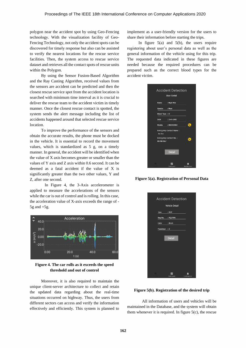
polygon near the accident spot by using Geo-Fencing
technology. With the visualization facility of Geo-
Fencing Technology, not only the accident spots can be
discovered for timely response but also can be assisted
to verify the nearest locations for the rescue service
facilities. Then, the system access to rescue service
dataset and retrieves all the contact spots of rescue units
within the Polygon.
By using the Sensor Fusion-Based Algorithm
and the Ray Casting Algorithm, received values from
the sensors are accident can be predicted and then the
closest rescue service spot from the accident location is
searched with minimum time interval as it is crucial to
deliver the rescue team to the accident victim in timely
manner. Once the closest rescue contact is spotted, the
system sends the alert message including the list of
accidents happened around that selected rescue service
location.
To improve the performance of the sensors and
obtain the accurate results, the phone must be docked
in the vehicle. It is essential to record the movement
values, which is standardized as 5 g, on a timely
manner. In general, the accident will be identified when
the value of X axis becomes greater or smaller than the
values of Y axis and Z axis within 0.6 second. It can be
deemed as a fatal accident if the value of X is
significantly greater than the two other values, Y and
Z, after one second.
In Figure 4, the 3-Axis accelerometer is
applied to measure the accelerations of the sensors
while the car is out of control and is rolling. In this case,
the acceleration value of X-axis exceeds the range of -
5g and +5g.
Figure 4. The car rolls as it exceeds the speed
threshold and out of control
Moreover, it is also required to maintain the
unique client-server architecture to collect and retain
the updated data regarding about the real-time
situations occurred on highway. Thus, the users from
different sectors can access and verify the information
effectively and efficiently. This system is planned to
implement as a user-friendly version for the users to
share their information before starting the trips.
In figure 5(a) and 5(b), the users require
registering about user’s personal data as well as the
general information of the vehicle using for this trip.
The requested data indicated in these figures are
needed because the required procedures can be
prepared such as the correct blood types for the
accident victim.
Figure 5(a). Registration of Personal Data
Figure 5(b). Registration of the desired trip
All information of users and vehicles will be
maintained in the Database, and the system will obtain
them whenever it is required. In figure 5(c), the rescue
Proceedings of The IEEE 18th International Conference on Computer Applications 2020
162

service, which is the closest to the accident location,
will receive the alert message from the system. In this
message, the data of user including emergency contact
as well as the notification of other accidents received
from database will be observed. The latest accident will
be shown on top of the list.
Figure 5(c). Accident Information
VI. CONCLUSION
When the rescue procedures presently used are
verified, it is noticed that the current accident detection
solutions including smartphone systems still have
some weaknesses such as the speed threshold
limitation, the higher false alarm rate, the manual
controls upon updating the database information, and
the lack of predefined dataset to analyze the accident
data.
In this paper, the proposed system will be
compatible with the various trained dataset as well as
operating with Google application programming
interfaces (APIs), and thus, the weaknesses mentioned
above will be solved. Once the well-trained datasets
are maintained in the systems, the user’s conditions
while using the highways are tracked and updated in
the database perpetually. Thus, the system can obtain
those data to validate the status of accident whenever
it is needed. Moreover, with the usage of Geo-fencing
and the Google APIs, the location of accident can be
accurately identified within a short time and, the
closest rescue services from the accident spot will be
pinpointed and informed to save the victims of
accidents.
Since this system is implemented as the user-
friendly version, the user can simply reply by pressing
the verification message whether he or she needs the
assistance of rescue team or not. Even the user is
unconscious; the system will wait for certain time
duration before contacting to the nearest rescue unit
via Geo-Fencing Technology to prepare the required
procedures. Moreover, the system always
synchronizes with user’s device and even the device is
switched off, the last information of users is still
captured in the system to verify the data of accident.
ACKNOWLEDGMENT
First and foremost, I am grateful to the
University of Computer Studies (Yangon) and the
Department of Highways of the Ministry of
Construction. A special word of gratitude is due to Dr.
Thin Lai Lai Thein, Professor, GIS Lab and Faculty of
Information Science (FIS), University of Computer
Studies, Yangon, for her kind and continued guidance,
motivation and support for my research work.
REFERENCES
[1] Chris T., White J., Dougherty B., Albright A. and
Schmidt DC., “WreckWatch: Automatic Traffic
Accident Detection and Notification with
Smartphones”, International Journal of mobile
network and application, Springer, Hingham,
MA, USA., Vol.16, Issue 3, PP. 285-303, March
2011.
[2] Sneha R.S. and Gawande A.D., “Crash
Notification System for Portable Devices”,
International Journal of Advanced Computer
Technology (IJACT), Vol.2, No-3, PP.33-38,
June 2013.
[3] Dipesh Suwal, Suresh Manandhar, Shashish
Maharjan and Ganesh Dhakal., “D-Fencing
Application”, International Journal of
International Workshop on Strengthening
Opportunity for Professional Development &
Spatial Data Infrastructure Development,
Kathmandu, Nepal, 25th-27th November 2015.
[4] Danish karim and Jaspal Singh., “Development of
Automatic Geo-Fencing and Accidental
Monitoring System based on GPS Technology”,
International Journal of Computer Science,
Engineering and Applications (IJCSEA), Vol.3,
No.4, August 2013.
[5] Nay Win Aung, Dr. Thin Lai Lai Thein., “Traffic
Accident Detection and Rescue Alert System for
Highway in Myanmar”, International Journal of
Proceedings of The IEEE 18th International Conference on Computer Applications 2020
163

International Conference on Science, Technology
and Innovation (IcSTIM 2019), PP.169-175, 16th
September 2019.
[6] Dinesh Udayakumar., Chandrasekar Rajah and
M.Saravanan., “Location Based Messaging”,
International Journal of Advanced Computational
Engineering and Networking, ISSN(p): 2320-
2106, ISSN(e): 2321-2063, Vol.5, Issue.12, Dec
2017.
[7] Sergio Ilarri and Eduardo Mena., “Location -
Dependent Query Processing: Where We Are and
Where We Are Heading”, International Journal of
ACM Computing Surveys, 21st November 2008.
[8] “Road Safety in Myanmar 2017” by Federation
Internationale de l’Automobile (FIA), Paris, April
2017.
Proceedings of The IEEE 18th International Conference on Computer Applications 2020
164

Natural Language and Speech Processing
Proceedings of The IEEE 18th International Conference on Computer Applications 2020

Proceedings of The IEEE 18th International Conference on Computer Applications 2020

Myat Sapal Phyu
Faculty of Computer Science
University of Information Technology
Yangon, Myanmar
Khin Thandar Nwet
Faculty of Computer Science
University of Information Technology
Yangon, Myanmar
Abstract
Text classification is one of the most critical
areas of research in the field of natural language
processing (NLP). Recently, most of the NLP tasks
achieve remarkable performance by using deep
learning models. Generally, deep learning models
require a huge amount of data to be utilized. This
paper uses pre-trained word vectors to handle the
resource-demanding problem and studies the
effectiveness of a joint Convolutional Neural Network
and Long Short Term Memory (CNN-LSTM) for
Myanmar text classification. The comparative
analysis is performed on the baseline Convolutional
Neural Networks (CNN), Recurrent Neural Networks
(RNN) and their combined model CNN-RNN.
Keywords—text classification, CNN, RNN, CNN-
RNN, CNN-LSTM, deep learning model.
I. INTRODUCTION
Text classification is one of the interesting
application areas in NLP such as sentiment analysis,
machine translation, automatic summarization, etc.
Nowadays, information overloading is one of the
important problems for today's people. People waste
too much time to select their interesting information
because they receive a vast amount of information from
various sources of internet. A powerful text classifier
can extract useful content from massive amounts of
information. It can classify text into associated
categories including sentiment analysis, spam
detection, articles, books, and hate speech detection. It
is among the most active research areas in the field of
NLP. Historically, many researchers performed text
classification by using various machine learning
algorithm and their variant models. The use of deep
learning models has achieved great interest in text
classification due to their ability to capture semantic
word relationships in recent years. All deep learning
1 https://github.com/bheinzerling/bpemb
models typically require a lot of data to accomplish a
specific task. Although most pre-trained vectors are
trained on general datasets, the use of pre-trained
vectors can handle data requirements. It can be used for
the specific task by transferring learning with the
appropriate amount of data. This paper focuses in
particular on the classification of Myanmar articles.
Words are considered as basic units in this paper. Since
Myanmar language has no standard rule to determine
word boundaries, it is important in the pre-processing
phase to determine the word boundaries. As Myanmar
language is a morphologically rich language, good
word representation is difficult to learn because many
word forms seldom occur in the training corpus. The
BPE tokenizer1 is used to determine the boundary of
the word. The segmented words are converted into an
embedding matrix by using the pre-trained vectors
trained on Wikipedia by the Skip-gram model [2]. The
effective use of pre-trained vectors is very supportive
of resource-scarce languages. In this paper, CNN and
LSTM models are jointly performed for Myanmar text
classification. The convolution process is performed on
the embedding matrix for selecting the features and the
LSTM model is used to capture long term information.
In this paper, the max-pooling layer is dropped in the
CNN model to prevent the loss of context information.
The next sections are as follows, the works
related to the text classification and other areas of
application are addressed for both Myanmar and
English in section 2. Section 3 describes Myanmar's
background knowledge. Section 4 discusses the
components of the CNN-LSTM joint model. Section 5
explains the findings of the experiment and the paper is
concluded in section 6.
II. RELATED WORK
Wang et al. [8] proposed a regional CNN-
LSTM model that captures regional information by
CNN and predicts valence arousal (VA) by LSTM
A Study on a Joint Deep Learning Model for Myanmar Text Classification
Proceedings of The IEEE 18th International Conference on Computer Applications 2020
167

model and outperforms than regression-based,
lexicon-based and NN-based methods on two datasets
for sentiment analysis. Kwaik et al. [5] proposed a
deep learning model that combines LSTM and CNN
models for dialectal Arabic sentiment analysis and this
model performs better than two baseline models on
three datasets. Zhang et al. [9] constructed the CNN
model on the top of LSTM. The output from the LSTM
model is further extracted by the CNN model and it
performed better in terms of accuracy than the baseline
models. Kim et al. [4] conducted the experiments with
variations of CNN model, CNN-rand, CNN-static and
CNN-multichannel on the top of pre-trained vectors
for sentence classification. These CNN models
performed better in 4 out of 7 tasks than the state-of-
the-art.
The previous research works in deep learning
and machine learning models for Myanmar language
in speech recognition, named entity recognition, and
text classification are also investigated. Aye et al. [1]
aimed to enhance the sentiment analysis for Myanmar
language in the food and restaurant domain by
considering intensifier and objective words and
improved the prediction accuracy. Hlaing et al. [3]
applied LSTM-RNN in Myanmar speech synthesis.
Mo et al. [6] annotated Named Entity tagged corpus
for Myanmar language and evaluation was performed
comparatively between neural sequence model and
baseline CRF. In our previous works [7], we
performed the comparative analysis of CNN and RNN
both on syllable and word level by using three pre-
trained vectors and also collected and annotate six
Myanmar articles datasets. In this paper, a
comparative analysis is performed on a joint CNN-
LSTM model against baseline CNN, RNN, and their
combine model by using Myanmar articles datasets.
III. MYANMAR LANGUAGE BACKGROUND
Myanmar language is the official language of
the Republic of the Union of Myanmar. It is a
morphologically rich language and Myanmar
sentences are basically constructed as the subject,
object, and verb pattern. The Myanmar script is written
from left to right and the characters are rounded in
appearance. There is no regular inter-word spacing in
Myanmar language like in the English language.
Though, spaces are used to mark phrases. Sentences are
clearly delimited by a sentence boundary marker.
Myanmar words are constructed by one or more
2 https://mcf.org.mm/myanmar-unicode/
syllables. There are thirteen three basic consonants,
eight vowels and eleven medial. A Myanmar syllable
is constructed by one initial consonant (C), zero or
more medial (M), zero or more vowels (V) and optional
dependent various signs. Words are considered a basic
unit in this paper.
A. Pre-processing
Pre-processing basically contains two steps, 1)
removing unnecessary characters, and 2) determining
the word boundaries. As this study focus on the
Myanmar text classification, Myanmar Unicode range
between [U1000-U104F]2 is removed to ignore non-
Myanmar characters. The numbers “၀-၉”, [U1040-
U1049] and punctuation marks “၊, ။”, [U104A- U104B]
are also removed. As Myanmar language has no rule to
determine word boundary, it is needed to determine the
boundary of words. In this work, word boundaries are
determined by the BPE tokenizer.
B. Pre-trained Model
The reuse of the pre-trained model by transfer
learning on a new task is very efficient because it can
train the deep learning models with not much data.
Typically, most of the NLP tasks don’t have sufficient
label data to be trained on such complex models. In
this paper, we use the pre-trained vector file that was
publicly released by the Facebook AI Research
(FAIR) lab3. It was trained on Wikipedia using the
fastText skip-gram model with 300 dimension. In this
paper, the pre-trained model is used as the starting
point instead of learning from scratch.
C. Construction of Embedding Matrix
The segmented words are transformed into word
vectors by matching the vocabulary in the pre-trained
vectors file. Figure 1 shows the construction of the
embedding matrix. Firstly, Myanmar text data are
extracted from online news websites. Secondly,
unnecessary characters are removed from the extracted
text. Then, word boundaries are determined by the BPE
tokenizer although sometimes the results are
meaningless as it is a frequency-based tokenizer. The
tokenized words are matched with pre-trained word
vectors file in order to construct the word embedding
matrix for the embedding layer.
Table I shows the sample of Myanmar text pre-
processing with the sample sentence “Corona ဗ ငးရပစ
3 https://fasttext.cc/docs/en/pretrained-vectors.html
Proceedings of The IEEE 18th International Conference on Computer Applications 2020
168

ကာကယရရး မြနြာတ းမြြ င မပငဆင။” and non-Myanmar
characters “Corona” is removed. Then, the text string
is segmented into words as
“ဗ ငးရပစ_ကာကယရရး_မြနြာ_တ းမြြ င _မပငဆင”, “_” shows
the boundary of words.
TABLE I. SAMPLE OF TEXT PRE-PROCESSING
Input Sentence Corona ဗ ငးရပစ ကာကယရရး
မြနြာတ းမြြ င မပငဆင။
English Meaning Myanmar ramps up the defense against
Coronavirus
Word
Segmentation ဗ ငးရပစ_ကာကယရရး_မြနြာ_တ းမြြ င _ မပငဆင
IV. A JOINT CNN-LSTM MODEL
The proposed joint CNN-LSTM model
basically consists of four components, 1) Embedding
Layer, 2) Convolution Layer, 3) LSTM layer, and 4)
Fully connected and output layer. Figure 2 illustrates
the joint CNN-LSTM model.
A. Embedding Layer
In the embedding layer, segmented words are
transformed into vector representation by matching the
pre-trained vectors file. The pre-trained vectors file is
like vocabulary and each word in the vocabulary
attached with their corresponding vectors that can catch
the context information.
B. Convolution Layer
In the convolution layer, the convolution
process is performed by the ReLU activation function
with stride size 1. Convolution layer selects the features
and the result of the convolution process is in the form
of the feature map. Max-pooling layer is discarded
because it captures only very important features and
ignores the un-important features and it can lead to
losing the context information.
C. LSTM Layer
LSTM layer is used instead of the max-pooling
layer to capture context information.
D. Fully Connected Layer and Output Layer
In the final output layer, the probability of the
class is predicted by using the sigmoid activation
function. In the hyper-parameter setting, Adam
optimization function and binary_crossentropy loss
function with 0.5 dropouts and 16 batch size on 10
epochs. Moreover, l2=0.01 is set in kernel and bias
regularizer to reduce overfitting.
Text
Documents
Extract Sentences
Remove Un-necessary
characters
Em
bed
din
g
Mat
rix
Word Segmentation
Match with Pre-trained
vectors
Fully
Connected Layer
(Use Sigmoid)
Em
bed
din
g
Mat
rix
Convolution
Layer
Dropout
Fea
ture
Map
LSTM Layer
Output
(Probability of each class)
P(c1)
P(c2)
P(cn)
Figure 1. Construction of embedding matrix.
Figure 2. A joint CNN-LSTM model
Proceedings of The IEEE 18th International Conference on Computer Applications 2020
169

V. EXPERIMENT
A. Dataset
Myanmar text data are collected from various
sources of Myanmar news websites including 7Day
Daily4 , DVB5 , The Voice6 , Thit Htoo Lwin 7 , and
Myanmar Wikipedia 8 . The text data contains five
categories art, sport, crime, education, and health. Each
category is collected in tab-separated values (.tsv) files
and each row contains a sentence that is annotated with
the corresponding label. The text data are converted
from Zawgyi to Unicode by Rabbit converter 9 and
shuffle and split 75% and 25% for train and test dataset
for each topic and the total number of sentences for the
training is 36,113 sentences and the testing is 12,037
sentences. The details of the dataset are listed in Table
II.
B. Comparison Models
In this work, the comparative analysis is
performed on a joint CNN-LSTM model with baseline
CNN, RNN, and their combined model CNN-RNN.
1) CNN: CNN is a feed-forward neural network
and a basic CNN contains three layers, convolution
layer, pooling layer, and fully connected layer. The
ReLU activation is mostly used in the convolution
layer, max-pooling is mostly used in the pooling layer
and Softmax function is mostly used in the fully
connected layer. In this paper, the simple CNN with
one convolution layer and sigmoid function is used in
the experiment.
2) RNN: RNN is an artificial neural network with
an internal memory that keeps information to persist.
It learns from the previous data and performs the same
function for all input data. RNN produces the output
yt as in equation10 (1).
4 https://7daydaily.com/ 5 http://burmese.dvb.no/ 6 http://thevoicemyanmar.com/ 7 http://www.thithtoolwin.com/ 8 https://my.wikipedia.org/wiki/ 9 https://www.rabbit-converter.org/
𝑦𝑡 = 𝑓(𝑊𝑦ℎ𝑡) (1)
ℎ𝑡 = 𝜎(𝑊ℎℎ𝑡−1 +𝑊𝑥𝑥𝑡) (2)
3) CNN-RNN: In this combined model, the
CNN model is used for feature extraction and RNN is
used to make a prediction by past words. The
drawbacks CNN model is its locality and it requires
many convolution layers to capture long term
information. RNN is a bias model and it predicts the
semantic of words by past words and reduces
performance when predicting long text. LSTM model
is an extension of the RNN model to be better
preservation of long term dependency problem.
C. Experimental Setup
The experiment is implemented on Google
Colaboratory (Colab) 11 that provides the Jupyter
notebook environment 12 , executes code in Python
3.6.9. No setup is required and runs in the cloud and
have a maximum lifetime for each user. The key
advantage of Colab is the support of the Tesla K80
GPU accelerator. Gensim13 3.6.0 is used to load the
pre-trained word vector file. Keras14 2.2.5 is run on the
TensorFlow backend. It enables fast experimentation
of deep learning models and can be run on both CPU
and GPU. Large size data such as pre-trained word
vector files can be stored in Google drive to reduce file
uploading time. The sklearn.metrics15 0.22.1 is used to
evaluate the classification performance of the models.
D. Experimental Result
The performance of the proposed model, CNN-
LSTM model is compared with comparison models
described in section 5.2 as listed in Table III. In this
paper, the experiment is performed on Myanmar news
articles text data that contains five topics and the detail
of the dataset is listed in Table II. The experiment
contains three main parts pre-processing, word
embedding and text classification. In the pre-
processing phase, we remove unnecessary characters
and segment words by BPE tokenizer. Word
embedding matrix is constructed by a pre-trained
model via the Gensim library and the CNN, RNN,
CNN-RNN and CNN-LSTM models are trained by
using Keras, model-level library. All models are
trained using 10 epochs, 16 batch size, 0.5 dropout
rate, 0.01 l2 bias and kernel regularizer, Adam
10 https://en.wikipedia.org/wiki/Recurrent_neural_network 11 https://colab.research.google.com/ 12 https://jupyter.org/install.html 13 https://pypi.org/project/gensim/3.6.0/ 14 https://keras.io/ 15 https://scikit-learn.org/stable/
TABLE II. MYANMAR TEXT DATASET FOR FIVE
TOPICS
Class Train Test Total
Sport 9,919 3,242 13,161
Art 9,483 3,173 12,656
Crime 6,718 2,184 8,902
Health 4,743 1,632 6,375
Education 5,250 1,806 7,056
Total 36,113 12,037 48,150
Proceedings of The IEEE 18th International Conference on Computer Applications 2020
170
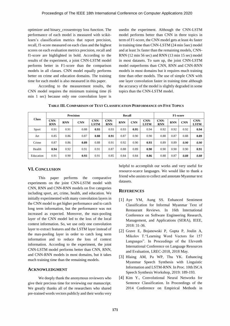
optimizer and binary_crossentropy loss function. The
performance of each model is measured with scikit-
learn’s classification metrics that report precision,
recall, f1-score measured on each class and the highest
scores on each evaluation metrics precision, recall and
f1-score are highlighted in bold. According to the
results of the experiment, a joint CNN-LSTM model
performs better in F1-score than the comparison
models in all classes. CNN model equally performs
better on crime and education domains. The training
time for each model is also measured in this paper.
According to the measurement results, the
CNN model requires the minimum training time (6
min 1 sec) because only one convolution layer is
usedin the experiment. Although the CNN-LSTM
model performs better than CNN in three topics in
term of F1-score, the CNN model gets at least 4x faster
in training time than CNN-LSTM (24 min 5sec) model
and at least 3x faster than the remaining models, CNN-
RNN (12 min 56 sec) and RNN (13 min 15 sec) model
in most datasets. To sum up, the joint CNN-LSTM
model outperforms than CNN, RNN and CNN-RNN
models in most domains but it requires much training
time than other models. The use of simple CNN with
one layer convolution faster in training time although
the accuracy of the model is slightly degraded in some
topics than the CNN-LSTM model.
TABLE III. COMPARISON OF TEXT CLASSIFICATION PERFORMANCE ON FIVE TOPICS
Class
Precision Recall F1-score
CNN-
RNN RNN CNN
CNN-
LSTM
CNN-
RNN RNN CNN
CNN-
LSTM
CNN-
RNN RNN CNN
CNN-
LSTM
Sport 0.91 0.91 0.88 0.93 0.93 0.93 0.95 0.94 0.92 0.92 0.92 0.94
Art 0.85 0.86 0.87 0.88 0.91 0.87 0.90 0.90 0.88 0.87 0.88 0.89
Crime 0.87 0.86 0.89 0.88 0.91 0.92 0.90 0.93 0.89 0.89 0.90 0.90
Health 0.94 0.92 0.91 0.91 0.87 0.88 0.89 0.90 0.90 0.90 0.90 0.91
Education 0.91 0.90 0.93 0.91 0.85 0.84 0.84 0.86 0.88 0.87 0.88 0.88
VI. CONCLUSION
This paper performs the comparative
experiments on the joint CNN-LSTM model with
CNN, RNN and CNN-RNN models on five categories
including sport, art, crime, health, and education. We
initially experimented with many convolution layers in
the CNN model to get higher performance and to catch
long term information, but the performance was not
increased as expected. Moreover, the max-pooling
layer of the CNN model led to the loss of the local
context information. So, we use only one convolution
layer to extract features and the LSTM layer instead of
the max-pooling layer in order to catch long term
information and to reduce the loss of context
information. According to the experiment, the joint
CNN-LSTM model performs better than CNN, RNN,
and CNN-RNN models in most domains, but it takes
much training time than the remaining models.
ACKNOWLEDGMENT
We deeply thank the anonymous reviewers who
give their precious time for reviewing our manuscript.
We greatly thanks all of the researchers who shared
pre-trained words vectors publicly and their works very
helpful to accomplish our works and very useful for
resource-scarce languages. We would like to thank a
friend who assists to collect and annotate Myanmar text
datasets.
REFERENCES
[1] Aye YM, Aung SS. Enhanced Sentiment
Classification for Informal Myanmar Text of
Restaurant Reviews. In 16th International
Conference on Software Engineering Research,
Management, and Applications (SERA), IEEE,
2018: 31-36.
[2] Grave E, Bojanowski P, Gupta P, Joulin A,
Mikolov T.“Learning Word Vectors for 157
Languages”. In Proceedings of the Eleventh
International Conference on Language Resources
and Evaluation, LREC-2018, 2018 May.
[3] Hlaing AM, Pa WP, Thu YK. Enhancing
Myanmar Speech Synthesis with Linguistic
Information and LSTM-RNN. In Proc. 10th ISCA
Speech Synthesis Workshop, 2019: 189-193.
[4] Kim Y., Convolutional Neural Networks for
Sentence Classification. In Proceedings of the
2014 Conference on Empirical Methods in
Proceedings of The IEEE 18th International Conference on Computer Applications 2020
171

Natural Language Processing (EMNLP), 2014:
1746-1751.
[5] Kwaik KA, Saad M, Chatzikyriakidis S, Dobnik
S. LSTM-CNN Deep Learning Model for
Sentiment Analysis of Dialectal Arabic. In
International Conference on Arabic Language
Processing 2019 Oct 16 (pp. 108-121). Springer,
Cham.
[6] Mo HM, Soe KM, Myanmar named entity corpus
and its use in syllable-based neural named entity
recognition, International Journal of Electrical
and Computer Engineering (IJECE), 2020.
[7] Phyu SP, Nwet KT. Article Classification in
Myanmar Language. In the Proceeding of 2019
International Conference on Advanced
Information Technologies (ICAIT), IEEE, 2019:
188-193.
[8] Wang J, Yu LC, Lai KR, Zhang X. Dimensional
sentiment analysis using a regional CNN-LSTM
model. In Proceedings of the 54th Annual
Meeting of the Association for Computational
Linguistics (Volume 2: Short Papers) 2016 Aug
(pp. 225-230).
[9] Zhang J, Li Y, Tian J, Li T. LSTM-CNN Hybrid
Model for Text Classification. In2018 IEEE 3rd
Advanced Information Technology, Electronic
and Automation Control Conference (IAEAC)
2018 Oct 12 (pp. 1675-1680). IEEE
Proceedings of The IEEE 18th International Conference on Computer Applications 2020
172

Hay Mar Su Aung
University of Computer Studies
Yangon, Myanmar
Win Pa Pa
University of Computer Studies
Yangon, Myanmar
Abstract
This paper presents a study of comparison on
three different machine learning techniques to
sentiment analysis for Myanmar language. The
fundamental part of sentiment analysis (SA) is to
extract and identify the subjective information that is
social sentiment in the source text. The sentiment class
is positive, neutral or negative of a comment. The
experiments are done on the collected 10,000
Facebook comments in Myanmar language. The
objective of this study is to increase the accuracy of
the sentiment identification by using the concept of
word embeddings. Word2Vec is used to train for
producing high-dimensional word vectors that learns
the syntactic and semantic of word. The resulting word
vectors train Machine Learning algorithms in the form
of classifiers for sentiment identification. This
experimental results prove that the use of word
embeddings from the collected real world datasets
improved the accuracy of sentiments classification
and Logistic Regression outperformed the other two
ML methods in terms of accuracy and F-measures.
Keywords— Multiclass classification, natural
language processing, sentiment analysis, Facebook
Page's comments, word embedding, Logistic
Regression.
I. INTRODUCTION
Sentiment Analysis (SA) is a type of contextual
mining of text that identifies and extracts the tendency
of people’s feelings via Natural Language Processing,
computational linguistics and text analysis, which are
helped to use extracting and analyzing subjective
information from the website majority social media
and similar sources. It is used to quantify the general
public’s social attitude of specific brand, product or
service when it monitors online conversations.
Sentiment Analysis (SA) is also known as opinion
mining. SA uses data mining techniques to extract and
capture analyzed data to classify the opinion of a
document or collection of documents, like blog posts,
reviews of product and social media feeds like Tweets,
status updates and comments.
In the distinctive events of technology, people
stored data from the internet. These storing data have
been grown every day and the large amount of data is
stored up to date. But very vital information is carried
by these data carry concerning the emotions of
different people around the world, so it has become
essential to summarize these large number of data with
particular automated systems. In this day, many people
use social media around the world like Twitter,
Facebook and so on. Among of them, Facebook is a
popular free social networking website. In Myanmar,
most people use Facebook to express their opinions
and feelings.
This paper analysis the performance of the
word vector techniques (Word2Vec , TFIDF text
feature vector representation and pre-trained
Word2Vec) with three different machine learning
techniques (Logistic Regression, SVM and Random
Forest) for public Facebook Page’s comments of
Myanmar text.
This paper is constructed as the following. The
related techniques of word vector is exhibited as
Section 2. Section 3 describes the details of proposed
system. The experiment results is explained at the
Section 4. Finally, Section 5 concludes the discussion
with possible enhancements to the proposed system.
II. RELATED TECHNIQUES
A. Word Embeddings
A word embedding learns the text
representation where words that have the same
meaning have a similar representation. It is emerged
Analysis of Word Vector Representation Techniques with Machine-Learning Classifiers for Sentiment Analysis of Public Facebook
Page’s Comments in Myanmar Text
Proceedings of The IEEE 18th International Conference on Computer Applications 2020
173

Word Embedding in the Natural Language Processing
(NLP) field. Word Embeddings, a text mining
technique, is to establish association between words in
the set of sentences. The syntactic and semantic
meanings of words are comprehend from the context.
The idea of distributional assumption propose that
words occurring in the alike words are semantically
alike. There are the two techniques of word
embeddings – (a) Frequency Based Embeddings (b)
Prediction Based Embeddings. The Frequency Based
Embeddings processed poorly at conserving the
contextual information in textual data such as the
traditional bag-of-words model. The Prediction Based
Embeddings predicts a target word from the given a
context word. The researchers developed Global
Vectors for Words Representation (GloVe) which is
the algorithm of an unsupervised learning to achieve
word vector representation does very well at context
preservation.
B. Word2Vec
Word2Vec is the producing of the model for
word embeddings from a set of sentences for word
representation.Word2Vec represents content of
vectors into vector space. Word2Vec models use
shallow two-layer neural networks, consists of one
hidden layer (projection layer) between input and
output, which are used to train for reconstructing
linguistic contexts of words. Word2Vec takes a set of
sentences (corpus) as its input and produces word
vectors in a vector space, generally several hundred of
dimensions, with each unique word in the text corpus
being placed a corresponding vector in the space.
Word vectors are placed in the vector space in such a
way the words that have similar contexts in the set of
sentences are appeared in approximately close to each
other in the space. In the same way, different meaning
of word contents are located far away from each other.
Word2Vec have two techniques to achieve word
vectors. They are (i) Continuous Bag of words (C-
BOW model) and (ii) Skip-Gram model as shown in
Figure 1 and Figure 2. The C-BOW model is used to
train for predicting the current word based on its
context words. The Skip-Gram model is used to train
the model for predicting the context words given a
current word. w(t) is the context word and [w(t-2),w(t-
1),w(t+1) and w(t+2)] are the surrounding words.
C. tfidf Vectorization
tfidf is an shorthand for term frequency-
inverse document frequency. The algorithm of tfidf is
a very common algorithm for converting word into a
meaningful numeric representation. tfidf vector is
based on the concurrency apporach. It is different from
the count vectorization approach because it takes into
account not just the number of times a text in a single
document but in all documents of the corpus. The
technique is widely used as features extraction across
various applications in NLP field. tfidf need to assign
weight for the word based on the number of a word
that occurs in the document also consideration the
occurrences of the word in all documents.
tf determines the frequency of word appears in
a specific document. The calculation equation is as:
𝑡𝑓 =occurencies of a word in the document
total words in the document (1)
Inverse Document Frequency for a specific
word measures the log of the division of the sum of all
document numbers and the document numbers with
concluding the particular word in it. It is calculated as
the following.
𝑖𝑑𝑓 = 𝑙𝑜𝑔Total number of docs
Number of docs ∈ the word (2)
𝑡𝑓 − 𝑖𝑑𝑓 = 𝑡𝑓 ∗ 𝑖𝑑𝑓 (3)
tfidf is needed to transform from the specific words to
numerical feature vectors.
Figure 1. Architecture of C-BOW Model
Proceedings of The IEEE 18th International Conference on Computer Applications 2020
174

I.
III. METHODOLOGY
The following steps are processed in this proposed system.
A. Data Collecting
There is no previously created dataset for
public Facebook page comments in Myanmar
language. So, the dataset is crawled public comments
of Facebook page related to “Myanmar Celebrity”
Page in Myanmar to create own dataset. Social media
data (Facebook comments) is collected through data
crawling using Facepager tool. These comments were
copied and saved as two text file (training text file and
testing text file). This corpus is comprised of posts
over 100 and comments of 10,000. The set of
sentences are antecedently identified with the labels
for indicating the user emotions each Facebook
comment. The following figure show the visual
analysis of imbalance between the three sentiment
classes of the dataset. There are 10,000 sentences
training dataset in which 2,316 sentences labeled by
negative, 1,461 sentences labeled by neutral and 6,223
sentences labeled by positive. There are 1,000
sentences testing data in which 345 sentences labeled
by negative, 148 sentences labeled by neutral and 507
sentences labeled by positive.
B. Data Preprocessing
Font Conversion
Most of Facebook user in Myanmar use Zawgyi font on social media. Application in technology field use Unicode. In this paper, the collected text data are both Zawgyi and Unicode format. So, the gather text data with Zawgyi format are converted to Unicode by using online Zawgyi-Unicode converter.
Data Cleaning
The collected text comments in the dataset consist of various kinds of noises. Before the training and testing are proceeded, these noises are removed all undesirable marks of punctuation, hash sign, additional spaces, unrecognised characters, number etc. from the set of sentences. Most of Facebook users tag the name in the comments so this tagging name is also removed. Due to occur noise in the corpus, the comments which may take place more than one time in the corpus are taken as one.
2316
1461
6223
345 148507
0
1000
2000
3000
4000
5000
6000
7000
Negative Neautral Positive
Analysis of Dataset
Training Dataset Testing Dataset
Fig. 1.
Figure 2. Architecture of Skip-Gram Model
Figure 3. Proposed System Design
Figure 4. Analysis of Facebook comments Dataset
Proceedings of The IEEE 18th International Conference on Computer Applications 2020
175

Segmentation
Word segmentation is a necessary part before to process Natural Language Processing in the Myanmar text, because a text of Myanmar language is a string of characters from left to right without explicit word boundary elimiters. It is firstly needed to segment text into separate meaningful words in order to extract words from the collected dataset in Myanmar text. In this paper, Myanmar text data are manually segmented.
TABLE I. EXAMPLE OF SEGMENTATION THE
COMMENTS
C. Word Vector Representation Method
Building Word2Vec Model
The study of this paper use C-BOW model of
the Word2Vec algorithm. The implementation
of Word2Vec in the Gensim python library was
used to train on the treated data. For achieving
the better implementation of Word
Embeddings, most consideration is needed to
give certain hyper-parameters. These
parameters are: training dataset,
dimensionality, context-window, minimum
word count, sub-sampling and iteration. The
training dataset trained 10,000 sentences of
comments (training data). Negative sampling
was set because it proved to be efficiently
computational relative to hierarchical softmax.
For resulting in the better Word Embeddings,
the projection layer of the neural network was
assigned 300. The context-window size was
used 50 to prescribe context-window size for C-
BOW model. 1e-3 was used the sub-sampling
rate to counter the imbalance dataset of frequent
words. 1 set as the minimum count for
considering each word in the set of sentences
during processing of training. It trained
Word2Vec model on the treated data with the
above mentioned settings of hyper-parameter
and stored in a data file format. The word
embedding model produced d*p dimension
word vectors where d is the dictionary size and
p is the projection layer (hidden layer) size. In
this study, the size of the dictionary for the
training set is 5,833 vocabulary in the
dictionary.
Building tfidf Vectorization
tfidf implementation of sklearn python library
was trained on the data for training. The same
training dataset was used to take as its input
corpus. The word embedding model produce
word vectors having ru dimension where r is
the number of row in the given training data and
u is the unique words from all text. In this study,
the rare words is 319 words.
Building Pre-trained Word2Vec Model
For pre-trained Word2Vec, the pre-trained C-
BOW model of Word2Vec are previously
created by using another dataset containing
750,000 sentences. The training data and
testing data may or may not contain in this
dataset. The pre-trained Word2Vec model is
similarly created with the Word2Vec
algorithm. In this paper, the 300 dimensions
of this model is assigned. The context
window of 5 was used for C-BOW models
with workers of 10 (the number of
processor). And then, the generated pre-
trained word vector model is the vocabulary
size of 49,740 unique words with 300
dimensions.
D. Classification
In the field of the sentiment analysis,
supervised learning is useful for training the data on a
pattern that may analyze for either the opinion is
positive, negative or neutral. In this paper, we have
chosen the three Machine Learning classification
techniques consisting of Logistic Regression (LR),
Support Vector Machine (SVM) and Random Forest
(RF).
IV. EXPERIMENTAL RESULTS
The analysis has been performed comparative
according to examine the performance of the three
အမမြအ ားပပားပေပါတယချစတြ မ ( I'm always encouraging lovely Ma ) အမမြ အ ားပပား ပေ ပါ တယ ချစ တြ မ
Positive
ဘ ပရားရမေားမသပတ ဘ ား😂😂😂 ( I don't know what to write 😂😂😂 ) ဘ ပရား ရ မေား မ သ ပတ ဘ ား 😂 😂 😂
Neutral
Mcက စတပျကလ ပ ( Mc is disappointed ) Mc က စတပျက လ ပ
Negative
Proceedings of The IEEE 18th International Conference on Computer Applications 2020
176
techniques of classification: Logistic Regression,
SVM and Random Forest. In the sentiment
classification field, the evaluation of the techniques
have used the common information retrieval metrics;
precision, recall and f-score. According to evaluate the
process of sentence classification, an information
retrieval task is considered. The precision can be
calculated as (4):
𝑃𝑟𝑒𝑐𝑖𝑠𝑖𝑜𝑛 = 𝑇𝑃
(𝑇𝑃+𝐹𝑃) (4)
In which, TP is true positive (the occurrences of
targets actually identified sentences) and FP is false
positive (the occurrences of targets that were not
correctly identified sentences). Moreover, recall can
be calculated as (5):
𝑅𝑒𝑐𝑎𝑙𝑙 = 𝑇𝑃
(𝑇𝑃+𝐹𝑁) (5)
In which, TP is true positive (the occurrences of
targets actually identified sentences) and FN is false
negative (the occurrences of sentences which were not
identified at all). It is possible to calculate the f-score
as follows (6):
𝐹1 − 𝑠𝑐𝑜𝑟𝑒 = 2∗(𝑃𝑟𝑒𝑐𝑖𝑠𝑖𝑜𝑛∗𝑅𝑒𝑐𝑎𝑙𝑙)
(𝑃𝑟𝑒𝑐𝑖𝑠𝑖𝑜𝑛+𝑅𝑒𝑐𝑎𝑙𝑙) (6)
A. Logistic Regression
Logistic Regression classifier is used to apply
with the proposed features vectors extraction (tfidf
vectorizer, Word2Vec and pre-trained Word2Vec).
Using the confusion metrics which are precision
(Positive Predictive Value), recall (True Positive Rate)
and F-score, the evaluation has been performed. The
following tables show the results.
In TABLE II, the evaluation of classification
details how the logistic regression classifier with tfidf
word vector representation technique carried out for
predicting every sentiment label. In the negative label,
the classifier exactly prophesied TPR of 38% with the
PPV of 63% and F1-score of 47% in supporting 345
negative test objects. In the neutral label, the classifier
exactly prophesied TPR of 0.1% with the PPV 44% and
F1-score of 16% in supporting 148 neutral test objects.
In the positive label, the classifier exactly predict 91%
of 507 positive test objects, properly with the PPV of
61% and F1-score of 73%. Logistic Regression
classifier with tfidf vectorizer also tried to precisely
predict like the other training algorithms. In TABLE
III, many objects that were not correctly prophesied
label as positive. For instance, according to the Table
3, 203 out of 345 negative comments were predicted to
be positive while 92 out of 148 neutral comments were
predicted to be positive.
TABLE II. EVALUATION OF LOGISTIC REGRESSION
WITH TFIDF VECTORIZER
TABLE III. CONFUSION MATRIX FOR LOGISTIC
REGRESSION WITH TFIDF VECTORIZER
In TABLE IV, the evaluation of classification
details the Word2Vec+Logistic Regression classifier
with carried out for predicting every sentiment class.
In the negative label, the classifier exactly prophesied
82% of rate 77% and F1-score of 80%. In the neutral
label, the classifier exactly prophesied 38% of 148
neutral test objects, properly with the PPV of 63% and
F1-score of 47%. In the positive label, the classifier
exactly prophesied 93% of 507 positive test objects,
properly with the PPV of 86% and F1-score of 89%.
This approach also tried to fit for precisely classifying
like other training algorithms. In TABLE V, 44 out of
345 negative comments were predicted to be positive
while 57 out of 148 neutral comments were predicted
to be negative.
TABLE IV. EVALUATION OF LOGISTIC
REGRESSION WITH WORD2VEC
PPV TPR F1-
score Support
Negative 0.788 0.82 0.804 345
Neutral 0.629 0.378 0.473 148
Positive 0.857 0.933 0.893 507
Average/
Total 0.80 0.81 0.80 1000
PPV TPR F1-
score Support
Negative 0.63 0.38 0.47 345
Neutral 0.44 0.1 0.16 148
Positive 0.61 0.92 0.73 507
Average/
Total 0.59 0.61 0.56 1000
Negative 130 12 203
Neutral 42 14 92
Positive 36 6 465
Negative Neutral positive
Proceedings of The IEEE 18th International Conference on Computer Applications 2020
177

TABLE V. CONFUSION MATRIX FOR LOGISTIC
REGRESSION WITH WORD2VEC
In TABLE VI, the evaluation of classification
details how Pre-trained Word2Vec word vector
representation technique + the Logistic Regression
classifier carried out to predict every sentiment class.
In the negative label, the classifier exactly prophesied
77% of 345 negative test objects properly with the
PPV of 77% and F1-score of 77%. For the neutral class,
the classifier exactly prophesied 38% of 148 neutral
test objects properly with the PPV of 53% and F1-
score of 44%. For the positive class, the classifier
exactly prophesied 92% of 507 positive test objects
properly with the PPV of 85% and F1-score of 88%.
TABELE VI. EVALUATION OF LOGISTIC
REGRESSION WITH PRE-TRAINED WORD2VEC
TABLE VII. CONFUSION MATRIX FOR LOGISTIC
REGRESSION WITH PRE-TRAINED WORD2VEC
B. Support Vector Machine (SVM)
SVM classifier is applied with the tfidf
vectorizer, Word2Vec and pre-trained Word2Vec.
Using the confusion metrics which are precision
(Positive Predictive Value), recall (True Positive Rate)
and F-score, the evaluation has been performed. The
following tables show the results.
In TABLE VIII, the evaluation of classification
details how the SVM classifier with tfidf word vector
representation technique carried out for each
sentiment class. In the negative label, the classifier
exactly prophesied 37% of 345 negative test objects
properly with 60% of the PPV and F1-score of 46%.
In the neutral label, the classifier definitely prophesied
0.4% of 148 neutral test objects correctly with 35% of
the PPVand F1-score of 0.7%. In the positive label, the
classifier exactly prophesied 91% of 507 positive test
objects correctly with the PPVof 60% and F1-score of
72%. Logistic Regression classifier with tfidf
vectorizer also struggled to precisely classify like
other training algorithms. As shown in TABLE IX,
many objects that were not correctly prophesied were
labeled as positive. For instance, in TABLE IX, 212
out of 345 negative comments were predicted to be
positive while 99 out of 148 neutral comments were
predicted to be positive.
TABLE VIII. EVALUATION OF SVM WITH TFIDF
VECTORIZER
TABLE IX. CONFUSION MATRIX SVM WITH IFIDF
VECTORIZER
In TABLE X, the evaluation of classification
details how the SVM classifier with Word2Vec word
vector representation technique processed for
predicting every sentiment label. In the negative label,
the classifier definitely prophesied 82% of 345
negative test objects properly with the PPV of 78%
and F1-score of 80%. In the neutral label, the classifier
definitely prophesied 34% of 148 neutral test objects
properly with the PPV of 56% and F1-score of 42%.
In the positive label, the classifier definitely
prophesied 92% of 507 positive test objects correctly
Negative 283 18 44
Neutral 57 56 35
Positive 19 15 473
Negative Neutral Positive
PPV TPR F1-
score Support
Negative 0.765 0.774 0.769 345
Neutral 0.533 0.378 0.443 148
Positive 0.85 0.915 0.881 507
Average/
Total 0.77 0.79 0.78 1000
Negative 267 33 45
Neutral 55 56 37
Positive 27 16 464
Negative Neutral Positive
PPV TPR F1-
score Support
Negative 0.604 0.371 0.46 345
Neutral 0.353 0.041 0.073 148
Positive 0.597 0.907 0.72 507
Average/
Total 0.56 0.59 0.53 1000
Negative 128 5 212
Neutral 43 6 99
Positive 41 6 460
Negative Neutral Positive
Proceedings of The IEEE 18th International Conference on Computer Applications 2020
178

with the PPV of 85% and F1-score of 89%. SVM
classifier with Word2Vec also struggled to precisely
classify like other training algorithms. According to
the TABLE XI, 42 out of 345 negative comments were
prophesied to be positive while 60 out of 148 neutral
comments were prophesied to be negative.
TABLE X. EVALUATION OF SVM WITH WORD2VEC
TABLE XI. CONFUSION MATRIX FOR SVM WITH
WORD2VEC
In TABLE XII, the evaluation of classification
details how the SVM classifier with Pre-trained
Word2Vec word vector representation technique
carried out predicting for every sentiment label. In the
negative label, the classifier definitely prophesied 80%
of 345 negative test objects correctly with the PPV of
75% and F1-score of 77%. In the neutral label, the
classifier definitely prophesied 32% of 148 neutral test
objects properly with the PPV of 53% and F1-score of
40%. In the positive label, the classifier definitely
prophesied 92% of 507 positive test objects properly
with the 85% of PPV and F1-score of 88%.
TABLE XII. EVALUATION OF SVM WITH PRE-TRAINED WORD2VEC
PPV TPR F1-
score Support
Negative 0.751 0.797 0.774 345
Neutral 0.533 0.324 0.403 148
Positive 0.853 0.915 0.883 507
Average/
Total 0.77 0.79
0.77 1000
TABLE XIII. CONFUSION MATRIX FOR SVM WITH
PRE-TRAINED WORD2VEC
C. Random Forest
Random Forest classifier is applied with the
proposed features extraction (tfidf vectorizer,
Word2Vec and pre-trained Word2Vec). Using the
confusion metrics which are precision (Positive
Predictive Value), recall (True Positive Rate) and F-
score, the evaluation has been performed. The
following tables show the results.
In TABLE XIV, the evaluation of classification
details how the Random Forest classifier with tfidf
word vector representation technique carried out for
every sentiment label. In the negative label, the
classifier definitely prophesied 36% of 345 negative
test objects properly with the PPV of 60% and F1-
score of 45%. In the neutral label, the classifier
definitely prophesied 10% of 148 neutral test objects
properly with the PPV of 26% and F1-score of 15 %.
In the positive label, the classifier definitely
prophesied 90% of 507 positive test objects properly
with the 62% of PPV and F1-score of 73%. Logistic
Regression classifier with tfidf vectorizer also
struggled to precisely classify like other training
algorithms. As TABLE XV, many objects that were
not correctly prophesied were labeled as positive. For
instance, in TABLE XV, 203 out of 345 negative
comments were prophesied to be positive while 92 out
of 148 neutral comments were prophesied to be
positive.
TABLE XIV. EVALUATION OF RANDOM FOREST
WITH TFIDF VECTORIZER
PPV TPR F1-
score Support
Negative 0.775 0.817 0.795 345
Neutral 0.556 0.338 0.42 148
Positive 0.853 0.919 0.885 507
Average/
Total 0.78 0.80 0.79 1000
Negative 282 21 42
Neutral 60 50 38
Positive 22 19 466
Negative Neutral Positive
Negative 275 26 44
Neutral 64 48 36
Positive 27 16 464
Negative Neutral Positive
PPV TPR F1-
score Support
Negative 0.6 0.357 0.447 345
Neutral 0.263 0.101 0.146 148
Positive 0.617 0.9 0.731 507
Average/
Total 0.56 0.59 0.55 1000
Proceedings of The IEEE 18th International Conference on Computer Applications 2020
179

TABLE XV. CONFUSION MATRIX FOR RANDOM
FOREST WITH TFIDF VECTORIZER
In TABLE XVI, the evaluation of classification
details how the Random Forest classifier with
Word2Vec word vector representation technique
carried out for every sentiment label. In the negative
label, the classifier definitely prophesied 78% of 345
negative test objects correctly with the PPV of 72%
and F1-score of 75%. In the neutral label, the classifier
definitely prophesied 12% of 148 neutral test objects
properly with the PPV of 43% and F1-score of 20%.
In the positive label, the classifier definitely
prophesied 93% of 507 positive test objects properly
with the PPV of 81% and F1-score of 93%. Random
Forest classifier with Word2Vec also struggled to
precisely classify like other training algorithms.
According to TABLE XVII, 58 out of 345 negative
comments were prophesied to be positive while 76 out
of 148 neutral comments were prophesied to be
negative.
TABLE XVI. EVALUATION OF RANDOM FOREST
WITH WORD2VEC
TABLE XVII. CONFUSION MATRIX FOR RANDOM
FOREST WITH WORD2VEC
In TABLE XVIII, the evaluation of
classification details how the Random Forest classifier
with Pre-trained Word2Vec word vector
representation technique carried out for every
sentiment label. In the negative label, the classifier
definitely predicted 75% of 345 negative test objects
properly with the PPV of 71% and F1-score of 73%.
In the neutral label, the classifier definitely prophesied
17% of 148 neutral test objects correctly with the PPV
of 46% and F1-score of 24%. In the positive label, the
classifier definitely prophesied 92% of 507 positive
test objects correctly with the PPV of 80% and F1-
score of 86%.
TABLE XVIII. EVALUATION OF RANDOM FOREST
WITH PRE-TRAINED WORD2VEC
TABLE XIX. CONFUSION MATRIX FOR RANDOM
FOREST WITH PRE-TRAINED WORD2VEC
V. CONCLUSION
The paper of this study compares the
performance of 3 different Machine Learning (ML)
techniques containing Logistic Regression, SVM and
Random Forest while using Myanmar sentiment
analysis based on word vector representation method.
The dataset that has been used is a collection of
Myanmar Facebook pages comments for the purposes
of sentiment analysis. The experimental results have
proved that Logistic Regression classifier with
Word2Vec has exceeded in performance than the other
two Machine Learning by obtaining 80% of F1-score.
Hence, we can draw to conclude that given a word
vector representation from Word2Vec instead of tfidf
and pre-trained Word2Vec for extracting feature
vectors, sentiment analysis in Myanmar on three labels
of ideas, will carried out better the use of Logistic
Regression than the use of SVM and Random Forest.
Negative 130 12 203
Neutral 42 14 92
Positive 36 6 465
Negative Neutral Positive
PPV TPR F1-
score Support
Negative 0.717 0.78 0.747 345
Neutral 0.429 0.122 0.189 148
Positive 0.808 0.929 0.864 507
Average/
Total 0.72 0.76 0.72 1000
Negative Neutral Positive
PPV TPR F1-
score Support
Negative 0.707 0.748 0.727 345
Neutral 0.463 0.169 0.2448 148
Positive 0.8 0.917 0.855 507
Average/
Total 0.72 0.75 0.72 1000
Negative 258 20 67
Neutral 74 25 49
Positive 33 9 465
Negative Neutral Positive
Negative 269 18 58
Neutral 76 18 54
Positive 30 6 471
Proceedings of The IEEE 18th International Conference on Computer Applications 2020
180

REFERENCES
[1] Aye Myat Mon, Khin Mar Soe. “Clustering
Analogous Words in Myanmar Language using
Word Embedding Model”, ICCA & ICFCC 2019
Conference, 27th February 2019.
[2] C. Emelda. “A comparative Study on Sentiment
Classification and Ranking on Product Reviews”,
ijirae, issn: 2349-2163, volume 1 issue 10, November
2014.
[3] Merfat M. Altawaier, Sabrina Tiun, “Comparison
of Machine Learning Approaches on Arabic
Twitter Sentiment Analysis”, volume.6 (2016)
no. 6, ISSN: 2088-5334
[4] Md. Al- Amin, Md. Saiful Islam, Shapan Das
Uzzal, "Sentiment Analysis of Bengali Comments
With Word2Vec and Sentiment Information of
Words", 978-1-5090-5627-9/17/$31.00 ©2017
IEEE.
[5] Joshua Acosta, Norissa Lamaute, Mingxiao Luo,
Ezra Finkelstein, and Andreea Cotoranu.
“Sentiment Analysis of Twitter Messages Using
Word2Vec”. Proceedings of Student-Faculty
Research Day, CSIS, Pace University, May 5th,
2017.
[6] Oscar B. Deho, William A. Agangiba,Felix L.
Aryeh, Jeffery A. Ansah. “Sentiment Analysis
with Word Embedding”.
[7] Soe Yu Maw, May Aye Khine, “Aspect based
Sentiment Analysis for travel and tourism in
Myanmar Language using LSTM”, ICCA &
ICFCC 2019 Conference Program Schedule 27th
February 2019.
[8] https://towardsdatascience.com/updated-text-
preprocessing-techniques-for-sentiment-analysis-
549af7fe412a
[9] https://www.analyticsvidhya.com/blog/2017/
06/word-embeddings-count-word2veec/
[10] https://machinelearningmastery.com/what-are-
word-embeddings/
[11] https://hackernoon.com/word-embeddings -in-
nlp-and-its-applications-fab15eaf7430
[12] https://www.analyticsvidhya.com/blog/
2017/06/word-embeddings-count-word2veec/
[13] https://medium.com/data-science-group-
iitr/word-embedding-2d05d270b285
[14] https://medium.com/@shiivangii/data-
representation -in-nlp-7bb6a771599a
Proceedings of The IEEE 18th International Conference on Computer Applications 2020
181

Building Speaker Identification Dataset for Noisy Conditions
Win Lai Lai Phyu
Natural Language Processing Lab.,
University of Computer Studies
Yangon, Myanmar
Win Pa Pa
Natural Language Processing Lab.,
University of Computer Studies
Yangon, Myanmar
Abstract
Speech signal processing plays a crucial role
in any speech-related system whether Automatic
Speech Recognition or Speaker Recognition or
Speech Synthesis or something else. Burmese
language can be considered as an under resourced
language due to its linguistic resource availability.
For building Burmese speaker identification system,
the sufficient amount of speech data collection is a
very challenging task in a short time. In order to get
higher data size, this paper analyzes that the getting
higher duration of speech data actually combining
with various noises encountering in our
surroundings. For increased noisy state speech data,
we also used the voice activity detection (VAD)
technique to acquire only the speaker specific
information. For feature extraction, we used MFCC,
Filter Banks and PLP techniques. The experiments
were developed with i-vector methods on GMM-UBM
together with PLDA and presented the performance
of different data set in the form of EER with two
models trained on clean and noisy data to prove that
the developed speaker identification system is noise
robust.
Keywords— Burmese Speaker Identification, noise
robustness, VAD, MFCC, Filter Banks, PLP, GMM-
UBM, PLDA
I. INTRODUCTION
The speech of living things especially for
human involves numerous discriminative acoustic
features that can be discerned who they are because of
the structural formation of vocal tract is unique for
everyone. Speaker identification is the process by
which the acoustic speech signals to its corresponding
speaker and is applied in many applicable areas.
Speech corpora collection is the very first step in
building speaker identification system. In order to
develop the speaker identification system, the
sufficient speech data are needed to train and test the
spoken speech data. The performance of the system is
also depended on the amount of speech data. There
are many variations in speaker identification system.
The first one is the duration of utterances. The longer
the utterances, the better recognizes the corresponding
speaker. A second variation is noise as any kinds of
noise make the identification process harder. The third
variation is accent or speaker specific facts. The
speaker is easier to identify if he/she speaks a standard
dialect or the ones that matches the speech data the
system trained on. The final variation is the speech
recorded conditions. Therefore, we will propose
Burmese speaker identification how to construct with
noisy data. The paper is organized as follows. Related
works will be presented in section II. In section III,
speaker identification process will be introduced.
Section IV will be described the types of speaker
recognition and the proposed architecture of speaker
identification system with noisy data will be
expressed in section V. Experimental setup will be
addressed in section VI and experimental results will
be discussed in section VII. Finally, conclusion will
be expressed in section VIII.
II. RELATED WORKS
There are many speaker recognitions with
various approaches found in publications.
Arnab Poddar, Md Sahidullah and Goutam
Saha [2] presented the comparison of two different
speaker recognition systems, i-vector based and
GMM_UBM in utterance duration variability. It
revealed that GMM_UBM system outperforms i-
vector system for very short test utterances if the
speaker are enrolled with sufficient amount of training
data whereas total variability (i-vector) based system
degrades with the reduction in test utterance length
and also require huge computational resource
development data for identifying the speaker although
GMM_UBM don’t require the huge amount of
development data.
Comparison of text independent speaker
identification systems using GMM and i-vector
Proceedings of The IEEE 18th International Conference on Computer Applications 2020
182

methods are done by Nayana P.K., Dominic Mathew,
and Abraham Thomas [3]. It was observed that
appending formants and pitch high level features to
basic features: PNCC (Power Normalized Cepstral
Coefficients) and RASTA PLP (Relative Spectral
PLP) obtain the better accuracy for speaker
identification. It was also showed that the accuracy of
i-vector method with PLDA classifier is better than
that of Cosine Distance Scoring (CDS) classifier.
Moreover, it revealed that the system performance
enhances when longer utterances are used.
Analysis of various feature extraction
techniques for robust speaker recognition was
presented by Qin Jin and Thomas Fang Zheng [4] to
help the researchers for catching the current front end
features classified as low level and high level features.
They surveyed the speaker recognition system on
different feature extraction techniques: MFCC,
MVDR, FDLP, MHEC, SCF/SCM, FFV, HSCC and
Multitaper MFCC and presented the strength and
weakness of these techniques.
R.ARUL JOTHI M.E [5] presented the
analysis of suitable extraction methods and classifiers
for speaker identification since 2017. It identified the
speaker’s voice whether original or disguised voice
based on MFCC, Delta MFCC and Delta-Delta
MFCC with SVM classifier. MFCC with SVM
classifier improves the performance of system and
accuracy rates up.
An improved approach for text independent
speaker recognition was proposed by Rania Chakroun
[6]. It proposed that the new feature extraction method
combining MFCC and Short Time Zero Crossing Rate
(ZCR) of the signal. ZCR is the number of times the
zero axes crossed by the signal per frame. By
comparing the performance of two speaker
recognition systems with the use of MFCC and
combination of MFCC and STZCR, it showed the
new proposed feature extraction yields better outcome
and reduced in EER.
III. SPEAKER IDENTIFICATION
Speaker identification determines the speaker
identity from which of the registered speakers a given
utterance comes. It is a very challenging task because
human speech signals are highly variable due to
various speaker characteristics, different speaking
styles, environmental noises, and so on. There exist
various feature extraction methods and approaches for
speaker identification system. There are three main
steps in speaker identification.
As part of feature extraction, a set of feature
vectors are obtained from the raw speech signal to
more emphasize the speaker related information
because the speech signal can contain many features
which are not required to claim the speaker.
Therefore, feature extraction process is advantageous
when you need to diminish the resources required for
processing without losing relevant information. There
are many different types of features that can be
extracted. The recognition accuracy rate varies
according to chosen extraction methods. Various
types of available features are high level features,
spectra-temporal features, short term (low level)
spectral features, and prosodic features [3]. In these,
low level features are easy to extract and very
effective to recognize the speaker. Although high
level features contain more speaker specific
information, the extraction process is more
complicated.
To generate the speaker models representing to
each speaker, the features attained from the feature
extraction stage are used and stored these speaker
models into a database as UBM for performing the
comparison during testing. It is the main session of
speaker identification system as the models created in
this stage are applied to perform comparison in the
identification stage. Different modeling methods are
HMM (Hidden Markov Models), GMM (Gaussian
Mixture Models), DNN (Deep Neural Network), and
i-vector method.
Identifying the test speech signal is the final
stage of every speaker identification system. Relative
scores corresponding to each of the speaker models
are computed and then the one which has the highest
score is identified as the target speaker. Different
scoring methods used for identification are CDS
(Cosine Distance Scoring), PLDA (Probabilistic
Linear Discriminant Analysis), LLR (Log Likelihood
Ratio), and SVM (Support Vector Machine) and so
on.
IV. TYPES OF SPEAKER RECOGNITION
There are two types of speaker recognition:
speaker verification and speaker identification. If the
speaker claims to be of a certain identity and the voice
is used to verify this claim, this is called verification
or authentication. Speaker verification is a 1:1 match
where one speaker's voice is matched to one template
(also called a "voice print" or "voice model"). Speaker
identification is the task of determining an unknown
speaker's identity. Therefore, it is a 1: N match where
the voice is compared against N templates. It involves
Proceedings of The IEEE 18th International Conference on Computer Applications 2020
183

two phases: enrollment and testing. During
enrollment, the speaker's voice is recorded and
typically a number of features are extracted to form a
voice print, template, or model. In testing phase, a
speech sample or "utterance" is compared against a
previously created voice print. Moreover, there exist
two types of speaker identification: text dependent
and text independent. Text dependent speaker
identification needs to utter exactly the same utterance
to determine who they are. Text independent speaker
identification has no limits and constraints on the
spoken words that are uttered. It is more flexible and
usable in real world applications. Verification is faster
than identification because of the processing time of
matching. This paper proposes text independent
speaker dependent identification because text
independent systems are most applicable in real
world.
V. PROPOSED ARCHITECTURE OF SPEAKER
IDENTIFICATION SYSTEM
Feature extraction, speaker modeling and
identification process are the three crucial stages of
any speaker recognition system. This section presents
the detail description of the whole speaker
identification process. The proposed architecture of
speaker identification system with noisy data exhibits
in Fig. 1.
A. Data Preprocessing
Before feature extraction, we need to firstly
preprocess the data. In this stage, the whole recorded
audio speech data is chopped into utterance level
speech segments with Audacity which is open source
and cross-platform audio multi-track audio editor and
recorder software. And then, the preprocessed speech
data are the utterance level speech segmented data
with 16 bits mono PCM in 16 kHz ranging from 10 to
27 seconds. After that, we randomly added the
utterance level segmented speech data with various
noises found in our surrounding prepared by
ourselves. By contaminating, our data set size
increases the duration than that of original clean data
set size. And then, the original clean data and noise-
combined data are combined to use in feature
extraction. Surrounding noises include car’s horn, fly
buzz, the dog’s bark, fire alarm, ringtone, cat meow,
whistle, roar, shouting, wind blowing, birds chirping,
banging of hammer, school bell, beating a drum and
so on.
B. Feature Extraction and Voice Activity
Detection
There is no standard rule for choosing among
these features for the question ‘Which feature
extraction technique should one use?’ It depends on
our needs like intended application, robustness,
computing resources and amount of data available.
Because short-term spectral (low level) features are
easy to compute and provide good results, exploring
with these types of feature enhances the system
performance. Feature extraction stage is one of the
most important components in any SR systems and its
objective is to find robust and discriminative features
in acoustic data because better features give the more
improved recognition rate. In our proposed system,
clean and noisy data are combined to extract the
features. And then, Voice activity detection (VAD) is
applied for noisy data. It is a technique used to detect
the speech or non-speech section in recorded speech
data with the aim of removing the silence frames in
segmented speech data, saving the computing time
and enhancing the recognition accuracy rate. It also
refers to the problem of distinguishing speech
segments from background noise in an audio stream
and is also language independent. Moreover, we
exploited with three kinds of low level feature
extraction techniques for system performance: Mel
Frequency Cepstral Coefficient (MFCC), Filter Bank
and Perceptual Linear Prediction (PLP). The system’s
recognition rate diverges depending on our choice
because there are no standard rules for choosing
among these features. It depends on our destined
needs in related applied areas.
C. Building Speaker Models
The feature vectors extracted in the feature
extraction stage take to build the speaker models.
UBM is the key element of an i-vector (existing in
low dimensional spaces that are smaller in size to
reduce the recognizing time) system as it is necessary
for collecting statistics from speech utterances. It is
constructed using feature values of sound speech
samples from the different speakers and Maximum A
Posteriori (MAP) is used to get the speaker models
each [1]. It is the central part of this system because it
is used in comparison with the test speech segment’s
feature vector for describing who the speaker is. In
this paper, we implement the speaker identification
system with i-vector method by using Kaldi ASR
open source toolkit to build the speaker models:
Proceedings of The IEEE 18th International Conference on Computer Applications 2020
184
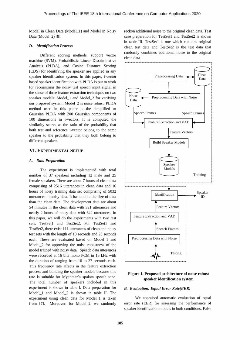
Model in Clean Data (Model_1) and Model in Noisy
Data (Model_2) [8].
D. Identification Process
Different scoring methods: support vector
machine (SVM), Probabilistic Linear Discriminative
Analysis (PLDA), and Cosine Distance Scoring
(CDS) for identifying the speaker are applied in any
speaker identification system. In this paper, i-vector
based speaker identification with PLDA is put to work
for recognizing the noisy test speech input signal in
the sense of three feature extraction techniques on two
speaker models: Model_1 and Model_2 for verifying
our proposed system, Model_2 is noise robust. PLDA
method used in this paper is the simplified or
Gaussian PLDA with 200 Gaussian components of
100 dimensions in i-vectors. It is computed the
similarity scores as the ratio of the probability that
both test and reference i-vector belong to the same
speaker to the probability that they both belong to
different speakers.
VI. EXPERIMENTAL SETUP
A. Data Preparation
The experiment is implemented with total
number of 37 speakers including 12 male and 25
female speakers. There are about 7 hours of clean data
comprising of 2516 utterances in clean data and 16
hours of noisy training data set comprising of 5032
utterances in noisy data. It has double the size of data
than the clean data. The development data are about
54 minutes in the clean data with 321 utterances and
nearly 2 hours of noisy data with 642 utterances. In
this paper, we will do the experiments with two test
sets: TestSet1 and TestSet2. For TestSet1 and
TestSet2, there exist 111 utterances of clean and noisy
test sets with the length of 18 seconds and 23 seconds
each. These are evaluated based on Model_1 and
Model_2 for approving the noise robustness of the
model trained with noisy data. Speech data utterances
were recorded at 16 bits mono PCM in 16 kHz with
the duration of ranging from 10 to 27 seconds each.
This frequency rate affects in the feature extraction
process and building the speaker models because this
rate is suitable for Myanmar’s spoken speech tone.
The total number of speakers included in this
experiment is shown in table I. Data preparation for
Model_1 and Model_2 is shown in table II. The
experiment using clean data for Model_1 is taken
from [7]. Moreover, for Model_2, we randomly
reckon additional noise to the original clean data. Test
case preparation for TestSet1 and TestSet2 is shown
in table III. TestSet1 is one which contains original
clean test data and TestSet2 is the test data that
randomly combines additional noise to the original
clean data.
Figure 1. Proposed architecture of noise robust
speaker identification system
B. Evaluation: Equal Error Rate(EER)
We appraised automatic evaluation of equal
error rate (EER) for assessing the performance of
speaker identification models in both conditions. False
Preprocessing Data
Preprocessing Data with Noise
Preprocessing Data with Noise
Clean
Data
Noise
Data
Feature Extraction and VAD
Build Speaker Models
Feature Extraction and VAD
Identification
Speaker
Models
Speech Frames Speech Frames
Feature Vectors
Training
Testing
Feature Vectors
Speech Frames
Speaker
ID
Proceedings of The IEEE 18th International Conference on Computer Applications 2020
185

acceptance rate (FAR) (1), is a type of error allowing
the impostor speaker is improperly identified as the
known speaker and false rejection rate (FRR) (2) is
incorrectly denied the actual speaker known by the
system as impostor. Equal Error Rate (EER) is one
where FAR equals to FRR and also the point where
FAR and FRR are optimal and minimal. EER of
speaker model is mainly based on the amount of
training data. Therefore, we are going to collect the
speech data more and more in the future. The lower
the EER value, the higher the recognizing rate of
speaker models.
TABLE I. TOTAL NUMBER OF SPEAKERS
Male Female Total Number of Speakers
12 25 37
TABLE II. DATA PREPARATION FOR THE
EXPERIMENTS
Data Number of Utterances Duration (hr: min: sec)
Model_1 Model _2 Model _1 Model _2
Train 2516 5032 07:10:39 16:05:04
Dev 321 642 00:54:36 01:58:35
TABLE III. STATISTICS OF THE TEST SETS
Test Sets Number of
Utterances
Duration (hr: min: sec)
TestSet1 111 00:18:26
TestSet2 111 00:23:12
C. Evaluation:Test Samples’ Accuracy
To evaluate the performance of every test
speech samples, we also applied the automatic
evaluation shown in (3). This automatic evaluation is
based on how many test speech samples recognized
by the speaker models differs from the correct test
speech samples.
Accuracy (%) = ((TTSs – WDSs) / TTSs) * 100 (3)
where, Accuracy=Test Case’s Accuracy in Percentage
TTSs=Total Test Speech Samples in Test Case
WDSs = Wrong Detected Samples .
VII. EXPERIMENTAL RESULTS
We will describe the experimental results
based on the models built in Model_1 and Model_2
using PLDA identification. Table IV shows the
performance of speaker models, Model_1 and
Model_2 on the development data, and two test sets.
To evaluate the performance of models, TestSet1 and
TestSet2 is used for assessments in terms of equal
error rate (EER%). TestSet1 is the original clean test
data and TestSet2 is the data prepared with additional
noise to the clean data. The performance of speaker
models in varying surrounding conditions on the
development data sets depicts with a chart in Fig. 2.
Figure 2. Performance of EER on building
speaker models
Figure 3. EER of TestSet1 and TestSet2 on
Model_1
Proceedings of The IEEE 18th International Conference on Computer Applications 2020
186

Figure 4. Performance of Model_1 with
three feature extraction methods
Figure 3 and Figure 4 reveals that the
evaluation results of TestSet1 and TestSet2 on speaker
models built in clean data. Although the EERs and
accuracies of models show good results on clean test
data, the performance degrades on noisy test data.
This experiment approves the noisy data needs to be
trained on the noisy data.
Table IV shows the performance of two
models in terms of EERs on two test sets: TestSet1
and TestSet2. It can be seen that the EER of clean
data, TestSet1 has got comparable results in both
clean and noisy models. It means, the noisy model can
give the similar performance on clean and noisy test
data. EER of noisy model, Model_2, was decreased
significantly on TestSet2, noisy data, by all feature
extraction techniques at most 20.72% than clean
model, showing the noisy training data are important
for noisy test data. From the experiments, we found
MFCC give better results among three feature
extraction techniques for clean and noisy conditions
of our data.
TABLE IV. PERFORMANCE OF TESTSET1 AND
TESTSET2 ON MODEL_1 AND MODEL_2
Fea
ture
E
xtr
acti
on
Meth
od
s
Equal Error Rate (%)
Dev TestSet1 TestSet2
Mod
el_
1
Mod
el_
2
Mod
el_
1
Mod
el_
2
Mod
el_
1
Mod
el_
2
MFCC 3.738 4.984 1.802 1.802 26.13 8.108
PLP 2.492 5.296 1.802 2.703 27.03 10.81
Filter
Bank 2.812 8.424 1.802 2.703 31.53 10.81
TABLE V. ACCURACIES ON TESTSETS (%)
Feature
Extraction
Methods
Accuracy Rate (%)
Model_1 Model_2
TestSet1 TestSet2 TestSet1 TestSet2
MFCC 97.27 46.36 93.64 76.36
PLP 95.45 41.82 92.73 75.45
Filter Bank 94.55 34.55 94.55 76.36
Figure 5. EER of TestSet1 and TestSet2 on
Model_2
Figure 6. Performance of Model_2 with three
feature extraction methods
Fig. 5 and Fig. 6 show that the results of
TestSet1 and TestSet2 on noisy speaker models. This
paper approaches to the point of view of every noise
aggravates the recognition rate on every speech-
related processing. The error rates of clean data are
sharply higher than that of testing on noisy data.
As Fig. 3, Fig. 4, Fig. 5, Fig. 6, Fig. 7 and Fig.
8 show, it can be seen clearly that the model with
noisy data is better than Model_1 in noisy condition
and noisy data helps to improve the performance of
Proceedings of The IEEE 18th International Conference on Computer Applications 2020
187

speaker identification in both clean and noisy
condition. According to the Table IV and V, TestSet2
of on Model_1 and Model_2, show the improved
equal error rate on our model, Model_2. The system
performance degrades in clean data when testing with
noisy test speech data but Model_2 yields satisfiable
results on both conditions clean and noisy. In this
analysis, we showed the error rates are obviously
decreased almost one-third by Model_2 compared to
Model_1.
Figure 7. EER on two models with TestSet2
Figure 8. Performance of TestSet2 on two
models with three feature extraction
methods
VIII. CONCLUSION
Noise delivers detriments in speech-related
processing. This paper shows the importance of noisy
data preparation for speaker identification.
Experiments were done on speaker identification
training on clean and noisy data. We also analyzed the
rate of change of EER with three feature extraction
methods in the experiments. From the experiments,
applying MFCC features gave the best results among
three different feature extraction techniques. We also
found that, integrating additional noise to the original
clean data improves the recognizing rate in every
feature extraction method with increasing the size of
data. From the experiments, it is clear that the
preparation of noisy data is effective for noise robust
speaker identification system and the results are
acceptable.
REFERENCES
[1] Win Lai Lai Phyu, and Win Pa Pa, “Text
Independent Speaker Identification for Myanmar
Speech”, ICFCC 2019, Yangon, Myanmar, 27-
28 February 2019.
[2] Arnab Poddar, Md Sahidullah, Goutam Saha,
“Performance Comparison of Duration
Variability”, IEEE 2015.
[3] Nayana P.K., Dominic Mathew, Abraham
Thomas, “Comparison of Text Independent
Speaker Identification Systems using GMM and
i-vector Methods”, ICACC 2017, Cochin, India,
pp.22-24 August 2017.
[4] Qin Jin, Thomas Fang Zheng, “Overview of
Front-end Features for Robust Speaker
Recognition”, APSIPA ASC 2011, Xi’an, China.
[5] R.ARUL JOTHI M.E, “Analysis of Suitable
Extraction Methods and Classifiers for Speaker
Identification”, IRJET 2017, Volume: 04 Issue:
03, Mar 2017.
[6] Rania Chakroun, Leila Beltaifa Zouari,
Mondher Frikha, “An Improved Approach for
Text-Independent Speaker Recognition”,
IJACSA 2016, Vol. 7, No. 8, 2016.
[7] Aye Nyein Mon, Win Pa Pa, Ye Kyaw Thu,
“Building HMM-SGMM Continuous Automatic
Speech Recognition on Myanmar Web News”,
ICCA 2017, Yangon, Myanmar, 16-17 February,
2017.
[8] Daniel Povey, Arnab Ghoshal, Petr Motlicek,
Yanmin Qian, Petr Schwarz, Jan Silovsky,
Georg Stemmer, Karel Vesely, “The Kaldi Spech
Recognition Toolkit”, ASRU, 2011.
Proceedings of The IEEE 18th International Conference on Computer Applications 2020
188

English-Myanmar (Burmese) Phrase-Based SMT with One-to-One and
One-to-Multiple Translations Corpora
Honey Htun
Department of Computer
Engineering and Information
Technology,
Yangon Technological
University,
Yangon, Myanmar,
Thepchai Supnithi
National Electronics and
Computer Technology Center
(NECTEC),
Pathum Thani,Thailand,
Ye Kyaw Thu
National Electronics and
Computer Technology Center
(NECTEC),
Pathum Thani,Thailand,
Language Understanding Lab,
Myanmar,
Nyein Nyein Oo
Department of Computer
Engineering and Information
Technology,
Yangon Technological
University,
Yangon, Myanmar,
Abstract
This paper contributes the first investigation
of machine translation (MT) performance differences
between Myanmar and English languages with the
use of several possible Myanmar translations for the
specific primary educational domain. We also
developed both one-to-one and many Myanmar
translations corpora (over 8K and 46K sentences)
based on old and new English textbooks (including
Grade 1 to 3) which are published by the Ministry of
Education. Our developing parallel corpora were
used for phrase-based statistical machine translation
(PBSMT) which is the de facto standard of statistical
machine translation. We measured machine
translation performance differences among one-to-
many English to Myanmar translation corpora. The
differences range between 19.68 and 52.38 BLEU
scores from English to Myanmar and between 50.17
and 75.12 BLEU scores from Myanmar to English
translation. We expect this study can be applied in
Myanmar-to-English automatic speech recognition
(ASR) development for primary English textbooks.
The main purpose is to translate primary English
textbooks data correctly even if the children use in
several Myanmar conversation styles.
Keywords—Phrase-based Statistical Machine
Translation (PBSMT), One-to-Many Parallel Corpus,
Myanmar-English Machine Translation, Primary
English Textbooks of Myanmar, Word Error Rate
(WER).
I. INTRODUCTION
Nowadays, our Myanmar children in rural and
less developing areas are facing many difficulties in
education. One of the challenges in their educational
lives is that English is taught as a second language
from kindergarten. The main point for continuous
education is to catch up with the knowledge of
English since childhood. However, there are no
enough of teaching staffs and teaching aid devices.
Consequently, most of the primary students in these
rural and less developing areas are weak in learning
English. To address these challenges, the machine
translation technologies can be applied to be more
interest in their lessons and to support as learning
assistance tool. Although English to Myanmar as in
bi-directional translation systems have been
successfully used in other domains such as travel, to
the best of our knowledge, there are no prior
researches targeting the application of machine
translation to the education sector. This paper
contributes to the first studying of the machine
translation performance between Myanmar primary
educational textbooks sentences and translated
Myanmar sentences by applying statistical machine
translation (SMT) approaches (especially PBSMT)
with one-to-one and one-to-many translated parallel
data. One more contribution is that we are developing
a parallel corpus of Myanmar-English on the primary
educational domain. We also consider one-to-many
possible manual translations for English to Myanmar
translation direction.
Proceedings of The IEEE 18th International Conference on Computer Applications 2020
189

The structure of the paper is as follows. In the
next section, we present a brief review of machine
translation systems for Myanmar-English as bi-
directional systems. Section III presents the current
state of English education at Primary schools in
Myanmar and section IV describes the Myanmar-
English parallel corpus building for machine
translation experiments. In section V, we describe
PBSMT as the experimental methodology used in
machine translation experiments. Section VI presents
the statistical information of the corpus and the
experimental settings. Section VII reports the
experimental results with discussions and section VIII
presents the error analysis on translated outputs.
Finally, section IX presents conclusion and future
work.
II. RELATED WORK
This section reviews the previous works in
statistical machine translation between Myanmar and
English languages. To date, there have been some
studies on the SMT of Myanmar language.
Thet Thet Zin et al. (2011) [1] described
statistical Myanmar phrase translation system with
morphological analysis. Here, the experiments were
conducted based on total data size of 13,042: 12,827
parallel sentences of which were training set and the
rest of 215 were test set. And Bayes’ rule was used to
reformulate the translation probability for translating
Myanmar phrases into English phrases. The
evaluation criteria of machine translation were
precision, recall and the F-measure. There were
problems with many out of vocabulary (OOV) words
such as proper noun, noun and verb phrases in the
first baseline system. As the second step, the
morphological analysis is applied on pre-processing
phrase of translation process to address the above
OOV problem. According to the results, the
morphological analysis method achieved the good
comparison with the baseline. However, there were
still most errors of post-positional markers that made
ambiguous meaning. Therefore, one way of helping
that problem, part-of-speech (POS) tagging
technique, was applied. Adding morphology and POS
of Myanmar language to baseline system gave the
best results and reduced OOV rates. But, there were
still 95 errors in 215 tested sentences such as
unknown foreign words, translation failure,
segmentation error, detecting verb phrases error,
untranslatable phrases and missing English particles.
Ye Kyaw Thu et al. (2016) [2] presented the
first large-scale study of the translation of the
Myanmar language. There were a total of 40
language pairs in the study that included languages
both similar and fundamentally different from
Myanmar. In this experiment, 457,249 sentences
were used for training, 5,000 sentences for
development and 3,000 sentences for evaluation. The
results showed that the hierarchical phrase-based
SMT (HPBSMT) [3] approach gave the highest
translation quality in terms of both the BLEU [4] and
RIBES scores [5].
Win Pa Pa et al. (2016) [6] presented the first
comparative study of five major machine translation
approaches applied to low-resource languages.
PBSMT, HPBSMT, tree-to-string (T2S), string-to-
tree (S2T) and Operation Sequence Model (OSM)
translation methods were applied to the translation of
limited quantities of travel domain data between
English and Thai, Laos, Myanmar in both
directions. Here, 20,000 sentences were used for
training, 500 sentences for development and 300
sentences for evaluation. The experimental results
indicated that in terms of adequacy (as measured by
BLEU score), the PBSMT approach produced the
highest quality translations. Here, the annotated tree
is used only for the English language for S2T and
T2S experiments. This is because there is no publicly
available tree parser for Lao, Myanmar and Thai
languages. From their RIBES scores, we noticed that
OSM approach achieved the best machine translation
performance for Myanmar to English translation.
Rui et al. had developed Neural Machine
Translation (NMT) and PBSMT systems with pre-
ordering for English-Myanmar in both translation
directions. All the provided parallel data for all the
targeted translation directions, including the training
corpus “ALT” and “UCSY” and the “ALT” dev/test
data: 226,500 sentences for training, 1,000 sentences
for testing and 900 sentences for evaluation were
used. The source English part was pre-ordered before
being input into NMT and SMT systems. The results
also confirmed the slight positive impact of using
pre-ordering in English-Myanmar PBSMT [7].
Based on the experimental results of the
previous works, in this paper, the PBSMT
experiments were carried out to study the
performance variations using PBSMT, one-to-one
and many translations corpora.
Proceedings of The IEEE 18th International Conference on Computer Applications 2020
190

III. ENGLISH EDUCATION AT PRIMARY
SCHOOLS IN MYANMAR
In this section, we would like to present about
English education at primary schools in Myanmar. In
Myanmar’s educational sector, English subject is
taught as a second language since primary level. It is
very important to catch up with the knowledge of the
next higher levels because almost next higher level
textbooks are published in English. Nowadays, there
are two types of primary level English textbooks in
Myanmar such as old primary curriculum and new
ones. In old ones, the lessons are in general teaching
style and the students are weak in interesting and
understanding as a consequence.
Today, a drastic education reform has been
implementing by the Ministry of Education in
Myanmar. And primary education reform is one of
the important topics. In 2014, CREATE Project (The
Project for Curriculum Reform for Primary Level of
Basic Education in Myanmar) was launched for
emerging new primary education textbooks,
Teacher’s Guide, updating assessment. And this
project introduced new primary education to in-
service and pre-service teachers. CREATE Project is
jointly organized by the Ministry of Education in
Myanmar and Japan International Cooperation
Agency.
From June 2017 to current 2020, new primary
Grade 1, 2 and 3 English textbooks were introduced
nationwide. New primary education textbooks are
richer and made up of attractive contents that promote
students’ active learning, considering diversification
like gender, ethnicities, disabilities, many pictures
and photos that stimulate students’ interests of
learning, colorful however applying universal color
style to be friendly for color-blinded students. There
are 36 weeks per year and one period is taken in 40
minutes for all Grades [8]. Grade 1 English textbooks
cover for alphabetical letters, numbers, short nouns
and Grade 2 English textbooks cover for adjective,
verb, greeting sentence and short sentence forms. In
Grade 3, long sentences, alternate practice sentences,
and usage of question words are covered [9].
IV. PARALLEL CORPUS BUILDING
For Myanmar NLP researchers, there are many
difficulties which are arisen from the lack of
resources; in particular parallel corpora are scare
[10]. Currently, there is no specific parallel corpus
that can be used for Myanmar Primary (MP) students
who would like to study Myanmar-English and vice
versa translation. Therefore, as a first step, we are
building a textual parallel MP corpus with the
purpose of developing a Machine Translation (MT)-
based approach for using technology to assist for MP
students in their educational life.
For this purpose, we collected the necessary
data as main sentences from old and new English
textbooks (including Grade 1 to 3) which are
published by the Ministry of Education. Then, we
translated them in Myanmar by using “The Khit Thit
English-Myanmar Pocket Dictionary”, compiled by
Khit Thit editorial staff and “Pocket Best Speaking”
by Professor Minn Nandar (Dr. Min Tin Mon). As in
nature of Myanmar language, we found the fact that
one English sentence can be translated into many
Myanmar sentences. Therefore, we prepared two
forms of translation style in our MP corpora such as
one-to-one and many translations.
A. One-to-One Translation
In this translation form, one English sentence
is translated into one meaningful, polite and written
form of Myanmar sentence as follows:
English: My name is Mg Mg.
Myanmar: ကျန ပ ၏ အမည သည မမောငမမောင ဖြစ ပါသည ။ English: I like this cake.
Myanmar: ကျန ပ သည ဤ ကတမ န အောား ကကကနစသက ပါသည ။
B. One-to-Many Translation
Unlike the above translation form, one English
sentence is translated into many possible Myanmar
sentences because there are many types of Myanmar
pronouns, daily conversation style and sentence
ending words.
For example, “I” can be translated into “ကျန ပ (I)", “ကျနမတော (I)”, “ကျမနော (I)”, “ကျနမ (I)”, “ကျမ (I)”, “ကျျပ (I)”, “ငါ (I)” and “is” can be “ရပါသည (is)”, “ရသည (is)”, “ရပါတယ (is)”, “ရတယ (is)”, “ရတယမေ (is)”, “ဖြစပါသည (is)”, “ဖြစသည (is)”, “ဖြစပါတယ (is)”, “ဖြစတယ (is)”, “ဖြစတယမေ (is)” in Myanmar.
For example, we can translate the “My name is
Mg Mg.” English sentence into several Myanmar
sentences as shown below.
English: My name is Mg Mg.
Myanmar: ကျန ပ ၏ အမည သည မမောငမမောင ဖြစ သည ။
Proceedings of The IEEE 18th International Conference on Computer Applications 2020
191

ကျန ပ ရ နောမည က မမောငမမောင ဖြစ ပါတယ ။ ကျန ပ ရ နောမည က မမောငမမောင ဖြစ တယ ။ ကျန ပ ရ နောမည က မမောငမမောင ပါ။ ကျန ပ ရ နောမည က မမောငမမောင မေ ။ ကျနမတော ရ နောမည က မမောငမမောင ဖြစ ပါတယ ။ ကျနမတော နောမည က မမောငမမောင မေ ။ ကျျပ နောမည က မမောငမမောင ပါ။ ငါ နောမည က မမောငမမောင မေ ။
In this study, we prepared MP one-to-many
corpus that contained 8,394 English sentences and
46,758 translated Myanmar sentences. Some English
sentences are translated into 10 or 20 or 30 Myanmar
sentences and so on. The maximum number of
translations from one English sentence into Myanmar
is 1,448.
V. PHRASE-BASED STATISTICAL MACHINE
TRANSLATION(PBSMT)
A PBSMT translation model is based on
phrasal units [11]. Here, a phrase means a contiguous
sequence of words and generally, not a linguistically
motivated phrase. Typically, phrase-based translation
model gives better translation performance than
word-based models. We can describe a simple
phrase-based translation model consisting of phrase-
pair probabilities extracted from corpus and a basic
reordering model, and an algorithm to extract the
phrases to build a phrase-table [12].
The phrase translation model is based on noisy
channel model. To find best translation e^ that
maximizes the translation probability P(e|f) given the
source sentences; mathematically. Here, the source
language is French and the target language is English.
The translation of a French sentence into an English
sentence is modeled as (1).
e^ = argmaxe P(e|f) (1)
Applying the Bayes’ rule, we can factorized the P(e|f)
into three parts as (2).
P(e|f) = 𝑃(𝑒)
𝑃(𝑓)P(f|e) (2)
The final mathematical formulation of phrase-
based model is as (3).
argmaxe P(e|f) = argmaxe P(f|e) P(e) (3)
We note that denominator P(f) can be dropped
because for all translations the probability of the
source sentence remains the same. The P(e|f) variable
can be viewed as the bilingual dictionary with
probabilities attached to each entry to the dictionary
(phrase table). The P(e) variable governs the
grammatically of the translation and we model it
using n-gram language model under the PBSMT
paradigm.
VI. EXPERIMENTAL SETUP
A. Corpus Statistics
For experiments, both one-to-one and many
translations corpora contain sentences from Myanmar
primary level English textbooks. Myanmar3 Unicode
font is used for both Myanmar and English sentences.
In one-to-one translation corpus, there are a total of
8,394 parallel sentences: 6,716 (80% of total
sentences) sentences for training, 839 (10% of the
remaining total sentences) sentences for development
and evaluation. And, there are a total of 46,758
parallel sentences in one-to-many translations corpus.
As presented in section IV, we considered the fact
that one English sentence can be translated into
several Myanmar sentences. This makes us more
motivation to study the performance of PBSMT with
respect to the various Myanmar translated sentences.
Therefore, we prepared different datasets for
several experiments. For example, in the dataset for
experiment-1, each English sentence is translated into
the maximum 10 Myanmar sentences. Similarly, in
the dataset for experiment-2, each English sentence is
translated into the maximum 20 Myanmar sentences
and so on. Therefore, the dataset for final experiment
contained the maximum 1,448 Myanmar translated
sentences for each English sentence. And, the
different datasets are divided into training (80%),
development (10%), and testing (10%) datasets
respectively. There are no overlap of parallel
sentences between training, development, and testing
datasets.
B. Word Segmentation
A core issue in SMT is the identification of
translation units. In phrase-based SMT, these units
are comprised of bilingual pairs consisting of
sequences of source and target tokens (words).
Therefore, word segmentation (which defines the
nature of these tokens) is one of the key
preprocessing steps in SMT [13]. In this paper, we
collect the necessary data as presented in section IV.
As we know, Myanmar sentences are written as
contiguous sequences of syllables and they are
usually not separated by white space. Spaces are used
Proceedings of The IEEE 18th International Conference on Computer Applications 2020
192

for separating phrases for easier reading. However, it
is not strictly necessary, and these spaces are rarely
used in short sentences. There are no clear rules for
using spaces in Myanmar language, and thus spaces
may (or may not) be inserted between words,
phrases, and even between a root words and their
affixes [13].
In this study, we did manual segmentation
process to identify the word boundary by using five
rules which are applied by proposed myPOS. These
five rules are described with some examples as
follows [14]:
Myanmar word can usually be identified by the combination of root word, prefix and suffix.
Unsegmented Word: သ ောားသည Segmented Word: သ ောား သည
Plural Nouns are identified by following the
particle.
Unsegmented Word: မကျောငားသောားမျောား Segmented Word: မကျောငားသောား မျောား
Possessive words are identified by following
post positional marker.
Unsegmented Word: သမ၏ အမြ Segmented Word: သမ ၏ အမြ
Noun is identified with the combination of
particle to the verb or the adjective.
Unsegmented Word: ကျနားမောမရား၊ ခငမငမ Segmented Word: ကျနားမော မရား၊ ခငမင မ
Particle state the type of noun, and used after
number or text number.
Unsegmented Word: စောအ ပ၂အ ပ၊ ပနားသ ားငါားေ ား Segmented Word: စောအ ပ ၂ အ ပ၊ ပနားသ ား ငါား ေ ား
Besides, in our manual word segmentation
rules, compound nouns are considered as one word
and thus, a Myanmar compound word “ေကြကရည + အ ား” (“tea” + “pot” in English) is segmented as one
word “ေကြကရညအ ား”. Myanmar adverb words such
as “မစောမစောစ ားစ ား” (“early” in English) are also
considered as one word.
C. Moses SMT System
We used the PBSMT system provided by the
Moses toolkit [15] for training the PBSMT statistical
machine translation systems. The word segmented
source language was aligned with the word segmented
target language using GIZA++ [16]. The alignment
was symmetrized by grow-diag-final and heuristic
[11]. The lexicalized reordering model was trained
with the msd-bidirectional-fe option [17]. We used
KenLM [18] for training the 5-gram language model
with modified Kneser-Ney discounting [19].
Minimum error rate training (MERT) [20] was used to
tune the decoder parameters and the decoding was
done using the Moses decoder (version 2.1.1) [15].
We used default settings of Moses for all experiments.
D. Evaluation
Two automatic criteria are used for the evaluation
of the machine translation output. One was the de
facto standard automatic evaluation metric Bilingual
Evaluation Understudy (BLEU) [21] and the other
was the Rank-based Intuitive Bilingual Evaluation
Measure (RIBES) [22]. The BLEU score measures the
precision of n-gram (over all n ≤ 4 in our case) with
respect to a reference translation with a penalty for
short translations [21]. Intuitively, the BLEU score
measures the adequacy of the translation and large
BLEU scores are better. RIBES is an automatic
evaluation metric based on rank correlation
coefficients modified with precision and special care
is paid to word order of the translation results. The
RIBES score is suitable for distance language pairs
such as Myanmar and English. Large RIBES scores
are better.
VII. RESULT AND DISCUSSION
The BLEU and RIBES score results for
machine translation experiments with PBSMT
between Myanmar and English languages are shown
in Table I and II. Here, bold numbers indicate the
highest scores among several PBSMT experiments.
The RIBES scores are shown in the round brackets.
“My” stands for Myanmar, “En” stands for English
respectively.
In one-to-one MT, English-Myanmar
translation achieved 59.28 BLEU and 0.8468 RIBES
scores and Myanmar-English translation achieved
89.42 and 0.9077 RIBES scores using PBSMT
approach.
When we measured the performance of
PBSMT using one-to-many translation corpora, we
found that the BLEU and RIBES scores are gradually
increased in both English to Myanmar and Myanmar
to English translations as shown in Table II. We
carried out these machine translation experiments by
incrementing the number of translated Myanmar
sentences. In other words, each English sentence is
translated into 10, 20, 30, ..., 100, 200, 300, …, 1,448
translated Myanmar sentences.
Proceedings of The IEEE 18th International Conference on Computer Applications 2020
193

From the English to Myanmar translation
results with one-to-many corpora (see Table II), it
can be seen clearly that the gain in BLEU and RIBES
scores of 1-20 translation model significantly
increased than 1-10 translation model (from 19.68 to
46.28 in terms of BLEU score and from 0.6969 to
0.8118 in terms of RIBES score). From the models 1-
30 to 1-90 and 1-200 to 1-1100 translation results, we
can assume that increasing the number of translated
Myanmar sentences slightly impact (only a small
fraction) on PBSMT performance. On the other hand,
the results of the 1-100 and 1-1200 models gains
significant BLEU scores (+1.64 and -1.52 in
average). One more factor we should consider is 839
sentences of the test-set that we used for all one-to-
many corpora experiments.
According to the results of Myanmar to
English translation models, we found that the gains in
BLEU score continuously increased (50.17 ~ 71.15
BLEU) between 1-10 and 1-400 translation model.
However, this 71.15 result slightly decreased
(average 0.25 BLEU) in 1-500 model. Then, there
were alternate changes in terms of BLEU and RIBES
scores. The gain in BLEU score of 1-800 translation
model is much larger (average 2.18 BLEU) than 1-
700 translation model. Generally, English to
Myanmar translation results are above 50 BLEU
scores for 1-700 to 1-1448 models and the highest
BLEU and RIBES scores are achieved by 1-1448
(52.38 BLEU score) and 1-1300 (0.8238 RIBES
score) translation models. Similarly, Myanmar to
English translation results are above 70 BLEU scores
from 1-400 to 1-1448 models and the highest BLEU
and RIBES scores (75.12 and 0.8838) are achieved
by 1-1300 translation model. Our results with current
one-to-one test dataset indicate that Myanmar to
English machine translation is better performance
(around 23 BLEU and 0.06 RIBES scores higher)
than English to Myanmar translation direction.
TABLE I. BLEU AND RIBES SCORES OF PBSMT FOR ONE-TO-ONE TRANSLATION CORPUS BETWEEN
MYANMAR AND ENGLISH
Corpus Size
En-My My-En
training = 6716
development = 839
testing = 839
59.28
(0.8468)
89.42
(0.9077)
TABLE II. BLEU AND RIBES SCORES OF PBSMT FOR ONE-TO-MANY TRANSLATION CORPUS BETWEEN
MYANMAR AND ENGLISH
No. of Myanmar
Translated Sentences
(En-My)
Corpus Size
[training, dev, test]
En-My
My-En
No. of Myanmar
Translated Sentences
(En-My)
Corpus Size
[training, dev, test]
En-My
My-En
1-10
[3591, 449, 449]
19.68
(0.6969)
50.17
(0.8245)
1-400
[22937, 2866, 2867]
49.71
(0.8209)
71.15
(0.8779)
1-20
[6081, 760, 760]
46.28
(0.8118)
57.05
(0.8439)
1-500
[24813, 3102, 3102]
49.80
(0.8174)
70.90
(0.8746)
1-30
[7878, 985, 985]
46.13
(0.8052)
61.52
(0.8639)
1-600
[25417, 3177, 3177]
49.62
(0.8181)
71.79
(0.8790)
1-40
[9255, 1157, 1157]
46.94
(0.81061)
61.97
(0.8650)
1-700
[25831, 3229, 3229]
50.33
(0.8220)
72.79
(0.8834)
1-50
[10313, 1289, 1289]
47.58
(0.8105)
63.22
(0.8670)
1-800
[26269, 3284, 3284]
50.74
(0.8192)
72.38
(0.8812)
1-60
[11098, 1387, 1387]
46.82
(0.8158)
64.48
(0.8691)
1-900
[26718, 3839, 3839]
51.10
(0.8224)
74.56
(0.8830)
1-70
[11777, 1472, 1472]
46.28
(0.8129)
66.86
(0.8758)
1-1000
[27114, 3388, 3389]
50.79
(0.820577)
74.08
(0.878125)
1-80
[12398, 1550, 1550]
46.96
(0.8110)
67.54
(0.8753)
1-1100
[27297, 3412, 3412]
51.85
(0.8225)
72.95
(0.8827)
Proceedings of The IEEE 18th International Conference on Computer Applications 2020
194

1-90
[12951, 1619, 1619]
46.78
(0.8115)
67.54
(0.8773)
1-1200
[27434, 3429, 3429]
50.33
(0.8213)
72.87
(0.8799)
1-100
[13470, 1684, 1684]
48.42
(0.8179)
68.54
(0.8778)
1-1300
[27585, 3448, 3448]
51.13
(0.8238)
75.12
(0.8838)
1-200
[17698, 2212, 2212]
49.11
(0.8117)
69.43
(0.8758)
1-1400
[27704, 3462, 3462]
52.09
(0.8224)
74.10
(0.8749)
1-300
[20789, 2599, 2599]
50.07
(0.8216)
69.76
(0.8752)
1-1448
[27741, 3468, 3468] 52.38
(0.8173)
74.49
(0.8777)
From the overall results of Table I and II, both
one-to-one and one-to-many models shown that
Myanmar to English machine translation achieved
better performance than English to Myanmar
translation direction. Here, note on corpus size
differences (including development and test datasets)
among one-to-many models (see Table II). Although,
we cannot directly compare between one-to-one and
one-to-many model results, we found that the best
BLEU and RIBES scores of one-to-many are lower
than one-to-one for both My-En and En-My
translation directions (BLEU: 52.38 < 59.28, RIBES:
0.8173 < 0.8468 for En-My and BLEU: 74.12 <
89.42, RIBES: 0.8838 < 0.9077 for My-En).
However, the series of BLEU and RIBES
scores of the one-to-many models (see Table II)
proved that multiple translations of English to
Myanmar gradually increased the machine translation
performance for both En-My and My-En.
VIII. ERROR ANALYSIS
For both one-to-one and many translation
corpora, we analyzed the translated outputs using
Word Error Rate (WER) [23]. We also used the
SCLITE (score speech recognition system output)
program from the NIST scoring toolkit SCTK version
2.4.10 [24] for making dynamic programming based
alignments between reference (ref) and hypothesis
(hyp) and calculation of WER. The formula for WER
can be stated as (4):
WER = 𝑆+𝐷+𝐼
𝑁 =
𝑆+𝐷+𝐼
𝑆+𝐷+𝐶 (4)
where S is the number of substitutions, D is the
number of deletions, I is the number of insertions, C
is the number of correct words and N is the number
of words in the reference (N = S + D + C) [23]. It is
needed to note that if the number of insertions is very
high, the WER can be greater than 100%.
The following examples show WER
calculation on the translated outputs of PBSMT
approach for Myanmar-English language pair with
two types of corpora. The first one is WER
calculation for the use of one-to-one Myanmar
translation corpus. For example, scoring I, D and S
for the translated Myanmar sentence “ကျမနော ကကက မသော အစောားအစော က မပါငမ န ဖြစ ပါ တယ ။” (“My
favourite food is bread .” in English) compare to a
reference sentence, the output of the SCLITE
program is as follows:
Scores: (#C #S #D #I) 9 1 1 0
REF: ငါ ရ ကကက မသော အစောားအစော က မပါငမ န ဖြစ ပါ တယ ။ HYP: ********* ကျမနော ကကက မသော အစောားအစော က မပါငမ န ဖြစ ပါ တယ ။ Eval: D S
In this case, one substitution (*** ==> ငါ) and one
deletion (ရ ==> ကျမနော) happened, that is C = 9, S
= 1, D = 1, I = 0, N = 11 and and thus its WER is
equal to 18%. The following is for Myanmar-English
translation example and all translated words are
correct, C = 6, S = 0, D = 0, I = 0, N = 0 and its WER
is equal to 0%.
Scores: (#C #S #D #I) 6 0 0 0
REF: my favourite food is bread .
HYP: my favourite food is bread .
Eval:
The next one is WER calculation for English-
Myanmar with one-to-many Myanmar translation
corpus. For example, scoring I, D and S for the
translated Myanmar sentence “ဒါက ငါ အဘ ား ဖြစ ပါတယ ။” (“This is my grandfather.”) in English)
compare to a reference sentence, the output of the
SCLITE program is as follows:
Scores: (#C #S #D #I) 7 1 0 1
REF: ဒါက ငါ *** အဘ ား ဖြစ ပါတယ ။ HYP: ဒါက ငါ ရ *** GRANDFATHER ဖြစပါတယ။
Eval: I S
Proceedings of The IEEE 18th International Conference on Computer Applications 2020
195

In this case, one substitution (*** ==> ရ ) and one
insertion (အဘ ား ==> GRANDFATHER) happened,
that is C = 7, S = 1, D = 0, I = 1, N = 8 and thus its
WER is equal to 25%. The following is for
Myanmar-English translation example. In this case,
one substitution အဘ ား ==> GRANDFATHER)
happened, that is C = 4, S = 1, D = 0, I = 0, N = 5 and
thus its WER is equal to 20%.
Scores: (#C #S #D #I) 4 1 0 0
REF: this is my GRANDFATHER .
HYP: this is my အဘ ား . Eval: S
Fig. 1 and 2 present the average WER percentages
of one-to-one and one-to-many translation models.
The results show that “Myanmar-English” translation
gave the lower WER value than “English-Myanmar”
translation.
After we made analysis of the confusion pairs
of PBSMT model in details, we found that most of the
confusion pairs are caused by (1) the nature of
Myanmar languages (written or speaking form), (2)
unknown short form (3) ambiguous article mistakes
and (4) limited size of the training data especially on
English language. For example, the top 10 confusion
pairs of one-to-many translation corpus based PBSMT
translation model are shown in Table III. In this table,
the 1st column is the reference and hypothesis pair (i.e.
output of the PBSMT translation model) for English
to Myanmar translation. The third one is for that of
Myanmar to English translation.
All of the confusion pairs in 1st column are
caused by the nature of Myanmar language. For
example, in Myanmar written or speaking form, the
words “ဟ တ (“is” in English)” are the same with the
words “ဖြစ (“is” in English)”. Also, the words “က (“is” in English)” and “သည (“is” in English)” in the
subject place and the words “ရ (“of or ‘s” in
English)” and “၏(“of or ‘s” in English)” in the
possessive place are the same meanings. In other
words, these hypotheses are synonyms of the
reference words.
TABLE III. THE TOP 10 CONFUSION PAIRS OF
PBSMT MODEL USING ONE-TO-MANY
TRANSLATION CORPUS BETWEEN MYANMAR AND
ENGLISH
En-My
(Ref Hyp)
Freq
My-En
(Ref Hyp)
Freq
ရ ၏
ဟ တ ဖြစ
ဒ ဟော ဒါ မန ဖြစ
အ ဒါ အ ဒါ ဒါ ဒ ဟော ဒ ဟော က
က သည တ မသော ကျမနော ရ
29
25
24
24
22
21
17
15
14
13
i’m am
uncle ဥ ားမေား window door
pudding ပတငား am the
it’s is
sing သ ချငားဆ a an
an a
aunt အမဒေါ
14
8
8
7
6
6
6
5
5
4
Also, for the machine translation from Myanmar
to English, the confusion pairs of “i’m am” and
“it’s is” are caused due to unknown short form.
And, we found that the confusion pairs of “am
the”, “a an” and “an a” are caused by the
Figure 1. Average WER% for PBSMT, with one-to- one translation corpus (lower is better)
Figure 2. Average WER% for PBSMT, with one-to- many translation corpus (lower is better)
Proceedings of The IEEE 18th International Conference on Computer Applications 2020
196

ambiguous article mistakes. And, the confusion pairs
of “window door” and “pudding ပတငား” and so
on are related to the limited size of our training data.
Thus, the translation models couldn’t learn well.
IX. CONCLUSION
This paper contributes the first PBSMT
machine translation evaluation between Myanmar and
English languages for specific primary educational
domain in Myanmar. We used over 8K Myanmar-
English parallel sentences as one-to-one translation
corpus and over 46K parallel sentences as one-to-
many translation corpus. We analyzed the
performance differences of PBSMT translation
models by using several number of Myanmar
translated sentences (1 English sentence to 10 or 20 of
30 Myanmar translated sentences and so on). The
results proved that the highest BLEU and RIBES
scores (52.38 and 0.8238 for English-Myanmar and
75.12 and 0.8838 for Myanmar-English) can be
achieved for Myanmar-English language pair with
one-to-many translation corpus. This paper also
presents detail analysis on confusion pairs of machine
translation between Myanmar-English and English-
Myanmar. In the near future, we plan to extend our
experiments with other SMT approaches such as
Hierarchical Phrase Based Statistical Machine
Translation (HPBSMT) and Operation Sequence
Model (OSM) on the one-to-many parallel corpus.
ACKNOWLEDGMENT
We would like to thank Daw Shun Mya Mya,
Lecturer at the Department of English, Yangon
Technological University for her kind checking to our
English to Myanmar translation process.
REFERENCES
[1] Thet Thet Zin, Khin Mar Soe, and Ni Lar Thein,
“Myanmar phrases translation model with
morphological analysis for statistical Myanmar
to English translation system”, In Proceedings of
the 25th Pacific Asia Conference on Language,
Information and Computation, Singapore,
December, 2011, pp. 130-139.
[2] Ye Kyaw Thu, Andrew Finch, Win Pa Pa, and
Eiichiro Sumita, “A large-scale study of
statistical machine translation methods for
Myanmar language”, In Proceedings of
Symposium on Natural Language Processing
2016, February 10-12, 2016.
[3] C. David, Hierarchical Phrase-Based
Translation, Computational Linguistics Volume
33, No. (2), June, 2007, pp. 201-228.
[4] P. Kishore, R. Salim, W. Todd, Z. Wei-Jaing,
“BLEU: a Method for automatic evaluation of
machine translation”, IBM Research Report
rc22176 (w0109022), Thomas J. Watson
Research Center, 2001.
[5] H. Isozaki, T. Hirao, K. Duh, K. Sudoh, and H.
Tsukada, “Automatic evaluation of translation
quality for distant language pairs”, In
Proceedings of the 2010 Conference on
Empirical Methods in Natural Language
Processing, MIT, Massachusetts, USA, October,
2010, pp. 944-952.
[6] Win Pa Pa, Ye Kyaw Thu, Andrew Finch and
Eiichiro Sumita, "A study of statistical machine
translation methods for under resourced
languages", 5th Workshop on Spoken Language
Technologies for Under-resourced Languages
(SLTU Workshop), Procedia Computer Science,
Yogyakarta, Indonesia, Volume 81, May 09-12,
2016, pp. 250–257.
[7] R. Wang, C. Ding, M. Utiyama, and E. Sumita,
“English-Myanmar NMT and SMT with Pre-
ordering: NICT’s Machine Translation Systems
at WAT-2018”, In Proceedings of the 32nd
Pacific Asia Conference on Language,
Information and Computation: 5th Workshop on
Asian Translation, Association for
Computational Linguistics, PACLIC Hong
Kong, December 01-03, 2018.
[8] New Primary School: https://createmm.org/en
[9] Elementary School Textbooks:
https://createmm.org/mm/primary-textbooks
[10] Ye Kyaw Thu, V. Chea, A. Finch, M. Utiyama
and E. Sumita, "A Large-scale Study of
Statistical Machine Translation Methods for
Khmer Language", 29th Pacific Asia Conference
on Language, Information and Computation,
Shanghai, China, October 30 - November 1,
2015, pp. 259-269.
[11] P. Koehn, F. J. Och, and D. Marcu, “Statistical
phrase-based translation.” In Proceedings of
HTL-NAACL, 2003, pp. 48–54.
[12] L.Specia, “Tutorial, Fundamental and New
Approaches to Statistical Machine Translation”,
International Conference Recent Advances in
Natural Language Processing, 2011.
[13] Ye Kyaw Thu, A. Finch, Y. Sagisaka, and E.
Sumita, “A Study of Word Segmentation
Schemes for Statistical Machine Translation”, In
Proceedings of the 11th International Conference
on Computer Applications (ICCA 2013),
Yangon, Myanmar, February 26-27, 2013, pp.
167-176.
[14] myPOS (Myanmar Part-of-Speech Corpus):
https://github.com/ye-kyaw-thu/myPOS
[15] P. Koehn, H. Hoang, A. Birch, C. Callison-
Burch, M. Federico, N. Bertoldi, B. Cowan, W.
Shen, C. Moran, R. Zens, C. Dyer, O. Bojar, A.
Constantin, and E. Herbst, Moses: Open Source
Toolkit for Statistical Machine Translation,
Proceedings of The IEEE 18th International Conference on Computer Applications 2020
197

Annual Meeting of the Association for
Computational Linguistics (ACL), demonstration
session, Prague, Czech Republic, June, 2007.
[16] O. F. Josef and N. Hermann, “Improved
Statistical Alignment Models”, In Proceedings of
the 38th Annual Meeting on Association for
Computational Linguistics, Hong Kong, China,
2000, pp. 440-447.
[17] T. Christoph, “A Unigram Orientation Model for
Statistical Machine Translation”, In Proceedings
of HLT- AACL 2004: Short Papers,
Stroudsburg, PA, USA, 2004, pp. 101-104.
[18] Heafield, Kenneth, “KenLM: Faster and Smaller
Language Model Queries”, In Proceedings of the
Sixth Workshop on Statistical Machine
Translation, WMT 11, Edinburgh, Scotland,
2011, pp. 187-197.
[19] C. Stanley and G. Joshua, “An empirical study of
smoothing techniques for language modeling”,
In Proceedings of the 34th annual meeting on
Association for Computational Linguistics, 1996,
pp. 310-318.
[20] O. Franz, “Minimum error rate training in
statistical machine translation”, In Proceedings
of the 41st Annual Meeting and Association for
Computational Linguistics Volume 1, Sapporo,
Japan, July, 2003, pp.160-167.
[21] Papineni, K., Roukos, S., Ward, T., Zhu, W.,
BLEU: a Method for Automatic Evaluation of
Machine Translation, IBM Research Report
rc22176 (w0109022), Thomas J. Watson
Research Center , 2001.
[24] (NIST) The National Institute of Stan- dards and
Technology. Speech recog- nition scoring toolkit
(sctk), version: 2.4.10, 2015.
[22] H. Isozaki, T. Hirao, K. Duh, K. Sudoh, and H.
Tsukada, “Automatic evaluation of translation
quality for distant language pairs”, In
Proceedings of the 2010 Conference on
Empirical Methods in Natural Language
Processing, pp. 944-952.
[23] Wikipedia of Word Error Rate:
https://en.wikipedia.org/wiki/Word_error_rate
Proceedings of The IEEE 18th International Conference on Computer Applications 2020
198
User
Underline
User
Underline

Yamin Thu
Natural Language Processing Lab
University of Computer Studies, Yangon
Yangon, Myanmar
Win Pa Pa
Natural language Processing Lab
University of Computer Studies,Yangon
Yangon, Myanmar
Abstract
Text summarization in the form of Headline
prediction for written articles becomes a popular
research recently. This paper presents a headline
prediction model using Recursive Recurrent Neural
Network (Recursive RNN) for Myanmar articles and
evaluates the performance by comparing with
sequence-to-sequence models. Recursive RNN model
use encoder-decoder LSTM model that generates a
single word forecast and call it recursively to text
summarization in the form of news headlines for
Myanmar news articles. A Recursive RNN, which
takes input as the sequence of variable length and has
to generate the variable length output by taking into
account the previous input. 5000 articles of Myanmar
news were collected to train headline prediction
model. The performance of Recursive RNN, Seq2Seq
with one-hot encoding and Seq2Seq with word
embedding (GloVe) were evaluated in terms of
ROUGE score values. The experimental results show
that Recursive RNN model significantly better than
other two models.
Keywords—LSTM, Recursive RNN, ROUGE, word
embedding
I. INTRODUCTION
Huge amount of information are available on
the internet news websites but users want to extract best
particular information within a short search time.
Document summarization has two types extractive and
abstractive. Extractive method chooses the salience
sentences from the original document. Abstractive
method uses the encoder-decoder architecture which
generates latent factor representation of the data and
decodes it to generate a summary1. Abstractive model
1 https://mc.ai/extractive-and-abstractive-text-summarization-methods/
can be more effective by performing generation from
scratch but slow and inaccurate encoding of very long
documents [9]. Recursive RNN-based text
summarization model was popular generating a new
headline or short summary consisting of a few
sentences that extract the most important point of
article or a passage. Recursive RNN based
summarization model to be very effective for
transforming Unicode Myanmar text from one to
another. These models are trained on large amount of
input sequence of Myanmar words and expected output
sequence of Myanmar words and generate output
sequences based on the given input. Text
summarization is the most challenging problem in
Myanmar Language. There are many automatic text
summarizers for other languages but a few for
Myanmar language. Therefore, as our motivation, we
was collected Myanmar news corpus including title of
Myanmar news articles and description of text using
Myanmar standard Unicode font in Myanmar news
web pages. Three contributions are described in this
paper. The first one is obtain the context vectors from
the Myanmar news document which can be used for
extractive summarization task. The second one is using
RNN headline training model for Myanmar news
summarization. The third one is using document
context vector, produce the Myanmar news
summarization. The rest of the paper is organized as
follows: section 2 describes related work and section3
describes challenges of Myanmar news summarization
section4 describe the overview of RNN-based
Myanmar text summarization. Section 5 experimental
setups and evaluation results and section 6 discusses
conclusion and future work direction.
Generating Myanmar News Headlines using Recursive Neural Network
Proceedings of The IEEE 18th International Conference on Computer Applications 2020
199

II. RELATED WORK
The author proposed abstractive text
summarization using Attention Encoder-Decoder
Recurrent Neural Networks and modeling key-words.
In this paper contain capturing the hierarchy of
sentence-to-word structure, and producing rare word
or unseen word at training time [1]. Khatri, Chandra,
Gyanit Singh, and Nish Parikh proposed Document-
context Sequence to sequence (Seq2Seq) learning has
recently been used for abstractive and extractive
summarization. It gives humans high-level
understanding of the document and Seq2Seq model
will generate much richer document specific
summaries [2]. In this paper, using headline generation
models, train the English GigWord corpus (Graff &
Cieri, 2003), consisting of news articles from number
of publishers. Summarize the first sentence of an
article is used to predict the headline, using RNN
model, RNN-based encoder-decoder models with
attention (seq2seq) perform well ROUGE (Lin, 2004),
an automatic metric often used in summarization, and
human evaluation [3]. Present Recursive Neural
Networks (R2N2) for the sentence ranking task of
multi-document summarization. It transforms the
ranking task into a hierarchical reversion process
which is modeled by recursive neural networks [4]. In
this paper describe about the performance of LSTM
bidirectional and Seq2Seq model on Amazon reviews
and news dataset is compared using BLEU,
ROUGE_1 and ROUGE_2 score [5]. In the paper [6]
describe about a fully data-driven approach to
abstractive sentence summarization. This technique
useful for local attention-based model that generates
each word of the summary based on the source
sentence. Although the model is simple, it can be
easily trained on a large amount of training dataset.
This paper emphasized on feed-forward neural
network with attention-based encoder to resolve the
challenge of abstractive summarization. Briefly
explain attentive recurrent neural network and
recurrent neural network encoder-decoder. Amazon
reviews dataset and Bidirectional LSTM model using
Sequence to Sequence model compared with the
human generated summary [7].
III. NATURE AND COLLATION OF
MYANMAR LANGUAGE AND
SEGMENTATION
The nature of Myanmar script has 33
consonants and the consonants combine with vowels
and medial to form the complete syllable in Myanmar
language. Myanmar language does not place spaces
between words but spaces are usually used to separate
phrases. In Myanmar language, sentences are clearly
delimited by a sentence boundary marker pote ma (။) but words are not always delimited by spaces. In
Myanmar language segmentation process is the
fundamental and very important step in generating the
summaries. Segmentation process includes sentence
and word segmentation that are finding boundaries of
sentences and word tokens. In English, word
boundaries can be easily defined but it is not easy in
Myanmar. Myanmar words are written continuously
without using space in sentences. Therefore word
segmentation process is very important phase to pass
word tokens and sentences to next steps of
summarization. For Myanmar sentence and word
segmentation, we used Myanmar word segmenter of
UCSY [8]. For example,
Input Myanmar Sentence:
ပြငဦးလငမမ ြဒဇငဘာပ ြ တငြနးအလဆငြတတာကျငးြမည။ Segmented Sentence:
ပြငဦးလငမမ ြ_ ဒဇငဘာ_ ပ ြ_ တင_ ြနး_ အလ_ ဆင_ ြတတာ_ ကျငးြမည_ ။
The overview of the proposed system described
in figure 1. The proposed system used the concept of
machine learning based Recursive RNN predicted
headline summary. And then preprocessing steps are
performed. In preprocessing step, the system performs
word segmentation, stop words removal such as
pronouns, prepositions, conjunction and particles etc.
Figure 1. Recursive RNN-based Summarization
model overview
Proceedings of The IEEE 18th International Conference on Computer Applications 2020
200

And then Headline Generator is using the
Recursive RNN-based model and consists of encoder
and decoder model, the encoder use one RNN and the
decoder use another RNN. The encoder encodes the
sequence of text and builds the context vector.
Secondly, the decoder read the input sequence from
the encoder and generates the predicted output
sequence of headline summary.
IV. EXPERIMENTAL SETUP
In this section, explained about experiments
that conduct better understands neural headline
generation system and describe about data preparation
and data processing.
A. Data Preparation
Myanmar news articles are collected written
with Myanmar Unicode font from Myanmar News
websites. In this experiment, we used a collection of
web pages from BBC Burmese news 2 , Irrawaddy
Burmese news 3 , Weekly Eleven Burmese news 4 ,
Mizzima Burmese news5. To build effective headline
prediction models, we had to prepare data preparation,
data cleaning and the model architecture. Preprocessed
data take as the input to the neural network for training
and validation. In this data meaningful sentences are
included.
TABLE I. DATA STATISTIC OF MYANMAR NEWS
DATASET
B. Data Processing
In my training corpus have two column, title and
description of text. It can be save CSV format. The
titles were used as training target. Before the raw text
can be fed into the neural network, it has to be
preprocessed. In preprocessing stage sentence
segmentation and word segmentation are correctly
processed. The input texts are split into an article and
summary part. We used preprocessed article text take
as input X and the preprocessed summary is target
2 https://www.bbc.com/burmese 3 https://burma.irrawaddy.com/category/news 4 https://news-eleven.com/news 5 http://www.mizzimaburmese.com/news
6https://en.wikipedia.org/wiki/Recursive_neural_network
product Y. In data preprocessing includes extracting
contents and titles. In this study, training model use the
training data 37.7 M news articles with 898 M words.
We collected Myanmar news from various Myanmar
News websites. The collected news is converted into
CSV format and takes as input to the neural
architecture for training and validation. Load the CSV
input file using python Pandas library [12]. Pandas
provide a platform for handling the data in a data frame.
It contains many open-source data analysis tool written
in Python, the methods to check missing data merge
data frames and reshape data structure etc. And then
split the dataset into input and output variables for
machine learning and apply preprocessing data
transforms to the input variables and then finally
produce the summarized data as outputs. In training
time, we use dimension words embedding by the
word2vec algorithm and use epoch for training time.
We have used randomly shuffled the training data at
every epoch. Training model is developed to identify
the sub sequence of words or text that needs to
summarize and consider the input text as a sequence of
words or text. In extraction phases, summarization
model extract the key sentences from the Myanmar
news. We implemented our model on the seq2seq and
encoder-decoder recurrent networks in Keras library.
Keras provides suitable libraries to load the dataset and
split it into training set and test set [10]. RNN based
Encoder-Decoder model using Google deep learning
framework, Tensorflow. Encoder encodes the input
Myanmar articles news as the context vector. Decoder
reads the encoded input text sequence of text from the
encoder and generates the output text sequences.
V. METHOLOGY
A. Neural Headline Generation Model
Neural headline generation targets at learning a
model to map a short text into a headline. Neural
headline generation means to map documents to
headlines with recurrent neural network. Given an
input document X=(x1,...,xm) where each word xi get
from a fixed vocabulary V, the neural headline
generation model to take X as input, and generates a
short headline Y=(y1,…,yn) with length n<m word by
word. Headline generator consists of an encoder and
decoder which are constructed with Long Short Term
Data Article Sentence
Training Sentences 3211 32110
Validation Sentences 412 4120
Testing Sentences 1377 13770
Proceedings of The IEEE 18th International Conference on Computer Applications 2020
201

Memory (LSTM), which is one of the recurrent neural
networks. The encoder constructs distributed
representation from the title sentence of Myanmar
article news and decoder generated Myanmar
headlines news from the distributed representation.
B. Recursive Recurrent Neural Network
Recursive Recurrent Neural Network (Recursive
RNN) is the deep neural network by applying the same
set of weight recursively to produce a variable size
input structure. Recursive RNN using parse-tree based
structure representation.6 Recursive RNN recursively
merge pairs of word and phrase representation.
Recursive RNN based encoder-decoder neural network
architecture. The encoder takes the input text of a news
articles one word at a time. Each word is passed
through an embedding layer that transforms the words
into distributed word representation. The distributed
representations of words are combined using multi-
layer neural network with the hidden layers generated
after serving in the previous word. The decoder must
generate two type of information. The first one is
context vector (or) fixed length vector and the second
one is generated output sequence as a predicted
summary. The encoder-decoder architecture means
recurrent neural networks for sequence prediction
problems that have a variable number of inputs text,
outputs text or both inputs and outputs text [11]. The
encoder reads the entire input sequence of variable
length of text and encodes it into an internal
representation of words called the context vector. The
decoder reads the encoded the variable input sequence
of length from the encoder and generates the output
sequence of the predicted headline. In figure 2 shows
the encoder and decoder architecture and text is input
and headline is generated as output.
7 https://machinelearningmastery.com/how-to-one-hot-encode-sequence-data-in-python/ 8 https://nlp.stanford.edu/projects/glove/
C. Baseline Sequence-to-Sequence with one
hot encoding
To verify the effectiveness of the proposed
method, has investigated various approaches for
comparison. In this work, as the baseline model has
considered Sequence to Sequence with one-hot
encoding summarization model and Sequence to
Sequence with word embedding (GloVe)
summarization model. In sequence to sequence one hot
encoding model, the sequence provides at least one
example of every possible value in the sequence. It
uses automatic methods to define the mapping of labels
to integers and integers to binary vectors7.
D. Baseline Sequence-to-Sequence with word
embedding (GloVe)
Sequence-to-sequence with word embedding
(GloVe) summarizer use for encoder input. GloVe
means word embedding because the global corpus
statistic is captured directly by the model. Global
model are widely used for learning distributed word
representation. This model is unsupervised learning
algorithm for obtaining vector representation for each
word GloVe model, as well as some auxiliary tools to
construct word-word co-occurrence matrices from
large corpora8. The model is an unsupervised learning
algorithm for obtaining vector representations for
words [14].
VI. EVALUATION
The performance of the model was measured by
two different ways. The first way is ROUGE score
evaluation and the second way is training and hold out
loss. ROUGE (Recall-Oriented Understudy for Gisting
Evaluation method based on N-gram statistics,
ROUGE-1, ROUGE-2 and ROUGE-L, ROUGE-SU
which are computed using the matches of unigrams,
bigrams and longest common subsequences and skip-
bigram plus unigram-based co-occurrence statistics
respectively [13].
Figure 2. Example Encoder-Decoder neural
network architecture
Proceedings of The IEEE 18th International Conference on Computer Applications 2020
202

A. Experimental Results
Three models are considered as our
assessments evaluation. These models produce the
results of original headlines and predicted headlines.
In table 2, table 3 and table 4 shows the ROUGE-1,
ROUGE-2 and ROUGE-L evaluation results of three
models. From the experimental results of Table 2,
Table 3 and Table 4, scores are given for ROUGE-1,
ROUGE-2 and ROUGE-L, word overlap between a
systems generated summary and reference summary.
We have noticed that Recursive RNN based
summarizer gives the better results of ROUGE-1,
ROUGE-2 and ROUGE-L than other two models.
TABLE II. ROUGE-1 SCORE RESULTS FOR THREE
MODELS
TABLE III. ROUGE-2 SCORE RESULTS FOR THREE
MODELS
TABLE IV. ROUGE-L SCORE RESULTS FOR THREE
MODELS
Table 5 shows the example of generated headlines for
articles from various Myanmar news websites.
In figure 3, figure 4 and figure 5 shows the training
plot below was obtain by running for 100 epochs by
using Recursive RNN model, Sequence to Sequence
with one hot encoding model and seq2seq with word
embedding model. Line plot shows the y-axis and x-
axis. Y-axis shows the accuracy of the model and x-
axis shows the number of epoch. In figure 3 shows the
evaluation metrics as a function of training epoch and
we can see that the train accuracy values are relatively
higher than the validation accuracy. In figure 3 shows
the model in which training loss suddenly decreases
but validation loss eventually goes up.
Accuracy vs Loss (Recursive RNN)
In Fig. 4 shows the learning curve of Seq2Seq with one
hot encoding model. From the output, we can see that
the train accuracy slightly higher than the validation
accuracy.
Accuracy vs vs Loss (Seq2Seq with one hot encoding)
In fig 5 shows the learning curve of Seq2Seq with word
embedding (GloVe) model. The output result shows that
difference between train accuracy and validation
accuracy. According to the training results, Recursive
RNN-based headline summarization model is good
performance results than other two models.
ROUGE-1
Model Precision Recall F-score
Seq2Seq with
one-hot
encoding
0.65377 0.53109 0.56808
Seq2Seq with
word
embedding
0.36879 0.30019 0.33097
Recursive RNN
0.71322 0.70159 0.70736
ROUGE-2
Model Precision Recall F-score
Seq2Seq with
one-hot encoding
0.28497 0.22821 0.25345
Seq2Seq with
word embedding
0.11774 0.08671 0.09609
Recursive
RNN 0.37352 0.36706 0.37027
ROUGE-L
Model Precision Recall F-score
Seq2Seq with
one-hot encoding
0.12234 0.13241 0.23385
Seq2Seq with
word embedding
0.09052 0.09987 0.14902
Recursive
RNN 0.11222 0.18937 0.31844
Figure 3. accuracy vs loss with Recursive RNN
Figure 4. accuracy vs loss with seq2seq with one
hot encoding
Proceedings of The IEEE 18th International Conference on Computer Applications 2020
203

TABLE V. EXAMPLE OF MYANMAR NEWS PREDICTED HEADLINE
Accuracy vs loss (Seq2Seq with word embedding GloVe)
embedding (GloVe)
VII. CONCLUSION AND FUTURE WORK
We trained an encoder-decoder recurrent neural
network model for generating Myanmar news
headlines using the text of Myanmar news articles.
The model generates a concise summary as generated
outputs. Recursive RNN can be more learn complex
linguistic large amount of training data. Moreover
evaluations on experimental summarized results have
been also discussed with related evaluation scores.
According to the evaluation results, this experiment
can easily provide predicted headline summaries from
Myanmar news web page with acceptable evaluation
scores within a particular time as the goal of our
motivation. In my future work, by using larger training
data sets and training these systems as auto encoders,
where input is expected to match output.
Text Actual Headline Predicted Headline တအာငလအနဆန ၏ ြစဉ အား ကကညြ ရအားတြး စဉ အသက ၇၀ တကျာ အဘ းအ တစဦး လ ကျ တသဆြ းမ တဒးဒရ မမ ြ တင ပြစြား ြ တကကာငး သ ရသည ။ ဧရာဝတ တ ငးတဒသကကး တဒးဒရ မမ ြ တမာဘ စ တကျးရာအ ြစ ထ န ြတ တကျးရာ တင တအာကတ ဘာ ၁၃ ရက ညြ ငး တင “ ပမနမာြ ဂ ဏ တဆာင တအာငလ ” ဟ တအာဟစ အားတြး ကာ လ ကျ တသဆြ း ြ ပ ငး ပြစတကကာငး တကျးရာ အ ြ ျျြ တရး မ း ရရြ း မ သ ရသည ။
တအာငလအနဆန ၏ ြစဉ အား ကကညြ ရ အားတြး စဉ အသက ၇၀ တကျာ အဘ းအ တစဦး လ ကျ တသဆြ း မ တဒးဒရ မမ ြ တင ပြစြား
တအာငလအနဆန ၏ ြစဉ ကကညြ ရ အားတြး စဉ အသက ၇၀ တကျာ အဘ းအ တစဦး တသဆြ း မ ပြစြား
၆၆ နစတပမာက တရ တ ပြညသ သမမတန ငငြ ထတထာငပ ငး အ မးအနား က ပမနမာန ငငြ ဆ ငရာ တရ တ သြ ရြ း မ ပြညတထာငစ နယတပမ တနပြညတတာ တင ြထမဆြ း အကက မ အပြစ စကတငဘာ ၂၄ ရက တင ကျငးြ ြသည ။ ပမနမာ အပြညပြညဆ ငရာ ကနဗငးရငး စင တာ ( MICC ) ၌ ကျငးြ သညြ အ မးအနား တင ၂၀၁၅ နစ သည တရ တ - ပမနမာ သြတမန ဆကဆြ တရး တညတဆာက ြ သညြ ၆၅ နစ ပြညြ သညြ နစ လညး ပြစသည ဟ ပမနမာန ငငြ ဆ ငရာ တရ တ သြအမတကကး မစစတာ ဟ န လျန က တပြာသည ။ တရ တ သြအမတကကး မစစတာ ဟ နလျန က ၂၀၁၁ နစ တင တရ တ - ပမနမာ နစန ငငြ ဘကစြ မဟာဗျျဟာ မ တတဆ ဆကဆြ တရး တညတထာင န င ြ ပြး ၊ တရ တ - ပမနမာ နစန ငငြ သည အနးကြ မ တတဆ အ မနး ျငး န ငငြ အပြစ ကြ ကကမမာ အကျ ျးတ အသ ကအဝနး က လညး ပြစတြေါ တစ ြ သည ဟ တရ တ သြအမတကကး တပြာသည ။
၆၆ နစတပမာက တရ တ ပြညသ သမမတ န ငငြ ထတထာငပ ငး မးအနား က ပမနမာန ငငြ ဆ ငရာ တရ တ သြ ရြ း မ ပြညတထာငစ နယတပမ တနပြညတတာ တင ြထမဆြ း အကက မ အပြစ စကတငဘာ ၂၄ ရက တင ကျငးြ ြ
၆၆ နစတပမာက တရ တ ပြညသ သမမတ န ငငြ ထတထာငပ ငး အ မးအနား က ပမနမာ န ငငြ ဆ ငရာ တရ တ သြ ရြ း မ ြထမဆြ း အကက မ အပြစ ကျငးြ ြ
"လာ မညြ န ဝငဘာလ ၈ ရက အတထတထတရးတကာကြ အတက ထ ငးန ငငြ ဘနတကာက မမ ြ နငြ ျငးမ င မမ ြ တ ြတင ကက တငမတြး ရန လာတရာက တလ ာကထားသ စ စ တြေါငး ၈၅၄ ဦး မ ၆၀၄ ဦး သာ မတြး ငြ ရ ပြး ကျန ၂၅၀ မာ မ စာရငး တင မ ြေါဝင ကက ဟ သ ရသည ။ ဘနတကာက မမ ြ ပမနမာ သြ ရြ း က ပြး ြ သညြ ဇလ ငလ နငြ စကတငဘာလ များ တင ကက တငမတြး ရန အသ တြး ြ ပြးတနာက လာတရာက တလ ာကထားသ တြေါငး ၇၁၂ ဦး ရ ရာ မ ၅၆၁ ဦး သာ မတြး ငြ ရပြး ၊ မ စာရငး တင မြေါ သ ၁၅၁ ဦး ရ သည ဟ ထ ငးန ငငြ ဘနတကာက မမ ြ ပမနမာ သြ ရြ း မ သြအမတကကး ဦး ဝဏဏဟန က တအာကတ ဘာလ ၁၅ ရက ၌ မဇဈ မ က တပြာသည ။
လာ မညြ န ဝငဘာလ ၈ ရက အတထတထ တရးတကာကြ အတက ထ ငး န ငငြ ဘနတကာက မမ ြ နငြ ျငးမ င မမ ြ တ ြတင ကက တငမတြး ရန လာတရာက တလ ာကထားသ စ စ တြေါငး ၈၅၄ ဦး မ ၆၀၄ ဦး သာ မတြး ငြ ရ
လာ မညြ န ဝငဘာလ ၈ ရက အတထတထ တရးတကာကြ အတက လာတရာက တလ ာကထားသ စ စ တြေါငး ၈၅၄ ဦး မ ၆၀၄ ဦး သာ မတြး ငြ ရ
Figure 5. accuracy vs loss with Seq2Seq with word
Proceedings of The IEEE 18th International Conference on Computer Applications 2020
204

REFERENCES
[1] “Abstractive text summarization using sequence-
to-sequence RNN and beyond", Ramesh
Nallapati, Bowen Zhou, Caglar Gulcehre, Bing
Xiang, 2016/2/19
[2] "Abstractive and Extractive Text Summarization
use Document Context Vector and Recurrent
Neural Networks." arXiv preprint arXiv:
1807.08000 (2018). Khatri, Chandra, Gyanit
Singh, and Nish Parikh
[3] “Neural abstractive summarization” was
pioneered in Rush et al. (2015),
[4] "Ranking with recursive neural networks and its
application to multi-document
summarization" Cao, Ziqiang,et al Twenty-ninth
AAAI conferences on artificial intelligence. 2015.
[5] "Abstractive Text Summarization Using Artificial
Intelligence”.Parmar, Chandu, Ranjan Chaubey,
and Kirtan Bhatt Available at SSRN 3370795
(2019).
[6] "Sequence to sequence learning with neural
networks." Sutskever, Ilya, Oriol Vinyals, and
Quoc V Advances in neural information
processing systems. 2014.
[7] "Abstractive Summarization for Amazon
Reviews." Yang, Lu. (2016).
[8] “Myanmar word segmentation using hybrid
approach”. In Proc. of ICCA. 166–170. Win Pa Pa
and Ni Lar Thein. 2008. [9] "Fast abstractive
summarization with reinforce-selected sentence
rewriting." Chen, Yen-Chun, and Mohit Bansal.
arXiv preprint arXiv:1805.11080 (2018).
[9] "Fast abstractive summarization with reinforce-
selected sentence rewriting." Chen, Yen-Chun,
and Mohit Bansal. arXiv preprint
arXiv:1805.11080 (2018).
[10] “Deep Learning with Keras. Gulli, Antonio, and
Sujit Pal. Packt Publishing Ltd, 2017.
[11] "Machine Learning Approach for Automatic Text
Summarization Using Neural Networks‖." Patel,
Meetkumar, et al. International Journal of
Advanced Research in Computer and
Communication Engineering 7.1 (2018).
[12] " Python for High Performance and Scientific
Computing 14 “,McKinney, Wes. "pandas: a
foundational Python library for data analysis and
statistics (2011).
[13] "Rouge: A package for automatic evaluation of
summaries." Lin,Chin-Yew. Text Summarization
Branches out (2004).
[14] Glove: Global vectors for word representation."
Pennington, Jeffrey, Richard Socher, and
Christopher Manning Proceedings of the 2014
conference on empirical methods in natural
language processing (EMNLP). 2014.
Proceedings of The IEEE 18th International Conference on Computer Applications 2020
205

Sann Su Su Yee
Natural Language Processing
Lab
University of Computer
Studies, Yangon
Myanmar
Khin Mar Soe
Natural Language Processing
Lab
University of Computer
Studies,Yangon
Myanmar
Ye Kyaw Thu
National Electronics and
Computer Technology
Center (NICT)
Thailand
Abstract
This research aim to make the very first
machine learning based Myanmar Dialog Act
Recognition (MDAR) for Myanmar Dialogue System.
As we know, Dialog Act (DA) recognition is the early
level of dialogue understanding which can capture
aspects of the user, and they are sentence-level units
that represent states of a dialogue, such as greeting,
question, inform, and so on. We focus on the current
works about DA recognition, especially for Myanmar
Dialogue. In this work, we used two machine learning
approaches, which are Naïve Bayes classifier and
Support Vector Machine (SVM), for dialogue act
tagging in the MmTravel (Myanmar Travel) corpus,
and the results of two approaches are slightly different
but the result of SVM approach attained in the term of
average F-measure scores of 0.79; showed that these
approach has moderately good accuracy for Myanmar
dialogue.
Keywords—Myanmar Dialogue Act Recognition
(MDAR), Naïve Bayes, Support Vector Machine
(SVM), MmTravel corpus
I. INTRODUCTION
Natural Language Understanding (NLU) is an
important component of dialogue management, and
NLU has been extraordinarily improved by deep
learning techniques, but current NLP techniques for
Myanmar language dialogue action classification is
new research area where it has been difficult to infer a
dialogue act from a surface utterance because it
depends on the context of the utterance and speaker
linguistic knowledge. From linguistic perspectives on
NLU, Allen [15] describes the following forms of
knowledge which are phonetic and phonological
knowledge, morphological knowledge, syntactic
knowledge, semantic knowledge and pragmatic
knowledge. Among them, pragmatic knowledge which
is focused on how sentences are used in different
situations and how to make interpretations of the
sentences. In there, one of the subfields of pragmatics,
speech act, that studies how words are used not only to
present information but also to carry out actions.
Dialogue act is also a type of speech act.
Dialogue act recognition is an essential task for
dialogue systems. Automatically Dialogue Act
Modeling [13][3] and detecting the structure of dialog
is critical to better interpret and help in understanding
a conversation. The minimal units of linguistic
communication of DAs are directly connected with the
speaker’s communicative intentions. Austin defines the
dialogue act is the function of a sentence in the dialogue
which means the function of a question is to request
some information, while an answer shall provide this
information. The former state of act recognition has
been addressed by Searle in 1969, which is based on
Austin (1962) work as a fundamental concept of
linguistic pragmatics, analyzing, for example, what it
means to ask a question or make a statement. To the
best of our knowledge, there is no research work on
Myanmar dialogue act recognition and modeling that
have been published in NLP, but there are several
works for other languages, especially for English.
Different sets of dialogue acts are defined depending
on the target application. In [4], standard of discourse
structure annotation, the Dialog Act Markup in Several
Layers (DAMSL) tag set [14], which designed by the
natural-language processing community (Core &
Allen) in 1997. In total, 42 dialogue act classes were
defined for English. Switchboard-DAMSL [6] tagset is
the modified of DAMSL in the telephone conversation
domain. And, another popular tagset is the Meeting
Recorder Dialogue Act (MRDA) tagset [MRDA],
where contains 11 general DA labels and 39 specific
labels, which is based on the taxonomy of SWBD-
DAMSL. The Map-Task [12] is English tagset, which
contains 19 tags. AMI [11], DIT++ [9] and other ISO
standards [10] are examples of dialogue act tagset.
Myanmar Dialogue Act Recognition (MDAR)
Proceedings of The IEEE 18th International Conference on Computer Applications 2020
206

Many researchers have been widely explored
over the years for dialogue act recognition as a task,
using multiple classical machine learning approaches,
Hidden Markov Models (HMM) [17], Maximum
Entropy (Maxent), Bayesian Network, and Support
Vector Machines (SVMs) [5][8]. Recently, the
research of DA recognition approaches applies by
Neural Network which will be our future work for
Myanmar dialogue. The authors proposed a fully-
automated method for the task of speech act
classification for Arabic discourse, as in [1]. Arabic
sentences have been collected from two Arabic news
sources: Al-Hayat newspaper and Aljazeera television
station, and defined 10 Arabic speech act. Naïve Bayes
and Decision Trees algorithms were used to induce
speech act classifiers for Arabic texts and used as
features by the word-tag pairs. Decision-tree based
classifiers worked slightly better for a 3-word context
while Naïve Bayes were better for 4- or 5-word
contexts. Results obtained using sequences (bigrams
and trigrams) of POS tags had higher accuracy when
using naïve Bayes classifier but lower or similar
accuracy scores when using decision trees. For model
evaluation, they evaluated by 10-fold cross-validation.
Reference [2] contributed a combination of a Naïve
Bayes classifier and n-grams based natural speech
dialogue act detection on two corpora: the Switchboard
and the Basurde tasks. 66% of accuracy is achieved on
the Switchboard corpus by using a uniform Naïve
Bayes classifier. And also, it has been used 3-grams
and Laplace smoothing to avoid zero probabilities. For
the Basurde corpus, they applied Naïve Bayes classifier
with 2-grams and Written Bell smoothing and achieved
the best accuracy of 89%.
For multiclass DA classification, [16] applied
SVMs on the ICSI meeting corpus that consists of 75
natural occurring meetings and each meeting has long
an hour by five participants. Act tags are grouped into
5 broad intuitive classes. In their evaluation, they
mention combining multiple binary SVMs via error
correction output codes (ECOC) achieved better
performance than representing a direct multiclass
SVM. Reference [7] used the SVM linear kernel
combine with HMM models in the HCRC MapTask
corpus which is a collection of 128 2-speaker dialogs
with twelve tags. The corpus’s each dialog has the
direction of a shared map from speaker to listener. The
authors approved the SVM can easily integrate sparse
high-dimensional text features and dense low-
dimensional acoustic features. The classification
accuracy of 42.5% and 59.1% respectively for acoustic
and text features with a linear SVM followed by Viterbi
decoding, and 65.5% for combination.
II. MMTRAVEL CORPUS
We proposed Myanmar dialogue corpus which
is based on ASEAN MT[16] Myanmar dataset and
online resources for travel domain. In our corpus, we
also modified ASEAN MT data to an informal
conversation between humans, and it has 60k
utterances about question and answer conversation.
The corpus has longer utterance, on average, there are
30 words and short utterance consists 5 words. The first
step in establishing a dialogue act recognition system
is defining the appropriate functions or the DA tag-set.
Different types of dialogue systems require labeling
different kinds of acts. Therefore, we categorized
twenty-nine DA tagsets based on five kinds of
Myanmar speech function is listed in Table 1 [18], [19],
[20], [21], [22], [23], [24].
A. Informational Function
Informational function concentrates on the
message between speaker and listener. It is used to give
new information and it depends on truth and value.
Inform (inf) act is included in this function. It conveys
information to make someone aware of something and
listener can decide that information is right or wrong.
Example: “အက ောငေားဆ း က ောောဖမန ော သ းထေားတောပါ (the best
coffee powder are used)”.
B. Expressive Function
The expressive function can be used to express
attitudes and feelings. Accept (ac) describes used to
agree to take something and to say ‘yes’ to an offer
or invitation. An act of saying sorry is the apology
(apol) act. Congratulate (cong) describes when we
praise (someone) for an achievement, for example:
“ဝ း တ ယော လေား ၊ ဂ ဏောယ ပါတယော (Wow really,
congratulation)”. Complain act (cp) expresses
dissatisfaction or annoyance about something.
Deny (dny) act used to not allow someone to have
or do something and state that one refuses to admit
the truth or existence of, example sentence is
“ခငောဗ ေား ကဖပောတော မဖဖစောန ငောဘး (It’s impossible)”. Opinion (op) act is a thought or belief about
something or someone, like this sentence “ပနေားသး ဆ ရငော က ောောငေားမယော (Apple is much better)”. Our
corpus is based on traveling dialogue therefore the
shopping and eating is a kind of categories where
Proceedings of The IEEE 18th International Conference on Computer Applications 2020
207

review (rev) act to evaluate a service or food. Wish
(wn) describes use to hope or express hope for
another person’s success or happiness or pleasure
on an occasion, for example “လမေားခရး တစောကလ ော ောလ း
အဆငောကဖပပါကစ (Have a safe journey)”.
C. Directive Function
Directive function, which aims to influence the
behavior or attitudes of others. There are many kinds
of act tag in here:
Command (cmd) describes acts used to control
over someone or something and tell them what
to do, for example “မလ ပောန (Don’t do it)”. Direction (dir) used to instruct someone about
how to find a particular place and pointing
(someone) towards.
Invite (inv) used to invite or request someone to
come or go to some places, especially formally
or politely.
TABLE I. PROPOSED MYANMAR DIALOGUE ACT
TAGSETS
Speech
Function Dialogue Act Abbrev
Informational Inform inf
Expressive Accept/Agree ac
Apology apol
Congratulate cong
Complain cp
Deny dny
Opinion op
Review rev
Wish w
Directive Command cmd
Directions dir
Invite inv
Instruction instr
Urge u
Prohibit proh
Request req
Suggestion sug
Thank thx
Warning wn
Confirm Question cfm_q
Choice Question ch_q
Complain Question cp_q
Inquiry Question inq_q
Request Question req_q
Other Question otr_q
Phatic Greeting gt
Speech
Function Dialogue Act Abbrev
Goodbye gb
Self_Intro s_i
Aesthetic Aesthetic as
Instruction (instr) used to advice and
information about how to do or use something.
Urge (u) used to strongly advise or try to
persuade someone to do a thing.
Prohibit (proh) used to officially refuse to allow
something.
Request (req) which is the act of politely or
officially asking for something.
Suggestion (sug) includes an idea, plan, or
action that is suggested or the act of suggestion
it.
Thank (thx) describes acts used to express to
someone that are grateful for something that
they have done.
Warning (wn) is something that makes you
understand there is a possible danger or
problem, especially one in the future.
Question has (6) kind of act tag: Confirm_Q
(cfm_q), Choice_Q (ch_q), Complain_Q(
(cp_q), Inquiry_Q (inq_q), Request_Q (req_q),
and Other_Q (otr_q), where we tagged them in
sentence or phrase used to find out information.
D.Phatic and Aesthetic Function
Phatic function uses to maintain social
relationships, and to begin or continue the
conversation, which helps us to interact with people.
Greeting (gt), goodbye (gb), and self_intro (s_i) are
kind of phatic function. Example: “မဂဂလော ကန လညောခငေားပါ ၊ ကတ ရတော ဝမေားသောပါတယော (Good afternoon, glad to meet
you)”. The aesthetic function includes the rhythm,
balance and contrast of sentence, clauses and words
also play.
TABLE II. PERCENTAGE OF UTTERANCES ASSIGNED TO EACH DIALOG ACT CONSIDERED IN THE CORPUS
No. act_tag % Example
1 inf 35.70 ဘော လ လ ဆ ရငော ဒမ ော လတောဆတောတ အသးကတ ျနောကတောော ကတ ခ ပါတယော 2 inq_q 31.78 ခငောဗ ေား လမေားညနောကဖမပ ပါ လေား 3 req 6.90 ကနော ော တစောပတော ကသောက ောကန မတ ငောခငော မန တကလး မမ သ ေား မယော ကလယောဉော မ ော လ ောမ တော တစောကစောငော က တငော မ ော ခ ငောလ ပါ 4 op 5.22 အက ောငေားဆ း လ ောဝတော ရတနော း 5 ac 4.07 အငေား ယ သ ေား ကပး မယော 6 req_q 3.30 ရ ငော က းဇးပပပပး ဒါ ပငောမငေားဆ ငော ယ သ ေား ကပး မလေား
Proceedings of The IEEE 18th International Conference on Computer Applications 2020
208

No. act_tag % Example
7 instr 1.40 အ ဒါကတ ေား ကပေါ တငောလ ော ပါ 8 thx 1.36 ကစောငော ကပး လ က းဇးတငော ပါတယော 9 apol 1.03 ျနောကတောော ကနော ော သ ေား လ ကတောငေားပနော ပါတယော
10 dny 1.00 မငေား အဝတောအစေား ဝယော ဖ ငါ ကတော ပ ောဆ တစောဖပေား မ မ ထ တောကပး န ငော ဘး 11 sug 1.00 ကလဆ ပော မန ော ၈ နောရ မတ ငောခငော ကရော ောရငော က ောငေား ပါတယော 12 gt 1.00 မဂဂလော ပါ ၊ ကနက ောငေား လေား 13 rev 0.84 ျနောကတောော သ သကလော ောကတော ဒါဟော ရ သမ ထ မ ော တ ယ ော အက ောငေားဆ း ပ 14 u 0.84 အက ောငေားဆ း ကမ ောောလင ော က ပါ စ 15 dir 0.71 ဟ ဘ ော လမေား မ ော ကစ းဝယောစငောတော ရ တယော 16 cp 0.64 မငေား ကက ောင ော ခ ကတော ငါ မ ော ကနော ောထပော အထ ပော တစောထ ပော ထပောပ ရဦး မ ော ကပါ 17 cfm_q 0.57 ခငောဗ ေား ျနောကတော ော တစောခ ခ ယလော ကစခ ငော တော လေား 18 ch_q 0.55 အကအး လေား အပ လေား 19 proh 0.45 ဒကနရော ကဆးလ ပော ငေားစငော ကနရော မ ကဆးလ ပော မကသော ောပါန 20 w 0.43 မငေား ရ ကလကက ောငေားခရး မ ော ကပ ောောရငော ပါကစ 21 cmd 0.37 တ တောတ တော ကန 22 s_i 0.19 ျနောမ နောမညော သဇော ပါ 23 as 0.18 အလ ငောလ အကန းဖဖစော ဆ တောလ ပ 24 gb 0.15 ျနောကတော ော ခ င ောပပ ပါဦး မန ောဖဖနော ကတ ပါမယော 25 inv 0.12 ခငောဗ ေား ျနောကတောောတ မ သေားစ အပမ က ဆ ပါတယော 26 wn < 0.1 ကနော ော ျနောကတောော ကဖပော တ အတ ငေား လ ပောပါ ၊ ဒါ ကနော ောဆ း အက မော ဖဖစော ပါကစ 27 cp_q < 0.1 ဘော လ အခ ထ ကရ မလောကသးတော လ ၊ အဆငော မကဖပဘး 28 cong < 0.1 ဟ တော လေား ၊ ဂ ဏောပပ ပါတယော ကနောော 29 otr_q < 0.1 မငေား ဘော မ ဝယော ခ သလ ဆ တော
Aesthetic (as) tag example sentence is “လကဖပောမသနော လသနောမကဖပော”.
The most top five frequent DA types include
INFORM, INQUIRY QUESTION, REQUEST,
OPINION, and AGREEMENT/ACCEPT. We list of
all dialogue acts in our corpus ordered by the highest
frequencies together with the example sentence can be
seen in Table 2, where Myanmar sentences translation
are given in Appendix A. Generally, our daily
conversation tends to give information about
something and implies the imparting of knowledge
especially of facts or occurrences to the listener, that
has been made the INFORM (inf) act tag to increase
the percentage.
III. METHODOLOGY
Dialogue act classification is a special case of
text classification, where the samples are the
utterances, and the attributes are the words of that.
A. Naïve Bayes Classifier
The supervised learning method, Bayesian
Classification, is also a statistical method to classify
document or text. Its algorithm based on applying
Bayes theorem with naïve assumption which means
every feature is independent of the others, in order to
predict the category of a given sample. The
probabilistic model calculates the probability of each
category using Bayes theorem, and categorize with the
highest probability will be output. To find a function
f*(.) which maps an utterance 𝑢𝑗 into an act label 𝑎𝑗.
The range is defined by the number of act labels A,
where includes 29 dialogue acts of the MmTravel task.
In the training, the learning function is done from a set
of samples with the form:
(uj, aj)J=1
J, uj ∈ U, aj ∈ A
where 𝑢𝑗 is the j-th sample, J is the number of samples,
and 𝑎𝑗 correspond act label. The decision of act tag is
assigned to each utterance, which is made by the Bayes
decision rule for minimizing error. The classifier
assigns the act with maximum probability to the
utterance u:
aMAP = argmax
a∈A P(a|u)
where MAP is “maximum posteriori” which means
most likely class are assigned the result. By Bayes
rule,
=argmax
a∈A
P(u|a)P(a)
P(u)
For dropping the denominator,
= 𝑎𝑟𝑔𝑚𝑎𝑥𝑎∈𝐴
𝑃(𝑢|𝑎)𝑃(𝑎)
aMAP = argmax
a∈A P(x1, x2, ..., xn|a)P(a)
where utterance u represented as features
𝑥1, 𝑥2, . . . , 𝑥𝑛.
Proceedings of The IEEE 18th International Conference on Computer Applications 2020
209

B. Support Vector Machine
SVM is one of the robust classification models
with good generalization ability on unseen data, and it
is also a binary classifier where it works on the concept
of identifying the separating hyper plane, as decision
boundary, with maximum margin between two classes.
The objective of SVM is to define the decision
boundary with the maximum margin, where it can be
defined the distance from the nearest training example
to the decision boundary. SVM classifier can be used
to classify not only two given classes but also multiple
classes.
The basic classifier is linear classifier which
separate a linearly separable data. In non-linear
decision boundary SVM draw boundary by
transforming the input original space to a high
dimensional space. The function transforming data to a
non-linear space is called Kernel functions. If the
classifier can determine the optimal separating hyper
plane, it guarantees to give better result for its model.
The decision boundary is determined by the
discriminant:
f(x) = ∑ aiλiK(u,ui) +b i
where 𝑢𝑖 and ai ∈ -1,1 are the utterance-tag pairs for
training set (ui, ai)i=1
N. The kernel function, K(u, a)
= ϕ (u) . ϕ(a) , which computes inter products, and
ϕ (u) is a transformation from the input space to a
higher dimensional space. ϕ (u) = u used for the
linearly separable case. In non-linear separable cases,
an SVM apply the mapping ϕ (.) to increase
dimensionality and after that applying a linear classifier
in the higher dimension. Kernel functions K(. , . ) of
SVM classifier are listed below:
For Linear Kernel,
K(u,ui) = uiT u
For Polynomial Kernel,
K(u,ui) = (uiT u + τ)
d
For Radial Basis Function (RBF) Kernel,
K(u,ui) = exp( - || u - ui ||22/σ2)
a Myanmar Dialogue Act Recognition
IV. MYANMAR DIALOGUE ACT
RECOGNITION
Dialogue act recognition task is the same as
classification which acts a dialogue label to sentence,
where multiple classification methods have been used
to do this undertaking. Most of them were supervised
approaches, which means that acquired a large amount
of annotated data to obtain models. For this reason, we
firstly prepared MmTravel corpus which coverage 12
categories, where includes transportation, tourism,
sightseeing, shopping, healthcare, food, emergency,
communication, airport, accommodation and other
online resources for travel domain. The illustration of
MDR proposed flow chart is shown in Fig. 1.
A. Pre-processing
In pre-processing phase, we applied Myanmar
word segmentation tool1 that published by UCSY2
NLP Lab. We split the dataset by using cross-
validation with 80% for the training set and 20% in the
test set to perform the experiments.
B. Feature Extraction
Feature extraction used to extract features from
datasets to a format supported by machine learning
approaches. DA classification is very similar to
sequence classification problem. Most of the other
languages dialogue act detection system uses the
feature-based statistical classification combine with
several feature such as linguistic and prosody, by using
appropriate machine learning approaches. But in our
work, we use tfidfvectorizer (term frequency-inverse
document frequency vectorizer) which turning a
1 http://www.nlpresearch-ucsy.edu.mm/NLP_UCSY/wsandpos.html 2 University of Computer Studies, Yangon – www.ucsy.edu.mm
Pre-
processing
Feature
Extraction
Training
Algorithms Model MDAR
a
Input
Utterance
Feature
Extraction
Dialogue
Act
Dialogue
Corpus
Utterance DA_tag Recognition Phase
Training Phase
Figure 1. Flow chart of the proposed Myanmar
Dialogue Act Recognition
Proceedings of The IEEE 18th International Conference on Computer Applications 2020
210

collection of raw data into numerical feature vectors
and show the resulting scores assigned to each word.
Term frequency summarizes how often a given word
appears within a document, and inverse document
frequency downscales words which appear a lot across
documents. The statistical measure, tf-idf weight:
wi,j = tfi,j x log (N
dfi), used to evaluate which word is
important in an utterance in a corpus.
C. Training
For the training algorithm, we analyzed
MultinomialNB and BernoulliNB for Naïve Bayes
classifier, and different kernel-based SVM machine
learning on our annotated data. Some of the top
features extracted by MultinomialNB and BernoulliNB
classifier on our datasets are listed in Table 3 and 4
respectively. Among them, some of the common
words in
TABLE III. TOP FEATURES BY MULTILNOMIAL
NAÏVE BAYES
Dialogue Act Features Words
Request
Question req_q ဝမေားနညေား ၊ န ငောမလေား ၊ လ ပောကပး ၊ ကပးပါ
Directions dir ဒ ေား ၊ ဒလမေား ၊ ဒမ ောပ ၊ ဒည ၊ ဒညကန ၊ ဒထ ော ၊ ဒနေား ၊ ဒကနရော ၊ ဒဘ ော
Command cmd ထညော ၊ ဖ ၊ ရဘး ၊ ကနောော ၊ ကတော ၊ ၊ မ ၊ န
Greeting gt ဟ လ ၊ မဂဂလော ၊ ကျနတ ၊ ဟ ငေား ၊ ဝမေားသော ၊ ရ ၊ ကနက ောငေား ၊ ခငဗ ျား
TABLE IV. TOP FEATURES BY BERNOULLI NAÏVE
BAYES
Dialogue Act Features Words
Instruction instr ရမယော ၊ ကသော ော ၊ ပါ ၊ မငျား ၊ ၊ ဖ ၊ ဒ ၊ န ၊
Apology apol အေားနော ၊ စ တောမက ောငေားပါဘး ၊ ကတောငေားပနော
Deny dny မဟ တောပါဘး ၊ ဘး ၊ မဟ တောဘး ၊ မ ၊ ဟငော အငေား ၊ န
Wish w ကမ ောောလငော ၊ ကပ ောောရငော ၊ မ ော ၊ ခရး ၊ ကျနတ ၊ ပါကစ
Myanmar language as ျနောကတောော (“I”), မငေား (“You”),
ခငောဗ ေား (“You”), are appear frequently in the corpus. So,
we will be estimated classification by deleting
stopwords from the utterances in our future work.
Support Vector Machine (SVM), as a powerful
supervised learning method, is suitable to deal with
classification problems and has high accuracy rate for
linearly inseparable data, which can be mapped into a
high dimensional space through kernel functions. In
our experiment, we study the impact of kernel
functions which are linear kernel, RBF kernel, and
Polynomial kernel. Our experiment among these three
kernels, the learning ability of RBF kernel is stronger
than the other kernels, we also express the training and
evaluation report for RBF kernel as follows:
Accuracy on Training Set : 0.8568779
Accuracy on Testing Set : 0.7913935
ကနော ောထပော ကရော ဘော ဖဖစောကသး လ Predicted Target: inq_q
Actual Target: inq_q
မငေား အခ နော ရ လော မ ော ပါ Predicted Target: inf
Actual Target: op
ဒါကလး ယသ ေား ကပးပါ လေား Predicted Target: req_q
Actual Target: req_q
ခငောဗ ေား စးခ ငော တ ကလကက ောငေားလ ငေား ကခေါ ပပး ခငောဗ ေား ဘောကတ သယောန ငော လ ဆ တော ကမးန ငော ပါတယော Predicted Target: inq_q
Actual Target: u
အခ လ ကတ ရတော ဝမေားသော ပါတယော Predicted Target: gt
Actual Target: gt
ဒလမေား အတ ငေား တည ောတည ော ကလ ော ော ပါ ပပးရငော ညောက Predicted Target: dir
Actual Target: dir
3Example sentences translation are given in Appendix B
Table 5. shows the classification report for (29)
dialogue act tags by using Precision (P), Recall (R), and
the F1 score (F1). But the result for act tag: as, cong,
gb, inv, and otr_q, are less than 0.1% because of the
small number of these tags contained in our corpus, and
we will be considered the data balancing for all tagsets
in our future work.
D. Experiment
We presented the classification result of the
Naïve Bayes and each kernel type of SVM classifier for
the DA classification task is shown in Table 6. Overall,
from the range of classification undertaken, SVM RBF
kernel was obtained the highest average classification
accuracy at 79 % compares favorably to the other
classifiers and it performs slightly better than linear and
polynomial kernels, suggesting that the RBF kernel
approach may be able to capture some discriminative
features that directly distinguish different classes.
Proceedings of The IEEE 18th International Conference on Computer Applications 2020
211

TABLE V. CLASSIFICATION RESULT OF RBF
KERNEL
Dialogue Act Precisio
n Recall F1
Accept/Agree ac 0.73 0.65 0.68
Apology apol 0.90 0.77 0.83
Aesthetic as < 0.1 < 0.1 < 0.1
Confirm Question cfm_
q 0.53 0.15 0.24
Choice Question ch_q 0.72 0.34 0.46
Command cmd 0.83 0.14 0.24
Congratulate cong < 0.1 < 0.1 < 0.1
Complain cp 1.00 0.08 0.14
Complain Question cp_q 0.50 0.20 0.29
Directions dir 0.78 0.27 0.40
Deny dny 0.84 0.47 0.60
Goodbye gb < 0.1 < 0.1 < 0.1
Greeting gt 0.87 0.58 0.69
Inform inf 0.72 0.93 0.81
Inquiry Question inq_
q 0.88 0.93 0.91
Instruciton instr 0.70 0.09 0.15
Invite inv < 0.1 < 0.1 < 0.1
Inquiry Question iq_q 0.83 0.35 0.50
Opinion op 0.61 0.36 0.46
Other Question otr_q < 0.1 < 0.1 < 0.1
Prohibit proh 0.53 0.19 0.28
Request req 0.86 0.78 0.82
Request Question req_q 0.90 0.72 0.80
Review rev 0.45 0.06 0.10
Self_Intro s_i 0.83 0.42 0.56
Suggestion sug 0.84 0.13 0.23
Thank thx 0.87 0.84 0.86
Urge u 0.87 0.57 0.69
Warning wn 0.93 0.53 0.68
TABLE VI. DIALOGUE ACT CLASSIFICATION SCORE
FOR NAÏVE BAYES AND DIFFERENT KERNEL OF
SVM CLASSIFIER
Precision Recall F-score
SVC Linear kernel
0.768 0.781 0.758
SVC RBF kernel 0.796 0.815 0.787
SVC Poly kernel 0.771 0.753 0.727
MultinomialNB 0.728 0.729 0.696
BernoulliNB 0.73 0.739 0.733
V. CONCLUSION AND FUTURE WORK
In this work, we have explored the use of
machine learning based MDAR, which can recognize
the sequence of utterances in a conversation with
multiclass DA classification on MmTravel corpus.
Experimental results highlight that the SVM RBF
kernel is better than the other approaches. Our
perspective for the near future is to improve our
MmTravel corpus from 60k to 100k, and also be aware
of the dialogue act tag unbalancing data which will be
overcome the zero F1 score for some act tags.
Nowadays, every research has a scope for
improvement with deep neural networks. As a future
extension to this work, we are planning to analyze the
performance of our MDAR with sequence learning
neural networks.
APPENDIX A
1. (Because I have found fresh fruits here)
2. (Do you have a map?)
3. (I want to book an air ticket to Mandalay until next Friday)
4. (The best jewelry)
5. (Ok, I will take it)
6. (Could you please bring it to the laundry?)
7. (Put them in the car)
8. (Thanks for waiting)
9. (I apologize for being late)
10. (I can’t give you any money to buy clothes)
11. (It is better to arrive at the airport before 8 am)
12. (Good morning, how are you?)
13. (As far as I know, this is the best of all)
14. (Hope for the best)
15. (There is a shopping center next street)
16. (Now I have to sent another packet because of you)
17. (Do you want me to bring something?)
18. (Hot or cold)
19. (Don’t smoke, this is non-smoking area)
20. (Enjoy your flight!)
21. (Silent!)
22. (I’m Thuzar)
24. (Let me go, see you tomorrow)
25. (We always welcome you)
26. (This is the last time to you, do what I say next time)
27. (Why font is not working, it is inconvenient?)
28. (Really, congratulation)
29. (Why you didn’t buy?)
Proceedings of The IEEE 18th International Conference on Computer Applications 2020
212

APPENDIX B
ကနော ောထပော ကရော ဘော ဖဖစောကသး လ (What else happened)
မငေား အခ နော ရ လော မ ော ပါ (You will have time)
ဒါကလး ယသ ေား ကပးပါ လေား (Please take this)
ခငောဗ ေား စးခ ငော တ ကလကက ောငေားလ ငေား ကခေါ ပပး ခငောဗ ေား ဘောကတ သယောန ငော လ ဆ တော ကမးန ငော ပါတယော (Contact the airline you
want to take and ask what you can bring) အခ လ ကတ ရတော ဝမေားသော ပါတယော (Nice to meet you too) ဒလမေား အတ ငေား တည ောတည ော ကလ ော ော ပါ ပပးရငော ညောက (Go
straight and turn right)
ACKNOWLEDGMENT
We are grateful to Dr. Saw Myat Sandi Lwin,
Myanmar Department, Hinthada University, for her
assistance and suggestions on Myanmar dialogue act
tag annotation. A special word of gratitude is due to the
staff at Myanmar Department of the University of
Yangon, who gave their time to discuss and advise us
on various aspects of this research.
REFERENCES
[1] A. Lubna Shala1, Vasile Rus, and C. Arthur
Graesser, “Automated Speech Act Classification
in Arabic, ” The University of Memphis.
[2] A. Grau, E. Sanchis, Mar´ıa Jos´e Castro and D.
Vilar, “Dialogue act classification using a
Bayesian approach,” SPECOM, 9th Conference
Speech and Computer, Russia.
[3] A. Stolcke and E. Shriberg (1998), “Dialog Act
Modeling for Conversational Speech,” AAAI
Technical Report SS-98-01, 98–105.
[4] A. Stolcke, K. Ries, N. Coccaro, E. Shriberg, R.
Bates, D. Jurafsky, P. Taylor, R. Martin, C. V.
Ess-Dykema, M. Meteer, “Dialogue Act
Modeling for Automatic Tagging and
Recognition of Conversational Speech,”
Computational Linguistics, vol. 26, pp. 339–373,
2000.
[5] B. Gambäck, F. Olsson, O. Täckström, “Active
Learning for Dialogue Act Classification,” In
Proceedings of the 12th Annual Conference of the
International Speech Communication Association
(INTERSPEECH), Florence, Italy, pp. 1329–
1332, 27–31 August 2011.
[6] D. Jurafsky, E. Shriberg and D. Biasca,
“Switchboard SWBD-DAMSL Shallow
Discourse Function Annotation,” (Coders
Manual, Draft 13). Tech. Rep. 97-01, University
of Colorado, Institute of Cognitive Science, 1997.
[7] D. Surendran and G.A. Levow, “Dialogue Act
Tagging with Support Vector Machines and
Hidden Markov Models,” University of Chicago.
[8] E. Ribeiro, R. Ribeiro, D. M. de Matos, “The
Influence of Context on Dialogue Act
Recognition,” arXiv 2015, arXiv:1506.00839.
[9] H. Bunt, “The DIT++ taxonomy for functional
dialogue markup,” AAMAS 2009 Workshop,
Towards a Standard Markup Language for
Embodied Dialogue Acts, pp. 13–24, 2009.
[10] H. Bunt, J. Alexandersson, J. Carletta, J. Choe,
A. C. Fang, K. Hasida, K. Lee, V. Petukhova, A.
Popescu-Belis, L. Romary, “Towards an ISO
standard for dialogue act annotation,” Seventh
conference on International Language Resources
and Evaluation (LREC’10), 2010.
[11] J. Carletta, “Unleashing the killer corpus:
experiences in creating the multi-everything AMI
meeting corpus,” Language Resources and
Evaluation, vol. 41, no.2, pp. 181–190, 2007.
[12] J. Carletta, A. Isard, S. Isard, J. Kowtko, A.
Newlands, G. Doherty-Sneddon and A.
Anderson, “The reliability of a dialogue structure
coding scheme,” Computational Linguistics, vol.
23, pp. 13–31, 1997.
[13] J. L. Austin, How to do things with words. Oxford
university pres, 1975.
[14] J. Allen and M. Core, “Draft of Damsl: Dialog
Act Markup in Several Layers,” 1997.
[15] J. Allen, Natural Language Understanding (2nd
Edition). [S.l.]: Addison Wesley, 1995.
[16] P. Boonkwan and T. Supnithi. 2013. Technical
report for the network-based asean language
translation public service project. Online
Materials of Network-based ASEAN Languages
Translation Public Service for Members,
NECTEC.
[17] Y. Liu, “Using SVM and Error Correcting Codes
for Multiclass Dialog Act Classification in
Meeting Corpus,” INTERSPEECH 2006,
Pittsburgh, Pennsylvania, pp 1938-1941,
September 17-21.
[18] ကဒါ ောတောခငောကအး၊ အတထကဗဒန ဒါနေား [19] ကဒါ ောတောကအောငောဖမငော ဦး၊ လမဘောသောကဗဒ မ တောဆ ော [20] ကဒါ ောတောကအောငောဖမငော ဦး၊ လမဘောသောကဗဒ သကဘော
တရေား [21] မဖမငော ဖမငော စနေား၊ ဖမနောမောဘောသောစ ေားတ ငော ဘောသောစ ေား
အသ းန ငော အန ောအဓ ပပောယောဆ ောသ ယောမ ၊ ပါရဂဘ အတ ော တငောသ ငေားကသော မေား၊ ဖမနောမောစောဌောန၊ ရနော နောတ ကသ လော
[22] မဉမမောစ း၊ ဖမနောမောဘောသောစ ေားရ လမေားညနောမ အသ းမ ေား၊ ပါရဂဘ အတ ော တငောသ ငေားကသော မေား၊ ဖမနောမောစောဌောန၊ ရနော နောတ ကသ လော
[23] ကမောငောခငောမငော(ဓန ဖဖြ)၊ လ ောကတ အတထကဗဒန ဒါနေား [24] ကမောငောခငောမငော(ဓန ဖဖြ)၊ အတထကဗဒန ဒါနေား
Proceedings of The IEEE 18th International Conference on Computer Applications 2020
213
Hay Man Oo
Natural language Processing Lab
University of Computer Studies
Yangon
Win Pa Pa
Natural language Processing Lab
University of Computer Studies
Yangon
Abstract
Information Retrieval (IR) is an effective
means of retrieving the best relevant document to user
query. Nowadays, the problem of documents similarity
deals with IR is retrieving required information from
a large amount of data. In this paper we studied a
Vector Space Model (VSM) that is used in IR and
represents a document as a vector in an n-dimensional
space, where each dimensional represents a term and
measured through cosine angle between two vectors.
The objective of this paper is to retrieve the relevant
file from Myanmar news data sets using cosine
similarity measure in VSM to user's query.
Evaluations are done in terms of similarity score by
Precision, Recall and F-score.
Keywords— Information Retrieval, TF-IDF weighting
scheme, cosine similarity measure, Vector Space
Model
I. INTRODUCTION
The basic form of Information Retrieval (IR) is
based on an input query for retrieving of documents.
Nowadays, many users are searched documents on the
web. The complete example for this application is web
search. Web search engines are the most visible in IR
applications. For this purpose, developed many
algorithms accept a user query and search it in the
documents collection and rank the results of similarity
score relevant to the user query. Against the individual
query terms, these algorithms based on maintain the
information deals with term frequencies and positions
which matched to indexed documents. Assigning to
each document focused on its value is similarity score.
High for a high frequency in the document is the query
term’s score. In analyzing this similarity and
computing the score, different algorithms take different
approaches. To do this work, the Vector Space Model
(VSM) is one of the best approaches. It overcomes the
Boolean Model, which uses Boolean desired queries
based on Boolean logic and searches it in the
documents, retrieval result is based on either the
desired terms are in the documents or not. This gives
too many or too few documents [9]. The role of textual
information retrieval is term weighting. Term
Frequency and Inverse Document Frequency (TF/IDF)
weighting scheme is one of the most popular schemes
of term weighting, followed by Okapi BM25. We
discuss three modified schemes in the following text.
A new term weighting scheme, Term Frequency
with Average Term Occurrences (TF-ATO), [3] which
is an advance than the TF/IDF weighting scheme.
These schemes use a discriminative approach depend
on the document based vector to discard fewer
significant weights from the documents and calculate
the average term occurrences of terms in documents.
TF-ATO effect of discriminative approach and the stop
words removal process on the IR system capability and
achievement than using the well-known TF-IDF that is
an importance part in the Vector Space Model (VSM).
Another modified TF-IDF scheme [4] which exploits
two features of within document term frequency
normalization to decide the critical of a term. One
component of the TF tends to adopt short documents,
while the other tends to adopt long documents and
combine these two TF components using the query
length information that keeps a balanced trade-off in
retrieving short and long documents, when the ranking
function allows queries of different lengths. The IDF of
a term is similar distance between the empty string and
the term which is approximated shown that M.
Shirakawa [5]. They have proposed a global term
weighting technique, N-gram IDF, by collaborating
IDF and described the clarity and durability of N-gram
IDF on key term abstraction and Web search query
tokenization functions. It able to achieve competitive
performance with advanced methods planned for any
task adding efforts and assets.
Myanmar News Retrieval in Vector Space Model using Cosine Similarity Measure
Proceedings of The IEEE 18th International Conference on Computer Applications 2020
214

II. MYANMAR INFORAMTION RETRIEVAL
One of the Natural Language Processing (NLP)
advanced techniques, Information retrieval (IR) is
defined to be the science of enhancing the
effectiveness of term-based document retrieval. An IR
system is an information system that collects, indexes
and keeps the data for extracting of relevant
information responding to a user's query (user
information need). An IR process begins when a user
enters a query into the system. Queries are formal
statements of information needs, for example search
strings in web search engines. IR is searching material
(usually documents) of an unstructured nature (usually
text) that satisfies an information need from within
large. In this paper, we used Myanmar information
retrieval for retrieving file containing Myanmar news
documents from Myanmar news corpus that is relevant
to user query.
III. DATA COLLECTION
In this part, we collects Myanmar news corpus
about 7000 documents written with Myanmar Unicode
font from Mizzima Burmese news website. Types of
news are shown in Table 1.
TABLE I. STATISTIC OF MYANMAR NEWS
CORPUS
IV. MYANMAR NEWS RETRIEVAL
Myanmar online news was collected for News
Corpus from Myanmar news website and was done the
word segmentation and stop words removal as in data
preprocessing steps. Vector Space Model (VSM)
using cosine similarity measure is applied in this work
to train and test the corpus for the final output is the
similarity score that are relevant to user query, and the
process is shown in Fig. 1. We used about 700 corpus
in training phrase and about 4000 corpus in testing
phase. Preprocessing steps is described in section V
with detail description of training phase with four
modules: loading the Myanmar news data collection,
unique the documents in data collection and counting
the term t occurrences in the documents d and
calculation the term frequency (tf), Initializing the
document frequency (df) that is the document d
occurrences in the term t and the last is normalized
term frequency (tf). Testing phase has contained two
parts: one is requested the user query and tokenized
these query and then calculated the cosine similarity
measure using TF-IDF weighting scheme and the final
results is relevant to user query.
V. DATA PREPROCESSING
In this step, we collected Myanmar news data
from Mizzima Burmese news website. All of this news
is used Zawgyi fonts. Therefore, we transformed to
Unicode fonts, tokenized this news and removed the
stop words as described below [13].
A. Word segmentation
Word segmentation is the fundamental task in
natural language processing. This process split into
word and sentences that are searching word tokens and
borders of sentences. English word boundaries can be
Type of news Number of documents Number of
documents Health 2115 18195
Sport 1349 2865
Entertainment 676 6277
Polictical 1423 15538
Economic 1437 11836
Total 7000 54711
Figure 1. The process of Myanmar news retrieval
Proceedings of The IEEE 18th International Conference on Computer Applications 2020
215

easily defined but it is not in Myanmar. In Myanmar
word boundaries, words are frequently written without
spacing in sentences. Therefore, for pass sentences and
word tokens, word segmentation is very useful for
Information Retrieval (IR). For this purpose, we used
Myanmar word segmenter of UCSY [10]. In
preprocessing steps, word segmentation is very
important for evaluation of IR.
B. Stop word removal
The objective of stop word removal is filter out
words that appear in most of the documents. The
examples of stop words removal are also shown in
Table 2 [12]. This step is very important step in
preprocessing techniques used in Natural Language
Processing application.
TABLE II. EXAMPLE OF PREPROCESSING SENTENCES
Original sentences Preprocessed sentences
ဧရာဝတတ င း တင တတ ေ ရ ခ ေ တ ာ ဒ ကခ ည မ ား က ရခ င ပြည နယ တင ယာယ
ထားရ တရး
ဧရာဝတတ င း တတ ေ ရ ဒ ကခ ည
ရခ င ပြည နယ ယာယ ထားရ တရး
အမ း ား လ ေ အခင ေအတရး တကာ မရ င ထ တစ ြတ အတင း
တ င ကကား ားမည
အမ း ား လ ေ အခင ေအတရး တကာ မရ င တစ ြတ တ င ကကား
ား
တ းတကာက ြ တကာ မရ င ၏
လ ြ တ ာင ခ က မ ား ည ဥြတဒ န င ေ မ ည ည ေ အမ ား မ ား အပြင မ မ ား င ေ ည မ ား က ြါ မ ားယင း တန ည ဟ
တဒေါတအာင န းစ ကကည ဦးတ ာင ည ေ အမ း ား
ဒမ ကတရစ အဖ ေခ ြ ( NLD ) က
ဇန လ ၃ ရက တင အ တ ဖင ေ တြးစာ တစ တစာင တြးြ ေ လ က
ည ။
တ းတကာက ြ တကာ မရ င လ ြ တ ာင ခ က
ဥြတဒ
မ ည
အမ ား မ မ ား င ေ မ ားယင း
တအာင န းစ ကကည ဦးတ ာင
အမ း ား ဒမ ကတရစ အဖ ေခ ြ NLD
ဇန လ ၃ ရက အ တ ဖင ေ တြးစာ တစ တစာင တြးြ ေ
ရ မ းပြည နယ တတာင ြ င း ပြည ေ ဖ ရမ တင ဖက ဒရယ မ န င ေ ြတ က ပြး တဒ ခ
ပြည မ ား န င ေ အရြ ဘက အဖ ေအစည းမ ား တ ခ ာစာ ရ နားလည တစရန တ းတနးြ တစ ခ ထည ေ င း တ းတနး
ားမည
ရ မ းပြည နယ တတာင ြ င း ပြည ေ ဖ ရမ
ဖက ဒရယ မ
ြတ က တဒ ခ ပြည
အရြ ဘက အဖ ေအစည း တ ခ ာ
ရ နားလည တ းတနးြ တစ ခ
ထည ေ င း တ းတနး ား ယခ န စ က န ြ င း
ယခ န စ က န ြ င း အတင း က င းြ ရန လ ာ ထား ည ေ အတထတထတ းတကာက ြ တင အစ းရအဖ ေ က အဖ ေအစည း အ း း န င ေ ြ းတြါင း မည
က င းြ လ ာ ထား
အတထတထတ းတကာက ြ အစ းရအဖ ေ
အဖ ေအစည း အ း း ြ းတြါင း
VI. VECTOR SPACE MODEL
The Vector Space Model (VSM) represents
documents and queries as vectors in multidimensional
space, whose dimensions are terms used to build an
index to represent the documents. In information
retrieval used the VSM, indexing and relevancy
rankings and can be successfully used in evaluation of
web search engines. The VSM procedure can be
divided into three steps. The first is the document
indexing where content carrying terms are extracted
from the document. The second is the weighting of the
indexed terms to improve retrieval of documents
relevant to the user. The last step ranks the document
with respect to the query according to a similarity
measure. A common similarity measure known as
cosine determines angle between the query vector and
the document vector as described in next section. The
angle between two vectors is considered as a measure
of difference between the vectors, cosine angle is used
to calculate the numeric similarity, determines angle
between the query vector and the document vector.
The VSM is an algebra model for characterizing text
documents which outperform the Boolean Model
limitations. The major advantage of VSM is used the
weights applied to the term which not binary. VSM
grants for more effectively eliminating results and
evaluating over similarity range values than the
Boolean Model. This model means vectors of weights
as documents and queries. Each weight is a measure
of the important of an index term in a document or a
query, commonly. The index term weights are applied
on the basic of the density of the index terms in the
document, the query or the collection. As a further
process, the document can be decreases different word
forms into a useful stem which provides improve the
matching the similarity between each documents. As
to give better results, the query terms perhaps
weighted assign to their related importance. This paper
tends to relevance the file in documents from the user
query.
A. Cosine Similarity Measure
In Vector Space Model (VSM), the query and
documents are represented by a two-dimensional
vector. The vector cosine measure is a useful method
Proceedings of The IEEE 18th International Conference on Computer Applications 2020
216

to measure the similarity between the two vectors. It
is measured by the cosine of the angle between the two
vectors and determines whether two vectors are
pointing in the same direction (Fig. 2). For considerate
this similarity between the two vectors, Euclidean
distance is a bad measure and it does not give for
realistic results. The two vectors are at 90 degrees to
each other is 0 for the cosine value and it has no match.
The smaller the angle and the greater the relevant
between vectors is near the cosine value to 1. If the
documents are similar, evaluation of 0o angle is 1 of
similarity score and if the documents are also entirely
dissimilar, evaluation of angle 90o is 0 of similarity
score.
For comparing their weights, implementation of length normalized vectors is the cosine weighting measure. For Cosine Similarity gives the formula, as in (1).
𝑆𝑖𝑚𝑖𝑙𝑎𝑟𝑖𝑡𝑦 = 𝑐𝑜𝑠(𝑑′, 𝑞′) = 𝑑′. 𝑞′
||𝑑′||. ||𝑞′||=
∑ 𝑑𝑖𝑞𝑖|𝑉|𝑖=1
√∑ 𝑑𝑖2√∑ 𝑞𝑖
2|𝑉|
𝑖=1
|𝑉|
𝑖=1
B. Term Weighting Scheme
The term frequency, tft,d is times of the term t
appears in document d. The term t computes the
document-query match scores. The log-frequency
weighting with term in the documents is defined as,
𝑊𝑡,𝑑 = 1 + 𝑙𝑜𝑔10(𝑡𝑓𝑡,𝑑) (2)
Rare in the collection for a term in a query that
is a document. To apply for this, document frequency,
dft is the document d occurrences appear anywhere
occurs the term t. idft means an inverse document
frequency is also usefulness of the term t.
idf𝑡 = log10(𝑁
𝑑𝑓𝑡) (3)
The tf-idf is the product together with tf weight
and idf weight that is one of the perfect weighting
schemes in the information retrieval.
𝑊𝑡,𝑑 = (1 + 𝑙𝑜𝑔10( 𝑡𝑓𝑡,𝑑)) ∗ 𝑙𝑜𝑔10(𝑁
𝑑𝑓𝑡)) (4)
It increases in a term occurrences appearing a
document and the term query rarity in the documents
collection.
VII. EXPERIMENTS AND EXPERIMENTAL
RESULTS
This paper evaluated Myanmar news data sets
over 7000 documents and used Vector Space Model
(VSM) with cosine similarity measure. As our
experiments, we used the VSM python module to
retrieve documents automatically. The similarity score
results retrieved from Myanmar news documents
corpus that is relevant to user query.
As our experimental results, the score of
similarity results are relevant to user query. In
preprocessing steps, we initially collects Myanmar
news corpus about 7000 documents from Mizzima
websites and used Myanmar word segmenter of UCSY
[10] for Myanmar sentences and word segmentation. In
our experimental results, we prepared Myanmar words
from collected Myanmar news corpus for user query to
request their required information. As in Fig. 3, we
randomly used one to nine words user queries about
300 words search, T1-T3 described one to three words
about 100 words search, T4-T6 also described four to
six words and T7-T9 also described seven to nine
words about 200 words search. The Fig. 3 shows the
average Precision, Recall and F-score value obtained
by calculating Vector Space Model (VSM) for 300 user
queries. The VSM rank the documents with their
similarity score. Each score calculated by VSM
measured with cosine similarity. The documents
having zero scores are irrelevant and assigned the
lowest possible rank. Therefore, their ranks are
required for calculating Precision, Recall and F-score.
These values are used in measure the relevancy of
documents. The results of Fig. 3 for retrieving the top
documents as our threshold value and calculated by
Precision, Recall and F-score. As shown in Fig. 3, the
maximum and minimum of Myanmar words queries
are present in the numbers of words length.
0
0.1
0.2
0.3
0.4
0.5
T1-T3 T4-T6 T7-T9
Precision(P)
Recall(R)
F-score(F)
Figure 2. Illustration of angle similarity between
two documents
Figure 3. Similarity results used cosine in vector
space model for user query
Proceedings of The IEEE 18th International Conference on Computer Applications 2020
217

The maximum numbers of T1-T3 means one to
three words search queries and the minimum numbers
of T7-T9 also means seven to nine words search
queries. As this result, we studied that the ranking of
documents can vary with words search query length
because of their weighting scheme. So, T1-T3 is
highest rate in other query length and T7-T9 is also
lowest rate in other query length. The final results are
obtained the similarity score of T1-T3, T4-T6 and T7-
T9 in Precision, Recall and F-score respectively shown
in Fig 3.
VIII. CONCLUSION AND FUTURE WORK
In this paper analyzed approach of Vector
Space Model (VSM) for check retrieval queries. The
similarity value is calculated by using approach of
VSM. After analyzing the weighting terms in
document collection, was evaluated by similarity
value between queries and documents. Documents
ranking based on the score of similarity value
evaluated by VSM approach. Experiments applied on
Myanmar news data sets and the proposed model show
that outperforms relevant file in Myanmar news data
sets to user query. In this field, future work would be
developing new similarity measures, new weighting
schemes and new models that can efficiently focused
on a huge amount of data sets utilizing semantic
information.
REFERENCES
[1] Salton, Gerard, and Christopher Buckley. "Term-
weighting approaches in automatic text retrieval."
Information processing & management 24.5
(1988): 513-523.
[2] Singh, Vaibhav Kant, and Vinay Kumar Singh.
"Vector space model: an information retrieval
system" Int. J. Adv. Engg. Res.
Studies/IV/II/Jan.-March 141 (2015): 143.
[3] Ibrahim, O., and D. Landa-Silva. "Term
frequency with average term occurrences for
textual information retrieval." Soft Comput 20.8
(2016): 3045-3061.
[4] Paik, Jiaul H. "A novel TF-IDF weighting
scheme for effective ranking." Proceedings of
the 36th international ACM SIGIR conference
on Research and development in information
retrieval. ACM, 2013.
[5] Shirakawa, Masumi, Takahiro Hara, and Shojiro
Nishio. “N-gram IDF: a global term weighting
scheme based on information distance”
Proceedings of the 24th International Conference
on World Wide Web. ACM, 2015.
[6] Choi, Seung-Seok, Sung-Hyuk Cha, and Charles
C. Tappert. "A survey of binary similarity and
distance measures." Journal of Systemics,
Cybernetics and Informatics 8.1 (2010): 43-48.
[7] S. Robertson, S. Walker, S. Jones, M. Hancock-
Beaulieu, and M. Gatford. Okapi at TREC-3. In
Proceedings of Text Retrieval Conference
(TREC), pages 109–126, 1994.
[8] Robertson, Stephen, and Hugo Zaragoza. The
probabilistic relevance framework: BM25 and
beyond. Now Publishers Inc, 2009.
[9] Arash Habibi Lashkari and Feresteh Mahdavi, “A
boolean model in information retrieval for search
engines”, 2009 International Conference on
Information Management and Engineering.
[10] Win Pa Pa and Ni Lar Thein. 2008. “Myanmar
word segmentation using hybrid approach.” In
Proc. of ICCA. 166–170.
[11] Joydip Datta , Dr. Pushpak Bhattacharyya.
“Ranking in information retrieval”, Department
of Computer Science and Engineering, Indian
Institute of Technology, Bombay Powai, Mumbai
– 400076.
[12] Htay, Hla Hla, G. Bharadwaja Kumar, and Kavi
Narayana Murthy. “Statistical analyses of
Myanmar corpora” Technical report, Department
of Computer and Information Sciences,
University of Hyderabad. 26 march, 2007.
[13] Nyein Thwet Thwet Aung and Ni Lar Thein .
“Word sense disambiguation system for
Myanmar word in support of Myanmar-English
machine translation” University of Computer
Studies, Yangon, Myanmar, 2011.
Proceedings of The IEEE 18th International Conference on Computer Applications 2020
218

Neural Machine Translation between Myanmar (Burmese) and Dawei (Tavoyan)
Thazin Myint Oo University of Computer
Studies, Yangon [email protected]
Thepchai Supnithi National Electronics and
Computer Technology Center, Thailand
Ye Kyaw Thu National Electronics and
Computer Technology Center, Thailand
Khin Mar Soe University of Computer
Studies, Yangon [email protected]
Abstract
This work explores the first evaluation of the
quality of neural machine translation between
Myanmar (Burmese) and Dawei (Tavoyan). We also
developed Myanmar-Dawei parallel corpus
(around 9K sentences) based on the Myanmar
language of ASEAN MT corpus. We implemented two
prominent neural machine translation systems:
Recurrent Neural Network (RNN) and Transformer
with syllable segmentation. We also investigated
various hyper-parameters such as batch size,
learning rate and cell types (GRU and LSTM). We
proved that LSTM cell type with RNN architecture is
the best for Dawei-Myanmar and Myanmar-Dawei
neural machine translation. Myanmar to Dawei NMT
achieved comparable results with PBSMT and
HPBSMT. Moreover, Dawei to Myanmar RNN
machine translation performance achieved higher
BLEU scores than PBSMT (+1.06 BLEU) and
HPBSMT (+1.37 BLEU) even with the limited
parallel corpus.
Keywords: neural machine translation, Myanmar-
Dawei parallel corpus, Recurrent Neural Network
and Transformer
I. INTRODUCTION
The Myanmar language includes a number
of mutually intellig ible Myanmar dialects, with a
largely uniform standard dialect used by most
Myanmar standard speakers. Speakers of the standard
Myanmar may find the dialects hard to follow. The
alternative phonology, morphology, and regional
vocabulary cause some problems in communication.
Machine translation (MT) has so far neglected the
importance of properly handling the spelling, lexical,
and grammar d ivergences among language varieties.
In the Republic of the Union of Myanmar, there are
many ethnical groups, and dialectal variet ies exist
within the standard Myanmar language. To address
this problem, we are developing a Myanmar
(Burmese) and Dawei (Tavoyan) parallel text . We
conducted statistical machine translation (SMT)
experiments between Myanmar and Dawei and
obtained the highest BLEU scores 45.58 BLEU score
for Myanmar to Dawei and 63.22 BLEU score for
Dawei to Myanmar [25]. Deep learning revolution
brings rapid and dramatic change to the field of
machine translation. The main reason for moving
from SMT to neural machine translation (NMT) is
that it achieved the fluency of translation that was a
huge step forward compared with the previous
models. In a trend that carries over from SMT, the
strongest NMT systems benefit from subtle
architecture modifications and hyperparameter
tuning.
NMT models have advanced the state of the
art by building a single neural network that can learn
representations better [4]. Other authors conducted
experiments with different NMTs for less-resourced
and morphologically rich languages, such as Estonian
and Russian [5]. They compared the mult i-way model
performance to one-way model performance, by
using different NMT architectures that allow
achieving state-of-the-art translation. For the
multiway model trained using the transformer
network architecture, the reported improvement over
the baseline methods was +3.27 BLEU points.
Honnet et al., 2017 [6] proposed solutions for the
machine translation of a family of dialects, Swiss
German, for which parallel corpora are scarcee. The
authors presented three strategies for normalizing
Swiss German input to address the regional and
spelling diversity. The results show that character-
based neural machine translation was the most
Proceedings of The IEEE 18th International Conference on Computer Applications 2020
219

promising strategy for text normalizat ion and that in
combination with phrase-based statistical machine
translation it achieved 36% BLEU score.
In their study, NMT outperformed SMT. In
our study, we performed the first comparative NMT
analysis of Myanmar dialectal language with two
prominent architectures: recurrent neural network
(RNN) and transformer. We investigated the
translation quality of the corresponding hyper-
parameters (batch size, learn ing rate and cell type) in
machine translation between the standard Myanmar
and Dawei (one of the dialects) languages. We used
syllable byte pair encoding (Sy llab le-BPE)
segmentation for all NMT experiments. In addition,
we compared the performance of SMT and NMT
experiments with the RNN and transformer.
We found that LSTM cell type with RNN
architecture is the best for Dawei Myanmar and
Myanmar-Dawei neural machine translation.
Myanmar to Dawei NMT achieved comparable
results with PBSMT and HPBSMT. Moreover,
Dawei to Myanmar RNN machine translation
performance achieved h igher BLEU scores than
PBSMT (+1.06 BLEU) and HPBSMT (+1.37 BLEU)
even with the limited parallel corpus.
II. RELATED WORK
Karima Meftouh et al. built PADIC (Parallel
Arabic Dialect Corpus) corpus from scratch, then
conducted experiments on cross dialect Arabic
machine translation [10]. PADIC is composed of
dialects from both the Maghreb and the Middle-East.
Some interesting results were achieved even with the
limited corpora of 6,400 parallel sentences.
Using SMT for dialectal varieties usually
suffers from data sparsity, but combining word-level
and character-level models can yield good results
even with small training data by explo iting the
relative p roximity between the two varieties [11].
Friedrich Neubarth et al. described a specific problem
and its solution, arising with the t ranslation between
standard Austrian German and Viennese dialect.
They used hybrid approach of rule-based
preprocessing and PBSMT for getting better
performance.
Pierre-Edouard Honnet et al. [6] proposed
solutions for the machine t ranslation of a family of
dialects, Swiss German, for which parallel corpora
are scarce. They presented three strategies for
normalizing Swiss German input in order to address
the regional and spelling diversity. The results show
that character-based neural MT was the most
promising one for text normalization and that in
combination with PBSMT achieved 36% BLEU
score.
III. DAWEI LANGUAGE
The Tavoyan or Dawei d ialect of Burmese is
spoken in Dawei (Tavoy), in the coastal Tanintharyi
Region of southern Myanmar (Burma). The large and
quite distinct Dawei or Tavoyan variety (tvn) is
spoken in and around Dawei (formerly Tavoy) in
Tanintharyi (formerly Tenasserim) by about 400,000
people; its sterotyped characteristic is the mesial ~/I/,
found in earlist Bagan inscriptions but by merger
there nearly 800 years ago; for further informat ion
see Pe Maung Tin (1933) and Okell (1995) [13].
Htawei formerly known as Tavoy is a city of south-
eastern Myanmar and is the capital of Tanintharyi
Region, formerly known as the Tenasserim is
bounded by Mon state to the north, Thailand to the
east and south, and the Andaman sea to the west.
Tavoyan retains /-l-/ medial that has since
merged into the /-j-/ medial in standard Burmese and
can form the following consonant clusters: /ɡl-/, /kl-/,
/kʰl-/, /bl-/, /pl-/, /pʰl-/, /ml-/, /ml-/. Examples include
မလေ (/mlè/ → Standard Burmese /mjè/) for "ground"
and မေောင း (/kláʊɴ/ → Standard Burmese /tʃáʊɴ/) for
"school"[14]. A lso, voicing only with unaspirated
consonants, whereas in standard Burmese, voicing
can occur with both aspirated and unaspirated
consonants. Also, there are many loan words from
Malay and Thai not found in Standard Burmese. An
example is the word for goat, which is hseit (ဆတ ) in
Standard Burmese but be (ဘ) in Tavoyan.
In the Tavoyan dialect, terms of endearment,
as well as family terms, are considerably different
from Standard Burmese. For instance, the terms for
"son" and "daughter" are ဖစ (/pʰa òu/) and လစ (/mḭ
òu/) respectively. Moreover, the honorific မ ောင
(Naung) is used in lieu of မလောင (Maung) for young
males.
Another evidence of "Dawei" is
"Dhommarazaka" pogoda inscription of Bagan
period. It was inscription o f Bagan period. It was
inscribed in AD 1196 during the region of Bagan
King Narapatisithu( AD 1174-1201). In this
inscription line 6 to 19, when the demarcat ion of
Bagan is mentioned "Taung-Kar-Htawei" (up to
Htawei to the south) and "Taninthaye" (Tanintharyi)
are includ ing. Therefore, the name of "Dawei"
Proceedings of The IEEE 18th International Conference on Computer Applications 2020
220

appeared particulary since Bagan period, at the time
of the first Myanmar Empire (Dawei was established
at Myanmar year 1116) is actually meant that the
present name Dawei appears as the name of the
settlers later and the original name of the city is
Tharyarwady, which was established at Myanmar
year 1116 according to the saying. As "Dawei"
nationality deserves as one nationalist in our country.
Actually, Dawei region is a place where local people
lived since very ancient Stone Age. After that, Stone
Age, Bronze Age and Iron Age culture developed.
Moreover, as there has sound evidence of Thargara
ancient city, comtemporary to Phu Period, the Dawei
people, can be assumed that they are one nationality
of high culture in Myanmar.
Dawei(Tavoyan) usage and vocabularies is
divided into three main groups. The first one is using
Myanmar vocabularies with Dawei speech, the
second is the vocabularies same with Myanmar
vocabularies and using isolated Dawei words and
vocabularies.
In Myanmar word “ ထ,ဟ” , “ here, there” is
used in Dawei “သယ ”, “here” and “မဟော ” ,
“there”. For example “သယ လ း”, “ဒလ” and
“မဟော လ း”, “ဟလ”. The question words in
Myanmar “ ည း(သ ည း)”, “လ(သလ)” is used and
the Dawei word “မလော,မလော ” is used instead of
“လေား(သလေား)”. For example “ဘောလ(what)” and
“ဘောဖဖစ တောလ(what happened)” is “ဖဖောန း” and “
ဖဖောဖဖစ န း” in Dawei usage. In negative sense of
Myanmar word “ဘ း” is not usually used in Dawei
word. The negative Dawei word “ဟ(ရ) ” “ or
“ဟ း” instead of “ No ” in Myanmar word.
Myanmar adverb word “သပ ” , “အလ ”,
“အလ အလ ” ( very , ext remely ) ” is used as Dawei
word “ရရော” , “ရလရရော” , “ ဖြင း” . There are many
Dawei vocabularies such as “ဝ းရင း ” is called in
Myanmar “ ယ ဝ မဆောင ” ( pregnant ) ” , in Dawei
word “မော သေား” , Myanmar word
“မောင မလး (boy) ” , “Dawei word ဝယ သေား”,
Myanmar word “ မောင လမလး (girl) ” , Dawei word ”
ပ ” , “ပ ဆ (money) ” , Dawei word “ မ ောျော-
တအးသး” , Myanmar word ” မောသး
(pomelo)” and Dawei word “သစ တ ေေား”, Myanmar
word “ ေားသစ (leopard)”.
The followings are some example parallel
sentences of Myanmar (my) and Dawei (dw):
dw : သယ ဝယ သေား လ ဖြင း ဟယ ။
my : ဒမောင လမလး လ လ း တယ ။
(“The girl is so beautiful” in English)
dw : လတ ဖတ ရယ ရ ဖြင း ဟယ ။
my : လ ဖ ရည လ း တယ ။
(“The tea is so sweet” in English)
dw : မော သေား မေော း လ းလ သေား ဟယ ။
my : မောင မလး မ ောင း လ လ တ တယ ။
(“The boy goes to school regularly” in English)
IV. METHODOLOGY
In this section, we describe the methodology
used in the machine translation experiments for this
paper.
A. Encoder-Decoder Model
The core idea is to encode a variable-length
input sequence of tokens into a sequence of vector
representations, and to then decode those
representations into a sequence of output tokens. This
decoding is conditioned on informat ion from both the
latent input vector encodings as well as its own
continually updated internal state, motivating the idea
that the model should be able to capture meanings
and interactions beyond those at the word level.
Formally, given source sentence X= x1,...,xn and
target sentenceY= y1,...,y m, an NMT system models
p(Y|X)as a target language sequence model,
conditioning the probability of the target word yt on
the target history Y 1:t−1 and source sentence X . Each
xI and yt are integer ids given by source and target
vocabulary mappings,Vsrc and Vtrg, built from the
training data tokens and represented as one-hot
vectors xi 0,1 |Vsrc| and yt 0,1|Vtrg|. These are
embedded into e-dimensional vector representations,
ESxi andETy, using embedding matrices e×|Vsrc | and
ET e×|Vtrg|. The target sequence is factorized as
p(Y|X;θ) = ∏m t=1 p(yt|Y 1:t−1,X;θ) . The model,
parameterized by θ, consists of an encoder and a
decoder part, which vary depending on the model
architecture . p(yt|Y 1:t−1,X;θ) is parameterized v ia a
Proceedings of The IEEE 18th International Conference on Computer Applications 2020
221

softmax output layer over some decoder
representation
(1) where Wo scales to the dimension of the target
vocabulary Vtrg. For parameterizing the encoder and
the decoder, Recurrent Neural Networks (RNNs)
constitute a natural way of encoding variable-length
sequences by updating an internal state and returning
a sequence of outputs, where the last output may
summarize the encoded sequence [15]. However,
with longer sequences, a fixed-size vector may not be
able to store sufficient information about the
sequence, and attention mechanisms help to reduce
this burden by dynamically adjusting the
representation of the encoded sequence given a state
[16].
B. Recurrent Neural Network
The first encoder layer consists of a bi-
directional RNN followed by a stack of uni-
directional RNNs. Specifically, the first layer
produces a forward sequence of hidden states, some
non-linear function, such as a Gated Recurrent Unit
(GRU) or Long Short Term Memory (LSTM) cell.
The reverse RNN processes the source sentence from
right to left: and the hidden states from both
directions are concatenated. The hidden state h0 it can
incorporate information from both tokens to the left,
as well as tokens to the right.
The decoder consists of an RNN to predict one
target word at a time through a state vector
(2)
where fdec is a mult i-layer RNN, s t−1 the previous state
vector, and s t−1 the source-depend attentional vector.
Providing the attentional vector as an input to the first
decoder layer is also called input feeding [17]. The
initial decoder hidden state is a non-linear
transformation of the last encoder hidden state:s0=
tanh(Winithn+binit). The attentional vector st combines
the decoder state with acontext vector ct:
where ct is a weighted sum of encoder
hidden states:ct=∑ni=1αtihi. The attention vector αt is
computed by an attention network αti= softmax
(score(s t,hi)) where score (s,h) could be defined as
(4)
, the computation of RNN hidden states cannot be
parallelized over time.
C. Transformer
The transformer model [17] uses attention to
replace recurrent dependencies, making the
representation at time step independent from the other
time steps. This allows for parallelization of the
computation for all time steps in encoder and
decoder.
The embedding is followed by several
identical encoder blocks consisting of two core sub
layers: self-attention and a feed-forward network. The
self-attention mechanis m is a variat ion of the dot-
product attention [16] but generalized to three inputs:
a query matrix Q n×d , a key matrix K n×d,
and a value matrix V n×d, where d denotes the
number of h idden units. Vaswani et al. [2017] further
extend attention to mult iple heads, allowing for
focusing on different parts of the input. A single head
u produces a context matrix
(5)
where matrices , b and belong to
R d×du. The final context matrix is given by concate-
nating the heads, followed by a linear t ransformat ion
: C= [C1;...;Ch]WO. The number of h idden units
chosen to be a mult iple of the number of units per
head. Given a sequence of hidden states hi (or input
embeddings), concatenated to H n×d, the encoder
computes self-attention using Q=K=V=H. The
second sub network of an encoder block is a feed-
forward network with ReLU activation defined as
(6)
which again is easily parallelizab le across time steps.
Each sub layer, self-attention and feed-forward
network, is followed by a post-processing stack of
dropout, layer normalizat ion [18], and residual
connection. A complete encoder block hence consists
of Self-attention → Post-process → Feed-forward →
Post-process can be stacked to form a mult i-layer
encoder. To maintain auto-regressiveness of the
model, attention on future time steps is masked out
accordingly [17]. In addition to self-attention, a
source attention layer which uses the encoder hidden
(3)
Proceedings of The IEEE 18th International Conference on Computer Applications 2020
222
states as key and value inputs is added. The sequence
of operations of a single decoder block is:
Selfattention→Postprocess→Encoderattention→Post
-process→Feed-forward→Post-process
Multiple blocks are stacked to form the full decoder
network and the representation of the last block is fed
into the output layer of Equation.
V. EXPERIMENTS
A.Corpus Statistics
We used 9K Myanmar sentences (without
name entity tags) of the ASEAN-MT Parallel Corpus
[19], which is a parallel corpus in the travel domain.
It contains six main categories and they are people
(greeting, introduction and communication), survival
(transportation, accommodation and finance), food
(food, beverage and restaurant), fun (recreation,
traveling, shopping and nightlife), resource (number,
time and accuracy), special needs (emergency and
health). We used 9k Myanmar-Dawei parallel corpus
and 6,883 sentences for traning, 1,215 sentences for
development and 902 sentences for testing.
B. Syllable Segmentation
We defined Generally, Myanmar words are
composed of mult iple syllab les, and most of the
syllables are composed of more than one character.
Syllables are composed of Myanmar words. If we
only focus on consonant-based syllables, the structure
of the syllable can be described with Backus normal
form (BNF) as follows:
Syllable := CMW[CK][D]
Here, C stands for consonants, M for medials,
V for vowel, K for vowel killer character, and D for
diacrit ic characters. Myanmar syllable segmentation
can be done with a rule-based approach, finite state
automation (FSA) or regular expressions (RE)
(https://github.com/yekyawthu/sylbreak).
In our experiments, we used RE based Myanmar
syllable segmentation tool named. The following is
an example o f syllable segmentation for a Dawei
sentence in our corpus and the meaning is
Unsegmented Dawei sentence:
dw: ဘယ ေား လောဟ ဘယ ေားသေားဟ ဘျောမသးန း ။
Syllable Segmented Dawei sentence:
dw: ဘယ ေား လော ဟ ဘယ ေား သေား ဟ ဘျော မသး
န း ။
C. Byte-Pair-Encoding
Sennrich et al., 2016 [21] proposed a method
to enable open-vocabulary translation of rare and
unknown words as a sequence of subword units as a
sequence of subword units representing BPE
algorithm [22]. The input is a monolingual corpus for
a language (one side of the parallel train ing data, in
our case) and starts with an in itial vocabulary, the
characters in the text corpus. The vocabulary is
updated using an iterative greedy algorithm. In every
iteration, the most frequent bigram (based on the
currebt vocabulary) in the corpus is added to the
vocabulary (the merge operation). The corpus is again
encoded the updated vocabulary, and this process is
repeated for a predetermined number of merge
operations. The number of merge operations is the
only hyper-parameter of the system that needs to be
tuned. A new word can be segmented by looking up
the learnt vocabulary.
D. Moses SMT System
We used the Moses toolkit (Koehn et al.,
2007) for tra ining the operation sequence model
(OSM) statistical machine translation systems. We
did not consider phrase-based statistical machine
translation (PBSMT) and hierarch ical phrase-based
statistical machine translation (HPBSMT), because
the OSM approach achieved the highest BLEU [7]
and RIBES [8] scores among three approaches [24]
for both Myanmar-Dawei to Dawei-Myanmar
statistical machine translations. The word-segmented
(i.e ., Syllable-BPE) source language was aligned with
the word-segmented target language using GIZA++.
The alignment was symmetrized by grow-d iag-final
and heuristic. The lexicalized reordering model was
trained with the msd-bid irect ional-fe option. We used
KenLM [9] for train ing the 5-gram language model
with modified Kneser- Ney d iscounting. Minimum
error rate training (MERT) was used to tune the
decoder parameters, and the decoding was done using
the Moses decoder (version 2.1.1) [23]. We used the
default settings of Moses for all experiments.
E. Framework of NMT System
An open-source sequence-to-sequence toolkit
for NMT written in Python [20] and built on Apache
MXNET, the toolkit offers scalable train ing and
Proceedings of The IEEE 18th International Conference on Computer Applications 2020
223

inference for the three most prominent encoder -
decoder architectures: attentional recurrent neural
network, self-attentional transformers.
F. Training Details
We used the Sockeye toolkit, which is based
on MXNet, to train NMT models. The in itial learn ing
rate is set to 0.0001. All experiments are runned with
maximum epoch. If the performance on the validation
set has improves for 8 checkpoints, the learning rate
is multip lied by 8 checkpoints. All the neural
networks have eight layers. For RNN Seq2Seq, the
encoder has one bi-directional LSTM and six stacked
unidirectional LSTMs, and the encoder is a stack of
eight unidirectional LSTMs. The size of h idden states
is 512. We apply layer-normalization and label
smoothing (0.1) in all models. We t ie the source and
target embedding. The dropout rate of the embedding
and transformer b locks is set to (0.1). The dropout
rate of RNNs is (0.2). The attention mechanism in the
transformer has eight heads.
We applied three d ifferent batch sizes (128,
256 ,512 and 1024) for RNN and Transformer
architectures. The learn ing rates varies from 0.0001
to 0.0005. Two memory cell types GRU and LSTM
were used for the RNN and transformer. The
comparison was done for both SMT (i.e ., PBSMT,
HPBSMT) and NMT (RNN, Transformer)
techniques. All experiments are run on NVIDIA
Tesla K80 24GB GDDR5, We trained all models for
the maximum number o f epochs using the AdaGrad
and adaptive moment estimation (Adam) optimizer.
The BPE segmentation models were trained with a
vocabulary of 8,000.
VI. RESULTS AND DISCUSSION
In discussion of Table I, different batch sizes
gained comparable results for both RNN and
Transformer architecture for both cell types. The
results of Table II, Batch size 128 is the best score in
RNN arch itecture. Therefore, we are runned batch
size 128 with two different cell types LSTM and
GRU with different learn ing rates. In evidence of the
results of Table III, the learn ing rate 0.0005 is the
best score of bi-direct ional Myanmar-Dawei machine
translation. In comparing the results of two cell type
of GRU and LSTM, LSTM is more suitable than
GRU in RNN architecture. For the results of Table III
and Table IV, we can be clearly say that RNN is
better results than transformer model architecture.
Discussion about batch size 256 shown in table
V and table VI. LSTM cell type of RNN arch itecture
is better results than GRU in bi-directional Myanmar
to Dawei machine translation for the result of table V.
But in transformer architecture of batch size 256
GRU cell type is get better results than LSTM shown
in the results of table VI.
In Table V, the learn ing rate 0.0005 is gained
the highest score the Myanmar-Dawei machine
translation that score is 44.68 on batch size 256 on
LSTM cell type in RNN arch itecture and Dawei-
Myanmar machine translation highest score is 61.84
is on batch size 128 on LSTM type on RNN. In
summarization of above facts, LSTM cell type of
RNN architecture is best score for Myanmar to Dawei
bi-directional machine translation.
In summarizat ion of the results of batch size
512 on Table VII and Table VIII LSTM cell type is
best score for Myanmar to Dawei machine translation
and GRU cell type is best score for Dawei to
Myanmar machine translation. Comparing the
discussion results is shown in Table IX. We found
that LSTM cell type with RNN arch itecture is the
best for Dawei-Myanmar bi-directional machine
translation. Myanmar to Dawei NMT achieved
comparable results with PBSMT and HPBSMT.
Moreover, Dawei to Myanmar RNN machine
translation performance achieved higher BLEU
scores than PBSMT (+1.06 BLEU) and HPBSMT
(+1.37 BLEU) even with the limited parallel corpus.
TABLE I. BLEU SCO RES O F SYLLABLE-BPE
SEGMENTATIO N FO R VARIO US BATCH SIZES WITH
TWO DIFFERENT CELL TYPE FO R TRANSFO RMER
MO DEL Batch
size Transformer
LSTM GRU my-dw dw-my my-dw dw-my
128 42.32 57.5 42.31 57.50 256 42.16 57.57 42.37 57.84 512 42.21 57.6 42.21 57.60
1024 41.85 57.12 41.85 56.38
TABLE II. BLEU SCO RES O F SYLLABLE-BPE
SEGMENTATIO N FO R VARIO US BATCH SIZES WITH
TWO DIFFERENT CELL TYPE FO R RNN MO DEL Batch
size
RNN LSTM GRU
my-dw dw-my my-dw dw-my
128 40.96 57.51 41.29 57.43 256 39.5 54.13 40.67 56.63
512 38.86 55.95 38.95 52.48
1024 35.82 51.08 37.43 53.63
TABLE III. BLEU SCO RES O F SYLLABLE-BPE
SEGMENTATIO N FO R VARIO US LEARNING RATES O N
DIFFERENT CELL TYPE FO R RNN MO DEL O N BATCH
128 Learning RNN
Proceedings of The IEEE 18th International Conference on Computer Applications 2020
224

rate LSTM GRU
my-dw dw-my my-dw dw-my 0.0002 43.47 58.04 41.6 59.27
0.0003 43.39 60.03 43.22 59.39
0.0004 42.94 60.6 42.94 60.00 0.0005 44.24 61.84 43.23 60.38
TABLE IV. BLEU SCO RES O F SYLLABLE-BPE
SEGMENTATIO N FO R VARIO US LEARNING RATES O N
DIFFERENT CELL TYPE FO R TRANSFO RMER MO DEL
O N BATCH 128 Learning
rate transformer
LSTM GRU
my-dw dw-my my-dw dw-my 0.0002 41.97 58.72 42.69 58.49
0.0003 42.62 58.84 42.23 60.17
0.0004 42.72 59.09 42.50 59.94 0.0005 43.03 58.85 41.84 60.44
TABLE V. BLEU SCO RES O F SYLLABLE-BPE
SEGMENTATIO N FO R VARIO US LEARNING RATES O N
DIFFERENT CELL TYPE FO R RNN MO DEL O N BATCH
256 Learning
rate RNN
LSTM GRU
my-dw dw-my my-dw dw-my 0.0002 41.93 59.55 43.34 59.46
0.0003 42.68 59.95 43.79 60.61
0.0004 43.28 59.55 43.84 60.77 0.0005 44.68 61.31 43.14 61.24
TABLE VI. BLEU SCO RES O F SYLLABLE-BPE
SEGMENTATIO N FO R VARIO US LEARNING RATES O N
DIFFERENT CELL TYPE FO R TRANSFO RMER MO DEL
O N BATCH 256 Learning
rate transformer
LSTM GRU
my-dw dw-my my-dw dw-my 0.0002 42.84 58.25 42.32 57.53
0.0003 42.57 58.35 43.79 58.35 0.0004 42.48 58.61 43.84 59.17
0.0005 42.70 59.17 43.14 59.17
TABLE VII. BLEU SCO RES O F SYLLABLE-BPE
SEGMENTATIO N FO R VARIO US LEARNING RATES O N
DIFFERENT CELL TYPE FO R RNN MO DEL O N BATCH
512 Learning
rate RNN
LSTM GRU
my-dw dw-my my-dw dw-my 0.0002 42.29 57.27 41.50 57.99
0.0003 43.46 59.64 42.71 57.19 0.0004 45.58 59.23 43.37 60.04 0.0005 43.72 59.86 44.23 60.20
TABLE VIII. BLEU SCO RES O F SYLLABLE-BPE
SEGMENTATIO N FO R VARIO US LEARNING RATES O N
DIFFERENT CELL TYPE FO R TRANSFO RMER MO DEL
O N BATCH 512 Learning
rate transformer
LSTM GRU
my-dw dw-my my-dw dw-my 0.0002 41.83 57.84 42.50 57.88
0.0003 42.97 58.41 42.04 58.41
0.0004 42.12 58.82 42.12 57.93
0.0005 41.22 59.71 41.94 60.44
TABLE IX. BLEU SCORES OF CO MPARISO N O F
SMT AND NMT
PBSMT HPBSMT RNN Trasnsformer
my-
dw
44.80 45.44 44.68 43.03
dw-my
60.78 60.47 61.84 60.44
VII. CONCLUSION
In this section, This work is the first evaluation
of the quality of neural machine translation between
Myanmar (Burmese) and Dawei (Tavoyan). We are
developing a Myanmar-Dawei parallel corpus
(around 9K sentences) based on the Myanmar
language of ASEAN MT corpus and implemented on
two prominent neural machine translation system :
Recurrent Neural Network (RNN) and Transformer
with syllable segmentation. We also investigated
various hyper-parameters such as batch size, learn ing
rate and cell types (GRU and LSTM). We proved that
LSTM cell type with RNN architecture is the best for
Dawei-Myanmar b i-directional machine translation.
We are compared results between SMT (PBSMT and
HPSMT) and NMT (RNN) in Myanmar to Dawei
machine translation. We found that LSTM cell type
with RNN architecture is the best for Dawei-
Myanmar bi-directional machine translation.
Myanmar to Dawei NMT achieved comparable
results with PBSMT and HPBSMT. Moreover,
Dawei to Myanmar RNN machine translation
performance achieved h igher BLEU scores than
PBSMT (+1.06 BLEU) and HPBSMT (+1.37 BLEU)
even with the limited parallel corpus. In the near
future, we plan to conduct a further study with a
focus on NMT models with one more subword
segmentation scheme SentencePiece for Myanmar-
Dawei NMT. Moreover, we intend to investigate
SMT and NMT approaches for Myeik dialectal
languages.
ACKNOWLEDGEMENT
We would like to thank U Aung Myo (Leading
Charge, Dawei Ethnic Organizing Committee,
DEOC) for his advice especially on writing system of
Dawei language with Myanmar characters. We are
very greatful to Daw Thiri Hlaing (Lecturer,
University of Computer Studies Dawei) for her
leading the Myanmar-Dawei Translation Team. We
would like to thank all students of Myanmar-Dawei
translation team namely, Aung Myat Shein, Aung
Proceedings of The IEEE 18th International Conference on Computer Applications 2020
225

Paing, Aye Thiri Htun, Aye Thiri Mon, Htet Soe San,
Ming Maung Hein, Nay Lin Htet, Thuzar Win Htet,
Win Theingi Kyaw, Zin Bo Hein and Zin Wai for
translation between Myanmar and Dawei sentences.
Last but not least, we would like to thank Daw Khin
Aye Than (Prorector, University of Computer Studies
Dawei) for all the help and support during our stay at
University of Computer Studies Dawei. We are very
greatful to Daw Thiri Naing ( Lecturer, University of
Computer Studies , Dawei) for her leading the
Myanmar-Dawei Translation Team.
REFERENCES
[1] P. Koehn, F. J. Och, and D. Marcu, “Statistical
phrase-based translation.” in Proc. of HTL-
NAACL, 2003, pp. 48–54.
[2] P. Koehn, H. Hoang, A. Birch, C. Callison-
Burch, M. Federico, N. Bertold i, B. Cowan, W.
Shen, C. Moran, R. Zens, C. Dyer, O. Bojar, A.
Constantin, and E. Herbst, “Moses: Open source
toolkit for statistical machine t ranslation.” in
Proc. of ACL, 2007, pp. 177–180.
[3] P. Koehn, “Europarl: A parallel corpus for
statistical machine translation.” in Proc. of MT
summit, 2005, pp. 79–86.
[4] lya Sutskever, Oriol Vinyals, and Quoc V.
Le.2014a. “Sequence to sequence learning with
neuralNetworks” In Proceedings of the 27th
InternationalConference on Neural
InformationProcessing Systems - Volume 2,
NIPS’14, pages3104–3112, Cambridge, MA,
USA. MIT Press.
[5] Matīss Rikters, Mārcis Pinnis, and Rihard
Krišlauks. 2018.” Train ing and Adapting
Multilingual NMT for Less-resourced and
Morphologically Rich Languages” In
Proceedings of the Eleventh International
Conference on Language Resources and
Evaluation (LREC 2018), Miyazaki, Japan.
European Language Resources Association
(ELRA).
[6] Pierre-Edouard Honnet, Andrei Popescu-Belis,
Claudiu Musat, and Michael Baeriswyl. 2017.
“Machine translation of low-resource spoken
dialects: Strategies for normalizing swiss
german.” CoRR, abs/1710.11035.
[7] Kishore Papineni, Salim Roukos, Todd Ward,
and Wei-Jing Zhu. 2002. “Bleu: A method for
automatic evaluation of machine translation”, In
Proceedings of the 40th Annual Meeting on
Associationfor Computational Linguistics, ACL
’02,pages 311–318, Stroudsburg, PA, USA.
Association for Computational Linguistics.
[8] Hideki Isozaki, Tsutomu Hirao, Kevin Duh,
KatsuhitoSudoh, and Hajime Tsukada. 2010.
“Automatic evaluation of translation quality for
distant language pairs. In Proceedings of the
2010 Conference on Empirical Methods in
Natural Language Processing”, pages 944–952,
Cambridge, MA. Association for Computational
Linguistics.
[9] Kenneth Heafield. 2011. “Kenlm: Faster and
smaller language model queries”, In Proceedings
of the Sixth Workshop on Statistical Machine
Translation, WMT’11, pages 187–197,
Stroudsburg, PA, USA. Association for
Computational Linguistics.
[10] Karima Meftouh, Salima Harrat, Salma
Jamoussi, Mourad Abbas and Kamel Smaili,
“Machine Translation Experiments on PADIC: A
Parallel Arabic DIalect Corpus”, oin Proc. of the
29th Pacific Asia Conference on Language,
Information and Computation, PACLIC 29,
Shanghai, China, October 30 - November 1,
2015, pp. 26-34.
[11] Neubarth Friedrich, Haddow Barry, Huerta
Adolfo Hernandez and Trost Harald, “A Hybrid
Approach to Statistical Machine Translation
Between Standard and Dialectal Variet ies”,
Human Language Technology, Challenges for
Computer Science and Linguistics: 6th Language
and Technology Conference, LTC 2013, Poznan,
Poland, December 7-9, 2013, Revised Selected
Papers, pp .341–353.
[12] Pierre-Edouard Honnet, Andrei Popescu-Belis,
Claudiu Musat and Michael Baeriswyl,
“Machine Translation of Low-Resource Spoken
Dialects: Strategies for Normalizing Swiss
German”, CoRR journal, volume
(abs/1710.11035), 2017.
[13] John Okell , ”Three Burmese Dialects”, 1981,
London Oxford University press, Univeristy of
London.
[14] https://en.wikipedia.org/wiki/Tavoyan_dialects
[15] Ilya Sutskever, Oriol Vinyals, and Quoc V.
Le.2014a, “Sequence to sequence learning with
neural Networks” In Proceedings of the 27th
International Conference on Neural Informat ion
Processing Systems - Volume 2, NIPS’14, pages
3104–3112, Cambridge, MA, USA. MIT Press.
[16] Minh-Thang Luong, Hieu Pham, Christopher D.
Manning, “ Effect ive Approaches to Attention-
Proceedings of The IEEE 18th International Conference on Computer Applications 2020
226

based Neural Machine Translation”,
Computation and Linguistics in Sep 2015
[17] Ashish Vaswani, Noam Shazeer, Niki Parmar,
Jakob Uszkoreit, Llion Jones, Aidan N Gomez,Ł
ukasz Kaiser, and Illia Polosukhin. 2017.
“Attention is all you need”. In I. Guyon, U.
V.Luxburg, S. Bengio, H. Wallach, R. Fergus,S.
Vishwanathan, and R. Garnett, editors, Advances
in Neural Information Processing Systems 30,
pages 5998–6008. Curran Associates, Inc.
[18] Lei Jimmy Ba, Ryan Kiros, and Geoffrey E.
Hinton. 2016.” Layer normalization.” CoRR,
abs/1607.06450.
[19] Prachya, Boonkwan and Thepchai, Supnithi,
“Technical Report for The Network-based
ASEAN Language Translation Public Service
Project”, Online Materials of Network-based
ASEAN Languages Translation Public Service
for Members, NECTEC, 2013
[20] Felix Hieber, Tobias Domhan, Michael
Denkowski, David Vilar, Artem Sokolov, Ann
Clifton, and Matt Post. 2017. Sockeye: “A toolkit
for neuralmachine translation”. CoRR,
abs/1712.05690.
[21] Rico Sennrich, Barry Haddow, and Alexandra
Birch. 2016. “Neural machine translation of rare
words with subword units”, In Proceedings of the
54th Annual Meeting of the Association for
Computational Linguistics (Volume 1: Long
Papers), pages 1715–1725. Association for
Computational Linguistics.
[22] Philip Gage. 1994. “A new algorithm for data
compression”C Users J., 12(2):23–38.
[23] Philipp Koehn, Hieu Hoang, A lexandra
Birch,Chris Callison-Burch, Marcello Federico,
Nico la Bertoldi, Brooke Cowan, Wade Shen,
Christine Moran, Richard Zens, Chris Dyer,
Ondřej Bojar, Alexandra Constantin, and Evan
Herbst. 2007. Moses: Open source toolkit for
statistical machine translation. In Proceedings of
the 45th Annual Meeting of the ACL on
Interactive Poster and Demonstration Sessions ,
ACL ’07, pages 177–180, Stroudsburg, PA,
USA. Association for Computational Linguistics
[24] Thazin Myint Oo, Ye Kyaw Thu, Khin Mar Soe
and Thepchai Supnithi “ Statistical Machine
Translation Between Myanmar (Burmese) and
Dawei (Tavoyan)”, The First International
Workshop on NLP Solutions for Under
Resourced Languages (NSURL 2019), 11-12,
September 2019, University of Trento, Italy
Proceedings of The IEEE 18th International Conference on Computer Applications 2020
227

Win Win Thant
Faculty of Computer Science
University of Information
Technology, Yangon
Yangon, Myanmar
Sandar Khaing
Department of Information
Technology Supporting and
Maintenance
University of Computer
Studies, Hinthada
Hinthada, Myanmar
Ei Ei Mon
Faculty of Computer Science
University of Computer
Studies, Hinthada
Hinthada, Myanmar
Abstract
Over the years, social media sites have become
an important role of communication and a source of
the tremendous amount of real-time data of images,
videos, etc. YouTube is likely the most popular of them,
with millions of uploaded videos and billions of
comments for all these videos. This paper presents a
new Music dataset, which has the YouTube comments
written in Myanmar language, to be applied in
sentiment analysis. Data preprocessing is very
important for our language because it allows
improving the quality of the raw data and converting
the raw data into a clean dataset. The preprocessing
of music comments is followed by basic phase,
removing phase, segmentation phase, replacement
phase and translation phase. The outcome of YouTube
comment preprocessing will aid in better sentiment
analysis. Results show that the preprocessing
approaches give a significant effect on the musical
opinion extraction process using information gain.
Keywords: preprocessing, opinion extraction,
Myanmar language, YouTube comments, information
gain
I. INTRODUCTION
Sentiment analysis is also known as opinion
mining, which gives positive, negative, neutral
feedback from users. This is widely used today in
selecting a restaurant, in buying any product from the
e-commerce site, feedback of any hotel [1]. YouTube
is one of the comprehensive video information sources
on the web where the video is uploaded continuously
in real-time. It is one of the most popular sites in social
media, where users interact with commenting, sharing
and rating videos [2]. The main work of the paper is to
retrieve and preprocess the YouTube comments written
in Myanmar language from the Music domain. Data
pre-processing is the process of cleaning and preparing
the data for analysis. Online comments normally
contain lots of noise. In addition, many words in the
comments do not have an effect on the general
orientation of it. Remaining those words makes the
dimensionality of the problem high and hence the
sentiment analysis more difficult since each word in the
comments is treated as one dimension. Here is the
hypothesis of having the data properly pre-processed:
to cut the noise in the comment should help improve
the performance of the classifier and speed up the
classification process, thus aiding in real time
sentiment analysis [3]. In this paper, the preprocessing
of the data is discussed in detail. Most of the work on
sentiment analysis has targeted English text since a
language like the Myanmar language which holds the
29th place among the most 30 languages spoken
worldwide [4] did not get enough focus. The main aim
of this study was to check the effect of several pre-
processing approaches in extracting musical opinions
by using information gain.
The rest of this article is organized as follows.
Section 2 reviews related work. Section 3 reports data
collection. Section 4 explains preprocessing steps in
detail. Information gain in preprocessed data for
musical opinion extraction is explained in section 5.
The experimental results are described and analyzed in
section 6. Finally, the conclusion and future work are
explained.
II. RELATED WORK
This section presents earlier work that deals
with preprocessing data for sentiment analysis.
R. Duwairi and M. El-Orfali [5] solved the
problem of three perspectives of Arabic sentiment
analysis: representation perspective, classifier
perspective and dataset perspective. In representation
perspective, they described the reviews in seven
representations as a pre-classification task. They are
base-line vectors, stemmed vectors and so on. In
Preprocessing of YouTube Myanmar Music Comments for Sentiment Analysis
Proceedings of The IEEE 18th International Conference on Computer Applications 2020
228

classifier perspective, they used three supervised
learning methods (K-NN, SVM and Naïve Bayes) to
classify the reviews on Arabic language into positive
or negative classes. In dataset perspective, they
analyzed the impacts of the data properties on their
obtained results. Politics dataset and Movie dataset
were applied for the experiments.
E. Haddia, X. Liua and Y. Shib [3] investigated
the text pre-processing role in sentiment analysis, and
reported on experimental results that demonstrated that
with suitable feature selection and representation, the
accuracies of sentiment analysis using Support Vector
Machines (SVM) may be remarkably improved. The
whole preprocessing steps involves text cleaning,
whitespace removing, abbreviation expanding,
negation handling, stemming, stopwords removing and
at last feature selection. They described extensive
experimental results with suitable text pre-processing
methods containing data transformation and filtering
for enhancing the classifier performance.
The authors [6] focused on the preprocessing
techniques on Twitter data to perform sentiment
analysis. Their preprocessing steps include filtering
and the removing of URLs, questions, special
characters and retweets. They applied SentiWordNet
for analysis, bigrams for increasing the accuracy of the
classifier and used SES algorithm to calculate
sentiment.
The researchers [7] explained the required
information to get preprocessed reviews for searching
sentiment. They used the StringToWordVector filter in
order to do the preprocessing task in WEKA. The filer
included weighting scheme (TF-IDF), stop-words
removal (Rainbow list), stemming (Snowball
stemmer), tokenization (NGram Tokenizer) and
feature selection. For the experiments, they used three
freely available twitter dataset and four classifier
namely Support Vector Machine, Naïve Bayes, k-
Nearest Neighbor and C4.5.
The authors [8] explored the impact on the pre-
processing strategies in online movie reviews
sentiment analysis and used supervised machine
learning approach, linear and non-linear kernel support
vector machine (SVM), to classify the reviews. Three
tier of cleaning strategies are described and they were
remove stop word (tier-1), remove stop word +
meaningless words (tier-2)and remove stop word +
meaningless words + numbers + words less than 3
character (tier-3). Their important finding was TF and
TFIDF are achieved the best results of features
representation on the SVM with non-linear kernel.
III. DATA COLLECTION
Before preprocessing on the data, we need to
collect the data from the source. This system creates
Music comment dataset. The dataset has been prepared
manually by collecting original unprocessed comments
from YouTube. The comments from YouTube music
video are scraped using YouTube Comment Scraper.
More than 32,000 comments from different music’s
web pages are gathered and have been evaluated by two
evaluators. Only about 14 percent of comments are not
having any noise and for this reason any cleaning is not
required.
IV. DATA PREPROCESSING
After collecting the data, it is ready for the
preprocessing. Preprocessing step is one of the basic
tasks in sentiment analysis and it will clean the dataset
by diminishing its complexity to make ready the data
for the opinion extraction task. There are several stages
in the preprocessing: from simple data cleaning by
removing URLs, white spaces and stopwords up to
more advanced normalization techniques such as
Myanmar word segmentation.
Generally, the main purpose of the
preprocessing is to keep all the Myanmar words that
are valuable for the analysis and, at the same moment,
get rid of all others, and the dataset should be kept in
one uniform format. The overall work of the system is
shown in Figure 1.
Figure 1. Overall Work
Proceedings of The IEEE 18th International Conference on Computer Applications 2020
229

The data preprocessing can vary based on the
source of the data. Key steps of comments
preprocessing are listed below with explanations: In
this task, five steps of cleaning approaches were
developed, which called basic step, removal step,
segmentation step, replacement step and translation
step. Some steps are done manually, and some are
solved by our created rules because it is impossible to
use other popular tools for our language.
A. Basic Step
This is the first step of preprocessing and the
steps are shown in Table 1. Zawgyi comments are
converted to Unicode using a conversion tool and the
spellings are corrected manually.
• Font Mapping
Most users use Zawgyi font in the comments
and can write with many forms.
This problem is addressed by converting
Zawgyi to Unicode with online font converter
[9] .
• Spelling Correction
Human mistake is not supposed to have an
effect on how computers learn, and that’s
essential. If computers do the same errors as
humans make, then they’ll be as much unusable
as those humans who make errors often. There
is no spelling checker for our language and we
do this works manually.
TABLE I. BASIC STEPS
No Basic Steps How to address
1 Font Mapping Tool
2 Spelling Correction Manual
B. Removal Step
In this step, unnecessary words or comments
will be removed since they do not play an important
part in deciding the sentiment.
• Whitespace and Blank Lines Removal
When dealing with raw comments, we normally
have a set of words, including many items we
are not interested in, such as blank lines, line
breaks and whitespace. Blank lines are also
unnecessary to calculate the real number of
comments.
• URLs, Hyperlinks and Hashtags Removal
URLs, Hyperlinks and Hashtags can be found
commonly in the comments, and these are
unnecessary items in the dataset.
• Punctuations and Non-Myanmar Words
Removal
To remove the noise from the comments,
punctuations such as (!, -, *, &) and other non-
Myanmar words such as Thai words, Rakhine
words in the comments are deleted. The special
characters may be combined with the words and
those words were inaccessible in the dictionary.
• Singers’ Names Removal
The way of removing singers’ names is to have
a predetermined list of names, which can be
deleted from the comments.
• Rare Words Removal
Some words appeared five or a smaller number
of times from the comments and these rare
words are removed. About 36.8% of the words
occurred just once.
• Repeated Syllables Removal
Sometimes there is a need to make some
corrections for the quality of the dataset. This
mentions to YouTube, where emotions can play
a title role and the comments contain multiple
syllables.
Repeated Myanmar syllables are reduced and
converted to the original word.
• Duplicate Comments Removal
It is noticed that multiple duplicates of the same
writer are very common in the comments. The
writer duplicated the same comments in many
sentences. In many instances, these duplicates
come from errors in data analysis process and it
is suggested to remove them in order to reduce
bias in our analysis.
• Stopwords Removal
Stopwords are very common in the comments,
and they’re so repeated, that their semantic
meaning is lost. Words like “တယ၊ သည” are
some examples of stopwords. Irrelevant and
frequent words consequently seem to be
nothing but very intrusive noise. Some
stopwords are shown in Table 2 and removing
steps are shown in Table 3.
Proceedings of The IEEE 18th International Conference on Computer Applications 2020
230

TABLE II. SAMPLE OF STOPWORDS
TABLE III. REMOVING STEPS
No Removing Steps How to address
1 Whitespace and Blank
Lines Removal Manual
2 URLs, Hyperlinks and
Hashtags Removal Regular Expression
3 Punctuations and Non-Myanmar Words Removal
Regular Expression and
Manual
4 Singers’ Names Removal Collected Name List
5 Rare Words Removal Count Frequency
6 Repeated Syllables
Removal Regular Expression
7 Duplicate Comments
Removal Manual
8 Stopwords Removal Collected Stopwords List
C. Segmentation Step
After removing the unnecessary words, words in
the comments are needed to be segmented for better
handling.
• Word Segmentation
Word segmentation is done using Myanmar
Word Segmentation Version 1.0 of Natural
Language Processing Lab of University of
Computer Studies, Yangon (UCSY) [10]. Some
words are recombined after word segmentation
to have opinion words. Some of merge rules are
shown in Table 4 and segmentation step is
shown in Table 5.
TABLE IV. SAMPLE OF MERGE RULES
TABLE V. SEGMENTATION STEP
No Segmentation Step How to address
1 Word Segmentation Tool
D. Replacement Step
In this step, some words in the comments will be
replaced with other words. The replacement words are
important to define the sentiment words.
• Replacement of Modifier Synonym
• Root Words Replacement
Words in comparative form are replaced with
the basic form.
This is done by using our created root word
rules and some rules are shown in Table 6 and
replacement steps are shown in Table 7.
TABLE VI. STEMMING RULES
• Emoticons Replacement
In this busy world, people do not bother likes to
use a large amounts of sentences for the posts.
But they can simply express a huge sentence
using a single emoticon. It may cause the entire
polarity of a comment. Emoticons, which are
composed of non-alphabets also play a role in
sentiment analysis. “:), :(, :D, xD”, all these,
when handled precisely, can assist with a better
sentiment analysis. They are replaced with their
respective Myanmar words.
Proceedings of The IEEE 18th International Conference on Computer Applications 2020
231

TABLE VII. REPLACEMENT STEPS
No Replacement Steps How to address
1 Replacement of Modifier
Synonym Collected Synonyms
2 Root Word Replacement Rule-based
3 Emoticons Replacement Rules-based
E. Translation Step
This final step is valuable in normalizing the
comments. This is not always required to use and it
relies on the need of a problem. In this step, some
words are translated to Myanmar words using collected
rules. Table 8 depicts the translation steps.
• Acronyms Translation
Some human expressions, like “lol, wow, haha”
can also be a helpful information when working
on sentiment analysis. English acronyms are
changed to similar Myanmar words.
• Combined Words Translation
English-Myanmar combined words are
converted to meaningful Myanmar words.
• Pronunciation Words Translation
Myanmar words with English pronunciation are
changed to Myanmar words.
• Loan Words Translation
Several useful English words and loan words
are first converted to lower case and then
translated to similar Myanmar words [11].
TABLE VIII. TRANSLATION STEPS
No Translation Steps How to address
1 Acronyms Translation Rule-based
2 Combined words Translation Rule-based
3 Pronunciation words Translation Rule-based
4 Loan words Translation Rule-based
V. INFORMATION GAIN IN PREPROCESSED
DATA FOR MUSICAL OPINIONS
EXTRACTION
Properly identified comments present a baseline
of information as an input to different systems.
Different algorithms can be applied on the proposed
dataset. Opinion extraction is the process of identifying
and removing as much of the irrelevant and redundant
information as possible. The Information Gain (IG) is
applied to the dataset as an opinion extraction method.
It computes how mixed up the words are [12] and is
used to calculate the pertinence of attribute A in class
C (positive or negative) in the domain for sentiment
analysis. The higher the mutual information value
between classes C and attribute A, the higher the
pertinence between classes and attribute.
The schemes used for opinions extraction in IG
include entropy of class, conditional entropy and
information gain. These are based on the following
values:
C: a class either positive (Pos) or negative (Neg)
A: attributes
P (𝐶): probability of class
H (𝐶 |𝐴): conditional probability of the class in a given
attribute
𝐼 (𝐶 | 𝐴): information gain for of the class in a given
attribute
A. Entropy of Class, H(C)
The entropy of the class is defined to be:
H(𝐶) = −Σ𝑐𝐸𝐶 𝑝(𝐶) log 𝑝(𝐶) ()
= −p(Pos) log 𝑝(Pos) − 𝑝(Neg) log 𝑝(Neg)
Assume we have balance comments, the
probability of positive and negative class C is
equivalent to 0.5. As a result, the entropy of classes,
H(C) is 1.
B. Conditional Entropy, H (𝐶 | 𝐴)
The conditional entropy of the classis defined to be:
H(𝐶 | 𝐴) = −Σ𝑐𝐸𝐶 𝑝(𝐶 |𝐴) log 𝑝(𝐶 | 𝐴) (2)
The following is the example of how to
calculate the conditional entropy of attribute (သချငး) and it is needed to know the count of this attribute in
positive comments and negative comments.
C. Information Gain, 𝐼 (𝐶 | 𝐴)
Information gain is defined to be:
Proceedings of The IEEE 18th International Conference on Computer Applications 2020
232

𝐼 (𝐶 | 𝐴) = H(𝐶)−𝐻(𝐶 | 𝐴) (3)
The minimum value of I (𝐶 | 𝐴) occurs if only if
H (𝐶 | 𝐴) =1 which means classes and attribute are not
correlated at all. In contrast, we tend to select attribute
A that mainly appears in one class C either positive or
negative. This means that the best opinions are the set
of attributes that only occur in one class[13]. Given the
training dataset, we computed the information gain for
words and removed from the feature space those terms
whose information gain was less than some
predetermined threshold. The calculation includes the
estimation of the conditional probabilities of a category
given a term, and entropy computations [14]. The
procedure for opinion extraction from the dataset is
shown in Fig. 2.
Input: preprocessed comments from dataset
Output: positive and negative musical opinions
for each word A from preprocessed comments do
calculate H (C|A)
calculate I (C|A)
end for
for I (C|A) of each word A do
d= difference between two classes of I (C|A)
if (d < threshold) then
A is not selected as opinion
else if (I (Pos|A) > I (Neg|A)) then
pos_opinion+=A
else neg_opinion+=A
end if
end for
Figure 2. Opinion Extraction Procedure
Some words commonly occur in positive class
or negative class only and they are selected as opinions.
Unfortunately, it may occur only a few times since the
sentiment can be expressed in a various way. As a
result, overfitting occurs since those words do not
appear. Some always appear in both classes and those
words are not selected as musical opinions because it
cannot differentiate the class to which it belongs.
VI. PERFORMANCE EVALUATION
Among 32000 comments, about 14% of the
comments are not needed to be preprocessed exception
in font mapping step. After applying each
preprocessing approaches separately, and a
combination of them, the comments that are
preprocessed become an input for machine learning
algorithms that are utilized for opinion extraction and
sentiment analysis.
This research work studies that text
preprocessing impacts the accuracy of opinion
extraction in case of information gain. The accuracy is
more increased in opinion extraction because of the
replacement and translation steps. The performance of
the proposed system is evaluated with our preprocessed
data (Section 4) and for this purpose five experiments
are done to extract positive and negative musical
opinions at different threshold values, and these are
shown in Table 9 w.r.t the accuracy rate % and error
rate %.
TABLE IX. FIVE EXPERIMENTS IN MUSICAL
OPINIONS EXTRACTION
Exp.
no
Thres
-hold
value
No. of
musical
opinions
Accuracy
rate %
Error rate
%
pos neg pos neg pos neg
1 0.01 248 302 76% 81% 24% 19%
2 0.03 226 289 79% 85% 21% 15%
3 0.05 211 253 83% 88% 17% 12%
4 0.07 204 235 87% 74% 13% 26%
5 0.09 185 223 81% 87% 19% 13%
From the above table, it is shown that the best
values of the performance measures are for that
experiment with threshold value equals 0.07 for
positive words and 0.05 for negative words. The most
important words are reduced to 204 for positive
opinions and 253 for negative opinions. Fig. 3 shows
the number of opinions resulted after applying the five
experiments at the above threshold values.
Figure 3. No. of Opinions for Five Experiments
0
100
200
300
400
exp1 exp2 exp3 exp4 exp5
op
inio
ns
Extracted Opinions
positive words negative words
Proceedings of The IEEE 18th International Conference on Computer Applications 2020
233

VII. CONCLUSION
The dataset is called the Music dataset and it
consists of about 32,000 comments. These comments
were collected by the authors of this paper from
YouTube website. The comments were preprocessed in
several ways and the effects of these are important for
accuracy of sentiment analysis. Opinions are extracted
using information gain and these are evaluated with
five experiments. We applied preprocessing
approaches and investigated their impact on accuracy
for opinion extraction using information gain.
This research work has opened many places for
future direction. Other big challenges of Myanmar
sentiment analysis are also needed to be addressed such
as sarcasm detection, slang detection, negation
handling, spam and fake opinion detection and so on.
REFERENCES
[1] R. Moraes, J. O. F Valiati, W. P. G. O. Neto:
“Document- level sentiment classification: An
empirical comparison between SVM and ANN”,
Expert Systems with Applications, vol. 40, pp.
621-633, 2013 – Elsevier.
[2] H. Bhuiyan et. al., “Retrieving YouTube Video by
Sentiment Analysis on User Comment”,
Proceedings of the 2017 IEEE International
Conference on Signal and Image Processing
Applications (IEEE ICSIPA 2017), Malaysia,
September 12-14, 2017.
[3] E. Haddia, X. Liua and Y. Shib, “The Role of Text
Pre- processing in Sentiment Analysis”,
Proceedings of the International Conference on
Information Technology and Quantitative
Management, doi: 10.1016/j.procs.2013.05.005
[4] Web. Top 30 Languages of the World.
http://www. vistawide.com/
languages/top_30_languages.ht m. Last
Accessed: 3 Sep. 2013.
[5] R. Duwairi and M. El-Orfali, “A Study of the
Effects of Preprocessing Strategies on Sentiment
Analysis for Arabic Text”, Journal of Information
Science, 2013, pp. 1-14 © The Author(s), DOI:
10.1177/0165551510000000
[6] I. Hemalatha, G. P. S. Varma and A. Govardhan,
“Preprocessing the Informal Text for efficient
Sentiment Analysis”, Proceedings of the
International Journal of Emerging Trends &
Technology in Computer Science (IJETTCS),
ISSN 2278-6856, Vol. 1, Issue 2, July – August
2012.
[7] A. Krouska, C. Troussas and M.Virvou, “The
effect of preprocessing techniques on Twitter
Sentiment Analysis”, Proceedings of the 7th
International Conference on Information,
Intelligence, Systems & Applications (IISA),
DOI: 10.1109/IISA.2016.7785373, Greece, pp. 1-
5, 13-15 July 2016.
[8] H. M. Zin et. al., “The effects of pre-processing
strategies in sentiment analysis of online movie
reviews”, Proceedings of the 2nd International
Conference on Applied Science and Technology
2017 (ICAST’17) AIP Conf. Proc. 1891, 020089-
1–020089-7.
[9] http:// http://www.mcf.org.mm/myanmar-
unicode-converter/
[10] http://www.nlpresearch-
ucsy.edu.mm/NLP_UCSY/wsandpos.html
[11] W. W. Thant and K. Shirai, “Automatic
Acquisition of Opinion Words from Myanmar
Facebook Movie Comments”, Proceedings of the
LREC 2018 Workshop “The 13th Workshop on
Asian Language Resources”, isbn : 979- 10-
95546-24-5, pp 75-81, Miyazaki, Japan, May 7,
2018.
[12] R. M. Gray, “Entropy and Information Theory”,
Springer Science and Business Media, 2011.
[13] A. I. Pratiwi and K. Adiwijaya, "On the Feature
Selection and Classification Based on
Information Gain for Document Sentiment
Analysis", Applied Computational Intelligence
and Soft Computing, 2018.
[14] Y. Yang and J. O. Pedersen, “A Comparative
Study on Feature Selection in Text
Categorization”, Proceedings of the Fourteenth
International Conference on Machine Learning,
pg. 412-420. July 8-12, 1997.
Proceedings of The IEEE 18th International Conference on Computer Applications 2020
234

Sentence-Final Prosody Analysis of Japanese Communicative Speech
Based on the Command-Response Model
Kazuma Takada
Pure&Applied Math
Waseda University
Tokyo, Japan
Hideharu Nakajima
NTT Communication Science
Labs.
NTT Corporation
Kyoto, Japan
Yoshinori Sagisaka
Pure&Applied Math
Waseda University
Tokyo, Japan
Abstract
Aiming at communicative speech synthesis, we
analyzed sentence-final prosody characteristics
through subjective impression on constituting
lexicons. Since Japanese sentence-final particles and
postpositionals are expected to be employed to
generate communicative prosody showing speaker's
intention and attitudes, we designed 52 single-phrase
utterances showing different strength of the speaker's
impressions about judgment. These impressions were
quantified in Semantic Differential (SD) scales. F0
contour characteristics were analyzed by using the
command-response model. To cope with sentence final
F0 characteristics, an additional accent command
was introduced for F0 rise and drop of sentence-final
particles. The analysis showed systematic
communicative prosody control by the accent
command reflecting effect of judgment impressions
which can be obtained from constituting lexicons.
These results indicate possibility of sentence-final
prosody control using impression obtained from
lexicons constituting output sentences.
Keywords— speech synthesis, communicative speech,
Semantic Differential (SD), Command-Response
Model, linguistic modality
I. INTRODUCTION
Prosodies in communicative speech have wider
variations than those in reading-style speech. In speech
engineering field, some of them have been studied as
para-linguistic or expressive speech prosody including
emotional one [1,2,3,4]. Most of these studies have
focused on predetermined speech categories such as
emotional ones for speech analysis and synthesis. In
real-field communications, there exist much wider
variations which cannot be treated by pre-determined
variation categories, which requires detailed analyses
between constituting lexicons and communicative
prosody [5].
Recently, communicative prosody variations
have been analyzed for Japanese human interactions
from data analysis viewpoint and sentence-final
prosodic characteristics have been analyzed [6,7].
These sentence-final prosody variations in Japanese
speech have already been studied by phoneticians
relating to their linguistic attributes [8]. These studies
in speech engineering and phonetics support the
control possibilities of communicative prosody using
lexicons constituting sentence-final parts.
For sentence-final prosody, we have analyzed
single phrase utterances consisting of a verb,
postpositionals working as a modality of judgment, and
final particles working as a modality of utterance [9] as
shown in the top row (phrase form) of Table I.
Throughout this analysis, we could have found the
correlation between sentence-final lexicons and F0
drops in the final mora.
In this paper, we have analyzed sentence-final
prosody of these single phrase utterances using the
command-response model [10] to understand the
prosody control characteristics more clearly and to
confirm quantitative control possibilities from
constituting lexicons. In the following sections, in
Section II we introduce our previous studies on the
correspondence between sentence-final prosody in
communicative speech and impressions obtained from
constituting particles and postpositionals. Section III
describes the analysis method we employed; the
introduction of the command-response model (what is
called Fujisaki Model), newly introduced parameters
for sentence-final F0 control, and the impression
measurement criteria. Section IV describes the
experimental results of model parameter characteristics
in communicative speech. Finally, we sum up the
findings in Section V.
Proceedings of The IEEE 18th International Conference on Computer Applications 2020
235

II. BACKGROUNG
Aiming at communicative speech synthesis, we
have been studying the differences between
communicative prosody and reading-style one based
on constituting lexicons of the utterance [11,12,13].
Through these analyses, we have found strong
correlation between F0 height and the strength of
degree adverbs [11]. Furthermore, based on the
correlations between F0 shape and impressions found
in short utterances [12], we have shown a possibility of
communicative speech computation using multi-
dimensional impressions obtained from constituting
lexicons [13].
In the most recent study, we found the
correlation between Japanese sentence-final
communicative prosody and impressions given by
constituting lexicons [9]. In Japanese sentences,
speaker's subjective information what is called
linguistic modality appears in grammar structure.
Masuoka pointed out speaker's belief or assertion of
what he says appears at the end of the sentence [14].
For example, Japanese particles and auxiliaries at the
sentence-final positions show speaker's judgment on
what he says expressing how probable (i.e.
/kamoshirenai/ (“may”)) or how obligatory (i.e.
/nakyadameda/ (“must”)). The final particle shows
speaker's attitude expressing confirmation or emphasis
(/ne/ or /yo/). Using utterances containing these
postpositionals and final particles referred in [14]
(Table I), we analyzed the correlation between
communicative prosody and subjective impressions
given by the lexicons. Especially, to measure
impression about speaker's judgment given by the
modality of judgment, we selected 3 axes related to
speaker's judgment, “convinced”, “assertive”, and
“advising”. The analyses showed weak negative
correlations between F0 rising at phrase-final mora and
the magnitude of impressions expressing the speaker's
judgment, convinced, assertive, and advising, obtained
from particles and auxiliaries [9]. The correlations
were found only in communicative speech but not in
reading speech. In this study, to understand sentence-
final prosody scientifically, we employed the
command-response model proposed by Fujisaki [10] to
represent observed F0 contour as parameters associated
with linguistical factors. Employing this F0 generation
model, we tried to find F0 control characteristics
through its model parameters in communicative
speech.
III. CHARACTERIZATION OF
JAPANESE COMMUNICATIVE FO
CONTOUR
In this section, we first briefly explain well-
known command-response model [10] and an
additional introduced accent command for quantitative
analysis of sentence-final prosody variation together
with speech data employed for the analysis.
A. F0 Contour Model
The command-response model is known as F0
contour generation model relating to linguistical
factors [10]. This model generates F0 contour as a sum
of phrase component, accent component, and base F0
parameter Fmin, shown in (1). α, β, and γ are constants
typically α = 3.0, β = 20.0, and γ = 0.9 respectively.
0 min 0
= 1
1 2
=1
( ) = ln + ( )
+ ( ( ) ( ))
lnI
pi p i
i
J
aj a j a j
j
F t F A G t T
A G t T G t T
(1)
2 for 0( )
0 for 0
t
p
t e tG t
t
(2)
min(1 (1 ) , ) for 0( )
0 for 0
t
a
t e tG t
t
(3)
In these equations, Fmin represents F0 baseline.
Api and T0i represents magnitude and occurred time of
phrase commands. Aaj, T1j, T2j represents magnitude,
onset time, and offset time of accent commands. As
shown in these equations, F0 contour is generated by
quite small number of parameters which can be directly
associated with prosody control factors given by the
input sentence. For this reason, we adopted this model
for our scientific F0 analysis.
B. Applying Additional Commands for Phrase
Final F0 Control
Previous study showed sentence-final
communicative prosody shape varies depending on
lexical impressions [9]. From the analysis, weak
negative correlation was observed between final
particle (i.e. sentence-final mora) F0 rising in Japanese
communicative prosody and lexical impression values
obtained from postpositionals. To see and quantify the
variation of sentence-final F0 shape affected by lexical
impression, we introduced an additional command
corresponding to sentence-final mora F0 contour.
Fujisaki et al. showed final particle prosody can be
Proceedings of The IEEE 18th International Conference on Computer Applications 2020
236

described as accent commands by dialogue prosody
analysis [15].
Therefore, in this study, we represented
sentence-final mora command as an accent command
(hereinafter called Aalast, T1last, T2last), which
shows local F0 control as shown in bottom layer of
Figure 1. In Japanese utterances, accent commands are
usually positive [16]. On the other hand, though the
commands are usually positive as well in English,
negative commands were used when speaker
exaggerates para-linguistic information [16]. Since
final mora F0 drop found in communicative prosody
[9], we allow sentence-final command Aalast to be
negative in the following analysis.
Figure 1. An additional accent command to control
sentence-final prosody
TABLE I. PHRASES USED FOR ANALYSES
(ENGLISH TRANSLATIONS OR EXPLANATION IN “”)
C. Data Sets for Experiments
Communicative speech utterances of 52
phrases with postpositionals showing different level of
speaker's impression about judgment [9] were
employed for the analysis. Table I shows the words
employed in the phrases. These phrases consist of a
verb, postpositionals working as modality of
judgment, showing speaker's judgment, and a final
particle working as modality of utterance, showing
speaker's attitude [14]. Impression given by text of the
constituting words is measured by Semantic
Differential (SD) scale method [17]. Communicative
speech samples were the ones uttered as the speaker
talks to their friends. Their F0 contours were extracted
by WaveSurfer and smoothened by simple moving
average. Reading-style speech samples were also
collected to compare with communicative speech. Fmin
parameters were treated as constant depending on
speakers and speech styles (communicative or
reading-style).
As natural communicative speech recording is
quite difficult, we carefully asked all speakers to
imagine real situation. Despite these considerations, as
it is difficult to utter communicative speech naturally,
it tends to be similar to reading speech. For that reason,
we selected utterances of 10 speakers which show
clear difference between communicative and reading
prosody for the analysis. The difference of these
prosodies was measured by F0 fluctuation range,
which is residual from regression line of F0 contour.
IV. EXPERIMENTAL RESULTS
A. Controllability of Sentence-Final
Communicative Prosody Based on
Constituting Lexicons
The analysis was carried out on the additional
sentence-final commands in communicative prosody.
The mean errors between measured F0 contours and
computed ones were less than a semitone
(communicative: 92 cents, reading: 80 cents). Not only
positive but negative sentence-final commands were
observed. As shown in the examples of Figure. 2a and
2b, sentence-final rising and falling F0 contours have
been nicely approximated by the adopted sentence-
final accent commands. These accent commands
suggest local F0 control at the phrase-final mora
occurs in communicative prosody. Also, these
characteristics seem to be resulted from strong
manifestation of speaker's judgment represented by
“kamosirenai” (maybe) in Figure 2a and “nichigainai”
(must be) in Figure 2b.
The sentence-final command magnitude Aalast
values in communicative speech turned out to be
significantly smaller than those in reading speech (p <
0.05). Especially, as shown in Figure 3, sentence-final
Phrase form:
Verb + Postpositionals + Final particle
(i.e. /suru shikanai ne/)
Verb (2 words)
suru (type 0; accentless) “do”
toru (type 1; head-accented) “take”
Postpositional (13 words)
working as modality of judgment; speaker's judgment
about contents
kamoshirenai “may” nichigainai “must” (very
likely)
mitaida “look like” rashii “sound”
hazuda “should” bekida “ought to”
rebaii “only have to” hougaii “had better”
nakyadameda “must”
(obligation)
shikanai “just have to”
temoii “can” (permission) nakutemoii “not have to”
chadameda “must not” (prohibition)
Final particle (2 words)
working as modality of utterance; speaker's attitude or
intention
yo ne
Proceedings of The IEEE 18th International Conference on Computer Applications 2020
237

F0 drop characteristic was observed more frequently
in the communicative speech (28.7%) than the reading
one (17.7%).
B. Effect of Lexical Impression to Sentence-
Final Communicative Prosody
In this analysis, we tried to find the possibilities
to use impression obtained from lexicons for the
control of communicative prosody. To focus on the
lexicons constituting sentence-final parts showing
judgment, we measured the magnitude of impressions
about judgment (“convinced”, “assertive” and
“advising”) obtained only from input lexicons. As we
did not ask speakers to produce these speech samples
with strict instructions, it is expected that individual
sample and speaker may reflect factors other than
impressions directly obtained from lexicons.
Table II shows the correlation scores between
Aalast and impression magnitudes about judgment
obtained from constituting lexicons. As shown in the
Table, weak correlations were observed in
communicative prosody compared with the
uncorrelated reading ones between Aalast and
impression magnitude of constituting lexicons for the
samples with sentence-final particle “yo”. As Japanese
final particle “yo” emphasizes speaker's judgment,
these correlations imply these lexical impressions
affect communicative prosody.
The smallness of the correlations even in
communicative speech looks due to high freedom of
judgment magnitude. To directly measure only the
constituting lexical effect, we should strictly control
the production context or apply listening-based
experiments we have used in the previous study [11].
However, all correlations were minus and those in
communicative prosody were larger than reading ones,
which suggests the involvement of input lexicons in
communicative prosody control.
TABLE II. CORRELATION COEFFICIENTS
BETWEEN AALAST AND IMPRESSIONS OBTAINED
FROM CONSTITUTING LEXICONS (WITH PARTICLE
“YO”, WHICH STRENGTHENS THE JUDGMENT
IMPRESSIONS)
Correlation
coefficients
Impression about judgment
Convinced assertive advising
Communicative -0.201 -0.171 -0.241
Reading -0.072 -0.076 -0.041
Figure .4 Aalast parameter within each impression
value “convinced” for communicative speech samples
with final particle “yo”
(a) An example of large F0 rising in speech
with weak judgment (/surukamoshirenaiyo/ (may do))
(b) An example of large F0 drop in speech with strong judgment
(/surunichigainaiyo/ (must do))
Figure 2 .Model parameters of communicative
utterances with sentence-final F0 rising (a) and
lowering (b) (bold line in accent command: sentence-
final command)
Figure 3. Distribution of Final mora command
magnitude (Aalast) in communicative/reading speech
samples
Proceedings of The IEEE 18th International Conference on Computer Applications 2020
238

Figure. 4 shows values of Aalast parameters for
each strength of judgment impression "convinced".
Although majority of samples show positive sentence-
final accent command, negative Aalast are also seen in
utterances with strong convincingness. Figure 5 shows
ratio of speech samples with negative Aalast command
for each judgment impression strength. As shown in
the figure, the negative Aalast command as exemplified
in Figure. 2b were mostly observed in speech samples
whose constituting lexicons show high scores for these
three judgment impressions. In other words, the
negative commands are only restricted to
communicative speech samples with lexicons showing
strong impression of judgment.
V. CONCLUSION
Aiming at the control of communicative
prosody reflecting information obtained from input
lexicons, we have analyzed F0 contours of
communicative prosody using the command-response
model by contrasting with reading-style prosody. For
communicative speech samples consisting of single
phrase with Japanese particles showing judgment
magnitude (“convinced”, “assertive”, and “advising”),
we could have observed their consistent control
characteristics reflecting constituting lexical effects.
The observed control characteristics are
summarized as follows.
An additional sentence-final accent command can work systematically to express sentence-final prosody variety.
Negative correlations were observed between final command magnitude and the all judgment impressions obtained from constituent lexicons.
Negative control of final prosody is restricted to speech samples constituting lexicons with strong judgment.
We expect that these control characteristics
enable to generate communicative speech prosody
using lexical impressions. The smallness of
correlations between communicative prosody and
lexical impressions suggests more strict control is
necessary for further analysis for computational
modeling.
REFERENCES
[1] M. Schröder, “Emotional speech synthesis: A review”, in Proc. EUROSPEECH, 2001, pp. 561-564.
[2] D. Erickson, “Expressive speech: Production, perception and application to speech synthesis”, Acoust. Sci. & Tech., Vol. 26, 2005, pp. 317-325.
[3] N. Campbell, W. Mamza, H. Höge, J. Tao and G. Bailly, “Special section on expressive speech synthesis”, IEEE Trans. Audio Speech Lang. Process., Vol. 14, 2006, pp. 1097-1098.
[4] Y. Yamashita, “A review of paralinguistic information processing for natural speech communication”, Acoust. Sci. & Tech., Vol. 34, Issues 2, 2013, pp.73-79.
[5] Y. Sagisaka and Y. Greenberg, “Communicative Speech Synthesis as Pan-Linguistic Prosody Control”, In Speech Prosody in Speech Synthesis: Modeling and generation of prosody edited by K. Hirose and J. Tao, Springer, 2015, pp.73-82.
[6] K. Iwata and T. Kobayashi, “Expression of speaker’s intentions through sentence-final particle/ intonation combinations in Japanese conversational speech synthesis”, SSW, 2013, pp. 235-240.
[7] J. Venditti, K. Maeda and J. P.H. van Santen, “Modeling Japanese Boundary Pitch Movements for Speech Synthesis”, ESCA/COCOSDA Workshop on Speech Synthesis, 1998, pp. 317-322.
[8] T. Koyama, “Bunmatsushi to Bunmatsu Intonation” [Sentence Final Particle and Its Intonation], In Bunpo to Onsei [Grammar and Speech], Kuroshio, 1997, pp. 97-119 (in Japanese).
[9] K. Takada, H. Nakajima, and Y. Sagisaka: “Analysis of communicative phrase prosody based on linguistic modalities of constituent words”, Proc. iSAI-NLP, 2018, pp. 217-221.
[10] H. Fujisaki and K. Hirose: “Analysis of voice fundamental frequency contours for declarative sentences of Japanese”, J. Acoust. Soc. Jpn. (E), 5, 1984, 233-242.
[11] Y. Sagisaka, T. Yamashita, and Y. Kokenawa, “Generation and perception of F0 markedness for communicative speech synthesis”, Speech Communication, Vol. 46, Issues 34, 2005, pp. 376-384.
[12] Y. Greenberg, M. Tsubaki, H. Kato, and Y. Sagisaka, “Analysis of impression-prosody mapping in communicative speech consisting of multiple lexicons with different impressions”, Oriental-COCOSDA (CDROM), 2010.
[13] S. Lu, Y. Greenberg, and Y. Sagisaka, “Communicative F0 generation based on impressions”, 5th IEEE Conference on Cognitive Infocommunications, 2014, pp. 115-119.
[14] T. Masuoka, Nihongo Modariti Tankyuu [Investigations of Japanese Modality], Kuroshio, 2007 (in Japanese), in press.
[15] H. Fujisaki, S. Ohno, M. Osame, and M. Sakata, “Prosodic characteristics of a spoken dialogue for information query”, ICSLP, 1994, pp. 1103-1106.
[16] H. Fujisaki, S. Ohno, and C. Wang, “A command-response model for F0 contour generation in multilingual speech synthesis”, the 3rd ESCA/COCOSDA Workshop (ETRW) on Speech Synthesis, 1998, pp. 299-304.
[17] Osgood C.E., “The nature and measurement of meaning”, Psychological Bulletin, Vol. 49, No. 3, 1952, pp. 197-237. G. Eason, B. Noble, and I. N. Sneddon, “On certain integrals of Lipschitz-Hankel type involving products of Bessel functions,” Phil. Trans. Roy. Soc. London, vol. A247, pp. 529–551, April.
Figure 5. Ratio of samples whose Aalast are negative
(communicative speech samples with final particle
“yo”)
Proceedings of The IEEE 18th International Conference on Computer Applications 2020
239
Sentiment Polarity in Translation
Thet Thet Zin
Faculty of Computer Science
University of Computer Studies (Thaton)
Yangon, Myanmar
Abstract
Previous year, many researchers have been
sentiment analysis on many focus languages. They
analyzed and categorizing opinions expressed in a
text. People express their opinions and feeling on
social media as a daily routine. For sentiment
analysis work, data plays an important role. Thus,
social media become interested platform for opinion
mining. On the other hand, low resource languages
face less of sentiment resources (such as sentiment
lexicon, corpus) than English language. It is needed
to overcome language barriers and realize a
sentiment platform capable of scoring in different
languages when global opinion is need to decide
something. In this paper, the expectations and
limitations of machine translation in sentiment
polarity task for Myanmar language is presented. We
experiment with comments of particular news and
general news that are expressed in social media news
pages. Results show that sentiment transfer can be
successful through human translation. This also
demonstrates that translation from Myanmar to
English has a significant eff ect on the preservation
of sentiment by using translation engine. This
happens primarily due to nature of Language but the
results show that machine translation quality plays
the important role in this work.
Keywords: sentiment polarity, machine translation,
sentiment transfer, language barriers
I. INTRODUCTION
During these years, researchers and business
industries have developed a platform for detecting
opinions about the products, markets, stocks and
news as expressed in social media and other media
sources. They extract content from social media sites,
blogs, news sites and analyze sentiment associated to
each content. By doing like this, researchers can
know the needs of customers, condition of specific
market in particular region, public opinion on
government’s activities, strong and weak points of
competitors and can get other benefits for industries,
governments and organizations. For opinion mining
work for around the world, there should not be
restricted to a specific language and locale even
though content appear in different languages. For
successful sentiment analysis work, the system
should overcome language barrier and provide
sentiment analysis across languages.
At the present time in Myanmar, most people
use Facebook and they read news from Facebook’s
news pages. They also write their opinions as
comments in relative news articles using Myanmar
Language. But the time of widespread information
flow, we also need to listen and know opinions from
other countries on our country news and events. We
have already known that people from other countries
use English language or their mother language to
communicate the global. Therefore, at this point
translation plays main role in sentiment analysis work
to understand global phenomena on target work.
After translating their focus language to English and
then doing sentiment analysis on it that can get more
opinion analysis results for particular domain from
global as much as the content available for the works.
Moreover, many tools developed for English such as
sentiment lexicon, normalization tools or other that
are not available for other languages yet. However,
we should not do translation of sentiment words of
one language to English without knowing how
translation impact on sentiment analysis work. We
should observe translation effect on sentiment work.
If the machine translation system is not very accurate,
there will be noise in the polarity words translated
from the source language.
In this work, human translation and google
machine translation are used for analysis. Human
translation is very expensive and it takes time for
preparation. It is not possible for many source
languages. But google supports bilingual translation
works. High quality machine translation from a target
Proceedings of The IEEE 18th International Conference on Computer Applications 2020
240

language to English can eliminate the necessity to
develop specific sentiment analysis resources for that
language.
There are two news Facebook comments
datasets for Myanmar language are used in this work.
In the first one comments are extracted from 21st
Century Panglong Conference news articles. The
second one contains comments from general news
articles. Firstly, sentiment analysis on target language
is done. And then target corpus is translated to
English using human translation and google machine
translation system. Second, translated corpus is apply
for sentiment analysis on English language. And then
we investigate how sentiment polarity appear in these
works. The paper is organized as follows. In the next
section related work for sentiment analysis in
translation is briefly described. Section 3 contains
motivation and contribution of this work. Data
collection and preparation is presented in section 4.
Section 5 provides methodology and section 6
describe experimental results of this work. The final
section contains a discussion of the obtained results,
some remarks and issues that remain to be addressed
and that we intend to investigate in future work.
II. Related works
As mention above, many researchers did
sentiment analysis (SA) research on various
languages. SA is the computational study of opinions,
sentiments and emotions as they are expressed in text.
A. Balahur and M.Turchi [1] expressed the impact of
machine translation (MT) on sentiment analysis in
French, German and Spanish. They employ three MT
systems for comparison- Bing translator, Google
translator and Moses. The performances of the
sentiment analysis on original language and translated
corpora were comparable. In the worst case, the
performance difference reached 8%. The approach in
[2] experiments that polarity-annotated datasets in
English and Turkish for movie and products reviews
domain. The authors concluded that the polarity
detection task is not affected by the amount of noise
introduced by MT. The publication [3] illustrate the
impact of Machine Translation on sentiment analysis.
The authors presented the development and evaluation
of Spanish resources for the multilingual sentiment
analysis tool SentiSAIL. And then they described
empirically the impact of MT on sentiment analysis
performance. The performance decrease in the worst
case remained within negligible 5%. They drew
conclusion as an outcome of the experimental setup is
that substituting multilingual sentiment analysis by
English sentiment analysis via MT may be an
acceptable alternative. The authors of [4] present a
lexicon-based sentiment analysis system in Spanish,
called Sentitext, which used three feature sets- the
dictionary of individual words, the dictionary of
multiword expressions and the set of context rules.
They concluded that multiword expressions are
critical for successful sentiment analysis. Sentitext is
also used in [5] to detect sentiments on Twitter
messages in Spanish.
Work on multilingual sentiment analysis has
mainly addressed mapping sentiment resources from
English into morphologically complex languages or
from target language to English language. The authors
[6] translated Chinese customer reviews to English
using a machine translation system. The translated
reviews are classified with a rule-based system
applied on English lexicons. A high accuracy is
achieved by combining knowledge from Chinese and
English resources. The publications [7] and [8] did
sentiment analysis and normalization work on
Myanmar language. In [7] researchers created
domain-specific lexicon for opinion mining work.
Based on experimental results that lexicon is suitable
for analysis work on particular domain.
Recent research papers show that google
translate has a good performance to European
languages but relatively poor in Asian languages.
Even thought, the effort in this paper takes a different
direction as it evaluated English sentiment analysis
applied to translated data from Myanmar language.
III. MOTIVATION AND CONTRIBUTION
In this golden age of social media, comments
and posts on social media is a part of people’s daily
routine. Social media allow people to express their
feeling, opinion and debate for many users and many
topics. In Myanmar, most people use Facebook for
many purposes. Government and organizations post
news on Facebook pages and every news journal and
media groups also post news on their Facebook pages.
Thus, many people read news from their favorite
pages and write their opinion on news article as
comments. Therefore, news from social media pages
are attractive point for analysis of opinion of people.
Most Myanmar people write comments using
Myanmar language and some people use English. On
the other hand, in the globalization age, we need to
mine opinion of people from international news pages
and should consider perception of people on
Myanmar news articles from other countries. In the
global news site, users use English or their native
Proceedings of The IEEE 18th International Conference on Computer Applications 2020
241

languages. Therefore, machine translation and
sentiment analysis on English language plays a major
role for capturing their opinions on news articles. In
this paper sentiment analysis on news domain for
Myanmar language is done. Myanmar sentiment
words are translated into English language using
Google translate. And then we did sentiment analysis
on English language again. After these steps, we have
surveyed translation effect on sentiment work.
Another fact for this work is that sentiment analysis
tool for English language can be more available for
low-resources language such as Myanmar and other
target language. Therefore, I motivated to analysis
how sentiment is preserved after machine translation.
In this work, sentiment annotated corpus for Myanmar
language for news domain is updated. There are two
datasets. One dataset, 21st century Panglong
Conference, has already built. Another dataset
contains comments from general news articles from
popular news pages in Myanmar. Contributions in this
paper are as follows: (1) Data preprocessing step and
building annotated general news corpus of Myanmar
language. (2) English sentiment labeled corpus is
created. (3) Polarity is calculated using annotated
corpus and point wise mutual information method. (4)
we investigate which translations that preserve
sentiment best. This is a crucial step towards
multilingual sentiment platform for news domain.
IV. DATA COLLECTION AND
PREPROCESSING
The internet is an active place with respect to
sentiment information. From a user’s view, people
are able to post their own content through various
social media and blogs. From a researcher’s view,
many social media sites release their API, allowing
data collection and analysis by researchers and
developers.
A. Data Collection
In this work there are two datasets. Data for
these two datasets are extracted from eight Myanmar
popular news Facebook pages according to
socialbaker.com: 7Day News Journal, Eleven Media
Group, BBC Burmese, MRTV-4, Mizzima-News in
Burmese, The Irrawaddy-Burmese Edition, VOA
Burmese News, DVB TV News. Detail data analysis
and description of 21st century Panglong Conference
dataset has already mentioned in [7]. It contains
27,337 comments from news pages. Average length
of the comments in this dataset is 21 words and the
average number of words is 238,532 words. Another
dataset contains comments on general news articles
from 1st September,2019 to 31st October,2019
extracted from pages. The second dataset contains
656 comments from 98 news articles and average
number of words is 13,214 words. Average words of
the comments are 15 words. For classification task,
the text fall into one of the following three classes:
positive, negative and neutral.
B.Data Collection
Nature of social media users, they write status
and comments using informal text. The dataset is
examined for better understanding of the nature of
collected data from Facebook. According to analysis,
they use abbreviating (short form or acronym), mix
usages (Myanmar and English words mixing eg.
today -It’s sunny today), slang words( -
-brother), multiword expressions ( -
-ok), emotion icons, syntactic mistake and using
myanglish (nay kg lar? -how are you? - ).
There are four types of comments in collected data
:(1) Comment does not contain sentiment words. (2)
Neutral comments (cannot consider in classification
work. In this work PMI value is zero, sentence is
noted as neutral sentence) (3) Comments suitable for
sentence level but it uses many conjunction words.
(4) Comments contain sentiment words. Example and
explanation of each type of comment is shown in
Table 1.
TABLE I. TYPE OF COMMENT IN COLLECTED DATA
Comment
Type
Example Explanation
1. -
writing poems and letters
Cannot extract
sentiment words
from comment.
2. -really? Cannot conclude
polarity for it.
3.
-
Even if you try hard but
work, but don’t get the
hearts of the people, pour
it into the sand
contains two
positive
sentiment words
- (try hard),
(work
hard),One
negative words-
- not get But
comment gives
negative
meaning
Proceedings of The IEEE 18th International Conference on Computer Applications 2020
242

4. -the
taste of peace
Positive
sentiment word
( -
peace)
C. Preprocessing
Online data have flaws that potentially hinder
the process of sentiment analysis. Many
preprocessing steps are applied on the available
dataset to optimize it for further experimentations.
There are three steps in preprocessing on collected
data.
1) Data cleaning process: New types of words
such as emoticons (😊 and <3),
hashtags(“#Bieber”), URLs, photos or stickers
comments are presented in social media data.
Data cleaning processing is done to eliminate the
incomplete, noisy and inconsistent data.
2) Syllable segmentation process: Myanmar
language does not have boundary word markers.
Syllable segmentation is done on cleaning dataset
by using syllable segmentation tool.
3) Words Extraction process: Syllable
segmented dataset is tokenized applying the n-
gram method by setting the minimum and
maximum grams. According to our analysis result
on 500 comments, bigrams is set as minimum and
5-grams as maximum gram.
In the previous publication works [7] and [8] detail
process for online data preprocessing is presented.
V. METHODOLOGY
In this work, we are interested to study the
impact of machine translation on Myanmar sentiment
analysis. The whole experimental stage is outlined
below:
1) Build the Myanmar general news dataset
MM_data and use previous domain specific
dataset MM_ Panglong_data.
2) Learn a SA system on the two datasets
based on pre-learned manually annotated
Myanmar SA lexicon. This is denoted as the
MMSA_baseline.
3) Test the MMSA_baseline system on two test
dataset MM_data and MM_ Panglong_data and
compute its performance.
4) Translate MM_data and MM_ Panglong
_data from Myanmar to English. The English
version of these datasets are obtained.
5) Learn a SA system on the two datasets
based on pre-learned manually annotated English
SA lexicon. This is denoted as the MSA_MT.
6) Test the MSA_MT system on two test
datasets and compute its performance.
7) Compare the performance of both systems
MMSA_baseline and MSA_MT and draw and
investigate some conclusions.
A. Pointwise Mutual Information (PMI)
based Sentiment Classification
Pointwise mutual information (PMI) is used
for sentiment classification. It is a measure of
association used in information theory and statistics.
In computational linguistics, PMI has been used for
finding collocations and associations between words.
For example, counting of occurrences and
cooccurrences of words in a text corpus can be used
to approximate the probabilities 𝑝(𝑥) and 𝑝 (𝑥, 𝑦)
respectively. This method calculates the PMI
between two words to obtain numeric score. The
formula is as follows.
(1)
𝑝
𝑝 𝑝
where, 𝑝 is the probability of word1
and word2 co-occur in the comments. Sentiment
orientation score is calculate using
𝑝 𝑝 and
𝑝 .
𝑝 𝑝 𝑝 𝑝 (3)
𝑝 is calculate for all phrases. If score value
is positive then comment sentence is categorized as
positive, if value is negative then sentence is
categorized as negative and if value is zero, it
categorized as neutral.
B. Creating Sentiment Labeled Data in
Myanmar and English
Manual sentiment annotations were performed
on the dataset. MM_ Panglong _data dataset has been
annotated by previous work. In this work, only
MM_data dataset is annotated sentiment label by
manually. To annotate English sentiment label, we
translated Myanmar words to English by human and
using google translate. MM_ Panglong _data dataset
Proceedings of The IEEE 18th International Conference on Computer Applications 2020
243

is larger than MM_data dataset. Thus, we select 400
Myanmar sentiment words from MM_ Panglong
_data for translation. And then we annotated
sentiment label on these translated datasets. As
mention above, there are three classes for annotating
sentiment labels: positive, negative and neutral.
In the publication [7] has already created
sentiment lexicon for 21st century panglong
conference news articles. This lexicon is updated by
adding some words from general news articles.
English sentiment lexicons are freely available for
research work. At the present time, we cannot apply
these available lexicons. Thus, English sentiment
lexicon is created by manually. This lexicon contains
101 positive words and 106 negative words. In the
future, we will use freely available sentiment
lexicons for English language and construct
automatic sentiment lexicons by using the
classification methods.
C. Impact of Translation on Sentiment
Analysis
In this section, how to get translation words
from Myanmar words to English words and how this
translation is impact on sentiment analysis work is
presented. There are two types of translation is done
in this work. The first one is human translation and
another one is by using google translation engine.
Firstly, we need to know the quality of machine
translation engine for Myanmar language. And then
We can survey how English translation of Myanmar
text alters or not in detection of sentiments. To
evaluate translation quality for the translation engine,
BLEU scores are calculated. Using human translation
as the reference. By comparing machine translation
to human translation, we can know how close it is to
the human translation.
On the other hand, human translation work is
very expensive and time-consuming process. Thus,
human translation is done for randomly selected 400
comments for 452 words as a training dataset. At the
same time, these selected comments are also
translated by using google translation engine.
Preprocessing for these sentences is done by
segmenting the Myanmar sentence using Myanmar
word segmenter which is described by [7]. Google
translate is primarily designed to translate sentences;
it can also provide one-word translations. Therefore,
google translate is used to translate Myanmar words
into English in comments.1-gram BLEU score for
selected sentences is 0.801 and 5-grams BLEU score
is 0.791.
The 1-gram is used to assess how much
information is maintain after translation. Among
other grams, 5-grams is the most correlated by human
translation by human. At the present time, google
performed a little poor quality in Asia language.
However, BLEU is not sufficient for sentiment
analysis. It only evaluates translation quality based
on human translation. Therefore, we need to do other
experiments for this work. Compare the sentiment
labels assigned to the translated English text with
manual sentiment annotations of the Myanmar text.
The more similar the sentiment annotations are, the
less is the impact of translation. Some extracted
words are shown in table2 which are impact on the
performance of sentiment analysis.
TABLE II. SOME EXAMPLES WHICH ARE IMPACT
ON THE PERFORMANCE OF SENTIMENT ANALYSIS
comment, sentiment
label
Translated by
Translated
by manually
, positive (It’s cool,
neutral)
ok, positive
(
,
positive
( , negative)
It’s good
(positive) to
say that
It
needs(negativ
e) to be
practical
good,
positive
need(negativ
e) to be
practical,
, negative Not a week,
neural
lie, negative
( , negative
I’m right,
positive
lie, negative
, positive It’s ugly,
negative
Neat and
tide, positive
Some Myanmar words need to normalized to
improve in translation. Eg. ( -sir (wrong
translation meaning because spelling mistake in
Myanmar word), if this word is normalized to the
word- (can get correct translation-teacher)). Out
of vocabulary words in the translated text are marked
as unknown words. Most of these words are slang
words and abbreviating words. Sentiment class of the
first comment in table2 changes positive to neutral
because google translate directly by input words. But
actually, it meaning is depend on content of articles.
In the second comment, there are two sentiment
words. Google translate gives correct translation for
word by word translation for this comment. If the
whole sentence is given as an input to google,
translated meaning is different (missing sentiment
word). ( -
well that’s good). Therefore, in this work, we
Proceedings of The IEEE 18th International Conference on Computer Applications 2020
244

translate from Myanmar to English by segmented
word by word. For the remaining three comments,
translated words effect to decrease the performance
of sentiment analysis. At the present time, human
translation can give more accurate translated word
than google from Myanmar to English language. But
for the big dataset, it is very expensive, time
consuming and not practical.
VI. EXPERIMENTAL RESULTS
For the experimental results the two training
datasets are used. The first one is 21st century
Panglong Conference dataset named dataset1 which
include comments from one activity, Panglong
Conference article. The second one is comments
from general news articles within two months which
is named as dataset2. Dataset1 contains 17,337
comments and dataset2 contains 656 comments.
Myanmar sentiment lexicon is constructed words
extracted from 10,200 comments from both datasets.
To evaluate the accuracy, we followed 3-fold and 5-
fold cross validation process on these two datasets.
For this experiment, we selected only 400 comments
from two datasets. Because this experiment requires
more manually work and human resources. To keep
the time, we choose this small size of data comments.
Firstly, we investigate whether translations can
maintain or not sentiment polarity from Myanmar
text. For this work, sentiment lexicons for both
languages are used. Firstly, sentiment analysis on
Myanmar language is performed. 3-fold and 5-fold
cross validation results are performed for
investigation. To answer the question that human
translation preserves sentiment score or not, we did
sentiment analysis with human translated sentences.
Figure 1. Sentiment Comparison: Myanmar and
Human Translated English Language
If there is no significant difference between
the sentiment score of Myanmar and English
translation, we can conclude that the sentiment value
did not change so much in translation work; if not the
sentiment value is already lost in human translations.
According to figure1, there is no significant
difference between Myanmar and human English
translation words.
According to 3-fold and 5-fold analysis
results, difference between Myanmar sentiment score
and human translated English sentiment score are not
large. Thus, we can draw conclusion that human
translation can preserve sentiment from original text.
Second, we need to know the performance of
machine translation engines on sentiment
preservation. We compared the sentiment of the
Myanmar with the sentiment of machine translation.
We found that there were significant differences
between this pairs. The results are shown in figure2.
Figure 2. Sentiment Comparison: Myanmar and
Machine Translated by google
In this experiment, the performance decrease
in the worst case remain between 5% and 6%. We
notice that both human and machine translation have
lower sentiment score than original text. But we can
ignore the difference between human translation and
original text. One of the reasons for performance
decreasing is that translations changes some words’
sentiment to neutral value. Actually, these words
have positive or negative sentiment values. Because
translation lose content information of the articles.
Other fact that complex nature of Myanmar language
and most social media users use many slang words
and grammar mistakes in comments. Moreover, other
native languages have more than one machine
translation engine such as Google, Microsoft. But
Myanmar language has only one translate engine,
Google. At the present time, the results indicate that
translations generated by machine engine are not of
the desired high quality and losing sentiment value.
We can conclude that human translation is successful
to preserve sentiment value. Thus, later we can use
human translation as benchmark to compare other
translation system.
65
.14
65
.18
63
.23
64
.12
65
.28
66
.41
64
.13
64
.15
D A T A S E T _ 1 D A T A S E T _ 2
sen
tim
ent
sco
re
Dataset
3-fold_M 3-fold_HT 5-fold_M 5-fold_HT
65
.14
65
.18
60
.12
59
.41
65
.28
66
.41
60
.45
61
.72
D A T A S E T _ 1 D A T A S E T _ 2
sen
tim
ent
sco
re
Dataset
3-fold_M 3-fold_MT 5-fold_M 5-fold_MT
Proceedings of The IEEE 18th International Conference on Computer Applications 2020
245

VII. CONCLUSION AND FUTURE WORK
In this paper, we presented experimental
results to study the impact of English machine
translation on sentiment analysis of Myanmar
comments on social media data. The results based on
these datasets show that sentiment analysis on
English translation by google translation engine is not
good as sentiment analysis of Myanmar language at
the present time. But English translation reach
competitive results by using human translated
English language. Thus, we observed that the quality
of translation system is very important for sentiment
analysis work on across languages. The important
fact that this approach fails to take into account the
divergence in the expression of sentiments across
languages and content of articles. Moreover,
according to this analysis 3-fold and 5-fold, accuracy
is not completely depending on the size of training
and testing data, but somewhere by increasing
training data to get higher testing data accuracy.
Other perspective is to investigate the use of deep
learning classifiers, CNN in sentiment analysis work
for better performance. In the future we will integrate
other machine translation system and normalization
process to enhance the performance and will evaluate
the performance on data from multilingual social
media platform. Moreover, we will use freely
available English sentiment resources for
comparative performances.
References
[1] A. Balahur and M. Turchi, “Multilingual Sentiment
Analysis Using Machine Translation?” in Proceedings
of the 3rd Workshop in Computational Approaches to
Subjectivity and Sentiment Analysis, ser. WASSA
’12. Stroudsburg, PA, USA:Association for
Computational Linguistics, 2012, pp. 52–60.
[2] E. Demirtas and M. Pechenizkiy, “Cross-lingual
Polarity Detection with Machine Translation,” in
Proceedings of the Second International Workshop on
Issues of Sentiment Discovery and Opinion Mining,
ser. WISDOM ’13. New York, NY, USA: ACM,
2013, pp. 9:1–9:8.
[3] Commeignes, “The Impact of Machine Translation on
Sentiment Analysis”, The fifth international
conference on data analytics, 2016, ISBN:978-1-
61208-510-4.
[4] A. Moreno-Ortiz and C. P. Hern´andez, “Lexicon-
based sentiment analysis of twitter messages in
spanish,” Procesamiento del Lenguaje Natural, vol.
50, 2013, pp. 93–100.
[5] E. Boldrini, A. Balahur, P. Martnez-Barco, and A.
Montoyo, “Emotiblog: an annotation scheme for
emotion detection and analysis in non-traditional
textual genres,” in Proceedings of the 5th International
Conference on Data Mining (DMIN). Las-Vegas,
USA: CSREA Press, 2009, pp. 491–497.
[6] Xiaojun Wan. “Using bilingual knowledge and
ensemble techniques for unsupervised Chinese
sentiment analysis”, In Proceedings of the Conference
on Empirical Methods in Natural Language
Processing, EMNLP ’08, pages 553–561, Stroudsburg,
PA, USA. Association for Computational
Linguistics,2008.
[7] T.T.Zin, K.T.Yar, S.S.Htay, K.K.Htwe, N.T.T.Aung.
W.W.Thant, “Domain-Specific Sentiment Lexicon for
Classification”, 1st International Conference on
Advanced Information Technologies (ICAIT), Nov.1-
2, 2017, Yangon, Myanmar.
[8] T.T.Zin, “Social Media Text Normalization”, 2nd
International Conference on Advanced Information
Technologies (ICAIT), Nov.1-2, 2018, Yangon,
Myanmar.
[9] S.M.Mohammad, M.Salameh, S.Kiritchenko, “How
Translation Alters Sentiment”, Journal of Artificial
Intelligence Research 55, pp 95-130,2016.
[10] C.Zhang, M.Capelletti, A.Poulis, T.Stemann,
J.Nemcova, “A Case Study of Machine Translation in
Financial Sentiment Analysis”, project co-financed by
the European Union, Connecting Europe Facility.
[11] A.Balahur and M.Turchi, “Multilingual Sentiment
Analysis using Machine Translation?”, Proceedings of
the 3rd Workshop on Computational Approaches to
Subjectivity and Sentiment Analysis, pp52-60, Jeju,
Republic of Korea, 12 July 2012.
[12] E.Demirtas, M.Pechenizkiy, “Cross-lingual Polarity
Detection with Machine Translation”, WISDOM’13,
August 11, 2013. Chicago, USA. ACM 978-1-4503-
2332-1/13/08.
[13] A. Balahur and M.Turchi, “Comparative Experiments
for Multilingual Sentiment Analysis Using Machine
Translation” ,published in SDAD@ECML/PKDD
2012.
[14] H.Aflli, S.McGuire and A.way, “Sentiment
Translation for low resourced languages: Experiments
on Irish General Election Tweets ”, April 2017.
[15] http://translate.google.com
[16] T.Zagibalov and J. Carroll, “Automatic Seed Word
Selection for Unsupervised Sentiment Classification
of Chinese Text”, Proceedings of the 22nd
International Conference on Computational
Linguistics (Coling 2008), pp1073-1080, Manchester,
August,2008
[17] A.Shirbhate and S.Deshmukh, “Feature Extraction for
Sentiment Classification on Twitter Data”,
International Journal of Science and Research (IJSR),
volume 5 Issue2, February 2016.
[18] Q.Zhao, H.Wang and Pin Lv, “Joint Propagation and
Refinement for Mining Opinion Words and Targets”,
Proceedings of The IEEE 18th International Conference on Computer Applications 2020
246

IEEE International Conference on Data Mining
Workshop, 2014.
[19] Lun.Ku, Yu.Liang and H.Chen, “Opinion Extraction,
Summarization and Tracking in News and Blog
Corpora”, American Association for Artificial
Intelligence, 2006.
[20] P.B.Filho, L.Avanco, T.S.Pardo, M.G.V.Nunes,
“NILC_USP: An Improved Hybrid System for
Sentiment Analysis in Twitter Messages”,
International Workshop on Semantic Evaluation, 8th
,2014, Dublin.
Proceedings of The IEEE 18th International Conference on Computer Applications 2020
247

Time Delay Neural Network for Myanmar Automatic Speech Recognition
Myat Aye Aye Aung Natural Language Processing Lab
University of Computer Studies,Yangon Yangon, Myanmar
Win Pa Pa Natural Language Processing Lab
University of Computer Studies,Yangon Yangon, Myanmar
Abstract
Time Delay Neural Network (TDNN) contains in neural network architectures. In Automatic Speech Recognition, TDNN is strong possibility in context modeling and recognizes phonemes and acoustic features, independent of position in time. There are many techniques have been applied for improving Myanmar speech processing. TDNN based acoustic model for Myanmar ASR in this paper. Myanmar language is a low resource language and no pre-collected data is available. A larger dataset and lexicon than our previous work are applied in this experiment. The speech corpus contains three domains: Names, Web News data and Daily conversational data. The size of the corpus is 77 Hrs and 2 Mins and 11 Secs and include 233 female speakers and 97 male speakers. The performance of TDNN for Myanmar ASR is shown by comparing with Gaussian Mixture Model (GMM) as a baseline system, Deep Neural Network (DNN) and Convolutional Neural Network (CNN). Experiments evaluation is used 2 test data: TestSet1, web news and TestSet2, recorded conversational data. The experimental results show that TDNN outperforms GMM-HMM, DNN and CNN.
Keywords: GMM-HMM, DNN, CNN, TDNN, acoustic modelling
I. INTRODUCTION
Automatic Speech Recognition (ASR) aims to enable computers to “understand” human speech and convert it into text. ASR is the next frontier in intelligent human-machine interaction and also a precondition for perfecting machine translation and natural language understanding. It contains two models; the language model models probabilities of word sequences and the acoustic model describes distributions of acoustic features for individual phones. Typically, the two statistical models are independently trained from large volumes of text data and annotated speech data, respectively. The component connecting these two models is the pronunciation lexicon mapping words into phone sequences [1].
ASR requires an acoustic model that can effectively learn the context of adjacent input speech features to improve the recognition performance [2]. Nowadays, almost all many speech recognition systems have been used neural networks to achieve recognition performance.
Neural Networks are requires many speech data in convergence of model training, and as a result, it consumes a lot of time in model training. Time-delay neural network (TDNN) [3] is utilized to model long-term dependencies. Sequence classification is transformed to multidimensional curve classification by TDNN.
Neural network architectures have been applied to advantage for speaker adaptation. iVectors is used to extract information about speaker or acoustic environment, which have been exposed to be valuable for instantaneous and discriminative adaptation of the neural network [4]. iVectors-TDNN based acoustic model is applied in this work to improve the performance of Myanmar ASR and the results are evaluated using our own Myanmar speech corpora, UCSY-SC1 [5].
There are some recent works on Myanmar ASR using different Machine Learning approaches. H. M. S. Naing, et. al., [6] presented a large vocabulary continuous speech recognition on Myanmar language, applying three acoustic models of One Gaussian Mixture Model (GMM) and two Deep Neural Networks (DNNs) on 40 hours of speech dataset. The evaluations were done on an open test set of 100 utterances, recorded by 25 Native speakers. Word Error Rate (WER) reached up to 15.63 % in the sequence discriminative training DNN.
A. N. Mon et. al., presented CNN based Myanmar ASR, building Myanmar speech corpus, 20 hours read speech recorded by 126 females speakers and 52 males speakers, and evaluated with two datasets, opened-data, web news data and closed-data, recorded data, and achieved 24.73% and 22.95% of Word-Error-Rates[7].
A speech corpus, UCSY-SC1, is introduced in [5], and it is evaluated by comparing GMM-HMM, DNN and CNN, for improving Myanmar ASR, showing their experimental results, 15.61% and 24.43% (WER).
Proceedings of The IEEE 18th International Conference on Computer Applications 2020
248

TDNN-based acoustic model is applied for Korean corpora [8] shows has an advantage in fast-convergence on TDNN when the size of training data is restricted, as sub-sampling excludes duplicated weights. and not as an independent document.
II. AUTOMATIC SPEECH RECOGNITION
Main Component of Automatic Speech Recognition system are Pre-processing, Feature Extractor, Acoustic Model, Language Model and Recognizer. An acoustic model’s task is to compute the P (O|W), i.e. the probability of generating a speech waveform for the model [9].
A. GMM-HMM Model
GMM is a probabilistic model which is signified as a biased amount of Gaussian element densities and used to model the distribution of the acoustic characteristics of speech. Gaussian distribution is intended by mean, variance and weight. HMM is used to represent the transition probabilities between states.
The transition between phones and corresponding observable can be modeled with the Hidden Markov Model (HMM). An HMM model composes of hidden variables and observables [10]. The horizontal arrows demonstrate the transition in the phone sequence. As shown in Fig. 1 [16].
Figure 1. Typical HMM architecture
GMM-HMM system, 39 features of employed for training and testing of this system using MFCC feature extraction technique. It contains 13 static energy of first and second changing derivations order delta features and cepstral mean and variant normalization. The implementation is done on 25 and 10 ms frame length and with a frame shift of 10ms is sliced from 9 frames with combination and project down into 40 feature vectors, followed by applying linear discriminant analysis (LDA) to lower 40 dimensions. The predictable vectors are handled with maximum likelihood linear transform (MLLT) method to produce de-correlation. The feature space maximum likelihood linear regression (fMLLR) is applied in this work for speaker adaptive training (SAT). The preparation of these vectors are combined with
GMM-HMM classifiers. The training is started with state of a decision tree for tri-phone model and mono-phone model.
B. Deep Neural Network (DNN)
Deep Neural Networks are many hidden layers of units between input and output layers. They are typically feed forward neural networks (FFNNs). DNNs contain many hidden layers with a large number of non-linear units and a large output layer. The large output layer is performance as an input to various number of HMM states. DNN-HMM outperformed traditional GMM-HMM due to increased modeling power [11].
For DNN-HMM based model, feature space MLLR (fMLLR) method is applied in this experiment. Mel-Filter Bank features estimated in speaker adaptive training approach and is worked on GMM based system. Four hidden layers with three hundred units per hidden layers used in this work. The process is started high dimension 1024. Same process of fMLLR transformation is done in development and testing phase which is applied in decoding module.
C. Convolutional Neural Network (CNN)
CNNs are popular models of deep learning that are widely used in ASR. They are decreasing spectral variations and modeling spectral correlations in acoustic features. Hybrid speech recognition systems including CNNs with HMM-GMM have accomplished the state-of-the-art. CNNs consists of weight sharing, convolutional filters, and pooling. Therefore, CNNs have reached an impressive performance in speech processing. CNNs are composed of many convolutional layers. Pooling is that decreases the dimensionality of a feature map [12]. The same setting of CNNs [5] is applied in this work for evaluation.
Figure 2. Typical structure of TDNN architecture
O6O5O4O3O2O1
Observation Sequence (spectral feature vectors)
a12 a23 a34
a33 a11
a01
b2 (O3)b1 (O1)
start0 n1 d3 end4
b1 (O2) b3 (O6)
a22
iy2
b2
(O5)
Word Model
Input layer +1 -1
t-7 t+4
t+2
t-6 t-3 t t+3
t-4
+1 -1 +1 -1 +1 -1
-2 +1 -2 +1
-4 +2
Output layer
2nd hidden layer
1st hidden layer
Proceedings of The IEEE 18th International Conference on Computer Applications 2020
249

D. Time Delay Neural Network (TDNN)
Time-delay neural networks are designed to express a relation among inputs in time for speech recognition. TDNN design the initial transforms are learned within narrow temporal contexts while the later layer operate a wider temporal context [8]. Example of TDNN architecture is shown in Fig. 2 [17].
TDNN architecture are tied across time steps, which is to decrease parameters and learn shift invariant feature transforms. Another way is used to reduce parameters and advance calculation is sub-sampling, for example, the splicing configuration -1, 1 means that splice the input at present period substract 1 and the current time step add 1 [2] [8]. Input context -1, 1 is applied in this experiment. 100-dimensional iVector to the 43-dimensional input apply on each frame. 11 hidden layers and bottleneck-dimension is 256 and a constant learning rate is 0.001. The number of epochs 20 and mini-batch-size 128 is used in this work.
III. PRONUNCIATION LEXICON
The acoustic model uses phonemes and language model is output words, a lexicon is needed to connection the gap. The lexicon is used to translate words or sentences into a sequence of phonemes. The lexicon needs to able to map each word in the language model to a sequence of phonemes. A Grapheme-to-Phoneme (G2P) converter can automatically transcribe the words needed for the lexicon.
This experiment of lexicon was created by training a G2P conversion model using Myanmar Dictionary. The dictionary includes in total about phonetically transcribed words. This paper used a lexicon that has the word size of 44,376 that is the extension of Myanmar Language Commission (MLC) [13]. There are 110 phonemes in the training set.
IV. SPEECH DATASET
UCSY-SC1 [5] formed by combining data with web news and conversational data. This speech corpus contains three domain: Names, Web News and Daily conversational data. Names are unique 2,250 sentences and obtained from UCSY website1, which is recorded with 10 intern students. Conversation data have been collected from UCSY NLP Lab members and Internship students with 58 speakers and have over 7,200 unique sentences. Names and Daily conversation are recorded with voice recorder Tascam DR-100MKIII2 . Sample frequency used with 16 kHz. 832,658 words and 15,095 unique words in this corpus. Web News Data are from Myanmar News Websites such as MRTV news, Eleven News, For Info News, 7Day TV. TestSet1 and TestSet2 are Web
1 http://ucsy.edu.mm/ 2 https://tascam.com/us/product/dr-100mkiii/top
News and conversation data. The statistics of corpus is shown in TABLE I.
TABLE I. STATISTICS OF SPEECH CORPUS
Data Size Speakers Utterances
Female Male Total
Names 6Hrs 30Mins 6 4 10 22,250
Web News 25Hrs 20Mins 177 84 261 9,066
Daily Conversati-on
45Hrs 3Mins 42 4 46 72,003
TestSet1 31Mins 55Secs 5 3 8 193
TestSet2 32Mins 40Secs 3 2 5 887
Total 77Hrs 2Mins 11Secs
233 97 330 104,399
TABLE II. INPUT FEATURES
Acoustic model
No. of Hidden layers
Learning rate No. of feature dimensions
(mfcc)
DNN 4 0.008 40
CNN 4 0.008 40
TDNN 11 0.001 43
The details input features are used in this work for neural network experiments as shown in TABLE II.
V. EXPERIMENTAL SETUP
This experiment developed with 76 Hrs and 53 Mins training data. SRILM language modeling toolkit [14] is used to build language model. The details statistics are shown at TABLE III. The development dataset was taken from training set. Dataset contain two sets: TestSet1 and TestSet2, which are the same with UCSY-SC1 [5] corpus. TestSet1 is open test data, which is Web News. It is generated by 8 speakers. TestSet2 is also open test set with native 5 speakers recorded to the conversational data with recorders. For all the neural networks training is worked on TESLA K80 GPU. The system experiments are done using Kaldi [15] toolkit version for development.
The evaluate of speech recognition systems is measured word error rate (WER) [7], which it can then be computed as:
𝑊𝐸𝑅 = %&&×()*+,-.)/*+0+12+.).1.)/*+03,4,.)/*+)6/.748/-9∈;/--,<.6-7*+<-)=.
(1)
Proceedings of The IEEE 18th International Conference on Computer Applications 2020
250

TABLE III. STATISTICS ON TRAIN AND TEST SETS
Data Setup Size Speakers Utterances
Female Male Total
Training 76Hrs 53Mins 225 92 317 103,319
Developm-ent
30Mins 12Secs 6 4 10 213
TestSet1 31Mins 55Secs 5 3 8 193
TestSet2 32Mins 40Secs 3 2 5 887
TABLE IV. EXPERIMENTAL RESULT
Model
Dev
(%WER)
TestSet1 (%WER)
TestSet2 (%WER)
Speaker Independent
Speaker Independent
Speaker Independent
GMM-HMM
21.50 26.11 28.78
DNN 15.84 20.20 22.60
CNN 15.55 18.44 20.50
TDNN 11.25 15.03 16.83
VI. EXPERIMENTAL RESULT
Myanmar ASR performance is evaluated using TDNN acoustic modeling technique and compared with baseline GMM-HMM, DNN, CNN model as shown in TABLE IV.
TABLE IV shows word error rates of Development data (Dev), TestSet1 and TestSet2 based on training data. Four acoustic model are compared. This experiment use the same lexicon and same language model. TDNN is outperforming than 4 acoustic models in speaker independent.
VII. CONCLUSION
This paper presents the extension of speech corpus UCSY-SC1 [5] for Myanmar ASR. The large speech corpus is to support for Myanmar speech development because Myanmar is a low-resourced language. GMM-HMM, DNN, CNN and TDNN are applied to evaluate the performance of extended speech corpus. TestSet1 and TestSet2 are used to estimate the ASR accuracy. TDNN is better than base line acoustic model GMM-HMM, and DNN and CNN. Applying sub-sampling in TDNN decreases the model size that reduces the number of parameters for the hidden layers, so that the dimensions of hidden layers decreased significantly. TDNN also leads to the lowest error rates on both TestSet1 and TestSet2.
Building the speech corpora is important for low-resourced Myanmar language and expected that this corpus will be some of use for more Myanmar speech processing. End-to-End learning approach will be applied in our future
work to improve the performance of Myanmar Automatic Speech Recognition.
REFERENCES
[1] A. Cloud, “Inter speech 2017 Series Acoustic Model for Speech Recognition Technology,” Alibaba Clouder Blog.
[2] V. Peddinti, D. Povey, S. Khudanpur, “A time delay neural network architecture for efficient modeling of long temporal contexts”, Proceedings of Interspeech, 2015, 3214–3218.
[3] A. Waibel, T. Hanazawa, G. Hinton, K. Shikano, and K. Lang, “Phoneme recognition using Time Delay Neural Network,” IEEE Transactions on Acoustics, Speech, and Signal Processing, vol. 37, no. 3, pp. 328-339, Mar. 1989.
[4] S. Xue, O. Abdel-Hamid, H. Jiang, L. Dai, and Q. –F. Liu, “ Fast Adaptation of Deep Neural Network based on Discriminant Codes for Speech Recognition,” IEEE/ACM Transactions on Audio, Speech, and Language Processing, vol. PP, no. 99, pp. 1-1, 2014.
[5] A. N. Mon, W. P. Pa and Y. K. Thu, “UCSY-SC1: A Myanmar speech corpus for automatic speech recognition,” International Journal of Electrical and Computer Engineering (IJECE) Vol. 9, No. 4, August 2019, pp. 3194_ 3202.
[6] H. M. S. Naing, A. M. Hlaing, W. P. Pa, X. Hu, Y. K. Thu, C. Hori, and H. Kawai, “A Myanmar Large Vocabulary Continuous Speech Recognition System”, In Asia Pacific Signal and Information Processing Association Annual Summit and Conference, APSIPA 2015, Hong Kong, December 16-19, 2015, pages 320–327, 2015.
[7] A. N. Mon, W. P. Pa, Y. K. Thu and Y. Sagisakaa, "Developing a speech corpus from web news for Myanmar (Burmese) language," 2017 20th Conference of the Oriental Chapter of the International Coordinating Committee on Speech Databases and Speech I/O Systems and Assessment (O-COCOSDA), Seoul, 2017, pp. 1-6.
[8] H. Park, D. Lee, M. Lim, Y. Kang, J. Oh and J. H. Kim, “A Fast- Converged Acoustic Modeling for Korean Speech Recognition: A Preleminary Study on Time Delay Neural Network”, To cite this article: Boji Liu et. al. 2019 J.Phys : Conf. Ser. 1229 012078.
[9] Suman K. Saksamudre, P. P. Shrishrimal, R. R. Deshmukh, “A Review from Different Approaches for Speech Recognition System,” International Journal of Computer Applications (0975-8887), Volume 115- No.22, April 2015.
[10] P. Bansal, A. Kant, S. Kumar, A. Sharda, S. Gupta, “IMPROVED HYBRID MODEL OF HMM/GMM FOR SPEECH RECOGNITION,” International
Proceedings of The IEEE 18th International Conference on Computer Applications 2020
251

Conference "Intelligent Information and Engineering Systems" INFOS 2008, Varna, Bulgaria, June-July 2008.
[11] Lekshmi.K.R, Dr.Elizabeth Sherly, “Automatic Speech Recognition using different Neural Network Architectures – A Survey,” Lekshmi.K.R et al, / (IJCSIT) International Journal of Computer Science and Information Technologies, Vol. 7 (6) , 2016, 2422-2427.
[12] Ossama Abdel-Hamid, Abdel-rahman Mohamed, Hui Jiang, Gerald Penn, “APPLYING CONVOLUTIONAL NEURAL NETWORKS CONCEPTS TO HYBRID NN-HMM MODEL FOR SPEECH RECOGNITION,” Conference Paper in Acoustics, Speech, and Signal Processing, 1988. ICASSP-88., 1988 International Conference on · May 2012.
[13] M.L.Commission, "Myanmar-English Dictionary," Department of the Myanmar Language Commission, Yangon, Ministry of Education, Myanmar, 1993.
[14] A.Stolcke, “Srilm - An Extensible Language Modeling Toolkit”, pp. 901--904 (2002).
[15] D.Povey, et al., "The Kaldi Speech Recognition Toolkit," Idiap, 2011.
[16] P. Janos-Pal, “Gaussian Mixture Model and the EM algorithm in Speech Recognition,” slideplayer.com.
[17] I. Kipyatkova, “Experimenting with Hybrid TDNN/HMM Acoustic Models for Russian Speech Recognition,” Springer International Publishing AG 2017, A. Karpov et. al. (Eds): SPECOM 2017, LNAI 10458, pp. 362-369, 2017.
Proceedings of The IEEE 18th International Conference on Computer Applications 2020
252

Naing Naing Khin
Natural Language Processing Lab
University of Computer Studies,Yangon
Yangon, Myanmar
Khin Mar Soe
Natural Language Processing Lab
University of Computer Studies,Yangon
Yangon, Myanmar
Abstract
Chatbots are conversational systems that can
do chat interactions with human automatically. It is
developed to be virtual assistant, making
entertainment for people, helping for answering the
questions, getting driving directions, serving as
human partner in smart homes etc. Most of the
chatbots utilize the algorithms of artificial intelligence
(AI) in order to get the required responses. In this
paper, we provide the design of a University Chatbot
that provides an efficient and accurate answer for any
user questions about university information. This is
the first University Chatbot for inquiring about school
information in Myanmar Language based on Artificial
Intelligence Markup Language and uses Pandorabots
as the interpreter.
Keywords—AIML, Natural Language Processsing,
Pandorabots, Pattern Matching, Response Generation
I. INTRODUCTION
Conversational agents become essential by
interacting of machines with the desired users to
provide natural language interfaces. So, the role of
chatbots in the information technology and
communication is widely in used. Many chatbots are
created day by day through marketing, medical,
education and banking. Chatbot is also a user assistant
substance that is intended to produce a communication
with human through their regular language. In
educational system, it is essential for teaching, learning
and searching the desired information for a specific
area. The obvious factor that leads us one step closer to
living in our fantastic world is that it knows our
messages and can respond to us. The bot would match
the input sentence from the user with that pattern
existed in the knowledge base. This system is simple
Myanmar chatbot using AIML but it can answer the
necessary information for the users. There are many
chat engines with different methods and can perform
chatting. Some famous chatbots are SimSimi, Mitsuku,
A.L.I.C.E, and now the machine learning chatbots like
Siri, Alexa, Cortana and so on. Although modern
chatbots apply the power of artificial intelligence to
answer complicated questions, they still need some
improvements for low resource languages.
II. LITERATURE REVIEW
B. A. Shawar and E. Atwell [2] described a
system to access Arabic language information using
chatbot without sophisticated natural language
processing or logical inference. They showed this
work properly with English and European
languages and how the same chatbot will react in
terms of Arabic FAQs. S. A. Prasetya, A. Erwin[3]
aimed to found right AIML interpreter which can be
used in Indonesian language E-Commerce website.
The system is built by using Artificial Intelligence
Markup Language (AIML) and Pandorabots as the
interpreter for the customers tending to buy things
online. S. Hussain, O. A. Sianaki, and N. Ababne[4]
discussed chatbots classification, design techniques
used in earlier chatbots and modern ones, and how the
main categories of chatbots can handle conversation
context. They presented with the emergence of new
technologies intelligent systems have emerged using
complex knowledge-based models. B. R. Ranoliya, N.
Raghuwanshi and S. Singh[5] provided the university
related FAQs for students by using the Artificial
Intelligence and Latent Semantic Analysis. They
implemented to solve the academic needs of the
visitors for Manipal University. A. Mondal, M. Dey,
D. Das, S. Nagpal, K. Garda[9] focused on the design
of texual communication in educational domain. They
developed and processed the accurate chatbot by using
random forest algorithm. R. Sharma, M. Patel[10]
presented the review of design techniques on chatbot
in speech conversation systems. They discussed the
performance and usability of many chatbots in our
everyday lives.
University Chatbot using Artificial Intelligence Markup Language
Proceedings of The IEEE 18th International Conference on Computer Applications 2020
253

III. HUMAN COMPUTER INTERACTION IN
CHATBOTS
Human Computer Interaction is a
communication field of study focusing on the design
of computer technology and the interaction between
human and computers. Conversation system between
a human and a computer is either chatting by typing
text or speech dialogue using the voice. Thus,
interaction with natural language is a feasible option
for connecting machine agents and human users. The
chatbot popularity has brought the new feeds for HCI
as it has changed the pattern of human interaction.
Human Computer Interaction may need to consider for
chatbots as the main object of design, focus on
services than user interfaces, and design for interaction
in networks of human and machine actors[13]. The
main parts which include human computer interaction
in conversation systems design are (a) the techniques
used to produce keywords, (b) pattern matching
techniques used inside the chatbot and (c) the type of
response. So, HCI is considered taking on human-
chatbot interaction design as an area of research and
practice.
IV. ARTIFICIAL INTELLIGENCE MARKUP
LANGUAGE
AIML is an XML based markup language for
specifying chatbot content. It was created by the
ALICE bot free software community in 1995-2000 for
the people to input dialogue pattern knowledge into
chatbots based on the ALICE free software
technology. An AIML Interpreter is able to load and
run the bot, then, it provides the bot’s responses in a
chat session with a user. AIML consists of data objects
called AIML objects, which are made up of units
called topics and categories. The topic is called an
optional top-level element, it has a name and a set of
categories related to that topic. Categories are the basic
units of knowledge in AIML. One category is a rule
for matching an input and converting to an output,
and consists of a pattern, which represents the user
input, and a template, which responses the answer.
The AIML pattern is simple and consists of words,
spaces, and the wildcard symbols _ and *.
A. AIML Categories
There are three AIML types: (a) atomic
categories, (b) default categories, and (c) recursive
categories[1].
(a) Atomic categories are those with patterns
that do not have wildcard symbols, _ and *.
(b) Default categories include wildcard
symbols * or _.
For such situation, if the user enters က ျောငးခ ျန ဘယအခ ျနမ ျော စတျောလ then the AIML class will search
until the wild symbol (*) and if there is a match it will
accompany response. (c) Recursive categories are the categories
with templates <srai> and <sr> tags, which represent
recursive artificial intelligence and symbolic
reduction. Applying a combination of wild cards and
srai, the stop words of the sentences can be carefully
checked out from the user input. Recursive categories
involve many applications: (i) symbolic reduction
which reduces the complex grammatical forms to
simpler ones; (ii) divide and conquer category splits
an input into two or more subparts and add the
responses to one; (iii) synonyms resolution is
possible to appear different words with the same
meanings depending on the consisting text; (iv)
keyword detection is possible to find the same
response when a definite keyword is found in the user
input [6]. These are some examples of different AIML
categories.
Conversation
Keywords Chatbot
Make a
Response
<?xml version="1.0" encoding="UTF-8"?>
<aiml version="2.0">
<!—AIML code goes here -->
</aiml>
<category>
<pattern>မငဂလျောပါ</pattern>
<template>ဟတ မငဂလျောပါ ရ င</template>
</category>
<category>
<pattern>က ျောငးခ ျန ဘယအခ ျနမ ျော * </pattern>
<template>က ျောငးခ ျန မန ၉ နျောရမ ျော စပါတယ </template>
</category>
Figure 1. Human Computer Interaction
Proceedings of The IEEE 18th International Conference on Computer Applications 2020
254

(i) symbolic reduction
(ii) divide and conquer
(iii) synonyms resolution
(iv) keyword detection
V. PROPOSED SYSTEM
We have implemented a Myanmar interactive
chatbot for university frequently asked questions.
AIML is defined with general inquiries and messages
which are replied by applying AIML formats.
According to the Artificial Intelligence Markup
Language, we have used different AIML tags to get the
user required information from the bot.
TABLE I. AIML TAGS USED IN SYSTEM
No. Tags used for AIML Categories
1. <topic> </topic>
2. <category></category>
3. <pattern></pattern>
4. <template> </template>
5. <srai></srai>
6. <random> </random> with <li> </li>
7. <set> </set>
8. <get> </get>
9. <that> </that>
10. <think> </think>
11. <condition> </condition>
The system operation is divided in three steps.
In the first step, the question is entered by the user. In
the second step, the system performs word processing
actions to match the user's input to a pre-defined format
and do the pattern matching between user input and the
Knowledge Base. Finally, the answer is presented to
the user in the third step.
A. Knowledge Base
Artificial Intelligence Markup Language is a
well-known XML derived language to build chatbot
knowledge base. Users' frequent asked question sets
are defined semantically the knowledge domain given
to the chatbot. The questions are available from the
university academic center related to nine topics and
manually collect from the teachers, students and their
parents that they want to ask about the university. We
have used 970 question-answer pairs as data
distribution. A well-designed knowledge base can
<category>
<pattern>တခ ယသ ျ သျလျေား</pattern>
<template> နပ ျတျောသျပပ မဟျောဌျောန မ ဌျောနမ း ဖြစပါတယ </template></category>
<category>
<pattern>တခ ယမနး ျ သျလျေား</pattern>
<template>သတသျပပ မဟျောဌျောန မ ဌျောနမ း ဖြစပါတယ </template></category>
<category>
<pattern>သင * ျ သျလျေား</pattern>
<template><srai><star/> ျ သျလျေား</srai>
</template></category>
<category>
<pattern>က းဇ းပါ ရ င</pattern>
<template>ဟတ ဖပနလည ကတ ဆြျ ကမ ျောလင ပါတယ </template> </category>
<category>
<pattern> က းဇ းပါ *</pattern>
<template> <srai>က းဇ းပါ ရ င </srai>
</template></category>
<category>
<pattern>က ျောငးလျပစျော သျခ ငလျ ပါ</pattern>
<template>အမ တ-၄ လမးမက း၊ က ေဖပညသျောမမျ ၊ ရန နတျ ငး ဖြစပါတယ</template>
</category>
<category>
<pattern>က ျောငး ဘယမ ျော ရ ျတျောလ</pattern>
<template><srai>က ျောငးလျပစျော သျခ ငလျ ပါ </srai>
</template> </category>
<category>
<pattern>သငယ ဖခငး</pattern>
<template> သငယ ဖခငးသည ကဖပျောငးလဖခငး ဆသျ ဥးတညကစကသျော လပငနးစဥ ဖြစသည</template>
</category>
<category>
<pattern> _ သငယ ဖခငး</pattern>
<template><srai>သငယ ဖခငး</srai></template>
</category>
<category>
<pattern>သငယ ဖခငး *</pattern>
<template><srai>သငယ ဖခငး</srai></template>
</category>
<category>
<pattern>_ သငယ ဖခငး *</pattern>
<template><srai>သငယ ဖခငး</srai></template>
</category>
Proceedings of The IEEE 18th International Conference on Computer Applications 2020
255

positively impact the effectiveness of chatbots that
will improve the interaction between users.
B. Workflow of the System
VI. IMPLEMENTATION OF THE PROPOSED
CHATBOT
Rule-based chatbot contains a faster time-to-
relevance, delivering a faster impact on user
interaction. This chatbot is one of rule-based chatbot
and developed on AIML language for the University of
Computer Studies, Yangon. We have purposed this
system to have a support for university routine. All the
questions files need to be uploaded to Pandorabots
server. The files include the university related
questions and information that the students, teachers
and parents frequently asked. The number of question-
answer pairs in the system that are utilized for different
topics and type of categories are as given:
TABLE II. THE TOPICS AND NUMBER OF QA PAIRS
USED IN THE SYSTEM
Topics Atomic Default Recursiv
e
Greeting 25 12 23
Location &
Address
13 15 7
Academic 172 200 61
Brief
History
18 20 15
Conference 39 35 11
Faculties &
Staff
50 25 22
Library 40 20 10
Research &
Lab
34 38 20
Alumni 12 25 8
The service requires internet connection to
access the system. The users can interact with the
chatbot in every time if there is a connection. The user
needs to input the questions as Myanmar Language.
The segmentation process is done by using the UCSY
word segmentor (http://www.nlpresearch-
ucsy.edu.mm/NLP_UCSY/wordsegmentation.html).
The input from the user is normalized and processed on
the Pandorabots server. The AIML files, which are
separated into several categories and the chatbot's
knowledge is uploaded into the server. After pattern
matching, the inquired user can ask the university
related questions about academic services and
activities. These are some sample results of our system:
Start
End
Accept User
Query
Word Segmentation
Fetch Query to
Pandorabots’ Server
Knowledge
Base Pattern Matching using the
Pandorabots API
Response of
Query
Figure 2. Flow of the System
Proceedings of The IEEE 18th International Conference on Computer Applications 2020
256

VII. TESTING AND EVALUATION
Testing can be made to measure the quality of
chatbot. The steps included to conduct the chatbot
experiments are (i) getting the overviews of questions
that can be asked, (ii) inquiring the user questions
related to the nine topics show in Table 2, (iii) asking
the questions to get the feedback about the system, (iv)
the experimental analysis whether they have correct or
wrong responses [12].
We have made user testing with the closed user
group by students, parents and staff. The system still
needs improvement due to some patterns that mismatch
with the chatbot knowledge. We also have adopted the
dialog efficiency matrix to evaluate the chatbot.
A. Dialogue Efficiency Metric
The proposed system is measured the efficiency
with four sample dialogues in terms of atomic
categories, default categories, recursive categories.
Adopted learning mechanism is used to see the ability
to find answers for user as shown in table III.
TABLE III. TESTING IN FOUR DIALOGUES TYPES
Matching Type D1 D2 D3 D4
Atomic Categories 8 13 20 10
Default Categories 25 9 7 19
Recursive Categories 14 10 15 20
Total 47 32 42 49
Mismatch Pairs 3 2 3 6
In the above table, we have tested the system with four
dialogues as D1, D2, D3 and D4 for three matching
categories. The bot can answer most of user questions
correctly. We have also found some miss-match
questions and answers as in figure 4. The error may
occur by the user input or may be the chatbot
knowledge. When we have multiple categories with
the same pattern, AIML interpreter chooses categories
from bottom to top within each individual files.
Unexpected bot responses can cause due to
normalization error. This can be solved by the
substitution file in the system. We also need to prepare
more data for chatbot's knowledge.
The frequency of matching type in each
dialogue generated between user and chatbot was
calculated in figure 5. These absolute frequencies are
normalized to relative probabilities.
0
10
20
30
40
50
60
D1 D2 D3 D4
Figure 3. Sample Outputs of the System
Figure 4. Mismatch Question Example
Figure 5. Dialogue Efficiency of the Tested
Dialogues
Proceedings of The IEEE 18th International Conference on Computer Applications 2020
257

VIII. CONCLUSION
Chatbots can interact with people in effective
ways. There are many chatbots in English and other
languages by using different algorithms and models
but there is little chatbot using Myanmar language.
This is one of the University Chatbots using Myanmar
Language to fulfill the information gaps between the
university and its related users. Now, we have
implemented a chatbot for the University of Computer
Studies, Yangon. This is simple chatbot using
Artificial Intelligence Markup Language and
implemented on the Pandorabots server. The user can
ask the useful questions about the university related
the academic sectors through chatbot. The bot will
help people to save time and get the information every
time. We still need some improvements for the bot and
we will develop this by using machine learning
techniques in coming jobs.
REFERENCES
[1] AIML Foundation, June 2018.
[2] B. A. Shawar, E. Atwell, "Arabic question-
answering via instance based learning from an
FAQ corpus", 2009.
[3] S. A. Prasetya, A. Erwin, M. Galinium, "
IMPLEMENTING INDONESIAN LANGUAGE
CHATBOT FOR ECOMMERCE SITE USING
ARTIFICIAL INTELLIGENCE MARKUP
LANGUAGE (AIML)", 2018.
[4] S. Hussain, O. A. Sianaki, N. Ababneh, "A Survey
on Conversational Agents/Chatbots Classification
and Design Techniques", 2019.
[5] B. R. Ranoliya, N.Raghuwanshi, S. Singh,
"Chatbot for university related FAQs," 2017
International Conference on Advances in
Computing, Communications and Informatics
(ICACCI), Udupi, 2017, pp. 1525-1530.
[6] AIML - Sets and Maps in AIML 2.0,
https://docs.google.com/document/d/1DWHiOO
cda58CflDZ0Wsm1CgP3Es6dpicb4MBbbpwzE
k/pub
[7] B. A. Shawar, E. Atwell ,"Chatbots: Are they
Really Useful?", 2007.
[8] A. Hajare, P. Bhosale, R. Nanaware, G. Hiremath,
"Chatbot for Education System", Vol.3, Issue 2,
April 2018.
[9] A. Mondal, M. Dey, D. Das, S. Nagpal, K. Garda,
"Chatbot: An automated conversation system for
the educational domain", IEEE, 2018.
[10] R. Sharma, M. Patel, "Review on Chatbot Design
Techniques in Speech Conversation Systems",
Vol.5, Issue 9, September 2018.
[11] A. S. Lokman, J. M. Zain, "Chatbot Enchanced
Algorithms: A Case Study on Implementation in
Bahasa Malaysia Human Language", 2010,
pp.31-44.
[12] B. A. Shawar, "Different measurements metrics to
evaluate a chatbot system", 19 May 2014.
[13] A. Følstad, P. B. Brandtzaeg, "Chatbots and the
new world of HCI", 15 April 2018.
[14] Giovanni De Gasperis, Isabella Chiari, "AIML
Knowledge Base Construction from Text
Corpora", 5 June 2014.
Proceedings of The IEEE 18th International Conference on Computer Applications 2020
258

Security and Safety Management
Proceedings of The IEEE 18th International Conference on Computer Applications 2020

Proceedings of The IEEE 18th International Conference on Computer Applications 2020

A Detection and Prevention Technique on SQL Injection Attacks
Zar Chi Su Su Hlaing
Faculty of Information Science
University of Computer Studies (Magway)
Magway, Myanmar
Myo Khaing
Faculty of Computer Science
University of Computer Studies (Maubin)
Maubin, Myanmar
Abstract
With the web advancements are rapidly developing,
the greater part of individuals makes their transactions on
web, for example, searching through data, banking,
shopping, managing, overseeing and controlling dam and
business exchanges, etc. Web applications have gotten fit to
numerous individuals' day by day lives activities. Dangers
pertinent to web applications have expanded to huge
development. Presently a day, the more the quantity of
vulnerabilities will be diminished, the more the quantity of
threats become to increment. Structured Query Language
Injection Attack (SQLIA) is one of the incredible dangers of
web applications threats. Lack of input validation
vulnerabilities where cause to SQL injection attack on web.
SQLIA is a malicious activity that takes negated SQL
statement to misuse data-driven applications. This
vulnerability admits an attacker to comply crafted input to
disclosure with the application’s interaction with back-end
databases. Therefore, the attacker can gain access to the
database by inserting, modifying or deleting critical
information without legitimate approval. The paper presents
an approach which detects a query token with reserved
words-based lexicon to detect SQLIA. The approach
consists of two highlights: the first one creates lexicon and
the second step tokenizes the input query statement and
each string token was detected to predefined words lexicon
to prevent SQLIA. In this paper, detection and prevention
technologies of SQL injection attacks are experimented and
the result are satisfactory.
Keywords—SQL Injection Attack, Web applications,
Malicious activity, Vulnerabilities, Input validation
I. INTRODUCTION
Web application is one of the most mainstream
communication streams with the rapid development of web
advances. Information is a significant job in data
frameworks. Many associations run their transactions on
database appended web applications to get information from
clients. Web application is a significant wellspring of data
for any organization to get business process basic
information and broadly utilized in different applications.
With the ubiquity of web applications, there are numerous
security issues in the web world and furthermore increment
in web application vulnerabilities. SQL injection is software
vulnerabilities in web applications which is brought about by
absence of information approval. The information approval
weakness is where user input is utilized in the product
without affirming its legitimacy. SQL represents Structured
Query Language, which is the standard programming
language for creating social databases. It an order and
control language utilized in the making, altering, erasing,
and recovering the information and structures that involve
the social database framework. SQL injection is one of the
most serious dangers to the security of backend database
from driven applications.
SQL injection is an assault method with negated SQL
articulations used to abuse how site pages speak with back-
end databases. It can take a shot at defenseless website pages
that adventure a backend database like MySQL, Oracle and
MSSQL. Attackers can give directions (made SQL
explanations) to a database utilizing input fields on a site.
Figure 1 shows the procedure of SQLIA. These directions
control a database server behind a web application to get
self-assertive information from the application, meddle with
its rationale, or execute directions on the database server
itself. Along these lines, the impacts of SQLIA are side step
verification, extricating information, loss of privacy and
respectability.
SQL injection is strikingly like a XSS. The essential
contrast being that a XSS attack is executed at the web front
end, though the SQL assault is executed at the server. The
issue in the two cases is that client input was never approved
appropriately.
There is assortment of methods are accessible to
identify SQLIA. The most favored are Web Framework,
Static Analysis, Dynamic Analysis, consolidated Static and
Dynamic Analysis and Machine Learning Technique. Web
Framework gives separating way to deal with channel
exceptional characters however different assaults are not
recognized. Static Analysis checks the information
parameter type, yet it neglects to identify assaults with right
info type. Dynamic Analysis method is equipped for
Proceedings of The IEEE 18th International Conference on Computer Applications 2020
261

checking vulnerabilities of web application however can't
distinguish a wide range of SQLIA. Joined Static and
Dynamic Analysis incorporates the advantage of both, yet
this technique is unpredictable so as to continue. AI strategy
can recognize a wide range of assaults however results in
number of bogus positives and negatives.
SQLIA can be presented with the following segment
of vulnerable Java code:
String uname= request.getParameter(“uname”); String pword= request.getParameter(“password”);
String sql_query= ''SELECT name FROM member
WHERE username=' ''+uname+'' ' AND password= ' ''+pword+'' ' ''; Statement stmt=connection.createStatement( ); ResultSet rset=stmt. executeQuery(sql_query);
In this code, string variable sql_query is used for
keeping the cunning SQL query statement that is being
executed in the database.
Figure 1. How SQL Injection Attack Works
II. RELATED WORKS
N. Lambert et al. [1][5] proposed a model that uses a
tokenization technique to detect SQL injection attacks, so
query containing Alias, Instances and Set operations can
also be blocked at the entry point. It checks whether the
generated query based on user’s input its intended result,
and compare the results by applying tokenization technique
on an original query and input query. If the results are same,
there is no injection, otherwise it is present. I. Balasundaram
et al. [2] proposed a technique for SQLIA using ASCII
based string matching. This technique is used to check the
user input field with static and dynamic analysis to detect
and prevent SQLIA.
M. Kumar et al. [4] and William G.J. Halfond et al,
G.Yiĝt, M. Arnavutoglu [14], discussed the detection and
prevention techniques of SQL injection attacks and analyze
existing techniques against such attacks. B.J.S. Kumar &
P.P. Anaswara [15] experimented on detection and
prevention of SQL injection attack. D. Kilaru [12] observed
how SQL injection occurs and how to update a web app
with SQL injection vulnerability. R. M. Nadeem et al. [13]
proposed a system which is based on dynamic analyzer
model. This model received the user request and analyzed to
check that request is for pages without vulnerabilities (P’)
and with vulnerabilities (P), with help of knowledge base.
J.O.Atoum and A.J.Qaralleh [16] described static and
runtime SQL queries analysis called hybrid techniques
which is to create a defense strategy that can detect and
prevent various types of SQLIA.
III. TYPES OF SQLIA
In web-based applications, most of work is to access
data from databases. If the user input data is not properly
performed or validated, users can access information they
were not supposed to get access to. The following
techniques are types of SQLIA.
A. Tautologies
In tautology based attack, the general goal of attacker
is to input crafted SQL tokens that cause the conditional
query statement to be evaluated always true. An attacker
undertakes an input field with vulnerability that is utilized in
the query’s WHERE predicated and transform the condition
into a tautology which is always true. This predicate logic is
assessed as the database examines each tuple in the table. If
the predicate logic at WHERE clause is evaluated as a
tautology, the database match and returns all tuples in the
table rather than associating only one tuple, as it would
normally do in the sense of injections. This type of attack
proceeds to bypass authentication and extract data [4, 7, and
14].
Smith
' OR 'a'='a SELECT name FROM member WHERE
username='Smith' AND password= ' ' OR
'a'= 'a'
' OR 'a'='a
' OR 'a'='a SELECT name FROM member WHERE
username =' ' OR 'a'='a' AND password=' '
OR 'a'='a'
'OR 'a'='a' - -
SELECT name FROM member WHERE
username =' ' OR 'a'='a' - - ' AND
password=' '
This query statement is always true because it have been
added by the tautology statement ( 'a'='a' ). Double dash “--”
instructs the SQL parser that the rest of statement is a
comment and should not be executed
Attacker success
to exploit
database
information
Login
username
password Web
Application
Web Server
Proceedings of The IEEE 18th International Conference on Computer Applications 2020
262

B. Malformed Queries
In this approach, when the attacker abuses an
illegitimate or deficient SQL token, the rejected error
message is come back from the database including helpful
debugging information. The error message causes assailants
to precisely distinguish which parameters are vulnerable in
an application and the total outline of the underlying
database. This situation was misused by assailant's crafted
SQL tokens or garbage input that causes syntax mistake,
type jumble or logical error into the database. To recognize
injectable parameters, syntax errors can be utilized. Type
errors can be applied to conclude the information kinds of
specific attribute or to remove information. Logical errors
can be out the table names and attribute names that cause
the mistake or error [9].
C. Union Query
In this technique, attackers injected invalid statement
is joined with the valid query by the utilizing UNION
keyword. Attackers misuse a query statement of the
structure "UNION <injected query>" as far as possible of
the end of legitimate statement. It makes the application
return information from the results of original query and
furthermore information from another table. Then, the
statement written the double dash “- -” will be comment out
[11].
SELECT name FROM member WHERE username=''UNION SELECT password FROM member
WHERE username='admin' -- AND password=''
In this query, the original query returns null set
whereas the exploited query statement returns data from the
same table.
D. Piggy-backed Queries
In the piggy-backed query-based attack, an attacker
attempts to add extra queries into the first inquiry string. It
abuses database by the query delimiter, for example, ";" to
add additional query to the first query. In the event that the
attack is fruitful, the database gets and executes a query
statement that contains numerous particular inquiries. The
first query is the original legitimate query, which is to
execute the database whereas the second query, malicious
query is to misuse the database [4].
SELECT name FROM member WHERE username='Smith'
AND password=''; DROP table users - -
The two queries were separated by the delimiter, “;”, and
both were executed. The second query makes the database
fails to client table information. Different sorts of queries
can be executed with this technique, for example, addition
of new clients into the database or execution of stored
procedures. It is worth nothing that numerous databases
don't require a special character to isolate distinct queries,
so basically examining for an exceptional or special
character isn't an effective way to prevent this type of
attack.
E. Inference
In inference-based technique, attackers make queries
that cause an application or database to act contrastingly
based on the consequences of the query. There are two well-
known assault strategies that depend on inference: blind
injection and timing attacks.
In blind injection, developers omit detail information
of error messages. These messages assist attackers to exploit
to the databases. In this case, Attackers are trying to exploit
the database with the vulnerable query statement that has a
boolean result. Then they analyze differences based on the
applications responses.
In timing attacks, attackers collect data from database
by detecting timing delays in the database’s responses. It
depend on the database pausing for a specified time limit,
then returning the information that is indicating successful
query executing [8].
SELECT name FROM member WHERE username= IF(((SELECT UPPER(MID(password,1,1)) FROM member
WHERE username='admin') ='A'), SLEEP(5),1)
F. Stored Procedure
In this approach, stored procedures are victims for
attackers to exploit database. Stored procedures are codes
that are stored in the database and execute directly by the
database engine. To activate SQLIA, attackers can create
injected text to exploit this stored procedure as
SELECT name FROM member WHERE username=''; SHUTDOWN; - - password=''
IV. PREVENTION TECHNIQUES
A. Prepared Statement
One of the best ways to prevent from SQL injection
is to use prepared statement instead of statement. The
problem of SQL injection is that user’s input is used as part
of the SQL statement. By using prepared statement, the
SQL statement uses a parameter to insert a value into the
database. Instead of inserting the values directly into the
statement, thus prevent the backend database from running
invalidated SQL queries that are unsafe and harmful to the
database.
Proceedings of The IEEE 18th International Conference on Computer Applications 2020
263

B. Using Stored Procedures
Stored Procedures adds an additional security layer
to the database other than utilizing Prepared Statements. It
performs the getting away from required so that the
application takes input as data to be worked on instead of
SQL code to be executed. The distinction between prepared
statement and stored procedure is that the SQL code for a
stored procedure is composed and stored in the database
server, and then called from the web application.
If user access to the database is just at any point
allowed by means of stored procedure strategies, permitted
access for user to legitimately get to data doesn’t not need to
be explicitly granted on any database table. Along these
lines, the database is still safe.
C. Validating User Input
In validating, user supplied input should be used after
confirming its validity. So, input validation is first to ensure
the user supplied input value is of the accepted type, length,
format, etc. Only the input which passed the validation
process prevent data from information sources, database.
D. Limitting Privileges
Limiting privileges is the concept of restricting resources from user’s accesses. When you do not need to access the important part of the database, don’t connect to your database using an administrator account because the attackers might have access to the entire source of system. Therefore, to identify the authenticated user there should be used an account with limited privileges to limit the extent of harms in the occurrence of SQL Injection.
E. Encrypting Data
Unencrypted data stored in database can be stolen if
missing authorization or invalidated input allows users to
read the data. If attackers try to gain access to database and
its table, the encrypted data value will prevent attacker to
read sensitive data and any further changes to databases
would have no effect.
V. PROPOSED APPROACH
There are many different techniques for detecting the
SQL injection attacks. The proposed technique is based on
sanitizing the query statement. This approach consists of
two steps: the first one is tokenizing the user inputted query.
The tokenization process is made by detecting a white
space, double dashes (--), sharp sign (#) and all strings
before each symbol are tokens. In second step, after the
query is tokenizing, each string token was detected with the
contents of predefined lexicon. The contents of lexicon are
most of reserved words (commands) and some logical
operators. The contents of lexicon are collected most of
injected commands or words in SQL injection attacks. The
following table, Table I describes some words of lexicon’s
contents. There are 20 words in it. When the input query
statement enters, whether to detect injection or not. During
execution, the inputted data are matched with the
corresponding lexicon’s contents to check for validity. If
there are matched to any other words, there is an attempt to
SQL injection attack. If no, there is not an injection.
TABLE I. SAMPLE CONTENS OF LEXICON
No Injected command
1 alter
2 concat
3 drop
4 delete
5 execute
6 sleep
7 shutdown
8 union
9 or
10 if
Figure 1.Flow of Proposed Approach
stop
tokenizing process
lexicon
detection process
Yes
start
No match?
No Injection Injection
SQL query statement
Proceedings of The IEEE 18th International Conference on Computer Applications 2020
264

OR operator
detection
reserved word
detection
TABLE II. ALGORITHM FOR PROPSED SYSTEM
Algorithm: Detection
begin Input: SQL query statement file= read contents in lexicon
N=Tokenize the query statement
flag=false
while (!eof(file))
flag= false;
for (int i=0; i< N; i++)
if (token[i]== word in lexicon) flag=true;
if (flag) print “Injection detected”;
else print “No injection”;
end
0 1 2 3 4
Select*from member where username= Smith
Figure 2. Tokening result without injection
0 1 2 3 4 5 6 7 8
Select*from member where username= Smith or 1 = 1
Figure 3.Tokening result with injection
0 1 2 3 4 5 6
Select name from member where username= union
7 8 9 11 12 13 14
Select cardno from Account where accNo= 11051
Figure 4. Tokening result with injection
The main concept of this approach is to detection to
SQLIA by searching each token in predefined word of
lexicon which causes to WHERE condition is always true.
VI. EXPERIMENT
In this section, the system performed some SQL
injection queries on vulnerable query statement. The system
tested 10 SQL query statements. These are 3 normal
statements and 7 injection statements. The result outcomes
describe in Table IV. The false positive and true negative
scores are 0 and 7 respectively and accuracy is very good.
The following table, TABLE V presents the outcomes of
analysis which have evaluated. Therefore, the proposed
system is done for successful prevention from various
malicious query for injections.
String uname= “alice”; String pass= “alice123”; String query= ''SELECT * FROM member WHERE username=' ''+uname+' '' AND password= ' ''+pass+'' ' ''; uname= “alice”; pass= “ ' or '1=1 ”; String query_bad= ''SELECT * FROM member WHERE username=' ''+uname+' '' AND password= ' ''+pass+ '' ' '';
Display Query Statement
Normal: select * from member where username= 'alice' and password= 'alice123' Injection: select * from member where username= 'alice' and password= '' or '1=1'
The normal query statement is no problem, as the proposed
system will get data from this member table that satisfy the
predicate. However, the approach detects the injection
attack with crafted SQL statement.
String uname= "'; DELETE FROM member WHERE 1 or username = '"; String query= ''SELECT * FROM member WHERE username=' ''+uname+'' ';
Display Query Statement
Injection: SELECT * FROM member WHERE username=''; DELETE FROM member WHERE 1 or username = ' '
When the system run this query, the injected delete
statement would completely empty the member table. This
system also detects the statement before to execute.
Proceedings of The IEEE 18th International Conference on Computer Applications 2020
265

TABLE III. SQL QUERY STATEMENT
input SQL statement
smith
123
SELECT * FROM member WHERE username ='smith' AND password ='123'
' or '1=1
' or '1=1
SELECT * FROM member WHERE username =' ' or '1=1' AND password =' ' or '1=1'
smith
' or 'a'='a
Select * from member where username ='smith' and password =' ' or 'a '=' a'
' or ''='
' or ''='
SELECT * FROM member WHERE username =' ' or ' '=' ' AND password =' ' or ' '=' '
smith
' or ''='
SELECT * FROM member WHERE username ='smith' AND password =' ' or ' '=' '
' or '1=1'--
123
SELECT * FROM member WHERE username ='' or '1=1' --' AND password ='123'
"'; DELETE FROM
member WHERE 1 or
username = '";
SELECT * FROM member WHERE username=' '; DELETE FROM member WHERE 1 or
username = ' '
''; SHUTDOWN; - - SELECT name FROM member WHERE username=''; SHUTDOWN; - - password='' Smith
''; DROP table users - -
SELECT name FROM member WHERE username='Smith' AND password=''; DROP table
users - -
john
john123
SELECT * FROM member WHERE username = 'john' AND password ='john123'
blake
blake123
SELECT * FROM member WHERE username = 'blake' AND password ='blake123'
TABLE IV. OUTCOMES OF QUERY STATEMENTS
Prediction Total
normal injection
Actual normal 3 0 3
injection 0 7 7
3 7 10
(1)
TABLE V. EXPERIMENT OUTCOMES
SQLIA Techniques Proposed approach’s outcomes
Tautologies Successful prevention
Malformed queries Successful prevention
Union queries Successful prevention
Piggy-back queries Successful prevention
Inference Successful prevention
Stored procedure Successful prevention
VII. CONCULSION
SQLIA is one of the dominant threats to web
application. Web applications need to protect their
database from varying number of threats in order to
provide confidentiality and integrity. In SQLIA,
intruders allow attacking with a crafted query statement
through a web input form into the system and then theft
identity, access to sensitive information, and tamper
with existing data, which can cause many disastrous
effects. This paper is presented on the techniques of
SQLIA and prevention approaches. The proposed
approach is used for the detection and prevention of
SQL injection and also suitable the outcomes.
ACKNOWLEDGMENT
I would like to express my deepest thanks to all
my teachers for their valuable advice, helpful
comments, and precious time for this research. Most
Proceedings of The IEEE 18th International Conference on Computer Applications 2020
266

importantly, none of this would have been possible
without the love and patience of my family throughout
the process. My heartfelt thanks also extend to all my
colleagues and friends for their help, interest and
valuable hints for discussions about this.
REFERENCES
[1] N. Lambert, K.S. Lin; "Use of Query tokenization to detect and prevent SQLinjection attacks", Proceedings of the 3rd International Conference on Computer Science and Information Technology (ICCSIT), Chengdu, China:IEEE (2010). pp: 438-440, 2010.
[2] I. Balasundaram, E. Ramaraj, “An Efficient Technique for Detection and Prevention of SQL Injection Attack using ASCII Based String Matching”, International Conference on Communication Technology and System Design, Prodedia Engineering, pp. 183-190, 2012.
[3] Dr. R. Shettar, A. Ghosh, A. Mohan, A. Pramod, C. Raikar, “ SQL Injection Attacks and Defensive Techniques”, International Journal of Computer Technology & Applications, vol. 5, no. 2, pp. 699-703, March-April 2014.
[4] M. Kumar, L. Indu, “Detection and Prevention of SQL Injection Attack”, International Journal of Computer Science and Information Technologies, vol. 5, no. 1, pp. 374-377, 2014.
[5] A. Kumar, S. Bhatt, “Use of Query Tokenization to Detect and Prevent SQL Injection Attacks”, International Journal of Science Technology & Engineering, vol. 2, issue. 01, pp. 97-103, July 2015.
[6] RubidhaDevi.D, R. Venkatesan, Raghuraman.K, “A Study on SQL Injection Techniques”, International Journal of Pharmacy & Technology, vol. 8, issue. 4, pp. 22405-22415, December 2016.
[7] A. Gupta, Dr. S. K. Yadav, “An Approach for Preventing SQL Injection Attack on Web Application”, International Journal of Computer Science and Mobile Computing , vol.5, issue. 6, pp. 01-10, June 2016.
[8] M. Ŝtamper, “Inferential SQL Injection Attacks”, International Journal of Network Security, vol 18, no. 2, pp. 316-325, Mar 2016.
[9] Sonakshi, R, Kumar, G. Gopal, “Case Study of SQL Injection Attacks”, International Journal of Engineering Science & Research Technology, pp. 176-189, July 2016.
[10] Z. S. Alwan, M. F. Younis, “Detection and Prevention of SQL Injection Attack: A Survey”, International Journal of Computer Science and Mobile Computing, vol. 6, issue. 8, pp. 5-17, August 2017.
[11] G. Yigit, M. Amavutoglu, “SQL Injection Attacks Detection & Prevention Techniques”, International Journal of Computer Theory and Engineering, vol. 9, no. 5, pp. 351-356, October 2017.
[12] D. Kilaru, “Improving Techniques for SQL Injection Defenses”, University of Colorado Colorado Springs, 2017.
[13] R. M. Nadeem, R.M. Saleem, R. Bashir, S. Habib, “Detection and Prevention of SQL Injection Attack by Dynamic Analyzer and Testing Model”, International Journal of Advanced Computer Science and Applications, vol. 8, no. 8, 2017.
[14] William G.J. Halfond, A. Orso, “Detection and Prevention of SQL Injection Attack”, Georgia Institute of Technology.
[15] B.J. S. Kumar, P.P. Anaswara, “Vulnerability Detection and Prevention of SQL Injection”, International Journal of Engineering & Technology, pp. 16-18, 2018.
[16] J.O.Atoum, A.J.Qaralleh, “A Hybrid Technique for SQL Injection Attacks Detection and Prevention”, International Journal of Database Management System, vol. 6, no. 1, February, 2014.
Proceedings of The IEEE 18th International Conference on Computer Applications 2020
267

A Hybrid Solution for Confidential Data Transfer Using PKI, Modified
AES Algorithm and Image as a Secret Key
Aye Aye Thinn
Cyber Security Research Lab
University of Computer Studies, Yangon
Yangon, Myanmar
Mie Mie Su Thwin
Cyber Security Research Lab
University of Computer Studies, Yangon
Yangon, Myanmar
Abstract
Nowadays the provision of online services by
government or business organizations has become a
standard and necessary operation. Transferring data
including the confidential or sensitive information via
Internet or insecure network and exchange of them is also
increased day by day. As a result, confidential information
leakage and cyber threats are also heightened. Confidential
information trading became one of the most profitable
businesses. Encrypting the data is a solution to secure the
data from being exposed. In this paper, we would like to
propose a solution for the secure transfer of data using
symmetric encryption, asymmetric encryption technologies
and Key Generation Server as a mixed hybrid solution. A
Symmetric encryption, modified AES algorithm, is used to
encrypt data. Digital certificate is used both for data
encryption and digital signing to assure data integrity. Key
generation server is used to generate the second secret key
from the publicly recognized information of a person and this
key is used as a second secret key in the modified AES. The
proposed hybrid solution can be utilized in any applications
that require high confidentiality, integrity of data and non-
repudiation.
Keywords—hybrid encryption, encryption, PKI, modified
AES
I. INTRODUCTION
With the rising use by businesses and government
agencies of the Internet as a major communication tool,
digital data sharing is increasing rapidly, leading to security
breaches, cyber bullying, and cyber-attacks. Many
applications or systems do not have sufficient security
implementation and confidential or sensitive data are
accessed by intruders or hackers. Secret sharing methods
protect the sensitive data from attackers.
Today, e-Government gained more and more attention
and can provide a non-stop government information service
through the introduction of online applications G2C, G2B
and G2G. However, there are many e-government issues that
need to be examined carefully, such as security issues, e-
government service requirements, e-government model, e-
government strategy and policy, and e-government. [1].
Cryptography, encryption techniques and security
products are introduced to provide confidentially of data.
Public-key cryptography is based on the asymmetric key
model. By using the public-key cryptography and digital
certificates, the communicating parties can authenticate each
other without sharing secret information in advance. With
public-key cryptography, each person gets a pair of keys, a
public key and a private key. The public key is published by
each user, while the private key is kept secret [2]. With the
support of X.509 digital certificates in servers as well as
browsers and many other communication equipment, digital
certificates are used for authentication. It becomes a security
solution for Internet or intranet applications to provide data
integrity and confidentiality of the data.
For symmetric key cryptography, both for encryption
and decryption, only one secret key is required.
Asymmetrical encryption makes use of a couple of keys, a
non-public (private) key and a public key. In public key
cryptography, different but related pair of secret key is used
both for encryption and decryption. Both asymmetric and
symmetric encryption have advantages and disadvantages.
And the asymmetric encryption is slower than symmetric
encryption.
A new hybrid encryption approach is used in this work
which combines symmetric cryptography, asymmetric
cryptography together for safe exchange of data. Asymmetric
encryption is used to hide the secret key of the symmetric
encryption algorithm. Symmetric encryption algorithm we
used in our work is a modified version of Advanced
Encryption Standard and it is named AES-R. AES-R
algorithm uses two secret keys and the additional secret key
will be generated by the Key Generation Server. Traditional
AES key will be generated from an image. Digital signature
technology is used to facilitate the data integrity and non-
Proceedings of The IEEE 18th International Conference on Computer Applications 2020
268

repudiation. Our proposed work combines all the best of the
different technologies for use in real time applications.
II. DIGITAL SIGNATURE TECHNOLOGYy
Digital signature becomes a standard for cryptographic
protocol suites, and it is widely used for the proof of
authenticity and non-repudiation of transactions, data
integrity, and communications. Financial transaction, online
banking, e-Government applications, software distributions,
auditing and Contract Management Software are now using
digital signatures to detect forgery or tampering of the
information.
Data signature technology can ensure that: information
cannot be revealed by other parties except the senders and
receivers; information will not be tampered during
transmission; the recipient is able to confirm the identity of
the sender; sender information for their own cannot be denied
[3].
A. RSA Public Key Encryption
RSA public key encryption was introduced by Ronald
Rivest, Adi Shamir, and Len Adleman in 1977. It is a block
cipher encryption. Unlike the symmetric key encryption, key
used for encryption and decryption is different, however they
are closely related.
If we denote the public key as PK and other secret key
(private key) as SK, Sender as X and Receiver as Y, the
RSA algorithm can be stated as below.
I. Encryption and Decryption
If the Sender X sends the plain text P to the Receiver
Y, first Sender X encrypts the message P with PK of Y. The
Receiver Y decrypts the cipher with his private key SK to get
the plain text P, namely.
Decrypt YSK (Encrypt YPK ( P ) ) = P
If the Y decrypts the cipher text with his public key, it
cannot be restored into original plain text P.
Decrypt YPK (Encrypt YPK ( P ) ) ≠ P
The security for RSA public key cryptography
depends on how difficult it is to calculate the private key SK
from the public key PK. This calculation is equivalent to a
lump sum for the decomposition into two prime number
multiplication factor. So far, no matter with what kind of
hardware and software, decomposing a lump sum to two
qualitative factors is extremely difficult. So the RSA public
key encryption algorithm is still very safe [3]. As the
hardware technology is improving and the unceasing
research and improvement made to the RSA algorithm, RSA
algorithm has been widely used by various applications to
date.
III. MODIFIED ADVANCED ENCRYPTION
STANDARD (AES-R)
To get better performance in encryption time, the
proposed work will use a standard symmetric encryption
algorithm. As the AES is the standard of now and it is sturdy
sufficient to face the attacks, our proposed security solution
used modified version of the AES algorithm, called AES-R.
Detail design and implementation of AES-R can be seen in
the research paper [4]. The encryption process of AES-R
algorithm can be seen in Fig. 1.
Figure 1. Encryption of AES-R
The decryption process of AES-R can be seen in Fig. 2.
Figure 2. Decryption of AES-R
Proceedings of The IEEE 18th International Conference on Computer Applications 2020
269

The reason AES is chosen for modification is that it
can work with different key sizes and block sizes. According
to the AES statement, it can accept only a block size of 128
bits and a choice of three keys; 128, 192, 256 bits [5].
IV. DESIGN OF PROPOSED WORK
Our proposed work is a combined solution that brings
symmetric encryption, Public Key Infrastructure (PKI) and
key generation server together.
Because symmetric encryption is faster than
asymmetric encryption and since it can be implemented with
hardware or software, our proposed solution has used the
symmetric encryption to reduce the time for encryption.
Among the symmetric encryption algorithms, AES has been
a standard until now and because of its good performance, our
proposed work has modified AES and proposed AES-R
algorithm.
Today, the legislation of many countries recognizes an
electronic document as a legal document, i.e. the same legal
status as the paper documents. PKI has been established in
many countries to make online identification available for
online services. Certification Authorities (CAs) issue digital
certificates to subscribers and the subscribers use their digital
certificates for identification, authorization and digital
signature signing. Currently, digital signature is the only
answer used for non-repudiation of the document signer and
data integrity. For that reason, our proposed work has been
using digital signature technology to verify the validity of
documents, and the Signer cannot refuse the transaction.
As described in Fig. 1 and Fig. 2 of AES-R algorithm,
AES-R algorithm requires two secret keys. Key-1 will be
used for key expanding and to generate the round keys. An
image file will be used as secret key (i.e. Key-1) after it is
converted into a SHA256 hash value. The flowchart of how
the image will transform into a secret key(SHA256 hash) is
shown in the Fig. 3.
Key-2 is an additional secret key for AES-R. To
produce Key-2 of our solution, a Key Generation Server will
be used. Key Generation Server will accept the user’s publicly
identifiable data such as public key of digital certificate, e-ID
number, Passport number or e-mail as input and then it
generates a secret key. Both the sender and the receiver
require Key Generation Server to generate the secret key
before they encrypt or decrypt the data.
A. Encryption
For the encryption, the process will perform as shown
in the Fig. 4 where P is plain text, H(P) is hash of plain text,
SKS is Secret Key generated from Key Server, KEY-1 is
secret key of AES-R algorithm generated from the input
image, C(P) is cipher of plain text P, C(KEY-1) is cipher of
the KEY-1 and Rpk is public key of Receiver.
Figure 3. SHA25 Hash Generation from an Image File
To begin with, digital signature algorithm uses plain
text P to generate H(P), where H(P) is the digital signature of
the plain text. For confidentiality of the data, AES-R is used
to encrypt the plain text by using KEY-1 and second secret
key(SKS). For the confidentiality of the KEY-1, it is again
encrypted with the public key of the Receiver so as to be
decrypted with private key of the Receiver.
Finally, when all the encryption processes are
finished, (H(P), C(P), C(KEY-1)) will be sent to the
Receiver. Fig. 4 shows the encryption process done in the
proposed solution.
Figure 4. Encryption Process
Base 64
String
Convert
Image to
Base64
String
SHA256 Hashing
algorithm
Start
End
Accept Image
SHA 256 Hash
SKS
KEY-1
(SHA256)
P
Digital
Signature
Algorithm
Encrypt with
AES-R
H (P)
P
C (P)
KEY-1 Encrypt
with Rpk C (KEY-1)
Proceedings of The IEEE 18th International Conference on Computer Applications 2020
270

B. Decryption
When the receiver has received the message (H(P),
C(P), C(KEY-1)), the decryption process will be performed as
shown in the Fig. 5. Here, Rsk is private key of Receiver and
H(P)’ is the new hash value generated by P after decryption
by AES-R.
In the decryption process, C(KEY-1) is decrypted first
to get the KEY-1. Then, KEY-1 together with secret key
generated by the Key Generation Server (SKS) and C(P) are
used and decrypted to get the plain text P. To verify the
integrity of the data, Hash of P is generated again and we get
H(P)’. Then two hash values, H(P)’ and H(P), are compared.
If they are equal or identical, signature is valid and data is not
altered during transfer. Otherwise, the message shall be
discarded.
The identical of two hash values also guarantees that
data is really sent by the Sender. Fig. 5 shows the decryption
process done in proposed solution.
Figure 5. Decryption Process
C. Advantages of Proposed Solution
The advantages of our proposed solution are described
briefly in below paragraphs.
1. Data Confidentiality
Confidentiality is the assurance of data privacy: No one
can read the data except for the intended specific entity (or
entities). If data or documents are transmitted over
unprotected or insecure networks, confidentiality or privacy is
a basic or desired requirement [6].
The proposed solution used symmetric encryption to
achieve faster performance and asymmetric encryption to
securely send the secret keys to the Receiver. Our proposed
solution can provide confidentiality even if the information is
intercepted during transfer. It cannot be restored to its original
without having two secret keys and private keys of the
Receiver.
2. Data Integrity
Data integrity is the assurance of no alteration whether
the data is either in transit or in the storage. A digital signature
provides both data origin authentication (evidence about who
originated the data) and data integrity (evidence that the data
has not been altered in any way) [6].
A digital signature is depending on the message
because it can be computed only by the Sender’s message and
requires private information. As our solution use digital
Signature that facilitates authentication of messages, it
guarantees that no one can forge the Sender's signature.
Besides that, the Sender cannot deny a message he has sent.
Our proposed work digitally signs the data so that it
can be verified later with the use of digital signature
technology. In addition to that, solution can facilitate identity
authentication and non-repudiation.
3. Security
As we use two secret keys and a private and public key
pair to encrypt and decrypt the data, it will take longer time
for hackers to find the right keys than the symmetric or
asymmetric solution alone. Finding the right keys to decrypt
the data will be difficult and not possible with having private
key of the Receiver.
V. CONCLUSION
Today, sensitive or confidential data are transferred
via Internet or insecure network for business purposes or
personal affairs. By using insecure network or applications,
electronic documents or information may be disclosed,
counterfeited, tampered or repudiated when transfer.
Confidentiality, integrity and non-repudiation become a
mandatory requirement for organizations and government
entities.
By using the proposed solution, secret key agreement
between the Sender and Receiver is not necessary. Any
public information of a person can be used as one of the secret
keys. The proposed work can be implemented to secure the
sensitive data, for example trade confidential data, credit card
information, Government’s SECRET and TOP SECRET
level documents, which are transferred over insecure
network. The proposed solution can be used when data is
shared between two people who have conflicting interests.
The solution can be used to guard against fraud and it is
secure than the analog signature of today.
Implementation of this proposed work will be
presented as future work and its performance and impacts
C (KEY-1) Decrypt with Rsk
Decrypt with
AES-R
KEY-1
C (P)
SKS
KEY-1
P
P
Digital Signature
Validation H (P)’
Proceedings of The IEEE 18th International Conference on Computer Applications 2020
271

will be analyzed by the view of time taken for
encryption/decryption and security analysis.
REFERENCES
[1] M. S. HWANG, C. T. Li, J. J. SHEN, and Y. P. CHU, “Challenges in
e-government and Security of Information”, An International Journal,
Information & Security, Vol. 15, No. 1, 2004, pp. 9-20
[2] T. Elgamal, J. Treuhaft, and F. Chen, “Securing Communications on
the Intranet and over the Internet”, http://home.netscape.com,
Netscape Communications Corp., July 1996
[3] Z.Junxuan, W. Zhong, “The Digital Signature Technology in E-
commerce systems”, 2009 International Conference on Electronic
Commerce and Business Intelligence, 2009 IEEE, pp-16-19, DOI
10.1109/ECBI.2009.90
[4] A. A. Thinn, M. M. S. Thwin, “Modification of AES Algorithm by
Using Second Key and Modified SubBytes Operation for Text
Encryption”, Fifth International Conference on Computational
Science and Technology 2018 (ICCST), Computational Science and
Technology, Lecture Notes in Electrical Engineering 481, pp. 435-
444, 2018, https://doi.org/10.1007/978-981-13-2622-6_42
[5] D. Gayathri, Manjula.A., “Double Encryption Using Rijndael
Algorithm for Data Security in Cloud Computing”, International
Journal of Emerging Technologies in Engineering Research
(IJETER), Volume 5, Issue 2, pp. 1-3, February 2017, ISSN: 2454-
6410, www.ijeter.everscience.org
[6] C. Adams and S. Lloyd, “Understanding PKI: Concepts, Standards,
and Deployment considerations”, second edition, Addison-Wesley,
2003
[7] Y. Kumar, R. Munjal, H. Sharma, “Comparison of Symmetric and
Asymmetric Cryptography with Existing Vulnerabilities and
Countermeasures”, International Journal of Computer Science and
Management Studies (IJCSMS), Vol. 11, Issue 03, pp. 60-63, Oct
2011, ISSN (Online): 2231-5268
[8] X. Hu, L. Ma, “A Study on the hybrid encryption technology in the
security transmission of electronic documents”, 2010 International
Conference of Information Science and Management Engineering,
IEEE Computer Society, pp. 60-63, 2010,
[9] B. Rajendra, S. N. Darade, Deshmukh, “An Efficient Certificateless
Encryption for Secure Data Sharing in Public Clouds”, International
Journal of Science Technology Management and Research, Volume
2, Issue 4, pp. 48-53, April 2017, ISSN (online): 2456-0006
Proceedings of The IEEE 18th International Conference on Computer Applications 2020
272

Comparative Analysis of Android Mobile Forensics Tools
Htar Htar Lwin
Faculty of Computer Systems
and Technologies
University of Computer
Studies,Yangon
Wai Phyo Aung
Department of Automation
Control System
Moscow Automobile and Road
Construction State Technical
University
Russia
Kyaw Kyaw Lin
Department of Computer
Technology
Defence Services Academy
Pyin Oo Lwin
Abstract
This paper performs a comparative analysis of
Android mobile forensics tools which are used for
acquisition and analyzing of Android mobile devices.
The major challenges of Android forensics
investigation are manufacturing of Android devices
with various operating system versions and there is
no single tool which can be used for all sorts of
Android devices. Aiming to overcome these
challenges and increase more accuracy and integrity
in Android forensic investigation, we made
comparative analysis on both open source tools and
one commercial tool. Logical and physical
acquisition methods were utilized to acquire data
from Android devices. Android Debug Bridge backup,
Linux Data Duplicator utility tool, Magnet Acquire
and Belkasoft Acquisition tools were used for
acquisition. Two popular analyzing tools such as
Autopsy and Belkasoft Evidence Center were utilized
to analyze acquired data. The results show that using
multiple tools can get more accuracy and integrity of
artifacts which is forensically sound.
Keywords: android forensics, logical acquisition,
physical acquisition, forensics investigation
I. INTRODUCTION
Digital forensics is an exciting, fast-paced field
that can have a powerful impact on a variety of
situations including internal corporate investigations,
civil litigation, criminal investigations, intelligence
gathering, and matters involving national security.
While the interesting part of Android forensics
involves the acquisition and analysis of data from
devices, it is important to have a broad understanding
of both the platform and the tools that will be used
throughout the investigation. A thorough
understanding will assist a forensic examiner or
security engineer through the successful investigation
and analysis of an Android device [1].
An investigator needs to observe about
forensics tools in order to select suitable tool based on
each scenario. In some cases, investigators use only
certain and important data while in other cases full
extraction of the physical memory and/or the
embedded file system of the mobile is desirable for
the potential recovery of deleted data and a full
forensic examination. Therefore, the development of
guidelines and processes for the extraction and
collecting of data from Android mobiles is especially
important, and researchers must periodically review
and improve those processes according to Android
technology development [2].
It is important for an examiner to understand
how a forensic tool acquires and analyzes data to
ensure nothing is missed and that the data is being
decoded correctly. While manual extraction and
analysis is useful, a forensic examiner may need the
help of tools to accomplish the tasks involved in
mobile device forensics. Forensic tools not only save
time, but also make the process a lot easier [3]. We
need to perform comparative analysis of important
tools that are widely used during forensic acquisition
and the analysis of Android devices.
As the use of mobile device continues to
increase, it is important to efficiently acquire as much
information as possible from those devices. In this
work, we analyzed Android mobile forensics tools
which are used for acquisition and analyzing. We
focused on both open source tools and one
commercial tool. The rest of this paper is organized as
follows. In section 2 we reviewed some papers related
with our work. Section 3 presents Android forensic
methods. In section 4 we describe our experiment in
detail. Comparison of forensic tools are presented in
Section 5. We discuss and conclude our work in
Section 6. In section 7, we plan our future works.
Proceedings of The IEEE 18th International Conference on Computer Applications 2020
273

II. RELATED WORK
In [4], a comparative study of the Android
forensic field in terms of Android forensic process for
acquiring and analyzing an Android disk image was
presented. The challenges of Android forensics,
including the complexity of the Android applications,
different procedures and tools for obtaining data,
difficulties with hardware set up, using expensive
commercial tools for acquiring logical data that fail to
retrieve physical data acquisition were described. To
solve these challenges and achieve high accuracy and
integrity in Android forensic processes, a new open
source technique was investigated. Manual, Logical
and physical acquisition techniques were used to
acquire data from an Android mobile device.
Following the manual acquisition, logical acquisition
was conducted using the AFLogical application in the
ViaExtract tool installed on a Santoku Linux Virtual
Machine. The image file is then created using the
AccessData FTK imager tool for physical acquisition.
Four tools were utilized to analyze recovered data: one
using ViaExtract on a Santoku Linux Virtual
Machine, two using the AccessData FTK Imager, and
one using file carving in Autopsy on a Kali Linux
Virtual Machine. The results of the analysis
demonstrated that the technique can retrieve Contacts,
Photos, Videos, Call Logs, and SMSs. Also, the
EaseUS Data Recovery Wizard Free tool was used for
the recovery of files from the LOST.DIR on external
memory.
The paper [5] gives an overview of forensic
software tools for Personal Digital Assistants (PDA).
A set of generic scenarios was devised to simulate
evidentiary situations and applied to a set of target
devices to gauge how selected tools react under
various situations. The paper summarized those
results, giving a snapshot of the capabilities and
limitations of present day tools, and also provided
background information on PDA hardware and
software.
In [6] the author highlighted various techniques
available in the market in terms of logical acquisition,
physical acquisition and analysis. They deals with the
survey of various Android forensics techniques and
tools. Forensics methods were discussed with respect
to logical and physical acquisition process. They
discussed about various tools in both the categories by
studying the functionalities existing in the tools and
drawbacks. Major tools are capable to provide
required results for cybercrime investigation and the
evidence and analysis results are acceptable in the
court of law. Using these tools the tests are repeatable
until unless the evidences are not tampered.
III. ANDROID FORENSIC METHODS
In forensic process, there are five phases such
as identification, preservation, acquisition, analyzing
and reporting. Identification is determining which
device will be processed. The main purpose of the
preservation is to maintain the data integrity of the
device. We focus on acquisition and analyzing phases
in the following sections. After analyzing phases,
reporting is imperative.
A. Forensics Acquisition
Forensic acquisition is imaging or extracting
data from digital devices. There are three types of
acquisition methods: manual, logical and physical.
The amount and sort of data that can be acquired may
be different based on the type of acquisition method
being utilized. Forensic acquisition tools we used in
our experiment is shown in Table 1.
TABLE I. FORENSIC ACQUISITION TOOLS
Tools Logical Physical
Android Debug Bridge
(ADB) Backup
√
Disk Duplicator (DD) √
Magnet Acquire √ √
Belkasoft Acquisition √ √
Logical acquisition is extracting allocated (non-
deleted) data and it accesses the Android file system.
Logical acquisition relies on Content Providers to
acquire forensically sound data with effective manner.
This technique can get only a fraction part of the
whole Android file system.
For data acquisition, we need to use Universal
Serial Bus (USB) cable to connect the mobile device
to forensic workstation. After connecting, the
workstation sends command to the device. These
commands are interpreted by the device processor.
Finally requested data is received from the device's
non-volatile memory and sent back to the forensic
workstation. This technique writes some data to the
mobile device and may change the integrity of the
evidence. With logical acquisition tools, deleted data
is never accessible.
Physical acquisition is not concerned to the file
system. The main advantage of this technique is it can
acquire significant amounts of deleted data. When a
user delete a file, it is not permanently removed by the
Android system. File system only marks data as
deleted, and does not actually erase the storage
medium as long as there is no need more storage
Proceedings of The IEEE 18th International Conference on Computer Applications 2020
274

space in the system. As physical forensic methods
directly access the storage medium, both the allocated
and the unallocated data can be obtained. Physical
acquisition is generally difficult and takes long times.
Wrong procedure in some steps could lead the device
broken.
B. Forensic Analysis
In analyzing step, we need to extract data from
acquired image file and analyze using various tools.
There is no single tool which can be used for all sorts
of Android device and scenario. We need to use
multiple tools in order not to lost valuable
information. Analysis tools we used in our experiment
are listed in Table 2.
TABLE II. FORENSIC ANALYSIS TOOLS
Tools Open Source Commercial
Autopsy √
Belkasoft
Evidence Center
√
IV. EXPERIMENT
The specifications of tested Android mobile
devices which we used in our experiment are shown in
Table 3. Samsung device has been used since 2015
and Oppo device has been used since 2018. These
device are owned by one of the authors.
Table III. Specification of Tested Android Devices
Brand Samsung Oppo
Device Name/Model
number
Galaxy Note 4/SM-N910H
Oppo A83/CPH1729
Android Version 6.0.1 7.1.1
Baseband version N910HXXU1DPD2 M_V3_10
Kernel Version 3.10.9-7284779 4.4.22-G2019111
Build Number MMB29K.N910HX
XS2DQH5
Micro SD Card 16 GB 16 GB
Before the acquisition is started, we isolated the
Android devices from networks such as Wi-Fi, Data
and Cellular to prevent changing data on the devices.
And then we prepared forensics workstation installing
forensics tools on a laptop computer with these
specifications— Dell Intel (R) Core i7 (2.70 GHz)
CPU, 8.0 GB RAM. In our experiment, after
identifying the tested devices and configuring forensic
workstation, we performed rooting, acquisition and
analyzing using various forensic tools.
A. Rooting
On un-rooted devices, data from /data/data
directory could not be accessed. Therefore, the tested
Android phones were first rooted utilizing Odin3
(version 3.10.6) to upload the root-kit (CF-Auto-
Root).
Installing a root-kit enables the user to gain
privilege access the Android Operating System,
permitting examiners to bypass a few restrictions that
the manufacturers put on the device. A rooted Android
phone enables the user to access protected directories
on the system that hold user data (e.g., /data/data
directory) and the entirety of the files in these
directories. These data files can hold a lot of that may
support an ongoing investigation.
B. Acquisition
We need to maintain the integrity of data by
write blocking and calculating cryptographic hash
value on the data. Therefore, write blocking and,
Message Digest 5 (MD5) and Secure Hash Algorithm
(SHA1) were used to calculate hash values and check
integrity of the data.
ADB Backup. In order to acquire logical data, we
used three tools such as ADB Backup, Belkasoft
Acquisition and Magnetic Acquire tools. For physical
acquisition, Linux DD, Belkasoft Evidence Center and
Magnetic Acquire tools were used. Belkasoft
Evidence Center and Magnetic Acquire can be used
for both logical acquisition and physical acquisition.
To get the logical data of the device, we used
the ‘adb backup’ command and also unpacked into
‘.tar’ as follow.
adb backup -f e:/backup.ab –shared –all
java –jar abe.jar unpack backup.ab backup.tar
DD tool. We used the following commands to get
physical image of the tested phones. Firstly, we need
to know which partition holds the data. So we used
‘mount’ command in first command window to take a
look at the location of our desire data partition.
adb –d shell
su
mount
From output of ‘mount’, we knew that data is
located in partition ‘mmcblk0p21’. In second
command window, we did TCP port forwarding in
order to transfer extracted data image to the forensics
work station.
adb forward tcp:8888 tcp:8888
In first command window again, we used ‘dd’
command to get image of data partition.
dd if=/dev/block/ mmcblk0p21 | busybox nc -l -p
8888
Proceedings of The IEEE 18th International Conference on Computer Applications 2020
275

In second command window, we used
netcat.exe to transfer acquired image file to the
forensics work station. Our image files were named as
dd_data.dd and O_dd_data.dd, respectively.
C:\netcat\nc64 127.0.0.1 8888 > dd.dd
Following is alternative to transfer image file to
the work station instead of TCP traffic.
dd if=/dev/block/mmcblk0p21 of=/sdcard/dd.img
bs=512 conv=notrunc, noerror,sync
adb pull /sdcard/dd.img
We calculated SHA1 hash values and
checked integrity of acquired image using these hash
values.
Magnet Acquire. By using several different methods
of extraction, Magnet Acquire can retrieve as much
data as possible, given the enhanced security on
Android. Magnet Acquire can also capture images
from common storage drives. In order to obtain
logical and physical images of device, we also used
Magnet Acquire. It calculated MD5 and SHA1 hash
values. Finally we checked integrity of acquired
image using these hash values. Acquisition
information of Magnet is listed in Table 4 and 5.
TABLE IV. ACQUISITION INFORMATION WITH
MAGNET (SAMSUNG)
Logical Physical
File name Magnet.tar .raw (MMCBLK0)
.raw (MMCBLK1)
Size 15.0 GB 29.1 GB (MMCBLK0)
14.8 GB (MMCBLK0)
Time taken 01:00:0 3:46:07
TABLE V. ACQUISITION INFORMATION OF MAGNET
(OPPO)
Logical Physical
File name O_Magnet.ab .raw (MMCBLK0)
.raw (MMCBLK1)
Size 5.0 GB 9.7 GB (MMCBLK0)
4.9 GB (MMCBLK0)
Time taken 00:20:0 1:15:03
Belkasoft. This tool can be used for ADB backup,
Agent backup, DD backup, Odin RAM image and
MTP backup. ADB backup is a method of acquiring
data from an Android device that utilizes pre-installed
ADB-services. Agent backup is a method for data
acquisition from Android devices by collecting user
data with a custom Agent-application. DD backup is a
method of acquiring data from an Android device that
creates a complete physical copy of its permanent.
Odin RAM-imaging acquisition method is based on
Odin commands utilization. We used ADB backup for
logical and DD backup for physical in our experiment.
Acquisition information of Belkasoft is listed in Table
6 and 7.
TABLE VI. ACQUISITION INFORMATION WITH
BELKASOFT (SAMSUNG)
Logical Physical
File name Blks.ab Blks.dd
Size 1.41 GB 25.1 GB
Time taken
(hh:mm:ss)
00:11:00
02:02:02
Table VII. Acquisition Information with Belkasoft
(oppo) Logical Physical
File name O_Blks.ab O_Blks.dd
Size 1.6 GB 8.3 GB
Time taken
(hh:mm:ss)
00:12:00
00:40:00
C. Analysis
For analysis of acquired data from previous
acquisition methods, we used Autopsy and Belkasoft
Evidence Center tools. We selected ‘Magnet.tar’
obtained from Magnet Acquire tool for logical data
analyzing because the size of this file is maximum
comparing to other files. It may contain more
information. We also selected ‘Blks.ab’ as a logical
file to be analyzed. As a physical image we choose
‘dd.dd’ getting form DD utility.
Autopsy. Autopsy is a free and open source analysis
tool. Autopsy can analyze most common Android file
systems. Ingest Modules are tools built into Autopsy
that can be run when the case is started, or at any point
afterward. There are the 17 ingest modules in Autopsy
version 4.13.0. We used 15 modules in the
experiment. Even though the case is still being loaded
and Ingest Modules being run, we can begin analyzing
the case. In our experiment, we found nothing artifacts
on ‘Blks.ab’. Artifacts we have got from ‘Magnet.tar’
and ‘dd.dd’ by analyzing Autopsy tool are shown in
Table 8 and 9, respectively.
TABLE VIII. ARTIFACTS OF MAGNET.TAR WITH
AUTOPSY
Artifacts of
Magnet.tar
Amount
(Samsung)
Amount
(Oppo)
Accounts 871 1161
Archives 178 59
Audio 1152 384
Contacts 615 820
Databases 653 217
Documents 1274 424
Encryption Suspected 4 5
Executable 62 20
EXIF Metadata 479 159
Extension Mismatch
Detected 2115
705
Images 7872 2624
Install Applications 48 64
Proceedings of The IEEE 18th International Conference on Computer Applications 2020
276

Keyword Hits 9782 3260
Videos 8 10
TABLE IX. ARTIFACTS OF PHYSICAL IMAGE WITH
AUTOPSY
Artifacts of dd.dd Amount
(Samsung)
Amount
(Oppp)
Accounts 40 53
Archives 907 302
Audio 2331 777
Call Logs 1000 333
Contacts 1023 1364
Databases 669 223
Deleted Files 37964 12654
Documents 1171 390
Download Source 79 105
Encryption Suspected 4 5
Executable 65 21
EXIF Metadata 1 1
Extension
Mismatch Detected
2115
705
Images 16053 10702
Install Applications 111 148
Messages 283 377
OS Information 1 1
Videos 21 28
Web Bookmarks 10 13
Web Cookies 3213 1071
Web Downloads 152 304
Web Form Autofill 754 1006
Web History 291 388
Belkasoft. Belkasoft Evidence Center is flagship
digital forensic suite. The product makes it easy for an
investigator to perform all steps of modern digital
investigation such as: Data acquisition from various
devices and clouds, artifact extraction and recovery,
analysis of extracted data, reporting, and sharing
evidence. Artifacts we have got from analyzing with
Belkasoft are shown in Table 10, 11 and 12,
respectively.
TABLE X. ARTIFACTS OF BLKS.AB WITH
BELKASOFT
Artifacts of Blks.ab Amount
(Samsung)
Amount
(Oppo)
Audio 3 9
Cache 52 69
Calendar 32 42
Contacts 10 13
Cookies 1908 636
Documents 715 953
Downloads 584 778
Encrypted files 4 5
Favorites 20 6
Form values 764 254
Geo location data 4 8
Installed applications 269 358
Most visited sites 2 2
Passwords 70 23
Pictures 2515 3353
URLs 846 282
TABLE XI. ARTIFACTS OF MAGNET.TAR WITH
BELKASOFT
Artifacts of
Magnet.tar
Amount
(Samsung)
Amount
(Oppo)
Audio 4 12
Cache 204 68
Calendar 32 42
Calls 4289 1429
Chats 25642 8547
Cloud Services 232 77
Contacts 8281 11041
Cookies 3781 1260
Documents 1688 562
Downloads 581 193
Encrypted files 63 21
Favorites 24 32
File transfers 2750 916
Form values 767 255
Geo location data 54 72
Herrevad 208 69
Installed applications 272 362
Instant messengers 28720 14360
Mailboxes 967 1289
Network connections 208 277
Other files 248 82
Passwords 70 23
Pictures 22142 7380
Sessions 1 1
SMS 4821 2410
Thumbnails 18 6
URLs 780 260
Videos 35 11
Voice mail 28 56
Wi-Fi connections 47 62
Wpa_supplicant.config 47 62
TABLE XII. ARTIFACTS OF DD.DD WITH BELKASOFT
Artifacts of dd.dd Amount
(Samsung)
Amount
(Oppo)
Audio 4 12
Cache 218 72
Calendar 33 42
Calls 3875 1291
Chats 25055 8351
Cloud Services 232 77
Contacts 8292 11041
Cookies 3739 1246
Documents 6250 2083
Downloads 583 193
Encrypted files 243 21
Favorites 24 32
File transfers 2687 895
Form values 767 255
Geo location data 53 72
Herrevad 208 69
Installed applications 253 337
Instant messengers 27996 13998
Mailboxes 1006 1289
Network connections 208 277
Other files 250 82
Passwords 70 23
Pictures 22332 7444
Sessions 1 1
SMS 4902 2410
Thumbnails 30 6
URLs 984 260
Videos 10 11
Voice mail 28 56
Wi-Fi connections 46 62
Wpa_supplicant.config 46 62
Proceedings of The IEEE 18th International Conference on Computer Applications 2020
277

V. COMPARISON OF FORENSICS TOOLS
According to experiment results, we performed
comparative analysis on both acquisition and
analyzing tools.
A. Acquisition Tools
As ADB Backup is command line tool, forensic examiners need to familiar with commands. Android Software Development Kit (SDK) is needed to be downloaded and located in forensic workstation because ADB Backup tool is included in SDK. Acquisition time is exactly 3 hours in Samsung and 1 hour in Oppo. It took longer time than other tools.
As Magnet and Belkasoft are GUI tools, they are user friendly and easy to use. Magnet can be used per request to their team. Magnet took exactly one hour in Samsung and 20 minutes in Oppo for logical acquisition.
Belkasoft is commercial tool. We used trial version requesting to their team. For Samsung, acquisition time is just 10 minutes. Acquired size of data is only 1.41 GB. The size of data is same with one which we tried second times to be sure the size of data. Comparison of logical acquisition tools is listed in Table 13 and 14, respectively.
TABLE XIII. COMPARISON OF LOGICAL
ACQUISITION TOOLS (SAMSUNG)
ADB
Backup
Magnet Belkasoft
Type .ab./.tar .tar .ab
Size 11.6 GB 15.0 GB 1.41 GB
Time
(hh:mm:ss)
03:00:0
0
01:00:00 00:10:00
GUI No Yes Yes
Cost Free Request Trial
TABLE XIV. COMPARISON OF LOGICAL
ACQUISITION TOOLS (OPPO)
ADB
Backup
Magnet Belkasoft
Type .ab./.tar .tar .ab
Size 3.8 GB 5.0 GB 1.6 GB
Time
(hh:mm:ss)
01:00:0
0
00:20:00 00:12:00
GUI No Yes Yes
Cost Free Request Trial
DD is Linux utility tool and can be used free of
charge. Examiners need to understand commands to
use it. It took longer time than other tools. We can
choose which partition we want to be acquired.
With Magnet tool, there is no option to choose
data partition. All data of device is imaged. It divided
the image file into two files: MMCBLK0.raw and
MMCBLK1.raw. MMCBLK0.raw contains data from
user data partition. Therefore we focused on this file.
Size of the files are much larger than other tools
because it imaged all data of the whole device.
Belkasoft image size is the same with DD
image but time taken is only half of it. We can also
choose desire partition such as user data partition.
Comparison of physical acquisition tools is listed in
Table 15 and 16, respectively.
TABLE XV. COMPARISON OF PHYSICAL
ACQUISITION TOOLS (SAMSUNG)
DD Magnet Belkasoft
Type .dd/.img .raw (2 files)
.dd
Size 25.1 GB 29.1 GB
14.8 GB
25.1 GB
Time
(hh:mm:ss)
05:00:00 03:46:07 02:02:02
GUI No Yes Yes
Cost Free Request Trial
TABLE XVI. COMPARISON OF PHYSICAL
ACQUISITION TOOLS (OPPO)
DD Magnet Belkasoft
Type .dd/.img .raw
(2 files)
.dd
Size 8.3 GB 9.7 GB 4.9 GB
8.3 GB
Time
(hh:mm:ss)
01:40:00 01:15:03 00:40:00
GUI No Yes Yes
Cost Free Request Trial
B. Analyzing Tools
In analysis of logical image, 14 categories of
artifacts was found by Autopsy. Belkasoft found 31
categories. In the findings of Belkasoft, there are voice
mail and Instant Messages such as Viper, Facebook
and Hangout. Although Belkasoft found encrypted
passwords, Autopsy could not do it. Comparison of
analysis tools for logical data is listed in Table 17 and
18, respectively.
TABLE XVII. COMPARISON FOR LOGICAL DATA
(SAMSUNG)
Autopsy Belkasoft
Categories 14 31
Artifacts 25113 107004
Report Yes Yes
Time
(hh:mm:ss)
00:39:00 00:40:00
GUI Yes Yes
Cost Open source Trial
TABLE XVIII. COMPARISON FOR LOGICAL
DATA (OPPO)
Autopsy Belkasoft
Categories 14 31
Artifacts 9912 51237
Report Yes Yes
Time
(hh:mm:ss)
00:15:00 00:20:00
GUI Yes Yes
Cost Open source Trial
Proceedings of The IEEE 18th International Conference on Computer Applications 2020
278
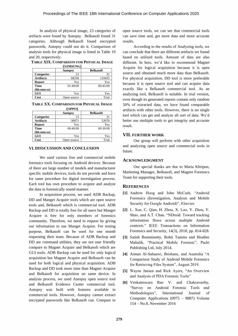
In analysis of physical image, 23 categories of
artifacts were found by Autopsy. Belkasoft found 31
categories. Although Belkasoft found encrypted
passwords, Autopsy could not do it. Comparison of
analysis tools for physical image is listed in Table 19
and 20, respectively.
TABLE XIX. COMPARISON FOR PHYSICAL IMAGE
(SAMSUNG) Autopsy Belkasoft
Categories 23 31
Artifacts 68258 110425
Report Yes Yes
Time
(hh:mm:ss)
01:49:00 00:45:00
GUI Yes Yes
Cost Open source Trial
TABLE XX. COMPARISON FOR PHYSICAL IMAGE
(OPPO) Autopsy Belkasoft
Categories 23 31
Artifacts 30971 52070
Report Yes Yes
Time
(hh:mm:ss)
00:49:00 00:30:00
GUI Yes Yes
Cost Open source Trial
VI. DISSCUSSION AND CONCLUSION
We used various free and commercial mobile
forensics tools focusing on Android devices. Because
of there are large number of models and manufacturer
specific mobile devices, tools do not provide and have
for same procedure for digital investigation process.
Each tool has own procedure to acquire and analyze
the data in forensically sound manner.
open source tools, we can see that commercial tools
can save time and, get more data and more accurate
results.
According to the results of Analyzing tools, we
can conclude that there are different artifacts we found
based on utilized tools. Amount of data are also
different. In here, we’d like to recommend Magnet
Acquire for logical acquisition because it is open
source and obtained much more data than Belkasoft.
For physical acquisition, DD tool is more preferable
because it is open source tool and can acquire data
exactly like a Belkasoft commercial tool. As an
analyzing tool, Belkasoft is suitable. In trial version,
even though its generated reports contain only random
50% of extracted data, we have found comparable
artifacts with other tools. However, there is no single
tool which can get and analyze all sort of data. We’d
better use multiple tools to get integrity and accurate
result.
VII. FURTHER WORK
Our group will perform with other acquisition
and analyzing open source and commercial tools in
future.
ACKNOWLEDGMENT
Our special thanks are due to Maria Khripun,
Marketing Manager, Belkasoft, and Magnet Forensics
Team for supporting their tools.
REFERENCES
[1] Andrew Hoog and John McCash, “Android
Forensics (Investigation, Analysis and Mobile
Security for Google Android)”, Elsevier.
[2] L. Xue, C. Qian, H. Zhou, X. Luo, Y. Zhou, Y.
Shao, and A.T. Chan. “NDroid: Toward tracking
information flows across multiple Android
contexts.” IEEE Transactions on Information
Forensics and Security, 14(3), 2018, pp. 814-828.
[3] Satish Bommisetty, Rohit Tamms and Heather
Mahalik, “Practical Mobile Forensic”, Packt
Publishing Ltd, July 2014.
[4] Aiman Al-Sabaawi, Brisbane, and Australia “A
Comparison Study of Android Mobile Forensics
for Retrieving Files System”, August 2019.
[5] Wayne Jansen and Rick Ayers, “An Overview
and Analysis of PDA Forensic Tools”
[6] Venkateswara Rao V. and Chakravarthy,
“Survey on Android Forensic Tools and
Methodologies”, International Journal of
Computer Applications (0975 – 8887) Volume
154 – No.8, November 2016
In acquisition process, we used ADB Backup,
DD and Manget Acquire tools which are open source
tools and, Belkasoft which is commercial tool. ADB
Backup and DD is totally free for all users but Manget
Acquire is free for only members of forensics
community. Therefore, we need to request by giving
our information to use Manget Acquire. For testing
purpose, Belkasoft can be used for one month
requesting their team. Because of ADB Backup and
DD are command utilities, they are not user friendly
compare to Magnet Acquire and Belkasoft which are
GUI tools. ADB Backup can be used for only logical
acquisition but Magnet Acquire and Belkasoft can be
used for both logical and physical acquisition. ADB
Backup and DD took more time than Magnet Acquire
and Belkasoft for acquisition on same device. In
analysis process, we used Autopsy open source tool
and Belkasoft Evidence Center commercial tool.
Autopsy was built with features available in
commercial tools. However, Autopsy cannot extract
encrypted passwords like Belkasoft can. Compare to
Proceedings of The IEEE 18th International Conference on Computer Applications 2020
279

Credit Card Fraud Detection Using Online Boosting
with Extremely Fast Decision Tree
Aye Aye Khine
Associate Professor,ICTRC
Yangon,Myanmar
Hint Wint Khin
Associate Professor,ICTRC
Yangon, Myanmar
Abstract
Nowadays, data stream mining is a very hot
and high attention research field due to the real-time
industrial applications from different sources are
generating amount of data continuously as the
streaming style. To process these growing and large
data streams, data stream mining, classification
algorithms have been proposed. These algorithms
have to deal with high processing time and memory
costs, class imbalance, overfitting and concept drift
and so on. It is sure that ensembles of classifiers are
being effectively used to make improvement in the
accuracy of single classifiers in either data mining or
data stream mining. Thus, to get higher performance
in prediction with largely no increasing memory and
time costs, this paper proposes an Online
Boosting(OLBoost) Approach, which is firstly use the
Extremely Fast Decision Tree (EFDT) as base (weak)
learner , in order to ensemble them into a single online
strong learner. The experiments of the proposed
method were carried out for credit card fraud
detection domain with the sample benchmark datasets.
Keywords: EFDT, Boosting, Credit Card Fraud, Data
Stream Mining
I. INTRODUCTON
Today, the volume of data generated from
different sources is increasing exponentially and the
analysis methods of such huge volumes give a
competitive advantages for the today’s business world.
Many applications, information systems used in the
modern business organizations are worked with the
rapidly changes in environments, in which data are
collected in the streaming form, i.e. “Data Streams”
(DS). Some obvious such examples are network
analysis, traffic control, GPS , mobile device tracking,
user’s click log mining, credit card fraud detection and
so on. In contrast with static data mining, processing
of streams need more computational requirements for
algorithms to incrementally process incoming
examples while using limited memory and time. In
addition, by reason of the non-stationary
characteristics, prediction models for data streams are
regularly also vital to adapt to concept drifts [1].
Data stream mining uses two main analytical
methods; classification and clustering. Among many
data stream classification learning methods, decision
tree learning method is ordinarily used, because of its
fast and it can be easily understood. Normally,
Decision Tree algorithms can be categorized based on
learning style: batch and incremental (online).
Likewise of batch data mining, there are data stream
classification algorithms and data stream clustering
algorithms. Typically, data stream classification is a
different alternative of incremental learning classifiers
that have to meets for massive streams of data with
restrictive processing time, limited memory, and
concept drift.
Based on our previous work [22], we have
learned that the Very Fast Decision Tree (VFDT)
algorithm [3] is one of the famous algorithm in
classifying data streams , being an online decision tree
with the advantage of a statistical property, the
Hoeffding Bound (HB). In the last years, the authors
[4, 5, and 6] have proposed a series of modifications to
increase the predictive performance of the VFDT
algorithm. Strict Very Fast Decision Tree (SVFDT) is
proposed in the paper [3] so that to address the memory
cost restrictions by keeping the predictive
performance,.
Moreover, in the paper [7], the authors
introduced the implementation of Hoeffding Anytime
Tree- “Extremely Fast Decision Tree” to improve upon
Hoeffding Tree (HT) by learning faster and ensuring
merging to the asymptotic batch decision tree on a
stationary distribution. Furthermore, the authors also
concluded that EFDT is good to consider of ensemble
by building as a forgetting, decay or subtree
replacement approaches in order to deal with the
concept drift.
Proceedings of The IEEE 18th International Conference on Computer Applications 2020
280

In recent year, it is sure that researchers in data
stream mining field are moving their focus to ensemble
based learning for various application domains. An
ensemble learning method; bagging, boosting and
stacking, also called a multiple classifier, is a number
of so-called base classifiers (weak learner), in which
the prediction results are combined to forecast new
received instances. Ensembles have been shown to be
a proficient way of improving predictive accuracy
or/and being a modeler for complex, difficult learning
problem by decomposing the easier sub-problems [1].
In the paper [8], the authors have investigated
the use of the SVFDT as base learner for ensemble
solutions such as OzaBag, OzaBoost, Leveraging
Bagging, Online Accuracy Updated Ensemble
(OUAE) and Adaptive Radom Forests (ARF), to
reduce memory consumption without harming the
predictive performance. The experimental and
comparable results are shown using thirteen
benchmark datasets.
Thus, inspired by these papers [ 7 and 8 ] , we
propose the Online Boosting Approach by coupling
with the Extremely Fast Decision Tree (EFDT) as base
(weak) learner in order to ensemble them into a single
online strong learner for credit card fraud detection.
The other remaining sections of this paper are
organized as follows. Section 2 discuss how to retrieve
information for our survey work of credit card fraud
detection. Section 3 describes ensemble approaches for
data stream and especially provides online boosting
methods while Section 4 discusses the proposed
methods in brief. Finally, Section 5 makes the
conclusion and identifies the directions for the future
work.
II. CREDIT CARD FRAUD DETECTION
Over the past few years, the usage of credit
cards is widespread in modern day society. As a result,
the fraud of credit card has been kept on growing.
However, the major causes of great financial losses is
credit card fraud although the careful and responsible
usage of credit card provides enormous benefits. In
addition, the improvement of new technologies offers
additional ways of crime may commit fraud. Actually,
Credit card fraud detection is considerably hard, but
also prevalent problem to solve [20]. In the literature,
many techniques have been proposed to conduct the
credit card fraud detection problem. Some researchers
use the advanced data mining methods while others use
data streams mining in order to detect credit card fraud.
It is certain that credit card frauds can costs
customers and banks billions of dollars totally. Thus,
the society needs a great and perfect fraud detection
system that not only can detect the fraud but also
prevent it in advance. Therefore, credit card fraud
detection methods need constant innovation and
attention.
In addition, some researchers did the parametric
comparisons of all the existing data mining technique
while some researchers did the literature review of all
the work done on fraud detection systems. Many AI
and machine learning techniques, data mining, fuzzy
logic, sequence alignment, neural network, logistic
regression, naïve bayesian, genetic programming,
decision tree etc., have developed in detecting for
various credit card frauds from massive credit card
transactions.
Normally, detection problems are solved with
two different styles: batch and online style. In the batch
learning style, a model detects occasionally relearnt
from scratch (e.g. once a year or month) while the
model is updated at once at the time of new data arrival
in the online learning style, that credit card transaction
in the form of data stream. Therefore, this also
subsequently, the detection of fraudulent use by data
stream mining is required.
In recent years, many researchers have paid a lot
of attention in stream data mining. Thus, streaming
data classification and clustering algorithms are
discussed with their key features and comparative
significance performances. Based upon the recent
survey of fraud detection techniques for credit card,
this paper mainly focus to present ensemble approach
coupling with online(incremental) decision tree
technique applied in credit card fraud detection
mechanisms in detail.
There are a lot of different credit card datasets
with different attributes such as type of fraud, number
of fraudulent records and etc., in order to detect fraud.
In this paper, we also follow the paper [21] to use
dataset obtained from UCSD-FICO competition. It
includes 100,000 records of credit card transactions.
Each record consists of 20 data fields. The label data as
legitimate and fraudulent, already defined by bank is
also included. That dataset includes 97% legitimate
transactions and the 3% of data records are fraudulent
transactions.
III. ENSEMBLES APPROACHES FOR DATA
STREAM
For the data stream mining, Ensemble
algorithms are most widely used techniques because
they can be combined with drift detection algorithms
Proceedings of The IEEE 18th International Conference on Computer Applications 2020
281

and include dynamic updates, such as selective
removal or addition of classifiers. In paper [9], the
authors proposed a taxonomy that is focused on
ensemble learning for data streams.
Based on their taxonomy, ensemble techniques
for data steams can be grouped as follow:
• Combination – Voting Method / Architecture
• Diversity–Inducer / Building Blocks for Ensemble
Solution
• Base Learner – Any stable classifier : Batch /
Incremental
• Update Dynamics – how learner takes place in the
ensemble manner.
From the paper [9], we have learned the various
base learners usage in ensemble approaches and also
known that decision trees, especially Hoeffding Tree
(HT) and its variations are the most common base
learner for ensemble learning in a streaming setting.
Likewise, in the paper [1] proposed the grouping of
ensemble learning approaches for data streams with
respect to the different points of view. The most
common categorization are the following:
• stationary vs non-stationary stream classifiers
• active vs passive approaches
• chunk based vs on-line learning modes
• distinguishing different techniques for updating
component classifiers and aggregating their
predictions.
From these systematic survey, though there
are serval not only bagging approaches but also
boosting approaches for data streaming, this paper only
focus on using the boosting ensemble methods as they
offer several recognized guarantees and are mostly
effective when the base models are simple.
A. Online Boosting Ensembles
In order to increase the predictive performance
of Online Decision Tree (ODTs), a lot techniques have
been proposed. Among them the three main groups
such as the structural modification of the decision tree
the additional prediction strategies with the same
structure; and the ensembles approaches are famous
[2]. From them, the last, ensembles methods have been
many proposed not only bagging and boosting with the
online style. Due to the focus of this paper is online
boosting, the following paragraph is described some
related works.
Oza and Russell introduced [10], a parallel
boosting strategy by just following AdaBoost with the
exception of weight calculation , because AdaBoost
can do training with prior knowledge of the number of
instances available and it cannot be use with data
stream setting. It is called OzaBoost. Due to its
simplicity and efficiency, OzaBoost has also got many
great achievement in the real-world applications,
especially for the computer vision [11],
Many other online boosting algorithms have
been addressed for different application needs, such as
semi-supervised learning [11], multi-instance learning
[12], and feature selection [13].
Online Gradient Boost [11] is an online variant
of Gradient Boost, which uses functional gradient
descent to decide the optimal example weights and
greedily minimizes the loss function of interest. It is
denoted as OGBoost. Online Smooth Boosting
(OSBoost) is proposed in paper [14].
In 2004, the paper [2], the authors proposed the
Adaptive Boosting ensemble algorithm and did
practical experiments with the real life data containing
100 k credit card transactions. In 2013, the paper [14]
proposed OzaBoost Dynamic, in which the weight
calculation is modified and the number of boosted
“weak” learners are used in order to improve its
performance in terms of memory consumption and also
presented the pragmatic results showing the
performance of all algorithms using data sets including
fifty and sixty million instances.
In the paper [15], the author proposed an
algorithm called Online Non-Stationary Boosting
(ONSBoost) that are similar with Online Boosting, and
also uses a static ensemble size without generating new
members. At each time, new examples are presented
and it adapts the changes in the data distribution. Using
a parallelizing virtual machine, ONSBoost is evaluated
with Online Boosting on the STAGGER dataset and
the derived three other datasets.
In the paper [8], the author proposed SVFDT as
base learner in not only OzaBoost but also bagging and
shown the experimental results. Inspirations based on
these literature, this paper propose Online Boosting
(OLBoost) Approach by coupling with the Extremely
Fast Decision Tree (EFDT) as base (weak) learner and
explain detail in the next section.
IV. PROPOSED METHOD- ONLINE BOOSTING
WITH EFDT
In 2000, the paper [18] presented Hoeffding
Tree, namely Very Fast Decision Tree (VFDT)
algorithm. For data stream classification, it is one of the
most popular and first algorithms, being capable of
Proceedings of The IEEE 18th International Conference on Computer Applications 2020
282

inducing a decision tree in an online fashion with a
statistical property, the Hoeffding Bound (HB).
Hoeffding bounds is usually applied in the decision
based on the number of instances to be trained to reach
a certain level of confidence. After that, many variants
or modifications of VFDT are emerged and that
summary is shown in the table 1, as we described in our
previous work [22].
TABLE I. SUMMARY OF ONLINE DECISION TREE
The paper [7] has introduced Hoeffding
Anytime Tree (HATT) and denoted as “Extremely Fast
Decision Tree (EFDT). Hoeffding Tree usually builds
a tree increment manner, making the delay in selecting
of a split at a node until not only it is confident but also
it has identified the best split, and never revisiting that
decision. Instead, HATT usually uses to select and split
as soon as it reaches confident level and that split is
useful, and then revisits that decision, make the
replacement with the split if it subsequently becomes
evident that split is better. Though EFDT is a learner
not for concept drift, the authors [7] observed that it is
highly effectively on benchmark dataset and has some
inbuilt acceptance to concept drift.
TABLE II. EXPERIMENTAL PLAN FOR
PROPOSED METHOD
Ensemble Base Learner Dataset
OzaBoost
EFDT(HATT) Public Dataset for Credit Card Fraud
Detection
OGBoost
OSBoost
OSBoost.OCP
OSBoost.EXP
ONSBoost
OzaBoostDync
V. CONCLUSION AND FUTUREWORK
With the aim to reduce costs of loss caused by
credit card frauds in every year, this paper proposed an
ensemble approach, online boosting using online
decision tree, namely EFDT, as base learner. The
experimental results of proposed method will be done
as our plan and also plan to make comparative study of
our proposed method with online boosting using others
base learners by using not only UCSD-FICO credit
card dataset but also another credit card dataset from
Kaggle website.
ACKNOWLEDGMENT
This work is supported and encouraged me by
my beloved supervisor, Dr. Hnit Wint Khin, Associate
Professor, Information and Communication
Technology Research Center (ICTRC) , Yangon
Myanmar.
REFERENCES
[1] B. Krawczyk, L. Minku, J. Gama, and J.
Stefanowski, “Ensemble learning for data stream
analysis: A survey,” Information Fusion, vol.
37,pp. 1–86, 2017.
[2] F. Chu, C. Zaniolo, “Fast and light boosting for
adaptive mining of data streams”, in: Proceedings
of the Eight Pacific-Asia Knowledge Discovery
and Data Mining Conference (PAKDD’04), 2004,
pp. 282–292. Sydney
[3] V. G. T. Costa, A. C. P. L. Carvalho, and S.
Barbon Junior, “Strict Very Fast Decision Tree: a
memory conservative algorithm for data stream
mining,” ArXiv e-prints, May 2018.
[4] Holmes, G., Richard, K., Pfahringer, B., 2005.
“Tie-breaking in Hoeffding trees” , in: Proc. of the
II Int. Workshop on Knowledge Discovery from
Data Streams
[5] Yang, H., Fong, S., 2011b. “OVFDT with
functional tree leaf - majority class, naive bayes
and adaptive hybrid integrations”, in: Proc. of the
III International Conference on Data Mining and
Intelligent Information Technology Applications,
pp. 65–70.
[6] Yang, H., Fong, S., 2013. “Incremental
optimization mechanism for constructing a
decision tree in data stream mining”,
Mathematical Problems in Engineering 2013,
114–144.
Proceedings of The IEEE 18th International Conference on Computer Applications 2020
283

[7] Manapragada, C., Webb, G. I., Salehi, M. (2018)
“Extremely Fast Decision Tree”, Proceedings
KDD 2018, ACM Press, New York, NY, USA,
pp. 1953-1962.
[8] Victor G. Turrisi da Costa, Saulo Martiello
Mastelini, Andre C. P. L. F. de Carvalho, and
Sylvio Barbon. “Making data stream
classification tree-based ensembles lighter” ,in
7th Brazilian Conference on Intelligent Systems,
BRACIS 2018, Sao Paulo, Brazil, October 22-25,
2018, pages 480–485, 2018.
[9] H. M. Gomes, J. P. Barddal, F. Enembereck, A.
Bieft, “ A Survey on Ensemble Learning for Data
Stream Classification”, ACM Computing
Surveys, Vol. 50, No. 2, Article 23, Publication
date: March 2017
[10] N.C. Oza. , “Online bagging and boosting”, In
Systems, Man and Cybernetics, 2005 IEEE
International Conference on, Vol. 3. 2340–2345
Vol.3.DOI:http://dx.doi.org/10.1109/ICSMC.200
5.1571498
[11] Grabner, H., Leistner, C., and Bischof, H.
“Semisupervised on-line boosting for robust
tracking”, in Proceedings of ECCV, pp. 234–247,
2008.
[12] B. Babenko, M. Yang, and, S. J. Belongie ,
“Visual tracking with online multiple instance
learning” , in Proceedings of CVPR, pp. 983–990,
2009b.
[13] Liu, X. and Yu, T., “Gradient feature selection for
online boosting”, in Proceedings of ICCV, pp. 1–
8, 2007.
[14] Erico N. de Souza and Stan Matwin ,
“Improvements to Boosting with Data Streams”,
[15] A. Pocock, P. Yiapanis, J. Singer,
M. Luj´an, and G. Brown, “Online Non-
Stationary Boosting”,
[16] A. Beygelzimer, S. Kale, and H. Luo. “Optimal
and adaptive algorithms for online boosting”, in
Proceedings of the 32nd International Conference
on Machine Learning, 2015.
[17] S.Tse Chen, H. Tien Lin, and C.Jen Lu, “An
Online Boosting Algorithm with Theoretical
Justifications” , in Proceedings of the 29th
International Conference on Machine Learning,
2012
[18] P. Domingos and G. Hulten. 2000. “Mining high-
speed data streams”, in proceedings of the sixth
ACM SIGKDD international conference on
Knowledge discovery and data mining. ACM,
71–80
[19] C. Marsh, “Boosting in the Online Setting”.
[20] D. Meenakshi. B, J. B. Gayathri. S , “Credit Card
Fraud Detection Using Random Forest” ,
Volume:06, Issue:03, March 2019,p-ISSN:2395-
0072
[21] M. Zareapoora, P. Shamsolmoalia, “Application
of Credit Card Fraud Detection: Based on
Bagging Ensemble Classifier”, International
Conference on Intelligent Computing,
Communication & Convergence
(ICCC-2014)
[22] A. Aye Khine, H. Wint Khine,”A Survey of
Decision Tree for Data Streams to Detect Credit
Card Fraud”, PROMAC-2019
Proceedings of The IEEE 18th International Conference on Computer Applications 2020
284

Developing and Analysis of Cyber Security Models for Security Operation
Center in Myanmar
Wai Phyo Aung
Department of Automation
Control System
Moscow Automobile and
Road Construction State
Technical University,Russia
Htar Htar Lwin
Faculty of Computer
Systems and Technologies
University of Computer
Studies,Yangon
Kyaw Kyaw Lin
Department of Computer
Technology
Defence Services Academy
Pyin Oo Lwin
Abstract
In counteraction to the increasing threat of
cyber terrorism, the modeling to be predicted in
guessing the predictive models for estimating the
incidence of cyber-attacks for enterprise network in
Myanmar are seriously needed. Although we need
these models, there is no record of attacks,
defenseless, outcome and threat to utilize the
developing predictive models and authentication. The
main purpose of this research is to determine
whether SOC (Security Operation Center) manager
uses cyber security model by using SOC results
figures to prepare further cyber defense and incident
response plan. The goal of this study was achieved by
conducting experiments on various cyber-attacks
occurred in security operation center of Industrial
Control System (ICS).
Keywords: Blue team, Incident Handling, SOC,
Cyber Security Model, Vulnerabilities, Threats,
Attack.
I. INTRODUCTION
Responding to cyber terrorism, the researchers
and practitioners need to develop and analyze the
cyber security prediction models and to serve as a
framework to be used as resource into the scheme to
support the decision. Due to the harshness of cyber
security problem and the confusion which can be
caused by cyber-attacks on the Enterprise’s
information infrastructure, we are induced to build up
the prediction models. The critical factor for cyber
threat problems will be expressed in excerpts from the
following our SOC reports.
Security analyst which represents the Blue
Team of Enterprise network always watching the
SOC. As per duties and responsibilities of SOC
analyst, there are many events in every times. When
he finds the critical events he will report that events to
red team and purple team at first [1]. And then he will
fix or patch that critical vulnerabilities. After that
security analyst had many questions. Which sectors
still get vulnerabilities and need to change or manage
for coming cyber-attacks? SOC shows events
according in their security directive rules. But SOC
cannot show which sectors need to change or manage
not to damage for upcoming attacks [2]. We will
focus beyond the SOC to develop the predictive cyber
security model.
Figure 1. Top 10 events and hosts according SOC
Building up and knowledge of the theory of
cyber security models is one of the important matters.
Let us mention the types of cyber security models: the
risk model and the exponential models. The risk
model form one of the models can foresee the threat
of attack in a weak position of indicated cyber
security situation. It supports the incident handling
including networking, log analysis, forensic and
packet analysis. The exponential model called the
second model, is time based and anticipate the
duration between the probability of attacks for a given
risk priority. It supports the incident response
Proceedings of The IEEE 18th International Conference on Computer Applications 2020
285

including logistic, communications, coordination and
planning. The occasion happening during attacks is
substitute measure of risks. When duration between
attacks becomes longer, the risk of the user is
becoming greater because of the result of a growing
number of attacks. It is vital to note that we cannot be
foreseeable the cyber-attacks which will happen in the
near future. So the models mentioned above can be
endorsed against the real-world attack. Illustration the
important parameters and variables in the security
operation center for researchers and SOC managers
from Blue team can be only done.
There are the reasons why the experiments
were conducted by solving with the help of cyber
security. To get the occurring response the OODA
Loop method, developed by US Air Force military
strategist John Boy is needed to be employed. The
OODA Loop method is aimed at attention to the
crucial methods to be able to act in response to any
information of security crisis: Observe, Orient,
Decide, and Act (OODA). SOC can support various
observation and orientation. Risk model can do
decision making and exponential model can take
response actions.
There may be coming up research questions
that are crucial in response to cyber security crisis.
These concerning questions are as below:
1) Can a variety of presentations and models of
cyber security which is advanced provide the
frame for researchers and practitioners to
promote the field?
2) Can the models of hypothetical predictions
be developed to evaluate the threat of different
types of cyber-attacks?
Nonetheless, it is still useful to answer the
upcoming questions after actions related to potential
attacks if we provide explanations, equations, plots
and analyses and synthesis. It stands to reason that we
need to learn about the components of predictive
models and their interactions to reflect objects and
events in the enterprise network. The target of these
models is for providing the SOC managers while
investigating the assumption about how to take
actions to cyber-attack prior to occurrence using risks,
weakness, duration between attacks and interruption
(number and time) concepts.
The rest of this paper is organized as follows.
In section 2, we explored related works. Model
structure of Risk Model was presented in section 3.
Experiment and analysis were mentioned in section 4.
We discussed and concluded our research in section 5.
We left some future works in section 6.
II. RELATED WORK
Cyber security of Industry Control System
(ICS) has become a major topic of active research [3].
It is of great importance and we need to realize the
complexity and obstacles with these. They focused a
main problem of cyber security research which means
that it is supposed to concentrate on occurrence of
security in dealing with the information and
communication technology [4], while they barely
calculate the real result of successful attacks. As a
result, Access to risk of quantity is not that easy to
get. Some of researches use Preliminary
Interdependency Analysis (PIA) models that are well
fitted for assessment of quantity of risk, as Both ICT
and ICS are widely employed in. Even though PIA
had not been used to explicitly express and inform
cyber security concerns.
In [5] the researchers extended the risk
assessments method Risk = (Asset Value * Event
Priority * Event Reliability) / 25. There are several
domains within cyber security end users related
models, or organizational level modeling, therefore it
supposed to narrow down his focus and then start
work on it. It also give introduction the perception of
cyber security according to its framework, workforces
and other related information of personal data in the
computer. Their works give results from an efficient
audit of time based attacks which ruled with SOC's
Host-based Intrusion Detection System (HIDS) and
Network-based Intrusion Detection System (NIDS)
correlation directives countermeasure. They
calculated and correspondence the risk and
exponential model under time based attacks. In their
study they explore the attack parameters (sensitivity
analysis) and time. As a result, the competitor would
decide the same even if attacker is addressed at
several times the same choice during the violence.
That’s why studying the behavior of one attacker and
attack-strategy at a time will be enough to find out;
comparison of the impact of multiple, different classes
of intruders and various attack-strategies require
building separated models and studies.
In this research [6] cyber security operations
center installment of models are proposed to provide
better and advancing awareness to situation in order to
detect common and frequent advantage, and also
approached and cross-channel exploits. 0 (Zero) day
exploits are now common and frequent, and impacts
far much greater than before. This situation is further
made worse by the lack of sufficient and well
deployed security operations centers to watch
Proceedings of The IEEE 18th International Conference on Computer Applications 2020
286

organizational cyber investments to get perimeter
defense.
In this research paper we used Open Source
Security Information Management (OSSIM) which
was provided AlienVault. It includes HIDS and
NIDS.
III. MODEL STRUCTURE OF RISK MODEL
This model relates the basic theory of
information security which is probability of attack,
likelihood of weak points and outcome of an attack.
We assume that risk can be accurately calculated by
using equation (1).The justification is that risk in
intuitive way would increase as all three quantities
comprising equation (1) increase.
Risk (R) = Relative Probability of Attack (A) *
Probability of Vulnerability (V) * Consequence (C)
As the symbol, we can assume their identification
R1 = Pai*Pvi*C ()
Examples of (2) include:
R1=Pai (Malware) * Pv1 (AD server down) * C1 (Consequence of Risk priority 1) ()
2R =Ra2 (Hash dump) * Pv2 (SMB open) * C2 (Consequence of
Risk Priority 2) (3)
The measure for probability of attack, relative
probability of attack, is estimating using the following
equation.
1
( )
( )
Lai n
L
i
T iP
T i=
=
(4)
aiP =
Relative probability of risk priority i (attack types).
( )LT i - Relative threat level of attack of risk priority i
IV. CYBER SECURITY IN
ENTERPRISE INFRASTRUCTURE
TABLE I. CYBER SECURITY IN CRITICAL
ENTERPRISE INFRASTRUCTURE Vulnerabilit
y
iV
Consequence
iC
Attack Vectors,Risk
Priority iA
1V -
Network
Firewall
1C
- Firewall
down
1A - Denial of Service
(DoS)
2V -Host
firewall
2C - AD server
down
2A - Man in the Middle
(MITM)
3V -
Password Capture
3C - Web server
down
3A - Information
disclosure
Protection (https)
4V - Web
Application Firewall
(WAF)
4C - Operating
System crash 4A - Malware
(Ransomware)
5V - Host
Malware
Protection
5C - Application
corrupted
5A - Virus (damage
Database and OS)
6V - Host
Endpoint Security
6C - Hardware
Failure
6A - Trojan
7V -
(Network
Instruction
Detection System
(NIDS)
7C -Router
Misconfiguration
7A - Remote Code
Execution (RCE)
8V - Data
Loss
Prevention (DLP)
8C -
Transmission
Link Down (ISP down)
-
9V - IP
security
9C - Proxy server
down
-
10C -Power
failure
-
iR - Risk of priority i. Risk priority is the
consequence of a given types of attack (DoS, Virus.
Malware,etc.)
aiP - Relative probability of risk priority i.
viP - Probability of vulnerability of risk priority i. we
must count or scan this probability in each endpoint.
iC - Consequence associated with risk priority i. The
numbers of network objects that affected (AD Server,
WEB server, UPS for power failure, etc.)
( )LT i - Relative threat level of attack of risk priority i.
N – Total numbers of various attacks.
V. EXPERIMENT AND ANALYSIS OF
MODELS
In this section, we calculate Risk Model and
Exponential Model. Then analyze Time based attacks
and Rate of change of Time between Attack events.
A. Calculation for Risk Model
We will calculate and plot that demonstrate
risk model outputs. The sensitive data in the Table I
was developed as follows. The first column of the
table shows 10 major types of attacks in our
Enterprise network. Starting with Alert – the most
severe and ending with Application the least severe.TL
(i) also represent a subjective assessments of the
relative threat level of various types of attacks,
Proceedings of The IEEE 18th International Conference on Computer Applications 2020
287

starting with Alert = 68,700 which was 37% of the
whole critical security events, and ending with corrupt
of Application = 704 is computed from (4).
Data is not still available for Pai .We calculate
the relative threat level (Pai ) from real time SOC
system. The desired output risk = Ri is computed from
Eq (1). The bold values in the table emphasize the
significant results. Figure 2 shows how risks differ
from the probability of attack. The plot is made notes
with the types of attacks associated with the major
risk values. As [7] a practical matter, the plot indicates
that risk would rise rapidly at a value of 0.15aiP .
This could be assumed a major risk and that the
blue team should prepare to incident response plan for
weak security policy.
TABLE II. ATTACK TYPES AND DATA FOR RISK
MODEL
Attack
Type ( )LT i Related Threat Level
= Relative
Probability of Attack
aiP
1 Alert 68,700 (37% ) 0.322
2 System 20,615 (11%) 0.096
3 Access 13,687 0.064
4 Info 3,475 0.016
5 Suspicious 1,288 0.006
6 Authenticat
ion
49,044 (26%) 0.230
7 Malware 18,230 (10%) 0.085
8 Exploit 3,734 0.017
9 Policy 3,3436 0.157
10 Application 704 0.003
1
( )a
L
i
T i=
1
( )
( )
L
a
L
i
T i
T i=
TABLE III. ATTACKED HOST AND DATA FOR
CALCULATION RISK MODEL
However we note in Table II that Ri is
significantly a function of consequences iC . Thus the
analysis of the assignment of iC to the relative threat
levels could be performed.
Figure 2. Risk Ri and probability of attack Pai
Figure (1) and (2) shows us the relationships
among risk, probability and consequences. We
analyzed to have more than one view of the
relationships to prove the others. (i.e Figure (3) make
proves that the Figure (2) show the Security Policy
weakness being the major risks.)
Figure 3. Risk Ri and consequence Ci
Figure (3) shows that risk increases with
consequences, as we would expect and again the
diagram is annotated with the major risk attacks of
Security Policy weakness.
B. Calculation for exponential model
The basic of this predictive cyber security
model is that the time between attacks, ta is a key
changeable in working against attacks. Pai is data on
probability of attack. We measure relating level of
threats, TL to estimate Pai. ta can measure the risk
because of the smaller the value of ta which can
happen the growing frequency of attack. (i.e. the
higher risk). This cyber security model opposed the
accounts of risk priority (i) and specific types of
attacks and attacked hosts from the events of SOC.
( )ai LP f T=
(5)
Attacked
Host
Rate of
Attack
(N(T))
Vulnerabilities
which is
scanning from
each endpoint
host viP
1 ai vi iR P P C= + +
iC
1 10.0.1.172 12 0.66 0.21 1
2 10.0.19.7 15 0.55 0.21 4
3 10.0.1.168 18 0.44 0.16 6
4 10.0.1.170 21 0.77 0.03 3
5 10.0.1.154 29 0.55 0.01 2
6 10.0.1.163 31 0.77 0.17 1
7 10.0.1.156 33 0.88 0.15 2
8 10.0.1.174 34 0.33 0.01 2
9 10.0.1.160 41 0.33 0.25 5
10 10.0.1.23 53 0.11 0.01 1
Proceedings of The IEEE 18th International Conference on Computer Applications 2020
288

In the above equation, to develop the model,
we formulate probability of attack as a function of
relative threat level.
Where, LT = relative threat level;
at = time between attack of type a day.
N (T) = number of attacks in Time T. (we
gets that data from our enterprise SOC)
T = specified attack time period in 365 days
( )N T
T = = rate of attack per day (6)
t
aiP e a −= (7)
In the above Eq means the probability of density function for the exponential distribution by assuming for Pai. We calculate the Eq (7) to produce the following equations (8) and (9)
log( ) logai aP t = − (8)
log log( )a ait P = − (9)
By solving equation (9) for at , we obtain
equation (10)
1log( )a
ai
tP
= (10)
C. Analyzing Time Based Attack
The plot of time between attacks ta and
probability of attack Pai is shown in Fig (4). In our
events data, there is no saturation ta > 24 hours.
Because of low value of ta imply high frequency of
attack.
Growing time of attack may also occur high
risk. This security policy would exclude all attacks
vectors except Denial of Service (DoS) / Distributed
Denial of Services (DDoS). This plot shows us how
much we can manage incident handling response as
quickly as possible.
Figure 4. Expected frequency of attack and
probable attack Pa(t) at time t 24 hours
If our enterprise network gets DDoS attack. We
can measure the increasing traffic based on . By
seeing upcoming NetFlow results, Firewall
throughputs and DDoS Protectors throughputs, we
can countermeasure the stability of DDoS protector
live.
TABLE IV. CALCULATION OF TIME BETWEEN
ATTACKS
D. Rate of change of Time between Attacks
events
The rate of change of time between attacks is
related to the possibility of attack is obtained by
making a distinction (10).
2 2
( ) 1 1 1 1( )( ) ( )( )
( )
a ai
ai ai ai
d t P
d P P P = − = −
(11)
It gives the (11) which tabulates in Table IV.
Figure 5. Rate of change of time between attacks
d(ta) / d(Pa) and probability of attacks Pai
That quantity is of interest because we can see
when the rate of change of ta which is a replacement
Rates of
Attack
in 365
days
(N(T))
aiP
Attack
by
Day( )N T
T
Days
between
Attack1
log( )aiP
Hours
between
Attack
( *24at )
Hours
between
Attack
( )
( )
a
ai
d t
d P
1200 0.322 3.2876
71
2.321313
915
16.9455915
8
-
0.286727058
1500 0.096 4.1095
89
3.748187
699
21.8894161
6
-0.611536032
1800 0.064 4.9315
07
4.340081
745
21.1217311
6
-0.639638551
2100 0.016 5.7534
25
5.865084
423
24.4657807
3
-1.850949244
2900 0.006 7.9452
05
7.180361
666
21.6896442
1
-2.618641519
3100 0.230 8.493151
3.607425814
10.19388714
-0.060183666
3300 0.085 9.0410
96
4.659595
437
12.3691078
9
-0.142880631
3400 0.017 9.3150
68
6.275036
943
16.1674481
2
-0.657136758
4100 0.157 11.232
88
4.270095
367
9.12342327
2
-0.050466813
5300 0.003 14.520
55
8.387425
3
13.8629897
4
-1.434377651
Proceedings of The IEEE 18th International Conference on Computer Applications 2020
289

for risk. ta becomes small that the threat is virtually
nonexistent. That saturation is demonstrated in Fig
(5), where Pai = 0.085 corresponds to a Malware
attack. At that point, the pace of change is too tiny,
meaning that the pace of change of risk is of little.
VI. DISCUSSION AND CONCLUSION
Having stated that time between attacks ta is a
delegate for risk Ri. We analyze and investigate this
hypothesis by scheming the former against latter. The
result is shown in Fig (6).
Figure 6. Time between Attacks ta and Risk Ri
It shows a fairly good correspondence. The fact
that the proponent model called exponential in another
way is much easier to execute than the risk model is
of importance. The former could use the SOC
manager’s prediction model of choice [8].
Internet203.81.x.x
ASR 1002
BGP Router
Next-Generation Firewall
Core
Switch
OSSIM SensorOSSIM Server
OSSIM Web UI
Productions/
Services Managements
OSSIM Sensor
Risk Model Exponential Model
Observe Orient Decide Act
Aggressive
Switch
Figure 7. Big picture of SOC analyst for incident
handling and response
There are many huge cyber attacks daily in real
world. SOC analyst should handle the top major
attacks which are pushed by the security policy and
best practice for infrastructure security. Risk and
Exponential models are fully effectiveness for priority
of incident handling and response as OODA loop
among that many huge cyber attacks: What is critical
and How is it protected ?
In the research question section, we suggested the
following questions were answered by this research
paper:
1) Can different show off and models of cyber
security which is advanced provide the frame for
researchers and practitioners to promote the ICT/ICS
security research field?
Our paper suggests that, explanation,
equations, plots, tables which comprise a frame work
depending on our blue team for ICT/ICS security
research, the answer is “true”.
2) Can the models of hypothetical predictions
be developed to evaluate the threat of various and
sophisticated types of cyber security attacks?
For answering this question is also “true” we
calculate and demonstrate as evidence relevant
scheme. (i.e. The Risk Model in Figure-2 identifies
the maximum risk attacks, which was security
weakness policy. Furthermore, with respect to the
Exponential model, Figure-4 provides us with the
probability of attack and Time between Attacks
threshold.
VII. FUTURE STUDY
We left some works to do as future research.
We are still developing in writing of SOC directive
rules to do as future research. Our study is limited to
the effect of a malware type of attack on system
behavior: a cyber-attack via the Ransomware of a sub-
station. According detective of SOC, cyber security
model need to extend for multiple stations..
ACKNOWLEDGMENTS
This work was partially provided by the private
data center under the development of open source
Security Operation Center (SOC) project that is called
Open Source Security Information Management
(OSSIM). We collected the required data for our
analysis.
REFERENCES
[1] SAN SEC450: Blue Team Fundamentals:
Security Operations and Analysis
[2] SAN SEC511: Continuous Monitoring and
Security Operations.
[3] O. Netkachov, P. Popov, and K. Salako, “Model-
Based Evaluation of the Resilience of Critical
Infrastructures Under Cyber Attacks”, 9th
International Conference on Critical Information
Infrastructures Security
Proceedings of The IEEE 18th International Conference on Computer Applications 2020
290

[4] C. Onwubiko, “Security operations centre:
Situation awareness, threat intelligence and
cybercrime”, International Conference on Cyber
Security And Protection Of Digital Services
(Cyber Security), 2017
[5] K. Thakur, M. Qiu, K. Gai and M.L. Ali, “An
Investigation on Cyber Security Threats and
Security Models”, IEEE 2nd International
Conference on Cyber Security and Cloud
Computing, 2015
[6] ICS410: ICS/SCADA Security Essentials
[7] L.Janczewski and A. M. Colarik, “Cyber warfare
and Cyber Terrorism”, ISBN- 9781591409922
[8] D. Murdoch, “A Condensed Guide for the
Security Operations Team and Threat Hunter”,
Blue Team Handbook: SOC, SIEM, and Threat
Hunting (V1.02), ISBN-10: 1091493898
Proceedings of The IEEE 18th International Conference on Computer Applications 2020
291

Influence of Voice Delay on Human Perception of Group Synchronization Error
for Remote Learning
One-way Communication Case
Hay Mar Mo Mo Lwin
Department of Hardware
University of Computer Studies
Yangon, Myanmar
Yutaka Ishibashi
Department of Computer Science
Nagoya Institute of Technology
Nagoya, Japan
Khin Than Mya
Department of Hardware
University of Computer Studies
Yangon, Myanmar
Abstract
This paper clarifies the influence of the voice
delay on human perception of group synchronization
error in remote learning by subjective assessment. In
our assessment, we produce the difference in output
timing of lecture video between a teacher terminal
and a student terminal. Each subject as a student
observes the output timing relation (i.e., group
synchronization) between the lecture video and
teacher’s voice, and then the subject answers
whether he/she perceives the group synchronization
error or not. We also examine the influence of
difference in voice contents on the error. Assessment
results demonstrate that the perception rate depends
on the group synchronization error plus the voice
delay, and all the subjects can hardly perceive group
synchronization errors (plus voice delays) less than
or equal to about 250 ms. We further illustrate that
the perception rate depends on the voice contents.
Keywords—Remote learning, Voice, Video, Group
synchronization error, Human perception, Subjective
assessment
I. INTRODUCTION
In multimedia applications such as video
conferencing, remote learning, and networked games,
the temporal relationships among multiple media
streams (for example, voice and video) are important
[1]-[3]. Such applications sometimes need to
synchronize the output timings of several media
streams at all the terminals. If the output timings of
each media unit (MU) [4], which is an information
unit such as a video picture and a voice packet for
media synchronization, among multiple terminals are
different from each other (that is, there exist group
synchronization errors), the quality of experience
(QoE) [5] may be damaged seriously [6]. This may
affect the learning effect in remote learning, for
example.
To solve the problem, we need to carry out
group (or inter-destination) synchronization control
[6]-[10], which adjusts the output timing of media
streams among multiple terminals (or destinations).
In [11] and [12], two error ranges are employed: One
is the imperceptible range in which the
synchronization error cannot be perceived by users,
and the other is the allowable range in which the
error is felt to be allowable for users. In [15], we
carry out the subjective assessment to clarify the
allowable and imperceptible ranges of group
synchronization error. However, the voice delay is
assumed to be negligible small. Also, we handle only
a set of voice and video contents. We need to clarify
influences of voice delay and voice and video
contents on the group synchronization errors. This is
because the imperceptible and allowable ranges have
not been clarified so far.
Therefore, in this paper, we carry out the
subjective assessment of group synchronization error
by changing the voice delay to investigate the
influence of voice delay in remote learning. We also
examine the influence of voice contents on the error.
The rest of this paper is organized as follows.
We give an outline of the group synchronization in
remote learning in Section 2. We also explain the
assessment method in Section 3. Then, assessment
results are presented in Section 4. Finally, Section 5
concludes the paper.
II. GROUP SYNCHRONIZATION IN
REMOTE LEARNING
In multicast communications, we need to
perform group synchronization control, which tries to
output each MU simultaneously at all the different
terminals. If the control is not carried out, the MU
cannot be outputted at the same time at the terminals;
that is, the group synchronization error occurs.
The configuration of our remote learning
system is shown in Fig. 1. The system consists of N
(≧ 1) terminals (one terminal is for a teacher, and the
other terminals are for students) [15]. The teacher
terminal uses a microphone, and each student
Proceedings of The IEEE 18th International Conference on Computer Applications 2020
292

Teacher
Student 2
Student 1
Student N
Video multicast
File server
Microphone
Headset 1
Headset N
Headset 2
Figure 1. System configuration of remote learning.
terminals employ a headset. The file server
multicasts a video stream to all the teacher and
student terminals. The teacher orally explains the
video contents while watching the video. A voice
stream of the teacher captured via the microphone is
multicast from the teacher terminal to all the student
terminals. Each student listens to the teacher’s voice
while watching the same video [15].
III. ASSESSMENT METHOD
In the assessment, we set N=1 for simplicity
as shown in Fig. 2, where two terminals were used;
one was for a teacher, and the other was for a
student. For simplicity, the two terminals were
located at different places in a room so that the
student (teacher) could not see the screen of the
teacher (student) terminal. We did not use the
microphone at the teacher terminal, but we used the
headset for the student terminal.
Alternatively, we saved the teacher’s oral
explanation as a voice file at the teacher and student
terminals, and the corresponding video file was also
saved at the two terminals. We produced the group
synchronization error of video by changing the start
time of video output at the two terminals. The
student terminal started to output the voice file after
the voice delay when the teacher terminal started to
output the voice and video files. By these setups,
we constructed our assessment environment without
transmitting voice and video between the two
terminals. We used the video and voice contents
explaining I/O devices such as a mouse and a
printer in remote learning, and their output duration
was 1 minute and 32 seconds [15].
At the beginning of assessment, we
presented a situation in which the group
synchronization error is zero and the voice delay is
zero to each subject at the student terminal; that is,
we started to output the voice and video files
simultaneously at the student terminal. We used the
single-stimulus method [13].
Teacher Student
Same video and voice
files are saved.
Figure 2. Assessment system
Proceedings of The IEEE 18th International Conference on Computer Applications 2020
293

During the assessment, each subject watched
the lecture video and listened to the teacher’s voice.
We changed the group synchronization error from –
700 ms to +550 ms at intervals of 50 ms, where
negative values denote the teacher ahead of the
student and positive values do the teacher behind of
the student, and we also changed the voice delay from
0 ms to 100 ms at intervals of 50 ms. Combinations of
the error and delay were presented to each subject in
random order. To examine the influence of the voice
delay more clearly, we also changed the error from –
100 ms to 100 ms and the delay from 0 ms to 600 ms
at intervals of 50 ms. The subject did not know the
value of the error and delay presented in the
assessment.
After presenting each combination of the error
and delay, we asked the question to each subject
(student) as follows: “Did you perceive the group
synchronization error?” The subject answered either
“Yes” or “No.” He/she judged whether the error was
perceived or not by monitoring the temporal relation
between the teacher’s voice and displayed video
images.
The total assessment time per subject was
about 95 minutes including the explanation time of
how to judge the error. The number of subjects
(students) was 15 females, and their ages were
between 28 and 37.
IV. ASSESSMENT RESULTS
We plot the perception rate which is here
defined as the percentage of subjects who perceived
group synchronization errors as a function of the
group synchronization error in Fig. 3, where we set
the voice delay is 0 ms, 50 ms, and 100 ms. We also
show the perception rate versus the voice delay for
group synchronization errors from –100 ms to 100
ms in Fig. 4.
In Fig. 3, we see that the perception rate is 0%
when the group synchronization error is between
around –250 ms and 250 ms and the voice delay
value is 0 ms. As the absolute error exceeds about
250 ms, the perception rate starts to increase; when
the absolute error is larger than or equal to about
500 ms, the perception rate is 100%. We also find in
the figure that when the delay is 50 ms and 100 ms,
we can obtain the perception rate by shifting the
results at the delay of 0 ms leftward (i.e., the
negative direction) by 50 ms and 100 ms,
respectively.
In Fig. 4, we notice that the perception rate
starts to increase when the voice delay exceeds
about 250 ms and the group synchronization error is
0 ms; for the other errors, we can obtain the
perception rates by shifting the rate at the error of 0
ms by the error. For example, the rate at the error of
100 ms is gotten by shifting that at the error of 0 ms
leftward by 100 ms.
According to the above discussions, we may
be able to say that the perception rate depends on
the group synchronization error plus the voice
delay. To confirm this, we plot the perception rate
versus the error + delay in Fig. 5, which includes
the perception rate versus the error (the delay: 0 ms)
for different voice contents from those in this paper
(called the latter Voice 1 and the former Voice 2
here. We will explain the results later). The figure
reveals that the perception rate is almost the same
as that at the voice delay of 0 ms in Fig. 3.
Therefore, we can conclude that the perception rate
depends on the group synchronization error + the
voice delay.
From Fig. 5, we can also know the
imperceptible range and the allowable range. If we
assume that the imperceptible range is a range in
which the perception rate is less than 20%, the
range is between around –250 ms and 250 ms. If the
allowable range is assumed to be a range in which
the perception rate is greater than or equal to 60%
(the value of 60% is just an example), the range of
the absolute error is larger than about 300ms.
Furthermore, in Fig. 5, the shape of the
perception rate seems to be almost line-symmetric.
To confirm the line-symmetric property, we
checked whether there are significant differences
between the positive part and the negative part in
the figure by carrying out t-test. As a result, the p-
value were greater than 0.05 [14]. Therefore, we
can say that the line symmetry property exists in the
figure.
In addition, to examine the influence of
difference in voice contents, we show the
perception rate in Fig. 5 when we used the voice
contents in [15] (i.e., Voice 2) and the voice delay
was 0 ms. Note that Voice 2 also explains the video
contents handled in this paper. The number of
words in Voice 1 is about 110, and that in Voice 2
is around 170; that is, Voice 1 is simplified from
Voice 2 by reducing the number of words, and
Voice 1 has longer silence periods than Voice 2.
From Fig. 5, we notice that the perception rate for
Voice 2 is 0% when the group synchronization
Proceedings of The IEEE 18th International Conference on Computer Applications 2020
294

error is between –150 ms and 150 ms (these results
are almost the same as those in [15]); as we described
earlier, the perception rate for Voice 1 is 0% when
the error is between –250 ms and 250 ms. That is, the
imperceptible range of Voice 1 is different from that
of Voice 2 (on the other hand, the allowable ranges of
Voices 1 and 2 are almost the same as each other).
Therefore, we can conclude that the perception rate
of group synchronization error depends on the voice
contents. We need to clarify the influence of the
voice and video contents on the perception rate; this
is for further study.
V. CONCLUSION
In this paper, we investigated the influence of
voice delay on human perception of group
synchronization error for remote learning by carry
out subjective assessment. Assessment results
showed that the perception rate depends on the group
synchronization error + the voice delay, and the
perception rate is 0% when the error + delay is from
about –250 ms to 250 ms. We also confirmed that the
perception rate is dependent on the voice contents.
As our future studies, we will carry out the
assessment with other video and voice contents. We
will investigate the two-way communication case in
which a teacher and students can interactively discuss
the lecture.
REFERENCES
[1] T. S. Georgiev and E. Georgieva, “A business
English multimedia distance learning application:
English for tourism,” in Proc. International
Scientific Conference CompSysTech, June 2002.
[2] A. Guercio, T. Arndt,andS. K. Chang, “A visual
editor for multimedia application development,”
in Proc. The 22nd International Conference on
Distributed Computing Systems Workshops,
July2002.
[3] A. VakiliandJ.C. Gregoire, “QoE management in
a video conferencing Application,” Computer
Networks, The International Journal of Computer
and Telecommunications Networking, vol. 57,
issue 7, pp. 1726-1738, May2013.
[4] Y. Ishibashi and S. Tasaka, “A synchronization
mechanism for continuous media in multimedia
communications,” in Proc. IEEE INFOCOM, pp.
1010–1019, Apr. 1995.
[5] ITU-T Recommendation G.1070, “Opinion model
for video-telephony applications,” International
Telecommunication Union, June2018.
[6] Y. Miyashita, Y. Ishibashi, N. Fukushima, S.
Sugawara, and K. E. Psannis, “QoE assessment of
group synchronization in networked chorus with
voice and video,” in Proc. IEEE TENCON, pp.
393-397, Nov. 2011.
[7] Y. Ida, Y. Ishibashi, N. Fukushima, and S.
Sugawara, “QoE assessment of interactivity and
fairness in first person shooting with group
synchronization control,” in Proc. The 9th Annual
Figure 3. Perception rate versus group synchronization error.
Proceedings of The IEEE 18th International Conference on Computer Applications 2020
295

Workshop on Network and Systems Support for
Games (NetGames), Nov. 2010.
[8] K. Hosoya, Y. Ishibashi, S. Sugawara, and K. E.
Psannis, “Group synchronization control
considering difference of conversation roles,” in
Proc. The 13th IEEE International Symposium on
Consumer Electronics (ISCE), pp. 948-952, May
2009.
[9] K. Hosoya, Y. Ishibashi, S. Sugawara, and K. E.
Psannis, “Effects of group synchronization
control in networked virtual environments with
avatars,” in Proc. The 12th IEEE/ACM
International Symposium on Distributed
Simulation andReal-Time Applications (DS-RT),
pp. 119-127, Oct. 2008.
[10] Y. Ishibashi, M. Nagasaka, and N. Fujiyoshi,
“Subjective assessment of fairness among users in
multipoint communications,” in Proc. ACM
SIGCHI ACE, June 2006.
[11]P. Huang, Y. Ishibashi, and M. Sithu,
“Enhancement of simultaneous output-timing
control with human perception of synchronization
errors among multiple destinations,” in Proc. The
2nd IEEE International Conference on Computer
and Communications (ICCC), pp. 2099-2103,
Oct. 2016.
[12] Y. Ishibashi, T. Kanbara, and S. Tasaka, “Inter-
stream synchronization between haptic media and
voice in collaborative virtual environments,” in
Proc. ACM Multimedia, pp. 604-611, Oct. 2004.
[13] ITU-R Recommendation BT.500, “Methodology
for the subjective assessment of the quality of
television pictures,” International
Telecommunication Union, Sep. 2009.
[14] D. Figueiredo, “When is statistical significance
not significant?”Brazilian Political Science
Review, vol. 7, no. 1, Jan.2013.
[15] H. M. Mo Mo Lwin, Y. Ishibashi, and K. T.
Mya, “Human perception of group
synchronization error for remote learning: One-
way communication case,” in Proc. IEEE
International Conference on Consumer
Electronics - Taiwan (ICCE-TW), May2019.
Figure 4. Perception rate versus voice delay.
Proceedings of The IEEE 18th International Conference on Computer Applications 2020
296

Figure 5. Perception rate versus group synchronization error + voice delay.
Proceedings of The IEEE 18th International Conference on Computer Applications 2020
297

Myint Soe Khaing
Faculty of Computer Science
University of Computer
Studies,Yangon
Yangon, Myanmar
Chaw Su Htwe
Faculty of Computer Science
University of Computer
Studies,Yangon
Yangon, Myanmar
Yee Mon Thant
Faculty of Computer Science
University of Computer
Studies,Yangon
Yangon, Myanmar
Mie Mie Su Thwin
Cyber Security Lab
University of Computer
Studies,Yangon
Yangon, Myanmar
Thazin Tun
Faculty of Computer Science
University of Computer
Studies,Yangon
Yangon, Myanmar
Abstract
Today is the time of the Internet of Things (IoT),
a great many devices, for example, smart homes, smart
retail, smart phone identification, smart lighting, and
so forth are being associated with the Internet. There
are different devices that are interconnected to a
different device on the Internet of things that offer
various procedures and forms. The Forensic specialist
will have many difficulties to look into gathering the
bit of proof from the tainted segment on the IoT
devices and furthermore will confront complexities to
break down those proof. This paper introduces a UDP
flood attack begins by sending countless UDP packet
from various IP addresses. The graphical proof is
likewise displayed for the DDOS attack utilizing UDP
packet flooding. We will do the network forensics
investigation for flooding attacks on IoT environments
Using Wireshark
Keywords: Internet of Things, IoT Forensics, Botnet, DoS,
DDoS
I. INTRODUCTION
The Internet-of-Things (IoT) is developing
quickly, making openings and difficulties for
investigators of a crime, including cyberattacks and
physical ambushes (Kebande, 2017, Akatyev and
James, 2017). By definition and configuration, keen
homes and other IoT situations are associated,
dynamic, and can be changed from anyplace whenever
(Minerva, 2015; Loung, 2018; Barnard-Wills, 2014).
Numerous IoT gadgets have sensors or actuators that
produce information, now and again independently and
at times in light of human activities (movement
discovery, entryway opening). This constantly
dynamic, continually producing makes them
astounding computerized observers, catching hints of
exercises of potential use in examinations. IoT gadgets
can be significant wellsprings of proof gave
computerized investigators can deal with the amount of
information created, the number and assortment of
gadgets, the heterogeneity of conventions utilized, and
their dispersed nature [1]. A DDoS Attack is one of the
most well-known and significant risks to the Internet in
which the objective of the attacker is to devour PC
assets of the person in question, generally by utilizing
numerous PCs to send a high volume of apparently
authentic traffic mentioning a few administrations from
the person in question. Accordingly, it makes arrange
blockage on the target, along these lines disturbing its
typical Internet activity.
The transport layer gives a mechanism to the
trading of information between end frameworks.
Transmission Control Protocol (TCP) and User
Datagram Protocol (UDP) are two primary transport
protocols that give connection-oriented and
connectionless administrations individually. TCP
guarantees dependable and requested information
conveyance while additionally presenting handling
overhead and bandwidth constraints because of
congestion and flow control mechanisms. The
lightweight UDP neither gives solid conveyance nor
experiences preparing overhead and bandwidth
confinements and subsequently is utilized in time-
sensitive applications on the grounds that dropping
IoT Botnet Detection Mechanism Based on UDP Protocol
Proceedings of The IEEE 18th International Conference on Computer Applications 2020
298

packets is desirable over hanging tight for postponed
packets, which may not be an alternative in a constant
framework like Voice over IP (VoIP), IPTV, video on
demand and web-based gaming [2]. Specifically, a
UDP flood attack happens when an attacker creates
various bundles to arbitrary goal ports on the
unfortunate victim’s computer. The unfortunate victim
system, on receipt of the UDP packet demands, would
react with proper ICMP bundles, if the port is shut. An
enormous number of packet reactions would hinder the
framework or crash.
II. RELATED WORK
Ryba in [3] in detail depicted the state of the art
of research suggestion for counteracting,
distinguishing, and the following upgrade and
dispersed reflected renouncing of organization
assaults similarly as investigated boundary
frameworks against the source an IP address spoof,
which is major for the increase and the DRDoS
assaults.
It is also imperative to suggest the paper of
Bekeneva in [4], where the tests DRDoS assaults and
security frameworks against them are presented.
IoT devices and DRDoS assaults. A couple of
investigators have inspected the DRDoS assault, in
any case, only two or three they have focused on IoT
devices. Generally, the investigators endeavored to
portray the condition around Mirai botnet and to set up
a specific proposition for the endorsed methodology or
for lively security models for IoT contraptions, and
wholesalers [5, 6].
Correspondingly, as in the past subject, there is
moreover a push to find numerical or amusement
models for DRDoS assault reliant on IoT contraptions
and their consequences for sorting out security, for
instance [7].
III. INTERNET OF THINGS (IOT)
The Internet of Things (IoT) depicts the
arrangement of physical items—"things"— that is
introduced with sensors, software, and various
advancements to partner and exchanging data with
various gadgets and frameworks over the internet.
These gadgets go from customary nuclear family
articles to complex mechanical contraptions. With
more than 7 billion related IoT gadgets today, masters
are envisioning that this number ought to create to 10
billion by 2020 and 22 billion by 2025 [8]. In the course
of recent years, IoT has gotten one of the most
significant advances of the 21st century. Since we can
interface ordinary objects—kitchen apparatuses,
vehicles, indoor regulators, child screens—to the
internet by means of embended devices, consistent
correspondence is conceivable between individuals,
procedures, and things.
While the possibility of IoT has been in presence
for quite a while, an assortment of ongoing advances in
various advances has made it down to earth.
Access to minimal effort, low-control
sensor
innovation.
Connectivity.
Cloud figuring stages
Machine learning and investigation.
Conversational computerized reasoning.
Industrial IoT (IIoT) alludes to the usage of IoT
development in industrial settings, especially for
instrumentation and control of sensors and gadgets that
interface with cloud advances. Starting late, businesses
have used machine-to-machine correspondence
(M2M) to achieve remote automation and control. In
any case, with the improvement of cloud and joined
progressions, (for instance, examination and AI),
adventures can achieve another computerization layer
and it makes new salaries and strategies. IIoT is now
and again called the fourth influx of the industrial
unrest, or Industry 4.0. Coming up next are some
essential uses for IIoT are Smart, assembling,
Preventive and prescient support, Smart power
networks, Smart urban networks, Connected and
shrewd collaborations and Smart mechanized
inventory chains.
A. IoT Lifecycle
An IoT system is involved in associated devices
that are much of the time sending information about
their status and condition around them.
Figure 1. IoT Lifecycle
Collect: The existence cycle of IoT begins with
gathering information from various sources conveyed
in a specific district. These sources could be any
sensors or devices equipped for transmitting
information associated with a portal. Information is
Proceedings of The IEEE 18th International Conference on Computer Applications 2020
299

productively gathered and gone ahead through a
correspondence channel for investigation.
Communicate: This stage includes the protected and
solid exchange of information. Switches, switches and
firewall advancements assume a crucial job in setting
up the correspondence between devices. The
Information is sent to the cloud or other server farms
utilizing the internet which is our significant methods
for correspondence in IoT.
Analysis: This stage is a significant piece of the IoT
lifecycle. In this stage information gathered from the
various sensors, devices are gathered and examined
dependent on the utilization case to separate some
valuable yield/data.
Action: This is the last phase of the IoT lifecycle. Data
got by the investigation of sensor information is
followed up on and appropriate moves and measures
are made dependent on the examination result [9].
B. IoT Forensics
IoT devices have limitations in battery,
calculation, memory, and radio data transfer capacity.
Along these lines, applying security arrangements that
for the most part requires overwhelming
correspondence burden and more calculation assets,
are difficult. Validation, get to control and malware
recognition of helpless IoT devices should be
considered. The IoT including devices, service, and
networks are defenseless against various attacks, for
example, physical, software, DoS, DDoS, sticking,
spoofing, man-in-the-center and protection spillage.
Most IoT security dangers originate from uncertain IoT
devices, the attacker focus to exhaust the compromised
IoT devices asset particularly network traffic. Network
forensics includes catching account and breaking down
of network traffic. Serves to gather data, proof
assembling and identify attacks. The procedure of
examination happened in the network with dealing
with the traffic and action. Not quite the same as the
other technique, the network forensics-identified with
dynamic data that effect is lost.
C. Forensic Investigation in IoT Environment
The Internet of Things (IoT) represents various
novel and convoluted difficulties in the field of
advanced crime scene investigation. Assessments
express that the quantity of arranged devices will
remain at 50 billion by 2020, and said devices will
create a significant measure of information (Botta ,
2014). The handling of gigantic measures of IoT
information will prompt a proportionate ascent in the
remaining tasks at hand borne by server farms; this
will, thus, imply that suppliers are left to manage new
provokes identified with limit, security, and
investigation.
Guaranteeing that said information is dealt
with advantageously comprises a significant test, since
the application execution, in general, depends intensely
on the information the board administrator's properties
(MacDermott, 2018). It is felt that IoT criminology
comprises of a blend of three advanced legal sciences
plans: cloud level forensics, device-level forensics, and
system level forensics (Zawoad and Hasan, 2015) as
appeared in figure 2.
Figure 2. IoT Forensics
Device-level forensics: At this level, a
criminological agent needs to gather information first
from the nearby memory contained in the IoT device to
be dissected. It is important to utilize the IoT device
that is missed in breaking down information on the
criminological level device.
Network-level forensics: To recognize
different sources of attacks can be distinguished from
network traffic logs. Hence, the log traffic network can
be critical to deciding the blame or opportunity of the
suspect. IoT infrastructure incorporates different types
of networks, for example, Body Area Networks
(BAN), Personal Area Networks (PAN), Home
/Hospital Area Networks (HAN), Local Area Networks
(LAN) and Wide Area Networks (WAN). Significant
proof acquired is gathered from one of these networks
with the goal that network forensics.
Cloud level forensics: Cloud forensics is one
of the most significant pieces of the IoT scientific
space. Why? Because of the way that most existing IoT
devices have a low stockpiling and registering limit,
information created from IoT devices and IoT
networks are put away and handled in the cloud. This
is on the grounds that cloud solvents offer an
assortment of points of interest including comfort,
Proceedings of The IEEE 18th International Conference on Computer Applications 2020
300

enormous limit, adaptability, and availability on
demand [1].
IV. BOTNET
In this segment, data identified with Botnets,
Botnet Environment, architecture, and activities are
given.
A. Botnet Environment
Botnets have had a rich history and movement
reliably, defiling and upsetting PC and framework
structures. From the outset, botnets were made for
caring purposes, with their basic limit being to give
credible help to Internet Relay Chats (IRC), a kind of
correspondence acclaimed during the '90s. The first
IRC bot appeared in 1993, was named Eggdrop and
offered help to IRC bot appeared in 1993, was named
Eggdrop and offered help to IRC channel
correspondence. Following Egg drop, the first perilous
bots appeared, with GTbot in 1998 being the first of its
sort, which had the choice to execute substance when
influenced through its Command and Control (C&C)
IRC channel. For example, different bots. It was
brought down in December 2009. Another obvious
achievement for botnets in 2009 was the proximity of
the ancestor of preservationist botnets, where botnets
use telephones as their bots (zombies), named SymbOS
\ Y xes which centered Symbian contraptions and
utilized SMS messages to self-duplicate. Following the
surfacing of SymbOS, the first botnet concentrating on
Android contraptions named Geinimi was seen, during
the completion of 2010. Basically found in China, it
utilized a brief HTTP-based C&C structure and was set
prepared for sending SMS, messages, bring the zone of
the undermined contraption and also made conceivable
the further spread of malware.
Generally, botnet makers have manhandled the
wide confirmation and strong widening of the IoT, and
we need to begin at now scene instances of IoT botnets
and what they are set up to do. Botnets included IoT
contraptions were the going with the formative
improvement of botnets. The most outstanding first
appeared in September 2016, under was related as
Mirai. Mirai played out probably the most
overwhelming DDoS attacks in Internet History,
explicitly: 620 Gbps against Brian Kreb's site page, 1.1
Tbps against French Cloud authority affiliation OVH
and in October 2016 ambushed Dyn ace concentration
and separate down bits of the web like Twitter, Netflix
and GitHub. After the nearness of Mirai's source code,
different assortments showed up Persirai which is
dynamic since, After the nearness of Mirai's source
code, different assortments showed up Persirai which
is dynamic since April 2017, a more refined
understanding of Mirai which targets specific devices
of select sellers. Other IoT botnets unite Hajime, which
appeared in October 2016, and utilized a decentralized
C&C framework that appeared to 'shield' contraptions
from Mirai ailments. At long last, BrickerBot was
found in April 2017, and as the name proposes
attempted to 'square' IoT contraptions in what can be
viewed as a permeant DoS assault [10].
B. Botnet Architectures and Characteristics
Botnet models join a few sections.
Notwithstanding, a bot is a program that, in the wake
of landing at a vulnerable host, sullies it and makes it a
pinch of the Botnet. Bots change from other malware,
in that they join a channel of correspondence with their
makers, empowering them to offer commands to their
arrangement of bots (i.e., zombies) and thusly making
botnets flexible concerning their handiness. A botnet's
malware gets given to frail fixations through what is
known as a spread instrument. Most usually there exist
two sorts of development, saved and dynamic. Torpid
growth strategies predict that clients should locate a
functional pace, or other exchanged off-sort out
portions and through client affiliation download the
malware (bot), dirtying it and making it part of the
botnet. Dynamic or self-development methodologies
use sub-segments of their framework to effectively
check the Internet for uncovered devices, endeavoring
to mishandle the identified vulnerabilities, changing
the undermined hosts into bots themselves.
The trademark that makes botnets fascinating is
where that they permit their controller, by and large,
suggested as a botmaster to offer orientation to their
arrangement of spoiled devices and get a responsibility,
as appeared in Figure 3.This is made conceivable
through a Command and Control (C&C) structure.
There exist different sorts of C&C frameworks subject
to their topology and those sorts are: bound together,
P2P, dynamic and crossbreed. In a consolidated
topology, bots accomplice, get rules and report/pass on
their work in the focal establishment, with most
essential developments used here being IRC and
HTTP shows. The basic weight of the bound together
Proceedings of The IEEE 18th International Conference on Computer Applications 2020
301

topology is that the C&C is a singular inspiration
driving disillusionment.
Figure 3. Centralized Botnet and activities
Finally, right now, botmaster fuses center
individual bots between their machine and the botnet,
with each bot sending commands to the bots that they
wrangled, making an other leveled topology and
making takedown endeavors difficult,
correspondingly as allowing the botmaster to rent bits
of their botnet [10].
C. Botnet Activities
Botnets are clearly the most versatile bits of
code to explore the Internet. The standard inspiration
driving why they get so a great deal of thought isn't an
inevitable result of the wonderful ways that botmasters
use to scatter their bots from law basic, yet rather the
pleasing farthest arrives at that botnets have and the
affiliations they oblige the botmasters and their clients.
There are varying hacking frameworks used by
botnets, including Distributed Denial of Service
ambushes (DDoS), Keylogging, Phishing, Spamming,
Snap mutilation, Click duplicity and even the
enlargement of other Bot malware [10].
V. WHAT IS DDOS ATTACK?
A Denial of Service (DoS) attack is an endeavor
by an attacker to make organize assets inert to its real
clients by flooding the service's host. Distributed
Denial of Service (DDoS) attack is a DoS attack that
is begun from various sources. By and large, DoS
attack is started from one gadget or virtual machine
utilizing Internet association while DDoS attacks are
started from a wide range of compromised devices,
virtual machines to over-burden the victim
frameworks. DDoS is performed by sending an
extensive number of solicitations all the while through
botnets and compromised IoT devices to exhaust
registering assets (Bandwidth and Traffic) of the
objective. The compromised devices which are
likewise called bot or Zombie works under the
supervision of one or huge numbers of the bot-masters
and attack controls gatherings of bots (botnet)
remotely as in Figure 4. Bots can be either malicious
clients whose expectation is an attack or authentic
clients who are contaminated.
Figure 4. DDoS attack network infrastructure.
A. Direct and Indirect DDoS attack
The DDoS attack can be launched in two
different ways either legitimately or with a reflector as
in Figure 5. In the immediate system attack, the
attackers legitimately send the packets to the objective
victim machine. Notwithstanding, an aberrant attack
which is likewise called enhancement or reflection
attack the attacker utilizes a reflector server and the
attacker spoofs the source IP. The attacker sends the
IP packet to the reflector server, and afterward, the
reflector server sends the reaction to the objective. In
the immediate attack, the victim gets the packet with a
similar payload as sent by the attacker while in a
circuitous attack the reflection server enhances the
solicitation it gets from the attacker and sends the
reaction to the victim.
Figure 5. Direct and Indirect Attack
Proceedings of The IEEE 18th International Conference on Computer Applications 2020
302

Begin to frame a DDoS attack, at first, attackers
recognize vulnerabilities of one or various gatherings
of IoT devices to introduce malicious software on
them. At the point when malicious software is
introduced on the devices, they are called zombies. At
that point, the attacker's structure an enormous
gathering of zombies geologically distributed which
are known as botnet. Each gathering of zombies has a
handler which is a software bundle set over the
Internet. The handlers are legitimately speaking with
attackers and zombies since they have data about the
dynamic zombies. While propelling an attack,
attackers send the attack to the zombie handlers who
will disseminate the attack to all zombies. At that
point, zombies will attack the objective framework.
DDoS attacks which are created by spoof IP is trying
to deal with and channel [11].
B. IP Address spoofing in DDoS attacks
IP address spoofing is utilized for two reasons
in DDoS attacks: to Masking botnet devices zones and
to arrange a Reflected DDoS.
Masking botnet devices: A botnet is a social event of
malware-contaminated gadgets remotely constrained
by blameworthy gatherings without the data on their
proprietors. They can be encouraged to everything
looked at entryways as a given district or server,
equipping liable gatherings with the arrangement and
frameworks organization preferences for delivering
colossal traffic floods. Such floods connect with
botnet managers, (a.k.a. shepherds), to help their
objective's preferred position limit, accomplishing
server singular time and framework immersion.
Botnets are generally included either discretionary,
topographically dispersed gadgets or PCs having a
spot with a similar exchanged off framework (e.g.,
hacked encouraging stage). By utilizing derided IP
passes on to shroud the genuine characters of their
botnet gadgets, blameworthy gatherings plan to:
Avoid revelation and suggestion by law need and legal
automated bosses. Keep bases on lighting up
contraption proprietors about an assault in which they
are accidentally taking an interest. Avoid security
substances, gadgets, and organizations that endeavor
to moderate DDoS attacks through the boycotting of
assaulting IP addresses.
Reflected DDoS: A reflected DDoS attack uses IP
parodying to make fake sales, clearly to support a goal,
to move responses from under-verified center
individual servers. The's guilty party will presumably
improve its traffic yield by enacting huge responses
from a ton of more diminutive sales. Fundamental
reflected DDoS attack systems include:
DNS amplification – An ANY request
beginning from an objective's satirize address
is sent to various unbound DNS resolvers.
Every 60-bytes deals can incite a 4000-bytes
reaction, drawing in assailants to increase
traffic yield by as much as 1:70.
Smurf attack – An ICMP Echo request is sent
from a goal's satirize address to a widely
appealing convey arrange, actuating answers
from every device on that system. The degree
of amplification relies upon the number of
devices to which the sales are imparted. For
example, a system with 50 related hosts
realizes a 1:50 amplification.
NTP amplification – A get monist request,
containing a goal's parodied IP address, is
sent to an unbound NTP server. As in DNS
amplification, a little sales trigger much
greater response, allowing the best
amplification extent of 1:200. for how the
ridiculed IP is delivered in DDoS attack[11].
VI. WHAT IS A UDP FLOOD ATTACK?
UDP flood is a kind of Denial of Service (DoS)
attack in which the assailant overwhelms random ports
on the concentrated on the host with IP parcels
containing UDP datagrams. The getting host checks
for applications identified with these datagrams and—
finding none—sends back a "Goal Unreachable"
bundle. As progressively more UDP bundles are
gotten and answered, the system gets overwhelms and
dormant to various clients. Some working framework
avoids the UDP flood by constraining the amount of
ICMP response [12].
A. UDP Flood DDoS Attack Scenarios
In this scenario uses to perform forensic testing
of the IoT device in recognizing flooding attacks using
Wireshark. The chose dataset is
"IoT_Dataset_UDP_DDoS__00001_2018060418010
3" in Bot-IoT Dataset was utilized for network
forensic in UDP DDoS flooding attack.
Proceedings of The IEEE 18th International Conference on Computer Applications 2020
303

Figure 6. BoT-IoT Dataset
Cyber Range Lab of The focal point of UNSW
Canberra Cyber, as appeared in Figure 6. The
environment consolidates a mix of typical and botnet
traffic. The dataset's source files are given in various
formats, including the first pcap files, the produced
argus files, and CSV files. The files were isolated, in
view of assault classification and subcategory, to all
the more likely aid the naming procedure.
The caught pcap files are 69.3 GB in size, with
more than 72.000.000 records. The extracted flow
traffic, in CSV format, is 16.7 GB in size. To facilitate
the handling of the dataset, we extracted 202.7MB of
the original dataset is 13.7GB of UDP_DDOS pcap
files.
Figure 7. IO Graph for IoT_Dataset_ UDP_DDOS
pcap file
Flooding attacks will be visible when the request to the
IoT device increased capture traffic that is an anomaly.
Then flooding attacks are sent from the attacker so that
traffic will increase.
Figure 8. Traffic Log in Wireshark
After the log files are recorded, the log file will be
taken and analyzed using Wireshark to have this
forensic evidence.
Figure 9. UDP Flood packet being sent to port 80
Above figure, the server IP is 192.168.100.149 and it
send UDP packets to 192.168.100.3 with port 80. This
is profoundly unusual and as a rule, UDP does not
have to send to port 80 genuinely. These are the first
signs of a UDP flood attack.
Figure 10. UDP Follow
Proceedings of The IEEE 18th International Conference on Computer Applications 2020
304

The data got from the proof follows is utilized to
distinguish the episode. This will help in source trace
back, reproduction of the assault situation and
attribution to a source. From the collection of the line
can have one line to perform analysis on any part of
the frame that represents a frame in an attack packet
flooding of IP address 192.168.100.46 has a length
(length) range in the 465 Bytes). On the Internet
Protocol Version 4, to read as 192.168.100.46 IP
source and destination IP address visible
192.168.100.5 with 20 Bytes header length and the
total length of 451. On the part of the user datagram
protocol, source port reads as 3456 and destination
port read as 80.
Figure 11. Detecting ICMP host unreachable
packet
Server IP is 192.168.100.3. The server is sent to
192.168.100.150, 149,147148 ICMP host unreachable
packet. So, this four IP address would be the victim IP.
Figure 12. Packet Lengths for Destination
Unreachable
ICMP destination unreachable packet number is 84
and Capture traffic increased in 40-79 packet length.
We noted the following:
If no service is listening on that UDP port, the
server responds to the client with an “ICMP
host unreachable” packet.
Thus there is a high chance of being this
DDoS UDP flood attack.
Logfile data with p.cap expansion can be
broke down by network forensic
investigation utilizing the Wireshark
application got 4 IP addresses for the
attacker.
VII. CONCLUSION
The Internet is one of the fundamental
necessities of society, yet it very well may be
effectively attacked. Generally speaking, through this
venture, we planned to completely appear and portray
how hazardous a focused on DoS/DDoS attack can be
in the present mechanical world through running the
open-source DoS UDP Packet Flood and reenacting a
DoS attack. Log file information with p.cap expansion
can be examined by network forensic examination
utilizing the Wireshark application. We presume that
the current IoT systems must fuse the forensic
arrangements inside its design to guarantee a sheltered
and secure condition. In this paper, we had done the
network forensics in IoT forensics investigation for
detecting DoS/DDoS flooding attacks on the Internet
of Things (IoT) devices.
REFERENCES
[1] Servida, Francesco, and Eoghan Casey. "IoT
forensic challenges and opportunities for digital
traces." Digital Investigation 28 (2019): S22-S29.
[2] Maheshwari, Sumit, Sudipta Mahapatra, and K.
Cheruvu. Measurement and Forecasting of Next
Generation Wireless Internet Traffic. No. 525.
EasyChair, 2018.
[3] F.J. Ryba, M.Orlinski, M. Wählisch, C. Rossow,
T.C. Schmidt, “Amplification and DRDoS Attack
Defense -A Survey and New Perspectives”,CoRR
abs/1505.07892,2015.
[4] Y. Bekeneva, N. Shipilov, A.
Shorov,“Investigation of Protection Mechanisms
Against DRDoS Attacks Using a Simulation
Approach”,Internet of Things, Smart Spaces, and
Next Generation Networks and Systems. Lect
Notes Comput Sc, vol 9870. Springer, 2016.
[5] Kolias, Constantinos, Georgios Kambourakis,
Angelos Stavrou, and Jeffrey Voas. "DDoS in the
IoT: Mirai and other botnets." Computer 50, no. 7
(2017): 80-84.
[6] I. van der Elzen, and J. van Heugten,“Techniques
for detecting compromised IoT devices”,Project
Report. University of Amsterdam,2017.
Proceedings of The IEEE 18th International Conference on Computer Applications 2020
305

[7] https://www.oracle.com
[8] https://www.aapnainfotech.com/iot-beginners-
perspective/?
[9] Karim, Ahmad, Rosli Bin Salleh, Muhammad
[10] Saeedi, Kubra. "Machine Learning for Ddos
Detection in Packet Core Network for IoT."
(2019)..
[11] https://www.imperva.com
[12] Zawoad, Shams, and Ragib Hasan. "FAIoT:
Towards Building a Forensics Aware Eco System
for the Internet of Things." Services Computing
(SCC), 2015 IEEE International Conference on.
IEEE, 2015.
[13] Nickolaos Koroniotis, Nour Moustafa, Elena
Sitnikova, Benjamin Turnbull, “Towards the
Development of Realistic Botnet Dataset in the
Internet of Things for Network Forensic
Analytics: Bot-IoT Dataset”,
https://arxiv.org/abs/1811.00701, 2018.
[14] Rizal, Randi, Imam Riadi, and Yudi Prayudi.
"Network Forensics for Detecting Flooding
Attack on Internet of Things (IoT) Device." Int. J.
Cyber-Security Digit. Forensics 7, no. 4 (2018):
382-390.
[15] J. D. T. Gonzalez, and W.Kinsner, “Zero-crossing
analysis of Lévy walks for real-time feature
extraction: Composite signal analysis for
strengthening the IoT against DDoS
attacks”,Proc. ofIEEE 15thInt.Conf.on Cognitive
Informatics & Cognitive Computing (ICCI* CC),
IEEE, 2016.
[16] Koroniotis, Nickolaos, Nour Moustafa, Elena
Sitnikova, and Benjamin Turnbull. "Towards the
development of realistic botnet dataset in the
internet of things for network forensic analytics:
Bot-iot dataset." Future Generation Computer
Systems 100 (2019): 779-796..
[17] https://www.cloudflare.com/enau/learning/ddos/?
Shiraz, Syed Adeel Ali Shah, Irfan Awan, and
Nor Badrul Anuar. "Botnet detection techniques:
review, future trends, and issues." Journal of
Zhejiang University SCIENCE C 15, no. 11
(2014): 943-983.
Proceedings of The IEEE 18th International Conference on Computer Applications 2020
306

Software Defined Network
Proceedings of The IEEE 18th International Conference on Computer Applications 2020

Proceedings of The IEEE 18th International Conference on Computer Applications 2020

Aye Myat Myat Paing
Faculty of Computer Science
University of Information Technology, Yangon
Yangon, Myanmar
Abstract
Deficiency of flexibility and programmability of
legacy network architecture has been the concern of
many networking admirers for some years. Software
defined networking (SDN) is a new emerging concept
to logically centralize the network control plane in
order to automate the configuration of individual
network elements. However, the failures of SDN
controller are every large impact on the network
performance and availability. There are different
failure modes in SDN controller outages such as
hardware and software. Unplanned downtime is
mostly caused by software failure due to software
aging rather than hardware failure. The aging related
faults have a huge effect on the availability for
software components, SDN controllers. For that
reason, the work presented in this paper offers the
availability model for software aging of SDN
controllers by applying software rejuvenation. A
stochastic reward net (SRN) is proposed to evaluate
the availability assessment of a cluster of SDN
controllers. And then how software rejuvenation can
improve the performance of SDN controllers is
studied. To evaluate the availability of proposed
model, mathematical analysis is performed.
Keywords: Software Defined Networking,
Availability, Software rejuvenation, SDN controller
I. INTRODUCTION
Software defined networking brought a
revolution in computer networks that is offered to
manage the entire network to be more flexible and
programmable [1]. The central approach for SDN is
built on a single controller which can be managing of
all the node in the infrastructure. However, it can be a
single point of failure. Distribute SDN controllers face
with all the above issue [2]. The availability of SDN
controller is more important issue for the overall
system availability and network performance.
However, SDN controllers’, software component
replication mechanism is not a good solution to
improve the availability, since the main issue of the
failure is often shared among the replicas, for example
a bug in a software code [3]. It can suffer unplanned
downtime due to computer failure, network failure and
software failure and so on. One of the causes of
unplanned software outages are the software aging
phenomenon due to the degradation of software. There
are aging related faults, Mandelbugs, which imitate the
gradual degradation of the system performance,
because memory leaks, data corruption and
accumulation of numeric errors, etc [4]. The most
effective solution to handle software failure due to
software aging is software rejuvenation. Since the
preventative action can be done at optimal time
interval, it reduces the cost of system downtime and
gets higher availability compared to reactive recovery
from failure.
Moreover, a cluster of SDN controllers’
architecture is focused in order to improve high
availability purposes for the network. ONOS, Open
Network Operating System, is a newly released open-
source SDN controller which is used to consider in this
work.
And then availability model of SDN controller
using stochastic reward net is illustrated in order to
evaluate the availability of cluster SDN controllers. In
order to solve the software failure, preventative
maintenance (such as software rejuvenation) is applied
for enhancing the performance of proposed model. To
show the performance of the proposed method,
analytic analysis is presented. To evaluate the models
throughout both analytic analysis and then SHARPE
tool [5] are considered.
The organization of this paper is as follows.
Section 2 provides an overview of the related work.
The proposed research approach for how to solve
software aging of a cluster of SDN controllers is
Analysis of Availability Model Based on Software Aging in SDN Controllers with Rejuvenation
Proceedings of The IEEE 18th International Conference on Computer Applications 2020
309

presented in section 3. The proposed model for
enhancing system availability follows in section 4.
Finally, the conclusion is described in section 5.
II. RELATED WORK
In this section, selected publications are
reviewed which are related to this work.
The researchers [6] presented that SDN is
developed to afford more effective configuration
enhance performance and more flexibility for huge
network designs
The researchers focused on the state-of-art
ONOS controller, designed to scale to large networks,
based on a cluster of self-coordinating controllers and
concentrate on the inter-controller control traffic in
[7]. Vizarreta et.al [4] presented Failure Dynamics in
SDN controllers’ model and evaluates the impact that
different controller failure modes have on its
availability. In case study, they showed how the
proposed model can be used to estimate the controller
steady state availability, quantify the impact of
different failure modes on controller outages, as well
as the effects of software aging, and impact of
software reliability growth on the transient behavior.
The authors [1] presented Software Defined
Networking (SDN) brought an unprecedented
flexibility and programmability into computer
networks. And then they evaluated the benefits by
enhancing the ONOS SDN-IP application with an
adaptive Robust Traffic Engineering Algorithm.
The authors [8] describe that many software
failures are those due to software aging phenomena.
So, they proposed a new framework for predicting in
real time the time-until-crash of web applications
which suffer from software aging using machine
learning techniques.
Ros et. al [9] have shown that in order to
achieve the availability of five nines, the forwarding
devices are required to connect at least two controllers,
for all wide area network include in their study.
Studies [9] and [4] separate between permanent and
transient hardware and software failures.
In the following section, an availability model
for software aging of SDN controllers is proposed
using stochastic reward nets model and analyze the
availability for cluster of SDN controllers in case of
software aging failure.
III. PROPOSED RESEARCH APPROACH FOR
SOFTWARE AGING IN SDN CONTROLLERS
With the aim of making networks not only more
programmable but also easier to manage, SDN based
network architecture has been presented. This system
consists of a cluster of ONOS controllers and then the
exchange of routing traffic among the controllers as
shown in Figure 1. In this SDN based network
scenario, the configuration, ONOS 1.2 [10, 11]
controllers are considered. It is based on all in one
SDN hub VM. To imitate the network controlled
OpenFlow protocols is used.
Each network device can connect to multiple
ONOS controllers, but each domain has its primary
controller with full control for forwarding tables and
so on. Each controller interacts with all the other
controllers and then they send and accept keep-alive
messages among controllers for monitoring in a cluster
member. If one controller fails, the other controller in
a cluster can take the operation from the affected
controller. Controller failure frustrates the network
ability to serve new requests coming from the network
application. Moreover, after node or link failure, it
needs to be routing or rerouting for the physical
network. There are different failure modes in
controller occur with different occurrence. In this
work, node failure cause of software aging failure is
considered on SDN controllers. Therefore, in order to
detect and solve the software aging in case of memory
exhaustion in SDN controllers, management server
which includes aging detector and rejuvenation
manager is considered. Accordingly, in this model two
kinds of preventive maintenance (software
rejuvenation methodology) have been considered and
evaluated.
Taking the rejuvenation action, there is a
downtime. For this reason, the rejuvenation action can
be done at optimal times in order to reduce the cost of
system downtime. The main process of aging detector
and how rejuvenation policy used to solve the aging
problem are discussed in subsection A and B.
Proceedings of The IEEE 18th International Conference on Computer Applications 2020
310

Figure 1. System Architecture
A. Aging Detector
In the management server, the Aging Detector
module make the detection of software aging. The
responsibility of the aging detector, it can detect the
resource exhaustion for memory due to the amount of
traffic exchange among a cluster of controllers and
updating their states.
SDN controller’s failures related to the software
aging are detected from both configuration and
network. In this work, Mandelbugs in SDN controller
is considered. So, the Aging Detector is collecting the
resource status Memory, and number of threads or
number of connections among the SDN controllers.
Because of these parameters can estimate the service
time to crash due to software aging. When the aging
detector detects resource exhaustion, the proposed
rejuvenation policies are applied. Some potential
failure happens in SDN controller, the rejuvenation
manager that is software component in management
server triggers the partial and full rejuvenation
according to the failure and estimation of time to crash
that detected form Aging Detector.
The work of aging detector and rejuvenation
manager is shown in the sequence diagram as figure 2.
Figure 2. Sequence Diagram for Aging Detector
and Rejuvenation Manager
B. Rejuvenation Policy
When Aging Detector detects software aging
happens in each SDN controller, the rejuvenation
manager will activate the rejuvenation action. The two
kinds of rejuvenation policies will be performed on
that system. It is based on the condition of the unstable
state a minimal maintenance (a partial system clean
and restart) or a major maintenance with rejuvenation
(clean and restart) is applied.
According to the collecting the resource from
Aging Detector, it can be detected some condition
could not work well. At that time minimum
maintenance is conducted. It is called partial restart
and can restore its not working or out of order service
such as configuration or Database connections and
some other resources back to a healthy state. During
the minimal maintenance, controller can provide
continued services because this maintenance is a
partial system cleanup.
Then, Aging Detector estimate the time to crash
of controllers that have violated the threshold (Time
Limit) defined by the system administrators per each
service or per the whole framework, the rejuvenation
manager triggers the major maintenance that is full
rejuvenation. So, OS and all services on that controller
must be stopped and the rejuvenation action restarts
the OS to recover all its free memory. This
rejuvenation is also called full restart. When one of the
controllers in cluster needs to do major maintenance
with rejuvenation, another SDN controller in cluster is
to take the responsible for that rejuvenation triggered
controller.
Proceedings of The IEEE 18th International Conference on Computer Applications 2020
311

When software rejuvenation is performed the
system stops serving resulting in a downtime that can
be affected the operational costs. But due to its
proactive feature, the downtime due to rejuvenation is
less than downtime due to an unscheduled software
failure. Furthermore, partial rejuvenation can be less
downtime cost than full rejuvenation. Therefore, two
kinds of rejuvenation (preventative maintenance) are
considered in order to reduce system downtime in case
of software aging.
IV. STICHASTIC REWARD NETS (SRN)
MODEL FOR PROPOSED SYSTEM
A stochastic reward nets (SRN) model with two
kinds of rejuvenation mechanism for a cluster of SDN
controllers is described in Figure 3. It has n tokens
which represented n SDN controllers in cluster. In
initial condition, all controllers are working well state,
indicated by a token in place PUp. When transition TI
fires the controller enters the inspection state and a
token moves from PUp to PI. After inspection is
complete (firing the transition Tup,) no action is taken
if the system is found to be in working state. Transition
TU,I models the unstable state of the controller. When
this transition fires, (i.e., a token reaches place PU,I) the
controller is operational but in the unstable state. The
transition TU,I models the unstable state and under
inspection state of the SDN controller. At that time,
some service in SDN controller is not working well but
it is still running. So, it needs to a partial system clean
and restart for SDN controller. After minimal
maintenance is complete (firing the transition Tm), the
controller enters the operational state.
As the time progress, each controller can
eventually transit to software aging state in place PFP
detected from the aging detector as memory leaks
which reproduces the gradual degradation of the
system performance through the transition TAging. If
the one of the SDN controller is about to be major
maintenance with rejuvenated, the traffic control and
the routing decision of the packet on affected
controller is switched to another controller in cluster
and then the effected controller will be started for the
new requests and sessions before rejuvenation through
the transition Tsw. It can return to the original SDN
after the accomplishment of the rejuvenation such as
system clean and restart.
Consequently, the rejuvenation interval is
defined through clock with guard function ginterval.
The tokens are in the place Pclock and PFP. If there is a
token in Ptrigger through guard gtrig, and there are
controllers to be rejuvenated. In that state token is
placed in PFP, immediate transition trej is enable
through the function grej as shown in Table 2. After
the controller has been rejuvenated, it will be in the
working state through transition TH_rej. And then,
immediate transition is enabled by using greset and a
token is switched to Pclock.
If the software aging failure cannot be detected,
the controller can fail because of software aging and
the controller is not working in the place of PAging. At
that time, there is no active controller in a cluster, the
system may outage and then the system goes to Down
state in the place of PDown through the transition THfail.
From a whole system down, the system can be
restoration with the transition TRepair. If one SDN
controller is used in system architecture, the downtime
can be more because it does not switch to routing
decision and some other services to another active
controller. Otherwise, there is an active controller in a
cluster; the controller can be replaced through the
transition TReplace. After repairing the fail controller
through TRepair, the controller can join in the cluster.
The Markov reward model which is mapped
from proposed SRN constructs a marking dependency
and enabling functions (or guards) facilitate the
construction of model in order to solve the steady state
availability for proposed model. Then, the SRN model
has been evaluated through numerical derivation that
can be shown how rejuvenation mechanism can reduce
downtime and the architecture for a cluster of SDN
controllers can improve the system availability with
the mapping of reachability graph in sub section A
Figure 3. Stochastic Reward Nets Model for
Software Aging in SDN controllers
Proceedings of The IEEE 18th International Conference on Computer Applications 2020
312

TABLE I. DESCRIPTION FOR PLACES OF PROPOSED
MODEL
Places Description
PUp A cluster of SDN controllers Up state
PI Inspection state in SDN controllers
PU,I SDN Controllers unstable state under
inspection
PFP Software Aging state in SDN
controller
PR Proactive Software Rejuvenation state
in SDN controller
PAging SDN controller Software aging failure
state
PReplace SDN controller replaced state
PDown Failure state of all SDN controller in
cluster
Pclock Rejuvenation interval state
Ppolicy_rej Rejuvenation policy state
Ptrigger Rejuvenation state
A. Reachability Analysis
In this section, the reachability graph is
constructed for the mapping of proposed model.
Let 7 tuples (πUp, πI i, πU,Ii, πR i, πAging, πDown,
and πReplace i) denote the marking with πx =1, if a token
is presented in place πx, and zero otherwiseas shown in
figure 4.
This figure illustrates with squares
representing the markings and arcs representing
possible transition between the markings. Let λI, λU,I,
μup, μm, λR, μrej, λsw-age, μreplace, λfailand μrepairbe the
transition rates associated with TI, TU,I,Tup, Tm, TR,
TH_rej, TAgingFailure, TReplace, THfail, and Trepairrespectively.
By mapping through actions of this graph with
stochastic process, steady-state solution can be
achieved.
TABLE II. GUARD FUNCTION FOR PROPOSED MODEL
Name : Guard Function
ginterval : (#(PFP) = =1)
grej : (#(Ptrigger) = =1)
greset : (#(PR) = =1)
gtrig : (#(Ppolicy_rej) = =1)
Figure 4. Reachability Graph for the proposed
model
The summing the probabilities of all states in
proposed system equation is described in Equation 1.
𝜋𝐼 + 𝜋𝑈,𝐼 + 𝜋𝑅 + 𝜋𝐴𝑔𝑖𝑛𝑔 + 𝜋𝐷𝑜𝑤𝑛 + 𝜋𝑅𝑒𝑝𝑙𝑎𝑐𝑒
+ 𝜋𝑈𝑝 = 1
(1)
The combination of balance equation that
obtained from figure 4 with the above the summing of
probabilities, the closed form solution can be
achieved.
𝜋𝐼 = ∑𝜆𝐼
𝜇𝑢𝑝⁄
𝑛
𝑖=1
𝜋𝑈𝑝 (2)
𝜋𝑈,𝐼 = ∑𝜆𝑈,𝐼
𝜇𝑚⁄
𝑛
𝑖=1
𝜋𝑈𝑝 (3)
𝜋𝑅 = ∑𝜆𝑠𝑤−𝑎𝑔𝑒
𝜇𝑟𝑒𝑗⁄
𝑛
𝑖=1
𝜋𝑈𝑝 (4)
𝜋𝐴𝑔𝑖𝑛𝑔 = 𝐴𝜋𝑈𝑝
(5)
𝜋𝐷𝑜𝑤𝑛 =𝜆𝑓𝑎𝑖𝑙
𝜇𝑟𝑒𝑝𝑎𝑖𝑟⁄ 𝐴𝜋𝑈𝑝
(6)
𝜋𝑅𝑒𝑝𝑙𝑎𝑐𝑒 = ∑𝜇𝑟𝑒𝑝𝑙𝑎𝑐𝑒
𝜇𝑟𝑒𝑝𝑎𝑖𝑟⁄
𝑛−1
𝑖=1
𝐴𝜋𝑈𝑝
(7)
Proceedings of The IEEE 18th International Conference on Computer Applications 2020
313

TABLE III. THE MEANING OF THE PROBABILITY’S
ARE AS FOLLOWS.
𝜋𝑈𝑝 : The probability of SDN controllers
are working state
𝜋𝐼𝑖 : The probability of SDN controller is
under inspection state
𝜋𝑈,𝐼𝑖 : The probability of SDN controller is
not working well state
𝜋𝑅𝑖 : The probability of SDN controller is
Rejuvenation state
𝜋𝐴𝑔𝑖𝑛𝑔 : The probability of SDN controller is
software aging failure state
𝜋𝐷𝑜𝑤𝑛 : The probability of SDN controllers
are Down state
𝜋𝑅𝑒𝑝𝑙𝑎𝑐𝑒𝑖 : The probability of SDN controller is
replace state
B. Analysis of Availability and Downtime
In this subsection, according to the numerical
derivation, availability and downtime are evaluated.
Availability is a probability of SDN concept-based
network infrastructure which provides the services in
each instant time through reachability graph. In this
model, SDN controller services have been focused.
Based on the proposed model, the whole system may
be totally down when all controllers failed because of
software aging failure and there is no hardware extra
for replace SDN based network. The system is not
available in Down state, there is a token in the place
(PDown). Downtime is the expected total downtime of a
cluster of SDN controllers-based network in an
interval of T (24*30*12 days). The system availability
in the steady-state and Downtime are defined as
follows:
Availability = 1-Unavailability (9)
Availability = 1-πDown (10)
Downtime (T) = T* πDown (11)
The applicability of the proposed model and
solution methodology through numerical examples are
illustrated using the transition firing rate. A good
estimate value for a range of the model is assumed
because the exact transition firing rates are not well
known normally. So, experiments are performed using
the following failure profile in literature [9, 4, and 12]
mentioned in Table 4.
TABLE IV. PARAMETERS VALUES AND DESCRIPTION
Transition Description Values
TI, TU,I Inspection of Aging
Probably
1time/a day
Tup After Inspection without
maintenance Rate
0.3
Tm After Inspection with
maintenance Rate
0.6
TAging Software Aging Rate 1 day
TAgingFailure Failure Rate that effect
of aging
7 days
Tsw Switch over rate 5 secs
THFail Hardware/Physical host
failure rate
6 months
TRepair SDN Controller
Physically Repair Time
24 hrs
TReplace Replacement Time for
Extra SDN Controller
2 hrs
Tinterval Rejuvenation interval 2times/a
month
TH_rej Rejuvenation rate 2 mins
T Unit Time Interval 24*30*12
days
The influence of number of SDN controller
along with different failure rate caused of software
aging on availability is shown in Figure 5. It can be
seen the result that the need of at least two or three
SDN controllers for achieving “five-nines”
availability. So, the availability is dependent on the
number of SDN controllers. According to the analysis,
Proceedings of The IEEE 18th International Conference on Computer Applications 2020
314

the higher mean time to software aging failure of SDN
controller, the higher availability can be obtained.
Figure 5. Availability vs different software aging
failure time for multiple SDN controllers
The Figure 6 shows the differences in
downtime with different number of SDN controller in
cluster through different controller software aging
failure time. The more controllers, the lower downtime
can be obtained. As a result, the downtime decreases
up to 5 minutes for three SDN controllers. According
to the analysis, the consideration of a cluster of
multiple controllers can be affected on system
downtime. Therefore, cluster of SDN controller’s
architecture are applied in this work.
Figure 6. Downtime vs different software aging
failure time for multiple SDN controllers
In our proposed research approach, two kinds
of proactive rejuvenation are used for counteracting
the software aging affected on SDN controller. With
the purpose of it, the inspection for probably of
software aging in SDN controller is very important
because it can be noticed that the rejuvenation action
applies or not. So, the influence of mean time between
inspections (MTBI) along with different controller of
software aging failure is evaluated through the
proposed model. The analysis result of availability
using above mentioned system-parameters is shown in
Figure 7. There are several different values of time to
carry out the inspection. The MTBI are assumed 6
hours and 12 hours. The lower MTBI, the higher
availability can be reached.
Figure 7. Availability vs different software aging
failure time with different Inspection time for
aging
The Figure 8 shows the differences in
downtime with different software aging failure using
various MTBI. From the result, the lower MTBI for
SDN controller, the lower downtime can be obtained.
For the best and most expensive of all SLA services,
the downtime will be up to five minutes per year and
application uptime would also be about 99.999% of
the time. According to the downtime analysis, the
inspection time for probably of software aging is
important in SDN controller.
Figure 8. Downtime vs different software aging
failure time with different Inspection time for
aging
Proceedings of The IEEE 18th International Conference on Computer Applications 2020
315

Figure 9. Availability vs different software aging
failure time with different Rejuvenation interval
The Figure 9 shows the differences in
availability with different software aging failure
between once a week starting one day using various
rejuvenation interval. From the result, if the
rejuvenation did many times, the lower availability
will be obtained. According to the analysis results, the
rejuvenation interval should be optimal time interval
and it is probably important for different software
aging failure in SDN controller.
Figure 10. Downtime vs different software aging
failure time with different Rejuvenation interval
The differences in downtime with different
software aging failure using various rejuvenation
interval is shown in figure 10. According to the
analysis results, the rejuvenation interval should be
optimum interval because the more rejuvenation, the
lower downtime can be achieved especially software
aging failure in a week.
According to the analysis results shown in
figures, the failure rate caused of aging has also an
impact on the numerical analysis of availability and
downtime of the proposed model. However, aging
failure rate is not accurate parameters, because it
depends on the many factors such as controller
utilization rate such as CPU, memory and so on. In our
studies, the cause of software aging is based on
memory exhaustion because SDN controller
responsible that the control plan of forwarding
networking devices is extracted and moved to the
entity. Therefore, the varying aging failure rates are
considered to evaluate the proposed model. The
software aging caused by other factors like CPU
utilization can be considered with different software
rejuvenation interval in future.
According to the figures, it is shown that the
derivation results and SHARPE [13] simulation results
are the almost same. Therefore, it can be proved that
the numerical derivation results for proposed model are
acceptable.
V. CONCLUSION
This research work is intended for SDN based
network infrastructure meant for improving the
network performance. The objective is specially
associated with how to solve software aging failure in
SDN controllers which can be impact on network
performance. Based on the numerical analysis using
failure profile, a stochastic reward nets model for
software aging of SDN controllers is evaluated in
available and downtime. As the obtained results shown
in figures, it can be said this approach get the high
availability and lower downtime (uptime about
99.999% of the time) when the number of SDN
controllers increased.
Two kinds of rejuvenations can also enhance the
availability of SDN based network with optimal
rejuvenation interval that can reduce the downtime of
the system as shown in results.
Although the (n) numbers of controllers in a
cluster are deployed in the proposed model, evaluation
result show that multiple SDN controllers, at least two
or three controllers offer the high availability of the
services and in order to achieve minimizes downtime
than traditional network. For future work, how
software aging failures influences the impact on SDN
based environment in other SDN controller instead of
ONOS.
REFERENCES
[1] D. Sanvito, D. Moro, M. Gulli, I. Filippini, A.
Capone, A. Campanella, ONOS Intent Monitor
and Reroute Service: enabling plug & play
routing logic, IEEE International Conference on
Network Softwarization 2018, NetSoft 2018,
Montreal, Canada.
Proceedings of The IEEE 18th International Conference on Computer Applications 2020
316

[2] A. Panday, C. Scotty, A. Ghodsiy, T. Koponen,
and S. Shenker, “CAP for networks,” in HotSDN.
ACM, 2013, pp. 91–96.
[3] T. A. Nguyen, T. Ecom, S. An, J. S. Park, J. B.,
Hong and D.S. Kim, Availability modeling and
analysis for software defined networks,
Dependable Computing (PRDC) 2015 IEEE 21st
Pacific Rim International Symposium on IEEE,
2015, pp. 159-168.
[4] P. Vizarreta, P. Heegaard, B. Helvik, W. Kellerer
and C. M. Machuca, Characterization of Failure
Dynamics in SDN Controllers, 9th International
Workshop on Resilient Networks Design and
Modeling (RNDM), 2017.
[5] K. S. Trivedi, SHARPE 2002: Symbolic
Hierarchical Automated Reliability and
Performance Evaluator. In Proc. Int. Conference
on Dependable Systems and Networks, 2002, pp.
544.
[6] T. E. Ali, A. H. Morad, M. A. Abdala, Load
Balance in Data Center SDN Networks,
International Journal of Electrical and Computer
Engineering (IJECE), Vol. 8, No.5, 2018, pp.
3086-3092.
[7] A. S. Muqaddas, A. Bianco, P.Giaccone, G.
Maier, Inter- controller Traffic in ONOS clusters
for SDN networks, 2016 IEEE International
Conference on Communications (ICC).
[8] J. Alonso, J. Torres, J. Ll. Berral and R. Gavalda,
Adaptive on-line software aging prediction based
on Machine Learning, 2010 IEEE/IFIP
International Conference on Dependable Systems
& Networks (DSN).
[9] F. J. Ros and P. M. Ruiz, Five nines of
southbound reliability in software-defined
networks, Proceedings of the third workshop on
Hot topics in software defined networking. ACM,
2014, pp. 31-36.
[10] Distributed ONOS Tutorial ONOS Wiki, Created
by Ali "The Bomb" AlShabibi, last modified by
Jonathan Hart on Apr 03, 2015.
[11] ON.Lab, ONOS: Open Network Operating
System, http://onosproject.orj/, 2017.
[12] Software Rejuvenation. Department of Electrical
and Computer Engineering, Duke University,
http://www.software-rejuvenation.com.
[13] J. Saisagar, K. D. Prashant, SDN Enabled Packet
Based Load-Balancing (Plb) Technique in Data
Center Networks‟ Department Of Computer
Science Engineering, Srm University, Vol. 12,
No. 16, August 2017.
Proceedings of The IEEE 18th International Conference on Computer Applications 2020
317

Flow Collision Avoiding in Software Defined Networking
Myat Thida Mon Faculty of Computer Systems and Technologies
University of Information Technology Yangon, Myanmar
Abstract
With the high volume of traffic in recent network, traffic between the switches has exchanged rapidly among the servers that may conduct the link congestion. In a traditional network, routing protocols are used the shortest path algorithm and congestion will occur in the network links. Equal-Cost Multi-Path (ECMP) algorithm cannot fairly distribute the bandwidth of the links between the flows. These flows suffer long queuing delays and degrades throughput. Flow Collision Avoidance algorithm (FCAA) is an efficient method to alleviate the network congestion by rerouting the flows to guarantee the performance of the network. Congestion occurs when flow demand exceeds link capacity and it leads to the degradation of QoS. The algorithm evaluates the existing flow’s demand based on port statistics to handle the collision of the large flow in the network avoiding the congestion. The evaluations indicate that SDN-based FCAA algorithm enforces the required end-to-end QoS for each traffic flow over ECMP.
Keywords: ECMP; FCAA; SDN; QoS
I. INTRODUCTION
Software Defined Networking can enable an effective programmable solution to allow flexible network for the current enterprise network. SDN is an architecture that reduces the network operation costs and optimizes the network resource usage. In SDN, network monitoring can be accomplished using OpenFlow statistics and the controller can keep track of available bandwidth on each link. SDN increases higher rates of innovation and it decreases the obstruction for a new technology in large scale network. The SDN represents a network framework with programmatic ways to control forwarding function.
ECMP is a networking strategy for load balancing to allocate flow to get an available path. ECMP is per-flow, hash based traffic distribution. It routes the flows on to the paths over static hashing. It is effective for small flows but it is not operative for large flows due to static hash collision. ECMP is a forwarding mechanism to forward packets along the multiple paths of equal cost with the goal to get distributed link load sharing. These static flows do not consider for
resulting collisions degrading overall utilization for existing network. To guarantee the desired overall performance a service, network operators need to offer accommodations for QoS applications.
The SDN Controller gets the commands using OpenFlow statistics and interconnects with the applications including port statistics from the network devices. OpenFlow allows network traffic control from the controller and it also offers many concepts like traffic engineering. OpenFlow is a protocol and OpenFlow switches connect with other switches with OpenFlow ports. OpenFlow messages forward the traffic between OpenFlow enabled switches through the network. Each switch maintains a flow table that contains forwarding information. The controller and switches communicate via OpenFlow messages. OpenFlow controller can arrange data flows by replying the OpenFlow messages from switches. By using the OpenFlow protocol, an OpenFlow controller can insert flow entries into OpenFlow allows network traffic control from the controller and it also offers many concepts like traffic engineering. Based on the traffic statistics along with the network bandwidth information, a controller can construct the network topology. The controller provides network control decision and network devices to forward packets through the traffic statistics.
To get the alternate path for the absence of failures, the existing forwarding protocols are improved. Congestion control is a key factor in ensuring network stability and robustness. In this paper, this paper compares FCAA against ECMP to handle the collision of the large flow in the network avoiding congestion. FCAA can also minimize the network congestion by rerouting the flows over the alternative paths. FCAA algorithm compute alternate light loaded path by forwarding the flow to avoid collision for the large flows.
The rest of the paper is designed as follows: Related work is explained in Section II. Then this paper
discusses flow congestion avoidance scheme in Section III. The evaluation results are discussed in Section IV. In Section V, this paper concludes and future work is provided.
II. RELATED WORK
The proposed method is based on Traffic Engineering. In this section, this paper will discuss the literature works.
Proceedings of The IEEE 18th International Conference on Computer Applications 2020
318

In [1], Ian F. Akyildiz, et al. provides an overview of traffic engineering mechanisms to manage data flow efficiently at both the control plane and the data plane in SDN architectures. They also discuss classical TE mechanisms developed for ATM, IP and MPLS networks, and then survey in detail the state-of-the-art in TE for SDN from both academia and industry perspectives.
An efficient method based on SDN discussed for reduction of congestion in data-center networks for rerouting of selected network flows in the switches with the congested links [2].
The authors proposed a method to reduce congestion in SDN data center networks. The controller finds the costs of each link and rerouted the flows through alternate paths with minimum load. The authors in [3] do not consider the overhead for the controller when the controller computes the link utilization and link load of each path.
The authors presented that link utilization is calculated in the SDN controller and recalculated rerouting algorithm is applied to switches which would be configured by using OpenFlow configuration protocol [4].
In [5], the authors proposed an efficient reallocating method for SDN based on genetic algorithm. This paper is compared with ECMP in terms of throughput, packet loss and data transfer to minimize network congestion.
The authors in [6], the problem proposed to obtain improved allocation of resources using the Genetic Algorithm but it is not able to realize the parallel optimization.
The paper in [7] utilizes the hierarchical fat-tree network to efficiently schedule flows based on traffic statistics that deliver multiple alternative paths among hosts and to handle the network congestion via OpenFlow protocol.
The authors in Mahout [8] proposed to monitor and detect the large flow on the terminal host through a shim layer in the operating system rather than directly detecting the switches in the network.
III. FLOW CONGESTION AVOIDANCE IN SDN
The concept of SDN enables an efficient network configuration by separating the control logic from the infrastructure network supporting centralization. The control plane controls the behavior of the network by installing forwarding rules to the infrastructure layer. Finding the optimal paths for traffic demands is a problem to define routes dynamically in traffic engineering (TE). Traffic engineering optimizes the performance of the network and avoids the congestion on any one path. It guarantees bandwidth guarantee in the network links. It has the capability to distribute QoS issue traffic when the network congestion occurs.
SDN enables the network control to convert directly programmable and centralized management and the infrastructure layer abstracts the network applications and
network services. The SDN makes simpler the network management to reduce operating costs and support innovation. The SDN controller monitors traffic statistics to install forwarding rules into the switches as shown in Figure 1. Traffic measurement in SDN is a vital task to gather statistical data about network flows from the switches in real-time.
Figure 1. SDN Architecture
The SDN Controller gets the information using OpenFlow statistics. OpenFlow provides access to the infrastructure layer over the network and it forwards the packets between the switches. The controller propagates the forwarding rules to all switches in the infrastructure layer.
Traditional enterprise networks use Equal Cost Multipath (ECMP). It is used to allocate a path for each new flow that depends on hashing. It also performs the static traffic splitting and it can collide on the switches between the large flows. So it can degrade the efficient resources utilization. ECMP cannot handle to select the path dynamically. This paper compares FCAA against ECMP to handle the collision of the large flow in the network avoiding congestion. FCAA considers rerouting flows when the network congestion occurs over the alternative links. It provides the efficient routing scheme to select a new path for the large flow with the minimum congestion when link congestion occurs.
The main contribution of this paper is to compute alternate light loaded path by forwarding the flow to avoid collision for the large flows and the FCAA algorithm that is outperformed the conventional ECMP in fat-tree network.
The controller sends Statistics Request message to the switches to achieve the required port statistics. The switches reply to the controller with Reply message. Then the
Proceedings of The IEEE 18th International Conference on Computer Applications 2020
319

controller provides the decision for the new flow to a virtual network composed by queues of appropriate links which meets its performance requirements. The controller computes the light loaded path for the flow and assigns this flow into the switch. When the controller occurs flow entries from switches on the heavy-loaded path, it will shift the flow entries into switches over the light-loaded path.
Figure 2. Algorithm Flowchart of FCAA
In the FCAA algorithm, the controller configures the estimated threshold value (10% of link capacity) to switches for classifying the large flow. When the large flow is detected, the proposed system will use the flow collision avoidance algorithm FCAA to deal with the corresponding large flow. The algorithm routes the flows along the lightly loaded path.
The method is to find the light-loaded path for a flow described in the Algorithm as shown in Figure 2. This system uses this information to build up the network G(V, E) where the vertex V corresponds to the switches and the edge E corresponds to the links.
IV. EXPERIMENTAL SETUP
The evaluation was presented to demonstrate the algorithm based on the fat-tree network topology as shown in Figure 3. The VM image has a 64-bits Ubuntu 16.04 installed as the guest OS. The system consider fat-tree of k=4. A fat-tree network has three layers: core, aggregation and edge. Nowadays, the fat-tree network is one of the most widely used topologies. It also consists of two types of elements: core and pods. The Fat-Tree topology consists of 20 switches and 16
hosts. Each pod has k/2 aggregation switches and number of k-port switches. In Ports Statistics Monitoring, the system sets the monitoring period as 5 seconds. And it sets the maximum capacity as 100 Mbps. The metric used to compare the ECMP is the throughput and flow completion time. The Mininet emulator is used to create the virtual networks to model the fat-tree network topology.
The SDN controller in the system is a free OpenFlow controller that runs with the Mininet in the Ubuntu. The algorithm can be applied to the fat-tree network topology as an example. The system uses iperf tool to test the performance. The system runs iperf servers on hosts H1, H2, while two iperf clients are started on each of H9, H10. In the FCAA algorithm, the controller configures the estimated threshold value (10% of link capacity) to switches for classifying the large flow. Lastly, when the measurements of a flow exceed threshold value, the controller determines that the flow is a large flow and it will forward some flows to the light loaded path based on port statistics. In the measurement, this paper has been tested with default window size is 85.3 kB for both tests.
The performance of FCAA is evaluated in terms of throughput. Throughput is calculated using the formula.
𝑇ℎ𝑟𝑜𝑢𝑔ℎ𝑝𝑢𝑡 = *+,-./,123/3/43.516446278+6/396./,/43.516423/3
(1)
Figure 3. Demand estimation between flows
Figure 4. The topology of Fat-Tree network in SDN with
k=4
Proceedings of The IEEE 18th International Conference on Computer Applications 2020
320

TABLE 1. SIMULATION PARAMETER SETTING Parameters Values
SDN Protocol OpenFlow 1.3
Controller OpenFlow Controller
Software Mininet 2.3
Link bandwidth 100 Mbps
Threshold 10 Mbps
Window Size 1 MB
In the testing, flow 1, 2 and 3 from source host H1 and H2 will take different routes to their destination hosts. A host sends packets to another host in the network. The FCAA algorithm is performed by generating the different numbers of flows as shown in Figure. 3. The parameter settings used in the testbed is shown in Table I. FCAA achieves better performance than ECMP. ECMP increases significantly due to congestion. FCAA outperforms ECMP. The system uses Iperf to generate traffic flows among switches in the different pods. Iperf is command line-only tool for the active measurement of the maximum network throughput for IP networks. The system tests the fat-tree network topology using Mininet network emulator as shown in Figure 4.
For example, assuming that flow f from h1 to h9 uses the primary path (S9 → S10 → C1 → S2 → S3), the alternate paths used to keep the link on the main path of flow obtained using FCAA. The algorithm calculates the light loaded path for each congested large flow. Therefore, the congested flow will be rerouted through (S9 → S12 → C2 → S4 → S3).
In this testbed, the throughput between flows from H1 to H15 was measured. In the depicted figure 5, 6, 7, the flow between H1 and H9 are steering the flows in the Flow-1. Then, the two hosts, H2 and H10 are forwarding the flows is shown in Flow-2. The final Flow-3 represents the flow between H3 and H11. The comparison of the experiment results was drawn by using FCAA and ECMP for the throughput of flow1 in Figure 5. According to the testing, the performance of FCAA flows increase quickly from 57.7 to 94.8. ECMP flows increase slightly to 87.4. The results produced by ECMP are receiving poorer due to congestion.
Figure 5. Throught result for Flow1 between Demand
estimation
The comparison of the experiment results was depicted by using FCAA and ECMP for the throughput of flow2 in Figure 6. According to the testing, the performance of FCAA
flows increase quickly from 82.2 to 95.6. ECMP flows increase slightly to 89.6. FCAA flows have the potential to improve long flow throughput at flow demand 0.1.
Figure 6. Throught result for Flow2 between Demand estimation
In figure 7, the comparison of the experiment results was presented by using FCAA and ECMP for the throughput of flow3. According to the testing, the performance of FCAA flows increase quickly from 32.7 to 67.7. The results produced by ECMP are receiving lesser due to collision. FCAA flows also can still balance the loads of flows more efficiently and have higher throughput at flow demand 0.1.
Figure 7. Throught result for Flow3 between Demand
estimation
Figure 8. Flow Completion Time between Flows
The test result of the flow completion time FCT for FCAA is shown in Figure 8. The FCT for ECMP increases
Proceedings of The IEEE 18th International Conference on Computer Applications 2020
321

from 9.6 to 16.4. In FCAA, FCT increases slightly from 8.8 to 14.5. For flow completion time, FCAA achieves better performance than ECMP.
V. CONCLUSION
In this paper, the traffic-based collision avoidance method was implemented that reduces network congestion according to their flow demands and flow statistics based on SDN. It can deal with the problem of large flow collision and the traditional ECMP. For the collision of large flows, the effect of FCAA collision avoidance was also presented to avoid congestion and focused on the problem of ECMP through fat-tree network topology. For the experiment, the Mininet emulator is used to evaluate the algorithm by comparing ECMP. The performance of the FCAA algorithm has the potential to improve higher throughput than the conventional flow hashing-based ECMP. In conclusion, more research is necessary to calculate optimized paths and to develop collision avoidance approaches to find collision free traffic. As for the future, the system will be planned to improve the congestion avoidance of fat-tree network management and to improve the effectiveness of network resource utilization.
REFERENCES
[1] I.F Akyildiz, A. Lee, P. Wang, M. Luo, and W. Chou,
“A roadmap for traffic engineering in SDN-OpenFlow networks”, 2014, Computer Networks, pp.1-30.
[2] Y. HanS.S. Seo, J. Li, “Software Defined Networking-based Traffic Engineering for Data Center Networks”, The 16th Asia-Pacific Network Operations and Management Symposium pp. 1-6. IEEE.
[3] M.Gholami, B. Akbari. “Congestion Control in Software Defined Data Center Networks Through Flow Rerouting”, 2015 IEEE, pp . 654-657.
[4] S. Seungbeom, L. Jaiyong, S. Kyuho, J. Hangyong and L. Jihoon, “A Congestion Avoidance Algorithm in SDN Environment”, 2016 IEEE.
[5] M.M Tajiki, B. Akbari, M. Shojafar, M., S.H Ghasemi, M.L Barazandeh, N. Mokari, L. Chiaraviglio, M. Zink, “CECT: computationally efficient congestion-avoidance and traffic engineering in software-defined cloud data centers”. Cluster Computing, 2018, pp.1881-1897.
[6] L. Yilan, P. Yun, Y. Muxi, W. Wenqing, F. Chi, J. Ruijuan , “The Multi-Path Routing Problem in the Software Defined Network” 2015, 11th International Conference on Natural Computation (ICNC).
[7] Y. Li, D. Pan, “Open Flow based load balancing for fat-tree networks with multipath support”, Proc. 12th IEEE ICC13, 2013, pp. 1-5. [8] A. R. Curtis, W. Kim, P. Yalagandula. “Mahout: Low-overhead datacenter traffic management using end-
host-based elephant detection”, INFOCOM, 2011 Proceedings IEEE, pp. 629-1637.
[8] A. R. Curtis, W. Kim, P. Yalagandula. “Mahout: Low-overhead datacenter traffic management using end-host-based elephant detection”, INFOCOM, 2011 Proceedings IEEE, pp. 629-1637.
Proceedings of The IEEE 18th International Conference on Computer Applications 2020
322

Khaing Suu Htet
GIS Research Lab
University of Computer Studies,
Yangon
Yangon
Myint Myint Sein
GIS Research Lab
University of Computer Studies,
Yangon
Yangon
Abstract
Nowadays, understanding demographic
information on social influencer events is important
for target customer analysis. Hence monitoring the
crowded event requires an intelligent sophisticated
technology with human gender classification and
classify age group. This paper is using hyper-
parameter optimization and SDN controller on age
gender classification on events cameras to monitor
and classify to cover the whole event. Many cameras
will need and lead to weak performance in
classification. This system targets for getting better
result in multi-IP-cameras managing port under SDN
controller. Classification for image processing is used
by fast R-CNN with hyper-parameter optimization
model data training and achieving result from SDNs
based web cameras. With constraints of hardware, this
system will rely on group of Sony IP-Cameras with
SDN controller environment. And OpenCV2 libraries
is used to train hyper-parameter optimization model,
SDN controller run on Mininet , Openflow protocol
and IMDB Image Datasets and Asia Image Dataset
are used to achieve better satisfactory performance.
Keywords: Gender classification, IP-Camera, SDN,
OpenCV, OpenFlow, IMDB image Datasets
I. INTRODUCTION
Present Days, Business Analytics is main driven
to not even business planning but also in Government
national planning. Hence, collection of data and data
mining are critical parts in demographic data. Video
analytics application helps in providing information as
people counting, evaluate impact of advertising and
determine optimal decision.
The system proposed to detect and compute in
human gender classification, tracking and counting
people with different age classes in events streaming
video. Gender classification and age estimation
automated systems have become relevant to many
applications, particularly since the rise of social media
and platform events [1]. In private event, many
cameras will need in monitoring all entrances and exits
and input to detection system. There is challenge in
accuracy of classification and delay due to traditional
network will leads to system performance and
reliability. The growing complexity of fast R-CNN
architectures causes many problems, an important one
is ”overfitting” and this happens when the network
trains the dataset, but is not able to recognize slightly
different objects outside of the dataset.
This study focuses on improving performance
of classification task can be defined as recognition rate,
i.e. percentage of correctly classified images. The
performance can be influenced not only different
datasets, but also changing training parameters and
additional parameters as hyper-parameters. To get
optimized hyper-parameters, this study used Nelder-
Mead method as applied to hyper-parameter tuning
problems. This searching algorithm will help to save a
lot of tedious effort using some intelligent search
strategy. This paper indicated that providing better fast
R-CNN architectures than a baseline method and
achieving nearly state of the art performance without
any user intervention provides better results under
certain conditions.
Monitoring events are play role in the growth of
business analysis data and placed huge demands on
data network. This system also tried to modify video
streaming performance by using port management on
SDN controller. The system improves the packet delay
and loss performance of streaming video over Mininet
and Open v-Switch based IP cameras cluster
OpenFlow networks.
In this paper has 6 Sections, Section 2 has
explained related works. Section 3 includes the brief
overall system flow, and explains fast R-CNN, Hyper-
Market Intelligence Analysis on Age Estimation and Gender Classification on Events with deep learning hyperparameters
optimization and SDN Controllers
Proceedings of The IEEE 18th International Conference on Computer Applications 2020
323

parameter optimization hybrid model and SDN
configurations to classify gender detection. Section 4
discusses preparation of datasets and training and
Section 5 has detail results and followed by conclusion
and future works are under in Section 6.
II. RELATED WORKS
Human gender classification and age estimation
have been developing many methods and platforms.
The major issue of gender prediction is how to extract
representation features from face detection and age. As
per “Real-time age and gender estimation from face
images” by JANG-HEE YOO, SO-HEE PARK
(iCMLDE-2017) [2] : Face Detection and pose
estimation methods are adopted to acquire frontal face
images. One famous method is CNN (Convolution
Neutral Network) and the enhancement fast R-CNN
proposed by ROSS GIRSHICK (iCCV-2015) [3] some
of the drawbacks of R-CNN to build a faster object
detection algorithm and similar approach on modified
R-CNN algorithm.
To get better performance on fast R-CNN,
hyper-parameters can add the pre-processing.
CHAIRE HAVAS proposed hyper-parameter
optimization on continuous parameters sets for better
machine learning. Hence, it can use input as additional
hyper-parameter sets in fast RCNN machine
learning[4]. It has also compared possible algorithm
and methods for better optimization results.
And then SDN (Software define Network) is a logically
centralized controller, with a global view of network,
which can monitor traffic flows, make forwarding
decisions and install efficient rules at runtime. The
flexibility control accomplished to provide services
like inter-domain network layer multicast. SDN-based
multicast frameworks supported to offer content and/or
network providers with sufficient control to realize and
better result on a video streaming service.
III. PROPOSED OVERALL SYSTEM
As Fig.1, the proposed overall system have two
main parts. First, the input streaming videos from many
cameras from multiple location and passed over the
SDN controller network with optimization streaming
flow. The centralized controller of network by
separating the control logic to its desired devices such
as routers, switches and IP based cameras. The
proposed network system can resolve delay video
streaming problems with SDN based networks. The
controller applications can be used configuring and
controlling the network. SDN controller run on POX
based controller rely on OpenFlow installed Raspberry
Pi clustered and mininet for its local testbed. The
proposed system aims to efficient real time video
streaming through SDN controller to reroute streaming
packets faster and efficient.
The second part is classification of input real
time video stream from events (such as music concerts,
festival) via SDN based controller to assign deep
learning system, which applied Fast RCNN based
gender classification for market analysis information.
Figure 1. Overall system architecture
Proceedings of The IEEE 18th International Conference on Computer Applications 2020
324

And the system used the hybrid system added with
hyper-parameter optimization method on
Figure 2. Fast R-CNN architecture
training dataset in preprocessing recursive Fast R-CNN
method to get better results as benchmark and accuracy
rate is higher with hybrid hyperparameters trained
system. The result can show to reduce time
consumption and performing to accurate result.
A. Fast R-CNN
As Fig. 2, at the pre-processing stage, the input
streaming videos has passed as the input image to the
Convolutional Neural Network, which one at a time
generates the convolutional feature maps. In view of
utilizing these maps, the region extracted due to
regional proposal. Then, a RoI pooling layer has
applied on all of these regions to reform them as per the
input of the ConvNet into a fixed size. Therefore, each
region can feed to a fully connected network. On the
softmax layer, it has applied on top of the fully
connected network and the linear regression layer has
applied parallel to output bounding box organized for
pre-trained predicted classes.
B. Hyper-parameter Optimization Hybrid
Model
In deep learning, a hyperparameter optimization
model can be formulated as a stochastic black box
optimization model to minimize a noisy black box
objective function f(x)[5].
min𝑥 ∈ℝ
𝑓(𝑥)
This system applied Nelder-Mead optimization
methods to adjust fewer hyper-parameters. It is
developed with fewer computing resources. The
Figure 3. Nelder-Mead Algorithm
following Algorithm:Nelder-Mead method (Fig. 3) is
applied for the hyperparameter tuning problem in
support vector machine modelling. This method also
finds better hyperparameter settings reliably for
support vector machines.
C. Configuration of SDN Controller
This paper used two IP based cameras
connected Raspberry Pi 3b+ as SDN based camera and
input to SDN controller based on Raspberry Pi 3b. And
then the output will lead to application layer (in this
case- OpenCV). All cameras are set up on each
entrance to catch up the people in events.
Figure 4. SDN basic configuration System
Figure 5. SDN basic configuration System
ROI from proposal method
conV features Map
C1 S
1
H1
H2
Proceedings of The IEEE 18th International Conference on Computer Applications 2020
325

In a software-defined network, there are two
types of architectures, physically distributed multi-
controller architecture and physically centralized, just
in the case of the physically distributed network. The
system used a physically centralized controller at each
pair of critical point for the underlying layer, there is
just one controller that manage the specified video port
over the whole network. The paper set SDN network
with 2 hosts (h1, h2), 1 SDN switch (s1) and Controller
(c1). POX SDN based controller is set up as centralized
controller and Mininet is used as network emulator
over Raspibian OS and emulate overall OpenFlow
network on the overall system [10]. IP configuration
for H1 and H2 is 10.0.0.2 and 10.0.0.3 respectively and
this work set openflow default port for controller as
6633. H1 and H2 are two Raspberry Pi 3B+ with
bypass port forwarding to entire system application
notebook via controller.
TABLE I. IP ASSIGN AND PORT FORWARDING IN
SDN CONTROLLER
Devices / Description IP or Port
Nodes c0 h1 h2 s1
Raspberry Pi with camera (h1) 10.0.0.2 (eth0)
Raspberry Pi with camera (h2) 10.0.0.3 (eth1)
SD Switch s1-eth1:h1-eth0 s1-
eth2:h2-eth0
Port forwarding (video) 8081
The above Table 1 shows the configuration set
up for each node in the system OpenFlow.
IV. DATASETS AND TRAINING
This paper defined Gender in two classes – Male
(0), Female (1) and trained in OpenCV to get
configuration with two different Datasets, IMDB and
Asia Image Dataset. Moreover, head position and
facial expression had not considered in this system.
Age class division did not follow equal interval, and
this system defined as divided ten classes for Age- (0-
2), (3-6), (7-13), (14-20), (21-24), (25-32), (33-37),(38-
43), (48-53) and (54-70). In each dataset, the image file
with metadata file included as following format - DOB,
phototaken, full_filepath, gender and age group.
All fast R-CNNs are trained with openCV2 and
additional hyperparameters are minimize the objective
function by repeating its evaluation vertex. To set and
generate initial parameters randomly, then perform
optimization for up to 600 evaluations (included
initialization). The system trained all two Datasets
IMDB and Asia Image Datasets. Since IMDB original
datasets has 460723, this system used IMDB wiki
images as 3209 facial images while the second, Asia
Image Dataset, is from Tsinghua Science and
Technology 2019 with 13322 images [7] as Fig. 6.
In training process, the system divided the
dataset into five sets, train the network with four sets,
and test it with one set. Note that these processes
require significant calculation time; thus, in the
optimization process, cross validations are not
performed. The system performs cross validation for
only the optimal solution among the optimal solutions
of all methods.
As per training time is too high, the system used
to run over Open CV2 with GPU 640 Cores (GeForce
GTX 1050 (2GB)) on desktop with 2 days.
V. EXPERIMENTAL RESULT AND FINDINGS
This system found that the classification on and
accuracy of detection for Myanmar video streaming,
used current Myanmar Idol season 4, as benchmark and
accuracy rate is higher with hybrid hyperparameters
trained system as Fig. 7. and Fig. 8.
VI. CONCLUSIONS AND FUTURE WORKS
In this system presented gender classification
method based on fast R-CNN with hyperparameter
optimizations and experimental results provided. The
major contributions are twofold: (1) organizing
Myanmar Image datasets for gender classification; (2)
proposing new hyperparameter optimization
configuring model for Myanmar people gender
classification with competitive performance on the
Myanmar Image Dataset and Asia Image dataset. To
get better results, Myanmar Image Dataset with more
images. Many tests and evaluation along with the
reliability of Software-defined network based
configuration and applications have many challenges.
These challenges include scaling to ability to adjust
easily between prototype and test environments.
Proceedings of The IEEE 18th International Conference on Computer Applications 2020
326

Figure 6. IMDB Datasets and Asia Image Datasets
Figure 7. Experiment results
Figure 8. Accuracy Experiment
0.0%
20.0%
40.0%
60.0%
80.0%
IMDB wiki 1 IMDB wiki 2 IMDB wiki 3 IMDB wiki 3 AsiaImage
Accuracy Experiment
Age Gender
Proceedings of The IEEE 18th International Conference on Computer Applications 2020
327

REFERENCES
[1] Gil Levi and Tal Hassner. “Age and Gender
Classification Using Convolutional Neural
Networks”. IEEE Workshop on Analysis and
Modeling of Faces and Gestures (AMFG), at the
IEEE Conf. on Computer Vision and Pattern
Recognition (CVPR), Boston, 2015.
[2] Yoo, Jang-Hee, So-Hee Park, and Yongjin Lee.
"Real-Time Age and Gender Estimation from
Face Images." Proc. 1st International Conference
on Machine Learning and Data Engineering
(iCMLDE2017) 20-22 Nov 2017, Sydney,
Australia
[3] Girshick R. Fast r-cnn. InProceedings of the IEEE
international conference on computer vision 2015
(pp. 1440-1448).
[4] Pedregosa, Fabian. "Hyperparameter
optimization with approximate gradient." arXiv
preprint arXiv:1602.02355 (2016).
[5] Bibaeva, Victoria. "Hyper-Parameter Search for
Convolutional Neural Networks-An Evolutionary
Approach." SKILL 2018-Studierendenkonferenz
Informatik (2018).
[6] Einstein, A., B. Podolsky, and N. Rosen, 1935,
“Can quantum-mechanical description of
physical reality be considered complete?”, Phys.
Rev. 47, 777-780
[7] Cheng, Jingchun, Yali Li, Jilong Wang, Le Yu,
and Shengjin Wang. "Exploiting effective facial
patches for robust gender recognition." Tsinghua
Science and Technology 24, no. 3 (2019): 333-
345.
[8] Girshick, Ross, Jeff Donahue, Trevor Darrell,
and Jitendra Malik. "Rich feature hierarchies for
accurate object detection and semantic
segmentation." In Proceedings of the IEEE
conference on computer vision and pattern
recognition, pp. 580-587. 2014.
[9] “What is a Raspberry Pi?”. Raspberry
Foundation, 2015. [Online]. Avail:
https://www.raspberrypi.org/help/what-is-a-
raspberry-pi/. [Accessed 12 03 2019].
[10] S. W. Smith. “Image Formation and Display,” in
The Scientists and Engineers' Guide to Digital
Signal Processing, San Diego, California,
California Technical Publishing, 199, pp. 373-
376.
[11] OpenFlow Specification 1.3, ONF
[12] NamHui Kang, “Internet of Things Security-IETF
Standard trends”, IETF mirror forum technology
workshop, 2015
[13] S. Syed Ameer Abbas, M. Anitha and X. Vinitha
Jaini, “Realization of Multiple Human Head
Detection and Direction Movement Using
Raspberry Pi”, IEEE WiSPNET 2017 conference.
2017
[14] Souhail Guennouni, Ali Ahaitouf, and Anass
Mansouri, “Multiple object detection using
OpenCV on an embedded platform,” IEEE
International colloquium in information science
and technology, IEEE, 2014.
[15] Ashfin Dehghan, Haroon Idrees, Amir Roshan
Zamir, and Mubrarak Shah, “Automatic detection
and tracking of Pedestrians in videos with various
crowd densities,” Computer vision lab, University
of Central Florida, Springer International
Publishing Switzerland, Orlando, USA, 2014.
[16] Dongping Zhang, Yafei Lu, Liwei Hu, and
Huailiang Peng, “Multi-human tracking in
crowds based on head detection and energy
optimization,” College of information
engineering, China Jiliang University, Hangzhou
310018, China, 2103 Asian Network for
Scientific Information.
[17] “OpenFlow Switch Specification”, Version
1.5.1. ONF.
Proceedings of The IEEE 18th International Conference on Computer Applications 2020
328

Software Engineering and Modeling
Proceedings of The IEEE 18th International Conference on Computer Applications 2020

Proceedings of The IEEE 18th International Conference on Computer Applications 2020

1st Myint Myint Moe
Faculty of Information Science
University of Computer Studies (Hpa-an),
Kayin State, Myanmar
2nd Khine Khine Oo
Faculty of Information Science
University of Computer Studies, Yangon
Myanmar
Abstract
The fundamental of software development was
Test-Driven Development but the individual tests must
be carried out previously the production code. To
research, the consequence of test-driven development
on product code quality and developer productivity
was the destination of this paper. This system builds
the acceptance test suite metric of regression analysis
to assess the impact of the process on dependent
variables and independent variables. This paper’s
results observed the positive effect of external quality
over function of the number tests, and slightly
decrease the effect of developer productivity over
function of the number of tests. TDD can affect
advance software products’ quality, also mend
programmers’ productivity. TDD undertook to help
the delivery of high-quality products, both operational
(fewer bugs) and technical perspective (cleaner code)
while improving developers’ productivity. TDD affects
to less defects and fewer debugging period which
correct code can be certified by writing tests first and
thus serving the developer get a finer understanding of
the software requirements.
Keywords-- Test-Driven development, Unit test, no: of
tests, External Quality, Developer Productivity
I. INTRODUCTION
By driving from Extreme Programming (XP)
and the primary of the Agile Platform, the foundation
fragment of the agile code development approach was
Test-driven development (TDD). The possibility of
TDD describes various positive effects. TDD isn't a
testing approach, yet rather a development and design
method in which the tests are composed before the
production code. During the implementation, the tests
are added step by step and when the test is passed, the
code is refactored to improve the inside structure of
the code, without changing its outside behavior. TDD
cycle is iterated until the whole functionality is
performed. An automated segment of code was a unit
test that applied a part of work in the system and a
unique idea about the execution of that part of work.
For each little function of an application, TDD begins
with designing and developing tests. First, the test is
created that distinguishes and approves what the code
will do in the TDD approach. Make the code and after
that test in the typical testing process. The developer
can be self- assurance that code refactoring is not
destroyed any existing functionality for re-executing
the test cases. Before the actual development of the
application, TDD is a process of evolving and running
automated tests. To create higher code quality,
developers can motivate by coding standards,
analyzing code automatically, doing code reviews and
refactoring legacy code. For bugs and defects count,
the system works by testing and debugging.
This paper is structured as follows. The issue of
Test-Driven Development initiated in Section (1). The
obviousness of the test numbers, quality of external
code and, developer product on test-driven
development (TDD) expressed in Section (2). Section
(3) describes related work. Section (4) presents a
framework of test-driven development. The
contribution of the relation of the test numbers, quality
of external code, and developer product is described in
Section (5). Next, observational analysis of the
proposed system is discussed in Section (6). Section
(7) expresses compatibility of results. Finally, Section
(8) concludes this paper.
II. OBJECTIVES
One of the approaches of software progression
was test-driven development. In recent years, this
approach has become familiar in the industry as a
requirements specification method. Before code
development, developers encourage to compose tests.
TDD is provided to carry the code clearer, simple and
Consequences of Dependent and Independent Variables based on
Acceptance Test Suite Metric Using Test Driven Development Approach
Proceedings of The IEEE 18th International Conference on Computer Applications 2020
331

XXX-X-XXXX-XXXX-X/XX/$XX.00 ©20XX IEEE
bug-free. The goal of the proposed system analyzes the
consequence of dependent variables and independent
variables on TDD. It observes the nature of the
interaction between test numbers (TEST), quality of
external code (QLTY), and the relation between the
test numbers (TEST) and developers’ product
(PROD). This decreases the fault of enhanced
software either instantly or in the long run. The
benefits of TDD enhanced software quality and speed
up the testing process. This approach aims more
productive and make fewer efforts per line of code. By
decreasing code complexity supporting, the proposed
system validates the exactness of all codes and allows
developers assurance. It is used persistently over time
and motivates developers to create higher code
quality.
III. RELATED WORK
In [5], Authors (Y. Rafique and V. B Misic)
described on “The effects of test-driven development
on external quality and productivity: A meta-
analysis”. Authors reported that TDD improves
external quality when compared to a waterfall
approach. However, this improvement is not strong.
Further, TDD becomes disadvantageous for the subset
containing only academic studies in which it is
compared to an iterative, test-last (ITL) process
instead of a waterfall approach. This result suggests
that sequencing might have a negative effect on
external quality, which we haven’t observed.
Productivity results are more inconclusive in that the
authors report a small productivity hit for TDD when
comparing TDD with waterfall but the effect, even
though still small, is reserved when ITL is compared
with TDD.
In [14], Authors (H. Munir, K. Wnuk, K.
Petersen, and M. Moayyed) proposed on “An
experimental evaluation of test-driven development
vs. test-last development with industry professionals”.
The authors were developed that it intended to
compare the effect performed by TDD and TLD (Test-
Last Development) on the quality of internal and
external code, and developer’s product. For this aim, 7
user stories’ a programming exercise was carried out.
The results of the analysis by the approved test cases’
number: McCabe's Cyclomatic complexity, branch
coverage, the no: of code lines person/hour, and user
stories’ number described person/ hour. The tests
expressed fewer significant enhancements in accept of
TDD, by reducing the defects. In terms of
productivity, the tests indicate that TDD than TLD
slightly decrease average productivity.
In [15], Authors (M. Moayyed, H. Munir, and
K. Petersen) described on “Considering rigor and
relevance when evaluating test-driven development: A
systematic review”. Authors were developed that the
primary studies are considered together; however, the
nine better-rigors, better-relevance studies describe
that TDD enhances quality of external code, while
developer’ product is not effected. The 21 studies in
the alike classification of the basis analyze and this
replication are ambiguous both results.
IV. BACKGROUND THEORY
Test-Driven Development is a coding
technique. TDD accelerates the before time
development of tests, at the time alternates are
accepted and improved with functional components.
Kent Beck invents Test-Driven Development applies
to a form of programming although three actions are
exactly interlinked. Three activities are Coding,
Testing, and Design. At first, its key idea is to execute
early initial tests for the code, must be actualized but
the accurate feature of it used. One of the features of
software system requirement is tackled subtask or user
stories, which are designed to easily express and
understand. These can be easy to change by the end-
user as they like during the project’s handle time.
A. Test-Driven Development
The TDD process is expressed in Figure 1, and
includes the consecutively steps:
1. Write only one test-case
2. Run or perform this test-case. If this test-case fails,
go to step 3. If the test-case succeeds, go to step 1.
3. Refactor the performance to get the elementary
design possible.
4. Enable the minimal code to do the test-case run.
5. Run the test-case again. If it fails again, go to step
3. If the test-case succeeds, go to step 5.
6. Again, run the test-case, to certify that the
refactored application until passes the test-case.
If the test-case fails, go to step 3. If the test-case
passes, go to step 1, if there are still
requirements, left in the specification.
Proceedings of The IEEE 18th International Conference on Computer Applications 2020
332
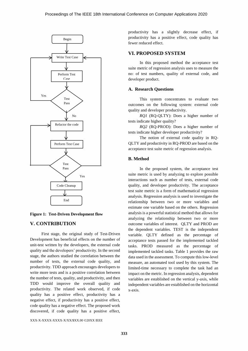
XXX-X-XXXX-XXXX-X/XX/$XX.00 ©20XX IEEE
Figure 1: Test-Driven Development flow
V. CONTRIBUTION
First stage, the original study of Test-Driven
Development has beneficial effects on the number of
unit-test written by the developers, the external code
quality and the developers’ productivity. In the second
stage, the authors studied the correlation between the
number of tests, the external code quality, and
productivity. TDD approach encourages developers to
write more tests and is a positive correlation between
the number of tests, quality, and productivity, and then
TDD would improve the overall quality and
productivity. The related work observed, if code
quality has a positive effect, productivity has a
negative effect, if productivity has a positive effect,
code quality has a negative effect. The proposed work
discovered, if code quality has a positive effect,
productivity has a slightly decrease effect, if
productivity has a positive effect, code quality has
fewer reduced effect.
VI. PROPOSED SYSTEM
In this proposed method the acceptance test
suite metric of regression analysis uses to measure the
no: of test numbers, quality of external code, and
developer product.
A. Research Questions
This system concentrates to evaluate two
outcomes on the following system: external code
quality and developer productivity.
RQ1 (RQ-QLTY): Does a higher number of
tests indicate higher quality?
RQ2 (RQ-PROD): Does a higher number of
tests indicate higher developer productivity?
The notion of external code quality in RQ-
QLTY and productivity in RQ-PROD are based on the
acceptance test suite metric of regression analysis.
B. Method
In the proposed system, the acceptance test
suite metric is used by analyzing to explore possible
interactions such as number of tests, external code
quality, and developer productivity. The acceptance
test suite metric is a form of mathematical regression
analysis. Regression analysis is used to investigate the
relationship between two or more variables and
estimate one variable based on the others. Regression
analysis is a powerful statistical method that allows for
analyzing the relationship between two or more
outcome variables of interest. QLTY and PROD are
the dependent variables. TEST is the independent
variable. QLTY defined as the percentage of
acceptance tests passed for the implemented tackled
tasks. PROD measured as the percentage of
implemented tackled tasks. Table 1 provides the raw
data used in the assessment. To compute this low-level
measure, an automated tool used by this system. The
limited-time necessary to complete the task had an
impact on the metric. In regression analysis, dependent
variables are established on the vertical y-axis, while
independent variables are established on the horizontal
x-axis.
Begin
Write Test Case
Perform Test
Case
Test
Pass
Refactor the code
Perform Test Case
Test
Pass
Yes
No
Yes
Code Cleanup
End
Proceedings of The IEEE 18th International Conference on Computer Applications 2020
333

XXX-X-XXXX-XXXX-X/XX/$XX.00 ©20XX IEEE
C. Test Numbers (TEST)
Test numbers (TEST) is identified as JUnit
assert statement numbers inside the unit test suite
written by the participants while tackling the task.
The numbers of test development as a single JUnit
assert statements. TEST assessed by the count of
the JUnit test cases. TEST is a ratio measure in the
range [0, ∞]. The formula for calculating TEST is
defined as [10]:
TEST = no: of subtasks out of result the no: of input
subtasks (1)
TEST = JUnit assert statement numbers inside the unit
test suite
Table 1: Summary of acceptance tests used to
calculate the metrics of Bowling Scorekeeper data-
sets [7].
Task Test Assert
T1 3 3
T2 3 3
T3 2 2
T4 3 10
T5 5 5
T6 6 6
T7 8 8
T8 5 5
T9 5 5
T10 4 4
T11 2 2
T12 3 3
T13 2 2
D. External code quality
The metric for external quality QLTY based on
the number of tackled subtasks (#TST) for a given task.
A subtask as tackled assesses if at least one assert
statement in the acceptance test suite associated with
that subtask passes. QLTY is a proportion measure in
the range 0 to 100.
The number of tackled subtasks (#TST) is
defined as:
#TST =
∑ 1 𝐴𝑠𝑠𝑒𝑟𝑡𝑖(𝑃𝑎𝑠𝑠) > 0
0 𝑜𝑡ℎ𝑒𝑟𝑤𝑖𝑠𝑒𝑛𝑖=0
(2)
#TST = the number of tackled subtasks
n = the total number of subtasks
The formula for measuring QLTY is defined as
[8]:
QLTY = ∑ 𝑄𝐿𝑇𝑌𝑖
#𝑇𝑆𝑇𝑖=0
#𝑇𝑆𝑇 × 100 (3)
QLTYi = the ith tackled subtask’s quality
Where QLTYi is the quality of the ith tackled
subtask and QLTYi is defined as:
QLTYi = #𝐴𝑠𝑠𝑒𝑟𝑡𝑖(𝑃𝑎𝑠𝑠)
#𝐴𝑠𝑠𝑒𝑟𝑡𝑖(𝐴𝑙𝑙) (4)
#Asserti (Pass) = the number of JUnit assertions
passing in the acceptance test suite associated with the
ith subtask
#Asserti (All) = the total number of JUnit
assertions in the acceptance test suite associated with
the ith subtask
For example, supposing that the thirteen
tackled subtasks (#TST = 13) assessed by a person, this
denotes that the thirteen tackled subtasks pass more
than one assert statement in the test suite. Assume us
that the acceptance test of the first analyzed tackled
task contains 3 assertions, out of results of three are
passing. The acceptance tests of the fourth tackled task
contain 10 assertions, out of results of three are
passing and so on.
Table 2: Solution of QLTY
Task Test Assert QLTY
T1 3 3 1
T2 3 3 1
T3 2 2 1
T4 3 10 0.3
T5 5 5 1
T6 6 6 1
T7 8 8 1
T8 5 5 1
T9 5 5 1
T10 4 4 1
T11 2 2 1
T12 3 3 1
T13 2 2 1
51 58 95
Proceedings of The IEEE 18th International Conference on Computer Applications 2020
334

XXX-X-XXXX-XXXX-X/XX/$XX.00 ©20XX IEEE
i.e. (QLTY4 = #𝐴𝑠𝑠𝑒𝑟𝑡4(𝑃𝑎𝑠𝑠)
#𝐴𝑆𝑆𝐸𝑅𝑇4(𝐴𝑙𝑙) =
3
10 = 0.3)
(QLTY = ∑ 𝑄𝐿𝑇𝑌𝑖#𝑇𝑆𝑇
𝑖=1
#𝑇𝑆𝑇 ×100
= 1+1+1+0.3+1+1+1+1+1+1+1+1+1
13 ×100 =95)
E. Productivity
The productivity metric (PROD) expresses the
amount of work effectively carried out by the subjects.
PROD is a proportion measure in the range 0 to100.
The metric of PROD is computed as follows [8]:
PROD = #𝐴𝑠𝑠𝑒𝑟𝑡(𝑃𝑎𝑠𝑠)
#𝐴𝑠𝑠𝑒𝑟𝑡(𝐴𝑙𝑙) ×100 (5)
For sample, assume a tacked task with all of 58
assert statements enabled by a person in a test suite.
After compiling, the person’s outcome 51 asserts
statements are passing.
i.e. (PROD = #𝐴𝑠𝑠𝑒𝑟𝑡(𝑃𝑎𝑠𝑠)
#𝐴𝑠𝑠𝑒𝑟𝑡(𝐴𝑙𝑙) ×100 =
51
58 × 100 = 88)
F. Assessment
The image below is a scatter plot. Scatter plots
are used when this paper want to show the relationship
between two variables. Scatter plots are known as
relationship plots because they show how two
variables are interrelated. This analytical tool is most
often applied to show data correlation between two
variables. This system expects that the regression
assessment of the tackled task compiled from the
quality of external code on test numbers by TDD
responds positively to questions RQ1. In the same
way, this system expects that the regression analysis
of the tackled task compiled from the developer
product on test numbers by TDD responds slightly
decrease to questions RQ2.
Figure 2: QLTY is on the function of TEST
In figure 2, the external code quality on the test
numbers is improved by measuring the acceptance test
suite metric of quality (QLTY).
Figure 3: PROD is on the function of TEST
In figure 3, the developer’s productivity over
the test numbers is slightly decreased by measuring the
acceptance test suite metric of productivity (PROD).
VII. COMPATIBILITY OF RESULT
In this portion, this paper presents the outcomes
acceptance test suite metric of regression analysis.
Further, a significant relation between TEST and
QLTY, as expressed in RQ1, with a positive was
found. Hence, scatter plot figure 2 is an arithmetically
expressive relationship between the number of tests
and external code quality. Additionally, a significant
relation between TEST and PORD, as expressed in
RQ2, with a somewhat down was found. So,
scatterplot figure 3 is an arithmetically expressive
correlation between the number of tests and
programmer productivity. In this study, the number of
tests is a good predictor for TDD programmer
productivity. Consequently, developer product on the
test numbers becomes lightly diminishment and
quality of external code on the test numbers becomes
improvement. Development time is relatively high in
the proposed work. It nearly takes as much as 16%
more time than that of related work. Proposed work
decreases the maintenance cost and overall increases
the productivity. There are as many as 52% more test
cases as of the related work. The related work codes
have a relatively small size. The inclusion of many
more test cases in the proposed work increases the size
of the code. The related work codes are simpler. The
cyclomatic complexity of the related work is relatively
smaller. The proposed work is relatively complex.
0
20
40
60
80
100
0 0.5 1 1.5 2 2.5
Dep
en
den
t va
ria
ble
(Q
LT
Y)
Independent variable (TEST)
TEST Vs QLTY
0
20
40
60
80
100
0 0.5 1 1.5 2 2.5Dep
en
den
t va
ria
ble
(P
OR
D)
Independent variable (TEST)
TEST Vs PORD
Proceedings of The IEEE 18th International Conference on Computer Applications 2020
335

VIII. CONCLUSION
Development time is relatively high in the
proposed work. It nearly takes as much as 16% more
time than that of related work. Proposed work
decreases the maintenance cost and overall increases
the productivity. There are as many as 52% more test
cases as of the related work. The related work codes
have a relatively small size. The inclusion of many
more test cases in the proposed work increases the size
of the code. The related work codes are simpler. The
cyclomatic complexity of the related work is relatively
smaller. The proposed work is relatively complex.
This approach allows thorough unit testing
which enhances the quality of the software and
advances customer satisfaction. They help with
retaining and varying the code. Moreover, the number
of acceptance test cases passed and number defects
found through static code analysis are used to measure
the external code quality. All these measures are
consistent with the studies and will be considered as
standard measures. When this proposed system
assesses the acceptance test suite metric of regression
analysis, the result of developer productivity over the
number of tests is fewer decreased and the result of
external code quality over the number of tests is
increased in giving a fixed time-frame.
ACKNOWLEDGMENTS
This research paper is partially supported by
academic studies. Professionals were fit to implement
more effective with test-driven development.
Furthermore, this proposed system observes that the
measurement reveal different aspects of a
development approach in academic studies.
REFERENCES
[1] Causineou and Chartier, 2010; Outliers
Detection and Treatment: a Review,
International Journal of Psychological Research,
3(1): 58-67.
[2] H. Kou, P. M. Johnson, and H. Erdogmus,
“Operational definition and automated inference
of test-driven development with Zorro,”
Automated Software Engineering, 2010.
[3] Shaweta Kumar, Sanjeev bansal, “Comparative
Study of Test driven Development with
Traditional Techniques”; International Journal of
Soft computing and Engineering (IJSCE);
ISSN:2231-2307,Volume-3, Issue-1, (March
2013).
[4] A.N. Seshu Kumar and S. Vasavi ; “Effective
Unit Testing Framework for Automation of
Windows Applications”; Aswatha Kumar M.et
al.(Eds); Proceedings of ICADC, AISC 174, pp.
813-822. Springerlink .com @ Springer India
2013
[5] Y. Rafique and V. B. Miˇsi´c, “The effects of
test-driven development on external quality and
productivity: A meta-analysis,” IEEE
Transactions on Software Engineering, vol. 39,
no. 6, pp. 835–856, 2013.
[6] Davide Fucci, Burak Turhan, “On the role of
tests in test- driven development: A
differentiated and partial replication”, Empirical
Software Engineering Journal (April 2014,
Volume 19, Issue 2, pp 277-302)
[7] Tosun A., Dieste O., Fucci D., Vegas S., Turhan
B., Erdogmus H., Santos A., Oivo M., Toro K.,
Jarvinen J., & Juristo N. An Industry Experiment
on the Effects of Test-Driven Development on
External Quality and Productivity
[8] Fucci, D., Turhan, B., & Oivo, M. The Impact of
Process Conformance on the Effects of Test-
driven Development (ESEM2014) 8th Empirical
Software Engineering and Measurement, 2014
ACM/IEEE International Symposium on. Turin,
Italy.
[9] Fucci, D., Turhan, B., & Oivo, M. On the Effects
of Programming and Testing Skills on External
Qualityand Productivity in a Test-driven
Development Context (EASE2015) 19th
Evaluation and Assessment in Software
Engineering 2015 ACM/IEEE International
Conference on., Nanjing, China.
[10] Viktor Farcic , Alex Garcia ; “Java Test-Driven
Development”; First published: August 2015;
Production reference: 1240815; Published by
Packt Publishing Ltd.; Livery Place; 35 Livery
Street; Birmingham B3 2PB, UK. ISBN 978-1-
78398-742-9; www.packtpub.com; www.it-
ebooks.in
[12] Christine Sarikas (GENERAL EDUCATION)
https:// blog.prepscholar.com/independent-and-
dependent-variables; Feb 12, 2018.
[12] https://chartio.com/learn/charts/what-is-a-
scatter-plot/ Jan 9, 2019
[13] Svetlana Cheusheva; ttps://www.ablebits.com/
office-add ins-blog/2019/01/09/add-trendline-
excel/ May 15, 2019.
[14] H. Munir, K. Wnuk, K. Petersen, and M.
Moayyed, “An experimental evaluation of test
driven development vs. test last development
with industry professionals,” Proc. 18th Int. Conf.
Eval. Assess. Softw. Eng. - EASE ’14, pp. 1–10,
2014.
[15] M. Moayyed, K. Petersen, H. Munir.
Considering rigor and relevance when evaluating
test driven dvelopment: A systematic review.
Information and Software Technology, 2014.
Proceedings of The IEEE 18th International Conference on Computer Applications 2020
336

Determining Spatial and Temporal Changes of Water Quality in Hlaing
River using Principal Component Analysis
Mu Mu Than Khin Mar Yee
Department of Higher Education Department of Higher Education
Sittway University Myeik University
Sittway, Myanmar Myeik, Myanmar
[email protected] [email protected]
Kyi Lint Marlar Han Thet Wai Hnin
Department of Higher Education Department of Higher Education Japan International
Dagon University Taungoo University Cooperation gency
Yangon, Myanmar Taungoo, Myanmar Yangon, Myanmar
Abstract
Water quality of a River is important as it is
used for drinking, domestic purpose and agriculture.
Hlaing River is one of the most important rivers in
Yangon Region. The River plays an important role to
supply water transportation for Hlaingtharyar, Insein
and Htantapin Townships. The objective of the paper
is to assess the change of water quality in Hlaing
River in the wet and dry seasons. The secondary data
used in the study are monthly mean temperature in
Yangon (Average) between 2007 and 2016 and
monthly rainfalls in Yangon (Average) between 2007
and 2016. Primary data are collected for sampling
points. 8 numbers of samples were collected at
different selective sampling points. A number of
physiochemical water quality parameters including
Biochemical Oxygen Demand (BOD), Chemical
Oxygen Demand (COD) and Total Suspended Solid
(TSS) are tested. Principal component analysis in
SPSS is used to know the correlations of the variables
and to determine how many important components
are present in the data. Sample points located at the
same river and nearer places are in same component.
According to the water quality surveys, the
water quality of Hlaing River met the level of Class
(III) of the Interim National Water Quality Standards of
Malaysia (for Water supply) in wet season because of
dilution process at that time and in dry season some
part of Hlaing River met the level of Class (IV) of the
Interim National Water Quality Standard of Malaysia
(for irrigation purpose).
Keywords: Hlaing River, spatial and temporal
changes, industrial zones, dilution, irrigation
I. INTRODUCTION
This paper is assessing water quality of Hlaing
river which is mainly use of transportation purposes
in Yangon Region. There are a lot of national and
international standards of water quality assessment.
In this paper the researchers classify and assess the
result of water quality by using the Interim National
Water Quality Standards of Malaysia (INWQS), a set
of standards derived based on beneficial uses of
water. As Myanmar and Malaysia are consisting of
South East Asia countries, they have similar
topography and environmental conditions.
Currently, Myanmar has already set up
emission standards. However, it is still need to lay
down the standards for ambient air quality and
drinking water quality standards. In the absence of
those national standards, the Ministry of Natural
Resources and Environmental Conservation
(MONREC) stated that internationally accepted
environmental standards of World Health
Organization (WHO) guidelines, to be adopted for
any environmental assessment.
The water quality survey from “Project on
capacity development in basic water environment
management and Environmental Impact Assessment
(EIA) system in Myanmar” is originally composed of
total five-time surveys: in February 2016, June-July
2016, January 2017, June-July 2017 and February
2018 in order to cover the dry season and rainy
season in two years, 2016 to 2017. In the water
quality surveys, 21 parameters are collected and
measured for water quality analysis. The assessment
of project paper is to analyze the resulted data from
water quality surveys which was implemented during
5 periods in 3 years.
Proceedings of The IEEE 18th International Conference on Computer Applications 2020
337

This paper aims to analyze the current status of
the Hlaing River through the on-site measurement
and laboratory analysis.
II. DATA AND METHODOLOGY
A. Guideline levels and Classification
Ministry of Health and Sports (MOHS) and
MONREC enacted Drinking water quality standard
and National Environmental Emission Guideline for
water. In Myanmar, there is no surface water quality
standard. So, the researcher uses INWQS for surface
water in order to compare with the results.
B. Sampling Parameters
For the water quality surveys the parameters
are BOD, COD and TSS. In this project paper, these
will be assessed and mentioned by using ArcGIS.
Table 1 shows the Interim National Water
Quality Standards of Malaysia for surface water and
the class mentioned in table are definitions of specific
use of water quality with limit values.
Table I: Limit value and class of surface water
quality parameters according to the Interim
National Water Quality Standards of Malaysia
(INWQS)
PARAM-
ETER
UNI
T
LIMIT VALUE and
CLASS
IIB III IV V
Biochemi
cal
Oxygen
Demand
(BOD)
mg/l 3 6 12 > 12
Chemical
Oxygen
Demand
(COD)
mg/l 25 50 100 > 100
Total
Suspende
d Solid
(TSS)
mg/l 50 150 300 > 300
Source: INWQS
Note: Class IIB is recreational use with body contact,
Class III is Water supply – Extensive treatment
required
and Common of economic value, and tolerant species;
livestock drinking,
Class IV is irrigation purpose, and
Class V is none of the above.
C. Sampling method
Water samples were collected three times and
then mixed in bucket. Then, take off 100 ml with
sample bottle and send to the laboratory. Surface
water was taken directly by a sampling bottle or
using a plastic sampling bucket. In addition, Van
Dorn Water Sampler was used to collect a water
sample from a specific depth as needed.
D. Laboratory analysis method
BOD is analyzed by using Respirometric
method (HACH Method 10099) in DOWA Eco-
system-Myanmar Co., Ltd.
The researchers analyzed COD Cr with the
Japanese Standard JIS K0102 (2016) 20.1 which is
developed by OSUMI CO., Ltd.
TSS is analyzed by OSUMI CO., Ltd. in order
to the method of Environment Agency Notification
No. 59, 1971.
III. RESULT AND DISCUSSION
A. Location of the Study Area
Hlaing River is the middle section of a
tributary of Ayeyarwaddy River, and its name
evolves as Myit Ma Kha River, Hlaing River, and
Yangon River as it flows down toward the sea. The
length of Hlaing River is around 110 km-long and the
starting point is the boundary between Yangon
Region and Bago Region, and the ending point is
before confluence of Pan Hlaing River between
Hlaing Township and Hlaing Thar Yar Township in
Yangon City (Figure 1).
The project mainly focuses on the downstream
area of Hlaing River located in Yangon City because
there are many industrial zones and the water quality
may be deteriorated by the impact of wastewater
from industrial zones.
This paper were be evaluated the water quality
status of Hliang River which is based on the collected
information and the data of “Project on capacity
development in basic water environment
management and EIA system in Myanmar” which is
bilateral technical cooperation project between
Myanmar and Japan during the project implement
from June, 2015 to May 2018 in Yangon Region.
Proceedings of The IEEE 18th International Conference on Computer Applications 2020
338

Figure 1. Location Map of the Study Area, Hlaing
River
B. Spatial and Temporal Variations of Water
Quality in Hlaing River
Basin map of Hlaing River with locations of
industrial zones in the river basin is shown in figure
2. Hlaing River Basin is long in North-South
direction, and the industrial zones are located in the
most downstream area. Hlaing River connects with
Yangon River and drains to the Andaman Sea.
Figure 2. Hlaing River Basin and Locations of
Industrial Zones
1): Comparison and Analysis of BOD in Dry
and Wet Season
At the points of Hlaing - 1 and Pan Hlaing - 2,
the value of BOD for all sampling points meets the
level of Class V of the Interim National Water
Quality Standard of Malaysia because the untreated
waste water discharge along the Hlaing River was
high at dry season. In the case of wet season, the
values of BOD along the Hlaing River and Pan
Hlaing River meet the level of Class IIB of INWQS
for recreational use with body contact. It can be
assumed that the dilution of heavy rain may have an
effect on the value of BOD in river water quality and
the suspension of distillery factories were happened
at that time (Figure 3).
Figure 3. Location of Industrial Zones in the
Study Area
According to the results of wet season, in
Shwe creek the value of BOD at the points of Shwe -
1 and Shwe - 2 meet the level of Class III of INWQS
with the purpose of water supply and fishery in the
requirement of extensive treatment while the point of
Shwe - 3 meets the level of Class V of INWQS which
is located at Shwe Pyi Thar IZ area, may be polluted
by the industrial waste water.
The following figure (4) shows comparison of
changing BOD along Hlaing River Basin in dry and wet
season.
(a) (b)
Figure 4. Comparison of Changing BOD along
Hlaing River Basin in Dry (a) and Wet Seasons (b)
2): Comparison and Analysis of COD in Dry
and Wet Season In the case of wet season, the value of COD
along the Hlaing River, Pan Hlaing River and some
points at the sub stream of Hlaing River, especially
Shwe - 1 and Shwe – 2, meet the level of Class IIB
because the dilution of heavy rain and the suspension
of distillery factories may effect on the value of COD
in river water quality. The upper stream of creek path
(Shwe-3) meets the level of Class III of INWQS with
the purpose of water supply and fishery in the
Proceedings of The IEEE 18th International Conference on Computer Applications 2020
339

requirement of extensive treatment. But the water
quality was relatively different from all sampling
points which can be caused by some other pollution
activities of Shwe Pyi Thar IZ so that further
investigation is needed near it.
In the dry season, the water quality at the
middle point of Hlaing River (Hlaing - 2), was better
than that of upstream and downstream points, which
was indicated by the impact of Shwe creek in which
the value of COD at the points of Shwe - 1 and Shwe
- 2 meet the level of Class III and Shwe - 3 meets the
level of Class V of INWQS.
In Pan Hlaing River that is flowing through the
Hlaing Thar Yar IZ into Hlaing River, the water
quality of Pan Hlaing - 1 meets the level of Class V
of the INWQS at the dry season. The downstream of
Pan Hlaing River (Pan Hlaing - 2) was within the
level of Class IIB.
Figure 5 shows comparison of changing COD
along Hlaing River Basin in dry and wet season.
(a) (b)
Figure 5. Comparison of Changing COD along
Hlaing River Basin in Dry (a) and Wet Seasons (b)
3): Comparison and Analysis of TSS in Dry
and Wet Season
In the dry season, the value of TSS at the
points of Hlaing-1 meets the level of Class IV of the
Interim National Water Quality Standard of Malaysia
with the purpose for irrigation while the other two
points of Hlaing-2 and Hlaing-3 meet the level of
Class V of INWQS. The former can be assumed that
there may have some other activities to happen
erosion at the upstream of Hlaing River and the latter
can be caused by increasing rate of erosion which is
higher than that of the upstream of Hlaing River. It
can be assumed that these two points is located at the
downstream and near of industrial zones.
In the wet season, the value of TSS along the
Hlaing River meets the level of Class V of INWQS
because the rate of erosion and tidal fluctuation were
relatively higher than the dry season. That is why the
water color of Hlaing River was turned to brownish with
the less transparency in color.
According to TSS results at the dry season,
Pan Hlaing - 2 can be used for irrigation with the
level of Class IV and Pan Hlaing -1 was within the
level of Class V in INWQS. Pan Hlaing -1 and Pan
Hlaing -2 meet the level of Class IV of INWQS at the
wet season. It can be assumed that the downstream of
Pan Hlaing is located at the downstream of industrial
zones and their activities.
In the case of Shwe creek at the dry season,
the value of TSS for Shwe - 1, meets the level of
Class IIB while Shwe - 2 and Shwe - 3 meet the level
of Class V according to INWQS. It can be assumed
that there are no erosion activities near Shwe - 3
point. The water quality of the other points at Shwe
Creek passed through Shwe Pyi Thar IZ area which
may be caused by industrial activities.
In the wet season, TSS value at the Shwe - 2
and Shwe - 3 points meet the level of Class IIB of
INWQS but the downstream point Shwe - 1 meet the
level of Class IV of INWQS. It can be assumed that
the downstream of Pan Hlaing is located at the
downstream which is passed through the Shwe Pyi
Thar industrial zone.
The differences between the dry and wet
season are that the activities in Hliang River Basin
and heavy rain can cause the erosion which is
resulted in changing the value of TSS.
The following figure shows comparison of
changing TSS along Hlaing River Basin in dry and wet
season.
(a) (b)
Figure 6. Comparison of Changing TSS along
Hlaing River Basin in Dry (a) and Wet Seasons (b)
Proceedings of The IEEE 18th International Conference on Computer Applications 2020
340

C. Principal Component Analysis
To know 8 sample points in Hlaing River have
similar patterns of responses i.e. do these points hang
together to create construct? Principal component
analysis (PCA) can explain the interrelationships
among the variables of 8 sample points.
The main idea of PCA is to reduce the
dimensionality of a data set consisting of many
variables correlated with each other, either heavily or
lightly, while retaining the variation present in the
dataset, up to the maximum extent.
The 1st principal component retains maximum
variation that was present in the original components.
The principal components are the eigenvectors of a
covariance matrix, and hence they are orthogonal.[5]
This paper studies water quality changes of 8
places. Each place is described by its attributes like
BOD and COD contents according to the time etc.
However, the complicated data will arise because
many of them measure related places and variables.
Therefore, PCA will do in this case is summarizing
each station in the dataset with less characteristics.
The following table shows correlations in
SPSS analyze by using bivariate. Form the table the
most items have some correlation with each other
ranging from r = -.146 for Shwe Creek 1 and Hlaing
2, “these are the nearest places” to r = 1 for the
sample points in the same river. Due to relatively
high correlations among items, this would be a good
component. Fewer interrelationships variables can be
broken up into multiple components such as sample
points in Shwe Creek and Hlaing River.
Eigenvalue represents the total amount of
variance. The total variance is made up to common
variance and unique variance, and unique variance is
composed of specific and error variance. Component
1 and 2 have the highest percentage of variance the
former is 69.186% of variance in initial Eigenvalues
and the latter is 30.669%and component 3 is 0.1%
(Table 3).
To select the optimal number of components
that are smaller than the total number of items, scree
plot is performed which plots the eigenvalue by the
component number. To choose components, one
criterion is to have eigenvalues greater than 1. In
Figure 7 the first two components have an eigenvalue
greater than1. The first component has the highest
total variance and the least components are at the last
of the plot. Component 2 is making the joint position.
The researcher selects two components on the basis
of the scree plot.
Figure 7. Scree Plot for Components
Component Matrix table contains component
loadings, which are the correlations between the
variable and the component. Hlaing 1, Hlaing 2,
Hlaing 3, Pan Hlaing 1, Pan Hlaing 2 and Shwe 3
load heavily on the first component and the other two
on the second component. This makes the output
easier to read by removing the clutter of low
correlations that are probably not meaningful
anyway. Pan Hlaing 1 and Shwe 3 has fairly
correlation with component 2. It can be clearly seen
in figure 8.
Table IV. Component Matrix
Component Matrixa
Component
1 2
Hlaing-1 .970 -.244
Hlaing-2 .963 -.269
Hlaing-3 .966 -.258
Pan Hlaing-1 .903 .426
Pan Hlaing-2 .962 -.271
Shwe-1 .128 .990
Shwe-2 .236 .971
Shwe-3 .959 .278
Extraction Method: Principal Component
Analysis.
Figure 8. Component Plot in Rotated Space
Proceedings of The IEEE 18th International Conference on Computer Applications 2020
341

Figure 9. Population density and Sample Points
The study area is located in the western part of
Yangon River. Rapid urbanization is pronounced in
these large townships – Shwepyithar, Hlaingtharyar,
Insein and Mayangon. Shwelinban industrial zone
and Shwepyithar industrial zones are established in
these townships. The consequences of human
activities such as municipal wastewater, waste from
the factories and urban drainage into the rivers effect
on the water quality of the area. Chemical and
biochemical contents in the water in dry season are
more pronounced than wet season. Huge discharge of
municipal wastewater into the river is one of the
important factors.
IV. CONCLUSION
Hlaing River in Yangon Region has been
selected as the study area because the impact of
industrial zones is important for the quality of water.
To examine the comparison of spatial and seasonal
changes of surface water quality in Hlaing River
physiochemical water quality parameters such as
BOD, COD and TSS are tested.
The paper is applied on-site measurement and
laboratory analysis result data of BOD, COD and
TSS from 3rd and 4th water quality surveys which are
mainly developed by the Project for Capacity
Development in Basic Water Environment
Management and EIA System.
The results of wet and dry season surveys were
evaluated with respect to each sampling points of
rivers and creek.
At the middle point of Shwe creek (Shwe-3),
the water quality was significantly deteriorated,
which was indicated by high level of COD and BOD.
The result did not show marked deterioration of
surface water quality in the flow direction of Hlaing
River and Pan Hlaing River. The creek passing
through the industrial zones and then flowing into
Hlaing River, its water quality is significantly
deteriorated by wastewater, which is indicated by low
Dissolved Oxygen (DO) as well as high
concentrations of COD and BOD.
In dry season, places located near the
industrial zones have the high COD and the opposite
true in wet season. Similarly, in dry season the
content of BOD is high in nearly all places, but the
value is less than 0.7 mg/l in wet season exception
Shwe 3 point. In the study area, the content of BOD
and COD in the water is high in dry season and low
in wet.
Conduct a principal component analysis can
determine how many important components are
present in the data. It can highlight the correlation
between the variables and components. Shwe 1 and
Shwe 2 points (located near the Creek from Shwe Pyi
Thar Industrial Zone to enter Hlaing River) have the same
environmental background and Shwe 3 and Pan
Hlaing 2 have the same situations such as located in
the industrial zones. Hlaing 1, Hlaing 2, Hlaing 3 and
Pan Hlaing 2 located along the rivers are one group.
Therefore, PCA can point out the grouping of the
variables on the plot.
In the Hlaing River of Yangon, the problem of
various water discharged manner from industrial
zones is one of the most important problems to
protect water quality and its environment especially
in Hlaingtharyar, Hlaing and Insein townships having
the large number of population.
REFERENCES
[1] Desalination and Water Treatment (April, 2018),
GIS – based analysis of water quality
deterioration in the Nerus River, Kuala
Terengganu, Malaysia
[2] How to perform a principal components analysis
(PCA), retrieved from https://statistics.laerd.com
› spss-tutorials › principal-components-analysis-
... 12 Nov 2019
Proceedings of The IEEE 18th International Conference on Computer Applications 2020
342

[3] Myanmar Statistical Yearbook, 2017 Central
Statistical Organization, Ministry of National
Planning Economic Development
[4] Progress Report No. (4) Of Project for capacity
development in basic water environment
management and EIA system in Myanmar by
JICA Expert Team (2018)
[5] Principal components Analysis, retrieved from
www.statstutor.ac.uk › resources › uploaded ›
principle-components-analy... 10 Nov 2019
[6] Karn, S.K.; Harada, H. Surface Water Pollution
in Three Urban Territories of Nepal, India, and
Bangladesh. Environmental Management. 2001,
28, 483–496
Appendix
Results of Laboratory Analysis
Correlation Matrixa
Hlaing-
1
Hlaing-
2
Hlaing-
3
Pan Hlaing-
1
Pan Hlaing-
2 Shwe-1 Shwe-2 Shwe-3
Correlatio
n
Hlaing-1 1.000 1.000 1.000 .772 1.000 -.118 -.008 .862
Hlaing-2 1.000 1.000 1.000 .755 1.000 -.144 -.034 .849
Hlaing-3 1.000 1.000 1.000 .762 1.000 -.131 -.023 .856
Pan Hlaing-
1 .772 .755 .762 1.000 .753 .534 .629 .982
Pan Hlaing-
2 1.000 1.000 1.000 .753 1.000 -.146 -.037 .848
Shwe-1 -.118 -.144 -.131 .534 -.146 1.000 .988 .401
Shwe-2 -.008 -.034 -.023 .629 -.037 .988 1.000 .494
Shwe-3 .862 .849 .856 .982 .848 .401 .494 1.000
a. This matrix is not positive definite.
Total Variance Explained
Compone
nt
Initial Eigenvalues Extraction Sums of Squared Loadings Rotation Sums of Squared Loadings
Total
% of
Variance
Cumulativ
e % Total
% of
Variance
Cumulative
% Total
% of
Variance
Cumulative
%
1 5.535 69.186 69.186 5.535 69.186 69.186 5.393 67.408 67.408
2 2.453 30.669 99.854 2.453 30.669 99.854 2.596 32.446 99.854
3 .012 .146 100.000
4 8.310E-16 1.039E-14 100.000
5 1.940E-16 2.425E-15 100.000
6 7.542E-17 9.428E-16 100.000
7 -2.145E-
16 -2.681E-15 100.000
8 -6.207E-
16 -7.759E-15 100.000
Extraction Method: Principal Component Analysis.
Table II. Correlation Matrix of Sampling Points in the Study Area
Table III. Total Variance Explained
Proceedings of The IEEE 18th International Conference on Computer Applications 2020
343
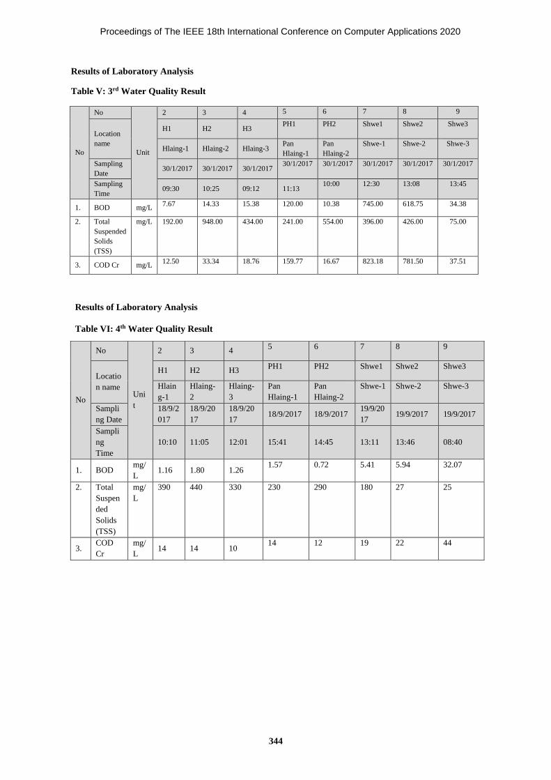
Results of Laboratory Analysis
Table V: 3rd Water Quality Result
No
No
Unit
2 3 4 5 6 7 8 9
Location
name
H1 H2 H3 PH1 PH2 Shwe1 Shwe2 Shwe3
Hlaing-1 Hlaing-2 Hlaing-3 Pan
Hlaing-1
Pan
Hlaing-2
Shwe-1 Shwe-2 Shwe-3
Sampling
Date 30/1/2017 30/1/2017 30/1/2017
30/1/2017 30/1/2017 30/1/2017 30/1/2017 30/1/2017
Sampling
Time 09:30 10:25 09:12 11:13
10:00 12:30 13:08 13:45
1. BOD mg/L 7.67 14.33 15.38 120.00 10.38 745.00 618.75 34.38
2. Total
Suspended
Solids
(TSS)
mg/L 192.00 948.00 434.00 241.00 554.00 396.00 426.00 75.00
3. COD Cr mg/L 12.50 33.34 18.76 159.77 16.67 823.18 781.50 37.51
No
No
Uni
t
2 3 4 5 6 7 8 9
Locatio
n name
H1 H2 H3 PH1 PH2 Shwe1 Shwe2 Shwe3
Hlain
g-1
Hlaing-
2
Hlaing-
3
Pan
Hlaing-1
Pan
Hlaing-2
Shwe-1 Shwe-2 Shwe-3
Sampli
ng Date
18/9/2
017
18/9/20
17
18/9/20
17 18/9/2017 18/9/2017
19/9/20
17 19/9/2017 19/9/2017
Sampli
ng
Time
10:10 11:05 12:01 15:41 14:45 13:11 13:46 08:40
1. BOD mg/
L 1.16 1.80 1.26
1.57 0.72 5.41 5.94 32.07
2. Total
Suspen
ded
Solids
(TSS)
mg/
L
390 440 330 230 290 180 27 25
3. COD
Cr
mg/
L 14 14 10
14 12 19 22 44
Results of Laboratory Analysis
Table VI: 4th Water Quality Result
4th Water Quality Result
Proceedings of The IEEE 18th International Conference on Computer Applications 2020
344

Aye Thida
Computer Engineering and Information
Technology
Mandalay Technological University
Mandalay, Myanmar
Thanda Shwe
Computer Engineering and Information
Technology
Mandalay Technological University
Mandalay, Myanmar
Abstract
With the increasing popularity and adoption
of IoT technology, fog computing has been used as an
advancement to cloud computing. Although trust
management issues in cloud have been addressed,
there are still very few studies in a fog area. Trust is
needed for collaborating among fog nodes and trust
can further improve the reliability by assisting in
selecting the fog nodes to collaborate. To address
this issue, we present a provenance based trust
mechanism that traces the behavior of the process
among fog nodes. Our approach adopts the
completion rate and failure rate as the process
provenance in trust scores of computing workload,
especially obvious measures of trustworthiness.
Simulation results demonstrate that the proposed
system can effectively be used for collaboration in a
fog environment.
Keywords: process provenance, trust, collaborative,
fog computing
I. INTRODUCTION
Cloud computing is a computing paradigm
that gathers and investigates real-time processing
data above the internet [1]. However, as the
substantial long-distance between cloud data centers
and IoT edge devices, cloud computing suffers from
traffic jams, significant end-to-end delay,
communication charges and processing of massive
amounts of data. Thus, to overwhelm these problems,
fog computing has appeared as an improvement to
the conventional cloud computing framework for
providing geographical distributions, low latency and
critical workload computation along with area
awareness [2]. It affords workload computation,
storage resources, and application services like a
cloud. To protect interconnection among fog
computing nodes, the following relations between
these nodes are to be defended: (i) relations between
fog computing nodes and IoT devices, and (ii) the
relations among fog computing nodes. Collaborating
among fog computing nodes is required to provide
the subsequent amount of localized control,
configuration and management, shared resources and
computing power.
One of the ultimate goals of Fog computing is
increasing the reliability of the network. Thus, the
trust management mechanism is necessarily needed
for efficient collaboration of fog computing nodes.
Trust can also provide reliability by allowing
assistance for selecting the fog nodes to cooperate.
Employing trust management in fog computing
environments will admit fog clients, resource-
constrained devices, and fog nodes to forecast future
behavior of each other. Based on the prediction of
future behavior of fog devices, fog clients can select
a fog node in the vicinity that will provide the best
service. To predict the future event, fog nodes need to
know how they work in the past to measure whether
it can be trusted or not. Thus, provenance information
is necessary for consideration of trust management.
Provenance is a procedure that traces the past
interaction of a process or data item, beginning from
its sources. Our approach is based on the concept of
provenance, as provenance gives important evidence
about the origin of the process or data item. Process
provenance, gathered about the progress, traces the
calling of services during a process’s execution and
enables recording of process flow and services in a
collaborator environment. Consequently, process
provenance is considered as one of the major
requirements for trust establishment in the IoT
devices and their attached fog nodes.
However, there were provenance-based trust
models in wireless sensor networks [3] but a
provenance-based trust model in fog environment has
not been addressed properly. The studies in [6,7,8]
show that feedback based trust models have been
provided in fog nodes but malicious fog node can
give a good recommendation to other malicious
nodes.
Process Provenance-based Trust Management in Collaborative Fog Environment
Proceedings of The IEEE 18th International Conference on Computer Applications 2020
345

To solve these issues, we propose the
provenance-based trust mechanism in a fog
environment. The main contribution of this work is to
develop a direct trust approach based on the trust
value of computing jobs among fog nodes, tracing
the behavior of the process flow within fog nodes.
We summarize the contributions of this paper as
follows:
a) We develop a direct trust mechanism for fog
collaboration which leads to efficient sharing of
resources based on the process provenance.
b) We compute the trust value based on the
computing history of jobs on each fog node.
c) We evaluate the trust among fog nodes
according to the provenance based trust value of
computing jobs.
The remainder of this paper is grouped as
follows: Section 2 presents the related works. Section
3 presents how the direct trust approach with
provenance in fog computing works. The method and
design used for the provenance-based trust
mechanism are described in Section 4. The
simulation results are analyzed in Section 5 and
finally, our conclusion and future work are drawn in
Section 6.
II. RELATED WORD
Many of researcher groups are carrying out in
the area of trust mechanism in fog and cloud
computing environments.
In [3], the authors proposed a provenance-
based trustworthiness assessment in sensor networks.
They emphasized the use of unreliable data may lead
to catastrophic failures as the main contribution of
the provenance system. However, they intended only
for the trust calculation framework of data elements
and network devices based on the interdependency
between data and network nodes, not for achieving
trust based on process provenance that can accelerate
the collaboration among fog nodes.
In [7], the authors proposed a reputation-based
trust management framework that provided a group
of process to provide Trust as a Service (TaaS),
which include a new protocol to validate the integrity
of feedbacks and protect the privacy of users. And it
was a flexible and robust integrity model for
estimating the integrity of trust feedbacks to cover
cloud services access from the unauthorized user.
Moreover, it implemented the decentralized trust
management service. However, this system mainly
depends on the user’s feedback to get the reliability
of cloud services, instead of calculating trust by
themselves.
A Reliable and Lightweight Trust Computing
Mechanism for IoT Edge Devices Based on Multi-
Source Feedback Information Fusion was proposed
in [8]. They used lightweight trust evaluating
mechanisms for the collaboration of IoT edge
devices. The multi-source feedback mechanisms are
used for overall trust computing methods to get more
trustworthy against bad-mouthing intrusions made by
malicious recommenders. However, this study mostly
focused on feedback mechanism that is based on
third party recommender, so misleading feedbacks
can lead the unauthorized user and waiting time to
get the feedback will be an issue. Our proposed
system, on the other hand, targets the direct trust
framework among fog devices to avoid malicious
recommenders.
In [9], the authors proposed ProvChain, a
provenance framework to support the cloud
environment. They adopted a blockchain mechanism
to protect the privacy and unauthorized access of data
provenance. The authors proposed a trust model for a
cloud environment using secure data provenance in
[10]. Their works had two parts to get assure
provenance method: keeping the user privacy and
historical data employing cryptographic mechanisms.
These trust frameworks involved collecting and
achieving historical data. However, these two studies
mainly focused on a secure data provenance scheme
in a cloud environment, not for process provenance in
fog architecture. Our work varies from them by
analyzing the trust among fog node to collaborate
based on the process provenance.
A blockchain-based process provenance for
cloud forensics was proposed in [15]. They proposed
a process provenance, which affords validation of
reality and privacy conservation for recording
workflows and cryptography group signature. As a
result, this study raises the trustworthiness of the
chain of protection for cloud forensics. However, the
privacy of their scheme is depending on the
trustworthiness of the third-party organization. Our
work differs from them by using the process
provenance to build a trust model for fog
environment. Our work leads to effective
collaboration among fog nodes with the support of
trusted fog devices.
Proceedings of The IEEE 18th International Conference on Computer Applications 2020
346

III. BACKGROUND
A. Fog Computing Architecture
We employ the architecture of fog computing
as shown in Fig. 1. It involved three layers: Cloud,
Fog and Edge. The cloud layer exists at the top core
layer and long distance from the IoT edge devices.
The fog layer exists at the center and is closely
connected to the IoT edge devices. The fog networks
can be connected to the cloud server. Each IoT edge
device is connected to a Fog node. Fog nodes are
serving as the management layer between the cloud
and edge devices. All communications such as Fog-
to-Fog, Fog-to-Cloud, and Fog-to-Edge are back and
forth communications.
1) Cloud Layer: Especially this layer serves as
high-administration services for computing, storage,
and processing. This layer also acts as the remote
server and management control center that maintains
a large amount of data and extremely complex
processes. But they can store and process the non-
critical computing jobs. The workloads from the IoT
devices are delivered to the cloud through the fog
network. Cloud servers grant inevitable and global
coverage [12].
2) Fog Layer: This layer acts as a management
layer between the cloud and the IoT edge devices. It
involves communication among Fog devices. It
affords geographical distributions, low latency and
critical workload computation along with area
awareness. Fog devices are also serving as a micro-
data center for resilient storage. The services that can
provide are distributed communications, workload
computation, storage resources, and service.
Comparison with the IoT edge devices, fog nodes
have more repository to process the computing
workload from the IoT edge devices. Otherwise, if
the fog nodes require a much more complex and
steady computation workload, this workload may be
dispatched to the cloud servers. The fog nodes also
act as bridges between the cloud and IoT edge
devices. The fog devices can be relevant for fog
cooperation. Collaborative and administrative
policies are adopted on fog devices to provide
management services. Fog collaboration can be
accomplished by remote or local interconnection
among them [12].
3) Edge Layer: It includes billions of
heterogeneous IoT edge devices allowed with their
unique identification, remote sensing, and
communication capacities, such as mobile devices,
smart cameras, sensors, and vehicles. IoT edge
devices can connect many of the Fog nodes. These are
very valuable and delayed to deliver all sensing data
from end-device to cloud server. Edge devices cannot
transfer important data to the cloud immediately.
Thus, they are connecting to the fog device [12].
Figure 1. The architecture of Fog Computing
B. Trust in Fog Computing
Generally, trust shows a vital part in advance
relations based on preceding interactions among fog
computing nodes and IoT edge devices. The fog
computing has a goal of increasing the reliability of
the network. Thus, trust can provide reliability by
allowing assistance for selecting the fog nodes to
cooperate. Trust management mechanisms can be
applied in fog computing architecture [5] to predict
the future behavior of each other. With the prediction
of future behavior of fog devices, client fog devices
can choose a fog node in the proximity.
A fog computing node itself may be the
malicious node to achieve the privacy and anonymity
of end-users [14]. Also, these nodes must be an
assurance for authorization, as the fog computing
node carried out encrypted data and process. Thus, all
fog nodes in the network have a certain trust level.
C. Process Provenance
Provenance indicates the derivation of origin
data and processes that involve constructing an
artifact. Provenance information is necessary to
check the current information is trusted, how to
organize different information origins and how to
support authority to innovator when reusing
information. It involved two parts: data provenance
and process provenance. The data provenance [9] is
Core
Communication connection
Edge
Fog-Fog
Cloud Server
Cloud layer
Fog layer
Edge layer
High-administration computing
service, Storage services, Data
centers, security, etc.
Fog-Cloud Fog-Cloud
Fog-Edge
Local network, Micro-data
center, low latency, geo-
distributed
Wired or wireless IoT sensor network
Fog-Edge
Fog Server
Fog Server
Laptop Mobile
devices sensors Smart
camera vehicles
Proceedings of The IEEE 18th International Conference on Computer Applications 2020
347

the origins of a sample of data that it takes place in a
database. The process provenance is the recording of
workflows that illustrates the service invoking within
a process execution and permits the tracing of
process and services in collaboratory environments.
Provenance in scientific workflow [13] is a
record of the derivation history of scientific results.
There are two types of provenance for scientific
workflows: prospective and retrospective.
Prospective provenance, takes an abstract workflow
as a receipt for future data derivation. Retrospective
provenance, takes past workflow execution and data
derivation information, affords critical contextual
information for the comprehensive analysis of
scientific results. Our proposed system adopts the
retrospective provenance to record the execution time
of the computational tasks historically arrived at the
application module because if we use prospective
provenance, it is necessary to predict the future jobs’
execution time.
IV. PROPOSED TRUST MECHANISM
A. Framework
The framework of the process provenance-
based trust management approach consists of
modules, namely, job history log, trust calculation
module and collaboration module as shown in Fig. 2.
a) Job History Log: The start time and finish
time of past computing jobs are recorded in the job
history log module to calculate the execution time of
jobs. When a user interacts with their application
module to the fog service, fog nodes recorded the
execution time of workload in each application
module. As the fog node maintains the history
interaction of computing jobs, the job history log for
each fog node is saved and stored at the fog node.
Figure 2. Framework
This job history log will be adopted by the trust
calculation module.
b) Trust Calculation Module: This module
calculates the trust value of each fog node. The trust
value of each fog node i can be calculated as Ti(Δt) =
Tc(Δt) – Tf(Δt) where Tc(Δt) is the trust value of job
completion rate within deadline and Tf(Δt) is the trust
value of job failure rate and (Δt) is a time window of
history interaction. To calculate the completion rate
of jobs Tc (Δt), compute the division of the number of
completion time of jobs within deadline Jtd+ (Δt) and
the total number of jobs. The job failure rate Tf(Δt)
can be computed from the division of the amount of
job failure Jtd- (Δt ) as some serious abnormalities and
the total number of jobs.
c) Collaboration Module: This module
determines which fog nodes will be chosen to
collaborate according to the trust value of each fog
node. Therefore, it maintains the trust value series of
each fog node, TS(Δt) = T1, T2,…., Tn. Then it
decides to choose the fog node that has the highest
trust value as trusted fog device for effective
collaboration.
B. Process Provenance Trust Mechanism
The pseudo-code of our proposed trust
mechanism is described in algorithm 1. Our proposed
trust framework requires supporting long-term trust
calculation for each fog device. Firstly, we take the
list of fog computing nodes that are connected to the
sensors and the job sets from sensors with a time
slide (Δt) of past interactions, which is the massive
number of past interaction records taken by our trust
model. Then, we calculate the trust value of each fog
node. According to the difference trust value of the
job completion rate and job failure rate, we achieve
the trust value of fog devices. The trust value
calculation process is iterated for all fog devices in
the system. According to the trust value series of fog
devices, a fog device with maximum trust value will
be chosen for collaboration.
Algorithm 1: Selection of Trusted Fog node for
collaboration
1: Input: Fog nodes (F=f1, f2,…, fi,….., fn);
A job set ( J = j1, j2,…., jk,….., jm);
and time-series of history interaction
(Δt) for trust calculation;
2: Output: To calculate trusted fog, TF(Δt) ;
3: Begin
4: Calculate the trust value of each fog node
for ( i = 1 to n ) do
Trust Calculation Module Collaboration Module
…
Calculate Completion rate
Calculate
Failure rate
Job History log
Trust
calculatio
n
Select the
trusted Fog node
Fog node
1
Fog node
2
Fog node
3
Fog node
n
Proceedings of The IEEE 18th International Conference on Computer Applications 2020
348

where Tc (Δt) =
Tf (Δt) =
Ti(Δt) = Tc(Δt) – Tf(Δt) ;
//trust value of job completion rate
// trust value of job failure rate
end for
5: According to the trust value of each fog node, we
can obtain the trust value series,
TS(Δt) = T1, T2,….,Tn;
6: Selection of trusted fog node to collaborate
TF(Δt) = max ( TS );
7: End;
C. Discussion
In our work, we implemented the process-
provenance based trust management scheme. As our
proposed trust model is based on the historical
interaction of computational tasks, we can calculate
the trust value among existing fog devices, not for
new arrival fog devices. Because of the lack of past
interaction of workload in the new fog device, it will
only have the fewest trust value. As our system is
intended only for choosing the fog node with the
highest trust value to effective collaboration in fog
environment, the new arrival fog node in the system
may not be selected for collaboration.
We noticed that the storage capacity of the
computing workload may impact on the performance
of fog node. The data storage for the recording of the
computing jobs may be increased time by time.
V. EVALUATION
A. Simulation Setup
To evaluate our proposed process provenance
trust mechanism, we illustrate the simulation
parameters in this section. We analyze fog
infrastructure by using iFogSim [4]. iFogSim is a
discrete event simulator for Fog and IoT
environments. iFogSim is composed of a set of
physical entities such as fog device, sensor, and
actuator and logical entities such as AppModule,
AppEdge, and Tuple. To simulate the trust value
calculation in iFogSim, we used the built-in
DCNSFog application.
TABLE I. SIMULATION PARAMETERS
Parameters Value
Area 4
Camera 4/area
Gateway 1/area
Fog device 7/area
Time window 100 second
The Intelligent Surveillance application has
been appraised on several physical infrastructure
configurations as shown in Table I. The number of
surveillant areas has been varied from 1 to 4. Note
that each surveillant area can have a lot of smart
cameras that monitoring the area. These cameras are
linked to an area gateway that maintains the action in
that surveillant area. In the simulated field, each
surveillant area has the four number of smart cameras
linked to an area gateway that provides Internet
access to them.
To simulate the trustworthiness of fog node
closely related to the realistic environment is crucial
to analyze the effectiveness of our system. Thus, to
examine the job failure rate, we adopted log-normal
distribution with the parameter value of (0.25,
0.0802) which effects the realistic failure rate of
computing jobs [11].
B. Results
We are interested in investigating the
effectiveness of our proposed scheme for long-term
fog collaboration.
As shown in Fig. 3, we investigated the total
trust value of all fog devices with time series to
investigate the long-term collaboration. We examine
that as the time window increases, the total trust
value of all fog nodes in each time window is also
increasing. The longer the time window, the number
of the historical interaction of computing jobs in each
fog node will increase. According to the simulation
result, if we start the trust value calculation in 500s,
we can get a steady trust value to collaborate. As we
can see, the increase in simulation time, our trust
result gradually rises. So, we expect that our trust
result can effectively be used for collaborating fog
nodes.
Fig. 4 plots the average trust value of all fog
nodes in each intelligence surveillance area. It can be
seen that area 4 has the highest trust value.
Proceedings of The IEEE 18th International Conference on Computer Applications 2020
349

However, as each fog device has been
configured variedly in terms of resource capacity, the
necessary computing resources of each area may
different. As area 4 needs only a few of resources
than other areas, the processing time of workload of
each fog node in this area can be faster. Thus, the
average trust value in area4 is high. As a result, we
can choose one of the fog devices with the highest
trust value for collaboration in the fog environment.
Figure 3. Total trust value with time series
Figure 4. Average trust value with different area
In Fig. 5, the maximum trust score of each fog
node in each area is displayed. As our proposed
scheme is intended for selecting the fog node with the
highest trust value to build the trust model, we
analyzed the trust score of each fog node in each
intelligence surveillance area.
Although fog devices have a high capacity,
some fog devices have a few history interactions of
workload. Thus, the completion rate of the workload
can high. According to our results, we can determine
to select the fog node with id-45 in area4 to
collaborate.
Figure 5. Trust value of fog devices in one area
VI. CONCLUSION
In this paper, we presented the trust evaluation
mechanism based on process provenance for fog
architecture. We proposed the direct trust mechanism
among fog nodes to calculate trust value for fog
collaboration. The results are approved through a lot
of several analyze and established its effectiveness.
We observe the possible expansions of the proposed
mechanism in the following indications: we are going
to evaluate the completion rate of history interaction
of workload in our proposed system with a
conventional approach in future work and we plan to
consider the data provenance for the data-intensive.
In an actual system, massive numbers of IoT devices
are allocated. Thus, we will extend to simulate a large
number of IoT devices like in the real environment
and investigate its effectiveness.
REFERENCES
[1] C. Mouradian, D. Naboulsi, S. Yangui, R.H.
Glitho, M.J. Morrow, and P.A. Polakos, “A
Comprehensive Survey on Fog Computing:
State-of-the-art and Research Challenges”, IEEE
Communications Surveys and Tutorials, 2018,
pp. 416-464.
[2] F. Bonomi, R. Milito, J. Zhu, and S. Addepalli,
“Fog Computing and Its Role in The Internet of
Things”, in Proc. of MCC'12, 2012, pp. 13-15.
[3] H. Lim, Y. Moon, and E. Bertino, “Provenance-
Based Trustworthiness Assessment in Sensor
Networks,” in Proceedings of Data Management
for Sensor Networks, 2010, pp. 2-7.
[4] H. Gupta, A.V. Dastjerdi, S.K. Ghosh, and R.
Buyya, “iFogSim: A Toolkit for Modeling and
Simulation of Resource Management Techniques
in The Internet of Things, Edge and Fog
Computing Environments”, WILEY, John Wiley
& Sons, Ltd., 2017.
Proceedings of The IEEE 18th International Conference on Computer Applications 2020
350

[5] T.S. Dybedokken, “Trust Management in Fog
Computing”, Master’s thesis, Norwegian
University of Science and Technology, 2017.
[6] R.K.L. Ko et al., “TrustCloud: A Framework for
Accountability and Trust in Cloud Computing,”
in IEEE World Congress on Services, 2011, pp.
584-588.
[7] T.H. Noor, Q.Z. Sheng, L. Yao, S. Dustdar, and
A.H. Ngu, “CloudArmor: Supporting
Reputation-Based Trust Management for Cloud
Services”, IEEE transactions on parallel and
distributed systems, 2106, pp. 367-380.
[8] J. Yuan and X. Li, “A Reliable and Lightweight
Trust Computing Mechanism for IoT Edge
Devices Based on Multi-Source Feedback
Information Fusion,” IEEE Access, vol. 6, 2018,
pp. 23626-23638.
[9] X. Liang, S. Shetty, D. Tosh, C. Kamhoua, K.
Kwiat, and L. Njilla, “Provchain: A Blockchain-
Based Data Provenance Architecture in Cloud
Environment with Enhanced Privacy and
Availability,” in Proceedings of the 17th
IEEE/ACM international symposium on cluster,
cloud and grid computing, 2017, pp. 468-477.
[10] M.I.M. Saad, K.A. Jalil, and M. Manaf,
“Achieving Trust in Cloud Computing Using
Secure Data Provenance,” in IEEE Conference
on Open Systems (ICOS), 2014, pp. 84-88.
[11] X. Xintao, C. Zhen, Z. Lijun, and Y. Xiaowei,
“Estimation on Reliability Models of Bearing
Failure Data,” Mathematical Problems in
Engineering, 2018, pp. 1-21.
[12] P. Zhang, M. Zhou, and G. Fortino, “Security
And Trust Issues in Fog Computing: A Survey,”
Future Gener. Comput. Syst., vol. 88, 2018, pp.
16-27.
[13] M. Herschel, R. Diestelkämper, and H. Ben
Lahmar, “A Survey on Provenance: What For?
What Form? What From?,” VLDB J., vol. 26,
no. 6, 2017, pp. 881-906.
[14] A. M. Elmisery, S. Rho, and D. Botvich, “A Fog
Based Middleware for Automated Compliance
with OECD Privacy Principles the Internet of
Healthcare Things”, IEEE Access, 2016, pp.
8418-8841.
[15] Y. Zhang, W. Songyang, B. Jin, J. Du, “A
Blockchain-Based Process Provenance for Cloud
Forensics”, in 3rd IEEE International Conference
on Computer and Communication, 2017, pp.
2470-2473.
Proceedings of The IEEE 18th International Conference on Computer Applications 2020
351

Software Quality Metrics Calculations for Java Programming Learning Assistant System
Khin Khin Zaw Department of Computer Engineereing and
Information Technology Yangon Technological University
Yangon, Myanmar [email protected]
Nobuo Funabiki
Department of Electrical and Communication Engineering
Okayama University Okayama, Japan
Hsu Wai Hnin Department of Computer Engineereing and
Information Technology Yangon Technological University
Yangon, Myanmar [email protected]
Khin Yadanar Kyaw
Department of Computer Engineering and Information Tetchnology
Yangon Technological University Yangon, Myanamar
Abstract
A Web-based Java Programming Learning Assistant System (JPLAS) has been proposed to assist Java programming educations in universities. In the code writing problem, the correctness of an answer code from a student is verified by running the test code on JUnit. Besides, their quality should be measured using the metrics to assess them. The currently using plugin could only be measured on eclipse for offline answering in JPLAS. To calculate the metrics and implement in web-based JPLAS, there are several equations that have been reported. In this paper, we find the proper equations to calculate the metrics that provide the same results as from Eclipse plugin. The application results for 45 source codes showed that the adopted metrics equations provide the same results as the plugin.
Keywords: JPLAS, JUnit, test code, code writing problem
I. INTRODUCTION
Java is a secure, portable, and platform independent programming language. Java engineers have been demand. Thus, Java is taught in many universities and colleges.
To assist Java educations, Java programming learning assistant system (JPLAS) has been developed. In JPLAS, the student can solve the exercise problems both on online and offline using
Eclipse. JPLAS provides different types of Java programming exercises to cover the different learning levels. The code writing problem asks a student to write a whole source code that passes the given test code on JUnit. Besides, software metrics should be measured to assess the quality of the answer code [1].
Software metrics can evaluate the software product under developments, which gives a vision on the quality to make a whole process more successful. These metrics are called software quality metrics or product metrics. In the code writing problem, seven quality metrics can be measured for assessment of the code. They include NOC - number of classes, NOM – number of methods, CC - cylomatic complexity, NBD – nested block depth, LCOM- the lack of cohesion, MLOC - method lines of code and TLOC – total lines of code [2]. They can be used for the size estimation, the complexity evaluation, and the maintenance of the code.
The currently using plugin can be used on Eclipsed to measure the metrics. Eclipse is used when the students solve the problems on offline. To measure the software metrics of a code, the equations to calculate them must be implementation in the JPLAS server. Unfortunately, there are several different equations to calculate some quality metrics. We need to find proper equation to calculate the metrics that provide the same results from Eclipse plugin.
Identify applicable funding agency here. If none, delete this text box.
In this paper, first, equations to calculate each metric are surveyed. Then, the proper one is selected by comparing the results with Eclipse plugin for 45
Proceedings of The IEEE 18th International Conference on Computer Applications 2020
352

answer codes. The results showed that the calculated metrics by the selected equations are equal to those of Eclipse plugin.
II. REVIEW OF JPLAS
In this section, we review JPLAS.
A. JPLAS
In JPLAS, Ubuntu is used as the operating system that is running on VMware. For web server, Tomcat is used to run HTML, JSP and servlets. HTML- hypertext Markup Language is the language to create the webpages. JSP is a script combined with Java code and it is embedded to HTML. Servlet is a small Java program that runs on web server. For database, MySQL is used for managing the data.
JPLAS implements supporting functions for teachers and students. In the teacher function, the teacher can show the problems to students by uploading them to the server. In the student function, the student can answer the problems from a Web browser and submit them to the server on online.
Besides, they can answer the problems using Eclipse on offline after receiving the problems by e-mail or downloading the problems from JPLAS, and submit the answer via email.
B. Exercies Problems in JPLAS
In JPLAS, four types of problems are provided. The three problems are the types of fill-in-blank problems to understand the grammar and reading studies. The last problem is for the code writing study. In this paper, the code writing problem is focused for the study of software metrics.
C. Fill-in-blank Problem
In this problem, the students need to fill the correct answers in blanks for a given Java code. The answer is marked by comparing with their original elements in the code. Thus, the original element must be unique correct answer for each blank. The blanks elements are identifiers, variable, reserved words and control symbols.
D. Value Trace Problem
This problem is another type of element fill-in-blank problem that keeps the process of filling and marking the answer. It questions a student about actual values of important variables in the code. The students need to fill the correct values of variables in
blanks. In this problem, the output data of variables from the code execution is blanked. The output data may contain one or more values. It blanks the output data line by line.
E. Statement Fill-in-blank Problem
In this problem, the students need to fill the whole statement in a blank for a give Java code. The answer is marked by using the test code on JUnit as the code writing problem.
F. Code Writing Problem
In this problem, the students need to write the whole code as the information given in test code. Then, the answer code is tested through the test code on JUnit as test driven development method (TDD). Besides, their quality is accessed by measuring the seven-quality metrics on Eclipse plugin.
G. JUnit
It is an open-source Java framework for unit testing on Java programming language and adopted in JPLAS. It is important in development of TDD - test driven development. Test code is implemented on JUnit. Although, test code is a test code programming language, it is rather simple for the Java programmers. This reason is that JUnit has been designed for Java programming language. In JUnit, one test can be performed by using one method in the JUnit library. In the code writing problem, the method whose name starts with ‘assert’ is used to check the execution results by comparing with the expected method [3].
H. TDD Method
In the TDD method, the following process can be done.
1)The source code must be prepared first to write test code from them. Thus, the test code includes the information on model source code, it will be tested in later.
2)Then, the answer code is written and tested it on JUnit through test code.
3)The source code can be re-factored until passing through the test code. Thus, the re-factoring process of a source code becomes easy, because the modified code can be tested instantly.
Proceedings of The IEEE 18th International Conference on Computer Applications 2020
353

I. Metric Plugin
Metric plugin for Eclipse is commonly used open source software plugin for metrics calculation. This plugin can measure the various metrics on source code and their results are shown by number in metric view. This plugin is used to measure software metrics to assess the quality of the code for the code writing problem [4][5].
III. SOFTWARE METRICS
Software metrics are the measurement and prediction of software products, which are essential resources for a project and products relevant for software evolutions. Measurements can be used throughout the software project for quality control by comparing the current measurements with past measurements for similar projects.
A. Overview of Metrics
There are many metrics that can be categorized into process and product metrics. Besides, due to the great interest in the use of object-oriented languages, many object-oriented design metrics has been proposed. Product metrics measure size, complexity, quality, and reliability of software product. Process metrics measure the various characteristics of the software development process. Object-oriented metrics measure the different aspects of object-oriented design, including complexity, cohesion, and coupling. Among them, product metrics and object-oriented metrics measure the quality of the code.
B. Product Metrics
Product metrics are known as quality metrics. They help improving the quality of the different system components, and comparisons between existing systems. Various kinds of product metrics have been proposed. They include reliability metrics, functionality metrics, performance metrics, usability metrics, cost metrics, size metrics, complexity metrics and style metrics. They are used to measure the properties of the software. Among them, some quality criteria can be used to predict a certain quality of the software [6] and they are as follows:
• NOC - number of classes and DIT - depth of inheritance are measured to assess maintainability and reusability of the program.
• LOC- lines of code is measured to assess the size of the code.
• CC - cyclomatic complexity is measured to assess reliability of the program.
C. Object- Oriented Metrics
Object-oriented designs are more beneficial in software development environment. Object-oriented metrics are used to measure properties of object-oriented designs. The object-oriented metrics measure on class and its design viz; localization, encapsulation, inheritance, polymorphism, and object abstraction techniques, which make the class unique. The object-oriented metrics are defined as follows:
• WMC - Weighted Methods Per Class • DIT - Depth of Inheritance Tree • NOC - Number of Children • CBO - Coupling between Objects • RFC - Response for a Class • LCOM - Lack of Cohesion in Methods
IV. CALCULATION OF SEVEN METRICS
Seven quality metrics are adopted for the code writing problem in JPLAS. They are as the followings:
• NOC - number of classes • NOM - number of methods • CC - cyclomatic complexity • LCOM - lack of cohesion in method • NBD - nested block depth • MLOC - method lines of code • TLOC- total lines of code
The equations of CC and LCOM have many variations, whereas other five metrics have a unique one. In this paper, firstly, all the equations are surveyed. Then, proper equations are selected to calculate them.
A. Number of Classes (NOC)
NOC measures the number of classes within the application package. It is a measure of how many subclasses are going to inherit the methods in the parent class. If a class has many subclasses, it is regarded as the bad design. The lower value of NOC helps maintainability and complexity of codes.
B. Number of Methods (NOM)
NOM measures the number of methods within classes. The number of methods that are local to the class and only those methods can be measured.
Proceedings of The IEEE 18th International Conference on Computer Applications 2020
354

C. Cyclomatic Complexity (CC)
CC measures the structural complexity of a procedure by counting the number of independent paths in a method. The paths represent the number of decision points in the code, which include if, while, do-while, for, switch-case-defaults, try-catch finally. The goal of CC is to evaluate the testability and maintainability of a software module [8].
The original complexity is calculated as follows:
CC= E - N + 2 (1)
Where: CC = cyclomatic complexity E = the number of edges of the graph N = the number of nodes of the graph
Then, the improve complexity is defined as the followings [9]:
1) If the source codes contain no decision points, their complexity would be 1 since there is only a single path through the code.
2) If the code has a single IF statement containing a single condition, there would be two paths through the code, one path for TRUE and one path for FALSE.
In above conditions, CC is calculated as follows:
CC=E-N+2P (2) where: P = the number of connected components
3) An alternate function is used when the cyclomatic complexity is applied to several subprograms at the same time.
CC=E-N+P (3) The following example code contains a single
IF statement. Thus, it contains the two paths to evaluate the path as TRUE of FALSE.
1. public class Circle 2. public static int minFunction(int n1,int n2) 3. int min; 4. if(n1>n2) 5. min=n2; 6. else 7. min=n1; 8. return min; 9. 10. Figure 1. Example code single If Statement
Firstly, the statements are transformed into a graph, where every piece of a statement is represented
as a node and their flows (sequence of execution of statements) are represented as the edges. For the single program, P is always equal to 1 since it has a single exit point. The cyclomatic complexity may be applied to several subprograms at the same time, where P will be equal to the number of programs. Figure 2 shows the flow chart of the source code containing single IF statements.
In this example, there are seven nodes, seven edges and one connected component. Then, CC= 7-7+2×1=2 is calculated by equation (2).
D. Lack of Cohesion in Methods (LCOM)
LCOM measures the cohesiveness of a class. It represents the difference between two methods whose similarity is zero or not. LCOM can judge the cohesiveness among the class methods. There are several LCOM metrics. The LCOM takes its values in the range 0 to 1.
• If the two methods share at least one field, Q is increased by one. Otherwise, Q is increased by one. It is noted that P and Q are initialized by 0. LCOM is calculated on each pair of metrics as follows [10]: LCOM = (P > Q)? (P - Q):0 (4)
Figure 2. Data flow diagram for source code with
single IF statement
Enter two numbers (n1,n2)
True n1>n2
Start
min=n2 min=n1
min
End
False
Proceedings of The IEEE 18th International Conference on Computer Applications 2020
355

• LCOM 1: A low value indicates the high coupling between methods. This also indicates the potentially high reusability and good class design. A high LCOM indicates that a class shall be considered for good design. LCOM = 0 is not a strong evidence that a class enjoys cohesiveness.
• LCOM 2: This is an improved version of LCOM 1.
LCOM = 1 -"#$($&)$∗)
(5)
Where: m = number of methods in class a = number of attributes in class mA = number of accessing times of attributes among the methods
• LCOM 3: A completely new expression for cohesion is proposed by Herderson-Sellers, that is called LCOM* [11].
LCOM = *1a ∑ µ (Aj)a
j=1 ,-m
1 - m (6)
Where: 𝜇(𝐴𝑗)= number of accessing times of attributes among the methods.
The following example code shows the accessing of attributes (member variables) among the methods. It contains two-member variables: radius and colour, and three methods: getRadius, getColor and getData. In this example, radius is accessed three times by getRadius and getData. color is accessed one time by getColor.
By equation (4), LCOM is calculated on the number of accessing times of attributes among the methods. The result is 0 because the value of Q is greater than P where P=0 and Q=4. Then, by equation (5), LCOM is calculated by using the number of methods, attributes and the number of accessing times of attributes. The result is 0.4 where m=3, a=2 and mA=4.
Fig.4 shows the diagram for the methods that accessing the attributes. By equation (6), LCOM is calculated by using the number of methods, attributes and the number of accessing times of attributes. LCOM is 0.5 where m=3, a=2 and 𝜇(𝐴𝑗) =4 respectively by equation (6).
According to the equation (4), LCOM is only 0 or 1. According to equation and (5) and (6), LCOM decreases and close to 0, when the accessing times of attributes are more. On the other hand, LCOM increases and close to 1 when the accessing times of attributes are less. The declared variables should be accessed among the methods In this time, equation
(6) is selected by the calculation result that is same with plugin in Section V.
1. public class Circle 2. private double radius; 3. private String color; 4. public Circle () 5. radius = 1.0; 6. color = red; 7. 8. public double getRadius () 9. return radius; 10. 11. public String getColor () 12. return color; 13. 14. public double getArea () 15. return 3.14*radius*radius; 16. 17.
Figure 3. Example code for method accessing
attributes
Figure 4. Block diagram of code for methods
accessing attributes
E. Nested Block Depth (NBD)
NBD represents the maximum nest depth in a method. The nest depth is given by the number of statements of blocks that are nested due to the use of control structure (branches and loops).
F. Total lines of Code (TLOC)
TLOC measures the total number of lines in the source code. It is calculated by counting on the executable lines, comment and empty lines.
G. Methodl lines of Code (MLOC)
MLOC represents the total number of method lines in method. It is calculated by counting on comments and empty lines.
getRadius V1
V2 getColor
getArea
color
M1
M2
M3
radius
Proceedings of The IEEE 18th International Conference on Computer Applications 2020
356

V. COMPARISON OF METRIC RESULTS
In this section, we evaluate the seven-quality metrics for the 45 source codes for five assignments from nine students in [11]. The first assignments ask the concepts of encapsulation, inheritance and polymorphism. The last two assignments ask the algorithms using those concepts for implementation it.
A. Calculated Metrics
Among the seven metrics, CC and LCOM have several equations to calculate them. For CC, the three equations (1), (2) and (3) are used. For LCOM, equation (6) is used.
B. Comparison of Metrics Values
The metrics values of CC and LCOM for each code are compared between the results by Eclipse plugin and those by the adopted equations to find the proper equations that give the same results. Other values represent the number of classes, methods, branches, and lines of code, which are unique. There is no equation for other metrics values. It can easily be calculated by counting the number of classes, methods, branches and lines of code as described in section IV- A, B, E, F, G. In this paper, the plugin result is represented as T1 and the equation result is represented as T2.
Tables 1-5 show the calculated metrics values of seven metrics for each code. NOC, NOM, NBD, TLOC and MLOC are calculated by counting the number of classes, methods, branches and lines in a code manually. CC is calculated by using Equation (1) (2) and (3). LCOM is calculated by Equation (6) for each code. Then, the values are compared between the plugin and calculated results.
In each assignment, the values NOC, NOM, NBD, TLOC and MLOC are same between T1 and T2. Besides for CC are the same values between them. The values of LCOM are slightly varied between T1 and T2 because of the difference of significant digits. Thus, the adopted equations and the counted number for them are the same as those in Eclipse plugin. In assignment 1, 2 and 3, they don’t need the conditions or branches (loops) to implement the concepts of OOP: encapsulation, inheritance and polymorphism. Thus, their CC and NBD are always 1 by both T1 and T2. In assignment 4 and 5, it needs the conditions or branches (loops) to implement the algorithms using the OOP concepts. In assignment 4, its CCs are 2-3 and NBD is 1-3. In assignment 4, its CCs are 2-4 and NBD is 1-3. The values are varied
among the codes depending on the student’s implementation on code.
TABLE I. COMPARISON OF METRIC VALUES FOR ASSIGNMENT 1
Assignment 1 NOC NOM MLOC TLOC
T1 T2 T1 T2 T1 T2 T1 T2 S1 1 1 6 6 8 8 26 26 S2 1 1 6 6 8 8 26 26 S3 1 1 6 6 8 8 26 26 S4 1 1 6 6 8 8 26 26 S5 1 1 6 6 8 8 27 27 S6 1 1 6 6 8 8 26 26 S7 1 1 6 6 8 8 26 26 S8 1 1 6 6 8 8 26 26 S9 1 1 6 6 8 8 26 26 NBD CC LCOM
T1 T2 T1 T2 T1 T2 S1 1 1 1 1 0.5 0.5 S2 1 1 1 1 0.5 0.533 S3 1 1 1 1 0.5 0.533 S4 1 1 1 1 0.5 0.533 S5 1 1 1 1 0.7 0.667 S6 1 1 1 1 0.5 0.533 S7 1 1 1 1 0.7 0.667 S8 1 1 1 1 0.6 0.6 S9 1 1 1 1 0.7 0.667
TABLE II. COMPARISON OF METRIC VALUES FOR ASSIGNMENT 2
Assignment 2 NOC NOM MLOC TLOC
T1 T2 T1 T2 T1 T2 T1 T2 S1 2 2 5 5 5 5 28 28 S2 2 2 5 5 5 5 24 24 S3 2 2 5 5 5 5 24 24 S4 2 2 5 5 5 5 24 24 S5 2 2 12 12 15 15 48 48 S6 2 2 6 6 9 9 28 28 S7 2 2 5 5 5 5 24 24 S8 2 2 5 5 5 5 22 22 S9 2 2 9 9 11 11 40 40 NBD CC LCOM
T1 T2 T1 T2 T1 T2 S1 1 1 1 1 0.5 0.5 S2 1 1 1 1 0.5 0.5 S3 1 1 1 1 0.5 0.5 S4 1 1 1 1 0.5 0.5 S5 1 1 1 1 0.7 0.68 S6 1 1 1 1 0.5 0.5 S7 1 1 1 1 0.7 0.667 S8 1 1 1 1 0.5 0.5 S9 1 1 1 1 0.7 0.667
TABLE III. COMPARISON OF METRIC VALUES FOR ASSIGNMENT 3
Assignment 3 NOC NOM MLOC TLOC
T1 T2 T1 T2 T1 T2 T1 T2 S1 1 1 3 3 3 3 14 14 S2 1 1 3 3 3 3 12 12 S3 1 1 3 3 3 3 12 12 S4 1 1 3 3 3 3 12 12 S5 1 1 3 3 9 9 21 21 S6 1 1 3 3 3 3 12 12 S7 1 1 3 3 3 3 12 12 S8 1 1 3 3 6 6 15 15
Proceedings of The IEEE 18th International Conference on Computer Applications 2020
357

S9 1 1 3 3 3 3 12 12 NBD CC LCOM
T1 T2 T1 T2 T1 T2 S1 1 1 1 1 0 0 S2 1 1 1 1 0 0 S3 1 1 1 1 0 0 S4 1 1 1 1 0 0 S5 1 1 1 1 0 0 S6 1 1 1 1 0 0 S7 1 1 1 1 0 0 S8 1 1 1 1 0 0 S9 1 1 1 1 0 0
TABLE IV. COMPARISON OF METRIC VALUES FOR ASSIGNMENT 4
Assignment 4 NOC NOM MLOC TLOC
T1 T2 T1 T2 T1 T2 T1 T2 S1 1 1 5 5 29 29 50 50 S2 1 1 4 4 37 37 53 53 S3 1 1 4 4 37 37 53 53 S4 1 1 3 3 7 7 19 19 S5 1 1 4 4 20 20 36 36 S6 2 2 9 9 26 26 55 55 S7 1 1 5 5 26 26 44 44 S8 1 1 4 4 24 24 40 40 S9 1 1 5 5 39 39 60 60 NBD CC LCOM
T1 T2 T1 T2 T1 T2 S1 3 3 4 4 0.4 0.4 S2 3 3 3 3 0.6 0.667 S3 3 3 3 3 0.6 0.667 S4 1 1 2 2 0.5 0.5 S5 2 2 2 2 0.8 0.8 S6 2 2 2 2 0.45 0.45 S7 2 2 2 2 0.2 0.2 S8 2 2 3 3 0.6 0.6 S9 3 3 3 3 0.5 0.5
TABLE V. COMPARISON OF METRIC VALUES FOR ASSIGNMENT 5
Assignment 5 NOC NOM TLOC MLOC
T1 T2 T1 T2 T1 T2 T1 T2 S1 3 3 5 5 10 10 34 34 S2 2 2 5 5 28 28 49 49 S3 2 2 5 5 28 28 49 49 S4 2 2 4 4 9 9 26 26 S5 2 2 5 5 17 17 39 39 S6 2 2 9 9 26 26 54 54 S7 2 2 6 6 36 36 59 59 S8 2 2 5 5 33 33 55 55 S9 2 2 13 13 45 45 87 87 NBD CC LCOM
T1 T2 T1 T2 T1 T2 S1 2 2 2 2 0.5 0.5 S2 2 2 2 2 0.8 0.8 S3 2 2 2 2 0.8 0.8 S4 1 1 2 2 0.5 0.5 S5 2 2 2 2 0.9 0.9 S6 2 2 2 2 0 0 S7 2 2 3 3 0.1 0.1 S8 2 2 3 3 0.6 0.6 S9 3 3 2 2 0.5 0.5
VI. CONCLUSIONS
In this paper, we surveyed equations for calculating software quality metrics, verified through comparison between T1 and T2 and found the equations that provide the same values as the Eclipse plugin through applications to 45 source codes. In future works, we will implement the equations in JPLAS and evaluate the quality of source codes from students on real time.
REFERENCES
[1] N. Funabiki, Y. Matsushima, T. Nakanishi and N. Amano, “A Java programming learning assistant system (JPLAS) using test-driven development method,” IAENG Int. J. Computer Science, vol. 40, no. 1, pp 38-46, 2013.
[2] K. K. Zaw and N. Funabiki, “A design-aware test code approach for code writing problem in Java programming learning assistant system,” Int. J. Spaced-based and Situated Computing, vol. 7, no.3, pp.145-154, 2017.
[3] K. Beck, Test-driven development: by example, Addison-Wesley, 2002.
[4] Metric Plugin, http:// metrics.sourceforge.net. [5] T. G. S. Filo and M. A. S. Bigonha, “A catalogue
of thresholds for object-oriented software metrics,” in Proc. Softeng, pp. 48-55. 2015.
[6] S. M. Jamali, “Object oriented metrics,” Software. Assurance Technology Center (SATC), 2006.
[7] R. D. Neal “The measurement theory validation of proposed object-oriented software metrics,” Dissertation, Virginaia Commonwealth University, 2008.
[8] Cyclomatic Complexity, http://www.projectcodemeter.com/cost_estimation/help/GL_cyclomatic.htm.
[9] K. K. Zaw and N. Funabiki, “A design-aware test code approach for code writing problem in Java programming learning assistant system,” Int. J. Space-Based and Situated Computing, vol. 7, no.3, 2017.
[10] Lack of cohesion, http://www.tusharma.in/technical.
[11] K. K. Zaw, W.Zaw, N. Funabiki, Wen-Chung Kao, “An informative test code approach in code writing problem for three object-oriented programming concepts in Java programming learning assistant system”, IAENG International Journal of Computer Science, vol.46, no.3, pp.445-453, 2019.
Proceedings of The IEEE 18th International Conference on Computer Applications 2020
358