CONFERENCE PROCEEDINGS - EUROMATH
220
EUROMATH & EUROSCIENCE 2018 Conference Proceedings i European Student Conference in Mathematics & Science 7 – 11 March 2018 Krakow, Poland CONFERENCE PROCEEDINGS Editors Gregory Makrides, Yiannis Kalaitzis ISBN 978-9963-713-27-1
-
Upload
khangminh22 -
Category
Documents
-
view
3 -
download
0
Transcript of CONFERENCE PROCEEDINGS - EUROMATH
EUROMATH & EUROSCIENCE 2018 Conference Proceedings
i
European Student Conference in Mathematics & Science 7 – 11 March 2018 Krakow, Poland
CONFERENCE PROCEEDINGS
Editors Gregory Makrides, Yiannis Kalaitzis
ISBN 978-9963-713-27-1

EUROMATH & EUROSCIENCE 2018 Conference Proceedings
ii
ORGANIZERS
Cyprus Mathematical Society www.cms.org.cy
Thales Foundation Cyprus www.thalescyprus.com
in cooperation with
Le-MATH Project Polish Mathematical Society
European Mathematical Society Mathematical Society of South Eastern Europe
CERN Pedagogical University of Krakow
Municipality of Krakow
EUROMATH & EUROSCIENCE 2018 Conference Proceedings
iii
ORGANIZING COMMITTEE
CHAIR Gregoris A. Makrides
President of the Cyprus Mathematical Society President of the Thales Foundation
MEMBERS Andreas Philippou
Cyprus Mathematical Society Andreas Skotinos
Cyprus Mathematical Society
Constantinos Papagiannis Cyprus Mathematical Society
Theoklitos Paragiiou Cyprus Mathematical Society
Soteris Loizias Cyprus Mathematical Society
Andreas Savvides Cyprus Mathematical Society
Karol Gryszka Pedagogical University of Krakow
Grzegorz Malara Pedagogical University of Krakow
Tomas Szemberg Pedagogical University of Krakow
Justyna Szpond Pedagogical University of Krakow
CONTACT DETAILS
Contact Email [email protected]
Contact Phone
00 357 22 283 600
EUROMATH & EUROSCIENCE 2018 Conference Proceedings
iv
TABLE OF CONTENT PAGE
STUDENT PRESENTATIONS IN MATHEMATICS .................................................................... 1
MATHEMATICS IN LIFE ........................................................................................................ 1
MATHEMATICS IN COMPUTING .......................................................................................... 9
THE MATHEMATICAL WAY OF WINNING AT MONOPOLY ................................................11
CALCULATING CUBE ROOT ...............................................................................................17
THE ROLE OF MATHEMATICS IN MEDICINE .....................................................................27
FRACTAL STRUCTURE OF DNA .........................................................................................33
EXPLORING THE ANCIENT GREEKS’ MYSTIC AND TOPOGRAPHICAL SYMMETRIES ..41
MATHEMATICS AND MUSIC CAN EXPLAIN EVERYTHING ...............................................51
MATHEMATICS AND POETRY: AN UNDOUBTEDLY CHARMING ENCOUNTER ..............58
THE PRINGLES® FUNCTION ..............................................................................................64
MAGIC SQUARES ................................................................................................................67
SEQUENCE RESULTING AS SOLUTION OF TWO COMBINATORIAL PROBLEMS ..........76
A CIRCLE ROTATES TOWARDS EXCITING MATHEMATICS .............................................83
ELLIPSE: AN INCREDIBLE, YET OFTEN OVERLOOKED, CURVE .....................................91
P VERSUS NP ......................................................................................................................98
MATHEMATICAL FALLACIES ............................................................................................ 107
WONDERWOMEN .............................................................................................................. 117
GOLDEN RATIO ................................................................................................................. 124
MATHEMATICS IN COMPUTER GAMES ........................................................................... 131
MATHS OR LUCK? ............................................................................................................. 137
DIDO AND HER PROBLEMS .............................................................................................. 145
STUDENT PRESENTATIONS IN SCIENCE ........................................................................... 151
CARTOONS IN PHYSICSLAND .......................................................................................... 151
EVOLUTION OF SPECIES AND ENTROPY ....................................................................... 156
FUTURISTIC HUMAN VISION WITH LENSES ................................................................... 164
THE MAGIC OF COSMOGENY, A NEVER-ENDING QUEST ............................................. 168
A QUANTUM BRAIN? ......................................................................................................... 175
ENLIGHTENING LIGHT: YOUNG’S DOUBLE SLIT EXPERIMENT .................................... 182
STRUCTURE, PROPERTIES AND FUNCTION; THE QUEST FOR MATTER'S MINIMAL PARTS ................................................................................................................................ 190
WORKSHOPS ........................................................................................................................ 196
MATHEMATICS AND CREATIVIY: AN APPROACH USING DIGITAL STORYTELLING .... 196
THE MATHEMATICS CUISINE ........................................................................................... 201

EUROMATH & EUROSCIENCE 2018 Conference Proceedings
v
LEARNING MATHEMATICS WITH RUBIK’S CUBE ............................................................ 209

EUROMATH & EUROSCIENCE 2018 Conference Proceedings
1
STUDENT PRESENTATIONS IN MATHEMATICS
MATHEMATICS IN LIFE Nikolay Malykh, Elizabeth Paula Kozlova, Bogdan Reshetnikov, Georgy Lisitsin, Alexandros
Konstantinou
Pupils of Pythagoras School, Cyprus
ABSTRACT In the work different fields of applications of mathematics are examined, namely: Mathematics and music,
Mathematics and education, Mathematics and sport, Mathematics and modern technologies. The purpose
of this work is to demonstrate on particular examples, the way mathematics has penetrated all spheres of
human activities, in one form or another. The use of mathematics in sports is represented by the example
of basketball (strategy and tactics of the game, calculation of results). Mathematics in music reveals itself
in symmetry, euphony and the construction of scales. The application of mathematics in education is
exemplified by the development of the schools of ancient Greece and Rome and schools of a later period.
The relation of Mathematics with modern life is shown in the section “Mathematics and modern
technologies”.
It is difficult to name at least one kind of human activity which is not related to mathematics anyhow. Of
course, it is impossible to disclose all the spheres of application of mathematics in one work, but the
students used the analytical and research approach to the given task, and the corresponding conclusions
were formulated by them.
CONTENTS
Mathematics in life
Mathematics and education
Mathematics and music Mathematics and sport
Mathematics and modern technologies
INTRODUCTION
Mathematics was developed to understand the cycles of nature as well as seasonal cycles.
Ancient people understood the need to define time in relation to celestial movements for
agricultural, astronomical and navigational reasons. They also understood that math is all
around us, in everything we do.
EUROMATH & EUROSCIENCE 2018 Conference Proceedings
2
MATHEMATICS IN LIFE
Sometimes we do not even notice how often we use math in our everyday routine. Math is the
building block for everything in our daily life.
Where do people use mathematics?
Currency exchanges (divisions)
Travelling (budget, fuel needed for the car)
Architecture (calculations, geometry)
Weather (probability, numbers)
Bank transactions (so we would not be deceived)
Planning family budget (money-spending)
Money (it is counted in numbers)
Which professions use maths?
Shopkeeper(giving change)
Cooker (proportions)
Teacher
Doctor (amounts of medicine)
Accountant (calculating budget)
Banker
Engineer (calculations, geometry)
FUTURE IS MATH
Today, it doesn’t come as a surprise when you hear that future belongs to robots. Robots help
people in routine problems, and math is the keystone of robotics. All commands executed by
robots are in fact thousands of numbers and equations transformed by the computers into
commands. Banking is something that we use every day. We also know about the FUTURE e-
banking system called blockchain, where data is gathered and ordered into blocks, which are
chained together securely using cryptography. There are also thousands of numbers and
proportions that are used in it.
MATHEMATICS AND EDUCATION
FIRST STEPS
The first civilization which started learning and discovering mathematics was Ancient Greece.
Here are some of the world-known Greek mathematicians: Pythagoras, Euclid, Thales of
Miletus, Plato, etc.
Greeks at the beginning used mathematics only to measure, count something or for rituals, but
by the 6th century B.C all the free Greeks (not including slaves) were educated and were
studied, among others, mathematics. There were two types of schools: Palaestras (where pupils

EUROMATH & EUROSCIENCE 2018 Conference Proceedings
3
only learned simple counting in mathematics lessons) and second type - Gymnasiums, private
schools of higher level (where pupils were taught arithmetic and geometry).
Pythagoras school was saying:”Numbers rule the world” and “Nature speaks with us using the
language of mathematics”.
Euclid (325 B.C) who was regarded as “Father of geometry”, wrote the famous book “Elements”
based on thirteen essays and on works of Hippocrates, Leon and Feudius. In Elements there
were basic geometrical axioms and theorems. Elements became the main book for learning
math for the next two thousand years.
ANCIENT ROME
Roman math took many things from the Greeks. Roman numerals and Julian calendar are well-
known in the world nowadays. The first mechanical calculator called abacus was invented in
Ancient Rome. However, there weren’t any famous mathematicians in Rome.
The education in Rome was different, rich families were sending their children to Greece or
invited teachers to their houses. Whereat poor people attended ordinary schools that had three
levels of education: primary, secondary and higher pupils learned counting only in primary
school, then they were only taught theoretical subjects like history and law.
THE MEDIEVAL AGES
When the barbarians destroyed the Roman Empire, in the fifth century A.C. there came medieval
period in Europe when there were terrible diseases and the majority of people weren’t able to
afford books and schools. Also many people were thinking about the church and their sins more
than education. But then the first universities started to appear, e.g. in the eleventh century in
the Italian city of Bologna. In Spain in the twelfth century scientists started to translate books
and essays of Greeks and Arabians. Also in the twelfth century Paris University, Cambridge and
Oxford were established.
EASTERN COUNTRIES
When the barbarians destroyed the Roman Empire, in the fifth century A.C. there came medieval
period in Europe when there were terrible diseases and the majority of people weren’t able to
afford books and schools. Also many people were thinking about the church and their sins more
than education. But then the first universities started to appear, e.g. in the eleventh century in
the Italian city of Bologna. In Spain in the twelfth century scientists started to translate books
and essays of Greeks and Arabians. Also in the twelfth century Paris University, Cambridge and
Oxford were established.
RENAISSANCE TIME
After the medieval ages, at the end of the fifteenth century people started thinking about science
and Byzantium became a knowledge centre of Europe. The sixteenth century was a turning
point in mathematics, where a big breakthrough was made based on previous knowledge. Del
Ferro Tartaglia and Ferrari came up with a method for solving cubic and quartic
EUROMATH & EUROSCIENCE 2018 Conference Proceedings
4
equations,something that was considered impossible until then. In 1585 Simon Stevin published
a book “Decimal” in which he explains actions with decimal fractions.
In the seventeenth century mathematics kept developing fast, but by the end of the century math
has changed a lot. Rene Descartes in his book “Geometry” corrected the mistake of ancient
scientists and restored algebraic understanding of numbers. Pierre Fermat, Jacob Bernoulli,
Huygens created the theory of relativity.
At that time many schools and universities were built and more subjects related to mathematics
were introduced at schools. The majority of people concentrated on learning math.
NOWADAYS
Nowadays modern math keeps developing, every day scientists find something new or
improving mistakes of the past. Mathematical subjects like geometry and algebra are now in
every school they are necessary to learn. In every exam we will see math and in order to get a
place in a university we need to undertake a mother language exam and math exam.
MATHEMATICS AND MUSIC
Math and music have a lot in common – especially in frequencies. Let’s talk about them.
HOW A STRING VIBRATES
When a string on a violin is vibrating, its ends are fixed to the instrument. This means the string
can vibrate only on certain waves - sine waves (like a jump ropes), with different number of
bumps between the ends. The more the bumps – the higher the pitch of a string is, and the
faster the string is vibrating (we will get to that later.)
String (ends fixed to the instrument)
Sine waves with: 1 bump, 2 bumps
FREQUENCY OF A STRINS’S VIBRATION
The frequency of a string's vibration is the number of bumps multiplied by its fundamental
frequency (frequency of a string vibrating with only 1 bump - when you play it without touching
it).
"A" string's fundamental frequency is 440 Hz (cycles per second). We will use that information
later.
Number of bumps
Frequency
1 F
2 2*F
3 3*F
4 4*F
"F" stands for string's fundamental frequency.

EUROMATH & EUROSCIENCE 2018 Conference Proceedings
5
INTERVALS
Ratios between different frequencies have their own names. These are the intervals.
Octave – 2:1
Fifth – 3:2
Fourth – 4:3
Major Third – 5:4
Minor Third – 6:5
7:6 and 8:7 don’t have names
Whole step – 9:8
Major Sixth – 5:3
Major Seventh – 15:8
DIATONIC SCALE
Diatonic scale is built using the base frequency and intervals.
It will be easier to show the diatonic scale of C than the diatonic scale of A, so I am going to find
the frequency of C.
C D E F G A B
There are 6 steps (including C) between C and A, so we are going to use the ratio of Major sixth,
5:3. If C:A is 5:3, then A:C is 3:5. So, to get the frequency of C, we need to multiply A by 3 and
divide by 5.
440 * 5:3 = 264
(Previously we said that the frequency of A is 440 Hz)
This is the diatonic scale of C Major. Everything seems to be all right until we change the key of
the scale...
A lot of frequencies don't match. This is why musicians need to tune their instruments right if
they want to change the key of the scale.
Equitemped (equal temped) scale was invited for a great reason:
It's impossible to tune a piano using diatonic methods! Each note has its own string, and there
are 12 notes in each 7 octaves on an average piano. If we try to multiply perfect ratios from the
diatonic scale, we'll never get 2 – we will never go an octave up perfectly.
So, equitempered scale is built on perfectly equal steps between these 12 semitones in an
octave.
Let's try to find a formula to get the frequency of any note between A4 (440 Hz) and A5 (880 Hz,
because we go an octave up).
A A# B C C# D D# E F F# G G# A
440 ? ? ? ? ? ? ? ? ? ? ? 880
*x *x *x *x *x *x *x *x *x *x *x *x
440 * x^12 = 880
x^12 = 2
x = 12√2 = ~1.0595
EUROMATH & EUROSCIENCE 2018 Conference Proceedings
6
Now we found our multiplier, so we can find all the missing frequencies.
A A# B C C# D D# E F F# G G# A
440|466.1|493.8|523.3|554.4|587.3|622.3|659.3|698.5|740.0|784.0|830.6|880
(*x) (* x) (* x) (* x) (* x) (* x) (* x) (* x) (* x) (* x) (* x) (* x)
x = 12√2
Any instrument tuned using equitempered scale can be used to play any key with a tiny
differences in tune. As I said earlier, most of modern pianos are tuned to this scale.
MATHEMATICS AND SPORTS
At first glance, sports and math seemingly have little in common. However, a closer look at the
sport reveals that there is a considerable amount of math in sports. Let’s take basketball as an
example.
The angle at which the ball is thrown is defined as the angle made by the extension of the
player's arms and a perpendicular line starting from the player's hips.
GEOMETRY IN BASKETBALL
Whether they realize it or not, basketball players make use of many geometric concepts while
playing a game. The most basic of these ideas is in the dimensions of the basketball court. The
diameter of the hoop (18 in), the diameter of the ball (9.4 in), the width of the court (50 ft) and
the length from the three point line to the hoop (19 ft) are all standard measures that must be
adhered to in any basketball court.
The path the basketball will take once it’s shot depends on the angle at which it is shot, the force
applied and the height of the player’s arms. When shooting from behind the free throw line, a
small angle is necessary to get the ball through the hoop. However, when making a field throw,
a larger angle is called for. When a defender is trying to block the shot, a higher shot is
necessary. In this case, the elbows should be as close to the face as possible.
Understanding arcs will help determine how to best shoot the ball. Basketball players
understand that throwing the ball right at the basket will not help it go into the hoop. On the other
hand, shooting the ball in an arc will increase its chances of falling through the hoop. Getting the
arc right is important to ensure that the ball does not fall in the wrong place.
The best height to dribble can also be determined mathematically. When standing in one place,
dribble from a lower height to maintain better control of the ball. When running, dribbling from
the height of your hips will allow you to move faster. To pass the ball while dribbling, use obtuse
angles to pass the ball along a greater distance.
Understanding geometry is also important for good defence. This will help predict the player’s
moves, and also determine how to face the player. Facing the player directly will give the player
EUROMATH & EUROSCIENCE 2018 Conference Proceedings
7
greater space to move on either side. However, facing the player at an angle will curb his
freedom. Mathematics can also be used to decide how to stand while going on defence. The
more you bend your knees, the quicker you can move. Utilizing geometry, math in basketball
plays a crucial role in the actual playing of the sport.
STATISTICS IN BASKETBALL
Statistics essential for analysing a game of basketball. For players, statistics can be used to
determine individual strengths and weaknesses. For spectators, statistics is used to determine
the value of players and analyse the performance of an individual or the entire team.
Percentages are a common way of comparing players’ performances. They are is used to get
values like the rebound rate, which is the percentage of missed shots a player rebounds while
on the court. Statistics is also used to rank a player based on the number of shots, steals and
assists made during a game. Averages are used to get values like the average points per game,
and ratios are used to get values like the turnover to assist ratio.
MATHEMATICS AND TECHNOLOGIES
More than 35 years of active discussions involving academic representatives and practitioners:
is math the Foundation of programming? Their opinions often vary greatly: some believe that
information technology is derived from math, others argue that information technology is a
separate science and math is just its equal partner. Here I will try to consider all points of view.
In the modern school, computers are increasingly used not only in science lessons but also in
the lessons of mathematics, chemistry, biology, literature and fine arts. Information technologies
not only facilitate access to information and the use of various educational activities,
individualization and differentiation, but also allow new ways of interaction of all subjects of study
and build an educational system in which student is an active and equal participant in
educational activities.
The use of new information technologies allows you to replace many of the traditional means of
learning. In many cases this substitution is effective, as it allows to maintain the students '
interest to the subject, creates an environment that stimulates the interest and curiosity of the
student. At school computers allow the teacher to quickly combine a variety of tools that promote
deeper and more conscious assimilation of the studied material, saves class time.
In mathematics lessons teachers use presentations that that they had created or found in the
Internet, for the following reasons:
- To demonstrate to the students neat, clear samples of solutions
- To demonstrate concepts and objects;
- To achieve the optimal pace of students;
- To improve clarity in the course of training;
- To study more material;
- To show students the beauty of geometric drawings
- To increase cognitive interest;
- To introduce elements of entertainment to enliven the educational process;
- To achieve the effect of rapid feedback.

EUROMATH & EUROSCIENCE 2018 Conference Proceedings
8
The intensity of mental activity during math class allows teachers to maintain students ' interest
to the subject throughout the lesson
The use of information computer technologies for classes has led to an increase in interest in
the subject of mathematics and experiment on their own thus becoming young researchers.
Mathematical methods are quite often used for data processing of information. They can act
either as a constituent element of other methods, or independently. Such mathematical methods
are used in Financial analysis, Decoding, Handwriting analysis. The role of mathematical
methods in data processing increases significantly with the development of computers and
information technology.
CONCLUSION
Despite the fact that mathematics appears grey and boring science, it is very diverse. It is difficult
to find areas of human activities not related to mathematics. Our project touched only some
areas, but there are many more, among them there are medicine, astronomy, theater and other.
Since the Ancient times, mathematics has not only lost its former knowledge, it has been
developing and improving human society.
LITERATURE AND RESOURCES
https://en.wikipedia.org/
https://www.youtube.com/user/minutephysics
https://www.youtube.com/user/waldorfmathematics
https://www.youtube.com/user/TheMadAstronomer
https://infourok.ru/sovremennie-pedagogicheskie-tehnologii-na-urokah-matematiki-
1172695.html
https://www.wikihow.com/Apply-Math-and-Geometry-in-Basketball
EUROMATH & EUROSCIENCE 2018 Conference Proceedings
9
MATHEMATICS IN COMPUTING Dmitry Grebenin
Pupils of Pythagoras School, Cyprus
ABSTRACT Computing heavily relies on mathematics. Such algebras as elementary, abstract and Boolean are the most commonly used in coding. Variables, equality, inequality and functions are concepts of elementary algebra applied in programming. The difference between mathematical and programming variables is that coding ones may be of different types. Programming equality and inequality do not differ from mathematical. Their application in coding is comparing variables. Functions in coding differ from mathematical ones a lot. In mathematics, a function is a relation between a set of inputs and a set of outputs with the property that each input is related to exactly one output, whereas in programming functions do not necessarily have an input and/or input. Abstract algebra is taught during the first year of Bachelor in Computing due to its wide use in the subject. Groups, sets, modules, structures studied by abstract algebra, are used in computing. For instance, a checksum mechanism CRC relies on finite fields. Boolean algebra is a form of mathematics that deals with statements and their Boolean values. It helps control the program flow depending on whether a programmer-specified Boolean condition evaluates to true or false. Languages with no explicit Boolean data type, like C90 and Lisp, may still represent truth values by some other data type. Mathematics are also applied in scientific software. Mathematics together with computers assist in physics, chemistry, biology, geology and even mathematics themselves. Computers are also used to teach mathematics to children. Thousands of programs are designed to help children with mathematics. • In elementary mathematics, a variable is an alphabetic character representing a number, called
the value of the variable, which is either arbitrary, not fully specified, or unknown.
In computer programming, a variable or scalar is a storage location paired with an associated
symbolic name (an identifier), which contains some known or unknown quantity of information
referred to as a value.
In mathematics, equality is a relationship between two quantities or, more generally two
mathematical expressions, asserting that the quantities have the same value, or that the
expressions represent the same mathematical object.
In mathematics, an inequality is a relation that holds between two values when they are different
In computer science, a relational operator is a programming language construct or operator that
tests or defines some kind of relation between two entities. These include numerical equality
(e.g., 5 = 5) and inequalities (e.g., 4 ≥ 3).
In mathematics, a function is a relation between a set of inputs and a set of permissible outputs
with the property that each input is related to exactly one output.

EUROMATH & EUROSCIENCE 2018 Conference Proceedings
10
In computer programming, a subroutine (also called a function) is a sequence of program
instructions that perform a specific task, packaged as a unit.
• Abstract algebra (occasionally called modern algebra) is the study of algebraic structures, such
as groups, rings, fields, modules, vector spaces, lattices, and algebras.
Group theory is very important in cryptography, for instance, especially finite groups in
asymmetric encryption schemes such as RSA and El Gamal.
Another application of group theory, or, to be more specific, finite fields, is checksums. The
widely-used checksum mechanism CRC is based on modular arithmetic in the polynomial ring
of the finite field GF.
• Boolean algebra is a form of mathematics that deals with statements and their Boolean values.
It is named after its inventor George Boole, who is thought to be one of the founders of computer
science.
In computer science, the Boolean data type is a data type, having two values (usually denoted
true and false), intended to represent the truth values of logic and Boolean algebra. Allows
different actions and changes control flow depending on whether a programmer-specified
Boolean condition evaluates to true or false.
Languages with no explicit Boolean data type, like C90 and Lisp, may still represent truth values
by some other data type.
• Software that aids in research, testing or design. The software allows to keep complicated
workflows based upon previous equations and chain those together to mock out a fully
functioning system, where interconnected sensors would deliver various pieces of data to the
overall equation.
• Computers are used in education in a number of ways, such as interactive tutorials,
hypermedia, simulations and educational games. Tutorials are types of software that present
information, check learning by question/answer method, judge responses, and provide
feedback. Educational games are more like simulations and are used from the elementary to
college level. The Incredible Machines is a good example of this type. E learning systems can
deliver math lessons and exercises and manage homework assignments.
https://en.wikipedia.org/wiki/Elementary_algebra
https://en.wikipedia.org/wiki/Abstract_algebra
https://en.wikipedia.org/wiki/Boolean_algebra
https://en.wikipedia.org/wiki/Educational_software
https://en.wikipedia.org/wiki/Subroutine
https://en.wikipedia.org/wiki/Function_(mathematics)
https://en.wikipedia.org/wiki/Equality_(mathematics)
https://en.wikipedia.org/wiki/Inequality_(mathematics)
https://en.wikipedia.org/wiki/Variable_(computer_science)
https://en.wikipedia.org/wiki/Variable_(mathematics)

EUROMATH & EUROSCIENCE 2018 Conference Proceedings
11
THE MATHEMATICAL WAY OF WINNING AT MONOPOLY Joel Anicic
Teacher: Zlatka Miculinić Mance
Prva Rijecka Hrvatska Gimnazija, Croatia
ABSTRACT
Everyone has played Monopoly at least once and either won excessively, controlling most of the properties and finances or lost everything in a horrible way. For the purposes of this paper, and for simplicity’s sake, all wealth exchanges will be ignored. The interest lies only on the movement around the board, and the probability of ending a turn on a given field/property.
To understand the mathematics behind the answer to this problem, the game itself must be
explained and understood first.
GAME MECHANICS Monopoly is a board game played with 2 – 8 players. It is a game mimicking real life business
and capitalism. All players start on the GO position and, throwing 2 six-sided dice, move around
a 11 by 11 board. As they go they can buy almost all of the properties, which are all colour
coded, excluding JAIL, GO TO JAIL, FREE PARKING, COMMUNITY CHEST fields… (Picture
1) The goal of the game is controlling most of the board’s finances and make all other players
go bankrupt. There are more aspects to the game too; like community chest and chance cards,
the “go to jail” mechanic and many more.
Picture 1 – Monopoly board
EUROMATH & EUROSCIENCE 2018 Conference Proceedings
12
LINEAR ALGEBRA AND MONOPOLY All the mathematics of Monopoly can be subsumed under the Probability theory. Using
Probability theory and linear algebra all movement probabilities can be calculated. It should be
noted that, because linear algebra is a complex field of mathematics, all mathematics connected
to it is simplified as well.
In this paper the following elements of linear algebra will be used: stochastic matrices, probability
vectors and Markov chains.
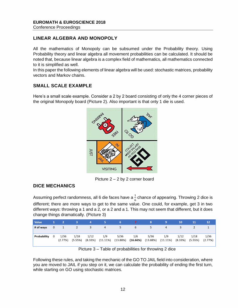
SMALL SCALE EXAMPLE Here’s a small scale example. Consider a 2 by 2 board consisting of only the 4 corner pieces of
the original Monopoly board (Picture 2). Also important is that only 1 die is used.
DICE MECHANICS
Assuming perfect randomness, all 6 die faces have a 1
6 chance of appearing. Throwing 2 dice is
different; there are more ways to get to the same value. One could, for example, get 3 in two
different ways: throwing a 1 and a 2, or a 2 and a 1. This may not seem that different, but it does
change things dramatically. (Picture 3)
Following these rules, and taking the mechanic of the GO TO JAIL field into consideration, where you are moved to JAIL if you step on it, we can calculate the probability of ending the first turn, while starting on GO using stochastic matrices.
Picture 2 – 2 by 2 corner board
Picture 3 – Table of probabilities for throwing 2 dice
EUROMATH & EUROSCIENCE 2018 Conference Proceedings
13
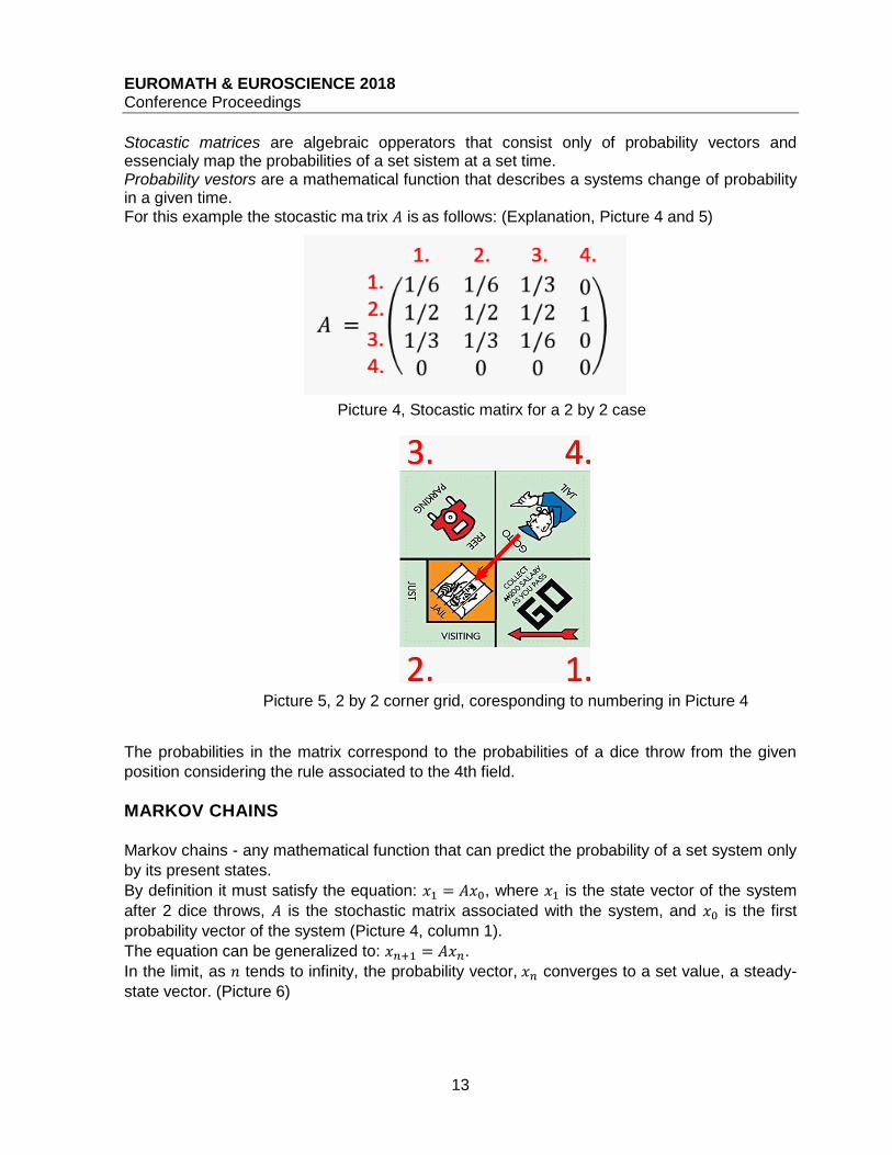
Stocastic matrices are algebraic opperators that consist only of probability vectors and essencialy map the probabilities of a set sistem at a set time. Probability vestors are a mathematical function that describes a systems change of probability in a given time.
For this example the stocastic ma trix 𝐴 is as follows: (Explanation, Picture 4 and 5)
The probabilities in the matrix correspond to the probabilities of a dice throw from the given
position considering the rule associated to the 4th field.
MARKOV CHAINS Markov chains - any mathematical function that can predict the probability of a set system only
by its present states.
By definition it must satisfy the equation: 𝑥1 = 𝐴𝑥0, where 𝑥1 is the state vector of the system
after 2 dice throws, 𝐴 is the stochastic matrix associated with the system, and 𝑥0 is the first
probability vector of the system (Picture 4, column 1).
The equation can be generalized to: 𝑥𝑛+1 = 𝐴𝑥𝑛.
In the limit, as 𝑛 tends to infinity, the probability vector, 𝑥𝑛 converges to a set value, a steady-
state vector. (Picture 6)
Picture 4, Stocastic matirx for a 2 by 2 case
Picture 5, 2 by 2 corner grid, coresponding to numbering in Picture 4

EUROMATH & EUROSCIENCE 2018 Conference Proceedings
14
A steady-state vector is a vector which represents the converged values of a Markov chains, in
other words, the probability of landing on a given square at a given time.
In this case it converges to 𝑥𝑛 = (
0.21429…0.5
0.28571…0
) , therefore the probability solution for a 2 by 2
board is represented in Picture 7.
SCALED UP CALCULATION Applying the same rules and calculations to a 11 by 11 board.
Picture 6, Extended Markov chain
Picture 7, Probability table for a 2 by 2
board
Picture 8, Extended Markov chain (general)

EUROMATH & EUROSCIENCE 2018 Conference Proceedings
15
Using the Markov chain extension (Picture 8) and a stochastic matrix 𝐴 with 21 rows and columns, the following results are obtained (Picture 9 and Picture 10):
Picture 9, Graph of the final probabilities
Picture 10, Table of the final probabilities
EUROMATH & EUROSCIENCE 2018 Conference Proceedings
16
SUMMARY
Jail is the most visited field.
Jail increases the probability of fields coming after it.
Orange and red properties are the most valuable by this theory.
Dark blue and brown properties are the least valuable.
It follows from the research and wealth calculation that it is better to buy 4 houses then
a hotel – “The monopoly on houses”.
REFERENCES
Allen, Donald; Matrices and Linear Algebra. In Lectures on Linear Algebra and Matrices (chapter
2) (2003), Retrieved from: http://www.math.tamu.edu/~dallen/m640_03c/lectures/chapter2.pdf
http://alumnus.caltech.edu/~leif/FRP/probability.html
Jorg Bewersdorff, Luck, Logic and White Lies: The Mathematics of Games, A K Peters (2005),
106-120.
J. Laurie Snell, Finite Markov Chains and their Applications, The American Mathematical
Monthly (1959), 66 (2), 99-104.
Richard Weber, Markov chain, Cambridge (2011), 1-15.

EUROMATH & EUROSCIENCE 2018 Conference Proceedings
17
CALCULATING CUBE ROOT Arnica Kiani, Sevin Vosughi
Meeraj Andisheh School, Iran
ABSTRACT
The cube root of a number means it is a value of that, when used in a multiplication by itself in three times, gives that number. In mathematics, a cube root of a number x is a number y such that y3 = x. In this paper explained about one simple and easy tip for finding Cube Roots of Perfect Cubes of two digits numbers. By this cube root formula we find cube root in fraction of seconds. These points to be remember for this cube root formula. The given number should be perfect cube. Remember cubes of 1 to 10 numbers. For per cubes identify as follow as Cube table 1 to 9. Identify the last three digits from right side and make group of these three digits. Take the last group and then find the cube root of it. Hence the right most digit of the cube root of the given number is obtained. Take the next group. Find out the value of it. The given number lies in between the cube of the numbers a3 and b3. Take small cube number. Hence the left neighbor digit of the answer is obtained. So our answer is solved and cube root is obtained. In this paper two methods were proposed to calculate the cube of numbers. One of these methods is using the power table 3 for number 0 to 9 and the cube of numbers, and the other is the decomposition of the number into the first factors and the extraction of the numbers with the power of 3.
FINDING CUBE ROOT OF A NUMBER QUICKLY
The third root is a radical number with a subfield 3 that is the third represented by the symbol
√x3
. If the number below the radical with the 3rd order reaches 3, the power of the number with
the simple power is simplified and the number is released from the sub-radical. To calculate the
third root of 64, it can be written as √433
with its third root equal to 4, and to calculate the third
root of 64, it can be written as √533
, that the third root It is equal to 5. In this paper, different
modes are calculated for calculating the third root, and the simplest method for each mode is
proposed And also in this paper explained about one simple and easy tip for finding Cube Roots
of Perfect Cubes of two digits numbers. By this cube root formula we find cube root in fraction
of seconds.
EUROMATH & EUROSCIENCE 2018 Conference Proceedings
18
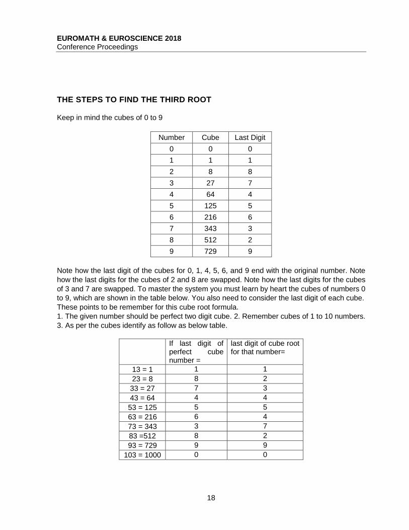
THE STEPS TO FIND THE THIRD ROOT
Keep in mind the cubes of 0 to 9
Number Cube Last Digit
0 0 0
1 1 1
2 8 8
3 27 7
4 64 4
5 125 5
6 216 6
7 343 3
8 512 2
9 729 9
Note how the last digit of the cubes for 0, 1, 4, 5, 6, and 9 end with the original number. Note
how the last digits for the cubes of 2 and 8 are swapped. Note how the last digits for the cubes
of 3 and 7 are swapped. To master the system you must learn by heart the cubes of numbers 0
to 9, which are shown in the table below. You also need to consider the last digit of each cube.
These points to be remember for this cube root formula.
1. The given number should be perfect two digit cube. 2. Remember cubes of 1 to 10 numbers.
3. As per the cubes identify as follow as below table.
If last digit of perfect cube number =
last digit of cube root for that number=
13 = 1 1 1
23 = 8 8 2
33 = 27 7 3
43 = 64 4 4
53 = 125 5 5
63 = 216 6 4
73 = 343 3 7
83 =512 8 2
93 = 729 9 9
103 = 1000 0 0

EUROMATH & EUROSCIENCE 2018 Conference Proceedings
19
DETERMINE THE CUBE ROOT
Ignore the last three digits of the number called out and choose the memorized cube which is
just lower (or equal) to the remaining number. The cube root of this is the first digit of your
answer. Now consider the last digit of the number called out. This will indicate the last digit of
your answer. For example, if the last digit of the number called out is 3, then the last digit of the
cube root is 7 (see the last digit values in the table above).
Examples:
Called Numbers
Ignore last 3
Lower Cube
First Digit
Last Digit
Cube Root
1728 1 1 1 2 12
21952 21 8 2 8 28
50653 50 27 3 7 37
117649 117 64 4 9 49
148877 148 125 5 3 53
216000 216 216 6 0 60
357911 357 343 7 1 71
636056 636 512 8 6 86
830584 830 729 9 4 94
Now let’s see how we can easily find out cube roots of perfect cubes with in fraction of seconds.
Take examples to easily understand the cube root formula.
Example 1: We get the third root of 405224 as follows:
√4052243
= cd
0 0 0
1 1 1
2 8 2
3 27 3
4 64 4
5 125 5
6 216 6
7 343 7
8 512 8
9 729 9
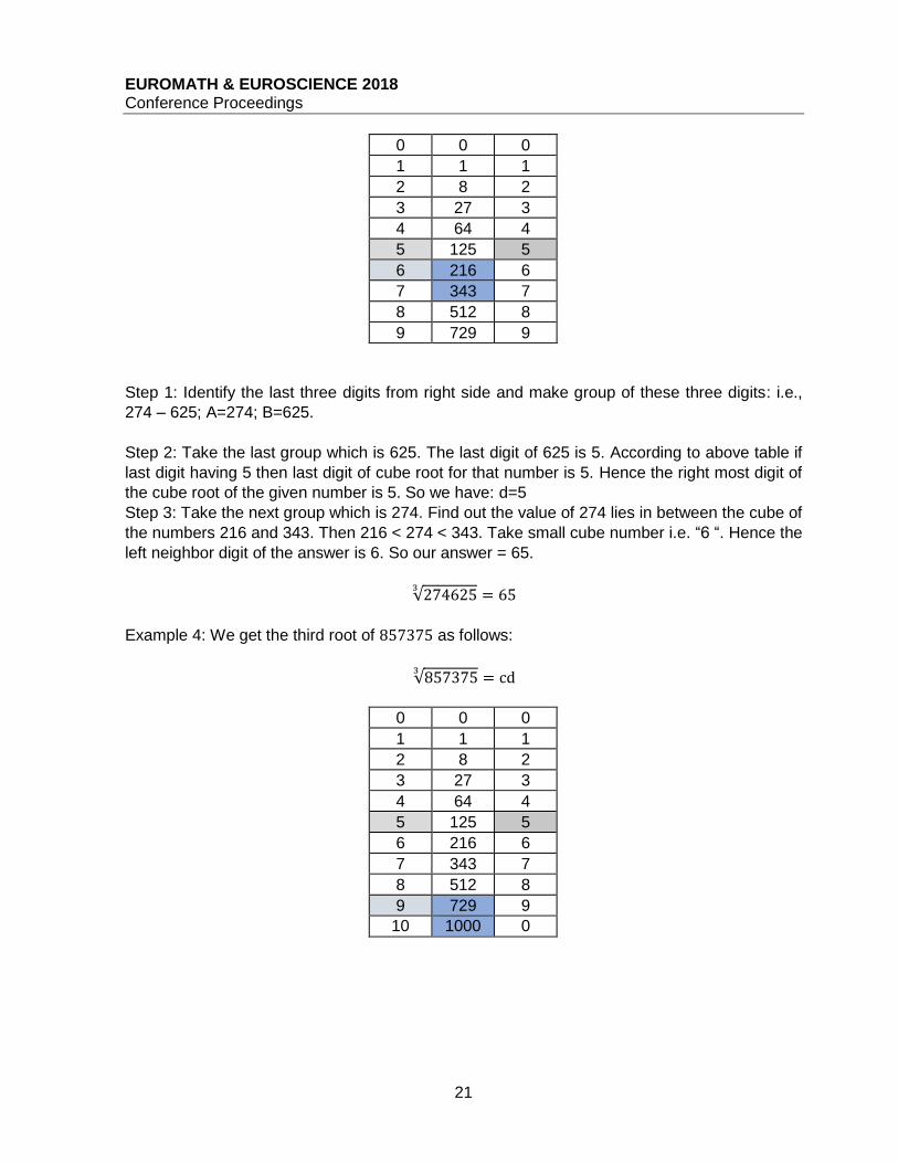
Step 1: Identify the last three digits from right side and make group of these three digits: i.e.,
405 – 224 ; A=405 ; B=224

EUROMATH & EUROSCIENCE 2018 Conference Proceedings
20
Step 2: Take the last group which is 224. The last digit of 224 is 4. According to above table if
last digit having 4 then last digit of cube root for that number is 4. Hence the right most digit of
the cube root of the given number is 4. So we have: d=4.
Step 3: Take the next group which is 405. Find out the value of 405 lies in between the cube of
the numbers 73 and 83. Then 343 < 405 < 512. Take small cube number i.e. “7“. Hence the left
neighbor digit of the answer is 7. So our answer = 74.
√4052243
= 74
Example 2: We get the third root of 97336 as follows:
√973363
= cd
0 0 0
1 1 1
2 8 2
3 27 3
4 64 4
5 125 5
6 216 6
7 343 7
8 512 8
9 729 9
Step 1: Identify the last three digits from right side and make group of these three digits: i.e., 97
– 336; A=97; B=336.
Step 2: Take the last group which is 336. The last digit of 336 is 6. According to above table if
last digit having 6 then last digit of cube root for that number is 6. Hence the right most digit of
the cube root of the given number is 6. So we have: d=6.
Step 3: Take the next group which is 97. Find out the value of 97 lies in between the cube of the
numbers 64 and 125. Then 64 < 97 < 125. Take small cube number i.e. “4“. Hence the left
neighbor digit of the answer is 4. So our answer = 46.
√973363
= 46
Example 3: We get the third root of 274625 as follows:
√2746253
= cd
EUROMATH & EUROSCIENCE 2018 Conference Proceedings
21
0 0 0
1 1 1
2 8 2
3 27 3
4 64 4
5 125 5
6 216 6
7 343 7
8 512 8
9 729 9
Step 1: Identify the last three digits from right side and make group of these three digits: i.e.,
274 – 625; A=274; B=625.
Step 2: Take the last group which is 625. The last digit of 625 is 5. According to above table if
last digit having 5 then last digit of cube root for that number is 5. Hence the right most digit of
the cube root of the given number is 5. So we have: d=5
Step 3: Take the next group which is 274. Find out the value of 274 lies in between the cube of
the numbers 216 and 343. Then 216 < 274 < 343. Take small cube number i.e. “6 “. Hence the
left neighbor digit of the answer is 6. So our answer = 65.
√2746253
= 65
Example 4: We get the third root of 857375 as follows:
√8573753
= cd
0 0 0
1 1 1
2 8 2
3 27 3
4 64 4
5 125 5
6 216 6
7 343 7
8 512 8
9 729 9
0 1000 10

EUROMATH & EUROSCIENCE 2018 Conference Proceedings
22
Step 1: Identify the last three digits from right side and make group of these three digits: i.e.,
857-375; A=857; B=375.
Step 2: Take the last group which is 375. The last digit of 375 is 5. According to above table if
last digit having 5 then last digit of cube root for that number is 5. Hence the right most digit of
the cube root of the given number is 5. So we have: d=5.
Step 3: Take the next group which is 857. Find out the value of 857 lies in between the cube of
the numbers 729 and 1000. Then 729 < 857 < 1000. Take small cube number i.e. “9 “. Hence
the left neighbor digit of the answer is 9. So our answer = 95.
√8573753
= 95
Example 5: We get the third root of 54872 as follows:
√54872 3
= cd
0 0 0
1 1 1
2 8 2
3 27 3
4 64 4
5 125 5
6 216 6
7 343 7
8 512 8
Step 1: Identify the last three digits from right side and make group of these three digits: i.e., 54
– 872; A=54; B=872.
Step 2: Take the last group which is 872. The last digit of 872 is 2. According to above table if
last digit having 2 then last digit of cube root for that number is 8. Hence the right most digit of
the cube root of the given number is 5. So we have: d=8.
Step 3: Take the next group which is 54. Find out the value of 54 lies in between the cube of the
numbers 729 and 1000. Then 27 < 54 < 64. Take small cube number i.e. “3 “. Hence the left
neighbor digit of the answer is 3. So our answer = 38.
√548723
= 38

EUROMATH & EUROSCIENCE 2018 Conference Proceedings
23
FINDING THE THIRD ROOT BY PRIME FACTORIZATION
We can find the cube root of a number by the method of prime factorization. Consider the
following example for a clear understanding: 2744 = 2 × 2 × 2 × 7 × 7 × 7 = (2 × 7)3. Therefore
the cube root of 2744 = √27443
= 2 × 7 = 14.
The steps to find the third root of the numbers are: Step 1. Decomposing the numbers into the
first counters. Step 2. Sort the counters with power. Step 3. Find the number that has the power
of 3. Step 4. The number that powers 3 can be released with a simplified substrate from the
radical. If the group of decomposable numbers has no power 3, then there is no third digit and
the cube is not complete. The following examples help to solve examples for the third root.
Example 1: Find the third root of the number 216 as follows:
We divide the number into the Prime Factorization
2 216
2 108
2 54
3 27
3 9
3 3
1
So the number 216 can be written as follows:
216 = 2 × 2 × 2 × 3 × 3 × 3 = (2 × 2 × 2) × (3 × 3 × 3)
√2163
=√(2 × 3)33
=√633
=6
Example 2: Find the third root of the number 343 as follows:
We divide the number into the Prime Factorization:
7 343
7 49
7 7
1
So the number 216 can be written as follows:
343 = 7 × 7 × 7 = (7 × 7 × 7) → √3433
= √733
=3
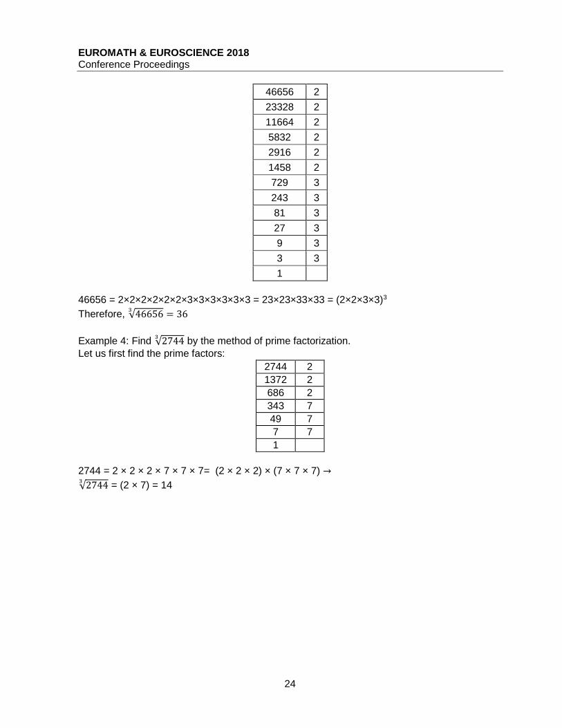
Example 3: Find √466563
by the method of prime factorization.
Let us first find the prime factors:
EUROMATH & EUROSCIENCE 2018 Conference Proceedings
24
46656 2
23328 2
11664 2
5832 2
2916 2
1458 2
729 3
243 3
81 3
27 3
9 3
3 3
1
46656 = 2×2×2×2×2×2×3×3×3×3×3×3 = 23×23×33×33 = (2×2×3×3)3
Therefore, √466563
= 36
Example 4: Find √27443
by the method of prime factorization.
Let us first find the prime factors:
2744 2
1372 2
686 2
343 7
49 7
7 7
1
2744 = 2 × 2 × 2 × 7 × 7 × 7= (2 × 2 × 2) × (7 × 7 × 7) →
√27443
= (2 × 7) = 14

EUROMATH & EUROSCIENCE 2018 Conference Proceedings
25
IDENTIFY COMPLETE CUBE NUMBERS
The number is broken down by the column or ladder method to the prime factors. If all the prime
factors are multiplied by 3 times, then the number is complete cube.
Example 1: Consider the number 250:
Parsing it into the prime factors is as follows:
250 2
125 5
25 5
5 5
1
250 = 2 × 5 × 5 × 5
The factor 2 is power 1 and does not have power 3. Therefore, the number 250 is not complete
cube.
Example 2: Consider the number 5832. Parsing it into the prime factors is as follows:
5832 2
2916 2
1458 2
729 3
243 3
81 3
27 3
9 3
3 3
1
5832 = 2 × 2 × 2 × 3 × 3 × 3 × 3 × 3 × 3
All factors have the power of 3. So the number 5832 is complete cube.
EUROMATH & EUROSCIENCE 2018 Conference Proceedings
26
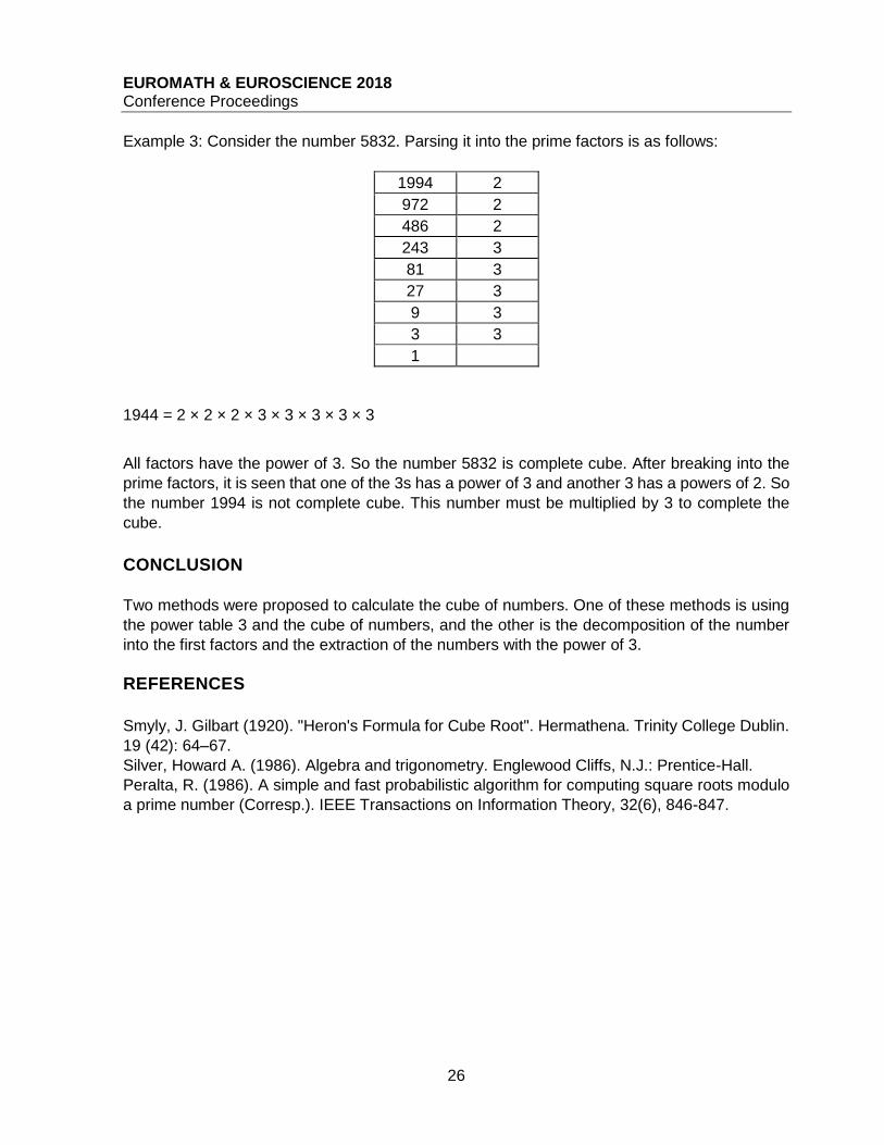
Example 3: Consider the number 5832. Parsing it into the prime factors is as follows:
1994 2
972 2
486 2
243 3
81 3
27 3
9 3
3 3
1
1944 = 2 × 2 × 2 × 3 × 3 × 3 × 3 × 3
All factors have the power of 3. So the number 5832 is complete cube. After breaking into the
prime factors, it is seen that one of the 3s has a power of 3 and another 3 has a powers of 2. So
the number 1994 is not complete cube. This number must be multiplied by 3 to complete the
cube.
CONCLUSION
Two methods were proposed to calculate the cube of numbers. One of these methods is using
the power table 3 and the cube of numbers, and the other is the decomposition of the number
into the first factors and the extraction of the numbers with the power of 3.
REFERENCES
Smyly, J. Gilbart (1920). "Heron's Formula for Cube Root". Hermathena. Trinity College Dublin.
19 (42): 64–67.
Silver, Howard A. (1986). Algebra and trigonometry. Englewood Cliffs, N.J.: Prentice-Hall.
Peralta, R. (1986). A simple and fast probabilistic algorithm for computing square roots modulo
a prime number (Corresp.). IEEE Transactions on Information Theory, 32(6), 846-847.

EUROMATH & EUROSCIENCE 2018 Conference Proceedings
27
THE ROLE OF MATHEMATICS IN MEDICINE Shakila Hamdy
Farzaneghan1 High School, Iran
ABSTRACT
In this article, you will find out many important things about the role of mathematics in medicine. For example, you will find out how doctors use mathematics to write prescriptions; You also discover the relationship between ellipse and treating gallstones and kidney stones; you see medical graphs too. You also learn that mathematics play an important role in the treatment of cancer and tumors. Finally, you will become aware of the most interesting role of mathematics, a model that predicts outbreaks of infectious diseases.
INTRODUCTION
Today, at advanced levels of research, mathematics has played a very important role in science
and medical studies. So that mathematical equations cannot be denied in different parts of
medicine. Undoubtedly, close interactions between physicians and mathematicians will
contribute to a more principled and more effective treatment, and the physician can use the
mathematical equations in the treatment of diseases and by using clinical and disease
management methods to fundamentally treat illnesses, to reduce the Side effects of medications
in treatment.
In Medicine three subjects are specially considered:
1. Diagnose the disease
2. Cure the disease
3. Control the disease
Infectious and non-infectious disease are a dynamic system. So, they have minor and ordinary
Differential Equations. They have such equations for Diabetes, HIV, Tuberculosis, Hepatitis,
Tumor… That they have been determined now and these mathematical models are getting
progress. In those three subjects mathematics have an incredible role that its result can help
medicine a lot.
WRITING PRESCRIPTIONS
Regularly, doctors write prescriptions to their patients for various ailments. Prescriptions
indicate a specific medication and dosage amount. Most medications have guidelines for
dosage amounts in milligrams (mg) per kilogram (kg). Doctors need to figure out how many

EUROMATH & EUROSCIENCE 2018 Conference Proceedings
28
milligrams of medication each patient will need, depending on their weight. If the weight of a
patient is only known in pounds, doctors need to convert that measurement to kilograms and
then find the amount of milligrams for the prescription. There is a very big difference between
mg/kg and mg/lbs, so it is imperative that doctors understand how to accurately convert weight
measurements. Doctors must also determine how long a prescription will last. For example, if
a patient needs to take their medication, say one pill, three times a day. Then one month of pills
is approximately 90 pills. However, most patients prefer two or three month prescriptions for
convenience and insurance purposes. Doctors must be able to do these calculations mentally
with speed and accuracy.
Doctors must also consider how long the medicine will stay in the patient’s body. This will
determine how often the patient needs to take their medication in order to keep a sufficient
amount of the medicine in the body. For example, a patient takes a pill in the morning that has
50mg of a particular medicine. When the patient wakes up the next day, their body has washed
out 40% of the medication. This means that 20mg have been washed out and only 30mg remain
in the body. The patient continues to take their 50mg pill each morning. This means that on the
morning of day two, the patient has the 30mg left over from day one, as well as another 50mg
from the morning of day two, which is a total of 80mg. As this continues, doctors must determine
how often a patient needs to take their medication, and for how long, in order to keep enough
medicine in the patient’s body to work effectively, but without overdosing.
The amount of medicine in the body after taking a medication decreases by a certain percentage
in a certain time (perhaps 10% each hour, for example). This percentage decrease can be
expressed as a rational number, 1/10. Hence in each hour, if the amount at the end of the hour
decreases by 1/10 then the amount remaining is 9/10 of the amount at the beginning of the hour.
This constant rational decrease creates a geometric sequence. So, if a patient takes a pill that
has 200mg of a certain drug, the decrease of medication in their body each hour can be seen in
the folowing table. The Start column contains the number of mg of the drug remaining in the
system at the start of the hour and the End column contains the number of mg of the drug
remaining in the system at the end of the hour.
The sequence of numbers shown below is geometric because there is a common ratio between
terms, in this case 9/10. Doctors can use this idea to quickly decide how often a patient needs
to take their prescribed medication.
Hour Start End
1 200 9/10 x 200 = 180
2 180 9/10 x 180 = 162
3 162 9/10 x 162 = 145.8
. . .
EUROMATH & EUROSCIENCE 2018 Conference Proceedings
29
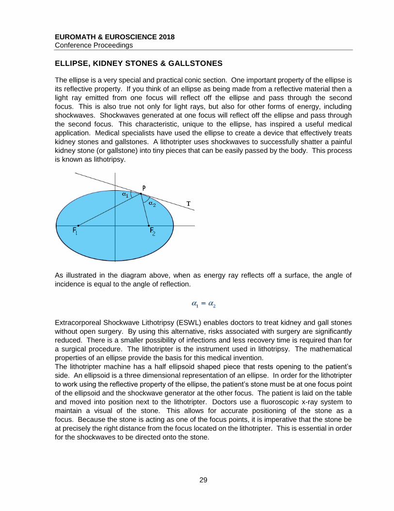
ELLIPSE, KIDNEY STONES & GALLSTONES The ellipse is a very special and practical conic section. One important property of the ellipse is
its reflective property. If you think of an ellipse as being made from a reflective material then a
light ray emitted from one focus will reflect off the ellipse and pass through the second
focus. This is also true not only for light rays, but also for other forms of energy, including
shockwaves. Shockwaves generated at one focus will reflect off the ellipse and pass through
the second focus. This characteristic, unique to the ellipse, has inspired a useful medical
application. Medical specialists have used the ellipse to create a device that effectively treats
kidney stones and gallstones. A lithotripter uses shockwaves to successfully shatter a painful
kidney stone (or gallstone) into tiny pieces that can be easily passed by the body. This process
is known as lithotripsy.
As illustrated in the diagram above, when as energy ray reflects off a surface, the angle of
incidence is equal to the angle of reflection.
Extracorporeal Shockwave Lithotripsy (ESWL) enables doctors to treat kidney and gall stones
without open surgery. By using this alternative, risks associated with surgery are significantly
reduced. There is a smaller possibility of infections and less recovery time is required than for
a surgical procedure. The lithotripter is the instrument used in lithotripsy. The mathematical
properties of an ellipse provide the basis for this medical invention.
The lithotripter machine has a half ellipsoid shaped piece that rests opening to the patient’s
side. An ellipsoid is a three dimensional representation of an ellipse. In order for the lithotripter
to work using the reflective property of the ellipse, the patient’s stone must be at one focus point
of the ellipsoid and the shockwave generator at the other focus. The patient is laid on the table
and moved into position next to the lithotripter. Doctors use a fluoroscopic x-ray system to
maintain a visual of the stone. This allows for accurate positioning of the stone as a
focus. Because the stone is acting as one of the focus points, it is imperative that the stone be
at precisely the right distance from the focus located on the lithotripter. This is essential in order
for the shockwaves to be directed onto the stone.

EUROMATH & EUROSCIENCE 2018 Conference Proceedings
30
MEDICAL GRAPHS
The open wound is the
circular region {0 ≤ r ≤ R(t)}, the partially
healed region is the annulus {R(t) ≤ r ≤ R(0)},
and the normal healthy tissue is
{R(0) ≤ r ≤ L}.
EUROMATH & EUROSCIENCE 2018 Conference Proceedings
31
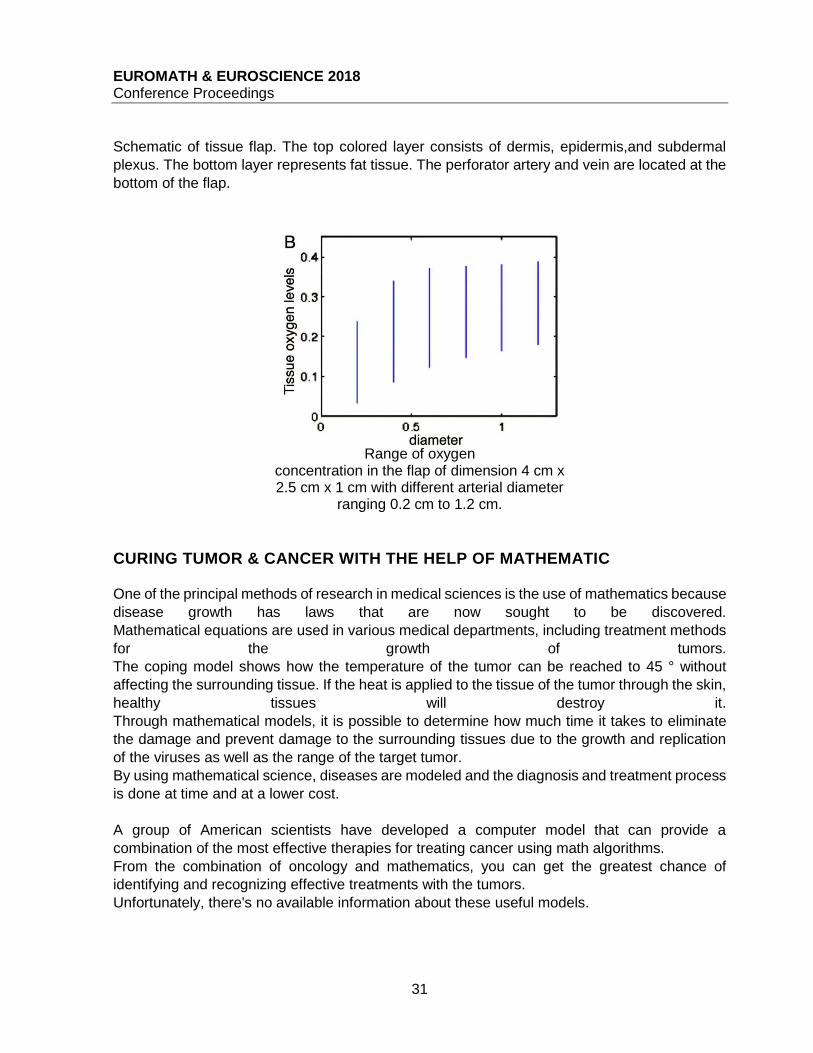
Schematic of tissue flap. The top colored layer consists of dermis, epidermis,and subdermal
plexus. The bottom layer represents fat tissue. The perforator artery and vein are located at the
bottom of the flap.
Range of oxygen
concentration in the flap of dimension 4 cm x 2.5 cm x 1 cm with different arterial diameter
ranging 0.2 cm to 1.2 cm.
CURING TUMOR & CANCER WITH THE HELP OF MATHEMATIC
One of the principal methods of research in medical sciences is the use of mathematics because
disease growth has laws that are now sought to be discovered.
Mathematical equations are used in various medical departments, including treatment methods
for the growth of tumors.
The coping model shows how the temperature of the tumor can be reached to 45 ° without
affecting the surrounding tissue. If the heat is applied to the tissue of the tumor through the skin,
healthy tissues will destroy it.
Through mathematical models, it is possible to determine how much time it takes to eliminate
the damage and prevent damage to the surrounding tissues due to the growth and replication
of the viruses as well as the range of the target tumor.
By using mathematical science, diseases are modeled and the diagnosis and treatment process
is done at time and at a lower cost.
A group of American scientists have developed a computer model that can provide a
combination of the most effective therapies for treating cancer using math algorithms.
From the combination of oncology and mathematics, you can get the greatest chance of
identifying and recognizing effective treatments with the tumors.
Unfortunately, there's no available information about these useful models.
EUROMATH & EUROSCIENCE 2018 Conference Proceedings
32
A MODEL TO PREDICT THE OUTBREAK OF THE INFECTIOUS DISEASES
American scientists have developed math algorithms that can help predict epidemics associated
with the most common infectious diseases based on weather parameters.
Researchers at the Tufts University School of Medicine in Boston have presented a
mathematical model that assesses the probability of an outbreak of these diseases on a daily
basis, based on the environmental parameters on each site, according to Health News.
Scientists have tested their math model based on data collected by the Massachusetts Public
Health Department regarding six diseases, according to the Medical News Todd.
The six diseases were Jardia and Cryptosporidium (two intestinal infectious diseases),
Salmonella and Campylobacter (two common intestinal diseases that occur in the intestines due
to the introduction of Salmonella and Campylobacter bacteria and are very common in Europe),
Shigellosis (A tropical disease that occurs as a result of infection with Shigella bacteria) and A-
hepatitis A due to infection with the Hiv virus.
Then, using these climatic data collected between 1992 and 2001, the scientists examined the
incidence of each of these diseases in Massachusetts based on the values of the average daily
temperature, the time and the course of each of these diseases.
The preliminary results of the experiment showed that the incidence of these diseases is related
to hepatocellular carcinoma A, other than heat.
Therefore, the current algorithmic models are based on seasonal and monthly information on
the epidemiology of infectious diseases, while the new model is being investigated daily.
CONCLUSION
Mathematics plays a crucial role in medicine and because people’s lives are involved, it is very
important for nurses and doctors to be very accurate in their mathematical calculations. Numbers
provide information for doctors, nurses, and even patients. Numbers are a way of
communicating information, which is very important in the medical field
Doctors can have a better diagnosis, curing and controlling with the help of mathematics.
REFERENCES
Ricky D Turgeon, Mathematics in medicine (article)
Anver Friedman, What is mathematical biology & how useful is it? (article)
Natasha Glydon, Medicine & Math (website)
http://mathcentral.uregina.ca/beyond/articles/medicine/med1.html
http://mathematical.blogfa.com/page/13.aspx
https://wmcm1392.persianblog.ir/g89BXemRqli5OQJ3AO1w
EUROMATH & EUROSCIENCE 2018 Conference Proceedings
33
FRACTAL STRUCTURE OF DNA Marija Pavlovic, Milica Jurisic, Mirjana Jovanovic
“Isidora Sekulic” Grammar School, Serbia
ABSTRACT
Fractals are formed from self-similar objects that ensue by self-repeating pattern thus forming smaller
look-alike parts same as the entire object. Although Mandelbrot is considered to be the father of fractals,
they owe its true existence to Giuseppe Peano, who defined a group of self-similar curves by which these
are explained. Micro and macro world are both of fractal nature and so is, by definition, DNA, being a
part of micro world itself. The paper will explain how fractal model of DNA, thanks to its characteristics,
represents the most suitable way for DNA to fold, while comparing it to less suitable polymer model. Ever
since the idea was first unveiled to scientific public, it has had a great influence on DNA structure
analysis. Fractals started being widely used in various fields.
1. INTRODUCTION
The term ‘fractal’ first appeared in Ancient Rome as fractus, which means broken. Gottfried
Leibniz, German mathematician and philosopher, first used the collocation of it to define and
explain self-similarity of a straight line. Helge von Koch, Waclaw Sierpinski, Felix Hausdorf and
Paul Levi made a great endowment to this mathematical discipline and Benoit Mandelbrot
unified all then-known characteristics of fractals referring to them as to geometric structures
whose fractal dimension is bigger than their topological one. Still, the simplest description says
that a fractal is a mathematical assemblage of self-similar objects that ensue by repeating one
identical procedure.
The world is full of fractals, but can we apply them on things we cannot perceive or even on
ourselves? Absolutely. Universe is a fractal so as many organs in our body: our brain, lungs,
blood vessels, whole nervous system. All systems of organs are of tissues generated by cells
and these are made of cytosol and organelles. The most perplexed one, nucleus, keeps in its
inwardness deoxyribonucleic acid (DNA), a genetic material which is the key to functioning of
all organisms. In this scientific work we will explain how meters of DNA are packed within the
nucleus’s radius of 5μm.
2. FRACTALS IN NATURE
Broccoli, snowflakes, bacteria, fungi, trees, lightening, river flows and steep mountain slopes
are just some of many fractal examples. As a part of the Universe we are also fractals. The most
complex structure in the whole known Universe is a fractal, and it is within us- the Brain. Besides
being rich with vitamins K and D, β-carotene and dietary fiber, Broccolo Romanesco of Brassica
Oleracea species is a fascinating illustration of a fractal. Every single bud acts as a duplicate of
EUROMATH & EUROSCIENCE 2018 Conference Proceedings
34
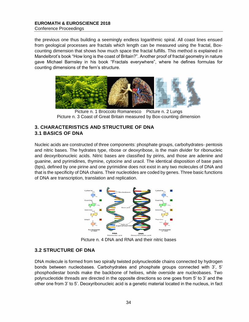
the previous one thus building a seemingly endless logarithmic spiral. All coast lines ensued
from geological processes are fractals which length can be measured using the fractal, Box-
counting dimension that shows how much space the fractal fulfills. This method is explained in
Mandelbrot’s book “How long is the coast of Britain?”. Another proof of fractal geometry in nature
gave Michael Barnsley in his book “Fractals everywhere”, where he defines formulas for
counting dimensions of the fern’s structure.
Picture n. 1 Broccolo Romanesco Picture n. 2 Lungs Picture n. 3 Coast of Great Britain measured by Box-counting dimension
3. CHARACTERISTICS AND STRUCTURE OF DNA
3.1 BASICS OF DNA
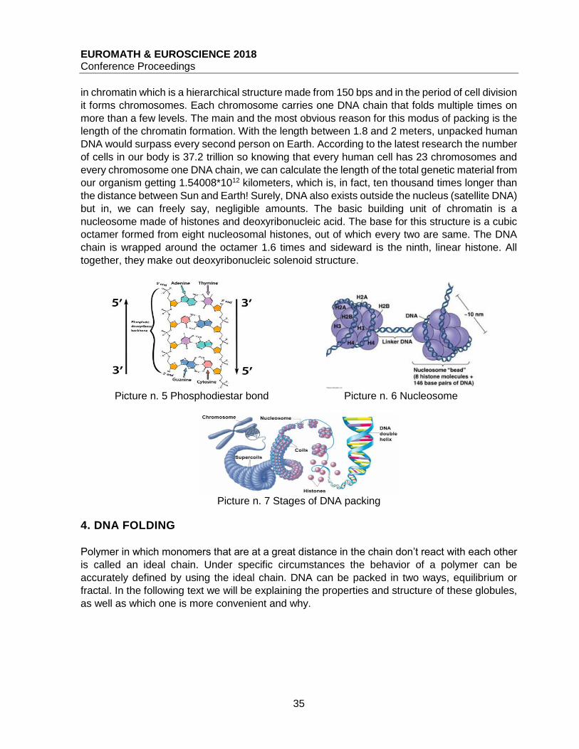
Nucleic acids are constructed of three components: phosphate groups, carbohydrates- pentosis
and nitric bases. The hydrates type, ribose or deoxyribose, is the main divider for ribonucleic
and deoxyribonucleic acids. Nitric bases are classified by pirins, and those are adenine and
guanine, and pyrimidines, thymine, cytocine and uracil. The identical disposition of base pairs
(bps), defined by one pirine and one pyrimidine does not exist in any two molecules of DNA and
that is the specificity of DNA chains. Their nucleotides are coded by genes. Three basic functions
of DNA are transcription, translation and replication.
Picture n. 4 DNA and RNA and their nitric bases
3.2 STRUCTURE OF DNA
DNA molecule is formed from two spirally twisted polynucleotide chains connected by hydrogen
bonds between nucleobases. Carbohydrates and phosphate groups connected with 3’, 5’
phosphodiestar bonds make the backbone of helixes, while overside are nucleobases. Two
polynucleotide threads are directed in the opposite directions so one goes from 5’ to 3’ and the
other one from 3’ to 5’. Deoxyribonucleic acid is a genetic material located in the nucleus, in fact
EUROMATH & EUROSCIENCE 2018 Conference Proceedings
35
in chromatin which is a hierarchical structure made from 150 bps and in the period of cell division
it forms chromosomes. Each chromosome carries one DNA chain that folds multiple times on
more than a few levels. The main and the most obvious reason for this modus of packing is the
length of the chromatin formation. With the length between 1.8 and 2 meters, unpacked human
DNA would surpass every second person on Earth. According to the latest research the number
of cells in our body is 37.2 trillion so knowing that every human cell has 23 chromosomes and
every chromosome one DNA chain, we can calculate the length of the total genetic material from
our organism getting 1.54008*1012 kilometers, which is, in fact, ten thousand times longer than
the distance between Sun and Earth! Surely, DNA also exists outside the nucleus (satellite DNA)
but in, we can freely say, negligible amounts. The basic building unit of chromatin is a
nucleosome made of histones and deoxyribonucleic acid. The base for this structure is a cubic
octamer formed from eight nucleosomal histones, out of which every two are same. The DNA
chain is wrapped around the octamer 1.6 times and sideward is the ninth, linear histone. All
together, they make out deoxyribonucleic solenoid structure.
Picture n. 5 Phosphodiestar bond Picture n. 6 Nucleosome
Picture n. 7 Stages of DNA packing
4. DNA FOLDING
Polymer in which monomers that are at a great distance in the chain don’t react with each other
is called an ideal chain. Under specific circumstances the behavior of a polymer can be
accurately defined by using the ideal chain. DNA can be packed in two ways, equilibrium or
fractal. In the following text we will be explaining the properties and structure of these globules,
as well as which one is more convenient and why.
EUROMATH & EUROSCIENCE 2018 Conference Proceedings
36
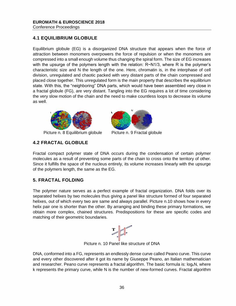
4.1 EQUILIBRIUM GLOBULE
Equilibrium globule (EG) is a disorganized DNA structure that appears when the force of
attraction between monomers overpowers the force of repulsion or when the monomers are
compressed into a small enough volume thus changing the spiral form. The size of EG increases
with the upsurge of the polymers length with the relation: R~N1/3, where R is the polymer’s
characteristic size and N the length of the one. Here, chromatin is, in the interphase of cell
division, unregulated and chaotic packed with very distant parts of the chain compressed and
placed close together. This unregulated form is the main property that describes the equilibrium
state. With this, the “neighboring” DNA parts, which would have been assembled very close in
a fractal globule (FG), are very distant. Tangling into the EG requires a lot of time considering
the very slow motion of the chain and the need to make countless loops to decrease its volume
as well.
Picture n. 8 Equilibrium globule Picture n. 9 Fractal globule
4.2 FRACTAL GLOBULE
Fractal compact polymer state of DNA occurs during the condensation of certain polymer
molecules as a result of preventing some parts of the chain to cross onto the territory of other.
Since it fulfills the space of the nucleus entirely, its volume increases linearly with the upsurge
of the polymers length, the same as the EG.
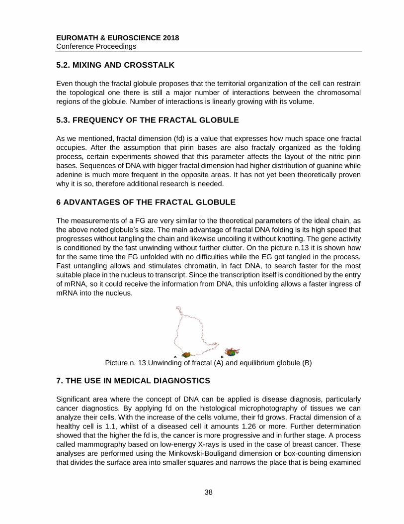
5. FRACTAL FOLDING
The polymer nature serves as a perfect example of fractal organization. DNA folds over its
separated helixes by two molecules thus giving a panel like structure formed of four separated
helixes, out of which every two are same and always parallel. Picture n.10 shows how in every
helix pair one is shorter than the other. By arranging and binding these primary formations, we
obtain more complex, chained structures. Predispositions for these are specific codes and
matching of their geometric boundaries.
Picture n. 10 Panel like structure of DNA
DNA, conformed into a FG, represents an endlessly dense curve called Peano curve. This curve
and every other discovered after it got its name by Giuseppe Peano, an Italian mathematician
and researcher. Peano curve represents a fractal algorithm. The basic formula is: logkN, where
k represents the primary curve, while N is the number of new-formed curves. Fractal algorithm

EUROMATH & EUROSCIENCE 2018 Conference Proceedings
37
creates from a line a Peano curve that occupies each point of that space and it stays a line
(topological dimension remains 1) despite the interminable iterations. This explains how 2
meters of DNA can be “stuffed” inside a nucleus of 523.33 μm3 volume. The fractal globule is
nothing but a Peano curve conformed into a spherical shape of the nucleus. The curved line is
not intersected or embrangled anywhere so if we pulled a randomly picked part, we could easily
stretch it out because it would not tangle anywhere and in the same way we could put it back as
it was. In the metaphase of cell division there are 23 chromosomes, respectively 23
chromosomal territories and each one makes out a small fractal molecule. Herewith, self-
similarity of the fractal in the nucleus is confirmed.
Picture n. 11 Peano’s curve
5.1. STABILITY OF A FRACTAL GLOBULE
Original theories suggest that the lifetime of a FG depends on the time required to thread the
ends of the chain through the whole globule allowing the formation to stay knotted and also on
its stringency and ability to firm its topological restrains. These restrains can be simply
interrupted by DNA topoisomerase II enzymes, products of the cells enzyme activity which are
able to crumple and unknot DNA chains, alleviating the replication and synthesis of proteins for
which the unknotting of the double helix is crucial. There are two types: topo I and topo II. Topo
II cuts the double helix by its two chains, passing through another unaffected DNA double helix
and relegating cut DNA. Topo I cuts only one DNA helix in order to bind it again after the process
of synthesis passes. Topoisomerase II aggravates the cell's natural homeostasis by knotting
and unknotting the chromatin several times. It has been proved that increased amount of topo
II added to the nucleus could develop a strong affection for topo II, during the interphase of the
cell, to destroy chromosomal territories leading to the equilibration of the FG. Such amounts of
topo II are able to break all the mechanisms of cytoskeleton to constrain the cell denaturation.
Such constrains will be effective only in the case of enabling topo II to destroy chromatin fibers.
Fortunately, topo II is not that huge antagonist in this role of the cell function. FG should be able
to oppose the equilibrium long enough for the duration of single cell cycle. Another encouraging
fact is that after the mitosis whole chromosomal architecture of a cell is re-established.
Picture n. 12 Equilibration of a fractal globule
EUROMATH & EUROSCIENCE 2018 Conference Proceedings
38
5.2. MIXING AND CROSSTALK
Even though the fractal globule proposes that the territorial organization of the cell can restrain
the topological one there is still a major number of interactions between the chromosomal
regions of the globule. Number of interactions is linearly growing with its volume.
5.3. FREQUENCY OF THE FRACTAL GLOBULE
As we mentioned, fractal dimension (fd) is a value that expresses how much space one fractal
occupies. After the assumption that pirin bases are also fractaly organized as the folding
process, certain experiments showed that this parameter affects the layout of the nitric pirin
bases. Sequences of DNA with bigger fractal dimension had higher distribution of guanine while
adenine is much more frequent in the opposite areas. It has not yet been theoretically proven
why it is so, therefore additional research is needed.
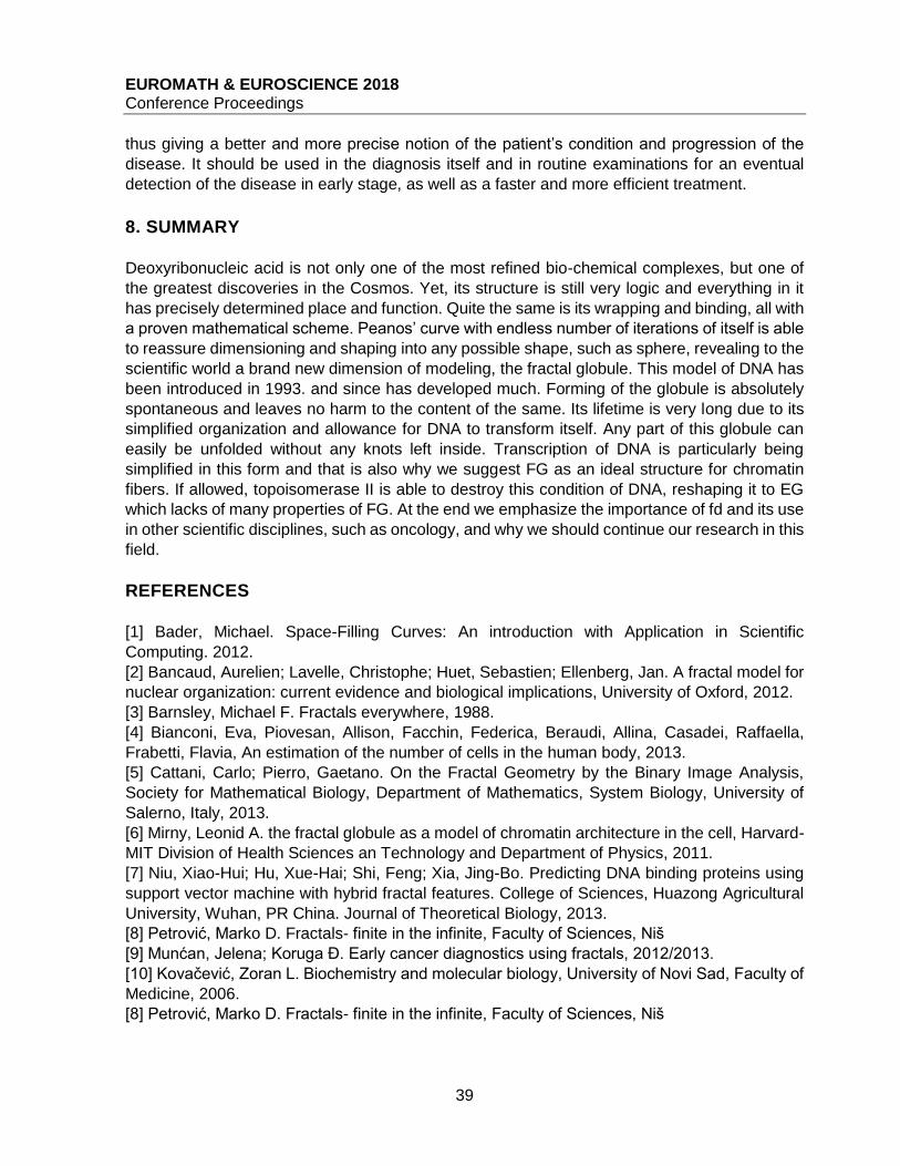
6 ADVANTAGES OF THE FRACTAL GLOBULE
The measurements of a FG are very similar to the theoretical parameters of the ideal chain, as
the above noted globule’s size. The main advantage of fractal DNA folding is its high speed that
progresses without tangling the chain and likewise uncoiling it without knotting. The gene activity
is conditioned by the fast unwinding without further clutter. On the picture n.13 it is shown how
for the same time the FG unfolded with no difficulties while the EG got tangled in the process.
Fast untangling allows and stimulates chromatin, in fact DNA, to search faster for the most
suitable place in the nucleus to transcript. Since the transcription itself is conditioned by the entry
of mRNA, so it could receive the information from DNA, this unfolding allows a faster ingress of
mRNA into the nucleus.
Picture n. 13 Unwinding of fractal (A) and equilibrium globule (B)
7. THE USE IN MEDICAL DIAGNOSTICS
Significant area where the concept of DNA can be applied is disease diagnosis, particularly
cancer diagnostics. By applying fd on the histological microphotography of tissues we can
analyze their cells. With the increase of the cells volume, their fd grows. Fractal dimension of a
healthy cell is 1.1, whilst of a diseased cell it amounts 1.26 or more. Further determination
showed that the higher the fd is, the cancer is more progressive and in further stage. A process
called mammography based on low-energy X-rays is used in the case of breast cancer. These
analyses are performed using the Minkowski-Bouligand dimension or box-counting dimension
that divides the surface area into smaller squares and narrows the place that is being examined
EUROMATH & EUROSCIENCE 2018 Conference Proceedings
39
thus giving a better and more precise notion of the patient’s condition and progression of the
disease. It should be used in the diagnosis itself and in routine examinations for an eventual
detection of the disease in early stage, as well as a faster and more efficient treatment.
8. SUMMARY
Deoxyribonucleic acid is not only one of the most refined bio-chemical complexes, but one of
the greatest discoveries in the Cosmos. Yet, its structure is still very logic and everything in it
has precisely determined place and function. Quite the same is its wrapping and binding, all with
a proven mathematical scheme. Peanos’ curve with endless number of iterations of itself is able
to reassure dimensioning and shaping into any possible shape, such as sphere, revealing to the
scientific world a brand new dimension of modeling, the fractal globule. This model of DNA has
been introduced in 1993. and since has developed much. Forming of the globule is absolutely
spontaneous and leaves no harm to the content of the same. Its lifetime is very long due to its
simplified organization and allowance for DNA to transform itself. Any part of this globule can
easily be unfolded without any knots left inside. Transcription of DNA is particularly being
simplified in this form and that is also why we suggest FG as an ideal structure for chromatin
fibers. If allowed, topoisomerase II is able to destroy this condition of DNA, reshaping it to EG
which lacks of many properties of FG. At the end we emphasize the importance of fd and its use
in other scientific disciplines, such as oncology, and why we should continue our research in this
field.
REFERENCES
[1] Bader, Michael. Space-Filling Curves: An introduction with Application in Scientific
Computing. 2012.
[2] Bancaud, Aurelien; Lavelle, Christophe; Huet, Sebastien; Ellenberg, Jan. A fractal model for
nuclear organization: current evidence and biological implications, University of Oxford, 2012.
[3] Barnsley, Michael F. Fractals everywhere, 1988.
[4] Bianconi, Eva, Piovesan, Allison, Facchin, Federica, Beraudi, Allina, Casadei, Raffaella,
Frabetti, Flavia, An estimation of the number of cells in the human body, 2013.
[5] Cattani, Carlo; Pierro, Gaetano. On the Fractal Geometry by the Binary Image Analysis,
Society for Mathematical Biology, Department of Mathematics, System Biology, University of
Salerno, Italy, 2013.
[6] Mirny, Leonid A. the fractal globule as a model of chromatin architecture in the cell, Harvard-
MIT Division of Health Sciences an Technology and Department of Physics, 2011.
[7] Niu, Xiao-Hui; Hu, Xue-Hai; Shi, Feng; Xia, Jing-Bo. Predicting DNA binding proteins using
support vector machine with hybrid fractal features. College of Sciences, Huazong Agricultural
University, Wuhan, PR China. Journal of Theoretical Biology, 2013.
[8] Petrović, Marko D. Fractals- finite in the infinite, Faculty of Sciences, Niš
[9] Munćan, Jelena; Koruga Đ. Early cancer diagnostics using fractals, 2012/2013.
[10] Kovačević, Zoran L. Biochemistry and molecular biology, University of Novi Sad, Faculty of
Medicine, 2006.
[8] Petrović, Marko D. Fractals- finite in the infinite, Faculty of Sciences, Niš

EUROMATH & EUROSCIENCE 2018 Conference Proceedings
40
[11] How Long is the Coast of Britain? Statistical Self-Similarity and Fractional Dimension,
Wikipedia, the free encyclopedia
[13] Tsang, Wai H. The Fractal Brain and Fractal Genome
[14] Wertenberger, Kimberly, University of Kentucky, Mandelbrot Sets and Julia Sets

EUROMATH & EUROSCIENCE 2018 Conference Proceedings
41
EXPLORING THE ANCIENT GREEKS’ MYSTIC AND TOPOGRAPHICAL SYMMETRIES
Sofia Bakali, Thanasis Bakalis, Stelios Samaras, Xristodoulos Karapatakhs
Diastaseis, Private School, Greece
ABSTRACT Geodesic triangulation of ancient Greece is a miraculous mystery. If we study the position of temples, sanctuaries and cities, we can see that geometrical patterns are formed such as isosceles and equilateral triangles, concentric circles passing from the same point as well as straight lines perceptibly joining cities together. This harmonious relation comes to us, the younger ones, as a picture of colossal conception, making us shiver from great excitement. It’s worth wondering thus, if all this happened by a curious coincidence or as a result of mathematical calculations able to touch perfection. Is there a well-hidden secret refusing to be revealed even in these days? Most of us have heard of the Parthenon, a great monument with such an architectural structure,
that even nowadays it would be difficult to construct.
One of its most marvellous traits is that if we extend its four columns despite the fact that they
appear parallel, they will meet up at a certain point, creating in this way a hypothetical pyramid.
The Ancient Greeks seemed to know, that in order for the monument to look stunning, the front
columns should be of a bigger diameter than the others, because under the sun light they would
seem smaller.
Considering these characteristics we may conclude that building a temple in ancient Greece
was more than just art. It was a science.
A matter of similar complexity was the choice of location for the erection of buildings of great
importance.
The location of each ancient sanctuary, temple, oracle, monument or even city was not randomly
chosen, but all the locations seem to be related in a certain way.
B. How marvellous is that? Many of you may have heard, that the aforementioned locations of importance for the ancient
Greeks, were chosen carefully so that they would shape hypothetical geometric shapes, like
triangles, polygons and concentric circles.
One cannot but be surprised when realising the extent of this phenomenon, which is called
geodetic triangulation. What we are really talking about is the existence of a geometric geodetic
network!

EUROMATH & EUROSCIENCE 2018 Conference Proceedings
42
What is geodetic triangulation? "Triangulation" generally means the coverage of a certain area with triangles, while geodesy, as
derived from the Greek word "geodesia" means "land split up", so geodetic triangulation actually
means the splitting up of land in triangular parts.
Geodesy is one of the oldest sciences to date as are maths and astronomy.
Aristotle, 4th century B.C, was the first to refer to the term geodesy and describe it as "the art
and the science of calculations for the division of an area"
According to Greek mythology, the location of a city or a temple was determined by the gods.
Aristotle wrote that the temples should be properly located. The monuments found in agricultural
lands' should be symmetrically distributed and devoted to gods and heroes.
Another ancient Greek geographer and historian, Stravon, wrote that those who undertake the
construction of such buildings should consulted with astronomers and geometers about the
shapes of the buildings and the distances between them.
Some say that the locations were also chosen in a specific way, so that they would be in harmony
with shapes which depict constellations.
Geodetic triangulation in ancient Greece and positions of temples and monuments are a mystery
and two questions arise.
Were the locations chosen following this motif, everywhere in the then known Greek land? The
most important question is, whether this phenomenon was premeditated, carefully following a
plan or was it just an impressionable coincidence?
There are many references of geodetic triangulation in ancient scripts, but the whole thing seems
to have passed as an unnoticed incident, since there are many more achievements to surprise
this planet.
Jean Rissen, in 1967, was the first one to study the harmony and the beauty of the
interconnection among Greek ancient temples. He tried to verify that ancient Greeks really liked
to play mathematical games on the map.
Right after that, Theofanis Manias, a brigadier of the military air force, also observed the
phenomenon by studying relevant references from many military pilots. He noticed that the
airplanes consumed the same amount of fuels when covering distances of triangular shape and
when he checked those routes on the map, he noted that these triangular routes were shaped
by ancient temples.
That was the trigger for him to further study the internal mathematical and astronomical
harmonization of the monuments.
EUROMATH & EUROSCIENCE 2018 Conference Proceedings
43
The proof of these assumptions came later with the use of GPS technology and geographical
pinpointing as prior to this, it was difficult to calculate distances using only compasses and rules.
Later on, several measurements of temples and monuments by Professor Markatos proved that
a unit of geodetic triangulation was probably an isosceles triangle. This also confirmed the
existence of symmetries, formally proving the existence of triangulation. GPS calculations also
showed that some of the triangles were indeed isosceles and the deviation in the lengths of each
side was only some meters or in some cases merely some centimeters!
Before the presentation of the existent shapes on the selected areas, we should review the
towns we are going to talk about.
We should also mention that the formal unit for distance measurements back then in ancient
Greece was a stadium or stadion. One stadium is equal to the length of an athletic stadium,
about 600 feet or 195,15 meters.
We will now, we present some information about the places we will examine in the present study.
Deplhi Deplhi is a region in ancient Greece, where one of the most important oracles is located. This
town gradually expanded and became one of the most important and sacred towns of ancient
Greece.
Eleusine Eleusine is a town near Athens. In ancient Greece, Eleusine, Athens, Olympia, Deplhi and
Delos were the five sacred towns of Greece. The Sacred Road ended up in Eleusine.
Olympia Olympia was the most famous sanctuary in ancient Greece and was devoted to Zeus. Τhe
Olympic Games took place there. Inside the glorious temple of the god, there was a statue of
Zeus made of gold and ivory. It was constructed by Phidias and is considered one of the Seven
Wonders of the Ancient World.
Iolkus Iolkus was an ancient town, located to the north of Athens. It is mentioned in Homers' epic poem,
the Iliad, but also by other writers, such as Isiodus and Euripides.
Ephesus
Ephesus was one of the most important towns in Asia Minor, on the Aegean coast. A famous
temple devoted to goddess Artemis was built 1 mile (10 stadia) from the town.
Idaean Anand Idaean Anand is a cave located on mount Ida, in Crete, where according to Greek mythology,
Zeus was born and raised. Greek mythology includes a lot of myths about the guardians of the
cave.

EUROMATH & EUROSCIENCE 2018 Conference Proceedings
44
Knossos This is nother important town in ancient Greece, located in Crete. It was the hometown of the
wise king Minoas and the center of minoan culture.
Smyrna Smyrna is one of the oldest towns and ports in the Mediterranean Sea. It was established in
3000 B.C. and still exists today.
Dodoni The first references to the Dodoni oracle as a sanctuary date back to 2600
B.C. It is the oldest oracle in the broader ancient Greek area.
- So the distance between Deplhi and Athens is 660 stadia and the distance between Deplhi
and Olympia is also 660 stadia. We can see that an isosceles triangle is formed and its vertices
are located on the towns of Deplhi, Athens and Olympia.
- Similarly the distance between Delphi, Eleusine and Iolkus is 550 stadia respectively. Here is
another isosceles triangle with its vertices located on the towns of Delphi, Eleusine and Iolkus.
- One of the most interesting triangles is the one with its vertices located on Delphi, Idaean
Anand in Crete and Smyrna. It is an equilateral triangle and the length of each side equals 2198
stadia. The vertices of the triangle are located on the towns of Deplhi, Knosos and Ephesus.
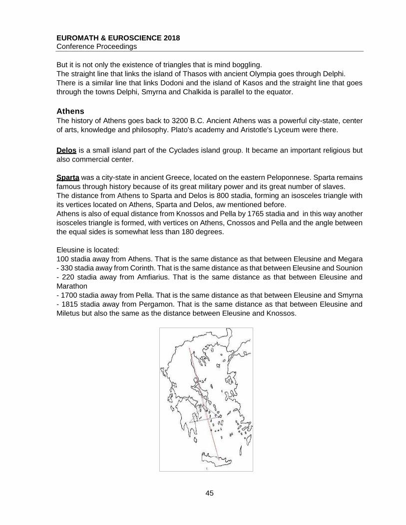
EUROMATH & EUROSCIENCE 2018 Conference Proceedings
45
But it is not only the existence of triangles that is mind boggling.
The straight line that links the island of Thasos with ancient Olympia goes through Delphi.
There is a similar line that links Dodoni and the island of Kasos and the straight line that goes
through the towns Delphi, Smyrna and Chalkida is parallel to the equator.
Athens The history of Athens goes back to 3200 B.C. Ancient Athens was a powerful city-state, center
of arts, knowledge and philosophy. Plato's academy and Aristotle's Lyceum were there.
Delos is a small island part of the Cyclades island group. It became an important religious but
also commercial center.
Sparta was a city-state in ancient Greece, located on the eastern Peloponnese. Sparta remains
famous through history because of its great military power and its great number of slaves.
The distance from Athens to Sparta and Delos is 800 stadia, forming an isosceles triangle with
its vertices located on Athens, Sparta and Delos, aw mentioned before.
Athens is also of equal distance from Knossos and Pella by 1765 stadia and in this way another
isosceles triangle is formed, with vertices on Athens, Cnossos and Pella and the angle between
the equal sides is somewhat less than 180 degrees.
Eleusine is located:
100 stadia away from Athens. That is the same distance as that between Eleusine and Megara
- 330 stadia away from Corinth. That is the same distance as that between Eleusine and Sounion
- 220 stadia away from Amfiarius. That is the same distance as that between Eleusine and
Marathon
- 1700 stadia away from Pella. That is the same distance as that between Eleusine and Smyrna
- 1815 stadia away from Pergamon. That is the same distance as that between Eleusine and
Miletus but also the same as the distance between Eleusine and Knossos.
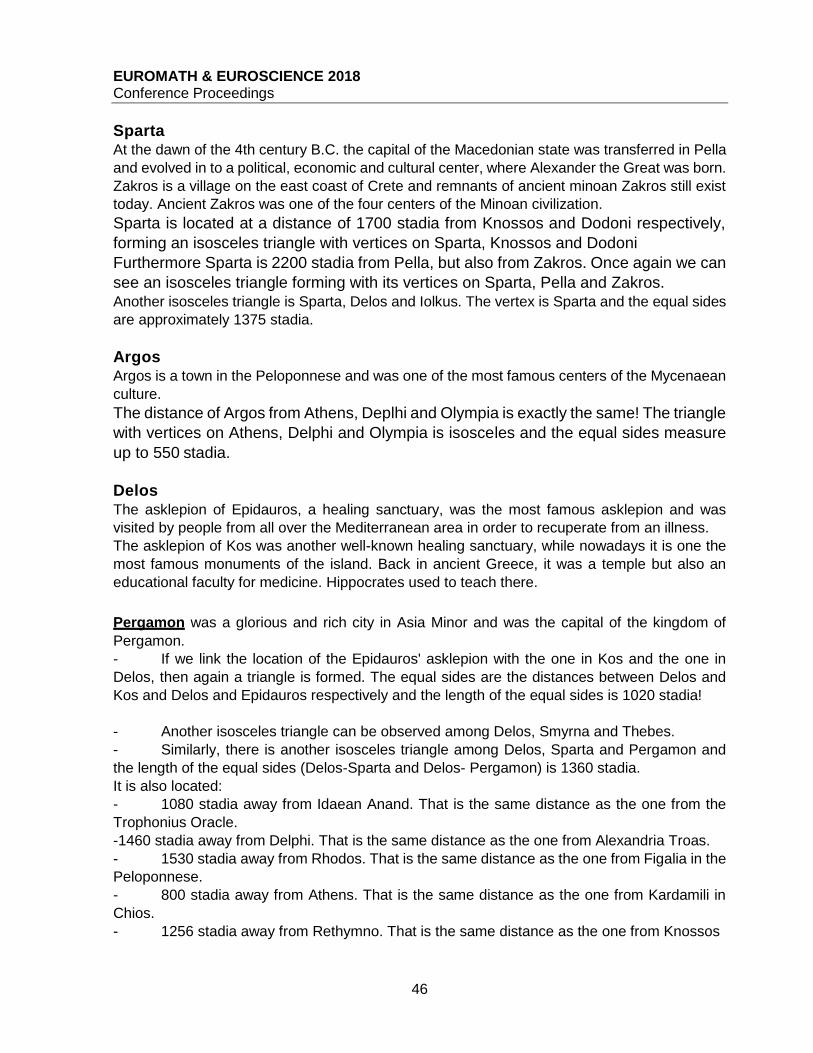
EUROMATH & EUROSCIENCE 2018 Conference Proceedings
46
Sparta At the dawn of the 4th century B.C. the capital of the Macedonian state was transferred in Pella
and evolved in to a political, economic and cultural center, where Alexander the Great was born.
Zakros is a village on the east coast of Crete and remnants of ancient minoan Zakros still exist
today. Ancient Zakros was one of the four centers of the Minoan civilization.
Sparta is located at a distance of 1700 stadia from Knossos and Dodoni respectively,
forming an isosceles triangle with vertices on Sparta, Knossos and Dodoni
Furthermore Sparta is 2200 stadia from Pella, but also from Zakros. Once again we can
see an isosceles triangle forming with its vertices on Sparta, Pella and Zakros. Another isosceles triangle is Sparta, Delos and Iolkus. The vertex is Sparta and the equal sides
are approximately 1375 stadia.
Argos Argos is a town in the Peloponnese and was one of the most famous centers of the Mycenaean
culture.
The distance of Argos from Athens, Deplhi and Olympia is exactly the same! The triangle
with vertices on Athens, Delphi and Olympia is isosceles and the equal sides measure
up to 550 stadia.
Delos The asklepion of Epidauros, a healing sanctuary, was the most famous asklepion and was
visited by people from all over the Mediterranean area in order to recuperate from an illness.
The asklepion of Kos was another well-known healing sanctuary, while nowadays it is one the
most famous monuments of the island. Back in ancient Greece, it was a temple but also an
educational faculty for medicine. Hippocrates used to teach there.
Pergamon was a glorious and rich city in Asia Minor and was the capital of the kingdom of
Pergamon.
- If we link the location of the Epidauros' asklepion with the one in Kos and the one in
Delos, then again a triangle is formed. The equal sides are the distances between Delos and
Kos and Delos and Epidauros respectively and the length of the equal sides is 1020 stadia!
- Another isosceles triangle can be observed among Delos, Smyrna and Thebes.
- Similarly, there is another isosceles triangle among Delos, Sparta and Pergamon and
the length of the equal sides (Delos-Sparta and Delos- Pergamon) is 1360 stadia.
It is also located:
- 1080 stadia away from Idaean Anand. That is the same distance as the one from the
Trophonius Oracle.
-1460 stadia away from Delphi. That is the same distance as the one from Alexandria Troas.
- 1530 stadia away from Rhodos. That is the same distance as the one from Figalia in the
Peloponnese.
- 800 stadia away from Athens. That is the same distance as the one from Kardamili in
Chios.
- 1256 stadia away from Rethymno. That is the same distance as the one from Knossos

EUROMATH & EUROSCIENCE 2018 Conference Proceedings
47
- 1188 stadia away from Corinth. That is the same distance as the one from Mytilene
- 1859 stadia away from Samothraki. That is the same distance as the one from Thermon.
-1859 stadia away from Mycenae. That is the same distance as the one from Argos.
Dodoni The Trophonius oracle was one of the least famous during the ancient years, but also very
unique as it does not look like any other oracle. It was located 130 km northwest of Athens.
Miletus was an ancient town in Ionia, built on the west coast of Asia Minor and was inhabited
since the Copper Age.
- It is of equal distance from Iolkus and Delphi by 1050 stadia
- It is located 1210 stadia away from Olympia and the Trophonius oracle
- Another isosceles triangle of interest is the one with its vertices on Dodoni, Athens and
Sparta. The length of the equal sides (Dodoni-Athens and Dodoni-Sparta) is 1700 stadia
- The biggest triangle observed is the one with a head vertex on Dodoni with equal sides
of 3300 stadia each that reach Knossos and Miletus.

EUROMATH & EUROSCIENCE 2018 Conference Proceedings
48
Knossos Mycenae was an ancient city located almost 90 km southwest of Athens. It was one of the
greatest cultural centers at the time.
Epidauros is a historic town the same region, in the Peloponnese. According to mythology it was
also the birth place of Asclepius. Its strategic location, but mainly its asklepion contributed to the
town's growth.
Knossos is equidistant from Sparta and Epidauros (1700 stadia)
It is also equidistant from Argos and Mycenes (1815 stadia)
Pella Samothraki is an island located on the northeast part of the Aegean sea. The island is known
for its ancient Greek statue of Nike (goddess of victory), which is exhibited in the Louvre, Paris
Alexandria was an ancient Greek town on the coast of Asia Minor.
Alexandria ad Issum or Alexandria Minor, located in Kilikia, Asia Minor was also a ancient
Greek town.
- Pella is equidistant at about 1360 stadia from Deplhi and Samothraki
- It is also equidistant from Athens and Alexandria Troas.
- Its distance from Paros, but also from Smyrna is 2350 stadia
- Similarly its distance from Alexandria in Egypt and Alexandria ad Issum is 6600 stadia.
Could we safely suppose that Alexander the Great established two different cities at a same
distance from the capital of Macedonia?
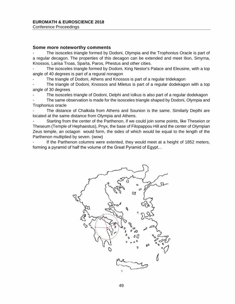
EUROMATH & EUROSCIENCE 2018 Conference Proceedings
49
Some more noteworthy comments - The isosceles triangle formed by Dodoni, Olympia and the Trophonius Oracle is part of
a regular decagon. The properties of this decagon can be extended and meet Ilion, Smyrna,
Knossos, Larisa Troas, Sparta, Paros, Phestus and other cities.
- The isosceles triangle formed by Dodoni, King Nestor's Palace and Eleusine, with a top
angle of 40 degrees is part of a regural nonagon
- The triangle of Dodoni, Athens and Knossos is part of a regular tridekagon
- The triangle of Dodoni, Knossos and Miletus is part of a regular dodekagon with a top
angle of 30 degrees
- The isosceles triangle of Dodoni, Delphi and Iolkus is also part of a regular dodekagon
- The same observation is made for the isosceles triangle shaped by Dodoni, Olympia and
Trophonius oracle
- The distance of Chalkida from Athens and Sounion is the same. Similarly Deplhi are
located at the same distance from Olympia and Athens.
- Starting from the center of the Parthenon, if we could join some points, like Theseion or
Theseum (Temple of Hephaestus), Pnyx, the base of Filopappou Hill and the center of Olympian
Zeus temple, an octagon would form, the sides of which would be equal to the length of the
Parthenon multiplied by seven. (wow)
- If the Parthenon columns were extented, they would meet at a height of 1852 meters,
forming a pyramid of half the volume of the Great Pyramid of Egypt…

EUROMATH & EUROSCIENCE 2018 Conference Proceedings
50
Someone may say that all of these are just coincidences and that it is only natural for such
correlations to exist. Possibly the found proportionate correlation of so many important points
with each other might be characterised as a really far-fetched notion, but it surely is a
phenomenon that is met too often, to just accept that it is a coincidental occurrence.
So what conclusions can we draw? Nothing more and nothing less than the fact that in ancient Greece the area for the erection of
buildings of importance, such as sacred temples, towns and cities were carefully chosen.
All of these are still inconceivable even for modern scientists. It is actually noteworthy how they
were able to measure distances with such precision. Also who inacted the "Law" that defined
the adoption of certain methods and criteria for the choice of the final locations.
But of greater interest is why ancient Greeks decided to follow this system? Is there a special
meaning attributed to the chosen areas?
The last question offers of course great opportunity for speculation.
Were the chosen place full of some kind of terrestrial energy? Or maybe it was just a symbolic
choice in order to conjugate and unify sacred places, assuring, according to their beliefs,
harmony with the whole universe? What else?
Despite all of the above, one thing is for sure. The wisdom of the ancient Greeks seems
to surpass even our wildest imagination.
http://m.huffingtonpost.gr/2017/07/06/culture-arhaia-ellada-geodaitikos-
trigonismos_n_17402366.html
http://wwwaporrito.blogspot.gr/2012/04/blog-post_18.html?m=1
http://thesecretrealtruth.blogspot.gr/2014/05/blog-post_7468.html?m=1
http://square.gr/h-chalkida-kai-to-mustirio-twn-ierwn-trigonwn/28256
http://www.amra.gr/forum/index.php?topic=2758.0
http://thesecretrealtruth.blogspot.gr/2012/05/blog-post_5922.html?m=1
http://revealedtheninthwave.blogspot.gr/2017/10/blog-post_298.html?m=1
EUROMATH & EUROSCIENCE 2018 Conference Proceedings
51
MATHEMATICS AND MUSIC CAN EXPLAIN EVERYTHING Soultana Fani Adamidou, Alexios Flamouropoulos
Diastaseis, Private School, Greece
ABSTRACT Mathematics and music are two sciences which are strongly interrelated. These two arts have been affecting each other since ancient times and this interaction comes to our days. Music is a way of life and expression. Through music you can “travel” by carrying melodies in your inner self and in this way you can feel the beauty filling your soul and spirit. Music therefore, is a way of expression that is common to every person. In parallel, the beauty of mathematics, for those who can comprehend it, lies in the simplicity, the symmetry and the elegance of their formulation. For Plato, mathematics was presumed “the utmost culmination of beauty”. In addition, mathematics is undoubtedly a universal communication code. When we seek for interrelations between music and mathematics, we reach the conclusion that MATHEMATICS AND MUSIC CAN EXPLAIN EVERYTHING. No harmony would exist if numbers were not in existence. There would be no harmony if no man existed so as to listen to it and reckon it as such in order for numbers to be the appropriate tools for it. No harmony can exist by itself. Is it mathematics of music or music of mathematics that affects the human brain and activates it?
Introduction Math and music are closely related on a scientific basis. Since ancient times, an interaction
between them was observed and that observation still applies nowadays.
Most people think of math as an enigma. The science of math is characterised by a vague
perception of numbers and calculations, as taught in school and is usually followed by
indifference. Most people think of math as a cold and "lifeless" subject.
Music on the other hand is about feelings and emotions, it is about life. Everybody has sang at
some point of his life or attempted to even play some music or just whistle a catchy rhythm.
Therefore, the relationship of these phenomenologically irrelevant sciences may not be obvious,
but is surely worth discovering it, since they are truly closely related.
The first bad impression that math make, always change when someone learns about
Pythagoras or about the applications of Johan Sebastian Bach.
What to refer to first? Fractions, quotients and proportions found in musical intervals?
Fibonacci sequences are found in musical synthesis but also used on musical instrument
construction?
Scale, trigonometry and the wave form of sound?
In order to answer these questions, we need to investigate the mathematical relationship
between music notes and the reason for the observed relationship.z
EUROMATH & EUROSCIENCE 2018 Conference Proceedings
52
What is really interesting is that those relationships arise from nature itself and are not human
contrivance.
Humans did not construct music, but it was eavesdropped and taught to human by nature.
The aim of this study is to investigate our aesthetic criteria about music as explained by math.
Structural elements of music are the sounds we call notes.
The notes were discovered long before music theory developed and of course they were only
chosen not for a particular reason, other than that they just sounded nice, so our ability to listen
and compose music is more congenital rather than acquired.
Sound are actually vibrations transferred through air and when these vibrations meet an obstacle
they cause a phenomenon called resonance.
That also means, that when listening to music, our ears are not the only organ participating in
the process but our whole body resonates with the vibrations and this happens even with closed
ears. We understand that resonance might be the key for our congenital ability to "feel" the
music, as we usually say.
Returning to the math-music relationship one can easily note while reading a book about music
theory, that it seems like reading a difficult math book.
How is music related to maths? Pythagoras, a mathematician and philosopher, was the first one to study musical sounds. He
was well aware of the relationship between music and numbers. Scientists believe that
Pythagoras and his students deepened their knowledge on the subject by studying the ancient
musical instrument "monochordon", an ancient instrument on which Pythagoras used to study
the music notes in relation with the length of the string, which produces each note.
This instrument in its simplest form consists of one string, streched over a box, which works as
a speaker. The produced sound depends on three factors:
1. The string thickness
2. The traction force of the string, i.e. the curling. The more the string is pulled, the more
acute is the sound emitted (sound of high frequency)
3. The length of the string. A short chord produces an acute sound, while a long one
produces a bass sound (a sound of lower frequency)
Pythagoras made an observation. A 90 cm string produces a specific sound. The sound with the
greater affinity to the first one is produced by a 45cm string, i.e from a string of half the length of
the first one. Following the affinity series of the sounds, the next more similar sound was
produced by a 60 cm string, this is two thirds of the length of the first string.
The glide up technique (which means the use of mobile frets) allows to change the string length
and therefore the tone of the sound. From the string length ratios derives the mathematical
relationship among sound tones.
For example, if the fret is located in the middle of the string, the mathematical relationship
occurring is expressed with a ratio 1:2, the well known in the music word octate.
Likewise, when a fret is located in a position corresponding to the 4/5 of the string length
προκύπτει το διάλυμα μεγάλης τρίτης…
Following this path of thoughts, lead him to observe that a mathematical normality is transformed
to music and vice versa and set the ground for further investigation of the relationship between
math and music.

EUROMATH & EUROSCIENCE 2018 Conference Proceedings
53
Pythagoras noticed a constant relationship between the string length of a lyre and the basic
chords (1/2 for the 8th chord, 3/2 for the 5th and 4/3 for the 4th one)
When two sounds combined produce a pleasant tone, then the string length ratio (from which
they are produced) is an integer number and those sounds are called harmonic.
This wonderful trait of the harmonic relationships is due to the fact that they contain the first four
natural numbers (1,2,3,4), the sum of which is 10, the sacred number of Delphi.
According to Plato and Aristotle music is not just art, but music in its core is math. Their writings
about music look like math or geometry textbooks.
Plato said that there are four subjects which cultivate human spirit. These are music, math,
geometry and astronomy.
The aforementioned related sciences, can be described as Math: stationary numbers
Music: numbers in motion
Geometry: stationary multidimensional units Astronomy: numbers in motion
Many mathematicians tried to calculate musical intervals, like Archetas worked on the ratios of
tetrachordon spaces.
Eratosthenis defined the difference between major tones (9/8) and minor (10/9) tones.
Maths, music and the golden ration The math-music relationship is not only limited to ratios and analogies of music intervals.
Fibonacci numbers, 1,1,2,3,4,5,8,13,21,34,55,89,…
Each one of them is produced by summing the two prior numbers.
Those number display an interesting property.
If two sequent numbers are divided with the bigger one as a numerator, the result comes any
time more closely to 1,618, which is the golden number φ.
What do all of all these have to do with the music scale? Indeed, they have.
A piano scale has 13 keys, 8 of which are white and 5 are black, while the last of them are
divided into themes of three and two keys.
In western culture, music notes are based on Fibonacci series, since the frequencies of the
tones are related to these numbers.
Musical compositions often reflect Fibonacci numbers. The dynamic golden ratio, besides other
various application, is also used in music to produce rhythm changes or to develop a melodic
line.
Main characteristic of many compositions is that their structure is divided in two parts either in a
symmetric way or according to the golden ratio.
A famous example is the song "Hallelujah" composed by Handel. Furthermore, the golden ration
is applied on every Mozart sonata.
TRIGONOMETRY-FOURIER Sound is transferred through waves.
The sound produced by a tuning fork (diapason) can be described by sinwave.
This sinwave is the graph of the function ψ=αsinβx, where α and β are positive numbers which
define the wavelength and frequency when x can take any value from a 360 point interval.
But what can math tell us about more complex sounds and how could the well sounding of some
sounds or the irritance some others cause be explained?

EUROMATH & EUROSCIENCE 2018 Conference Proceedings
54
The graphs describing all sound, including our voices, follow a normality, which means that the
displacement-time graphs reoccur precisely many times per second.
Sound that are characterised by periodicity are generally pleasant and technically called music.
Fourier further clarified this topic by stating that every periodic sound is the sum of various
sinwaves of the above mentioned form and the frequencies of these equations are integer
multiples of the lowest frequency.
We conclude that any complex sound is just a combination of simpler sounds like those
produced by tuning forks (diapason).
It is now more than obvious that every sound can be mathematically described. Even the most
complex sound, in math it is just a sinwave function.
KEPPLER: THE MUSIC OF PLANETS The music of the stellar globes was first mentioned by Plato, 2500 years ago. He used to call
music as the beauty of the universe and also said that "Music is the sound motion in order to
reach the soul and teach us virtuousness. Music is a moral compass. It gives soul to the
universe, wings to our thoughts, lifts off our imagination, gives joy to sadness and life to
everything".
Prior to Plato, Pythagoras had reached such a level of sensitivity that was able to listen to skies
symphony, to the music of the stellar globes.
Music reflects the harmony of the skies. The harmonic relationships of the numbers can be met
at the planets. The planets produce various music sounds, while rotating, sound that cannot be
heard.
Keppler studied the scripts of ancient Greeks, mainly Plato, and concluded that every planet
emits a different note while in its orbit.
Some of these sounds are similar to the sounds of dolphins, waves, birds, wind…
The sounds that arise from the planets are closely related to the seven music notes.
The correspondance of the planets with the produced notes are
1. Sun=E
2. Venus=F
3. Mercury=G
4. Moon=A
5. Cronos=B
6. Mars=D
7. Zupiter=C
In his work De Harmonic Mundi he designed a partiture, which depicts the planets to perform
their universal concert.
This way a book about the music of the skies was written.
……Περίεργη σύνταξη
Bach The european music relied on the principles of harmony of the pythagorians, until Johan
Sebastian Bach composed "The well-tempered clavier" and suggested the division of the octate
into twelve semitones. This was also prosposed by Aristoxenos 2000 years before Bach.
EUROMATH & EUROSCIENCE 2018 Conference Proceedings
55
Beethoven How was Beethoven able to compose such masterpieces while being deaf? Once again math
can give us some answers.
Natalya St. Clair used the famous "Moonlight Sonata" in an attempt to explain how Beethoven
could have expressed such feelings with some help of mathematic precision.
The answer for his achievement can be found on his partitures.
"Moonlight Sonata" starts with a steady slow rhythm consisting of triplets of notes.
One and two and three and one…
Despite the fact that, the notes seem simple, every triplet of notes contains an elegant melodic
structure revealing the extraordinary relationship between music and math.
Beethoven once said "I have always had a vision in my mind when composing and always
followed that vision"
Imagine an octate piano with 13 keys και καθένα διαχωρίζεται από ένα βήμα
A basic scale or a typical secondary one uses 8 of these keys with 5 whole intervals and 2 ….
Beethoven added the non defined spectres of emotion and creativity and of course a little math.
Δεν καταλαβαίνω το ελληνικό κείμενο.
So, although we can see the mathematical concept in the partitures we still cannot understand
why this music touches the heart of the audiences. Beethoven's intelligence lead him to
compose without even being able to listen to the music. In a similar way, musicians feel the math
and mathematicians think of the music. Music is the dream and math is the work in our lives.
NOWADAYS Nowadays many musicians use math to compose. A main representative is Iannis Xenakis.
Xenakis is a pioneer in algorithmic music composition. He has also developed a theory about
digital composition based on sound production using mathematical functions.
Notworthy is the fact, that he is also interested in the relationship between math and music, in
order to find out how "The art of fugue" (Bach) can be
described by mathematical models, so that the music can be depicted by graphs like a visual
representation of music.
He tried to apply the laws of physics to music.
The first work toward this pioneering direction is called "stochastic music"
This is the first work, which includes audible sets that consist of various single sounds.
Xenakis also uses a variety of mathematical theories, like:
- Set theory, as applied on his work "Erma". The whole length of a piano is considered as set A
including 3 sub-sets. The result is a variety of sounds.
- Game theory. When this theory-technique is followed, two conductors react to each others'
choices.
- Bull algebra combined with Set theory. This theory is used by Xenakis in his works "Erma" and
"Eonta" and is called "symbolic music" by him.
EUROMATH & EUROSCIENCE 2018 Conference Proceedings
56
What are the benefits of music? We refer only to some of them.
- music helps speech development
- helps children learn math. When children learn about rhythm, they basically learn about
quotients and fractions
- music promotes socialization
- music promotes mental growth of children as it enhances neural system and brain activity
- music encourages self-expression and self-esteem, while commuting plenty feelings and offers
shy children or children with other speaking difficulties a way to express themselves.
BRAIN-MUSIC-MATHS Let' see how music and math influence the human brain.
When listening or playing music the right cerebral hemisphere is activated.
When learning to study music, to understand the music and the partitures the left cerebral
hemisphere is activated, more specifically the same area that is in charge for analytical thought
and mathematical thought.
A 1997 study suggest that listening to music arouses the brain neurons, which determine the
spatial-temporal reasoning.
This kind of reasoning is used in higher brain activities such as those in which we engage while
doing math, playing chess or composing music.
Furthermore, studies have shown that children that study music from an early age have better
math skills. This happens because:
Recognition and understanding of basic numbers is necessary in both music and math
Problem solving skills are required in both activities
Both activities require an ability of motif recognition, which promotes mental growth of students
Motifs are structural constituents of mathematical knowledge
If a musician was asked about the common ground between Bach and Joplin, would surely look
like he would have seen an alien. What kind of relationship could there be between a master
musician , favourited by the church and the Woodstock priestess Janet Joplin?
Brain scientists say:
" The input of audible stimulus is actually located on neurons at the upper part of the brain lobes,
which are called aesthetic neurons and when a chord is harmonic and pleasant the ratios
between its frequencies are equal to small natural numbers."
In a relevant study, 1800 music tracks were analysed, covering as a sample 4 centuries of
western music and it was found that all of them consisted from a repeated rythmic motif, an
"audible fractal". Because of this motif, the music of Beethoven, Bach, Haydn and Mozart were
of such great resonance, similar to that of the song "Summertime" of Joplin.
We may say that this motif is an emotional code, hidden in our brains and when aroused, causes
vibrations to our souls.
Physicist Shaw, who studies brain activity, says that music plays a pedagogical role in math. He
suggested that those who listen to the sounds of Mozart seem to have better mathematic abilities
and logical reasoning.
Is there a relationship between neurons and harmony?
In 1978, the first brain neuron model was produced. Shaw corresponded music notes on this
model.

EUROMATH & EUROSCIENCE 2018 Conference Proceedings
57
He found himself surprised, when he listened to an harmonic music as a result and not some
unclarified and irrelevant sounds. Based on this occurrence he made the assumption that music
generally improves mental activities.
The first official study towards this hypothesis, in 1993, showed that students who took part in
logic exercises, achieved better scores after listening to a particular Mozart sonata. The increase
of the observed scores was about 35%. The phenomenon was later called 'The Mozart effect"
We should keep in mind, that:
Music, just like as math, is part of our everyday lives although this is not always actively
perceived.
Music related education from an early age seems to modify brain structure.
It is commonly accepted that math is not always a pleasant subject for students, while it is often
characterised as a difficult topic
Rhythm and emotions are independent of the place and the time that goes by and so they remain
unalterable and are perceived in a natural way.
Nowadays science and technology tend to keep us remote from nature, some may say they
even make us miserable. Art and especially music may become a forgotten mean of
communication between us and our true nature.
Maybe we should have listened Pythagoras calling:
"The whole world is numbers and music is its beauty, didn't I told you so?"

EUROMATH & EUROSCIENCE 2018 Conference Proceedings
58
MATHEMATICS AND POETRY: AN UNDOUBTEDLY CHARMING ENCOUNTER
Alexios Flamouropoulos
Diastaseis, Private School, Greece
ABSTRACT As Nobelist Theoretical Physicist Heisenberg once said: “...There are only two languages with which man can describe nature; Mathematics and Poetry” Do mathematics and poetry have common characteristics, similarities, some relation, or are they separated by a vast gap as many believe? Poetry is not only a way of expressing emotions, but also an attempt to interpret the world. It is man’s general perception of beauty, which becomes the cause of inspiration for all areas in which it is expressed. Mathematics is the science concerned with quantity (meaning numbers), structure (that is, shapes), the connection between all countable things in reality and imagination. - Is there such thing as a relationship between mathematics and poetry? - How can mathematics and poetry bring together logic and emotion? - How much and to what extent is our brain influenced by the poetry of mathematics and the mathematics of poetry? - Could, perhaps, mathematics and poetry be the two windows which we need to open in order to gaze into and realize the chaos of reality?
Foreword The relationship between mathematics and poetry is not something known to exist by many.
Few are the people who realise how closely related they truly are. As one explores these two
concepts, they begin to understand in how many ways one supports, or even completes, the
other.
What are mathematics? It is the science that researches all matters concerning numbers, shapes and the relations
between all countable things.
Mathematics research structures which either come from natural sciences or from mathematics
itself. In school, for example, maths study quantities, shapes and distances. This is done by
using productive logic and then compiling the results in systems, axioms, theorems et cetera.
What is poetry? It is art. Its roots are the expressive capabilities of language. It is musical thought, thought that
expresses our inner world.

EUROMATH & EUROSCIENCE 2018 Conference Proceedings
59
Interaction between mathematics and poetry Mathematics and poetry constitute two different areas of human spiritual activity which develop
in different ways, but serve common, individual or otherwise, goals and needs. Each of these
spiritual activities has its own tools and means of expression.
The interaction between them is completely natural. It stems from the fact that mathematics is
based on our need to logically describe the world, while poetry approaches things through
emotion. In the end, both give us a better understanding of ourselves, since mathematics delve
deeper into the human consciousness and poetry further explores the human soul.
More than often, poetry uses mathematical terms to describe situations, feelings, characters.
On the other hand, mathematics only use patterns to help us memorize things. Besides, it is a
fact that the algorithms that most easily stay in memory, are those that have a rhythm, a pattern.
We are undoubtedly talking about two ancient creative and spiritual human processes. People
developed myths in order to explain the surrounding world. They created myths about the birth
of the world, myths about gods, myths filled with mystery, all based on man’s awe about all that
he could not explain.
And on the other hand, mathematics was a useful tool, even for the primitive man. There had to
be a tool for measuring time, days, the phases of the moon. Through the ages, all this became
what we know as science, which attempted to explain nature and myths through logic.
Poetry and mathematics answer the three questions that always bothered humans.
1) What is our position towards nature?
2) What is our position towards society?
3) What is our position towards death?
It becomes clearer that the common points between mathematics and poetry are not so much a
fiction, as one may immediately conclude.
Additionally, great mathematician Hardy writes in his biography:
«The mathematician, just like a painter or poet, is a designer. Their designs are made of ideas.
The painter designs using shapes and colours, the poet uses words, instead. In poetry, too,
ideas count greatly.»
Mathematics used in poetry Through the ages, countless poets have attempted to express, define and elaborate on maths
through their poetry. Besides, let us not forget that the structure of most poems is based on
metres, syllables and sequences, through which we can discern mathematics. While the content
of a poem may vary, its structure will always be purely mathematical business.
Most poems are in an alignment. By the term alignment we mean the verses, lines and metre of
a poem.
Initially, let’s take a look at what these terms exactly mean.
Verses can be defined as the “paragraphs” of a poem, and are made up of lines.
Lines are, well… the lines of words of a poem. These words, in turn, are constructed of syllables.

EUROMATH & EUROSCIENCE 2018 Conference Proceedings
60
The rhythm in which we pronounce and entone these syllables is called a metre.
All poems have a number of syllables and verses. That way, the poet kind of “builds” on a
mathematical motif.
In some cases, poets will write a poem intended to have a geometrical structure as its main
feature.
In a poem written by Lewis Carroll in his book “Alice in Wonderland”m the words had been
carefully picked in order to fit into the shape of a mouse’s tail.
A poem structured in such manner, to resemble geometric shapes, are called visual poems and
are one of the many examples of the use of mathematics in poetry.
In other cases, poems are written with a strictly defined number of syllables and verses. For
example, the haiku poems, of Japanese origin, almost always consist of 17 syllables in 3 verses.
The alignment is as follows: Seven syllables in the first verse, five in the second and seven in
the third.
Ever since Homer’s age, up until ours, many poets insert numbers and mathematical terms in
their works. It is also noteworthy that many mathematicians, of various origin, write poetry.
It is not rare for people to decide and work on both mathematics and poetry simultaneously. Let
us not forget that in ancient Greece, important people from the area of mathematics used to
study more theoretical sciences as well, such as literature, music and rhetoric.
Accordingly, in Arabia, scientists usually owned the title of poet, astronomer and mathematicians
at the same time.
Subsequently, many poems decide to express their thoughts on mathematics through their
works, by comparing science with a more “romantic” side of life, or by describing how
mathematics are everywhere in our daily life.
This way, a new form of poetry was formed, lyrical mathematics. The one who introduced this
term was nobelist poet Odysseas Elitis, whose poem “The way of thus” revolved around a very
simple and understandable term, “thus”. This term is used to show that we have solved an
equation or mathematical problem. Elitis compares the
proccess of solving a problem with life. This way, he concludes that the secret of life is always
reaching a “thus”, while always having the right answer.
I will now attempt to analyze for you some poems that revolve around mathematics in our life.
- Odysseas Elitis, in his poem «Little Sailor», compares the sea to a school. In the poem,
he explains how this unusual school taught him two very basic mathematical functions. First,
Elitis explains mathematical analysis. He analyzes his country, Greece, to three parts: an olive
tree, a vineyard and a ship. Subsequently, he states the very simple operation of addition. By
combining the aforementioned olive tree, vineyard and ship, the result of the addition would be,
of course, Greece.
- In «Six Significant Landscapes», Wallace Stevens talks about rationalists.
Rationalists, wearing square hats, Think, in square rooms,
EUROMATH & EUROSCIENCE 2018 Conference Proceedings
61
Looking at the floor, Looking at the ceiling. They confine themselves To right-angled triangles.
If they tried rhomboids,
Cones, waving lines, ellipses --
As, for example, the ellipse of the half-moon--
Rationalists would wear sombreros.
In this poem, Stevens wonders about rationalists’ “rigid” thinking. The square shape usually
resembles something sturdy, something rigid. He claims that, were rationalists to change their
confined views, they would trade in their square hats for… sombreros. As we know, sombreros
have swirly shapes and elliptical lines. With this analogy, the poet associates open-mindedness
with bent shapes.
- Next on, the poet Ector Kaknavatos, who was one the most genuine supporters of
surrealism during his time. In one of his poems, he describes a city that is being pillaged by an
unknown force. To our great surprise, however, this force is not a hostile army, but an equation.
An equation is attacking the city. Kaknavatos aims to show how mathematics can shake us up.
He additionally describes the equation as being dressed in iron armor. With this, he attempts to
show how challenging, yet important, finding the solution can be.
- One specific mathematician did a great amount of work on poetry as well. Manolis
Kseksakis. He used to say that poetry and mathematics were two sides of the same coin. He
wrote a whole collection of mathematical problems in the form of poems. For example, «The
Horseman»
A horseman rides with 12,5 km per hour
And hunts a pedestrian who started walking
Many years ago, and still is
After how many hours will the horseman reach him
And at what distance from the starting point
Will he murder him?
The poet begins by calling a very simple problem. A horseman pursues a pedestrian, who
started before him. We are tasked with we are tasked with figuring after how many hours the
horseman will reach the pedestrian, and at what distance from the initiation point the horseman’s
purpose will be fulfilled.
- Finally, the poet George Vafopoulos, wrote an amazing poem called
«The great Cone». In this poem, the world is depicted as a purely mathematical model; the cone.
This cone is ran from bottom to top by a spiraling line, resembling the life of a person, the course
which they follow. Childhood is located at the bottom, on the big spirals. During these, the person
slowly forms and matures, but still has quite a small line of sight. By living life, moving up the
cone, the spirals get smaller and smaller, but the line of sight gradually enlarges, until the person
has reached the top of the cone.
EUROMATH & EUROSCIENCE 2018 Conference Proceedings
62
The different meanings of numbers in poetry Numbers, the base of mathematics and all other sciences, have been troubling philosophers
and poets forages. Through poetry, the supernatural properties of numbers are expressed.
The number zero has been a source of inspiration and thought for many poets and is regularly
featured in poetry. It usually represents nihilism, complete nonexistence, but sometimes
represents existence itself.
The “magic” number three is considered by many to be the perfect number, due to being the
first number to have a beginning, a middle and an end. This property has given it a special
position in poetry, as it is regularly used to highlight important persons and situations.
Last but not least, the number seven also has a crucial role in poetry. It mainly symbolises the
seven colours of the rainbow, but additionally has great religious value.
Differences between poetry and mathematics
Even though there is no denying their similarities, it would be a lie if we claimed that poetry and
mathematics are the same.
Their differences are what make their encounter so enthralling. Poetry is an ancient way of
translating our experiences. It is a form of communication that aims directly at our emotions.
Human curiousness, however, always demanded a more intricate, more “technical” means to
describe the world. That is how sciences were created. They narrate life, not with words, but
with the mathematical language of nature.
Let’s not forget that they are two different means for the accomplishment of the same task. Writer
Antonio Tabucchi, in his book “Tristano dies”, explains that geometry conflicts with chaos and
that’s why humans created windows, to confine the outside world into a rectangle. It is thus
necessary to open windows, in order to understand reality and uncover its secrets.
Could mathematics and poetry be two such windows? Perhaps.
Or even better, could they be one single window with two different angles, depending on how
one looks at it? Two angles that interact with us in the aforementioned ways. Through emotion
and through logic.
How mathematics and poetry affect the human mind
A shared attribute of poets and mathematicians is that they help us put chaos in order, through
their work, they change our view of things, they encourage us to look again. They… change our
mind.
Now, let’s talk aesthetics.
The aesthetical result a mathematician feels after, through an exhausting line of work, manages
to prove some mathematical theorem, is the same that a poet feels when they manage to
perfectly express and display their ideas through a poem.
Both are products of fantasy, inspiration and talent. Besides, Poincare stated, among other
things:
«A mathematician receives, from their work, the same sentiment as an artist does. Their joy is
of the same quality and quantity.»
Paul Dirac, one of the founders of quantum physics, emphasized:
EUROMATH & EUROSCIENCE 2018 Conference Proceedings
63
«We cannot determine mathematical beauty more than we can determine artistic beauty, but
those studying mathematics have no trouble appreciating it.»
According to studies, a mathematical proof can stimulate the same part of the brain that is
affected by art and our perception of beauty.
Poetry is quite beautiful, through its use of words and its meaning, we can all see that. Beauty
in mathematics, though, comes in two different types; logic and visual. Logical beauty is
described as cold and strict, but those who don’t understand it. Visual beauty, on the other hand,
is directly appealing, because it is symmetrical.
But what makes symmetry so engaging? The answer is repetition. Our brains like repetition, up
to a point. A snowflake is pretty because it repeats the same shapes in symmetry. Music is
enjoyable because, in its core, it is a rhythmically repeating sound. Of course, there are several
themes and variations in music, but they, too, consist of repetitions.4
If we removed fantasy and inspiration from mathematics, we would be left with plain, appalling
formulas, the ones our infertile, unimaginative educational system teaches. The same way, if
we removed fantasy and inspiration from poetry, there would be only words, without meaning.
To summarize:
I hope that you can all see now how close, and ultimately relative, poetry and mathematics are
to each other. How one completes and complements the other. How they shift our view of the
world. And of course, how important it is for us to learn to use them.
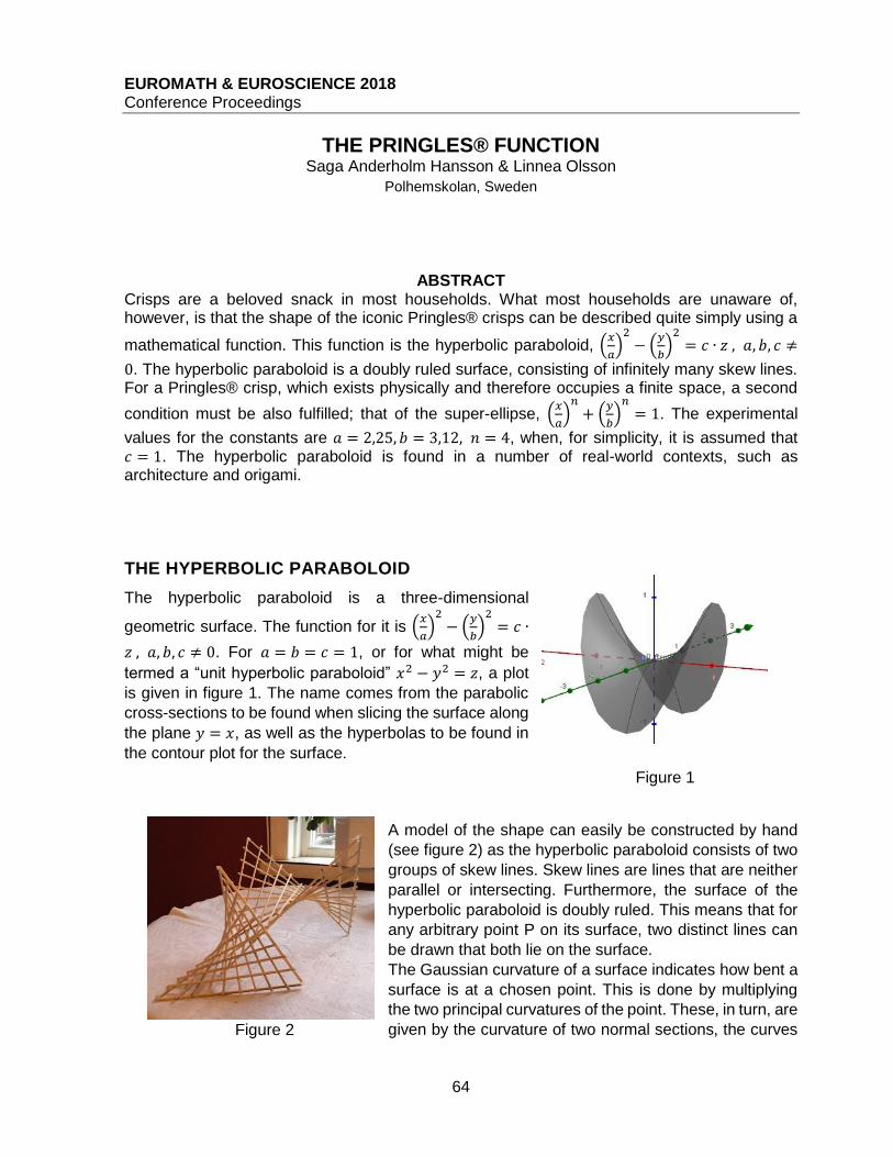
EUROMATH & EUROSCIENCE 2018 Conference Proceedings
64
THE PRINGLES® FUNCTION Saga Anderholm Hansson & Linnea Olsson
Polhemskolan, Sweden
ABSTRACT Crisps are a beloved snack in most households. What most households are unaware of, however, is that the shape of the iconic Pringles® crisps can be described quite simply using a
mathematical function. This function is the hyperbolic paraboloid, (𝑥
𝑎)2− (
𝑦
𝑏)2= 𝑐 ∙ 𝑧 , 𝑎, 𝑏, 𝑐 ≠
0. The hyperbolic paraboloid is a doubly ruled surface, consisting of infinitely many skew lines. For a Pringles® crisp, which exists physically and therefore occupies a finite space, a second
condition must be also fulfilled; that of the super-ellipse, (𝑥
𝑎)𝑛+ (
𝑦
𝑏)𝑛= 1. The experimental
values for the constants are 𝑎 = 2,25, 𝑏 = 3,12, 𝑛 = 4, when, for simplicity, it is assumed that 𝑐 = 1. The hyperbolic paraboloid is found in a number of real-world contexts, such as architecture and origami.
THE HYPERBOLIC PARABOLOID
The hyperbolic paraboloid is a three-dimensional
geometric surface. The function for it is (𝑥
𝑎)2− (
𝑦
𝑏)2= 𝑐 ∙
𝑧 , 𝑎, 𝑏, 𝑐 ≠ 0. For 𝑎 = 𝑏 = 𝑐 = 1, or for what might be
termed a “unit hyperbolic paraboloid” 𝑥2 − 𝑦2 = 𝑧, a plot
is given in figure 1. The name comes from the parabolic
cross-sections to be found when slicing the surface along
the plane 𝑦 = 𝑥, as well as the hyperbolas to be found in
the contour plot for the surface.
A model of the shape can easily be constructed by hand
(see figure 2) as the hyperbolic paraboloid consists of two
groups of skew lines. Skew lines are lines that are neither
parallel or intersecting. Furthermore, the surface of the
hyperbolic paraboloid is doubly ruled. This means that for
any arbitrary point P on its surface, two distinct lines can
be drawn that both lie on the surface.
The Gaussian curvature of a surface indicates how bent a
surface is at a chosen point. This is done by multiplying
the two principal curvatures of the point. These, in turn, are
given by the curvature of two normal sections, the curves
Figure 1
Figure 2
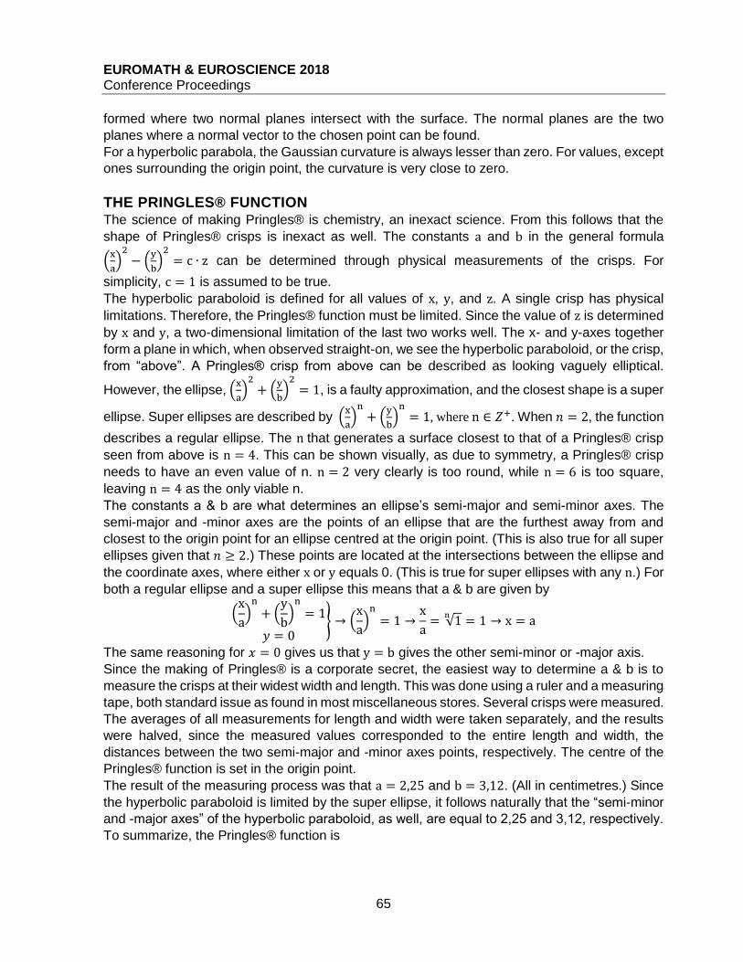
EUROMATH & EUROSCIENCE 2018 Conference Proceedings
65
formed where two normal planes intersect with the surface. The normal planes are the two
planes where a normal vector to the chosen point can be found.
For a hyperbolic parabola, the Gaussian curvature is always lesser than zero. For values, except
ones surrounding the origin point, the curvature is very close to zero.
THE PRINGLES® FUNCTION The science of making Pringles® is chemistry, an inexact science. From this follows that the
shape of Pringles® crisps is inexact as well. The constants a and b in the general formula
(x
a)2− (
y
b)2= c ∙ z can be determined through physical measurements of the crisps. For
simplicity, c = 1 is assumed to be true.
The hyperbolic paraboloid is defined for all values of x, y, and z. A single crisp has physical
limitations. Therefore, the Pringles® function must be limited. Since the value of z is determined
by x and y, a two-dimensional limitation of the last two works well. The x- and y-axes together
form a plane in which, when observed straight-on, we see the hyperbolic paraboloid, or the crisp,
from “above”. A Pringles® crisp from above can be described as looking vaguely elliptical.
However, the ellipse, (x
a)2+ (
y
b)2= 1, is a faulty approximation, and the closest shape is a super
ellipse. Super ellipses are described by (x
a)n+ (
y
b)n= 1, where n ∈ 𝑍+. When 𝑛 = 2, the function
describes a regular ellipse. The n that generates a surface closest to that of a Pringles® crisp
seen from above is n = 4. This can be shown visually, as due to symmetry, a Pringles® crisp
needs to have an even value of n. n = 2 very clearly is too round, while n = 6 is too square,
leaving n = 4 as the only viable n.
The constants a & b are what determines an ellipse’s semi-major and semi-minor axes. The
semi-major and -minor axes are the points of an ellipse that are the furthest away from and
closest to the origin point for an ellipse centred at the origin point. (This is also true for all super
ellipses given that 𝑛 ≥ 2.) These points are located at the intersections between the ellipse and
the coordinate axes, where either x or y equals 0. (This is true for super ellipses with any n.) For
both a regular ellipse and a super ellipse this means that a & b are given by
(x
a)n
+ (y
b)n
= 1
𝑦 = 0} → (
x
a)n
= 1 →x
a= √1
n= 1 → x = a
The same reasoning for 𝑥 = 0 gives us that y = b gives the other semi-minor or -major axis.
Since the making of Pringles® is a corporate secret, the easiest way to determine a & b is to
measure the crisps at their widest width and length. This was done using a ruler and a measuring
tape, both standard issue as found in most miscellaneous stores. Several crisps were measured.
The averages of all measurements for length and width were taken separately, and the results
were halved, since the measured values corresponded to the entire length and width, the
distances between the two semi-major and -minor axes points, respectively. The centre of the
Pringles® function is set in the origin point.
The result of the measuring process was that a = 2,25 and b = 3,12. (All in centimetres.) Since
the hyperbolic paraboloid is limited by the super ellipse, it follows naturally that the “semi-minor
and -major axes” of the hyperbolic paraboloid, as well, are equal to 2,25 and 3,12, respectively.
To summarize, the Pringles® function is

EUROMATH & EUROSCIENCE 2018 Conference Proceedings
66
{
(𝑥
2,25)2
− (𝑦
3,12)2
= 𝑧
(x
2,25)4
+ (y
3,12)4
= 1
WHY IT WORKS AND OTHER USES
A Pringles® crisp has the shape it does for the following reasons: they are easy to stack, fit
easily in a tube, break less, and the unique shape make them easily identifiable. Since the two
points of either the semi-minor or the -major axes are touching whatever surface they are lying
on, two points of balance are created. Their uniformity means that the entire surface of one crisp
touches the entire surface of another crisp. There is very little room for “wiggling”, which is what
makes them easier to stack, especially in a tube as they have a semi-round shape, and less
likely to break in their tube.
Aside from its place in pure mathematics, the
hyperbolic paraboloid can be found in varying
contexts. As it is a fascinating shape to look at, it is
often used in architecture, such as the Ochota
railway station roof in Warsaw, Poland. The
negative Gaussian curvature means that rain and
other downpour easily slides off a structure made up
of a hyperbolic paraboloid, which is useful for roofs.
Approximations of the surface serve as playground
equipment, and a model of the hyperbolic
paraboloid can be folded out of simple paper.
REFERENCES
Weiqing Gu, The Hyperbolic Paraboloid,
https://www.math.hmc.edu/~gu/curves_and_surfaces/surfaces/hyp-par.html
Gaussian Curvature, https://en.wikipedia.org/wiki/Gaussian_curvature (2018)

EUROMATH & EUROSCIENCE 2018 Conference Proceedings
67
MAGIC SQUARES Ailin Mirzaei
Roshd school, Iran
ABSTRACT
A magic square is a square grid filled with numbers, in such a way that each row, each column, and the two diagonals add up to the same number. The n × n magic square has n rows and n columns, and two diagonal. If you add up the numbers in any row, column or diagonal, you always get a constant number. The squares that have n by n are home and the sum of the numbers of rows, columns, and diagonals is constant. Also, for arbitrary numbers, a square can be constructed, which means that the numbers are in the table so that the sum of rows, columns, and diagonals is the arbitrary number. In this article we successfully demonstrate, first, how to generate the base magic squares, and then how to generate a magic square for arbitrary numbers.
GENERATING 3 BY 3 MAGIC SQUARES A magic square is a matrix filled with numbers, in such a way that each row, each column, and
the two diagonals add up to the same number. The 3 × 3 magic square has three rows and three
columns, and if you add up the numbers in any row, column or diagonal, you always get a
constant number.
The base 3 × 3 magic square has 9 houses, in which houses the numbers from 1 to 9 are filled
in such a way that the sum of rows and columns is a constant number. In 3 × 3 magic square,
magic number is 15. This number is obtained by dividing the total number of table numbers by
the number of rows or columns.
S = ∑n
n
1
= 1 + 2 + 3 +⋯+ 9 =n(n + 1)
2= 45
A =∑ n𝑛1R
=45
3= 15
Here is a 3 × 3 magic square
4 9 2
3 5 7
8 1 6
The central number of 3 × 3 magic square is 5. Table homes can be filled in different modes. In
filling the tables in the table, two conditions must be met. The central number of the table should
be 5 and the sum of the numbers should be 15.
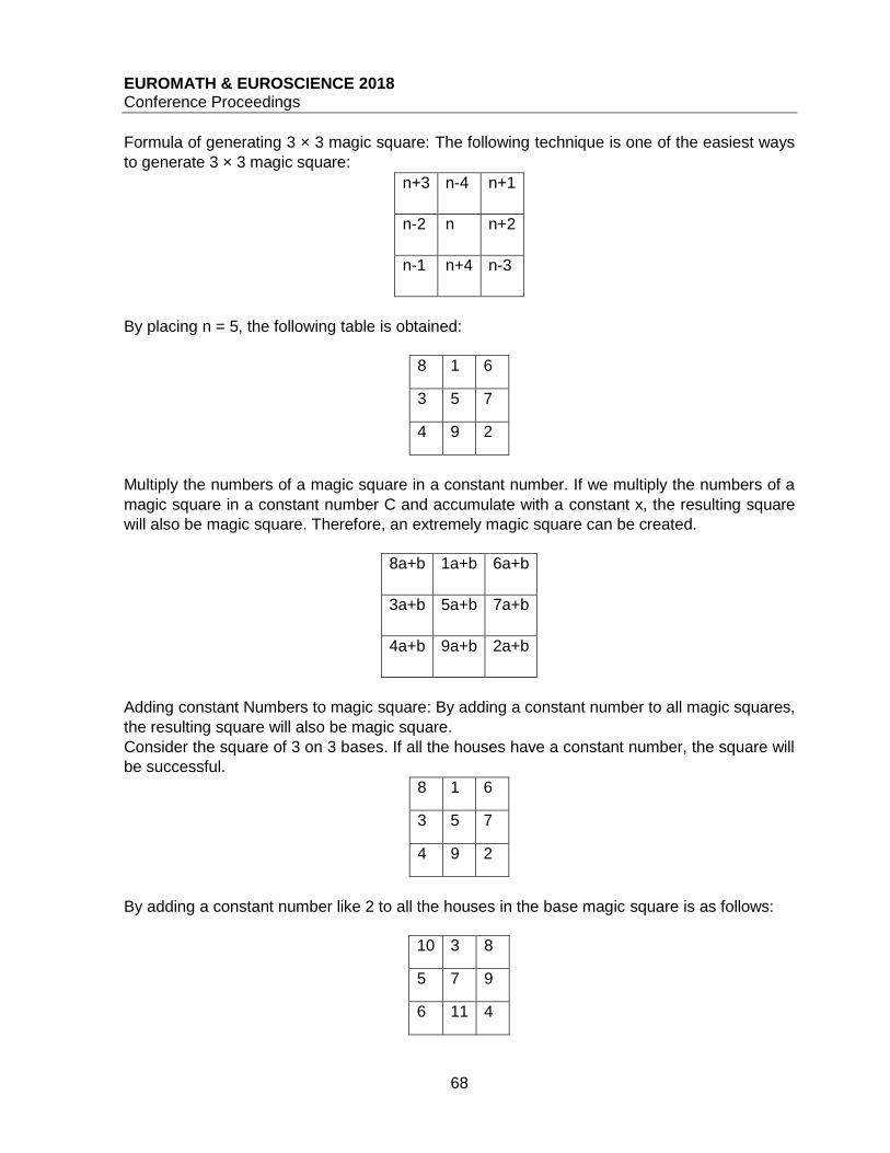
EUROMATH & EUROSCIENCE 2018 Conference Proceedings
68
Formula of generating 3 × 3 magic square: The following technique is one of the easiest ways
to generate 3 × 3 magic square:
n+1 n-4 n+3
n+2 n n-2
n-3 n+4 n-1
By placing n = 5, the following table is obtained:
6 1 8
7 5 3
2 9 4
Multiply the numbers of a magic square in a constant number. If we multiply the numbers of a
magic square in a constant number C and accumulate with a constant x, the resulting square
will also be magic square. Therefore, an extremely magic square can be created.
6a+b 1a+b 8a+b
7a+b 5a+b 3a+b
2a+b 9a+b 4a+b
Adding constant Numbers to magic square: By adding a constant number to all magic squares,
the resulting square will also be magic square.
Consider the square of 3 on 3 bases. If all the houses have a constant number, the square will
be successful.
6 1 8
7 5 3
2 9 4
By adding a constant number like 2 to all the houses in the base magic square is as follows:
8 3 10
9 7 5
4 11 6
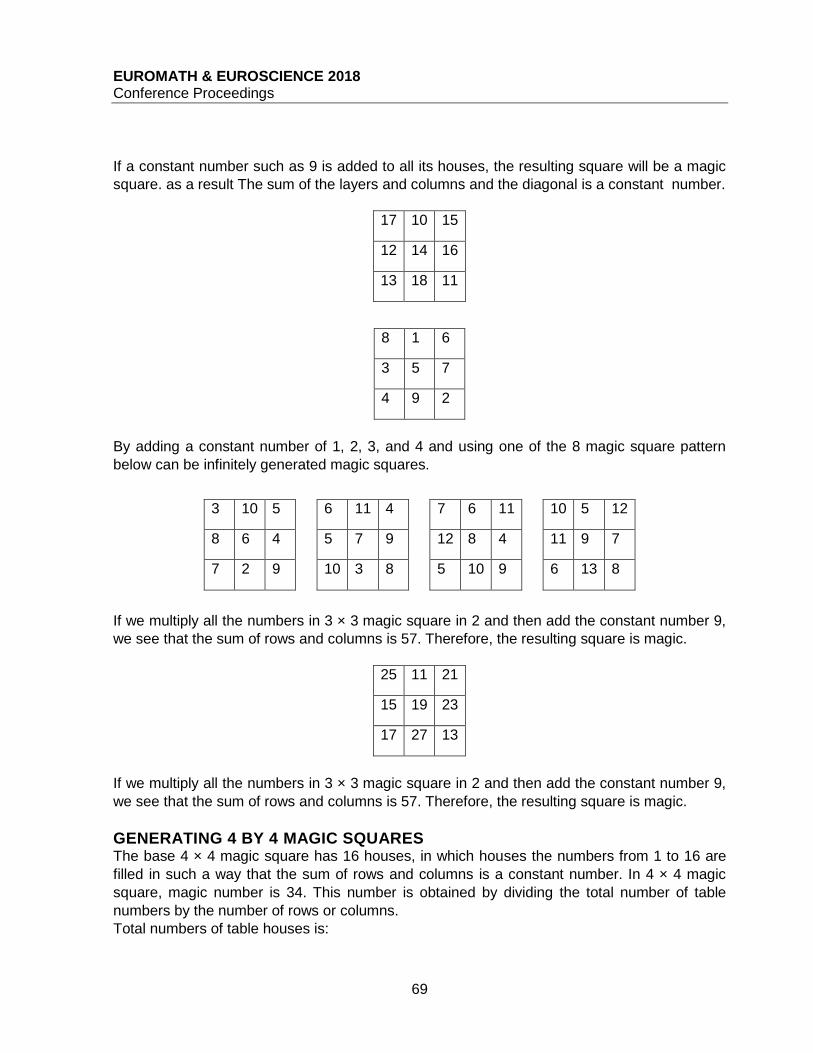
EUROMATH & EUROSCIENCE 2018 Conference Proceedings
69
If a constant number such as 9 is added to all its houses, the resulting square will be a magic
square. as a result The sum of the layers and columns and the diagonal is a constant number.
15 10 17
16 14 12
11 18 13
6 1 8
7 5 3
2 9 4
By adding a constant number of 1, 2, 3, and 4 and using one of the 8 magic square pattern
below can be infinitely generated magic squares.
12 5 10
7 9 11
8 13 6
11 6 7
4 8 12
9 10 5
4 11 6
9 7 5
8 3 10
5 10 3
4 6 8
9 2 7
If we multiply all the numbers in 3 × 3 magic square in 2 and then add the constant number 9,
we see that the sum of rows and columns is 57. Therefore, the resulting square is magic.
21 11 25
23 19 15
13 27 17
If we multiply all the numbers in 3 × 3 magic square in 2 and then add the constant number 9,
we see that the sum of rows and columns is 57. Therefore, the resulting square is magic.
GENERATING 4 BY 4 MAGIC SQUARES The base 4 × 4 magic square has 16 houses, in which houses the numbers from 1 to 16 are
filled in such a way that the sum of rows and columns is a constant number. In 4 × 4 magic
square, magic number is 34. This number is obtained by dividing the total number of table
numbers by the number of rows or columns.
Total numbers of table houses is:
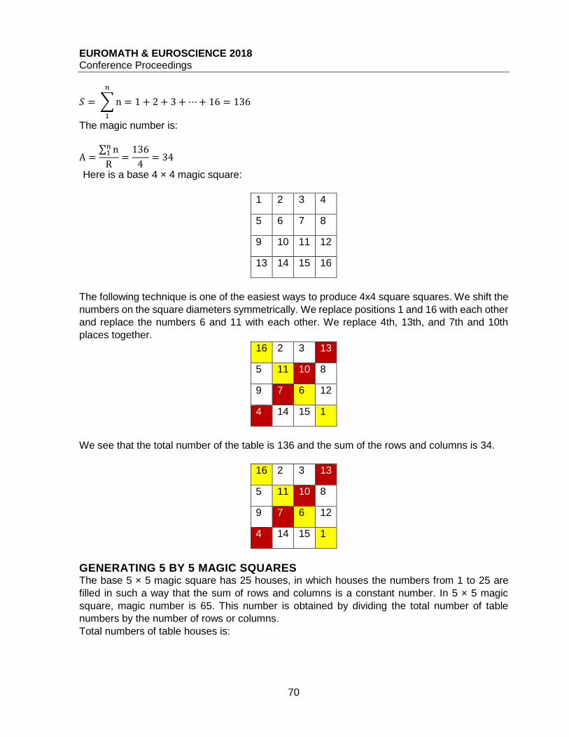
EUROMATH & EUROSCIENCE 2018 Conference Proceedings
70
𝑆 = ∑n
𝑛
1
= 1 + 2 + 3 +⋯+ 16 = 136
The magic number is:
A =∑ n𝑛1R
=136
4= 34
Here is a base 4 × 4 magic square:
1 2 3 4
5 6 7 8
9 10 11 12
13 14 15 16
The following technique is one of the easiest ways to produce 4x4 square squares. We shift the
numbers on the square diameters symmetrically. We replace positions 1 and 16 with each other
and replace the numbers 6 and 11 with each other. We replace 4th, 13th, and 7th and 10th
places together. 16 2 3 13
5 11 10 8
9 7 6 12
4 14 15 1
We see that the total number of the table is 136 and the sum of the rows and columns is 34.
16 2 3 13
5 11 10 8
9 7 6 12
4 14 15 1
GENERATING 5 BY 5 MAGIC SQUARES The base 5 × 5 magic square has 25 houses, in which houses the numbers from 1 to 25 are
filled in such a way that the sum of rows and columns is a constant number. In 5 × 5 magic
square, magic number is 65. This number is obtained by dividing the total number of table
numbers by the number of rows or columns.
Total numbers of table houses is:
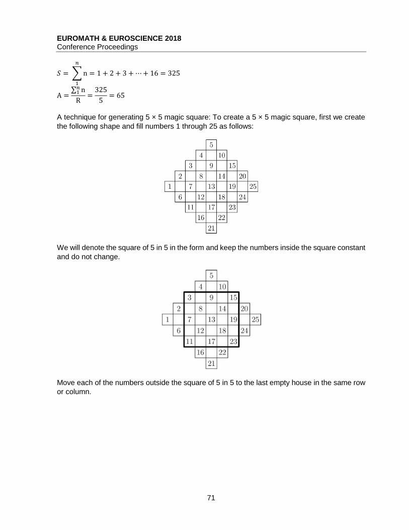
EUROMATH & EUROSCIENCE 2018 Conference Proceedings
71
𝑆 = ∑n
𝑛
1
= 1 + 2 + 3 +⋯+ 16 = 325
A =∑ n𝑛1R
=325
5= 65
A technique for generating 5 × 5 magic square: To create a 5 × 5 magic square, first we create
the following shape and fill numbers 1 through 25 as follows:
We will denote the square of 5 in 5 in the form and keep the numbers inside the square constant
and do not change.
Move each of the numbers outside the square of 5 in 5 to the last empty house in the same row
or column.
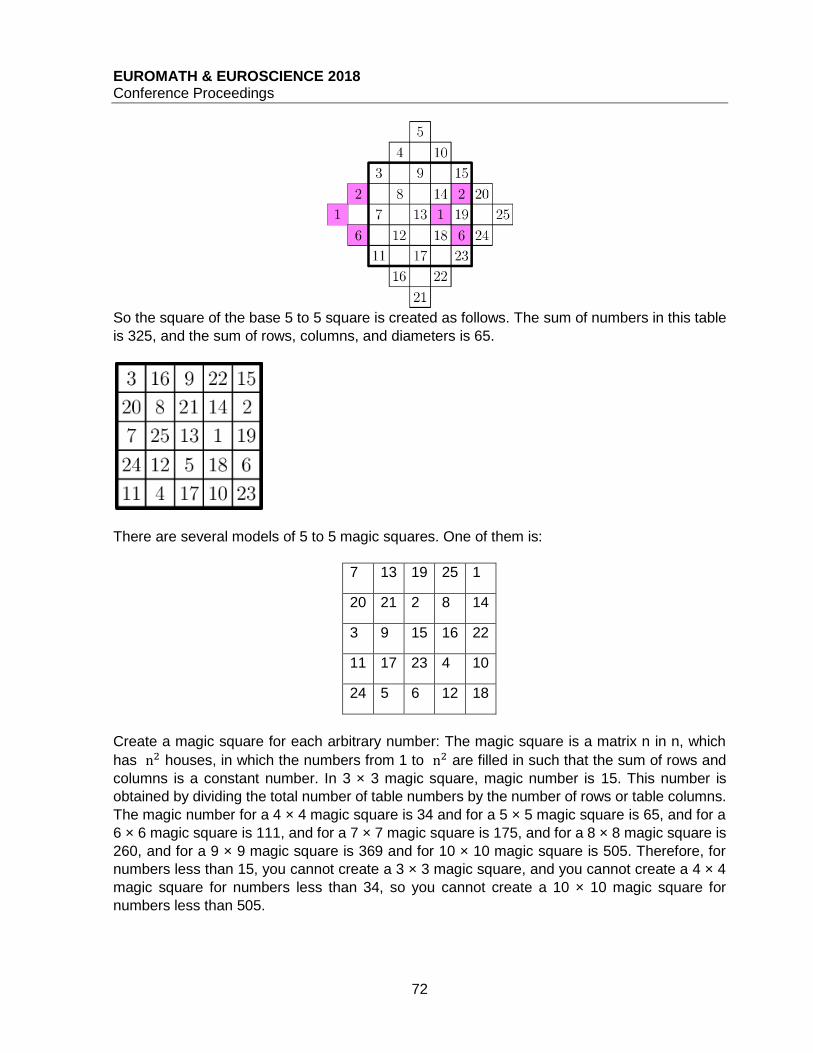
EUROMATH & EUROSCIENCE 2018 Conference Proceedings
72
So the square of the base 5 to 5 square is created as follows. The sum of numbers in this table
is 325, and the sum of rows, columns, and diameters is 65.
There are several models of 5 to 5 magic squares. One of them is:
1 25 19 13 7
14 8 2 21 20
22 16 15 9 3
10 4 23 17 11
18 12 6 5 24
Create a magic square for each arbitrary number: The magic square is a matrix n in n, which
has n2 houses, in which the numbers from 1 to n2 are filled in such that the sum of rows and
columns is a constant number. In 3 × 3 magic square, magic number is 15. This number is
obtained by dividing the total number of table numbers by the number of rows or table columns.
The magic number for a 4 × 4 magic square is 34 and for a 5 × 5 magic square is 65, and for a
6 × 6 magic square is 111, and for a 7 × 7 magic square is 175, and for a 8 × 8 magic square is
260, and for a 9 × 9 magic square is 369 and for 10 × 10 magic square is 505. Therefore, for
numbers less than 15, you cannot create a 3 × 3 magic square, and you cannot create a 4 × 4
magic square for numbers less than 34, so you cannot create a 10 × 10 magic square for
numbers less than 505.
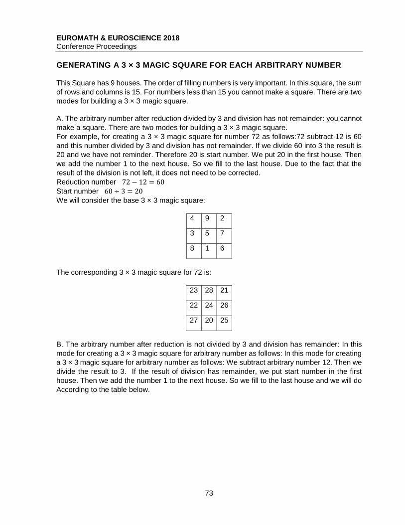
EUROMATH & EUROSCIENCE 2018 Conference Proceedings
73
GENERATING A 3 × 3 MAGIC SQUARE FOR EACH ARBITRARY NUMBER
This Square has 9 houses. The order of filling numbers is very important. In this square, the sum
of rows and columns is 15. For numbers less than 15 you cannot make a square. There are two
modes for building a 3 × 3 magic square.
A. The arbitrary number after reduction divided by 3 and division has not remainder: you cannot
make a square. There are two modes for building a 3 × 3 magic square.
For example, for creating a 3 × 3 magic square for number 72 as follows:72 subtract 12 is 60
and this number divided by 3 and division has not remainder. If we divide 60 into 3 the result is
20 and we have not reminder. Therefore 20 is start number. We put 20 in the first house. Then
we add the number 1 to the next house. So we fill to the last house. Due to the fact that the
result of the division is not left, it does not need to be corrected. Reduction number 72 − 12 = 60 Start number 60 ÷ 3 = 20 We will consider the base 3 × 3 magic square:
4 9 2
3 5 7
8 1 6
The corresponding 3 × 3 magic square for 72 is:
23 28 21
22 24 26
27 20 25
B. The arbitrary number after reduction is not divided by 3 and division has remainder: In this
mode for creating a 3 × 3 magic square for arbitrary number as follows: In this mode for creating
a 3 × 3 magic square for arbitrary number as follows: We subtract arbitrary number 12. Then we
divide the result to 3. If the result of division has remainder, we put start number in the first
house. Then we add the number 1 to the next house. So we fill to the last house and we will do
According to the table below.
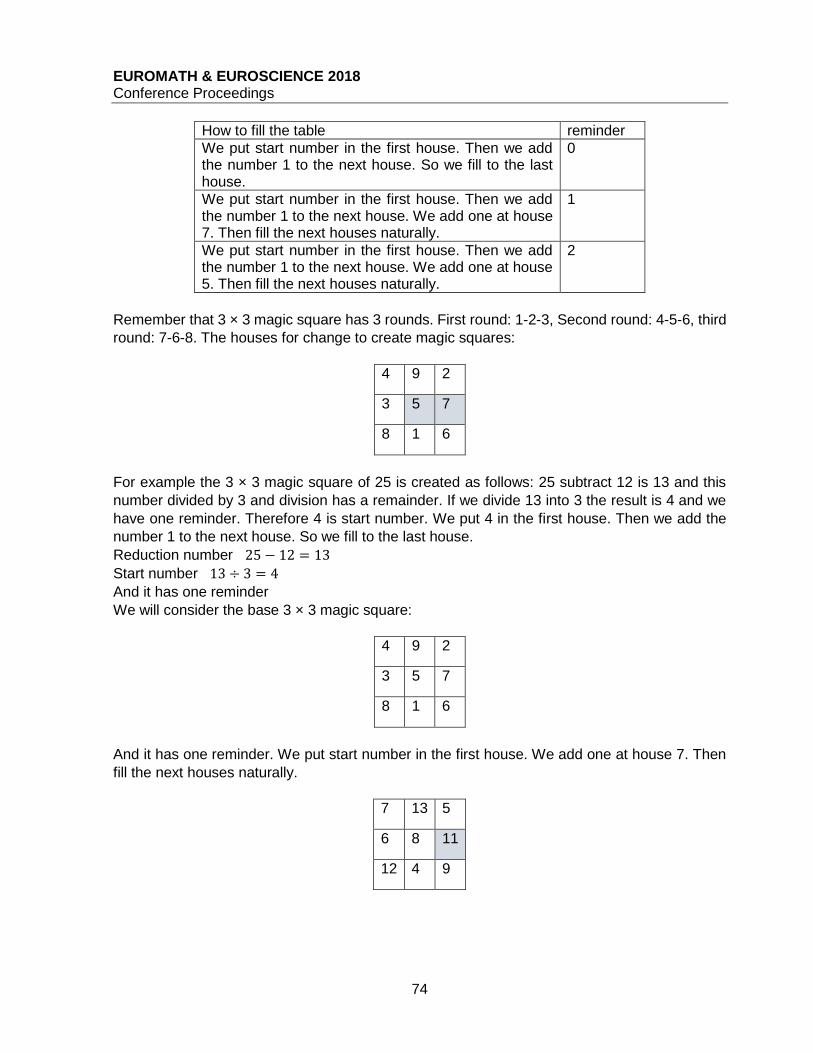
EUROMATH & EUROSCIENCE 2018 Conference Proceedings
74
How to fill the table reminder
We put start number in the first house. Then we add the number 1 to the next house. So we fill to the last house.
0
We put start number in the first house. Then we add the number 1 to the next house. We add one at house 7. Then fill the next houses naturally.
1
We put start number in the first house. Then we add the number 1 to the next house. We add one at house 5. Then fill the next houses naturally.
2
Remember that 3 × 3 magic square has 3 rounds. First round: 1-2-3, Second round: 4-5-6, third
round: 7-6-8. The houses for change to create magic squares:
4 9 2
3 5 7
8 1 6
For example the 3 × 3 magic square of 25 is created as follows: 25 subtract 12 is 13 and this
number divided by 3 and division has a remainder. If we divide 13 into 3 the result is 4 and we
have one reminder. Therefore 4 is start number. We put 4 in the first house. Then we add the
number 1 to the next house. So we fill to the last house.
Reduction number 25 − 12 = 13
Start number 13 ÷ 3 = 4
And it has one reminder We will consider the base 3 × 3 magic square:
4 9 2
3 5 7
8 1 6
And it has one reminder. We put start number in the first house. We add one at house 7. Then
fill the next houses naturally.
7 13 5
6 8 11
12 4 9

EUROMATH & EUROSCIENCE 2018 Conference Proceedings
75
For creating the n × n magic square for arbitrary number, we act like 3 by 3 magic square. It
should be noted that the reduction number for 3 by 3 magic square is 12 and for 4 by 4 magic
square is 30 and for 5 by 5 magic square is 60.
CONCLUSION
For arbitrary numbers, a magic square can be constructed. For creating the n × n magic square
for arbitrary number, we subtract reduction number from arbitrary number. The reduction
number for 3 by 3 magic square is 12 and for 4 by 4 magic square is 30 and for 5 by 5 magic
square is 60. Then we divide the result to n. If the result of division has not remainder, we put
start number in the first house. Then we add the number 1 to the next house. So we fill to the
last house. And if the result of division has a remainder we add number 1 in the one of the
houses 3n + 1 , 4n + 1 , 5n + 1 number one , and In the remaining houses we add naturally
number one unit.
REFERENCES
Abe, G. (1994). Unsolved problems on magic squares. Discrete Mathematics, 127(1-3), 3-13.
Andrews, W. S. (2004). Magic squares and cubes. Cosimo, Inc.
Barton, C. H., & Sudbery, A. (2003). Magic squares and matrix models of Lie algebras.
Advances in Mathematics, 180(2), 596-647.
Beck, M., Cohen, M., Cuomo, J., & Gribelyuk, P. (2003). The number of magic squares, cubes,
and hypercube. The American mathematical monthly, 110(8), 707-717.
Benson, W. H., & Jacoby, O. (1976). New recreations with magic squares (No. 04; QA165, B4.).
New York: Dover Publications.
Block, S. S., & Tavares, S. A. (2009). Before Sudoku: The world of magic squares. Oxford
University Press, USA.
Henrich, C. J. (1991). Magic squares and linear algebra. The American mathematical monthly,
98(6), 481-488.
Moran, J. (1982). The Wonders of Magic Squares. Random House Inc.
Peter, J. Barta, The Seal-Ring of Proportion and the magic rings (2016), pp. 6–9. Rogers, A., & Loly, P. (2004). The Inertial Properties of Magic Squares and Cubes.
Xie, T., & Kang, L. (2003, December). An evolutionary algorithm for magic squares. In
Evolutionary Computation, 2003. CEC'03. The 2003 Congress on (Vol. 2, pp. 906-913). IEEE.

EUROMATH & EUROSCIENCE 2018 Conference Proceedings
76
SEQUENCE RESULTING AS SOLUTION OF TWO COMBINATORIAL PROBLEMS Russu Vladimir
Theoretical lyceum A. Puskin, Republic of Moldova
ABSTRACT Often combinatorial problems are very difficult. However, a difficult combinatorial problem can be simplified that is the goal of science – to serve people. For example, a common problem: a city has the form of a rectangle and a network of n streets towards North-South and m streets towards East-West. How many ways are there for tourist to get from vertex South-West to the North-East one of the city moving in the direction from West to East and from South to North across the streets. This problem can be reduced down to the similar one that is about the number of ways to place m red balls and n yellow ones in a tube. Our purpose is to examine the
sequence resulting as the solution of 2 combinatorial problems. First problem: 2 × 𝑘 an 2 × 𝑛 rectangles are given; dominos represent 1× 2 rectangles. How many ways are there to full 2 ×𝑘 and 2 × 𝑛 rectangles with dominos so that they will contain an equal number of vertical dominos? Second problem: two parallel lines are given. The first contains k, the second one n indicated points. These points form pairs so, that segments, connecting points in each pair, do not intersect. What is the number of pairs? Solutions of these two problems result in a reasonable sequence. In our work we study properties of this sequence and its connection with other well-known sequences.
Introduction In this work we regard, how identic sequences can appear in different combinatorial problems. This research was inspired by the following problem, which was offered on Saint-Petersburg Math Olympiad in year 2014: “On each of two parallel lines 40 points are indicated. They are connected into pairs so that segments, which connect points in each pair do not intersect (in particular, no point belongs to several segments and no point does not have a pair). Prove that the number of ways to form such configurations is less than 339” So, we will make generalization of this combinatorial sequence. In order to make clearer the context of this work, in part I we will represent on the example of another three combinatorial problems, how different problems can be reduced to common sequence and common solution.

EUROMATH & EUROSCIENCE 2018 Conference Proceedings
77
I “Town m, n” problem
A town in form of a rectangle is given with vertexes: A(south-west), B(north-west), C(north-east), D(south-east). The streets are situated parallel to AB or parallel to BC. Let n – be length of AB, m – length of BC. The tourist sets from A to B, passing the streets of the town so that in the northern or eastern direction. How many ways are there for the tourist to manage that? Following the data of the problem, n – the distance passed in the northern direction, m – the distance passed in the eastern direction. Let l1, l2, l3, …, lm - be the fragments of the northern way and k1, k2, k3, …, kn - be the fragments of the eastern way. Then number of possible ways for the tourist to reach the point A from point B can be found by solving in positive integers equation:
l1+ l2+ l3+ …+lm =n or equation:
k1+ k2+ k3+ …+kn = m
Obviously, the choice of northern way determines the choice of the eastern ways (therefore, chose of the whole way) and vice versa. So, to answer the question of the problem is enough to solve one of equations, demonstrated above.
And on this point the given problem intersects with well-known Moivre problem
“How many positive integer solutions does the equation x1+ x2+ x3+ …+xn = k have?”
On this step, not solving these two problems, we offer to regard another combinatorial problem, which will help to solve last ones.
Tube problem A tube is given. It is filled with blue and red balls of the same size (in particular, radius of the bottom equals radius of the balls, so that balls can be placed in the tube one by one in vertical trajectory) in the following way: first, k1 blue balls are placed, the one red one is added, after that k2 blue balls are added and the one red ball is added and so on, …, finally, kn blue balls are added and the last red ball is added. So, n – is the number of red balls, k1+ k2+ k3+ …+kn = m – the number of blue balls.
m
n
D
C B

EUROMATH & EUROSCIENCE 2018 Conference Proceedings
78
How many ways are there to place m blue balls in tube? To manage that we need to solve in positive integers equation k1+ k2+ k3+ …+kn = m –
here we see identity with Moivre problem (theory of numbers) and identity with “town m, n”
problem.
1) How many ways are there to situate n-1 red balls in the tube? (we do not take into account
one red ball, because it is always on the top of the tube)
Taking into consideration that there are n-1 red balls and m+n-1 all balls, we can answer
question 2), using the combinatorial formula:
Cn
mn
1
1
and using a well-known combinatorial property we can transform this formula in such a way:
CCCт
mn
nтт
mn
n
mn 1
)1(1
1
1
1
So, we got formula for calculating number of ways to situate m blue balls, which, as it is proved above, equals the number of ways to situate n red balls. We easily see that Moivre problem and tube problem are solved using the same formula:
CCCт
mn
nтт
mn
n
mn 1
)1(1
1
1
1
And, as Moivre problem and “town m, n” problem are identic, this formula solves all the three problems. So, we got the following scheme: while solving “town m, n” problem we noticed that it is identic to Moivre problem. With the help of identic sequence from tube problem we got the common solution and the common sequence.
II “Configurations
Now let’s return to Saint-Petersburg Olympiad problem, making the generalization of this problem. Two parallel lines are given. On the first line k points are indicated, on the second one n points are indicated. These points are connected into pairs so that segments, which connect points in each pair do not intersect (in particular, no point belongs to several segments and no point does not have a pair, which means that k and n are of the same parity). Let such combinatorial constructions be named “configurations” and the number of all possible “configurations” be ck,n.
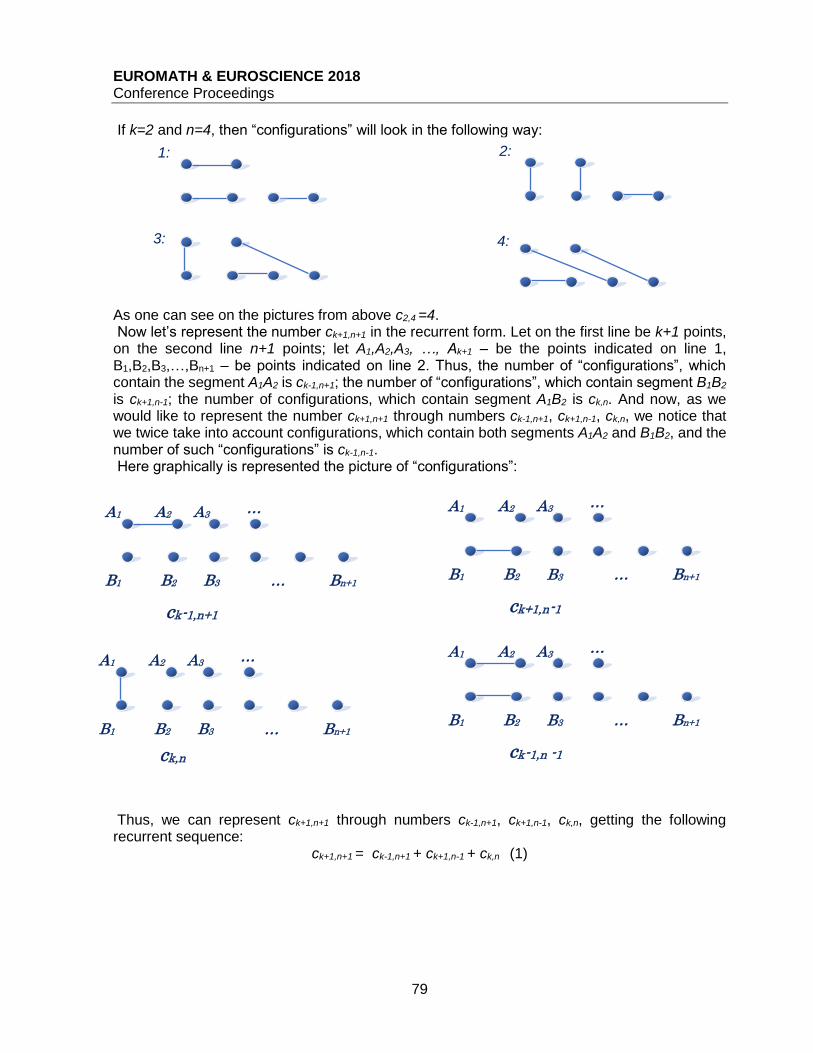
EUROMATH & EUROSCIENCE 2018 Conference Proceedings
79
If k=2 and n=4, then “configurations” will look in the following way: As one can see on the pictures from above c2,4 =4. Now let’s represent the number ck+1,n+1 in the recurrent form. Let on the first line be k+1 points, on the second line n+1 points; let A1,A2,A3, …, Ak+1 – be the points indicated on line 1, B1,B2,B3,…,Bn+1 – be points indicated on line 2. Thus, the number of “configurations”, which contain the segment A1A2 is ck-1,n+1; the number of “configurations”, which contain segment B1B2 is ck+1,n-1; the number of configurations, which contain segment A1B2 is ck,n. And now, as we would like to represent the number ck+1,n+1 through numbers ck-1,n+1, ck+1,n-1, ck,n, we notice that we twice take into account configurations, which contain both segments A1A2 and B1B2, and the number of such “configurations” is ck-1,n-1. Here graphically is represented the picture of “configurations”: Thus, we can represent ck+1,n+1 through numbers ck-1,n+1, ck+1,n-1, ck,n, getting the following recurrent sequence:
ck+1,n+1 = ck-1,n+1 + ck+1,n-1 + ck,n (1)
1: 2:
3: 4:
… A3 A2 A1
B1 B2 B3 … Bn+1
ck-1,n+1
… A3 A2 A1
B1 B2 B3 … Bn+1
ck+1,n-1
… A3 A2 A1
B1 B2 B3 … Bn+1
ck,n
… A3 A2 A1
B1 B2 B3 … Bn+1
ck-1,n -1

EUROMATH & EUROSCIENCE 2018 Conference Proceedings
80
Motskin’s “no-pick” routes Motskin’s “no-pick” route is an oriented angled line, situated on coordinate plane, each fragment of which is situated in one of the directions represented below:
Given angled line also does not have any “picks”, the fragments of the following kind:
Below we will represent all possible Motskin’s “no-pick routes”, oriented from point with coordinates (0;0) in point with coordinates (3;1):
Let the number of all possible Motskin’s “no-pick routes”, coming from point A(0;0) into point Z(k;n) be bk,n. Now, let’s see how Motskin’s “no-pick” route can reach the point Z(k;n). Clearly, from point X(k-1,n) or from point Y(k-1;n-1) or from point V(k-1;n+1); but it cannot reach the point V(k-1;n+1) from the point P(k-2;n), because in such a case in the point V(k-1;n+1) a “pick” appears. Thus, we get recurrent sequence in the following way:
bk,n = bk-1,n + bk-1,n-1 - bk-2,n (2) It is not difficult to notice that sequence 1 and sequence 2 are almost the same and are absolutely identic in structure and principle, which proves connection between combinatorial construction “configurations” and properties of Motskin’s “no-pick routes”, to which, as we have demonstrated, combinatory can be applied and which are related to the theory of graphs.
Calculating ck,n Let’s return to “configurations” and calculate ck,n. After we arrange “configurations”, we erase segments, which connect into pairs points, which lay on different lines. So, from all the segments we leave only the horizontal ones:
(0;0)
(3;1)

EUROMATH & EUROSCIENCE 2018 Conference Proceedings
81
We notice that using the set of horizontal segments we can reestablish the initial picture: So, we conclude that the choice of horizontal segments determines the choice of other segments and, thus, the picture of “configurations”, which means that, if we find the number of ways to choose horizontal segments, we automatically find ck,n as well. On this point we temporary leave target to find ck,n and regard another combinatorial construction.
Domino Domino – is a rectangle of the kind 1×2 or 2×1. Let dk,n – be the number of ways to place in rectangle of the size 2×k and 2×n vertical dominos, and j – the number of vertical dominos in rectangle. Below we represent this in a table:
k n j 2×k 2×n d dk,n
3
5 1 4
10 3 6
Now we set target to find out how we can calculate the number of ways to place vertical dominos in rectangles, because the number of these ways, obviously, determines the whole picture of filling rectangles with dominos. But first, to find out that, we will regard an auxiliary problem, which will help us to find ck,n as well.
“Configurations j, l ” So, auxiliary problem: let “configurations j, l ” on a line be a set, which consists of l not intersecting segments and j points, which do not lay on these segments. Let the ends of the segments be green points, other points be red. How many “configurations j, l ” on a line are possible? To get that picture, let’s, firstly, draw l green points and j red points, then on the right side of each green point add one more green and connect green points with segments into pairs. During this operation we can notice that the choice of the number of initial green points determines the picture of “configurations j, l ”. And the number of ways to choose green points can be found by formula
l
ljC

EUROMATH & EUROSCIENCE 2018 Conference Proceedings
82
l – is the number of initial green points and j+l – is the initial number of all points. Using a well-known combinatorial property and representing the final number of points as k=j+l (k and j are of the same parity), that formula can be got in such a way:
We can see that the number of ways to choose red points also determines the picture of “configurations j, l ”.
Provement: ck,n= dk,n
And now we notice the connection between domino and “configurations j, l ”: red points correspond to vertical dominos and pairs of green points connected with segments correspond to horizontal dominos. So, we can apply the last formula for “configurations” on two lines and finally calculate ck,n:
And, as we have demonstrated parallelism between domino and “configurations”, we can represent identic formula for domino in rectangles 2×k and 2×n:
Conclusion So, in part II we have generalized the sequence of the problem offered on Saint-Petersburg school Olympiad. Like in part I we have demonstrated how in particular combinatorial constructions the choice of objects of one kind determines the choice of objects of another kind; how common properties and sequences appear in different mathematical constructions. And in the whole work we have connected different fields of mathematics: combinatory, theory of numbers (Moivre problem) and theory of graphs (Motskin’s “no-pick” routes).
References 1. Titu Andriescu, Zuming Feng “102 Combinatorial Problems from the Training of the USA
IMO Team”, 2003, Birkhäuser.
2. Vasile Pop, Marcel Teleuca “Combinatorial problems. Counting, graphs, games” (in
Romanian language), 2013, Romanian Mathematical Society.
3. K. P. Kohasi, A. I. Hrabrov “Points on lines, laces and dominos”, Mathematical
enlightenment, series 3, 19 (2015), 139-163
4. K. P. Kohasi, “Domino partition”, Mathematical enlightenment, series 3, 9 (2005), 143-163
j
jk
jkjk
jk
jk
jkCCC
l
ljC
2
2
)(
2
2
2
j
jn
nk
nkj
j
jk
jn
jn
nk
nkj
jk
jkCCCCс
nk2
)2(mod
};min{0 2
2
2
)2(mod
};min{0
2
2
,
j
jn
nk
nkj
j
jk
jn
jn
nk
nkj
jk
jkCCCCсd
nknk2
)2(mod
};min{0 2
2
2
)2(mod
};min{0
2
2
,,

EUROMATH & EUROSCIENCE 2018 Conference Proceedings
83
A CIRCLE ROTATES TOWARDS EXCITING MATHEMATICS Galati Kyriaki, Pachni Ioanna, Perroti Loukia, Pimbli Natalia, Tzanetou Eleni
The Moraitis School, Greece
ABSTRACT Suppose you wish to construct a waterslide that will take you in the least time down to a given point. Which would the waterslide’s curve be? Also, imagine that you have a circle rotating inside another circle of twice the diameter. What shape would any point on the small circle make? In our paper, we address these two problems that have one main common characteristic: the (rotating) circle. We also show that these problems are not only brainteasers with mind-blowing solutions, but, more importantly, the Brachistochrone led to the rise of fields within Mathematics such as the Calculus of Variations.
INTRODUCTION
"The circle" is an object, a drawing, a geometrical shape that everyone recognises. It is used to
describe cyclic forms for a variety of things in our everyday life. In this paper, we examine two
applications of the circle, namely the Brachistochrone and the Tusi Couple.
The Brachistochrone problem: Imagine that you have two points in a vertical plane and you want
to go from point A to point B travelling only by the force of gravity in the fastest way possible.
How does the route that you should follow look like? Johann Bernoulli first addressed this
problem to the readers of Acta Eruditorum in 1696 [5]. Some ideas would be the straight line,
the arc of a circle, the semi-ellipse, the cycloid, an extreme curve, or any other curve one may
imagine. In fact, it was proven in 1697 that the cycloid gives the fastest route [5].
What is more fascinating is that the cycloid curve is the only curve that possesses the
Tautochrone property: an object will reach the bottom (point B) at the same amount of time
independently of its starting position on the curve!
The Tusi Couple: A small circle C1 of a given diameter constantly rolls inside a bigger circle C2
of double the diameter. If a random point M that belongs to the circumference of C1 had the
ability to draw its route as it rolled inside the other circle, what shape would it make?
The solution to this brainteaser is mind-blowing and we provide the proof in the respective
section.
THE BRACHISTOCHRONE PROBLEM
The problem of finding the fastest way to go from one place to another is one that we face in our
daily life. In Mathematics, we have various ways to find solutions to such problems, such as
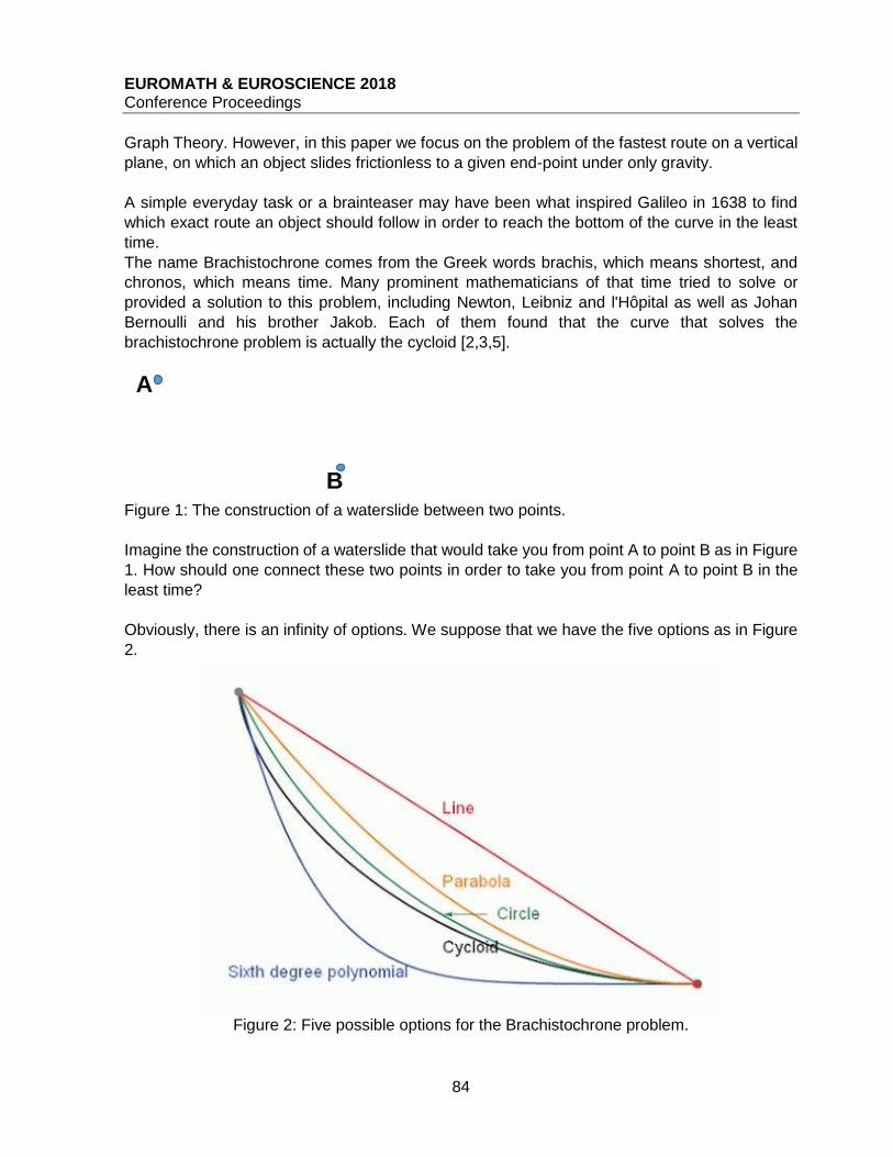
EUROMATH & EUROSCIENCE 2018 Conference Proceedings
84
Graph Theory. However, in this paper we focus on the problem of the fastest route on a vertical
plane, on which an object slides frictionless to a given end-point under only gravity.
A simple everyday task or a brainteaser may have been what inspired Galileo in 1638 to find
which exact route an object should follow in order to reach the bottom of the curve in the least
time.
The name Brachistochrone comes from the Greek words brachis, which means shortest, and
chronos, which means time. Many prominent mathematicians of that time tried to solve or
provided a solution to this problem, including Newton, Leibniz and l'Hôpital as well as Johan
Bernoulli and his brother Jakob. Each of them found that the curve that solves the
brachistochrone problem is actually the cycloid [2,3,5].
Figure 1: The construction of a waterslide between two points.
Imagine the construction of a waterslide that would take you from point A to point B as in Figure
1. How should one connect these two points in order to take you from point A to point B in the
least time?
Obviously, there is an infinity of options. We suppose that we have the five options as in Figure
2.
Figure 2: Five possible options for the Brachistochrone problem.
A
B
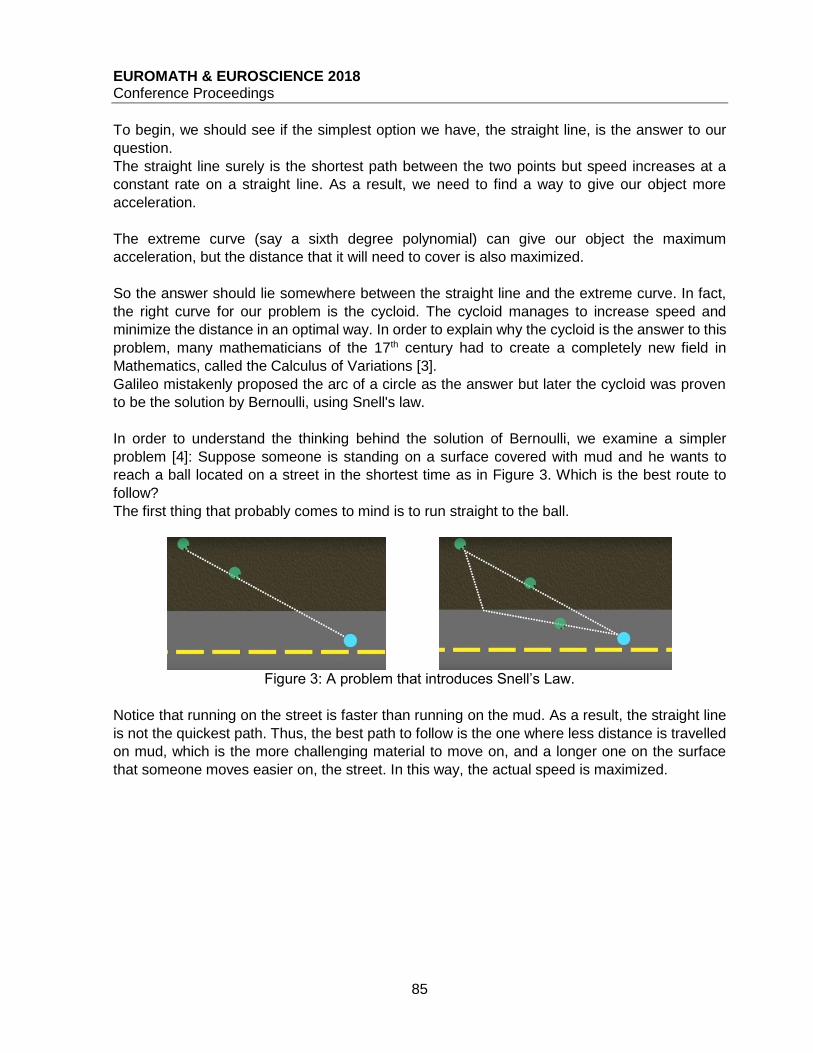
EUROMATH & EUROSCIENCE 2018 Conference Proceedings
85
To begin, we should see if the simplest option we have, the straight line, is the answer to our
question.
The straight line surely is the shortest path between the two points but speed increases at a
constant rate on a straight line. As a result, we need to find a way to give our object more
acceleration.
The extreme curve (say a sixth degree polynomial) can give our object the maximum
acceleration, but the distance that it will need to cover is also maximized.
So the answer should lie somewhere between the straight line and the extreme curve. In fact,
the right curve for our problem is the cycloid. The cycloid manages to increase speed and
minimize the distance in an optimal way. In order to explain why the cycloid is the answer to this
problem, many mathematicians of the 17th century had to create a completely new field in
Mathematics, called the Calculus of Variations [3].
Galileo mistakenly proposed the arc of a circle as the answer but later the cycloid was proven
to be the solution by Bernoulli, using Snell's law.
In order to understand the thinking behind the solution of Bernoulli, we examine a simpler
problem [4]: Suppose someone is standing on a surface covered with mud and he wants to
reach a ball located on a street in the shortest time as in Figure 3. Which is the best route to
follow?
The first thing that probably comes to mind is to run straight to the ball.
Figure 3: A problem that introduces Snell’s Law.
Notice that running on the street is faster than running on the mud. As a result, the straight line
is not the quickest path. Thus, the best path to follow is the one where less distance is travelled
on mud, which is the more challenging material to move on, and a longer one on the surface
that someone moves easier on, the street. In this way, the actual speed is maximized.

EUROMATH & EUROSCIENCE 2018 Conference Proceedings
86
Figure 4: Snell’s Law
So, as the person enters the street two angles are formed, θ1 and θ2.
If the ratio of sinθ1 and sinθ2 is equal to the ratio of the speed in mud and the speed on the
street (see Figure 4), then the resulting line is the fastest route. In other words, Snell’s Law,
which is also known as the law of refraction, states that when a ray of light crosses the boundary
between transparent media, it experiences a change in direction characterized by the relation
[2,4] sin 𝜃1sin 𝜃2
= 𝜐1𝜐2
in which θ1 is the angle of incidence, θ2 is the angle of refraction and υ1 and υ2 are the velocities
depending on the nature of the two media (Figure 4).
According to the principle of least time, light will always travel along a path with the shortest
traversal time and apparently, what Bernoulli did was to add thinner and thinner layers for the
light to move on. In fact, consider a situation with a light ray traveling downward through many
transparent layers, with each medium less dense than the layer above it. The speed of light
increases in every next media as it progresses through deeper layers and the ray of light bends
further away from one to another medium at point of contact. As the number of layers increases
to infinity, the path becomes a curve that is actually the cycloid [2,4].
CYCLOID
The cycloid is the curve traced by a point on a circle when the circle rotates on a straight line as
in Figure 5.
Figure 5: The cycloid.
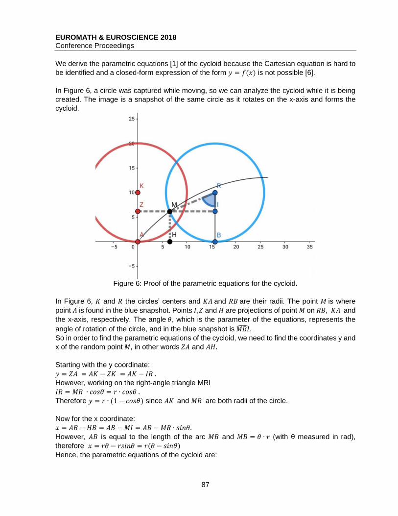
EUROMATH & EUROSCIENCE 2018 Conference Proceedings
87
We derive the parametric equations [1] of the cycloid because the Cartesian equation is hard to
be identified and a closed-form expression of the form 𝑦 = 𝑓(𝑥) is not possible [6].
In Figure 6, a circle was captured while moving, so we can analyze the cycloid while it is being
created. The image is a snapshot of the same circle as it rotates on the x-axis and forms the
cycloid.
Figure 6: Proof of the parametric equations for the cycloid.
In Figure 6, 𝐾 and 𝑅 the circles’ centers and 𝐾𝐴 and 𝑅𝐵 are their radii. The point 𝑀 is where
point 𝐴 is found in the blue snapshot. Points 𝐼,𝑍 and 𝐻 are projections of point 𝑀 on 𝑅𝐵, 𝐾𝐴 and
the x-axis, respectively. The angle 𝜃, which is the parameter of the equations, represents the
angle of rotation of the circle, and in the blue snapshot is 𝑀𝑅��. So in order to find the parametric equations of the cycloid, we need to find the coordinates y and
x of the random point 𝑀, in other words 𝑍𝐴 and 𝐴𝐻.
Starting with the y coordinate:
𝑦 = 𝑍𝐴 = 𝐴𝐾 − 𝑍𝐾 = 𝐴𝐾 − 𝐼𝑅 . However, working on the right-angle triangle MRI
𝐼𝑅 = 𝑀𝑅 ∙ 𝑐𝑜𝑠𝜃 = 𝑟 ∙ 𝑐𝑜𝑠𝜃 . Therefore 𝑦 = 𝑟 ∙ (1 − 𝑐𝑜𝑠𝜃) since 𝐴𝛫 and 𝑀𝑅 are both radii of the circle.
Now for the x coordinate:
𝑥 = 𝐴𝐵 − 𝐻𝐵 = 𝐴𝐵 −𝑀𝐼 = 𝐴𝐵 −𝑀𝑅 ∙ 𝑠𝑖𝑛𝜃.
However, 𝐴𝐵 is equal to the length of the arc 𝑀𝐵 and 𝑀𝐵 = 𝜃 ∙ 𝑟 (with θ measured in rad),
therefore 𝑥 = 𝑟𝜃 − 𝑟𝑠𝑖𝑛𝜃 = 𝑟(𝜃 − 𝑠𝑖𝑛𝜃)
Hence, the parametric equations of the cycloid are:
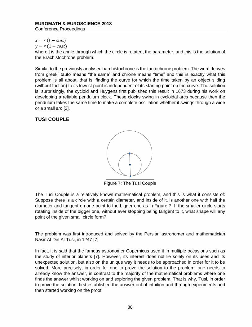
EUROMATH & EUROSCIENCE 2018 Conference Proceedings
88
𝑥 = 𝑟 (𝑡 − 𝑠𝑖𝑛𝑡)
𝑦 = 𝑟 (1 − 𝑐𝑜𝑠𝑡)
where t is the angle through which the circle is rotated, the parameter, and this is the solution of
the Brachistochrone problem.
Similar to the previously analysed barchistochrone is the tautochrone problem. The word derives
from greek; tauto means “the same” and chrone means “time” and this is exactly what this
problem is all about, that is: finding the curve for which the time taken by an object sliding
(without friction) to its lowest point is independent of its starting point on the curve. The solution
is, surprisingly, the cycloid and Huygens first published this result in 1673 during his work on
developing a reliable pendulum clock. These clocks swing in cycloidal arcs because then the
pendulum takes the same time to make a complete oscillation whether it swings through a wide
or a small arc [2].
TUSI COUPLE
Figure 7: The Tusi Couple
The Tusi Couple is a relatively known mathematical problem, and this is what it consists of:
Suppose there is a circle with a certain diameter, and inside of it, is another one with half the
diameter and tangent on one point to the bigger one as in Figure 7. If the smaller circle starts
rotating inside of the bigger one, without ever stopping being tangent to it, what shape will any
point of the given small circle form?
The problem was first introduced and solved by the Persian astronomer and mathematician
Nasir Al-Din Al-Tusi, in 1247 [7].
In fact, it is said that the famous astronomer Copernicus used it in multiple occasions such as
the study of inferior planets [7]. However, its interest does not lie solely on its uses and its
unexpected solution, but also on the unique way it needs to be approached in order for it to be
solved. More precisely, in order for one to prove the solution to the problem, one needs to
already know the answer, in contrast to the majority of the mathematical problems where one
finds the answer whilst working on and exploring the given problem. That is why, Tusi, in order
to prove the solution, first established the answer out of intuition and through experiments and
then started working on the proof.
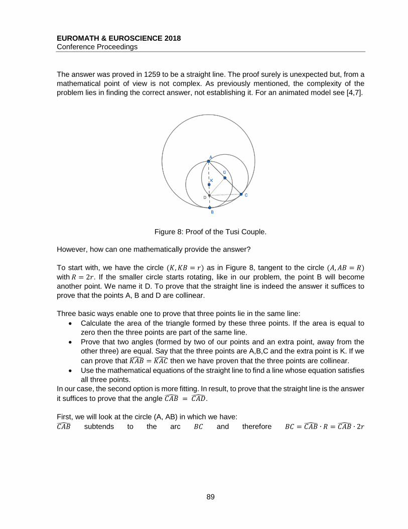
EUROMATH & EUROSCIENCE 2018 Conference Proceedings
89
The answer was proved in 1259 to be a straight line. The proof surely is unexpected but, from a
mathematical point of view is not complex. As previously mentioned, the complexity of the
problem lies in finding the correct answer, not establishing it. For an animated model see [4,7].
Figure 8: Proof of the Tusi Couple.
However, how can one mathematically provide the answer?
To start with, we have the circle (𝐾, 𝐾𝐵 = 𝑟) as in Figure 8, tangent to the circle (𝐴, 𝐴𝐵 = 𝑅)
with 𝑅 = 2𝑟. If the smaller circle starts rotating, like in our problem, the point B will become
another point. We name it D. To prove that the straight line is indeed the answer it suffices to
prove that the points A, B and D are collinear.
Three basic ways enable one to prove that three points lie in the same line:
Calculate the area of the triangle formed by these three points. If the area is equal to
zero then the three points are part of the same line.
Prove that two angles (formed by two of our points and an extra point, away from the
other three) are equal. Say that the three points are A,B,C and the extra point is K. If we
can prove that 𝐾𝐴�� = 𝐾𝐴�� then we have proven that the three points are collinear.
Use the mathematical equations of the straight line to find a line whose equation satisfies
all three points.
In our case, the second option is more fitting. In result, to prove that the straight line is the answer
it suffices to prove that the angle 𝐶𝐴�� = 𝐶𝐴��.
First, we will look at the circle (A, AB) in which we have:
𝐶𝐴�� subtends to the arc 𝐵𝐶 and therefore 𝐵𝐶 = 𝐶𝐴�� ∙ 𝑅 = 𝐶𝐴�� ∙ 2𝑟
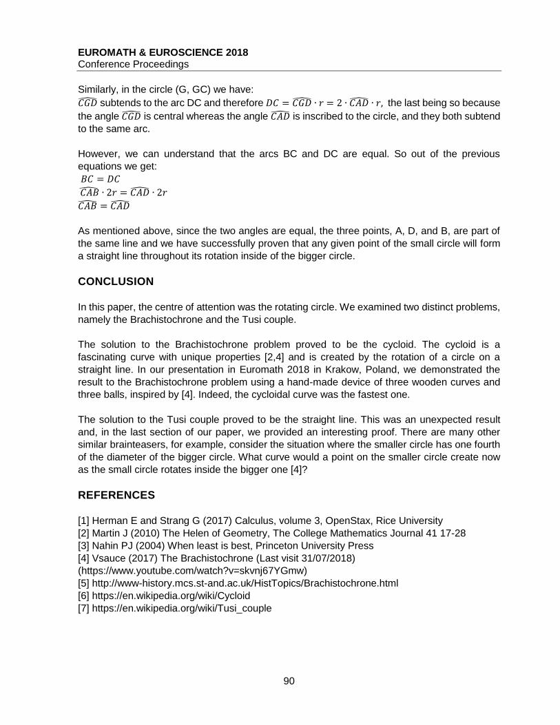
EUROMATH & EUROSCIENCE 2018 Conference Proceedings
90
Similarly, in the circle (G, GC) we have:
𝐶𝐺�� subtends to the arc DC and therefore 𝐷𝐶 = 𝐶𝐺�� ∙ 𝑟 = 2 ∙ 𝐶𝐴�� ∙ 𝑟, the last being so because
the angle 𝐶𝐺�� is central whereas the angle 𝐶𝐴�� is inscribed to the circle, and they both subtend
to the same arc.
However, we can understand that the arcs BC and DC are equal. So out of the previous
equations we get:
𝐵𝐶 = 𝐷𝐶
𝐶𝐴�� ∙ 2𝑟 = 𝐶𝐴�� ∙ 2𝑟
𝐶𝐴�� = 𝐶𝐴��
As mentioned above, since the two angles are equal, the three points, A, D, and B, are part of
the same line and we have successfully proven that any given point of the small circle will form
a straight line throughout its rotation inside of the bigger circle.
CONCLUSION
In this paper, the centre of attention was the rotating circle. We examined two distinct problems,
namely the Brachistochrone and the Tusi couple.
The solution to the Brachistochrone problem proved to be the cycloid. The cycloid is a
fascinating curve with unique properties [2,4] and is created by the rotation of a circle on a
straight line. In our presentation in Euromath 2018 in Krakow, Poland, we demonstrated the
result to the Brachistochrone problem using a hand-made device of three wooden curves and
three balls, inspired by [4]. Indeed, the cycloidal curve was the fastest one.
The solution to the Tusi couple proved to be the straight line. This was an unexpected result
and, in the last section of our paper, we provided an interesting proof. There are many other
similar brainteasers, for example, consider the situation where the smaller circle has one fourth
of the diameter of the bigger circle. What curve would a point on the smaller circle create now
as the small circle rotates inside the bigger one [4]?
REFERENCES
[1] Herman E and Strang G (2017) Calculus, volume 3, OpenStax, Rice University
[2] Martin J (2010) The Helen of Geometry, The College Mathematics Journal 41 17-28
[3] Nahin PJ (2004) When least is best, Princeton University Press
[4] Vsauce (2017) The Brachistochrone (Last visit 31/07/2018)
(https://www.youtube.com/watch?v=skvnj67YGmw)
[5] http://www-history.mcs.st-and.ac.uk/HistTopics/Brachistochrone.html
[6] https://en.wikipedia.org/wiki/Cycloid
[7] https://en.wikipedia.org/wiki/Tusi_couple
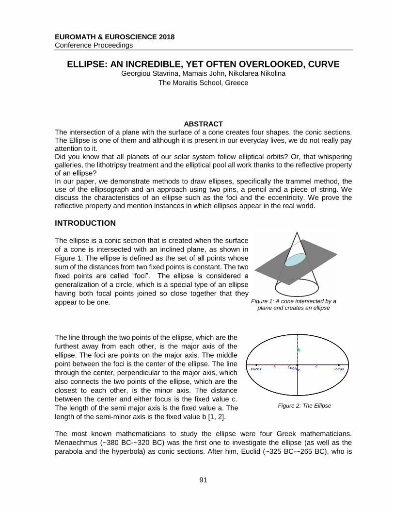
EUROMATH & EUROSCIENCE 2018 Conference Proceedings
91
ELLIPSE: AN INCREDIBLE, YET OFTEN OVERLOOKED, CURVE Georgiou Stavrina, Mamais John, Nikolarea Nikolina
The Moraitis School, Greece
ABSTRACT The intersection of a plane with the surface of a cone creates four shapes, the conic sections. The Ellipse is one of them and although it is present in our everyday lives, we do not really pay attention to it. Did you know that all planets of our solar system follow elliptical orbits? Or, that whispering galleries, the lithotripsy treatment and the elliptical pool all work thanks to the reflective property of an ellipse? In our paper, we demonstrate methods to draw ellipses, specifically the trammel method, the use of the ellipsograph and an approach using two pins, a pencil and a piece of string. We discuss the characteristics of an ellipse such as the foci and the eccentricity. We prove the reflective property and mention instances in which ellipses appear in the real world.
INTRODUCTION
The ellipse is a conic section that is created when the surface
of a cone is intersected with an inclined plane, as shown in
Figure 1. The ellipse is defined as the set of all points whose
sum of the distances from two fixed points is constant. The two
fixed points are called “foci”. The ellipse is considered a
generalization of a circle, which is a special type of an ellipse
having both focal points joined so close together that they
appear to be one.
The line through the two points of the ellipse, which are the
furthest away from each other, is the major axis of the
ellipse. The foci are points on the major axis. The middle
point between the foci is the center of the ellipse. The line
through the center, perpendicular to the major axis, which
also connects the two points of the ellipse, which are the
closest to each other, is the minor axis. The distance
between the center and either focus is the fixed value c.
The length of the semi major axis is the fixed value a. The
length of the semi-minor axis is the fixed value b [1, 2].
The most known mathematicians to study the ellipse were four Greek mathematicians.
Menaechmus (~380 BC-~320 BC) was the first one to investigate the ellipse (as well as the
parabola and the hyperbola) as conic sections. After him, Euclid (~325 BC-~265 BC), who is
Figure 1: A cone intersected by a plane and creates an ellipse
Figure 2: The Ellipse
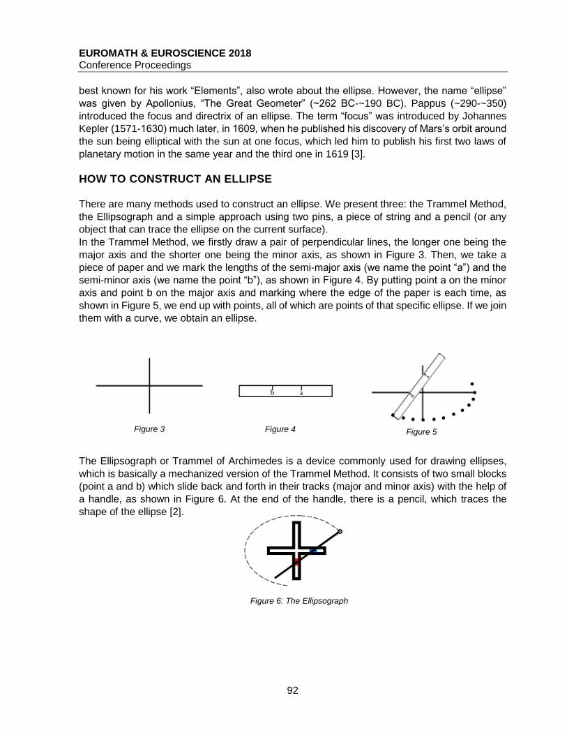
EUROMATH & EUROSCIENCE 2018 Conference Proceedings
92
best known for his work “Elements”, also wrote about the ellipse. However, the name “ellipse”
was given by Apollonius, “The Great Geometer” (~262 BC-~190 BC). Pappus (~290-~350)
introduced the focus and directrix of an ellipse. The term “focus” was introduced by Johannes
Kepler (1571-1630) much later, in 1609, when he published his discovery of Mars’s orbit around
the sun being elliptical with the sun at one focus, which led him to publish his first two laws of
planetary motion in the same year and the third one in 1619 [3].
HOW TO CONSTRUCT AN ELLIPSE There are many methods used to construct an ellipse. We present three: the Trammel Method,
the Ellipsograph and a simple approach using two pins, a piece of string and a pencil (or any
object that can trace the ellipse on the current surface).
In the Trammel Method, we firstly draw a pair of perpendicular lines, the longer one being the
major axis and the shorter one being the minor axis, as shown in Figure 3. Then, we take a
piece of paper and we mark the lengths of the semi-major axis (we name the point “a”) and the
semi-minor axis (we name the point “b”), as shown in Figure 4. By putting point a on the minor
axis and point b on the major axis and marking where the edge of the paper is each time, as
shown in Figure 5, we end up with points, all of which are points of that specific ellipse. If we join
them with a curve, we obtain an ellipse.
The Ellipsograph or Trammel of Archimedes is a device commonly used for drawing ellipses,
which is basically a mechanized version of the Trammel Method. It consists of two small blocks
(point a and b) which slide back and forth in their tracks (major and minor axis) with the help of
a handle, as shown in Figure 6. At the end of the handle, there is a pencil, which traces the
shape of the ellipse [2].
Figure 4 Figure 3 Figure 5
Figure 6: The Ellipsograph

EUROMATH & EUROSCIENCE 2018 Conference Proceedings
93
Lastly, there is a very easy way to construct an ellipse, which requires only two pins, a piece of string and a pencil. We push the two pins in a surface and tie a piece of string around each one, long enough to be able to go around them. Using the pencil, we stretch the string the furthest it allows us and by dragging it, it traces an ellipse, as shown in Figure 7 [2].
THE EQUATION OF THE ELLIPSE In order to obtain the equation of the ellipse, we need the
distances between a random point M(x, y) and each of the foci:
𝑀𝐹 = √(𝑥 − 𝑐)2 + 𝑦2 (1) and
𝑀𝐹′ = √(𝑥 − (−𝑐))2 + 𝑦2 = √(𝑥 + 𝑐)2 + 𝑦2 (2)
the sum of which, by definition, is equal to 2a:
𝑀𝐹 +𝑀𝐹 ′ = 2𝑎 (3)
Equations (1), (2) and (3) yield
√(𝑥 + 𝑐)2 + 𝑦2 +√(𝑥 − 𝑐)2 + 𝑦2 = 2𝑎
After squaring both sides, doing some basic mathematical
operations and also replacing 𝑎2 − 𝑐2 with 𝑏2 (since the relation that connects a, b and c is 𝑎2 =
𝑏2 + 𝑐2), we obtain the equation of the ellipse:
𝑥2
𝑎2+𝑦2
𝑏2= 1
ECCENTRICITY The shape of an ellipse (how "elongated" it is) is represented by its eccentricity, which can be
any real number from 0 (the limiting case of a circle) to arbitrarily close to, but less than, 1. The
eccentricity is denoted by the letter “e” and is defined by the ratio:
𝑒 =𝑐
𝑎
where c is the distance from the center to the focus of the ellipse and a is the length of the semi-
major axis. Due to the fact that 𝑐 = √𝑎2 − 𝑏2 ,
𝑒 =√𝑎2−𝑏2
𝑎 𝑒2 =
𝑎2−𝑏2
𝑎2= 1 − (
𝑏
𝑎)2
𝑏
𝑎= √1 − e2
We observe that the greater the eccentricity is, the smaller the ratio b/a becomes, which makes
the ellipse more elongated. This happens because for the ratio b/a to become smaller, either b
gets smaller or a gets greater (or both). If b gets smaller the ellipse loses width and if a gets
greater the ellipse gains length, which both result in the elongation of the ellipse.
Figure 7: A simpler way to construct an ellipse
Figure 8: A random point M(x, y) of an ellipse and its distances from the foci.
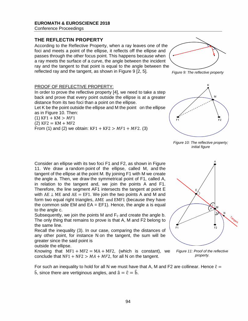
EUROMATH & EUROSCIENCE 2018 Conference Proceedings
94
THE REFLECTIN PROPERTY According to the Reflective Property, when a ray leaves one of the foci and meets a point of the ellipse, it reflects off the ellipse and passes through the other focus point. This happens because when a ray meets the surface of a curve, the angle between the incident ray and the tangent to that point is equal to the angle between the reflected ray and the tangent, as shown in Figure 9 [2, 5].
PROOF OF REFLECTIVE PROPERTY:
In order to prove the reflective property [4], we need to take a step back and prove that every point outside the ellipse is at a greater distance from its two foci than a point on the ellipse. Let K be the point outside the ellipse and M the point on the ellipse as in Figure 10. Then: (1) KF1 + KM > 𝑀𝐹1
(2) KF2 = KM+MF2 From (1) and (2) we obtain: KF1 + KF2 > 𝑀𝐹1 +𝑀𝐹2. (3)
Consider an ellipse with its two foci F1 and F2, as shown in Figure 11. We draw a random point of the ellipse, called M, and the
tangent of the ellipse at the point M. By joining F1 with M we create the angle a. Then, we draw the symmetrical point of F1, called A,
in relation to the tangent and, we join the points A and F1. Therefore, the line segment AF1 intersects the tangent at point E with AE ⊥ ME and AE = EF1. We join the two points A and M and
form two equal right triangles, AME and EMF1 (because they have the common side EM and EA = EF1). Hence, the angle a is equal to the angle c. Subsequently, we join the points M and F2 and create the angle b. The only thing that remains to prove is that A, M and F2 belong to the same line. Recall the inequality (3). In our case, comparing the distances of any other point, for instance N on the tangent, the sum will be
greater since the said point is outside the ellipse. Knowing that MF1 +MF2 = MA +MF2, (which is constant), we
conclude that NF1 + NF2 > 𝑀𝐴 +𝑀𝐹2, for all N on the tangent. For such an inequality to hold for all N we must have that A, M and F2 are collinear. Hence c =
b, since there are vertiginous angles, and a = c = b.
Figure 9: The reflective property
Figure 10: The reflective property; initial figure
Figure 11: Proof of the reflective property.

EUROMATH & EUROSCIENCE 2018 Conference Proceedings
95
APPLICATION OF THE ELLIPSE: WHISPERING GALLERY A whispering gallery is a construction based on the reflective property of the ellipse and on
elliptical reflectors. The sound waves from someone who whispers at a focus point travel directly
to the other focus point and what is said can be heard clearly by someone standing at that point
but by nobody else. This happens because of the reflective property of the ellipse.
There exist several constructions that are examples of whispering galleries such as the
National Statuary Hall in Washington D.C., St. Paul's Cathedral in London and Gol Gumbaz
Mausoleum in Bijapur, India. [5]
APPLICATIONS OF THE ELLIPSE: LITHOTRIPSY Lithotripsy is a medical procedure used to destroy kidney stones. The patient lies in a lithotripter
machine of an ellipsoid shape, which can be considered as a three-dimensional generalization
of an ellipse. The kidney stone, inside the patient’s body, is positioned at one focus. In order to
achieve positioning of the kidney stone at a focus, doctors use a fluoroscopic x-ray system to
detect the position of the kidney stone. Shockwaves, which originate from the other focus, meet
a point of the ellipsoid and are reflected and therefore are concentrated on the kidney stone.
This way, the kidney stone breaks into little pieces which are able to pass through the patient’s
body without causing any pain [6].
Figure 12: How Whispering Galleries work
Figure 13: St. Paul’s Cathedral, London
Figure 14: How lithotripsy works
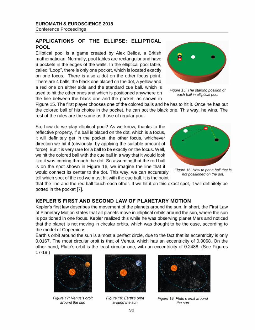
EUROMATH & EUROSCIENCE 2018 Conference Proceedings
96
APPLICATIONS OF THE ELLIPSE: ELLIPTICAL
POOL Elliptical pool is a game created by Alex Bellos, a British
mathematician. Normally, pool tables are rectangular and have
6 pockets in the edges of the walls. In the elliptical pool table,
called “Loop”, there is only one pocket, which is located exactly
on one focus. There is also a dot on the other focus point.
There are 4 balls, the black one placed on the dot, a yellow and
a red one on either side and the standard cue ball, which is
used to hit the other ones and which is positioned anywhere on
the line between the black one and the pocket, as shown in
Figure 15. The first player chooses one of the colored balls and he has to hit it. Once he has put
the colored ball of his choice in the pocket, he can pot the black one. This way, he wins. The
rest of the rules are the same as those of regular pool.
So, how do we play elliptical pool? As we know, thanks to the
reflective property, if a ball is placed on the dot, which is a focus,
it will definitely get in the pocket, the other focus, whichever
direction we hit it (obviously by applying the suitable amount of
force). But it is very rare for a ball to be exactly on the focus. Well,
we hit the colored ball with the cue ball in a way that it would look
like it was coming through the dot. So assuming that the red ball
is on the spot shown in Figure 16, we imagine the line that it
would connect its center to the dot. This way, we can accurately
tell which spot of the red we must hit with the cue ball. It is the point
that the line and the red ball touch each other. If we hit it on this exact spot, it will definitely be
potted in the pocket [7].
KEPLER’S FIRST AND SECOND LAW OF PLANETARY MOTION Kepler’s first law describes the movement of the planets around the sun. In short, the First Law
of Planetary Motion states that all planets move in elliptical orbits around the sun, where the sun
is positioned in one focus. Kepler realized this while he was observing planet Mars and noticed
that the planet is not moving in circular orbits, which was thought to be the case, according to
the model of Copernicus.
Earth’s orbit around the sun is almost a perfect circle, due to the fact that its eccentricity is only
0.0167. The most circular orbit is that of Venus, which has an eccentricity of 0.0068. On the
other hand, Pluto’s orbit is the least circular one, with an eccentricity of 0.2488. (See Figures
17-19.)
Figure 15: The starting position of each ball in elliptical pool
Figure 16: How to pot a ball that is not positioned on the dot.
Figure 17: Venus’s orbit around the sun
Figure 18: Earth’s orbit around the sun
Figure 19: Pluto’s orbit around the sun

EUROMATH & EUROSCIENCE 2018 Conference Proceedings
97
In his Second Law of Planetary Motion, Kepler explains how
planets’ speed is greater when they are closer to the sun than
when they are further away, which results in different distances
being covered in equal time periods. This is well explained in
Figure 20, in which the three green sections cover the same area.
The curved side of each section is a part of the planet’s orbit, which
Kepler realized that the planet travelled in equal times.
Subsequently, while travelling a relatively longer distance, the
velocity of the planet will increase and while travelling a relatively
shorter distance, it will decrease [2, 8].
REFERENCES [1] Strang G (2016) Calculus, Volume 3, MIT
[2] Downs JW (1993) Practical conic sections, Dover, New York
[3] http://www-groups.dcs.st-and.ac.uk/history/Curves/Ellipse.html (Last visit: 05/07/2018)
[4] Mourouzis P (in greek) (Last visit: 05/07/2018)
http://dide.ker.sch.gr/ekfe/epiloges/6_artra/48_newtonkepler.pdf
[5] https://study.com/academy/lesson/reflective-properties-of-ellipses.html (Last visit:
05/07/2018)
[6] http://mathcentral.uregina.ca/beyond/articles/Lithotripsy/lithotripsy1.html (Last visit:
05/07/2018)
[7] http://www.loop-the-game.com/snoop#howtoplay (Last visit: 05/07/2018)
[8] Hasan H (2005) Kepler and the Laws of Planetary Motion, The Rosen Publishing Group
Figure 20: Kepler’s Second Law of Planetary Motion
EUROMATH & EUROSCIENCE 2018 Conference Proceedings
98
P VERSUS NP Authors: Antonis Bourtzinakos, Dimitra Iosifidou, Stefanos Kantaros*, Panagiota Mouteveli,
Evgenia Skagkou, Elena Tziveleki, Georgia Okka, Dimitris Proios
Zanneio Experimental Lyceum of Piraeus, Greece
ABSTRACT In this work we study one of the most famous mathematical problems that is yet unsolved, namely P vs NP. The P vs NP question (one of the six millennium prize problems) regards the difference between the class of problems that can be solved in polynomial time by a deterministic algorithm and the class of problems that can be solved in polynomial time non-deterministically. Are these problems identical in terms of time complexity or not? We present the history behind the problem, explain its importance in various domains (from science to art) and explore the various applications that its solution will provide. We then proceed by giving all the necessary definitions needed to describe the problem in a concrete way, we present some problems from both P and NP, while we also try to catch the essence of the difference of these two classes by also exploring their meaning from a philosophical point of view. Finally, we conclude by studying the reduction proof method, the main mathematical tool used in order to understand in which class each problem belongs.
INTRODUCTION At the current work we examine the problem ‘P vs NP’, which is one of the most famous
mathematical problems that is yet unsolved. This problem has great significance for both
Mathematics and Computer Science and in addition is one of the Millennium Prize Problems.
The Millennium Prize Problems are seven problems that were stated by the Clay Mathematics
Institute in 2000. As their name states, if someone solves one of these problems, he would get
one million dollars as a prize.
The other six problems are:
Poincaré conjecture is solved by Grigori Perelman in 2003. His proof is based on work
by Richard Hamilton; Perelman was selected to receive the Fields medal for his solution
and he was officially awarded the Millennium Prize but he declined both awards.
Hodge conjecture.
Riemann Hypothesis.
Yang – Mills existence and mass gap.
Navier – Stokes existence and smoothness.
Birch and Swinnerton – Dyer conjecture.
The outline of the current paper will be the following: we start by discussing briefly the history of
‘P vs NP’ question and explore why is so important. Then we give the necessary definitions of
EUROMATH & EUROSCIENCE 2018 Conference Proceedings
99
the notions needed to describe it while we also present some problems from both P and NP.
These problems help to capture the essence of the difference between these two classes.
Moreover, we give some philosophical aspects and applications that its solution will provide.
Finally we present the reduction proof method which helps us to understand in which class each
problem belongs and we finish by presenting the conclusions.
WHAT EXACTLY IS THE ‘P VS NP’ PROBLEM? The P versus NP problem asks whether every problem whose solution can be quickly verified
(technically, verified in polynomial time, see definitions below) can also be solved quickly (again,
in polynomial time). This simple question is a major problem which remains unsolved until today.
The informal term quickly, used above, means the existence of an algorithm solving the task
that runs in polynomial time (P), such that the time to complete the task varies as a polynomial
function on the size of the input to the algorithm (as opposed to polynomial time (NP), say,
exponential time). For some questions, there is no known way to find an answer quickly, but if
one is provided, with information showing what the answer is, it is possible to verify the answer
quickly.
So the question is: Is P = NP or P ≠ NP?
An answer to the P vs NP question would determine whether problems that can be verified in
polynomial time can also be solved in polynomial time or not. If it turned out that P ≠ NP, it would
mean that there are problems in NP that are harder to compute than to verify: they could not be
solved in polynomial time, but the answer could be verified in polynomial time.
A BRIEF HISTORY ABOUT THE ‘P VS NP’ PROBLEM Although the P versus NP problem was formally defined in 1971 by Stephen Cook in his seminal
paper "The complexity of theorem proving procedures", there were previous inklings of the
problems involved, the difficulty of proof, and the potential consequences. In 1955,
mathematician John Nash wrote a letter to the NSA (National Security Agency), where he
speculated that cracking a sufficiently complex code would require time exponential in the length
of the key. If proved (and Nash was suitably skeptical) this would imply what we today would
call P ≠ NP, since a proposed key can easily be verified in polynomial time. Another mention of
the underlying problem occurred in a 1956 letter written by Kurt Gӧdel to John von Neumann.
Gödel asked whether theorem-proving (now known to be co-NP-complete) could be solved in
polynomial time, and pointed out one of the most important consequences—that if so, then the
discovery of mathematical proofs could be automated.
P PROBLEMS: DEFINITIONS AND EXAMPLES Firstly, we examine what is the meaning of P problems and we give an example.
P problems:
P stands for Polynomial and its meaning is that it is a set that contains the problems that can be
solved in polynomial time by a deterministic(?) procedure.
Most of the times we call this procedure an algorithm. In general, we use P in order to describe
easy problems.
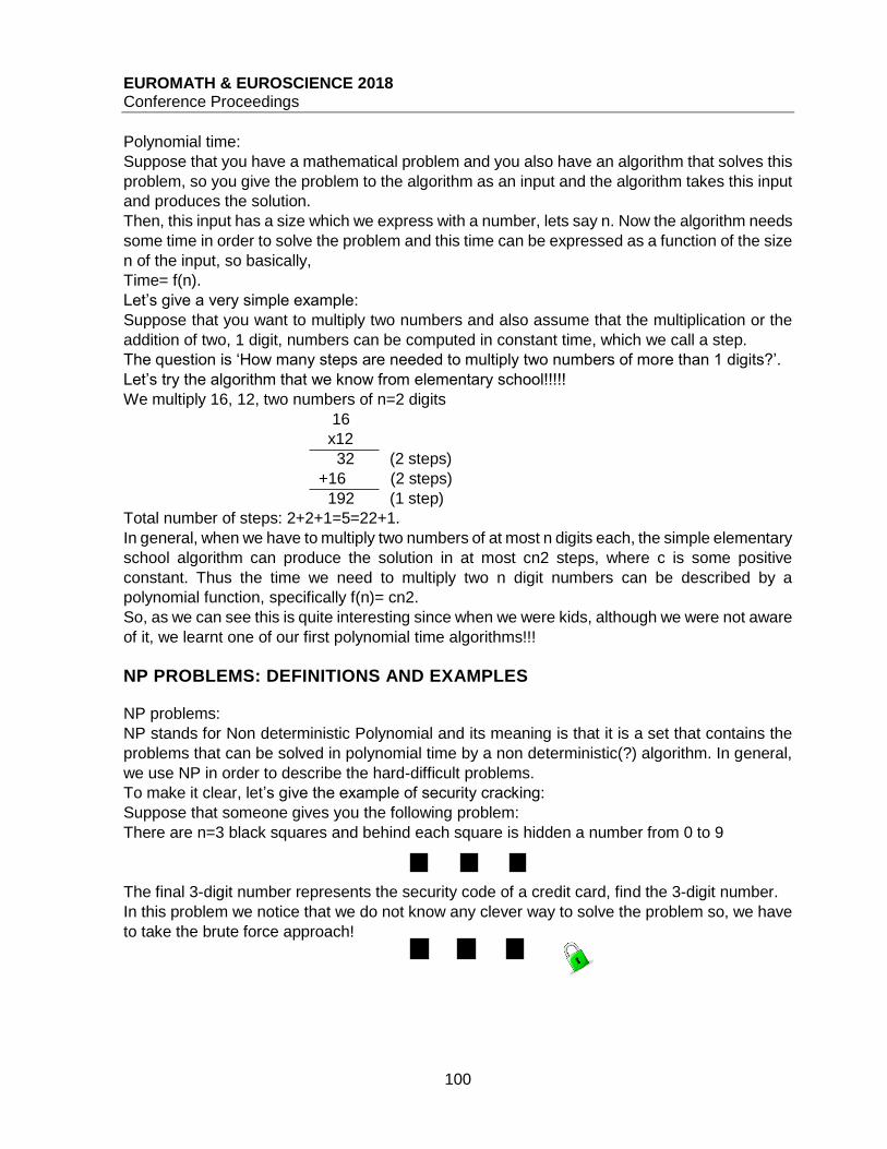
EUROMATH & EUROSCIENCE 2018 Conference Proceedings
100
Polynomial time:
Suppose that you have a mathematical problem and you also have an algorithm that solves this
problem, so you give the problem to the algorithm as an input and the algorithm takes this input
and produces the solution.
Then, this input has a size which we express with a number, lets say n. Now the algorithm needs
some time in order to solve the problem and this time can be expressed as a function of the size
n of the input, so basically,
Time= f(n).
Let’s give a very simple example:
Suppose that you want to multiply two numbers and also assume that the multiplication or the
addition of two, 1 digit, numbers can be computed in constant time, which we call a step.
The question is ‘How many steps are needed to multiply two numbers of more than 1 digits?’.
Let’s try the algorithm that we know from elementary school!!!!!
We multiply 16, 12, two numbers of n=2 digits
16
x12
32 (2 steps)
+16 (2 steps)
192 (1 step)
Total number of steps: 2+2+1=5=22+1.
In general, when we have to multiply two numbers of at most n digits each, the simple elementary
school algorithm can produce the solution in at most cn2 steps, where c is some positive
constant. Thus the time we need to multiply two n digit numbers can be described by a
polynomial function, specifically f(n)= cn2.
So, as we can see this is quite interesting since when we were kids, although we were not aware
of it, we learnt one of our first polynomial time algorithms!!!
NP PROBLEMS: DEFINITIONS AND EXAMPLES NP problems:
NP stands for Non deterministic Polynomial and its meaning is that it is a set that contains the
problems that can be solved in polynomial time by a non deterministic(?) algorithm. In general,
we use NP in order to describe the hard-difficult problems.
To make it clear, let’s give the example of security cracking:
Suppose that someone gives you the following problem:
There are n=3 black squares and behind each square is hidden a number from 0 to 9
The final 3-digit number represents the security code of a credit card, find the 3-digit number.
In this problem we notice that we do not know any clever way to solve the problem so, we have
to take the brute force approach!
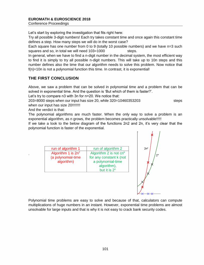
EUROMATH & EUROSCIENCE 2018 Conference Proceedings
101
Let’s start by exploring the investigation that fits right here:
Try all possible 3-digit numbers! Each try takes constant time and once again this constant time
defines a step. How many steps we will do in the worst case?
Each square has one number from 0 to 9 (totally 10 possible numbers) and we have n=3 such
squares and so, in total we will need 103=1000 steps.
In general, when we have to find a n-digit number in the decimal system, the most efficient way
to find it is simply to try all possible n-digit numbers. This will take up to 10n steps and this
number defines also the time that our algorithm needs to solve this problem. Now notice that
f(n)=10n is not a polynomial function this time. In contrast, it is exponential!
THE FIRST CONCLUSION Above, we saw a problem that can be solved in polynomial time and a problem that can be
solved in exponential time. And the question is ‘But which of them is faster?’.
Let’s try to compare n3 with 3n for n=20. We notice that:
203=8000 steps when our input has size 20, while 320=10460353203 steps
when our input has size 20!!!!!!!!
And the verdict is that:
The polynomial algorithms are much faster. When the only way to solve a problem is an
exponential algorithm, as n grows, the problem becomes practically unsolvable!!!!!
If we take a look to the below diagram of the functions 2n2 and 2n, it’s very clear that the
polynomial function is faster of the exponential.
. Polynomial time problems are easy to solve and because of that, calculators can compute
multiplications of huge numbers in an instant. However, exponential time problems are almost
unsolvable for large inputs and that is why it is not easy to crack bank security codes.
run of algorithm 1 run of algorithm 2
Algorithm 1 is 2n2
(a polynomial-time algorithm)
Algorithm 2 is not cnk for any constant k (not
a polynomial-time algorithm), but it is 2n

EUROMATH & EUROSCIENCE 2018 Conference Proceedings
102
DETERMINISM – NON DETERMINISM DEFINITIONS AND THE DIFFERENCE We saw how we define the ‘time’ a problem needs to be solved and we also saw what polynomial
time means, as well as what is the difference with other classes of functions, like exponential.
But what about determinism and what is the difference with the non determinism?
Let’s start with determinism. The easiest way to think of this notion is to imagine how a human
being approaches a problem or a situation. You usually make one step at a time. These steps
follow a serial pattern. You are restricted by nature limitations.
For instance, Luffy wants to go to a certain destination, but does not know which route to take.
As a result, he has to try each and every one of them in order to find the right one.
On the other hand, in a non deterministic universe you can forget about human beings and
their limitations, you have the powers of a god. You can make multiple steps at a time and these
steps can be done in parallel.
So let’s return to the previous example and let Luffy once again search for the right route. This
time he has the power to go to the destinations at once. This way, he can find the solution in an
instant.
So, the difference between determinism and non determinism is that:
In a deterministic universe, given a problem you have to produce the solution and this might
take some time. In contrast, in a non deterministic universe, given a problem you once again
have to produce the solution, however this time you can produce it in an instant and you only
need to verify if it is correct.
THE SECOND CONCLUSION If we return to security cracking we notice that the best deterministic algorithm that we have, as
we saw,
takes exponential time and this will take up to 10n steps.
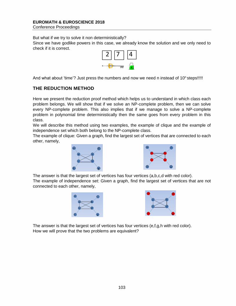
EUROMATH & EUROSCIENCE 2018 Conference Proceedings
103
But what if we try to solve it non deterministically?
Since we have godlike powers in this case, we already know the solution and we only need to
check if it is correct.
And what about ‘time’? Just press the numbers and now we need n instead of 10n steps!!!!!
THE REDUCTION METHOD Here we present the reduction proof method which helps us to understand in which class each
problem belongs. We will show that if we solve an NP-complete problem, then we can solve
every NP-complete problem. This also implies that if we manage to solve a NP-complete
problem in polynomial time deterministically then the same goes from every problem in this
class.
We will describe this method using two examples, the example of clique and the example of
independence set which both belong to the NP-complete class.
The example of clique: Given a graph, find the largest set of vertices that are connected to each
other, namely,
The answer is that the largest set of vertices has four vertices (a,b,c,d with red color).
The example of independence set: Given a graph, find the largest set of vertices that are not
connected to each other, namely,
The answer is that the largest set of vertices has four vertices (e,f,g,h with red color).
How we will prove that the two problems are equivalent?
2 4 7

EUROMATH & EUROSCIENCE 2018 Conference Proceedings
104
We start from one problem and go to the other. Suppose we have an algorithm that solves the
clique. Then the algorithm solves the problem in each graph, thus it also solves it both in ours
and in its complementary, where complementary is called the graph that does not have the
edges of the original but has those that did not exist in the original.
We solve the clique problem in the complementary graph then this solution is a set of
independence in the original graph !!!
What exactly happened?
Each set of vertices which are connected to each other in the complementary graph, due to its
definition, are not connected to the original graph. The maximum complementary of clique is
always the maximum set of independence in the original!!! By doing this conversion, each time
we can solve one problem then we can solve the other. And so, the two problems are equivalent
!!!
A QUESTION AND AN ANSWER To sum up, we have that:
P: The set of problems that we can produce the solution in polynomial time.
NP: The set of problems that if we could produce the solution in an instant (or if we basically
knew the solution), we could check if it is correct in polynomial time.
But there is one more question which is very important:
What is more difficult?
To produce the solution of a problem in polynomial time or to check in polynomial time if the
solution is correct (given that we already know it)?
Let’s rephrase the question for being a bit informal.
Question: Do we really have limitations and some problems can not be solved fast enough or
we can solve even the problems that we believe that are unsolvable in terms of time?
Are we really restricted by our human nature or we can actually achieve a state far beyond that?
A state where no limitations exist, a state where no matter what we face, there is no real
challenge?
Answer: We do not know…Although we compare humans with something much more powerful,
although most of the mathematicians believe that P and NP are not equal, we can not prove it.

EUROMATH & EUROSCIENCE 2018 Conference Proceedings
105
THE EFFECTS OF THE ‘P VS NP’ ON ART Aside from being an important problem in mathematics and computer science, a proof either
way would have profound implications for mathematics, cryptography, algorithm research,
artificial intelligence, game theory, multimedia processing, philosophy, ecomics and many other
fields.
‘P vs NP’ problem has influenced many fields of art.
One famous problem which belongs in the class of NP problems is the travelling salesman
problem (TSP). TSP asks the following question: "Given a list of cities and the distances
between each pair of cities, what is the shortest possible route that visits each city and returns
to the origin city?" . This problem has influenced the art of design, cinema and literature.
In "TSP art" an image's tonal quality is reproduced with a single, continuous path. This single
path meanders over the entire canvas.
The thriller novel The Steradian Trail by M. N. Krish weaves the traveling salesman problem and
mathematician Srinivasa Ramanujan and his accidental discovery into its plot connecting
religion, mathematics, finance and economics.
The film Travelling Salesman, by director Timothy Lanzone, is the story of four mathematicians
hired by the US government to solve the P versus NP problem.
In the sixth episode of The Simpson’s seventh season ‘Treehouse of Horror VI’, the
equation P=NP is seen shortly after Homer accidentally stumbles into the "third dimension".
P=NP
In the second episode of season 2 of Elementary, ‘Solve for X’ revolves around Sherlock and
Watson investigating the murders of mathematicians who were attempting to solve P versus NP.
CONCLUSION AND A PHILOSOPHICAL ASPECT As we saw, there is no answer in the question ‘is P and NP problems identical?’.
However, most scientist believe that these sets are not identical. But there is another question
which is important:
‘what P=NP would mean if that was the case?’
The American Theoretical computer scientist Scott Aaronson has wrote:
‘The world would be a profoundly different place than we usually assume it to be. There would
be no special value in ‘creative leaps’, no fundamental gap between solving a problem and

EUROMATH & EUROSCIENCE 2018 Conference Proceedings
106
recognizing the solution once it’s found. Everyone who could appreciate a symphony would be
Motzart; Everyone who could follow step by step an argument would be Gauss.’
Frédéric Chopin once said the following which could be an answer to the above question :
‘Simplicity is the final achievement. After one has played a vast quantity of notes and more
notes, it is simplicity that emerges as the crowning reward of art’.
Similarly, Jack Kerouac has said:
’One day I will find the right words, and they will be simple’.
AKNOWLEDGMENTS We would like to thank our supervisor Dr. Sophia Birmpa – Pappa for her help and support
during the preparation of this work and, also, our classmates and members of Zanneio Club of
Mathematics ‘Maths in Reality’ for their ideas.
REFERENCES 1. Lecture notes on Algorithms. Georgios Birmpas, Athens University of Economics and
Business 2. https://web.cs.hacettepe.edu.tr/~aykut/classes/spring2017/bbm202/ 3. https://wiki.evilmadscientist.com/TSP_art 4. https://www.youtube.com/watch?v=YX40hbAHx3s 5. Algorithms. Sanjoy Dasgupta, Christos Papadimitriou, Umesh Vazirani, McGraw Hill,
Boston (2007) 6. Wikipedia.

EUROMATH & EUROSCIENCE 2018 Conference Proceedings
107
MATHEMATICAL FALLACIES Christia Kai, Vasiliki Kalimera, Georgia Tzyrka, Savvas-Odysseas Makariou
The English School Nicosia, Cyprus
ABSTRACT As Galileo Galilei said, the universe cannot be read until we have learned its language and become familiar with the characters in which it is written. This is the Mathematical Language! This ‘language’ is indeed Mathematical Language and And the ‘letters’ are the infinite numbers, curves and other geometrical figures. It is Mathematics that directs the flow of the universe, a precise model of real phenomena and an explanation to common fallacies, we, as human beings have. Imagine that you are watching the end of a long action movie. The hero and villain are in a mad chase over a city skyline to deactivate and trigger a nuclear bomb respectively. The villain throws himself down on a curved building and the hero throws himself into the air and hits a lower part of the curve with the intent to slide to the bottom faster. Both however, take the same time to reach the end of the curve. How, and why is that? Well, this is due to the Tautochrone curve theorem, proved by Huygens back in the 17th century. Yet as far as the laws of this ingenious language refer to reality, in fact its numerical letters are not certain, and as far as they are certain, they do not refer to reality. We tend to look at all numbers as fixed finite figures,
without questioning why. Why is it that we take 0.9 to be 1, or why 1 may be equal to 2? Well, all this can be proved!
INTRODUCTION
In this report, we investigate various everyday situations that we have mistakenly believed to
have fully understood. We will in fact examine a number of ideas that a lot of people think to be
true, but which are in fact false. In trying to do this, we need to consider that to understand the
universe and question things in it we must, as Galileo Galilei said, understand its language, the
mathematical language.
You see, maths is all about uncertainty and reality, proving why ideas might be ‘invalid’ and the
hidden truth behind what we think is correct. FALLACIES. For example, we delve into a situation
where various similar-surfaced objects are projected from different parts of a cycloid curve and
calculate as well as compare the time taken for each one to reach the minimum point of the
curve. Furthermore, we look into how arguments about numerical theories come about and
counter argued, backed with mathematical proofs. Specifically, we examine whether 1 can be
considered equal to 2, or whether it is valid to say that 1 is equal to 0.9 recurring.
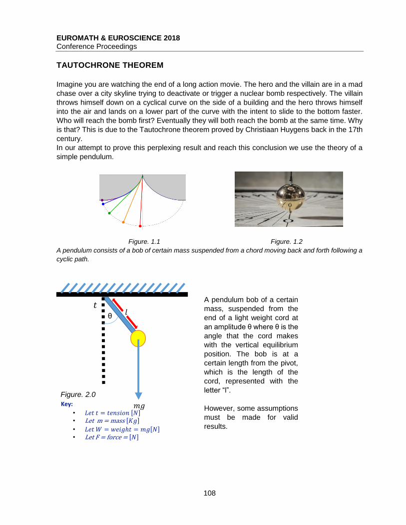
EUROMATH & EUROSCIENCE 2018 Conference Proceedings
108
TAUTOCHRONE THEOREM
Imagine you are watching the end of a long action movie. The hero and the villain are in a mad
chase over a city skyline trying to deactivate or trigger a nuclear bomb respectively. The villain
throws himself down on a cyclical curve on the side of a building and the hero throws himself
into the air and lands on a lower part of the curve with the intent to slide to the bottom faster.
Who will reach the bomb first? Eventually they will both reach the bomb at the same time. Why
is that? This is due to the Tautochrone theorem proved by Christiaan Huygens back in the 17th
century.
In our attempt to prove this perplexing result and reach this conclusion we use the theory of a
simple pendulum.
Figure. 1.1 Figure. 1.2
A pendulum consists of a bob of certain mass suspended from a chord moving back and forth following a
cyclic path.
𝑚𝑔
𝑡 θ
𝑙
Key:
• 𝐿𝑒𝑡 𝑡 = 𝑡𝑒𝑛𝑠𝑖𝑜𝑛 [𝑁] • Let m = mass [𝐾𝑔] • 𝐿𝑒𝑡 𝑊 = 𝑤𝑒𝑖𝑔ℎ𝑡 = 𝑚𝑔[𝑁] • Let F = force = [𝑁]
A pendulum bob of a certain
mass, suspended from the
end of a light weight cord at
an amplitude θ where θ is the
angle that the cord makes
with the vertical equilibrium
position. The bob is at a
certain length from the pivot,
which is the length of the
cord, represented with the
letter “l”.
However, some assumptions
must be made for valid
results.
Figure. 2.0
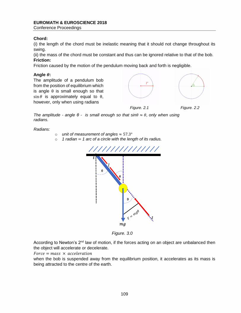
EUROMATH & EUROSCIENCE 2018 Conference Proceedings
109
Figure. 2.1 Figure. 2.2
Chord:
(i) the length of the chord must be inelastic meaning that it should not change throughout its
swing.
(ii) the mass of the chord must be constant and thus can be ignored relative to that of the bob.
Friction:
Friction caused by the motion of the pendulum moving back and forth is negligible.
According to Newton’s 2nd law of motion, if the forces acting on an object are unbalanced then
the object will accelerate or decelerate.
𝐹𝑜𝑟𝑐𝑒 = 𝑚𝑎𝑠𝑠 × 𝑎𝑐𝑐𝑒𝑙𝑒𝑟𝑎𝑡𝑖𝑜𝑛
when the bob is suspended away from the equilibrium position, it accelerates as its mass is
being attracted to the centre of the earth.
Angle 𝜽:
The amplitude of a pendulum bob
from the position of equilibrium which
is angle θ is small enough so that
sin𝜃 is approximately equal to θ,
however, only when using radians
The amplitude - angle θ - is small enough so that sin𝜃 ≈ 𝜃, only when using radians. Radians:
o unit of measurement of angles ≈ 57.3° o 1 radian = 1 arc of a circle with the length of its radius.
Figure. 3.0
EUROMATH & EUROSCIENCE 2018 Conference Proceedings
110
In this way, the downward force (the weight) is the only force acting on the bob when it is hanging
freely, assuming however that the friction created by the bob moving is negligible. Therefore,
acceleration is equal to the gravitational field strength on every planet we are on. Thus, we get
𝑎 = 𝑔. As a result, we deduce that the downward force is equal 𝑚𝑔.
However, what causes the pendulum bob to swing is the force which is perpendicular to the
tension. (Note that the tension is parallel to the cord).
To calculate the force, we use trigonometry as a right-angle triangle is formed between the 𝑚𝑔,
the tension and the perpendicular force to be calculated. So, we can use the angle between 𝑚𝑔
and tension which is corresponding to the angle 𝜃 and create the equation
𝑠𝑖𝑛𝜃 =𝑝𝑒𝑟𝑝𝑒𝑛𝑑𝑖𝑐𝑢𝑙𝑎𝑟 𝑓𝑜𝑟𝑐𝑒
𝑚𝑔
then we rearrange the equation and we get that
𝐹𝑜𝑟𝑐𝑒 = 𝑚𝑔𝑠𝑖𝑛𝜃
which by using our initial assumption that 𝑠𝑖𝑛𝜃 ≈ 𝜃, can be expressed as
𝐹𝑜𝑟𝑐𝑒 = 𝑚𝑔𝜃
However, as discovered previously, 𝐹𝑜𝑟𝑐𝑒 = 𝑚𝑔𝜃, therefore substituting this equation into the
Newton’s equation above we get that
𝑎 =𝑚𝑔𝜃
𝑚
The masses are cancelled out ∴ 𝑎 = 𝑔𝜃
We know that 𝑔𝜃 = −𝑤2𝑦, where 𝑦 is the displacement from the equilibrium position and 𝑤 is
the angular velocity. Hence, now we can express 𝜃 in terms of 𝑙 𝑎𝑛𝑑 𝑦. 𝑦 forms a horizontal
perpendicular line from the pendulum bob to the vertical equilibrium line. Thus, again using
trigonometry 𝑛𝜃 =𝑦
𝑙 , and according to the initial assumption that 𝑠𝑖𝑛𝜃 ≈ 𝜃, 𝜃 =
𝑦
𝑙.
Back to the equation that 𝑔𝜃 = −𝑤2𝑦, we substitute 𝜃 =𝑦
𝑙 and end up with 𝑔 (
𝑦
𝑙) = −𝑤2𝑦. We
cancel out the minus sign as it only symbolises direction, thus leading to the equation 𝑔 (𝑦
𝑙) =
𝑤2𝑦
We know that 𝜔 =2𝜋
𝑇 where 𝑇 is the time of the pendulum swing, called a period and 𝜔 is the
angular velocity. Squaring both sides, we get
𝜔2 = (2𝜋)2
(𝛵)2 and since 𝜔2 =
𝑔
𝑙 ∴
𝑔
𝑙=
(2𝜋)2
(𝛵)2=
4𝜋2
𝑇2.
Rearranging in terms of T,
𝑇2 =4𝜋2𝑙
𝑔
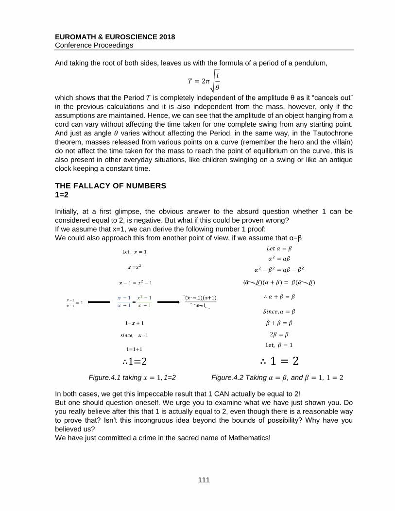
EUROMATH & EUROSCIENCE 2018 Conference Proceedings
111
And taking the root of both sides, leaves us with the formula of a period of a pendulum,
𝑇 = 2𝜋√𝑙
𝑔
which shows that the Period 𝑇 is completely independent of the amplitude θ as it “cancels out”
in the previous calculations and it is also independent from the mass, however, only if the
assumptions are maintained. Hence, we can see that the amplitude of an object hanging from a
cord can vary without affecting the time taken for one complete swing from any starting point.
And just as angle 𝜃 varies without affecting the Period, in the same way, in the Tautochrone
theorem, masses released from various points on a curve (remember the hero and the villain)
do not affect the time taken for the mass to reach the point of equilibrium on the curve, this is
also present in other everyday situations, like children swinging on a swing or like an antique
clock keeping a constant time.
THE FALLACY OF NUMBERS 1=2 Initially, at a first glimpse, the obvious answer to the absurd question whether 1 can be
considered equal to 2, is negative. But what if this could be proven wrong?
If we assume that x=1, we can derive the following number 1 proof:
We could also approach this from another point of view, if we assume that α=β
Figure.4.1 taking 𝑥 = 1, 1=2 Figure.4.2 Taking 𝛼 = 𝛽, and 𝛽 = 1, 1 = 2 In both cases, we get this impeccable result that 1 CAN actually be equal to 2!
But one should question oneself. We urge you to examine what we have just shown you. Do
you really believe after this that 1 is actually equal to 2, even though there is a reasonable way
to prove that? Isn’t this incongruous idea beyond the bounds of possibility? Why have you
believed us?
We have just committed a crime in the sacred name of Mathematics!
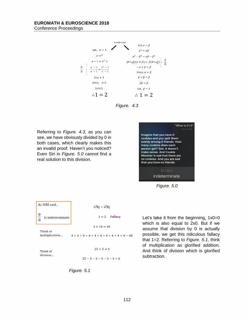
EUROMATH & EUROSCIENCE 2018 Conference Proceedings
112
Figure. 4.3
Let’s take it from the beginning. 1x0=0
which is also equal to 2x0. But if we
assume that division by 0 is actually
possible, we get this ridiculous fallacy
that 1=2. Referring to Figure. 5.1, think
of multiplication as glorified addition.
And think of division which is glorified
subtraction.
Referring to Figure. 4.3, as you can
see, we have obviously divided by 0 in
both cases, which clearly makes this
an invalid proof. Haven’t you noticed?
Even Siri in Figure. 5.0 cannot find a
real solution to this division.
Figure. 5.1
Figure. 5.1
Figure. 5.0

EUROMATH & EUROSCIENCE 2018 Conference Proceedings
113
Figure. 5.2 As a number is being divided by a smaller denominator the answer gets greater and greater.
For instance, 1
1=1 ,
1
0.1=10 and it goes on. Therefore, as the denominator decreases by the factor
of x0.10 and gets closer to 0 the answer increases by the factor of x10. However, since a
denominator can be decreased an infinite number of times in this way and never reach 0, the
answer increases infinitely. Hence, division by 0 is equal to infinity. Taking another number, 2
1
=2, 2
0.1 =20 and it goes on. Thus, it would also be correct to say that division by 0 is equal to
infinity. Since 1
0 is equal to infinity,
2
0 is equal to infinity as well. However, assuming that division
by 0 is actually possible, we get this fallacy that 1=2. Therefore, we say that 1
0 and
2
0 are
undefined.
Figure. 6.0
But what happens when we divide 0? Let’s consider 5
0 . As you can see in Figure. 5.2, it is 5-0-0-0-0-0-0
and it goes on. There is no end to this subtraction.
So, wouldn’t it make sense to say that 5
0 is equal to
infinity?

EUROMATH & EUROSCIENCE 2018 Conference Proceedings
114
Previously, we attempted to go downwards towards 0 leading us to positive infinity. But there is
another way to approach 0, going upwards towards 0, by dividing 1
−1 = -1,
1
−0.1 =-10 and it goes
on, thus leading us to negative infinity.
Figure. 6.1
Figure. 7.0 Graphical representation as interpreted by the reciprocal function 1
𝓍 . On the right
side, we’re going downwards towards 0 approaching positive infinity and on the left side we’re
going upwards towards 0 approaching negative infinity. As you can see 𝑥 cannot be divided by
0. Therefore, both axes are asymptotes to the function, showing us that division by 0 is not
possible.
To conclude, division by 0 is undefined. It cannot be defined or worked out, it is UNDEFINABLE.
There is no number that you can pick which makes sense regarding infinity. Remember, infinity
is not a number, but an idea. Therefore, division by 0 is indeterminate. Therefore 1 is NOT equal
to 2.
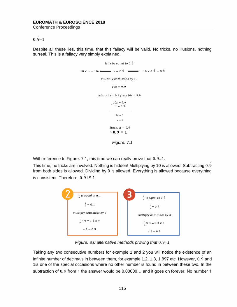
EUROMATH & EUROSCIENCE 2018 Conference Proceedings
115
𝟎. ��=1
Despite all these lies, this time, that this fallacy will be valid. No tricks, no illusions, nothing surreal. This is a fallacy very simply explained.
Figure. 7.1
With reference to Figure. 7.1, this time we can really prove that 0. 9=1.
This time, no tricks are involved. Nothing is hidden! Multiplying by 10 is allowed. Subtracting 0. 9
from both sides is allowed. Dividing by 9 is allowed. Everything is allowed because everything
is consistent. Therefore, 0. 9 IS 1.
Figure. 8.0 alternative methods proving that 0. 9=1 Taking any two consecutive numbers for example 1 and 2 you will notice the existence of an
infinite number of decimals in between them, for example 1.2, 1.3, 1.897 etc. However, 0. 9 and
1is one of the special occasions where no other number is found in between these two. In the
subtraction of 0. 9 from 1 the answer would be 0.00000… and it goes on forever. No number 1
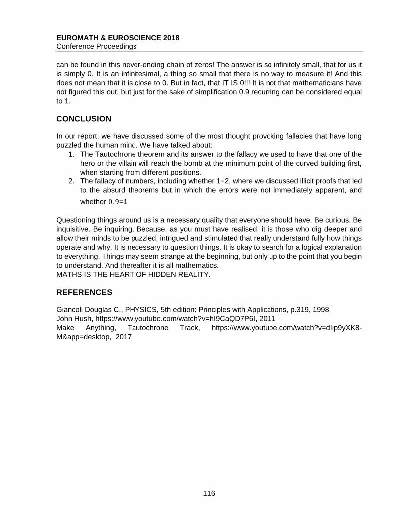
EUROMATH & EUROSCIENCE 2018 Conference Proceedings
116
can be found in this never-ending chain of zeros! The answer is so infinitely small, that for us it
is simply 0. It is an infinitesimal, a thing so small that there is no way to measure it! And this
does not mean that it is close to 0. But in fact, that IT IS 0!!! It is not that mathematicians have
not figured this out, but just for the sake of simplification 0.9 recurring can be considered equal
to 1.
CONCLUSION In our report, we have discussed some of the most thought provoking fallacies that have long
puzzled the human mind. We have talked about:
1. The Tautochrone theorem and its answer to the fallacy we used to have that one of the
hero or the villain will reach the bomb at the minimum point of the curved building first,
when starting from different positions.
2. The fallacy of numbers, including whether 1=2, where we discussed illicit proofs that led
to the absurd theorems but in which the errors were not immediately apparent, and
whether 0. 9=1
Questioning things around us is a necessary quality that everyone should have. Be curious. Be
inquisitive. Be inquiring. Because, as you must have realised, it is those who dig deeper and
allow their minds to be puzzled, intrigued and stimulated that really understand fully how things
operate and why. It is necessary to question things. It is okay to search for a logical explanation
to everything. Things may seem strange at the beginning, but only up to the point that you begin
to understand. And thereafter it is all mathematics.
MATHS IS THE HEART OF HIDDEN REALITY.
REFERENCES
Giancoli Douglas C., PHYSICS, 5th edition: Principles with Applications, p.319, 1998
John Hush, https://www.youtube.com/watch?v=hI9CaQD7P6I, 2011
Make Anything, Tautochrone Track, https://www.youtube.com/watch?v=dIip9yXK8-
M&app=desktop, 2017

EUROMATH & EUROSCIENCE 2018 Conference Proceedings
117
WONDERWOMEN Lilikaki Marianna, Mavragani Christina, Safarika Eleftheria, Zein Christina
Pierce - The American College of Greece, Greece
ABSTRACT Mathematics as a science have existed for a period of approximately 2500 years and throughout this period many people have had a significant effect in their development. Most of us are indeed aware of prominent mathematicians such as Archimedes, Newton, Gauss and others. However, what most of us seem to be unaware of is the fact that very few women mathematicians enjoy similar levels of recognition. This does not mean that Mathematics were shaped into the science we know today by men only, as a large number of women have also added their inputs and ideas and have assisted in the creation of modern day Mathematics. In this paper we have selected four women mathematicians who have contributed greatly to their discipline and we will present their celebrated work as well as their extraordinary lives. Throughout history, many extraordinary women passionate about STEM fields have left their
mark. From mathematician Hypatia of Alexandria in the 4th century B.C. to many other women
in the 21st century, women connected only by their insatiable interest in sciences have fought
against vast cultural obstacles to become an inspiration for us all. We have decided to focus our
research on four of these women who we believe have made a considerable impact in the world
of Mathematics. Emmy Noether, Katherine Johnson, Shafi Goldwasser and Maryam Mirzakhani
are all cases of exceptional women, who, against stereotypes, managed to prove that the power
of the mind is not a matter of sex, and have become an ideal model of genius and willpower,
especially for all of us, who want to pursue a career in science. Despite their achievements
though, we are not sure their names are familiar to most people. It is our hope that through this
presentation their contribution to Mathematics and Science in general will receive more attention
and their accomplishments will inspire more and more young women to follow in their footsteps.
EMMY NOETHER Amalie Emmy Noether was born in Erlangen, Germany, on the 23rd of March 1882. Her family
was Jewish and her father was a mathematician at the University of Erlangen. She attended the
same university as a student where she studied mathematics. Her final grades were high enough
that she was automatically awarded the equivalent of a bachelor’s degree and started working
at the Mathematical Institute of Erlangen. She worked there for almost a decade but was not
paid for her work since women at the time were not allowed to hold academic positions. She
was then invited to the University of Göttingen but objections from members of the existing
faculty forced her to publish papers and give lectures under David Hilbert's name instead. It was
during this period that Einstein published his general theory of relativity (1915). Noether applied

EUROMATH & EUROSCIENCE 2018 Conference Proceedings
118
her work to Einstein's theory and as a result she ended up with what we now acknowledge as
Noether’s theorem. She stayed at the University of Göttingen until 1933 as a prominent
mathematician. A large part of her work and ideas were described in Dutch mathematician B. L.
van der Waerden's “Moderne Algebra” which was published in 1924. In 1933, as the Nazi party
gained power in Germany, Noether along with other university professors were forced to
abandon their positions. She then moved to Pennsylvania in the U.S.A. and took up a position
at Bryn Mawr College. She passed away in 1935, at the age of 53, after she underwent surgery
for an ovarian cyst.
Noether's main areas of focus were non commutative algebra, linear transformations, and
commutative number fields. She is known for laying the foundations of abstract algebra as well
as for her contribution to theoretical physics. She formulated her groundbreaking theorem,
named after her "Noether's theorem", in which she states that every differentiable symmetry of
the action of a physical system has a corresponding conservation law. In layman's words she
said that wherever you find some sort of symmetry in a system you will also find a conservation
of some quantity, for instance of momentum, or of energy or something else. Noether’s theorem
in fact demostrates that a symmetry of time (time translation symmetry) can be linked to the
conservation of energy. In simpler words, Noether’s theorem explains how energy can be neither
created nor destroyed but merely changes form.
Noether also worked on ring theory (1920-1926), which is an area of abstract algebra. Rings are
sets of elements in which addition and multiplication are possible between the elements
contained in these sets, meaning that the resulting element would still belong in the set. Ring
theory, as the name suggests, is the study of rings, meaning the study of the structure of rings
and the properties of rings. However, Noether's contribution to Algebra and specifically to the
commutative ring theory is quite abstract. This makes it hard to pinpoint her exact contribution,
especially to anyone who does not yet possess a decent knowledge of algebra. But it was
through Noether's work, that the connection between rings came to light. This in turn allowed us
to provide answers for problems on all "alike" rings and algebraic structures, effectively solving
a problem only for one of the rings and transferring the result to all alike rings.
Some rings were even named after her, as she was the one who studied them. Noether noted
an attribute in certain types of rings (named "Noetherian Rings" in her honor) that are commonly
studied in many mathematical fields and came up with a definition useful for distinguishing this
specific type of rings. Noetherian rings are important in both commutative and non commutative
ring theory. Nevertheless, trying to document and clarify Noether's contribution to mathematics
remains at large an elusive hope. It is perhaps fitting to say that trying to study abstract algebra
without Noether's input would be similar to trying to study and compare the grammatical
structure of phrases without knowledge of the notions of subject, object, verb and other
fundamental terms or to try to study triangles without knowing trigonometry.
KATHERINE JOHNSON Katherine Johnson is one of the most notable mathematical figures of the 20th century. She has
contributed greatly to the United States aeronautics and space programs and was instrumental
in many of NASA's early projects such as Project Mercury, the Space Shuttle Program and
various Apollo flights. Her main responsibility was calculating the trajectories of space flights but
she also helped in many other areas of the programs as well. Katherine Johnson's contributions

EUROMATH & EUROSCIENCE 2018 Conference Proceedings
119
however, were brought to attention only recently through the release of the movie "Hidden
Figures" in 2016. What makes her achievements even greater is the fact that in order to win the
respect of her colleagues and the scientific community she had to overcome prejudices
concerning both her gender and - more notably - the fact that she is African-American. Katherine
Johnson retained her pride and dignity throughout her professional career and despite the odds
stacked against her. In the end, it was the high quality of her work that made her invaluable to
her team and also made it impossible for people to ignore her because of her skin color. Today
she has received her due accolades and the respect she deserves for her efforts in the
advancement of science.
Katherine Johnson had decided early in her life on becoming a research mathematician even
though this was a difficult field for African Americans and especially for women. Consequently,
after her graduation summa cum laude from college with degrees in Mathematics and French in
1937, Katherine initially worked as a teacher. During this time her aim was to “advance the race”
by not just using book knowledge but also by inspiring discipline and self-respect in her students.
She worked as a teacher until 1952 when she found out, from a relative, that the National
Aeronautics and Space Administration (NASA) was hiring mathematicians. One year later she
was offered a job and she became part of the early NASA team. Katherine spent the rest of her
professional career at NASA and eventually retired from NASA in 1986.
From 1953 to 1958, Johnson worked as a "computer", analyzing topics such as gust alleviation
for aircrafts. In mid-1960s Katherine, along with a colleague of hers, focused on the topic of
computer failure. They formulated possible problems and backup solutions and finally developed
simple navigational methods for the astronauts to use in case they lost contact with ground
control. From 1958 until her retirement in 1986, Katherine worked as an aerospace technologist,
at the Spacecraft Controls Branch. She calculated the trajectory for the May 5, 1961 space flight
of Alan Shepard, the first American in space. When NASA used electronic computers for the
first time in order to calculate John Glenn's orbit around Earth, Glenn refused to fly unless
Katherine verified the calculations. At a later age, Katherine worked directly with digital
computers. Her ability and reputation for accuracy helped to establish confidence in the new
technology.
One of the important problems NASA scientists were faced with when trying to send the first
rocket into space was trying to pinpoint where on the surface of our planet would a spaceship
return after completing its travel. This was necessary both for collecting data from the actual
flight as well as recovering the person or persons manning the spaceship. Katherine Johnson
calculated the trajectory for Alan Shepard, the first American in space. An important aspect of
this problem was determining the angle between the spaceship's trajectory and the earth's
atmosphere at the point of reentry. Too steep and the spaceship would be destroyed by its high
velocity, too shallow and the spaceship would "bounce off" the atmosphere and wander into
space. So the basic question was calculating the exact position over the Earth to fire the
retrorockets in order to land in the center of the ocean recovery zone.
Other aspects of the problem that would have to be taken into account were the earth's rotation
around its axis, the earth's fluctuating gravitational pull on the spaceship, etc. In order then to
solve this problem, one would have to somehow figure out the equation that would describe the
exact trajectory of the spaceship during its flight time. Without any room for trials and with no
room for error this problem was presented to Katherine Johnson and she solved it by working
backwards. Initially she asked her superiors where on the surface of the earth did they want this
EUROMATH & EUROSCIENCE 2018 Conference Proceedings
120
spaceship to land. After she found out the ideal recovery points for the spaceship, she then
worked out the equations that would give her the answer she needed. Her work is described in
detail in "Determination of azimuth angle at burnout for placing a satellite over a selected earth
position", a paper she co-authored with T. H. Skopinski.
In her own words: "The early trajectory was a parabola, and it was easy to predict where it would
be at any point. Early on, when they said they wanted the capsule to come down at a certain
place, they were trying to compute when it should start. I said, 'Let me do it. You tell me when
you want it and where you want it to land, and I'll do it backwards and tell you when to take off.'
That was my forte."
Katherine has since received several awards for her professional accomplishments. In 1999,
Katherine was named West Virginia State College Outstanding Alumnus of the Year. On
November 24, 2015 President Barack Obama presented Katherine with the Presidential Medal
of Freedom; Katherine was one of the 17 Americans who were awarded this metal. In 2016,
Johnson was included in the list of "100 Women", BBC's list of 100 most influential women
worldwide and in the same year NASA named a3,700 m2 building Katherine G. Johnson
Computational Research Facility, thus effectively dedicating it to Katherine.
SHAFI GOLDWASSER
Shafrira (Shafi) Goldwasser is an American-Israeli computer scientist, born in New York City in
1958. Her studies involve mathematics and science at Carnegie Mellon University, and also a
master’s degree and PhD in computer science at the University of California, Berkeley.
Afterwards, she joined MIT and became the first to acquire the RSA Professorship. She also
became a professor at the Weizmann Institute of Science and is a member of the Theory of
Computation group at MIT Computer Science and Artificial Intelligence Laboratory, where she
teaches engineering and computer science. Goldwasser has twice won the Gödel Prize in
theoretical computer science. Amongst other awards, she was awarded the 2012 Turing Award
along with Silvio Micali for their work in the field of cryptography.
As it is widely known, cryptography has been, throughout the course of time, a capital way of
secret communication, influencing even the outcome of wars! Today, however, its role is even
more paramount, since the digital reality in which we live imposes delicate and complex
challenges to cryptography, which require shifting the traditional goals of cryptography, namely
secure and authenticated communication, and move towards systems that are simultaneously
highly efficient, highly secure and highly functional.
Shafi Goldwasser has made fundamental contributions to this kind of cryptography,
computational complexity, computational number theory and probabilistic algorithms. Her
innovative approaches have had an impact on everything within her scientific field, and they
ensure security in many aspects of the digital age. It has been said for her (and her co-worker
Micali): “they created mathematical structures that turned cryptography from an art into a
science”.
More specifically, what Goldwasser is mainly known for is her participation in the development
of Probabilistic Encryption, which won her the Turing award, and is what I am going to present.
But, let’s start from the beginning. The general idea behind encryption schemes is how to find a
way to ensure secure and private communication through an insecure channel, which may or
may not be tapped by an attacker. The information wanted to be communicated is called the
EUROMATH & EUROSCIENCE 2018 Conference Proceedings
121
plaintext, which must be transformed (encrypted), in order to be illegible to an adversary, but
legible to the intended receiver, and the form which is produced is called the ciphertext. The
latter must have some valuable information, known only to him, which would enable him to
decrypt the message and obtain the original plaintext. That special information is called the key.
Three algorithms form an encryption scheme: the encryption algorithm, which converts the
plaintext into a ciphertext, the decryption algorithm, which does the opposite procedure, and the
key generator, which creates pairs of keys, the encryption and decryption keys. The key
generator is considered to be a probabilistic algorithm.
The first encryption schemes were symmetrical, which meant that the same key was used for
both encryption and decryption, thus it was better kept private. In the 1970s a new type of
encryption was introduced by Diffie and Hellman, called public-key or asymmetric encryption,
where there are two different keys for encryption and decryption, and, given the former, it must
be impossible to find the latter. The encryption and decryption keys are otherwise called public
and private keys, respectively.
The first public-key encryption schemes were based on trapdoor functions, and were what we
call deterministic algorithms. These are algorithms that are easy to compute but hard to invert,
unless some information is known, which is called the trapdoor. So, while everyone can encrypt
a message, only the legal receiver can decrypt them using the trapdoor, which works as the
decryption key.
However, Goldwasser and Micali, acknowledging two main drawbacks in encryption schemes
based on trapdoor functions, inspired them to develop probabilistic public-key encryption
schemes, where they substituted trapdoor functions with trapdoor predicates: A predicate B is
trapdoor and unapproximable if anyone can select an x such that B(x) = 0 or y such that B(y) =
1, but only those who know the trapdoor information can, given z, compute the value of B(z).
Goldwasser used the predicate “is quadratic residue modulo composite n”.
Her scheme uses bitwise encryption, meaning it depends on a sequence of random computer
bits. However, messages are always uniquely decryptable. Two properties of Goldwasser’s
probabilistic encryption scheme are: Firstly, decoding of a message is easy for the legal
recipient, who knows the trapdoor information, but provably hard for an attacker. Secondly, no
information about the plaintext could be obtained from the ciphertext by an attacker.
Goldwasser has also contributed to computer science in various different ways. She is the co-
inventor of zero-knowledge proofs, which probabilistically and interactively demonstrate the
validity of an assertion without conveying any additional knowledge, and are a key tool in the
design of cryptographic protocols. Her work in complexity theory includes the classification of
approximation problems, showing that some problems in NP remain hard even when only an
approximate solution is needed.
MARYAM MIRZAKHANI Dr. Maryam Mirzakhani was born in 1977 in Tehran, Iran. She was just 3 years old when the 8-
year Iran-Iraq war began. Admitting that these were hard times, she considered herself lucky
that the situation in her country had stabilized by the time she reached adolescence.
As a child, she dreamt of becoming a writer and spent her free time reading anything she could
find. However, she credited her older brother as the person who piqued her interest in science
in general, as he used to come home from school and talk over what he had learned with her.
EUROMATH & EUROSCIENCE 2018 Conference Proceedings
122
During her middle school years, she attended the Farzanegan School for girls in Tehran. While
there, she didn’t do particularly well at mathematics. Surprisingly, a teacher discouraged her
interest in the subject by telling her that she wasn’t particularly good at it because she wasn’t at
the top of her class. As a result, she lost interest. Fortunately, a subsequent teacher encouraged
her and this led to her showing great talent in mathematics during her remaining high school
education. Mirzakhani once indicated that she never thought she would pursue mathematics
before her last year in high school. She once happened to find a copy of six Mathematical
Olympiad problems and managed to solve three of them. Encouraged by this, she asked her
high school principle if she could take part in the Iranian Mathematical Olympiad team even
though no girls had ever done so before. The principle agreed and Mirzakhani went on to
become an outstanding competitor, earning a gold medal both years she competed along with
a perfect score the second year.
By 1999, she had earned her BSc degree from the Sharif University of Technology. During her
time there, she had befriended inspiring mathematicians and found that the more time she spent
on the subject, the more excited she became. She then went to the US for graduate work,
earning her Ph.D. in 2004 from Harvard University. While attending Harvard, she was known for
her persistent questioning despite not being a native English speaker and for taking her class
notes in Persian. After graduating from Harvard, she became a Clay Mathematics Research
Fellow and a professor at Princeton University.
Mirzakhani once said that mathematics is fun, and it made her feel like a detective; that it’s like
solving a puzzle or connecting the dots in a detective case. This great love of mathematics
together with her brilliant mind is what brought Dr. Mirzakhani to the pinnacle of her field. In
2014, she received her most internationally recognized achievement at 37 years old by
becoming the first woman ever to be honored with the Field’s Medal since the award’s
establishment nearly eighty years ago.
Some of Dr. Mirzakhani’s main contributions are in the dynamics and geometry of Riemann
surfaces. Riemann surfaces are one dimensional complex manifolds. In differential geometry, a
complex manifold is a manifold with an atlas of charts to the open unit disk in Cn. A complex
number is a number that can be expressed in the form a + bi, where a and b are real numbers,
and i is a solution of the equation x2 = −1, which is called an imaginary number because there
is no real number that satisfies this equation. For the complex number a + bi, a is called the real
part, and b is called the imaginary part. One of her contributions was determining a general
formula for the number of closed geodesic curves in a Riemann surface that has a very large
genus. A geodesic curve is the shortest path between two points on a Riemann surface. A closed
geodesic curve is when the geodesic curve forms a closed loop. A genus is an integer
representing the maximum number of cuttings along non-intersecting closed simple curves
without rendering the resultant manifold disconnected. Generally, the most common concept is
the number of “holes” the surface has.
Farb said that solving each of the problems that Dr. Mirzakhani solved “would have been an
event, and connecting them would have been an event”. Mirzakhani did both.
Dr. Maryam Mirzakhani, who passed away on July 14, 2017 due to breast cancer, left a lasting
legacy which will always serve as an important reminder that the language of mathematics is a
universal language, indiscriminate of where someone is from, what language they speak or their
gender. Although Dr. Mirzakhani once stated that she didn’t believe she’d made a very big
contribution, most would disagree. Indeed, she led an intriguing, albeit short, life which is marked
EUROMATH & EUROSCIENCE 2018 Conference Proceedings
123
by a great legacy of accomplishments and achieved phenomenal heights of renown as a
mathematician.
CONCLUSION
Upon being awarded the Field’s Medal, Dr. Mirzakhani stated that she would be happy if her
winning encourages young female scientists and mathematicians so that many more women
will aspire to win this kind of award in coming years. Perhaps her greatest legacy will not only
be her brilliant contributions to mathematics, but the inspiration that young women and girls like
us from around the world draw from her trailblazing success.
REFERENCES
Angier, N., The Mighty Mathematician You've Never Heard Of, The New York Times, (2012).
Freiberger, M., Maryam Mirzakhani: counting curves. Available on line:
https://plus.maths.org/content/mm, last seen 18/12/2017.
Fuchsbauer, G.J., An Introduction to Probabilistic Encryption Osječkimatematički list, 6, 37 – 44,
(2006).
Goldwasser, S., Breaking the code, Lecture by Prof. Shafi Goldwasser, American Academy of
Arts and Science, (2012). Available on line: https://www.youtube.com/watch?v=NLkAtyaccP8,
last seen 19/11/2017.
Popova, M., An Illustrated Celebration of Trailblazing Women in Science. Available on line:
https://www.brainpickings.org/2016/07/28/women-in-science-rachel-ignotofsky/, last seen
22/11/2017.
Roberts, S., Maryam Mirzakhani’s Pioneering Mathematical Legacy, The New Yorker, 17 July
2017.
Shetterly, M.L., Hidden Figures. HarperCollins Publishers, (2017).
Shetterly, M.L., The Woman the Mercury Astronauts Couldn't Do Without. Available on line:
http://nautil.us/issue/43/Heroes/the-woman-the-mercury-astronauts-couldnt-do-without, last
seen 11/10/2017.
Shetterly, M. L., Katherine Johnson Biography. Available on line:
https://www.nasa.gov/content/katherine-johnson-biography, last seen 13/10/2017.
Singh, S., The Code Book, London: Fourth Estate, (1999).
The Plus Team, Remembering Maryam Mirzakhani. Available on line:
https://plus.maths.org/content/remembering-maryam-mirzakhani, last seen 18/12/2017.
EUROMATH & EUROSCIENCE 2018 Conference Proceedings
124
GOLDEN RATIO Barla Anastasia, Barla Dimitra, Theofani Ioanna - Myrto, Theofani Maro - Athina
Pierce - The American College of Greece, Greece
ABSTRACT The science of Mathematics with its numerous theorems and propositions plays an important role in several areas of our lives. This is true, despite the fact that we may not always be able to recognize the application of mathematical results every single time we encounter or use them. In order to justify this argument we have decided to focus on a particular mathematical discovery - namely the golden ratio. The golden ratio, denoted by mathematicians with the symbol φ, corresponds to a particular irrational number. What makes φ unique and deserving of our attention is the large number of instances where we come across it. Indeed, we will demonstrate how φ and its properties have influenced almost every aspect of human life and we will present occasions where the number φ is found in natural circumstances. Greek letters are very frequently used to denote and communicate concepts that are often
complicated and difficult to understand. They represent notation that is well recognized by
mathematicians, engineers and scientists in all fields, internationally. One such number is the
number represented by the Greek letter φ, which is an irrational number with a value of
1.6180339887… Simply looked at as a number, φ does not seem to present any interest at all.
As an irrational number, it is defined as the ratio of lengths of two line segments, which share
no “measure” in common, meaning that the ratio of their lengths cannot be expressed as a ratio
of whole numbers. As such, it may appear that φ has no interest from a geometry point of view,
either. Nevertheless, φ has two mathematical properties, that make it unique and seem to add
‘magic’ to it. These two properties are the following:
- If you square φ you get a number exactly 1 greater than itself: 2.6180339887… (or φ2 =
φ+ 1)
- If you divide φ into 1 to get its reciprocal, you get a number exactly one less than itself:
0.6180339887… (or 1/φ = φ - 1)
Furthermore, from a geometry point of view, φ is a ratio of the length of two line segments,
defined as follows. Consider a straight line segment A cut in two segments B and C, as shown
in the figure below, so that the ratio of the length of segment B to that of segment C is the same
as the ratio of A to B (mean and extreme ratio). This ratio is equal to φ. These properties make
φ a really unique number, which excited many scientists from the ancient times.
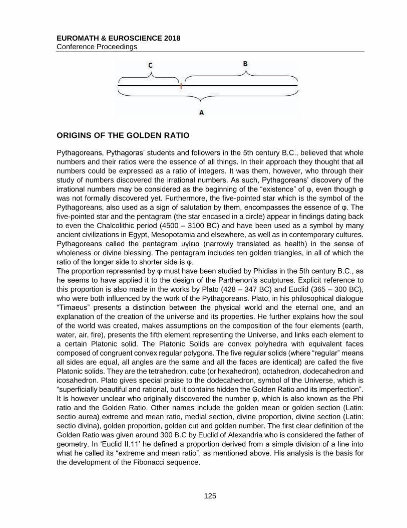
EUROMATH & EUROSCIENCE 2018 Conference Proceedings
125
ORIGINS OF THE GOLDEN RATIO Pythagoreans, Pythagoras’ students and followers in the 5th century B.C., believed that whole
numbers and their ratios were the essence of all things. In their approach they thought that all
numbers could be expressed as a ratio of integers. It was them, however, who through their
study of numbers discovered the irrational numbers. As such, Pythagoreans’ discovery of the
irrational numbers may be considered as the beginning of the “existence” of φ, even though φ
was not formally discovered yet. Furthermore, the five-pointed star which is the symbol of the
Pythagoreans, also used as a sign of salutation by them, encompasses the essence of φ. The
five-pointed star and the pentagram (the star encased in a circle) appear in findings dating back
to even the Chalcolithic period (4500 – 3100 BC) and have been used as a symbol by many
ancient civilizations in Egypt, Mesopotamia and elsewhere, as well as in contemporary cultures.
Pythagoreans called the pentagram υγίεια (narrowly translated as health) in the sense of
wholeness or divine blessing. The pentagram includes ten golden triangles, in all of which the
ratio of the longer side to shorter side is φ.
The proportion represented by φ must have been studied by Phidias in the 5th century B.C., as
he seems to have applied it to the design of the Parthenon’s sculptures. Explicit reference to
this proportion is also made in the works by Plato (428 – 347 BC) and Euclid (365 – 300 BC),
who were both influenced by the work of the Pythagoreans. Plato, in his philosophical dialogue
“Timaeus” presents a distinction between the physical world and the eternal one, and an
explanation of the creation of the universe and its properties. He further explains how the soul
of the world was created, makes assumptions on the composition of the four elements (earth,
water, air, fire), presents the fifth element representing the Universe, and links each element to
a certain Platonic solid. The Platonic Solids are convex polyhedra with equivalent faces
composed of congruent convex regular polygons. The five regular solids (where “regular” means
all sides are equal, all angles are the same and all the faces are identical) are called the five
Platonic solids. They are the tetrahedron, cube (or hexahedron), octahedron, dodecahedron and
icosahedron. Plato gives special praise to the dodecahedron, symbol of the Universe, which is
“superficially beautiful and rational, but it contains hidden the Golden Ratio and its imperfection”.
It is however unclear who originally discovered the number φ, which is also known as the Phi
ratio and the Golden Ratio. Other names include the golden mean or golden section (Latin:
sectio aurea) extreme and mean ratio, medial section, divine proportion, divine section (Latin:
sectio divina), golden proportion, golden cut and golden number. The first clear definition of the
Golden Ratio was given around 300 B.C by Euclid of Alexandria who is considered the father of
geometry. In ‘Euclid II.11’ he defined a proportion derived from a simple division of a line into
what he called its “extreme and mean ratio”, as mentioned above. His analysis is the basis for
the development of the Fibonacci sequence.

EUROMATH & EUROSCIENCE 2018 Conference Proceedings
126
The Fibonacci sequence is another way to derive Phi mathematically. It is formed as a series of
numbers derived by starting with 0 and adding 1 to get 1. Then the process is repeated by adding
the sum of the last two numbers as the next number in the series: 0, 1, 1, 2, 3, 5, 8, 13, 21, 34,
55, 89, 144, 233 and so on. The relationship to the Golden Ratio is found by dividing each
number by the one before it. The further you move in the series, the closer the result gets to the
number φ. For example:
1/1=1 2/1=2 3/2=1.5 5/3=1.666
13/8=1.625 21/13=1.615 ...
This sequence was known as early as the 6th century AD by Indian mathematicians but it was
Fibonacci that introduced it to the west.
THE GOLDEN RATIO IN ART AND DESIGN From Renaissance till today, artists have recognized the ability of Phi to give a sense of balance
and harmony and have used it in some of the world’s greatest works of art. According to some
researchers and analysts, the golden proportion is considered to be the most aesthetically
pleasing and it is said to be found in the human body as well as in animals and in the growth
pattern of many plants. As such it could be considered natural that artists follow it in their work.
Other researchers and analysts, however, challenge the importance of the Golden Ratio in
aesthetics and the extent to which it has been intentionally used in the arts.
As an example, the drawing of the Vitruvian Man, by Leonardo da Vinci is perceived to be a
picture of perfection. The standing image of the man is inscribed in a square while the image
drawn with legs and arms spread apart is inscribed in a circle. It is considered to be a
characteristic example of how art and science are compound and exemplifies da Vinci’s interest
in proportion. Actually, the Vitruvian Man demonstrates a broad variety of proportions in the
human body. Some of these proportions coincide with the Golden Ratio. Another piece of work
by da Vinci, in which the artist seems to have used the Golden Ratio is “Mona Lisa”. It is said
that if you draw a rectangle around the face of Mona Lisa, the ratio of the height to the width of
the rectangle is equal to the Golden Ratio. However, it is not said where exactly should the
rectangle be drawn. In his painting “The Last Supper”, da Vinci used the Golden Section in
framing the whole picture, meaning in positioning the table and Jesus within the frame, as well
as in many details of the painting. Evidently, da Vinci used the Golden Ratio extensively in his
work. However, whether he did it consciously or not is subject of heated debate.
Salvadore Dali is another artist who is considered to have used the Divine Proportion in his work.
In his painting ‘The Sacrament of the Last Supper’, Dali used a golden rectangle as the frame
of the painting and the golden proportion in the way the table was placed in the painting and the
way the two disciples were placed at Christ’s side. Moreover, the windows are formed by a
dodecahedron, one of the Platonic Solids.
In sculpture, the statue of Venus de Milo is found to be strictly in the Golden Proportion. The
statue Doryphoros by Polykleitos, which is one of the best known Greek sculptures of classical
antiquity, may be considered to be divided in three zones. The first one from the top till the right
nipple, the second from the right nipple to the knee and the third from the right knee to the right
big toe. The second zone is given a length of 1.61803 while the other two are given a length of
1. Some claim that these measurements are not accurate and that the left side of Doryphoros
does not have the same proportions.
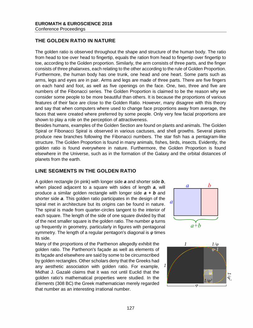
EUROMATH & EUROSCIENCE 2018 Conference Proceedings
127
THE GOLDEN RATIO IN NATURE
The golden ratio is observed throughout the shape and structure of the human body. The ratio
from head to toe over head to fingertip, equals the ration from head to fingertip over fingertip to
toe, according to the Golden proportion. Similarly, the arm consists of three parts, and the finger
consists of three phalanxes, each relating to the other according to the rule of Golden Proportion.
Furthermore, the human body has one trunk, one head and one heart. Some parts such as
arms, legs and eyes are in pair. Arms and legs are made of three parts. There are five fingers
on each hand and foot, as well as five openings on the face. One, two, three and five are
numbers of the Fibonacci series. The Golden Proportion is claimed to be the reason why we
consider some people to be more beautiful than others. It is because the proportions of various
features of their face are close to the Golden Ratio. However, many disagree with this theory
and say that when computers where used to change face proportions away from average, the
faces that were created where preferred by some people. Only very few facial proportions are
shown to play a role on the perception of attractiveness.
Besides humans, examples of the Golden Section are found on plants and animals. The Golden
Spiral or Fibonacci Spiral is observed in various cactuses, and shell growths. Several plants
produce new branches following the Fibonacci numbers. The star fish has a pentagram-like
structure. The Golden Proportion is found in many animals, fishes, birds, insects. Evidently, the
golden ratio is found everywhere in nature. Furthermore, the Golden Proportion is found
elsewhere in the Universe, such as in the formation of the Galaxy and the orbital distances of
planets from the earth.
LINE SEGMENTS IN THE GOLDEN RATIO A golden rectangle (in pink) with longer side a and shorter side b,
when placed adjacent to a square with sides of length a, will
produce a similar golden rectangle with longer side a + b and
shorter side a. This golden ratio participates in the design of the
spiral met in architecture but its origins can be found in nature.
The spiral is made from quarter-circles tangent to the interior of
each square. The length of the side of one square divided by that
of the next smaller square is the golden ratio. The number φ turns
up frequently in geometry, particularly in figures with pentagonal
symmetry. The length of a regular pentagon's diagonal is φ times
its side.
Many of the proportions of the Parthenon allegedly exhibit the
golden ratio. The Parthenon's façade as well as elements of
its façade and elsewhere are said by some to be circumscribed
by golden rectangles. Other scholars deny that the Greeks had
any aesthetic association with golden ratio. For example,
Midhat J. Gazalé claims that it was not until Euclid that the
golden ratio's mathematical properties were studied. In the
Elements (308 BC) the Greek mathematician merely regarded
that number as an interesting irrational number.
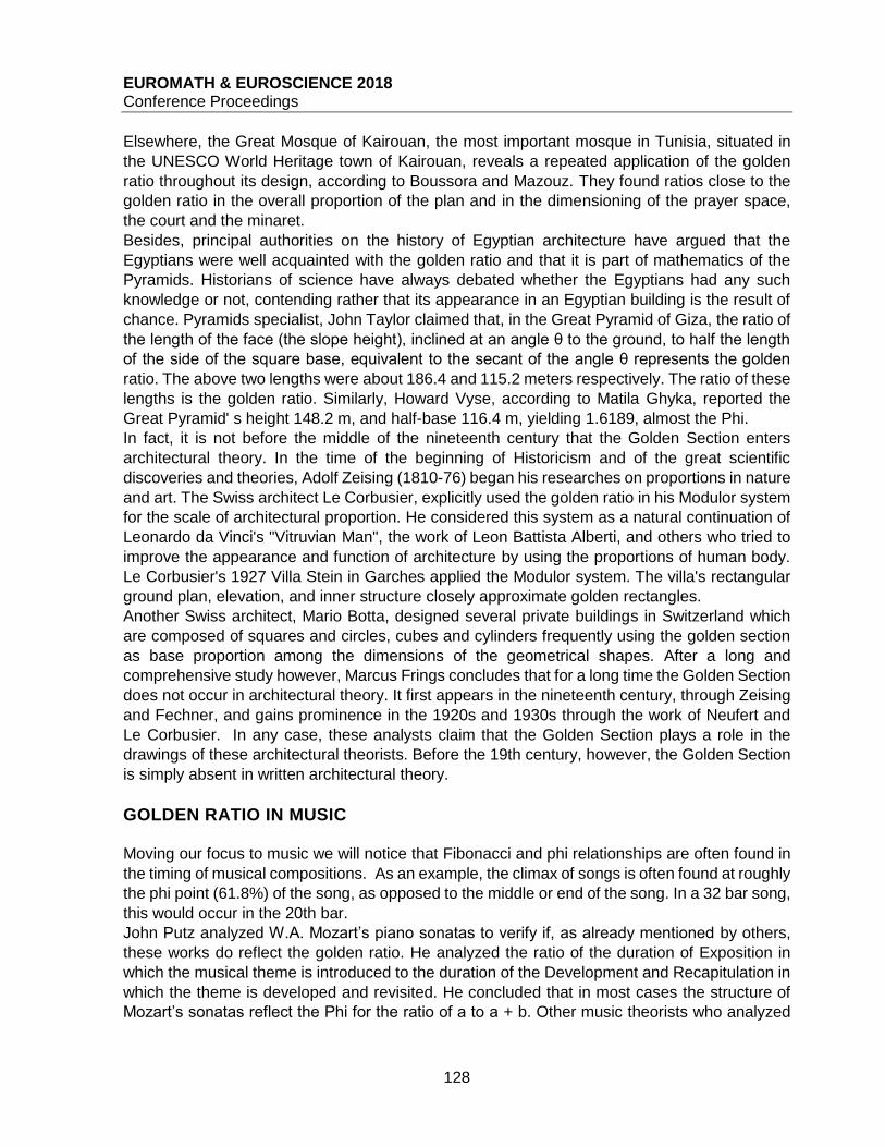
EUROMATH & EUROSCIENCE 2018 Conference Proceedings
128
Elsewhere, the Great Mosque of Kairouan, the most important mosque in Tunisia, situated in
the UNESCO World Heritage town of Kairouan, reveals a repeated application of the golden
ratio throughout its design, according to Boussora and Mazouz. They found ratios close to the
golden ratio in the overall proportion of the plan and in the dimensioning of the prayer space,
the court and the minaret.
Besides, principal authorities on the history of Egyptian architecture have argued that the
Egyptians were well acquainted with the golden ratio and that it is part of mathematics of the
Pyramids. Historians of science have always debated whether the Egyptians had any such
knowledge or not, contending rather that its appearance in an Egyptian building is the result of
chance. Pyramids specialist, John Taylor claimed that, in the Great Pyramid of Giza, the ratio of
the length of the face (the slope height), inclined at an angle θ to the ground, to half the length
of the side of the square base, equivalent to the secant of the angle θ represents the golden
ratio. The above two lengths were about 186.4 and 115.2 meters respectively. The ratio of these
lengths is the golden ratio. Similarly, Howard Vyse, according to Matila Ghyka, reported the
Great Pyramid' s height 148.2 m, and half-base 116.4 m, yielding 1.6189, almost the Phi.
In fact, it is not before the middle of the nineteenth century that the Golden Section enters
architectural theory. In the time of the beginning of Historicism and of the great scientific
discoveries and theories, Adolf Zeising (1810-76) began his researches on proportions in nature
and art. The Swiss architect Le Corbusier, explicitly used the golden ratio in his Modulor system
for the scale of architectural proportion. He considered this system as a natural continuation of
Leonardo da Vinci's "Vitruvian Man", the work of Leon Battista Alberti, and others who tried to
improve the appearance and function of architecture by using the proportions of human body.
Le Corbusier's 1927 Villa Stein in Garches applied the Modulor system. The villa's rectangular
ground plan, elevation, and inner structure closely approximate golden rectangles.
Another Swiss architect, Mario Botta, designed several private buildings in Switzerland which
are composed of squares and circles, cubes and cylinders frequently using the golden section
as base proportion among the dimensions of the geometrical shapes. After a long and
comprehensive study however, Marcus Frings concludes that for a long time the Golden Section
does not occur in architectural theory. It first appears in the nineteenth century, through Zeising
and Fechner, and gains prominence in the 1920s and 1930s through the work of Neufert and
Le Corbusier. In any case, these analysts claim that the Golden Section plays a role in the
drawings of these architectural theorists. Before the 19th century, however, the Golden Section
is simply absent in written architectural theory.
GOLDEN RATIO IN MUSIC
Moving our focus to music we will notice that Fibonacci and phi relationships are often found in
the timing of musical compositions. As an example, the climax of songs is often found at roughly
the phi point (61.8%) of the song, as opposed to the middle or end of the song. In a 32 bar song,
this would occur in the 20th bar.
John Putz analyzed W.A. Mozart’s piano sonatas to verify if, as already mentioned by others,
these works do reflect the golden ratio. He analyzed the ratio of the duration of Exposition in
which the musical theme is introduced to the duration of the Development and Recapitulation in
which the theme is developed and revisited. He concluded that in most cases the structure of
Mozart’s sonatas reflect the Phi for the ratio of a to a + b. Other music theorists who analyzed

EUROMATH & EUROSCIENCE 2018 Conference Proceedings
129
Bela Bartok’s works, one of the most important composers of the 20th century, have found out
that they are created according to two opposing systems, that of the golden ratio and the
acoustic scale.
Besides, Erik Satie, a French composer used the golden ratio in several of his pieces, including
Sonneries de la Rose+Croix. The golden ratio is also met in the structure of the sections in the
music of Debussy's Reflections in Water, from Images (1st series, 1905), in which the sequence
of keys is marked out by the intervals 34, 21, 13 and 8, and the main climax sits at the phi
position. Musicologist Roy Howat has observed that the formal boundaries of La Mer correspond
exactly to the golden section.
The golden ratio does not only influence the structure of some musical masterpieces but is also
taken into account in the manufacturing of some musical instruments. Fibonacci and phi are
used in the design of violins and even in the design of high quality speaker wire. The percussion
and drums producer company Pearl Drums positions the air vents on its Masters Premium
models based on the golden ratio. The company claims that this arrangement improves bass
response and has applied for a patent on this innovation.
Furthermore, it seems that the golden ratio is an inherent feature of western music itself. Musical
scales are related to Fibonacci numbers whose ratios tend to Phi:
There are 13 notes in the span of any note through its octave (count the black and white
keys from C to next C).
A scale is composed of 8 notes (take only the white keys), of which the 5th and 3rd notes
create the basic foundation of all chords, and are based on a tone which are combination
of 2 steps and 1 step from the root tone, that is the 1st note of the scale.
In a scale, the dominant note is the 5th note of the major scale, which is also the 8th note of all
13 notes that comprise the octave. This provides an additional example of Fibonacci numbers
in key musical relations. Interestingly, 8/13 is 0.61538, which approximates phi. Looking now
deeper into the musical frequencies, we realize that they are based on Fibonacci ratios and Phi.
Notes in the scale of western music are based on natural harmonics that are created by ratios
of frequencies. Ratios found in the first seven numbers of the Fibonacci series ( 0, 1, 1, 2, 3, 5,
8 ) are related to key frequencies of musical notes.
REFERENCES
Akhtaruzzaman Md., Shafie A.A., Geometrical Substantiation of Phi, the golden Ratio and the
Baroque of Nature, Architecture, Design and Engineering, International Journal of Arts, 1.1: 1-
22, (2011). Available on line: http://article.sapub.org/pdf/10.5923.j.arts.20110101.01.pdf, last
seen 15/1/2018.
Dunlap, R.A., The golden ratio and Fibonacci numbers. World Scientific, 1997.
Frings, M., The golden section in architectural theory, Nexus Network Journal, 4.1: 9-32, (2002).
Livio, M., The golden ratio and aesthetics, Plus Magazine, 22, (2002). Available on line:
https://plus.maths.org/issue22/features/golden/2pdf/index.html/op.pdf, last seen 25/11/2018.
Livio, M., The golden ratio: The story of phi, the world's most astonishing number, Broadway
Books, (2008)
Markowsky, G., Misconceptions about the golden ratio, The College Mathematics Journal, 23.1:
2-19, (1992).
Olsen, S., The golden section: nature's greatest secret, Bloomsbury Publishing USA, (2006).

EUROMATH & EUROSCIENCE 2018 Conference Proceedings
130
Prokopakis, E.P., et al. The golden ratio in facial symmetry, Rhinology, 51.1: 18-21, (2013).
Available on line:
https://www.researchgate.net/profile/Emmanuel_Prokopakis/publication/235730861_The_gold
en_ratio_in_facial_symmetry/links/0deec53847c878d2c7000000/The-golden-ratio-in-facial-
symmetry.pdf, last seen 11/12/2018.
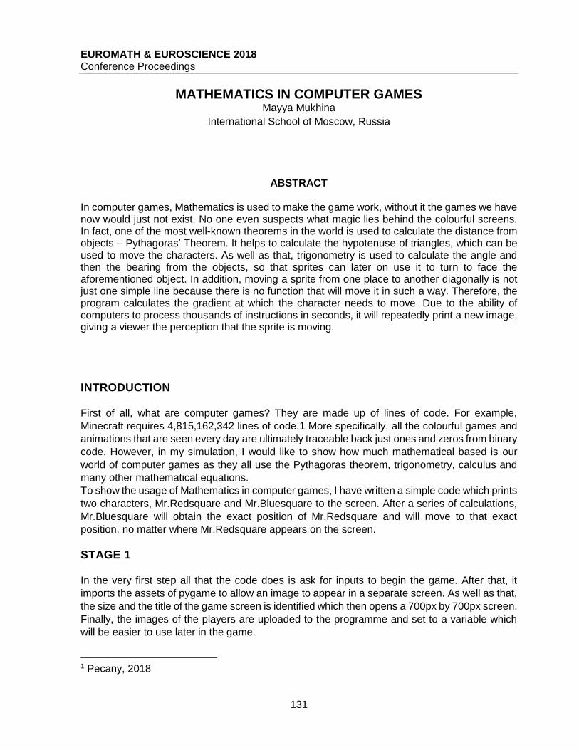
EUROMATH & EUROSCIENCE 2018 Conference Proceedings
131
MATHEMATICS IN COMPUTER GAMES Mayya Mukhina
International School of Moscow, Russia
ABSTRACT In computer games, Mathematics is used to make the game work, without it the games we have now would just not exist. No one even suspects what magic lies behind the colourful screens. In fact, one of the most well-known theorems in the world is used to calculate the distance from objects – Pythagoras’ Theorem. It helps to calculate the hypotenuse of triangles, which can be used to move the characters. As well as that, trigonometry is used to calculate the angle and then the bearing from the objects, so that sprites can later on use it to turn to face the aforementioned object. In addition, moving a sprite from one place to another diagonally is not just one simple line because there is no function that will move it in such a way. Therefore, the program calculates the gradient at which the character needs to move. Due to the ability of computers to process thousands of instructions in seconds, it will repeatedly print a new image, giving a viewer the perception that the sprite is moving.
INTRODUCTION
First of all, what are computer games? They are made up of lines of code. For example,
Minecraft requires 4,815,162,342 lines of code.1 More specifically, all the colourful games and
animations that are seen every day are ultimately traceable back just ones and zeros from binary
code. However, in my simulation, I would like to show how much mathematical based is our
world of computer games as they all use the Pythagoras theorem, trigonometry, calculus and
many other mathematical equations.
To show the usage of Mathematics in computer games, I have written a simple code which prints
two characters, Mr.Redsquare and Mr.Bluesquare to the screen. After a series of calculations,
Mr.Bluesquare will obtain the exact position of Mr.Redsquare and will move to that exact
position, no matter where Mr.Redsquare appears on the screen.
STAGE 1
In the very first step all that the code does is ask for inputs to begin the game. After that, it
imports the assets of pygame to allow an image to appear in a separate screen. As well as that,
the size and the title of the game screen is identified which then opens a 700px by 700px screen.
Finally, the images of the players are uploaded to the programme and set to a variable which
will be easier to use later in the game.
1 Pecany, 2018

EUROMATH & EUROSCIENCE 2018 Conference Proceedings
132
In the second part, I have imported the random function to enable my code to choose a random
value. As this simulation must show that at any position on the screen, Mr.Bluesquare will be
able to identify the exact coordinates of Mr.Redsquare, therefore both characters must be
printed in a random position on the screen every time. Giving the computer a range of values
between 0 and 600, it will randomly choose 4 values and give each sprite an x and y axis
coordinate. The last few lines paint the screen white and print the characters to the game board.
STAGE 2
At stage 2, the code is 61 lines in and due to the need for mathematical functions, the asset,
‘math’, is imported to enable trigonometry and many other mathematical calculations.
Between two objects a right-angled triangle can always be formed, as a result of this, now we
can calculate Side x and Side y of this triangle which will be extremely helpful in our next stage.
In addition, due to combinatorics we can identify that there are only four possible ways the
triangle can be orientated to show the path of Mr.Bluesquare, as well as showing how many
varieties of the same code need to be written for the stimulation to work every time. There will
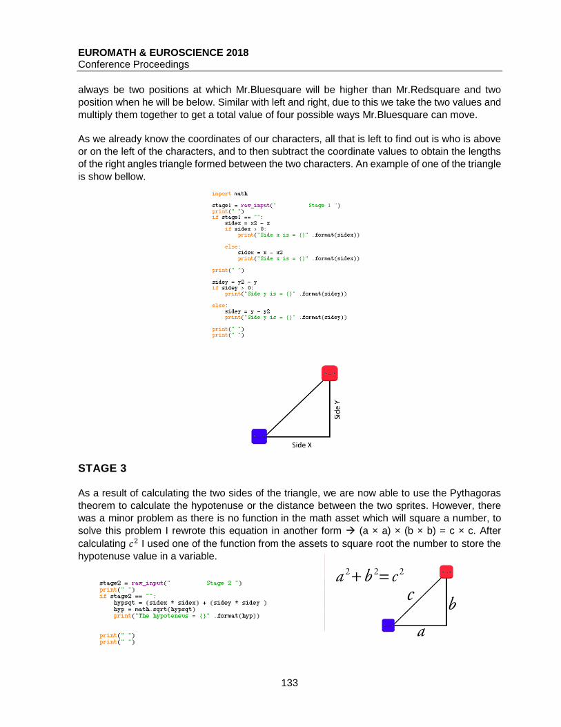
EUROMATH & EUROSCIENCE 2018 Conference Proceedings
133
always be two positions at which Mr.Bluesquare will be higher than Mr.Redsquare and two
position when he will be below. Similar with left and right, due to this we take the two values and
multiply them together to get a total value of four possible ways Mr.Bluesquare can move.
As we already know the coordinates of our characters, all that is left to find out is who is above
or on the left of the characters, and to then subtract the coordinate values to obtain the lengths
of the right angles triangle formed between the two characters. An example of one of the triangle
is show bellow.
STAGE 3
As a result of calculating the two sides of the triangle, we are now able to use the Pythagoras
theorem to calculate the hypotenuse or the distance between the two sprites. However, there
was a minor problem as there is no function in the math asset which will square a number, to
solve this problem I rewrote this equation in another form (a × a) × (b × b) = c × c. After
calculating 𝑐2 I used one of the function from the assets to square root the number to store the
hypotenuse value in a variable.

EUROMATH & EUROSCIENCE 2018 Conference Proceedings
134
STAGE 4
In stage four, the code calculates the angle between the hypotenuse and the adjacent using
trigonometry, more specifically using the tangent rule.
First of all, the program will figure out how the triangle is orientated and then according to that
will divide the sides. After obtaining tan(A) using inverse tangent, the tan(A) will be converted
into an angle.
STAGE 5
In most games, it is vital for enemies to turn to face where they are going, therefore, using
bearing and the angle we calculated in the previous stage will help to calculate the angle at
which Mr.Bluesquare needs to turn if he is already facing north. Again, according to the triangle
the variable bearing will either be the angle, 360 + angle or 180 ± angle.
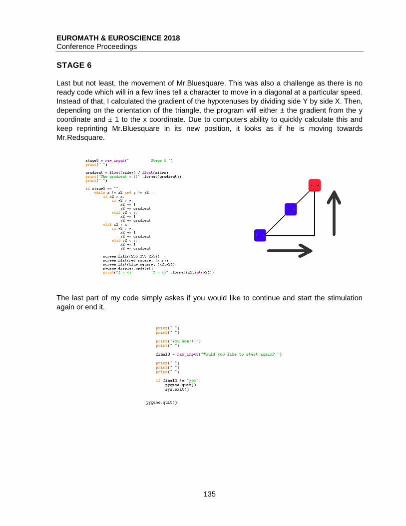
EUROMATH & EUROSCIENCE 2018 Conference Proceedings
135
STAGE 6
Last but not least, the movement of Mr.Bluesquare. This was also a challenge as there is no
ready code which will in a few lines tell a character to move in a diagonal at a particular speed.
Instead of that, I calculated the gradient of the hypotenuses by dividing side Y by side X. Then,
depending on the orientation of the triangle, the program will either ± the gradient from the y
coordinate and ± 1 to the x coordinate. Due to computers ability to quickly calculate this and
keep reprinting Mr.Bluesquare in its new position, it looks as if he is moving towards
Mr.Redsquare.
The last part of my code simply askes if you would like to continue and start the stimulation
again or end it.
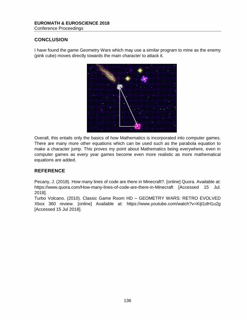
EUROMATH & EUROSCIENCE 2018 Conference Proceedings
136
CONCLUSION I have found the game Geometry Wars which may use a similar program to mine as the enemy
(pink cube) moves directly towards the main character to attack it.
Overall, this entails only the basics of how Mathematics is incorporated into computer games.
There are many more other equations which can be used such as the parabola equation to
make a character jump. This proves my point about Mathematics being everywhere, even in
computer games as every year games become even more realistic as more mathematical
equations are added.
REFERENCE
Pecany, J. (2018). How many lines of code are there in Minecraft?. [online] Quora. Available at:
https://www.quora.com/How-many-lines-of-code-are-there-in-Minecraft [Accessed 15 Jul.
2018].
Turbo Volcano. (2010). Classic Game Room HD – GEOMETRY WARS: RETRO EVOLVED
Xbox 360 review. [online] Available at: https://www.youtube.com/watch?v=Kijt1dH1u2g
[Accessed 15 Jul 2018].
EUROMATH & EUROSCIENCE 2018 Conference Proceedings
137
MATHS OR LUCK? Alexandra Anastassiadou, Andreas Lordos, Andreas Yiakoumi, Christos Antoniou, Petros
Vassiliades
The English School of Nicosia, Cyprus
ABSTRACT
In this paper, we will be explaining how one can use mathematics in order to increase the probabilities of winning at traditional board games. The best strategies are the ones based on mathematics and we are going to prove this by showing how the probabilities of victory can be drastically increased using such methods. We will be using Monte Carlo simulations and other computational algorithms to back up our research and claims. Through the paper, we will show you which regions are the best for controlling in Risk, when the best time is to attack and when to defend and prove it all using mathematics. We will also show you which are the best questions to ask in Guess Who, and prove why they are the most effective. Finally, we will demonstrate the best properties to buy in Monopoly. We aim to change the way you approach board games, not just as games of chance but as games of skill, knowledge and strategy.
RISK
Risk is a game of world domination, where your objective is to command an army to take over
the world. The board is a world map split up into continents, and continents are split up into
territories. You win when you control all the continents on the board. At the start of the game,
players take turns choosing territories to control. This is done until the map is fully occupied.
Players who have troops in a territory can attack adjacent territories on their turn. If you are the
sole owner of a continent, you gain bonus troops each turn. Therefore, it is in your interest to
control and defend continents in order to build up your army. So, how do you attack? Well, it
depends on how many troops you have. As the attacker, you roll as many dice as there are
attackers, up to three dice. If you are a defender, you roll as many dice as there are defenders,
up to two dice. After the dice are rolled, the highest rolls of the defender’s contest with the highest
rolls of the attackers. For each roll of the defender which is lower than a roll of the attacker, the
defender loses one troop. If the defending territory has 0 troops left, you win the territory. You
can attack as many times as you want per turn, as long as you have troops.
In a common 5 player game of risk, each player starts the game with 25 units and every player
selects territories one after the other until all territories have been selected. This results to
dividing the 42 territories in the following way; 3 players get 9 territories and 2 players get 8
players each. Afterwards, the game begins where all players fight amongst themselves to control
entire continents as a bonus number of units per round can be very helpful to shift the
probabilities of winning towards their favour.

EUROMATH & EUROSCIENCE 2018 Conference Proceedings
138
Therefore, a good question to ask would be which continent is the right to go for? Which
territories should you focus at controlling initially? To find out, a player should take in
consideration the amount of territories in each continent and the respective amount of bonus
units each one rewards:
To make it much clearer, we must deduce the ratio between the bonus number of units to the
number of territories (Armies per turn: territories). As we can see from the graph below Europe
seems as the better continent to control as it gives the highest ratio, while smaller continents
like South America and Australia are less attractive since they have a reasonably low ratio.
Continent Number of territories Number of bonus armies per turn
Africa 6 3
Asia 12 7
Australia 4 2
Europe 7 5
North America 9 5
South America 4 2
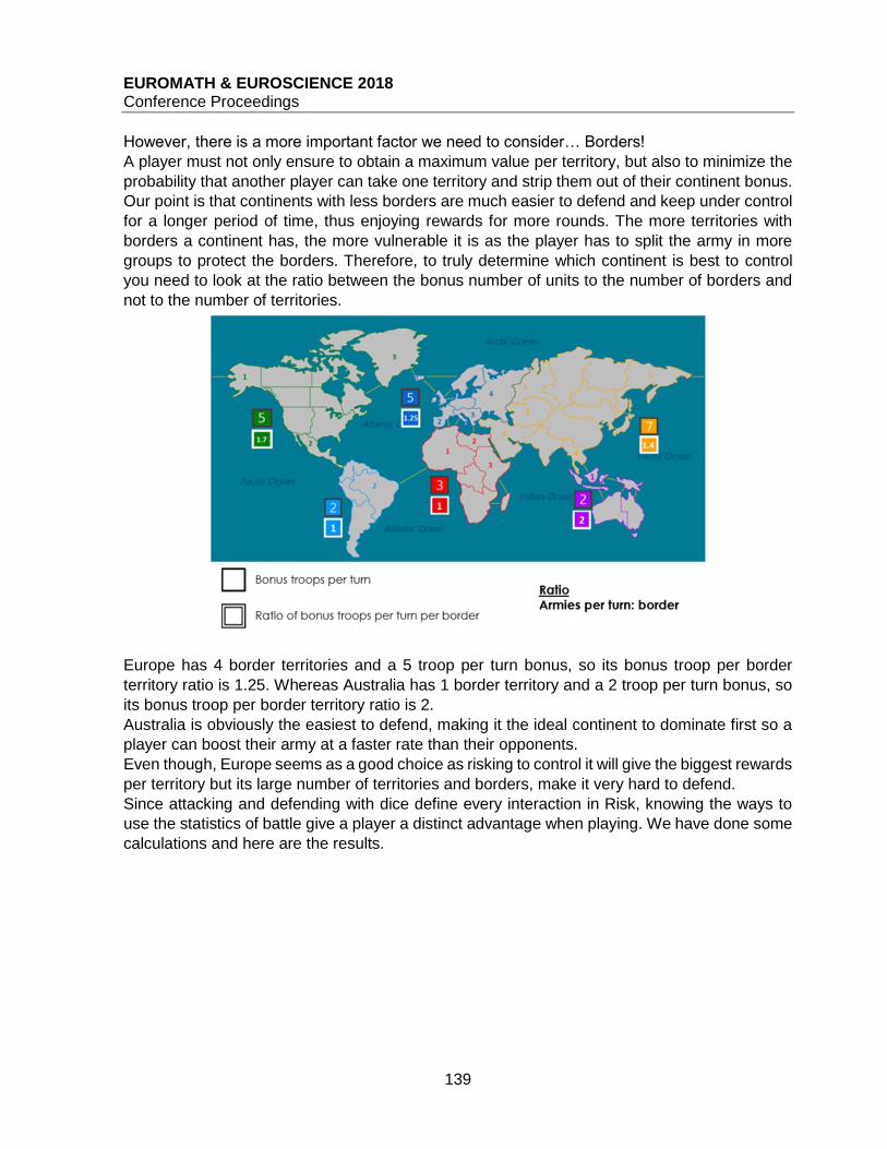
EUROMATH & EUROSCIENCE 2018 Conference Proceedings
139
However, there is a more important factor we need to consider… Borders!
A player must not only ensure to obtain a maximum value per territory, but also to minimize the
probability that another player can take one territory and strip them out of their continent bonus.
Our point is that continents with less borders are much easier to defend and keep under control
for a longer period of time, thus enjoying rewards for more rounds. The more territories with
borders a continent has, the more vulnerable it is as the player has to split the army in more
groups to protect the borders. Therefore, to truly determine which continent is best to control
you need to look at the ratio between the bonus number of units to the number of borders and
not to the number of territories.
Europe has 4 border territories and a 5 troop per turn bonus, so its bonus troop per border
territory ratio is 1.25. Whereas Australia has 1 border territory and a 2 troop per turn bonus, so
its bonus troop per border territory ratio is 2.
Australia is obviously the easiest to defend, making it the ideal continent to dominate first so a
player can boost their army at a faster rate than their opponents.
Even though, Europe seems as a good choice as risking to control it will give the biggest rewards
per territory but its large number of territories and borders, make it very hard to defend.
Since attacking and defending with dice define every interaction in Risk, knowing the ways to
use the statistics of battle give a player a distinct advantage when playing. We have done some
calculations and here are the results.
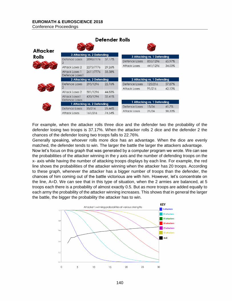
EUROMATH & EUROSCIENCE 2018 Conference Proceedings
140
For example, when the attacker rolls three dice and the defender two the probability of the
defender losing two troops is 37.17%. When the attacker rolls 2 dice and the defender 2 the
chances of the defender losing two troops falls to 22.76%.
Generally speaking, whoever rolls more dice has an advantage. When the dice are evenly
matched, the defender tends to win. The larger the battle the larger the attackers advantage.
Now let’s focus on this graph that was generated by a computer program we wrote. We can see
the probabilities of the attacker winning in the y axis and the number of defending troops on the
x- axis while having the number of attacking troops displays by each line. For example, the red
line shows the probabilities of the attacker winning when the attacker has 20 troops. According
to these graph, whenever the attacker has a bigger number of troops than the defender, the
chances of him coming out of the battle victorious are with him. However, let’s concentrate on
the line, A=D. We can see that in this type of situation, when the 2 armies are balanced, at 5
troops each there is a probability of almost exactly 0.5. But as more troops are added equally to
each army the probability of the attacker winning increases. This shows that in general the larger
the battle, the bigger the probability the attacker has to win.
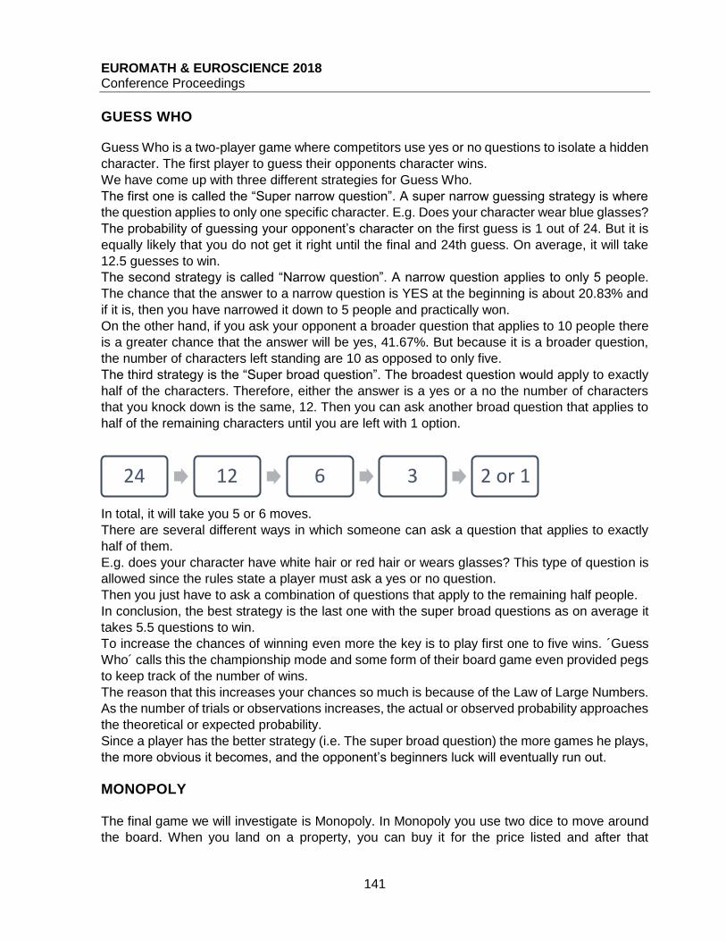
EUROMATH & EUROSCIENCE 2018 Conference Proceedings
141
GUESS WHO Guess Who is a two-player game where competitors use yes or no questions to isolate a hidden
character. The first player to guess their opponents character wins.
We have come up with three different strategies for Guess Who.
The first one is called the “Super narrow question”. A super narrow guessing strategy is where
the question applies to only one specific character. E.g. Does your character wear blue glasses?
The probability of guessing your opponent’s character on the first guess is 1 out of 24. But it is
equally likely that you do not get it right until the final and 24th guess. On average, it will take
12.5 guesses to win.
The second strategy is called “Narrow question”. A narrow question applies to only 5 people.
The chance that the answer to a narrow question is YES at the beginning is about 20.83% and
if it is, then you have narrowed it down to 5 people and practically won.
On the other hand, if you ask your opponent a broader question that applies to 10 people there
is a greater chance that the answer will be yes, 41.67%. But because it is a broader question,
the number of characters left standing are 10 as opposed to only five.
The third strategy is the “Super broad question”. The broadest question would apply to exactly
half of the characters. Therefore, either the answer is a yes or a no the number of characters
that you knock down is the same, 12. Then you can ask another broad question that applies to
half of the remaining characters until you are left with 1 option.
In total, it will take you 5 or 6 moves.
There are several different ways in which someone can ask a question that applies to exactly
half of them.
E.g. does your character have white hair or red hair or wears glasses? This type of question is
allowed since the rules state a player must ask a yes or no question.
Then you just have to ask a combination of questions that apply to the remaining half people.
In conclusion, the best strategy is the last one with the super broad questions as on average it
takes 5.5 questions to win.
To increase the chances of winning even more the key is to play first one to five wins. ´Guess
Who´ calls this the championship mode and some form of their board game even provided pegs
to keep track of the number of wins.
The reason that this increases your chances so much is because of the Law of Large Numbers.
As the number of trials or observations increases, the actual or observed probability approaches
the theoretical or expected probability.
Since a player has the better strategy (i.e. The super broad question) the more games he plays,
the more obvious it becomes, and the opponent’s beginners luck will eventually run out.
MONOPOLY
The final game we will investigate is Monopoly. In Monopoly you use two dice to move around
the board. When you land on a property, you can buy it for the price listed and after that
24 12 6 3 2 or 1

EUROMATH & EUROSCIENCE 2018 Conference Proceedings
142
whenever someone else lands on that property they have to pay rent. Whenever you pass the
starting position of the board, you gain extra money, and if you land on the "GO TO JAIL" square
you are immediately taken to the JAIL square. The aim of the game is to lead all of your
opponents to bankruptcy, giving you a monopoly over the board.
Buying properties is an essential aspect of the game and knowing what properties to buy can
increase your chances of winning. So, which are the best properties in “Monopoly”? For
simplicity reasons we will use the board below for our examples referring to each square with
its number.
The first thing we need to realise is that since we are using two dice to move around, not all
outcomes have an equal probability of being rolled.
For example, there is a greater chance you will roll a seven than any other number. This is
because there are more combinations that give out a seven than anything else.
Dice Roll Combinations Probability
2 (1.1) 2.78%
3 (1.2),(2.1) 5.56%
4 (1.3),(3.1),(2.2) 8.33%
5 (1.4),(4.1),(2.3),(3.2) 11.11%
6 (1.5),(5.1),(2.4),(4.2),(3.3) 13.89%
7 (1.6),(6.1),(2.5),(5.2),(3.4),(4.3) 16.67%
8 (2.6),(6.2),(3.5),(5.3),(4.4) 13.89%
9 (3.6),(6.3),(4.5),(5.4) 11.11%
10 (4.6),(6.4),(5.5) 8.33%
11 (5.6),(6.5) 5.56%
12 (6.6) 2.78%
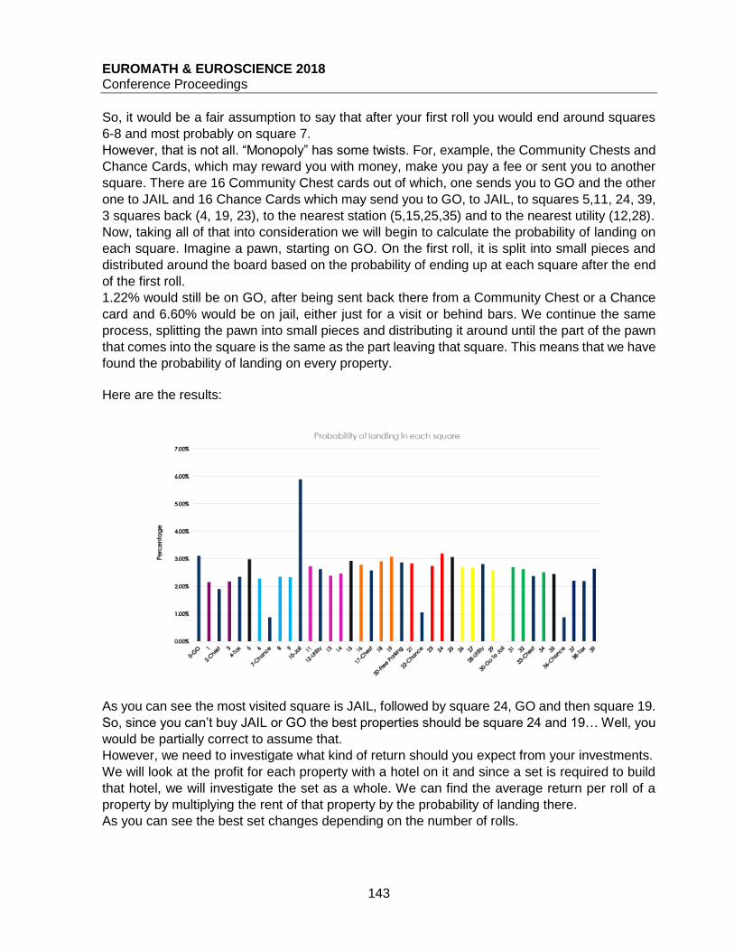
EUROMATH & EUROSCIENCE 2018 Conference Proceedings
143
So, it would be a fair assumption to say that after your first roll you would end around squares
6-8 and most probably on square 7.
However, that is not all. “Monopoly” has some twists. For, example, the Community Chests and
Chance Cards, which may reward you with money, make you pay a fee or sent you to another
square. There are 16 Community Chest cards out of which, one sends you to GO and the other
one to JAIL and 16 Chance Cards which may send you to GO, to JAIL, to squares 5,11, 24, 39,
3 squares back (4, 19, 23), to the nearest station (5,15,25,35) and to the nearest utility (12,28).
Now, taking all of that into consideration we will begin to calculate the probability of landing on
each square. Imagine a pawn, starting on GO. On the first roll, it is split into small pieces and
distributed around the board based on the probability of ending up at each square after the end
of the first roll.
1.22% would still be on GO, after being sent back there from a Community Chest or a Chance
card and 6.60% would be on jail, either just for a visit or behind bars. We continue the same
process, splitting the pawn into small pieces and distributing it around until the part of the pawn
that comes into the square is the same as the part leaving that square. This means that we have
found the probability of landing on every property.
Here are the results:
As you can see the most visited square is JAIL, followed by square 24, GO and then square 19.
So, since you can’t buy JAIL or GO the best properties should be square 24 and 19… Well, you
would be partially correct to assume that.
However, we need to investigate what kind of return should you expect from your investments.
We will look at the profit for each property with a hotel on it and since a set is required to build
that hotel, we will investigate the set as a whole. We can find the average return per roll of a
property by multiplying the rent of that property by the probability of landing there.
As you can see the best set changes depending on the number of rolls.

EUROMATH & EUROSCIENCE 2018 Conference Proceedings
144
An average game takes 30 rolls per player therefore the oranges would be the best option for a
2-3 player game, but the reds become better for a 4-player game and for 5 players or more the
greens are your best bet.
CONCLUSION
To recap:
For Risk, Australia is the best continent to control in order to boost your army in the early game.
When you know battle is inevitable, attack as soon as you have the same number of attacking
troops as your opponent has defending troops, you hold the advantage. And the larger the battle
the larger the attacker advantage. For Guess Who, the broad questions are the best. Always
ask the broadest question possible and since you have the better strategy try to play multiple
rounds to ensure that you come up on top. Finally, for Monopoly, for a 2-3 player game go for
the oranges, for a 4-player game go for the red and for a 5+ player game go for the greens.
REFERENCES www.github.com/andreaslordos/euromath - code we’ve written to three different simulations
Garret Robinson, ‘The Strategy Of Risk’,
youtube.com/watch?v=FRlbNOno5VA – Guess Who
youtube.com/watch?v=ubQXz5RBBtU – Monopoly
Dr Hannah Fry and Dr Thomas Oléron Evans, ‘The Indisputable Existance of Santa Claus’,
pages 126-137
EUROMATH & EUROSCIENCE 2018 Conference Proceedings
145
DIDO AND HER PROBLEMS Sofia Giannopoulou, Katerina Grigoriou, Aggelos Raptis, Zak Taraboulous
Nea Genia Ziridis School, Greece
ABSTRACT
Dido’s problem of maximizing the area which is enclosed within a certain perimeter is probably the oldest problem of optimization. It is also known as the “Isoperimetric Problem”. In antiquity, Zenodorous gave a geometrical solution to this problem using polygons. Zenodorous is conciderd by Constantin Carathéodory to be the founder of Calculus of Variations. Twenty centuries later Steiner gave his own geometrical proof. Other mathematicians, such as Weierstrass, solved the Isoperimetric Problem using the tools of Calculus of Variations. Nowadays Dido’ s problem is an active field of research in several areas of Mathematics.
INTRODUCTION
If we are to learn something from the history of mathematics is that very often, the most unique
and important mathematical ideas and discoveries emerge from simple problems. These
problems could be referring to everyday situations such as the need to construct something with
certain specifications. A characteristic example is that of the isoperimetric problem, a classical
problem of shape optimization with great impact on society and the production of new
mathematics.
The word “iso-perimetric” is consisted from the Greek word “iso” which means equal and
“perimetric” which refers to the perimeter, the length of the boundary of a two-dimensional figure.
Consequently, the isoperimetric problem is formulated as following:
“Find a closed plane curve of a given perimeter which encloses the greatest area”.
THE MYTH "The Kingdom you see is Carthage, the Tyrians, the town of Agenor;
But the country around is Libya, no folk to meet in war.
Dido, who left the city of Tyre to escape her brother,
Rules here--a long and labyrinthine tale of wrong
Is hers, but I will touch on its salient points in order...Dido, in great disquiet, organised her friends for
escape.
They met together, all those who harshly hated the tyrant
Or keenly feared him: they seized some ships which chanced to be ready...
They came to this spot, where to-day you can behold the mighty
Battlements and the rising citadel of New Carthage,
And purchased a site, which was named 'Bull's Hide' after the bargain
By which they should get as much land as they could enclose with a bull's hide.”

EUROMATH & EUROSCIENCE 2018 Conference Proceedings
146
Virgil in “Aeneid” narrates the myth of
Dido, the beautiful princess of Tyros
who left her country, as she was trying
to escape from her brother, and went
to North Africa, in Lybia. After arriving
to Carthage, she found herself wanting
to build her own city within the country.
After talking with the king, she was
given the chance to do so as long as
the city was as big as the skin of a cow.
After cutting the skin into thin strings,
forming a rope, she was confronted
with the isoperimetric problem. What
shape was she supposed to form
using the rope, in order for her town to
cover the largest area possible?
ISOPERIMETRIC PROBLEM IN ANTIQUITY According to Blasjo (2008): “The Greeks pretty much solved isoperimetric problem, by their
standards, when Zenodorus (200 BC - 140 BC) proved that a circle has greater area than any
polygon with the same perimeter. His work was lost. We know of it mainly through Pappus and
Theon of Alexandria”. Zenodorous is a Greek mathematician who probably lived during the same
era as Archimedes. His work was relevant with isoperimetric figures. Constantin Carathéodory
considers Zenodorous to be the founder of Calculus of Variations. This statement indicates the
importance of the first steps being made in a field of mathematical research even though the
“pioneer” might not have the slightest idea of where that could lead.
Subsequently Blasio presents Zenodorus polygon proof:

EUROMATH & EUROSCIENCE 2018 Conference Proceedings
147
The idea of this proof is very simple: Since the perimeter is fixed, the apothem determines the
enclosed area. So the area increases when the apothem becomes bigger. This happens when
the number of sides is increased.
Yet, it seems that ancient Greeks were aware of the solution of the isoperimetric problem even
earlier. John Philoponus (490 AC- 570 AC) says that Plato supported that circle encloses the
maximal domain among all two-dimensional shapes with the same perimeter. Philoponous also
comments Aristotle’s belief that among isoperimetric shapes, greater area is enclosed by the
one that has the greater number of angles.

EUROMATH & EUROSCIENCE 2018 Conference Proceedings
148
THE ISOPERIMETRIC PROBLEM IN THE NINETEENTH CENTURY In 1838 Jacob Steiner gave his own geometrical proof for the isoperimetric problem (Blasio,
2005):
In fact, Steiner gave five proofs. The problem is that in all proofs he assumed the existence of a
solution (his strategy was always to take a figure that is not a circle and show that its area can
be improved). This led to many contemporary mathematicians criticizing his proofs:
Peter Dirichlet: “Jakob, you have an incomplete proof. You have assumed that a solution exists.”
Jakob Steiner: “Peter, I have a valid proof and I’m not going to let you rain on my parade, please
go away.”

EUROMATH & EUROSCIENCE 2018 Conference Proceedings
149
Perron, (1913):
Proof of isoperimetric problem using the tools of calculus of variations
According to Blasio (2005) many mathematicians, such as Weierstrass, gave their own proof.
The basic idea is this “Take a curve and wiggle it a little bit, while keep in gits perimeter fixed. If
the curve is the one with maximal area then we are at an optimum, so an infinitesimal wiggle will
cause zero change in the area. In order to find the optimal figure, therefore, we calculate the
change in area caused by an infinite simal wiggle and set this equal to zero. This leads to a
differential equation that must be satisfied by an optimal figure, and indeed that is satisfied only
by circles”.
IMPACT ON CONTEMPORARY MATHEMATICS
Isoperimetric problem is an optimization problem. Professor Taria mentions that “Optimization
problems are relatively easy to understand when compared with problems in many other
branches of mathematics. Controversy invariably leads to interest. Hence, important
optimization problems embedded in some controversy have played major roles in motivating
and promoting mathematical activity”. The fact that we are discussing about an active field of
research in several areas such as differential geometry, discrete and convex geometry,
probability and Banach spaces theory shows the importance of this early posed problem.
CONCLUSIONS
The isoperimetric problem, the first ever problem to be created in the field of maximization,
wasn’t a source of trouble for just Dido. To the contrary, it became a topic of study for many
important mathematicians who either solved it or at least tried to. Subsequently, it is concluded
that mathematical breakthroughs are not necessarily a result of complex problems. It is possible
that simple, everyday hurdles become a source of inspiration for research and great
mathematical discoveries.

EUROMATH & EUROSCIENCE 2018 Conference Proceedings
150
REFERENCES
Blasio V., The isoperimetric problem. The Mathematical Association of America [Monthly 112]
(2005).
Perron, O. Zur Existenzfrage eines Maximums oder Minimums, Jahresber. Deutsch. Math.-
Verein. 22 (1913) 140–144.
Tapia, R., The Remarkable Life of the Isoperimetric Problem: The World’s Most Influential
Mathematics Problem. School Math Project Houston (2009).
Σπανδάγος, Ε., Ζηνόδωρος ο Παιανιεύς : Ένας μεγάλος μαθηματικός. Αίθρα (2011)
https://pdfs.semanticscholar.org/presentation/e997/31a43c500204a4f2886d2483e8300d844b1
6.pdf
http://mathworld.wolfram.com/IsoperimetricProblem.html
http://mathworld.wolfram.com/DidosProblem.html
https://en.wikipedia.org/wiki/Aeneid
EUROMATH & EUROSCIENCE 2018 Conference Proceedings
151
STUDENT PRESENTATIONS IN SCIENCE
CARTOONS IN PHYSICSLAND Maria Kaltaveridou, Daria Kovanova
Diastaseis, Private School, Greece
ABSTRACT
“What would cartoons be like if physics laws were in effect?” The truth is that all of us have spent hours on watching animated cartoons. We have all laughed with the heroes’ blunders. We have all felt anguish while watching Sylvester chasing Tweety orTom chasing Jerry and we have all felt joy while watching Elmer razed to the ground in his effort to catch Bugs Bunny. Innumerable times, we have seen the heroes experiencing complete disaster but in the end, they always came back to their former shape, safe and sound. No wound, no scar or movements and motion in general, were affected by gravity. We could watch the heroes’ thoughts suddenly take shape and acquire entity skills. They could also become completely flat. It seems that for the animation cartoonists no physics law exists. But what would happen if they followed those laws?
How would animation be if the laws of physics were in place? The truth is that we have all spent hours watching cartoons and we have all laughed with the
heroes' goofiness. We all feel angry when watching Sylvester chase Tweety, or Tom hunting
Jerry and of course we all feel joy watching Elmer Fan falling on the ground while trying to catch
Bugs Bunny. We have seen the heroes, countless times, to experience complete destruction,
but in the end, they have always returned to their original form, safe and sound. No trauma, no
scar.
Their movements are not affected by gravity. Their thoughts suddenly getting into existence and
became matter. They can become completely flat, disappear and appear from nowhere. It
seems that cartoons defy the laws of physics.
But what would happen if they followed these laws? The laws of physics govern our lives and no one can defy them except animation.
Cartoon physics is a playful system of rules that replace the usual laws used in cartoons to
achieve a funny and hilarious effect. In particular, the laws of physics are objective and sturdy
whereas the corresponding laws of animation are subjective and volatile.
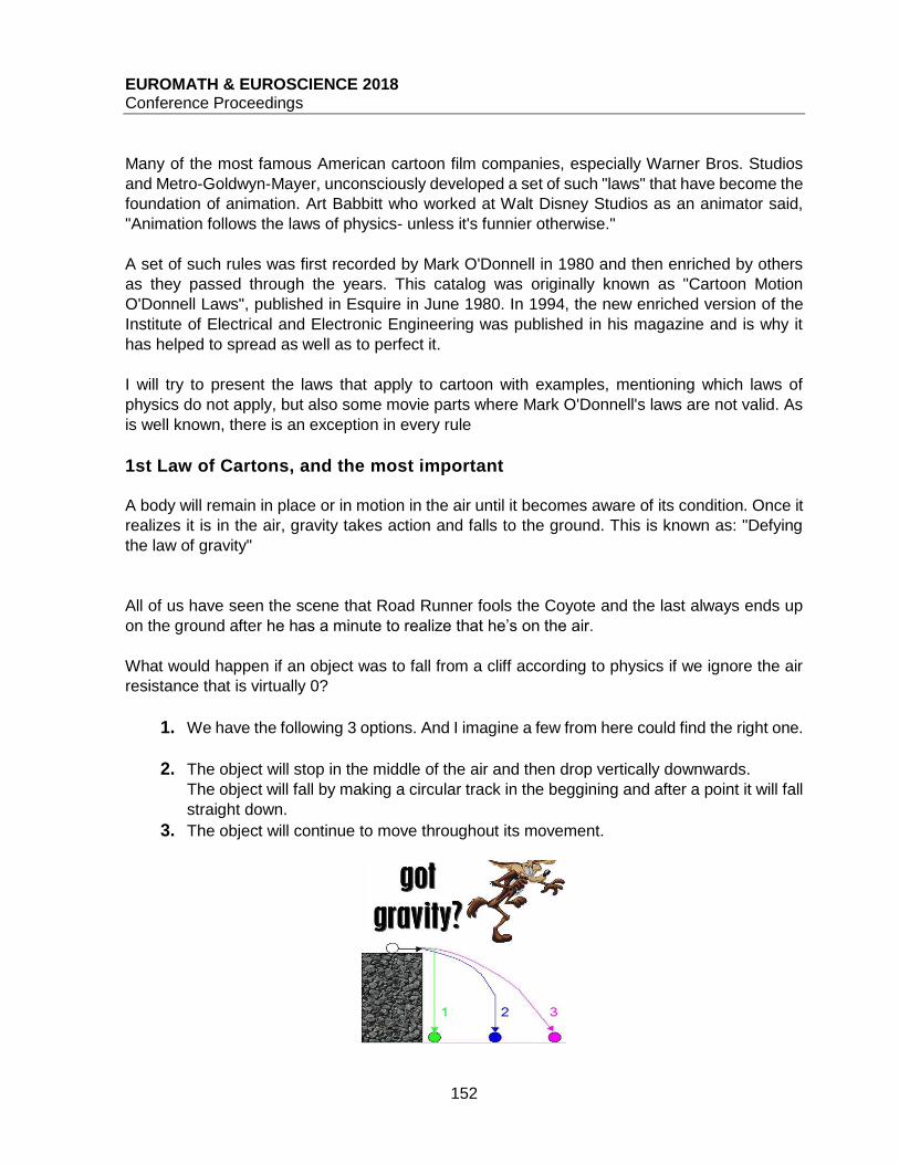
EUROMATH & EUROSCIENCE 2018 Conference Proceedings
152
Many of the most famous American cartoon film companies, especially Warner Bros. Studios
and Metro-Goldwyn-Mayer, unconsciously developed a set of such "laws" that have become the
foundation of animation. Art Babbitt who worked at Walt Disney Studios as an animator said,
"Animation follows the laws of physics- unless it's funnier otherwise."
A set of such rules was first recorded by Mark O'Donnell in 1980 and then enriched by others
as they passed through the years. This catalog was originally known as "Cartoon Motion
O'Donnell Laws", published in Esquire in June 1980. In 1994, the new enriched version of the
Institute of Electrical and Electronic Engineering was published in his magazine and is why it
has helped to spread as well as to perfect it.
I will try to present the laws that apply to cartoon with examples, mentioning which laws of
physics do not apply, but also some movie parts where Mark O'Donnell's laws are not valid. As
is well known, there is an exception in every rule
1st Law of Cartons, and the most important A body will remain in place or in motion in the air until it becomes aware of its condition. Once it
realizes it is in the air, gravity takes action and falls to the ground. This is known as: "Defying
the law of gravity"
All of us have seen the scene that Road Runner fools the Coyote and the last always ends up
on the ground after he has a minute to realize that he’s on the air.
What would happen if an object was to fall from a cliff according to physics if we ignore the air
resistance that is virtually 0?
1. We have the following 3 options. And I imagine a few from here could find the right one.
2. The object will stop in the middle of the air and then drop vertically downwards.
The object will fall by making a circular track in the beggining and after a point it will fall
straight down.
3. The object will continue to move throughout its movement.

EUROMATH & EUROSCIENCE 2018 Conference Proceedings
153
The first move is the one that always appears in the cartoons, but the correct answer is the third
one.
What laws apply to the object’s movement?
All the forces acting on it are balanced. So we are in equilibrium, meaning the sum of all forces
on it is 0 (ΣF=0)
According to Newton's first law or otherwise the law of motion (or the law of inertia) an
object at rest stays in a resting state until a force acts on it. Αn object in motion continues
to move (linear motion and steady speed) until a force changes this movement
In this example, the force acting on the Coyote is gravity, which is exerted on every body
regardless of whether it falls, is raised or moved. The weight has a vertical direction.
The blue arrows on the horizontal axis in the above image depict the speed of the Coyote uo
and the pink darts on the vertical axis the gravitational force. So the path to be followed is
designed with green, and that is the result of the above forces. So we can say that we have a
horizontal shot, meaning a complex motion consisting of 2 simple ones.

EUROMATH & EUROSCIENCE 2018 Conference Proceedings
154
Silhouette of Passage Everybody in the cartoon, while running, can penetrate with its body any object or physical
obstacle (wall / snow) leaving the print of its silhouette on it and this in the cartoon world is known
as the "silhouette of passage". But in the world of physics this would not be possible. Let's see
what exactly plays a role and how it will become reality.
In this example Gossamer (the orange monster) and the bullet have a mass “m” and runs at a
velocity “u”. In general, the behavior of a moving body depends both on the mass “m” and the
velocity of “u”. So, to study this case of “Collision” and others similar to this, we introduce another
vector quantity called momentum P and expresses the product of the mass “m” of the object and
its velocity “u” and is given by the formula: P = m * u. So we can study collision
phenomenons like this and the following example in which we shoot an apple with a gun and
the bullet passes through it. But what is their difference and the first is almost impossible while
the second one actually is? The speed… The velocity of the ball is far greater than that of
Gossamer, so it would realistically be impossible for him to penetrate the snow or the wall.
Balloon House Most of us have seen the Up movie and we remember the wonderful scene that the house takes
off using balloons. But can this eventually become a reality?
Helium balloons have a lifting force of 1 gram per liter. A normal balloon may have a diameter
of about 30 cm. The formula to calculate how many liters of helium can fit into a sphere is:
4/3*π*r3 where r is its radius. Thus, a normal balloon can lift about 14 grams, assuming that the
weight of the balloon and the string itself is negligible.

EUROMATH & EUROSCIENCE 2018 Conference Proceedings
155
A body weighing 50 kilos, which means 50,000 grams, will need 3,571.42 balloons to barely get
of the ground. In order to make sure that this mass will fly, we will need 500 balloons more, so:
4000 balloons total.
Lets take look from the perspective of physics on that:
Newton's first law applies if the balloons are exactly 3.571.42 . That means that total force is 0,
ΣF = 0. If there are 4000 ballons then we have Buonancy. Buoyant force =object’s weight -
apparent immersed weight. That way the mass can fly. Disney managed to lift a home using 300
huge balloons.
All these examples are creation of our own imagination but as we can see there is hope that
maybe someday with the help of science, the cartoons will become reality. What would happen
if could run with the speed of the Road Runner or walk in the air? Time will tell!
EUROMATH & EUROSCIENCE 2018 Conference Proceedings
156
EVOLUTION OF SPECIES AND ENTROPY Stelios Samaras, Sofia Bakali, Thanasis Bakalis, Christodoulos Karapatakis
Diastaseis, Private School, Greece
ABSTRACT It is a common misconception that the evolution of life contradicts the 2nd Thermodynamic Law. We argue that such a configured phenomenon as species evolution could not but be in accordance with the laws of physics. The 2nd Thermodynamic Law states that in a closed system entropy always increases. For the purposes of our study, we consider entropy as a measure of energy disorder and we will take into account that thermal energy is the most degraded, disordered, hence highly entropic form of energy. The Earth is an open system which constantly receives solar energy. During this process, while life evolves, living organisms may store energy in an orderly, low entropic way, but at the same time the sun entropy increases, while living organisms and functional ecosystems release highly entropic thermal energy. We may say that in a non-equilibrium system such as Earth, the variable species are the dissipating structures, with the ultimate goal of solar energy degradation to a disordered thermal form. Considering the aforementioned, life is not only compatible with the 2nd Law of Thermodynamics, but also necessary for its application. Despite the various approaches to determine whether evolution has connection with physics, from Boltzmann to Schrödinger and Eiger, there is still one question that arises. Since Earth and the evolving terrestrial life is a non-equilibrium system can entropy really be defined? Or maybe there should be some other parameters to estimate, in order to clarify this long-term debate about life being an improbable occurrence or an inevitable path given the circumstances of its origins.
Τheoretical Approach A. Introduction
Living organisms are highly organised and orderly structures, derived from a primodial soup of
elements and simple organic molecules and evolved following two main paths as described by
the Darwinian theory of Evolution to gradually more and more complex structures, such as
human, the most complex organism known today.
All these are a nicely put theory, not really difficult to understand and in general a quite easy
topic to wrap our heads around. But what happens when physics enter the topic? Does physics
clarify the origins of life and evolution?
EUROMATH & EUROSCIENCE 2018 Conference Proceedings
157
The 2nd Law of thermodynamics suggest that, spontaneous processes always cause an
increase in entropy, or simply tends to increase disorder.
Well, living organisms evolved to such orderly structures from a chaotic pool of elements and
simple molecules, while physics say that this is impossible. Does this imply that our whole
existence is impossible?
The scientific community is still in a debate considering the topic. For the purpose of our study
we tried to gather some of the current scientific aspects on the subject and lean to the conclusion
that life does not violate the 2nd Law of thermodynamics. Evolution may be a seemingly
contradicting process, but this does not make life impossible. Improbable maybe, but not
impossible. Some scientist also claim that life may be a necessity for the application of the 2nd
Law of Thermodynamics imperative.
Before coming to present the discussion of the topic evolution versus physics, we think it is
necessary to summarise the basics principles and theories of each scientific domain, since this
would give a more complete aspect of the topic.
B. Origins of life
Early earth formed 4 billion years ago and contained the building ingredients of life such as liquid
water, oxygen, hydrogen, carbon, nitrogen, sulfur and phosphorus, which are considered the
most important. Shortly after the earths formation, life occurred at about 3.8 billion years ago.
The main energy source for the necessary reactions and transformations was of course the solar
energy. The most popular and widely accepted theory for life formation is Oparin's theory of the
primordial or primeval soup, according to which the first simple organic molecules formed and
were later transformed or reacted to synthesize more complex organic molecules, such as
proteins, carbohydrates and of course nucleic acids, in an oxygen-less atmosphere, using the
solar energy. Here we are talking about order and organised structures again.
C. Evolution of species
Darwin describes the evolution of species as a process called natural selection and his
observations are driven to 3 basic conclusions.
- A survival battle occurs among the organisms of a population
- The outcome of the battle is not circumstancial, but depends on the characteristics that each
organism has heredited. Organisms with traits suitable for the current environmental conditions,
are those with the higher survival rate, i.e "survival of the fittest" as it prevailed to be said.
-The suitable or helpful traits, we may say, seem to be heredited more frequently, but of course
this is a result of the survival of the fittest. The organism that survives, reproduces and the "good
genes" go on to the next generation.
It is noteworthy that the unit of evolution is a population and not a single organism.
EUROMATH & EUROSCIENCE 2018 Conference Proceedings
158
Evolutionary theory affects populations, not single members of a population. A member may
appear one new trait at most but evolution in order to happen needs accumulation of new
hereditable traits.
Going on from the yet "orderly talk" about living organisms, we are talking about physics and
embracing chaos.
D. Entropy and 2nd Thermodynamic Law
We just skipped in a far more complex and intriguing topic.
We will try to explain what is entropy, or more specifically, what we consider entropy for the
purpose of our study, since this term alone is a conflicting one for the scientific world.
Entropy is usually defined as a measure of disorder, but that is a vague definition, that it is
misconcepted by the vast majority of students, but also scientists.
We try to clarify entropy definition, as used in our study, through simple examples.
Let's imagine a meadow with 3 sheep grazing happily. Let' s also imagine that this meadow is
divided in three land plots. The sheep move freely from one plot to another. If we take some
time to figure out all the possible configurations for the sheep, we will note that there are 10
possible configurations, as seen in figure 1.
A closer look to the possible combinations reveals, that there are 7 combinations where the
sheep are spread to more than one land plot, while there are only 3 "orderly" combinations
where the sheep are located only in one plot.
We automatically conclude, that it is more possible to see the sheep spread out at a certain
moment, than to see them all together grazing in one plot.
This is exactly what happens with energy. Energy tends to spread out. There is no specific
driving force for this process. It is just that when, sheep, thing, units are spread, there are more
possible configurations for them to be, this is what we call "microstate". In the case of the sheep,
there are 7 microstates where the sheep are spread out, but they all correspond to the same
"macrostate", we just see sheep spread out. This spread out image is a disordered one. It is a
state that is highly entropic. In others words, according to the aforementioned, it is a state with
more configurations and therefore a more probable outcome.
So, returning to energy, when energy is spread out we are talking about a high entropy state.
An why energy spreads out? Simply because there are more possible ways for the energy
packets, called quanta, to be placed among the particles of the matter.
The 2nd Thermodynamic Law requires an entropy increase during a spontaneous process. A
spontaneous process is a process that does not require work to be done in order to occur.
Does entropy always have to increase?
EUROMATH & EUROSCIENCE 2018 Conference Proceedings
159
Well, an increased entropy state, as we mentioned is a very probable one. As the number of the
sheep and the numbers of the plots increase, so do the possible configurations for the sheep.
Same goes for energy and particles. As the energy packets and the particles increase, more
and more possible way for the parcels to be placed to the particles arise. Since the whole number
of possible configurations increase, the chance of the "spread out" configurations also increases
against the chance of the "orderly" configuration. But it is useful to remember that a chance
always remains a chance, this means that there is always a possibility for an unlikely events or
process to occur.
Extending our examples, let's see something closer to our used definition of entropy.
Imagine a glass of liquid water and a glass of ice. If one was asked about which glass he thinks
is more entropic, the answer might be the glass with the ice, because our vision is a tricky sense
and may influence our reasoning. In order to be able to make any correlation between entropy
and evolution, we always need to think in terms of energy configurations. The liquid water has
more energy, since the liquid molecules are more mobile, so there are more energy
configurations in the liquid state of the water, i.e. there are more ways for energy to spread out.
According to that, one may say that entropy is a measure of energy spread out. Heat or thermal
energy is the most entropic energy form since it is characterised by intense movement of matter
particles and has a great tend to spread, hence heat moves from a hotter to a cooler object. But
since it is all about energy configurations, how come heat flow only from a hot object to a cold
one? Theoretically heat can also flow from a cold object to a hot one, but this just does not
happen because of the size of the system. As the size of a system increases, meaning atoms,
molecules and energy packets increase, so does the probability of the "spread out"
configuration, against the probability of the "orderly" configuration, which becomes extremely
improbable. Such a path of thought helps us woven out the usefulness of entropy. Entropy can
explain why some processes only go one way. Heat flows from hot to cold objects, air leaks out
of a punctured tyre, sheep are distributed all over the grazing area and we only evolve, we
haven't seen a species un-evolve, but can entropy really apply to living organisms? We made
an attempt to ascertain whether such a relationship exist and if so, we tried to figure out if these
to concepts, entropy and evolution have a contrasting relationship.
E. Energy degradation
A term usually met in this kind of arguments is energy degradation. Heat is the more degraded
form of energy, which means that it is difficult to convert thermal energy to another more useful
energy form. Heat usually appears as energy loss from a system. While driving out cars for
example, chemical energy of the fuels is converted to motion and that is the useful work we
need to be done, while heat generated in the car's engine is just energy loss, therefore we call
thermal energy degraded and when we talk about energy degradation, in essence, we are
talking about various kinds of energy transformed to heat.
Let's think for a moment, why is heat degraded and why it is difficult to convert it to other energy
forms. But because energy is as spread out as energy can be, or an energy form with great
spread out tendencies, hence highly entropic, so more probable state.
EUROMATH & EUROSCIENCE 2018 Conference Proceedings
160
Discussion Having explained all the necessary terms and concepts we can move on and examine the
debated matter of an existing contradiction between the 2nd Law of Thermodynamics and
Darwinian evolution.
Some inquisitive mind have wondered, and still do, about what is life. Schrodinger in 1943 issued
a book, "What is life?", trying to shed some light on this topic.
Schrodinger states that although life evolution seemingly defies the 2nd Law imperative, in
reality one does not exclude another. After all, the 2nd Law applies in isolated systems, while
living organisms exist in a world of constant energy ang matter fluxes, meaning a non-equilibrium
system. Entropy is actually defined in a closed system. This statement indicates the need for a
different, maybe more "elastic" approach of the law. Schrodinger' comments were food for
thought for his subsequents.
The more simplistic approach which suggest that life does not violate the 2nd Thermodynamic
Law, emphasizes on the fact that Earth is an open system, which constantly receives solar
radiation. Fusion processes in the sun's core release gamma-rays as a by-product. Gamma-
rays are transformed to the solar energy finally emitted towards earth, by the time they reach
the photosphere of the sun, which consists of visible light, infrared radiation and ultraviolet
radiation.
This theory further suggest that despite the decrease of entropy on earth due to evolution of
species, the 2nd Law is not violated because the total entropy of the sun-earth system increases.
In other words the sun's spreads its "orderly" packets of energy, increasing its entropy, while the
outer space absorbs solar energy and is heated therefore also increasing its entropy. Not to
mention that life on earth, despite its organised form, it also produces heat, also causing an
entropy increase. These processes are thought to cause such a big increase in entropy, that
compensate the small decrease cause by living organisms and their evolution. This opinion is
also supported by Styer (2008) and by Bunn (2009). Both scientist made some hypothetical
calculations of the entropy decrease due to species evolution and concluded that this decrease
is so small, that is compensated by the overall entropy increase in entorpy of the sun.
Sewel (2013) on the other hand, thinks that the compensation argument is invalid and does not
refute the fact that evolution is still an improbable occurrence.
Styer' and Bunn's approaches, also supported by many other scientist, all make the same
assumption, that all that is needed, so that the 2nd Law still applies, despite evolution, is just an
external energy source, the sun. Sewel states that the external energy source and its entropy
increase, still does not explain how or why the decrease of entropy because of evolution occurs.
He also states that the 2nd law is all about predicting the most probable macroscopic outcome,
while taking into account what happens at a microscopic level. (Remember, the most possible
outcome is to observe heat transfer from a hot object to a cold object, because there are more
energy configurations this way and this makes the heat flux from hot to cold more probable). He
EUROMATH & EUROSCIENCE 2018 Conference Proceedings
161
also uses an extreme paradigm of a tornado hitting a town and turning it into rubble. Then a
second tornado hits the same town and turns the town back to its initial form! The case of the
second tornado is a violation of the 2nd law that defies common sense. But still talking about
probabilities, anything can happen, even if we are talking about something that none of us will
see in a lifetime. This way Sewell wants to underline that the simplistic approaches, as described
above, cannot apply to living organisms in a way that could really describe the phenomenon of
evolution and the origins of life.
A more integrated approach was given by Schneider and Kay, in 1994, although it was not given
the appropriate value and has not really been discussed.
The authors of this paper relied on a restatement of the 2nd law in order to explain how the
beginning of life is really in accordance with physics.
The reformulated 2nd law says that when a system tends to resist or even "neutralise" the
gradients which are submitted on them. A simpler way to put this is that, under certain
circumstances, organised structures can emerge, in order to help the progress of a physical
process.
An everyday example of these emerging organised structures is seen when we are washing a
bottle with a narrow orifice. We fill the bottle with water, turn in upside down, so that the soap is
washed off. Leaving aside difficult terms such as entropies, energies, systems etc for a moment
and just focusing on the expected, on the physical we may say result, what do we get? Just
water flowing down from the bottle to the sink. Let' see what will happen, if we are in a hurry,
while washing this bottle and give it a little twist. A mini vortex will appear and the bottle will
empty much more quickly. What happened there? We gave a little energy and water molecules
organised in a highly ordered structure of numerous molecules combined, just to help the water
flow to a lower part and all of these just seem so logical, so "natural".
Using this simple observation as an analogy, we can now think of living organisms as dissipating
structures! Energy flows from the sun towards earth. Energy also tends to spread and the energy
form with the greatest tend to spread is heat. That may be considered the "natural" process, as
mentioned above, according to the laws of physics, not to forget entropy increases, disorder
increases. How? Through the spread of heat. Now it starts to make sense. Life is for the sun-
earth system the same thing as the mini swirl observed in the bottle. Living organisms help the
flow of the incoming solar energy and its degradation to heat, the most disordered and highly
entropic energy form. In other words, evolution helps the application of the 2nd Law of
Thermodynamics.
The initial statement of the law is quite restrictive, since it applies to closed systems in an
equilibrium state, without energy or matter fluxes. In context of the restated law, life is a
dissipating structure, formed within a non-equilibrium system, to help the solar energy flow and
its degradation to heat. The ultimate "goal" of a system, is to reach at an equilibrium. And what
can be considered equilibrium for our terrestial circumstances? The equalization of temperature,
according to Boltzmann, achieved by the heat spread out. And why is that? Because a spread

EUROMATH & EUROSCIENCE 2018 Conference Proceedings
162
state for the energy is the most probable one, as explained above. As simple as that, a matter
of chance.
Summing up, order can arise from disorder in a simple physical systems, if this is for the purpose
of helping the system reach an equilibrium, do the expected natural thing. Highly organised
structures can emerge in order to neutralise an incoming gradient. This way from an element
soup the first organic molecules were formed, which gradually transformed into more and more
complex structures, according to Oparin's theory and under the continuous influence of solar
energy the first living organisms arose. From then on, evolution of these organisms took place
in order to create more solar energy dissipative pathways, resulting in its degradation, its spread
out. From this aspect, evolution seems to be an inevitable phenomenon, necessary for the
application of the 2nd Thermodynamic Law imperative, as Eigen has stated.
The well-known darwinian "survival of the fittest" driven by environmentally appropriate
hereditable traits and maybe some random "good" mutations can now be seen as survival of the
species which are more effective into dissipating energy and thus producing entropy. The more
developed the living structures, the more energy they will be able to degrade.
Biological systems develop in a manner as to increase their energy degradation rate. Evolution
occures for the shake of new dissipating pathways formation. Species diversity and even
ecosystem growth can now be attributed to solar energy, as the more simplistic approaches
describe, but now it makes more sense and might be an answer to Sewell's justifiable
speculations about life being an improbable occurrence.
Ecosystem development increase energy degradation, thus follows the 2nd law of
thermodynamics. More biomass means there are more dissipative pathways, while species
diversity can be translated in means of more different pathways, all for one purpose, energy
spread out and entropy increase.
From a clearly biological point of view, life is more abundant where food and energy sources are
profuse. Life thrives at the equator tropical zone, but isn't that the region where the incoming
solar energy is the greatest? More sun, more dissipating structures needed, more life. Under
this path of thoughts, the conjugation of biology and physics is achieved. Life and evolution, not
only does not contradict the laws of physics, but emerged because of them.
Conclusions We still aren't able to verify a relationship between evolution and entropy, but given a try to really
understand the entropy, we think that these two concepts are not really that incompatible. From
oversimplified approaches and calculations by Styer and Bunn, to reasonable questioning of
life's improbability by Sewell, the idea of dissipating structures described by Schneider and Kay
looks like a quite solid and complete description of the reasons for life's origins and evolution.
The most important achievement of this theory is the successful conjugation of the two sciences.
So is life an improbable phenomenon, an impossible occurrence, in complete accordance with
physics or even a necessary incident? That is a question that still, no one can answer with
certainty. We what we actually noted through our study, is that, when keeping an open mind
EUROMATH & EUROSCIENCE 2018 Conference Proceedings
163
about specific scientific terms, such as entropy, then the two sciences do not seem so
incompatible.
Schrodinger was one of the first to put the question of what life really is, in a scientific way. Our
guess is that we are still far away from such answers.
At this point we would like to quote some words of an enlightened modern day physisist, Aatish
Bhatia, "The story of our universe is that of climbing Mount Entropy. Both the base and the peak
of the mountain are inhospitable to life, but somewhere along those rising slopes, the conditions
were just right for complex and wondrous things to emerge, things like trees and jellyfish and
heartache and cheesecakes "
Maybe we are just a swirl in a bottle charged with an Aristotelian "final cause", with a duty, to
drive the universe to energy degradation, to an equilibrium. Since that sounds a little sad, we
prefer Bhatia's approach of life as a wondrous journey.
From there on we are entering the real of philosophy, and philosophy is clearly a matter of
perception.
Acknowledgments We would like to thank, Dr. Aatish Bhatia, for his excellent description of the entropy concept,
which made the understanding of such a difficult term as entropy fiesible.
Video of Jeff Phillips, giving every day examples of entropy were also of great help for the
completion of this study.
EUROMATH & EUROSCIENCE 2018 Conference Proceedings
164
FUTURISTIC HUMAN VISION WITH LENSES Tsempis Konstantinos
Diastaseis, Private School, Greece
ABSTRACT
Glasses have already ‘invaded’ in everyday lives due to the continuous use of technological devices and gadgets, which cause a lot of eye strain. Furthermore, many people are taking advantage of their aesthetic presence and incorporating them into their entire look. However, this eye strain, ends up developing refractive errors on the individuals’ eyes. Contact lenses, prescription frames, and refractive surgeries are all together aiming to correct all the abnormalities that are caused from the refractive errors (myopia, hypermetropia, astigmatism, presbyopia, a.o.), thus providing better vision quality. - Do they address the problem at its roots? In the future, there is a possibility that our glasses will be adjusting themselves for different purposes of use, for example we will able to focus on an object several kilometers far away, see through solid structures like X-rays, they will protect our visual system from radiations either natural e.g. solar or man-made e.g. nuclear power, e.t.c. Our contacts will send an SMS when our eyes need hydration or the eye pressure is above the set limits. - How will optics, ophthalmology and human eye system biology develop in the following years? This presentation will be addressing general informative content about lenses, and refractive errors, and we will all disodiscuss the future of human vision.
FUTURE ASPECTS ON GLASSES AND HUMAN VISION INDRODUCTION Optics is the branch of optics that involves the general behavior and the properties of light. Light provides us the opportunity of the visual understanding of the world we live in. Without our eyes we could see nothing but an empty black, being unable to admire nature’s miracles, the life itself. Today we will discuss the way we see, the refractive errors of our optical system and some futuristic aspects of human vision.
LENSES
First and foremost, the light is a wave itself and needs to be altered in order to be ‘used’ properly
by almost all beings. This is when a lens takes up a role in the game! A lens has the ability to
change light’s direction in a specific order. Futhermore, there are two major lenses types convex
and concave. A convex lens can converge or concentrate the light onto a certain point and its
called positive+, while a concave lens takes the light from a point and diverges or spreads it out
to another and its called negative-. These two take their power of concentrating or spreading out
from their structure and curvature and they seem to appear spherical. Either they have a wider
side in the middle or on the edges. We measure lens power in diopters (equivalent 1m of light
direction change per 1D). That curvature gives them refractive power, due to the fuction of

EUROMATH & EUROSCIENCE 2018 Conference Proceedings
165
prisms. Prisms are more complicated bodies that again have the ability to alter light’s direction
and break the beam up to its spectral lights (a beautiful rainbow).
The most common convex lens is the magnifying glass used to enlarge small letters, see
something small in detail, etc. Another not really known type of lenses, though they are widely
used, are the cylindrical lenses. That ones, concentrate or spread out light in a line and not on
a point. They are specifically curved in order to have their power on an axis and not on the whole
surface. Additionally, there are some lenses that combine different powers onto their surface, a
very useful faction when presbyopia takes place. Now all the refractice errors of one person can
be treated with on pair of glasses and not multiple ones. Bifocals combine 2 focal powers,
Trifocals combine 3 focal powers and progressive have a more stable change focal powers
throughout their surface.
(BRIDGE-CONTACT LENSES)
We talk about lenses as we will use them afterwards in the refractive errors section. As you may
have understood lenses are used to cure some visual problems.
Lenses could be fabricated from plastic or glass. Nowadays many people rather prefer contact
lenses instead of concentional glasses. Contact lenses do exactly the same job with frame
glasses with some benefits like aesthetics, better vision quality for high power problems, wider
range of vision not restricted on the glasses surface. Nonetheless, the can be proved to be fatal
for some individuals. We will talk about that later.
REFRACTIVE ERRORS AND ABNORMALITIES Its sure that all people have heard of myopia or nearsightedness. Myopia is the inability to see
clearly or in quality over a distance. That happens because when the light enters the eye it
focuses in front of the retina, reflecting back on. The eye might be bigger than normal and it
follows that light doesn’t reach its point on the retina. Otherwise, our natural eye lens is more
powerful than needed and thus the light is not properly focused again. There is a specific type
of myopia, pseudomyopia and its caused due to poor lighting conditions, long hours of short
distance focusing, like computing, typing, etc. Eye lens becomes stiff and less flexible due to all
above practices, adapting a myopia finally. During darkness, some people do not see properly,
like having myopia, whether they really have it or not. First symptoms of patients start when not
being able to see the white board, read advertising panels, driving as they used to and others.
The most common practice of myopes is that they to shut their eyes a little in order to see better,
successfully. There is no problem with short distances like reading, except in myopias of more
that -5D. If myopia is derived from biological causes it starts about 7-8 years old to progress. In
many adolescents their myopia starts to thrice and ceases at biological maturity.
Myopia is cured with concave lenses that push light back paroperly onto the retina.In myopias
under -1.00 it is suggested that prescription glasses are not used to put eyes to adjust naturally
in long distances, though if eye strain and seazuress are caused another treatment takes place.
Contanct lenses and surgery precedures can be utilized.
Hypermpertropia or hyperopia or farsightedness is vastly noticed at toddlers and young children,
as their eyes are not formed well till that age and the lens is unable to focus light in such a short
distance. Hypermetropia is determined by a strenuous constant try to see properly especially in
EUROMATH & EUROSCIENCE 2018 Conference Proceedings
166
short distances. Eye strain and headaches follow, as long with vision distortion like missing a
line while reading. What is more, light is focused behind the retina providing a bad quality image.
Most of the times its goes away without doing anything as the eye becomes larger and more
addaptice to all conditions. Convex lenses are used to pull the light forwards on to the retina.
Last but not least, untreated conditions of high hypermetropia could even lead to sever damage
over the optical nerves and other conditions like amplyopia or neural problems.
Astigmatism exists in every person as our eyes cannot be by nature perfectly spherical, most of
the times combined with myopia or hypearmetropia. Astigmatism’s cause is not known exactly
till now, but the main cause is cornea’s (the front part of the eye) shape. Cornea becomes
sharper in some parts and less wide in others ending up to a general light misalignment inside
the eye its is like saying that the cornea should be round like a football but in astigmatism it’s
more egg shaped like a rugby ball. Light focuses either in front of the retina or behind, as
astigmastism is almost always with the refractive errors of myopia and hypermetropia.
Hypermetropia does not occur with myopia as they are contrary cases. Astigmatism regards to
a generally distorted sight but the worst problem is on the meridians (axis of astigmatism). Eye
strain with headeaches are also induced. It is the most difficult problem to cure as it is in favour
of specific cylindrical lenses on the frame or toric conantc lenses curved in position of your eye.
High astigmatisms are not operated properly through regular surgery as the part of the cornea
is aligned and cut by hand, laser operations are more accurate though a little portion of
astigmatism is still left over.
Presbyopia takes place after forties. The muscles that control the lens of the eye become stiff
and they do not contract properly for short distances. In most cases patients barely see their
newspaper or small letters. They do the characteristical move by getting their whole head far
away. Additional focal power is introduced to the patient with a change in prescription in current
glasses or new reading glasses. Surgeries are not that effective as an implement lens gets in,
though concex lenses work fine focusing the light on the retina.
ASPECTS
Glasses frames come in a variety of shapes, colours and structures in order to compensate each
person’s need. They provide an aesthetic appearance and they even make a more sophisticated
look.
Contact lenses are all disposable and they have an expiration date and certain days of use.
They can even change iris colours giving an elegant style to the user. They can be proved to be
fatal as an unwise use can lead to severe allergies, eye soreness, infections and finally even
death.
What is more and not that researched, is the beneficial use for certain diseases like diabetes
and hypoglycemia, allergies, diabetic eye and high eye pressure, conjunctivitis or even anemia!.
Nano circuits can be implemented on the silicone lens, working like a small laboratory taking
measurements of the eye stability, all the enzymes or percentages of certain substances. For
example, tear levels are below the set limits, the lens will connect with your phone sending an
SMS alerting you to get some drops instantly. Your insulin injection time can be instructed by
the lenses giving you specific details for your sugar lenses.

EUROMATH & EUROSCIENCE 2018 Conference Proceedings
167
Some electric lenses like that one in games like call of duty etc, can be focusing on target far
away or even zooming on it. The soldier can now see body temperature, water concentration,
oxygen supply.
Contact lenses are really effective for the cure of keratoconus also.
Some substances could be fabricated and poured onto the eye surface as UVA UVB radiations
become dangerous for our everyday life. Even more, blue light from monitors and smartphone
screens, can be reflected or absorbed by that kind of substance.
Furthermore, other lenses could be changing shape constantly in order to ensure the perfect
visual acuity for the user.it has been suggested that atropine could prevent the adoption of
myopia in teenagers when myopia is firstly recorded about 8-9 years old. Although, the post
effects of atropine are not really knonw (expirement Asia).
Glasses that beam X-Rays can provide a wide range of vision within buildings like where
something is hidden, helping police forces, or in security forces in airports where guards can
wear that glasses and determine some criminals for example.
Karyotype research in molecular level, can prevent the creation of high powers of myopia more
than -7D, with targeted chromosomal treatments.
WE ALL NEED TO REMEMBER THAT GLASSES AND ALL KIND OF EQUIEPPMENT USED
PROVIDE US A SUBSTITUTE OF REALITY AND THERE IS NO MACHINE THAT CAN
OVERPASS HUMAN VISION OR OTHERS’ ANIMALS EVEN BETTER THAN OURS. THERE
IS NO SUCH THING LIKE PERFECT VISION!

EUROMATH & EUROSCIENCE 2018 Conference Proceedings
168
THE MAGIC OF COSMOGENY, A NEVER-ENDING QUEST Georgiadis Doukas
Diastaseis, Private School, Greece
ABSTRACT The journey began 14 billion years ago… Man’s journey though started when the first men - as thinking beings – asked themselves “why?” and “How?”. Man has always had the need to explain anything existing, moving or functioning around him. That is the reason why he queried “why” and “how”. How was the world created? That is how it all started. Firstly, theologians tried to explain cosmogeny on the basis of divine or metaphysical forces. On the other hand, common people, throughout the years, turned to myth-making in order to give explanations about the creation of the world. Further to myth-makers, it was the philosophers’ turn to give their own interpretations. The first attempt of explaining the world creation philosophically was by Thales of Miletus. Plato and subsequent philosophers as well, based their ideas on the qualities and propensities of the four elements. In the meantime, the Enlightenment, research and eventually natural sciences bring to light important results and essential conclusions after a series of great discoveries and inventions. Science and technology therefore, after billions of years, make man’s long lasting journey reach its peak. The dominating theories on the creation of the world are two. First is the theory of the great explosion and second is the one of superstring theory. Finally, how was the world created? What happens with time, place and any other dimension? Are we talking about a restless circular course of beginning and end, creation and collapse? In this essay, there will be an attempt for the most of the above questions to be answered.
Man has always wanted to know how he was born and how the world was created. And that is
what I am going to present here today. I’m going to present the endless journey of man in order
for him to find out how the entire universe was created.
As man has always wanted answers on this matter, he turned to any source available to satisfy
this thirst for answers.
That is why we are going to see a series of gradual steps that led him to some explanations on
the issue of the world creation.
Starting from Mythology, Philosophy, Theology and Religion and finally Science:
Starting from Mythology, we can refer, for example, to the Chinese belief that the entire universe
was concentrated in an egg. All matter was in there with a sleeping giant Pangu. When Pangu
woke up, the egg broke and all substance was spread everywhere forming this way the sky and
the earth. Later on, the sun was created from Pangu’s eye and so on. So, we can easily
EUROMATH & EUROSCIENCE 2018 Conference Proceedings
169
understand that in the Chinese people’s imagination, everything started from an egg, that is to
say a central core.
The Egyptians, on the other hand, believed that Atum, a divinity, cried once and her tears, tears
of joy, gave birth to mankind. It is easy to see that anything that cannot be explained is credited
to divine power.
Now let’s go on with the Babylonians. According to their myths, chaos existed everywhere and
out of chaos, a God-creator was born. That was Abzu (means freshness) who created with his
wife the Gods and then mortal people for hard or manual labor. It is clear here that at that time
people needed not only Gods to protect them but also workers to work in the land (for agriculture
and cattle-breeding).
At the same time, the ancient Greeks, according to the Orphean myth, believe that the world
creation begins from water and from a divinity an egg is born. This egg breaks and the sky and
the earth are formed. Here we have the egg again the same as the Chinese myth.
Well, one thing we can only see from all these myths: OUT OF IMAGINATION, THE JOURNEY
OF QUEST HAD ALREADY BEGUN AND THE SEED OF DISCOVERIES HAD ALREADY
SPRUNG UP.
Not accidentally, Albert Einstein said: “IMAGINATION IS THE HIGHEST FORM OF
RESEARCH”
And, as the intelligence of man develops, the world creation cannot be explained on mythological
basis. Man can realize the inaccuracy and the vagueness of these explanations. It was then that
philosophy appeared.
Philosophy was mainly developed in Ancient Greece. Greek philosophers put fundamental
questions about the existence of the world and natural phenomena in general.
Democritus, Socrates, Plato and Aristotle are considered to be the pioneers of a more scientific
and rationalistic approach to the matter of cosmogeny.
Of course, their ideas had also influence by theological, metaphysical and philosophical
extensions. Meanwhile, mathematics is used to help people understand and explain the laws of
nature.
After philosophy had put the questions about the world creation and several voices were heard.
There came the time when the first scientists came to the front. For example, some of the most
important ones are:
EUROMATH & EUROSCIENCE 2018 Conference Proceedings
170
First scientists:
Euclides – the creator of geometry – 3rd century B.C.
Archimedes – famous mathematician, physicist, engineer – about 212 B.C.
Aristarchus - astronomer and mathematician who presented the heliocentric system - about 230
B.C.
It was then that astronomers appeared as well:
Astronomers:
Eudoxus – about 355 B.C. – Plato’s student – creator of a geocentric system
Hipparchus – about 125 B.C. – the most famous one that time
Of course, astronomy then could not get rid of the ideological and mythical elements of that
period of time.
Nevertheless, the important thing here is to focus on the geocentric model of Plato and the more
realistic model of Aristotle, yet geocentric too.
After the 3rd century A.D., comes the Age of Obscurantism, the Middle Ages.
The source of truth is all written in the scripts where nature was created by God and the laws
that govern it come from God’s will.
This belief automatically pushes aside science and philosophy. It is a time of decline for those
two.
Renaissance:
The bridge between the Middle Ages and Modern Times.
Europe makes its first steps out of “darkness” and the birth of a great personality to mark the
evolution of science. The Polish monk, Nicolaus Copernicus, develops the idea of the
heliocentric system as well as the idea that both the earth and the moon revolve round the sun
and other celestial bodies of the solar system, too.
Copernicus was inspired by Plato’s and Pythagoras’ ideas. In his book “De Revolutionibus”, he
puts forward his heliocentric theory and names “gravity” the power that moves the celestial
bodies.
That is how Copernicus displaced the geocentric and in extension, the anthropocentric system
and put the sun in the centre of the universe.
What a reversal!!! These ideas could not, of course, run with any objections and rejections! The
Christian and the Protestant world could not accept but only the geocentric and anthropocentric
world.
EUROMATH & EUROSCIENCE 2018 Conference Proceedings
171
Copernicus though, described the laws of nature and Kepler completed it, (he formulated the
laws of the motion of the planets).
Galileo then formulated the first laws of mechanics and contributed to the turn of science for
observation, experiment and mathematical calculation.
Finally, this entire journey would reach Newton’s formation of a mechanistic cosmic idol of nature
with solid and undivided atoms, forces from distance, the Euclidean and infinite space.
After 2000 years of human history, Aristarchus, Copernicus, Kepler and Galileo, the heliocentric
system had finally been proved.
TOWARDS THE 19TH CENTURY
Since the 19th century the development of science and technology has been rapid. Albert
Einstein and Relativity Theory (it’s about a physical phenomenon description).
Quantum Theory (it’s the theory of light, the idea that light exists as tiny packets, or particles,
which he called photons)
“BigBang” theory (it’s the leading explanation about how the universe began) which we are going
to see later on, in this presentation.
All these are some of the theories and speculations formed that period of time. Newton’s theories
on gravity effects were determinant in the development of mechanics and cosmology. Newton
speculated that gravitational interaction is transmitted within space at an infinite speed.
Now, any quest for the creation of the world is based on positivistic and rationalistic perceptions.
Hume’s and Kant’s theories are such, accordingly.
For Hume: an inexhaustible source of knowledge is experience.
For Kant: all matter was at first as gas, spread more or less same in the universe.
Today we know that laws of nature are not eternal but just “instant” approaches to reality, which
they do not exhaust.
THE SCIENTIFIC TRUTH OF TODAY
Ιn 1924, Hubble established the Andromeda nebula as a galaxy just the same as ours.
This establishment opened new horizons to cosmology and the evolution and structure of an
approachable part of the universe.

EUROMATH & EUROSCIENCE 2018 Conference Proceedings
172
Mathematical frame and microphysics in cooperation
As we said before, with Einstein, the mathematical frame for cosmological models existed, but
microphysics completed the large-scale undertaking.
Their dialectical combination led to contemporary cosmological models.
So, their dialectical combination brought about the cosmological models we are going to see
right away.
CONTEMPORARY COSMOLOGICAL MODELS
- Expanding universe model ( Alexander Friedman, 1922)
Α pioneering theory that the universe was expanding, governed by a set of equations.
- Steady state universe model (1948, Hermann Bondi, Thomas Gold and Fred Hoyle)
The steady state model is based on the assumption that on the large scales the universe is
completely homogenous.
The density of matter in the expanding universe remains unchanged due to a continuous
creation of matter. That is, the observable universe is basically the same at any time as well as
at any place.
- Big Bang model ( Georges Lemaître, 1931 – model advocated and developed by George
Gamow, 1952)
- Big Rip theory (2003 - Marcelo Disconzi)
At the time the Big Rip occurs, even space time itself will be ripped apart and the scale factor
will be infinity. That is the end of the universe based on its increasing expansion rate.
FOCUS ON THE PREVAILING THEORY OF BIG BANG – A BRIEF TIMELINE
As we can see, the big bang starts at 10 to minus the 35th power of a second. The universe is
shaped at 10 to minus the 6th power of a second and at 3 seconds we have the basic elements
formed. After 10.000 years comes the Radiation Era and Matter dominates after 300 thousand
years. Finally, it needs 300 million years for stars and galaxies to form.

EUROMATH & EUROSCIENCE 2018 Conference Proceedings
173
Conclusion
Man in need of answers on cosmogeny. To sum up, the following brief chronicle can show us
the great leaps forward
1791: Erasmus Darwin: The description of a universe that expanded and contracted in a cyclic
manner was first put forward in a poem.
1848: Edgar Allan Poe: presented a similar cyclic system in his essay titled “Eureka: A Prose
Poem”
1927: Georges Lemaître: proposed an expanding model for the universe to explain the observed
redshifts of spiral nebulae.
1929: Hubble: discovered that, relative to the Earth and all other observed bodies, galaxies are
receding in every direction at velocities (calculated from their observed red-shifts) directly
proportional to their distance from the Earth and each other.
1931: Lemaître: proposed in his "hypothèse de l'atome primitif" (hypothesis of the primeval
atom) that the universe began with the "explosion" of the "primeval atom" — what was later
called the Big Bang.
The Big Bang theory could explain both the formation and the observed
abundances of hydrogen and helium.
1990s and the early 21st century:
Huge advances in Big Bang cosmology were made as a result of major
advances in telescope technology in combination with large amounts of satellite data, such as
COBE (COpenhagen and BErlin – the two founders’ origin), the Hubble Space Telescope
and WMAP
(Wilkinson Microwave Anisotropy Probe)
That is how we can understand how galaxies form in the context of the Big Bang and we can
also understand what happened in the earliest times after the Big Bang and reconcile
observations with the basic theory.
BUT: - Actually, what existed before the explosion?
- What is that dark energy in the universe?
- Will a similar explosion happen again?
- Is there an end somewhere?
- Is there going to be a total disaster and start from scratch, all over again?
- Is there someone, something protecting man kind and life, up there?
SOURCES:
https://el.wikipedia.org/wiki/cosmology
https://ultraculture.org/blog/2016/04/28/5-mythological-stories-world-created

EUROMATH & EUROSCIENCE 2018 Conference Proceedings
174
https://plato.stanford.edu/entries/cosmology-theology
https://www.space.com/16042-cosmology.html
http://www.atnf.csiro.au/outreach/education/senior/cosmicengine/classicalastronomy.html
https://www.encyclopedia.com/science/science-magazines/astronomy-and-cosmology-big-
bang-theory-and-modern-cosmology
https://en.wikipedia.org/wiki/Timeline_of_cosmological_theories
https://en.wikipedia.org/wiki/Johannes_Kepler
https://en.wikipedia.org/wiki/Edwin_Hubble
https://en.wikipedia.org/wiki/George_Gamow
https://en.wikipedia.org/wiki/Georges_Lemaître
https://en.wikipedia.org/wiki/Big_Rip
http://www.wired.co.uk/article/big-rip-end-of-the-universe
EUROMATH & EUROSCIENCE 2018 Conference Proceedings
175
A QUANTUM BRAIN? Apostolou Era., Dimitrakopoulou Athina. Dimitrakopoulou M., Gennaraki Garyfallia, Minaretzi
Fani, Mpakella Aikaterini, Karalekas Ioannis, Koumpi Olga, Koudigkeli Geogia, Safarika
Eleftheria, Sapounaki Ioanna, Syrigou Kassiani
Pierce - The American College of Greece, Greece
ABSTRACT The inconsistencies of Bohr’s model, Schrodinger’s equation and Heisenberg’s uncertainty principle contribute to the evolution of the quantum mechanical model. Many concepts of this model (e.g., particle-wave duality, superposition) are counter-intuitive. But is this due to our cognitive inability or to inherent obstacle in nature? Abbott with his famous “Flatland” would argue in favor of the first whereas Heisenberg for the second. Interestingly, many researchers propose that quantum processes may also happen in the brain. Quantum entanglement is a phenomenon that might underlie neural processes. If this holds true, then could it also be true that the brain can engage in two or more thoughts at the same time by quantum superposition? Moreover, could it be true that quantum computers might lead to human-like intelligence in computers?
BOHR’S MODEL OF THE ATOM
Danish physicist Niels Bohr won the Nobel prize in Physics in 1922 for his work that founded his
model for the atom. Bohr’s model can be described with the following statements:
a) Electrons circle the nucleus in certain orbits.
b) The number of the orbits in an atom is finite.
c) Electrons can move from one orbit to another.
d) The energy of the orbits is quantized.
e) Each orbit is of certain energy, meaning, that the lowest energy is found in the smallest and
closest to the nucleus orbit, while the highest energy is found in the bigger and most distant from
the nucleus orbit. Each orbit is characterized with a number n, (ex: n=1, 2, 3 etc.) called the
principle quantum number.
Although Bohr had proposed a good model of the atomic structure, used even today for
educational reasons, it was later proved that it fails to explain the real atomic structure. For
example, Bohr’s atomic model only works for atoms with one electron (hydrogen), as his
calculations do not include repulsions between electrons. Moreover, the Bohr model is
incompatible with Heisenberg’s Uncertainty principle. This happens because the Bohr model
stated that in the atom we know both the location and the energy of an electron simultaneously.
However, according to the Uncertainty principle we can’t know both exactly the position and the
momentum at the same time.

EUROMATH & EUROSCIENCE 2018 Conference Proceedings
176
De BROGLIE HYPOTHESIS AND EXPERIMENTAL PROOF In 1924, Louis-Victor-Pierre-Raymond de Broglie, influenced by Einstein’s papers published
about 20 years before (in 1905) concerning the behavior of electromagnetic radiation as
particles, stated a theory which gave him the Nobel Prize for physics in 1929. he was nominated
for “the discovery of the wave nature of the electron”. De Broglie suggested that all matter has
wave properties, a concept known as “de Broglie hypothesis”.
His revolutionary idea, which is, nowadays scientifically proved, through several experiments,
with widely known the once performed by C. J. Davisson and L. H. Germer.
The Davisson-Germer experiment was conducted in 1923-1927 and their goal was to study the
bouncing of electrons when they were fired by an electron gun towards a nickel crystal in a
vacuum chamber. In order to detect the bounced electrons, a moveable detector was used.
When an accident happened during the experiment, air was introduced in the vacuum chamber
and a film of nickel oxide was formed on the surface of the metal. When the two physicists
heated the metal to remove the oxygen, the nickel atoms were rearranged, but the scientists did
not know it. When the experiment started again, electrons were diffracted from atoms that were
also inside the nickel lattice. At certain angles, the detector resulted in peak intensity which could
be explained by the wave behavior of electrons. These intensity peaks were the constructive
interference of electron diffraction. The hypothesized de Broglie wavelength of the electrons was
expected to be 0,167 nm. The measured wavelength through Davisson-Germer experiment was
0,165 nm according to Bragg’s Law (i.e., Bragg’s Law correlates the wavelength of a wave (λ),
the distances (d) of particles in a crystal lattice and the scattering angle, θ). Two waves can
interact in a constructive manner (they are added) or in a deconstructive manner (they cancel
each other).
SCHROEDINGER’S EQUATION AND HIS CAT
Schrodinger equation is extremely important in quantum physics and governs many phenomena
of the microscopic world. Erwin Schrodinger was a physicist who set out to find a wave equation
to describe the electron of a hydrogen atom (1926).
Schrödinger applied it to the hydrogen atom, predicting many of its properties with remarkable
accuracy and by that, he established the correctness of his equation.
In his “thought experiment”, a cat was placed in a closed box with some certain objects like a
radioactive source, a Geiger counter to measure radioactivity and a bottle of poison.
If radioactivity is detected, the Geiger counter will trigger a hammer to break the poisonous bottle
and the cat will be killed.
This experiment was aimed to reveal the flaws of the ‘Copenhagen interpretation’ of quantum
mechanics. This interpretation supports that a particle exists in all states at once until it is
observed.
In similar context, the cat too is both alive and dead until the box is opened. Schrödinger actually
tried to use common logic that says this can’t happen in order to emphasize the limits of the
Copenhagen interpretation when applied to practical positions.
But as irrational as it may seem, Schrodinger’s cat is actually real!

EUROMATH & EUROSCIENCE 2018 Conference Proceedings
177
HEISENBERG’S UNCERTAINTY PRINCIPLE
Heisenberg’s Uncertainty Principle was firstly discovered by the German physicist Werner
Heisenberg back in 1927. With this principle Heisenberg won the Nobel prize in 1932. According
to this principle, humans cannot define the exact position (x) and the exact momentum (p) of a
particle at one specific time. This does not happen because we are unable to define these two
phenomena, but it is an inherent principle in our world. The mathematical formula for
Heisenberg’s principle of uncertainty is Δx ∙ Δp ≥ h/2π. Heisenberg said, that when we measure
the position of a particle with uncertainty (Δx) and at the same time we measure its momentum
(Δp), again with uncertainty, then the product of these two quantities can’t be less than a specific
number (h/2π). Having said that, the more precisely the position of some particle is determined,
the less precisely its momentum can be known and vice versa. The uncertainty principle is one
of the most famous aspects of quantum mechanics and through this principle we can see how
quantum mechanics (physics in the microcosm) differ from the classical theories (physics in the
macroworld).
QUANTUM SUPERPOSITION AND QUANTUM ENTANGLEMENT
Quantum superposition and quantum entanglement are two of the most fundamental concepts
of quantum physics. Quantum physics as a theory was born from the need to explain physical
phenomena classical mechanics could not explain rationally, through classical laws.
In quantum mechanics, a particle is simultaneously in all possible places its wavefunction allows
it to be, it is at the same time in multiple states. This is called “superposition” of the particle, and
we say that the particle is in a “superposition of states”. Only by observing the particle, it is forced
to pick a specific place to be in, or a specific state, and this picking is random, within the
constraints of the wavefunction. With observation we create reality, and we move from quantum
to classical realms.
Next, another notion of quantum physics, closely related to the superposition idea, is the one of
quantum entanglement. Quantum entanglement is a quantum phenomenon in which the
quantum states of two or more objects in a system have to be described with a reference to
each other, even though the individual objects may be spatially separated. In simplistic words,
we could imagine quantum entanglement this way: if a system S consists of two particles A and
B, which have once interfered with one another, then connections of a non-classical character
are developed between them, and the quantum state of one can influence that of the other. So,
if both particles are in a superposition of states, and one of them is detected, and acquires a
specific state, the other particle, no matter how far away, will always acquire the other, opposite
state. This principle suggests that events happening in one place could influence other events
happening someplace very far away.
EUROMATH & EUROSCIENCE 2018 Conference Proceedings
178
WAVE-PARTICLE DUALITY
Albert Einstein was the physicist, who showed in 1905 that electromagnetic radiation consists
of particles of energy and thus should not only be considered as a form of electromagnetic
waves, but also as particle-like.
In his independent experiments, Arthur Holly Compton discovered the Compton Effect and also
proposed that light is a particle.
On the other hand, Thomas Young back in 1801 had demonstrated through light diffraction
experiments that light is a wave.
However, these two characteristics, that seem totally different theories, are related to each other.
In fact, both of them co-exist and hence every type of wave should present a particle character
and vice versa. This idea contributed to the discovery quantum mechanics and was a
revolutionary idea in the field of physics. Schrödinger gave a mathematical form to Broglie’s
hypothesis, referring to the wave behavior of particles, which later became a popular applicable
equation in quantum mechanics.
QUANTUM COMPUTERS
Nowadays, many of our daily problems such as problems in mathematics, in economics,
problems concerning public transportation, in modern and robotic medicine are solved easily by
using computers. Classical computers use memory registers in order to store data, which is
expressed with a sequence of binary digits (bits). The process of these data drive to the solution
of a problem. Classical computers need to be more powerful in order to manipulate large
amounts of data and solve more demanding and of higher complexity problems. For instance, a
problem of this kind could be the management of data which is transferred through the worldwide
web when a number of three billion users are connected at the same time. In order to solve
problems like these, classical computers need to use very efficient processors.
The same problem could be solved more easily if we use quantum computers. Quantum
computers transform data in the form of qubit. A bit can exist in two states, namely “0” and “1”.
A qubit can follow the principle of superposition and exist as “0” and “1” at the same time (i.e.,
similar to Schrodinger’s cat!).
What quantum computers can do in the present is to function faster the classical computers
and distribute larger amounts of data. The first attempt in the making of quantum computers was
a few years ago.
There are many different ideas and methods we could follow in order to develop a quantum
computer.
One idea is based in “Nuclear Magnetic Resonance (NMR)”. The theory is based on the
collection of a large number of chloroform molecules in a water tank, at room temperature. An
external magnetic field is applied to the chloroform molecules. As a result, the nuclear spin in
the molecules could be of the same direction with the external magnetic field or of the opposite
direction. A nucleus with spin in the same direction of the external magnetic field is interpreted
as "1" and a nucleus with spin in the opposite direction is interpreted as "0". When we use
electromagnetic pulses to the chloroform molecules we cause spin states to flip. Thus, we create
superposition phenomenon with parallel and anti-parallel states of spin. With the superposition
phenomenon we can succeed not 2-qubit but also 10-qubit or even 15-qubit.

EUROMATH & EUROSCIENCE 2018 Conference Proceedings
179
FLATLAND
In 1884, Edwin A. Abbott wrote a stunning piece of work, a book which is called “Flatland” and
since then it has been striking a strong chord with readers everywhere. This book is known as
“A romance of many dimensions”.
This coming-of-age romance introduces the readers into another ultimate world, the world of two
dimensions which is called Flatland. In other words, this world can be easily imagined as a huge
piece of paper on which many shapes such as lines and hexagons live, but they are unable to
rise above this. To put it another way, they can only move forward, backward, leftward or
rightward, but no upward or downward.
What will happen when a three-dimensional object (e.g., a cube) enters the two-dimensional
world? Well, the two-dimensional organisms will observe their intersection. If the cube touches
the 2D-world only with one vertice, then the 2D organisms will observe a dot. If the cube touches
the 2D-world with one edge, then it will be observed as a line. If the cube is merged in the 2D-
world, it will be observed as a rectangle.
In a similar context, we, humans, understand only three dimensions and live in a 3D-world. Is it
then possible that we can observe the same object (e.g., an electron) in different ways (e.g.,
wave or particle), although the true nature of the object is one? Abbot would definitely argue in
favor of this idea.
QUANTUM COGNITION
Quantum mechanics (QMs) is unanimously fundamental in physics and chemistry. Recently,
the role of QMs in biological phenomena is explored. Some researchers propose that QMs may
play a role in brain activity.
“A neuron is a nerve cell that receives, processes, and transmits information through electrical
and chemical signals.”
Synapses are the specialized connections between the end of one neuron (i.e., axon terminal)
and the “start” of another neuron (i.e., dendrite). Chemical substances called “neurotransmitters”
mediate the propagation of the signal in synapses.
Physicist Mathew Fischer published a study in 2015 that claims that quantum phenomena like
entanglement might occur in the brain.
Fischer reports a study from 1985, where lithium drugs, known for treatment of mental illnesses,
where used in experiments with rats. Researchers used two different isotopes of lithium. Pure
lithium-6 had the exactly opposite result in the behavior of mother-rats when compared with pure
lithium-7. These two isotopes differ in the number of nucleons that they contain. Lithium-6 has
3 protons and 3 neutrons, whereas lithium-7 has one additional neutron. Nucleons produce a
magnetic field and “act like little magnets” which can be described by a concept called “nuclear
spin”. The spin can be “up” or “down” (i.e., opposite orientation of the magnetic field).
Atoms like phosphorus are potential candidates that can act like lithium-7. Phosphorus nuclei
have odd number of nucleons which makes the nuclei behave like “little magnets”. When two
phosphorus atoms are entangled, then the spin of one atom is correlated to the spin of another.
Phosphorus is ubiquitous in human cells. Adenosine triphosphate (ATP) has three phosphate
groups (PO43-). Pyrophosphatase (P2O7
4-) contains two phosphate groups that are entangled.

EUROMATH & EUROSCIENCE 2018 Conference Proceedings
180
Phosphate ions (PO43-) can aggregate with calcium ions to form a “Posner cluster”. Two Posner
clusters can make a Posner dimer. This dimer is proposed to enter into neurons.
Fischer hypotheses that when Posner molecules are hydrolyzed, then they can release calcium
and trigger the firing of a signal from a neuron to another. With entangled Posner molecules, the
signal firing might also be entangled. This process is confirmed in vitro.
HUMAN BRAIN VERSUS COMPUTERS
The human brain presents similar functions to a computer since, both are used for storage,
processing information and execute tasks.
Computers have certain primary purposes: Entering data, manipulating data, viewing processed
data and storing data. They can transform raw data into information and operate under the
control of instructions stored in its own memory unit.
Brain and computer both work with electrical signals. As it concerns the memory, computers can
continue to store memories as they add more RAM and stores them in a more orderly way than
the human brain.
However, computers can only follow instructions made by a programmer and act under logic,
while the brain seem to behave freely, using emotions, reasoning and common sense, without
having something to guide it. Moreover, the human brain can easily adapt to new circumstances
and learn faster. Complex computer processes can be achieved by a few hundred neuron
transmissions, requiring much less energy and performing at a greater efficiency.
One of the things that truly makes the brain stand out is the flexibility that it displays. Τhe human
brain has the ability to rewire itself (neuroplasticity). Neurons have the ability to disconnect and
reconnect with others, and even change their basic features, something that even a carefully
constructed computer can’t do.
Interestingly, the fastest supercomputers created, which are massive, haven’t even reached the
human brain’s processing speed, yet.
ARTIFICIAL INTELLIGENCE
Artificial Intelligence, also known as AI, could be considered as a science that combines
computer science and engineering. In fact, computer programs and algorithms are applied in
machines providing them with human intelligence that enables them to react and to work as
human beings. More precisely, these machines, also known as robots, have affective computing
systems, which enable them to detect human emotions and reply appropriately.
Nevertheless, the use of algorithms is one of the most important characteristics of an artificial
intelligence machine. In fact, algorithms allow the intelligent machines to work on information
and to make calculations step by step. In that way, robots are able to reach conclusions and
provide themselves with knowledge that they created by themselves.
Furthermore, these machines have the ability of solving complex signal processing and pattern
recognition problems by using the ANN (artificial neural networks). These networks “learn” to
perform tasks without being programmed so. For example, image recognition is a system that
can learn to identify a dog in a picture, if the system is provided with random images that contain
dogs.
EUROMATH & EUROSCIENCE 2018 Conference Proceedings
181
Moreover, a really important characteristic in AI are the heuristics which function when someone
makes a question or gives an order for which the response needs to be immediate, but there is
not an algorithm for it, so the machine does an approximation so that it can fill the gap with the
most proper way.
In fact, all these functions characterize an artificial intelligence because of all these quantum
machines that have been applied and are still being applied into computers. It is thought that the
artificial intelligence is a scientific invention that will soon resemble a lot more the human
intelligence. In fact, it is believed that virtual scientists would be able to look deeply into scientific
issues. Also, they would be able to create more powerful computer programs and they could
come up with new theorems for mathematics and for our universe. Consequently, quantum
machines contribute greatly to the progress of our world.
CONCLUSION
In quantum mechanics, many counter-intuitive concepts exist. Quantum superposition and
entanglement is a reality in quantum computers. Researchers propose that these phenomena
may also occur in biological procedures (e.g., neuron signal firing). If this holds true, then could
it also be true that the brain can engage in two or more thoughts at the same time? Moreover,
quantum phenomena in computers exponentially increase their processing capacity. Could it
also be true that quantum computers bring us a step closer to human-like intelligence in
computers?

EUROMATH & EUROSCIENCE 2018 Conference Proceedings
182
ENLIGHTENING LIGHT: YOUNG’S DOUBLE SLIT EXPERIMENT Eleftheria Safarika
Pierce-The American College of Greece, Greece
ABSTRACT
Young’s Double Slit experiment, firstly implemented to scrutinize the true nature of light, a question which had created contradistinctions between physicists everywhere, undoubtedly proved its wave nature. We present his experiment, and explain the interference pattern we saw as its result. We also demonstrate its latest version, using single electrons, and explain single-particle interference according to the Copenhagen and Many Worlds Interpretations. We analyze fundamental notions of quantum physics, such as the wavefunction, superposition, complementarity, and multiverse. We conclude that this experiment was a breakthrough, establishing the radical theory of light’s wave nature. Extending, we reflect on the boundaries between classic and quantum realms. Finally, we acknowledge the need to broaden our already formulated perspective of the world, in order to understand quantum physics. Keywords: Double-slit experiment, quantum physics, wave interference, light’s nature.
“Perhaps the light will prove another tyranny.
Who knows what new things it will expose.”
C. Cavafy
INTRODUCTION
The light entering through the closed windows will lead our great poet to an existential
apocalypse. An apocalypse, however, was also the unveiling of light’s dual nature. Perhaps one
of the most famous experiments conducted for the sake of understanding the behavior of light,
particles, matter and radiation, was the optics Double Slit Experiment, which sought out to
scrutinize and determine the true nature of light. It began as a thought experiment, and was
implemented by the British physicist Thomas Young in the early 19th century.
THE SCIENTIFIC CONTRADISTINCTION ABOUT LIGHT’S NATURE
Up until that time, a major contradistinction was going on between physicists all around the
world, concerning light’s nature, but also light’s speed. For the second question, scientists have
agreed that light travels with extremely fast, but not infinite, speed. For the first question
however, matters have not been quite as simple. There were two theories that physicists
advocated: Some, including Newton, supported the view that light was made of particles,
acquiring that thesis based on optical phenomena such as light’s reflection and refraction, while
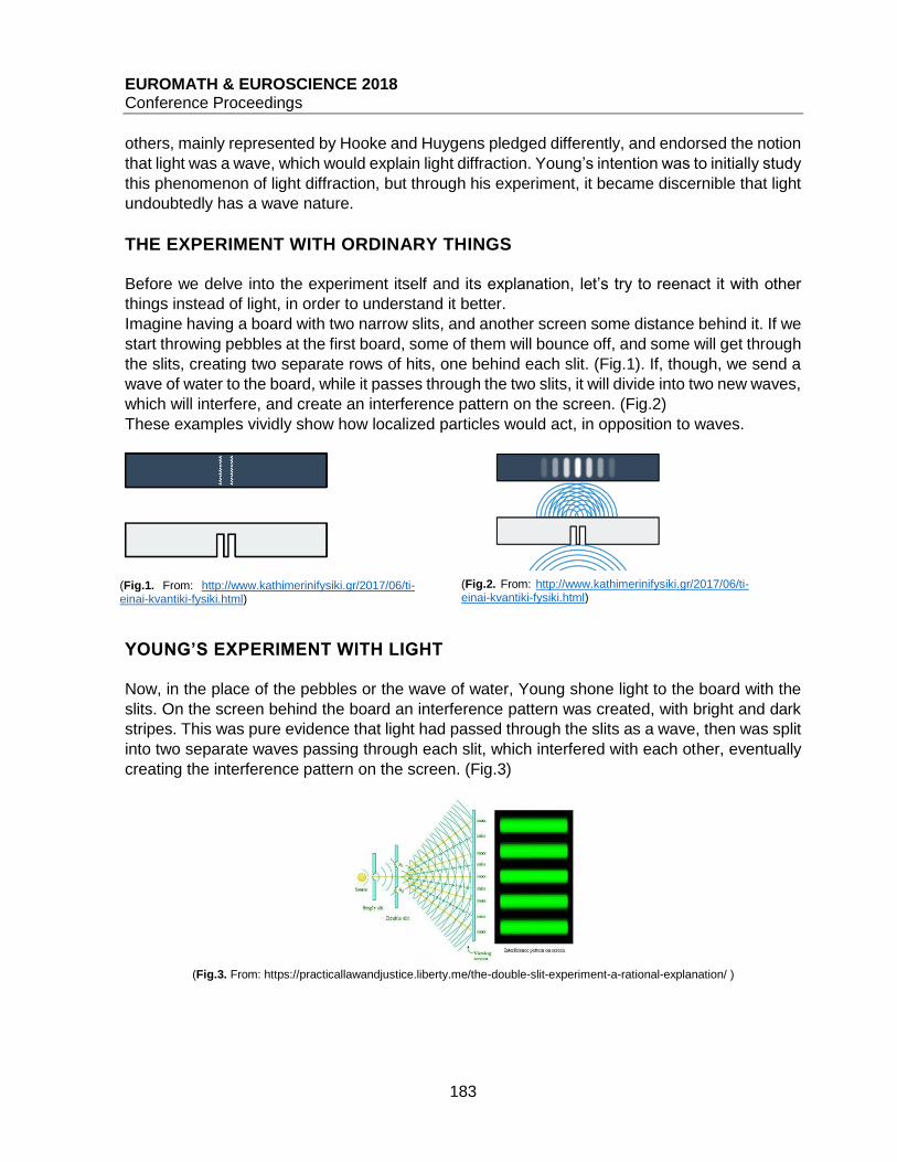
EUROMATH & EUROSCIENCE 2018 Conference Proceedings
183
others, mainly represented by Hooke and Huygens pledged differently, and endorsed the notion
that light was a wave, which would explain light diffraction. Young’s intention was to initially study
this phenomenon of light diffraction, but through his experiment, it became discernible that light
undoubtedly has a wave nature.
THE EXPERIMENT WITH ORDINARY THINGS
Before we delve into the experiment itself and its explanation, let’s try to reenact it with other
things instead of light, in order to understand it better.
Imagine having a board with two narrow slits, and another screen some distance behind it. If we
start throwing pebbles at the first board, some of them will bounce off, and some will get through
the slits, creating two separate rows of hits, one behind each slit. (Fig.1). If, though, we send a
wave of water to the board, while it passes through the two slits, it will divide into two new waves,
which will interfere, and create an interference pattern on the screen. (Fig.2)
These examples vividly show how localized particles would act, in opposition to waves.
YOUNG’S EXPERIMENT WITH LIGHT
Now, in the place of the pebbles or the wave of water, Young shone light to the board with the
slits. On the screen behind the board an interference pattern was created, with bright and dark
stripes. This was pure evidence that light had passed through the slits as a wave, then was split
into two separate waves passing through each slit, which interfered with each other, eventually
creating the interference pattern on the screen. (Fig.3)
(Fig.3. From: https://practicallawandjustice.liberty.me/the-double-slit-experiment-a-rational-explanation/ )
(Fig.1. From: http://www.kathimerinifysiki.gr/2017/06/ti-einai-kvantiki-fysiki.html)
(Fig.2. From: http://www.kathimerinifysiki.gr/2017/06/ti-einai-kvantiki-fysiki.html)

EUROMATH & EUROSCIENCE 2018 Conference Proceedings
184
The bright stripes were the result of the two waves of light arriving in phase, which means that
each crest of one wave overlapped with a crest of the other one, and the same goes for their
troughs. The interference, in this case, is called constructive interference. Oppositely, the dark
stripes were the result of the two waves arriving on the screen out of phase, meaning that the
crests of one wave overlapped with the troughs of the other, canceling each other out. This is
called destructive interference.
But how exactly is the constructive and destructive interference produced? The wave that arrives
at the double slit splits into two new waves, each of them leaving one slit. These two waves, as
they leave the two slits, are in phase, since they were produced at the same moment, from the
same source, the initial wave. For the central bright point we could say that the two waves
interfered constructively, and, more specifically, since they are in phase, they travelled the exact
same distance to the screen. The next bright line would have to be the result of constructive
interference too. But in this case, the two waves would not travel the same distance to the
screen; one of them would travel less, and the other more. But how much exactly would that
extra distance be? Well, since the waves leave the slits in phase, and we need the peaks and
the troughs of the waves overlapping for constructive interference, the extra distance would be
one more wavelength. For the next bright spot, we will apply the same way of thinking, and we
would see that the difference between the distances the two waves travelled would be two more
wavelengths. We call this difference path-length difference (PD). We come to the conclusion
that if the waves leave the source in phase, the points where we observe constructive
interference are the points where the path length difference takes values of an integer times the
wavelength (1λ, 2λ, 3λ… mλ). The exact type for this is PD= mλ, where m ∈ ℤ.
The opposite happens when we observe destructive interference. The two waves, as mentioned,
leave the slits in phase. If the bright bands are the result of integer times the wavelength, and
the dark bands are exactly inbetween the bright ones, then this would have to mean that the
light travelled half as much as it did to reach the next constructive point. This would have to
mean that it travelled a length which is a half-integer multiple of the wavelength. Indeed, for the
waves to interfere destructively, we would need a peak overlapping a valley. To achieve that,
the path length difference of the waves, which were initially in phase, would have to be half as
much as previously, to have the peaks overlapping the valleys. So in this case, PD= mλ, where
m= 0.5, 1.5, 2.5…
We conducted the experiment ourselves in Pierce College, using red and green laser and
diffraction gratings of 100, 300 and 600 slits. We saw from the results that in both cases, as we
used diffraction gratings with more slits, the maximum points moved farther away. To understand
this, let’s imagine two slits instead. If we have a larger distance between the slits, the lines that
would lead to the bright points are closer, and so are the points. Oppositely, if we decrease the
distance between the slits, the lines of constructive interference move farther away, along with
the maximum points. So, the more slits in the same space, the farther the constructive points
would be. Furthermore, we observed that with green laser, the maximums appeared slightly
closer. This is because green light, compared to red, has a smaller wavelength.
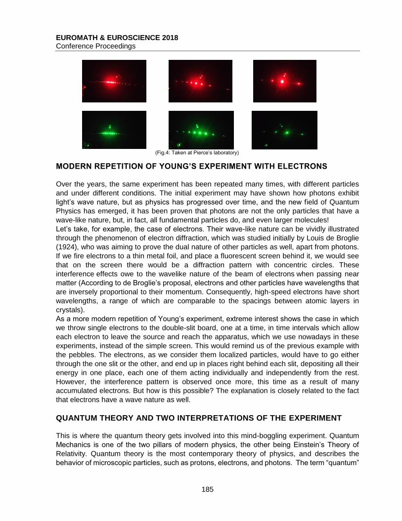
EUROMATH & EUROSCIENCE 2018 Conference Proceedings
185
(Fig.4: Taken at Pierce’s laboratory)
MODERN REPETITION OF YOUNG’S EXPERIMENT WITH ELECTRONS
Over the years, the same experiment has been repeated many times, with different particles
and under different conditions. The initial experiment may have shown how photons exhibit
light’s wave nature, but as physics has progressed over time, and the new field of Quantum
Physics has emerged, it has been proven that photons are not the only particles that have a
wave-like nature, but, in fact, all fundamental particles do, and even larger molecules!
Let’s take, for example, the case of electrons. Their wave-like nature can be vividly illustrated
through the phenomenon of electron diffraction, which was studied initially by Louis de Broglie
(1924), who was aiming to prove the dual nature of other particles as well, apart from photons.
If we fire electrons to a thin metal foil, and place a fluorescent screen behind it, we would see
that on the screen there would be a diffraction pattern with concentric circles. These
interference effects owe to the wavelike nature of the beam of electrons when passing near
matter (According to de Broglie’s proposal, electrons and other particles have wavelengths that
are inversely proportional to their momentum. Consequently, high-speed electrons have short
wavelengths, a range of which are comparable to the spacings between atomic layers in
crystals).
As a more modern repetition of Young’s experiment, extreme interest shows the case in which
we throw single electrons to the double-slit board, one at a time, in time intervals which allow
each electron to leave the source and reach the apparatus, which we use nowadays in these
experiments, instead of the simple screen. This would remind us of the previous example with
the pebbles. The electrons, as we consider them localized particles, would have to go either
through the one slit or the other, and end up in places right behind each slit, depositing all their
energy in one place, each one of them acting individually and independently from the rest.
However, the interference pattern is observed once more, this time as a result of many
accumulated electrons. But how is this possible? The explanation is closely related to the fact
that electrons have a wave nature as well.
QUANTUM THEORY AND TWO INTERPRETATIONS OF THE EXPERIMENT
This is where the quantum theory gets involved into this mind-boggling experiment. Quantum
Mechanics is one of the two pillars of modern physics, the other being Einstein’s Theory of
Relativity. Quantum theory is the most contemporary theory of physics, and describes the
behavior of microscopic particles, such as protons, electrons, and photons. The term “quantum”
EUROMATH & EUROSCIENCE 2018 Conference Proceedings
186
derives from Latin, and means “how much”. For example, the electron is a quantum of negative
charge, meaning it’s the smallest quantity of negative charge there can be. From this directly
derives the fact that quantum physics is discrete. This means that the energy contained in a
quantum field comes in integer multiples of some fundamental discrete energy amounts.
To return to our experiment, quantum physics has been able to give explanations to its results,
however convoluted and counter-intuitive they might appear.
According to the Copenhagen Interpretation of quantum physics, mainly proposed by Neils Bohr
and Werner Heisenberg, a particle in the double slit experiment exists only as a wave of possible
positions that includes all its possible paths. The possibilities that we find the electron in a
specific place constitute its wavefunction. Furthermore, this theory suggests that there is no
point in discussing where the particle is until we detect it. It is only when the particle is observed
that the wavefunction collapses and the position of the electron is finally decided.
It looks as though the universe allows all possible paths of the electron to happen, but choses
which one actually took place the last moment. And, furthermore, all those possibilities interfere,
and hence produce the result seen on the screen. The particle simultaneously takes all possible
paths, which means it passes through both slits. It attempts all possible trajectories, which
interact with one another, to produce the final outcome, the interference pattern. This means
that the electron is in a state of superposition. Superposition is the ability of a quantum system
to be in multiple states at the same time until it is measured. Each possible position of the
electron constitutes one possible state for it to be in. So we say now that the electron is in a
“superposition of states”, since we theorize that it is not in a specific place, but in all places
where its wavefunction allows it to be. According to the Copenhagen Interpretation, only
measurement collapses the possibility space of the wavefunction, and stimulates the choosing
of a specific reality. The collapse of the wavefunction signifies the transition between quantum
and classical realms, since we stop talking about quantum states of superposition, and we
observe a single, specific reality. Moreover, in this interpretation, the final choice of the
experiment is non-deterministic, meaning that it is random, within the constraints of the
wavefunction. In this case, the interference is not between . electrons, but rather that each
electron interferes only with itself due to the quantum uncertainty of which path through the
optical apparatus it takes. What we observe as an interference pattern is the accumulated sum
of many single particle interference events (Rueckner & Peidle 2013). Therefore, the
Copenhagen Interpretation suggests that there is no specific reality. Reality is created by
observation.
However, there is another way to explain this phenomenon. The Many Worlds Interpretation’s,
main idea is that the wavefunction never collapses. It was proposed by Hugh Everett in 1957. It
proposes that when a different path occurs in a situation, such as in our experiment, the universe
splits into more universes, each one allowing one possible reality to happen. The many
universes combined together form the multiverse. All the different possible histories, all the
possible trajectories of the electron continue existing, one in each separate universe. The many
separate universes somehow interfere, producing the result on the apparatus. By observing the
position of the electron, the interference of the different universes ceases to exist, so the
interference pattern disappears. Unlike the Copenhagen interpretation, the Many Worlds
Interpretation is a deterministic one. And, oppositely to the Copenhagen Interpretation, the Many
Worlds Interpretation does not dismiss the notion of existing realities. However, it suggests that
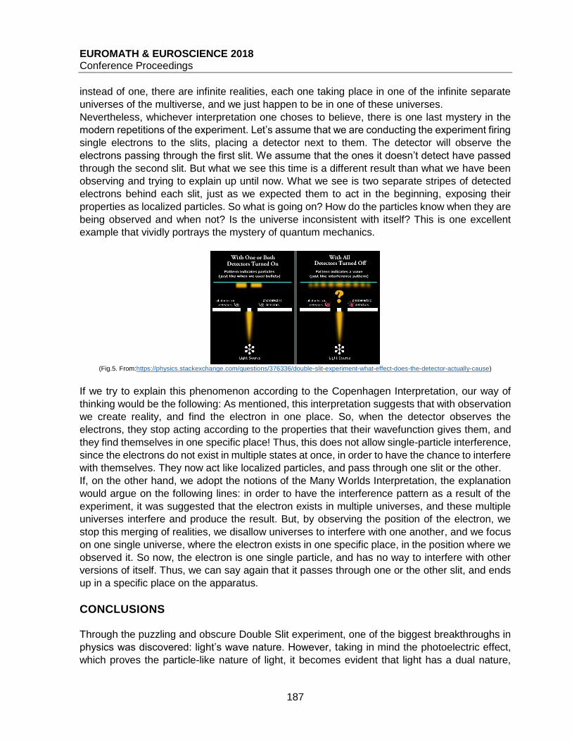
EUROMATH & EUROSCIENCE 2018 Conference Proceedings
187
instead of one, there are infinite realities, each one taking place in one of the infinite separate
universes of the multiverse, and we just happen to be in one of these universes.
Nevertheless, whichever interpretation one choses to believe, there is one last mystery in the
modern repetitions of the experiment. Let’s assume that we are conducting the experiment firing
single electrons to the slits, placing a detector next to them. The detector will observe the
electrons passing through the first slit. We assume that the ones it doesn’t detect have passed
through the second slit. But what we see this time is a different result than what we have been
observing and trying to explain up until now. What we see is two separate stripes of detected
electrons behind each slit, just as we expected them to act in the beginning, exposing their
properties as localized particles. So what is going on? How do the particles know when they are
being observed and when not? Is the universe inconsistent with itself? This is one excellent
example that vividly portrays the mystery of quantum mechanics.
(Fig.5. From:https://physics.stackexchange.com/questions/376336/double-slit-experiment-what-effect-does-the-detector-actually-cause)
If we try to explain this phenomenon according to the Copenhagen Interpretation, our way of
thinking would be the following: As mentioned, this interpretation suggests that with observation
we create reality, and find the electron in one place. So, when the detector observes the
electrons, they stop acting according to the properties that their wavefunction gives them, and
they find themselves in one specific place! Thus, this does not allow single-particle interference,
since the electrons do not exist in multiple states at once, in order to have the chance to interfere
with themselves. They now act like localized particles, and pass through one slit or the other.
If, on the other hand, we adopt the notions of the Many Worlds Interpretation, the explanation
would argue on the following lines: in order to have the interference pattern as a result of the
experiment, it was suggested that the electron exists in multiple universes, and these multiple
universes interfere and produce the result. But, by observing the position of the electron, we
stop this merging of realities, we disallow universes to interfere with one another, and we focus
on one single universe, where the electron exists in one specific place, in the position where we
observed it. So now, the electron is one single particle, and has no way to interfere with other
versions of itself. Thus, we can say again that it passes through one or the other slit, and ends
up in a specific place on the apparatus.
CONCLUSIONS
Through the puzzling and obscure Double Slit experiment, one of the biggest breakthroughs in
physics was discovered: light’s wave nature. However, taking in mind the photoelectric effect,
which proves the particle-like nature of light, it becomes evident that light has a dual nature,

EUROMATH & EUROSCIENCE 2018 Conference Proceedings
188
acting both as particles and as a wave. The fact that wave and particle natures “coexist”, is what
Bohr called “complementarity” (Haroche & Raimond, 2006: 11-12). This was extremely
important, since it gave an undeniable answer to the argument about light’s nature, revealing
clearly its also being a wave. It became, therefore, the basis for later theories and further
scientific research on light.
This experiment, especially in its modern variations, gives us a glimpse of what is going on in
the quantum world. It reveals the wave nature of all particles. This notion is also one of the
fundamental principles of quantum mechanics, suggesting that everything in the universe has
both particle and wave nature. Moreover, since this experiment has also been conducted with
atoms and large molecules, and has given the same results as when conducted with smaller
particles, it is ideal for the exhibition of the boundary between the microscopic world, explained
by quantum theory, and the macroscopic, explained by classical physics. By gradually
increasing the size of the particles in our experiments, we might hope to explore the frontier
between quantum and classical physics. So, obviously, the question is also provoked: “Why do
macroscopic objects made of particles which, individually, obey quantum rules, behave
classically?” (Haroche& Raimond, 2006:68). Anyhow, quantum mechanics is an “uncommon-
sensy theory” (Feynman, 1985:5), which provokes the interest of the researchers, and laymen
as well, but still is ambiguous and, many times, incomprehensible.
After, however, we have comprehended in depth the philosophy of the Many Worlds
Interpretation, we see that many philosophical questions arise, as to how we, as people,
experience and understand reality. This interpretation suggests that there are infinite universes,
each one hosting a different reality. So now, we might contemplate that there are actually infinite
versions of us out there, each one experiencing a wholly different reality. We are just one of our
infinite versions, who, in this universe live this specific life, while in another parallel universe we
could be entirely different people! So, could we say that our actions are really results of our own
free will? Are we creatures with the chance to formulate our own life as we want it, and take our
own initiatives, or is our path in life predestined by the multiverse? Are we just beings that fulfill
the universe’s where we live in purposes?
But all these profound questions could be further discussed and… enlightened not only in
another conference, but even perhaps in another… universe!
REFERENCES
Al-Khalili, J. (2013). Double Slit Experiment explained. Retrieved from:
https://www.youtube.com/watch?v=A9tKncAdlHQ
Cartlidge, Ed. (2011). New 'Double Slit' Experiment Skirts Uncertainty Principle. Retrieved from
the Scientific American website: https://www.scientificamerican.com/article/new-double-slit-
experiment-skirts-uncertainty-principle/
Feynman, R. (1985). QED, The Strange Theory of Light and Matter. Princeton: Princeton
University Press.
Forbes Science (2015, July 8). Six Things Everyone Should Know About Quantum Physics.
Retrieved From the Forbes website : https://www.forbes.com/sites/chadorzel/2015/07/08/six-
things-everyone-should-know-about-quantum-physics/#f0705bd7d467
Haroche, S. and Raimond, J.-M. Exploring the Quantum: Atoms, Cavities, and Photons.
Oxford University Press, New York, 2006.

EUROMATH & EUROSCIENCE 2018 Conference Proceedings
189
Khan Academy (2016, July 29). Constructive and Destructive interference. Retrieved From the
Khan Academy website: https://www.khanacademy.org/science/physics/light-
waves/interference-of-light-waves/v/constructive-and-destructive-interference
Khan Academy (2014, July 7). Young's double slit introduction. Retrieved From the Khan
Academy website: https://www.khanacademy.org/science/physics/light-waves/interference-of-
light-waves/v/youngs-double-split-part-1
Khan Academy (2014, July 7). Young's double slit problem solving. Retrieved From the Khan
Academy website: https://www.khanacademy.org/science/physics/light-waves/interference-of-
light-waves/v/youngs-double-slit-problem-solving
Levine, M. (2013, December 12). Double-Slit Science: How Light Can Be Both a Particle and a
Wave. Retrieved from the Scientific American website:
https://www.scientificamerican.com/article/bring-science-home-light-wave-particle/
O’Dowd, M. (writer) & Brown, K. (producer) (2016). The Quantum Experiment that Broke
Reality. PBS Digital Studios. Retrieved from: https://www.youtube.com/watch?v=p-MNSLsjjdo
O’Dowd, M. (writer) & Ward, R. (producer) (2016). The Many Worlds of the Quantum
Multiverse. PBS Digital Studios. Retrieved from:
https://www.youtube.com/watch?v=dzKWfw68M5U
Rueckner, W. and Peidle J. (2013). Young’s Double Slit Experiment with Single Photons and
Quantum Eraser. American Journal of Physics 81 (12): 951. doi:10.1119/1.4819882.
Singh, S. (1999). The code book. London: Fourth Estate
EUROMATH & EUROSCIENCE 2018 Conference Proceedings
190
STRUCTURE, PROPERTIES AND FUNCTION; THE QUEST FOR MATTER'S MINIMAL PARTS
Aris Siotis
Pierce-The American College of Greece, Greece
ABSTRACT
The Standard Model of Particle Physics represents the current state of Humanity's age old quest for matter's minimal parts. In spite of its success it displays a feature that is common to the early stages of almost all scientific fields. In their early stages scientific fields go through a phase of classification of the various elements that they study which is based on certain conserved properties of the elements within each class. For example, the classes "Genus " in Biology or "Periods" in Chemistry. As the fields progress the basis of these properties and classification is understood as being due to the relatively stable combination of certain entities that constitute the minimal parts of matter specific to each field. These minimal parts would be "Nucleotides" for Biology, "Nuclei and Electrons" for Chemistry etc. If we break up these structures we pass from one scientific field to another, from Biology to Biochemistry to Chemistry to Physics. In this sequence the energy required to break up the structure at each level is smaller than the mass of the constituents involved at that level. However, if we want to explore even smaller scales, Heisenberg's uncertainty principle implies that the energy required to achieve this becomes equal or even greater than the mass of the constituents. In addition, the constituents' masses become smaller than the energy that binds them together. Have we therefore reached the end to this sequence? Are the minimal parts of the so called "Standard Model" of the world i.e. Quarks and Leptons truly "fundamental" or "elementary" or should we expect another level of structure on an even smaller scale? Does it make sense to think in terms of structure and constituents beyond a certain scale?
INTRODUCTION
In this presentation, addressed to high school students, we will try to outline the centuries' old
quest for the nature of matter's properties in terms of constituents, from Demokritos' "atoms" to
today's Standard Model "particles" and to point to what may lie beyond. A key feature of all
these searches involves the distinction between "intrinsic" and "structural" properties. An
intrinsic property is one that an object possesses independently of being alone in the world
whereas a "structural" property is one that is due to the internal organization of certain smaller
constituents. Another key feature is that of a "conserved" property, that is a property that persists
when an object undergoes transformations. A conserved property can either be intrinsic or can
be structural, in which case it disappears if this structure is altered.
Conserved Properties form the basis of classification schemes in different branches of Science
. This classification (Taxonomy) characterizes the early stage of every science and is based on
phenomenology, that is on the apparent behaviour of the objects under study.
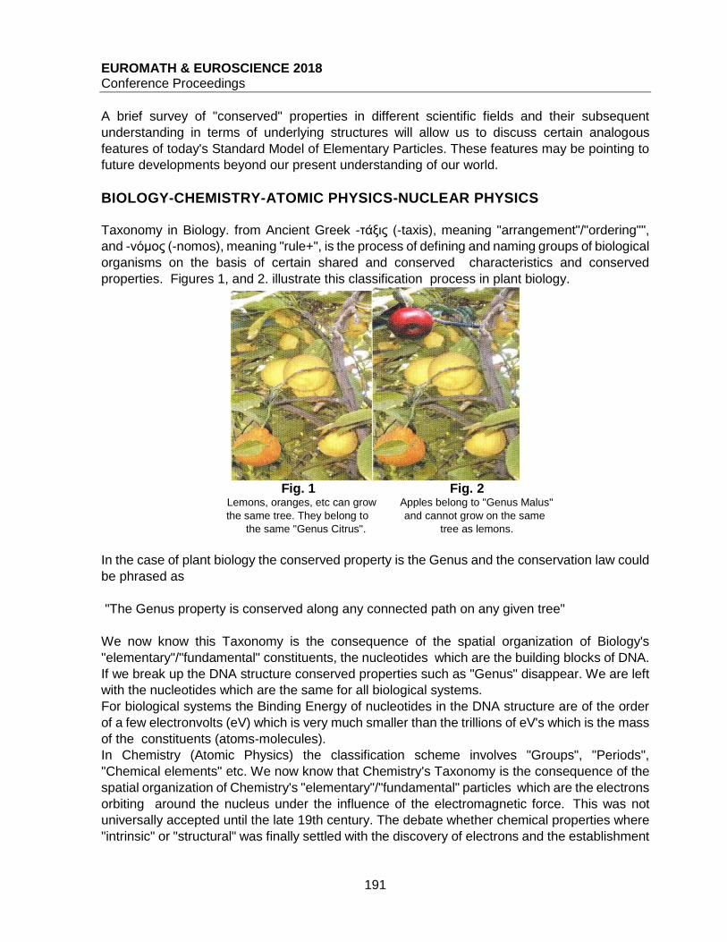
EUROMATH & EUROSCIENCE 2018 Conference Proceedings
191
A brief survey of "conserved" properties in different scientific fields and their subsequent
understanding in terms of underlying structures will allow us to discuss certain analogous
features of today's Standard Model of Elementary Particles. These features may be pointing to
future developments beyond our present understanding of our world.
BIOLOGY-CHEMISTRY-ATOMIC PHYSICS-NUCLEAR PHYSICS
Taxonomy in Biology. from Ancient Greek -τάξις (-taxis), meaning "arrangement"/"ordering"",
and -νόμος (-nomos), meaning "rule+", is the process of defining and naming groups of biological
organisms on the basis of certain shared and conserved characteristics and conserved
properties. Figures 1, and 2. illustrate this classification process in plant biology.
Fig. 1 Fig. 2
Lemons, oranges, etc can grow Apples belong to "Genus Malus"
the same tree. They belong to and cannot grow on the same
the same "Genus Citrus". tree as lemons.
In the case of plant biology the conserved property is the Genus and the conservation law could
be phrased as
"The Genus property is conserved along any connected path on any given tree"
We now know this Taxonomy is the consequence of the spatial organization of Biology's "elementary"/"fundamental" constituents, the nucleotides which are the building blocks of DNA.
If we break up the DNA structure conserved properties such as "Genus" disappear. We are left
with the nucleotides which are the same for all biological systems.
For biological systems the Binding Energy of nucleotides in the DNA structure are of the order
of a few electronvolts (eV) which is very much smaller than the trillions of eV's which is the mass
of the constituents (atoms-molecules).
In Chemistry (Atomic Physics) the classification scheme involves "Groups", "Periods",
"Chemical elements" etc. We now know that Chemistry's Taxonomy is the consequence of the
spatial organization of Chemistry's "elementary"/"fundamental" particles which are the electrons
orbiting around the nucleus under the influence of the electromagnetic force. This was not
universally accepted until the late 19th century. The debate whether chemical properties where
"intrinsic" or "structural" was finally settled with the discovery of electrons and the establishment
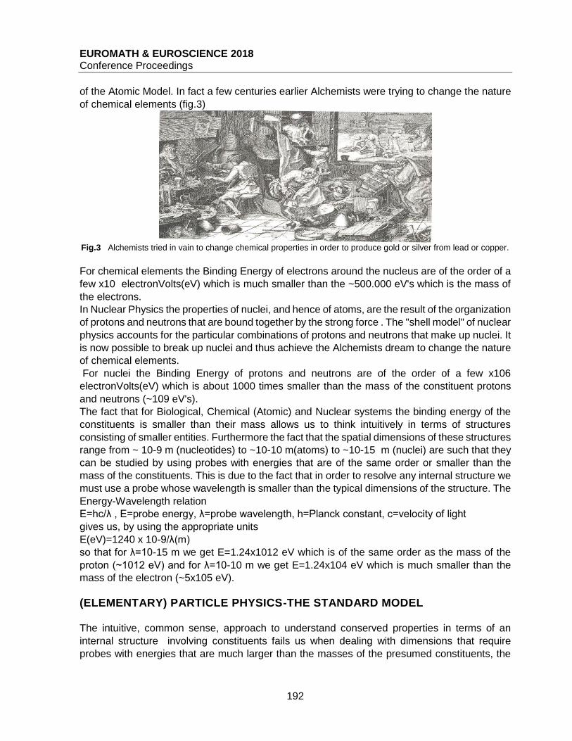
EUROMATH & EUROSCIENCE 2018 Conference Proceedings
192
of the Atomic Model. In fact a few centuries earlier Alchemists were trying to change the nature
of chemical elements (fig.3)
Fig.3 Alchemists tried in vain to change chemical properties in order to produce gold or silver from lead or copper.
For chemical elements the Binding Energy of electrons around the nucleus are of the order of a
few x10 electronVolts(eV) which is much smaller than the ~500.000 eV's which is the mass of
the electrons.
In Nuclear Physics the properties of nuclei, and hence of atoms, are the result of the organization
of protons and neutrons that are bound together by the strong force . The "shell model" of nuclear
physics accounts for the particular combinations of protons and neutrons that make up nuclei. It
is now possible to break up nuclei and thus achieve the Alchemists dream to change the nature
of chemical elements.
For nuclei the Binding Energy of protons and neutrons are of the order of a few x106
electronVolts(eV) which is about 1000 times smaller than the mass of the constituent protons
and neutrons (~109 eV's).
The fact that for Biological, Chemical (Atomic) and Nuclear systems the binding energy of the
constituents is smaller than their mass allows us to think intuitively in terms of structures
consisting of smaller entities. Furthermore the fact that the spatial dimensions of these structures
range from ~ 10-9 m (nucleotides) to ~10-10 m(atoms) to ~10-15 m (nuclei) are such that they
can be studied by using probes with energies that are of the same order or smaller than the
mass of the constituents. This is due to the fact that in order to resolve any internal structure we
must use a probe whose wavelength is smaller than the typical dimensions of the structure. The
Energy-Wavelength relation
E=hc/λ , E=probe energy, λ=probe wavelength, h=Planck constant, c=velocity of light
gives us, by using the appropriate units
E(eV)=1240 x 10-9/λ(m)
so that for λ=10-15 m we get E=1.24x10¹² eV which is of the same order as the mass of the
proton (~1012 eV) and for λ=10-10 m we get E=1.24x10⁴ eV which is much smaller than the
mass of the electron (~5x10⁵ eV).
(ELEMENTARY) PARTICLE PHYSICS-THE STANDARD MODEL
The intuitive, common sense, approach to understand conserved properties in terms of an
internal structure involving constituents fails us when dealing with dimensions that require
probes with energies that are much larger than the masses of the presumed constituents, the
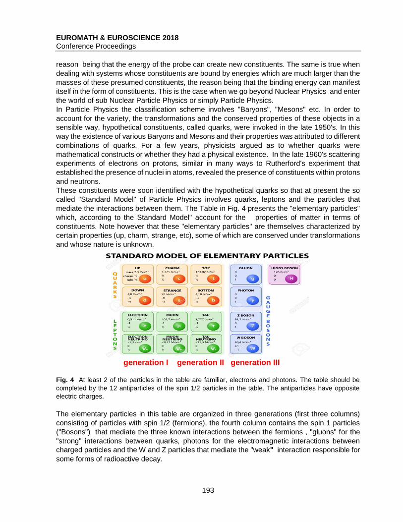
EUROMATH & EUROSCIENCE 2018 Conference Proceedings
193
reason being that the energy of the probe can create new constituents. The same is true when
dealing with systems whose constituents are bound by energies which are much larger than the
masses of these presumed constituents, the reason being that the binding energy can manifest
itself in the form of constituents. This is the case when we go beyond Nuclear Physics and enter
the world of sub Nuclear Particle Physics or simply Particle Physics.
In Particle Physics the classification scheme involves "Baryons", "Mesons" etc. In order to
account for the variety, the transformations and the conserved properties of these objects in a
sensible way, hypothetical constituents, called quarks, were invoked in the late 1950's. In this
way the existence of various Baryons and Mesons and their properties was attributed to different
combinations of quarks. For a few years, physicists argued as to whether quarks were
mathematical constructs or whether they had a physical existence. In the late 1960's scattering
experiments of electrons on protons, similar in many ways to Rutherford's experiment that
established the presence of nuclei in atoms, revealed the presence of constituents within protons
and neutrons.
These constituents were soon identified with the hypothetical quarks so that at present the so
called "Standard Model" of Particle Physics involves quarks, leptons and the particles that
mediate the interactions between them. The Table in Fig. 4 presents the "elementary particles"
which, according to the Standard Model" account for the properties of matter in terms of
constituents. Note however that these "elementary particles" are themselves characterized by
certain properties (up, charm, strange, etc), some of which are conserved under transformations
and whose nature is unknown.
generation I generation II generation III Fig. 4 At least 2 of the particles in the table are familiar, electrons and photons. The table should be
completed by the 12 antiparticles of the spin 1/2 particles in the table. The antiparticles have opposite
electric charges.
The elementary particles in this table are organized in three generations (first three columns)
consisting of particles with spin 1/2 (fermions), the fourth column contains the spin 1 particles
("Bosons") that mediate the three known interactions between the fermions , "gluons" for the
"strong" interactions between quarks, photons for the electromagnetic interactions between
charged particles and the W and Z particles that mediate the "weak" interaction responsible for
some forms of radioactive decay.
EUROMATH & EUROSCIENCE 2018 Conference Proceedings
194
The final column contains just the recently discovered, spin 0, Higgs boson. This last member
is an essential ingredient of the Standard Model. It provides the Model with a mechanism that
explains the fact that some of the particles have a non zero mass. Without the Higgs mechanism
all the Elementary Particles of the Standard Model would have zero mass. The Higgs
mechanism can account for the masses of the W and Z bosons and, with some further
extensions, for the masses of the charged quarks and leptons. However, the neutral neutrinos
do not acquire any mass through this mechanism.
As it is not our purpose to present here the workings of the Standard Model or the Higgs
mechanism we will focus on the reasons why the model classifies the quarks and leptons in
three different generations.
By way of illustration we note that for a given electric charge, say q=2/3, the three quarks, up,
charm and top have different masses. The same applies to three members of the lepton family
with charge q=-1, the familiar electron, the muon and the tau. If, however, masses were the only
difference between the three generations one would expect that, say, the muon (μ) with a mass
of ~108 eV should rapidly decay into an electron (e) with mass ~5x10⁵ eV by emitting a photon
(γ) as no law of nature would forbid the decay
μ==>e+γ (does not happen)
This however does not happen. Instead the muon (generation II) decays mainly into an electron
(generation I), a neutrino from generation II and an antineutrino from
generation I.
μ-->e+(anti)νe + νμ
In order to account for this behaviour one attributes to members of each generation a conserved
property called the lepton generation number LI,LII,LIII (or Le,Lμ,Lτ) with value 1 or 0 (and -1 or 0
for the corresponding antiparticles) as shown in the Table in Fig 5.
Le-number Lμ-number Lτ-number
Generation I , e and νe 1 0 0
Generation II, μ and νμ 0 1 0
Generation ΙΙΙ, τ and ντ 0 0 1
Fig 5. Lepton number assignment. For the corresponding antiparticles 1=>-1
By invoking the "conservation of Lepton number", i.e. asserting that Lepton number is a
conserved property in the charged Lepton transformations one accounts for the fact that the
decay μ=>e+γ is forbidden whereas μ=>e+(anti)νe+νμ is allowed.
μ≠>e+γ (Lμ=1-->Lμ=0 and Le=0-->Le=1, hence forbidden)
μ=>e+(anti)νe+νμ (Lμ=1-->Lμ=1 and Le=0-->Le=0, hence allowed)
The question that arises naturally with respect to this experimentally observed "conserved" property is whether it is "intrinsic" or whether it is "structural". The "conserved" properties involving Lepton number generations have their counterparts in the
three quark generations.
So far all experimental efforts to understand this "conserved" property as resulting from a
composite nature of the muon have failed. The present spatial limits on internal structure are of
the order of ~10-18 m corresponding to the limits of available probing energies at the CERN
EUROMATH & EUROSCIENCE 2018 Conference Proceedings
195
LHC which are of the order of ~1015 eV. As the shortest meaningful length, the limiting distance
below which we believe that the very notions of space and length cease to exist is of the order
of 10-35m, the so called Planck Length, there is a long way to go, about 17 orders of magnitude,
in the quest for structure of elementary particles.
In the Table of Fig.4 we also note that the neutrino masses are given as being smaller than a
certain value rather than equal to 0 as predicted by the Standard Model. This arises from the
experimental observation of "neutrino oscillations" i.e. the fact that neutrinos of any given
generation evolve, as they travel through space, into neutrinos of a different generation. For
such oscillations to take place Quantum Mechanics implies that neutrinos cannot be massless.
The neutrino mass limits in Fig.5 have been deduced from the experimentally measured period
of these oscillations. There are several proposed solutions to this anomaly all of which go
beyond the Standard Model.
CONCLUSION
In the Standard Model of elementary particles the conserved properties, such as the Lepton
generation number, attributed to the different generations of leptons are features that are
introduced "by hand". They do not arise from some more fundamental theoretical considerations.
In addition the behaviour of neutrinos suggests that the Standard Model is just the early version
of a more complete theory.
It may be that the answer to these questions and in particular the understanding of the nature
and role of neutrinos may hold the key to many other open problems, not only in Particle Physics
but also in Cosmology, such as the so called Dark Matter problem and the fact that our Universe
is not symmetric between matter and antimatter as expected from the Big Bang creation
theories.
EUROMATH & EUROSCIENCE 2018 Conference Proceedings
196
WORKSHOPS
MATHEMATICS AND CREATIVIY: AN APPROACH USING DIGITAL STORYTELLING
Anna Alfieri
Liceo Scientifico “L. Siciliani” Catanzaro, Italy
ABSTRACT Studying mathematics involves a scientific point of view of reality, whereas inventing and telling stories involve an empirical and imaginative point of view about it. This paper is focused on these two aspects: to combine together mathematics and creativity. The use of mathematical rules and formula and the use of storytelling allow us to think of a “different” mathematics more engaging for the students: cosine function, hyperbola, Gaussian function and Dirac Delta function are protagonists of two stories made by multimedia tools. It is a classroom activity, whose main goal is to improve mathematics knowledge based on creative and non-standard processes.
INTRODUCTION
A better understanding of the real world implies the knowledge of mathematics, without any fear
or concern that it is a difficult subject. Real world means everything around us: nature, society
or culture, including everyday life. The real world is complex, but a mathematical approach could
help in describing this complexity. This passage from reality to mathematics and vice versa is
achieved by the mathematical models and in addition to mathematical formula and rules.
What is a mathematical model? The starting point is normally a certain situation in the real
world. If we are able to simplify it, to structure it and to make it more precise, according to the
problem solver’s knowledge, it will lead to the formulation of a problem and to a real model of
the situation (Bloom 2002):
If appropriate, real data are collected in order to provide more information about the situation
at one’s disposal. If possible and adequate, this realistic model – still a part of the real world in
our sense – is mathematised, that is, the objects, data, relations and conditions involved in it
are translated into mathematics, resulting in a mathematical model of the original situation.
Now mathematical methods come into play, and are used to derive mathematical results.
At the same time the problem solver validates the model by checking whether the problem
solution obtained by interpreting the mathematical results and he decides if it is appropriate and

EUROMATH & EUROSCIENCE 2018 Conference Proceedings
197
reasonable for his purposes. If necessary, the whole process has to be repeated with a modified
or a completely different model. At the end, the solution of the original real world problem is
stated and communicated.
DIGITAL STORYTELLING IN MATHEMATICS
During the solution of a mathematical problem or question, we cannot conceive to use anything
of different from mathematical rules or formula, nevertheless we can create a story to solve it.
While teaching, it might be that we occasionally tell a ‘mathematical’ story, but the stories usually
concern the most famous mathematician’s life or a problem formulated like a story. This is an
important aspect, but it does not represent a new educational approach to solve a problem.
Digital storytelling is an educational activity to make mathematics more accessible to students,
as well as more engaging through.
But firstly, what is a story? A dictionary definition suggests that a story is “a factual or a fictional
account of an event or series of events”. Despite the feeling that “no definition is necessary”, or
that “every child knows what a story is”, we can say that a story is a narrative unit that can fix
the affective meaning of the elements that compose it (Egan 2005). Another definition is (Green
2004):
In essence, a narrative account requires a story that raises unanswered questions or
unresolved conflicts; characters may encounter and then resolve a crisis or crises. A story line,
with a beginning, middle and an end, is identifiable. […] It is generally agreed that stories are a
powerful structure for organizing and transmitting information, and for creating meaning in our
lives and environments.
The common feature in both descriptions is the structure. The story must have a structure. While
Green’s attention is mainly on the information embedded in a story, Egan’s additional focus is
on the effect, on orienting feelings. Egan describes a story as a particular kind of narrative unit
that orients our emotions to the events presented through the narration. That is, stories make
us feel. We ascribe emotional meaning to events, and to people, and to our own lives by plotting
them into partial or provisional stories. We orient ourselves emotionally to our environment by
involving it in our stories. The value of the story is precisely its power to engage the students’
emotions and also, connectedly, their imaginations in the material of the curriculum. In the
educational activity described in this paper, the story is functional to understand geometric
graphics, in doing this, it has not given precedence to student entertainment over education
goals, because the main aim was to engage them. Engaging students with mathematical activity
as an essential aspect of successful education. The great power of stories (Egan 2005), is in
their dual mission: they communicate information in an unforgettable form and they shape the
hearer’s feelings about the information being communicated. These feelings can capture the
attention of the pupil and involve him totally in the learning process, especially in mathematics,
that is often considered as a cold discipline. Moreover, a story implies a message or a meaning
as well as mathematics, which we manipulate symbols for reasoning and finding solutions.

EUROMATH & EUROSCIENCE 2018 Conference Proceedings
198
MODELLING AND DIGITAL STORYTELLING IN MATHEMATICS. AN EXAMPLE.
In a scientific era, storytelling is considered appropriate only for language arts and advertising
projects. However, in today’s multimedia world, we can develop digital storytelling to practice
and master a high number of skills and contents according to technological standards. The
process of crafting the digital story becomes rich in skills such as: communication, collaboration,
oral speaking, creativity, visual and sound literacy, project management. It also helps to develop
a range of digital communication styles necessary to function in a knowledge society (Porter
2008). Two multimedia stories “The waves of the heart” and “Loving is a δ-function” are
presented in this paper as an educational approach to mathematical modelling through digital
storytelling.
“The waves of the heart”
Digital storytelling enables innovation and creativity. Authors (students and teachers) become
creative in designing information and communicating understandings with the images, graphics,
movement and music of digital media. Digital storytelling provides a unique opportunity for
mixing media and mathematical contents in order to involve many pupils. This work deals with
the following mathematical contents:
Sinus and cosine graphs
Absolute value and cosine function
Hyperbola: definition and its properties.
The story, that we propose, has “a beginning, a middle and an end” (Green 2004).
The beginning. The protagonists are one girl (Emmy) and one boy (Stefano), they are falling in
love, but later, as it often happens, Stefano breaks off their engagement and obviously Emmy is
suffering.
The middle. Emmy is a good student in mathematics, therefore she begins to turn her love
sickness in mathematical concepts: trigonometric function (see fig. 1) and absolute value in
trigonometric function (see fig. 2) Suggest to her that love sickness will not last forever.
fig. 1 y = cos (x) fig. 2 y = |cos (x)|

EUROMATH & EUROSCIENCE 2018 Conference Proceedings
199
The end. Studying some properties about the cosine function and hyperbola, Emmy discovers
her pain will decrease more and more, until it disappears. The other events of her life overcome
her suffering, therefore she draws a new graph (see fig.3):
fig.3 y = |cos (x)|/x
The figures 1,2,3 are frames of a video, whose link is
“Loving is a δ-function ”.
The Emmy’s story goes on. It's been a while and now Emmy is less sad, one night she dreams
of being a princess who dismisses all her suitors. Her sisters try to help her using Gaussian
curves. But Emmy wishes to fall in love, a new great love for one boy and she uses the Dirac
delta function to model her new love. In this story, the protagonists are: Gaussian function and
its properties and Dirac delta function. The qr-code for looking at the video is following:
EUROMATH & EUROSCIENCE 2018 Conference Proceedings
200
CONCLUSION
Modelling reality means applying rules and logic process of the mathematics to the real world
for knowing it better. The methodology, that teachers use for it, can stave off or approach the
students. Digital storytelling has an important role in the activity in order to create a “good”
empathic relationship between student and mathematics.
REFERENCES
Alm, C.O.,Sproat, R.. Perceptions of emotions in expressive storytelling. In Interspeec, 533-
536. (2005)
Blum, W.. ICMI study 14: Applications and modelling in mathematics education - Discussion
document. Zentralblatt für Didaktik der Mathematik, 34(5), 229-239. (2002)
Brandi, P., Salvatori A. Modelli matematici elementari. Bruno Mondadori. Milano (2004).
Dreon, O., Kerper, R. M., & Landis, J.. Digital Storytelling: A Tool for Teaching and Learning in
the YouTube Generation. Middle School Journal (J1),42(5), 4-9. (2011)
Egan, K. An Imaginative approach to teaching. www. ejmste. com, 203(3), 247-248. (2005).
Green, M.C. Storytelling in Teaching. APS Observer 17,37-54. (2004).
Porter, B.. Digital storytelling. San Jose, CA: Adobe Systems Incorporated. www. adobe.
com/education/instruction/adsc/pdf/digital_storytelling. pdf. (2008)
Robin, B. R. Digital Storytelling: A Powerful Technology Tool for the 21st Century
Classroom. Theory Into Practice, 47, 220-228. (2008).
van Gils, F. Potential applications of digital storytelling in education. In 3rd Twente student
conference on IT (Vol. 7). University of Twente, Faculty of Electrical Engineering, Mathematics
and Computer Science Enschede. (2005).

EUROMATH & EUROSCIENCE 2018 Conference Proceedings
201
THE MATHEMATICS CUISINE Gerovasileiou Antonia, Dimitropoulos Emmanouil, Kopaila Iliana
Diastaseis, Private School, Greece
ABSTRACT
Who of all of us who teach mathematics have not heard questions such as: -Why do I need mathematics? Why do I have to learn mathematics?
Within the context of teaching mathematics in schools this subject is seen as strict and hostile by the students. However the interactive teaching of mathematics through a plethora of games can introduce students to this “unusual world”. Studies have shown that children who integrate mathematical games into their everyday lives develop skills such as the ability to solve practical problems, end exhibit, a better understanding of aesthetics, logic and geometry. The “cooking” of mathematics is an attempt to show its interactive side and to prove that through the use of games it is possible to improve the relationship between children and mathematics. An infectious disease has contaminated the atmosphere of our planet and is threatening to wipe
out the human race. The scientist who has the antidote is intelligent but also forgetful. Because
he was afraid he would not be able to remember the code that unlocks his lab, he has given his
three colleagues some clues ... so that he can open it under any circumstances
We will need the best detectives in order to break the code. His three colleagues have in their
hands a series of puzzles given to them by the scientist. But the puzzles are demanding, they
require attention and thought. If you are a detective, you are invited to find the "key" that unlocks
the lab so that the antidote can save humanity.
That is why you will be divided into groups. Each team will appoint a leader and all together you
will name your team.
Each puzzle is rewarded with 10 points (when solved without any help).
You can ask for help, but you will be penalized by having points removed
for the 1st tip, 2 points are removed
for the 2nd tip, 3 points are removed
for the 3rd tip, 4 points are removed
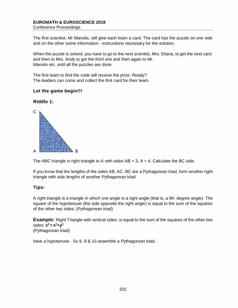
EUROMATH & EUROSCIENCE 2018 Conference Proceedings
202
The first scientist, Mr Manolis, will give each team a card. The card has the puzzle on one side
and on the other some information - instructions necessary for the solution.
When the puzzle is solved, you have to go to the next scientist, Mrs. Eliana, to get the next card.
and then to Mrs. Andy to get the third one and then again to Mr.
Manolis etc. until all the puzzles are done.
The first team to find the code will receive the prize. Ready?
The leaders can come and collect the first card for their team.
Let the game begin!!! Riddle 1: C A B The ABC triangle is right triangle to A with sides AB = 3, A = 4. Calculate the BC side.
If you know that the lengths of the sides AB, AC, BC are a Pythagorean triad, form another right
triangle with side lengths of another Pythagorean triad.
Tips:
A right triangle is a triangle in which one angle is a right angle (that is, a 90- degree angle). The
square of the hypotenuse (the side opposite the right angle) is equal to the sum of the squares
of the other two sides: (Pythagorean triad)
Example: Right Triangle with vertical sides: is equal to the sum of the squares of the other two
sides: z2 = x2+y2
(Pythagorean triad)
have a hypotenuse . So 6, 8 & 10 assemble a Pythagorean triad.
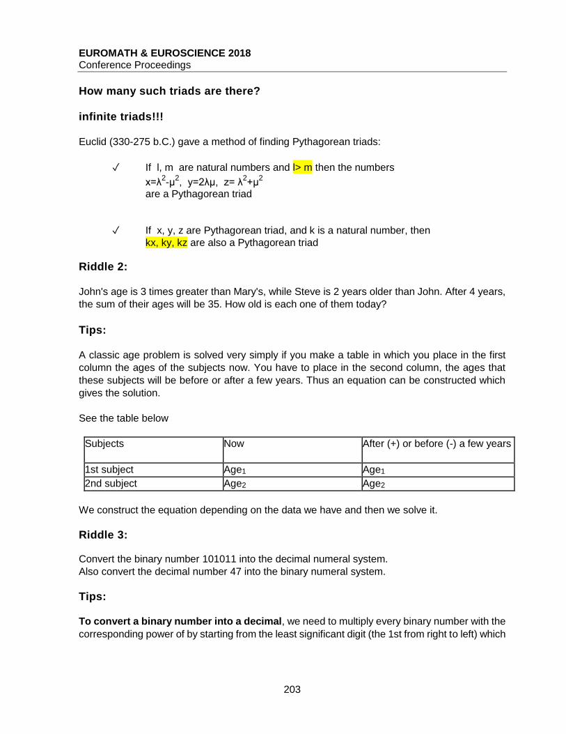
EUROMATH & EUROSCIENCE 2018 Conference Proceedings
203
How many such triads are there? infinite triads!!! Euclid (330-275 b.C.) gave a method of finding Pythagorean triads:
✓ If l, m are natural numbers and l> m then the numbers
x=λ2-μ
2, y=2λμ, z= λ
2+μ
2
are a Pythagorean triad
✓ If x, y, z are Pythagorean triad, and k is a natural number, then
kx, ky, kz are also a Pythagorean triad
Riddle 2:
John's age is 3 times greater than Mary's, while Steve is 2 years older than John. After 4 years,
the sum of their ages will be 35. How old is each one of them today?
Tips:
A classic age problem is solved very simply if you make a table in which you place in the first
column the ages of the subjects now. You have to place in the second column, the ages that
these subjects will be before or after a few years. Thus an equation can be constructed which
gives the solution.
See the table below
Subjects Now After (+) or before (-) a few years
1st subject Age1 Age1
2nd subject Age2 Age2
We construct the equation depending on the data we have and then we solve it.
Riddle 3: Convert the binary number 101011 into the decimal numeral system.
Also convert the decimal number 47 into the binary numeral system.
Tips:
To convert a binary number into a decimal, we need to multiply every binary number with the
corresponding power of by starting from the least significant digit (the 1st from right to left) which
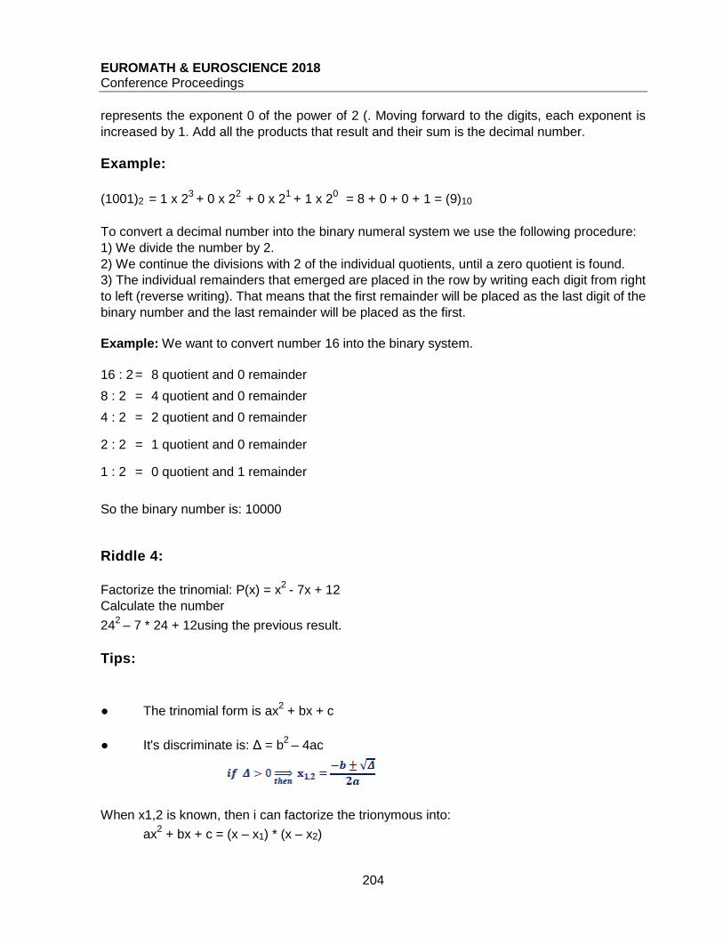
EUROMATH & EUROSCIENCE 2018 Conference Proceedings
204
represents the exponent 0 of the power of 2 (. Moving forward to the digits, each exponent is
increased by 1. Add all the products that result and their sum is the decimal number.
Example:
(1001)2 = 1 x 23
+ 0 x 22
+ 0 x 21
+ 1 x 20
= 8 + 0 + 0 + 1 = (9)10
To convert a decimal number into the binary numeral system we use the following procedure:
1) We divide the number by 2.
2) We continue the divisions with 2 of the individual quotients, until a zero quotient is found.
3) The individual remainders that emerged are placed in the row by writing each digit from right
to left (reverse writing). That means that the first remainder will be placed as the last digit of the
binary number and the last remainder will be placed as the first.
Example: We want to convert number 16 into the binary system.
16 : 2 = 8 quotient and 0 remainder
8 : 2 = 4 quotient and 0 remainder
4 : 2 = 2 quotient and 0 remainder
2 : 2 = 1 quotient and 0 remainder
1 : 2 = 0 quotient and 1 remainder
So the binary number is: 10000
Riddle 4:
Factorize the trinomial: P(x) = x2
- 7x + 12
Calculate the number
242
– 7 * 24 + 12using the previous result.
Tips:
● The trinomial form is ax2 + bx + c
● It's discriminate is: Δ = b2
– 4ac
When x1,2 is known, then i can factorize the trionymous into:
ax2 + bx + c = (x – x1) * (x – x2)
EUROMATH & EUROSCIENCE 2018 Conference Proceedings
205
Riddle 5:
A teacher splits his students into groups of 3 but there are two left over Then he decides to split
the students into groups of 4 but, again, there are two left over.
Finally he decides to split them into groups of 5 and there are none left over. How many students
does this teacher have?
Tips:
1. Multiples of an integer value a, are the products that result if we multiply a with all integer
values
e.g. 0 . a, 1 . a, 2 . a, 3 . a, 4 . a etc
2. Every integer value can divide all of its multiples
3. If an integer value a is divided by an integer value b
then it is a multiple of b.
The digits of the Lab's key are:
1st and 2nd digit: The number of kids from the 5th riddle
3rd digit: John's age in the 2nd riddle
4th and 5th digit: The (101011) number to decimal form in the 3rd riddle
6th and 7th digit: The 2 first digits from the result in the 4th riddle
8th digit: Hypotenuse's side length in the 5th riddle
9th digit: The first letter of the female name in the 2nd riddle
Lab's Key: _ _ _ _ _ _ _ _ _
(50 9 43 4 2 Μ)
CONGRATULATIONS
the humanity will be saved.
the team .... found the code and took the prize which is a great chocolate.

EUROMATH & EUROSCIENCE 2018 Conference Proceedings
206
SOLUTIONS
Riddle 1:
According to Pythagorean Theorem:
Thus the number 3, 4, 5 consist of a Pythagorean triad.
If l = 5 & m then
x = l2 – m
2 = 25 – 16 = 9
y = 2 * l * m = 2 * 5 * 4 = 40
z = l2 + m
2 = 25 +16 = 41
Thus the numbers: 9, 40, 41 consist of a Pythagorean triad
Riddle 2:
Subjects Now After 3 years
John 3 . x 3 . x + 4
Mary X X + 4
Steve 3 . x + 2 (3 . x +2) + 4 = 3x +6
Thus: 3x + 4 + x +4 + 3x + 6 = 35
7x + 14 = 35
7x = 21
X = 3
So today Mary is 3 years old, John is 9 years old and Steve is 11 years old.
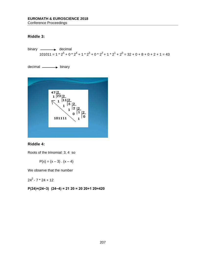
EUROMATH & EUROSCIENCE 2018 Conference Proceedings
207
Riddle 3: binary decimal
101011 = 1 * 25 + 0 * 2
4 + 1 * 2
3 + 0 * 2
2 + 1 * 2
1 + 2
0 = 32 + 0 + 8 + 0 + 2 + 1 = 43
decimal binary
Riddle 4: Roots of the trinomial: 3, 4 so
P(x) = (x – 3) . (x – 4)
We observe that the number
242
- 7 * 24 + 12
P(24)=(24−3) (24−4) = 21 20 = 20 20+1 20=420
EUROMATH & EUROSCIENCE 2018 Conference Proceedings
208
Riddle 5:
If the number of children is x then x-2 is a multiple of 3.
Also x-2 is a multiple of 4.
The integer multiples of 12 are: 12, 24, 36, 48, 60, 72 etc.
But x is a multiple of 5.
So if we add up to the previous multiples the number 2 we need to get a multiple of 5.
Thus the answer is 48 + 2 = 50
So x=50
When does the game end and begin serious math? For many, maths is considered a deadly
boring subject which has nothing to do with gaming. It is a set of acts, rules, theorems strictly
described without any relationship to games and pleasure.
On the contrary, in the eyes of most mathematicians it never ceases to be a game, but it is also
many other things.
Today we tried to give a sample of our "kitchen", so we dealt with:
● the Pythagorean theorem and the Pythagorean triads.
● problems solved with equations,
● the binary and decimal numbering system,
● trinomials
● multiple numbers,
Is it possible that playing games is actually mathematics?
EUROMATH & EUROSCIENCE 2018 Conference Proceedings
209
LEARNING MATHEMATICS WITH RUBIK’S CUBE Karol Gryszka
Pedagogical University of Cracow, Poland
ABSTRACT When you have a first contact with the Rubik’s Cube, You admire its shape, color patterns and eventually you start moving its faces. The color pattern changes with each rotation, from the solved state to the scrambled state where many stickers are mismatched. Couple moves later the cube is now really messed up and that is the right moment to start thinking about the inverse problem – given a scrambled cube you want to restore its original pattern, where each face has only one color of the stickers. In this article we present a journey via some mathematical aspects of the cube and explain how to solve it by using some abstract yet intuitive ideas. 1. INTRODUCTION
The Rubik’s Cube was invented by Erno Rubik [2], a Hungarian inventor and architect. His
adventure with creation of the puzzle finished in 1974, when he completed his first wooden
version of the cube. Three years later the cube was released in the Budapest; it took three more
years to release the cube to the world. It quickly became one of the best-selling puzzle at that
time, and it holds that title up to present day with more than 300 million units.
Astonishing fact about the cube is that it took its inventor about a month to solve it. Today, we
have many websites offering guides and tutorials [1], both video presentation and spreadsheets
with algorithms. They offer set of moves that one has to follow to complete the puzzle. While
that is an “easy” way to complete the cube, it does not carry any logic behind the actual solution.
By the logic we understand the following problem: how to figure out the actual sequence of
moves?
In this article we provide a simple mathematical approach to the problem of solving Rubik’s
Cube. We introduce some simple algebraic notions that are necessary to fully understand the
process of creating the solution. Thus, we divide the article into several sections. Firstly, we
provide a background theory of groups and (non-)commutative actions. Then we describe the
Rubik’s Cube as a group of a special kind of actions – permutations. We use notions of
conjugacy and commutator to explain the idea behind some sequences of moves. Finally, we
present the complete solution of the puzzle.
Throughout the article we use some convenient name for different pieces of the cube: we call
each of the 26 composing cubes “cubies”, a cubie with 2 stickers an edge and a cubie with 3
stickers a corner. Recall that if a fixed orientation of the cube is set (that is: we only rotate faces
so that the position between center pieces does not change), the middle stickers define the color
of the face at solved state as well as these cubies cannot swap between one another.

EUROMATH & EUROSCIENCE 2018 Conference Proceedings
210
2. SOME ASPECTS OF GROUP THEORY
The Rubik’s Cube can be seen as a group with a very specific action.
Definition 2.1. Consider any set G and an algebraic operation ∗. We call a pair (𝐺,∗) a group if
the following set of conditions is satisfied:
𝑎 ∗ 𝑏 ∈ 𝐺 for any 𝑎, 𝑏 ∈ 𝐺 (well-defined operation),
(𝑎 ∗ 𝑏) ∗ 𝑐 = 𝑎 ∗ (𝑏 ∗ 𝑐) for any 𝑎, 𝑏, 𝑐 ∈ 𝐺 (associative operation),
there exits an element 𝑒 ∈ 𝐺 such that 𝑒 ∗ 𝑎 = 𝑎 ∗ 𝑒 = 𝑎 for any 𝑎 ∈ 𝐺 (neutral element
property),
for any 𝑎 ∈ 𝐺 there is #𝑎 ∈ 𝐺 such that 𝑎 ∗ #𝑎 = #𝑎 ∗ 𝑎 = 𝑒 (inverse element property).
It is casual to denote the inverse element by 𝑎−1. We call a group (𝐺,∗) commutative (abelian)
if additionally
𝑎 ∗ 𝑏 = 𝑏 ∗ 𝑎 for any 𝑎, 𝑏 ∈ 𝐺.
Example 2.2. The following pairs are groups: (ℤ,+), (ℚ\{0},×) (the cross stands for
multiplication sign), the set of all polynomials with the " + " operation, the set of all congruences
on the plane (non-commutative), permutation group of the Rubik’s Cube (non-commutative as
well). The pairs (ℤ,×) and (ℝ,×) are not groups.
We leave the proof of the above statement as a simple exercise for the Reader.
We now describe the group of permutation. Consider any finite set 𝐴.
Definition 2.3. A permutation is arbitrary arrangement of the elements of 𝐴.
A group of permutations of 𝐴 is a collection of all permutations of 𝐴 with the operation of
composition of permutations.
We explain the above definition in the following example.
Example 2.4. Let 𝐴 = {1,2,3,4}. A permutation changes the order of the elements by defining
the outcome for each element of 𝐴. Take for instance the following permutation: 4, 3, 2, 1. In this
permutation first element is on the fourth place, second is on third etc. This can be represented
in the arrow notation as follows (the left column is the number and the right column is the position
it is mapped to):
1 → 4
2 → 3
3 → 2
4 → 1, We can briefly describe that permutation using the bracket-cycle notation:
(1 4)(2 3),

EUROMATH & EUROSCIENCE 2018 Conference Proceedings
211
which is understood in the following way: we look at each sequence in the bracket and follow
the path from left to right; if there is no number to follow, we cycle back to the first number. The
cycle is a single bracket described as above. Consider two more examples:
1 → 3
2 → 4
3 → 2
4 → 1,
briefly: (1 3 2 4);
The second example is the following:
1 → 2
2 → 3
3 → 1,
briefly: (1 2 3). Note that we skip 4 in the second example – if the number is not permutated we do not include
it in the bracket-cycle notation. We suggest, as an exercise, to decode two permutations to the
arrow notation: (1 3)(2 4), (4 2 3).
We now describe how to compose two permutations. Consider two permutations (1 2 3 4) and
(1 2 3). In order to compose them, that is to find the permutation
(1 2 3 4)(1 2 3),
we follow the change in values from right to left: 1 goes to 2 (the right permutation) and 2 goes
to 3 (the left permutation). Using the arrow notation we can write it as follows:
1 → 2 → 3,
2 → 3 → 4,
3 → 1 → 2,
4 → 4 → 1. Briefly: (1 3 2 4).
We can check that in such a case the set of all permutations of the set 𝐴 is
a group with the operation of composition. In particular, each permutation has its inverse one
and the neutral element of such an operation is the identity permutation, that is the arrangement
1, 2, 3, 4 for the case of the above example.
We now need to establish the notion of disjoint cycles.
Definition 2.5. Two cycles are disjoint if no common number appears in their description.
One can think of that property as some sort of the property of the entire permutation. The
permutation itself can be a composition of several cycles (the first permutation described in
Example 2.4 is such) or a single cycle. Cycles that are disjoint cannot be composed to form a
new cycle consisting of all elements of initial cycles, while the ones that are not disjoint can (like
it was for the case (1 2 3 4)(1 2 3) = (1 3 2 4)).
EUROMATH & EUROSCIENCE 2018 Conference Proceedings
212
Remark 2.6. Any permutation can be decomposed into the composition of disjoint cycles.
Definition 2.7. The order of the cycle is the number of elements in the cycle. The order of the
permutation is the least common multiplier of orders of composing and disjoint cycles.
One can also think of the order as the number of applications of the same permutations to obtain
the identity permutation.
Example 2.8. The permutation (1 2 3 4)(1 2 3) = (1 3 2 4) has order 4. The permutation
(1 4)(2 3) has order 2.
We leave the following as an exercise: evaluate the order of the following permutation:
(1 3)(2 4)(2 3)(1 3).
Definition 2.9. Consider two elements 𝑎 and 𝑏 of the group (𝐺,∗). The commutator of them is
the element [𝑎 𝑏] defined by the relation
[𝑎, 𝑏] = 𝑎 ∗ 𝑏 ∗ 𝑎−1 ∗ 𝑏−1. Definition 2.10. We call two elements 𝑎 and 𝑏 of the group (𝐺,∗) conjugated (and their
respective relation conjugacy) if there exists an element 𝑔 ∈ 𝐺 such that
𝑔 ∗ 𝑎 ∗ 𝑔−1 = 𝑏.
In that case we also say that 𝑎 is conjugated to 𝑏 and vice versa.
3. DESCRIPTION OF THE RUBIK’S CUBE
Each cubie of the Rubik’s Cube can be described using two or three letters from the set
{𝑅, 𝐹, 𝑈, 𝐿, 𝐵, 𝐷} – each letter corresponds to one of 6 faces: [R]ight, [F]ront, [U]p, [L]eft, [B]ack,
[D]own. In order to describe the cube using permutation we fix an orientation of it: for instance
the middle sticker on the front face can be red and the middle sticker on the up face can be
green. Then we associate with each cubie 2 (the edge piece) or 3 letters (the corner piece). For
instance,
𝑅𝐹 denotes the cubie that is on the 𝑅 face as well as on the 𝐹 face (in our fixed orientation
it is white-red edge),
𝑅𝐹𝑈 denotes the cubie that is on 𝑅, 𝐹 and 𝑈 faces (in our fixed orientation it is white-red-
green corner).
Note that the order of letters matters – 𝐹𝑅 describes the same edge, but with different order of
colors.
We can now describe a permutation of elements of the cube when the right face is turned 90
degrees clockwise. The resulting permutation is the following pattern
(𝐹𝑅𝑈 𝑈𝑅𝐵 𝐵𝑅𝐷 𝐷𝑅𝐹)(𝐹𝑅 𝑈𝑅 𝐵𝑅 𝐷𝑅),
which in particular is composition of two cycles of order 4, hence the entire permutation is of
order 4 and 4 rotations of the right face restore the original permutation of the cube. That agrees
with the intuition built without the mathematical background.
Let us also highlight the fact that one can actually choose 𝐹𝑈𝑅 as first element of the cycle, and
then the following ones would change accordingly – this describes the permutation of the same
pieces of the cube, but with different stickers order. We chose one, but the Reader can choose
EUROMATH & EUROSCIENCE 2018 Conference Proceedings
213
any other – the resulting permutation will slightly differ – the difference would be the order of
letters in following elements, but not the elements itself.
Remark 3.1. Every arrangement of the cube can be described as some permutation.
Example 3.2. If we rotate the right face clockwise and then top face counter-clockwise, both 90
degrees, the resulting permutation is
(𝐹𝑅 𝑈𝐵 𝑈𝐿 𝑈𝐹 𝑈𝑅 𝐵𝑅 𝐷𝑅)(𝐹𝑈𝑅 𝑈𝐿𝐵 𝑈𝐹𝐿 𝑈𝑅𝐹 𝐿𝐵𝑈 𝐹𝐿𝑈 𝐹𝑅𝑈 𝐵𝑈𝐿 𝐿𝑈𝐹) (𝐹𝐷𝑅 𝑈𝑅𝐵 𝐵𝑅𝐷 𝐷𝑅𝐹 𝑅𝐵𝑈 𝑅𝐷𝐵 𝑅𝐹𝐷 𝐵𝑈𝑅 𝐷𝐵𝑅).
The permutation consists of three disjoint cycles of orders 7, 9, 9, respectively. Hence, the entire
permutation is of order 63. We suggest checking with the actual cube rotations that 63 alternated
rotations of the right and the top face in a clockwise direction restore the cube to the solved
state.
We propose the Reader to describe a rotation of the right face 90 degrees clockwise followed
by a rotation of the top faces 90 degrees clockwise.
We can now see that the Rubik’s Cube is actually a group of permutations with the operation of
composition of permutations. This allows us to use the group theory, especially the notions of
conjugacy and commutator to find a solution to the puzzle.
4. SOLUTION
In this Section we use basic principles and ideas presented previously to provide a set of
algorithms that allows to solve the cube.
The first step is to introduce a convenient notation for rations of each face or slide of the cube.
We use:
𝑅,𝑈, 𝐹, 𝐿, 𝐵, 𝐷 for a 90 degrees rotation of right, up, front, left, bottom and down face,
respectively,
𝑀, 𝑆, 𝐸 for a 90 degree rotation of the slice between 𝑅 and 𝐿 (according to 𝐿), 𝐹 and 𝐵
(according to 𝐹) and 𝑈 and 𝐷 (according to 𝐷), respectively.
if the same move 𝑋 is applied twice in a row, we shorten 𝑋𝑋 to 𝑋2,
we denote the inverse move to 𝑋 by 𝑋′. Remark 4.1. We have the following:
(𝑋2)′ = 𝑋2,
(𝑋𝑌)′ = 𝑌′𝑋′ (this is the general rule for non-commutative groups).
There are more than 42 quintillion scrambles of the cube. To solve them all, it is sufficient to use
the specific set of algorithms that we describe and explain below.
Orientation of two edges: let
𝑋 = 𝐿 𝐸 𝐿2 𝐸2 𝐿,
𝑌 = 𝑈.
EUROMATH & EUROSCIENCE 2018 Conference Proceedings
214
Then
[𝑋, 𝑌] = (𝐿 𝐸 𝐿2 𝐸2 𝐿)𝑈 (𝐿′𝐸2 𝐿2 𝐸′𝐿′)𝑈′
is a commutator that swaps the orientation (but not the position) of 𝑈𝐿 and 𝑈𝐹 edges (the
notation is according to the one introduced in Section 3).
The algorithm works as follows: the 𝑋 move flips the orientation of the 𝑈𝐿 edge while keeping
the rest of upper face intact. By performing the 𝑌 move we change the edge that is now affected
by the 𝑋′ move, that undo the scrambled part of the cube while flipping the 𝑈𝑅 edge. The entire
algorithm therefore flips two adjacent edges on the top face (changes their orientation).
This algorithm is of order 2.
Permutation of three edges: let
𝑋 = 𝑀′,
𝑌 = 𝑈2.
Then
[𝑋, 𝑌] = 𝑀′ 𝑈2 𝑀 𝑈2
is a commutator that permutes 𝐹𝐷, 𝐹𝑈 and 𝑈𝐵 edges (it preserves their orientation).
The breakdown of this algorithm is simple: the 𝑀′𝑈2 sequence swaps 3 edges in the middle
slice, then the 𝑀 move restores centers to their original position. Finally, the 𝑈2 move fixes the
positioning of most top pieces.
Since three pieces are affected, the permutation has order 3.
Orientation of two corners: let
𝑋 = 𝐹′𝐷 𝐹 𝐿 𝐷 𝐿′,
𝑌 = 𝑈. Then
[𝑋, 𝑌] = (𝐹′𝐷 𝐹 𝐿 𝐷 𝐿′) 𝑈 (𝐿 𝐷′ 𝐿′ 𝐹′ 𝐷′ 𝐹) 𝑈′
is a commutator that rotates 𝐹𝑈𝑅 corner clockwise and 𝑈𝐹𝐿 corner counter-clockwise.
This slightly harder algorithm rotates the 𝐹𝑈𝑅 corner first while keeping the rest of the upper
layer intact (the 𝑋 move). Then we proceed similar to edge orientation – we place other corner
in place of 𝐹𝑈𝑅 one and reverse the 𝑋 move.
Since two pieces having three possible states are affected, the order of this permutation is 3.
Permutation of three corners: let
𝑋 = 𝐹 𝐿 𝐹′,
𝑌 = 𝑅2,
𝑍 = 𝐹2. Then
𝑍 [𝑋, 𝑌] 𝑍′ = 𝐹2 (𝐹 𝐿 𝐹′𝑅2 𝐹 𝐿′ 𝐹′ 𝑅2) 𝐹2
Is a conjugacy that permutes 𝑈𝐿𝐹, 𝑈𝑅𝐹 and 𝑈𝑅𝐵 corners.
The 𝐹2 moves are simply setup moves for the actual commutator. Unlike in other cases, this
algorithm has no simple intuition.
This permutation has order 3.
In order to solve the Rubik’s cube using these algorithms we first solve edges, then corners (or
corners first – it does not matter, but we find edges easier as first). Note that in order to solve
the edges one has to first permute the pieces, then to orient them. In order to permute them,

EUROMATH & EUROSCIENCE 2018 Conference Proceedings
215
one has to make a setup moves so that all pieces that are affected by the commutator are in
correct places. The same principle follows for the permutation of edges. For orientation, careful
solution can reduce the number of setup moves to 2 − 3.
Once the setup moves are performed, we can apply the algorithm and then undo the setup
moves, but we have to remember that they have to be done in reverse order and each move
must be an inverse as well. For example, if the setup moves where 𝑅 𝐹 𝑈, then to undo them
we do 𝑈′ 𝐹′ 𝑅′.
One can think of the above idea as the conjugacy – setup moves are followed by the actual
algorithm which is followed by the inversed setup moves.
5. FINAL REMARKS
There are many other algorithms that can be used to solve the cube, like for instance the
sequence
(𝑀′𝑈′𝑀′𝑈′𝑀′𝑈′𝑀′) 𝑈 (𝑀 𝑈 𝑀 𝑈 𝑀 𝑈 𝑀)𝑈′
is a different pattern of moves that swaps the orientation of two edges. In fact, the basic principle
of most algorithms that we have presented or one could search for is usually based on the two
notions: conjugacy and commutator. They allow to manipulate the cubies in a specific and
controlled way. Such a solution is also a good approach not only for a person willing to find out
the solution on their own, but also for mathematicians.
REFERENCES [1] Important Dates in Rubik’s Cube History, https://ruwix.com/the-rubiks-cube/history-rubiks-
cube/important-dates-timeline/
[2] Rubik’s Cube Guide, https://eu.rubiks.com/how-to-solve-rubiks-cube/