1

PROCEEDINGS OF THE

SAWTOOTH SOFTWARE

CONFERENCE

March 2009

2

Copyright 2009

All rights reserved. No part of this volume may be reproduced

or transmitted in any form or by any means, electronic or mechanical,

including photocopying, recording, or by any information storage and

retrieval system, without permission in writing from

Sawtooth Software, Inc.

3

FOREWORD

These proceedings are a written report of the fourteenth Sawtooth Software Conference, held

in Delray Beach, Florida, March 25-27, 2009. As a new element this year, our 2009 conference

was combined with the second Conjoint Analysis in Healthcare Conference, chaired by John

Bridges of Johns Hopkins University. Conference sessions were held at the same venue, and ran

concurrently. The presentations of the healthcare conference are published in a special edition of

The Patient—Patient Centered Outcomes Research.

The focus of the Sawtooth Software Conference continues to be quantitative methods in

marketing research. The authors were charged with delivering presentations of value to both the

most sophisticated and least sophisticated attendees. Topics included designing effective web-

based survey instruments, choice/conjoint analysis, MaxDiff, cluster ensemble analysis, and

hierarchical Bayes estimation.

The papers are in the words of the authors, with generally very little copy editing done on our

part. We are grateful to the authors who sacrificed time and effort in making this conference one

of the most useful and practical quantitative methods conferences in the industry. While

preparing this volume takes significant effort, we‘ll be able to review and enjoy the results for

years to come.

Sawtooth Software

August, 2009

i

CONTENTS

TO DRAG-N-DROP OR NOT? DO INTERACTIVE SURVEY ELEMENTS IMPROVE THE RESPONDENT

EXPERIENCE AND DATA QUALITY?: ...................................................................................... 11 Chris Goglia and Alison Strandberg Turner, Critical Mix

DESIGN DECISIONS TO OPTIMIZE SCALE DATA FOR BRAND IMAGE STUDIES ................................. 15 Deb Ploskonka, Cambia Information Group

Raji Srinivasan, The University of Texas at Austin

PLAYING FOR FUN AND PROFIT: SERIOUS GAMES FOR MARKETING DECISION-MAKING ................ 39 Lynd Bacon, Loma Buena Associates

Ashwin Sridhar, ZLINQ Solutions

SURVEY QUALITY AND MAXDIFF: AN ASSESSMENT OF WHO FAILS, AND WHY ............................ 55 Andrew Elder and Terry Pan, Illuminas

A NEW MODEL FOR THE FUSION OF MAXDIFF SCALING AND RATINGS DATA .............................. 83 Jay Magidson, Statistical Innovations Inc.

Dave Thomas, Synovate

Jeroen K. Vermunt, Tilburg University

BENEFITS OF DEVIATING FROM ORTHOGONAL DESIGNS ......................................................... 105 John Ashraf, Marco Hoogerbrugge, and Juan Tello, SKIM

COLLABORATIVE PANEL MANAGEMENT:

THE STATED AND ACTUAL PREFERENCE OF INCENTIVE STRUCTURE ............................................. 113 Bob Fawson and Paul Johnson, Western Wats Center, Inc.

ACHIEVING CONSENSUS IN CLUSTER ENSEMBLE ANALYSIS ..................................................... 123 Joseph Retzer, Sharon Alberg, and Jianping Yuan, Maritz Research

HAVING YOUR CAKE AND EATING IT TOO?

APPROACHES FOR ATTITUDINALLY INSIGHTFUL AND TARGETABLE SEGMENTATIONS ...................... 135 Chris Diener and Urszula Jones, Lieberman Research Worldwide (LRW)

ii

AN IMPROVED METHOD FOR THE QUANTITATIVE ASSESSMENT OF CUSTOMER PRIORITIES ............. 143 V. Srinivasan, Stanford University

Gordon A. Wyner, Millward Brown Inc.

TOURNAMENT-AUGMENTED CHOICE-BASED CONJOINT ....................................................... 163 Keith Chrzan and Daniel Yardley, Maritz Research

COUPLING STATED PREFERENCES WITH CONJOINT TASKS TO BETTER ESTIMATE

INDIVIDUAL-LEVEL UTILITIES ............................................................................................... 171 Kevin Lattery, Maritz Research

INTRODUCTION OF QUANTITATIVE MARKETING RESEARCH SOLUTIONS IN A TRADITIONAL

MANUFACTURING FIRM: PRACTICAL EXPERIENCES ............................................................... 185 Robert J. Goodwin, Lifetime Products, Inc.

CBC VS. ACBC: COMPARING RESULTS WITH REAL PRODUCT SELECTION ................................ 199 Christopher N. Chapman, Microsoft Corporation

James L. Alford, Volt Information Sciences

Chad Johnson and Ron Weidemann, Answers Research

Michal Lahav, Sakson & Taylor Consulting

NON-COMPENSATORY (AND COMPENSATORY) MODELS OF CONSIDERATION-SET DECISIONS ... 207 John Hauser, MIT

Min Ding, Pennsylvania State University

Steven Gaskin, Applied Marketing Sciences

USING AGENT-BASED SIMULATION TO INVESTIGATE THE ROBUSTNESS OF CBC-HB MODELS ....... 233 Robert A. Hart and David G. Bakken, Harris Interactive

INFLUENCING FEATURE PRICE TRADEOFF DECISIONS IN CBC EXPERIMENTS ............................... 247 Jane Tang and Andrew Grenville, Angus Reid Strategies

Vicki G. Morwitz and Amitav Chakravarti, New York University

Gülden Ülkümen, University of Southern California

WHEN IS HYPOTHETICAL BIAS A PROBLEM IN CHOICE TASKS, AND

WHAT CAN WE DO ABOUT IT? ......................................................................................... 263 Min Ding, Pennsylvania State University

Joel Huber, Duke University

iii

COMPARING HIERARCHICAL BAYES AND LATENT CLASS CHOICE:

PRACTICAL ISSUES FOR SPARSE DATA SETS ........................................................................... 273 Paul Richard McCullough, MACRO Consulting, Inc.

ESTIMATING MAXDIFF UTILITIES: DEALING WITH RESPONDENT HETEROGENEITY ........................... 285 Curtis Frazier, Probit Research, Inc.

Urszula Jones, Lieberman Research Worldwide (LRW)

Michael Patterson, Probit Research, Inc.

AGGREGATE CHOICE AND INDIVIDUAL MODELS:

A COMPARISON OF TOP-DOWN AND BOTTOM-UP APPROACHES .......................................... 291 Towhidul Islam, Jordan Louviere, and David Pihlens, University of Technology, Sydney

USING CONJOINT ANALYSIS FOR MARKET-LEVEL DEMAND

PREDICTION AND BRAND VALUATION ................................................................................. 299 Kamel Jedidi, Columbia University

Sharan Jagpal, Rutgers University

Madiha Ferjani, South Mediterranean University, Tunis

1

SUMMARY OF FINDINGS

The fourteenth Sawtooth Software Conference was held in Delray Beach, Florida, March 25-

27, 2009. The summaries below capture some of the main points of the presentations and

provide a quick overview of the articles available within these 2009 Sawtooth Software

Conference Proceedings.

To Drag-n-Drop or Not? Do Interactive Survey Elements Improve the Respondent

Experience and Data Quality? (Chris Goglia and Alison Strandberg Turner, Critical Mix):

Interactive survey elements programmed in Flash are increasingly being used by market

researchers for web-based surveys. Examples include sliders and drag-and-drop sorting

exercises. Chris‘ presentation focused on whether these interactive survey elements affect

respondent attention, participation and resulting data quality in an online survey. He and his co-

author examined completion speed, statistical differences between responses, stated satisfaction

with the questionnaire, and verbatim feedback. Interactive questions took longer, provided

almost identical responses, and resulted in slightly lower respondent satisfaction. Chris

mentioned that many individuals are now accessing the internet via smart phones, but the top-

selling phones currently don‘t support Flash. He expressed concern regarding the drive that

some clients have to use fancier Flash-style versions of standard question types. ―Just because

you can do something doesn‘t mean you should,‖ he cautioned. That said, he speculated that for

certain audiences (especially the young and technologically savvy), sliders and drag-and-drop

may make sense and be more defensible from a research-quality standpoint. And, there are other

ways to increase the polish and engaging quality of interviews (via skins, styles, and perhaps

even adding a graphic of a person on the page) that may improve the experience for general

respondent groups without having much impact on data quality and time to complete.

Design Decisions to Optimize Scale Data for Brand Image Studies (Deb Ploskonka,

Cambia Information Group, Raji Srinivasan, The University of Texas at Austin): Researchers

approach common scaling exercises in different ways. For example, there are different ways to

ask respondents to rate brands on multiple dimensions, and decisions regarding these scales can

have a significant effect on the results. Should a horizontal scale run from low to high, or from

high to low? Although a literature review suggested that market researchers tend to orient the

high point of the scale on the left, the audience at the Sawtooth Software conference (by a raise

of hands) indicated that right-side placement was more prevalent. Deb presented results of a

study showing that respondents complete questions faster when Best is on the Left, but more

discrimination of the items occurs when Best is oriented on the Right. Next, the authors studied

whether the number of brands rated had an effect on the distribution of brand ratings. Deb and

her co-authors observed lower scores on average when more brands are presented. This, she

cautioned, could have implications for brand tracking research. The last two topics she

investigated were the effects of including a Don‘t Know category on a scale, and whether it was

better to ask respondents to rate brands-within-attributes or attributes-within-brands. Some

respondents were frustrated by the lack of a Don‘t Know category, but Deb concluded that the

data were not harmed by its absence. Regarding rotation of brands with attribute or attributes

within brands, the authors found that asking respondents to rate brands within an attribute

(before moving to the next attribute) led to slightly lower multicollinearity and halo (though both

were quite high regardless).

2

Playing for Fun and Profit: Serious Games for Marketing Decision-Making (Lynd

Bacon, Loma Buena Associates and Ashwin Sridhar, ZLINQ Solutions): Lynd described how

academics and firms have begun to use games to predict, explain preferences, solve problems,

and generate ideas. These games are "purposive;" they have objectives other than entertainment

or education. Lynd reviewed recent applications, and discussed game design principles and

deployment issues. He mentioned a few of the games that have been devised by other

researchers to study preferences, including prediction markets (trading conjoint cards or

predictions of future events like stock), ―conjoint poker‖ and performance-aligned conjoint.

Games can also be useful for generating ideas for products or services. Lynd showed how an

online platform might work for running group problem-solving games. To date, the game he

described has been used for 56 rounds of the game, studying such problems as brand extensions,

attribute definition, package design improvement, and web site design.

Survey Quality and MaxDiff: An Assessment of Who Fails, and Why (Andrew Elder and

Terry Pan, Illuminas): Survey response quality has come under scrutiny due to the widespread

use of internet panels and the suspicion surrounding ―professional respondents.‖ Andrew

described some quality metrics that can identify ―bad‖ respondents who answer quickly or

haphazardly. Those include time to complete, speeding, consistency checks, and straightlining.

MaxDiff models are especially well-suited for identifying respondents who answer randomly

because of the fit statistic computed during HB estimation of scores. Andrew and his co-author

analyzed numerous datasets to investigate the response characteristics that threaten survey

quality. Not surprisingly, they found that respondents who suffer from low fit in MaxDiff also

tend to exhibit worse performance on other quality measures stemming from non-MaxDiff

questions. What may surprise some is that respondents who do fewer surveys per month tend to

have lower fit in MaxDiff. The cohort that tends to be the worst offender in terms of survey

quality is young+male+US/Canada. The presence of bad-quality responders tends to compress

MaxDiff scores somewhat (reduce variance). Even in the presence of a moderate degree of

quality problems with the data, Andrew and his co-author found that MaxDiff scores are

generally quite robust.

A New Model for the Fusion of MaxDiff Scaling and Ratings Data (Jay Magidson,

Statistical Innovations Inc., Dave Thomas, Synovate., and Jeroen K. Vermunt, Tilburg

University): A now well-known characteristic of MaxDiff (Maximum Difference Scaling) is the

fact that since only relative judgments are made regarding the items, the items are placed on a

relative scale. Jay illustrated that one can directly compare the relative strength of each item to

the others within a segment, but it can be problematic to compare scores for individual items

directly across segments. The problem stems from potential differences in the scale factor

between segments and the fact that some segments may feel all the items are more/less preferred

than other segments (which standard MaxDiff cannot determine). Jay presented a method for

combining MaxDiff information with stated ratings in a fused model to obtain scores that no

longer are subject to these limitations. Jay‘s approach involves a continuous latent variable to

account for individual differences in scale usage for the ratings, and scale factors for both the

ratings and MaxDiff portions of the model to account for respondents who exhibit more or lesser

amounts of uncertainty in their responses. Using a real MaxDiff dataset, Jay showed that

inferences for a standard MaxDiff model regarding the preferences for segments are different

from the model that fuses MaxDiff data with rating data. Jay noted that the fused model he

described is available within the syntax version of the Latent GOLD Choice program.

3

Benefits of Deviating from Orthogonal Designs (John Ashraf, Marco Hoogerbrugge, and

Juan Tello, SKIM): The authors noted that the typical orthogonal designs used in practice for

FMCG (Fast Moving Consumer Goods) CBC studies often present price variations that are at

odds with how price variations are actually done in the real world. Often, a brand has multiple

SKUs, representing different product forms and sizes. When brands alter their prices, they often

do so uniformly across all SKUs. The authors compared the psychological processes that may be

at work when respondents to CBC surveys see orthogonal prices that vary significantly across

SKUs within the same brands vs. CBC surveys if prices vary in step for a brand across its SKUs.

They described these as tending to promote a ―brand-focus,‖ or a ―price-focus‖ in tradeoff

behavior. A hybrid design strategy was recommended that blends aspects of pure orthogonality

with task realism of brands‘ prices moving in-step across SKUs. They compared results across

different CBC studies, concluding that the derived price sensitivities can differ substantially

depending on the design approach. On average, price sensitivity was lower when brands‘ prices

move in-step across SKUs, and hit rates for similarly-designed holdout tasks (which the authors

argued may better reflect reality) were higher than for orthogonal array price designs..

Collaborative Panel Management: The Stated and Actual Preference of Incentive

Structure (Bob Fawson and Edward Paul Johnson, Western Wats Center, Inc.): Keeping

panelists engaged and satisfied with the research process is essential to managing panels.

Western Wats employs a compensation strategy that rewards respondents whether they qualify

for a study or are disqualified. This reduces the incentive to cheat by trying to answer the

screening questions in a particular way that might lead to being qualified for a survey. Paul

discussed a research initiative at his company that focused on finding effective ways to provide

cost-effective incentives to panelists who do not qualify for a study. They used a stated

preference CBC study to investigate different rewards and (expected value) amounts for those

rewards. They observed actual panelist behavior over the next few months to see if the

conclusions from the CBC would be seen in actual, subsequent choices. They found that

respondents reacted much more positively to guaranteed rewards (with a small payout) rather

than sweepstakes (with a large payout to the few winners). This confirmed their company‘s

strategy, as Western Wats currently uses a guaranteed rewards system. Though there was

generally good correspondence between CBC predictions and subsequent behavior, there were

some systematic differences. Possible reasons for those differences were proposed and

investigated.

Achieving Consensus in Cluster Ensemble Analysis (Joseph Retzer, Sharon Alberg, and

Jianping Yuan, Maritz Research): Joe and his authors presented an impressive amount of

analysis comparing different methods of achieving a consensus solution in cluster ensemble

analysis. Cluster ensemble analysis is not a new clustering algorithm: it is a way of combining

multiple candidate segmentation solutions to develop a stronger final (consensus) solution than

any of the input solutions. Joe described a few methods for developing consensus solutions that

have been proposed in the literature, including a) direct approach, b) feature-based approach, c)

pair-wise approach, d) Sawtooth Software approach. The comparisons were made using a series

of artificial data sets where the true cluster membership was known (but where the respondent

data has been perturbed by random error). The Direct and Sawtooth Software methods

performed the best, and the other two methods performed nearly as well. Joe concluded that for

ensemble analysis, the quality and diversity of the segmentation solutions represented within the

4

ensemble is probably more important than the method (among those he tested) one chooses to

develop the consensus solution.

Having Your Cake and Eating It Too? Approaches for Attitudinally Insightful and

Targetable Segmentations (Chris Diener and Urszula Jones, Lieberman Research Worldwide

(LRW)): Urszula restated the common challenge of creating segmentation solutions that contain

segments that differ meaningfully and significantly on both the ―softer‖ attitudinal measures and

the ―harder‖ targeting variables such as demographics and transactions. Often, segments

developed based on attitudinal or preference data do not profile well on the targeting variables.

She presented a continuum of methods from purely demographic to purely attitudinal, and

showed that as one moves along that continuum, one shifts the focus from clean differentiation

on hard characteristics to clean profiling softer measures. The intermediate methods along the

continuum use both types of information to create a segmentation solution that has meaningful

differences on both hard and soft characteristics. Examples of those middling methods that

Urszula showed were Reverse Segmentation, Canonical Correlation, and Nascent Linkage

Maximization. She and her co-author Chris concluded that there is no perfect segmentation

approach. They recommended that researchers consider the main purpose for the segmentation,

the business decisions it drives, whether attitudinal or demographic differentiation is more

important, sample size, missing data, and whether a database needs to be flagged.

An Improved Method for the Quantitative Assessment of Customer Priorities (V.

Srinivasan, Stanford University, Gordon A. Wyner, Millward Brown Inc.): Seenu and Gordon

described a new method that Seenu has developed with Oded Netzer of Columbia University,

called Adaptive Self-Explication of Multi-Attribute Preferences (ASEMAP), for eliciting and

estimating the importance/preference of items. ASEMAP is an adaptive computer-interviewing

approach that involves asking respondents to first rank-order the full set of items (typically done

in multiple stages using selection into piles, then drag-and-drop within the piles). Then, it

strategically picks pairs of items and asks respondents to allocate (via a slider) a constant number

of points between the two items. The pairs are chosen adaptively and strategically to reduce the

amount of interpolation error of items not included in the paired comparisons. Log-linear OLS is

employed to estimate the weights of items included in the paired comparisons. The scaling of

any items not included in the pairs is done via interpolation based on the initial rank order.

Seenu and Gordon showed results of a study comparing constant sum scaling to ASEMAP. They

found that ASEMAP provided higher predictive validity (of holdout pairs) compared to the more

traditional Constant Sum (CSUM) method. The mean scores showed differences between the

methods. They briefly mentioned that a similar investigation comparing ASEMAP to MaxDiff

found ASEMAP to be superior, and it takes about the same time to complete as MaxDiff.

Tournament-Augmented Choice-Based Conjoint (Keith Chrzan and Daniel Yardley,

Maritz Research): Standard CBC questionnaires follow a relatively D-efficient (near-orthogonal)

design that does not vary depending on respondent answers. Such designs are highly efficient at

estimating all parameters of interest, but they involve asking respondents about a lot of product

concepts that are potentially far from their ideal. Additional (adaptive) choice tasks can be

constructed by retrieving and assembling winning (i.e. higher utility) product concepts from

earlier choice tasks. These customized tasks can follow a single-elimination tournament until an

overall winning concept is identified. Such tournaments involve comparing higher-utility

concepts and thus require deeper thinking on the part of the respondent. Across two studies,

Keith and Dan compared standard CBC to a tournament-augmented CBC in terms of a) hit rates

5

for holdout D-efficient choice sets and choice sets comprised of alternatives chosen in previous

sets, b) equivalence of model parameters. They found that augmenting CBC with tournament

tasks leads to very similar (but not equivalent) parameter estimates, with one parameter

demonstrating a statistically significant difference in both studies. Relative to standard CBC, the

tournament-augmented CBC predicted the higher-utility tournament holdouts a bit better, and the

standard CBC holdouts a bit worse. The authors concluded that the possible extra predictive

accuracy for the tournament augmented CBC was not worth the additional effort. Furthermore,

respondents required an extra minute on average to answer the same number of questions, so the

tournament also imposed an added cost to respondents.

Coupling Stated Preferences with Conjoint Tasks to Better Estimate Individual-Level

Utilities (Kevin Lattery, Maritz Research): Conjoint estimation of individual level utilities is

often done as a completely derived method based on responses to scenarios (revealed

preferences). In his presentation, Kevin argued that incorporating stated preferences about

unacceptable or highly desired levels of attributes can offer significant improvement in

estimating individual utilities. Incorporating this stated information resulted in higher hit rates

and more consistent utilities for the CBC dataset he described. Kevin asserted that incorporating

this stated information can significantly change the findings, most likely towards the truth. He

described different methods for incorporating stated preference information into utility

estimation. One method involves adding new synthetic choice tasks to each respondent‘s record,

indicating that certain levels are preferred to others. These synthetic tasks add information about

stated preferences or a priori information regarding preferences of levels. This strongly nudges

(but doesn‘t constrain) utilities in the correct direction. He also described imposing individual

constraints (via EM), and estimating non-compensatory screening rules. He concluded with the

recommendation to augment conjoint models with stated information. He suggested that the

stated preference questions should have limited scale points, so as not to force respondents to

distinguish between levels that really don‘t have much preference difference (such as a ranking

exercise might do).

Introduction of Quantitative Marketing Research Solutions in a Traditional

Manufacturing Firm: Practical Experiences (Robert J. Goodwin, Lifetime Products, Inc.):

Lifetime products is a manufacturing firm that creates consumer products constructed of blow-

molded polyethylene resin and power-coated steel, such as chairs, tables, portable basketball

standards, and storage sheds. Bob described the company‘s progression over the last three years

from using standard card-sort conjoint (SPSS) to CBC, to partial-profile CBC, to Adaptive CBC

(ACBC), spanning 17 total conjoint projects to date. He outlined what they have learned during

that time, and relayed some ―conjoint success stories.‖ First, Bob described how the research

department involved managers in trust-building exercises with conjoint. Managers were first

incredulous that sorting a few conjoint cards could lead to accurate predictions of thousands of

possible product combinations. By asking managers to participate in conjoint interviews and by

showing them the results (including market simulators developed in Excel), Bob was able to

obtain buy-in to complete more ambitious studies with consumers. Bob was able to demonstrate

the effectiveness of conjoint via a series of studies for which results were validated in subsequent

sales data. For example, conjoint pointed to price resistance beyond $999 for a fold-up trailer,

and subsequent sales experience validated that inflection point. Conjoint analysis revealed a

consumer segment that recognized the quality in Lifetime‘s folding chairs, and was willing to

pay a bit more for the benefits. As managers became more comfortable with the methods, their

6

demands escalated (particularly in numbers of attributes). Graphical representation of attributes

has helped manage the complexities. Bob discussed how Adaptive CBC (ACBC) has given his

research department even greater flexibility to handle manager‘s requests and led to cost savings

and greater respondent engagement. ACBC has allowed them to study more attributes and with

smaller sample sizes than partial-profile CBC.

CBC vs. ACBC: Comparing Results with Real Product Selection (Christopher N.

Chapman, Microsoft Corporation, James L. Alford, Volt Information Sciences, Chad Johnson

and Ron Weidemann, Answers Research, and Michal Lahav, Sakson & Taylor Consulting): Chris

and his coauthors summarized an investigation into the comparative merits of CBC and Adaptive

CBC (ACBC). At Microsoft Corporation, Chris was recently asked to forecast the likely demand

of a peripheral device. He used CBC and ACBC to forecast demand, and both methods

forecasted well. Based on later sales data, the ACBC results were slightly better than CBC.

When conducting market simulations, the scale factor for both methods needed to be ―tuned

down‖ to best predict actual market shares. ACBC required an even lower scale factor tuning,

implying more information and less error at the individual level than CBC. Because respondents

had completed both ACBC and CBC questionnaires, the researchers were also able to make

strong comparisons. They found ACBC part-worths to have greater face validity (fewer

reversals), and price sensitivity to be more diverse and stronger than CBC. A within-subjects

correlation showed that part-worths between the methods were similar, but not identical. Even

though ACBC took respondents longer to complete than CBC (7 minutes vs. 4 minutes),

respondents reported that it was less boring. The authors concluded that ACBC works well, and

they like to use multiple methods to forecast when there is significant cost for wrong decisions.

Non-Compensatory (and Compensatory) Models of Consideration-Set Decisions (John

R. Hauser, MIT, Min Ding, Pennsylvania State University, and Steven P. Gaskin, Applied

Marketing Sciences, Inc.): John and his coauthors conducted an extensive review of academic

papers dealing with consideration-set decisions. John stated that for many businesses (such as

for GM), consideration set theory is key to their survival. If only a minority of customers will

even consider a GM car, then it matters little that Buick was recently rated the top rated

American car by Consumer Reports or that JD Powers rates Buick best on reliability next to

Lexus. Research on consideration-set measurement began in the 1970s and continues today

(with recent dramatic growth in interest). Experiments suggest that the majority of respondents

employ non-compensatory decision behavior in situations that are detailed in the paper.

Academics suggest that buyers are more likely to employ non-compensatory heuristics when

there are more product alternatives, more product features, during the early phases of the

decision, when there is more time pressure, when the effort to make a decision is salient, and for

mature products. The authors examined a few published comparisons between compensatory

and non-compensatory rules. They point out that the standard additive part-worth rule is actually

a mixed rule because it nests both compensatory and non-compensatory decision rules. Non-

compensatory rules usually outperform purely compensatory rules, but the (mixed) additive rule

often performs well. The authors warn that managerial implications may be different even when

decision rules cannot be distinguished on predictive ability. And, the more a product category

would favor non-compensatory processing, the more value is found in models that incorporate

non-compensatory processing and consideration set theory.

Using Agent-Based Simulation to Investigate the Robustness of CBC-HB Models (Robert A. Hart and David G. Bakken, Harris Interactive): David explained that CBC/HB

7

assumes a compensatory data generation process (it assumes that respondents add the value of

each feature before making a product choice). But, research has shown that most respondents

actually employ choice strategies that do not conform to the compensatory, additive assumption.

The question becomes how well CBC/HB performs under varying amounts of non-compensatory

processing among respondents. To investigate this, David and his co-author used agent-based

modeling to generate respondent data. Each respondent was an agent that answered CBC

questionnaires under different strategies, and with different degrees of error. The strategies

included pure compensatory, Elimination by Aspects (EBA), and satisficing (along with a

mixture of these behaviors). They found that CBC/HB worked very well for modeling

compensatory respondents, and reasonably well even when dealing with respondents that used

strictly non-compensatory strategies.

Influencing Feature Price Tradeoff Decisions in CBC Experiments (Jane Tang and

Andrew Grenville, Angus Reid Strategies, Vicki G. Morwitz and Amitav Chakravarti, New York

University, and Gülden Ülkümen, University of Southern California): Jane and her coauthors

indicated that the implied willingness-to-pay (WTP) resulting from conjoint analysis is

sometimes much higher than seems realistic. A possible explanation they gave was that

respondents are often educated (via intro screens) about other features, but not necessarily about

price. They also reminded the audience that question order and context effects can influence the

answers to survey research questions. To see what kinds of elements might affect implied WTP

in CBC studies, they tested a number of treatments in a series of split-sample studies. The

treatment that had the largest positive effect on price sensitivity for standard CBC (resulting in

lower WTP) was placing a BYO/configurator question prior to the CBC exercise. Also, they

found that using Adaptive CBC (ACBC), which includes BYO as its first phase, led to the

greatest increase in price sensitivity among the methods they tested. Their results also showed

the choice of number of scale points (fine vs. broad scale) for questions asked prior to the CBC

section may also have an impact on the results. They cautioned that researchers should pay

attention to the exercises leading into the CBC portions of the study, as they can have an impact

on the part-worth estimates (and derived WTP) from CBC.

When Is Hypothetical Bias a Problem in Choice Tasks, and What Can We Do About It? (Min Ding, Pennsylvania State University, and Joel Huber, Duke University): Min and Joel

reminded us that most all conjoint/choice research we do involves asking respondents

hypothetical questions. The quality of insights from these preference measurement methods is

limited by the quality of respondent answers. Hypothetical bias occurs when respondents give

different answers in hypothetical settings than what they would actually do. The authors

reviewed recent research on incentive aligning respondents, aimed to improve data quality by

ensuring it is in the respondent‘s best interest to state truthfully. Some of these methods involve a

reward system such that respondents receive (or have a chance of receiving via lottery) a product

directly related to their stated preferences (utilities). This gives respondents an incentive to

answer truthfully, as their choices can have practical consequences for them. Min and Joel

reviewed studies showing that incentive-aligned respondents lead to greater predictive accuracy

and different parameter estimates, such as greater (and less heterogeneous) price sensitivity. For

many studies, it may not be feasible to incentive align respondents by giving them a product

corresponding to their choices (e.g. automobiles). The authors reviewed other techniques for

engaging respondents and encouraging them to report values that correspond to their actions in

the marketplace. Adaptive conjoint surveys are seen to keep respondents engaged. Also, the

8

authors indicated that they think panel respondents are less likely to express hypothetical bias

than non-panelists. Such respondents enjoy taking surveys, are good at them, trust that their

answers are anonymous, are relatively dispassionate, and can be selected to ensure their

relevance and interest in the topic.

Comparing Hierarchical Bayes and Latent Class Choice: Practical Issues for Sparse

Data Sets (Paul Richard McCullough, MACRO Consulting, Inc.): Two common tools used for

analyzing CBC data are Latent Class (LC) and hierarchical Bayes (HB). Richard suggested that

some researchers regard LC as a more effective tool for especially sparse datasets than HB, since

its aim is not to estimate individual-level parameters. He noted that past research has shown that

partial-profile studies may be so sparse that HB is not terribly effective at estimating robust

individual-level parameters. Richard compared HB and LC estimation using three commercial

datasets with varying numbers of parameters to be estimated relative to amount of information

for each individual. Overall, LC and HB performed very similarly in terms of hit rates and share

predictions (after tuning scale for comparability). Hit rates for LC benefited from an advanced

procedure offered in Latent Gold software called ―Cfactors.‖ Also, for especially sparse datasets,

adjusting HB‘s ―priors‖ helped to improve hit rates. He suggested that sample size probably has

more effect on model success than the choice of LC or HB. Richard concluded by stating that

for the naïve user, HB is especially robust and actually faster from start to finish than LC. Also,

in his opinion, LC (especially with the advanced procedures that Richard found useful) requires

more expertise and hands-on decisions than HB, at least using existing software solutions. But,

if the researcher is interested in developing strategic segmentations, then one could benefit

substantially from the LC segmentation solutions.

Estimating MaxDiff Utilities: Dealing with Respondent Heterogeneity (Curtis Frazier,

Probit Research, Inc., Urszula Jones, Lieberman Research Worldwide (LRW), and Michael

Patterson, Probit Research, Inc.): A long-standing issue with generic HB (and its assumption of a

single population with normally distributed preferences) has been whether to estimate the model

with all respondents together, or to run HB within segments. Michael‘s presentation investigated

how problematic the effects of pooled estimation and Bayesian shrinkage to global population

parameters are. The conclusion of these authors mimics and confirms earlier (2001) research

dealing with the same question for CBC data at the Sawtooth Software conference presented by

Sentis & Li. They found that segmenting using a priori segments (not necessarily closely linked

to preferences) and estimating HB within segments actually hurt results. Even segmenting using

cluster analysis based on preferences slightly degraded recovery of known parameters for the

synthetic datasets. It should be noted that their sample size of 1000 was larger than those used

by Sentis and Li, but still may not be enough for this type of sub-group analysis. If the sub-

segment size becomes too small, the possible benefit from running HB within segments is

counterbalanced by the lower precision of the population estimates of means and covariances,

and the resulting negative repercussions on individual-level parameters.

*Aggregate Choice and Individual Models: A Comparison of Top-Down and Bottom-Up

Approaches (Towhidul Islam, Jordan Louviere, and David Pihlens, University of Technology,

Sydney): Jordan reviewed the fact that for choice models estimated via logit, scale factor and

parameters are confounded, making it difficult to compare raw part-worth parameters across

respondents. He illustrated the problem by showing hypothetical results for two respondents,

one who is very consistent and has high scale and another that is inconsistent and has low scale.

When such is the case, it is foolish to claim that a single part-worth parameter from one

9

respondent reflects higher or lower preference than another, since the scale and the size of the

parameter are confounded. He argued in favor of choice models that capture more information at

the individual level, using techniques such as asking respondents to give a full ranking of

concepts within choice sets, first choosing the best, then the worst, then intermediate alternatives

within the set. With such models, Jordan reports that enough information is available for purely

individual-level estimation. Such models he described as ―bottom up‖ models. In contrast, ―top

down‖ models are those that estimate respondent parameters using a combination of individual

choices as well as population-level means and covariances. Jordan argued that the majority of

the preference heterogeneity that researchers believe to be finding in top-down approaches is due

to differences in scale rather than true differences in preference. Finally, Jordan showed

empirical results for four CBC datasets, where purely individual-level estimation via weighted

logit generally outperforms top-down methods, including HB.

(*Recipient of best-presentation award as voted by conference attendees.)

Using Conjoint Analysis for Market-Level Demand Prediction and Brand Valuation (Kamel Jedidi, Columbia University, Sharan Jagpal, Rutgers University, and Madiha Ferjani,

South Mediterranean University, Tunis): Kamel and his co-authors developed and tested a

conjoint-based methodology for measuring the financial value of a brand. Their approach

provides an objective dollarmetric value for brand equity without requiring one to collect

subjective perceptual or brand association data from consumers. In particular, the model allows

for complex information-processing strategies by consumers and, importantly, allows industry

volume to vary when a product becomes unbranded. Kamel described how the model defines

firm-level brand equity as the incremental profitability that the firm would earn operating with

the brand name compared to operating without it. To compute the profitability of a product when

it loses its brand name, the authors used a competitive equilibrium approach to capture the

effects of competitive reactions by all firms in the industry when inferring the market level

demand for the product when it becomes unbranded. The methodology is tested using data for

the yogurt industry and the authors compared the results to those from several extant methods for

measuring brand equity. Kamel reported that the method is externally valid and is quite accurate

in predicting market-level shares; furthermore, branding has a significant effect on industry

volume.

11

TO DRAG-N-DROP OR NOT?

DO INTERACTIVE SURVEY ELEMENTS IMPROVE THE RESPONDENT

EXPERIENCE AND DATA QUALITY?

CHRIS GOGLIA

ALISON STRANDBERG TURNER CRITICAL MIX, INC.

For the most part, online survey questions look the same today as they did five years ago.

And we, as online survey programmers, have encouraged our clients to keep them that way!

We‘ve been concerned about whether or not respondents have JavaScript, the speed of their

Internet connection, and the size of their screen resolution. However, there have been

technological changes over the past five years that give us reason to re-examine this issue.

Two separate research-on-research studies, one done recently, and one conducted five years

ago, show that almost all online survey respondents now have high-speed Internet connections

while only half did five years ago. Web sites like thecounter.com, which track browser and

computer information from all sorts of web site visitors, show that respondents are far more

likely to have JavaScript and large computer displays with high resolution than ever before.

These types of statistics support that it might be okay to begin using more advanced technologies

and/or question layouts in online surveys.

Two of the most common interactive exercises that marketing professionals consider adding

to online surveys are drag-n-drop card sorts and interactive sliders. But do respondents

understand these exercises? Will respondents recognize these exercises and be comfortable

using them based on their previous web experiences? And are there any significant reasons,

technological or otherwise, why we should continue to not use these in our online surveys?

To begin to answer these questions we found a list of the 20 most visited web sites in the

United States and searched each one for the aforementioned types of interactive features. We

found drag-n-drop exercises at ESPN and Yahoo, but we found nothing interactive at Google,

craigslist, Wikipedia, eBay, or Amazon. Our conclusion is that while these interactive capabilities

do exist, they‘re not prevalent, and it‘s not safe to assume that online survey respondents are used

to encountering them during their normal daily Internet usage.

We also considered the growing usage of smart phones — mobile phones with a web

browser. We found syndicated research showing that the top-five selling phones in the United

States are all smart phones, but that none of them support Flash — a technology often used to

implement interactive exercises. What if smart phone users want to take online surveys from

these devices? Might there be a recruitment bias if we only interview respondents willing to take

an online survey from a traditional computer? The growing usage of smart phones could be a

significant barrier to the widespread adoption of interactive exercises.

With that background research in mind, we conducted a research-on-research online survey

to answer one main question: Do interactive survey elements have an effect on respondent

12

attention, participation and resulting data quality in an online survey? We sought to answer this

question with the following techniques:

Measuring the speed at which respondents took the survey

Checking for statistical differences between responses to the same question displayed in

different formats: traditional vs. interactive

Evaluating stated satisfaction with the survey experience

Analyzing verbatim feedback provided by respondents

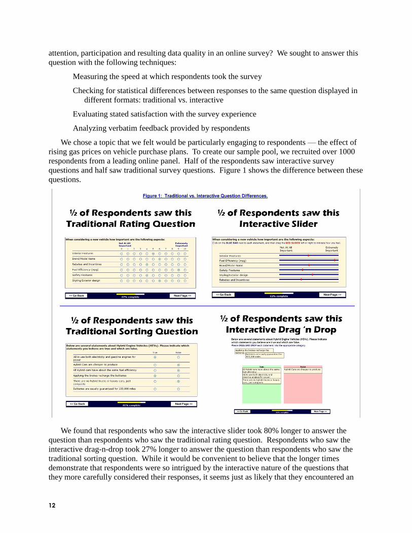
We chose a topic that we felt would be particularly engaging to respondents — the effect of

rising gas prices on vehicle purchase plans. To create our sample pool, we recruited over 1000

respondents from a leading online panel. Half of the respondents saw interactive survey

questions and half saw traditional survey questions. Figure 1 shows the difference between these

questions.

We found that respondents who saw the interactive slider took 80% longer to answer the

question than respondents who saw the traditional rating question. Respondents who saw the

interactive drag-n-drop took 27% longer to answer the question than respondents who saw the

traditional sorting question. While it would be convenient to believe that the longer times

demonstrate that respondents were so intrigued by the interactive nature of the questions that

they more carefully considered their responses, it seems just as likely that they encountered an

13

exercise they weren‘t use to seeing in other online surveys and elsewhere on the Internet, and it

just took them longer to figure out what to do. It may have just taken them longer to provide the

same answer they would have provided anyway!

Most agree longer surveys are not desirable as they can lead to increased respondent fatigue

and data quality problems. And as survey length increases, you‘re also likely to experience

higher abandonment rates, lower incidence, higher recruitment costs, and higher incentive costs.

The increased time it took respondents to answer the interactive exercises would only be worth it

if their responses to those questions were different, and, hopefully better.

We discovered that there were almost no meaningful differences between data from

respondents who saw the interactive questions compared with those who saw the traditional

questions. In general, the statements being tested were rated or sorted similarly, in the same

order, and with no statistical differences. There was one exception in the interactive drag-n-drop

exercise. There was a statistical difference with one of the statements, and it was the statement

that respondents were least sure about.

Before completing the survey, respondents were asked what they thought about the survey

experience relative to other online surveys they had taken. There was no significant difference in

stated satisfaction between respondents who did and did not see the interactive exercises. This

was true with the average ratings, top box ratings, top-2 box ratings, and top-3 box ratings.

Finally, respondents were given the opportunity to provide verbatim feedback about their

survey experience. Respondents who saw the interactive exercises did provide positive feedback

about them but for every respondent who mentioned an interactive exercise, there were far more

respondents who commented on the relevance of the topic and the design of the questionnaire.

Perhaps putting more effort into sampling and questionnaire design could have a far larger

impact on respondent engagement and resulting data quality than throwing in a couple of

interactive exercises.

So do interactive survey elements improve the respondent experience and data quality?

Interactive question types can require more sophisticated and expensive web surveying software,

more highly skilled survey programmers, and longer programming times. The data from our

research-on-research study suggest that interactive questions take longer to complete while

eliciting the same data from respondents as do traditional survey questions. And as the use of

mobile devices like smart phones continues to grow, surveys may need to be made shorter and

simpler to run on them, instead of longer and more complex. While there is no simple answer to

our question, we believe there are many valid reasons for carefully considering whether or not to

include interactive elements in your next online survey.

15

DESIGN DECISIONS TO OPTIMIZE SCALE DATA

FOR BRAND IMAGE STUDIES

DEB PLOSKONKA

CAMBIA INFORMATION GROUP, LLC

RAJI SRINIVASAN, PH.D. THE UNIVERSITY OF TEXAS AT AUSTIN, MCCOMBS SCHOOL OF BUSINESS

BACKGROUND

The writing of every survey question requires a plethora of decisions. Do we ask questions

or make statements? Do we detail the scale just in the response options or both the text and

response options? Do we anchor scale points with words or only use numbers? Do we ask

questions in a grid or one by one?

Each decision we make, whether active or passive, may have an impact of unknown degree

on the results we achieve. In each case we want to:

maximize the respondent experience (to the extent we care about our respondents both

giving valid answers and having a positive experience)

differentiate one respondent from another, one brand from another, one attribute from

another

obtain reliable results from one time to the next

and, bottom line, deliver a story with our data that will contribute to the client‘s success.

These questions and objectives are not new. But as we go through our careers from one

market research company to another – or supplier-side to client-side and back again – we may

accumulate an accretion of unintended biases regarding how we write our survey questions that

are not tied to objective results but instead to ―this is how we‘ve always done it.‖

This paper undertakes two missions:

Sample the existing academic literature in four areas to help practitioners make conscious

those decisions which may previously have been unconscious or assumed

Through research on research using our own experimental data with brand-attribute scale

questions, address four design decisions for online studies:

1. Do we place the best value in a scale at the left or at the right?

2. Do we offer a ―don‘t know‖ response option?

3. Does it make a difference how many brands respondents rate at once?

4. In collecting brand image ratings, should we randomize attributes within brands

or brands within attributes?

16

STUDY 1: BEST ON THE LEFT OR BEST ON THE RIGHT IN A LIKERT SCALE

In an informal poll of 150 educated research professionals attending the 2009 Sawtooth

Conference, 100% of those who voted raised their hands to indicate they would put the best

value in a scale at the right. Nevertheless, since then the author has seen a number of panel

surveys and others with the best at the left.

Initially and at the time of the conference, we would have agreed with the 150 without

reservation. Some of our results since are not as straightforward and we encourage researchers

to continue examining this issue in different industries, with different respondent types, and with

brand sets that are both similar and others that are quite diverse.

Prior Work The first substantive work we found on this topic presented four to seven-scale point items

on paper, in person, vertically (Belson, 1966). Belson reminds us that there is (as yet) no

evidence which scale direction more accurately reflects the respondent‘s mindset … only that the

scale presentation order influences the results. They tested ―traditional‖ (high to low) [sic] order

against the reversed, across respondents. Among the results they found (n=332):

Items at the ends of the scale are particularly subject to order effects, in particular the first

item presented experienced a bump

The effect was consistent regardless of the length of the scale, or type of scale (approval,

satisfaction, liking, agreement, interest)

Belson concludes by questioning if horizontal scales or products or issues where the

respondent is less familiar or interested would see the same effect. This topic will be addressed

later within this paper.

Holmes (1974) tested horizontal bipolar scales among 240 beer-drinking respondents. Two

of his results relate:

Respondents‘ responses were regressing toward the center from the beginning of the

questionnaire to the end

Respondents were more likely to choose the response at the left side of the page (that is,

the first presented for an English reader)

Holmes notes that our assumption in sampling theory that measurement errors will be

uncorrelated and cancel each other out may not be so.

Another variation tested was to include both favorable and unfavorable statements with a 5-

point strongly agree to strongly disagree scale (or SD to SA) (Friedman, Herskovitz and Pollack,

1994). The researchers continued to find a bias towards the left side of the scale (n=208

undergraduates), but only for those statements where the attribute was worded positively. In

general the attitudes measured (towards their college) were quite positive and it appeared the

students would disagree with the unfavorable statements no matter where ‗disagree‘ was located.

Our Study We intended to evaluate the pros and cons of each orientation so that we can could advise our

clients on the design of future surveys. We wanted to be able to evaluate the respondent

17

experience, as these are real people who we want to come back and take our surveys again.

Indeed, our respondents may be future clients, so offering an intuitive and user-friendly survey is

paramount to our company‘s current and future success. We also wanted to measure if either

orientation increases discrimination between brands and the impact on rating differences.

Our study differs from the past studies we reviewed in that it was conducted online, with

ratings of multiple targets or brands on multiple attributes.

Respondents were administered a roughly 13-minute questionnaire on some aspects of the

healthcare industry. Greenfield Online provided the sample, with the following respondent

qualification criteria:

Age 18+

Covered by health insurance

Makes health insurance decisions for their household

Differences in the control and test groups were as follows:

Control Test

Location of best value Left Right

Interviews (n) 1,047 203

Field dates June 11 – July 4, 2008 September 8 – 16, 2008

Respondents rated three brands with which they were familiar, one brand per screen, on a

series of 14 attributes, on a grid with a bipolar seven-point scale (the one very top company,

world class, stronger than most, average, weaker than most, much worse than other companies,

the one worst company – and the reverse, followed by don‘t know) as seen in Figure 2.

Figure 2

Control and Test Questions for Left-Right vs. Right-Left Study

18

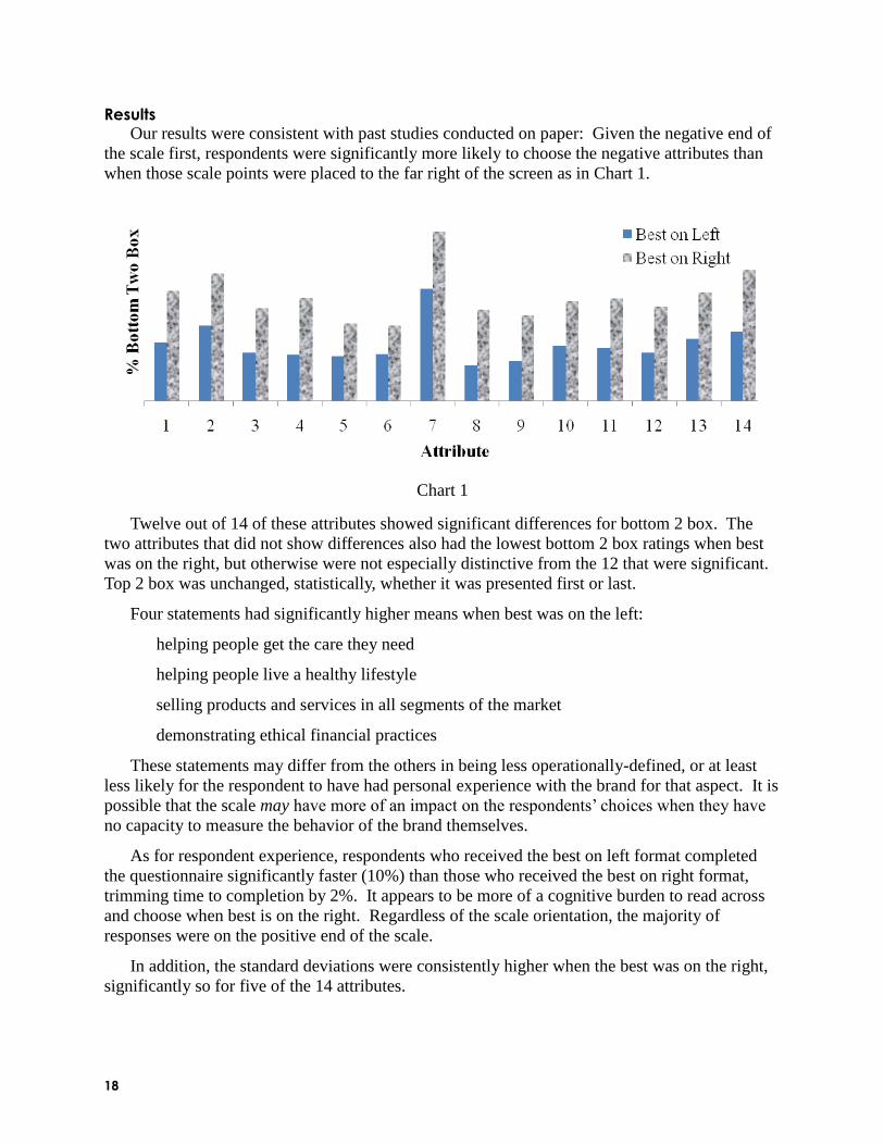
Results Our results were consistent with past studies conducted on paper: Given the negative end of

the scale first, respondents were significantly more likely to choose the negative attributes than

when those scale points were placed to the far right of the screen as in Chart 1.

Chart 1

Twelve out of 14 of these attributes showed significant differences for bottom 2 box. The

two attributes that did not show differences also had the lowest bottom 2 box ratings when best

was on the right, but otherwise were not especially distinctive from the 12 that were significant.

Top 2 box was unchanged, statistically, whether it was presented first or last.

Four statements had significantly higher means when best was on the left:

helping people get the care they need

helping people live a healthy lifestyle

selling products and services in all segments of the market

demonstrating ethical financial practices

These statements may differ from the others in being less operationally-defined, or at least

less likely for the respondent to have had personal experience with the brand for that aspect. It is

possible that the scale may have more of an impact on the respondents‘ choices when they have

no capacity to measure the behavior of the brand themselves.

As for respondent experience, respondents who received the best on left format completed

the questionnaire significantly faster (10%) than those who received the best on right format,

trimming time to completion by 2%. It appears to be more of a cognitive burden to read across

and choose when best is on the right. Regardless of the scale orientation, the majority of

responses were on the positive end of the scale.

In addition, the standard deviations were consistently higher when the best was on the right,

significantly so for five of the 14 attributes.

19

We then considered how well respondents were able to differentiate between brands.

Stacking the data by attribute shows that at least on a gross level (grand mean), respondents are

separating the brands more distinctly when best is on the left, in particular between Brand 3 and

4 (Chart 2). Means could be masking differences occurring on a more granular level.

Moreover, using discriminant analysis, measuring the Euclidean distance from the origin for

centroids, shows 3 brands are undiscriminated when the best value is on the right, as in Chart 3.

Charts 2 and 3

It would appear that while best on the right produces more variance within brands using this

Euclidean distance algorithm, best on the left produces more variance between brands, for our

limited dataset with four brands only, and one quite different from the rest. The means, on the

other hand, demonstrate Brand 3 aligning with Brand 1 in one case and with Brand 4 in the other.

The story told by this is therefore not clearly about differentiation but instead about a change in

scores following a change in presentation style.

Comparing regression coefficients using ―likelihood to recommend‖ as the dependent

variable resulted in insignificant results using the Chow test. However, multicollinearity in all

four studies is quite high.

Conclusion Our results of a survey conducted online support past results from paper surveys: The

orientation in which a scale is presented will influence the outcome, and the negative end of the

scale is more likely to be selected when presented first. It might be further hypothesized that

seeing the most negative end first gave respondents implicit permission to choose it.

Past results did not delve into the differentiation of the items being measured, only the

difference in means. Simply looking at means leaves the differentiation unclear. Using a

Euclidean algorithm, with only four brands we see more differentiation between brands with the

best on the left. This result deserves further exploration – would the results repeat with different

questions, sample, brands, or context?

20

Furthermore, we hypothesize that repeating these tests with languages that are read in a

different direction would show similar effects for primacy and not just for absolute orientation.

STUDY 2: NUMBER OF BRANDS RATED

In this study we looked at how many brands respondents rated at a time and if this impacted

the results. The null hypothesis would be that there is no difference, and we were able to reject

this hypothesis.

Prior Work Exhaustive secondary research uncovered only one somewhat related study. Working off the

classic study by Miller (1956), Hulbert (1975) applied the information processing rule of thumb

of ―seven units (plus or minus two)‖ to scale usage. This rule of thumb briefly summarized:

researchers have found that humans have the ability to hold or evaluate seven individual items in

mind at once, whether that be remembering a sequence of numbers, counting dots on a screen,

perception of speech variations, et cetera. After seven (+/- two) items, we must organize the

material into chunks in order to continue to retain or evaluate it.

Hulbert wanted to assess whether this principle would be true in scale ratings. And so rather

than presenting respondents with a preset scale, they were allowed to assign any positive number

they wished in rating the stimuli, on three different scales [―scale‖ used here in the test

construction sense], each over 50 items each. He hypothesized the number of distinct

assignments respondents would use would be less than or equal to 10.

Indeed, respondents (97 salesman) used between 6 and 10 ratings, on average, to express

their opinions of dissatisfaction, motivation or satisfaction with their job. Hulbert writes,

One of the goals of scale design is generally to avoid preventing the respondent from

expressing his true feelings because of some property of the scale itself. Thus, a necessary

though not sufficient condition to attain measurement at some level equal to or higher

than ordinal is that the scale used should enable preservation of strict monotonicity

between obtained measures and the underlying (latent) continuum. This condition is met

simply by ensuring that the number of categories in the scale is greater than the number

of stimuli to be rated.

In applying his results to market research, he suggests that the small number of items (often

brands) usually rated should avoid measurement error, but due to information capacity limits,

rating more could lead to more measurement error.

21

Our Study In our study we asked respondents to rate either up to three brands or up to six brands on a

five point scale (the one very top firm, world class, stronger than most, average, weak), for

sixteen attributes regarding brands in the financial industry, as in Figure 3.

Figure 3:

Control and Test Questions for Number of Brands Rated Study

To qualify for this study, respondents needed to have voted, attained a certain minimum level

of investments and income, and be actively involved in expressing their opinions publicly on

financial issues. The screener averaged three minutes to complete, followed by a six-minute

questionnaire, half of which was the brand rating series. The e-Rewards panel provided the

online sample.

Differences in the control and test groups were as follows:

Control Test

Number of brands rated Up to 3 familiar with Up to 6 familiar with

Interviews (n) 272 of which 222 qualified for

more than three brands

155 of which 127 qualified and

were asked more than three brands

Field dates November 5 – December 2, 2008 December 5 – 12, 2008

22

Results If respondents are indeed constricted by information processing capacity, or simply

overwhelmed or fatigued by an increased requirement to process and provide information, what

may happen? Measurement error. While we can‘t necessarily label it error, we can definitely

label it ―different‖ – respondents gave lower responses when presented with more brands:

Chart 4

However, this difference could have been driven by familiarity. Brands the respondents rated

were those with which they were ―very familiar‖ or ―somewhat familiar,‖ with those with which

they were ―very familiar‖ receiving priority. Chart 5 shows that brands with which a respondent

is very familiar received consistently higher scores than those brands with lower familiarity.

Chart 5

As it turned out, familiarity did not impact the results. For the key client brand respondents

were more likely to give lower ratings for that brand when asked in the context of more brands,

even when controlling for familiarity. Chart 6 shows the differences in ratings for the main

brand, according to levels of familiarity. Observe the six brand very familiar line (long dashes).

It is noticeably offset (and significantly different) from the three-brand very familiar distribution.

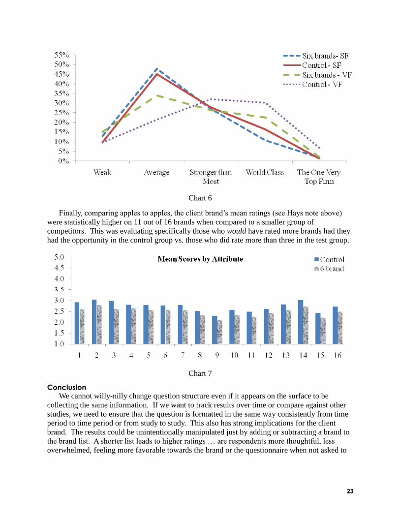
23

Chart 6

Finally, comparing apples to apples, the client brand‘s mean ratings (see Hays note above)

were statistically higher on 11 out of 16 brands when compared to a smaller group of

competitors. This was evaluating specifically those who would have rated more brands had they

had the opportunity in the control group vs. those who did rate more than three in the test group.

Chart 7

Conclusion We cannot willy-nilly change question structure even if it appears on the surface to be

collecting the same information. If we want to track results over time or compare against other

studies, we need to ensure that the question is formatted in the same way consistently from time

period to time period or from study to study. This also has strong implications for the client

brand. The results could be unintentionally manipulated just by adding or subtracting a brand to

the brand list. A shorter list leads to higher ratings … are respondents more thoughtful, less

overwhelmed, feeling more favorable towards the brand or the questionnaire when not asked to

24

rate as many? Or in view of a larger list does the entire industry look the same? The ‗why‘ is

missing without further investigation.

STUDY 3: OFFERING A DON’T KNOW

Your company or university may already have a standard for whether to allow a ―don‘t

know‖ response option or not with image rating questions. Regardless, it is worth a review of

some of the literature to date, which is extensive. Our own expectation going into the study was

that a don‘t know response option should be included, but some of the readings as well as some

of the results from our research have challenged that assumption.

Prior Work Two types of errors may occur with don‘t know (DK). One – a respondent not offered a DK

may give a response not reflecting his or her true opinion (or lack thereof). Two – a respondent

offered a DK may choose it even when they do have an opinion. Of course, there is no guarantee

that with or without a DK respondents will give or even be able to give 100% valid and reliable

responses.

Feick (1989) in his own review helps us think about where the DK might be coming from –

qualities of the respondent vs. qualities of the questionnaire. Older, less educated, nonwhite,

lower income categories and women are more likely to use DK. Questions that are: more

complex, require the respondent to think far ahead, poorly constructed, or on a topic of little

interest or familiarity to the respondent all may increase the incidence of DK. To avoid the

nonrandom bias introduced by a DK, one solution he suggests is to eliminate them altogether.

Feick notes other authors have seen a halo effect where respondents answer based on their

general feelings rather than specific attitudes, including giving opinions on non-existent entities.

Feick went further into DK with latent class analysis but for our paper we just want to extract

elements of his lit review.

Opposition to Don’t Know Not every author agrees that DK should be included. This is part of what makes it

interesting. Krosnick and a host of distinguished co-authors (2002) ran nine experiments in three

household surveys to test respondents‘ use of DK, questioning if adding a DK would only draw

those who were otherwise giving meaningless data or if it would also entice those who might

have an opinion and would have otherwise given it. They note:

If offering a no-opinion option reduces non-attitude reporting, it should strengthen

correlations between opinion reports and other variables that should, in principle, be

correlated with them. If non-attitude reports are random responses, then offering a no-

opinion option should reduce the amount of random variance in the attitude reports

obtained.

Krosnick‘s theory of satisficing suggests respondents may be unmotivated to answer

particular questions, especially complex ones, and so may choose ―don‘t know‖ simply as a way

to continue the interview, especially when cued that this option exists. Krosnick hypothesized

that omitting the no-opinion option would cause the strong ―satisficers‖ to give their substantive

answer instead and eliminate this shortcut to cognitive laziness, as it were.

25

Nine studies later, they concluded that including a no-opinion option did not increase the

quality of the data, but instead that the respondents drawn to no-opinion options ―would have

provided substantive answers of the same reliability and validity as were provided by people not

attracted to those options.‖ One suggestion they make to researchers who still wish to include a

no-opinion response is to probe respondents who say DK with whether they lean one direction or

another. This would reduce the satisficing (if it is happening) in encouraging the respondent to

think and not allowing an easy out.

In favor of including Don’t Know In early work, Converse (1970) suggests that respondents will give random responses if they

don‘t know but don‘t want to appear ignorant.

Stieger, Reips and Voracek (2007) notes that if we force a respondent to respond, we may

induce reactance – and that this is a possible outcome of the (relatively) new mode of online

surveys. Reactance is an emotionally triggered state in response to excessive control where the

individual feels their freedom is threatened, and therefore attempts to re-establish their freedom

by acting in the opposite mode of what the situation requires or requests. Reactance theory was

first proposed by Brehm (1966), and is the idea behind the popularized reverse psychology.

Stieger et al. hypothesize the lack of a DK will lead to respondents deliberately giving

misleading or inaccurate responses, or to simply dropping out of the study altogether.

In Stieger‘s methodology with 4,409 University of Vienna students, test group respondents

who attempted to advance without filling in a question on the infidelity questionnaire would

receive an error screen asking them to completely fill in the questionnaire. The event was logged

for later analysis. Control group respondents did not receive the error page.

Instructionally, 394 respondents dropped out immediately after receiving their first error

page, particularly on the ―demographics‖ page (it appears all demographics were collected on

one screen). Another 121 dropped out later. Only 288 received an error page and still completed

the questionnaire. The dropout rate of those who did not attempt to skip a page was 18.6% vs.

64.1% of those who did so at least once. In addition, the authors did find indicators of reactance

– the data for respondents after receiving an error page was significantly different from the data

for those same questions for respondents who did not. In addition, Stieger found men dropping

out faster than women in the forced-response condition (this author supposes it might have

something to do with the content material and might not be a finding with less provocative

questions).

In their discussion, Stieger et al. would like to distinguish between ―good dropout‖ and ―bad

dropout.‖ If respondents are not going to give us quality data due to poor motivation then we

wish them well but don‘t want to include them in our study. Bad dropouts may be due to

inadequate questionnaire design, programming errors, lack of feedback on progress, et cetera. A

very low dropout rate may in fact be a bad thing if we‘re keeping ‗bad‘ respondents in our data.

Finally, Stieger suggests criteria for forced-response design:

1. It is necessary to have a complete set of replies from the participants (e.g., semantic

differentials, multivariate analyses, pairwise comparisons, required for skip patterns)

2. A high response rate is expected and so dropout is not a concern

26

3. The distribution of respondents’ sex is not a main factor in the study

Friedman and Amoo (1999) propose that if subjects are undecided and have no ‗out‘ they will

probably select a rating from the middle of the scale, biasing the data in two ways: ―(a) it will

appear that more subjects have opinions than actually do (b) the mean and median will be shifted

toward the middle of the scale.‖ They also remark on the usefulness of % don‘t know, especially

in political polling where the previously undecideds can change an election. Note the probably

italicized above, as Friedman did not back this assertion up with data.

In favor of including Don’t Know, delineated In an intriguing bit of research on online surveys, Tourangeau, Couper and Conrad (2004)

investigate the placement on the screen of ―nonsubstantive‖ response options such as don‘t know

in relation to their substantive counterparts.

Tourangeau et al. present results for three different interpretative heuristics they believe

respondents are using that may lead to misreadings of survey questions:

1. Middle means typical

2. Left and top mean first (either worst or best)

3. Near means related

Note that prior research (cited by Tourangeau) already supports the first heuristic, and must

be taken into account when delivering closed-ended range questions to respondents in lieu of

open numeric questions. An implication of ―near means related‖ is higher correlations in items

presented as a grid than those presented on separate screens.

The authors ran two surveys testing the middle means typical in 2001 and 2002, through

Gallup, with 2,987 interviews of 25,000 invitations in the first study and 1,590 of 30,000 in the

second study. Respondents received an attitude question with a vertically presented scale, five

substantive points ordered high to low (‗far too much‘ to ‗far too little‘), followed by both a

―don‘t know‖ and a ―no opinion.‖ Test groups had a short divider line, a long divider line, or a

space between the five and the two. The control group saw all seven options contiguously.

In all cases, the means are statistically closer to the ―far too little‖ point when there is no

separation between the substantive and non-substantive responses. However, a side effect of

setting apart the non-substantive responses in this case led them to being chosen more often.

Tourangeau followed up with an experiment simply adjusting the spacing in the scale

question, horizontally, either visually crowding some of the responses to one side or spacing

them evenly. Again, the means moved towards the visual center, not the labeled center of the

scale.

They conclude,

Our results indicate that [respondents] may also make unintended inferences based on

the visual cues offered by the question. Basing their reading on the questions' visual

appearance, respondents may miss key verbal distinctions and interpret the questions in

ways the survey designers never intended.

27

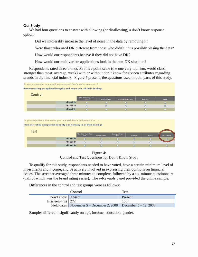
Our Study We had four questions to answer with allowing (or disallowing) a don‘t know response

option:

Did we intolerably increase the level of noise in the data by removing it?

Were those who used DK different from those who didn‘t, thus possibly biasing the data?

How would our respondents behave if they did not have DK?

How would our multivariate applications look in the non-DK situation?

Respondents rated three brands on a five point scale (the one very top firm, world class,

stronger than most, average, weak) with or without don‘t know for sixteen attributes regarding

brands in the financial industry. Figure 4 presents the questions used in both parts of this study.

Figure 4:

Control and Test Questions for Don‘t Know Study

To qualify for this study, respondents needed to have voted, have a certain minimum level of

investments and income, and be actively involved in expressing their opinions on financial

issues. The screener averaged three minutes to complete, followed by a six-minute questionnaire

(half of which was the brand rating series). The e-Rewards panel provided the online sample.

Differences in the control and test groups were as follows:

Control Test

Don‘t know Absent Present

Interviews (n) 272 155

Field dates November 5 – December 2, 2008 December 5 – 12, 2008

Samples differed insignificantly on age, income, education, gender.

28

Results If our goal had been to avoid frustrating responses, removing DK would have caused us to

miss the target. Of respondents not given the option to select DK, over 20 commented on it

negatively when asked at the end of the survey to evaluate the questionnaire, for example:

There was no option to say I don't know, forcing me to make choices on some questions I

was not qualified to answer.

Just because I indicated I was 'familiar' with some companies doesn't mean that I'm in a

position to answer such detailed questions about them. I often felt that 'don't know' or NA

should have been an option.

There should always be an opt-out response on questions as the respondent may not have

a response and then is forced to respond if there is no opt out response. This is very basic

stuff.

When DK was present, over half the test group respondents took advantage of it at least once

in the 16-attribute section (and none complained). But what about those who didn‘t have DK -

what did they do?

A Series of Hypotheses First let‘s compare actual results in allowing a DK or not (stacked data across all attributes).

Chart 8

The respondents without a DK response option did select ―average‘ slightly more often than

those who were provided a DK option. To understand the dynamic more deeply, we then used

several simulation designs in an attempt to replicate analytically the process that these

respondents were going through mentally.

What if they plumped for the most neutral response of ―average,‖ as Friedman and Amoo

(1999) suggested they might? As Chart 9A below demonstrates where the DK value has been

29

replaced by ―average,‖ that‘s clearly not happening. What if the respondents just randomly

chose one of the five responses, as Converse (1970) says might happen when respondents would

prefer not to appear ignorant? Chart 9B replaces the DKs with random responses. This

simulation is closer to the actual responses, but still varies by a significant degree.

Charts 9A and 9B

Another possibility is respondents restrict their choices to the middle values. We‘re not

providing a graph illustrating this as the standard deviations were virtually identical between the

DK and No DK group, thus allowing us to discard it as a hypothesis.

Finally, as Feick and other authors suggest, the respondents may infer (or impute) from what

they know generally about the brand to score an attribute. Using a simplistic imputation,

replacing the DKs with the integer nearest to the mean score of all other attributes for that

respondent, we obtain the results shown in Chart 10.

Chart 10

As you can see, populating the DKs from the ―Allow DK‖ group with what they generally

knew about the brand lines up very closely with the No DK group. And this was not a small

percent; 28% of the observations (brand x attribute) were DK.

30

These simulations give us more confidence that when DK is not available as a response

option, respondents will act in good faith and impute reasonably.

Back to Real Data We then looked at how respondents with access to the DK response option behaved. Do they

also act in good faith?

Chart 11

As seen in Chart 11, respondents used don‘t know significantly more often as the series of

grid questions progressed (p<.001 for linear contrast), at almost a 40% increase compared to the

beginning. And both groups gave answers with less and less variance as time went on.

Respondents allowed a DK do not always act in good faith.

In addition, we saw some differences in means, even when controlling for familiarity. The

mean value was lower for the DK group than the non-DK group six out of sixteen times when

―somewhat familiar‖ with the brand and four out of sixteen when ―very familiar‖ with the brand.

Two possible explanations come to mind:

As we know the financial industry did not have a very good 2008, either financially or in

the public perception. Our test group was fielded a bit later than the control group

and may have had exposure to even more bad news at that point.

31

The DK response option was placed contiguous with all other points, with no

distinguishing visual features whatsoever. Corresponding to Tourangeau and co-

authors‘ findings (2004), this unfortunate placement may have visually shifted the

mean in respondents‘ minds towards the right, the lower level of the scale. (As an

aside, Cambia intentionally uses an unbalanced scale as our clients really only want to

be ―The one very top firm‖ but this may throw off panelists who expect the middle

point to be average.)

Figure 5:

Revisiting the scales

As one of our goals was to compare the impact of DK on the variables that mattered, we

correlated the attributes (stacked) with several outcome variables. Note that this methodology

was chosen over regression as the multicollinearity made regression comparisons untenable.

3 brands

No DK

3 brands

DK

6 brands

No DK

How likely are you to recommend this firm to a

professional colleague who is looking to do

business with a firm in this industry

.620 .601 .621

How likely are you to invest with this firm .581 .582 .623

Extent to which you want to see firm succeed .443 .381 .373

Table 1:

Correlations of Attributes (as composite) with Outcome Variables

The results showed that allowing respondents a DK response option did not strengthen the

correlation with outcome variables; if anything, it decreased the correlation. This was similar to

Krosnick‘s findings. For further comparison, the 6 brand test is also shown, and the results are

parallel to the DK set.

To round out the analyses, we looked at the demographics of those who used DK and those

who didn‘t. As mentioned in Feick (1989), women used don‘t know more often than men (33%

to 26%). Other demographic variables did not follow published outcomes for DK:

Those more highly educated used don‘t knows more often than those with less education

(Krosnick, 2002 had the reverse)

Higher income respondents used more don‘t knows

Age was virtually unrelated to use of don‘t know (again, Feick had younger using don‘t

know more often)

Note that as a set of (older) panelists with $100K+ in investments our sample is not

representative of the general population.

32

Conclusion We came into this research effort with an expectation that, in general, providing a don‘t know

response is advantageous over omitting it. However, for this study, for this context, this sample,

this time period, this content area… taking away DK

did not increase noise,

did not change the distribution across attributes (though some means were affected), and

did not negatively impact the relationships with outcome variables.

Respondents seemed to do a fine job of self-imputation. Had the variables been less

intercorrelated so that we were able to do multivariate analyses with the data, we would have had

an easier time with the non-DK group than the DK group, avoiding the need for imputation.

Some respondents with the DK response option clearly used it when they did not ―need‖ to, if not

at the beginning of the series then certainly by the end.

But, one must weigh the relative benefits of having a clean data set with the drawbacks of

potentially frustrating respondents (who also may be prospective clients). The questionnaire was

so short that we did not have an appreciable number of partials to contrast if the DK absence

were leading to greater dropouts. But our questionnaire feedback question provided them an

opportunity to vent, and vent they did.

We also saw some demographic differences in DK usage which could lead to unintentionally

biased data.

Our takeaway is to graphically alter where we place the DK so it is clearly visually separated

from the grid (and perhaps in a smaller font to de-emphasize it). And should we have a request

to omit DK, we can feel marginally more comfortable this will not negatively affect the results.

STUDY 4: RATING BRAND WITHIN ATTRIBUTE OR ATTRIBUTE WITHIN BRAND

Although randomizing brands within attributes is often accepted as the best approach for

gathering comparative data in image ratings, not all agree. In fact in our literature review we

found at least one strong argument for also randomizing attributes within brands. Nevertheless,

our attributes are strongly intercorrelated and it was our hypothesis that they might be less so if

the question were formatted to ask the respondent to rate a group of brands for one attribute

before proceeding to the next attribute. You will see as you read ahead that we did succeed, but

only minutely.

Prior Work Ninety-four years ago, Edward Thorndike observed that respondents had difficulty separating

their ratings of individual attributes for a person from that of their overall perception of the

person. As a result, correlations between attributes were higher than reality. The term ―halo

effect‖ comes from this study, published in 1920.

As researchers, we generally find halo effect to be a bad thing. We want respondents to be

able to distinguish brands one from another, to distinguish attributes one from another, and in the

end provide data that allow us to identify which attributes are distinctive drivers of success for

our clients.

33

It is possible to take another viewpoint, though. The ‗halo‘ itself can be extracted as a single

dimension and treated as brand reputation (Laroche, 1978) or brand equity (Leuthesser, et al.,

1995, Dillon, et al., 2001) – with the remainder examined for differences. Leuthesser suggests

double-centering the data to make it ipsative and then running analyses on it. Other authors

(McClean and Chissom, 1986) suggest this is unwise. Rossi, Gilula, and Allenby (2001) have

followed up with a Bayesian alternative to ipsatization, Dillon et al. with a decompositional

model – we recommend these resources to you for a more detailed explanation and examination.

However, for the purposes of this research we sought to diminish the halo effect, and we

believe that randomizing brands within attributes is a better way to achieve this than randomizing

attributes within brands. But before we jump to conclusions, Torres and Bijmolt (2009) found

… when the association between brands and attributes is measured asking brand-to-

attribute associations, which is a non-comparative format, the stronger links from the

brands to the attributes dominate the associations. On the other hand, if a researcher

measures brand image asking attribute-to-brand associations (a comparative format),

stronger links from the attributes to the brands will determine the perceptions of the

consumers…we suggest that both directions of associations should be considered when

brand image is assessed to make managerial recommendations.

To translate this to plain English, think of a brand in a particular category, for example cars.

What attributes come to mind? Now, think about just one of those attributes. Which cars come

to mind when you think of this attribute? The order in which the question is asked may result in

an asymmetrical correspondence between brands and attributes, depending on the strength of the

brand‘s personality and the impact of the particular attribute.

Our Study In our study we hoped to evaluate the level of halo effect in our data, and decrease it by

randomizing brands within attributes in comparison to the control group where attributes would

be randomized within brands.

In addition, pre-tests showed a shorter study time when one brand was asked at a time for all

attributes. We would monitor and report on this as well.

Similar to the left-right vs. right-left study, respondents were administered a roughly 13-

minute questionnaire on some aspects of the healthcare industry. Greenfield Online provided the

sample, with the following respondent qualification criteria:

Age 18+

Covered by health insurance

Makes health insurance decisions for their household

34

Differences in the control and test groups were as follows:

Control Test Randomization Attributes within Brands Brands within Attributes

Interviews (n) 1,047 266

Field dates June 11 – July 4, 2008 September 8 – 16, 2008

Respondents rated three brands with which they were familiar, one brand per screen, on a

series of 14 attributes on a grid with a bipolar seven-point scale (the one very top company,

world class, stronger than most, average, weaker than most, much worse than other companies,

the one worst company, don‘t know) as in Figure 6.

Figure 6:

Screen shots of Brand within Attribute vs. Attribute within Brand questions

Results In brief, we found that the mean is higher in the ―across brand‖ (Test) condition, as is top 2

box (by 9% on average) and standard deviation. These results strongly indicate that it would be

unwise to switch formats from one wave of research to the next. It actually remarkably changes

the order of the means … the ranking of the attributes only correlates .44 from one group to

another (compared to .92 for the left-right, right-left study).

Again, Chow tests of differences in regression coefficients across the two samples using the

rating variables are not significant, using likelihood to recommend as a dependent variable. We

advise caution due to the high multicollinearity. The average inter-correlation for attribute within

brand was .81. For brand within attribute the average inter-correlation was .76. We cannot say

35

that we succeeded in reducing multicollinearity. A rule of thumb suggesting the presence of a

halo effect is an intercorrelation between .60 and .70. We beat that handily.

The differentiation analysis performed earlier for the left-right, right-left study is repeated on

the rotation order data below.

Chart 12

While at first there appears to be better differentiation asking attributes within brand, it

makes sense that one could be reducing multicollinearity at the expense of discrimination. This

leads us back to Torres and Bijmolt (2009)‘s advice … we may be provoking a different response

and gathering a different (and yet still valid) story in changing how the question is asked.

One interesting finding was in applying the ipsative approach suggested by Leuthesser, et al.

With the normalized, standardized healthcare data we derived two very interesting varimax

factors, each easily labeled on a bipolar scale and very intuitive. The financial data was not as

amenable to our attempts to reduce the multicollinearity this way, however.

Finally, there was no statistical difference in the time to complete the survey.

Conclusion The halo effect is very high, and only slightly less so when brands are asked within attribute.

The means changed and the mean order changed. Brands were rated more highly when they

were compared with other brands.

We will continue exploring the ipsative and other approaches to multicollinearity.

36

FINDINGS ACROSS STUDIES

With timestamps on every screen, we were able to assess respondents‘ behavior on the

financial studies and discovered they were flat-lining after about six attributes:

Chart 13

Have they just learned the task really well? Are they tired, bored? We might say this shows

the learning curve for the task, but if you remember the previous charts, not only are the

respondents going faster but they are using don‘t know more often and straight-lining (lower

variance) more often.

Moreover, in any regression we were only able to fit at most five or six attributes before

signs began to flip and the multicollinearity flags were being tripped.

Given the enormous ‗reliability‘ of our data acting as one construct loading very nicely on

one factor, eight statements would have done as well as 16. But if client requirements need all

16 it may be worthwhile to ask the respondents no more than six at a time. This will be tested in

future studies.

37

REFERENCES

Belson, W.A. (1966). The Effects of Reversing the Presentation Order of Verbal Rating

Scales. Journal of Advertising Research, 6 (December), 30-37.

Brehm, J.W. (1966). A Theory of Psychological Reactance. New York: Academic Press.

Churchill, G. A. (1979). A Paradigm for Developing Better Measures of Marketing

Constructs. Journal of Marketing Research, XVI, 64-73.

Converse, P. E. (1970). Attitudes and Non-Attitudes: Continuation of a Dialogue. In: Tufte,

E.R. (ed.), The Quantitative Analysis of Social Problems. Reading, MA: Addison-Wesley,

168-189.

Dillon, W. R., Mulani, N., & Frederick, D. G. (1984). Removing Perceptual Distortions in

Product Space Analysis. Journal of Marketing Research, 21 (2), 184-193.

Dillon, W. R., Madden, T. J., Kirmani, A., & Mukherjee, S. (2001). Understanding What‘s

in a Brand Rating: A Model for Assessing Brand and Attribute Effects and Their

Relationship of Brand Equity. Journal of Marketing Research, 38 (November), 415–429.

Feick, Lawrence F. (1989). Latent Class Analysis of Survey Questions that Include Don' t

Know Responses. Public Opinion Quarterly, 53(4, Winter), 525-547.

Friedman, H., & Amoo, T. (1999). Rating the Rating Scales. Journal of Marketing

Management, 9 (3), 114-123.

Friedman, H., Friedman, L., & Gluck, B. (1988). The Effects of Scale-Checking Styles on

Responses to a Semantic Differential Scale, Journal of the Market Research Society, 30

(October), 477-481.

Friedman, H., Herskovitz, P., & Pollack, S. (1994). The Biasing Effects of Scale-Checking

Styles on Response to a Likert Scale. Proceedings of the American Statistical Association

Annual Conference: Survey Research Methods, 792-795.

Hays, W.L. (1981). Statistics (3rd ed.). New York, NY: Holt, Rinehart and Winston.

Holmes, C. (1974). A Statistical Evaluation of Rating Scales. Journal of the Market

Research Society, 16 (April), 87-107.

Hulbert, J. (1975). Information Processing Capacity and Attitude Measurement. Journal of

Marketing Research, 12 (February), 104-106.

Johnson, B., & Christensen, L. (2007). Educational Research: Quantitative, Qualitative and

Mixed Approaches (3rd ed.). Thousand Oaks, CA: Sage Publications. 664 pp.

Krosnick, J. A., Holbrook, A. L., Berent, M. K., Carson, R. T., Hanemann, W. M., Kopp,

R. J., Mitchell, R. C., Presser, S., Ruud, P. A., Smith, V. K., Moody, W. R., Green,

M. C., & Conaway, M. (2002). The Impact of "No Opinion" Response Options on Data

Quality. Public Opinion Quarterly, 66, 371-403.

38

Laroche, M. (1978). Four Methodological Problems in Multiattribute Attitude Models. In:

H.K. Hunt (ed.), Advances in Consumer Research, Vol 5. Ann Arbor, MI: Association for

Consumer Research, 175-179.

Leuthesser, L., Kohli, C. S., & Harich, K. S. (1995). Brand Equity: The Halo Effect

Measure. European Journal of Marketing, 29 (4), 57-66.

McLean, J., & Chissom, B. (1986). Multivariate Analysis of Ipsative Data: Problems and

Solutions. Paper presented at the Annual Meeting of the Mid-South Educational Research

Association, Memphis, TN, November 1986.

Miller, G.A. (1956). The Magical Number Seven, Plus or Minus Two: Some Limits on Our

Capacity for Processing Information. The Psychological Review, 63, 81-97.

Rossi, P.E., Gilula, Z. and Allenby, G.M. (2001). Overcoming Scale Usage Heterogeneity:

A Bayesian Hierarchical Approach. Journal of the American Statistical Association, 96

(March), 20-31.

Schaeffer, N. C., & Presser, S. (2003). The Science of Asking Questions. Annual Review of

Sociology, 29 (1), 65-88.

Stieger, S., Reips, U.-D., & Voracek, M. (2007). Forced-Response in Online Surveys: Bias

from Reactance and an Increase in Sex-Specific Dropout. Journal of the American Society

for Information Science & Technology, 58 (11), 1653-1660.

Thorndike, E. L. (1920). A Constant Error in Psychological Ratings. Journal of Applied

Psychology, 4, 469-477.

Torres, A., & Bijmolt, T. H. (2009). Assessing Brand Image through Communalities and

Asymmetries in Brand-to-Attribute and Attribute-to-Brand Associations. European Journal

of Operational Research, 195, 628-640.

Tourangeau, R., Couper, M. P., & Conrad, F. (2004). Spacing, Position and Order:

Interpretive Heuristics for Visual Features of Survey Questions. Public Opinion Quarterly,

68 (3), 368-393.

39

PLAYING FOR FUN AND PROFIT:

SERIOUS GAMES FOR MARKETING DECISION-MAKING

LYND BACON LOMA BUENA ASSOCIATES

ASHWIN SRIDHAR ZLINQ SOLUTIONS

INTRODUCTION

Much of marketing research concerns organizing activities of consumers so as to enable

inferences about their attitudes, beliefs, values, or preferences. Traditional procedures like

surveys, interviews, experiments, and focus groups structure the activities of participants, and

constrain what they do by way of explicit requirements and implicit rules of interaction. Games

are a more natural form of organized activity for people than are conventional research

procedures, and are in fact a type of activity that people engage in energetically of their own

volition. When properly implemented in regard to organizational learning objectives, games

have advantages that include being able to motivate participants, or ―players,‖ to produce desired

results. They also provide a framework for rewarding players in proportion to their contribution

to desired outcomes, as has been illustrated by recently published academic research. In this

paper we:

review the characteristics of games and game play;

summarize who plays electronic and online games, and what the underlying technologies

are;

describe the growing areas of serious and purposive games;

summarize games recently developed to address marketing issues;

describe design and implementation issues, and

wrap up by describing a linguistic game platform we developed and deployed.

GAMES AND PLAY

To grasp how and why games are useful for marketing research purposes, it's important to

understand what a game is, and what the nature of play is. A reading of the game design

literature yields a wide array of definitions for what a game is. Saleen and Zimmerman (2006)

distill several definitions. We prefer ours, a synthesis of various authors' definitions, as general

and flexible enough for research applications:

―A game is an activity engaged in individually or in groups that is played by rules and

with intent to achieve a particular outcome.‖

Huizinga (1950) provided an often-cited definition of ―play.‖ According to Huizinga, the key

attributes of play are:

40

1. Participation is voluntary

2. Pretending is involved

3. The experience is often immersive

4. It's done in a particular time and place

5. It is based on rules, but the rules may only be implied

6. It is often social, and can create groups

―Pretending,‖ above, refers to imagining some circumstance. ―Immersive‖ suggests

engrossing, or perhaps ―flow-like‖ experience, perhaps in the sense described by

Csíkszentmihályi (1990). Rules may only be implied. When tossing a ball back and forth, for

example, one implied rule is ―don't drop the ball.‖ Uncertainty about outcomes is another, oft-

noted, feature of play. In any case, play is something other than ―work.‖

Caillois (2001) studied the cultural significance of games, and perceived gameplay

experience as being an mixture of improvisation, joy, and gratuitous difficulty. He defined four

types of games:

Competitive

Chance

Simulation

Vertigo

Games of chance are gambling games, like blackjack or the lottery. Simulation games

include role-playing games. Vertigo games are games that cause dizziness, such as the kind of

playground games children invent that alter their balance by spinning around. Note that these are

game types of which most games are hybrids. Of Caillois's four types, ―Vertigo‖ games seem the

least adaptable for research on consumers, at least at the present time.

WHO IS PLAYING ELECTRONIC GAMES?

Using games to accomplish objectives like problem solving, idea generation, or forecasting is

not a new practice. A recent example is Ethiosys's ―Innovation Games‖ (Hohmann, 2007), a

structured collaborative play activity in which groups, sometimes in competition with each other,

create new product ―artifacts‖ using common stationary and art materials. Ethiosys's game and

most other games for business purposes require that players be physically co-located, and they

aren't very scalable due either to the nature of player activities and interactions, or because

analysis of their results isn't easily (or even feasibly) automatable.

We believe that on- or off-line electronic games offer the best opportunities for innovation in

research practice. Our reasons include their potential scalability, and the possibility of

embedding certain kinds of games in existing data collection contexts such as online surveys or

focus groups. The prospect of using such games begs the question of who is likely to find

playing them at least tolerable.

41

The Entertainment Software Association (ESA; www.theesa.com) conducts an annual survey

of U.S. households to find out who is playing computer games, and how they are doing it. The

ESA's 2008 study included the following findings:

1. Computer games are played by 65% of U.S. households

2. The average player age is approximately 35 years

3. 40% of players are female

4. Adult computer game players average 13 years of game-playing experience

5. 26% of adults older than 50 years of age play computer games

6. 36% of players said they played with others present

7. 36% of responding heads of households reported playing on wireless devices such as

phones and PDAs

It would appear from the ESA's results that computer games are not solely the province of

adolescent males, and that playing them is prevalent in U.S. households. Given their ubiquity,

research participants should not find games too off-putting, assuming that they are adequately

executed. It's our guess that the proportion of players who play games on wireless and mobile

devices will increase as the power and flexibility of mobile computing platforms continues to

evolve, and as game applications that run on them become more numerous and more

sophisticated.

Theories about motives for playing computer games abound in the game design and

development literatures. In some cases, purportedly causal explanations for game play are

tautological, e.g. players play a game because they enjoy it, and because they continue to play

they must enjoy it. There are some more thoughtful perspectives, however. Bing Gordon and his

colleagues at Electronic Arts, perhaps the largest manufacturer of computer games, believe that

the fundamental motives for playing games vary with age and gender (Moggridge, 2007, Chapter

5). Pre-teenage boys, for example, seek power and freedom from authority. As a result, sports

and combat games are likely to be preferred by them. Teens seek to explore their identity and so

tend to prefer rich and engrossing role-playing fantasy games. Adults seek mental stimulation

and self-improvement, and so will prefer games like puzzles or the famous Flight Simulator that

allow knowledge or skills development.

WHAT MAKES GAMES GO?

Over the years, advances in computing hardware, user interface and communication

technologies have shaped developments in the computer gaming industry. There has been a

steady increase in the level of sophistication of games through application of these technologies,

and players can now choose from a wide variety of platforms to play games on, including

dedicated gaming consoles, general-purpose personal computers, as well as hand-held devices

and mobile phones.

The user interface of a game depends on the platform on which the game is played. Most

modern games take advantage of high-resolution graphics capabilities of display devices such as

television sets, computer monitors or dedicated LCD screens built into gaming devices. Game

42

consoles have dedicated input devices designed specifically for the console, typically with

buttons providing specific game actions and a joystick to facilitate navigation. A computer

keyboard and mouse serve as input devices on a personal computer. Special purpose input

devices are often available to enhance playability on a computer. These devices typically

connect to the computer via standard interfaces such as USB, serial or parallel ports. Hand-held

gaming devices vary in their level of sophistication. They are self-contained units combining a

display device, input device and a mechanism to incorporate the game module, which enables a

single device to play multiple games. Modern mobile phones including smartphones, with

increasingly more processing and graphics capabilities and are gaining popularity as devices for

playing games.

Networking and communication technologies are also taking on an increased supporting role

in gaming. Internet connectivity is being exploited not only as a means of delivering the game to

players, but also to shape the interactions among players. Early forms of multiplayer games only

allowed multiple, typically two, co-located players, each with their own input devices to interact

competitively within a game. This social aspect has evolved, through use of high-speed Internet,

and development of multiplayer and massively multiplayer online games, to where players can

be geographically dispersed, and still interact cooperatively or competitively within long-running

games. Such interactions among players are coordinated through servers on the Internet, which

host games and also serve as a more general ecosystems for online interactions among gamers

and enthusiasts.

Developing modern, sophisticated games across multiple platforms requires a complex,

multidisciplinary approach sometimes taking years to take a single game from concept to market.

The team often comprises of producers, game designers, artists, programmers, engineers and

testers. There are, however, some common components that are required by nearly all games.

Game engines provide such reusable software components and can be used to facilitate relatively

rapid game development. They enable game-specific artifacts to be developed in their entirety

and used along with customized, reusable components related to such aspects as rendering,

sound, animation, networking etc. Game engines also abstract the platform layer, enabling a

more streamlined development of code that can be targeted at multiple platforms. Special

purpose engines, also called middleware are available for specific applications such as massively

multiplayer online games.

Even with advances in game engines and the availability of reusable components,

development of modern games for consoles and personal computers remains complicated and

expensive. A class of infrastructure targeting game development on new platforms such as

mobile phones and web browsers has emerged. Platforms such as Shockwave and Flash are

increasingly being used since they can be used to enable games directly within web browsers

using plugins. There is also increased focus on diverse and higher level development languages

such as Java, Python, and PHP.

Targeting the browser as a platform has yielded a class of games, simpler than modern

console based games, but with characteristics that are similar in a number of ways with more

general purpose Rich Internet Applications. They are hosted on a web server, often store game

and player data in a database and enable interaction of the player with server-based components

as well as other players. Input devices for such games tend to be computer keyboards and mice.

In the simpler cases, the web interfaces can be constructed using popular web technologies such

43

as dynamic HTML and Javascript, and techniques such as asynchronous Javascript and XML

(AJAX) can be employed to enhance user experience. More sophisticated interfaces can be built

using technologies such as Shockwave and Flash. Such games can still be developed quite

rapidly, embedded within multiple websites simultaneously and can be accessed using a personal

computer with Internet connectivity.

Mobile phones have seen a surge in being used as simple gaming devices. Games for these

devices are developed to target the specific operating system or platforms supported on the

phone. They need not necessarily be networked, however, availability of Internet connectivity on

such devices can easily be exploited to deliver games that behave much like the ones in a web

browser. Games for mobile devices are, however, designed to make effective use of the limited

hardware and processing capabilities. Multiplayer capabilities are also somewhat limited in such

mobile devices.

SERIOUS GAMES

It should be obvious to the reader that the kind of games we're discussing are designed with

objectives in mind other than the sole entertainment of the player. Developers and educational

researchers have been combining computer game design and learning principles to grow a class

of games referred to as ―serious games.‖ Serious games have ―an explicit educational objective,

and are not intended to be played primarily for amusement.‖ (Michael & Chen, 2006, p. 21).

Given that serious games are designed with the intent to bring about change in beliefs, attitudes,

perceptions, knowledge, or behaviors, they are a kind of ―persuasive technology‖ as defined by

Fogg (2003).

Despite the newness of serious games, a number of good examples of them can be found.

HopeLab of Palo Alto CA (www.hopelab.org) has been developing games that help people cope

with various kinds of health issues. Their Re-Mission game is designed to help minors cope with

cancer by shaping good health behaviors and attitudes.

As another example of a serious game, America's Army (www.americasarmy.com) is

considered by some to be one of the most highly visible serious games to date. The game was

developed with both recruiting and entertainment objectives in mind. Based on its popularity it

was ported for use on consumer game consoles.

Humana Inc. launched an initiative in 2007 called games for health

(www.humanagames.com). Their games, and the research program underlying them, are

intended to promote physical and mental well-being. Their premise is that you can ―play your

way to better health.‖

The emerging importance of serious game applications has been noted by the academic

community. A number of U.S. universities that include Michigan State, University of Southern

California, Wisconsin, and Simon Frasier have graduate level curricula or degree programs on

serious games. Each year there are conferences held around the world about serious games that

facilitate the growth of a global interest community.

44

PURPOSIVE GAMES

The focus of serious games is on change in the player. What we call ―purposive games‖ are

designed with the intention of satisfying organizational learning objectives. Examples of such

objectives include making predictions, and taming unstructured data in order to provide better

discovery and decision support services. The distinction between serious games and purposive

games can be fuzzy, since games designed for a purpose other than player pleasure can be

intended to achieve multiple goals. America's Army is an example of this.

Purposive games are being deployed in a variety of domains. Hopelab has RuckusNation, a

community-based on-line game designed to fight childhood obesity by generating new ideas for

leading more active lifestyles. The Institute For The Future (www.iftf.org) has launched

SuperStruct (www.superstructgame.org), a massive multiplayer online game (―MMOG‖)

designed for forecasting. Free Rice (www.freerice.org) is a vocabulary game for ending world

hunger and also providing some free education.

Louis (―Big Lou‖) von Ahn and his colleagues at Carnegie Mellon University (CMU) have

developed a series of games that have been implemented by Google and elsewhere. They are

generally about solving difficult computing and machine intelligence problems by harnessing

human perceptual and cognitive abilities. They embed what we call ―human computing tasks‖ in

games for generating labels for images, for dealing with semantic ambiguity, and for other

problems that computers have difficulty with as compared to humans. Google's implementation

of some of von Ahn et al.'s games can be found at www.gwap.com. CMU versions are currently

at www.espgame.org.

As far as we can tell, a widely accepted taxonomy of purposive game types has yet to

emerge. We currently classify them as follows. Note that in each case, the primary intention is to

generate some kind of new information or knowledge for the main stakeholder in the game, its

sponsoring organization. Also, note that the boundaries of these categories are fuzzy, and that

any single game may have the DNA of more than one type.

Labelling games. these are games used to classify or label exemplars. Von Ahn and

Dabbish (2008) provide several examples of games we consider to be of this type.

Prelec's (2001) Information Pump is an example applied in the marketing research

arena.

Prediction games. These are for forecasting or predicting events that have yet to occur.

Accuracy/consistency games. These are games in which players are rewarded for the

precision or reliability of their responses.

Content Generating games. In these games, players generate new content. The nature of

the content is constrained by the rules of the game.

PURPOSIVE GAMES IN MARKETING SCIENCE

Academic researchers have begun to develop and test a variety of purposive games. Of

them, predictive markets, also called ―virtual stock markets,‖ may be the best known. A

predictive market is one in which participants, or ―traders,‖ buy and sell ―contracts,‖ or shares,

based on an event that has not yet been observed (Spann & Skiera, 2003). The contracts express

45

some future event, such as a particular team winning a championship, or a product achieving

market share dominance by a particular date. Wolfers and Zitziwitz (2004) provide a useful

summary of common types of contracts. But suppose, for example, that the objective was to

predict whether Boston Red Sox would win the 2009 World Series. You could define a stock, or

contract, for this prediction that would be worth $1 per share if the Red Sox actually did win,

with an initial offer price of, say 10 cents a share. When this stock is traded in an efficient

enough market, the trading price per share is arguably the best predictor of the probability of a

Red Sox win that can be had. The market would close when it was possible to know with

complete certainty whether the Red Sox would win the Series. If they didn't make the play-offs,

for example, the market would close then. The many issues to be considered in designing and

running predictive markets are reviewed by Spann & Skierra (2003) and Wolfers and Zitziwitz

(2004). Pennock (2004) proposes a procedure for dealing with inadequate liquidity and ―thin‖

markets.

In the arena of marketing research, Ely Dahan and his colleagues have described different

kinds of predictive market applications. Dahan and Hauser (2002) and Dahan, Lo, Poggio, Chan

and Kim (2007) describe using markets to evaluate concepts. Dahan and Spann (2006) describe

using them to evaluate concepts as well as product attributes. Note that in the applications of

these authors to the case of product concepts, few or none of the concepts treated may ever be

turned into real products. The markets for them are closed at a pre-defined time, and they are

usually run for not more than 60 minutes. The prices at market close are the measures of

interest. Gruca and Goins (2008) have examined the influence of social network characteristics

on how traders price contracts in predictive markets. Not surprisingly, we consider prediction

markets as prediction games.

Drezen Prelec (2001; Dahan & Hauser, 2002) has described a game that is a kind of labeling

game. His ―Information Pump‖ is a game that consists of players viewing images and asking

each other ―true or false‖ questions about them. Their interactions occur over a network. One

player sees a scrambled, undecipherable image, and functions as the ―dummy,‖ or control.

Prelec claims that the Information Pump can be used for generating consumer language about a

product or concept. Matthews and Chesters (2006) have done conceptual replications of Prelec's

procedure while having their players interact face-to-face. We consider the Information Pump to

be a type of labeling game, but the case can be made that it's a content generating game.

Min Ding (2007) and his colleagues (Ding, Grewal & Liechty 2005) have extended

conventional conjoint tasks into what they call ―incentive-aligned conjoint.‖ The objective is to

improve the reliability of preference measurement. Their procedure creates a real financial

incentive for research participants to provide their most accurate and reliable responses by

offering them an opportunity to obtain a real product in a true economic exchange, the specific

terms of which are determined by their modeled responses in the conjoint task. Ding and Ding et

al.'s results unequivocally indicate that the financial incentives they used significantly improved

data quality.

Ding, Park and Bradlow (2009) describe an alternative to traditional conjoint measurement

they call ―barter markets for conjoint analysis‖ in which players are assigned specific concept

and cash, and over a series of rounds in which they are randomly paired and in which they can

exchange their concepts and cash. Subsequent to this play, a round and a player are randomly

selected, and the player is given the cash and concept they have at the end of that round. Ding et

46

al. demonstrated that barter markets can produce results with better external validity than

choice-based conjoint, and that the advantage they observed persisted at least two weeks after the

tasks were performed. We classify barter markets as an accuracy/consistency game, since as is

the case with incentive-aligned conjoint, consistent responding on the part of players is what is

rewarded in them.

Toubia (2006) designed and evaluated a kind of group ideation game in which players

address a particular issue or problem, making contributions to generated content that is organized

in an interface that is like a outliner. He experimented with how game points for contributions

by players are allocated, and demonstrated that he could vary the extent to which particular ideas

are elaborated by changing the balance of points allocated to individual contributions versus

those given for contributing content that other players built from. Toubia's method is being

applied to commercial applications by the firm Applied Marketing Science, Inc. (www.ams-

inc.com) under the moniker ―IDEALYST.‖ This game is a content generating game. We discuss

an application that is similar in spirit in the section ―Discussion Games,‖ which follows below.

In our application, we used rules based on linguistics theory, a player interface metaphor

consisting of a discussion forum, and incentives aligned with performance in the form of game

points that converted into cash, chances to win prizes, or other rewards.

Some very recent developments include Ding and Hauser's (2009) ―Sleuth Game,‖ and

Toubia et al.'s ―product poker‖ (Toubia, Stieger, De Jong & Fueller, 2009). Ding and Hauser's

game is a game of clues with a survey built into it. The players have either the role of sleuth or

clue-giver, with the former having the task of inferring the preferences or other responses of the

latter. Incentives are aligned with performance in these games, with the payoff for both roles

depending on the accuracy of inferences made by the sleuths. Toubia et al. have adapted the

game of poker to define a purposive game that has incentives aligned with measurement

outcomes and that produces results analogous to conjoint measurement. Ding and Hauser's and

Toubia et al.'s procedures are accuracy/consistency games.

GAME DESIGN AND IMPLEMENTATION ISSUES

The superordinate goal is to define a game activity that will produce the knowledge that is

sought. Accomplishing this in an effective while practical way requires addressing a number of

different issues. Following is an enumeration of some of the significant issues that we have had

to consider in developing game applications, or that are discussed in the game design or human-

computer interaction literatures. They pertain to games that are electronic and that mostly are

played over networks.

1. It must be possible to define game rules that will enable the desired observations or

inferences. One implication of this is that explicit measurement objectives must be

specified. The essential question is, “What is it that the game is supposed to allow us to

learn?” This seems like an obvious point, but even if so it's not necessarily an easy

objective to satisfy. It can be a challenge to design an activity that people will engage in.

It can also be difficult to design an effective measurement task. The intersection of the

two can be at least doubly difficult. It's useful to think of a purposive game as a new

product. Successful launch and productive play require care in design and testing.

2. The intended players should be likely to possess the skills and knowledge that make it

possible for them to play “successfully.” At least some players should be able to

47

experience some modicum of success, and if not in terms of winning, at least in the

process of playing. If the game is too hard, players won't attempt it for long. If it is too

easy, they also won't play it for long.

3. If the process or outcomes of the game itself are not going to be rewarding enough to

compel the desired behaviors and outcomes, rewards external to the game itself should be

implemented. We'll discuss this issue further in the section that follows that is about

motives and incentives. In some cases you may need to, or want to, pay players for

participating or based on their performance.

4. For games in which the rules and measurement objectives require players to interact,

rather than playing independently, the nature of possible player interactions should at

least do no harm to accomplishing the game objectives, and in best case it should

promote accomplishing them. Depending on the nature of the game, the desired

interactions between players may be competitive, cooperative, or both. In some kinds of

games, such as Ding et al.'s “barter markets,” predictive markets, and the Information

Pump, players benefit by being able to observe the in-game behavior of other players, but

behind-the-scenes collusion between players in these games would be injurious to the

quality of the game results. On the other hand, in other kinds of games, like Toubia's

(2006) ideation game or in the Discussion Game to be described below, players can

benefit by working together in ways constrained by the prevailing rules. In some

circumstances it may be very difficult to prevent collusion behind the scenes.

5. The nature of the knowledge generation process underlying the design of a game

determines when a game reaches its “end state,” i.e., when it is finished. Some games

end naturally or by design, e.g. the predictive market for a contract on the occurrence of

some event by a particular time, Ding et al.'s incentive-aligned conjoint measurement.

Other games, such as the discussion games described below, end when the players stop

playing. In this case it can be difficult to predict with any precision how long it will take

for a game to complete.

6. Whether a game in which players interact is designed to be played in “real time” or

asynchronously should depend on the nature of the player's task. Play in real time can

encourage player engagement, and promote excitement. A good example is Von Ahn's

ESP game (www.espgame.org). When coupled with a short play duration, real time play

may also discourage complex problem-solving behavior and creative ideation. A sense of

urgency may be imparted in asynchronous play scenarios if there are enough players

involved. In our Discussion Game, for example, a typical game is run for two to three

days, and players do not need to be logged in on a continuous basis. It is clear to us that

players' perceptions of the rate of competitive activity of other players motivated many to

log in often. This has been particularly apparent in cases in which the rewards for

performance were zero sum, or when they were unconstrained.

7. What kind of analyses will be enabled (or required) by the data produced by the game.

The kinds of data produced vary greatly as does the difficulty in analyzing them. Games

like incentive-aligned conjoint and barter markets produce utility measures comparable to

conventional conjoint procedures. Conventional modeling procedures can be used to

analyze them. Predictive markets produce aggregate level estimates, e.g. of the

probability of an event occurring, as a direct result of trading activity, but little in the way

48

of data that can be used to understand player heterogeneity. Toubia's ideation game and

our Discussion Game produce poorly structured text data. They require the most use of

“human computing” to make the best use of it, and as a result are the least scalable from

the perspective of knowledge extraction.

8. What kind of feedback can be provided during and after the game. Game players benefit

from, and usually appreciate, feedback on their performance, as a general rule. Feedback

during play can increase engagement and encourage completing a game.

9. Whether adequate usability and system performance can be attained. The player

experience is important for purposive games to be as effective as possible. When games

are intended to be played over networks by players using their own technologies, it is

critical to design and engineer for the lowest level of capability their technologies should

adequately support, or to define the player universe in terms of what their technologies

are. There are both client side and server side issues for game implemented across the

Web. Client side constraints include the processing capacity of players' computers and

the capabilities of the various browsers they might be using. On the server side,

bandwidth, processing speed, response time, and reliability (e.g. in terms of up-time) are

the major concerns. Security is also an important consideration, given that the code and

the data generated by using it are likely to be proprietary. These issues are not

qualitatively different than those pertaining to online survey platforms, but they will

generally be more critical to successful implementation.

10. Whether the case for implementation can be made based on development cost and

expected useful lifecycle. Complex game systems like predictive markets and our

Discussion Games require significant investment in development, and so it's important

that an adequate business case can be made for them. Other, simpler games, like

incentive-aligned conjoint, can be run without developing special technology, albeit at the

cost of some additional administrative overhead and human effort as compared to choice-

based conjoint.

11. Can the benefits be demonstrated? Marketing researchers and decision-makers often

hesitate to adopt measurement or idea generating procedures that are new or unfamiliar.

And clients are unlikely to fund controlled experiments to assess a game's efficacy, or

even to have the patience to see them done. But it still may be necessary to provide

empirical evidence that a particular game “works.”

12. Is it legal? It may or may not be; whether it is depends on what and how players win, and

where they play. See the next section.

GAMES CAN GET YOU INTO TROUBLE: LEGAL ISSUES1

When implementing purposive games where as incentives in the form of money or other real

assets are at stake, it is essential to ensure that the regulations and legal requirements of where

they are to be played, are taken into account. Different legal jurisdictions have different rules

regarding games in which money or other assets can be won. They all make a distinction

1 The authors are not attorneys and are not in this section offering legal advice. The sole purpose is to summarize some issues that may be

sources of risk for those who may implement purposive games. Readers who have particular game implementations in mind should seek the counsel of an attorney for a review of the issues relevant to their intended application.

49

between games of chance and games of skill. The key differentiation between these two types of

games is what predominantly determines who wins, skill or chance. The distinction is often

blurry and it varies across locales.

What defines predominance is often based on legal precedent and the decision-making of

local court systems. For example, poker is considered to be a game of skill in some jurisdictions

(e.g. South Carolina), and so where money is involved it may or may not be gambling. In other

places, e.g. Illinois, any game, skill or chance, that is played for money or other winnings is

considered to be gambling and is illegal. In Canada, only the ―purest‖ of games of skill (i.e.,

games without chance playing any role in who wins) are arguably legal. Anything else may be

considered to be a game of chance, and illegal. In many countries and all U.S. states, games of

chance are illegal or are highly regulated.

One tactic to consider when implementing purposive games with money or other real assets

as prizes is to mention language like ―void where prohibited by law‖ in a terms of participation

document that all players must agree to before playing. A terms of participation agreement that

players must indicate acceptance of is an essential component for games implemented for

commercial or research purposes. It should make explicit game rules, how prizes will be

awarded, who owns what at the end, and other features of a game and its purposes.

The distinction between lotteries and sweepstakes may also be relevant in some

circumstances. A ―lottery‖ requires a purchase. Lotteries are illegal in all 50 U.S. states (unless

they are run by the states themselves, of course), and in many countries. A sweepstakes is a

game of chance in which winners are determined by some kind of drawing. Sweepstakes are,

strictly speaking, only legal when there is no ―consideration‖ (payment or significant expenditure

by the player). Generally, consideration may be monetary in form, or in terms of effort made,

e.g. playing a game or answering survey questions. Most U.S. states (Michigan is one exception)

have adhered to a monetary definition of consideration. So, purposive games in which

participants have to pay or make a purchase in order to play and in which chance will determine

winnings, can be expected to be seen by the authorities as illegal, while those in which their

investment is effort are less likely to be so. In the case where payment or a purchase is required,

a common tactic is to allow some alternative means of free chance to win. Hence the frequent

use of the language ―no purchase required‖ in contest rules.

Another legal issue is whether what players do in return for monetary or real asset winnings

is ―work for hire.‖ If players receive incentives for ―making‖ their responses in a game, then it's

possible that what they win is subject to tax withholding and perhaps payment of some kinds of

employment benefits will be required. Game winnings of any sort are taxable as income, of

course, at least they are in the U.S. A related issue is who owns the ―work product‖ of

participants. Ownership of the results, as well as confidentiality terms, should be spelled out in

the participation agreement, as should the understanding that the player will not be entitled to

any additional compensation beyond the specified prizes, and that the player is responsible for

any required tax payments.

50

“WHAT'S IN IT FOR THEM?” MOTIVATIONS TO PLAY AND

PERFORMANCE-ALIGNED INCENTIVES

People play games for a variety of reasons, as suggested above. In the case of purposive

games, whatever enjoyment or fame2 may be had by playing them may be insufficient to

motivate enough players to do what is needed, like trying hard and being truthful. In such cases,

monetary rewards may be required to inspire adequate levels of play. The work by Ding (Ding

& Hauser, 2009; Ding 2007; Ding et al. 2005), Toubia et al. (2006) and others demonstrates that,

not only do monetary incentives have a beneficial impact on player performance, but particularly

so when the amount of incentive received by players is proportional to the extent to which they

contribute to the desired outcomes of the game. Ding et al. refer to their conjoint procedure as

―incentive-aligned conjoint.‖ We refer to games in which cash or other real assets are awarded

based on player performance as having ―performance-aligned‖ incentives. The impact of

financial incentives on the behavior of individuals participating in experiments can be complex

(Cammerer and Hogarth, 1999), and so their use in purposive games should be given careful

deliberation. More research is needed on this issue in order to derive a set of practical guidelines

for use.

A PURPOSIVE GAME EXAMPLE:

A MULTIPLAYER LINGUISTIC PROBLEM-SOLVING AND IDEATION GAME SYSTEM

Beginning in 2005 we developed and then deployed a purposive game system designed for

solving hard problems and generating new ideas by leveraging the collective efforts of

participants. At the core of this system is supported a multiplayer activity that we call a

―Discussion Game.‖ In a Discussion Game, players address a problem statement, or ―game

topic,‖ by making contributions consisting of a type label and explanatory text. These

contributions are a player's ―moves,‖ and what they can be and where they are made in the game,

are constrained by rules. A Discussion game is an asynchronous activity that is not moderated by

a leader. Players receive points for their various contributions, and for the extent to which their

contributions are built upon by others. The allocation of points is adjustable to emphasize

different kinds of results as described by Toubia (2006).

The contribution types and some of the game rules are derived from Speech Act Theory

(Searle, 1969). In Figure 1 is the state space diagram for the linguistic rules used. It shows the

allowable types of contributions in the ovals, e.g. ―Answer‖ or ―Question,‖ and the allowable

relationships between them as arrows. As an example of the latter, by referring to Figure 1 you

can see that an Argument can be made for or against an Answer, but neither kind of argument can

be made in response to a Question. These state-space rules are enforced by the system, which

only allows players to use legal types for their contributions. Adaptations of versions of them to

organizing collaborative problem solving efforts have been made by others (Conklin &

Begeman, 1988; Kunz & Rittel, 1970; Rittel, 1980; Wittes Shlack, 2006).

2 In some kinds of games, leader boards, or public rankings, have proved to be powerful motivators for some players.

51

The linguistic rules are just one kind of rule used in a Discussion Game. Another type of

rule, which we refer to as ―soft rule,‖ is enforced by the players themselves. One kind of soft

rule, for example, is that what a player contributes to a game must be new and relevant to the

discussion topic or problem statement. To enforce rules such as this one, we use a ―challenge

system‖ that would reward players for detecting rule violations committed by other players. It

uses a process similar to that described by Toubia (2006). Such challenges are adjudicated by a

―discussion manager,‖ a person whose role is to monitor game progress and to be the ―adult at

the wheel.‖ The discussion manager has complete authority over all game activities, including

ending games and getting rid of any misbehaving players. Her word is Law. Other kinds of soft

rules are the contribution type and text entered to explain it must agree, and what is added as a

contribution must make sense to other players; it can't be just gibberish.

Here is how a game is run. First, players are recruited if the desired type and number of them

is not already registered on the game system. Next, the problem statement or discussion topic for

the game is created. It typically consists of a couple of sentences given some background

information, and a statement of the issue to be addressed. The issue may be in the form of a

question, such as ―What kind of movie plot would make for a blockbuster?‖ The discussion

topic may include supporting content such as images or references. The game is begun by giving

the players selected to play it access to it by making it visible to them when they log in to the

system. Each player can then make contributions following the game rules. This is done using

pull down menus and dialog boxes available in the game interface. The interface looks like an

online discussion forum 3, but it also includes contribution typing menus, help and instructions,

and game discourse navigation tools. Players log in and contribute at will until the game is

ended by its Discussion Manager. This is usually when activity in the game ceases, or when

there is no more time to let it run.

3 The premise behind a discussion forum as the interface metaphor is that new players' familiarity with online discussion forums will inspire

some confidence in them.

Figure 1:

State space for Discussion Game linguistic rules.

For details, see text.

52

This games system as a whole is run from a multiprocessor internet server, which when

properly configured is securely accessible by players and game managers from anywhere on the

Internet using only a common web browser. It is built on open source components that include

Linux, Apache, Javascript, Java, Tomcat, and PostgreSQL, and can support multiple game

instances running simultaneously. The names of the contribution type that players see in a game

can be customized on a per game basis. For example, the ―Argument Against‖ contribution type

can be shown to players as ―Disagree.‖ Other interface elements are configurable, as well. The

system provides each player with an account page for tracking activities and their game points,

and provides all players with tutorials about how to play, example games, and games for fun. It

also provides some complementary game types for summarizing and scoring the results of

discussion games, and player and game management functions for assigning players to particular

games, player communications, managing rich media content, and so on.

Since we began to use this system for commercial purposes in 2006, we have run over 50

rounds4 of games with applications to issues that included brand extension opportunities, product

attribute definition, web site improvement, and event design and planning. The individual games

have involved from a dozen to approximately 900 players. Most have run over a two to three

day period. The incentives used have ranged from cash prizes based on both points earned and

drawings, to discount coupons with levels of value corresponding to game points earned, to

weights for votes on what charities should receive cash contributions.

OUTSTANDING ISSUES AND CONCLUSIONS

Purposive games in marketing research are a recent innovation, and there are many issues to

be addressed regarding using them most effectively. One of these is how to choose players. For

some kinds of games, like for incentive-aligned conjoint, what's probably most important is that

they are a sample that the required generalizations can be made from, and that they are

competent enough to understand and perform the task. For games like the Information Pump,

Toubia's (2006) ideation game, or our Discussion Game, diversity and depth of topic-related

knowledge and opinions may be relatively important.

Another issue is the design of incentives. It's clear (at least anecdotally) that in some

applications, non-monetary rewards like recognition on leader-boards, championships, and

donations to worthy causes can be effective. But from a practical perspective, and in particular

where financial incentives are involved, it's not obvious how much is enough to attain results that

are better in the sense of leading better policy decisions than might be obtained using

conventional methods.

All in all, and despite the questions that remain to be answered about purposive games, we

believe that the evidence of their efficacy is accumulating. We expect to see purposive games

continue to get attention in academia as a worthy research topic. Given that there are examples

like incentive-aligned conjoint that require no investment in new technology, we also expect

them to be adopted by practitioners seeking to improve the quality of their results, or to generate

data that otherwise couldn't be produced.

4 A ―round‖ is a sequence of usually three or four games that are related by an overarching learning objective.

53

REFERENCES

Caillois, R. Man, Play, and Games. Urbana IL: University of Illinois Press, 2001.

Camerer, Colin F. and Robin M. Hogarth (1999), ―The effects of financial incentives in

experiments: A review and capital- labor-production framework,‖ Journal of Risk and

Uncertainty, 19(1–3), 7–42.

Conklin, J. & Begeman, M. (1988) ―gIBIS: A hypertext tool for exploratory policy

discussion.‖ ACM Transactions on Office Information Systems, 6(4), 303-331.

Csíkszentmihályi, M. Flow: The Psychology of Optimal Experience. New York: Harper

and Row, 1990.

Dahan, E. & Hauser, J (2002) ―The Virtual Customer.‖ Journal of Product Innovation

Management, 19, 332-353.

Dahan, E., Lo, A., Poggio., T., Chan, N, & Kim, A. (2007) ―Securities Trading of Concepts

(STOC).‖ Los Angeles CA: University of California at Los Angeles Anderson School of

Business working paper, 1-35.

Ding, M. (2007) ―An Incentive-Aligned Mechanism for Conjoint Analysis.‖ Journal of

Marketing Research, 44(2), 214-223.

Ding, M., Grewal, R. & Liechty. J. (2005) ―Incentive-Aligned Conjoint Analysis.‖ Journal of

Marketing Research, 42(1), 67-82.

Ding, M. & Hauser, J. (2009) ―An Incentive-Aligned Sleuthing Game for Survey Research.‖

Paper presented at the 2009 INFORMS Marketing Science conference, Univ. of Michigan,

June 4th – 6th.

Ding, M., Park, Y., & Bradlow, E. (2009, in press) ―Barter Markets. ‖ Marketing Science.

Entertainment Software Association (2008) ―Essential Facts about the Computer and Video

Game Industry.‖ Washington, D.C. www.theesa.com.

Fogg, B.J. Persuasive Technology: Using Computers to Change What We Think and Do.

San Francisco CA: Morgan-Kaufmann, 2003.

Gruca, T. & Goins, S. (2008) ―The Influence of Social Networks on Prediction Market

Behavior.‖ Paper presented at the 2008 INFORMS Annual Conference, Washington D.C.

October 12th – 15th.

Hohmann, L. Innovation Games: Creating Breakthrough Products through Collaborative

Play. Upper Saddle River NJ: Addison-Wesley, 2007.

Huizinga, J. Homo Ludens: A Study of the Play Element in Culture. Boston MA: Beacon

Press, 1955.

Kunz, W. & Rittel, H. (1970) ―Issues as Elements of Information Systems.‖ Berkeley CA:

Institute of Urban and Regional Development. Working paper No. 131.

Matthews, P. & Chesters, P.E. (2006) ―Implementing the Information Pump Using Accessible

Technology.‖ Journal of Engineering Design, 17(6), 563-585.

54

Michael, D. & Chen, S. Serious Games: Games that Educate, Train, and Inform. Boston:

Thompson Course Technology PTR, 2006, p. 21

Moggridge, B. Designing Interactions. Cambridge, MA: MIT, 2007, Chapter 5.

Pennock, D. (2004) ―A Dynamic Pari-Mutuel Market for Hedging, Wagering, and

Information Aggregation.‖ Proceedings of EC04. New York: ACM www.acm.org.

Prelec, D. (2001). ―The Information Pump Information Packet.‖ Cambridge, MA: MIT

Virtual Customer Initiative, 1-31.

Rittel, H. (1980) ―APIS: A Concept for an Argumentative Planning Information System.‖

Berkeley CA: Institute of Urban and Regional Development. Working paper No. 324.

Searle, J. Speech Acts. New York: Cambridge University Press, 1969.

Spann, M. & Skiera, B. (2003) ―Internet-Based Virtual Stock Markets for Business

Forecasting.‖ Management Science, 49(10), 1310-1326.

Toubia, O. (2006) ―Idea Generation, Creativity, and Incentives. ‖ Marketing Science, 25(5),

411-425.

Toubia, O., De Jong, M., Fueller, J. & Stieger, D. (2009) ―Measuring Consumer Preferences

using Product Poker.‖ Paper presented at the 2009 INFORMS Marketing Science

conference, Univ. of Michigan, Ann Arbor MI, June 4th – 6th.

Von Ahn, L. & Dabbish, L. (2008) ―Designing Games with a Purpose.‖ Communications of

the ACM, 51(8), 58-63.

Wittes Shlack, J. (2006) Personal communication. Watertown, MA: Communispace

Corporation, www.communispace.com.

Wolfers, J. & Zitzewitz, E. (2004) ―Prediction Markets.‖ NBER Working Paper No.

Q10504, NBER, www.NBER.org.

55

SURVEY QUALITY AND MAXDIFF:

AN ASSESSMENT OF WHO FAILS, AND WHY

ANDREW ELDER

TERRY PAN ILLUMINAS

INTRODUCTION: SURVEY QUALITY TO THE FORE

The topic of survey response quality has come under renewed scrutiny as online panels have

become the de facto sample source in many sectors of the marketing research industry. The

increased reliance upon online surveys has brought about industrialization of respondent

recruitment, and with it an increased awareness of the types of individuals who feed the survey

production line. Professional Respondents, Quick Responders, Late Responders, Straightliners,

Hyperactives, Cheaters … don‘t people take surveys for the good of society any more?

Concerns over online survey and polling quality are merely the latest representation of a

historical tug-of-war between the difficulties of reaching a target audience and the adaptation of

survey methods. The public failure to predict Truman‘s presidency in 1948 came at a time when

social participation was greater than it is today, but with relatively limited channels for surveying

individuals. In 2009, we are at the other end of that spectrum, and face challenges aligned with

technologically-advanced survey tools that are applied to a fragmented and uncooperative

general public. (Figure 1)

Figure 1.

The evolving environment for survey research

The difference in the quality discussion today versus 10 or 20 years ago is that it is grounded

in an unprecedented amount of information available for analysis, regarding respondents and

survey topics. These forces were reflected in the 2008 US Presidential election which featured

ongoing meta-analysis of polls from Nate Silver‘s 538.com tracking website and popular

1948

“Opt-In”

Privacy

Do-Not-Call

Registry

Active

Participation

Social

Fragmentation

Media

Saturation

Consumer

Panels

Internet

SurveysRDD

List

Brokers

Multi-

Mode

Multi-

Source

Answering

Machines

Internet

Adoption

Cell Phone

Adoption

Landline

Adoption

Mobility /

Convergence

2009

Declining

Response

Sociological

Hurdles

Technology

Changes

Legislative

Initiatives

Industry

Adaptation

1948

“Opt-In”

Privacy

Do-Not-Call

Registry

Active

Participation

Social

Fragmentation

Media

Saturation

Consumer

Panels

Internet

SurveysRDD

List

Brokers

Multi-

Mode

Multi-

Source

Answering

Machines

Internet

Adoption

Cell Phone

Adoption

Landline

Adoption

Mobility /

Convergence

2009

Declining

Response

Sociological

Hurdles

Technology

Changes

Legislative

Initiatives

Industry

Adaptation

56

discussion of voter segments, under-representation, and other heretofore esoteric methodological

topics.

For many companies, the speed and cost-effectiveness of online survey methods has enabled

research to become an ongoing process that touches multiple stages of a product or corporate

lifecycle. If studies don‘t produce consistent results, this creates obvious problems for both

research supplies and consumers. Such was the case in 2006, when Kim Dedeker (then a VP at

Proctor & Gamble) presented her company‘s issues with respondent quality at the Research

Industry Summit on Respondent Cooperation. She later summarized her comments in writing:

“There are many examples I could share of what can happen when research quality is

compromised. Instead, I’d like to tell a story about the real pain for P&G. It’s something

that we’ve seen time, and time again across businesses and across geographies. It’s when

we field a concept test that identifies a strong concept. Then our CMK manager

recommends that the brand put resources behind it. The marketing, R&D and research

teams all invest countless hours and make a huge investment in further developing the

product and the copy. Then later, closer to launch, we field concept and use tests and get

disappointing results. And rather than finding an issue with the product, we find that the

concept was no good. We realize that the data we’d been basing our decisions on, was

flawed from the start.” (Dedeker 2006)

With this call to action, the industry quickly focused on two key aspects of online survey

quality – panels and respondents. Panels have long been the subject of scrutiny regardless of

mode, questioned for their ability to represent audiences based solely on self-selected

participants. In the Internet age, those participants are able to generate more survey responses

with less validation than in days when a mailing address or landline telephone provided slower

response but some semblance of identity.

To be fair, there are other aspects of quantitative survey methodology that have as much if

not greater impact on the overall quality of the research. (see Figure 2) These ―usual suspects‖

are the most visible link in the quality chain and the easiest to quantify, so in some respects they

warrant the attention. Without holding all other components constant, any discussion of survey

quality is necessarily incomplete.

Figure 2.

Elements of survey quality

• Target definition (understanding the market)

• Sample frame (panels, lists, intercepts, modality)

• Sampling (consistency in access, management)

• Survey design (asking the right questions)

• Survey implementation (asking the questions right)

• Survey administration (programming, quotas)

• Survey response (understanding, authenticity)

• Survey results (interpretation, validity)

57

Nonetheless, a renewed focus on sample sources and respondent activity has yielded

substantial industry progress as panel providers and researchers delve into the behavior that

defines our primary product. Conferences and monographs dedicated to the subject have focused

on three aspects of quality control:

Respondent validation and sample management

Survey design considerations

Data review

The first element is largely under the purview of sample providers, who are in the primary

position to manage respondent recruiting, validation, and relationship management. For the

typical research supplier or client, items 2 and 3 are proximate elements of survey quality that

can be addressed immediately.

Survey design in the online environment has experienced the inertia of standards and

practices ingrained through years of paper and telephone surveys. Checkboxes and grids have

not only survived but flourished, veiled behind the illusory simplicity of automated skip patterns

and piping. The mechanics of computerized interviews put quality at risk when ease of survey

implementation is summarily equated with attention to survey response. Researchers have

pointed out that simply forcing response and shortening the omnipresent grids have tangible

benefits to survey quality (Cartwright 2008).

Looking beyond the incongruity between online and offline surveys, there are varying

opinions about how to leverage the particular benefits of the web-enabled survey environment.

Since the browser enables an interactive survey environment, even basic visual cues can improve

survey quality when they imply interaction analogous to a moderated interview (Miller and

Jeavons 2008). The use of real-time chat moves beyond implied observation to actual

interaction, with additional quality benefits.

How far should survey design go to incorporate all the possibilities offered by a web-based

interface? Flash-based surveys use animation and interactive elements to make surveys more

graphically appealing and engaging than the traditional radio buttons and check boxes.

Proponents argue that such advances are the realization of what online surveys should be, and

that departing from the old paradigm brings a new vitality to the survey experience, all of which

presumably translates to higher quality information. Others point out that very few web

destinations actually integrate graphical elements such as slider bars or drag-and-drop, and that

these survey innovations actually remove the respondent from their comfortable norms (Goglia

and Turner 2009).

MEASURING SURVEY QUALITY

Regardless of whether you are a traditionalist or innovator regarding survey design, the

impact of quality is ultimately measured in the responses obtained. In this arena, there is greater

continuity across researchers as to how to approach the quality issue. To varying degrees, data

quality is measured by a series of metrics that attempt to capture aberrant and undesirable

activity within the survey – laziness, inattentiveness, inconsistency, exaggeration, and outright

lies. Figure 3 provides examples of metrics and the aspects of quality we hypothesize that they

reflect.

58

Figure 3.

Quality metrics and proposed dimensions

While there are various categorization schemes relating metrics to the underlying behavior,

there seems to be general agreement upon a core set of quality indicators. After assessing the

state of online research quality, the publishers of ―Platforms for Data Quality Progress‖ (RFL

2008) recommend implementing ―traps‖ to identify the following types of quality violations:

Speeding – moving through the survey too fast to provide legitimate attention

Straightlining – repetitive use of scale positions

Contradictions – providing inconsistent or false information

Collecting metrics is only half the battle: What is to be done with the results? When quality

reviews have been published, the metrics are used to generate a scoring system that associates

poor quality with greater incidence of springing the various ―traps‖ (Baker and Downes-Le Guin

2007). This approach reflects research into respondent behavior that reveals individuals engage

in various forms of ―satisficing‖ to simplify the cognitive process of wading through surveys

(Krosnick 1995). Some elements of satisficing are captured directly through metrics while

others are implied based on assumptions about how a particular metric relates to quality. For

example, straightlining is a specific form of satisficing, while speeding is likely indicative of

cognitive shortcuts in general.

The primary issue confronting any quality assessment is the identification of cut-off criteria

that separates low quality respondents from those providing acceptable survey data. This task is

daunting given the multi-dimensionality of the quality issue.

Fraudulent respondents should ideally be purged, but lies and mistakes are not always

indistinguishable within a data stream. Many respondents will invariably falter at a particular

question type or in the latter stage of a survey, setting off quality alarms although taking the

Days to respond

Day of response

# of Online surveys

# of Phone surveys

Time to completion

Straightlining scales

Use of scale midpoint

Opt outs / Don’t Know

Use of none / zero

Multi-response activity

Open end quality

Survey evaluations

Consistency

Low / High incidence

Conflict checks

Multivariate reliability

Professional / active responder

Lazy / fraudulent response

Satisficing behaviors

Engagement / relevance

Accuracy / truth

Internal validity

59

survey in good faith. There is seldom a bright line of performance that tells us when a

respondent is unreliable enough to warrant exclusion. Ultimately it is up to the analyst to define

their own standards of fraud and their own tolerance for inconsistency.

Those standards must necessarily change across studies, which place varying demands upon

respondents and provide varying opportunities for validation. Various methods for standardized

validation include a periodic ―check question‖ in which the respondent is asked to select a

particular value (e.g. ―select 2 to continue‖), or consistency checks across questions that are

repeated at the beginning and end of the survey. Failure to perform such tasks is assumed to be

indicative of fraud or extreme inattentiveness.

While such overt validation has the benefits of simplicity and consistency across studies, it is

a blunt instrument that can frustrate legitimate respondents and alert illegitimate ones (Baker and

Downes Le-Guin 2007). Additionally, these tasks contain little analytic content that can be

compared against other metrics for multivariate consistency. A preferable quality measure would

be one that evaluates consistency in a more complex fashion that overcomes these limitations.

Fortunately, there is such a measure widely available in marketing research surveys.

ENTER MAXDIFF

Maximum Difference Scaling (MaxDiff) has become a widely used method to gauge

differing levels of response (importance, association, etc.) across list items (Finn and Louviere

1992, Cohen 2003). The technique has many benefits over traditional rating scale measurement,

primarily the elicitation of greater differentiation and elimination of various scale usage biases.

Through the course of a MaxDiff exercise, the participant will see any given list item

multiple times, and compare it against other list items both explicitly and implicitly. For the

purposes of data quality, this provides an interesting test of consistency within a self-contained

experimental context. In effect the respondent is asked to replicate their preference, but the

context of a MaxDiff design is not as heavy-handed as a value selection test or question

repetition.

The responses to MaxDiff are typically analyzed using Hierarchical Bayes (HB) to estimate

individual-level coefficients associated with each list item. Modeling with HB leverages

parameters from the entire sample to produce each respondent‘s coefficients, and produces a fit

statistic indicating how well the resulting model fits their observations (Orme 2005).

Turning this perspective around, the Root Likelihood (RLH) fit statistic is indicative of

consistency – a person who answers at random will score a very low RLH while the person who

answers with extreme consistency will score a very high RLH. Theoretically the RLH score can

range from 0 to 1.0 (reported * 1000 in Sawtooth‘s tools), but in practice the low end will be

dictated by the MaxDiff design. In a typical MaxDiff showing 5 items per set, responding at

random should yield an RLH in the low-to-mid 200‘s (Sawtooth 2005).

Those familiar with HB estimation of conjoint data will know of the RLH statistic. It is

important to note that in a choice-based conjoint, RLH may not be indicative of quality as the

respondent may adopt a response strategy that appears consistent but in fact represents the very

simplification we are trying to eliminate. For example, a respondent who simplifies a

motorcycle conjoint by always selecting the ―blue‖ option to the exclusion of model and

performance may yield a high RLH while producing spurious coefficients. This scenario is not

60

applicable in MaxDiff, as the rotating combination of list items confounds a simplification

strategy predicated on repeatedly favoring one or two items. Thus satisficing in MaxDiff is

much more likely to appear as random responses, and low RLH.

Another benefit of MaxDiff is that it typically relates directly to the content of interest in the

survey. Quality metrics that stem from ―trap‖ questions might well be expected to suffer greater

attention lapses to the degree that they tangentially related to the topic of interest, and thus seem

less deserving of the respondent‘s attention. A MaxDiff exercise that is a core survey component

should be less susceptible to transitory quality lapses associated with off-topic material.

Consider this effect in comparison to straightlining metrics compiled from rating scales

across an entire questionnaire. In a typical product- or brand-oriented survey, it is not

uncommon to have rating scales that pertain to the core topic (e.g. importance) supplemented

with ratings for profiling product usage, category engagement, personality types, past or intended

behavior, concept assessment, or attitudinal assessments. Rating ―grids‖ (multiple rating

questions stacked together) are known contributors to survey fatigue and satisficing,

compounded through repetition and declining content relevance. In comparison to straightlining

metrics, a focused MaxDiff exercise might be more indicative of quality of consequence rather

than quality from fatigue or design.

IMPLEMENTING MAXDIFF AS A QUALITY METRIC

At Illuminas, we have long taken the issue of survey quality to heart, and incorporated a

series of quality assessments into each survey to help identify ―bad‖ respondents. Those who

answer too quickly, too haphazardly, or too intransigently are jettisoned from the research. Yet

lacking external validation, our approach has typically been conservative, only removing those

who exhibit the most extreme combination of speeding, straightlining, and inconsistency.

The increasing popularity of MaxDiff assessments and individual-response models courtesy

of HB have provided a fresh perspectives on survey quality. We have the opportunity to

integrate MaxDiff performance, specifically we attempt to determine whether there is a

relationship between poor MaxDiff model fit and standard quality assessment metrics. With this

combined perspective, we hope to establish guidelines that incorporate multiple aspects of

response quality, and understand the specific response characteristics that are most likely to

contribute to poor data quality. Given the inherent consistency of the RLH fit measurement, this

analysis can incorporate multiple studies of different content and subject matter.

Over the course of our assessment, we seek to evaluate several questions related to quality:

Can MD serve as a validation of quality?

Does the presence of MD moderate or add to quality issues overall?

How does MD perform in the presence of ―traditional‖ quality issues?

Does MD performance tell us anything about how traditional quality metrics can identify

problem responders?

Does MD suffer from any unique quality issues that should be monitored?

Who does ―well‘ at MD, who fails, and why?

61

META-ANALYSIS

Over the past few years, Illuminas has developed an extensive database of historical projects

that track the following quality measures:

Time to survey completion

Propensity to ―opt out‖ of questions1

Propensity to ―straightline‖ grid questions2

Various metrics of survey satisfaction3

Number of surveys completed in the last 30 days (self-explicated)

From this combination of characteristics, we systematically eliminate a portion of

respondents who exhibit multiple questionable survey behaviors. Rejected individuals are most

notable for the tendency to complete surveys far faster than average and have a greater

propensity to straightline.

We selected eight studies from 2008, representing a broad cross-selection of 10,604

respondents, to evaluate MaxDiff and historical quality measures. These studies consist of

consumers and commercial influencers in North America, Europe, Asia Pacific and Latin

America. While Illuminas‘ client base is predominantly technology-oriented, the survey content

spanned a relatively broad combination of software, IT infrastructure, media, lifestyles and

leisure. Most respondents were sourced from panels, although some commercial studies were

split between panels and customer-provided lists.

For all subsequent analysis, previously-rejected individuals have been reclaimed to ensure

full representation of suspect quality data.

Looking at the traditional quality metrics, the respondents in these eight studies largely took

their time, answered questions responsibly, and left the survey with positive evaluations. The

range of metrics does show that dramatic extremes are present for every aspect of quality

tracked, although in very small numbers. Notably the MaxDiff studies did not differ appreciably

from the entire research portfolio, other than being slightly longer overall.

1 The ―opt out‖ variable is the sum of all ―None‖ and ―Don‘t Know‖ responses divided by the total number of such response opportunities.

2 The ―straightlining‖ variable is the sum of all grid questions sharing the same response within a grid divided by the total number of grid

questions. 3 Survey satisfaction represents the average of four ratings related to the survey experience; interesting, efficient, relevant, and time well spent.

62

Figure 4.

Quality metrics aggregated across studies

If we look at the compilation of the ―goodness of fit‖ metric (RLH) from MaxDiff across

these same eight studies, the distribution is immediately notable for the tiered clustering around

poor performance. Several factors play into the RLH, which can fluctuate depending on the

number and complexity of attributes tested and the number of choices shown per task. In all

eight studies, respondents evaluated 5 attributes at a time, although the total number of attributes

ranged from 12 to 22 within 6 to 12 tasks.

Figure 5.

MaxDiff RLH metric aggregated across studies

0 to 500.3# of phone surveys in last

30 days

1 to 998.5# of online surveys in last

30 days

1 to 75.24Average rating for survey

experience

0% to 100%14.5%Straightlining grid

questions 2

0% to 100%9.4%Opt Out with None / DK

options 1

1.1 minutes to

120.9 minutes

21.1 minutesSurvey Length

RangeMeanMetric

0 to 500.3# of phone surveys in last

30 days

1 to 998.5# of online surveys in last

30 days

1 to 75.24Average rating for survey

experience

0% to 100%14.5%Straightlining grid

questions 2

0% to 100%9.4%Opt Out with None / DK

options 1

1.1 minutes to

120.9 minutes

21.1 minutesSurvey Length

RangeMeanMetric

63

Even after standardizing RLH by study, this group of low performers remained apparent in

the distribution. Since standardization should have nullified much of the design effect (number

of attributes, number of tasks), it may be that many MaxDiff studies will be subject to a

persistent group of individuals who do poorly at the task.

Lower-tiered respondents (more than 1 SD below average RLH) demonstrated features that

are comparable to our low-quality stereotype – completing surveys quicker than average and

exhibiting greater tendency to straightline grid questions. Notably, this group was no more likely

to opt out of questions and did not take more surveys, disputing two stereotypes of ―professional

respondent‖ behavior.

While most of these findings conform with our expectations of response quality, the

magnitude of the correlations (while significant) was quite small. This lower-than-expected

impact, coupled with the clustering of poor MaxDiff performers, led to exploring the non-linear

relationship between RLH and the quality metrics.

Distributing respondents according to common percentiles allowed us to isolate any non-

linear associations among extreme performers, and in the case of RLH also created buckets that

aligned with the distribution of poor performers. From Figure 6, it is apparent why survey length

(s_length) and straightlining (pct2) had the most significant correlation with RLH despite their

non-linear relationships; the drop-off in quality metrics among the lowest 10% MaxDiff

performers is substantial enough to generate a significant overall linear trend.

Figure 6.

Quality metrics in relation to MaxDiff RLH percentile distribution

This comparison validates the assumption that poor MaxDiff performance can be considered

a quality issue, and the lowest 10% (equivalent to RLH < 300) are most suspect. It also validates

that speeders and straightliners suffer consistency problems in an experimental design, while

varying levels of satisfaction and survey participation have little to no impact.

12.6 12.714.7

20.4

22.724.0 24.0 24.4

22.723.7

27%

23%22%

15%

12% 11% 11% 11%13% 12%

0

5

10

15

20

25

30

1

1st

% (

203)

2

5th

% (

245)

3

10th

% (

290)

4

25th

% (

389)

5

50th

% (

484)

6

75th

% (

567)

7

90th

% (

634)

8

95th

% (

667)

9

99th

% (

720)

10

100th

% (

>720)

0%

5%

10%

15%

20%

25%

30%s_length Time

research1 Survey Ratings

research2 Online surveys

research3 Phone surveys

pct1 Opt Out

pct2 Straightline

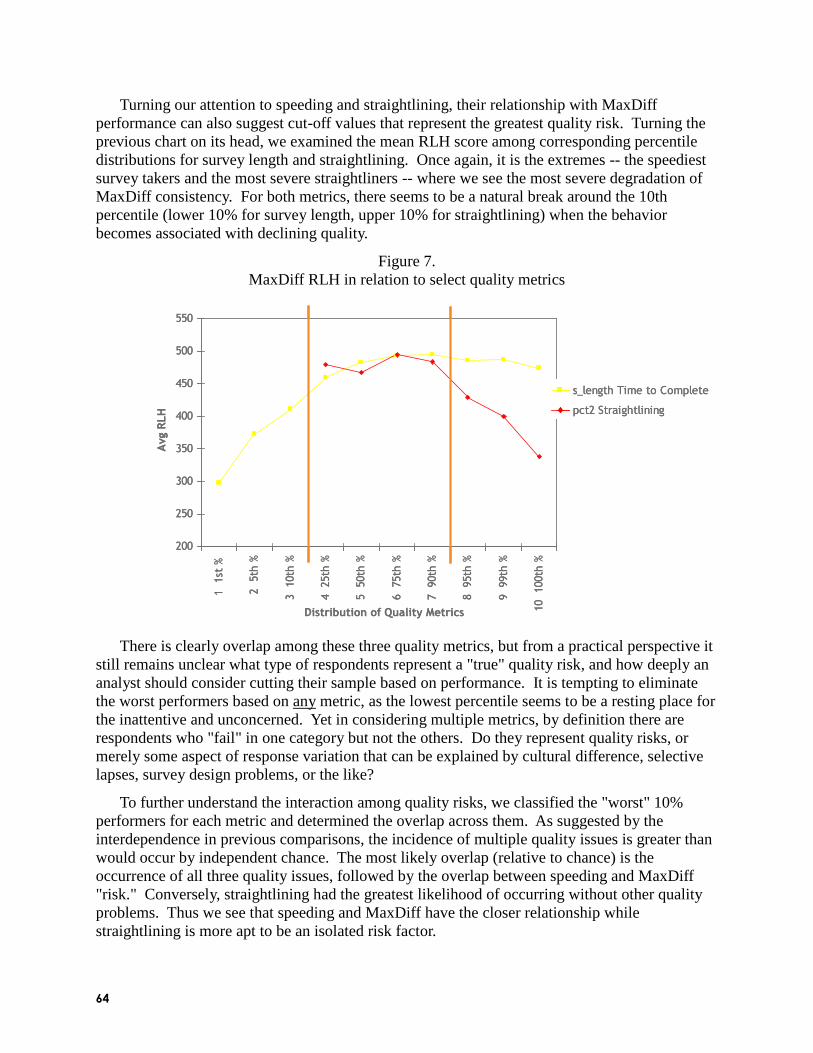
64

Turning our attention to speeding and straightlining, their relationship with MaxDiff

performance can also suggest cut-off values that represent the greatest quality risk. Turning the

previous chart on its head, we examined the mean RLH score among corresponding percentile

distributions for survey length and straightlining. Once again, it is the extremes -- the speediest

survey takers and the most severe straightliners -- where we see the most severe degradation of

MaxDiff consistency. For both metrics, there seems to be a natural break around the 10th

percentile (lower 10% for survey length, upper 10% for straightlining) when the behavior

becomes associated with declining quality.

Figure 7.

MaxDiff RLH in relation to select quality metrics

There is clearly overlap among these three quality metrics, but from a practical perspective it

still remains unclear what type of respondents represent a "true" quality risk, and how deeply an

analyst should consider cutting their sample based on performance. It is tempting to eliminate

the worst performers based on any metric, as the lowest percentile seems to be a resting place for

the inattentive and unconcerned. Yet in considering multiple metrics, by definition there are

respondents who "fail" in one category but not the others. Do they represent quality risks, or

merely some aspect of response variation that can be explained by cultural difference, selective

lapses, survey design problems, or the like?

To further understand the interaction among quality risks, we classified the "worst" 10%

performers for each metric and determined the overlap across them. As suggested by the

interdependence in previous comparisons, the incidence of multiple quality issues is greater than

would occur by independent chance. The most likely overlap (relative to chance) is the

occurrence of all three quality issues, followed by the overlap between speeding and MaxDiff

"risk." Conversely, straightlining had the greatest likelihood of occurring without other quality

problems. Thus we see that speeding and MaxDiff have the closer relationship while

straightlining is more apt to be an isolated risk factor.

200

250

300

350

400

450

500

550

1

1st

%

2

5th

%

3

10th

%

4

25th

%

5

50th

%

6

75th

%

7

90th

%

8

95th

%

9

99th

%

10

100th

%

s_length Time to Complete

pct2 Straightlining

Distribution of Quality Metrics

Avg

RLH

200

250

300

350

400

450

500

550

1

1st

%

2

5th

%

3

10th

%

4

25th

%

5

50th

%

6

75th

%

7

90th

%

8

95th

%

9

99th

%

10

100th

%

s_length Time to Complete

pct2 Straightlining

Distribution of Quality Metrics

Avg

RLH

65

Figure 8.

Overlap among key quality metrics

Once categorized, profiling by the quality metrics shows how strongly each group deviates

from the norm. The complete overlap group is obviously undesirable, as they complete the

survey in a quarter of the typical time, straightline nearly 2/3rds of all grid questions, and answer

the MaxDiff as if at random.

Figure 9.

Quality metrics among various quality classifications

Other combinations become steadily more difficult to discount as each has a redeeming

characteristic. Can we confidently exclude speeders who straightline if they answer the MaxDiff

exercise consistently? The resulting actions may depend upon how closely each metric relates to

Actual Chance Ratio

Speed, Straightline, MD Risk 1.20% 0.10% 12.0

Straightline, MD Risk 1.40% 1.00% 1.4

Speed, MD Risk 2.40% 1.00% 2.4

Speed, Straightline 1.20% 1.00% 1.2

Speed only 4.90% 7.90% 0.6

MD Risk only 5.00% 7.90% 0.6

Straightline only 6.20% 7.90% 0.8

No issues 77.70% 73.20% 1.1

Speeding

Straightlining

9.6 mins.

10.5% str.

476 RLH

21.0 mins.

56.1% str.

472 RLH8.0 mins.

61.9% str.

445 RLH

6.0 mins.

7.2% str.

241 RLH

6.2 mins.

65.2% str.

235 RLH

15.0 mins.

63.3% str.

241 RLH

19.4 mins.

8.6% str.

246 RLH

23.0 mins.

12.1% str.

500 RLH

MaxDiff

66

the integrity of the study in question and the analyst's insight into the risks associated with each.

In a broader sense, it also helps to understand how distinctive the problem groups are, and how

indicative they are of specific audiences or respondent types.

Figure 10 shows the relative strength with which different profiling characteristics are

associated with each quality metric. To derive the indices shown, the incidence of each

characteristic within the low quality decile was compared against the incidence across the total

meta-sample. A score of 100 indicates that a particular profiling group was no more likely than

average to be represented in the low quality decile.

Figure 10.

Profiling among various quality classifications

The three quality areas reveal similar profiling patterns, with some specific variations by

metric.

Commercial studies are more prone to straightlining and MaxDiff problems, but speeding

is equally prevalent in consumer and commercial studies;

The US and Canada are most prone to straightlining and MaxDiff problems, and Europe

has a moderate tendency to join these them in speeding;

Young males are at risk for all three quality areas.

60.7

167.6

145.5

37.450.4

35.6

124.4

101.5

90.5

34.8

128.4

64.3

78.6

136.8

154.6

29.617.8

38.5

117.2104.6

67.9

87.8

133.2

58.3

Speedin

gStr

aig

htl

inin

gM

axD

iff

Ris

k

100.8

98.7

118.2104.7

68

14.8

126.5

108.3

75.4

38.6

113.9

82.6

Con-

sumer

Biz US/

Canada

Europe APAC LatAm 20’s 30’s 40’s 50’s Male Female

60.7

167.6

145.5

37.450.4

35.6

124.4

101.5

90.5

34.8

128.4

64.3

78.6

136.8

154.6

29.617.8

38.5

117.2104.6

67.9

87.8

133.2

58.3

Speedin

gStr

aig

htl

inin

gM

axD

iff

Ris

k

100.8

98.7

118.2104.7

68

14.8

126.5

108.3

75.4

38.6

113.9

82.6

Con-

sumer

Biz US/

Canada

Europe APAC LatAm 20’s 30’s 40’s 50’s Male Female

67

These profiles hold when looking at the overlapping quality issues illustrated in Figure 9;

young males in North American commercial studies are disproportionate violators of multiple

quality flags. When we look at the profile for individual quality violations (e.g. only one of the

three), the typical profiles change. As shown in Figure 11, the commercial tendency to

straightline does not inherently bleed over into other quality issues. The European speeders

mentioned above are disproportionately speeding without further quality issues. And those who

only have problems with MaxDiff tend to be older, unlike the youthful orientation of

combination offenders.

Figure 11.

Profiling among single-quality violations

When contrasted with the consistent profile of multiple quality offenders, the heterogeneity

among single-quality violations suggests that each quality component has a particular response

effect associated with it that may be related to cultural or social norms in addition to quality.

Only when issues appear in tandem do they show a consistent trend towards quality violation

among a particular group.

For the analyst, this calls into question the wisdom of culling respondents on the basis of a

single quality flag. If Europeans indeed take surveys faster than others with no other adverse

indications, then indiscriminate deletion will introduce bias (under-representation of a particular

region and response style) rather than improve quality.

Likewise, the age effect associated with MaxDiff complications serves as a warning that not

all individuals play along with our research games exactly as we intend. While orthogonal

experimental designs may make perfect sense to practitioners, older respondents may find these

exercises particularly confusing, tedious, manipulative, or wasteful. Although it is unclear what

Speed Only

MD Risk

Only

Straight-

line Only

1 Consumer Research 112.6 78.5 42.4

2 Commercial Research 78.3 136.9 198.9

Total 100.0 100.0 100.0

Speed Only

MD Risk

Only

Straight-

line Only

1 US / Canada 92.2 154.6 129.8

2 Europe 154.3 23.7 48.1

3 APAC 95.5 8.7 77.9

4 LatAm 18.2 64.8 72.3

Total 100.0 100.0 100.0

Speed Only

MD Risk

Only

Straight-

line Only

1 20s 119.8 94.1 113.0

2 30s 114.9 107.6 98.6

3 40s 74.3 66.7 101.0

4 50s+ 48.4 157.2 59.9

Total 100.0 100.0 100.0

68

aspect of MaxDiff creates dissonance with this group, it should give pause to those who impose

blunt quality gates or consistency checks within surveys, because they are unlikely to be

interpreted and acted upon consistently across groups.

THE DEEP DIVE

The meta-analysis provided a broad perspective on metrics, cut-offs, and relationships, but

raised questions for further exploration:

If speeding, straightlining and RLH have disproportionate impact among specific

respondent types, do other commonly-used quality metrics have similar biases

lurking?

Can we measure these biases in terms of varying results?

For practical and methodological purposes, both questions are better addressed within the

context of a single study rather than the meta-analysis. Practically, it was not likely we could

implement a new battery of quality metrics across eight studies that did not have comparable

question structures (e.g. use of multiple response, open ends, scales with and without midpoints,

etc.). Methodologically, it is impossible to divine a consistent "result" when each study has

unique goals and hypotheses. To better address the next stage of analysis, we turned to a single

research project that offered both breadth and depth.

Of the 10,604 respondents used in the meta-analysis, 2,919 of them came from a single study.

This study provided an exemplary source of data since it was broad in many ways beyond its

respondent count.

International scope -- X countries with Y different languages.

Universal topic -- lifestyle preferences for 14 activities

Question variety -- MaxDiff, rating grids, open-ends, and multi-punch

In addition to the core quality metrics evaluated in the meta-analysis, this study incorporated

other measures to capture a greater variety of quality components.

Number of days in field (early vs. late responders)

Day of the week

Out-out specifically for "none" or "no response" (low involvement)

Out-out specifically for "don't know" (low knowledge)

Perseveration of overall scale point usage (scale point repetition)

Perseveration of midpoint usage (ambivalence)

Usage of multiple response items, including open ends (over/understatement)

The MaxDiff consisted of a typical exercise, measuring 14 attributes of low complexity (an

average of 2.4 words per attribute). Respondents were asked to identify the activity that was

most / least defining of their lifestyle through the course of 8 tasks. With 5 attributes shown per

69

task, each item was viewed 2.9 times on average. Individual utilities were derived through HB,

which also provided the RLH model fit statistic.

After further consideration, we hypothesized different ways to track respondent inconsistency

in the MaxDiff exercise beyond the RLH. To this end, there were two additional sets of quality

metrics introduced to this analysis.

The first type of MaxDiff measures is similar to the perseveration measures for rating grids.

In much the same way a person might focus their scale responses around a specific rating, they

might also focus their MaxDiff responses around a specific response position regardless of

content. Perseveration would contribute to random-looking RLH fit scores to the degree that the

design did not favor any particular attributes in any given positions. Perseveration statistics were

calculated for both ―most‖ and ―least‖ responses.

An example of perseveration is provided in Figure 12. In this case, the respondent

consistently chooses position 4 for ―most‖ and position 3 for ―least,‖ even though the content of

those positions fluctuates.

Figure 12.

Example of MaxDiff perseveration

The second type of MaxDiff measures is an assessment of the conflicting information

provided during the exercise. Each task represents a series of pairwise comparisons, such that

selecting position 1 as ―most‖ would reveal several relationships: 1 > 2, 1 > 3, 1 > 4, and 1 > 5.

Selecting position 5 as ―least‖ would reveal additional relationships: 1 > 5 (which we already

know), 2 > 5, 3 > 5, and 4 > 5. Since the MaxDiff computation assumes all such pairings are

evaluated during the task, any subsequent violation of this ordering will add variability to the

estimates, which ultimately reduces RLH.

An example of conflicts is provided in Figure 13. In this scenario, the individual is not

perseverating on particular response position, but their answers do create violations in preference

order. These violations can occur in a number of ways.

OReliabilityO

OPerformanceO

OSupportO

OValueO

OQualityO

LeastMost

OReliabilityO

OPerformanceO

OSupportO

OValueO

OQualityO

LeastMost

OReliabilityO

OSecurityO

OUsabilityO

OInnovationO

OQualityO

LeastMost

OReliabilityO

OSecurityO

OUsabilityO

OInnovationO

OQualityO

LeastMost

OUsabilityO

OSupportO

OPerformanceO

OInnovationO

OLow CostO

LeastMost

OUsabilityO

OSupportO

OPerformanceO

OInnovationO

OLow CostO

LeastMost

70

Figure 13.

Example of MaxDiff conflicts

In one scenario, the respondent is inattentive to their ―most‖ responses, as demonstrated

between tasks 1 and 2. In task 1, the individual cites ―quality‖ as most important attribute,

placing it implicitly above all other items in importance. In task 2, ―reliability‖ is most

important. This generates an inconsistency in ―most‖ responses, since both ―quality‖ and

―reliability‖ appear in both lists; regardless of the other three attributes that change, there is no

reasonable justification for reversing the order of preference between tasks.

This type of consistency within response also applies to the ―least‖ assessments. Our

example above is fully consistent in this regard, as ―performance‖ is chosen twice with no

conflict in ordering. ―Usability‖ is chosen in task 2 and not task 3, but not at the expense of any

implied orderings between the questions.

Another type of conflict occurs across response, whereby the ―most‖ and ―least‖ assessments

conflict. The example in Figure 13 shows such a case between tasks 2 and 3. In task 2, the

respondent asserts that ―usability‖ is the least important attribute, placing it below ―innovation.‖

However, in task 3 a conflicting order occurs when ―usability‖ is chosen as the most important

attribute, placing it above ―innovation.‖ Neither task generates conflicting relationships within

the ―most‖ or ―least‖ responses, only when the relationships are viewed across all preference

assertions.

Clearly there must be overlap across these MaxDiff metrics. Even though perseveration is

conceptually separate from conflict, extreme perseveration will create conflicts. Similarly,

conflicts within ―most‖ / ―least‖ responses are distinct from those that happen across response,

but elevated levels of one will assuredly contribute to the other. But interestingly, these metrics

appear to be relatively independent of all other quality metrics.

A factor analysis of all quality metrics reveals the broad underlying associations that link

many of them together. The varimax rotation from principal components is shown in Figure 14,

with a relatively even distribution of quality metrics across implied dimensions. Some of the

more interesting combinations include:

Engagement: Active use of multiple response options (e.g. providing more responses) is

diametrically opposed to the likelihood to opt out, almost by definition. More notable

is that it is also associated with higher survey evaluations (satisfaction). This

combination would seem to reflect the respondent's involvement with the survey

content rather than an explicit quality connotation.

OReliabilityO

OPerformanceO

OSupportO

OValueO

OQualityO

LeastMost

OReliabilityO

OPerformanceO

OSupportO

OValueO

OQualityO

LeastMost

OReliabilityO

OSecurityO

OUsabilityO

OInnovationO

OQualityO

LeastMost

OReliabilityO

OSecurityO

OUsabilityO

OInnovationO

OQualityO

LeastMost

OUsabilityO

OSupportO

OPerformanceO

OInnovationO

OLow CostO

LeastMost

OUsabilityO

OSupportO

OPerformanceO

OInnovationO

OLow CostO

LeastMost

71

Lazy / Fraud: Straightlining ratings grids is associated with shorter survey length

(speeding). This relationship is interesting because it suggests that satisficing may be

a strategy for actively shortening a survey rather than a reaction to longer surveys

(which would have resulted in complementary signs rather than opposing ones).

Active / Pro: The more online surveys an individual completes, the more likely they are

to be an early responder. If you are concerned about "professional respondents"

filling up your survey, manage invitations accordingly to allow more time for late

responders to participate.

Relevance: The tendency to use the don't know option is opposite to the tendency to

perseverate on scale midpoints. Since many of the DK responses occur within scales,

this may well reflect a zero-sum decision to either opt out or rate items ambiguously.

Perhaps this dimension could also be labeled as "scale design" as it would likely be

affected by the inclusion or exclusion of a DK response option.

Figure 14.

Factor analysis of expanded quality metrics

Loading on separate dimensions confirms that MaxDiff performance is, broadly speaking, a

different aspect of quality than all other metrics collected. While we have seen that extremely

low RLH fit is strongly associated with some aspects of speeding and straightlining, the entire

distribution of MaxDiff perseveration and conflict is orthogonal to the full spectrum of other

quality indicators. MaxDiff is indeed bringing something new to the quality conversation.

A secondary observation comes from the splitting of MaxDiff dimensions between "most"

and "least" metrics, with the cross response conflict splitting the difference. Previous research

has pointed out that individuals answer the two questions somewhat differently, in that they will

generate different utilities if modeled separately. (Chrzan) This difference appears to hold true

for the errors that people make in MaxDiff as well. It serves as an important reminder that our

.467

.555

.809

MaxDiff

Least

.652

-.758

Active /

Pro

-.647

.709

Rele-

vance

.422MaxDiff conflicts (Most vs Least)

MaxDiff conflicts (within Least)

.768MaxDiff conflicts (within Most)

MaxDiff perseverations (Least)

.731MaxDiff perseverations (Most)

.915Number of phone surveys

Number of online surveys

.561Survey evaluation

.797Multiple-response

MaxDiff

Most

-.779Opt out for none / 0

Midpoint repetition

.728Straightlining / Perseveration

Opt out for DK

Days in field

-.646Survey Length

Phone

Surveys

Lazy /

Fraud

Engage-

ment

Metric

.467

.555

.809

MaxDiff

Least

.652

-.758

Active /

Pro

-.647

.709

Rele-

vance

.422MaxDiff conflicts (Most vs Least)

MaxDiff conflicts (within Least)

.768MaxDiff conflicts (within Most)

MaxDiff perseverations (Least)

.731MaxDiff perseverations (Most)

.915Number of phone surveys

Number of online surveys

.561Survey evaluation

.797Multiple-response

MaxDiff

Most

-.779Opt out for none / 0

Midpoint repetition

.728Straightlining / Perseveration

Opt out for DK

Days in field

-.646Survey Length

Phone

Surveys

Lazy /

Fraud

Engage-

ment

Metric

72

definition of quality is dependent upon the cognitive process involved; how individuals approach

a question will dictate their success at answering it.

With these tools in place, we went about replicating the meta-analysis within the narrowed

context of this single study. First, we broke out the enhanced quality metrics by the RLH

distribution, just as performed with the multi-study data. However, the RLH distribution for this

study was skewed higher (i.e. was more "consistent") than for the multi-study data, and thus our

definitions of the percentiles shifted to accommodate reasonable base sizes for each group. As a

consequence, the quality interactions are compressed into a smaller part of the RLH scale

relative to the broader assessment, as shown in Figure 15. Note that quality metrics with non-

significant variation across RLH categories are removed for interpretability.

Figure 15.

Quality metrics in relation to MaxDiff RLH percentile distribution

While the quality metrics seem to have shifted downwards within the percentile distribution,

they actually reveal a very similar threshold for RLH that was observed in the meta-analysis. In

the cross-study assessment, quality metrics stabilized around an RLH of ~300, which occurred

above the 10th percentile. Here, a similar stabilization occurs before the 5th percentile, which

also represents RLH scores of ~ 300, suggesting that absolute RLH scores are likely to be more

reliable quality indicators than are relative RLH scores.

When we replicate the relationship between RLH and the remaining quality metrics, we see

that MaxDiff fit behaves very comparably within the single-study context. Our two primary

metrics – straightlining and time to completion – behave as expected at the same 10th

percentile

breaks we observed in the cross-study analysis.

7.6

18.8 19.4 19.820.8 21.3 20.8

21.8

19.321.6

29%

13%

7% 7% 6% 7%6% 5%

7%5%

0

5

10

15

20

25

30

35

1

1st

% (

242)

2

5th

% (

314)

3

10th

% (

342)

4

25th

% (

399)

5

50th

% (

476)

6

75th

% (

558)

7

90th

% (

628)

8

95th

% (

667)

9

99th

% (

723)

10

100th

% (

>723)

0%

5%

10%

15%

20%

25%

30%

35%s_length Time

research1 Survey Ratings

research2 Online surveys

research3 Phone surveys

pct1 Opt Out

pct2 Straightline

pct3 Midpoint

pct4 None / 0

pct5 Multi-Response

Distribution of Avg RLH

73

Figure 16.

MaxDiff RLH in relation to select quality metrics

Two additional metrics have notable associations with MaxDiff quality. Perseveration, the

more granular version of the straightlining metric, yields insight into the lowest part of the

distribution where there is no variation for straightlining (a quarter of individuals do not

straightline any question blocks, but may perseverate on individual scale values). People who

have extremely low perseveration, which means they seldom answer with the same scale point in

any battery, experience a slight decline in MaxDiff quality. The lowest users of multiple

response are similarly likely to trend slightly lower in MaxDiff quality.

These additional two metrics only indicate nuanced quality concerns from MaxDiff

associated with extremes in their own performance. From this, it appears that our original

formulation of speeding, straightlining and MaxDiff is the combination that generates the

greatest quality concerns, even when several other types of hypothesized quality violations are

observed.

Recall our Venn diagram of quality from Figure 9. Continuing with these segments defined

by speeding, straightlining, and MaxDiff fit, we can now review these same 8 groups according

to their MaxDiff-specific quality measures and utilities from the particular MaxDiff exercise

presented in the ―deep dive‖ study. The Venn diagram is duplicated below, this time with the 8

segments enumerated for future reference.

200

250

300

350

400

450

500

550

1 1st

%

2 5th

%

3 10th

%

4 25th

%

5 50th

%

6 75th

%

7 90th

%

8 95th

%

9 99th

%

10 100th

%

s_length Time to Complete

pct2 Straightlining

pct2a Perseveration

pct5 Multi-Response

Avg

RLH

Distribution of Quality Metrics

74

Figure 17.

Overlapping quality metrics, labeled

The base sizes are quite small for the problem segments. Yet despite this paucity of cases,

there are statistically significant (p < .001) differences across all five of the MaxDiff-specific

metrics that point to specific issues exhibited among those with combined quality issues present.

Figure 18.

MaxDiff-specific quality measures by overlapping quality segments

4.8

4.5

3.6

3.1

3.1

3.4

2.9

3.0

4.9

4.5

3.8

3.2

3.2

3.2

3.1

3.1

1

2

3

4

5

6

7

8

Perseveration, Most

Perseveration, Least

1.6

1.0

1.1

0.7

0.4

1.0

0.4

0.3

2.5

1.7

2.3

0.4

0.2

1.7

0.2

0.1

2.6

2.3

2.2

0.9

0.7

2.2

0.8

0.5

1

2

3

4

5

6

7

8

Conflicts, Most

Conflicts, Least

Conflicts, Cross

1

23

45

6

7

8

1. Speeding, Straightlining, MD Risk (N=13)

2. Straightlining, MD Risk (N=6)

3. Speeding, MD Risk (N=33)

4. Speeding, Straightlining (N=37)

5. Speeding Only (N=210)

6. MD Risk Only (N=41)

7. Straightlining Only (N=55)

8. No Issues (N=2524)

75

Despite the clear difference in tasks, there is a pronounced tendency for straightlining

behavior to bleed into the MaxDiff task among those who exhibit combined quality problems.

For those who combine straightlining of ratings grids with poor MaxDiff quality (segments 1 and

2), more than half of the 8 MaxDiff ―most‖ and ―least‖ tasks were answered with the same

response position. In the cases of greatest quality risk, perseveration transcends question format.

Our other aspect of MaxDiff quality – conflicting preference – also shows a pronounced

difficulty among the most at-risk segments. Any group with MaxDiff problems registered

significantly more conflicts of all types than did those with other problems exclusive of MaxDiff,

reflecting the basis of the overall exercise. However, those with all combined quality issues

(segment 1) also produced the highest number of all conflict types. If we consider this aspect of

the MaxDiff exercise to be analogous to ad hoc consistency checks, this suggests that

consistency problems about as likely to be encountered from those with no other quality issues

(segment 6) than from those who have combined quality problems (segments 1 2 and 3).

We were able to profile these problem segments in the same manner as our meta-analysis,

this time with somewhat more descriptive detail. The greatest risk to quality still comes from

young males in the US, although this focused example yielded issues in Spain as well. The ―at

risk‖ segment is also about twice as likely to claim to have purchased an auto recently, with TVs

and .mp3 players also showing a boost in claimed adoption. Similar adoption patterns are

observed among straightliners without MaxDiff issues (segments 4 and 7), whereas pure

speeders are less apt to indicate any recent purchases.

Figure 19.

Profiling among various quality classifications

Metric At Risk Speeding,

Straight.

Speeding

Only

MaxDiff

Risk Only

Straight.

Only

No Issues

N 52 37 210 41 55 2524

Country Spain (168)

US (189)

US (245) UK (195)

US (159)

Brazil (175)

Mexico (248)

Spain (178)

US (191) *

Age 18-24 (139) 30-39 (138) * 30-39 (124)

50-59 (128)

* *

Gender Male (142) Male (125) * * * *

Recent

Purchases

Cars (205)

.mp3 (142)

TV (181)

Cars (209)

TV (175)

None (153) * Cars (150)

Clothes (148)

TV (160)

*

1 2 3 4 5 6 7 8

We previously observed that MaxDiff issues can be uniquely tied to older respondents, which

we confirmed in this focused observation. But we also see an issue among various Latin

American countries as well, which may demonstrate unique cultural or linguistic hurdles to

MaxDiff. This finding warrants further study, but alone points to the need to understand the

causes and implications of each quality metric beyond simply assuming that each is inherently

―quality related.‖

What are the implications of excluding individuals with particular quality problems? For this

answer we look to the MaxDiff utilities to serve as a reference for results. If poor quality

respondents are contributing to conflicting survey findings, then we would assume to find

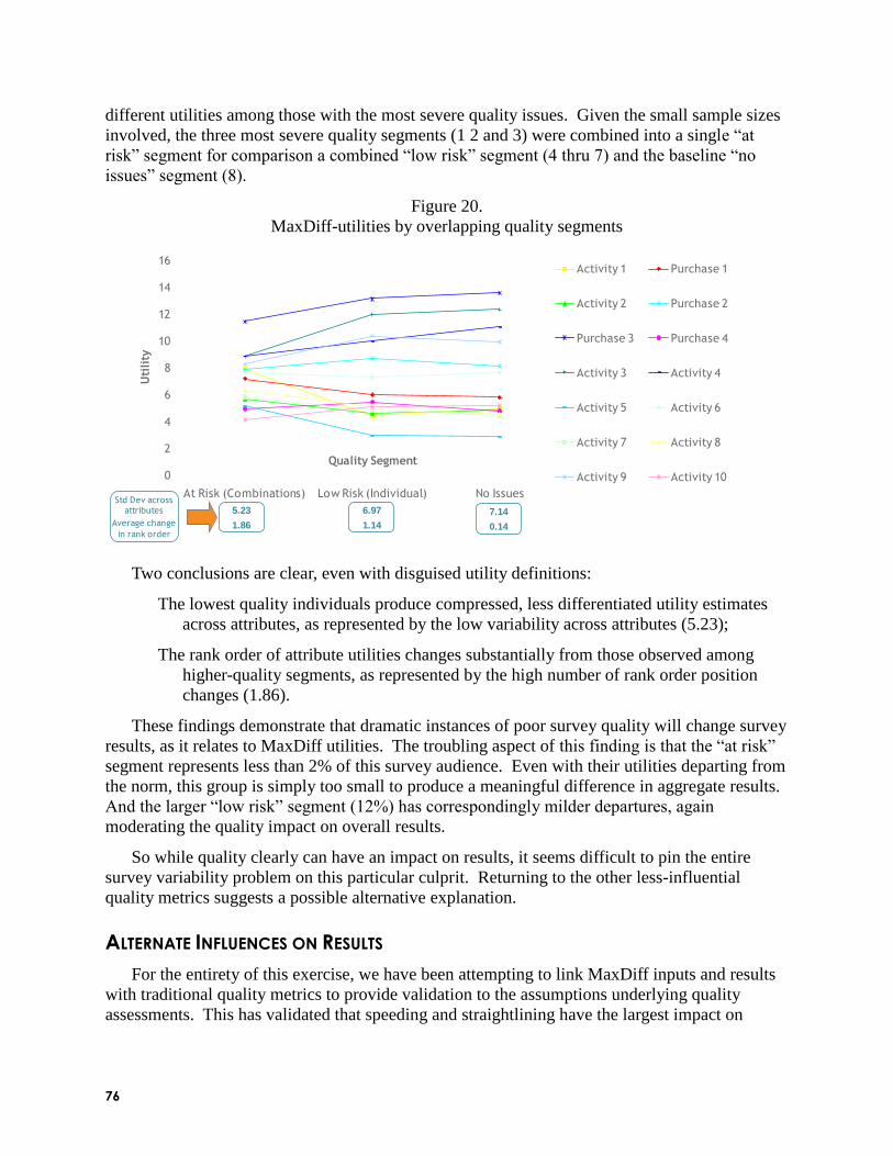
76

different utilities among those with the most severe quality issues. Given the small sample sizes

involved, the three most severe quality segments (1 2 and 3) were combined into a single ―at

risk‖ segment for comparison a combined ―low risk‖ segment (4 thru 7) and the baseline ―no

issues‖ segment (8).

Figure 20.

MaxDiff-utilities by overlapping quality segments

Two conclusions are clear, even with disguised utility definitions:

The lowest quality individuals produce compressed, less differentiated utility estimates

across attributes, as represented by the low variability across attributes (5.23);

The rank order of attribute utilities changes substantially from those observed among

higher-quality segments, as represented by the high number of rank order position

changes (1.86).

These findings demonstrate that dramatic instances of poor survey quality will change survey

results, as it relates to MaxDiff utilities. The troubling aspect of this finding is that the ―at risk‖

segment represents less than 2% of this survey audience. Even with their utilities departing from

the norm, this group is simply too small to produce a meaningful difference in aggregate results.

And the larger ―low risk‖ segment (12%) has correspondingly milder departures, again

moderating the quality impact on overall results.

So while quality clearly can have an impact on results, it seems difficult to pin the entire

survey variability problem on this particular culprit. Returning to the other less-influential

quality metrics suggests a possible alternative explanation.

ALTERNATE INFLUENCES ON RESULTS

For the entirety of this exercise, we have been attempting to link MaxDiff inputs and results

with traditional quality metrics to provide validation to the assumptions underlying quality

assessments. This has validated that speeding and straightlining have the largest impact on

0

2

4

6

8

10

12

14

16

At Risk (Combinations) Low Risk (Individual) No Issues

Activity 1 Purchase 1

Activity 2 Purchase 2

Purchase 3 Purchase 4

Activity 3 Activity 4

Activity 5 Activity 6

Activity 7 Activity 8

Activity 9 Activity 10

Uti

lity

Quality Segment

5.23

1.86

6.97

1.14

7.14

0.14

Std Dev across attributes

Average change

in rank order

Uti

lity

77

MaxDiff results, and likewise that MaxDiff performance issues can contribute to a meaningful

quality risk assessment.

For the remaining quality metrics that have gone relatively unmentioned – opt outs, multiple

response, number of surveys, and the like – their lack of association with MaxDiff fit suggested

they were not strong indicators of broader quality issues. However, comparing these indicators

against MaxDiff utilities yields some further understanding of the survey process that bears

discussing.

Consider the multiple-response metric – the ratio of multiple choice responses given to the

maximum number of responses available. There are some theoretical reasons why this metric

should be suggestive of quality:

Providing too many selections could be indicative of intentional overstatement, whereby the

respondent is attempting to avoid disqualification due to lack of involvement;

Providing too few selections could be indicative of satisficing, whereby the respondent is

skipping through options, selecting the minimum necessary to complete the task;

But variable levels of multiple response can also be indicative of, most obviously, varying

levels of participation, sophistication, or experience (depending upon what the multiple response

items are measuring, of course). When we examine all aspects of MaxDiff response – quality

and utility – against multiple response levels, there is a very strong relationship with the resulting

preferences with almost no quality implications.

The differences in MaxDiff utility (Figure 21) show a similar pattern to that exhibited across

quality segments. Lower levels of multiple response are associated with reduced utility for

Purchase 3 (which is technology-oriented) and elevated utility for Activities 3 and 5 (which are

entertainment-oriented).

However the change in utilities differs in this scenario to what we observed in the quality

assessment. With the quality segments, we observed that utilities changed rank order

substantially among ―at risk‖ respondents, then stabilized towards aggregate results as quality

increase. With multiple response groupings, however, the change in rank order is equally

extreme on both ends of the extreme, but with clearly reversed positions.

And yet this fluctuation in utilities is not associated with the same degree of compression

observed with reduced quality. While the average rank order levels fluctuate across multiple

response groupings, the variability across attributes remains fairly consistent. This suggests that

respondents are providing meaningfully different preferences that are related to their activity

with multiple response lists, rather than exhibiting random response or indecision.

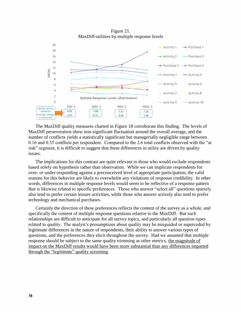
78

Figure 21.

MaxDiff-utilities by multiple response levels

The MaxDiff quality measures charted in Figure 18 corroborate this finding. The levels of

MaxDiff perseveration show non-significant fluctuation around the overall average, and the

number of conflicts yields a statistically significant but managerially negligible range between

0.16 and 0.35 conflicts per respondent. Compared to the 2.6 total conflicts observed with the ―at

risk‖ segment, it is difficult to suggest that these differences in utility are driven by quality

issues.

The implications for this contrast are quite relevant to those who would exclude respondents

based solely on hypothesis rather than observation. While we can implicate respondents for

over- or under-responding against a preconceived level of appropriate participation, the valid

reasons for this behavior are likely to overwhelm any violations of response credibility. In other

words, differences in multiple response levels would seem to be reflective of a response pattern

that is likewise related to specific preferences. Those who answer ―select all‖ questions sparsely

also tend to prefer certain leisure activities, while those who answer actively also tend to prefer

technology and mechanical purchases.

Certainly the direction of these preferences reflects the content of the survey as a whole, and

specifically the content of multiple response questions relative to the MaxDiff. But such

relationships are difficult to anticipate for all survey topics, and particularly all question types

related to quality. The analyst‘s presumptions about quality may be misguided or superceded by

legitimate differences in the nature of respondents, their ability to answer various types of

questions, and the preferences they elicit throughout the survey. Had we assumed that multiple

response should be subject to the same quality trimming as other metrics, the magnitude of

impact on the MaxDiff results would have been more substantial than any differences imparted

through the ―legitimate‖ quality screening.

0

2

4

6

8

10

12

14

16

18

20

10th % 50th % 90th % 100th %

Activity 1 Purchase 1

Activity 2 Purchase 2

Purchase 3 Purchase 4

Activity 3 Activity 4

Activity 5 Activity 6

Activity 7 Activity 8

Activity 9 Activity 10

Uti

lity

Multiple Response Levels (distribution)

6.91

1.57

7.08

0.71

7.11

0.43

Std Dev across attributes

Average change

in rank order

Uti

lity

7.13

1.43

79

CONCLUSIONS

Through our assessments, both broad and narrow, we have determined that MaxDiff is a

useful tool for data quality review, providing an alternate perspective into response behavior as

well as an outcome for evaluating the implications of data quality. Relative to our specific

questions, we found:

MD can serve as a validation of quality, as individuals who exhibit certain quality problems

have notable issues with MaxDiff.

MD does not appear to moderate or add to quality issues overall, as thus far we have seen no

substantive difference in quality between studies with and without MD.

MD is robust in the presence of moderate levels from ―traditional‖ quality issues, but

extreme levels of speeding and straightlining compress utilities and promote changes in rank

order.

MD helps us identify problem responders when we overlay MD issues against ―traditional‖

quality metrics, and multiple violations produce skewed results and respondent profiles.

MD does exhibit unique quality issues, particularly among a distinct group of respondents

who ―fail‖ at MD independently from other quality metrics.

The key to success for MD is the ability to maintain consistent responses between ―most‖

and ―least‖ assessments.

These results have helped Illuminas hone its quality review process, both with and without

MaxDiff as a component. Regardless of the presence of a MaxDiff exercise, we have used this

information to validate the reliance upon speeding and straightlining as key quality components.

The interaction of these metrics with MaxDiff quality and results has proven to us that only the

most extreme cases of quality violation (typically less than 10%) are worth consideration, and

individuals are only excluded when they exhibit multiple quality violations. Rejection between 1

and 4% of completed surveys is the norm.

We have also rejected certain aspects of conventional wisdom regarding survey quality as a

result of this assessment. It is common to rail against ―professional respondents‖ as the root of

all survey ills, but the negligible (in fact, positive) relationship between the number of online

surveys taken and the quality of MaxDiff fit (Figures 6 and 15) suggests to us that, in fact, it is

the frequent survey participants who are most knowledgeable about the survey task and likely to

provide the greatest insight. Demonizing those who willing support our industry, albeit

sometimes at surprisingly elevated levels, is neither an accurate nor productive portrayal.

Another common practice is the use of tactical hurdles or obvious question repetitions /

reversals to trap respondent inconsistency. Certainly there are individuals whose fallacious

survey behavior can be snared in this particular net. Since MaxDiff essentially serves this

purpose, we feel comfortable using our results to validate that such inconsistency is a clear

quality issue when corroborated by other quality issues. However, isolated violations of such

traps should be interpreted with caution, as individuals may be merely distracted, mistaken, or

intentionally mischievous when presented with questions that could be interpreted as an insulting

waste of time to the legitimate respondent. The fact that a distinct segment of our sample had

80

trouble with MaxDiff exclusive of other quality metrics indicates that rejecting inconsistent

respondents will likely produce skewed demographics, with possible implications for broader

survey results.

With regard to survey results, we are heartened by the robustness of our MaxDiff results in

the face of moderate to strong quality violations. We did not assess similar resiliency across

other question types, so it is left to further analysis to determine the threshold upon which quality

threatens to change the results and interpretation of rating scales and other data types.

With any question type or survey format, however, it seems that the survey quality issue as it

has been thus defined is not a threat to the credibility of survey research results unless quality

offenders rise well above 1 to 4%. On this specific issue, there appear to be greater risks

associated with unguided quality purges that bias results away from individuals with certain

response styles rather than a valid quality concern.

Ultimately, data and respondent quality is an important issue for maintaining the credibility

and viability of survey research. Combined efforts from sample providers and research suppliers

will continue to enhance our understanding of this issue and keep it in check. As outlined in

Figure 2, these issues are only a small component of overall research quality. We must not be

distracted by efforts to isolate problem respondents and ignore the issues that create problem

surveys and problem analysis. Anyone can write a survey and present it to respondents, good or

bad. But only the research professionals will exercise the care to sample, design, and interpret

their surveys to truly address quality in ways that response quality assessments will never

address.

81

REFERENCES

Baker, Reg and Theo Downes-Le Guin (2007). ―Separating the Wheat from the Chaff:

Ensuring Data Quality in Internet Samples,‖ presented at ESDS: The Challenges of a

Changing World (Southampton, UK September 12-14).

Cartwright, Trixie (2008). ―Panelist Behavior and Survey Design – Key Drivers in Research

Quality,‖ presented at The 2008 CASRO Panel Conference (Miami, Florida, February 5-

6).

Chrzan, Keith (2004). ―The Options Pricing Model: An Application of Best-Worst

Measurement to Multi-Item Pricing,‖ 2004 Sawtooth Software Conference Proceedings,

Sequim, WA.

Cohen, Steve (2003). ―Maximum Difference Scaling: Improved Measures of Importance and

Preference for Segmentation,‖ 2003 Sawtooth Software Conference Proceedings, Sequim,

WA.

Dedeker, Kim (2006). ―Research Quality: The Next MR Industry Challenge, ‖ Research

Business Report (October).

Downes-Le Guin, Theo (2005). ―Satisficing Behavior in Online Panelists,‖ presented at MRA

Annual Conference & Symposium (June 2),

Finn, Adam and Jordan J. Louviere (1992). ―Determining the Appropriate Response to

Evidence of Public Concern: The Case of Food Safety, ‖Journal of Public Policy and

Marketing, 11: 12-25.

Giacobbe, Joe and Annie Pettit (2008). ―Data Quality: Prevalence and Types of Survey

Response Sets,‖ presented at The CASRO Panel Conference (Miami, Florida, February 5-

6).

Goglia, Chris and Alison Strandberg Turner (2009), ―To Drag-n-Drop or Not? Do Interactive

Survey Elements Improve the Respondent Experience and Data Quality?‖ presented at

2009 Sawtooth Software Conference (Delray Beach, Florida, March 23-27).

Krosnick, J. A., Narayan, S. S., & Smith, W. R. (1996). ―Satisficing in surveys: Initial

evidence.‖ In M. T. Braverman & J. K. Slater (Eds.), Advances in survey research (pp.

29-44). San Francisco: Jossey-Bass.

Miller, Jeff and Andrew Jeavons (2008). ―Online Interview Interventions: Can ―Bad‖

Panelists be Rehabilitated?‖ presented at The CASRO Panel Conference (Miami, Florida,

February 5-6).

Orme, Bryan (2005). ―Accuracy of HB Estimation in MaxDiff Experiments,‖ Sawtooth

Software Research Paper Series,

http://www.sawtoothsoftware.com/download/techpap/maxdacc.pdf

RFL Communications, Inc. (2008). Platforms for Data Quality Progress: The Client‘s Guide

to Rapid Improvement of Online Research, 1st edition, edited by Marc Dresner.

Sawtooth Software (2005). Identifying “Bad” Respondents, Sawtooth Software, Inc.

82

Sawtooth Software (2005). The MaxDiff/Web System Technical Paper, Sawtooth Software,

Inc.

Smith, Renee et al. (2008). ―Hyperactive Respondents and Multi-Panel Members: A

Continuing Investigation,‖ presented at The CASRO Panel Conference (Miami, Florida,

February 5-6).

83

A NEW MODEL FOR THE FUSION OF MAXDIFF SCALING

AND RATINGS DATA

JAY MAGIDSON1

STATISTICAL INNOVATIONS INC.

DAVE THOMAS SYNOVATE

JEROEN K. VERMUNT TILBURG UNIVERSITY

ABSTRACT

A property of MaxDiff (Maximum Difference Scaling) is that only relative judgments are

made regarding the items, which implies that items are placed on separate relative scales for each

segment. One can directly compare item preference for a given segment, but comparisons

between respondents in different segments may be problematic. In this paper we show that when

stated ratings are available to supplement the MaxDiff data, both sets of responses can be

analyzed simultaneously in a fused model, thus converting to an absolute (ratio) scale. This

allows individual worth coefficients to be compared directly between respondents on a common

calibrated scale.

Our approach employs latent class methods, so that respondents who show similar

preferences are classified into the same segment. The fused model also includes a continuous

latent variable to account for individual differences in scale usage for the ratings, and scale

factors for both the ratings and MaxDiff portions of the model to account for respondents who

exhibit more or less amounts of uncertainty in their responses. The Latent GOLD Choice

program is used to analyze a real MaxDiff dataset and show the differences resulting from the

inclusion of ratings data.

INTRODUCTION

Ratings attempt to ascertain measures of absolute importance which allow respondents (or

segments) to be compared directly to each other with respect to their preferences for each

attribute. However, when measured in the usual way with a Likert scale, they suffer in the

following respects:

1. Lack of discrimination – many respondents rate all attributes as important, and with

more than 5 attributes, all respondents necessarily rate some attributes as equally

important (on a 5-point scale).

2. Confounded with scale usage – ratings may not be directly interpretable as measures

of preference because ratings elicited from a respondent are affected by that

1 The authors gratefully acknowledge the assistance Michael Patterson from Probit Research Inc. for the MaxDiff design used and Mike

MacNulty from Roche Diagnostics Corp. for providing the data and allowing it to be freely distributed via Statistical Innovations‘ website

www.statisticalinnovations.com.

84

respondent‘s scale usage. Some respondents tend to avoid extreme ratings, while

others prefer the extremes, etc.

Because of these limitations, the use of ratings alone has been avoided in favor of MaxDiff

and other choice designs.

MaxDiff scaling and other discrete-choice modeling approaches have their own limitations,

since they estimate worth (part-worth) coefficients based on relative as opposed to absolute

judgments. This allows options for a given subject (segment) to be ranked on relative

importance, but does not allow subjects (segments) to be compared with each other according to

their preferences for any particular attribute.

For example, on a relative basis Mary may judge attribute D to be more important than C.

However, in absolute terms she does not consider either to be very important (see Figure A). On

the other hand, Jim may consider C to be more important than D, and consider both C and D to

be very important. Given only their relative judgments, it may be tempting, but it is not valid, to

infer that Mary considers D to be more important than does Jim (Bacon et al. 2007, 2008).

Figure A.

Comparison of Worths between 4 Respondents on a Common Absolute Scale

APPROACH

Our approach is to obtain maximum likelihood (ML) estimates for the segment sizes, worths,

and other parameters that maximize the joint likelihood function based on both ratings and

responses to MaxDiff tasks. A single nominal latent categorical variable is used for the

segmentation. In order to equate the common information elicited in the ratings and MaxDiff

tasks, a continuous latent variable is specified to account for individual differences in scale usage

for the ratings (Magidson and Vermunt, 2007a), and scale factors are included in both the ratings

and MaxDiff portions of the model which control for respondents who exhibit more or lesser

amounts of uncertainty in their responses (Magidson and Vermunt, 2007b), as well as scale

differences between rating and MaxDiff tasks.

A constant is added so that the calibrated worths correspond to expected log-odds of a higher,

as opposed to a lower, attribute rating, thus providing a meaningful absolute metric for the

*

ji

85

worths. Hence, meaningful preference comparisons can be made between segments as well as

between respondents.

Bacon, et al. (2007) utilized ratings data to uncover the zero point in individual MaxDiff

worths using a somewhat similar data fusion methodology. Our approach differs from that of

Bacon/Lenk in that it a) yields a segmentation, b) utilizes a simpler model, and c) it is

implemented using commercially available software. Specifically, all models used here are

developed using the syntax version of Latent GOLD Choice, release 4.5 (Vermunt and

Magidson, 2008).

Our general approach extends directly to the use of ratings data in conjunction with any

discrete choice model, including those where a ―None‖ option is included in the design to

provide an additional absolute alternative. Future research is planned that address such

extensions.

We begin by discussing some important psychometric properties of ratings and choice data,

and show that the lack of a common origin for choice data requires the use of identifying

restrictions. In particular, we employ a simple example to show that the interpretation of the

resulting MaxDiff worths may be very tricky and proper interpretation depends on the particular

restrictions used (e.g., dummy or effect coding). We then present the results of a case study

where a fused model is estimated and compared to results from a comparable MaxDiff model

developed without use of ratings.

SOME PSYCHOMETRIC PROPERTIES OF RATINGS AND CHOICE DATA

Worth coefficients obtained with a choice/ranking/MaxDiff task for a particular latent class

segment provide an interval scale, which is a relative scale in which the absolute zero point is

unknown and/or unspecified. In a traditional latent class (LC) MaxDiff analysis where K

segments (classes) are obtained, each segment k is associated with its own separate interval

scale. The unknown zero points may be located at different positions along each of these scales.

For attribute j, denote the worth coefficient for segment-level k and individual level i as

follows:

= worth (―Importance‖) for attribute j with respect to class k

j = 1,2,…,J items (attributes)

k = 1,2,…,K respondent segments (latent classes)

= individual worth coefficient for attribute j with respect to respondent i

i = 1,2,…,N respondents

Because the absolute zero points are unknown, the worth coefficients are not (uniquely)

identifiable without imposing some restrictions. The most common identifying restrictions for

LC choice analyses are effect and dummy coding, while for hierarchical Bayesian (HB) methods

dummy coding is typically used2. As a simple hypothetical example, consider K = 3 segments

2 Although this paper deals primarily with latent class (LC) analyses of MaxDiff data, identifying restrictions are also required in HB analyses.

In traditional HB analyses of MaxDiff data, dummy coding restrictions are employed, in which individual worths for a particular (reference)

attribute are taken to be 0 for all individuals. After obtaining such individual worths for each attribute, often the worths are ‗normalized‘ by a)

subtracting the mean worth across all attributes j=1,2,…,J for each individual i from that respondent‘s (non-normalized) worths, or b) converting the worths for each respondent to ranks for that respondent. Such normalized worths are similar to the use of ‗effect‘ coding.

jk

jk

86

and J = 5 attributes (A, B, C, D and E), where each segment has the same importance ordering

A > B > C > D > E.

With effect coding, the identifying restrictions are:

while for dummy coding with j=5 (E) as the reference category, the corresponding

restrictions are:

Table 1 below provides worths resulting from the use of effect coding on a hypothetical

example, where for each segment k=1,2,3 a zero worth corresponds to the average importance

for that segment.

Table 1.

Example of Worths Resulting from Effect Coding

Table 2 provides worths resulting from the use of dummy coding for the same example,

where for each segment k=1,2,3 a zero worth corresponds to the importance of E, the reference

attribute.

Table 2.

Example of Worths Resulting from Dummy Coding with Reference Attribute

To see that the worth coefficients are not unique, it is easy to verify that the choice

probability for any attribute j0 obtained from effect coding, (Pj0.k), and dummy coding with

attribute j as the reference (P*j0.k), are identical; that is,

1,2,...,k K

5 0k 1,2,...,k K

0 0

5

.

1

exp( ) / exp( )j k j k jk

j

P

. 00 0

5 5* * *

' '

1 1

exp( ) / exp( ) exp( ) / exp( )j k j k jk j k j k jk j k

j j

P

0

5

1

exp( ) / exp( )j k jk

j

0

5

' '

1

exp( )exp( ) / exp( ) exp( )j k j k j k jk

j

0jk

j

87

As suggested earlier, the true (but unknown) zero may be at a different place for each

segment along the interval scale for that segment. Thus, a comparison of worths between 2

segments for a given attribute cannot be used to determine whether segment #1 prefers that

attribute more or less than segment #2. In this sense, it is not appropriate to compare worths

between segments. Such comparisons can result in seemingly contradictory conclusions

suggested by different identifying restrictions applied to the same worths as shown in Table 3

below:

Table 3.

Comparison of Worths Resulting from Different Identifying Restrictions

INDIVIDUAL WORTH COEFFICIENTS

From the example illustrated in Table 3 for segment-level worths, it is straightforward to

show that the interpretation of individual-level worth coefficients is very tricky, whether such

coefficients are obtained using LC or HB. Regarding LC, individual coefficients can be obtained

from segment-level worths using the posterior membership probabilities for individual i, as

weights, where the posterior probabilities are obtained from LC analysis.

(1)

For simplicity, suppose Mary has posteriors (1,0,0), Fred (0,1,0) and Jane (0,0,1). As seen

above regarding the segment-level comparisons, seemingly contradictory conclusions can be

obtained from dummy vs. effects coding. Table 4 suggests that Mary, Fred and Jane all have

1. , 2. , 3.( )i i i ip p p p

Dummy Coding with j=1 as reference:

Faulty Conclusion: Segment 3 believes B is less important

than the other segments (relies on the mistaken assumption

that the importance of A is identical for all segments)

Effects Coding:

Faulty Conclusion: Segment 3 believes B is as important

as the other segments (relies on the mistaken assumption that

the average importance for the 5 attributes is identical for all

segments)

Dummy Coding with j=5 as reference:

Faulty Conclusion: Segment 3 believes B is more important

than the other segments (relies on the mistaken assumption

that the importance of E is identical for all segments)

.ji k i jk

k

p

88

similar preferences for attribute B under effect coding. However, the preferences appear to be

different when dummy coding is used with attribute A as reference.

Table 4.

Individual Coefficients Resulting from Dummy Vs. Effect Coding

This apparent discrepancy is resolved when we realize that under dummy coding with A as

reference, the worths for individual i measure the importance of each attribute relative to the

importance of attribute A for individual i. Under effect coding, the worths measure the

importance of each attribute relative to the average attribute importance for that individual.

We conclude this section by revisiting our earlier example where worths were displayed in an

absolute scale in Figure A with K=4 respondents. Figure B (below) displays the worths on a

relative scale corresponding to dummy coding with D as reference.

Figure B.

Worths Corresponding to Dummy Coding with Item D as Reference

Suppose we know the absolute 0 for each individual (or segment), as determined from an

analysis based on the additional ratings data. Then, the worths given in Figure B could be

calibrated to provide the absolute scale as shown in Figure A, where for each of the N = 4

ji

Identifying restriction = Dummy Coding (with A as reference):

Individual i‘s worth for attribute j refers to

his/her inferred importance (preference) for attribute j

relative to his/her inferred importance for attribute A

Identifying restriction = Effects Coding:

Individual i‘s worth for attribute j refers to his/her inferred

importance (preference) for attribute j

relative to the average inferred importance (preference)

for all of the attributes

89

respondents, or segments, (Jim, Maya, Mary and Jong), the J = 4 attributes (A, B, C, and D) are

positioned according to the calibrated score for that respondent. Since we now have a ratio scale

(with a common zero point), it is appropriate to infer, for example, that C is more important to

Jim than to Jong (i.e., 1.5 > 0.7).

Specifically, the worths displayed as separate interval scales for each segment (respondent) in

Figure B may be calibrated to the ratio scale (Figure A) by adding the appropriate class-specific

constants:

For this example, the constants are: c1 = 0.2, c2 = -0.8, c3 = -0.8, c4 = -1.6.

CASE STUDY OF LAB MANAGERS

To illustrate the process of obtaining interval scales and transforming them to a common ratio

scale, we utilize a MaxDiff Case Study of N = 305 Lab Managers. Each respondent was

randomly assigned to 1 of 5 blocks, each being exposed to 16 different MaxDiff tasks. Each of

the 16 x 5 = 80 choice sets contained 5 randomly selected items from J = 36 total attributes

measured. From each choice set, respondents selected the Most and Least Important attribute.

Latent GOLD Choice (Vermunt and Magidson, 2008) models the traditional MaxDiff as a

sequential choice process. The selection of the best option is equivalent to a first choice. The

selection of the worst alternative is a (first) choice out of the remaining alternatives, where the

choice probabilities are negatively related to the worths of these attributes. Scale weights of +1

and -1 are used to distinguish the most from the least important and thus obtain the appropriate

likelihood function.

Table 5.

Cross-Tabulation of Most (+1) and Least (-1) Important Choices for MaxDiff Task #1

Figure C shows the LG Choice data file setup indicating that respondent #13 selected the 4th

alternative (Q5 = 4) as most important in choice tasks #49 and #50, the 5th as least important in

task #49 and the 3rd as least important in task #50 (setid2 = 49 and 50).

*

jk jk kc 1,2,...,k K

90

Figure C.

Response file for MaxDiff Model estimated using Latent GOLD Choice program.

Following the MaxDiff section, all respondents rated all 36 attributes on a 5-point importance

scale with the end points labeled 1 ―Not Important‖ and 5 ―Extremely Important‖.

We begin by analyzing the data without ratings and compare the results with these obtained

from the data fusion model.

RESULTS FROM MAXDIFF MODEL DEVELOPMENT WITHOUT RATINGS:

In this section we present results from the estimation of MaxDiff models without use of the

ratings. We began by estimating traditional LC MaxDiff (models without use of the ratings).

Such models specify a single categorical latent variable with K classes to account for

heterogeneity among K latent segments. We found that the 5- and 6-class models fit these data

best (i.e., corresponding to 5 or 6 latent segments) according to the BIC3 criterion (see Table 6).

Table 6.

Model Summary Statistics for Traditional LC MaxDiff Models

MD1: MaxDiff without Scale Factors

# Classes (K) LL BIC(LL) Npar

1 -11944.36 24088.94 35

2 -11750.41 23906.96 71

3 -11612.85 23837.77 107

4 -11491.34 23800.69 143

5 -11383.80 23791.53 179

6 -11280.74 23791.34 215

7 -11188.79 23813.39 251

3 BIC balances fit with parsimony by penalizing the log-likelihood (LL) for the number of parameters (Npar) in the model. The model(s) with

the lowest BIC (highlighted) are selected as best.

91

jks s jk

However, these traditional models make the simplifying assumption that all respondents have

the same error variance, which can yield misleading results (see Magidson and Vermunt, 2005,

Louviere, et al., 2009). Since this assumption tends to be overly restrictive, we specify a 2nd

latent factor with S latent scale classes to account for differential uncertainty in the models. That

is, we allow K x S total latent classes to account for heterogeneity in the data, where the S

classes are structured such that

where s denotes the scale factor for respondents in sClass = s,

s=1,2,…,S. Thus, > 1 yields greater spread among the

choice probabilities for the alternatives j=1,2,…,J, which reflects more

certainty. For identification purposes, we restrict 1=1, and require that s > 1

for s>1, so that the first sClass corresponds to the least certain class.

For these data we found that S = 2 scale factor levels4 fit best, such models resulting in lower

BIC values (Table 7) than the corresponding models with S = 1 (Table 6).

Table 7.

Model Summary Statistics for MaxDiff Models with S = 2 Scale Factors

MD2: MaxDiff with Scale Factors

# Classes LL BIC(LL) Npar

2 -11709.50 23842.29 74

3 -11575.23 23785.41 111

4 -11457.39 23761.39 148

5 -11349.27 23756.79 185

6 -11248.05 23766.00 222

The 5 class model fits best, which yields a structured LC model with 2x5 = 10 joint latent

classes (Magidson, and Vermunt, 2007b). The less certain sClass (s=1) consists of 61.3% of all

respondents. A scale factor of 2.14 was estimated for sClass #2, the more certain class, compared

to the scale factor of 1 for sClass #1. The 2 latent variables Class and sClass are highly correlated

in this solution, as evident from the cross-tabulation shown in Table 8.

4 The inclusion of a 3-level scale factor in the 5-class model resulted in a worse model fit (higher BIC).

92

Table 8.

Cross-tabulation of the Segments (Class) by the Scale Classes (sClass)

Most of the cases in Classes 3 and 5 are in the more certain sClass (sClass #2), while the

reverse is true for cases in the other Classes.

Regardless of the sClass, cases in the same class have similar preferences that differ from the

preferences of cases in other Classes. For example, in MaxDiff choice task #1 (shown as set #1

in Table 9), cases in segment 1 (Class 1) selected alternatives #1 or #4 as most important

regardless of their sClass. Similarly, Class 2 selected alternative #3, Class 3 selected alternative

#4 or #1, Class 4 cases express a very strong preference for alternative #1 and Class 5 tends

toward alternatives #4 and #5.

Table 9.

Predicted Choice Probabilities* for Items in MaxDiff Task #1 by Class and sClass

* All results reported are maximum likelihood estimates as obtained from the syntax version of the Latent GOLD Choice program.

The estimates for the worths for the 5-class solution with scale factors are given in Table 10.

93

Table 10.

MaxDiff Worths for the 5-class Model with 2 Scale Factor Classes – Effect Coding (Worths

shown are for s = 1). Alternatives selected most and least frequently are shaded.

94

ESTIMATION OF THE FUSED MODEL

The model results discussed thus far were all based solely on the MaxDiff tasks alone. In

contrast, the fused model utilizes both the MaxDiff tasks (response type = 1) and the ratings

(response type = 2) for all 36 attributes. Figure D below illustrates what the response file looks

like for respondent #13 for MaxDiff tasks #63 and #64 and ratings for attributes 1 – 6.

Figure D.

Data File Containing Responses to the MaxDiff Tasks (responsetype = 1) Followed by the

Ratings (responsetype=2)

As before, the parameters of the MaxDiff part of the model are the worths jk and scale

factors s , where 1 1 for identification. The worths vary across latent segments and the scale

factors across scale classes. The ratings are modeled using the following cumulative logit model:

'log ( | , ) / ( | , ) ( )ji ji s d k jk iP y d k s P y d k s c (2)

Here, jk are the common worth parameters of the rating and MaxDiff models, kc are the

parameters determining the location of the classes (the key additional information obtained from

the ratings), d is the threshold parameter corresponding to response category d, i is the

random effects for dealing with individual scale usage differences, and '

s are the scale factors

for the rating part of the model.

Calibrated worths can be obtained by setting the random effects to zero and selecting a value

for d. We select d=4, which allows the calibrated scale to be interpreted as the cumulative logit

associated with levels 4-5 vs. 1-3. Thus, a value of 0 for a given attribute means that the

probability of rating it above 3 equals .5. The formula for the calibrated worths is:

*

4( )jks s k jkc (3)

95

The fusion between the MaxDiff and Ratings models is provided by the common joint

discrete latent factors Class and sClass, together with the equality restriction placed on worths

estimated in the 2 models. More specifically, the latent variable ―Class‖ provides a common

segmentation – respondents in the same class have the same worths. The latent variable sClass

distinguishes respondents who are more certain from those who are less certain in their responses

to the MaxDiff and Rating tasks. For identification, the scale factor for the first sClass is set to

one for the MaxDiff tasks, and corresponds to the least certain group with respect to their

responses to the MaxDiff tasks. That is, the sClasses are ordered from low to high based on the

estimated scale factor. The scale factors for the Rating tasks are unrestricted.

Detailed model specifications based on the Latent GOLD Choice program are provided in the

appendix for all models.

The best fitting fused model again had five classes and two scale classes. However, unlike

the 5-class MaxDiff model presented above, there was no significant correlation between the

classes (Class) and the scale classes (sClass). Compare Table 11 with Table 8.

Table 11.

Cross-Tabulation of the Segments (Class) by the Scale Classes (sClass)

Again, for identification we ordered the sClasses such that the first sClass is associated with

the least certain group, corresponding to a scale factor of 1 for the MaxDiff model. Compared to

the earlier solution without use of the ratings (Table 8), the less certain scale class, corresponding

to =1, is now the smaller of the 2 sClasses, consisting of only 24.9% of the respondents. sClass

#2, with scale factor =1.37 is the more certain group. In addition, the standard errors for the

estimated worths are much smaller than in the earlier model. These results are consistent with the

utilization of the additional information provided by the ratings.

Regarding the ratings model, the scale factors are 1.81 for the more certain class and 1.11 for

the less certain sClass. This shows that the ratings are consistent with those for the MaxDiff tasks

in that respondents in the second sClass were again found to be more certain in their preferences

via their assigned ratings as they are via their MaxDiff choices. In addition, respondents in both

sClasses were somewhat more certain in providing ratings than providing MaxDiff selections

(i.e., 1.11 > 1.00 and 1.81 > 1.37). However, there was less variation between the less and more

certain groups with respect to the MaxDiff tasks than the Ratings (1.37/1.00 > 1.81/1.11).

96

As before, the worth estimates are shown (Table 12) for the less certain scale class, s = 1.

Table 12.

MaxDiff Worths for the 5 class Fused Model with 2 Scale Factor Classes – Effect Coding

(Worths shown are for s = 1)

The worths in Table 12 can be converted to the calibrated worths by applying Eq. (3). This

has been done in Table 13. The estimates of the class effects, ck, are shown in the 3rd

row of

Table 13. The largest class effect .27, is for class 2, the smallest, -.23, for class 3. Thus, the

largest change due to the calibration is that the effect-coded MaxDiff worths associated with

class 2 are increased relative to those for class 3. Note that for some attributes, the relative

ordering between the segments change. For example, for attribute 10, the calibrated worth (Table

13) for segment 2 is higher than that for segment 1 (i.e., 1.24 > 1.13) while the reverse is true for

the uncalibrated worths (i.e., .46 < .60), obtained from Table 12.

97

Table 13.

Calibrated Worths for the 5 class fused model with 2 Scale Factor Classes

(Worths shown are for s = 1)

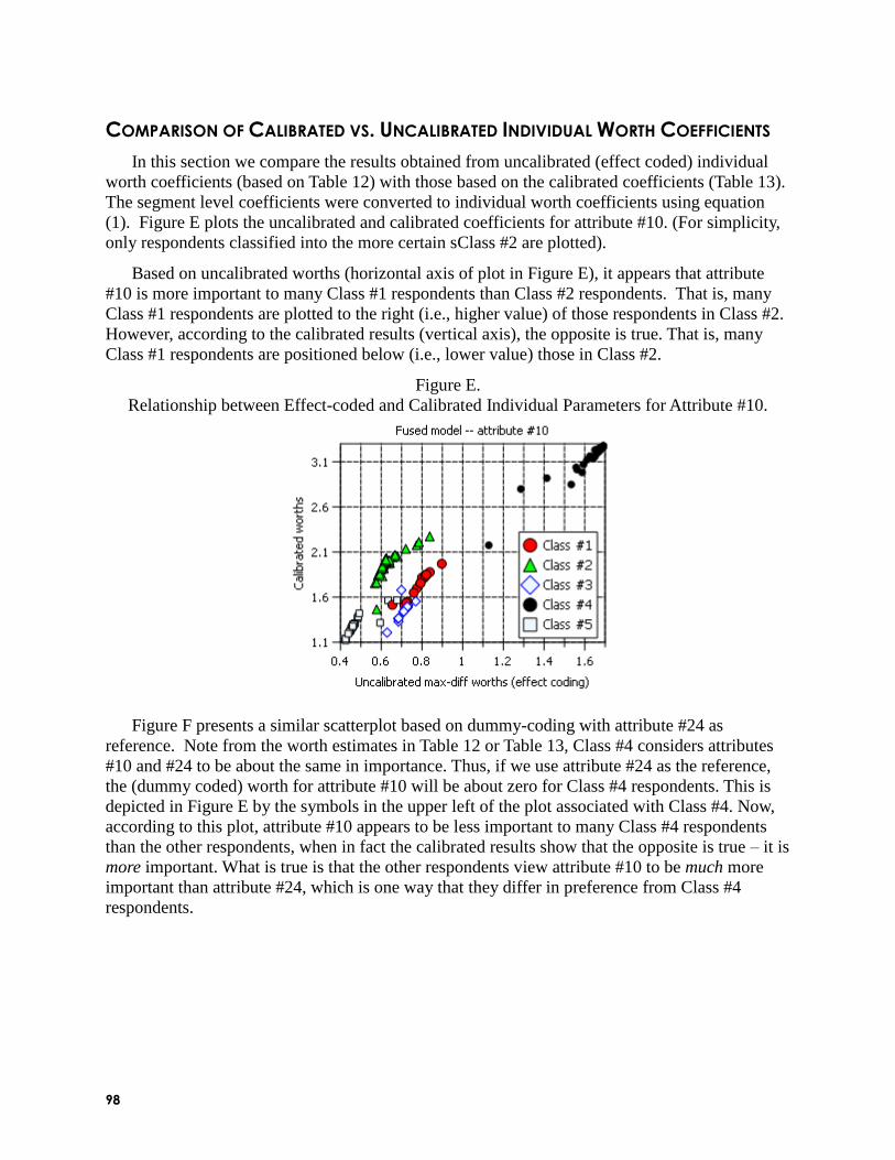
98

COMPARISON OF CALIBRATED VS. UNCALIBRATED INDIVIDUAL WORTH COEFFICIENTS

In this section we compare the results obtained from uncalibrated (effect coded) individual

worth coefficients (based on Table 12) with those based on the calibrated coefficients (Table 13).

The segment level coefficients were converted to individual worth coefficients using equation

(1). Figure E plots the uncalibrated and calibrated coefficients for attribute #10. (For simplicity,

only respondents classified into the more certain sClass #2 are plotted).

Based on uncalibrated worths (horizontal axis of plot in Figure E), it appears that attribute

#10 is more important to many Class #1 respondents than Class #2 respondents. That is, many

Class #1 respondents are plotted to the right (i.e., higher value) of those respondents in Class #2.

However, according to the calibrated results (vertical axis), the opposite is true. That is, many

Class #1 respondents are positioned below (i.e., lower value) those in Class #2.

Figure E.

Relationship between Effect-coded and Calibrated Individual Parameters for Attribute #10.

Figure F presents a similar scatterplot based on dummy-coding with attribute #24 as

reference. Note from the worth estimates in Table 12 or Table 13, Class #4 considers attributes

#10 and #24 to be about the same in importance. Thus, if we use attribute #24 as the reference,

the (dummy coded) worth for attribute #10 will be about zero for Class #4 respondents. This is

depicted in Figure E by the symbols in the upper left of the plot associated with Class #4. Now,

according to this plot, attribute #10 appears to be less important to many Class #4 respondents

than the other respondents, when in fact the calibrated results show that the opposite is true – it is

more important. What is true is that the other respondents view attribute #10 to be much more

important than attribute #24, which is one way that they differ in preference from Class #4

respondents.

99

Figure F.

Relationship between Dummy-Coded and Calibrated Individual Parameters for Attribute #10.

(Reference Attribute #24).

Next, we examine the correlation between calibrated and uncalibrated individual MaxDiff

worths where the uncalibrated worths are based on different identifying restrictions. The

correlation between individual coefficients obtained from uncalibrated MaxDiff worths and the

calibrated worths in Figure F assesses the extent to which all respondents consider attribute #24

to be equally important. A correlation of 1 would occur if the calibrated worths for attribute #24

were equal for all respondents. As can be seen in Table 13, the worths for attribute #24 differ

considerably across segments. Thus, it should be no surprise that the correlation turns out to be

-.39. The negative correlation can also be seen in Figure E as it is clear that the best fitting line

through the points would have a negative slope.

In contrast, the correlation between individual coefficients obtained from uncalibrated

MaxDiff worths and the calibrated worths in Figure E assesses the extent to which all

respondents consider the 36 attributes as a whole to be equally important. A correlation of 1

would occur if the average worth across all attributes were equal for all respondents. As can be

seen in Table 13, the average worths across the 5 classes are about the same. Thus, it should be

no surprise that the correlation turns out to be .89. This can also be seen in Figure E, where the

slope of the best fitting line would be close to 1.

Table 14 provides the associated correlations between the calibrated and uncalibrated

individual worths for all 36 attributes where the uncalibrated worths are obtained under effect

coding -- for the traditional MaxDiff model estimated under HB (‘HB‘) and LC (‘MD1‘),

LC/scale adjusted (‘MD2‘), and LC fused (‘Fused‘) -- as well as dummy coding with attribute

100

#24 as reference under the traditional MaxDiff model estimated under LC (‘MD1‘), LC/scale

adjusted (‘MD2‘), and fused (‘Fused‘). For this application, correlations based on the fused

model are about twice as high as obtained from the traditional MaxDiff models (HB and MD1)

as well as the scale adjusted model (MD2) under effects coding. Under dummy coding,

correlations are much more variable than under effects coding, and correlations based on the

fused model again tend to be somewhat higher than those based on the other approaches.

Table 14.

Correlations between Calibrated and Uncalibrated Individual Worth Coefficients where the

Uncalibrated Worths are Based on Different Approaches

SUMMARY AND FUTURE RESEARCH DIRECTIONS

Overall, the fused model provided much smaller standard errors than the MaxDiff worth

coefficients and fewer respondents in the less certain sClass. The fused model can also yield

calibrated worths which provide absolute as well as relative information. The more traditional

101

MaxDiff models provide worth coefficients that are very tricky to interpret and proper

interpretation depends upon the identifying criterion that is employed.

The current fused model is estimable using only a subset of the ratings, and in fact can be

applied when ratings are available for as few as 1 attribute (see e.g., Bochenholt, 2004).

Future research will examine how the quality of the solution is affected by

a. the number of ratings used, and

b. the particular attributes that are used in the model.

It may be that the highest rated attributes are best to use or it may be the highest and/or

lowest rated attributes are best. Or, it may be that use of the middle rated attributes provides the

best bang for the buck.

MODEL SPECIFICATION

Compared to the Bacon/Lenk approach:

we model MaxDiff somewhat differently (we treat it as first and second choice)

we use latent classes instead of individual effects (thus, it yields a segmentation)

we account for scale usage heterogeneity somewhat differently (we use a CFactor)

we also allow the scale factors in choice and rating to differ across persons (sClasses)

The specific model specifications are provided below.

LG 4.5 SYNTAX SPECIFICATIONS FOR MAXDIFF MODELS

//Traditional LC MaxDiff //Class denotes the nominal latent variable

//sweight distinguishes the choice of the

//MOST (+1) from the LEAST (-1) important,

//Q5 represents the alternative (1-5)

//selected from the given choice set

//and attr is the attribute id

variables

caseid ID;

repscale sweight;

choicesetid setid2 ;

dependent Q5 ranking;

attribute attr nominal;

latent

Class nominal 6;

equations

Class <- 1;

102

Q5 <- attr | Class;

//LC MAXDIFF WITH 2 SCALE FACTORS

variables

caseid ID;

repscale sweight;

choicesetid setid2 ;

dependent Q5 ranking;

independent set nominal inactive;

attribute attr nominal;

latent

Class nominal 5, sClass nominal 2 coding=first, scale continuous;

equations

Class <- 1;

sClass <- 1;

Scale <- (1)1 + (+) sClass;

(0) Scale;

Class <-> sClass; Q5 <- attr scale | Class;

Note: Since the nominal latent factor sClass has 2 categories (2 classes), ‗coding = first‘

causes the first category to have a coefficient of ‗0‘ in the equation for ‗Scale‘, and the

coefficient for the second category is estimated. The ‗(+)‘ causes these 2 coefficients to be non-

decreasing, and since the first equals 0, the second must be ≥ 0. The first term in the equation for

Scale ‗(1) 1‘ is an intercept restricted to equal ‗1‘. Thus, we have ‗1 + 0‘ for the scale factor

associated with the first sClass, and ‗1 + a non-negative coefficient‘ for the scale factor

associated with the second sClass.

LATENT GOLD CHOICE SYNTAX SPECIFICATIONS FOR THE FUSED MODEL

Maxdiff fused with 2 scale classes

//index is the attribute id for attributes rated

variables

103

caseid ID;

repscale sweight;

choicesetid setid2;

dependent RATING cumlogit, Q5 ranking;

independent Index nominal;

attribute attr nominal;

latent

Class nominal 5, sClass nominal 2 coding = first, Scale continuous,

Scale2 continuous, CFactor1 continuous;

equations

Class <- 1;

sClass <- 1;

Scale <- (1)1 + (+) sClass;

Scale2 <- 1 | sClass;

(0) Scale;

(0) Scale2;

(1) CFactor1;

Q5 <- (b1)attr scale | Class;

RATING <- 1 scale2 + Class scale2 + CFactor1 scale2 + (b2)Index scale2 | Class;

b2=b1;

REFERENCES:

Bacon, L., Lenk, P., Seryakova, K., and Veccia, E. (2007). Making MaxDiff more

informative: statistical data fusion by way of latent variable modeling. October 2007

Sawtooth Software Conference Proceedings,

Bacon, L., Lenk, P., Seryakova, K., and Veccia, E. (2008). Comparing Apples to Oranges.

Marketing Research Magazine. Spring 2008 vol.20 no.1.

Bochenholt, U. (2004). ―Comparative judgements as an alternative to ratings: Identifying the

scale origen,‖ Psychological Methods, 9 (4), 453-465.

Louviere, Marley, A.A.J., Flynn, T., Pihlens, D. (2009) Best-Worst Scaling: Theory,

Methods and Applications, CenSoc: forthcoming,

Magidson, J., and Vermunt, J.K. (2007a). Use of a random intercept in latent class regression

models to remove response level effects in ratings data. Bulletin of the International

Statistical Institute, 56th Session, paper #1604, 1-4. ISI 2007: Lisboa, Portugal.

Magidson, J., and Vermunt, J.K. (2007b). Removing the scale factor confound in multinomial

logit choice models to obtain better estimates of preference. October 2007 Sawtooth

Software Conference Proceedings

Vermunt and Magidson (2008). LG Syntax User‘s Guide: Manual for Latent GOLD Choice

4.5 Syntax Module.

105

BENEFITS OF DEVIATING FROM ORTHOGONAL DESIGNS

JOHN ASHRAF,

MARCO HOOGERBRUGGE,

JUAN TELLO SKIM

SUMMARY

Orthogonal designs in conjoint analysis are generated to get maximum statistical robustness,

that is, maximum accuracy for utility estimates. However, orthogonal design choice tasks may

well be far off from real world choice situations. This discrepancy with reality influences the

respondents‘ choice patterns systematically and hence leads to biased results. The aim of

maximum accuracy and the aim of getting unbiased estimates are apparently in conflict with

each other. We should therefore look more carefully at how markets behave in reality and adapt

the choice task design to realistic situations.

This paper is based on a meta analysis of six commercial studies in FMCG (Fast Moving

Consumer Goods) markets. In these markets, usually, a brand has multiple SKUs, representing

different product forms, different flavors, etc. When brands alter their prices, they often do so

uniformly across all SKUs. This phenomenon is often called line pricing and is something that a

standard orthogonal design does not account for.

CHOICE BEHAVIOR IN LINE-PRICING SITUATIONS

Let us illustrate consumer choice behavior in a market with line pricing. It is not about

research designs per se, it is just how consumers behave in the real world. The example is very

simple: we have two brands, each with three flavors. Brand 1 is less expensive, brand 2 is more

expensive. See Figure 1.

A consumer may choose between brand 1 and 2, trading off brand value with price, and may

for example prefer the cheaper brand 1. Within brand 1, there are three different flavors A, B and

C, and the consumer may prefer flavor B the most. Because prices do not vary (we have

assumed line pricing), the consumer does not have to make a tradeoff and picks the most

preferred flavor C.

106

Figure 1.

Example of Consumer Choice in a Market with 2 Brands x 3 Flavors

20

Base

case

price

Price

A B C

X Y Z

Now, suppose brand 1 is increasing its price. So, all SKUs (within brand) increase their price

by the same amount. Up to a certain price point the consumer may stay with brand 1. Within the

brand the consumer will again pick flavor C, since this is the most preferred flavor. There is no

reason whatsoever to switch to flavor A or B due to a brand price increase. See Figure 2.

Figure 2.

Example of Consumer Choice after a Price Increase of Brand 1

20

Base

case

price

Price

A B C

X Y Z

Let us now make the step from consumer behavior in reality to respondent behavior in a

research design. We can recreate the (real-life) line-pricing situations easily in CBC software by

importing manual designs and enforcing that all SKUs within a brand have the same price level.

We may assume that respondents will then choose the same way as they do in reality, apart from

random noise in their responses.

107

Respondent behavior becomes quite a bit different though when we use a standard orthogonal

design. Let us take the same consumer as in the example above and have him/her conduct a

CBC interview with an orthogonal design. The choice task may look like Figure 3. The flavors

of brand 1 have different prices, the flavors of brand 2 have different prices, and there is overlap

between prices of some flavors of brand 1 and some flavors of brand 2.

In this situation the consumer may choose flavor B in the interview because she is now

forced to make a tradeoff between flavor and price, and may think that flavor C is not worth so

much extra money in comparison to flavor B. So the respondent chooses something in the

interview that would never be chosen in reality and the utility values of price will be influenced

by the switching behavior within brand.

Figure 3

Choice Task Example with Orthogonal Design

19

Base

case

price

Price

A

B

C

X

Y

Z

Please note that this is a simple illustration. There may be much more complex situations.

For example certain flavors cost more than other flavors, but in a situation with line pricing they

cost consistently more. So the principle remains the same: once a consumer has established that

she is prepared to pay extra for the more expensive flavor, she will always choose that flavor in

line-pricing variations.

The same principle even applies to different pack sizes where the price ranges are completely

different but there are fixed rules such as: a double pack size always costs 1.9 times more. So

once a consumer has decided she wants to have the smaller pack size, she will want to have that

pack size just as well if SKU prices of this brand increase by any identical percentage.

The example above was just for one consumer. More generally, we can describe archetypes

of consumer behavior and we can deduct how research designs would impact the choice behavior

of them.

108

We can distinguish three archetypes:

1. a very price-focused consumer: always chooses the cheapest option in the market

2. a moderately brand-focused consumer: chooses a certain brand up to a certain price point

or up to certain price gap with another brand; after that point the consumer switches to

the other brand

3. an extremely brand-focused consumer: always chooses one brand

Let us assume all three archetypes do not care too much about the particular flavor. So, in an

orthogonal design, they may easily switch to a cheaper flavor. We might add consumers with

specific flavor preference as additional archetypes which would make the situation only more

complex.

The expected choice behavior in a CBC interview is as follows:

Archetype Orthogonal

CBC

CBC with Line

Pricing

Difference

Very price-

focused

Chooses

cheapest SKU

across brands

Chooses preferred

SKU of cheapest

brand

Price utilities will probably be

the same; in orthogonal design

we just miss information about

preferred SKU.

Moderately

brand-

focused

Chooses

cheapest SKU

of preferred

brand1)

Choose preferred

SKU of preferred

brand; may switch to

other brand after

certain price increase

Price utilities will probably

differ, but it is not clear upfront

in which direction.

Extremely

brand-

focused

Chooses

cheapest SKU

of preferred

brand

Chooses preferred

SKU of preferred

brand

Price utilities will come out more

extreme than in a (more realistic)

line-pricing design

1) In an orthogonal design at least one of the SKUs of the preferred brand will have an acceptable price

level (at least nearly always)

So from this, two things are clear:

The two different research designs will very likely result in different price sensitivities.

It is not possible to predict upfront which of the designs will yield a higher price

sensitivity (especially because of the middle group)

Therefore we will also take look at empirical data in the next section.

109

ANALYSIS OF EMPIRICAL DATA

In six FMCG projects we combined an orthogonal design with a line-pricing design. The

same respondents evaluated both types of choice tasks (mixed throughout the design). We will

refer to this as a hybrid design. Please note that a hybrid design addresses two business

objectives simultaneously, namely:

What happens if our brand changes its overall price?

What happens if we change the price of one of our SKUs while leaving the price of the

other SKUs constant?

The six studies ranged from diapers to cigarettes. For the analysis we made a split between

the orthogonal and the line-pricing choice tasks.

D-efficiency As discussed in the introduction, it seems we need to make a tradeoff between being

unbiased and the accuracy of the utility estimates. It is therefore important to know how much

accuracy we sacrifice when applying line-pricing research design. The results are shown in

Figure 4. Surprisingly and luckily, the D-efficiencies of a line-pricing design remain very high,

between 90% and 100% of an orthogonal design. So in practice we sacrifice very little accuracy

when applying a line-pricing research design.

Figure 4

Line-Pricing Designs Are Almost as Efficient as Orthogonal Designs

31

0.00

0.02

0.04

0.06

0.08

0.10

1 2 3 4 5 6

50%

60%

70%

80%

90%

100%

avg SE of Brand SKU in hybrid

avg SE of Brand SKU in orthogonal

avg SE of price in hybrid

avg SE of price in orthogonal

D-efficiency ratio (H vs O)

Study number

D-efficiency

ratio

Standard

error

Prediction of holdouts We can also ask the question from the reverse perspective: how much bias do we reduce in

predicting a realistic line-pricing scenario by using a line-pricing design instead of an orthogonal

design. We cannot measure bias directly, but instead we use prediction rates for holdout tasks as

a measure for bias, i.e. we compare prediction.

110

It is very natural to expect that utilities from line-pricing choice tasks predict another line-

pricing choice task better than utilities from an orthogonal design. The question is rather

whether the difference is so big that it is worthwhile to use line-pricing choice tasks. In Figure 5

we see that the differences are indeed very substantial.

Figure 5

Utilities from a Line-Pricing Design Predict Actual Responses to a

Line-Pricing Choice Task Better

32

40%

60%

80%

100%

1 2 3 4 5 6

hybrid design orthogonal design

Study number

Hit rate

• Translating into a more accurate prediction of actual market shares,

since prices of SKUs typically move in tandem within a brand

We can now safely conclude that it is better to include line-pricing choice tasks when we are

planning to simulate (mainly) line-pricing scenarios.

Differences in price sensitivity Another question that we can ask ourselves, suppose we apply orthogonal designs, do we

consistently make an over- or underestimation of price sensitivity? We are especially interested

in this, because the theoretical framework in the previous paragraph does not really give an

answer to this question. There we concluded it can be either way: more or less price sensitive.

For all SKUs in the six studies we have calculated price elasticity (dq/q / (dp/p)) based on

simulations using the utility values of the line-pricing designs and of the orthogonal designs. All

pairs of price elasticities are plotted in Figure 6.

Price elasiticity in an orthogonal design is significantly higher than in a line-pricing design,

by about 15% (the t-value of this difference is 4). At the individual level there are exceptions

though, sometimes the price elasticity is near-identical and in rare cases the price elasticity in an

orthogonal design is lower. So it would be too easy to use an orthogonal design and then apply a

standard correction factor of 1.15.

111

Figure 6

Brand Level Price Elasticity Is Consistently Higher for Orthogonal Designs

33

-4

-3

-2

-1

0

-4 -3 -2 -1 0

Brand-level price elasticity with hybrid design Bra

nd

-level p

rice

ela

stic

ity with

orth

og

on

al d

esig

n

Each dot represents a brand from a study

* standard error 3.7%

DISCUSSION

In the discussion after the presentation at the Sawtooth Software Conference a comment was

made that line-pricing designs are orthogonal designs after all – but on a different level, namely

on a brand level rather than on a SKU level.

That was a very clever and of course also a proper observation. However, the main objective

of our presentation was to show that one needs to address the particularities of the markets when

creating the research design. Orthogonality can of course still be applied after having identified

and incorporated the market conditions.

CONCLUSIONS

In this paper we have identified when and why hybrid designs, i.e. a combination of an

orthogonal design and a line-pricing design, may deliver more accurate price sensitivities at the

market level

We also developed a theoretical framework in order to explain that tandem designs or hybrid

designs may well lead to different price sensitivities than orthogonal designs. However, from the

theoretical framework we cannot tell whether we should have higher or lower price sensitivities

in an orthogonal design. In empirical studies price sensitivity was on average higher in

orthogonal designs.

The recommendation of the paper is to always have a close look at how markets behave in

reality in order to develop an appropriate choice task design.

Although the paper has focused on FMCG, we believe that this overall recommendation –

adapt choice tasks better to realistic market situations – will apply to other markets as well.

113

COLLABORATIVE PANEL MANAGEMENT:

THE STATED AND ACTUAL PREFERENCE OF INCENTIVE STRUCTURE

BOB FAWSON

EDWARD PAUL JOHNSON WESTERN WATS CENTER, INC.

ABSTRACT

Online access panels face increasing competition from other online activities. While research

design considerations often define respondent experience, panel managers do retain control over

some aspects of this experience. To better understand how to most effectively incentivize

panelists, Western Wats conducted both a conjoint choice task and an experimental choice task

during the summer of 2008. We compared a number of metrics from the initial conjoint

questionnaire, experimental results, and a follow up survey. Specifically, we look at before and

after differences in panelist perceptions and before and after response rates. Lastly, we use

conjoint results to predict actual choice.

Engaging panelists in a collaborative effort to determine incentive choices improves both

response rates and panelist attitude. Conjoint results predict actual choice with mixed results

(54.8%) probably due in large part to the change in the sweepstakes criteria.

INTRODUCTION

Good online panel managers strive to maintain an active and healthy community of willing

participants in the survey research process. This complex process requires optimization of

incentive structure, participation limits, survey design elements, and other salient variables with

respect to a set of tightly binding constraints. Ultimately, the health of a panel can be partially

gauged by participation rates and panelist engagement.

Incentive plays a key role in every theory of respondent motivation. Incentives serve as an

important trust building mechanism within the social exchange framework. Within the economic

exchange framework respondents seek to maximize incentive, making it one of the most

important determinants of participation (Dillman 2007). Leverage-salience theory suggests that

a panelist‘s level of participation is a function of the relative prominence and personal relevance

of variables found in each survey invitation (Marcus, et al. 2007, p. 374). Common invitation

variables are topic, potential for personal feedback, interview length, incentive, and use of the

end data, but incentive is the only variable consistently within the panel manager‘s control.

Panel managers effectively walk a tightrope; they must maximize both social and economic

rewards while respecting constraints. Economic rewards, for example, are constrained by both

budget and the potential behavioral effects they may cause as the amount is increased. Panel

Managers seeking to maximize the non-economic rewards of participation also face the

popularity of alternative online methods of social exchange such as Facebook and blogs

(Poynter 2008).

114

Within this context, during the summer of 2008, Western Wats solicited panelist feedback on

incentives, and manipulated their incentive structure in an attempt to increase both the economic

and social benefits of panel membership. Fundamental to the approach was collaboration with

panelists themselves. Ultimately, the bifurcated process chosen shed light on the benefits of

collaborative panel management and provided an opportunity to empirically test the power of

stated preference data to predict actual behavior.

MOTIVATIONS FOR THE RESEARCH

Today‘s online environment offers a wide range of activities that vie for the attention of

potential respondents. Some of these activities offer a compelling, multimedia-rich experience

(i.e. YouTube, Hulu and Pandora). Other activities are compelling because they offer a forum for

substantive, and often free-form, dialogue around personally salient topics (i.e. forums, blogs and

news sites). These features disadvantage online panels that must respect the relatively rigid

structure required by quantitative survey research. Furthermore, the majority of online

questionnaires offer scant opportunity for multimedia experience. Even the look and user

interface of some online questionnaires is spartan and reminiscent of an earlier internet era.

Opinion Outpost does offer a forum for open discussion through direct telephone and email

contact with project management staff. This feedback channel has revealed lack of

incentivization for disqualified respondents as Opinion Outpost‘s primary panelist complaint.

Additionally, clear strata of both ―social benefit maximizers‖ and ―economic benefit

maximizers‖ emerge among the group of vocal panelists who provide feedback. The ―social

maximizers‖ express violated trust as a result of being prevented from sharing their opinions

without a token thank you. ―Economic maximizers,‖ on the other hand, tend to be most vocal

about missed opportunities for receiving an incentive.

Offering an incentive for unqualified respondents should help maintain trust with the ―social

maximizers‖ as well as offer the incentive that will satisfy ―economic maximizers.‖

Additionally, offering a choice of incentive type should increase the sense of community among

Opinion Outpost members by giving them a substantive vote in their experience as panelists.

RESEARCH DESIGN

Opinion Outpost, Western Wats‘ online access panel, utilizes a points-for-cash incentive

structure. Opinion Points, redeemable at $.10 per point, are awarded for each completed

interview. The number of points is a function of survey length and survey difficulty. These

factors are clearly stated within each survey invitation.

Previous internal research shows that, over a month-long period, offering larger incentives

within Opinion Outpost‘s current incentive structure does not materially affect response rates

(unpublished research by Taylor, 2007). Göritz (2004, p. 335) reported analogous findings from

a different survey employing a points-based incentive. On the other hand, she did observe

decreased respondent dropout rates when offering larger incentives.

Other online panels have utilized lottery incentives as a way to minimize cost. The literature

on the efficacy of lotteries is mixed. Across 6 experiments, for example, ―cash lotteries relative

to no incentives did not reliably increase response or retention; neither did it make a significant

difference if one large prize or multiple smaller prizes were raffled‖ (Göritz 2006, p. 445).

115

Tuten, Galešič, and Bošnjak (2004) found evidence for the motivational power of immediacy

effects for lotteries. In other words, both response rates and dropout rates improved when lottery

outcomes were presented to respondents immediately. We presented this ―immediate lottery‖

idea to panelists under the name ―instant win.‖

This literature heavily influenced our decision to explore panelist utility derived from

different types of incentives, in addition to different incentive values. Specifically, our research

design needed to measure the impact of three factors: payment type, expected value of reward,

and rewards program. As outlined in Table 1, three levels of payment type, five levels of

expected value, and seven levels of rewards programs were analyzed resulting in 105 possible

reward combinations.

Table 1

Rewards Program Expected Value Payment Type Guaranteed Rewards $.10 Opinion Points

Instant Win (2% win rate) $.20 Cash/Check

Instant Win (1% win rate) $.30 Item

Instant Win (.5% win rate) $.40

Sweepstakes (.04% win rate) $.50

Sweepstakes (.02% win rate)

Sweepstakes (.01% win rate)

Conducting a within panel experiment evaluating panelist behavior before and after receiving

these 105 treatments would be cumbersome and expensive. We chose instead to present a

stratified random sample of panelist members with an online choice-based conjoint (CBC) task

to elicit relative preference measures for the 105 distinct options.

It is reasonable to expect that Opinion Outpost‘s extant incentive structure has influenced

activity level within the panel. To mitigate these potential conditioning effects, we chose a

stratified random sample from Opinion Outpost to participate in the choice task. Strata were

defined according to panelist activity level. Strata are: New panelists, defined by tenure of two

weeks or less. Inactive panelists, defined as those who have not responded to a survey invitation

for 6 months or more. Finally, we chose a stratum of active panelists who do not belong to either

the new or inactive strata. We do not expect either the inactive or new strata to exhibit the

conditioning effects that may be present among the active panelists.

In addition to the choice task, the initial questionnaire measured panelist activity level,

recruitment method, and solicited feedback on panelist experience in multiple open-ended

questions. Three detailed incentive concepts were presented before the choice task, and each

panelist completed three questions about the concepts to provide self-explicated preference data.

The flexibility of Western Wats‘ panel management system presented a unique opportunity to

externally validate the results of the conjoint study. The conjoint data was used to determine the

most popular reward system at a fixed cost. We then designed a revealed preference experiment

with 18 possible choice tasks (Table 2) identified from the conjoint. One randomly-selected

choice task was presented to the panelists who participated in the CBC exercise each time a

panelist did not qualify for a survey. The choice tasks were constrained to include one

guaranteed reward, one instant win, and one sweepstakes option. Choice presentation was

visually and experientially consistent with the conjoint choice task in order to avoid potentially

116

confounding variables when comparing the stated and revealed preference data. Expected value

of the reward was held constant across all experimental choices.

Table 2

Task Number Choice 1 Choice 2 Choice 3

1 GR 3 Opinion Points IW 6" Digital Picture Frame SW Rebel XTi Camera

2 GR $.30 Red Cross IW 6" Digital Picture Frame SW Rebel XTi Camera

3 GR 3 Opinion Points IW $60 check SW Rebel XTi Camera

4 GR $.30 Red Cross IW $60 check SW Rebel XTi Camera

5 GR 3 Opinion Points IW 600 Opinion Points SW Rebel XTi Camera

6 GR $.30 Red Cross IW 600 Opinion Points SW Rebel XTi Camera

7 GR 3 Opinion Points IW 6" Digital Picture Frame SW $750 check

8 GR $.30 Red Cross IW 6" Digital Picture Frame SW $750 check

9 GR 3 Opinion Points IW $60 check SW $750 check

10 GR $.30 Red Cross IW $60 check SW $750 check

11 GR 3 Opinion Points IW 600 Opinion Points SW $750 check

12 GR $.30 Red Cross IW 600 Opinion Points SW $750 check

13 GR 3 Opinion Points IW 6" Digital Picture Frame SW 7,500 Opinion Points

14 GR $.30 Red Cross IW 6" Digital Picture Frame SW 7,500 Opinion Points

15 GR 3 Opinion Points IW $60 check SW 7,500 Opinion Points

16 GR $.30 Red Cross IW $60 check SW 7,500 Opinion Points

17 GR 3 Opinion Points IW 600 Opinion Points SW 7,500 Opinion Points

18 GR $.30 Red Cross IW 600 Opinion Points SW 7,500 Opinion Points

Next, we used the conjoint data to predict each panelist‘s first choice using a market

simulator for every screen they were presented. We compared these predictions to actual

behavior as an evaluation of the consistency of panelist stated to revealed preference. Lastly, a

follow-up survey was given to these panelists to measure their experience in the collaborative

panel management process.

The research experiment has three main hypotheses. The first one compares unaided

respondent suggestions for improvement as a proxy for direct measurement of social exchange

benefits.

H1A: The percentage of suggestions for improvements that specifically refer to incentives

will decrease in the follow-up survey after participation in both the conjoint and

experimental choice tasks.

H2A: The percentage of suggestions for improvements that specifically refer to incentives

will not decrease in the follow-up survey after participation in both the conjoint and

experimental choice tasks.

Furthermore, the combination of positive social and economic benefits should lead to higher

response rates (AAPOR 1). Response was calculated for the month previous to the conjoint

choice task and for the month following the conjoint choice task.

117

H1B: Response rate will increase for panelists who participated in the collaborative panel

management relative to those who did not.

H2B: Response rate will not increase for panelists who participated in the collaborative

panel management relative to those who did not.

The last hypothesis deals with how well the panelists followed their stated preference when

actually given the options within the conjoint. Our testable hypothesis for conjoint hit rate is as

follows.

H1C: Stated preference data will predict actual choice correctly in 65% of cases.

H2C: Stated preference data will not predict actual choice correctly in 65% of cases.

CONJOINT RESULTS

The actual amount or item seen by the panelists as the terminate reward was conditional upon

the levels of all three attributes found in Table 1 (Rewards Program, Expected Value, and

Payment Type). For example, the reward seen for an Instant Win (2%) with an Expected Value

of $0.30 given in Opinion Outpost Points was $0.30/.02*10 points/dollar or 150 Opinion Outpost

Points. As a result of this relationship a statistically significant three-way interaction was found.

However, the practical significance could be explained by only using the main effect of Expected

Value and the interaction between Rewards Program and Payment Type.

As expected, the utility increased as the Expected Value increased as seen in Figure 1.

Surprisingly, Expected Value was the least important attribute as can be seen by the relatively

level utility across all 5 levels. This pattern might change if the range of Expected Value was

increased. However, this reward is for panelists who do not qualify and thus spend very little

time in the survey (approximately 1-2 minutes). At the highest value of $.50 panelists still

average $15-$30 dollars an hour and we did not feel comfortable giving consumer panelists more

than this amount. However, it should be noted that if this experiment was repeated for

completed surveys where the dollar amount is much higher, Expected Value could make much

more of an impact. For the results of this study, we determined $.30 to be the optimal point for

the expected value and used that reward amount in the actual preference tasks.

Figure 1

The two attributes that made the most difference for panelist preference were Reward

Program and Payment Type. Figure 2 shows the interesting results we found in this interaction.

118

First, the Reward Type made the most difference with Cash being preferred to both Points and

Items for all types of Reward Programs. However, the relative magnitude of this preference was

dependent on the Reward Program. For the Guaranteed Rewards Program, the Points and Cash

preferences are very close. Thus panelists are relatively indifferent to small amounts ($.10-$.50)

of cash in the mail when compared to OO (Opinion Outpost) points that they can later redeem

for cash. However, as you go to other reward programs that displayed higher nominal amounts

(resulting from the decreased chance of obtaining the reward) this gap widens significantly.

Panelists would rather have a large check than they would have the same amount in OO points.

Lastly, we determined from this initial survey that items did not have the widespread appeal that

cash or points had, but the preference of the higher ticket items in a sweepstakes became more

popular relative to the alternatives of points of cash.

Figure 2

EXPERIMENTAL TRIAL RESULTS

When comparing the Stated Preference data from the initial conjoint survey to the month-

long trial period where panelists actually chose their rewards, we see some unexpected

differences. Figure 3 shows that on average panelists systematically chose the Instant Win

Program more than expected at the expense of the Sweepstakes Program. This tendency was

found across all three segments of our study. As a result the hit rate was 53% rather than the

65% we predicted. Possible explanations for this difference, including a change in the

sweepstakes timeline, will be discussed in the next section. Still, overall we had to reject

hypothesis H1C in favor of H2C and report that the stated preference did not match the actual

preference 65% of the time.

119

Figure 3

The overall collaborative panel management system was successful at engaging and pleasing

panelists. The relative response rate increased across all three segments of the panel, with the

most gain seen in the new and inactive panelists. Figure 4 depicts the magnitude of this change

varying from 14% among Active panelists to 24% among New panelists. Thus, active panelists

who participated in the collaborative panel management system were 14% more likely to

respond to additional survey invitations than their counterparts in the panel that were not part of

the collaborative panel management system. This increase in participation was even more

prevalent amongst Inactive and New panelists, so we reject H2B in favor of H1B and conclude that

collaborative panel management does increase the responsiveness of a panel.

Figure 4

Lastly, the percent of incentive suggestions was lower in the follow-up survey than in the

initial conjoint survey. In the initial conjoint survey, 53% of the respondents suggested a change

in the incentive structure. This percentage was reduced to 40% in the follow-up survey. This

13% decrease is statistically and practically significant, so we also reject H2A in favor of H1A and

conclude that the collaborative panel management did increase the panel‘s attitude towards the

incentive structure we offered.

120

EXAMINING REASONS FOR THE DIFFERENCE BETWEEN STATED AND ACTUAL PREFERENCE

Overall, the only result of this survey that surprised us was that the stated preference was not

in line with the actual observed preference. We explored four possibilities that could have

caused this shift from Sweepstakes to Instant Win: time effect, multiple answers, and lastly a

necessary change in the sweepstakes timeline.

First we examined the reward preference over time. We thought that panelists might not

realize the value of the immediacy of a reward until they actually experienced it. What we found

was a surprising validation of our existing incentive structure. Figure 5 shows the linear trend of

the percent preference for reward program over the course of the month-long experiment. We

can see that although the Sweepstakes program became less popular over time, the Instant Win

program also became less popular at about the same rate. The only program that became more

popular was the Guaranteed Rewards program. This finding has important ramifications to those

panels that move away from a Guaranteed Rewards model and towards a sweepstakes model.

These panels will see more panel churn and fewer seasoned respondents which are important not

only for cost but also for data quality (Gailey, 2008). This finding validated Opinion Outpost‘s

policy of always giving a guaranteed incentive for completed surveys rather than moving to a

sweepstakes or an instant win model, but it did not explain the difference between the stated and

actual preference.

Figure 5

Then we tried to take out the confounding factor of multiple responses. Rather than counting

every time a panelist was shown the terminate reward screen, we limited it to just the first time

they terminated from a survey and saw the reward page. Because of the reduced sample size we

decided to run an aggregate logit model and then use a randomized first choice preference

simulator and compare aggregate results. Table 3 shows the results of the aggregate logit model

when run on all 18 of the tasks used in the actual preference experiment. We see the same trend

here where we predicted Guaranteed Rewards correctly, but over predicted the Sweepstakes

preference and under predicted the Instant Win preference.

121

Table 3

Results Guaranteed Instant Win Sweepstakes

Over (Scheffe) 1 0 10

Over 2 0 4

Within Limits 13 5 4

Under 1 1 0

Under (Scheffe) 1 12 0

In the end, the difference between the actual and stated preference might be explained by an

unavoidable change in the timeline of the sweepstakes. In the initial conjoint survey, the time

period for picking a winner was one week. This time period reflected the number of entries we

would have from our entire panel. However, when we only had the subset of the panel chosen

for the experiment the time needed to obtain the requisite entries changed to a month. Thus, the

sweepstakes timeline changed from one week to one month. According to Göritz‘s research

(2006), this change in the timeline would result in immediacy effects that could easily explain

why the sweepstakes offering was less attractive in the actual preference experiment.

CONCLUSIONS

The study was a success in engaging and pleasing our panelists. Our collaborative panel

management system exerted a positive effect on response rates across all segments of our panel

as well as decreased the complaint rate about incentives. Due to an unavoidable change in the

timeline of a sweepstakes, the actual behavior did not match the stated behavior. However, it is

still advisable to test a product in the real world before making decisions on the stated preference

data, especially when the product features are more intangible. Still, cash stood out as a clear

favorite for rewards in both stated and actual preference data, regardless of prior conditioning.

Furthermore, significant time effects indicated that guaranteed reward incentive systems should

be used rather than sweepstakes to ensure retention of an online panel asset. Future work can be

done to isolate the survey aspect of the collaborative panel management process from the actual

incentive change implemented.

122

REFERENCES

Dillman, Don A. Mail and Internet Surveys, the Tailored Design Method. Second Edition,

Hoboken, NJ: John Wiley & Sons, Inc., 2007.

Gailey, Ron, Teal, David, et al. (2008) Research & Consumer Insight – Sample Factors that

Influence Data Quality. ARF Knowledge Sharing and Proposed Metrics Conference 2008,

Cincinnati, Ohio.

Göritz, Anja S. (2004) The impact of material incentives on response quantity, response

quality, sample composition, survey outcome, and cost in online access panels.

International Journal of Market Research, 46, Quarter 3, pp. 327-345.

Göritz, Anja S. (2006) Cash Lotteries as Incentives in Online Panels. Social Science Computer

Review, 24, pp. 445-459.

Marcus, Bernd, Bosnjak, Michael, et al. (2007) Compensating for Low Topic Interest and

Long Surveys: A Field Experiment on Nonresponse in Web Surveys. Social Science

Computer Review, 25, pp.372-383.

Poynter, Ray (2008) Viewpoint: Facebook: the future of networking with customers.

International Journal of Market Research, 50(1), pp. 11-12.

Taylor, Eric (2007) Are panelists Employees or Respondents? Social versus Economic

Exchange. ESOMAR Panel Conference 2007, Orlando, Florida.

Tuten, Tracy, Galesic, Mirta, et al. (2004) Effects of Immediate Versus Delayed Notification

of Prize Draw Results on Response Behavior in Web Surveys: An Experiment. Social

Science Computer Review, 22, pp. 377-384.

123

ACHIEVING CONSENSUS IN CLUSTER ENSEMBLE ANALYSIS

JOSEPH RETZER

SHARON ALBERG

JIANPING YUAN MARITZ RESEARCH

CLUSTER ENSEMBLES: AN OVERVIEW

Cluster ensemble, or consensus clustering, analysis is a relatively new advance in

unsupervised learning. It has been suggested as a generic approach for improving the accuracy

and stability of ―base‖ clustering algorithm results, e.g., k-means.

Cluster ensemble analysis may be described as follows:

Consider p1, p2, ... , pM to be a set of partitions of data set Z.

(together these partitions form an ensemble).

Goal: find a partition P based on p1, p2, ... , pM which best represents the structure

of Z.(P is the combined decision called a ―consensus‖)

Given the above, we may say, tongue in cheek, that there are only two concerns to address:

How do we generate diverse yet accurate partitions 1 through M ? and in addition;

How do we combine those partitions?

It turns out that both (1) and (2) may be accomplished in numerous ways. While the

literature outlines various approaches to both (1) and (2), little work has been found by the

authors that compares those methods. This paper will focus on comparative performance of

competing methods for combining partitions aka ―achieving consensus.‖ We begin with a brief

outline of ways to generate the set of partitions, known as the ensemble, and then describe

consensus methods to be used for comparison.

In addition to comparing consensus methods, we also develop and describe a graphical

depiction of ensemble diversity, useful in evaluating the performance of our ensemble-generating

mechanism.

GENERATING THE ENSEMBLE

A brief list of ways in which ensemble member partitions may be generated is given below. It

is important to note that this list is not exhaustive and that any one or combination of these

techniques may be employed for this purpose.

Ensemble generation techniques:

Random selection of basis variable subsets / segment features:

Simply put, subsets of the variables are chosen and each is used to generate one or

more partitions.

124

Random initializations:

E.g., multiple selection of starting centroids in k-means.

Sub-sampling / re-sampling:

This approach uses, for example, bootstrap samples of the data for generating

partitions.

Use different types of clustering algorithms:

This particularly effective approach generates multiple partitions using differing

clustering algorithms, e.g. k-means, latent class, hierarchical, etc.

Randomly choose number of clusters for each clusterer:

Another particularly effective approach which specifies a varying number of cluster

solutions within a given algorithm.

A brief overview of various methods for combining ensemble partitions taken from the

literature is given below. All but the last approach (hyper-graph) will be described in more detail

in the next section.

Consensus Methods: Direct Approach:

Re-label ensemble solutions to find single solution which best matches individual

ones.

Feature Based:

Treat partitions as M categorical features and build a clusterer thereupon.

Pair-wise:

Average over similarity matrix depiction of each of the M ensemble partitions.

Hyper-graph:

Create hyper-graph representing total clusterers output and cut redundant edges.

CONSENSUS METHODS COMPARED

The following section will provide a brief overview of each consensus method used in our

empirical comparisons. Consensus performance will be based on its ability to recover known

cluster partitions from synthetic data sets.

Direct Approach The first, and intuitively the most straightforward, technique is appropriately referred to as

the ―direct approach.‖ The direct approach re-labels individual ensemble partitions and creates a

consensus solution which is, on average, as close as possible to the individual partitions. It may

be described as follows:

1. Generate M partitions on data with sample size N.

2. Specify a membership matrix for each of M partitions, where k is the number of groups

in each partition:

125

3. Define a dissimilarity measure between the true classification of individual i, (pi) and that

produced by partition m, (ui(m)) as:

4. Averaging over all cases, for partition m, gives the dissimilarity between U(m)

and P as:

5. The previous equation assumes cluster labels are “fixed.” In actuality we need to

consider all permutations of U(m)

→ ∏m(U(m)

) when arriving at an optimal P. So our

minimization problem becomes:

Feature Based Approach This method treats individual clusterer outputs as M categorical features and builds a cluster

consensus thereupon. The steps necessary to carry out a feature based consensus analysis are

given as:

1. Consider each cluster solution as representative of a “feature” of the data.

2. Replace the raw data (cluster basis variables) with k-tuple cluster labels.

3. Assume the data arises, in varying proportions, from a mixture of probability

distributions, each representing a different cluster.

4. The goal is then to partition data into groups associated with component distributions

(clusters).

5. The analysis necessary to accomplish this is referred to as Finite Mixture Modeling.

Pair-wise Approach The pair-wise approach depicts each ensemble member with a similarity matrix, averages

across all member similarity matrices and uses that average to generate a consensus solution.

This approach may best be described with an illustration.

Assume our first ensemble partition contains 6 respondents assigned to 2 clusters as shown

below. A similarity matrix S(1)

may be constructed as follows:

126

Next, a similarity matrix depiction of each ensemble partition is generated and labeled as:

The similarity matrices are then averaged to get a ―consensus‖ similarity matrix ―S” as:

Finally, we may apply any clustering algorithm which accepts a similarity matrix as its input

(e.g. ,“single linkage,” PAM, etc.) to S in order to produce a consensus solution.

Sawtooth Software Approach The Sawtooth Software (hereafter, ―Sawtooth‖) approach is a modification of the meta-

clustering algorithm discussed in Strehl and Gosh (2002). The first step is to dummy code

ensemble members as shown in the tables below.

Three ensemble members, e.g., for the first four cases:

Dummy code above to create basis variables:

The second step varies from the Strehl and Gosh approach of repeatedly clustering using a

graph partitioning approach with relabeling of clusterers. A secondary cluster analysis is

performed on the dummy coded values (8 variables above) using Sawtooth Software CCA‘s

(Convergent Cluster Analysis) standard approach. This involves running multiple replicates and

selecting the most reproducible solution. If several solutions are created from the second step, a

third step involves clustering on cluster solutions of cluster solutions (CCC). Additional CCA‘s

can be performed indefinitely (CCC…C). Sawtooth has found that the process converges very

quickly.

EVALUATING THE CONSENSUS WITH THE ADJUSTED RAND INDEX

Standard cluster analysis quality measures may be used to evaluate cluster solutions when the

true underlying partition is unknown. These include measures such as:

Hubert's Gamma: Correlation between distances and a 0-1-vector where 0 means same

cluster, 1 means different clusters.

Dunn Index: Minimum separation / maximum diameter.

127

Silhouette Index

Calinski & Harabasz C(g)

This investigation, however, employs known ―true‖ groupings and hence the focus of

partition evaluation shifts away from ―cluster quality‖ to ―cluster recovery‖ where the partition

to be recovered is the known solution.

While various cluster recovery measures were considered, support in the literature along with

other aspects such as intuitive appeal, led the authors to choose the ―Adjusted Rand Index‖ (ARI)

for this purpose. Since the ARI is critical to our comparisons and in addition leads to an

innovative depiction of ensemble diversity, its derivation and underpinnings are next presented in

some detail.

The adjusted rand index (ARI) is based on Rand Index (Rand 1971). Hubert and Arabie

(1985) adjusts the Rand Index to correct for chance levels of agreement, thereby avoiding

spuriously large obtained values. Anecdotal evidence of its support in the literature is found in a

1988 article by Collins & Dent where the authors note “ ... based on current evidence it seems

that the Hubert and Arabie ARI is the cluster recovery index of choice.” We begin by providing

an intuitive description of the Rand Index and next show how it may be extended to the

―Adjusted‖ Rand index.

The Rand Index measures the correspondence between two cluster partitions by focusing on

pairs of objects. Specifically, it classifies pairs of objects in disjoint cluster solutions (partitions)

in one of two ways:

together (same cluster) or

apart (different clusters).

The Rand Index is then a measure of the degree to which each pair of objects is classified the

same by the two cluster solutions being compared.

Consider the following cross tabulation table:

where e.g., a = frequency of two objects in same cluster in both U and V

b = frequency two objects same in U, apart in V, etc.

It is clear that given n objects,

128

Using the table above, we may define the Rand Index as:

A problem with the Rand Index is that as the number of segments in the compared partitions

falls, spuriously higher values of the index may result. Hubert & Arabie set about to correct this

by creating what is referred to as the Adjusted Rand Index (ARI). Simply put, the ARI is:

(Where clearly the max Rand index = 1).

In order to calculate the expected RI, we need only replace a, b, c and d with expected

frequencies conditioned on the assumption of partition independence using rules of probability.

Specifically,

replace a with (a+b)(a+c) →

replace d with (c+d)(b+d) →

The expected Rand Index is then:

Substituting this back into our original ARI formula we find the ARI is equal to:

REFLECTING ENSEMBLE DIVERSITY

Another useful application of the ARI is to compare ensemble member partitions and hence

portray overall ensemble diversity (a necessary and critical condition for arriving at useful

consensus solutions). This can be accomplished in the following way:

1. Calculate all pairwise partition ARI values.

2. Subtract each ARI value from previous step from 1 and create an M × M diversity matrix.

3. Graphically depict the diversity matrix from step (2) with a heat map.

129

Step (3) above produces a novel graphical depiction of overall ensemble diversity that

provides an easily comprehendible synopsis of a single ensemble‘s diversity as well as an

effective means for comparison of diversity across multiple ensembles.

THE DATA

We employ 10 synthetic data sets with known underlying clusters provided by Bryan Orme

of Sawtooth Software for comparison of consensus algorithms. The data sets were deliberately

designed to reflect fairly different sorts of underlying groups that may be found in market

research. A brief overview describing each is given in the table below.

Data Set Descriptions

METHODOLOGY

First and foremost, the focus of this paper is on comparing consensus performance in terms

of its ability to recover known underlying clusters. To that end, the following steps were taken:

1. Run each method on each data set

2. Calculate the ARI comparing the consensus solution to the known underlying groups for

all runs

3. Compare the performance of each consensus algorithm, for each data set, using the ARI

values from step (2)

The table below provides ARI measures comparing the consensus solution with the known

underlying clusters for each algorithm on each data set.

130

It‘s clear from the results that, for these data, the Direct and Sawtooth approaches out-

perform all others. It is also apparent however that the Pair-wise and Feature Based approaches

are not far behind in their ability to recover underlying true partitions.

DEPICTING ENSEMBLE DIVERSITY

In addition to comparing consensus performance, the authors also employed the ARI to

examine ensemble diversity. Diversity, as noted earlier, is an essential ensemble property which

is necessary, but not sufficient, in arriving at useful consensus solutions. Ensemble diversity was

depicted with a heat map graphic of the matrix composed of ARI pairwise comparisons of all

ensemble members. For purposes of illustration, the authors chose 2 data sets and created heat

map depictions of each ensemble. We then reduced the ensemble by removing specific partitions

which added to the diversity of the set. The ―diversity reduced‖ ensemble was also depicted

graphically via heat maps and resultant ARI‘s associated with their consensus‘ ability to recover

the known partition were estimated for each consensus algorithm.

It is important to note that the approach described above may not be used as a general

measure of the effectiveness of a consensus algorithm‘s ability to deal with less diverse

ensembles. The reason for this is that another critical property of the ensemble is being ignored,

i.e., quality. If quality were controlled for, this approach may be used to add empirical support

for or against a specific consensus algorithm‘s robustness to lack of diversity.

The following section presents heat map representations of ensemble diversity for both full

(RHS) and reduced (LHS - less diverse) sets of partitions using data sets (1) and (2). Note that in

both cases the drop in diversity is easily discerned by comparing adjacent heat maps. In

addition, we see that a drop in performance (as measured by the ARI comparing consensus vs.

true solution) is evident when using the less diverse ensemble. As noted however, the drop in

ARI across ensembles may not be attributed solely to a drop in diversity since ensemble member

quality is not being controlled.

Data Set 1

131

Data Set 2

CONCLUSIONS & FUTURE WORK

Superior consensus performance provided by the Direct and Sawtooth approaches is the

primary observation of this exercise. A secondary observation which, while not central to this

paper is of no less importance, is the highly diverse ensemble produced by Sawtooth‘s program

as evidenced in the heat maps. Details on Sawtooth‘s approach may be found in the appendix.

It is also apparent that cluster diversity may impact consensus solution performance directly.

Specifically, as diversity decreases the risk of poorer consensus performance increases. This

interpretation must be tempered by the realization that an important determinant of ensemble

viability, individual partition quality, was not controlled for in these experiments.

We note that the literature recommends generating a large number of partitions and reducing

down to a subset which is both diverse and of high quality. The authors feel this approach could

be facilitated both numerically and graphically using pairwise ARI measurement to depict

ensemble diversity. Specifically, partitions could be grouped based on similarity and selections

from each group made using a measure of cluster quality. Overall diversity of the final ensemble

could be depicted graphically via a diversity heat map.

Lastly, it is important to keep in mind the flexibility of the C.E. approach which adds value

beyond its ability to create high quality solutions. For example, C.E.‘s may also be used to

construct partitions which profile well on marketing strategy variables by incorporating solutions

132

from supervised learning analyses. Such a hybrid model is known as a Semi-Supervised

Learning model and may be straightforwardly implemented in a cluster ensemble framework.

APPENDIX I: GENERATING THE ENSEMBLE

While this paper focuses on the comparison of consensus clustering techniques, it is

important to be aware of the ensemble generation algorithm employed as well. The algorithm

used is part of Sawtooth Software‘s Cluster Ensemble package (CCEA) which proved quite

capable of handling the difficult and critical task of generating a diverse ensemble. A detailed

discussion of this process is given below.

CCEA software allows for creating an ensemble that can vary by the number of groups and

cluster strategies. The default setting consists of 70 separate solutions, 2 to 30 groups, and the

following five cluster strategies:

1. k-means (distance-based starting point)

2. k-means (density-based starting point)

3. k-means (hierarchical starting point)

4. hierarchical (average linkage criterion)

5. hierarchical (complete linkage criterion)

The ensemble is very diverse, but not assessed for quality, e.g., using CCA‘s reproducibility

procedure. Reproducibility, however, is assessed for the ensemble consensus solution during the

CCEA consensus stage.1

1 In addition we may note that partitions generated outside CCEA may also be included in the ensemble for consensus creation using the

software.

133

REFERENCES

Gordon, A. D. (1999), ―Classification.‖ Chapman & Hall/CRC.

Hornik, K. (2007), ―A CLUE for CLUster Ensembles.‖ R package version 0.3-18. URL

http://cran.r-project.org/doc/vignettes/clue/clue.pdf.

Kaufman, L. & P. J. Rousseeuw (2005), ―Finding Groups in Data, An Introduction to Cluster

Analysis.‖ Wiley-Interscience.

Kuncheva, L. I. & D. P. Vetrov (2006), ―Evaluation of stability of k-Means cluster ensembles

with respect to random initialization.‖ IEEE Transactions on Pattern Analysis and Machine

Intelligence, Vo. 28, 11, November.

Orme, B. & R. Johnson (2008), ―Improving K-Means Cluster Analysis: Ensemble Analysis

Instead of Highest Reproducibility Replicates.‖ Sawtooth Software.

Sawtooth Software (2008), ―CCEA System,‖ Sequim, WA.

Strehl, A. & J. Gosh (2002), ―Cluster Ensembles - A knowledge reuse framework for

combining multiple partitions.‖ Journal of Machine Learning Research, 3, 583-617.

Topchy, A., A. Jain & W. Punch (2004), ―A mixture model for clustering ensembles.‖ Proc.

of the SIAM conference on Data Mining, 379-390.

Vermunt and Magidson (2003), ―LatentGOLD Version 3.0.1.‖ Belmont Massachusetts:

Statistical Innovations Inc.

Weingessel, A., E. Dimitriadou & K. Hornik (2003), ―An ensemble method for clustering.‖

DSC Working Papers.

Xiaoli, F., & C. Brodley (2003), ―Random projection for high dimensional data clustering: a

cluster ensemble approach.‖ Proc. of the twentieth conference on machine learning,

Washington D.C.

135

HAVING YOUR CAKE AND EATING IT TOO?

APPROACHES FOR ATTITUDINALLY INSIGHTFUL AND

TARGETABLE SEGMENTATIONS

CHRIS DIENER

URSZULA JONES LIEBERMAN RESEARCH WORLDWIDE (LRW)

BACKGROUND

When it comes to segmentation, there is a clear disconnect between client needs and

traditional segmentation approaches. Let‘s face it, we all want attitudinally insightful

segmentations…and we want those segmentations to be practically targetable. We want these

attitudinally rich segments to differ starkly on those attributes that allow us to precisely target

them directly or through specific combinations of media consumption. In other words, we want

the segments to have unique demographic and transactional profiles. We want actionability on all

fronts. First, we want ―subjective efficacy‖ (SE) – the rich attitudinal (needs, motivations,

attitudes, evaluations, etc.) characterization which allows us to create the best products,

positioning and communications content. Next, but not necessarily second, we want ―objective

efficacy‖ (OE) – this comes from differentiated segmentation profiles based on the tangible,

―hard,‖ measures like age, income, purchase history, and channel usage. These OE measures

allow predictive linking or fusing with internal database information, external direct marketing

data, media usage markers and other information sources that promote our ability to practically

identify, contact, communicate and make products or services available on a selectively targeted

basis.

Experience has revealed that combining SE and OE measures in a single segmentation is like

trying to mix oil and water. You either get a segmentation well differentiated on SE and poorly

on OE or vice-versa: one well differentiated on OE but poorly on SE. If you force the OE and

SE to have equal weighting, you most often end up making fatal compromises in both areas,

coming up with a segmentation that lacks subjective and objective actionability on an acceptable

level. The frustration with traditional clustering approaches has led to the recent development of

analytic innovations that attempt to address the apparent natural opposition between SE and OE.

These unconventional approaches include Nascent Linkage Maximization (ART 2002),

Canonical Correlation Segmentation, and Reverse Segmentation (Sawtooth Software 2006)

(SKIM 2007).

This paper develops a framework for understanding the SE/OE trade-off. It focuses attention

on the SE/OE issue, raises awareness of approaches to this problem and the thinking behind

them, and generates discussion which will lead to further contributions in this area. Furthermore,

this paper specifically introduces and compares the efficacy of several methods of combining SE

and EO measures. Finally, the paper will conclude with observations and recommendations that

follow from the comparison.

136

OVERVIEW OF ALTERNATIVE SEGMENTATION APPROACHES

Analytic innovations such as Nascent Linkage Maximization, Canonical Correlation

Segmentation, and Reverse Segmentation are alternative segmentation approaches that reveal

associations and structure in the data, which are difficult to achieve with traditional methods.

They do it by connecting attitudes and behaviors with known targetable attributes such as

demographics and firmographics.

Even though this is not a requirement, oftentimes demographics and firmographics that are

being used in these approaches reside in the client database. In these cases, these approaches are

used as tools for accurate scoring of the transactional database. In other cases where a database

is not present, these approaches can be used for developing direct mail campaigns, making media

and channel decisions, or simply for building more targeted consumer communications.

NASCENT LINKAGE MAXIMIZATION (NLM)

NLM is a constrained optimization segmentation routine. It uses a traditional clustering

procedure followed by the NLM algorithm. Application of the NLM algorithm adjusts the pre-

defined segmentation solution to increase discrimination on specific ―new‖ measures (often

demographics and transactional information) while at the same time maintaining the meaning

and differentiation of the original solution. NLM maximizes ―new‖ measure differentiation

between the segments by reassignment of fence-sitters. Fence-sitters are respondents who

attitudinally could belong to more than one segment. These people have minimal impact on

original segment definition, but maximal impact on increasing segment classification using the

new data.

To illustrate, respondent X is assigned to segment 1, but attitudinally could belong to either

segment 1 or segment 2. When demographic and transactional data is fused into the solution, it

turns out that respondent X is very similar in his purchase behavior and demographics to

segment 2. In such a case, the NLM algorithm would move respondent X to segment 2.

Movement of respondent X does not hurt the definition of segment 1 nor segment 2. Both

segments remain stable attitudinally, however, with better demographic and transactional

alignment, the database scoring model improves significantly.

In a typical study, the NLM algorithm reassigns between 20% and 30% of the respondents.

By movement of segment membership, classification rates increase 50% to 100%, making a

segmentation solution more actionable for segment targeting.

CANONICAL CORRELATION

Canonical Correlation is an analytic approach that can be used for segmentation of measures

that differ in their scales. This multi-dimensional approach allows for mixing of attitudinal,

demographic, and transactional information in one clustering routine. As a result, it generates

segments which discriminate on different types of measures (e.g. continuous and discrete

variables).

Canonical Correlation produces canonical component scores for each respondent. These

respondent level scores can be either used in a clustering routine itself or can be used to identify

measures to include in a more standard clustering approach.

137

Since both attitudinal and demographic variables are clustered together, Canonical

Correlation creates segmentation solutions that differ sufficiently attitudinally and

demographically. Additionally the resulting segments tend to tell a coherent or meaningful story

in which all measures contribute in a substantial way.

REVERSE SEGMENTATION

Reverse Segmentation uses a traditional clustering algorithm to derive respondent clusters.

What makes the Reverse Segmentation approach truly unique is the fact that the unit of analysis

is NOT a respondent. Instead of clustering respondents, groups of respondents (aka objects) are

being clustered. Objects are groups of respondents that fit a specific demographic profile (see

Figure 1). Respondents in Object 1 reside in the northwest region, have high income, are female,

and do not have children. Respondents in Object 2 fit a similar description, except that they do

have children. What makes this approach similar to traditional attitudinal segmentation is that

objects are grouped on attitudinal/behavioral types of variables.

Once all possible objects are created, the attitudinal data are summarized into object means.

This can be done using an aggregate command in the SPSS software. Then standard clustering

procedure is applied to the aggregated file and various segmentation solutions are created.

The initial outcome of reverse segmentation produces clusters that are comprised of objects

instead of respondents. An additional step is required to translate the objects into respondents.

Using the example in Figure 1, everyone who is in Object 1 (resides in the northwest region, has

high income, is female, and does not have children) is in segment 1. Once respondents are

assigned to corresponding segments, the segmentation solution should be evaluated to ensure

that it is not only statistically sound, but also meaningful.

Figure 1

138

EVALUATION OF SEGMENTATION METHODS

In this comparison of approaches, traditional and alternative segmentation methods were

evaluated in terms of their classification rates on both attitudinal/behavioral measures and

targeting variables/demographics. Classification rates were generated using the discriminant

function on the holdout samples. There were three data sets used with the following

specifications:

Case Study 1: 1,659 respondents, survey data merged with database data

Case Study 2: 9,066 respondents, survey data merged with database data

Case Study 3: 1,627 respondents, survey data only

All segmentation approaches used common attitudinal/behavioral and demographic

variables. For ease of comparison each approach is contrasted using five-segment solutions.

CLASSIFICATION RATES

As expected (see Figure 2 for an overview and Figure 3 for a detailed view), as you move

through the segmentation continuum from demographic segmentation towards attitudinal

segmentation, classification rates increase on attitudes and decrease on demographics. Also

within each approach (see Figure 3), you will notice that there tends to be a trade-off between

classification rate on attitudes and demographics. As you compare the case studies within each

approach, you will notice that as attitudinal rates go up, demographic rates tend to go down and

vice versa.

In these comparisons, the NLM approach performs the best in terms of acceptable

classification rates on both attitudes and demographics. In contrast, Canonical Correlation

provides only mediocre classification rates on both measures.

Reverse Segmentation performs very similarly to demographic segmentation showing high

demographic classification rates and poor discrimination rates in terms of attitudes. Even though

classification rates on attitudes remain low with the reverse approach, segments are more

meaningful attitudinally than the ones generated via purely demographic segmentation. Also

another thing to keep in mind is that the rates presented are generated using discriminant

analysis. With the Reverse Segmentation segment, assignment is automatic. No modeling is

required, since respondents are assigned to objects, which have a predetermined segment

membership.

139

Figure 2:

Figure 3:

Classification Rates Using Discriminant Function Analysis

Attitudinal/

Behavioral-

Based

NLM Canonical

Correlation

Segmentation

Reverse

Segmentation

Demographic

Segmentation

Case

Study 1

(T)

Classification

rate on

attitudes/

behaviors

92% 68% 50% 38% 40%

Classification

rate on

targeting

variables

31% 65% 68% 89% 95%

Case

Study 2

(H)

Classification

rate on

attitudes/

behaviors

93% 72% 57% 29% 29%

Classification

rate on

targeting

variables

35% 61% 65% 99% 98%

Case

Study 3

(Q)

Classification

rate on

attitudes/

behaviors

84% 73% 60% 33% 27%

Classification

rate on

targeting

variables

34% 63% 63% 90%** 93%

140

ADVANTAGES AND DISADVANTAGES OF EACH SEGMENTATION APPROACH

Each of the approaches evaluated in this experiment has its benefits and shortcomings.

Traditional approaches are much easier to implement in comparison to the alternative approaches

that tend to be not only more difficult computationally, but also more difficult to explain to

clients. Figure 4 highlights some of the most common pros and cons of each segmentation

approach.

Figure 4:

Attitudinal/

Behavioral-Based

NLM Canonical Correlation

Segmentation

Reverse Segmentation Demographic

Segmentation

Pros • Very good

differentiation on attitudinal/ behavioral

data

• Accurate segment

assignment using attitudinal/ behavioral

data

• Very suitable for

communication, positioning, product

development

• Easy to implement

• Very flexible in terms of number of solutions

it can generate

• Preserves learning

from fully attitudinal segmentation (―pure‖

as some people would

say) • Provides a solution

which has

substantially better

targetability while not sacrificing much

attitudinal

discrimination

• Generates a

segmentation that takes both types of

measures into account

in its formation – instead of starting with

one and accentuating

or modifying with the

other set of measures

• Generates a solution

which produces

reasonable discrimination on both

types of measures

• Creates perfectly

identifiable groups using case assignment

and very accurate

classification using demographics

• Works well for

flagging database and

customer targeting • Segments are

sufficiently and

meaningfully different

in terms of attitudes

• Very good

differentiation on demographics

• Accurate segment

assignment using

demographics • Very suitable for

targeting (aids in

making media,

channel, and direct mail campaign

decisions)

• Easy to implement

• Very flexible in terms of number of solutions

it can generate

Cons • Sensitive to scale

usage

• Poor differentiation in

terms of demographics (often cannot be used

for targeting)

• Complex to implement

and hone for best

results • Can produce client-

end confusion as it

does change the initial

solutions in terms of

segment membership

and some of the

measures on which the NLM increases

discrimination or other

measures not directly involved with

segmentation or NLM

• Potentially requires a

longer analytics process

• Understanding of

canonical algorithms

and their implementation

required

• Difficult for clients to

understand that their

solution will not have

more than 60% or so

correct classification on either attitudes or

demographics

• Gives less

differentiation on

attitudinal questions • Classification rates on

attitudes remain low,

even though

differentiation is

meaningful

• Limitation in number

of solutions that can be

generated • Results are driven by

number of objects (can

be blocky)

• Requires larger sample size

• Does not handle

missing data on

targeting variables • Time

consuming/difficult to

implement

• Poor differentiation in

terms of attitudes/

behaviors (often cannot be used for

customer

communication, product development ,

product positioning)

141

CLIENT IMPLICATIONS

Achieving differentiation on softer attitudinal measures and on harder targeting measures has

been a continuous challenge faced by researchers and marketers. Various segmentation

approaches differ in terms of how well they discriminate on either measure. Traditional

segmentation approaches discriminate well on measures that are being used to derive the

segments. However, they show poor differentiation on measures that are not being used for the

clustering. The fusion methods fall somewhere in-between, showing some promise for better

discrimination and in turn for better classification rates on variables that were not part of the

clustering.

Approach selection should be always driven by client-specific needs. A careful consideration

should be given to client objectives, intended uses of the segmentation, consequences of

incorrect classification, and data requirements for each approach. Before selecting an approach,

the following questions should be answered:

What is the main purpose or objective of the segmentation?

What business decisions am I trying to make?

Will I be flagging the database?

Which differentiation is more important: attitudinal or demographic?

What is the tolerance for or cost of misclassification?

Is meaningful differentiation sufficient or do classification rates need to be highly

accurate?

How much sample do I have?

Do I have missing data?

Always keep in mind that there is no “perfect” segmentation approach.

REFERENCES

Diener, Chris and Pierre Uldry (2002), ―Fusing Data from Surveys to Databases: Segmenting

For Effective Linkages,‖ 2002 AMA Advanced Research Techniques Forum, Vail,

Colorado.

Jones, Urszula, Curtis L. Frazier, Christopher Murphy, and John Wurst (2006), ―Reverse

Segmentation: An Alternative Approach to Segmentation, ‖ 2006 Sawtooth Software

Conference, Delray Beach Fl, March 2006.

Jones, Urszula Curtis L. Frazier, and Jing Yeh (2007), ―Reverse Segmentation: Findings and

Refinements, ‖ SKIM Software Conference, Dusseldorf, Germany, May 2007.

143

AN IMPROVED METHOD FOR THE QUANTITATIVE ASSESSMENT OF

CUSTOMER PRIORITIES

V. SRINIVASAN STANFORD UNIVERSITY

GORDON A. WYNER MILLWARD BROWN INC.

INTRODUCTION

A number of marketing contexts require the quantitative assessment of customer priorities:

Consider the introduction of a newer version of a product. A number of features can

potentially be added to the product. In order to determine which subset of features

should be included, the firm first needs to determine the values customers attach to

the different features. The firm can then combine that information with internal

information on the development cost and time for incorporating the features to decide

on the actual features to include.

Consider enhancing a service such as a hotel or an airline. We need to determine the

values customers attach to the different service improvements. This information can

then be combined with internal information on the incremental cost of providing those

improvements to decide on the actual improvements to provide.

The empirical study reported here was done in cooperation with the Marketing Science

Institute (hereafter, MSI), an organization that links marketing academics with

marketing practitioners. MSI surveys its trustees to assess the priorities they place on

different marketing topics such as ―managing brands,‖ ―channels and retailing,‖ and

―new media.‖ The priorities are then used by MSI in deciding which academic

research proposals to fund and to inform marketing academics as to the topics on

which research would be most useful for addressing important business issues.

Our focus in this paper is on measuring the importances (or values) customers attach to a

large (ten or more) number of topics (or features, or attributes). It is related to, but different

from, conjoint analysis in which the measurement of values takes place over topics and the levels

of those topics. Our focus is on the measurement of topic importances at the individual

respondent level, rather than merely at the aggregate level. Aggregate level measurement can be

misleading. For instance, suppose the first half of the respondents consider the first half of topics

to be (equally) important and the second half of topics to be unimportant, and the reverse is true

for the second half of respondents. Aggregate measurement would lead to the misleading

conclusion that all topics are equally important. Measuring importances at the individual level,

on the other hand, would permit the determination of benefit segments, i.e., clusters of

respondents who are similar in terms of the importances they attach to the topics. Individual

level measurement also permits cross-classifying importances against respondent descriptors,

e.g., demographics, psychographics, and purchase behavior.

144

In this paper, we compare the constant sum method (hereafter, CSUM) with a new method

called ASEMAP (pronounced Ace-map, Adaptive Self-Explication of Multi-Attribute

Preferences, Netzer and Srinivasan 2009) for the quantitative assessment of customer priorities.

After describing the methods, we detail the research set-up to examine the relative performance

of the two methods in the context of MSI‘s assessment of research priorities for different

marketing topics by managers from MSI member companies. We then present the empirical

results and offer our conclusions.

METHODS FOR MEASURING IMPORTANCE

One of the simplest ways of measuring the importance of topics is through the use of rating

scales. For instance, respondents are asked to rate different topics on a 5-point rating scale,

varying from ―not at all important‖ to ―extremely important.‖ The main problem with such a

rating task is that respondents tend to say every topic is important, thereby minimizing the

variability across items. Netzer and Srinivasan (2009) compare ASEMAP to preference

measurement methods based on rating scales in the context of conjoint analysis and conclude

that ASEMAP produces a substantial and statistically significant improvement in predictive

validity. Chrzan and Golovashkina (2006) compare six different methods for measuring

importance and conclude that MaxDiff, CSUM, and Q-Sort are the preferred methods. (The

other three methods are ratings, unbounded ratings, and magnitude estimation.) Q-Sort asks the

respondent to give 10% of the items a rating of 5 (most important), 20% of the items a rating of

4, 40% a rating of 3, 20% a rating of 4, and 10% a rating of 1 (least important). Forcing such a

distribution on every respondent is theoretically unappealing. In the present paper, we compare

CSUM against ASEMAP. For many years, MSI has been employing CSUM to measure research

priorities. Thus MSI provided a natural setting for a head-to-head comparison of CSUM against

ASEMAP. At the very end of this paper, we briefly summarize the results from a different

empirical study by Srinivasan and Makarevich (2009) comparing CSUM, ASEMAP, and

MaxDiff.

THE CONSTANT SUM APPROACH (CSUM)

The data collection format for CSUM in the context of the MSI study is shown in Figure 1.

The order of presentation of the topics is randomized across respondents. Because it is a web-

based survey, the computer provides feedback regarding the current total. An error message

appears when the respondent tries to move to the next screen, but the total is not equal to 100.

The main advantage of CSUM over rating-based approaches is that it avoids the tendency of

respondents, mentioned earlier, to state that everything is important. Also it recognizes the ratio-

scaled nature of importance by asking the respondent to give twice as many points to one topic

compared to another, if the first topic is twice as important. The CSUM approach works well

when the number of topics is small; however, if the number of topics is large (say, ten or larger),

respondents have great difficulty in allocating points across a large number of topics; they resort

to simplifying tactics such as placing large round numbers for a few topics and zero (or blank)

for the remaining topics.

145

Figure 1:

Constant Sum Approach (CSUM)

Please distribute a total of 100 points across the 15 research topics to indicate how important

each topic is to you. Please allocate twice as many points to one topic compared to a second

topic if you feel the first topic is twice as important as the second topic.

Innovation and new products

Engaging customers

…

Driving loyalty

Total

ADAPTIVE SELF-EXPLICATION (ASEMAP)

The ASEMAP procedure starts with the respondent ranking a randomized list of topics from

the most important to the least important. In case the number of topics is large, the ranking is

facilitated by first categorizing the topics into two (or three) categories in terms of importance.

For instance, in the MSI context, there were fifteen topics that were categorized into more

important topics (8) and less important topics (7). The categorization step in shown in Figure 2.

The respondent then ranks the items within each category by a ―drag and drop‖ as shown in

Figure 3. The end result of the above two steps is a rank order of the full list of topics.

Figure 2:

ASEMAP Categorization Step

From the list of 15 topics below, place a check mark on the eight topics that are most

important to you:

Emerging markets

Engaging customers

…

Developing marketing competencies

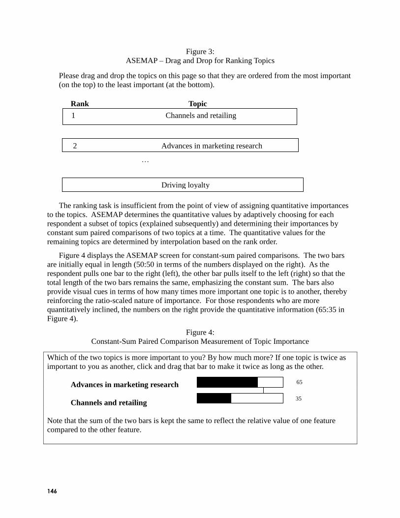
146

Figure 3:

ASEMAP – Drag and Drop for Ranking Topics

Please drag and drop the topics on this page so that they are ordered from the most important

(on the top) to the least important (at the bottom).

Rank Topic

…

…

…

The ranking task is insufficient from the point of view of assigning quantitative importances

to the topics. ASEMAP determines the quantitative values by adaptively choosing for each

respondent a subset of topics (explained subsequently) and determining their importances by

constant sum paired comparisons of two topics at a time. The quantitative values for the

remaining topics are determined by interpolation based on the rank order.

Figure 4 displays the ASEMAP screen for constant-sum paired comparisons. The two bars

are initially equal in length (50:50 in terms of the numbers displayed on the right). As the

respondent pulls one bar to the right (left), the other bar pulls itself to the left (right) so that the

total length of the two bars remains the same, emphasizing the constant sum. The bars also

provide visual cues in terms of how many times more important one topic is to another, thereby

reinforcing the ratio-scaled nature of importance. For those respondents who are more

quantitatively inclined, the numbers on the right provide the quantitative information (65:35 in

Figure 4).

Figure 4:

Constant-Sum Paired Comparison Measurement of Topic Importance

Which of the two topics is more important to you? By how much more? If one topic is twice as

important to you as another, click and drag that bar to make it twice as long as the other.

Advances in marketing research

Channels and retailing

Note that the sum of the two bars is kept the same to reflect the relative value of one feature

compared to the other feature.

1 Channels and retailing

2 Advances in marketing research

techniques

Driving loyalty

65

35

147

Estimation of Weights Suppose three among the full list of topics are A, B, and C, and the rank order among these

three topics are A (most important), B, and C (least important). Suppose the respondent provides

the following paired comparison data (ratio of bar lengths = ratio of the numbers on the right-

side of the bars in Figure 4):

WA/WB = 2,

WB/WC = 3, and

WA/WC = 5.

Note that the redundancy among the three pairs provides information on the ratio-scaled

consistency of the respondent‘s data. (The data would have been perfectly consistent had

WA/WC been 6.) The ratio of the two weights would be undefined in the rare situation if the

respondent had moved one bar all the way to the end (100:0). We recode such cases as (97.5:

2.5) because the allocations go in steps of 5, i.e., (85,15), (90,10), (95,5). Taking logarithms to

the base 10, we obtain (taking the logarithms to any other base would not affect the obtained

importances as long as the importances are normalized to sum to 100):

Log (WA) – Log (WB) = Log (2) = 0.301,

Log (WB) – Log (WC) = Log (3) = 0.477, and

Log (WA) – Log (WC) = Log (5) = 0.699.

To estimate the weights relative to the most important topic, we set WA = 100 so that

Log (WA) = 2 and substituting this value in the previous three equations, we obtain

- Log (WB) = 0.301 – Log (WA) = 0.301 – 2 = -1.699

Log (WB) – Log (WC) = 0.477, and

- Log (WC) = 0.699 – Log (WA) = 0.699 – 2 = -1.301.

These three ―observations‖ can be represented in the form of an OLS (ordinary least squares)

multiple regression dataset:

3011

4770

6991

10

11

01

)C(WLog)B(WLog

.

.

.

The left hand side matrix shows three ―observations‖ on two ―independent dummy variables‖

whose regression coefficients are Log (WB) and Log (WC), respectively, and the right hand side

column vector provides the values for the dependent variable. There is 3 – 2 = 1 degree of

freedom in this example. Performing an OLS multiple regression with no intercept, we obtain

Log (WB) = 1.725 and Log (WC) = 1.275.

148

Taking anti-logs we obtain

WB = 10 1.725

= 53.09 and WC = 10 1.275

= 18.84.

It is possible to estimate the standard errors for the estimated weights by a Taylor series

approximation (Netzer and Srinivasan 2009).

Suppose there actually were a total of six topics and the initial rank order provided by the

respondent was (A (most important), D, B, E, F, C (least important)). If we did not collect any

paired comparisons in addition to the three paired comparisons stated earlier, we could infer the

weights for D, E, and F by linear interpolation:

WD = (WA+WB)/2 = (100 + 53.09)/2 = 76.55,

WE = WB – (WB-WC)/3 = 53.09 – (53.09-18.84)/3 = 41.67, and

WF = WB – 2*(WB-WC)/3 = 53.09-2*(53.09-18.84)/3 = 30.26.

To normalize the weights so that they add to 100, we first compute

WA + WB + WC + WD + WE + WF = 320.41.

Multiplying all the weights by (100/320.41) we obtain the normalized weights

W′A = 31.21, W′B = 16.57, W′C = 5.88, W′D = 23.89, W′E = 13.01, and W′F = 9.44,

which add to 100. Note that W′A/W′B = 1.88, W′B/W′C = 2.82, and W′A/W′C = 5.31, which

are close to the input data of 2, 3, and 5 for the corresponding paired comparisons.

Adaptive Measurement of Importances In the example above, ASEMAP interpolates the importance weights for the intermediate

topics not included in the paired comparisons. ASEMAP adaptively chooses the next topic to

include in the paired comparisons so as to minimize the maximum sum of interpolation errors

(hereafter denoted as MSIE). The ―sum‖ in MSIE is computed over the interpolated topics.

Because we do not know what the topic importances will be for the intermediate topics had they

been estimated, we take the ―worst case scenario,‖ i.e., the maximum sum of interpolation errors

that can happen assuming that the rank order information is correct. The guiding notion is that

ranking data are a lot more reliable than rating data (Krosnick 1999). (Empirical evidence

indicates that only about 10% of the paired comparisons implied by the rank order get overturned

in the paired comparison phase of data collection.)

We now illustrate the adaptive procedure for picking the next topic. In the MSI application

there were 15 topics and suppose we relabeled the topics so that 1 denotes the most important

topic, 8 denotes the topic with the middle rank in importance, and 15 denotes the least important

topic. Because only interpolation is allowed and no extrapolation, we have no choice but to

measure the importances of the most (#1) and least (#15) important topics. Figure 5 shows the

general case in which we have a top attribute (at the very beginning adaptive estimation, it is

topic #1), a bottom attribute (at the beginning, it is topic #15) for which the importances have

been estimated, as shown by the solid dots in Figure 5. In the absence of any further paired

comparison data, the importances of the intermediate topics will be obtained by linear

interpolation (shown by the slanted line in Figure 5). (It can be shown that linear interpolation is

149

better than any curvilinear interpolation in terms of MSIE.) The worst interpolation error

scenario is shown by the open dots in Figure 5 in which all the intermediate topics have

importance equal to that of the top attribute. (The other worst case scenario in which all the

intermediate topics have importance equal to that of the bottom attribute will lead to the same

value for MSIE.) It can be readily seen that the MSIE is approximated by the area of the triangle

= difference in importance between the top and bottom topics times the number of intermediate

topics/2. (This result can be shown to be an exact mathematical result, not merely a geometric

approximation.)

Figure 5:

Maximum Sum of Interpolation Errors (MSIE)

Figure 6:

Choice of the Next Topic to Include in Estimation

Middle topic is chosen

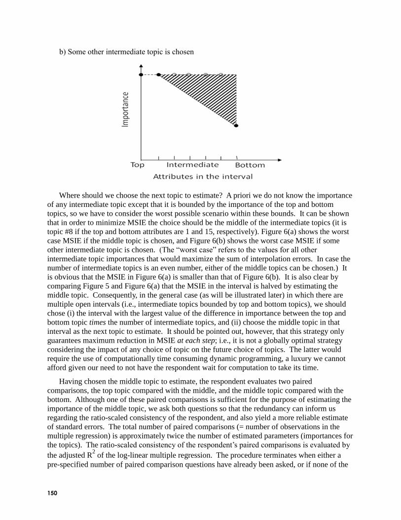
150

b) Some other intermediate topic is chosen

Where should we choose the next topic to estimate? A priori we do not know the importance

of any intermediate topic except that it is bounded by the importance of the top and bottom

topics, so we have to consider the worst possible scenario within these bounds. It can be shown

that in order to minimize MSIE the choice should be the middle of the intermediate topics (it is

topic #8 if the top and bottom attributes are 1 and 15, respectively). Figure 6(a) shows the worst

case MSIE if the middle topic is chosen, and Figure 6(b) shows the worst case MSIE if some

other intermediate topic is chosen. (The ―worst case‖ refers to the values for all other

intermediate topic importances that would maximize the sum of interpolation errors. In case the

number of intermediate topics is an even number, either of the middle topics can be chosen.) It

is obvious that the MSIE in Figure 6(a) is smaller than that of Figure 6(b). It is also clear by

comparing Figure 5 and Figure 6(a) that the MSIE in the interval is halved by estimating the

middle topic. Consequently, in the general case (as will be illustrated later) in which there are

multiple open intervals (i.e., intermediate topics bounded by top and bottom topics), we should

chose (i) the interval with the largest value of the difference in importance between the top and

bottom topic times the number of intermediate topics, and (ii) choose the middle topic in that

interval as the next topic to estimate. It should be pointed out, however, that this strategy only

guarantees maximum reduction in MSIE at each step; i.e., it is not a globally optimal strategy

considering the impact of any choice of topic on the future choice of topics. The latter would

require the use of computationally time consuming dynamic programming, a luxury we cannot

afford given our need to not have the respondent wait for computation to take its time.

Having chosen the middle topic to estimate, the respondent evaluates two paired

comparisons, the top topic compared with the middle, and the middle topic compared with the

bottom. Although one of these paired comparisons is sufficient for the purpose of estimating the

importance of the middle topic, we ask both questions so that the redundancy can inform us

regarding the ratio-scaled consistency of the respondent, and also yield a more reliable estimate

of standard errors. The total number of paired comparisons (= number of observations in the

multiple regression) is approximately twice the number of estimated parameters (importances for

the topics). The ratio-scaled consistency of the respondent‘s paired comparisons is evaluated by

the adjusted R2 of the log-linear multiple regression. The procedure terminates when either a

pre-specified number of paired comparison questions have already been asked, or if none of the

151

differences in importance between the top and bottom topics of the intervals is statistically

significant, as per a t-test (Netzer and Srinivasan 2009).

The ASEMAP approach is adaptive in that the paired comparison questions at each point in

time are chosen based on the rank order information and the log-linear multiple regression-based

importances estimated up to that point in time. The log-linear multiple regression computations

are quick so that the respondent does not have to wait at the computer for the next paired

comparison question to appear.

An Example Figure 7 provides an example of the adaptive sequence of the paired comparison questions

for one respondent. The rank order of the topics given by this respondent is shown on the left

hand side of Figure 7.

1. We first ask the paired comparison comparing the top (most important) topic (#1) with

the bottom topic (#15). As discussed in the previous section, the topic to be selected next

is in the middle of the interval [1, 2, …, 15], i.e., #8, and we ask two questions comparing

1 with 8, and 8 with 15. These three paired comparisons are shown by the right bracket-

like double arrows. The log-linear multiple regression of the answers to these three

questions yields the importances for #1 = 18.60, #8 = 5.48, and #15 = 0.54. These

numbers are scaled in such a way that these numbers together with the interpolated values

for all other topics sum to 100.

2. We now have two intervals [1, 2, …, 8] and [8, 9, …, 15]. The number of intermediate

attributes in each of these two intervals is the same (=6) so that the choice of the next

topic is based only on the difference in importance between the top and bottom topics of

the intervals. The larger difference corresponds to [1, 2, …, 8], so we open that interval

(denoted by the vertical line with arrows at both ends) with its middle topic #4

(alternatively #5 could have been chosen). We ask two paired comparisons (1, 4) and (4,

8) again shown by the right bracket-like double arrows. The answers to these two paired

comparisons together with the previous three (a total of five paired comparisons) are

analyzed by log-linear multiple regression to yield the results #1 = 20.83, #4= 9.03, #8 =

6.09, and #15 = 0.60. Note that the topic importance for 1, 8, and 15 has changed

somewhat from the previous iteration. One reason is that the relative importance of 1 vs.

8 is now determined by the paired comparison (1,8) and also by (1, 4) together with (4,

8).

3. We now have three intervals [1, 2, 3, 4], [4, 5, 6, 7, 8], and [8, 9,…,15]. We compute the

quantity [difference in importance between the top and bottom topics times the number of

intermediate topics] and find that the interval [8, 9,…, 15] has the highest quantity, thus

we choose this interval. We choose topic #11 as the next topic to evaluate and use two

paired comparisons (8, 11) and (11, 15). The results of the log-linear regression of all

seven paired comparisons are reported in the last column of Figure 7. Note that five topic

importances are obtained from seven paired comparisons. Because the importances are

estimated only relative to the most important attribute (see the earlier explanation of the

multiple regression procedure), only four relative importances are estimated from seven

paired comparisons. Thus there are three (=7-4) degrees of freedom at this stage in the

procedure.

152

4. The procedure continues in this manner until a pre-specified number of paired

comparisons (9 pairs in the MSI application) are asked.

Figure 7:

Example: Adaptive Sequence of Questions for One Respondent

ASEMAP Summary To summarize, ASEMAP involves the following steps:

1. Divide the attributes into two (or three) sets.

2. Rank within each set.

3. The previous two steps results in an overall rank order.

4. Use the adaptive method described earlier to choose paired comparisons.

153

5. Estimate the importance of attributes included in the pairs by log-linear multiple

regression.

6. The remaining attributes’ importances are estimated by interpolation based on the rank

order.

7. The importances are normalized to sum to 100.

See Netzer and Srinivasan (2009) for additional details of the ASEMAP procedure.

EMPIRICAL STUDY

Selection of Topics MSI had conducted focus group-like qualitative discussions with its trustees to identify

research topics of significant interest to them. Based on the qualitative study and other inputs

from practitioner members and academics, MSI staff assembled the list of fifteen major research

topics in marketing, shown in Table 1. To elaborate on what each topic meant, MSI listed several

examples of research projects subsumed by the topic label. To illustrate, the topic of ―advances

in marketing research techniques‖ had the following examples:

Internet-based marketing research

RFID-based research opportunities

Internet auctions

Text analysis of blogs

Cognitive science applications for marketing research

Permission-based marketing research

Use of virtual worlds in marketing research

Table 1:

Fifteen MSI Major Research Topics in Marketing

Emerging markets

Engaging customers

Driving loyalty

Social networks and word-of mouth

Marketing and the organization

Developing marketing competencies

Improving executive decision making

Advances in marketing research techniques

Innovation and new products

Managing brands

154

Solutions selling

Channels and retailing

New media

Forward-looking metrics

Marketing and firm value

Respondents The respondents for the present empirical study were non-trustee managers from MSI

member companies who had attended past MSI conference(s) and/or had requested MSI

publications. E-mails were sent to managers requesting their participation with the MSI survey

of research priorities; up to two reminder e-mails were sent to respondents who did not respond

to the earlier e-mail(s). The e-mail stated that MSI plans to use the results to better serve

individuals in member companies. No other incentive was provided. The response rate was

17.2%. There were no statistically significant differences between respondents and non-

respondents in terms of the proportions of different types of companies (B to C, B to B, Services)

represented.

The managers were e-mailed either the CSUM or ASEMAP web-based questionnaires

(random assignment). In the ASEMAP survey the number of paired comparisons for each

respondent was limited to nine pairs. Previous research (Netzer and Srinivasan 2009) has shown

that ASEMAP‘s predictive validity does not increase appreciably as the number of paired

comparisons is increased past nine pairs. The final sample sizes were nCSUM = 161 and nASEMAP = 159. No statistically significant differences were found across the two samples in terms of the

proportions of different types of companies (B to C, B to B, or Services) represented.

Research Design Figure 8 displays the research design employed in the study. After a description of the fifteen

topics (in terms of examples of research projects for each topic), respondents prioritized the

fifteen topics by CSUM or ASEMAP. This was followed by a set of eight demographic

questions. The demographic questions also helped minimize short term memory effects from the

measurement of importances by CSUM or ASEMAP to the ―validation task,‖ described next.

Figure 8:

Empirical Research Design

155

Validation MSI funds a limited set of research proposals submitted by academics. We used that context

to set up a validation task that would be meaningful to MSI. For each respondent, we chose

randomly six out of the fifteen topics and asked the respondent to choose three out of the six

topics that s/he recommends MSI to fund, as shown in Figure 9. A second validation task with

another random set of six topics followed.

We computed the extent to which the quantitative importances measured by CSUM or

ASEMAP predicted the paired comparisons implied by the validation data. This served as a

measure of predictive validity of the method. We illustrate below the computation of predictive

validity measure. In the validation task the respondent chooses three out of the six topics.

Suppose we denote by (A, B, C) the three topics chosen and (D, E, F) the three topics not chosen

in a validation task. From the choices we can infer that topics A, B, and C should each have a

higher importance than each of the topics D, E, and F. Thus, there are nine pairs that can be

inferred from this choice task (see Table 2). From the validation task, we cannot infer anything

about the relative importances of (A, B, C) among themselves, or among (D, E, F).

Figure 9:

Validation Task

Suppose MSI has received six proposals for research on the following topics. Suppose,

however, that MSI can fund only three out of the six topics. Place a check (√) next to the

three topics you want MSI to fund.

Marketing and firm value

Channels and retailing

Driving loyalty

Developing marketing competencies

Managing brands

New Media

156

Table 2:

Calculation of the Percent of Pairs Correctly Predicted

Let (A, B, C) be the topics chosen over (D, E, F) in the validation task. To illustrate the

calculation of the percent by pairs correctly predicted, suppose

A = 10, B = 20, C = 0, D = 10, E = 15, and F = 0

are the importances measured by a method (CSUM or ASEMAP).

Validation Do the Measured Preferences Predict the Pairs?

Pair (1 = Yes, 0 = No, 0.5 =Tie)

Strict Defn. Weak Defn.

A>D 0 0.5

A>E 0 0

A>F 1 1

B>D 1 1

B>E 1 1

B>F 1 1

C>D 0 0

C>E 0 0

C>F 0 0.5

Total 9 4 5

Percent Correct 44.4% 55.5%

We use the percent of pairs correctly predicted as the measure of validity. Table 2 illustrates

the calculations. Consider for instance, the pair comparing A and F. In the validation data A was

chosen but F was not chosen which implies A>F. The example preference data (measured by

CSUM or ASEMAP) listed in Table 2 are A = 10 and F = 0. Thus the A>F is predicted by the

preference data and it gets counted as a 1(i.e., correct). On the other hand, consider the case of A

and D. A was chosen but D was not so that A>D. But the example preference data presented in

Table 12 has A=10 and D=10. Because the preferences are tied, they do not predict A>D so it

gets counted as 0 (i.e., incorrect) as far as strict definition is concerned, but 0.5 if the weak

definition is used (the prediction is neither correct, nor incorrect). The percent correct is

computed for both validation tasks (each involves choosing 3 topics out of 6), and the result

averaged across the two tasks to yield the measure of predictive validity of the method (CSUM

or ASEMAP) for that particular respondent.

RESULTS

Predictive Validity Table 3 compares the predictive validity results for CSUM with ASEMAP. The percent of

pairs correctly predicted was computed as described earlier for each of the respondents in the

CSUM sample (n=161) and likewise for the respondents in the ASEMAP sample (n = 159). A

two samples comparison test reveals that ASEMAP‘S predictive validity is significantly larger

than that of CSUM (p <.01) under both the strict and weak definitions. Furthermore, the

157

differences are substantial. Under the strict definition ASEMAP is 36.9% better; even under the

weak definition ASEMAP is 8.7% better. ASEMAP with hierarchical Bayes estimation is likely

to produce an even larger improvement in predictive validity (Netzer and Srinivasan 2009). (The

hierarchical Bayes method is not applicable for the CSUM approach). We believe that the strict

definition is more appropriate in applied marketing contexts because one reason for assessing the

importance is to guide decision making in terms of which topic is more important. A naïve

method that says all topics are equally important will obtain a 50% predictive validity under the

weak definition, but will obtain only a 0% predictive validity under the strict definition.

The constant sum method produces a large percentage of ties, 37% compared to 2.5% for

ASEMAP. As expected, CSUM is significantly faster than ASEMAP. The CSUM questionnaire

took on average, only 6.10 minutes compared to 8.97 minutes for the ASEMAP questionnaire

(p<.01).

Consistency of ASEMAP Data

The average adjusted R2 of the ASEMAP log-linear regression was 0.93 indicating that the

constant-sum paired comparison data were very good in terms of ratio-scaled consistency.

Furthermore, the average rank order correlation coefficient between the initial rank order of the

topics and final rank order of the topics (based on ASEMAP importances) was 0.90 showing that

the paired comparisons were mostly consistent with the initial rank order. Unlike the above two

statistics, there is no internal consistency measure for CSUM data.

Table 3:

Average Percent of Pairs Correctly Predicted

CSUM ASEMAP Z-stat

Strict defn. 59.6 81.6 9.23**

Weak defn. 75.9 82.5 3.9**

** The differences are substantial and highly statistically significant (p <.01)

Comparison of Average Topic Importances across Methods Table 4 reports the average topic importances for ASEMAP and CSUM. The topic

importances are self-explanatory in terms of which topics were perceived to be more important

and to what extent. The correlation between the two sets of means is 0.74. Overall the two

methods give similar but not identical results. On three of the fifteen topics the differences in

means across the two methods are statistically significant (p <.05). Some notable differences are

that ―advances in market research techniques‖ was the highest rated item by CSUM but only the

fifth highest item by ASEMAP. ―Forward looking metrics‖ was the second highest item by

ASEMAP but only the sixth rated item by CSUM.

Benefit Segments We determined benefit segments based on the more valid ASEMAP importances. A benefit

segment is a cluster of respondents who are close to each other in terms of importances for the

158

topics. We used the k-means methods for cluster analysis and chose a three-segment solution

based on the pseudo-F criterion. Table 5 provides the results.

Segment 1 (76.1% of the respondents) is a ―customer-focused‖ segment that places more

importance on ―engaging customers‖ and ―driving loyalty.‖ Segment 2 (12.6% of the

respondents) is an ―innovation and new products‖ oriented segment. Segment 3 (11.3% of the

respondents) emphasizes ―advances in market research techniques‖ and ―forward looking

metrics.‖ The demographic variables such as industry type and managerial position in the

company do not, in general, discriminate significantly across the three segments except that

segment 3 has a disproportionately large percentage of market researchers (78% in segment 3

compared to 44% for segments 1 and 2 combined, p < .01).

Table 4:

Average Topic Importances for ASEMAP and CSUM

Topics rearranged in decreasing order of ASEMAP-based average importance

Topic ASEMAP CSUM

Means Means

Innovation and new products 9.93 10.40

Forward-looking metrics 9.17 7.01 (p <.05)

Engaging customers 8.44 7.59

Driving loyalty 8.06 7.14

Adv. Marketing research techniques 7.61 10.54 (p <.05)

Managing brands 7.02 6.94

Improving executive decision making 6.77 4.93 (p <.01)

Developing marketing competencies 5.87 5.78

Channels and retailing 5.80 5.53

Emerging markets 5.78 7.13

Social networks and word-of-mouth 5.54 6.17

Solutions selling 5.27 6.52

New media 5.12 5.35

Marketing and firm value 4.87 4.61

Marketing and the organization 4.76 4.36

Total 100.00 100.00

Note: Statistically significant differences are highlighted.

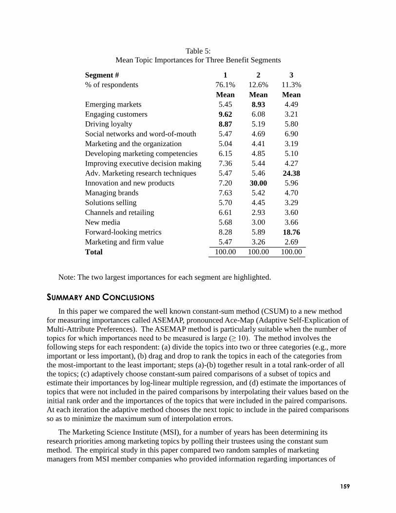
159

Table 5:

Mean Topic Importances for Three Benefit Segments

Segment # 1 2 3

% of respondents 76.1% 12.6% 11.3%

Mean Mean Mean

Emerging markets 5.45 8.93 4.49

Engaging customers 9.62 6.08 3.21

Driving loyalty 8.87 5.19 5.80

Social networks and word-of-mouth 5.47 4.69 6.90

Marketing and the organization 5.04 4.41 3.19

Developing marketing competencies 6.15 4.85 5.10

Improving executive decision making 7.36 5.44 4.27

Adv. Marketing research techniques 5.47 5.46 24.38

Innovation and new products 7.20 30.00 5.96

Managing brands 7.63 5.42 4.70

Solutions selling 5.70 4.45 3.29

Channels and retailing 6.61 2.93 3.60

New media 5.68 3.00 3.66

Forward-looking metrics 8.28 5.89 18.76

Marketing and firm value 5.47 3.26 2.69

Total 100.00 100.00 100.00

Note: The two largest importances for each segment are highlighted.

SUMMARY AND CONCLUSIONS

In this paper we compared the well known constant-sum method (CSUM) to a new method

for measuring importances called ASEMAP, pronounced Ace-Map (Adaptive Self-Explication of

Multi-Attribute Preferences). The ASEMAP method is particularly suitable when the number of

topics for which importances need to be measured is large (≥ 10). The method involves the

following steps for each respondent: (a) divide the topics into two or three categories (e.g., more

important or less important), (b) drag and drop to rank the topics in each of the categories from

the most-important to the least important; steps (a)-(b) together result in a total rank-order of all

the topics; (c) adaptively choose constant-sum paired comparisons of a subset of topics and

estimate their importances by log-linear multiple regression, and (d) estimate the importances of

topics that were not included in the paired comparisons by interpolating their values based on the

initial rank order and the importances of the topics that were included in the paired comparisons.

At each iteration the adaptive method chooses the next topic to include in the paired comparisons

so as to minimize the maximum sum of interpolation errors.

The Marketing Science Institute (MSI), for a number of years has been determining its

research priorities among marketing topics by polling their trustees using the constant sum

method. The empirical study in this paper compared two random samples of marketing

managers from MSI member companies who provided information regarding importances of

160

fifteen marketing topics, one group by the CSUM method and the other group by the ASEMAP

method. The methods were compared on the basis of their ability to predict which three of a

random subset of six topics the managers would choose as more important. ASEMAP produced

a substantial and statistically significant improvement in validity, with the percent of correctly

predicted pairs increasing from 60% for CSUM to 82% for ASEMAP. Even after giving tied

predictions half-credit each (rather than zero credit), the percentage of correctly predicted pairs

was higher for ASEMAP by seven percentage points. Both these improvements are substantial

and statistically significant at the .01 level. CSUM produced 37% tied pairs of importances

compared to 2.5% for ASEMAP. The ASEMAP survey took three minutes more, on average,

compared to CSUM. The average importances across methods differed statistically significantly

on three of the fifteen topics.

A Replication The empirical result of this study was replicated in a second study on assessing priority

issues for the U.S. presidential election, as seen by voters in July 2008 (Srinivasan and

Makarevich 2009). A set of seventeen topics were included in the study with a random third of

the respondents providing their priorities by (a) CSUM, (b) ASEMAP, and (c) MaxDiff

(Sawtooth Software 2007). After the data collection regarding priorities and an intervening data

collection on demographics and past political participation, the validation task involved a

constant-sum task on two random subsets of four topics each. (The idea is that with a small

subset of topics such as four, respondents would be able to provide importance information more

accurately in CSUM.) The methods were compared on the basis of mean absolute error between

the validation responses and rescaled importances from the original data collection by the three

methods. As seen from Table 6, ASEMAP significantly (p <.01) and substantially out-performed

CSUM and MaxDiff in terms of both mean absolute error and its standard deviation (computed

across respondents). CSUM took significantly shorter time than ASEMAP and MaxDiff. The

difference in average times between MaxDiff and ASEMAP was not statistically significant.

Table 6:

Comparison of Mean Prediction Errors and Times across

Methods in the Presidential Priorities Study

Method Mean

absolute

error

Improvement in

mean absolute

error over CSUM

Std. dev.

in error

Average time

(minutes)

CSUM

MAXDIFF

ASEMAP

12.62

11.31

8.73

----

10.4%

30.8%

7.36

4.91

4.29

6.11

8.63

9.38

Overall our research indicates that ASEMAP produces better predictive validity than CSUM

and MaxDiff when the number of topics is large (in our studies the number of topics varied from

15 to 17).

161

Epilog The Marketing Science Institute chose to use ASEMAP as the research method (rather than

CSUM) for the subsequent research priorities study conducted with its trustees in 2008.

ACKNOWLEDGMENTS

Our thanks to Mike Hanssens, Russ Winer, Earl Taylor, Ross Rizley, Marni Clippinger, and

Michelle Rainforth of the Marketing Science Institute, Andrew Latzman and Ronit Aviv of

Dynamic Logic Inc., Linda Bethel, Ravi Pillai, and Jeannine Williams of Stanford University

Graduate School of Business, Taylan Yildiz of Google, Inc., and Oded Netzer of Columbia

University for their help with this study.

REFERENCES

Chrzan, Keith and Natalia Golovashkina (2006), ―An Empirical Test of Six Stated Importance

Measures,‖ International Journal of Market Research, 4:6, pp. 717-740.

Krosnick, Jon A. (1999), ―Maximizing Questionnaire Quality,‖ in John P. Robinson, Philip

R. Shaver, and Lois S. Wrightsman (Eds.), Measures of Political Attitudes, New York:

Academic Press.

Netzer, O. and V. Srinivasan (2009), ―Adaptive Self-Explication of Multi-Attribute

Preferences,‖ Working paper, Stanford, CA: Graduate School of Business, Stanford

University.

Sawtooth Software Inc. (2007), ―The MaxDiff/Web System Technical Paper,‖ Sequim, WA:

Sawtooth Software, Inc.

Srinivasan, V. and Alex Makarevich (2009), ―Assessing Presidential Priorities: A Comparison

of Three Methods,‖ Working paper (under preparation), Stanford, CA: Graduate School

of Business, Stanford University.

163

TOURNAMENT-AUGMENTED CHOICE-BASED CONJOINT

KEITH CHRZAN

DANIEL YARDLEY MARITZ RESEARCH

INTRODUCTION

Conjoint analysis provides insight about customer preferences and about how customers

trade-off those preferences against one another. Marketers seeking to make evidence-based

decisions about trade-offs inherent in the new product development process often find conjoint

analysis to be an ideal tool. For their part, researchers often try to collect conjoint data frugally,

using efficient experimental designs to get as much information about customer preferences as

they can, using numbers of conjoint questions they consider small enough to keep research

expenses low and respondents responsive.

Other researchers, however, seek to get respondents to provide better conjoint data by forcing

them to process their answers more ―deeply.‖ For example, the Sawtooth Software ACBC

(Adaptive CBC) product uses a BYO question, a consideration/screening exercise, and direct

confirmations from respondents regarding cutoff rules to identify the attributes and levels that

most appeal to each respondent before tailoring difficult choice tasks constructed just of those

product concepts in the consideration set (Johnson and Orme 2007). Elsewhere in these

proceedings, Islam et al. describe using a full best-worst rank ordering of alternatives in each

choice set as a way of getting more information from respondents. Tournament-augmented

conjoint analysis (TAC) represents a third way to try to get more information from respondents.

TOURNAMENT-AUGMENTED CHOICE-BASED CONJOINT

A standard D-efficient experimental design minimizes the total error around all the

coefficients of a conjoint experiment: reducing the variance around the part worth utility of an

attribute level respondents uniformly avoid counts just as much as reducing error around very

appealing attribute levels which might appear more often in a real market. Put another way, a D-

efficient experimental design seeks to minimize total error around the utilities from all around

the ―design space‖ of all possible product configurations. But marketers, keen on introducing

successful products, will focus their product development efforts on the higher utility parts of the

design space – highly refined utility estimates for unwanted attribute levels will be no more than

a remote ―nice to have‖ for a marketer developing products in the high-utility parts of the design

space.

TAC combines a standard D-efficient experimental design with a follow-up tournament of

winners a respondent chooses from the D-efficient choice sets. For example, imagine a D-

efficient design consisting of 12 choice sets of triples. Respondent Socrates goes through this

task and chooses 12 profiles, one from each choice set. In TAC, we randomly combine these 12

chosen profiles into four new triples, from which Socrates again chooses one winner each. The

four twice-chosen profiles now become one final choice set, a quad, from which Socrates

164

constructs a best-worst rank ordering (he chooses the best and the worst profiles, then the better

of the two remaining).

Note that, while the original D-efficient experiment covers the whole design space, each

subsequent level of the tournament will tend to focus more on the higher utility parts of the

design space. Chosen (and more so, twice-chosen) profiles in the tournament choice sets will

tend to be devoid of unacceptable levels, and rich in more highly desirable attribute levels. Thus

TAC uses the original D-efficient design to get a good measure of all part worth utilities, and the

tournament to get more refined measures of the more appealing part worth utilities.

QUESTIONS ABOUT TOURNAMENT-AUGMENTED CHOICE-BASED CONJOINT

Several aspects of TAC raise questions that deserve empirical testing. First, will TAC

produce a tangible benefit? That is, will the utilities TAC produces be better than those from the

D-efficient experiment by itself? Will TAC do a better job of predicting choice sets composed of

high-utility alternatives than do utilities generated from a D-efficient experiment by itself?

Assuming that a benefit results, how does that benefit stack up against its costs? ACBC takes

longer than a standard choice-based conjoint experiment, because of the number of questions and

because of the harder judgments it requires from respondents. So, it seems likely that TAC will

take longer to administer as well, adding incremental burden on respondents. Moreover, while

the programming required for adaptive construction of the tournament choice sets is

straightforward, how much work will setting up the data for analysis involve?

Finally, will the utilities that result from the tournament portion of TAC be the same as or

different from those that result from the D-efficient portion of the experiment? Will they reflect

the same or different preferences, and the same or different scale parameters? If different

preference parameters result, will it really make sense to combine the D-efficient and tournament

sections of TAC into a single model?

To address these questions, we conducted an empirical test. Some additional questions arose

after the empirical test, which led us to conduct a second empirical test.

EMPIRICAL TEST 1

The first empirical test of TAC was part of a web-based commercial study of combination

oral contraceptive products. The 4 x 3 x 24 design featured one metric variable, ―dosing,‖ while

the rest were categorical. About half of the categorical variables featured a predictable

monotonic ordering. Physicians, obstetricians and gynecologists, qualified for the study with a

sufficient patient volume, and 200 completed the survey.

The TAC matched exactly the one described above – a D-efficient design in 12 choice sets of

triples, followed by a two-level tournament design: four triples constructed of the 12 profiles

chosen in the 12 D-efficient choice sets, followed by a final quad composed of first choices from

those four triples. Respondents did a best-worst rank ordering of the profiles in the final quad.

In addition, each respondent received a holdout section, in two parts. The first portion of the

holdout included three choice sets randomly selected from a second D-efficient design of 12

choice sets. From the three profiles chosen from these choice sets results a new triple, and

165

respondents do a best-worst rank ordering of the three profiles in the triple. Thus we have D-

efficient and tournament holdouts to predict.

To test for parameter and scale equality, we estimated separate models from the D-efficient

and tournament portions of the experiment, and subjected these to the Swait-Louviere (1993) test

for scale and preference heterogeneity. These utilities resulted from the D-efficient and

tournament portions of the experiment:

Level D-efficient Tournament

att1_1 0.29 0.00

att1_2 -0.19 -0.23

att1_3 -0.10 0.22

att2_1 -1.83 -1.50

att2_2 -1.00 -0.88

att2_3 -0.29 -0.43

att2_4 3.12 2.81

att3_1 0.62 0.62

att3_2 -0.62 -0.62

att4_1 -0.18 -0.22

att4_2 0.18 0.22

att5_1 1.03 0.88

att5_2 -1.03 -0.88

att6_1 0.65 0.76

att6_2 -0.65 -0.76

The Swait-Louviere test rejects parameter equality, so the D-efficient and tournament

sections of the experiment produce significantly different preferences. The largest difference

occurs in the very low utility level of the most important attribute (Attribute 2), which is also the

attribute level least likely to have been present in the tournament section of the interview. It

seems likely that the small number of observations produced a large amount of error around this

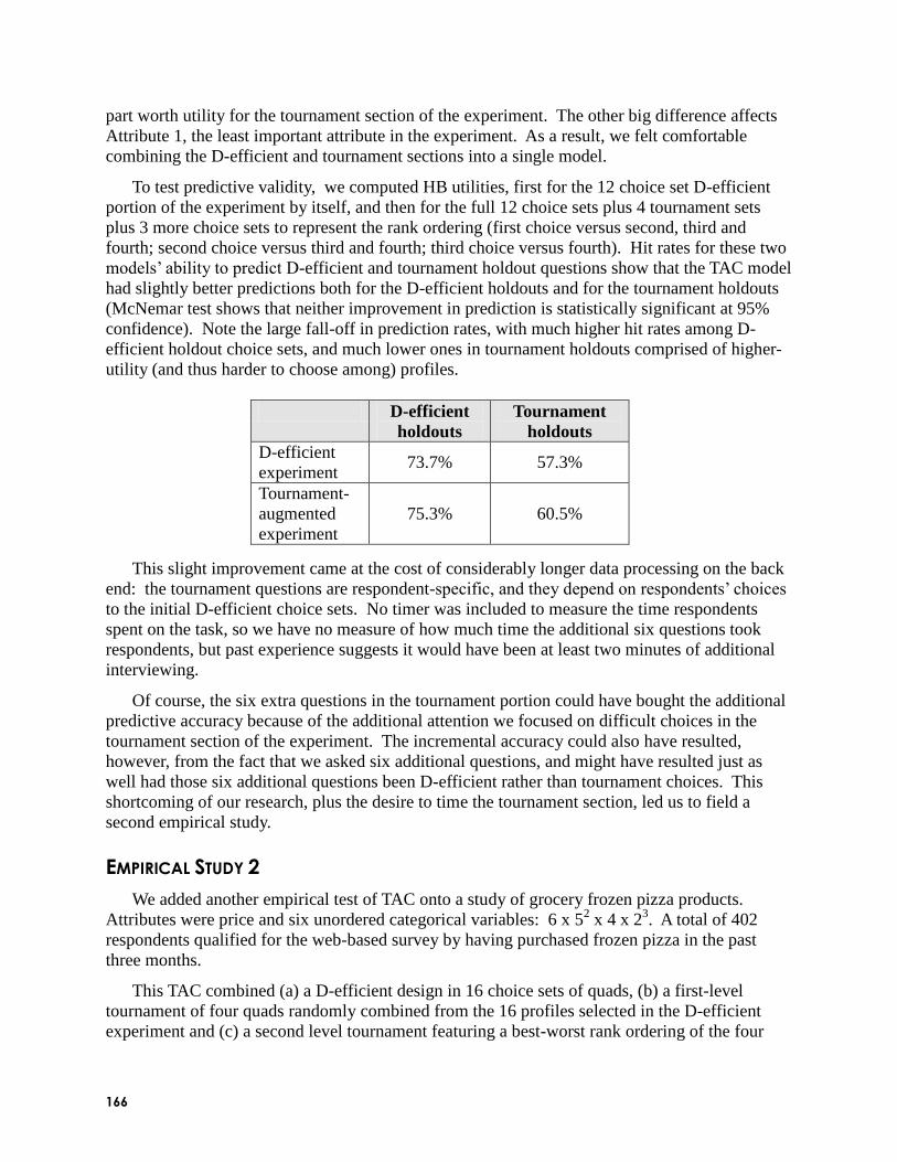
166

part worth utility for the tournament section of the experiment. The other big difference affects

Attribute 1, the least important attribute in the experiment. As a result, we felt comfortable

combining the D-efficient and tournament sections into a single model.

To test predictive validity, we computed HB utilities, first for the 12 choice set D-efficient

portion of the experiment by itself, and then for the full 12 choice sets plus 4 tournament sets

plus 3 more choice sets to represent the rank ordering (first choice versus second, third and

fourth; second choice versus third and fourth; third choice versus fourth). Hit rates for these two

models‘ ability to predict D-efficient and tournament holdout questions show that the TAC model

had slightly better predictions both for the D-efficient holdouts and for the tournament holdouts

(McNemar test shows that neither improvement in prediction is statistically significant at 95%

confidence). Note the large fall-off in prediction rates, with much higher hit rates among D-

efficient holdout choice sets, and much lower ones in tournament holdouts comprised of higher-

utility (and thus harder to choose among) profiles.

D-efficient

holdouts

Tournament

holdouts

D-efficient

experiment 73.7% 57.3%

Tournament-

augmented

experiment

75.3% 60.5%

This slight improvement came at the cost of considerably longer data processing on the back

end: the tournament questions are respondent-specific, and they depend on respondents‘ choices

to the initial D-efficient choice sets. No timer was included to measure the time respondents

spent on the task, so we have no measure of how much time the additional six questions took

respondents, but past experience suggests it would have been at least two minutes of additional

interviewing.

Of course, the six extra questions in the tournament portion could have bought the additional

predictive accuracy because of the additional attention we focused on difficult choices in the

tournament section of the experiment. The incremental accuracy could also have resulted,

however, from the fact that we asked six additional questions, and might have resulted just as

well had those six additional questions been D-efficient rather than tournament choices. This

shortcoming of our research, plus the desire to time the tournament section, led us to field a

second empirical study.

EMPIRICAL STUDY 2

We added another empirical test of TAC onto a study of grocery frozen pizza products.

Attributes were price and six unordered categorical variables: 6 x 52 x 4 x 2

3. A total of 402

respondents qualified for the web-based survey by having purchased frozen pizza in the past

three months.

This TAC combined (a) a D-efficient design in 16 choice sets of quads, (b) a first-level

tournament of four quads randomly combined from the 16 profiles selected in the D-efficient

experiment and (c) a second level tournament featuring a best-worst rank ordering of the four

167

profiles selected in the first level of the tournament. The entire TAC experiment included 21

choice sets.

In addition, only half of the respondents received the TAC described above. The other half

received a D-efficient design in 21 choice sets. This aspect of the design allows us to discern if

any improvement in prediction owes to the tournament nature of the additional questions, or

from the mere presence of additional questions.

Again each respondent received a holdout section: an initial portion contained four choice

sets randomly selected from a D-efficient design of 16 choice sets, different from the D-efficient

design used above. The four chosen profiles contribute to a new quad, from which respondents

selected their preferred product.

Separate models from the D-efficient and tournament portions of the experiment, and the

Swait-Louviere (1993) test for scale and preference heterogeneity again show that the two

models produce significantly different part worth utilities:

Level D-efficient Tournament

att1_1 0.31 0.48

att1_2 0.13 0.15

att1_3 0.07 0.30

att1_4 0.14 0.15

att1_5 -0.65 -1.08

att2_1 0.08 0.33

att2_2 0.44 0.58

att2_3 0.52 0.71

att2_4 0.00 0.09

att2_5 0.78 0.78

att2_6 -1.82 -2.50

att3_1 0.05 0.11

att3_2 -0.05 -0.11

att4_1 -0.06 0.06

att4_2 0.06 -0.06

att5_1 0.06 0.10

att5_2 -0.06 -0.10

att6_1 -0.01 0.07

att6_2 -0.12 -0.13

att6_3 -0.03 0.00

att6_4 -0.06 0.07

att6_5 0.22 -0.01

att7_1 0.38 0.48

att7_2 0.17 0.28

att7_3 0.07 0.13

att7_4 -0.63 -0.89

168

As in the first empirical study, the largest difference occurs on the infrequently-seen lowest

utility level of the most important attribute. No other large utility differences occur, so again we

combined the D-efficient and tournament sections into a single model.

For this test of predictive validity we have the two D-efficient experiments (16 set and 21 set

experiment) and the TAC model. The TAC model predicts higher-utility tournament holdouts

slightly better than either the 16-set or the 21-set D-efficient experiment. Among D-efficient

holdouts, however, the 21-set D-efficient experiment has the highest hit rate. Again, however,

McNemar tests show that none of these differences in hit rates are statistically significant (at

95% confidence).

D-efficient holdouts Tournament holdouts

16 set D-efficient experiment 65.8% 35.6%

21-set D-efficient experiment 70.5% 37.8%

Tournament-augmented experiment 64.8% 40.0%

Again predictions of D-efficient holdouts are easier than those of tournament holdouts,

because the latter require choices among already chosen higher utility alternatives.

It appears that part of the incremental prediction in TAC comes from the mere fact of having

respondents make additional choices; part, too, appears to come from having them make difficult

choices among higher-utility alternatives. Timers embedded in the survey bear this out: the 21

set TAC took a minute (14%) longer for respondents to complete than did the 21 set D-efficient

experiment.

ACROSS STUDIES

For this final test of predictive validity we stacked the D-efficient results across the two

studies as well as the tournament holdouts. The TAC model predicts higher-utility tournament

holdouts slightly better than D-efficient experiment alone. McNemar tests show that this

difference in hit rates is not statistically significant (at 95% confidence).

169

D-efficient

holdouts

Tournament

holdouts

D-efficient

experiment 68.8% 48.9%

Tournament-

augmented

experiment

68.8% 52.3%

DISCUSSION

To sum up, TAC produced statistically, but not substantively significant differences in

utilities compared to a D-efficient design by itself. These differences allowed TAC to make

slightly better predictions of more difficult choices – choice sets comprised of high utility

tournament holdouts. The TAC questions take respondents a little longer to do, and they add

considerable processing time, so there is additional burden for both respondents and analysts.

Perhaps TAC would perform better in different studies. In both of the empirical studies, the

ratio of observations to parameters was high, so that HB produced accurate utilities, and little

room remained for additional precision from the tournament questions. Maybe in a study with

fewer observations per parameter, the additional tournament questions would improve results (of

course, using a larger D-efficient design might also improve results).

For now, we think that TAC‘s modest and non-significant improvements come at too high a

cost.

REFERENCES

Islam, Towhidul, Jordan Louviere, David Pihlens (2009), ―Aggregate Choice and Individual

Models: A Comparison of Top-Down and Bottom-Up Approaches, ‖ Sawtooth Software

Conference Proceedings, in press.

Johnson, Rich and Bryan Orme (2007), ―A New Approach to Adaptive CBC,‖ Sawtooth

Software Conference Proceedings, Sequim: Sawtooth Software.

Swait, Joffre and Jordan Louviere (1993) ―The Role of the Scale Parameter in the Estimation

and Comparison of Multinomial Logit Models,‖ Journal of Marketing Research, 30, 305-

14.

171

COUPLING STATED PREFERENCES WITH CONJOINT TASKS TO

BETTER ESTIMATE INDIVIDUAL-LEVEL UTILITIES

KEVIN LATTERY MARITZ RESEARCH

INTRODUCTION

Any method of conjoint estimation, in the absence of constraints, can result in what are

commonly called ―reversals.‖ For instance, in the case of ordinal variables, where one level of

an attribute should universally have a higher utility than another, we may find that the lower

level actually has a higher utility. With individual conjoint utility estimates, this reversal is

almost certainly observed for some respondents, and with enough reversals it may show up at the

aggregate level.

The problem of reversals is one aspect of a more general problem. The solution space,

especially for individual-level conjoint estimation, is extremely large while the amount of

information we collect tends to be relatively small. Making 12 or 15 choices to scenarios

provides excellent information, but within the grand universe of potential solutions, it is typically

not enough information to understand a respondent‘s decision process with great robustness. For

this reason, researchers often apply constraints to ordinal attributes during conjoint estimation of

individual-level utilities. This greatly constrains the solution space, forcing utilities to have the

proper direction and giving them a better chance to reflect the respondent‘s decision process.

This paper shows that when we turn to nominal variables, the same kinds of reversals

happen. Of course, with nominal variables, reversals are far less obvious. The only way we can

verify a reversal for a nominal variable at the respondent level is if we ask respondents whether

they have a preference. If we ask respondents about their preferences, then we will observe

reversals, just as we do with ordinal variables. Incorporating stated preferences provides an

excellent way to constrain the solution space, giving individual-level conjoint estimates a much

better chance of avoiding reversals and more accurately modeling individual decision processes.

Even when we have what appears to be a good fitting conjoint model, incorporating individual

stated preferences may be essential for getting the story right.

Previous research shows that universal constraints applied to ordinal variables tend to

improve individual-level hit rates (Allenby 1995), but may adversely impact aggregate

predictions (Wittink 2000). We found the same to be true when coupling individual-level

preferences with HB estimation. However, constraints of any kind do not appear to negatively

influence the aggregate predictions from EM estimates of individual-level utilities. For this

reason, we recommend EM models when many constraints are incorporated and aggregate share

prediction is important. If HB models are run with many constraints on individual preferences,

we recommend the aggregate predictions be checked carefully to ensure the results predict

holdout tasks accurately.

Finally, we also show how stated preference information can be incorporated in a second

useful way: non-compensatory modeling. This more accurately reflects the way we believe

172

consumers make decisions, further improving hit-rates while having no adverse effect on

aggregate predictions. We show the improvement which can be gained by adding non-

compensatory modeling to individual-level constraints using the EM CBC estimation technique.

Incorporating stated information not only allows more accurate models, it results in models

that better predict holdout tasks, and are more consistent with the story which should be told.

This means if we only do simple HB estimation (no stated preference information) we may be

developing a model with inferior fit and one that tells the wrong story.

PRIMARY CONJOINT CASE STUDY

To illustrate the importance of coupling stated preferences with conjoint tasks, we make use

of a case study. This study was an ideal case study because of its excellent sample and relatively

small size from a design standpoint. In addition, three other similar case studies have followed,

though we will only briefly touch on those results.

Our client asked to remain anonymous, but is analogous to a high end exclusive Country

Club. One must be invited to become a member of the Country Club. Nearly 1400 emails were

sent to all the members inviting them to an online study. Letters were mailed beforehand

notifying people of the survey and the email link coming. The online study was left open for

over three weeks, with a few reminders sent to those who had not taken the survey.

The sample was ideal in that the survey was completely optional, with no incentive and no

reason to cheat. Respondents were very engaged, and were obviously interested in providing

thoughtful answers since it was their ―Country Club.‖ They provided detailed verbatims and

spent an average/median of 24 seconds per conjoint task (high outliers excluded). A total of 709

members responded, with two of those doing a mail version of the survey without the conjoint.

In addition to the excellent sample, the conjoint was relatively small, with 6 attributes (3^3

4^1 5^2) totaling 17 independent parameters (degrees of freedom). The total design was 3

blocks of 12 tasks with excellent balance and D-efficiency of 98.41. All attributes were purely

nominal with no prohibitions or constraints. Respondents were shown 12 tasks (each with two

choices) and one holdout task with the following structure:

Country Club 1 Country Club 2

Membership Size Size 1 Size 5

Activities Status quo Change 2

Committee Structure Status quo Change 2

Exclusivity Level 1 Level 3

Recruiting Focus Level 1 Level 5

Time Level 1 Level 4

The HB estimates using Sawtooth Software‘s CBC/HB converged fairly well after 30,000

iterations and the next 10,000 iterations were used for utility estimates.

1 The design algorithm constrained the choice tasks to have minimal level overlap, while striving for high level balance and D-efficiency. D-

efficiency was computed based on a stacked design, where each concept is a row in the design matrix.

173

In-sample hit-rate was 100% with an average probability of 99.64%. The holdout task was

designed to be hard to predict, with the HB model yielding a reasonable 68.5% hit rate. In most

cases, we‘d think a job reasonably well done and write up our findings. But as we will see, this

would have told the wrong story.

CONJOINT COMPARED WITH STATED PREFERENCE QUESTIONS

In addition to the conjoint tasks, the survey also asked respondents to state their preferences

about each attribute. In particular for a given attribute we asked them a question like this:

We used just three categories to measure preferences in order to get at clear preferences. We

assumed if a respondent said one level was better than another (using the categories above) that

implied it would have a higher utility. While we could have done a ranking of levels for

instance, we have found this may force respondents to state they prefer one level even when

there is not a clear preference.

To further ensure respondents gave us clear preferences, we allowed a ―No Opinion‖

response. ―No opinion‖ was typically used by respondents across all options of an attribute, but

occasionally respondents applied to only a subset of the levels.

Thinking about the Committee Structure, what is your opinion about the following

options?

If you have no opinion about any or all of the options check the "No Opinion" box. You may use any response as many times as you wish

Committee Structure

Completely

Unacceptable Acceptable

Very

Highly Desired No Opinion

Current committee structure

Change 1

Change 2

174

Another objective of this form of questioning was to model non-compensatory decisions.

The basic idea is that if a respondent said a level was ―Completely Unacceptable‖ and in the

conjoint tasks never chose an option with that level, they were assumed to apply a screening rule.

While we would have preferred asking this form of stated preference question for all

attributes, it was shown for four of the six attributes. For the remaining two attributes we asked a

―Select All‖ and a ―Select Best‖ question due to client request.

We can directly compare the individual-level stated preferences with the conjoint utilities.

This is shown in the table below for the ―Committee Structure‖ attribute. 188 respondents stated

they preferred Change 1 over Change 2. Among those 188 respondents, 58 showed a higher

utility for Change 1 over Change 2. Just to play fair, we actually relaxed this to Change 1 –

Change 2 > -.1). This means that a small reversal will still count as a match.

Stated Preference

(Col beat Row)

Utility Also Greater

(>-.1)

Status

Quo

Change

1

Change

2

Status

Quo

Change

1

Change

2

Status Quo 246 173 176 160

Change 1 91 57 42 53

Change 2 143 188 35 58

Total 898 524

There are 898 total pairs for the stated preferences committee attribute with a total of 524

matches. This means the individual-level utilities match the stated preferences only 58.4% of the

time. This is not very good, as one has a 50% chance of matching the direction by chance, and

even better than 50% in this case since we relaxed the matching criteria to count a small reversal

as a match. So at the individual level, this attribute does not match stated preferences very well.

The table below summarizes the fit for each of the attributes.

Attribute Conjoint Levels

Stated Question Type # Pairs

% Matching (>-.1)

Membership Size 5 Unacceptable/

Acceptable/ Highly Desired

3231 67.4%

Activities 3 1415 80.6%

Committee Structure 3 898 58.4%

Exclusivity 3 1115 69.9%

Recruiting Focus 5 Select All 2698 69.8%

Time 4 Best Level 1641 75.1%

All Attributes 9357 70.3%

The overall match of 70.3% is consistent with what other researchers find for ordinal

variables modeled in HB without constraints (Allenby 1995).

It is more difficult to definitively test reversals at the aggregate level since we have no

definitive picture of how the aggregate findings should look. But we can view the frequencies of

the stated preferences to get some idea of the aggregate findings.

175

For instance, with the

committee structure attribute,

Change 1 shows a

significantly higher

percentage of ―Very Highly

Desired‖ ratings, and by far

the fewest ―Completely

Unacceptable‖ ratings. This

strongly suggests Change 1 is

most likely the best level.

This is shown in the chart

below.

It is not clear from the

stated preferences whether Status Quo or Change 2 is next best. Status quo is safer, while

Change 2 is more polarizing, having more enthusiastic supporters than the status quo, but also

more respondents who find

the idea completely

unacceptable.

When we turn to the

conjoint findings, we get a

different story. HB analysis

claims that Change 2 is best,

and by a fair margin. This is

highly suspect, given the aggregate stated preferences above that show Change 1 as a clear

winner. It is made more questionable when we recall that only 58% of the individual-level

utilities for Committee Structure match the stated preferences. Finally, as we will see later it is

even more questionable when a better fitting conjoint model tells a different story with Change 1

as the best.

Another example of this

discrepancy between stated

preference and conjoint

utilities is illustrated by the

Membership Size attribute.

Stated preferences show a

clean Goldilocks type

principle at work, with Size 1

being too small, and Size 5

too large. Size 3 appears the

best, followed closely by Size

2, with Size 4 a more distant

third place. In general it

appears respondents are a bit

more concerned about being too big than being too small.

Committee Structure

40.9% 35.7%

15.4%37.4%

24.7%

10.7%3.5%

15.9%

No Opinion

No Opinion

No Opinion

57.1%

-20%

0%

20%

40%

60%

80%

100%

Status Quo Change 1 Change 2

Very Highly Desired

Acceptable

Completely Unacceptable

-48.2%

Best

-69.3%-80%

-60%

-40%

-20%

0%

Status Quo Change 1 Change 2

Conjoint Deviations

Membership Size

36.8% 41.6%29.8%

13.8%

10.3%

23.7%23.7%

11.0%

3.9%

42.3%

15.9% 9.0%

30.2%

51.2%

No

Opinion

No

Opinion

No

Opinion

No

Opinion

No

Opinion

19.7%

-60%

-40%

-20%

0%

20%

40%

60%

80%

100%

Size 1 Size 2 Size 3 Size 4 Size 5

Very Highly Desired

Acceptable

Completely Unacceptable

176

When we turn to the

conjoint estimates we see that

Size 1 and Size 5 are still

clearly the worst levels (though

likely reversed). Conjoint

estimates claim Size 2 is the

best level, which is possible but questionable. Much more suspect is that Size 3 is actually so

much worse than Size 2, and even worse than Size 4.

Again, my intention here is to point out the discrepancies between stated and conjoint results,

both at the individual level and at the aggregate level. In the following section we estimate other

models that incorporate stated information. In doing this we see that the composite model:

Shows results consistent with stated information (individual and aggregate)

Retains excellent in-sample fit

Better predicts holdout task

So, incorporating stated information improves the conjoint model and significantly changes

the story. This means if we only do simple HB estimation (no individual preferences) then we

may be developing a model with inferior fit and one that tells the wrong story.

INCORPORATING INDIVIDUAL STATED INFORMATION INTO CONJOINT ESTIMATION

Hierarchical Bayes is a random coefficient model. It estimates individual-level utilities by

drawing from distributions across the entire sample with the goal of estimating the distribution of

utilities across respondents. While this framework allows universal constraints, it is very

difficult to incorporate non-universal constraints that are unique for each individual. This is most

likely one of the key reasons no commercially available CBC software allows one to specify

individual-specific constraints (though the new Adaptive CBC—ACBC software does so).

One of the ways to incorporate stated information into HB is to add simulated conjoint tasks.

Assume a respondent states that for the Committee structure attribute, Change 1 is ―Acceptable‖

while Change 2 is ―Completely Unacceptable.‖ This information can be described as a partial

profile conjoint with one attribute as shown below, where option one wins.

Country Club 1 Country Club 2

Membership Size

Activities

Committee Structure Change 1 Change 2

Exclusivity

Recruiting Focus

Time

For each respondent we compute each pairwise victory implied by the stated preferences and

add it as if the respondent completed the task. Across the 707 respondents, 9357 partial profile

tasks were added in addition to the 8484 (707 x 12) tasks actually shown them. So the net result

-15.9%-13.4%

-22.1%

Best

-24.1%-30%

-20%

-10%

0%

Size 1 Size 2 Size 3 Size 4 Size 5

Conjoint Deviations

177

is adding lots of simulated conjoint tasks (more than the real conjoint tasks) to translate stated

preferences into additional information about partial profile pairs. Of course, for some

respondents little to no new simulated tasks would be created, while others had many simulated

tasks added. For instance, a respondent who said all levels were acceptable for all attributes

would have no new information added.

This method of adding simulated conjoint tasks is used in the ACBC software by Sawtooth

Software. Thomas Otter (2007) has noted that adding these simulated scenarios creates

differences in scale parameter, which should be adjusted. These differences should have only a

small effect, but it should be noted that the results shown here do not make this adjustment, and

adding this adjustment should improve the new HB model even more than what we show.

The table at right shows that

adding stated preferences via

simulated partial profiles results in

utilities that are very consistent

with the stated preferences. There

are now fewer than 5% reversals at

the individual level. In sample fit

remains excellent, and the hit rate

of the holdout task jumps nearly

7%.

The only issue with adding the simulated task information is the aggregate prediction of the

holdout task, which is slightly worse than the simple HB model. Our other three case studies

have shown the same pattern. In all studies the hit-rate has improved, while the aggregate

differences are the same (1 study) or worse (2 studies). These findings are consistent with the

expectation that adding constraints to HB models improves hit-rate while possibly sacrificing

aggregate prediction (Wittink 2000).

For this reason, we also modeled the results using EM CBC (Lattery 2007). EM has the

advantage of running individual-level regressions one at a time. One does not need to add

simulated tasks. The EM individual regressions can be tailored to each individual as much as

desired, including individual constraints.

Simple HB HB with

Pairs Constrained

EM

Match Individual Stated Preferences 69.5% 95.4% 100.0%

In Sample 12 Tasks

Hit Rate (707 x 12 = 8484) 100.0% 99.4% 100.0%

Average Probability 99.64% 99.01% 99.95%

Holdout Task

Hit Rate 68.3% 75.1% 73.3%

Agg Diff (61.4% Choice 1) -6.7% +8.7% +1.7%

The table above shows that EM with the stated preferences as constraints beats the simple

HB model in every way. The EM model shows that we can develop a model that is perfectly

consistent with the stated preferences while outperforming the simple HB model. Stated

preferences and conjoint data are consistent with one another. It‘s a matter of finding the right

utilities to make them match. Without informing the conjoint, it is unlikely the conjoint tasks

Simple

HB HB with

Pairs

Match Individual Stated Preferences 70.3% 95.4%

In Sample 12 Tasks

Hit Rate (707 x 12 = 8484) 100.0% 99.4%

Average Probability 99.64% 99.01%

Holdout Task

Hit Rate 68.3% 75.1%

Agg Diff (61.4% Choice 1) -6.7% +8.7%

178

alone have enough information given the large solution space. Most importantly, the EM model

not only fits the stated preferences perfectly, it improves holdout task hit-rate and aggregate

prediction.

We have found similar results with the additional three studies. It should be noted that in all

these studies HB continues to have a slightly better hit-rate than EM, though the constrained EM

model does far better than a simple HB model that does not use any stated preference

information. However, because of the issue with aggregate predictions we prefer to use EM

when incorporating stated preferences, though in one of these studies the HB results were so

similar that either method could have been used.

DIFFERENCE IN THE STORY

EM (with constraints) and HB with pairs tell us that Change 1 is the preferred option for

Committee Structure, as one would likely expect. Interestingly, all 3 methods confirm that

Change 2 is better than the Status Quo, something that is not obvious from the stated preferences.

Committee Structure

40.9% 35.7%

15.4%37.4%

24.7%

10.7%3.5%

15.9%

No Opinion

No Opinion

No Opinion

57.1%

-20%

0%

20%

40%

60%

80%

100%

Status Quo Change 1 Change 2

Very Highly Desired

Acceptable

Completely Unacceptable

-80%

-60%

-40%

-20%

0%

HB

EM

HB w /Pairs

EM and HB w/Pairs also tell us that Size 3 is the preferred Membership Size (chart below).

These two methods also preserve the aggregate bias toward smaller sizes over larger sizes. So

Size 1 is better than Size 5, while Size 2 is better than Size 4.

179

Membership Size

36.8% 41.6%29.8%

13.8%

10.3%

23.7%23.7%

11.0%

3.9%

42.3%

15.9% 9.0%

30.2%

51.2%

No

Opinion

No

Opinion

No

Opinion

No

Opinion

No

Opinion

19.7%

-60%

-40%

-20%

0%

20%

40%

60%

80%

100%

Size 1 Size 2 Size 3 Size 4 Size 5

Very Highly Desired

Acceptable

Completely Unacceptable

-80%

-60%

-40%

-20%

0%

Simple HB

EM

HB w /Pair

While EM and HB w/Pair agree in the story they tell for most of the attributes, there is one

attribute where they disagree. EM and HB w/Pairs both suggest that Level 3 is the worst for the

Exclusivity attribute, as one would expect given the stated preferences since Level 3 has the most

Completely Unacceptable ratings, and the fewest Highly Desired ratings. However, they differ

as to whether Level 1 or Level 2 is the best. Stated preferences cannot decide this since the two

levels have different strengths.

In any case, both HB w/pairs and EM are better than simple HB which suggests that Level 3

is best. This seems highly implausible. One should note however, that this attribute is the least

significant driver, so it may be that Simple HB captures the big picture for most of the key

attributes, but for less important attributes there is too much freedom in the parameters.

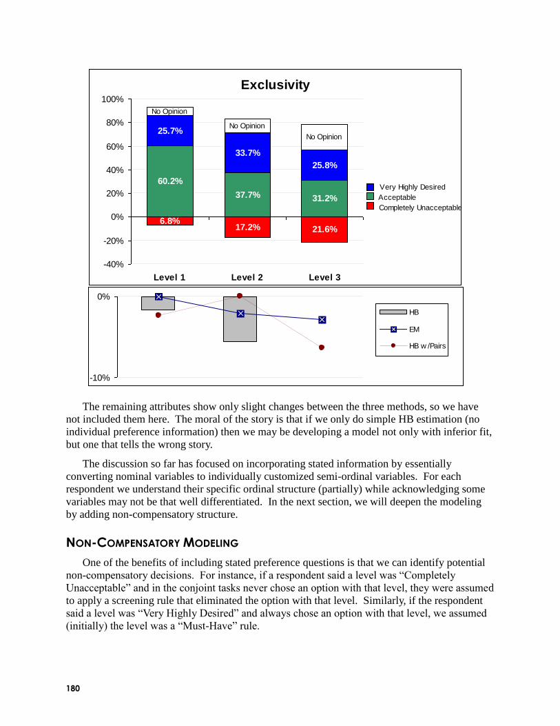
180

Exclusivity

37.7% 31.2%

25.7%

33.7%

25.8%

6.8%17.2% 21.6%

No Opinion

No Opinion

No Opinion

60.2%

-40%

-20%

0%

20%

40%

60%

80%

100%

Level 1 Level 2 Level 3

Very Highly Desired

Acceptable

Completely Unacceptable

-10%

0%

HB

EM

HB w /Pairs

The remaining attributes show only slight changes between the three methods, so we have

not included them here. The moral of the story is that if we only do simple HB estimation (no

individual preference information) then we may be developing a model not only with inferior fit,

but one that tells the wrong story.

The discussion so far has focused on incorporating stated information by essentially

converting nominal variables to individually customized semi-ordinal variables. For each

respondent we understand their specific ordinal structure (partially) while acknowledging some

variables may not be that well differentiated. In the next section, we will deepen the modeling

by adding non-compensatory structure.

NON-COMPENSATORY MODELING

One of the benefits of including stated preference questions is that we can identify potential

non-compensatory decisions. For instance, if a respondent said a level was ―Completely

Unacceptable‖ and in the conjoint tasks never chose an option with that level, they were assumed

to apply a screening rule that eliminated the option with that level. Similarly, if the respondent

said a level was ―Very Highly Desired‖ and always chose an option with that level, we assumed

(initially) the level was a ―Must-Have‖ rule.

181

It is well known that respondents tend to overstate their opinions about unacceptable or must-

have levels. This is the reason we confirmed their statements with their conjoint choices. For

instance, 90.5% of respondents reported at least one completely unacceptable level. But

comparing this against 12 actual choices, only 23.2% (164) were confirmed to apply an

unacceptable screening rule in their choice tasks.

The table below shows the number of respondents who were confirmed to apply screening

rules in their choice tasks.

Note that the column

totals do not add up

since there is overlap in

respondents. For

instance, a respondent

could say that Size 5 and

Change 2 of Activities

were both ―Completely

Unacceptable.‖

The highlighted

levels were those tested

in the holdout task. As

chance would have it,

most of the screening

rules did not apply to the

holdout task. Change 2

of the Activities attribute

where most people

screened did not appear

in the holdout task. Nor did the next most common screening levels – Size 1 and Size 5 appear

in the holdout task. Out of the 215 respondents who appeared to use non-compensatory rules,

only 107 of them used rules that applied in the holdout task.

The table below shows the results from adding the non-compensatory modeling, including

both the unacceptable and must-have levels.

Group

Size

EM Ordinal

Hit Rate

EM + Non-

Compensatory

Non-Comp Applied to Holdout 107 81 84

Other 600 437 439

Total 707 518 523

Hit Rate 73.3% 74.0%

Among the 107 respondents for whom the holdout task was non-compensatory, the number

of correctly predicted respondents only increased from 81 to 84. Most of the incorrectly

predicted holdout tasks among the 107 holdout relevant were caused by the ―Very Highly

Desired‖ non-compensatory rules (85% vs. 40%). So we also modeled just the ―Completely

Unacceptable,‖ with much better results.

Attribute Level

Completely

Unacceptable

Very Highly

Desired

Membership

Size 1 43 7

Size 2 12 12

Size 3 2

Size 4 10 7

Size 5 40 1

Activities

Status Quo 7 27

Change 1 1 4

Change 2 52

Committee

Structure

Status Quo 5

Change 1 6

Change 2 1 1

Private 1

(Exclusivity)

Level 1

Level 2 9 24

Level 3 12 5

Total 215 Unique Respondents 164 94

182

Group

Size

EM Ordinal

Hit Rate

EM + Completely

Unacceptable

Non-Comp Applied to Holdout 67 56 65

Other 640 462 468

Total 707 518 533

Hit Rate 73.3% 75.4%

Among those to whom the holdout tasks applied, the hit rate was 65 out of 67, or 97%. Had

the holdout tasks asked about more relevant levels, the 97% rate would translate into a

significant lift in hit rate.

In addition, this study was not ideal for the study of non-compensatory modeling. One

expects non-compensatory modeling to work better when there are more choices available

(rather than just two), and when a ―None‖ option is available.

Of the additional three case studies we have done, two were similar to this one and showed

only modest improvements in hit-rate with non-compensatory modeling. The third study was an

alternative-specific discrete choice study with 5 brands and a ―None‖ option available. In this

latter study hit rate improved from 56% to 61% when non-compensatory rules were added.

Most of that 5% lift in hit-rate was due to the ―Completely Unacceptable‖ screening rule.

CONCLUSIONS

Incorporating stated preference information by capturing the customized ordinal level of each

attribute for each respondent constrains the solution space and gives individual-level conjoint

estimates a much better chance of avoiding reversals. It also improves prediction of holdout

tasks. Failure to incorporate this kind of information risks reversals not only at the individual

level, but also at the aggregate story level. This means if we only do simple HB estimation (no

stated preference information) then we may be developing a model with inferior fit and one that

tells the wrong story.

The second use of stated preferences as described here is their potential for non-

compensatory modeling. Non-compensatory modeling will improve hit-rate with varying

degrees. It appears most effective when there are many choices and when the respondent has the

option to choose ―None.‖

Of course it is important to remember that this kind of linkage between stated preferences

and conjoint tasks depends upon respondents accurately reporting their preferences, and carefully

evaluating the conjoint tasks. Bad, confused, or lazy respondents will answer stated preferences

and conjoint scenarios in ways that do not align well. In those cases hit-rates may actually drop

with the addition of extra noise.

The degree to which incorporating stated preferences improves the results will likely depend

in part on the amount of information contained in the conjoint tasks relative to the total number

of parameters. If one were to ask respondents several hundred conjoint tasks (and they actually

evaluated all scenarios carefully), one would likely see little improvement by including stated

preferences (assuming there are a moderate number of parameters). But in most business

settings, respondents evaluate a limited number of scenarios relative to the number of

183

parameters. In these cases, there is a great deal of freedom in the solution space. Stated

preferences constrain that space, providing much additional information, and will likely improve

results. In the context of business applications, we think the case study described contains

information from the conjoint tasks that is high relative to the total parameters. Bear in mind that

there were only 17 parameters to estimate, and respondents were shown 12 binary conjoint tasks.

In practical business settings we often see alternative-specific designs with a much lower amount

of conjoint information relative to the number of parameters.

While the method described here shares some similarities with self-explicated conjoint

(Srinivasan 1988), it differs in several significant respects:

First, respondents only tell us whether an attribute is ―Completely Unacceptable,‖

―Acceptable,‖ or ―Very Highly Desired.‖ They are not required to give a specific rating

on a finer scale, which is likely to be a much more difficult task.

Second, stated preferences of levels are never compared across attributes. In the model

we described, a highly desired level from attribute A may have a lower utility than an

acceptable level of attribute B. We have tested cross-attribute constraints, and these did

not improve hit rate. The context of evaluating each level is within an attribute across

other levels within that attribute, and the analysis we recommend reflects that context.

Third, we do not ask respondents to tell us the relative importance of each attribute. We

believe trying to state the importance of an attribute defined by certain levels is a difficult

task for respondents to do accurately. Instead, the method described here derives the

importance of each attribute, as well as the relative spacing between each level based on

responses from the conjoint.

Finally, we want to issue caution in applying these methods. We have found that adding

simulated partial profiles in HB analysis requires many more iterations before convergence.

While stated preferences constraining the solution space are important, one must verify that the

added information is not impacting aggregate results negatively, especially when applying HB.

We recommend EM as the safer method for incorporating individual-level information, even if it

means slightly lower hit-rates.

184

REFERENCES

Allenby, Greg M., Neeraj Arora, and James L. Ginter: Incorporating Prior Knowledge into

the Analysis of Conjoint Studies. 1995. Journal of Marketing Research 32 (May), pp.

152-162.

Gilbride and Allenby: A Choice Model with Conjunctive, Disjunctive, and Compensatory

Screening Rules. 2004. Marketing Science 23(3), pp. 391–406.

Lattery, Kevin: EM CBC: A New Framework For Deriving Individual Conjoint Utilities by

Estimating Responses to Unobserved Tasks via Expectation-Maximization (EM). 2007.

Proceedings of the Sawtooth Software Conference, pp 127-138.

Otter, Thomas: HB-Analysis for Multi-Format Adaptive CBC. 2007. Proceedings of the

Sawtooth Software Conference, pp 111-126.

Srinivasan, S.: A Conjunctive-Compensatory Approach to the Self-Explication of

Multiattributes Preferences. 1988. Decision Sciences, 19 (Spring), 295–305.

Wittink, Dick: Predictive Validity of Conjoint Analysis. 2000. Proceedings of the Sawtooth

Software Conference.

185

INTRODUCTION OF QUANTITATIVE MARKETING

RESEARCH SOLUTIONS IN A TRADITIONAL

MANUFACTURING FIRM: PRACTICAL EXPERIENCES

ROBERT J. GOODWIN LIFETIME PRODUCTS, INC.

ABSTRACT

Lifetime Products, Inc., a traditional manufacturing company based in Clearfield, Utah, has

introduced progressively more sophisticated conjoint and other quantitative marketing research

tools over the past three years. Along the way, the company has gained valuable insight into the

process of adopting conjoint and choice analysis tools in this corporate environment.

This paper presents some of Lifetime‘s practical experiences as they relate to (a) challenges

experienced by key stakeholders in accepting and trusting conjoint analysis, (b) success stories

with conjoint analysis, and (c) the resulting escalation in client demands for more sophisticated

and robust conjoint tools. This case study should provide useful insight to marketing research

practitioners, especially those who either have or are planning to acquire similar conjoint tools

in-house.

INTRODUCTION

In a very general sense, entities that use – or are interested in – conjoint and choice analysis

may be classified into one of the following groups:

1. Academics who research and generate new statistical procedures and explore variations

and improvements in those procedures to meet specific research needs;

2. Research consultants who provide specialized and even customized research and

statistical services to corporate and other clients; and

3. Corporate and institutional research users who either retain the services of research

consultants or act as their own research practitioners to complete needed statistical

analyses to support management decision making.

While the work of the first two groups is well-represented in literature dealing with conjoint

and choice analysis, the third group – corporate research users – often receives less attention in

journal articles and conference presentations.

This paper presents a case history of Lifetime Products, Inc., a medium-size, traditionally

managed manufacturing company, as it decided to adopt a program of quantitative marketing

research to enhance its decision making process. In particular, this paper will:

1. Describe some of the challenges faced by the corporate marketing research department

and the proactive activities it employed to build trust among an often-skeptical in-house

clientele generally unfamiliar with conjoint and choice analysis;

186

2. Recount a few key examples of conjoint success stories that generated confidence in the

efficacy of these new statistical procedures; and

3. Demonstrate how this increased management confidence and the resulting escalation in

client demands required the corporate marketing research department to incrementally

increase its conjoint and choice analysis capabilities commensurately.

COMPANY BACKGROUND

Lifetime Products, Inc. is a privately held, vertically integrated manufacturing company

headquartered in Clearfield, Utah. Founded in 1986, Lifetime currently employs approximately

1,700 employees at multiple facilities in the United States, Mexico, and China. The company

manufactures consumer hard goods typically constructed of blow-molded polyethylene resin

and/or powder-coated steel. (See examples in Figure 1.) The company is considered ―vertically

integrated‖ because, in addition to product assembly, it also fabricates its own metal components

from steel coil and blow-molds its own plastic parts from high-density polyethylene pellets. Its

products are sold mainly to consumers and small businesses worldwide through a wide range of

department and discount stores, home improvement centers, warehouse clubs, office supply

stores, sporting goods stores, and other retail outlets.

Figure 1

Throughout its 23-year history, Lifetime Products has prided itself in the application of

innovation and cutting-edge technology in plastics and metals to create a family of affordable

lifestyle products that feature superior strength and durability. A few of the product ―firsts‖ for

the company include:

First home portable basketball system with height-adjustable rim and backboard

First folding utility tables and chairs using light-weight plastic resins and rust-resistant

steel structures

187

First resin-based outdoor storage/garden sheds with steel-reinforced roof and walls

First utility trailer featuring longitudinal fold-in-half functionality for easy storage

Lifetime‘s track record in product innovation and market success over the years had been

supported by an often-informal mix of qualitative marketing research efforts, including

secondary research, competitor analysis, focus groups, and feedback from purchasing agents at

key retail chain accounts. Over time, company management realized that it also needed more

sophisticated quantitative tools to better inform its decision making process and to facilitate

future success in its often-crowded and -maturing markets.

In 2006, Lifetime‘s marketing research department embarked on a program of conjoint and

choice analysis to help the company formalize its product development program by the use of

quantitative consumer input. Over the next three years, the company gradually increased the

sophistication of its conjoint and choice analysis capabilities to keep pace with escalating

management information demands (described later), adopting the following analytic programs in

fairly rapid succession:

1. SPSS Conventional Conjoint (2006);

2. Sawtooth Software Choice-based Conjoint (CBC) with Latent Class analysis (early

2007);

3. Sawtooth Software Partial-profile CBC using Advanced Design Module (late 2007); and

4. Sawtooth Software Adaptive Choice/ACBC with Hierarchical Bayes analysis (2008 beta

test; 2009 full implementation).

From 2006 to the present (late April 2009 at this writing), the company has engaged in 19

conjoint and choice analysis studies against a half-dozen product categories. The company‘s

practical experiences in implementing these quantitative research tools and using them in

multiple studies provides a foundation for the three main sections that follow.

I. CLIENT CHALLENGES IN ACCEPTING CONJOINT ANALYSIS

Lifetime Products implemented a number of ―trust-building‖ activities to help key

stakeholders to better understand – and trust – conjoint analysis as a tool to reduce uncertainty in

marketing decision making.

Despite the management‘s desire to augment its marketing research capabilities with

quantitative methods, they initially had many questions and even doubts about the conjoint

analysis tool as proposed by the marketing research director in 2006. They expressed incredulity

that with conjoint one could indeed (a) determine the relative value of attributes/levels, (b)

analyze all possible product combinations, and (c) conduct realistic market simulations, all by

simply asking respondents to sort a few product concept cards! Consequently, these stakeholders

were initially reluctant to make – or change – product development decisions based on conjoint

findings.

To allay some of these management concerns, the marketing research department instituted a

number of learning and trust-building activities and procedures to help management (a) to

become better acquainted with conjoint, (b) to bolster their confidence in the results therefrom,

188

and (c) to become a more integral part of the research process itself. The following section

describes some of these learning and trusting-building initiatives.

In-house Pretests. Since the beginning of the current decade, the company had used in-house

pretests occasionally as a means of debugging and ―wordsmithing‖ quantitative survey

instruments prior to fielding. With the introduction of conjoint analysis in 2006, however, the

pretest function took on increased importance. Since the conjoint survey method (i.e., card-

sorting initially) was so different from ―normal‖ survey protocols, efforts were made to ensure

that all key stakeholders (category and product managers, design engineers, marketing directors,

and even some senior management) were invited to serve as subjects in pretest interviews. The

purpose of this effort (in addition to the usual debugging) was to allow these stakeholders to

―walk through‖ the conjoint interview personally so they could better understand the conjoint

process and appreciate what ―live‖ respondents would be doing. Rudimentary conjoint utilities

were calculated from this collected pretest dataset, allowing stakeholders to see pro forma results

similar to those which would be generated from the consumer interviews to follow.

Out-of-House Pilot Tests. Prior to the full field work in many of these early conjoint studies,

the company also used out-of-house pilot tests against small convenience samples. These were

generally conducted as intercept interviews at a local mall research facility or appended to

already-scheduled focus-group discussions on the same topic. This procedure allowed category

and product managers to test ―straw-man‖ conjoint designs – often with large numbers of

attributes and/or levels that they felt were reflective of the customer mindset – in a relatively

inexpensive research setting. If the preliminary results (generally using sample sizes of only 40

to 80) suggested that a given attribute was contributing only a percent or two of importance to

the overall model, the stakeholders were more inclined to drop that attribute in favor of a more

parsimonious conjoint model prior to proceeding with the production phase of the study.

Proactive Demonstrations of Conjoint Capabilities. The initial SPSS conventional conjoint

software was ―sold‖ to management on the basis that, in general terms, it would be an excellent

way to provide consumer feedback on the relative value of product features and options, and thus

guide product development and marketing efforts. Ultimately, however, study results would

need to be presented in such a way that management was comfortable in relying on the

information for its decision making. The typical output of conjoint analysis – part-worth utilities

and average importance percentages – was found by stakeholders to be interesting but not always

useful. They sometimes asked that conjoint utility data be converted to a more understandable

―price-per-utile‖ indicator, but attempts to provide this type of dollar-equivalent metric often met

with theoretical and computational roadblocks (as discussed by Orme, pp. 1 & 5).

In an effort to provide more palatable delivery of conjoint results, Lifetime‘s marketing

research department began to conduct market simulations using realistic assumptions germane to

pending management decisions. However, early attempts to present these simulation results to

stakeholders left them with a feeling that the process was fairly ―black box.‖ They needed to

have a more flexible and insightful view of how the simulations worked in order to gain

confidence in the results. Consequently, the marketing research department began to construct

Excel-based market simulators for hands-on client use. (See Outdoor Storage Shed example in

static view in Figure 2.)

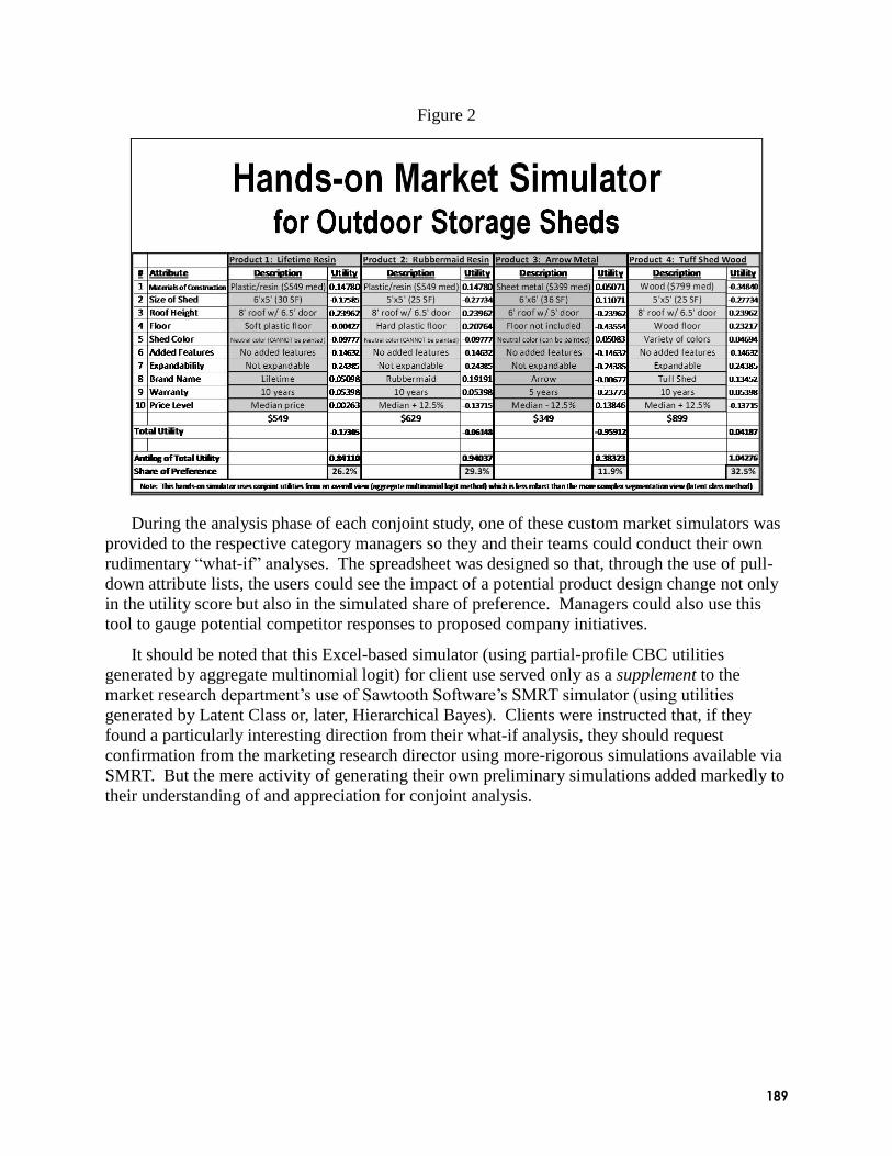
189

Figure 2

During the analysis phase of each conjoint study, one of these custom market simulators was

provided to the respective category managers so they and their teams could conduct their own

rudimentary ―what-if‖ analyses. The spreadsheet was designed so that, through the use of pull-

down attribute lists, the users could see the impact of a potential product design change not only

in the utility score but also in the simulated share of preference. Managers could also use this

tool to gauge potential competitor responses to proposed company initiatives.

It should be noted that this Excel-based simulator (using partial-profile CBC utilities

generated by aggregate multinomial logit) for client use served only as a supplement to the

market research department‘s use of Sawtooth Software‘s SMRT simulator (using utilities

generated by Latent Class or, later, Hierarchical Bayes). Clients were instructed that, if they

found a particularly interesting direction from their what-if analysis, they should request

confirmation from the marketing research director using more-rigorous simulations available via

SMRT. But the mere activity of generating their own preliminary simulations added markedly to

their understanding of and appreciation for conjoint analysis.

190

II. SUCCESS STORIES WITH CONJOINT ANALYSIS

As Lifetime progressed in its use of conjoint analysis tools, a number of conjoint findings

have had a direct impact on product and marketing decision-making. This section will describe

some of these success stories.

Success Story #1: Fold-in-half Utility Trailer. Lifetime Products conducted its first conjoint

study in 2006 as it was planning the market introduction of an innovative new fold-in-half design

of utility trailer. (See fold-up sequence in Figure 3.) This survey was administered in four mall

locations across the U.S. (the folded-up trailer was even wheeled into the small interview rooms

to demonstrate the fold-up feature ―live‖) and the analysis done using SPSS Conventional

Conjoint from a card-sort survey method.

Figure 3

One of the primary objectives of this study was to determine an appropriate initial retail price

point for the fold-in-half trailer. A pre-conjoint question asked respondents to project what price

they would expect to see on the price tag for this new product. The distribution of responses had

a noticeable downward inflection above the $999 price point. Subsequent conjoint analysis

using part-worth plots and market simulations confirmed that demand for this new concept might

be considerably restrained if it were priced above $999.

“The Rest of the Story...” Due to cost and other considerations, the new fold-in-half utility

trailer was introduced at a manufacturer‘s suggested retail price (MSRP) somewhat above the

$999 price point suggested by the conjoint findings. First-year sales of the product were

substantially lower than hoped for. However, subsequent sales promotions down to $999 or less

often resulted in substantial boosts in unit sales. As a result, management gained initial respect

for conjoint analysis as a tool to help predict consumer price sensitivity.

Success Story #2: Folding Utility Chair. This conjoint study involved a visual and tactile

comparison of Lifetime‘s commercial-grade folding utility chair (at far left in Figure 4) against

three other similar steel-and-plastic offerings and a popular padded vinyl model. These folding

utility chairs are used not only as supplemental seating in the home, but also in large numbers by

churches, clubs, schools, and businesses for banquets, meetings, temporary work use, and the

like.

191

Figure 4

One of the key objectives of this study was to determine price sensitivity for the Lifetime

commercial-grade folding utility chair. Most retailers had been pricing the chair at $19.99 and

were hesitant to breach this perceptual price barrier. This study, using mall-intercept surveying

in five U.S. cities, was one of the company‘s first uses of Sawtooth Software‘s Choice-based

Conjoint (CBC) with Latent Class segmentation analysis.

The conventional wisdom was that, at first glance, the padded vinyl chair would be perceived

as the most comfortable of the five models, simply because it was the only padded option.

However, qualitative research by Lifetime had found that many consumers were ―pleasantly

surprised‖ at the ergonomic comfort of the ―hard‖ Lifetime steel-and-polyethylene chair.

Therefore it was considered essential that respondents not only view but also sit in each chair

before proceeding with the conjoint experiment.

The CBC and Latent Class analyses produced evidence that the market was somewhat price-

insensitive to the Lifetime commercial-grade folding utility chair at retail prices above $19.99.

Crosstabulations of the price utilities by chair model showed a definite flattening above $19.99

for the Lifetime chair, especially when contrasted with the other, more price-sensitive models.

Results of market simulations showed virtually no degradation in share of preference for the

Lifetime chair when priced above $19.99 (even with the non-commercial competitors simulated

at $17.99 or below). Thus, it appeared that consumers who were most sensitive to a $20-plus

price had already decided to purchase a lower-cost, non-commercial model, even without a

Lifetime price increase. Latent Class analysis confirmed that there was indeed a very loyal

Lifetime-friendly segment that was relatively price-tolerant to the Lifetime chair within the

$19.99 to $21.99 range. (See Figure 5.)

192

Figure 5

“The rest of the story…” The Lifetime sales department began to ―educate‖ retail accounts

on the results of this pricing analysis and its potential ramifications for increasing the

profitability of this SKU. Eventually several retailers decided to boost their prices above the

traditional $19.99 price point. Initially, there were no serious sales consequences to this action.

However, the current worldwide economic downturn eventually depressed sales volumes for all

furniture products (including the Lifetime chair), so the issue is presently clouded (i.e., ―the jury

is still out‖). Even so, Lifetime sales managers say they like having this type of concrete data on

consumer price perceptions, considering it to be valuable ―ammunition‖ when negotiating with

their retail accounts.

Success Story #3: Market Segmentation. For many years, Lifetime‘s products were

developed nominally with the ―mass market‖ in mind. The company conducted little if any

segmentation analysis to examine differences in preferences or price sensitivity among different

segments of the market. As the company began to develop different product grades or models

for various market segments, management began to feel the need to study differences in segment

preferences more formally.

“The rest of the story…” With the introduction of Sawtooth Software‘s CBC with Latent

Class analysis in 2007, Lifetime had to ability to explore behavioral market segments within the

context of conjoint analysis projects. In all product categories studied, these analyses revealed

several distinct market segments, often defined by quality, product features, and price sensitivity.

(For example, see generalized visualization of Basketball consumer segments in Figure 6.)

These findings supported nascent company efforts to position itself as the supplier of choice for

consumer market segments demanding high-quality, feature-rich product designs (though not

necessarily at the lowest price). (The company has since acquired Sawtooth Software‘s

193

Convergent Cluster & Ensemble Analysis package – CCEA – for more generalized segmentation

analysis.)

Figure 6

Small Backboard Medium Backboard Large Backboard

Pri

ce S

ensi

tivi

tyLo

wM

od

erat

eH

igh

Group A

Group C

Group B

Group D

Highly price-sensitive, so prefers small-backboard systems at lowest price; little else matters!

30-something downscale female; probably a prospect or owns a portable bought at a discount store for a pre-teen primary user

Somewhat price-sensitive; prefers medium-backboard

with some premium features30-something male; probably

owns in-ground system bought at sporting goods store for a

teenage primary user

Somewhat price-sensitive; prefers small- or medium-backboard

systems; wants some features (esp. easy height adjustment)

Demographic mix; owns a portable bought at a discount store for a pre-

teen primary user

Least price-sensitive, so strongly prefers large-backboard systems with beefed-up construction and premium features

20-something male, probably college-educated; owns either a portable or in-ground system bought at a sporting goods store (probably for himself)

Generalized Visualization of Basketball Latent-class Segments

Success Story #4: Folding Utility Table ―Back-forecast.‖ Lifetime Products recently

conducted a cooperative partial-profile CBC study on polyethylene-and-steel folding utility

tables with a retail chain store account. While most of the results of this study are proprietary, a

summary of a ―back-forecast‖ calibration simulation can be shared in this paper.

A key component of the analysis was to generate market simulations of the array of different

sizes of Lifetime tables and compare the share-of-preference results with the actual sales

distributions for these table models. Regardless of the simulation assumptions employed, it was

clear that (a) the conjoint model consistently overestimated sales of larger tables and

underestimated sales of smaller tables and (b) the mean absolute errors (MAEs) of prediction

were in the 7% to 9% range. Tuning the sensitivity of the market simulator using of a scaling

factor (or exponent) of 0.45 provided the best possible MAE improvement (to just under 5%),

but the pattern of over- and underestimation was still evident.

“The rest of the story…” While these findings were of some concern to the company and its

retail account, further analysis of the consumer purchasing process led to an interesting

explanation for this apparent conjoint model ―residual‖ error. It was concluded that the purchase

decision making process is probably somewhat different for small vs. large tables (as described

in Figure 7). As a result, what began as an initially disturbing finding became the springboard

for illuminated understanding of customer behavior.

194

Figure 7

III. ESCALATING CLIENT DEMANDS ON CONJOINT ANALYSIS

As Lifetime managers gained confidence in the conjoint method, they began to place

increasingly greater demands on the analysis. This section will describe company actions taken

to respond to this demand.

Use of Graphics in Partial-profile CBC. As Lifetime managers gained greater confidence in

conjoint analysis, particularly with the adoption of choice-based conjoint, they were no longer

satisfied with simplified product models involving only five or six attributes (a generally

accepted limit for reasonable respondent understanding and attention). When the company

upgraded from full-profile to partial-profile CBC (using Sawtooth Software‘s Advanced Design

Module), it was possible to design models with ten, fifteen, or more attributes, while displaying

only five or six at a time in each choice task. Given the rotation of attributes and changing

product configurations from task to task, however, the marketing research department concluded

that it would be helpful to use graphics to facilitate respondent comprehension. (See Trailer

example in Figure 8; note that animated GIF files were included in the actual online interview to

demonstrate the trailer‘s fold-in-half feature in the choice task at far right.)

Figure 8

195

The Next Step: Adaptive Choice/ACBC. While partial-profile CBC with use of graphics

became Lifetime‘s conjoint method of choice in late 2007 and 2008, it still had several perceived

shortcomings. The use of graphic attribute representations did much to facilitate respondent

understanding during the interview, but it was still felt that the task assignments involving only a

portion of the attributes in each task were not as realistic as desired. There was always some

doubt as to how respondents behaved as they read ―assume any feature not listed is the same for

all three options.‖ Of even greater concern to the company was the need for larger sample sizes

to compensate for the reduced individual information in each sample point. Analysis of standard

errors in the CBC designs suggested that sample sizes in the order of 700 to 800 (or more) might

be needed for a typical Lifetime study of 12 to 15 attributes shown only five at a time.

Because of these concerns, the company watched the development of Adaptive

Choice/ACBC by Sawtooth Software with great interest and was excited to serve as a beta tester

in late 2008. Lifetime viewed the value proposition for ACBC as having the flexibility of

adaptive conjoint (such as Sawtooth‘s ACA application), the realism of choice-based conjoint,

and the task simplification of partial-profile CBC, all with more reasonable sample sizes.

The company‘s first ACBC beta-test study, involving Outdoor Storage Sheds, consisted of 16

attributes and 45 levels (eight brand names was the maximum levels used for any one attribute).

Constructed-list technology was used to reduce the attributes shown to each respondent from 16

to 10 (see screenshot example in Figure 9) and brand names from eight to four. In essence, each

respondent had to deal with his/her most important 10 attributes, but the entire market considered

all 16. The sample size was reduced considerably from the level needed in comparable partial-

profile CBC studies (400 vs. 800 or more).

Figure 9

196

At the same time, the company was favorably impressed by the innovative survey devices in

the ACBC interview, such as the Build Your Own worksheet (or BYO; see screenshot example in

Figures 10a & 10b), Must Have and Unacceptable reality checks (to more accurately capture

non-compensatory decision behaviors), and an engaging adaptive interview protocol

(personalized by the use of ―sales associate‖ model photographs).

Figures 10a & 10b

197

With the upgrades available in version 1 of ACBC, Lifetime now has the ability to use the

conditional graphics feature demonstrated in static form in Figure 11. The company is currently

(late April 2009) conducting an ACBC project on Backyard Playsets where various

configurations of swings, clubhouse designs, and other activity centers, along with different color

combinations, are depicted graphically throughout the ACBC online interview.

Figure 11

CONCLUSION

As a relatively new user of quantitative marketing analysis, Lifetime Products, Inc. has been

able to increase its analytic sophistication using conjoint and choice analysis. The company‘s

internal clients have gradually increased in their understanding of and trust in these analytic

techniques and are starting to rely more heavily on the results in their product and marketing

decision-making. As the level of trust has increased, these clients have begun to demand

increasingly more sophisticated solutions, leading up to Adaptive Choice/ACBC. Graphic

representations of products in survey instruments are being used to enhance respondent

understanding of complex product designs in conjoint models.

198

ADVICE TO NEW CONJOINT PRACTITIONERS

This paper represents a summary of key actions and practical experiences that have helped

Lifetime Products, Inc. to adopt sophisticated conjoint and choice analysis tools for better

decision making. To the extent that this case study may help other conjoint practitioners,

particularly those using or planning to implement similar tools in-house, here is a brief list of

suggestions for consideration:

1. Solicit support from a marketing research “champion” within the organization (i.e.,

someone already familiar with the benefits – if not the technical details – of quantitative

research tools);

2. Ask internal clients (and key management!) to participate “hands-on” in conjoint study

planning and development processes;

3. Demonstrate conjoint capabilities to stakeholders using lower-risk (i.e., lower-cost) tools

first;

4. Benchmark conjoint results against actual performance wherever possible; and

5. As managers gain trust and confidence in the conjoint method, upgrade tools to provide

the increased functionality they demand.

Referring to the third and fifth points above, Andrew Elder, discussant for this paper at the

2009 Sawtooth Software Conference, posed the question as to whether, in retrospect, Lifetime

would have adopted ACBC if that product had been immediately available when the company

started using conjoint tools in 2006. Given the price sensitivities of a medium-size

manufacturing company such as Lifetime and its virtual lack of prior use of quantitative

marketing research tools, it is doubtful that the company would have ―sprung for‖ a new,

sophisticated, and admittedly pricey option such as ACBC without any in-house track record to

examine. Internal clients were initially unfamiliar with the methods and results of these tools

and probably needed the ―conjoint acclimatization‖ from less-sophisticated and less-expensive

options. Only after they began to see the real value of conjoint and choice analysis – and they

started to demand increasingly more sophisticated tools – did their decisions to upgrade come

with relative ease.

REFERENCE

Orme, Bryan K. (2001); Assessing the Monetary Value of Attribute Levels with Conjoint

Analysis: Warnings and Suggestions; Sawtooth Software Research Paper Series.

199

CBC VS. ACBC: COMPARING RESULTS WITH

REAL PRODUCT SELECTION

CHRISTOPHER N. CHAPMAN MICROSOFT CORPORATION

JAMES L. ALFORD VOLT INFORMATION SCIENCES

CHAD JOHNSON, RON WEIDEMANN

ANSWERS RESEARCH

MICHAL LAHAV

SAKSON & TAYLOR CONSULTING

ABSTRACT

We examined consumer preference for a computer accessory product line with an online

survey. Every respondent completed both a choice-based conjoint (CBC) procedure and an

adaptive choice-based conjoint (ACBC) procedure using the same attributes. Our goal was to

predict market share and to answer both methodological and managerial questions. In evaluating

within-subjects results, CBC and ACBC gave generally similar estimates, with ACBC estimating

greater price sensitivity and giving a smaller standard deviation of respondent utilities. When

estimated head-to-head preference between two products was compared to actual market data,

ACBC agreed closely with actual market data. In a 4-product portfolio, ACBC predictions of

preference share were in somewhat closer agreement to observed market data than those using

CBC data; the ACBC error proportion was 15-25% lower than the error rate with CBC data.

BACKGROUND AND MANAGERIAL QUESTION

Our product team was preparing to launch a PC accessory consumer electronics (CE) product

(hereafter Product A) when a competitor released an identically priced product (Product B) that

had a higher specification in one feature area that is highly salient to consumers. We wished to

determine the competitive threat from Product B and decide whether to immediately launch a

development effort to update Product A so that it would match the specification of Product B.

Working with the product management team, we refined the competitive question to one that

was amenable to research. Balancing the development cost against market size, we determined a

threshold for action of 25% head-to-head preference share. That is, if Product A achieved at least

25% consumer preference vs. Product B, we would keep Product A unchanged. However, if its

preference share was less than 25% vs. Product B, we would undertake to update the product.

Because of the managerial importance of this question, we wished to assess the preference

with multiple methods in order to have maximal confidence in the result. To assess preference,

we chose to use four methods: traditional Choice-Based Conjoint analysis (CBC; Sawtooth

Software, 2008); the newly developed Adaptive Choice-Based Conjoint analysis (ACBC;

Johnson & Orme, 2007); a single monadic item presented as a CBC holdout task; and a final

offer in which respondents were allowed to receive either Product A or B at no cost.

200

METHOD

We designed a single online survey using Sawtooth Software‘s SSI Web, comprising both

CBC and ACBC exercises. The choice exercises had eight attributes: brand, price, and six

product features, ranging from 2-5 levels per attribute. All attributes and levels were identical on

the CBC and ACBC portions, except that Price showed minor variance between the two due to

different methods for constructing conditional pricing in Sawtooth Software CBC vs. ACBC

questionnaires. The difference was typically no more than $5-10 for comparable products, well

within the range of conditional price randomization.

The survey was designed for all respondents to answer both CBC and ACBC exercises in

randomly counterbalanced order. The CBC section included a fixed task that directly assessed

the preference between Product A, Product B, and a third product designed to have minimal

appeal. The CBC exercise comprised 12 random tasks plus 2 fixed tasks. The ACBC exercise

comprised a BYO configurator task, 9 screening tasks of 3 concepts each, a choice tournament

with 3 concepts in each group, and a final four-item calibration section (unused in the analyses

presented here).

At the end of the survey, 25% of respondents were randomly selected and offered a free

product, where they could choose to receive either Product A or Product B at no cost.

We also wished to examine the extent to which traditional randomized task/attribute format

choice tasks could predict real market behavior (where products may be described differently

than as a list of features). Thus, the final ―real‖ product selection task presented a richer, more

complete description of the available products than the CBC and ACBC exercises, comprising a

superset of the choice exercises‘ feature descriptions. By doing this, we could contrast the rich

selection task with both CBC and ACBC estimates and with a traditional holdout task presented

in CBC format, potentially yielding a different estimate of overall preference that would be

informative for the managerial question with regards to the sensitivity of our findings.

Respondent utility scores were computed for both CBC and ACBC sections using Sawtooth

Software Hierarchical Bayes (HB) estimation with 40000 total iterations. CBC and ACBC

results were compared on the basis of overall utility estimation pattern, sample-level correlation

between equivalent attribute/level utilities, within-subject correlation across utilities, holdout

task prediction, and prediction of actual product selection. We used respondents‘ individually

estimated mean HB scores (i.e., beta scores), converted to zero-centered difference scores to

reduce between-respondent scale effects (Sawtooth Software, 1999).

After six months, actual market data was available for comparison of real channel sales

performance as compared to the predicted preference in the survey. The product team agreed at

the inception of the product that we were interested in consumer preference with all other factors

being equal – as opposed to actual market share in which other factors are not equal. Still, it was

of interest to determine the degree to which the methods reflected actual market performance.

RESULTS

N=400 respondents (PC-using adults in the US, enriched for broadband users) completed the

survey. Median time to completion for CBC (when it was taken first, N=201) was 244 seconds,

while ACBC (taken first, N=199) had median 442 seconds.

201

In terms of subjective respondent experience, on the scales proposed by Johnson & Orme

(2007), respondents showed no significant differences between CBC and ACBC tasks on self-

report ratings of product realism, survey interest, realistic answers, or attention (t-test, all p>.05).

There was a modest effect for "This survey is at times monotonous and boring,‖ where

respondents who took CBC first reported being more bored after the first choice section than

were those who started with ACBC (means 3.04 and 2.75 on 5-point scale; t=2.33, df=397,

p<.05). In other words, ACBC was perceived as somewhat less boring than CBC despite that it

took 80% longer on average (including the calibration items, which were not used in HB

estimation).

ACBC and CBC yielded moderately different utility estimates. Figure 1 shows the mean

utility by feature and level, for zero-centered difference (normalized) utility scores. Apart from

Brand, ACBC yielded utilities with an equivalent or larger range than CBC between best and

worst mean levels within an attribute. This is consistent with the ACBC method‘s hope to obtain

better estimates of feature value beyond a few important attributes (Johnson & Orme, 2007). In

particular, ACBC yielded a higher utility weight for Price (at the low point), i.e., ACBC

estimated a higher average respondent price sensitivity than did CBC.

Figure 1

Although the mean utility levels were somewhat more extreme, ACBC generally yielded

lower standard deviations within feature level than CBC. The ratio of ACBC:CBC standard

deviations ranged from 0.46 to 1.24 with an average ratio of 0.79 ACBC:CBC standard deviation

on raw scores; and 0.45 to 1.50 with mean 0.69 for zero-centered differences (normalized)

utilities. This suggests that to achieve comparable standard errors of group-level utility means

with a similar product and feature set, ACBC would need about 38% fewer respondents than

CBC.

202

Figure 2

One product attribute, Feature 2, had five levels, of which two sets of two levels were

naturally ordered (e.g., similar to memory size or price, where one level should always be

preferred to another). Within Feature 2, we expected to see level 4 > Level 2, and Level 5 >

Level 3. As shown in Figure 3, without constraints on HB estimation, we observed reversal on

both sets with CBC/HB estimation, but ordering as expected with ACBC/HB estimation.

Figure 3

Across respondents, correlations between zero-centered difference utilities estimated by CBC

and ACBC on 18 identical attribute levels (e.g., a specific brand; we omitted one level from two-

level attributes, as they are identical except for direction) ranged from r=0.12 (for one level of a

5-valued attribute; p<.05, df=398) to r=0.62 (for Price, estimated at one point; p<.01, df=398),

with a median correlation of r=0.42 Correlation after transforming to multinormality with the

Box-Cox procedure (Box & Cox, 1964) yielded nearly identical correlations. These correlations

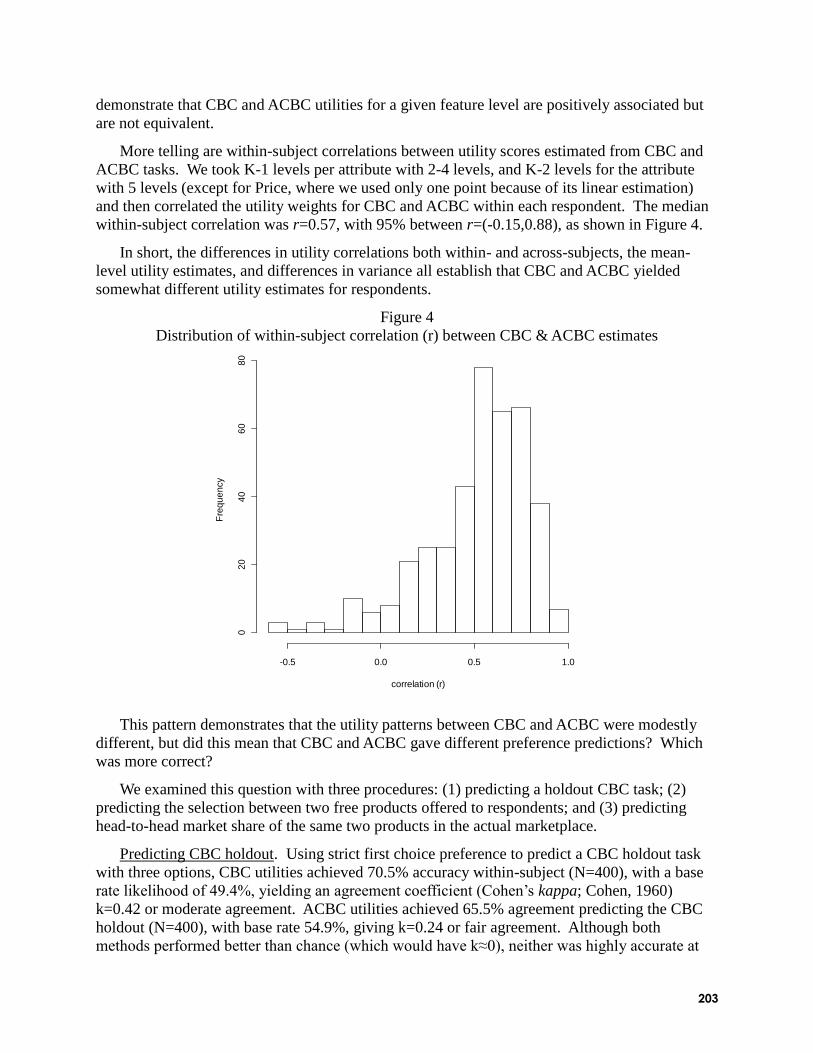
203

demonstrate that CBC and ACBC utilities for a given feature level are positively associated but

are not equivalent.

More telling are within-subject correlations between utility scores estimated from CBC and

ACBC tasks. We took K-1 levels per attribute with 2-4 levels, and K-2 levels for the attribute

with 5 levels (except for Price, where we used only one point because of its linear estimation)

and then correlated the utility weights for CBC and ACBC within each respondent. The median

within-subject correlation was r=0.57, with 95% between r=(-0.15,0.88), as shown in Figure 4.

In short, the differences in utility correlations both within- and across-subjects, the mean-

level utility estimates, and differences in variance all establish that CBC and ACBC yielded

somewhat different utility estimates for respondents.

Figure 4

Distribution of within-subject correlation (r) between CBC & ACBC estimates Chart 2: Within-subject correlation of CBC and ACBC utilities

correlation (r)

Fre

qu

en

cy

-0.5 0.0 0.5 1.0

02

04

06

08

0

This pattern demonstrates that the utility patterns between CBC and ACBC were modestly

different, but did this mean that CBC and ACBC gave different preference predictions? Which

was more correct?

We examined this question with three procedures: (1) predicting a holdout CBC task; (2)

predicting the selection between two free products offered to respondents; and (3) predicting

head-to-head market share of the same two products in the actual marketplace.

Predicting CBC holdout. Using strict first choice preference to predict a CBC holdout task

with three options, CBC utilities achieved 70.5% accuracy within-subject (N=400), with a base

rate likelihood of 49.4%, yielding an agreement coefficient (Cohen‘s kappa; Cohen, 1960)

k=0.42 or moderate agreement. ACBC utilities achieved 65.5% agreement predicting the CBC

holdout (N=400), with base rate 54.9%, giving k=0.24 or fair agreement. Although both

methods performed better than chance (which would have k≈0), neither was highly accurate at

204

within-subject prediction (which would occur with k>0.7). Not surprisingly, CBC did slightly

better as the holdout task was in CBC-style format and was part of the CBC trial block.

Predicting final product selection. N=100 respondents were offered a dichotomous free

choice between Products A and B, presented at the end of survey with a rich product description

(similar to a web-based shopping format). 53/100 respondents chose to receive Product A, while

47/100 chose Product B.

Preference differentiation was stronger for CBC utilities than for ACBC utilities. Of N=162

respondents estimated by CBC to prefer Product 1 in head-to-head preference, the median

preference estimate (i.e., logit rule summed utility value) was 0.927, with sd=0.158; of N=130

estimated by ACBC to prefer Product 1, the median preference was 0.802, sd=0.157.

Using strict first-choice preference, CBC utilities accurately predicted 56/100 actual choices

of the free product, while ACBC correctly predicted 53/100 actual choices. With a standardized

base rate (combined marginal probability) of 49/100, this yields kappa agreement coefficients of

k=0.14 and k=0.08, respectively, or ―slight‖ agreement between within-subject prediction and

actual behavior. Thus, in this study, neither CBC nor ACBC utilities were very good predictors

of within-subject choice on the free product offer, and their performance was lower for this task

than for the assessed holdout task described above. The reasons for these low agreement rates

are unknown, and may include the effects of differing task presentation, respondent

inconsistency, ―found money‖ effects from a free product offer (although the prices were

equivalent), or a novelty effect (e.g., if a respondent happened to own one of the products

already).

More interesting is the group-level difference in preference share between CBC, ACBC, and

real choice. CBC utilities estimate a head-to-head preference for the product of interest (using

strict first-choice preference) as 43.5%±5.0%, while ACBC utilities estimate 33.0%±4.8%

preference. Actual selection by N=100 respondents was 53/100 choosing the target product on

the free selection offer, with a binomial confidence interval of ±10% (i.e., confidence range of

43%-63% preference). Thus, the CBC confidence range (but not center) overlapped the

confidence range for observed product selection on the free product offer, while the ACBC range

did not.

It is important to emphasize that the free selection task differed from CBC/ACBC tasks in

two ways: (1) it was an actual, not a hypothetical choice; (2) it came at the end of the survey and

presented more features, with more descriptive text, in richer context, emulating an Internet-style

product display. We have found previously (Chapman et al, unpublished) that CBC performance

at predicting actual behavior was higher when the CBC survey format closely matched the actual

product selection format (cf. also Martin & Rayner, 2008).

Predicting market response. As noted above, in a head-to-head comparison, CBC predicted

43.5%±5.0% preference share for Product A, while ACBC predicted 33.0%±4.8% preference

share. Actual market data for Product A showed a head-to-head market share of 34.6% (this was

calculated as unit sales of A / (unit sales of A + unit sales of B), with an unknown confidence

interval). The ACBC prediction of preference share was not statistically significantly different

from the observed actual market share – an impressive result for the product team.

Tuning of response. Although head-to-head preference prediction was the key research

question and ACBC answered the question quite well, a more interesting question involves

205

prediction among more than 2 products. Utility estimates from conjoint analysis surveys often

need to be ―tuned‖ to adjust the utilities by a constant factor that allows better prediction in

comparison to actual market results (Orme & Heft, 1999).

We evaluated the tuning coefficients vs. actual market data using the Sawtooth Software

SMRT market simulator with randomized first choice selection, including in the simulation all

four products in the studied category that have greater than 5% unit share and are in the price

range we studied. We selected the best-selling product as the baseline and adjusted the utility

exponent until that product‘s share most closely matched actual sales data. The best fit for CBC

data was obtained with a utility multiplier (i.e., exponent) of 0.28, while ACBC best fit had an

exponent of 0.14.

As shown in Table 1, mean absolute error (MAE) and root mean squared error (RMSE) were

reduced by 20-50% by tuning the utility exponent. After tuning, ACBC had errors that were 15-

25% smaller than those of CBC.

Table 1

Actual and Predicted Shares, Before and After Utility Exponent Tuning

Product

Actual

Market

share

CBC

Exp 1

TUNED

CBC

Exp 0.28

ACBC

Exp 1

TUNED

ACBC

Exp 0.14

Product A 0.141 0.285 0.282 0.164 0.252

Product B 0.266 0.122 0.172 0.169 0.181

Other 1

[tuning baseline]

0.401 0.511 0.403 0.636 0.403

Other 2 0.192 0.082 0.143 0.031 0.164

MAE (3 products) -- 0.127 0.095 0.129 0.082

RMSE (3 products) -- 0.128 0.102 0.151 0.075

CONCLUSION

For our consumer electronics (CE) product, ACBC and CBC yielded generally comparable

utility estimates. Combining the two methods gave us high confidence in the ability to answer

the managerial question of interest with reduced dependence on a single method. The ACBC

procedure gave slightly smaller standard deviation of utility beta estimates across respondents,

indicating that it may produce stable results with smaller sample sizes. ACBC also estimated

higher price sensitivity of respondents, and yielded preference order for certain levels (without

constraints) that were more closely aligned to expectation than CBC. Neither method was highly

effective at prediction of within-subject preference, but this was of marginal interest for our

application, as we wished to predict group-level preference.

In head-to-head product preference estimation, ACBC was a substantially closer match to

observed market data, with no statistically significant difference between predicted and observed

206

head-to-head preference between the two products of interest. When modeling a lineup of three

products, with exponent tuning to match a holdout product share, ACBC had an average error of

7.5-8.2% vs. market data, compared to 9.5-10.2% for CBC.

In short, the performance of ACBC for our CE product was similar to CBC and somewhat

better in alignment with market data. We believe future research would be useful to determine

whether this pattern of results (better prediction; higher price sensitivity; lower standard

deviation) continues with other product categories. We hope other researchers will

systematically include the kinds of external market validity and between-methods measures that

we investigated.

REFERENCES

Box, G. E. P., and Cox, D. R. (1964). An Analysis of Transformations. Journal of the Royal

Statistical Society, Series B 26: 211–246. http://www.jstor.org/stable/2984418.

Chapman, C. N., Alford, J., Lahav, M., Johnson, C., and Weidemann, R. (unpublished).

Conjoint Analysis Prediction and Actual Behavior: Three Studies.

Cohen, J. (1960). A Coefficient of Agreement for Nominal Scales. Educational and

Psychological Measurement, vol.20, no.1, pp. 37–46.

Johnson, R. M., and Orme, B. K. (2007). A New Approach to Adaptive CBC. Sawtooth

Software, Sequim, WA.

Martin, B, and Rayner, B. (2008). An Empirical Test of Pricing Techniques. Paper presented

at Advanced Research Techniques Forum (A/R/T Forum) 2008, Asheville, NC.

Orme, B. K., and Heft, M.A. (1999), Predicting Actual Sales with CBC: How Capturing

Heterogeneity Improves Results. Available online at

http://www.sawtoothsoftware.com/download/techpap/predict.pdf; last accessed April 13,

2009.

Sawtooth Software (1999). Scaling Conjoint Part Worths: Points vs. Zero-Centered Diffs.

Available online at http://www.sawtoothsoftware.com/education/ss/ss10.shtml; last accessed

April 13, 2009.

Sawtooth Software (2008). CBC 6.0 Technical Paper. Available online at

http://www.sawtoothsoftware.com/download/techpap/cbctech.pdf; last accessed April 13,

2009.

ACKNOWLEDGEMENTS

The authors thank Bryan Orme of Sawtooth Software for extensive feedback and discussion

of both the research plan and data analysis, as well as discussion at the Sawtooth Software

Conference (SSC) 2009, and thank Rich Johnson of Sawtooth Software for review and

comments on initial results. We also thank Dr. Edwin Love of Western Washington University,

with whom we had fruitful discussions of the research plan and data analysis; colleagues at

Microsoft Hardware who posed the initial research questions and supported our sharing methods

and results with the research community; and many attendees of SSC 2009 for their insightful

questions and discussion.

207

NON-COMPENSATORY (AND COMPENSATORY) MODELS OF

CONSIDERATION-SET DECISIONS

JOHN R. HAUSER MIT

MIN DING PENNSYLVANIA STATE UNIVERSITY

STEVEN P. GASKIN APPLIED MARKETING SCIENCES, INC.

WHY STUDY CONSIDERATION SETS

If customers do not consider your product, they can‘t choose it. There is evidence that 80%

of the uncertainty in choice models can be explained by simply knowing the consideration set

(Hauser 1978). Many important managerial decisions rely on identifying how customers form

consideration sets: Which features lead customers to eliminate certain products from further

consideration? Which features lead customers to seek further information and thus open the

opportunity for a sale? How do technical specifications and quantifiable features of a product

interact with more qualitative features such as service or reliability? Does ―brand‖ drive

consideration? And what can a firm do about it?

This problem is real. Even though a Buick was tied in 2008 with Lexus as the top-ranked

automobile on a J. D. Power dependability study, was the top-ranked American car by Consumer

Reports, and produced cars from the top-ranked US factory for quality, in 2008 few US

consumers would even consider a Buick – in California almost two-thirds of consumers rejected

GM cars without evaluating them; nationwide the percentage was closer to 50%. Investments in

reliability, quality, safety, ride and handling, comfort, navigation, interiors, and Onstar become

irrelevant if consumers never get beyond the consideration stage. For this and other reasons, the

US automobile manufacturers were considering or entering bankruptcy in the spring of 2009.

Autos are but one example. In frequently-purchased products, such as deodorants,

consumers consider only a small fraction of those available (typically 10%, Hauser and

Wernerfelt 1990). Leverage can be huge. There are 350+ auto/truck brands on the market, but

the typical consumer considers roughly 5-6 brands. A strategy that increases the likelihood that

an automobile brand is considered could increase a firm‘s odds of making a sale from 1 in 350 to

1 in 6 – a substantial improvement.

208

Much of the conjoint-analysis literature and most conjoint-analysis applications have focused

on preference or choice. Recently, a number of papers have focused on choice, conditioned on

consideration, providing evidence that two-stage, consider-then-choose models often improve

both realism and accuracy.1 Sometimes these papers measure consideration explicitly; other

times consideration is an inferred construct.

More recently, papers have begun to focus on the consideration decision itself recognizing

that managerial actions can be taken to affect consideration directly. For example, advertising

might stress a J. D. Power result, make salient a screening feature, or select product features that

are likely to lead to consideration.

Research in consumer behavior suggests that the consideration decision might be

fundamentally different than the choice decision (e.g., Bronnenberg and Vanhonacker 1996;

DeSarbo et al., 1996; Hauser and Wernerfelt 1990; Jedidi, Kohli and DeSarbo, 1996; Mehta,

Rajiv, and Srinivasan, 2003; Montgomery and Svenson 1976; Payne 1976; Roberts and Lattin,

1991, 1997; Shocker et al., 1991; Wu and Rangaswamy 2003). Consumers often process a large

number of products (possibly hundreds) or a large number of features (possibly 50 or more) and

make decisions rapidly, sometimes in seconds (Payne, Bettman and Johnson 1988, 1993). In

many, but not all, cases, consumers use heuristic rules to screen products for future

consideration. These rules are often simpler than those implied by the traditional additive-

partworth rules used in conjoint analysis. Consumers might rank features and choose

accordingly (lexicographic), focus on a few features to accept or eliminate alternatives

(conjunctive, disjunctive, disjunctions of conjunctions), or use mixed rules (conjunctive to

eliminate most alternatives, then compensatory for the remaining). Such rules can be ―rational‖

because they balance cognitive or search efforts with the utility of choosing from the

consideration set. They might also be ecologically rational because consumers can rely on

market regularities and ignore certain features. Cars with large engines tend to be fast, have low

mpg, and have sporty suspensions. In general, we expect consideration heuristics to be

cognitively simpler than compensatory choice rules (e.g., Bettman, Luce and Payne 1998; Bröder

2000; Chakravarti and Janiszewski 2003; Chase, Hertwig and Gigerenzer 1998; Gigerenzer and

Goldstein 1996; Gigerenzer and Todd 1999; Hogarth and Karelaia 2005; Kahneman and Tversky

1996; Johnson and Payne 1985; Murray and Häubl 2006; Newell, Weston and Shanks 2002,

2003; Payne, Johnson and Bettman 1988, 1993; Martignon and Hoffrage 2002; Martignon and

Schmitt 1999; Schmitt and Martignon 2006; Simon 1955; Shugan 1980).

In this paper we review and contrast recent research on non-compensatory (and

compensatory) consideration decisions. These papers propose a variety of ―revealed‖ and ―self-

explicated‖ methods that attempt to infer potentially non-compensatory decision rules that

consumers use to form consideration sets. Some methods measure consideration directly; others

infer consideration as a latent construct. In some cases data are collected via on-line

questionnaire; in other cases not. Some use incentive-compatible measures; others not. In some

cases, non-compensatory models perform better; in some cases we cannot reject compensatory

models. And, the product categories vary: some are more complex than others.

1 Papers using two- (or more) stage models include: Andrews and Manrai 1998; Andrews and Srinivasan 1995; Desai and Hoyer 2000; Desarbo

and Jedidi 1995; Ding, et al. 2009; Erdem and Swait 2004; Gensch 1987; Gensch and Soofi 1995a, 1995b; Gilbride and Allenby 2004; 2006; Haübl and Trifts 2000; Hauser, et al. 2009; Jedidi, Kohli and DeSarbo 1996; Jedidi and Kohli 2005; Kamis 2006; Kardes, et al. 1993;

Lapersonne, Laurent and Le Goff 1995; Moe 2006; Nedungadi 1990; Newman and Staelin 1972; Oppewal, Louviere and Timmermans 1994;

Posavac, et al. 2001; Punj and Staelin 1983; Roberts and Lattin 1997; Shocker, et al. 1991; Siddarth, Bucklin and Morrison 1995; Swait 2001; Swait and Ben-Akiva 1987; Urban, Hauser and Roberts 1990; and Yee, et al. 2007.

209

Through this comparison we posit empirical generalizations suggesting differences among

data collection procedures, estimation methods, underlying theoretical models and, most

importantly, which are most appropriate for which product-category characteristics.

THE CONSIDERATION SET

In the early 1970s most new products were tested in expensive test markets often costing

between one and two million dollars. In response, many researchers developed laboratory test

markets based on simulated stores and choice models (e.g., Silk and Urban 1978). Researchers

quickly discovered that the average consumer did not consider all brands on the market. For

example, if there were 32 deodorants on the market, the average consumer considered only 4

brands. More importantly, accurate forecasts of market share or volume required that choice

models be conditioned on the consideration set, with separate models to indicate how a new

product would enter the consideration set. The laboratory test markets modeled a consumer‘s

consideration set explicitly and, in doing so, allowed managers to evaluate advertising and

distribution spending designed to enable the new product to be considered.

Since the 1970s, the consideration-set phenomenon has been well-documented (e.g., Jedidi,

Kohli and DeSarbo, 1996; Montgomery and Svenson 1976; Paulssen and Bagozzi 2005; Payne

1976; Roberts and Lattin, 1991; Shocker et al., 1991). The phenomenon has an economic

rationale (Hauser and Wernerfelt 1990). The basic idea is that value of a consideration set is

based on the ―utility‖ that a consumer receives by choosing a set‘s maximum element minus the

cost of searching for the maximum element. If a new item is to be considered then the expected

value of choosing from the expanded set (now n + 1 products) minus the expected value of

choosing from n products must exceed the cost of searching over n + 1 rather than n products.

Managers can increase the perceived value of the n + 1st product with new product features or

advertising or decrease the search cost with communication, sampling, or promotion. Of course,

competitors will, in turn, enhance their brands in the same way as they defend their brands

(Hauser and Shugan 1983).

Fortunately, consideration decisions can be measured directly. Much as a researcher might

ask respondents to choose among profiles in a choice-based conjoint-analysis exercise, modified

formats enable researchers to ask respondents which profiles they would consider. See Figure 1.

In this particular format a profile is highlighted in a center box as respondents run their mouse

over a ―bullpen‖ of profiles. Respondents then indicate whether or not they would consider the

profile. Considered profiles are displayed on the right and respondents can add or delete profiles

until they are satisfied with their consideration sets. Such formats are easy to program and

respondents find them easy to use.

210

Figure 1

―Bullpen‖ Measures of Consideration

Such formats beg the question: does it help to measure and model consideration decisions?

For example, if the focus is on ultimate choice, why not simply model the decision to choose a

profile from the set of all profiles, rather than model the decision in two steps? As illustrated in

Figure 2, we can write equivalently that Prob(choose a) = Prob(choose a from consideration set

C)*Prob(consider set C). The motivation for modeling consideration lies in research that

indicates that consumers often use different (heuristic) decision rules for consideration than for

choice. (In addition, as argued above, managers can affect consideration directly.)

Figure 2

Conceptual Representation of Choice within a Consideration Set*

*The red circle is the chosen profile, the shaded irregular region is the consideration set, and the grey area is the full choice set.

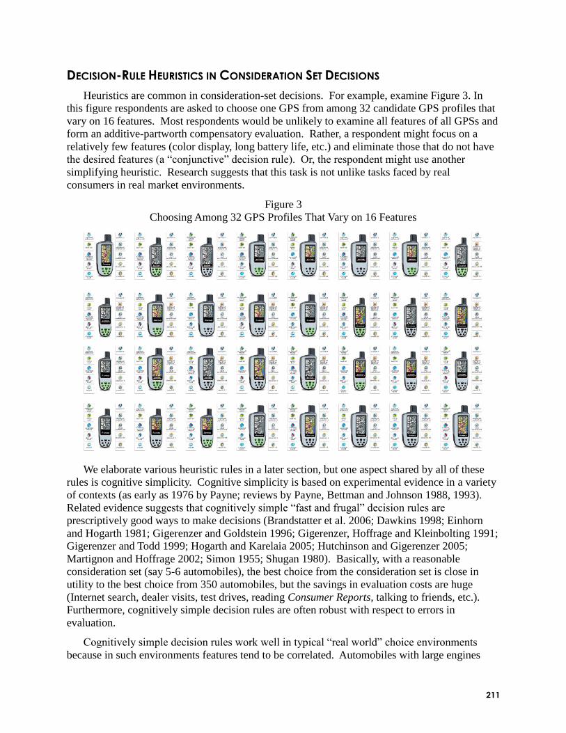
211

DECISION-RULE HEURISTICS IN CONSIDERATION SET DECISIONS

Heuristics are common in consideration-set decisions. For example, examine Figure 3. In

this figure respondents are asked to choose one GPS from among 32 candidate GPS profiles that

vary on 16 features. Most respondents would be unlikely to examine all features of all GPSs and

form an additive-partworth compensatory evaluation. Rather, a respondent might focus on a

relatively few features (color display, long battery life, etc.) and eliminate those that do not have

the desired features (a ―conjunctive‖ decision rule). Or, the respondent might use another

simplifying heuristic. Research suggests that this task is not unlike tasks faced by real

consumers in real market environments.

Figure 3

Choosing Among 32 GPS Profiles That Vary on 16 Features

We elaborate various heuristic rules in a later section, but one aspect shared by all of these

rules is cognitive simplicity. Cognitive simplicity is based on experimental evidence in a variety

of contexts (as early as 1976 by Payne; reviews by Payne, Bettman and Johnson 1988, 1993).

Related evidence suggests that cognitively simple ―fast and frugal‖ decision rules are

prescriptively good ways to make decisions (Brandstatter et al. 2006; Dawkins 1998; Einhorn

and Hogarth 1981; Gigerenzer and Goldstein 1996; Gigerenzer, Hoffrage and Kleinbolting 1991;

Gigerenzer and Todd 1999; Hogarth and Karelaia 2005; Hutchinson and Gigerenzer 2005;

Martignon and Hoffrage 2002; Simon 1955; Shugan 1980). Basically, with a reasonable

consideration set (say 5-6 automobiles), the best choice from the consideration set is close in

utility to the best choice from 350 automobiles, but the savings in evaluation costs are huge

(Internet search, dealer visits, test drives, reading Consumer Reports, talking to friends, etc.).

Furthermore, cognitively simple decision rules are often robust with respect to errors in

evaluation.

Cognitively simple decision rules work well in typical ―real world‖ choice environments

because in such environments features tend to be correlated. Automobiles with large engines

212

tend to have good leg room, good trunk room, seat five comfortably, and are often luxurious.

However, such automobiles also get lower gas mileage and are expensive. Market offerings tend

to evolve jointly with consumer heuristics. If heuristics worked well in past decisions,

consumers tend to continue to use the heuristics. If consumers use heuristics, firms react with

their product offerings which, in turn, further justify consumer heuristics. Heuristics might even

diffuse through word of mouth. While it is possible to show violations when heuristics lead to

absurd outcomes, such extreme situations are less common in everyday decisions.

In one illustration a recent MIT study asked respondents to sort the profiles into ―definitely

would consider,‖ ―definitely would not consider,‖ or ―not sure.‖ (More detail in Hauser, et al.

2009.) Respondents first sorted quietly 50 profiles, then made verbal comments as they sorted

the remaining 50 profiles. When they finished sorting, respondents re-examined the card stacks

and articulated decision rules. All sorting was videotaped with a camera on the cards and a

camera on the respondent. Afterwards, independent judges evaluated the consumers‘ decision

rules (with high reliability using procedures recommended by Hughes and Garrett 1990;

Perreault and Leigh 1989). The results were informative. Most respondents (87%) took less

than 8 seconds per vehicle and most respondents (76%) used a cognitively-simple decision rule.

HEURISTICS ARE MORE LIKELY IN SOME CONTEXTS THAN OTHERS

Heuristics are important, but not necessarily in every managerial context. For complex

technical business-to-business products, such as a high speed printer, in which there are

relatively few alternatives, we might expect a buying center to evaluate all alternatives using a

full-information compensatory decision process. On the other hand, in a category such as GPSs

in which there are many alternatives, many features, and much information available (on the

Internet) from a variety of sources, we might expect consumers to use a cognitively-simple

screening heuristic to balance search/evaluation cost with the value of a higher-value ―best‖

product.

Fortunately, the behavioral literature suggests characteristics of decision environments where

heuristics are more likely (Bettman, Luce and Payne 1998; Bettman and Park 1980b; Bettman

and Zins 1977; Chakravarti, Janiszewski and Ülkumen 2009; Chernev 2005; Frederick 2002;

Kardes, et al. 2002; Levin and Jasper 1995; Lussier and Olshavsky 1997; Luce, Payne and

Bettman 1999; Payne, Bettman and Johnson 1988; 1993; Payne, Bettman and Luce 1996; Punj

and Brookes 2002; Ratneshwar, Pechmann and Shocker 1996; and Steckel, et al. 2005; among

others). Heuristic decision rules are more likely when:

there are more products

there are more features to be evaluated

quantifiable features are more salient

there is more time pressure

the consumer is in an early phase of his/her decision process (heuristics are dynamic; they

change as the consumer goes through phases of his/her decision process)

the effort required to make a decision is more salient

the reference class is well-defined (e.g., mature products)

213

consumers are more familiar with the category (and have constructed well-defined

decision rules)

consumers have cognitive styles focused on task completion

Decision context influences decision rules. Context affects both survey design and

projections to decision environments. For example, the following context effects influence the

use of and type of decision heuristics.

response mode – choice tasks (as in CBC), rating tasks (as in ACA), matching, or bidding

(for example, respondents are more lexicographic in choice than matching)

familiarity with the product category – preferences are more robust among experienced

consumers and, hence, less dependent on response mode

choice set composition – influences such as asymmetric dominance, compromise effects,

and other contexts encourage heuristic decision rules

negative correlation among features in the choice set – when environments are more

regular (e.g., ―efficient frontier), the cost of ―mistakes‖ is less and heuristics perform

better (Johnson and Meyer 1984). However, if the choice set is small, negative

correlation induces utility balance which makes the decision more difficult, thus

leading to more compensatory rules.

We illustrate these insights with two decision contexts: automobiles and web-based

purchasing. Automobiles have a large number of features and a large number of brands (and

variations within brands). The effort to search for the information is extensive (e.g., dealership

experience, WOM, in addition to product features), and the decision is complex. Most

automobile purchasing happens over a period of months, so there is an early phase in which

brands are eliminated. This is particularly true because many alternatives (SUV, light truck, van,

sporty coupe, cross-over) are difficult to compare. All of these characteristics imply heuristic

processes are likely in the early phases of a consumer‘s automobile decision.

Many web-based buying situations include many alternatives. For example, in March 2009

there were 181 flat-panel televisions available at bestbuy.com. Figure 4 illustrates just a portion

of a page listing the large number of mobile telephones available at various web sources. Both

mobile telephones and flat-panel televisions have many features and specifications. Without

filtering, consumers easily face information overload and an overwhelming choice decision.

Filtering based on price, screen size, brand, etc. makes heuristics even less cognitively taxing.

All of these characteristics lead to greater heuristic processing. However, web-based buying also

reduces time pressure and search cost, mitigating some of the tendency to favor heuristic

processing.

214

Figure 4

Illustrative Web Page for Mobile Telephones

Not all decisions encourage heuristics. The following decision characteristics make

heuristics less likely:

simple choice sets with few alternatives

few features or levels

really new products with really new features

low time pressure and search costs

final decisions after initial heuristic screening

DECISION-RULE HEURISTICS STUDIED IN THE LITERATURE

There is a rich set of heuristics identified and studied in the literature (e.g., Bettman and Park

1980a, 1980b; Chu and Spires 2003; Einhorn 1970, 1971; Fader and McAlister 1990; Fishburn

1974; Frederick (2002), Ganzach and Czaczkes 1995; Gilbride and Allenby 2004, 2006; Hauser

1986; Hauser et al. 2009; Jedidi and Kohli 2005; Jedidi, Kohli and DeSarbo 1996; Johnson,

Meyer and Ghose 1989; Leven and Levine 1996; Lohse and Johnson 1996; Lussier and

Olshavsky 1986; Mela and Lehmann 1995; Moe 2006; Montgomery and Svenson 1976;

Nakamura 2002; Payne 1976; Payne, Bettman, and Johnson 1988; Punj 2001; Shao 2006;

215

Svenson 1979; Swait 2001; Tversky 1969, 1972; Tversky and Sattath 1987; Tversky and

Simonson 1993; Vroomen, Franses and van Nierop 2004; Wright and Barbour 1977; Wu and

Rangaswamy 2003; Yee et al. 2007). We illustrate the most commonly-studied heuristics with

examples drawn from a hypothetical evaluation of automobiles. The heuristics are disjunctive,

conjunctive, subset conjunctive, lexicographic, elimination-by-aspects, and disjunctions of

conjunctions.

Disjunctive. In a disjunctive rule a profile is considered if one feature or set of features is

above a threshold. For example, a consumer might consider all hybrid sedans or all sporty

sedans. Hybrids would be considered even if they were not sporty and sporty sedans would be

considered even if they were not hybrids. In a disjunctive rule, the other features do not matter.

Conjunctive. In a conjunctive rule a profile must have all of its features above minimum

levels. Of course, some minimum levels can be such that all profiles satisfy them, e.g., at least 5

miles per gallon. For example, a consumer might set minimum levels for fuel economy, crash

test ratings, quality ratings. leg room, acceleration, ride & handling, safety, audio systems,

navigation systems, warranty, price, etc. Technically, minimum levels must be set for all

features, even if the minimum levels are so low that all profiles pass.

Subset conjunctive. In a subset conjunctive rule a profile must have S features above a

threshold. Subset conjunctive generalizes both disjunctive (S = 1) and conjunctive (S = number

of features). As defined and applied, any S of the features need to be above the threshold. For

example, if the consumer had already limited his/her search to profiles that vary only on fuel

economy, quality ratings, and ride & handling, then a subset conjunctive model (S = 2) would

imply that a vehicle is considered if either (fuel economy and quality) or (fuel economy and ride

& handling) or (quality and ride & handling) were above minimum thresholds.

Disjunctions of conjunctions (DOC). In a DOC rule a profile will be considered if one or

more conjunctions is satisfied. DOC thus generalizes disjunctive, conjunctive, and subset

conjunctive models. For example, a consumer might consider a sedan if it is a hybrid that seats

five passengers or a sporty sedan that has great ride & handling. The sporty sedan need not be a

hybrid and the hybrid need not have great ride & handling. In the MIT/GM study cited

respondents described DOC models when they articulated their decision processes.

Lexicographic. In a lexicographic rule the consumer first ranks the features. He/she then

ranks the profiles using successively the first-ranked feature, breaking ties with the second-

ranked feature, breaking ties further with the third-ranked features, etc. For example, a consumer

might rank all hybrids over other fuel classes. Within hybrids, he/she might next rank vehicles

on crash test ratings, then on quality ratings, then on ride & handling, etc. Lexicographic rules

are usually defined for choice providing a ranking (allowing ties) of all profiles in the choice set.

When applied to the consideration decision, we must also define a cutoff which can either be a

limit on the number of profiles or on the depth of ranking of the features used in the rule. With

the latter, if we only observe the consideration set and not the ranking within the consideration

set, a lexicographic rule is indistinguishable from a conjunctive rule.

Elimination-by-Aspects (EBA). In a (deterministic) EBA rule the consumer successively

chooses aspects (feature levels) and eliminates all profiles that have that aspect. Because an

aspect is binary, a profile either has it or not, we can define aspects by their negation to produce

an equivalent rule of acceptance-by-aspects (ABA). For example, in EBA a consumer might first

216

eliminate all conventional gasoline/diesel powered vehicles. (Alternatively, accept all hybrids.)

The consumer might next eliminate all vehicles with crash test ratings below 3 stars, etc. Like

lexicographic rules, EBA provides a ranking (with potential ties) of all profiles and, like

lexicographic rules, EBA is indistinguishable from a conjunctive rule if we just observe the

consideration set. EBA was originally defined by Tversky (1972) as a probabilistic rule in which

the consumer chooses aspects with probability proportional to their measures. However, many

researchers have interpreted that probability as the analyst‘s uncertainty and have assumed that

the consumer eliminates aspects in a fixed order (Johnson, Meyer and Ghose 1989; Montgomery

and Svenson 1976; Payne, Bettman and Johnson 1988; and Thorngate 1980).

Additive partworth rule (and q-compensatory rules). We normally think of an additive

partworth model as a compensatory model, that is, high levels on some features can compensate

for low levels on other features. However, if the partworths are extreme, an additive partworth

rule can act like a non-compensatory rule. For example, if there are F binary features and if

partworths are in the ratios of 2F-1

, 2F-2

, …, 2, 1, then no combination of lower-ranked features

can compensate for a low level on a higher-ranked feature. In this case, the additive partworth

model acts as if it were lexicographic. Other non-compensatory rules also have additive

representations (Jedidi and Kohli 2005; Kohli and Jedidi 2007; Meyer and Johnson 1995;

Olshavsky and Acito 1980). Thus, an additive-partworth rule is, in fact, a mixed

compensatory/non-compensatory rule. To address this issue some researchers define a q-

compensatory rule as an additive-partworth rule in which the ratio of any two feature

importances (max – min partworths for a feature) is no more than q (Bröder 2000; Hogarth and

Karelaia 2005; Martignon and Hoffrage 2002; Yee, et al. 2007). With small q (typically q = 4),

q-compensatory rules and non-compensatory rules form disjoint sets.

RELEVANCE TO MANAGERS

Non-compensatory decision rules, whether applied to choice or consideration, have received

considerable academic attention. But do they have practical managerial relevance? We know of

no general study to indicate when they do and when they do not have managerial relevance. For

example, it is entirely possible that a heterogeneous mix of conjunctive screening rules could be

approximated well by an additive-partworth model (e.g., Abe 1999; Andrews, Ainslie and Currim

2008; Dawes 1979; Dawes and Corrigan 1974; Meyer and Johnson 1995). This is particularly

true because, as cited earlier, many non-compensatory rules can be represented by additive-

partworth models. While we await more systematic research, we provide two published

anecdotes from Hauser, et al. (2009).

Hauser, et al. studied consideration decisions for handheld GPSs. There were two brands in

their study: Magellan and Garmin. On average the Magellan brand had higher partworths, thus

in any additive-partworth market simulator a switch from Garmin to Magellan would improve

market share. However, when non-compensatory models were estimated, the researchers found

that 12% of the respondents screened on brand and, of those, 82% preferred Garmin. For the

other 88% (100% – 12%), brand had no impact on consideration. If this model was correct (and

it did predict a holdout task better), then a switch from Garmin to Magellan would reduce market

share – exactly the opposite of that predicted by an additive-partworth model.

In the same study, ―extra bright display‖ for a handheld GPS was the most important feature

based on additive partworths. A market simulator predicted that adding an extra bright display

217

for an addition $50 would increase share by 11%. However, DOC rules suggested that those

respondents who screened for extra bright displays also tended to screen against higher price. A

DOC-based simulator predicted only a 2% increase in share.

GENERAL APPROACHES TO UNCOVER HEURISTICS

Researchers have addressed consideration sets and non-compensatory decision rules with a

myriad of approaches. There are many potential taxonomies; we feel the following taxonomy

captures the essence of the approaches:

consideration and decision rules revealed as latent constructs

consideration measured directly and decision rules revealed by the ability of the rules to

fit the survey measures

decision rules measured directly through self-explicated questions.

We discuss each in turn.

CONSIDERATION AND DECISION RULES AS LATENT CONSTRUCTS

In these approaches the researcher observes only choices and the feature-levels of the profiles

in the choice set. The researcher postulates a two-stage consider-then-choose decision process

and postulates basic decision rules for each stage. The parameters of the model, for example

minimum feature levels in the first stage and partworths in the second stage, are then inferred by

either Bayesian or maximum-likelihood methods. We illustrate this approach with three

perspectives: Bayesian, choice-set explosion, and soft constraints.

Bayesian. Gilbride and Allenby (2004; 2006) use a Bayesian approach. In their 2004 paper

they establish either conjunctive, disjunctive, or linear screening rules for the consideration stage

and a compensatory (probit-like) decision rules for choice from the consideration set.

Consideration is not measured, but rather modeled with data augmentation; both the first and

second stages of the decision process are inferred simultaneously. Because the first stage is

streamlined, their model scales well in a camera application with 6 profiles (plus a none option),

seven features, and a total of 23 levels. They find that 92% of their respondents are likely to

have used a non-compensatory first-stage screening rule even though the number of alternatives

and features was relatively modest.

Choice-set Explosion. Andrews and Srinivasan (1995), Chiang, Chib and Narasimhan

(1999), Erdem and Swait (2004), Swait and Ben-Akiva (1987) and others use choice-set

explosion and maximum-likelihood methods. These researchers assume that the consideration

decision is made with a logit-like compensatory decision rule enabling the researcher to model

the probability of consideration for all 2n – 1 consideration sets, where n is the number of profiles

in the choice set. They then assume a second-stage logit for choice from within the consideration

set. They reduce the dimensionality with assumptions of independence, but the models still have

complexity that is exponential in n. If n gets too large the curse of dimensionality makes the

model too onerous to estimate. For appropriate-sized problems the choice-set-explosion models

enable researchers to explore the drivers of consideration and enable researchers to relate these

drivers to characteristics of the consumers and/or choice environment.

218

Soft constraints. Recognizing the curse of dimensionality, Swait (2001) proposes a two-

stage-like model with conjunctive and disjunctive cutoffs. The key idea is that these constraints

come directly from respondents‘ self-statements and are treated as ―soft‖ in the sense that they

influence cutoffs but are not necessarily binding. Swait claims superior predictive ability relative

to choice-set explosion based on an ―extremely powerful‖ increase in the log-likelihood values.

Swait also points out that the model itself is estimated simultaneously and, thus, does not assume

an ordering of the two stages of cutoffs and additive partworths.

CONSIDERATION MEASURED, DECISION RULES INFERRED

Since the early 1970s researchers have measured consideration sets directly. Respondents

find the task intuitive and such measures significantly enhance new product forecasts (Brown

and Wildt 1992; Hauser 1978; Silk and Urban 1978; Urban and Katz 1983). Figure 1 provides

one example. For a variety of web-based formats see also Ding, et al. (2009), Gaskin, et al.

(2007), Hauser, et al. (2009), and Yee, et al. (2007). Direct measurement presents three

challenges. First, if we believe the evaluation-cost theory of consideration sets, then consumers

form consideration sets by making tradeoffs between the increased utility from larger sets and

the increased search cost for larger sets. In vivo search cost is set by the marketplace

environment, but in vitro it is set by the measurement instrument. For example, Hauser et al.

(2009) test four web-based formats that vary in vitro search cost. They find that respondents

choose smaller consideration sets when respondents are asked to indicate only considered

profiles versus when they are asked to indicate only rejected profiles. The size of the

consideration set when respondents need evaluate all profiles is in-between. Fortunately, the

choice rules do not seem to vary that dramatically; the process of choice can still be measured

with some fidelity. The second challenge is that context matters (see references cited in a

previous section). The size of the evaluation set, the number of features, how decisions are

framed, whether there is negative correlation among features, whether some profiles are

dominated asymmetrically, and other context effects can all influence decision rules, rules that

might be constructed on the fly. The third challenge is when incentive alignment is coupled with

consideration-set measurement. Consideration is an intermediate construct, not the final choice.

Incentives must be sufficiently vague, yet effective, so that the respondent believes that he/she

should specify a consideration set that applies in vivo. See examples in Ding et al. (2009) and

Kugelberg (2004). The important caveat for all three challenges is that researchers must pay

attention to context and work to ensure that the in vitro measurements approximate in vivo

projections.

Once consideration is measured in vitro, there are a variety of methods to estimate the

decision rules that best explain the consideration decisions observed on calibration tasks. There

are two basic estimation strategies: Bayesian with simpler structure and machine-learning

pattern-matching algorithms. For example, the Gilbride-Allenby (2004) approach is easily

modified for explicitly measure consideration. Bayesian methods can easily be written for subset

conjunctive, q-compensatory (rejection sampling), and, of course, additive partworth models.

Machine-learning algorithms use either math programming or logical analysis of data (LAD,

Boros, et al. 1997; 2000).

There are at least two issues to be addressed when using revealed estimation for

consideration-set rules. First is the curse of dimensionality. Non-compensatory models can

easily over fit data. For example, there are 323

= 94,143,178,827 potential DOC rules with 23

219

binary features. With such large numbers it is not feasible to have prior or posterior probabilities

for each decision rule. Rather, researchers must simplify the model as in Gilbride or Allenby

(2004) or impose constraints that the decision rules are cognitively simple as in Hauser et al.

(2009). The second issue is the robustness of the additive-partworth model. An additive-

partworth model is likely to fit the data well, even if the process is non-compensatory. To

address this issue, researchers often estimate a q-compensatory model and compare it to a non-

compensatory model. This two-step evaluation provides insight because the additive-partworth

model can nest both.

We are aware of only one comprehensive comparison of the predictive ability of revealed-

decision-rule estimation on directly-measured consideration. Hauser, et al. (2009) compare five

Bayesian models (conjunctive, disjunctive, subset conjunctive, q-compensatory, additive

partworth) and seven pattern-recognition models (conjunctive, disjunctive, subset conjunctive, q-

compensatory, additive-partworth, DOC math program, DOC LAD) on the same data. The

models were estimated when respondents were asked to evaluate an orthogonal design of 32

GPSs. Predictions were evaluated on a different set of 32 GPSs (after a memory-cleansing task).

They found that:

the relative predictive ability of Bayesian vs. pattern-recognition methods depended upon

the posited decision model

DOC models improved prediction significantly relative to conjunctive, disjunctive, or

subset conjunctive for both Bayesian and pattern-recognition methods

there was no significant difference between the math programming and LAD DOC

models

non-compensatory models did better than q-compensatory models, but

additive partworth models did almost as well as DOC models.

Their study is limited to a single category in an environment chosen to favor non-

compensatory models. Abundant research opportunities will increase our knowledge with

further testing.

DECISION RULES MEASURED DIRECTLY THROUGH SELF-EXPLICATED QUESTIONS

Directly-elicited non-compensatory measures have been used almost since the beginning of

conjoint analysis. Casemap, Adaptive Conjoint Analysis (ACA), and other methods all include

options to ask respondents to indicate unacceptable levels or products (Green, Krieger and Banal

1988; Malhotra 1986; Klein 1986; Srinivasan 1988; Srinivasan and Wyner 1988; Sawtooth

1996). However, these modules have met with mixed success; respondents happily choose

profiles with unacceptable levels. More recently, researchers have experimented with improved

formats. Swait (2001) uses self-explicated cutoffs as soft constraints. Adaptive Choice-Based

Conjoint Analysis (ACBC) uses a multi-step procedure in which (1) respondents are asked to

indicate a profile that they would consider, (2) a pool of profiles is created as perturbations on

that profile, (3) respondents are shown screens of 3-5 profiles and asked for consideration, and

(4) if a feature-level is always rejected or accepted a pop-up ―avatar‖ (a graphic of an attractive

interviewer can be included, though is not required) confirms the non-compensatory decision

rule (Sawtooth Software 2008). Ding, et al. (2009) ask respondents to write an unstructured e-

220

mail to a friend who will act as their agent and purchase the product for them. Figure 5 provides

an example e-mail from a Hong Kong respondent who was evaluating mobile telephones.

Figure 5

Example ―E-Mail‖ Direct Elicitation

Dear friend, I want to buy a mobile phone recently and I hope u can provide

some advice to me. The following are some requirement of my preferences.

Firstly, my budget is about $2000, the price should not more than it. The

brand of mobile phone is better Nokia, Sony-Ericsson, Motorola, because I

don't like much about Lenovo. I don't like any mobile phone in pink color.

Also, the mobile phone should be large in screen size, but the thickness is

not very important for me. Also, the camera resolution is not important too,

because i don't always take photo, but it should be at least 1.0Mp.

Furthermore, I prefer slide and rotational phone design. It is hoped that you

can help me to choose a mobile phone suitable for me.

Dear friend, I want to buy a mobile phone recently and I hope u can provide

some advice to me. The following are some requirement of my preferences.

Firstly, my budget is about $2000, the price should not more than it. The

brand of mobile phone is better Nokia, Sony-Ericsson, Motorola, because I

don't like much about Lenovo. I don't like any mobile phone in pink color.

Also, the mobile phone should be large in screen size, but the thickness is

not very important for me. Also, the camera resolution is not important too,

because i don't always take photo, but it should be at least 1.0Mp.

Furthermore, I prefer slide and rotational phone design. It is hoped that you

can help me to choose a mobile phone suitable for me.

Directly-elicited decision-rule measures have become more accurate for a number of

important reasons. Formats can now be incentive-aligned, that is, the respondent believes that

he/she will receive a prize (in a lottery) and that the prize depends upon his/her answers to the

questions (Ding 2007; Ding, Grewal and Liechty 2005; Park, Ding and Rao 2008). With

incentive-aligned methods, truthful questions are dominant. If the incentives are sufficient, then

the respondent is also encouraged to think hard about the answers. ―Natural tasks‖ further

enhance accuracy. In ACBC respondents evaluate profiles and then respond to an avatar. In

Ding et al. respondents write e-mails that are similar to those that they would write to friends.

Researchers are beginning to appreciate the value of ―build your own (BYO)‖ profiles as in the

first phase of ACBC. Typically, consumers consider but a small fraction of the available

products, thus one gains significantly more information from knowing a profile is considered

than from knowing a profile is not considered (Silinskaia and Hauser 2009). Finally, the wide

use of voice-of-the-customer methods has led to a market-research workforce that is adept at

quantifiable coding of qualitative data (Griffin and Hauser 1993; Hughes and Garrett 1990;

Perreault and Leigh 1989).

Ding et al. (2009) compare directly-elicited decision rules to decision rules inferred from the

analysis of directly-measured consideration (decomposition). The decompositional benchmarks

are a q-compensatory logit model, an additive-partworth logit model, a lexicographic model

estimated with Yee, et al.‘s (2007) Greedoid dynamic program, and LAD. Respondents were

asked to either evaluate profiles or state decision rules (calibration data). Predictions were based

221

on data collected three weeks later when respondents evaluated 32 profiles. The researchers

found:

direct elicitation predicts as well as decomposition (no significant difference)

non-compensatory rules predict better than q-compensatory rules,

additive partworths do as well as pure non-compensatory rules

While there is no improvement in predictive ability relative to decomposition, the directly-

elicited rules have the advantage that they are less subject to the curse of dimensionality. They

scale well to large problems. For example, Ding, et al. demonstrate that respondents can answer

easily questions about a very complex category that would have required over 13 thousand

profiles in an orthogonal design.

TAKE HOME LESSONS

No review of the literature is perfect and ours is not without its caveats. It is very difficult to

compare across sub-literatures and it is not yet feasible to do a meta-analysis because the criteria

with which researchers evaluate models varies widely. Among the measures we found were hit

rates, log likelihood measures, Kullback-Leibler divergence, t-tests, 2 (pseudo-R

2), and U

2

(percent of information explained). Some papers correct for the number of profiles (predicting

choice from among 2 profiles is easier than from among 32 profiles), others do not and do not

report the number of profiles. In consideration decisions null models are particularly strong. For

example, if only 20% of the profiles are considered, then a null model which predicts that

nothing is considered will predict all not-considered profiles correct – an 80% hit rate. Even a

random model will predict 68% of the profiles correctly (0.82 + 0.2

2). In the papers we reviewed

benchmarks varied considerably and the null models were not equally challenging. Predictive

ability alone should not be used to distinguish models. Detailed information on the

choice/consideration context was often omitted even though research suggests that context can

have a considerable influence.

Nonetheless, we were able to identify empirical generalizations that appear to hold. These

include:

non-compensatory decision rules for consideration decisions are common in many

categories (see Table 1 for some examples).

non-compensatory decision rules often predict better than purely compensatory rules

(e.g., q-compensatory rules), but

the unconstrained additive-partworth model is robust and hard to beat on predictive

measures.

complex situations favor non-compensatory decision rules, but

non-compensatory rules often predict well in even simple situations.

there are many ways to measure and/or estimate non-compensatory decision rules but, to

date, no single approach appears to dominate.

222

there are excellent (and intuitive) anecdotes that managers should pay attention to non-

compensatory decision rules but, to date, there is no comprehensive theory as to

when.

SUMMARY

Non-compensatory decision rules for consideration decisions are growing in relevance.

Figure 6 provides the date of publication of the 132 articles we reviewed. This is not a random

sample, but it does suggest a growing interest. Non-compensatory decision rules for

consideration have a long history in marketing, but powerful computers, efficient algorithms, and

new theory is providing exciting new measurement and estimation methods. This research is

likely to have increasing impact as researchers push further the limits of scalability, develop

easy-to-use software, and explore synergies with behavioral experiments.

And there are many research opportunities. We need a theory (or generalization) of when

and how models of non-compensatory decision rules for consideration influence managerial

theories. We do not yet have practical models of the effect of such decision rules on market-

structure equilibria. And we need many more predictive tests of current (and yet-to-be-

developed) models. The future is indeed exciting and, we hope, fun.

Table 1

Example Predictive Ability of Non-Compensatory Models

PRODUCT CATEGORY Percent non-compensatory Fit Equal/ Better

Air conditioners (Shao 2006, protocol) 89% screen, 67% two-stage Automobiles (Hauser, et al. 2009, process tracing) 76% cognitively simple Automobiles (Levin, Jasper 1995, process tracing) 86% non-compensatory Batteries (Jedidi, Kohli 2005, subset conjunctive) equal (a)* Cameras (Gilbride, Allenby 2004, conj., disjunctive)

92% non-compensatory better

Cell phones (Ding, et al., 2009 conj./compensatory)

78% mixed better (q), equal (a)

Computers (Kohli, Jedidi, 2007, lexicographic) 2/3rds lexicographic equal (a) Computers (Jedidi, Kohli 2005, subset conjunctive) “virtually identical” Computers (Yee, et al. 2007, lexicographic) 58% lexicographic (17% tied) better (q), equal (a) Documentaries (Gilbride, Allenby 2006, screening) better in-sample fit GPSs (Hauser, et al. 2009, disjunctions of conj.) better

MBA admissions (Elrod, et al. 2004, GNH) better model selection

Rental cars (Swait 2001, soft cutoffs) better in-sample fit Smartphones (Yee, et al. 2007, lexicographic) 56% lexicographic better (q), equal (a) Supermarket product (Fader, McAlister 1990, EBA) equal to logit

* a = relative to an additive-partworth model, q = relative to a q-compensatory model, conj. = conjunctive

223

Figure 6

Dates of Non-Compensatory Articles

(Projected through the end of 2010)

0

5

10

15

20

25

30

1970 1975 1980 1985 1990 1995 2000 2005 2010

5-year Period

Nu

mb

er

of

art

icle

s in

peri

od

REFERENCES

Abe, Makoto (1999), ―A Generalized Additive Model for Discrete-Choice Data, ‖

Journal of Business & Economic Statistics, 17 (Summer), 271-84.

Andrews, Rick L., Andrew Ainslie and Imran S. Currim (2008), "On the Recoverability of

Choice Behaviors with Random Coefficients Choice Models in the Context of Limited

Data and Unobserved Effects," Management Science, 54 (January), 83-99.

------ and Ajay K. Manrai (1998) , ―Simulation Experiments in Choice Simplification: The

Effects of Task and Context on Forecasting Performance,‖ Journal of Marketing Research,

35 (May), 198-209.

------ and T. C. Srinivasan (1995), ―Studying Consideration Effects in Empirical Choice

Models Using Scanner Panel Data, ‖ Journal of Marketing Research, 32 (February), 30-41.

Bettman, James R., Mary Frances Luce, and John W. Payne (1998), ―Constructive Consumer

Choice Processes, ‖ Journal of Consumer Research, 25, 3 (December), 187-217.

------ and L. W. Park (1980a), ―Effects of Prior Knowledge and Experience and Phase of the

Choice Process on Consumer Decision Processes: A Protocol Analysis,‖ Journal of

Consumer Research, 7 (December), 234-248.

------ and ------ (1980b), ―Implications of a Constructive View of Choice for Analysis of

Protocol Data: A Coding Scheme for Elements of Choice Processes, ‖ (Journal Unknown),

148-153.

224

------ and Michel A. Zins (1977), ―Constructive Processes in Consumer Choice, ‖ Journal of

Consumer Research, 4 (September), 75-85.

Boros, Endre, Peter L. Hammer, Toshihide Ibaraki, and Alexander Kogan (1997), ―Logical

Analysis of Numerical Data,‖ Mathematical Programming, 79:163--190, August 1997

------, ------, ------, ------, Eddy Mayoraz, and Ilya Muchnik (2000), ―An Implementation of

Logical Analysis of Data,‖ IEEE Transactions on Knowledge and Data Engineering,

12(2), 292-306.

Brandstaetter, Eduard, Gerd Gigerenzer and Ralph Hertwig (2006), ―The Priority Heuristic:

Making Choices Without Trade-Offs, ‖ Psychological Review, 113, 409-32.

Bröder, Arndt (2000), ―Assessing the Empirical Validity of the ‗Take the Best‘ Heuristic as a

Model of Human Probabilistic Inference, ‖ Journal of Experimental Psychology: Learning,

Memory, and Cognition, 26, 5, 1332-1346.

Bronnenberg, Bart J., and Wilfried R. Vanhonacker (1996), ―Limited Choice Sets, Local

Price Response, and Implied Measures of Price Competition,‖ Journal of Marketing

Research, 33 (May), 163-173.

Brown, Juanita J. and Albert R. Wildt (1992), ―Consideration Set Measurement,‖ Journal of

the Academy of Marketing Science, 20 (3), 235-263.

Chakravarti, Amitav and Chris Janiszewski, (2003), ―The Influence of Macro-Level Motives

on Consideration Set Composition in Novel Purchase Situations,‖ Journal of Consumer

Research, 30 (September), 244-58.

------, ------ and Gülden Ülkumen (2009), ―The Neglect of Prescreening Information,‖ Journal

of Marketing Research (forthcoming).

Chase, Valerie M., Ralph Hertwig, and Gerd Gigerenzer (1998), ―Visions of Rationality,‖

Trends in Cognitive Sciences, 2, 6 (June), 206-214.

Chernev, Alexander (2005), ―Feature Complementarity and Assortment in Choice,‖ Journal

of Consumer Research, 31 (March), 748-59.

Chiang, Jeongwen, Siddhartha Chib, and Chakravarthi Narasimhan (1999), ―Markov Chain

Monte Carlo and Models of Consideration Set and Parameter Heterogeneity,‖ Journal of

Econometrics, 89, 223-48.

Chu, P.C. and Eric E. Spires (2003), ―Perceptions of Accuracy and Effort of Decision

Strategies,‖ Organizational Behavior and Human Decision Processes, 91, 203-14.

Dawes, R. M. (1979), ―The Robust Beauty of Improper Linear Models in Decision Making,‖

American Psychologist, 34, 571-582.

------ and B. Corrigan (1974), ―Linear Models in Decision Making,‖ Psychological Bulletin,

81, 95-106.

Desai, Kalpesh K. and Wayne D. Hoyer (2000), ―Descriptive Characteristics of Memory-

Based Consideration Sets: Influence of Usage Occasion Frequency and Usage Location

Familiarity,‖ Journal of Consumer Research, 27 (December), 309-323.

225

Desarbo, Wayne S. and Kamel Jedidi (1995), ―The Spatial Representation of Heterogeneous

Consideration Sets,‖ Marketing Science, 14, 326-342.

------, Donald R. Lehmann, Greg Carpenter, and I. Sinha (1996), ―A Stochastic

Multidimensional Unfolding Approach for Representing Phased Decision Outcomes,‖

Psychometrica, 61 (September), 485-508.

Dawkins, Richard (1998), Unweaving the Rainbow: Science, Delusion, and the Appetite for

Wonder, (Boston, MA: Houghton Mifflin Company).

Ding, Min (2007), ―An Incentive-Aligned Mechanism for Conjoint Analysis,‖ Journal of

Marketing Research, 54, (May), 214-223.

-----, Rajdeep Grewal, and John Liechty (2005), ―Incentive-Aligned Conjoint Analysis,‖

Journal of Marketing Research, 42, (February), 67–82.

------, John R. Hauser, Songting Dong, Daria Silinskaia, Zhilin Yang, Chenting Su, and

Steven Gaskin (2009), ―Incentive-Aligned Direct Elicitation of Decision Rules: An

Empirical Test, ‖ Working Paper.

Einhorn, Hillel J. (1970), ―The Use of Nonlinear, Noncompensatory Models in Decision

Making,‖ Psychological Bulletin, 73, 3, 221-230.

------ (1971), ―Use of Non-linear, Non-compensatory Models as a Function of Task and

Amount of Information,‖ Organizational Behavior and Human Performance,6, 1-27.

Einhorn, Hillel J. , and Robin M. Hogarth (1981), ―Behavioral Decision Theory: Processes of

Judgment and Choice,‖ Annual Review of Psychology, 32, 52-88.

Elrod, Terry, Richard D. Johnson, and Joan White (2004), ―A New Integrated Model Of

Noncompensatory And Compensatory Decision Strategies,‖ Organizational Behavior and

Human Decision Processes, 95, 1–19.

Erdem, Tülin and Joffre Swait (2004), ―Brand Credibility, Brand Consideration, and Choice,‖

Journal of Consumer Research, 31 (June), 191-98.

Fader, Peter S. and Leigh McAlister (1990), ―An Elimination by Aspects Model of Consumer

Response to Promotion Calibrated on UPC Scanner Data,‖ Journal of Marketing

Research, 27 (August), 322-32.

Fishburn, Peter C. (1974), ―Lexicographic Orders, Utilities and Decision Rules: A Survey,‖

Management Science, 20, 11 (Theory, July), 1442-1471.

Frederick, Shane (2002), ―Automated Choice Heuristics,‖ in Thomas Gilovich, Dale Griffin,

and Daniel Kahneman, eds., Heuristics and Biases: The Psychology of Intuitive Judgment,

(Cambridge, UK: Cambridge University Press, chapter 30, 548-558.

Ganzach, Yoav and Benjamin Czaczkes (1995), ―On Detecting Nonlinear Noncompensatory

Judgment Strategies: Comparison of Alternative Regression Models,‖ Organizational

Behavior and Human Decision Processes, 61 (February), 168-76.

Gaskin, Steven, Theodoros Evgeniou, Daniel Bailiff, John Hauser (2007), ―Two-Stage

Models: Identifying Non-Compensatory Heuristics for the Consideration Set then Adaptive

226

Polyhedral Methods Within the Consideration Set,‖ Proceedings of the Sawtooth Software

Conference in Santa Rosa, CA, October 17-19, 2007.

Gensch, Dennis H. (1987), ―A Two-stage Disaggregate Attribute Choice Model,‖ Marketing

Science, 6 (Summer), 223-231.

------ and Ehsan S. Soofi (1995a), ―Information-Theoretic Estimation of Individual

Consideration Sets,‖ International Journal of Research in Marketing, 12 (May), 25-38.

------ and ------ (1995b), ―An Information-Theoretic Two-Stage, Two-Decision Rule, Choice

Model,‖ European Journal of Operational Research, 81, 271-80.

Gigerenzer, Gerd and Daniel G. Goldstein (1996), ―Reasoning the Fast and Frugal Way:

Models of Bounded Rationality,‖ Psychological Review, 103, 4, 650-669.

------, Ulrich Hoffrage, and H. Kleinbölting (1991), ―Probabilistic Mental Models: A

Brunswikian Theory of Confidence,‖ Psychological Review, 98, 506-528.

------, Peter M. Todd, and the ABC Research Group (1999), Simple Heuristics That Make Us

Smart, (Oxford, UK: Oxford University Press).

Gilbride, Timothy and Greg M. Allenby (2004), ―A Choice Model with Conjunctive,

Disjunctive, and Compensatory Screening Rules,‖ Marketing Science, 23, 3 (Summer),

391-406.

------ and ------ (2006), ―Estimating Heterogeneous EBA and Economic Screening Rule Choice

Models,‖ Marketing Science, 25 (September-October), 494-509.

Green, Paul E., Abba M. Krieger, and Pradeep Bansal (1988), ―Completely Unacceptable

Levels in Conjoint Analysis: A Cautionary Note,‖ Journal of Marketing Research, 25

(August), 293-300.

Griffin, Abbie and John R. Hauser (1993), "The Voice of the Customer," Marketing Science,

12, 1, (Winter), 1-27.

Haübl, Gerald and Valerie Trifts (2000), ―Consumer Decision Making in Online Shopping

Environments: The Effects of Interactive Decision Aids,‖ Marketing Science, 19 (Winter),

4-21.

Hauser, John R. (1978), "Testing the Accuracy, Usefulness and Significance of Probabilistic

Models: An Information Theoretic Approach," Operations Research, Vol. 26, 3 (May-

June), 406-421.

------ (1986), "Agendas and Consumer Choice," Journal of Marketing Research, 23 (August),

199-212.

------ and Steven M. Shugan (1983), "Defensive Marketing Strategy," Marketing Science, 2,

4, (Fall), 319-360.

------, Olivier Toubia, Theodoros Evgeniou, Rene Befurt and Daria Silinskaia (2009),

―Cognitive Simplicity and Consideration Sets,‖ forthcoming, Journal of Marketing

Research.

227

------ and Birger Wernerfelt (1990), ―An Evaluation Cost Model of Consideration Sets,‖

Journal of Consumer Research, 16 (March), 393-408.

Hogarth, Robin M. and Natalia Karelaia (2005), ―Simple Models for Multiattribute Choice

with Many Alternatives: When It Does and Does Not Pay to Face Trade-offs with Binary

Attributes,‖ Management Science, 51, 12, (December), 1860-1872.

Hughes, Marie Adele and Dennis E. Garrett (1990), ―Intercoder Reliability Estimation

Approaches in Marketing: A Generalizability Theory Framework for Quantitative Data,‖

Journal of Marketing Research, 27, (May), 185-195.

Hutchinson, John M. C. and Gerd Gigerenzer (2005), ―Simple Heuristics and Rules of

Thumb: Where Psychologists and Behavioural Biologists Might Meet,‖ Behavioural

Processes, 69, 97-124.

Jedidi, Kamel, Rajiv Kohli, and Wayne S. DeSarbo (1996), ―Consideration Sets in Conjoint

Analysis,‖ Journal of Marketing Research, 33 (August), 364-372.

------ and ------ (2005), ―Probabilistic Subset-Conjunctive Models for Heterogeneous

Consumers,‖ Journal of Marketing Research, 42 (November), 483-494.

Johnson, Eric J. and Robert J. Meyer (1984), ―Compensatory Choice Models of

Noncompensatory Processes: The Effect of Varying Context,‖ Journal of Consumer

Research, 11 (June), 528-541.

------, ------, and Sanjoy Ghose (1989), ―When Choice Models Fail: Compensatory Models in

Negatively Correlated Environments,‖ Journal of Marketing Research, 26 (August), 255-

290.

------ and John W. Payne (1985), ―Effort and Accuracy in Choice,‖ Management Science, 31,

395-414.

Kahneman, Daniel and Amos Tversky (1996), ―On the Reality of Cognitive Illusions,‖

Psychological Review, 103, 3, 582-591.

Kamis, Arnold (2006), ―Search Strategies in Shopping Engines An Experimental

Investigation,‖ International Journal of Electronic Commerce, 11 (Fall), 63-84.

Kardes, Frank, Gurumurthy Kalyanaram, Murali Chandrashekaran, and Ronald J. Dornoff

(1993), ―Brand Retrieval, Consideration Set Composition, Consumer Choice, and the

Pioneering Advantage,‖ Journal of Consumer Research, 20 (June), 528-541.

------, David M. Sanbonmatsu, Maria L. Cronley, and David C. Houghton (2002),

―Consideration Set Overvaluation: When Impossibly Favorable Ratings of a Set of Brands

Are Observed,‖ Journal of Consumer Psychology, 12, 4, 353-61.

Klein, Noreen M. (1988), ―Assessing Unacceptable Attribute Levels in Conjoint Analysis,‖

Advances in Consumer Research vol. XIV, pp. 154-158.

Kohli, Rajiv and Kamel Jedidi (2007), ―Representation and Inference of Lexicographic

Preference Models and Their Variants,‖ Marketing Science, 26 (May-June), 380-99.

228

Kugelberg, Ellen (2004), ―Information Scoring and Conjoint Analysis,‖ Department of

Industrial Economics and Management, Royal Institute of Technology, Stockholm,

Sweden.

Lapersonne, Eric, Giles Laurent and Jean-Jacques Le Goff (1995), ―Consideration Sets Of

Size One: An Empirical Investigation Of Automobile Purchases, ‖ International Journal of

Research in Marketing, 12, 55-66.

Leven, Samuel J. and Daniel S. Levine (1996), ―Multiattribute Decision Making in Context:

A Dynamic Neural Network Methodology,‖ Cognitive Science, 20, 271-299.

Levin, Irwin P. and J. D. Jasper (1995), ―Phased Narrowing: A New Process Tracing Method

for Decision Making,‖ Organizational Behavior and Human Decision Processes, 64

(October), 1-8.

Lohse, Gerald J. and Eric J. Johnson (1996), ―A Comparison of Two Process Tracing

Methods for Choice Tasks,‖ Organizational Behavior and Human Decision Processes, 68

(October), 28-43.

Luce, Mary Frances, John W. Payne, and James R. Bettman (1999), ―Emotional Trade-off

Difficulty and Choice, ‖ Journal of Marketing Research, 36, 143-159.

Lussier, Denis A. and Richard W. Olshavsky (1997), ―Task Complexity and Contingent

Processing in Brand Choice,‖ Journal of Consumer Research, 6 (September), 154-65.

Malhotra, Naresh (1986), ―An Approach to the Measurement of Consumer Preferences Using

Limited Information,‖ Journal of Marketing Research, 23 (February), 33-40.

Martignon, Laura and Ulrich Hoffrage (2002), ―Fast, Frugal, and Fit: Simple Heuristics for

Paired Comparisons, ‖ Theory and Decision, 52, 29-71.

------ and Michael Schmitt (1999), ―Simplicity and Robustness of Fast and Frugal Heuristics,‖

Minds and Machines, 9, 565-93.

Mehta, Nitin, Surendra Rajiv, and Kannan Srinivasan (2003), ―Price Uncertainty and

Consumer Search: A Structural Model of Consideration Set Formation,‖ Marketing

Science, 22(1), 58-84.

Mela, Carl F. and Donald R. Lehmann (1995), ―Using Fuzzy Set Theoretic Techniques to

Identify Preference Rules From Interactions in the Linear Model: An Empirical Study,‖

Fuzzy Sets and Systems, 71, 165-181.

Meyer, Robert and Eric J. Johnson (1995), ―Empirical Generalizations in the Modeling of

Consumer Choice,‖ Marketing Science, 14, 3, Part 2 of 2, G180-G189.

Moe, Wendy W. (2006), ―An Empirical Two-Stage Choice Model with Varying Decision

Rules Applied to Internet Clickstream Data,‖ Journal of Marketing Research, 43

(November), 680-692.

Montgomery, H. and O. Svenson (1976), ―On Decision Rules and Information Processing

Strategies for Choices among Multiattribute Alternatives,‖ Scandinavian Journal of

Psychology, 17, 283-291.

229

Murray, Kyle B. and Gerald Häubl (2006), ―Explaining Cognitive Lock-In: The Role of Skill-

Based Habits of Use in Consumer Choice,‖ manuscript, (January 23).

Nakamura, Yutaka (2002), ―Lexicographic Quasilinear Utility,‖ Journal of Mathematical

Economics, 37, 157-178.

Nedungadi, Prakash (1990), ―Recall and Consideration Sets: Influencing Choice without

Altering Brand Evaluations,‖ Journal of Consumer Research, 17 (December), 263-276.

Newell, Ben R., Nicola J. Weston, and David R. Shanks (2002), ―Empirical Tests Of A Fast-

And-Frugal Heuristic: Not Everyone ‗Takes-The-Best,‘‖ Organizational Behavior and

Human Decision Processes, 91, 82-96.

------ and David R. Shanks (2003), ―Take the Best or Look at the Rest? Factors Influencing

‗One-Reason‘ Decision Making,‖ Journal of Experimental Psychology: Learning, Memory

and Cognition, 29, 1, 53-65.

Newman, Joseph W. and Richard Staelin (1972), ―Prepurchase Information Seeking for New

Cars and Major Household Appliances,‖ Journal of Marketing Research, 9 (August), 249-

57.

Olshavsky, Richard W. and Franklin Acito (1980), ―An Information Processing Probe into

Conjoint Analysis,‖ Decision Sciences, 11, (July), 451-470.

Oppewal, Harmen, Jordan J. Louviere, and Harry J. P. Timmermans (1994), ―Modeling

Hierarchical Conjoint Processes with Integrated Choice Experiments,‖ Journal of

Marketing Research, 31 (February), 92-105.

Park, Young-Hoon, Min Ding and Vithala R. Rao (2008), ―Eliciting Preference for Complex

Products: A Web-Based Upgrading Method,‖ Journal of Marketing Research, 45

(October), 562-574.

Paulssen, Marcel and Richard P. Bagozzi (2005), ―A Self-Regulatory Model of Consideration

Set Formation,‖ Psychology & Marketing, 22 (October), 785-812.

Payne, John W. (1976), ―Task Complexity and Contingent Processing in Decision Making:

An Information Search,‖ Organizational Behavior and Human Performance, 16, 366-387.

------, James R. Bettman, and Eric J. Johnson (1988), ―Adaptive Strategy Selection in

Decision Making,‖ Journal of Experimental Psychology: Learning, Memory, and

Cognition, 14, 534-552.

------, ------, and ------ (1993), The Adaptive Decision Maker, (Cambridge, UK: Cambridge

University Press).

------, ------, and Mary Frances Luce (1996), ―When Time is Money: Decision Behavior

Under Opportunity-Cost Time Pressure,‖ Organizational Behavior and Human Decision

Processes, 66 (May), 131-152.

Perreault, William D., Jr. and Laurence E. Leigh (1989), ―Reliability of Nominal Data Based

on Qualitative Judgments,‖ Journal of Marketing Research, 26, (May), 135-148.

Posavac, Steven S., David M. Sanbonmatsu, Maria L. Cronley, and Frank R. Kardes (2001),

―The Effects of Strengthening Category-Brand Associations on Consideration Set

230

Composition and Purchase Intent in Memory-Based Choice, ‖ Advances in Consumer

Research, 28, 186-189.

Punj, Brookes (2001), ―Decision Constraints and Consideration-Set Formation in Consumer

Durables,‖ Psychology & Marketing, 18 (August), 843-863.

Punj, Girish and Richard Brookes (2002), ―The Influence Of Pre-Decisional Constraints On

Information Search And Consideration Set Formation In New Automobile Purchases, ‖

Internal Journal of Research in Marketing, 19, 383-400.

------ and Staelin, Richard (1983), ―A Model of Consumer Information Search Behavior for

New Automobiles,‖ Journal of Consumer Research, 9, 366-380.

Ratneshwar, S., Cornelia Pechmann and Allan D. Shocker (1996), ―Goal-Derived Categories

and the Antecedents of Across-Category Consideration,‖ Journal of Consumer Research,

23 (December), 240-250.

Roberts, John H. and James M. Lattin (1991), ―Development and Testing of a Model of

Consideration Set Composition,‖ Journal of Marketing Research, 28 (November), 429-

440.

------ and ------ (1997), ―Consideration: Review of Research and Prospects for Future

Insights,‖ Journal of Marketing Research, 34 (August), 406-410.

Sawtooth Software, Inc. (1996), ―ACA System: Adaptive Conjoint Analysis,‖ ACA Manual,

(Sequim, WA: Sawtooth Software, Inc.)

------ (2008), ―ACBC Technical Paper, ‖ (Sequim WA; Sawtooth Software, Inc.)

Schmitt, Michael and Laura Martignon (2006), ―On the Complexity of Learning

Lexicographic Strategies,‖ Journal of Machine Learning Research, 7, 55-83.

Shao, Wei (2006), ―Consumer Decision-Making: An Empirical Exploration of Multi-Phased

Decision Processes,‖ doctoral dissertation, Department of Philosophy, Griffith University.

Shocker, Allen D., Moshe Ben-Akiva, B. Boccara, and P. Nedungadi (1991), ―Consideration

Set Influences on Customer Decision-Making and Choice: Issues, Models and

Suggestions,‖ Marketing Letters, 2, 181-198.

Shugan, Steven M. (1980), ―The Cost of Thinking,‖ Journal of Consumer Research, 7, 2

(September), 99-111.

Siddarth, S., Randolph E. Bucklin, and Donald G. Morrison (1995), ―Making the Cut:

Modeling and Analyzing Choice Set Restriction in Scanner Panel Data,‖ Journal of

Marketing Research, 33 (August), 255-266.

Silinskaia, Daria, John R. Hauser, and Glen L. Urban (2009), ―Adaptive Profile Evaluation to

Identify Heuristic Decision Rules in ‗Large‘ and Challenging Experimental Designs,‖

NFORMS Marketing Science Conference, Ann Arbor, MI, June 2009.

Silk, Alvin J. and Glen L. Urban (1978), ―Pre-test Market Evaluation of New Packaged

Goods: A Model and Measurement Methodology,‖ Journal of Marketing Research, 15

(May), 171-191.

231

Simon, Herbert A. (1955), ―A Behavioral Model of Rational Choice,‖ The Quarterly Journal

of Economics, 69(1). 99-118.

Srinivasan, V. (1988), ―A Conjunctive-Compensatory Approach to The Self-Explication of

Multiattributed Preferences,‖ Decision Sciences, 295-305.

------ and Gordon A. Wyner (1988), ―Casemap: Computer-Assisted Self-Explication of

Multiattributed Preferences,‖ in W. Henry, M. Menasco, and K. Takada, Eds, Handbook

on New Product Development and Testing, (Lexington, MA: D. C. Heath), 91-112.

Steckel, Joel H. and Russell S. Weiner, Randolph E. Bucklin, Benedict G.C. Dellaert, Xavier

Drèze, Gerald Häubl, Sandy D. Jap, John D.C. Little, Tom Meyvis, Alan L.

Montgomery, and Arvind Rangaswamy (2005) ―Choice in Interactive Environments,‖

Marketing Letters, 16, 3, 309-320.

Svenson, O. (1979), ―Process Descriptions of Decision Making,‖ Organizational Behavior

and Human Performance, 23, 86-112.

Swait, Joffre (2001), ―A Noncompensatory Choice Model Incorporating Cutoffs,‖

Transportation Research, 35, Part B, 903-928.

------ and Moshe Ben-Akiva (1987). "Incorporating Random Constraints in Discrete Models of

Choice Set Generation," Transportation Research, 21, Part B, 92-102.

Thorngate, W. (1980), ―Efficient Decision Heuristics,‖ Behavioral Science, 25 (May), 219-

225.

Tversky, Amos (1969), ―Intransitivity of Preferences,‖ Psychological Review, 76, 31-48.

------ (1972), ―Elimination by Aspects: A Theory of Choice,‖ Psychological Review, 79, 4,

281-299.

------ and Shmuel Sattath (1979), ―Preference Trees,‖ Psychological Review, 86, 6, 542-573.

------, Shmuel Sattath, and Paul Slovic (1987), ―Contingent Weighting in Judgment and

Choice, ‖ Psychological Review, 95 (July), 371-384.

------ and Itamar Simonson (1993), ―Context-Dependent Preferences,‖ Management Science,

39 (October), 1179-1189.

Urban, Glen. L., John. R. Hauser, and John. H. Roberts (1990), "Prelaunch Forecasting of

New Automobiles: Models and Implementation," Management Science, Vol. 36, No. 4,

(April), 401-421.

------ and Gerald M. Katz, ―Pre-Test Market Models: Validation and Managerial

Implications,‖ Journal of Marketing Research, Vol. 20 (August 1983), 221-34.

Vroomen, Björn, Philip Hans Franses, and Erjen van Nierop (2004), ―Modeling

Consideration Sets And Brand Choice Using Artificial Neural Networks,‖ European

Journal of Operational Research, 154, 206-217.

Wright, Peter and Fredrick Barbour (1977), ―Phased Decision Making Strategies: Sequels to

an Initial Screening,‖ TIMS Studies in the Management Sciences, 6, 91-109

232

Wu, Jianan and Arvind Rangaswamy (2003), ―A Fuzzy Set Model of Search and

Consideration with an Application to an Online Market,‖ Marketing Science, 22

(Summer), 411-434.

Yee, Michael, Ely Dahan, John R. Hauser, and James Orlin (2007), ―Greedoid-Based

Noncompensatory Inference,‖ Marketing Science, 26 (July-August), 532-549.

Zhang, Jiao, Christopher K. Hsee, Zhixing Xiao (2006), ―The Majority Rule in Individual

Decision Making,‖ Organizational Behavior and Human Decision Processes, 99, 102-111.

233

USING AGENT-BASED SIMULATION TO INVESTIGATE THE

ROBUSTNESS OF CBC-HB MODELS

ROBERT A. HART, JR.

DAVID G. BAKKEN HARRIS INTERACTIVE

In this paper we describe the use of agent-based simulation to generate pseudo populations

for investigating the robustness of CBC-HB models in the face of various consumer choice

heuristics.

INTRODUCTION

Latent variable models that estimate the values for one or more unobserved factors from the

relationship among a set of observed variables are the cornerstone of a variety of methods for

explaining and predicting the behavior of consumers in a marketplace. The most widely-used

latent variable model is the classic linear regression model, in which the latent variables are

coefficients that define the functional relationship between one or more independent or predictor

variables and a single scalar dependent variable. Many of the latent variable models used by

market researchers are variations on the classic linear regression model that accommodate one or

more departures from the core assumptions of the classic linear regression model. For example,

logistic regression deals with cases where the dependent variable is categorical rather than scalar.

All latent variable models make some assumptions about the underlying process that

generates the observations (the pairings of values of independent and dependent variables) that

are used to estimate the latent variables. One of the essential aspects of our ability to make

inferences about the latent variables depends on the assumption that any observed relationship

between independent and dependent variables consists of a deterministic component and a

random (noise) component. The classic regression model assumes, for example, that the

deterministic component is linear over the range of observed values, and that the noise

component is IID, or independently and identically distributed across all the values of the

observed variables. This last assumption about the distribution of the ―errors‖ is critical to

inference since this assumption allows us to compare the variability attributable to the

deterministic component to the variability due to the noise in the data.

Real world data are not always as well-behaved as we would like, at least from the standpoint

of methods for estimating latent variable models. For that reason, it is important to find ways to

deal with deviations from the core assumptions of the model we are trying to estimate. It is now

common practice to investigate the performance of an estimator, such as the ordinary least

squares (OLS) regression estimator, under violations of core assumptions by generating a

synthetic dataset where the key aspects of the data generating process can be controlled. For

example, we might want to test OLS performance under varying degrees of correlation between

the independent variables and the error term, across varying sample sizes. We can use Monte

Carlo simulation to generate one or more pseudo populations where the values of the latent

variables are known, draw many random samples from the pseudo population, and run OLS

234

regression on each sample and compare the estimated latent variables with the known latent

variables.1 This comparison allows us to determine the extent to which the conditions (in this

case, errors that are not IID) introduce bias into the estimator.

Discrete choice models represent a class of latent variable models of particular interest to

market researchers. Monte Carlo (MC) simulation has played a significant role in the

development of discrete choice models. However, the specification of a pseudo population for

testing estimation of disaggregate random utility models presents a number of challenges. In

effect, MC simulation starts with the ―result‖ of the modeling and works backward to generate

the dependent variable. As the error structure becomes more complex, this becomes more

difficult. Generating a pseudo population for a discrete choice model is mechanically similar to

running a market simulation but instead of a predicted probability of choice we want to specify

an actual choice (or allocation) among a given set of alternatives. There are some important

differences, however. Foremost, we need to isolate the ―utility‖ for a choice from the error term,

since it‘s the error term that we‘ll set using a Monte Carlo process. Second, recent work suggests

the existence of heterogeneity in the error term across individuals. This heterogeneity arises in

part from differences in decision strategies. For example, some respondents might use a

compensatory decision rule, other might use strictly non-compensatory rules, and still others

might employ both types at different points in the decision process (e.g., screening alternatives

using a non-compensatory rule and then making a selection among the remaining set using a

compensatory rule).

Such heterogeneity in choice strategies has generated much interest in recent years. In

particular, market researchers would like to know the extent to which different decision

processes bias the parameter estimation in a discrete choice model. There is plenty of evidence

that consumers use a variety of heuristics to simplify their decisions, such as a first stage

screening rule. Gilbride and Allenby (2004) developed a choice modeling approach that permits

conjunctive screening. The model was applied to an actual data set from a choice-based conjoint

experiment. The model was evaluated by comparing various in-sample fit statistics for this

model against a ―standard‖ model that did not allow for conjunctive screening. Based on the

improved fit of the conjunctive screening model, the authors infer that a conjunctive screening

rule is a better explanation for the observed choices than the standard compensatory rule.

GENERATING PSEUDO POPULATIONS FOR CBC-HB MODELS

The introduction of hierarchical Bayes (HB) estimation for choice-based conjoint (CBC)

models of buyer decision-making has led to new ways of modeling consumer decision processes.

Hierarchical Bayes models are so-called because they have at least two levels. In the case of

CBC, a ―lower‖ model describes the decision process for a single individual, and an ―upper‖

model captures the heterogeneity in parameter values across respondents. For most market

research applications, the individual-level decision process is expressed as the multinomial logit

likelihood function, while the variation across individuals is represented by a multivariate normal

distribution.

1 Many readers will be familiar with methods for generating synthetic datasets. In a nutshell, we reverse engineer the estimation process by

pairing a value for the latent variable with a value for an independent variable and adding a random variable to represent the error term.

Values for the latent variable are usually generated by specifying a distribution of the latent parameter for each independent variable and

drawing a value at random from that distribution. Similarly, the error terms are generated by specifying the characteristic distribution for the error term and drawing a value at random. The value of the dependent variable is then calculated.

235

For our purposes, the most important aspect of HB choice models is the ability to explore

decision processes at the level of the individual consumer. As noted above, HB facilitates

specification of models that reflect non-compensatory decision processes. We believe that it is

desirable to test such models using simulated data. The challenge lies in generating synthetic

data, given that it‘s not just a matter of drawing parameter values from a particular distribution

and then calculating the value of the dependent variable. To create synthetic CBC data the

pseudo population has to interact with the choice experiment in some fashion to generate a

chosen alternative for each choice scenario. For a simple compensatory model this is not too

difficult. We can take the mechanism used in the typical choice simulator, replace the estimated

parameter values with synthetic values, and run the simulator (using a first choice rule) against

all the choice scenarios to generate the choice data.

This is a bit more challenging for non-compensatory models, such as Gilbride and Allenby‘s

(2004) screening rule model, or an elimination by aspects (EBA) model. For one thing, these

models may reflect sequential multi-step processes. In the case of EBA, the consumer selects an

attribute and evaluates the available alternatives on that attribute, keeping those alternatives that

have some minimally acceptable level for that attribute. This process is repeated for other

attributes until an alternative is found that is acceptable on all considered attributes. The order in

which the consumer considers the attributes can impact the choice of an alternative, so additional

steps must be incorporated into the data simulation process to capture these effects.

For this reason, we propose using agent-based simulation to generate pseudo populations of

consumers and synthetic choice data. While, as we have indicated, traditional approaches to data

simulation will work, agent-based simulation has features which we believe offer some benefits

to market researchers wishing to synthesize data that represent extended models of consumer

decision making.

WHAT IS AN AGENT-BASED SIMULATION?

Agent-based models have emerged in the social sciences as a method for simulating the

emergence of complex social behavior. An agent-based model represents a complex social

system as a collection of autonomous agents that make decisions or take action in response to

interactions with their environment (which includes other agents). Agent-based models vary

greatly in complexity. Cellular automata are simple agent-based models in which the agents

populate a grid. Agents possess some trait that can take on different values, and the value

expressed by a given agent at any particular point in time is a function of the values expressed by

that agent‘s neighbors. The agents in a cellular automata typically have one simple decision rule

that tells an agent what state to express based on the states expressed by its neighbors.

In more complex models, agents can interact over space and time (that is, they can move

around), they can learn new responses to environmental stimuli (that is, their decision rules can

change as a result of experience), they can acquire personal histories (records of past decisions

and interactions with other agents), and they can leave and reenter a simulation. These

properties make agent-based simulations suitable for generating synthetic choice data under a

wide variety of conditions. As a result, we believe that such synthetic data can be used to

investigate the robustness of different estimation methods and models of consumer decision-

making.

236

INVESTIGATING THE ROBUSTNESS OF CBC-HB FOR NON-COMPENSATORY DECISIONS

The overall objective of this paper is to demonstrate the feasibility and value of agent-based

simulation for generating synthetic choice-based conjoint responses for different behavioral

models of consumer choice.

BUILDING THE AGENT-BASED SIMULATIONS

Agent-based simulations can be created using any object oriented programming environment,

such as Microsoft® Excel, Java, and Objective C. Several ―toolkits‖ are available which

simplify the process of programming agent-based simulations. NetLogo (available at

http://ccl.northwestern.edu/netlogo) is a free Java-based toolkit that includes a library of models

(useful for code examples). Anylogic is a feature-rich commercial toolkit (also Java-based) that

includes systems-dynamics and discrete event simulation capabilities in addition to agent-based

models (www.xjtek.com).

The first step in building any agent-based simulation is specification of the process to be

modeled. In this case, we are primarily interested in the decision processes that consumers

employ when choosing among several alternatives differentiated by a fixed set of attributes, such

as price, brand, and features. We identified four possible processes: compensatory, two-stage

with screening rule, elimination by aspects (EBA), and satisficing.

Under a compensatory process, a consumer evaluates each alternative on all attributes. All

levels of all attributes are assumed to be at least minimally acceptable, and no specific

combinations of attributes are unacceptable to the consumer.2 The probability of choosing an

alternative depends on ratios of utilities for the choices, and there is no stopping rule for search.

With the two-stage process (as described by Gilbride and Allenby, 2004), the alternatives are

first screened on a subset of attributes. Alternatives that pass the screening are evaluated using

the compensatory decision process described above.

Elimination by aspects is a sequential decision process that considers alternatives one

attribute at a time. Alternatives that are minimally acceptable on an attribute remain in the

consideration set. To be selected, an alternative must have acceptable levels on all attributes. A

stopping rule may be implemented, as in ―screen alternatives until one that is acceptable on all

attributes is found, then stop.‖ Without a stopping rule, some other process must be in place to

choose among the acceptable alternatives. With a compensatory ―tie breaker‖ process, EBA is

identical to the two-stage process above. Alternatives to the two-stage process include a coin

toss tie-breaker and simple ordinal comparison of attribute pairs (e.g., with attributes selected at

random until a winner is found).3

Under a satisficing rule, consumers aim to minimize search costs by finding a satisfactory

rather than utility-maximizing alternative. While consumers may occasionally satisfice in the real

world, satisficing is of particular concern to researchers when it arises as a consequence of the

survey process. According to Krosnick and Alwin (1987), satisficing respondents do not attempt

to understand the question completely or to retrieve all relevant material. Instead, they try to

2 This does not preclude prohibited combinations of attributes or levels in the design. Rather, all combinations that are actually included in the

design are minimally acceptable. 3 We should note that we are representing an EBA strategy in terms that can be implemented as an agent-based and our definition is therefore

slightly different from the theoretical definition of EBA.

237

understand it just well enough and retrieve just enough material to arrive at an answer. For CBC

tasks, satisficing resembles EBA, except that only a subset of attributes are considered, and the

first alternative that is acceptable on that subset is chosen.

Once the process to be modeled is defined, we can define the necessary agent traits and

processes for assigning those traits to agents. We specify the agent decision rules needed to

implement the different choice processes. We may need to specify environmental traits. Finally,

we specify the process steps and sequence for the simulation.

The agent traits include a preference structure for the compensatory and two-stage decision

processes and ―cut-points‖ for attribute levels to determine minimally acceptable levels for the

two-stage screening rule, EBA, and satisficing processes. Finally, we assign a primary decision

strategy to each agent.

STUDY DESIGN

In order to explore the extent to which CBC-HB may be biased in the face of non-

compensatory decision processes, we compared different consumer decision strategies using two

different CBC-HB models: the compensatory model implemented by Sawtooth Software, and

Gilbride and Allenby‘s two-stage model, implemented in R.

We began by creating the design for the CBC experiment (in this case adapting a design from

an actual study). We then generated a population of 300 consumer agents possessing innate

utilities for each of the attributes in the CBC design. The actual estimated utilities from the study

were used to populate the agent utilities. The choice tasks consist of 8 concepts that each have

four attributes: Hotel Brand (18 levels), Tier (4 levels), Promotional Offer (12 levels), Price (6

levels for each Tier – 24 price levels total). A none option is included in each task and each

respondent completes 14 tasks.4

We created five synthetic datasets using the same 300 consumers by varying the decision

rules. Four datasets consisted of agents with a single, consistent decision rule, and one contained

equal proportions of the four decision rules. The only difference in the datasets is the mix of

decision rules used by the agents. To run the simulation that generates the synthetic choice data,

we select a consumer agent at random from the pseudo population and then select a set of choice

tasks and ―present‖ it to the selected agent. The agent evaluates each task by applying its

decision strategy and returns a ―choice‖ for that task. This is repeated for each of the agents.

Individual level utilities were estimated for each dataset using both the basic CBC-HB

compensatory model and the two-stage screening rule model.

We chose to have agents screen alternatives (for those simulations where agents employ a

decision rule that has a screening component) using the Brand and Price attributes only. This

was done for simplicity and we expect that in reality consumers can screen on many attributes of

a product or service and for those screening ―preferences‖ to be heterogeneous both with respect

to which attributes are used to screen and the specific screening levels within those attributes.

In previous work thresholds are often characterized in terms of specific attribute levels (e.g.

he will not pay more than $199, she will only buy red or blue cars, etc.). We chose instead to

4 Again this design is taken directly from a study completed in 2007 (several attributes from the original study were omitted to simplify this

model).

238

think of thresholds in terms of the underlying utility values, which is slightly more general

conceptually but results in the same outcome in terms of choice decisions.5 We operationalized

the thresholds by looking at all agent utilities across all Brands and Prices. The Brand threshold

for an agent is a random variable with mean equal to the value at 30% of the cumulative

distribution for all Brand utilities.

The decision rules themselves are operationalized using the following guidelines. The full

compensatory rule uses simple utility maximization. The two-stage screening rule has agents

screening out all alternatives that have a Brand or Price utility below that agent‘s threshold level

and the choice is the remaining alternative with maximum utility (including None option). For

the EBA rule agents choose alternatives at random and choose the first alternative that meets

minimum Brand and Price thresholds. Finally, for the satisficing rule agents choose to screen on

either Brand or Price randomly (50/50), and then select alternatives at random with the choice

being the first alternative that meets the screening threshold.

The following figures use actual choice tasks generated in the simulation to illustrate how the

decision rules operate in practice. Each task has the same attribute levels and associated utilities,

the only element that changes is the decision rule.

Figure 1

5 Programming the agent-based simulation using specific utility-level thresholds turns out to be a much simpler exercise.

239

Figure One shows a task where an agent uses a full compensatory decision rule, which is a

simple utility maximization rule. Since the final option (Paris for $59) has the highest combined

utility, it is the resulting choice for this task.

Figure 2

Figure Two shows the same task but the agent chooses using a two-stage screening rule.

Using the simulated threshold values for both Brand and Price (shown above the task) the first

step is to screen out unacceptable alternatives. In this case the cells in red indicate a utility value

below the threshold and thus alternatives that are screened out. The only remaining alternative is

the Venetian at $749, but since the utility for this option is less than that for the None option this

agent chooses None for this task.

240

Figure 3

Figure Three demonstrates an elimination by aspects (EBA) decision rule. The agent

randomly selects an alternative, if that alternative meets the screening criteria for both Brand and

Price then the search is completed and that alternative is chosen. The agent continues until a

choice is made (None being chosen only after all alternatives have been exhausted). In this case

the starburst above the task indicates the order of random selection, and this agent screened out

Excalibur, Treasure Island and Mirage before choosing Venetian.

241

Figure 4

Finally Figure Four shows the satisficing decision rule. In this case either Brand or Price is

chosen as the satisficing attribute and then alternatives are chosen at random until one

successfully meets the threshold. In this example THEhotel, Paris and Flamingo each fail to

clear the hurdle and Mandalay Bay is chosen (note that in the full compensatory model this

alternative is the least preferred option!).

RESULTS

We evaluate the performance of the two CBC-HB models (compensatory and two-stage)

across the five decision rule scenarios by looking at holdout task hit rates as well as comparing

the utility estimates derived from the two models to the actual utilities used to populate the

simulation. To illustrate the impact that the decision rule has on choices we begin by showing

the distribution of actual agent choices for the two holdout choice tasks. Tables One and Two

show the actual choices for the two holdout tasks.

242

Table One

Table Two

For holdout task #1 in Table One we see alternatives 2, 4, and 8 are only chosen a couple of

times each when using the full compensatory decision rule. Using the two-stage screening

decision rule doesn‘t affect choices among these alternatives, but about half of the choices for the

most preferred alternative switch to the ―None‖ option. Under the EBA rule, however, there are

far fewer ―None‖ choices and sharp increases for alternatives 2, 4, and 8 (as well as alternatives

1 and 3). For holdout task #2 this is even more pronounced as alternative 6 gets over 50% of the

choices for the full compensatory decision rule, yet this is reduced to around 30% when the two-

stage screening decision rule is employed and less than 20% for the EBA rule.

Table Three shows holdout task hit rates for both the CBC-HB model and the 2-Stage model

for each of the five decision rules.

243

Table Three

For both the full compensatory and 2-Stage screening decision rules the CBC-HB model

performs very well with hit rates approaching 100%. The 2-Stage model predicts slightly better

than 50% for these decision rules. For the EBA decision rule the 2-Stage model improves to

over 60% while the CBC-HB drops below 80%. When agents use the Satisficing decision rule

both estimation approaches are accurate just over 60% of the time. The mixed decision rule

yields results similar to the EBA. Since hit rates for a limited number of holdouts are sensitive to

the composition of the holdout tasks (which were generated by the same method used to create

the training tasks), the differences between the estimation methods are more meaningful than the

absolute values of the hit rates.

In the final analysis we compare estimated utilities to the actual utilities used to generate the

simulated data for each approach (and across the five decision rules). Table Four displays these

results.

Table Four

For space consideration, the utility correlations are only shown for a few of the 30+ attribute

levels – four Brand levels, one Offer, Price and the None option. For the full compensatory

244

decision rule, the CBC-HB utilities are more closely correlated for 3 of the 4 Resort levels but

the 2-Stage model is very close. For the Offer variable CBC-HB performs much better (.46 v

.07) and the difference is dramatic for the Price and None options (both greater than .8 v

correlations below .2). Results for the two-stage screening decision rule are very similar.

For the EBA decision rule both models perform poorly but the 2-Stage model slightly

outperforms the CBC-HB model for 4 of the 7 variables. With the Satisficing decision rule the

correlations are also very low, and the CBC-HB estimates correlate marginally higher for 4

variables. For the Mixed decision rule the CBC utilities show higher correlations than the 2-

Stage utilities across the board, but the correlations are much lower than we saw for the

Compensatory and Screening decision rules.

DISCUSSION

Although the CBC-HB models generally seem to perform better than the 2-Stage model

several factors merit further discussion.

The Gilbride and Allenby model and its R implementation were tailored to the specific

empirical data set they used. There are some important differences between that dataset (in

terms of design) and the empirical study on which we based our simulations. These differences

include some interdependencies in the design (resort brand and room price are related via ―tiers‖

in the market) that created some problems in using the 2-Stage screening estimation method. We

also tossed some of the variables that were in the original empirical study because of the longer

run times required for the R-2-Stage screening estimation procedure.

Run times also influenced the number of runs used in estimation of each method. The CBC-

HB data reflects about 50k runs for each model estimated while the 2-Stage models are based on

about 2.5k iterations (each rule requiring about 6 hours of run time). It‘s possible that additional

estimation time could have improved the 2-Stage models but given the other issues it‘s not likely

to have improved results much.

CONCLUSIONS

As we noted previously, our primary objective for this paper was to explore the feasibility of

using agent-based simulation to generate synthetic datasets to enable investigations of the impact

of different consumer decision strategies on the robustness of CBC-HB when consumer use non-

compensatory decision rules.

While our effort was exploratory at this stage, our results indicate that CBC-HB performs

reasonably well when consumers use a two-stage decision process rather than a purely

compensatory process. In other words, if the goal of the modeling exercise is to generate

simulated choice shares, CBC-HB is likely to lead to the same marketing actions as a model that

explicitly incorporates a screening stage. Our results suggest that for models with many dummy-

coded variables, CBC-HB may be somewhat better than a two-stage model.

However, if consumers use either EBA or ―satisficing‖ rules, both CBC-HB and the two-

stage model perform poorly. If EBA is suspected, a model designed specifically to capture EBA,

such as the one proposed in more recent work by Gilbride and Allenby (2006) should be used.

245

We found that the two-stage screening model, which estimates ―cut-points‖ for the attributes,

might be useful for detecting the presence of either EBA or satisficing strategies. For example,

the distribution of room rate thresholds under a satisficing strategy was well outside the range of

prices that were included in the exercise (by a factor of four).

We believe that agent-based simulation (ABS) offers some advantages with respect to

generating synthetic datasets reflecting individual-level buying decisions. In particular, ABS

allows us to specify decision rules and create pseudo populations that are heterogeneous with

respect to those decision rules. ABS offers a great deal of flexibility. For example, we can

introduce variation in a given agent‘s behavior, incorporating notions such as fatigue. We can

provide agents with fuzzy or moving preferences, and preference structures that change as a

result of past decisions. While our simulation was fairly simple, ABS can accommodate many

decision parameters. For example, we might introduce a true economic screening rule, where

agents have a search cost function as well as a preference function.

BIBLIOGRAPHY

Bakken, D. G., ―Visualize It: Agent-Based Simulations May Help You Make Better

Marketing Decisions.‖ Marketing Research, Winter 2007, pp. 22-29.

Epstein, J. M., ―Generative Social Science: Studies in Agent-Based Computational

Modeling.‖ Princeton: Princeton University Press, 2006.

Gilbert, N., Agent-Based Models (Quantitative Applications in the Social Sciences), Thousand

Oaks, California: Sage Publications, 2008.

Gilbride, T. J. and G. M. Allenby (2005), ―A Choice Model with Conjunctive, Disjunctive,

and Compensatory Screening Rules,‖ Marketing Science, 23, 3, pp. 391-406.

Gilbride, T. J. and G. M. Allenby (2006), ―Estimating Heterogeneous EBA and Economic

Screening Rule Choice Models,‖ Marketing Science, 25, 5, pp. 494-509.

Krosnick, J. A., & Alwin, D. F. (1987). An Evaluation of a Cognitive Theory of Response

Order Effects in Survey Measurement. Public Opinion Quarterly, 51, 201-219.

Tversky, A. (1972), ―Elimination by Aspects: A Theory of Choice.‖ Psychological Review,

79, 4, pp. 281-299.

247

INFLUENCING FEATURE PRICE TRADEOFF DECISIONS

IN CBC EXPERIMENTS

JANE TANG

ANDREW GRENVILLE ANGUS REID STRATEGIES

VICKI G. MORWITZ

AMITAV CHAKRAVARTI STERN SCHOOL OF BUSINESS, NEW YORK UNIVERSITY

GÜLDEN ÜLKÜMEN MARSHALL SCHOOL OF BUSINESS, UNIVERSITY OF SOUTHERN CALIFORNIA

ABSTRACT

In a typical CBC exercise, respondents are shown combinations of product features at

different prices and are asked for their choices. Often, the prices respondents imply that they are

willing to pay to obtain these features are unrealistically high. The purpose of this research is to

test, in a field experiment, whether questions and tasks performed before a CBC exercise affect

respondents‘ price sensitivity.

Morwitz et al. (2008, and Ülkümen et al. 2009) demonstrated that the use of survey questions

early in the survey, using narrow (i.e., many scale points for responding) vs. broad (i.e., few scale

points for responding) response scales had an influence on how respondents reacted to

subsequent questions. In particular, they showed that when respondents were asked questions

about products, they used more dimensions when they were later asked to evaluate the product if

they previously answered a long series of unrelated questions using narrow instead of broad

scales. We attempted to replicate their effect and test if it would occur in a different setting. We

also tested whether this effect would still occur if a shorter list of questions was used for the

manipulation. We incorporated a short series of questions that used narrow or broad response

scales prior to the CBC exercise. We then examined the impact of this manipulation on

respondents‘ tradeoff decisions in the CBC task. Our results showed that the shortened

manipulation did impact respondent price elasticity, but that the direction of the effect was

different from what we had first predicted.

We also studied the impact of several other manipulations on respondents‘ tradeoff decisions.

These included a Build-Your-Own (BYO) exercise, alone and in combination with a budgeting

session, a Van Westendorp pricing exercise, and a simulation of point of sale price comparisons.

The BYO exercise was effective in increasing respondent price elasticity.

In addition, we compared the traditional CBC experiment to an Adaptive CBC (ACBC)

experiment. Our results showed that ACBC was surprisingly effective in reducing the price

premiums respondents placed on product features.

248

INTRODUCTION

During product development, it is desirable to evaluate the monetary value of possible key

features of the product. This is often estimated through the use of Choice-Based Conjoint (CBC)

studies.

In a typical CBC exercise, respondents are shown combinations of product features at

different prices and are asked for their choices. Often, the prices respondents imply they are

willing to trade for features are unrealistically high in comparison to manufacturer product prices

in the retail market.

For example, a recent CBC study conducted by one of the authors in the Mobile Internet

Device (MID) category estimated a price premium of over $300 for the ―connect to the Internet

anytime/anywhere‖ feature. We think the estimate of a $300 premium is likely too high. Of

course, without an actual market test, this is difficult to determine, but there is at least anecdotal

evidence from the retail market that this premium is high. For example, the Apple iPhone sells at

$499 and the Apple iPod touch at $329. The iPhone is essentially a first generation MID with

the ―connect to the Internet anytime/anywhere‖ feature, and is offered for a much lower premium

than $300. We see this phenomenon repeated often in CBC studies and believe that it is

important to examine how this effect might be moderated through the manipulations of survey

design.

We examined whether questions asked at the beginning of the survey can influence price

sensitivity. A large body of research has shown that questions asked earlier in a survey can

impact responses to questions that come later in that same survey (Feldman and Lynch 1988,

McFarland 1981, Simmons et al. 1993). For example, Simmons et al. (1993) conducted an

experiment in June of 1992 prior to the Bush – Clinton Presidential election. When people were

first asked questions about their primary voting behavior (vs. not being asked), their responses to

later questions that were designed to favor either Bush or Clinton were less polarized. They

argued this occurred because asking the primary questions made other thoughts about the

candidates accessible, and because these thoughts varied considerably across respondents, their

answers to the questions that favored one or the other candidate were less polarized.

More recently, research has also shown that even when the questions that are asked earlier do

not vary, differences in the number of scale points offered for the response alternatives can lead

to differences in responses to subsequent, unrelated questions, even those in a different survey.

Morwitz et al. (2008) and Ülkümen et al. (2009) found that when respondents were randomly

assigned in a first task to answer a series of questions that had response alternatives with narrow

(i.e., many scale points) or broad (i.e., few scale point) response scales, their information

processing style varied in subsequent and unrelated tasks. Respondents in the broad scale

condition tended to base their subsequent decisions on fewer pieces of information, typically

those made salient by the environment. In contrast, those in the narrow scale condition tended to

employ multiple pieces of information, those made salient by the environment, but also less

salient information, when making subsequent decisions.

In this research, we used a variant of these types of manipulations to examine whether the

number of scale points used in questions that came before a CBC exercise might alter the way

respondents valued product features and made tradeoffs between product features in a

249

subsequent CBC task. The questions in the screening part of the questionnaire were used to

manipulate broad / narrow scales.

In addition to testing the impact of the number of alternatives, we also tested several

manipulations that we thought had the potential to alter price sensitivity. To provide respondents

in a CBC study with enough information to evaluate the product features, respondents typically

first go through an education session about the various product features before they complete the

choice tasks. In our experience, price is often understated in the education session. We

suspected this had an impact on how respondents behave in the CBC tasks. Our study sought to

determine how a pricing exercise between the education session and the CBC exercise

influenced respondents‘ choice decisions. The pricing exercises we tested were a budgeting

session, a Van Westendorp (1976) pricing session, and a point-of-sale information session.

In prior studies we found that, when the respondent completed the pricing exercises, there

was an effect when they focused on one particular product configuration. A Build-Your-Own

(BYO) exercise provides a natural focal point for respondents in this setting. We decided to

include a BYO only cell as well.

With the introduction of Adaptive CBC (ACBC) from Sawtooth Software, we also extended

our study to provide a point of comparison between this new methodology and the traditional

CBC exercise.

To summarize, the design of the study consists of the following cells:

Cell Name

A Control cell

B Scale manipulation – Broad

C Scale manipulation – Narrow

D BYO/ Budgeting session

E BYO/ van Westendorp pricing

F BYO/ Point of Sale information

G ACBC

H BYO only

Our preliminary analysis of the data yielded surprisingly positive results for the BYO only

cell (H). So we decided to add two additional cells and re-field the study for confirmation.

I BYO only (repeated)

J BYO + Likely price

THE QUESTIONNAIRE

The questionnaire for our study consisted of the following sections:

A screening section; where we asked respondents to give us information regarding

decision making in the consumer electronics category. Any respondents who were not

decision makers, or those did not own or plan to purchase at least one mobile device

were excluded from the survey. All others qualified to continue in the questionnaire.

In this section we also collected information on gender, age, occupation, and device

inventory;

250

A mobile device usage section; in which we asked respondents to give us frequencies of

usage or intended frequency of usage for the various mobile devices they

owned/planned to purchase;

A concept exposure section; respondents were introduced to the Mobile Internet Device

(MID) concept. Respondents were asked to evaluate the MID concept for overall

appeal and specific impressions;

An education section; where respondents were exposed to information relating to MID

features.

BYO and/or pricing exercises were undertaken by respondents in those cells;

The CBC exercise, except for those in cell G who received the ACBC exercise;

A profiling section where respondents were asked about their attitudes towards game

playing, technology, and any open-ended thoughts regarding the study.

Cells B and C received the scale manipulations. The scale manipulation was applied to the

screening section, device usage section, and the concept evaluation sections of the questionnaire

and these sections formed a continuous block. Questions in these sections were ordered so that

any ―broad‖ or ―narrow‖ response categories were applied to all questions without interruption.

The number of questions we used for this manipulation was considerably fewer than what was

used by Morwitz et al (2008). One of our interests was to see if a shorter version of this

manipulation could still have an impact.

The numbers of response categories in each of the cells were as follows:

In terms of the numbers of response categories, the ―broad‖ manipulation cell (cell B) was

similar to the ―control‖ (cell A). Although we did see some differences for ―broad‖ vs. control,

we did not expect their responses to vary much since most questions used the same number of

scale points.

Respondents who received the BYO manipulation were asked about the Mobile Internet

Device (MID) they would be most likely to purchase. The BYO exercise itself did not ask for a

likely price for this configuration. The BYO questions were worded to maximize the focus on

respondent‘s own feature selection.

251

In cell G (ACBC) and cell J (BYO + Likely Price) respondents were also asked about the

price they thought they would likely have to pay for their BYO configuration.

Cell D respondents were asked about their budget amount for MID using their BYO

configuration as well as their household budget for consumer electronics.

252

Cell E respondents were asked the four van Westendorp Price Sensitivity Meter (PSM)

questions using their BYO configuration of MID.

Cell F respondents were shown 6 pieces of information from various retailer websites for

products that were in the MID related categories. These products ranged from video players to

GPS devices to smart phones, with prices from $99 to $399. An example of what respondents

saw is shown below:

We decided to keep the CBC exercise fairly simple. The factors and levels we included in

the study are as follows:

253

We used SAS to generate a randomized block design for the CBC choice tasks. Respondents

from the relevant cells were randomly assigned into one of the 15 blocks. Within each choice

task, respondents were asked to choose their most preferred configuration among 5 MID options

and state their intent to purchase for that option. Each respondent repeated the CBC task 6 times.

Cell G respondents were asked to go through an Adaptive CBC exercise. The ACBC

exercise contained a BYO section similar to that described above. There were 6 screening tasks,

each with 4 MID configurations, including 3 ―must have‖ questions and 2 ―unacceptable‖

questions. Although respondents were asked a ―likely price‖ question after their BYO section,

―price‖ was not a factor involved in generating the ―near neighbor‖ concepts for the screening

task. The ACBC exercise concluded with a choice task tournament consisting of 5 choice tasks

and 4 calibration tasks.

OUR HYPOTHESES

Morwitz et al. (2008) concluded that respondents assigned to the narrow scale cell used more

dimensions when evaluating products than those assigned to the ―broad‖ scale cell. Further,

―broads‖ relied on the most salient dimensions while ―narrows‖ also sought out less salient

dimensions. When we initially designed this study, we went in with an a priori hypothesis that

respondents were not paying attention to price and that price was not salient. We therefore

expected that those assigned to the ―narrow‖ cell would be more likely to use price information

than those in the ―broad‖ cell and would therefore be more price sensitive. A secondary goal was

to test whether our manipulation, which was shorter than the one used in Morwitz et al. (2008),

would be strong enough to have any impact at all.

For the other cells, we expected that any type of ―price‖ reminder would make respondents

more sensitive to price. Further, we expected the BYO exercise would give respondents a

chance to better ―digest‖ the information from the education material, and solidify what was

really important to them. We expected that this would then in turn lead to higher price

sensitivity.

254

To summarize, our expectations were as follows:

THE DATA

The study was fielded on the Angus Reid Forum, an on-line panel of Canadians recruited to

mirror the demographics of the Canadian population, in November and December 2008.

Although the design called for respondents to be randomly assigned into one of these cells, due

to technical difficulties, the ACBC cell was fielded one week after the other cells. Cells I and J

were fielded two weeks later. Each cell was in field for a full 72 hours (Friday, Saturday and

Sunday) before the fielding closed.

The median completion times ranged between 9 minutes (cell B - ―broad‖ scale

manipulation) to 13 minutes (cell G – ACBC). Interestingly, the ―narrow‖ manipulation cell took

2 minutes longer (or 20%) than the control cell, but closer to the time of all other conditions.

The ―BYO‖ section took 1.5 minutes (16%) longer than the control cell. The ACBC cell took

3.5 minutes longer (37%) than the control cell.

255

Sawtooth Software‘s CBC/HB was used to produce the models. For the sake of simplicity in

calculation, we estimated one linear price parameter. Utility constraints were also applied

throughout.

The RLH statistics in the following table were based on models where all choice tasks were

used. Because the design lacked a common holdout task for all respondents, we randomly held

out one of the choice tasks in each block, estimated the model and calculated the holdout hit rate

on the random holdout task.

Cell G ACBC had a model with better fit (but it also uses different formats, such as concepts

per task, in its varied choice exercises, which greatly affects fit). None of the manipulations had

a significant effect on model fit.

IMPACT ON PRICE ELASTICITY

Price elasticity was derived through an algebraic simulation using a share of preference

calculation. We simulated the choice share of a MID at $99, holding all other factors at the

neutral level to eliminate their impact, and again at $499. Price elasticity was calculated as the

percentage change in share of preference over the percentage change in price.

The shortened scale manipulation had an impact on price elasticity. The estimated price

elasticity for those assigned to the ―broad‖ cell was higher than that for those in the control cell,

while the elasticity for those assigned to the ―narrow‖ cell was lower than control. This was the

opposite of what we had expected a priori.

256

* P-value for “broad” compared to control is 0.22, “narrow” compared to control is 0.10.

P-values are based on bootstrap samples (conducted after CBC/HB).

The ―BYO‖ exercise itself, with or without questions about likely price, was effective in

increasing price elasticity on advanced features.

* Both BYO only cells are statistically significantly different from control (95% confidence level).

** The “BYO + likely price” cell has a p-value of 0.057.

Among the ―BYO + price manipulation‖ cells, two of the cells showed an increase in price

elasticity while the ―BYO/Budget‖ cell had similar price elasticity to the control cell.

* “BYO/POS info” is statistically significantly different from control (95% confidence level).

** P-value for “BYO/budget” is 0.42. P-value for “BYO/Van Westendorp” is 0.10.

The ACBC cell had an increase in price elasticity compared to control.

257

* ACBC is statistically significantly different from control (95% confidence level).

IMPACT ON PRICE PREMIUM FOR ADVANCED FEATURES

We calculated the price premium that respondent would pay for an advanced feature over the

base level of that feature algebraically through a share of preference simulation. To calculate the

premium for the ―anytime/anywhere‖ over the ―Wi-Fi only‖ feature, we first set up the

simulation scenario as follows:

We then increased the price for option 1 until there was no difference in shares (defined as a

difference of less than 1%) between option 1 and option 2. The difference in prices between the

two options was considered to be the premium of the advanced feature over the base feature.

258

Although it is desirable for marketers to be able to evaluate the monetary value consumers

place on an advanced feature over a base version of the same feature, in this category it is

difficult to obtain a benchmark for a reasonable value in the retail market. In particular, in the

MID category, it is difficult to obtain a benchmark for a true market premium for features

because many products come with a multi-year subscription package. However, in general we

thought a premium of more than $300 for any feature was not reasonable for a device with a total

price around $400. We felt that $200 was the maximum value that could be considered at all

reasonable, while a value of around $100 seems to be more realistic.

To obtain some market-based evidence on realistic values, we looked in the marketplace for

related categories that had 2 or more similar models and examined what the prices were for each

of these items. The Apple iPhone allows access to the Internet anytime/anywhere while the iPod

Touch requires a Wi-Fi connection. The Apple iPhone is also a true cell phone. Apple

introduced the iPhone at $499. The iPod touch retails for $329. Although this is only one

product and offers only anecdotal evidence, it suggests the premium on these two features

together is about $170. As well, there is a $100 premium for upgrading an Apple iPhone with 8

GB memory to 16 GB memory. These numbers can provide some general guideline in judging

the price premiums derived from our experiment.

Similar to what we showed in the price elasticity section, it appeared that the shortened scale

manipulation does have an impact on price premiums. The direction of the effect was, as before,

opposite to our a priori expectations. At least for the larger premium features (i.e.,

anytime/anywhere, full web browsing, full cell phone), respondents assigned to the narrow scale

condition were willing to pay more than those assigned to control, who in turn were willing to

pay more than those assigned to the broad scale condition.

In hindsight, we realized that the effects of the response scales were not surprising. We

realized that whether our ―broad‖ and ―narrow‖ scale manipulations make people more or less

price sensitive would depend on what information they naturally paid attention to in the control

condition. If in the control condition, they naturally focused on a few product features and did

not attend much to price, than using narrow scales should increase price sensitivity. In contrast,

if people in the control condition focused on price and one or two other attributes, then using

narrow scales would increase their reliance on a larger set of product features and therefore made

them less sensitive to price.

259

In retrospect, we did not have the information we needed to make a strong directional

hypothesis about what our scales would do to price sensitivity. Our prediction was that

respondents were not yet thinking about price, and therefore the ―narrow‖ scales would make

them more likely to think about price and should therefore increase price sensitivity. However,

the results suggested that instead they were already thinking about price and another significant

feature or two, and therefore the ―narrow‖ scale made them think of still more attributes and

reduced their focus on price. Our results were surprising only because we implicitly

hypothesized that respondents were not thinking about price.

The ―BYO‖ exercise itself, with or without asking about likely price, was effective in

reducing price premiums on advanced features.

Among the ―BYO + price manipulation‖ cells, two of the cells showed good reduction in

feature premiums. The ―BYO/Budget‖ cell, however, had larger premiums than control.

* Premium of more than $400 cannot be calculated as it was beyond the range of prices tested.

The results here are based on 50% of the bootstrap samples where the premium is less than $400 only.

It appeared that reminding respondents about their budget was not a good idea if the goal was

to reduce price premiums. When we asked them to think about their budget for the next 12

months we might have inadvertently freed them from worrying about money. The amount of

money they contemplated spending for this particular electronics purchase was relatively small

260

compared perhaps to their anticipated overall spending over the course of the next year. We

should also note that this was the only BYO condition that did not increase price sensitivity.

The ACBC cell also yielded premiums much lower than the control cell and closest to the

market premiums.

CONCLUSIONS AND FUTURE DIRECTIONS

The scale manipulations worked, even the shortened ones. The direction of the impact of

these scales on ―price‖ required further examination, as it may vary based on what information

consumers attend to for different types of products. BYO appeared to be a good method for

reducing price premiums on advanced features. ―Price‖ manipulations generally had positive

impact on price sensitivity. ACBC performs very well in our results.

To summarize,

More generally, our results showed that many simple things could change how people reacted

to price and other features in a CBC task. This is both interesting and potentially disturbing as

many of the manipulations we look at here are things one might normally do before a CBC task

merely as a way to obtain information from our respondents. The reactive nature of these

common tasks is an important learning in and of itself.

261

The fact that the BYO exercise increased respondents‘ price elasticity is a very positive

finding since it is easily applied in the field and can be transferred to many other categories. We

look forward to repeats of this experiment in other settings. Also, we need to reformulate our

hypotheses regarding the impact of scale manipulations on ―price‖ relative to other factors.

Lastly, it would be interesting to see if a shortened ―ACBC‖ exercise can achieve similar results.

262

REFERENCES

Feldman J.M., Lynch J.G. (1988), ―Self-generated validity and other effects of measurement

on belief, attitude, intention, and behavior, ‖ Journal of Applied Psychology, 73, 421-435.

McFarland S.G. (1981), ―Effects of Question Order on Survey Responses, ‖ Public Opinions

Quarterly, 45, 208-215.

Morwitz V., Ülkümen G., and Chakravarti A. (2008), American Marketing Association,

Advanced Research Techniques Forum, ―The Effect of Exposure to Fine versus Broad

Survey Scales on Subsequent Decision Making.‖

Simmons C.J., Bickart B.A., and Lynch, J.M., (1993), ―Capturing and Creating Public

Opinion in Survey Research,‖ Journal of Consumer Research, 20, 316-329.

Ülkümen G., Chakravarti, A., and Morwitz V. (2009), ―The Effect of Exposure to Narrow

versus Broad Categorizations on Subsequent Decision Making, ‖ Working Paper, Marshall

School of Business, University of Southern California.

Van Westendorp, P (1976) ―NSS-Price Sensitivity Meter (PSM)- A new approach to study

consumer perception of price.‖ Proceedings of the ESOMAR Congress.

263

WHEN IS HYPOTHETICAL BIAS A PROBLEM IN CHOICE TASKS,

AND WHAT CAN WE DO ABOUT IT?

MIN DING PENNSYLVANIA STATE UNIVERSITY

JOEL HUBER DUKE UNIVERSITY

Almost all the choices in practical discrete choice experiments are hypothetical. That is, in a

choice-based conjoint task respondents indicate which item they would choose from a set of

arrayed alternatives, but their compensation is unrelated to the choices they make. We define

hypothetical bias as the difference between a choice made in a hypothetical setting and one made

in the market. This paper seeks to identify contexts in which this hypothetical bias is a problem

and what can be done about it. We will review a number of factors that lead respondents to

choose differently than they would in the market. For each factor we will summarize what some

experienced researchers (including many Sawtooth Software users) told us they do to motivate

respondents and limit hypothetical bias. Then we will give evidence from studies showing that

the use of incentive-aligned mechanisms helps limit distortion associated with boredom,

confusion, simplification, and the desire to project a positive social image. We propose that

marketing research should use incentive-aligned mechanisms when it is possible, but

acknowledge that cost or difficulty of doing so may limit their use. Finally, we speculate that

respondents who complete many questionnaires on panels are less likely to distort their

responses than the general population.

MAKING CHOICES INCENTIVE-ALIGNED

There is a large literature on mechanisms that make choices incentive-compatible. Strict

incentive compatibility arises out of the game theory literature and typically requires proof that

respondents are strictly better off by actions that reveal their true state. However, in the context

of experimental economics, Vernon Smith (1976) more than 30 years ago argued that

experimental earnings should be:

Salient—Directly related to the decisions in the study

Monotonic—More of the incentive is always desired

Dominant—The value of the incentive should be greater than the desire to distort

Smith‘s development of Induced Value Theory requires that the payment depends on

participants‘ decisions in a study, thus providing an incentive to reveal that truth. In a context of

choice based conjoint, we have similar goals. To differentiate our work from ―incentive

compatibility,‖ we will use the term ―incentive alignment‖ to refer to a broader goal of aligning

conjoint analysis with market behavior. Incentive alignment then refers to mechanisms that

encourage respondents to choose more carefully and truthfully, and under which the obvious

strategy to maximize one‘s utility (earning) is to be truthful. Incentive alignment in conjoint

264

analysis brings respondents‘ goals in the study closer to their goals in real life by linking their

conjoint responses with the configuration of a real product they may receive.

Such alignment is not easy. Even if the respondent wants to be truthful, informational and

task differences between conjoint choices and those in the market may frustrate correspondence.

In terms of informational differences, a conjoint choice task provides relatively unambiguous

information on the alternatives in a neat array, providing both information and a rational display

that is normally not available in the market. In terms of task differences, the repeated nature of

the choices from different choice sets enables respondents to develop a pattern of relatively

consistent behavior. Despite these apparent differences, choice based methods are the most

accepted and generally the most accurate methods available to predict market behavior.

This paper considers the role of incentive alignment for conjoint analysis given this objective of

matching market choices. We present evidence that incentive alignment helps achieve two

interconnected goals. First, because respondents may receive what they choose in the conjoint,

they can better relate the alternative to their own needs and wants. Second, because they could

receive a product they do not want, they are motivated to put more effort into examining the

choices and making better decisions. Thus, incentive alignment provides benefits both in terms

of increasing the effort put into the task and by increasing the focus on actual product ownership.

The next section considers four responses to conjoint that can lead to distortion. We then

provide a number of ways to mitigate those biases through incentive-aligned mechanisms and

through direct ways to position the task and the choices so that respondents will be motivated

and able to reveal what they are likely to do in a marketplace.

REASONS FOR DISTORTION

The table below gives four general reasons why what we get from a conjoint choice task may

not match that of the market. These rather broad categories reflect the more common demons we

would like to purge from our studies. As each is discussed, we will indicate the standard ways

that those in marketing research deal with them, and then speculate on the impact of incentive

alignment. Our sources for these ideas come from responses to a query about how to motivate a

respondent to respond enthusiastically and truthfully from Mike Mulhern, David Bakken,

Richard Carson, Jordan Louviere, Jeff Brazell, John Hauser and Lynd Bacon. We thank them for

their ideas and wisdom.

Sources of Distortion between Conjoint Choices and Marketplace Behavior

Reason for distortion Solutions

Boredom Pick motivated respondents. Screen out

speeders, streakers, randomizers. Make tasks

varied and responsive.

Confusion Spend time allowing respondents to learn about

the attributes. Build complexity slowly. Check

understanding.

Simplification Encourage tradeoffs—test non-compensatory

responses. Vary tasks.

Project a desired image Stress anonymity of respondent, sponsor. Avoid

direct questions of value.

265

Boredom. One of the main threats to successive choice tasks is boredom. The first few

choices may be interesting, but by the time a respondent is cranking through successive 10-

second choices, the task is likely to be one that reflects a repeated but automatic decision rule.

Worse, boredom with the task could engender frustration, leading to random or perverse

responses.

There are several remedies to boredom. A simple solution is to make the task more varied

and responsive. One of the reasons that Sawtooth Software‘s new Adaptive CBC (ACBC,

Sawtooth Software 2008) delights respondents is that it links a number of lively tasks and gives

respondents illuminating interpretations of their past choices. Even within a standard (non-

adaptive) choice task it is possible to stimulate respondents by varying the number of attributes

and the number of alternatives. It is best to begin with simple tasks and move to more

challenging ones, for example beginning say with pairs and moving to triples.

A second response to boredom is to make sure the task is relevant to respondents. Thus, it is

critical to select respondents who are interested in being in the market. Alternatively, it is

sometimes possible to craft a scenario that would generate a realistic need for a product. For

example, one might ask respondents to imagine that their current car was totaled in a parking lot

and now needs replacement. In such cases it is possible to estimate the impact of different

budget levels by manipulating the amount of cash received for their car.

Incentive alignment is likely to reduce the possibility that boredom will distort the results.

The possibility of getting an undesired alternative provides a reason to pay attention to the task

and choose carefully, even if it is repetitious.

Confusion. The second enemy to valid choices is confusion. If a person is unclear about

what an attribute means, then the attribute may be ignored, or wrongly used. Thus, a common

theme among the researchers who responded to our query is the importance of prechoice sections

of the exercise that help respondents understand not only the definitions of the attributes but

what they mean to the respondent. Sometimes it helps to put respondents through the

importances task of ACA (i.e. asking the importance of each attribute, referencing the worst and

best levels in each case) to help them understand the ranges of the attributes and their relative

importances. Such warm-up tasks are useful even if the direct attribute importance judgments

are not used to estimate preferences.

Incentive alignment has promise to reduce confusion in two ways. First, if respondents know

that they may own one of their conjoint choices, then they are more motivated to learn about

what the attributes mean. Perhaps more important, the possibility of ownership clarifies what

choosing an alternative means—encouraging a more focused assessment of both its ownership

benefits and its acquisition costs. Below, we will provide evidence for both of these effects.

Simplification. Simplification of the choice task by respondents occurs in three ways. First,

attribute simplification occurs when a respondent ignores one or more attributes. Second, level

simplification occurs when only some levels within an attribute are noticed. Typically, this

occurs in choice when a person only notices a level when it is at its lowest level, and uses that

information to screen out the alternative (Huber, Ariely and Fischer 2002). Less often it occurs

when a high level of an attribute is required for purchase, screening out all profiles that do not

have that level.

266

Finally, a less known version of simplification that can arise is from an equal weight strategy.

In that case every attribute is given equal weight, regardless of what it is. This relieves the

respondent of having to make real tradeoffs, as they can simply count the number of attributes on

which an alterative does well or poorly. Notice that the equal weight strategy may be hard to

identify in that it appears to lead to many attributes that are statistically significant. However, we

will show that this simplification becomes apparent when these significant differences are ones

that respondents would have ignored if they had appropriately considered their impact on their

purchase or usage experience.

It is important to understand that simplification per se is not a problem. Indeed, we know

that most market decisions use all three kinds of simplification. Seen that way, the value of a

conjoint choice task is to mimic the simplification in the marketplace. What is important is that

the level of simplification in the conjoint task be similar to that of actual choices.

Incentive alignment also helps reduce simplification to the extent that it generates similar

tradeoffs between effort and accuracy that occur in the marketplace. By contrast, lacking

incentive alignment, there is no reason why a person should not continue to simplify through a

hypothetical conjoint task, since the benefit of speed increases over time and there is no penalty

for poor decisions.

Project a desired image. There has been substantial work done on how to adjust responses

for various forms of social desirability bias. For a review of current methods there are two

excellent current papers by Steenkamp, de Jong and Baumgartner (2009) and de Jong, Pieters

and Fox (2009). These methods generally deal with taking the social desirability bias out of a

particular measure, such as an attitude towards a brand or towards pornography. To date these

methods have not been applied to complex patterns of distortion across the various kinds of

attributes in conjoint choice tasks.

That said, conjoint choice tasks can clearly be altered if the choices project a desired social

image. The distortion comes in two forms, supporting either an egotistical or a moral social

image. In the egotistical case, choices may be slanted to provide ego support by helping

respondents look good in terms of being richer, stronger or more skilled than others. Thus,

respondents might pay less attention to price to appear richer; they might want a more complex

cell phone to appear more sophisticated, or they might desire less medicine to appear healthier.

Alternatively, moral considerations may alter choices to help respondents feel that the choices

are ones they hope they would make or what they believe society expects them to make. Thus,

they may distort choices by increasing preference for safety features in a car, recycled materials

in bookshelves, or sugar free but less tasty soft drinks.

Clearly, social acceptability bias can be a real problem for conjoint studies, made more so

because respondents may not be aware that they are making distorted projections of their future

behavior. However, there are two reasons to be hopeful. First, the complexity of successive

choice tasks may make it more difficult to alter choices to reveal desirable images in conjoint

choices. By contrast, consider a direct question about the willingness to pay for a bookshelf

made with tree farm versus virgin forest wood. One could want to have a preference for the

recycled materials, and want others to believe it as well, and thereby bias such a direct question.

However, suppose the material is just one of a half-dozen important aspects of a profile of a

bookcase. In that context, it is often easier to just ignore the ecological source of the wood and

let choices rest on the other aspects. Thus, by not bringing special attention to any particular

267

attribute, choice based conjoint makes it more difficult for a person to bias their answers in any

particular direction.

A second way to limit social desirability bias is to stress the anonymity of both the

respondent and the client. If so, personalization may be problematic when dealing with a topic

that may evoke social desirability bias. Suppose, as is an option in Sawtooth Software‘s web

applications, the survey displays an image of an attractive interviewer or, as is possible with

ACBC, the program leads one to believe that there is a human interested in the respondent‘s

answers. These techniques arguably increase satisfaction with, and interest in the survey, but

they also may cue a natural desire to project a positive image when someone (attractive) is

watching. Thus, where the topic is controversial or potentially embarrassing, it is may be

appropriate to frame the choices in formal, abstract terms rather than colloquial and personal

ones.

Incentive alignment may also have promise to reduce social desirability bias. By focusing on

having to pay for the item and use it, incentive alignment can divert attention from making

choices that may make one look or feel good. Thus, we can expect greater price sensitivity, more

realistic response to social responsibility, and fewer exhibitions of unlikely self control in

incentive-aligned compared with hypothetical choices.

EXAMPLES OF INCENTIVE-ALIGNED CHOICE TASKS

We now review a number of new mechanisms that have been developed to generate

incentive-aligned choice tasks. We will illustrate various implementation strategies and show that

incentive-aligned methods limit distortion and better predict holdout choices than hypothetical

conjoint.

Chinese dinner study. Ding, Grewal and Liechty (2005) provided the first direct comparison

of hypothetical compared with incentive-aligned conjoint. The choices were menu selections for

dinner at a Chinese restaurant. The selections differed across aspects such as appetizers, starch

(e.g., rice), sauces, vegetables and meats, and price. There were seven attributes, each with three

levels. In the hypothetical condition respondents chose from the 12 sets of three meals (plus no-

purchase) as they might in a restaurant. By contrast, in the incentive-aligned condition,

respondents were told they might receive one of their selections from a choice set chosen at

random with the price of the dinner subtracted from the compensation for the study.

The authors also implemented a realistic holdout task at the end of the study. Participants in

both conditions chose a Chinese dinner from a menu of 20 combinations, including no-purchase.

In the hypothetical condition the holdout choice was real, as the restaurant cooked the chosen

meal right away and its cost was deducted from the respondent‘s compensation. For participants

in the incentive-aligned condition, a coin flip determined whether they would receive the

combination picked during the conjoint choices or from the holdout menu.

Accuracy of prediction improved with incentive alignment, matching the holdout choice for

36% of items out of the top 2 predicted choices compared with 16% for the hypothetical choices.

Further, the hypothetical conjoint revealed a greater emphasis on desired but expensive entrees,

such as shrimp, and less concern with the price of the dinner. In a follow-up study regular Coke

was preferred in the incentive-aligned condition while Diet Coke did better in the hypothetical

268

one. These results illustrate the ways that hypothetical responses can be less sensitive to the

monetary or the taste costs attached to products.

This study is relevant for two reasons. First it demonstrates that making a choice task

incentive-aligned produces greater predictive accuracy and alters the pattern of partworths in

ways consistent with lessened distortion. Second, it illustrates how difficult it can be to

implement a study that is truly incentive-aligned—demonstrating how hard it is to satisfy the

conditions of salience, monotonicity and dominance. For example, one of the issues the authors

worried about was that respondents would choose the no-purchase option and use the money at a

neighboring McDonalds. To limit that possibility, respondents were screened for interest in a

Chinese dinner. To further encourage the respondents to eat there, the conjoint survey was done

at the restaurant at dinner time with a scent of Chinese cooking in the air.

It should be acknowledged that providing respondents with change from the cost of the item

can be problematic with respect to incentive alignment. The problem has two components.

First, endowing a person with money can alter their behavior relative to the marketplace. The

unavoidable shift in income produced by an economic incentive suggests that substantial

endowments required for incentive alignment on a car, may or may not project well to market

behavior. Second, the fact that the incentive focuses attention on a particular product class

means that respondents are likely to choose within that class and avoid the no-purchase option.

If so, then the results are appropriate to valuations within the category, but are likely to overstate

category demand.

Additionally, there are very few conjoint contexts where any of the items in the choice sets

can be reasonably delivered to respondents, the way customized food was delivered in the

Chinese meal study. The next two studies demonstrate more feasible incentive-alignment

mechanisms. The iPod study illustrates a mechanism where respondents may only get one (non-

customized) item, while the Weekend Trip study only requires a small list of items.

iPod Study. Ding (2007) designed an incentive-aligned mechanism that requires only one

reward version of the product. The method does need an estimate of the willingness of the

person to pay for the iPod, requiring a price variable and a no-purchase alternative. Under the

mechanism, a randomly generated price is compared with the estimated price from the conjoint

the respondent is willing to pay for the iPod. If the respondent‘s inferred value is greater than the

random price, the respondent gets the reward IPod at that random price (less change from a fixed

incentive amount). This mechanism provides a motive for respondents to generate true choices.

Otherwise, they could pay for a product they do not want, or miss getting an item at a price they

are willing to accept.

The iPod study examined choices among iPod packages with five three-level attributes and

two two-level attributes plus price. The attributes included features such as the case,

headphones, car linkage and battery packs. There were 24 choice tasks each offering three

options plus no-purchase. The holdout choice task was one choice out of 16 items. Again, the

incentive-aligned condition was more accurate at predicting these holdout choices. Across two

experiments taken at different times after the iPod introduction, the incentive-aligned mechanism

predicted the item chosen first or second 60% of the time vs. 39% for the hypothetical choices,

averaged between two experiments.

269

The patterns of mean partworths between mechanisms were not importantly different, but

there were strong differences in the variances of those partworths across respondents. By a 35%

to 65% margin, more attributes revealed greater variation across subjects in the incentive-aligned

than the hypothetical choices. The lower variation in the hypothetical condition is consistent

with respondents in that condition simplifying by moving to an equal weight strategy. The

greater variance in the incentive-aligned condition occurred because respondent were deciding

which features were important, rather than indicating that they all were equally so. This

difference is particularly telling with the heterogeneity of the price coefficient. It was more than

three times larger under the hypothetical than the incentive-aligned condition, despite having

similar means. This result suggests that some people in the hypothetical condition ignored price

while others focused strongly on it. By contrast, in the incentive-aligned condition, price has a

similar coefficient across respondents with very little evidence that anyone ignored it or used it

as a sole criterion.

Weekend trip study. Basing incentive alignment on price as above clearly works, but can

be difficult to apply. In particular, it requires that there be both a price attribute and a no-

purchase alternative to permit an assessment of the absolute monetary value of the reward

version. It is also difficult for respondents to understand the concept and meaning of a

randomized price. To get around this problem, Dong, Ding and Huber (2009) base incentive

alignment on using an individual‘s conjoint utilities to predict that person‘s preference for a list

of test products. The respondent then gets the item on the list with the greatest predicted

preference. Respondents are motivated to carefully perform their conjoint choices so that they

are most likely to receive their most preferred product from the list.

How well does this simpler incentive alignment mechanism work? The authors tested it on

preferences towards a weekend trip to a major city. There were 7 attributes, each at 3 levels,

related to attributes of the trip like transportation, shows, dinner, the hotel, spas and museums.

The incentive-aligned conjoint correctly predicted 41% of respondent‘s choices in a 9-alternative

holdout task, while the hypothetical conjoint correctly predicted 24%. There were differences in

the pattern of results indicating that those in the incentive-aligned condition were more careful in

their responses. In particular, there was no significant difference between access to three vs. five

evening clubs or between three vs. five museums, a reasonable valuation since the two-day

weekend hardly allowed for more than three visits. By contrast, those differences were

significant in the hypothetical condition, a result consistent with their using an equal weighting

heuristic rather than considering whether increasing the options would actually improve their

trip.

To summarize, these studies and others have demonstrated that incentive alignment alters

respondents‘ orientation to the choice task and does a substantially better job predicting choice.

Differences in partworths varied across studies, but the empirical evidence is consistent with

hypothetical conjoint having greater problems with boredom, confusion, simplification and the

tendency to project a desired image. For its part, incentive-aligned conjoint focuses the mind in

an appropriate direction. It not only provides a motive to be accurate, but by drawing attention

to actual ownership it encourages respondents to think more deeply about the costs and benefits

of acquiring an object or service.

This evidence for doing incentive-aligned preference measurement tasks has led a number of

researchers to introduce similar incentives. As examples, Toubia et al. (2004) endowed all

270

respondents with $200 each. After completing the conjoint analysis, each participant configured

their preferred laptop bag and got it plus change from $200. While the incentives were not

directly related to conjoint, the holdout test becomes a real life decision. Similarly, Toubia et al.

(2007) implemented a lottery for a $100 case of wine where the number of bottles in a case

depended upon the prices of each bottle. Hauser et al. (2009) evaluated Global Positioning

systems in a study where the specific system the respondents received (and change from $500)

depended upon answers to the conjoint analysis-like task. Ding et al. (2009) adopted incentive

alignment in conjoint analysis and a self-explicated direct elicitation of decision rules, and

implemented it in the context of cell phones in Hong Kong. Finally, Lusk, Fields and Prevatt

(2008) also implemented an incentive-aligned conjoint analysis in the context of agriculture

products.

IMPLICATIONS FOR SAWTOOTH SOFTWARE USERS

Incentive alignment is not for every choice study. In many contexts, delivering a chosen

product or service is simply not feasible because the prize items are too difficult or too expensive

to create. That said, we hope to have given enough successful examples of incentive-aligned

conjoint to motivate its greater use. We believe incentive alignment increases the interest and

validity of any study. Furthermore it is easy to test the impact of incentive alignment by

contrasting the result against a group given hypothetical choices. However, if incentive

alignment is infeasible or too expensive, then focus should move to limit the major reasons for

distortion reviewed earlier. In that case, focus should be on a variety of tasks to limit boredom,

on careful development of the task to avoid confusion, on tasks that force tradeoffs to reduce

simplification, and on anonymity and abstract wording to limit the desire to project a desired

image.

The value of managed panels in limiting hypothetical bias. There is a final change in the

way conjoint is implemented that promises more accuracy—greater use of managed panels.

Managed panels actively remove speeders (those who complete surveys too fast), streakers

(always choosing the first alternative) or randomizers (do not pay attention to the question and

produce a very low fit score). Our experience is that surveys from such panels are filled out in a

more professional manner, with relatively high indices of fit and better links between choices and

demographic or psychographic measures. Below, we suggest that self selection of panel

members plus their experience with surveys suggest that regular panel members are less likely to

distort their preferences as a result of boredom, confusion, simplification and the motive to

produce socially desirable responses.

Consider first boredom. Regular panel members tend to be less affected by boredom because

they have selected the study, or because panels permit prescreening to an appropriate target

audience. Boredom arises from responding to a topic that arouses little intrinsic interest.

Additionally, panel members are likely to be members because they enjoy taking surveys.

Further, the best panels check their members for consistency across surveys and check their

clients‘ surveys for boredom by asking at the end their members‘ evaluation of the survey. The

net result is substantially lower percent of dropped questionnaires from managed panels.

Second, panel members are less likely to become confused, largely because they are easier to

teach. Like good undergraduate students, they know how to read instructions and answer

difficult questions. We have also found them to be intellectually flexible. For example, they

271

have little difficulty imagining what they would choose if something happened to their current

car, or specifying the kind of flat-screen TV that would be appropriate for a new apartment.

Third, panel members are less likely to overly simplify their responses. Our experience is

that they are less likely to ignore attributes, overweight attribute levels, or use a simplistic equal

weighting strategy.

Finally, we believe that panel members are less susceptible to social desirability bias. Since

distorting one‘s choices takes additional work, and the quasi-professional respondent does not

have to spend such time. Further the long-term panel member has tested the system for

anonymity and typically feels comfortable about that issue.

We acknowledge that the statements above about long-term panel members being less

susceptible to systematic distortion of choices has seen little empirical testing. It comes from our

own experience and the suggestions we received from Sawtooth Software users. Since these

results are speculative, they call for users to test the predictive reliability of long- vs. short-term

panel members and cross those studies with experiments employing incentive alignment.

CONCLUSION

There are three take-aways from this paper. First, there are relatively simple ways that

choices can be made incentive-aligned. Second, there is considerable evidence across a number

of contexts that incentive alignment substantially improves predictions. More importantly, it

reduces the biases arising from boredom, confusion, simplification, and the desire to project a

positive image, and thus should be used where possible. Finally, when incentive alignment is not

feasible, then the techniques market researchers use to increase interest, understanding, effort and

truthfulness on the part of respondents become more important than ever.

272

REFERENCES

de Jong, Martijn G., Rik Pieters and Jean-Paul Fox (2009), ―Reducing Social Desirability

Bias via Item Randomized Response: An Application to Measure Underreported Desires,‖

Forthcoming, Journal of Marketing Research.

Ding, M., Y.-H. Park, and E. Bradlow (2009) ―Barter Market for Conjoint Analysis, ‖

Management Science, forthcoming.

Ding, M., J. R. Hauser, S. Dong, D. Silinskaia, Z. Yang, C. Su and S. Gaskin. (2009),

― Incentive-Aligned Direct Elicitation of Decision Rules: An Empirical Test, ‖ Working

paper.

Ding, Min, John Hauser, et al. (2009), ―Incentive-Aligned Direct Elicitation of Decision

Rules: An Empirical Test,‖ under review at the Journal of Marketing Research.

Dong, S., M. Ding, and J. Huber (2009), ―Incentive aligning conjoint analysis with a few

real versions of products,‖ Working paper, Fuqua School of Business, Duke University.

Hauser, John R., Olivier Toubia, Theodoros Evgeniou, Daria Silinskiai, and Rene Befurt

(2009), ―Disjunctions of Conjunctions, Cognitive Simplicity and Consideration Sets,‖

forthcoming Journal of Marketing Research.

Huber, Joel, Dan Ariely and Gregory Fischer (2002), ―Expressing Preferences in a Principal-

Agent Task: A Comparison of Choice, Rating and Matching,‖ Organizational Behavior

and Human Decision Processes, 87.1 (January), 66-90.

Lusk, J. L., D. Fields, and J. Prevatt (2008), ―An Incentive Compatible Conjoint Ranking

Mechanism,‖ American Journal of Agricultural Economics. 90 (2008):487-498.

Sawtooth Software (2008), ―Adaptive CBC Technical Paper,‖ available from

www.sawtoothsoftware.com.

Smith, Vernon L. (1976), ―Experimental Economics: Induced Value Theory,‖ American

Economic Review, 66 (2), 274–79.

Steenkamp, Jan-Benedict E.M., Martijn G. de Jong and Hans Baumgartner (2009), ―Socially

Desirable Response Tendencies in Survey Research,‖ Forthcoming, Journal of Marketing

Research.

Toubia, Olivier, Duncan I. Simester, John R. Hauser, and Ely Dahan (2003), ―Fast

Polyhedral Adaptive Conjoint Estimation,‖ Marketing Science, 22, 3, (Summer), 273-303.

Toubia, Olivier, John R. Hauser and Rosanna Garcia (2007), ―Probabilistic Polyhedral

Methods for Adaptive Choice-Based Conjoint Analysis: Theory and Application,‖

Marketing Science, 26, 5, (September-October), 596-610.

273

COMPARING HIERARCHICAL BAYES AND LATENT

CLASS CHOICE: PRACTICAL ISSUES FOR SPARSE DATA SETS

PAUL RICHARD MCCULLOUGH MACRO CONSULTING, INC.

ABSTRACT

Choice-based Conjoint is the most often used method of conjoint analysis among today‘s

practitioners. In commercial studies, practitioners frequently find it necessary to design complex

choice experiments to accurately reflect the marketplace in which the client‘s product resides.

The purpose of this paper is to compare the performance of several HB (hierarchical Bayes)

models and LCC (Latent Class Choice) models in the practical context of sparse real-world data

sets using commercially available software. The author finds that HB and LCC perform

similarly and well, both in the default and more advanced forms (HB with adjusted priors and

LCC with Cfactors). LCC may estimate parameters with slightly less bias and HB may capture

more heterogeneity. Sample size may have more potential to improve model performance than

using advanced forms of either HB or LCC.

INTRODUCTION

Choice-based Conjoint is the most often used method of conjoint analysis among today‘s

practitioners. In commercial studies, practitioners frequently find it necessary to design complex

choice experiments to accurately reflect the marketplace in which the client‘s product resides.

Studies with large numbers of attributes and/or heavily nested designs are common. However,

the number of tasks available for an individual respondent is limited not only by respondent

fatigue but also project budgets. Estimating a fairly large number of parameters with a minimum

number of choice tasks per respondent can, and in practice often does, create a sparse data set.

Disaggregate choice utility estimation is typically done using Hierarchical Bayes (HB), even

with sparse data sets. Jon Pinnell and Lisa Fridley (2001) have shown that HB performance can

degrade when applied to some partial profile designs. Bryan Orme (2003) has shown that HB

performance with sparse data sets can be improved by adjusting the priors.

Latent Class Choice Models (LCC) are an alternative to HB that, for sparse data sets, may

offer the practitioner potentially significant managerial as well as statistical advantages:

More managerial insight:

Powerful market segmentation

Identification of insignificant attributes and/or levels

Identification of class independent attributes

More parsimonious; less overfitting in the sense that statistically insignificant parameters

can be easily identified and omitted

274

MAEs (Mean Absolute Error of share prediction accuracy) and hit rates equal or nearly

equal to that of HB

Further, Andrews, et al. (2002) raise the possibility that LCC models may capture more

respondent heterogeneity than HB models given sufficiently sparse data at the respondent level.

However, in commercial practice, LCC may have some limitations:

Computation time and computer capacity

Real-time to final results (despite some claims to the contrary, LCC models can be both

computationally and real-time intensive)

Required expertise

OBJECTIVES

The purpose of this paper is to compare the performance of HB models and LCC models in

the practical context of sparse real-world data sets using commercially available software. Of

particular interest is whether or not LCC models capture more heterogeneity than HB models

with these data sets.

The software used for this analysis was Sawtooth Software‘s CBC/HB Version 4.6.4 (2005)

and Statistical Innovation‘s Latent Gold Choice 4.5 (Vermunt and Magidson, 2005).

STUDY DESIGN

Using three commercial data sets, model performance for utilities based on versions of HB

and LCC will be compared. One data set will be based on a partial profile choice design.

Another data set will be based on a heavily nested alternative-specific design.

Utilities will be estimated using the following techniques:

Default HB- Sawtooth‘s HB module with default settings

MAE Adjusted Priors HB- Sawtooth‘s HB module with prior variance and prior

degrees of freedom of covariance matrix tuned to optimize holdout MAE (Mean

Absolute Error)

Hit Rate Adjusted Priors HB- Sawtooth‘s HB module with prior variance and prior

degrees of freedom of covariance matrix tuned to optimize holdout hit rate

Default LCC- Statistical Innovation‘s Latent Gold Choice

CFactor LCC - Statistical Innovation‘s Latent Gold Choice with one or more continuous

factors

Aggregate Logit Model- Estimated within Sawtooth‘s SMRT module

Note: While the utilities for default HB were estimated by simply running the choice data

through Sawtooth‘s HB program, the default LCC estimation routine included various manual

adjustments to the model based on output diagnostics, e.g., the omission of all statistically

insignificant parameters, designating certain attributes as class independent, merging attribute

275

effects across selected classes, constraining certain class parameters to zero, etc. Thus, the

amount of effort and expertise for the two ―default‖ approaches differs substantially.

Adjusted Priors HB is HB with prior variance and degrees of freedom of the covariance

matrix adjusted either up or down from the default. Adjusting the priors has the effect of either

increasing or decreasing the influence of the upper model over the lower or subject-level models.

With sparse data sets, it has been shown (Orme, 2003) that increasing the weight of the upper

model improves model performance. A grid search is undertaken to find the optimal

combination of prior variance and degrees of freedom weights to input as priors. Optimal is

defined to be either minimizing holdout MAE or maximizing hit rate.

Statistical Innovation‘s Latent Gold Choice program allows the user to introduce one or more

continuous factors (Cfactors) to overlay on parameter estimates (Magidson and Vermunt, 2007).

Cfactors have the effect of distributing heterogeneity continuously across respondents. A Cfactor

on which only the intercept loads, for example, creates a unique random intercept for each

respondent. For the models reported here, one Cfactor was used.

Aggregate Choice Model is defined to be the choice model estimated when all respondents

are pooled to estimate one set of parameters. For this paper, the aggregate choice model was

estimated using Sawtooth Software‘s SMRT program. No additional parameters, such as

interaction effects or cross effects, were included in the aggregate model. The purpose of the

aggregate model was not to build the best aggregate model possible but to be a ―worst case‖

reference point.

Models were compared using these diagnostics:

Tuned MAEs

Disaggregate MAEs– fixed tasks

Disaggregate MAEs– random tasks

Hit Rates– fixed tasks

Hit Rates– random tasks

Average Holdout Variance Ratio– Variance per alternative averaged across holdout tasks;

actual divided by predicted

Fixed tasks refer to holdout tasks. Each of the three data sets had at least one holdout task

which was not used in the estimation of the utilities. Random tasks are the choice tasks that were

used in the estimation of utilities. It was the case for all three data sets that the random tasks

varied across respondents. All of the data collected in the three data sets reported here were

collected online, using Sawtooth Software‘s SSI/Web software. The fixed tasks did not vary

across respondents.

276

MAES

Mean Absolute Error (MAE) is an aggregate measure of how well a model predicts choices.

As illustrated in Table 1 below, MAE is calculated as the absolute difference between actual

choice task alternative share and predicted share, averaged across all alternatives.

Table 1.

Raw

Choice

Predict

ed

Delta

Alt #1 20% 33% 13%

Alt #2 30% 33% 3%

Alt #3 50% 33% 17%

Sum of

Errors 33%

MAE 11%

Disaggregate MAE is a disaggregate measure of model performance. The calculation is

similar to that of MAE except the calculation is done at the respondent level rather than

aggregate.

Table 2.

Resp#1 Raw

Choic

e

Predicte

d

Delta

Alt #1 0 33% 33%

Alt #2 0 33% 33%

Alt #3 1 33% 67%

Sum of

Errors 133%

MAE 44%

Exponential tuning is an aggregate method of empirically adjusting for the net effect of scale

factors, from within the simulator. With exponential tuning, all utilities are multiplied by a

constant prior to projecting choice via the logit rule. Constants less than 1 flatten simulated

preference shares and constants greater than 1 heighten simulated preference share differences.

The constant is adjusted to minimize MAEs to holdout tasks.

277

HI RATES

Hit rates are defined to be the percentage of times the alternative in a task (fixed or random)

with the largest predicted purchase probability is the alternative selected by the respondent.

Average Holdout Variance Ratio Average Holdout Variance Ratio is defined to be the average variance across the population

for each alternative in the holdout task(s) divided by the average variance of the predicted

choices. These average variances are calculated by first calculating the variance across the

population for each alternative in the holdout task(s). These alternative-specific variances are

then averaged (see Table 3 below).

Table 3.

Actual Predicte

d

A 33 45

B 28 38

C 35 50

AHV 32 44

AHVR 0.73

The purpose of this diagnostic is to measure captured heterogeneity. The goal of any

predictive model is not to manufacture a large amount of variance. The goal of the model is to

reflect and replicate the true variance from the population. If the model is working well, that is,

if the model is capturing heterogeneity, the average holdout variance ratio should be near 1.

Of the four model diagnostic measures, MAE, DMAE, hit rate and AHVR, all but MAE will

reflect captured heterogeneity to some degree.

DATA SETS

Data set # 1 is from the biotech industry and is B2B:

634 respondents

Assumed heterogeneous:

All scientists who analyze organic materials

Variety of analytic tools used

Variety of research areas of interest (pharma, environ, etc.)

Variety of company types (research lab, QC, contract, etc.)

Purchasing authority/non-authority

278

Large budgets/small (±$100,000)

9 attributes, 34 levels, full profile, no prohibitions or nesting

8 choice tasks per respondent; 3 alternatives per task; 9 attributes per alternative

Data set # 2 is from the consumer electronics category and is B2C:

1,231 respondents

Assumed heterogeneous (study purpose was segmentation):

Broad consumer profile:

o 16-64 years of age

o $45,000 +

o Own or lease a car

27 attributes, 69 levels, alternative-specific (nested) design

12 choice tasks per respondent; 6 alternatives per task; up to 12 attributes per alternative

Data set # 3 is also from the consumer electronics category and is B2C:

301 respondents

Assumed heterogeneous:

28-54 years of age

White collar, professional, educator, business owner

Work on a laptop

Income $80,000 or more

15 attributes, 45 levels, partial profile design

12 choice tasks per respondent; 3 alternatives per task; 7 attributes per alternative

To characterize these data sets:

Data set # 1 is not sparse

Data set # 2 is sparse with a large sample

Data set # 3 is sparse with a small sample

279

RESULTS

Overall, all HB models and all LCC models performed similarly and well. Referring to Table

4, all disaggregate models outperformed the aggregate model, with the exception of default HB,

data set # 3 and the MAE measure. Recall data set # 3 was the most ―sparse‖ in the sense that

there were a large number of attributes and levels, the design was partial profile and sample size

was relatively small. Also recall that Pinnell and Fridley (2001) got a similar result for some

partial profile designs.

All disaggregate models had excellent MAEs and acceptable hit rates. From a practical

perspective, if a practitioner estimated any one of these disaggregate models, including default

HB, and saw these MAEs and hit rates, he/she would likely be pleased.

Overall, the two LCC models had superior MAEs and two of the HB models (default and hit

rate-tuned priors HB) had superior hit rates. This may indicate that LCC parameter estimates

have less bias and HB may capture more heterogeneity.

Also note that tuning the priors to MAEs and tuning to hit rates sometimes yielded different

results. In both data sets # 1 and # 2, hit rate-tuned HB performed better than MAE-tuned HB.

MAEs for the two techniques were similar but hit rates were substantially better for hit rate-

tuned HB. In the third data set, the priors were the same for the two approaches.

Although there isn‘t conclusive evidence here, the data suggest that sample size may have a

significant impact on model performance, particularly hit rate, a measure of captured

heterogeneity. Data set # 2 had the largest sample size of 1,231. Hit rates for all disaggregate

models were significantly higher than for the other two data sets. Further, DMAEs were

substantially lower and AHVRs were noticeably closer to 1 (Table 5). Methods such as HB

benefit from large sample size to improve the population estimates of means and covariances,

and better individual-level estimates naturally should result.

Finally, LCC models, while demonstrating comparable performance to the HB models, did so

occasionally with much more parsimony. The Cfactor LCC model for data set # 2 used only 8 of

the 27 attributes. For data set # 3, the most sparse of the three data sets, the LCC models used 13

of the 15 total attributes.

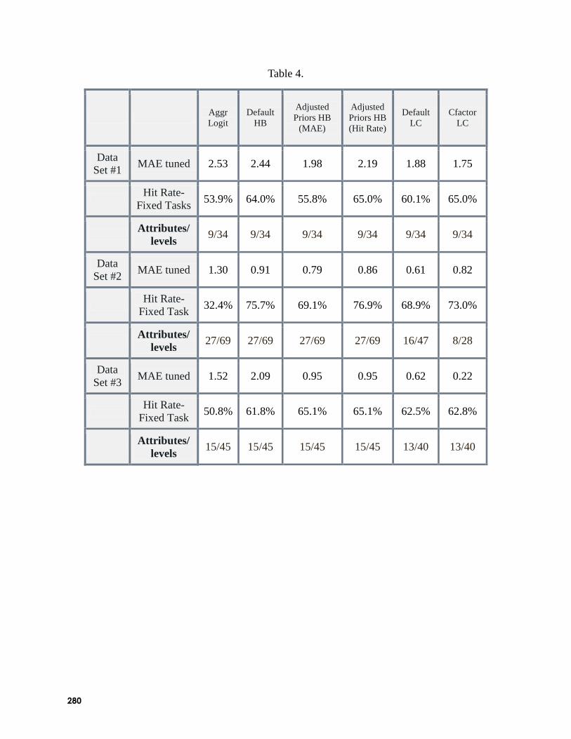
280

Table 4.

Aggr

Logit

Default

HB

Adjusted

Priors HB

(MAE)

Adjusted

Priors HB

(Hit Rate)

Default

LC

Cfactor

LC

Data

Set #1 MAE tuned 2.53 2.44 1.98 2.19 1.88 1.75

Hit Rate-

Fixed Tasks 53.9% 64.0% 55.8% 65.0% 60.1% 65.0%

Attributes/

levels 9/34 9/34 9/34 9/34 9/34 9/34

Data

Set #2 MAE tuned 1.30 0.91 0.79 0.86 0.61 0.82

Hit Rate-

Fixed Task 32.4% 75.7% 69.1% 76.9% 68.9% 73.0%

Attributes/

levels 27/69 27/69 27/69 27/69 16/47 8/28

Data

Set #3 MAE tuned 1.52 2.09 0.95 0.95 0.62 0.22

Hit Rate-

Fixed Task 50.8% 61.8% 65.1% 65.1% 62.5% 62.8%

Attributes/

levels 15/45 15/45 15/45 15/45 13/40 13/40

281

Table 5 below lists hit rates, DMAEs and Average Holdout Variance Ratios; three measures

of captured heterogeneity. For all three data sets, both default HB and hit rate-tuned HB capture

more heterogeneity than either LCC model, relative to the three measures listed, with the

exception of default HB, hit rate and data set # 3.

Table 5.

Aggr

Logit

Default

HB

Adjusted

Priors HB

(MAE)

Adjusted

Priors HB

(Hit Rate)

Default

LC

Cfactor

LC

Data Set #1 Hit Rate-

Fixed Tasks 53.9% 64.0% 55.8% 65.0% 60.1% 65.0%

DMAE-

Fixed Tasks 29.07 19.03 27.03 19.58 25.51 22.82

Variances

Ratio n/a 1.38 4.11 1.43 2.54 1.56

Data Set #2 Hit Rate-

Fixed Task 32.4% 75.7% 69.1% 76.9% 68.9% 73.0%

DMAE-

Fixed Task 21.70 7.26 13.70 7.34 12.45 14.29

Variances

Ratio n/a 1.03 1.15 1.03 1.02 1.03

Data Set #3 Hit Rate-

Fixed Task 50.8% 61.8% 65.1% 65.1% 62.5% 62.8%

DMAE-

Fixed Task 33.35 20.49 21.84 21.84 27.02 26.17

Variances

Ratio n/a 1.03 1.09 1.09 1.81 1.58

Table 6 compares hit rates for holdout tasks and hit rates for random tasks. Random task hit

rates for the HB models approach 100% and are dramatically higher than holdout task hit rates.

Random task hit rates for the LCC models are comparable to holdout task hit rates.

Table 7 compares DMAEs for holdout tasks and DMAEs for random tasks. Similarly to

Table 6 data, random task DMAEs for the HB models are dramatically lower than holdout task

DMAEs. Random task DMAEs for the LCC models are comparable to holdout task DMAEs.

For data set # 1, the LCC models used all available attributes. However, three attributes were

class independent and three others had one or more class parameters dropped. For data set # 3,

the LCC models used 13 of 15 available attributes. Additionally, one attribute was class

independent and one class parameter was omitted.

282

Given the dramatic improvement in hit rate and DMAE for the HB random task measures

relative to holdout task measures and the relative parsimony of the LCC models, it appears that

HB may overfit the data.

Table 6.

Hit Rates

Aggr

Logit

Default

HB

Adjusted

Priors HB

(MAE)

Adjusted

Priors HB

(Hit Rate)

Default

LC

Cfactor

LC

Data

Set #1

Hit Rate-Fixed

Tasks 53.9% 64.0% 55.8% 65.0% 60.1% 65.0%

Hit Rate-

Random Tasks 47.3% 99.3% 71.9% 98.2% 61.0% 69.4%

Attributes/levels 9/34 9/34 9/34 9/34 9/34 9/34

Data

Set #2

Hit Rate-Fixed

Task 32.4% 75.7% 69.1% 76.9% 68.9% 73.0%

Hit Rate-

Random Tasks 35.9% 96.3% 80.1% 94.6% 74.4% 78.1%

Attributes/levels 27/69 27/69 27/69 27/69 16/47 8/28

Data

Set #3

Hit Rate-Fixed

Task 50.8% 61.8% 65.1% 65.1% 62.5% 62.8%

Hit Rate-

Random Tasks 45.7% 98.6% 88.7% 88.7% 55.2% 61.2%

Attributes/levels 15/45 15/45 15/45 15/45 13/40 13/40

283

Table 7.

DMAEs

Aggr

Logit

Default

HB

Adjusted

Priors HB

(MAE)

Adjusted

Priors HB

(Hit Rate)

Default

LC

Cfactor

LC

Data

Set #1

DMAE-

Fixed Tasks 29.07 19.03 27.03 19.58 25.51 22.82

DMAE-

Random Tasks 32.75 1.78 25.86 4.89 26.72 22.30

Attributes/

levels 9/34 9/34 9/34 9/34 9/34 9/34

Data

Set #2

DMAE-

Fixed Task 21.70 7.26 13.70 7.34 12.45 14.29

DMAE-

Random Tasks 21.49 1.89 11.81 2.85 10.77 9.15

Attributes/

levels 27/69 27/69 27/69 27/69 16/47 8/28

Data

Set #3

DMAE-

Fixed Task 33.35 20.49 21.84 21.84 27.02 26.17

DMAE-

Random Tasks 33.51 3.23 14.45 14.45 28.17 25.79

Attributes/

levels 15/45 15/45 15/45 15/45 13/40 13/40

CONCLUSIONS

Default HB is by far the easiest of the examined models to build, yet it performed nearly as

well as more sophisticated models even though two of the three data sets used in the analysis

were quite sparse.

HB and LCC perform similarly and well, both in the default and more advanced forms (HB

with adjusted priors and LCC with Cfactors).

At least for these sparse data sets, LCC may estimate parameters with slightly less bias and

HB may capture more heterogeneity.

Sample size may have more potential to improve model performance than using advanced

forms of either HB or LCC.

Tuning HB priors to hit rates, rather than MAEs, appears to be the more productive approach.

284

DISCUSSION

HB and LCC may be reaching the limit of their potential. Both models, despite sophisticated

adjustments performed similarly to each other and also similarly to their default versions.

Further advances may need to come from a different source. For example, perhaps changing the

way questions are asked may yield higher quality data which would, in turn, improve model

performance.

For naïve users, default HB seems clearly to be the preferred method. It requires virtually no

tweaking, it is extremely simple to run and generates adequate results.

If however, the user is more advanced and either requires a segmentation as well as choice

utilities, or is interested in building a parsimonious model (and the managerial insight that

parsimony yields), LCC offers a viable alternative.

A word of caution, however, regarding LCC models. LCC models run fairly quickly if no

Cfactors are included. Including Cfactors increases computation substantially. Models that may

have taken a couple minutes to run might take a couple hours with Cfactors included. If the

modeler wishes to additionally model scale factor lamda, which can be done with the Latent

Gold Choice Syntax Module, run times might increase to 10-12 hours. In the commercial world,

these run times may occasionally prove impractical.

ADDITIONAL READING

Andrews, Rick L. Andrew Ainslie and Imran S. Currim (2002), An Empirical Comparison of

Logit Choice Models with Discrete Versus Continuous Representations of Heterogeneity,

Journal of Marketing Research (November), 479-87

Magidson, Jay and Tom Eagle (2005), Using Parsimonious Conjoint and Choice Models to

Improve the Accuracy of Out-of-Sample Share Predictions, ART Forum, American

Marketing Association, Coeur D' Alene, ID

Magidson, Jay and Jeroen Vermunt (2007), Use of a Random Intercept in Latent Class

Regression Models to Remove Response Level Effects in Ratings Data, Bulletin of the

International Statistical Institute, 56th Session, paper #1604, 1-4

Orme, Bryan (2003), New Advances Shed Light on HB Anomalies, Sawtooth Software Research

Paper Series, Sawtooth Software, Inc., Sequim, WA

Orme, Bryan and Peter Lenk (2004), HB Estimation for “Sparse” Data Sets: The Priors Can

Matter, ART Forum, American Marketing Association, Whistler, BC

Pinnell, Jon and Lisa Fridley (2001), The Effects of Disaggregation with Partial Profile Choice

Experiments, Sawtooth Software Conference, Victoria, BC

Sawtooth Software (2005), The CBC/HB System for Hierarchical Bayes Estimation Version 4.0

Technical Paper, accessible from

www.sawtoothsoftware.com/download/techpap/hbtech.pdf.

Vermunt, J. K. and J. Magidson (2005), Technical Guide for Latent GOLD Choice 4.0: Basic

and Advanced, Belmont Massachusetts: Statistical Innovations Inc.

285

ESTIMATING MAXDIFF UTILITIES:

DEALING WITH RESPONDENT HETEROGENEITY

CURTIS FRAZIER PROBIT RESEARCH

URSZULA JONES LIEBERMAN RESEARCH WORLDWIDE

MICHAEL PATTERSON PROBIT RESEARCH

OVERVIEW

While the use of hierarchical Bayes has several advantages over aggregate level models,

perhaps the primary advantage is the ability to capture respondent level heterogeneity. With

individual-level utilities, a number of new research questions can be answered. For example, we

can identify the existence of latent segments within our population and we can determine

whether a portfolio of distinct products is preferable to a single product.

While the promise of accurately capturing respondent heterogeneity is attractive, the authors‘

experience with both choice models and MaxDiff models was a source of concern about whether

HB was delivering on the promise, or whether a change in approach would be beneficial.

BACKGROUND

The general structure of the HB estimation procedure is relatively simple. HB works through

two stages. In an ―upper level model,‖ HB estimates the distribution of individual utilities. This

upper-level model provides a starting point to estimate the ―lower level model.‖ The upper-level

model defines the distribution, while the lower-level model examines the relationship between

individuals‘ utilities and their survey responses. Because we rarely have enough data available at

the respondent level to run truly independent analyses, the estimation for each individual

borrows data from other individuals through the upper-level model to fill in the gaps.

Key to the functioning of this two-level process is the amount of data available for each

individual. As the amount of data increases, the degree of borrowing that is necessary decreases.

Therefore, our ability to estimate true respondent heterogeneity increases as information at the

individual level increases. However, with sparse or ―thin‖ designs, HB must rely more and more

on the upper-level model when estimating individual-level utilities.

The issue then, is that our ability to detect respondent heterogeneity depends on two

elements:

1. The amount of information we have at the individual level, and

2. Paradoxically, the degree to which we have a homogeneous sample.

The second of these elements is the focus of this paper. Because of the data borrowing

process, any information gaps at the individual-level will be filled in with information from our

286

upper-level model. The issue is whether the average of the upper-level model represents the

views of the individual. In a situation with general homogeneity of preferences, the average of

the upper-level model should be a good predictor of individuals‘ preferences. However, in a

situation with high degrees of heterogeneity, how well does it work? The situation is analogous

to using means-substitution versus model-based methods for data imputation.

Across dozens of studies, the authors have found that HB, when applied to MaxDiff and

discrete choice models, does not consistently produce individual-level utilities that conform to

expectations. That is, the amount of variance in the sample is lower than expected and the

individual-level utilities do not differ based on hypothesized a priori segments. Based on this

experience, we set out to test whether estimating MaxDiff models using a homogeneous sample

for an upper-level model would produce more distinct (and meaningful) individual level utilities.

(Note: this paper uses the same basic framework that Keith Sentis and Lihua Li used in their

2001 Sawtooth paper on heterogeneity in discrete choice models.)

APPROACH

In order to test the impact of a homogeneous sample for an upper level model, we used 6

separate datasets. These datasets can be categorized as follows:

Real-World Data Synthetic Data

Low information

72 attributes

20 choice sets

6 alternatives per set

20 attributes

20 choice sets

5 alternatives per set

Medium information

30 attributes

10 choice sets

6 alternatives per set

20 attributes

10 choice sets

5 alternatives per set

High information

14 attributes

10 choice sets

5 alternatives per set

20 attributes

8 choice sets

5 alternatives per set

The synthetic data allow for testing the ability of the models to accurately re-create known

utility values, while the difference in ―information‖ levels allows for testing the impact of the

degree of data borrowing.

The synthetic data set was built by creating random utility value seeds for four separate

segments – three smaller (13%) segments and one larger (60%) segment. Total sample size for

each synthetic data set was n=1000. Because the synthetic data were created using specific rules,

the segments were derived from simple rules during the creation process. That is, the first X

number of cases were assigned one set of group values, while the second set was assigned a

different set. Using these segment level utilities as a starting point, the individual-level utilities

were estimated by adding random variation to each respondent‘s utility scores and then adding

second set of random error to account for response error. The result was utility values that were

distinct between segments, but with substantial overlap to add realism to the synthetic data.

287

Using both the real-world and synthetic data, our analysis plan includes estimating measures

of:

1. Goodness of fit

2. Difference from “true” utility values (synthetic data only), and

3. Between segment heterogeneity

RESULTS

Goodness of Fit When testing goodness of fit measures, we found a small, but consistent, increase in fit

measures as we moved from analysis at the total sample to analysis at the post hoc segment level.

This was particularly true when looking at the synthetic data. We attribute the results being

clearer in the synthetic data to the cleaner segment definition in the data construction process.

Analysis at the a priori level, however, was not found to be associated with better fitting

models. These models work less well than the post hoc segment models because they are not

truly functioning in line with our hypothesis. Our hypothesis is that we will find more distinct

segments when we have a more homogeneous population in terms of their MaxDiff preferences.

Our a priori segments are homogeneous. But, they are homogeneous on metrics such as gender

and income, not on MaxDiff preference. Therefore, these models not only have an upper-level

model based on a heterogeneous population, but they have a smaller overall base size.

Analysis at

Total Sample

Level

Analysis at A

Priori

Segment

Level

Analysis at

Post Hoc

Segment Level

Synth

etic

Dat

a High Information

Design

RLH 495 -- 569

Pct. Cert. 56% -- 65%

Medium Information

Design

RLH 587 -- 592

Pct. Cert. 66% -- 67%

Low Information

Design

RLH 618 -- 629

Pct. Cert. 69% -- 70%

Rea

l-W

orl

d

Dat

a

High Information

Design

RLH 500 500 490

Pct. Cert. 57% 56% 56%

Medium Information

Design

RLH 400 420 420

Pct. Cert. 49% 50% 50%

Low Information

Design

RLH 410 420 440

Pct. Cert. 50% 51% 53%

In his review of this paper, Rich Johnson provided a competing (but, unfortunately

overlooked) explanation for the better fit for the models analyzed at the segment level. Because

of the sheer number of parameters being estimated at the segment level, we would expect the in-

sample fit to be better. So, it is certainly possible that there is some measure of over-fitting

happening with the segment-level models.

288

Differences from “True” Utility Values Because of the way they were constructed, we know the ―true‖ utility values for our synthetic

data. To estimate accuracy, we used a simple difference in means:

Difference = Absolute Value (True utility – Estimated utility)

The example table below (representing the High Information scenario) illustrates the

consistent pattern. That is, analysis at the segment level resulted in more, rather than less, error

in utility estimates. This finding was somewhat counter-intuitive. Given that the upper-level

models were estimated using a homogeneous population, we expected better point estimates.

Analysis at Total Sample Level Analysis by Segment

Total Seg.

1

Seg.

2

Seg.

3

Seg.

4

Total Seg. 1 Seg. 2 Seg. 3 Seg. 4

Attribute 1 9% 4% 6% 1% 15% 11% 6% 16% 6% 21%

Attribute 2 4% 12% 10% 7% 0% 4% 16% 15% 8% 1%

Attribute 3 11% 2% 3% 1% 18% 13% 1% 5% 1% 23%

Attribute 4 12% 4% 17% 0% 15% 15% 4% 24% 0% 19%

Attribute 5 2% 9% 4% 10% 1% 1% 12% 9% 18% 6%

Attribute …

Attribute 20 1% 1% 11% 12% 7% 3% 3% 22% 22% 14%

Average

Error:

6% 7% 7% 7% 9% 7% 9% 12% 12% 12%

Rather than achieving better estimates of the ―true‖ utility values, segmenting the sample

prior to utility estimates effectively reduces our accuracy by reducing our sample size.

Between segment heterogeneity After finding that analysis at the sub-group level leads to less accurate estimates of ―true‖

utilities, we found ourselves in the somewhat unexpected position of asking ourselves whether or

not analysis at the sub-group level might also lead to some bias in the utility estimates. Our

analysis shows that it does.

The illustration below depicts the average utility scores for the same respondents given the

change in approach. The left side of the illustration represents average utilities when we use our

total sample in the utility estimation. The right side represents average utilities when our sample

is restricted to only those respondents in the post hoc segment. What is evident is that the utility

estimates (again, these are for the exact same respondents) are consistently more extreme when

analyzed at the segment level than when analyzed at the total sample level.

289

This finding, while somewhat unexpected, makes sense. The total sample model has a

moderating effect. Because the upper-level model is based on a heterogeneous population, those

aggregate-level utilities should converge towards the mid-point (in our scaling, the mid-point is

50%). However, when we use a homogeneous population for our upper-level model, the

―gravitational pull‖ towards the mid-point is gone. This allows the utility scores to diverge from

the mid-point and become more extreme.

This finding, if it were made in isolation, may have lead us to believe that analysis at the sub-

group level is a good thing. After all, we are finding more and more distinctiveness in our

results. However, coupled with the previous findings – particularly those showing the lower

ability to replicate known utility values – this provides little reassurance that estimation of

utilities at the sub-group level is providing better estimates.

The figure above illustrates the results for one segment. This finding was true for all

segments in each of our three information level scenarios. However, the resulting bias towards

the extremes was more evident in our low information scenarios and for smaller segments. This

leads us to believe two things:

1. The positive moderating impact increases as data borrowing increases. While the

assertion that data borrowing leads to increased moderation is obvious, the positive

impact is somewhat new.

2. The small sample sizes associated with estimating utilities for smaller and smaller

homogeneous sub-groups has a significant, negative impact on data accuracy and leads to

utility bias (towards more extreme values).

Again, it should be noted that the segment-level models may suffer from over-fitting. The

over-fitting problem leads to larger estimates. So, while the outcome is the same, the cause

matters because this result may be more a matter of scale than it is less ―gravitational‖ pull.

290

CONCLUSIONS

Our investigation began based on years of conducting both MaxDiff and Discrete Choice

models. In study after study, the degree of differentiation that was found between a priori

segments was lower than expected. We identified two likely sources for this:

1. Incorrect hypotheses when choosing the a priori segments, and

2. A moderating and “muddling” effect of estimating HB utilities using a highly

heterogeneous population

Our findings show that CBC-HB performs as well, and in most cases, better, when MaxDiff

utilities are estimated using a larger sample size, even if that larger sample is heterogeneous. The

amount of information available at the individual level appears to have little impact (given the

parameters that we used to identify high, medium and low information).

REFERENCES

Sentis, Keith and Lihua Li (2002), ―One Size Fits All or Custom Tailored: Which HB Fits

Better?‖, Sawtooth Software Research Paper Series,

http://www.sawtoothsoftware.com/download/techpap/hbfit.pdf.

Many thanks to Rich Johnson for his thoughtful comments on our paper and presentation.

291

AGGREGATE CHOICE AND INDIVIDUAL MODELS:

A COMPARISON OF TOP-DOWN AND BOTTOM-UP APPROACHES.

TOWHIDUL ISLAM

JORDAN LOUVIERE

DAVID PIHLENS SCHOOL OF MARKETING AND CENTRE FOR THE STUDY OF CHOICE (CENSOC)

UNIVERSITY OF TECHNOLOGY, SYDNEY

INTRODUCTION

Several recent papers discuss the role of the error variance in choice models, noting that

models that do not take error variance differences within and between people (and other

differences) into account may be biased (e.g., Swait & Louviere 1993; Swait & Adamowicz

2001; Louviere 2001; Louviere & Eagle 2006; Magidson & Vermunt 2007; Louviere, et al. 2008;

Salisbury & Feinberg 2009). Indeed, it seems fair to say that many published results in

marketing and other fields should be reconsidered due to potentially biased and incorrect model

estimates. To wit, in any real dataset there is likely a distribution of error variances and a

distribution of preferences; error variance differences can arise from between-subject

heterogeneity (with differences arising in both taste and preference intensity), and within-subject

inconsistency over choice occasions. Other factors also likely impact variability differences,

such as respondent education or age, task complexity, etc (see Louviere, et al. 2002). So, one

must account for such differences in analyses to avoid potential biases.

It is well-known that error variance (scale) differences arise in comparing DCE and real

market choices, as noted by Swait and Louviere (JMR, 1993). That is, typically (but not

always), there is more variability in real market choices because there are (many) more random

influences on choice in a real market than relatively well-controlled discrete choice experiments

(DCEs). So, to predict real choices accurately, one should (must) have a source of real market

choice data that can be used to calibrate (rescale) DCE model parameters. Swait and Louviere

show how to estimate the variance-scale ratio for real and DCE choices using a simple grid

search procedure, but there are more sophisticated estimation methods, as discussed in Louviere,

Hensher and Swait (2000, Chapters 8 and 13). Surprisingly, estimated variance scale ratios often

are around 0.4, indicating about 2.5 times as much variability in real market choices as DCE

choices. More generally, many anecdotes suggest that models estimated in DCEs or similar

preference surveys over-predict real choices by about three times, which would be consistent

with a variance-scale ratio in the 0.35-0.45 range, which aligns well with many such ratios we

have observed. The foregoing comments apply to the ―Exponent‖ in Sawtooth Software;

estimating the variance-scale ratio is equivalent to ―tuning the Exponent/Scale Factor in a market

simulator,‖ as suggested by Sawtooth Software.

To illustrate the problem, we designed a choice experiment with k=2 binary attributes, and

m=2 options per choice set, and all N=6 pairs. Each option‘s indirect utility was specified as a

linear effect of each attribute (with endpoints coded using -1 and 1), and a linear-by-linear

292

interaction. We defined G=4 types of people, each with the same indirect utility, but different

error variances. We write the utility of the ith option for the gth group as

Uig = 1,1 x1 + 2,1 x2 + 12,11 x1 x2 + ig, i = 1,2, g=1,…,4 and igEV1(0,g).

A graphical example of this case with 7 instead of 4 groups (to emphasize the point) is shown

in Figure 1 below, where one can see very different choice probabilities resulting from

differences in scale, despite identical indirect utility functions.

The values of the indirect utility parameters for each of the 4 groups are identical (1,1= 1,

2,1= -1.125, 12,11=0.375), while each group‘s different error variance differed (1=2, 2=1,

3=1/2, and 4=1/4). We simulated sg=200 respondents per group. Parameter estimates from

calibration of a conditional logit model on the simulation data (from SAS) are in Table 1.

Parameter True Group 1 (1=2) Group 2 (2=1) Group 3 (3=1/2) Group 4 (4=1/4)

1,1 1 0.58375 1.01959 2.09143 6.20875

2,1 -1.125 -0.55485 -1.12983 -2.18352 -6.69689

12,11 0.375 0.17729 0.34227 0.87882 3.40125

Table 1

Maximum likelihood estimates of the preference parameters for the four groups.

As expected, as error variances decrease (from Group 1 to Group 4) magnitudes of indirect

utility parameters increase. For example, the linear effect of attribute one, 1,1, increases in

magnitude from 0.58375 for group 1 to 6.20875 for group 4. One might be tempted to conclude

that the utilities differ across the four groups. However, we know from our simulation that group

utilities are homogenous, with only error variance (scale) differences. Fiebig et al. (2009) use

293

monte carlos to show that random coefficient models that do not take scale differences like these

into account will incorrectly identify this as preference heterogeneity 100% of the time.

Much recent research in our centre (CenSoC) has focused on issues related to error variance

differences between individuals. However, it is likely from much prior work in psychology that

there also are error variance differences within individuals. That is, individuals differ in how

consistently they make choices, but they also differ within themselves over choice occasions

(choice sets) in the consistency of their choices. In the latter case, an individual‘s choice

consistency can vary over trials – initially she is more inconsistent, she then becomes more

consistent, and then in larger DCEs, she becomes more inconsistent again due to inattention,

fatigue, boredom, etc. Likewise, individuals tend to identify extreme attribute levels, and as

Louviere (2000) suggested, react more consistently to them than middle levels. They also may

use decision rules or heuristics that are inconsistent with assumptions of additive indirect utility

functions, which rules lead to seemingly systematic variability in choice with levels of attributes

and/or combinations of levels of attributes. While variability between individuals might be dealt

with by normalizing part-worths within and between people (such as using Sawtooth Software‘s

―Zero-Centered Diffs‖), there typically are several (if not many) sources of variability in choice

that are unobserved in a DCE, which lead to systematic confounds with estimated parameters.

Also worrisome is the fact that in almost all DCEs many factors are held constant, but these

factors are not constant in real markets, and can vary within and between individuals. This, too,

poses potential sources of confounds with estimated parameters, but also challenges researchers

who want to extrapolate models estimated from DCEs to predict choices in real markets. The

only solutions to the latter problem are strong a priori behavioral theory and/or spending

considerable time and effort in advance of designing and implementing a DCE to understand

potential differences and take them into account to the extent possible in the DCE.

Now we can state that the purpose of this paper is to compare three ways to model choices

that potentially can accommodate error variance differences between people. The approaches

are: 1) a classicist mixed logit random coefficient model estimated using simulated maximum

likelihood (Revelt and Train 1998), 2) a Hierarchical Bayes random coefficient model estimated

using MCMC (Allenby and Rossi 1993), and 3) a new way to estimate choice models for single

individuals (Louviere et al. 2008). We view the first two approaches as ―top-down‖ modeling

approaches because one makes assumptions about distributions of errors and preferences,

indirect utility functions and choice processes, which if correct, allow one to capture an

aggregate distribution of preferences in a sample population. We view the third approach as a

―bottom-up‖ approach: it makes assumptions about indirect utility functions, choice processes

and error distributions for individuals, models each person separately, and then aggregates

predictions from each person‘s model separately. This paper focuses on the third approach,

namely estimating a separate choice model for each person.

2. MODELING INDIVIDUAL CHOICES

Louviere, et al. (2008) proposed a way to estimate conditional logit models for single

individuals that can be described briefly as follows:

1. Obtain a full or partial ranking of options in each choice set by asking respondents two or

more questions about their most and least preferred options in each set (e.g., if 4 options

per set, ask most preferred and least preferred; then ask most or least preferred of the

294

remaining two). That is, instead of asking respondents to “do” more choice sets, ask

them more choice questions about each choice set.

2. Use the ranking obtained from 1 above to estimate choice models via the method of rank

order explosion (Luce and Suppes 1965; Chapman and Staelin 1982); or use the ranking

to assign weights to each rank order position based on the expected choice counts that

should be observed if a person chose consistently with their ranking in each possible

choice set (there are 2J subsets of J choice options in each set). For example, four options

per set (J=4) gives 16 possible choice sets (one is empty). Let the options be A, B, C, D,

respectively ranked, 1, 2, 3, 4 (1= best, 4=worst), the expected choices (weights) are 8, 4,

2, 1 for these ranks.

Louviere, et al. (2008) show how to estimate conditional logit models using these weights,

and test whether the resulting model estimates are unbiased (they were in their test). We use this

weighted conditional logit approach to estimate models for individuals. We compare in- and out-

of-sample predictions of this approach to predictions from mixed logit (MIXL) and Hierarchical

Bayes (HB) models for four data sets described below. Table 2 lists attributes and levels for four

discrete choice experiments (DCEs) used in the model comparison. Brand and price were in all

DCEs. We compare how well preferences can be captured using four attributes (brand and price

always included) compared with seven attributes (brand and price always included). We

constructed optimal Street and Burgess (2007) main effects only designs for each DCE.

Study participants were recruited by Pureprofile, a large Australian online panel provider that

maintains a panel of approximately 300,000 households selected to be as representative of the

Australian population as possible (the panel over-represents higher income, higher education and

younger Australians). The 4 DCE conditions are (pizza, juice) x (4, 7 attributes). Participants

were randomly assigned to each DCE.

Table 2:

Design Specifications for DCEs in Study

No Pizza Attributes Level 1 Level 2 Level 3 Level 4

1 Brand Pizza Hut Dominos Eagleboys Pizza Haven

2 Price $12 $14 $16 $18

3 Delivery Time 10 min. 20 min. 30 min. 40 min.

4 No. Toppings 1 3

5 Free Dessert No Yes

6 Free Delivery No Yes

7 Free Salad No Yes

No Juice Attributes Level 1 Level 2 Level 3 Level 4

1 Brand Berri Just Juice Daily Juice Spring Valley

2 Price $1.00 $1.30 $1.60 $1.90

3 % Real Juice 10%. 40% 70% 100%.

4 Made From Concentrate Fresh

5 Pulp Not added Added

6 Calcium Not added Added

7 Package Materials Plastic Glass

295

3. RESULTS

As previously noted, we estimated MIXL and HB models (Allenby & Rossi 1993). The

probability of choosing option i in MIXL can be written as:

Pi = exp[(k + k)Xki] / ∑jC exp[ (k + k)Xkj],

where k is a vector of random effects including alternative-specific intercepts with

associated disturbance terms, k, corresponding to the design matrix of covariates, Xki and Xkj.

Like many researchers, we assume that the random effects are normally distributed. The MIXL

model is not closed form, so we estimate it with simulated maximum likelihood (Revelt & Train

1998) using Ken Train‘s GAUSS code. We use Bayes rule to estimate the posterior distribution

for each person following Train (2003, Chap 11) to estimate utilities for each person. We also

compared the Louviere, et al. (2008) individual level model estimates with HB estimates from a

similar model specification. We used the HB information on the aggregate taste distribution

together with the individuals‘ choices to derive conditional estimates of each individual‘s

parameters. For both MIXL and HB we use individual-level estimates to predict choice

probabilities for each person; we use the method of sample enumeration to aggregate the

probabilities.

Previous MIXL and HB comparisons (e.g., Huber & Train 2001), suggest both models yield

similar conditional estimates; so, familiarity, personal preference and estimation ease typically

underlie which one a researcher uses. Our experience is that estimates of means and standard

deviations of assumed preference distributions are similar, but individual-level estimates can

differ, particularly if less than full design information is used in estimation (typical of many

applications), which is why we chose to compare the models using full design information

(maximizing the chance that MIXL and HB should perform well).

Within and Cross-Sample Model Performance Sample sizes are, respectively, Pizza with 7 attributes = 459; Pizza with 4 attributes = 458;

Juice with 7 attributes = 455 and Juice with 4 attributes = 454. We evaluated the fit of the

models in- and out-of-sample using different model fit criteria (R2, MSE & 2

). All fit criteria

agree, so we only report R2

values in Table 3. Most choice modelers are not accustomed to R2

values, so we note that many DCEs assign the same choice sets to multiple choosers, allowing

calculation of choice proportions for each option in each choice set. Discrete choice models

predict choice probabilities, so it is natural to ask how well observed and predicted choice

proportions agree.

296

% Juice estimates Vs Error Var

10% = 8.16x - 1.73, R2 = 0.80

40% = 2.60x - 0.54, R2 = 0.34

70% = -3.32x + 0.69, R2 = 0.27

100% = -7.44x + 1.57, R2 = 0.79

-1.50

-1.00

-0.50

0.00

0.50

1.00

1.50

0.06 0.08 0.10 0.12 0.14 0.16 0.18 0.20 0.22 0.24 0.26

Error Var

% J

uic

e E

stim

ate

s

RJ=10%

RJ=40%

RJ=70%

RJ=100%

R2: in-sample R

2: cross sample

1

Pizza

MIXL Sample 1

[7 attrib]

0.9283 0.8786

HB 0.9482 0.9312

Indv. Model 0.9868 0.9085

MIXL Sample 2

[4 attrib.]

0.9440 0.6702

HB 0.9542 0.6373

Indv. Model 0.9913 0.6737

Juice

MIXL Sample 1

[7 attrib]

0.9202 0.8878

HB 0.9259 0.8940

Indv. Model 0.9946 0.9641

MIXL Sample 2

[4 attrib.]

0.9282 0.9018

HB 0.9297 0.8930

Indv. Model 0.9883 0.9809 1

Sample 1 estimates used to predict Sample 2 and vice versa

Table 3:

Comparison of in- and out-of-sample predictive validity (R-square)

Table 3 suggests that the Louviere, et al. (2008) individual-level model approach dominates

MIXL and HB: HB won one of the four cross-sample comparisons; individual-level models won

the other three; and individual-level models won all four in-sample comparisons. Interestingly,

comparing just MIXL and HB shows that each had the same number of wins in four cross-

sample comparisons with each other (two each). Despite predicting observed choices well, all

model estimates are biased due to failure to take differences in error variances into account, as

shown in Figure 1, which graphs individual error variances against individual model estimates

for pizza prices and %real juice. Figure 1 clearly shows that as error variability increases, model

estimates go to zero, and as it decreases, model estimates grow large. Thus, estimates are biased

at either end of the unobserved variability distribution. Indeed, as much as 80% of the variance

in %real juice estimates is simply due to error variability differences, not preference differences!

Price Estimates Vs Error Var

$12 = -8.71x + 1.64, R2 = 0.39

$14 = -6.12x + 1.14, R2 = 0.39

$16 = 3.94x - 0.74, R2 = 0.25

$18 = 10.88x - 2.04, R2 = 0.45

-1.50

-1.00

-0.50

0.00

0.50

1.00

1.50

0.12 0.13 0.14 0.15 0.16 0.17 0.18 0.19 0.20

Error Var

Pric

e E

stim

ate

s

Price=$12

Price=$14

Price=$16

Price=$18

Figure 1:

Unobserved Variability Vs Estimated Price/Juice Parameters

297

4. DISCUSSION AND CONCLUSION

We compared three approaches to estimating choice models that can provide individual-level

parameter estimates. The bottom-up approach of Louviere et al. (2008) gave consistently

superior in-sample fits, and won three of the four out-of-sample fit comparisons. This approach

is easy to implement and apply, and can be used in conjunction with many other discrete choice

model approaches. It does not require assumptions about preference distributions, and so is to be

preferred to approaches that require such assumptions. Because one can estimate the unobserved

variability associated with each person, one can ―adjust‖ the models to take this into account.

Another advantage is that it can identify lexicographic and similar strategies, as demonstrated by

Louviere et al. (2008).

Naturally, there are limitations, such as assumptions about choice processes and indirect

utility functions. We do not yet know the extent to which this can be relaxed and made more

flexible. There also probably are upper limits to possible numbers of attributes and choice sets,

although to date we have had success with problems as large as 32 choice sets, with five options

per set and 13 attributes. Our results suggest that researchers should give this approach at least

as much attention as popular, but more complex top-down models.

Finally, our research group often is accused of being anti-Bayesian, which is simply false, as

exemplified by two recent CenSoC/UTS hires (Christine Ebling and John Geweke). As many

would know, John Geweke is a world leader in Bayesian econometrics, and joins CenSoC as

Director of Academic Affairs. Indeed, CenSoC‘s position is very simple – groups that claim

special insights into ―truth‖ in fact rarely do. We prefer a balanced approach, preferably a cross-

disciplinary approach, where scholars and practitioners can discuss and research issues in an

independent and objective manner, and where theory and empirical evidence are valued more

than opinions. Thus, we developed the individual-level, bottom-up modeling approach to allow

us to provide new and different evidence regarding whether one or more groups had better

approximations to ―truth‖ than others. Thus far, on the evidence, bottom-up approaches seem to

have key advantages when one can design DCEs that are sufficiently small to be able to use

them. If one cannot use a bottom-up approach, top-down approaches are the next best option,

but our experience is that one needs a) as much individual-level data (choice sets) as possible, b)

to be sure that distributional assumptions about model parameters are well-satisfied (e.g.,

parameter distributions are not highly skewed or multi-modal), and most importantly, c) to be

very careful to take differences in error variabilities between real and experimental markets into

account.

5. REFERENCES

Allenby, G.M. and Rossi, P.E. (1993) ―A bayesian approach to estimating household

parameters,‖ Journal of Marketing Research, 30, 2, 171-182.

Chapman, R.G. & R. Staelin (1982) ―Exploiting rank order choice set data within the

stochastic utility model,‖ Journal of Marketing Research, 19, 288-301.

Huber, J. & Train, K. (2001) ―On the similarity of bayesian estimates of individual mean

partworths,‖ Marketing Letters, 12, 3, 259-269.

298

Louviere, J.J. (1988) Analyzing Decision Making: Metric Conjoint Analysis. Sage University

Papers Series No. 67: Newbury Park, CA: Sage Publications, Inc.

Louviere, J.J. (2001), ―What if consumer experiments impact variances as well as means:

Response variability as a behavioral phenomenon,‖ Journal of Consumer Research, 28,

506-511.

Louviere, J.J. & Eagle, T. (2006) ―Confound It! That pesky little scale constant messes up

our convenient assumptions,‖ Proceedings, 2006 Sawtooth Software Conference, 211-228:

Sawtooth Software, Inc. , Sequim, WA, USA.

Louviere, J., Hensher, D. & J. Swait (2000) Stated Choice Methods: Analysis and

Application. Cambridge, UK: Cambridge University Press.

Louviere, J.J. Street, D., Carson, R., Ainslie, A., DeShazo, J.R. Cameron, T., Hensher, D.,

Kohn, R. & T. Marley (2002) ―Dissecting the random component of utility,‖ Marketing

Letters, 13, 3, 177-193.

Louviere, J.J. , Street, D., Burgess, L. Wasi, N., Islam, T. & Marley, A.A.J. (2008)

―Modeling the choices of individual decision-makers by combining efficient choice

experiment designs with extra preference information,‖ The Journal of Choice Modeling,

1, 1, 128-163.

Magidson, J. & Vermunt, J.K. (2007) ―Removing the scale factor confound in multinomial

logit choice models to obtain better estimates of preference, ‖ Proceedings, Sawtooth

Software Conference, Santa Rosa, CA (October).

Revelt, D. & K. Train (1998) ―Mixed logit with repeated choices: Household choices of

appliance efficiency level,‖ Review of Economic Statistics, 80, 647–57.

Salisbury, L. & F. Feinberg, F. (2008) ―Alleviating the constant stochastic variance

assumption in decision research: Theory, measurement and experimental test, ‖ Marketing

Science, forthcoming.

Salisbury, L. and F. Feinberg (2008) Alleviating the Constant Stochastic Variance Assumption

in Marketing Research: Theory, Measurement and Experimental Test, ‖Marketing Science,

forthcoming.

Street, D.J. & Burgess, L. (2007), The Construction of Optimal Stated Choice Experiments:

Theory and Methods. Hoboken, New Jersey: Wiley.

Swait, J. & Louviere, J. J. (1993) ―The Role of the Scale Parameter in the Estimation and

Comparison of Multinomial Logit Models‖, Journal of Marketing Research, 30, 305-314.

Swait, J. & Adamowicz, V. (2001) ―The influence of task complexity on consumer choice: A

latent class model of decision strategy switching,‖ Journal of Consumer Research, 28, 1,

135-148.

Train, K. (2003) Discrete Choice Methods with Simulation. Cambridge: Cambridge

University Press.

299

USING CONJOINT ANALYSIS FOR MARKET-LEVEL DEMAND

PREDICTION AND BRAND VALUATION

KAMEL JEDIDI COLUMBIA UNIVERSITY

SHARAN JAGPAL RUTGERS UNIVERSITY

MADIHA FERJANI SOUTH MEDITERRANEAN UNIVERSITY, TUNIS

ABSTRACT

This paper develops and tests a conjoint-based methodology for measuring the financial

value of a brand. The proposed approach uses a simple, reduced-form representation that

provides an objective dollarmetric value for brand equity without requiring one to collect

subjective perceptual or brand association data from consumers. In particular, the model allows

for complex information-processing strategies by consumers ranging from central and peripheral

information-processing to using prices and brands as signals of quality. Importantly, the model

allows industry volume to vary when a product becomes unbranded.

We define firm-level brand equity as the incremental profitability that the firm would earn

operating with the brand name compared to operating without it. In computing the product

profitability when branded, we show how to use consideration set theory to account for

incomplete product awareness and limited availability in the distribution channel when inferring

market-level demand using choice-based conjoint experiments. To compute the profitability of a

product when it loses its brand name, we use a competitive equilibrium approach to capture the

effects of competitive reactions by all firms in the industry when inferring the market level

demand for the product when it becomes unbranded.

We tested our methodology using data for the yogurt industry and compared the results to

those from several extant methods for measuring brand equity. The results show that our method

is externally valid and is quite accurate in predicting market-level shares; furthermore, branding

has a significant effect on industry volume. For the yogurt category, our model predicts that

industry volume will fall by approximately one-fifth (a reduction of 22.9%) if the market leader

were to become unbranded.

1. INTRODUCTION

This paper focuses on the managerial aspects of the conjoint methodology that the authors

developed to measure brand equity in a forthcoming Journal of Marketing Resarch article. In

addition, it summarizes the key findings of the empirical study that the authors conducted to test

their methodology. For more details, please refer to: Ferjani, Madiha, Kamel Jedidi, and Sharan

Jagpal (2009), ―A Conjoint Approach for Consumer- and Firm-Level Brand Valuation,‖ Journal

of Marketing Research, forthcoming.

Firms often allocate considerable resources to develop brand equity to improve their long-run

financial performance. Hence they urgently need answers to such questions as: What is the

‗health‘ of the firm‘s brand? How is the health of the firm‘s brand changing over time? What is

the financial value of the firm‘s brand? How much should the firm be willing to pay in a merger

300

and acquisitions deal to acquire another brand? Should the firm extend its brand, license another

brand, or create a new one? In this paper, we develop and test a conjoint methodology for

answering these and other key managerial questions.

There is a vast and burgeoning literature on how to measure firm-level brand equity (see

Keller and Lehmann 2006 for a detailed literature review). Some researchers (e.g., Ailawadi et

al. 2003) propose that firm-level brand equity be measured directly using market-level data.

Others (e.g., Srinivasan et al. 2005) suggest that one should first collect primary data to measure

consumer-level brand equity and then use this information, combined with market-level data, to

estimate firm-level brand equity. There is also a stream of brand equity research that measures

the value of a brand as a financial asset using market-level data (see for example Mahajan, Rao,

and Srivastava 1994; Simon and Sullivan 1993; and Mizik and Jacobson 2007). The proposed

method is in the spirit of the Srinivasan et al. 2005 approach.

In this paper, we propose a choice-based conjoint method that captures multiple sources of

brand equity without requiring one to collect subjective perceptual or brand association data

from consumers. Three critical features of our conjoint approach are that: (i) The experiment

must include unbranded products. This is critical for determining the part-worth values of

products with no brand equity, (ii) All choice sets in the conjoint experiment must include the no-

purchase option. This is necessary to capture both industry shrinkage and market expansion

effects when a product becomes unbranded, and (iii) The model must include brand-attribute

interactions. This is necessary for capturing multiple sources of brand equity such as those

proposed by Keller and Lehmann 2006 (e.g., biased perceptions, image associations, inertia

value). In addition, this specification simplifies the measurement of brand equity since it

obviates the need to collect perceptual and brand association data.

We define firm-level brand equity as the incremental profitability that the firm would earn

operating with the brand name compared to operating without it (Dubin 1998). A novel feature

of our method is that we use consideration set theory to compute brand profitability. This step is

necessary so that one can aggregate the results from a choice-based conjoint experiment to infer

market-level demand for the product after accounting for the differential effects across brands of

incomplete product awareness and limited availability in the distribution channel. A key

distinguishing feature of our consideration-set-based method is how we adjust for all commodity

distribution (ACV) and market-level awareness for each brand when projecting the market share

results from the experiment to the marketplace. The conventional industry practice is to adjust

the market shares from a conjoint experiment by weighting each brand choice share by the

product of that brand‘s ACV and awareness level. Although this practice is easy to implement, it

is ad hoc. As we show in the paper and implement using our methodology, it is necessary to

make these adjustments based on consideration set theory.

To compute the profitability of a product when it loses its brand name, we use a competitive

equilibrium approach. In contrast to the industry expert approach (Srinivasan et al. 2005) and

the generic-product approach (Ailawadi et al. 2003), our competitive equilibrium approach

captures the effects of competitive reactions by all firms in the industry (i.e., manufacturers and

retailers) when inferring the market level demand for the product when it becomes unbranded.

We tested our methodology using data for the yogurt industry and compared the results to

those from several extant methods for measuring brand equity, including the generic and industry

expert approaches. The results show that our method is quite accurate in predicting market-level

shares; furthermore, branding has a significant effect on industry volume. In the example, our

301

model predicts that industry volume will fall by approximately one-fifth (a reduction of 22.9%)

if the market leader were to become unbranded.

In summary, our method for measuring brand equity provides several advantages.

Managerially, it provides a method for managers to value their brands internally for diagnostic

and control purposes, and externally for mergers and acquisitions. Methodologically, the paper

shows (i) How to accurately extrapolate choice shares from a conjoint experiment to market-

level brand shares after allowing for differential awareness and distribution effects across brands,

and (ii) How to capture the effects of competitive reaction by all firms in the supply chain (i.e.,

manufacturers and retailers) when predicting the share of a brand that becomes unbranded.

The rest of the paper is organized as follows. First, we describe the conjoint model. Then,

we present our brand equity measurement approach. Next, we report the results from a

commercial application; in particular, we compare the results from our model with those

obtained by using extant measurement approaches. We conclude by discussing the main findings

of the study and proposing directions for future research.

2. THE CONJOINT MODEL

Consider a choice set consisting of J-1 branded products (or services), one unbranded product

indexed by J, and the no-purchase option. Including the unbranded product is critical for

determining the part-worth values of products with no brand equity. Including the no-choice

option is necessary to derive a dollametric value for brand equity and to capture both industry

shrinkage and market expansion effects when a product becomes unbranded.

By definition, the unbranded product is a product with no brand equity. Previous researchers

have used various definitions of an unbranded product including a private label, a generic

product, a store brand, or a weak national brand. In our study, we use a nonstandard approach

and operationalize the unbranded product as a hypothetical new product. As will be discussed

shortly, this nonstandard conjoint experimental design provides significant methodological

advantages over previous methods for measuring brand equity and is a critical part of our

methodology.

Let jmx be the objective level of attribute m (m=1. …, M) for product j (j=1. …, J) and pj be

the price of product j. Then, we model the utility of consumer i (i=1. …, I) for product j as

follows:

(1) J,,1,=jI,,1,=iallfor,pβ-xββ=U jpijjmijm

M

=1m

ij0ij ij

where βijm is a regression coefficient (part-worth) that captures the brand-specific effect of

objective attribute m, pijβ captures the effect of price on the utility of Brand j, ij0 is a brand-

specific coefficient, and ijε is an error term. We discuss the distributional assumptions

for ijε (j=1, …, J) in the Model Estimation subsection below. Note that we estimate a separate

set of conjoint coefficients for the unbranded product J M)., 1,m ,(βiJm These coefficients

are critical for determining the part-worth values (and hence the utility) of a product when it

turns unbranded. Specifically, when product j turns unbranded, its utility becomes

.pβ-xββ=U j

p

iJjmiJm

M

=1m

iJ0ij iJ

302

Ferjani et al. (2009) show that the reduced-form utility model in Equation (1) where both

attribute and price effects vary across brands and individuals is sufficient for capturing multiple

sources of brand value (biased perceptions, image associations, and inertia value—see Keller and

Lehmann 2006, p. 751); in addition, Equation (1) captures price signalling effects. It is

important to note that while Equation (1) captures multiple sources of brand equity, it does not

reveal which specific perceptions or image association(s) brand equity arises from. Thus, if the

managerial objective is to understand brand equity at the perception or image association levels,

it will be necessary to augment the experimental design by collecting perceptual data.

In its most general form, Equation (1) allows all model parameters to vary across brands.

This specification is feasible if the number of brands and/or attributes is reasonable. However, if

the number of brands and/or attributes is large, it will be necessary to constrain the model. For

example, suppose one assumes that the consumer perceptual biases are invariant across attributes

(i.e., halo effects do not vary across attributes). Given this assumption, let ijθ be consumer i‘s

‗halo‘ parameter for product j.1 Then, Equation (1) simplifies to:

(2) J,1,j,εpβ-xbθβ=U ijj

p

ijjmim

M

=1m

ijij0ij

where bim is the (brand-invariant) part-worth coefficient for attribute m. Note that, because of

the parametric restrictions in Equation (2), only the intercept, price coefficient, and the ‗halo‘

parameter ijθ vary by brand.

Our model allows for different information–processing strategies by consumers. For

example, suppose consumers process information peripherally (see Petty, Cacioppo, and

Schumann 1983). Then, brand does not affect the perceived levels of product attributes; instead,

brand has a direct effect on preferences. Consequently, the brand equity of a product for any

given consumer is fully captured by the individual-specific intercept term for that product

(Kamakura and Russell 1993). Alternatively, suppose consumers process information centrally.

Then, brand affects the perceived levels of product attributes and/or perceived benefits and hence

preferences. Consequently, the brand equity of a product for any given consumer depends on

both the intercept and the other regression parameters for that consumer. Note that, regardless of

which information-processing strategies different consumers follow, our utility model can allow

for general forms of perceptual bias including halo effects. Importantly, because we use a

reduced-form representation of the preference model, there is no need to obtain subjective data

on brand-level attribute perceptions or brand image associations. Hence the model is not subject

to multicollinearity or measurement error. As noted earlier, our goal is to develop a

parsimonious model for quantifying the dollarmetric value of brand equity. If the goal is broader

(e.g., to modify message strategy to enhance brand equity), it will be necessary to explicitly

model the consumer‘s information-processing model, including the mapping from objective

attributes to perceptions.

Model Estimation A utility-maximizing consumer will select product j if and only if two conditions are

simultaneously satisfied: (i) His or her utility for product j is greater than the utility from the no-

1 For example, suppose consumer i is fully informed about all the attributes in product j or can verify their levels prior to purchase. Then, there are no halo

effects and hence 1.θij Alternatively, suppose consumer i misperceives that the attribute levels for product j are higher than their true values. Then

1θij . Similarly, if the consumer misperceives that the attribute levels for product j are lower than their true values, then 1.θij

303

purchase option, and (ii) The utility from product j has the maximum value in a given choice set.

Let s index a choice task or observation (s=1,…,S) in a conjoint choice experiment. Let j=0

index the no-purchase option. Let ijsijsijs εV=U and i0si0s εU denote the utility from the

purchase of product j and the no-purchase option on choice occasion s, respectively. Vijs is the

systematic utility component in Equation (1) and is given by ,pβ-xββ=V sj

pij

sjmijm

M

=1m

ij0ijs where

sj

sjm pandx are, respectively, the value of attribute m and the price of product j in choice task s.

Then, consumer i will choose product j on choice occasion s if

(3) ,Umax=U 0ilsJl1

ijs siU

and will choose the no-purchase option if

(4) S., 1,s J,,1,=j, U<U i0sijs

Assume that each of the ijs‘s (j=0, …, J) follows an independent and identical extreme value

distribution. Both distributional assumptions are reasonable given our choice-based conjoint

design. Specifically, we randomize brand alternatives both within and across choice sets. Hence

the independence assumption holds. At first glance, the homoskedasticity assumption may seem

anomalous. However, this is not an issue because scale and taste parameters are inherently

confounded in all multinomial logit models (see Swait and Bernardino 2000, p.4); in addition,

our model parameters are both brand- and individual-specific. Hence the ―identical‖ assumption

is not an issue. Then the probability that consumer i chooses product j on occasion s is:

(5) ,

)exp(V1

)exp(VP

J

1l

ils

ijs

ijs

and the probability of non-purchase on occasion s is

(6) .

)exp(V1

1P

J

1l

ils

i0s

Recall that when a product turns unbranded, its beta coefficients will equal the corresponding

values of the unbranded product. Hence Equation (6) implies that the no-choice probability in

Equation (6) changes when a product turns unbranded. Aggregating results across consumers,

this means that the average no-choice probability in the sample )P( 0 will change when a product

becomes unbranded. Hence the market size (= )P1( 0T where T denote market potential) can

either shrink or expand when a brand exits or enters the market. Note that unless the no-

purchase option is included in all choice sets, the model will implicitly make the unrealistic

assumption that the market size is unaffected when brands enter or exit the industry.

To capture consumer heterogeneity, we assume that i = {ijm, , p

ij j=1, …, J; m=1, …, M},

the joint vector of regression (part-worth) parameters, follows a multivariate normal distribution

). , N( Ωβ To allow for general patterns of randomness, we allow the covariance matrix Ω to be

non-diagonal. Hence the model captures the covariation of the model parameters (including the

brand intercepts) in the population.

304

Because the model includes the no-purchase option, all main effects and interactions are

identified. In addition, the model allows the probability of the no-purchase option (and thus the

total share of the J brands) to vary as a result of changes in competitive prices or branding status

(e.g., a brand loses its name). This is a critical feature of the model because it allows branding,

marketing policy, and competitive reaction to jointly affect the size of the market.

We estimate the model parameters using a Bayesian estimation procedure (see Appendix A).

From a technical viewpoint, the Bayesian procedure is computationally efficient. In addition, it

allows one to compute the corresponding confidence intervals for brand equity values.

Consequently, decision makers can use the results to perform a risk-return analysis for strategic

purposes (e.g., determining the value of a brand for a merger or acquisition).

3. THE MEASUREMENT OF BRAND EQUITY

From the firm‘s perspective, we define brand equity as the incremental profit that the firm

would earn by operating with the brand name compared to operating without it. Let

)p, ,(p J1 p be the vector of market prices for products j=1, …, J. Let

J},1,j;Z,,{ZZ jLj1 be a vector of L marketing activities such as advertising. Let

),(M j Zp be product j‘s expected market share given the competitive marketing decisions p and

Z. Let ,c and p jj respectively, be the unit price and variable cost per unit of product j. Let Fj(Zj)

be the sum of the fixed costs for product j and other costs associated with nonprice marketing

activities (e.g., advertising). Let Qj denote the expected quantity of product j that is sold and T

the total product category purchase quantity per year for the entire market. Then the expected

annual profit earned by product j is given by

(7) J,,1,j),(F)c - (pQProfit jjjjjj Z

where

(8) ).,(MTQ jj Zp

Similarly, the expected profit that product j would have earned if it were unbranded is given

by

(9) ,)(F-)c - (pQProfit jjj'j

'j

'j Z

where ) ,(MTQ '

j

'

j Zp is the expected quantity that product j would have sold if it were

unbranded and priced at '

jp , and Zp and are the new industry equilibrium values for prices and

marketing activities. Note that the model explicitly allows the probability of the no-purchase

option to depend, in general, on whether a product is branded. This is a critical feature of the

model. Thus, although Equation (9) implies that the total category volume T is unaffected when

a branded product becomes unbranded, the total sales volume of the J products can change when

any product turns unbranded (i.e.,

j

j

j

'j QQ ). The brand equity of product j can therefore be

expressed as

(10) J.,1,j,ProfitProfitBE '

jjj

We now discuss how to measure j'jj Q,M,M and .Q'

j

305

Determining :M j It is straightforward to calculate the expected market shares, ,M j if all

products enjoy full awareness and full distribution. In this case, jM is simply the average choice

probability in the sample (see Equation (5)). Note that the assumption of full awareness and full

distribution for all brands is unrealistic; for example, channel members are more likely to stock

well-known brands or brands that are heavily advertised. Hence it is necessary to adjust for lack

of full awareness and full availability in the marketplace.

To illustrate how we make these differential adjustments for awareness and availability,

consider a market with three products j=1, 2 and 3. (This analysis will be extended to the general

case where the market contains more than 3 products.) Let c= (d1, d2, d3) be a subset of products

where dj is a dummy (coded 1= yes and 0 = no) that indicates whether product j belongs to the

subset. Let A

j denote the proportion of consumers in the population who are aware of product j

and D

j the proportion of distribution outlets where product j is available (e.g., % ACV). In

general, both these proportions are endogenous and depend on the marketing policies chosen by

different firms in the industry. In our analysis, we follow the standard approach and assume that

these proportions are locally independent (see, for example, Silk and Urban 1978). Clearly, this

assumption cannot hold under all market conditions. For example, a consumer‘s store purchase

decisions could depend on his or her awareness levels for different brands. Assuming local

independence, D

jjj A is the proportion of consumers who are aware of product j and are

able to purchase it from a distribution outlet. This implies that the awareness- and availability-

adjusted market share for product j=1 (say) is given by

(11) ,PπππP)ππ-(1π)Pπ(1ππ)Pπ)(1π(1πM (1,1,1)

1321

(1,0,1)

1321

(1,1,0)

1321

(1,0,0)

13211

where, for example, )π)(1π(1π 321 is the probability that product 1 is the only product that a

consumer is aware of and that is available for purchase and (1,0,0)1P is the choice probability of

product 1 in the set c=(1,0,0) computed using Equation (5). Note that, in contrast to

conventional models, Equation (11) does not constrain the sum of market shares to equal one.

This model property is critical because it allows marketing policies (e.g., the advertising budgets

chosen by branded and unbranded products) to affect the market shares and volumes for different

products and hence the dollar values of brand equity for different firms.

Suppose the market contains more than three products. Let Ckc be a subset of brands

(including the no-purchase option in all cases) sold in the marketplace and k be the associated

probability for that choice subset. Let kc

jP be the probability of choosing product j from choice

set kc . Then, the awareness- and distribution-adjusted market share for product j is:2

(12) .PMk

k

c

c

jj

C

k

2 An alternative approach is to compute the average weighted choice probability. That is, ))exp(V(1)exp(Vπ

I

1M

i l

illijjj . However, this

approach is not theoretically correct.

306

Determining :Q '

j We need to determine the price levels '

jp and the marketing policies

'jZ that the firm would choose for product j if it were unbranded.

3 In addition, we need to

determine their combined effect on the levels of awareness and distribution ) and ('D

j

'A

j and on

.M '

j

Several methods can be used to determine these values. One approach is to follow

Srinivasan et al. (2005) and use ratings by experts to estimate the levels of ―push-based‖

awareness and ―push-based‖ availability.4 This method is easy to implement. However, it is

subjective and does not provide guidance on how to determine the ―push-based‖ prices for

different brands. An alternative approach is to assume that the branded product would have

price, awareness, and distribution levels equal to the corresponding values of a private label or a

weak national brand (e.g., Park and Srinivasan 1994 and Ailawadi et al. 2003). This method

provides objective values for price, awareness, and distribution. However, like the previous

method, it does not allow these values to depend on the joint effects of the marketing policies

chosen by different firms in the industry including both branded and other products (e.g.,

generics and private labels).

To address these issues, we use a third approach that is similar in spirit to Goldfarb et al.

(2008). As discussed earlier, the joint effect of awareness and availability for product j is given

by .D

jjj A In general, the relationship between awareness and availability is nonrecursive.

For example, more retailers will stock a product whose awareness is high. But, if more retailers

stock a product, consumer awareness will also increase (e.g., as a result of in-store displays for

that product). To simultaneously allow for these feedback effects between awareness and

availability and the effects of the marketing policies jLj1 Z,,Z (e.g., advertising spending and

trade promotions), let

(13a) J,,1,j,)(Z)(πγπL

1l

γ

jl

γA

j

D

0

D

j

Dl

DA

(13b) J,,1,j,)(Z)(πγπL

1l

γ

jl

γD

j

A

0

A

j

Al

AD

where γandγ D

0

A

0 are constants and L),1,(l γandγ,γ,γ D

l

A

l

D

A

A

D are elasticity parameters.

Combining Equations (13a ) and (13b), we obtain the following reduced-form equation:

(14) J,,1,j,ZγπL

1l

γ

jl0jl

where the sγ' are elasticity parameters that measure the joint effects of marketing activities on

,π j the joint probability of awareness and availability. As we discuss in the empirical example,

these parameters can be estimated using objective data on awareness, availability, and marketing

activities for existing brands in the marketplace. Note that our specifications (see Equations

(13a), (13b), and (14)) assume a current effects model; in general, however, the awareness and

3 We substitute the unbranded product coefficients for those of the branded product when computing the choice probability of a product when it turns

unbranded. 4 In their study, Srinivasan et al. (2005) asked a panel of six experts the following question to measure push-based awareness and push-based availability:

―In your best judgment, what would have been the level of the brand‘s availability (in terms of the brand‘s share of shelf space in retail outlets of cellular

phones) and its awareness had the brand not conducted any brand building activities and relied entirely on the current level of push through the channel (by the salesforce)?‖

307

distribution proportions can depend on the lagged effects of marketing variables such as

advertising. To capture such effects it will be necessary to use a dynamic specification for the

awareness and distribution modules and to embed this in a multiperiod game-theoretic model.

The Market Equilibrium. The previous results can be used to determine the market

equilibrium. Suppose each firm produces a single product, firms do not cooperate, and all firms

choose their marketing policies simultaneously. (The model can be extended to the multiproduct

case. Thus, the multiproduct firm will coordinate its price and marketing policies across

products to maximize product-line profits.) Then, each firm chooses jj Zandp (and the implied

awareness and distribution levels) to maximize:

(15) J,,1,=j),F(Z-Z)(p,)Qc-(p jjjj

where Qj(.) is given by Equation (8). Then the first-order conditions for the Nash equilibrium

are:

(16)

J. , 1,j0,Z

F

Z

Q)c(p

0,p

Q)c(pQ

j

j

j

j

jj

j

j

jjj

Given the estimates for the model parameters, we can numerically solve the system of

equations in (16) to calculate the set of equilibrium prices p j and marketing decisions jZ (j=1,

…, J) that would be chosen when product j becomes unbranded. We can then use these

equilibrium quantities to calculate '

jProfit .

Note that for this method the levels of price, awareness, and availability for any given

product (branded or unbranded) are endogenously determined. In our study, we use all three

approaches to calculate '

jProfit and to compute the dollar values of brand equity.

4. AN EMPIRICAL APPLICATION: DESIGN AND MODEL SPECIFICATION

We illustrate the proposed methodology using data from a choice-based conjoint study on

yogurt that was commissioned by one of the major yogurt brands in a Mediterranean country.

We chose the yogurt category for several reasons. Yogurt is a product category that most

consumers are familiar with; in particular, the yogurt industry in the country we chose is very

competitive. The competitive set includes both national and multinational brands (e.g., Danone

and Yoplait). Hence, by examining the yogurt category we have the opportunity to test whether

perceptions have a significant effect on brand equity. Importantly, the sponsoring firm was

willing to provide us with confidential internal cost and demand information. This information

was critical because it allowed us to illustrate and validate all aspects of the methodology.

The respondents were 425 consumers. Based on demographics, the sample was fairly

representative (mean age in sample = 33 years, national mean age = 29.5 years; percentage of

females in sample = 49.6%; average number of children per family in sample=2.7;

corresponding national average = 2.9).

Prior to designing the conjoint experiment, we conducted a pilot study using a convenience

sample of twenty-one yogurt consumers. We determined the attributes to include in the conjoint

design by asking these subjects to state the attributes that were most important to them when

308

choosing among yogurt brands. The most frequently mentioned attributes were brand name

(95%), flavor (71%), yogurt quality (52%), quality of packaging (47%), and price (42%). The

result that brand was the most important attribute for 95% of the subjects is not surprising given

the industry‘s heavy emphasis on advertising and consumer marketing. This finding is also

consistent with the result from a study by Triki (1998) who found that only 27.5% of subjects (33

out of 120) were able to correctly identify yogurt brands in a three-product, blind-taste test.

These results suggest that the available yogurt products are not highly differentiated in terms of

physical attributes; in addition, consumers often rely on brand as a cue of product quality in the

yogurt market.

To choose a credible price range for the conjoint experiment, we asked each subject to state

the maximum price that he or she would be willing to pay for a 125 gram (4.4 oz.) container of

yogurt made by each of the available brands in the market. Based on the results, we concluded

that prices ranging from $0.15 to $0.30 per 125-gram container were credible. At the time of the

study, the market prices for 125-gram containers of yogurt varied between $0.18 and $0.24.

Design of Conjoint Experiment Basd on the results of the pilot study, we used the three most important attributes to create the

conjoint profiles: (1) Brand name, (2) Price, and (3) Flavor. We did not include fat content or

package size as attributes because the products are totally undifferentiated in the ingredients they

contain; furthermore, all brands are sold in the same package sizes (125-gram containers). In

addition, as the pilot study showed, most consumers associate quality, taste, and texture with the

brand name rather than with the product attributes.

The brand design attribute has six levels: A hypothetical new product with the name Semsem

and five of the leading brand names in the market (STIL, Yoplait, Chambourcy, Mamie Nova,

and Delice Danone). According to the sponsoring company‘s internal documents, these five

leading brands taken together account for 88% market share.

The hypothetical new product was introduced to respondents using the following neutral

concept test format:

―Semsem is a new flavored yogurt about to be introduced in the market. Semsem offers the

same package size and flavor assortments as the brands currently available in the market.

Semsem is the product of a new dairy company.‖

Note that the attribute-level details of Semsem (e.g., price) were not included in the concept

description; however, they were included as treatment variables in the choice-based conjoint

experiment described below.

The experimental design used six price levels for a 125-gram yogurt container ($0.15, $0.18,

$0.21, $0.24, $0.27, and $0.30) and the three most popular flavors (vanilla, banana, and

strawberry). These three flavors combined account for 95% of consumer purchases. Thus, the

conjoint experiment contained 6*6*3=108 yogurt profiles.

We used a cyclic design approach for constructing choice sets (see Huber and Zwerina 1996).

This approach was used because it is easy to implement and generates choice sets with perfect

level balance, orthogonality, and minimum overlap. To implement the cyclic design, we first

generated an orthogonal plan with 18 profiles from the full factorial design (Addelman 1962).

Each of these profiles represents the first choice alternative in the choice set. To construct the

n‘th (n=2, 3) alternative in a choice set, we augmented each of the attribute levels of the (n -1)‘th

309

alternative by one. When an attribute level reached the highest level, the assignment recycled to

the lowest level.

We generated six choice designs of 18 choice sets each for the conjoint experiment. We first

divided the full factorial of 108 profiles into six mutually exclusive and collectively exhaustive

orthogonal designs of 18 profiles each. For each orthogonal plan, we used the procedure

described above to generate a choice design of 18 choice sets each. Note that including all

possible profiles in the experimental design allows us to estimate individual-specific attribute

effects that vary by brands (i.e., brand interaction effects). As previously noted, this feature of the

experimental design is necessary in order to capture general behavioral modes of information-

processing by consumers (e.g., central or peripheral information-processing.)

Each participant in the study was randomly assigned to one of the six choice designs. After

the conjoint task was explained to each participant, that participant was presented a sequence of

eighteen choice sets of yogurt in show-card format. Each choice set included three yogurt

profiles constructed according to the cyclic design described above. The participant‘s task was to

choose at most one of the three alternatives (including the no-purchase option in all cases) from

each choice set the participant was shown.

We controlled for order and position effects by counterbalancing the position of the brand

and randomizing the order of profiles across subjects. For validation purposes, we asked each

respondent to perform the same choice task on five holdout choice sets. The holdout choice sets

were designed so that no yogurt profile dominated any other profile on all attributes. We used

different holdout choice sets across the six choice designs.

Model Specifications We use the data from the conjoint experiment to estimate a family of six nested models. The

six nested models were selected to test for all possible sources of brand equity. Let BRANDkj

denote a 0/1 dummy variable that indicates whether yogurt profile j is made by Brand k. The

following brand indexes were used: The hypothetical new product Semsem (k=1), STIL (k=2),

Yoplait (k=3), Chambourcy (k=4), Mamie Nova (k=5), and Delice Danone (k=6). Using vanilla

as the base level, let FLAV1j and FLAV2j, respectively, be the dummy variable indicators of the

strawberry and banana flavors. Let PRICEj be the price level of yogurt profile j. We specify the

following general utility function (for simplicity we omit the subscript denoting choice task):

(17) 3,2,1,=j,PRICEBRANDβFLAVBRANDβBRANDβ=V6

1k

jkj

p

k

6

1k

ljkj

2

1l

f

ilk

6

1k

kj

b

ikij

where the b

ikβ parameters measure the main effect of brand and the f

ilkβ and p

kβ parameters

measure the brand-specific effects of flavor and price respectively. This model is consistent with

a central information processing by consumers (Petty, Cacioppo, and Schumann 1983), where

brands affect both the intercept and the part-worth parameters.

We estimated the general model in Equation (17) and five special cases. To assess the effect

of brands, we estimated a nested model in which the intercept, the effect of flavor, and price

sensitivity are all common across brands. This model, which we refer to as the ―No Brand-

Effect Model‖ is specified as:

(18) 3.2,1,=j,PRICEβFLAVββ=V j

p2

1l

lj

f

il

b

iij

Thus, in this model, brands do not play any role in consumer choice.

310

The second model captures the brand effect only through the intercepts as in Kamakura and

Russell (1993). We refer to this model as the ―Brand Main-Effect Model.‖ It is given by:

(19) 3.2,1,=j,PRICEβFLAVβBRANDβ=V j

p2

1l

lj

f

il

6

1k

kj

b

ikij

Note that this model is consistent with a behavioral mode in which consumers process non-

brand information centrally but process brand information peripherally.

The third model captures the incremental utility due to enhanced attribute perception from

the brand. It allows brands to affect consumer utility through both the intercept and the attributes

(flavor in this case) but not through price signalling. We refer to this model as the ―Brand-

Attribute Interaction Model.‖

(20) 3.2,1,=j,PRICEβFLAVBRANDβBRANDβ=V j

p6

1k

ljkj

2

1l

f

ilk

6

1k

kj

b

ikij

The fourth model, which we refer to as the ―Brand-Price Interaction Model‖ allows price

sensitivity to vary across brands as follows:

(21) 3,2,1,=j,PRICEBRANDβFLAVβBRANDβ=V6

1k

jkj

p

k

2

1l

lj

f

il

6

1k

kj

b

ikij

The fifth model is highly parsimonious and constrains all the parameters in the general model

(Equation (17) ) to be fixed across respondents. We refer to this model as the ―No

Heterogeneity Model.‖

5. EMPIRICAL RESULTS: MODEL COMPARISONS

We used Markov Chain Monte Carlo (MCMC) methods to estimate each of the five models

described above. (See Appendix A for a description of the MCMC methodology.) For each

model, we ran sampling chains for 100,000 iterations. In each case, convergence was assessed

by monitoring the time-series of the draws and by assessing the Gelman-Rubin (1992) statistics.

In all cases, the Gelman-Rubin statistics were less than 1.1, suggesting that satisfactory

convergence had been achieved. We report the results based on 40,000 draws retained after

discarding the initial 60,000 draws as burn-in iterations.

Goodness of fit. We used the Bayes Factor (BF) to compare the models. This measure

accounts for model fit and automatically penalizes model complexity (Kass and Raftery 1995).

Let M1 and M2 be two models to be compared. Then BF is the ratio of the observed marginal

densities of M1 and M2. We used the MCMC draws to estimate the log-marginal likelihood

(LML) for each of the models to be compared. Table 1 reports the log-marginal likelihoods

(LML) for all the models. Kass and Raftery (1995, p. 777) suggest that a value of log

BF= )LML(LML21 MM greater than 5.0 provides strong evidence for the superiority of model

M1 over M2. The LML results in Table 1 provide strong evidence for the empirical superiority of

the Brand-Attribute Interaction Model relative to all other models.

311

Table 1:

Model Performance Comparison1

Model LML Hit rate Holdout Hit

Brand Main Effect (ME) 6144.9 0.768 0.623

ME+Brand-Attribute Interaction 6049.9 0.771 0.628

ME+Brand-Price Interaction 6159.9 0.770 0.632

General-All Effects 6054.9 0.771 0.629

No Brand Effect 9019.2 0.495 0.408

No Heterogeneity 9789.7 0.413 0.245 1. LML denotes Log-Marginal Likelihood.

The ―No Heterogeneity‖ model performed very poorly. This result shows that a parsimonious

model that fails to allow for differences among consumers is unsatisfactory. The ―No Brand

Effect‖ model also provides a poor fit. Hence, although this model captures some differences

across consumers (including heterogeneous perceptions regarding attributes), it fails to capture

the effect of brands on consumer preferences.

All other models performed much better than the ―No Heterogeneity‖ and ―No Brand Effect‖

models. As Table 1 shows, the main effects of brand contributed most to the improvement in

LML, followed by the brand-attribute interaction effects. Allowing brands to have different price

sensitivities did not contribute significantly to overall model fit. These results show that, in the

yogurt industry, brands have a significant effect on attribute perceptions. However, brands do

not have differential effects on price sensitivity.

Predictive validity. We used the estimated parameters for each model to test that model‘s

predictive validity for both the calibration and holdout samples. As discussed, the calibration

data for each consumer included eighteen choice sets and the holdout sample included five

choice sets. The last two columns, respectively, in Table 1 report the mean in-sample hit rate and

the mean holdout hit rate across subjects for each model.

Except for the ―No Heterogeneity‖ model, all models have hit rates that are significantly

higher than the 25% hit rate implied by the chance criterion. Consistent with the earlier model

comparison results, the ―No Brand Effect‖ model has relatively poor predictive validity. All

other models have hit rates that are statistically indistinguishable.

Parameter Values. We now discuss the parameter estimates for the model selected based on

goodness-of-fit (i.e., the brand-attribute interaction model). As is common in Bayesian analysis,

we summarize the posterior distributions of the parameters by reporting their posterior means

and 95% posterior confidence intervals. Table 2 reports these results.

Brand Main Effects. The results show that there is considerable variability in the brand-

specific intercepts; in particular, these mean values range from a low of 3.36 for Semsem (the

unbranded product) to a high of 5.71 for Delice Danone (the market leader). Note that the

unbranded product (Semsem) has the lowest mean intercept value. This shows that our

methodology has face validity. In addition, the mean intercept value for STIL is not significantly

different from that of the unbranded product (Semsem). This result is not surprising since STIL

is a weak national brand that has historically spent very little on brand-building activity.

Interestingly, the brand-specific intercepts for the other three brands (Yoplait, Chambourcy, and

Mamie Nova) all have overlapping 95% posterior confidence intervals.

312

Table 2:

Parameter Estimates For Selected Model: Posterior Means

And 95% Confidence Intervals

Strawberry Banana Price (in Cents)

3.36*

-0.63 -0.89 -0.16 -3.64

(3.05, 3.69)**

(-1.30, -0.22) (-1.29, -0.41) (-0.167, -0.150) (-3.84, -3.44)

0.57***

0.39 0.52

3.47 -0.43 -1.1 -0.16 -3.55

(3.11, 3.81) (-0.94, 0.02) (-1.49, -0.69) (-0.167, -0.150) (-3.75, -3.36)

0.90 0.45 0.45

3.97 -0.03 -0.72 -0.16 -3.60

(3.64, 4.26) (-0.31, 0.27) (-1.11, -0.37) (-0.167, -0.150) (-3.80, -3.40)

0.56 0.19 0.31

4.16 -0.16 -1.01 -0.16 -3.42

(3.81, 4.48) (-0.44, 0.11) (-1.40, -0.65) (-0.167, -0.150) (-3.61, -3.23)

0.77 0.27 0.64

4.63 -0.13 -0.49 -0.16 -3.29

(4.29, 4.98) (-0.41, 0.14) (-0.84, -0.16) (-0.167, -0.150) (-3.47, -3.09)

0.77 0.38 0.745.71 0.06 -0.69 -0.16 -2.42

(5.38, 6.02) (-0.17, 0.30) (-1.00, -0.40) (-0.167, -0.150) (-2.56, -2.28)

0.78 0.35 0.58

Delice Danone

STIL

Yoplait

Chambourcy

Mamie Nova

* Posterior mean for parameter. All "significant" coefficients are highlighted in boldface.

** 95% posterior confidence interval for parameter.

*** Heterogeneity variance.

Interaction Effects with

Semsem

Average Price

ElasticityBrand

Main Effects

(Intercepts)

These results show that the brand main effects can be grouped as follows: Delice Danone (the

market leader) has the highest value; Yoplait, Chambourcy, and Mamie Nova have similar

values; and STIL has no brand value compared to an unbranded product (Semsem). This result

is not surprising. STIL is an unprofitable brand that has been heavily subsidized by the

government over the years; in addition, as noted above, STIL has historically not invested in

brand-building activities.

Note that although we used a neutral concept to operationalize an unbranded product, it is

possible that consumers could draw inferences about attributes/benefits based on the information

provided for the unbranded product, including the name itself (Semsem in our study).

Empirically, however, our results do have face validity since the unbranded product (Semsem)

has the lowest mean brand intercept value (see Table 2); in addition, this value is statistically

indistinguishable from the corresponding mean intercept for STIL, a weak national brand with

minimal or no equity.

Brand Interaction Effects. Since vanilla was chosen as the base yogurt flavor, all parameter

estimates should be interpreted relative to vanilla. The main findings are as follows. Overall,

consumers in the sample prefer the vanilla flavor over a banana flavor. Except for the unbranded

product (Semsem), consumers are indifferent between the vanilla and strawberry flavors for any

313

given brand. However, these results vary across brands. For example, consumers have a

significantly higher utility for a strawberry-flavored yogurt from Delice Danone than from one

made by the unbranded product (Semsem). The results show that the aggregate responses to a

question asking respondents to specify the percent of times they buy each flavor were as follows:

vanilla (39%), strawberry (37%), and banana (24%). Hence the model results are consistent with

consumers‘ self-stated preferences for yogurt flavors.

Price Effects. The main effect of price has the expected sign and is significant. To provide

more insight into the magnitudes of consumer price sensitivities across products, Table 2 reports

the average price elasticity of each product across respondents when price is $0.24

(approximately the average market price across brands) for a 125-gram yogurt container. Note

that, since the price coefficients are the same for all brands, the price elasticity differences across

brands in Table 2 are due to the differences in brand choice probabilities.

Consumer heterogeneity. Consumers in the sample appear to be heterogeneous in their

yogurt preferences. This is evident from the very large value of LML for the no-heterogeneity

model (see Table 1) and the relatively large heterogeneity variances for the estimated parameters

(see Table 2).

6. EMPIRICAL RESULTS: PROFITABILITY AND FIRM-LEVEL BRAND EQUITY

In this section, we compare different methods for determining the dollar values of firm-level

brand equity. In addition, we report the results of external validation tests to examine model

robustness.

Profitability Table 3 presents the predicted profitabilities for each brand in the market. The calculations

are based on the following industry information for 125-gram yogurt containers provided by the

sponsoring company: common variable costs across brands of $0.1307, fixed 7% wholesale

margins, and fixed $0.04 retail margins. The predicted market share for each brand was obtained

by computing the choice probability of each brand/flavor conditional on its retail price for each

MCMC draw of the parameters and conditional on the current brand awareness and availability

for that brand (see Equation (12)). We collected the individual-level brand awareness data

directly from respondents by asking them at the beginning of the survey to list all brands of

yogurts they were aware of. (The correlation between our survey awareness measures and those

from internal company records is 0.97.) We obtained the brand availability, annual advertising

spending, and market price data from our sponsor company‘s internal records. Table 3 reports

these statistics. Note that the annual advertising budgets appear to be low by U.S. standards.

However, this comparison is not appropriate. Thus, the annual advertising budget for yogurt by

the market leader alone (Delice Danone) represents 2.7% of the total annual advertising spending

in the country. In addition, advertising rates were extremely low vis-à-vis the corresponding rates

in more developed countries such as the United States.5 Hence the real levels of advertising as a

brand-building tool in the yogurt industry are considerably higher than the absolute values of

advertising in U.S. dollars by different brands might suggest.

5 Around the time of the study, the average advertising rate for a 30-second TV spot in the Mediterranean country was only $2904; in addition, the national

TV channel (the main TV channel) had an average daily viewership of 48.3%. See http://www.marocinfocom.com/detail.php?id=1617. We used this information to approximate the real advertising spending by Delice Danone (the market leader). Suppose Delice Danone had spent its entire advertising

budget ($1.1 million) on TV. Then Delice Danone would have obtained 18,295 GRPs (=48.3*1.1m/2,904) per annum. Note that this level of real

advertising is almost double the corresponding average level of real advertising by packaged-goods firms in the United States (about 10,000 GRPs per annum).

314

Table 3 also reports the weighted market shares for each brand and their associated 95%

posterior confidence intervals. (Later in this section, we will discuss the external validity of

these market share estimates.) Profitability varies considerably across the five brands. STIL (a

weak national brand) is barely profitable, primarily because of its low price and low availability.

Delice Danone, the market leader, makes the most profit because of its attractiveness, high

awareness, and high availability, all of which translate into high market share.

Firm-Level Brand Equity As discussed in Section 3, we define firm-level brand equity as the incremental profitability

that the firm would earn operating with the brand name compared to operating without it. To

predict the profit of a product if it were unbranded, we used each of the three methods discussed

in Section 3 (i.e., the competitive Nash equilibrium method, the industry expert method, and the

private label method).

Brand Awareness Availability

STIL 0.56 0.25 0.185 0.136 0.005 0.001 0.025 0.10

(0.019, 0.031)

Yoplait 0.62 0.40 0.235 0.182 0.052 0.120 0.047 1.88

(0.040, 0.055)

Chambourcy 0.62 0.32 0.240 0.187 0.056 0.169 0.036 1.50

(0.030, 0.044)

Mamie Nova 0.88 0.70 0.240 0.187 0.056 0.306 0.160 7.11

(0.140, 0.180)

Délice Danone 0.98 0.90 0.240 0.187 0.056 1.099 0.590 26.31

(0.553, 0.630)

125 grams.

**Annual Advertising budget in millions of dollars.

*Variable cost per unit is $0.1307. Retailers make $0.04 per yogurt container of 125 grams. Wholesalers

make 7% of the manufacturer price. Total market size is 826,875 yogurt containers of 125 grams.

TABLE 3: BRAND PROFITS*

Retail

Price ($)

Mfr.

Price ($)

Margin

($)

Adv.

($M)**

Pred. Share

(95% C.I.)

Profit

($M)

Competitive (Nash) Equilibrium Approach. To implement this approach, it is necessary to

determine how the marketing policies of different firms affect awareness and availability. Using

the data in Table 3, we estimated the following equation:

0.23

jAdv57.0j

where j is the joint probability of awareness and availability and Advj is the annual advertising

spending (in $ million) for brand j (see Table 3). Both parameter estimates are significant at p

<0.01 and Adj. R-square=0.52. Thus a 1% increase in advertising is expected to lead to a 0.23%

increase in the joint probability of awareness and availability for any product j. In fact, the

advertising elasticities based on market share are: Yoplait (0.09), Chambourcy (0.05), Mamie

Nova (0.12), and Delice Danone (0.12).6

Interestingly, these values are similar to the advertising elasticity of 0.11 reported for the

same product category (yogurt) in California by Hall and Foik (1983, p. 22).

6 The advertising share elasticity for Brand j is given by (0.23*Mj)/Advj. We could not compute STIL‘s advertising elasticity because of STIL‘s very low

(almost null) advertising budget.

315

Brand

STIL 0.46 0.248 0.194 0.063 0.389 0.032 1.285

(0.025,0.040)

Yoplait 0.48 0.248 0.194 0.064 0.415 0.034 1.368

(0.027,0.043)

Chambourcy 0.48 0.248 0.194 0.064 0.420 0.034 1.389

(0.027,0.043)

Mamie Nova 0.49 0.248 0.195 0.064 0.471 0.038 1.558

(0.030,0.048)

Délice Danone* 0.55 0.251 0.197 0.066 0.711 0.056 2.330

(0.045,0.068)

Pred. Share

(95% C.I.)

Profit

($M)

TABLE 4: PROFITS WHEN PRODUCTS TURN UNBRANDED: THE NASH APPROACH

Awareness

Availability

Retail

Price ($)

Mfr.

Price ($)

Margin

($)

Adv.

($M)

* Reads as follows: If Delice Danone turns unbranded, its Nash price would be $0.251 and its Nash

advertising spending $0.711 million. The outcome of these decisions is a joint probability of awareness

and availability of 0.55 and a market share of 0.056.

Next, we used MATLAB to derive the equilibrium marketing strategies (prices and

advertising budgets) for each product when that product turns unbranded (See Equation 16). We

checked for the stability of the Nash solutions by varying the starting values and verifying that

the Hessian was negative definite. In predicting the market share for an unbranded product, we

used the estimated conjoint parameter values for the hypothetical new product (Semsem). Table

4 reports the equilibrium prices, advertising budgets, market shares, and profits for each product

when it becomes unbranded. (Table 4 does not report the equilibrium market prices and

advertising levels for the other products in the market when any given branded product becomes

unbranded.)

For example, without its brand equity, Delice Danone (the market leader) would have

achieved only 5.6% of market share and an annual profit of $2.33 million. This implies that

Delice Danone‘s brand-building efforts contributed an incremental 53.4% (= 59%-5.6%) share

points and an incremental annual profit of about $24 million (= $26.31-$2.33 million).

The Industry Expert Approach. To determine the would-be levels of availability and

awareness when a product becomes unbranded, we followed Srinivasan et al. (2005) and asked a

panel of three industry experts: ―In your best judgement, what would have been the levels of the

brand‘s availability and its awareness had the brand not conducted any brand-building activities

and relied entirely on the current level of push through the channel?‖ Srinivasan et al. (2005)

refer to these estimates as ―push-based‖ awareness and ―push-based‖ availability.

All experts in our panel hold senior executive positions in their respective firms and have

more than ten years of industry experience. The average inter-judge correlation is 0.69 for push-

based awareness and 0.61 for push-based availability. This suggests that the ratings are fairly

reliable.

316

Brand Awareness Availability

STIL 0.25 0.20 0.249 0.196 0.065 0.000 0.0043 0.230

(0.0034,0.0054)

Yoplait 0.16 0.20 0.250 0.196 0.065 0.000 0.0029 0.155

(0.0023,0.0036)

Chambourcy 0.13 0.20 0.250 0.196 0.065 0.000 0.0024 0.127

(0.0019,0.0030)

Mamie Nova 0.47 0.37 0.251 0.198 0.067 0.000 0.0186 1.026

(0.015,0.023)

Délice Danone 0.62 0.52 0.255 0.201 0.070 0.000 0.0455 2.635

(0.037,0.055)

TABLE 5: PROFITS WHEN PRODUCTS TURN UNBRANDED: THE INDUSTRY EXPERT

APPROACH

Retail

Price ($)

Mfr.

Price ($)

Margin

($)

Adv.

($M)*

Pred. Share

(95% C.I.)

Profit

($M)

Push-Based

* Since advertising is a brand-building activity, this approach implicitly assumes that advertising spending

is zero if a product turns unbranded.

Table 5 reports the average estimates of push-based awareness and push-based availability

across experts in the panel. Note that, to implement the Srinivasan et al. method in a competitive

context, it was necessary to choose a value for the ―push-based‖ price. We used the Nash

methodology to compute these values. Table 5 reports these equilibrium prices and the resulting

market shares and profits when each product turns unbranded.

Interestingly, although the industry expert approach led to prices that are similar to those

obtained using our method, it led to market share and profit estimates that are considerably

lower. The primary reason for this discrepancy is that the experts‘ estimates of push-based

awareness and push-based availability appear to be significantly biased downwards. For

example, the experts‘ estimate of the joint probability of push-based awareness and availability

for STIL is =0.05 (=0.25×0.20), which is approximately one-tenth the corresponding value of

0.46 obtained using the Nash approach (see Table 4). Besides the effect of errors in human

judgment, the downward bias of the industry expert approach stems from the fact that the

experts‘ estimates of awareness and availability focus exclusively on push-based factors. For

example, the industry expert approach implicitly assumes that unbranded products do not engage

in any pull-based marketing activities (e.g., advertising for building awareness). The Nash

method, in contrast, allows both push-based and pull-based factors (e.g., advertising

expenditures) to affect availability and awareness. Consequently, the experts‘ estimates of

awareness and availability are considerably lower than the corresponding values using the Nash

method.

The Private Label Approach. This approach assumes that a branded product would attain the

same levels of awareness, availability, and price as the corresponding values for a private label if

it becomes unbranded. Since there is no private label in the industry, we use STIL, a weak

national brand, as a proxy for a private label. Table 6 reports the market shares and profits for

each product if it were to become unbranded. Overall, the private label approach resulted in

much lower profit values for the unbranded product than the Nash method implies. This result is

not surprising since STIL is a heavily subsidized government-owned product; consequently,

STIL‘s price and advertising levels are sub-optimal. Specifically, STIL‘s price of $0.185 is

lower than the optimal Nash price of $0.248 (see Table 4). Similarly, STIL‘s annual advertising

317

budget of $0.001M is very small compared to the corresponding optimal Nash advertising budget

of $0.389M (see Table 4). Thus STIL, which is a government-owned company, may not serve as

a good private label benchmark.

Brand Awareness Availability

STIL 0.56 0.25 0.185 0.136 0.005 0.001 0.023 0.088

(0.018, 0.028)

Yoplait 0.56 0.25 0.185 0.136 0.005 0.001 0.023 0.090

(0.018, 0.028)

Chambourcy 0.56 0.25 0.185 0.136 0.005 0.001 0.023 0.089

(0.018, 0.028)

Mamie Nova 0.56 0.25 0.185 0.136 0.005 0.001 0.026 0.103

(0.021, 0.032)

Délice Danone 0.56 0.25 0.185 0.136 0.005 0.001 0.049 0.191

(0.041, 0.057)

Profit

($M)

Private Label Retail

Price ($)

Mfr.

Price ($)

Margin

($)

Adv.

($M)

Pred. Share

(95% C.I.)

TABLE 6: PROFITS WHEN PRODUCTS TURN UNBRANDED: THE PRIVATE LABEL APPROACH

Table 7 presents each brand‘s equity computed as the difference between that brand‘s current

profit and the profit the product would have earned if it were unbranded (see Tables 4-6). As

Table 7 shows, brand equity varies considerably across the five brands. At first glance, it appears

paradoxical that STIL (a branded product) should make higher profits when it is unbranded.

However, there is a historical reason for this. STIL is a government-owned product that had

monopoly power till the mid 1980s; in particular, STIL has been mismanaged and has made

continuous losses in spite of being heavily subsidized by the government. Consequently, STIL

has negative brand equity. Thus, it is not surprising that our model predicts that STIL will be

more profitable if it becomes unbranded.

Brand Nash Expert P. Label

STIL -1.19 -0.13 0.01 * * 0.11

Yoplait 0.51 1.73 1.79 27% 92% 95%

Chambourcy 0.11 1.37 1.41 7% 92% 94%

Mamie Nova 5.55 6.08 7.00 78% 86% 99%

Délice Danone 23.98 23.67 26.12 91% 90% 99%

* % profit due to brand equity cannot be computed because brand equity is negative.

Nash

Indust.

Expert

Private

Label

% Profit due to Brand Equity

TABLE 7: FIRM-LEVEL BRAND EQUITY ESTIMATES ($Million)

Table 7 also reports the proportion of profit for each product that is due to the brand name.

Except in the case of the market leader (Delice Danone), these proportions vary considerably

across methods. Interestingly, both the expert and private-label methods attribute a very high

proportion of profits to the brand name for brands with low market shares. For example,

according to the Nash method, only 7% of Chambourcy‘s profits can be attributed to brand

name. In contrast, the expert and private label methods attribute almost all of Chambourcy‘s

profit (92% and 94%, respectively) to the Chambourcy brand name. These discrepancies across

318

methods for computing the value of a brand name are not surprising. As Tables 5 and 6 show,

compared to the Nash methodology, the industry expert method yields significantly lower joint

probabilities for awareness and availability for all brands, especially for brands with low market

shares (e.g., Chambourcy). Hence the industry expert method tends to assign a higher proportion

of profits to brand name than the Nash method does for brands with low market shares. As

Tables 4 and 6 show, compared to the Nash methodology, the private label approach leads to

considerably lower profits for all brands when they lose their brand names. Hence the

discrepancies in the dollar value of brand name across the private label and Nash methods (in

proportional terms) tend to be larger for brands with low profits (e.g., Chambourcy and Yoplait).

Brand Unadjust. Adj. Elasticity % Profit Equity

STIL -2.89

Yoplait 4.25 1.90 -3.58 0.74 1.48

Chambourcy 2.73 1.57 -3.70 0.71 1.19

Mamie Nova 21.84 7.31 -3.23 0.87 6.42

Délice Danone 88.36 27.31 -1.57 0.95 25.90

TABLE 8: ALTERNATIVE MEASURES OF BRAND EQUITY

($M)*

Dubin's ApproachRevenue Premium

* The revenue premium and Dubin's measures of brand equity are

computed relative to STIL.

Validity of Firm-Level Brand Equity Measures To validate our measures of firm-level brand equity, we compared the market share estimates

for our model with two other sets of market share estimates (see Table 8). The first is based on

the average self-stated market shares7 in the sample for different brands. The second set of

market shares was obtained in a separate study of 600 respondents conducted by an independent

consulting firm. (It was not possible to perform an additional validation analysis using scanner

data. Such data were not collected at the time of the study in the Mediterranean country where

the study was conducted.) The Mean Absolute Deviation (MAD) between our estimates and

those obtained by the consulting firm is 0.025. The corresponding MAD between our estimates

and the self-stated market shares in our sample is 0.021. These results show excellent

congruence among the three sets of market share estimates. Since the computation of brand

profits depends crucially on the market share estimates, this result provides strong support for the

external validity of our firm-level brand equity measures.

We also compared our firm-level brand equity measures to other measures suggested in the

literature (Ailawadi et al. 2003 and Dubin 1998). Our results suggest that these methods are

likely to overstate firm-level brand equity, especially for products with low market shares. See

Ferjani et al. 2009 for details.

7. CONCLUSIONS AND FUTURE RESEARCH DIRECTIONS

This paper proposes a method for managers to determine the financial value of their brands

internally for diagnostic and control purposes, and externally for mergers and acquisitions. A

key feature of the methodology is that it provides an objective dollarmetric value for measuring

7 In the survey, we asked respondents to state the proportion of times they buy each of the brands.

319

brand equity. In particular, the methodology is parsimonious and is easy to implement because it

does not require one to estimate unobservable constructs (e.g., perceived quality or perceived

risk) or to collect perceptual data. Importantly, the model allows industry volume to vary when a

product becomes unbranded. Methodologically, the paper shows (i) How to accurately

extrapolate choice shares from a conjoint experiment to market-level brand shares after allowing

for differential awareness and distribution effects across brands, and (ii) How to capture the

effects of competitive reaction by all firms in the supply chain (i.e., manufacturers and retailers)

when predicting the share of a brand that becomes unbranded.

We tested our methodology using data for the yogurt industry and compared the results to

those from several extant methods for measuring brand equity, including the generic and industry

expert approaches. The results show that our method is quite accurate in predicting market-level

shares; furthermore, branding has a significant effect on market shares and on industry volume.

In the example, our model predicts that industry volume will shrink by approximately one-fifth

(a reduction of 22.9%) if the market leader were to become unbranded.

Although we have illustrated our conjoint-based methodology for measuring brand equity

using a simple product category (yogurt), our method can be used to measure brand equity for

more complex products such as mutual funds (Wilcox 2003), telecommunications (Iyengar et al.

2008), durable goods (Srinivasan et al. 2005), and products in different phases of the product life

cycle. However, future research is necessary to address a number of issues. These include

developing a more general approach for estimating the model when the number of brands and

attributes is large; generalizing the awareness and availability modules to relax the independence

assumption; and allowing for dynamic marketing mix effects in a game-theoretic setting.

320

REFERENCES

Addelman, Sidney (1962), ―Orthogonal Main-Effect Plans for Asymmetrical Factorial

Experiments," Technometrics, 4, 21-58.

Ailawadi, Kusum L., Donald R. Lehmann, and Scott A. Neslin (2003), ―Revenue Premium as

an Outcome Measure of Brand Equity,‖ Journal of Marketing, 67, 1-17.

Dubin, Jeffrey A. (1998), ―The Demand for Branded and Unbranded Products: An

Econometric Method for Valuing Intangible Assets,‖ Chapter 4 in Studies in Consumer

Demand: Econometric Methods Applied to Market Data. Norwell, MA: Kluwer Academic

Publishers, 77–127.

Ferjani, Madiha, Kamel Jedidi, and Sharan Jagpal (2009), ―A Conjoint Approach for

Consumer- and Firm-Level Brand Valuation,‖ Journal of Marketing Research,

forthcoming.

Gelman, Andrew and Donald B. Rubin (1992), ― Inference from Iterative Simulation Using

Multiple Sequences,‖ Statistical Science, 7 (4), 457-472.

Goldfarb, Avi, Qiang Lu, and Sridhar Moorthy (2008), ―Measuring Brand Value in an

Equilibrium Framework,‖ Marketing Science, forthcoming.

Hall, Lana and Ingrid Foik (1983), ―Generic versus Brand Advertised Manufactured Milk

Products: The Case of Yogurt, ‖ North Central Journal of Agricultural Economics, Vol. 5,

No. 1, pp. 19-24.

Huber, Joel and Klaus Zwerina (1996), ―The Importance of Utility Balance in Efficient

Choice Designs,‖ Journal of Marketing Research, 33 (3), 307-317.

Iyengar, Raghuram, Kamel Jedidi, and Rajeev Kohli (2008), ―A Conjoint Approach to Multi-

Part Pricing,‖ Journal of Marketing Research, 45, 2, 195-210.

Kamakura, Wagner A. and Gary J. Russell (1993), ―Measuring Brand Value with Scanner

Data,‖ International Journal of Research in Marketing, 10 (April), 9–22.

Kass, Robert E. and Adrian Raftery (1995), ―Bayes Factors,‖ Journal of the American

Statistical Association, 90, 773-795.

Keller, Kevin Lane and Donald R. Lehmann (2006), ―Brands and Branding: Research

Findings and Future Priorities, ‖ Marketing Science, 25 (6), 740–759.

Mahajan, Vijay, Vithala Rao, and Rajendra K. Srivastava (1994), ―An Approach to Assess the

Importance of Brand Equity in Acquisition Decisions, ‖ Journal of Product Innovation

Management, 11 (3), 221–235.

Mizik, Natalie and Robert Jacobson (2008), ―The Financial Value Impact of Brand

Attributes, ‖ Journal of Marketing Research, 45, 15-32.

Petty, Richard E., John T. Cacioppo, and David Schumann (1983), ―Central and Peripheral

Routes to Advertising Effectiveness: The Moderating Role of Involvement,‖ Journal of

Consumer Research, 10, September, 135-146.

Park, Chan Su and V. Srinivasan (1994), ―A Survey-Based Method for Measuring and

Understanding Brand Equity and its Extendibility,‖ Journal of Marketing Research, 31 (5),

271-88.

321

Simon, Carol J. and Mary W. Sullivan (1993), ―The Measurement and Determinants of Brand

Equity: A Financial Approach, ‖ Marketing Science, 12 (Winter), 28–52.

Srinivasan, V., Chan Su Park, and Dae Ryun Chang (2005), ―An Approach to the

Measurement, Analysis, and Prediction of Brand Equity and Its Sources,‖ Management

Science, 51 (9), 1433-1448.

Swait, Joffre and Adriana Bernardino (2000), ―Distinguishing Taste Variation from Error

Structure in Discrete Choice Data, ‖ Transportation Research, Part B (34), 1-15.

Triki, Abdelfattah (1998), ―Testing the Theoretical Relevance For the Perceived Product

Instrumentality Construct of Family Purchasing Behaviour, ‖ Proceedings of the Annual

Academy of Marketing Conference, Sheffield, Great Britain.

Wilcox, Ronald (2003), ―Bargain Hunting or Star Gazing? Investors‘ Preferences for Stock

Mutual Funds,‖ Journal of Business, 76, 4, 645-663.

322

APPENDIX A

Model Estimation We estimate the utility model in Equation (1) using a hierarchical Bayesian, multinomial

logit approach. Consider a sample of I consumers, each choosing at most one product from a set

of J products. Let s indicate a choice occasion. If consumer i contributes Si such observations,

then the total number of observations in the data is given by i

I

1=iS=S . Let yijs = 1 if the choice

of product j is recorded for choice occasion s; otherwise, yijs = 0. Let j = 0 denote the index for

the no-choice alternative. Thus, yi0s = 1 if the consumer chooses none of the products. Let i =

{ijm, , p

ij j=1, …, J; m=1, …, M} denote the joint vector of regression parameters. Then the

conditional likelihood, Lii, of observing the choices consumer i makes across the Si choice

occasions is given by

(A1) ,P=)(|L ijsy

ijs

J

0j=

iS

1=s

ii β

where the Pijs are the choice probabilities defined in Equations (5) and (6).

To capture consumer heterogeneity, we assume that the individual-level regression

parameters, i, are distributed multivariate normal with mean vector β and nondiagonal

covariance matrix . Then, the unconditional likelihood, L, for a random sample of I consumers

is given by

(A2) ,)d,|f(|L=L iii

I

1=i

βΩβββ

where ),|f( i Ωββ is the multivariate normal ) , N( Ωβ density function.

The likelihood function in Equation (A2) is complicated because it involves

multidimensional integrals, making classical inference using maximum likelihood methods

difficult. We circumvent this complexity by adopting a Bayesian framework to make inferences

about the parameters and using MCMC methods, which avoid the need for numerical integration.

The MCMC methods yield random draws from the joint posterior distribution and inference is

based on the distribution of the drawn samples.

For the Bayesian estimation, we use the following set of proper but noninformative priors for

all the population-level parameters. Suppose β is a p × 1 vector and -1

is a p × p matrix. Then

the prior for β is a multivariate normal with mean 0 and covariance C = diag(100). The

prior for -1

is a Wishart distribution, W(R, ) where = p+1 and R is a p p identity matrix.