www.elsevier.com/locate/visres

Vision Research 46 (2006) 1–13

Brief communication

Pooling signals from vertically and non-verticallyorientation-tuned disparity mechanisms in human stereopsis

Saumil S. Patel a,b,c,*, Harold E. Bedell b,c, Preetha Sampat b

a College of Engineering, University of Houston, Houston, TX 77204-4005, USAb College of Optometry, University of Houston, Houston, TX 77204-4005, USA

c Center for Neuro-Engineering and Cognitive Science, University of Houston, Houston, TX 77204-4005, USA

Received 12 January 2005; received in revised form 12 July 2005

Abstract

To understand the role that orientation-tuned disparity-sensitive mechanisms play in the perception of stereoscopic depth, wemeasured stereothresholds using two sets of random-dot stimuli that produce identical stimulation of disparity mechanisms tunedto vertical orientation but dissimilar stimulation of disparity mechanisms tuned to non-vertical orientations. Either 1 or 1.5 D ofastigmatic blur was simulated in the random-dot images presented to both eyes, using two axis configurations. In the parallel-axisconditions, the axis of simulated astigmatic blur was same in the two eyes (0, 45 or 135 o[rientation] deg). In the orthogonal-axisconditions, the axes of astigmatic blur were orthogonal in the two eyes (LE: 180, RE: 90; LE: 90, RE: 180; LE: 45, RE: 135;and LE: 135, RE: 45). Whereas the stimulation of disparity mechanisms tuned to near-vertical orientations should be similar inthe oblique parallel- and orthogonal-axis conditions, the stimulation of non-vertically tuned disparity mechanisms should be dissim-ilar. Measured stereothresholds were higher in the orthogonal compared to the parallel-axis condition by factors of approximately 2and 5, for 1 and 1.5 D of simulated oblique astigmatic blur, respectively. Further, for comparable magnitudes of simulated astig-matic blur, stereothresholds in the (LE: 180, RE: 90 and LE: 90, RE: 180) conditions were similar to those in the (LE: 45, RE:135 and LE: 135, RE: 45) conditions. These results suggest that the computation of horizontal disparity includes substantial con-tributions from disparity mechanisms tuned to non-vertical orientations. Simulations using a modified version of a disparity-energymodel [Qian, N., & Zhu, Y. (1997). Physiological computation of binocular disparity. Vision Research, 37, 1811–1827], show (1) thatpooling across disparity mechanisms tuned to vertical and non-vertical orientations is required to account for our data and (2) thatthis pooling can provide the spatial resolution needed to encode spatially changing horizontal disparities.� 2005 Elsevier Ltd. All rights reserved.

Keywords: Stereoscopic depth perception; Orientation tuning; Energy model; Oblique disparity

1. Introduction

The slightly different views of the visual world thatare registered in the two eyes are combined in the brainto create a three dimensional percept (Wheatstone,1838). The common belief is that cortical neurons tunedto vertical orientation are largely responsible for encod-

0042-6989/$ - see front matter � 2005 Elsevier Ltd. All rights reserved.doi:10.1016/j.visres.2005.07.011

* Corresponding author. Tel.: +1 713 743 1995; fax: +1 713 7432053.

E-mail address: saumil@swbell.net (S.S. Patel).

ing horizontal disparities in the two views and hence theperception of stereoscopic depth. However, a large num-ber of neurons are found in visual cortical areas that aresensitive to disparities between stimuli with non-verticalorientations (Anzai, Ohzawa, & Freeman, 1997; Barlow,Blakemore, & Pettigrew, 1967; Chino, Smith, Hatta, &Cheng, 1997; Felleman & Van Essen, 1987; Gonzalez,Krause, Perez, Alonso, & Acuna, 1993; Hubel & Wiesel,1970; Maske, Yamane, & Bishop, 1986; Maunsell & VanEssen, 1983; Ohzawa, DeAngelis, & Freeman, 1990;Poggio, Motter, Squatrito, & Trotter, 1985; Prince,

2 S.S. Patel et al. / Vision Research 46 (2006) 1–13

Pointon, Cumming, & Parker, 2002; Smith et al., 1997).It is not known what role, if any, this large number ofneurons tuned to non-vertical orientations play instereovision.

Disparity in Broadband Stimulus

LERE

Sti

mu

lus

Fourier Phase Disparity Matrix

0

360o

fv

fh

EL

ER

EL

ER

EL

ER

EL

ER

A

B

Fig. 1. (A) Distribution of phase disparities for a broad-band random-dot stiare shown in the top half of the figure. Each eye�s image consists of a 100 · 1outer frame are correlated. Horizontal disparity is created in the stimulus by sleft eye�s image by two pixels. If the images are cross-fused, a central squarevarious orientations and SFs are computed by first transforming each eyedisparity matrix is computed as the difference between the spatial phase mawithin the phase disparity matrix by the vertical and horizontal lines. The orhorizontal (vertical) line in the phase disparity matrix represents vertically (hrepresent oriented SF components, whose vertical and horizontal luminance(fv) and horizontal axis (fh), respectively. Note that this decomposition of lumBased on the fact that neurons that process disparities from oriented SF comcomponents and the disparities they carry as unitary quantities, i.e., as obliquof points on the circle in the phase disparity matrix represents a set of Fourierbroad-band models of horizontal disparity computation. In the vertical modused to compute horizontal image disparity. In the broad-band model, non-

When a horizontal position disparity is introduced ina broad-band binocular stimulus, phase disparities ariseat all orientations (shown in the Fourier phase disparitymatrix in Fig. 1A). Phase disparity is defined as the dif-

Disparity Computation Models

ledoM lacitreV

ledoM dnabdaorB

ytirapsiD latnoziroH

ytirapsiD latnoziroH

mulus containing horizontal position disparity. The images for each eye00 pixel outer frame and a 31 · 31 pixel central square. The dots in thehifting the central square in the right eye�s image leftward relative to thewill be perceived in front of the outer frame. The phase disparities at�s central 31 · 31 pixel sub-image to the Fourier domain. The phasetrix of the sub-images of the two eyes. A coordinate system is definedigin of the coordinate system corresponds to the DC component. Theorizontally) oriented SF components. All other elements in the matrixmodulation components are given by projections on to the vertical axisinance modulation in oriented SF components is largely mathematical.ponents are orientation tuned, it is more appropriate to treat these SFe SF components and oblique phase disparities, respectively. The locuscomponents having the same SF. (B) Representation of the vertical andel, only the neurons tuned to vertical orientations in the stimulus arevertical as well as vertically tuned neurons contribute.

S.S. Patel et al. / Vision Research 46 (2006) 1–13 3

ference between the spatial phases of a spatial frequency(SF) component in the images seen by the two eyes. Thespatial phase is defined as the position shift of a singleSF grating (with respect to an arbitrary reference, forexample, center of the stimulus) along the direction ofmaximum luminance modulation, expressed in angularunits. For a given spatial frequency (e.g., the points onthe circle in the Fourier matrix in Fig. 1A), the phasedisparity is largest in the vertical orientation, which isrepresented on the horizontal axis of the matrix. Asthe orientation of the SF component changes from ver-tical to horizontal, the phase disparity decreases towardzero according to a cosine function. Consequently, if weassume that the level of phase disparity noise is similarin all disparity-tuned neurons, then the disparity neu-rons tuned to near-vertical orientations should havethe highest signal-to-noise ratio for phase disparity foreach preferred SF. It is therefore possible that the ste-reovision system processes disparity information usingonly the most sensitive (termed vertically-tuned hereaf-ter) neurons, and entirely ignores the information fromneurons tuned to non-vertical orientations.

Contrary to this possibility, previous psychophysicalstudies suggested that oblique disparities play a substan-tial role in perception of stereoscopic depth (Blake,Camisa, & Antoinetti, 1976; Farell, 1998; Mansfield &Parker, 1993; Morgan & Castet, 1997; Patel et al.,2003b; Simmons & Kingdom, 1995; van Ee & Anderson,2001). However, it is not clear what type of mechanismsprocesses the disparity information from oblique spatialfrequency components in a broad-band stimulus, orwhat kind of processing is involved. Here, we provideclear psychophysical evidence that the disparity infor-mation from non-vertical orientations substantially im-proves the performance of the stereovision system. Inparticular, we present data that reject a disparity-com-putation model based solely on vertically tuned binocu-lar cells (the vertical model) in favor of a model that isbased on non-vertically as well as vertically tuned binoc-ular cells (referred to hereafter as a broad-band model).

The logic of our experiments depends on the wellestablished observation that stereoacuity, defined asthe smallest horizontal disparity that produces a reli-able perception of stereoscopic depth, is degraded ifthe contrast in the two monocular images is reduced,and is degraded even more so if the contrast in themonocular images is reduced unequally (Halpern &Blake, 1989; Hess, Liu, & Wang, 2003; Legge &Gu, 1989; Schor & Heckmann, 1989; Simons, 1984;Stevenson & Cormack, 2000; Westheimer & McKee,1980; Wood, 1983). The additional degradation of ste-reoacuity when the contrast of the monocular images isunequal is a consequence of a mismatch between thetwo monocular signals. By spatially filtering each mon-ocular image separately, it is possible to create mis-matches between the contrast of specific spatial

frequency (SF) components in the two images. We usedthis strategy to evaluate the role of oblique disparitiesin the perception of stereoscopic depth, by comparingthe stereothresholds for filtered random-dot stimulithat included inter-ocular mismatches between the con-trast of oblique SF components to those for similarstimuli with the same contrast in each eye�s image forall SF components.

The random-dot stimuli were spatially filtered in anorientation- and SF-dependent manner. A key featureof the spatial filter used for each eye�s image was thatit was designed to attenuate the contrast of SF compo-nents in an orientation-dependant manner (seeFig. 2A). In each monocular image, contrast attenua-tion was maximal for SF components oriented parallelto a specific angle, which is defined as increasing from 0to 180 in the counter-clockwise direction with respect tothe physical horizontal. This angle is called the axis ofthe filter and the filter simulates blurring induced by aplus-power cylindrical lens with the same axis. For SFcomponents oriented at off-axis angles, the contrastattenuation decreased as the angular difference fromthe filter axis increased. Minimum contrast attenuationoccurred for SF components oriented orthogonally tothe axis of the filter. For one set of stimuli, the axisof the filter was 45 o(orientation)deg in the left eyeand 135 odeg in the right eye (i.e., 45, 135), or vice-ver-sa. For the second set of stimuli, the axis of the filterwas either 45 odeg or 135 odeg in both eyes. We callthe experimental condition that used the first set ofstimuli the orthogonal-axis condition and the conditionthat used the second set of stimuli the parallel-axis con-dition. Sample stimuli from our experiments are shownin Fig. 2B. The main point to notice is that the stimuliin both the orthogonal- and parallel-axis conditionsprovide identical inter-ocular contrast to disparity-de-tecting mechanisms that are tuned to the vertical orien-tation (termed vertically tuned disparity-detectingmechanism hereafter). Consequently, if the sensitivityof the stereovision system is determined solely by mech-anisms tuned to near-vertical orientations (verticalmodel) then compared to a condition with no filtering,the reduction in stereoacuity should be similar in theorthogonal- and parallel-axis conditions. On the otherhand, the inter-ocular contrast in the orthogonal-axiscondition is mismatched for the SF components atnearly every orientation. The largest mismatch of in-ter-ocular contrast occurs in this condition for SF com-ponents at 45 and 135 odeg, whereas an equalreduction of contrast in each eye�s image occurs onlyfor horizontal and vertical SF components. Therefore,if the sensitivity of the stereovision system depends alsoon mechanisms tuned to non-vertical orientations(broad-band model) then a greater reduction of ste-reoacuity is predicted in the orthogonal- compared tothe parallel-axis condition.

Unfiltered

Parallel axis (45 odeg) filtering

Orthogonal axis (45 & 135 odeg) filtering

Disparity(arc-sec )

27

300

300

B StimuliA Filter Properties

0 5 10 15-0.2

0.2

0.6

1 1.5 D1 D

Gai

n

Spatial Frequency - cpd

Axis = 45 odeg

Axis = 135 odeg

Fig. 2. (A) Illustration of the properties of the spatial filters used in our experiments. The top and middle panels depict the gains of sample filters(axis = 45 and axis = 135) as a function of the orientation angle and SF of the Fourier components. The panels depict the Fourier amplitudematrices of the filters. The Fourier components on a vertical line that passes through the center of the Fourier matrix are arbitrarily assigned thewithin-matrix reference orientation of zero and represent SF components that are oriented horizontally. The orientation angle of SF componentsincreases in the clockwise direction and reaches 90 odeg (or vertical) on an imaginary horizontal line that passes through the center of the Fouriermatrix. Examples of the physical orientations of SF components for several within-matrix orientations are depicted by the cartoons that surroundeach matrix. The axis of the filter in the top and middle panel is indicated by a black line. The gray shading in the top and middle panels indicatesthe contrast gain produced by the filter for SF components at various orientations, with black and white representing zero and maximum gain,respectively. In other words, for the filter depicted in the top (middle) square, gain is a minimum for SF components oriented at within-matrix 45(135) odeg, i.e., for SF components oriented parallel to the axis of the filter. For off-axis SF components, contrast attenuation decreases as theorientation angle with respect to the axis increases. Filter gain as a function of SF (for the orientation parallel to the filter axis) is shown in thebottom panel for 1 and 1.5 D of simulated astigmatic blur. (B) Examples of the random-dot stimuli used in our experiments. Note that electronicconversion of file formats may have spatially distorted these images. No distortion was present in images used for our experiments. Each imagewithin a pair is presented to just one eye. The images in the top row are unfiltered, and those in the middle and bottom rows are filtered to simulatean astigmatic blur of 1.5 D. The filter axes are the same for the images presented to each eye in the middle row, and are orthogonal for the images inthe bottom row. Each monocular image contains an inner and an outer frame. The imaginary outline of the inner square and all of the random-dotsin the outer frame are at zero disparity. Phase disparities that are consistent with a specific horizontal position disparity are introduced in all SFcomponents of the inner squares presented to each eye. If the reader cross-fuses the images, the inner square should be perceived in front of theouter frame in each of the top two pairs. The values of horizontal position disparity shown at the left of each image pair are correct if the figure isviewed from a distance where each outer frame subtends 3.3 deg.

4 S.S. Patel et al. / Vision Research 46 (2006) 1–13

S.S. Patel et al. / Vision Research 46 (2006) 1–13 5

2. Methods

2.1. Procedure

Observers (N = 3, all authors but one of the authors atthe time of data collection was naı̈ve about the purpose ofthe experiments) fused a pair of random-dot (RD) images,presented separately to each eye on the left and right sidesof a Macintosh computer monitor, using pairs of orthog-onal polarizers. Each eye�s unfiltered image consisted of a1-deg (31 · 31 pixels) inner square of RDs centered in a3.3-deg (100 · 100 pixels) outer frame of RDs. TheMichelson contrast for the inner square and the outerframe in the unfiltered images was 50%. The backgroundand mean luminance of the random-dot stimuli, afteraccounting for attenuation by the polarizers placed infront of the screen and on the eyes, were 0.12 and3.1 cd/sq-m, respectively. The outer frames in the twoimages provided a reference plane for the disparities thatwere introduced in the inner square. The outline of thetwo inner squares remained fixed at zero disparity andcoherent position disparities were produced within thetwo inner squares by manipulating each image�s Fourierphase spectrum. The amplitude spectrum of each eye�sunfiltered image was identical. Stereothresholds weremeasured for stimulus conditions that varied accordingto the spatial filter used for each eye�s image. For eachset of conditions, the monocular images were spatially fil-tered to simulate 1.0 and 1.5 D of astigmatic blur with apupil diameter of 3.5 mm(for details see below).The gainsof the 1 and 1.5 D filters for spatial frequencies parallel tothe filter axis are shown as a function of spatial frequencyin Fig. 2A (bottom left). The principal cut-off (i.e., firstzero crossing) frequencies that correspond to 1 and1.5 D of astigmatic blur are 7 and 4.6 cpd, respectively.Experimental conditions were grouped based on whetherthe axis of the filter (or, the axis of astigmatic blur) was thesame (parallel condition) or orthogonal (orthogonal con-dition) in the two eyes. The filter axes used were 45, 90(vertical), 135, and 180 (horizontal) o[rientation]deg.The gains of sample filters, with 135 and 45 odeg axes,as a function of orientation, are illustrated in Fig. 2A (lefttop and middle). On each trial, the observer used a joy-stick to indicate whether the inner square was in frontor behind the outer frame. The stimulus remained onthe screen until the observer responded. From trial to tri-al, the disparity in the inner square varied randomlyaccording to themethod of constant stimuli and stereoth-resholds were defined as the inverse slope (50–84%) of theresulting psychometric function. Stereothresholds weremeasured for each condition and observer at least twice.

2.2. Spatial filtering

The orientation-dependant spatial filtering of eacheye�s image was achieved by simulating astigmatic blur,

created by modifying a technique used previously tosimulate spherical blur (Akutsu, Bedell, & Patel, 2000).All image manipulations were performed in Matlab. Im-age blur was produced after introducing the appropriatedisparities between the two monocular images. The filterfor a given magnitude and axis of astigmatic blur wasdesigned in the Fourier domain. The size of the Fouriermatrix was the same as the size of each eye�s image, i.e.,100 · 100 elements. The imaginary component of eachelement in the Fourier matrix was set to zero. Each realelement of the Fourier matrix A (i, j) was computed asfollows:

Aði; jÞ ¼ J 0ðxijÞ þ J 2ðxijÞ; ð1Þwhere, Jn() is the nth order Bessel function and, i and jare the row and column indices of the selected Fouriercomponent. The DC component is located at element(51,51) in the matrix. The argument of the Bessel func-tions, xij, is computed as follows:

xij ¼ pxijpDcos2ða� hijÞ: ð2ÞHere, xij is the angular SF and is given by,

xij ¼fij

0:0214ð3Þ

where fij is the SF in cycles per degree that correspondsto the (i, j) matrix element. In Eq. (3), the SF, fij is givenby:

fij ¼ fs

ffiffiffiffiffiffiffiffiffiffiffiffiffiffiffiffiffiffiffiffiffiffiffiffiffiffiffiffiffiffiffiffiffiffiffiffiffiffiffiffiffiffiði� 51Þ2 þ ðj� 51Þ2

q; ð4Þ

where fs is the scale factor for conversion of discrete SFto SF in cycles per degree. Referring back to Eq. (2), p isthe pupil diameter in meters, which was set to 0.0035. Dis the magnitude of the astigmatic blur in Diopters andhij is the within matrix orientation angle correspondingto the (i, j) matrix element with respect to the vertical linethat passes through the DC component in the Fouriermatrix. hij is given by:

hij ¼p2� arctanðð51� iÞ=ðj� 51ÞÞ: ð5Þ

The case in which the denominator of Eq. (5) is zero wasspecially handled. Note that the Fourier component thatrepresents a vertically oriented grating is assumed to lieon the horizontal line that passes through the DC com-ponent in the Fourier matrix and will have hij equal to90 odeg. This convention differs from that in our previ-ous papers (Patel, Ukwade, Bedell, & Sampath, 2003a;Patel et al., 2003b), in which the within-matrix orienta-tion angle of each SF component was defined with re-spect to the horizontal line passing through the DCcomponent in the Fourier matrix. In Eq. (2), note thata is the axis of the astigmatic blur, which is defined withrespect to the physical horizontal and is the same as theclinical axis of astigmatism. The Fourier matrix for thefilter was inverse transformed to obtain a filter kernel.

6 S.S. Patel et al. / Vision Research 46 (2006) 1–13

Each monocular image was filtered in the image domainby convolving it with the appropriate kernel.

3. Results and discussion

3.1. Psychophysics

The observers fused the stimuli used in our experi-ments and did not report diplopia or binocular rivalrywhen asked after each session. However, we mustacknowledge that the observers were not actively look-ing for binocular rivalry and its occasional occurrencecould have largely gone unnoticed. The measured ste-reoacuity in the orthogonal- and parallel-axis conditionsis shown for two experienced and one naı̈ve observer inFig. 3A (see caption for details). A repeated-measuresANOVA was used to analyze the data collected fromthe three observers. The ANOVA model was a full-inter-action model with two main factors: axis configurationand blur amplitude. The levels of axis configurationwere parallel (average of 45/45 and 135/135) andorthogonal (average of 45/135 and 135/45). The levelsof blur amplitude were 1 and 1.5 D. Contrary to the pre-

1

10

100

1000

Ste

reo

thre

sho

ld -

(ar

csec

)

-0.5 0 0.5 1 1.5 2

Astigmatic Blur - (D)

1

10

100

1000

Ste

reo

thre

sho

ld -

(ar

csec

)

-0.5 0 0.5 1 1.5 2

Astigmatic Blur - (D)

A B

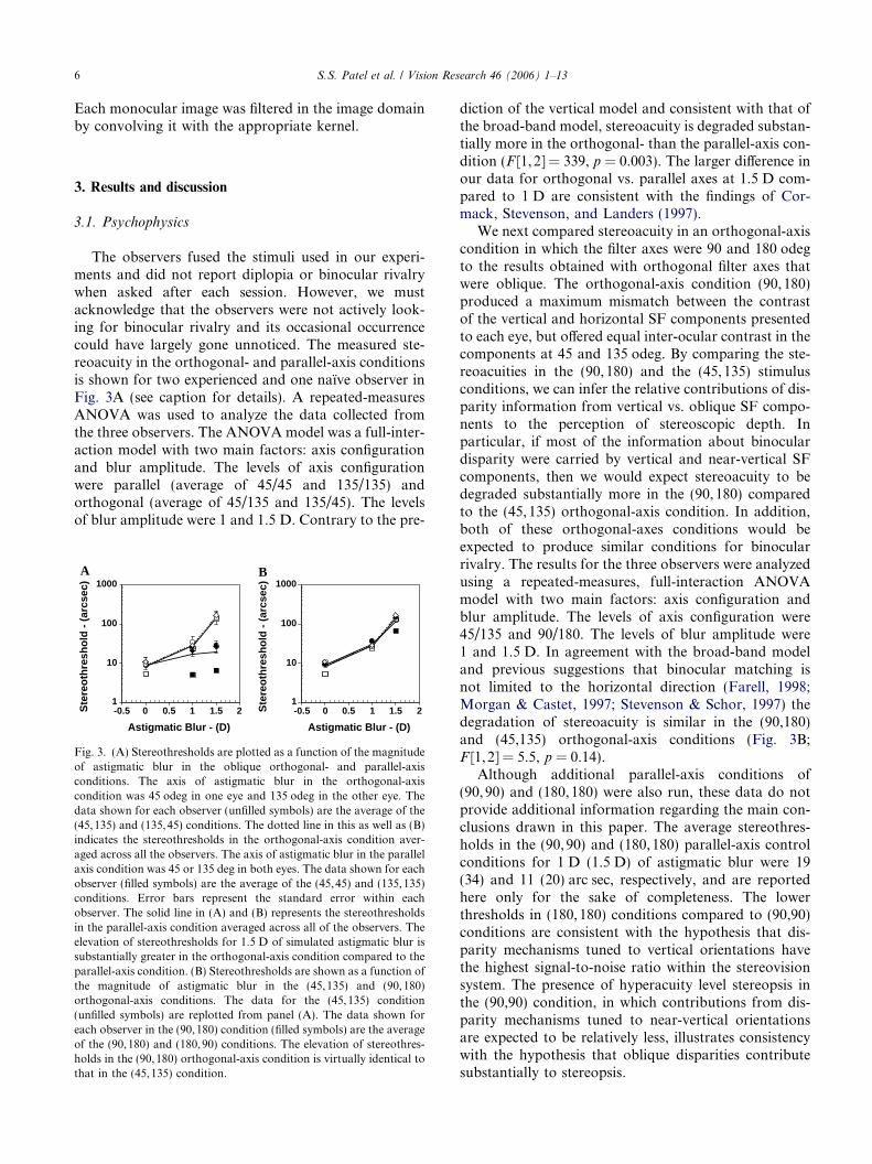
Fig. 3. (A) Stereothresholds are plotted as a function of the magnitudeof astigmatic blur in the oblique orthogonal- and parallel-axisconditions. The axis of astigmatic blur in the orthogonal-axiscondition was 45 odeg in one eye and 135 odeg in the other eye. Thedata shown for each observer (unfilled symbols) are the average of the(45,135) and (135,45) conditions. The dotted line in this as well as (B)indicates the stereothresholds in the orthogonal-axis condition aver-aged across all the observers. The axis of astigmatic blur in the parallelaxis condition was 45 or 135 deg in both eyes. The data shown for eachobserver (filled symbols) are the average of the (45,45) and (135,135)conditions. Error bars represent the standard error within eachobserver. The solid line in (A) and (B) represents the stereothresholdsin the parallel-axis condition averaged across all of the observers. Theelevation of stereothresholds for 1.5 D of simulated astigmatic blur issubstantially greater in the orthogonal-axis condition compared to theparallel-axis condition. (B) Stereothresholds are shown as a function ofthe magnitude of astigmatic blur in the (45,135) and (90,180)orthogonal-axis conditions. The data for the (45,135) condition(unfilled symbols) are replotted from panel (A). The data shown foreach observer in the (90,180) condition (filled symbols) are the averageof the (90,180) and (180,90) conditions. The elevation of stereothres-holds in the (90,180) orthogonal-axis condition is virtually identical tothat in the (45,135) condition.

diction of the vertical model and consistent with that ofthe broad-band model, stereoacuity is degraded substan-tially more in the orthogonal- than the parallel-axis con-dition (F [1,2] = 339, p = 0.003). The larger difference inour data for orthogonal vs. parallel axes at 1.5 D com-pared to 1 D are consistent with the findings of Cor-mack, Stevenson, and Landers (1997).

We next compared stereoacuity in an orthogonal-axiscondition in which the filter axes were 90 and 180 odegto the results obtained with orthogonal filter axes thatwere oblique. The orthogonal-axis condition (90,180)produced a maximum mismatch between the contrastof the vertical and horizontal SF components presentedto each eye, but offered equal inter-ocular contrast in thecomponents at 45 and 135 odeg. By comparing the ste-reoacuities in the (90,180) and the (45,135) stimulusconditions, we can infer the relative contributions of dis-parity information from vertical vs. oblique SF compo-nents to the perception of stereoscopic depth. Inparticular, if most of the information about binoculardisparity were carried by vertical and near-vertical SFcomponents, then we would expect stereoacuity to bedegraded substantially more in the (90,180) comparedto the (45,135) orthogonal-axis condition. In addition,both of these orthogonal-axes conditions would beexpected to produce similar conditions for binocularrivalry. The results for the three observers were analyzedusing a repeated-measures, full-interaction ANOVAmodel with two main factors: axis configuration andblur amplitude. The levels of axis configuration were45/135 and 90/180. The levels of blur amplitude were1 and 1.5 D. In agreement with the broad-band modeland previous suggestions that binocular matching isnot limited to the horizontal direction (Farell, 1998;Morgan & Castet, 1997; Stevenson & Schor, 1997) thedegradation of stereoacuity is similar in the (90,180)and (45,135) orthogonal-axis conditions (Fig. 3B;F [1,2] = 5.5, p = 0.14).

Although additional parallel-axis conditions of(90,90) and (180,180) were also run, these data do notprovide additional information regarding the main con-clusions drawn in this paper. The average stereothres-holds in the (90,90) and (180,180) parallel-axis controlconditions for 1 D (1.5 D) of astigmatic blur were 19(34) and 11 (20) arc sec, respectively, and are reportedhere only for the sake of completeness. The lowerthresholds in (180,180) conditions compared to (90,90)conditions are consistent with the hypothesis that dis-parity mechanisms tuned to vertical orientations havethe highest signal-to-noise ratio within the stereovisionsystem. The presence of hyperacuity level stereopsis inthe (90,90) condition, in which contributions from dis-parity mechanisms tuned to near-vertical orientationsare expected to be relatively less, illustrates consistencywith the hypothesis that oblique disparities contributesubstantially to stereopsis.

S.S. Patel et al. / Vision Research 46 (2006) 1–13 7

Previously, Chen, Hove, McCloskey, and Kaye (2005)measured stereoacuity for stimuli that were subjected tooptical astigmatic blur at various axes. They also foundthat stereothresholds were substantially higher in theiroblique orthogonal-axis (45,135) condition compared tothe vertical (90,90) and horizontal (180,180) parallel-axisconditions. However, they did not measure stereoacuityin the oblique parallel-axis condition. Also, the stimuliin their experiments did not contain contrast energy atall non-vertical orientations, which makes the contribu-tion of oblique disparities to their results difficult to inter-pret. Finally, because they produced orientation-specificstimulus blur using cylindrical spectacle lenses insteadof spatial filtering, they introduced meridional differencesin image magnification that can degrade stereoacuityindependently of image blur (Lovasik & Szymkiw, 1985).

3.2. Additional analyses and modeling

To illustrate how our results indicate the need fornon-vertically oriented SF components in the computa-tion of horizontal disparity, we performed horizontalcross-correlations between sample pairs of images thatwere used in the parallel and orthogonal axes conditions

0 10 20 30 40 50 60 70-80

-60

-40

-20

0

20

40

60

80

100

Near-Ve

Orienta

0 10 20 30-60

-40

-20

0

20

40

60

80

100

120

140

0 10 20 30-60

-40

-20

0

20

40

60

80

100

120

140

Parallel

Orthogonal

Bin

ocu

lar

Ho

rizo

nta

l Co

rrel

atio

n

Vertical Orientations

0 10 20 30 40 50 60 70-80

-60

-40

-20

0

20

40

60

80

100Orthogonal

Parallel

Pixels Pix

A B

Fig. 4. Horizontal correlation between the 31 · 31-pixel inner squares in theinner squares. The panels in the top (bottom) row show horizontal correlatiomean luminance was removed from all of the images before the computaticomputed from images that were filtered to contain only vertical orientationsthe middle column (B), similar correlations are still obtained in the orthorientations within ±15 deg from vertical. In the right column (C), the corsubstantially higher in the parallel- than in the orthogonal-axes condition. Aparallel condition is also higher than in columns (A) and (B). The horizontalcorrelation in this figure was 5.3 arc min. Each pixel on the x-axis is 2 arc m

in our experiments. For the images in each condition,cross-correlation was performed on images that were(a) filtered to contain only vertically oriented SF compo-nents, (b) filtered to contain a small ±15 deg band oforiented SF components around vertical, or (c) leftunfiltered. The results of the cross-correlations areshown in Fig. 4; details of the analysis are provided inthe figure caption. Whereas the disparity energy in ourtwo sets of stimuli is similar in the vertically (Fig. 4A)and near-vertically (Fig. 4B) oriented spatial frequencycomponents presented to the two eyes, the disparityenergy differs substantially between these sets of stimuliwhen all of oriented spatial frequency components areconsidered (Fig. 4C). In particular, the horizontal in-ter-ocular correlation is substantially weaker for theunfiltered stimuli in the orthogonal-axis condition thanin the parallel-axis condition. This analysis indicatesthat the large difference in stereo-sensitivity that wefound in the parallel and orthogonal conditions of ourexperiments requires that the horizontal inter-ocularcorrelation be computed from non-vertically as well asvertically oriented SF components in the stimulus.

We propose potential broad-band models that usevertically and non-vertically oriented SF components

rtical

tions All Orientations

40 50 60 70

0 10 20 30 40 50 60 70-200

-100

0

100

200

300

400

500

600

0 10 20 30 40 50 60 70-200

-100

0

100

200

300

400

500

600

40 50 60 70

Orthogonal

Parallel

els Pixels

C

images of the two eyes as a function of the orientation content of then for stimuli used in the orthogonal-axis (parallel-axis) condition. Theon of horizontal correlation. In the left column (A), the correlationsare nearly identical for the orthogonal- and parallel-axis conditions. Inogonal- and parallel-axis conditions when the images contained allrelation computed from images that contained all the orientations islthough disguised by the change in y-axis scale, the correlation in thedisparity between the inner squares of the images used to compute thein. The vertical dotted line in each panel represents zero disparity.

8 S.S. Patel et al. / Vision Research 46 (2006) 1–13

in the stimulus to compute the horizontal inter-ocularcorrelation (Fig. 5). Neurons tuned to spatial phase dis-parities have been found in the visual cortex of monkeysand cats (e.g., Anzai et al., 1997; Ohzawa et al., 1990).These binocular phase-sensitive neurons display pre-ferred orientations that are distributed uniformly be-tween horizontal and vertical (Anzai et al., 1997), andtherefore represent the neural basis for our model[s] inwhich the disparity signals from various orientationsare pooled. The general scheme of pooling across neu-rons with different orientation and spatial frequency

A Pooling Models

Pooling Scheme

Pre-Pooling Model Post-Pooling M

+

+OpCp

Cp

Cp

Cp

Fx

FyPool

Fig. 5. Broad-band models for the computation of horizontal disparity and cThe proposed pre-pooling and post-pooling broad-band models of disparitylabeled pooling scheme, the proposed rule for combining signals across variouFourier plane (Fx,Fy) depicts a quadrature pair of orientation and SF tuned bBoth simple cells in a quadrature pair have the same preferred orientation aneach circle and the vertical axis represents the preferred orientation of the qrepresents the ‘‘horizontal component’’ of each pair�s preferred SF. This companel labeled pre-pooling model, for simplicity, circuitry is illustrated for onlconsists of several simple-cell pairs with preferred orientations ranging frorepresents a pair of simple cells. Notice that the preferred SF of each simplehorizontal, to keep the ‘‘horizontal component’’ of the SF constant and equacell pairs tuned to various orientations are pooled prior to becoming inputsmodel, the output of the simple cell pairs are not pooled, and instead the resvarious orientations are summed by a hyper-complex cell prior to conversioncell pairs is derived from orientation- and spatial frequency-tuned monocularwhich is characterized by a multiplier a (see appendix for definition of a)conditions. A larger value of a represents larger internal neural noise. The apin the stimuli for the parallel (orthogonal) simulation condition was 27 (160averaged across observers in the corresponding conditions. (C) d 0 as a functiothat were used in (B).

tuning is illustrated in Fig. 5A. This pooling schemewas chosen because it qualitatively mimics a one-dimen-sional horizontal image correlator, similar to the oneused to determine the disparity energy in Fig. 4. Anotherreason for this choice is that, for any broad-band tex-tured stimulus that contains a horizontal position dis-parity, as shown in Fig. 1, the distribution of equalphase disparities corresponds to vertical lines in theFourier domain, which is the direction of pooling thatis illustrated in Fig. 5A. A simple learning rule in whichneurons that fire similarly cooperate, would be sufficient

odel

OpH

B Vertical Model Output

-0.20

0.20.40.60.8

11.21.41.6

Mo

del

d'

0.1 1 10 100

Noise Multiplier - α

Orthogonal

Parallel

C Post-Pooling Model Output

-0.20

0.20.40.60.8

11.21.41.6

Mo

del

d'

0.1 1 10 100

Noise Multiplier - α

Orthogonal

Parallel

omparison of model responses for stimuli used in our experiments. (A)computations. This panel consists of three sub panels. In the sub-panels orientations and SFs is illustrated. Each circle in the two-dimensionalinocular simple cells (see simulation method in Appendix A for details).d SF. The angle between the line that joins the origin and the center ofuadrature pair. The vertical line that joins the centers of all the circlesmon ‘‘horizontal component’’ is defined as the primary SF. In the sub-y a single preferred phase disparity, p, where p = 2/ + 90. The modelm 5 to 175 deg from vertical. Each box with the receptive field iconcell increases as the preferred orientation changes from vertical to nearl to the primary SF. In the pre-pooling model, the responses of simplefor a complex cell with preferred phase disparity p. In the post-poolingponses of complex cells with preferred phase disparity, p, and tuned toto the final horizontal disparity. In both models, the input to the simplefilters. (B) d 0 as a function of neuronal noise level in the vertical model,, for stimuli used in 1.5 D parallel (45/45) and orthogonal (45/135)pendix provides details about how model d 0 is calculated. The disparity) arc sec. In (B) and (C), these disparities represented stereothresholdsn of neuronal noise level in the post-pooling model, for the same stimuli

S.S. Patel et al. / Vision Research 46 (2006) 1–13 9

to develop this proposed scheme of neural pooling in thebrain.

We considered two specific strategies for pooling dis-parity energy across orientation and spatial frequency.In the pre-pooling broad-band model, the outputs ofsimple cells tuned to various orientations and spatial fre-quencies in a phase-based disparity-energy model (Ohz-awa et al., 1990; Qian & Zhu, 1997) were added prior tosending the summed signals to complex cells. In thepost-pooling broad-band model, the outputs of thecomplex cells tuned to various orientations and spatial

A Test Stimulus

B Model Simulations

3cpd

6cpd

12 cpd

PostPreVert

frequencies in the phase-based disparity-energy modelwere summed by a hyper-complex cell prior to the com-putation of horizontal disparity. As pointed out by ananonymous reviewer, the pre-pooling model is less plau-sible physiologically because pre-pooling would requirethat complex cells are isotropic, which they are generallynot (e.g., Smith et al., 1997).

We tested the performance of the vertical and post-pooling broad-band models illustrated in Fig. 5A withstimuli used in our present experiments. Details aboutthe implementation of these models is provided in theAppendix A. Although the pre-pooling model was nottested with the stimuli used in our experiments, due tothe long time required to run simulations, it was testedwith suprathreshold stimuli as described in the followingparagraphs. To simulate the models with inputs thatyield stereothresholds, we included additive noise atthe output of all the neurons in the model. However, adifficulty with this approach is that, a priori, the levelof noise that has to be added to each model cell is un-known. Therefore, our approach to test which modelbetter accounts for our experimental data was as follows(see Appendix A for further details): We created onepair of images (left and right eyes) for the (45,45) paral-lel-axis condition and another pair of images for the(45,135) orthogonal-axes condition. The horizontal dis-parity between the images in each pair of stimuli was setto the empirically determined stereothreshold, averagedacross observers, for each condition. Using these twoimages pairs, we simulated the vertical and post-poolingmodels with various levels of added noise. For eachnoise level, the model simulation was run five times,which represents a tradeoff between the requirement toaverage the results across runs and the duration of a sin-gle simulation run. The output of each simulation runwas a disparity map; these maps were averaged across

Fig. 6(A) The binocular stimulus used for comparing the two broad-band pooling models to the vertical model. When fusion is achieved,observers should see one cycle of sinusoidal depth modulation in thevertical direction. If viewed from a distance where the total size of eachimage is 3.3 deg, the peak disparity of the sinusoidal modulation is2 arc min. (B) Each gray image is a spatial representation of thehorizontal disparities (disparity map) computed by the model labeledat the top of the column using the stimulus shown in (A). Themagnitude and sign of the disparity in the inner rectangle arerepresented by the luminance contrast: positive contrast representsuncrossed and negative contrast represents crossed disparities in thecross-fused stimulus. The plot below each disparity map represents thehorizontal disparity values at spatial locations along a vertical linepassing through the middle of the disparity map and is ideally expectedto be a sinusoidal waveform. The first, second and third columns showsimulation results for the vertical, pre-pooling and post-poolingmodels, respectively. The orientation- and SF-tuned simple andcomplex cells were modeled by modifying the formulations of Qianand Zhu (see simulation methods in Appendix A for details). Details ofthe circuitry for simple and complex cells can be found in Qian andZhu�s original (1997) paper. Simulations were performed for primaryspatial frequencies of 3, 6 and 12 cpd.

b

Stimulus

PostPre

3cpd

6cpd

12 cpd

Model SimulationsVert

A

B

Fig. 7. Comparison of model responses for a binocular stimulusconsisting of spatial frequency gratings at different orientations in thetwo eyes. (A) Gratings of different orientations and SF in the innersquares of the images presented to the two eyes. The outer frame inboth the images consists of correlated random-dots with no disparity.The SF of the oriented grating is such that the horizontal luminancemodulations have the same spatial frequency in the two eyes. Uponfusion, observers should see a slanted surface with depth changingfrom behind to in-front of the outer frame (or vice-versa) as a functionof the vertical distance from the top of the inner square. Despiteminimal overlap in the SF and orientation content of the images in thetwo eyes, a robust perception of depth is obtained from the stimulus.(B). The disparity maps obtained for the stimulus in (A) using thevertical, pre- and post-pooling models of disparity computation. Themodels were simulated for primary SFs of 3, 6, and 12 cpd. Forobservers who could fuse the stimulus, the perceived depth of theinclined plane is predicted most closely by the disparity map from thepost-pooling model that corresponds to a primary SF of 3 cpd. Boththe pre- and post-pooling models suggest that the robust perception ofslant arises as a result of pooling disparity signals from variousorientation- and SF-tuned disparity neurons.

10 S.S. Patel et al. / Vision Research 46 (2006) 1–13

the five simulations for each combination of stimuli andmodel noise. The averaged disparity maps were analyzedto obtain values of d 0, which represents the discrimina-bility between the distribution of disparity values inthe inner 31 · 31 pixel square and those in a 31 · 31-pix-el square region in the outer frame of each map. Weclaim that if the inputs used for the simulation are stere-othresholds, and if the model is valid, thenfor some critical noise level the calculated d 0 for theparallel-axis and the orthogonal-axes conditions shouldbe equal. Expressed graphically, if d 0 is plotted as a func-tion of the model noise then the curves for the parallel-axis and orthogonal-axes conditions should intersect atsome noise level.

The results of these simulations for the vertical andpost-pooling models are shown in Figs. 5B and C. No-tice that the plots of d 0 for the parallel-axis and orthog-onal-axes conditions intersect for the post-poolingmodel but not for the vertical model. Also note thatthe d 0 values determined in parallel-axis condition forthe vertical model are negative for some noise levels,indicating that the model�s aggregate disparity for theinner square is reversed in sign. Finally, the d 0 valuesdetermined for the vertical model in the parallel-axiscondition are lower than those in the orthogonal-axescondition for the entire range of tested noise levels.These simulation results contradict our experimentalfinding that the stereothreshold is lower in the paral-lel-axis compared to orthogonal-axes condition. Takentogether, the outcomes of these simulations indicatethat the post-pooling model, but not the vertical mod-el, can account for the empirical data reported in thispaper.

The d 0 values that are plotted in Figs. 5B and C forthe post-pooling model are not close to unity at the crit-ical noise level. This is because only five disparity mapswere averaged for each noise level; averaging a largernumber of maps should reduce the disparity noise inthe average map and increase the values of d 0 substan-tially. Although more averaging of disparity mapswould also be expected to improve the performance ofthe vertical model, it is unlikely that the results for thismodel would change qualitatively to become more con-sistent with our data.

We hypothesize that pooling across orientation-tuneddisparity mechanisms should enhance the lateral spatialresolution of the stereovision system. To evaluate thishypothesis, we tested the performance of the verticaland broad-band models with the spatially modulatedsuprathreshold disparity stimuli shown in Figs. 6A and7A (for detailed simulation methods please see Appen-dix A). In Figs. 6B and 7B, the performance of bothof the pooling models is compared with that of the ver-tical model. (Note that the vertical model is tested onlyfor comparison and not as a viable model for stereopsisbecause it fails to account for the principal aspects of the

data in Fig. 3) Although all three models can detect thedisparity modulations to some extent, the broad-bandmodels perform substantially better than the verticalmodel in encoding a spatially changing disparity. It isalso clear that the post-pooling model is more robustthan the pre-pooling model in encoding the sinusoidaldisparity modulation at spatial scales corresponding to3 and 6 cpd. This means that a further enhancement in

S.S. Patel et al. / Vision Research 46 (2006) 1–13 11

disparity estimation may be possible if disparity infor-mation is combined subsequently across spatial scales.Because the post-pooling model is more robust, we fa-vor this broad-band model over the pre-pooling modeland suggest that the functional site of orientation pool-ing is beyond the binocular complex cells.

The results of this study are consistent with our pre-vious conclusion (Patel et al., 2003b) that oblique retinalimage disparities carry a substantial proportion of theinformation about stereoscopic depth that is used bythe human visual system. The data suggest that the hor-izontal inter-ocular correlator (Banks, Gepshtein, &Landy, 2004; Cormack, Stevenson, & Schor, 1991) thatcomputes horizontal image disparity should use the dis-parity signals from non-vertically as well as from verti-cally tuned neurons. By pooling signals from a largenumber of obliquely tuned binocular neurons, the ste-reovision system can encode spatial changes in horizon-tal disparity with high signal-to-noise ratio (Fleet,Wagner, & Heeger, 1996; Patel et al., 2003b) and im-proved spatial resolution. The physiologically plausiblepost-pooling model proposed in this paper clarifieshow disparity-tuned neurons in V1, which have spatiallyextended receptive fields, can account for the perceiveddepth of a surface that has steep variations in depth(Mahew & Frisby, 1979). Along-with a recent study byNienborg, Bridge, Parker, and Cumming (2004), thismodel suggests that the site at which changes in horizon-tal disparities are encoded may be beyond V1, perhapsin area V2 or MT. Because a spatio-temporal correlatoris required to analyze visual motion signals as well, wehypothesize that pooling signals from motion mecha-nisms tuned to non-primary as well as to the primarydirection of stimulus motion could similarly enhancethe spatial resolution of the visual motion system, i.e.,its ability to encode spatially changing visual motionsignals.

Fig. 8. Schematic of the elementary module in Qian and Zhu�simplementation of the disparity-energy model. The OF moduleconsists of four monocular cells, two binocular simple cells and onebinocular complex cell. The binocular cell�s orientation, SF and phasedisparity tuning properties are derived from the antecedent monocularcells. Each module has a preferred orientation, SF and phase disparity.Each simple cell receives input from two monocular filters, one fromeach eye. The receptive field of each monocular filter is modeled as anoriented Gabor function (G). The space-constant of the circularlysymmetric Gaussian envelope of G was equal to half the spatial periodof the oriented carrier grating. G was defined within a square matrix of

Acknowledgments

We thank Drs. Gopathy Purushothaman, Scott Ste-venson, and Jianliang Tong for helpful discussions onvarious topics in this paper. We also thank the twoanonymous reviewers for their suggestions to improvethe clarity of our paper. This work was supported byR01 EY05068 and R01 MH49892.

dimension corresponding to six times the space-constant of theGaussian envelope. The monocular filters for one simple cell (S/)have the sum of spatial phases (LE + RE) of �90 pdeg while those forthe other simple cell (S/ + 90) have the sum of spatial phases as90 pdeg. Further, for each eye, the absolute difference between thespatial phase of the monocular filters is 90 pdeg. Together, the twosimple cells connected in this configuration form a linear quadraturepair. A complex cell (Cp) sums the rectified signals from the two simplecells to produce the output Op of the OF module. The preferred phasedisparity (p) of a OF module is determined by the phase parameter (/)of the Gabor functions and is equal to 2/.

Appendix A. Simulation method

The energy model of Qian and Zhu (1997) wasextended to generate the various models used in thisstudy. Details of the original model can be found inQian and Zhu�s, 1997 paper and in Patel et al.(2003b). Briefly, the generic module in Qian�s and Zhu�s

model is shown in the panel labeled OF module inFig. 8.

In the complete model, a bank of OF modules ex-tracts the disparity energy at each location in the (fused)retinal image. Each bank contains OF modules tuned toa range of SFs, orientations, and phase disparities. Thepattern of connections between the OF modules in abank distinguishes the pre-pooling and the post-poolingmodels that are described in this paper.

A.1. Pre-pooling model

In this model, one complex cell receives signals thatare pooled from various orientation and SF tuned quad-rature pairs of simple cells at each spatial location andvalue of phase disparity, (Fig. 5A). The quadrature pairsof simple cells that form a pool have a definite relation-ship between preferred orientation and preferred SF.For a given preferred orientation, the ‘‘horizontal com-ponent’’ of the preferred SF is equal to the primary SF(see Fig. 5A) of the pool. The primary SF, which alsocharacterizes the pool, is defined to be equal to the pre-ferred SF of the cell in the pool whose preferred orienta-tion is vertical. For each preferred phase disparity andprimary SF, the model includes 19 quadrature-pairsimple cells with preferred orientations spaced equally

12 S.S. Patel et al. / Vision Research 46 (2006) 1–13

between 5 and 175 deg (orientation resolution of10 odeg, where 90 odeg represents vertical orientation).For each primary SF (e.g., 3 cpd), the preferred SF forthe 19 quadrature pairs of cells was a function of pre-ferred orientation (preferred SF = primary SF/sin(pre-ferred orientation)) and ranged from approximately 3to 34 cpd. For each primary SF, 80 phase-disparitytuned complex cells with preferred phase disparities arespaced equally in the range between �180 and175.5 pdeg (phase disparity resolution of 4.5 pdeg). Foreach preferred phase disparity, the output of all 19 quad-rature pairs of simple cells are added as shown in Fig. 5Aand the summed signals are sent to a complex cell. Thephase disparity preferred by the most active of the 80complex cells is finally converted to horizontal disparity,according to the primary SF of the pool. Identical com-putations are performed for each spatial location in theinput retinal image. The final output of the model is atwo-dimensional representation of horizontal disparity(e.g., Fig. 6B), corresponding to the (fused) two-dimen-sional retinal image. This 2-D representation of dispari-ties is called a disparity map. Note that Qian and Zhu(1997) applied a low-pass disparity filter to the disparitymaps obtained from the responses of the model neurons.In Figs. 6B and 7B, we show the unfiltered disparitymaps. We simulated the model for primary SFs of 3,6, and 12 cpd. Because the pooling of disparity signalsin this model occurs prior to the non-linear operationof rectification, this pooling scheme is linear.

A.2. Post-pooling model

For each spatial location and value of single phasedisparity tuning, this model consists of a bank of com-plete OF modules, each with a different orientationand SF preference. The model includes 19 OF moduleswith preferred orientations spaced equally between 5and 175 odeg, for each preferred phase disparity andprimary SF. A hyper-complex cell pools the output ofthe 19 OF modules for each phase disparity (Fig. 5A).The preferred phase disparity of the hyper complex cellis the same as its 19 input OF modules. The model uses80 phase-disparity tuned hyper complex cells with pre-ferred phase disparities spaced equally in the range be-tween �180 and 175.5 pdeg for each primary SF. Thepreferred phase disparity of the most active of the 80 hy-per complex cells is finally converted to a horizontal dis-parity, based on the primary SF of the pool. Thesecomputations are performed for each spatial locationin the fused retinal image. The final output of the modelis a two-dimensional representation of horizontal dis-parities (e.g., Fig. 6B) corresponding to the two-dimen-sional retinal images. We simulated the model forprimary SFs of 3, 6, and 12 cpd. Because pooling in thismodel occurs after the non-linear operation of rectifica-tion, this pooling scheme is non-linear.

A.3. Vertical model

For each spatial location and value of single phase dis-parity tuning, this model consists of just one OF moduletuned to a vertical orientation at a given SF. For eachSF, the model uses 80 phase-disparity tuned complexcells with preferred phase disparities spaced equally inthe range between �180 and 175.5 pdeg. The preferredphase disparity of the most active of the 80 complex cellsis finally converted to a horizontal disparity, based on thegiven SF. These computations are performed for eachspatial location in the fused retinal image. The final out-put of the model is a two-dimensional representation ofhorizontal disparities (e.g., Fig. 6B) corresponding tothe two-dimensional retinal images. We simulated themodel for SFs of 3, 6, and 12 cpd.

A.4. Noise in the model

To properly simulate the models with inputs thatyield stereothresholds, we included additive noise atthe output of all the neurons in the models. Due to timeconstraints, we only tested the vertical and the post-pooling models. We assumed that the additive noiseadded to the output of each cell, which represented fir-ing rate noise, was uniformly distributed. The peak-to-peak range of noise was different for each type of cell.The noise range for all the monocular filters was sym-metric and bi-polar (�25a to 25a) while that for the restof the cells was unipolar. The noise range for all the sim-ple and complex cells was 0–a and 0–0.1a, respectively.For the post-pooling model, the noise range for all thehyper-complex cells was 0 to 0.1a. The noise in the mod-el was uncorrelated across all the neurons regardless ofthe spatial location they represent.

Both of the models were in all other ways identical tothose described in the above sections. Both models weresimulated with two inputs: (1) 45,45 1.5 D parallel-axiscondition stimulus with 27 arc sec disparity and (2)45,135 1.5 D orthogonal-axis condition with 160 arc secdisparity. The values, 27 and 160 arc sec correspond tothe stereothreshold averaged across observers in the par-allel and the orthogonal conditions, respectively (seeFig. 3A). Both models were simulated with these inputsfor different values of a ranging from 0.1 to 100. For eacha and input the models were simulated five times, yield-ing five disparity maps which were averaged for furtheranalysis. Consequently, for each a, there were finally fouraveraged disparity maps (two inputs · two models).

From each averaged disparity map, d 0 was computed.A histogram of disparity values corresponding to the31 · 31 inner square was computed in bins of 0.01 arc -min. Another similar histogram of disparity values rep-resenting the outer frame was also computed. For theouter-frame�s histogram, a 31 · 31 square patch of pixelsto the left of the inner square was used. From each

S.S. Patel et al. / Vision Research 46 (2006) 1–13 13

histogram, the first (equivalent to mean) and second(equivalent to standard-deviation) order moments werecomputed. Let lc (lo) and rc (ro) represent the firstand the second order moments for the inner (outer)square (frame). Then,

d 0 ¼ 2ðlc � loÞrc þ ro

:

References

Akutsu, H., Bedell, H. E., & Patel, S. S. (2000). Recognition thresholdsfor letter with simulated dioptric blur. Optometry and Vision

Science, 77, 524–530.Anzai, A., Ohzawa, I., & Freeman, R. D. (1997). Neural mechanisms

underlying binocular fusion and stereopsis: Position vs. phase.Proceedings of the National Academy of Sciences of the United

States of America, 94, 5438–5443.Banks, M. S., Gepshtein, S., & Landy, M. S. (2004). Why is spatial

stereoresolution so low? Journal of Neuroscience, 24, 2077–2089.Barlow, H. B., Blakemore, C., & Pettigrew, J. D. (1967). The neural

mechanism of binocular depth discrimination. Journal of Physiol-ogy, 193, 327–342.

Blake, R., Camisa, J. M., & Antoinetti, D. N. (1976). Binocular depthdiscrimination depends on orientation. Perception & Psychophysics,

20, 113–118.Chen, S. I., Hove, M., McCloskey, C. L., & Kaye, S. B. (2005). The

effect of monocularly and binocularly induced astigmatic blur ondepth discrimination is orientation dependent. Optometry and

Vision Science, 82, 101–113s.Chino, Y. M., Smith, E. L., Hatta, S., & Cheng, H. (1997). Postnatal

development of binocular disparity sensitivity in neurons of theprimary visual cortex. Journal of Neuroscience, 17, 296–307.

Cormack, L. K., Stevenson, S. B., & Schor, C. M. (1991). Interocularcorrelation, luminance contrast and cyclopean processing. VisionResearch, 31, 2195–2207.

Cormack, L. K., Stevenson, S. B., & Landers, D. D. (1997).Interactions of spatial frequency and unequal monocular contrastsin stereopsis. Perception, 26, 1121–1136.

Farell, B. (1998). Two-dimensional matches from one-dimensionalstimulus components in human stereopsis. Nature, 395, 689–693.

Felleman, D. J., & Van Essen, D. C. (1987). Receptive field propertiesof neurons in area V3 of macaque monkey extrastriate cortex.Journal of Neurophysiology, 57, 889–920.

Fleet, D. J., Wagner, H., & Heeger, D. J. (1996). Neural encoding ofbinocular disparity: Energy models, position shifts and phaseshifts. Vision Research, 36, 1839–1859.

Gonzalez, F., Krause, F., Perez, R., Alonso, J. M., & Acuna, C.(1993). Binocular matching in monkey visual cortex: Single cellresponses to correlated and uncorrelated dynamic random dotstereograms. Neuroscience, 52, 933–939.

Halpern, D. L., & Blake, R. (1989). How contrast affects stereoacuity.Perception, 17, 483–495.

Hess, R. F., Liu, C. H., & Wang, Y. Z. (2003). Differential binocularinput and local stereopsis. Vision Research, 43, 2303–2313.

Hubel, D. H., & Wiesel, T. N. (1970). Stereoscopic vision in macaquemonkey. Nature, 225, 41–42.

Legge, G. E., & Gu, Y. (1989). Stereopsis and contrast. Vision

Research, 29, 989–1004.Lovasik, J. V., & Szymkiw, M. (1985). Effects of aniseikonia,

anisometropia, accommodation, retinal illuminance, and pupil sizeon stereopsis. Investigative Ophthalmology & Visual Science, 26,741–750.

Mahew, J. E. W., & Frisby, J. P. (1979). Surfaces with steep variationsin depth pose difficulties for orientationally tuned disparity filters.Perception, 8, 691–698.

Mansfield, J. S., & Parker, A. J. (1993). An orientation-tunedcomponent in the contrast masking of stereopsis. Vision Research,

33, 1535–1544.Maske, R., Yamane, S., & Bishop, P. O. (1986). Stereoscopic

mechanisms: Binocular responses of the striate cells of cats.Proceedings of the Royal Society of London. Series B. Biological

Sciences, 229, 227–256.Maunsell, J. H. R., & Van Essen, D. C. (1983). Functional properties

of neurons in middle temporal visual area of the macaque monkey.II Binocular interactions and sensitivity to binocular disparity.Journal of Neurophysiology, 49, 1148–1167.

Morgan, M. J., & Castet, E. (1997). The aperture problem instereopsis. Vision Research, 37, 2737–2744.

Nienborg, H., Bridge, H., Parker, A. J., & Cumming, B. G. (2004).Receptive field size in V1 neurons limits acuity for perceivingdisparity modulation. Journal of Neuroscience, 24, 2065–2076.

Ohzawa, I., DeAngelis, G. C., & Freeman, R. D. (1990). Stereoscopicdepth discrimination in the visual cortex: Neurons ideally suited asdisparity detectors. Science, 249, 1037–1041.

Patel, S. S., Ukwade, M. T., Bedell, H. E., & Sampath, V. (2003a).Near stereothresholds measured with random-dot stereogramsusing phase disparities. Optometry, 74, 453–461.

Patel, S. S., Ukwade, M. T., Stevenson, S. B., Bedell, H. E., Sampath,V., & Ogmen, H. (2003b). Stereoscopic depth perception fromoblique phase disparities. Vision Research, 43, 2479–2492.

Poggio,G.F.,Motter,B.C., Squatrito, S.,&Trotter,Y. (1985).Responsesof neurons in visual cortex (V1 and V2) of the alert Macaque todynamic random-dot stereograms. Vision Research, 25, 397–406.

Prince, S. J, Pointon, A. D, Cumming, B. G, & Parker, A. J. (2002).Quantitative analysis of the responses of V1 neurons to horizontaldisparity in dynamic random-dot stereograms. Journal of Neuro-

physiology, 87, 191–208.Qian, N., & Zhu, Y. (1997). Physiological computation of binocular

disparity. Vision Research, 37, 1811–1827.Schor, C. M., & Heckmann, T. (1989). Interocular differences in

contrast and spatial frequency: Effects on stereopsis and fusion.Vision Research, 29, 837–847.

Simons, K. (1984). Effects of stereopsis on monocular vs. binoculardegradation of image contrast. Investigative Ophthalmology &

Vision Science, 25, 987–989.Simmons, D. R., & Kingdom, F. A. A. (1995). Differences between

stereopsis with isoluminant and isochromatic stimuli. Journal of theOptical Society of America. A, Optics and Image Science, 12,2094–2104.

Smith, E. L., III, Chino, Y. M., Ni Jinren Ridder, W. H., III, &Crawford, M. L. J. (1997). Binocular spatial phase tuningcharacteristics of neurons in the macaque striate cortex. Journalof Neurophysiology, 78, 351–365.

Stevenson, S. B., & Cormack, L. K. (2000). A contrast paradox instereopsis, motion detection and Vernier acuity. Vision Research,

40, 2881–2884.Stevenson, S. B., & Schor, C. M. (1997). Human stereo matching is not

restricted to epipolar lines. Vision Research, 37, 2717–2723.van Ee, R., & Anderson, B. L. (2001). Motion direction, speed and

orientation in binocular matching. Nature, 410, 690–694.Westheimer, G., & McKee, S. P. (1980). Stereoscopic acuity with

defocussed and spatially filtered retinal images. Journal of theOptical

Society of America. A, Optics and Image Sciences, 70, 772–778.Wheatstone, C. (1838). Contributions to the physiology of vision - Part

the first. On some remarkable, and hitherto unobserved, phenom-ena of binocular vision. Philosophical Transactions of the Royal

Society of London. Series B, Biological Sciences, 2, 371–393.Wood, I. C. J. (1983). Stereopsis with spatially degraded images.

Opthalmic and Physiological Optics, 3, 337–340.