1

Vertically Globalized Production Structure in New Keynesian Phillips Curve

Wong Chin-Yoong

*

Universiti Tunku Abdul Rahman

Eng Yoke-Kee**

Universiti Tunku Abdul Rahman

Department of Economics and Finance, Faculty of Business and Finance, Universiti Tunku

Abdul Rahman, Perak Campus, Jalan Universiti, Bandar Barat, 31900 Kampar, Perak, Malaysia.

* Graduate student, Universiti Putra Malaysia. Corresponding author. E-mail address:

wongcy@mail.utar.edu.my

** Ph.D candidate, Universiti Putra Malaysia. E-mail address: engyk@mail.utar.edu.my

This paper revisits the hypothesis that globalization may weaken central bank’s monetary control

by analyzing the potential effect of vertically globalized production structure that increasingly

permeates the international production process on domestic macroeconomic dynamics under the

foreign disturbances of productivity, demand, and inflation. We do so through the lens of New

Keynesian model with Calvo-type staggered price setting and production function that uses

foreign intermediate inputs. We find that central bank has to confront a policy tradeoff between

stabilizing inflation and real output as exchange rates have transformed aforementioned foreign

disturbances into domestic supply shocks channeled thorough real marginal cost.

Keywords: Vertically globalized production structure; Vertical specialization; New Keynesian

Phillips curve; Policy trade-off

JEL classification: E3-5, F4

2

1. Introduction

The recent wave of globalization of goods markets, factor markets, and financial markets have

raised at least two important challenges to monetary policy making: that globalization has

changed the slope of inflation-output tradeoff, and has undermined the ability of home central

banks to affect home inflation dynamics through their own monetary policy actions. For some,

these effects are welcome. Rogoff (2003, 2006), for example, suggests that the deregulation and

privatization spurred by globalization create favorable competitive environment that helps drive

down the trend inflation in the 1990s, and make prices and wages more flexible. Flexible price

reduces real gain from surprised inflationary monetary policy stance, thereby moderating the

inflation bias in policy making.

There are many views that cast doubt on the merits of globalization in bringing down the

trend inflation and altering the output-inflation dynamics. Sbordone (2008), for instance,

considers a New Keynesian Phillips curve with elasticity of demand that varies accordingly to

the numbers of traded goods, and finds no convincing evidence supporting the claim that the

increasing variety of traded goods of the magnitude observed in the United States in the 1990s as

a result of growing globalization has altered the dynamic response of inflation to marginal cost

and so real output. No less subtle criticism from the empirical point of view is that globalization

actually leads to a more output elastic inflation (see e.g., Duca and VanHoose, 2000; Borio and

Filardo, 2007; Ihrig et al., 2007; Pain et al., 2006).

For influential others, the “Great Moderation” can in fact be attributed to the very

effectiveness of monetary policy. Clarida et al. (2000), and Boivin and Giannoni (2006), for

instance, argue that effectively-conducted monetary policy, particularly with more elastic Fed’s

responsiveness to inflation fluctuations, by and large underlies the “great moderation” in

3

macroeconomic volatility post-1980. Robert (2006) suggests that a more predictable monetary

environment with more aggressive reaction to inflation fluctuation and better output gap

estimates can account for most or all of the change in the inflation-unemployment relationship.

In other words, contrary to what is commonly champagne

Having this found means that that globalization has eroded the policy effectiveness is

nothing more than an overestimation. By considering a thorough sort of globalization that spans

global liquidity, global saving and investment, and foreign output gap, Woodford (2007)

eloquently argues that globalization is unlikely to compromise the national central bank’s control

over the inflation dynamics. In the same volume, Bolvin and Giannoni (2007) also find that

globalization neither becomes influential on U.S. inflation dynamics nor alters the U.S. monetary

transmission mechanism between 1984 and 1999. The often-cited Ball (2006) argues that the

foreign economic conditions are at most a secondary influence on national inflation.

Of interest in this paper, thus, is about the very ability of national central bank to retain

control over domestic output and inflation dynamics in the presence of globalization. This paper

contributes to the contentious debates on the monetary policy effectiveness under globalization

by having considered the role of vertical fragmentation in production structure across the

sovereign borders.

This is motivated by the recent development in the international trade literature that has been

widely documenting the rise of cross-country production networks and as corollary of vertical

trade. Productions are hardly to be completed within a single stage at a single country. Rather,

goods are produced in multiple-sequential stages in which the country will use at certain portion

imported intermediate inputs in its stage of production process, and some of the resulting output

4

will be exported. In this respect, the productions of two or more countries are linked vertically

and sequentially. We coin this phenomenon as vertically globalized production structure.

This vertically globalized production structure has been an increasingly important feature of

today’s pattern of production and trade. For instance, Chen et al. (2005) infers that Germany

vertical trade as a share of total export has increased steadily from 18.4 percent in 1978 to 22.4

percent in 1995 while U.S. share being more than doubled from 5.9 percent in 1972 to 12.3

percent in 1997. They further show that the fraction of U.S. exports of manufactured goods went

to foreign affiliates of U.S. multinationals for further manufacture has risen from 15.6 percent in

1977 to 22 percent by 1999. Throughout, the share of these re-manufactured products of U.S.

foreign affiliates for re-export has risen from 31 percent to 41 percent. (see also e.g., Feenstra,

1998; Hummels et al., 2001; Yi, 2003).

On top of that, Dean et al. (2007) documents that about 35 percent, in some sectors more

than half, of China’s exports to the world is attributed to imported inputs. Seeing that East Asian

countries are heavily dependent on international production fragmentation for export dynamism,

the economic integration of China has deepened production fragmentation and contributed

significantly to the growth of East Asia (e.g., Athukorala and Yamashita, 2006; Cheng and

Kierzkowski, 2001 for South-East Asia, Haddad, 2007 for the role of China). All these hard

evidences overwhelmingly point to a fact that the globally vertical fragmentation has been

permeating the used-to-be national production structures.

Peculiarly enough, this defining feature of the second wave of globalization has been

completely overlooked in the received literature on why globalization might, or might not, be

expected to substantially complicate the task of national central banks to control the inflation

within their borders. In this paper, we investigate its importance by offering a formal analysis on

5

the macroeconomic effects of vertically globalized production structure by using the canonical

open-economy two-country New Keynesian model with Calvo-type staggered price setting (e.g.,

Gali, 2008; Gali and Monacelli, 2005; Monacelli, 2004). However, we depart here from the

standard assumption of single stage with sovereign border constrained Cobb-Douglas production

function, and use a specification that captures the presence of vertically globalized production

structure defined above. Doing so enables us to introduce an alternative channel of globalization

that transmits the world shocks into the home economy.

Our results can be summarized as follows. We find that globalization, formalized in terms of

vertically globalized production structure, does complicate the conduct of monetary policy,

though not undermine the ability, in such a way that the central bank has to confront an

unpleasant policy tradeoff between stabilizing inflation and real output in face of foreign demand

as well as foreign cost-push shocks. This said, we indeed suggest that in the presence of

continuously growing vertically globalized production structure, exchange rates have channeled

the cost effect of foreign monetary policy into home economy. This alternative transmission

channel of external shock could have overturned the Mundell-Fleming-Poole insight that flexible

exchange rates shield the home country from foreign real shock the best.

To illustrate the intuition behind this conjecture, consider that there is a positive foreign

demand shock. Suppose the process of production remains confined by the national boundary.

Given the foreign policy stance, increasing foreign expenditure on home export tends to

appreciate home currency, which, in turn, automatically shuffles the rising demand toward

foreign own products. Home economy is thus insulated from external real shock. This is the

infamous Poole (1961) analysis.

6

However, once the firm has to import foreign intermediate inputs, and export partly their

remanufactured inputs, real appreciation will inevitably affect home economy. In particular, the

aggregate supply of remanufactured intermediate goods will expand as real marginal cost is

lower. Exports and aggregate demand, however, will retard specifically if intermediate input

constitutes part and parcel the export volumes. No less important, inflation rate will decline

along with falling real marginal cost1. In a nutshell, flexible exchange rate is no longer a firewall,

and thus external shock is no longer neutral.

At question is can monetary policy remain effective? Consider then that as a response of

rising demand the foreign central bank raises the foreign interest rate, resulting in real foreign

appreciation. Although the reflective home depreciation could have bolstered home export and

thus aggregate demand, which, coupled with more expensive imported final goods, leads to

higher consumer price inflation, without much difficulty national central bank could raise the

interest rate sufficiently to simultaneously counterbalance the inflationary external shocks on

domestic output and inflation. Sovereign-bordered production structure allows central bank to

retain effective control over the inflation-output dynamics.

Nonetheless, in a world of vertically globalized production structures, the reflective home

real depreciation will increase the real marginal cost, cutback the aggregate supply of

remanufactured intermediate input, push up the inflation rate. Here comes the dilemma. If

national central bank aggressively raises the interest rate to choke off the inflation, the home real

economy will be jeopardized. A more accommodative stance to stabilize real output, however,

put the potential scary inflation at hand. After all, an external demand shock has been

transformed into domestic supply shock, placing the central bank in a very uncomfortable

position.

1 This inference is based on the producer-currency pricing strategy.

7

In what follows, Section 2 sets up an open-economy two-country New Keynesian model

with staggered price setting and vertically globalized production structure. Section 3 derives the

equilibrium dynamics of the model. Section 4 proposes a solution to the linear difference model

under rational expectation. Section 5 conducts the numerical simulation to show how the

presence of this structural factor generates a meaningful policy tradeoff between stabilizing

inflation and real output gap. Section 6 investigates if the nominal rigidity matter in creating the

policy tradeoff, and show that the tradeoff remains in the absence of nominal rigidity. Section 7

concluded with suggestion for future research.

2. New Keynesian Model with Globalized Production Structures

In this section we construct a two-country new Keynesian model with ],1[ Nn ∈ stages of

production that incorporate both domestic and foreign intermediate inputs flowing from

upstream to downstream industry. By generalizing the number of stages to N, output produced in

stage n at date t will be used as an input subsequently at date t +1 either for home or foreign

productions at stage n +1. It is worthy to emphasize that the share of outputs exported abroad as

intermediate inputs for subsequent stage of production – as well as the share of imported foreign

intermediate input produced at stage-(n–1) at date t-1 for stage-n production at date t – indicates

the degree of globalized production structure. The chain of production ends at stage-N

production for final consumption goods.

2.1. Household

The economy comprises a continuum of infinitely-lived households of measure one. Each

household consumes a basket of all internationally traded stage N final consumption goods NC :

[ ] )1()1(

,,

1)1(

,,

1

, )1(−−− +−=

ηηηηηηηη γγ tFNtHNtN CCC (1)

8

where η is the elasticity of substitution between home and foreign final consumption goods.

The parameter 10 << γ refers to the share of imported goods in consumption basket.

Because we assume the binding constraint of the law of one price throughout the discussion, the

size of γ therefore indicates not the openness of economy (as world good markets are

completely integrated) but the home (foreign) biasness in consumption. Note that if γ is large,

household consumes a great deal of imported goods produced at foreign country (foreign

biasness) while most of the home production is for export purpose. To the contrary, smaller γ

simply means that home production mainly serves for home market (home biasness). As in

Woodford (2007), in later discussion we use γ as parameter for the country size in which

0→γ denotes large open economy while 1→γ small open economy.

The subscript H and F represent the country origin of producer.

)1(1

0

)1(

,,,, )(−

−

≡ ∫

χχχχ djjCC tHNtHN and

)1(1

0

)1(

,,,, )(−

−

≡ ∫

χχχχ djjCC tFNtFN thus denote the composite

indexes of home-produced and imported foreign-produced goods of a variety j respectively. The

optimal allocation of any given expenditure within each category of goods yields the following

demand function for any variety j:

tHN

tHN

tHN

tHN CP

jPjC ,,

,,

,,

,,

)()(

χ−

= ; tFN

tFN

tFN

tFN CP

jPjC ,,

,,

,,

,,

)()(

χ−

= (2)

for all ]1,0[∈j .)1(1

1

0

1

,,,, )(χ

χ−

−

≡ ∫ djjPP tHNtHN and

)1(11

0

1

,,,, )(χ

χ−

−

≡ ∫ djjPP tFNtFN respectively

denote the utility-based price indexes associated to the baskets of domestic and foreign varieties

of goods. 1>χ is the elasticity of substitution between varieties j within home and foreign

9

goods baskets. To save on the notation, the following discussion presumes j = 1 such that

tHNtHN CjC ,,,, )( = .

At attention here are two particularly important allocation decisions that household faces. On

one hand, household has to allocate the expenditure across home and foreign goods at a point of

time subject to intratemporal budget constraint. The optimal allocation is in the form

tHN

tFN

tHN

tFN CP

PC ,,

,,

,,

,,1

η

γ

γ

−= (3)

By substituting (3) into (2) for HNC , and FNC , sequentially, we can derive the following

optimal isoelastic demand schedules for home and foreign consumption goods.

tN

tN

tHN

tHN CP

PC ,

,

,,

,, )1(

η

γ

−

−= (4)

tN

tN

tFN

tFN CP

PC ,

,

,,

,, )(

η

γ

−

= (5)

for the utility-based consumer price index (CPI) in the form

[ ] )1(11

,,

1

,,, )1(ηηη γγ

−−− +−= tFNtHNtN PPP (6)

The foreign demand schedules and CPI that correspond to (4)-(6) are given by

F

tNF

tN

F

tFNF

tFN CP

PC ,

,

,,

,, )1(

η

γ

−

−= (7)

F

tNF

tN

F

tHNF

tHN CP

PC ,

,

,,

,, )(

η

γ

−

= (8)

[ ] )1(11

,,

1

,,, )())(1(ηηη γγ

−−− +−= F

tHN

F

tFN

F

tN PPP (9)

10

where the superscript F indicates the country origin of consumer. The parameter for which we do

not impose the superscript F has value identical to the home country.

On the other hand, household also seeks optimal intertemporal allocation across different

states of economy. Household maximizes the following expected discounted sum of utilities over

feasible paths of consumption and work:

( )tytntN

t

t

t LCuE ,,,

0

;, εβ∑∞

=

(10)

where ( ) υσ υσ 11

,

111

,

11

, )1()1(, +−−−− +−−= tntNttN LCLCu , and ty,ε is independently, identically, and

normally distributed preference (demand) shock with null mean. We assume the arguments in

the utility to be strictly positive and increasing, addictively separable, and meeting Inada

condition. σ and υ , respectively, denotes the intertemporal elasticity of substitution between

future and current consumptions, and wage elasticity of labor supply.

We can describe household’s problem in the following Lagrangian setting:

( )( )( )∑

∞

=−

−

−−+Ω++0 ,

1

,1

,,

,,

;,

, t tNttNttNtttt

tyttNt

tBLC PBRCPBLw

LCuEMax

tttNtλ

εβ (11)

Household offers labor service at a given real wage tw , which, combined with the distributed

profits tΩ and initial holding of state contingent nominal bond 1−tB , to finance her spending on

tNC , and on asset accumulation tB of a given market price )1(11

tt iR +≡− that will yield a unit

nominal payoff at one period later.

For any given states of the world, the following consumption Euler equation must hold:

( ) tNtttN CRC .11,

σβ ++ Π= (12)

11

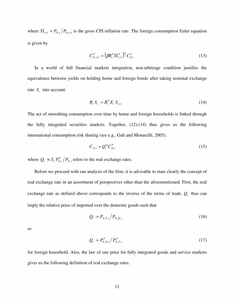
where 1,,1 ++ =Π tNtNt PP is the gross CPI inflation rate. The foreign consumption Euler equation

is given by

( ) F

tN

F

t

F

t

F

tN CRC .11,

σβ ++ Π= (13)

In a world of full financial markets integration, non-arbitrage condition justifies the

equivalence between yields on holding home and foreign bonds after taking nominal exchange

rate tS into account.

1+= tt

F

ttt SERSR (14)

The act of smoothing consumption over time by home and foreign households is linked through

the fully integrated securities markets. Together, (12)-(14) thus gives us the following

international consumption risk sharing (see e.g., Gali and Monacelli, 2005).

F

tNttN CQC ,,

σ= (15)

where tN

F

tNtt PPSQ ,,≡ refers to the real exchange rates.

Before we proceed with our analysis of the firm, it is advisable to state clearly the concept of

real exchange rate in an assortment of perspectives other than the aforementioned. First, the real

exchange rate as defined above corresponds to the inverse of the terms of trade. tQ thus can

imply the relative price of imported over the domestic goods such that

tHNtFNt PPQ ,,,,= (16)

or

F

tFN

F

tHNt PPQ ,,,,= (17)

for foreign household. Also, the law of one price for fully integrated goods and service markets

gives us the following definition of real exchange rates.

12

tFN

F

tFNttHN

F

tHNtt PPSPPSQ ,,,,,,,, == (18)

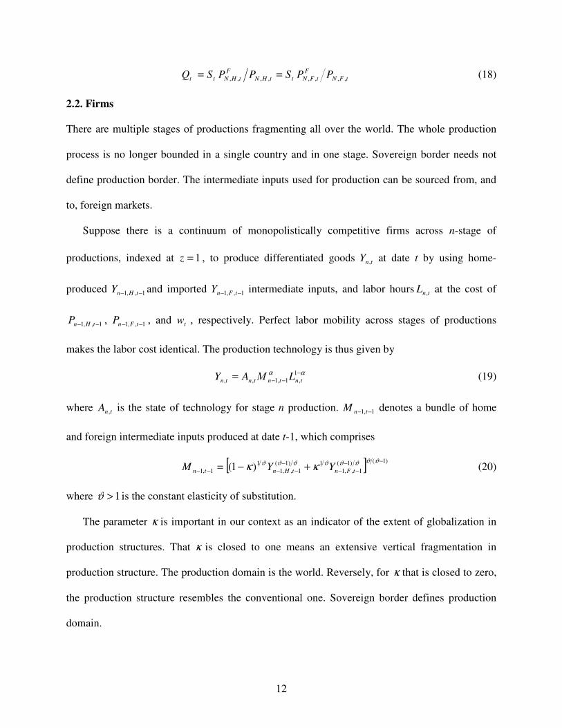
2.2. Firms

There are multiple stages of productions fragmenting all over the world. The whole production

process is no longer bounded in a single country and in one stage. Sovereign border needs not

define production border. The intermediate inputs used for production can be sourced from, and

to, foreign markets.

Suppose there is a continuum of monopolistically competitive firms across n-stage of

productions, indexed at 1=z , to produce differentiated goods tnY , at date t by using home-

produced 1,,1 −− tHnY and imported 1,,1 −− tFnY intermediate inputs, and labor hours tnL , at the cost of

1,,1 −− tHnP , 1,,1 −− tFnP , and tw , respectively. Perfect labor mobility across stages of productions

makes the labor cost identical. The production technology is thus given by

αα −

−−= 1

,1,1,, tntntntn LΜAY (19)

where tnA , is the state of technology for stage n production. 1,1 −− tnM denotes a bundle of home

and foreign intermediate inputs produced at date t-1, which comprises

[ ] )1()1(

1,,1

1)1(

1,,1

1

1,1 )1(−−

−−

−

−−−− +−=ϑϑϑϑϑϑϑϑ κκ tFntHntn YYM (20)

where 1>ϑ is the constant elasticity of substitution.

The parameter κ is important in our context as an indicator of the extent of globalization in

production structures. That κ is closed to one means an extensive vertical fragmentation in

production structure. The production domain is the world. Reversely, for κ that is closed to zero,

the production structure resembles the conventional one. Sovereign border defines production

domain.

13

The produce of stage n at date t can be either used by local downstream industry or exported

to foreign downstream industry. The firm’s problem can be formulated as minimizing the cost of

structure of (21) subject to (19) and (20).

tnttFntFntHntHn LwYPYP ,1,,11,,11,,11,,1 ++ −−−−−−−− (21)

Let the Lagrangian multiplier be the real marginal cost tnRMC , , the first order conditions are

given by

ϑϑϑϑκα )1(

1,

1

1,,1

1

,,1,,1 )1( −

−

−

−−−− −= tntHntntntHn MYYRMCP (22)

ϑϑϑϑκα )1(

1,

1

1,,1

1

,,1,,1

−

−

−

−−−− = tntFntntntFn MYYRMCP (23)

tntntnt LYRMCw ,,, )1( α−= (24)

Equation (22) and (23) if combined give the relative demand for home and foreign intermediate

inputs in the form

ϑ

κ

κ−

−−

−−

−−

−−

−=

1,,1

1,,1

1,,1

1,,1 1

tFn

tHn

tFn

tHn

P

P

Y

Y (25)

Substituting (25) sequentially for 1,,1 −− tFnY and 1,,1 −− tHnY into (20) yields the optimal demand

schedules for home and foreign intermediate inputs as follows:

1,1

1,1

1,,1

1,,1 −−

−

−−

−−

−−

= tn

tn

tFn

tFn MP

PY

ϑ

κ (26)

1,1

1,1

1,,1

1,,1 )1( −−

−

−−

−−

−−

−= tn

tn

tHn

tHn MP

PY

ϑ

κ (27)

with the use of utility-based producer price index (PPI).

[ ] )1(11

1,,1

1

1,,11,1 )1(ϑϑϑ κκ

−−

−−

−

−−−− +−= tFntHntn PPP (28)

14

Lastly, placing the first order conditions of (22)-(24) into the production function of (19), we

now come at the real marginal cost in the form

αα −

−−Φ=1

1,1, ttntn wPRMC (29)

where )1(1

, )1( αα αα −−−− −=Φ tnA .

2.3. Monetary Policy

The central bank is assumed to set the short-term nominal interest rate every period according to

a simple linear interest rate rule:

)ˆˆ()( ,,

*

, tNtNyNtNNt ayi −+−++= νππνπρ π (30)

where 0,0 ≥≥ yνν π , 11 −= −βρ is the steady-state real interest rate, and *

Nπ denotes the

central bank’s CPI inflation target. Assume a zero steady-state inflation, and NN ππ =* , this

“Taylor rule” can be simplified into

)ˆˆ(ˆ,,, tNtNytNt ayi −+= νπν π (31)

What makes (31) differ from the typical Taylor rule is the explicit consideration of technological

advance in the conduct of policy. Because technological improvement tends to drive the actual

inflation inversely away from the steady state, which is also the rate of inflation target, it is

optimal for central bank to respond by lowering the interest rate to provoke greater demand in

order to attain the inflation target. Nonetheless, if the technological advance raises the income

and thus greater demand in offsetting manner via the permanent income effect, the optimal

response certainly is to keep the nominal interest rate constant (e.g., Clarida et al., 1999).

15

3. Equilibrium Dynamics

3.1. Open-Economy Intertemporal Aggregate Demand

In an environment without government spending and physical investment, the market of final

goods is in equilibrium when

tFN

F

tHNtHNtN CCCY ,,,,,,, −+= (32)

The last two terms combined denote the trade balance. Considering the optimal demand

schedules of (4), (5), and (8), with the use of the international risk sharing of (15), we can rewrite

the market equilibrium as

( ) ( ) ( )( ) ησηηγγ

−−−−−+−= tNtFNt

F

tN

F

tHNtNtHNtNtN PPQPPPPCY ,,,,,,,,,,, )1( (33)

With the use of log-linearized utility-based CPI of (6) and (9), and of log-linearized real

exchange rates of (16) and (17), the log-linearization of (32) thus gives us

( )[ ] ttNtN qyc ˆ1ˆˆ,, σηγγ −−−= (34)

where a variable with small letter denotes its log value, while a hat over the variable represents

the log deviation from its steady state. Together with log-linearized consumption Euler equation

of (12), we can obtain the dynamics of intertemporal aggregate demand in the form

( ) ( )[ ][ ] tyttttNtttNttN qEqEiyEy ,11,1,,ˆˆ1ˆˆˆ εσηγγπσ +−−−+−−= +++ (35)

3.2. Optimal Price Setting

The firm of stage n for ],1[ Nn ∈ sets nominal prices on a Calvo-typed staggered basis (Calvo,

1983). We assume that each period firm z adjusts its price tnx , with state-independent probability

θ−1 . The average price of firms that do not adjust, with probability θ , is simply last period’s

price level 1, −tnP . In a symmetric equilibrium, all firms that adjust in period t choose the same

price. The price index can be expressed as

16

[ ] )1(11

,

1

1,, )1(κκκ θθ

−−−− −+= tntntn xPP (36)

which can be rewritten in the log-linearized form as

tntntn xpp ,1,,ˆ)1(ˆˆ θθ −+= − (37)

Optimal pricing strategy implies that firm chooses a log-price tnx , that approximates the

optimal reset price *

,tnp in order to minimize the following loss function

2*

,,

0

)ˆˆ()(min,

jtntnt

j

j

xpxEL

jn

+

∞

=

−=∑ θβ (38)

But until then, let us first derive the optimal reset price.

Let tnMC , be the nominal marginal cost, and jt+Ξ be the stochastic discount factor for

earnings at t + j. A monopolistically competitive firm z that is allowed to change its nominal

price at date t resets price )(*

, zP tn to maximize

( ) ( ) )()()( ,,

*

,

0

zYzMCzPE ktn

N

tntnjtt

j

j

++

∞

=

−Ξ∑ θβ (39)

subject to the demand constraint [ ] jtnjtntnjtn YPzPzY +

−

++ = ,,

*

,, )()(η

. As there is no firm-specific

shock, each and every firm z, ]1,0[∈z , chooses the same *

,tnP . The first order condition is given

by

∑ ∑∞

=

∞

=

−

++++ Ξ=−Ξ0 0

1*

,,,, )()1()(j j

tnjtntnjt

j

tjtnjt

j

t PYMCEYE ηθβηθβ (40)

Rearrange it, we get the log deviation of optimal reset price as log deviation of nominal marginal

cost.

tntn cmp ,

*

,ˆˆ = (41)

Now, we can solve the firm’s pricing problem by minimizing (38) subject to (41) to obtain

17

∑∞

=

+−=0

,ˆ)()1(ˆ

j

jtt

j

tn cmEx θβθβ (42)

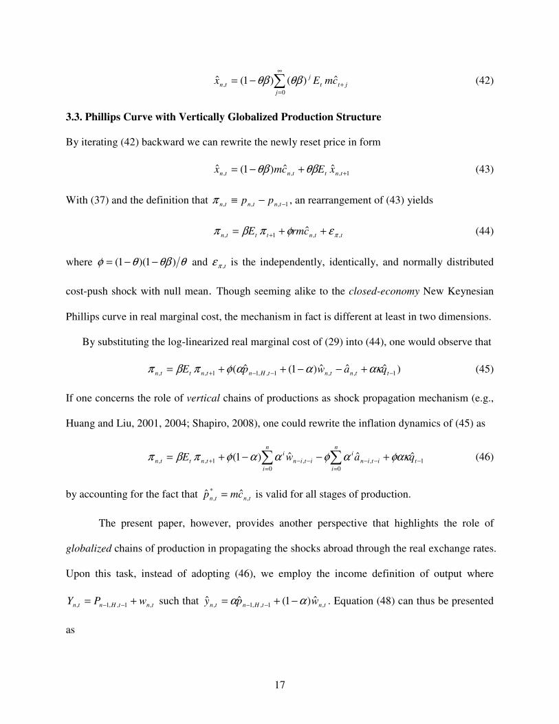
3.3. Phillips Curve with Vertically Globalized Production Structure

By iterating (42) backward we can rewrite the newly reset price in form

1,,,ˆˆ)1(ˆ

++−= tnttntn xEcmx θβθβ (43)

With (37) and the definition that 1,,, −−≡ tntntn ppπ , an rearrangement of (43) yields

ttntttn crmE ,,1,ˆ

πεφπβπ ++= + (44)

where θθβθφ )1)(1( −−= and t,πε is the independently, identically, and normally distributed

cost-push shock with null mean. Though seeming alike to the closed-economy New Keynesian

Phillips curve in real marginal cost, the mechanism in fact is different at least in two dimensions.

By substituting the log-linearized real marginal cost of (29) into (44), one would observe that

)ˆˆˆ)1(ˆ( 1,,1,,11,, −−−+ +−−++= ttntntHntnttn qawpE ακααφπβπ (45)

If one concerns the role of vertical chains of productions as shock propagation mechanism (e.g.,

Huang and Liu, 2001, 2004; Shapiro, 2008), one could rewrite the inflation dynamics of (45) as

1

0

,

0

,1,,ˆˆˆ)1( −

=

−−

=

−−+ +−−+= ∑∑ t

n

i

itin

in

i

itin

i

tnttn qawE φακαφααφπβπ (46)

by accounting for the fact that tntn cmp ,

*

,ˆˆ = is valid for all stages of production.

The present paper, however, provides another perspective that highlights the role of

globalized chains of production in propagating the shocks abroad through the real exchange rates.

Upon this task, instead of adopting (46), we employ the income definition of output where

tntHntn wPY ,1,,1, += −− such that tntHntn wpy ,1,,1,ˆ)1(ˆˆ αα −+= −− . Equation (48) can thus be presented

as

18

tttNtntnttn qayE ,1,,1,,ˆ)ˆˆ( πεφακφπβπ ++−+= −+ (47)

Current inflation is influenced not only by expected future inflation and economic condition,

but also the relative prices. Real depreciation, or deterioration in terms of trade, is inflationary to

an extent determined by the price stickiness φ , the share of intermediate inputs in output that

hints at the depth of verticalness in production structure α , and the share of foreign intermediate

inputs that reveals the degree of globalized production structure κ . In particular, a depreciated

level of real exchange rate raises the cost of imported foreign intermediate inputs, and thus the

real marginal costs, which, in turn, cause a higher inflation rate. An increasing inflation rate is at

hand if the real exchange rates keep depreciating at faster rate. The transmission from real

exchange rates to real marginal cost and so inflation rate is propagated by the depth of vertically

globalized production structure.

4. Solving the Linearized Dynamic Model

In this section we derive and characterize a structural vector autoregressive (SVAR) model to

examine how home economy is influenced by the development of foreign country. We use the

method of Binder and Pesaran (1995) to obtain an explicit solution for linear difference model of

(35) and (47) under rational expectations for final goods market ( Nn = ). By inserting the

monetary policy rule of (31), together with the uncovered interest rate parity of (14) and real

exchange rates as defined in (18), into (35) and (47), we cast the derived model in matrix

notation as follows:

ttttNtN

tNt

tNt

tN

tN

tN

tNaa

E

yEyyε

πππICCBBAAA +Λ+Λ+++

+

=

−−−−

+

+

−

−

−

− 111,1,

1,

1,

1

1,

1,

1

,

, ˆˆˆˆˆ

(48)

where [ ]′=Λ F

tN

F

tN

F

tNt ya ,,,ˆˆ π [ ]′= ttyt ,, πεεε

19

−−

ΓΓ+=

φακφ

νν π

1

1 yA

−−=−

πφακνφακν y

001A

Γ=+

β0

11A [ ]′−Γ= φν yB [ ]′=− yφακν01B

( )

−

−−=

φακ

ρνϕϕνϕν ππ

00

FFF

y

F

yC

−=− FF

y

F

y πφακνφακνφακν

0001C

=

10

01I ( )( )γησγ +−=Γ 1 ( )[ ]σηγγϕ −−= 1

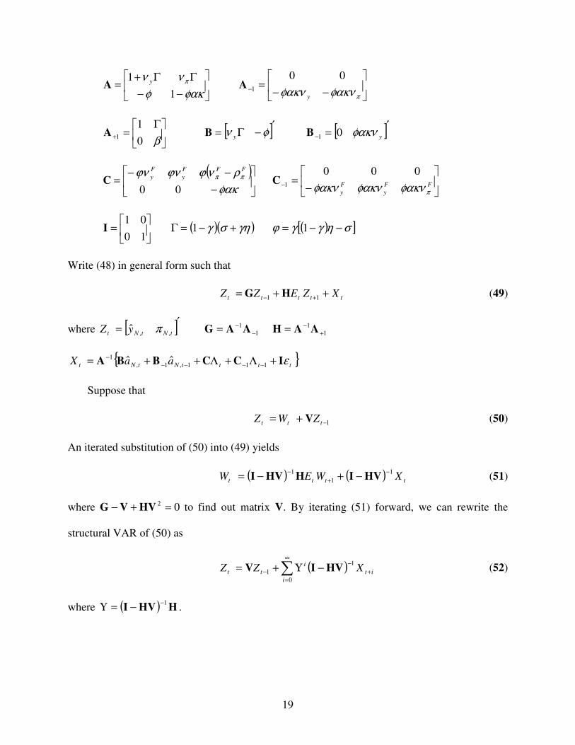
Write (48) in general form such that

ttttt XZEZZ ++= +− 11 HG (49)

where [ ]′= tNtNt yZ ,,ˆ π 1

1

−−= AAG 1

1

+−= AAH

ttttNtNt aaX εICCBBA +Λ+Λ++= −−−−−

111,1,

1 ˆˆ

Suppose that

1−+= ttt ZWZ V (50)

An iterated substitution of (50) into (49) yields

( ) ( ) tttt XWEW1

1

1 −

+

−−+−= HVIHHVI (51)

where 02 =+− HVVG to find out matrix V. By iterating (51) forward, we can rewrite the

structural VAR of (50) as

( )∑∞

=

+

−

− −Υ+=0

1

1

i

it

i

tt XZZ HVIV (52)

where ( ) HHVI1−

−=Υ .

20

5. Numerical Simulations

To inquire into the role of vertically globalized production structure in transmitting the foreign

disturbances, we conduct numerical simulations on (52) with the benchmark parameters as

shown in Table 1. One period in our model represents one quarter. In view of four percent real

interest rate per annum (Prescott, 1986), we choose 99.0=β . We set 75.0=θ such that the firm

revises price at an interval of once a year while the intertemporal elasticity of consumption is 0.5.

These values are consistent with the standard values used in the business-cycle literature. We set

2=η so that it fits the range of long run industry-level U.S. Armington elasticity (Gallaway et

al., 2001). We consider 5.0=α as a reasonable value in light of the empirical studies by

Jorgenson et al. (1987) and Nevo (2001) (see e.g., Huang and Liu, 2004). Besides, using 2=πν

and 1=yν is in line with the estimates of Clarida et al. (2000) for Volcker-Greenspan period in

which 15.2=πν 93.0=yν (see also Woodford, 2007). We assume that foreign country has an

identical policy weights on stabilizing inflation and output gap. Last but not least, we assume the

first order autocorrelation of CPI inflation in foreign country is 0.94.

[Insert Table 1 here]

Upon these benchmark parameters, we consider three possibilities about the degree of

globalization of production structures, ranging from sovereign-bounded ( 0=κ ) to moderate

( 5.0=κ ) and to highly vertically globalized production structure ( 9.0=κ ). We take into

account three different possible combinations in terms of country size, which are of small home

large foreign (SHLF) ( 1.0;9.0 == Fγγ ), large home small foreign (LHSF)( 9.0;1.0 == Fγγ ),

and of equal size (ES)( 5.0== Fγγ ) to obtain the estimated SVAR of home country in reduced

form for respective 1.0=γ , 5.0=γ and 9.0=γ under three different degrees of vertically

21

globalized production structure. Using the simulated reduced-form SVAR functions we generate

the impulse response of real output and CPI inflation to a one percentage shock in foreign

productivity innovation, in foreign demand innovation, and in foreign inflation innovation. These

impulse response functions are plotted in Figure 1 throughout Figure 3.

[Insert Figure 1 to Figure 3]

A cursory observation on panel (i) of Figure 1 certainly confirms that the classic Mundell-

Fleming-Poole insight is still right for the case of sovereign-bounded production function.

Having the flexible exchange rate as shock absorber, domestic real output and inflation do not

respond at all to the foreign productivity shock. The home real appreciation due to the fall in

foreign interest rate has tilted the increasing foreign expenditure toward foreign own produce.

Even in face of foreign demand and cost-push shock, home central bank faces no difficulty in

controlling home real output and inflation dynamics. Home central bank could choke off the

inflationary foreign demand propagated by foreign real appreciation (due to the rise in foreign

interest rate) by increasing home interest rate. The inflationary impact of one percentage increase

in foreign demand, as well as in foreign inflation shock2, on domestic output and inflation is thus

mild and short-lived. Note that if foreign counterpart is too large for home country, the

contractionary income effect due to a rise in foreign interest rate shall dominate the expansionary

substitution effect due to a home real depreciation in the foreign demand on home exports. As a

result, real output and inflation fall on impact in the case of SHLF.

Of main concern here is if globalization of a much more structural sort will complicate the

conduct of monetary policy. The figures reveal that the answer is unfortunately yes. In the case

of foreign productivity shock, home real appreciation due to the fall in foreign interest rate in

2 Foreign inflation shock has an impact identical to demand shock is due to the fact that rising foreign inflation rate

has tilted the foreign demand toward home exports.

22

responding to foreign productivity shock lowers the price of imported foreign intermediate inputs

and thus real marginal cost. Given the markup, the resultant fall in home inflation prompts the

central bank to lower the interest rate, which in turn excites the real output. However, the

magnitude of impulse response is negligible, and the dynamics exhibit a light degree of inertia

though not persistent across a spectrum of degree of vertically globalized production structure

and country size.

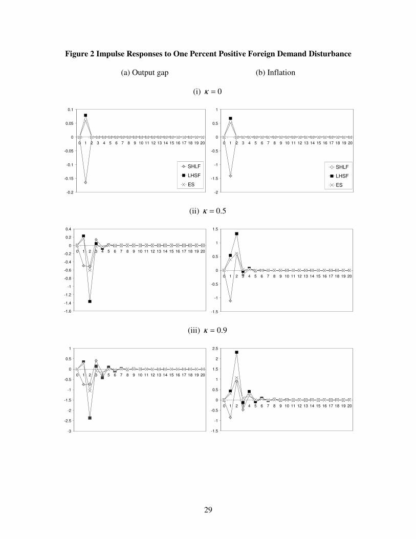
This tradeoff turns out to be an unpleasant one if the home central bank faces foreign demand

and cost-push shocks. On one hand, home real depreciation, as a reflection of higher foreign

interest rate, induces more final goods exports. On the other hand, real depreciation raises the

real marginal cost, and holds back the production of remanufactured intermediated inputs, which,

after all, increases the CPI inflation. The reaction of national central bank that raises interest rate,

however, gets rid of the output gain generated by prior real depreciation. As illustrated in

medium and lower panels of Figure 2, real output nose dives after one period of trivial increase.

Besides, the high interest rate-induced home appreciation will result in a slowdown in inflation.

However, because firms use one-period lag imported intermediate inputs, the effect of real

appreciation on inflation will come at pace slower than on real output.

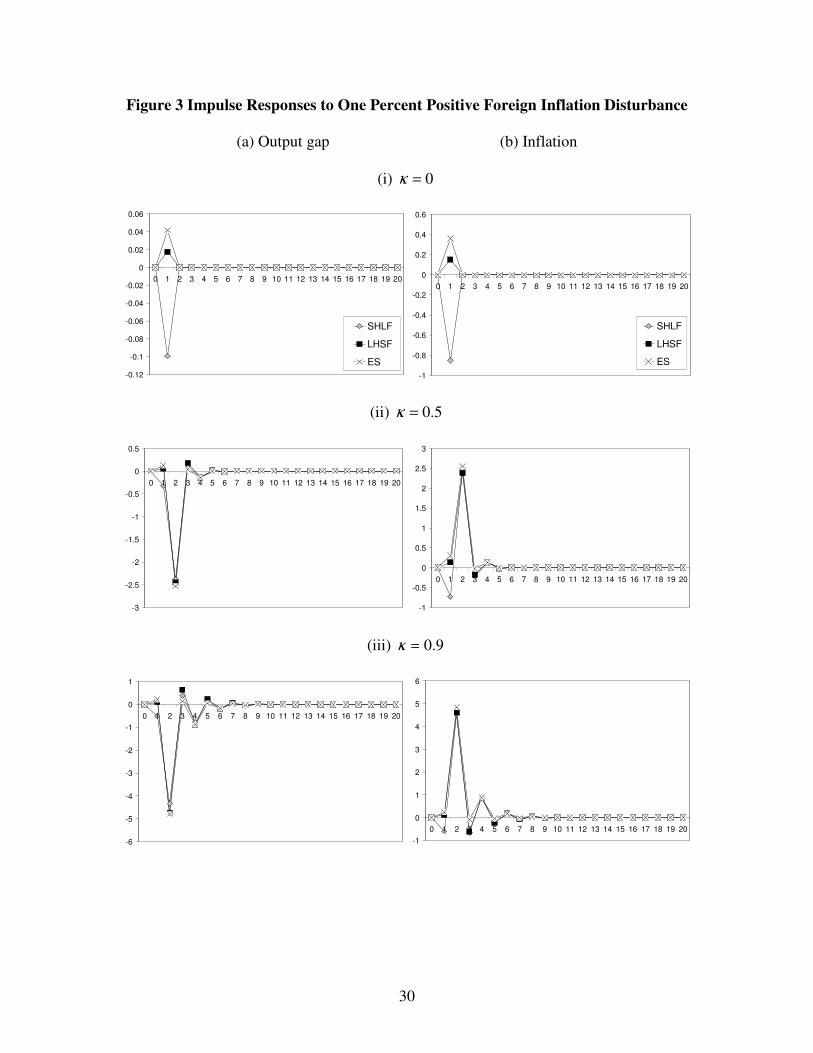
What we can conclude is that central bank faces a tradeoff, favorably and unfavorably, in

stabilizing the real output and inflation, brought about by the vertically globalized production

structure that magnifies the cost effect of foreign monetary policy through exchange rates.

Noticeably, ceteris paribus, this tradeoff becomes more unpleasant if the production structure is

vertically more globalized, and when in face of foreign cost-push shock as in Figure 3.

23

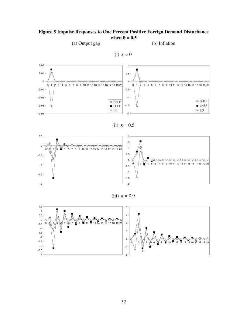
6. Does Nominal Rigidity Matter?

In light of the above analysis, a doubt that arises naturally is whether the staggered price setting,

instead of the structural factor, is responsible for the policy tradeoff. To check the robustness of

out result, we reset 5.0=θ such that the firm can adjust the price more frequently at an interval

of twice a year. Figure 4 throughout 6 illustrate that the policy tradeoff is still there. Notably, the

hump shaped inflation dynamics under three different foreign disturbances remains matched by

the inverted hump shaped output dynamics.

At about the same amplitude, the damped fluctuations of output and inflation around the

steady states, however, have been proliferated under a more flexible price environment. Besides,

the effect of foreign cost-push shock on home inflation and output dynamics becomes more

moderate across different country size and depth of the globally vertical fragmentation. For

instance, one percentage point increase in foreign cost-push innovation has been transmitted into

higher home inflation and lower home output by less than ±1.5 percentage point, respectively at

9.0=κ compared to more than ± 4 percentage point in the case of sticky price.

Overall, at this juncture it appears that the case of incorporating vertically globalized

production structure into an open-economy New Keynesian model, regardless the price

stickiness, is sensibly persuasive. As Blanchard and Gali (2005) have compellingly demonstrated

that the interaction between real wage rigidities and shock has made the divine coincidence

disappears, we argue that the interaction between foreign monetary policy and foreign

disturbances can be channeled into home economy through exchange rates propagated by

internationally linked production structures, which, as a result, creates policy tradeoff between

inflation and output stabilization that obscures the task of national central banks.

[Insert Figure 4 to Figure 6]

24

7. Concluding Remarks

To what extent globalization has kept a tight rein on central bank’s ability to control national

macroeconomic dynamics remains an open question. By laying out an open-economy two-

country New Keynesian model with staggered price setting and vertically globalized production

structure, we demonstrate that globalization in the sort of cross-border vertical production

sharing complicates the conduct of monetary policy. With the use of foreign intermediate inputs,

exchange-rate movements transmit interaction between foreign policy stance and foreign shocks

into domestic supply shock. Central bank thus faces tradeoff between stabilizing inflation and

output gap fluctuations. This finding is robust toward the absence of nominal rigidities.

There are several dimensions that we think are worthwhile for more hard works in the future.

First, as real wage and price of intermediate inputs constitute the real marginal cost, one may

construct a quantitative model of join real wage rigidities, the depth of verticalness and of

globalized production structure to explore the relative importance of these three factors in

accounting for the policy tradeoff. Second, one may use the framework developed in this paper

to estimate the inflation and output dynamics of East Asian as well as small Scandinavian

countries that depend heavily on international production fragmentation. Third, we think that

vertically globalized production structure has opened up a new perspective on the role of

exchange rates as a transmission mechanism. Should the exchange rate be included in the

monetary policy reaction function, or even be fixed for small open economy with extensive

cross-border vertical production sharing should be high on international macroeconomists’

research agenda.

No less important, seeing that stabilizing inflation comes at the cost of real output loss, strict

inflation targeting regime is no longer optimal. Thus, forth, what is the optimal monetary policy

25

rule in the presence of vertically globalized production structure? To be more exhaustive, one

may revisit the optimal international policy coordination for East Asian countries in light of the

above analysis.

Last but not least, as a by-product, we find that incorporation of vertically globalized

production structure allows the model to exhibit some form of inertia and persistence in inflation

and output dynamics after a shock. Note that the shocks assumed in the model occur at and last

for only one period. In other words, any persistence shown in the model must be endogenously

inherited. We hope that the incorporation of this structural factor into the New Keynesian model,

with further refinement, could overcome the well-know caveat – lack of inflation inertia and

endogenous persistence – of New Keynesian model.

References

Athukorala, P.C., and N. Yamashita, 2006, Production fragmentation and trade integration: East

Asian in a global context. The North American Journal of Economics and Finance, 17, pp.

233-56.

Ball, L., 2006, Has globalization changed inflation? NBER Working Paper No. 12687,

Cambridge, Massachusetts.

Blanchard, O. & J. Gali, 2007, Real wage rigidities and new Keynesian model. Journal of Money,

Credit, and Banking, 39(1), p.p. 35-66.

Boivin, J. & M.P. Giannoni, 2006, Has monetary policy become more effective? Review of

Economics and Statistics, 88(3), p.p. 445-462.

Boivin, J. & M.P. Giannoni, 2007, Global forces and monetary policy effectiveness.

Forthcoming in J. Gali. & M.J. Gertler (eds) International Dimensions of Monetary Policy.

University of Chicago Press.

Borio, C. & A. Filardo, 2007, Globalization and inflation: new cross-country evidence on the

global determinants of domestic inflation. BIS Working Papers No 227, Bank for

International Settlements.

Chen H., M. Kondratowicz, and K. Yi, 2005, Vertical specialization and three facts about U.S.

international trade. The North American Journal of Economics and Finance, 16, p.p. 35-59.

Cheng, L.K., and Kierzkowski, H. (eds), 2001, Global production and trade in East Asia,

Kluwer, Dordrecht.

Clarida, R., J. Gali & M. Gertler, 2002, The science of monetary policy: a new Keynesian

perspective. Journal of Economic Literature, 37, p.p. 1661-1707.

26

Clarida, R., J. Gali & M. Gertler, 2000, Monetary policy rules and macroeconomic stability:

evidence and some theory. Quarterly Journal of Economics, 115(1), p.p. 147-180.

Dean, J., K.C. Fung, and Z. Wang, 2007, Measuring the vertical specialization in Chinese trade.

Paper presented at IMF Conference on Global Implications of China’s Trade, Investment and

Growth.

Duca, J.V & D. VanHoose, 2000, Has greater competition restrained U.S. inflation? Southern

Economic Journal, 66(3), p.p. 729-741.

Feenstra, R., 1998, Integration of trade and disintegration of production in the global economy.

Journal of Economic Perspectives, 14(4), p.p. 31-50.

Gali, J., 2008, Monetary Policy, Inflation, and the Business Cycle. Princeton: Princeton

University Press.

Gali, J. & T. Monacelli, 2005, Monetary policy and exchange rate volatility in a small open

economy. Review of Economic Studies, 72(3), p.p. 707-734.

Gallaway, M.P., C.A. McDaniel & S.A. Rivera, 2001, Long-Run industry-level estimates of U.S.

Armington elasticities. U.S. ITC Working Paper No.2000-09a.

Haddad, M., 2007, Trade integration in East Asia: the role of China and production networks.

World Bank Policy Research Working Paper 4160, Washington: World Bank.

Huang, K.X.D. & Z. Liu, 2001, Production chains and general equilibrium aggregate dynamics.

Journal of Monetary Economics, 48, p.p. 437-462.

Huang, K.X.D & Z. Liu, 2004, Input-output structure and nominal rigidity: the persistence

problem revisited. Macroeconomic Dynamics, 8, p.p. 188-206.

Hummels, D., J. Ishii, and K. Yi, 2001, The nature and growth of vertical specialization in world

trade. Journal of International Economics, 54(1), p.p. 75-96.

Ihrig, J., S.B. Kamin, D. Lindner & J. Marquez, 2007, Some simple tests of the globalization and

inflation hypothesis. International Finance Discussion Papers 891. Washington: Board of

Governors of the Federal Reserve System.

International Monetary Fund, 2006, How has globalization affected inflation? World Economic

Outlook, spring, p.p 97-134.

Jorgenson, D.W., F.M. Gollop & B.M. Fraumeni, 1987, Productivity and U.S. economic growth.

Cambridge, MA: Harvard University Press.

Kamin, S.B., M. Marazzi & J.W. Schindler, 2006, The impact of Chinese exports on global

import prices. Review of International Economics, 14, p.p. 179-201.

Monacelli, T., 2004, Into the Mussa puzzle: monetary policy regimes and the real exchange rate

in a small open economy. Journal of International Economics, 62, p.p. 191-217.

Nevo, A., 2001, Measuring market power in the ready-to-eat cereal industry. Econometrica, 69,

p.p. 307-342.

Pain, N., I. Koske & M. Sollie, 2006, Globalization and inflation in the OECD economies.

OECD Economics Department Working Paper No.524. Paris: Organization for Economic

Cooperation and Development.

Prescott, E.C., 1986, Theory ahead of business cycle measurement. Federal Reserve Bank of

Minneapolis Quarterly Review, 10, p.p. 9-22.

Robert, J.M, 2006, Monetary policy and inflation dynamics. International Journal of Central

Banking, 2(September), p.p. 193-230.

Rogoff, K., 2003, Globalization and global disinflation. Federal Reserve Bank of Kansas City

Economic Review, 88(4), p.p. 45-78.

27

Sbordone, A.M., 2008, Globalization and inflation dynamics: the impact of increased

competition. Federal Reserve Bank of New York Staff Reports No.324, Federal Reserve Bank

of New York.

Rogoff, K., 2006, The impact of globalization on monetary policy. In Federal Reserve Bank of

Kansas City The New Economic Geography: Effects and Policy Implication, proceeding of

the 2006 Jackson Hole symposium sponsored by the Federal Reserve Bank of Kansas City.

Shapiro A.H., 2008, Estimating the new Keynesian Phillips curve: a vertical production chain

approach. Journal of Money, Credit, and Banking, 40(4), 627-666.

Woodford M., 2007, Globalization and monetary control. Forthcoming in J. Gali. & M.J. Gertler

(eds) International Dimensions of Monetary Policy. University of Chicago Press.

Yi, K., 2003, Can vertical specialization explain the growth of world trade? Journal of Political

Economy, 111(1), 52-102.

Table 1 Benchmark Parameter Values

β 0.99

θ 0.75

σ 0.50

η 2.00

α 0.50 F

ππ νν = 2.00

F

yy νν = 1.00

F

πρ 0.94

28

Figure 1 Impulse Responses to One Percent Favorable Foreign Productivity Disturbance

(a) Output gap (b) Inflation

(i) 0=κ

0

0.1

0.2

0.3

0.4

0.5

0.6

0.7

0.8

0.9

1

0 1 2 3 4 5 6 7 8 9 10 11 12 13 14 15 16 17 18 19 20

SHLF

LHSF

ES

0

0.1

0.2

0.3

0.4

0.5

0.6

0.7

0.8

0.9

1

0 1 2 3 4 5 6 7 8 9 10 11 12 13 14 15 16 17 18 19 20

SHLF

LHSF

ES

(ii) 5.0=κ

-0.02

-0.01

0

0.01

0.02

0.03

0.04

0.05

0.06

0 1 2 3 4 5 6 7 8 9 10 11 12 13 14 15 16 17 18 19 20

-0.07

-0.06

-0.05

-0.04

-0.03

-0.02

-0.01

0

0.01

0.02

0.03

0 1 2 3 4 5 6 7 8 9 10 11 12 13 14 15 16 17 18 19 20

(iii) 9.0=κ

-0.1

-0.05

0

0.05

0.1

0.15

0.2

0 1 2 3 4 5 6 7 8 9 10 11 12 13 14 15 16 17 18 19 20

-0.2

-0.15

-0.1

-0.05

0

0.05

0 1 2 3 4 5 6 7 8 9 10 11 12 13 14 15 16 17 18 19 20

29

Figure 2 Impulse Responses to One Percent Positive Foreign Demand Disturbance

(a) Output gap (b) Inflation

(i) 0=κ

-0.2

-0.15

-0.1

-0.05

0

0.05

0.1

0 1 2 3 4 5 6 7 8 9 10 11 12 13 14 15 16 17 18 19 20

SHLF

LHSF

ES

-2

-1.5

-1

-0.5

0

0.5

1

0 1 2 3 4 5 6 7 8 9 10 11 12 13 14 15 16 17 18 19 20

SHLF

LHSF

ES

(ii) 5.0=κ

-1.6

-1.4

-1.2

-1

-0.8

-0.6

-0.4

-0.2

0

0.2

0.4

0 1 2 3 4 5 6 7 8 9 10 11 12 13 14 15 16 17 18 19 20

-1.5

-1

-0.5

0

0.5

1

1.5

0 1 2 3 4 5 6 7 8 9 10 11 12 13 14 15 16 17 18 19 20

(iii) 9.0=κ

-3

-2.5

-2

-1.5

-1

-0.5

0

0.5

1

0 1 2 3 4 5 6 7 8 9 10 11 12 13 14 15 16 17 18 19 20

-1.5

-1

-0.5

0

0.5

1

1.5

2

2.5

0 1 2 3 4 5 6 7 8 9 10 11 12 13 14 15 16 17 18 19 20

30

Figure 3 Impulse Responses to One Percent Positive Foreign Inflation Disturbance

(a) Output gap (b) Inflation

(i) 0=κ

-0.12

-0.1

-0.08

-0.06

-0.04

-0.02

0

0.02

0.04

0.06

0 1 2 3 4 5 6 7 8 9 10 11 12 13 14 15 16 17 18 19 20

SHLF

LHSF

ES

-1

-0.8

-0.6

-0.4

-0.2

0

0.2

0.4

0.6

0 1 2 3 4 5 6 7 8 9 10 11 12 13 14 15 16 17 18 19 20

SHLF

LHSF

ES

(ii) 5.0=κ

-3

-2.5

-2

-1.5

-1

-0.5

0

0.5

0 1 2 3 4 5 6 7 8 9 10 11 12 13 14 15 16 17 18 19 20

-1

-0.5

0

0.5

1

1.5

2

2.5

3

0 1 2 3 4 5 6 7 8 9 10 11 12 13 14 15 16 17 18 19 20

(iii) 9.0=κ

-6

-5

-4

-3

-2

-1

0

1

0 1 2 3 4 5 6 7 8 9 10 11 12 13 14 15 16 17 18 19 20

-1

0

1

2

3

4

5

6

0 1 2 3 4 5 6 7 8 9 10 11 12 13 14 15 16 17 18 19 20

31

Figure 4 Impulse Responses to One Percent Favorable Foreign Productivity Disturbance

when θθθθ = 0.5

(a) Output gap (b) Inflation

(i) 0=κ

0

0.1

0.2

0.3

0.4

0.5

0.6

0.7

0.8

0.9

1

0 1 2 3 4 5 6 7 8 9 10 11 12 13 14 15 16 17 18 19 20

SHLF

LHSF

ES

0

0.1

0.2

0.3

0.4

0.5

0.6

0.7

0.8

0.9

1

0 1 2 3 4 5 6 7 8 9 10 11 12 13 14 15 16 17 18 19 20

SHLF

LHSF

ES

(ii) 5.0=κ

-0.02

-0.01

0

0.01

0.02

0.03

0.04

0.05

0 1 2 3 4 5 6 7 8 9 10 11 12 13 14 15 16 17 18 19 20

-0.08

-0.06

-0.04

-0.02

0

0.02

0.04

0.06

0 1 2 3 4 5 6 7 8 9 10 11 12 13 14 15 16 17 18 19 20

(iii) 9.0=κ

-0.1

-0.05

0

0.05

0.1

0.15

0.2

0 1 2 3 4 5 6 7 8 9 10 11 12 13 14 15 16 17 18 19 20

-0.2

-0.15

-0.1

-0.05

0

0.05

0.1

0 1 2 3 4 5 6 7 8 9 10 11 12 13 14 15 16 17 18 19 20

32

Figure 5 Impulse Responses to One Percent Positive Foreign Demand Disturbance

when θθθθ = 0.5

(a) Output gap (b) Inflation

(i) 0=κ

-0.04

-0.03

-0.02

-0.01

0

0.01

0.02

0 1 2 3 4 5 6 7 8 9 10 11 12 13 14 15 16 17 18 19 20

SHLF

LHSF

ES

-2

-1.5

-1

-0.5

0

0.5

1

0 1 2 3 4 5 6 7 8 9 10 11 12 13 14 15 16 17 18 19 20

SHLF

LHSF

ES

(ii) 5.0=κ

-2

-1.5

-1

-0.5

0

0.5

0 1 2 3 4 5 6 7 8 9 10 11 12 13 14 15 16 17 18 19 20

-2

-1.5

-1

-0.5

0

0.5

1

1.5

2

0 1 2 3 4 5 6 7 8 9 10 11 12 13 14 15 16 17 18 19 20

(iii) 9.0=κ

-4

-3.5

-3

-2.5

-2

-1.5

-1

-0.5

0

0.5

1

1.5

0 1 2 3 4 5 6 7 8 9 10 11 12 13 14 15 16 17 18 19 20

-2

-1

0

1

2

3

4

0 1 2 3 4 5 6 7 8 9 10 11 12 13 14 15 16 17 18 19 20

33

Figure 6 Impulse Responses to One Percent Positive Foreign Inflation Disturbance

when θθθθ = 0.5.

(a) Output gap (b) Inflation

(i) 0=κ

-0.004

-0.003

-0.002

-0.001

0

0.001

0.002

0 1 2 3 4 5 6 7 8 9 10 11 12 13 14 15 16 17 18 19 20

SHLF

LHSF

ES-0.2

-0.15

-0.1

-0.05

0

0.05

0.1

0 1 2 3 4 5 6 7 8 9 10 11 12 13 14 15 16 17 18 19 20

SHLF

LHSF

ES

(ii) 5.0=κ

-0.7

-0.6

-0.5

-0.4

-0.3

-0.2

-0.1

0

0.1

0.2

0 1 2 3 4 5 6 7 8 9 10 11 12 13 14 15 16 17 18 19 20

-0.3

-0.2

-0.1

0

0.1

0.2

0.3

0.4

0.5

0.6

0.7

0.8

0 1 2 3 4 5 6 7 8 9 10 11 12 13 14 15 16 17 18 19 20

(iii) 9.0=κ

-2

-1.5

-1

-0.5

0

0.5

1

0 1 2 3 4 5 6 7 8 9 10 11 12 13 14 15 16 17 18 19 20

-1

-0.5

0

0.5

1

1.5

0 1 2 3 4 5 6 7 8 9 10 11 12 13 14 15 16 17 18 19 20

34