New-Keynesian Macroeconomics and the TermStructure∗

Geert Bekaert† Seonghoon Cho‡ Antonio Moreno§

JEL Classification: E31, E32, E43, E52, G12

Keywords: Monetary Policy, Inflation Target, Term Structure of Interest Rates,Phillips Curve

∗We benefited from the comments of two referees, the editor, Pok-sang Lam, Glenn Rudebusch,Adrian Pagan and seminar participants at Columbia University, Carleton University, the KoreaDevelopment Institute, the University of Navarra, the University of Rochester (Finance Department),Tilburg University, the National Bank of Belgium, the Singapore Management University, the 2004Meeting of the Society for Economic Dynamics in Florence, the 2005 Econometric Society WorldCongress in London, the 2005 European Finance Association Annual Meeting in Moscow and the2006 EC2 Conference in Rotterdam.

†Graduate School of Business, Columbia University. Email: gb241@columbia.edu‡School of Economics, Yonsei University, Korea. Email: sc719@yonsei.ac.kr§Department of Economics, University of Navarra, Spain. Email: antmoreno@unav.es

Abstract

This article complements the structural New-Keynesian macro framework with

a no-arbitrage affine term structure model. Whereas our methodology is general,

we focus on an extended macro-model with unobservable processes for the inflation

target and the natural rate of output which are filtered from macro and term structure

data. We find that term structure information helps generate large and significant

parameters governing the monetary policy transmission mechanism. Our model also

delivers strong contemporaneous responses of the entire term structure to various

macroeconomic shocks. The inflation target shock dominates the variation in the

“level factor” whereas monetary policy shocks dominate the variation in the “slope

and curvature factors”.

1 Introduction

Structural New-Keynesian models, featuring dynamic aggregate supply (AS), aggre-

gate demand (IS) and monetary policy equations are becoming pervasive in macroeco-

nomic analysis. In this article we complement this structural macroeconomic frame-

work with a no-arbitrage term structure model.

Our analysis overcomes three deficiencies in previous work on New-Keynesian

macro models. First, the parsimony of such models implies very limited information

sets for both the monetary authority and the private sector. The critical variables

in most macro models are the output gap, expected inflation and a short-term inter-

est rate. It is well known, however, that monetary policy is conducted in a data-rich

environment. Consequently, lags of inflation, the output gap and the short-term inter-

est rate do not suffice to adequately forecast their future behavior. Recent research

by Bernanke and Boivin (2003) and Bernanke, Boivin, and Eliasz (2005) collapses

multiple observable time series into a small number of factors and embeds them in

standard vector autoregressive (VAR) analyses. Instead, we use term structure data.

Under the null of the Expectations Hypothesis, term spreads embed all relevant in-

formation about future interest rates. Additionally, a host of studies have shown that

term spreads are very good predictors of future economic activity (see, for instance,

Harvey (1988), Estrella and Mishkin (1998), Ang, Piazzesi, and Wei (2006)) and of

future inflation (Mishkin (1990) or Stock and Watson (2003)). In our proposed model,

the conditional expectations of inflation and the detrended output are a function of

the past realizations of macro variables and of unobserved components which are

extracted from term structure data through a no-arbitrage pricing model.

Second, the additional information from the term structure model transforms a

version of a New-Keynesian model with a number of unobservable variables into a

very tractable linear model which can be efficiently estimated by maximum likelihood

or the general method of moments (GMM). Hence, the term structure information

1

helps recover important structural parameters, such as those describing the monetary

transmission mechanism, in an econometrically convenient manner.

Third, incorporating term structure information leads to a simple VAR in macro

variables and term spreads but the reduced-form model for the macro variables is a

dynamically rich process with both autoregressive and moving average components.

This is important because one disadvantage of most structural New-Keynesian models

is the absence of sufficient endogenous persistence. We generate additional channels of

persistence by introducing unobservable variables in the macro model and then iden-

tify their dynamics using the arbitrage-free term structure model and term spreads.

The approach set forth in this paper also contributes to the term structure lit-

erature. In this literature it is common to have latent factors drive most of the

dynamics of the term structure of interest rates. These factors are often interpreted

ex-post as level, slope and curvature factors. A classic example of this approach is

Dai and Singleton (2000), who construct an arbitrage-free three factor model of the

term structure.1 While the Dai and Singleton (2000) model provides a satisfactory fit

of the data, it remains silent about the economic forces behind the latent factors. In

contrast, we construct a no-arbitrage term structure model where all the factors have

a clear economic meaning. Apart from inflation, detrended output and the short term

interest rate, we introduce two unobservable variables in the underlying macro model.

While there are many possible implementations, our main application here introduces

a time-varying inflation target and the natural rate of output. Consequently, we con-

struct a 5 factor affine term structure model that obeys New-Keynesian structural

relations.

Our main empirical findings are as follows. First, the model matches the persis-

tence displayed by the three macro variables despite being nested in a parsimonious

VAR(1) for macro variables and term spreads. Second, in contrast to previous maxi-

1Other examples include Knez, Litterman, and Scheinkman (1994) and Pearson and Sun (1994).

2

mum likelihood (MLE) or GMM estimations of the standard New-Keynesian model,

we obtain large and significant estimates of the Phillips curve and real interest rate

response parameters. Third, our model exhibits strong contemporaneous responses

of the entire term structure to the various structural shocks in the model.

Our article is part of a rapidly growing literature exploring the relation between

the term structure and macro economic dynamics. Kozicki and Tinsley (2001) and

Ang and Piazzesi (2003) were among the first to incorporate macroeconomic factors

in a term structure model to improve its fit. Evans and Marshall (2003) use a VAR

framework to trace the effect of macroeconomic shocks on the yield curve whereas

Dewachter and Lyrio (2006) assign macroeconomic interpretations to standard term

structure factors. Our paper differs from these articles in that all the macro variables

obey a set of structural macro relations. This facilitates a meaningful economic

interpretation of the term structure dynamics, relating them to macroeconomic shocks

or “deep” parameters characterizing the behavior of the private sector or the monetary

authority.

Two related studies are Hordahl, Tristani, and Vestin (2006) and Rudebusch and

Wu (2008), who also append a term structure model to a New-Keynesian macro

model. Our modelling approach is quite different however. First, our pricing kernel is

consistent with the IS equation, whereas in these two papers, it is exogenously deter-

mined. Because standard linearized New-Keynesian models display constant prices

of risk, this implies that our model’s term premiums do not vary through time by

construction. While there is some evidence of time-variation in term premiums, we

find it useful to examine how incorporating term structure data in a familiar setting

affects standard structural parameters and macro dynamics. Imposing the restriction

that the Expectations Hypothesis accounts for most of the variation in long rates

appears reasonable too. Second, these two articles add a somewhat arbitrary lag

structure to the supply and demand equations, whereas we analyze a standard opti-

3

mizing sticky price model with endogenous persistence. While this modelling choice

may adversely affect our ability to fit the data dynamics, it generates a parsimonious

state space representation for the macro-economic and term structure variables, with

a clear structural interpretation.

Another related article is Wu (2006). He formulates and calibrates a structural

macro model with adjustment costs for pricing and only two shocks (a technology

shock and a monetary policy shock). Wu (2006) then gauges the fit of the model

relative to the dynamics implied by an auxiliary standard term structure model based

exclusively on unobservables. Instead of following this indirect approach, we estimate

a structural macroeconomic model which directly implies an affine term structure

model with five observable and interpretable factors.

The remainder of the paper is organized as follows. Section 2 describes the struc-

tural macroeconomic model, whereas section 3 outlines how to combine the macro

model with an affine term structure model. Section 4 discusses the data and the

estimation methodology employed. Section 5 analyzes the macroeconomic implica-

tions while section 6 studies the term structure implications of our model. Section 7

concludes.

2 A New-Keynesian Macro Model with Unobserv-

able State Variables

We present a standard New-Keynesian model featuring AS, IS and monetary policy

equations with two additions. First, we assume the existence of a natural rate of

output which follows a persistent stochastic process. Second, the inflation target is

assumed to vary through time according to a persistent linear process. The monetary

authorities react to the output gap which is the deviation of output from the natural

rate of output. We allow for endogenous persistence in the AS, IS and monetary policy

4

equations. In what follows, we describe each equation in turn and describe the model

solution. In Bekaert, Cho, and Moreno (2005) we describe the microfoundations of

the AS and IS equations. Related theoretical derivations can be found in Clarida,

Galı, and Gertler (1999) or Woodford (2003).

2.1 The IS Equation

A standard intertemporal IS equation is usually derived from the first-order conditions

for a representative agent with power utility as in the original Lucas (1978) economy.

Standard estimation approaches have experienced difficulty pinning down the risk

aversion parameter, which is at the same time an important parameter underlying

the monetary transmission mechanism. Another discomforting feature implied by a

standard IS equation is that it typically fails to match the well-documented persistence

of output. We derive an alternative IS equation from a utility maximizing framework

with external habit formation similar to Fuhrer (2000). In particular, we assume that

the representative agent maximizes:

Et

∞∑s=t

ψs−tU(Cs; Fs) = Et

∞∑s=t

ψs−t

[FsC

1−σs − 1

1− σ

](1)

where Ct is the composite index of consumption, Ft represents an aggregate demand

shifting factor; ψ denotes the time discount factor and σ is the inverse of the intertem-

poral elasticity of substitution. We specify Ft as follows:

Ft = HtGt (2)

where Ht is an external habit level, that is, the agent takes Ht as exogenously given,

even though it may depend on past consumption. Gt is an exogenous aggregate

demand shock that can also be interpreted as a preference shock. Following Fuhrer

(2000), we assume that Ht = Cηt−1 where η measures the degree of habit dependence

5

on the past consumption level. It is this assumption that delivers endogenous output

persistence.

Imposing the resource constraint (Ct = Yt, with Yt output) and assuming log-

normality, the Euler equation for the interest rate yields a Fuhrer-type IS equation:

yt = αIS + µEtyt+1 + (1− µ)yt−1 − φ(it − Etπt+1) + εIS,t (3)

where yt is detrended log output and it is the short term interest rate. The parameter

φ measures the response of detrended output to the real interest rate; φ = 1σ+η

and

µ = σφ. The IS shock, εIS,t = φ ln Gt, is assumed to be independently and identically

distributed with homoskedastic variance σ2IS.

2.2 The AS Equation (Phillips Curve)

Building on the Calvo (1983) pricing framework with monopolistic competition in

the intermediate good markets, a forward-looking AS equation can be derived, linking

inflation to future expected inflation and the real marginal cost. By assuming that the

fraction of price-setters which does not adjust prices optimally, indexes their prices

to past inflation, we obtain endogenous persistence in the AS equation. Moreover,

we follow Woodford (2003) assuming the real marginal cost to be proportional to the

output gap. Consequently, we obtain a standard New-Keynesian aggregate supply

(AS) curve relating inflation to the output gap:

πt = δEtπt+1 + (1− δ)πt−1 + κ(yt − ynt ) + εAS

t (4)

where πt is inflation, ynt is the natural rate of detrended output that would arise in

the case of perfectly flexible prices and yt − ynt is the output gap;2 εAS

t is an exoge-

2The output gap is measured as the percentage deviation of detrended output with respect to

the natural rate of output. Both detrended output and the natural rate of output are measured

6

nous supply shock, assumed to be independently and identically distributed with ho-

moskedastic variance σ2AS. The parameter κ captures the short-run tradeoff between

inflation and the output gap and (1− δ) characterizes the endogenous persistence of

inflation.

In practice, structural estimates of the Phillips curve based on output gap mea-

sures seem less successful than those based on marginal cost (see Galı and Gertler

(1999)). However, whereas in most studies an exogenously detrended output variable

serves as the output gap measure in the AS equation, our output gap measure is

endogenous and filtered through macro and term structure information. We let the

natural rate follow an AR(1) process:

ynt = λyn

t−1 + εyn,t (5)

where εyn,t can be interpreted as a negative markup shock with standard deviation

σyn .3

2.3 The Monetary Policy Rule

We assume that the monetary authority specifies the nominal interest rate target, i∗t ,

as in the forward-looking Taylor rule proposed by Clarida, Galı, and Gertler (1999):

i∗t = [ıt + β (Etπt+1 − π∗t ) + γ (yt − ynt )] (6)

as percentage deviations with respect to a linear trend. Therefore, the means of the output gap,

detrended output and the natural rate of output are 0.3In a previous version of the paper (Bekaert, Cho, and Moreno (2005)), we used the utility

function in (1) and a simple production technology to derive an AS equation that provided an

explicit link between the marginal cost and the current and past output gap, and also yielded a

process for the natural rate of output endogenously. While some of the versions of the structural

model converged, it proved very difficult to estimate.

7

where π∗t is a time-varying inflation target and ıt is the desired level of the nominal

interest rate that would prevail when Etπt+1 = π∗t and yt = ynt . We assume that

ıt is constant.4 Note that β measures the long-run response of the interest rate to

expected inflation, a typical measure of the Fed’s stance against inflation.

We further assume that the monetary authority sets the short term interest rate

as a weighted average of the interest rate target and a lag of the short term interest

rate to capture the tendency by central banks to smooth interest rate changes:

it = ρit−1 + (1− ρ) i∗t + εMP,t (7)

where ρ is the smoothing parameter and εMP,t is an exogenous monetary policy shock,

assumed to be i.i.d. with standard deviation, σMP . The resulting monetary policy

rule for the interest rate is given by:

it = αMP + ρit−1 + (1− ρ) [β (Etπt+1 − π∗t ) + γ (yt − ynt )] + εMP,t (8)

where αMP = (1− ρ)ı.

2.4 Inflation Target π∗t

We close our model by specifying a stochastic process for the inflation target, π∗t .

Little is known about how the monetary authority sets the inflation target. Hordahl,

Tristani, and Vestin (2006) assume an AR(1) process for the inflation target. Gurkaynak,

Sack, and Swanson (2005) specify it as a weighted average of the past inflation target

and past inflation rates. While their specification is empirically supported to some

extent, we deem it plausible that the Central Bank takes the long-run inflation ex-

pectations of the private sector into account in a forward-looking manner. Therefore,

4We estimated alternative model specifications with a time-varying ıt in Bekaert, Cho, and

Moreno (2005) and the main results in the article are not altered.

8

we define πLRt as the conditional expected value of a weighted average of all future

inflation rates.

πLRt = (1− d)

∞∑j=0

djEtπt+j (9)

with 0 ≤ d ≤ 1. This equation can be succinctly written as:

πLRt = dEtπ

LRt+1 + (1− d)πt (10)

When d equals 0, πLRt collapses to current inflation, when d approaches 1, long-run

inflation approaches unconditional expected inflation. We assume that the monetary

authority anchors its inflation target around πLRt , but smooths target changes, so

that:

π∗t = ωπ∗t−1 + (1− ω)πLRt + επ∗,t. (11)

We view επ∗,t as an exogenous shift in the policy stance regarding the long term rate

of inflation or the target, and assume it to be i.i.d. with standard deviation σπ∗ .

Substituting out πLRt in equation (11) using equation (10), we obtain:

π∗t = ϕ1Etπ∗t+1 + ϕ2π

∗t−1 + ϕ3πt + επ∗,t (12)

where ϕ1 = d1+dω

, ϕ2 = ω1+dω

and ϕ3 = 1 − ϕ1 − ϕ2. In Bekaert, Cho, and Moreno

(2005) we also estimated a backward-looking inflation target process similar to that

of Gurkaynak, Sack, and Swanson (2005), producing results qualitatively similar to

the ones we present below.

9

2.5 The Full Model

Bringing together all the equations, we have a five variable system with three observed

and two unobserved macro factors:

πt = δEtπt+1 + (1− δ)πt−1 + κ(yt − ynt ) + εAS

t (13)

yt = αIS + µEtyt+1 + (1− µ)yt−1 − φ(it − Etπt+1) + εIS,t (14)

it = αMP + ρit−1 + (1− ρ) [β (Etπt+1 − π∗t ) + γ (yt − ynt )] + εMP,t (15)

ynt = λyn

t−1 + εyn,t (16)

π∗t = ϕ1Etπ∗t+1 + ϕ2π

∗t−1 + ϕ3πt + επ∗,t. (17)

Our macroeconomic model can be expressed in matrix form as:

Bxt = α + AEtxt+1 + Jxt−1 + Cεt (18)

where xt = [πt yt it ynt π∗t ]

′ and εt = [εAS,t εIS,t εMP,t εyn,t επ∗,t]′. α is a 5× 1 vector of

constants and B, A, J and C are appropriately defined 5× 5 matrices. The Rational

Expectations (RE) equilibrium can be written as a first-order VAR:

xt = c + Ωxt−1 + Γεt. (19)

Hence, the implied model dynamics are a simple VAR subject to a set of non-linear

restrictions. Note that Ω cannot be solved analytically in general. We solve for Ω

numerically using the QZ method (see Klein (2000) and Cho and Moreno (2008)).

Once Ω is solved for, Γ and c follow straightforwardly.

As the Appendix shows, the reduced-form representation of the vector of observ-

able macro variables is very similar to a VARMA(3,2) process. By adding unobserv-

ables, we potentially deliver more realistic joint dynamics for inflation, the output

10

gap and the interest rate, and overcome the lack of persistence implied by previous

studies.

3 Incorporating Term Structure Information

We derive the term structure model implicit in the IS curve that we presented in

section 2. This effort results in an easily estimable linear system in observable macro

variables and term spreads.

3.1 Affine Term Structure Models with New-Keynesian Fac-

tor Dynamics

Affine term structure models require linear state variable dynamics and a linear pric-

ing kernel process with conditionally normal shocks (see Duffie and Kan (1996)). For

the state variable dynamics implied by the New-Keynesian model in equation (19)

to fall in the affine class, we assume that the shocks are conditionally normally dis-

tributed, εt ∼ N(0, Dt−1). The pricing kernel process Mt+1 prices all securities such

that:

Et[Mt+1Rt+1] = 1. (20)

In particular, for an n-period bond, Rt+1 = Pn−1,t+1

Pn,twith Pn,t the time t price of an

n-period zero-coupon bond. If Mt+1 > 0 for all t, the resulting returns satisfy the

no-arbitrage condition (Harrison and Kreps (1979)). In affine models, the log of the

pricing kernel is modelled as a conditionally linear process. Consider, for instance:

mt+1 = ln(Mt+1) = −it − 1

2Λ′tDtΛt − Λ′tεt+1. (21)

Here Λt = Λ0 + Λ1xt, where Λ0 is a 5 × 1 vector and Λ1 is a 5 × 5 matrix. First,

setting Dt = D, we obtain a Gaussian price of risk model. Dai and Singleton (2002)

11

study such a model and claim that it accounts for the deviations of the Expectations

Hypothesis (EH) observed in U.S. term structure data. An alternative model sets

Λt = Λ and εt ∼ N(0, Dt−1) with Dt = D0+D1diag(xt), where diag(xt) is the diagonal

matrix with the vector xt on its diagonal. This model introduces heteroskedasticity

of the square-root form and has a long tradition in finance (see Cox, Ingersoll, and

Ross (1985)). Finally, setting Λt = Λ0 and Dt = D results in a homoskedastic model.

All three of these models imply an affine term structure. That is, log bond prices,

pn,t are an affine function of the state variables. The maturity-dependent coefficients

follow recursive equations. The three models have different implications for the be-

havior of term spreads and holding period returns. First, the homoskedastic model

implies that the EH holds: there may be a term premium but it does not vary through

time. Both the Gaussian prices of risk model and the square root model imply time-

varying term premiums. Second, our model includes inflation as a state variable and

the real pricing kernel (the kernel that prices bonds perfectly indexed against infla-

tion) and inflation are correlated. It is this correlation that determines the inflation

risk premium. If the covariance term is constant, the risk premium is constant over

time and this will be true in a homoskedastic model.

The kernel model implied by the IS curve derived above fits in the homoskedastic

class. It is possible to modify the pricing framework into one of the two other models,

but we defer this to future work. Bekaert, Hodrick, and Marshall (2001) show that

a model with minimal variation in the term premium suffices to match the evidence

regarding the Expectations Hypothesis for the US. Moreover, the current practice

of using linear regressions to infer the properties of term premiums almost surely

leads to the over-estimation of their variability (see Bekaert, Wei, and Xing (2007)

for simulation evidence).

12

3.2 The Term Structure Model Implied by the Macro Model

Because our derivation of the IS curve assumed a particular preference structure, the

pricing kernel is given by the intertemporal consumption marginal rate of substitution

of the model. That is:

mt+1 = ln ψ − σyt+1 + (σ + η)yt − ηyt−1 + (gt+1 − gt)− πt+1. (22)

The no-arbitrage condition holds by construction. In a log-normal model, pricing a

one period bond implies

Et[mt+1] + 0.5Vt[mt+1] = −it. (23)

For our particular model, (21) holds with Λ, a vector of prices of risk entirely restricted

by the structural parameters,

Λ′t = Λ′ = [1 σ 0 0 0]Γ− [0 (σ + η) 0 0 0] . (24)

Logarithmic bond prices and hence, bond yields (yt = −ln(Pt,n)

n), are an affine function

of the state variables:

yn,t = −an

n− b′n

nxt. (25)

The recursive formulas for an and bn can be constructed using equations (19)- (22).5

Term spreads are also an affine function of the state variables:

spn,t = −an

n− (

bn

n+ e3)

′xt (26)

where spn,t ≡ yn,t − it is the spread between the n period yield and the short rate.

This model provides a particular convenient form for the joint dynamics of the macro

5They are: an = an−1+b′n−1c+0.5b′n−1ΓDΓ′bn−1−Λ′DΓ′bn−1 and b′n = −e′3+b′n−1Ω, respectively.

13

variables and the term spreads. Let zt = [πt yt it spn1,t spn2,t]′, where n1 and n2

refer to two different yield maturities for the long-term bond in the spread. Then

xt = c + Ωxt−1 + Γεt (27)

zt = Az + Bzxt (28)

where

Az =

03×1

−an1

n1

−an2

n2

, Bz =

I3 03×2

−(bn1

n1+ e3)

′

−(bn2

n2+ e3)

′

.

Using xt = B−1z (zt − Az), we find:

zt = az + Ωzzt−1 + Γzεt (29)

where

Ωz = BzΩB−1z

Γz = BzΓ

az = Bzc + (I −BzΩB−1z )Az

In other words, the macro variables and the term spreads follow a first-order VAR

with complex cross-equation restrictions. This feature also differentiates our method

from previous work in the literature. Because equation (29) consists of observed

macro and term spread data, we can directly estimate it employing exactly two term

spreads. Once the model is estimated, we can back out the natural rate of output

and the inflation target using equation (28).

14

4 Data and Estimation

In this section, we first describe the data used in the estimation of our macro-finance

model. Then we present the general estimation methodology employed.

4.1 Data Description

The sample period is from the first quarter of 1961 to the fourth quarter of 2003.

We measure inflation with the CPI (collected from the Bureau of Labor Statistics)

but check robustness using the GDP deflator, from the National Income and Product

Accounts (NIPA). Detrended output is measured as the output deviation from a linear

trend. We also estimated the model with quadratically detrended output, producing

qualitatively similar results. The results are by and large similar across alternative

detrending methods. Output is real GDP from NIPA. We use the 3-month T-bill

rate, taken from the Federal Reserve of St. Louis database, as the short-term interest

rate. Finally, our analysis uses term-structure data at the one, three, five and ten

year maturities from the CRSP database. 6 We use the three and five year spreads

directly in the estimation and use additional term spreads to test the model ex-post.

Consequently, we do not use measurement error in the estimation and do not rely on

a Kalman filter to extract the unobservables from the data.

4.2 Estimation Methodology

Because our macro-finance model implies a first-order VAR on zt with complex cross-

equation, non-linear restrictions, we first verify that the BIC criterion indeed selects a

first-order VAR among unconstrained VARs of lag-lengths 1 through 5. We perform

the estimation on de-meaned data, zt = zt − Ezt with Ezt the sample mean of zt.

6The ten year zero-coupon yield was constructed splicing two series. We use the McCulloch andKwon series up to the 3rd quarter of 1987; from the 4th quarter of 1987 to the end of the sample,we use the ten year zero-coupon yield estimated using the method of Svensson (2004). We thankRefet Gurkaynak for kindly providing this second part of the series.

15

The structural parameters to be estimated are therefore θ = (δ κ σ η ρ β γ λ ω d σAS

σIS σMP σyn σπ∗). Assuming normal errors, it is straightforward to write down

the likelihood function for this problem and produce Full Information Likelihood

Estimates (FIML) estimates. However, to accommodate possible deviations from the

strong normality and homoskedasticity assumptions underlying maximum likelihood,

we use a two-step GMM estimation procedure based on Hansen (1982). To do so,

re-write the model in the following form:

zt = Ωz zt−1 + Γzεt = Ωz zt−1 + ΓzΣut (30)

where ut = Σ−1εt ∼ (0, I5) and Σ = diag([σAS σIS σMP σyn σπ∗ ]′), that is Σ2 = D.

To construct the moment conditions, consider the following vector valued pro-

cesses:

h1,t = ut ⊗ zt−1 (31)

h2,t = vech(utu′t − I5) (32)

ht = [h′1,t h′2,t]′ (33)

where vech represents an operator stacking the elements on or below the principle

diagonal of a matrix. The model imposes E[ht] = 0. The 25 h1,t moment conditions

capture the feedback parameters; the 15 h2,t moment conditions capture the structure

imposed by the model on the variance-covariance matrix of the innovations. Rather

than using an initial identity matrix as the weighting matrix, which may give rise

to poor first-stage estimates, we use a weighting matrix implied by the model under

normality. That is under the null of the model, the weighting matrix must be:

W = (E[hth′t])−1. (34)

16

Using normality and the error structure implied by the model, it is then straightfor-

ward to show that the optimal weighting matrix is given by:

W =

I ⊗ 1T

∑Tt=1 zt−1z

′t−1 025×15

015×25 I15 + vech(I5)vech(I5)′

−1

. (35)

This weighting matrix does not depend on the parameters. Then we minimize the

standard GMM objective function:

Q =(E[ht]

)′W

(E[ht]

)(36)

where E[ht] = 1T

∑Tt=1 ht. This gives rise to estimates that are quite close to what

would be obtained with maximum likelihood. Given these estimates, we produce

a second-stage weighting matrix allowing for heteroskedasticity and 5 Newey-West

(Newey and West (1987)) lags in constructing the variance covariance matrix of the

orthogonality conditions. We iterate this system until convergence. This estimation

proved overall rather robust with parameter estimates varying little after the first

round.

5 Macroeconomic Implications

5.1 Structural Parameter Estimates

In order to assess the fit of the model, we first comment on the standard GMM test

of the over-identifying restrictions, which follows a χ2 distribution with 25 degrees of

freedom because there are 40 moment conditions but only 15 parameters. We find

that the test fails to reject the model at the 5% level when 5 Newey-West lags are used

in the construction of the weighting matrix (the p-value is 26.3%). While the model

is not rejected either with 4 Newey-West lags (the p-value is 9.4%), it is rejected when

17

only 3 Newey-West lags are used (the p-value is 1.3%). This in itself suggests that

the orthogonality conditions still display substantial persistence. Nevertheless, the

model fits the autocorrelograms of the data series very well (not reported).

The second to fourth columns in table 1 show the parameter estimates of the

model and their GMM and bootstrap standard errors.7 The bootstrap analysis will

prove useful in generating standard errors for a number of model-implied statistics. A

first important finding is the size and significance of κ, the Phillips curve parameter.

As Galı and Gertler (1999) point out, previous studies fail to obtain reasonable and

significant estimates of κ with quarterly data. Galı and Gertler (1999) do obtain larger

and significant estimates using a measure for marginal cost replacing the output gap.

Our estimates of κ, using the output gap and term spreads are even larger than those

obtained by Galı and Gertler (1999). Using the (larger) standard error from the

bootstrap, κ remains statistically significantly different from zero. We estimate the

forward-looking parameter in the AS equation to be close to 0.61, consistent with

previous studies.

When structural models are estimated with techniques such as GMM or MLE,

they often give rise to large estimates of σ rendering the IS equation a rather ineffec-

tive channel of monetary policy transmission. Two examples are Ireland (2001) and

Cho and Moreno (2006). Lucas (2003) argues that the curvature parameter in the

representative agent’s utility function consistent with most macro and public finance

models should be between 1 and 4. While the Lucas’ statement does not strictly apply

to models with habit persistence, in our multiplicative habit model σ still represents

7We bootstrap from the 172 observations on the vector of structural standard errors (εt) withreplacement and re-create a sample of artificial data using the estimated parameter matrices (Ω, Γ)and historical initial values. For each replication, we create a sample of 672 observations, discard thefirst 500 and retain the last 172 observations to create a sample of length equal to the data sample.We then re-estimate the model with these artificial data and replicate this process 1,000 times tocreate the small sample distributions of the parameters. Since we identified some serial correlationin the residuals, we also perform a block bootstrap using the Kunsch’s rule with a block length of7, as explained in Hall, Horowitz, and Jing (1995). The implied small-sample distributions are verysimilar to the ones presented in the paper.

18

local risk aversion. Our estimation yields a small (slightly larger than 3) and sig-

nificant estimate of σ, although its significance is more marginal using bootstrapped

standard errors. Smets and Wouters (2003) and Lubik and Schorfheide (2004) find

small estimates of σ using Bayesian estimation techniques. Rotemberg and Wood-

ford (1998) and Boivin and Giannoni (2006) also find small estimates of σ but they

modify the estimation procedure towards fitting particular impulse responses. Our

model exhibits large habit persistence effects, as the habit persistence parameter, η,

is close to 4. Other studies have also found an important role for habit persistence

(Fuhrer (2000), Boldrin, Christiano, and Fisher (2001)).8 In summary, the parameter

estimates for the AS and IS equations imply that our model delivers large economic

effects of monetary policy on inflation and output.

Why do we obtain large and significant estimates of κ and φ? Two channels seem

to be at work: First, expectations are based on both observable and unobservable

macro variables. Therefore, an important variable in the AS equation, such as ex-

pected inflation, is directly affected by the inflation target. As a result, changes in

the inflation target shift the AS curve. As we show below in variance decomposi-

tions, the inflation target shock contributes significantly to variation in the inflation

rate. Similarly, the natural rate shock significantly contributes to the dynamics of

detrended output. Second, our measure of the output gap is different from the usual

detrended output and contains additional valuable information extracted from the

term structure. For instance, the first order autocorrelation of the implied output

gap is 0.92, which is smaller than 0.96, the first order autocorrelation of linearly de-

trended output. The Phillips curve coefficients found in previous studies reflect the

8Our habit persistence parameter is not directly comparable to that derived by Fuhrer (2000).

There is however a linear relationship between them: η = (σ−1)h, where h is the Fuhrer (2000) habit

persistence parameter. Our implied h is close to 2, larger than in previous studies, and violating a

theoretical bound in Fuhrer (2000). This implies that µ < 0.5, as in Boivin and Giannoni (2006),

for instance. Imposing h ≤ 1 significantly worsens the fit of the empirical model.

19

weak link between detrended output and inflation in the data and the large difference

in persistence between these two variables. In our model, even though κ is rather

large, the relationship between inflation and the output gap is still not strongly pos-

itive because the inflation target also moves the AS-curve. In sum, the presence of

both the inflation target and the natural rate of output in the AS equation implies

a significantly positive conditional co-movement between the output gap and infla-

tion, even though the unconditional correlation between them remains low as it is

in the data. The unobservables are also critical in fitting the relative persistence of

the output gap and inflation. Similarly, the φ parameter still fits the dependence of

detrended output on the real interest rate, but the real interest rate is now an implicit

function of all the state variables, including the natural rate of output.

The estimates of the policy rule parameters are similar to those found in the

literature. The estimated long-run response to expected inflation is larger than 1.

The response to the output gap is always close to 0 and insignificantly different from

0. Finally, the smoothing parameter, ρ, is estimated to be 0.72, similar to previous

studies.

The two unobservables are quite persistent, but clearly stationary processes. The

natural rate of output’s persistence is close to 0.96, while the weight on the past

inflation target in the inflation target equation is 0.88. Furthermore, the weight on

current inflation in the construction of the long-run inflation target (1-d) is close to

0.15. Finally, the five shock standard deviations are significant, with the monetary

policy shock standard deviation larger than the others. There has been some evidence

pointing towards a structural break in the β parameter (see, for instance, Clarida,

Galı, and Gertler (1999) or Lubik and Schorfheide (2004)). The large estimate of

σMP may reflect the absence of such a break in our model.

20

5.2 Output Gap and Inflation Target

One important feature of our analysis is that we can extract two economically impor-

tant unobservable variables from the observable macro and term structure variables.

The output gap is of special interest to the monetary authority, as it plays a cru-

cial role in the monetary transmission mechanism of most macro models. Smets and

Wouters (2003) and Laubach and Williams (2003) also extract the natural rate of

output for the European and US economies from theoretical and empirical models

respectively. An important difference between our work and theirs is that we use

term structure information to filter out the natural rate, whereas they back it out of

pure macro models through Kalman filter techniques. The dynamics of the inflation

target are particularly important for the private sector, as the Federal Reserve has

never announced targets for inflation and knowledge of the inflation target would be

useful for both real and financial investment decisions.

The top panel in figure 1 shows the evolution of the output gap implied by the

model. Several facts are worth noting. Before 1980, the output gap stayed above

zero for most of the time. A positive output gap is typically interpreted as a proxy

for excess demand. A popular view is that a high output gap made inflation rise

through the second half of the 70s. Our output gap graph is consistent with that

view. However, right before 1980, the output gap becomes negative. The aggressive

monetary policy response to the high inflation rate is responsible for this sharp decline.

After this, the output gap remains negative for most of the time up to 1995. This

negative output gap was mainly caused by a surge in the natural rate of output, which

remains above trend well into the mid-90s. Finally, the output gap grows during the

mid-1990s and starts to fall around 2000, coinciding with the latest recession in our

sample.

The bottom panel in figure 1 analogously presents the natural rate of output

implied by the model. Note that, first, there is a steady upward trend in the natural

21

rate throughout the 60s. While it is possible that the natural rate did increase during

that period, we think that the linear filtering of output overstates this growth. Second,

the natural rate falls around 1973 and the late 70s. While the natural rate is exogenous

in our setting, this may reflect the side-effects of the productivity slow-down brought

about by oil price increases. Third, the natural rate stayed high throughout most of

the 80s. Fourth, the natural rate did fall coinciding with the recession of the early

80s, but it remained above trend during the rest of the 80s. In the early nineties it

fell below trend and has stayed close to trend since the mid nineties.

Figure 2 focusses on the inflation target. The top panel shows the filtered inflation

target.9 The bottom anel shows the CPI inflation series for comparison. Three well

differentiated sections can be identified along the sample. In the first one, the inflation

target grows steadily up to the early 80s. Private sector expectations seem to have

built up through the 60s and 70s contributing to the progressive increase in inflation.

In the second one, the inflation target remains high for about 5 years. Finally, since

the mid-eighties, the inflation target declines and remains low for the rest of the

sample, tracking inflation closely.10

5.3 Implied Macro Dynamics

In this section, we characterize the dynamics implied by the structural model using

standard impulse response and variance decomposition analysis. Figure 3 shows the

9Because we estimate the model with demeaned data, we add the mean of inflation back to the

actual inflation target. This procedure is consistent with our model, where the mean of the inflation

target coincides with that of inflation.10Notice that the inflation target turns negative at the end of the sample. This occurs because

the implied regression coefficient of the inflation target on the short-term interest rate is positive

(1.58) and the interest rate rapidly declined during the last years of our sample. However, we also

computed a 95% confidence interval for the implied inflation target process, using the bootstrapped

parameter estimates and conditioning on the observed macro and term structure information. The

inflation target is not significantly different from 0 at the 5% level at the end of the sample.

22

impulse response functions of the five macro variables to (one standard deviation)

structural shocks. The AS shock is a negative technology or supply shock which

decreases the productivity of firms. A typical example of an AS shock is an oil shock,

as it raises marginal costs overall. As expected, the AS shock pushes inflation almost

2 percentage points above its steady state, but it soon returns to its original level,

given the highly forward-looking nature of our AS equation. The monetary authority

increases the interest rate following the supply shock. Because of the strong reaction

of the Fed to the AS shock (the Taylor principle holds), the real rate increases and

output exhibits a hump-shaped decline for several quarters. The inflation target

initially increases after the AS shock but then decreases and stays below steady state

due to the decline in inflation.

Our IS shock is a demand shock, which can also be interpreted as a preference

shock (see Woodford (2003)). Consistent with economic intuition and the results in

the empirical VARs of Evans and Marshall (2003), the IS shock increases output,

inflation, the interest rate and the inflation target for several quarters.

The monetary policy shock reflects shifts to the interest rate unexplained by the

state of the economy. Given our strong monetary transmission mechanism and, anal-

ogous to the results obtained in the structural model of Christiano and Eichenbaum

(2005), a contractionary monetary policy shock yields a decline of both output and

inflation. The inflation target also declines, reinforcing the contractionary effect of the

monetary policy shock on inflation and output. The interest rate increases following

the monetary policy shock, but after three quarters it undershoots its steady-state

level. This undershooting is related to the strong endogenous decrease of output and

inflation to the monetary policy shock. As we show below, this reaction of the short-

term interest rate to the monetary policy shock has implications for the reaction of

the entire term structure to the monetary policy shock.

A standard microeconomic mechanism for our natural rate shock is an increase

23

in the number of firms, which decreases the wedge between prices and the marginal

cost (a negative markup shock) and increases output. In other words, a natural rate

shock shifts the AS curve down and, not surprisingly, we see that an expansive natural

rate shock increases output and lowers inflation. Through the monetary policy rule,

the interest rate follows initially a similar path to inflation, decreasing substantially.

Eventually, inflation rises above steady state again and so does the interest rate,

both overshooting their steady state during several periods. As a result, the inflation

target, which partially reflects expected inflation, rises above steady-state almost

immediately. Notice how output converges towards its natural level after 10 quarters

following the natural rate shock and moves in parallel with it from then onwards.

An expansionary inflation target shock is an exogenous shift in the preferences of

the Fed regarding its monetary policy goal. Because the inflation target is a long-term

policy objective, a positive inflation target shock is akin to a persistent expansionary

monetary policy shock. As a result, output and inflation exhibit a strong hump-

shaped increase in response to the target shock. This response is larger than that

estimated by Rudebusch and Wu (2008) and Diebold, Rudebusch, and Aruoba (2006),

who explicitly model a level factor instead of the inflation target. Notice that in our

setup, the strong response of inflation to a target shock is due to the relation between

the inflation target, inflation expectations and inflation.

Figure 4 shows the variance decompositions at different horizons for the five macro

variables in terms of the five structural shocks. The variance decompositions show

the contribution of each macroeconomic shock to the overall forecast variance of each

of the variables at different horizons. Inflation is mostly explained by the AS shock

at short horizons. However, at medium and long-run horizons inflation dynamics are

mostly driven by the monetary policy shock and the inflation target shock. Short-run

output dynamics are mostly due to the IS and monetary policy shocks. The natural

rate shock has a growing influence on output dynamics as the time horizon advances,

24

reflecting the fact that in the long-run output tends to its natural level. Interest rate

dynamics are dominated by the monetary policy shock at short horizons whereas in

the long-run the inflation target shock has more influence. Given that the monetary

authority is responsible for both the monetary policy and inflation target shocks, our

results reveal monetary policy to be a key driver of macro dynamics. Smets and

Wouters (2003) also find monetary policy shocks to play a key role in explaining

macro dynamics in the Euro area.

6 Term Structure Implications

6.1 Model Fit for Yields

Our model represents a five factor term structure model with three observed and two

unobserved variables. Dai and Singleton (2000) claim that a model with three latent

factors provides an adequate fit with the data. To investigate how well our model

fits the complete term structure, we examine its fit with respect to the yields (one

year and ten year) not used in the estimation. The difference between the actual and

model-predicted yields can be viewed as measurement error and should not be too

variable if the model fits the data well. We find that the measurement error for the

one and ten-year yields is 45 and 54 basis points (annualized) respectively. While

this is significantly different from zero, the fit is reasonable given the parsimonious

structural nature of our model.

We also compare the fit of our model to that of a pure macro model in the three

observable macro variables. We generate yields under the null of the Expectations

Hypothesis, using a VAR(3) for the three variables. Such a VAR can be shown to fit

the macro data very well. In figure 5, the left-hand-side graphs plot the one year and

ten year yields and their predicted values from the structural model, the right hand

side depicts the yields implied by the VAR(3) macro model. The fit of the VAR(3)

25

is visibly worse for the ten year yield, but similar for the one year yield. Indeed, the

implied measurement error standard deviations of the one and ten year yields are 45

and 169 basis points, respectively.

6.2 Structural Term Structure Factors

It is standard to label the three factors that are necessary to fit term structure dy-

namics as the level, the slope and the curvature factors. We measure the level as

the equally weighted average of the three month rate, one year and five year yields,

the slope as the five year to three month spread and the curvature as the sum of the

three month rate and five year rate minus twice the one year rate. Figure 6 shows

the impulse responses of the level, slope and curvature factors to the five structural

shocks. The AS shock initially raises the level, but then the level factor undershoots

its steady state for several quarters. As explained in section 5.3, the interest rate

undershooting is related to the strong endogenous response of the monetary policy

authority to inflation, which ends up lowering inflation below its steady-state for

some quarters. The Expectation Hypothesis implies that the initial rise in yields is

strongest at short maturities. Consequently, it is no surprise that the AS shock ini-

tially lowers the slope, and then, when the level effect turns negative, raises the slope

above its steady-state. The curvature effect follows the slope effect closely.

As in Evans and Marshall (2003), the IS or demand shock raises the level factor for

several years. The IS shock also lowers the slope and curvature during some quarters.

These two responses are again related to the hump-shaped response of the short-term

interest rate to the IS shock and the fact that the Expectation Hypothesis holds in

our setup. Essentially, a positive IS shock causes a flattening upward shift in the yield

curve. The monetary policy shock initially raises the level factor, but then it produces

a strong hump-shaped negative response on the level. This is again related to the

undershooting of the short-term interest rate after a monetary policy shock. The slope

26

initially decreases after the monetary policy shock but then it increases during several

quarters. The initial slope decline happens because a monetary policy shock naturally

shifts up the short-end of the yield curve, while it lowers the medium and long part

of the yield curve, through its effect on inflationary expectations. The subsequent

slope increase arises because the short rate undershoots after a few quarters. Finally,

the curvature of the yield curve increases for ten quarters after the monetary policy

shock.

The natural rate shock, which is essentially a positive supply shock, not surpris-

ingly induces an initial decline in the level of the yield curve. After four quarters,

the level exhibits a persistent increase, mimicking the response of the short-term rate

to the natural rate shock. Both the slope and the curvature factors increase after

the natural rate shock for ten quarters. As figure 3 shows, the natural rate shock

raises the future expected short-term rates whereas it lowers the current short rate.

Since the Expectations Hypothesis holds in our setup, that implies that the spread

increases. Figure 8 below corroborates this intuition.

Finally, the inflation target shock has a very pronounced positive effect on the

level of the yield curve. This effect has to do with the strong persistent hump-shaped

response of the interest rate to the target shock. It also makes the slope initially

increase, but after three or four quarters the response becomes negative. Thus, the

target shock ends up having a stronger positive effect on short term rates than on

long rates.11 Finally, the curvature declines after the inflation target shock during

several periods.

To complement the impulse response functions, figure 7 shows the variance de-

compositions of the three factors at different time horizons. The inflation target shock

11Rudebusch and Wu (2008) obtain the opposite reaction of the spread to their level shock. This is

probably related to the fact that they incorporate a time-varying risk premium in the term structure

whereas we maintain the Expectation Hypothesis throughout.

27

explains more than 50% of the variation in the level of the term structure at all time

horizons and over 75% at short horizons. Ang, Bekaert, and Wei (2008) also find that

inflation factors account for a large part of the variation of nominal yields at both

short and long horizons. After the fifth quarter, the monetary policy shock explains

around 25% of the level dynamics. In the short-run, the IS shock explains around

15%, whereas in the long-run, it is the natural rate shock which explains around 15%

of the variation in the level factor.

The monetary policy shock is the dominant factor behind the slope dynamics at all

horizons, as it primarily affects the short end of the yield curve. This fact is especially

evident at short horizons, where almost 90% of the slope variance is explained by the

monetary policy shock. The inflation target shock, which has a dominant effect at

the long end of the yield curve gains importance at longer horizons. The IS shock and

the natural rate shock explain each around 10% of the slope dynamics at virtually all

horizons.

The variance decomposition of the curvature factor yields similar results to the

slope factor, with the monetary policy shock being the dominant factor again, ex-

plaining around 60% of the curvature factor dynamics at all horizons. Finally, it is

worthwhile noting that the AS shock influence on the dynamics of the term structure

is overall very small.

An implication of our study is that the inflation target shock drives much of time-

variation of the level, as figure 7 shows, whereas the monetary policy shock drives

both the slope and curvature factors. These results are consistent with the those in

Rudebusch and Wu (2008), where the unobservable variables are directly labeled level

and slope.

28

6.3 “Endogenous” Excess Sensitivity

Our model can shed light on an empirical regularity that has received much attention

in recent work, the excess sensitivity of long term interest rates. Gurkaynak, Sack, and

Swanson (2005) show a particularly intriguing empirical failure of standard structural

models: they fail to generate significant responses of forward interest rates to any

macroeconomic and monetary policy shocks. However, in the data, US long-term

forward interest rates react considerably to surprises in macroeconomics data releases

and monetary policy announcements. They use a model with a slow-moving inflation

target to better match these empirical facts. We now show that our model yields a

strong contemporaneous response of the term structure to several macro shocks.

Figure 8 shows the contemporaneous responses of the entire term structure to

our five structural shocks. The AS shock shifts the short end of the yield curve

but has virtually no effect on yields of maturities beyond ten quarters. Our model-

predicts a long-lasting response of bond yields to the IS shock and the shocks to the

unobservable macro variables. The IS shock produces an upward shift in the entire

term structure, but affects more strongly the yields of maturities close to one year,

leading to a hump-shaped response. The IS and natural rate shocks have inverse but

symmetric effects on the term structure. While the IS shock shifts the term structure

upwards, the natural rate shifts the term structure down for maturities up to 5 years.

This is to be expected as the IS shock is a demand shock, whereas the natural rate

shock is essentially a supply shock.

The monetary policy shock shifts the short end of the curve upward but it has a

negative, if small, contemporaneous effect on yields of maturities of five quarters and

higher. Gurkaynak, Sack, and Swanson (2005) also show this pattern, but in their

exercise, the monetary policy shock starts having a negative effect on bond rates at

a longer maturities. Our result is again due to the interest rate undershooting in

response to the monetary policy shock. Since the Expectations Hypothesis holds,

29

future expected decreases in short-term rates imply declines of medium and long-

term rates. Finally, the inflation target shock produces a very persistent, strong and

hump-shaped positive response of the entire term structure. As agents perceive a

change in the monetary authority’s stance, they adjust their inflation expectations

upwards so that interest rates increase at all maturities.

Note that the sensitivity of long rates to the inflation target, the natural rate

and the IS shocks remains very strong even at maturities of 10 years. Ellingsen

and Soderstrom (2004) and Gurkaynak, Sack, and Swanson (2005) show that their

structural macro models can explain the sensitivity of long-rates to structural macro

shocks. While their models use several lags of the macro variables in the AS, IS and

inflation target equations to generate additional persistence, our model can account

for the variability of the long rates with a parsimonious VAR(1) specification. More

importantly, whereas Ellingsen and Soderstrom (2004) stress the importance of the

monetary policy shock, in our model the IS shock and the shocks to the unobservable

macro variables are much more important in explaining the sensitivity of the long

rates than the monetary policy shock is.

7 Conclusions

The first contribution of our paper is to use a no-arbitrage term structure model to

help identify a standard New-Keynesian macro model with additional unobservable

factors. Whereas there are many possible implementations of our framework, in this

article we introduce the natural rate of output and time-varying inflation target in

an otherwise standard model.

From a macroeconomic perspective, our contribution is that we use term structure

information to help identify structural macroeconomic and monetary policy parame-

ters and at the same time match the persistence of the key macro variables. From a

30

finance perspective, our contribution is that we derive a no-arbitrage tractable term

structure model where all the factors obey New-Keynesian structural relations.

Our key findings are as follows. First, our structural estimation identifies a large

Phillips curve parameter and a large response of output to the real interest rate.

Second, the inflation target shock accounts for most of variation in the level factor

whereas the monetary policy shocks dominate the variation in slope and curvature

factors.

There are a number of avenues for future work. First, the finance literature

has stressed the importance of stochastic risk aversion in helping to explain salient

features of asset returns (see Campbell and Cochrane (1999) and Bekaert, Engstrom,

and Grenadier (2006)). Dai and Singleton (2002) show how time-varying prices of

risk play a critical role in explaining deviations of the Expectations Hypothesis for the

U.S. term structure. However, their model has no structural interpretation. Piazzesi

and Swanson (2004) find risk premiums in federal funds futures rates which appear

counter-cyclical. A follow-up paper will explore the effect of stochastic risk aversion

on our findings. Second, Diebold, Rudebusch, and Aruoba (2006) find that macro

factors have strong effects on future movements in interest rates and that the reverse

effect is much weaker. Our model actually fits this pattern of the data, but we defer

a further analysis of the structural origin of these interactions to future work.

31

Appendix

We now derive the VARMA(3,2) type representation of the three observable macro

variables implied by the five state variable dynamics. For simplicity, we work with a

demeaned system.

Let x1,t = [πt yt it]′

and x2,t = [ynt π∗t ]

′. Let vt = Γεt be the vector of the

five reduced-form errors. Using the lag operator L, the reduced-form model can be

decomposed as x1,t = Ω11Lx1,t + Ω12Lx2,t + v1,t and x2,t = Ω21Lx1,t + Ω22Lx2,t + v2,t.

Note that both v1,t and v2,t are functions of all five structural shocks. The task is

then to substitute out x2,t in the first equation in terms of x1,t and v2,t as x2,t =

(I2 − Ω22L)−1(Ω21Lx1,t + v2,t), where (I2 − Ω22L)−1 can be expressed as:

(I2 − Ω22L)−1 = (1− ωnnL)(1− ωppL)− ωnpωpnL2)−1

(1− ωppL) ωnpL

ωpnL (1− ωnnL)

= d(L)−1(I2 −BL)

where Ω22 =

ωnn ωnp

ωpn ωpp

, B =

ωpp −ωnp

−ωpn ωnn

, d(L) = 1 − b1L + b2L

2, b1 =

ωpp+ωnn, b2 = ωppωnn−ωpnωnp. Therefore x1,t can be expressed as a linear function

of its lags and the reduced-form residual vectors as:

x1,t = Φ1x1,t−1 + Φ2x1,t−2 + Φ3x1,t−3 + Ψ0εt + Ψ1εt−1 + Ψ2εt−2,

where Φ1 = b1I3 +Ω11, Φ2 = −b2I3−b1Ω11 +Ω12Ω21, Φ3 = b2Ω11−Ω12BΩ21, Ψ0 =

[I3 03x2]Γ, Ψ1 = [−b1I3 Ω12]Γ, Ψ2 = [b2I3 − Ω12B]Γ.

32

References

Ang, Andrew, Geert Bekaert, and Min Wei, 2008, The Term Structure of Real Rates

and Expected Inflation, Journal of Finance 63, 797–849.

Ang, Andrew, and Monika Piazzesi, 2003, A No-Arbitrage Vector Autoregression of

Term Structure Dynamics with Macroeconomic and Latent Variables, Journal of

Monetary Economics 50, 745–787.

Ang, Andrew, Monika Piazzesi, and Min Wei, 2006, What does the Yield Curve tell

us about GDP Growth?, Journal of Econometrics 131, 359–403.

Bekaert, Geert, Seonghoon Cho, and Antonio Moreno, 2005, New-Keynesian Macroe-

conomics and the Term Structure, NBER Working Paper No 11340.

Bekaert, Geert, Eric Engstrom, and Steven R. Grenadier, 2006, Stock and Bond

Returns with Moody Investors, NBER Working Paper No 12248.

Bekaert, Geert, Robert J. Hodrick, and David A. Marshall, 2001, Peso problem expla-

nations for term structure anomalies, Journal of Monetary Economics 48, 241–270.

Bekaert, Geert, Min Wei, and Yuhang Xing, 2007, Uncovered interest rate parity and

the term structure, Journal of International Money and Finance 26, 1038–1069.

Bernanke, Ben, and Jean Boivin, 2003, Monetary Policy in a Data-Rich Environment,

Journal of Monetary Economics 50.

Bernanke, Ben, Jean Boivin, and Piotr Eliasz, 2005, Measuring Monetary Policy:

A Factor Augmented Autoregressive (FAVAR) Approach, Quarterly Journal of

Economics 120, 387–422.

Boivin, Jean, and Marc Giannoni, 2006, Has Monetary Policy Become More Effec-

tive?, Review of Economics and Statistics 88, 445–462.

Boldrin, Michele, Lawrence J. Christiano, and Jonas Fisher, 2001, Asset Returns and

the Business Cycle, American Economic Review 91, 149–166.

Calvo, Guillermo, 1983, Staggered Prices in a Utility Maximizing Framework, Journal

of Monetary Economics 12, 383–98.

Campbell, John Y., and John H. Cochrane, 1999, By Force of Habit: A Consumption-

Based explanation of Aggregate Stock Market Behavior, Journal of Political Econ-

omy 107, 205–251.

Cho, Seonghoon, and Antonio Moreno, 2006, A Small-Sample Analysis of the New-

Keynesian Macro Model, Journal of Money, Credit and Banking 38, 1461–1481.

Cho, Seonghoon, and Antonio Moreno, 2008, The Forward Method as a Solution

Refinement in Rational Expectations Models, Mimeo, Yonsei University and Uni-

versity of Navarra.

Christiano, Lawrence J., and Martin Eichenbaum, 2005, Nominal Rigidities and the

Dynamic Effects of a shock to Monetary Policy, Journal of Political Economy 113,

1–45.

Clarida, Richard H., Jordi Galı, and Mark Gertler, 1999, The Science of Monetary

Policy: A New Keynesian Perspective, Journal of Economic Literature 37, 1661–

707.

Cox, John, Jonathan Ingersoll, and Stephen Ross, 1985, A theory of term structure

of interest rates, Econometrica 53, 385–408.

Dai, Qiang, and Kenneth Singleton, 2000, Specification Analysis of Affine Term Struc-

ture Models, Journal of Finance 55, 531–552.

Dai, Qiang, and Kenneth J. Singleton, 2002, Expectation Puzzles, Time-varying Risk

Premia, and Affine Models of the Term Structure, Journal of Financial Economics

63, 415–441.

Dewachter, Hans, and Marco Lyrio, 2006, Macro factors and the term structure of

interest rates, Journal of Money, Credit and Banking 38, 119–140.

Diebold, Francis X., Glenn D. Rudebusch, and S. Boragan Aruoba, 2006, The Macroe-

conomy and the Yield Curve, Journal of Econometrics 131, 309–339.

Duffie, Darrell, and Rui Kan, 1996, A yield-factor model of interest rates, Mathemat-

ical Finance 6, 379–406.

Ellingsen, Tore, and Ulf Soderstrom, 2004, Why are long rates sensitive to monetary

policy?, Mimeo, Stockholm School of Economics and IGIER.

Estrella, Arturo, and Frederic S. Mishkin, 1998, Predicting U.S. recessions: Financial

variables as leading indicators, Review of Economics and Statistics 80, 45–61.

Evans, Charles L., and David A. Marshall, 2003, Economic Determinants of the

Nominal Treasury Yield Curve, Working Paper, Federal Reserve of Chicago.

Fuhrer, Jeffrey C., 2000, Habit Formation in Consumption and Its Implications for

Monetary-Policy Models, American Economic Review 90, 367–89.

Galı, Jordi, and Mark Gertler, 1999, Inflation Dynamics, Journal of Monetary Eco-

nomics 44, 195–222.

Gurkaynak, Refet T., Brian Sack, and Eric Swanson, 2005, The Sensitivity of Long-

Term Interest Rates to Economic News: Evidence and Implications for Macroeco-

nomic Models, American Economic Review 95, 425–436.

Hall, Peter, Joel L. Horowitz, and Bing-Yi Jing, 1995, On Blocking Rules for the

Bootstrap with Dependent Data, Biometrika 82, 561–574.

Hansen, L. P., 1982, Large Sample Properties of Generalized Method of Moments

Estimators, Econometrica 50, 1029–1054.

Harrison, J. Michael, and David Kreps, 1979, Martingales and arbitrage in multi-

period securities markets, Journal of Economic Theory 20, 381–408.

Harvey, Campbell R., 1988, The Real Term Structure and Consumption Growth,

Journal of Financial Economics 22.

Hordahl, Peter, Oreste Tristani, and David Vestin, 2006, A joint econometric model

of macroeconomic and term structure dynamics, Journal of Econometrics 131,

405–444.

Ireland, Peter N., 2001, Sticky-Price Models of the Business Cycle: Specification and

Stability, Journal of Monetary Economics 47, 3–18.

Klein, Paul, 2000, Using the Generalized Schur Form to Solve a Multivariate Linear

Rational Expectations Model, Journal of Economics Dynamics and Control 24,

1405–1423.

Knez, Peter J., Robert Litterman, and Jose A. Scheinkman, 1994, Explorations into

Factors Explaining Money Market Returns, Journal of Finance 49, 1861–1882.

Kozicki, Sharon, and Peter A. Tinsley, 2001, Shifting Endpoints in the Term Structure

of Interest Rates, Journal of Monetary Economics 47, 613–652.

Laubach, Thomas, and John C. Williams, 2003, Measuring the Natural Rate of In-

terest, Review of Economics and Statistics 85, 1063–1070.

Lubik, Thomas A., and Frank Schorfheide, 2004, Testing for indeterminacy: An

Application to U.S. Monetary Policy, American Economic Review 94, 190–217.

Lucas, Robert E., 1978, Asset prices in an exchange economy, Econometrica 46,

1426–1446.

Lucas, Robert E., 2003, Macroeconomic Priorities, American Economic Review 93,

1–14.

Mishkin, Frederic S., 1990, The information of the longer maturity term structure

about future inflation, Quarterly Journal of Economics 55, 815–828.

Newey, Whitney K, and Kenneth D West, 1987, A Simple, Positive Semi-definite,

Heteroskedasticity and Autocorrelation Consistent Covariance Matrix, Economet-

rica 55, 703–708.

Pearson, Neil D., and Tong-Shen Sun, 1994, Exploiting the Conditional Density Func-

tion in Estimating the Term Structure: An Application to the Cox, Ingersoll and

Ross Model, Journal of Finance 49, 1279–1304.

Piazzesi, Monika, and Eric Swanson, 2004, Futures Prices as Risk-adjusted Forecasts

of Monetary Policy, Forthcoming, Journal of Monetary Economics.

Rotemberg, Julio J., and Michael Woodford, 1998, An Optimization-Based Econo-

metric Framework for the Evaluation of Monetary Policy: Expanded Version,

NBER Working Paper No T0233.

Rudebusch, Glenn D., and Tao Wu, 2008, A Macro-Finance Model of the Term

Structure, Monetary Policy, and the Economy, Economic Journal 118, 906–926.

Smets, Frank, and Raf Wouters, 2003, An Estimated Dynamic Stochastic General

Equilibrium Model of the Euro Area, Journal of the European Economic Associa-

tion 1, 1123–1175.

Stock, James, and Mark W. Watson, 2003, Understanding Changes in International

Business Cycle Dynamics, NBER Working Paper No 9859.

Svensson, Lars E. O., 2004, Estimating and Interpreting Forward Interest Rates:

Sweden 1992-1994, Center for Economic Policy Research Discussion Paper 1051.

Woodford, Michael, 2003, Interest and Prices: Foundations of a Theory of Monetary

Policy. (Princeton University Press).

Wu, Tao, 2006, Macro Factors and the Affine Term Structure of Interest Rates,

Journal of Money, Credit and Banking 51, 1847–1875.

Table 1: GMM Estimates of the Structural Parameters

Std ErrorParameter Estimate GMM Bootstrapδ 0.611 ( 0.010) ( 0.031)κ 0.064 ( 0.007) ( 0.022)σ 3.156 ( 0.466) ( 1.632)η 4.294 ( 0.470) ( 1.383)ρ 0.723 ( 0.028) ( 0.083)β 1.525 ( 0.148) ( 0.251)γ 0.001 ( 0.047) ( 0.020)λ 0.958 ( 0.006) ( 0.026)ω 0.877 ( 0.013) ( 0.031)d 0.866 ( 0.014) ( 0.041)σAS 1.249 ( 0.053) ( 0.123)σIS 0.671 ( 0.033) ( 0.055)σMP 2.177 ( 0.119) ( 0.287)σyn 1.380 ( 0.115) ( 0.817)σπ∗ 0.730 ( 0.059) ( 0.723)

Implied Std ErrorParameter Estimate GMM Bootstrapµ 0.424 ( 0.013) ( 0.026)φ 0.134 ( 0.017) ( 0.029)ϕ1 0.500 ( 0.003) ( 0.007)ϕ2 0.492 ( 0.003) ( 0.005)ϕ3 0.008 ( 0.002) ( 0.003)

The second column reports the parameter estimates for our macro-finance model. The third and

fourth columns list the GMM standard errors of the structural parameters and those obtained

through the bootstrap procedure described in the text.

Figure 1: Output Gap and Natural Rate of Output

66 71 76 81 86 91 96 01−10

−5

0

5

10

Per

cent

66 71 76 81 86 91 96 01−15

−10

−5

0

5

10

Per

cent

OUTPUT GAP

NATURAL RATE

The top panel shows the output gap implied by the New-Keynesian model for our sample period:

1961:1Q-2003:4Q. The bottom panel shows the filtered natural rate of output.

Figure 2: Inflation Target and Inflation

66 71 76 81 86 91 96 01−5

0

5

10

15

20

Per

cent

66 71 76 81 86 91 96 010

5

10

15

20

Per

cent

The top panel shows the inflation target implied by the New-Keynesian model for our sample period:

1961:1Q-2003:4Q. The bottom panel shows the CPI inflation rate.

Figure 3: Impulse Response Functions of Macro Variables

0 20 40−2

0

2

4

π

εAS

0 20 40−1

−0.5

0

0.5

y

0 20 40−0.5

0

0.5

1

i

0 20 40−1

0

1

yn

0 20 40−0.1

0

0.1

π*

0 20 40−1

0

1

2

εIS

0 20 40−1

0

1

2

0 20 40−0.5

0

0.5

1

0 20 40−1

0

1

0 20 40−0.5

0

0.5

0 20 40−4

−2

0

2

εMP

0 20 40−4

−2

0

2

0 20 40−4

−2

0

2

0 20 40−1

0

1

0 20 40−1

−0.5

0

0 20 40−1

0

1

εy

n

0 20 40−1

0

1

2

0 20 40−1

0

1

0 20 40−2

0

2

4

0 20 40−0.5

0

0.5

1

0 20 400

1

2

3

επ

*

0 20 40−1

0

1

2

0 20 400

1

2

0 20 40−1

0

1

0 20 40−5

0

5

Quarters

This figure shows the impulse response functions (in percentage deviations from steady state) of the

five macro variables to the structural shocks. 95% confidence intervals appear in dashed lines and

were constructed using the bootstrap procedure described in the text.

Figure 4: Variance Decompositions for the Macro Variables

0 5 10 15 20 25 30 35 400

0.2

0.4

0.6

0.8

π

0 5 10 15 20 25 30 35 400

0.2

0.4

0.6

0.8

y

0 5 10 15 20 25 30 35 400

0.2

0.4

0.6

0.8

i

Quarters

ASISMPy

n

π*

This figure shows the variance decomposition at different time horizons for the macro variables in

terms of the five structural macro shocks. The variance decomposition of a variable at quarter h

represents the percentage of the h-step forecast variance explained by each shock.

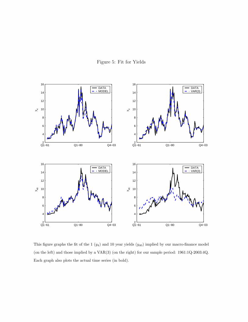
Figure 5: Fit for Yields

Q1−61 Q1−80 Q4−032

4

6

8

10

12

14

16

y 4

DATAMODEL

Q1−61 Q1−80 Q4−032

4

6

8

10

12

14

16

y 40

DATAMODEL

Q1−61 Q1−80 Q4−032

4

6

8

10

12

14

16

y 4

DATAVAR(3)

Q1−61 Q1−80 Q4−032

4

6

8

10

12

14

16

y 40

DATAVAR(3)

This figure graphs the fit of the 1 (y4) and 10 year yields (y40) implied by our macro-finance model

(on the left) and those implied by a VAR(3) (on the right) for our sample period: 1961:1Q-2003:4Q.

Each graph also plots the actual time series (in bold).

Figure 6: Impulse Responses of Term Structure Factors to Macro Shocks

0 20 40−0.4

−0.2

0

0.2

0.4

εAS

Level

0 20 40−0.2

0

0.2

0.4

0.6

0.8

εIS

0 20 40−2

−1.5

−1

−0.5

0

0.5

εMP

0 20 40−0.5

0

0.5

1

εy

n

0 20 400

0.5

1

1.5

2

επ

*

0 20 40−0.6

−0.4

−0.2

0

0.2

0.4

Slope

0 20 40−0.8

−0.6

−0.4

−0.2

0

0.2

0 20 40−3

−2

−1

0

1

2

0 20 40−0.2

0

0.2

0.4

0.6

0.8

0 20 40−1.5

−1

−0.5

0

0.5

1

0 20 40−0.4

−0.2

0

0.2

0.4

Curvature

0 20 40−1

−0.5

0

0.5

0 20 40−0.5

0

0.5

1

1.5

2

0 20 40−0.2

0

0.2

0.4

0.6

0.8

0 20 40−1.5

−1

−0.5

0

Quarter

This figure shows the impulse response functions (in percentage deviations from steady state) of the

three term structure factors - level, slope and curvature - to the structural shocks. 95% confidence

intervals appear in dashed lines.

Figure 7: Variance Decompositions for the Term Structure Factors

0 5 10 15 20 25 30 35 400

0.2

0.4

0.6

0.8

Leve

l

0 5 10 15 20 25 30 35 400

0.2

0.4

0.6

0.8

1

Slo

pe

0 5 10 15 20 25 30 35 400

0.2

0.4

0.6

0.8

Cur

vatu

re

Quarters

ASISMPy

n

π*

This figure shows the variance decomposition of the term structure factors in terms of the five

structural macro shocks. The variance decomposition of a variable at quarter h represents the

percentage of the h-step forecast variance explained by each shock.

Figure 8: Contemporaneous Responses of Yields to Macro Shocks

0 10 20 30 40−0.2

0

0.2

0.4

0.6

εAS

0 10 20 30 400

0.2

0.4

0.6

0.8

1

εIS

0 10 20 30 40−2

−1

0

1

2

εMP

0 10 20 30 40−1

−0.5

0

0.5

εy

n

Maturity

0 10 20 30 400

0.5

1

1.5

2

επ

*

Maturity

This figure shows the contemporaneous responses of yields of different maturities to the five structural

macro shocks. 95% confidence bands appear in dashed lines and were constructed using the bootstrap

procedure described in the text.