econstorMake Your Publications Visible.

A Service of

zbwLeibniz-InformationszentrumWirtschaftLeibniz Information Centrefor Economics

Züllig, Gabriel

Doctoral Thesis

Empirical essays in macroeconomics heterogeneousfirms, workers, and industries

PhD Series, No. 209

Provided in Cooperation with:University of Copenhagen, Department of Economics

Suggested Citation: Züllig, Gabriel (2020) : Empirical essays in macroeconomics heterogeneousfirms, workers, and industries, PhD Series, No. 209, University of Copenhagen, Department ofEconomics, Copenhagen

This Version is available at:http://hdl.handle.net/10419/240557

Standard-Nutzungsbedingungen:

Die Dokumente auf EconStor dürfen zu eigenen wissenschaftlichenZwecken und zum Privatgebrauch gespeichert und kopiert werden.

Sie dürfen die Dokumente nicht für öffentliche oder kommerzielleZwecke vervielfältigen, öffentlich ausstellen, öffentlich zugänglichmachen, vertreiben oder anderweitig nutzen.

Sofern die Verfasser die Dokumente unter Open-Content-Lizenzen(insbesondere CC-Lizenzen) zur Verfügung gestellt haben sollten,gelten abweichend von diesen Nutzungsbedingungen die in der dortgenannten Lizenz gewährten Nutzungsrechte.

Terms of use:

Documents in EconStor may be saved and copied for yourpersonal and scholarly purposes.

You are not to copy documents for public or commercialpurposes, to exhibit the documents publicly, to make thempublicly available on the internet, or to distribute or otherwiseuse the documents in public.

If the documents have been made available under an OpenContent Licence (especially Creative Commons Licences), youmay exercise further usage rights as specified in the indicatedlicence.

www.econstor.eu

Empirical Essays in Macroeconomics

Heterogeneous Firms, Workers, and Industries

Gabriel Zullig

A thesis presented for the degree of

Doctor of Philosophy

Supervisor: Emiliano Santoro

Department of Economics

University of Copenhagen

4 May 2020

Contents

Introduction ii

Acknowledgements iii

Summary (in English) iv

Resume (in Danish) vi

1 Heterogeneous employment effects of firms’ financial constraints and

wageless recoveries 1

2 The extensive and intensive margin of price adjustment to cost shocks:

Evidence from Danish multiproduct firms 44

3 Forecasting the production side of GDP 90

i

.

Introduction

I first became interested in Macroeconomics during an economic crisis that came to be

known as the Great Recession of 2008/09. Little did I know then that I would be ending

my PhD in the midst of another time of unprecedented macroeconomic turbulence, as the

Coronavirus lockdown takes its toll on the economy.

When I started my dissertation in 2016, macroeconomists were trying to work through

the mechanisms at play during the financial crisis and its long and sluggish recovery

thereafter. I stumbled upon a speech by Janet Yellen, the Chairwoman of the Federal

Reserve at the time, titled “Macroeconomic Research After the Crisis”. In her remarks,

she laid out four questions that ended up guiding me during my research, which I take the

liberty to paraphrase: What can explain hysteresis, the persistent shortfall of aggregate

demand during the recovery from the Great Recession? Does heterogeneity change our

understanding of Macroeconomics? What real effects do disturbances in financial markets

have? And finally, what determines inflation?

In one way or the other, my research speaks to all of these questions. I show that

the financial crisis had permanent effects on the level of employment in firms whose

access to liquidity eroded. My contribution to this growing literature is that the very

granular data on Danish firms and their workers allow me to better understand the

margins of adjustment. I show that the way credit-constrained firms re-allocate their

workforce can explain a phenomenon many economies have experienced since the Great

Recession, namely low inflation. Together with co-authors, I study the rationale behind

pricing decisions of heterogeneous firms. In doing so, we develop a methodology that

is able to explicitly account and test for several features and frictions implemented in

many structural macroeconomic models. The last chapter examines whether modelling

the economy as a network of interlinked production sectors helps forecasting aggregate

output.

So, are the answers I provide useful for our understanding of 2020, or is this time different

after all? My research directly addresses the role of liquidity in firm dynamics, an issue

many businesses struggle with during the Great Lockdown. The second chapter will

help policymakers understand the pass-through of a historical, negative oil price shock

to inflation. Finally, the fact that industries will experience the nature of the Covid

shock differently and that it will transmit to other sectors along supply chains is explicitly

accounted for in chapter three. Therefore, I wish you a stimulating and insightful reading.

ii

.

Acknowledgements

First and foremost, I owe immense gratitude to Emiliano Santoro for his outstanding

support and supervision, his levelheadedness, and for opening doors that would otherwise

have stayed closed. Secondly, I would like to say thank you to the Research Unit at Dan-

marks Nationalbank for funding my scholarship and for providing a research environment

that was both encouraging and challenging. In particular, I would like to name the Head

of Research, Federico Ravenna, and colleagues I collaborated closely with in the last two

years, and, hopefully, will continue to do so in the future: Saman Darougheh, Alessia De

Stefani, Renato Faccini, Denis Gorea, Johannes Poschl, Tobias Renkin, Filip Roszypal,

and Stine von Ruden. You taught me how to use the vast amount of data available in this

country, and how to interpret it for the purpose of answering macroeconomic questions. I

learned a great deal from my co-authors Luca Dedola, Mark Strøm Kristoffersen, Gregor

Baurle, and Elizabeth Steiner, who I cannot thank enough. My fellow PhD students, both

at the Bank and at the Department of Economics, deserve credit, too. In particular, many

thanks in particular to Christofer, Luca, Marcus, and Rasmus.

I have enjoyed a collaborative and interactive research environment with many interesting

exchanges. The most influential for my work were, in no particular order, Yuriy Gorod-

nichenko, Andreas I. Muller, Alex Clymo, and Giovanni Pellegrino. Additionally, let

me thank Kim Abildgren, Konrad Adler, Fernando Alvarez, Christoph Basten, Antoine

Bertheau, Saroj Bhattarai, Hafedh Bouakez, Antoine Bouet, Olivier Coibion, Wei Cui,

Danilo Cascardi-Garcia, Ana Galvao, Sebastian Heise, Kerstin Holzheu, Simon Juul Hviid,

Gregor Kastner, Massimiliano Marcellino, James Mitchell, Gisle Natvik, Maria Olsson,

Ivan Petrella, Søren Hove Ravn, Farzad Saidi, Alireza Sapahsalari, Rolf Scheufele, Michael

Siemer, Fabian Siuda, Emil Verner, Mark Weder, Joseph Vavra, and Horng Wong. My

work has greatly benefited from your comments! There were numerous critical participants

and discussants at workshops all over Europe, from Stockholm to Frankfurt and from

Cambridge to, ultimately, a recently popular place called Zoom.

Finally, I would like to thank my family and friends, especially Daniel Van Nguyen, for

believing in me when I myself did not.

iii

.

Summary (in English)

This thesis consists of three self-contained chapters in the area of Macroeconomics. The

common thread throughout the studies is the role of heterogeneous and interconnected

firms in the economy. The first two chapters use granular data on firms from Denmark to

study the adjustment to shocks: In chapter 1, I identify credit constrained firms during the

Great Recession and explore the adjustment margin along many dimensions, in particular

their workers’ wages. The results I find are in line with large swings in employment after

financial shocks, and the following low wage growth. In chapter 2, I study how firms

adjust prices to changes in cost. For the final analysis, the last chapter assesses whether

the presence of interlinkages between firms at the sector level can be used to improve a

policymaker’s forecast of the aggregate economy.

Chapter 1 / Heterogeneous employment effects of firms’ financial constraints

and wageless recoveries

This chapter studies the adjustment of the labor market to a large reduction in credit

supply to firms. I begin by documenting the existence of credit shocks to some firms in

Denmark. In particular, I use administrative data on relationships between Danish firms

and their banks. The fact that banks were hit by the global financial crisis to different

degrees can be used to show that the liquidity reduction in exposed banks propagated to

the credit supply to their pre-crisis borrowing firms. Businesses without access to internal

or external liquidity reduced employment, but did not cut their employees’ wages.

The most important contribution of this paper is that I can show, using matched employer-

employee data, that the reduction in employment was heterogeneous across workers:

Constrained firms disproportionately cut employment of workers with previously high

wages. Because of the liquidity constraint, this margin of adjustment is the most effective

to retain the firm’s cash flow. I support this view by comparing the compositional effect to

a shock that is unrelated to firms’ financial positions, after which the margin of adjustment

is higher for low-wage workers.

I supplement this finding at the micro level with implications for the macroeconomy:

Because workers with previously high wages are only re-employed at lower wages, my

findings are not only consistent with large employment effects of financial shocks (as

previously documented in the literature), but also with low wage growth during the

subsequent recovery.

iv

Chapter 2 / The extensive and intensive margin of price adjustment to cost

shocks: Evidence from Danish multiproduct firms

with Luca Dedola & Mark Strøm Kristoffersen

In this chapter, my co-authors and I estimate the pass-through of shocks to the operating

costs of firms. In doing so, we develop a new methodology that allows us to account and

test for many of the nominal and real rigidities that are implemented in many structural

models in Macroeconomics.

For example, consider the case where price adjustment is costly. Under these circum-

stances, firms will only choose to adjust prices if the current price is sufficiently far away

from the ideal price, given their cost. This would lead to a selection bias in the estimation

of the pass-through. Our econometric approach accounts for this bias, and we leverage

the fact that we can merge monthly price quotes of Danish manufacturing firms to high-

frequency measures of their marginal cost. We consider, first, a change in the price of

imports, and second, an exogenous shock to the price of energy they produce with.

We show that the selection bias is indeed statistically significant but economically small.

Furthermore, we document a number of interesting features in firms’ responses: First, pass-

through of firm-level cost shocks is incomplete, indicating that more than half of the shocks

are absorbed by mark-ups. Second, we show that firms (marginally) adjust their prices in

response to price changes of their competitors, even though their cost have not changed.

The literature refers to these interactions as strategic complementarities. Third, smaller

firms adjust prices more and faster, in line with the above described complementarities.

Fourth, the pass-through of an energy cost shock is eventually complete, which we explain

by the fact that energy cost shocks are much more common across different firms. Fifth,

the pass-through is delayed by about a year, a fact which we can partially explain by firms’

position in the supply chain.

Chapter 3 / Forecasting the production side of GDP

with Gregor Baurle & Elizabeth Steiner

In chapter 3, we take the idea of inter-connected firms to a forecasting exercise. If firms

of different sectors are interlinked, shocks to a particular sector will transmit along supply

chains to other sectors over time. This feature is not accounted for in most competitive

models that are used to forecast economic output.

We set up a range of time series models and let them compete, in a horse race, to the

determine the best forecasts of past realizations of GDP, given the data that was available

at the time. We show that the dynamic factor model that includes interlinked sectoral

series produces the best results. The competitiveness can be traced back to the fact that

the model is best able to understand the degree of sectoral comovement, i.e. to distinguish

between sectoral and common shocks.

v

Resume (in Danish)

Denne afhandling bestar af tre selvstændige kapitler indenfor makroøkonomiens genstands-

felt. Gennemgaende for hele afhandlingen er undersøgelsen af betydningen af heterogene

og indbyrdes forbundne virksomheder i økonomien. De første to kapitler benytter sig

af mikrodata over danske virksomheder i analysen af justeringer i forhold til økonomisk

chok. I første kapitel identificeres virksomheder, som var kreditbegrænsede under den

store recession, hvorefter justeringsmargenen undersøges ud fra flere parametre, særligt

ift. arbejdslønnen. Resultaterne af undersøgelsen stemmer overens med store udsving i

beskæftigelsen efter økonomisk chok og den efterfølgende lave vækst i arbejdslønnen i en

længerevarende periode. I andet kapitel undersøges hvordan virksomheder justerer priser

ift. ændringer i omkostninger. I den afsluttende analyse i det sidste kapitel vurderes

hvorvidt de optrædende indbyrdes forbindelser mellem virksomheder pa sektorniveau kan

udnyttes til at forbedre prognoseudarbejdelse indenfor økonomisk planlægning.

Kapitel 1 / Heterogeneous employment effects of firms’ financial constraints

and wageless recoveries

Dette kapitel omhandler justering af arbejdsmarkedet ift. den store reducering af kredit-

udbuddet til virksomheder. Indledende dokumenteres der for forekomsten af kreditchok,

som nogle danske virksomheder oplevede. Konkret gør jeg brug af administrativ data over

forholdet mellem danske virksomheder og deres banker. Det at banksektoren blev ramt

af den globale finanskrise i varierende grad, kan udnyttes til at pavise at reduceringen

af likviditeten i udsatte banker bredte sig til virksomhedernes kreditudbuddet. Virk-

somheder med hverken adgang til intern eller ekstern likviditet nedskar i ansættelse fremfor

beskæringer i ansattes arbejdsløn.

Denne afhandlings største bidrag er pavisningen vha. afstemt arbejdsgiver-arbejdstager

data af at faldet i beskæftigelsen var heterogen pa tværs af arbejdsstyrken: Begrænsede

virksomheder skar uforholdsmæssigt i ansættelsen af arbejdere med tidligere høje lønninger.

Pga. den begrænsede likviditet er justeringsmargenen den mest effektive made for vir-

somheder at opretholde penge. Dette synspunkt understøttes gennem en sammenlign-

ing med den sammensatte effekt af et chok som ikke er forbundet med virksomheders

økonomiske tilstand, hvorefter justeringen viser sig at være forskellig.

Denne konstatering pa mikroniveau suppleres med en perspektivering til makroøkonomien.

Da arbejdstagere med tidligere høje lønninger udelukkende ansættes til lavere arbejdsløn,

er min konklusion ikke blot i overensstemmelse med den høje beskæftigelse som effekt

af økonomisk chok (som dokumenteret for i litteraturen) men ogsa ift. den lave vækst i

arbejdslønnen under den efterfølgende økonomiske genopretning.

vi

Kapitel 2 / The extensive and intensive margin of price adjustment to cost

shocks: Evidence from Danish multiproduct firms

med Luca Dedola & Mark Strøm Kristoffersen

I dette kapitel vurderer mine medforfattere og jeg forplantningen af økonomiske chok i

virksomheders driftsomkostninger. I forbindelse med dette udvikler vi metodologi som

gør det muligt at forklare og gennemprøve mange af de nominelle og reale stivheder der

er implementeret i mange strukturelle modeller indenfor makroøkonomi.

Overvej tilfældet hvor prisjustering er omkostningstungt som et eksempel. Under den

omstændighed vil virksomheder udelukkende vælge at justere pris hvis den gældende pris

er tilstrækkeligt langt fra idealprisen taget i betragtningen af deres omkostninger. Dette

ville resultere i en selektionbias i vurderingen af forplantningen. Vores økonometriske

tilgang gør rede for denne bias, og vi sammenlægger data pa danske virksomheders priser

med to af deres marginalomkostninger – importpriser og energipriser – til at vurdere den.

Pa trods af den minimale økonomiske indflydelse, paviser vi at selektionbias er statistisk

signifikant. Endvidere dokumenteres der for en række interessante træk ved virksomheders

reaktioner. For det første er forplantningen af omkostningschok pa virksomhedsplan

ufuldendt hvilket indikerer at over halvdelen af alle chok absorberes af avancetillæg.

For det andet viser det sig at firmaer (marginalt) justerer deres priser som reaktion

pa prisændring hos konkurrenter pa trods af ingen forandringer i omkostningsudgifter.

Litteraturen forklarer disse vekselvirkninger som strategisk komplimentariteter. For det

tredje justerer mindre virksomheder deres priser oftere og i højere grad i overensstem-

melse med overnævnte komplimentariteter. Et fjerde træk er forplantningen af et chok i

energisektoren som efterhanden fuldendes. Et sidste interessant træk er at forplantningen

er forskudt med et ar, hvilket delvist forklares af virksomheders position i forsyningskæden.

Kapitel 3 / Forecasting the production side of GDP

med Gregor Baurle & Elizabeth Steiner

I tredje kapitel overføres ideen om indbyrdes forbundne virksomheder til en øvelse i

prognoseudarbejdelse. Hvis virksomheder i forskellige sektorer er indbydes forbundne,

vil økonomiske chok i en bestemt sektor transmitteres langs forsyningskæden til andre

sektorer med tiden. Denne egenskab indgar ikke i størstedelen af konkurrencemodeller

som bruges til udarbejdelse af prognoser for økonomisk produktion.

Gennem en opstilling af en række tidsseriemodeller, som vi har ladt konkurrere i et

hestevæddeløb, bestemmes den bedste prognoseudarbejdelse for BNP. Vi paviser at den

dynamiske faktormodel, som inkluderer indbyrdes forbundne sektor serier, producerer de

bedste resultater. Dens konkurrencedygtighed forklares ud fra modellens nøjagtighed til

at forsta grader af sektorernes comovement, dvs. evnen til at bedre skelne mellem chok

pa sektorernes og aggregeret niveau.

vii

Chapter 1

Heterogeneous employment effects of firms’

financial constraints and wageless recoveries

1

.

Heterogeneous employment effects of firms’

financial constraints and wageless recoveries

Gabriel Zullig∗

Abstract

This paper studies the interaction of firm liquidity, employment and wages in light ofcredit supply disruptions. I establish that firms borrowing from banks highly exposed tothe money-market freeze during the Global Financial Crisis received a shock to externalliquidity, relative to otherwise similar firms. This constraint led to a significant drop inemployment in affected firms, while wages did not fall relative to unaffected firms. Inorder to retain cash flow and build up internal liquidity, constrained firms cut labor costpredominantly by changing the composition of their labor force in favor of workers withlower wages. I provide evidence that this adjustment gradient is distinctly related toshocks to firms’ access to liquidity. Employees separated from jobs with high residualwages are re-employed quickly, albeit at lower wages. This leads to sluggish wage growtheven in unconstrained firms, and well into the recovery after a financial recession.

JEL classification: E24, E32, E44, J64

Keywords: business cycles, credit supply shock, heterogeneity, wage stickiness

∗University of Copenhagen, Danmarks NationalbankI am grateful to Konrad Adler, Christoph Basten, Morten Bennedsen, Antoine Bertheau, Hafedh Bouakez,Alex Clymo, Wei Cui, Saman Darougheh, Kerstin Holzheu, Mark Strøm Kristoffersen, Andreas I. Mueller,Gisle Natvik, Maria Olsson, Filip Roszypal, Farzad Saidi, Emiliano Santoro, Alireza Sapahsalari, MichaelSiemer, Fabian Siuda, Emil Verner, Mark Weder, and Horng Wong for helpful comments and discussions.I also thank seminar participants at the University of Copenhagen, Danmarks Nationalbank, StockholmSchool of Economics, the EDGE Jamboree at the University of Cambridge, and the annual workshopof the Swiss Economists Abroad for their feedback. The views, opinions, findings, and conclusions orrecommendations expressed in this paper are strictly those of the author. They do not necessarily reflectthe views of Danmarks Nationalbanken. All remaining errors or omissions are my own.

2

1 Introduction

Since the global financial crisis, many contributions have highlighted the large employment

effects of disruptions in the credit supply to firms (Chodorow-Reich, 2014). There is

accelerated interest in studying the interactions between frictional financial and labor

markets, and what implications they have for cyclical dynamics of the economy. I show

that not only do financially constrained firms decrease employment, but they change the

composition of their labor force in a way that is consistent with deep and persistent slumps

in employment after financial crises and anemic wage growth for an extended period of

time thereafter.

I study how disruptions in the financial sector transmit to firms’ ability to fund their

operations and eventually labor market outcomes. I do so using administrative micro

data that allows to link private-sector firms in Denmark to their bank lenders on one and

their workers on the other hand. Bank lending is the prevalent source of outside liquidity in

most Danish firms, and bank lending to non-financial corporations was reduced by almost

50% in the wake of the Great Recession of 2008/09. During the same time private-sector

employment fell by 18%.

Two approaches are used to identify firms affected by unanticipated financial constraints:

First, I exploit the fact that banks in Denmark were affected by the Global Financial Crisis

(GFC) to different degrees. I build on Jensen and Johannesen (2017) in that I use the

variation in that exposure and show that a cut in lending by exposed banks leads to a shift

in credit supply to their pre-crisis borrowers that is orthogonal to the firm itself. Second,

survey evidence suggests that retained cash buffers are an effective insurance against a

funding squeeze during the crisis. Thus, the firms with a low degree of liquid assets as of

2007, relative to their fixed costs, are compared to those which do not rely on short-term

external liquidity to stay liquid.

In both cases, I find that firms whose credit lines are withdrawn shrink in size to an

economically and statistically significant degree. The effect on the level of employment

is estimated to be up to 20% by 2011, and persists thereafter. A common structural

interpretation is that financial crises prevent labor hoarding; the fact that firms can smooth

employment over the business cycle to avoid costly displacements and future re-hiring

cost. With squeezed funds, this is no longer possible, leading to a sharp downturns in

employment. In the data, two thirds of the adjustment to the shock happens through a

surge in separations, as opposed to a drop in hires. Even though the constrained, downsized

firms generate lower profits, they manage to build up liquidity reserves to protect them

against future funding shocks.

Making use of the possibility to match employers to the entire population and – to a

large extent – their (not top-coded) wages, I study the heterogeneity of this labor market

adjustment along the dimension of wages. In the firm-level estimates, wages do not

3

adjust to reduce the outflow of cash.1 Instead, constrained firms change the composition

of employment to a less costly labor force: Employment of workers with wages in the

upper tail relative to their colleagues is reduced substantially more. While low-wage

workers are per se more likely to be unemployed during recessions, high-wage workers are

disproportionately affected by their employer’s lack of funds. In order to improve their

liquidity position as effectively as possible, constrained firms reduce employment of the

most expensive workers most.

Labor market mobility in Denmark is comparable to U.S. levels, and I use the micro

data at the individual job level to track the re-allocation after this shock. In contrast

to U.S. evidence (Mueller, 2017), the pool of unemployed does not shift toward workers

with previously high wages in my data. Instead, they have a lower likelihood of moving

int ounemployment, but take wage cuts of up to 10% in their next jobs. In the macro

view, wage growth is low in both constrained and unconstrained firms, albeit for different

reasons: Constrained firms end up with a labor force that is composed of less costly

workers, while firms with access to liquid assets can hire workers at lower rates. This

mechanism introduces substantial persistence into workers’ wage profiles and long memory

of the labor market. It can partly explain why wage growth is sluggish even well into the

recovery.

The rest of the paper develops as follows. Section 2 summarizes the recent and growing

literature on employment effects of credit supply shocks and its importance for business

cycles fluctuations. Section 3 discusses the identification of these shocks in bank-borrower

and firm-level data, after which section 4 provides estimations for firms’ responses. In

particular, it documents the compositional change of the labor force in constrained firms

based on their workers’ previously negotiated wages. Section 5 moves to a job-level analysis

to exploit the granularity of the Danish matched employer-employee data and studies

labor market flows from constrained firms by worker type. I conclude by discussing the

cyclicality of employment and wages and the macroeconomic implications.

2 Related literature

This paper bridges the gap between two strands of literature: the micro evidence of labor

demand effects of firms’ credit conditions and the macro movements of employment and

wages of heterogeneous workers over the business cycle.

A growing literature is empirically investigating the real effects of financial shocks to

firms using micro data. Typically, it is argued that sticky relationships between corporate

borrowers and their lenders arise due to asymmetric information (Banerjee et al., 2017),

such that a credit tightening by a lender cannot easily be substituted by lending elsewhere,

1The literature finds that the degree of wage stickiness among incumbent workers is why firms adjust alongthe extensive margin in the first place (Schoefer, 2015).

4

leading to a decrease of credit supply at the firm level (Khwaja and Mian, 2008, Iyer et al.,

2014).2 The real effects of such shocks have been documented, for instance, on invest-

ment (Amiti and Weinstein, 2018) and, more closely related to this paper, employment

Chodorow-Reich (2014). The latter finds that firms which used to borrow from highly

levered banks through the U.S. syndicated loan market had a higher probability of having

their credit lines cut after the financial turmoil of the GFC in 2008/09. These firms display

a sharp contraction of employment relative to firms with otherwise similar characteristics,

because employment requires the firm to fund the period between the creating a vacancy

and receiving the cash flow generated by the match, similar to investment. This finding

has been confirmed for other countries and identification strategies (Baurle et al., 2017,

Bentolila et al., 2018, Cornille et al., 2017, Melcangi, 2018). It is well-established that

credit supply disruptions were crucial to explaining employment contractions during the

Great Recession, particularly among smaller, less transparent firms (Gertler and Gilchrist,

2018, Siemer, 2019). Furthermore, the effects seem to propagate to unconstrained firms

through local demand, are persistent and have a dampening effect on productivity (Huber,

2018), even though this transmission mechanism remains in the shadow.

This paper conveys the idea that the heterogeneity of the employment effects of funding

shocks is a promising avenue to explore. For example, Barbosa et al. (2019) find that

employment of high-skill workers falls at firms operating with banks which had unexpected

pension obligations and therefore had to reduce credit supply. They attribute this finding

to increased difficulties of constrained firms to attract workers with high human capital.

The literature further finds that credit constraints disproportionately affect employment

of workers on temporary contracts (Caggese and Cunat, 2008, Berton et al., 2018, both

for Italy). Caggese et al. (2019) look at labor force adjustments of financially constrained

firms to exogenous productivity shocks to Swedish firms and conclude that, due to firms

placing a higher weight on short-term returns, they fire workers with short tenure, who

have lower current productivity but high expected productivity growth.

Moser et al. (2019) study worker allocations across constrained and unconstrained firms

in Germany. They argue that the introduction of negative interest rates in the euro

area in 2014 caused deposit-funded banks to reduce lending relative to banks relying on

wholesale funding (Heider et al., 2019). The two main findings are that a negative credit

supply shock decreases wage inequality between firms and increases it within. The first is

attributed to the fact that low-pay firms are more risky, and thus receive relatively more

2It has been challenged whether Denmark has experiences a credit slump during the financial crisis in thefirst place, especially given its institutional framework of government-backed and bond-financed mortgagebanks (Abildgren, 2012). However, Jensen and Johannesen (2017) have used a very similar identificationstrategy to this paper and conclude that household borrowing from their vulnerable house banks didindeed see loans decrease, interest rates increase and consumption fall by around 4%, pointing to thepresence of a credit supply shock. I confirm this result for the supply side of the economy. While firmsare more financially flexible than households, who typically borrow from a single bank, their borrowinghorizon is much more short-run. Additionally, limited liability in firms potentially gives rise to largerdegrees of relationship banking in firms compared to households, which exacerbates the pass-through ofbank-level shocks to their borrowers.

5

credit than high-paying firms after a credit contraction. The latter is directly at odds with

the results of this paper, which impliy firm-level inequality to fall after a funding squeeze.

Structural differences in labor markets might explain these contradicting results, as the

extensive margin of labor force adjustment is considerably more flexible than Germany’s

(Andersen, 2012).

A further key contribution of this paper is that it connects the micro findings to the

(empirical and theoretical) macro literature on the cyclicality of employment and wages of

heterogeneous workers. In this respect, it is closely related to to Mueller (2017), where the

composition of the pool of unemployed shifts to workers with higher wages in their previous

job in recessions. An explanation put forward for this phenomenon in the paper are indeed

cash flow constraints. As this potentially increases the incentive to hire from said pool,

it poses an additional challenge to the excess volatility puzzle in canonial search and

matching models with productivity shocks (Shimer, 2005). Previously, it had been argued

that a deterioration of worker quality among the pool of job seekers during recessions

could address the Shimer puzzle (Pries, 2008, Ravenna and Walsh, 2012).

Petrosky-Nadeau and Wasmer (2013), too, have shown that financial frictions provide

a promising avenue to exacerbate labor market volatility in light of productivity shock.

Whether they be implemented as search cost in credit markets (Petrosky-Nadeau and

Wasmer, 2013, 2015), an agency cost setting where vacancies are being financing with a

constraint on firm net worth (Petrosky-Nadeau, 2014) or firm income (Boeri et al., 2018),

they all have one feature in common: They increase the cost of vacancy creation when

financial constraints are tight, and therefore have large employment effects.

The case of wages conditional on funding shocks is a particularly interesting one. Michelacci

and Quadrini (2009) develop and test a model in which externally constrained – typically

young – firms pay low wages in return for future wage growth, effectively borrowing from

their employees. In contrast, in Quadrini and Sun (2018), a deleveraging shock deteriorates

the bargaining position of the firm and therefore increases wages and reduces the incentive

to hire, leading to larger volatility of employment. Schoefer (2015) proposes that wage

stickiness among incumbents can create the need for layoffs of workers when firms become

cash constrained, without the need to deviate from relatively flexible wages of new hires,

which is a well-established empirical finding (Pissarides, 2009). I confirm the stickiness

of incumbents’ wages, even during large downswings such as the Great Recession. Since

wages of new hires are more flexible, workers with previously high wages are hired from

the pool of unemployed with a persistent cut in their nominal wage. This is consistent

with a flattening of the Phillips curve, a key consideration in the conduct of monetary

policy.

6

3 Identifying financially constrained firms

The GFC was characterized by disruptions in the financial intermediation process, partic-

ularly in the banking sector. Besides internal liquidity in the form of retained profits, firms

heavily rely on access to external liquidity in order to fund payrolls and other operating

cost, and bank credit lines are the principal source to do so (Lins et al., 2010). The banking

crisis which unfolded in 2008 and 2009 interrupted this supply of credit. Accordingly, I use

strategies to identify negative credit supply shocks at the firm level: the coffers of internal

pre-crisis liquidity, as well as two measures on the health of the pre-crisis lenders. The

following two subsections motivate and validate those strategies, all of which have been

used previously in the literature.

3.1 Exogenous disruptions in bank credit supply

First, I use data on bank-borrower balances and variation in bank health to estimate credit

availability to firm j by bank b. To obtain a measure which is independent of the borrower,

I instrument credit supply in a lending relationship by the lender’s credit supply to all

other corporate borrowers in the data, similar to Chodorow-Reich (2014). Specifically, let

Lj,b,t be credit outstanding of j at b in period t, and L−j,b,t the lending of b to all other

firms. I will then proxy the growth rate of credit with the respective growth rate of Lj,b,t:

lj,b,t = β0 + β1l−j,b,t + ut

lj,b,t ≡Lj,b,t − Lj,b,t−1

0.5(Lj,b,t−1 + Lj,b,t)

.

This instrument is referred to as IV A. Because the firm’s loans constitute a small part

of the bank’s overall lending, this instrument satisfies the exclusion restriction if credit

demand is idiosyncratic to the firm. If credit demand is correlated across firms, however,

this assumption might be violated. Therefore, I construct a second measure of loan supply

shocks following Jensen and Johannesen (2017).

Consider a bank with high levels of lending (to all firms and households) relative to the

amount of deposits, where the difference has to be financed through wholesale funding

or equity markets, both of which became considerably tighter during the recession. This

bank will have to cut credit, relative to its competitor with a more stable and long-term

funding base. The structure of a bank’s balance sheet prior to the global financial crisis

therefore induces a shifter in banks’ supply of funds which is plausibly orthogonal to the

credit demand of its borrowers, something which is verified below. Let us define a measure

7

of bank health in 2007 as the ratio of total loans to deposits, i.e.

LTDb,07 =loansb,07

depositsb,07.

Due to the non-linear nature of this metric, a bank-invariant dummy 1[LTD07]b takes the

value 1 if either its exposure measure in 2007 was above the median of its competitors, or

if it stopped lending altogether in the period between 2008 and 2011. It will be referred

to as IV B.

Data on banks and bank-borrower relationships Both instruments are brought

to data relying on tax filings in which financial institutions in Denmark report amounts

outstanding of unsecured loans and deposits at the end of the calendar year, as well as

interest paid on loans and deposits over the course of said year. The data contains no

information on other terms of the loan contract. The raw data is at the loan account level

and covers unsecured loans to the corporate sector by banks as well as non-banks. The

first part of the analysis is performed at the lending relationship level, where I sum over

loan amounts and interest paid within a firm-bank pair. Later on, I will show that the

transmission of credit carries over to the firm level.

The loan-level data is merged to balance sheets of 101 banks, collected by the Danish

financial supervisory authority, which are publicly available. In doing so, I disregard non-

bank and collateralized lending such as mortgages. To validate the loan-level dataset, I

compare the sum of all loans outstanding within a bank-year to the aggregate number

of loans to Danish non-financial corporations, which is reported to the central bank’s

Monetary and Financial Statistics (MFI). The correlation coefficient is 0.97, and also

tracks the time series dimension of aggregate lending to the corporate sector well.

On the firm side, I match the data to detailed annual accounts (balance sheets and income

statements, and employment) of private-sector firms that, at some point between 2003 and

2016, have at least 10 employees. This data is described in greater detail below.3

Danish financial markets Between 2003 and the end of 2008, bank lending to non-

financial corporations according to the MFI increased by a factor of 2, while deposits grew

at a substantially lower pace. Direct exposure to the market of mortgage-backed securities

at the origin of the GFC was limited among Danish banks, liquidity decreased substantially

when international money markets dried up. As a result, the Danish central bank injected

liquidity into the market. Regardless, a range of banks became insolvent, and total lending

to the corporate sector contracted by 15% from the peak through October 2009. A second,

3It should be noted already that not all firms have unsecured bank loans: Of the baseline firm sample, Ican identify bank loans for only 46%, raising concerns of a potential selection bias in the sample. 53%(62%) of firms with at least 10 (50) employees are matched. The fact that even for large firms the rateof matches is well below 100% indicates that the reason is related to data reporting, rather than sampleselection. In all regressions using the bank-borrower relationship data, I will exclude unmatched firms tominimize selection bias. However, I will complement the bank lending identification strategy with onethat solely relies on the firm balance sheet data to confirm my results on the full sample of firms.

8

more gradual phase of credit tightening followed in the fall of 2010 and lasted through

mid-2014, after which the level of outstanding loans was another 30% lower. The size

of the increase in the loan portfolio has been very modest since. Note that the financial

shock did not originate in the Danish corporate sector.

These movements matter because of the prevalence of bank lending in the funding structure

of Danish firms. The median ratio of total debt to assets is 72% over the entire sample,

whereas more than 3/4 of this amount has a maturity of less than 1 year. Short-term debt

summarizes different sources of credit such as firm-to-firm lending (including accounts

payable), export credit, government loans, or bank credit with and without collateral.

While I have no data on collateralized loans, the possibility to match the uncollateralized

loans from the bank-borrower relationship dataset onto other firm-level data is the most

promising route to study shocks to external liquidity because of the short-term nature of

these credit lines. The median firm that can be matched to a bank has a ratio of bank

credit to its assets of 15%. Figure 1(b) shows the distributions of these different debt

ratios across firms.

3.1.1 Credit market outcomes at the bank level

This section validates the choice of the bank health measure (IV B) and documents lending

behavior after the global financial crisis at the bank level.

For the measure of bank health to be a valid supply shifter, it is required that the

instrument is uncorrelated with characteristics of the borrower, in particular its hiring

decisions. If lenders specialize in terms of size, geographical location or riskiness of their

borrowers, their loan/deposit ratios might be jointly determined with the outcome variable

I study. In Figure 2, I show that this is not the case in the bank health measure I use.

The distributions of firm size and growth, as well as the growth rate of debt and wages

all overlap for firms borrowing from banks with high/low exposure banks for the period

before the onset of the GFC.

To characterize bank behavior throughout the period of de-leveraging during and after the

banking crisis, I regress bank-level outcomes on 1[LTD07]b interacted with yearly dummies

and plot coefficients and clustered standard errors in Figure 3.

In Figure 3(a), the dependent variable is the log of the sum of loans outstanding to

businesses in the bank-borrower micro data, with the year 2007 being the base level. There

is no significant difference in the trend prior to the onset of the crisis. A wedge opens in

2008: Banks for which assets have been covered less by long-term funding sources such

as deposits contracted lending significantly and permanently. At the same time, lending

by non-exposed banks was stable, such that the exposed banks explain almost the entire

decline in the aggregate quarterly time series of business lending, depicted in Figure 1(a).

Could this be the result of risk-averse businesses avoiding to operate with risky banks? To

9

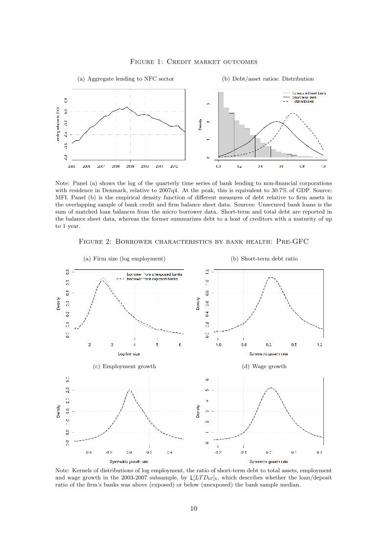
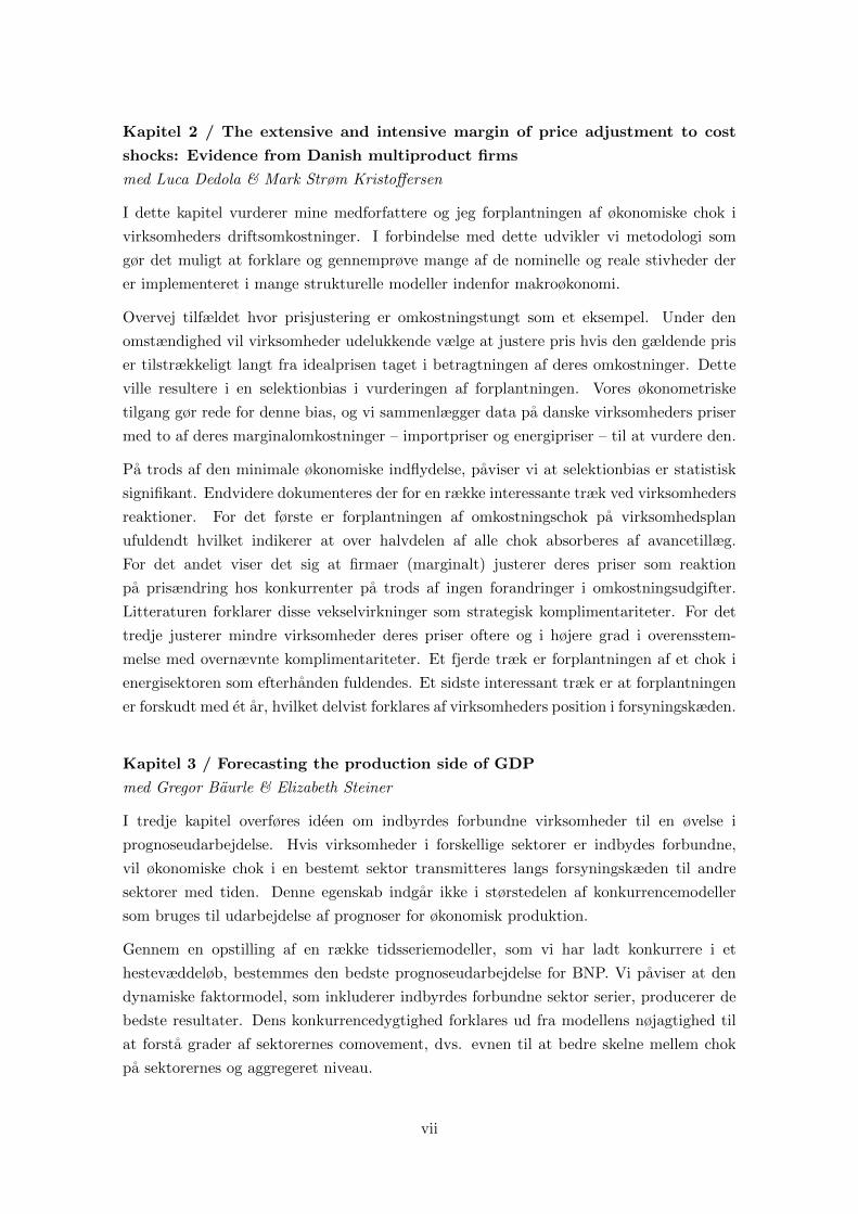
Figure 1: Credit market outcomes

(a) Aggregate lending to NFC sector (b) Debt/asset ratios: Distribution

Note: Panel (a) shows the log of the quarterly time series of bank lending to non-financial corporationswith residence in Denmark, relative to 2007q4. At the peak, this is equivalent to 30.7% of GDP. Source:MFI. Panel (b) is the empirical density function of different measures of debt relative to firm assets inthe overlapping sample of bank credit and firm balance sheet data. Sources: Unsecured bank loans is thesum of matched loan balances from the micro borrower data. Short-term and total debt are reported inthe balance sheet data, whereas the former summarizes debt to a host of creditors with a maturity of upto 1 year.

Figure 2: Borrower characteristics by bank health: Pre-GFC

(a) Firm size (log employment) (b) Short-term debt ratio

(c) Employment growth (d) Wage growth

Note: Kernels of distributions of log employment, the ratio of short-term debt to total assets, employmentand wage growth in the 2003-2007 subsample, by 1[LTD07]b, which describes whether the loan/depositratio of the firm’s banks was above (exposed) or below (unexposed) the bank sample median.

10

Figure 3: Credit market outcomes

(a) Business loans by exposure (b) Average interest rate on loans

Note: Coefficients and standard errors of a regression of loan market outcomes (log of loans to all corporatelenders in the micro data, and the weighted average interest rate on those loans) on a dummy indicatingwhether the bank had above-median exposure to wholesale money markets in 2007 as measured by theloan-to-deposit ratio, interacted with dummies for all years but 2007. The 101 banks are weighted by thesize of their loan portfolio in 2007, and standard errors are clustered at the bank level.

rule out the possibility of a shift in aggregate demand for loans from the exposed banks,

I use again the bank-borrower data of unsecured debt and calculate a relationship-level

interest rate by dividing the interest paid throughout a year by the mean of current and

lagged balances. The weighted mean of interest rates within a bank by exposure measure

is depicted in panel (b). Interest rate developments are relatively similar and, if anything,

increase in exposed banks.

Consequently, market shares of exposed banks decrease significantly, and so do other bank-

level outcomes that are omitted but available upon request. The number of (new) clients at

exposed banks decreases, even though the difference between exposed and unexposed banks

is not statistically significant. I conclude that banks have been heterogeneously affected

by the global financial crisis, and will next discuss how this heterogeneity transmits to

differential credit supply shocks at their pre-crisis borrowers that are plausibly exogenous

to the firms’ performance, credit demand or hiring decisions, including labor supply.

3.1.2 Credit market outcomes at the firm level

The type of propagation relies on the existence of sticky lending relationships. In a

frictionless credit market, a tightening of credit conditions of a pre-crisis lender could

be fully compensated by increasing credit lines from one or more others. In a principal-

agent credit market, however, borrowers and lenders form relationships, over the course of

which informational asymmetries are reduces, and switching lenders becomes costly. The

emergence of relationship lending has been studied using similar datasets, including the

effects on employment (see for example Banerjee et al. (2017)).

Since the raw data is at the lending account, rather than the relationship level, I test

11

whether new loan accounts are opened at banks with which a relationship history exists.

In particular, consider all newly opened loan accounts over the course of the sample, and

define a dummy variable equal to 1 if the bank identifier is equal to the primary bank of

the previous year, and zero otherwise. In a linear probability model, the constant describes

the probability that new loans are taken up at banks with which the firm has operated

previously.

Even after controlling for the bank’s market share, a bank that used to be a firm’s

primary lender has a high likelihood of being the provider of the new loan, too. The

estimated coefficient is 0.42, and thus very close to the estimate of Bharath et al. (2007).4

Furthermore, this likelihood decreases with the number of lenders the borrower has had

in the past and the size of the loan, all of which supports the hypothesis of information

asymmetries, especially among small borrowers. When including only the most connected

firms, i.e. borrowers with at least two lenders, the stickiness of lending relationships

decreases and the importance of lender size increases significantly. However, 79% of firms

in the dataset only have loans with one bank.

To test the first stage of shock transmission from banks to their incumbent borrowers

more rigorously, I first regress loan amount growth of a firm-bank pair during the crisis

on instruments A and B,

∆lj,b,t = β Z ′t + ut,

where Zt is either of the two instruments described. In the case of bank-lending to all

other borrowers, this elasticity is estimated to be 0.2 (see Table 1, column (1)), suggesting

that aggregate loan conditions by banks significantly impact a firm’s capacity to borrow.

I exploit the fact that some, if not many, firms have multiple lending relationships, which

allows to include a firm-year fixed effect and controls for unobservable firm characteristics

such as idiosyncratic productivity or loan demand, provided that the firm’s demand for

credit is not specific to lender health (Amiti and Weinstein, 2018, Khwaja and Mian,

2008). Column (2) confirms the robustness to the inclusion of firm-year fixed effects.

The second panel of rows in Table 1 repeats the analysis at the firm-level. Since L is

defined at the lending relationship level, I weight it the regressors by the lagged share of

b in j’s loan portfolio, αj,b,t−1, where

αj,b,t =Lj,b,t∑b Lj,b,t

.

The regression result suggests that a decrease in lending carries over to firm-level supply

of external liquidity entirely.

For instrument B, I preserve the binary nature of the treatment variable and let Zt be the

4This is expectedly smaller than in the syndicated loan market in the U.S., in which large firms lend largeramounts of money from a relatively small pool of lead and supporting lenders. Chodorow-Reich (2014)estimates the coefficient to be 0.72 in this market.

12

Table 1: Credit supply at the firm level

IV A: Loans to others IV B: Loan/deposit ratio

(1) (2) (1) (2) (3)

Panel I: ∆lj,b,t

∆l−j,b,t 0.186*** 0.200***(0.015) (0.040)

1[LTD07]b −0.039*** −0.071*** −0.089***(0.013) (0.016) (0.035)

Panel II: ∆lj,t∑b αj,b,t−1 ×∆l−j,b,t 0.215***

(0.024)∑b αj,b,07 × 1[LTD07]b 0.000 −0.058***

(0.015) (0.015)

Year FE Yes No No No NoFirm-year FE No Yes No No YesSample 2008-12 2008-12 2008 2009 2009# observations 165,453 40,776 14,566 12,526 3,769# firms 17,673 3,691 12,323 10,796 2,039

The dependent variables is the growth rate of gross lending within a firm-bank pair (panel I) and at thefirm level (panel II), respectively. Instrument A is the growth rate of bank credit to all other borrowers ofthe bank, excluding the firm itself. Instrument B is a dummy taking the value 1 if the loan/deposit ratiowas above the median of all banks in 2007. To aggregate instruments to the firm level, I weight regressorsusing α, which denotes the bank’s weight in the firm’s total bank debt. Firm-year fixed effects in column(A2) and (B3) absorb unobserved borrower characteristics, including credit demand. Standard errors areclustered by firm identifier. Significance levels: * p < 0.10, ** p < 0.05, *** p < 0.01

indicator 1[LTD07]b describing the loan/deposit ratio in 2007. It shows that about half of

the shock at the bank level presented in Figure 3 is transmitted to the relationship level:

Credit to firms operating with highly levered banks in 2007 decreased by 3.9% more than

those operating with healthier banks over the course of 2008. A year later, the decrease

(relative to 2007) was 7.1% larger. Again, the effect is robust to including firm-time fixed

effects for the firms with multiple lenders. At the firm level, the effect is insignificant in

2008, but the data for 2009 show that only a small part of the decrease from high-exposure

banks could be substituted by loans from other banks.

3.2 Retained liquidity

While I have shown that bank liquidity shocks provide an exogenous shift in credit supply

to their pre-crisis borrowers, not all firms rely on external liquidity to fund their operations.

If this selection is positively correlated with the availability to access other sources of

funding, estimates would be bias downwards. Therefore, I want to complement this

analysis using an alternative identification scheme which solely relies on firm balance

sheet data, allowing for a larger sample size.

13

Cash holdings, while not productive, act as an insurance against cash-flow shocks, in

particular in times when credit becomes scarce and for firms that rely on short-term

refinancing. In the spirit of Gilchrist et al. (2017), I use the lagged end-of-year liquidity

ratio obtained from the longitudinal dataset of balance sheets of Danish private-sector

firms as an explanatory variable to analyze differences in firm-level outcomes.

Balance sheet data The firm level-analysis relies heavily on the accounting statistics

compiled by the Danish statistical office (DST) and covers a large sample of active corpo-

rations at an annual frequency. I will consider the sample period of 2003 through 2016.

Primary sectors as well as financial services are excluded. The dataset is based on firms’

tax assessments for variables relevant for taxation such as sales, profits, debt or equity.

It is then augmented with other third-party reported information such as the number of

employees and their remunerations, and detailed information on other income statement

and balance sheet positions such as investment, liquid/illquid financial assets, tangible

and intangible fixed assets, etc. are obtained for a subset of firms in regular surveys.

I constrain the sample to companies which during the sample period report having 10 or

more employees (in full-time equivalents) at least once. This applies to between 25,000 and

29,000 firms per year, which account for more than 80% of private sector employment.

Table 2 in the data appendix summarizes descriptives of accounting and employment

statistics of these firms.

The baseline definition of the liquidity ratio of firm j in year t is defined as the stock of

cash, Mj,t, at the end the period as a share of the nominal wage bill during the period.

`j,t =Mj,t∑

iwi,j,tNi,j,t∗ 12

where i is the worker-related subscript. This definition emphasizes the fact that liquid

assets are necessary to fund cash outflows the firm has committed to, and is equivalent

to the number of months the payroll is funded by the stock of internal liquidity, should

operations remain unchanged.

3.2.1 Survey evidence

To further motivate to choice of internal liquidity as a predictor of financial constraints, I

apply an algorithm of unsupervised learning to a subset of the balance sheets matched to

business tendency surveys.

Survey data on financial constraints The survey covers firms operating in the

manufacturing and construction industries.5 Firms respond to whether or not financial

5It is an extension to the monthly harmonized Business and Consumer Survey. Documentation andaggregated time series are provided by the Danish statistical office and referred to as KBI for the industrysurvey and KBB for the construction survey.

14

constraints pose a limitation to their production. They are repeatedly interviewed once a

quarter, which is why the data are collapsed to a quarterly frequency. Figure 4(a) depicts

the time series of the share of firms that perceive themselves to be financially constrained.

Although the share of positive responses is low, it documents the squeeze in access to

liquidity at the onset of the global financial crisis and its persistence therafter. Of the

1’300 firms reporting throughout the Great Recession, I am interested in predicting those

who are financially constrained. Therefore, firms are matched to the latest previously

available filing of annual firm accounting statistics. These include balance sheet items

such as the liquidity ratio (as defined above), profits, inventories and investment (as shares

of sales) and short-term debt as a share of the total balance sheet, as well as other firm

characteristics, the 3-digit NACE industry, and geographical location. Further, the growth

rates of short-term debt and employment, the average wage paid by the firm and the

identifier of the main lending bank, if available from the bank-borrower micro data, are

included as predictors.

Random forest A random forest is trained on this data. The advantage, as opposed

to parametric estimation with a binomial distribution, is that it allows for higher-order

interactions of these features.6 Building 1,000 trees and allowing to randomly split on 4

variables at each split, the algorithm has an accuracy rate of predicting the survey response

of 96.4%.

Permuting each variable and comparing the accuracy rate thereafter reveals that the

liquidity ratio at the end of a year is the single most powerful predictor of whether or

not a firm will have binding credit constraints subsequently (Figure 4(b)). If disregarded,

the accuracy rate falls by 0.65%, which implies an increase of the error rate by a fifth.

The algorithm further highlights two more variables related to cash flow: the stock of final

goods inventories and profits made throughout the previous year.

Treatment I classify firms according to their pre-crisis liquidity ratio `07, and consider,

in the baseline specification, firms that have a liquidity ratio lower than the median of firms.

Most firms operate with low liquidity buffers: The median across all firms is equivalent

to 1.7 monthly payrolls. Results are robust with respect to alternative definitions of the

cutoff, for example the median of competitors within an industry, or alternative definitions

of the liquidity ratio.

High- and low-liquidity firms differ in terms of the pre-crisis characteristics. Panel (c) of

Figure 5 shows that low-liquidity firms are larger. They are also more highly levered. In

contrast, the growth rates of both employment and debt show very similar distributions for

both groups. In order to compare firm-level outcomes such as the labor force adjustment

throughout the Great Recession, it is crucial to control for those differences in the levels.

6Even in a logit model, the average marginal effect of a low liquidity ratio on having a positive surveyresponse is significant.

15

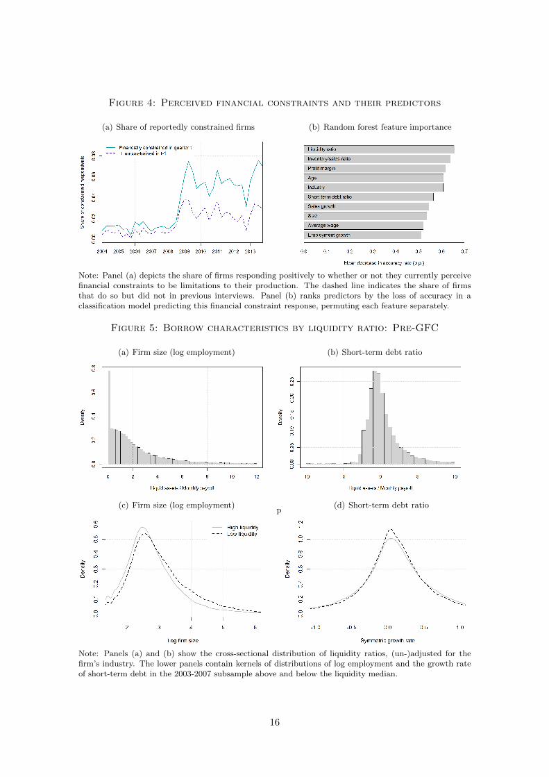
Figure 4: Perceived financial constraints and their predictors

(a) Share of reportedly constrained firms (b) Random forest feature importance

Note: Panel (a) depicts the share of firms responding positively to whether or not they currently perceivefinancial constraints to be limitations to their production. The dashed line indicates the share of firmsthat do so but did not in previous interviews. Panel (b) ranks predictors by the loss of accuracy in aclassification model predicting this financial constraint response, permuting each feature separately.

Figure 5: Borrow characteristics by liquidity ratio: Pre-GFC

(a) Firm size (log employment) (b) Short-term debt ratio

(c) Firm size (log employment)p

(d) Short-term debt ratio

Note: Panels (a) and (b) show the cross-sectional distribution of liquidity ratios, (un-)adjusted for thefirm’s industry. The lower panels contain kernels of distributions of log employment and the growth rateof short-term debt in the 2003-2007 subsample above and below the liquidity median.

16

4 Labor force adjustments

To investigate the effect of this negative shock in credit supply on the size and composition

of firms’ labor force, I use matched employer-employee data, after which I present firm-level

regression results using the above described instruments.

Matched employer-employee data This data covers all (anonymized) employer-

employee matches of Denmark’s private sector, each year in November. On the employer

side, I use the sample of private sector firms for which I have balance sheet data described

above. On the employee side, I observe the workers’ amount of hours worked and total

compensation over the course of the year (provided she is employed in November), as

well as the occupation (according to the standardized ISCO classification). Other relevant

registers at the individual level contain the highest completed level of education, age, and

a variable on how many weeks throughout the calendar year the worker was supported by

unemployment benefits. I only consider the workers between 25 and 60 years of age, and

disregard jobs with an amount of hours lower than the equivalent of one full-time month.

I define a new match as the first observation of a worker-firm pair and a separation as

the last. I further distinguish between job-to-job transitions (EE) if, in the year after a

separation, the worker is linked to a new firm identifier (regardless of whether the firm is

in my sample) and did not receive unemployment support in that or the previous year. If

the worker has held multiple jobs in November of one year but only one in the next, the

terminated job is considered an EE transition.

I observe hourly wages paid for a subset of approximately 70% of jobs in each year. They

are obtained from the labor market survey of the Danish statistical office.7 When studying

compositional effects, I will bin workers by the last reported hourly wage I observe up to

2007. For the purpose of the analysis in this section, I collapse the number of total

employees, hires, separations, and employment in each 2007-wage bin to the firm-year

level.

I list the exact sources of micro data registers in Table A1 in the appendix and present

descriptive (time series) statistics. To summarize, employees matched to the sample firms

cover more than 40% of aggregate employment in Denmark.8 The matched and full

samples show very similar dynamics over the course of the recession: employment in

both sample decreases by 300,000 employees from the peak of 2007 to the trough in 2009.

Because the private sector contributed most to the job losses in the respective time period,

firm-level outcomes can be interpreted in light of their implications for macroeconomic

outcomes.

7Wage information from annual tax filings is available for the whole population. However, Lund and Vejlin(2016) have documented performance issues with this measure of hourly wages. My data are not proneto these issues.

8Note that Denmark has a large public sector, which is excluded from the firm data. The sample covers80% of employment in the nonfarm business sector.

17

In the ensuing analysis, the relevant outcome variables are counted at the level of the firm.

The first of these outcomes is employment.

4.1 Effects on aggregate employment

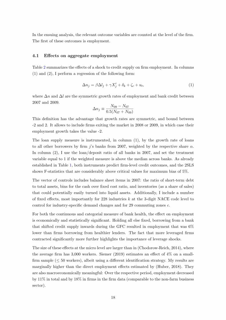
Table 2 summarizes the effects of a shock to credit supply on firm employment. In columns

(1) and (2), I perform a regression of the following form:

∆nj = β∆lj + γX ′j + δk + ζc + ut, (1)

where ∆n and ∆l are the symmetric growth rates of employment and bank credit between

2007 and 2009.

∆nj ≡N09 −N07

0.5(N07 +N09)

This definition has the advantage that growth rates are symmetric, and bound between

-2 and 2. It allows to include firms exiting the market in 2008 or 2009, in which case their

employment growth takes the value -2.

The loan supply measure is instrumented, in column (1), by the growth rate of loans

to all other borrowers by firm j’s banks from 2007, weighted by the respective share α.

In column (2), I use the loan/deposit ratio of all banks in 2007, and set the treatment

variable equal to 1 if the weighted measure is above the median across banks. As already

established in Table 1, both instruments predict firm-level credit outcomes, and the 2SLS

shows F-statistics that are considerably above critical values for maximum bias of 5%.

The vector of controls includes balance sheet items in 2007: the ratio of short-term debt

to total assets, bins for the cash over fixed cost ratio, and inventories (as a share of sales)

that could potentially easily turned into liquid assets. Additionally, I include a number

of fixed effects, most importantly for 228 industries k at the 3-digit NACE code level to

control for industry-specific demand changes and for 29 commuting zones c.

For both the continuous and categorial measure of bank health, the effect on employment

is economically and statistically significant. Holding all else fixed, borrowing from a bank

that shifted credit supply inwards during the GFC resulted in employment that was 6%

lower than firms borrowing from healthier lenders. The fact that more leveraged firms

contracted significantly more further highlights the importance of leverage shocks.

The size of these effects at the micro level are larger than in (Chodorow-Reich, 2014), where

the average firm has 3,000 workers. Siemer (2019) estimates an effect of 4% on a small-

firm sample (≤ 50 workers), albeit using a different identification strategy. My results are

marginally higher than the direct employment effects estimated by (Huber, 2018). They

are also macroeconomically meaningful: Over the respective period, employment decreased

by 11% in total and by 18% in firms in the firm data (comparable to the non-farm business

sector).

18

Table 2: Employment outcomes in 2009

IV A (2SLS) IV B (2SLS) Liquidity (OLS)

Dep. var.: ∆nj,b,07−09 (1) (2) (3)

∆L−j,b,07−09(∆Lj,b,07−09) 0.064***(0.009)

1[LTD07 above median]b(∆Lj,b,07−09) 0.063***(0.007)

1[low `07] −0.111***(0.008)

Short-run debt ratioj,07 −0.278*** −0.290*** −0.065***(0.024) (0.023) (0.007)

Inventory/salesj,07 −0.092 −0.031 0.180*

(0.127) (0.123) (0.098)Employmentj,07 0.000 −0.002 −0.001

(0.000) (0.002) (0.002)

Liquidity bin fixed effects Yes Yes NoNACE3 sector fixed effects Yes Yes YesCommuting zone fixed effects Yes Yes Yes# firms 9,980 10,833 25,123First-stage F-statistics 46.53 65.07Adj. R2 0.069 0.068 0.045

Note: The dependent variables is the geometric growth rate of the sum of matched employees betweenNovember 2007 and 2009. The first two columns perform a 2SLS estimation where the 2-year growth rateof bank credit is instrumented by the weighted growth rate of lending to other firms by the firms’ banks(column 1), and a dummy for whether the firms’ banks in 2007 had a weighted loan-to-deposit ratio abovethe median of all 101 banks (column 2). Firms that cannot be matched to a lending bank are excludedfrom the regression. Column (3) is an OLS regression on a dummy indicating whether the firms’ liquidityratio was below the industry-adjusted median. Standard errors are clustered by industry. Significancelevels: * p < 0.10, ** p < 0.05, *** p < 0.01

The sample is restricted to the firms that can be matched to a bank loan in 2007 to avoid

an endogenous selection of the treatment variable. To the extent that unmatched firms

do not have any bank loans and are thus not affected by a shock to credit supply, these

estimates should be considered a lower bound. I can extend the sample by considering the

pre-crisis level of retained liquidity instead of the health of connected banks. This is done

in column (3) of Table 2. I estimate it directly using OLS because the first-stage effect of

this measure is less compelling, as it is unclear in both theory and the data whether the

amount of lending of these firms should increase or decrease.9 Trying to control for as many

variables as possible, having a liquidity ratio ` below the median within the firm’s industry

in 2007 resulted in a decrease of employment by 11% within two years. This finding is line

with Baurle et al. (2017), who estimate demand-employment elasticities under financial

constraints, and find larger estimates for internal relative to external liquidity constraints.

9On the one hand, liquidity-constrained firms would like to fund their continued operations by obtainingoutside loans. On the other hand, low demand and cash flow might make it questionable if these loansare bearable.

19

According to specification (3), firms with higher stocks of final goods inventories were able

to generate more cash flow and keep workers on the payroll (Gertler and Gilchrist, 1994,

Kashyap et al., 1994).

To study the dynamics beyond this 2-year window, I re-run the regression as a difference-

in-difference estimation on the full panel of firms, rather than the 2009 cross-section.

∆nj,t10 = β(Tj × γt) + δk,t + ζl,t + ηj + uj,t (2)

In the figures presented as follows, I use IV B as the treatment variable T , but the main

results are robust to using the other binary variable describing internal liquidity at the

end of 2007 (see Figure A5 in the appendix). Beyond the industry demand control,

this specification allows the inclusion of firm fixed effects (ηj) to control for unobserved

heterogeneity, for example in time-independent firm productivity.

Figure 6 shows, first, that the y/y growth rate of employment is similar across firm’s

lending from high and low exposure banks prior to 2007. Second, the firms receiving

shocks to external liquidity due to their banks’ exposure downsize throghout the Great

Recession. The effects is significant for all the years up to and including 2010, and the

point estimates imply a permanent 20% reduction in firm size.

In a model with flexible wages and homogenous workers, such a fall in labor demand would

reduce wages. However, repeating regression (2) with the average wage paid by the firm

as the left-hand side variable shows no significant difference, neither prior nor during the

Great Recession (similar to Huber (2018)). This holds true if I consider the average wage of

incumbent workers and new hires (for firms that do hire) separetely. The main contribution

of this paper is to put forward an explanation for this wage rigidity conditional on the

credit supply shock: The differential effects on labor demand for heterogeneous workers

that is specific to a liquidity shock masks the down-ward pressure on wages at the firm

level.

Other firm-level outcomes Before proceeding to this compositional effect, I repeat

the difference-in-difference model for a number of other firm-level outcomes regarding labor

market and cash flow variables. Figure A3 includes the log number of hires and separations

and suggests that, contrary to many labor market models with constant separation rates,

they account for a larger share of the decline in employment than the drop in hiring, which

only manifests in 2009. Separations in constrained firms increase 10% above the level of

unconstrained firms. Unfortunately, the data does not allow to distinguish between quits

and layoffs.

Operational profits react with a lag. Downsized firms generate an estimated 10% lower

profits in 2009 due to the funding shock. Dividends and investments fall, too, even though

it is difficult to establish a statistically significant effect. Interestingly, the amount of

10Consequently, ∆nj,t now is the one-period geometric growth rate (Nj,t −Nj,t−1)/(0.5(Nj,t +Nj,t−1))

20

Figure 6: DiD regression results: Employment and wages

(a) Employment growth (b) Average nominal wage

(c) Average wage of new hires (d) Average wage of incumbent workers

Note: The black line represents difference-in-difference estimates of a negative credit supply shock,measured by the weighted loan/deposit ratio of a firms’ banks in 2007. The left-hand side variables arethe annual symmetric growth rates of employment (since November of the previous year, panel (a)) andthe average hourly wage paid at the firm in the respective year (panel b), paid to newly hired workers (c)and incumbents workers (d). The grey bands represent 95% confidence intervals of the point estimate.Standard errors are clustered at the firm level.

liquidity hoarded by firms hit by the funding shock increases and plateaus 10% above

the 2007 level (Kahle and Stulz, 2013). This emphasizes the trade-off credit-constrained

firms face between retaining their labor force to generate cash flow and accumulating cash

reserves simultaneously.

Figure A5 contains the same set of results by pre-crisis internal liquidity. Separations surge

in low-liquidity firms and employment drops sharply. However, the pre-crisis difference

suggests that this measure is not entirely free of endogeneity bias: Employment growth in

the firms with low liquidity, which I classify as constrained, exhibit 4% higher employment

growth in 2006, which might indicate an over-accumulation of workers and a resulting

squeeze in liquidity. Yet, even in this case, where one could expect nominal wages to grow

excessively in the boom, the average wage at the firm level does not fall significantly.11

11Additionally, I highlight the non-linearity of the liquidity-employment nexus in the same section in theappendix. In boom times, the elasticity is small, and the mechanism presented in Table 2 are by far thestrongest during the recession.

21

4.2 Labor force composition

I provide evidence of a novel stylized fact that the composition of the labor force in

constrained firms shifts toward less expensive workers. To do so, I assign workers to ten

bins according to their wage in 2007, and I refer to those bins as qw,07. Thereafter, I collect

the stock of employees for each firm-wage bin cell and regress symmetric growth rates of

these composites as in regression (2).

∆nj,q,t = βq1[qw,07]× Tj × γt + δk,t + uj,q,t (3)

The interaction of the treatment term with an additional dummy for each q will give an

estimate of labor adjustment for each of those bins separately.

Figure 7 shows estimates of the vector βq for the year 2012, when the growth rate of

firm-level employment (according to the previous section) has stabilized. The 2007 wage

bin (from lowest to highest) is depicted on the x-axis. Relative to unshocked firms, the

ones receiving a shock to liquidity disproportionately reduce employment of workers with

previously high wages. The growth rate of workers with the lowest and highest wages are

significantly different, with the latter falling three times as much as low-wage employees.

Figure 8(a) tests whether this effect is driven by firm piling up too many high-wage workers

prior to the onset of the credit tightening. In this case, the partial effects on either side

of the wage spectrum are not significantly different from zero.

Figure 7: Heterogeneous employment effects by pre-shock wage

(a) Composition changes, 2012 rel. to 2007

Note: Difference-in-difference estimator for each wage bin ofworkers in 2007. The dependent variable is the growth rateof employment in each firm-wage bin pair between 2007 and2012 Therefore, estimates show the change in labor forcecomposition relative to unconstrained firms. The greay barsdenote point estimates, and black whiskers represent 95%confidence intervals. Standard errors are clustered at the firmlevel.

22

Figure 8: Pre-Trend composition and wage response

(a) Composition changes, 2007 rel. to 2006 (b) Wage changes, 2009 rel. to 2007

Note: Difference-in-difference estimator for each wage bin of workers in 2007. The dependent variable inpanel (a) is the growth rate of employment in each firm-wage bin pair between 2007 and 2006, respectively.In panel (b), it is the average growth rate of wages paid to workers in the respective bin between 2007and 2009, given that they were employed in both periods. The greay bars denote point estimates, andblack whiskers represent 95% confidence intervals. Standard errors are clustered at the firm level.

How should we interpret these findings in light of existing evidence and economic theory?

One theory is suggested by Caggese et al. (2019). Binding credit constraints increase the

opportunity cost of liquidity and discount the future benefits of a job more heavily. In

light of this, jobs that pay high wages would be discontinued disproportionately. This

effect would be exacerbated if the return to a high-wage job, say a researcher, lied further

ahead in the future than the return generated by a typical low-wage job. A decrease

in labor supply to financially constrained firms could offer an alternative explanation, as

employees are anxious to receive wage cuts in the future (Barbosa et al., 2019). However,

I provide suggestive evidence below that raises concerns about labor supply as a driver of

the gradient presented in Figure 7. In short, displaced high-wage workers experience large

decreases in their wage in a new job.

Carlsson and Westermark (2016) show that wage rigidities of incumbent workers, as

opposed to wages of newly hires workers as in Pissarides (2009) matter for employment

adjustment to shocks if the separation rate reacts endogenously. My data allows me to

test this in light of a financial shock, which has large effects if incumbent wages are rigid

and workers are paid with the liquid asset Schoefer (2015).

I can test to what extent my finding is contributed to by higher wage rigidities among high-

wage workers, which could explain why labor cost is cust more sharply at the extensive

margin. Take regression (3) and replace the left-hand side with the average wage growth

rate of workers within the respective bin qw,07. This automatically selects incumbent

workers only.

Figure 8(b) plots the equivalent vector of estimated coefficients. The point estimates do

point to the fact that workers that already are highly paid managed to increase their wages

from constrained firms. A possible rationale could be provided by Quadrini and Sun (2018)

23

who argue that a deleveraging shock increases the bargaining power of workers. However,

wages of the lower bins do fall slightly; and effects are rather imprecisely estimated and

not significantly different from each other.

I conclude from this exercise that wage stickiness of incumbent workers is present, and

is indeed an explanation for large effects on employment, but it cannot alone explain the

differential findings provided in Figure 7.

The dispersion of wages can represent a host of different heterogeneities of workers and

firms such as dispersion in actual (observed or unobserved) productivities or frictional

competition in the labor market (Bagger and Lentz, 2019). To test whether the gradient

observed above is driven by fundamental productivity or “excess wages”, I perform the

same analysis on deciles of workers sorted by a measure of fundamental worker productivity

and a wage measure residualized of this worker heterogeneity. I perform a two-way fixed

effect regression on job observations of worker i and firm j, as in Abowd et al. (1999).

The regression takes the following form

wi,j,t = αi + ψj(i,t) + βX ′i,t + ωi,j,t

The vector X includes dummies age, tenure within the current job, overall labor market

experience, the occupation and the typical years of schooling to complete the highest

completed education. Since this regression can only be identified on the connected set

of workers with at least two jobs spells, the unobserved worker productivity αi and the

residualized, job-specific wage ωi,j,t can only be assigned to a subset of the data.

I then collect again the firm-specific composition of each of 10 bins of these variables,

denoted qα,07 and qω,07, and proceed as in regression (3). Figure 9 presents the results,

suggesting that the negative gradient of the employment response is not driven by inherent,

unobserved worker ability α. In fact, it appears as though employment of workers with

a low estimated α falls the most, whereas constrained firms seem to hold on to most of

the highest types. In contrast, the negative gradient originates from workers with high

residual wages. Note, however, that the AKM approach is silent about the exact nature

of ω, as it could represent both match-specific productivity (sorting) or the worker’s rent

extracted from the frictional surplus.

The results presented here have used the pre-crisis lender exposure to the banking crisis

to estimate the differential effects of a credit supply shock on the composition of the labor

force. The main result, namely that contrained firms adjust labor cost predominantly by

reducing employment of the most costly workers (especially relative to their productivity),

is robust to using the alternative classification using internal liquidity.

24

Figure 9: Heterogeneous effects by pre-shock worker characteristics

(a) Residualized wage (b) Unobserved worker productivity

Note: Difference-in-difference estimator for each “ability type ”(α) and “residual wage”(ω) bin of workersin 2007. The dependent variable is the growth rate of employment in each firm-group bin pair between2007 and 2012. Therefore, estimates show the change in labor force composition relative to unconstrainedfirms. The greay bars denote point estimates, and black whiskers represent 95% confidence intervals.Standard errors are clustered at the firm level.

4.3 Benchmark labor demand shock

These findings contradict the fact that employment of low-wage (Bils et al., 2012) and low-

skill (Keane and Prasad, 1993, Mueller, 2017, online appendix) workers shows a higher

degree of procyclicality over the business cycle. Therefore, I want to contrast the results of

labor force adjustment after financial disturbances from Section 4.2 with a different source

of business cycle fluctuation. Contrary to the financial shock studies in detail above, the

effects of a local labor demand shock has by far the strongest effects on workers with the

lowest wages.

Bartik instrument I construct a shift-share instrument based on the notion that local

employment growth rates can be predicted by an interaction of local industry employment

shares with national industry employment growth rates. If sNk,l,t−1 is the employment

share of industry k in location l in a pre-determined year t-1 and ∆nk,−l,t is the national

employment leave-on-out-growth rate of said industry, then firms in a region with a high

exposure to that industry will experience a larger effect of aggregate variations in that

industry.12 These changes are unrelated to labor supply to the firm, but do not require to

take a stance on the interpretation of the source of the underlying shock. The instrument

has been used to study local labor market effects in many contexts, including rising

competition to local manufacturers by Chinese imports (Autor et al., 2013) or sectoral

reallocation of labor (Chodorow-Reich and Wieland, forthcoming).

12Following Goldsmith-Pinkham et al. (2019), I exclude the region itself when calculating the nationalgrowth rate because of the finite sample of locations.

25

Table 3: Local labor demand shock: 2SLS estimates

Bartik (2SLS) Bartik (2SLS)

Dep. var.: ∆nj,t (1) (2)

∆nk,l,t (Shift-share) 0.461*** 0.689***(0.024) (0.047)

Firm fixed effects Yes YesSample 2003-2016 2008-2009# observations 343,019 55,865# firms 39,229 29,610First-stage F-statistics 36.41 21.29Adj. R2 0.077 0.148

Note: The table reports 2SLS regressions of local labor market shocks and firm-level employment of alltypes of employees. The growth rate of the local labor market is instrumented using the interaction of theindustry’s share of employment in the commuting zone and the leave-on-out growth of the industry’semployment in all other commuting zones (shift-share). Standard errors are clustered by industry.Significance levels: * p < 0.10, ** p < 0.05, *** p < 0.01

The first stage is specified as

∆nk,l,t =∑k

sNk,l,t−1∆nk,−l,t + ut.

Data Danmarks Statistiks allocates all 98 municipalities into 29 commuting zones based

on people’s actual commuting behavior, which I denote l.13 Both the location and the

industry k in which firms operate are taken from the accounting registers, and the latter

are defined at level 3 of the NACE/ISIC industry classification system. The growth rates

∆n of each sector are calculated by aggregating employment N over all firms for which

employment data is available (not just the firms in the baseline sample used throughout

the paper).

Results To observe the effect on employment of any kind at the firm level, I regress

the firms’ outcome ∆nj,t on local labor demand growth, instrumenting with the above

described shift-share product. Table 3 confirms that firm-level employment co-moves with

local labor market conditions. A firm adversely affected by such a shock therefore cuts

employment.

Moreover, the compositional effects are the opposite of the financial shock presented in

Figure 7. To show this, I again repeat the exercise at the level of firm-bin level, with bins

being constructed using employee’s relative position in the wage distribution of the firm.

For each year, I construct the growth rate of employees in that bin ∆nj,qt and regress it

13The algorithm selects commuting zones, among other requirements, in order to maximize the share ofpeople who live in the same region they work. The average of the resulting shares based on the year 2014is 76%. Workers have become more mobile and the amount of commuting zones has declined steadily,making it important to use a timely classification.

26

Figure 10: Heterogeneous employment effects based on pre-shock wage

(a) Compositional changes

Note: Growth rates of firm-level employment to alocal labor demand shock of -1, for 10 bins of workersgrouped according to their wage position within thefirm prior to the shock. Estimation is performed usinga Bartik instrument.

on the above instrument. The coefficient obtained for low-wage bins is much larger and

strikingly different from workers in the center and upper tail of the distribution, who are

much less affected. Figure 10 shows the negative of estimated coefficients, showing the

much higher cyclicality of low-wage employees.

In contrast, Carlsson et al. (2016) find that in response to a TFP shock (to which overall

wages do adjust), firms do not change the composition of their labor force. Overall, I

thus conclude that the compositional changes financially constrained firms engage in is

different from other sources of business cycle fluctuations.

5 Job flows and aggregate implications

This section explores how the labor market as a whole adjusts after some of the firms

become financially constrained. It relies on the same data as described in Section 4, but

the unit of analysis is now at the job level (i.e. worker i and firm j), as we want to explore

worker flows from shocked firms.

Worker flows Separations in constrained firms increase, and the adjustment is

disproportionate for high-wage workers. In order to study the flow of these workers, I

classify each separation as a transition into unemployment (referred to as EU) if the

worker cannot be matched to a firm in the subsequent year, or if the worker has received

unemployment benefits throughout that year. Unfortunately, the data do not allow me

to re-construct the precise timing of these unemployment benefits. Furthermore, the

data on unemployment spells should be considered incomplete, as the first safety net of

unemployment insurance in Denmark is organized privately. A regression of the following

27

form for all separations of 2008 and 2009 is run in order to retrieve the likelihood of a

worker moving into unemployment based on her previous firm and wage.

1[EUi|si = 1] = βq 1[qw,07]i × Tj + ui (4)

T is again the indicator variables for whether the firm lendt from an exposed bank prior

to the GFC. Figure 11(a) presents this estimated coefficients βq. The following patterns

emerge: First, high-wage workers have lower unemployment risk. Based on the measure

of unemployment I use, the likelihood of moving into unemployment is 50% higher for

workers in the low bin. The second is that workers with the same wage, employed at

a firm with different exposure to the GFC, have very similar probabilities of becoming

unemployed.

Combined, these two findings imply that while labor-market adjustments in financially

constrained firms disproportionately affect costly workers, they have a lower incidence of

ending up unemployed as a result. As opposed to Mueller (2017) for U.S. data, I do not

find that the pool of unemployed in Denmark shifted towards workers with previously high

wages after the GFC.14 The reason is that they are re-employed quickly.

Wage developments The data allows to estimate what labor market conditions the

separated workers face once matched to a new firm. To do so, I replace the left-hand side

of equation (4) with the growth rate of the wage in the new, relative to the old job. Note

that the new job can be in any firm, including the public sector, as long as an hourly wage

is reported. I take the log of the first oberved wage after a separation in 2008/09, and

subtract the log of the wage in the separated job.

Figure 11(b) shows, first, that the between-jobs wage growth after separations during

the Great Recession is negative for the 6 highest deciles of workers. Second, workers

with previously high wages take considerably larger wage cuts once re-employed. The

differences are large: Workers with the highest wages in 2007 take a 5-10% wage cut.

Third, there is again no difference in wage growth across the financial position of previous

employers.

The data does not allow to distinguish between voluntary and involuntary separations,

and the findings presented above can indeed be interpreted as labor demand and labor

supply adjustments. Barbosa et al. (2019) argue that workers with high human capital (in

my application with high wages) sort themselves into jobs at firms with continued access

to credit and therefore the ability to pay wages continuously. A purely supply-driven

interpretation would imply, however, that this insurance is worth a premium of up to 10%

of the wage. Especially in light of the stickiness of incumbent workers, a reduction of firm

demand for workers with the highest wage is more preferable.

14Although, it should again be noted that my data is set up to track the employed, and that the pool ofunemployed is measured rather imprecisely, given data limitations.

28

Figure 11: Labor market re-allocation

(a) Transitions into unemployment (b) Wage in next job

Note: Probability of observing an unemployment spell (panel a) and wage growth from current to nextjob (panel b) conditional on having a separation in 2008 or 2009, by pre-crisis wage bin and by financialposition of the previous employer. The latter is defined as having loans from banks that are exposed tothe liquidity shock in the banking sector of 2008.

Taken together, the firm-level results and the subsequent job market flows provide a

rationale for large employment effects of financial shocks, followed by low wage growth

for an extended period of time. Constrained firms reduce labor cost where it most

effective: with the highest-paid employees. Low-wage workers are more likely to move

into unemployment, while high-wage workers are re-employed quickly. Pries (2008) and

Ravenna and Walsh (2012) have proposed channels for this effect to make recessions

endogenously deeper: As the pool of unemployed deteriorates, firms have lower incentives

to post vacancies. Firms prefer to hire workers with previously high wages, but pay them

considerably less. As the economy recovers, lower-wage workers move out of unemployment

and further depress aggregate wage growth.

6 Conclusions

My empirical analysis delivers four main findings: First, I use variation in the exposure

of Danish banks to the Global Financial Crisis to show that liquidity shocks in the

financial system are transmitted to credit supply at the firm level. Second, access to

(both internal and external) liquidity plays a role in firms’ ability to fund their working

capital. Constrained firms retain cash flow predominantly by reducing employment,

rather than the wage paid to each worker. At the same time, they build up liquidity

buffers to insure themselves against future shocks. Third, I provide novel evidence of a

margin to most effectively improve cash flow: Employment of the most costly workers is

reduced disproportionately in constrained firms. I do not directly address the normative

implications of this composition effect. However, the fact that the gradient in wage

composition adjustments is driven by residualized wages rather than worker productivity

could point to the fact that these adjustments could have cleansing effects (Baley et al.,

29

2018). Fourth, I show that this compositional adjustment is different for an alternative

source of business cycles. In a local labor demand shock, the strongest decline is in

employment for low-wage workers, while high-wage workers are almost unaffected.

Finally, I discuss and test implications for the cyclicality of employment and wages when

workers re-allocate and wages adjust in a new job spell. As wages within job spells

are sticky, the extensive margin of employment absorbs most of the need to shrink the

outflow of cash. The previously highly paid workers find new work quickly, but take wage

cuts relative to their previous job. Therefore, wage growth is low in constrained firms

because of the described compositional shifts and in unconstrained because wages of new

hires adjust downward. Low-wage workers spend more time in unemployment, depressing

firms’ incentive to hire and leading to slow recoveries. Once re-hired, the composition shift

of the employed workforce once more depresses growth in the aggregate wage rate. My

findings are therefore consistent with large drops of employment after financial shocks,

and sluggish wage growth well after the labor market has stabilized.

References

Abildgren, K. (2012): “Financial Structures and the Real Effects of Credit Supply

Shocks in Denmark 1922-2011,” European Review of Economic History, 16, 490–510.

Abowd, J. M., F. Kramarz, and D. N. Margolis (1999): “High Wage Workers and

High Wage Firms,” Econometrica, 67, 251–333.

Amiti, M. and D. E. Weinstein (2018): “How Much Do Idiosyncratic Bank Shocks

Affect Investment? Evidence from Matched Bank-Firm Loan Data,” Journal of Political

Economy, 126, 525–587.

Andersen, T. M. (2012): “A Flexicurity Labour Market in the Great Recession: The

Case of Denmark,” De Economist, 160, 117–140.

Autor, D. H., D. Dorn, and G. H. Hanson (2013): “The China Syndrome: Local

Labor Market Effects of Import Competition in the United States,” American Economic

Review, 103, 2121–2168.

Bagger, J. and R. Lentz (2019): “An Empirical Model of Wage Dispersion with

Sorting,” The Review of Economic Studies, 86, 153190.

Baley, I., A. Figueiredo, and R. Ulbricht (2018): “Mismatch Cycles,” mimeo.

Banerjee, R. N., L. Gambacorta, and E. Sette (2017): “The Real Effects of

Relationship Lending,” BIS Working Papers, 662.

Barbosa, L., A. Bilan, and C. Celerier (2019): “Credit Supply and Human Capital:

Evidence from Bank Pension Liabilities,” ECB Working Paper, 2271.

30

Baurle, G., S. M. Lein, and E. Steiner (2017): “Employment Adjustment and

Financial Constraints - Evidence from Firm-Level Data,” Swiss National Bank Working

Papers, 18.

Bentolila, S., M. Jansen, and G. Jimenez (2018): “When Credit Dries Up: Job

Losses in the Great Recession,” Journal of the European Economic Association, 16,

650–695.

Berton, F., S. Mocetti, A. F. Presbitero, and M. Richiardi (2018): “Banks,

Firms, and Jobs,” The Review of Financial Studies, 31, 21132156.

Bharath, S., S. Dahiya, and A. S. A. Srinivasan (2007): “So What Do I Get? The

Banks View of Lending Relationships,” Journal of Financial Economics, 85, 368–419.

Bils, M., Y. Chang, and S. Kim (2012): “Comparative Advantage and

Unemployment,” Journal of Monetary Economics, 59, 150–165.

Boeri, T., P. Garibaldi, and E. R. Moen (2018): “Financial Constraints in

Search Equilibrium: Mortensen and Pissarides Meet Holmstrom and Tirole,” Labour

Economics, 50, 144–155.

Caggese, A. and V. Cunat (2008): “Financing Constraints and Fixed-Term

Employment Contracts,” The Economic Journal, 118, 2013–2046.

Caggese, A., V. Cunat, and D. Metzger (2019): “Firing the Wrong Worker:

Financing Constraints and Labor Misallocation,” Journal of Financial Economics, 133,

589–607.

Carlsson, M., J. Messina, and O. N. Skans (2016): “Wage Adjustment and

Productivity Shocks,” Economic Journal, 126, 1739–1773.

Carlsson, M. and A. Westermark (2016): “Endogenous Separations, Wage Rigidities

and Employment,” Uppsala Universitet Working Paper Series, 12.

Chodorow-Reich, G. (2014): “The Employment Effects of Credit Market Disruptions:

Firm-level Evidence from the 2008-09 Financial Crisis,” Quarterly Journal of

Economics, 129, 1–59.

Chodorow-Reich, G. and J. Wieland (forthcoming): “Secular Labor Reallocation

and Business Cycles,” Journal of Political Economy.

Cornille, D., F. Rycx, and I. Tojerow (2017): “The Employment Consequences of

SME’s Credit Constraints in the Wake of the Great Recession,” European Central Bank

Working Paper Series, 2117.

Gertler, M. and S. Gilchrist (1994): “Monetary Policy, Business Cycles, and the

Behavior of Small Manufacturing Firms,” Quarterly Journal of Economics, 109, 309–

340.

31

——— (2018): “What Happened: Financial Factors in the Great Recession,” Journal of

Economic Perspectives, 32, 3–30.

Gilchrist, S., R. Schoenle, J. Sim, and E. Zakrajsek (2017): “Inflation Dynamics

During the Financial Crisis,” American Economic Review, 107, 785–823.

Goldsmith-Pinkham, P., I. Sorkin, and H. Swift (2019): “Bartik Instruments:

What, When, Why, and How,” NBER Working Papers, 24408.

Heider, F., F. Saidi, and G. Schepens (2019): “Life Below Zero: Bank Lending Under

Negative Policy Rates,” The Review of Financial Studies, 32, 728–3761.

Huber, K. (2018): “Disentangling the Effects of a Banking Crisis: Evidence from German

Firms and Counties,” American Economics Review, 108, 868–898.

Iyer, R., J.-L. Peydro, S. da Rocha-Lopes, and A. Schoar (2014): “Interbank

Liquidity Crunch and the Firm Credit Crunch: Evidence from the 2007-2009 Crisis,”

The Review of Financial Studies, 27, 347372.

Jensen, T. L. and N. Johannesen (2017): “The Consumption Effects of the 2007-2008

Financial Crisis: Evidence from Households in Denmark,” American Economic Review,

107, 3386–3414.

Kahle, K. M. and R. M. Stulz (2013): “Access to Capital, Investment, and the

Financial Crisis,” Journal of Financial Economics, 110, 280–299.

Kashyap, A. K., O. A. Lamont, and J. C. Stein (1994): “Credit Conditions and the

Cyclical Behavior of Inventories,” The Quarterly Journal of Economics, 109, 565–592.

Keane, M. and E. Prasad (1993): “Skill Levels and the Cyclical Variability of

Employment, Hours, and Wages,” International Monetary Fund Staff Papers, 40, 711–

743.

Khwaja, A. I. and A. Mian (2008): “Tracing the Impact of Bank Liquidity Shocks:

Evidence from an Emerging Market,” American Economic Review, 98, 1413–1442.

Lins, K. V., H. Servaes, and P. Tufano (2010): “What Drives Corporate Liquidity?

An Internal Survey of Cash Holdings and Lines of Credit,” Journal of Financial

Economics, 98, 160–176.

Lund, C. and R. Vejlin (2016): “Documenting and Improving the Hourly Wage

Measure in the Danish IDA Database,” Danish Journal of Economics, 1, 1–35.

Melcangi, D. (2018): “The Marginal Propensity to Hire,” Federal Reserve Bank of New

York Staff Report, 875.

Michelacci, C. and V. Quadrini (2009): “Financial Markets and Wages,” Review of

Economic Studies, 76, 795–827.

32

Moser, C., F. Saidi, B. Wirth, and S. Wolter (2019): “Credit Supply, Firms, and

Earnings Inequality,” mimeo.

Mueller, A. I. (2017): “Separations, Sorting, and Cyclical Unemployment,” American

Economic Review, 107, 2081–2107.

Olsson, M. (2020): “Labor Cost Adjustments During the Great Recession,” mimeo.

Petrosky-Nadeau, N. (2014): “Credit, Vacancies and Unemployment Fluctuations,”

Review of Economic Dynamics, 17, 191–205.

Petrosky-Nadeau, N. and E. Wasmer (2013): “The Cyclical Volatility of

Labor Markets under Frictional Financial Markets,” American Economic Journal:

Macroeconomics, 5, 193–221.

——— (2015): “Macroeconomic Dynamics in a Model of Goods, Labor, and Credit Market

Frictions,” Journal of Monetary Economics, 72, 97–113.

Pissarides, C. A. (2009): “The Unemployment Volatility Puzzle: Is Wage Stickiness the

Answer?” Econometrica, 77, 1339–1369.

Pries, M. J. (2008): “Worker Heterogeneity and Labor Market Volatility in Matching

Models,” Review of Economic Dynamics, 11, 664–678.

Quadrini, V. and Q. Sun (2018): “Credit and Firm-Level Volatility of Employment,”

Journal of the European Economic Association, 16, 1433–1475.

Ravenna, F. and C. E. Walsh (2012): “Screening and Labor Market Flows in a Model

with Heterogeneous Workers,” Journal of Money, Credit and Banking, 44, 31–71.

Schoefer, J. (2015): “The Financial Channel of Wage Rigidity,” mimeo.

Shimer, R. (2005): “The Cyclical Behavior of Equilibrium Unemployment and

Vacancies,” American Economics Review, 95, 25–49.

Siemer, M. (2019): “Employment Effects of Financial Constraints During the Great

Recession,” Review of Economics and Statistics, 101, 16–29.

33

A Data appendix

A.1 Data sources and coverage

I compile detailed micro data from 10 different sources. This section describes the original

data compiled and kindly made available by Danmarks Statistik. They are, for the most

part, based on tax-relevant filings, and augmented by surveys on firm accounting statistics

(FIRE), annual payrolls (LON) and financial statements of banks (URTEVIRK). Before

describing the coverage and treatment of the data in more detail, Table A1 summarizes

the data sources and main variables used.

On the individual side, the registers cover the universe of individuals with residence in

Denmark, and the firm registers cover very closely the aggregate employment series in

the country, which includes the large public sector. However, accounting data is only

available for a subsample of firms; public sector, financial and agriculture are excluded

altogether. More than half of employment (1.5 million individuals on average) are working

at firms which are covered by the 300,000 firms for which accounting statistics are available

(see green lines in Figure A1). The average firm size is therefore 7.5 employees. More

importantly, the sample replicates the cyclical patterns in absolute terms, rather than

relative. Employment in the whole economy falls by a little over 0.33 million (13%)

during the Great Recession, the amount of jobs captured in the accounting statistics falls

by 0.29 million (18%). This reflects the relative acyclicality of the unconvered firms.

Dropping firms that consistently have less than 10 employees reduces the amount of unique

firms from almost 300,000 in the average year to between 25,000 and 29,000 firms per year.

This selects a constant share of private sector of employment of 80-82% (see orange line

in Figure A1), and is the baseline sample of firms analyzed.

Figure A1: Sample coverage

(a) Number of firms (b) Employment

Note: Number of firms (panel a) and workers in November (panel b), compared across time and differentsample selection criteria. The selected sample (in orange) only makes up a small fraction of the universe offirms, but a large share of private-sector employment and has the same cyclical properties. Furthermore,entry and exit rates are more stable, reducing extensive margin adjustment.

34

Table A1: Original data sources used

Register Description Identifier Years used Selected variables

BanksURTE-VIRK

Bank-borrowerbalances

bank,cvrnr

2003-2016 Year-end credit balance,interest

Finanstil-synet

Bank balancesheets

bank 2007 Total loans and deposits

FirmsFIRM Register of all

firmscvrnr 2003-2016 Year of entry and exit,

November employment (HC)FIRE Firm-level

accountingcvrnr 2003-2016 Balance sheets, income

statements, investment,aggregate employment overthe course of the year (FTE)

KBI/KBB Businesstendency survey

cvrnr 2003-2016 Perceived financialconstraints

Jobs/wagesFIDA Employer-

employeelink

cvrnr,pnr

1995-2013 Primary and secondary jobsin November each year

LON(N) Annual wagestatistics

cvrnr,pnr

1997-2016 Hourly wage, hours worked1

IndividualsIDAP Individuals pnr 1990-2016 Income per calendar year,

age, weeks of unemployment,years of employmentexperience

UDDA Education pnr 1990-2016 DISCED-15 code of highestcompleted education2

AKM Occupations pnr 1991-2016 DISCO code of main laborincome, DISCO-08 as of20103

Registers are made available through and documented by Danmarks Statistisk’s Danmarks Statistik’sForksningsservice. HC = head count, FTE = full-time equivalents. Identifiers: pnr is the personalregistration number, cvrnr is the firm identifier. A firm can consist of of multiple establishments (arbnr).1 Definition of hours worked and hourly wage is subject to changes over time. They are described in moredetail in section A.22 DISCED-15 is the Danish education classification system aligned with the international ISCED 2011. Itcan be translated to eight levels from primary school to a doctoral degree as well as the standard years ofschooling to complete.3 DISCO is the Danish application of the International Standard Classification of Occupations ISCO-88.As of 2010, the most recent version DISCO-08 (equivalent to ISCO-08) is used.

35

This sample has several appealing features: First, it preserves the boom and bust of

private-sector employment: It explains 96% of the variance of nation-wide employment.

Second, it reduces potential biases induces by firm entry and exit. While in the unrestricted

sample, less than 60% of firms survive the decade after the Great Recession. The average

annual exit rate of firms in the selected sample is 1.7%, (4.1% in 2009), mitigating

concerns about the extensive margin of employment adjustment. Ultimately, only firms of

a sufficient size consistently report wage data on their employees and allow to study the

effects on workforce composition in a meaningful way.

35% of firms report their balance sheets throughout the entire sample period, the mean

length of uninterrupted observations is 9.4 (out of 14) years. When accounting for firms

entering and exiting the market, these numbers climb to 63% of firms and 12.2 years,

respectively.

Observable variables include a detailed disposition of balance sheets, including liquid

assets, financial securities in both sales and fixed assets, as well as tangible and intangible

fixed assets. The sum of the latter two is defined as the firm’s capital. Furthermore, lia-

bilities are classified as short-(/long-)term financial debt based on whether their maturity

is less (more) than one year, accounts payable to suppliers, as well as equity. The income

statement also follows standard accounting principles, and apart from sales and expenses

on raw materials, salaries and interest payments, taxes and depreciation, the distribution

of profits, which emerges from the income statement, will be considered in the regression

analysis because it too is a margin of adjustment when credit constraints are binding.

On the financial side, I merge firms to loans in the URTEVIRK register, which is a

third-party reported snapshot of not securitized loans at lenders in Denmark. However, I

restrict the lender side to 101 actual banks, which annual balance sheets to the financial

supervisory authority (Finanstilsynet) and, if of sufficient size, monthly loans to the non-

financial corporate sector in the Monetary and Financial Statistics to the Danish central

bank.

46% of firm-years can be matched to a bank loan. This share increases with the size of

the firm, but even for large corporations, the match rate stays below 90%. However, the

firms that do match obtain the same dynamcis in terms of employment than the baseline

firm sample (see black line in Figure A1)

Finally, Section 3.2 of the paper uses the Business Tendency Surveys for the manufacturing

and construction sectors linked to the balance sheets of 2’766 firms between 2003 and 2016.

36

A.2 Data treatment: Jobs and wages

The FIDA registers are annual snapshots of the labor market at the end of November,

starting in 1997, include both primary and secondary jobs, and serve as the core dataset

of the job-level analysis. This section describes the procedure merging and handling the

data: First, multiple employer-employee links in the same year are collapsed to only one

observations. Second, employees who never work at any of the firms described above

are disregarded. This concerns 64% of individuals. Third, the dataset is merged to

the individual-level registers described in the data source description, and observations of

individuals younger than 25 or older than 60 are dropped. Fourth, information on job-level

salary payments is added from the LON(N) registers.

Wages Prior to 2002, the hourly wage in the definition used post-2002 has to be imputed

by by summing the has to be added manually, comprising of the “narrow ”wage definition,

pension contributions, and well as payments for holidays, sick leave and payments in kind,

all divided by the registered work hours carried out.

Residualized wages In Section 4.2 of the paper, I residualize nominal wages following

Abowd et al. (1999) on the subset of connected workers and firms. Practically, the two-way

fixed effect regression performs can only identify worker and firm fixed effects if a worker

has – between 1997 and 2016 – worked for at least two different firms, which in turn have

employed at least two different workers. This is the case for 57.53% of worker-firm-years.

For those observations, the log hourly wage is regressed on a set of explanatory variables

using two-way fixed effects on worker i and firm j identifiers.

wi,t = αi + ψj(i,t) + Π′ × Zi,t + ωi,t

The vector of covariates Z includes the following variables: age and squared age, the ex-

pected years of schooling for the highest degree obtained, a fixed effect for the occupation,

labor market experience since graduation, as well as tenure in the current job.

Unionization Labor unions play a central role in the Danish labor market, and more

than 70% of Danish wage-earners are union members. Absent a national minimum wage or

the like, unions and employers negotiate sector-specific collective agreements which cover

non-members as well, but neither companies nor workers are legally required to comply. If

union-negotiated wage agreements constitute a source of downward nominal wage rigidity,

one would assume this effect to be stronger for workers with lower wages. Consequently,

the wage stickiness would lead to more adjustments along the extensive margin, as indeed

shown by Olsson (2020). This effect would work against findings presented in this paper.

37

A.3 Descriptive statistics

Figure A2: Descriptive distributions: Firms

(a) Profit ratio (b) Investment / lagged capital

(c) Inventories/sales (d) Dividends/profit

Note: Histograms/cross-sectional distributions of key balance sheet variables used in the regressions.

38

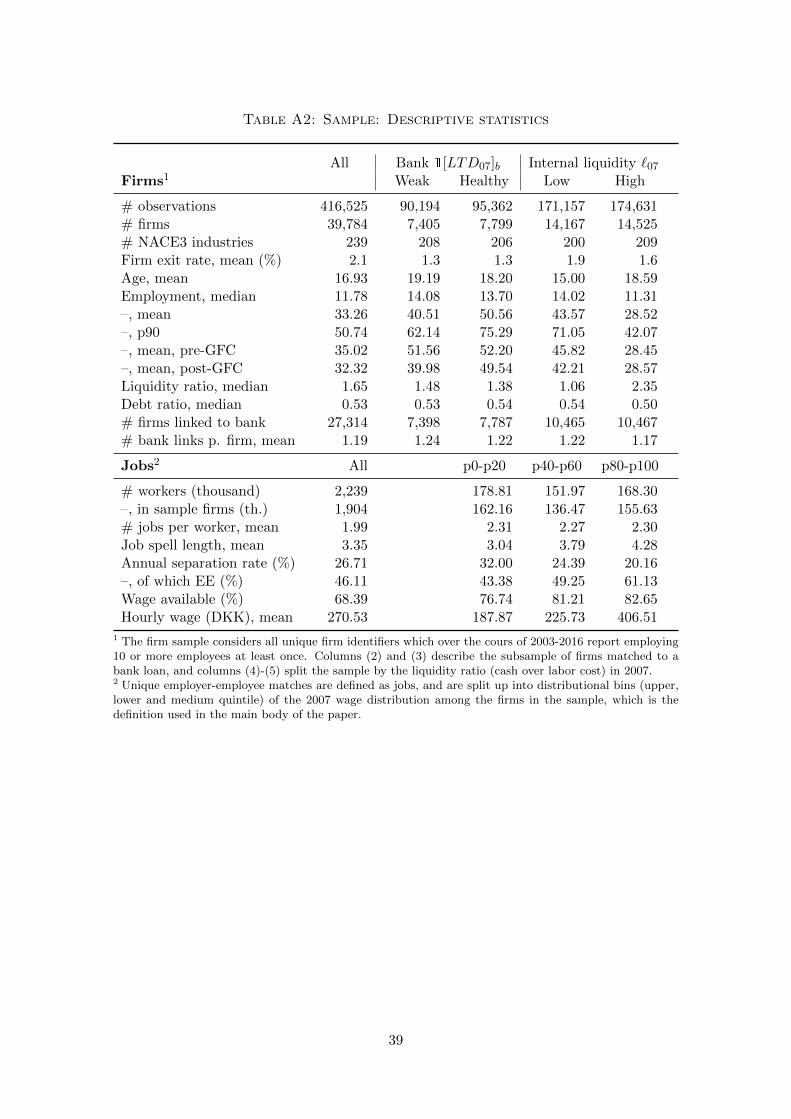
Table A2: Sample: Descriptive statistics

All Bank 1[LTD07]b Internal liquidity `07Firms1 Weak Healthy Low High

# observations 416,525 90,194 95,362 171,157 174,631# firms 39,784 7,405 7,799 14,167 14,525# NACE3 industries 239 208 206 200 209Firm exit rate, mean (%) 2.1 1.3 1.3 1.9 1.6Age, mean 16.93 19.19 18.20 15.00 18.59Employment, median 11.78 14.08 13.70 14.02 11.31–, mean 33.26 40.51 50.56 43.57 28.52–, p90 50.74 62.14 75.29 71.05 42.07–, mean, pre-GFC 35.02 51.56 52.20 45.82 28.45–, mean, post-GFC 32.32 39.98 49.54 42.21 28.57Liquidity ratio, median 1.65 1.48 1.38 1.06 2.35Debt ratio, median 0.53 0.53 0.54 0.54 0.50# firms linked to bank 27,314 7,398 7,787 10,465 10,467# bank links p. firm, mean 1.19 1.24 1.22 1.22 1.17

Jobs2 All p0-p20 p40-p60 p80-p100

# workers (thousand) 2,239 178.81 151.97 168.30–, in sample firms (th.) 1,904 162.16 136.47 155.63# jobs per worker, mean 1.99 2.31 2.27 2.30Job spell length, mean 3.35 3.04 3.79 4.28Annual separation rate (%) 26.71 32.00 24.39 20.16–, of which EE (%) 46.11 43.38 49.25 61.13Wage available (%) 68.39 76.74 81.21 82.65Hourly wage (DKK), mean 270.53 187.87 225.73 406.51

1 The firm sample considers all unique firm identifiers which over the cours of 2003-2016 report employing10 or more employees at least once. Columns (2) and (3) describe the subsample of firms matched to abank loan, and columns (4)-(5) split the sample by the liquidity ratio (cash over labor cost) in 2007.2 Unique employer-employee matches are defined as jobs, and are split up into distributional bins (upper,lower and medium quintile) of the 2007 wage distribution among the firms in the sample, which is thedefinition used in the main body of the paper.

39

B Supporting empirical results and robustness checks

B.1 Further results and robustness on firm-level outcomes

B.1.1 Other firm-level outcomes

The following graphs complement Figure 6 by repeating the difference-in-difference regres-

sion with other firm-level variables. The treatment is defined as having a pre-crisis lending

relationship with a bank that, in 2007, has a loan/deposit ratio larger than the median

across banks, and is thus highly exposed to the money market freeze during the financial

crisis.

Figure A3: DiD regression results: Other firm-level outcomes

(a) New hires (b) Separations

(c) Profits (d) Liquidity

Note: The black line represents difference-in-difference estimates of a negative credit supply shock,measured by the weighted loan/deposit ratio of a firms’ banks in 2007. The left-hand side variables arethe log of all new matches observed since November of the previous year (panel (a)) and the log of numberof employees that were previously employed but no longer work at that firm (panel b). Panel (c)/(d)depict regression results using the symmetric growth rate of profits (where the highest and lowest 5% ofthe data are winsorized) and log liquid assets, respectively. The grey bands represent 95% confidenceintervals of the point estimate. Standard errors are clustered at the firm level.

40

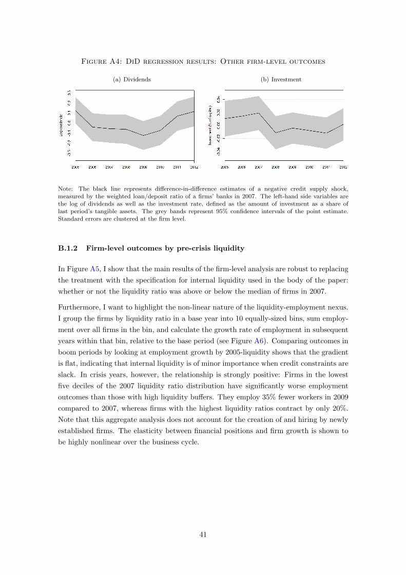
Figure A4: DiD regression results: Other firm-level outcomes

(a) Dividends (b) Investment

Note: The black line represents difference-in-difference estimates of a negative credit supply shock,measured by the weighted loan/deposit ratio of a firms’ banks in 2007. The left-hand side variables arethe log of dividends as well as the investment rate, defined as the amount of investment as a share oflast period’s tangible assets. The grey bands represent 95% confidence intervals of the point estimate.Standard errors are clustered at the firm level.

B.1.2 Firm-level outcomes by pre-crisis liquidity

In Figure A5, I show that the main results of the firm-level analysis are robust to replacing

the treatment with the specification for internal liquidity used in the body of the paper:

whether or not the liquidity ratio was above or below the median of firms in 2007.

Furthermore, I want to highlight the non-linear nature of the liquidity-employment nexus.

I group the firms by liquidity ratio in a base year into 10 equally-sized bins, sum employ-

ment over all firms in the bin, and calculate the growth rate of employment in subsequent

years within that bin, relative to the base period (see Figure A6). Comparing outcomes in

boom periods by looking at employment growth by 2005-liquidity shows that the gradient

is flat, indicating that internal liquidity is of minor importance when credit constraints are

slack. In crisis years, however, the relationship is strongly positive: Firms in the lowest

five deciles of the 2007 liquidity ratio distribution have significantly worse employment

outcomes than those with high liquidity buffers. They employ 35% fewer workers in 2009

compared to 2007, whereas firms with the highest liquidity ratios contract by only 20%.

Note that this aggregate analysis does not account for the creation of and hiring by newly

established firms. The elasticity between financial positions and firm growth is shown to

be highly nonlinear over the business cycle.

41

Figure A5: DiD regression results: By 2007 liquidity ratio

(a) Employment growth (b) Average nominal wage

(c) New hires (d) Separations

(e) Dividends (f) Investment

Note: The black line represents difference-in-difference estimates where the treatment group consists ofall firms with a ratio of liquidity to lagged fixed cost below the median of their 3-digit NACE industry.The left-hand side variables are the annual symmetric growth rate of employment (since November of theprevious year, panel (a)) and the average annual wage paid at the firm in the respective year (panel b).Further included are the log of all new matches observed since November of the previous year (panel (c))and the log of number of employees that were previously employed but no longer work at that firm (paneld). Panel (e) depicts regression results using the log of dividends as the dependent variable and panel(f) is for investment. The grey bands represent 95% confidence intervals of the point estimate. Standarderrors are clustered at the firm level.

42

Figure A6: Liquidity and employment growth: A non-linear relationship

Note: Growth rates of employment relative to a base year in all firms within a decile of liquidity ratio inthe base year. The used liquidity ratio is the stock of cash as a share of previous labor cost.

43

Chapter 2

The extensive and intensive margin of price

adjustment to cost shocks: Evidence from

Danish multiproduct firms

44

The extensive and intensive margin of price adjustment to

cost shocks: Evidence from Danish multiproduct firms

Luca Dedola∗ Mark Strøm Kristoffersen† Gabriel Zullig‡

Abstract

This paper studies price adjustment in a novel monthly dataset of individual product pricesof multiproduct firms, merged with firm-level balance sheet and cost data. The theoreticalliterature on price setting has pointed out that the interdependence between the decision towhether or not change prices (the extensive margin) and the actual amount by which priceschange (the intensive margin) contributes to determine the real effects of monetary policy.We estimate the adjustment to shocks to firm-level import costs and energy costs (due tooil supply shocks) along extensive and intensive margins, modelling them jointly to addressendogenous selection bias due to state-dependent pricing. In the first step, we estimate theprobability of price changes over horizons from 1 to 24 months (extensive margin) usinga multinomial logit model. There is evidence of synchronization of adjustment decisionswithin firms, especially as the number of goods increases, in line with price-setting modelsof multiproduct firms. We find evidence of state dependence as the probability of priceadjustment over time is affected by cost shocks, but also by aggregate variables suchas inflation and exchange rates. Using first-step estimates to correct for selection bias,similarly to Heckmans classic approach, we find that state-dependence translates onlyinto a small bias in the intensive margin conditional on price adjustment. Moreover, pass-through of energy and import cost shocks is quite heterogeneous across sectors and firms.Gradual adjustment to energy costs mainly reflects faster price responses in intermediateand energy intensive sectors, in line with pipeline pressures along the supply chain. Forimport-cost shocks, pass-through of larger firms with more products is lower than thatof smaller firms with fewer products. Since the latter shocks have a much smaller effecton competitors’ prices than shocks to energy costs, our findings are consistent with thepresence of strategic complementarities in price setting.

JEL classification: D22, E31, F41

Keywords: producer prices, cost shocks, nominal rigidities, strategic complementarities

∗European Central Bank, CEPR†Fagbevægelsens Hovedorganisation‡University of Copenhagen, Danmarks NationalbankWe are grateful to Kim Abildgren, Fernando Alvarez, Guido Ascari, Saroj Bhattarai, Antoine Bouet,Olivier Coibion, Wouter Den Haan, Timo Haber, Sebastian Heise, Francesco Lippi, Morten O. Ravnand Joseph Vavra for helpful comments and discussions. Furthermore, we thank participants at theEconometric Society Winter Meeting 2019, the ECB conference on Inflation in a Changing EconomicEnvironment, the conference on Alternative Datasets for Macro Analysis and Monetary Policy at BocconiUniversity, the 1st NuCamp Virtual PhD Workshop, as well as seminar participants at DanmarksNationalbank and the Universities of Bordeaux and Copenhagen for helpful comments and suggestions. Wewould also like to thank Janni Stavad and Nicklas Elversøe from Statistics Denmark for their substantialhelp and effort regarding the Danish PPI data. The views expressed in this paper do not necessarily reflectthe views of the European Central Bank or Danmarks Nationalbank. All remaining errors or omissionsremain our own.

45

1 Introduction

Price adjustment by firms is lumpy: individual good prices alternate between long spells

in which they are unchanged, and large but also small increases and decreases, largely

idiosyncratic, in “reset”prices. State-of-the-art macro models of price setting by firms

stress the relevance of lumpiness and heterogeneity in shaping aggregate inflation deter-

mination. Specifically, the theoretical literature on price setting has pointed out that

the interdependence between the decision to whether or not change prices (the extensive

margin) and the actual amount by which prices change (the intensive margin) contributes

to determine the real effects of monetary policy. Menu costs models of multiproduct firms

have been shown to be able to generate empirically plausible real effects of monetary

policy because of within-firm price synchronization (Alvarez and Lippi, 2014) or many

small cost shocks (Midrigan, 2011); this is particularly so when they also feature some

degree of time-dependence in price changes (Alvarez et al. (2016)). These mechanisms

attenuate “selection bias ”due to the interaction between the extensive and the intensive

margin of price adjustment under menu costs, namely that the prices which are more likely

to change are those farther from their desired level, so that reset prices display large(r)

changes. Microeconomic evidence on actual price decisions of multiproduct firms is thus

crucial to understand the monetary transmission and aggregate inflation determination.

This paper studies price adjustment in a novel monthly dataset of prices of multiproduct

firms, merged with firm-level balance sheet and cost data, including monthly wages and

intermediates. Specifically, we use monthly producer price micro data from the dataset

that is used to compute the producer price index (PPI) by the Danish statistical office.1 A

crucial feature of the data that makes it relevant to an analysis of pricing by multiproduct

firms is that there is substantial variation in the number of goods across more than 1,000

firms. This allows us to study how price-setting features vary with the number of goods.

Moreover, PPI micro data are especially useful to analyze in light of the above literature,

as noted already by Bhattarai and Schoenle (2014), since they are consistent with the basic

assumptions of virtually all price-setting models in macroeconomics, where it is producing

firms that set prices (rather than retailers whose prices are comprised in the CPI). A

similar analysis of producer pricing decisions is not feasible with CPI data since the CPI

sampling procedure maps to stores, so-called “outlets”, which may sell goods from any

number of firms, including imports. This makes pricing a complicated web of decisions

that involves the whole distribution network. Moreover, it is generally also not possible

to identify the producing firms for specific CPI items. In contrast, a further advantage of

1See Nakamura and Steinsson (2008) for a description of the U.S. PPI data; PPI microdata of otherEuropean countries were analyzed in Vermeulen et al. (2012).

46

our dataset is that we can link prices to balance sheet and cost data at the firm level.2

We first document key descriptive properties of price dynamics across firms, finding that

these statistics are broadly invariant to the number of goods firms produce, in contrast

with the predictions in multiproduct firm models with menu costs common across goods.

However, we show that the (unconditional) size distribution of price changes is quite

leptokurtic and thus similar to that generated by multiproduct firm models when they

also allow for some degree of time dependence along with menu costs. Remarkably, we

find that firm-level variable costs are similarly leptokurtic, with a large proportion of very

small cost changes, in line with assumptions in the models of Midrigan (2011) and Karadi

and Reiff (2019).

Second, we exploit the richness of our dataset to estimate the pass-through of cost shocks

along extensive and intensive margins, modelling them jointly to address endogenous

selection bias due to state-dependent pricing decisions. Specifically, it is possible to show

that in the general class of state-dependent pricing models studied by Alvarez and Lippi

(2019), selection bias conditional on changing prices in response to a permanent cost

shock is lower, the higher the degree of time-dependence in the decision to change prices.

In order to address and estimate selection bias, we rely on econometric techniques from

labor economics, adapting them to a dynamic setting to estimate the impulse responses

to shocks to energy costs (due to oil supply shocks) and to firm-level import costs using

local projections.

In our first step, we model the probability of price changes over horizons from 1 to 24

months (extensive margin), by using a flexible multinomial logit model, after Bourguignon

et al. (2007). We find that there is evidence of synchronization of adjustment decisions

within firms, especially as the number of goods increases. Namely, within a multiproduct

firm the probability that a given price increases is larger, the larger the fraction of other

prices that are decreasing. We also find evidence of state dependence as the probability

of upwards and downwards adjustment over time is affected by our cost shocks, but also

by aggregate variables such as CPI inflation and even exchange rates.

Concerning the intensive margin conditional on price adjustment, we find that state-

dependence does not translate into a strong selection bias. Carlsson (2017) has already

shown that the elasticity of marginal cost changes on the probability of changing prices is

an order of magnitude lower in the data than expected in a canonical menu-cost model.

While those probabilities do react to our measures of shocks to marginal costs, they do not

translate into disproportionate responses of reset prices when we estimate the intensive

margin of pass-through.

2A second advantage of PPI micro data, relative to consumer prices, is that they contain very few “sales”prices (namely very short-lived price changes that are quickly reverted, see e.g. Bils and Klenow (2004)and Nakamura and Steinsson (2008)). For this reason, PPI microdata do not necessitate any necessarilyad-hoc “filtering” to make them amenable to interpretation through the lens of standard price settingmodels. This is especially useful in econometric analyses like ours (we confirm this feature in our datasetbelow).

47

Moreover, pass-through of shocks to import and energy costs is quite heterogeneous across

sectors, and firms of different size, respectively. These findings support menu cost models

with imperfect price change synchronization, but also other sources of attenuation in selec-

tion such as time dependence and/or predominantly small (unobserved) shocks. Namely,

since our shocks to energy and import costs are well approximated by random walks,

strong selection would imply that OLS estimates of price impulse responses conditional

on adjustment should converge from above to their medium run values, when nominal

rigidities are less important. They should also be above the impulse responses estimated

by our two steps procedure that corrects for selection bias using estimates from the discrete

choice first step. Instead, we find that impulse responses to both shocks do not overshoot

in the short run.

Price adjustment to energy cost shocks is gradual over time, consistent with incomplete

pass-through within a year (Ganapati et al., 2020). This gradual adjustment mainly

reflects sectoral heterogeneity of the position in the supply chain and the intensity of direct

and indirect use of energy, with faster price adjustment in intermediate sectors and sectors

highly intense in energy both directly and indirectly. These results provide novel micro-

based evidence on the debate about the propagation of idiosyncratic and more common

shocks to aggregate inflation (see e.g. Boivin et al. (2009)). Firm-specific import cost

shocks elicit a faster adjustment than energy cost shocks, whose effects instead gradually

build up through different sectors along the supply chain, in line with pipeline pressures

(see e.g. Smets et al. (2018) or Duprez and Magerman (2019)). Finally, concerning

firm heterogeneity, for import cost shocks we find that pass-through of larger firms with

more products is lower than that of smaller firms with fewer products. Given their

idiosyncratic nature, the latter shocks have a much smaller effect on competitors’ prices

than energy costs, implying that our findings are consistent with the presence of strategic

complementarities in price setting.

The rest of the paper is organized as follows: Section 2 describes our datasets (while

details are relegated to the appendix) and presents key descriptive statistics on price

changes, where we focus on the multiproduct dimension of firms. Section 3 explains the

method we use to estimate structural pass-through coefficients in a way that accounts for

both sticky prices and strategic complementarities. Section 4 discusses the results of our

empirical analysis of two (random walk) cost shocks: a oil supply shock to energy costs,

as well idiosyncratic import cost shocks at the firm level.

2 Data and descriptive statistics

Before turning to our investigation of price adjustment in response to structural cost

shocks, we find it useful to provide a description of our dataset. The main part of the

data we compile consists of the confidential microdata underlying the Danish producer

48

price index from 1993 to 2017. In our analysis, we will leverage the fact that we can

link the producer price data to high-frequency statements on sales and cost, as well

as the degree of competition in the market the good is sold. By the same token, we

report common descriptive statistics on unconditional price adjustment in our dataset of

multiproduct firms, following Bhattarai and Schoenle (2014). However, in contrast to

the latter paper, we find that across Danish firms with different numbers of goods there

are very few differences in aggregate statistics on price adjustment, such as frequency,

size, direction, and dispersion of price changes. These findings are consistent with some

specifications of the fixed costs of changing prices at the firm level in Alvarez and Lippi

(2014) and Bonomo et al. (2019), where those costs increase with the number of price

changes, rather than being constant across them.

2.1 Producer prices

The Danish PPI contains monthly price quotes of actual transactions for 558 products,

that is, particular items define by 8-digit codes according to the Harmonized Commodity

Description and Coding Systems (HS). At the firm-good level, we track 5,354 goods for

both domestic sales and exports. The most important firms within selected areas are

requested to report prices in order to ensure that the producer price index covers at least

70% of Danish production. Appendix A describes the multi-stage sampling design.

This is the first paper that uses this dataset for the analysis of price rigidity. Therefore,

and to benchmark moments of the data against the U.S. PPI more commonly used in

the literature, we first document key characteristics of the panel.3 Note that we do not

observe quantities, so we use equal weights of goods within firms and categories wherever

needed.

2.1.1 Multiproduct firms

The PPI data allow us to identify firms according to the number of goods they produce.

Using the firm identifier, we are able to determine the number of goods reported by a

firm in a given month, and to the extent that this is representative for the total number

of goods produced, put special emphasis on multiproduct firms in the analysis. Following

Bhattarai and Schoenle (2014), we then allocate the firms to five groups according to the

mean of products reported over the sample period.

Table 1 presents descriptive statistics on the distribution of firms and products across

these groups. The cutoffs used on the mean number of products reported are 1, 3, 5, and

3Two key differences relative to the U.S. PPI data used in the literature are that first, Danish PPI pricesare collected at the firm/enterprise level rather than the establishment level (“price-forming units” usuallydefined to be “production entities in a single location”, by the BLS); and second, that both domestic andexport prices are reported. Both features of the data imply that relying on the U.S. PPI micro data mayactually lead to underestimating the number of products at the firm level.

49

Table 1: Summary statistics by number of products

All 1 1-3 3-5 5-7 7+

No. of firms 942 92 449 200 118 83Mean employment (FTE) 630.5 76.4 168.4 259.2 249.3 1601.8Median employment (FTE) 161.5 44.1 62.4 134.9 146.8 534.9Mean employment per good 70.5 76.4 66.6 63.5 44.2 96.6Median employment per good 32.9 44.1 25.1 34.1 24.9 51Mean age (years) 33.5 31.5 29.6 34.1 32.0 37.5Median age (years) 29.0 28.0 28.0 31.0 26.0 32.0

Share of total prices 100.0 1.3 20.5 22.2 18.5 37.5Mean no. of products 9.0 1.0 2.7 4.1 5.8 19.4Std. err. no. of products 12.9 0.0 0.5 0.6 0.5 18.625th percentile 3.0 1.0 2.5 3.6 5.4 8.8Median 5.1 1.0 3.0 4.1 5.8 11.675th percentile 8.7 1.0 3.0 4.6 6.0 16.9

Mean adj. freq. acr. goods 20.6 22.6 18.4 20.3 16.4 24.2Median adj. freq. acr. goods 8.0 8.1 6.1 8.0 7.1 10.0Mean adj. freq., median good 17.9 22.1 17.6 18.5 14.2 18.9Median adj. freq., median good 7.0 8.0 6.3 7.7 6.8 8.8Mean fraction of increases 68.0 67.7 67.6 67.5 70.8 67.6

Mean abs. size of price adj. 6.2 5.8 6.6 5.5 6.1 7.1Increases only 6.0 5.7 6.3 5.4 5.7 6.6Decreases only 7.4 6.0 7.2 7.8 7.3 8.2

Kurtosis 4.9 4.5 5.0 4.9 5.0 4.8

Note: Summary statistics on distribution of firms and prices across distinct bins of the average number ofproduct reported between January 2008 and December 2017. Frequencies are reported in % per month,and computed as in Bhattarai and Schoenle (2014): Take the mean of adjustment frequencies at the goodlevel, then compute the median frequency of price changes across goods in a firm. Finally, we report themean and median across firms in a given subsample. Fractions are reported in percentages. We reportprice change statistics by broad economic categories in the data appendix.

7. The product dispersion is comparable to that in the US PPI dataset, with the exception

that the dispersion of firms with the most product is higher in our data. Observe that the

Danish data contains 1,140 firms, compared to more than 28,000 in the U.S. PPI.

The table also shows that while the majority of firms, around 80%, fall in bins 1 to 3,

firms in bins 4 and 5 produce more goods, so that they account for a much larger share

of prices than of firms. Firms in bins 4 and 5 set around 50% of all prices in our data,

again comparable with U.S. data. The distribution across bins is robust to only including

goods sold in the domestic market. When grouping the firms according to the number of

domestic goods they sell, goods of firms with up to 3 products represent a larger share

of our sample, but prices set by firms with 5 or more products still make up 40% of the

dataset.

Finally, regarding firm size, the table reports two statistics, mean and median employment

50

at the firm level, where mean employment is defined both at the firm level and as

employment per average number of goods per firm. Clearly, in line with the results in

Bhattarai and Schoenle (2014), firms producing more goods do not have more employees

per good, but they are overall larger than firms producing fewer goods.

2.1.2 Frequency of price adjustment

Our price observations are actual transaction prices. We can therefore decompose price

changes into an extensive margin of price increases/decreases and their size and thus assess

the degree of price stickiness.

We first compute frequencies as the mean fraction of price changes during the life of

a good. For exported goods, we define as a price change if both the value in Danish

kroner and in the currency in which the price is reported change, if the two differ.

Also, we do not explicitly take into account issues of left-censoring of price-spells. For

our purpose, it is most relevant that we apply our method consistently across all firms.

The mean adjustment frequency across all goods for the subsamples are depicted in the

third panel of table 1. The mean (median) adjustment frequency in the sample is 20.6%

(8.00%), corresponding to a median implied duration of a price spell of 12 months. Price

adjustments are therefore slightly less frequent than in the U.S. PPI (10.8% in Nakamura

and Steinsson (2008)) but very close to euro area statistics Vermeulen et al. (2012).4

We further document that neither the frequency nor the size of price changes are a function

of the number of products produced. We proceed as in Bhattarai and Schoenle (2014)

and aggregate goods within multiproduct firms by taking the median of good-level price

change frequencies, and then report moments of the firm-level distribution in table 1.

While the levels are comparable to evidence from the U.S. PPI, there is no monotone

or statistically significant relationship between the number of goods produced and price

adjustment statistics. Further, we find that across all bins more than 67% of these changes

(over all non-zero price changes) are positive price changes. Firms thus adjust prices

upward with similar frequency independently of the number of goods they produce.5

Since we are interested in dynamic pass-through, we also report the unconditional fre-

quencies for cumulative price changes in Figure 1(a). It cumulates log price changes over

a period of up to 2 years and reports, for every month, the share of prices have increased

or decreased. The figure re-emphasizes the notion of price stickiness in the data: more

than 30% of price spells remain unchanged after 12 months, and 20% even survive at least

24 months.

4We find no evidence of systematic time variation of price stickiness, which could potentially haveimplications for the dynamics of aggregate inflation (Petrella et al., 2019).

5Two notable differences could explain this: First, the Danish PPI includes export goods, but conditioningon domestically sold goods only does not change this results qualitatively. Second, the U.S. PPI data isreported at the establishment level, whereas our data is reported by the firm.

51

Figure 1: Price adjustments: Frequency and size of price paths

(a) Frequencies of cumulated price changes (b) Absolute size of price changes by month

Note: (a) For every horizon k, this figure depicts the probability of having changed (increased ordecreased) the price between month 0 and k. (b) Conditional on price changes in period t, what isthe average path of the price during the following subsequent 5 months? Sales are defined as pricechanges that are fully reverted after 1-3 months.

2.1.3 Corrections

In relation to recent studies of price adjustment using CPI micro data from scanners at

retail stores, it is worth noting the following aspects of the Danish PPI data as regards

temporary sales and product replacements. First, while sales are important in the CPI

data as documented by Bils and Klenow (2004), Nakamura and Steinsson (2008), Berardi

et al. (2015) or to a lesser degree Wulfsberg (2016), they are not a major source of price

adjustments in the PPI data. In order to check the relevance of sales in our data, we

apply a sales filter similar to “filter B” in Nakamura and Steinsson (2008), where we

define as a “sale” every price decrease that is fully reverted after 1, 2, or 3 months. This

is the case for just 0.31% of all price observations or 3.5% of all price decreases. There

is instead no evidence of “reversed sales”, i.e. temporary price increases that are fully

reverted according to “filter B”. Figure 1(b) shows the average price index after price

increases, decreases without sales and the identified sales prices separately. Interestingly,

not only is the typical price decrease identified as a sale price much less persistent (by

construction) than the typical non-sale price decrease, but it is also smaller. Therefore, we

do not exclude sales prices from our analysis (but do control for them in our econometric

analysis).

Second, Nakamura and Steinsson (2008) also show that for aggregate statistics on price

changes, accounting for product substitutions can make a difference, especially in the

CPI. In our PPI dataset, product replacements are flagged with a counterfactual price

correcting for the replacement or quality adjustment. However, they are less important

since only 0.7% of all price changes (including zero changes) and 0.8% of all non-zero price

changes are due to product replacements.

52

Figure 2: Seasonality of frequency and size of price changes

(a) Frequency of price changes by month (b) Absolute size of price changes by month

Note: Mean frequency of price changes of firms per month of the year. Price changes (particularlyincreases) are most frequent in January, with local peaks at the first month of any quarter. Salesremain quantitatively minor and do not have a sesonal pattern different from regular price decreases.

2.1.4 Seasonality

We find a substantial seasonal component of PPI price changes, in striking similarity to

Nakamura and Steinsson (2008). Figure 2 presents the median frequency and the mean

absolute size of both price increases and decreases by calendar month – whereas results

for decreases are very similar whether we include or exclude sales. Four results stand out.

First, the frequency of price changes declines monotonically over the first three quarters,

and then is roughly constant. Second, in all four quarters, the frequency of price changes

is largest in the first month of the quarter and declines monotonically within the quarter

with the exception of September. This gives rise to the pattern of local peaks in the

frequency of price changes in January, April, July, and October. Third, price increases

play a disproportionate role in generating seasonality in price changes. Producer prices

are twice as likely to change and increase in January than on average in other months of

the year. Fourth, seasonality is much less apparent in the mean size of price increases and

decreases, and if anything follows a different pattern than in the price change frequency.

Mean price increases are not larger in the months at the beginning of quarters, when the

frequency is higher; price decreases are larger and more frequent in January.

Overall, these results suggest some time dependence of price changes, with possibly sig-

nificant implications for the transmission of shocks. Olivei and Tenreyro (2007) show that

the real effects of monetary policy in the U.S. differ depending on the quarter of the year

in which the shock hits. They argue that seasonality in the flexibility of wages can explain

their empirical findings. Our result that a disproportionate number of price increases

are recorded in January could point to similar effects in Denmark and also in the euro

area, where price are significantly more likely to adjust in January (Alvarez et al., 2006).

However, the size of price changes does not seem to be much larger in January, pointing

to other mechanisms beyond large seasonal changes in firms’ costs or demand.

53

Figure 3: Histograms of standardized price changes

Note: Price changes are the log difference in price, standardizedby good category (first two digits of the product HS code).Price changes equal to zero or smaller than 0.1% are discarded.A normal and Laplace distribution with unit variance aresuperimposed.

2.1.5 Size and distribution of price changes

The size of price changes is defined as the absolute log difference of monthly price obser-

vations, conditional on a price change. Again, we compute this at the good level, take the

median across goods in a firm, and then report the mean across firms. Table 1 (bottom

panel) shows that the typical price change observed is around 6.2%. Decreases tend to be

larger than increases. We do not find, however, that price changes vary by the number of

products sold by the firm.

In light of theories of price adjustment, we do not confirm empirical evidence of firm-level

menu cost such as Bhattarai and Schoenle (2014), needed to explain a large mass of small

price changes observed in the data. This excess kurtosis is a feature that is present in

the Danish PPI, as Figure 3 shows. To account for the heterogeneity across goods, we

standardize price changes by the 2-digit HS code level, and even exclude price changes

smaller than 0.1%, to account for possible measurement error (Alvarez et al., 2016). The

distribution of non-zero price changes has more mass around zero than would be implied

by a normal distribution. It’s kurtosis is 4.73 and thus closer to a Laplace distribution

(with a kurtosis of 6). Interestingly, these distributions can be well approximated by the

model with both random menu costs and firms with 4 or more goods studied in Alvarez

et al. (2016).

54

2.2 Firms

2.2.1 Competitors

As we will lay out below, firms’ pricing decisions are a function of their competitors prices

under imperfect competition. The 942 firms we include in the analysis compete on different

markets. We define competitors to be firms that sell products in the same 2-digit category

of the Harmonized System in the same month. 74 such product sectors are identified. The

average number of competing firms in each sector is 42, whereas the first/second/third

quantile of numbers of competitors for which we observe prices is 11/26.5/47. We will

refer to the geometric average of all known firms in the same product sector as the price

change of competitors.

Figure 4(a) illustrates the heterogeneity in the degree of competition across goods. We do

observe competitors’ prices even in the markets in which there is the least competition.

On the other end, 20% of goods are sold in markets where they compete against up to 10%

of all goods in the data. Furthermore, the dashed line underlines the network structure

of the producer price data: Because firms operate in more than one product sector, 30%

of products not only face direct competition from other firms in the same sector, but also

indirectly from firms operating in the same and other markets. Our data allows us to

analyze the strategic complementarities at play when cost shocks are transmitted through

supply chains.

2.2.2 Cost data

We merge the PPI survey to firm-level data on the cost structure of production using a

masked firm identifier. First, data from VAT filings contains information on nominal values

of total sales and exports, as well as the purchases of foreign and total intermediate inputs.

Second, we merge data from annual accounting statistics in Danish private-sector firms and

information on firm age and size from business registers. The accounting statistics gives

us a complete picture of all the firms’ cost structure at the annual frequency. Ultimately,

we have access to monthly payrolls the firm pays to all its employees. The availability

of the payroll data dictates the time span (2008-2017) used in the following econometric

analysis.

We measure variable costs as the sum of domestic and imported intermediate goods

purchased according to the VAT reporting, and the monthly wage bill. Comparing the

distribution of firms prices and variable costs is useful, as several theories show that the

latter are crucial to account for the aggregate effects of nominal shocks. Figure 4(b) thus

shows the standardized distribution of changes in variable cost with superimposed Normal

and Laplace distributions with unit variance. First, contrary to prices, there are very few

zero cost changes in our sample. Second, the distribution of cost changes is even more

55

Figure 4: Competition and cost shock distributions

(a) Competition intensity across goods (b) Histogram of standardized cost changes

Note: (a) To illustrate the degree of competition, we define 74 product sectors according to thefirst two digits of the HS code. We count the number of other goods and competing firms in thesame product sector for every good, and divide it by the total amount of goods and firms in thesample in the respective period. (b) Histogram of changes in variable cost measured as the sum oftotal intermediate purchases (domestic and import) at the monthly frequency. We exclude zero-costchanges and cost changes smaller than 0.01% in absolute value and superimpose a normal and Laplacedistribution with unit variance.

leptokurtic than the price distribution, with a larger incidence of small changes.

We focus on two different kinds of cost shocks, the first one with a predominantly idiosyn-

cratic component, i.e. a shock to firm-specific prices of imported inputs; the second one

with a predominantly common component across firms, namely oil supply shocks (which

we show directly affect the price of energy in Denmark, see Appendix A.3). To obtain

firm-level marginal cost, we interact the change in the respective input cost with the lagged

intensity of the firm’s cost structure in the respective input.

Import shares are computed using the VAT reports, by dividing the total value of imports

in a given month by total cost. The changes in import prices are directly observed in the

import wave of the PPI data. Since we do not observe product-level weights, we take a

geometric average of import cost changes (in Danish kroner) of all goods imported by the

firm in a given month. If the firm does not purchase abroad, we set this to zero.

Another shock to marginal cost we will consider is energy costs due to oil supply shocks,

which is more aggregate in nature. We obtain a firm-level shock by interacting the

(fitted) energy price in Danish kroner with the lagged share of energy in total cost. This

information is reported in the annual accounting statistics, and will measure the exposure

of the firm’s marginal cost to changes in energy prices. The energy share includes, apart

from the expenditure on refined oil and petroleum, also electricity and heating. While the

share of cost spent on energy is relatively small in the median firm, its price fluctuations

provide a source of aggregate shocks that are common across firms, but to which firms

have different direct exposure given by their energy intensity. We provide histograms of

the cost shares of imports and energy in data appendix A.2.2. To address concerns of

56

demand-side drivers of the price of energy, we regress the energy price changes on the

series of exogenous oil supply shocks provided by Baumeister and Hamilton (2019) and

use the fitted values as true shocks to the cost of energy.

3 Estimation of dynamic price adjustment under sticky prices

In this section we briefly review some useful theoretical results on lumpy price adjustment,

starting with the case when firm prices are fully flexible, and then looking at the case of

time- and state-dependent price stickiness. We use these results to guide our empirical

analysis.

3.1 Cost pass-through under price flexibility: Intensive margin

Let pijt be the log price of one (of possible many) good i in firm j. The general price setting

equation under imperfect competition for the (static) optimal (log) price p∗ijt postulates

that it is a function of a markup (µijt) over marginal costs (mcijt):

p∗ijt = mcijt + µijt, (1)

Under fairly general conditions, including separability of the firm-level demand for each

product, (Amiti et al., 2019, henceforth AIK) show that markups are a function of marginal

costs and competitors’ prices p−j,t, so that in first differences we obtain the following

pricing relation:6

∆p∗ijt =1

1 + Γ∆mcijt +

Γ

1 + Γ∆p−j,t. (2)

Marginal costs are generally unobservable, but under fairly general assumptions, AIK

show that they can be written as the sum of all variable input prices weighted by their

respective shares in total variable costs at the firm level, plus a product-specific cost

component. When assessing the pass-through of specific, observed cost shocks, they enter

equation (2) by taking a shock to a specific cost component, ∆ct, multiplied by its share

of total cost, φcjt. Controlling for competitors’ prices, this equation can be implemented

in a linear regression framework.7

6When the demand for goods produced by multiproduct firms is not separable and has a different elasticitywithin the firm than across firms, then the good-specific markup cannot be easily expressed as simply afunction of the prices of competitors of the same good. Conversely, the markup becomes a function ofthe sensitivity of the firm-specific demand for other goods, which in turn can be affected by competitors’prices in all these other markets.

7This approach has nevertheless the limitation that in computing ∆p−j,t we cannot easily measure pricesof foreign competitors (both for domestic prices and for export prices), so that the estimated 1

1+Γmay also

reflect to some extent the elasticity of foreign competitors’ prices to shocks to Danish imported inputs,for instance due to common suppliers in third countries.

57

3.2 Cost pass-through under price stickiness: Extensive and intensive

margin

Price pass-through of cost shocks may not be instantaneous for a variety of reasons. Re-

garding equation 2, this raises the following two observations. First, including unchanged

prices will bias the estimates downward. This bias is present under both time-dependent

and state-dependent pricing (e.g. Berger and Vavra (2019) formally show that the bias is

proportional to the frequency of adjustment). To be clear, zero price changes are crucial to

understanding aggregate inflation dynamics in response to cost shocks, but it is equally key

to precisely estimate how much firms change their prices conditional on adjustment. This

intensive margin is central to shed light on the role of real rigidities in price adjustment

separately from that of nominal rigidities. Therefore, a typical solution in the empirical

literature is to run pass-through regressions conditioning on non-zero price changes.

However, and this is the second observation, even conditioning on non-zero price changes

in general does not allow recovering the structural pass-through coefficients, in particular

under state-dependent pricing.8 In this case, the above pass-through regression is biased

by endogenous selection into optimally adjusting prices. Selection induces a positive corre-

lation between the observed cost shock, and any other unobserved good-level idiosyncratic

shock. To wit: in the standard menu cost model, the price of a good receiving a large

idiosyncratic shock of the same sign as the cost shock of interest is more likely to be

adjusted, other things equal. This selection bias is likely to be present at any horizon

t0 + k at which the probability that the price may not change is non-negligible, making

OLS estimates biased upward.

This can be formally shown using the analytical methods recently developed by Alvarez

and Lippi (2019) to solve for a broad class of state-dependent models with (random walk)

8Optimal price adjustment under time-dependent pricing is different from flexible prices in response to thesame shocks. For instance, assuming a constant markup, the optimal flexible price is given by:

p∗jt = const+ lnCjt;

but this coincides with the optimal reset price in the time-dependent Calvo model only when cost shocksare close to a random walk. As shown by Gagnon (2009), in a stationary equilibrium with zero inflationthe optimal reset price p∗jt in the Calvo model with idiosyncratic cost shocks is given by

p∗jt = const+ ln

∞∑s=0

(βζ)s exp

[ρsACjt +

1− ρ2sA

1− ρ2A

σ2u

],

where 1−ζ is the exogenous probability of adjusting prices, and idiosyncratic cost shocks Cjt are assumedlog-normal as follows:

Cjt = ln(Cjt/C

)lnCjt = (1− ρA) lnC + ρA lnCjt−1 + ut

ut ∼ N(0, σ2

u

)=> Cjt|Cjt−1 ∼ N

(ρACjt−1, σ

2u

), Cjt ∼ N

(0,

σ2u

1− ρ2A

).

Therefore the reset price is the same as under flexible prices only when ρA → 1, namely shocks are closeto a random walk.

58

idiosyncratic cost shocks. These (single-good) models flexibly encompass both the menu

cost model of Golosov and Lucas (2007) and the purely time-dependent Calvo model;

while in the former setting firms decide to change prices endogenously, in the latter the

probability of changing prices is determined by the exogenous parameter ζ. While we

relegate the details to the appendix, Alvarez and Lippi (2019) shows that in response to

a small permanent nominal cost shock δ at t0 = 0, in this class of models the cumulated

aggregate price change (including zero and non-zero changes) at t0 + k, P (k, δ) , could be

approximated as follows:9

P (k, δ) = δ

1−∞∑j=1

e−ζ[1+

(2·jπ)2

8φ

]·k 2

1 + (2·jπ)28φ

1− cosh(2√φ)

(−1)2·j/2

1− cosh(2√φ)

.

In the expression, the parameter φ ∈ (0,∞) determines how close the model is to Golosov-

Lucas (φ → 0) or to Calvo (φ → ∞), with intermediate values denoting an intermediate

degree of time-dependence. It is possible to show that in the Golosov-Lucas model the

solution is (see equation 27 in Alvarez and Lippi (2019):

P (k, δ) = δ

1−∞∑j=0

32

((2 + 4j)π)2e−N

((2+4j)π)2

8·k

,

where N is the average number (frequency) of price changes per period in the Golosov-

Lucas model; in the Calvo model we have instead

P (k, δ) = δ ·(

1− e−ζk),

so that setting N = ζ, the two models have the same frequency of price changes per unit

of time.

Defining with S (k, δ) the probability of survival of an unchanged price (= fraction of

unchanged prices as of k after shock δ), we can compute an approximation to cumulated

non-zero price changes between t0 and t0+k as the ratioP (k, δ)

1− S (k, δ). Clearly, in the Calvo

model S (k, δ) = e−ζk, independent of δ, so that

Calvo :P (k, δ)

1− S (k, δ)= δ.

Intuitively, averaging across exogenous non-zero price changes exactly retrieves the optimal

marginal price adjustment equal to the (random walk) cost shock δ, with no selection bias.

Price changes reflect both idiosyncratic shocks and δ, but the former are just a random

sample from their distribution across firms and thus wash out in the cross section.

In the Golosov-Lucas model we also have that S (k, δ) = S (k) is independent of δ for a

9The paper looks at a random-walk monetary policy shock which permanently increases marginal costs byδ.

59

small shock; non-zero cumulated price changes can be approximated as follows:

GL :P (k, δ)

1− S (k)= δ

1−∞∑j=0

32

((2+4j)π)2e−N

((2+4j)π)2

8 ·k

1+∞∑j=1

e−N((2j−1)π)2

8 ·k[

2(2j−1)π

(cos((2j−1)π)−1) sin(j·πion2 )] ≈ δ1− 32

(2π)2e−N

(2π)2

8·k

1− 4πe−N π2

8·k

,

where in the last expression on the right hand side we have focused on the first (dominant)

non-zero terms in the summations for simplicity. Clearly, the ratio on the right-hand side

is larger than 1, since

e−Nπ2

8·k >

2

πe−N

(2π)2

8·k,∀k ≥ 0;

this implies that averaging across non-zero state-dependent price changes overestimates

the correct marginal price adjustment to the cost shock δ because of endogenous selection

into price adjustment, for all horizons k.

Finally, we can approximate non-zero price changes for the intermediate case φ ∈ (0,∞),

obtaining (again focusing on the dominant term):

P (k, δ)

1− S (k)= δ

1−∞∑j=1

e−ζ[1+

(2·jπ)2

8φ

]·k 2

1+(2·jπ)2

8φ

1−cosh(2√φ)(−1)2·j/2

1−cosh(2√φ)

1+∞∑j=1

e−ζ[1+

((2j−1)π)2

8φ

]·k[

2(2j−1)π

(cos((2j−1)π)−1) sin(j π2 )]

≈ δ1− 2

1+(2π)2

8φ

1+cosh(2√φ)

1−cosh(2√φ)e−ζ[1+π2

2φ

]·k

1− 4πe−ζ[1+π2

8φ

]·k

.

For φ ∈ (0,∞), the ratio on the right hand side is larger than 1 but decreasing in φ, the

degree of state dependence. This implies that the selection bias falls with the degree of

state dependence.10

The conclusion is that it is important to take the extensive margin, the likelihood of

price changes, into account when estimating cost pass-through at different time horizons,

particularly in the short-run. Moreover, accounting for selection bias can provide direct

evidence on the significance of state-dependence in shaping price adjustment.

3.3 Selection-bias corrected estimation

To estimate cost pass-through taking into account the non-linear extensive margin of price

adjustment inducing selection, we propose the following two-step procedure, drawing from

10Formally:

1

πe−ζ[1+ π2

8φ

]·k>

4φ

2φ+ π2

1 + cosh(2√φ)

1− cosh(2√φ)e−ζ[1+ π2

2φ

]·k, ∀k ≥ 0.

Observe that for φ → ∞ the expressions do not exactly converge to those for the Calvo model, asexplained in Alvarez and Lippi (2019). Morever, the results here on selection bias obviously are tightlyrelated to the discussion in Section 5 in the paper on the selection effect.

60

the selection bias correction approach by Bourguignon et al. (2007).11 Specifically, in the

first step we model selection into price adjustment as a multinomial logit, while in the

linear projections in the second step we include a “bias correction ”based on the first step.

Consider the following local projection model of joint extensive and intensive margin of

price setting over horizons k = 0, ...,K :

r∗ij,m,t+k = γkmZij,t + ηij,m,t+k, m = −1, 0, 1 (3)

pij,t+k − pij,t−1 = βkXijt + uijt+k, m 6= 0

where r∗ is the (profit) outcome of a categorial variable m taking the value 1 if the price

increases between periods t and t + k. Maximizing firms choose to increase the price if

r∗1 > max(r∗m). Under the assumption that η are (cross-sectionally) independently and

identically Gumbel distributed, this leads to a multinomial logit model for each horizon k

(McFadden, 1973, Dubin and McFadden, 1984):

Pr (mij,t+k = 1, 0,−1 |Zijt ) = Φ(γkmZijt

)=

eγkmZijt

1 +∑

m eγkmZijt

. (4)

Observe that (3) assumes that coefficients γkm and βk are specific across outcomes m and

horizons k. In particular, this flexible specification implies that explanatory variables Zij,t

can have asymmetric effects at any horizon k on the probability of price hikes or cuts, so

that outcomes m are not ordered. However, we allow the intensive margin of price changes

to vary across horizons, but restrict it to be the same across outcomes.

The observation equation in (3) is the intensive margin of price adjustment conditional

on observing outcome m in the first step. Consistent estimation of the pass-through

coefficients βk requires additional restrictions because the error term u might not be

independent of all ηm, introducing correlation between explanatory variables and the

disturbance term in equations (3), as for instance implied by state-dependent pricing.

These restrictions are linearity assumptions on the dependence between the model residuals

(u, ηm). Variant 2 of the Dubin and McFadden (1984) approach does not restrict the

correlation between the error terms of the selection and linear projection step, but assumes

that the conditional expectation of the latter is a linear function of know convolutions of

the former, turning the second step estimation into

pij,t+k − pij,t−1 = βkXijt + λm∗µ(Prm∗) +∑m6=m∗

λm

(µ(Prm)

Prm(Prm − 1)

)︸ ︷︷ ︸

selection bias correction

1[m 6= 0] (5)

11The logic is similar to a Heckman (1979) bias-correction with more than two categorical outcomes in thefirst step. The literature has often relied on Tobit Type II to accomodate discreteness in price changes,but given the binomial restriction of its outcome variable, the model needs to be estimated twice (Berardiet al., 2015) to account for asymmetries in the probability of price increases and decreases. We arguethat our multinomial approach is better suited for this purpose, as the selection will be a bi-product ofestimating only one equation.

61

where µ are integrals over the individual observation probabilities from the multinomial

first step, computed numerically. Note that we exclude unchanged prices from the second

step altogether. The aim of the selection bias correction term in (5) is to correct the bias

induced by endogenous selection into these non-zero price changes.

4 Evidence on extensive and intensive margin of price ad-

justment

In the rest of this section we present evidence on the extensive margin, and then on the

intensive margin of price adjustment. We start describing variables we use in the vectors

Z and X. First and foremost, we include the cost shocks, given by φEjt−1∆pEt , the energy

share times the Danish price of energy projected over oil supply shocks, and φMjt−1∆pMjt ,

our measure of firm specific import costs. We also include the price change of competitors

at the good-level, ∆p−jt (constructed using the first two digits of the product in the PPI

database, for a total of 74 industries); the controls in firm-level cost, namely the change in

domestic and imported purchases over the last 3 months, total change in the wage bill; we

also control for the 3-month change in firm-level sales. We also include the monthly CPI

inflation rate and the change in the Danish nominal effective (trade-weighted) exchange

rate (NEER). Moreover, both Z and X include good-level dummies for exports, temporary

sales, product replacements which we identify as changes in the base price at resampling

as well as breaks (see Appendix A for details). We also control for the size of the firm by

including the log number of employees.

To identify the pass-through coefficients in β non-parametrically, we use exclusion re-

strictions, by including some variables only in the multinomial logit estimation step, while

excluding them from the second linear projection step, guided by theoretical considerations

from the literature on state-dependent price setting in multiproduct firms. Therefore,

among the regressors Zijt, we include the following covariates, which are then excluded

from the linear projections in the second step. First, we use the fact that most firms in our

sample sell many products whose prices we observe (see section 2.1.1). In line with Alvarez

and Lippi (2014) and Bhattarai and Schoenle (2014), we use the fractions of positive and

negative price changes within the same firm, excluding the price change of the good we are

trying to explain. Note that these fractions may be expected to have different influences

on the likelihood of increasing or decreasing prices, and our approach allows for that. We

also include the standard deviation of all price changes in the firm in the last 5 years, to

take into account that in our sample we have firms with only one reported product, and

the average of absolute price changes of goods in the same firm. Second, we include the

fraction of positive and negative price changes in the same industry at the 2-digit NACE

sector (excluding firm j), excluding the i-th good price. Furthermore, we include month

fixed effects (dummies) to let the seasonality in price adjustments help identify the model.

62

To sum up our main results, we find that shocks to energy costs and the cost of imported

inputs significantly affect the probability of changing firm-level prices; however, despite this

evidence in support of state-dependent pricing, selection bias, while statistically significant,

does not seem to be economically relevant. Moreover, conditional on changing prices,

estimated price adjustment is quite different across these two cost shocks, despite the fact

that both closely resemble random walks. Price adjustment to import cost is about one

third and well below one even after two years (similar to the unit labor cost shocks in

Carlsson and Skans (2012) and Hviid and Renkin (2020)), whereas the medium-run pass-

through of an energy price shock is significantly larger. These differences are accounted for

by the fact that shocks to energy costs have an economy-wide impact and diffuse slowly

through different sectors in the economy, while import cost shocks are largely idiosyncratic.

4.1 Shocks

Here we show the response of the marginal cost variables itself, as well as firm-level cost

measures to the shock in Figures 5(a) through 6(b).

4.1.1 Import cost shock

Panel 5(a) shows the response of firm-level import costs, and the right-hand side panel

shows the response of total domestic variable costs; the dark and light grey areas indicate

68% and 95% HAC robust confidence bands, where standard errors are clustered at the

firm level. Import costs are affected very persistently and their response is very similar to

a random walk, although after 12 months it settles on a level slightly below the impact

response. Conversely, the response of domestic variable costs, including wages, is not

statistically significant. On the basis of this cost dynamics, we would expect under time-

dependent Calvo pricing that firms changing their prices would do so by closely matching

the random walk dynamics in import costs. Under state-dependent pricing, firms changing

their prices earlier should do so by more than the increase in import costs, because of the

selection effect.

4.1.2 Energy cost shock

To clean changes in the price of energy from energy demand, we take series of oil supply

shocks estimated by Baumeister and Hamilton (2019) to proxy for changes in the price of

energy. The details are described in Section A.3 in the appendix. Effectively, we rescale

the BH series of oil supply shocks to have the same volatility as domestic energy prices.

We do this because, in our data, we observe energy shares of cost, rather than oil shares.

The left-hand side panel of Figure 6 shows the response of the cumulated price of energy

in Denmark times the firm-level energy share, and the right-hand side panel shows the

63

Figure 5: Import cost shock

(a) Shock (b) Domestic variable cost

Figure 6: Energy cost shock

(a) Energy price (b) Total variable cost

Note: Panels (a): Estimated coefficients of firm-level regressions of the cumulated 1 to kth lead of thecost share variable φc interacted with the input cost changes ∆P c on the contemporaneous shift-shareshock. Panels (b): of regressions of cumulative changes of domestic/total intermediate purchases fromVAT data on the same regressors. 95% (68%) confidence bands in (dark) grey.

response of total variable costs (i.e. wages plus domestic and imported intermediates);

the dark and light grey areas indicate 68% and 95% HAC robust confidence bands. While

the cumulated BH oil supply shocks follow a random walk by construction as they are

iid, also the response of the cumulated cost of energy at the firm level is very close to a

random walk. The implication is that we can interpret the oil supply shock as a shock to

Danish energy costs, with a high persistence similar to the shock to import costs. Thus,

on the basis of the energy cost dynamics, we would expect under time-dependent, Calvo

pricing that firms changing their prices would do so once and for all, closely matching the

random walk behavior of the cost. Under state-dependent pricing, firms changing their

prices earlier should do so by more than the increase in costs, because of the selection

effect. However, looking at the response of total variable costs in the right-hand side

graph, it is clear that the shock persistently affects also intermediates and wages, contrary

to the import cost shock. This pervasive response of all cost measures is important to

keep in mind when interpreting conditional price adjustment to this shock, since it implies

64

that firms in different positions in supply chains are likely to be affected by the shock at

different times, depending on the timing of the reaction of their suppliers. As we show

below, these “pipeline ”pressures are an important feature of the propagation of energy

costs to firms’ prices and inflation, in addition to the role of nominal and real rigidities.

4.2 The extensive margin of price adjustment and synchronization of

price changes

As we discussed in the previous section, in the first stage we estimate a multinomial logit

model of the following form:

Pr (mij,t+k = 1, 0,−1 |Zijt ) = Φ(γkmZijt

)=

eγkmZijt

1 +∑

m eγkmZijt

,

where mi,j,t+k is an indicator variable for positive, zero, or negative (log) price changes of

good i produced by firm j, cumulated between time t and t + k, with 0 as the base (no

price change) category. The logit model has the convenient property that the estimated

coefficients take on the natural interpretation of the effect of the explanatory variables on

the probability of adjusting prices up or down over taking no action.

To preview our results, the following stand out: First, there is substantial synchronization

of price changes within a firm which suggests a key role played by complementarities in

the cost of changing prices, especially as the number of goods increases. Specifically, we

find that, other things equal, the likelihood of an individual price cut (hike) rises with the

number of positive (negative) changes in the other prices within a firm, consistent with

common costs of changing prices. Second, there is substantially more synchronization of

individual adjustment decisions at the firm level relative to the industry. Third, we find

evidence for state-dependent pricing in response not only to the cost shocks of interest

(energy costs and the cost of imported inputs), but also more broadly to changes in

aggregate inflation and the effective exchange rate, and to competitors’ prices.

Table 2 shows the results of the multinomial logit model for the horizon k = 0, where

the top panel reports results for price hikes and the bottom panel for price cuts. We

report marginal effects on the change in the probability of adjustment, given one-standard-

deviation changes around the mean of Zij . We report results for all firms and by splitting

them in two groups according to the average number of their product (no more than 5

goods, and more than 5 goods, respectively).

A first key finding is that there is evidence of imperfect synchronization within the firm.

Specifically, the probability of raising (reducing) prices significantly increases with both

the fraction of positive and negative price changes. The fraction of positive and negative

price changes within the firm are especially large and significant across all columns. These

results are strongly consistent with synchronization in price changes because of both firm-

65

Table 2: Multinomial logit, first stage results

All 1-5 5+

Marg. effect on probability of price increaseFraction of pos. price changes in firm 6.33∗∗∗ 5.22∗∗∗ 7.83∗∗∗

(0.36) (0.21) (0.64)Fraction of neg. price changes in firm 2.56∗∗∗ 2.19∗∗∗ 2.67∗∗∗

(0.16) (0.11) (0.25)Fraction of pos. price changes in industry 0.15 0.46∗∗∗ 0.03

(0.14) (0.09) (0.13)Fraction of neg. price changes in industry −0.12 −0.25 −0.10

(0.07) (0.15) (0.06)Avg. price change in industry, excl. firm 0.14∗∗∗ 0.11∗∗ 0.11∗

(0.04) (0.04) (0.06)Energy price change x lagged energy cost share −0.11 −0.17 0.11

(0.15) (0.17) (0.20)Import price change x lagged import cost share 0.29∗∗∗ 0.50∗∗∗ 0.12∗

(0.07) (0.19) (0.06)CPI, log difference 0.57∗ 0.55 0.31

(0.25) (0.35) (0.33)

Marg. effect on probability of price decreaseFraction of pos. price changes in firm 2.36∗∗∗ 2.01∗∗∗ 2.48∗∗∗

(0.19) (0.13) (0.29)Fraction of neg. price changes in firm 3.95∗∗∗ 3.27∗∗∗ 4.99∗∗∗

(0.27) (9.18) (0.51)Fraction of pos. price changes in industry 0.02 −0.13 −0.00

(0.10) (0.11) (0.14)Fraction of neg. price changes in industry 0.14 0.59∗∗∗ 0.03

(0.15) (0.12) (0.12)Avg. price change in industry, excl. firm −0.14∗∗∗ −0.12∗∗∗ −0.138∗∗

(0.04) (0.03) (0.06)Energy price change x lagged energy cost share −0.24 −0.18 −0.26

(0.14) (0.15) (0.23)Import price change x lagged import cost share −0.31∗∗∗ −0.47∗∗∗ −0.16∗∗

(0.04) (0.11) (0.05)CPI, log difference −0.82∗∗∗ −1.08∗∗∗ −0.38

(0.29) (0.41) (0.36)

N 267670 126185 141485R2 0.40 0.44 0.38

Significance levels: ∗ p < 0.05, ∗∗ p < 0.01, ∗∗∗ p < 0.001Note: Marginal effects (in percentage points) on increasing and decreasing the price relative to not changingthe price. The variables of within firm and industry synchronization show the effect of a one standarddeviation change of the regressor around its mean; the other variables do so for a 1% change in the inputvariable. Columns (2) and (3) split the sample along the median number of products. Standard errors inparentheses. The change in firm sales and domestic purchases over the past quarter as well as the changein the hourly wage rate interacted with the labor share account for other firm-level cost components (notreported). Further controls: Log firm size, dummies for product replacement, sales, exported and energyproducts, the change in the nominal effective exchange rate, month fixed effects.

level shocks to marginal costs, for the fraction of similarly signed price changes, and

common costs of changing prices within the firm, for the fraction of opposite-signed price

changes. However, the former effect is twice than the latter for both price increases and

66

decreases. Nevertheless, the effect of price changes of the opposite sign within the firm

increases in a statistically significant way with the number of goods produced by firms, in

line with models with complementarities in the cost of changing prices.

Conversely, we find significant but quantitatively smaller evidence of synchronization at

the industry level. The probability of a positive (negative) price change decreases with

the fraction of negative (positive) price changes in the same industry, but it is in general

much less affected by the fraction of price changes with the same sign. This marginal effect

is of the opposite sign and an order of magnitude smaller than that for the within-firm

fraction of opposite signed price changes. This evidence seems consistent with common

shocks to marginal costs across firms rather than strategic complementarities, since it is

entirely driven by firms with fewer products. Synchronization in the likelihood of price

adjustment across firms is thus decreasing with the number of products, in contrast with

synchronization within firms.

The first row of Figure 7 reports marginal effects for the fraction of price changes in the

case of price hikes over selected horizons k. The left-hand side graph shows that both

marginal effects within the firm peak between 3-6 months and persist over time; this

persistence is in line with the model with multiproduct firms by Bonomo et al. (2019).

The marginal effects for the fraction of price changes across firms, shown in the right-hand

side graph, display a similar dynamics.

Our second sets of results speaks to a long-debated and important question in macroeco-

nomics, namely whether price setting is time-dependent or state-dependent. On the one

hand, we find that there is substantial time-dependence in the probability of changing

prices because of calendar effects, as already discussed in Section 2. Specifically, the

probability of a price increase is significantly larger in January, April, July and October,

than in other months, irrespective of the number of goods produced; conversely, the

seasonal pattern for price decreases is not statistically significant.

On the other hand, there is evidence in support of some degree of state-dependent pricing.

Consistent with standard menu cost models, not only is the probability of price hikes and

cuts increasing in its past volatility. Several time series also significantly and persistently

affect the probability of price changes over time. Specifically, a 1% increase (decrease) in

energy costs (φEjt−1∆pEt ), import costs (φMjt−1∆p

Mjt ), the aggregate CPI, the NEER and

competitors’ prices all significantly raise the likelihood of a price hike (cut), and reduce

the probability of a price cut (hike). As shown in the second row of Figure 7, which

reports these marginal effects over selected horizons, they build up over time and are very

persistent. CPI changes have the larger effect, implying that a 1% rise (fall) at its peak

after around 12 months significantly increases the probability of a price hike (cut) by

10% (5.3%). The marginal effects for a 1% rise (fall) in energy and import costs imply a

statistically significant increase in the probability of a price hike (cut) of 3% (3.5%) and

1% (0.5%), respectively.

67

Figure 7: Marginal effects on price increases at selected horizons k

(a) Within-firm synchronization (b) Industry synchronization

(c) Marginal cost shocks (d) Other state dependence

Note: Marginal effects of an increase in the following regressors on the probability of an increasein the price after k months. The regressors include the normalized share of positive and negativeprice changes at the firm level, excluding the good (panel a) and the equivalent share at the industrylevel excluding the firm (panel b). Panel (c) shows the elasticities of the shocks to marginal cost:energy and import price changes. Finally, panel (d) depicts the marginal effects on the probabilitiesof increasing the price after an increase in the CPI and competitor’s prices by 1%.

4.3 The intensive margin of price adjustment to cost shocks

In this section we report the results of the estimation in the second stage of the dynamic

pass-through conditional on price adjustment. We use local projections a la Jorda (2005),

where the dependent variable is the cumulated price change of product i of firm j from

period t to t+k, denoted ∆kpijt = pi,j,t+k − pi,j,t−1, conditional on it being non-zero over

this time interval. On the right-hand side, the cost shocks are given by φEjt−1∆pEt and

φMjt−1∆pMjt (in Danish kroner). We also include as controls the price change of competitors,

∆p−j,t, and the above mentioned controls for firm-level costs, namely: total change in

domestic purchases over last 3 months, total change in the wage bill, and the change

in total (domestic and exported) sales over last three months. We also include the

monthly CPI inflation rate and the change in the Danish nominal effective (trade-weighted)

exchange rate (NEER). Finally, we again control for the following set of firm/product level

time-invariant variables: the number of full-time equivalent employees and the number of

68

products in the year, as well as dummies for price replacement, sales, and export prices and

industry fixed effects at the 2-digit level.12 Finally, in line with our two-stage procedure to

take into account selection, following Bourguignon et al. (2007) we include “correction bias

”terms from the first stage estimation for each horizon t+k. Specifically, we use variant 2 of

the Dubin-McFadden approach, which does not restrict the correlation between the error

terms of the selection stage and linear projection stage, but assumes that the conditional

expectation of the latter is a linear function of known convolutions of the former. We

present first results for the shock to import costs and then for the shock to energy costs;

the former is a firm-level shock, while the latter has a much larger common component

across firms.

4.3.1 Price pass-through of firm-level import costs

Figure 8 presents three estimates of the price pass-through coefficient on import costs,

βMk , for each horizon k. The dashed black line shows OLS estimates of βMk including zero

and non-zero price changes, while the solid black line also shows OLS estimates of βMkincluding only non-zero price changes; the red line shows the estimates of pass-through

coefficients conditional on non-zero price changes from our two-stage procedure, for which

the grey areas indicate 95% HAC robust confidence bands.13 The following results emerge.

First, the immediate and very persistent increase in import costs brings about a similarly

persistent increase in prices, which are significantly affected even after 2 years, with all

three estimates basically stable after 12 months. However, OLS pass-through estimates

over zero and non-zero price changes display a more gradual adjustment to a (medium-run)

elasticity of around 0.2 over horizons after 15 months. The gradual price adjustment in

the first 12 months is entirely driven by price stickiness, but the low value of the medium-

run elasticity seems to point to an incomplete pass-through of the import cost shock

independent of nominal rigidities. This is confirmed by the OLS estimates conditional on

non-zero price adjustment, which are very close to those including zeros after 12 months.

Our evidence point to the existence of variation in mark-ups of the firms in our data

(Amiti et al., 2019). Second, OLS and bias-corrected point estimates are also very similar

over all horizons. Therefore, even though we find that the bias correction terms in the

second stage are significantly different from zero for all three categorial outcomes, the

state-dependence in the first stage does not translate into an economically large OLS bias.

Next, we try to better understand the reasons why the medium run pass-through seems to

be incomplete and much lower than 1. A first reason could be that by using the firm-level

import share we are introducing measurement error in the import share at the good level;

this could result in downward bias in our estimates. Nevertheless, results do not change

12Given their computational complexity in the multinomial logit step we do not include firm-level fixedeffects; we plan to explore their role in future revisions of the paper.

13Standard errors are clustered at the firm level and corrected for first stage uncertainty, the procedure ofwhich is described in Appendix B.

69

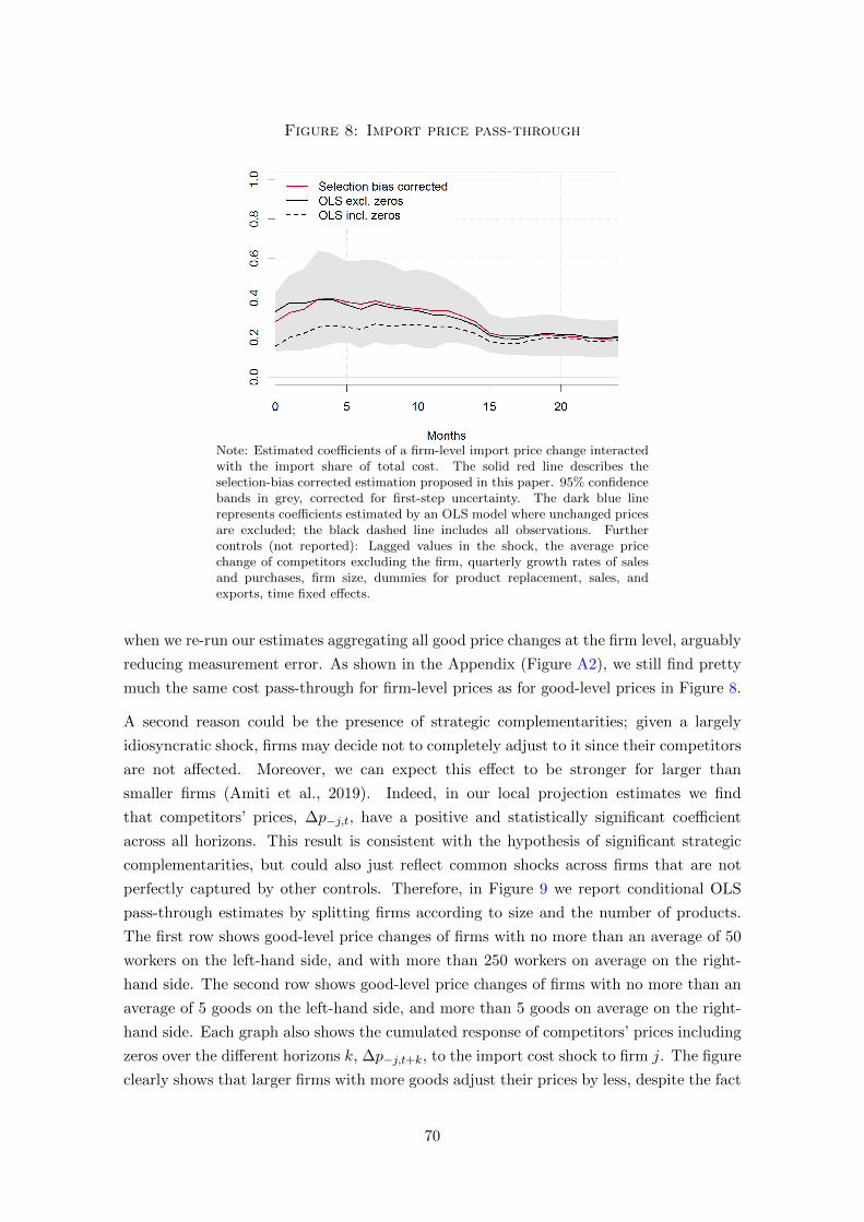
Figure 8: Import price pass-through

Note: Estimated coefficients of a firm-level import price change interactedwith the import share of total cost. The solid red line describes theselection-bias corrected estimation proposed in this paper. 95% confidencebands in grey, corrected for first-step uncertainty. The dark blue linerepresents coefficients estimated by an OLS model where unchanged pricesare excluded; the black dashed line includes all observations. Furthercontrols (not reported): Lagged values in the shock, the average pricechange of competitors excluding the firm, quarterly growth rates of salesand purchases, firm size, dummies for product replacement, sales, andexports, time fixed effects.

when we re-run our estimates aggregating all good price changes at the firm level, arguably

reducing measurement error. As shown in the Appendix (Figure A2), we still find pretty

much the same cost pass-through for firm-level prices as for good-level prices in Figure 8.

A second reason could be the presence of strategic complementarities; given a largely

idiosyncratic shock, firms may decide not to completely adjust to it since their competitors

are not affected. Moreover, we can expect this effect to be stronger for larger than

smaller firms (Amiti et al., 2019). Indeed, in our local projection estimates we find

that competitors’ prices, ∆p−j,t, have a positive and statistically significant coefficient

across all horizons. This result is consistent with the hypothesis of significant strategic

complementarities, but could also just reflect common shocks across firms that are not

perfectly captured by other controls. Therefore, in Figure 9 we report conditional OLS

pass-through estimates by splitting firms according to size and the number of products.

The first row shows good-level price changes of firms with no more than an average of 50

workers on the left-hand side, and with more than 250 workers on average on the right-

hand side. The second row shows good-level price changes of firms with no more than an

average of 5 goods on the left-hand side, and more than 5 goods on average on the right-

hand side. Each graph also shows the cumulated response of competitors’ prices including

zeros over the different horizons k, ∆p−j,t+k, to the import cost shock to firm j. The figure

clearly shows that larger firms with more goods adjust their prices by less, despite the fact

70

Figure 9: Import cost shock by firm size and number of products

(a) < 50 employees (b) > 250 employees

(c) < 5 goods (d) > 5 goods

Note: Red solid lines show estimated coefficients of price pass-through in response to a firm-levelchange in import prices interacted with the import share, conditional on that the price has changed.95% confidence bands in grey. The black line (and corresponding dashed error bands) show thechange in prices of firms competing in the same product sector. Firms are split in groups by theaverage number of employees or products reported throughout the sample.

that their competitors’ prices are in turn more affected by the shock. Pass-through in

firms with more goods is about one half of that in firms with fewer goods, and close to

the 0.2 estimate in Figure 8 pooling all firms; however, the estimated coefficients are still

far below 1 even for smaller firms.

Finally, Figure 10 shows that the selection bias is positive only for firms with less than

5 goods; this is consistent with the evidence of stronger synchronization in the extensive

margin and thus the multiproduct firm model of Alvarez and Lippi (2014). In this model,

the larger the number of products, the higher synchronization in price adjustment and the

lower the selection bias.

Summing up, we find evidence that in the case of idiosyncratic cost shocks, price adjust-

ment is subdued because of nominal rigidities in the short run, and real rigidities in the

medium run. Nominal rigidities do not result in a significant selection bias conditional on

changing prices, while real rigidities seem to reflect in part by strategic complementarities,

with the incomplete medium run pass-through mainly due to the behavior of larger firms.

71

Figure 10: Selection by number of products

(a) < 5 goods (b) > 5 goods

Note: Red solid lines show estimated coefficients of price pass-through in response to a firm-levelchange in import prices interacted with the import share, corrected for the bias induced by endogenousselection. 95% confidence bands in grey. The black solid (dashed) line shows the OLS coefficientsexcluding (including) unchanged prices. Firms are split in groups by the average number of productsreported throughout the sample.

4.3.2 Price pass-through of energy cost shocks

Next, we explore price adjustment to a shock to energy costs due to oil supply shocks.

Figure 11 presents as before three estimates of the price pass-through coefficients on

energy costs, βEk , for each horizon k. Again, the dashed, black line shows OLS estimates

of βEk including zero and non-zero price changes, while the solid black line shows OLS

estimates of βEk including only non-zero price changes; the solid red line shows the estimates

of pass-through coefficients conditional on non-zero price changes from our two-stage

procedure. The following findings stand out. First, despite the immediate and very

persistent increase in energy costs in Figure 6, prices increase only very gradually, from a

small and statistically insignificant level on impact, to around 0.5 after 6 months, and then

peaking close to 1 after 15 months. Remarkably, this is true regardless of the exclusion

of zero price changes or correcting for selection bias. Therefore, price stickiness seems to

play a smaller role in short-run price adjustment in the case of energy costs than import

costs. This is consistent with the fact that energy costs have larger effect on the extensive

margin of price adjustment in our first stage estimates, as shown above. Finally, even

though we estimate a medium-run pass-through coefficient of 1, we should keep in mind

that the oil-driven shock to energy costs persistently affects all variable costs. Therefore,

there can still be “real rigidities”in the intensive margin of price adjustment.

We next turn to investigating the reasons behind the gradual conditional adjustment in the

short run, including the role of strategic complementarities. We first explore the idea that

the gradual adjustment may be due to the slow transmission of the shock along the supply

chain, with up-stream sectors and sectors more exposed to energy (directly and indirectly)

reacting faster than downstream sectors and sectors less exposed to energy. Therefore, in

72

Figure 11: Oil price pass-through

Note: Estimated coefficients of an oil supply shock interacted with thefirm-level energy share of total cost. The solid red line describes theselection-bias corrected estimation proposed in this paper. 95% confidencebands in grey, corrected for first-step uncertainty. The dark blue linerepresents coefficients estimated by an OLS model where unchanged pricesare excluded; the black dashed line includes all observations. Furthercontrols (not reported): Lagged values in the shock, the average pricechange of competitors excluding the firm, quarterly growth rates of salesand purchases, firm size, dummies for product replacement, sales, andexports, time fixed effects.

Figure 12 we report conditional OLS pass-through estimates by splitting price changes in

those of upstream and downstream goods, and in those of sectors with a different exposure

to energy (which apart from oil and petroleum products includes electricity and heating).

Specifically, the first row shows price changes for intermediate and final goods, on the

left-hand side and right-hand side, respectively. The second row shows price changes for

goods in sectors with overall energy intensity below and above the median, on the left-

hand and right-hand side respectively. The overall energy intensity is calculated using

detailed input-output tables, taking into account the direct and indirect content of energy

through purchases of intermediates. Each graph also shows the cumulated response of

competitors’ prices including zeros over the different horizons k, ∆p−j,t+k, to the shock

to energy costs to firm j (i.e. shocked energy price interacted with the firm-level energy

share). The figure clearly shows that prices of intermediates and products with a higher

energy intensity respond much faster than those of final goods and products with lower

energy intensity. The former’s response is positive and statistically significant almost on

impact, while the latter’s becomes significantly positive well after 6 months (even 12 for

low exposure ones). Nevertheless, the response of prices of intermediates and products

with a higher energy intensity still builds up over time, peaking only after 12 months at

values that are significantly larger than those in the first few months. Moreover, medium-

run adjustment is very similar across goods, in line with the pervasive effects of the shock

73

Figure 12: price pass-through by SNA and energy exposure

(a) Intermediate goods (b) Final goods

(c) High oil exposure (d) Low oil exposure

Note: Red solid lines show estimated coefficients of price pass-through in response to an oil supplyshock interacted with the firm-level energy share, conditional on that the price has changed. 95%confidence bands in grey. The black line (and corresponding dashed error bands) show the changein prices of firms competing in the same product sector. Products are split by the UN classificationof HS codes into intermediate and consumption goods. In (c) and (d), firms are split at the medianbased on the energy intensity of the sector they operate in, drawn from input-output tables, i.e.taking into account the indirect exposure to energy through intermediate inputs.

on variable costs in Figure 6. Interestingly, competitors ’ prices display a similar dynamics

to that of individual prices across the different types of firms.

Finally, we report results by splitting firms by their size and number of goods, similarly

to Figure 9 above, in Figure 13. The key finding is that larger firms (with more products)

tend to have a more gradual adjustment than smaller firms (with fewer products) — even

though confidence bands are large. However, given that the shock is fairly common across

firms, there is little difference in medium-run price adjustment along these dimensions.

This result is again consistent with the presence of strategic complementarities, in line

with the lower medium run pass-through of the more firm-specific shocks to import costs

found above, as prices adjust more when competitors’ prices also adjust more.

Overall, we interpret the heterogeneity of those impulse responses in light of the different

natures of the two shocks examined. In the case of pure firm-level cost shocks, aggregate

price adjustment is subdued because of nominal rigidities in the short run, and real

74

Figure 13: Price pass-through by firm size and number of products

(a) < 50 employees (b) > 250 employees

(c) < 5 goods (d) > 5 goods

Note: Red solid lines show estimated coefficients of price pass-through in response to a firm-levelchange in import prices interacted with the import share, conditional on that the price has changed.95% confidence bands in grey. The black line (and corresponding dashed error bands) show thechange in prices of firms competing in the same product sector. Firms are split in groups by theaverage number of employees or products reported throughout the sample.

rigidities in the medium run. Mark-ups absorb a large part of cost shocks to firms in

competition with others, in order to retain market share. Interestingly, those competitors

react to firm j’s cost shock by increasing their markups only if j is large, and only to a

limited degree. If the shock is more common, the situation presents itself very differently.

While the medium-run pass-through is complete, firms allow the change in cost to fully

pass on to the producer price eventually, but the adjustment takes place over the course

of a year. A large part of this delayed response is driven by firms’ position in the supply

chain.14 For both shocks, however, the state-dependence we estimate in the first stage of

our methodology does not translate into economically meaningful selection biases of the

pass-through estimation.

14We are currently exploring other explanations and test, in particular, whether the staggered adjustmentcan be related to competitors’ adjustment.

75

5 Conclusions

This paper studies price adjustment in a novel monthly dataset of prices of multiproduct

firms, merged with firm-level balance sheet and cost data. The theoretical literature on

price setting has pointed out that the interdependence between the decision to whether

or not change prices (the extensive margin) and the actual amount by which prices

change (the intensive margin) contributes to determine the real effects of monetary policy.

Specifically, in standard menu costs models, firms change those prices that are most

misaligned and furthest from their optimal values, resulting in a selection bias that

attenuates monetary non-neutrality.

We exploit the richness of our dataset to estimate the pass-through of shocks to firm-level

import costs and energy costs (due to oil supply shocks) along extensive and intensive mar-

gins, modelling them jointly to address endogenous selection bias due to state-dependent

pricing decisions. We develop a novel, two-step estimation procedure that can identify the

interaction of both margins and estimate the structural pass-through estimation in light

of many nominal and real rigidities used in structural macroeconomic models.

In our first step, we model the probability of price changes over horizons from 1 to 24

months (extensive margin), by using a flexible multinomial logit model. We find that

there is evidence of synchronization of adjustment decisions within firms, especially as the

number of goods increases, consistent with models of multiproduct firms. We also find

evidence of state dependence as the probability of price adjustment over time is affected

by our cost shocks, but also by aggregate inflation and even exchange rates.

Using first-stage estimates to correct for selection bias, we find that state-dependence

however does not translate into a large bias in the intensive margin conditional on price

adjustment. Instead, we find that the pass-through of firm-level import cost shocks is

incomplete, i.e. that a large part of cost changes is absorbed by mark-ups. In contrast,

the medium-run pass-through of an energy price shock, which arguably is more common

across firms, is close to complete.

We argue that the heterogeneity of these responses is driven by the different nature of

shocks (and implied differences in strategic complementarities), and provide a range of

results that support this view. First, even though larger firms respond less to the change in

marginal cost, their competitors respond by (slightly) increasing their own prices, allowing

them to expand their own mark-ups. Second, the gradual adjustment to an energy cost

shock mainly reflects the firms’ position in the supply chain: Firms producing intermediate

goods and firms operating in sectors highly exposed to energy adjust their prices faster.

For all these classes of firms, nominal rigidities are muted, despite a high degree of

unconditional price stickiness observed in the data. We find the strongest evidence of

selection in firms producing only a small amount of goods, in line with the theory on

76

multiproduct firms. Furthermore, our findings are consistent with the presence of strategic

complementarities in price-setting.

Finally, our results provide micro-based evidence on the debate about the propagation of

idiosyncratic and common shocks to aggregate inflation, since firm-specific import cost

shocks elicit a faster adjustment than energy cost shocks, whose effects instead build up

through the supply chain in line with the pipeline pressure view.

References

Alvarez, F., H. Le Bihan, and F. Lippi (2016): “The Real Effects of Monetary Shocks

in Sticky Price Models: A Sufficient Statistic Approach,” American Economic Review,

106, 2817–2851.

Alvarez, F. and F. Lippi (2014): “Price Setting with Menu Cost for Multiproduct

Firms,” Econometrica, 82, 89–135.

——— (2019): “The Analytic Theory of a Monetary Shock,” EIEF Working Paper, 1910.

Alvarez, L. J., E. Dhyne, M. M. Hoeberichts, C. Kwapil, H. L. Bihan,

P. Lunnemann, F. Martins, R. Sabbatini, H. Stahl, P. Vermeulen, and

J. Vilmunen (2006): “Sticky Prices in the Euro Area: A Summary of New Micro

Evidence,” Journal of the European Economic Association, 4, 575–584.

Amiti, M., O. Itskhoki, and J. Konings (2019): “International Shocks, Variable

Markups and Domestic Prices,” The Review of Economic Studies, 86, 2356–2402.

Baumeister, C. and J. D. Hamilton (2019): “Structural Interpretation of Vector

Autoregressions with Incomplete Identification: Revisiting the Role of Oil Supply and

Demand Shocks,” American Economic Review, 109, 1873–1910.

Berardi, N., E. Gautier, and H. Le Bihan (2015): “More Facts about Prices: France

Before and During the Great Recession,” Journal of Money, Credit and Banking, 47,

1465–1502.

Berger, D. and J. Vavra (2019): “Shocks vs. Responsiveness: What Drives Time-

Varying Dispersion?” Journal of Political Economy, 127, 2104–2142.

Bhattarai, S. and R. Schoenle (2014): “Multiproduct Firms and Price-setting:

Theory and Evidence from U.S. Producer Prices,” Journal of Monetary Economics,

66, 178–192.

Bils, M. and P. J. Klenow (2004): “Some Evidence on the Importance of Sticky

Prices,” Journal of Political Economy, 112, 947–985.

77

Boivin, J., M. P. Giannoni, and I. Mihov (2009): “Sticky Prices and Monetary Policy:

Evidence from Disaggregated US Data,” American Economic Review, 99, 350–384.

Bonomo, M., C. Carvalho, O. Kryvtsov, S. Ribon, and R. Rigato (2019): “Multi-

Product Pricing: Theory and Evidence From Large Retailers in Israel,” mimeo.

Bourguignon, F., M. Fournier, and M. Gurgang (2007): “Selection Bias

Corrections Based on the Multinomial Logit Model: Monte Carlo Comparisons,”

Journal of Economic Surveys, 21, 174–205.

Carlsson, M. (2017): “Microdata Evidence on the Empirical Importance of Selection

Effects in Menu-Cost Models,” Journal of Money, Credit and Banking, 49, 1803–1830.

Carlsson, M. and O. N. Skans (2012): “Evaluating Microfoundations for Aggregate

Price Rigidities: Evidence from Matched Firm-Level Data on Producer Prices and Unit

Labor Cost,” American Economic Review, 102, 1571–1595.

Dubin, J. A. and D. L. McFadden (1984): “An Econometric Analysis of Residential

Electric Appliance Holdings and Consumption,” Econometrica, 52, 345–362.

Duprez, C. and G. Magerman (2019): “Price Updating in Production Networks,”

mimeo.

Gagnon, E. (2009): “Price Setting During Low and High Inflation: Evidence from

Mexico,” Quarterly Journal of Economics, 124, 1221–1263.

Ganapati, S., J. S. Shapiro, and R. Walker (2020): “Energy Cost Pass-Through in

US Manufacturing: Estimates and Implications for Carbon Taxes,” American Economic

Journal: Applied Economics.

Golosov, M. and R. E. Lucas (2007): “Menu Costs and Phillips Curves,” Journal of

Political Economy, 115, 171–199.

Heckman, J. (1979): “Sample Selection Bias as a Specification Error,” Econometrica,

47, 153–161.

Hviid, S. J. and T. Renkin (2020): “Labor Cost Pass-through to Producer Prices in

Denmark,” mimeo.

Jorda, O. (2005): “Estimation and Inference of Impulse Responses by Local Projections,”

American Economic Review, 95, 161–182.

Karadi, P. and A. Reiff (2019): “Menu Costs, Aggregate Fluctuations, and Large

Shocks,” American Economic Journal: Macroeconomics, 11, 111–146.

McFadden, D. L. (1973): “Conditional Logit Analysis of Qualitative Choice Behavior,”

in Frontiers in Econometrics, New York: Academic Press.

78

Midrigan, V. (2011): “Menu Costs, Multiproduct Firms, and Aggregate Fluctuations,”

Econometrica, 79, 1139–1180.

Nakamura, E. and J. Steinsson (2008): “Five Facts about Prices: A Reevaluation of

Menu Cost Models,” Quarterly Journal of Economics, 123, 1415–1464.

Olivei, G. and S. Tenreyro (2007): “The Timing of Monetary Policy Shocks,”

American Economic Review, 97, 636–663.

Petrella, I., E. Santoro, and L. de la Porte Simonsen (2019): “Time-varying

Price Flexibility and Inflation Dynamics,” mimeo.

Smets, F., J. Tielens, and J. V. Hove (2018): “Pipeline Pressures and Sectoral

Inflation Dynamics,” National Bank of Belgium Working Paper, 351.

Statistics Denmark (2017): “Documentation of statistics for Accounts Statistics for

Non-Agricultural Private Sector,” Tech. rep.

——— (2018): “Documentation of statistics for Purchases and Sales by Firms,” Tech. rep.

——— (2019): “Documentation of statistics for Producer and Import Price Index for

Commodities,” Tech. rep.

Vermeulen, P., D. Dias, M. Dossche, E. Gautier, I. Hernando, R. Sabbatini,

and H. Stahl (2012): “Price Setting in the Euro Area: Some Stylised Facts from

Individual Producer Price Data,” Journal of Money, Credit and Banking, 44, 1631–

1650.

Wulfsberg, F. (2016): “Inflation and Price Adjustments: Micro Evidence from Nor-

wegian Consumer Prices 1975-2004,” American Economic Journal: Macroeconomics, 8,

175–194.

79

Appendix

A Data

A.1 Producer price micro data

We use the confidential microdata underlying the Danish producer and import price index

for commodities compiled by Statistics Denmark. The raw data covers the time period

from January 1993 until June 2017. The producer and import price index for commodities

is based on approximately 6,400 prices at the firm-good level per month across 1,050

different commodities, reported by selected producers and importers in Denmark, see

also Statistics Denmark (2019). Approximately 3,500 prices are used for calculating the

producer price index, approximately 2,900 prices are used for calculating the import price

index. The most important firms within selected areas are requested to report prices in

order to ensure that the producer and import price index covers at least 70% of Danish

production and imports.

The population covers all commodities that are imported or produced in Denmark for the

domestic market or export, with the exception of some well-defined exemptions. Some

commodities are not included because the turnover is too small and some commodities

are not included because of the nature of the commodities.

Statistics Denmark undertakes great efforts to adjust for quality changes and product

substitutions so that only true price changes are measured. When a product is substituted,

Statistics Denmark re-computes the base price, and therefore we are able to identify

replacements. They constitute only 0.7% of all prices changes (including zero price

changes) and 0.8% of all non-zero price changes. We include these in the baseline results

we report, but control for identified product replacements in regressions.

Goods are defined relatively narrowly in our dataset, as products are classified using

the 8-digit combined nomenclature (CN). The first 6 digits of the CN codes correspond

to the World Harmonized System (HS). We address breaks in product classifications by

identifying changes in product codes within a firm which do not lead to a change in the

price. The vast majority of identified breaks coincides with the months where Statistics

Denmark re-defines product categories. The breaks constitutes only 0.04% of all price

changes (including zero changes), and per construction 0% of all non-zero price changes.

Similar to product replacements, we include these incidents in the baseline results we

report, but control for identified breaks in regressions.

The prices used for the index are actual prices, which means that the prices must include

all possible discounts. Therefore, list prices do not apply unless the prices never include

discounts. A distinction is made between the prices of imported commodities and the

80

prices of commodities for the domestic market or the export market:

• Imported commodities: Actual transaction prices (in some cases transfer prices) c.i.f.

excluding all duties and taxes on the goods as far as possible on the 15th day of the

month. For the firms reporting import prices, we calculate a firm-level import price

index using the equally weighted average log differences in each month.

• Danish commodities for the domestic market or export: Actual transaction price (in

a few cases transfer prices) ex producer excluding VAT and excise duties as far as

possible on the 15th day of the month.

One advantage of this data is the relatively long time spans during which we observe

uninterrupted price spells, allowing us to study dynamic pass-through at the good level.

On average, the price of a good is reported for 115 subsequent months. During the time

range we use in our pass-through analysis (2008m1-2017m6), a total of 5,354 product

spells (at the firm-good level) can be identified, 79% of which we observe for at least 2

subsequent years. 30% of good id’s can even be tracked along the entire sample of 9.5

years. Re-classification of products in January of 2009 (2014) leads to spikes in the exit

and entry rate of products of 30% (9%), which we do not link because we do not observe

quantities and are therefore unable to compute counterfactually weighted prices. In other

months, half of entry and exit of products is driven by firm re-sampling, whereas smaller

firms are re-sampled more frequently.

Products reported cover a broad set of goods representative of the Danish economy. The

manufacturing sector makes up more than 75% of firms in the data and even more in

terms of goods. The second largest industry is wholesale trading. Within manufacturing,

machinery, food products, fabricated metal, plastic and computer and electronics are the

most commonly found industries. We define sub-markets in terms of products sold at the 2-

digit level of HS codes, which results in 74 product categories such as meat, pharmaceutical

products, or furniture. Further, we link product identifiers to broad economic categories

(BEC) according to UN correspondence tables and report price statistics of frequency and

size of price adjustment for each category in Table A1.

A.2 Firm registers

We combine the pricing data with annual firm-level data from Statistics Denmark’s ac-

counts statistics for the Danish business sector in the period from 1996 to 2016 (FIRE

registers). A firm is identified at the enterprise level, i.e. the legal unit, see also Statistics

Denmark (2017). The primary industries, the financial sector and the public sector are

excluded.

The share of firm identifiers in the price data we match to accounting statistics lies between

89% (in 2008) and 99% (in 2017).

81

Table A1: Price change statistics by broad economic category (BEC)

# unique Frequency Sizeproducts Mean Median Mean Median

All 5’354 20.6 8.0 7.0 5.0Consumer goods

Food 1’081 32.4 15.3 6.9 5.3Nondurable non-food 462 14.2 6.0 8.4 5.0Durables 534 11.7 5.3 6.6 4.7Intermediate goods 1’710 22.1 9.1 7.1 5.1

Energy 85 80.9 96.8 8.8 8.5Capital goods 1’413 11.9 6.1 6.6 4.5

Note: Summary statistics by broad product categories, 2008-2017. We compute themean at the product level first, based on which the mean/median is taken acrossproducts in the category, classified from HS codes using UN correspondence tables.Frequencies and size of price adjustments are in %.

Income statement items we use include total sales and profits, from which we impute

total cost. Firms report the total amount spent on purchasing energy throughout a year.

Furthermore, we observe the number of employees in full-time equivalents, firm age (for a

subsample of 81% of the firms), as well as expenditure on imported goods.

A.2.1 Monthly sales, purchases, and payrolls

For all firms covered by the Danish VAT system, we have information on purchases and

sales, see also Statistics Denmark (2018). The data (referred to by Statistics Denmark by

the mnemonic “FIKS”) contains information on total sales and total purchases from 2001

to 2017, with the category of imported purchases reported separately starting in 2002.

The monthly frequency of this dataset allows us to leverage the high frequency of the

pricing data. However, some firms to not report on a monthly basis, whereas the annual

turnover of a firm determines its VAT declaration frequency. The frequency is monthly if

the amount exceeds DKK 50 million, quarterly in the interval between DKK 5 million and

DKK 50 million, and half-yearly if it is less than DKK 5 million (and above DKK 50,000).

Quarterly and semi-annual data are recalculated and spread onto months by Statistics

Denmark using information from firms with monthly VAT reporting in the same industry

(at the DB-127 level).

Due to the universal nature of the VAT registers, we match more than 99% of good-month

observations for the time range used in this paper (2008m1-2017m6).

Furthermore, we use monthly payrolls from the BFL registers starting in January 2008.

Danish firms register hours worked by and total compensation of employees in the tax

authority’s e-Indkomst with the payment of every remuneration. While the raw registers

82

Figure A1: Histograms of cost shares

(a) Import share (b) Energy share

Note: Imports (from VAT declarations) and energy cost (from annual accounting statistics) dividedby total cost at the firm level.

are matched employer-employee data, we aggregate monthly wage payments and hours to

the level of the firm id and link changes to the PPI data.

A.2.2 Cost shares

From these registers, we calculate exposure to cost share in order to estimate elasticities

of prices to marginal cost. We calculate lagged import and energy shares by dividing

the respective nominal cost by total cost and display their cross-sectional distribution in

Figure A1. The mean (median) spending on energy as a share of total cost is 1.8% (1.09%).

The mean (median) import intensity is 26% (23.1%).

A.3 Aggregate energy price shocks

The aggregate shock we consider in this paper is a shock to the price of energy. Changes in

the price of energy arguably have a strong demand component, with different implications

for the behavior of firms’ prices. We address this issue in two ways: First, we consider

oil price changes as a predictor of energy price changes. Since Denmark is a small open

economy, changes in domestic demand are unlikely to systematically affect the price of

Brent crude oil. Still, domestic and world demand for oil might be correlated, which is

why rely on a series of oil supply shocks provided by Baumeister and Hamilton (2019)

instead. This paper estimates a VAR with oil prices, production and inventories as well

as world industrial production, identified using prior information to distinguish between

oil supply and consumption shocks. The prior conjectures that short-run elasticities of

production are small. The prior mode is 0.1 (whereas the resulting posterior has a mode

of 0.15). Impulse responses show that a one-standard deviation shock to oil production

increases the oil price by 3%. When replicating this elasticity for the time period of our

83

Table A2: Elasticities of oil and energy prices with respect to oil supplyshocks

∆pO ∆pE

BH oil supply shock −4.86∗∗∗ −4.87∗∗∗ −1.57∗∗∗ −1.52∗∗∗

— t−1 −0.55 −1.40∗∗∗

— t−2 −0.63 −0.25— t−3 0.39 −0.15— t−4 0.82 0.17— t−5 −0.09 −0.25— t−6 0.15 −0.11

N 114 114 114 114R2 0.37 0.39 0.16 0.32

Significance levels: ∗ p < 0.05, ∗∗ p < 0.01, ∗∗∗ p < 0.001Note: Dependent variables: Monthly log differences of the priceof Brent crude oil (∆PO) and the Danish energy price index (incl.oil, electricity and heating) provided by the Danish statistical office(∆PE). Regressions on contemporaneous and lagged values of theBaumeister and Hamilton (2019) oil supply shock series. Sample:2008m1-2017m6.

sample, we find it to be higher. Table A2 reports the results of a projection of the end-of-

month Brent crude oil price on the BH supply series. Baumeister and Hamilton (2019) find

that the lion’s share of oil price movements is indeed driven by supply shocks, and that

inventories play a minor role in the transmission of this shock, which further motivates

our approach.

The cost measure for which we want to estimate the pass-through to producer prices is the

price of domestic energy, which apart from oil and petroleum products includes electricity

and heating. The index is constructed by the Danish statistical office using a subsample

of our PPI data. Its correlation with the oil price changes is 0.46. As the right-hand side

columns of Table A2 shows, the domestic energy price reacts about a third of how oil

prices do on impact, but the loading of the first lag of the BH oil supply shock is positive,

indicating that it takes (a relatively short amount of) time for oil shocks to transmit to

firms’ energy cost.

We build the aggregate series as fitted values from the regression ˆ∆pEt = β0 + β1BHt (i.e.

column 3 of Table A2), normalized to have the variance of the original series ∆pEt . This

way, we can interpret the size of the shock as an exogenous shock to world supply of oil

equivalent to a 2.4% increase in the oil price and a 1% increase in domestic energy cost.

84

B Econometrics appendix

B.1 Dubin and McFadden (1984) linearity assumption

Following Bourguignon et al. (2007), consider the following model

r∗m = γmZ + ηm, m = −1, 0, 1 (6)

∆p1 = β1X + u1, m = 1 (7)

m is a categorical variable that describes whether to increase/decrease the price, or keep

it unchanged. The observation equation is observed, without loss of generality, if the the

price is chosen to increase following

r∗m > maxm 6=1

(r∗m)

Therefore,

ε1 = maxm 6=1

(r∗m − r∗1)

= maxm 6=1

(γmZ + ηm − γ1Z − η1) < 0

If ηm are independent and identically Gumbel distributed, their cumulative and density

functions are

G(η) = exp(−e−η)

g(η) = exp(−η − e−η)

such that

P (ε1 < 0|Z) =eγ1Z

1 +∑

m eγmZ

(8)

This is a multinomial logit model, whose parameters γm can be estimated using maximum

likelihood. This is the first step of our estimation.

Regarding the parameter vector β1, one needs to take into account that u1 may be

correlated with any ηm. Start with the vector of stacked regressors Γ = [γ−1Z, γ0Z, γ1Z]

and consider Heckman (1979)’s bias correction model where the condition mean of u1 can

be expressed as

E(u1|ε1 < 0,Γ) =

∫ ∫ 0

∞

u1f(u1, ε1|Γ)

P (ε < 0|Γ)dε1du1 = λ(Γ),

with the function f being the conditional joint density uf u1 and ε1. The observation

85

equation (7) can thus be expressed as

∆p1 = β1X + λ(Γ) + w1 (9)

Additionally, there needs to be restrictions on the joint distribution of the model residuals

(Dubin and McFadden, 1984). We follow Bourguignon et al. (2007) who introduces the

linearity assumption in equation (10), in which ρ are the correlations between u1 and ηm.

Conveniently, this setup allows u1 to be normally distributed while η’s are bivariate normal

for each m. The paper derives the subsequent conditional expectations of the first-step

residuals µ, which have to be computed numerically.

E(u1|η−1, η0, η1) = σ∑m

ρ∗mη∗m (10)

E(η∗1|r∗1 > maxm6=1

(r∗m),Γ) = µ(P1) µ(Pm) =

∫J(v − logPm)g(v)dv

E(η∗m|r∗m > maxm6=1

(r∗m),Γ) = µ(Pm)Pm

Pm − 1

The obervation equation for positive price changes then becomes

∆p1 = βX + σρ∗1µ(P1) + σ∑m 6=1

ρ∗mµ(Pm)Pm

Pm − 1+ w1, (11)

which is the equation we estimate. The first term is the standard OLS equation, the second

is the correct for selection into positive price adjustments, and the latter is the selection

bias correction for the other outcomes. Note that the right-hand side of the equation (11)

differs depending on the chosen outcome category m.

B.2 Standard error estimation in selection-biased corrected pass-through

regression

We account for the fact that when estimating equation (11), the regressors µ(P1) and

µ(Pm) PmPm−1 are generated, which is why we want to correct standard errors for the

uncertainty of said estimation.

Since it is estimated with OLS, we obtain the variance-covariance matrix(N∑i=1

x′ixi

)−1( N∑i=1

x′ixiu2i

)(N∑i=1

x′ixi

)−1or

(N∑i=1

∇βm(xi, β)′∇βm(xi, β)

)−1( N∑i=1

sis′i

)(N∑i=1

∇βm(xi, β)′∇βm(xi, β)

)−1

86

In order to adjust for the first-step uncertainty, we need to add the following term to si:

gi = si + F qi

with q being the estimated scores from the first-step multinomial logit regression. The

matrix F contains the derivatives of s with respect to q. It contains, by row, the sensi-

tivity of each second-regressor to first-step regressors. We compute them numerically by

simulating marginal perturbations of γ’s from the first step and computing the numerical

derivative of s.

Finally, we compile the corrected variance-covariance matrix for the estimation of (11) as

follows:(N∑i=1

∇βm(xi, β)′∇βm(xi, β)

)−1( N∑i=1

gig′i

)(N∑i=1

∇βm(xi, β)′∇βm(xi, β)

)−1,

after which the standard errors are readily available from the diagonal of the matrix.

87

C Synchronization

The following table replicates the finding of on price synchronization within firms and, to

a much smaller extent, industries (Bhattarai and Schoenle, 2014). The synchronization of

both same- and opposite-signed price changes is larger in multiproduct firms.

Table A3: Multinomial logit, price synchronization

All 1-3 3-5 5-7 7+

Marg. effect on probability of decreaseFraction of pos. price changes in firm 2.44∗∗∗ 1.85∗∗∗ 2.26∗∗∗ 2.12∗∗∗ 2.76∗∗∗

(0.00) (0.03) (0.00) (0.05) (0.06)Fraction of neg. price changes in firm 3.95∗∗∗ 2.57∗∗∗ 3.87∗∗∗ 4.01∗∗∗ 5.26∗∗∗

(0.00) (0.03) (0.00) (0.05) (0.05)Frac. of pos. price changes in industry 0.14∗∗∗ 0.038 -0.117 0.040 0.22∗∗∗

(0.03) (0.07) (0.06) (0.07) (0.05)Frac. of neg. price changes in industry 0.41∗∗∗ 0.62∗∗∗ 0.58∗∗∗ 0.44∗∗∗ 0.26∗∗∗

(0.02) (0.07) (0.05) (0.06) (0.05)Avg. price change in firm, excl. good -0.09∗∗∗ -0.066 -0.04∗∗∗ -0.038 -0.261∗∗

(0.00) (0.04) (0.00) (0.04) (0.09)Avg. abs. change in firm, excl. good 0.02∗∗∗ -0.004 0.04∗∗∗ 0.041 -0.079

(0.00) (0.04) (0.00) (0.04) (0.08)Avg. change in industry, excl. firm -0.25∗∗∗ -0.22∗∗∗ -0.098 -0.137∗ -0.34∗∗∗

(0.03) (0.05) (0.06) (0.07) (0.07)CPI, log difference -0.460∗∗ -0.536∗ -0.627∗ -0.612∗ 0.170

(0.14) (0.26) (0.28) (0.29) (0.30)

Marg. effect on probability of increaseFraction of pos. price changes in firm 6.18∗∗∗ 4.37∗∗∗ 5.96∗∗∗ 6.31∗∗∗ 8.30∗∗∗

(0.00) (0.03) (0.00) (0.05) (0.05)Fraction of neg. price changes in firm 2.79∗∗∗ 2.07∗∗∗ 2.59∗∗∗ 2.65∗∗∗ 2.81∗∗∗

(0.00) (0.03) (0.00) (0.06) (0.06)Frac. of pos. price changes in industry 0.35∗∗∗ 0.46∗∗∗ 0.51∗∗∗ 0.214∗∗ 0.26∗∗∗

(0.03) (0.07) (0.07) (0.08) (0.06)Frac. of neg. price changes in industry 0.044 0.053 -0.125∗ -0.134 0.153∗

(0.02) (0.08) (0.06) (0.07) (0.06)Avg. price change in firm, excl. good 0.10∗∗∗ 0.095∗ 0.04∗∗∗ -0.015 0.38∗∗∗

(0.00) (0.04) (0.00) (0.05) (0.09)Avg. abs. change in firm, excl. good -0.02∗∗∗ 0.005 0.05∗∗∗ 0.015 -0.251∗∗

(0.00) (0.05) (0.00) (0.05) (0.09)Avg. change in industry, excl. firm 0.27∗∗∗ 0.24∗∗∗ 0.154∗∗ 0.101 0.38∗∗∗

(0.03) (0.05) (0.05) (0.06) (0.06)CPI, log difference 0.69∗∗∗ 0.695∗ 0.960∗∗ 0.261 0.427

(0.16) (0.28) (0.31) (0.32) (0.33)

N 599310 157652 151956 112730 161751R2 0.404 0.445 0.437 0.473 0.369

Significance levels: ∗ p < 0.05, ∗∗ p < 0.01, ∗∗∗ p < 0.001Note: Marginal effects (in percentage points) of a one standard deviation change in the regressor fromthe mean on the probability of increasing and decreasing the price relative to not changing the price.Exception: 1% in CPI inflation. Standard errors in parentheses. Further controls (not reported): Firmsize, dummies for product replacement, sales, and exports, month fixed effects.

88

D Robustness

D.1 Firm-level pass-through regressions

All our shocks measure shocks to cost at the firm level, rather than at the good level.

Rather than obtaining good-level cost measures, we can address potential concerns of

measurement error in the cost measures by running regressions by firm, rather than by

good. To do so, we calculate a geometric average of firm-level price changes between t

and t + k, conditional on the price of the good having changed. Those firm-level price

indices are used as right-hand side variable regression as in the main body of the paper.

A comparison between Figure A2 and Figures 8 and 11 reveals that there is very little

evidence of a bias introduced by the fact that the shift-share cost shocks are only measured

by firm.

Figure A2: Pass-through estimations at firm level

(a) Import cost pass-through (b) Oil price pass-through

Note: Estimated coefficients of a firm-level import price change interacted with the import share oftotal cost, and equivalent for energy. The left-hand side variable is the average change of prices withina firm over k months, given that the price of the underlying product has changed. The coefficientsare estimated using OLS. 95% (68%) confidence bands in (dark) grey.

89

Chapter 3

Forecasting the production side of GDP

90

.

Forecasting the production side of GDP

Gregor Baurle∗ Elizabeth Steiner∗ Gabriel Zullig†

Abstract

We evaluate the forecasting performance of time series models for the production side ofGDP, that is, for the sectoral real value added series summing up to aggregate output.We focus on two strategies to model a large number of heterogeneous, interdependentsectors simultaneously: a Bayesian vector autoregressive model (BVAR) and a factormodel structure; and compare them to simple aggregate and disaggregate benchmarks. Weevaluate point and density forecasts for aggregate GDP and the cross-sectional distributionof sectoral real value added growth in the euro area and Switzerland. We find that thefactor model structure outperforms the benchmarks in most tests, and in many cases alsothe BVAR. An analysis of the covariance matrix of the sectoral forecast errors suggeststhat the superiority can be traced back to the ability to capture sectoral comovement moreaccurately.

JEL classification: C11, C32, C38, E32, E37

Keywords: forecasting, GDP, sectoral heterogeneity, Bayesian vector autoregression, dy-namic factor model

∗Swiss National Bank†University of Copenhagen, Danmarks NationalbankWe are grateful to Rasmus Bisgaard Larsen, Danilo Cascaldi-Garcia, Ana Galvao, Gregor Kastner,Massimiliano Marcellino, James Mitchell, Ivan Petrella, Emiliano Santoro and Rolf Scheufele for helpfulcomments and discussions. We also thank seminar participants at the Vienna Workshop on EconomicForecasting 2018, the University of Copenhagen, the SNB Brown Bag seminar, and the Swiss EconomistsAbroad Annual Meeting 2017 for their feedback. The views, opinions, findings, and conclusions orrecommendations expressed in this paper are strictly those of the authors. They do not necessarily reflectthe views of the Swiss National Bank or Danmarks Nationalbank. The Swiss National Bank and DanmarksNationalbank take no responsibility for any errors or omissions in, or for the correctness of, the informationcontained in this paper.

91

1 Introduction

There is an extensive literature that proposes and evaluates methods for forecasting real

GDP. For a long time, researchers concentrated on analyzing the most precise forecasts,

i.e. “point” forecasts. More recently, they have turned to a second aspect of forecast

analysis, looking at “density” forecasts, that is estimating the uncertainty contained in

GDP forecasts. However, there is also a further aspect, which has been much neglected up

to now. Not least the stark, long-lasting policy interventions during and after the financial

crisis sparked an interest in the joint evolution of macroeconomic variables and sectoral

heterogeneity, i.e. in the dispersion of the production sectors that together constitute the

real economy.

In this paper, we evaluate the forecasting performance of time series models describing

value added series for the many production sectors that sum up to aggregate output. A

useful production-side model should arguably perform well in all three aspects mentioned

above. We therefore evaluate the model forecasting performance comprehensively by

assessing the point and density forecasts for aggregate GDP, as well as the cross-sectional

distribution of the production sectors. We focus on the forecast performance of different

“macro-econometric”, production-side models, i.e. models that are able to capture the

joint dynamics of the sectoral series and important macroeconomic variables, relative to

several simpler benchmark models.

Our analysis proceeds in three steps. First, we present our set of models and describe

how they can be estimated using Bayesian methods. We concentrate on models that are

suited for the many sectoral time series jointly with important macroeconomic variables.

We therefore include a Bayesian vector autoregressive model (BVAR), which is probably

the most popular choice for modelling many macroeconomic time series simultaneously.

In addition, taking into account the literature on factor-augmented vector autoregressive

models, we propose an alternative approach relying on a dynamic factor model structure

(DFM). In short, this approach assumes that each of the sectoral series can be decomposed

into a component driven by macroeconomic factors and a sector-specific component that

is orthogonal to these factors. The macroeconomic factors are modelled as a BVAR, while

the sector-specific component follows a univariate process. Our set of models is completed

with a number of simpler benchmark models.

In a second step, we evaluate the point and density forecast performance of these models

for aggregate GDP using data for the euro area and Switzerland. As sectoral real value

added sums up to aggregate GDP, all our sectoral models provide us directly with a

prediction for aggregate GDP. The evaluation always considers forecasting performance

of the short and the medium run. In addition to the evaluation of standard measures

such as the RMSE, we analyze the decomposition of the aggregate forecast error variances

into the weighted sum of sectoral forecast error variance and the covariances between the

92

sectors. If a model performs better owing to a reduction in the covariance terms, this

indicates that the model captures the comovement between the series more accurately.

We furthermore analyze the role of sectoral comovement by looking separately at episodes

with high and low comovement and find that the advantage of disaggregate models stems

from low comovement periods, which tend to be more prevalent around business cycle

turning points.

In a third step, we turn to the evaluation of the cross-sectional forecast distribution.

For this evaluation, we rely on standard measures for multivariate forecasts such as the

multivariate mean squared error.1 But we also propose two new measures comparing

specific aspects of the forecast distribution. The first measure compares the weighted

share of sectors that were correctly projected to grow above and below their long-term

average, respectively. This criterion reflects the idea that a model is useful if it is able to

forecast what stage in the business cycle a sector might be in. The second measure assesses

how well models predict the dispersion of growth across the economy as measured by its

cross-sectoral standard deviation. Looking at the second moment of the cross-sectional

distribution allows us to tell whether a model is able to predict the future dispersion of the

sectors, abstracting from its sectoral point forecast performance. In other words, a model

can perform well if it correctly predicts how different the sectors are from each other, even

if it is not able to tell precisely how each sector will grow.

We find quite distinct evidence that the factor model performs very well, irrespective of

the evaluation measure. Indeed, it outperforms the simple benchmarks in most tests, and

in many cases also the BVAR. This is true for both point and density forecasts. In the

latter case, the superiority tends to be even more pronounced. Our decomposition of

the forecast error variances into sector-specific variances and covariances between sectors

supports the hypothesis that the factor model outperforms its competitors because it

is better able to understand the degree of sectoral comovement. Interestingly, this is

particularly the case if idiosyncratic factors are important, such that sectoral comovement

is low. Moreover, the factor model tends to outperform the other models also at forecasting

sectoral heterogeneity. In particular, it more accurately forecasts the sectoral dispersion

as measured by the cross-sectional standard deviation of the sectors.

Before turning to the description of the models and their evaluation, we present some

remarks on the existing literature. We then show the results of the sectoral heterogeneity

analysis.

2 Related literature

Our paper contributes to the strand of literature that compares the forecasting perfor-

mance of models using aggregate data with those that incorporate disaggregate informa-

1In the literature, this criterion is also labelled “weighted trace mean squared forecast error”.

93

tion. A key prediction from the theoretical literature is that an optimal model trades off

potential model misspecification in aggregate models and increased estimation uncertainty,

due to the higher number of parameters in disaggregate models (see e.g. Hendry and

Hubrich (2011)). General analytical results regarding the determinants of this trade-off

are scarce. One exception is an early conjecture by Taylor (1978), who concludes that the

trade-off depends on the extent of comovement between the disaggregate series. Models

using aggregate series or univariate models for disaggregate series are inefficient if the

disaggregate series exhibit heterogenous dynamics. At the same time, gains of multivariate

disaggregate models are predicted to be rather small if the series move homogeneously.

We assess this hypothesis empirically in our setting in Section 5.3.

Given that the relative forecast performance of disaggregate and aggregate models depends

on the specifics of the data, a number of papers provide empirical assessments. Marcellino

et al. (2003) propose an indicator model using a geographical disaggregation of GDP

for the euro area. Zellner and Tobias (2000) put forward a similar model for a set of 18

countries. Stock and Watson (2016) use sectoral inflation data in a multivariate extensions

of an unobserved component model to infer a measure of trend inflation, which is used to

forecast inflation over the long run. These papers show that models using disaggregate

data tend to outperform univariate models. There are, however, only few studies that

look at the disaggregation of GDP. Most of them focus on the point forecast performance

of indicator-based models, and therefore concentrate mostly on short-term forecasts.

For the euro area, Hahn and Skudelny (2008) find that choosing the best-performing bridge

equations for each sector of production outperforms an AR model forecasting aggregate

GDP directly. Barhoumi et al. (2012) perform a similar analysis for the French economy

and reach the same conclusion. Drechsel and Scheufele (2018) analyze the performance of

a production-side disaggregation and a disaggregation into the expenditure components of

German GDP, comparing the resultant forecasts to those of aggregate benchmarks. They

find only limited evidence that bottom-up approaches lead to better predictions. However,

in certain cases the production-side approach produces statistically significantly smaller

forecast errors than the direct GDP forecasts. More recently, Martinsen et al. (2014) find

that disaggregate survey data at a regional and sectoral level improve the performance

of factor models in forecasting overall output growth. In a similar fashion, factor models

have been used to filter information from sector-specific euro area indicators and surveys,

and to construct real-time composite indicators for 6 production-side disaggregates, both

for point (Frale et al., 2011) and density now- and forecasts (Proietti et al., 2017).

Along with these analyses, a vast literature has emerged that tests the optimal number of

indicators needed to forecast a specific aggregate target variable. Barhoumi et al. (2012)

and Boivin and Ng (2006) provide evidence that a medium-sized number of indicators

often leads to better performance than a very large one because idiosyncratic errors are

often cross-correlated.

94

A major caveat of most of these indicator models is, however, that they are not able

to capture sectoral linkages and comovement explicitly. Production networks play an

important role in the propagation of shocks throughout the economy, and can cause

low-level shocks to lead to sizeable aggregate fluctuations, as argued by Horvath (1998)

and more recently Carvalho et al. (2016). As sectoral linkages are important amplifiers

of aggregate movements, their inclusion in a model should presumably help to improve

forecasts of aggregate variables. Additionally, if a shock is common or idiosyncratic can

have very different implications for the aggregate cycle (Holly et al., 2012). Therefore, it

is desirable to have a model that is able to capture the difference between the two.

A number of studies have measured the forecasting performance of models that take

linkages into account, and have compared these to models with non-disaggregated data.

The bulk of them is applied to forecasting inflation, with ambiguous results. Hubrich

(2005) simulates out-of-sample forecasts for euro area inflation and its five sub-components,

and finds that using disaggregate data does not necessarily help, although there are some

improvements on medium-term forecast horizons. The reason is that in the models used,

many shocks affect the sub-components of inflation in similar ways. This creates highly

correlated errors of the components, which are then added up rather than cancelled out.

Additionally, more disaggregation comes at the cost of a higher number of parameters

to estimate, with decreasing precision. As a consequence, Hendry and Hubrich (2011)

favor forecasting aggregate inflation directly using disaggregate information, rather than

combining disaggregate forecasts.

These findings have, however, been refuted by Dees and Gunther (2014)’s work. They use

a panel of sectoral price data from five geographical areas to forecast different measures

of inflation, and find that the disaggregate approach improves forecast performance, es-

pecially for medium-term horizons. Bermingham and D’Agostino (2014) emphasize that

the benefits of disaggregation increase with the number of disaggregate series, but only

when one uses models that pick up common factors and feedback effects, such as factor-

augmented or BVAR models.

Based on this literature, we test whether modelling the production side of GDP using

models that allow for dynamic linkages is beneficial. To the best of our knowledge, we

are the first to do so. We move beyond the evaluation of point forecasts and also test

the quality of the density forecasts. The tests are carried out for the short run as well as

for the medium run (eight quarters ahead). Furthermore, we assess the accuracy of the

sector-level forecasts.

3 Models

For the forecasting of macroeconomic time series, a vector autoregressive model (VAR)

is usually a good starting point. Each variable is modelled as a function of its own lags

95

and the lags of all other variables included in the model. Such models can be used for

forecasting and, with the need for some restrictions, for more structural analyses. Because

we use a large set of variables including macro and sectoral series, some shrinkage of the

parameter space is required, as the number of parameters increases quadratically with the

number of observed variables in a VAR.

In the literature, there are two popular approaches for achieving a parsimonious, simul-

taneous modelling of a large number of time series. The first is a BVAR approach, i.e. a

Bayesian version of a standard VAR (Litterman, 1979, Doan et al., 1984). The shrinkage

of the parameter space is achieved by means of informative priors on the coefficients of the

model. The second strategy that has become increasingly popular for modelling a large

set of macroeconomic time series and for forecasting is a dynamic factor structure (Stock

and Watson, 2002). It is assumed that the comovement between observed series can be

described appropriately with few common factors. Each observed series is then a linear

combination of these factors and their lags, and an idiosyncratic component. The factors

themselves are modelled as a dynamic process,2 giving it its characteristic name Dynamic

Factor Model (DFM).3

A strong point of both types of model, the BVAR and the DFM, is that they are able

to track down which macroeconomic shocks are driving the economy. Baurle and Steiner

(2015), for example, measure the response of macroeconomic shocks on sector-specific

value added within a DFM framework. Such analyses enable us to quantify the impact of

aggregate shocks on the individual production sectors of an economy. As the transmission

of such shocks often takes a few quarters, in addition to the results for the short run we

also analyze the medium-run forecasts (eight quarters ahead). To evaluate how well both

model types are able to forecast the economy in different dimensions (point and density

forecast, as well as sectoral dispersion), we simulate a horse race between them and a set

of simpler benchmark models. The latter cannot be used for structural analysis, but are

known to perform relatively well for forecasting. Both of the two main models (which

operate on the full set of sectoral series) and the simpler benchmark models are described

in the rest of this section.

We denote quarter-on-quarter value added growth of a single sector s at time t by xst and

the stacked vector of xst in all S sectors by XSt . The vector of macro variables is denoted by

XMt . The vector of XS

t and XMt stacked into one vector is denoted by Xt. This contains

all data that is jointly used for the two baseline models. Growth in aggregate GDP yt

equals the weighted sum of sectoral value added growth,∑S

s=1 ωs,t−1xst , where the weights

ωs,t−1 are the nominal shares of total value added in the preceding period.

2The terms “dynamic” vs “static” factor models are not used uniformly in the literature. Bai and Ng(2002) refer to a “dynamic” factor model if the observed series load on the factors and also their lags.Note, however, that such a model can be rewritten in a “static” form by redefining the state vector.

3Note that when the primary interest is not to model the large set of variables per se but merely to extractinformation from these variables that can be included in a standard VAR, then the model is typicallyreferred to as a factor-augmented vector autoregression (FAVAR, see e.g. Bernanke et al. (2005)).

96

3.1 Large Vector Autoregressive Model (VAR-L)

We set up a large vector autoregressive model (VAR-L) using all macro variables XMt

and sectoral value added series XSt , and estimate the model with Bayesian methods. The

stacked vector Xt is assumed to depend linearly on its lags and some disturbances εt:

Xt = c+

p∑k=1

ΦkXt−k + εt (1)

where the constant c and Φk, k = 1, . . . , p are coefficient matrices and εt is a vector of

innovations, which are assumed to be Gaussian white noise, i.e. εt ∼ N(0,Σ).

With Xt reaching a large dimension, the number of parameters to be estimated is large,

relative to the number of available observations. Thus some shrinking of the parameter

space is needed. Following the vast majority of the literature, this is achieved by using a

Minnesota type prior. Our implementation follows Banbura et al. (2010) and sets the first

and the second prior moments of the elements in the i-th row and the j-th column of Φk,

k = 1, .., p as follows:

E(φijk) =

{δi

0

j = i, k = 1

otherwise, V (φijk) =

λ2

k2

ϑλ2σ2

i

k2σ2j

j = i

j 6= i

The prior distribution implements the uncertain belief that the first own lag of each series

i is δi and the other coefficients are zero, where the uncertainty with respect to cross-

variable coefficients (i.e. the coefficient relating the series i to a lag of series j, i 6= j)

is proportional to the relative variance of the residuals for the respective variables. The

tightness of the “own” coefficients relative to the “cross-variable” coefficients is scaled

with an additional factor ϑ. Importantly, the uncertainty decreases with the lag length k,

making feasible the specification of models with large lag length. The overall tightness of

the prior is controlled by the scale parameter λ.

3.2 Dynamic factor Model (DFM)

The DFM relates a panel of economic indicators to a limited number of observed and

unobserved common factors. The premise behind this type of model is that the economy

can be characterised by a small number of factors that drive the comovements of the

indicators in the panel. Rather than summarizing indicator data by means of factor

analysis, we use it to extract information contained in sectoral value added series by

including them in the dynamic system. Formally, the model consists of two different

equations: an observation equation and a state equation. The observation equation relates

97

sectoral value added growth XSt to the common factors ft that drive the economy:

XSt = c+

p∑k=1

Λkft−k + ut, (2)

where Λk, k = 1, . . . , p are the factor loadings and ut is a vector of item-specific compo-

nents. Thus, XSt is allowed to load on the factors both contemporaneously and on their

lags. Importantly, ft consists of both unobserved and observed factors.4 In our case, the

observed factors are the macro variables XMt . Following Boivin and Giannoni (2006), we

allow ut to be autocorrelated of order one by specifying ut = ψut−1+ξt with ξt ∼ N(0, R).

The joint dynamics of the factor ft are described by the following state equation:

ft =

p∑k=1

Φkft−k + εt, (3)

where Φk, k = 1, . . . , p are coefficient matrices, εt is a vector of white noise innovations, i.e.

εt ∼ N(0,Σ). Moreover, εt and the idiosyncratic shocks ut are assumed to be uncorrelated.

The model is estimated using Bayesian methods. Since it is not possible to derive analytical

results for high-dimensional estimation problems such as the one at hand, we have to rely

on numerical techniques to approximate the posterior. In particular, we use a Gibbs

Sampler, iterating over conditional draws of the factors and parameters. A detailed

account of the step-by-step estimation algorithm is provided in Appendix A.

Our choices for the prior distributions are the following. The prior for the coefficients in

the observation equation, Λk, is proper. This mitigates the problem that the likelihood is

invariant to an invertible rotation of the factors. The problem of rotational indeterminacy

in this Bayesian context is discussed in detail in Baurle (2013).5 We assume that, a

priori, the variances of the parameters in Λk are decreasing with the squared lag number

k, in analogy to the idea implemented in the Minnesota prior that longer lags are less

important. The determination of the coefficients describing the factor dynamics reduces

to the estimation of a standard VAR. We assume a Minnesota-type prior for the parameters

in the state equation.

3.3 Benchmark models

Four different benchmarks, two sectoral and two aggregate ones, complete our suite of

models used in the horse race. All of them can be formulated as a special case of the VAR

described in Section 3.1. The Bayesian estimation procedure can thus be directly applied,

4In order to estimate the model, we rewrite the model in a static state space form. Observed factors aretreated as unobserved factors without noise in the observation equation.

5Bayesian analysis is always possible in the context of non-identified models, as long as a proper prior onall coefficients is specified, see e.g. Poirier (1998). Note that rotating the factors does not impact theimpulse response functions as long as no restrictions are set on the responses of the factors to shocks.

98

and we get a distribution of forecasts for each of the models. This enables us to evaluate

the density forecasts.

The first benchmark model is a combination of VARs, which include the baseline macro

variables, XMt , plus one sectoral value added series xst and the aggregate of the remaining

sectors X−st , i.e., xst

X−stXMt

= c+

p∑k=1

Φk

xst−kX−st−kXMt−k

+ εt (4)

We first estimate this model for each sector separately and then aggregate the sector

forecasts to compute GDP, using nominal value added weights of the last available time

period, ωs,t−1. This model has been used e.g. by Fares and Srour (2001) for Canada

and Ganley and Salmon (1997) for the UK to analyze the impact of monetary policy at

the sectoral level. We label it VAR-S to highlight the sectoral component, as it takes into

account the heterogeneity of sectors responding to macroeconomic conditions and shocks.6

The second benchmark model, called VAR-A, is the direct aggregate counterpart to VAR-

S. This model differs only with respect to the target variable such that it includes GDP

yt directly as a variable in the dynamic system:(yt

XMt

)= c+

p∑k=1

Φk

(yt−k

XMt−k

)+ εt (5)

Ultimately, we have included two univariate AR processes: The AR-S estimates an inde-

pendent sectoral process and makes predictions which are then aggregated up, equivalent

to VAR-S:

xst = c+

p∑k=1

φk,s xst−k + εt. (6)

The AR-A is again the aggregate counterpart, which has a minimal number of parameters

and is a natural choice as a simple but competitive benchmark for forecasting GDP:

yt = c+

p∑k=1

ϕk yt−k + εt. (7)

6This model shows similarities to a “Global VAR” as proposed by Pesaran et al. (2010). It actuallycorresponds to a Global VAR in which the weight in the aggregation is the sectoral share in aggregateGDP, as opposed to weights based on patterns of trade as is typical in Global VARs that model differentcountries or regions. An alternative weighting scheme in the case of sectoral variables could be basedon input-output tables. Due to data limitations, we do not pursue this avenue. Giannone and Reichlin(2009) evaluate the forecasting performance of a GVAR in comparison with a BVAR and find that theBVAR outperforms the GVAR in the US and the euro area, but not in China.

99

3.4 Specification

We set the number of lags to four for all models. The relative point forecast performance

neither increases nor deteriorates systematically when using only one lag instead, but

density forecasts tend to worsen. On the backdrop of the well-known difficulties with

choosing the appropriate number of factors based on statistical criteria, we set the number

of unobserved factors to one. This is in line with evidence from Baurle and Steiner (2015)

who find that in a very similar setting one unobserved factors, in addition to the set of

observed factors, accurately captures the dynamics of real output.

The prior means, δi, are set to zero in the specification for the autoregressive coefficients.

Following Banbura et al. (2010), the factor ϑ, controlling the relative importance of other

lags relative to own lags, is set to one. This allows us to implement the Minnesota prior

with a (conjugate) normal inverted Wishart prior (see e.g. Karlsson (2013)). The overall

scaling factor of the prior variance, λ, is chosen according to recommendations by Banbura

et al. (2010) based on an optimization criterion for VARs of similar size, and summarized

in Table 1.7 We take 20,000 draws from the posterior distribution, whereas in the DFM

case, we discard an additional 2,000 initial draws to alleviate the effect of the initial values

in the MCMC algorithm.

Table 1: Evaluated models and their specifications: Overview

DFM, see eq. (2),(3) VAR-L (1) VAR-S (4)

Description Dynamic factormodel w/ all sectoraland macro series

Large BVAR w/ allsectoral and macroseries

VAR w/ 1 sectoralseries at a time andmacro series

Real variables SVA SVA SVA# models / # variables 1 / S+M 1 / S + M S / 1 + Mλ 0.2 0.1 0.2

VAR-A (5) AR-S (6) AR-A (7)

Description Agg. VAR w/ GDPand macro series

Univ. AR w/ 1sector at a time

Univ. AR w/ GDP

Real variables GDP SVA GDP# models / # variables 1 / 1+M S / 1 1 / 1λ 0.2 large large

Note: (SVA) Sector value added series, (S) The number of sectors, (M) The amount of macrovariables.

7Note that in principle, it is possible to estimate the weight based on marginal data densities (Giannoneand Primiceri, 2015). As we re-estimate our models many times in our forecasting evaluation, and thecalculation of the marginal data density is not available in an analytical form in the DFM case, we refrainfrom this. A numerical approximation to the marginal data density is possible in principle, but theaccuracy of such estimators deteriorates with growing dimensionality of the parameter space. See e.g.Fuentes-Albero and Melosi (2013) for a Monte Carlo study and Baurle (2013) for an application.

100

4 Data

We fit the models to production-side national account data for Switzerland and the euro

area. Real value added time series on a quarterly frequency are provided by the Swiss

Confederation’s State Secretariat for Economic Affairs (SECO, starting in 1990) and

Eurostat (starting in 1995), respectively. In contrast to the quarterly GDP series for

the U.S., the estimation of GDP in Switzerland and in the euro area are both calculated

as the sum of the individual production sectors. Switzerland publishes the production-side

at a slightly more disaggregate level than Eurostat. For instance, banking and insurance

services are reported as separate accounts in Switzerland (and together account for a tenth

of GDP) but are merged together in the euro area (where the equivalent share is less than

5 percent of GDP). Overall, the models include a diversified set of industry and services

sectors - 13 for the Swiss models and 10 for the European models - which together sum

up to GDP.8 A full descriptive summary of the sectoral series, their volatility, correlation

with GDP and autocorrelation is documented in Table 2.

The aggregate picture is very similar for Switzerland and the euro area: In the estimation

sample, the mean of quarterly GDP growth was 0.39 and 0.38%, respectively, and they also

share a similar degree of volatility. The persistence of aggregate growth rates, measured

as the first-degree autocorrelation, is higher in the euro area, but overall, the aggregate

characteristics of both GDP series display a high degree of similarity. Figure 1 shows,

however, that the downturn during the Great Recession was much more severe in the euro

area than in Switzerland.

At the disaggregated sectoral level, the Swiss series are more volatile than their euro

area counterparts and less correlated with the aggregate dynamics, indicating that sector-

specific features play a larger role in Switzerland. Manufacturing, typically a sector that

shows a high correlation with GDP, is the only production sector with a contemporaneous

correlation coefficient higher than 0.50.

Besides the growth path of aggregate GDP, Figure 1 shows the time series of cross-sectoral

dispersion of sectoral value added growth, measured as the difference between the top

and bottom quintile of growth rates. Cross-sectoral dispersion is higher in Switzerland

throughout the entire estimation sample: The mean of the chosen measure is 1.60% (in

quarterly growth rates) for Switzerland, as opposed to 0.92% for the euro area. It tends

to be countercyclical; dispersion typically peaks in recession episodes. Countercyclical

dispersion is common to many contexts (for example Bloom (2009)) and can either stem

from higher idiosyncratic (stochastic) volatility or a higher degree of responsiveness.

Another measure of comovement can be obtained by computing each sector’s correlation

with aggregate value added, as in Christiano and Fitzgerald (1998), weighted by the

8An advantage of using the production side to forecast GDP is that it is not necessary to produce a forecastfor the inventories, which are often not explicable and therefore hardly predictable.

101

Table 2: Sectoral value added growth statistics

Variable Share Mean Std Corr Auto

Switzerland: GDP 100.00 0.39 0.59 1.00 0.50Manufacturing (10-33) 19.41 0.51 1.66 0.75 0.25Energy (35-39) 2.32 -0.17 2.90 0.10 0.19Construction (41-43) 5.50 0.00 1.42 0.15 0.21Trade, repair (45-47) 14.18 0.44 1.09 0.45 0.63Transportation, ICT (45-53, 58-63) 8.37 0.33 1.20 0.39 0.48Tourism, gastronomy (55-56) 2.01 -0.07 1.98 0.33 0.33Finance (64) 6.04 0.49 3.48 0.46 0.34Insurance (65) 4.33 1.02 0.83 0.12 0.83Professional services (68-75, 77-82) 15.36 0.30 0.57 0.33 0.55Public administration (84) 10.39 0.26 0.41 0.18 -0.02Health, social services (86-88) 6.51 0.73 0.81 0.16 0.21Recreation, other (90-96) 2.10 -0.07 3.03 0.16 0.45Taxes (+) and subsidies (-) 3.46 0.49 0.81 0.66 0.57

Euro area: GDP 100.00 0.38 0.57 1.00 0.65Industry (C-E) 19.10 0.38 1.42 0.87 0.54Construction (F) 5.18 -0.05 1.26 0.53 0.08Trade, transport, tourism (G-I) 17.47 0.41 0.76 0.91 0.51ICT (J) 4.20 1.22 1.14 0.52 0.27Finance, insurance (K) 4.51 0.36 1.41 0.25 0.06Real estate (L) 9.80 0.43 0.45 0.22 0.06Professional services (M-N) 9.35 0.54 0.94 0.81 0.39Public administration (O-Q) 16.97 0.28 0.18 0.26 0.14Recreation, other (R-U) 3.17 0.30 0.49 0.53 0.38Taxes (+) and subsidies (-) 10.27 0.30 0.91 0.62 0.05

Note: NOGA (CH) and NACE Rev.2 (EA) codes in brackets. Share is the average ofnominal sectoral value added as a share of GDP between 1990 and 2018. Mean andstandard deviation of 100 times quarterly log differences, as well as their correlationwith aggregate real GDP growth and first-degree autocorrelation.

respective nominal shares. We repeat the computation in a rolling window of 8 quarters

and get a time-varying estimate of sectoral comovement that is displayed as the red line

in Figure 1.9

While the level of comovement is on average higher in the euro area (0.47 compared to

0.31 in Switzerland), it is also subject to more frequent fluctuations. In both economic

areas, regimes of high and low comovement can be identified, but their cyclicality is non-

trivial.10 In general, recessions are associated with high comovement, indicating that

economic contractions often affect a large share of the production sectors, but booms can

9The comovement time series is defined as ρct =∑Ss=1 ωs,t−1 ρ

st , where ρst is the correlation coefficient of

GDP and the growth rates of each sector s over the preceding 8 quarters. The findings presented in Table3 are robust to choosing a backward-looking window of 1 or 3 years.

10Note that the discussed time-variability in sectoral comovement is not per se inconsistent with time-constant parameters. For example, aggregate shocks may coincidentally cluster at certain points intime.

102

Figure 1: GDP growth and its dispersion: Time series

Note: Aggregate vs. disaggregate time series in Switzerland and the euro area. Dispersion (blue line) isdefined as the difference between the 80th and 20th quantile of the cross-sectional distribution of sectors.Sectoral comovement is calculated as a weighted correlation coefficient of each sectoral value added withthe aggregate over a rolling window of 8 quarters.

as well, as the economy expands on a broad base. For example, the highest degree of

comovement across Swiss production sectors is obtained in the first half of the boom in

the 2000s.

Contrary, low degrees of comovement can be observed around business cycle turning points

(Chang and Hwang, 2015). To formalize this notion, Table 3 presents regressions of the

comovement variable ρc on the state of the business cycle. The coefficient on the aggregate

growth rate is negative (and insignificantly different from zero), the coefficient on the

square of GDP growth is significantly positive. If the economy expands or contracts at

an unusually high or low frequency, it tends to do so on a broad basis, leading to high

sectoral comovement.

These series allow us to assess whether the forecasting performance varies with the degree

of comovement in the target variables, and therefore with the state of the business cycle.

Note that Table 3 also documents formally the statistically significant counter-cyclical

behaviour of the cross-sectional dispersion.

In addition to the value added series, a set of observable macro factors enters the system

of equations. Key economic variables include inflation (CPI and HICP, in log differences)

and the nominal short-term interest rates (CHF Libor and Euribor). As Switzerland is a

small open economy, in the Swiss models we add a nominal effective exchange rate vis-a-vis

its most important trading partners as well as a measure of world GDP. Both series are

weighted with respect to exports and are defined in log differences.

Our evaluation is based on pseudo out-of-sample forecasts because the availability of real-

103

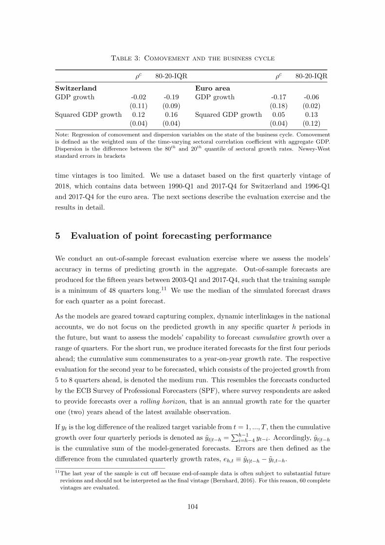
Table 3: Comovement and the business cycle

ρc 80-20-IQR ρc 80-20-IQR

Switzerland Euro areaGDP growth -0.02 -0.19 GDP growth -0.17 -0.06

(0.11) (0.09) (0.18) (0.02)Squared GDP growth 0.12 0.16 Squared GDP growth 0.05 0.13

(0.04) (0.04) (0.04) (0.12)

Note: Regression of comovement and dispersion variables on the state of the business cycle. Comovementis defined as the weighted sum of the time-varying sectoral correlation coefficient with aggregate GDP.Dispersion is the difference between the 80th and 20th quantile of sectoral growth rates. Newey-Weststandard errors in brackets

time vintages is too limited. We use a dataset based on the first quarterly vintage of

2018, which contains data between 1990-Q1 and 2017-Q4 for Switzerland and 1996-Q1

and 2017-Q4 for the euro area. The next sections describe the evaluation exercise and the

results in detail.

5 Evaluation of point forecasting performance

We conduct an out-of-sample forecast evaluation exercise where we assess the models’

accuracy in terms of predicting growth in the aggregate. Out-of-sample forecasts are

produced for the fifteen years between 2003-Q1 and 2017-Q4, such that the training sample

is a minimum of 48 quarters long.11 We use the median of the simulated forecast draws

for each quarter as a point forecast.

As the models are geared toward capturing complex, dynamic interlinkages in the national

accounts, we do not focus on the predicted growth in any specific quarter h periods in

the future, but want to assess the models’ capability to forecast cumulative growth over a

range of quarters. For the short run, we produce iterated forecasts for the first four periods

ahead; the cumulative sum commensurates to a year-on-year growth rate. The respective

evaluation for the second year to be forecasted, which consists of the projected growth from

5 to 8 quarters ahead, is denoted the medium run. This resembles the forecasts conducted

by the ECB Survey of Professional Forecasters (SPF), where survey respondents are asked

to provide forecasts over a rolling horizon, that is an annual growth rate for the quarter

one (two) years ahead of the latest available observation.

If yt is the log difference of the realized target variable from t = 1, ..., T , then the cumulative

growth over four quarterly periods is denoted as yt|t−h =∑h−1

i=h−4 yt−i. Accordingly, yt|t−h

is the cumulative sum of the model-generated forecasts. Errors are then defined as the

difference from the cumulated quarterly growth rates, eh,t ≡ yt|t−h − yt,t−h.

11The last year of the sample is cut off because end-of-sample data is often subject to substantial futurerevisions and should not be interpreted as the final vintage (Bernhard, 2016). For this reason, 60 completevintages are evaluated.

104

For the euro area, forecasts from the Survey of Professional Forecasters (SPF), conducted

and published by the European Central Bank, are used as an additional benchmark. Note

that all models under evaluation fight an uphill battle against the Survey of Professional

Forecasters due to the frequency of real-time data releases. Given that all models described

rely on national accounts data only, forecasts for all quarters ahead can be updated

approximately 30 days into the quarter, when the first estimate is released. The SPF

benchmark, however, is produced almost a quarter later. As the SPF not only relies on

national accounts data but also on respondents’ judgement of a set of early indicators, this

extra quarter gives the forecasters a sizeable informational advantage. As an illustrative

example, a sample of around 50 respondents to the survey submit their forecast in early

2015-Q1, at which point national accounts data for the preceding quarter have not yet

been published, making 2015-Q3 the target period. The rolling forecast horizon for one

year ahead of the latest available observation therefore effectively implies a forecast horizon

of only 3 quarters, giving the SPF a considerable head start.

The following section evaluates the relative performance of the horse race. The absolute

performance, where every model’s capabilities in terms of bias and efficiency of short-run

forecasts are evaluated by Mincer-Zarnowitz regressions, is displayed in the appendix.

5.1 Relative performance of aggregate forecasts

The relevant metric by which we compare errors across the alternative models (indexed

by m) is the square root of the mean squared error (RMSE):

RMSEm,h =

√√√√ 1

T

T∑t

e2m,h,t.

The respective measures are displayed as part of Table 4 and summarized in Figure 2. To

keep the representation of the results tractable, we do not report measures for all forecast

horizons separately, but restrict ourselves to two horizons: The short run (SR) is the

cumulative forecast error over the first four quarters and the medium run (MR) is the

cumulative forecast error over eight quarters.

Furthermore, we use a test following Diebold and Mariano (1995) to assess whether the

difference of squared errors of a given model and that of a simple benchmark is statistically

significant. As a benchmark we use the simplest of our models, the autoregressive process

of the aggregate target variable, AR-A. Table 4 contains the results. If the regression

coefficient is negative, the respective model has beaten the benchmark on average over the

evaluation period.

For Switzerland, the different models produce short-run forecasts that are not significantly

105

Figure 2: Root mean squared errors compared

different from the AR-A model.12 When forecasting the medium run, i.e. 5 through 8

quarters ahead, a significant pattern emerges: The DFM has the lowest errors over the

medium run, with an improvement of 8% relative to the aggregate AR. According to our

test procedure, this difference is significant at the 10% significance level. In contrast,

the VAR-L, which relies on the same variables but does not impose the factor structure,

performs substantially worse than the DFM. This indicates that shrinking the parameter

space by using the factor model proves to be crucial for medium-run forecast performance.

Among the simpler benchmarks, the RMSE show that in Switzerland, where sectoral

comovement is relatively weak, using disaggregated series helps to improve the medium-

run forecast: Both the sectoral AR-S and VAR-S beat their aggregate counterparts.

Errors for euro area GDP forecasts are generally higher, especially in the medium run.

This can partly be explained by a limited training sample for estimation and the fact that

the downturn during the Great Recession was much more severe in the euro area than in

Switzerland and that such strong fluctuations are difficult for any model to capture. This

is especially true for the univariate models. Indeed, both in the short run as well as in the

medium run, the AR-A and AR-S models perform badly for the euro area.

In the presence of such a large economic shock, more sophisticated models provide superior

results. The short-run forecasts of the DFM and both VAR benchmarks have errors that

are 25% below the aggregate AR. All models perform substantially worse than the SPF in

the short run. This is not surprising given that, as mentioned above, at time of production

it is possible to exploit evidence from a broader set of (high-frequency) leading economic

indicators. In the medium run, the DFM and the VAR-A are competitive with the SPF.

These models perform better than simple benchmarks, even if it is difficult to establish an

improvement in terms of statistical significance.

Overall, these findings show that including sector information can lead to more accurate

12The RMSE for h = 1 are depicted in the appendix for reference. The results show that for one quarterahead, the DFM and the VAR-S produce the best results.

106

Table 4: RMSE and Diebold-Mariano test coefficients

DFM VAR-L VAR-S VAR-A AR-S AR-A

SwitzerlandRMSE SR 1.87 1.92 1.78 1.86 1.83 1.75

MR 1.65 2.01 1.75 1.90 1.84 1.79Diebold-Mariano: βDM SR 0.25 0.44 -0.06 0.20 -0.18 -

(0.52) (0.84) (0.69) (0.69) (0.21) -MR -0.64 0.67 -0.30 0.22 -0.17 -

(0.41) (0.51) (0.34) (0.58) (0.15) -

Euro areaRMSE SR 2.28 2.82 2.44 2.25 2.98 3.00

MR 2.33 3.65 2.78 2.23 4.89 3.85Diebold-Mariano: βDM SR -3.79 -1.01 -3.02 -3.93 -0.06 -

(2.93) (0.69) (1.33) (2.30) (0.28) -MR -9.39 -1.51 -7.06 -9.84 9.05 -

(9.49) (2.73) (6.78) (8.82) (8.46) -

Note: Root mean squared errors for the short-run (SR) and medium-run (MR) forecasts. Newey-West standard errors in brackets

point estimates. The best performance, however, comes from our DFM model, which

simultaneously models the sectoral value added series and macroeconomic variables while

shrinking the parameter space by imposing a factor structure.

5.2 Decomposition of the forecast error variance

One strength of the multivariate models is that they are, in principle, able to capture joint

dynamics between sectors. In the below section, we investigate whether the differences

in performance documented previously are indeed driven by differential capabilities to

capture the joint dynamics. In order to do so, we exploit the fact that in the case of the

sectoral models, the aggregate error is a weighted sum of the sectoral errors, and decompose

its variance into the sum of the sectoral forecast error variances and covariances:13

Var(ey) = Var

(S∑s=1

ωses

)

=

S∑s=1

ω2sVar(es) + 2

∑1≤s<ς≤S

ωsωςCov(es, eς). (8)

Table 5 and Figure 3 document the two components of the variance of the aggregate error

in equation (8): the weighted sum of the sectoral errors and the covariances between errors

of different sectors. The decomposition for the aggregate models is computed by replacing

13Note that the mean squared GDP forecast error in the previous section is the sum of the variance of theforecast error and the squared bias. Mincer-Zarnowitz regressions suggests that the bias is small, seeTable A1 in the appendix.

107

Figure 3: Decomposition of error variances into a sectoral errorcomponent (grey) and a comovement component (colorized)

the sectoral prediction with the aggregate prediction. That is, we assume that all sectoral

forecasts grow at the same rate, equal to the aggregate one. In Figure 3, the contribution

of the sectoral errors is depicted in grey bars, while the sum of the covariances is shown

in the color of the respective model.

In both economic areas, the contribution of the covariance of sectoral errors decreases

in absolute and relative terms when sectoral information is included in the models. For

the medium-term forecasts in Switzerland, the error due to the covariance term of the

decomposition is reduced by a third (from 0.14 to 0.09).

In contrast, the sectoral error variance does not vary much across the different models.

The VAR-L is almost equally as successful in capturing sectoral covariance, despite having

larger aggregate errors. Using euro area data, the reduction in variance of the aggregate

error due to lower covariance of sectoral errors is more distinct. The sectoral models

produce substantially lower covariance terms. The differences between aggregate and

disaggregate benchmark models can be attributed to the differences in the information set

and also to the quite rudimentary construction of the sector forecasts within the aggregate

model.

The DFM produces the lowest sectoral error covariance in both economic areas. The

figures in Table 5 show that the superior performance of the DFM is mainly due to a

reduction in the covariance term, and not primarily to better forecasts for single sectors.

This suggests that by modelling sectoral comovement using a factor structure improves

the forecast error by reducing the forecast error covariance.

108

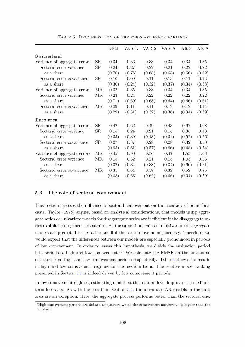
Table 5: Decomposition of the forecast error variance

DFM VAR-L VAR-S VAR-A AR-S AR-A

SwitzerlandVariance of aggregate errors SR 0.34 0.36 0.33 0.34 0.34 0.35

Sectoral error variance SR 0.24 0.27 0.22 0.21 0.22 0.22as a share (0.70) (0.76) (0.68) (0.63) (0.66) (0.62)

Sectoral error covariance SR 0.10 0.09 0.11 0.13 0.11 0.13as a share (0.30) (0.24) (0.32) (0.37) (0.34) (0.38)

Variance of aggregate errors MR 0.32 0.35 0.33 0.34 0.34 0.35Sectoral error variance MR 0.23 0.24 0.22 0.22 0.22 0.22

as a share (0.71) (0.69) (0.68) (0.64) (0.66) (0.61)Sectoral error covariance MR 0.09 0.11 0.11 0.12 0.12 0.14

as a share (0.29) (0.31) (0.32) (0.36) (0.34) (0.39)

Euro areaVariance of aggregate errors SR 0.42 0.62 0.49 0.43 0.67 0.68

Sectoral error variance SR 0.15 0.24 0.21 0.15 0.35 0.18as a share (0.35) (0.39) (0.43) (0.34) (0.52) (0.26)

Sectoral error covariance SR 0.27 0.37 0.28 0.28 0.32 0.50as a share (0.65) (0.61) (0.57) (0.66) (0.48) (0.74)

Variance of aggregate errors MR 0.45 0.96 0.56 0.47 1.55 1.08Sectoral error variance MR 0.15 0.32 0.21 0.15 1.03 0.23

as a share (0.32) (0.34) (0.38) (0.34) (0.66) (0.21)Sectoral error covariance MR 0.31 0.64 0.38 0.32 0.52 0.85

as a share (0.68) (0.66) (0.62) (0.66) (0.34) (0.79)

5.3 The role of sectoral comovement

This section assesses the influence of sectoral comovement on the accuracy of point fore-

casts. Taylor (1978) argues, based on analytical considerations, that models using aggre-

gate series or univariate models for disaggregate series are inefficient if the disaggregate se-

ries exhibit heterogeneous dynamics. At the same time, gains of multivariate disaggregate

models are predicted to be rather small if the series move homogeneously. Therefore, we

would expect that the differences between our models are especially pronounced in periods

of low comovement. In order to assess this hypothesis, we divide the evaluation period

into periods of high and low comovement.14 We calculate the RMSE on the subsample

of errors from high and low comovement periods respectively. Table 6 shows the results

in high and low comovement regimes for the medium term. The relative model ranking

presented in Section 5.1 is indeed driven by low comovement periods.

In low comovement regimes, estimating models at the sectoral level improves the medium-

term forecasts. As with the results in Section 5.1, the univariate AR models in the euro

area are an exception. Here, the aggregate process performs better than the sectoral one.

14High comovement periods are defined as quarters where the comovement measure ρc is higher than themedian.

109

Table 6: RMSE in high/low sectoral comovement regimes

DFM VAR-L VAR-S VAR-A AR-S AR-A

SwitzerlandLow comovement MR 1.22 1.97 1.66 1.90 1.43 1.57High comovement MR 1.99 2.05 1.84 1.89 2.08 2.06

Euro areaLow comovement MR 1.42 5.32 3.27 1.86 6.89 4.98High comovement MR 3.39 3.00 3.02 2.93 3.35 3.17

Furthermore, the VAR-L performs poorly, while the DFM, which not only includes the

sectoral series jointly but also manages to filter relevant information at the disaggregate

level, produces the most accurate forecasts.

In contrast, in times of high comovement, i.e. when the sectoral idiosyncratic factors are

less important and the sectors develop more homogeneously, the gain of disaggregation is

much smaller. The sectoral approach does not lead to a systematic improvement in the

RMSE. By contrast, we find no systematic differences between times of high vs low growth

rates or high vs. low volatility of quarterly GDP growth rates. We conclude that when

heterogeneity across sectors is high, forecasting models including sectoral series perform

better. Moreover, the DFM is best able to filter comovement and sectoral noise, and

therefore produces the best results.

6 Evaluation of density forecasting performance

Point forecasts do not capture the uncertainty around which a central prediction is made.

Density forecasts have, therefore, become an increasingly popular tool to communicate

how likely it is that the predictions will fit the realization. We devote this section to the

evaluation of the predictive densities of our models. For each model m, we simulate from

the Bayesian posterior distribution of the forecasts in order to determine the density of

the cumulative forecast φ(ym,t|t−h).

The fundamental problem of evaluating density forecasts in contrast to point forecasts

is that the actual density is unobserved, i.e. we observe just one realization, not many

realizations of the same density. A number of methods have been developed to address

this. These include the probability integral transforms (PIT), evaluations based on the

log score and, related to this, the ranked probability score. We discuss the results based

on these measures in the following sections.

110

6.1 Predictive accuracy: Probability integral transform

To assess whether the predictive density is correctly specified, we compute probability

integral transforms (PIT), i.e. we evaluate the cumulative density of a given forecast up

to the realized value:

PITm,h,t(yt|t−h) =

∫ yt|t−h

−∞φt(ym,t|t−h)dym,t|t−h ≡ Φt(ym,t|t−h).

A PIT of 0 indicates that, in advance, no probability was assigned to the possibility that

growth could be lower than the realized value of the target variable. If the PIT has the

maximum value of 1, then all the predictive density underestimated the realization. For

any well-behaved density forecast, the PIT should be uniformly distributed between 0 and

1 (Diebold et al., 1998). On average over time, the probability that the realized value is

lower than the forecasted value should be the same no matter whether we consider high

or low realizations. Figure 4 shows the empirical cumulative distribution of GDP PITs

against the theoretical uniform distribution and its confidence interval.

If they followed a uniform distribution, their empirical cumulative distribution function

(CDF) would follow the 45-degree line. To test this formally, we apply an augmented

version of the Kolmogorov-Smirnov test for uniformity, which accounts for the fact that

model parameters are estimated on a finite sample, as proposed by Rossi and Sekhposyan

(2013). Based on a fine grid r ∈ [0, 1] we calculate

ξm,t|t−h(r) ≡ (1{Φt(ym,t|t−h) ≤ r)− r})

for every grid point.15 For low values of r, the indicator is typically zero and thus ξ(r) is

negative but small. For r in the region of a half, dispersion of the ξ(r) vector is highest as

some values are close to 0.5 and some close to -0.5. And for values close to 1, the indicator

function is usually 1, and thus ξ(r) positive and small. For every grid point, we calculate

this objective, whose absolute value we maximize:

κKS = supr

∣∣∣∣∣ 1√T

T∑t

ξm,t|t−h(r)

∣∣∣∣∣ .The resulting κKS is evaluated against critical values obtained from a simulation: In a

large number of Monte Carlo replications, we draw T random variables from the uniform

distribution, calculate κ and use the (1−α)-th percentile of all simulations as the critical

value for the α% significance level. If κKS > κα, then the test rejects that the empirical

distribution could be the result of a uniform data-generating process at the α% significance

level. The corresponding p-values are reported in Table 7.

15Conveniently, one can set the grid r so as to put a special emphasis on parts of the distribution whichare of particular interest, such as lower and/or upper tails.

111

Figure 4: Empirical cumulative distribution of PIT vs uniform

Note: Cumulative distribution of PITs, i.e. cumulated density evaluated at therealized value forecasted.

The two left-hand side panels of Figure 4 show the CDFs for Switzerland. The DFM

narrowly follows the pattern of the uniform distribution for most of the distribution, both

for the short run and the medium run. The test of uniformity for the VAR-L cannot

be rejected, although there are some deviations at the lower end of the distribution

for the medium-run CDF. The rather convex CDF of the benchmark VARs (in green)

indicate the opposite: too often, the PITs are at the very high end, indicating that the

models significantly underestimate the probability of high growth rates. The univariate

models, both on the aggregate and sectoral level, have an inverted S-shape. This pattern

is especially pronounced for the medium run and suggests that uncertainty has been

underestimated with these models.

For the euro area, the CDFs show that the PITs are overall less uniformly distributed than

for Switzerland. By inspection, the VARs perform better than the DFM and, of all models

under consideration, this is the one that most closely follows the uniform distribution.

However, for the VAR-S only, the null of a uniform distribution cannot be rejected at the

5% level. Using euro area data, the DFM tends to overestimate the realized values. Over

the entire range, the realized probability is lower than the model implied. However, this

112

misalignment is also visible for the univariate benchmarks. Overall, density forecasts for

the euro area perform worse than for Switzerland. Again, this may be related to the fact

that the estimation sample is quite short in this case.

6.2 Relative performance: Ranked probability score

When comparing the predictive densities across models, scoring rules derived from the

concept of PIT are helpful tools. Various scoring rules such as loss functions may help

evaluate models against alternatives (Giacomini and White (2006), Kenny et al. (2014),

Boero et al. (2011)). We separate the argument space of the probability density into

mutually exclusive events, which can be thought of as bins k = (1, 2, ...,K) in the predictive

density of the forecast. We use K = 16 intervals set according to the Survey of Professional

Forecasters.16 Every bin is assigned a probability from the distribution, for example for the

first bin ψm,k,t =∫ v(k=1)−∞ φ(ym,t|t−h)dym,t|t−h. Additionally, we define a vector of length

K with binary values: 1 if the realized value is within the respective bin and 0 otherwise

(dm,1,t, dm,2,t, ..., dm,K,t). Then the inherently Bayesian predictive likelihood score (log

score) would be defined as follows:

Sm,h =1

T

T∑t

Sm,h,t, Sm,h,t =

K∑k

dm,k,tlog(ψm,k,t).

A problem with the log score arises if the specific bin of realizations is assigned a probability

of zero. A possible fix would imply reducing the number of bins to make sure every bin

carries positive probability, but this would ultimately violate the purpose and spirit of the

exercise.

We therefore use the ranked probability score (RPS, or Epstein score) as the alternative,

which is a measure of the cumulative probabilities and indicators.

The RPS is defined as follows:

Ψm,k,t =k∑j=1

ψm,j,t, Dm,k,t =k∑j=1

dm,j,t,

RPSm,h =1

T

T∑t

RPSm,h,t, RPSm,h,t =

K∑k

(Ψm,k,t −Dm,k,t)2.

As values are now in the positive range, it is desirable to have them as small as possible.17

Figure 5 summarizes the results, which can be found in Table 7 in detail.

16The partitioning of half a percentage point is used on a grid between annual growth rates from -3 to 4percent.

17This measure is a discrete approximation to the measure discussed, e.g., in Gneiting and Raftery (2007).Evaluating the continuous version using expression (21) in their paper yields similar results. Onedifference is that the VAR-L and the DFM perform somewhat worse in the euro area, but the differenceis quite small against the backdrop of the estimation uncertainty.

113

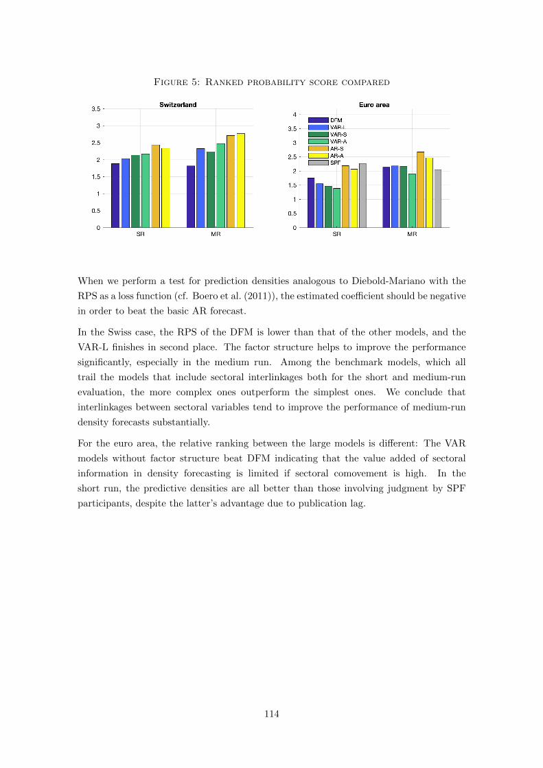
Figure 5: Ranked probability score compared

When we perform a test for prediction densities analogous to Diebold-Mariano with the

RPS as a loss function (cf. Boero et al. (2011)), the estimated coefficient should be negative

in order to beat the basic AR forecast.

In the Swiss case, the RPS of the DFM is lower than that of the other models, and the

VAR-L finishes in second place. The factor structure helps to improve the performance

significantly, especially in the medium run. Among the benchmark models, which all

trail the models that include sectoral interlinkages both for the short and medium-run

evaluation, the more complex ones outperform the simplest ones. We conclude that

interlinkages between sectoral variables tend to improve the performance of medium-run

density forecasts substantially.

For the euro area, the relative ranking between the large models is different: The VAR

models without factor structure beat DFM indicating that the value added of sectoral

information in density forecasting is limited if sectoral comovement is high. In the

short run, the predictive densities are all better than those involving judgment by SPF

participants, despite the latter’s advantage due to publication lag.

114

Table 7: Density forecast performance

DFM VAR-L VAR-S VAR-A AR-S AR-A

SwitzerlandMean PIT SR 0.42 0.55 0.55 0.58 0.60 0.59

MR 0.47 0.62 0.64 0.70 0.66 0.66KS/RS p-value SR 0.09 0.34 0.00 0.00 0.00 0.00

MR 0.32 0.00 0.00 0.00 0.00 0.00RPS SR 1.89 2.03 2.14 2.17 2.44 2.34

MR 1.82 2.33 2.24 2.48 2.71 2.77DM test: βRPS SR -0.45 -0.30 -0.20 -0.17 0.10 -

(0.26) (0.24) (0.25) (0.23) (0.14) -MR -0.95 -0.44 -0.53 -0.30 -0.06 -

(0.32) (0.26) (0.16) (0.22) (0.08) -

Euro areaMean PIT SR 0.36 0.35 0.43 0.34 0.35 0.33

MR 0.41 0.49 0.48 0.52 0.43 0.44KS/RS p-value SR 0.00 0.00 0.00 0.00 0.00 0.00

MR 0.01 0.25 0.01 0.33 0.00 0.00RPS SR 1.75 1.56 1.47 1.39 2.19 2.07

MR 2.14 2.18 2.17 1.90 2.67 2.47DM test: βRPS SR -0.32 -0.51 -0.60 -0.68 0.12 -

(0.27) (0.22) (0.27) (0.27) (0.09) -MR -0.33 -0.28 -0.30 -0.56 0.21 -

(0.20) (0.31) (0.15) (0.24) (0.09) -

Note: The mean PIT of an unbiased density forecast would be 0.5. The Kolmogorov-Smirnov/Rossi-Sekhposyan test rejects uniformity at the p-significance level. The RPSscore has positive support and an inverted scale, i.e. optimum 0, and the respectiveDiebold-Mariano test coefficient is negative if the respective model beats the benchmarkmodel AR-A (Newey-West standard errors in brackets).

7 Sectoral heterogeneity

Having shown that jointly modelling the dynamics of sectoral production improves point

and density forecasts for aggregate GDP for the medium term, we now analyze the cross-

sectional forecast distribution. For this evaluation, we rely on the multivariate mean

squared error as a standard measures for multivariate forecast performance in the following

section. Subsequently, we propose two new measures comparing specific aspects of the

forecast distribution.18

18We focus on point forecast as the limited amount of data does not allow for a reliable multivariate densityevaluation. A multivariate extension of the RPS, for example, compares the predicted probability ofall combinations of sectoral bins with the realized probability. Not only for the quite fine grid withK = 16 as in the univariate analysis, but also for K set to a smaller number, a reliable analysis seemsfutile. However, investigating the univariate density forecast for each sector confirms the result fromthe aggregate analysis that modelling sectoral interactions potentially improves the performance. Theresults are available from the authors upon request.

115

7.1 Multivariate root mean squared error

The cross-sectional distribution of point forecasts can be evaluated using standard mea-

sures for the evaluation of multivariate densities. We follow Carriero et al. (2011) and

calculate the multivariate mean squared error as

MV-RMSEm,h =

√√√√trace

(1

T

T∑t=1

(eSm,h,t)′M−1 (eSm,h,t)

),

where eSh is the matrix of h-step ahead forecast errors of all sectors over time and M

a weighting matrix with dimensions SxS containing the variances of the sectoral target

series along its diagonal.19

The results are shown in the first lines of Table 8. In the Swiss case, we find that sectoral

point forecasts from univariate models do not necessarily outperform their aggregate

counterparts, and that the gains from modelling comovement explicitly are small.

This result stands in some contradiction to the evaluation of the RMSE in Section 5.1

only at first sight. Indeed, the MSE for aggregate GDP and the multivariate MSE are

closely connected in the sense that both measures are weighted sums of sectoral forecast

errors. Specifically, the MSE for aggregate GDP is a version of the multivariate MSE, but

with a time-varying weighting matrix Mt = ωt−1ω′t−1 where ωt is the vector of nominal

shares of the sectors in aggregate GDP.20 Two differences from the multivariate MSE as

specified above appear. First, the weights on the diagonal are proportional to the squared

weight in aggregate GDP. They thus represent the importance of the sector and not the

unconditional variances of the sectors. Secondly, the off-diagonal elements are not zero,

but represent the product of the respective sectoral share in the MSE for GDP. So the

covariances of the sectoral errors are taken into account according to their weights in

aggregate GDP in the RMSE. This is not the case in the standard implementation of

the MSE with a diagonal weighting matrix M . Interestingly, given the results from the

decomposition in Section 5.2, we may even expect that the multivariate error measure

does not favour the DFM over the simple models, as the gain in forecast performance

19We use the variances of the 8-quarter growth rates for the short run as well as for the medium run, inorder to obtain more stable results. An alternative measure, Bayesian in spirit, considers the naturallogarithm of the determinant of the weighted error covariance matrix:

Log determinantm,h = ln

∣∣∣∣∣ 1

T

T∑t=1

(M−1/2eSm,h,t

)(M−1/2eSm,h,t

)′ ∣∣∣∣∣ .Since the relative ranking is the same, we do not report the log determinant separately. Overall, thismeasure confirms the results from the multivariate mean squared error.

20This can be seen as follows:

1

T

T∑t=1

e2m,h,t =

1

T

T∑t=1

(ω′t−1eSm,h,t)

2 =1

T

T∑t=1

(ω′t−1eSm,h,t)

′(ω′t−1eSm,h,t) =

1

T

T∑t=1

eS′m,h,tωt−1ω

′t−1e

Sm,h,t.

116

Table 8: Evaluation measures for sectoral heterogeneity

DFM VAR-L VAR-S VAR-A AR-S AR-A

SwitzerlandMultivariate error measuresMV-RMSE SR 4.59 5.17 4.69 4.71 3.98 4.35

MR 4.18 5.03 4.55 4.47 4.06 4.09Sectoral dispersionAbove/below average SR 0.55 0.51 0.56 0.54 0.56 0.52

MR 0.53 0.52 0.52 0.49 0.55 0.48RMS dispersion error SR 2.79 3.86 2.25 4.42 2.24 4.42

MR 3.61 11.48 2.98 4.42 2.85 4.42

Euro areaMultivariate error measuresMV-RMSE SR 3.80 5.64 4.62 6.17 4.83 7.68

MR 3.91 6.47 4.62 4.02 5.96 9.11Sectoral dispersionAbove/below average SR 0.56 0.54 0.55 0.60 0.53 0.56

MR 0.53 0.53 0.55 0.47 0.53 0.45RMS dispersion error SR 1.54 3.85 2.44 2.11 2.74 2.11

MR 1.99 19.37 4.94 2.11 7.61 2.11

mainly stems from a better description of the sectoral covariances. Taken together, we

think that the evaluation of the RMSE for aggregate GDP is a better summary of the

sectoral forecast performance than the multivariate MSE as specified in this section.

7.2 Alternative measures for sectoral developments

The measures analyzed so far aim at providing an encompassing assessment of the mul-

tivariate forecast distribution. This comes with the drawback that it is difficult to know

where the differences in forecasting performance stem from. We therefore now evaluate the

forecasting performance based on two additional criteria geared towards capturing other

relevant aspects of the cross-sectional forecast distribution.

The first measure compares the weighted share of sectors that were correctly projected to

grow above or below a moving average of 2 years prior to the forecasting vintage. This

reflects the idea that a model is useful if it is able to tell in which direction the specific

sectors are going to develop.

The results too are shown in Table 8. Using Swiss data, the weighted share of sectors

correctly predicted for the first (second) year forecasted was 55% (53%) for the DFM,

compared to 52% (48%) for the aggregate AR that assumes all sectors grow the same.

Adding sectoral components improves the share predominantly in the medium run (both

in Switzerland and the euro area), while modelling sectoral linkages and comovement does

117

not seem to add value. This is consistent with the notion that the dynamic factor model

does not improve the sector error variance, but rather the covariance of disaggregate errors

(see Section 5.2).

The second measure assesses how well models predict the dispersion of growth across

the economy as measured by its cross-sectoral standard deviation. The idea behind this

measure is that a model can be useful if it correctly predicts how different the sectors are

from each other, independent of its sectoral point forecast performance.

We construct the measure as follows. For each forecast horizon, we take the mean of the

cross-sectoral standard deviation σs across draws from the posterior forecast distribution

and compare it to the realized cross-sectoral dispersion in the corresponding time period

(σs). The root mean squared dispersion error is then defined as

RMSDEm,h =

√√√√ 1

T

T∑t

(σs,t,m,h − σs,t)2, σs,t,m,h =

√√√√ 1

S

S∑s=1

(xst,m,h −1

S

S∑s=1

xst,m,h)2.

The results in the bottom row of Table 8 show that, for this measure, the DFM yields the

best performance in the euro area, while it is comparable with the simple benchmarks in

Switzerland. However, it is quite striking that the VAR-L performs worse than the other

models in both regions. This suggests that treating macro variables and sectoral variables

symmetrically as in the VAR-L is probably too crude a way of shrinking the parameter

space.

We have also tested whether forecasting errors at the sectoral level vary with the degree to

which a sector typically comoves with the rest of the economy. The fact that we did not find

conclusive evidence across models is further highlights that our proposed models are not

necessarily forecasting sectoral value added more accurately but are able to significantly

increase forecasting performance by capturing sectoral comovement.

8 Conclusions

The economy is a network of firms in different sectors, which can experience both common

and idiosyncratic shocks, and possibly transmit, through input-output linkages, to other

sectors of the economy. Most empirical models used for forecasting typically neglect at

least one of those two elements. This paper proposes a model of interconnected sectors to

forecast the economy, measured as the real value added by different production sectors.

We assess whether the granular view increases forecasting performance.

118

In our evaluation, we focus on medium-term projections for real output.21 We find quite

distinct evidence that a factor model structure performs very well. It very generally

outperforms the simple benchmarks, and in many cases also the BVAR. This is true for

both point and density forecasts. In the latter case, the differences tend to be even more

pronounced.

Our analysis of the covariance matrix of the sectoral forecast errors suggests that the supe-

riority of the factor model can be traced back to its ability to capture sectoral comovement

more accurately than its competitors. This is desirable, because the forecaster wants to

distinguish between a common component of the shock and sector-specific innovations

that, at different horizons, spill over to other sectors. Moreover, the factor model tends

to outperform the other models also at forecasting sectoral heterogeneity. In particular,

it forecasts more accurately the sectoral dispersion as measured by the cross-sectional

standard deviation of the sectors.

Production-side models, and especially the DFM, provide a valuable complement to demand-

side, medium-term models. This is particularly because they allow us to study how

different sectors behave in alternative macroeconomic scenarios.

References

Anderson, B. D. O. and J. B. Moore (1979): Optimal Filtering, Prentice Hall.

Bai, J. and S. Ng (2002): “Determining the Number of Factors in Approximate Factor

Models,” Econometrica, 70, 191–221.

Banbura, M., D. Giannone, and L. Reichlin (2010): “Large Bayesian Vector

Autoregressions,” Journal of Applied Econometrics, 25, 71–92.

Barhoumi, K., O. Darne, L. Ferrara, and B. Pluyaud (2012): “Monthly GDP

Forecasting Using Bridge Models: Application for the French Economy.” Bulletin of

Economic Research, 64, 53–70.

Baurle, G. (2013): “Structural Dynamic Factor Analysis Using Prior Information From

Macroeconomic Theory,” Journal of Business and Economic Statistics, 31, 136–150.

Baurle, G. and E. Steiner (2015): “How Do Individual Sectors Respond to

Macroeconomic Shocks? A Structural Dynamic Factor Approach Applied to Swiss

Data,” Swiss Journal of Economics and Statistics, 151, 167–225.

21Equivalent measures for point and density forecasts of CPI/HICP inflation can be found in the appendixB.2. The RMSE (RPS) gain in percent is between 15 (36) in Swiss data and 13 (22) if applied to euroarea data. Differences among sectoral and aggregate benchmarks are only marginal, but note that wedo not include prices on a sectoral level. The factor model performs very competitively.

119

Bauwens, L., M. Lubrano, and J.-F. Richard (1999): Bayesian Inference in

Dynamic Econometric Models, Oxford University Press.

Bermingham, C. and A. D’Agostino (2014): “Understanding and Forecasting

Aggregate and Disaggregate Price Dynamics,” Empirical Economics, 46, 765–788.

Bernanke, B., J. Boivin, and P. S. Eliasz (2005): “Measuring the Effects of

Monetary Policy: A Factor-Augmented Vector Autoregressive (FAVAR) Approach,”

The Quarterly Journal of Economics, 120, 387–422.

Bernhard, S. (2016): “A Real-time GDP Data Set for Switzerland,” Tech. rep., Swiss

National Bank Economic Studies 2016-09.

Bloom, N. (2009): “The Impact of Uncertainty Shocks,” Econometrica, 77, 623–685.

Boero, G., J. Smith, and K. F. Wallis (2011): “Scoring Rules and Survey Density

Forecasts,” International Journal of Forecasting, 27, 379–393.

Boivin, J. and M. Giannoni (2006): “DSGE Models in a Data-Rich Environment,”

NBER Technical Working Paper 0332, National Bureau of Economic Research, Inc.

Boivin, J. and S. Ng (2006): “Are More Data Always Better for Factor Analysis?”

Journal of Econometrics, 132, 169–194.

Carriero, A., G. Kapetanios, and M. Marcellino (2011): “Forecasting Large

Datasets with Bayesian Reduced Rank Multivariate Models,” Journal of Applied

Econometrics, 26, 735–761.

Carter, C. K. and P. Kohn (1994): “On Gibbs Sampling for State Space Models,”

Biometrica, 81, 541–553.

Carvalho, V. M., M. Nirei, Y. U. Saito, and A. Tahbaz-Salehi (2016):

“Supply Chain Disruptions: Evidence from the Great East Japan Earthquake,” CEPR

Discussion Papers, 11711.

Chang, Y. and S. Hwang (2015): “Asymmetric Phase Shifts in U.S. Industrial

Production Cycles,” Review of Economics and Statistics, 97, 116–133.

Chib, S. (1993): “Bayes Regression with Autoregressive Errors: A Gibbs Sampling

Approach,” Journal of Econometrics, 58, 275–294.

Christiano, L. and T. Fitzgerald (1998): “The Business Cycle: It’s Still a Puzzle,”

Economic Perspectives, 22, 56–83.

Dees, S. and J. Gunther (2014): “Analysing and Forecasting Price Dynamics Across

Euro Area Countries and Sectors: A Panel VAR Approach,” European Central Banking

Working Paper Series, 1724.

120

Diebold, F. X., T. A. Gunther, and A. S. Tay (1998): “Evaluating Density Forecasts

with Application to Financial Risk Management,” International Economic Review, 39,

863–883.

Diebold, F. X. and R. S. Mariano (1995): “Comparing Predictive Accuracy,” Journal

of Business and Economic Statistics, 13, 253–263.

Doan, T., R. B. Litterman, and C. A. Sims (1984): “Forecasting and Conditional

Projection Using Realistic Prior Distributions,” Econometric Reviews, 3, 1–100.

Drechsel, K. and R. Scheufele (2018): “Bottom-up or Direct? Forecasting German

GDP in a Data-rich Environment,” Empirical Economics, 54, 705–745.

Fares, J. and G. Srour (2001): “The Monetary Transmission Mechanism at the

Sectoral Level,” Working Paper 2001-27, Bank of Canada.

Frale, C., M. Marcellino, G. Mazzi, and T. Proietti (2011): “Euromind: A

Monthly Indicator of the Euro Area Economic Conditions,” Journal of the Royal

Statistical Society, 174, 439–470.

Fruhwirth-Schnatter, S. (1994): “Data Augmentation in Dynamic Linear Models,”

Journal of Time Series Analysis, 15, 183–202.

Fuentes-Albero, C. and L. Melosi (2013): “Methods for Computing Marginal Data

Densities from the Gibbs Output,” Journal of Econometrics, 175, 132–141.

Ganley, J. and C. Salmon (1997): “The Industrial Impact of Monetary Policy Shocks:

Some Stylized Facts,” Working Paper 68, Bank of England.

Giacomini, R. and H. White (2006): “Tests of Conditional Predictive Ability,”

Econometrica, 74, 1545–1578.

Giannone, D. and L. Reichlin (2009): “Comments on ”Forecasting Economic and

Financial Variables with Global VARs”,” International Journal of Forecasting, 25, 8.

Giannone, Domenico, M. L. and G. E. Primiceri (2015): “Prior Selection for Vector

Autoregressions,” Review of Economics and Statistics, 97, 436–451.

Gneiting, T. and A. E. Raftery (2007): “Strictly Proper Scoring Rules, Prediction

and Estimation,” Journal of the American Statistical Association, 102, 359–378.

Hahn, E. and F. Skudelny (2008): “Eearly Estimates of Euro Area real GDP Growth.

A Bottom Up Approach from the Production Side,” European Central Bank Working

Paper Series, 975.

Hendry, D. F. and K. Hubrich (2011): “Combining Disaggregate Forecasts or

Combining Disaggregate Information to Forecast an Aggregate,” Journal of Business

and Economic Statistics, 29, 216–227.

121

Holly, S., I. Petrella, and E. Santoro (2012): “Factor Demand Linkages,

Technology Shocks, and the Business Cycle,” The Review of Economics and Statistics,

94, 948–963.

Horvath, M. (1998): “Cyclicality and Sectoral Linkages: Aggregate Fluctuations from

Independent Sectoral Shocks,” Review of Economic Dynamics.

Hubrich, K. (2005): “Forecasting Euro Area Inflation: Does Aggregating Forecasts by

HICP Component Improve Forecast Accuracy?” International Journal of Forecasting,

21, 119–136.

Karlsson, S. (2013): “Forecasting with Bayesian Vector Autoregressions,” in Handbook

of Economic Forecasting, ed. by G. Elliott and A. Timmermann, Elsevier, vol. 2,

chap. 15, 791–897.

Kenny, G., T. Kostka, and F. Masera (2014): “How Informative Are the Subjective

Density Forecasts of Macroeconomists?” Journal of Forecasting, 33, 163–185.

Kim, C.-J. and C. R. Nelson (1999): State-Space Models with Regime Switching, The

MIT Press.

Litterman, R. (1979): “Techniques of Forecasting Using Vector Autoregressions,”

Federal Reserve of Minneapolis Working Paper.

Marcellino, M., J. H. Stock, and M. W. Watson (2003): “Macroeconomic

Forecasting in the Euro area: Country Specific Versus Area-wide Information,”

European Economic Review, 47, 1–18.

Martinsen, K., F. Ravazzolo, and F. Wulfsberg (2014): “Forecasting

Macroeconomic Variables Using Disaggregate Survey Data,” International Journal of

Forecasting, 30, 65–77.

Mincer, J. A. and V. Zarnowitz (1969): The Evaluation of Economic Forecasts,

National Bureau of Economic Research, New York.

Newey, W. K. and K. D. West (1987): “A Simple, Positive Semi-definite,

Heteroskedasticity and Autocorrelation Consistent Covariance Matrix,” Econometrica,

55, 703–708.

Pesaran, M. H., T. Schuermann, , and S. M. Weiner (2010): “Modelling Regional

Interdependencies Using a Global Error-correcting Macroeconometric Model,” Journal

of Business and Economics Statistics, 22, 129–162.

Poirier, D. (1998): “Revising Beliefs in Nonidentified Models,” Econometric Theory, 14,

483–509.

122

Proietti, T., M. Marczak, and G. Mazzi (2017): “Euromind-D: A Density

Estimate of Monthly Gross Domestic Product for the Euro Area,” Journal of Applied

Econometrics, 32, 683–703.

Rossi, B. and T. Sekhposyan (2013): “Conditional Predictive Density Evaluation in

the Presence of Instabilities,” Journal of Econometrics, 177, 199–212.

Stock, J. H. and M. W. Watson (2002): “Macroeconomic Forecasting Using Diffusion

Indexes,” Journal of Business and Economic Statistics, 20, 147–162.

——— (2016): “Core Inflation and Trend Inflation,” The Review of Economics and

Statistics, 98, 770–784.

Taylor, J. (1978): “Comments on ”The Temporal and Sectoral Aggregation of Seasonally

Adjusted Time Series” by John Geweke,” Economic research report, US Department of

Commerce, Bureau of the Census.

Zellner, A. and J. Tobias (2000): “A Note on Aggregation, Disaggregation and

Forecasting Performance,” Journal of Forecasting, 19, 457–469.

123

Appendix

A Model description and estimation

We provide some details on the estimation procedure, allowing the reader to replicate our

empirical results. Additionally, we provide detailed references to previous work where the

formal derivations of the (conditional) posterior distributions can be found.

As the posterior distribution cannot be derived analytically, we use Markov Chain Monte

Carlo (MCMC) methods to simulate from the posterior distribution. In our setting, this

can be done using a Gibbs sampling approach (see e.g. Kim and Nelson (1999) with one

iteration of the Gibbs sampler involving the following steps:

Step 1: Draw the factors conditional on a set of model parameters

Step 2: Draw parameters in the observation equation conditional on the factors

Step 3: Draw parameters in the state equation conditional on the factors

Iterating over these steps delivers draws from the posterior distribution of the parameters

and the factors. Subsequently, we provide a detailed description of the three steps including

the specification of the prior distribution.

Step 1: Drawing the factors To draw from the joint distribution of the factors

given the parameters in the model, we use the algorithm of Carter and Kohn (1994)

and Fruhwirth-Schnatter (1994). The algorithm uses a Kalman filter. In our setting, the

filter has to be adapted for autoregressive errors and potentially co-linear states. See, e.g.,

Anderson and Moore (1979) and Kim and Nelson (1999).

Step 2: Drawing parameters in the observation equation We use an informative

prior on the factor loadings as this “identifies” the factors in the sense that it puts curvature

into the posterior density function for regions in which the likelihood function is flat. See,

for example, the discussion in Baurle (2013). In our implementation, the prior is centred

such that, a priori, the series are all related with loading one to the unobserved factors

contemporaneously and with loading zero to the lagged factors. However, the variance of

the prior is chosen to be large, such that if the data is informative about the loadings, this

will be reflected in the posterior distribution.

Regarding the parametric form of the prior, we use the specification of the conjugate prior

described in Bauwens et al. (1999), p.58: The prior distribution p(Rn,Λn | Ψn), where n

denotes the respective row in the observation equation, is of the normal-inverted gamma-2

124

form (as defined in the appendix of Bauwens et al. (1999)):

Rn ∼ iG2(s, ν)

Λn ∼ N(Λ0,n, RnM−10,n)

Λ0 is the prior mean of the distribution. The parameters s and ν parametrize the

distribution of the variance of the measurement error. M0 is a matrix of parameters that

influences the tightness of the priors in the observation equation. The larger the elements

of M0, the closer we relate the observed series to the factors a priori. The choice of the

tightness is determined by the a priori confidence in the prior belief. We set M0,n,% = %2

for all n and % = 1, . . . , q. Thus the tightness of the prior increases quadratically with the

lag of the factor. Following Boivin and Giannoni (2006), we set s = 3 and ν = 0.001. By

adding a standard normal prior for Ψn, we have specified a complete prior distribution for

the parameters in the observation equation. The derivation of the posterior distribution

is standard, see e.g. Chib (1993) and Bauwens et al. (1999).

Step 3: Drawing parameters in the state equation The procedure for drawing

from the state equation conditional on the factor is identical to the estimation of the

BVAR. We implement a normal Wishart prior for the parameters in the state equation.

The prior mean and variances are of a Minnesota type, following Banbura et al. (2010).

In that notation, we set the prior mean of the first own lag to zero as we model stationary

series. The prior is conjugate, i.e. the conditional densities p(Σ|F,Φ) and p(Φ|F,Σ) can be

shown to be multivariate normal and inverse Wishart densities respectively (see Bauwens

et al. (1999) or Karlsson (2013)). We therefore introduce this additional Gibbs-sampling

step into our MCMC algorithm.

B Auxiliary evaluations

B.1 GDP nowcast

For completeness, we test if the models are correctly specified using the Mincer-Zarnowitz

test. Mincer and Zarnowitz (1969) argue that even if estimated coefficients are unbiased,

the resulting forecasts may underestimate high values and overestimate low values. How-

ever, if β0 = 0 and β1 = 1 in the following regression, the forecast is unbiased and high

forecasts are followed by equally high realisations in expectation:

yt,t−h = β0 + β1yt|t−h + ut, H0 : β0 = 0, β1 = 1

Table A1 reports the respective regression coefficients for the one-quarter-ahead predic-

tion. We report Newey-West standard errors in brackets, which are adjusted for possible

125

heteroskedasticity and autocorrelation (Newey and West, 1987). It also contains other

metrics discussed in the article, such as RMSE and RPS, for GDP forecasts one quarter

ahead, to make them comparable to other evaluations in the literature.

Table A1: Evaluation measures for short-run GDP forecasts

DFM VAR-L VAR-S VAR-A AR-S AR-A

Switzerlandβ0 h=1 0.04 0.08 0.02 0.07 -0.08 0.03

(0.13) (0.13) (0.15) (0.13) (0.32) (0.16)β1 0.81 0.69 0.82 0.76 1.03 0.83

(0.18) (0.15) (0.19) (0.16) (0.49) (0.20)RMSE h=1 0.52 0.53 0.52 0.51 0.55 0.53RPS h=1 0.57 0.58 0.61 0.62 0.79 0.69

Euro areaβ0 h=1 0.02 -0.07 -0.04 -0.13 -0.04 -0.04

(0.13) (0.16) (0.15) (0.16) (0.17) (0.17)β1 0.67 0.62 0.67 0.69 0.61 0.56

(0.19) (0.16) (0.20) (0.19) (0.22) (0.20)RMSE h=1 0.55 0.63 0.57 0.61 0.65 0.67RPS h=1 0.56 0.50 0.53 0.50 0.68 0.64

Note: Regression of the GDP point one-step-ahead forecast on realized values withNewey-West standard errors in brackets

B.2 Inflation forecast evaluation

All multivariate models can be used to produce forecasts of CPI (Switzerland) and HICP

(euro area) inflation. Instead of the AR-S and AR-A benchmark, we run a simple

univariate AR of inflation. The following table contains a small subset of the results

analogous to GDP in Sections 5 and 6.

Table A2: Evaluation measures for inflation

DFM VAR-L VAR-S VAR-A AR SPF

SwitzerlandRMSE SR 1.38 1.83 1.87 1.82 1.77

MR 1.35 1.69 1.76 1.76 1.61RPS SR 1.31 1.75 2.55 2.13 2.36

MR 1.37 1.80 2.38 2.14 2.18

Euro areaRMSE SR 1.11 1.65 1.25 1.23 1.59 0.91

MR 1.17 1.49 1.18 1.10 1.34 1.01RPS SR 1.19 1.62 1.62 1.46 1.65 1.21

MR 1.28 1.78 1.63 1.56 1.65 1.20

126