Principles of Macroeconomics for AP® Courses - cloudfront.net
539
-
Upload
khangminh22 -
Category
Documents
-
view
0 -
download
0
Transcript of Principles of Macroeconomics for AP® Courses - cloudfront.net


Principles of Macroeconomics for AP® Courses
SENIOR CONTRIBUTING AUTHORS STEVEN A. GREENLAW, UNIVERSITY OF MARY WASHINGTON TIMOTHY TAYLOR, MACALESTER COLLEGE
OpenStax Rice University 6100 Main Street MS-375 Houston, Texas 77005 To learn more about OpenStax, visit https://openstax.org. Individual print copies and bulk orders can be purchased through our website. ©2017 Rice University. Textbook content produced by OpenStax is licensed under a Creative Commons Attribution 4.0 International License (CC BY 4.0). Under this license, any user of this textbook or the textbook contents herein must provide proper attribution as follows: - If you redistribute this textbook in a digital format (including but not limited to PDF and HTML), then you
must retain on every page the following attribution: “Download for free at https://openstax.org/details/books/principles-macroeconomics-ap-courses.”
- If you redistribute this textbook in a print format, then you must include on every physical page the following attribution: “Download for free at https://openstax.org/details/books/principles-macroeconomics-ap-courses.”
- If you redistribute part of this textbook, then you must retain in every digital format page view (including but not limited to PDF and HTML) and on every physical printed page the following attribution: “Download for free at https://openstax.org/details/books/principles-macroeconomics-ap-courses.”
- If you use this textbook as a bibliographic reference, please include https://openstax.org/details/books/principles-macroeconomics-ap-courses in your citation.
For questions regarding this licensing, please contact [email protected]. Trademarks The OpenStax name, OpenStax logo, OpenStax book covers, OpenStax CNX name, OpenStax CNX logo, OpenStax Tutor name, Openstax Tutor logo, Connexions name, Connexions logo, Rice University name, and Rice University logo are not subject to the license and may not be reproduced without the prior and express written consent of Rice University. PRINT BOOK ISBN-10 1-938168-96-8 PRINT BOOK ISBN-13 978-1-938168-96-3 PDF VERSION ISBN-10 1-947172-32-8 PDF VERSION ISBN-13 978-1-947172-32-6 Revision Number MAAC-2015-001(03/16)-LC Original Publication Year 2015

OPENSTAX OpenStax provides free, peer-reviewed, openly licensed textbooks for introductory college and Advanced Placement® courses and low-cost, personalized courseware that helps students learn. A nonprofit ed tech initiative based at Rice University, we’re committed to helping students access the tools they need to complete their courses and meet their educational goals.
RICE UNIVERSITY OpenStax, OpenStax CNX, and OpenStax Tutor are initiatives of Rice University. As a leading research university with a distinctive commitment to undergraduate education, Rice University aspires to path-breaking research, unsurpassed teaching, and contributions to the betterment of our world. It seeks to fulfill this mission by cultivating a diverse community of learning and discovery that produces leaders across the spectrum of human endeavor.
FOUNDATION SUPPORT OpenStax is grateful for the tremendous support of our sponsors. Without their strong engagement, the goal of free access to high-quality textbooks would remain just a dream.
Laura and John Arnold Foundation (LJAF) actively seeks opportunities to invest in organizations and thought leaders that have a sincere interest in implementing fundamental changes that not only yield immediate gains, but also repair broken systems for future generations. LJAF currently focuses its strategic investments on education, criminal justice, research integrity, and public accountability.
The William and Flora Hewlett Foundation has been making grants since 1967 to help solve social and environmental problems at home and around the world. The Foundation concentrates its resources on activities in education, the environment, global development and population, performing arts, and philanthropy, and makes grants to support disadvantaged communities in the San Francisco Bay Area. Calvin K. Kazanjian was the founder and president of Peter Paul (Almond Joy), Inc. He firmly believed that the more people understood about basic economics the happier and more prosperous they would be. Accordingly, he established the Calvin K. Kazanjian Economics Foundation Inc, in 1949 as a philanthropic, nonpolitical educational organization to support efforts that enhanced economic understanding.
Guided by the belief that every life has equal value, the Bill & Melinda Gates Foundation works to help all people lead healthy, productive lives. In developing countries, it focuses on improving people’s health with vaccines and other life-saving tools and giving them the chance to lift themselves out of hunger and extreme poverty. In the United States, it seeks to significantly improve education so that all young people have the opportunity to reach their full potential. Based in Seattle, Washington, the foundation is led by CEO Jeff Raikes and Co-chair William H. Gates Sr., under the direction of Bill and Melinda Gates and Warren Buffett. The Maxfield Foundation supports projects with potential for high impact in science, education, sustainability, and other areas of social importance.
Our mission at The Michelson 20MM Foundation is to grow access and success by eliminating unnecessary hurdles to affordability. We support the creation, sharing, and proliferation of more effective, more affordable educational content by leveraging disruptive technologies, open educational resources, and new models for collaboration between for-profit, nonprofit, and public entities. The Bill and Stephanie Sick Fund supports innovative projects in the areas of Education, Art, Science and Engineering.

IT’S INNOVATION IN EDUCATION. A HII PENSTAX CII TUDENTS FREE TE MEET SCOPE AND SE QUIREMENTS FOR MII URSES. THESE ARE PEER-REVIEWED TEXTS WRITTEN BY PROFESSIONAL CONTENT A DEVELOPERS. ADOPT A BOOK TODAY FOR A TURNKEY CLASSROOM SOLUTION OR MODIFY IT TO SUIT YOUR TEACHING APPROACH. FREE ONLINE AND LOW-COST IN PRINT, OPENSTAX
WOULDN’T THISLOOK BETTERON A BRAND
MINI?Knowing where our textbooks are used can
help us provide better services to students and receive more grant support for future projects.
If you’re using an OpenStax textbook, either as required for your course or just as an
extra resource, send your course syllabus to [email protected] and you’ll
be entered to win an iPad Mini.
If you don’t win, don’t worry – we’ll be holding a new contest each semester.
NEW IPAD
Table of ContentsPreface . . . . . . . . . . . . . . . . . . . . . . . . . . . . . . . . . . . . . . . . . . . . . . . . . . . 1Chapter 1: Welcome to Economics! . . . . . . . . . . . . . . . . . . . . . . . . . . . . . . . . . . . 7
1.1 What Is Economics, and Why Is It Important? . . . . . . . . . . . . . . . . . . . . . . . . . . 81.2 Microeconomics and Macroeconomics . . . . . . . . . . . . . . . . . . . . . . . . . . . . . 121.3 How Economists Use Theories and Models to Understand Economic Issues . . . . . . . . . . 131.4 How Economies Can Be Organized: An Overview of Economic Systems . . . . . . . . . . . . 15
Chapter 2: Choice in a World of Scarcity . . . . . . . . . . . . . . . . . . . . . . . . . . . . . . . . 252.1 How Individuals Make Choices Based on Their Budget Constraint . . . . . . . . . . . . . . . 262.2 The Production Possibilities Frontier and Social Choices . . . . . . . . . . . . . . . . . . . . 312.3 Confronting Objections to the Economic Approach . . . . . . . . . . . . . . . . . . . . . . . 36
Chapter 3: Demand and Supply . . . . . . . . . . . . . . . . . . . . . . . . . . . . . . . . . . . . . 433.1 Demand, Supply, and Equilibrium in Markets for Goods and Services . . . . . . . . . . . . . 443.2 Shifts in Demand and Supply for Goods and Services . . . . . . . . . . . . . . . . . . . . . 493.3 Changes in Equilibrium Price and Quantity: The Four-Step Process . . . . . . . . . . . . . . 593.4 Price Ceilings and Price Floors . . . . . . . . . . . . . . . . . . . . . . . . . . . . . . . . . 653.5 Demand, Supply and Efficiency . . . . . . . . . . . . . . . . . . . . . . . . . . . . . . . . . 68
Chapter 4: Labor and Financial Markets . . . . . . . . . . . . . . . . . . . . . . . . . . . . . . . . 794.1 Demand and Supply at Work in Labor Markets . . . . . . . . . . . . . . . . . . . . . . . . . 804.2 Demand and Supply in Financial Markets . . . . . . . . . . . . . . . . . . . . . . . . . . . . 894.3 The Market System as an Efficient Mechanism for Information . . . . . . . . . . . . . . . . . 94
Chapter 5: The Macroeconomic Perspective . . . . . . . . . . . . . . . . . . . . . . . . . . . . . 1035.1 Measuring the Size of the Economy: Gross Domestic Product . . . . . . . . . . . . . . . . 1055.2 Adjusting Nominal Values to Real Values . . . . . . . . . . . . . . . . . . . . . . . . . . . 1135.3 Tracking Real GDP over Time . . . . . . . . . . . . . . . . . . . . . . . . . . . . . . . . . 1185.4 Comparing GDP among Countries . . . . . . . . . . . . . . . . . . . . . . . . . . . . . . . 1205.5 How Well GDP Measures the Well-Being of Society . . . . . . . . . . . . . . . . . . . . . . 123
Chapter 6: Economic Growth . . . . . . . . . . . . . . . . . . . . . . . . . . . . . . . . . . . . . 1316.1 The Relatively Recent Arrival of Economic Growth . . . . . . . . . . . . . . . . . . . . . . 1326.2 Labor Productivity and Economic Growth . . . . . . . . . . . . . . . . . . . . . . . . . . . 1356.3 Components of Economic Growth . . . . . . . . . . . . . . . . . . . . . . . . . . . . . . . 1416.4 Economic Convergence . . . . . . . . . . . . . . . . . . . . . . . . . . . . . . . . . . . . 145
Chapter 7: Unemployment . . . . . . . . . . . . . . . . . . . . . . . . . . . . . . . . . . . . . . . 1557.1 How the Unemployment Rate Is Defined and Computed . . . . . . . . . . . . . . . . . . . 1567.2 Patterns of Unemployment . . . . . . . . . . . . . . . . . . . . . . . . . . . . . . . . . . . 1617.3 What Causes Changes in Unemployment over the Short Run . . . . . . . . . . . . . . . . 1657.4 What Causes Changes in Unemployment over the Long Run . . . . . . . . . . . . . . . . . 169
Chapter 8: Inflation . . . . . . . . . . . . . . . . . . . . . . . . . . . . . . . . . . . . . . . . . . . 1818.1 Tracking Inflation . . . . . . . . . . . . . . . . . . . . . . . . . . . . . . . . . . . . . . . . 1828.2 How Changes in the Cost of Living Are Measured . . . . . . . . . . . . . . . . . . . . . . . 1868.3 How the U.S. and Other Countries Experience Inflation . . . . . . . . . . . . . . . . . . . . 1908.4 The Confusion Over Inflation . . . . . . . . . . . . . . . . . . . . . . . . . . . . . . . . . . 1958.5 Indexing and Its Limitations . . . . . . . . . . . . . . . . . . . . . . . . . . . . . . . . . . 200
Chapter 9: The International Trade and Capital Flows . . . . . . . . . . . . . . . . . . . . . . . . 2099.1 Measuring Trade Balances . . . . . . . . . . . . . . . . . . . . . . . . . . . . . . . . . . . 2109.2 Trade Balances in Historical and International Context . . . . . . . . . . . . . . . . . . . . 2149.3 Trade Balances and Flows of Financial Capital . . . . . . . . . . . . . . . . . . . . . . . . 2169.4 The National Saving and Investment Identity . . . . . . . . . . . . . . . . . . . . . . . . . 2199.5 The Pros and Cons of Trade Deficits and Surpluses . . . . . . . . . . . . . . . . . . . . . 2239.6 The Difference between Level of Trade and the Trade Balance . . . . . . . . . . . . . . . . 225
Chapter 10: The Aggregate Demand/Aggregate Supply Model . . . . . . . . . . . . . . . . . . . 23310.1 Macroeconomic Perspectives on Demand and Supply . . . . . . . . . . . . . . . . . . . . 23510.2 Building a Model of Aggregate Demand and Aggregate Supply . . . . . . . . . . . . . . . 23610.3 Shifts in Aggregate Supply . . . . . . . . . . . . . . . . . . . . . . . . . . . . . . . . . . 24210.4 Shifts in Aggregate Demand . . . . . . . . . . . . . . . . . . . . . . . . . . . . . . . . . 24410.5 How the AD/AS Model Incorporates Growth, Unemployment, and Inflation . . . . . . . . . 24810.6 Keynes’ Law and Say’s Law in the AD/AS Model . . . . . . . . . . . . . . . . . . . . . . 251
Chapter 11: The Keynesian Perspective . . . . . . . . . . . . . . . . . . . . . . . . . . . . . . . 261
11.1 Aggregate Demand in Keynesian Analysis . . . . . . . . . . . . . . . . . . . . . . . . . . 26211.2 The Building Blocks of Keynesian Analysis . . . . . . . . . . . . . . . . . . . . . . . . . . 26611.3 The Expenditure-Output (or Keynesian Cross) Model . . . . . . . . . . . . . . . . . . . . 27011.4 The Phillips Curve . . . . . . . . . . . . . . . . . . . . . . . . . . . . . . . . . . . . . . 28811.5 The Keynesian Perspective on Market Forces . . . . . . . . . . . . . . . . . . . . . . . . 292
Chapter 12: The Neoclassical Perspective . . . . . . . . . . . . . . . . . . . . . . . . . . . . . . 29912.1 The Building Blocks of Neoclassical Analysis . . . . . . . . . . . . . . . . . . . . . . . . 30112.2 The Policy Implications of the Neoclassical Perspective . . . . . . . . . . . . . . . . . . . 30612.3 Balancing Keynesian and Neoclassical Models . . . . . . . . . . . . . . . . . . . . . . . 313
Chapter 13: Money and Banking . . . . . . . . . . . . . . . . . . . . . . . . . . . . . . . . . . . . 31913.1 Defining Money by Its Functions . . . . . . . . . . . . . . . . . . . . . . . . . . . . . . . 32013.2 Measuring Money: Currency, M1, and M2 . . . . . . . . . . . . . . . . . . . . . . . . . . 32213.3 The Role of Banks . . . . . . . . . . . . . . . . . . . . . . . . . . . . . . . . . . . . . . 32513.4 How Banks Create Money . . . . . . . . . . . . . . . . . . . . . . . . . . . . . . . . . . 330
Chapter 14: Monetary Policy and Bank Regulation . . . . . . . . . . . . . . . . . . . . . . . . . 33914.1 The Federal Reserve Banking System and Central Banks . . . . . . . . . . . . . . . . . . 34014.2 Bank Regulation . . . . . . . . . . . . . . . . . . . . . . . . . . . . . . . . . . . . . . . 34314.3 How a Central Bank Executes Monetary Policy . . . . . . . . . . . . . . . . . . . . . . . 34614.4 Monetary Policy and Economic Outcomes . . . . . . . . . . . . . . . . . . . . . . . . . . 34914.5 Pitfalls for Monetary Policy . . . . . . . . . . . . . . . . . . . . . . . . . . . . . . . . . . 354
Chapter 15: Exchange Rates and International Capital Flows . . . . . . . . . . . . . . . . . . . . 36515.1 How the Foreign Exchange Market Works . . . . . . . . . . . . . . . . . . . . . . . . . . 36615.2 Demand and Supply Shifts in Foreign Exchange Markets . . . . . . . . . . . . . . . . . . 37415.3 Macroeconomic Effects of Exchange Rates . . . . . . . . . . . . . . . . . . . . . . . . . 37815.4 Exchange Rate Policies . . . . . . . . . . . . . . . . . . . . . . . . . . . . . . . . . . . 381
Chapter 16: Government Budgets and Fiscal Policy . . . . . . . . . . . . . . . . . . . . . . . . . 39316.1 Government Spending . . . . . . . . . . . . . . . . . . . . . . . . . . . . . . . . . . . . 39416.2 Taxation . . . . . . . . . . . . . . . . . . . . . . . . . . . . . . . . . . . . . . . . . . . . 39716.3 Federal Deficits and the National Debt . . . . . . . . . . . . . . . . . . . . . . . . . . . . 39916.4 Using Fiscal Policy to Fight Recession, Unemployment, and Inflation . . . . . . . . . . . . 40216.5 Automatic Stabilizers . . . . . . . . . . . . . . . . . . . . . . . . . . . . . . . . . . . . . 40516.6 Practical Problems with Discretionary Fiscal Policy . . . . . . . . . . . . . . . . . . . . . 40716.7 The Question of a Balanced Budget . . . . . . . . . . . . . . . . . . . . . . . . . . . . . 411
Chapter 17: The Impacts of Government Borrowing . . . . . . . . . . . . . . . . . . . . . . . . . 41917.1 How Government Borrowing Affects Investment and the Trade Balance . . . . . . . . . . 42017.2 Fiscal Policy, Investment, and Economic Growth . . . . . . . . . . . . . . . . . . . . . . . 42317.3 How Government Borrowing Affects Private Saving . . . . . . . . . . . . . . . . . . . . . 42817.4 Fiscal Policy and the Trade Balance . . . . . . . . . . . . . . . . . . . . . . . . . . . . . 429
Chapter 18: Macroeconomic Policy Around the World . . . . . . . . . . . . . . . . . . . . . . . 43718.1 The Diversity of Countries and Economies across the World . . . . . . . . . . . . . . . . 43918.2 Improving Countries’ Standards of Living . . . . . . . . . . . . . . . . . . . . . . . . . . . 44218.3 Causes of Unemployment around the World . . . . . . . . . . . . . . . . . . . . . . . . . 44718.4 Causes of Inflation in Various Countries and Regions . . . . . . . . . . . . . . . . . . . . 44818.5 Balance of Trade Concerns . . . . . . . . . . . . . . . . . . . . . . . . . . . . . . . . . . 449
Appendix A: The Use of Mathematics in Principles of Economics . . . . . . . . . . . . . . . . . 459Appendix B: Indifference Curves . . . . . . . . . . . . . . . . . . . . . . . . . . . . . . . . . . . 477Appendix C: Present Discounted Value . . . . . . . . . . . . . . . . . . . . . . . . . . . . . . . . 491Index . . . . . . . . . . . . . . . . . . . . . . . . . . . . . . . . . . . . . . . . . . . . . . . . . . . 527
This OpenStax book is available for free at http://cnx.org/content/col11864/1.2
PREFACEWelcome to Principles of Macroeconomics for AP® Courses, an OpenStax resource. This textbook has been createdwith several goals in mind: accessibility, customization, and student engagement—all while encouraging studentstoward high levels of academic scholarship. Instructors and students alike will find that this textbook offers a strongfoundation in macroeconomics in an accessible format.
About OpenStaxOpenStax is a non-profit organization committed to improving student access to quality learning materials. Our freetextbooks go through a rigorous editorial publishing process. Our texts are developed and peer-reviewed by educatorsto ensure they are readable, accurate, and meet the scope and sequence requirements of today’s college courses.Unlike traditional textbooks, OpenStax resources live online and are owned by the community of educators usingthem. Through our partnerships with companies and foundations committed to reducing costs for students, OpenStaxis working to improve access to higher education for all. OpenStax is an initiative of Rice University and is madepossible through the generous support of several philanthropic foundations.
About OpenStax’s ResourcesOpenStax resources provide quality academic instruction. Three key features set our materials apart from others: theycan be customized by instructors for each class, they are a "living" resource that grows online through contributionsfrom science educators, and they are available free or for minimal cost.
CustomizationOpenStax learning resources are designed to be customized for each course. Our textbooks provide a solid foundationon which instructors can build, and our resources are conceived and written with flexibility in mind. Instructors canselect the sections most relevant to their curricula and create a textbook that speaks directly to the needs of theirclasses and student body. Teachers are encouraged to expand on existing examples by adding unique context viageographically localized applications and topical connections.
Principles of Macroeconomics for AP® Courses can be easily customized using our online platform (http://cnx.org/content/col11626/). Simply select the content most relevant to your current semester and create a textbook that speaksdirectly to the needs of your class. Principles of Macroeconomics for AP® Courses is organized as a collection ofsections that can be rearranged, modified, and enhanced through localized examples or to incorporate a specific themeof your course. This customization feature will ensure that your textbook truly reflects the goals of your course.
CurationTo broaden access and encourage community curation, Principles of Macroeconomics for AP® Courses is “opensource” licensed under a Creative Commons Attribution (CC-BY) license. The economics community is invited tosubmit examples, emerging research, and other feedback to enhance and strengthen the material and keep it currentand relevant for today’s students.
CostOur textbooks are available for free online, and in low-cost print and e-book editions.
About Principles of Macroeconomics for AP® CoursesPrinciples of Macroeconomics for AP® Courses has been developed to meet the scope and sequence of mostintroductory macroeconomics courses. At the same time, the book includes a number of innovative features designedto enhance student learning. Instructors can also customize the book, adapting it to the approach that works best intheir classroom.
Coverage and ScopeTo develop Principles of Macroeconomics for AP® Courses, we acquired the rights to Timothy Taylor’s secondedition of Principles of Economics and solicited ideas from economics instructors at all levels of higher education,
Preface 1
from community colleges to Ph.D.-granting universities. They told us about their courses, students, challenges,resources, and how a textbook can best meet their and their students’ needs.
The result is a book that covers the breadth of economics topics and also provides the necessary depth to ensure thecourse is manageable for instructors and students alike. And to make it more applied, we have incorporated manycurrent topics. We hope students will be interested to know just how far-reaching the recent recession was (and stillis). The housing bubble and housing crisis, Zimbabwe’s hyperinflation, global unemployment, and the appointmentof the United States’ first female Federal Reserve chair, Janet Yellen, are just a few of the other important topicscovered.
The pedagogical choices, chapter arrangements, and learning objective fulfillment were developed and vetted withfeedback from educators dedicated to the project. They thoroughly read the material and offered critical and detailedcommentary. The outcome is a balanced approach to macroeconomics, to both Keynesian and classical views, andto the theory and application of economics concepts. New 2015 data are incorporated for topics, such as the averageU.S. household consumption in Chapter 2. Current events are treated in a politically-balanced way as well.
The book is organized into seven main parts:
What is Economics? The first two chapters introduce students to the study of economics with a focus onmaking choices in a world of scarce resources.
Supply and Demand, Chapters 3 and 4, introduces and explains the first analytical model in economics:supply, demand, and equilibrium, before showing applications in the markets for labor and finance.
Elasticity and Price, Chapter 5, introduces and explains elasticity and price, two key concepts in economics.
The Macroeconomic Perspective and Goals, Chapters 6 through 10, introduces a number of key concepts inmacro: economic growth, unemployment and inflation, and international trade and capital flows.
A Framework for Macroeconomic Analysis, Chapters 11 through 13, introduces the principal analyticmodel in macro, namely the Aggregate Demand/Aggregate Supply Model. The model is then applied to theKeynesian and Neoclassical perspectives. The Expenditure/Output model is fully explained in a stand-aloneappendix.
Monetary and Fiscal Policy, Chapters 14 through 18, explains the role of money and the banking system,as well as monetary policy and financial regulation. Then the discussion switches to government deficits andfiscal policy.
International Economics, Chapters 19 through 21, the final part of the text, introduces the internationaldimensions of economics, including international trade and protectionism.
Chapter 1 Welcome to Economics!Chapter 2 Choice in a World of ScarcityChapter 3 Demand and SupplyChapter 4 Labor and Financial MarketsChapter 5 ElasticityChapter 6 The Macroeconomic PerspectiveChapter 7 Economic GrowthChapter 8 UnemploymentChapter 9 InflationChapter 10 The International Trade and Capital FlowsChapter 11 The Aggregate Demand/Aggregate Supply ModelChapter 12 The Keynesian PerspectiveChapter 13 The Neoclassical PerspectiveChapter 14 Money and BankingChapter 15 Monetary Policy and Bank RegulationChapter 16 Exchange Rates and International Capital FlowsChapter 17 Government Budgets and Fiscal PolicyChapter 18 The Impacts of Government BorrowingChapter 19 Macroeconomic Policy Around the WorldChapter 20 International TradeChapter 21 Globalization and Protectionism
2 Preface
This OpenStax book is available for free at http://cnx.org/content/col11864/1.2
Appendix A The Use of Mathematics in Principles of Economics
Alternate Sequencing
Principles of Macroeconomics for AP® Courses was conceived and written to fit a particular topical sequence,but it can be used flexibly to accommodate other course structures. One such potential structure, which will fitreasonably well with the textbook content, is provided. Please consider, however, that the chapters were not writtento be completely independent, and that the proposed alternate sequence should be carefully considered for studentpreparation and textual consistency.
Chapter 1 Welcome to Economics!Chapter 2 Choice in a World of ScarcityChapter 3 Demand and SupplyChapter 4 Labor and Financial MarketsChapter 5 ElasticityChapter 20 International TradeChapter 6 The Macroeconomic PerspectiveChapter 7 Economic GrowthChapter 8 UnemploymentChapter 9 InflationChapter 10 The International Trade and Capital FlowsChapter 12 The Keynesian PerspectiveChapter 13 The Neoclassical PerspectiveChapter 14 Money and BankingChapter 15 Monetary Policy and Bank RegulationChapter 16 Exchange Rates and International Capital FlowsChapter 17 Government Budgets and Fiscal PolicyChapter 11 The Aggregate Demand/Aggregate Supply ModelChapter 18 The Impacts of Government BorrowingChapter 19 Macroeconomic Policy Around the WorldChapter 21 Globalization and Protectionism
Appendix A The Use of Mathematics in Principles of Economics
Pedagogical FoundationThroughout the OpenStax version of Principles of Macroeconomics for AP® Courses, you will find new features thatengage the students in economic inquiry by taking selected topics a step further. Our features include:
Bring It Home: This added feature is a brief case study, specific to each chapter, which connects the chapter’smain topic to the real word. It is broken up into two parts: the first at the beginning of the chapter (in the Intromodule) and the second at chapter’s end, when students have learned what’s necessary to understand the caseand “bring home” the chapter’s core concepts.
Work It Out: This added feature asks students to work through a generally analytical or computationalproblem, and guides them step-by-step to find out how its solution is derived.
Clear It Up: This boxed feature, which includes pre-existing features from Taylor’s text, addresses commonstudent misconceptions about the content. Clear It Ups are usually deeper explanations of something in themain body of the text. Each CIU starts with a question. The rest of the feature explains the answer.
Link It Up: This added feature is a very brief introduction to a website that is pertinent to students’understanding and enjoyment of the topic at hand.
Questions for Each Level of LearningThe OpenStax version of Principles of Macroeconomics for AP® Courses further expands on Taylor’s original end ofchapter materials by offering four types of end-of-module questions for students.
Self-Checks: Are analytical self-assessment questions that appear at the end of each module. They “click–to-reveal” an answer in the web view so students can check their understanding before moving on to the next
Preface 3
module. Self-Check questions are not simple look-up questions. They push the student to think a bit beyondwhat is said in the text. Self-Check questions are designed for formative (rather than summative) assessment.The questions and answers are explained so that students feel like they are being walked through the problem.
Review Questions: Have been retained from Taylor’s version, and are simple recall questions from thechapter and are in open-response format (not multiple choice or true/false). The answers can be looked up inthe text.
Critical Thinking Questions: Are new higher-level, conceptual questions that ask students to demonstratetheir understanding by applying what they have learned in different contexts. They ask for outside-the-boxthinking, for reasoning about the concepts. They push the student to places they wouldn’t have thought ofgoing themselves.
Problems: Are exercises that give students additional practice working with the analytic and computationalconcepts in the module.
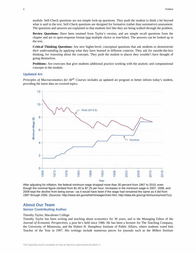
Updated ArtPrinciples of Macroeconomics for AP® Courses includes an updated art program to better inform today’s student,providing the latest data on covered topics.
After adjusting for inflation, the federal minimum wage dropped more than 30 percent from 1967 to 2010, eventhough the nominal figure climbed from $1.40 to $7.25 per hour. Increases in the minimum wage in 2007, 2008, and2009 kept the decline from being worse—as it would have been if the wage had remained the same as it did from1997 through 2006. (Sources: http://www.dol.gov/whd/minwage/chart.htm; http://data.bls.gov/cgi-bin/surveymost?cu)
About Our TeamSenior Contributing AuthorTimothy Taylor, Macalester CollegeTimothy Taylor has been writing and teaching about economics for 30 years, and is the Managing Editor of theJournal of Economic Perspectives, a post he’s held since 1986. He has been a lecturer for The Teaching Company,the University of Minnesota, and the Hubert H. Humphrey Institute of Public Affairs, where students voted himTeacher of the Year in 1997. His writings include numerous pieces for journals such as the Milken Institute
4 Preface
This OpenStax book is available for free at http://cnx.org/content/col11864/1.2

Review and The Public Interest, and he has been an editor on many projects, most notably for the BrookingsInstitution and the World Bank, where he was Chief Outside Editor for the World Development Report 1999/2000,Entering the 21st Century: The Changing Development Landscape. He also blogs four to five times per week athttp://conversableeconomist.blogspot.com. Timothy Taylor lives near Minneapolis with his wife Kimberley and theirthree children.
Senior Content ExpertSteven A. Greenlaw, University of Mary WashingtonSteven Greenlaw has been teaching principles of economics for more than 30 years. In 1999, he received the GrelletC. Simpson Award for Excellence in Undergraduate Teaching at the University of Mary Washington. He is the authorof Doing Economics: A Guide to Doing and Understanding Economic Research, as well as a variety of articles oneconomics pedagogy and instructional technology, published in the Journal of Economic Education, the InternationalReview of Economic Education, and other outlets. He wrote the module on Quantitative Writing for Starting Point:Teaching and Learning Economics, the web portal on best practices in teaching economics. Steven Greenlaw lives inAlexandria, Virginia with his wife Kathy and their three children.
Senior ContributorsEric Dodge Hanover College
Cynthia Gamez University of Texas at El Paso
Andres Jauregui Columbus State University
Diane Keenan Cerritos College
Dan MacDonald California State University San Bernardino
Amyaz Moledina The College of Wooster
Craig Richardson Winston-Salem State University
David Shapiro Pennsylvania State University
Ralph Sonenshine American University
ReviewersBryan Aguiar Northwest Arkansas Community College
Basil Al Hashimi Mesa Community College
Emil Berendt Mount St. Mary's University
Zena Buser Adams State University
Douglas Campbell The University of Memphis
Sanjukta Chaudhuri University of Wisconsin - Eau Claire
Xueyu Cheng Alabama State University
Robert Cunningham Alma College
Rosa Lea Danielson College of DuPage
Steven Deloach Elon University
Michael Enz Framingham State University
Debbie Evercloud University of Colorado Denver
Preface 5

Reza Ghorashi Richard Stockton College of New Jersey
Robert Gillette University of Kentucky
Shaomin Huang Lewis-Clark State College
George Jones University of Wisconsin-Rock County
Charles Kroncke College of Mount St. Joseph
Teresa Laughlin Palomar Community College
Carlos Liard-Muriente Central Connecticut State University
Heather Luea Kansas State University
Steven Lugauer University of Notre Dame
William Mosher Nashua Community College
Michael Netta Hudson County Community College
Nick Noble Miami University
Joe Nowakowski Muskingum University
Shawn Osell University of Wisconsin, Superior
Mark Owens Middle Tennessee State University
Sonia Pereira Barnard College
Jennifer Platania Elon University
Robert Rycroft University of Mary Washington
Adrienne Sachse Florida State College at Jacksonville
Hans Schumann Texas AM
Gina Shamshak Goucher College
Chris Warburton John Jay College of Criminal Justice, CUNY
Mark Witte Northwestern
AncillariesOpenStax projects offer an array of ancillaries for students and instructors. Please visit http://openstaxcollege.org andview the learning resources for this title.
6 Preface
This OpenStax book is available for free at http://cnx.org/content/col11864/1.2
1 | Welcome to Economics!
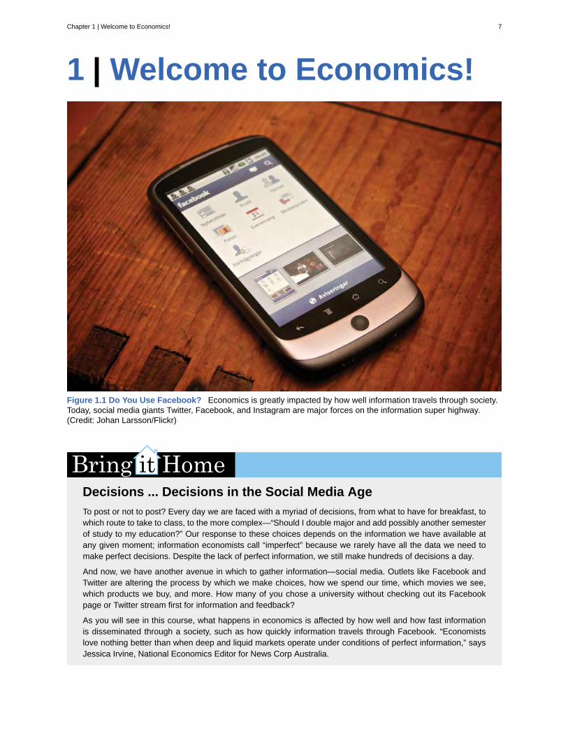
Figure 1.1 Do You Use Facebook? Economics is greatly impacted by how well information travels through society.Today, social media giants Twitter, Facebook, and Instagram are major forces on the information super highway.(Credit: Johan Larsson/Flickr)
Decisions ... Decisions in the Social Media AgeTo post or not to post? Every day we are faced with a myriad of decisions, from what to have for breakfast, towhich route to take to class, to the more complex—“Should I double major and add possibly another semesterof study to my education?” Our response to these choices depends on the information we have available atany given moment; information economists call “imperfect” because we rarely have all the data we need tomake perfect decisions. Despite the lack of perfect information, we still make hundreds of decisions a day.
And now, we have another avenue in which to gather information—social media. Outlets like Facebook andTwitter are altering the process by which we make choices, how we spend our time, which movies we see,which products we buy, and more. How many of you chose a university without checking out its Facebookpage or Twitter stream first for information and feedback?
As you will see in this course, what happens in economics is affected by how well and how fast informationis disseminated through a society, such as how quickly information travels through Facebook. “Economistslove nothing better than when deep and liquid markets operate under conditions of perfect information,” saysJessica Irvine, National Economics Editor for News Corp Australia.
Chapter 1 | Welcome to Economics! 7
This leads us to the topic of this chapter, an introduction to the world of making decisions, processinginformation, and understanding behavior in markets —the world of economics. Each chapter in this book willstart with a discussion about current (or sometimes past) events and revisit it at chapter’s end—to “bringhome” the concepts in play.
IntroductionIn this chapter, you will learn about:
• What Is Economics, and Why Is It Important?
• Microeconomics and Macroeconomics
• How Economists Use Theories and Models to Understand Economic Issues
• How Economies Can Be Organized: An Overview of Economic Systems
What is economics and why should you spend your time learning it? After all, there are other disciplines you couldbe studying, and other ways you could be spending your time. As the Bring it Home feature just mentioned, makingchoices is at the heart of what economists study, and your decision to take this course is as much as economic decisionas anything else.
Economics is probably not what you think. It is not primarily about money or finance. It is not primarily aboutbusiness. It is not mathematics. What is it then? It is both a subject area and a way of viewing the world.
1.1 | What Is Economics, and Why Is It Important?By the end of this section, you will be able to:
• Discuss the importance of studying economics• Explain the relationship between production and division of labor• Evaluate the significance of scarcity
Economics is the study of how humans make decisions in the face of scarcity. These can be individual decisions,family decisions, business decisions or societal decisions. If you look around carefully, you will see that scarcity is afact of life. Scarcity means that human wants for goods, services and resources exceed what is available. Resources,such as labor, tools, land, and raw materials are necessary to produce the goods and services we want but they existin limited supply. Of course, the ultimate scarce resource is time- everyone, rich or poor, has just 24 hours in the dayto try to acquire the goods they want. At any point in time, there is only a finite amount of resources available.
Think about it this way: In 2015 the labor force in the United States contained over 158.6 million workers, accordingto the U.S. Bureau of Labor Statistics. Similarly, the total area of the United States is 3,794,101 square miles. Theseare large numbers for such crucial resources, however, they are limited. Because these resources are limited, so arethe numbers of goods and services we produce with them. Combine this with the fact that human wants seem to bevirtually infinite, and you can see why scarcity is a problem.
8 Chapter 1 | Welcome to Economics!
This OpenStax book is available for free at http://cnx.org/content/col11864/1.2
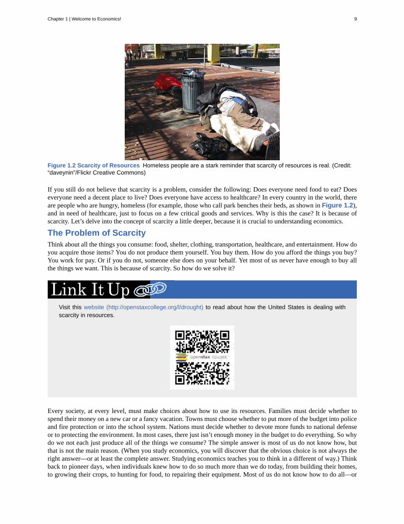
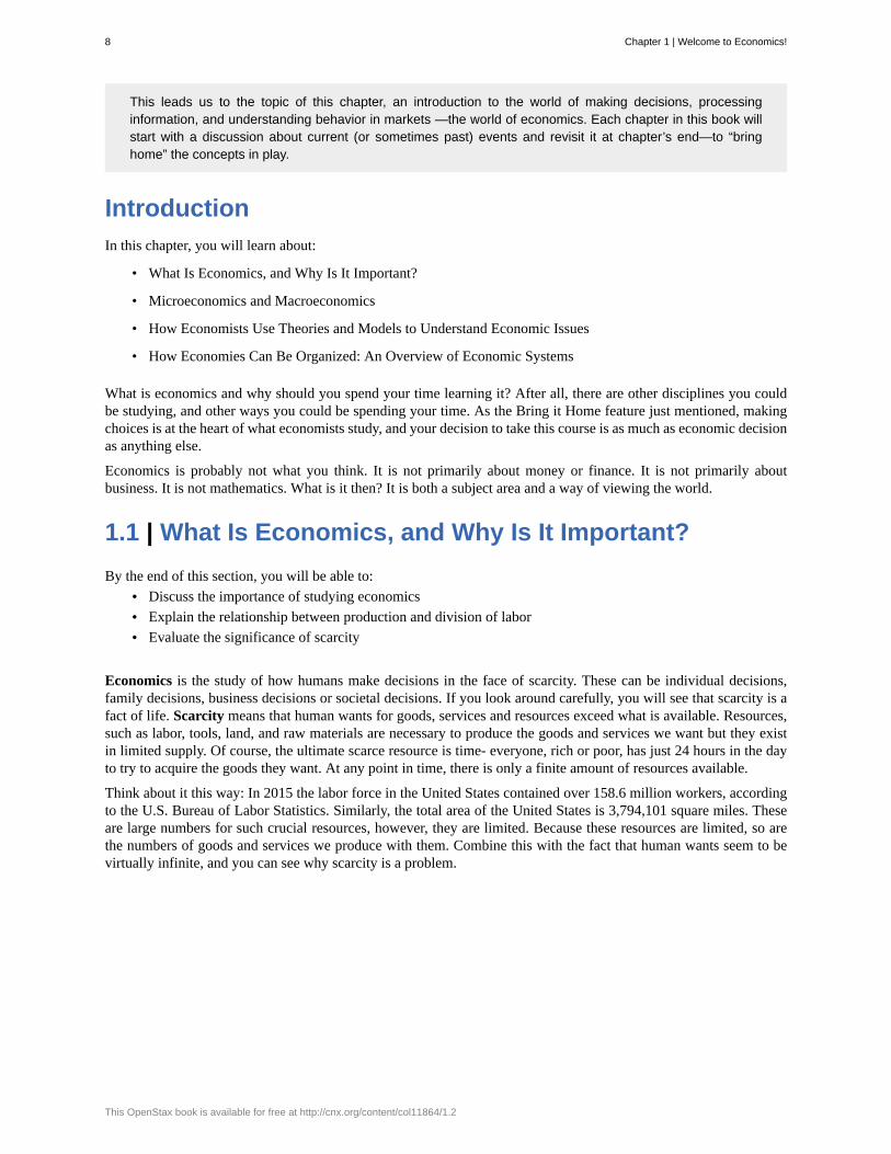
Figure 1.2 Scarcity of Resources Homeless people are a stark reminder that scarcity of resources is real. (Credit:“daveynin”/Flickr Creative Commons)
If you still do not believe that scarcity is a problem, consider the following: Does everyone need food to eat? Doeseveryone need a decent place to live? Does everyone have access to healthcare? In every country in the world, thereare people who are hungry, homeless (for example, those who call park benches their beds, as shown in Figure 1.2),and in need of healthcare, just to focus on a few critical goods and services. Why is this the case? It is because ofscarcity. Let’s delve into the concept of scarcity a little deeper, because it is crucial to understanding economics.
The Problem of ScarcityThink about all the things you consume: food, shelter, clothing, transportation, healthcare, and entertainment. How doyou acquire those items? You do not produce them yourself. You buy them. How do you afford the things you buy?You work for pay. Or if you do not, someone else does on your behalf. Yet most of us never have enough to buy allthe things we want. This is because of scarcity. So how do we solve it?
Visit this website (http://openstaxcollege.org/l/drought) to read about how the United States is dealing withscarcity in resources.
Every society, at every level, must make choices about how to use its resources. Families must decide whether tospend their money on a new car or a fancy vacation. Towns must choose whether to put more of the budget into policeand fire protection or into the school system. Nations must decide whether to devote more funds to national defenseor to protecting the environment. In most cases, there just isn’t enough money in the budget to do everything. So whydo we not each just produce all of the things we consume? The simple answer is most of us do not know how, butthat is not the main reason. (When you study economics, you will discover that the obvious choice is not always theright answer—or at least the complete answer. Studying economics teaches you to think in a different of way.) Thinkback to pioneer days, when individuals knew how to do so much more than we do today, from building their homes,to growing their crops, to hunting for food, to repairing their equipment. Most of us do not know how to do all—or
Chapter 1 | Welcome to Economics! 9
any—of those things. It is not because we could not learn. Rather, we do not have to. The reason why is somethingcalled the division and specialization of labor, a production innovation first put forth by Adam Smith, Figure 1.3, inhis book, The Wealth of Nations.
Figure 1.3 Adam Smith Adam Smith introduced the idea of dividing labor into discrete tasks. (Credit: WikimediaCommons)
The Division of and Specialization of LaborThe formal study of economics began when Adam Smith (1723–1790) published his famous book The Wealth ofNations in 1776. Many authors had written on economics in the centuries before Smith, but he was the first to addressthe subject in a comprehensive way. In the first chapter, Smith introduces the division of labor, which means that theway a good or service is produced is divided into a number of tasks that are performed by different workers, insteadof all the tasks being done by the same person.
To illustrate the division of labor, Smith counted how many tasks went into making a pin: drawing out a piece of wire,cutting it to the right length, straightening it, putting a head on one end and a point on the other, and packaging pinsfor sale, to name just a few. Smith counted 18 distinct tasks that were often done by different people—all for a pin,believe it or not!
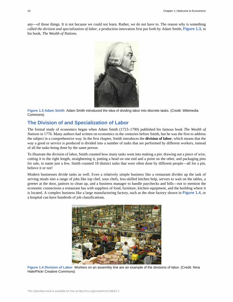
Modern businesses divide tasks as well. Even a relatively simple business like a restaurant divides up the task ofserving meals into a range of jobs like top chef, sous chefs, less-skilled kitchen help, servers to wait on the tables, agreeter at the door, janitors to clean up, and a business manager to handle paychecks and bills—not to mention theeconomic connections a restaurant has with suppliers of food, furniture, kitchen equipment, and the building where itis located. A complex business like a large manufacturing factory, such as the shoe factory shown in Figure 1.4, ora hospital can have hundreds of job classifications.
Figure 1.4 Division of Labor Workers on an assembly line are an example of the divisions of labor. (Credit: NinaHale/Flickr Creative Commons)
10 Chapter 1 | Welcome to Economics!
This OpenStax book is available for free at http://cnx.org/content/col11864/1.2
Why the Division of Labor Increases ProductionWhen the tasks involved with producing a good or service are divided and subdivided, workers and businesses canproduce a greater quantity of output. In his observations of pin factories, Smith observed that one worker alone mightmake 20 pins in a day, but that a small business of 10 workers (some of whom would need to do two or three of the 18tasks involved with pin-making), could make 48,000 pins in a day. How can a group of workers, each specializing incertain tasks, produce so much more than the same number of workers who try to produce the entire good or serviceby themselves? Smith offered three reasons.
First, specialization in a particular small job allows workers to focus on the parts of the production process wherethey have an advantage. (In later chapters, we will develop this idea by discussing comparative advantage.) Peoplehave different skills, talents, and interests, so they will be better at some jobs than at others. The particular advantagesmay be based on educational choices, which are in turn shaped by interests and talents. Only those with medicaldegrees qualify to become doctors, for instance. For some goods, specialization will be affected by geography—it iseasier to be a wheat farmer in North Dakota than in Florida, but easier to run a tourist hotel in Florida than in NorthDakota. If you live in or near a big city, it is easier to attract enough customers to operate a successful dry cleaningbusiness or movie theater than if you live in a sparsely populated rural area. Whatever the reason, if people specializein the production of what they do best, they will be more productive than if they produce a combination of things,some of which they are good at and some of which they are not.
Second, workers who specialize in certain tasks often learn to produce more quickly and with higher quality. Thispattern holds true for many workers, including assembly line laborers who build cars, stylists who cut hair, anddoctors who perform heart surgery. In fact, specialized workers often know their jobs well enough to suggestinnovative ways to do their work faster and better.
A similar pattern often operates within businesses. In many cases, a business that focuses on one or a few products(sometimes called its “core competency”) is more successful than firms that try to make a wide range of products.
Third, specialization allows businesses to take advantage of economies of scale, which means that for many goods,as the level of production increases, the average cost of producing each individual unit declines. For example, if afactory produces only 100 cars per year, each car will be quite expensive to make on average. However, if a factoryproduces 50,000 cars each year, then it can set up an assembly line with huge machines and workers performingspecialized tasks, and the average cost of production per car will be lower. The ultimate result of workers who canfocus on their preferences and talents, learn to do their specialized jobs better, and work in larger organizations is thatsociety as a whole can produce and consume far more than if each person tried to produce all of their own goods andservices. The division and specialization of labor has been a force against the problem of scarcity.
Trade and MarketsSpecialization only makes sense, though, if workers can use the pay they receive for doing their jobs to purchase theother goods and services that they need. In short, specialization requires trade.
You do not have to know anything about electronics or sound systems to play music—you just buy an iPod or MP3player, download the music and listen. You do not have to know anything about artificial fibers or the construction ofsewing machines if you need a jacket—you just buy the jacket and wear it. You do not need to know anything aboutinternal combustion engines to operate a car—you just get in and drive. Instead of trying to acquire all the knowledgeand skills involved in producing all of the goods and services that you wish to consume, the market allows you tolearn a specialized set of skills and then use the pay you receive to buy the goods and services you need or want. Thisis how our modern society has evolved into a strong economy.
Why Study Economics?Now that we have gotten an overview on what economics studies, let’s quickly discuss why you are right to study it.Economics is not primarily a collection of facts to be memorized, though there are plenty of important concepts to belearned. Instead, economics is better thought of as a collection of questions to be answered or puzzles to be workedout. Most important, economics provides the tools to work out those puzzles. If you have yet to be been bitten by theeconomics “bug,” there are other reasons why you should study economics.
• Virtually every major problem facing the world today, from global warming, to world poverty, to the conflictsin Syria, Afghanistan, and Somalia, has an economic dimension. If you are going to be part of solving thoseproblems, you need to be able to understand them. Economics is crucial.
Chapter 1 | Welcome to Economics! 11
• It is hard to overstate the importance of economics to good citizenship. You need to be able to voteintelligently on budgets, regulations, and laws in general. When the U.S. government came close to a standstillat the end of 2012 due to the “fiscal cliff,” what were the issues involved? Did you know?
• A basic understanding of economics makes you a well-rounded thinker. When you read articles abouteconomic issues, you will understand and be able to evaluate the writer’s argument. When you hearclassmates, co-workers, or political candidates talking about economics, you will be able to distinguishbetween common sense and nonsense. You will find new ways of thinking about current events and aboutpersonal and business decisions, as well as current events and politics.
The study of economics does not dictate the answers, but it can illuminate the different choices.
1.2 | Microeconomics and MacroeconomicsBy the end of this section, you will be able to:
• Describe microeconomics• Describe macroeconomics• Contrast monetary policy and fiscal policy
Economics is concerned with the well-being of all people, including those with jobs and those without jobs, as well asthose with high incomes and those with low incomes. Economics acknowledges that production of useful goods andservices can create problems of environmental pollution. It explores the question of how investing in education helpsto develop workers’ skills. It probes questions like how to tell when big businesses or big labor unions are operating ina way that benefits society as a whole and when they are operating in a way that benefits their owners or members atthe expense of others. It looks at how government spending, taxes, and regulations affect decisions about productionand consumption.
It should be clear by now that economics covers a lot of ground. That ground can be divided into two parts:Microeconomics focuses on the actions of individual agents within the economy, like households, workers, andbusinesses; Macroeconomics looks at the economy as a whole. It focuses on broad issues such as growth ofproduction, the number of unemployed people, the inflationary increase in prices, government deficits, and levelsof exports and imports. Microeconomics and macroeconomics are not separate subjects, but rather complementaryperspectives on the overall subject of the economy.
To understand why both microeconomic and macroeconomic perspectives are useful, consider the problem ofstudying a biological ecosystem like a lake. One person who sets out to study the lake might focus on specific topics:certain kinds of algae or plant life; the characteristics of particular fish or snails; or the trees surrounding the lake.Another person might take an overall view and instead consider the entire ecosystem of the lake from top to bottom;what eats what, how the system stays in a rough balance, and what environmental stresses affect this balance. Bothapproaches are useful, and both examine the same lake, but the viewpoints are different. In a similar way, bothmicroeconomics and macroeconomics study the same economy, but each has a different viewpoint.
Whether you are looking at lakes or economics, the micro and the macro insights should blend with each other. Instudying a lake, the micro insights about particular plants and animals help to understand the overall food chain,while the macro insights about the overall food chain help to explain the environment in which individual plants andanimals live.
In economics, the micro decisions of individual businesses are influenced by whether the macroeconomy is healthy;for example, firms will be more likely to hire workers if the overall economy is growing. In turn, the performanceof the macroeconomy ultimately depends on the microeconomic decisions made by individual households andbusinesses.
MicroeconomicsWhat determines how households and individuals spend their budgets? What combination of goods and services willbest fit their needs and wants, given the budget they have to spend? How do people decide whether to work, and ifso, whether to work full time or part time? How do people decide how much to save for the future, or whether theyshould borrow to spend beyond their current means?
12 Chapter 1 | Welcome to Economics!
This OpenStax book is available for free at http://cnx.org/content/col11864/1.2
What determines the products, and how many of each, a firm will produce and sell? What determines what pricesa firm will charge? What determines how a firm will produce its products? What determines how many workers itwill hire? How will a firm finance its business? When will a firm decide to expand, downsize, or even close? In themicroeconomic part of this book, we will learn about the theory of consumer behavior and the theory of the firm.
MacroeconomicsWhat determines the level of economic activity in a society? In other words, what determines how many goods andservices a nation actually produces? What determines how many jobs are available in an economy? What determinesa nation’s standard of living? What causes the economy to speed up or slow down? What causes firms to hire moreworkers or to lay workers off? Finally, what causes the economy to grow over the long term?
An economy's macroeconomic health can be defined by a number of goals: growth in the standard of living, lowunemployment, and low inflation, to name the most important. How can macroeconomic policy be used to pursuethese goals? Monetary policy, which involves policies that affect bank lending, interest rates, and financial capitalmarkets, is conducted by a nation’s central bank. For the United States, this is the Federal Reserve. Fiscal policy,which involves government spending and taxes, is determined by a nation’s legislative body. For the United States,this is the Congress and the executive branch, which originates the federal budget. These are the main tools thegovernment has to work with. Americans tend to expect that government can fix whatever economic problems weencounter, but to what extent is that expectation realistic? These are just some of the issues that will be explored inthe macroeconomic chapters of this book.
1.3 | How Economists Use Theories and Models toUnderstand Economic IssuesBy the end of this section, you will be able to:
• Interpret a circular flow diagram• Explain the importance of economic theories and models• Describe goods and services markets and labor markets
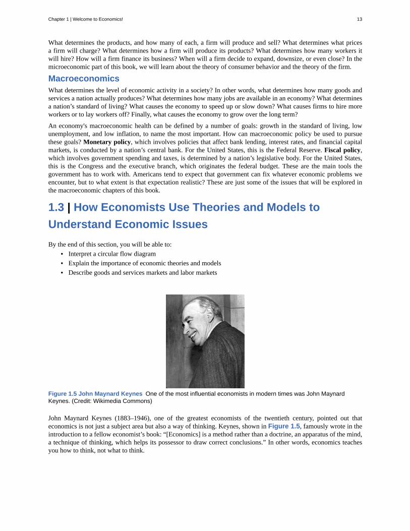
Figure 1.5 John Maynard Keynes One of the most influential economists in modern times was John MaynardKeynes. (Credit: Wikimedia Commons)
John Maynard Keynes (1883–1946), one of the greatest economists of the twentieth century, pointed out thateconomics is not just a subject area but also a way of thinking. Keynes, shown in Figure 1.5, famously wrote in theintroduction to a fellow economist’s book: “[Economics] is a method rather than a doctrine, an apparatus of the mind,a technique of thinking, which helps its possessor to draw correct conclusions.” In other words, economics teachesyou how to think, not what to think.
Chapter 1 | Welcome to Economics! 13
Watch this video (http://openstaxcollege.org/l/Keynes) about John Maynard Keynes and his influence oneconomics.
Economists see the world through a different lens than anthropologists, biologists, classicists, or practitioners of anyother discipline. They analyze issues and problems with economic theories that are based on particular assumptionsabout human behavior, that are different than the assumptions an anthropologist or psychologist might use. A theoryis a simplified representation of how two or more variables interact with each other. The purpose of a theory is to takea complex, real-world issue and simplify it down to its essentials. If done well, this enables the analyst to understandthe issue and any problems around it. A good theory is simple enough to be understood, while complex enough tocapture the key features of the object or situation being studied.
Sometimes economists use the term model instead of theory. Strictly speaking, a theory is a more abstractrepresentation, while a model is more applied or empirical representation. Models are used to test theories, but forthis course we will use the terms interchangeably.
For example, an architect who is planning a major office building will often build a physical model that sits on atabletop to show how the entire city block will look after the new building is constructed. Companies often buildmodels of their new products, which are more rough and unfinished than the final product will be, but can stilldemonstrate how the new product will work.
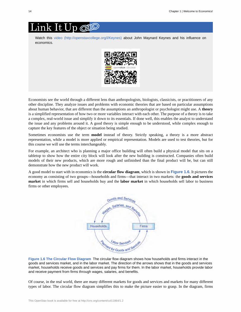
A good model to start with in economics is the circular flow diagram, which is shown in Figure 1.6. It pictures theeconomy as consisting of two groups—households and firms—that interact in two markets: the goods and servicesmarket in which firms sell and households buy and the labor market in which households sell labor to businessfirms or other employees.
Figure 1.6 The Circular Flow Diagram The circular flow diagram shows how households and firms interact in thegoods and services market, and in the labor market. The direction of the arrows shows that in the goods and servicesmarket, households receive goods and services and pay firms for them. In the labor market, households provide laborand receive payment from firms through wages, salaries, and benefits.
Of course, in the real world, there are many different markets for goods and services and markets for many differenttypes of labor. The circular flow diagram simplifies this to make the picture easier to grasp. In the diagram, firms
14 Chapter 1 | Welcome to Economics!
This OpenStax book is available for free at http://cnx.org/content/col11864/1.2
produce goods and services, which they sell to households in return for revenues. This is shown in the outer circle, andrepresents the two sides of the product market (for example, the market for goods and services) in which householdsdemand and firms supply. Households sell their labor as workers to firms in return for wages, salaries and benefits.This is shown in the inner circle and represents the two sides of the labor market in which households supply andfirms demand.
This version of the circular flow model is stripped down to the essentials, but it has enough features to explain howthe product and labor markets work in the economy. We could easily add details to this basic model if we wanted tointroduce more real-world elements, like financial markets, governments, and interactions with the rest of the globe(imports and exports).
Economists carry a set of theories in their heads like a carpenter carries around a toolkit. When they see an economicissue or problem, they go through the theories they know to see if they can find one that fits. Then they use the theoryto derive insights about the issue or problem. In economics, theories are expressed as diagrams, graphs, or even asmathematical equations. (Do not worry. In this course, we will mostly use graphs.) Economists do not figure out theanswer to the problem first and then draw the graph to illustrate. Rather, they use the graph of the theory to helpthem figure out the answer. Although at the introductory level, you can sometimes figure out the right answer withoutapplying a model, if you keep studying economics, before too long you will run into issues and problems that youwill need to graph to solve. Both micro and macroeconomics are explained in terms of theories and models. The mostwell-known theories are probably those of supply and demand, but you will learn a number of others.
1.4 | How Economies Can Be Organized: An Overview ofEconomic SystemsBy the end of this section, you will be able to:
• Contrast traditional economies, command economies, and market economies• Explain gross domestic product (GDP)• Assess the importance and effects of globalization
Think about what a complex system a modern economy is. It includes all production of goods and services, all buyingand selling, all employment. The economic life of every individual is interrelated, at least to a small extent, with theeconomic lives of thousands or even millions of other individuals. Who organizes and coordinates this system? Whoinsures that, for example, the number of televisions a society provides is the same as the amount it needs and wants?Who insures that the right number of employees work in the electronics industry? Who insures that televisions areproduced in the best way possible? How does it all get done?
There are at least three ways societies have found to organize an economy. The first is the traditional economy,which is the oldest economic system and can be found in parts of Asia, Africa, and South America. Traditionaleconomies organize their economic affairs the way they have always done (i.e., tradition). Occupations stay in thefamily. Most families are farmers who grow the crops they have always grown using traditional methods. What youproduce is what you get to consume. Because things are driven by tradition, there is little economic progress ordevelopment.
Chapter 1 | Welcome to Economics! 15
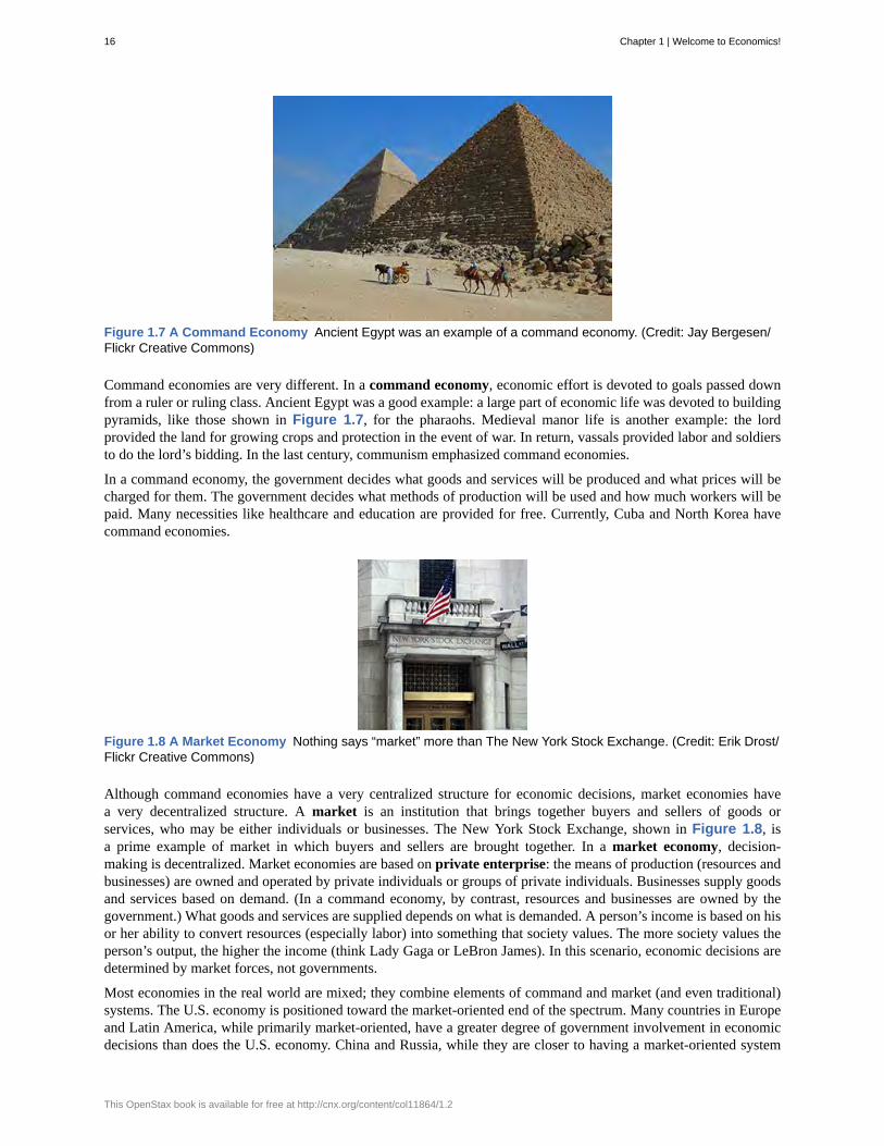
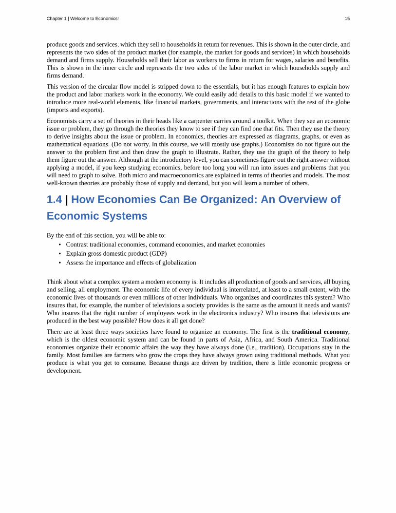
Figure 1.7 A Command Economy Ancient Egypt was an example of a command economy. (Credit: Jay Bergesen/Flickr Creative Commons)
Command economies are very different. In a command economy, economic effort is devoted to goals passed downfrom a ruler or ruling class. Ancient Egypt was a good example: a large part of economic life was devoted to buildingpyramids, like those shown in Figure 1.7, for the pharaohs. Medieval manor life is another example: the lordprovided the land for growing crops and protection in the event of war. In return, vassals provided labor and soldiersto do the lord’s bidding. In the last century, communism emphasized command economies.
In a command economy, the government decides what goods and services will be produced and what prices will becharged for them. The government decides what methods of production will be used and how much workers will bepaid. Many necessities like healthcare and education are provided for free. Currently, Cuba and North Korea havecommand economies.
Figure 1.8 A Market Economy Nothing says “market” more than The New York Stock Exchange. (Credit: Erik Drost/Flickr Creative Commons)
Although command economies have a very centralized structure for economic decisions, market economies havea very decentralized structure. A market is an institution that brings together buyers and sellers of goods orservices, who may be either individuals or businesses. The New York Stock Exchange, shown in Figure 1.8, isa prime example of market in which buyers and sellers are brought together. In a market economy, decision-making is decentralized. Market economies are based on private enterprise: the means of production (resources andbusinesses) are owned and operated by private individuals or groups of private individuals. Businesses supply goodsand services based on demand. (In a command economy, by contrast, resources and businesses are owned by thegovernment.) What goods and services are supplied depends on what is demanded. A person’s income is based on hisor her ability to convert resources (especially labor) into something that society values. The more society values theperson’s output, the higher the income (think Lady Gaga or LeBron James). In this scenario, economic decisions aredetermined by market forces, not governments.
Most economies in the real world are mixed; they combine elements of command and market (and even traditional)systems. The U.S. economy is positioned toward the market-oriented end of the spectrum. Many countries in Europeand Latin America, while primarily market-oriented, have a greater degree of government involvement in economicdecisions than does the U.S. economy. China and Russia, while they are closer to having a market-oriented system
16 Chapter 1 | Welcome to Economics!
This OpenStax book is available for free at http://cnx.org/content/col11864/1.2
now than several decades ago, remain closer to the command economy end of the spectrum. A rich resource ofinformation about countries and their economies can be found on the Heritage Foundation’s website, as the followingClear It Up feature discusses.
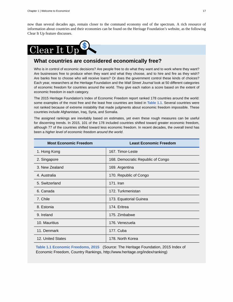
What countries are considered economically free?Who is in control of economic decisions? Are people free to do what they want and to work where they want?Are businesses free to produce when they want and what they choose, and to hire and fire as they wish?Are banks free to choose who will receive loans? Or does the government control these kinds of choices?Each year, researchers at the Heritage Foundation and the Wall Street Journal look at 50 different categoriesof economic freedom for countries around the world. They give each nation a score based on the extent ofeconomic freedom in each category.
The 2015 Heritage Foundation’s Index of Economic Freedom report ranked 178 countries around the world:some examples of the most free and the least free countries are listed in Table 1.1. Several countries werenot ranked because of extreme instability that made judgments about economic freedom impossible. Thesecountries include Afghanistan, Iraq, Syria, and Somalia.
The assigned rankings are inevitably based on estimates, yet even these rough measures can be usefulfor discerning trends. In 2015, 101 of the 178 included countries shifted toward greater economic freedom,although 77 of the countries shifted toward less economic freedom. In recent decades, the overall trend hasbeen a higher level of economic freedom around the world.
Most Economic Freedom Least Economic Freedom
1. Hong Kong 167. Timor-Leste
2. Singapore 168. Democratic Republic of Congo
3. New Zealand 169. Argentina
4. Australia 170. Republic of Congo
5. Switzerland 171. Iran
6. Canada 172. Turkmenistan
7. Chile 173. Equatorial Guinea
8. Estonia 174. Eritrea
9. Ireland 175. Zimbabwe
10. Mauritius 176. Venezuela
11. Denmark 177. Cuba
12. United States 178. North Korea
Table 1.1 Economic Freedoms, 2015 (Source: The Heritage Foundation, 2015 Index ofEconomic Freedom, Country Rankings, http://www.heritage.org/index/ranking)
Chapter 1 | Welcome to Economics! 17
Regulations: The Rules of the GameMarkets and government regulations are always entangled. There is no such thing as an absolutely free market.Regulations always define the “rules of the game” in the economy. Economies that are primarily market-orientedhave fewer regulations—ideally just enough to maintain an even playing field for participants. At a minimum, theselaws govern matters like safeguarding private property against theft, protecting people from violence, enforcing legalcontracts, preventing fraud, and collecting taxes. Conversely, even the most command-oriented economies operateusing markets. How else would buying and selling occur? But the decisions of what will be produced and what priceswill be charged are heavily regulated. Heavily regulated economies often have underground economies, which aremarkets where the buyers and sellers make transactions without the government’s approval.
The question of how to organize economic institutions is typically not a black-or-white choice between all marketor all government, but instead involves a balancing act over the appropriate combination of market freedom andgovernment rules.
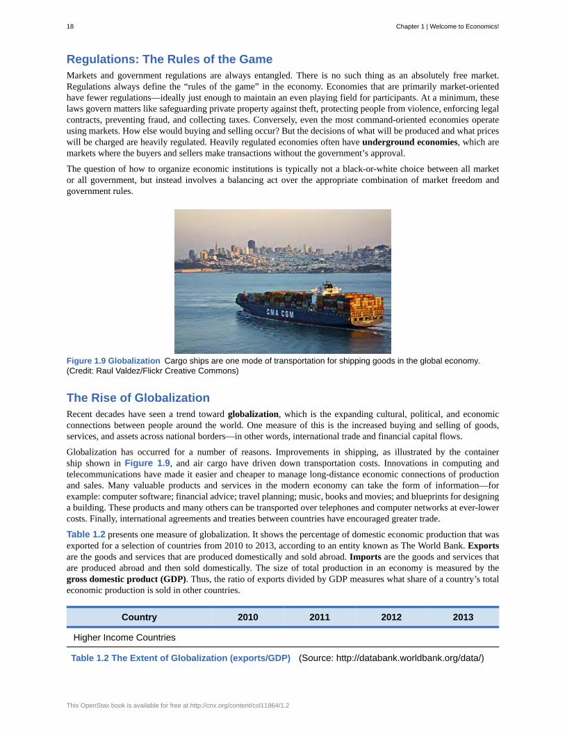
Figure 1.9 Globalization Cargo ships are one mode of transportation for shipping goods in the global economy.(Credit: Raul Valdez/Flickr Creative Commons)
The Rise of GlobalizationRecent decades have seen a trend toward globalization, which is the expanding cultural, political, and economicconnections between people around the world. One measure of this is the increased buying and selling of goods,services, and assets across national borders—in other words, international trade and financial capital flows.
Globalization has occurred for a number of reasons. Improvements in shipping, as illustrated by the containership shown in Figure 1.9, and air cargo have driven down transportation costs. Innovations in computing andtelecommunications have made it easier and cheaper to manage long-distance economic connections of productionand sales. Many valuable products and services in the modern economy can take the form of information—forexample: computer software; financial advice; travel planning; music, books and movies; and blueprints for designinga building. These products and many others can be transported over telephones and computer networks at ever-lowercosts. Finally, international agreements and treaties between countries have encouraged greater trade.
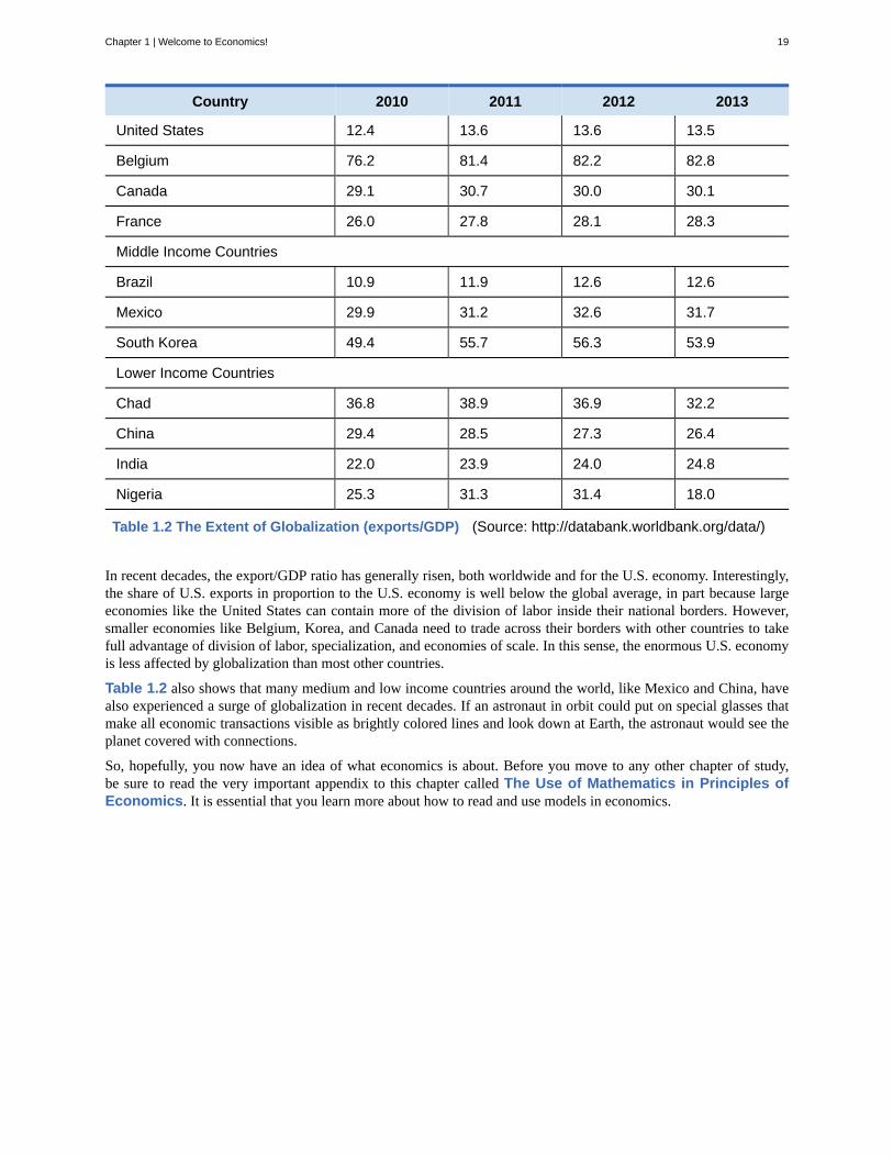
Table 1.2 presents one measure of globalization. It shows the percentage of domestic economic production that wasexported for a selection of countries from 2010 to 2013, according to an entity known as The World Bank. Exportsare the goods and services that are produced domestically and sold abroad. Imports are the goods and services thatare produced abroad and then sold domestically. The size of total production in an economy is measured by thegross domestic product (GDP). Thus, the ratio of exports divided by GDP measures what share of a country’s totaleconomic production is sold in other countries.
Country 2010 2011 2012 2013
Higher Income Countries
Table 1.2 The Extent of Globalization (exports/GDP) (Source: http://databank.worldbank.org/data/)
18 Chapter 1 | Welcome to Economics!
This OpenStax book is available for free at http://cnx.org/content/col11864/1.2
Country 2010 2011 2012 2013
United States 12.4 13.6 13.6 13.5
Belgium 76.2 81.4 82.2 82.8
Canada 29.1 30.7 30.0 30.1
France 26.0 27.8 28.1 28.3
Middle Income Countries
Brazil 10.9 11.9 12.6 12.6
Mexico 29.9 31.2 32.6 31.7
South Korea 49.4 55.7 56.3 53.9
Lower Income Countries
Chad 36.8 38.9 36.9 32.2
China 29.4 28.5 27.3 26.4
India 22.0 23.9 24.0 24.8
Nigeria 25.3 31.3 31.4 18.0
Table 1.2 The Extent of Globalization (exports/GDP) (Source: http://databank.worldbank.org/data/)
In recent decades, the export/GDP ratio has generally risen, both worldwide and for the U.S. economy. Interestingly,the share of U.S. exports in proportion to the U.S. economy is well below the global average, in part because largeeconomies like the United States can contain more of the division of labor inside their national borders. However,smaller economies like Belgium, Korea, and Canada need to trade across their borders with other countries to takefull advantage of division of labor, specialization, and economies of scale. In this sense, the enormous U.S. economyis less affected by globalization than most other countries.
Table 1.2 also shows that many medium and low income countries around the world, like Mexico and China, havealso experienced a surge of globalization in recent decades. If an astronaut in orbit could put on special glasses thatmake all economic transactions visible as brightly colored lines and look down at Earth, the astronaut would see theplanet covered with connections.
So, hopefully, you now have an idea of what economics is about. Before you move to any other chapter of study,be sure to read the very important appendix to this chapter called The Use of Mathematics in Principles ofEconomics. It is essential that you learn more about how to read and use models in economics.
Chapter 1 | Welcome to Economics! 19
Decisions ... Decisions in the Social Media AgeThe world we live in today provides nearly instant access to a wealth of information. Consider that asrecently as the late 1970s, the Farmer’s Almanac, along with the Weather Bureau of the U.S. Department ofAgriculture, were the primary sources American farmers used to determine when to plant and harvest theircrops. Today, farmers are more likely to access, online, weather forecasts from the National Oceanic andAtmospheric Administration or watch the Weather Channel. After all, knowing the upcoming forecast coulddrive when to harvest crops. Consequently, knowing the upcoming weather could change the amount of cropharvested.
Some relatively new information forums, such as Facebook, are rapidly changing how information isdistributed; hence, influencing decision making. In 2014, the Pew Research Center reported that 71% ofonline adults use Facebook. Facebook post topics range from the National Basketball Association, to celebritysingers and performers, to farmers.
Information helps us make decisions. Decisions as simple as what to wear today to how many reportersshould be sent to cover a crash. Each of these decisions is an economic decision. After all, resources arescarce. If ten reporters are sent to cover an accident, they are not available to cover other stories or completeother tasks. Information provides the knowledge needed to make the best possible decisions on how to utilizescarce resources. Welcome to the world of economics!
20 Chapter 1 | Welcome to Economics!
This OpenStax book is available for free at http://cnx.org/content/col11864/1.2
circular flow diagram
command economy
division of labor
economics
economies of scale
exports
fiscal policy
globalization
goods and services market
gross domestic product (GDP)
imports
labor market
macroeconomics
market
market economy
microeconomics
model
monetary policy
private enterprise
scarcity
specialization
theory
traditional economy
KEY TERMS
a diagram that views the economy as consisting of households and firms interacting in a goodsand services market and a labor market
an economy where economic decisions are passed down from government authority and whereresources are owned by the government
the way in which the work required to produce a good or service is divided into tasks performed bydifferent workers
the study of how humans make choices under conditions of scarcity
when the average cost of producing each individual unit declines as total output increases
products (goods and services) made domestically and sold abroad
economic policies that involve government spending and taxes
the trend in which buying and selling in markets have increasingly crossed national borders
a market in which firms are sellers of what they produce and households are buyers
measure of the size of total production in an economy
products (goods and services) made abroad and then sold domestically
the market in which households sell their labor as workers to business firms or other employers
the branch of economics that focuses on broad issues such as growth, unemployment, inflation, andtrade balance.
interaction between potential buyers and sellers; a combination of demand and supply
an economy where economic decisions are decentralized, resources are owned by private individuals,and businesses supply goods and services based on demand
the branch of economics that focuses on actions of particular agents within the economy, likehouseholds, workers, and business firms
see theory
policy that involves altering the level of interest rates, the availability of credit in the economy, andthe extent of borrowing
system where the means of production (resources and businesses) are owned and operated byprivate individuals or groups of private individuals
when human wants for goods and services exceed the available supply
when workers or firms focus on particular tasks for which they are well-suited within the overallproduction process
a representation of an object or situation that is simplified while including enough of the key features to help usunderstand the object or situation
typically an agricultural economy where things are done the same as they have always been done
Chapter 1 | Welcome to Economics! 21

underground economy a market where the buyers and sellers make transactions in violation of one or moregovernment regulations
KEY CONCEPTS AND SUMMARY
1.1 What Is Economics, and Why Is It Important?Economics seeks to solve the problem of scarcity, which is when human wants for goods and services exceed theavailable supply. A modern economy displays a division of labor, in which people earn income by specializing inwhat they produce and then use that income to purchase the products they need or want. The division of labor allowsindividuals and firms to specialize and to produce more for several reasons: a) It allows the agents to focus on areas ofadvantage due to natural factors and skill levels; b) It encourages the agents to learn and invent; c) It allows agents totake advantage of economies of scale. Division and specialization of labor only work when individuals can purchasewhat they do not produce in markets. Learning about economics helps you understand the major problems facing theworld today, prepares you to be a good citizen, and helps you become a well-rounded thinker.
1.2 Microeconomics and MacroeconomicsMicroeconomics and macroeconomics are two different perspectives on the economy. The microeconomicperspective focuses on parts of the economy: individuals, firms, and industries. The macroeconomic perspective looksat the economy as a whole, focusing on goals like growth in the standard of living, unemployment, and inflation.Macroeconomics has two types of policies for pursuing these goals: monetary policy and fiscal policy.
1.3 How Economists Use Theories and Models to Understand Economic IssuesEconomists analyze problems differently than do other disciplinary experts. The main tools economists use areeconomic theories or models. A theory is not an illustration of the answer to a problem. Rather, a theory is a tool fordetermining the answer.
1.4 How Economies Can Be Organized: An Overview of Economic SystemsSocieties can be organized as traditional, command, or market-oriented economies. Most societies are a mix. The lastfew decades have seen globalization evolve as a result of growth in commercial and financial networks that crossnational borders, making businesses and workers from different economies increasingly interdependent.
SELF-CHECK QUESTIONS1. What is scarcity? Can you think of two causes of scarcity?
2. Residents of the town of Smithfield like to consume hams, but each ham requires 10 people to produce it andtakes a month. If the town has a total of 100 people, what is the maximum amount of ham the residents can consumein a month?
3. A consultant works for $200 per hour. She likes to eat vegetables, but is not very good at growing them. Whydoes it make more economic sense for her to spend her time at the consulting job and shop for her vegetables?
4. A computer systems engineer could paint his house, but it makes more sense for him to hire a painter to do it.Explain why.
5. What would be another example of a “system” in the real world that could serve as a metaphor for micro andmacroeconomics?
6. Suppose we extend the circular flow model to add imports and exports. Copy the circular flow diagram onto asheet of paper and then add a foreign country as a third agent. Draw a rough sketch of the flows of imports, exports,and the payments for each on your diagram.
7. What is an example of a problem in the world today, not mentioned in the chapter, that has an economicdimension?
22 Chapter 1 | Welcome to Economics!
This OpenStax book is available for free at http://cnx.org/content/col11864/1.2
8. The chapter defines private enterprise as a characteristic of market-oriented economies. What would publicenterprise be? Hint: It is a characteristic of command economies.
9. Why might Belgium, France, Italy, and Sweden have a higher export to GDP ratio than the United States?
REVIEW QUESTIONS
10. Give the three reasons that explain why the divisionof labor increases an economy’s level of production.
11. What are three reasons to study economics?
12. What is the difference between microeconomicsand macroeconomics?
13. What are examples of individual economic agents?
14. What are the three main goals of macroeconomics?
15. How did John Maynard Keynes define economics?
16. Are households primarily buyers or sellers in thegoods and services market? In the labor market?
17. Are firms primarily buyers or sellers in the goodsand services market? In the labor market?
18. What are the three ways that societies can organizethemselves economically?
19. What is globalization? How do you think it mighthave affected the economy over the past decade?
CRITICAL THINKING QUESTIONS
20. Suppose you have a team of two workers: one isa baker and one is a chef. Explain why the kitchen canproduce more meals in a given period of time if eachworker specializes in what they do best than if eachworker tries to do everything from appetizer to dessert.
21. Why would division of labor without trade notwork?
22. Can you think of any examples of free goods, thatis, goods or services that are not scarce?
23. A balanced federal budget and a balance of tradeare considered secondary goals of macroeconomics,while growth in the standard of living (for example) isconsidered a primary goal. Why do you think that is so?
24. Macroeconomics is an aggregate of what happensat the microeconomic level. Would it be possible for
what happens at the macro level to differ from howeconomic agents would react to some stimulus at themicro level? Hint: Think about the behavior of crowds.
25. Why is it unfair or meaningless to criticize a theoryas “unrealistic?”
26. Suppose, as an economist, you are asked to analyzean issue unlike anything you have ever done before.Also, suppose you do not have a specific model foranalyzing that issue. What should you do? Hint: Whatwould a carpenter do in a similar situation?
27. Why do you think that most modern countries’economies are a mix of command and market types?
28. Can you think of ways that globalization has helpedyou economically? Can you think of ways that it hasnot?
Chapter 1 | Welcome to Economics! 23
24 Chapter 1 | Welcome to Economics!
This OpenStax book is available for free at http://cnx.org/content/col11864/1.2

2 | Choice in a World ofScarcity
Figure 2.1 Choices and Tradeoffs In general, the higher the degree, the higher the salary. So why aren’t morepeople pursuing higher degrees? The short answer: choices and tradeoffs. (Credit: modification of work by “Jim, thePhotographer”/Flickr Creative Commons)
Choices ... To What Degree?In 2015, the median income for workers who hold master's degrees varies from males to females. Theaverage of the two is $2,951 weekly. Multiply this average by 52 weeks, and you get an average salary of$153,452. Compare that to the median weekly earnings for a full-time worker over 25 with no higher than abachelor’s degree: $1,224 weekly and $63,648 a year. What about those with no higher than a high schooldiploma in 2015? They earn just $664 weekly and $34,528 over 12 months. In other words, says the Bureau ofLabor Statistics (BLS), earning a bachelor’s degree boosted salaries 54% over what you would have earnedif you had stopped your education after high school. A master’s degree yields a salary almost double that of ahigh school diploma.
Given these statistics, we might expect a lot of people to choose to go to college and at least earn a bachelor’sdegree. Assuming that people want to improve their material well-being, it seems like they would make thosechoices that give them the greatest opportunity to consume goods and services. As it turns out, the analysisis not nearly as simple as this. In fact, in 2014, the BLS reported that while almost 88% of the population inthe United States had a high school diploma, only 33.6% of 25–65 year olds had bachelor’s degrees, and only7.4% of 25–65 year olds in 2014 had earned a master’s.
This brings us to the subject of this chapter: why people make the choices they make and how economists goabout explaining those choices.
Chapter 2 | Choice in a World of Scarcity 25
Introduction to Choice in a World of ScarcityIn this chapter, you will learn about:
• How Individuals Make Choices Based on Their Budget Constraint
• The Production Possibilities Frontier and Social Choices
• Confronting Objections to the Economic Approach
You will learn quickly when you examine the relationship between economics and scarcity that choices involvetradeoffs. Every choice has a cost.
In 1968, the Rolling Stones recorded “You Can’t Always Get What You Want.” Economists chuckled, because theyhad been singing a similar tune for decades. English economist Lionel Robbins (1898–1984), in his Essay on theNature and Significance of Economic Science in 1932, described not always getting what you want in this way:
The time at our disposal is limited. There are only twenty-four hours in the day. We have to choosebetween the different uses to which they may be put. ... Everywhere we turn, if we choose one thing wemust relinquish others which, in different circumstances, we would wish not to have relinquished. Scarcityof means to satisfy given ends is an almost ubiquitous condition of human nature.
Because people live in a world of scarcity, they cannot have all the time, money, possessions, and experiences theywish. Neither can society.
This chapter will continue our discussion of scarcity and the economic way of thinking by first introducing threecritical concepts: opportunity cost, marginal decision making, and diminishing returns. Later, it will consider whetherthe economic way of thinking accurately describes either how choices are made or how they should be made.
2.1 | How Individuals Make Choices Based on TheirBudget ConstraintBy the end of this section, you will be able to:
• Calculate and graph budgets constraints• Explain opportunity sets and opportunity costs• Evaluate the law of diminishing marginal utility• Explain how marginal analysis and utility influence choices
Consider the typical consumer’s budget problem. Consumers have a limited amount of income to spend on the thingsthey need and want. Suppose Alphonso has $10 in spending money each week that he can allocate between bus ticketsfor getting to work and the burgers that he eats for lunch. Burgers cost $2 each, and bus tickets are 50 cents each.Figure 2.2 shows Alphonso’s budget constraint, that is, the outer boundary of his opportunity set. The opportunityset identifies all the opportunities for spending within his budget. The budget constraint indicates all the combinationsof burgers and bus tickets Alphonso can afford when he exhausts his budget, given the prices of the two goods. (Thereare actually many different kinds of budget constraints. You will learn more about them in the chapter on ConsumerChoices (http://cnx.org/content/m57229/latest/) .)
26 Chapter 2 | Choice in a World of Scarcity
This OpenStax book is available for free at http://cnx.org/content/col11864/1.2
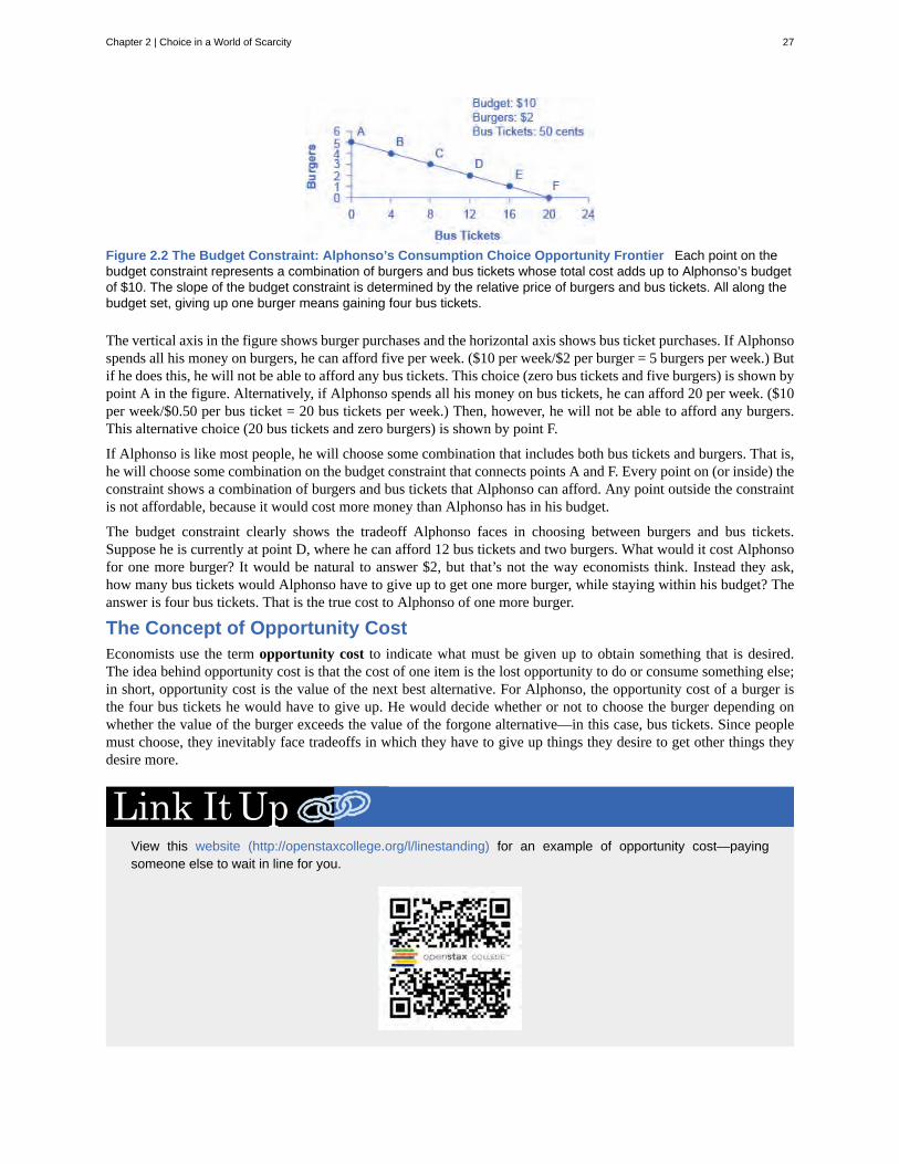
Figure 2.2 The Budget Constraint: Alphonso’s Consumption Choice Opportunity Frontier Each point on thebudget constraint represents a combination of burgers and bus tickets whose total cost adds up to Alphonso’s budgetof $10. The slope of the budget constraint is determined by the relative price of burgers and bus tickets. All along thebudget set, giving up one burger means gaining four bus tickets.
The vertical axis in the figure shows burger purchases and the horizontal axis shows bus ticket purchases. If Alphonsospends all his money on burgers, he can afford five per week. ($10 per week/$2 per burger = 5 burgers per week.) Butif he does this, he will not be able to afford any bus tickets. This choice (zero bus tickets and five burgers) is shown bypoint A in the figure. Alternatively, if Alphonso spends all his money on bus tickets, he can afford 20 per week. ($10per week/$0.50 per bus ticket = 20 bus tickets per week.) Then, however, he will not be able to afford any burgers.This alternative choice (20 bus tickets and zero burgers) is shown by point F.
If Alphonso is like most people, he will choose some combination that includes both bus tickets and burgers. That is,he will choose some combination on the budget constraint that connects points A and F. Every point on (or inside) theconstraint shows a combination of burgers and bus tickets that Alphonso can afford. Any point outside the constraintis not affordable, because it would cost more money than Alphonso has in his budget.
The budget constraint clearly shows the tradeoff Alphonso faces in choosing between burgers and bus tickets.Suppose he is currently at point D, where he can afford 12 bus tickets and two burgers. What would it cost Alphonsofor one more burger? It would be natural to answer $2, but that’s not the way economists think. Instead they ask,how many bus tickets would Alphonso have to give up to get one more burger, while staying within his budget? Theanswer is four bus tickets. That is the true cost to Alphonso of one more burger.
The Concept of Opportunity CostEconomists use the term opportunity cost to indicate what must be given up to obtain something that is desired.The idea behind opportunity cost is that the cost of one item is the lost opportunity to do or consume something else;in short, opportunity cost is the value of the next best alternative. For Alphonso, the opportunity cost of a burger isthe four bus tickets he would have to give up. He would decide whether or not to choose the burger depending onwhether the value of the burger exceeds the value of the forgone alternative—in this case, bus tickets. Since peoplemust choose, they inevitably face tradeoffs in which they have to give up things they desire to get other things theydesire more.
View this website (http://openstaxcollege.org/l/linestanding) for an example of opportunity cost—payingsomeone else to wait in line for you.
Chapter 2 | Choice in a World of Scarcity 27
A fundamental principle of economics is that every choice has an opportunity cost. If you sleep through youreconomics class (not recommended, by the way), the opportunity cost is the learning you miss from not attendingclass. If you spend your income on video games, you cannot spend it on movies. If you choose to marry one person,you give up the opportunity to marry anyone else. In short, opportunity cost is all around us and part of humanexistence.
The following Work It Out feature shows a step-by-step analysis of a budget constraint calculation. Read through it tounderstand another important concept—slope—that is further explained in the appendix The Use of Mathematicsin Principles of Economics.
Understanding Budget ConstraintsBudget constraints are easy to understand if you apply a little math. The appendix The Use of Mathematicsin Principles of Economics explains all the math you are likely to need in this book. So if math is not yourstrength, you might want to take a look at the appendix.
Step 1: The equation for any budget constraint is:
Budget = P1 × Q1 + P2 × Q2
where P and Q are the price and quantity of items purchased and Budget is the amount of income one has tospend.
Step 2. Apply the budget constraint equation to the scenario. In Alphonso’s case, this works out to be:
Budget = P1 × Q1 + P2 × Q2$10 budget = $2 per burger × quantity of burgers + $0.50 per bus ticket × quantity of bus tickets
$10 = $2 × Qburgers + $0.50 × Qbus tickets
Step 3. Using a little algebra, we can turn this into the familiar equation of a line:
y = b + mx
For Alphonso, this is:
$10 = $2 × Qburgers + $0.50 × Qbus tickets
Step 4. Simplify the equation. Begin by multiplying both sides of the equation by 2:
2 × 10 = 2 × 2 × Qburgers + 2 × 0.5 × Qbus tickets 20 = 4 × Qburgers + 1 × Qbus tickets
Step 5. Subtract one bus ticket from both sides:
20 – Qbus tickets = 4 × Qburgers
Divide each side by 4 to yield the answer:
5 – 0.25 × Qbus tickets = Qburgersor
Qburgers = 5 – 0.25 × Qbus tickets
Step 6. Notice that this equation fits the budget constraint in Figure 2.2. The vertical intercept is 5 and theslope is –0.25, just as the equation says. If you plug 20 bus tickets into the equation, you get 0 burgers. Ifyou plug other numbers of bus tickets into the equation, you get the results shown in Table 2.1, which are thepoints on Alphonso’s budget constraint.
28 Chapter 2 | Choice in a World of Scarcity
This OpenStax book is available for free at http://cnx.org/content/col11864/1.2
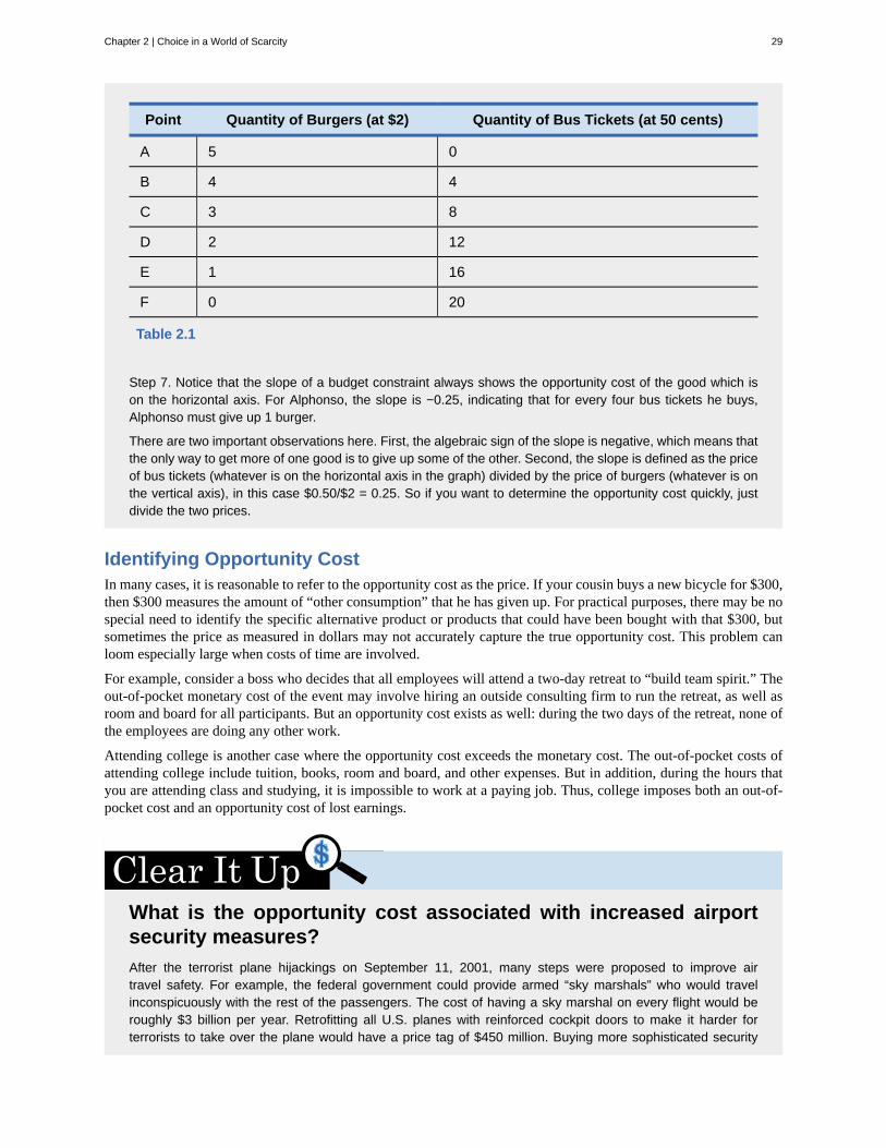
Point Quantity of Burgers (at $2) Quantity of Bus Tickets (at 50 cents)
A 5 0
B 4 4
C 3 8
D 2 12
E 1 16
F 0 20
Table 2.1
Step 7. Notice that the slope of a budget constraint always shows the opportunity cost of the good which ison the horizontal axis. For Alphonso, the slope is −0.25, indicating that for every four bus tickets he buys,Alphonso must give up 1 burger.
There are two important observations here. First, the algebraic sign of the slope is negative, which means thatthe only way to get more of one good is to give up some of the other. Second, the slope is defined as the priceof bus tickets (whatever is on the horizontal axis in the graph) divided by the price of burgers (whatever is onthe vertical axis), in this case $0.50/$2 = 0.25. So if you want to determine the opportunity cost quickly, justdivide the two prices.
Identifying Opportunity CostIn many cases, it is reasonable to refer to the opportunity cost as the price. If your cousin buys a new bicycle for $300,then $300 measures the amount of “other consumption” that he has given up. For practical purposes, there may be nospecial need to identify the specific alternative product or products that could have been bought with that $300, butsometimes the price as measured in dollars may not accurately capture the true opportunity cost. This problem canloom especially large when costs of time are involved.
For example, consider a boss who decides that all employees will attend a two-day retreat to “build team spirit.” Theout-of-pocket monetary cost of the event may involve hiring an outside consulting firm to run the retreat, as well asroom and board for all participants. But an opportunity cost exists as well: during the two days of the retreat, none ofthe employees are doing any other work.
Attending college is another case where the opportunity cost exceeds the monetary cost. The out-of-pocket costs ofattending college include tuition, books, room and board, and other expenses. But in addition, during the hours thatyou are attending class and studying, it is impossible to work at a paying job. Thus, college imposes both an out-of-pocket cost and an opportunity cost of lost earnings.
What is the opportunity cost associated with increased airportsecurity measures?After the terrorist plane hijackings on September 11, 2001, many steps were proposed to improve airtravel safety. For example, the federal government could provide armed “sky marshals” who would travelinconspicuously with the rest of the passengers. The cost of having a sky marshal on every flight would beroughly $3 billion per year. Retrofitting all U.S. planes with reinforced cockpit doors to make it harder forterrorists to take over the plane would have a price tag of $450 million. Buying more sophisticated security
Chapter 2 | Choice in a World of Scarcity 29
equipment for airports, like three-dimensional baggage scanners and cameras linked to face recognitionsoftware, could cost another $2 billion.
But the single biggest cost of greater airline security does not involve spending money. It is the opportunitycost of additional waiting time at the airport. According to the United States Department of Transportation(DOT), more than 800 million passengers took plane trips in the United States in 2012. Since the 9/11hijackings, security screening has become more intensive, and consequently, the procedure takes longer thanin the past. Say that, on average, each air passenger spends an extra 30 minutes in the airport per trip.Economists commonly place a value on time to convert an opportunity cost in time into a monetary figure.Because many air travelers are relatively high-paid business people, conservative estimates set the averageprice of time for air travelers at $20 per hour. By these back-of-the-envelope calculations, the opportunity costof delays in airports could be as much as 800 million × 0.5 hours × $20/hour, or $8 billion per year. Clearly, theopportunity costs of waiting time can be just as important as costs that involve direct spending.
In some cases, realizing the opportunity cost can alter behavior. Imagine, for example, that you spend $8 on lunchevery day at work. You may know perfectly well that bringing a lunch from home would cost only $3 a day, so theopportunity cost of buying lunch at the restaurant is $5 each day (that is, the $8 buying lunch costs minus the $3 yourlunch from home would cost). $5 each day does not seem to be that much. However, if you project what that adds upto in a year—250 days a year × $5 per day equals $1,250, the cost, perhaps, of a decent vacation. If the opportunitycost is described as “a nice vacation” instead of “$5 a day,” you might make different choices.
Marginal Decision-Making and Diminishing Marginal UtilityThe budget constraint framework helps to emphasize that most choices in the real world are not about getting all ofone thing or all of another; that is, they are not about choosing either the point at one end of the budget constraint orelse the point all the way at the other end. Instead, most choices involve marginal analysis, which means comparingthe benefits and costs of choosing a little more or a little less of a good.
People desire goods and services for the satisfaction or utility those goods and services provide. Utility, as we willsee in the chapter on Consumer Choices (http://cnx.org/content/m57229/latest/) , is subjective but that doesnot make it less real. Economists typically assume that the more of some good one consumes (for example, slices ofpizza), the more utility one obtains. At the same time, the utility a person receives from consuming the first unit of agood is typically more than the utility received from consuming the fifth or the tenth unit of that same good. WhenAlphonso chooses between burgers and bus tickets, for example, the first few bus rides that he chooses might providehim with a great deal of utility—perhaps they help him get to a job interview or a doctor’s appointment. But later busrides might provide much less utility—they may only serve to kill time on a rainy day. Similarly, the first burger thatAlphonso chooses to buy may be on a day when he missed breakfast and is ravenously hungry. However, if Alphonsohas a burger every single day, the last few burgers may taste pretty boring. The general pattern that consumption ofthe first few units of any good tends to bring a higher level of utility to a person than consumption of later units is acommon pattern. Economists refer to this pattern as the law of diminishing marginal utility, which means that as aperson receives more of a good, the additional (or marginal) utility from each additional unit of the good declines. Inother words, the first slice of pizza brings more satisfaction than the sixth.
The law of diminishing marginal utility explains why people and societies rarely make all-or-nothing choices. Youwould not say, “My favorite food is ice cream, so I will eat nothing but ice cream from now on.” Instead, even if youget a very high level of utility from your favorite food, if you ate it exclusively, the additional or marginal utility fromthose last few servings would not be very high. Similarly, most workers do not say: “I enjoy leisure, so I’ll neverwork.” Instead, workers recognize that even though some leisure is very nice, a combination of all leisure and noincome is not so attractive. The budget constraint framework suggests that when people make choices in a world ofscarcity, they will use marginal analysis and think about whether they would prefer a little more or a little less.
Sunk CostsIn the budget constraint framework, all decisions involve what will happen next: that is, what quantities of goods willyou consume, how many hours will you work, or how much will you save. These decisions do not look back to pastchoices. Thus, the budget constraint framework assumes that sunk costs, which are costs that were incurred in thepast and cannot be recovered, should not affect the current decision.
30 Chapter 2 | Choice in a World of Scarcity
This OpenStax book is available for free at http://cnx.org/content/col11864/1.2

Consider the case of Selena, who pays $8 to see a movie, but after watching the film for 30 minutes, she knows that itis truly terrible. Should she stay and watch the rest of the movie because she paid for the ticket, or should she leave?The money she spent is a sunk cost, and unless the theater manager is feeling kindly, Selena will not get a refund.But staying in the movie still means paying an opportunity cost in time. Her choice is whether to spend the next 90minutes suffering through a cinematic disaster or to do something—anything—else. The lesson of sunk costs is toforget about the money and time that is irretrievably gone and instead to focus on the marginal costs and benefits ofcurrent and future options.
For people and firms alike, dealing with sunk costs can be frustrating. It often means admitting an earlier error injudgment. Many firms, for example, find it hard to give up on a new product that is doing poorly because they spent somuch money in creating and launching the product. But the lesson of sunk costs is to ignore them and make decisionsbased on what will happen in the future.
From a Model with Two Goods to One of Many GoodsThe budget constraint diagram containing just two goods, like most models used in this book, is not realistic. Afterall, in a modern economy people choose from thousands of goods. However, thinking about a model with many goodsis a straightforward extension of what we discussed here. Instead of drawing just one budget constraint, showingthe tradeoff between two goods, you can draw multiple budget constraints, showing the possible tradeoffs betweenmany different pairs of goods. Or in more advanced classes in economics, you would use mathematical equations thatinclude many possible goods and services that can be purchased, together with their quantities and prices, and showhow the total spending on all goods and services is limited to the overall budget available. The graph with two goodsthat was presented here clearly illustrates that every choice has an opportunity cost, which is the point that does carryover to the real world.
2.2 | The Production Possibilities Frontier and SocialChoicesBy the end of this section, you will be able to:
• Interpret production possibilities frontier graphs• Contrast a budget constraint and a production possibilities frontier• Explain the relationship between a production possibilities frontier and the law of diminishing returns• Contrast productive efficiency and allocative efficiency• Define comparative advantage
Just as individuals cannot have everything they want and must instead make choices, society as a whole cannot haveeverything it might want, either. This section of the chapter will explain the constraints faced by society, using a modelcalled the production possibilities frontier (PPF). There are more similarities than differences between individualchoice and social choice. As you read this section, focus on the similarities.
Because society has limited resources (e.g., labor, land, capital, raw materials) at any point in time, there is a limit tothe quantities of goods and services it can produce. Suppose a society desires two products, healthcare and education.This situation is illustrated by the production possibilities frontier in Figure 2.3.
Chapter 2 | Choice in a World of Scarcity 31
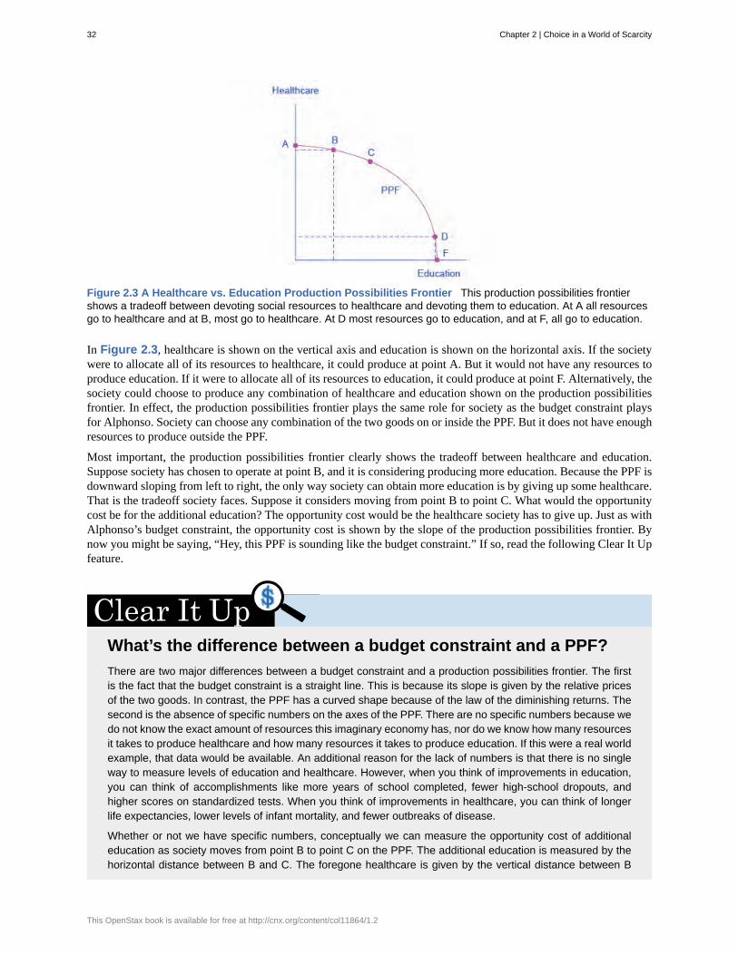
Figure 2.3 A Healthcare vs. Education Production Possibilities Frontier This production possibilities frontiershows a tradeoff between devoting social resources to healthcare and devoting them to education. At A all resourcesgo to healthcare and at B, most go to healthcare. At D most resources go to education, and at F, all go to education.
In Figure 2.3, healthcare is shown on the vertical axis and education is shown on the horizontal axis. If the societywere to allocate all of its resources to healthcare, it could produce at point A. But it would not have any resources toproduce education. If it were to allocate all of its resources to education, it could produce at point F. Alternatively, thesociety could choose to produce any combination of healthcare and education shown on the production possibilitiesfrontier. In effect, the production possibilities frontier plays the same role for society as the budget constraint playsfor Alphonso. Society can choose any combination of the two goods on or inside the PPF. But it does not have enoughresources to produce outside the PPF.
Most important, the production possibilities frontier clearly shows the tradeoff between healthcare and education.Suppose society has chosen to operate at point B, and it is considering producing more education. Because the PPF isdownward sloping from left to right, the only way society can obtain more education is by giving up some healthcare.That is the tradeoff society faces. Suppose it considers moving from point B to point C. What would the opportunitycost be for the additional education? The opportunity cost would be the healthcare society has to give up. Just as withAlphonso’s budget constraint, the opportunity cost is shown by the slope of the production possibilities frontier. Bynow you might be saying, “Hey, this PPF is sounding like the budget constraint.” If so, read the following Clear It Upfeature.
What’s the difference between a budget constraint and a PPF?There are two major differences between a budget constraint and a production possibilities frontier. The firstis the fact that the budget constraint is a straight line. This is because its slope is given by the relative pricesof the two goods. In contrast, the PPF has a curved shape because of the law of the diminishing returns. Thesecond is the absence of specific numbers on the axes of the PPF. There are no specific numbers because wedo not know the exact amount of resources this imaginary economy has, nor do we know how many resourcesit takes to produce healthcare and how many resources it takes to produce education. If this were a real worldexample, that data would be available. An additional reason for the lack of numbers is that there is no singleway to measure levels of education and healthcare. However, when you think of improvements in education,you can think of accomplishments like more years of school completed, fewer high-school dropouts, andhigher scores on standardized tests. When you think of improvements in healthcare, you can think of longerlife expectancies, lower levels of infant mortality, and fewer outbreaks of disease.
Whether or not we have specific numbers, conceptually we can measure the opportunity cost of additionaleducation as society moves from point B to point C on the PPF. The additional education is measured by thehorizontal distance between B and C. The foregone healthcare is given by the vertical distance between B
32 Chapter 2 | Choice in a World of Scarcity
This OpenStax book is available for free at http://cnx.org/content/col11864/1.2
and C. The slope of the PPF between B and C is (approximately) the vertical distance (the “rise”) over thehorizontal distance (the “run”). This is the opportunity cost of the additional education.
The Shape of the PPF and the Law of Diminishing ReturnsThe budget constraints presented earlier in this chapter, showing individual choices about what quantities of goodsto consume, were all straight lines. The reason for these straight lines was that the slope of the budget constraintwas determined by relative prices of the two goods in the consumption budget constraint. However, the productionpossibilities frontier for healthcare and education was drawn as a curved line. Why does the PPF have a differentshape?
To understand why the PPF is curved, start by considering point A at the top left-hand side of the PPF. At point A,all available resources are devoted to healthcare and none are left for education. This situation would be extreme andeven ridiculous. For example, children are seeing a doctor every day, whether they are sick or not, but not attendingschool. People are having cosmetic surgery on every part of their bodies, but no high school or college educationexists. Now imagine that some of these resources are diverted from healthcare to education, so that the economyis at point B instead of point A. Diverting some resources away from A to B causes relatively little reduction inhealth because the last few marginal dollars going into healthcare services are not producing much additional gainin health. However, putting those marginal dollars into education, which is completely without resources at point A,can produce relatively large gains. For this reason, the shape of the PPF from A to B is relatively flat, representing arelatively small drop-off in health and a relatively large gain in education.
Now consider the other end, at the lower right, of the production possibilities frontier. Imagine that society starts atchoice D, which is devoting nearly all resources to education and very few to healthcare, and moves to point F, whichis devoting all spending to education and none to healthcare. For the sake of concreteness, you can imagine that inthe movement from D to F, the last few doctors must become high school science teachers, the last few nurses mustbecome school librarians rather than dispensers of vaccinations, and the last few emergency rooms are turned intokindergartens. The gains to education from adding these last few resources to education are very small. However, theopportunity cost lost to health will be fairly large, and thus the slope of the PPF between D and F is steep, showing alarge drop in health for only a small gain in education.
The lesson is not that society is likely to make an extreme choice like devoting no resources to education at point A orno resources to health at point F. Instead, the lesson is that the gains from committing additional marginal resources toeducation depend on how much is already being spent. If on the one hand, very few resources are currently committedto education, then an increase in resources used can bring relatively large gains. On the other hand, if a large numberof resources are already committed to education, then committing additional resources will bring relatively smallergains.
This pattern is common enough that it has been given a name: the law of diminishing returns, which holds thatas additional increments of resources are added to a certain purpose, the marginal benefit from those additionalincrements will decline. When government spends a certain amount more on reducing crime, for example, the originalgains in reducing crime could be relatively large. But additional increases typically cause relatively smaller reductionsin crime, and paying for enough police and security to reduce crime to nothing at all would be tremendouslyexpensive.
The curvature of the production possibilities frontier shows that as additional resources are added to education,moving from left to right along the horizontal axis, the original gains are fairly large, but gradually diminish.Similarly, as additional resources are added to healthcare, moving from bottom to top on the vertical axis, the originalgains are fairly large, but again gradually diminish. In this way, the law of diminishing returns produces the outward-bending shape of the production possibilities frontier.
Productive Efficiency and Allocative EfficiencyThe study of economics does not presume to tell a society what choice it should make along its productionpossibilities frontier. In a market-oriented economy with a democratic government, the choice will involve amixture of decisions by individuals, firms, and government. However, economics can point out that some choicesare unambiguously better than others. This observation is based on the concept of efficiency. In everyday usage,efficiency refers to lack of waste. An inefficient machine operates at high cost, while an efficient machine operates
Chapter 2 | Choice in a World of Scarcity 33
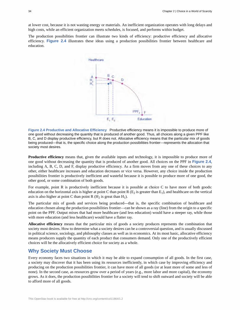
at lower cost, because it is not wasting energy or materials. An inefficient organization operates with long delays andhigh costs, while an efficient organization meets schedules, is focused, and performs within budget.
The production possibilities frontier can illustrate two kinds of efficiency: productive efficiency and allocativeefficiency. Figure 2.4 illustrates these ideas using a production possibilities frontier between healthcare andeducation.
Figure 2.4 Productive and Allocative Efficiency Productive efficiency means it is impossible to produce more ofone good without decreasing the quantity that is produced of another good. Thus, all choices along a given PPF likeB, C, and D display productive efficiency, but R does not. Allocative efficiency means that the particular mix of goodsbeing produced—that is, the specific choice along the production possibilities frontier—represents the allocation thatsociety most desires.
Productive efficiency means that, given the available inputs and technology, it is impossible to produce more ofone good without decreasing the quantity that is produced of another good. All choices on the PPF in Figure 2.4,including A, B, C, D, and F, display productive efficiency. As a firm moves from any one of these choices to anyother, either healthcare increases and education decreases or vice versa. However, any choice inside the productionpossibilities frontier is productively inefficient and wasteful because it is possible to produce more of one good, theother good, or some combination of both goods.
For example, point R is productively inefficient because it is possible at choice C to have more of both goods:education on the horizontal axis is higher at point C than point R (E2 is greater than E1), and healthcare on the verticalaxis is also higher at point C than point R (H2 is great than H1).
The particular mix of goods and services being produced—that is, the specific combination of healthcare andeducation chosen along the production possibilities frontier—can be shown as a ray (line) from the origin to a specificpoint on the PPF. Output mixes that had more healthcare (and less education) would have a steeper ray, while thosewith more education (and less healthcare) would have a flatter ray.
Allocative efficiency means that the particular mix of goods a society produces represents the combination thatsociety most desires. How to determine what a society desires can be a controversial question, and is usually discussedin political science, sociology, and philosophy classes as well as in economics. At its most basic, allocative efficiencymeans producers supply the quantity of each product that consumers demand. Only one of the productively efficientchoices will be the allocatively efficient choice for society as a whole.
Why Society Must ChooseEvery economy faces two situations in which it may be able to expand consumption of all goods. In the first case,a society may discover that it has been using its resources inefficiently, in which case by improving efficiency andproducing on the production possibilities frontier, it can have more of all goods (or at least more of some and less ofnone). In the second case, as resources grow over a period of years (e.g., more labor and more capital), the economygrows. As it does, the production possibilities frontier for a society will tend to shift outward and society will be ableto afford more of all goods.
34 Chapter 2 | Choice in a World of Scarcity
This OpenStax book is available for free at http://cnx.org/content/col11864/1.2
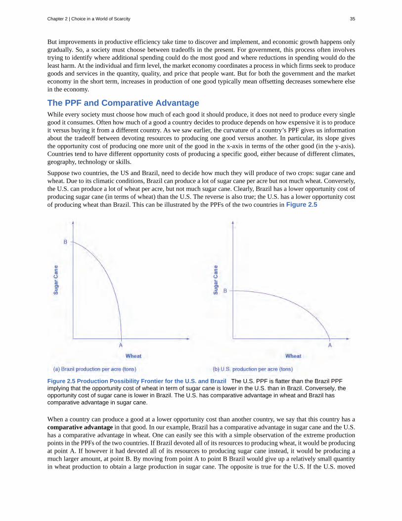
But improvements in productive efficiency take time to discover and implement, and economic growth happens onlygradually. So, a society must choose between tradeoffs in the present. For government, this process often involvestrying to identify where additional spending could do the most good and where reductions in spending would do theleast harm. At the individual and firm level, the market economy coordinates a process in which firms seek to producegoods and services in the quantity, quality, and price that people want. But for both the government and the marketeconomy in the short term, increases in production of one good typically mean offsetting decreases somewhere elsein the economy.
The PPF and Comparative AdvantageWhile every society must choose how much of each good it should produce, it does not need to produce every singlegood it consumes. Often how much of a good a country decides to produce depends on how expensive it is to produceit versus buying it from a different country. As we saw earlier, the curvature of a country’s PPF gives us informationabout the tradeoff between devoting resources to producing one good versus another. In particular, its slope givesthe opportunity cost of producing one more unit of the good in the x-axis in terms of the other good (in the y-axis).Countries tend to have different opportunity costs of producing a specific good, either because of different climates,geography, technology or skills.
Suppose two countries, the US and Brazil, need to decide how much they will produce of two crops: sugar cane andwheat. Due to its climatic conditions, Brazil can produce a lot of sugar cane per acre but not much wheat. Conversely,the U.S. can produce a lot of wheat per acre, but not much sugar cane. Clearly, Brazil has a lower opportunity cost ofproducing sugar cane (in terms of wheat) than the U.S. The reverse is also true; the U.S. has a lower opportunity costof producing wheat than Brazil. This can be illustrated by the PPFs of the two countries in Figure 2.5
Figure 2.5 Production Possibility Frontier for the U.S. and Brazil The U.S. PPF is flatter than the Brazil PPFimplying that the opportunity cost of wheat in term of sugar cane is lower in the U.S. than in Brazil. Conversely, theopportunity cost of sugar cane is lower in Brazil. The U.S. has comparative advantage in wheat and Brazil hascomparative advantage in sugar cane.
When a country can produce a good at a lower opportunity cost than another country, we say that this country has acomparative advantage in that good. In our example, Brazil has a comparative advantage in sugar cane and the U.S.has a comparative advantage in wheat. One can easily see this with a simple observation of the extreme productionpoints in the PPFs of the two countries. If Brazil devoted all of its resources to producing wheat, it would be producingat point A. If however it had devoted all of its resources to producing sugar cane instead, it would be producing amuch larger amount, at point B. By moving from point A to point B Brazil would give up a relatively small quantityin wheat production to obtain a large production in sugar cane. The opposite is true for the U.S. If the U.S. moved
Chapter 2 | Choice in a World of Scarcity 35
from point A to B and produced only sugar cane, this would result in a large opportunity cost in terms of foregonewheat production.
The slope of the PPF gives the opportunity cost of producing an additional unit of wheat. While the slope is notconstant throughout the PPFs, it is quite apparent that the PPF in Brazil is much steeper than in the U.S., and thereforethe opportunity cost of wheat generally higher in Brazil. In the chapter on International Trade (http://cnx.org/content/m57383/latest/) you will learn that countries’ differences in comparative advantage determine whichgoods they will choose to produce and trade. When countries engage in trade, they specialize in the production ofthe goods that they have comparative advantage in, and trade part of that production for goods they do not havecomparative advantage in. With trade, goods are produced where the opportunity cost is lowest, so total productionincreases, benefiting both trading parties.
2.3 | Confronting Objections to the Economic ApproachBy the end of this section, you will be able to:
• Analyze arguments against economic approaches to decision-making• Interpret a tradeoff diagram• Contrast normative statements and positive statements
It is one thing to understand the economic approach to decision-making and another thing to feel comfortableapplying it. The sources of discomfort typically fall into two categories: that people do not act in the way that fitsthe economic way of thinking, and that even if people did act that way, they should try not to. Let’s consider thesearguments in turn.
First Objection: People, Firms, and Society Do Not Act Like ThisThe economic approach to decision-making seems to require more information than most individuals possess andmore careful decision-making than most individuals actually display. After all, do you or any of your friends draw abudget constraint and mutter to yourself about maximizing utility before you head to the shopping mall? Do membersof the U.S. Congress contemplate production possibilities frontiers before they vote on the annual budget? The messyways in which people and societies operate somehow doesn’t look much like neat budget constraints or smoothlycurving production possibilities frontiers.
However, the economics approach can be a useful way to analyze and understand the tradeoffs of economic decisionseven so. To appreciate this point, imagine for a moment that you are playing basketball, dribbling to the right, andthrowing a bounce-pass to the left to a teammate who is running toward the basket. A physicist or engineer couldwork out the correct speed and trajectory for the pass, given the different movements involved and the weight andbounciness of the ball. But when you are playing basketball, you do not perform any of these calculations. You justpass the ball, and if you are a good player, you will do so with high accuracy.
Someone might argue: “The scientist’s formula of the bounce-pass requires a far greater knowledge of physics andfar more specific information about speeds of movement and weights than the basketball player actually has, so itmust be an unrealistic description of how basketball passes are actually made.” This reaction would be wrongheaded.The fact that a good player can throw the ball accurately because of practice and skill, without making a physicscalculation, does not mean that the physics calculation is wrong.
Similarly, from an economic point of view, someone who goes shopping for groceries every week has a great dealof practice with how to purchase the combination of goods that will provide that person with utility, even if theshopper does not phrase decisions in terms of a budget constraint. Government institutions may work imperfectly andslowly, but in general, a democratic form of government feels pressure from voters and social institutions to makethe choices that are most widely preferred by people in that society. So, when thinking about the economic actionsof groups of people, firms, and society, it is reasonable, as a first approximation, to analyze them with the toolsof economic analysis. For more on this, read about behavioral economics in the chapter on Consumer Choices(http://cnx.org/content/m57229/latest/) .
36 Chapter 2 | Choice in a World of Scarcity
This OpenStax book is available for free at http://cnx.org/content/col11864/1.2
Second Objection: People, Firms, and Society Should Not Act This WayThe economics approach portrays people as self-interested. For some critics of this approach, even if self-interest isan accurate description of how people behave, these behaviors are not moral. Instead, the critics argue that peopleshould be taught to care more deeply about others. Economists offer several answers to these concerns.
First, economics is not a form of moral instruction. Rather, it seeks to describe economic behavior as it actuallyexists. Philosophers draw a distinction between positive statements, which describe the world as it is, and normativestatements, which describe how the world should be. For example, an economist could analyze a proposed subwaysystem in a certain city. If the expected benefits exceed the costs, he concludes that the project is worth doing—anexample of positive analysis. Another economist argues for extended unemployment compensation during the GreatDepression because a rich country like the United States should take care of its less fortunate citizens—an exampleof normative analysis.
Even if the line between positive and normative statements is not always crystal clear, economic analysis does try toremain rooted in the study of the actual people who inhabit the actual economy. Fortunately however, the assumptionthat individuals are purely self-interested is a simplification about human nature. In fact, we need to look no furtherthan to Adam Smith, the very father of modern economics to find evidence of this. The opening sentence of his book,The Theory of Moral Sentiments, puts it very clearly: “How selfish soever man may be supposed, there are evidentlysome principles in his nature, which interest him in the fortune of others, and render their happiness necessary to him,though he derives nothing from it except the pleasure of seeing it.” Clearly, individuals are both self-interested andaltruistic.
Second, self-interested behavior and profit-seeking can be labeled with other names, such as personal choice andfreedom. The ability to make personal choices about buying, working, and saving is an important personal freedom.Some people may choose high-pressure, high-paying jobs so that they can earn and spend a lot of money onthemselves. Others may earn a lot of money and give it to charity or spend it on their friends and family. Othersmay devote themselves to a career that can require a great deal of time, energy, and expertise but does not offer highfinancial rewards, like being an elementary school teacher or a social worker. Still others may choose a job that doesnot take lots of their time or provide a high level of income, but still leaves time for family, friends, and contemplation.Some people may prefer to work for a large company; others might want to start their own business. People’s freedomto make their own economic choices has a moral value worth respecting.
Is a diagram by any other name the same?When you study economics, you may feel buried under an avalanche of diagrams: diagrams in the text,diagrams in the lectures, diagrams in the problems, and diagrams on exams. Your goal should be to recognizethe common underlying logic and pattern of the diagrams, not to memorize each of the individual diagrams.
This chapter uses only one basic diagram, although it is presented with different sets of labels. Theconsumption budget constraint and the production possibilities frontier for society, as a whole, are the samebasic diagram. Figure 2.6 shows an individual budget constraint and a production possibilities frontier for twogoods, Good 1 and Good 2. The tradeoff diagram always illustrates three basic themes: scarcity, tradeoffs,and economic efficiency.
The first theme is scarcity. It is not feasible to have unlimited amounts of both goods. But even if the budgetconstraint or a PPF shifts, scarcity remains—just at a different level. The second theme is tradeoffs. Asdepicted in the budget constraint or the production possibilities frontier, it is necessary to give up some ofone good to gain more of the other good. The details of this tradeoff vary. In a budget constraint, the tradeoffis determined by the relative prices of the goods: that is, the relative price of two goods in the consumptionchoice budget constraint. These tradeoffs appear as a straight line. However, the tradeoffs in many productionpossibilities frontiers are represented by a curved line because the law of diminishing returns holds thatas resources are added to an area, the marginal gains tend to diminish. Regardless of the specific shape,tradeoffs remain.
Chapter 2 | Choice in a World of Scarcity 37
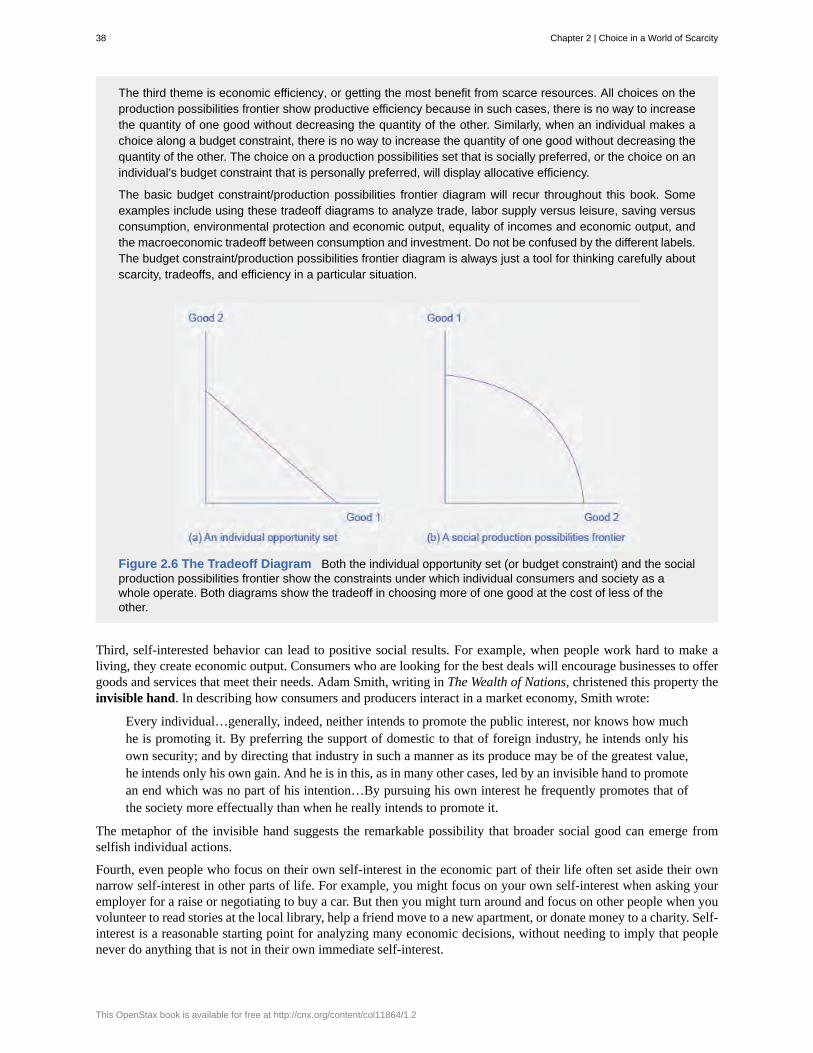
The third theme is economic efficiency, or getting the most benefit from scarce resources. All choices on theproduction possibilities frontier show productive efficiency because in such cases, there is no way to increasethe quantity of one good without decreasing the quantity of the other. Similarly, when an individual makes achoice along a budget constraint, there is no way to increase the quantity of one good without decreasing thequantity of the other. The choice on a production possibilities set that is socially preferred, or the choice on anindividual’s budget constraint that is personally preferred, will display allocative efficiency.
The basic budget constraint/production possibilities frontier diagram will recur throughout this book. Someexamples include using these tradeoff diagrams to analyze trade, labor supply versus leisure, saving versusconsumption, environmental protection and economic output, equality of incomes and economic output, andthe macroeconomic tradeoff between consumption and investment. Do not be confused by the different labels.The budget constraint/production possibilities frontier diagram is always just a tool for thinking carefully aboutscarcity, tradeoffs, and efficiency in a particular situation.
Figure 2.6 The Tradeoff Diagram Both the individual opportunity set (or budget constraint) and the socialproduction possibilities frontier show the constraints under which individual consumers and society as awhole operate. Both diagrams show the tradeoff in choosing more of one good at the cost of less of theother.
Third, self-interested behavior can lead to positive social results. For example, when people work hard to make aliving, they create economic output. Consumers who are looking for the best deals will encourage businesses to offergoods and services that meet their needs. Adam Smith, writing in The Wealth of Nations, christened this property theinvisible hand. In describing how consumers and producers interact in a market economy, Smith wrote:
Every individual…generally, indeed, neither intends to promote the public interest, nor knows how muchhe is promoting it. By preferring the support of domestic to that of foreign industry, he intends only hisown security; and by directing that industry in such a manner as its produce may be of the greatest value,he intends only his own gain. And he is in this, as in many other cases, led by an invisible hand to promotean end which was no part of his intention…By pursuing his own interest he frequently promotes that ofthe society more effectually than when he really intends to promote it.
The metaphor of the invisible hand suggests the remarkable possibility that broader social good can emerge fromselfish individual actions.
Fourth, even people who focus on their own self-interest in the economic part of their life often set aside their ownnarrow self-interest in other parts of life. For example, you might focus on your own self-interest when asking youremployer for a raise or negotiating to buy a car. But then you might turn around and focus on other people when youvolunteer to read stories at the local library, help a friend move to a new apartment, or donate money to a charity. Self-interest is a reasonable starting point for analyzing many economic decisions, without needing to imply that peoplenever do anything that is not in their own immediate self-interest.
38 Chapter 2 | Choice in a World of Scarcity
This OpenStax book is available for free at http://cnx.org/content/col11864/1.2
Choices ... To What Degree?What have we learned? We know that scarcity impacts all the choices we make. So, an economist mightargue that people do not go on to get bachelor’s degrees or master’s degrees because they do not have theresources to make those choices or because their incomes are too low and/or the price of these degrees istoo high. A bachelor’s degree or a master’s degree may not be available in their opportunity set.
The price of these degrees may be too high not only because the actual price, college tuition (and perhapsroom and board), is too high. An economist might also say that for many people, the full opportunity cost ofa bachelor’s degree or a master’s degree is too high. For these people, they are unwilling or unable to makethe tradeoff of giving up years of working, and earning an income, to earn a degree.
Finally, the statistics introduced at the start of the chapter reveal information about intertemporal choices. Aneconomist might say that people choose not to get a college degree because they may have to borrow moneyto go to college, and the interest they have to pay on that loan in the future will affect their decisions today.Also, it could be that some people have a preference for current consumption over future consumption, sothey choose to work now at a lower salary and consume now, rather than putting that consumption off untilafter they graduate college.
Chapter 2 | Choice in a World of Scarcity 39
allocative efficiency
budget constraint
comparative advantage
invisible hand
law of diminishing marginal utility
law of diminishing returns
marginal analysis
normative statement
opportunity cost
opportunity set
positive statement
production possibilities frontier (PPF)
productive efficiency
sunk costs
utility
KEY TERMS
when the mix of goods being produced represents the mix that society most desires
all possible consumption combinations of goods that someone can afford, given the prices of goods,when all income is spent; the boundary of the opportunity set
when a country can produce a good at a lower cost in terms of other goods; or, when acountry has a lower opportunity cost of production
idea that self-interested behavior by individuals can lead to positive social outcomes
as we consume more of a good or service, the utility we get from additional unitsof the good or service tend to become smaller than what we received from earlier units
as additional increments of resources are added to producing a good or service, themarginal benefit from those additional increments will decline
examination of decisions on the margin, meaning a little more or a little less from the status quo
statement which describes how the world should be
measures cost by what is given up in exchange; opportunity cost measures the value of the forgonealternative
all possible combinations of consumption that someone can afford given the prices of goods and theindividual’s income
statement which describes the world as it is
a diagram that shows the productively efficient combinations of twoproducts that an economy can produce given the resources it has available.
when it is impossible to produce more of one good (or service) without decreasing the quantityproduced of another good (or service)
costs that are made in the past and cannot be recovered
satisfaction, usefulness, or value one obtains from consuming goods and services
KEY CONCEPTS AND SUMMARY
2.1 How Individuals Make Choices Based on Their Budget ConstraintEconomists see the real world as one of scarcity: that is, a world in which people’s desires exceed what is possible.As a result, economic behavior involves tradeoffs in which individuals, firms, and society must give up somethingthat they desire to obtain things that they desire more. Individuals face the tradeoff of what quantities of goods andservices to consume. The budget constraint, which is the frontier of the opportunity set, illustrates the range of choicesavailable. The slope of the budget constraint is determined by the relative price of the choices. Choices beyond thebudget constraint are not affordable.
Opportunity cost measures cost by what is given up in exchange. Sometimes opportunity cost can be measured inmoney, but it is often useful to consider time as well, or to measure it in terms of the actual resources that must begiven up.
Most economic decisions and tradeoffs are not all-or-nothing. Instead, they involve marginal analysis, which meansthey are about decisions on the margin, involving a little more or a little less. The law of diminishing marginal
40 Chapter 2 | Choice in a World of Scarcity
This OpenStax book is available for free at http://cnx.org/content/col11864/1.2
utility points out that as a person receives more of something—whether it is a specific good or another resource—theadditional marginal gains tend to become smaller. Because sunk costs occurred in the past and cannot be recovered,they should be disregarded in making current decisions.
2.2 The Production Possibilities Frontier and Social ChoicesA production possibilities frontier defines the set of choices society faces for the combinations of goods and servicesit can produce given the resources available. The shape of the PPF is typically curved outward, rather than straight.Choices outside the PPF are unattainable and choices inside the PPF are wasteful. Over time, a growing economy willtend to shift the PPF outwards.
The law of diminishing returns holds that as increments of additional resources are devoted to producing something,the marginal increase in output will become smaller and smaller. All choices along a production possibilities frontierdisplay productive efficiency; that is, it is impossible to use society’s resources to produce more of one good withoutdecreasing production of the other good. The specific choice along a production possibilities frontier that reflects themix of goods society prefers is the choice with allocative efficiency. The curvature of the PPF is likely to differ bycountry, which results in different countries having comparative advantage in different goods. Total production canincrease if countries specialize in the goods they have comparative advantage in and trade some of their productionfor the remaining goods.
2.3 Confronting Objections to the Economic ApproachThe economic way of thinking provides a useful approach to understanding human behavior. Economists make thecareful distinction between positive statements, which describe the world as it is, and normative statements, whichdescribe how the world should be. Even when economics analyzes the gains and losses from various events orpolicies, and thus draws normative conclusions about how the world should be, the analysis of economics is rooted ina positive analysis of how people, firms, and governments actually behave, not how they should behave.
SELF-CHECK QUESTIONS1. Suppose Alphonso’s town raised the price of bus tickets to $1 per trip (while the price of burgers stayed at $2 andhis budget remained $10 per week.) Draw Alphonso’s new budget constraint. What happens to the opportunity costof bus tickets?
2. Return to the example in Figure 2.4. Suppose there is an improvement in medical technology that enables morehealthcare to be provided with the same amount of resources. How would this affect the production possibilities curveand, in particular, how would it affect the opportunity cost of education?
3. Could a nation be producing in a way that is allocatively efficient, but productively inefficient?
4. What are the similarities between a consumer’s budget constraint and society’s production possibilities frontier,not just graphically but analytically?
5. Individuals may not act in the rational, calculating way described by the economic model of decision making,measuring utility and costs at the margin, but can you make a case that they behave approximately that way?
6. Would an op-ed piece in a newspaper urging the adoption of a particular economic policy be considered a positiveor normative statement?
7. Would a research study on the effects of soft drink consumption on children’s cognitive development beconsidered a positive or normative statement?
REVIEW QUESTIONS
8. Explain why scarcity leads to tradeoffs. 9. Explain why individuals make choices that aredirectly on the budget constraint, rather than inside thebudget constraint or outside it.
Chapter 2 | Choice in a World of Scarcity 41
10. What is comparative advantage?
11. What does a production possibilities frontierillustrate?
12. Why is a production possibilities frontier typicallydrawn as a curve, rather than a straight line?
13. Explain why societies cannot make a choice abovetheir production possibilities frontier and should notmake a choice below it.
14. What are diminishing marginal returns?
15. What is productive efficiency? Allocativeefficiency?
16. What is the difference between a positive and anormative statement?
17. Is the economic model of decision-making intendedas a literal description of how individuals, firms, and thegovernments actually make decisions?
18. What are four responses to the claim that peopleshould not behave in the way described in this chapter?
CRITICAL THINKING QUESTIONS
19. Suppose Alphonso’s town raises the price of bustickets from $0.50 to $1 and the price of burgers risesfrom $2 to $4. Why is the opportunity cost of bus ticketsunchanged? Suppose Alphonso’s weekly spendingmoney increases from $10 to $20. How is his budgetconstraint affected from all three changes? Explain.
20. During the Second World War, Germany’s factorieswere decimated. It also suffered many human casualties,both soldiers and civilians. How did the war affectGermany’s production possibilities curve?
21. It is clear that productive inefficiency is a wastesince resources are being used in a way that produces
less goods and services than a nation is capable of. Whyis allocative inefficiency also wasteful?
22. What assumptions about the economy must be truefor the invisible hand to work? To what extent are thoseassumptions valid in the real world?
23. Do economists have any particular expertise atmaking normative arguments? In other words, they haveexpertise at making positive statements (i.e., what willhappen) about some economic policy, for example, butdo they have special expertise to judge whether or notthe policy should be undertaken?
PROBLEMSUse this information to answer the following 4questions: Marie has a weekly budget of $24, which shelikes to spend on magazines and pies.
24. If the price of a magazine is $4 each, what isthe maximum number of magazines she could buy in aweek?
25. If the price of a pie is $12, what is the maximumnumber of pies she could buy in a week?
26. Draw Marie’s budget constraint with pies on thehorizontal axis and magazines on the vertical axis. Whatis the slope of the budget constraint?
27. What is Marie’s opportunity cost of purchasing apie?
42 Chapter 2 | Choice in a World of Scarcity
This OpenStax book is available for free at http://cnx.org/content/col11864/1.2

3 | Demand and Supply
Figure 3.1 Farmer’s Market Organic vegetables and fruits that are grown and sold within a specific geographicalregion should, in theory, cost less than conventional produce because the transportation costs are less. That is not,however, usually the case. (Credit: modification of work by Natalie Maynor/Flickr Creative Commons)
Why Can We Not Get Enough of Organic?Organic food is increasingly popular, not just in the United States, but worldwide. At one time, consumers hadto go to specialty stores or farmer’s markets to find organic produce. Now it is available in most grocery stores.In short, organic is part of the mainstream.
Ever wonder why organic food costs more than conventional food? Why, say, does an organic Fuji apple cost$1.99 a pound, while its conventional counterpart costs $1.49 a pound? The same price relationship is true forjust about every organic product on the market. If many organic foods are locally grown, would they not takeless time to get to market and therefore be cheaper? What are the forces that keep those prices from comingdown? Turns out those forces have a lot to do with this chapter’s topic: demand and supply.
Introduction to Demand and SupplyIn this chapter, you will learn about:
• Demand, Supply, and Equilibrium in Markets for Goods and Services
• Shifts in Demand and Supply for Goods and Services
• Changes in Equilibrium Price and Quantity: The Four-Step Process
Chapter 3 | Demand and Supply 43
• Price Ceilings and Price Floors
An auction bidder pays thousands of dollars for a dress Whitney Houston wore. A collector spends a small fortunefor a few drawings by John Lennon. People usually react to purchases like these in two ways: their jaw drops becausethey think these are high prices to pay for such goods or they think these are rare, desirable items and the amount paidseems right.
Visit this website (http://openstaxcollege.org/l/celebauction) to read a list of bizarre items that have beenpurchased for their ties to celebrities. These examples represent an interesting facet of demand and supply.
When economists talk about prices, they are less interested in making judgments than in gaining a practicalunderstanding of what determines prices and why prices change. Consider a price most of us contend with weekly:that of a gallon of gas. Why was the average price of gasoline in the United States $3.71 per gallon in June 2014?Why did the price for gasoline fall sharply to $2.07 per gallon by January 2015? To explain these price movements,economists focus on the determinants of what gasoline buyers are willing to pay and what gasoline sellers are willingto accept.
As it turns out, the price of gasoline in June of any given year is nearly always higher than the price in January of thatsame year; over recent decades, gasoline prices in midsummer have averaged about 10 cents per gallon more thantheir midwinter low. The likely reason is that people drive more in the summer, and are also willing to pay more forgas, but that does not explain how steeply gas prices fell. Other factors were at work during those six months, such asincreases in supply and decreases in the demand for crude oil.
This chapter introduces the economic model of demand and supply—one of the most powerful models in all ofeconomics. The discussion here begins by examining how demand and supply determine the price and the quantitysold in markets for goods and services, and how changes in demand and supply lead to changes in prices andquantities.
3.1 | Demand, Supply, and Equilibrium in Markets forGoods and ServicesBy the end of this section, you will be able to:
• Explain demand, quantity demanded, and the law of demand• Identify a demand curve and a supply curve• Explain supply, quantity supply, and the law of supply• Explain equilibrium, equilibrium price, and equilibrium quantity
First let’s first focus on what economists mean by demand, what they mean by supply, and then how demand andsupply interact in a market.
44 Chapter 3 | Demand and Supply
This OpenStax book is available for free at http://cnx.org/content/col11864/1.2
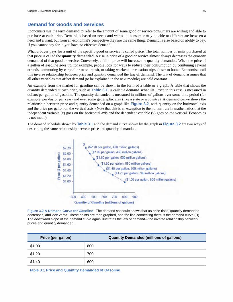
Demand for Goods and ServicesEconomists use the term demand to refer to the amount of some good or service consumers are willing and able topurchase at each price. Demand is based on needs and wants—a consumer may be able to differentiate between aneed and a want, but from an economist’s perspective they are the same thing. Demand is also based on ability to pay.If you cannot pay for it, you have no effective demand.
What a buyer pays for a unit of the specific good or service is called price. The total number of units purchased atthat price is called the quantity demanded. A rise in price of a good or service almost always decreases the quantitydemanded of that good or service. Conversely, a fall in price will increase the quantity demanded. When the price ofa gallon of gasoline goes up, for example, people look for ways to reduce their consumption by combining severalerrands, commuting by carpool or mass transit, or taking weekend or vacation trips closer to home. Economists callthis inverse relationship between price and quantity demanded the law of demand. The law of demand assumes thatall other variables that affect demand (to be explained in the next module) are held constant.
An example from the market for gasoline can be shown in the form of a table or a graph. A table that shows thequantity demanded at each price, such as Table 3.1, is called a demand schedule. Price in this case is measured indollars per gallon of gasoline. The quantity demanded is measured in millions of gallons over some time period (forexample, per day or per year) and over some geographic area (like a state or a country). A demand curve shows therelationship between price and quantity demanded on a graph like Figure 3.2, with quantity on the horizontal axisand the price per gallon on the vertical axis. (Note that this is an exception to the normal rule in mathematics that theindependent variable (x) goes on the horizontal axis and the dependent variable (y) goes on the vertical. Economicsis not math.)
The demand schedule shown by Table 3.1 and the demand curve shown by the graph in Figure 3.2 are two ways ofdescribing the same relationship between price and quantity demanded.
Figure 3.2 A Demand Curve for Gasoline The demand schedule shows that as price rises, quantity demandeddecreases, and vice versa. These points are then graphed, and the line connecting them is the demand curve (D).The downward slope of the demand curve again illustrates the law of demand—the inverse relationship betweenprices and quantity demanded.
Price (per gallon) Quantity Demanded (millions of gallons)
$1.00 800
$1.20 700
$1.40 600
Table 3.1 Price and Quantity Demanded of Gasoline
Chapter 3 | Demand and Supply 45
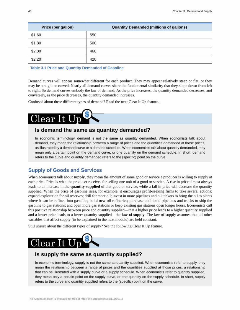
Price (per gallon) Quantity Demanded (millions of gallons)
$1.60 550
$1.80 500
$2.00 460
$2.20 420
Table 3.1 Price and Quantity Demanded of Gasoline
Demand curves will appear somewhat different for each product. They may appear relatively steep or flat, or theymay be straight or curved. Nearly all demand curves share the fundamental similarity that they slope down from leftto right. So demand curves embody the law of demand: As the price increases, the quantity demanded decreases, andconversely, as the price decreases, the quantity demanded increases.
Confused about these different types of demand? Read the next Clear It Up feature.
Is demand the same as quantity demanded?In economic terminology, demand is not the same as quantity demanded. When economists talk aboutdemand, they mean the relationship between a range of prices and the quantities demanded at those prices,as illustrated by a demand curve or a demand schedule. When economists talk about quantity demanded, theymean only a certain point on the demand curve, or one quantity on the demand schedule. In short, demandrefers to the curve and quantity demanded refers to the (specific) point on the curve.
Supply of Goods and ServicesWhen economists talk about supply, they mean the amount of some good or service a producer is willing to supply ateach price. Price is what the producer receives for selling one unit of a good or service. A rise in price almost alwaysleads to an increase in the quantity supplied of that good or service, while a fall in price will decrease the quantitysupplied. When the price of gasoline rises, for example, it encourages profit-seeking firms to take several actions:expand exploration for oil reserves; drill for more oil; invest in more pipelines and oil tankers to bring the oil to plantswhere it can be refined into gasoline; build new oil refineries; purchase additional pipelines and trucks to ship thegasoline to gas stations; and open more gas stations or keep existing gas stations open longer hours. Economists callthis positive relationship between price and quantity supplied—that a higher price leads to a higher quantity suppliedand a lower price leads to a lower quantity supplied—the law of supply. The law of supply assumes that all othervariables that affect supply (to be explained in the next module) are held constant.
Still unsure about the different types of supply? See the following Clear It Up feature.
Is supply the same as quantity supplied?In economic terminology, supply is not the same as quantity supplied. When economists refer to supply, theymean the relationship between a range of prices and the quantities supplied at those prices, a relationshipthat can be illustrated with a supply curve or a supply schedule. When economists refer to quantity supplied,they mean only a certain point on the supply curve, or one quantity on the supply schedule. In short, supplyrefers to the curve and quantity supplied refers to the (specific) point on the curve.
46 Chapter 3 | Demand and Supply
This OpenStax book is available for free at http://cnx.org/content/col11864/1.2

Figure 3.3 illustrates the law of supply, again using the market for gasoline as an example. Like demand, supply canbe illustrated using a table or a graph. A supply schedule is a table, like Table 3.2, that shows the quantity suppliedat a range of different prices. Again, price is measured in dollars per gallon of gasoline and quantity demanded ismeasured in millions of gallons. A supply curve is a graphic illustration of the relationship between price, shownon the vertical axis, and quantity, shown on the horizontal axis. The supply schedule and the supply curve are justtwo different ways of showing the same information. Notice that the horizontal and vertical axes on the graph for thesupply curve are the same as for the demand curve.
Figure 3.3 A Supply Curve for Gasoline The supply schedule is the table that shows quantity supplied of gasolineat each price. As price rises, quantity supplied also increases, and vice versa. The supply curve (S) is created bygraphing the points from the supply schedule and then connecting them. The upward slope of the supply curveillustrates the law of supply—that a higher price leads to a higher quantity supplied, and vice versa.
Price (per gallon) Quantity Supplied (millions of gallons)
$1.00 500
$1.20 550
$1.40 600
$1.60 640
$1.80 680
$2.00 700
$2.20 720
Table 3.2 Price and Supply of Gasoline
The shape of supply curves will vary somewhat according to the product: steeper, flatter, straighter, or curved. Nearlyall supply curves, however, share a basic similarity: they slope up from left to right and illustrate the law of supply:as the price rises, say, from $1.00 per gallon to $2.20 per gallon, the quantity supplied increases from 500 gallons to720 gallons. Conversely, as the price falls, the quantity supplied decreases.
Equilibrium—Where Demand and Supply IntersectBecause the graphs for demand and supply curves both have price on the vertical axis and quantity on the horizontalaxis, the demand curve and supply curve for a particular good or service can appear on the same graph. Together,demand and supply determine the price and the quantity that will be bought and sold in a market.
Chapter 3 | Demand and Supply 47
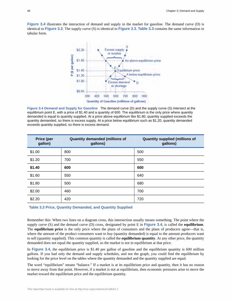
Figure 3.4 illustrates the interaction of demand and supply in the market for gasoline. The demand curve (D) isidentical to Figure 3.2. The supply curve (S) is identical to Figure 3.3. Table 3.3 contains the same information intabular form.
Figure 3.4 Demand and Supply for Gasoline The demand curve (D) and the supply curve (S) intersect at theequilibrium point E, with a price of $1.40 and a quantity of 600. The equilibrium is the only price where quantitydemanded is equal to quantity supplied. At a price above equilibrium like $1.80, quantity supplied exceeds thequantity demanded, so there is excess supply. At a price below equilibrium such as $1.20, quantity demandedexceeds quantity supplied, so there is excess demand.
Price (pergallon)
Quantity demanded (millions ofgallons)
Quantity supplied (millions ofgallons)
$1.00 800 500
$1.20 700 550
$1.40 600 600
$1.60 550 640
$1.80 500 680
$2.00 460 700
$2.20 420 720
Table 3.3 Price, Quantity Demanded, and Quantity Supplied
Remember this: When two lines on a diagram cross, this intersection usually means something. The point where thesupply curve (S) and the demand curve (D) cross, designated by point E in Figure 3.4, is called the equilibrium.The equilibrium price is the only price where the plans of consumers and the plans of producers agree—that is,where the amount of the product consumers want to buy (quantity demanded) is equal to the amount producers wantto sell (quantity supplied). This common quantity is called the equilibrium quantity. At any other price, the quantitydemanded does not equal the quantity supplied, so the market is not in equilibrium at that price.
In Figure 3.4, the equilibrium price is $1.40 per gallon of gasoline and the equilibrium quantity is 600 milliongallons. If you had only the demand and supply schedules, and not the graph, you could find the equilibrium bylooking for the price level on the tables where the quantity demanded and the quantity supplied are equal.
The word “equilibrium” means “balance.” If a market is at its equilibrium price and quantity, then it has no reasonto move away from that point. However, if a market is not at equilibrium, then economic pressures arise to move themarket toward the equilibrium price and the equilibrium quantity.
48 Chapter 3 | Demand and Supply
This OpenStax book is available for free at http://cnx.org/content/col11864/1.2
Imagine, for example, that the price of a gallon of gasoline was above the equilibrium price—that is, instead of $1.40per gallon, the price is $1.80 per gallon. This above-equilibrium price is illustrated by the dashed horizontal line atthe price of $1.80 in Figure 3.4. At this higher price, the quantity demanded drops from 600 to 500. This decline inquantity reflects how consumers react to the higher price by finding ways to use less gasoline.
Moreover, at this higher price of $1.80, the quantity of gasoline supplied rises from the 600 to 680, as the higherprice makes it more profitable for gasoline producers to expand their output. Now, consider how quantity demandedand quantity supplied are related at this above-equilibrium price. Quantity demanded has fallen to 500 gallons, whilequantity supplied has risen to 680 gallons. In fact, at any above-equilibrium price, the quantity supplied exceeds thequantity demanded. We call this an excess supply or a surplus.
With a surplus, gasoline accumulates at gas stations, in tanker trucks, in pipelines, and at oil refineries. Thisaccumulation puts pressure on gasoline sellers. If a surplus remains unsold, those firms involved in making andselling gasoline are not receiving enough cash to pay their workers and to cover their expenses. In this situation, someproducers and sellers will want to cut prices, because it is better to sell at a lower price than not to sell at all. Oncesome sellers start cutting prices, others will follow to avoid losing sales. These price reductions in turn will stimulate ahigher quantity demanded. So, if the price is above the equilibrium level, incentives built into the structure of demandand supply will create pressures for the price to fall toward the equilibrium.
Now suppose that the price is below its equilibrium level at $1.20 per gallon, as the dashed horizontal line at thisprice in Figure 3.4 shows. At this lower price, the quantity demanded increases from 600 to 700 as drivers takelonger trips, spend more minutes warming up the car in the driveway in wintertime, stop sharing rides to work, andbuy larger cars that get fewer miles to the gallon. However, the below-equilibrium price reduces gasoline producers’incentives to produce and sell gasoline, and the quantity supplied falls from 600 to 550.
When the price is below equilibrium, there is excess demand, or a shortage—that is, at the given price the quantitydemanded, which has been stimulated by the lower price, now exceeds the quantity supplied, which had beendepressed by the lower price. In this situation, eager gasoline buyers mob the gas stations, only to find many stationsrunning short of fuel. Oil companies and gas stations recognize that they have an opportunity to make higher profitsby selling what gasoline they have at a higher price. As a result, the price rises toward the equilibrium level. ReadDemand, Supply, and Efficiency for more discussion on the importance of the demand and supply model.
3.2 | Shifts in Demand and Supply for Goods andServicesBy the end of this section, you will be able to:
• Identify factors that affect demand• Graph demand curves and demand shifts• Identify factors that affect supply• Graph supply curves and supply shifts
The previous module explored how price affects the quantity demanded and the quantity supplied. The result was thedemand curve and the supply curve. Price, however, is not the only thing that influences demand. Nor is it the onlything that influences supply. For example, how is demand for vegetarian food affected if, say, health concerns causemore consumers to avoid eating meat? Or how is the supply of diamonds affected if diamond producers discoverseveral new diamond mines? What are the major factors, in addition to the price, that influence demand or supply?
Visit this website (http://openstaxcollege.org/l/toothfish) to read a brief note on how marketing strategies caninfluence supply and demand of products.
Chapter 3 | Demand and Supply 49
What Factors Affect Demand?We defined demand as the amount of some product a consumer is willing and able to purchase at each price. Thatsuggests at least two factors in addition to price that affect demand. Willingness to purchase suggests a desire, basedon what economists call tastes and preferences. If you neither need nor want something, you will not buy it. Abilityto purchase suggests that income is important. Professors are usually able to afford better housing and transportationthan students, because they have more income. Prices of related goods can affect demand also. If you need a newcar, the price of a Honda may affect your demand for a Ford. Finally, the size or composition of the population canaffect demand. The more children a family has, the greater their demand for clothing. The more driving-age childrena family has, the greater their demand for car insurance, and the less for diapers and baby formula.
These factors matter both for demand by an individual and demand by the market as a whole. Exactly how do thesevarious factors affect demand, and how do we show the effects graphically? To answer those questions, we need theceteris paribus assumption.
The Ceteris Paribus AssumptionA demand curve or a supply curve is a relationship between two, and only two, variables: quantity on the horizontalaxis and price on the vertical axis. The assumption behind a demand curve or a supply curve is that no relevanteconomic factors, other than the product’s price, are changing. Economists call this assumption ceteris paribus, aLatin phrase meaning “other things being equal.” Any given demand or supply curve is based on the ceteris paribusassumption that all else is held equal. A demand curve or a supply curve is a relationship between two, and only two,variables when all other variables are kept constant. If all else is not held equal, then the laws of supply and demandwill not necessarily hold, as the following Clear It Up feature shows.
When does ceteris paribus apply?Ceteris paribus is typically applied when we look at how changes in price affect demand or supply, but ceterisparibus can be applied more generally. In the real world, demand and supply depend on more factors than justprice. For example, a consumer’s demand depends on income and a producer’s supply depends on the costof producing the product. How can we analyze the effect on demand or supply if multiple factors are changingat the same time—say price rises and income falls? The answer is that we examine the changes one at atime, assuming the other factors are held constant.
For example, we can say that an increase in the price reduces the amount consumers will buy (assumingincome, and anything else that affects demand, is unchanged). Additionally, a decrease in income reduces theamount consumers can afford to buy (assuming price, and anything else that affects demand, is unchanged).This is what the ceteris paribus assumption really means. In this particular case, after we analyze each factorseparately, we can combine the results. The amount consumers buy falls for two reasons: first because of thehigher price and second because of the lower income.
50 Chapter 3 | Demand and Supply
This OpenStax book is available for free at http://cnx.org/content/col11864/1.2
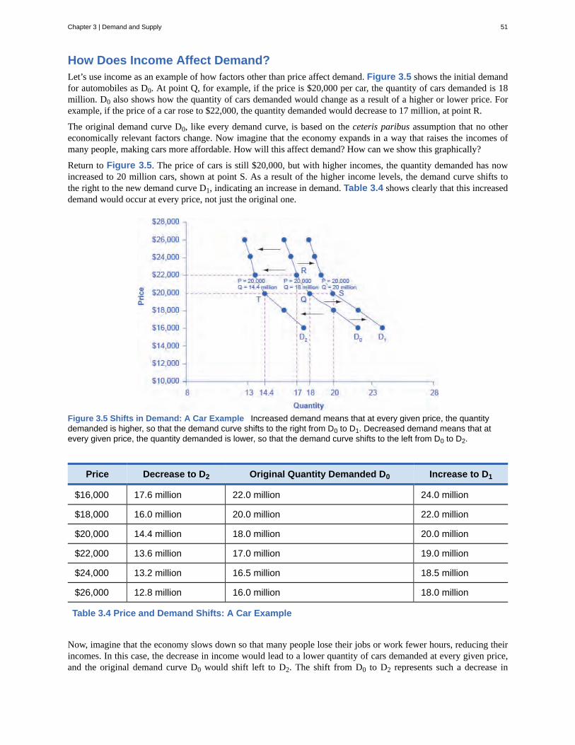
How Does Income Affect Demand?Let’s use income as an example of how factors other than price affect demand. Figure 3.5 shows the initial demandfor automobiles as D0. At point Q, for example, if the price is $20,000 per car, the quantity of cars demanded is 18million. D0 also shows how the quantity of cars demanded would change as a result of a higher or lower price. Forexample, if the price of a car rose to $22,000, the quantity demanded would decrease to 17 million, at point R.
The original demand curve D0, like every demand curve, is based on the ceteris paribus assumption that no othereconomically relevant factors change. Now imagine that the economy expands in a way that raises the incomes ofmany people, making cars more affordable. How will this affect demand? How can we show this graphically?
Return to Figure 3.5. The price of cars is still $20,000, but with higher incomes, the quantity demanded has nowincreased to 20 million cars, shown at point S. As a result of the higher income levels, the demand curve shifts tothe right to the new demand curve D1, indicating an increase in demand. Table 3.4 shows clearly that this increaseddemand would occur at every price, not just the original one.
Figure 3.5 Shifts in Demand: A Car Example Increased demand means that at every given price, the quantitydemanded is higher, so that the demand curve shifts to the right from D0 to D1. Decreased demand means that atevery given price, the quantity demanded is lower, so that the demand curve shifts to the left from D0 to D2.
Price Decrease to D2 Original Quantity Demanded D0 Increase to D1
$16,000 17.6 million 22.0 million 24.0 million
$18,000 16.0 million 20.0 million 22.0 million
$20,000 14.4 million 18.0 million 20.0 million
$22,000 13.6 million 17.0 million 19.0 million
$24,000 13.2 million 16.5 million 18.5 million
$26,000 12.8 million 16.0 million 18.0 million
Table 3.4 Price and Demand Shifts: A Car Example
Now, imagine that the economy slows down so that many people lose their jobs or work fewer hours, reducing theirincomes. In this case, the decrease in income would lead to a lower quantity of cars demanded at every given price,and the original demand curve D0 would shift left to D2. The shift from D0 to D2 represents such a decrease in
Chapter 3 | Demand and Supply 51
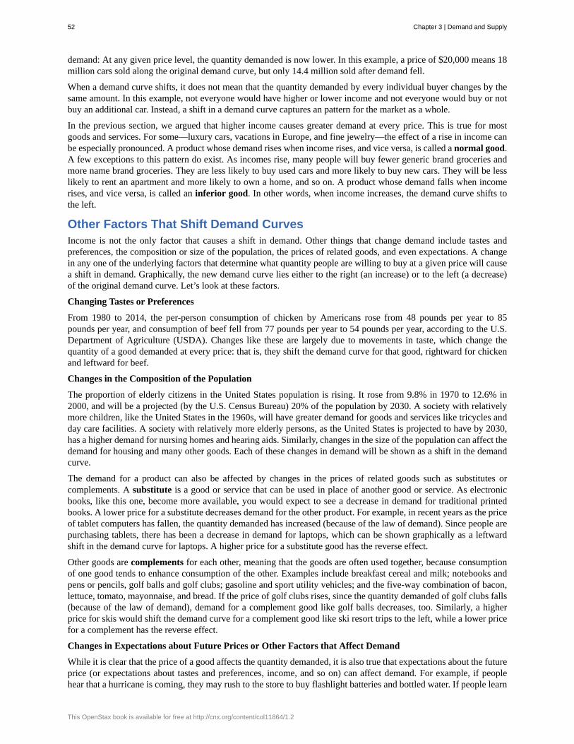
demand: At any given price level, the quantity demanded is now lower. In this example, a price of $20,000 means 18million cars sold along the original demand curve, but only 14.4 million sold after demand fell.
When a demand curve shifts, it does not mean that the quantity demanded by every individual buyer changes by thesame amount. In this example, not everyone would have higher or lower income and not everyone would buy or notbuy an additional car. Instead, a shift in a demand curve captures an pattern for the market as a whole.
In the previous section, we argued that higher income causes greater demand at every price. This is true for mostgoods and services. For some—luxury cars, vacations in Europe, and fine jewelry—the effect of a rise in income canbe especially pronounced. A product whose demand rises when income rises, and vice versa, is called a normal good.A few exceptions to this pattern do exist. As incomes rise, many people will buy fewer generic brand groceries andmore name brand groceries. They are less likely to buy used cars and more likely to buy new cars. They will be lesslikely to rent an apartment and more likely to own a home, and so on. A product whose demand falls when incomerises, and vice versa, is called an inferior good. In other words, when income increases, the demand curve shifts tothe left.
Other Factors That Shift Demand CurvesIncome is not the only factor that causes a shift in demand. Other things that change demand include tastes andpreferences, the composition or size of the population, the prices of related goods, and even expectations. A changein any one of the underlying factors that determine what quantity people are willing to buy at a given price will causea shift in demand. Graphically, the new demand curve lies either to the right (an increase) or to the left (a decrease)of the original demand curve. Let’s look at these factors.
Changing Tastes or Preferences
From 1980 to 2014, the per-person consumption of chicken by Americans rose from 48 pounds per year to 85pounds per year, and consumption of beef fell from 77 pounds per year to 54 pounds per year, according to the U.S.Department of Agriculture (USDA). Changes like these are largely due to movements in taste, which change thequantity of a good demanded at every price: that is, they shift the demand curve for that good, rightward for chickenand leftward for beef.
Changes in the Composition of the Population
The proportion of elderly citizens in the United States population is rising. It rose from 9.8% in 1970 to 12.6% in2000, and will be a projected (by the U.S. Census Bureau) 20% of the population by 2030. A society with relativelymore children, like the United States in the 1960s, will have greater demand for goods and services like tricycles andday care facilities. A society with relatively more elderly persons, as the United States is projected to have by 2030,has a higher demand for nursing homes and hearing aids. Similarly, changes in the size of the population can affect thedemand for housing and many other goods. Each of these changes in demand will be shown as a shift in the demandcurve.
The demand for a product can also be affected by changes in the prices of related goods such as substitutes orcomplements. A substitute is a good or service that can be used in place of another good or service. As electronicbooks, like this one, become more available, you would expect to see a decrease in demand for traditional printedbooks. A lower price for a substitute decreases demand for the other product. For example, in recent years as the priceof tablet computers has fallen, the quantity demanded has increased (because of the law of demand). Since people arepurchasing tablets, there has been a decrease in demand for laptops, which can be shown graphically as a leftwardshift in the demand curve for laptops. A higher price for a substitute good has the reverse effect.
Other goods are complements for each other, meaning that the goods are often used together, because consumptionof one good tends to enhance consumption of the other. Examples include breakfast cereal and milk; notebooks andpens or pencils, golf balls and golf clubs; gasoline and sport utility vehicles; and the five-way combination of bacon,lettuce, tomato, mayonnaise, and bread. If the price of golf clubs rises, since the quantity demanded of golf clubs falls(because of the law of demand), demand for a complement good like golf balls decreases, too. Similarly, a higherprice for skis would shift the demand curve for a complement good like ski resort trips to the left, while a lower pricefor a complement has the reverse effect.
Changes in Expectations about Future Prices or Other Factors that Affect Demand
While it is clear that the price of a good affects the quantity demanded, it is also true that expectations about the futureprice (or expectations about tastes and preferences, income, and so on) can affect demand. For example, if peoplehear that a hurricane is coming, they may rush to the store to buy flashlight batteries and bottled water. If people learn
52 Chapter 3 | Demand and Supply
This OpenStax book is available for free at http://cnx.org/content/col11864/1.2
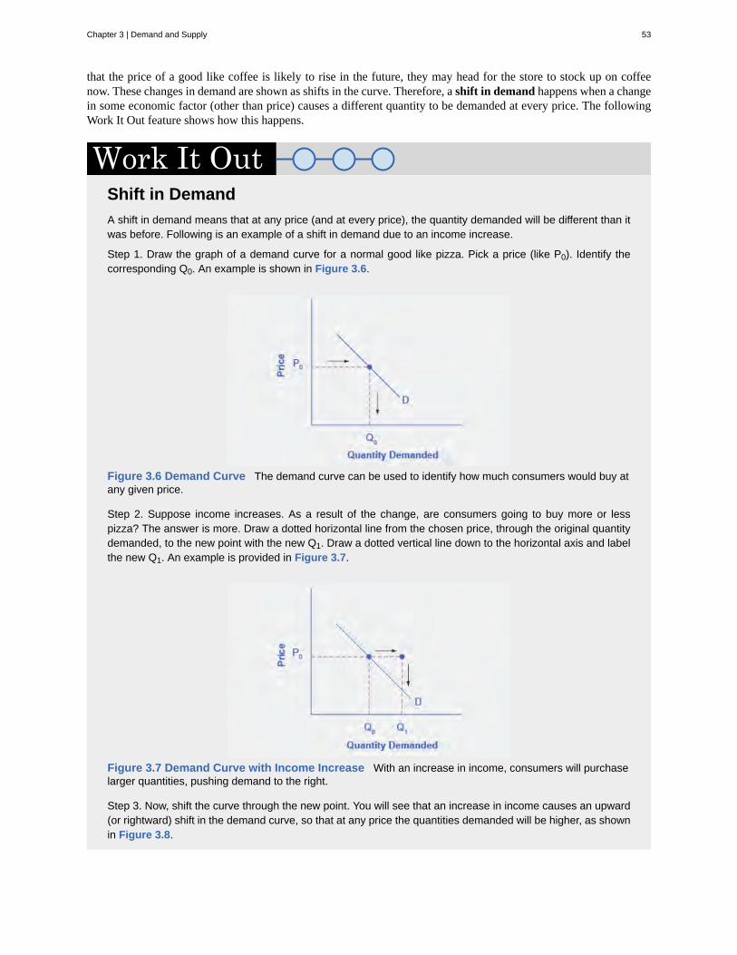
that the price of a good like coffee is likely to rise in the future, they may head for the store to stock up on coffeenow. These changes in demand are shown as shifts in the curve. Therefore, a shift in demand happens when a changein some economic factor (other than price) causes a different quantity to be demanded at every price. The followingWork It Out feature shows how this happens.
Shift in DemandA shift in demand means that at any price (and at every price), the quantity demanded will be different than itwas before. Following is an example of a shift in demand due to an income increase.
Step 1. Draw the graph of a demand curve for a normal good like pizza. Pick a price (like P0). Identify thecorresponding Q0. An example is shown in Figure 3.6.
Figure 3.6 Demand Curve The demand curve can be used to identify how much consumers would buy atany given price.
Step 2. Suppose income increases. As a result of the change, are consumers going to buy more or lesspizza? The answer is more. Draw a dotted horizontal line from the chosen price, through the original quantitydemanded, to the new point with the new Q1. Draw a dotted vertical line down to the horizontal axis and labelthe new Q1. An example is provided in Figure 3.7.
Figure 3.7 Demand Curve with Income Increase With an increase in income, consumers will purchaselarger quantities, pushing demand to the right.
Step 3. Now, shift the curve through the new point. You will see that an increase in income causes an upward(or rightward) shift in the demand curve, so that at any price the quantities demanded will be higher, as shownin Figure 3.8.
Chapter 3 | Demand and Supply 53
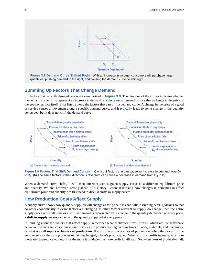
Figure 3.8 Demand Curve Shifted Right With an increase in income, consumers will purchase largerquantities, pushing demand to the right, and causing the demand curve to shift right.
Summing Up Factors That Change DemandSix factors that can shift demand curves are summarized in Figure 3.9. The direction of the arrows indicates whetherthe demand curve shifts represent an increase in demand or a decrease in demand. Notice that a change in the price ofthe good or service itself is not listed among the factors that can shift a demand curve. A change in the price of a goodor service causes a movement along a specific demand curve, and it typically leads to some change in the quantitydemanded, but it does not shift the demand curve.
Figure 3.9 Factors That Shift Demand Curves (a) A list of factors that can cause an increase in demand from D0to D1. (b) The same factors, if their direction is reversed, can cause a decrease in demand from D0 to D1.
When a demand curve shifts, it will then intersect with a given supply curve at a different equilibrium priceand quantity. We are, however, getting ahead of our story. Before discussing how changes in demand can affectequilibrium price and quantity, we first need to discuss shifts in supply curves.
How Production Costs Affect SupplyA supply curve shows how quantity supplied will change as the price rises and falls, assuming ceteris paribus so thatno other economically relevant factors are changing. If other factors relevant to supply do change, then the entiresupply curve will shift. Just as a shift in demand is represented by a change in the quantity demanded at every price,a shift in supply means a change in the quantity supplied at every price.
In thinking about the factors that affect supply, remember what motivates firms: profits, which are the differencebetween revenues and costs. Goods and services are produced using combinations of labor, materials, and machinery,or what we call inputs or factors of production. If a firm faces lower costs of production, while the prices for thegood or service the firm produces remain unchanged, a firm’s profits go up. When a firm’s profits increase, it is moremotivated to produce output, since the more it produces the more profit it will earn. So, when costs of production fall,
54 Chapter 3 | Demand and Supply
This OpenStax book is available for free at http://cnx.org/content/col11864/1.2
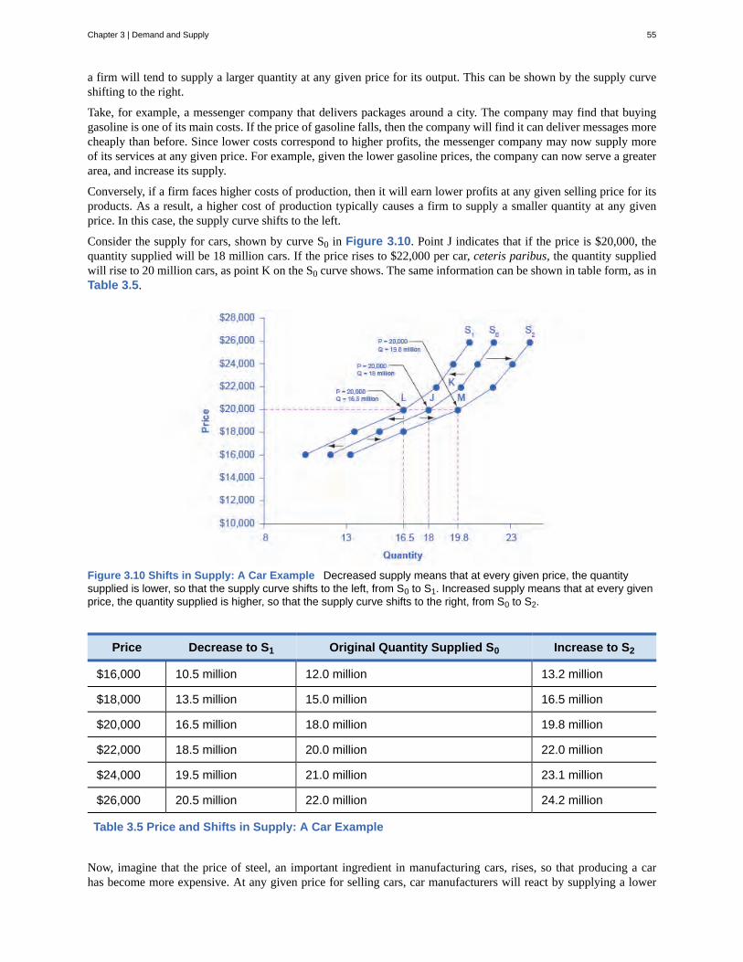
a firm will tend to supply a larger quantity at any given price for its output. This can be shown by the supply curveshifting to the right.
Take, for example, a messenger company that delivers packages around a city. The company may find that buyinggasoline is one of its main costs. If the price of gasoline falls, then the company will find it can deliver messages morecheaply than before. Since lower costs correspond to higher profits, the messenger company may now supply moreof its services at any given price. For example, given the lower gasoline prices, the company can now serve a greaterarea, and increase its supply.
Conversely, if a firm faces higher costs of production, then it will earn lower profits at any given selling price for itsproducts. As a result, a higher cost of production typically causes a firm to supply a smaller quantity at any givenprice. In this case, the supply curve shifts to the left.
Consider the supply for cars, shown by curve S0 in Figure 3.10. Point J indicates that if the price is $20,000, thequantity supplied will be 18 million cars. If the price rises to $22,000 per car, ceteris paribus, the quantity suppliedwill rise to 20 million cars, as point K on the S0 curve shows. The same information can be shown in table form, as inTable 3.5.
Figure 3.10 Shifts in Supply: A Car Example Decreased supply means that at every given price, the quantitysupplied is lower, so that the supply curve shifts to the left, from S0 to S1. Increased supply means that at every givenprice, the quantity supplied is higher, so that the supply curve shifts to the right, from S0 to S2.
Price Decrease to S1 Original Quantity Supplied S0 Increase to S2
$16,000 10.5 million 12.0 million 13.2 million
$18,000 13.5 million 15.0 million 16.5 million
$20,000 16.5 million 18.0 million 19.8 million
$22,000 18.5 million 20.0 million 22.0 million
$24,000 19.5 million 21.0 million 23.1 million
$26,000 20.5 million 22.0 million 24.2 million
Table 3.5 Price and Shifts in Supply: A Car Example
Now, imagine that the price of steel, an important ingredient in manufacturing cars, rises, so that producing a carhas become more expensive. At any given price for selling cars, car manufacturers will react by supplying a lower
Chapter 3 | Demand and Supply 55
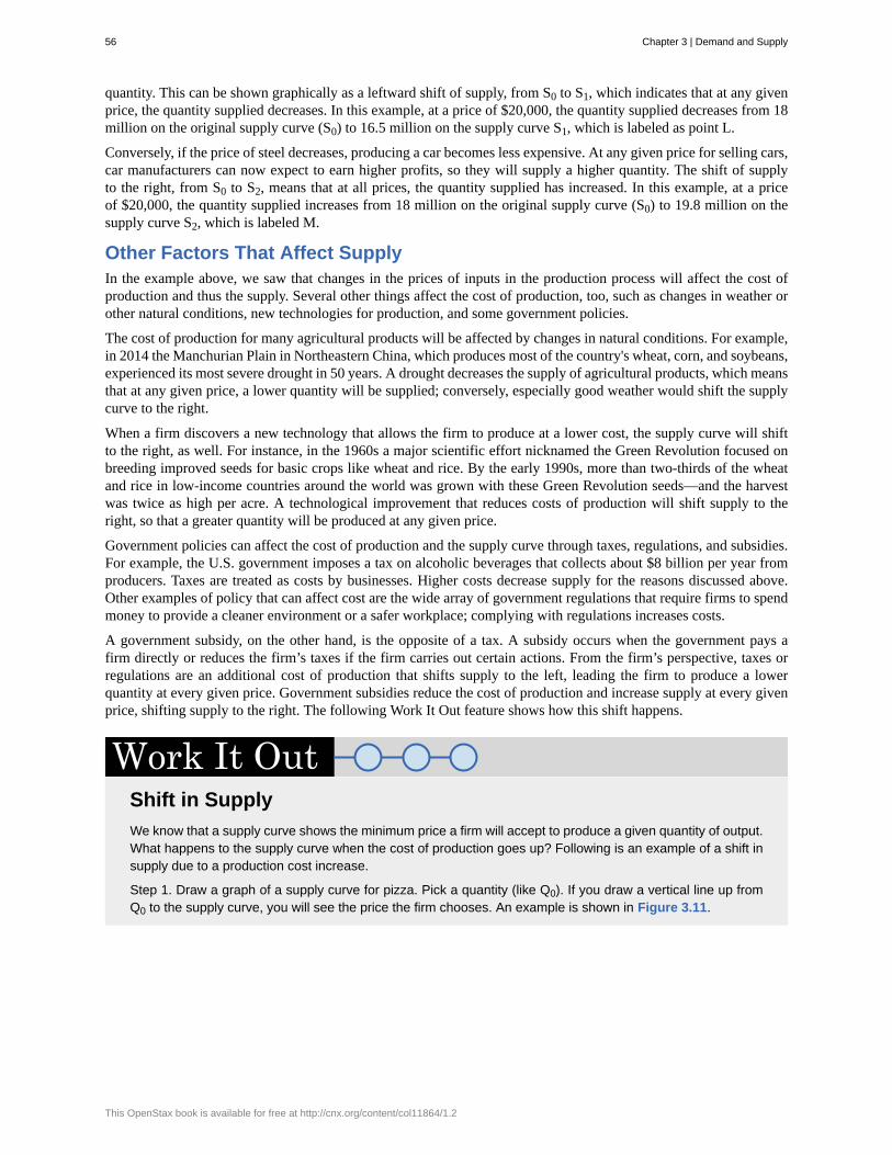
quantity. This can be shown graphically as a leftward shift of supply, from S0 to S1, which indicates that at any givenprice, the quantity supplied decreases. In this example, at a price of $20,000, the quantity supplied decreases from 18million on the original supply curve (S0) to 16.5 million on the supply curve S1, which is labeled as point L.
Conversely, if the price of steel decreases, producing a car becomes less expensive. At any given price for selling cars,car manufacturers can now expect to earn higher profits, so they will supply a higher quantity. The shift of supplyto the right, from S0 to S2, means that at all prices, the quantity supplied has increased. In this example, at a priceof $20,000, the quantity supplied increases from 18 million on the original supply curve (S0) to 19.8 million on thesupply curve S2, which is labeled M.
Other Factors That Affect SupplyIn the example above, we saw that changes in the prices of inputs in the production process will affect the cost ofproduction and thus the supply. Several other things affect the cost of production, too, such as changes in weather orother natural conditions, new technologies for production, and some government policies.
The cost of production for many agricultural products will be affected by changes in natural conditions. For example,in 2014 the Manchurian Plain in Northeastern China, which produces most of the country's wheat, corn, and soybeans,experienced its most severe drought in 50 years. A drought decreases the supply of agricultural products, which meansthat at any given price, a lower quantity will be supplied; conversely, especially good weather would shift the supplycurve to the right.
When a firm discovers a new technology that allows the firm to produce at a lower cost, the supply curve will shiftto the right, as well. For instance, in the 1960s a major scientific effort nicknamed the Green Revolution focused onbreeding improved seeds for basic crops like wheat and rice. By the early 1990s, more than two-thirds of the wheatand rice in low-income countries around the world was grown with these Green Revolution seeds—and the harvestwas twice as high per acre. A technological improvement that reduces costs of production will shift supply to theright, so that a greater quantity will be produced at any given price.
Government policies can affect the cost of production and the supply curve through taxes, regulations, and subsidies.For example, the U.S. government imposes a tax on alcoholic beverages that collects about $8 billion per year fromproducers. Taxes are treated as costs by businesses. Higher costs decrease supply for the reasons discussed above.Other examples of policy that can affect cost are the wide array of government regulations that require firms to spendmoney to provide a cleaner environment or a safer workplace; complying with regulations increases costs.
A government subsidy, on the other hand, is the opposite of a tax. A subsidy occurs when the government pays afirm directly or reduces the firm’s taxes if the firm carries out certain actions. From the firm’s perspective, taxes orregulations are an additional cost of production that shifts supply to the left, leading the firm to produce a lowerquantity at every given price. Government subsidies reduce the cost of production and increase supply at every givenprice, shifting supply to the right. The following Work It Out feature shows how this shift happens.
Shift in SupplyWe know that a supply curve shows the minimum price a firm will accept to produce a given quantity of output.What happens to the supply curve when the cost of production goes up? Following is an example of a shift insupply due to a production cost increase.
Step 1. Draw a graph of a supply curve for pizza. Pick a quantity (like Q0). If you draw a vertical line up fromQ0 to the supply curve, you will see the price the firm chooses. An example is shown in Figure 3.11.
56 Chapter 3 | Demand and Supply
This OpenStax book is available for free at http://cnx.org/content/col11864/1.2
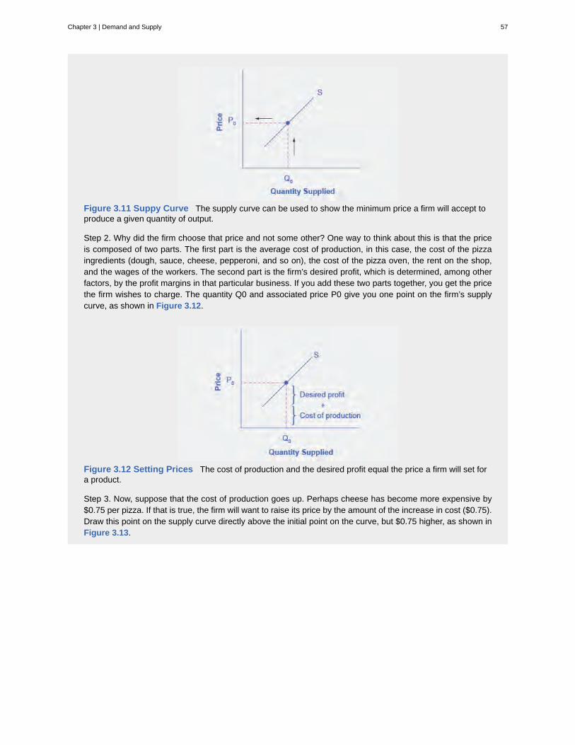
Figure 3.11 Suppy Curve The supply curve can be used to show the minimum price a firm will accept toproduce a given quantity of output.
Step 2. Why did the firm choose that price and not some other? One way to think about this is that the priceis composed of two parts. The first part is the average cost of production, in this case, the cost of the pizzaingredients (dough, sauce, cheese, pepperoni, and so on), the cost of the pizza oven, the rent on the shop,and the wages of the workers. The second part is the firm’s desired profit, which is determined, among otherfactors, by the profit margins in that particular business. If you add these two parts together, you get the pricethe firm wishes to charge. The quantity Q0 and associated price P0 give you one point on the firm’s supplycurve, as shown in Figure 3.12.
Figure 3.12 Setting Prices The cost of production and the desired profit equal the price a firm will set fora product.
Step 3. Now, suppose that the cost of production goes up. Perhaps cheese has become more expensive by$0.75 per pizza. If that is true, the firm will want to raise its price by the amount of the increase in cost ($0.75).Draw this point on the supply curve directly above the initial point on the curve, but $0.75 higher, as shown inFigure 3.13.
Chapter 3 | Demand and Supply 57
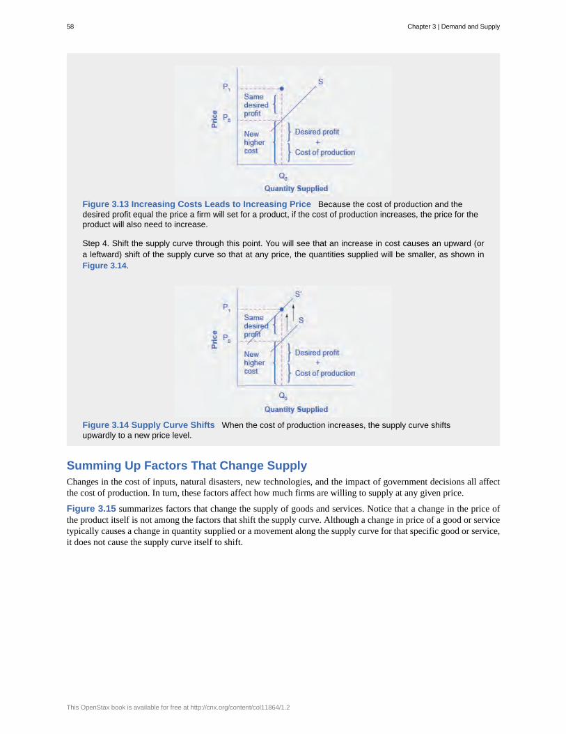
Figure 3.13 Increasing Costs Leads to Increasing Price Because the cost of production and thedesired profit equal the price a firm will set for a product, if the cost of production increases, the price for theproduct will also need to increase.
Step 4. Shift the supply curve through this point. You will see that an increase in cost causes an upward (ora leftward) shift of the supply curve so that at any price, the quantities supplied will be smaller, as shown inFigure 3.14.
Figure 3.14 Supply Curve Shifts When the cost of production increases, the supply curve shiftsupwardly to a new price level.
Summing Up Factors That Change SupplyChanges in the cost of inputs, natural disasters, new technologies, and the impact of government decisions all affectthe cost of production. In turn, these factors affect how much firms are willing to supply at any given price.
Figure 3.15 summarizes factors that change the supply of goods and services. Notice that a change in the price ofthe product itself is not among the factors that shift the supply curve. Although a change in price of a good or servicetypically causes a change in quantity supplied or a movement along the supply curve for that specific good or service,it does not cause the supply curve itself to shift.
58 Chapter 3 | Demand and Supply
This OpenStax book is available for free at http://cnx.org/content/col11864/1.2
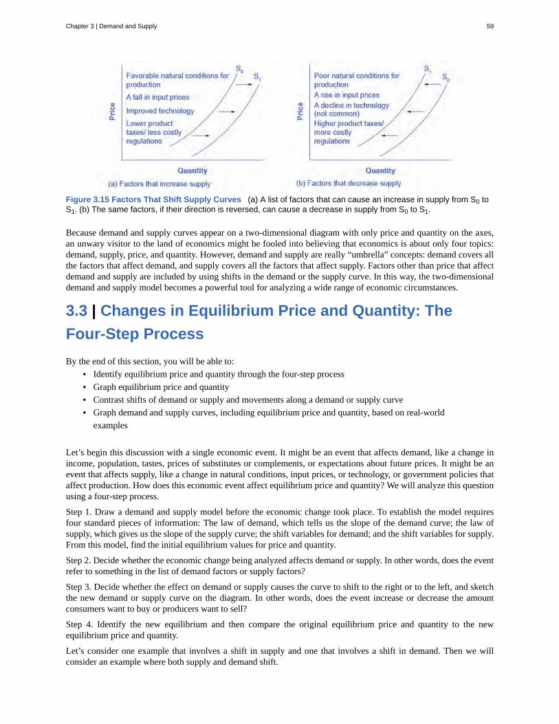
Figure 3.15 Factors That Shift Supply Curves (a) A list of factors that can cause an increase in supply from S0 toS1. (b) The same factors, if their direction is reversed, can cause a decrease in supply from S0 to S1.
Because demand and supply curves appear on a two-dimensional diagram with only price and quantity on the axes,an unwary visitor to the land of economics might be fooled into believing that economics is about only four topics:demand, supply, price, and quantity. However, demand and supply are really “umbrella” concepts: demand covers allthe factors that affect demand, and supply covers all the factors that affect supply. Factors other than price that affectdemand and supply are included by using shifts in the demand or the supply curve. In this way, the two-dimensionaldemand and supply model becomes a powerful tool for analyzing a wide range of economic circumstances.
3.3 | Changes in Equilibrium Price and Quantity: TheFour-Step ProcessBy the end of this section, you will be able to:
• Identify equilibrium price and quantity through the four-step process• Graph equilibrium price and quantity• Contrast shifts of demand or supply and movements along a demand or supply curve• Graph demand and supply curves, including equilibrium price and quantity, based on real-world
examples
Let’s begin this discussion with a single economic event. It might be an event that affects demand, like a change inincome, population, tastes, prices of substitutes or complements, or expectations about future prices. It might be anevent that affects supply, like a change in natural conditions, input prices, or technology, or government policies thataffect production. How does this economic event affect equilibrium price and quantity? We will analyze this questionusing a four-step process.
Step 1. Draw a demand and supply model before the economic change took place. To establish the model requiresfour standard pieces of information: The law of demand, which tells us the slope of the demand curve; the law ofsupply, which gives us the slope of the supply curve; the shift variables for demand; and the shift variables for supply.From this model, find the initial equilibrium values for price and quantity.
Step 2. Decide whether the economic change being analyzed affects demand or supply. In other words, does the eventrefer to something in the list of demand factors or supply factors?
Step 3. Decide whether the effect on demand or supply causes the curve to shift to the right or to the left, and sketchthe new demand or supply curve on the diagram. In other words, does the event increase or decrease the amountconsumers want to buy or producers want to sell?
Step 4. Identify the new equilibrium and then compare the original equilibrium price and quantity to the newequilibrium price and quantity.
Let’s consider one example that involves a shift in supply and one that involves a shift in demand. Then we willconsider an example where both supply and demand shift.
Chapter 3 | Demand and Supply 59

Good Weather for Salmon FishingIn the summer of 2000, weather conditions were excellent for commercial salmon fishing off the California coast.Heavy rains meant higher than normal levels of water in the rivers, which helps the salmon to breed. Slightly coolerocean temperatures stimulated the growth of plankton, the microscopic organisms at the bottom of the ocean foodchain, providing everything in the ocean with a hearty food supply. The ocean stayed calm during fishing season,so commercial fishing operations did not lose many days to bad weather. How did these climate conditions affectthe quantity and price of salmon? Figure 3.16 illustrates the four-step approach, which is explained below, to workthrough this problem. Table 3.6 provides the information to work the problem as well.
Figure 3.16 Good Weather for Salmon Fishing: The Four-Step Process Unusually good weather leads tochanges in the price and quantity of salmon.
Price perPound
Quantity Supplied in1999
Quantity Supplied in2000
QuantityDemanded
$2.00 80 400 840
$2.25 120 480 680
$2.50 160 550 550
$2.75 200 600 450
$3.00 230 640 350
$3.25 250 670 250
$3.50 270 700 200
Table 3.6 Salmon Fishing
Step 1. Draw a demand and supply model to illustrate the market for salmon in the year before the good weatherconditions began. The demand curve D0 and the supply curve S0 show that the original equilibrium price is $3.25 perpound and the original equilibrium quantity is 250,000 fish. (This price per pound is what commercial buyers pay atthe fishing docks; what consumers pay at the grocery is higher.)
Step 2. Did the economic event affect supply or demand? Good weather is an example of a natural condition thataffects supply.
60 Chapter 3 | Demand and Supply
This OpenStax book is available for free at http://cnx.org/content/col11864/1.2
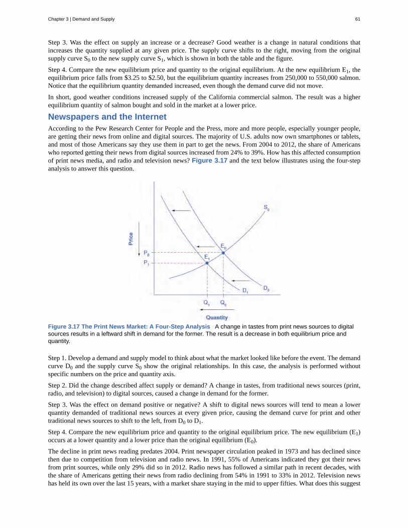
Step 3. Was the effect on supply an increase or a decrease? Good weather is a change in natural conditions thatincreases the quantity supplied at any given price. The supply curve shifts to the right, moving from the originalsupply curve S0 to the new supply curve S1, which is shown in both the table and the figure.
Step 4. Compare the new equilibrium price and quantity to the original equilibrium. At the new equilibrium E1, theequilibrium price falls from $3.25 to $2.50, but the equilibrium quantity increases from 250,000 to 550,000 salmon.Notice that the equilibrium quantity demanded increased, even though the demand curve did not move.
In short, good weather conditions increased supply of the California commercial salmon. The result was a higherequilibrium quantity of salmon bought and sold in the market at a lower price.
Newspapers and the InternetAccording to the Pew Research Center for People and the Press, more and more people, especially younger people,are getting their news from online and digital sources. The majority of U.S. adults now own smartphones or tablets,and most of those Americans say they use them in part to get the news. From 2004 to 2012, the share of Americanswho reported getting their news from digital sources increased from 24% to 39%. How has this affected consumptionof print news media, and radio and television news? Figure 3.17 and the text below illustrates using the four-stepanalysis to answer this question.
Figure 3.17 The Print News Market: A Four-Step Analysis A change in tastes from print news sources to digitalsources results in a leftward shift in demand for the former. The result is a decrease in both equilibrium price andquantity.
Step 1. Develop a demand and supply model to think about what the market looked like before the event. The demandcurve D0 and the supply curve S0 show the original relationships. In this case, the analysis is performed withoutspecific numbers on the price and quantity axis.
Step 2. Did the change described affect supply or demand? A change in tastes, from traditional news sources (print,radio, and television) to digital sources, caused a change in demand for the former.
Step 3. Was the effect on demand positive or negative? A shift to digital news sources will tend to mean a lowerquantity demanded of traditional news sources at every given price, causing the demand curve for print and othertraditional news sources to shift to the left, from D0 to D1.
Step 4. Compare the new equilibrium price and quantity to the original equilibrium price. The new equilibrium (E1)occurs at a lower quantity and a lower price than the original equilibrium (E0).
The decline in print news reading predates 2004. Print newspaper circulation peaked in 1973 and has declined sincethen due to competition from television and radio news. In 1991, 55% of Americans indicated they got their newsfrom print sources, while only 29% did so in 2012. Radio news has followed a similar path in recent decades, withthe share of Americans getting their news from radio declining from 54% in 1991 to 33% in 2012. Television newshas held its own over the last 15 years, with a market share staying in the mid to upper fifties. What does this suggest
Chapter 3 | Demand and Supply 61
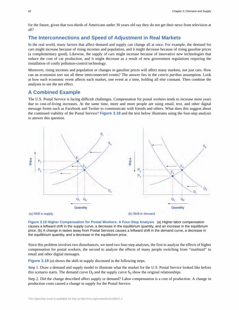
for the future, given that two-thirds of Americans under 30 years old say they do not get their news from television atall?
The Interconnections and Speed of Adjustment in Real MarketsIn the real world, many factors that affect demand and supply can change all at once. For example, the demand forcars might increase because of rising incomes and population, and it might decrease because of rising gasoline prices(a complementary good). Likewise, the supply of cars might increase because of innovative new technologies thatreduce the cost of car production, and it might decrease as a result of new government regulations requiring theinstallation of costly pollution-control technology.
Moreover, rising incomes and population or changes in gasoline prices will affect many markets, not just cars. Howcan an economist sort out all these interconnected events? The answer lies in the ceteris paribus assumption. Lookat how each economic event affects each market, one event at a time, holding all else constant. Then combine theanalyses to see the net effect.
A Combined ExampleThe U.S. Postal Service is facing difficult challenges. Compensation for postal workers tends to increase most yearsdue to cost-of-living increases. At the same time, more and more people are using email, text, and other digitalmessage forms such as Facebook and Twitter to communicate with friends and others. What does this suggest aboutthe continued viability of the Postal Service? Figure 3.18 and the text below illustrates using the four-step analysisto answer this question.
Figure 3.18 Higher Compensation for Postal Workers: A Four-Step Analysis (a) Higher labor compensationcauses a leftward shift in the supply curve, a decrease in the equilibrium quantity, and an increase in the equilibriumprice. (b) A change in tastes away from Postal Services causes a leftward shift in the demand curve, a decrease inthe equilibrium quantity, and a decrease in the equilibrium price.
Since this problem involves two disturbances, we need two four-step analyses, the first to analyze the effects of highercompensation for postal workers, the second to analyze the effects of many people switching from “snailmail” toemail and other digital messages.
Figure 3.18 (a) shows the shift in supply discussed in the following steps.
Step 1. Draw a demand and supply model to illustrate what the market for the U.S. Postal Service looked like beforethis scenario starts. The demand curve D0 and the supply curve S0 show the original relationships.
Step 2. Did the change described affect supply or demand? Labor compensation is a cost of production. A change inproduction costs caused a change in supply for the Postal Service.
62 Chapter 3 | Demand and Supply
This OpenStax book is available for free at http://cnx.org/content/col11864/1.2
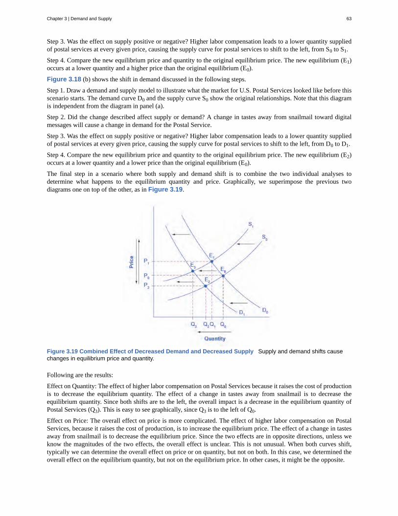
Step 3. Was the effect on supply positive or negative? Higher labor compensation leads to a lower quantity suppliedof postal services at every given price, causing the supply curve for postal services to shift to the left, from S0 to S1.
Step 4. Compare the new equilibrium price and quantity to the original equilibrium price. The new equilibrium (E1)occurs at a lower quantity and a higher price than the original equilibrium (E0).
Figure 3.18 (b) shows the shift in demand discussed in the following steps.
Step 1. Draw a demand and supply model to illustrate what the market for U.S. Postal Services looked like before thisscenario starts. The demand curve D0 and the supply curve S0 show the original relationships. Note that this diagramis independent from the diagram in panel (a).
Step 2. Did the change described affect supply or demand? A change in tastes away from snailmail toward digitalmessages will cause a change in demand for the Postal Service.
Step 3. Was the effect on supply positive or negative? Higher labor compensation leads to a lower quantity suppliedof postal services at every given price, causing the supply curve for postal services to shift to the left, from D0 to D1.
Step 4. Compare the new equilibrium price and quantity to the original equilibrium price. The new equilibrium (E2)occurs at a lower quantity and a lower price than the original equilibrium (E0).
The final step in a scenario where both supply and demand shift is to combine the two individual analyses todetermine what happens to the equilibrium quantity and price. Graphically, we superimpose the previous twodiagrams one on top of the other, as in Figure 3.19.
Figure 3.19 Combined Effect of Decreased Demand and Decreased Supply Supply and demand shifts causechanges in equilibrium price and quantity.
Following are the results:
Effect on Quantity: The effect of higher labor compensation on Postal Services because it raises the cost of productionis to decrease the equilibrium quantity. The effect of a change in tastes away from snailmail is to decrease theequilibrium quantity. Since both shifts are to the left, the overall impact is a decrease in the equilibrium quantity ofPostal Services (Q3). This is easy to see graphically, since Q3 is to the left of Q0.
Effect on Price: The overall effect on price is more complicated. The effect of higher labor compensation on PostalServices, because it raises the cost of production, is to increase the equilibrium price. The effect of a change in tastesaway from snailmail is to decrease the equilibrium price. Since the two effects are in opposite directions, unless weknow the magnitudes of the two effects, the overall effect is unclear. This is not unusual. When both curves shift,typically we can determine the overall effect on price or on quantity, but not on both. In this case, we determined theoverall effect on the equilibrium quantity, but not on the equilibrium price. In other cases, it might be the opposite.
Chapter 3 | Demand and Supply 63
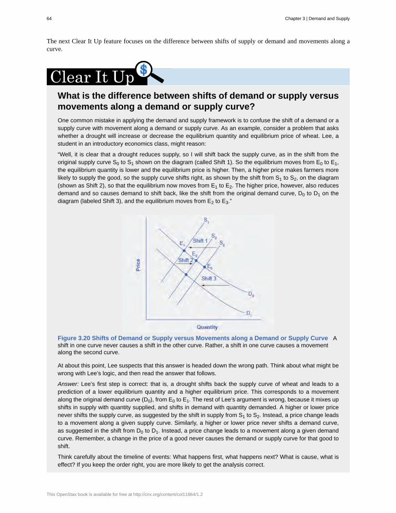
The next Clear It Up feature focuses on the difference between shifts of supply or demand and movements along acurve.
What is the difference between shifts of demand or supply versusmovements along a demand or supply curve?One common mistake in applying the demand and supply framework is to confuse the shift of a demand or asupply curve with movement along a demand or supply curve. As an example, consider a problem that askswhether a drought will increase or decrease the equilibrium quantity and equilibrium price of wheat. Lee, astudent in an introductory economics class, might reason:
“Well, it is clear that a drought reduces supply, so I will shift back the supply curve, as in the shift from theoriginal supply curve S0 to S1 shown on the diagram (called Shift 1). So the equilibrium moves from E0 to E1,the equilibrium quantity is lower and the equilibrium price is higher. Then, a higher price makes farmers morelikely to supply the good, so the supply curve shifts right, as shown by the shift from S1 to S2, on the diagram(shown as Shift 2), so that the equilibrium now moves from E1 to E2. The higher price, however, also reducesdemand and so causes demand to shift back, like the shift from the original demand curve, D0 to D1 on thediagram (labeled Shift 3), and the equilibrium moves from E2 to E3.”
Figure 3.20 Shifts of Demand or Supply versus Movements along a Demand or Supply Curve Ashift in one curve never causes a shift in the other curve. Rather, a shift in one curve causes a movementalong the second curve.
At about this point, Lee suspects that this answer is headed down the wrong path. Think about what might bewrong with Lee’s logic, and then read the answer that follows.
Answer: Lee’s first step is correct: that is, a drought shifts back the supply curve of wheat and leads to aprediction of a lower equilibrium quantity and a higher equilibrium price. This corresponds to a movementalong the original demand curve (D0), from E0 to E1. The rest of Lee’s argument is wrong, because it mixes upshifts in supply with quantity supplied, and shifts in demand with quantity demanded. A higher or lower pricenever shifts the supply curve, as suggested by the shift in supply from S1 to S2. Instead, a price change leadsto a movement along a given supply curve. Similarly, a higher or lower price never shifts a demand curve,as suggested in the shift from D0 to D1. Instead, a price change leads to a movement along a given demandcurve. Remember, a change in the price of a good never causes the demand or supply curve for that good toshift.
Think carefully about the timeline of events: What happens first, what happens next? What is cause, what iseffect? If you keep the order right, you are more likely to get the analysis correct.
64 Chapter 3 | Demand and Supply
This OpenStax book is available for free at http://cnx.org/content/col11864/1.2
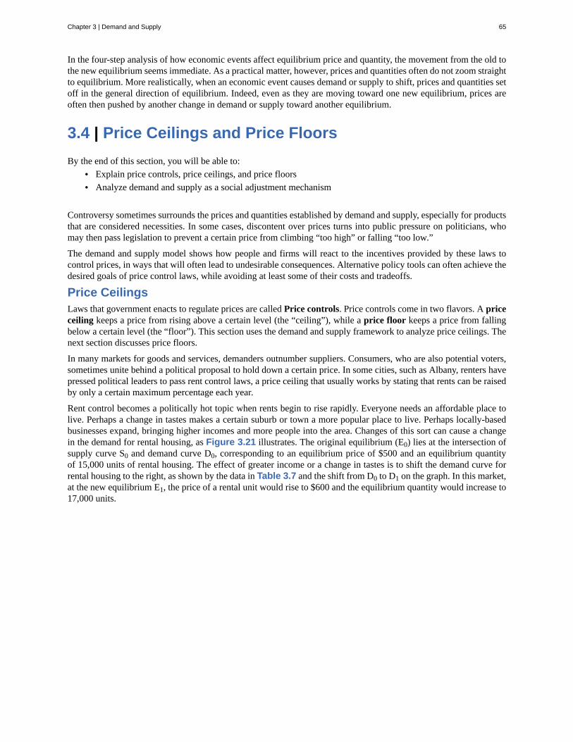
In the four-step analysis of how economic events affect equilibrium price and quantity, the movement from the old tothe new equilibrium seems immediate. As a practical matter, however, prices and quantities often do not zoom straightto equilibrium. More realistically, when an economic event causes demand or supply to shift, prices and quantities setoff in the general direction of equilibrium. Indeed, even as they are moving toward one new equilibrium, prices areoften then pushed by another change in demand or supply toward another equilibrium.
3.4 | Price Ceilings and Price FloorsBy the end of this section, you will be able to:
• Explain price controls, price ceilings, and price floors• Analyze demand and supply as a social adjustment mechanism
Controversy sometimes surrounds the prices and quantities established by demand and supply, especially for productsthat are considered necessities. In some cases, discontent over prices turns into public pressure on politicians, whomay then pass legislation to prevent a certain price from climbing “too high” or falling “too low.”
The demand and supply model shows how people and firms will react to the incentives provided by these laws tocontrol prices, in ways that will often lead to undesirable consequences. Alternative policy tools can often achieve thedesired goals of price control laws, while avoiding at least some of their costs and tradeoffs.
Price CeilingsLaws that government enacts to regulate prices are called Price controls. Price controls come in two flavors. A priceceiling keeps a price from rising above a certain level (the “ceiling”), while a price floor keeps a price from fallingbelow a certain level (the “floor”). This section uses the demand and supply framework to analyze price ceilings. Thenext section discusses price floors.
In many markets for goods and services, demanders outnumber suppliers. Consumers, who are also potential voters,sometimes unite behind a political proposal to hold down a certain price. In some cities, such as Albany, renters havepressed political leaders to pass rent control laws, a price ceiling that usually works by stating that rents can be raisedby only a certain maximum percentage each year.
Rent control becomes a politically hot topic when rents begin to rise rapidly. Everyone needs an affordable place tolive. Perhaps a change in tastes makes a certain suburb or town a more popular place to live. Perhaps locally-basedbusinesses expand, bringing higher incomes and more people into the area. Changes of this sort can cause a changein the demand for rental housing, as Figure 3.21 illustrates. The original equilibrium (E0) lies at the intersection ofsupply curve S0 and demand curve D0, corresponding to an equilibrium price of $500 and an equilibrium quantityof 15,000 units of rental housing. The effect of greater income or a change in tastes is to shift the demand curve forrental housing to the right, as shown by the data in Table 3.7 and the shift from D0 to D1 on the graph. In this market,at the new equilibrium E1, the price of a rental unit would rise to $600 and the equilibrium quantity would increase to17,000 units.
Chapter 3 | Demand and Supply 65
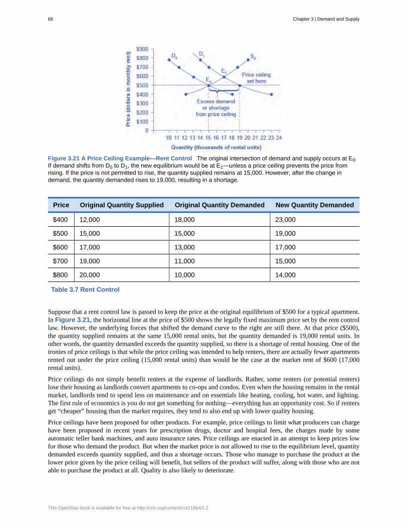
Figure 3.21 A Price Ceiling Example—Rent Control The original intersection of demand and supply occurs at E0.If demand shifts from D0 to D1, the new equilibrium would be at E1—unless a price ceiling prevents the price fromrising. If the price is not permitted to rise, the quantity supplied remains at 15,000. However, after the change indemand, the quantity demanded rises to 19,000, resulting in a shortage.
Price Original Quantity Supplied Original Quantity Demanded New Quantity Demanded
$400 12,000 18,000 23,000
$500 15,000 15,000 19,000
$600 17,000 13,000 17,000
$700 19,000 11,000 15,000
$800 20,000 10,000 14,000
Table 3.7 Rent Control
Suppose that a rent control law is passed to keep the price at the original equilibrium of $500 for a typical apartment.In Figure 3.21, the horizontal line at the price of $500 shows the legally fixed maximum price set by the rent controllaw. However, the underlying forces that shifted the demand curve to the right are still there. At that price ($500),the quantity supplied remains at the same 15,000 rental units, but the quantity demanded is 19,000 rental units. Inother words, the quantity demanded exceeds the quantity supplied, so there is a shortage of rental housing. One of theironies of price ceilings is that while the price ceiling was intended to help renters, there are actually fewer apartmentsrented out under the price ceiling (15,000 rental units) than would be the case at the market rent of $600 (17,000rental units).
Price ceilings do not simply benefit renters at the expense of landlords. Rather, some renters (or potential renters)lose their housing as landlords convert apartments to co-ops and condos. Even when the housing remains in the rentalmarket, landlords tend to spend less on maintenance and on essentials like heating, cooling, hot water, and lighting.The first rule of economics is you do not get something for nothing—everything has an opportunity cost. So if rentersget “cheaper” housing than the market requires, they tend to also end up with lower quality housing.
Price ceilings have been proposed for other products. For example, price ceilings to limit what producers can chargehave been proposed in recent years for prescription drugs, doctor and hospital fees, the charges made by someautomatic teller bank machines, and auto insurance rates. Price ceilings are enacted in an attempt to keep prices lowfor those who demand the product. But when the market price is not allowed to rise to the equilibrium level, quantitydemanded exceeds quantity supplied, and thus a shortage occurs. Those who manage to purchase the product at thelower price given by the price ceiling will benefit, but sellers of the product will suffer, along with those who are notable to purchase the product at all. Quality is also likely to deteriorate.
66 Chapter 3 | Demand and Supply
This OpenStax book is available for free at http://cnx.org/content/col11864/1.2
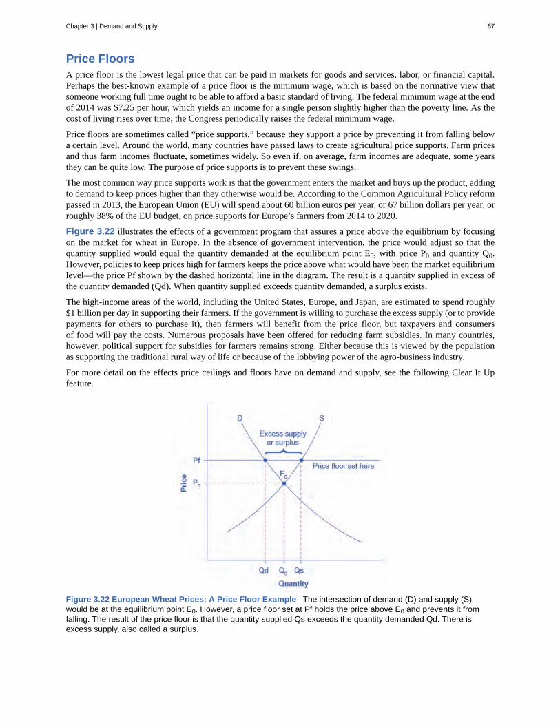
Price FloorsA price floor is the lowest legal price that can be paid in markets for goods and services, labor, or financial capital.Perhaps the best-known example of a price floor is the minimum wage, which is based on the normative view thatsomeone working full time ought to be able to afford a basic standard of living. The federal minimum wage at the endof 2014 was $7.25 per hour, which yields an income for a single person slightly higher than the poverty line. As thecost of living rises over time, the Congress periodically raises the federal minimum wage.
Price floors are sometimes called “price supports,” because they support a price by preventing it from falling belowa certain level. Around the world, many countries have passed laws to create agricultural price supports. Farm pricesand thus farm incomes fluctuate, sometimes widely. So even if, on average, farm incomes are adequate, some yearsthey can be quite low. The purpose of price supports is to prevent these swings.
The most common way price supports work is that the government enters the market and buys up the product, addingto demand to keep prices higher than they otherwise would be. According to the Common Agricultural Policy reformpassed in 2013, the European Union (EU) will spend about 60 billion euros per year, or 67 billion dollars per year, orroughly 38% of the EU budget, on price supports for Europe’s farmers from 2014 to 2020.
Figure 3.22 illustrates the effects of a government program that assures a price above the equilibrium by focusingon the market for wheat in Europe. In the absence of government intervention, the price would adjust so that thequantity supplied would equal the quantity demanded at the equilibrium point E0, with price P0 and quantity Q0.However, policies to keep prices high for farmers keeps the price above what would have been the market equilibriumlevel—the price Pf shown by the dashed horizontal line in the diagram. The result is a quantity supplied in excess ofthe quantity demanded (Qd). When quantity supplied exceeds quantity demanded, a surplus exists.
The high-income areas of the world, including the United States, Europe, and Japan, are estimated to spend roughly$1 billion per day in supporting their farmers. If the government is willing to purchase the excess supply (or to providepayments for others to purchase it), then farmers will benefit from the price floor, but taxpayers and consumersof food will pay the costs. Numerous proposals have been offered for reducing farm subsidies. In many countries,however, political support for subsidies for farmers remains strong. Either because this is viewed by the populationas supporting the traditional rural way of life or because of the lobbying power of the agro-business industry.
For more detail on the effects price ceilings and floors have on demand and supply, see the following Clear It Upfeature.
Figure 3.22 European Wheat Prices: A Price Floor Example The intersection of demand (D) and supply (S)would be at the equilibrium point E0. However, a price floor set at Pf holds the price above E0 and prevents it fromfalling. The result of the price floor is that the quantity supplied Qs exceeds the quantity demanded Qd. There isexcess supply, also called a surplus.
Chapter 3 | Demand and Supply 67
Do price ceilings and floors change demand or supply?Neither price ceilings nor price floors cause demand or supply to change. They simply set a price that limitswhat can be legally charged in the market. Remember, changes in price do not cause demand or supply tochange. Price ceilings and price floors can cause a different choice of quantity demanded along a demandcurve, but they do not move the demand curve. Price controls can cause a different choice of quantity suppliedalong a supply curve, but they do not shift the supply curve.
3.5 | Demand, Supply and EfficiencyThe familiar demand and supply diagram holds within it the concept of economic efficiency. To economists,efficiency means it is impossible to improve the situation of one party without imposing a cost on another. Conversely,if a situation is inefficient, it becomes possible to benefit at least one party without imposing costs on others.
Efficiency in the demand and supply model has the same basic meaning: The economy is getting as much benefitas possible from its scarce resources and all the possible gains from trade have been achieved. In other words, theoptimal amount of each good and service is being produced and consumed.
Consumer Surplus, Producer Surplus, Social SurplusConsider a market for tablet computers, as shown in Figure 3.23. The equilibrium price is $80 and the equilibriumquantity is 28 million. To see the benefits to consumers, look at the segment of the demand curve above theequilibrium point and to the left. This portion of the demand curve shows that at least some demanders would havebeen willing to pay more than $80 for a tablet.
For example, point J shows that if the price was $90, 20 million tablets would be sold. Those consumers who wouldhave been willing to pay $90 for a tablet based on the utility they expect to receive from it, but who were able to paythe equilibrium price of $80, clearly received a benefit beyond what they had to pay for. Remember, the demand curvetraces consumers’ willingness to pay for different quantities. The amount that individuals would have been willingto pay, minus the amount that they actually paid, is called consumer surplus. Consumer surplus is the area labeledF—that is, the area above the market price and below the demand curve.
68 Chapter 3 | Demand and Supply
This OpenStax book is available for free at http://cnx.org/content/col11864/1.2

Figure 3.23 Consumer and Producer Surplus The somewhat triangular area labeled by F shows the area ofconsumer surplus, which shows that the equilibrium price in the market was less than what many of the consumerswere willing to pay. Point J on the demand curve shows that, even at the price of $90, consumers would have beenwilling to purchase a quantity of 20 million. The somewhat triangular area labeled by G shows the area of producersurplus, which shows that the equilibrium price received in the market was more than what many of the producerswere willing to accept for their products. For example, point K on the supply curve shows that at a price of $45, firmswould have been willing to supply a quantity of 14 million.
The supply curve shows the quantity that firms are willing to supply at each price. For example, point K in Figure3.23 illustrates that, at $45, firms would still have been willing to supply a quantity of 14 million. Those producerswho would have been willing to supply the tablets at $45, but who were instead able to charge the equilibrium priceof $80, clearly received an extra benefit beyond what they required to supply the product. The amount that a seller ispaid for a good minus the seller’s actual cost is called producer surplus. In Figure 3.23, producer surplus is the arealabeled G—that is, the area between the market price and the segment of the supply curve below the equilibrium.
The sum of consumer surplus and producer surplus is social surplus, also referred to as economic surplus. In Figure3.23, social surplus would be shown as the area F + G. Social surplus is larger at equilibrium quantity and price thanit would be at any other quantity. This demonstrates the economic efficiency of the market equilibrium. In addition, atthe efficient level of output, it is impossible to produce greater consumer surplus without reducing producer surplus,and it is impossible to produce greater producer surplus without reducing consumer surplus.
Inefficiency of Price Floors and Price CeilingsThe imposition of a price floor or a price ceiling will prevent a market from adjusting to its equilibrium price andquantity, and thus will create an inefficient outcome. But there is an additional twist here. Along with creatinginefficiency, price floors and ceilings will also transfer some consumer surplus to producers, or some producer surplusto consumers.
Imagine that several firms develop a promising but expensive new drug for treating back pain. If this therapy isleft to the market, the equilibrium price will be $600 per month and 20,000 people will use the drug, as shown inFigure 3.24 (a). The original level of consumer surplus is T + U and producer surplus is V + W + X. However, thegovernment decides to impose a price ceiling of $400 to make the drug more affordable. At this price ceiling, firmsin the market now produce only 15,000.
As a result, two changes occur. First, an inefficient outcome occurs and the total surplus of society is reduced. Theloss in social surplus that occurs when the economy produces at an inefficient quantity is called deadweight loss. In avery real sense, it is like money thrown away that benefits no one. In Figure 3.24 (a), the deadweight loss is the areaU + W. When deadweight loss exists, it is possible for both consumer and producer surplus to be higher, in this casebecause the price control is blocking some suppliers and demanders from transactions they would both be willing tomake.
Chapter 3 | Demand and Supply 69
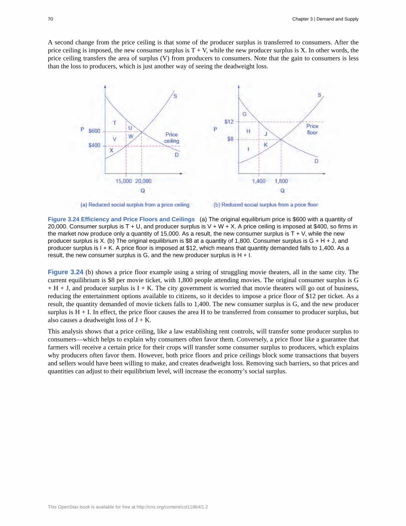
A second change from the price ceiling is that some of the producer surplus is transferred to consumers. After theprice ceiling is imposed, the new consumer surplus is T + V, while the new producer surplus is X. In other words, theprice ceiling transfers the area of surplus (V) from producers to consumers. Note that the gain to consumers is lessthan the loss to producers, which is just another way of seeing the deadweight loss.
Figure 3.24 Efficiency and Price Floors and Ceilings (a) The original equilibrium price is $600 with a quantity of20,000. Consumer surplus is T + U, and producer surplus is V + W + X. A price ceiling is imposed at $400, so firms inthe market now produce only a quantity of 15,000. As a result, the new consumer surplus is T + V, while the newproducer surplus is X. (b) The original equilibrium is $8 at a quantity of 1,800. Consumer surplus is G + H + J, andproducer surplus is I + K. A price floor is imposed at $12, which means that quantity demanded falls to 1,400. As aresult, the new consumer surplus is G, and the new producer surplus is H + I.
Figure 3.24 (b) shows a price floor example using a string of struggling movie theaters, all in the same city. Thecurrent equilibrium is $8 per movie ticket, with 1,800 people attending movies. The original consumer surplus is G+ H + J, and producer surplus is I + K. The city government is worried that movie theaters will go out of business,reducing the entertainment options available to citizens, so it decides to impose a price floor of $12 per ticket. As aresult, the quantity demanded of movie tickets falls to 1,400. The new consumer surplus is G, and the new producersurplus is H + I. In effect, the price floor causes the area H to be transferred from consumer to producer surplus, butalso causes a deadweight loss of J + K.
This analysis shows that a price ceiling, like a law establishing rent controls, will transfer some producer surplus toconsumers—which helps to explain why consumers often favor them. Conversely, a price floor like a guarantee thatfarmers will receive a certain price for their crops will transfer some consumer surplus to producers, which explainswhy producers often favor them. However, both price floors and price ceilings block some transactions that buyersand sellers would have been willing to make, and creates deadweight loss. Removing such barriers, so that prices andquantities can adjust to their equilibrium level, will increase the economy’s social surplus.
70 Chapter 3 | Demand and Supply
This OpenStax book is available for free at http://cnx.org/content/col11864/1.2
ceteris paribus
complements
demand
demand curve
demand schedule
equilibrium
equilibrium price
equilibrium quantity
excess demand
excess supply
factors of production
inferior good
inputs
law of demand
law of supply
normal good
price
price ceiling
price control
price floor
quantity demanded
quantity supplied
KEY TERMS
other things being equal
goods that are often used together so that consumption of one good tends to enhance consumption of theother
the relationship between price and the quantity demanded of a certain good or service
a graphic representation of the relationship between price and quantity demanded of a certain good orservice, with quantity on the horizontal axis and the price on the vertical axis
a table that shows a range of prices for a certain good or service and the quantity demanded at eachprice
the situation where quantity demanded is equal to the quantity supplied; the combination of price andquantity where there is no economic pressure from surpluses or shortages that would cause price or quantity tochange
the price where quantity demanded is equal to quantity supplied
the quantity at which quantity demanded and quantity supplied are equal for a certain price level
at the existing price, the quantity demanded exceeds the quantity supplied; also called a shortage
at the existing price, quantity supplied exceeds the quantity demanded; also called a surplus
the combination of labor, materials, and machinery that is used to produce goods and services;also called inputs
a good in which the quantity demanded falls as income rises, and in which quantity demanded rises andincome falls
the combination of labor, materials, and machinery that is used to produce goods and services; also called factorsof production
the common relationship that a higher price leads to a lower quantity demanded of a certain good orservice and a lower price leads to a higher quantity demanded, while all other variables are held constant
the common relationship that a higher price leads to a greater quantity supplied and a lower price leads toa lower quantity supplied, while all other variables are held constant
a good in which the quantity demanded rises as income rises, and in which quantity demanded falls asincome falls
what a buyer pays for a unit of the specific good or service
a legal maximum price
government laws to regulate prices instead of letting market forces determine prices
a legal minimum price
the total number of units of a good or service consumers are willing to purchase at a given price
the total number of units of a good or service producers are willing to sell at a given price
Chapter 3 | Demand and Supply 71
shift in demand
shift in supply
shortage
substitute
supply
supply curve
supply schedule
surplus
total surplus
when a change in some economic factor (other than price) causes a different quantity to be demandedat every price
when a change in some economic factor (other than price) causes a different quantity to be supplied atevery price
at the existing price, the quantity demanded exceeds the quantity supplied; also called excess demand
a good that can replace another to some extent, so that greater consumption of one good can mean less of theother
the relationship between price and the quantity supplied of a certain good or service
a line that shows the relationship between price and quantity supplied on a graph, with quantity suppliedon the horizontal axis and price on the vertical axis
a table that shows a range of prices for a good or service and the quantity supplied at each price
at the existing price, quantity supplied exceeds the quantity demanded; also called excess supply
see social surplus
KEY CONCEPTS AND SUMMARY
3.1 Demand, Supply, and Equilibrium in Markets for Goods and ServicesA demand schedule is a table that shows the quantity demanded at different prices in the market. A demand curveshows the relationship between quantity demanded and price in a given market on a graph. The law of demand statesthat a higher price typically leads to a lower quantity demanded.
A supply schedule is a table that shows the quantity supplied at different prices in the market. A supply curve showsthe relationship between quantity supplied and price on a graph. The law of supply says that a higher price typicallyleads to a higher quantity supplied.
The equilibrium price and equilibrium quantity occur where the supply and demand curves cross. The equilibriumoccurs where the quantity demanded is equal to the quantity supplied. If the price is below the equilibrium level, thenthe quantity demanded will exceed the quantity supplied. Excess demand or a shortage will exist. If the price is abovethe equilibrium level, then the quantity supplied will exceed the quantity demanded. Excess supply or a surplus willexist. In either case, economic pressures will push the price toward the equilibrium level.
3.2 Shifts in Demand and Supply for Goods and ServicesEconomists often use the ceteris paribus or “other things being equal” assumption: while examining the economicimpact of one event, all other factors remain unchanged for the purpose of the analysis. Factors that can shift thedemand curve for goods and services, causing a different quantity to be demanded at any given price, include changesin tastes, population, income, prices of substitute or complement goods, and expectations about future conditions andprices. Factors that can shift the supply curve for goods and services, causing a different quantity to be supplied atany given price, include input prices, natural conditions, changes in technology, and government taxes, regulations,or subsidies.
3.3 Changes in Equilibrium Price and Quantity: The Four-Step ProcessWhen using the supply and demand framework to think about how an event will affect the equilibrium price andquantity, proceed through four steps: (1) sketch a supply and demand diagram to think about what the market lookedlike before the event; (2) decide whether the event will affect supply or demand; (3) decide whether the effect onsupply or demand is negative or positive, and draw the appropriate shifted supply or demand curve; (4) compare thenew equilibrium price and quantity to the original ones.
72 Chapter 3 | Demand and Supply
This OpenStax book is available for free at http://cnx.org/content/col11864/1.2

3.4 Price Ceilings and Price FloorsPrice ceilings prevent a price from rising above a certain level. When a price ceiling is set below the equilibrium price,quantity demanded will exceed quantity supplied, and excess demand or shortages will result. Price floors prevent aprice from falling below a certain level. When a price floor is set above the equilibrium price, quantity supplied willexceed quantity demanded, and excess supply or surpluses will result. Price floors and price ceilings often lead tounintended consequences.
3.5 Demand, Supply and EfficiencyConsumer surplus is the gap between the price that consumers are willing to pay, based on their preferences, andthe market equilibrium price. Producer surplus is the gap between the price for which producers are willing to sella product, based on their costs, and the market equilibrium price. Social surplus is the sum of consumer surplus andproducer surplus. Total surplus is larger at the equilibrium quantity and price than it will be at any other quantity andprice. Deadweight loss is loss in total surplus that occurs when the economy produces at an inefficient quantity.
SELF-CHECK QUESTIONS1. Review Figure 3.4. Suppose the price of gasoline is $1.60 per gallon. Is the quantity demanded higher or lowerthan at the equilibrium price of $1.40 per gallon? And what about the quantity supplied? Is there a shortage or asurplus in the market? If so, of how much?
2. Why do economists use the ceteris paribus assumption?
3. In an analysis of the market for paint, an economist discovers the facts listed below. State whether each of thesechanges will affect supply or demand, and in what direction.
a. There have recently been some important cost-saving inventions in the technology for making paint.b. Paint is lasting longer, so that property owners need not repaint as often.c. Because of severe hailstorms, many people need to repaint now.d. The hailstorms damaged several factories that make paint, forcing them to close down for several months.
4. Many changes are affecting the market for oil. Predict how each of the following events will affect the equilibriumprice and quantity in the market for oil. In each case, state how the event will affect the supply and demand diagram.Create a sketch of the diagram if necessary.
a. Cars are becoming more fuel efficient, and therefore get more miles to the gallon.b. The winter is exceptionally cold.c. A major discovery of new oil is made off the coast of Norway.d. The economies of some major oil-using nations, like Japan, slow down.e. A war in the Middle East disrupts oil-pumping schedules.f. Landlords install additional insulation in buildings.g. The price of solar energy falls dramatically.h. Chemical companies invent a new, popular kind of plastic made from oil.
5. Let’s think about the market for air travel. From August 2014 to January 2015, the price of jet fuel decreasedroughly 47%. Using the four-step analysis, how do you think this fuel price decrease affected the equilibrium priceand quantity of air travel?
6. A tariff is a tax on imported goods. Suppose the U.S. government cuts the tariff on imported flat screen televisions.Using the four-step analysis, how do you think the tariff reduction will affect the equilibrium price and quantity offlat screen TVs?
7. What is the effect of a price ceiling on the quantity demanded of the product? What is the effect of a price ceilingon the quantity supplied? Why exactly does a price ceiling cause a shortage?
8. Does a price ceiling change the equilibrium price?
9. What would be the impact of imposing a price floor below the equilibrium price?
Chapter 3 | Demand and Supply 73
10. Does a price ceiling increase or decrease the number of transactions in a market? Why? What about a pricefloor?
Assuming that people obey the price ceiling, the market price will be above equilibrium, which means that Qd willbe less than Qs. Firms can only sell what is demanded, so the number of transactions will fall to Qd. This is easy tosee graphically. By analogous reasoning, with a price floor the market price will be below the equilibrium price, soQd will be greater than Qs. Since the limit on transactions here is demand, the number of transactions will fall to Qd.Note that because both price floors and price ceilings reduce the number of transactions, social surplus is less.
11. If a price floor benefits producers, why does a price floor reduce social surplus?
Because the losses to consumers are greater than the benefits to producers, so the net effect is negative. Since the lostconsumer surplus is greater than the additional producer surplus, social surplus falls.
REVIEW QUESTIONS
12. What determines the level of prices in a market?
13. What does a downward-sloping demand curvemean about how buyers in a market will react to a higherprice?
14. Will demand curves have the same exact shape inall markets? If not, how will they differ?
15. Will supply curves have the same shape in allmarkets? If not, how will they differ?
16. What is the relationship between quantitydemanded and quantity supplied at equilibrium? What isthe relationship when there is a shortage? What is therelationship when there is a surplus?
17. How can you locate the equilibrium point on ademand and supply graph?
18. If the price is above the equilibrium level, wouldyou predict a surplus or a shortage? If the price is belowthe equilibrium level, would you predict a surplus or ashortage? Why?
19. When the price is above the equilibrium, explainhow market forces move the market price toequilibrium. Do the same when the price is below theequilibrium.
20. What is the difference between the demand and thequantity demanded of a product, say milk? Explain inwords and show the difference on a graph with a demandcurve for milk.
21. What is the difference between the supply andthe quantity supplied of a product, say milk? Explainin words and show the difference on a graph with thesupply curve for milk.
22. When analyzing a market, how do economists dealwith the problem that many factors that affect the marketare changing at the same time?
23. Name some factors that can cause a shift in thedemand curve in markets for goods and services.
24. Name some factors that can cause a shift in thesupply curve in markets for goods and services.
25. How does one analyze a market where bothdemand and supply shift?
26. What causes a movement along the demand curve?What causes a movement along the supply curve?
27. Does a price ceiling attempt to make a price higheror lower?
28. How does a price ceiling set below the equilibriumlevel affect quantity demanded and quantity supplied?
29. Does a price floor attempt to make a price higher orlower?
30. How does a price floor set above the equilibriumlevel affect quantity demanded and quantity supplied?
31. What is consumer surplus? How is it illustrated ona demand and supply diagram?
32. What is producer surplus? How is it illustrated on ademand and supply diagram?
33. What is total surplus? How is it illustrated on ademand and supply diagram?
34. What is the relationship between total surplus andeconomic efficiency?
35. What is deadweight loss?
74 Chapter 3 | Demand and Supply
This OpenStax book is available for free at http://cnx.org/content/col11864/1.2
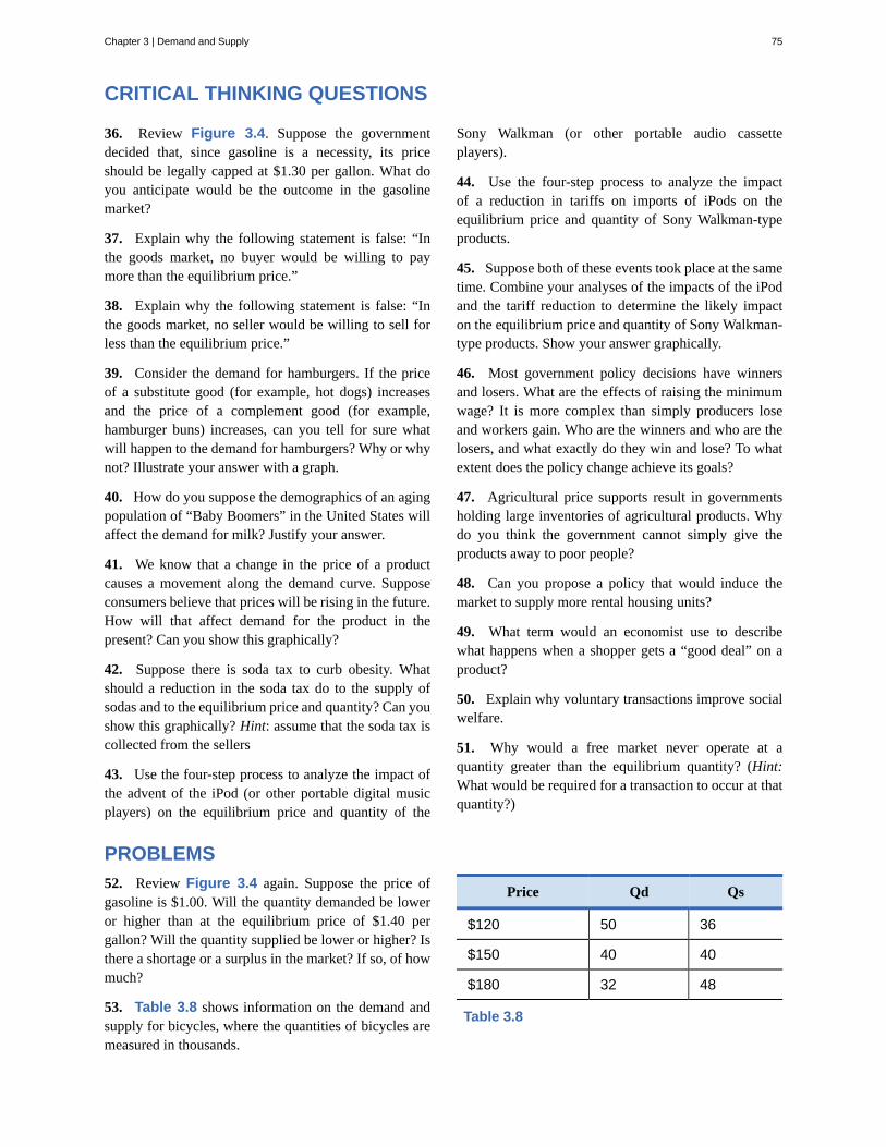
CRITICAL THINKING QUESTIONS
36. Review Figure 3.4. Suppose the governmentdecided that, since gasoline is a necessity, its priceshould be legally capped at $1.30 per gallon. What doyou anticipate would be the outcome in the gasolinemarket?
37. Explain why the following statement is false: “Inthe goods market, no buyer would be willing to paymore than the equilibrium price.”
38. Explain why the following statement is false: “Inthe goods market, no seller would be willing to sell forless than the equilibrium price.”
39. Consider the demand for hamburgers. If the priceof a substitute good (for example, hot dogs) increasesand the price of a complement good (for example,hamburger buns) increases, can you tell for sure whatwill happen to the demand for hamburgers? Why or whynot? Illustrate your answer with a graph.
40. How do you suppose the demographics of an agingpopulation of “Baby Boomers” in the United States willaffect the demand for milk? Justify your answer.
41. We know that a change in the price of a productcauses a movement along the demand curve. Supposeconsumers believe that prices will be rising in the future.How will that affect demand for the product in thepresent? Can you show this graphically?
42. Suppose there is soda tax to curb obesity. Whatshould a reduction in the soda tax do to the supply ofsodas and to the equilibrium price and quantity? Can youshow this graphically? Hint: assume that the soda tax iscollected from the sellers
43. Use the four-step process to analyze the impact ofthe advent of the iPod (or other portable digital musicplayers) on the equilibrium price and quantity of the
Sony Walkman (or other portable audio cassetteplayers).
44. Use the four-step process to analyze the impactof a reduction in tariffs on imports of iPods on theequilibrium price and quantity of Sony Walkman-typeproducts.
45. Suppose both of these events took place at the sametime. Combine your analyses of the impacts of the iPodand the tariff reduction to determine the likely impacton the equilibrium price and quantity of Sony Walkman-type products. Show your answer graphically.
46. Most government policy decisions have winnersand losers. What are the effects of raising the minimumwage? It is more complex than simply producers loseand workers gain. Who are the winners and who are thelosers, and what exactly do they win and lose? To whatextent does the policy change achieve its goals?
47. Agricultural price supports result in governmentsholding large inventories of agricultural products. Whydo you think the government cannot simply give theproducts away to poor people?
48. Can you propose a policy that would induce themarket to supply more rental housing units?
49. What term would an economist use to describewhat happens when a shopper gets a “good deal” on aproduct?
50. Explain why voluntary transactions improve socialwelfare.
51. Why would a free market never operate at aquantity greater than the equilibrium quantity? (Hint:What would be required for a transaction to occur at thatquantity?)
PROBLEMS52. Review Figure 3.4 again. Suppose the price ofgasoline is $1.00. Will the quantity demanded be loweror higher than at the equilibrium price of $1.40 pergallon? Will the quantity supplied be lower or higher? Isthere a shortage or a surplus in the market? If so, of howmuch?
53. Table 3.8 shows information on the demand andsupply for bicycles, where the quantities of bicycles aremeasured in thousands.
Price Qd Qs
$120 50 36
$150 40 40
$180 32 48
Table 3.8
Chapter 3 | Demand and Supply 75
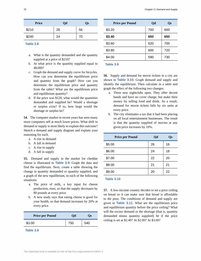
Price Qd Qs
$210 28 56
$240 24 70
Table 3.8
a. What is the quantity demanded and the quantitysupplied at a price of $210?
b. At what price is the quantity supplied equal to48,000?
c. Graph the demand and supply curve for bicycles.How can you determine the equilibrium priceand quantity from the graph? How can youdetermine the equilibrium price and quantityfrom the table? What are the equilibrium priceand equilibrium quantity?
d. If the price was $120, what would the quantitiesdemanded and supplied be? Would a shortageor surplus exist? If so, how large would theshortage or surplus be?
54. The computer market in recent years has seen manymore computers sell at much lower prices. What shift indemand or supply is most likely to explain this outcome?Sketch a demand and supply diagram and explain yourreasoning for each.
a. A rise in demandb. A fall in demandc. A rise in supplyd. A fall in supply
55. Demand and supply in the market for cheddarcheese is illustrated in Table 3.9. Graph the data andfind the equilibrium. Next, create a table showing thechange in quantity demanded or quantity supplied, anda graph of the new equilibrium, in each of the followingsituations:
a. The price of milk, a key input for cheeseproduction, rises, so that the supply decreases by80 pounds at every price.
b. A new study says that eating cheese is good foryour health, so that demand increases by 20% atevery price.
Price per Pound Qd Qs
$3.00 750 540
Table 3.9
Price per Pound Qd Qs
$3.20 700 600
$3.40 650 650
$3.60 620 700
$3.80 600 720
$4.00 590 730
Table 3.9
56. Supply and demand for movie tickets in a city areshown in Table 3.10. Graph demand and supply andidentify the equilibrium. Then calculate in a table andgraph the effect of the following two changes.
a. Three new nightclubs open. They offer decentbands and have no cover charge, but make theirmoney by selling food and drink. As a result,demand for movie tickets falls by six units atevery price.
b. The city eliminates a tax that it had been placingon all local entertainment businesses. The resultis that the quantity supplied of movies at anygiven price increases by 10%.
Price per Pound Qd Qs
$5.00 26 16
$6.00 24 18
$7.00 22 20
$8.00 21 21
$9.00 20 22
Table 3.10
57. A low-income country decides to set a price ceilingon bread so it can make sure that bread is affordableto the poor. The conditions of demand and supply aregiven in Table 3.11. What are the equilibrium priceand equilibrium quantity before the price ceiling? Whatwill the excess demand or the shortage (that is, quantitydemanded minus quantity supplied) be if the priceceiling is set at $2.40? At $2.00? At $3.60?
76 Chapter 3 | Demand and Supply
This OpenStax book is available for free at http://cnx.org/content/col11864/1.2
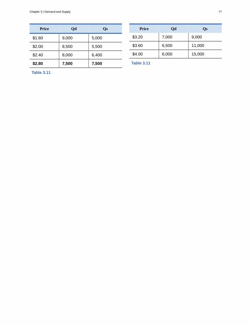
Price Qd Qs
$1.60 9,000 5,000
$2.00 8,500 5,500
$2.40 8,000 6,400
$2.80 7,500 7,500
Table 3.11
Price Qd Qs
$3.20 7,000 9,000
$3.60 6,500 11,000
$4.00 6,000 15,000
Table 3.11
Chapter 3 | Demand and Supply 77
78 Chapter 3 | Demand and Supply
This OpenStax book is available for free at http://cnx.org/content/col11864/1.2

4 | Labor and FinancialMarkets
Figure 4.1 People often think of demand and supply in relation to goods, but labor markets, such as the nursingprofession, can also apply to this analysis. (Credit: modification of work by "Fotos GOVBA"/Flickr Creative Commons)
Baby Boomers Come of AgeThe Census Bureau reports that as of 2013, 20% of the U.S. population was over 60 years old, which meansthat almost 63 million people are reaching an age when they will need increased medical care.
The baby boomer population, the group born between 1946 and 1964, is comprised of approximately74 million people who have just reached retirement age. As this population grows older, they will befaced with common healthcare issues such as heart conditions, arthritis, and Alzheimer’s that may requirehospitalization, long-term, or at-home nursing care. Aging baby boomers and advances in life-saving and life-extending technologies will increase the demand for healthcare and nursing. Additionally, the Affordable CareAct, which expands access to healthcare for millions of Americans, will further increase the demand.
According to the Bureau of Labor Statistics, registered nursing jobs are expected to increase by 19% between2012 and 2022. The median annual wage of $67,930 (in 2012) is also expected to increase. The BLSforecasts that 526,000 new nurses will be needed by 2022. One concern is the low rate of enrollment innursing programs to help meet the growing demand. According to the American Association of Colleges ofNursing (AACN), enrollment in 2011 increased by only 5.1% due to a shortage of nursing educators andteaching facilities.
Chapter 4 | Labor and Financial Markets 79
These data tell us, as economists, that the market for healthcare professionals, and nurses in particular, willface several challenges. Our study of supply and demand will help us to analyze in the second half of thiscase at chapter’s end what might happen in the labor market for nursing and other healthcare professionals.
Introduction to Labor and Financial MarketsIn this chapter, you will learn about:
• Demand and Supply at Work in Labor Markets
• Demand and Supply in Financial Markets
• The Market System as an Efficient Mechanism for Information
The theories of supply and demand do not apply just to markets for goods. They apply to any market, even marketsfor financial services like labor and financial investments. Labor markets are markets for employees or jobs. Financialservices markets are markets for saving or borrowing.
When we think about demand and supply curves in goods and services markets, it is easy to picture who thedemanders and suppliers are: businesses produce the products and households buy them. Who are the demanders andsuppliers in labor and financial service markets? In labor markets job seekers (individuals) are the suppliers of labor,while firms and other employers who hire labor are the demanders for labor. In financial markets, any individual orfirm who saves contributes to the supply of money, and any who borrows (person, firm, or government) contributesto the demand for money.
As a college student, you most likely participate in both labor and financial markets. Employment is a fact of life formost college students: In 2011, says the BLS, 52% of undergraduates worked part time and another 20% worked fulltime. Most college students are also heavily involved in financial markets, primarily as borrowers. Among full-timestudents, about half take out a loan to help finance their education each year, and those loans average about $6,000per year. Many students also borrow for other expenses, like purchasing a car. As this chapter will illustrate, we cananalyze labor markets and financial markets with the same tools we use to analyze demand and supply in the goodsmarkets.
4.1 | Demand and Supply at Work in Labor MarketsBy the end of this section, you will be able to:
• Predict shifts in the demand and supply curves of the labor market• Explain the impact of new technology on the demand and supply curves of the labor market• Explain price floors in the labor market such as minimum wage or a living wage
Markets for labor have demand and supply curves, just like markets for goods. The law of demand applies in labormarkets this way: A higher salary or wage—that is, a higher price in the labor market—leads to a decrease in thequantity of labor demanded by employers, while a lower salary or wage leads to an increase in the quantity of labordemanded. The law of supply functions in labor markets, too: A higher price for labor leads to a higher quantity oflabor supplied; a lower price leads to a lower quantity supplied.
Equilibrium in the Labor MarketIn 2013, about 34,000 registered nurses worked in the Minneapolis-St. Paul-Bloomington, Minnesota-Wisconsinmetropolitan area, according to the BLS. They worked for a variety of employers: hospitals, doctors’ offices, schools,health clinics, and nursing homes. Figure 4.2 illustrates how demand and supply determine equilibrium in this labormarket. The demand and supply schedules in Table 4.1 list the quantity supplied and quantity demanded of nurses atdifferent salaries.
80 Chapter 4 | Labor and Financial Markets
This OpenStax book is available for free at http://cnx.org/content/col11864/1.2
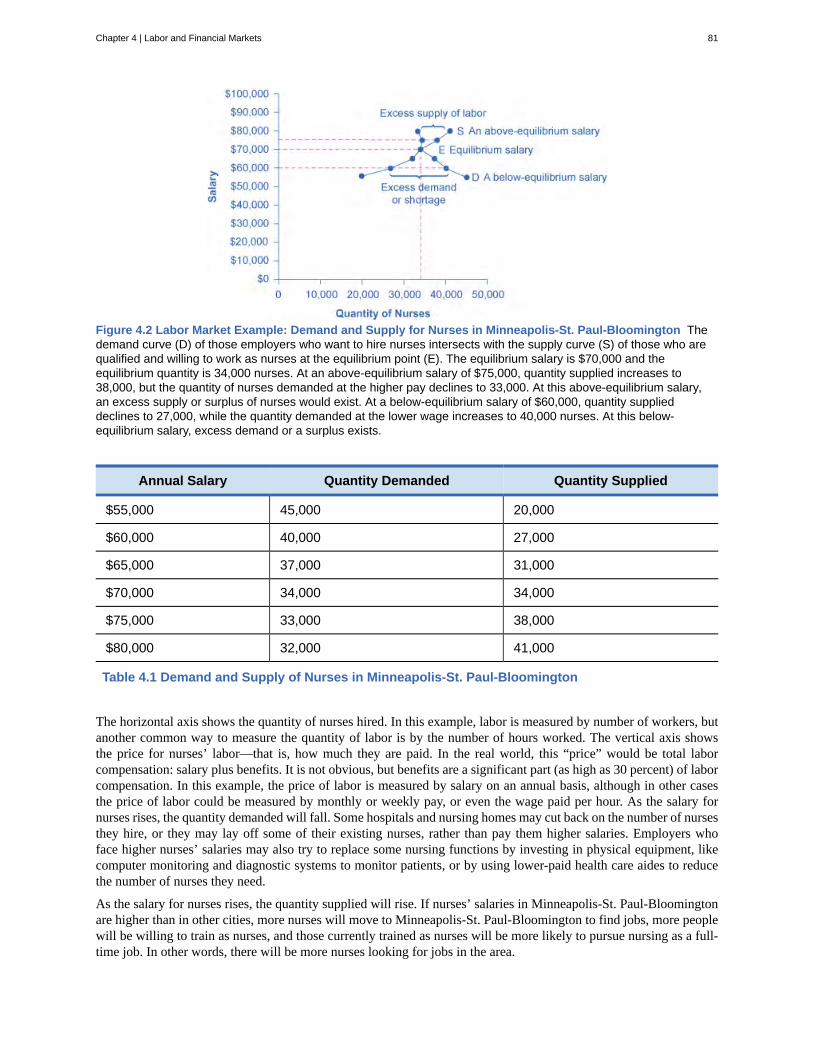
Figure 4.2 Labor Market Example: Demand and Supply for Nurses in Minneapolis-St. Paul-Bloomington Thedemand curve (D) of those employers who want to hire nurses intersects with the supply curve (S) of those who arequalified and willing to work as nurses at the equilibrium point (E). The equilibrium salary is $70,000 and theequilibrium quantity is 34,000 nurses. At an above-equilibrium salary of $75,000, quantity supplied increases to38,000, but the quantity of nurses demanded at the higher pay declines to 33,000. At this above-equilibrium salary,an excess supply or surplus of nurses would exist. At a below-equilibrium salary of $60,000, quantity supplieddeclines to 27,000, while the quantity demanded at the lower wage increases to 40,000 nurses. At this below-equilibrium salary, excess demand or a surplus exists.
Annual Salary Quantity Demanded Quantity Supplied
$55,000 45,000 20,000
$60,000 40,000 27,000
$65,000 37,000 31,000
$70,000 34,000 34,000
$75,000 33,000 38,000
$80,000 32,000 41,000
Table 4.1 Demand and Supply of Nurses in Minneapolis-St. Paul-Bloomington
The horizontal axis shows the quantity of nurses hired. In this example, labor is measured by number of workers, butanother common way to measure the quantity of labor is by the number of hours worked. The vertical axis showsthe price for nurses’ labor—that is, how much they are paid. In the real world, this “price” would be total laborcompensation: salary plus benefits. It is not obvious, but benefits are a significant part (as high as 30 percent) of laborcompensation. In this example, the price of labor is measured by salary on an annual basis, although in other casesthe price of labor could be measured by monthly or weekly pay, or even the wage paid per hour. As the salary fornurses rises, the quantity demanded will fall. Some hospitals and nursing homes may cut back on the number of nursesthey hire, or they may lay off some of their existing nurses, rather than pay them higher salaries. Employers whoface higher nurses’ salaries may also try to replace some nursing functions by investing in physical equipment, likecomputer monitoring and diagnostic systems to monitor patients, or by using lower-paid health care aides to reducethe number of nurses they need.
As the salary for nurses rises, the quantity supplied will rise. If nurses’ salaries in Minneapolis-St. Paul-Bloomingtonare higher than in other cities, more nurses will move to Minneapolis-St. Paul-Bloomington to find jobs, more peoplewill be willing to train as nurses, and those currently trained as nurses will be more likely to pursue nursing as a full-time job. In other words, there will be more nurses looking for jobs in the area.
Chapter 4 | Labor and Financial Markets 81
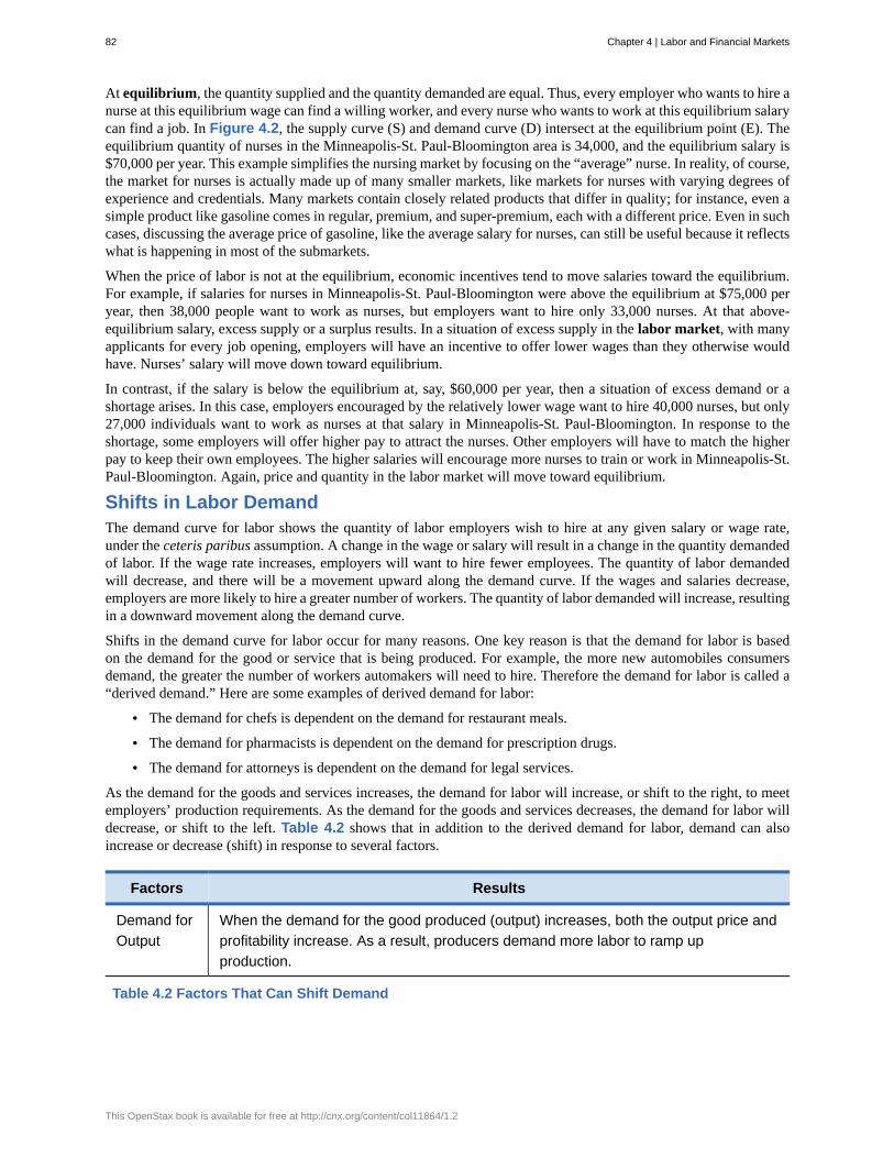
At equilibrium, the quantity supplied and the quantity demanded are equal. Thus, every employer who wants to hire anurse at this equilibrium wage can find a willing worker, and every nurse who wants to work at this equilibrium salarycan find a job. In Figure 4.2, the supply curve (S) and demand curve (D) intersect at the equilibrium point (E). Theequilibrium quantity of nurses in the Minneapolis-St. Paul-Bloomington area is 34,000, and the equilibrium salary is$70,000 per year. This example simplifies the nursing market by focusing on the “average” nurse. In reality, of course,the market for nurses is actually made up of many smaller markets, like markets for nurses with varying degrees ofexperience and credentials. Many markets contain closely related products that differ in quality; for instance, even asimple product like gasoline comes in regular, premium, and super-premium, each with a different price. Even in suchcases, discussing the average price of gasoline, like the average salary for nurses, can still be useful because it reflectswhat is happening in most of the submarkets.
When the price of labor is not at the equilibrium, economic incentives tend to move salaries toward the equilibrium.For example, if salaries for nurses in Minneapolis-St. Paul-Bloomington were above the equilibrium at $75,000 peryear, then 38,000 people want to work as nurses, but employers want to hire only 33,000 nurses. At that above-equilibrium salary, excess supply or a surplus results. In a situation of excess supply in the labor market, with manyapplicants for every job opening, employers will have an incentive to offer lower wages than they otherwise wouldhave. Nurses’ salary will move down toward equilibrium.
In contrast, if the salary is below the equilibrium at, say, $60,000 per year, then a situation of excess demand or ashortage arises. In this case, employers encouraged by the relatively lower wage want to hire 40,000 nurses, but only27,000 individuals want to work as nurses at that salary in Minneapolis-St. Paul-Bloomington. In response to theshortage, some employers will offer higher pay to attract the nurses. Other employers will have to match the higherpay to keep their own employees. The higher salaries will encourage more nurses to train or work in Minneapolis-St.Paul-Bloomington. Again, price and quantity in the labor market will move toward equilibrium.
Shifts in Labor DemandThe demand curve for labor shows the quantity of labor employers wish to hire at any given salary or wage rate,under the ceteris paribus assumption. A change in the wage or salary will result in a change in the quantity demandedof labor. If the wage rate increases, employers will want to hire fewer employees. The quantity of labor demandedwill decrease, and there will be a movement upward along the demand curve. If the wages and salaries decrease,employers are more likely to hire a greater number of workers. The quantity of labor demanded will increase, resultingin a downward movement along the demand curve.
Shifts in the demand curve for labor occur for many reasons. One key reason is that the demand for labor is basedon the demand for the good or service that is being produced. For example, the more new automobiles consumersdemand, the greater the number of workers automakers will need to hire. Therefore the demand for labor is called a“derived demand.” Here are some examples of derived demand for labor:
• The demand for chefs is dependent on the demand for restaurant meals.
• The demand for pharmacists is dependent on the demand for prescription drugs.
• The demand for attorneys is dependent on the demand for legal services.
As the demand for the goods and services increases, the demand for labor will increase, or shift to the right, to meetemployers’ production requirements. As the demand for the goods and services decreases, the demand for labor willdecrease, or shift to the left. Table 4.2 shows that in addition to the derived demand for labor, demand can alsoincrease or decrease (shift) in response to several factors.
Factors Results
Demand forOutput
When the demand for the good produced (output) increases, both the output price andprofitability increase. As a result, producers demand more labor to ramp upproduction.
Table 4.2 Factors That Can Shift Demand
82 Chapter 4 | Labor and Financial Markets
This OpenStax book is available for free at http://cnx.org/content/col11864/1.2
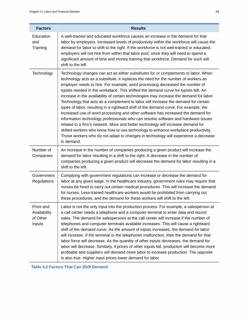
Factors Results
EducationandTraining
A well-trained and educated workforce causes an increase in the demand for thatlabor by employers. Increased levels of productivity within the workforce will cause thedemand for labor to shift to the right. If the workforce is not well-trained or educated,employers will not hire from within that labor pool, since they will need to spend asignificant amount of time and money training that workforce. Demand for such willshift to the left.
Technology Technology changes can act as either substitutes for or complements to labor. Whentechnology acts as a substitute, it replaces the need for the number of workers anemployer needs to hire. For example, word processing decreased the number oftypists needed in the workplace. This shifted the demand curve for typists left. Anincrease in the availability of certain technologies may increase the demand for labor.Technology that acts as a complement to labor will increase the demand for certaintypes of labor, resulting in a rightward shift of the demand curve. For example, theincreased use of word processing and other software has increased the demand forinformation technology professionals who can resolve software and hardware issuesrelated to a firm’s network. More and better technology will increase demand forskilled workers who know how to use technology to enhance workplace productivity.Those workers who do not adapt to changes in technology will experience a decreasein demand.
Number ofCompanies
An increase in the number of companies producing a given product will increase thedemand for labor resulting in a shift to the right. A decrease in the number ofcompanies producing a given product will decrease the demand for labor resulting in ashift to the left.
GovernmentRegulations
Complying with government regulations can increase or decrease the demand forlabor at any given wage. In the healthcare industry, government rules may require thatnurses be hired to carry out certain medical procedures. This will increase the demandfor nurses. Less-trained healthcare workers would be prohibited from carrying outthese procedures, and the demand for these workers will shift to the left.
Price andAvailabilityof OtherInputs
Labor is not the only input into the production process. For example, a salesperson ata call center needs a telephone and a computer terminal to enter data and recordsales. The demand for salespersons at the call center will increase if the number oftelephones and computer terminals available increases. This will cause a rightwardshift of the demand curve. As the amount of inputs increases, the demand for laborwill increase. If the terminal or the telephones malfunction, then the demand for thatlabor force will decrease. As the quantity of other inputs decreases, the demand forlabor will decrease. Similarly, if prices of other inputs fall, production will become moreprofitable and suppliers will demand more labor to increase production. The oppositeis also true. Higher input prices lower demand for labor
Table 4.2 Factors That Can Shift Demand
Chapter 4 | Labor and Financial Markets 83
Click here (http://openstaxcollege.org/l/Futurework) to read more about “Trends and Challenges for Work inthe 21st Century.”
Shifts in Labor SupplyThe supply of labor is upward-sloping and adheres to the law of supply: The higher the price, the greater the quantitysupplied and the lower the price, the less quantity supplied. The supply curve models the tradeoff between supplyinglabor into the market or using time in leisure activities at every given price level. The higher the wage, the morelabor is willing to work and forego leisure activities. Table 4.3 lists some of the factors that will cause the supply toincrease or decrease.
Factors Results
Number ofWorkers
An increased number of workers will cause the supply curve to shift to the right. Anincreased number of workers can be due to several factors, such as immigration,increasing population, an aging population, and changing demographics. Policies thatencourage immigration will increase the supply of labor, and vice versa. Populationgrows when birth rates exceed death rates; this eventually increases supply of laborwhen the former reach working age. An aging and therefore retiring population willdecrease the supply of labor. Another example of changing demographics is morewomen working outside of the home, which increases the supply of labor.
RequiredEducation
The more required education, the lower the supply. There is a lower supply of PhDmathematicians than of high school mathematics teachers; there is a lower supply ofcardiologists than of primary care physicians; and there is a lower supply of physiciansthan of nurses.
Table 4.3 Factors that Can Shift Supply
84 Chapter 4 | Labor and Financial Markets
This OpenStax book is available for free at http://cnx.org/content/col11864/1.2
Factors Results
GovernmentPolicies
Government policies can also affect the supply of labor for jobs. On the one hand, thegovernment may support rules that set high qualifications for certain jobs: academictraining, certificates or licenses, or experience. When these qualifications are madetougher, the number of qualified workers will decrease at any given wage. On theother hand, the government may also subsidize training or even reduce the requiredlevel of qualifications. For example, government might offer subsidies for nursingschools or nursing students. Such provisions would shift the supply curve of nurses tothe right. In addition, government policies that change the relative desirability ofworking versus not working also affect the labor supply. These include unemploymentbenefits, maternity leave, child care benefits and welfare policy. For example, childcare benefits may increase the labor supply of working mothers. Long termunemployment benefits may discourage job searching for unemployed workers. Allthese policies must therefore be carefully designed to minimize any negative laborsupply effects.
Table 4.3 Factors that Can Shift Supply
A change in salary will lead to a movement along labor demand or labor supply curves, but it will not shift thosecurves. However, other events like those outlined here will cause either the demand or the supply of labor to shift,and thus will move the labor market to a new equilibrium salary and quantity.
Technology and Wage Inequality: The Four-Step ProcessEconomic events can change the equilibrium salary (or wage) and quantity of labor. Consider how the wave ofnew information technologies, like computer and telecommunications networks, has affected low-skill and high-skillworkers in the U.S. economy. From the perspective of employers who demand labor, these new technologies are oftena substitute for low-skill laborers like file clerks who used to keep file cabinets full of paper records of transactions.However, the same new technologies are a complement to high-skill workers like managers, who benefit from thetechnological advances by being able to monitor more information, communicate more easily, and juggle a widerarray of responsibilities. So, how will the new technologies affect the wages of high-skill and low-skill workers?For this question, the four-step process of analyzing how shifts in supply or demand affect a market (introduced inDemand and Supply) works in this way:
Step 1. What did the markets for low-skill labor and high-skill labor look like before the arrival of the newtechnologies? In Figure 4.3 (a) and Figure 4.3 (b), S0 is the original supply curve for labor and D0 is the originaldemand curve for labor in each market. In each graph, the original point of equilibrium, E0, occurs at the price W0and the quantity Q0.
Chapter 4 | Labor and Financial Markets 85
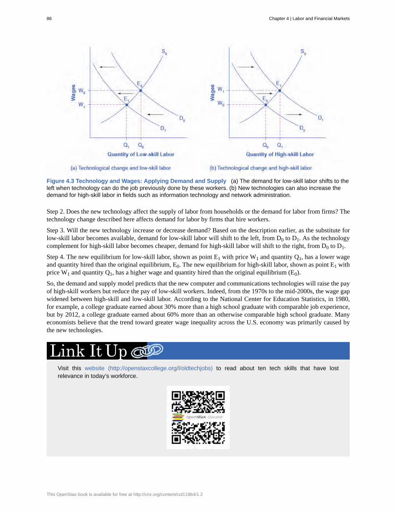
Figure 4.3 Technology and Wages: Applying Demand and Supply (a) The demand for low-skill labor shifts to theleft when technology can do the job previously done by these workers. (b) New technologies can also increase thedemand for high-skill labor in fields such as information technology and network administration.
Step 2. Does the new technology affect the supply of labor from households or the demand for labor from firms? Thetechnology change described here affects demand for labor by firms that hire workers.
Step 3. Will the new technology increase or decrease demand? Based on the description earlier, as the substitute forlow-skill labor becomes available, demand for low-skill labor will shift to the left, from D0 to D1. As the technologycomplement for high-skill labor becomes cheaper, demand for high-skill labor will shift to the right, from D0 to D1.
Step 4. The new equilibrium for low-skill labor, shown as point E1 with price W1 and quantity Q1, has a lower wageand quantity hired than the original equilibrium, E0. The new equilibrium for high-skill labor, shown as point E1 withprice W1 and quantity Q1, has a higher wage and quantity hired than the original equilibrium (E0).
So, the demand and supply model predicts that the new computer and communications technologies will raise the payof high-skill workers but reduce the pay of low-skill workers. Indeed, from the 1970s to the mid-2000s, the wage gapwidened between high-skill and low-skill labor. According to the National Center for Education Statistics, in 1980,for example, a college graduate earned about 30% more than a high school graduate with comparable job experience,but by 2012, a college graduate earned about 60% more than an otherwise comparable high school graduate. Manyeconomists believe that the trend toward greater wage inequality across the U.S. economy was primarily caused bythe new technologies.
Visit this website (http://openstaxcollege.org/l/oldtechjobs) to read about ten tech skills that have lostrelevance in today’s workforce.
86 Chapter 4 | Labor and Financial Markets
This OpenStax book is available for free at http://cnx.org/content/col11864/1.2
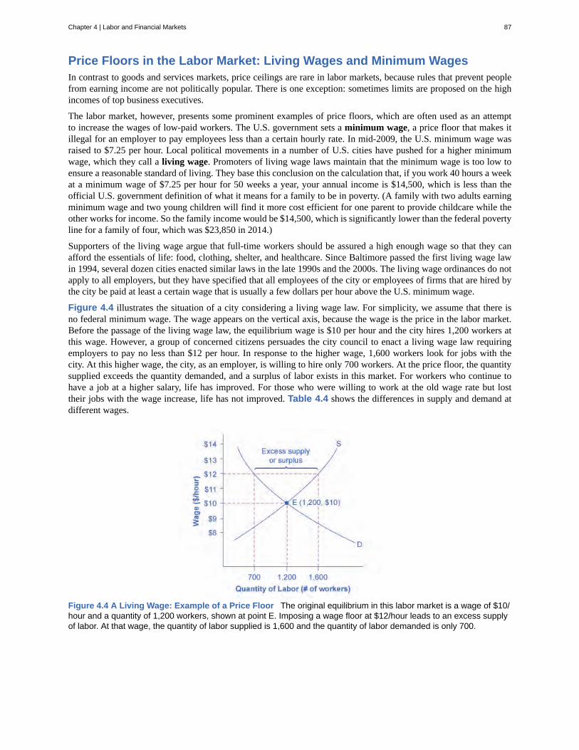
Price Floors in the Labor Market: Living Wages and Minimum WagesIn contrast to goods and services markets, price ceilings are rare in labor markets, because rules that prevent peoplefrom earning income are not politically popular. There is one exception: sometimes limits are proposed on the highincomes of top business executives.
The labor market, however, presents some prominent examples of price floors, which are often used as an attemptto increase the wages of low-paid workers. The U.S. government sets a minimum wage, a price floor that makes itillegal for an employer to pay employees less than a certain hourly rate. In mid-2009, the U.S. minimum wage wasraised to $7.25 per hour. Local political movements in a number of U.S. cities have pushed for a higher minimumwage, which they call a living wage. Promoters of living wage laws maintain that the minimum wage is too low toensure a reasonable standard of living. They base this conclusion on the calculation that, if you work 40 hours a weekat a minimum wage of $7.25 per hour for 50 weeks a year, your annual income is $14,500, which is less than theofficial U.S. government definition of what it means for a family to be in poverty. (A family with two adults earningminimum wage and two young children will find it more cost efficient for one parent to provide childcare while theother works for income. So the family income would be $14,500, which is significantly lower than the federal povertyline for a family of four, which was $23,850 in 2014.)
Supporters of the living wage argue that full-time workers should be assured a high enough wage so that they canafford the essentials of life: food, clothing, shelter, and healthcare. Since Baltimore passed the first living wage lawin 1994, several dozen cities enacted similar laws in the late 1990s and the 2000s. The living wage ordinances do notapply to all employers, but they have specified that all employees of the city or employees of firms that are hired bythe city be paid at least a certain wage that is usually a few dollars per hour above the U.S. minimum wage.
Figure 4.4 illustrates the situation of a city considering a living wage law. For simplicity, we assume that there isno federal minimum wage. The wage appears on the vertical axis, because the wage is the price in the labor market.Before the passage of the living wage law, the equilibrium wage is $10 per hour and the city hires 1,200 workers atthis wage. However, a group of concerned citizens persuades the city council to enact a living wage law requiringemployers to pay no less than $12 per hour. In response to the higher wage, 1,600 workers look for jobs with thecity. At this higher wage, the city, as an employer, is willing to hire only 700 workers. At the price floor, the quantitysupplied exceeds the quantity demanded, and a surplus of labor exists in this market. For workers who continue tohave a job at a higher salary, life has improved. For those who were willing to work at the old wage rate but losttheir jobs with the wage increase, life has not improved. Table 4.4 shows the differences in supply and demand atdifferent wages.
Figure 4.4 A Living Wage: Example of a Price Floor The original equilibrium in this labor market is a wage of $10/hour and a quantity of 1,200 workers, shown at point E. Imposing a wage floor at $12/hour leads to an excess supplyof labor. At that wage, the quantity of labor supplied is 1,600 and the quantity of labor demanded is only 700.
Chapter 4 | Labor and Financial Markets 87
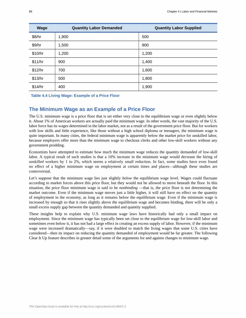
Wage Quantity Labor Demanded Quantity Labor Supplied
$8/hr 1,900 500
$9/hr 1,500 900
$10/hr 1,200 1,200
$11/hr 900 1,400
$12/hr 700 1,600
$13/hr 500 1,800
$14/hr 400 1,900
Table 4.4 Living Wage: Example of a Price Floor
The Minimum Wage as an Example of a Price FloorThe U.S. minimum wage is a price floor that is set either very close to the equilibrium wage or even slightly belowit. About 1% of American workers are actually paid the minimum wage. In other words, the vast majority of the U.S.labor force has its wages determined in the labor market, not as a result of the government price floor. But for workerswith low skills and little experience, like those without a high school diploma or teenagers, the minimum wage isquite important. In many cities, the federal minimum wage is apparently below the market price for unskilled labor,because employers offer more than the minimum wage to checkout clerks and other low-skill workers without anygovernment prodding.
Economists have attempted to estimate how much the minimum wage reduces the quantity demanded of low-skilllabor. A typical result of such studies is that a 10% increase in the minimum wage would decrease the hiring ofunskilled workers by 1 to 2%, which seems a relatively small reduction. In fact, some studies have even foundno effect of a higher minimum wage on employment at certain times and places—although these studies arecontroversial.
Let’s suppose that the minimum wage lies just slightly below the equilibrium wage level. Wages could fluctuateaccording to market forces above this price floor, but they would not be allowed to move beneath the floor. In thissituation, the price floor minimum wage is said to be nonbinding —that is, the price floor is not determining themarket outcome. Even if the minimum wage moves just a little higher, it will still have no effect on the quantityof employment in the economy, as long as it remains below the equilibrium wage. Even if the minimum wage isincreased by enough so that it rises slightly above the equilibrium wage and becomes binding, there will be only asmall excess supply gap between the quantity demanded and quantity supplied.
These insights help to explain why U.S. minimum wage laws have historically had only a small impact onemployment. Since the minimum wage has typically been set close to the equilibrium wage for low-skill labor andsometimes even below it, it has not had a large effect in creating an excess supply of labor. However, if the minimumwage were increased dramatically—say, if it were doubled to match the living wages that some U.S. cities haveconsidered—then its impact on reducing the quantity demanded of employment would be far greater. The followingClear It Up feature describes in greater detail some of the arguments for and against changes to minimum wage.
88 Chapter 4 | Labor and Financial Markets
This OpenStax book is available for free at http://cnx.org/content/col11864/1.2
What’s the harm in raising the minimum wage?Because of the law of demand, a higher required wage will reduce the amount of low-skill employment eitherin terms of employees or in terms of work hours. Although there is controversy over the numbers, let’s say forthe sake of the argument that a 10% rise in the minimum wage will reduce the employment of low-skill workersby 2%. Does this outcome mean that raising the minimum wage by 10% is bad public policy? Not necessarily.
If 98% of those receiving the minimum wage have a pay increase of 10%, but 2% of those receiving theminimum wage lose their jobs, are the gains for society as a whole greater than the losses? The answer is notclear, because job losses, even for a small group, may cause more pain than modest income gains for others.For one thing, we need to consider which minimum wage workers are losing their jobs. If the 2% of minimumwage workers who lose their jobs are struggling to support families, that is one thing. If those who lose theirjob are high school students picking up spending money over summer vacation, that is something else.
Another complexity is that many minimum wage workers do not work full-time for an entire year. Imaginea minimum wage worker who holds different part-time jobs for a few months at a time, with bouts ofunemployment in between. The worker in this situation receives the 10% raise in the minimum wage whenworking, but also ends up working 2% fewer hours during the year because the higher minimum wage reduceshow much employers want people to work. Overall, this worker’s income would rise because the 10% payraise would more than offset the 2% fewer hours worked.
Of course, these arguments do not prove that raising the minimum wage is necessarily a good idea either.There may well be other, better public policy options for helping low-wage workers. (The Poverty andEconomic Inequality (http://cnx.org/content/m57266/latest/) chapter discusses some possibilities.) Thelesson from this maze of minimum wage arguments is that complex social problems rarely have simpleanswers. Even those who agree on how a proposed economic policy affects quantity demanded and quantitysupplied may still disagree on whether the policy is a good idea.
4.2 | Demand and Supply in Financial MarketsBy the end of this section, you will be able to:
• Identify the demanders and suppliers in a financial market.• Explain how interest rates can affect supply and demand• Analyze the economic effects of U.S. debt in terms of domestic financial markets• Explain the role of price ceilings and usury laws in the U.S.
United States' households, institutions, and domestic businesses saved almost $1.9 trillion in 2013. Where did thatsavings go and what was it used for? Some of the savings ended up in banks, which in turn loaned the moneyto individuals or businesses that wanted to borrow money. Some was invested in private companies or loaned togovernment agencies that wanted to borrow money to raise funds for purposes like building roads or mass transit.Some firms reinvested their savings in their own businesses.
In this section, we will determine how the demand and supply model links those who wish to supply financial capital(i.e., savings) with those who demand financial capital (i.e., borrowing). Those who save money (or make financialinvestments, which is the same thing), whether individuals or businesses, are on the supply side of the financialmarket. Those who borrow money are on the demand side of the financial market. For a more detailed treatmentof the different kinds of financial investments like bank accounts, stocks and bonds, see the Financial Markets(http://cnx.org/content/m57283/latest/) chapter.
Who Demands and Who Supplies in Financial Markets?In any market, the price is what suppliers receive and what demanders pay. In financial markets, those who supplyfinancial capital through saving expect to receive a rate of return, while those who demand financial capital by
Chapter 4 | Labor and Financial Markets 89
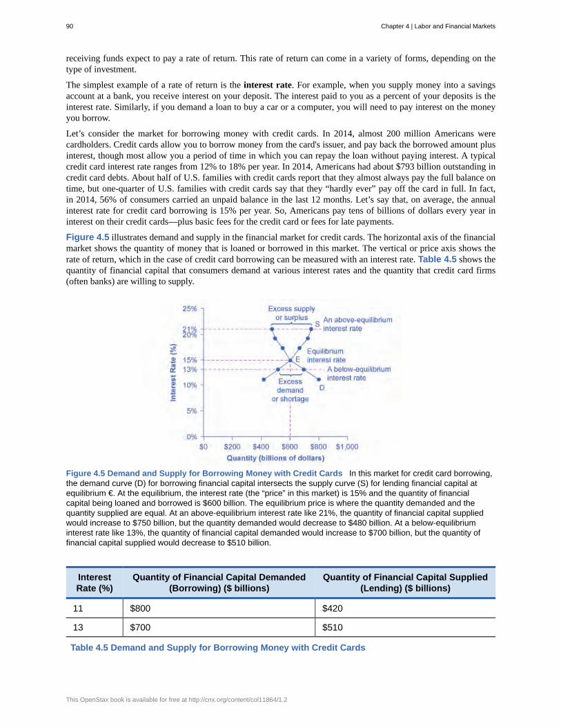
receiving funds expect to pay a rate of return. This rate of return can come in a variety of forms, depending on thetype of investment.
The simplest example of a rate of return is the interest rate. For example, when you supply money into a savingsaccount at a bank, you receive interest on your deposit. The interest paid to you as a percent of your deposits is theinterest rate. Similarly, if you demand a loan to buy a car or a computer, you will need to pay interest on the moneyyou borrow.
Let’s consider the market for borrowing money with credit cards. In 2014, almost 200 million Americans werecardholders. Credit cards allow you to borrow money from the card's issuer, and pay back the borrowed amount plusinterest, though most allow you a period of time in which you can repay the loan without paying interest. A typicalcredit card interest rate ranges from 12% to 18% per year. In 2014, Americans had about $793 billion outstanding incredit card debts. About half of U.S. families with credit cards report that they almost always pay the full balance ontime, but one-quarter of U.S. families with credit cards say that they “hardly ever” pay off the card in full. In fact,in 2014, 56% of consumers carried an unpaid balance in the last 12 months. Let’s say that, on average, the annualinterest rate for credit card borrowing is 15% per year. So, Americans pay tens of billions of dollars every year ininterest on their credit cards—plus basic fees for the credit card or fees for late payments.
Figure 4.5 illustrates demand and supply in the financial market for credit cards. The horizontal axis of the financialmarket shows the quantity of money that is loaned or borrowed in this market. The vertical or price axis shows therate of return, which in the case of credit card borrowing can be measured with an interest rate. Table 4.5 shows thequantity of financial capital that consumers demand at various interest rates and the quantity that credit card firms(often banks) are willing to supply.
Figure 4.5 Demand and Supply for Borrowing Money with Credit Cards In this market for credit card borrowing,the demand curve (D) for borrowing financial capital intersects the supply curve (S) for lending financial capital atequilibrium €. At the equilibrium, the interest rate (the “price” in this market) is 15% and the quantity of financialcapital being loaned and borrowed is $600 billion. The equilibrium price is where the quantity demanded and thequantity supplied are equal. At an above-equilibrium interest rate like 21%, the quantity of financial capital suppliedwould increase to $750 billion, but the quantity demanded would decrease to $480 billion. At a below-equilibriuminterest rate like 13%, the quantity of financial capital demanded would increase to $700 billion, but the quantity offinancial capital supplied would decrease to $510 billion.
InterestRate (%)
Quantity of Financial Capital Demanded(Borrowing) ($ billions)
Quantity of Financial Capital Supplied(Lending) ($ billions)
11 $800 $420
13 $700 $510
Table 4.5 Demand and Supply for Borrowing Money with Credit Cards
90 Chapter 4 | Labor and Financial Markets
This OpenStax book is available for free at http://cnx.org/content/col11864/1.2
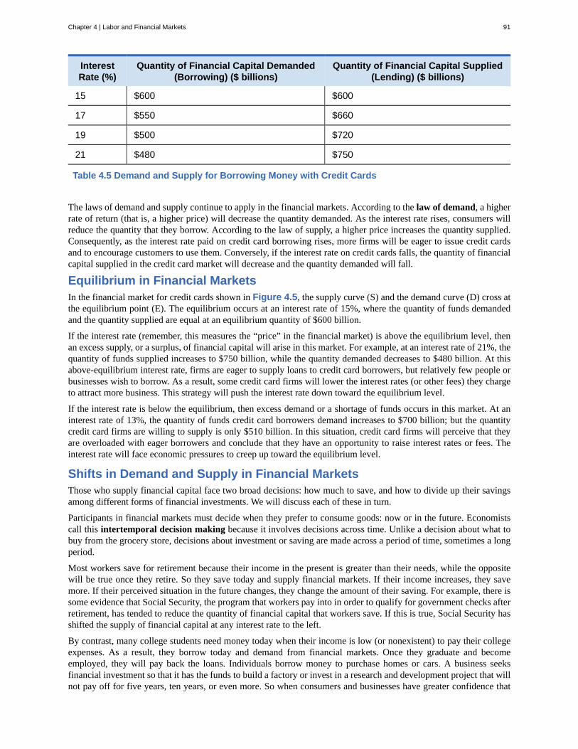
InterestRate (%)
Quantity of Financial Capital Demanded(Borrowing) ($ billions)
Quantity of Financial Capital Supplied(Lending) ($ billions)
15 $600 $600
17 $550 $660
19 $500 $720
21 $480 $750
Table 4.5 Demand and Supply for Borrowing Money with Credit Cards
The laws of demand and supply continue to apply in the financial markets. According to the law of demand, a higherrate of return (that is, a higher price) will decrease the quantity demanded. As the interest rate rises, consumers willreduce the quantity that they borrow. According to the law of supply, a higher price increases the quantity supplied.Consequently, as the interest rate paid on credit card borrowing rises, more firms will be eager to issue credit cardsand to encourage customers to use them. Conversely, if the interest rate on credit cards falls, the quantity of financialcapital supplied in the credit card market will decrease and the quantity demanded will fall.
Equilibrium in Financial MarketsIn the financial market for credit cards shown in Figure 4.5, the supply curve (S) and the demand curve (D) cross atthe equilibrium point (E). The equilibrium occurs at an interest rate of 15%, where the quantity of funds demandedand the quantity supplied are equal at an equilibrium quantity of $600 billion.
If the interest rate (remember, this measures the “price” in the financial market) is above the equilibrium level, thenan excess supply, or a surplus, of financial capital will arise in this market. For example, at an interest rate of 21%, thequantity of funds supplied increases to $750 billion, while the quantity demanded decreases to $480 billion. At thisabove-equilibrium interest rate, firms are eager to supply loans to credit card borrowers, but relatively few people orbusinesses wish to borrow. As a result, some credit card firms will lower the interest rates (or other fees) they chargeto attract more business. This strategy will push the interest rate down toward the equilibrium level.
If the interest rate is below the equilibrium, then excess demand or a shortage of funds occurs in this market. At aninterest rate of 13%, the quantity of funds credit card borrowers demand increases to $700 billion; but the quantitycredit card firms are willing to supply is only $510 billion. In this situation, credit card firms will perceive that theyare overloaded with eager borrowers and conclude that they have an opportunity to raise interest rates or fees. Theinterest rate will face economic pressures to creep up toward the equilibrium level.
Shifts in Demand and Supply in Financial MarketsThose who supply financial capital face two broad decisions: how much to save, and how to divide up their savingsamong different forms of financial investments. We will discuss each of these in turn.
Participants in financial markets must decide when they prefer to consume goods: now or in the future. Economistscall this intertemporal decision making because it involves decisions across time. Unlike a decision about what tobuy from the grocery store, decisions about investment or saving are made across a period of time, sometimes a longperiod.
Most workers save for retirement because their income in the present is greater than their needs, while the oppositewill be true once they retire. So they save today and supply financial markets. If their income increases, they savemore. If their perceived situation in the future changes, they change the amount of their saving. For example, there issome evidence that Social Security, the program that workers pay into in order to qualify for government checks afterretirement, has tended to reduce the quantity of financial capital that workers save. If this is true, Social Security hasshifted the supply of financial capital at any interest rate to the left.
By contrast, many college students need money today when their income is low (or nonexistent) to pay their collegeexpenses. As a result, they borrow today and demand from financial markets. Once they graduate and becomeemployed, they will pay back the loans. Individuals borrow money to purchase homes or cars. A business seeksfinancial investment so that it has the funds to build a factory or invest in a research and development project that willnot pay off for five years, ten years, or even more. So when consumers and businesses have greater confidence that
Chapter 4 | Labor and Financial Markets 91
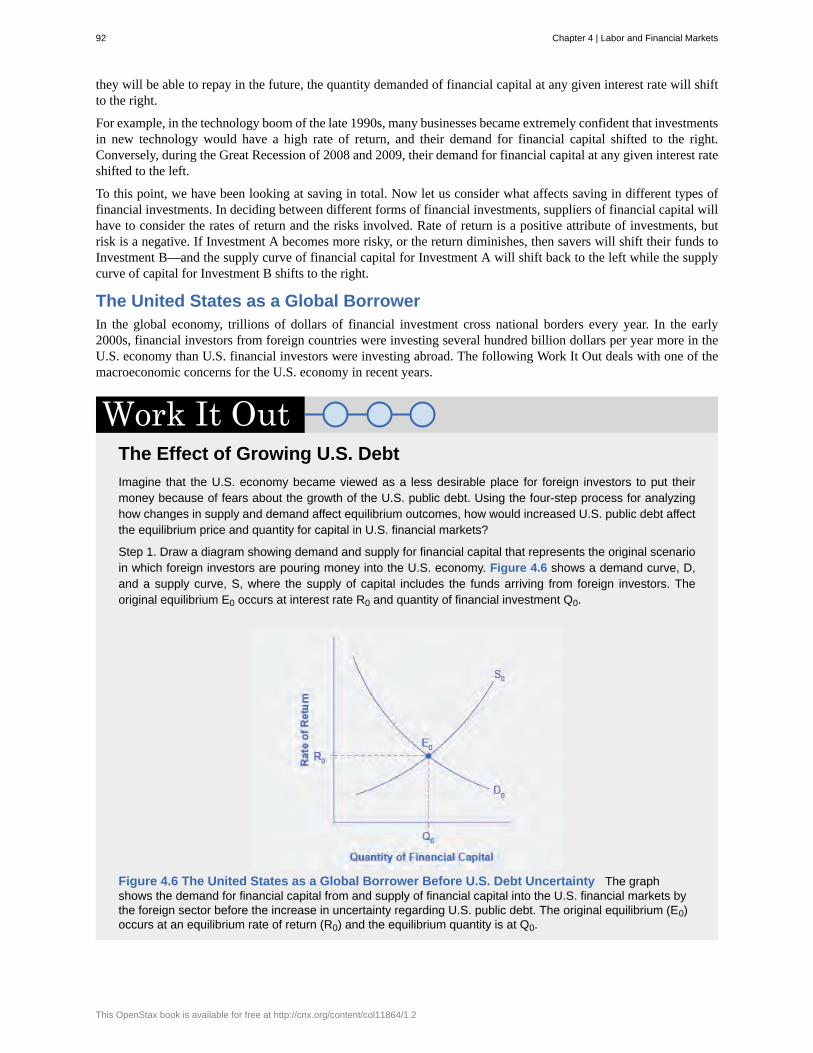
they will be able to repay in the future, the quantity demanded of financial capital at any given interest rate will shiftto the right.
For example, in the technology boom of the late 1990s, many businesses became extremely confident that investmentsin new technology would have a high rate of return, and their demand for financial capital shifted to the right.Conversely, during the Great Recession of 2008 and 2009, their demand for financial capital at any given interest rateshifted to the left.
To this point, we have been looking at saving in total. Now let us consider what affects saving in different types offinancial investments. In deciding between different forms of financial investments, suppliers of financial capital willhave to consider the rates of return and the risks involved. Rate of return is a positive attribute of investments, butrisk is a negative. If Investment A becomes more risky, or the return diminishes, then savers will shift their funds toInvestment B—and the supply curve of financial capital for Investment A will shift back to the left while the supplycurve of capital for Investment B shifts to the right.
The United States as a Global BorrowerIn the global economy, trillions of dollars of financial investment cross national borders every year. In the early2000s, financial investors from foreign countries were investing several hundred billion dollars per year more in theU.S. economy than U.S. financial investors were investing abroad. The following Work It Out deals with one of themacroeconomic concerns for the U.S. economy in recent years.
The Effect of Growing U.S. DebtImagine that the U.S. economy became viewed as a less desirable place for foreign investors to put theirmoney because of fears about the growth of the U.S. public debt. Using the four-step process for analyzinghow changes in supply and demand affect equilibrium outcomes, how would increased U.S. public debt affectthe equilibrium price and quantity for capital in U.S. financial markets?
Step 1. Draw a diagram showing demand and supply for financial capital that represents the original scenarioin which foreign investors are pouring money into the U.S. economy. Figure 4.6 shows a demand curve, D,and a supply curve, S, where the supply of capital includes the funds arriving from foreign investors. Theoriginal equilibrium E0 occurs at interest rate R0 and quantity of financial investment Q0.
Figure 4.6 The United States as a Global Borrower Before U.S. Debt Uncertainty The graphshows the demand for financial capital from and supply of financial capital into the U.S. financial markets bythe foreign sector before the increase in uncertainty regarding U.S. public debt. The original equilibrium (E0)occurs at an equilibrium rate of return (R0) and the equilibrium quantity is at Q0.
92 Chapter 4 | Labor and Financial Markets
This OpenStax book is available for free at http://cnx.org/content/col11864/1.2
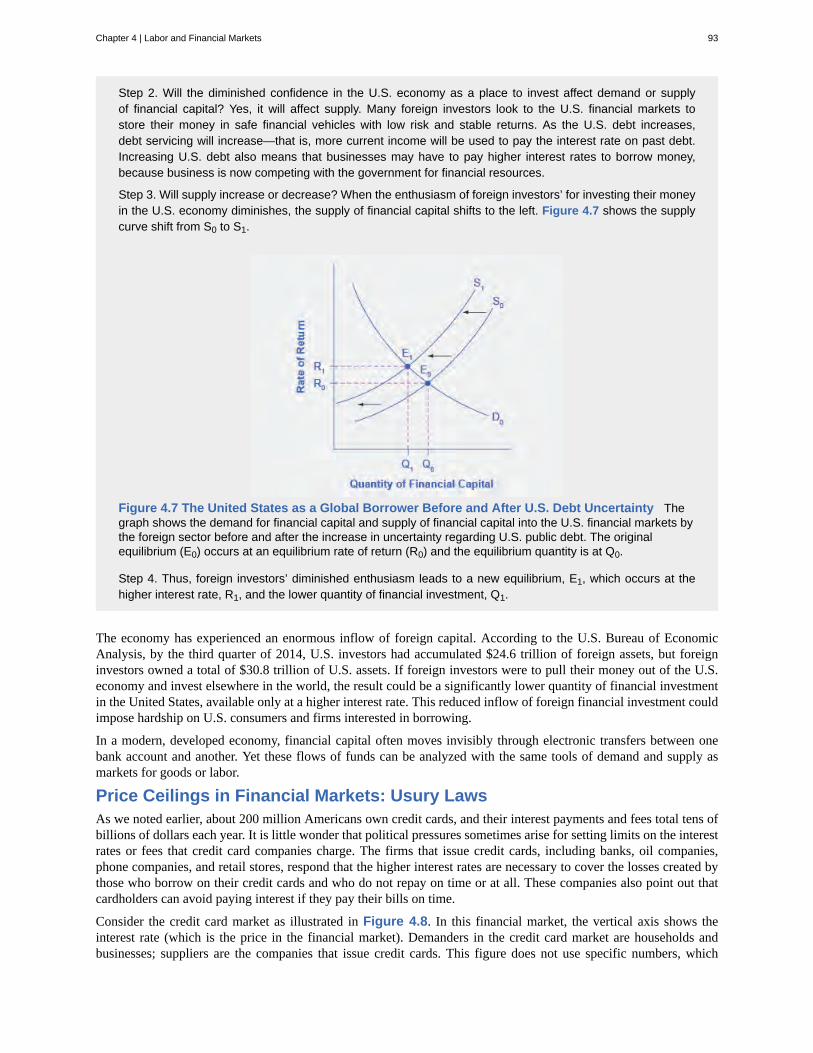
Step 2. Will the diminished confidence in the U.S. economy as a place to invest affect demand or supplyof financial capital? Yes, it will affect supply. Many foreign investors look to the U.S. financial markets tostore their money in safe financial vehicles with low risk and stable returns. As the U.S. debt increases,debt servicing will increase—that is, more current income will be used to pay the interest rate on past debt.Increasing U.S. debt also means that businesses may have to pay higher interest rates to borrow money,because business is now competing with the government for financial resources.
Step 3. Will supply increase or decrease? When the enthusiasm of foreign investors’ for investing their moneyin the U.S. economy diminishes, the supply of financial capital shifts to the left. Figure 4.7 shows the supplycurve shift from S0 to S1.
Figure 4.7 The United States as a Global Borrower Before and After U.S. Debt Uncertainty Thegraph shows the demand for financial capital and supply of financial capital into the U.S. financial markets bythe foreign sector before and after the increase in uncertainty regarding U.S. public debt. The originalequilibrium (E0) occurs at an equilibrium rate of return (R0) and the equilibrium quantity is at Q0.
Step 4. Thus, foreign investors’ diminished enthusiasm leads to a new equilibrium, E1, which occurs at thehigher interest rate, R1, and the lower quantity of financial investment, Q1.
The economy has experienced an enormous inflow of foreign capital. According to the U.S. Bureau of EconomicAnalysis, by the third quarter of 2014, U.S. investors had accumulated $24.6 trillion of foreign assets, but foreigninvestors owned a total of $30.8 trillion of U.S. assets. If foreign investors were to pull their money out of the U.S.economy and invest elsewhere in the world, the result could be a significantly lower quantity of financial investmentin the United States, available only at a higher interest rate. This reduced inflow of foreign financial investment couldimpose hardship on U.S. consumers and firms interested in borrowing.
In a modern, developed economy, financial capital often moves invisibly through electronic transfers between onebank account and another. Yet these flows of funds can be analyzed with the same tools of demand and supply asmarkets for goods or labor.
Price Ceilings in Financial Markets: Usury LawsAs we noted earlier, about 200 million Americans own credit cards, and their interest payments and fees total tens ofbillions of dollars each year. It is little wonder that political pressures sometimes arise for setting limits on the interestrates or fees that credit card companies charge. The firms that issue credit cards, including banks, oil companies,phone companies, and retail stores, respond that the higher interest rates are necessary to cover the losses created bythose who borrow on their credit cards and who do not repay on time or at all. These companies also point out thatcardholders can avoid paying interest if they pay their bills on time.
Consider the credit card market as illustrated in Figure 4.8. In this financial market, the vertical axis shows theinterest rate (which is the price in the financial market). Demanders in the credit card market are households andbusinesses; suppliers are the companies that issue credit cards. This figure does not use specific numbers, which
Chapter 4 | Labor and Financial Markets 93
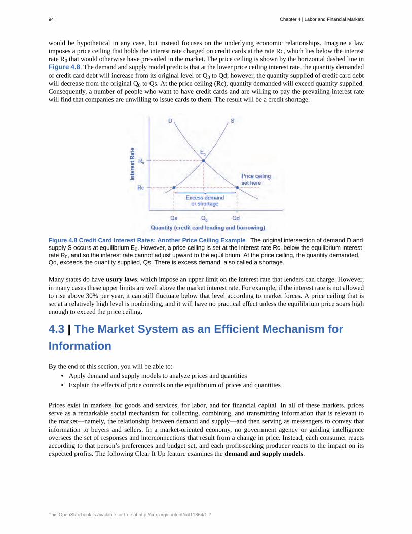
would be hypothetical in any case, but instead focuses on the underlying economic relationships. Imagine a lawimposes a price ceiling that holds the interest rate charged on credit cards at the rate Rc, which lies below the interestrate R0 that would otherwise have prevailed in the market. The price ceiling is shown by the horizontal dashed line inFigure 4.8. The demand and supply model predicts that at the lower price ceiling interest rate, the quantity demandedof credit card debt will increase from its original level of Q0 to Qd; however, the quantity supplied of credit card debtwill decrease from the original Q0 to Qs. At the price ceiling (Rc), quantity demanded will exceed quantity supplied.Consequently, a number of people who want to have credit cards and are willing to pay the prevailing interest ratewill find that companies are unwilling to issue cards to them. The result will be a credit shortage.
Figure 4.8 Credit Card Interest Rates: Another Price Ceiling Example The original intersection of demand D andsupply S occurs at equilibrium E0. However, a price ceiling is set at the interest rate Rc, below the equilibrium interestrate R0, and so the interest rate cannot adjust upward to the equilibrium. At the price ceiling, the quantity demanded,Qd, exceeds the quantity supplied, Qs. There is excess demand, also called a shortage.
Many states do have usury laws, which impose an upper limit on the interest rate that lenders can charge. However,in many cases these upper limits are well above the market interest rate. For example, if the interest rate is not allowedto rise above 30% per year, it can still fluctuate below that level according to market forces. A price ceiling that isset at a relatively high level is nonbinding, and it will have no practical effect unless the equilibrium price soars highenough to exceed the price ceiling.
4.3 | The Market System as an Efficient Mechanism forInformationBy the end of this section, you will be able to:
• Apply demand and supply models to analyze prices and quantities• Explain the effects of price controls on the equilibrium of prices and quantities
Prices exist in markets for goods and services, for labor, and for financial capital. In all of these markets, pricesserve as a remarkable social mechanism for collecting, combining, and transmitting information that is relevant tothe market—namely, the relationship between demand and supply—and then serving as messengers to convey thatinformation to buyers and sellers. In a market-oriented economy, no government agency or guiding intelligenceoversees the set of responses and interconnections that result from a change in price. Instead, each consumer reactsaccording to that person’s preferences and budget set, and each profit-seeking producer reacts to the impact on itsexpected profits. The following Clear It Up feature examines the demand and supply models.
94 Chapter 4 | Labor and Financial Markets
This OpenStax book is available for free at http://cnx.org/content/col11864/1.2
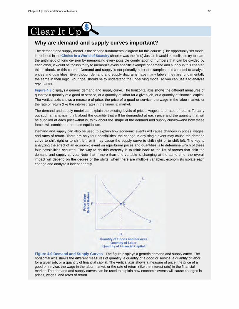
Why are demand and supply curves important?The demand and supply model is the second fundamental diagram for this course. (The opportunity set modelintroduced in the Choice in a World of Scarcity chapter was the first.) Just as it would be foolish to try to learnthe arithmetic of long division by memorizing every possible combination of numbers that can be divided byeach other, it would be foolish to try to memorize every specific example of demand and supply in this chapter,this textbook, or this course. Demand and supply is not primarily a list of examples; it is a model to analyzeprices and quantities. Even though demand and supply diagrams have many labels, they are fundamentallythe same in their logic. Your goal should be to understand the underlying model so you can use it to analyzeany market.
Figure 4.9 displays a generic demand and supply curve. The horizontal axis shows the different measures ofquantity: a quantity of a good or service, or a quantity of labor for a given job, or a quantity of financial capital.The vertical axis shows a measure of price: the price of a good or service, the wage in the labor market, orthe rate of return (like the interest rate) in the financial market.
The demand and supply model can explain the existing levels of prices, wages, and rates of return. To carryout such an analysis, think about the quantity that will be demanded at each price and the quantity that willbe supplied at each price—that is, think about the shape of the demand and supply curves—and how theseforces will combine to produce equilibrium.
Demand and supply can also be used to explain how economic events will cause changes in prices, wages,and rates of return. There are only four possibilities: the change in any single event may cause the demandcurve to shift right or to shift left; or it may cause the supply curve to shift right or to shift left. The key toanalyzing the effect of an economic event on equilibrium prices and quantities is to determine which of thesefour possibilities occurred. The way to do this correctly is to think back to the list of factors that shift thedemand and supply curves. Note that if more than one variable is changing at the same time, the overallimpact will depend on the degree of the shifts; when there are multiple variables, economists isolate eachchange and analyze it independently.
Figure 4.9 Demand and Supply Curves The figure displays a generic demand and supply curve. Thehorizontal axis shows the different measures of quantity: a quantity of a good or service, a quantity of laborfor a given job, or a quantity of financial capital. The vertical axis shows a measure of price: the price of agood or service, the wage in the labor market, or the rate of return (like the interest rate) in the financialmarket. The demand and supply curves can be used to explain how economic events will cause changes inprices, wages, and rates of return.
Chapter 4 | Labor and Financial Markets 95
An increase in the price of some product signals consumers that there is a shortage and the product should perhapsbe economized on. For example, if you are thinking about taking a plane trip to Hawaii, but the ticket turns out tobe expensive during the week you intend to go, you might consider other weeks when the ticket might be cheaper.The price could be high because you were planning to travel during a holiday when demand for traveling is high.Or, maybe the cost of an input like jet fuel increased or the airline has raised the price temporarily to see how manypeople are willing to pay it. Perhaps all of these factors are present at the same time. You do not need to analyze themarket and break down the price change into its underlying factors. You just have to look at the price of a ticket anddecide whether and when to fly.
In the same way, price changes provide useful information to producers. Imagine the situation of a farmer who growsoats and learns that the price of oats has risen. The higher price could be due to an increase in demand caused by anew scientific study proclaiming that eating oats is especially healthful. Or perhaps the price of a substitute grain, likecorn, has risen, and people have responded by buying more oats. But the oat farmer does not need to know the details.The farmer only needs to know that the price of oats has risen and that it will be profitable to expand production as aresult.
The actions of individual consumers and producers as they react to prices overlap and interlock in markets for goods,labor, and financial capital. A change in any single market is transmitted through these multiple interconnections toother markets. The vision of the role of flexible prices helping markets to reach equilibrium and linking differentmarkets together helps to explain why price controls can be so counterproductive. Price controls are government lawsthat serve to regulate prices rather than allow the various markets to determine prices. There is an old proverb: “Don’tkill the messenger.” In ancient times, messengers carried information between distant cities and kingdoms. When theybrought bad news, there was an emotional impulse to kill the messenger. But killing the messenger did not kill thebad news. Moreover, killing the messenger had an undesirable side effect: Other messengers would refuse to bringnews to that city or kingdom, depriving its citizens of vital information.
Those who seek price controls are trying to kill the messenger—or at least to stifle an unwelcome message that pricesare bringing about the equilibrium level of price and quantity. But price controls do nothing to affect the underlyingforces of demand and supply, and this can have serious repercussions. During China’s “Great Leap Forward” in thelate 1950s, food prices were kept artificially low, with the result that 30 to 40 million people died of starvation becausethe low prices depressed farm production. Changes in demand and supply will continue to reveal themselves throughconsumers’ and producers’ behavior. Immobilizing the price messenger through price controls will deprive everyonein the economy of critical information. Without this information, it becomes difficult for everyone—buyers and sellersalike—to react in a flexible and appropriate manner as changes occur throughout the economy.
Baby Boomers Come of AgeThe theory of supply and demand can explain what happens in the labor markets and suggests that thedemand for nurses will increase as healthcare needs of baby boomers increase, as Figure 4.10 shows. Theimpact of that increase will result in an average salary higher than the $67,930 earned in 2012 referencedin the first part of this case. The new equilibrium (E1) will be at the new equilibrium price (Pe1).Equilibriumquantity will also increase from Qe0 to Qe1.
96 Chapter 4 | Labor and Financial Markets
This OpenStax book is available for free at http://cnx.org/content/col11864/1.2
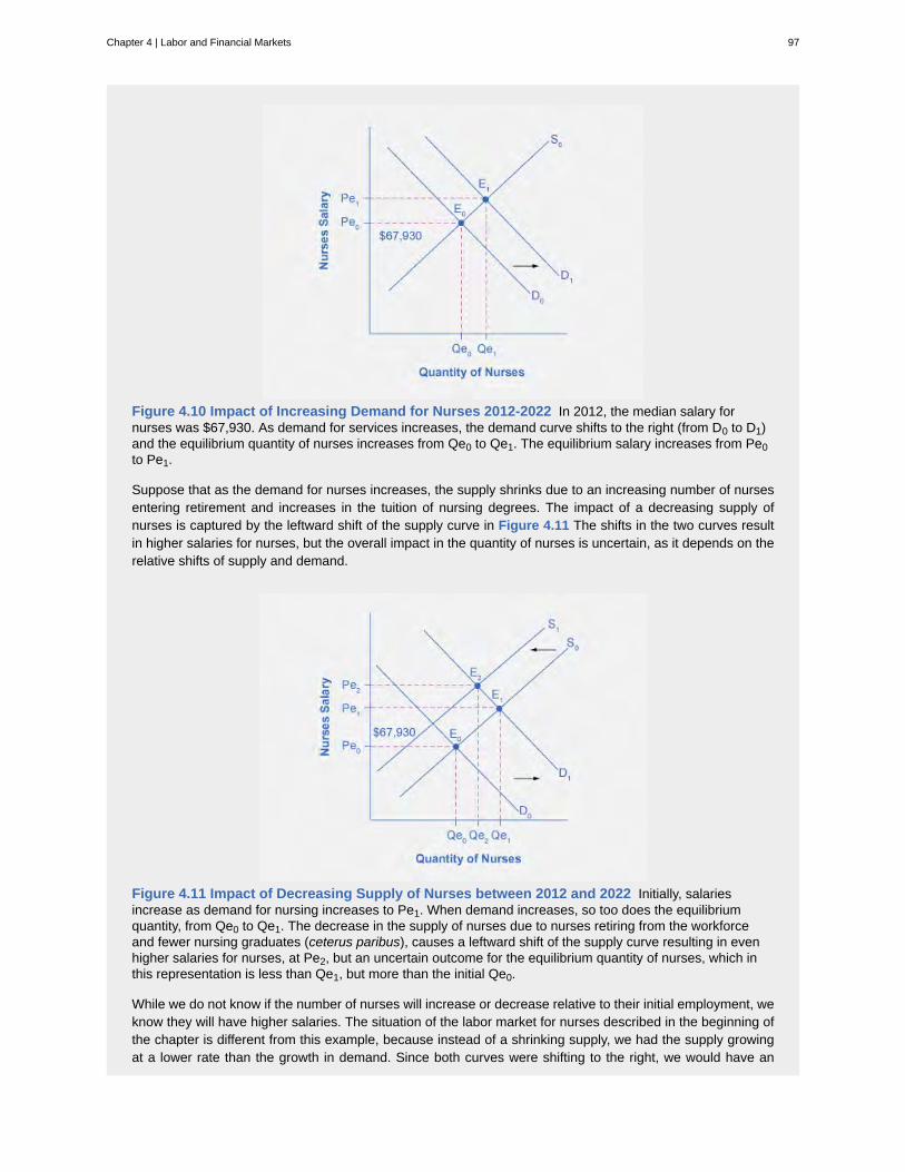
Figure 4.10 Impact of Increasing Demand for Nurses 2012-2022 In 2012, the median salary fornurses was $67,930. As demand for services increases, the demand curve shifts to the right (from D0 to D1)and the equilibrium quantity of nurses increases from Qe0 to Qe1. The equilibrium salary increases from Pe0to Pe1.
Suppose that as the demand for nurses increases, the supply shrinks due to an increasing number of nursesentering retirement and increases in the tuition of nursing degrees. The impact of a decreasing supply ofnurses is captured by the leftward shift of the supply curve in Figure 4.11 The shifts in the two curves resultin higher salaries for nurses, but the overall impact in the quantity of nurses is uncertain, as it depends on therelative shifts of supply and demand.
Figure 4.11 Impact of Decreasing Supply of Nurses between 2012 and 2022 Initially, salariesincrease as demand for nursing increases to Pe1. When demand increases, so too does the equilibriumquantity, from Qe0 to Qe1. The decrease in the supply of nurses due to nurses retiring from the workforceand fewer nursing graduates (ceterus paribus), causes a leftward shift of the supply curve resulting in evenhigher salaries for nurses, at Pe2, but an uncertain outcome for the equilibrium quantity of nurses, which inthis representation is less than Qe1, but more than the initial Qe0.
While we do not know if the number of nurses will increase or decrease relative to their initial employment, weknow they will have higher salaries. The situation of the labor market for nurses described in the beginning ofthe chapter is different from this example, because instead of a shrinking supply, we had the supply growingat a lower rate than the growth in demand. Since both curves were shifting to the right, we would have an
Chapter 4 | Labor and Financial Markets 97
unequivocal increase in the quantity of nurses. And because the shift in the demand curve was larger than theone in the supply, we would expect higher wages as a result.
98 Chapter 4 | Labor and Financial Markets
This OpenStax book is available for free at http://cnx.org/content/col11864/1.2
interest rate
minimum wage
usury laws
KEY TERMS
the “price” of borrowing in the financial market; a rate of return on an investment
a price floor that makes it illegal for an employer to pay employees less than a certain hourly rate
laws that impose an upper limit on the interest rate that lenders can charge
KEY CONCEPTS AND SUMMARY
4.1 Demand and Supply at Work in Labor MarketsIn the labor market, households are on the supply side of the market and firms are on the demand side. In the marketfor financial capital, households and firms can be on either side of the market: they are suppliers of financial capitalwhen they save or make financial investments, and demanders of financial capital when they borrow or receivefinancial investments.
In the demand and supply analysis of labor markets, the price can be measured by the annual salary or hourly wagereceived. The quantity of labor can be measured in various ways, like number of workers or the number of hoursworked.
Factors that can shift the demand curve for labor include: a change in the quantity demanded of the product that thelabor produces; a change in the production process that uses more or less labor; and a change in government policythat affects the quantity of labor that firms wish to hire at a given wage. Demand can also increase or decrease (shift)in response to: workers’ level of education and training, technology, the number of companies, and availability andprice of other inputs.
The main factors that can shift the supply curve for labor are: how desirable a job appears to workers relative tothe alternatives, government policy that either restricts or encourages the quantity of workers trained for the job, thenumber of workers in the economy, and required education.
4.2 Demand and Supply in Financial MarketsIn the demand and supply analysis of financial markets, the “price” is the rate of return or the interest rate received.The quantity is measured by the money that flows from those who supply financial capital to those who demand it.
Two factors can shift the supply of financial capital to a certain investment: if people want to alter their existinglevels of consumption, and if the riskiness or return on one investment changes relative to other investments. Factorsthat can shift demand for capital include business confidence and consumer confidence in the future—since financialinvestments received in the present are typically repaid in the future.
4.3 The Market System as an Efficient Mechanism for InformationThe market price system provides a highly efficient mechanism for disseminating information about relative scarcitiesof goods, services, labor, and financial capital. Market participants do not need to know why prices have changed,only that the changes require them to revisit previous decisions they made about supply and demand. Price controlshide information about the true scarcity of products and thereby cause misallocation of resources.
SELF-CHECK QUESTIONS1. In the labor market, what causes a movement along the demand curve? What causes a shift in the demand curve?
2. In the labor market, what causes a movement along the supply curve? What causes a shift in the supply curve?
3. Why is a living wage considered a price floor? Does imposing a living wage have the same outcome as a minimumwage?
4. In the financial market, what causes a movement along the demand curve? What causes a shift in the demandcurve?
Chapter 4 | Labor and Financial Markets 99
5. In the financial market, what causes a movement along the supply curve? What causes a shift in the supply curve?
6. If a usury law limits interest rates to no more than 35%, what would the likely impact be on the amount of loansmade and interest rates paid?
7. Which of the following changes in the financial market will lead to a decline in interest rates:a. a rise in demandb. a fall in demandc. a rise in supplyd. a fall in supply
8. Which of the following changes in the financial market will lead to an increase in the quantity of loans made andreceived:
a. a rise in demandb. a fall in demandc. a rise in supplyd. a fall in supply
9. Identify the most accurate statement. A price floor will have the largest effect if it is set:a. substantially above the equilibrium priceb. slightly above the equilibrium pricec. slightly below the equilibrium priced. substantially below the equilibrium price
Sketch all four of these possibilities on a demand and supply diagram to illustrate your answer.
10. A price ceiling will have the largest effect:a. substantially below the equilibrium priceb. slightly below the equilibrium pricec. substantially above the equilibrium priced. slightly above the equilibrium price
Sketch all four of these possibilities on a demand and supply diagram to illustrate your answer.
11. Select the correct answer. A price floor will usually shift:a. demandb. supplyc. bothd. neither
Illustrate your answer with a diagram.
12. Select the correct answer. A price ceiling will usually shift:a. demandb. supplyc. bothd. neither
REVIEW QUESTIONS
13. What is the “price” commonly called in the labormarket?
14. Are households demanders or suppliers in thegoods market? Are firms demanders or suppliers in thegoods market? What about the labor market and thefinancial market?
15. Name some factors that can cause a shift in thedemand curve in labor markets.
16. Name some factors that can cause a shift in thesupply curve in labor markets.
17. How is equilibrium defined in financial markets?
100 Chapter 4 | Labor and Financial Markets
This OpenStax book is available for free at http://cnx.org/content/col11864/1.2

18. What would be a sign of a shortage in financialmarkets?
19. Would usury laws help or hinder resolution of ashortage in financial markets?
20. Whether the product market or the labor market,what happens to the equilibrium price and quantity foreach of the four possibilities: increase in demand,decrease in demand, increase in supply, and decrease insupply.
CRITICAL THINKING QUESTIONS
21. Other than the demand for labor, what would beanother example of a “derived demand?”
22. Suppose that a 5% increase in the minimum wagecauses a 5% reduction in employment. How would thisaffect employers and how would it affect workers? Inyour opinion, would this be a good policy?
23. What assumption is made for a minimum wage tobe a nonbinding price floor? What assumption is madefor a living wage price floor to be binding?
24. Suppose the U.S. economy began to grow morerapidly than other countries in the world. What would bethe likely impact on U.S. financial markets as part of theglobal economy?
25. If the government imposed a federal interest rateceiling of 20% on all loans, who would gain and whowould lose?
26. Why are the factors that shift the demand for aproduct different from the factors that shift the demandfor labor? Why are the factors that shift the supply of
a product different from those that shift the supply oflabor?
27. During a discussion several years ago on building apipeline to Alaska to carry natural gas, the U.S. Senatepassed a bill stipulating that there should be a guaranteedminimum price for the natural gas that would be carriedthrough the pipeline. The thinking behind the bill wasthat if private firms had a guaranteed price for theirnatural gas, they would be more willing to drill for gasand to pay to build the pipeline.
a. Using the demand and supply framework,predict the effects of this price floor on the price,quantity demanded, and quantity supplied.
b. With the enactment of this price floor for naturalgas, what are some of the likely unintendedconsequences in the market?
c. Suggest some policies other than the price floorthat the government can pursue if it wishes toencourage drilling for natural gas and for a newpipeline in Alaska.
PROBLEMS28. Identify each of the following as involving eitherdemand or supply. Draw a circular flow diagram andlabel the flows A through F. (Some choices can be onboth sides of the goods market.)
a. Households in the labor marketb. Firms in the goods marketc. Firms in the financial marketd. Households in the goods markete. Firms in the labor marketf. Households in the financial market
29. Predict how each of the following events will raiseor lower the equilibrium wage and quantity of coalminers in West Virginia. In each case, sketch a demandand supply diagram to illustrate your answer.
a. The price of oil rises.b. New coal-mining equipment is invented that is
cheap and requires few workers to run.
c. Several major companies that do not mine coalopen factories in West Virginia, offering a lot ofwell-paid jobs.
d. Government imposes costly new regulations tomake coal-mining a safer job.
30. Predict how each of the following economicchanges will affect the equilibrium price and quantity inthe financial market for home loans. Sketch a demandand supply diagram to support your answers.
a. The number of people at the most common agesfor home-buying increases.
b. People gain confidence that the economy isgrowing and that their jobs are secure.
c. Banks that have made home loans find that alarger number of people than they expected arenot repaying those loans.
d. Because of a threat of a war, people becomeuncertain about their economic future.
Chapter 4 | Labor and Financial Markets 101
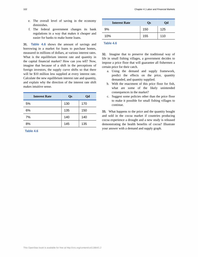
e. The overall level of saving in the economydiminishes.
f. The federal government changes its bankregulations in a way that makes it cheaper andeasier for banks to make home loans.
31. Table 4.6 shows the amount of savings andborrowing in a market for loans to purchase homes,measured in millions of dollars, at various interest rates.What is the equilibrium interest rate and quantity inthe capital financial market? How can you tell? Now,imagine that because of a shift in the perceptions offoreign investors, the supply curve shifts so that therewill be $10 million less supplied at every interest rate.Calculate the new equilibrium interest rate and quantity,and explain why the direction of the interest rate shiftmakes intuitive sense.
Interest Rate Qs Qd
5% 130 170
6% 135 150
7% 140 140
8% 145 135
Table 4.6
Interest Rate Qs Qd
9% 150 125
10% 155 110
Table 4.6
32. Imagine that to preserve the traditional way oflife in small fishing villages, a government decides toimpose a price floor that will guarantee all fishermen acertain price for their catch.
a. Using the demand and supply framework,predict the effects on the price, quantitydemanded, and quantity supplied.
b. With the enactment of this price floor for fish,what are some of the likely unintendedconsequences in the market?
c. Suggest some policies other than the price floorto make it possible for small fishing villages tocontinue.
33. What happens to the price and the quantity boughtand sold in the cocoa market if countries producingcocoa experience a drought and a new study is releaseddemonstrating the health benefits of cocoa? Illustrateyour answer with a demand and supply graph.
102 Chapter 4 | Labor and Financial Markets
This OpenStax book is available for free at http://cnx.org/content/col11864/1.2
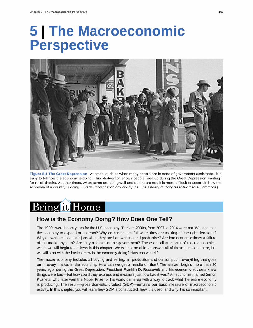
5 | The MacroeconomicPerspective
Figure 5.1 The Great Depression At times, such as when many people are in need of government assistance, it iseasy to tell how the economy is doing. This photograph shows people lined up during the Great Depression, waitingfor relief checks. At other times, when some are doing well and others are not, it is more difficult to ascertain how theeconomy of a country is doing. (Credit: modification of work by the U.S. Library of Congress/Wikimedia Commons)
How is the Economy Doing? How Does One Tell?The 1990s were boom years for the U.S. economy. The late 2000s, from 2007 to 2014 were not. What causesthe economy to expand or contract? Why do businesses fail when they are making all the right decisions?Why do workers lose their jobs when they are hardworking and productive? Are bad economic times a failureof the market system? Are they a failure of the government? These are all questions of macroeconomics,which we will begin to address in this chapter. We will not be able to answer all of these questions here, butwe will start with the basics: How is the economy doing? How can we tell?
The macro economy includes all buying and selling, all production and consumption; everything that goeson in every market in the economy. How can we get a handle on that? The answer begins more than 80years ago, during the Great Depression. President Franklin D. Roosevelt and his economic advisers knewthings were bad—but how could they express and measure just how bad it was? An economist named SimonKuznets, who later won the Nobel Prize for his work, came up with a way to track what the entire economyis producing. The result—gross domestic product (GDP)—remains our basic measure of macroeconomicactivity. In this chapter, you will learn how GDP is constructed, how it is used, and why it is so important.
Chapter 5 | The Macroeconomic Perspective 103
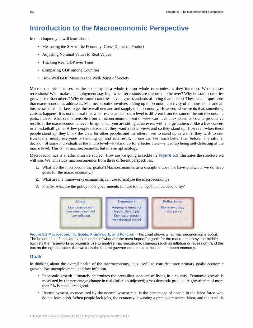
Introduction to the Macroeconomic PerspectiveIn this chapter, you will learn about:
• Measuring the Size of the Economy: Gross Domestic Product
• Adjusting Nominal Values to Real Values
• Tracking Real GDP over Time
• Comparing GDP among Countries
• How Well GDP Measures the Well-Being of Society
Macroeconomics focuses on the economy as a whole (or on whole economies as they interact). What causesrecessions? What makes unemployment stay high when recessions are supposed to be over? Why do some countriesgrow faster than others? Why do some countries have higher standards of living than others? These are all questionsthat macroeconomics addresses. Macroeconomics involves adding up the economic activity of all households and allbusinesses in all markets to get the overall demand and supply in the economy. However, when we do that, somethingcurious happens. It is not unusual that what results at the macro level is different from the sum of the microeconomicparts. Indeed, what seems sensible from a microeconomic point of view can have unexpected or counterproductiveresults at the macroeconomic level. Imagine that you are sitting at an event with a large audience, like a live concertor a basketball game. A few people decide that they want a better view, and so they stand up. However, when thesepeople stand up, they block the view for other people, and the others need to stand up as well if they wish to see.Eventually, nearly everyone is standing up, and as a result, no one can see much better than before. The rationaldecision of some individuals at the micro level—to stand up for a better view—ended up being self-defeating at themacro level. This is not macroeconomics, but it is an apt analogy.
Macroeconomics is a rather massive subject. How are we going to tackle it? Figure 5.2 illustrates the structure wewill use. We will study macroeconomics from three different perspectives:
1. What are the macroeconomic goals? (Macroeconomics as a discipline does not have goals, but we do havegoals for the macro economy.)
2. What are the frameworks economists can use to analyze the macroeconomy?
3. Finally, what are the policy tools governments can use to manage the macroeconomy?
Figure 5.2 Macroeconomic Goals, Framework, and Policies This chart shows what macroeconomics is about.The box on the left indicates a consensus of what are the most important goals for the macro economy, the middlebox lists the frameworks economists use to analyze macroeconomic changes (such as inflation or recession), and thebox on the right indicates the two tools the federal government uses to influence the macro economy.
GoalsIn thinking about the overall health of the macroeconomy, it is useful to consider three primary goals: economicgrowth, low unemployment, and low inflation.
• Economic growth ultimately determines the prevailing standard of living in a country. Economic growth ismeasured by the percentage change in real (inflation-adjusted) gross domestic product. A growth rate of morethan 3% is considered good.
• Unemployment, as measured by the unemployment rate, is the percentage of people in the labor force whodo not have a job. When people lack jobs, the economy is wasting a precious resource-labor, and the result is
104 Chapter 5 | The Macroeconomic Perspective
This OpenStax book is available for free at http://cnx.org/content/col11864/1.2
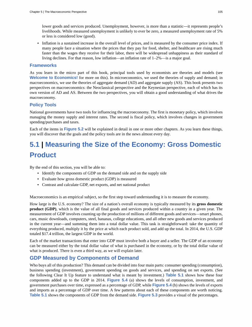
lower goods and services produced. Unemployment, however, is more than a statistic—it represents people’slivelihoods. While measured unemployment is unlikely to ever be zero, a measured unemployment rate of 5%or less is considered low (good).
• Inflation is a sustained increase in the overall level of prices, and is measured by the consumer price index. Ifmany people face a situation where the prices that they pay for food, shelter, and healthcare are rising muchfaster than the wages they receive for their labor, there will be widespread unhappiness as their standard ofliving declines. For that reason, low inflation—an inflation rate of 1–2%—is a major goal.
FrameworksAs you learn in the micro part of this book, principal tools used by economists are theories and models (seeWelcome to Economics! for more on this). In microeconomics, we used the theories of supply and demand; inmacroeconomics, we use the theories of aggregate demand (AD) and aggregate supply (AS). This book presents twoperspectives on macroeconomics: the Neoclassical perspective and the Keynesian perspective, each of which has itsown version of AD and AS. Between the two perspectives, you will obtain a good understanding of what drives themacroeconomy.
Policy ToolsNational governments have two tools for influencing the macroeconomy. The first is monetary policy, which involvesmanaging the money supply and interest rates. The second is fiscal policy, which involves changes in governmentspending/purchases and taxes.
Each of the items in Figure 5.2 will be explained in detail in one or more other chapters. As you learn these things,you will discover that the goals and the policy tools are in the news almost every day.
5.1 | Measuring the Size of the Economy: Gross DomesticProductBy the end of this section, you will be able to:
• Identify the components of GDP on the demand side and on the supply side• Evaluate how gross domestic product (GDP) is measured• Contrast and calculate GDP, net exports, and net national product
Macroeconomics is an empirical subject, so the first step toward understanding it is to measure the economy.
How large is the U.S. economy? The size of a nation’s overall economy is typically measured by its gross domesticproduct (GDP), which is the value of all final goods and services produced within a country in a given year. Themeasurement of GDP involves counting up the production of millions of different goods and services—smart phones,cars, music downloads, computers, steel, bananas, college educations, and all other new goods and services producedin the current year—and summing them into a total dollar value. This task is straightforward: take the quantity ofeverything produced, multiply it by the price at which each product sold, and add up the total. In 2014, the U.S. GDPtotaled $17.4 trillion, the largest GDP in the world.
Each of the market transactions that enter into GDP must involve both a buyer and a seller. The GDP of an economycan be measured either by the total dollar value of what is purchased in the economy, or by the total dollar value ofwhat is produced. There is even a third way, as we will explain later.
GDP Measured by Components of DemandWho buys all of this production? This demand can be divided into four main parts: consumer spending (consumption),business spending (investment), government spending on goods and services, and spending on net exports. (Seethe following Clear It Up feature to understand what is meant by investment.) Table 5.1 shows how these fourcomponents added up to the GDP in 2014. Figure 5.4 (a) shows the levels of consumption, investment, andgovernment purchases over time, expressed as a percentage of GDP, while Figure 5.4 (b) shows the levels of exportsand imports as a percentage of GDP over time. A few patterns about each of these components are worth noticing.Table 5.1 shows the components of GDP from the demand side. Figure 5.3 provides a visual of the percentages.
Chapter 5 | The Macroeconomic Perspective 105
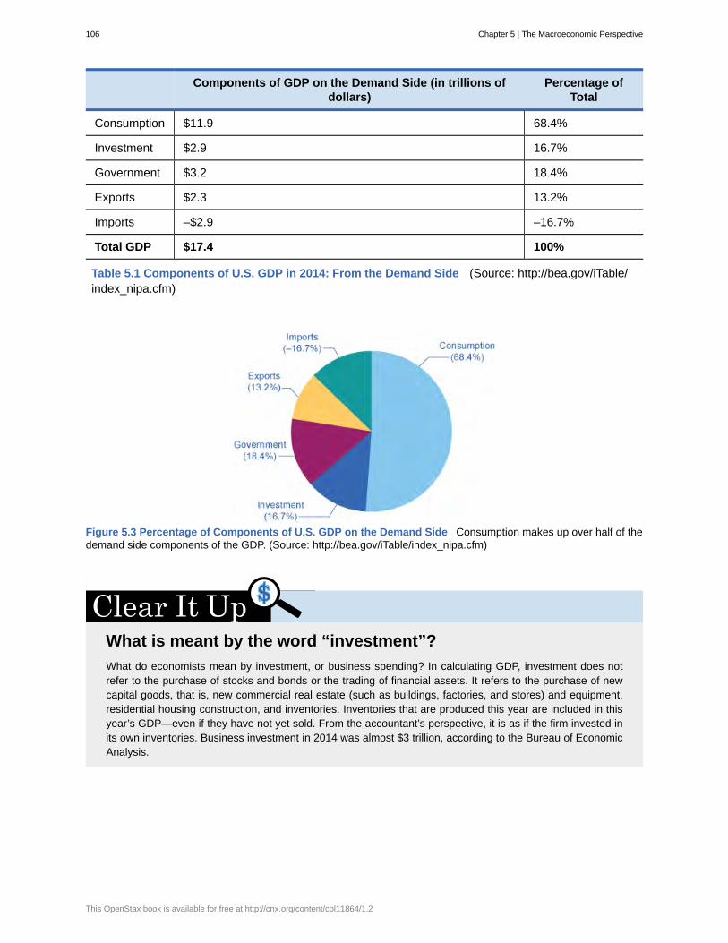
Components of GDP on the Demand Side (in trillions ofdollars)
Percentage ofTotal
Consumption $11.9 68.4%
Investment $2.9 16.7%
Government $3.2 18.4%
Exports $2.3 13.2%
Imports –$2.9 –16.7%
Total GDP $17.4 100%
Table 5.1 Components of U.S. GDP in 2014: From the Demand Side (Source: http://bea.gov/iTable/index_nipa.cfm)
Figure 5.3 Percentage of Components of U.S. GDP on the Demand Side Consumption makes up over half of thedemand side components of the GDP. (Source: http://bea.gov/iTable/index_nipa.cfm)
What is meant by the word “investment”?What do economists mean by investment, or business spending? In calculating GDP, investment does notrefer to the purchase of stocks and bonds or the trading of financial assets. It refers to the purchase of newcapital goods, that is, new commercial real estate (such as buildings, factories, and stores) and equipment,residential housing construction, and inventories. Inventories that are produced this year are included in thisyear’s GDP—even if they have not yet sold. From the accountant’s perspective, it is as if the firm invested inits own inventories. Business investment in 2014 was almost $3 trillion, according to the Bureau of EconomicAnalysis.
106 Chapter 5 | The Macroeconomic Perspective
This OpenStax book is available for free at http://cnx.org/content/col11864/1.2
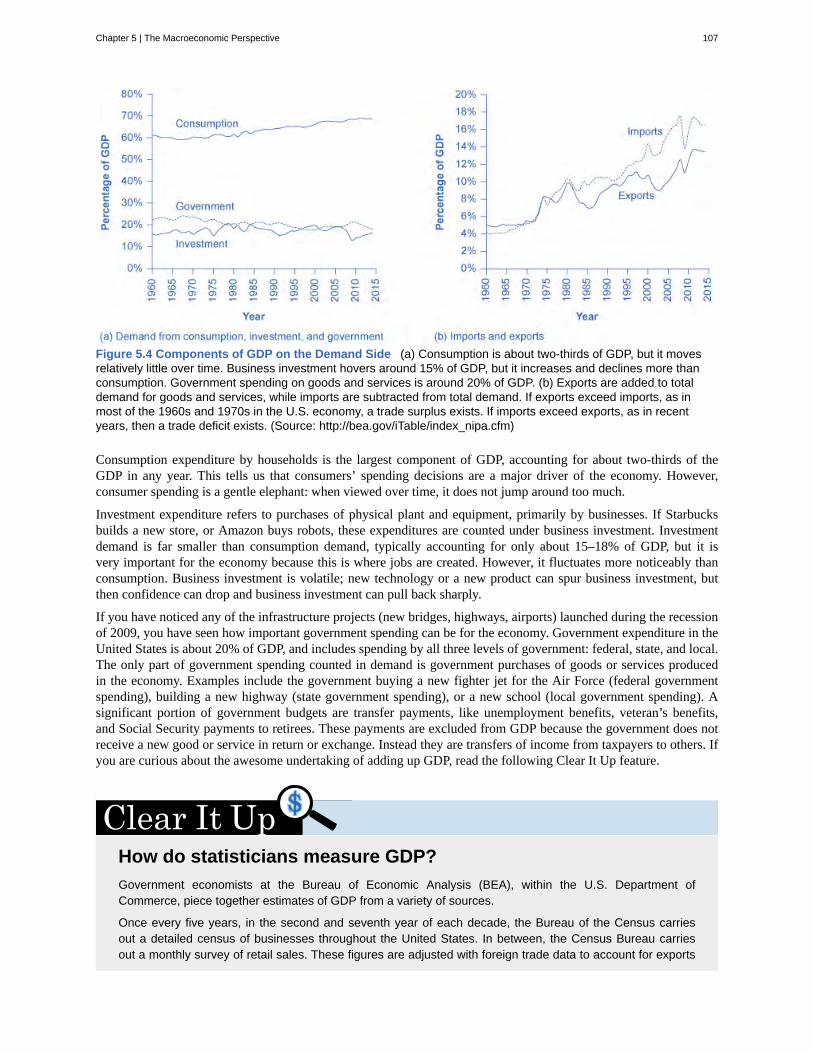
Figure 5.4 Components of GDP on the Demand Side (a) Consumption is about two-thirds of GDP, but it movesrelatively little over time. Business investment hovers around 15% of GDP, but it increases and declines more thanconsumption. Government spending on goods and services is around 20% of GDP. (b) Exports are added to totaldemand for goods and services, while imports are subtracted from total demand. If exports exceed imports, as inmost of the 1960s and 1970s in the U.S. economy, a trade surplus exists. If imports exceed exports, as in recentyears, then a trade deficit exists. (Source: http://bea.gov/iTable/index_nipa.cfm)
Consumption expenditure by households is the largest component of GDP, accounting for about two-thirds of theGDP in any year. This tells us that consumers’ spending decisions are a major driver of the economy. However,consumer spending is a gentle elephant: when viewed over time, it does not jump around too much.
Investment expenditure refers to purchases of physical plant and equipment, primarily by businesses. If Starbucksbuilds a new store, or Amazon buys robots, these expenditures are counted under business investment. Investmentdemand is far smaller than consumption demand, typically accounting for only about 15–18% of GDP, but it isvery important for the economy because this is where jobs are created. However, it fluctuates more noticeably thanconsumption. Business investment is volatile; new technology or a new product can spur business investment, butthen confidence can drop and business investment can pull back sharply.
If you have noticed any of the infrastructure projects (new bridges, highways, airports) launched during the recessionof 2009, you have seen how important government spending can be for the economy. Government expenditure in theUnited States is about 20% of GDP, and includes spending by all three levels of government: federal, state, and local.The only part of government spending counted in demand is government purchases of goods or services producedin the economy. Examples include the government buying a new fighter jet for the Air Force (federal governmentspending), building a new highway (state government spending), or a new school (local government spending). Asignificant portion of government budgets are transfer payments, like unemployment benefits, veteran’s benefits,and Social Security payments to retirees. These payments are excluded from GDP because the government does notreceive a new good or service in return or exchange. Instead they are transfers of income from taxpayers to others. Ifyou are curious about the awesome undertaking of adding up GDP, read the following Clear It Up feature.
How do statisticians measure GDP?Government economists at the Bureau of Economic Analysis (BEA), within the U.S. Department ofCommerce, piece together estimates of GDP from a variety of sources.
Once every five years, in the second and seventh year of each decade, the Bureau of the Census carriesout a detailed census of businesses throughout the United States. In between, the Census Bureau carriesout a monthly survey of retail sales. These figures are adjusted with foreign trade data to account for exports
Chapter 5 | The Macroeconomic Perspective 107
that are produced in the United States and sold abroad and for imports that are produced abroad and soldhere. Once every ten years, the Census Bureau conducts a comprehensive survey of housing and residentialfinance. Together, these sources provide the main basis for figuring out what is produced for consumers.
For investment, the Census Bureau carries out a monthly survey of construction and an annual survey ofexpenditures on physical capital equipment.
For what is purchased by the federal government, the statisticians rely on the U.S. Department of the Treasury.An annual Census of Governments gathers information on state and local governments. Because a lot ofgovernment spending at all levels involves hiring people to provide services, a large portion of governmentspending is also tracked through payroll records collected by state governments and by the Social SecurityAdministration.
With regard to foreign trade, the Census Bureau compiles a monthly record of all import and exportdocuments. Additional surveys cover transportation and travel, and adjustment is made for financial servicesthat are produced in the United States for foreign customers.
Many other sources contribute to the estimates of GDP. Information on energy comes from the U.S.Department of Transportation and Department of Energy. Information on healthcare is collected by the Agencyfor Health Care Research and Quality. Surveys of landlords find out about rental income. The Department ofAgriculture collects statistics on farming.
All of these bits and pieces of information arrive in different forms, at different time intervals. The BEA meldsthem together to produce estimates of GDP on a quarterly basis (every three months). These numbers arethen “annualized” by multiplying by four. As more information comes in, these estimates are updated andrevised. The “advance” estimate of GDP for a certain quarter is released one month after a quarter. The“preliminary” estimate comes out one month after that. The “final” estimate is published one month later, butit is not actually final. In July, roughly updated estimates for the previous calendar year are released. Then,once every five years, after the results of the latest detailed five-year business census have been processed,the BEA revises all of the past estimates of GDP according to the newest methods and data, going all the wayback to 1929.
Visit this website (http://openstaxcollege.org/l/beafaq) to read FAQs on the BEA site. You can even email yourown questions!
When thinking about the demand for domestically produced goods in a global economy, it is important to countspending on exports—domestically produced goods that are sold abroad. By the same token, we must also subtractspending on imports—goods produced in other countries that are purchased by residents of this country. The netexport component of GDP is equal to the dollar value of exports (X) minus the dollar value of imports (M), (X – M).The gap between exports and imports is called the trade balance. If a country’s exports are larger than its imports,then a country is said to have a trade surplus. In the United States, exports typically exceeded imports in the 1960sand 1970s, as shown in Figure 5.4 (b).
Since the early 1980s, imports have typically exceeded exports, and so the United States has experienced a tradedeficit in most years. Indeed, the trade deficit grew quite large in the late 1990s and in the mid-2000s. Figure 5.4 (b)also shows that imports and exports have both risen substantially in recent decades, even after the declines during the
108 Chapter 5 | The Macroeconomic Perspective
This OpenStax book is available for free at http://cnx.org/content/col11864/1.2
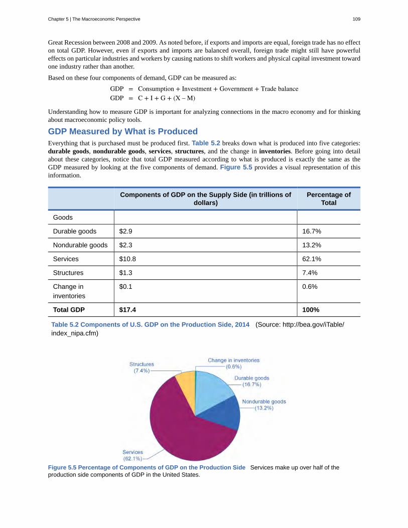
Great Recession between 2008 and 2009. As noted before, if exports and imports are equal, foreign trade has no effecton total GDP. However, even if exports and imports are balanced overall, foreign trade might still have powerfuleffects on particular industries and workers by causing nations to shift workers and physical capital investment towardone industry rather than another.
Based on these four components of demand, GDP can be measured as:
GDP = Consumption + Investment + Government + Trade balanceGDP = C + I + G + (X – M)
Understanding how to measure GDP is important for analyzing connections in the macro economy and for thinkingabout macroeconomic policy tools.
GDP Measured by What is ProducedEverything that is purchased must be produced first. Table 5.2 breaks down what is produced into five categories:durable goods, nondurable goods, services, structures, and the change in inventories. Before going into detailabout these categories, notice that total GDP measured according to what is produced is exactly the same as theGDP measured by looking at the five components of demand. Figure 5.5 provides a visual representation of thisinformation.
Components of GDP on the Supply Side (in trillions ofdollars)
Percentage ofTotal
Goods
Durable goods $2.9 16.7%
Nondurable goods $2.3 13.2%
Services $10.8 62.1%
Structures $1.3 7.4%
Change ininventories
$0.1 0.6%
Total GDP $17.4 100%
Table 5.2 Components of U.S. GDP on the Production Side, 2014 (Source: http://bea.gov/iTable/index_nipa.cfm)
Figure 5.5 Percentage of Components of GDP on the Production Side Services make up over half of theproduction side components of GDP in the United States.
Chapter 5 | The Macroeconomic Perspective 109
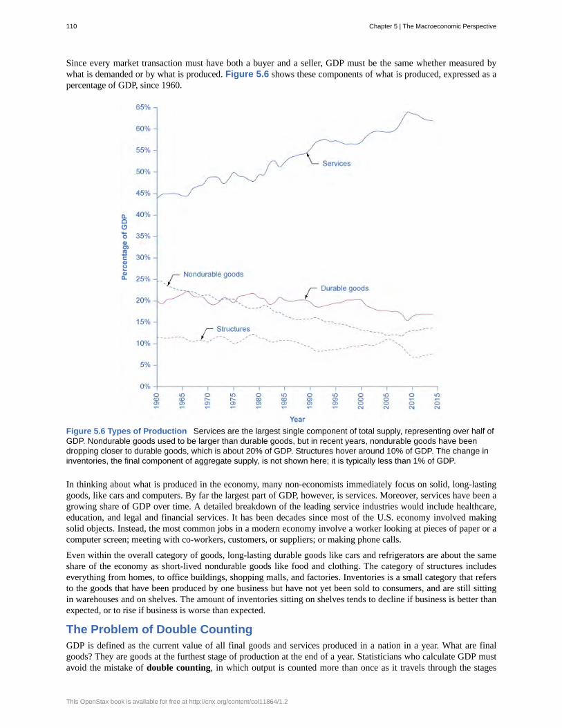
Since every market transaction must have both a buyer and a seller, GDP must be the same whether measured bywhat is demanded or by what is produced. Figure 5.6 shows these components of what is produced, expressed as apercentage of GDP, since 1960.
Figure 5.6 Types of Production Services are the largest single component of total supply, representing over half ofGDP. Nondurable goods used to be larger than durable goods, but in recent years, nondurable goods have beendropping closer to durable goods, which is about 20% of GDP. Structures hover around 10% of GDP. The change ininventories, the final component of aggregate supply, is not shown here; it is typically less than 1% of GDP.
In thinking about what is produced in the economy, many non-economists immediately focus on solid, long-lastinggoods, like cars and computers. By far the largest part of GDP, however, is services. Moreover, services have been agrowing share of GDP over time. A detailed breakdown of the leading service industries would include healthcare,education, and legal and financial services. It has been decades since most of the U.S. economy involved makingsolid objects. Instead, the most common jobs in a modern economy involve a worker looking at pieces of paper or acomputer screen; meeting with co-workers, customers, or suppliers; or making phone calls.
Even within the overall category of goods, long-lasting durable goods like cars and refrigerators are about the sameshare of the economy as short-lived nondurable goods like food and clothing. The category of structures includeseverything from homes, to office buildings, shopping malls, and factories. Inventories is a small category that refersto the goods that have been produced by one business but have not yet been sold to consumers, and are still sittingin warehouses and on shelves. The amount of inventories sitting on shelves tends to decline if business is better thanexpected, or to rise if business is worse than expected.
The Problem of Double CountingGDP is defined as the current value of all final goods and services produced in a nation in a year. What are finalgoods? They are goods at the furthest stage of production at the end of a year. Statisticians who calculate GDP mustavoid the mistake of double counting, in which output is counted more than once as it travels through the stages
110 Chapter 5 | The Macroeconomic Perspective
This OpenStax book is available for free at http://cnx.org/content/col11864/1.2
of production. For example, imagine what would happen if government statisticians first counted the value of tiresproduced by a tire manufacturer, and then counted the value of a new truck sold by an automaker that contains thosetires. In this example, the value of the tires would have been counted twice-because the price of the truck includes thevalue of the tires.
To avoid this problem, which would overstate the size of the economy considerably, government statisticians countjust the value of final goods and services in the chain of production that are sold for consumption, investment,government, and trade purposes. Intermediate goods, which are goods that go into the production of other goods,are excluded from GDP calculations. From the example above, only the value of the Ford truck will be counted. Thevalue of what businesses provide to other businesses is captured in the final products at the end of the productionchain.
The concept of GDP is fairly straightforward: it is just the dollar value of all final goods and services produced inthe economy in a year. In our decentralized, market-oriented economy, actually calculating the more than $16 trillion-dollar U.S. GDP—along with how it is changing every few months—is a full-time job for a brigade of governmentstatisticians.
What is Counted in GDP What is not included in GDP
Consumption Intermediate goods
Business investment Transfer payments and non-market activities
Government spending on goods and services Used goods
Net exports Illegal goods
Table 5.3 Counting GDP
Notice the items that are not counted into GDP, as outlined in Table 5.3. The sales of used goods are not includedbecause they were produced in a previous year and are part of that year’s GDP. The entire underground economy ofservices paid “under the table” and illegal sales should be counted, but is not, because it is impossible to track thesesales. In a recent study by Friedrich Schneider of shadow economies, the underground economy in the United Stateswas estimated to be 6.6% of GDP, or close to $2 trillion dollars in 2013 alone. Transfer payments, such as payment bythe government to individuals, are not included, because they do not represent production. Also, production of somegoods—such as home production as when you make your breakfast—is not counted because these goods are not soldin the marketplace.
Visit this website (http://openstaxcollege.org/l/undergroundecon) to read about the “New UndergroundEconomy.”
Chapter 5 | The Macroeconomic Perspective 111
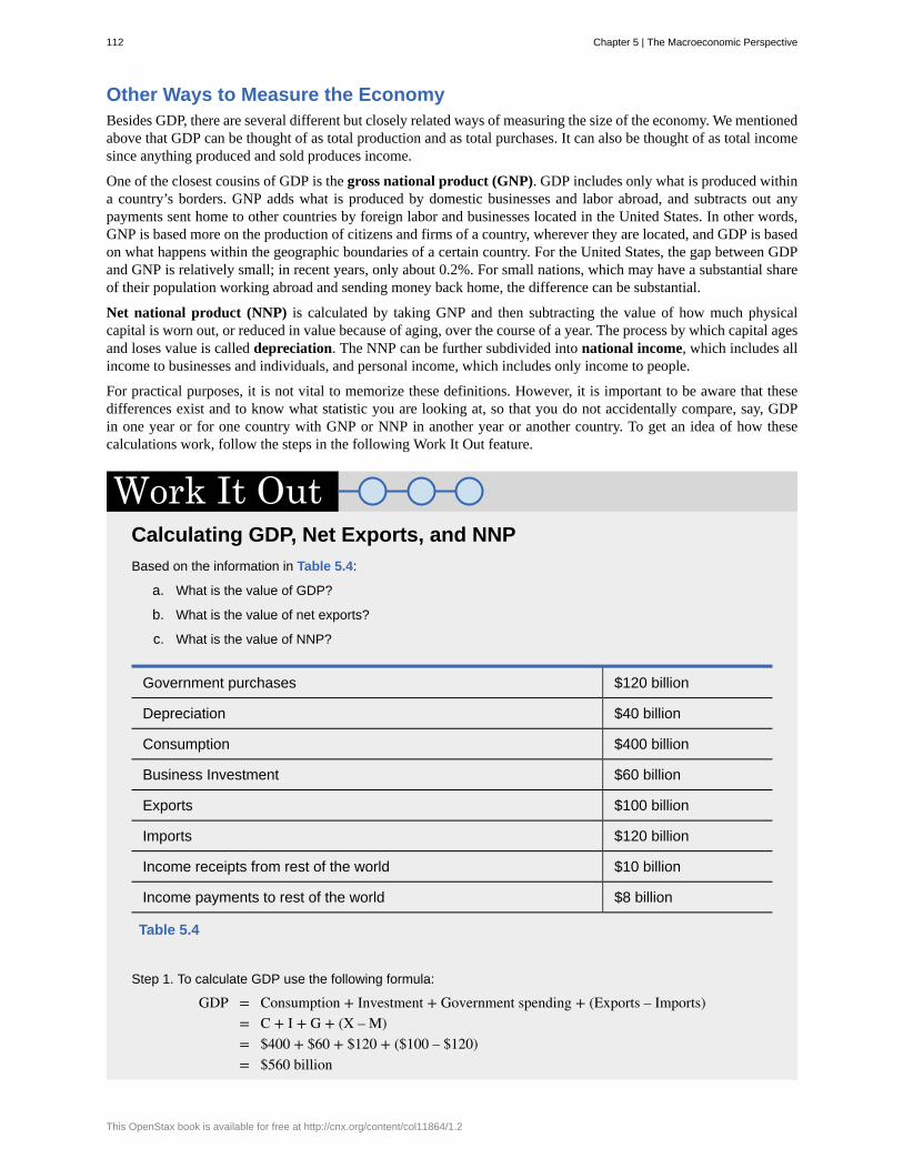
Other Ways to Measure the EconomyBesides GDP, there are several different but closely related ways of measuring the size of the economy. We mentionedabove that GDP can be thought of as total production and as total purchases. It can also be thought of as total incomesince anything produced and sold produces income.
One of the closest cousins of GDP is the gross national product (GNP). GDP includes only what is produced withina country’s borders. GNP adds what is produced by domestic businesses and labor abroad, and subtracts out anypayments sent home to other countries by foreign labor and businesses located in the United States. In other words,GNP is based more on the production of citizens and firms of a country, wherever they are located, and GDP is basedon what happens within the geographic boundaries of a certain country. For the United States, the gap between GDPand GNP is relatively small; in recent years, only about 0.2%. For small nations, which may have a substantial shareof their population working abroad and sending money back home, the difference can be substantial.
Net national product (NNP) is calculated by taking GNP and then subtracting the value of how much physicalcapital is worn out, or reduced in value because of aging, over the course of a year. The process by which capital agesand loses value is called depreciation. The NNP can be further subdivided into national income, which includes allincome to businesses and individuals, and personal income, which includes only income to people.
For practical purposes, it is not vital to memorize these definitions. However, it is important to be aware that thesedifferences exist and to know what statistic you are looking at, so that you do not accidentally compare, say, GDPin one year or for one country with GNP or NNP in another year or another country. To get an idea of how thesecalculations work, follow the steps in the following Work It Out feature.
Calculating GDP, Net Exports, and NNPBased on the information in Table 5.4:
a. What is the value of GDP?
b. What is the value of net exports?
c. What is the value of NNP?
Government purchases $120 billion
Depreciation $40 billion
Consumption $400 billion
Business Investment $60 billion
Exports $100 billion
Imports $120 billion
Income receipts from rest of the world $10 billion
Income payments to rest of the world $8 billion
Table 5.4
Step 1. To calculate GDP use the following formula:
GDP = Consumption + Investment + Government spending + (Exports – Imports) = C + I + G + (X – M) = $400 + $60 + $120 + ($100 – $120) = $560 billion
112 Chapter 5 | The Macroeconomic Perspective
This OpenStax book is available for free at http://cnx.org/content/col11864/1.2
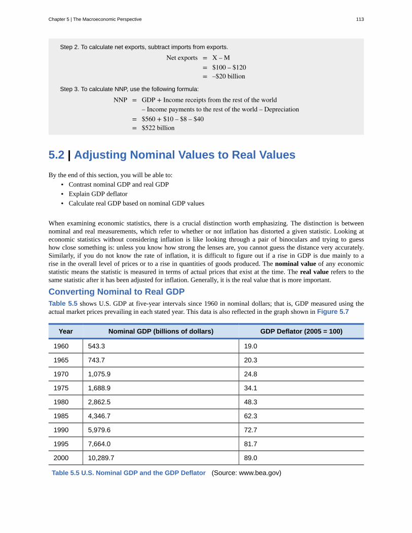
Step 2. To calculate net exports, subtract imports from exports.
Net exports = X – M = $100 – $120 = –$20 billion
Step 3. To calculate NNP, use the following formula:
NNP = GDP + Income receipts from the rest of the world– Income payments to the rest of the world – Depreciation
= $560 + $10 – $8 – $40= $522 billion
5.2 | Adjusting Nominal Values to Real ValuesBy the end of this section, you will be able to:
• Contrast nominal GDP and real GDP• Explain GDP deflator• Calculate real GDP based on nominal GDP values
When examining economic statistics, there is a crucial distinction worth emphasizing. The distinction is betweennominal and real measurements, which refer to whether or not inflation has distorted a given statistic. Looking ateconomic statistics without considering inflation is like looking through a pair of binoculars and trying to guesshow close something is: unless you know how strong the lenses are, you cannot guess the distance very accurately.Similarly, if you do not know the rate of inflation, it is difficult to figure out if a rise in GDP is due mainly to arise in the overall level of prices or to a rise in quantities of goods produced. The nominal value of any economicstatistic means the statistic is measured in terms of actual prices that exist at the time. The real value refers to thesame statistic after it has been adjusted for inflation. Generally, it is the real value that is more important.
Converting Nominal to Real GDPTable 5.5 shows U.S. GDP at five-year intervals since 1960 in nominal dollars; that is, GDP measured using theactual market prices prevailing in each stated year. This data is also reflected in the graph shown in Figure 5.7
Year Nominal GDP (billions of dollars) GDP Deflator (2005 = 100)
1960 543.3 19.0
1965 743.7 20.3
1970 1,075.9 24.8
1975 1,688.9 34.1
1980 2,862.5 48.3
1985 4,346.7 62.3
1990 5,979.6 72.7
1995 7,664.0 81.7
2000 10,289.7 89.0
Table 5.5 U.S. Nominal GDP and the GDP Deflator (Source: www.bea.gov)
Chapter 5 | The Macroeconomic Perspective 113
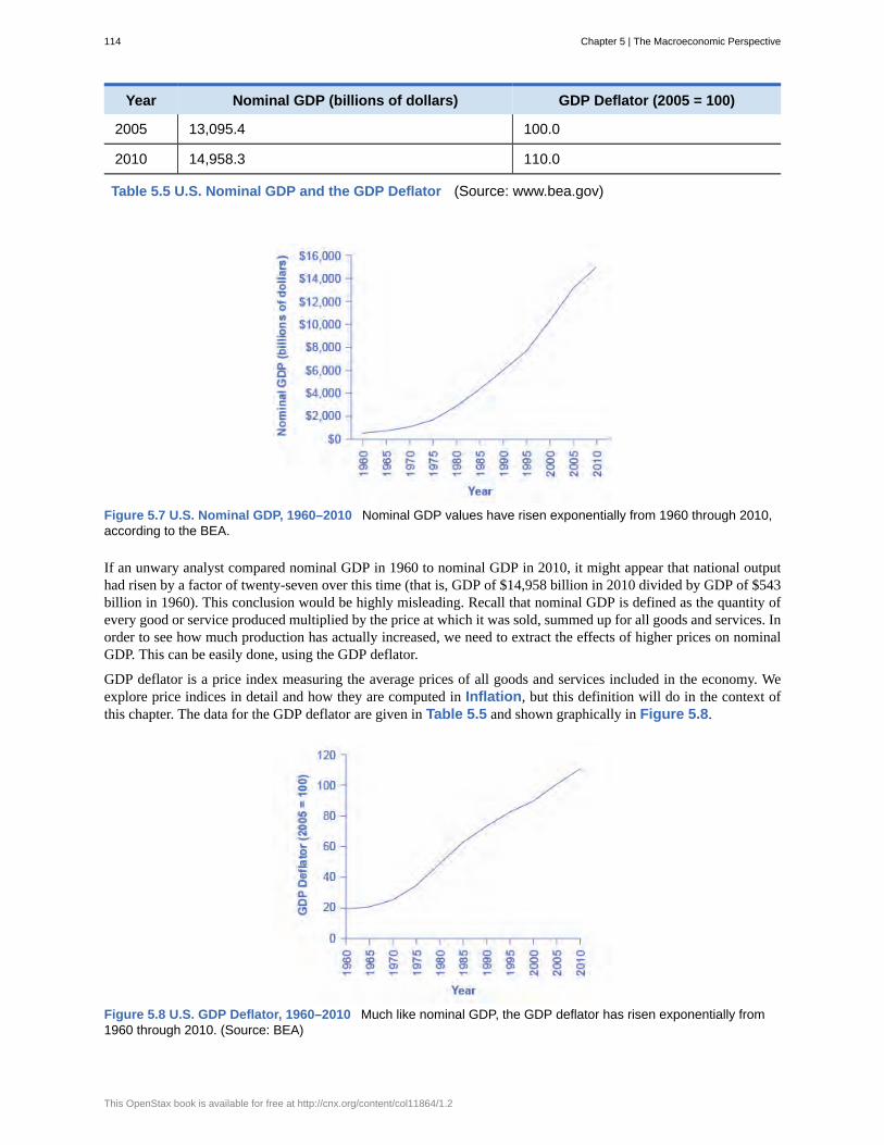
Year Nominal GDP (billions of dollars) GDP Deflator (2005 = 100)
2005 13,095.4 100.0
2010 14,958.3 110.0
Table 5.5 U.S. Nominal GDP and the GDP Deflator (Source: www.bea.gov)
Figure 5.7 U.S. Nominal GDP, 1960–2010 Nominal GDP values have risen exponentially from 1960 through 2010,according to the BEA.
If an unwary analyst compared nominal GDP in 1960 to nominal GDP in 2010, it might appear that national outputhad risen by a factor of twenty-seven over this time (that is, GDP of $14,958 billion in 2010 divided by GDP of $543billion in 1960). This conclusion would be highly misleading. Recall that nominal GDP is defined as the quantity ofevery good or service produced multiplied by the price at which it was sold, summed up for all goods and services. Inorder to see how much production has actually increased, we need to extract the effects of higher prices on nominalGDP. This can be easily done, using the GDP deflator.
GDP deflator is a price index measuring the average prices of all goods and services included in the economy. Weexplore price indices in detail and how they are computed in Inflation, but this definition will do in the context ofthis chapter. The data for the GDP deflator are given in Table 5.5 and shown graphically in Figure 5.8.
Figure 5.8 U.S. GDP Deflator, 1960–2010 Much like nominal GDP, the GDP deflator has risen exponentially from1960 through 2010. (Source: BEA)
114 Chapter 5 | The Macroeconomic Perspective
This OpenStax book is available for free at http://cnx.org/content/col11864/1.2
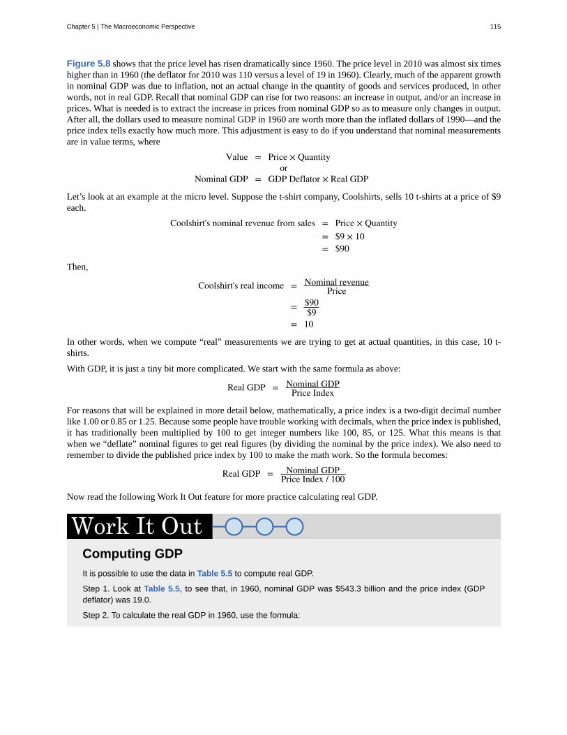
Figure 5.8 shows that the price level has risen dramatically since 1960. The price level in 2010 was almost six timeshigher than in 1960 (the deflator for 2010 was 110 versus a level of 19 in 1960). Clearly, much of the apparent growthin nominal GDP was due to inflation, not an actual change in the quantity of goods and services produced, in otherwords, not in real GDP. Recall that nominal GDP can rise for two reasons: an increase in output, and/or an increase inprices. What is needed is to extract the increase in prices from nominal GDP so as to measure only changes in output.After all, the dollars used to measure nominal GDP in 1960 are worth more than the inflated dollars of 1990—and theprice index tells exactly how much more. This adjustment is easy to do if you understand that nominal measurementsare in value terms, where
Value = Price × Quantity or
Nominal GDP = GDP Deflator × Real GDP
Let’s look at an example at the micro level. Suppose the t-shirt company, Coolshirts, sells 10 t-shirts at a price of $9each.
Coolshirt's nominal revenue from sales = Price × Quantity = $9 × 10 = $90
Then,
Coolshirt's real income = Nominal revenuePrice
= $90$9
= 10
In other words, when we compute “real” measurements we are trying to get at actual quantities, in this case, 10 t-shirts.
With GDP, it is just a tiny bit more complicated. We start with the same formula as above:
Real GDP = Nominal GDPPrice Index
For reasons that will be explained in more detail below, mathematically, a price index is a two-digit decimal numberlike 1.00 or 0.85 or 1.25. Because some people have trouble working with decimals, when the price index is published,it has traditionally been multiplied by 100 to get integer numbers like 100, 85, or 125. What this means is thatwhen we “deflate” nominal figures to get real figures (by dividing the nominal by the price index). We also need toremember to divide the published price index by 100 to make the math work. So the formula becomes:
Real GDP = Nominal GDPPrice Index / 100
Now read the following Work It Out feature for more practice calculating real GDP.
Computing GDPIt is possible to use the data in Table 5.5 to compute real GDP.
Step 1. Look at Table 5.5, to see that, in 1960, nominal GDP was $543.3 billion and the price index (GDPdeflator) was 19.0.
Step 2. To calculate the real GDP in 1960, use the formula:
Chapter 5 | The Macroeconomic Perspective 115
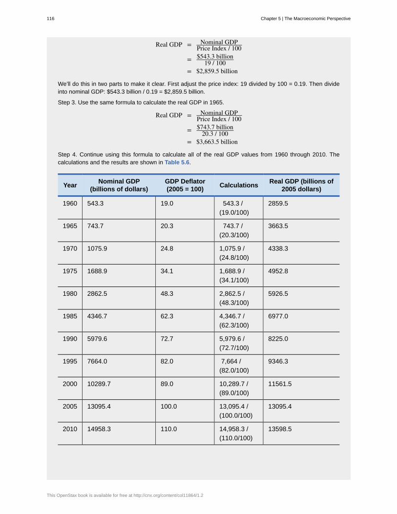
Real GDP = Nominal GDPPrice Index / 100
= $543.3 billion19 / 100
= $2,859.5 billion
We’ll do this in two parts to make it clear. First adjust the price index: 19 divided by 100 = 0.19. Then divideinto nominal GDP: $543.3 billion / 0.19 = $2,859.5 billion.
Step 3. Use the same formula to calculate the real GDP in 1965.
Real GDP = Nominal GDPPrice Index / 100
= $743.7 billion20.3 / 100
= $3,663.5 billion
Step 4. Continue using this formula to calculate all of the real GDP values from 1960 through 2010. Thecalculations and the results are shown in Table 5.6.
Year Nominal GDP(billions of dollars)
GDP Deflator(2005 = 100) Calculations Real GDP (billions of
2005 dollars)
1960 543.3 19.0 543.3 /(19.0/100)
2859.5
1965 743.7 20.3 743.7 /(20.3/100)
3663.5
1970 1075.9 24.8 1,075.9 /(24.8/100)
4338.3
1975 1688.9 34.1 1,688.9 /(34.1/100)
4952.8
1980 2862.5 48.3 2,862.5 /(48.3/100)
5926.5
1985 4346.7 62.3 4,346.7 /(62.3/100)
6977.0
1990 5979.6 72.7 5,979.6 /(72.7/100)
8225.0
1995 7664.0 82.0 7,664 /(82.0/100)
9346.3
2000 10289.7 89.0 10,289.7 /(89.0/100)
11561.5
2005 13095.4 100.0 13,095.4 /(100.0/100)
13095.4
2010 14958.3 110.0 14,958.3 /(110.0/100)
13598.5
116 Chapter 5 | The Macroeconomic Perspective
This OpenStax book is available for free at http://cnx.org/content/col11864/1.2
There are a couple things to notice here. Whenever you compute a real statistic, one year (or period) playsa special role. It is called the base year (or base period). The base year is the year whose prices are usedto compute the real statistic. When we calculate real GDP, for example, we take the quantities of goods andservices produced in each year (for example, 1960 or 1973) and multiply them by their prices in the base year(in this case, 2005), so we get a measure of GDP that uses prices that do not change from year to year. Thatis why real GDP is labeled “Constant Dollars” or “2005 Dollars,” which means that real GDP is constructedusing prices that existed in 2005. The formula used is:
GDP deflator = Nominal GDPReal GDP × 100
Rearranging the formula and using the data from 2005:
Real GDP = Nominal GDPPrice Index / 100
= $13,095.4 billion100 / 100
= $13,095.4 billion
Comparing real GDP and nominal GDP for 2005, you see they are the same. This is no accident. It is because2005 has been chosen as the “base year” in this example. Since the price index in the base year always hasa value of 100 (by definition), nominal and real GDP are always the same in the base year.
Look at the data for 2010.
Real GDP = Nominal GDPPrice Index / 100
= $14,958.3 billion110 / 100
= $13,598.5 billion
Use this data to make another observation: As long as inflation is positive, meaning prices increase onaverage from year to year, real GDP should be less than nominal GDP in any year after the base year. Thereason for this should be clear: The value of nominal GDP is “inflated” by inflation. Similarly, as long as inflationis positive, real GDP should be greater than nominal GDP in any year before the base year.
Figure 5.9 shows the U.S. nominal and real GDP since 1960. Because 2005 is the base year, the nominal and realvalues are exactly the same in that year. However, over time, the rise in nominal GDP looks much larger than the risein real GDP (that is, the nominal GDP line rises more steeply than the real GDP line), because the rise in nominalGDP is exaggerated by the presence of inflation, especially in the 1970s.
Chapter 5 | The Macroeconomic Perspective 117
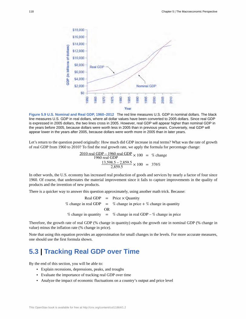
Figure 5.9 U.S. Nominal and Real GDP, 1960–2012 The red line measures U.S. GDP in nominal dollars. The blackline measures U.S. GDP in real dollars, where all dollar values have been converted to 2005 dollars. Since real GDPis expressed in 2005 dollars, the two lines cross in 2005. However, real GDP will appear higher than nominal GDP inthe years before 2005, because dollars were worth less in 2005 than in previous years. Conversely, real GDP willappear lower in the years after 2005, because dollars were worth more in 2005 than in later years.
Let’s return to the question posed originally: How much did GDP increase in real terms? What was the rate of growthof real GDP from 1960 to 2010? To find the real growth rate, we apply the formula for percentage change:
2010 real GDP – 1960 real GDP1960 real GDP × 100 = % change
13,598.5 – 2,859.52,859.5 × 100 = 376%
In other words, the U.S. economy has increased real production of goods and services by nearly a factor of four since1960. Of course, that understates the material improvement since it fails to capture improvements in the quality ofproducts and the invention of new products.
There is a quicker way to answer this question approximately, using another math trick. Because:
Real GDP = Price × Quantity% change in real GDP = % change in price + % change in quantity
OR % change in quantity = % change in real GDP – % change in price
Therefore, the growth rate of real GDP (% change in quantity) equals the growth rate in nominal GDP (% change invalue) minus the inflation rate (% change in price).
Note that using this equation provides an approximation for small changes in the levels. For more accurate measures,one should use the first formula shown.
5.3 | Tracking Real GDP over TimeBy the end of this section, you will be able to:
• Explain recessions, depressions, peaks, and troughs• Evaluate the importance of tracking real GDP over time• Analyze the impact of economic fluctuations on a country’s output and price level
118 Chapter 5 | The Macroeconomic Perspective
This OpenStax book is available for free at http://cnx.org/content/col11864/1.2
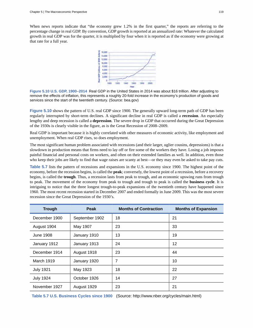
When news reports indicate that “the economy grew 1.2% in the first quarter,” the reports are referring to thepercentage change in real GDP. By convention, GDP growth is reported at an annualized rate: Whatever the calculatedgrowth in real GDP was for the quarter, it is multiplied by four when it is reported as if the economy were growing atthat rate for a full year.
Figure 5.10 U.S. GDP, 1900–2014 Real GDP in the United States in 2014 was about $16 trillion. After adjusting toremove the effects of inflation, this represents a roughly 20-fold increase in the economy’s production of goods andservices since the start of the twentieth century. (Source: bea.gov)
Figure 5.10 shows the pattern of U.S. real GDP since 1900. The generally upward long-term path of GDP has beenregularly interrupted by short-term declines. A significant decline in real GDP is called a recession. An especiallylengthy and deep recession is called a depression. The severe drop in GDP that occurred during the Great Depressionof the 1930s is clearly visible in the figure, as is the Great Recession of 2008–2009.
Real GDP is important because it is highly correlated with other measures of economic activity, like employment andunemployment. When real GDP rises, so does employment.
The most significant human problem associated with recessions (and their larger, uglier cousins, depressions) is that aslowdown in production means that firms need to lay off or fire some of the workers they have. Losing a job imposespainful financial and personal costs on workers, and often on their extended families as well. In addition, even thosewho keep their jobs are likely to find that wage raises are scanty at best—or they may even be asked to take pay cuts.
Table 5.7 lists the pattern of recessions and expansions in the U.S. economy since 1900. The highest point of theeconomy, before the recession begins, is called the peak; conversely, the lowest point of a recession, before a recoverybegins, is called the trough. Thus, a recession lasts from peak to trough, and an economic upswing runs from troughto peak. The movement of the economy from peak to trough and trough to peak is called the business cycle. It isintriguing to notice that the three longest trough-to-peak expansions of the twentieth century have happened since1960. The most recent recession started in December 2007 and ended formally in June 2009. This was the most severerecession since the Great Depression of the 1930’s.
Trough Peak Months of Contraction Months of Expansion
December 1900 September 1902 18 21
August 1904 May 1907 23 33
June 1908 January 1910 13 19
January 1912 January 1913 24 12
December 1914 August 1918 23 44
March 1919 January 1920 7 10
July 1921 May 1923 18 22
July 1924 October 1926 14 27
November 1927 August 1929 23 21
Table 5.7 U.S. Business Cycles since 1900 (Source: http://www.nber.org/cycles/main.html)
Chapter 5 | The Macroeconomic Perspective 119
Trough Peak Months of Contraction Months of Expansion
March 1933 May 1937 43 50
June 1938 February 1945 13 80
October 1945 November 1948 8 37
October 1949 July 1953 11 45
May 1954 August 1957 10 39
April 1958 April 1960 8 24
February 1961 December 1969 10 106
November 1970 November 1973 11 36
March 1975 January 1980 16 58
July 1980 July 1981 6 12
November 1982 July 1990 16 92
March 2001 November 2001 8 120
December 2007 June 2009 18 73
Table 5.7 U.S. Business Cycles since 1900 (Source: http://www.nber.org/cycles/main.html)
A private think tank, the National Bureau of Economic Research (NBER), is the official tracker of business cycles forthe U.S. economy. However, the effects of a severe recession often linger on after the official ending date assigned bythe NBER.
5.4 | Comparing GDP among CountriesBy the end of this section, you will be able to:
• Explain how GDP can be used to compare the economic welfare of different nations• Calculate the conversion of GDP to a common currency by using exchange rates• Calculate GDP per capita using population data
It is common to use GDP as a measure of economic welfare or standard of living in a nation. When comparing theGDP of different nations for this purpose, two issues immediately arise. First, the GDP of a country is measuredin its own currency: the United States uses the U.S. dollar; Canada, the Canadian dollar; most countries of WesternEurope, the euro; Japan, the yen; Mexico, the peso; and so on. Thus, comparing GDP between two countries requiresconverting to a common currency. A second issue is that countries have very different numbers of people. Forinstance, the United States has a much larger economy than Mexico or Canada, but it also has roughly three times asmany people as Mexico and nine times as many people as Canada. So, if we are trying to compare standards of livingacross countries, we need to divide GDP by population.
Converting Currencies with Exchange RatesTo compare the GDP of countries with different currencies, it is necessary to convert to a “common denominator”using an exchange rate, which is the value of one currency in terms of another currency. Exchange rates are expressedeither as the units of country A’s currency that need to be traded for a single unit of country B’s currency (forexample, Japanese yen per British pound), or as the inverse (for example, British pounds per Japanese yen). Twotypes of exchange rates can be used for this purpose, market exchange rates and purchasing power parity (PPP)
120 Chapter 5 | The Macroeconomic Perspective
This OpenStax book is available for free at http://cnx.org/content/col11864/1.2
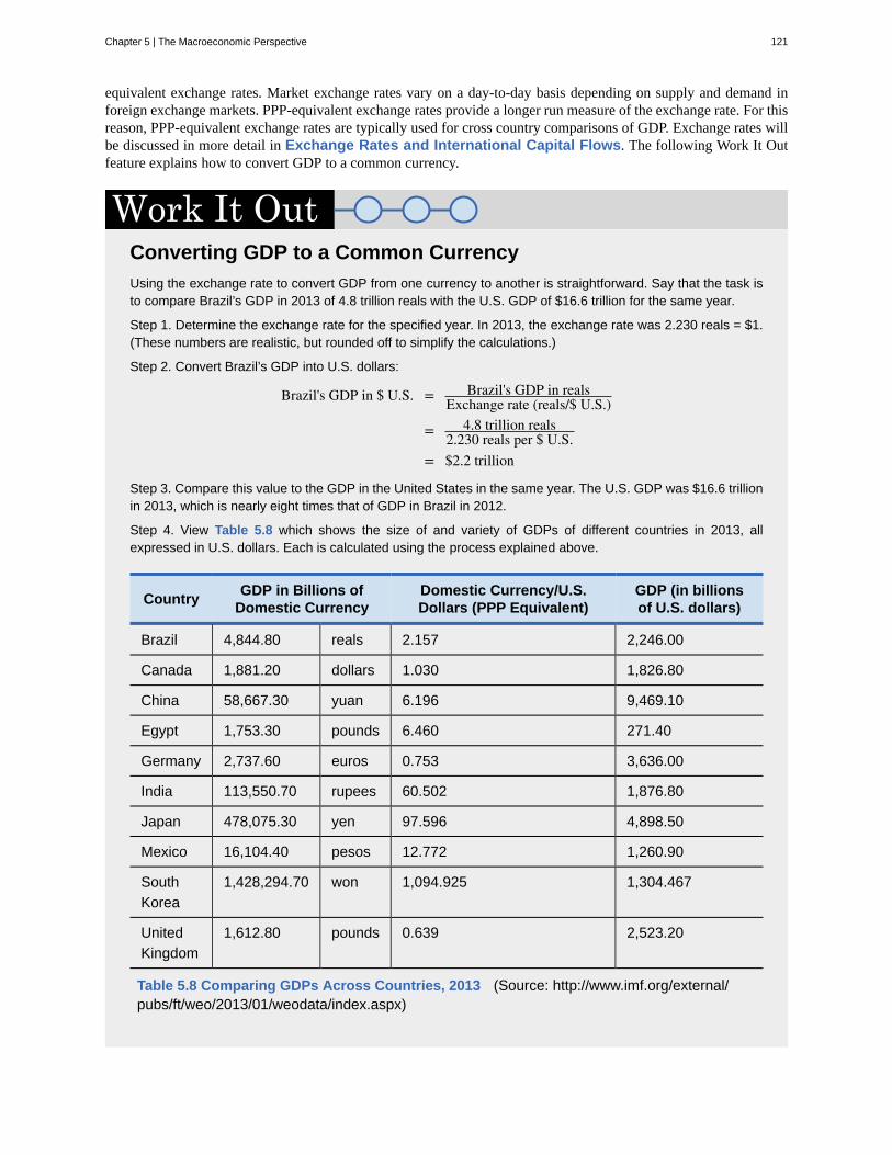
equivalent exchange rates. Market exchange rates vary on a day-to-day basis depending on supply and demand inforeign exchange markets. PPP-equivalent exchange rates provide a longer run measure of the exchange rate. For thisreason, PPP-equivalent exchange rates are typically used for cross country comparisons of GDP. Exchange rates willbe discussed in more detail in Exchange Rates and International Capital Flows. The following Work It Outfeature explains how to convert GDP to a common currency.
Converting GDP to a Common CurrencyUsing the exchange rate to convert GDP from one currency to another is straightforward. Say that the task isto compare Brazil’s GDP in 2013 of 4.8 trillion reals with the U.S. GDP of $16.6 trillion for the same year.
Step 1. Determine the exchange rate for the specified year. In 2013, the exchange rate was 2.230 reals = $1.(These numbers are realistic, but rounded off to simplify the calculations.)
Step 2. Convert Brazil’s GDP into U.S. dollars:
Brazil's GDP in $ U.S. = Brazil's GDP in realsExchange rate (reals/$ U.S.)
= 4.8 trillion reals2.230 reals per $ U.S.
= $2.2 trillion
Step 3. Compare this value to the GDP in the United States in the same year. The U.S. GDP was $16.6 trillionin 2013, which is nearly eight times that of GDP in Brazil in 2012.
Step 4. View Table 5.8 which shows the size of and variety of GDPs of different countries in 2013, allexpressed in U.S. dollars. Each is calculated using the process explained above.
Country GDP in Billions ofDomestic Currency
Domestic Currency/U.S.Dollars (PPP Equivalent)
GDP (in billionsof U.S. dollars)
Brazil 4,844.80 reals 2.157 2,246.00
Canada 1,881.20 dollars 1.030 1,826.80
China 58,667.30 yuan 6.196 9,469.10
Egypt 1,753.30 pounds 6.460 271.40
Germany 2,737.60 euros 0.753 3,636.00
India 113,550.70 rupees 60.502 1,876.80
Japan 478,075.30 yen 97.596 4,898.50
Mexico 16,104.40 pesos 12.772 1,260.90
SouthKorea
1,428,294.70 won 1,094.925 1,304.467
UnitedKingdom
1,612.80 pounds 0.639 2,523.20
Table 5.8 Comparing GDPs Across Countries, 2013 (Source: http://www.imf.org/external/pubs/ft/weo/2013/01/weodata/index.aspx)
Chapter 5 | The Macroeconomic Perspective 121
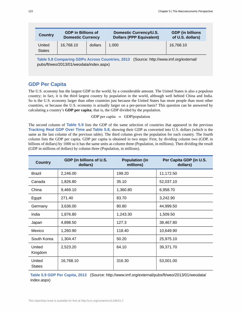
Country GDP in Billions ofDomestic Currency
Domestic Currency/U.S.Dollars (PPP Equivalent)
GDP (in billionsof U.S. dollars)
UnitedStates
16,768.10 dollars 1.000 16,768.10
Table 5.8 Comparing GDPs Across Countries, 2013 (Source: http://www.imf.org/external/pubs/ft/weo/2013/01/weodata/index.aspx)
GDP Per CapitaThe U.S. economy has the largest GDP in the world, by a considerable amount. The United States is also a populouscountry; in fact, it is the third largest country by population in the world, although well behind China and India.So is the U.S. economy larger than other countries just because the United States has more people than most othercountries, or because the U.S. economy is actually larger on a per-person basis? This question can be answered bycalculating a country’s GDP per capita; that is, the GDP divided by the population.
GDP per capita = GDP/population
The second column of Table 5.9 lists the GDP of the same selection of countries that appeared in the previousTracking Real GDP Over Time and Table 5.8, showing their GDP as converted into U.S. dollars (which is thesame as the last column of the previous table). The third column gives the population for each country. The fourthcolumn lists the GDP per capita. GDP per capita is obtained in two steps: First, by dividing column two (GDP, inbillions of dollars) by 1000 so it has the same units as column three (Population, in millions). Then dividing the result(GDP in millions of dollars) by column three (Population, in millions).
Country GDP (in billions of U.S.dollars)
Population (inmillions)
Per Capita GDP (in U.S.dollars)
Brazil 2,246.00 199.20 11,172.50
Canada 1,826.80 35.10 52,037.10
China 9,469.10 1,360.80 6,958.70
Egypt 271.40 83.70 3,242.90
Germany 3,636.00 80.80 44,999.50
India 1,876.80 1,243.30 1,509.50
Japan 4,898.50 127.3 38,467.80
Mexico 1,260.90 118.40 10,649.90
South Korea 1,304.47 50.20 25,975.10
UnitedKingdom
2,523.20 64.10 39,371.70
UnitedStates
16,768.10 316.30 53,001.00
Table 5.9 GDP Per Capita, 2013 (Source: http://www.imf.org/external/pubs/ft/weo/2013/01/weodata/index.aspx)
122 Chapter 5 | The Macroeconomic Perspective
This OpenStax book is available for free at http://cnx.org/content/col11864/1.2
Notice that the ranking by GDP is different from the ranking by GDP per capita. India has a somewhat larger GDPthan Germany, but on a per capita basis, Germany has more than 10 times India’s standard of living. Will China soonhave a better standard of living than the U.S.? Read the following Clear It Up feature to find out.
Is China going to surpass the United States in terms of standardof living?As shown in Table 5.9, China has the second largest GDP of the countries: $9.5 trillion compared to theUnited States’ $16.8 trillion. Perhaps it will surpass the United States, but probably not any time soon. Chinahas a much larger population so that in per capita terms, its GDP is less than one fifth that of the United States($6,958.70 compared to $53,001). The Chinese people are still quite poor relative to the United States andother developed countries. One caveat: For reasons to be discussed shortly, GDP per capita can give us onlya rough idea of the differences in living standards across countries.
The high-income nations of the world—including the United States, Canada, the Western European countries, andJapan—typically have GDP per capita in the range of $20,000 to $50,000. Middle-income countries, which includemuch of Latin America, Eastern Europe, and some countries in East Asia, have GDP per capita in the range of $6,000to $12,000. The low-income countries in the world, many of them located in Africa and Asia, often have GDP percapita of less than $2,000 per year.
5.5 | How Well GDP Measures the Well-Being of SocietyBy the end of this section, you will be able to:
• Discuss how productivity influences the standard of living• Explain the limitations of GDP as a measure of the standard of living• Analyze the relationship between GDP data and fluctuations in the standard of living
The level of GDP per capita clearly captures some of what we mean by the phrase “standard of living.” Most of themigration in the world, for example, involves people who are moving from countries with relatively low GDP percapita to countries with relatively high GDP per capita.
“Standard of living” is a broader term than GDP. While GDP focuses on production that is bought and sold in markets,standard of living includes all elements that affect people’s well-being, whether they are bought and sold in themarket or not. To illuminate the gap between GDP and standard of living, it is useful to spell out some things thatGDP does not cover that are clearly relevant to standard of living.
Limitations of GDP as a Measure of the Standard of LivingWhile GDP includes spending on recreation and travel, it does not cover leisure time. Clearly, however, there is asubstantial difference between an economy that is large because people work long hours, and an economy that is justas large because people are more productive with their time so they do not have to work as many hours. The GDP percapita of the U.S. economy is larger than the GDP per capita of Germany, as was shown in Table 5.9, but does thatprove that the standard of living in the United States is higher? Not necessarily, since it is also true that the averageU.S. worker works several hundred hours more per year more than the average German worker. The calculation ofGDP does not take the German worker’s extra weeks of vacation into account.
While GDP includes what is spent on environmental protection, healthcare, and education, it does not includeactual levels of environmental cleanliness, health, and learning. GDP includes the cost of buying pollution-controlequipment, but it does not address whether the air and water are actually cleaner or dirtier. GDP includes spendingon medical care, but does not address whether life expectancy or infant mortality have risen or fallen. Similarly, it
Chapter 5 | The Macroeconomic Perspective 123
counts spending on education, but does not address directly how much of the population can read, write, or do basicmathematics.
GDP includes production that is exchanged in the market, but it does not cover production that is not exchanged inthe market. For example, hiring someone to mow your lawn or clean your house is part of GDP, but doing these tasksyourself is not part of GDP. One remarkable change in the U.S. economy in recent decades is that, as of 1970, onlyabout 42% of women participated in the paid labor force. By the second decade of the 2000s, nearly 60% of womenparticipated in the paid labor force according to the Bureau of Labor Statistics. As women are now in the labor force,many of the services they used to produce in the non-market economy like food preparation and child care haveshifted to some extent into the market economy, which makes the GDP appear larger even if more services are notactually being consumed.
GDP has nothing to say about the level of inequality in society. GDP per capita is only an average. When GDP percapita rises by 5%, it could mean that GDP for everyone in the society has risen by 5%, or that of some groups hasrisen by more while that of others has risen by less—or even declined. GDP also has nothing in particular to say aboutthe amount of variety available. If a family buys 100 loaves of bread in a year, GDP does not care whether they areall white bread, or whether the family can choose from wheat, rye, pumpernickel, and many others—it just looks atwhether the total amount spent on bread is the same.
Likewise, GDP has nothing much to say about what technology and products are available. The standard of living in,for example, 1950 or 1900 was not affected only by how much money people had—it was also affected by what theycould buy. No matter how much money you had in 1950, you could not buy an iPhone or a personal computer.
In certain cases, it is not clear that a rise in GDP is even a good thing. If a city is wrecked by a hurricane, and thenexperiences a surge of rebuilding construction activity, it would be peculiar to claim that the hurricane was thereforeeconomically beneficial. If people are led by a rising fear of crime, to pay for installation of bars and burglar alarmson all their windows, it is hard to believe that this increase in GDP has made them better off. In that same vein, somepeople would argue that sales of certain goods, like pornography or extremely violent movies, do not represent a gainto society’s standard of living.
Does a Rise in GDP Overstate or Understate the Rise in the Standard ofLiving?The fact that GDP per capita does not fully capture the broader idea of standard of living has led to a concern thatthe increases in GDP over time are illusory. It is theoretically possible that while GDP is rising, the standard ofliving could be falling if human health, environmental cleanliness, and other factors that are not included in GDP areworsening. Fortunately, this fear appears to be overstated.
In some ways, the rise in GDP understates the actual rise in the standard of living. For example, the typical workweekfor a U.S. worker has fallen over the last century from about 60 hours per week to less than 40 hours per week. Lifeexpectancy and health have risen dramatically, and so has the average level of education. Since 1970, the air and waterin the United States have generally been getting cleaner. New technologies have been developed for entertainment,travel, information, and health. A much wider variety of basic products like food and clothing is available today thanseveral decades ago. Because GDP does not capture leisure, health, a cleaner environment, the possibilities createdby new technology, or an increase in variety, the actual rise in the standard of living for Americans in recent decadeshas exceeded the rise in GDP.
On the other side, rates of crime, levels of traffic congestion, and inequality of incomes are higher in the United Statesnow than they were in the 1960s. Moreover, a substantial number of services that used to be provided, primarily bywomen, in the non-market economy are now part of the market economy that is counted by GDP. By ignoring thesefactors, GDP would tend to overstate the true rise in the standard of living.
Visit this website (http://openstaxcollege.org/l/amdreamvalue) to read about the American Dream andstandards of living.
124 Chapter 5 | The Macroeconomic Perspective
This OpenStax book is available for free at http://cnx.org/content/col11864/1.2
GDP is Rough, but UsefulA high level of GDP should not be the only goal of macroeconomic policy, or government policy more broadly. Eventhough GDP does not measure the broader standard of living with any precision, it does measure production welland it does indicate when a country is materially better or worse off in terms of jobs and incomes. In most countries,a significantly higher GDP per capita occurs hand in hand with other improvements in everyday life along manydimensions, like education, health, and environmental protection.
No single number can capture all the elements of a term as broad as “standard of living.” Nonetheless, GDP per capitais a reasonable, rough-and-ready measure of the standard of living.
How is the Economy Doing? How Does One Tell?To determine the state of the economy, one needs to examine economic indicators, such as GDP. To calculateGDP is quite an undertaking. It is the broadest measure of a nation’s economic activity and we owe a debt toSimon Kuznets, the creator of the measurement, for that.
The sheer size of the U.S. economy as measured by GDP is huge—as of the third quarter of 2013, $16.6trillion worth of goods and services were produced annually. Real GDP informed us that the recession of2008–2009 was a severe one and that the recovery from that has been slow, but is improving. GDP per capitagives a rough estimate of a nation’s standard of living. This chapter is the building block for other chaptersthat explore more economic indicators such as unemployment, inflation, or interest rates, and perhaps moreimportantly, will explain how they are related and what causes them to rise or fall.
Chapter 5 | The Macroeconomic Perspective 125
business cycle
depreciation
depression
double counting
durable good
exchange rate
final good and service
GDP per capita
gross domestic product (GDP)
gross national product (GNP)
intermediate good
inventory
national income
net national product (NNP)
nominal value
nondurable good
peak
real value
recession
service
standard of living
structure
trade balance
trade deficit
trade surplus
trough
KEY TERMS
the relatively short-term movement of the economy in and out of recession
the process by which capital ages over time and therefore loses its value
an especially lengthy and deep decline in output
a potential mistake to be avoided in measuring GDP, in which output is counted more than once as ittravels through the stages of production
long-lasting good like a car or a refrigerator
the price of one currency in terms of another currency
output used directly for consumption, investment, government, and trade purposes; contrastwith “intermediate good”
GDP divided by the population
the value of the output of all goods and services produced within a country in a year
includes what is produced domestically and what is produced by domestic labor andbusiness abroad in a year
output provided to other businesses at an intermediate stage of production, not for final users;contrast with “final good and service”
good that has been produced, but not yet been sold
includes all income earned: wages, profits, rent, and profit income
GDP minus depreciation
the economic statistic actually announced at that time, not adjusted for inflation; contrast with real value
short-lived good like food and clothing
during the business cycle, the highest point of output before a recession begins
an economic statistic after it has been adjusted for inflation; contrast with nominal value
a significant decline in national output
product which is intangible (in contrast to goods) such as entertainment, healthcare, or education
all elements that affect people’s happiness, whether these elements are bought and sold in themarket or not
building used as residence, factory, office building, retail store, or for other purposes
gap between exports and imports
exists when a nation's imports exceed its exports and is calculated as imports –exports
exists when a nation's exports exceed its imports and is calculated as exports – imports
during the business cycle, the lowest point of output in a recession, before a recovery begins
126 Chapter 5 | The Macroeconomic Perspective
This OpenStax book is available for free at http://cnx.org/content/col11864/1.2
KEY CONCEPTS AND SUMMARY
5.1 Measuring the Size of the Economy: Gross Domestic ProductThe size of a nation’s economy is commonly expressed as its gross domestic product (GDP), which measures thevalue of the output of all goods and services produced within the country in a year. GDP is measured by taking thequantities of all goods and services produced, multiplying them by their prices, and summing the total. Since GDPmeasures what is bought and sold in the economy, it can be measured either by the sum of what is purchased in theeconomy or what is produced.
Demand can be divided into consumption, investment, government, exports, and imports. What is produced in theeconomy can be divided into durable goods, nondurable goods, services, structures, and inventories. To avoid doublecounting, GDP counts only final output of goods and services, not the production of intermediate goods or the valueof labor in the chain of production.
5.2 Adjusting Nominal Values to Real ValuesThe nominal value of an economic statistic is the commonly announced value. The real value is the value afteradjusting for changes in inflation. To convert nominal economic data from several different years into real, inflation-adjusted data, the starting point is to choose a base year arbitrarily and then use a price index to convert themeasurements so that they are measured in the money prevailing in the base year.
5.3 Tracking Real GDP over TimeOver the long term, U.S. real GDP have increased dramatically. At the same time, GDP has not increased the sameamount each year. The speeding up and slowing down of GDP growth represents the business cycle. When GDPdeclines significantly, a recession occurs. A longer and deeper decline is a depression. Recessions begin at the peakof the business cycle and end at the trough.
5.4 Comparing GDP among CountriesSince GDP is measured in a country’s currency, in order to compare different countries’ GDPs, we need to convertthem to a common currency. One way to do that is with the exchange rate, which is the price of one country’s currencyin terms of another. Once GDPs are expressed in a common currency, we can compare each country’s GDP per capitaby dividing GDP by population. Countries with large populations often have large GDPs, but GDP alone can be amisleading indicator of the wealth of a nation. A better measure is GDP per capita.
5.5 How Well GDP Measures the Well-Being of SocietyGDP is an indicator of a society’s standard of living, but it is only a rough indicator. GDP does not directly takeaccount of leisure, environmental quality, levels of health and education, activities conducted outside the market,changes in inequality of income, increases in variety, increases in technology, or the (positive or negative) value thatsociety may place on certain types of output.
SELF-CHECK QUESTIONS1. Country A has export sales of $20 billion, government purchases of $1,000 billion, business investment is $50billion, imports are $40 billion, and consumption spending is $2,000 billion. What is the dollar value of GDP?
2. Which of the following are included in GDP, and which are not?a. The cost of hospital staysb. The rise in life expectancy over timec. Child care provided by a licensed day care centerd. Child care provided by a grandmothere. The sale of a used carf. The sale of a new carg. The greater variety of cheese available in supermarketsh. The iron that goes into the steel that goes into a refrigerator bought by a consumer.
Chapter 5 | The Macroeconomic Perspective 127
3. Using data from Table 5.5 how much of the nominal GDP growth from 1980 to 1990 was real GDP and howmuch was inflation?
4. Without looking at Table 5.7, return to Figure 5.10. If a recession is defined as a significant decline innational output, can you identify any post-1960 recessions in addition to the recession of 2008–2009? (This requiresa judgment call.)
5. According to Table 5.7, how often have recessions occurred since the end of World War II (1945)?
6. According to Table 5.7, how long has the average recession lasted since the end of World War II?
7. According to Table 5.7, how long has the average expansion lasted since the end of World War II?
8. Is it possible for GDP to rise while at the same time per capita GDP is falling? Is it possible for GDP to fall whileper capita GDP is rising?
9. The Central African Republic has a GDP of 1,107,689 million CFA francs and a population of 4.862 million. Theexchange rate is 284.681CFA francs per dollar. Calculate the GDP per capita of Central African Republic.
10. Explain briefly whether each of the following would cause GDP to overstate or understate the degree of changein the broad standard of living.
a. The environment becomes dirtierb. The crime rate declinesc. A greater variety of goods become available to consumersd. Infant mortality declines
REVIEW QUESTIONS
11. What are the main components of measuring GDPwith what is demanded?
12. What are the main components of measuring GDPwith what is produced?
13. Would you usually expect GDP as measured bywhat is demanded to be greater than GDP measured bywhat is supplied, or the reverse?
14. Why must double counting be avoided whenmeasuring GDP?
15. What is the difference between a series of economicdata over time measured in nominal terms versus thesame data series over time measured in real terms?
16. How do you convert a series of nominal economicdata over time to real terms?
17. What are the typical patterns of GDP for a high-income economy like the United States in the long runand the short run?
18. What are the two main difficulties that arise incomparing the GDP of different countries?
19. List some of the reasons why GDP should not beconsidered an effective measure of the standard of livingin a country.
CRITICAL THINKING QUESTIONS
20. U.S. macroeconomic data are thought to be amongthe best in the world. Given what you learned in theClear It Up "How do statisticians measure GDP?",does this surprise you? Or does this simply reflect thecomplexity of a modern economy?
21. What does GDP not tell us about the economy?
22. Should people typically pay more attention to theirreal income or their nominal income? If you choose thelatter, why would that make sense in today’s world?Would your answer be the same for the 1970s?
23. Why do you suppose that U.S. GDP is so muchhigher today than 50 or 100 years ago?
128 Chapter 5 | The Macroeconomic Perspective
This OpenStax book is available for free at http://cnx.org/content/col11864/1.2
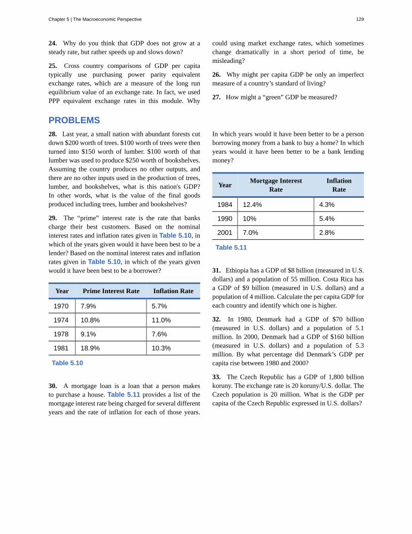
24. Why do you think that GDP does not grow at asteady rate, but rather speeds up and slows down?
25. Cross country comparisons of GDP per capitatypically use purchasing power parity equivalentexchange rates, which are a measure of the long runequilibrium value of an exchange rate. In fact, we usedPPP equivalent exchange rates in this module. Why
could using market exchange rates, which sometimeschange dramatically in a short period of time, bemisleading?
26. Why might per capita GDP be only an imperfectmeasure of a country’s standard of living?
27. How might a “green” GDP be measured?
PROBLEMS28. Last year, a small nation with abundant forests cutdown $200 worth of trees. $100 worth of trees were thenturned into $150 worth of lumber. $100 worth of thatlumber was used to produce $250 worth of bookshelves.Assuming the country produces no other outputs, andthere are no other inputs used in the production of trees,lumber, and bookshelves, what is this nation's GDP?In other words, what is the value of the final goodsproduced including trees, lumber and bookshelves?
29. The “prime” interest rate is the rate that bankscharge their best customers. Based on the nominalinterest rates and inflation rates given in Table 5.10, inwhich of the years given would it have been best to be alender? Based on the nominal interest rates and inflationrates given in Table 5.10, in which of the years givenwould it have been best to be a borrower?
Year Prime Interest Rate Inflation Rate
1970 7.9% 5.7%
1974 10.8% 11.0%
1978 9.1% 7.6%
1981 18.9% 10.3%
Table 5.10
30. A mortgage loan is a loan that a person makesto purchase a house. Table 5.11 provides a list of themortgage interest rate being charged for several differentyears and the rate of inflation for each of those years.
In which years would it have been better to be a personborrowing money from a bank to buy a home? In whichyears would it have been better to be a bank lendingmoney?
Year Mortgage InterestRate
InflationRate
1984 12.4% 4.3%
1990 10% 5.4%
2001 7.0% 2.8%
Table 5.11
31. Ethiopia has a GDP of $8 billion (measured in U.S.dollars) and a population of 55 million. Costa Rica hasa GDP of $9 billion (measured in U.S. dollars) and apopulation of 4 million. Calculate the per capita GDP foreach country and identify which one is higher.
32. In 1980, Denmark had a GDP of $70 billion(measured in U.S. dollars) and a population of 5.1million. In 2000, Denmark had a GDP of $160 billion(measured in U.S. dollars) and a population of 5.3million. By what percentage did Denmark’s GDP percapita rise between 1980 and 2000?
33. The Czech Republic has a GDP of 1,800 billionkoruny. The exchange rate is 20 koruny/U.S. dollar. TheCzech population is 20 million. What is the GDP percapita of the Czech Republic expressed in U.S. dollars?
Chapter 5 | The Macroeconomic Perspective 129
130 Chapter 5 | The Macroeconomic Perspective
This OpenStax book is available for free at http://cnx.org/content/col11864/1.2
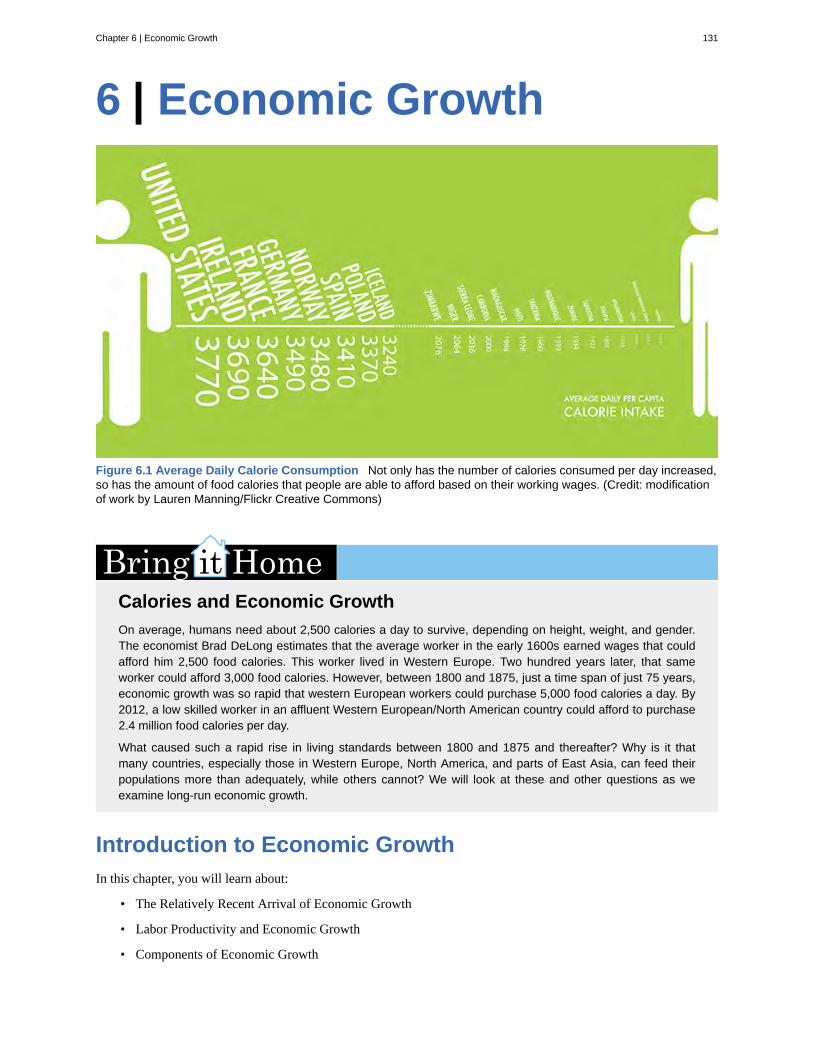
6 | Economic Growth
Figure 6.1 Average Daily Calorie Consumption Not only has the number of calories consumed per day increased,so has the amount of food calories that people are able to afford based on their working wages. (Credit: modificationof work by Lauren Manning/Flickr Creative Commons)
Calories and Economic GrowthOn average, humans need about 2,500 calories a day to survive, depending on height, weight, and gender.The economist Brad DeLong estimates that the average worker in the early 1600s earned wages that couldafford him 2,500 food calories. This worker lived in Western Europe. Two hundred years later, that sameworker could afford 3,000 food calories. However, between 1800 and 1875, just a time span of just 75 years,economic growth was so rapid that western European workers could purchase 5,000 food calories a day. By2012, a low skilled worker in an affluent Western European/North American country could afford to purchase2.4 million food calories per day.
What caused such a rapid rise in living standards between 1800 and 1875 and thereafter? Why is it thatmany countries, especially those in Western Europe, North America, and parts of East Asia, can feed theirpopulations more than adequately, while others cannot? We will look at these and other questions as weexamine long-run economic growth.
Introduction to Economic GrowthIn this chapter, you will learn about:
• The Relatively Recent Arrival of Economic Growth
• Labor Productivity and Economic Growth
• Components of Economic Growth
Chapter 6 | Economic Growth 131
• Economic Convergence
Every country worries about economic growth. In the United States and other high-income countries, the question iswhether economic growth continues to provide the same remarkable gains in our standard of living as it did during thetwentieth century. Meanwhile, can middle-income countries like South Korea, Brazil, Egypt, or Poland catch up tothe higher-income countries? Or must they remain in the second tier of per capita income? Of the world’s populationof roughly 6.7 billion people, about 2.6 billion are scraping by on incomes that average less than $2 per day, not thatdifferent from the standard of living 2,000 years ago. Can the world’s poor be lifted from their fearful poverty? As the1995 Nobel laureate in economics, Robert E. Lucas Jr., once noted: “The consequences for human welfare involvedin questions like these are simply staggering: Once one starts to think about them, it is hard to think about anythingelse.”
Dramatic improvements in a nation’s standard of living are possible. After the Korean War in the late 1950s, theRepublic of Korea, often called South Korea, was one of the poorest economies in the world. Most South Koreansworked in peasant agriculture. According to the British economist Angus Maddison, whose life’s work was themeasurement of GDP and population in the world economy, GDP per capita in 1990 international dollars was $854per year. From the 1960s to the early twenty-first century, a time period well within the lifetime and memory of manyadults, the South Korean economy grew rapidly. Over these four decades, GDP per capita increased by more than6% per year. According to the World Bank, GDP for South Korea now exceeds $30,000 in nominal terms, placing itfirmly among high-income countries like Italy, New Zealand, and Israel. Measured by total GDP in 2012, South Koreais the thirteenth-largest economy in the world. For a nation of 49 million people, this transformation is extraordinary.
South Korea is a standout example, but it is not the only case of rapid and sustained economic growth. Other nationsof East Asia, like Thailand and Indonesia, have seen very rapid growth as well. China has grown enormously sincemarket-oriented economic reforms were enacted around 1980. GDP per capita in high-income economies like theUnited States also has grown dramatically albeit over a longer time frame. Since the Civil War, the U.S. economy hasbeen transformed from a primarily rural and agricultural economy to an economy based on services, manufacturing,and technology.
6.1 | The Relatively Recent Arrival of Economic GrowthBy the end of this section, you will be able to:
• Explain the conditions that have allowed for modern economic growth in the last two centuries• Analyze the influence of public policies on the long-run economic growth of an economy
Let’s begin with a brief overview of the spectacular patterns of economic growth around the world in the last twocenturies, commonly referred to as the period of modern economic growth. (Later in the chapter we will discusslower rates of economic growth and some key ingredients for economic progress.) Rapid and sustained economicgrowth is a relatively recent experience for the human race. Before the last two centuries, although rulers, nobles, andconquerors could afford some extravagances and although economies rose above the subsistence level, the averageperson’s standard of living had not changed much for centuries.
Progressive, powerful economic and institutional changes started to have a significant effect in the late eighteenthand early nineteenth centuries. According to the Dutch economic historian Jan Luiten van Zanden, slavery-basedsocieties, favorable demographics, global trading routes, and standardized trading institutions that spread withdifferent empires set the stage for the Industrial Revolution to succeed. The Industrial Revolution refers to thewidespread use of power-driven machinery and the economic and social changes that resulted in the first half of the1800s. Ingenious machines—the steam engine, the power loom, and the steam locomotive—performed tasks thatotherwise would have taken vast numbers of workers to do. The Industrial Revolution began in Great Britain, andsoon spread to the United States, Germany, and other countries.
The jobs for ordinary people working with these machines were often dirty and dangerous by modern standards, butthe alternative jobs of that time in peasant agriculture and small-village industry were often dirty and dangerous,too. The new jobs of the Industrial Revolution typically offered higher pay and a chance for social mobility. Aself-reinforcing cycle began: New inventions and investments generated profits, the profits provided funds for newinvestment and inventions, and the investments and inventions provided opportunities for further profits. Slowly, a
132 Chapter 6 | Economic Growth
This OpenStax book is available for free at http://cnx.org/content/col11864/1.2
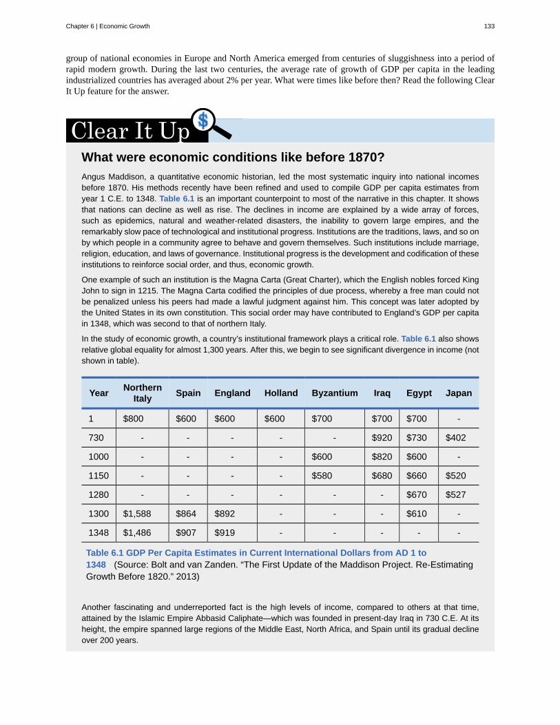
group of national economies in Europe and North America emerged from centuries of sluggishness into a period ofrapid modern growth. During the last two centuries, the average rate of growth of GDP per capita in the leadingindustrialized countries has averaged about 2% per year. What were times like before then? Read the following ClearIt Up feature for the answer.
What were economic conditions like before 1870?Angus Maddison, a quantitative economic historian, led the most systematic inquiry into national incomesbefore 1870. His methods recently have been refined and used to compile GDP per capita estimates fromyear 1 C.E. to 1348. Table 6.1 is an important counterpoint to most of the narrative in this chapter. It showsthat nations can decline as well as rise. The declines in income are explained by a wide array of forces,such as epidemics, natural and weather-related disasters, the inability to govern large empires, and theremarkably slow pace of technological and institutional progress. Institutions are the traditions, laws, and so onby which people in a community agree to behave and govern themselves. Such institutions include marriage,religion, education, and laws of governance. Institutional progress is the development and codification of theseinstitutions to reinforce social order, and thus, economic growth.
One example of such an institution is the Magna Carta (Great Charter), which the English nobles forced KingJohn to sign in 1215. The Magna Carta codified the principles of due process, whereby a free man could notbe penalized unless his peers had made a lawful judgment against him. This concept was later adopted bythe United States in its own constitution. This social order may have contributed to England’s GDP per capitain 1348, which was second to that of northern Italy.
In the study of economic growth, a country’s institutional framework plays a critical role. Table 6.1 also showsrelative global equality for almost 1,300 years. After this, we begin to see significant divergence in income (notshown in table).
Year NorthernItaly Spain England Holland Byzantium Iraq Egypt Japan
1 $800 $600 $600 $600 $700 $700 $700 -
730 - - - - - $920 $730 $402
1000 - - - - $600 $820 $600 -
1150 - - - - $580 $680 $660 $520
1280 - - - - - - $670 $527
1300 $1,588 $864 $892 - - - $610 -
1348 $1,486 $907 $919 - - - - -
Table 6.1 GDP Per Capita Estimates in Current International Dollars from AD 1 to1348 (Source: Bolt and van Zanden. “The First Update of the Maddison Project. Re-EstimatingGrowth Before 1820.” 2013)
Another fascinating and underreported fact is the high levels of income, compared to others at that time,attained by the Islamic Empire Abbasid Caliphate—which was founded in present-day Iraq in 730 C.E. At itsheight, the empire spanned large regions of the Middle East, North Africa, and Spain until its gradual declineover 200 years.
Chapter 6 | Economic Growth 133

The Industrial Revolution led to increasing inequality among nations. Some economies took off, whereas others, likemany of those in Africa or Asia, remained close to a subsistence standard of living. General calculations show thatthe 17 countries of the world with the most-developed economies had, on average, 2.4 times the GDP per capita ofthe world’s poorest economies in 1870. By 1960, the most developed economies had 4.2 times the GDP per capita ofthe poorest economies.
However, by the middle of the twentieth century, some countries had shown that catching up was possible. Japan’seconomic growth took off in the 1960s and 1970s, with a growth rate of real GDP per capita averaging 11% per yearduring those decades. Certain countries in Latin America experienced a boom in economic growth in the 1960s aswell. In Brazil, for example, GDP per capita expanded by an average annual rate of 11.1% from 1968 to 1973. Inthe 1970s, some East Asian economies, including South Korea, Thailand, and Taiwan, saw rapid growth. In thesecountries, growth rates of 11% to 12% per year in GDP per capita were not uncommon. More recently, China, withits population of 1.3 billion people, grew at a per capita rate 9% per year from 1984 into the 2000s. India, with apopulation of 1.1 billion, has shown promising signs of economic growth, with growth in GDP per capita of about4% per year during the 1990s and climbing toward 7% to 8% per year in the 2000s.
Visit this website (http://openstaxcollege.org/l/asiadevbank) to read about the Asian Development Bank.
These waves of catch-up economic growth have not reached all shores. In certain African countries like Niger,Tanzania, and Sudan, for example, GDP per capita at the start of the 2000s was still less than $300, not much higherthan it was in the nineteenth century and for centuries before that. In the context of the overall situation of low-incomepeople around the world, the good economic news from China (population: 1.3 billion) and India (population: 1.1billion) is, nonetheless, astounding and heartening.
Economic growth in the last two centuries has made a striking change in the human condition. Richard Easterlin, aneconomist at the University of Southern California, wrote in 2000:
By many measures, a revolution in the human condition is sweeping the world. Most people today arebetter fed, clothed, and housed than their predecessors two centuries ago. They are healthier, live longer,and are better educated. Women’s lives are less centered on reproduction and political democracy hasgained a foothold. Although Western Europe and its offshoots have been the leaders of this advance, mostof the less developed nations have joined in during the 20th century, with the newly emerging nations ofsub-Saharan Africa the latest to participate. Although the picture is not one of universal progress, it is thegreatest advance in the human condition of the world’s population ever achieved in such a brief span oftime.
Rule of Law and Economic GrowthEconomic growth depends on many factors. Key among those factors is adherence to the rule of law and protection ofproperty rights and contractual rights by a country’s government so that markets can work effectively and efficiently.Laws must be clear, public, fair, enforced, and equally applicable to all members of society. Property rights, asyou might recall from Environmental Protection and Negative Externalities (http://cnx.org/content/m57254/latest/) are the rights of individuals and firms to own property and use it as they see fit. If you have $100,you have the right to use that money, whether you spend it, lend it, or keep it in a jar. It is your property. The definitionof property includes physical property as well as the right to your training and experience, especially since your
134 Chapter 6 | Economic Growth
This OpenStax book is available for free at http://cnx.org/content/col11864/1.2
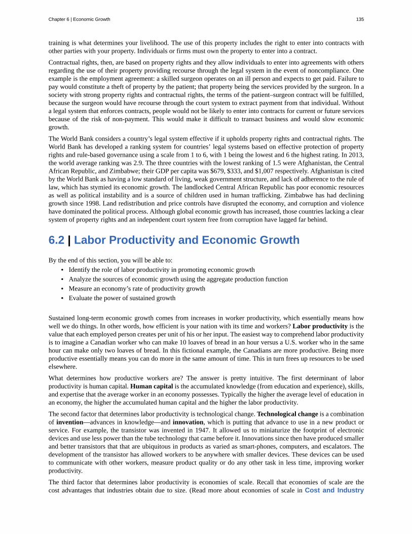
training is what determines your livelihood. The use of this property includes the right to enter into contracts withother parties with your property. Individuals or firms must own the property to enter into a contract.
Contractual rights, then, are based on property rights and they allow individuals to enter into agreements with othersregarding the use of their property providing recourse through the legal system in the event of noncompliance. Oneexample is the employment agreement: a skilled surgeon operates on an ill person and expects to get paid. Failure topay would constitute a theft of property by the patient; that property being the services provided by the surgeon. In asociety with strong property rights and contractual rights, the terms of the patient–surgeon contract will be fulfilled,because the surgeon would have recourse through the court system to extract payment from that individual. Withouta legal system that enforces contracts, people would not be likely to enter into contracts for current or future servicesbecause of the risk of non-payment. This would make it difficult to transact business and would slow economicgrowth.
The World Bank considers a country’s legal system effective if it upholds property rights and contractual rights. TheWorld Bank has developed a ranking system for countries’ legal systems based on effective protection of propertyrights and rule-based governance using a scale from 1 to 6, with 1 being the lowest and 6 the highest rating. In 2013,the world average ranking was 2.9. The three countries with the lowest ranking of 1.5 were Afghanistan, the CentralAfrican Republic, and Zimbabwe; their GDP per capita was $679, $333, and $1,007 respectively. Afghanistan is citedby the World Bank as having a low standard of living, weak government structure, and lack of adherence to the rule oflaw, which has stymied its economic growth. The landlocked Central African Republic has poor economic resourcesas well as political instability and is a source of children used in human trafficking. Zimbabwe has had declininggrowth since 1998. Land redistribution and price controls have disrupted the economy, and corruption and violencehave dominated the political process. Although global economic growth has increased, those countries lacking a clearsystem of property rights and an independent court system free from corruption have lagged far behind.
6.2 | Labor Productivity and Economic GrowthBy the end of this section, you will be able to:
• Identify the role of labor productivity in promoting economic growth• Analyze the sources of economic growth using the aggregate production function• Measure an economy’s rate of productivity growth• Evaluate the power of sustained growth
Sustained long-term economic growth comes from increases in worker productivity, which essentially means howwell we do things. In other words, how efficient is your nation with its time and workers? Labor productivity is thevalue that each employed person creates per unit of his or her input. The easiest way to comprehend labor productivityis to imagine a Canadian worker who can make 10 loaves of bread in an hour versus a U.S. worker who in the samehour can make only two loaves of bread. In this fictional example, the Canadians are more productive. Being moreproductive essentially means you can do more in the same amount of time. This in turn frees up resources to be usedelsewhere.
What determines how productive workers are? The answer is pretty intuitive. The first determinant of laborproductivity is human capital. Human capital is the accumulated knowledge (from education and experience), skills,and expertise that the average worker in an economy possesses. Typically the higher the average level of education inan economy, the higher the accumulated human capital and the higher the labor productivity.
The second factor that determines labor productivity is technological change. Technological change is a combinationof invention—advances in knowledge—and innovation, which is putting that advance to use in a new product orservice. For example, the transistor was invented in 1947. It allowed us to miniaturize the footprint of electronicdevices and use less power than the tube technology that came before it. Innovations since then have produced smallerand better transistors that that are ubiquitous in products as varied as smart-phones, computers, and escalators. Thedevelopment of the transistor has allowed workers to be anywhere with smaller devices. These devices can be usedto communicate with other workers, measure product quality or do any other task in less time, improving workerproductivity.
The third factor that determines labor productivity is economies of scale. Recall that economies of scale are thecost advantages that industries obtain due to size. (Read more about economies of scale in Cost and Industry
Chapter 6 | Economic Growth 135
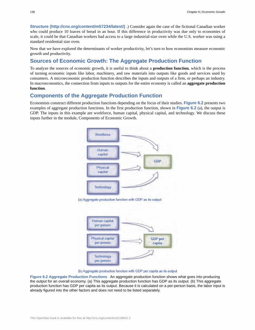
Structure (http://cnx.org/content/m57234/latest/) .) Consider again the case of the fictional Canadian workerwho could produce 10 loaves of bread in an hour. If this difference in productivity was due only to economies ofscale, it could be that Canadian workers had access to a large industrial-size oven while the U.S. worker was using astandard residential size oven.
Now that we have explored the determinants of worker productivity, let’s turn to how economists measure economicgrowth and productivity.
Sources of Economic Growth: The Aggregate Production FunctionTo analyze the sources of economic growth, it is useful to think about a production function, which is the processof turning economic inputs like labor, machinery, and raw materials into outputs like goods and services used byconsumers. A microeconomic production function describes the inputs and outputs of a firm, or perhaps an industry.In macroeconomics, the connection from inputs to outputs for the entire economy is called an aggregate productionfunction.
Components of the Aggregate Production FunctionEconomists construct different production functions depending on the focus of their studies. Figure 6.2 presents twoexamples of aggregate production functions. In the first production function, shown in Figure 6.2 (a), the output isGDP. The inputs in this example are workforce, human capital, physical capital, and technology. We discuss theseinputs further in the module, Components of Economic Growth.
Figure 6.2 Aggregate Production Functions An aggregate production function shows what goes into producingthe output for an overall economy. (a) This aggregate production function has GDP as its output. (b) This aggregateproduction function has GDP per capita as its output. Because it is calculated on a per-person basis, the labor input isalready figured into the other factors and does not need to be listed separately.
136 Chapter 6 | Economic Growth
This OpenStax book is available for free at http://cnx.org/content/col11864/1.2
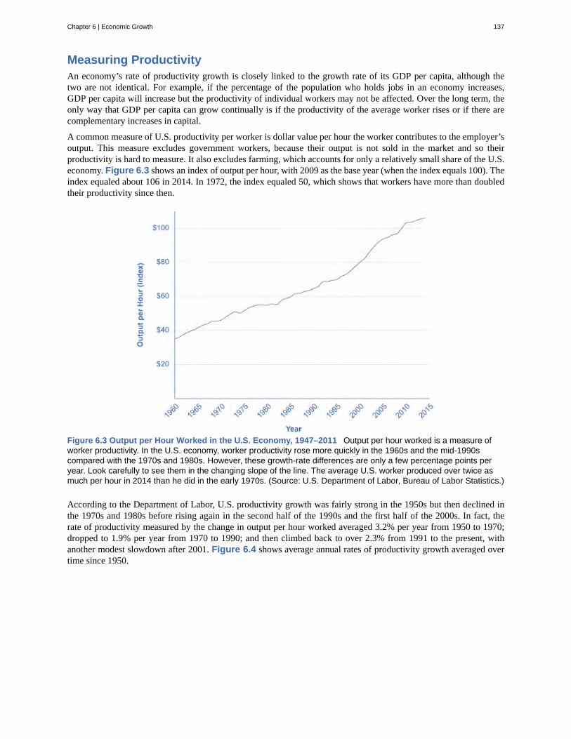
Measuring ProductivityAn economy’s rate of productivity growth is closely linked to the growth rate of its GDP per capita, although thetwo are not identical. For example, if the percentage of the population who holds jobs in an economy increases,GDP per capita will increase but the productivity of individual workers may not be affected. Over the long term, theonly way that GDP per capita can grow continually is if the productivity of the average worker rises or if there arecomplementary increases in capital.
A common measure of U.S. productivity per worker is dollar value per hour the worker contributes to the employer’soutput. This measure excludes government workers, because their output is not sold in the market and so theirproductivity is hard to measure. It also excludes farming, which accounts for only a relatively small share of the U.S.economy. Figure 6.3 shows an index of output per hour, with 2009 as the base year (when the index equals 100). Theindex equaled about 106 in 2014. In 1972, the index equaled 50, which shows that workers have more than doubledtheir productivity since then.
Figure 6.3 Output per Hour Worked in the U.S. Economy, 1947–2011 Output per hour worked is a measure ofworker productivity. In the U.S. economy, worker productivity rose more quickly in the 1960s and the mid-1990scompared with the 1970s and 1980s. However, these growth-rate differences are only a few percentage points peryear. Look carefully to see them in the changing slope of the line. The average U.S. worker produced over twice asmuch per hour in 2014 than he did in the early 1970s. (Source: U.S. Department of Labor, Bureau of Labor Statistics.)
According to the Department of Labor, U.S. productivity growth was fairly strong in the 1950s but then declined inthe 1970s and 1980s before rising again in the second half of the 1990s and the first half of the 2000s. In fact, therate of productivity measured by the change in output per hour worked averaged 3.2% per year from 1950 to 1970;dropped to 1.9% per year from 1970 to 1990; and then climbed back to over 2.3% from 1991 to the present, withanother modest slowdown after 2001. Figure 6.4 shows average annual rates of productivity growth averaged overtime since 1950.
Chapter 6 | Economic Growth 137
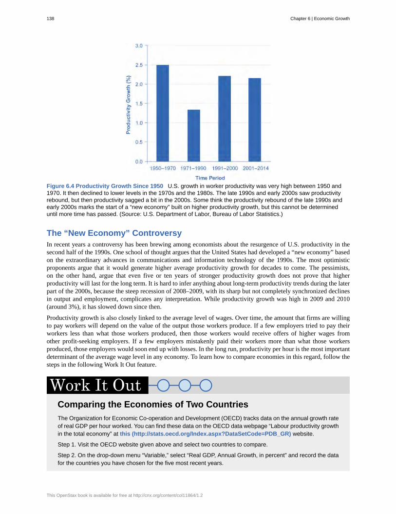
Figure 6.4 Productivity Growth Since 1950 U.S. growth in worker productivity was very high between 1950 and1970. It then declined to lower levels in the 1970s and the 1980s. The late 1990s and early 2000s saw productivityrebound, but then productivity sagged a bit in the 2000s. Some think the productivity rebound of the late 1990s andearly 2000s marks the start of a “new economy” built on higher productivity growth, but this cannot be determineduntil more time has passed. (Source: U.S. Department of Labor, Bureau of Labor Statistics.)
The “New Economy” ControversyIn recent years a controversy has been brewing among economists about the resurgence of U.S. productivity in thesecond half of the 1990s. One school of thought argues that the United States had developed a “new economy” basedon the extraordinary advances in communications and information technology of the 1990s. The most optimisticproponents argue that it would generate higher average productivity growth for decades to come. The pessimists,on the other hand, argue that even five or ten years of stronger productivity growth does not prove that higherproductivity will last for the long term. It is hard to infer anything about long-term productivity trends during the laterpart of the 2000s, because the steep recession of 2008–2009, with its sharp but not completely synchronized declinesin output and employment, complicates any interpretation. While productivity growth was high in 2009 and 2010(around 3%), it has slowed down since then.
Productivity growth is also closely linked to the average level of wages. Over time, the amount that firms are willingto pay workers will depend on the value of the output those workers produce. If a few employers tried to pay theirworkers less than what those workers produced, then those workers would receive offers of higher wages fromother profit-seeking employers. If a few employers mistakenly paid their workers more than what those workersproduced, those employers would soon end up with losses. In the long run, productivity per hour is the most importantdeterminant of the average wage level in any economy. To learn how to compare economies in this regard, follow thesteps in the following Work It Out feature.
Comparing the Economies of Two CountriesThe Organization for Economic Co-operation and Development (OECD) tracks data on the annual growth rateof real GDP per hour worked. You can find these data on the OECD data webpage “Labour productivity growthin the total economy” at this (http://stats.oecd.org/Index.aspx?DataSetCode=PDB_GR) website.
Step 1. Visit the OECD website given above and select two countries to compare.
Step 2. On the drop-down menu “Variable,” select “Real GDP, Annual Growth, in percent” and record the datafor the countries you have chosen for the five most recent years.
138 Chapter 6 | Economic Growth
This OpenStax book is available for free at http://cnx.org/content/col11864/1.2
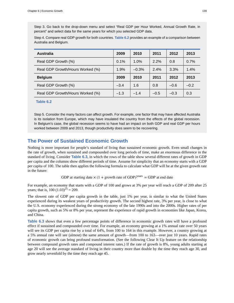
Step 3. Go back to the drop-down menu and select “Real GDP per Hour Worked, Annual Growth Rate, inpercent” and select data for the same years for which you selected GDP data.
Step 4. Compare real GDP growth for both countries. Table 6.2 provides an example of a comparison betweenAustralia and Belgium.
Australia 2009 2010 2011 2012 2013
Real GDP Growth (%) 0.1% 1.0% 2.2% 0.8 0.7%
Real GDP Growth/Hours Worked (%) 1.9% –0.3% 2.4% 3.3% 1.4%
Belgium 2009 2010 2011 2012 2013
Real GDP Growth (%) –3.4 1.6 0.8 –0.6 –0.2
Real GDP Growth/Hours Worked (%) –1.3 –1.4 –0.5 –0.3 0.3
Table 6.2
Step 5. Consider the many factors can affect growth. For example, one factor that may have affected Australiais its isolation from Europe, which may have insulated the country from the effects of the global recession.In Belgium’s case, the global recession seems to have had an impact on both GDP and real GDP per hoursworked between 2009 and 2013, though productivity does seem to be recovering.
The Power of Sustained Economic GrowthNothing is more important for people’s standard of living than sustained economic growth. Even small changes inthe rate of growth, when sustained and compounded over long periods of time, make an enormous difference in thestandard of living. Consider Table 6.3, in which the rows of the table show several different rates of growth in GDPper capita and the columns show different periods of time. Assume for simplicity that an economy starts with a GDPper capita of 100. The table then applies the following formula to calculate what GDP will be at the given growth ratein the future:
GDP at starting date × (1 + growth rate of GDP)years = GDP at end date
For example, an economy that starts with a GDP of 100 and grows at 3% per year will reach a GDP of 209 after 25years; that is, 100 (1.03)25 = 209.
The slowest rate of GDP per capita growth in the table, just 1% per year, is similar to what the United Statesexperienced during its weakest years of productivity growth. The second highest rate, 3% per year, is close to whatthe U.S. economy experienced during the strong economy of the late 1990s and into the 2000s. Higher rates of percapita growth, such as 5% or 8% per year, represent the experience of rapid growth in economies like Japan, Korea,and China.
Table 6.3 shows that even a few percentage points of difference in economic growth rates will have a profoundeffect if sustained and compounded over time. For example, an economy growing at a 1% annual rate over 50 yearswill see its GDP per capita rise by a total of 64%, from 100 to 164 in this example. However, a country growing ata 5% annual rate will see (almost) the same amount of growth—from 100 to 163—over just 10 years. Rapid ratesof economic growth can bring profound transformation. (See the following Clear It Up feature on the relationshipbetween compound growth rates and compound interest rates.) If the rate of growth is 8%, young adults starting atage 20 will see the average standard of living in their country more than double by the time they reach age 30, andgrow nearly sevenfold by the time they reach age 45.
Chapter 6 | Economic Growth 139
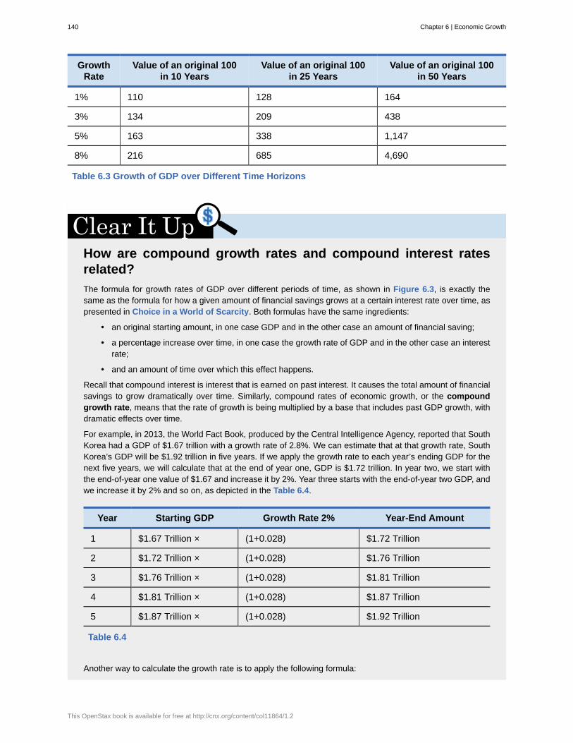
GrowthRate
Value of an original 100in 10 Years
Value of an original 100in 25 Years
Value of an original 100in 50 Years
1% 110 128 164
3% 134 209 438
5% 163 338 1,147
8% 216 685 4,690
Table 6.3 Growth of GDP over Different Time Horizons
How are compound growth rates and compound interest ratesrelated?The formula for growth rates of GDP over different periods of time, as shown in Figure 6.3, is exactly thesame as the formula for how a given amount of financial savings grows at a certain interest rate over time, aspresented in Choice in a World of Scarcity. Both formulas have the same ingredients:
• an original starting amount, in one case GDP and in the other case an amount of financial saving;
• a percentage increase over time, in one case the growth rate of GDP and in the other case an interestrate;
• and an amount of time over which this effect happens.
Recall that compound interest is interest that is earned on past interest. It causes the total amount of financialsavings to grow dramatically over time. Similarly, compound rates of economic growth, or the compoundgrowth rate, means that the rate of growth is being multiplied by a base that includes past GDP growth, withdramatic effects over time.
For example, in 2013, the World Fact Book, produced by the Central Intelligence Agency, reported that SouthKorea had a GDP of $1.67 trillion with a growth rate of 2.8%. We can estimate that at that growth rate, SouthKorea’s GDP will be $1.92 trillion in five years. If we apply the growth rate to each year’s ending GDP for thenext five years, we will calculate that at the end of year one, GDP is $1.72 trillion. In year two, we start withthe end-of-year one value of $1.67 and increase it by 2%. Year three starts with the end-of-year two GDP, andwe increase it by 2% and so on, as depicted in the Table 6.4.
Year Starting GDP Growth Rate 2% Year-End Amount
1 $1.67 Trillion × (1+0.028) $1.72 Trillion
2 $1.72 Trillion × (1+0.028) $1.76 Trillion
3 $1.76 Trillion × (1+0.028) $1.81 Trillion
4 $1.81 Trillion × (1+0.028) $1.87 Trillion
5 $1.87 Trillion × (1+0.028) $1.92 Trillion
Table 6.4
Another way to calculate the growth rate is to apply the following formula:
140 Chapter 6 | Economic Growth
This OpenStax book is available for free at http://cnx.org/content/col11864/1.2
Future Value = Present Value × (1 + g)n
Where “future value” is the value of GDP five years hence, “present value” is the starting GDP amount of$1.64 trillion, “g” is the growth rate of 2%, and “n” is the number of periods for which we are calculating growth.
Future Value = 1.67 × (1+0.028)5 = $1.92 trillion
6.3 | Components of Economic GrowthBy the end of this section, you will be able to:
• Discuss the components of economic growth, including physical capital, human capital, andtechnology
• Explain capital deepening and its significance• Analyze the methods employed in economic growth accounting studies• Identify factors that contribute to a healthy climate for economic growth
Over decades and generations, seemingly small differences of a few percentage points in the annual rate of economicgrowth make an enormous difference in GDP per capita. In this module, we discuss some of the components ofeconomic growth, including physical capital, human capital, and technology.
The category of physical capital includes the plant and equipment used by firms and also things like roads (alsocalled infrastructure). Again, greater physical capital implies more output. Physical capital can affect productivity intwo ways: (1) an increase in the quantity of physical capital (for example, more computers of the same quality); and(2) an increase in the quality of physical capital (same number of computers but the computers are faster, and so on).Human capital and physical capital accumulation are similar: In both cases, investment now pays off in longer-termproductivity in the future.
The category of technology is the “joker in the deck.” Earlier we described it as the combination of invention andinnovation. When most people think of new technology, the invention of new products like the laser, the smartphone,or some new wonder drug come to mind. In food production, the development of more drought-resistant seeds isanother example of technology. Technology, as economists use the term, however, includes still more. It includes newways of organizing work, like the invention of the assembly line, new methods for ensuring better quality of output infactories, and innovative institutions that facilitate the process of converting inputs into output. In short, technologycomprises all the advances that make the existing machines and other inputs produce more, and at higher quality, aswell as altogether new products.
It may not make sense to compare the GDPs of China and say, Benin, simply because of the great difference inpopulation size. To understand economic growth, which is really concerned with the growth in living standards of anaverage person, it is often useful to focus on GDP per capita. Using GDP per capita also makes it easier to comparecountries with smaller numbers of people, like Belgium, Uruguay, or Zimbabwe, with countries that have largerpopulations, like the United States, the Russian Federation, or Nigeria.
To obtain a per capita production function, divide each input in Figure 6.2(a) by the population. This creates asecond aggregate production function where the output is GDP per capita (that is, GDP divided by population).The inputs are the average level of human capital per person, the average level of physical capital per person,and the level of technology per person—see Figure 6.2(b). The result of having population in the denominatoris mathematically appealing. Increases in population lower per capita income. However, increasing population isimportant for the average person only if the rate of income growth exceeds population growth. A more importantreason for constructing a per capita production function is to understand the contribution of human and physicalcapital.
Capital DeepeningWhen society increases the level of capital per person, the result is called capital deepening. The idea of capitaldeepening can apply both to additional human capital per worker and to additional physical capital per worker.
Chapter 6 | Economic Growth 141
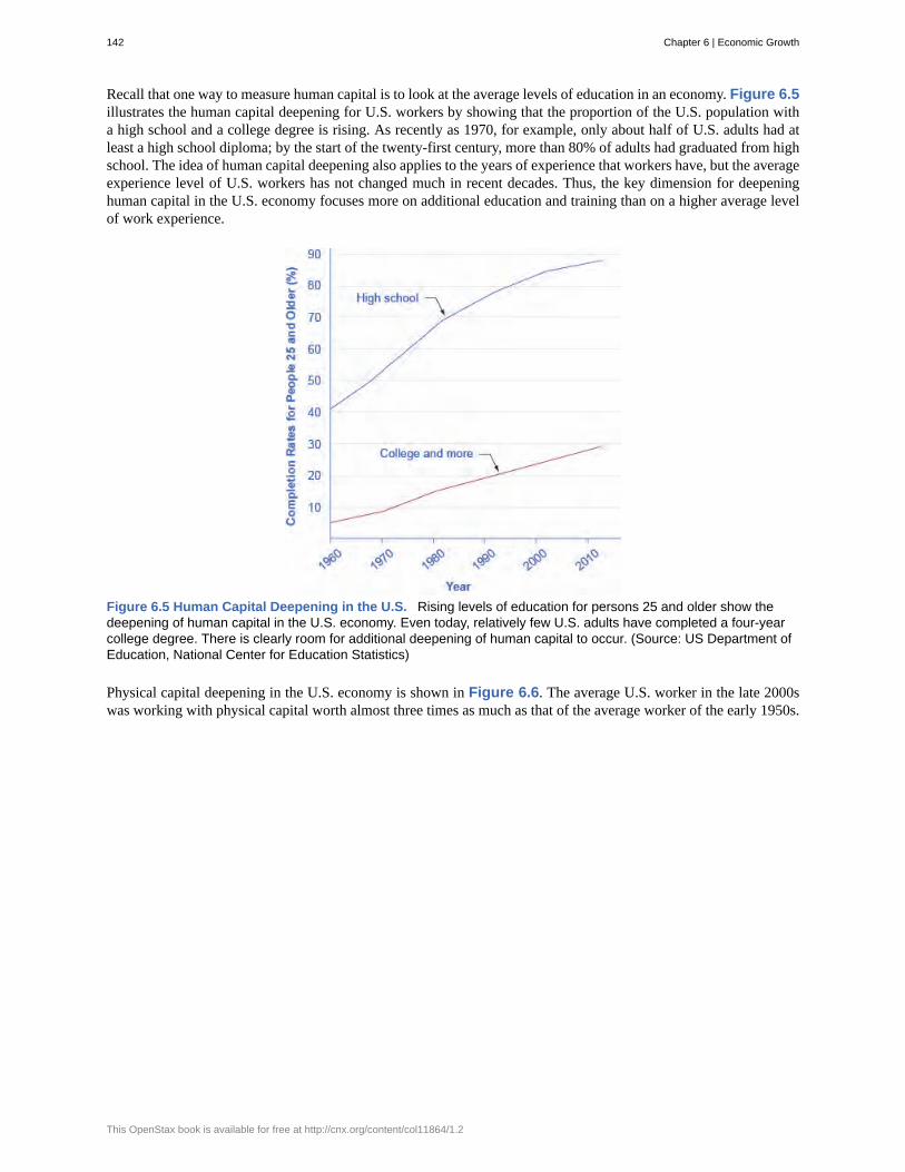
Recall that one way to measure human capital is to look at the average levels of education in an economy. Figure 6.5illustrates the human capital deepening for U.S. workers by showing that the proportion of the U.S. population witha high school and a college degree is rising. As recently as 1970, for example, only about half of U.S. adults had atleast a high school diploma; by the start of the twenty-first century, more than 80% of adults had graduated from highschool. The idea of human capital deepening also applies to the years of experience that workers have, but the averageexperience level of U.S. workers has not changed much in recent decades. Thus, the key dimension for deepeninghuman capital in the U.S. economy focuses more on additional education and training than on a higher average levelof work experience.
Figure 6.5 Human Capital Deepening in the U.S. Rising levels of education for persons 25 and older show thedeepening of human capital in the U.S. economy. Even today, relatively few U.S. adults have completed a four-yearcollege degree. There is clearly room for additional deepening of human capital to occur. (Source: US Department ofEducation, National Center for Education Statistics)
Physical capital deepening in the U.S. economy is shown in Figure 6.6. The average U.S. worker in the late 2000swas working with physical capital worth almost three times as much as that of the average worker of the early 1950s.
142 Chapter 6 | Economic Growth
This OpenStax book is available for free at http://cnx.org/content/col11864/1.2
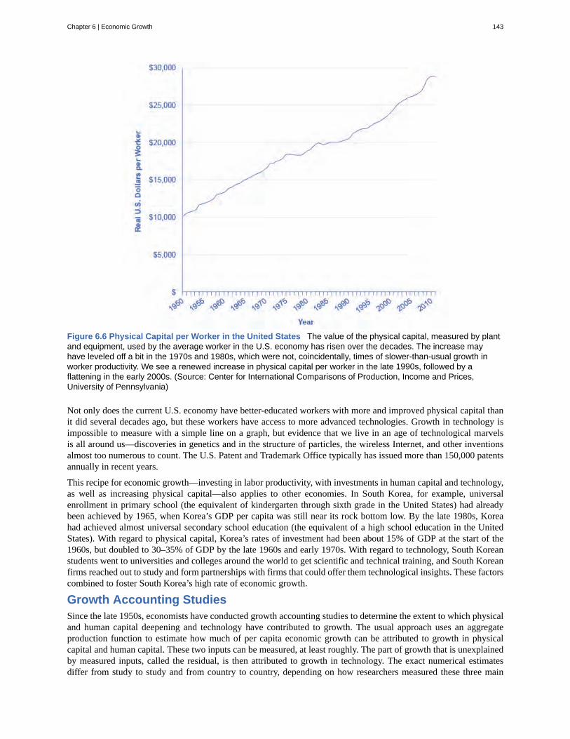
Figure 6.6 Physical Capital per Worker in the United States The value of the physical capital, measured by plantand equipment, used by the average worker in the U.S. economy has risen over the decades. The increase mayhave leveled off a bit in the 1970s and 1980s, which were not, coincidentally, times of slower-than-usual growth inworker productivity. We see a renewed increase in physical capital per worker in the late 1990s, followed by aflattening in the early 2000s. (Source: Center for International Comparisons of Production, Income and Prices,University of Pennsylvania)
Not only does the current U.S. economy have better-educated workers with more and improved physical capital thanit did several decades ago, but these workers have access to more advanced technologies. Growth in technology isimpossible to measure with a simple line on a graph, but evidence that we live in an age of technological marvelsis all around us—discoveries in genetics and in the structure of particles, the wireless Internet, and other inventionsalmost too numerous to count. The U.S. Patent and Trademark Office typically has issued more than 150,000 patentsannually in recent years.
This recipe for economic growth—investing in labor productivity, with investments in human capital and technology,as well as increasing physical capital—also applies to other economies. In South Korea, for example, universalenrollment in primary school (the equivalent of kindergarten through sixth grade in the United States) had alreadybeen achieved by 1965, when Korea’s GDP per capita was still near its rock bottom low. By the late 1980s, Koreahad achieved almost universal secondary school education (the equivalent of a high school education in the UnitedStates). With regard to physical capital, Korea’s rates of investment had been about 15% of GDP at the start of the1960s, but doubled to 30–35% of GDP by the late 1960s and early 1970s. With regard to technology, South Koreanstudents went to universities and colleges around the world to get scientific and technical training, and South Koreanfirms reached out to study and form partnerships with firms that could offer them technological insights. These factorscombined to foster South Korea’s high rate of economic growth.
Growth Accounting StudiesSince the late 1950s, economists have conducted growth accounting studies to determine the extent to which physicaland human capital deepening and technology have contributed to growth. The usual approach uses an aggregateproduction function to estimate how much of per capita economic growth can be attributed to growth in physicalcapital and human capital. These two inputs can be measured, at least roughly. The part of growth that is unexplainedby measured inputs, called the residual, is then attributed to growth in technology. The exact numerical estimatesdiffer from study to study and from country to country, depending on how researchers measured these three main
Chapter 6 | Economic Growth 143

factors over what time horizons. For studies of the U.S. economy, three lessons commonly emerge from growthaccounting studies.
First, technology is typically the most important contributor to U.S. economic growth. Growth in human capital andphysical capital often explains only half or less than half of the economic growth that occurs. New ways of doingthings are tremendously important.
Second, while investment in physical capital is essential to growth in labor productivity and GDP per capita, buildinghuman capital is at least as important. Economic growth is not just a matter of more machines and buildings. Onevivid example of the power of human capital and technological knowledge occurred in Europe in the years after WorldWar II (1939–1945). During the war, a large share of Europe’s physical capital, such as factories, roads, and vehicles,was destroyed. Europe also lost an overwhelming amount of human capital in the form of millions of men, women,and children who died during the war. However, the powerful combination of skilled workers and technologicalknowledge, working within a market-oriented economic framework, rebuilt Europe’s productive capacity to an evenhigher level within less than two decades.
A third lesson is that these three factors of human capital, physical capital, and technology work together. Workerswith a higher level of education and skills are often better at coming up with new technological innovations. Thesetechnological innovations are often ideas that cannot increase production until they become a part of new investmentin physical capital. New machines that embody technological innovations often require additional training, whichbuilds worker skills further. If the recipe for economic growth is to succeed, an economy needs all the ingredientsof the aggregate production function. See the following Clear It Up feature for an example of how human capital,physical capital, and technology can combine to significantly impact lives.
How do girls’ education and economic growth relate in low-income countries?In the early 2000s, according to the World Bank, about 110 million children between the ages of 6 and 11were not in school—and about two-thirds of them were girls. In Bangladesh, for example, the illiteracy rate forthose aged 15 to 24 was 78% for females, compared to 75% for males. In Egypt, for this age group, illiteracywas 84% for females and 91% for males. Cambodia had 86% illiteracy for females and 88% for males. Nigeriahad 66% illiteracy for females in the 15 to 24 age bracket and 78% for males.
Whenever any child does not receive a basic education, it is both a human and an economic loss. In low-income countries, wages typically increase by an average of 10 to 20% with each additional year of education.There is, however, some intriguing evidence that helping girls in low-income countries to close the educationgap with boys may be especially important, because of the social role that many of the girls will play asmothers and homemakers.
Girls in low-income countries who receive more education tend to grow up to have fewer, healthier, better-educated children. Their children are more likely to be better nourished and to receive basic health care likeimmunizations. Economic research on women in low-income economies backs up these findings. When 20women get one additional year of schooling, as a group they will, on average, have one less child. When 1,000women get one additional year of schooling, on average one to two fewer women from that group will die inchildbirth. When a woman stays in school an additional year, that factor alone means that, on average, eachof her children will spend an additional half-year in school. Education for girls is a good investment because itis an investment in economic growth with benefits beyond the current generation.
A Healthy Climate for Economic GrowthWhile physical and human capital deepening and better technology are important, equally important to a nation’swell-being is the climate or system within which these inputs are cultivated. Both the type of market economy and alegal system that governs and sustains property rights and contractual rights are important contributors to a healthyeconomic climate.
144 Chapter 6 | Economic Growth
This OpenStax book is available for free at http://cnx.org/content/col11864/1.2
A healthy economic climate usually involves some sort of market orientation at the microeconomic, individual,or firm decision-making level. Markets that allow personal and business rewards and incentives for increasinghuman and physical capital encourage overall macroeconomic growth. For example, when workers participate in acompetitive and well-functioning labor market, they have an incentive to acquire additional human capital, becauseadditional education and skills will pay off in higher wages. Firms have an incentive to invest in physical capitaland in training workers, because they expect to earn higher profits for their shareholders. Both individuals and firmslook for new technologies, because even small inventions can make work easier or lead to product improvement.Collectively, such individual and business decisions made within a market structure add up to macroeconomic growth.Much of the rapid growth since the late nineteenth century has come from harnessing the power of competitivemarkets to allocate resources. This market orientation typically reaches beyond national borders and includesopenness to international trade.
A general orientation toward markets does not rule out important roles for government. There are times when marketsfail to allocate capital or technology in a manner that provides the greatest benefit for society as a whole. The roleof the government is to correct these failures. In addition, government can guide or influence markets toward certainoutcomes. The following examples highlight some important areas that governments around the world have chosento invest in to facilitate capital deepening and technology:
• Education. The Danish government requires all children under 16 to attend school. They can choose to attenda public school (Folkeskole) or a private school. Students do not pay tuition to attend Folkeskole. Thirteenpercent of primary/secondary (elementary/high) school is private, and the government supplies vouchers tocitizens who choose private school.
• Savings and Investment. In the United States, as in other countries, private investment is taxed. Low capitalgains taxes encourage investment and so also economic growth.
• Infrastructure. The Japanese government in the mid-1990s undertook significant infrastructure projects toimprove roads and public works. This in turn increased the stock of physical capital and ultimately economicgrowth.
• Special Economic Zones. The island of Mauritius is one of the few African nations to encourage internationaltrade in government-supported special economic zones (SEZ). These are areas of the country, usuallywith access to a port where, among other benefits, the government does not tax trade. As a result of itsSEZ, Mauritius has enjoyed above-average economic growth since the 1980s. Free trade does not have tooccur in an SEZ however. Governments can encourage international trade across the board, or surrender toprotectionism.
• Scientific Research. The European Union has strong programs to invest in scientific research. The researchersAbraham García and Pierre Mohnen demonstrate that firms which received support from the Austriangovernment actually increased their research intensity and had more sales. Governments can support scientificresearch and technical training that helps to create and spread new technologies. Governments can alsoprovide a legal environment that protects the ability of inventors to profit from their inventions.
There are many more ways in which the government can play an active role in promoting economic growth; weexplore them in other chapters and in particular in Macroeconomic Policy Around the World. A healthy climatefor growth in GDP per capita and labor productivity includes human capital deepening, physical capital deepening,and technological gains, operating in a market-oriented economy with supportive government policies.
6.4 | Economic ConvergenceBy the end of this section, you will be able to:
• Explain economic convergence• Analyze various arguments for and against economic convergence• Evaluate the speed of economic convergence between high-income countries and the rest of the world
Some low-income and middle-income economies around the world have shown a pattern of convergence, in whichtheir economies grow faster than those of high-income countries. GDP increased by an average rate of 2.7% per year
Chapter 6 | Economic Growth 145
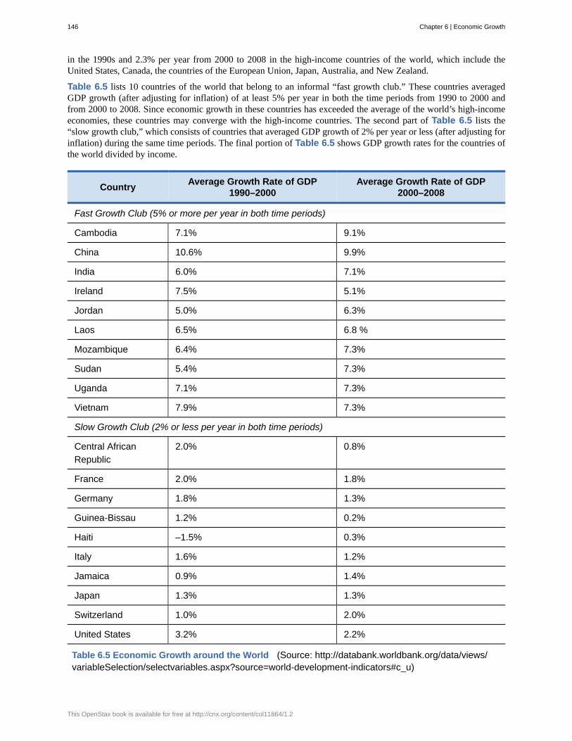
in the 1990s and 2.3% per year from 2000 to 2008 in the high-income countries of the world, which include theUnited States, Canada, the countries of the European Union, Japan, Australia, and New Zealand.
Table 6.5 lists 10 countries of the world that belong to an informal “fast growth club.” These countries averagedGDP growth (after adjusting for inflation) of at least 5% per year in both the time periods from 1990 to 2000 andfrom 2000 to 2008. Since economic growth in these countries has exceeded the average of the world’s high-incomeeconomies, these countries may converge with the high-income countries. The second part of Table 6.5 lists the“slow growth club,” which consists of countries that averaged GDP growth of 2% per year or less (after adjusting forinflation) during the same time periods. The final portion of Table 6.5 shows GDP growth rates for the countries ofthe world divided by income.
Country Average Growth Rate of GDP1990–2000
Average Growth Rate of GDP2000–2008
Fast Growth Club (5% or more per year in both time periods)
Cambodia 7.1% 9.1%
China 10.6% 9.9%
India 6.0% 7.1%
Ireland 7.5% 5.1%
Jordan 5.0% 6.3%
Laos 6.5% 6.8 %
Mozambique 6.4% 7.3%
Sudan 5.4% 7.3%
Uganda 7.1% 7.3%
Vietnam 7.9% 7.3%
Slow Growth Club (2% or less per year in both time periods)
Central AfricanRepublic
2.0% 0.8%
France 2.0% 1.8%
Germany 1.8% 1.3%
Guinea-Bissau 1.2% 0.2%
Haiti –1.5% 0.3%
Italy 1.6% 1.2%
Jamaica 0.9% 1.4%
Japan 1.3% 1.3%
Switzerland 1.0% 2.0%
United States 3.2% 2.2%
Table 6.5 Economic Growth around the World (Source: http://databank.worldbank.org/data/views/variableSelection/selectvariables.aspx?source=world-development-indicators#c_u)
146 Chapter 6 | Economic Growth
This OpenStax book is available for free at http://cnx.org/content/col11864/1.2
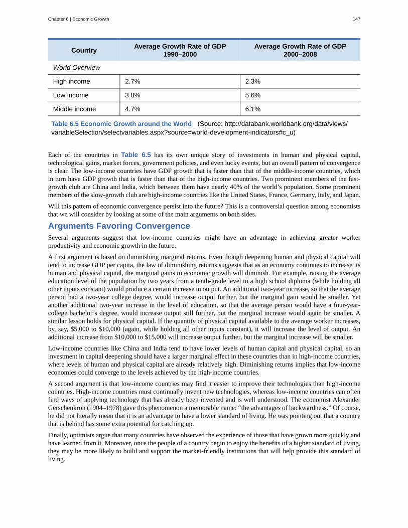
Country Average Growth Rate of GDP1990–2000
Average Growth Rate of GDP2000–2008
World Overview
High income 2.7% 2.3%
Low income 3.8% 5.6%
Middle income 4.7% 6.1%
Table 6.5 Economic Growth around the World (Source: http://databank.worldbank.org/data/views/variableSelection/selectvariables.aspx?source=world-development-indicators#c_u)
Each of the countries in Table 6.5 has its own unique story of investments in human and physical capital,technological gains, market forces, government policies, and even lucky events, but an overall pattern of convergenceis clear. The low-income countries have GDP growth that is faster than that of the middle-income countries, whichin turn have GDP growth that is faster than that of the high-income countries. Two prominent members of the fast-growth club are China and India, which between them have nearly 40% of the world’s population. Some prominentmembers of the slow-growth club are high-income countries like the United States, France, Germany, Italy, and Japan.
Will this pattern of economic convergence persist into the future? This is a controversial question among economiststhat we will consider by looking at some of the main arguments on both sides.
Arguments Favoring ConvergenceSeveral arguments suggest that low-income countries might have an advantage in achieving greater workerproductivity and economic growth in the future.
A first argument is based on diminishing marginal returns. Even though deepening human and physical capital willtend to increase GDP per capita, the law of diminishing returns suggests that as an economy continues to increase itshuman and physical capital, the marginal gains to economic growth will diminish. For example, raising the averageeducation level of the population by two years from a tenth-grade level to a high school diploma (while holding allother inputs constant) would produce a certain increase in output. An additional two-year increase, so that the averageperson had a two-year college degree, would increase output further, but the marginal gain would be smaller. Yetanother additional two-year increase in the level of education, so that the average person would have a four-year-college bachelor’s degree, would increase output still further, but the marginal increase would again be smaller. Asimilar lesson holds for physical capital. If the quantity of physical capital available to the average worker increases,by, say, $5,000 to $10,000 (again, while holding all other inputs constant), it will increase the level of output. Anadditional increase from $10,000 to $15,000 will increase output further, but the marginal increase will be smaller.
Low-income countries like China and India tend to have lower levels of human capital and physical capital, so aninvestment in capital deepening should have a larger marginal effect in these countries than in high-income countries,where levels of human and physical capital are already relatively high. Diminishing returns implies that low-incomeeconomies could converge to the levels achieved by the high-income countries.
A second argument is that low-income countries may find it easier to improve their technologies than high-incomecountries. High-income countries must continually invent new technologies, whereas low-income countries can oftenfind ways of applying technology that has already been invented and is well understood. The economist AlexanderGerschenkron (1904–1978) gave this phenomenon a memorable name: “the advantages of backwardness.” Of course,he did not literally mean that it is an advantage to have a lower standard of living. He was pointing out that a countrythat is behind has some extra potential for catching up.
Finally, optimists argue that many countries have observed the experience of those that have grown more quickly andhave learned from it. Moreover, once the people of a country begin to enjoy the benefits of a higher standard of living,they may be more likely to build and support the market-friendly institutions that will help provide this standard ofliving.
Chapter 6 | Economic Growth 147
View this video (http://openstaxcollege.org/l/tedhansrosling) to learn about economic growth across the world.
Arguments That Convergence Is neither Inevitable nor LikelyIf the growth of an economy depended only on the deepening of human capital and physical capital, then the growthrate of that economy would be expected to slow down over the long run because of diminishing marginal returns.However, there is another crucial factor in the aggregate production function: technology.
The development of new technology can provide a way for an economy to sidestep the diminishing marginal returnsof capital deepening. Figure 6.7 shows how. The horizontal axis of the figure measures the amount of capitaldeepening, which on this figure is an overall measure that includes deepening of both physical and human capital. Theamount of human and physical capital per worker increases as you move from left to right, from C1 to C2 to C3. Thevertical axis of the diagram measures per capita output. Start by considering the lowest line in this diagram, labeledTechnology 1. Along this aggregate production function, the level of technology is being held constant, so the lineshows only the relationship between capital deepening and output. As capital deepens from C1 to C2 to C3 and theeconomy moves from R to U to W, per capita output does increase—but the way in which the line starts out steeperon the left but then flattens as it moves to the right shows the diminishing marginal returns, as additional marginalamounts of capital deepening increase output by ever-smaller amounts. The shape of the aggregate production line(Technology 1) shows that the ability of capital deepening, by itself, to generate sustained economic growth is limited,since diminishing returns will eventually set in.
Figure 6.7 Capital Deepening and New Technology Imagine that the economy starts at point R, with the level ofphysical and human capital C1 and the output per capita at G1. If the economy relies only on capital deepening, whileremaining at the technology level shown by the Technology 1 line, then it would face diminishing marginal returns asit moved from point R to point U to point W. However, now imagine that capital deepening is combined withimprovements in technology. Then, as capital deepens from C1 to C2, technology improves from Technology 1 toTechnology 2, and the economy moves from R to S. Similarly, as capital deepens from C2 to C3, technologyincreases from Technology 2 to Technology 3, and the economy moves from S to T. With improvements intechnology, there is no longer any reason that economic growth must necessarily slow down.
Now, bring improvements in technology into the picture. Improved technology means that with a given set ofinputs, more output is possible. The production function labeled Technology 1 in the figure is based on one level oftechnology, but Technology 2 is based on an improved level of technology, so for every level of capital deepening on
148 Chapter 6 | Economic Growth
This OpenStax book is available for free at http://cnx.org/content/col11864/1.2
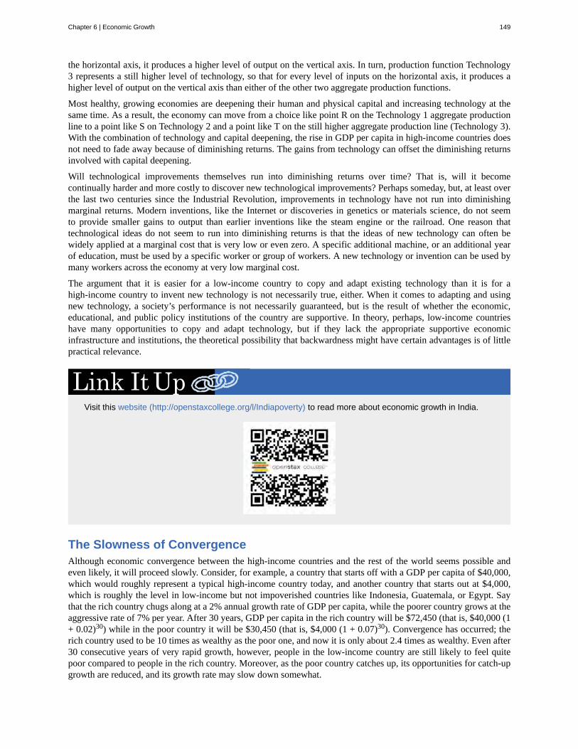
the horizontal axis, it produces a higher level of output on the vertical axis. In turn, production function Technology3 represents a still higher level of technology, so that for every level of inputs on the horizontal axis, it produces ahigher level of output on the vertical axis than either of the other two aggregate production functions.
Most healthy, growing economies are deepening their human and physical capital and increasing technology at thesame time. As a result, the economy can move from a choice like point R on the Technology 1 aggregate productionline to a point like S on Technology 2 and a point like T on the still higher aggregate production line (Technology 3).With the combination of technology and capital deepening, the rise in GDP per capita in high-income countries doesnot need to fade away because of diminishing returns. The gains from technology can offset the diminishing returnsinvolved with capital deepening.
Will technological improvements themselves run into diminishing returns over time? That is, will it becomecontinually harder and more costly to discover new technological improvements? Perhaps someday, but, at least overthe last two centuries since the Industrial Revolution, improvements in technology have not run into diminishingmarginal returns. Modern inventions, like the Internet or discoveries in genetics or materials science, do not seemto provide smaller gains to output than earlier inventions like the steam engine or the railroad. One reason thattechnological ideas do not seem to run into diminishing returns is that the ideas of new technology can often bewidely applied at a marginal cost that is very low or even zero. A specific additional machine, or an additional yearof education, must be used by a specific worker or group of workers. A new technology or invention can be used bymany workers across the economy at very low marginal cost.
The argument that it is easier for a low-income country to copy and adapt existing technology than it is for ahigh-income country to invent new technology is not necessarily true, either. When it comes to adapting and usingnew technology, a society’s performance is not necessarily guaranteed, but is the result of whether the economic,educational, and public policy institutions of the country are supportive. In theory, perhaps, low-income countrieshave many opportunities to copy and adapt technology, but if they lack the appropriate supportive economicinfrastructure and institutions, the theoretical possibility that backwardness might have certain advantages is of littlepractical relevance.
Visit this website (http://openstaxcollege.org/l/Indiapoverty) to read more about economic growth in India.
The Slowness of ConvergenceAlthough economic convergence between the high-income countries and the rest of the world seems possible andeven likely, it will proceed slowly. Consider, for example, a country that starts off with a GDP per capita of $40,000,which would roughly represent a typical high-income country today, and another country that starts out at $4,000,which is roughly the level in low-income but not impoverished countries like Indonesia, Guatemala, or Egypt. Saythat the rich country chugs along at a 2% annual growth rate of GDP per capita, while the poorer country grows at theaggressive rate of 7% per year. After 30 years, GDP per capita in the rich country will be $72,450 (that is, $40,000 (1+ 0.02)30) while in the poor country it will be $30,450 (that is, $4,000 (1 + 0.07)30). Convergence has occurred; therich country used to be 10 times as wealthy as the poor one, and now it is only about 2.4 times as wealthy. Even after30 consecutive years of very rapid growth, however, people in the low-income country are still likely to feel quitepoor compared to people in the rich country. Moreover, as the poor country catches up, its opportunities for catch-upgrowth are reduced, and its growth rate may slow down somewhat.
Chapter 6 | Economic Growth 149
The slowness of convergence illustrates again that small differences in annual rates of economic growth become hugedifferences over time. The high-income countries have been building up their advantage in standard of living overdecades—more than a century in some cases. Even in an optimistic scenario, it will take decades for the low-incomecountries of the world to catch up significantly.
Calories and Economic GrowthThe story of modern economic growth can be told by looking at calorie consumption over time. The dramaticrise in incomes allowed the average person to eat better and consume more calories. How did these incomesincrease? The neoclassical growth consensus uses the aggregate production function to suggest that theperiod of modern economic growth came about because of increases in inputs such as technology andphysical and human capital. Also important was the way in which technological progress combined withphysical and human capital deepening to create growth and convergence. The issue of distribution of incomenotwithstanding, it is clear that the average worker can afford more calories in 2014 than in 1875.
Aside from increases in income, there is another reason why the average person can afford more food.Modern agriculture has allowed many countries to produce more food than they need. Despite having morethan enough food, however, many governments and multilateral agencies have not solved the food distributionproblem. In fact, food shortages, famine, or general food insecurity are caused more often by the failureof government macroeconomic policy, according to the Nobel Prize-winning economist Amartya Sen. Senhas conducted extensive research into issues of inequality, poverty, and the role of government in improvingstandards of living. Macroeconomic policies that strive toward stable inflation, full employment, education ofwomen, and preservation of property rights are more likely to eliminate starvation and provide for a more evendistribution of food.
Because we have more food per capita, global food prices have decreased since 1875. The prices of somefoods, however, have decreased more than the prices of others. For example, researchers from the Universityof Washington have shown that in the United States, calories from zucchini and lettuce are 100 times moreexpensive than calories from oil, butter, and sugar. Research from countries like India, China, and the UnitedStates suggests that as incomes rise, individuals want more calories from fats and protein and fewer fromcarbohydrates. This has very interesting implications for global food production, obesity, and environmentalconsequences. Affluent urban India has an obesity problem much like many parts of the United States. Theforces of convergence are at work.
150 Chapter 6 | Economic Growth
This OpenStax book is available for free at http://cnx.org/content/col11864/1.2
aggregate production function
capital deepening
compound growth rate
contractual rights
convergence
human capital
Industrial Revolution
infrastructure
innovation
invention
labor productivity
modern economic growth
physical capital
production function
rule of law
special economic zone (SEZ)
technological change
technology
KEY TERMS
the process whereby an economy as a whole turns economic inputs such as humancapital, physical capital, and technology into output measured as GDP per capita
an increase by society in the average level of physical and/or human capital per person
the rate of growth when multiplied by a base that includes past GDP growth
the rights of individuals to enter into agreements with others regarding the use of their propertyproviding recourse through the legal system in the event of noncompliance
pattern in which economies with low per capita incomes grow faster than economies with high per capitaincomes
the accumulated skills and education of workers
the widespread use of power-driven machinery and the economic and social changes thatoccurred in the first half of the 1800s
a component of physical capital such as roads, rail systems, and so on
putting advances in knowledge to use in a new product or service
advances in knowledge
the value of what is produced per worker, or per hour worked (sometimes called workerproductivity)
the period of rapid economic growth from 1870 onward
the plant and equipment used by firms in production; this includes infrastructure
the process whereby a firm turns economic inputs like labor, machinery, and raw materials intooutputs like goods and services used by consumers
the process of enacting laws that protect individual and entity rights to use their property as they see fit.Laws must be clear, public, fair, and enforced, and applicable to all members of society
area of a country, usually with access to a port where, among other benefits, thegovernment does not tax trade
a combination of invention—advances in knowledge—and innovation
all the ways in which existing inputs produce more or higher quality, as well as different and altogether newproducts
KEY CONCEPTS AND SUMMARY
6.1 The Relatively Recent Arrival of Economic GrowthSince the early nineteenth century, there has been a spectacular process of long-run economic growth during whichthe world’s leading economies—mostly those in Western Europe and North America—expanded GDP per capita atan average rate of about 2% per year. In the last half-century, countries like Japan, South Korea, and China haveshown the potential to catch up. The extensive process of economic growth, often referred to as modern economic
Chapter 6 | Economic Growth 151
growth, was facilitated by the Industrial Revolution, which increased worker productivity and trade, as well as thedevelopment of governance and market institutions.
6.2 Labor Productivity and Economic GrowthProductivity, the value of what is produced per worker, or per hour worked, can be measured as the level of GDP perworker or GDP per hour. The United States experienced a productivity slowdown between 1973 and 1989. Since then,U.S. productivity has rebounded (the current global recession notwithstanding). It is not clear whether the currentgrowth in productivity will be sustained. The rate of productivity growth is the primary determinant of an economy’srate of long-term economic growth and higher wages. Over decades and generations, seemingly small differences ofa few percentage points in the annual rate of economic growth make an enormous difference in GDP per capita. Anaggregate production function specifies how certain inputs in the economy, like human capital, physical capital, andtechnology, lead to the output measured as GDP per capita.
Compound interest and compound growth rates behave in the same way as productivity rates. Seemingly smallchanges in percentage points can have big impacts on income over time.
6.3 Components of Economic GrowthOver decades and generations, seemingly small differences of a few percentage points in the annual rate of economicgrowth make an enormous difference in GDP per capita. Capital deepening refers to an increase in the amount ofcapital per worker, either human capital per worker, in the form of higher education or skills, or physical capital perworker. Technology, in its economic meaning, refers broadly to all new methods of production, which includes majorscientific inventions but also small inventions and even better forms of management or other types of institutions.A healthy climate for growth in GDP per capita consists of improvements in human capital, physical capital, andtechnology, in a market-oriented environment with supportive public policies and institutions.
6.4 Economic ConvergenceWhen countries with lower levels of GDP per capita catch up to countries with higher levels of GDP per capita,the process is called convergence. Convergence can occur even when both high- and low-income countries increaseinvestment in physical and human capital with the objective of growing GDP. This is because the impact of newinvestment in physical and human capital on a low-income country may result in huge gains as new skills orequipment are combined with the labor force. In higher-income countries, however, a level of investment equal tothat of the low income country is not likely to have as big an impact, because the more developed country mostlikely has high levels of capital investment. Therefore, the marginal gain from this additional investment tends to besuccessively less and less. Higher income countries are more likely to have diminishing returns to their investmentsand must continually invent new technologies; this allows lower-income economies to have a chance for convergentgrowth. However, many high-income economies have developed economic and political institutions that provide ahealthy economic climate for an ongoing stream of technological innovations. Continuous technological innovationcan counterbalance diminishing returns to investments in human and physical capital.
SELF-CHECK QUESTIONS1. Explain what the Industrial Revolution was and where it began.
2. Explain the difference between property rights and contractual rights. Why do they matter to economic growth?
3. Are there other ways in which we can measure productivity besides the amount produced per hour of work?
4. Assume there are two countries: South Korea and the United States. South Korea grows at 4% and the UnitedStates grows at 1%. For the sake of simplicity, assume they both start from the same fictional income level, $10,000.What will the incomes of the United States and South Korea be in 20 years? By how many multiples will eachcountry’s income grow in 20 years?
5. What do the growth accounting studies conclude are the determinants of growth? Which is more important, thedeterminants or how they are combined?
6. What policies can the government of a free-market economy implement to stimulate economic growth?
152 Chapter 6 | Economic Growth
This OpenStax book is available for free at http://cnx.org/content/col11864/1.2
7. List the areas where government policy can help economic growth.
8. Use an example to explain why, after periods of rapid growth, a low-income country that has not caught up to ahigh-income country may feel poor.
9. Would the following events usually lead to capital deepening? Why or why not?a. A weak economy in which businesses become reluctant to make long-term investments in physical capital.b. A rise in international trade.c. A trend in which many more adults participate in continuing education courses through their employers and
at colleges and universities.
10. What are the “advantages of backwardness” for economic growth?
11. Would you expect capital deepening to result in diminished returns? Why or why not? Would you expectimprovements in technology to result in diminished returns? Why or why not?
12. Why does productivity growth in high-income economies not slow down as it runs into diminishing returnsfrom additional investments in physical capital and human capital? Does this show one area where the theory ofdiminishing returns fails to apply? Why or why not?
REVIEW QUESTIONS
13. How did the Industrial Revolution increase the rateof economic growth and income levels in the UnitedStates?
14. How much should a nation be concerned if itsrate of economic growth is just 2% slower than othernations?
15. How is GDP per capita calculated differently fromlabor productivity?
16. How do gains in labor productivity lead to gains inGDP per capita?
17. What is an aggregate production function?
18. What is capital deepening?
19. What do economists mean when they refer toimprovements in technology?
20. For a high-income economy like the United States,what elements of the aggregate production function aremost important in bringing about growth in GDP percapita? What about a middle-income country such asBrazil? A low-income country such as Niger?
21. List some arguments for and against the likelihoodof convergence.
CRITICAL THINKING QUESTIONS
22. Over the past 50 years, many countries haveexperienced an annual growth rate in real GDP percapita greater than that of the United States. Someexamples are China, Japan, South Korea, and Taiwan.Does that mean the United States is regressing relativeto other countries? Does that mean these countries willeventually overtake the United States in terms of rate ofgrowth of real GDP per capita? Explain.
23. Labor Productivity and Economic Growthoutlined the logic of how increased productivity isassociated with increased wages. Detail a situationwhere this is not the case and explain why it is not.
24. Change in labor productivity is one of the mostwatched international statistics of growth. Visit the St.
Louis Federal Reserve website and find the data section(http://research.stlouisfed.org). Find internationalcomparisons of labor productivity, listed under theFRED Economic database (Growth Rate of Total LaborProductivity), and compare two countries in the recentpast. State what you think the reasons for differences inlabor productivity could be.
25. Refer back to the Work It Out about Comparingthe Economies of Two Countries and examine the datafor the two countries you chose. How are they similar?How are they different?
26. Education seems to be important for human capitaldeepening. As people become better educated and more
Chapter 6 | Economic Growth 153
knowledgeable, are there limits to how much additionalbenefit more education can provide? Why or why not?
27. Describe some of the political and social tradeoffsthat might occur when a less developed country adoptsa strategy to promote labor force participation andeconomic growth via investment in girls’ education.
28. Why is investing in girls’ education beneficial forgrowth?
29. How is the concept of technology, as defined withthe aggregate production function, different from oureveryday use of the word?
30. What sorts of policies can governments implementto encourage convergence?
31. As technological change makes us more sedentaryand food costs increase, obesity is likely. What factorsdo you think may limit obesity?
PROBLEMS32. An economy starts off with a GDP per capita of$5,000. How large will the GDP per capita be if it growsat an annual rate of 2% for 20 years? 2% for 40 years?4% for 40 years? 6% for 40 years?
33. An economy starts off with a GDP per capita of12,000 euros. How large will the GDP per capita be if itgrows at an annual rate of 3% for 10 years? 3% for 30years? 6% for 30 years?
34. Say that the average worker in Canada has aproductivity level of $30 per hour while the averageworker in the United Kingdom has a productivity level
of $25 per hour (both measured in U.S. dollars). Overthe next five years, say that worker productivity inCanada grows at 1% per year while worker productivityin the UK grows 3% per year. After five years, who willhave the higher productivity level, and by how much?
35. Say that the average worker in the U.S. economyis eight times as productive as an average worker inMexico. If the productivity of U.S. workers grows at 2%for 25 years and the productivity of Mexico’s workersgrows at 6% for 25 years, which country will havehigher worker productivity at that point?
154 Chapter 6 | Economic Growth
This OpenStax book is available for free at http://cnx.org/content/col11864/1.2

7 | Unemployment
Figure 7.1 Out of Business Borders was one of the many companies unable to recover from the economicrecession of 2008-2009. (Credit: modification of work by Luis Villa del Campo/Flickr Creative Commons)
The Mysterious Case of the Missing CandidatesNearly eight million U.S. jobs were lost during the Great Recession of 2008-2009, with unemployment peakingat 10% in October 2009, according to the Bureau of Labor Statistics (BLS). That is a huge number of positionsgone. During the tepid recovery, some positions were added, but as of summer 2013, unemployment hadremained persistently higher than the pre-recession rate of less than 5%. Some economists and policymakersworried the recovery would be “jobless.” With the economy growing, albeit slowly, why wasn’t theunemployment number falling? Why were firms not hiring?
Peter Cappelli, noted Wharton management professor and Director of Wharton’s Center for HumanResources, does not believe the job search process is akin to what he terms the “Home Depot” view of hiring.According to him, this view “basically says that filling a job is like replacing a part in a washing machine. Yousimply find someone who does the exact same job as that broken part, plug him or her into the washingmachine and that is it.” The job search, for both the prospective employee and the employer, is more complexthan that.
In a hiring situation, employers hold all the cards. They write the job descriptions, determine the salaries,decide when and how to advertise positions, and set the controls on employment application screeningsoftware. Advertising for positions has increased as the economic recovery progresses, yet here’s the kicker:Employers say there are no applicants out there who meet their needs. While the unemployment rate is nowbelow 6% as of the beginning of 2015, many economists and policymakers (including the Chair of the Federal
Chapter 7 | Unemployment 155
Reserve, Janet Yellen) are still concerned about "slack" in the labor market. So the question arises: where arethe job candidates?
That question leads us to the topic of this chapter—unemployment. What constitutes it? How is it measured?And if the economy is growing, why isn’t the pool of job openings growing along with it? Sounds like theeconomy has a case of “missing” candidates.
Introduction to UnemploymentIn this chapter, you will learn about:
• How the Unemployment Rate is Defined and Computed
• Patterns of Unemployment
• What Causes Changes in Unemployment over the Short Run
• What Causes Changes in Unemployment over the Long Run
Unemployment can be a terrible and wrenching life experience—like a serious automobile accident or a messydivorce—whose consequences can be fully understood only by someone who has gone through it. For unemployedindividuals and their families, there is the day-to-day financial stress of not knowing where the next paycheck iscoming from. There are painful adjustments, like watching your savings account dwindle, selling a car and buyinga cheaper one, or moving to a less expensive place to live. Even when the unemployed person finds a new job,it may pay less than the previous one. For many people, their job is an important part of their self worth. Whenunemployment separates people from the workforce, it can affect family relationships as well as mental and physicalhealth.
The human costs of unemployment alone would justify making a low level of unemployment an important publicpolicy priority. But unemployment also includes economic costs to the broader society. When millions of unemployedbut willing workers cannot find jobs, an economic resource is going unused. An economy with high unemploymentis like a company operating with a functional but unused factory. The opportunity cost of unemployment is the outputthat could have been produced by the unemployed workers.
This chapter will discuss how the unemployment rate is defined and computed. It will examine the patterns ofunemployment over time, for the U.S. economy as a whole, for different demographic groups in the U.S. economy,and for other countries. It will then consider an economic explanation for unemployment, and how it explains thepatterns of unemployment and suggests public policies for reducing it.
7.1 | How the Unemployment Rate Is Defined andComputedBy the end of this section, you will be able to:
• Calculate the labor force percentage and the unemployment rate• Explain hidden unemployment and what it means to be in or out of the labor force• Evaluate the collection and interpretation of unemployment data
Unemployment is typically described in newspaper or television reports as a percentage or a rate. A recent reportmight have said, for example, from August 2009 to November 2009, the U.S. unemployment rate rose from 9.7% to10.0%, but by June 2010, it had fallen to 9.5%. At a glance, the changes between the percentages may seem small.But remember that the U.S. economy has about 155 million adults who either have jobs or are looking for them. A riseor fall of just 0.1% in the unemployment rate of 155 million potential workers translates into 155,000 people, whichis roughly the total population of a city like Syracuse, New York, Brownsville, Texas, or Pasadena, California. Largerises in the unemployment rate mean large numbers of job losses. In November 2009, at the peak of the recession,
156 Chapter 7 | Unemployment
This OpenStax book is available for free at http://cnx.org/content/col11864/1.2
about 15 million people were out of work. Even with the unemployment rate now at 5.5% as of February 2015, about8 million people total are out of work.
The Bureau of Labor Statistics (http://openstaxcollege.org/l/BLS1) tracks and reports all data related tounemployment.
Who’s In or Out of the Labor Force?Should everyone without a job be counted as unemployed? Of course not. Children, for example, should not becounted as unemployed. Surely, the retired should not be counted as unemployed. Many full-time college studentshave only a part-time job, or no job at all, but it seems inappropriate to count them as suffering the pains ofunemployment. Some people are not working because they are rearing children, ill, on vacation, or on parental leave.
The point is that the adult population is not just divided into employed and unemployed. A third group exists: peoplewho do not have a job, and for some reason—retirement, looking after children, taking a voluntary break before anew job—are not interested in having a job, either. It also includes those who do want a job but have quit looking,often due to being discouraged by their inability to find suitable employment. Economists refer to this third group ofthose who are not working and not looking for work as out of the labor force or not in the labor force.
The U.S. unemployment rate, which is based on a monthly survey carried out by the U.S. Bureau of the Census, asksa series of questions to divide up the adult population into employed, unemployed, or not in the labor force. To beclassified as unemployed, a person must be without a job, currently available to work, and actively looking for workin the previous four weeks. Thus, a person who does not have a job but who is not currently available to work or hasnot actively looked for work in the last four weeks is counted as out of the labor force.
Employed: currently working for pay
Unemployed: Out of work and actively looking for a job
Out of the labor force: Out of paid work and not actively looking for a job
Labor force: the number of employed plus the unemployed
Calculating the Unemployment RateFigure 7.2 shows the three-way division of the over-16 adult population. In February 2015, about 62.8% of the adultpopulation was "in the labor force"; that is, people are either employed or without a job but looking for work. Thosein the labor force can be divided into the employed and the unemployed. These values are also shown in Table 7.1.The unemployment rate is not the percentage of the total adult population without jobs, but rather the percentage ofadults who are in the labor force but who do not have jobs:
Unemployment rate = Unemployed peopleTotal labor force
× 100
Chapter 7 | Unemployment 157
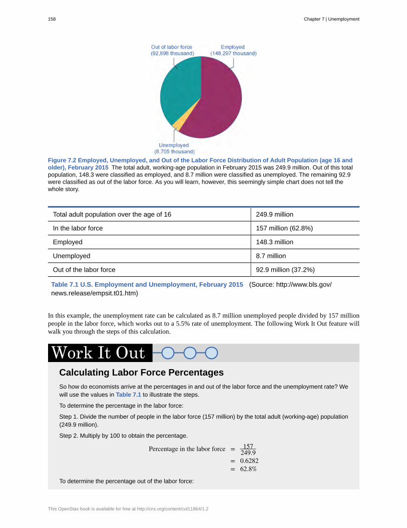
Figure 7.2 Employed, Unemployed, and Out of the Labor Force Distribution of Adult Population (age 16 andolder), February 2015 The total adult, working-age population in February 2015 was 249.9 million. Out of this totalpopulation, 148.3 were classified as employed, and 8.7 million were classified as unemployed. The remaining 92.9were classified as out of the labor force. As you will learn, however, this seemingly simple chart does not tell thewhole story.
Total adult population over the age of 16 249.9 million
In the labor force 157 million (62.8%)
Employed 148.3 million
Unemployed 8.7 million
Out of the labor force 92.9 million (37.2%)
Table 7.1 U.S. Employment and Unemployment, February 2015 (Source: http://www.bls.gov/news.release/empsit.t01.htm)
In this example, the unemployment rate can be calculated as 8.7 million unemployed people divided by 157 millionpeople in the labor force, which works out to a 5.5% rate of unemployment. The following Work It Out feature willwalk you through the steps of this calculation.
Calculating Labor Force PercentagesSo how do economists arrive at the percentages in and out of the labor force and the unemployment rate? Wewill use the values in Table 7.1 to illustrate the steps.
To determine the percentage in the labor force:
Step 1. Divide the number of people in the labor force (157 million) by the total adult (working-age) population(249.9 million).
Step 2. Multiply by 100 to obtain the percentage.
Percentage in the labor force = 157249.9
= 0.6282= 62.8%
To determine the percentage out of the labor force:
158 Chapter 7 | Unemployment
This OpenStax book is available for free at http://cnx.org/content/col11864/1.2
Step 1. Divide the number of people out the labor force (92.9 million) by the total adult (working-age)population (249.9 million).
Step 2. Multiply by 100 to obtain the percentage.
Percentage in the labor force = 92.9249.9
= 0.3717= 37.2%
To determine the unemployment rate:
Step 1. Divide the number of unemployed people (8.7 million) by the total labor force (157 million).
Step 2. Multiply by 100 to obtain the rate.
Unemployment rate = 8.7157
= 0.0554= 5.5%
Hidden UnemploymentEven with the “out of the labor force” category, there are still some people that are mislabeled in the categorizationof employed, unemployed, or out of the labor force. There are some people who have only part time or temporaryjobs and who are looking for full time and permanent employment that are counted as employed, though they arenot employed in the way they would like or need to be. Additionally, there are individuals who are underemployed.This includes those that are trained or skilled for one type or level of work who are working in a lower paying jobor one that does not utilize their skills. For example, an individual with a college degree in finance who is workingas a sales clerk would be considered underemployed. They are, however, also counted in the employed group. All ofthese individuals fall under the umbrella of the term “hidden unemployment.” Discouraged workers, those who havestopped looking for employment and, hence, are no longer counted in the unemployed also fall into this group
Labor Force Participation RateAnother important statistic is the labor force participation rate. This is the percentage of adults in an economy whoare either employed or who are unemployed and looking for a job. So, using the data in Figure 7.2 and Table 7.1,those included in this calculation would be the 157 million individuals in the labor force. The rate is calculated bytaking the number of people in the labor force, that is, the number employed and the number unemployed, divided bythe total adult population and multiplying by 100 to get the percentage. For the data from February 2015, the laborforce participation rate is 62.8%. Historically, the civilian labor force participation rate in the United States climbedbeginning in the 1960s as women increasingly entered the workforce, and it peaked at around 68% in late 1999 toearly 2000. Since then, the labor force participation rate has steadily declined.
The Establishment Payroll SurveyWhen the unemployment report comes out each month, the Bureau of Labor Statistics (BLS) also reports on thenumber of jobs created—which comes from the establishment payroll survey. The payroll survey is based on a surveyof about 140,000 businesses and government agencies throughout the United States. It generates payroll employmentestimates by the following criteria: all employees, average weekly hours worked, and average hourly, weekly, andovertime earnings. One of the criticisms of this survey is that it does not count the self-employed. It also does notmake a distinction between new, minimum wage, part time or temporary jobs and full time jobs with “decent” pay.
How Is the U.S. Unemployment Data Collected?The unemployment rate announced by the U.S. Bureau of Labor Statistics each month is based on the CurrentPopulation Survey (CPS), which has been carried out every month since 1940. Great care is taken to make this surveyrepresentative of the country as a whole. The country is first divided into 3,137 areas. The U.S. Bureau of the Censusthen selects 729 of these areas to survey. The 729 areas are then divided into districts of about 300 households each,and each district is divided into clusters of about four dwelling units. Every month, Census Bureau employees callabout 15,000 of the four-household clusters, for a total of 60,000 households. Households are interviewed for four
Chapter 7 | Unemployment 159
consecutive months, then rotated out of the survey for eight months, and then interviewed again for the same fourmonths the following year, before leaving the sample permanently.
Based on this survey, unemployment rates are calculated by state, industry, urban and rural areas, gender, age, race orethnicity, and level of education. A wide variety of other information is available, too. For example, how long havepeople been unemployed? Did they become unemployed because they quit, or were laid off, or their employer wentout of business? Is the unemployed person the only wage earner in the family? The Current Population Survey isa treasure trove of information about employment and unemployment. If you are wondering what the difference isbetween the CPS and EPS, read the following Clear it Up feature.
What is the difference between CPS and EPS?The Current Population Survey (CPS) conducted by the United States Census Bureau measures thepercentage of the labor force that is unemployed. The establishment payroll survey (EPS) by the Bureau ofLabor Statistics is a payroll survey that measures the net change in jobs created for the month.
Criticisms of Measuring UnemploymentThere are always complications in measuring the number of unemployed. For example, what about people who donot have jobs and would be available to work, but have gotten discouraged at the lack of available jobs in their areaand stopped looking? Such people, and their families, may be suffering the pains of unemployment. But the surveycounts them as out of the labor force because they are not actively looking for work. Other people may tell the CensusBureau that they are ready to work and looking for a job but, truly, they are not that eager to work and are not lookingvery hard at all. They are counted as unemployed, although they might more accurately be classified as out of thelabor force. Still other people may have a job, perhaps doing something like yard work, child care, or cleaning houses,but are not reporting the income earned to the tax authorities. They may report being unemployed, when they actuallyare working.
Although the unemployment rate gets most of the public and media attention, economic researchers at the Bureau ofLabor Statistics publish a wide array of surveys and reports that try to measure these kinds of issues and to developa more nuanced and complete view of the labor market. It is not exactly a hot news flash that economic statisticsare imperfect. Even imperfect measures like the unemployment rate, however, can still be quite informative, wheninterpreted knowledgeably and sensibly.
Click here (http://openstaxcollege.org/l/BLS_CPS) to learn more about the CPS to read frequently askedquestions about employment and labor.
160 Chapter 7 | Unemployment
This OpenStax book is available for free at http://cnx.org/content/col11864/1.2
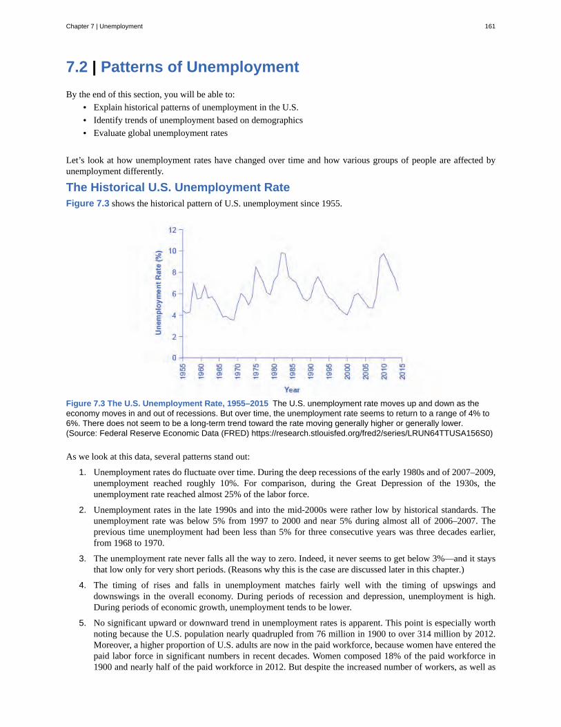
7.2 | Patterns of UnemploymentBy the end of this section, you will be able to:
• Explain historical patterns of unemployment in the U.S.• Identify trends of unemployment based on demographics• Evaluate global unemployment rates
Let’s look at how unemployment rates have changed over time and how various groups of people are affected byunemployment differently.
The Historical U.S. Unemployment RateFigure 7.3 shows the historical pattern of U.S. unemployment since 1955.
Figure 7.3 The U.S. Unemployment Rate, 1955–2015 The U.S. unemployment rate moves up and down as theeconomy moves in and out of recessions. But over time, the unemployment rate seems to return to a range of 4% to6%. There does not seem to be a long-term trend toward the rate moving generally higher or generally lower.(Source: Federal Reserve Economic Data (FRED) https://research.stlouisfed.org/fred2/series/LRUN64TTUSA156S0)
As we look at this data, several patterns stand out:
1. Unemployment rates do fluctuate over time. During the deep recessions of the early 1980s and of 2007–2009,unemployment reached roughly 10%. For comparison, during the Great Depression of the 1930s, theunemployment rate reached almost 25% of the labor force.
2. Unemployment rates in the late 1990s and into the mid-2000s were rather low by historical standards. Theunemployment rate was below 5% from 1997 to 2000 and near 5% during almost all of 2006–2007. Theprevious time unemployment had been less than 5% for three consecutive years was three decades earlier,from 1968 to 1970.
3. The unemployment rate never falls all the way to zero. Indeed, it never seems to get below 3%—and it staysthat low only for very short periods. (Reasons why this is the case are discussed later in this chapter.)
4. The timing of rises and falls in unemployment matches fairly well with the timing of upswings anddownswings in the overall economy. During periods of recession and depression, unemployment is high.During periods of economic growth, unemployment tends to be lower.
5. No significant upward or downward trend in unemployment rates is apparent. This point is especially worthnoting because the U.S. population nearly quadrupled from 76 million in 1900 to over 314 million by 2012.Moreover, a higher proportion of U.S. adults are now in the paid workforce, because women have entered thepaid labor force in significant numbers in recent decades. Women composed 18% of the paid workforce in1900 and nearly half of the paid workforce in 2012. But despite the increased number of workers, as well as
Chapter 7 | Unemployment 161
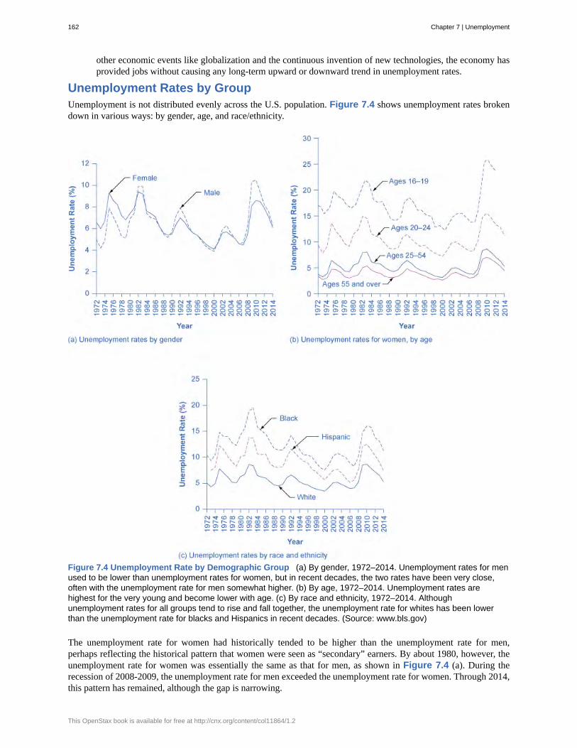
other economic events like globalization and the continuous invention of new technologies, the economy hasprovided jobs without causing any long-term upward or downward trend in unemployment rates.
Unemployment Rates by GroupUnemployment is not distributed evenly across the U.S. population. Figure 7.4 shows unemployment rates brokendown in various ways: by gender, age, and race/ethnicity.
Figure 7.4 Unemployment Rate by Demographic Group (a) By gender, 1972–2014. Unemployment rates for menused to be lower than unemployment rates for women, but in recent decades, the two rates have been very close,often with the unemployment rate for men somewhat higher. (b) By age, 1972–2014. Unemployment rates arehighest for the very young and become lower with age. (c) By race and ethnicity, 1972–2014. Althoughunemployment rates for all groups tend to rise and fall together, the unemployment rate for whites has been lowerthan the unemployment rate for blacks and Hispanics in recent decades. (Source: www.bls.gov)
The unemployment rate for women had historically tended to be higher than the unemployment rate for men,perhaps reflecting the historical pattern that women were seen as “secondary” earners. By about 1980, however, theunemployment rate for women was essentially the same as that for men, as shown in Figure 7.4 (a). During therecession of 2008-2009, the unemployment rate for men exceeded the unemployment rate for women. Through 2014,this pattern has remained, although the gap is narrowing.
162 Chapter 7 | Unemployment
This OpenStax book is available for free at http://cnx.org/content/col11864/1.2
Read this report (http://openstaxcollege.org/l/BLS_recession) for detailed information on the recession of2008–2009. It also provides some very useful information on the statistics of unemployment.
Younger workers tend to have higher unemployment, while middle-aged workers tend to have lower unemployment,probably because the middle-aged workers feel the responsibility of needing to have a job more heavily. Youngerworkers move in and out of jobs (and in and out of the labor force) more easily. Elderly workers have extremely lowrates of unemployment, because those who do not have jobs often exit the labor force by retiring, and thus are notcounted in the unemployment statistics. Figure 7.4 (b) shows unemployment rates for women divided by age; thepattern for men is similar.
The unemployment rate for African-Americans is substantially higher than the rate for other racial or ethnic groups,a fact that surely reflects, to some extent, a pattern of discrimination that has constrained blacks’ labor marketopportunities. However, the gaps between unemployment rates for whites and for blacks and Hispanics diminishedin the 1990s, as shown in Figure 7.4 (c). In fact, unemployment rates for blacks and Hispanics were at the lowestlevels for several decades in the mid-2000s before rising during the recent Great Recession.
Finally, those with less education typically suffer higher unemployment. In February 2015, for example, theunemployment rate for those with a college degree was 2.7%; for those with some college but not a four year degree,the unemployment rate was 5.1%; for high school graduates with no additional degree, the unemployment rate was5.4%; and for those without a high school diploma, the unemployment rate was 8.4%. This pattern may arise becauseadditional education offers better connections to the labor market and higher demand, or it may occur because thelabor market opportunities for low-skilled workers are less attractive than the opportunities for the more highly-skilled. Because of lower pay, low-skilled workers may be less motivated to find jobs.
Breaking Down Unemployment in Other WaysThe Bureau of Labor Statistics also gives information about the reasons for being unemployed as well as the lengthof time individuals have been unemployed. Table 7.2, for example, shows the four reasons for being unemployedand the percentages of the currently unemployed that fall into each category. Table 7.3 shows the length ofunemployment. For both of these, the data is from February of 2015. (bls.gov)
Reason Percentage
New Entrants 11.2%
Re-entrants 30.5%
Job Leavers 10.2%
Job Losers: Temporary 11.7%
Job Losers: Non Temporary 36.3%
Table 7.2 Reasons for Being Unemployed, February 2015
Chapter 7 | Unemployment 163
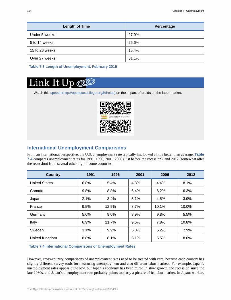
Length of Time Percentage
Under 5 weeks 27.9%
5 to 14 weeks 25.6%
15 to 26 weeks 15.4%
Over 27 weeks 31.1%
Table 7.3 Length of Unemployment, February 2015
Watch this speech (http://openstaxcollege.org/l/droids) on the impact of droids on the labor market.
International Unemployment ComparisonsFrom an international perspective, the U.S. unemployment rate typically has looked a little better than average. Table7.4 compares unemployment rates for 1991, 1996, 2001, 2006 (just before the recession), and 2012 (somewhat afterthe recession) from several other high-income countries.
Country 1991 1996 2001 2006 2012
United States 6.8% 5.4% 4.8% 4.4% 8.1%
Canada 9.8% 8.8% 6.4% 6.2% 6.3%
Japan 2.1% 3.4% 5.1% 4.5% 3.9%
France 9.5% 12.5% 8.7% 10.1% 10.0%
Germany 5.6% 9.0% 8.9% 9.8% 5.5%
Italy 6.9% 11.7% 9.6% 7.8% 10.8%
Sweden 3.1% 9.9% 5.0% 5.2% 7.9%
United Kingdom 8.8% 8.1% 5.1% 5.5% 8.0%
Table 7.4 International Comparisons of Unemployment Rates
However, cross-country comparisons of unemployment rates need to be treated with care, because each country hasslightly different survey tools for measuring unemployment and also different labor markets. For example, Japan’sunemployment rates appear quite low, but Japan’s economy has been mired in slow growth and recession since thelate 1980s, and Japan’s unemployment rate probably paints too rosy a picture of its labor market. In Japan, workers
164 Chapter 7 | Unemployment
This OpenStax book is available for free at http://cnx.org/content/col11864/1.2
who lose their jobs are often quick to exit the labor force and not look for a new job, in which case they are not countedas unemployed. In addition, Japanese firms are often quite reluctant to fire workers, and so firms have substantialnumbers of workers who are on reduced hours or officially employed, but doing very little. This Japanese pattern isperhaps best viewed as an unusual method for society to provide support for the unemployed, rather than a sign of ahealthy economy.
We hear about the Chinese economy in the news all the time. The value of the Chinese yuan in comparison tothe U.S. dollar is likely to be part of the nightly business report. So why is the Chinese economy not includedin this discussion of international unemployment? The lack of reliable statistics is probably the reason. Thisarticle (http://openstaxcollege.org/l/ChinaEmployment) explains why.
Comparing unemployment rates in the United States and other high-income economies with unemployment ratesin Latin America, Africa, Eastern Europe, and Asia is very difficult. One reason is that the statistical agencies inmany poorer countries lack the resources and technical capabilities of the U.S. Bureau of the Census. But a moredifficult problem with international comparisons is that in many low-income countries, most workers are not involvedin the labor market through an employer who pays them regularly. Instead, workers in these countries are engagedin short-term work, subsistence activities, and barter. Moreover, the effect of unemployment is very different inhigh-income and low-income countries. Unemployed workers in the developed economies have access to variousgovernment programs like unemployment insurance, welfare, and food stamps; such programs may barely exist inpoorer countries. Although unemployment is a serious problem in many low-income countries, it manifests itself in adifferent way than in high-income countries.
7.3 | What Causes Changes in Unemployment over theShort RunBy the end of this section, you will be able to:
• Analyze cyclical unemployment• Explain the relationship between sticky wages and employment using various economic arguments• Apply supply and demand models to unemployment and wages
We have seen that unemployment varies across times and places. What causes changes in unemployment? There aredifferent answers in the short run and in the long run. Let's look at the short run first.
Cyclical UnemploymentLet’s make the plausible assumption that in the short run, from a few months to a few years, the quantity of hours thatthe average person is willing to work for a given wage does not change much, so the labor supply curve does not shiftmuch. In addition, make the standard ceteris paribus assumption that there is no substantial short-term change in theage structure of the labor force, institutions and laws affecting the labor market, or other possibly relevant factors.
One primary determinant of the demand for labor from firms is how they perceive the state of the macro economy. Iffirms believe that business is expanding, then at any given wage they will desire to hire a greater quantity of labor, and
Chapter 7 | Unemployment 165
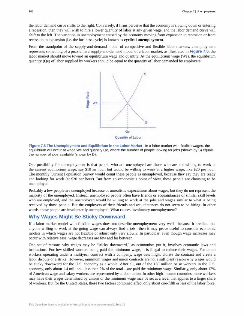
the labor demand curve shifts to the right. Conversely, if firms perceive that the economy is slowing down or enteringa recession, then they will wish to hire a lower quantity of labor at any given wage, and the labor demand curve willshift to the left. The variation in unemployment caused by the economy moving from expansion to recession or fromrecession to expansion (i.e. the business cycle) is known as cyclical unemployment.
From the standpoint of the supply-and-demand model of competitive and flexible labor markets, unemploymentrepresents something of a puzzle. In a supply-and-demand model of a labor market, as illustrated in Figure 7.5, thelabor market should move toward an equilibrium wage and quantity. At the equilibrium wage (We), the equilibriumquantity (Qe) of labor supplied by workers should be equal to the quantity of labor demanded by employers.
Figure 7.5 The Unemployment and Equilibrium in the Labor Market In a labor market with flexible wages, theequilibrium will occur at wage We and quantity Qe, where the number of people looking for jobs (shown by S) equalsthe number of jobs available (shown by D).
One possibility for unemployment is that people who are unemployed are those who are not willing to work atthe current equilibrium wage, say $10 an hour, but would be willing to work at a higher wage, like $20 per hour.The monthly Current Population Survey would count these people as unemployed, because they say they are readyand looking for work (at $20 per hour). But from an economist’s point of view, these people are choosing to beunemployed.
Probably a few people are unemployed because of unrealistic expectations about wages, but they do not represent themajority of the unemployed. Instead, unemployed people often have friends or acquaintances of similar skill levelswho are employed, and the unemployed would be willing to work at the jobs and wages similar to what is beingreceived by those people. But the employers of their friends and acquaintances do not seem to be hiring. In otherwords, these people are involuntarily unemployed. What causes involuntary unemployment?
Why Wages Might Be Sticky DownwardIf a labor market model with flexible wages does not describe unemployment very well—because it predicts thatanyone willing to work at the going wage can always find a job—then it may prove useful to consider economicmodels in which wages are not flexible or adjust only very slowly. In particular, even though wage increases mayoccur with relative ease, wage decreases are few and far between.
One set of reasons why wages may be “sticky downward,” as economists put it, involves economic laws andinstitutions. For low-skilled workers being paid the minimum wage, it is illegal to reduce their wages. For unionworkers operating under a multiyear contract with a company, wage cuts might violate the contract and create alabor dispute or a strike. However, minimum wages and union contracts are not a sufficient reason why wages wouldbe sticky downward for the U.S. economy as a whole. After all, out of the 150 million or so workers in the U.S.economy, only about 1.4 million—less than 2% of the total—are paid the minimum wage. Similarly, only about 12%of American wage and salary workers are represented by a labor union. In other high-income countries, more workersmay have their wages determined by unions or the minimum wage may be set at a level that applies to a larger shareof workers. But for the United States, these two factors combined affect only about one-fifth or less of the labor force.
166 Chapter 7 | Unemployment
This OpenStax book is available for free at http://cnx.org/content/col11864/1.2
Economists looking for reasons why wages might be sticky downwards have focused on factors that may characterizemost labor relationships in the economy, not just a few. A number of different theories have been proposed, but theyshare a common tone.
One argument is that even employees who are not union members often work under an implicit contract, which isthat the employer will try to keep wages from falling when the economy is weak or the business is having trouble, andthe employee will not expect huge salary increases when the economy or the business is strong. This wage-settingbehavior acts like a form of insurance: the employee has some protection against wage declines in bad times, but paysfor that protection with lower wages in good times. Clearly, this sort of implicit contract means that firms will behesitant to cut wages, lest workers feel betrayed and work less hard or even leave the firm.
Efficiency wage theory argues that the productivity of workers depends on their pay, and so employers will oftenfind it worthwhile to pay their employees somewhat more than market conditions might dictate. One reason is thatemployees who are paid better than others will be more productive because they recognize that if they were to losetheir current jobs, they would suffer a decline in salary. As a result, they are motivated to work harder and to staywith the current employer. In addition, employers know that it is costly and time-consuming to hire and train newemployees, so they would prefer to pay workers a little extra now rather than to lose them and have to hire and trainnew workers. Thus, by avoiding wage cuts, the employer minimizes costs of training and hiring new workers, andreaps the benefits of well-motivated employees.
The adverse selection of wage cuts argument points out that if an employer reacts to poor business conditions byreducing wages for all workers, then the best workers, those with the best employment alternatives at other firms, arethe most likely to leave. The least attractive workers, with fewer employment alternatives, are more likely to stay.Consequently, firms are more likely to choose which workers should depart, through layoffs and firings, rather thantrimming wages across the board. Sometimes companies that are going through tough times can persuade workers totake a pay cut for the short term, and still retain most of the firm’s workers. But these stories are notable because theyare so uncommon. It is far more typical for companies to lay off some workers, rather than to cut wages for everyone.
The insider-outsider model of the labor force, in simple terms, argues that those already working for firms are“insiders,” while new employees, at least for a time, are “outsiders.” A firm depends on its insiders to grease thewheels of the organization, to be familiar with routine procedures, to train new employees, and so on. However,cutting wages will alienate the insiders and damage the firm’s productivity and prospects.
Finally, the relative wage coordination argument points out that even if most workers were hypothetically willingto see a decline in their own wages in bad economic times as long as everyone else also experiences such a decline,there is no obvious way for a decentralized economy to implement such a plan. Instead, workers confronted with thepossibility of a wage cut will worry that other workers will not have such a wage cut, and so a wage cut means beingworse off both in absolute terms and relative to others. As a result, workers fight hard against wage cuts.
These theories of why wages tend not to move downward differ in their logic and their implications, and figuring outthe strengths and weaknesses of each theory is an ongoing subject of research and controversy among economists. Alltend to imply that wages will decline only very slowly, if at all, even when the economy or a business is having toughtimes. When wages are inflexible and unlikely to fall, then either short-run or long-run unemployment can result. Thiscan be seen in Figure 7.6.
Chapter 7 | Unemployment 167
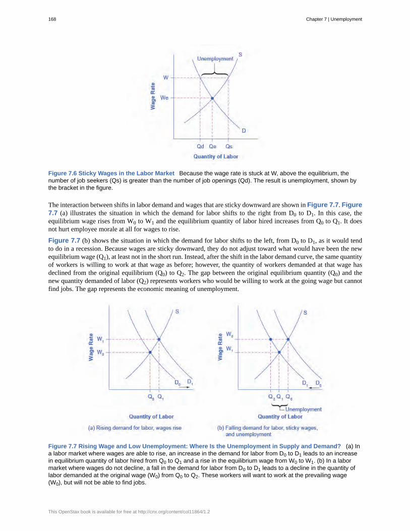
Figure 7.6 Sticky Wages in the Labor Market Because the wage rate is stuck at W, above the equilibrium, thenumber of job seekers (Qs) is greater than the number of job openings (Qd). The result is unemployment, shown bythe bracket in the figure.
The interaction between shifts in labor demand and wages that are sticky downward are shown in Figure 7.7. Figure7.7 (a) illustrates the situation in which the demand for labor shifts to the right from D0 to D1. In this case, theequilibrium wage rises from W0 to W1 and the equilibrium quantity of labor hired increases from Q0 to Q1. It doesnot hurt employee morale at all for wages to rise.
Figure 7.7 (b) shows the situation in which the demand for labor shifts to the left, from D0 to D1, as it would tendto do in a recession. Because wages are sticky downward, they do not adjust toward what would have been the newequilibrium wage (Q1), at least not in the short run. Instead, after the shift in the labor demand curve, the same quantityof workers is willing to work at that wage as before; however, the quantity of workers demanded at that wage hasdeclined from the original equilibrium (Q0) to Q2. The gap between the original equilibrium quantity (Q0) and thenew quantity demanded of labor (Q2) represents workers who would be willing to work at the going wage but cannotfind jobs. The gap represents the economic meaning of unemployment.
Figure 7.7 Rising Wage and Low Unemployment: Where Is the Unemployment in Supply and Demand? (a) Ina labor market where wages are able to rise, an increase in the demand for labor from D0 to D1 leads to an increasein equilibrium quantity of labor hired from Q0 to Q1 and a rise in the equilibrium wage from W0 to W1. (b) In a labormarket where wages do not decline, a fall in the demand for labor from D0 to D1 leads to a decline in the quantity oflabor demanded at the original wage (W0) from Q0 to Q2. These workers will want to work at the prevailing wage(W0), but will not be able to find jobs.
168 Chapter 7 | Unemployment
This OpenStax book is available for free at http://cnx.org/content/col11864/1.2
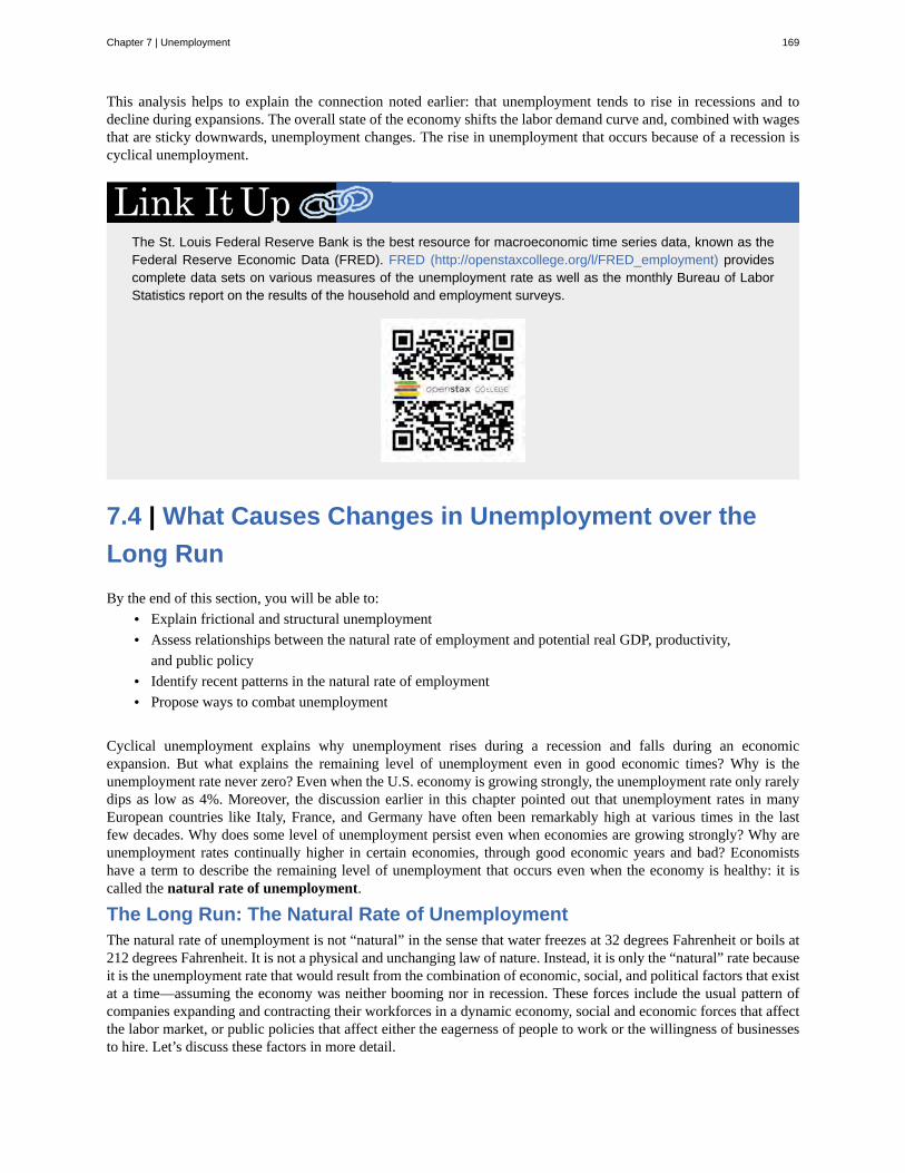
This analysis helps to explain the connection noted earlier: that unemployment tends to rise in recessions and todecline during expansions. The overall state of the economy shifts the labor demand curve and, combined with wagesthat are sticky downwards, unemployment changes. The rise in unemployment that occurs because of a recession iscyclical unemployment.
The St. Louis Federal Reserve Bank is the best resource for macroeconomic time series data, known as theFederal Reserve Economic Data (FRED). FRED (http://openstaxcollege.org/l/FRED_employment) providescomplete data sets on various measures of the unemployment rate as well as the monthly Bureau of LaborStatistics report on the results of the household and employment surveys.
7.4 | What Causes Changes in Unemployment over theLong RunBy the end of this section, you will be able to:
• Explain frictional and structural unemployment• Assess relationships between the natural rate of employment and potential real GDP, productivity,
and public policy• Identify recent patterns in the natural rate of employment• Propose ways to combat unemployment
Cyclical unemployment explains why unemployment rises during a recession and falls during an economicexpansion. But what explains the remaining level of unemployment even in good economic times? Why is theunemployment rate never zero? Even when the U.S. economy is growing strongly, the unemployment rate only rarelydips as low as 4%. Moreover, the discussion earlier in this chapter pointed out that unemployment rates in manyEuropean countries like Italy, France, and Germany have often been remarkably high at various times in the lastfew decades. Why does some level of unemployment persist even when economies are growing strongly? Why areunemployment rates continually higher in certain economies, through good economic years and bad? Economistshave a term to describe the remaining level of unemployment that occurs even when the economy is healthy: it iscalled the natural rate of unemployment.
The Long Run: The Natural Rate of UnemploymentThe natural rate of unemployment is not “natural” in the sense that water freezes at 32 degrees Fahrenheit or boils at212 degrees Fahrenheit. It is not a physical and unchanging law of nature. Instead, it is only the “natural” rate becauseit is the unemployment rate that would result from the combination of economic, social, and political factors that existat a time—assuming the economy was neither booming nor in recession. These forces include the usual pattern ofcompanies expanding and contracting their workforces in a dynamic economy, social and economic forces that affectthe labor market, or public policies that affect either the eagerness of people to work or the willingness of businessesto hire. Let’s discuss these factors in more detail.
Chapter 7 | Unemployment 169
Frictional UnemploymentIn a market economy, some companies are always going broke for a variety of reasons: old technology; poormanagement; good management that happened to make bad decisions; shifts in tastes of consumers so that less of thefirm’s product is desired; a large customer who went broke; or tough domestic or foreign competitors. Conversely,other companies will be doing very well for just the opposite reasons and looking to hire more employees. In aperfect world, all of those who lost jobs would immediately find new ones. But in the real world, even if the numberof job seekers is equal to the number of job vacancies, it takes time to find out about new jobs, to interview andfigure out if the new job is a good match, or perhaps to sell a house and buy another in proximity to a new job.The unemployment that occurs in the meantime, as workers move between jobs, is called frictional unemployment.Frictional unemployment is not inherently a bad thing. It takes time on part of both the employer and the individualto match those looking for employment with the correct job openings. For individuals and companies to be successfuland productive, you want people to find the job for which they are best suited, not just the first job offered.
In the mid-2000s, before the recession of 2008–2009, it was true that about 7% of U.S. workers saw their jobsdisappear in any three-month period. But in periods of economic growth, these destroyed jobs are counterbalancedfor the economy as a whole by a larger number of jobs created. In 2005, for example, there were typically about7.5 million unemployed people at any given time in the U.S. economy. Even though about two-thirds of thoseunemployed people found a job in 14 weeks or fewer, the unemployment rate did not change much during the year,because those who found new jobs were largely offset by others who lost jobs.
Of course, it would be preferable if people who were losing jobs could immediately and easily move into the newjobs being created, but in the real world, that is not possible. Someone who is laid off by a textile mill in SouthCarolina cannot turn around and immediately start working for a textile mill in California. Instead, the adjustmentprocess happens in ripples. Some people find new jobs near their old ones, while others find that they must move tonew locations. Some people can do a very similar job with a different company, while others must start new careerpaths. Some people may be near retirement and decide to look only for part-time work, while others want an employerthat offers a long-term career path. The frictional unemployment that results from people moving between jobs in adynamic economy may account for one to two percentage points of total unemployment.
The level of frictional unemployment will depend on how easy it is for workers to learn about alternative jobs, whichmay reflect the ease of communications about job prospects in the economy. The extent of frictional unemploymentwill also depend to some extent on how willing people are to move to new areas to find jobs—which in turn maydepend on history and culture.
Frictional unemployment and the natural rate of unemployment also seem to depend on the age distribution of thepopulation. Figure 7.4 (b) showed that unemployment rates are typically lower for people between 25–54 years ofage than they are for those who are either younger or older. “Prime-age workers,” as those in the 25–54 age bracket aresometimes called, are typically at a place in their lives when they want to have a job and income arriving at all times.But some proportion of those who are under 30 may still be trying out jobs and life options and some proportion ofthose over 55 are eyeing retirement. In both cases, the relatively young or old tend to worry less about unemploymentthan those in-between, and their periods of frictional unemployment may be longer as a result. Thus, a society witha relatively high proportion of relatively young or old workers will tend to have a higher unemployment rate than asociety with a higher proportion of its workers in middle age.
Structural UnemploymentAnother factor that influences the natural rate of unemployment is the amount of structural unemployment. Thestructurally unemployed are individuals who have no jobs because they lack skills valued by the labor market, eitherbecause demand has shifted away from the skills they do have, or because they never learned any skills. An exampleof the former would be the unemployment among aerospace engineers after the U.S. space program downsized in the1970s. An example of the latter would be high school dropouts.
Some people worry that technology causes structural unemployment. In the past, new technologies have put lowerskilled employees out of work, but at the same time they create demand for higher skilled workers to use the newtechnologies. Education seems to be the key in minimizing the amount of structural unemployment. Individuals whohave degrees can be retrained if they become structurally unemployed. For people with no skills and little education,that option is more limited.
170 Chapter 7 | Unemployment
This OpenStax book is available for free at http://cnx.org/content/col11864/1.2
Natural Unemployment and Potential Real GDPThe natural unemployment rate is related to two other important concepts: full employment and potential real GDP.The economy is considered to be at full employment when the actual unemployment rate is equal to the naturalunemployment. When the economy is at full employment, real GPD is equal to potential real GDP. By contrast, whenthe economy is below full employment, the unemployment rate is greater than the natural unemployment rate and realGDP is less than potential. Finally, when the economy above full employment, then the unemployment rate is lessthan the natural unemployment rate and real GDP is greater than potential. Operating above potential is only possiblefor a short while, since it is analogous to all workers working overtime.
Productivity Shifts and the Natural Rate of UnemploymentUnexpected shifts in productivity can have a powerful effect on the natural rate of unemployment. Over time, the levelof wages in an economy will be determined by the productivity of workers. After all, if a business paid workers morethan could be justified by their productivity, the business will ultimately lose money and go bankrupt. Conversely, ifa business tries to pay workers less than their productivity then, in a competitive labor market, other businesses willfind it worthwhile to hire away those workers and pay them more.
However, adjustments of wages to productivity levels will not happen quickly or smoothly. Wages are typicallyreviewed only once or twice a year. In many modern jobs, it is difficult to measure productivity at the individual level.For example, how precisely would one measure the quantity produced by an accountant who is one of many peopleworking in the tax department of a large corporation? Because productivity is difficult to observe, wage increases areoften determined based on recent experience with productivity; if productivity has been rising at, say, 2% per year,then wages rise at that level as well. However, when productivity changes unexpectedly, it can affect the natural rateof unemployment for a time.
The U.S. economy in the 1970s and 1990s provides two vivid examples of this process. In the 1970s, productivitygrowth slowed down unexpectedly (as discussed in Economic Growth). For example, output per hour of U.S.workers in the business sector increased at an annual rate of 3.3% per year from 1960 to 1973, but only 0.8% from1973 to 1982. Figure 7.8 (a) illustrates the situation where the demand for labor—that is, the quantity of labor thatbusiness is willing to hire at any given wage—has been shifting out a little each year because of rising productivity,from D0 to D1 to D2. As a result, equilibrium wages have been rising each year from W0 to W1 to W2. But whenproductivity unexpectedly slows down, the pattern of wage increases does not adjust right away. Wages keep risingeach year from W2 to W3 to W4. But the demand for labor is no longer shifting up. A gap opens where the quantityof labor supplied at wage level W4 is greater than the quantity demanded. The natural rate of unemployment rises;indeed, in the aftermath of this unexpectedly low productivity in the 1970s, the national unemployment rate did notfall below 7% from May, 1980 until 1986. Over time, the rise in wages will adjust to match the slower gains inproductivity, and the unemployment rate will ease back down. But this process may take years.
Chapter 7 | Unemployment 171
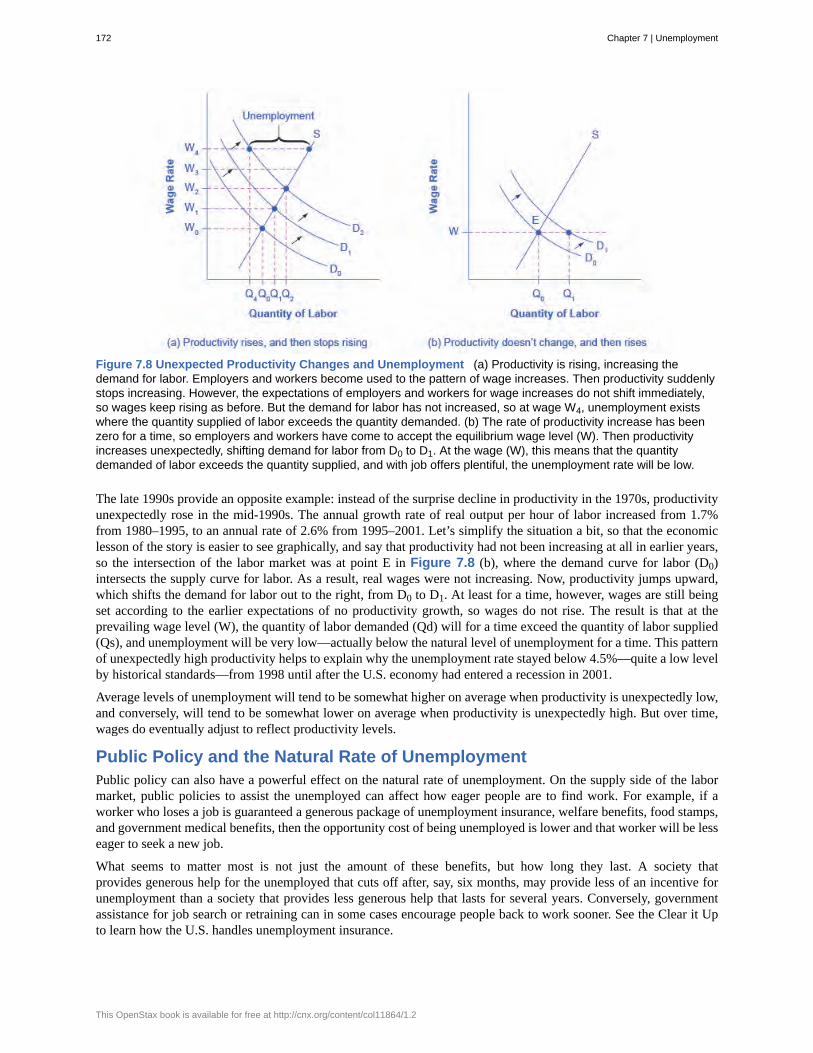
Figure 7.8 Unexpected Productivity Changes and Unemployment (a) Productivity is rising, increasing thedemand for labor. Employers and workers become used to the pattern of wage increases. Then productivity suddenlystops increasing. However, the expectations of employers and workers for wage increases do not shift immediately,so wages keep rising as before. But the demand for labor has not increased, so at wage W4, unemployment existswhere the quantity supplied of labor exceeds the quantity demanded. (b) The rate of productivity increase has beenzero for a time, so employers and workers have come to accept the equilibrium wage level (W). Then productivityincreases unexpectedly, shifting demand for labor from D0 to D1. At the wage (W), this means that the quantitydemanded of labor exceeds the quantity supplied, and with job offers plentiful, the unemployment rate will be low.
The late 1990s provide an opposite example: instead of the surprise decline in productivity in the 1970s, productivityunexpectedly rose in the mid-1990s. The annual growth rate of real output per hour of labor increased from 1.7%from 1980–1995, to an annual rate of 2.6% from 1995–2001. Let’s simplify the situation a bit, so that the economiclesson of the story is easier to see graphically, and say that productivity had not been increasing at all in earlier years,so the intersection of the labor market was at point E in Figure 7.8 (b), where the demand curve for labor (D0)intersects the supply curve for labor. As a result, real wages were not increasing. Now, productivity jumps upward,which shifts the demand for labor out to the right, from D0 to D1. At least for a time, however, wages are still beingset according to the earlier expectations of no productivity growth, so wages do not rise. The result is that at theprevailing wage level (W), the quantity of labor demanded (Qd) will for a time exceed the quantity of labor supplied(Qs), and unemployment will be very low—actually below the natural level of unemployment for a time. This patternof unexpectedly high productivity helps to explain why the unemployment rate stayed below 4.5%—quite a low levelby historical standards—from 1998 until after the U.S. economy had entered a recession in 2001.
Average levels of unemployment will tend to be somewhat higher on average when productivity is unexpectedly low,and conversely, will tend to be somewhat lower on average when productivity is unexpectedly high. But over time,wages do eventually adjust to reflect productivity levels.
Public Policy and the Natural Rate of UnemploymentPublic policy can also have a powerful effect on the natural rate of unemployment. On the supply side of the labormarket, public policies to assist the unemployed can affect how eager people are to find work. For example, if aworker who loses a job is guaranteed a generous package of unemployment insurance, welfare benefits, food stamps,and government medical benefits, then the opportunity cost of being unemployed is lower and that worker will be lesseager to seek a new job.
What seems to matter most is not just the amount of these benefits, but how long they last. A society thatprovides generous help for the unemployed that cuts off after, say, six months, may provide less of an incentive forunemployment than a society that provides less generous help that lasts for several years. Conversely, governmentassistance for job search or retraining can in some cases encourage people back to work sooner. See the Clear it Upto learn how the U.S. handles unemployment insurance.
172 Chapter 7 | Unemployment
This OpenStax book is available for free at http://cnx.org/content/col11864/1.2
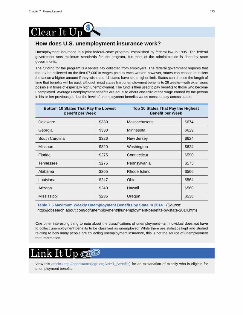
How does U.S. unemployment insurance work?Unemployment insurance is a joint federal–state program, established by federal law in 1935. The federalgovernment sets minimum standards for the program, but most of the administration is done by stategovernments.
The funding for the program is a federal tax collected from employers. The federal government requires thatthe tax be collected on the first $7,000 in wages paid to each worker; however, states can choose to collectthe tax on a higher amount if they wish, and 41 states have set a higher limit. States can choose the length oftime that benefits will be paid, although most states limit unemployment benefits to 26 weeks—with extensionspossible in times of especially high unemployment. The fund is then used to pay benefits to those who becomeunemployed. Average unemployment benefits are equal to about one-third of the wage earned by the personin his or her previous job, but the level of unemployment benefits varies considerably across states.
Bottom 10 States That Pay the LowestBenefit per Week
Top 10 States That Pay the HighestBenefit per Week
Delaware $330 Massachusetts $674
Georgia $330 Minnesota $629
South Carolina $326 New Jersey $624
Missouri $320 Washington $624
Florida $275 Connecticut $590
Tennessee $275 Pennsylvania $573
Alabama $265 Rhode Island $566
Louisiana $247 Ohio $564
Arizona $240 Hawaii $560
Mississippi $235 Oregon $538
Table 7.5 Maximum Weekly Unemployment Benefits by State in 2014 (Source:http://jobsearch.about.com/od/unemployment/fl/unemployment-benefits-by-state-2014.htm)
One other interesting thing to note about the classifications of unemployment—an individual does not haveto collect unemployment benefits to be classified as unemployed. While there are statistics kept and studiedrelating to how many people are collecting unemployment insurance, this is not the source of unemploymentrate information.
View this article (http://openstaxcollege.org/l/NYT_Benefits) for an explanation of exactly who is eligible forunemployment benefits.
Chapter 7 | Unemployment 173
On the demand side of the labor market, government rules social institutions, and the presence of unions can affectthe willingness of firms to hire. For example, if a government makes it hard for businesses to start up or to expand,by wrapping new businesses in bureaucratic red tape, then businesses will become more discouraged about hiring.Government regulations can make it harder to start a business by requiring that a new business obtain many permitsand pay many fees, or by restricting the types and quality of products that can be sold. Other government regulations,like zoning laws, may limit where business can be done, or whether businesses are allowed to be open during eveningsor on Sunday.
Whatever defenses may be offered for such laws in terms of social value—like the value some Christians place onnot working on Sunday—these kinds of restrictions impose a barrier between some willing workers and other willingemployers, and thus contribute to a higher natural rate of unemployment. Similarly, if government makes it difficultto fire or lay off workers, businesses may react by trying not to hire more workers than strictly necessary—sincelaying these workers off would be costly and difficult. High minimum wages may discourage businesses from hiringlow-skill workers. Government rules may encourage and support powerful unions, which can then push up wages forunion workers, but at a cost of discouraging businesses from hiring those workers.
The Natural Rate of Unemployment in Recent YearsThe underlying economic, social, and political factors that determine the natural rate of unemployment can changeover time, which means that the natural rate of unemployment can change over time, too.
Estimates by economists of the natural rate of unemployment in the U.S. economy in the early 2000s run at about 4.5to 5.5%. This is a lower estimate than earlier. Three of the common reasons proposed by economists for this changeare outlined below.
1. The Internet has provided a remarkable new tool through which job seekers can find out about jobs at differentcompanies and can make contact with relative ease. An Internet search is far easier than trying to find a list oflocal employers and then hunting up phone numbers for all of their human resources departments, requestinga list of jobs and application forms, and so on. Social networking sites such as LinkedIn have changed howpeople find work as well.
2. The growth of the temporary worker industry has probably helped to reduce the natural rate of unemployment.In the early 1980s, only about 0.5% of all workers held jobs through temp agencies; by the early 2000s, thefigure had risen above 2%. Temp agencies can provide jobs for workers while they are looking for permanentwork. They can also serve as a clearinghouse, helping workers find out about jobs with certain employers andgetting a tryout with the employer. For many workers, a temp job is a stepping-stone to a permanent job thatthey might not have heard about or gotten any other way, so the growth of temp jobs will also tend to reducefrictional unemployment.
3. The aging of the “baby boom generation”—the especially large generation of Americans born between 1946and 1963—meant that the proportion of young workers in the economy was relatively high in the 1970s, asthe boomers entered the labor market, but is relatively low today. As noted earlier, middle-aged workers arefar more likely to keep steady jobs than younger workers, a factor that tends to reduce the natural rate ofunemployment.
The combined result of these factors is that the natural rate of unemployment was on average lower in the 1990s andthe early 2000s than in the 1980s. The Great Recession of 2008–2009 pushed monthly unemployment rates above10% in late 2009. But even at that time, the Congressional Budget Office was forecasting that by 2015, unemployment
174 Chapter 7 | Unemployment
This OpenStax book is available for free at http://cnx.org/content/col11864/1.2
rates would fall back to about 5%—lower than it currently is, though not by much. As of early 2015, policymakersstill think that unemployment has not yet reached its natural rate.
The Natural Rate of Unemployment in EuropeBy the standards of other high-income economies, the natural rate of unemployment in the U.S. economy appearsrelatively low. Through good economic years and bad, many European economies have had unemployment rateshovering near 10%, or even higher, since the 1970s. European rates of unemployment have been higher not becauserecessions in Europe have been deeper, but rather because the conditions underlying supply and demand for laborhave been different in Europe, in a way that has created a much higher natural rate of unemployment.
Many European countries have a combination of generous welfare and unemployment benefits, together with nestsof rules that impose additional costs on businesses when they hire. In addition, many countries have laws that requirefirms to give workers months of notice before laying them off and to provide substantial severance or retrainingpackages after laying them off. The legally required notice before laying off a worker can be more than three monthsin Spain, Germany, Denmark, and Belgium, and the legally required severance package can be as high as a year’ssalary or more in Austria, Spain, Portugal, Italy, and Greece. Such laws will surely discourage laying off or firingcurrent workers. But when companies know that it will be difficult to fire or lay off workers, they also become hesitantabout hiring in the first place.
The typically higher levels of unemployment in many European countries in recent years, which have prevailed evenwhen economies are growing at a solid pace, are attributable to the fact that the sorts of laws and regulations that leadto a high natural rate of unemployment are much more prevalent in Europe than in the United States.
A Preview of Policies to Fight UnemploymentThe Government Budgets and Fiscal Policy and Macroeconomic Policy Around the World chaptersprovide a detailed discussion of how to fight unemployment, when these policies can be discussed in the context ofthe full array of macroeconomic goals and frameworks for analysis. But even at this preliminary stage, it is useful topreview the main issues concerning policies to fight unemployment.
The remedy for unemployment will depend on the diagnosis. Cyclical unemployment is a short-term problem, causedbecause the economy is in a recession. Thus, the preferred solution will be to avoid or minimize recessions. AsGovernment Budgets and Fiscal Policy discusses, this policy can be enacted by stimulating the overall buyingpower in the economy, so that firms perceive that sales and profits are possible, which makes them eager to hire.
Dealing with the natural rate of unemployment is trickier. There is not much to be done about the fact that in amarket-oriented economy, firms will hire and fire workers. Nor is there much to be done about how the evolving agestructure of the economy, or unexpected shifts in productivity, will affect the natural rate of unemployment for a time.However, as the example of high ongoing unemployment rates for many European countries illustrates, governmentpolicy clearly can affect the natural rate of unemployment that will persist even when GDP is growing.
When a government enacts policies that will affect workers or employers, it must examine how these policieswill affect the information and incentives employees and employers have to seek each other out. For example, thegovernment may have a role to play in helping some of the unemployed with job searches. The design of governmentprograms that offer assistance to unemployed workers and protections to employed workers may need to be rethoughtso that they will not unduly discourage the supply of labor. Similarly, rules that make it difficult for businesses tobegin or to expand may need to be redesigned so that they will not unduly discourage the demand for labor. Themessage is not that all laws affecting labor markets should be repealed, but only that when such laws are enacted, asociety that cares about unemployment will need to consider the tradeoffs involved.
The Mysterious Case of the Missing CandidatesAfter reading the chapter you might think the current unemployment conundrum may be due to structuralunemployment. Indeed, there is a mismatch between the skills employers are seeking and the skills the
Chapter 7 | Unemployment 175
unemployed possess. But Peter Cappelli has a slightly different view on this—it is called the purple squirrel.The what?
In human resource parlance, a purple squirrel is a job candidate who is a perfect fit for all of the manydifferent responsibilities of a position. A purple squirrel candidate could step into a multi-faceted position withno training and permit the firm to higher fewer people because the worker is so versatile. During the GreatRecession, Human Resources (HR) positions were reduced. This means today’s hiring managers are draftingjob descriptions and requirements without much, if any HR feedback. “It turns out it's typically the case thatemployers' requirements are crazy, they're not paying enough, or their applicant screening is so rigid thatnobody gets through,” Cappelli stated in a 2012 Knowledge@Wharton interview about the findings in his book,Why Good People Can’t Find Jobs: Chasing After the Purple Squirrel. In short, managers are searching for“purple squirrels” when what they really need are just versatile workers. There really is not a shortage of“normal squirrels”—candidates who are versatile workers. The managers just cannot find them because theirrequirements, screening processes, and compensation will filter out all but the “purple” ones.
176 Chapter 7 | Unemployment
This OpenStax book is available for free at http://cnx.org/content/col11864/1.2
adverse selection of wage cuts argument
cyclical unemployment
discouraged workers
efficiency wage theory
frictional unemployment
implicit contract
insider-outsider model
labor force participation rate
natural rate of unemployment
out of the labor force
relative wage coordination argument
structural unemployment
underemployed
unemployment rate
KEY TERMS
if employers reduce wages for all workers, the best will leave
unemployment closely tied to the business cycle, like higher unemployment during arecession
those who have stopped looking for employment due to the lack of suitable positions available
the theory that the productivity of workers, either individually or as a group, will increase ifthey are paid more
unemployment that occurs as workers move between jobs
an unwritten agreement in the labor market that the employer will try to keep wages from fallingwhen the economy is weak or the business is having trouble, and the employee will not expect huge salary increaseswhen the economy or the business is strong
those already working for the firm are “insiders” who know the procedures; the other workersare “outsiders” who are recent or prospective hires
this is the percentage of adults in an economy who are either employed or who areunemployed and looking for a job
the unemployment rate that would exist in a growing and healthy economy from thecombination of economic, social, and political factors that exist at a given time
those who are not working and not looking for work—whether they want employment or not;also termed “not in the labor force”
across-the-board wage cuts are hard for an economy to implement, andworkers fight against them
unemployment that occurs because individuals lack skills valued by employers
individuals who are employed in a job that is below their skills
the percentage of adults who are in the labor force and thus seeking jobs, but who do not havejobs
KEY CONCEPTS AND SUMMARY
7.1 How the Unemployment Rate Is Defined and ComputedUnemployment imposes high costs. Unemployed individuals suffer from loss of income and from stress. An economywith high unemployment suffers an opportunity cost of unused resources. The adult population can be divided intothose in the labor force and those out of the labor force. In turn, those in the labor force are divided into employed andunemployed. A person without a job must be willing and able to work and actively looking for work to be countedas unemployed; otherwise, a person without a job is counted as being out of the labor force. The unemployment rateis defined as the number of unemployed persons divided by the number of persons in the labor force (not the overalladult population). The Current Population Survey (CPS) conducted by the United States Census Bureau measures thepercentage of the labor force that is unemployed. The establishment payroll survey by the Bureau of Labor Statisticsmeasures the net change in jobs created for the month.
Chapter 7 | Unemployment 177
7.2 Patterns of UnemploymentThe U.S. unemployment rate rises during periods of recession and depression, but falls back to the range of 4% to6% when the economy is strong. The unemployment rate never falls to zero. Despite enormous growth in the size ofthe U.S. population and labor force in the twentieth century, along with other major trends like globalization and newtechnology, the unemployment rate shows no long-term rising trend.
Unemployment rates differ by group: higher for African-Americans and Hispanics than for whites; higher for lesseducated than more educated; higher for the young than the middle-aged. Women’s unemployment rates used to behigher than men’s, but in recent years men’s and women’s unemployment rates have been very similar. In recentyears, unemployment rates in the United States have compared favorably with unemployment rates in most otherhigh-income economies.
7.3 What Causes Changes in Unemployment over the Short RunCyclical unemployment rises and falls with the business cycle. In a labor market with flexible wages, wages willadjust in such a market so that quantity demanded of labor always equals the quantity supplied of labor at theequilibrium wage. Many theories have been proposed for why wages might not be flexible, but instead may adjustonly in a “sticky” way, especially when it comes to downward adjustments: implicit contracts, efficiency wage theory,adverse selection of wage cuts, insider-outsider model, and relative wage coordination.
7.4 What Causes Changes in Unemployment over the Long RunThe natural rate of unemployment is the rate of unemployment that would be caused by the economic, social, andpolitical forces in the economy even when the economy is not in a recession. These factors include the frictionalunemployment that occurs when people are put out of work for a time by the shifts of a dynamic and changingeconomy and any laws concerning conditions of hiring and firing have the undesired side effect of discouraging jobformation. They also include structural unemployment, which occurs when demand shifts permanently away from acertain type of job skill.
SELF-CHECK QUESTIONS1. Suppose the adult population over the age of 16 is 237.8 million and the labor force is 153.9 million (of whom139.1 million are employed). How many people are “not in the labor force?” What are the proportions of employed,unemployed and not in the labor force in the population? Hint: Proportions are percentages.
2. Using the above data, what is the unemployment rate? These data are U.S. statistics from 2010. How does itcompare to the February 2015 unemployment rate computed earlier?
3. Over the long term, has the U.S. unemployment rate generally trended up, trended down, or remained at basicallythe same level?
4. Whose unemployment rates are commonly higher in the U.S. economy:a. Whites or nonwhites?b. The young or the middle-aged?c. College graduates or high school graduates?
5. Beginning in the 1970s and continuing for three decades, women entered the U.S. labor force in a big way. If weassume that wages are sticky in a downward direction, but that around 1970 the demand for labor equaled the supplyof labor at the current wage rate, what do you imagine happened to the wage rate, employment, and unemploymentas a result of increased labor force participation?
6. Is the increase in labor force participation rates among women better thought of as causing an increase in cyclicalunemployment or an increase in the natural rate of unemployment? Why?
7. Many college students graduate from college before they have found a job. When graduates begin to look for ajob, they are counted as what category of unemployed?
178 Chapter 7 | Unemployment
This OpenStax book is available for free at http://cnx.org/content/col11864/1.2
REVIEW QUESTIONS
8. What is the difference between being unemployedand being out of the labor force?
9. How is the unemployment rate calculated? How isthe labor force participation rate calculated?
10. Are all adults who do not hold jobs counted asunemployed?
11. If you are out of school but working part time, areyou considered employed or unemployed in U.S. laborstatistics? If you are a full time student and working 12hours a week at the college cafeteria are you consideredemployed or not in the labor force? If you are a seniorcitizen who is collecting social security and a pensionand working as a greeter at Wal-Mart are you consideredemployed or not in the labor force?
12. What happens to the unemployment rate whenunemployed workers are reclassified as discouragedworkers?
13. What happens to the labor force participation ratewhen employed individuals are reclassified asunemployed? What happens when they are reclassifiedas discouraged workers?
14. What are some of the problems with using theunemployment rate as an accurate measure of overalljoblessness?
15. What criteria are used by the BLS to count someoneas employed? As unemployed?
16. Assess whether the following would be countedas “unemployed” in the Current Employment Statisticssurvey.
a. A husband willingly stays home with childrenwhile his wife works.
b. A manufacturing worker whose factory justclosed down.
c. A college student doing an unpaid summerinternship.
d. A retiree.e. Someone who has been out of work for two years
but keeps looking for a job.f. Someone who has been out of work for two
months but isn’t looking for a job.g. Someone who hates her present job and is
actively looking for another one.h. Someone who decides to take a part time job
because she could not find a full time position.
17. Are U.S. unemployment rates typically higher,lower, or about the same as unemployment rates in otherhigh-income countries?
18. Are U.S. unemployment rates distributed evenlyacross the population?
19. When would you expect cyclical unemployment tobe rising? Falling?
20. Why is there unemployment in a labor market withflexible wages?
21. Name and explain some of the reasons why wagesare likely to be sticky, especially in downwardadjustments.
22. What term describes the remaining level ofunemployment that occurs even when the economy ishealthy?
23. What forces create the natural rate ofunemployment for an economy?
24. Would you expect the natural rate of unemploymentto be roughly the same in different countries?
25. Would you expect the natural rate of unemploymentto remain the same within one country over the long runof several decades?
26. What is frictional unemployment? Give examplesof frictional unemployment.
27. What is structural unemployment? Give examplesof structural unemployment.
28. After several years of economic growth, would youexpect the unemployment in an economy to be mainlycyclical or mainly due to the natural rate ofunemployment? Why?
29. What type of unemployment (cyclical, frictional, orstructural) applies to each of the following:
a. landscapers laid off in response to drop in newhousing construction during a recession.
b. coal miners laid off due to EPA regulations thatshut down coal fired power
c. a financial analyst who quits his/her job inChicago and is pursing similar work in Arizona
d. printers laid off due to drop in demand forprinted catalogues and flyers as firms go theinternet to promote an advertise their products.
Chapter 7 | Unemployment 179
e. factory workers in the U.S. laid off as the plantsshut down and move to Mexico and Ireland.
CRITICAL THINKING QUESTIONS
30. Using the definition of the unemployment rate, isan increase in the unemployment rate necessarily a badthing for a nation?
31. Is a decrease in the unemployment rate necessarilya good thing for a nation? Explain.
32. If many workers become discouraged from lookingfor jobs, explain how the number of jobs could declinebut the unemployment rate could fall at the same time.
33. Would you expect hidden unemployment to behigher, lower, or about the same when theunemployment rate is high, say 10%, versus low, say4%? Explain.
34. Is the higher unemployment rates for minorityworkers necessarily an indication of discrimination?What could be some other reasons for the higherunemployment rate?
35. While unemployment is highly negativelycorrelated with the level of economic activity, in the realworld it responds with a lag. In other words, firms donot immediately lay off workers in response to a salesdecline. They wait a while before responding. Similarly,firms do not immediately hire workers when sales pickup. What do you think accounts for the lag in responsetime?
36. Why do you think that unemployment rates arelower for individuals with more education?
37. Do you think it is rational for workers to prefersticky wages to wage cuts, when the consequence ofsticky wages is unemployment for some workers? Why
or why not? How do the reasons for sticky wagesexplained in this section apply to your argument?
38. Under what condition would a decrease inunemployment be bad for the economy?
39. Under what condition would an increase in theunemployment rate be a positive sign?
40. As the baby boom generation retires, the ratio ofretirees to workers will increase noticeably. How willthis affect the Social Security program? How will thisaffect the standard of living of the average American?
41. Unemployment rates have been higher in manyEuropean countries in recent decades than in the UnitedStates. Is the main reason for this long-term differencein unemployment rates more likely to be cyclicalunemployment or the natural rate of unemployment?Explain briefly.
42. Is it desirable to pursue a goal of zerounemployment? Why or why not?
43. Is it desirable to eliminate natural unemployment?Why or why not? Hint: Think about what our economywould look like today and what assumptions would haveto be met to have a zero rate of natural unemployment.
44. The U.S. unemployment rate increased from 4.6%in July 2001 to 5.9% by June 2002. Without studyingthe subject in any detail, would you expect that a changeof this kind is more likely to be due to cyclicalunemployment or a change in the natural rate ofunemployment? Why?
PROBLEMS45. A country with a population of eight million adultshas five million employed, 500,000 unemployed, andthe rest of the adult population is out of the labor force.What’s the unemployment rate? What share ofpopulation is in the labor force? Sketch a pie chart thatdivides the adult population into these three groups.
46. A government passes a family-friendly law thatno companies can have evening, nighttime, or weekend
hours, so that everyone can be home with their familiesduring these times. Analyze the effect of this law usinga demand and supply diagram for the labor market: firstassuming that wages are flexible, and then assuming thatwages are sticky downward.
47. As the baby boomer generation retires, what shouldhappen to wages and employment? Can you show thisgraphically?
180 Chapter 7 | Unemployment
This OpenStax book is available for free at http://cnx.org/content/col11864/1.2
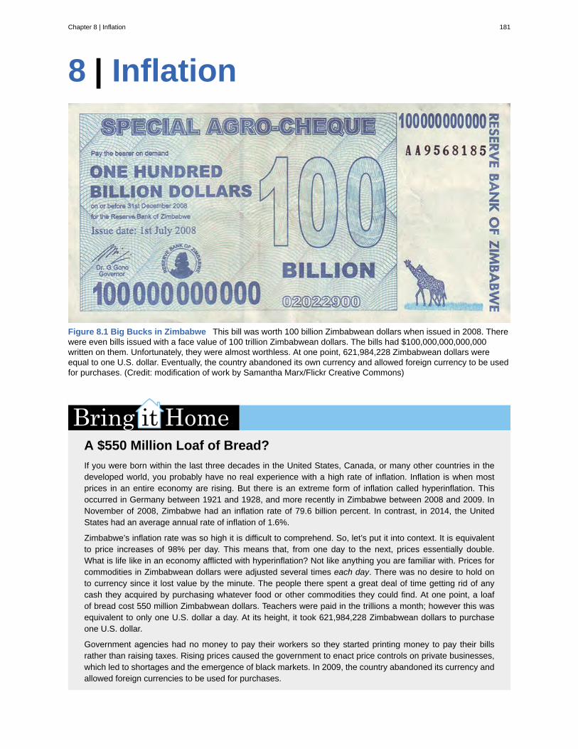
8 | Inflation
Figure 8.1 Big Bucks in Zimbabwe This bill was worth 100 billion Zimbabwean dollars when issued in 2008. Therewere even bills issued with a face value of 100 trillion Zimbabwean dollars. The bills had $100,000,000,000,000written on them. Unfortunately, they were almost worthless. At one point, 621,984,228 Zimbabwean dollars wereequal to one U.S. dollar. Eventually, the country abandoned its own currency and allowed foreign currency to be usedfor purchases. (Credit: modification of work by Samantha Marx/Flickr Creative Commons)
A $550 Million Loaf of Bread?If you were born within the last three decades in the United States, Canada, or many other countries in thedeveloped world, you probably have no real experience with a high rate of inflation. Inflation is when mostprices in an entire economy are rising. But there is an extreme form of inflation called hyperinflation. Thisoccurred in Germany between 1921 and 1928, and more recently in Zimbabwe between 2008 and 2009. InNovember of 2008, Zimbabwe had an inflation rate of 79.6 billion percent. In contrast, in 2014, the UnitedStates had an average annual rate of inflation of 1.6%.
Zimbabwe’s inflation rate was so high it is difficult to comprehend. So, let’s put it into context. It is equivalentto price increases of 98% per day. This means that, from one day to the next, prices essentially double.What is life like in an economy afflicted with hyperinflation? Not like anything you are familiar with. Prices forcommodities in Zimbabwean dollars were adjusted several times each day. There was no desire to hold onto currency since it lost value by the minute. The people there spent a great deal of time getting rid of anycash they acquired by purchasing whatever food or other commodities they could find. At one point, a loafof bread cost 550 million Zimbabwean dollars. Teachers were paid in the trillions a month; however this wasequivalent to only one U.S. dollar a day. At its height, it took 621,984,228 Zimbabwean dollars to purchaseone U.S. dollar.
Government agencies had no money to pay their workers so they started printing money to pay their billsrather than raising taxes. Rising prices caused the government to enact price controls on private businesses,which led to shortages and the emergence of black markets. In 2009, the country abandoned its currency andallowed foreign currencies to be used for purchases.
Chapter 8 | Inflation 181
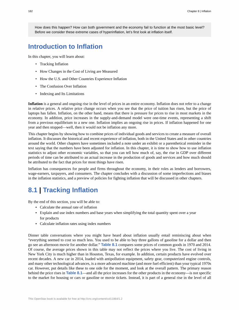
How does this happen? How can both government and the economy fail to function at the most basic level?Before we consider these extreme cases of hyperinflation, let’s first look at inflation itself.
Introduction to InflationIn this chapter, you will learn about:
• Tracking Inflation
• How Changes in the Cost of Living are Measured
• How the U.S. and Other Countries Experience Inflation
• The Confusion Over Inflation
• Indexing and Its Limitations
Inflation is a general and ongoing rise in the level of prices in an entire economy. Inflation does not refer to a changein relative prices. A relative price change occurs when you see that the price of tuition has risen, but the price oflaptops has fallen. Inflation, on the other hand, means that there is pressure for prices to rise in most markets in theeconomy. In addition, price increases in the supply-and-demand model were one-time events, representing a shiftfrom a previous equilibrium to a new one. Inflation implies an ongoing rise in prices. If inflation happened for oneyear and then stopped—well, then it would not be inflation any more.
This chapter begins by showing how to combine prices of individual goods and services to create a measure of overallinflation. It discusses the historical and recent experience of inflation, both in the United States and in other countriesaround the world. Other chapters have sometimes included a note under an exhibit or a parenthetical reminder in thetext saying that the numbers have been adjusted for inflation. In this chapter, it is time to show how to use inflationstatistics to adjust other economic variables, so that you can tell how much of, say, the rise in GDP over differentperiods of time can be attributed to an actual increase in the production of goods and services and how much shouldbe attributed to the fact that prices for most things have risen.
Inflation has consequences for people and firms throughout the economy, in their roles as lenders and borrowers,wage-earners, taxpayers, and consumers. The chapter concludes with a discussion of some imperfections and biasesin the inflation statistics, and a preview of policies for fighting inflation that will be discussed in other chapters.
8.1 | Tracking InflationBy the end of this section, you will be able to:
• Calculate the annual rate of inflation• Explain and use index numbers and base years when simplifying the total quantity spent over a year
for products• Calculate inflation rates using index numbers
Dinner table conversations where you might have heard about inflation usually entail reminiscing about when“everything seemed to cost so much less. You used to be able to buy three gallons of gasoline for a dollar and thengo see an afternoon movie for another dollar.” Table 8.1 compares some prices of common goods in 1970 and 2014.Of course, the average prices shown in this table may not reflect the prices where you live. The cost of living inNew York City is much higher than in Houston, Texas, for example. In addition, certain products have evolved overrecent decades. A new car in 2014, loaded with antipollution equipment, safety gear, computerized engine controls,and many other technological advances, is a more advanced machine (and more fuel efficient) than your typical 1970scar. However, put details like these to one side for the moment, and look at the overall pattern. The primary reasonbehind the price rises in Table 8.1—and all the price increases for the other products in the economy—is not specificto the market for housing or cars or gasoline or movie tickets. Instead, it is part of a general rise in the level of all
182 Chapter 8 | Inflation
This OpenStax book is available for free at http://cnx.org/content/col11864/1.2
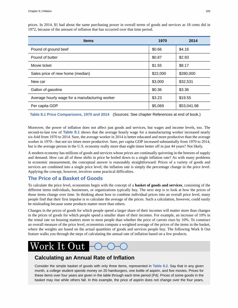
prices. In 2014, $1 had about the same purchasing power in overall terms of goods and services as 18 cents did in1972, because of the amount of inflation that has occurred over that time period.
Items 1970 2014
Pound of ground beef $0.66 $4.16
Pound of butter $0.87 $2.93
Movie ticket $1.55 $8.17
Sales price of new home (median) $22,000 $280,000
New car $3,000 $32,531
Gallon of gasoline $0.36 $3.36
Average hourly wage for a manufacturing worker $3.23 $19.55
Per capita GDP $5,069 $53,041.98
Table 8.1 Price Comparisons, 1970 and 2014 (Sources: See chapter References at end of book.)
Moreover, the power of inflation does not affect just goods and services, but wages and income levels, too. Thesecond-to-last row of Table 8.1 shows that the average hourly wage for a manufacturing worker increased nearlysix-fold from 1970 to 2014. Sure, the average worker in 2014 is better educated and more productive than the averageworker in 1970—but not six times more productive. Sure, per capita GDP increased substantially from 1970 to 2014,but is the average person in the U.S. economy really more than eight times better off in just 44 years? Not likely.
A modern economy has millions of goods and services whose prices are continually quivering in the breezes of supplyand demand. How can all of these shifts in price be boiled down to a single inflation rate? As with many problemsin economic measurement, the conceptual answer is reasonably straightforward: Prices of a variety of goods andservices are combined into a single price level; the inflation rate is simply the percentage change in the price level.Applying the concept, however, involves some practical difficulties.
The Price of a Basket of GoodsTo calculate the price level, economists begin with the concept of a basket of goods and services, consisting of thedifferent items individuals, businesses, or organizations typically buy. The next step is to look at how the prices ofthose items change over time. In thinking about how to combine individual prices into an overall price level, manypeople find that their first impulse is to calculate the average of the prices. Such a calculation, however, could easilybe misleading because some products matter more than others.
Changes in the prices of goods for which people spend a larger share of their incomes will matter more than changesin the prices of goods for which people spend a smaller share of their incomes. For example, an increase of 10% inthe rental rate on housing matters more to most people than whether the price of carrots rises by 10%. To constructan overall measure of the price level, economists compute a weighted average of the prices of the items in the basket,where the weights are based on the actual quantities of goods and services people buy. The following Work It Outfeature walks you through the steps of calculating the annual rate of inflation based on a few products.
Calculating an Annual Rate of InflationConsider the simple basket of goods with only three items, represented in Table 8.2. Say that in any givenmonth, a college student spends money on 20 hamburgers, one bottle of aspirin, and five movies. Prices forthese items over four years are given in the table through each time period (Pd). Prices of some goods in thebasket may rise while others fall. In this example, the price of aspirin does not change over the four years,
Chapter 8 | Inflation 183
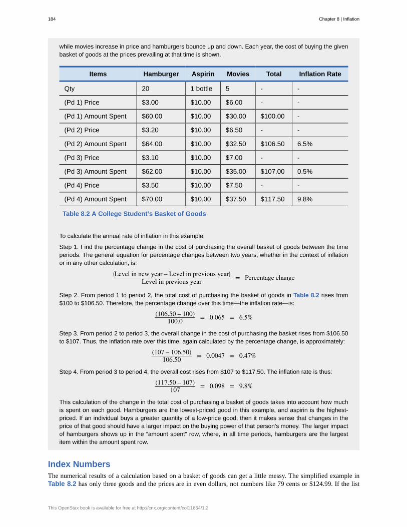
while movies increase in price and hamburgers bounce up and down. Each year, the cost of buying the givenbasket of goods at the prices prevailing at that time is shown.
Items Hamburger Aspirin Movies Total Inflation Rate
Qty 20 1 bottle 5 - -
(Pd 1) Price $3.00 $10.00 $6.00 - -
(Pd 1) Amount Spent $60.00 $10.00 $30.00 $100.00 -
(Pd 2) Price $3.20 $10.00 $6.50 - -
(Pd 2) Amount Spent $64.00 $10.00 $32.50 $106.50 6.5%
(Pd 3) Price $3.10 $10.00 $7.00 - -
(Pd 3) Amount Spent $62.00 $10.00 $35.00 $107.00 0.5%
(Pd 4) Price $3.50 $10.00 $7.50 - -
(Pd 4) Amount Spent $70.00 $10.00 $37.50 $117.50 9.8%
Table 8.2 A College Student’s Basket of Goods
To calculate the annual rate of inflation in this example:
Step 1. Find the percentage change in the cost of purchasing the overall basket of goods between the timeperiods. The general equation for percentage changes between two years, whether in the context of inflationor in any other calculation, is:
⎛⎝Level in new year – Level in previous year⎞
⎠
Level in previous year = Percentage change
Step 2. From period 1 to period 2, the total cost of purchasing the basket of goods in Table 8.2 rises from$100 to $106.50. Therefore, the percentage change over this time—the inflation rate—is:
(106.50 – 100)100.0 = 0.065 = 6.5%
Step 3. From period 2 to period 3, the overall change in the cost of purchasing the basket rises from $106.50to $107. Thus, the inflation rate over this time, again calculated by the percentage change, is approximately:
(107 – 106.50)106.50 = 0.0047 = 0.47%
Step 4. From period 3 to period 4, the overall cost rises from $107 to $117.50. The inflation rate is thus:
(117.50 – 107)107 = 0.098 = 9.8%
This calculation of the change in the total cost of purchasing a basket of goods takes into account how muchis spent on each good. Hamburgers are the lowest-priced good in this example, and aspirin is the highest-priced. If an individual buys a greater quantity of a low-price good, then it makes sense that changes in theprice of that good should have a larger impact on the buying power of that person’s money. The larger impactof hamburgers shows up in the “amount spent” row, where, in all time periods, hamburgers are the largestitem within the amount spent row.
Index NumbersThe numerical results of a calculation based on a basket of goods can get a little messy. The simplified example inTable 8.2 has only three goods and the prices are in even dollars, not numbers like 79 cents or $124.99. If the list
184 Chapter 8 | Inflation
This OpenStax book is available for free at http://cnx.org/content/col11864/1.2
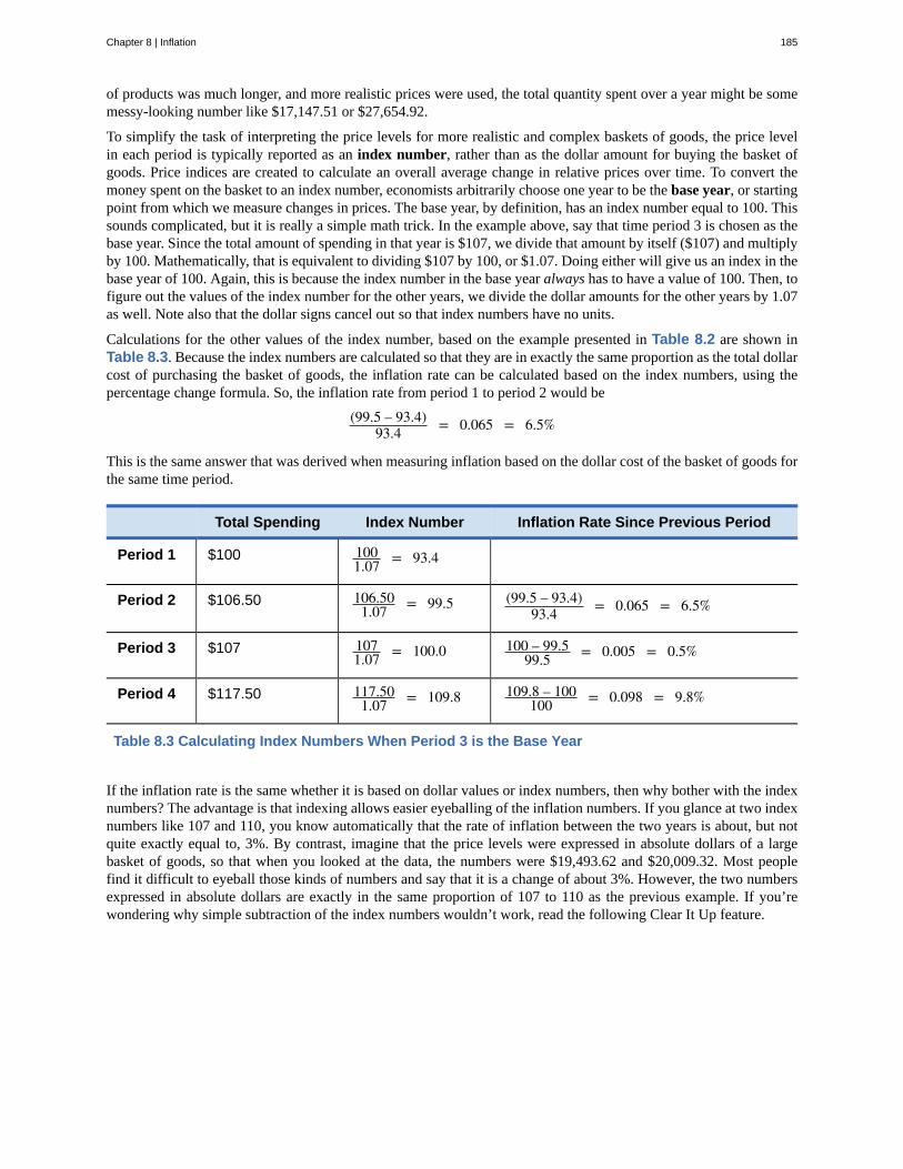
of products was much longer, and more realistic prices were used, the total quantity spent over a year might be somemessy-looking number like $17,147.51 or $27,654.92.
To simplify the task of interpreting the price levels for more realistic and complex baskets of goods, the price levelin each period is typically reported as an index number, rather than as the dollar amount for buying the basket ofgoods. Price indices are created to calculate an overall average change in relative prices over time. To convert themoney spent on the basket to an index number, economists arbitrarily choose one year to be the base year, or startingpoint from which we measure changes in prices. The base year, by definition, has an index number equal to 100. Thissounds complicated, but it is really a simple math trick. In the example above, say that time period 3 is chosen as thebase year. Since the total amount of spending in that year is $107, we divide that amount by itself ($107) and multiplyby 100. Mathematically, that is equivalent to dividing $107 by 100, or $1.07. Doing either will give us an index in thebase year of 100. Again, this is because the index number in the base year always has to have a value of 100. Then, tofigure out the values of the index number for the other years, we divide the dollar amounts for the other years by 1.07as well. Note also that the dollar signs cancel out so that index numbers have no units.
Calculations for the other values of the index number, based on the example presented in Table 8.2 are shown inTable 8.3. Because the index numbers are calculated so that they are in exactly the same proportion as the total dollarcost of purchasing the basket of goods, the inflation rate can be calculated based on the index numbers, using thepercentage change formula. So, the inflation rate from period 1 to period 2 would be
(99.5 – 93.4)93.4 = 0.065 = 6.5%
This is the same answer that was derived when measuring inflation based on the dollar cost of the basket of goods forthe same time period.
Total Spending Index Number Inflation Rate Since Previous Period
Period 1 $100 1001.07 = 93.4
Period 2 $106.50 106.501.07 = 99.5 (99.5 – 93.4)
93.4 = 0.065 = 6.5%
Period 3 $107 1071.07 = 100.0 100 – 99.5
99.5 = 0.005 = 0.5%
Period 4 $117.50 117.501.07 = 109.8 109.8 – 100
100 = 0.098 = 9.8%
Table 8.3 Calculating Index Numbers When Period 3 is the Base Year
If the inflation rate is the same whether it is based on dollar values or index numbers, then why bother with the indexnumbers? The advantage is that indexing allows easier eyeballing of the inflation numbers. If you glance at two indexnumbers like 107 and 110, you know automatically that the rate of inflation between the two years is about, but notquite exactly equal to, 3%. By contrast, imagine that the price levels were expressed in absolute dollars of a largebasket of goods, so that when you looked at the data, the numbers were $19,493.62 and $20,009.32. Most peoplefind it difficult to eyeball those kinds of numbers and say that it is a change of about 3%. However, the two numbersexpressed in absolute dollars are exactly in the same proportion of 107 to 110 as the previous example. If you’rewondering why simple subtraction of the index numbers wouldn’t work, read the following Clear It Up feature.
Chapter 8 | Inflation 185
Why do you not just subtract index numbers?A word of warning: When a price index moves from, say, 107 to 110, the rate of inflation is not exactly3%. Remember, the inflation rate is not derived by subtracting the index numbers, but rather through thepercentage-change calculation. The precise inflation rate as the price index moves from 107 to 110 iscalculated as (110 – 107) / 107 = 0.028 = 2.8%. When the base year is fairly close to 100, a quick subtraction isnot a terrible shortcut to calculating the inflation rate—but when precision matters down to tenths of a percent,subtracting will not give the right answer.
Two final points about index numbers are worth remembering. First, index numbers have no dollar signs or otherunits attached to them. Although index numbers can be used to calculate a percentage inflation rate, the indexnumbers themselves do not have percentage signs. Index numbers just mirror the proportions found in other data.They transform the other data so that the data are easier to work with.
Second, the choice of a base year for the index number—that is, the year that is automatically set equal to 100—isarbitrary. It is chosen as a starting point from which changes in prices are tracked. In the official inflation statistics, itis common to use one base year for a few years, and then to update it, so that the base year of 100 is relatively closeto the present. But any base year that is chosen for the index numbers will result in exactly the same inflation rate. Tosee this in the previous example, imagine that period 1, when total spending was $100, was also chosen as the baseyear, and given an index number of 100. At a glance, you can see that the index numbers would now exactly matchthe dollar figures, the inflation rate in the first period would be 6.5%, and so on.
Now that we see how indexes work to track inflation, the next module will show us how the cost of living is measured.
Watch this video (http://openstaxcollege.org/l/Duck_Tales) from the cartoon Duck Tales to view a mini-lessonon inflation.
8.2 | How Changes in the Cost of Living Are MeasuredBy the end of this section, you will be able to:
• Use the Consumer Price Index (CPI) to calculate U.S. inflation rates• Identify several ways the Bureau of Labor Statistics avoids baises in the Consumer Price Index (CPI)• Differentiate among the Consumer Price Index (CPI), the Producer Price Index (PPI), the
International Price Index, the Employment Cost Index, and the GDP deflator.
The most commonly cited measure of inflation in the United States is the Consumer Price Index (CPI). The CPI iscalculated by government statisticians at the U.S. Bureau of Labor Statistics based on the prices in a fixed basket of
186 Chapter 8 | Inflation
This OpenStax book is available for free at http://cnx.org/content/col11864/1.2
goods and services that represents the purchases of the average family of four. In recent years, the statisticians havepaid considerable attention to a subtle problem: that the change in the total cost of buying a fixed basket of goods andservices over time is conceptually not quite the same as the change in the cost of living, because the cost of livingrepresents how much it costs for a person to feel that his or her consumption provides an equal level of satisfaction orutility.
To understand the distinction, imagine that over the past 10 years, the cost of purchasing a fixed basket of goodsincreased by 25% and your salary also increased by 25%. Has your personal standard of living held constant? If youdo not necessarily purchase an identical fixed basket of goods every year, then an inflation calculation based on thecost of a fixed basket of goods may be a misleading measure of how your cost of living has changed. Two problemsarise here: substitution bias and quality/new goods bias.
When the price of a good rises, consumers tend to purchase less of it and to seek out substitutes instead. Conversely,as the price of a good falls, people will tend to purchase more of it. This pattern implies that goods with generallyrising prices should tend over time to become less important in the overall basket of goods used to calculate inflation,while goods with falling prices should tend to become more important. Consider, as an example, a rise in theprice of peaches by $100 per pound. If consumers were utterly inflexible in their demand for peaches, this wouldlead to a big rise in the price of food for consumers. Alternatively, imagine that people are utterly indifferent towhether they have peaches or other types of fruit. Now, if peach prices rise, people completely switch to other fruitchoices and the average price of food does not change at all. A fixed and unchanging basket of goods assumes thatconsumers are locked into buying exactly the same goods, regardless of price changes—not a very likely assumption.Thus, substitution bias—the rise in the price of a fixed basket of goods over time—tends to overstate the rise in aconsumer’s true cost of living, because it does not take into account that the person can substitute away from goodswhose relative prices have risen.
The other major problem in using a fixed basket of goods as the basis for calculating inflation is how to deal withthe arrival of improved versions of older goods or altogether new goods. Consider the problem that arises if a cerealis improved by adding 12 essential vitamins and minerals—and also if a box of the cereal costs 5% more. It wouldclearly be misleading to count the entire resulting higher price as inflation, because the new price is being charged fora product of higher (or at least different) quality. Ideally, one would like to know how much of the higher price is dueto the quality change, and how much of it is just a higher price. The Bureau of Labor Statistics, which is responsiblefor the computation of the Consumer Price Index, must deal with these difficulties in adjusting for quality changes.
Visit this website (http://openstaxcollege.org/l/Fords) to view a list of Ford car prices between 1909 and 1927.Consider how these prices compare to today’s models. Is the product today of a different quality?
A new product can be thought of as an extreme improvement in quality—from something that did not exist tosomething that does. However, the basket of goods that was fixed in the past obviously does not include new goodscreated since then. The basket of goods and services used in the Consumer Price Index (CPI) is revised and updatedover time, and so new products are gradually included. But the process takes some time. For example, room airconditioners were widely sold in the early 1950s, but were not introduced into the basket of goods behind theConsumer Price Index until 1964. The VCR and personal computer were available in the late 1970s and widely soldby the early 1980s, but did not enter the CPI basket of goods until 1987. By 1996, there were more than 40 millioncellular phone subscribers in the United States—but cell phones were not yet part of the CPI basket of goods. Theparade of inventions has continued, with the CPI inevitably lagging a few years behind.
Chapter 8 | Inflation 187
The arrival of new goods creates problems with respect to the accuracy of measuring inflation. The reason peoplebuy new goods, presumably, is that the new goods offer better value for money than existing goods. Thus, if the priceindex leaves out new goods, it overlooks one of the ways in which the cost of living is improving. In addition, theprice of a new good is often higher when it is first introduced and then declines over time. If the new good is notincluded in the CPI for some years, until its price is already lower, the CPI may miss counting this price declinealtogether. Taking these arguments together, the quality/new goods bias means that the rise in the price of a fixedbasket of goods over time tends to overstate the rise in a consumer’s true cost of living, because it does not take intoaccount how improvements in the quality of existing goods or the invention of new goods improves the standard ofliving. The following Clear It Up feature is a must-read on how the CPI is comprised and calculated.
How do U.S. government statisticians measure the ConsumerPrice Index?When the U.S. Bureau of Labor Statistics (BLS) calculates the Consumer Price Index, the first task is to decideon a basket of goods that is representative of the purchases of the average household. This is done by usingthe Consumer Expenditure Survey, a national survey of about 7,000 households, which provides detailedinformation on spending habits. Consumer expenditures are broken up into eight major groups, shown below,which in turn are broken up into more than 200 individual item categories. The BLS currently uses 1982–1984as the base period.
For each of the 200 individual expenditure items, the BLS chooses several hundred very specific examplesof that item and looks at the prices of those examples. So, in figuring out the “breakfast cereal” item underthe overall category of “foods and beverages,” the BLS picks several hundred examples of breakfast cereal.One example might be the price of a 24-oz. box of a particular brand of cereal sold at a particular store. Thespecific products and sizes and stores chosen are statistically selected to reflect what people buy and wherethey shop. The basket of goods in the Consumer Price Index thus consists of about 80,000 products; thatis, several hundred specific products in over 200 broad-item categories. About one-quarter of these 80,000specific products are rotated out of the sample each year, and replaced with a different set of products.
The next step is to collect data on prices. Data collectors visit or call about 23,000 stores in 87 urban areasall over the United States every month to collect prices on these 80,000 specific products. A survey of 50,000landlords or tenants is also carried out to collect information about rents.
The Consumer Price Index is then calculated by taking the 80,000 prices of individual products and combiningthem, using weights (as shown in Figure 8.2) determined by the quantities of these products that people buyand allowing for factors like substitution between goods and quality improvements, into price indices for the200 or so overall items. Then, the price indices for the 200 items are combined into an overall Consumer PriceIndex. According the Consumer Price Index website, there are eight categories used by data collectors:
The Eight Major Categories in the Consumer Price Index
1. Food and beverages (breakfast cereal, milk, coffee, chicken, wine, full-service meals, and snacks)
2. Housing (renter’s cost of housing, homeowner’s cost of housing, fuel oil, bedroom furniture)
3. Apparel (men’s shirts and sweaters, women’s dresses, jewelry)
4. Transportation (new vehicles, airline fares, gasoline, motor vehicle insurance)
5. Medical care (prescription drugs and medical supplies, physicians’ services, eyeglasses and eye care,hospital services)
6. Recreation (televisions, cable television, pets and pet products, sports equipment, admissions)
7. Education and communication (college tuition, postage, telephone services, computer software andaccessories)
8. Other goods and services (tobacco and smoking products, haircuts and other personal services,funeral expenses)
188 Chapter 8 | Inflation
This OpenStax book is available for free at http://cnx.org/content/col11864/1.2
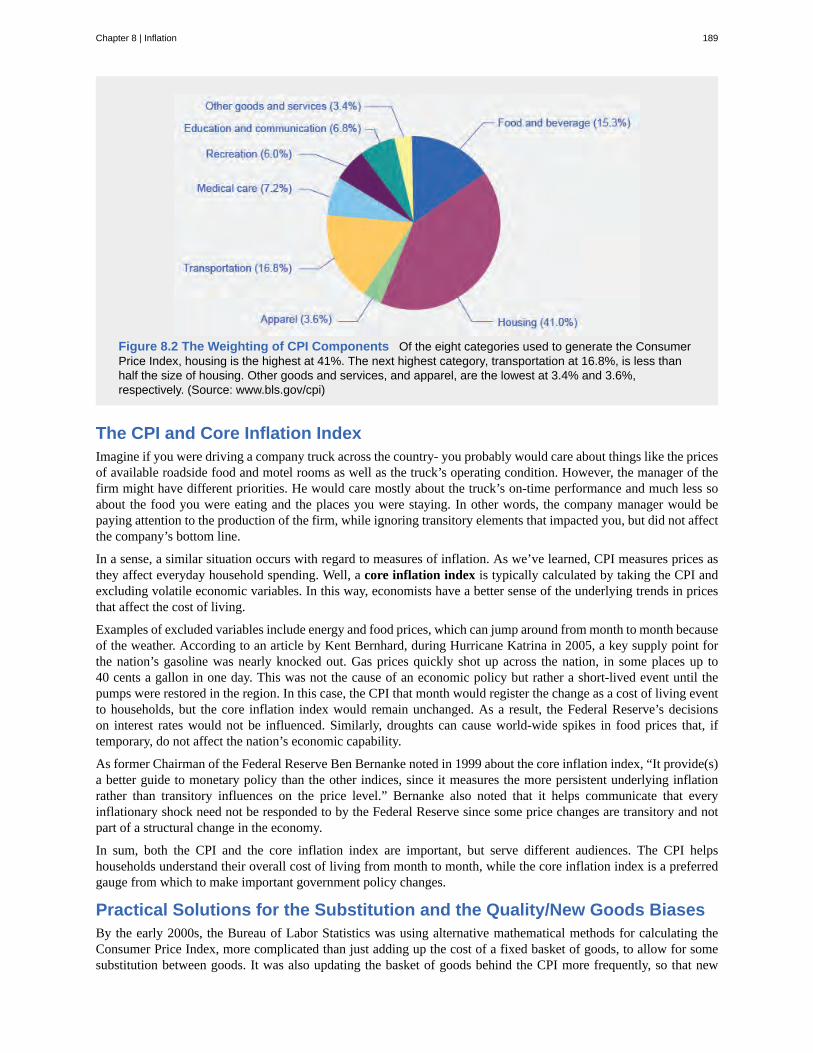
Figure 8.2 The Weighting of CPI Components Of the eight categories used to generate the ConsumerPrice Index, housing is the highest at 41%. The next highest category, transportation at 16.8%, is less thanhalf the size of housing. Other goods and services, and apparel, are the lowest at 3.4% and 3.6%,respectively. (Source: www.bls.gov/cpi)
The CPI and Core Inflation IndexImagine if you were driving a company truck across the country- you probably would care about things like the pricesof available roadside food and motel rooms as well as the truck’s operating condition. However, the manager of thefirm might have different priorities. He would care mostly about the truck’s on-time performance and much less soabout the food you were eating and the places you were staying. In other words, the company manager would bepaying attention to the production of the firm, while ignoring transitory elements that impacted you, but did not affectthe company’s bottom line.
In a sense, a similar situation occurs with regard to measures of inflation. As we’ve learned, CPI measures prices asthey affect everyday household spending. Well, a core inflation index is typically calculated by taking the CPI andexcluding volatile economic variables. In this way, economists have a better sense of the underlying trends in pricesthat affect the cost of living.
Examples of excluded variables include energy and food prices, which can jump around from month to month becauseof the weather. According to an article by Kent Bernhard, during Hurricane Katrina in 2005, a key supply point forthe nation’s gasoline was nearly knocked out. Gas prices quickly shot up across the nation, in some places up to40 cents a gallon in one day. This was not the cause of an economic policy but rather a short-lived event until thepumps were restored in the region. In this case, the CPI that month would register the change as a cost of living eventto households, but the core inflation index would remain unchanged. As a result, the Federal Reserve’s decisionson interest rates would not be influenced. Similarly, droughts can cause world-wide spikes in food prices that, iftemporary, do not affect the nation’s economic capability.
As former Chairman of the Federal Reserve Ben Bernanke noted in 1999 about the core inflation index, “It provide(s)a better guide to monetary policy than the other indices, since it measures the more persistent underlying inflationrather than transitory influences on the price level.” Bernanke also noted that it helps communicate that everyinflationary shock need not be responded to by the Federal Reserve since some price changes are transitory and notpart of a structural change in the economy.
In sum, both the CPI and the core inflation index are important, but serve different audiences. The CPI helpshouseholds understand their overall cost of living from month to month, while the core inflation index is a preferredgauge from which to make important government policy changes.
Practical Solutions for the Substitution and the Quality/New Goods BiasesBy the early 2000s, the Bureau of Labor Statistics was using alternative mathematical methods for calculating theConsumer Price Index, more complicated than just adding up the cost of a fixed basket of goods, to allow for somesubstitution between goods. It was also updating the basket of goods behind the CPI more frequently, so that new
Chapter 8 | Inflation 189
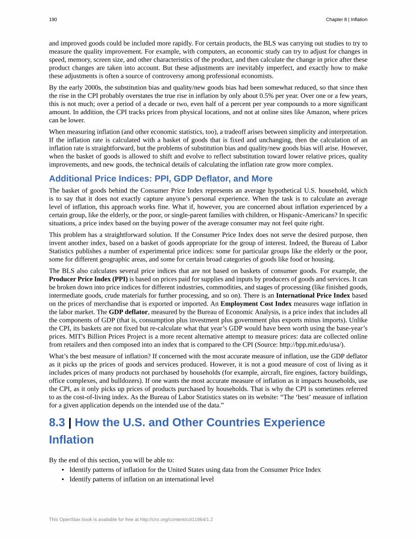
and improved goods could be included more rapidly. For certain products, the BLS was carrying out studies to try tomeasure the quality improvement. For example, with computers, an economic study can try to adjust for changes inspeed, memory, screen size, and other characteristics of the product, and then calculate the change in price after theseproduct changes are taken into account. But these adjustments are inevitably imperfect, and exactly how to makethese adjustments is often a source of controversy among professional economists.
By the early 2000s, the substitution bias and quality/new goods bias had been somewhat reduced, so that since thenthe rise in the CPI probably overstates the true rise in inflation by only about 0.5% per year. Over one or a few years,this is not much; over a period of a decade or two, even half of a percent per year compounds to a more significantamount. In addition, the CPI tracks prices from physical locations, and not at online sites like Amazon, where pricescan be lower.
When measuring inflation (and other economic statistics, too), a tradeoff arises between simplicity and interpretation.If the inflation rate is calculated with a basket of goods that is fixed and unchanging, then the calculation of aninflation rate is straightforward, but the problems of substitution bias and quality/new goods bias will arise. However,when the basket of goods is allowed to shift and evolve to reflect substitution toward lower relative prices, qualityimprovements, and new goods, the technical details of calculating the inflation rate grow more complex.
Additional Price Indices: PPI, GDP Deflator, and MoreThe basket of goods behind the Consumer Price Index represents an average hypothetical U.S. household, whichis to say that it does not exactly capture anyone’s personal experience. When the task is to calculate an averagelevel of inflation, this approach works fine. What if, however, you are concerned about inflation experienced by acertain group, like the elderly, or the poor, or single-parent families with children, or Hispanic-Americans? In specificsituations, a price index based on the buying power of the average consumer may not feel quite right.
This problem has a straightforward solution. If the Consumer Price Index does not serve the desired purpose, theninvent another index, based on a basket of goods appropriate for the group of interest. Indeed, the Bureau of LaborStatistics publishes a number of experimental price indices: some for particular groups like the elderly or the poor,some for different geographic areas, and some for certain broad categories of goods like food or housing.
The BLS also calculates several price indices that are not based on baskets of consumer goods. For example, theProducer Price Index (PPI) is based on prices paid for supplies and inputs by producers of goods and services. It canbe broken down into price indices for different industries, commodities, and stages of processing (like finished goods,intermediate goods, crude materials for further processing, and so on). There is an International Price Index basedon the prices of merchandise that is exported or imported. An Employment Cost Index measures wage inflation inthe labor market. The GDP deflator, measured by the Bureau of Economic Analysis, is a price index that includes allthe components of GDP (that is, consumption plus investment plus government plus exports minus imports). Unlikethe CPI, its baskets are not fixed but re-calculate what that year’s GDP would have been worth using the base-year’sprices. MIT's Billion Prices Project is a more recent alternative attempt to measure prices: data are collected onlinefrom retailers and then composed into an index that is compared to the CPI (Source: http://bpp.mit.edu/usa/).
What’s the best measure of inflation? If concerned with the most accurate measure of inflation, use the GDP deflatoras it picks up the prices of goods and services produced. However, it is not a good measure of cost of living as itincludes prices of many products not purchased by households (for example, aircraft, fire engines, factory buildings,office complexes, and bulldozers). If one wants the most accurate measure of inflation as it impacts households, usethe CPI, as it only picks up prices of products purchased by households. That is why the CPI is sometimes referredto as the cost-of-living index. As the Bureau of Labor Statistics states on its website: “The ‘best’ measure of inflationfor a given application depends on the intended use of the data.”
8.3 | How the U.S. and Other Countries ExperienceInflationBy the end of this section, you will be able to:
• Identify patterns of inflation for the United States using data from the Consumer Price Index• Identify patterns of inflation on an international level
190 Chapter 8 | Inflation
This OpenStax book is available for free at http://cnx.org/content/col11864/1.2
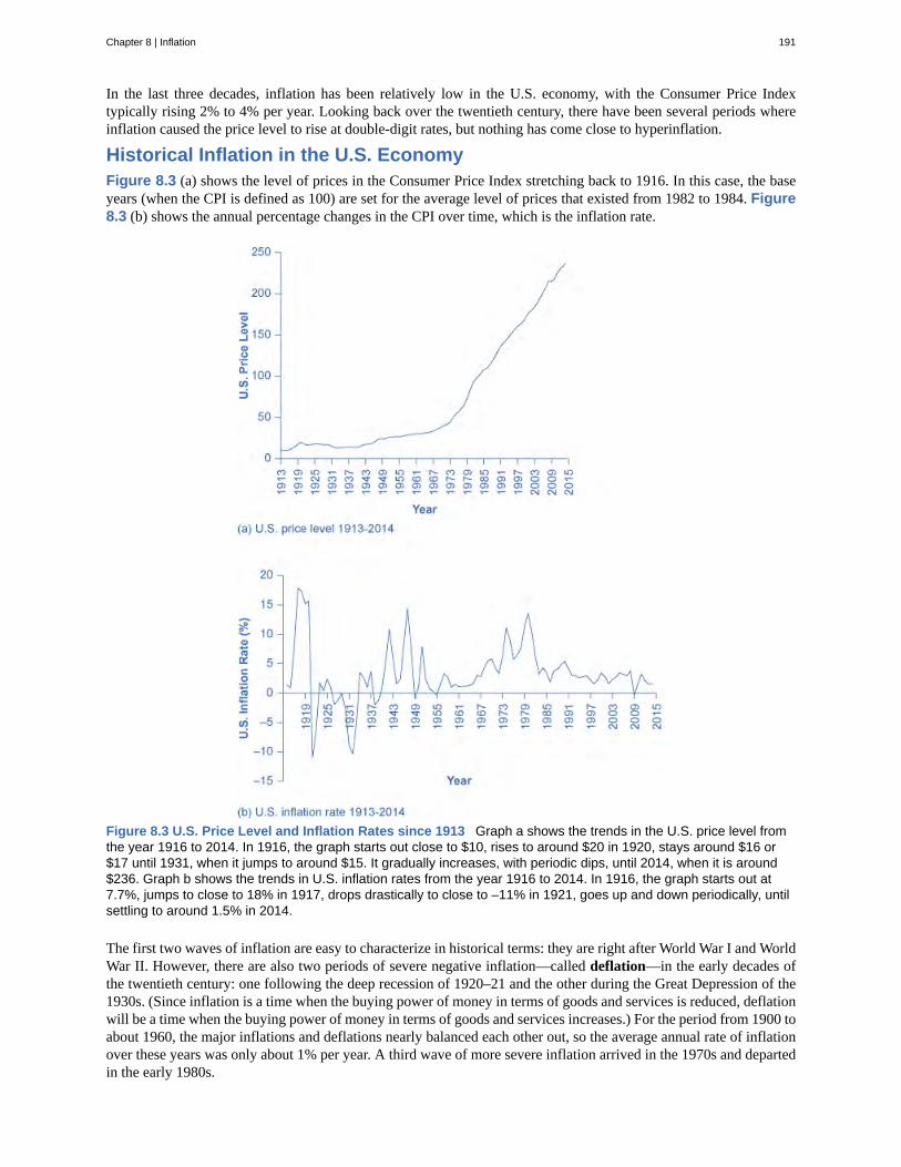
In the last three decades, inflation has been relatively low in the U.S. economy, with the Consumer Price Indextypically rising 2% to 4% per year. Looking back over the twentieth century, there have been several periods whereinflation caused the price level to rise at double-digit rates, but nothing has come close to hyperinflation.
Historical Inflation in the U.S. EconomyFigure 8.3 (a) shows the level of prices in the Consumer Price Index stretching back to 1916. In this case, the baseyears (when the CPI is defined as 100) are set for the average level of prices that existed from 1982 to 1984. Figure8.3 (b) shows the annual percentage changes in the CPI over time, which is the inflation rate.
Figure 8.3 U.S. Price Level and Inflation Rates since 1913 Graph a shows the trends in the U.S. price level fromthe year 1916 to 2014. In 1916, the graph starts out close to $10, rises to around $20 in 1920, stays around $16 or$17 until 1931, when it jumps to around $15. It gradually increases, with periodic dips, until 2014, when it is around$236. Graph b shows the trends in U.S. inflation rates from the year 1916 to 2014. In 1916, the graph starts out at7.7%, jumps to close to 18% in 1917, drops drastically to close to –11% in 1921, goes up and down periodically, untilsettling to around 1.5% in 2014.
The first two waves of inflation are easy to characterize in historical terms: they are right after World War I and WorldWar II. However, there are also two periods of severe negative inflation—called deflation—in the early decades ofthe twentieth century: one following the deep recession of 1920–21 and the other during the Great Depression of the1930s. (Since inflation is a time when the buying power of money in terms of goods and services is reduced, deflationwill be a time when the buying power of money in terms of goods and services increases.) For the period from 1900 toabout 1960, the major inflations and deflations nearly balanced each other out, so the average annual rate of inflationover these years was only about 1% per year. A third wave of more severe inflation arrived in the 1970s and departedin the early 1980s.
Chapter 8 | Inflation 191
Visit this website (http://openstaxcollege.org/l/CPI_calculator) to use an inflation calculator and discover howprices have changed in the last 100 years.
Times of recession or depression often seem to be times when the inflation rate is lower, as in the recession of1920–1921, the Great Depression, the recession of 1980–1982, and the Great Recession in 2008–2009. There werea few months in 2009 that were deflationary, but not at an annual rate. Recessions are typically accompanied byhigher levels of unemployment, and the total demand for goods falls, pulling the price level down. Conversely, therate of inflation often, but not always, seems to start moving up when the economy is growing very strongly, like rightafter wartime or during the 1960s. The frameworks for macroeconomic analysis, developed in other chapters, willexplain why recession often accompanies higher unemployment and lower inflation, while rapid economic growthoften brings lower unemployment but higher inflation.
Inflation around the WorldAround the rest of the world, the pattern of inflation has been very mixed, as can be seen in Figure 8.4 which showsinflation rates over the last several decades. Many industrialized countries, not just the United States, had relativelyhigh inflation rates in the 1970s. For example, in 1975, Japan’s inflation rate was over 8% and the inflation rate forthe United Kingdom was almost 25%. In the 1980s, inflation rates came down in the United States and in Europe andhave largely stayed down.
Figure 8.4 Countries with Relatively Low Inflation Rates, 1960–2014 This chart shows the annual percentagechange in consumer prices compared with the previous year’s consumer prices in the United States, the UnitedKingdom, Japan, and Germany.
Countries with controlled economies in the 1970s, like the Soviet Union and China, historically had very low ratesof measured inflation—because prices were forbidden to rise by law, except for the cases where the government
192 Chapter 8 | Inflation
This OpenStax book is available for free at http://cnx.org/content/col11864/1.2
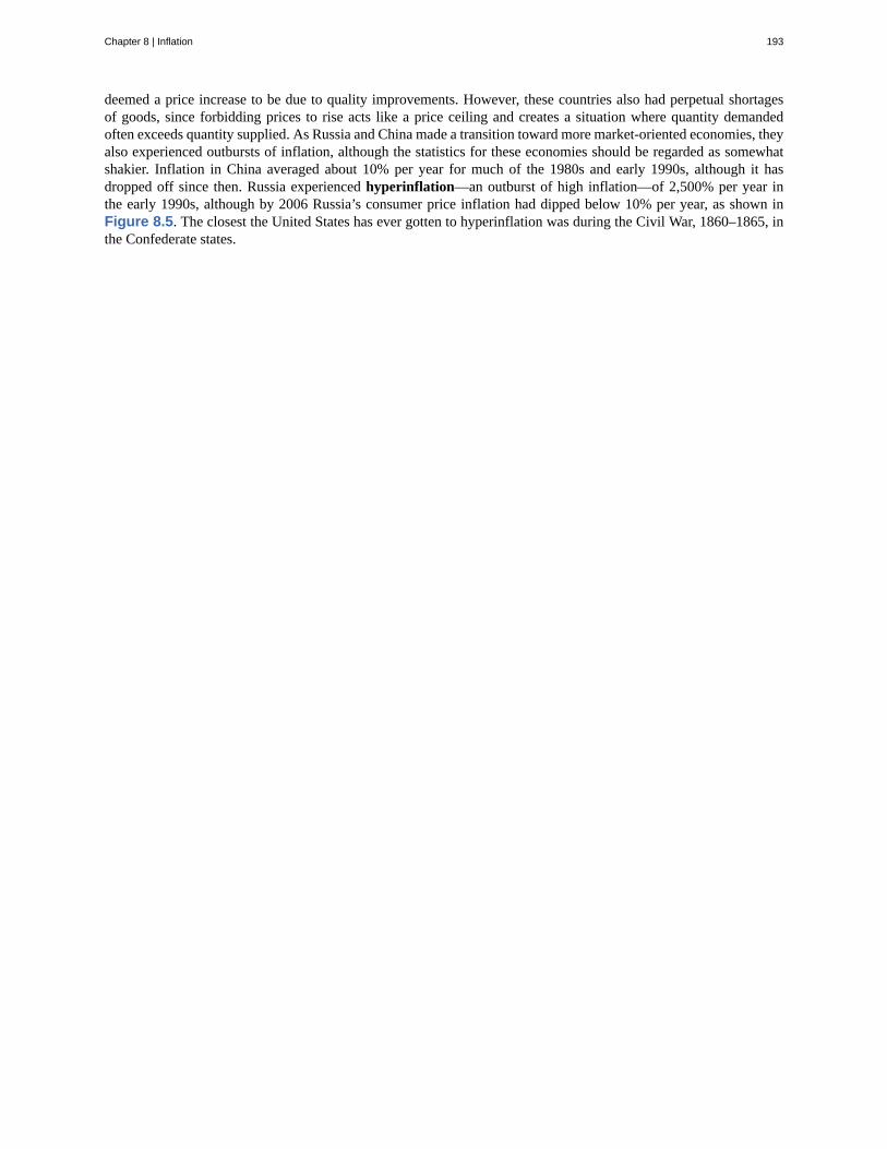
deemed a price increase to be due to quality improvements. However, these countries also had perpetual shortagesof goods, since forbidding prices to rise acts like a price ceiling and creates a situation where quantity demandedoften exceeds quantity supplied. As Russia and China made a transition toward more market-oriented economies, theyalso experienced outbursts of inflation, although the statistics for these economies should be regarded as somewhatshakier. Inflation in China averaged about 10% per year for much of the 1980s and early 1990s, although it hasdropped off since then. Russia experienced hyperinflation—an outburst of high inflation—of 2,500% per year inthe early 1990s, although by 2006 Russia’s consumer price inflation had dipped below 10% per year, as shown inFigure 8.5. The closest the United States has ever gotten to hyperinflation was during the Civil War, 1860–1865, inthe Confederate states.
Chapter 8 | Inflation 193
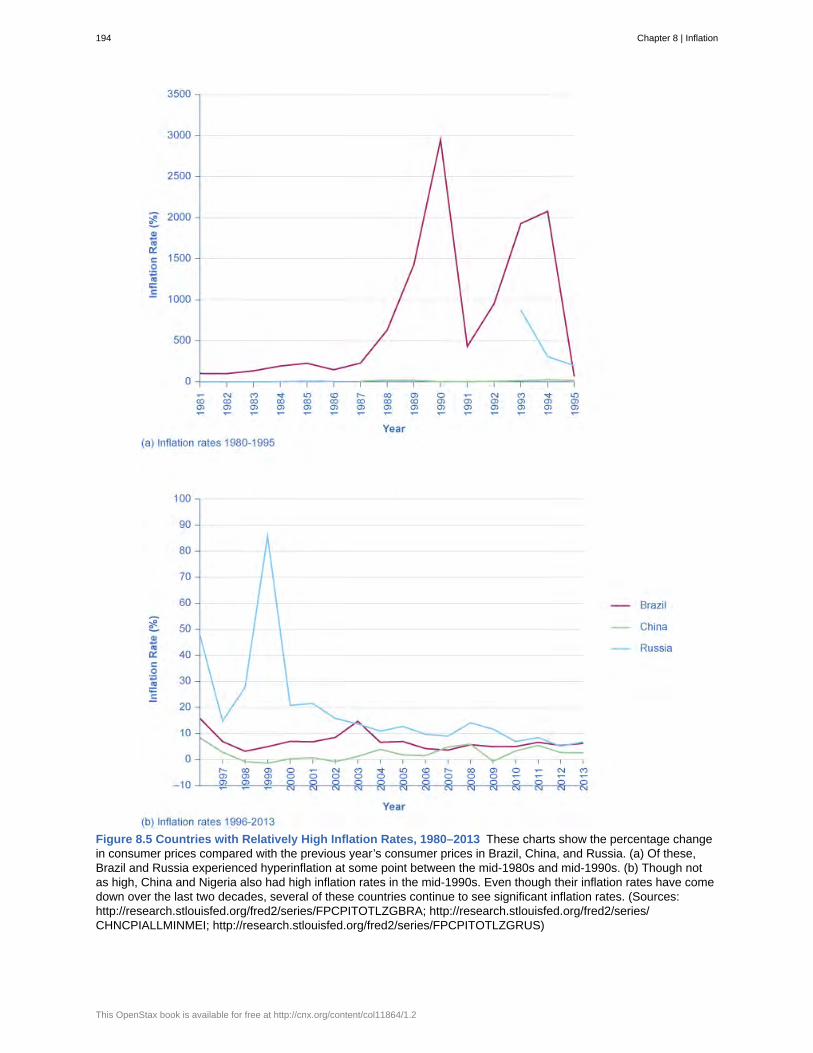
Figure 8.5 Countries with Relatively High Inflation Rates, 1980–2013 These charts show the percentage changein consumer prices compared with the previous year’s consumer prices in Brazil, China, and Russia. (a) Of these,Brazil and Russia experienced hyperinflation at some point between the mid-1980s and mid-1990s. (b) Though notas high, China and Nigeria also had high inflation rates in the mid-1990s. Even though their inflation rates have comedown over the last two decades, several of these countries continue to see significant inflation rates. (Sources:http://research.stlouisfed.org/fred2/series/FPCPITOTLZGBRA; http://research.stlouisfed.org/fred2/series/CHNCPIALLMINMEI; http://research.stlouisfed.org/fred2/series/FPCPITOTLZGRUS)
194 Chapter 8 | Inflation
This OpenStax book is available for free at http://cnx.org/content/col11864/1.2
Many countries in Latin America experienced raging hyperinflation during the 1980s and early 1990s, with inflationrates often well above 100% per year. In 1990, for example, both Brazil and Argentina saw inflation climbabove 2000%. Certain countries in Africa experienced extremely high rates of inflation, sometimes bordering onhyperinflation, in the 1990s. Nigeria, the most populous country in Africa, had an inflation rate of 75% in 1995.
In the early 2000s, the problem of inflation appears to have diminished for most countries, at least in comparison tothe worst times of recent decades. As we noted in this earlier Bring it Home feature, in recent years, the world’s worstexample of hyperinflation was in Zimbabwe, where at one point the government was issuing bills with a face valueof $100 trillion (in Zimbabwean dollars)—that is, the bills had $100,000,000,000,000 written on the front, but werealmost worthless. In many countries, the memory of double-digit, triple-digit, and even quadruple-digit inflation isnot very far in the past.
8.4 | The Confusion Over InflationBy the end of this section, you will be able to:
• Explain how inflation can cause redistributions of purchasing power• Identify ways inflation can blur the perception of supply and demand• Explain the economic benefits and challenges of inflation
Economists usually oppose high inflation, but they oppose it in a milder way than many non-economists. RobertShiller, one of 2013’s Nobel Prize winners in economics, carried out several surveys during the 1990s about attitudestoward inflation. One of his questions asked, “Do you agree that preventing high inflation is an important nationalpriority, as important as preventing drug abuse or preventing deterioration in the quality of our schools?” Answerswere on a scale of 1–5, where 1 meant “Fully agree” and 5 meant “Completely disagree.” For the U.S. population asa whole, 52% answered “Fully agree” that preventing high inflation was a highly important national priority and just4% said “Completely disagree.” However, among professional economists, only 18% answered “Fully agree,” whilethe same percentage of 18% answered “Completely disagree.”
The Land of Funny MoneyWhat are the economic problems caused by inflation, and why do economists often regard them with less concernthan the general public? Consider a very short story: “The Land of Funny Money.”
One morning, everyone in the Land of Funny Money awakened to find that everything denominated in money hadincreased by 20%. The change was completely unexpected. Every price in every store was 20% higher. Paycheckswere 20% higher. Interest rates were 20 % higher. The amount of money, everywhere from wallets to savingsaccounts, was 20% larger. This overnight inflation of prices made newspaper headlines everywhere in the Land ofFunny Money. But the headlines quickly disappeared, as people realized that in terms of what they could actuallybuy with their incomes, this inflation had no economic impact. Everyone’s pay could still buy exactly the same setof goods as it did before. Everyone’s savings were still sufficient to buy exactly the same car, vacation, or retirementthat they could have bought before. Equal levels of inflation in all wages and prices ended up not mattering much atall.
When the people in Robert Shiller’s surveys explained their concern about inflation, one typical reason was that theyfeared that as prices rose, they would not be able to afford to buy as much. In other words, people were worriedbecause they did not live in a place like the Land of Funny Money, where all prices and wages rose simultaneously.Instead, people live here on Planet Earth, where prices might rise while wages do not rise at all, or where wages risemore slowly than prices.
Economists note that over most periods, the inflation level in prices is roughly similar to the inflation level in wages,and so they reason that, on average, over time, people’s economic status is not greatly changed by inflation. If allprices, wages, and interest rates adjusted automatically and immediately with inflation, as in the Land of FunnyMoney, then no one’s purchasing power, profits, or real loan payments would change. However, if other economicvariables do not move exactly in sync with inflation, or if they adjust for inflation only after a time lag, theninflation can cause three types of problems: unintended redistributions of purchasing power, blurred price signals, anddifficulties in long-term planning.
Chapter 8 | Inflation 195
Unintended Redistributions of Purchasing PowerInflation can cause redistributions of purchasing power that hurt some and help others. People who are hurt byinflation include those who are holding a lot of cash, whether it is in a safe deposit box or in a cardboard box under thebed. When inflation happens, the buying power of cash is diminished. But cash is only an example of a more generalproblem: anyone who has financial assets invested in a way that the nominal return does not keep up with inflationwill tend to suffer from inflation. For example, if a person has money in a bank account that pays 4% interest, butinflation rises to 5%, then the real rate of return for the money invested in that bank account is negative 1%.
The problem of a good-looking nominal interest rate being transformed into an ugly-looking real interest rate canbe worsened by taxes. The U.S. income tax is charged on the nominal interest received in dollar terms, without anadjustment for inflation. So, a person who invests $10,000 and receives a 5% nominal rate of interest is taxed on the$500 received—no matter whether the inflation rate is 0%, 5%, or 10%. If inflation is 0%, then the real interest rateis 5% and all $500 is a gain in buying power. But if inflation is 5%, then the real interest rate is zero and the personhad no real gain—but owes income tax on the nominal gain anyway. If inflation is 10%, then the real interest rateis negative 5% and the person is actually falling behind in buying power, but would still owe taxes on the $500 innominal gains.
Inflation can cause unintended redistributions for wage earners, too. Wages do typically creep up with inflation overtime eventually. The last row of Table 8.1 at the start of this chapter showed that average hourly wage in the U.S.economy increased from $3.23 in 1970 to $19.55 in 2014, which is an increase by a factor of almost six. Over thattime period, the Consumer Price Index increased by an almost identical amount. However, increases in wages maylag behind inflation for a year or two, since wage adjustments are often somewhat sticky and occur only once or twicea year. Moreover, the extent to which wages keep up with inflation creates insecurity for workers and may involvepainful, prolonged conflicts between employers and employees. If the minimum wage is adjusted for inflation onlyinfrequently, minimum wage workers are losing purchasing power from their nominal wages, as shown in Figure8.6.
196 Chapter 8 | Inflation
This OpenStax book is available for free at http://cnx.org/content/col11864/1.2
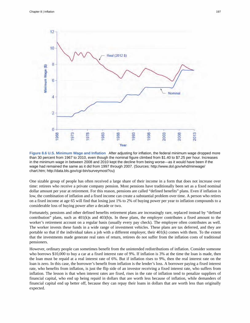
Figure 8.6 U.S. Minimum Wage and Inflation After adjusting for inflation, the federal minimum wage dropped morethan 30 percent from 1967 to 2010, even though the nominal figure climbed from $1.40 to $7.25 per hour. Increasesin the minimum wage in between 2008 and 2010 kept the decline from being worse—as it would have been if thewage had remained the same as it did from 1997 through 2007. (Sources: http://www.dol.gov/whd/minwage/chart.htm; http://data.bls.gov/cgi-bin/surveymost?cu)
One sizable group of people has often received a large share of their income in a form that does not increase overtime: retirees who receive a private company pension. Most pensions have traditionally been set as a fixed nominaldollar amount per year at retirement. For this reason, pensions are called “defined benefits” plans. Even if inflation islow, the combination of inflation and a fixed income can create a substantial problem over time. A person who retireson a fixed income at age 65 will find that losing just 1% to 2% of buying power per year to inflation compounds to aconsiderable loss of buying power after a decade or two.
Fortunately, pensions and other defined benefits retirement plans are increasingly rare, replaced instead by “definedcontribution” plans, such as 401(k)s and 403(b)s. In these plans, the employer contributes a fixed amount to theworker’s retirement account on a regular basis (usually every pay check). The employee often contributes as well.The worker invests these funds in a wide range of investment vehicles. These plans are tax deferred, and they areportable so that if the individual takes a job with a different employer, their 401(k) comes with them. To the extentthat the investments made generate real rates of return, retirees do not suffer from the inflation costs of traditionalpensioners.
However, ordinary people can sometimes benefit from the unintended redistributions of inflation. Consider someonewho borrows $10,000 to buy a car at a fixed interest rate of 9%. If inflation is 3% at the time the loan is made, thenthe loan must be repaid at a real interest rate of 6%. But if inflation rises to 9%, then the real interest rate on theloan is zero. In this case, the borrower’s benefit from inflation is the lender’s loss. A borrower paying a fixed interestrate, who benefits from inflation, is just the flip side of an investor receiving a fixed interest rate, who suffers frominflation. The lesson is that when interest rates are fixed, rises in the rate of inflation tend to penalize suppliers offinancial capital, who end up being repaid in dollars that are worth less because of inflation, while demanders offinancial capital end up better off, because they can repay their loans in dollars that are worth less than originallyexpected.
Chapter 8 | Inflation 197
The unintended redistributions of buying power caused by inflation may have a broader effect on society. America’swidespread acceptance of market forces rests on a perception that people’s actions have a reasonable connection tomarket outcomes. When inflation causes a retiree who built up a pension or invested at a fixed interest rate to suffer,however, while someone who borrowed at a fixed interest rate benefits from inflation, it is hard to believe that thisoutcome was deserved in any way. Similarly, when homeowners benefit from inflation because the price of theirhomes rises, while renters suffer because they are paying higher rent, it is hard to see any useful incentive effects.One of the reasons that inflation is so disliked by the general public is a sense that it makes economic rewards andpenalties more arbitrary—and therefore likely to be perceived as unfair – even dangerous, as the next Clear It Upfeature shows.
Is there a connection between German hyperinflation and Hitler’srise to power?Germany suffered an intense hyperinflation of its currency, the Mark, in the years after World War I, when theWeimar Republic in Germany resorted to printing money to pay its bills and the onset of the Great Depressioncreated the social turmoil that Adolf Hitler could take advantage of in his rise to power. Shiller described theconnection this way in a National Bureau of Economic Research 1996 Working Paper:
A fact that is probably little known to young people today, even in Germany, is that the final collapseof the Mark in 1923, the time when the Mark’s inflation reached astronomical levels (inflation of35,974.9% in November 1923 alone, for an annual rate that month of 4.69 × 1028%), came inthe same month as did Hitler’s Beer Hall Putsch, his Nazi Party’s armed attempt to overthrow theGerman government. This failed putsch resulted in Hitler’s imprisonment, at which time he wrotehis book Mein Kampf, setting forth an inspirational plan for Germany’s future, suggesting plans forworld domination. . .
. . . Most people in Germany today probably do not clearly remember these events; this lack ofattention to it may be because its memory is blurred by the more dramatic events that succeeded it(the Nazi seizure of power and World War II). However, to someone living through these historicalevents in sequence . . . [the putsch] may have been remembered as vivid evidence of the potentialeffects of inflation.
Blurred Price SignalsPrices are the messengers in a market economy, conveying information about conditions of demand and supply.Inflation blurs those price messages. Inflation means that price signals are perceived more vaguely, like a radioprogram received with a lot of static. If the static becomes severe, it is hard to tell what is happening.
In Israel, when inflation accelerated to an annual rate of 500% in 1985, some stores stopped posting prices directlyon items, since they would have had to put new labels on the items or shelves every few days to reflect inflation.Instead, a shopper just took items from a shelf and went up to the checkout register to find out the price for that day.Obviously, this situation makes comparing prices and shopping for the best deal rather difficult. When the levels andchanges of prices become uncertain, businesses and individuals find it harder to react to economic signals. In a worldwhere inflation is at a high rate, but bouncing up and down to some extent, does a higher price of a good mean thatinflation has risen, or that supply of that good has decreased, or that demand for that good has increased? Should abuyer of the good take the higher prices as an economic hint to start substituting other products—or have the pricesof the substitutes risen by an equal amount? Should a seller of the good take a higher price as a reason to increaseproduction—or is the higher price only a sign of a general inflation in which the prices of all inputs to production arerising as well? The true story will presumably become clear over time, but at a given moment, who can say?
High and variable inflation means that the incentives in the economy to adjust in response to changes in prices areweaker. Markets will adjust toward their equilibrium prices and quantities more erratically and slowly, and manyindividual markets will experience a greater chance of surpluses and shortages.
198 Chapter 8 | Inflation
This OpenStax book is available for free at http://cnx.org/content/col11864/1.2
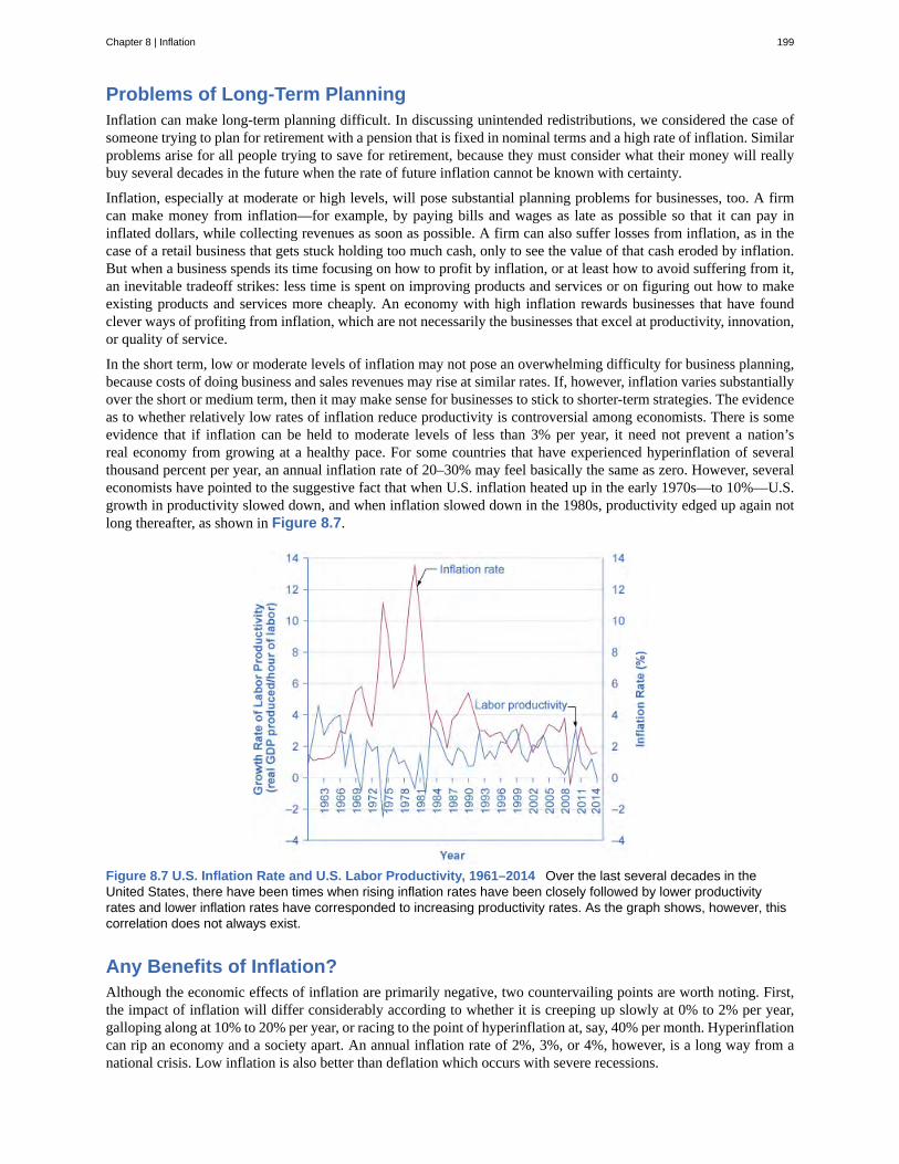
Problems of Long-Term PlanningInflation can make long-term planning difficult. In discussing unintended redistributions, we considered the case ofsomeone trying to plan for retirement with a pension that is fixed in nominal terms and a high rate of inflation. Similarproblems arise for all people trying to save for retirement, because they must consider what their money will reallybuy several decades in the future when the rate of future inflation cannot be known with certainty.
Inflation, especially at moderate or high levels, will pose substantial planning problems for businesses, too. A firmcan make money from inflation—for example, by paying bills and wages as late as possible so that it can pay ininflated dollars, while collecting revenues as soon as possible. A firm can also suffer losses from inflation, as in thecase of a retail business that gets stuck holding too much cash, only to see the value of that cash eroded by inflation.But when a business spends its time focusing on how to profit by inflation, or at least how to avoid suffering from it,an inevitable tradeoff strikes: less time is spent on improving products and services or on figuring out how to makeexisting products and services more cheaply. An economy with high inflation rewards businesses that have foundclever ways of profiting from inflation, which are not necessarily the businesses that excel at productivity, innovation,or quality of service.
In the short term, low or moderate levels of inflation may not pose an overwhelming difficulty for business planning,because costs of doing business and sales revenues may rise at similar rates. If, however, inflation varies substantiallyover the short or medium term, then it may make sense for businesses to stick to shorter-term strategies. The evidenceas to whether relatively low rates of inflation reduce productivity is controversial among economists. There is someevidence that if inflation can be held to moderate levels of less than 3% per year, it need not prevent a nation’sreal economy from growing at a healthy pace. For some countries that have experienced hyperinflation of severalthousand percent per year, an annual inflation rate of 20–30% may feel basically the same as zero. However, severaleconomists have pointed to the suggestive fact that when U.S. inflation heated up in the early 1970s—to 10%—U.S.growth in productivity slowed down, and when inflation slowed down in the 1980s, productivity edged up again notlong thereafter, as shown in Figure 8.7.
Figure 8.7 U.S. Inflation Rate and U.S. Labor Productivity, 1961–2014 Over the last several decades in theUnited States, there have been times when rising inflation rates have been closely followed by lower productivityrates and lower inflation rates have corresponded to increasing productivity rates. As the graph shows, however, thiscorrelation does not always exist.
Any Benefits of Inflation?Although the economic effects of inflation are primarily negative, two countervailing points are worth noting. First,the impact of inflation will differ considerably according to whether it is creeping up slowly at 0% to 2% per year,galloping along at 10% to 20% per year, or racing to the point of hyperinflation at, say, 40% per month. Hyperinflationcan rip an economy and a society apart. An annual inflation rate of 2%, 3%, or 4%, however, is a long way from anational crisis. Low inflation is also better than deflation which occurs with severe recessions.
Chapter 8 | Inflation 199
Second, an argument is sometimes made that moderate inflation may help the economy by making wages in labormarkets more flexible. The discussion in Unemployment pointed out that wages tend to be sticky in their downwardmovements and that unemployment can result. A little inflation could nibble away at real wages, and thus help realwages to decline if necessary. In this way, even if a moderate or high rate of inflation may act as sand in the gearsof the economy, perhaps a low rate of inflation serves as oil for the gears of the labor market. This argument iscontroversial. A full analysis would have to take all the effects of inflation into account. It does, however, offeranother reason to believe that, all things considered, very low rates of inflation may not be especially harmful.
8.5 | Indexing and Its LimitationsBy the end of this section, you will be able to:
• Explain the relationship between indexing and inflation• Identify three ways the government can control inflation through macroeconomic policy
When a price, wage, or interest rate is adjusted automatically with inflation, it is said to be indexed. An indexedpayment increases according to the index number that measures inflation. A wide array of indexing arrangements isobserved in private markets and government programs. Since the negative effects of inflation depend in large part onhaving inflation unexpectedly affect one part of the economy but not another—say, increasing the prices that peoplepay but not the wages that workers receive—indexing will take some of the sting out of inflation.
Indexing in Private MarketsIn the 1970s and 1980s, labor unions commonly negotiated wage contracts that had cost-of-living adjustments(COLAs) which guaranteed that their wages would keep up with inflation. These contracts were sometimes writtenas, for example, COLA plus 3%. Thus, if inflation was 5%, the wage increase would automatically be 8%, but ifinflation rose to 9%, the wage increase would automatically be 12%. COLAs are a form of indexing applied to wages.
Loans often have built-in inflation adjustments, too, so that if the inflation rate rises by two percentage points, thenthe interest rate charged on the loan rises by two percentage points as well. An adjustable-rate mortgage (ARM) isa kind of loan used to purchase a home in which the interest rate varies with the rate of inflation. Often, a borrowerwill be able receive a lower interest rate if borrowing with an ARM, compared to a fixed-rate loan. The reason is thatwith an ARM, the lender is protected against the risk that higher inflation will reduce the real loan payments, and sothe risk premium part of the interest rate can be correspondingly lower.
A number of ongoing or long-term business contracts also have provisions that prices will be adjusted automaticallyaccording to inflation. Sellers like such contracts because they are not locked into a low nominal selling price ifinflation turns out higher than expected; buyers like such contracts because they are not locked into a high buyingprice if inflation turns out to be lower than expected. A contract with automatic adjustments for inflation in effectagrees on a real price to be paid, rather than a nominal price.
Indexing in Government ProgramsMany government programs are indexed to inflation. The U.S. income tax code is designed so that as a person’sincome rises above certain levels, the tax rate on the marginal income earned rises as well; this is what is meant by theexpression “move into a higher tax bracket.” For example, according to the basic tax tables from the Internal RevenueService, in 2014 a single person owed 10% of all taxable income from $0 to $9,075; 15% of all income from $9,076 to$36,900; 25% of all taxable income from $36,901 to $89,350; 28% of all taxable income from $89,351 to $186,350;33% of all taxable income from $186,351 to $405,100; 35% of all taxable income from $405,101 to $406,750; and39.6% of all income from $406,751 and above.
Because of the many complex provisions in the rest of the tax code, the taxes owed by any individual cannot beexactly determined based on these numbers, but the numbers illustrate the basic theme that tax rates rise as themarginal dollar of income rises. Until the late 1970s, if nominal wages increased along with inflation, people weremoved into higher tax brackets and owed a higher proportion of their income in taxes, even though their real incomehad not risen. This “bracket creep,” as it was called, was eliminated by law in 1981. Now, the income levels wherehigher tax rates kick in are indexed to rise automatically with inflation.
The Social Security program offers two examples of indexing. Since the passage of the Social Security Indexing Actof 1972, the level of Social Security benefits increases each year along with the Consumer Price Index. Also, Social
200 Chapter 8 | Inflation
This OpenStax book is available for free at http://cnx.org/content/col11864/1.2
Security is funded by payroll taxes, which are imposed on the income earned up to a certain amount—$117,000 in2014. This level of income is adjusted upward each year according to the rate of inflation, so that the indexed rise inthe benefit level is accompanied by an indexed increase in the Social Security tax base.
As yet another example of a government program affected by indexing, in 1996 the U.S., government began offeringindexed bonds. Bonds are means by which the U.S. government (and many private-sector companies as well) borrowsmoney; that is, investors buy the bonds, and then the government repays the money with interest. Traditionally,government bonds have paid a fixed rate of interest. This policy gave a government that had borrowed an incentive toencourage inflation, because it could then repay its past borrowing in inflated dollars at a lower real interest rate. Butindexed bonds promise to pay a certain real rate of interest above whatever inflation rate occurs. In the case of a retireetrying to plan for the long term and worried about the risk of inflation, for example, indexed bonds that guarantee arate of return higher than inflation—no matter the level of inflation—can be a very comforting investment.
Might Indexing Reduce Concern over Inflation?Indexing may seem like an obviously useful step. After all, when individuals, firms, and government programs areindexed against inflation, then people can worry less about arbitrary redistributions and other effects of inflation.
However, some of the fiercest opponents of inflation express grave concern about indexing. They point out thatindexing is always partial. Not every employer will provide COLAs for workers. Not all companies can assume thatcosts and revenues will rise in lockstep with the general rates of inflation. Not all interest rates for borrowers andsavers will change to match inflation exactly. But as partial inflation indexing spreads, the political opposition toinflation may diminish. After all, older people whose Social Security benefits are protected against inflation, or banksthat have loaned their money with adjustable-rate loans, no longer have as much reason to care whether inflationheats up. In a world where some people are indexed against inflation and some are not, financially savvy businessesand investors may seek out ways to be protected against inflation, while the financially unsophisticated and smallbusinesses may suffer from it most.
A Preview of Policy Discussions of InflationThis chapter has focused on how inflation is measured, historical experience with inflation, how to adjust nominalvariables into real ones, how inflation affects the economy, and how indexing works. The causes of inflation havebarely been hinted at, and government policies to deal with inflation have not been addressed at all. These issues willbe taken up in depth in other chapters. However, it is useful to offer a preview here.
The cause of inflation can be summed up in one sentence: Too many dollars chasing too few goods. The great surgesof inflation early in the twentieth century came after wars, which are a time when government spending is very high,but consumers have little to buy, because production is going to the war effort. Governments also commonly imposeprice controls during wartime. After the war, the price controls end and pent-up buying power surges forth, drivingup inflation. On the other hand, if too few dollars are chasing too many goods, then inflation will decline or eventurn into deflation. Therefore, slowdowns in economic activity, as in major recessions and the Great Depression, aretypically associated with a reduction in inflation or even outright deflation.
The policy implications are clear. If inflation is to be avoided, the amount of purchasing power in the economy mustgrow at roughly the same rate as the production of goods. Macroeconomic policies that the government can use toaffect the amount of purchasing power—through taxes, spending, and regulation of interest rates and credit—can thuscause inflation to rise or reduce inflation to lower levels.
A $550 Million Loaf of Bread?As we will learn in Money and Banking, the existence of money provides enormous benefits to an economy.In a real sense, money is the lubrication that enhances the workings of markets. Money makes transactionseasier. It allows people to find employment producing one product, then use the money earned to purchasethe other products they need to live on. However, too much money in circulation can lead to inflation. Extremecases of governments recklessly printing money lead to hyperinflation. Inflation reduces the value of money.Hyperinflation, because money loses value so quickly, ultimately results in people no longer using money.
Chapter 8 | Inflation 201
The economy reverts to barter, or it adopts another country’s more stable currency, like U.S. dollars. In themeantime, the economy literally falls apart as people leave jobs and fend for themselves because it is notworth the time to work for money that will be worthless in a few days.
Only national governments have the power to cause hyperinflation. Hyperinflation typically happens whengovernment faces extraordinary demands for spending, which it cannot finance by taxes or borrowing. Theonly option is to print money—more and more of it. With more money in circulation chasing the same amount(or even less) goods and services, the only result is higher and higher prices until the economy and/or thegovernment collapses. This is why economists are generally wary of letting inflation get out of control.
202 Chapter 8 | Inflation
This OpenStax book is available for free at http://cnx.org/content/col11864/1.2
adjustable-rate mortgage (ARM)
base year
basket of goods and services
Consumer Price Index (CPI)
core inflation index
cost-of-living adjustments (COLAs)
deflation
Employment Cost Index
GDP deflator
hyperinflation
index number
indexed
inflation
International Price Index
Producer Price Index (PPI)
quality/new goods bias
substitution bias
KEY TERMS
a loan used to purchase a home in which the interest rate varies with marketinterest rates
arbitrary year whose value as an index number is defined as 100; inflation from the base year to other yearscan easily be seen by comparing the index number in the other year to the index number in the base year—forexample, 100; so, if the index number for a year is 105, then there has been exactly 5% inflation between that yearand the base year
a hypothetical group of different items, with specified quantities of each one meant torepresent a “typical” set of consumer purchases, used as a basis for calculating how the price level changes overtime
a measure of inflation calculated by U.S. government statisticians based on the pricelevel from a fixed basket of goods and services that represents the purchases of the average consumer
a measure of inflation typically calculated by taking the CPI and excluding volatile economicvariables such as food and energy prices to better measure the underlying and persistent trend in long-term prices
a contractual provision that wage increases will keep up with inflation
negative inflation; most prices in the economy are falling
a measure of inflation based on wages paid in the labor market
a measure of inflation based on the prices of all the components of GDP
an outburst of high inflation that is often seen (although not exclusively) when economies shift from acontrolled economy to a market-oriented economy
a unit-free number derived from the price level over a number of years, which makes computinginflation rates easier, since the index number has values around 100
a price, wage, or interest rate is adjusted automatically for inflation
a general and ongoing rise in the level of prices in an economy
a measure of inflation based on the prices of merchandise that is exported or imported
a measure of inflation based on prices paid for supplies and inputs by producers of goodsand services
inflation calculated using a fixed basket of goods over time tends to overstate the true rise incost of living, because it does not take into account improvements in the quality of existing goods or the invention ofnew goods
an inflation rate calculated using a fixed basket of goods over time tends to overstate the true rise inthe cost of living, because it does not take into account that the person can substitute away from goods whose pricesrise by a lot
KEY CONCEPTS AND SUMMARY
Chapter 8 | Inflation 203
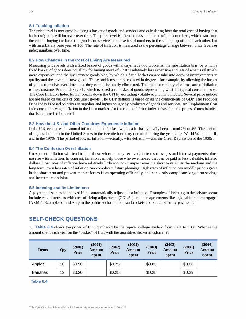
8.1 Tracking InflationThe price level is measured by using a basket of goods and services and calculating how the total cost of buying thatbasket of goods will increase over time. The price level is often expressed in terms of index numbers, which transformthe cost of buying the basket of goods and services into a series of numbers in the same proportion to each other, butwith an arbitrary base year of 100. The rate of inflation is measured as the percentage change between price levels orindex numbers over time.
8.2 How Changes in the Cost of Living Are MeasuredMeasuring price levels with a fixed basket of goods will always have two problems: the substitution bias, by which afixed basket of goods does not allow for buying more of what is relatively less expensive and less of what is relativelymore expensive; and the quality/new goods bias, by which a fixed basket cannot take into account improvements inquality and the advent of new goods. These problems can be reduced in degree—for example, by allowing the basketof goods to evolve over time—but they cannot be totally eliminated. The most commonly cited measure of inflationis the Consumer Price Index (CPI), which is based on a basket of goods representing what the typical consumer buys.The Core Inflation Index further breaks down the CPI by excluding volatile economic variables. Several price indicesare not based on baskets of consumer goods. The GDP deflator is based on all the components of GDP. The ProducerPrice Index is based on prices of supplies and inputs bought by producers of goods and services. An Employment CostIndex measures wage inflation in the labor market. An International Price Index is based on the prices of merchandisethat is exported or imported.
8.3 How the U.S. and Other Countries Experience InflationIn the U.S. economy, the annual inflation rate in the last two decades has typically been around 2% to 4%. The periodsof highest inflation in the United States in the twentieth century occurred during the years after World Wars I and II,and in the 1970s. The period of lowest inflation—actually, with deflation—was the Great Depression of the 1930s.
8.4 The Confusion Over InflationUnexpected inflation will tend to hurt those whose money received, in terms of wages and interest payments, doesnot rise with inflation. In contrast, inflation can help those who owe money that can be paid in less valuable, inflateddollars. Low rates of inflation have relatively little economic impact over the short term. Over the medium and thelong term, even low rates of inflation can complicate future planning. High rates of inflation can muddle price signalsin the short term and prevent market forces from operating efficiently, and can vastly complicate long-term savingsand investment decisions.
8.5 Indexing and Its LimitationsA payment is said to be indexed if it is automatically adjusted for inflation. Examples of indexing in the private sectorinclude wage contracts with cost-of-living adjustments (COLAs) and loan agreements like adjustable-rate mortgages(ARMs). Examples of indexing in the public sector include tax brackets and Social Security payments.
SELF-CHECK QUESTIONS1. Table 8.4 shows the prices of fruit purchased by the typical college student from 2001 to 2004. What is theamount spent each year on the “basket” of fruit with the quantities shown in column 2?
Items Qty (2001)Price
(2001)Amount
Spent
(2002)Price
(2002)Amount
Spent
(2003)Price
(2003)Amount
Spent
(2004)Price
(2004)Amount
Spent
Apples 10 $0.50 $0.75 $0.85 $0.88
Bananas 12 $0.20 $0.25 $0.25 $0.29
Table 8.4
204 Chapter 8 | Inflation
This OpenStax book is available for free at http://cnx.org/content/col11864/1.2
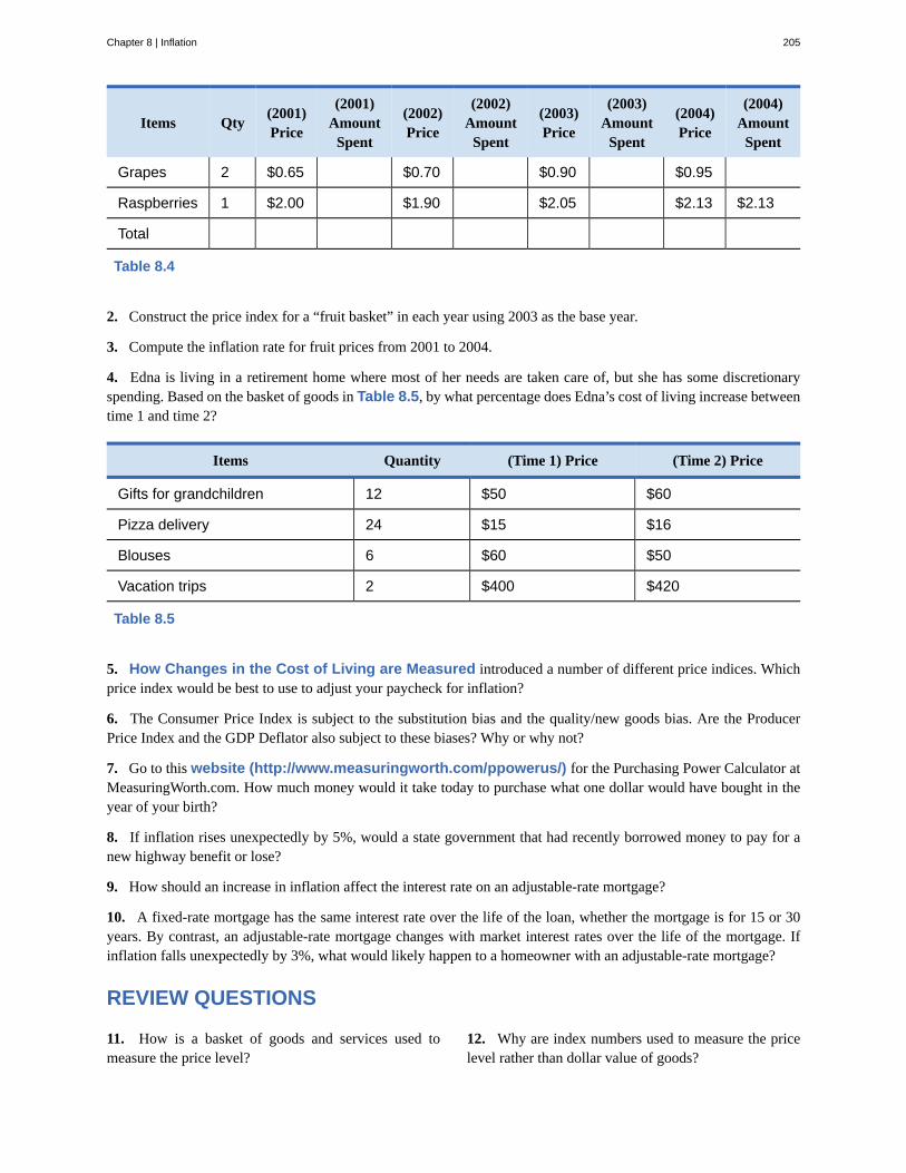
Items Qty (2001)Price
(2001)Amount
Spent
(2002)Price
(2002)Amount
Spent
(2003)Price
(2003)Amount
Spent
(2004)Price
(2004)Amount
Spent
Grapes 2 $0.65 $0.70 $0.90 $0.95
Raspberries 1 $2.00 $1.90 $2.05 $2.13 $2.13
Total
Table 8.4
2. Construct the price index for a “fruit basket” in each year using 2003 as the base year.
3. Compute the inflation rate for fruit prices from 2001 to 2004.
4. Edna is living in a retirement home where most of her needs are taken care of, but she has some discretionaryspending. Based on the basket of goods in Table 8.5, by what percentage does Edna’s cost of living increase betweentime 1 and time 2?
Items Quantity (Time 1) Price (Time 2) Price
Gifts for grandchildren 12 $50 $60
Pizza delivery 24 $15 $16
Blouses 6 $60 $50
Vacation trips 2 $400 $420
Table 8.5
5. How Changes in the Cost of Living are Measured introduced a number of different price indices. Whichprice index would be best to use to adjust your paycheck for inflation?
6. The Consumer Price Index is subject to the substitution bias and the quality/new goods bias. Are the ProducerPrice Index and the GDP Deflator also subject to these biases? Why or why not?
7. Go to this website (http://www.measuringworth.com/ppowerus/) for the Purchasing Power Calculator atMeasuringWorth.com. How much money would it take today to purchase what one dollar would have bought in theyear of your birth?
8. If inflation rises unexpectedly by 5%, would a state government that had recently borrowed money to pay for anew highway benefit or lose?
9. How should an increase in inflation affect the interest rate on an adjustable-rate mortgage?
10. A fixed-rate mortgage has the same interest rate over the life of the loan, whether the mortgage is for 15 or 30years. By contrast, an adjustable-rate mortgage changes with market interest rates over the life of the mortgage. Ifinflation falls unexpectedly by 3%, what would likely happen to a homeowner with an adjustable-rate mortgage?
REVIEW QUESTIONS
11. How is a basket of goods and services used tomeasure the price level?
12. Why are index numbers used to measure the pricelevel rather than dollar value of goods?
Chapter 8 | Inflation 205
13. What is the difference between the price level andthe rate of inflation?
14. Why does “substitution bias” arise if the inflationrate is calculated based on a fixed basket of goods?
15. Why does the “quality/new goods bias” arise if theinflation rate is calculated based on a fixed basket ofgoods?
16. What has been a typical range of inflation in theU.S. economy in the last decade or so?
17. Over the last century, during what periods was theU.S. inflation rate highest and lowest?
18. What is deflation?
19. Identify several parties likely to be helped and hurtby inflation.
20. What is indexing?
21. Name several forms of indexing in the private andpublic sector.
CRITICAL THINKING QUESTIONS
22. Inflation rates, like most statistics, are imperfectmeasures. Can you identify some ways that the inflationrate for fruit does not perfectly capture the rising priceof fruit?
23. Given the federal budget deficit in recent years,some economists have argued that by adjusting SocialSecurity payments for inflation using the CPI, SocialSecurity is overpaying recipients. What is the argumentbeing made, and do you agree or disagree with it?
24. Why is the GDP deflator not an accurate measureof inflation as it impacts a household?
25. Imagine that the government statisticians whocalculate the inflation rate have been updating the basicbasket of goods once every 10 years, but now theydecide to update it every five years. How will thischange affect the amount of substitution bias andquality/new goods bias?
26. Describe a situation, either a government policysituation, an economic problem, or a private sectorsituation, where using the CPI to convert from nominalto real would be more appropriate than using the GDPdeflator.
27. Describe a situation, either a government policysituation, an economic problem, or a private sectorsituation, where using the GDP deflator to convert fromnominal to real would be more appropriate than usingthe CPI.
28. Why do you think the U.S. experience withinflation over the last 50 years has been so much milderthan in many other countries?
29. If, over time, wages and salaries on average rise atleast as fast as inflation, why do people worry about howinflation affects incomes?
30. Who in an economy is the big winner frominflation?
31. If a government gains from unexpected inflationwhen it borrows, why would it choose to offer indexedbonds?
32. Do you think perfect indexing is possible? Why orwhy not?
PROBLEMS33. The index number representing the price levelchanges from 110 to 115 in one year, and then from 115to 120 the next year. Since the index number increasesby five each year, is five the inflation rate each year?Is the inflation rate the same each year? Explain youranswer.
34. The total price of purchasing a basket of goods inthe United Kingdom over four years is: year 1=£940,year 2=£970, year 3=£1000, and year 4=£1070.Calculate two price indices, one using year 1 as the base
year (set equal to 100) and the other using year 4 as thebase year (set equal to 100). Then, calculate the inflationrate based on the first price index. If you had used theother price index, would you get a different inflationrate? If you are unsure, do the calculation and find out.
35. Within 1 or 2 percentage points, what has the U.S.inflation rate been during the last 20 years? Draw agraph to show the data.
206 Chapter 8 | Inflation
This OpenStax book is available for free at http://cnx.org/content/col11864/1.2
36. If inflation rises unexpectedly by 5%, indicate foreach of the following whether the economic actor ishelped, hurt, or unaffected:
a. A union member with a COLA wage contractb. Someone with a large stash of cash in a safe
deposit boxc. A bank lending money at a fixed rate of interestd. A person who is not due to receive a pay raise for
another 11 months
37. Rosalie the Retiree knows that when she retires in16 years, her company will give her a one-time paymentof $20,000. However, if the inflation rate is 6% per year,how much buying power will that $20,000 have whenmeasured in today’s dollars? Hint: Start by calculatingthe rise in the price level over the 16 years.
Chapter 8 | Inflation 207
208 Chapter 8 | Inflation
This OpenStax book is available for free at http://cnx.org/content/col11864/1.2
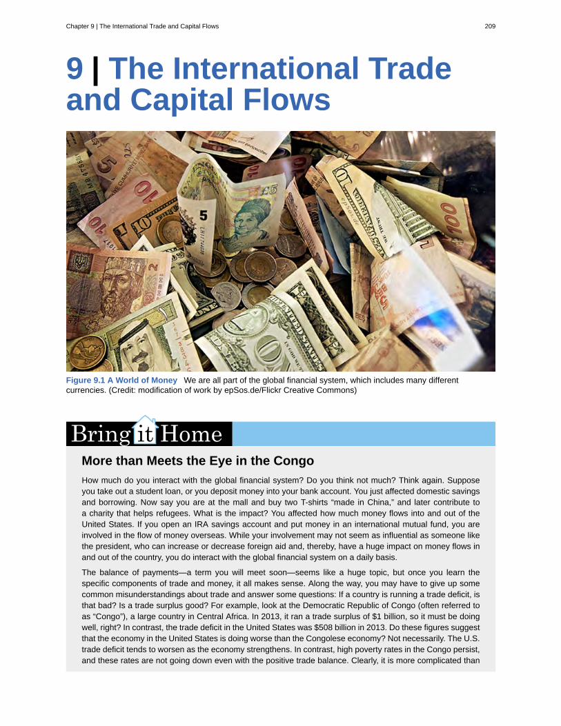
9 | The International Tradeand Capital Flows
Figure 9.1 A World of Money We are all part of the global financial system, which includes many differentcurrencies. (Credit: modification of work by epSos.de/Flickr Creative Commons)
More than Meets the Eye in the CongoHow much do you interact with the global financial system? Do you think not much? Think again. Supposeyou take out a student loan, or you deposit money into your bank account. You just affected domestic savingsand borrowing. Now say you are at the mall and buy two T-shirts “made in China,” and later contribute toa charity that helps refugees. What is the impact? You affected how much money flows into and out of theUnited States. If you open an IRA savings account and put money in an international mutual fund, you areinvolved in the flow of money overseas. While your involvement may not seem as influential as someone likethe president, who can increase or decrease foreign aid and, thereby, have a huge impact on money flows inand out of the country, you do interact with the global financial system on a daily basis.
The balance of payments—a term you will meet soon—seems like a huge topic, but once you learn thespecific components of trade and money, it all makes sense. Along the way, you may have to give up somecommon misunderstandings about trade and answer some questions: If a country is running a trade deficit, isthat bad? Is a trade surplus good? For example, look at the Democratic Republic of Congo (often referred toas “Congo”), a large country in Central Africa. In 2013, it ran a trade surplus of $1 billion, so it must be doingwell, right? In contrast, the trade deficit in the United States was $508 billion in 2013. Do these figures suggestthat the economy in the United States is doing worse than the Congolese economy? Not necessarily. The U.S.trade deficit tends to worsen as the economy strengthens. In contrast, high poverty rates in the Congo persist,and these rates are not going down even with the positive trade balance. Clearly, it is more complicated than
Chapter 9 | The International Trade and Capital Flows 209
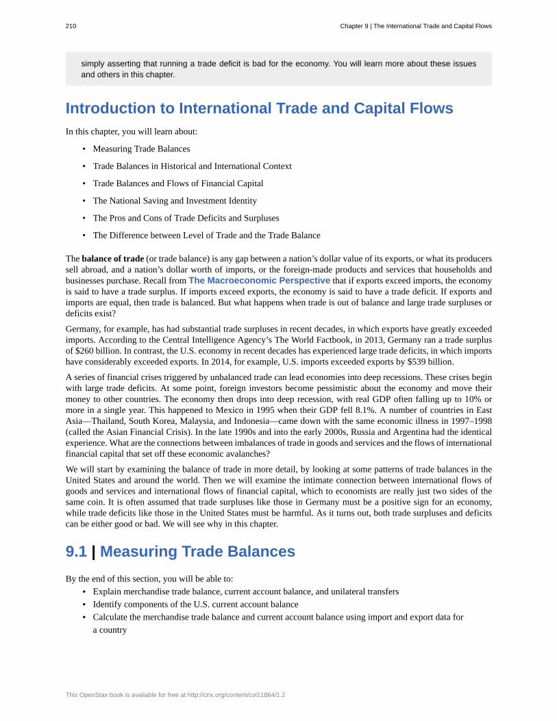
simply asserting that running a trade deficit is bad for the economy. You will learn more about these issuesand others in this chapter.
Introduction to International Trade and Capital FlowsIn this chapter, you will learn about:
• Measuring Trade Balances
• Trade Balances in Historical and International Context
• Trade Balances and Flows of Financial Capital
• The National Saving and Investment Identity
• The Pros and Cons of Trade Deficits and Surpluses
• The Difference between Level of Trade and the Trade Balance
The balance of trade (or trade balance) is any gap between a nation’s dollar value of its exports, or what its producerssell abroad, and a nation’s dollar worth of imports, or the foreign-made products and services that households andbusinesses purchase. Recall from The Macroeconomic Perspective that if exports exceed imports, the economyis said to have a trade surplus. If imports exceed exports, the economy is said to have a trade deficit. If exports andimports are equal, then trade is balanced. But what happens when trade is out of balance and large trade surpluses ordeficits exist?
Germany, for example, has had substantial trade surpluses in recent decades, in which exports have greatly exceededimports. According to the Central Intelligence Agency’s The World Factbook, in 2013, Germany ran a trade surplusof $260 billion. In contrast, the U.S. economy in recent decades has experienced large trade deficits, in which importshave considerably exceeded exports. In 2014, for example, U.S. imports exceeded exports by $539 billion.
A series of financial crises triggered by unbalanced trade can lead economies into deep recessions. These crises beginwith large trade deficits. At some point, foreign investors become pessimistic about the economy and move theirmoney to other countries. The economy then drops into deep recession, with real GDP often falling up to 10% ormore in a single year. This happened to Mexico in 1995 when their GDP fell 8.1%. A number of countries in EastAsia—Thailand, South Korea, Malaysia, and Indonesia—came down with the same economic illness in 1997–1998(called the Asian Financial Crisis). In the late 1990s and into the early 2000s, Russia and Argentina had the identicalexperience. What are the connections between imbalances of trade in goods and services and the flows of internationalfinancial capital that set off these economic avalanches?
We will start by examining the balance of trade in more detail, by looking at some patterns of trade balances in theUnited States and around the world. Then we will examine the intimate connection between international flows ofgoods and services and international flows of financial capital, which to economists are really just two sides of thesame coin. It is often assumed that trade surpluses like those in Germany must be a positive sign for an economy,while trade deficits like those in the United States must be harmful. As it turns out, both trade surpluses and deficitscan be either good or bad. We will see why in this chapter.
9.1 | Measuring Trade BalancesBy the end of this section, you will be able to:
• Explain merchandise trade balance, current account balance, and unilateral transfers• Identify components of the U.S. current account balance• Calculate the merchandise trade balance and current account balance using import and export data for
a country
210 Chapter 9 | The International Trade and Capital Flows
This OpenStax book is available for free at http://cnx.org/content/col11864/1.2
A few decades ago, it was common to track the solid or physical items that were transported by planes, trains, andtrucks between countries as a way of measuring the balance of trade. This measurement is called the merchandisetrade balance. In most high-income economies, including the United States, goods make up less than half of acountry’s total production, while services compose more than half. The last two decades have seen a surge ininternational trade in services, powered by technological advances in telecommunications and computers that havemade it possible to export or import customer services, finance, law, advertising, management consulting, software,construction engineering, and product design. Most global trade still takes the form of goods rather than services, andthe merchandise trade balance is still announced by the government and reported prominently in the newspapers. Oldhabits are hard to break. Economists, however, typically rely on broader measures such as the balance of trade or thecurrent account balance which includes other international flows of income and foreign aid.
Components of the U.S. Current Account BalanceTable 9.1 breaks down the four main components of the U.S. current account balance for the last quarter of 2014(seasonally adjusted). The first line shows the merchandise trade balance; that is, exports and imports of goods.Because imports exceed exports, the trade balance in the final column is negative, showing a merchandise tradedeficit. How this trade information is collected is explained in the following Clear It Up feature.
Value of Exports (moneyflowing into the United States)
Value of Imports (moneyflowing out of the United
States)Balance
Goods $410.0 $595.5 –$185.3
Services $180.4 $122.3 $58.1
Income receiptsand payments
$203.0 $152.4 $50.6
Unilateraltransfers
$27.3 $64.4 –$37.1
Currentaccountbalance
$820.7 $934.4 –$113.7
Table 9.1 Components of the U.S. Current Account Balance for 2014 (in billions)
How does the U.S. government collect trade statistics?Do not confuse the balance of trade (which tracks imports and exports), with the current account balance,which includes not just exports and imports, but also income from investment and transfers.
Statistics on the balance of trade are compiled by the Bureau of Economic Analysis (BEA) within the U.S.Department of Commerce, using a variety of different sources. Importers and exporters of merchandise mustfile monthly documents with the Census Bureau, which provides the basic data for tracking trade. To measureinternational trade in services—which can happen over a telephone line or computer network without anyphysical goods being shipped—the BEA carries out a set of surveys. Another set of BEA surveys trackinvestment flows, and there are even specific surveys to collect travel information from U.S. residents visitingCanada and Mexico. For measuring unilateral transfers, the BEA has access to official U.S. governmentspending on aid, and then also carries out a survey of charitable organizations that make foreign donations.
Chapter 9 | The International Trade and Capital Flows 211
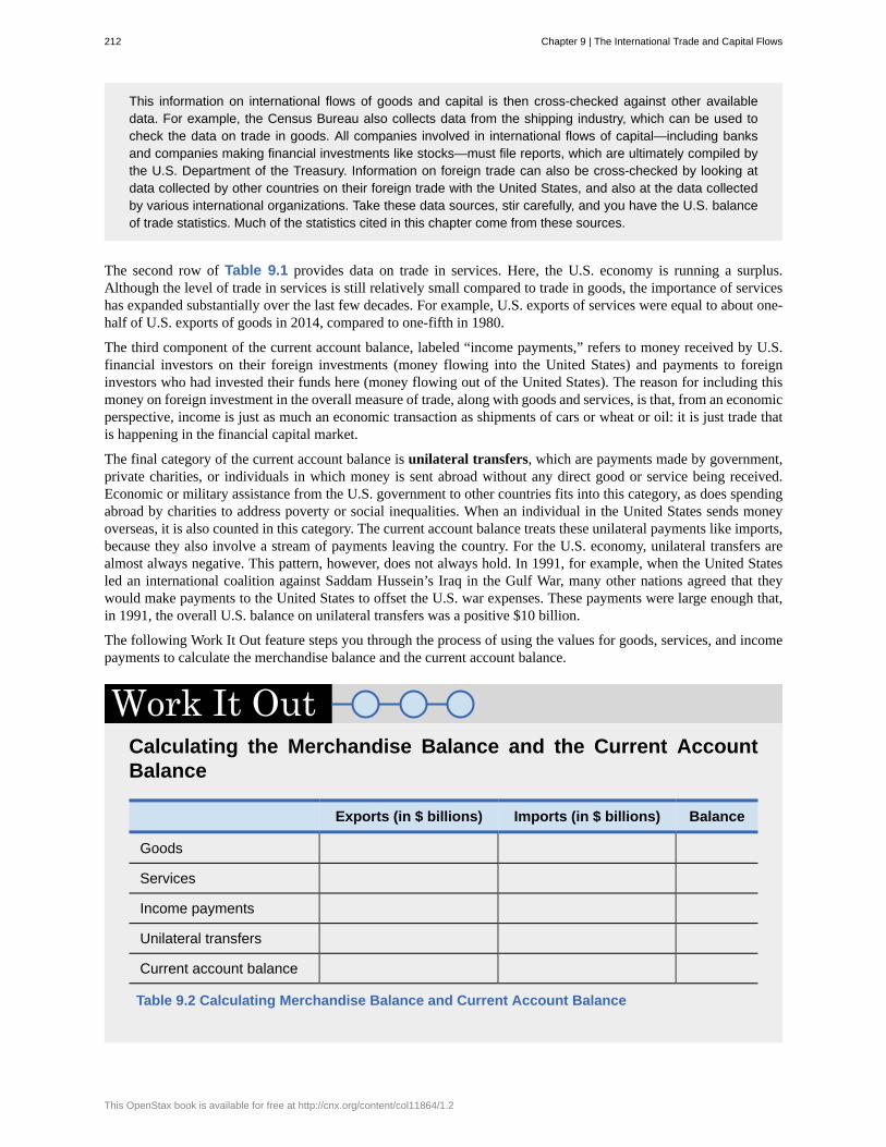
This information on international flows of goods and capital is then cross-checked against other availabledata. For example, the Census Bureau also collects data from the shipping industry, which can be used tocheck the data on trade in goods. All companies involved in international flows of capital—including banksand companies making financial investments like stocks—must file reports, which are ultimately compiled bythe U.S. Department of the Treasury. Information on foreign trade can also be cross-checked by looking atdata collected by other countries on their foreign trade with the United States, and also at the data collectedby various international organizations. Take these data sources, stir carefully, and you have the U.S. balanceof trade statistics. Much of the statistics cited in this chapter come from these sources.
The second row of Table 9.1 provides data on trade in services. Here, the U.S. economy is running a surplus.Although the level of trade in services is still relatively small compared to trade in goods, the importance of serviceshas expanded substantially over the last few decades. For example, U.S. exports of services were equal to about one-half of U.S. exports of goods in 2014, compared to one-fifth in 1980.
The third component of the current account balance, labeled “income payments,” refers to money received by U.S.financial investors on their foreign investments (money flowing into the United States) and payments to foreigninvestors who had invested their funds here (money flowing out of the United States). The reason for including thismoney on foreign investment in the overall measure of trade, along with goods and services, is that, from an economicperspective, income is just as much an economic transaction as shipments of cars or wheat or oil: it is just trade thatis happening in the financial capital market.
The final category of the current account balance is unilateral transfers, which are payments made by government,private charities, or individuals in which money is sent abroad without any direct good or service being received.Economic or military assistance from the U.S. government to other countries fits into this category, as does spendingabroad by charities to address poverty or social inequalities. When an individual in the United States sends moneyoverseas, it is also counted in this category. The current account balance treats these unilateral payments like imports,because they also involve a stream of payments leaving the country. For the U.S. economy, unilateral transfers arealmost always negative. This pattern, however, does not always hold. In 1991, for example, when the United Statesled an international coalition against Saddam Hussein’s Iraq in the Gulf War, many other nations agreed that theywould make payments to the United States to offset the U.S. war expenses. These payments were large enough that,in 1991, the overall U.S. balance on unilateral transfers was a positive $10 billion.
The following Work It Out feature steps you through the process of using the values for goods, services, and incomepayments to calculate the merchandise balance and the current account balance.
Calculating the Merchandise Balance and the Current AccountBalance
Exports (in $ billions) Imports (in $ billions) Balance
Goods
Services
Income payments
Unilateral transfers
Current account balance
Table 9.2 Calculating Merchandise Balance and Current Account Balance
212 Chapter 9 | The International Trade and Capital Flows
This OpenStax book is available for free at http://cnx.org/content/col11864/1.2
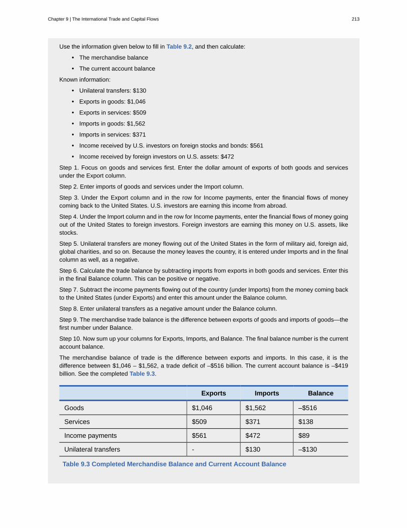
Use the information given below to fill in Table 9.2, and then calculate:
• The merchandise balance
• The current account balance
Known information:
• Unilateral transfers: $130
• Exports in goods: $1,046
• Exports in services: $509
• Imports in goods: $1,562
• Imports in services: $371
• Income received by U.S. investors on foreign stocks and bonds: $561
• Income received by foreign investors on U.S. assets: $472
Step 1. Focus on goods and services first. Enter the dollar amount of exports of both goods and servicesunder the Export column.
Step 2. Enter imports of goods and services under the Import column.
Step 3. Under the Export column and in the row for Income payments, enter the financial flows of moneycoming back to the United States. U.S. investors are earning this income from abroad.
Step 4. Under the Import column and in the row for Income payments, enter the financial flows of money goingout of the United States to foreign investors. Foreign investors are earning this money on U.S. assets, likestocks.
Step 5. Unilateral transfers are money flowing out of the United States in the form of military aid, foreign aid,global charities, and so on. Because the money leaves the country, it is entered under Imports and in the finalcolumn as well, as a negative.
Step 6. Calculate the trade balance by subtracting imports from exports in both goods and services. Enter thisin the final Balance column. This can be positive or negative.
Step 7. Subtract the income payments flowing out of the country (under Imports) from the money coming backto the United States (under Exports) and enter this amount under the Balance column.
Step 8. Enter unilateral transfers as a negative amount under the Balance column.
Step 9. The merchandise trade balance is the difference between exports of goods and imports of goods—thefirst number under Balance.
Step 10. Now sum up your columns for Exports, Imports, and Balance. The final balance number is the currentaccount balance.
The merchandise balance of trade is the difference between exports and imports. In this case, it is thedifference between $1,046 – $1,562, a trade deficit of –$516 billion. The current account balance is –$419billion. See the completed Table 9.3.
Exports Imports Balance
Goods $1,046 $1,562 –$516
Services $509 $371 $138
Income payments $561 $472 $89
Unilateral transfers - $130 –$130
Table 9.3 Completed Merchandise Balance and Current Account Balance
Chapter 9 | The International Trade and Capital Flows 213
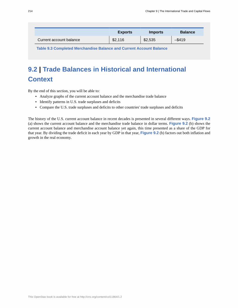
Exports Imports Balance
Current account balance $2,116 $2,535 –$419
Table 9.3 Completed Merchandise Balance and Current Account Balance
9.2 | Trade Balances in Historical and InternationalContextBy the end of this section, you will be able to:
• Analyze graphs of the current account balance and the merchandise trade balance• Identify patterns in U.S. trade surpluses and deficits• Compare the U.S. trade surpluses and deficits to other countries' trade surpluses and deficits
The history of the U.S. current account balance in recent decades is presented in several different ways. Figure 9.2(a) shows the current account balance and the merchandise trade balance in dollar terms. Figure 9.2 (b) shows thecurrent account balance and merchandise account balance yet again, this time presented as a share of the GDP forthat year. By dividing the trade deficit in each year by GDP in that year, Figure 9.2 (b) factors out both inflation andgrowth in the real economy.
214 Chapter 9 | The International Trade and Capital Flows
This OpenStax book is available for free at http://cnx.org/content/col11864/1.2
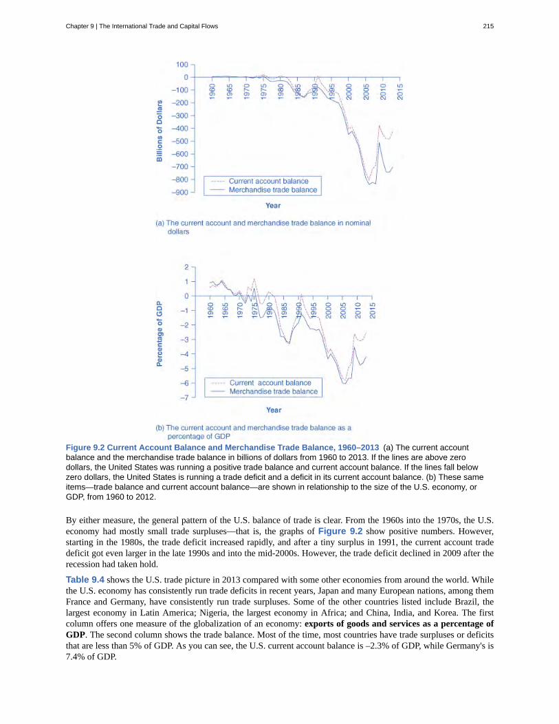
Figure 9.2 Current Account Balance and Merchandise Trade Balance, 1960–2013 (a) The current accountbalance and the merchandise trade balance in billions of dollars from 1960 to 2013. If the lines are above zerodollars, the United States was running a positive trade balance and current account balance. If the lines fall belowzero dollars, the United States is running a trade deficit and a deficit in its current account balance. (b) These sameitems—trade balance and current account balance—are shown in relationship to the size of the U.S. economy, orGDP, from 1960 to 2012.
By either measure, the general pattern of the U.S. balance of trade is clear. From the 1960s into the 1970s, the U.S.economy had mostly small trade surpluses—that is, the graphs of Figure 9.2 show positive numbers. However,starting in the 1980s, the trade deficit increased rapidly, and after a tiny surplus in 1991, the current account tradedeficit got even larger in the late 1990s and into the mid-2000s. However, the trade deficit declined in 2009 after therecession had taken hold.
Table 9.4 shows the U.S. trade picture in 2013 compared with some other economies from around the world. Whilethe U.S. economy has consistently run trade deficits in recent years, Japan and many European nations, among themFrance and Germany, have consistently run trade surpluses. Some of the other countries listed include Brazil, thelargest economy in Latin America; Nigeria, the largest economy in Africa; and China, India, and Korea. The firstcolumn offers one measure of the globalization of an economy: exports of goods and services as a percentage ofGDP. The second column shows the trade balance. Most of the time, most countries have trade surpluses or deficitsthat are less than 5% of GDP. As you can see, the U.S. current account balance is –2.3% of GDP, while Germany's is7.4% of GDP.
Chapter 9 | The International Trade and Capital Flows 215
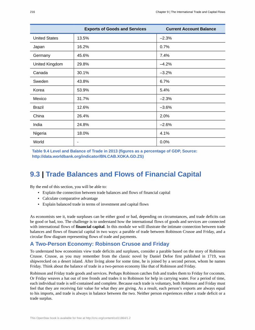
Exports of Goods and Services Current Account Balance
United States 13.5% –2.3%
Japan 16.2% 0.7%
Germany 45.6% 7.4%
United Kingdom 29.8% –4.2%
Canada 30.1% –3.2%
Sweden 43.8% 6.7%
Korea 53.9% 5.4%
Mexico 31.7% –2.3%
Brazil 12.6% –3.6%
China 26.4% 2.0%
India 24.8% –2.6%
Nigeria 18.0% 4.1%
World - 0.0%
Table 9.4 Level and Balance of Trade in 2013 (figures as a percentage of GDP, Source:http://data.worldbank.org/indicator/BN.CAB.XOKA.GD.ZS)
9.3 | Trade Balances and Flows of Financial CapitalBy the end of this section, you will be able to:
• Explain the connection between trade balances and flows of financial capital• Calculate comparative advantage• Explain balanced trade in terms of investment and capital flows
As economists see it, trade surpluses can be either good or bad, depending on circumstances, and trade deficits canbe good or bad, too. The challenge is to understand how the international flows of goods and services are connectedwith international flows of financial capital. In this module we will illustrate the intimate connection between tradebalances and flows of financial capital in two ways: a parable of trade between Robinson Crusoe and Friday, and acircular flow diagram representing flows of trade and payments.
A Two-Person Economy: Robinson Crusoe and FridayTo understand how economists view trade deficits and surpluses, consider a parable based on the story of RobinsonCrusoe. Crusoe, as you may remember from the classic novel by Daniel Defoe first published in 1719, wasshipwrecked on a desert island. After living alone for some time, he is joined by a second person, whom he namesFriday. Think about the balance of trade in a two-person economy like that of Robinson and Friday.
Robinson and Friday trade goods and services. Perhaps Robinson catches fish and trades them to Friday for coconuts.Or Friday weaves a hat out of tree fronds and trades it to Robinson for help in carrying water. For a period of time,each individual trade is self-contained and complete. Because each trade is voluntary, both Robinson and Friday mustfeel that they are receiving fair value for what they are giving. As a result, each person’s exports are always equalto his imports, and trade is always in balance between the two. Neither person experiences either a trade deficit or atrade surplus.
216 Chapter 9 | The International Trade and Capital Flows
This OpenStax book is available for free at http://cnx.org/content/col11864/1.2
However, one day Robinson approaches Friday with a proposition. Robinson wants to dig ditches for an irrigationsystem for his garden, but he knows that if he starts this project, he will not have much time left to fish and gathercoconuts to feed himself each day. He proposes that Friday supply him with a certain number of fish and coconuts forseveral months, and then after that time, he promises to repay Friday out of the extra produce that he will be able togrow in his irrigated garden. If Friday accepts this offer, then a trade imbalance comes into being. For several months,Friday will have a trade surplus: that is, he is exporting to Robinson more than he is importing. More precisely, heis giving Robinson fish and coconuts, and at least for the moment, he is receiving nothing in return. Conversely,Robinson will have a trade deficit, because he is importing more from Friday than he is exporting.
This parable raises several useful issues in thinking about what a trade deficit and a trade surplus really mean ineconomic terms. The first issue raised by this story of Robinson and Friday is this: Is it better to have a trade surplusor a trade deficit? The answer, as in any voluntary market interaction, is that if both parties agree to the transaction,then they may both be better off. Over time, if Robinson’s irrigated garden is a success, it is certainly possible thatboth Robinson and Friday can benefit from this agreement.
A second issue raised by the parable: What can go wrong? Robinson’s proposal to Friday introduces an element ofuncertainty. Friday is, in effect, making a loan of fish and coconuts to Robinson, and Friday’s happiness with thisarrangement will depend on whether that loan is repaid as planned, in full and on time. Perhaps Robinson spendsseveral months loafing and never builds the irrigation system. Or perhaps Robinson has been too optimistic abouthow much he will be able to grow with the new irrigation system, which turns out not to be very productive. Perhaps,after building the irrigation system, Robinson decides that he does not want to repay Friday as much as previouslyagreed. Any of these developments will prompt a new round of negotiations between Friday and Robinson. Friday’sattitude toward these renegotiations is likely to be shaped by why the repayment failed. If Robinson worked very hardand the irrigation system just did not increase production as intended, Friday may have some sympathy. If Robinsonloafed or if he just refuses to pay, Friday may become irritated.
A third issue raised by the parable of Robinson and Friday is that an intimate relationship exists between a tradedeficit and international borrowing, and between a trade surplus and international lending. The size of Friday’s tradesurplus is exactly how much he is lending to Robinson. The size of Robinson’s trade deficit is exactly how muchhe is borrowing from Friday. Indeed, to economists, a trade surplus literally means the same thing as an outflow offinancial capital, and a trade deficit literally means the same thing as an inflow of financial capital. This last insightis worth exploring in greater detail, which we will do in the following section.
The story of Robinson and Friday also provides a good opportunity to consider the law of comparative advantage,which you learn more about in the International Trade (http://cnx.org/content/m57383/latest/) chapter. Thefollowing Work It Out feature steps you through calculating comparative advantage for the wheat and cloth tradedbetween the United States and Great Britain in the 1800s.
Calculating Comparative AdvantageIn the 1800s, the United States and Britain traded wheat and cloth. Table 9.5 shows the varying hours of laborper unit of output.
Chapter 9 | The International Trade and Capital Flows 217
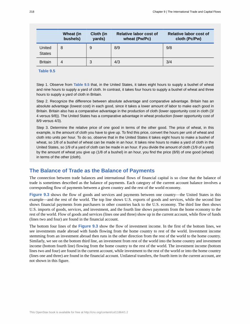
Wheat (inbushels)
Cloth (inyards)
Relative labor cost ofwheat (Pw/Pc)
Relative labor cost ofcloth (Pc/Pw)
UnitedStates
8 9 8/9 9/8
Britain 4 3 4/3 3/4
Table 9.5
Step 1. Observe from Table 9.5 that, in the United States, it takes eight hours to supply a bushel of wheatand nine hours to supply a yard of cloth. In contrast, it takes four hours to supply a bushel of wheat and threehours to supply a yard of cloth in Britain.
Step 2. Recognize the difference between absolute advantage and comparative advantage. Britain has anabsolute advantage (lowest cost) in each good, since it takes a lower amount of labor to make each good inBritain. Britain also has a comparative advantage in the production of cloth (lower opportunity cost in cloth (3/4 versus 9/8)). The United States has a comparative advantage in wheat production (lower opportunity cost of8/9 versus 4/3).
Step 3. Determine the relative price of one good in terms of the other good. The price of wheat, in thisexample, is the amount of cloth you have to give up. To find this price, convert the hours per unit of wheat andcloth into units per hour. To do so, observe that in the United States it takes eight hours to make a bushel ofwheat, so 1/8 of a bushel of wheat can be made in an hour. It takes nine hours to make a yard of cloth in theUnited States, so 1/9 of a yard of cloth can be made in an hour. If you divide the amount of cloth (1/9 of a yard)by the amount of wheat you give up (1/8 of a bushel) in an hour, you find the price (8/9) of one good (wheat)in terms of the other (cloth).
The Balance of Trade as the Balance of PaymentsThe connection between trade balances and international flows of financial capital is so close that the balance oftrade is sometimes described as the balance of payments. Each category of the current account balance involves acorresponding flow of payments between a given country and the rest of the world economy.
Figure 9.3 shows the flow of goods and services and payments between one country—the United States in thisexample—and the rest of the world. The top line shows U.S. exports of goods and services, while the second lineshows financial payments from purchasers in other countries back to the U.S. economy. The third line then showsU.S. imports of goods, services, and investment, and the fourth line shows payments from the home economy to therest of the world. Flow of goods and services (lines one and three) show up in the current account, while flow of funds(lines two and four) are found in the financial account.
The bottom four lines of the Figure 9.3 show the flow of investment income. In the first of the bottom lines, wesee investments made abroad with funds flowing from the home country to rest of the world. Investment incomestemming from an investment abroad then runs in the other direction from the rest of the world to the home country.Similarly, we see on the bottom third line, an investment from rest of the world into the home country and investmentincome (bottom fourth line) flowing from the home country to the rest of the world. The investment income (bottomlines two and four) are found in the current account, while investment to the rest of the world or into the home country(lines one and three) are found in the financial account. Unilateral transfers, the fourth item in the current account, arenot shown in this figure.
218 Chapter 9 | The International Trade and Capital Flows
This OpenStax book is available for free at http://cnx.org/content/col11864/1.2
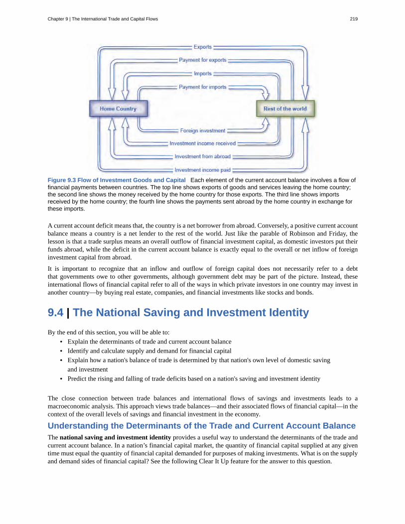
Figure 9.3 Flow of Investment Goods and Capital Each element of the current account balance involves a flow offinancial payments between countries. The top line shows exports of goods and services leaving the home country;the second line shows the money received by the home country for those exports. The third line shows importsreceived by the home country; the fourth line shows the payments sent abroad by the home country in exchange forthese imports.
A current account deficit means that, the country is a net borrower from abroad. Conversely, a positive current accountbalance means a country is a net lender to the rest of the world. Just like the parable of Robinson and Friday, thelesson is that a trade surplus means an overall outflow of financial investment capital, as domestic investors put theirfunds abroad, while the deficit in the current account balance is exactly equal to the overall or net inflow of foreigninvestment capital from abroad.
It is important to recognize that an inflow and outflow of foreign capital does not necessarily refer to a debtthat governments owe to other governments, although government debt may be part of the picture. Instead, theseinternational flows of financial capital refer to all of the ways in which private investors in one country may invest inanother country—by buying real estate, companies, and financial investments like stocks and bonds.
9.4 | The National Saving and Investment IdentityBy the end of this section, you will be able to:
• Explain the determinants of trade and current account balance• Identify and calculate supply and demand for financial capital• Explain how a nation's balance of trade is determined by that nation's own level of domestic saving
and investment• Predict the rising and falling of trade deficits based on a nation's saving and investment identity
The close connection between trade balances and international flows of savings and investments leads to amacroeconomic analysis. This approach views trade balances—and their associated flows of financial capital—in thecontext of the overall levels of savings and financial investment in the economy.
Understanding the Determinants of the Trade and Current Account BalanceThe national saving and investment identity provides a useful way to understand the determinants of the trade andcurrent account balance. In a nation’s financial capital market, the quantity of financial capital supplied at any giventime must equal the quantity of financial capital demanded for purposes of making investments. What is on the supplyand demand sides of financial capital? See the following Clear It Up feature for the answer to this question.
Chapter 9 | The International Trade and Capital Flows 219
What comprises the supply and demand of financial capital?A country’s national savings is the total of its domestic savings by household and companies (private savings)as well as the government (public savings). If a country is running a trade deficit, it means money from abroadis entering the country and is considered part of the supply of financial capital.
The demand for financial capital (money) represents groups that are borrowing the money. Businesses needto borrow to finance their investments in factories, materials, and personnel. When the federal governmentruns a budget deficit, it is also borrowing money from investors by selling Treasury bonds. So both businessinvestment and the federal government can demand (or borrow) the supply of savings.
There are two main sources for the supply of financial capital in the U.S. economy: saving by individuals and firms,called S, and the inflow of financial capital from foreign investors, which is equal to the trade deficit (M – X), orimports minus exports. There are also two main sources of demand for financial capital in the U.S. economy: privatesector investment, I, and government borrowing, where the government needs to borrow when government spending,G, is higher than the taxes collected, T. This national savings and investment identity can be expressed in algebraicterms:
Supply of financial capital = Demand for financial capitalS + (M – X) = I + (G – T)
Again, in this equation, S is private savings, T is taxes, G is government spending, M is imports, X is exports, and I isinvestment. This relationship is true as a matter of definition because, for the macro economy, the quantity suppliedof financial capital must be equal to the quantity demanded.
However, certain components of the national savings and investment identity can switch between the supply side andthe demand side. Some countries, like the United States in most years since the 1970s, have budget deficits, whichmean the government is spending more than it collects in taxes, and so the government needs to borrow funds. Inthis case, the government term would be G – T > 0, showing that spending is larger than taxes, and the governmentwould be a demander of financial capital on the right-hand side of the equation (that is, a borrower), not a supplierof financial capital on the right-hand side. However, if the government runs a budget surplus so that the taxes exceedspending, as the U.S. government did from 1998 to 2001, then the government in that year was contributing tothe supply of financial capital (T – G > 0), and would appear on the left (saving) side of the national savings andinvestment identity.
Similarly, if a national economy runs a trade surplus, the trade sector will involve an outflow of financial capital toother countries. A trade surplus means that the domestic financial capital is in surplus within a country and can beinvested in other countries.
The fundamental notion that total quantity of financial capital demanded equals total quantity of financial capitalsupplied must always remain true. Domestic savings will always appear as part of the supply of financial capital anddomestic investment will always appear as part of the demand for financial capital. However, the government andtrade balance elements of the equation can move back and forth as either suppliers or demanders of financial capital,depending on whether government budgets and the trade balance are in surplus or deficit.
Domestic Saving and Investment Determine the Trade BalanceOne insight from the national saving and investment identity is that a nation’s balance of trade is determined by thatnation’s own levels of domestic saving and domestic investment. To understand this point, rearrange the identity toput the balance of trade all by itself on one side of the equation. Consider first the situation with a trade deficit, andthen the situation with a trade surplus.
In the case of a trade deficit, the national saving and investment identity can be rewritten as:
Trade deficit = Domestic investment – Private domestic saving – Government (or public) savings(M – X) = I – S – (T – G)
220 Chapter 9 | The International Trade and Capital Flows
This OpenStax book is available for free at http://cnx.org/content/col11864/1.2
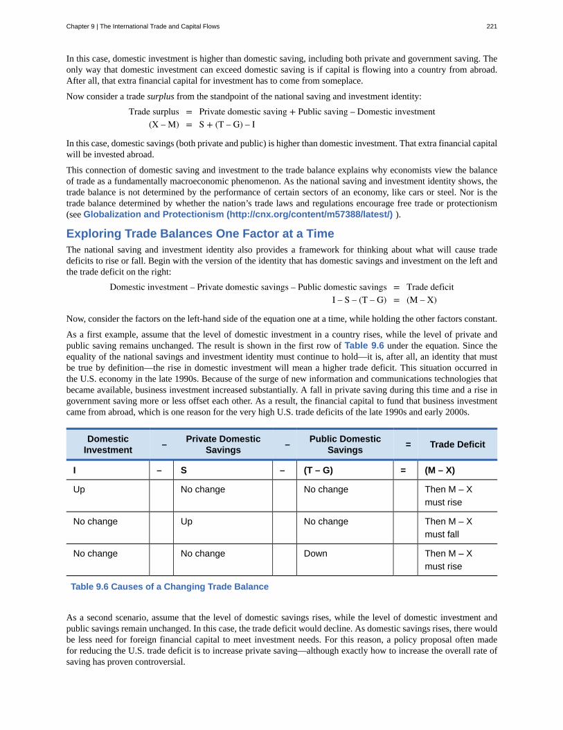
In this case, domestic investment is higher than domestic saving, including both private and government saving. Theonly way that domestic investment can exceed domestic saving is if capital is flowing into a country from abroad.After all, that extra financial capital for investment has to come from someplace.
Now consider a trade surplus from the standpoint of the national saving and investment identity:
Trade surplus = Private domestic saving + Public saving – Domestic investment(X – M) = S + (T – G) – I
In this case, domestic savings (both private and public) is higher than domestic investment. That extra financial capitalwill be invested abroad.
This connection of domestic saving and investment to the trade balance explains why economists view the balanceof trade as a fundamentally macroeconomic phenomenon. As the national saving and investment identity shows, thetrade balance is not determined by the performance of certain sectors of an economy, like cars or steel. Nor is thetrade balance determined by whether the nation’s trade laws and regulations encourage free trade or protectionism(see Globalization and Protectionism (http://cnx.org/content/m57388/latest/) ).
Exploring Trade Balances One Factor at a TimeThe national saving and investment identity also provides a framework for thinking about what will cause tradedeficits to rise or fall. Begin with the version of the identity that has domestic savings and investment on the left andthe trade deficit on the right:
Domestic investment – Private domestic savings – Public domestic savings = Trade deficitI – S – (T – G) = (M – X)
Now, consider the factors on the left-hand side of the equation one at a time, while holding the other factors constant.
As a first example, assume that the level of domestic investment in a country rises, while the level of private andpublic saving remains unchanged. The result is shown in the first row of Table 9.6 under the equation. Since theequality of the national savings and investment identity must continue to hold—it is, after all, an identity that mustbe true by definition—the rise in domestic investment will mean a higher trade deficit. This situation occurred inthe U.S. economy in the late 1990s. Because of the surge of new information and communications technologies thatbecame available, business investment increased substantially. A fall in private saving during this time and a rise ingovernment saving more or less offset each other. As a result, the financial capital to fund that business investmentcame from abroad, which is one reason for the very high U.S. trade deficits of the late 1990s and early 2000s.
DomesticInvestment – Private Domestic
Savings – Public DomesticSavings = Trade Deficit
I – S – (T – G) = (M – X)
Up No change No change Then M – Xmust rise
No change Up No change Then M – Xmust fall
No change No change Down Then M – Xmust rise
Table 9.6 Causes of a Changing Trade Balance
As a second scenario, assume that the level of domestic savings rises, while the level of domestic investment andpublic savings remain unchanged. In this case, the trade deficit would decline. As domestic savings rises, there wouldbe less need for foreign financial capital to meet investment needs. For this reason, a policy proposal often madefor reducing the U.S. trade deficit is to increase private saving—although exactly how to increase the overall rate ofsaving has proven controversial.
Chapter 9 | The International Trade and Capital Flows 221
As a third scenario, imagine that the government budget deficit increased dramatically, while domestic investmentand private savings remained unchanged. This scenario occurred in the U.S. economy in the mid-1980s. The federalbudget deficit increased from $79 billion in 1981 to $221 billion in 1986—an increase in the demand for financialcapital of $142 billion. The current account balance collapsed from a surplus of $5 billion in 1981 to a deficit of $147million in 1986—an increase in the supply of financial capital from abroad of $152 billion. The two numbers do notmatch exactly, since in the real world, private savings and investment did not remain fixed. The connection at thattime is clear: a sharp increase in government borrowing increased the U.S. economy’s demand for financial capital,and that increase was primarily supplied by foreign investors through the trade deficit. The following Work It Outfeature walks you through a scenario in which private domestic savings has to rise by a certain amount to reduce atrade deficit.
Solving Problems with the Saving and Investment IdentityUse the saving and investment identity to answer the following question: Country A has a trade deficit of $200billion, private domestic savings of $500 billion, a government deficit of $200 billion, and private domesticinvestment of $500 billion. To reduce the $200 billion trade deficit by $100 billion, by how much does privatedomestic savings have to increase?
Step 1. Write out the savings investment formula solving for the trade deficit or surplus on the left:
(X – M) = S + (T – G) – I
Step 2. In the formula, put the amount for the trade deficit in as a negative number (X – M). The left side ofyour formula is now:
–200 = S + (T – G) – I
Step 3. Enter the private domestic savings (S) of $500 in the formula:
–200 = 500 + (T – G) – I
Step 4. Enter domestic investment (I) of $500 into the formula:
–200 = 500 + (T – G) – 500
Step 5. The government budget surplus or balance is represented by (T – G). Enter a budget deficit amountfor (T – G) of –200:
–200 = 500 + (–200) – 500
Step 6. Your formula now is:
(X – M) = S + (T – G) – I–200 = 500 + (–200) – 500
The question is: To reduce your trade deficit (X – M) of –200 to –100 (in billions of dollars), by how much willsavings have to rise?
(X – M) = S + (T – G) – I–100 = S + (–200) – 500600 = S
Step 7. Summarize the answer: Private domestic savings needs to rise by $100 billion, to a total of $600billion, for the two sides of the equation to remain equal (–100 = –100).
Short-Term Movements in the Business Cycle and the Trade BalanceIn the short run, trade imbalances can be affected by whether an economy is in a recession or on the upswing. Arecession tends to make a trade deficit smaller, or a trade surplus larger, while a period of strong economic growthtends to make a trade deficit larger, or a trade surplus smaller.
222 Chapter 9 | The International Trade and Capital Flows
This OpenStax book is available for free at http://cnx.org/content/col11864/1.2
As an example, note in Figure 9.2 that the U.S. trade deficit declined by almost half from 2006 to 2009. One primaryreason for this change is that during the recession, as the U.S. economy slowed down, it purchased fewer of all goods,including fewer imports from abroad. However, buying power abroad fell less, and so U.S. exports did not fall by asmuch.
Conversely, in the mid-2000s, when the U.S. trade deficit became very large, a contributing short-term reason is thatthe U.S. economy was growing. As a result, there was lots of aggressive buying in the U.S. economy, including thebuying of imports. Thus, a rapidly growing domestic economy is often accompanied by a trade deficit (or a muchlower trade surplus), while a slowing or recessionary domestic economy is accompanied by a trade surplus (or a muchlower trade deficit).
When the trade deficit rises, it necessarily means a greater net inflow of foreign financial capital. The national savingand investment identity teaches that the rest of the economy can absorb this inflow of foreign financial capital inseveral different ways. For example, the additional inflow of financial capital from abroad could be offset by reducedprivate savings, leaving domestic investment and public saving unchanged. Alternatively, the inflow of foreignfinancial capital could result in higher domestic investment, leaving private and public saving unchanged. Yet anotherpossibility is that the inflow of foreign financial capital could be absorbed by greater government borrowing, leavingdomestic saving and investment unchanged. The national saving and investment identity does not specify which ofthese scenarios, alone or in combination, will occur—only that one of them must occur.
9.5 | The Pros and Cons of Trade Deficits and SurplusesBy the end of this section, you will be able to:
• Identify three ways in which borrowing money or running a trade deficit can result in a healthyeconomy
• Identify three ways in which borrowing money or running a trade deficit can result in a weakereconomy
Because flows of trade always involve flows of financial payments, flows of international trade are actually the sameas flows of international financial capital. The question of whether trade deficits or surpluses are good or bad for aneconomy is, in economic terms, exactly the same question as whether it is a good idea for an economy to rely on netinflows of financial capital from abroad or to make net investments of financial capital abroad. Conventional wisdomoften holds that borrowing money is foolhardy, and that a prudent country, like a prudent person, should always relyon its own resources. While it is certainly possible to borrow too much—as anyone with an overloaded credit card cantestify—borrowing at certain times can also make sound economic sense. For both individuals and countries, there isno economic merit in a policy of abstaining from participation in financial capital markets.
It makes economic sense to borrow when you are buying something with a long-run payoff; that is, when you aremaking an investment. For this reason, it can make economic sense to borrow for a college education, because theeducation will typically allow you to earn higher wages, and so to repay the loan and still come out ahead. It can alsomake sense for a business to borrow in order to purchase a machine that will last 10 years, as long as the machinewill increase output and profits by more than enough to repay the loan. Similarly, it can make economic sense for anational economy to borrow from abroad, as long as the money is wisely invested in ways that will tend to raise thenation’s economic growth over time. Then, it will be possible for the national economy to repay the borrowed moneyover time and still end up better off than before.
One vivid example of a country that borrowed heavily from abroad, invested wisely, and did perfectly well is theUnited States during the nineteenth century. The United States ran a trade deficit in 40 of the 45 years from 1831 to1875, which meant that it was importing capital from abroad over that time. However, that financial capital was, byand large, invested in projects like railroads that brought a substantial economic payoff. (See the following Clear ItUp feature for more on this.)
A more recent example along these lines is the experience of South Korea, which had trade deficits during much ofthe 1970s—and so was an importer of capital over that time. However, South Korea also had high rates of investmentin physical plant and equipment, and its economy grew rapidly. From the mid-1980s into the mid-1990s, South Koreaoften had trade surpluses—that is, it was repaying its past borrowing by sending capital abroad.
Chapter 9 | The International Trade and Capital Flows 223
In contrast, some countries have run large trade deficits, borrowed heavily in global capital markets, and ended upin all kinds of trouble. Two specific sorts of trouble are worth examining. First, a borrower nation can find itself ina bind if the incoming funds from abroad are not invested in a way that leads to increased productivity. Several ofthe large economies of Latin America, including Mexico and Brazil, ran large trade deficits and borrowed heavilyfrom abroad in the 1970s, but the inflow of financial capital did not boost productivity sufficiently, which meant thatthese countries faced enormous troubles repaying the money borrowed when economic conditions shifted during the1980s. Similarly, it appears that a number of African nations that borrowed foreign funds in the 1970s and 1980s didnot invest in productive economic assets. As a result, several of those countries later faced large interest payments,with no economic growth to show for the borrowed funds.
Are trade deficits always harmful?For most years of the nineteenth century, U.S. imports exceeded exports and the U.S. economy had atrade deficit. Yet the string of trade deficits did not hold back the economy at all; instead, the trade deficitscontributed to the strong economic growth that gave the U.S. economy the highest per capita GDP in theworld by around 1900.
The U.S. trade deficits meant that the U.S. economy was receiving a net inflow of foreign capital from abroad.Much of that foreign capital flowed into two areas of investment—railroads and public infrastructure like roads,water systems, and schools—which were important to helping the growth of the U.S. economy.
The effect of foreign investment capital on U.S. economic growth should not be overstated. In most years theforeign financial capital represented no more than 6–10% of the funds used for overall physical investment inthe economy. Nonetheless, the trade deficit and the accompanying investment funds from abroad were clearlya help, not a hindrance, to the U.S. economy in the nineteenth century.
A second “trouble” is: What happens if the foreign money flows in, and then suddenly flows out again? This scenariowas raised at the start of the chapter. In the mid-1990s, a number of countries in East Asia—Thailand, Indonesia,Malaysia, and South Korea—ran large trade deficits and imported capital from abroad. However, in 1997 and 1998many foreign investors became concerned about the health of these economies, and quickly pulled their money outof stock and bond markets, real estate, and banks. The extremely rapid departure of that foreign capital staggered thebanking systems and economies of these countries, plunging them into deep recession. We investigate and discuss thelinks between international capital flows, banks, and recession in The Impacts of Government Borrowing.
While a trade deficit is not always harmful, there is no guarantee that running a trade surplus will bring robusteconomic health. For example, Germany and Japan ran substantial trade surpluses for most of the last three decades.Regardless of their persistent trade surpluses, both countries have experienced occasional recessions and neithercountry has had especially robust annual growth in recent years. Read more about Japan’s trade surplus in the nextClear It Up feature.
Watch this video (http://openstaxcollege.org/l/tradedeficit) on whether or not trade deficit is good for theeconomy.
224 Chapter 9 | The International Trade and Capital Flows
This OpenStax book is available for free at http://cnx.org/content/col11864/1.2
The sheer size and persistence of the U.S. trade deficits and inflows of foreign capital since the 1980s are a legitimatecause for concern. The huge U.S. economy will not be destabilized by an outflow of international capital as easily as,say, the comparatively tiny economies of Thailand and Indonesia were in 1997–1998. Even an economy that is notknocked down, however, can still be shaken. American policymakers should certainly be paying attention to thosecases where a pattern of extensive and sustained current account deficits and foreign borrowing has gone badly—ifonly as a cautionary tale.
Are trade surpluses always beneficial? Considering Japan sincethe 1990s.Perhaps no economy around the world is better known for its trade surpluses than Japan. Since 1990, the sizeof these surpluses has often been near $100 billion per year. When Japan’s economy was growing vigorouslyin the 1960s and 1970s, its large trade surpluses were often described, especially by non-economists, aseither a cause or a result of its robust economic health. But from a standpoint of economic growth, Japan’seconomy has been teetering in and out of recession since 1990, with real GDP growth averaging only about1% per year, and an unemployment rate that has been creeping higher. Clearly, a whopping trade surplus isno guarantee of economic good health.
Instead, Japan’s trade surplus reflects that Japan has a very high rate of domestic savings, more than theJapanese economy can invest domestically, and so the extra funds are invested abroad. In Japan’s sloweconomy, the growth of consumption is relatively low, which also means that consumption of imports isrelatively low. Thus, Japan’s exports continually exceed its imports, leaving the trade surplus continually high.Recently, Japan’s trade surpluses began to deteriorate. In 2013, Japan ran a trade deficit due to the high costof imported oil.
9.6 | The Difference between Level of Trade and the TradeBalanceBy the end of this section, you will be able to:
• Identify three factors that influence a country's level of trade• Differentiate between balance of trade and level of trade
A nation’s level of trade may at first sound like much the same issue as the balance of trade, but these two are actuallyquite separate. It is perfectly possible for a country to have a very high level of trade—measured by its exports ofgoods and services as a share of its GDP—while it also has a near-balance between exports and imports. A high levelof trade indicates that a good portion of the nation’s production is exported. It is also possible for a country’s trade tobe a relatively low share of GDP, relative to global averages, but for the imbalance between its exports and its imports
Chapter 9 | The International Trade and Capital Flows 225
to be quite large. This general theme was emphasized earlier in Measuring Trade Balances, which offered someillustrative figures on trade levels and balances.
A country’s level of trade tells how much of its production it exports. This is measured by the percent of exports out ofGDP. It indicates how globalized an economy is. Some countries, such as Germany, have a high level of trade—theyexport almost 50% of their total production. The balance of trade tells us if the country is running a trade surplus ortrade deficit. A country can have a low level of trade but a high trade deficit. (For example, the United States onlyexports 14% of GDP, but it has a trade deficit of $540 billion.)
Three factors strongly influence a nation’s level of trade: the size of its economy, its geographic location, andits history of trade. Large economies like the United States can do much of their trading internally, while smalleconomies like Sweden have less ability to provide what they want internally and tend to have higher ratios of exportsand imports to GDP. Nations that are neighbors tend to trade more, since costs of transportation and communicationare lower. Moreover, some nations have long and established patterns of international trade, while others do not.
Consequently, a relatively small economy like Sweden, with many nearby trading partners across Europe and along history of foreign trade, has a high level of trade. Brazil and India, which are fairly large economies that haveoften sought to inhibit trade in recent decades, have lower levels of trade. Whereas, the United States and Japan areextremely large economies that have comparatively few nearby trading partners. Both countries actually have quitelow levels of trade by world standards. The ratio of exports to GDP in either the United States or in Japan is abouthalf of the world average.
The balance of trade is a separate issue from the level of trade. The United States has a low level of trade, but hadenormous trade deficits for most years from the mid-1980s into the 2000s. Japan has a low level of trade by worldstandards, but has typically shown large trade surpluses in recent decades. Nations like Germany and the UnitedKingdom have medium to high levels of trade by world standards, but Germany had a moderate trade surplus in 2008,while the United Kingdom had a moderate trade deficit. Their trade picture was roughly in balance in the late 1990s.Sweden had a high level of trade and a large trade surplus in 2007, while Mexico had a high level of trade and amoderate trade deficit that same year.
In short, it is quite possible for nations with a relatively low level of trade, expressed as a percentage of GDP, to haverelatively large trade deficits. It is also quite possible for nations with a near balance between exports and importsto worry about the consequences of high levels of trade for the economy. It is not inconsistent to believe that a highlevel of trade is potentially beneficial to an economy, because of the way it allows nations to play to their comparativeadvantages, and to also be concerned about any macroeconomic instability caused by a long-term pattern of largetrade deficits. The following Clear It Up feature discusses how this sort of dynamic played out in Colonial India.
Are trade surpluses always beneficial? Considering ColonialIndia.India was formally under British rule from 1858 to 1947. During that time, India consistently had tradesurpluses with Great Britain. Anyone who believes that trade surpluses are a sign of economic strength anddominance while trade deficits are a sign of economic weakness must find this pattern odd, since it wouldmean that colonial India was successfully dominating and exploiting Great Britain for almost a century—whichwas not true.
Instead, India’s trade surpluses with Great Britain meant that each year there was an overall flow of financialcapital from India to Great Britain. In India, this flow of financial capital was heavily criticized as the “drain,”and eliminating the drain of financial capital was viewed as one of the many reasons why India would benefitfrom achieving independence.
Final Thoughts about Trade BalancesTrade deficits can be a good or a bad sign for an economy, and trade surpluses can be a good or a bad sign. Evena trade balance of zero—which just means that a nation is neither a net borrower nor lender in the international
226 Chapter 9 | The International Trade and Capital Flows
This OpenStax book is available for free at http://cnx.org/content/col11864/1.2
economy—can be either a good or bad sign. The fundamental economic question is not whether a nation’s economyis borrowing or lending at all, but whether the particular borrowing or lending in the particular economic conditionsof that country makes sense.
It is interesting to reflect on how public attitudes toward trade deficits and surpluses might change if we couldsomehow change the labels that people and the news media affix to them. If a trade deficit was called “attractingforeign financial capital”—which accurately describes what a trade deficit means—then trade deficits might lookmore attractive. Conversely, if a trade surplus were called “shipping financial capital abroad”—which accuratelycaptures what a trade surplus does—then trade surpluses might look less attractive. Either way, the key tounderstanding trade balances is to understand the relationships between flows of trade and flows of internationalpayments, and what these relationships imply about the causes, benefits, and risks of different kinds of trade balances.The first step along this journey of understanding is to move beyond knee-jerk reactions to terms like “trade surplus,”“trade balance,” and “trade deficit.”
More than Meets the Eye in the CongoNow that you see the big picture, you undoubtedly realize that all of the economic choices you make, such asdepositing savings or investing in an international mutual fund, do influence the flow of goods and services aswell as the flows of money around the world.
You now know that a trade surplus does not necessarily tell us whether an economy is doing well or not. TheDemocratic Republic of Congo ran a trade surplus in 2013, as we learned in the beginning of the chapter. Yetits current account balance was –$2.8 billion. However, the return of political stability and the rebuilding in theaftermath of the civil war there has meant a flow of investment and financial capital into the country. In thiscase, a negative current account balance means the country is being rebuilt—and that is a good thing.
Chapter 9 | The International Trade and Capital Flows 227
balance of trade (trade balance)
current account balance
exports of goods and services as a percentage of GDP
financial capital
merchandise trade balance
national savings and investment identity
unilateral transfers
KEY TERMS
the gap, if any, between a nation’s exports and imports
a broad measure of the balance of trade that includes trade in goods and services, as well asinternational flows of income and foreign aid
the dollar value of exports divided by the dollar value ofa country’s GDP
the international flows of money that facilitates trade and investment
the balance of trade looking only at goods
the total of private savings and public savings (a government budgetsurplus)
“one-way payments” made by governments, private entities, or individuals that are sent abroadwith nothing received in return
KEY CONCEPTS AND SUMMARY
9.1 Measuring Trade BalancesThe trade balance measures the gap between a country’s exports and its imports. In most high-income economies,goods make up less than half of a country’s total production, while services compose more than half. The last twodecades have seen a surge in international trade in services; however, most global trade still takes the form of goodsrather than services. The current account balance includes the trade in goods, services, and money flowing into andout of a country from investments and unilateral transfers.
9.2 Trade Balances in Historical and International ContextThe United States developed large trade surpluses in the early 1980s, swung back to a tiny trade surplus in 1991, andthen had even larger trade deficits in the late 1990s and early 2000s. As we will see below, a trade deficit necessarilymeans a net inflow of financial capital from abroad, while a trade surplus necessarily means a net outflow of financialcapital from an economy to other countries.
9.3 Trade Balances and Flows of Financial CapitalInternational flows of goods and services are closely connected to the international flows of financial capital. Acurrent account deficit means that, after taking all the flows of payments from goods, services, and income together,the country is a net borrower from the rest of the world. A current account surplus is the opposite and means thecountry is a net lender to the rest of the world.
9.4 The National Saving and Investment IdentityThe national saving and investment identity is based on the relationship that the total quantity of financial capitalsupplied from all sources must equal the total quantity of financial capital demanded from all sources. If S is privatesaving, T is taxes, G is government spending, M is imports, X is exports, and I is investment, then for an economywith a current account deficit and a budget deficit:
Supply of financial capital = Demand for financial capitalS + (M – X) = I + (G – T)
A recession tends to increase the trade balance (meaning a higher trade surplus or lower trade deficit), while economicboom will tend to decrease the trade balance (meaning a lower trade surplus or a larger trade deficit).
228 Chapter 9 | The International Trade and Capital Flows
This OpenStax book is available for free at http://cnx.org/content/col11864/1.2
9.5 The Pros and Cons of Trade Deficits and SurplusesTrade surpluses are no guarantee of economic health, and trade deficits are no guarantee of economic weakness.Either trade deficits or trade surpluses can work out well or poorly, depending on whether the corresponding flows offinancial capital are wisely invested.
9.6 The Difference between Level of Trade and the Trade BalanceThere is a difference between the level of a country’s trade and the balance of trade. The level of trade is measured bythe percentage of exports out of GDP, or the size of the economy. Small economies that have nearby trading partnersand a history of international trade will tend to have higher levels of trade. Larger economies with few nearby tradingpartners and a limited history of international trade will tend to have lower levels of trade. The level of trade isdifferent from the trade balance. The level of trade depends on a country’s history of trade, its geography, and the sizeof its economy. A country’s balance of trade is the dollar difference between its exports and imports.
Trade deficits and trade surpluses are not necessarily good or bad—it depends on the circumstances. Even if a countryis borrowing, if that money is invested in productivity-boosting investments it can lead to an improvement in long-term economic growth.
SELF-CHECK QUESTIONS1. If foreign investors buy more U.S. stocks and bonds, how would that show up in the current account balance?
2. If the trade deficit of the United States increases, how is the current account balance affected?
3. State whether each of the following events involves a financial flow to the Mexican economy or a financial flowout of the Mexican economy:
a. Mexico imports services from Japanb. Mexico exports goods to Canadac. U.S. investors receive a return from past financial investments in Mexico
4. In what way does comparing a country’s exports to GDP reflect how globalized it is?
5. Canada’s GDP is $1,800 billion and its exports are $542 billion. What is Canada’s export ratio?
6. The GDP for the United States is $16,800 billion and its current account balance is –$400 billion. What percentof GDP is the current account balance?
7. Why does the trade balance and the current account balance track so closely together over time?
8. State whether each of the following events involves a financial flow to the U.S. economy or away from the U.S.economy:
a. Export sales to Germanyb. Returns being paid on past U.S. financial investments in Brazilc. Foreign aid from the U.S. government to Egyptd. Imported oil from the Russian Federatione. Japanese investors buying U.S. real estate
9. How does the bottom portion of Figure 9.3, showing the international flow of investments and capital, differfrom the upper portion?
10. Explain the relationship between a current account deficit or surplus and the flow of funds.
11. Using the national savings and investment identity, explain how each of the following changes (ceteris paribus)will increase or decrease the trade balance:
a. A lower domestic savings rateb. The government changes from running a budget surplus to running a budget deficitc. The rate of domestic investment surges
Chapter 9 | The International Trade and Capital Flows 229
12. If a country is running a government budget surplus, why is (T – G) on the left side of the saving-investmentidentity?
13. What determines the size of a country’s trade deficit?
14. If domestic investment increases, and there is no change in the amount of private and public saving, what musthappen to the size of the trade deficit?
15. Why does a recession cause a trade deficit to increase?
16. Both the United States and global economies are booming. Will U.S. imports and/or exports increase?
17. For each of the following, indicate which type of government spending would justify a budget deficit and whichwould not.
a. Increased federal spending on Medicareb. Increased spending on educationc. Increased spending on the space programd. Increased spending on airports and air traffic control
18. How did large trade deficits hurt the East Asian countries in the mid 1980’s? (Recall that trade deficits areequivalent to inflows of financial capital from abroad.)
19. Describe a scenario in which a trade surplus benefits an economy and one in which a trade surplus is occurringin an economy that performs poorly. What key factor or factors are making the difference in the outcome that resultsfrom a trade surplus?
20. The United States exports 14% of GDP while Germany exports about 50% of its GDP. Explain what that means.
21. Explain briefly whether each of the following would be more likely to lead to a higher level of trade for aneconomy, or a greater imbalance of trade for an economy.
a. Living in an especially large countryb. Having a domestic investment rate much higher than the domestic savings ratec. Having many other large economies geographically nearbyd. Having an especially large budget deficite. Having countries with a tradition of strong protectionist legislation shutting out imports
REVIEW QUESTIONS
22. If imports exceed exports, is it a trade deficit or atrade surplus? What about if exports exceed imports?
23. What is included in the current account balance?
24. In recent decades, has the U.S. trade balanceusually been in deficit, surplus, or balanced?
25. Does a trade surplus mean an overall inflow offinancial capital to an economy, or an overall outflow offinancial capital? What about a trade deficit?
26. What are the two main sides of the national savingsand investment identity?
27. What are the main components of the nationalsavings and investment identity?
28. When is a trade deficit likely to work out well foran economy? When is it likely to work out poorly?
29. Does a trade surplus help to guarantee strongeconomic growth?
30. What three factors will determine whether a nationhas a higher or lower share of trade relative to its GDP?
31. What is the difference between trade deficits andbalance of trade?
CRITICAL THINKING QUESTIONS
230 Chapter 9 | The International Trade and Capital Flows
This OpenStax book is available for free at http://cnx.org/content/col11864/1.2
32. From time to time, a government official will arguethat a country should strive for both a trade surplus and ahealthy inflow of capital from abroad. Explain why sucha statement is economically impossible.
33. A government official announces a new policy. Thecountry wishes to eliminate its trade deficit, but willstrongly encourage financial investment from foreignfirms. Explain why such a statement is contradictory.
34. If a country is a big exporter, is it more exposed toglobal financial crises?
35. If countries reduced trade barriers, would theinternational flows of money increase?
36. Is it better for your country to be an internationallender or borrower?
37. Many think that the size of a trade deficit is due toa lack of competitiveness of domestic sectors, such asautos. Explain why this is not true.
38. If you observed a country with a rapidly growingtrade surplus over a period of a year or so, would you bemore likely to believe that the economy of that countrywas in a period of recession or of rapid growth?Explain.
39. From time to time, a government official will arguethat a country should strive for both a trade surplus and ahealthy inflow of capital from abroad. Is this possible?
40. What is more important, a country’s currentaccount balance or the growth of GDP? Why?
41. Will nations that are more involved in foreign tradetend to have higher trade imbalances, lower tradeimbalances, or is the pattern unpredictable?
42. Some economists warn that the persistent tradedeficits and a negative current account balance that theUnited States has run will be a problem in the long run.Do you agree or not? Explain your answer.
PROBLEMS43. In 2001, the economy of the United Kingdomexported goods worth £192 billion and services worthanother £77 billion. It imported goods worth £225billion and services worth £66 billion. Receipts ofincome from abroad were £140 billion while incomepayments going abroad were £131 billion. Governmenttransfers from the United Kingdom to the rest of theworld were £23 billion, while various U.K governmentagencies received payments of £16 billion from the restof the world.
a. Calculate the U.K. merchandise trade deficit for2001.
b. Calculate the current account balance for 2001.c. Explain how you decided whether payments on
foreign investment and government transferscounted on the positive or the negative side ofthe current account balance for the UnitedKingdom in 2001.
44. Imagine that the U.S. economy finds itself in thefollowing situation: a government budget deficit of $100billion, total domestic savings of $1,500 billion, andtotal domestic physical capital investment of $1,600billion. According to the national saving and investmentidentity, what will be the current account balance? Whatwill be the current account balance if investment rises by$50 billion, while the budget deficit and national savingsremain the same?
45. Table 9.7 provides some hypothetical data onmacroeconomic accounts for three countries representedby A, B, and C and measured in billions of currencyunits. In Table 9.7, private household saving is SH, taxrevenue is T, government spending is G, and investmentspending is I.
A B C
SH 700 500 600
T 00 500 500
G 600 350 650
I 800 400 450
Table 9.7 Macroeconomic Accounts
a. Calculate the trade balance and the net inflow offoreign saving for each country.
b. State whether each one has a trade surplus ordeficit (or balanced trade).
c. State whether each is a net lender or borrowerinternationally and explain.
46. Imagine that the economy of Germany finds itselfin the following situation: the government budget hasa surplus of 1% of Germany’s GDP; private savings is20% of GDP; and physical investment is 18% of GDP.
Chapter 9 | The International Trade and Capital Flows 231
a. Based on the national saving and investmentidentity, what is the current account balance?
b. If the government budget surplus falls to zero,how will this affect the current account balance?
232 Chapter 9 | The International Trade and Capital Flows
This OpenStax book is available for free at http://cnx.org/content/col11864/1.2

10 | The Aggregate Demand/Aggregate Supply Model
Figure 10.1 New Home Construction At the peak of the housing bubble, many people across the country were ableto secure the loans necessary to build new houses. (Credit: modification of work by Tim Pierce/Flickr CreativeCommons)
From Housing Bubble to Housing BustThe United States experienced rising home ownership rates for most of the last two decades. Between 1990and 2006, the U.S. housing market grew. Homeownership rates grew from 64% to a high of over 69% between2004 and 2005. For many people, this was a period in which they could either buy first homes or buy a largerand more expensive home. During this time mortgage values tripled. Housing became more accessible toAmericans and was considered to be a safe financial investment. Figure 10.2 shows how new single familyhome sales peaked in 2005 at 107,000 units.
Chapter 10 | The Aggregate Demand/Aggregate Supply Model 233
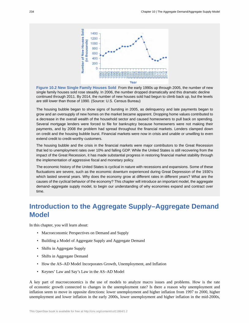
Figure 10.2 New Single Family Houses Sold From the early 1990s up through 2005, the number of newsingle family houses sold rose steadily. In 2006, the number dropped dramatically and this dramatic declinecontinued through 2011. By 2014, the number of new houses sold had begun to climb back up, but the levelsare still lower than those of 1990. (Source: U.S. Census Bureau)
The housing bubble began to show signs of bursting in 2005, as delinquency and late payments began togrow and an oversupply of new homes on the market became apparent. Dropping home values contributed toa decrease in the overall wealth of the household sector and caused homeowners to pull back on spending.Several mortgage lenders were forced to file for bankruptcy because homeowners were not making theirpayments, and by 2008 the problem had spread throughout the financial markets. Lenders clamped downon credit and the housing bubble burst. Financial markets were now in crisis and unable or unwilling to evenextend credit to credit-worthy customers.
The housing bubble and the crisis in the financial markets were major contributors to the Great Recessionthat led to unemployment rates over 10% and falling GDP. While the United States is still recovering from theimpact of the Great Recession, it has made substantial progress in restoring financial market stability throughthe implementation of aggressive fiscal and monetary policy.
The economic history of the United States is cyclical in nature with recessions and expansions. Some of thesefluctuations are severe, such as the economic downturn experienced during Great Depression of the 1930’swhich lasted several years. Why does the economy grow at different rates in different years? What are thecauses of the cyclical behavior of the economy? This chapter will introduce an important model, the aggregatedemand–aggregate supply model, to begin our understanding of why economies expand and contract overtime.
Introduction to the Aggregate Supply–Aggregate DemandModelIn this chapter, you will learn about:
• Macroeconomic Perspectives on Demand and Supply
• Building a Model of Aggregate Supply and Aggregate Demand
• Shifts in Aggregate Supply
• Shifts in Aggregate Demand
• How the AS–AD Model Incorporates Growth, Unemployment, and Inflation
• Keynes’ Law and Say’s Law in the AS–AD Model
A key part of macroeconomics is the use of models to analyze macro issues and problems. How is the rateof economic growth connected to changes in the unemployment rate? Is there a reason why unemployment andinflation seem to move in opposite directions: lower unemployment and higher inflation from 1997 to 2000, higherunemployment and lower inflation in the early 2000s, lower unemployment and higher inflation in the mid-2000s,
234 Chapter 10 | The Aggregate Demand/Aggregate Supply Model
This OpenStax book is available for free at http://cnx.org/content/col11864/1.2
and then higher unemployment and lower inflation in 2009? Why did the current account deficit rise so high, but thendecline in 2009?
To analyze questions like these, we must move beyond discussing macroeconomic issues one at a time, and beginbuilding economic models that will capture the relationships and interconnections between them. The next threechapters take up this task. This chapter introduces the macroeconomic model of aggregate supply and aggregatedemand, how the two interact to reach a macroeconomic equilibrium, and how shifts in aggregate demand oraggregate supply will affect that equilibrium. This chapter also relates the model of aggregate supply and aggregatedemand to the three goals of economic policy (growth, unemployment, and inflation), and provides a frameworkfor thinking about many of the connections and tradeoffs between these goals. The chapter on The KeynesianPerspective focuses on the macroeconomy in the short run, where aggregate demand plays a crucial role. Thechapter on The Neoclassical Perspective explores the macroeconomy in the long run, where aggregate supplyplays a crucial role.
10.1 | Macroeconomic Perspectives on Demand andSupplyBy the end of this section, you will be able to:
• Explain Say’s Law and determine whether it applies in the short run or the long run• Explain Keynes’ Law and determine whether it applies in the short run or the long run
Macroeconomists over the last two centuries have often divided into two groups: those who argue that supply is themost important determinant of the size of the macroeconomy while demand just tags along, and those who argue thatdemand is the most important factor in the size of the macroeconomy while supply just tags along.
Say’s Law and the Macroeconomics of SupplyThose economists who emphasize the role of supply in the macroeconomy often refer to the work of a famous Frencheconomist of the early nineteenth century named Jean-Baptiste Say (1767–1832). Say’s law is: “Supply creates itsown demand.” As a matter of historical accuracy, it seems clear that Say never actually wrote down this law and thatit oversimplifies his beliefs, but the law lives on as useful shorthand for summarizing a point of view.
The intuition behind Say’s law is that each time a good or service is produced and sold, it generates income that isearned for someone: a worker, a manager, an owner, or those who are workers, managers, and owners at firms thatsupply inputs along the chain of production. The forces of supply and demand in individual markets will cause pricesto rise and fall. The bottom line remains, however, that every sale represents income to someone, and so, Say’s lawargues, a given value of supply must create an equivalent value of demand somewhere else in the economy. BecauseJean-Baptiste Say, Adam Smith, and other economists writing around the turn of the nineteenth century who discussedthis view were known as “classical” economists, modern economists who generally subscribe to the Say’s law viewon the importance of supply for determining the size of the macroeconomy are called neoclassical economists.
If supply always creates exactly enough demand at the macroeconomic level, then (as Say himself recognized) it ishard to understand why periods of recession and high unemployment should ever occur. To be sure, even if totalsupply always creates an equal amount of total demand, the economy could still experience a situation of some firmsearning profits while other firms suffer losses. Nevertheless, a recession is not a situation where all business failuresare exactly counterbalanced by an offsetting number of successes. A recession is a situation in which the economyas a whole is shrinking in size, business failures outnumber the remaining success stories, and many firms end upsuffering losses and laying off workers.
Say’s law that supply creates its own demand does seem a good approximation for the long run. Over periods of someyears or decades, as the productive power of an economy to supply goods and services increases, total demand inthe economy grows at roughly the same pace. However, over shorter time horizons of a few months or even years,recessions or even depressions occur in which firms, as a group, seem to face a lack of demand for their products.
Keynes’ Law and the Macroeconomics of DemandThe alternative to Say’s law, with its emphasis on supply, can be named Keynes’ law: “Demand creates its ownsupply.” As a matter of historical accuracy, just as Jean-Baptiste Say never wrote down anything as simpleminded as
Chapter 10 | The Aggregate Demand/Aggregate Supply Model 235
Say’s law, John Maynard Keynes never wrote down Keynes’ law, but the law is a useful simplification that conveysa certain point of view.
When Keynes wrote his great work The General Theory of Employment, Interest, and Money during the GreatDepression of the 1930s, he pointed out that during the Depression, the capacity of the economy to supply goods andservices had not changed much. U.S. unemployment rates soared higher than 20% from 1933 to 1935, but the numberof possible workers had not increased or decreased much. Factories were closed and shuttered, but machinery andequipment had not disappeared. Technologies that had been invented in the 1920s were not un-invented and forgottenin the 1930s. Thus, Keynes argued that the Great Depression—and many ordinary recessions as well—were notcaused by a drop in the ability of the economy to supply goods as measured by labor, physical capital, or technology.He argued the economy often produced less than its full potential, not because it was technically impossible toproduce more with the existing workers and machines, but because a lack of demand in the economy as a whole ledto inadequate incentives for firms to produce. In such cases, he argued, the level of GDP in the economy was notprimarily determined by the potential of what the economy could supply, but rather by the amount of total demand.
Keynes’ law seems to apply fairly well in the short run of a few months to a few years, when many firms experienceeither a drop in demand for their output during a recession or so much demand that they have trouble producingenough during an economic boom. However, demand cannot tell the whole macroeconomic story, either. After all,if demand was all that mattered at the macroeconomic level, then the government could make the economy as largeas it wanted just by pumping up total demand through a large increase in the government spending component or bylegislating large tax cuts to push up the consumption component. Economies do, however, face genuine limits to howmuch they can produce, limits determined by the quantity of labor, physical capital, technology, and the institutionaland market structures that bring these factors of production together. These constraints on what an economy cansupply at the macroeconomic level do not disappear just because of an increase in demand.
Combining Supply and Demand in MacroeconomicsTwo insights emerge from this overview of Say’s law with its emphasis on macroeconomic supply and Keynes’ lawwith its emphasis on macroeconomic demand. The first conclusion, which is not exactly a hot news flash, is thatan economic approach focused only on the supply side or only on the demand side can be only a partial success.Both supply and demand need to be taken into account. The second conclusion is that since Keynes’ law appliesmore accurately in the short run and Say’s law applies more accurately in the long run, the tradeoffs and connectionsbetween the three goals of macroeconomics may be different in the short run and the long run.
10.2 | Building a Model of Aggregate Demand andAggregate SupplyBy the end of this section, you will be able to:
• Explain the aggregate supply curve and how it relates to real GDP and potential GDP• Explain the aggregate demand curve and how it is influenced by price levels• Interpret the aggregate demand/aggregate supply model• Identify the point of equilibrium in the aggregate demand/aggregate supply model• Define short run aggregate supply and long run aggregate supply
To build a useful macroeconomic model, we need a model that shows what determines total supply or total demandfor the economy, and how total demand and total supply interact at the macroeconomic level. This model is called theaggregate demand/aggregate supply model. This module will explain aggregate supply, aggregate demand, and theequilibrium between them. The following modules will discuss the causes of shifts in aggregate supply and aggregatedemand.
The Aggregate Supply Curve and Potential GDPFirms make decisions about what quantity to supply based on the profits they expect to earn. Profits, in turn, are alsodetermined by the price of the outputs the firm sells and by the price of the inputs, like labor or raw materials, thefirm needs to buy. Aggregate supply (AS) refers to the total quantity of output (i.e. real GDP) firms will produce and
236 Chapter 10 | The Aggregate Demand/Aggregate Supply Model
This OpenStax book is available for free at http://cnx.org/content/col11864/1.2
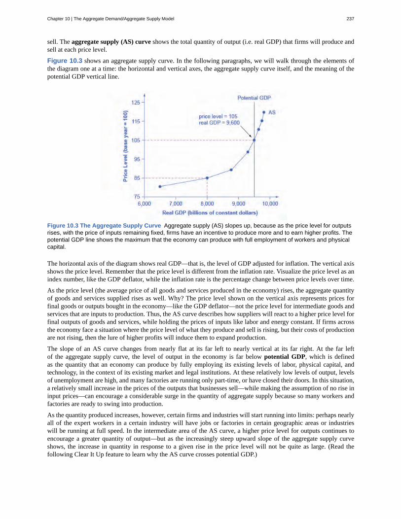
sell. The aggregate supply (AS) curve shows the total quantity of output (i.e. real GDP) that firms will produce andsell at each price level.
Figure 10.3 shows an aggregate supply curve. In the following paragraphs, we will walk through the elements ofthe diagram one at a time: the horizontal and vertical axes, the aggregate supply curve itself, and the meaning of thepotential GDP vertical line.
Figure 10.3 The Aggregate Supply Curve Aggregate supply (AS) slopes up, because as the price level for outputsrises, with the price of inputs remaining fixed, firms have an incentive to produce more and to earn higher profits. Thepotential GDP line shows the maximum that the economy can produce with full employment of workers and physicalcapital.
The horizontal axis of the diagram shows real GDP—that is, the level of GDP adjusted for inflation. The vertical axisshows the price level. Remember that the price level is different from the inflation rate. Visualize the price level as anindex number, like the GDP deflator, while the inflation rate is the percentage change between price levels over time.
As the price level (the average price of all goods and services produced in the economy) rises, the aggregate quantityof goods and services supplied rises as well. Why? The price level shown on the vertical axis represents prices forfinal goods or outputs bought in the economy—like the GDP deflator—not the price level for intermediate goods andservices that are inputs to production. Thus, the AS curve describes how suppliers will react to a higher price level forfinal outputs of goods and services, while holding the prices of inputs like labor and energy constant. If firms acrossthe economy face a situation where the price level of what they produce and sell is rising, but their costs of productionare not rising, then the lure of higher profits will induce them to expand production.
The slope of an AS curve changes from nearly flat at its far left to nearly vertical at its far right. At the far leftof the aggregate supply curve, the level of output in the economy is far below potential GDP, which is definedas the quantity that an economy can produce by fully employing its existing levels of labor, physical capital, andtechnology, in the context of its existing market and legal institutions. At these relatively low levels of output, levelsof unemployment are high, and many factories are running only part-time, or have closed their doors. In this situation,a relatively small increase in the prices of the outputs that businesses sell—while making the assumption of no rise ininput prices—can encourage a considerable surge in the quantity of aggregate supply because so many workers andfactories are ready to swing into production.
As the quantity produced increases, however, certain firms and industries will start running into limits: perhaps nearlyall of the expert workers in a certain industry will have jobs or factories in certain geographic areas or industrieswill be running at full speed. In the intermediate area of the AS curve, a higher price level for outputs continues toencourage a greater quantity of output—but as the increasingly steep upward slope of the aggregate supply curveshows, the increase in quantity in response to a given rise in the price level will not be quite as large. (Read thefollowing Clear It Up feature to learn why the AS curve crosses potential GDP.)
Chapter 10 | The Aggregate Demand/Aggregate Supply Model 237
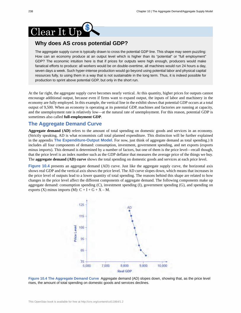
Why does AS cross potential GDP?The aggregate supply curve is typically drawn to cross the potential GDP line. This shape may seem puzzling:How can an economy produce at an output level which is higher than its “potential” or “full employment”GDP? The economic intuition here is that if prices for outputs were high enough, producers would makefanatical efforts to produce: all workers would be on double-overtime, all machines would run 24 hours a day,seven days a week. Such hyper-intense production would go beyond using potential labor and physical capitalresources fully, to using them in a way that is not sustainable in the long term. Thus, it is indeed possible forproduction to sprint above potential GDP, but only in the short run.
At the far right, the aggregate supply curve becomes nearly vertical. At this quantity, higher prices for outputs cannotencourage additional output, because even if firms want to expand output, the inputs of labor and machinery in theeconomy are fully employed. In this example, the vertical line in the exhibit shows that potential GDP occurs at a totaloutput of 9,500. When an economy is operating at its potential GDP, machines and factories are running at capacity,and the unemployment rate is relatively low—at the natural rate of unemployment. For this reason, potential GDP issometimes also called full-employment GDP.
The Aggregate Demand CurveAggregate demand (AD) refers to the amount of total spending on domestic goods and services in an economy.(Strictly speaking, AD is what economists call total planned expenditure. This distinction will be further explainedin the appendix The Expenditure-Output Model. For now, just think of aggregate demand as total spending.) Itincludes all four components of demand: consumption, investment, government spending, and net exports (exportsminus imports). This demand is determined by a number of factors, but one of them is the price level—recall though,that the price level is an index number such as the GDP deflator that measures the average price of the things we buy.The aggregate demand (AD) curve shows the total spending on domestic goods and services at each price level.
Figure 10.4 presents an aggregate demand (AD) curve. Just like the aggregate supply curve, the horizontal axisshows real GDP and the vertical axis shows the price level. The AD curve slopes down, which means that increases inthe price level of outputs lead to a lower quantity of total spending. The reasons behind this shape are related to howchanges in the price level affect the different components of aggregate demand. The following components make upaggregate demand: consumption spending (C), investment spending (I), government spending (G), and spending onexports (X) minus imports (M): C + I + G + X – M.
Figure 10.4 The Aggregate Demand Curve Aggregate demand (AD) slopes down, showing that, as the price levelrises, the amount of total spending on domestic goods and services declines.
238 Chapter 10 | The Aggregate Demand/Aggregate Supply Model
This OpenStax book is available for free at http://cnx.org/content/col11864/1.2
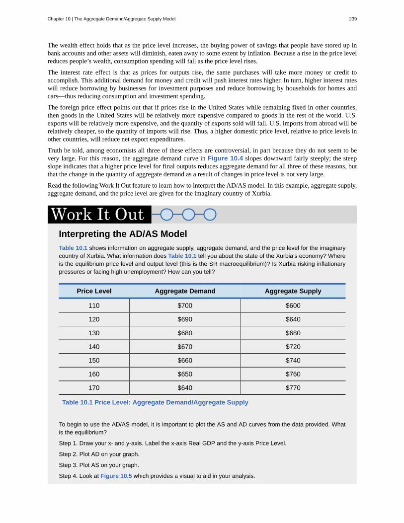
The wealth effect holds that as the price level increases, the buying power of savings that people have stored up inbank accounts and other assets will diminish, eaten away to some extent by inflation. Because a rise in the price levelreduces people’s wealth, consumption spending will fall as the price level rises.
The interest rate effect is that as prices for outputs rise, the same purchases will take more money or credit toaccomplish. This additional demand for money and credit will push interest rates higher. In turn, higher interest rateswill reduce borrowing by businesses for investment purposes and reduce borrowing by households for homes andcars—thus reducing consumption and investment spending.
The foreign price effect points out that if prices rise in the United States while remaining fixed in other countries,then goods in the United States will be relatively more expensive compared to goods in the rest of the world. U.S.exports will be relatively more expensive, and the quantity of exports sold will fall. U.S. imports from abroad will berelatively cheaper, so the quantity of imports will rise. Thus, a higher domestic price level, relative to price levels inother countries, will reduce net export expenditures.
Truth be told, among economists all three of these effects are controversial, in part because they do not seem to bevery large. For this reason, the aggregate demand curve in Figure 10.4 slopes downward fairly steeply; the steepslope indicates that a higher price level for final outputs reduces aggregate demand for all three of these reasons, butthat the change in the quantity of aggregate demand as a result of changes in price level is not very large.
Read the following Work It Out feature to learn how to interpret the AD/AS model. In this example, aggregate supply,aggregate demand, and the price level are given for the imaginary country of Xurbia.
Interpreting the AD/AS ModelTable 10.1 shows information on aggregate supply, aggregate demand, and the price level for the imaginarycountry of Xurbia. What information does Table 10.1 tell you about the state of the Xurbia’s economy? Whereis the equilibrium price level and output level (this is the SR macroequilibrium)? Is Xurbia risking inflationarypressures or facing high unemployment? How can you tell?
Price Level Aggregate Demand Aggregate Supply
110 $700 $600
120 $690 $640
130 $680 $680
140 $670 $720
150 $660 $740
160 $650 $760
170 $640 $770
Table 10.1 Price Level: Aggregate Demand/Aggregate Supply
To begin to use the AD/AS model, it is important to plot the AS and AD curves from the data provided. Whatis the equilibrium?
Step 1. Draw your x- and y-axis. Label the x-axis Real GDP and the y-axis Price Level.
Step 2. Plot AD on your graph.
Step 3. Plot AS on your graph.
Step 4. Look at Figure 10.5 which provides a visual to aid in your analysis.
Chapter 10 | The Aggregate Demand/Aggregate Supply Model 239
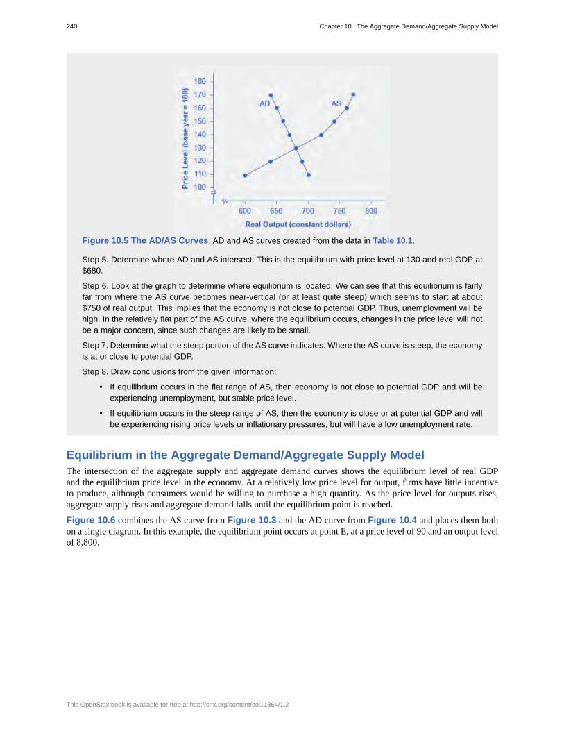
Figure 10.5 The AD/AS Curves AD and AS curves created from the data in Table 10.1.
Step 5. Determine where AD and AS intersect. This is the equilibrium with price level at 130 and real GDP at$680.
Step 6. Look at the graph to determine where equilibrium is located. We can see that this equilibrium is fairlyfar from where the AS curve becomes near-vertical (or at least quite steep) which seems to start at about$750 of real output. This implies that the economy is not close to potential GDP. Thus, unemployment will behigh. In the relatively flat part of the AS curve, where the equilibrium occurs, changes in the price level will notbe a major concern, since such changes are likely to be small.
Step 7. Determine what the steep portion of the AS curve indicates. Where the AS curve is steep, the economyis at or close to potential GDP.
Step 8. Draw conclusions from the given information:
• If equilibrium occurs in the flat range of AS, then economy is not close to potential GDP and will beexperiencing unemployment, but stable price level.
• If equilibrium occurs in the steep range of AS, then the economy is close or at potential GDP and willbe experiencing rising price levels or inflationary pressures, but will have a low unemployment rate.
Equilibrium in the Aggregate Demand/Aggregate Supply ModelThe intersection of the aggregate supply and aggregate demand curves shows the equilibrium level of real GDPand the equilibrium price level in the economy. At a relatively low price level for output, firms have little incentiveto produce, although consumers would be willing to purchase a high quantity. As the price level for outputs rises,aggregate supply rises and aggregate demand falls until the equilibrium point is reached.
Figure 10.6 combines the AS curve from Figure 10.3 and the AD curve from Figure 10.4 and places them bothon a single diagram. In this example, the equilibrium point occurs at point E, at a price level of 90 and an output levelof 8,800.
240 Chapter 10 | The Aggregate Demand/Aggregate Supply Model
This OpenStax book is available for free at http://cnx.org/content/col11864/1.2
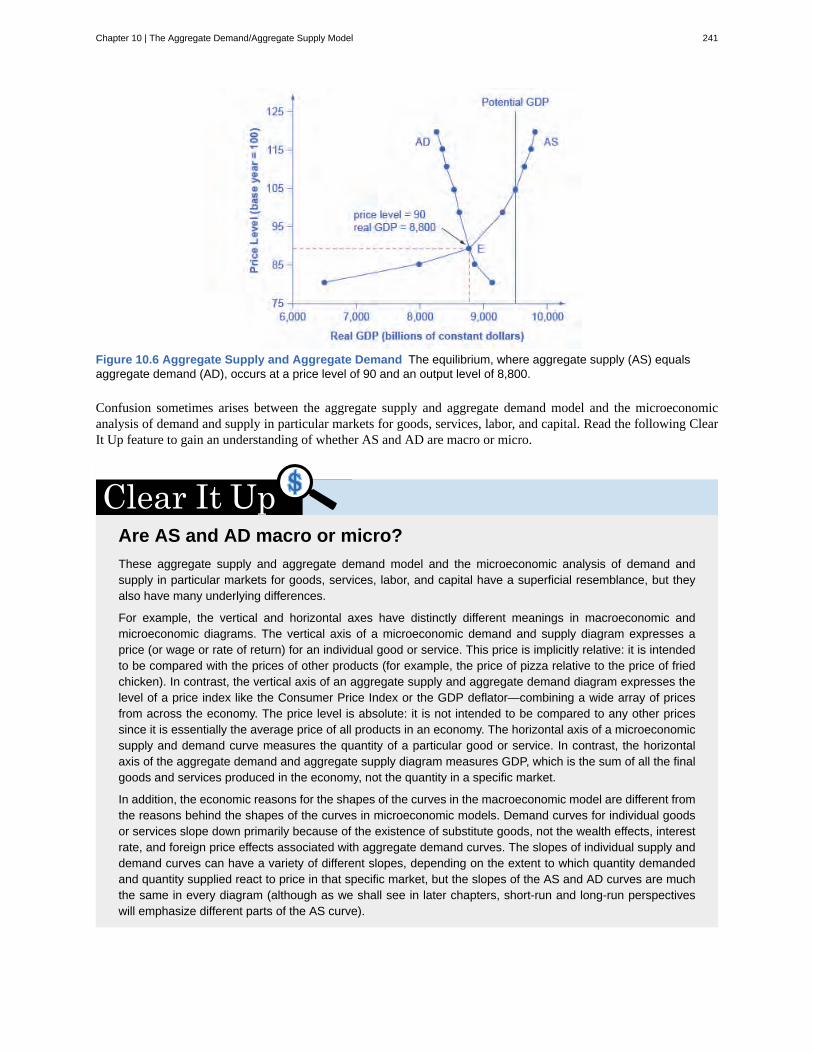
Figure 10.6 Aggregate Supply and Aggregate Demand The equilibrium, where aggregate supply (AS) equalsaggregate demand (AD), occurs at a price level of 90 and an output level of 8,800.
Confusion sometimes arises between the aggregate supply and aggregate demand model and the microeconomicanalysis of demand and supply in particular markets for goods, services, labor, and capital. Read the following ClearIt Up feature to gain an understanding of whether AS and AD are macro or micro.
Are AS and AD macro or micro?These aggregate supply and aggregate demand model and the microeconomic analysis of demand andsupply in particular markets for goods, services, labor, and capital have a superficial resemblance, but theyalso have many underlying differences.
For example, the vertical and horizontal axes have distinctly different meanings in macroeconomic andmicroeconomic diagrams. The vertical axis of a microeconomic demand and supply diagram expresses aprice (or wage or rate of return) for an individual good or service. This price is implicitly relative: it is intendedto be compared with the prices of other products (for example, the price of pizza relative to the price of friedchicken). In contrast, the vertical axis of an aggregate supply and aggregate demand diagram expresses thelevel of a price index like the Consumer Price Index or the GDP deflator—combining a wide array of pricesfrom across the economy. The price level is absolute: it is not intended to be compared to any other pricessince it is essentially the average price of all products in an economy. The horizontal axis of a microeconomicsupply and demand curve measures the quantity of a particular good or service. In contrast, the horizontalaxis of the aggregate demand and aggregate supply diagram measures GDP, which is the sum of all the finalgoods and services produced in the economy, not the quantity in a specific market.
In addition, the economic reasons for the shapes of the curves in the macroeconomic model are different fromthe reasons behind the shapes of the curves in microeconomic models. Demand curves for individual goodsor services slope down primarily because of the existence of substitute goods, not the wealth effects, interestrate, and foreign price effects associated with aggregate demand curves. The slopes of individual supply anddemand curves can have a variety of different slopes, depending on the extent to which quantity demandedand quantity supplied react to price in that specific market, but the slopes of the AS and AD curves are muchthe same in every diagram (although as we shall see in later chapters, short-run and long-run perspectiveswill emphasize different parts of the AS curve).
Chapter 10 | The Aggregate Demand/Aggregate Supply Model 241
In short, just because the AD/AS diagram has two lines that cross, do not assume that it is the same as everyother diagram where two lines cross. The intuitions and meanings of the macro and micro diagrams are onlydistant cousins from different branches of the economics family tree.
Defining SRAS and LRASIn the Clear It Up feature titled “Why does AS cross potential GDP?” we differentiated between short run changesin aggregate supply which are shown by the AS curve and long run changes in aggregate supply which are definedby the vertical line at potential GDP. In the short run, if demand is too low (or too high), it is possible for producersto supply less GDP (or more GDP) than potential. In the long run, however, producers are limited to producing atpotential GDP. For this reason, what we have been calling the AS curve, will from this point on may also be referredto as the short run aggregate supply (SRAS) curve. The vertical line at potential GDP may also be referred to asthe long run aggregate supply (LRAS) curve.
10.3 | Shifts in Aggregate SupplyBy the end of this section, you will be able to:
• Explain how productivity growth changes the aggregate supply curve• Explain how changes in input prices changes the aggregate supply curve
The original equilibrium in the AD/AS diagram will shift to a new equilibrium if the AS or AD curve shifts. Whenthe aggregate supply curve shifts to the right, then at every price level, a greater quantity of real GDP is produced.When the SRAS curve shifts to the left, then at every price level, a lower quantity of real GDP is produced. Thismodule discusses two of the most important factors that can lead to shifts in the AS curve: productivity growth andinput prices.
How Productivity Growth Shifts the AS CurveIn the long run, the most important factor shifting the AS curve is productivity growth. Productivity means howmuch output can be produced with a given quantity of labor. One measure of this is output per worker or GDP percapita. Over time, productivity grows so that the same quantity of labor can produce more output. Historically, thereal growth in GDP per capita in an advanced economy like the United States has averaged about 2% to 3% per year,but productivity growth has been faster during certain extended periods like the 1960s and the late 1990s through theearly 2000s, or slower during periods like the 1970s. A higher level of productivity shifts the AS curve to the right,because with improved productivity, firms can produce a greater quantity of output at every price level. Figure 10.7(a) shows an outward shift in productivity over two time periods. The AS curve shifts out from SRAS0 to SRAS1 toSRAS2, reflecting the rise in potential GDP in this economy, and the equilibrium shifts from E0 to E1 to E2.
242 Chapter 10 | The Aggregate Demand/Aggregate Supply Model
This OpenStax book is available for free at http://cnx.org/content/col11864/1.2
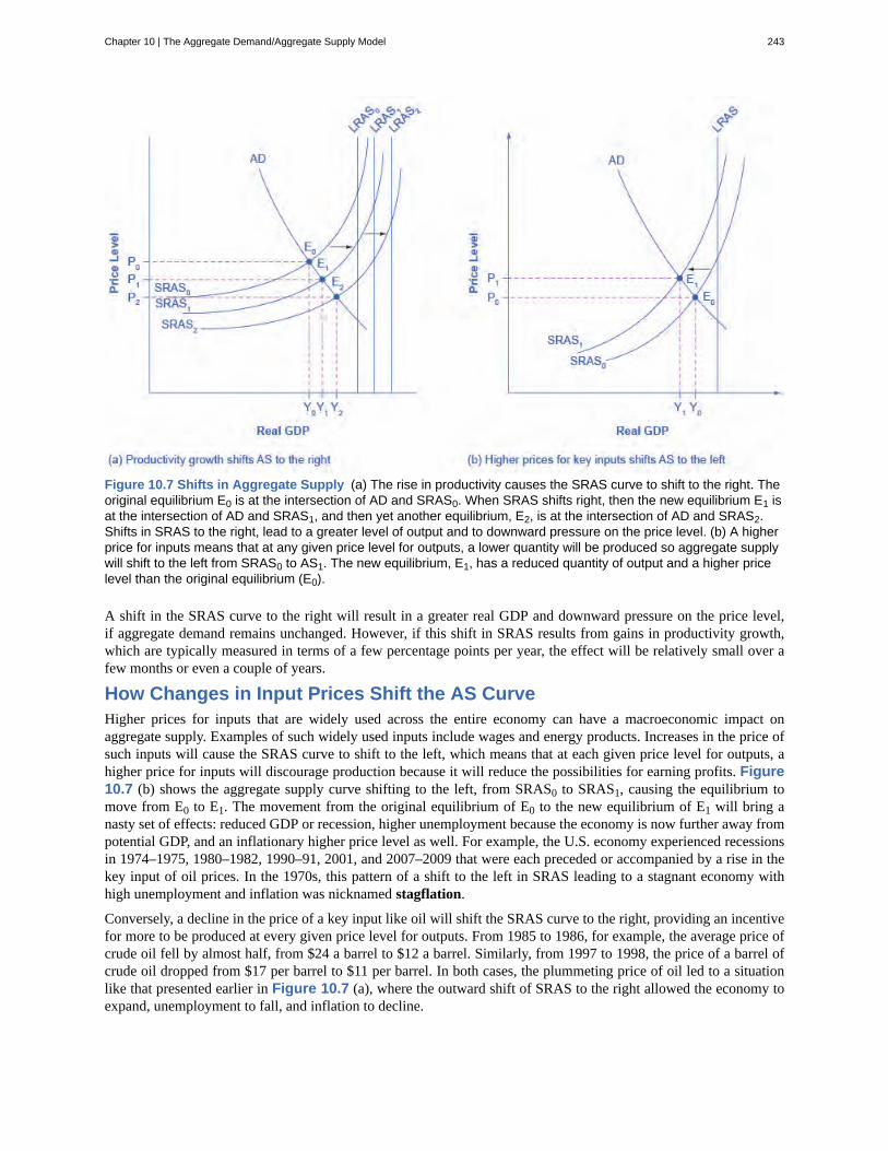
Figure 10.7 Shifts in Aggregate Supply (a) The rise in productivity causes the SRAS curve to shift to the right. Theoriginal equilibrium E0 is at the intersection of AD and SRAS0. When SRAS shifts right, then the new equilibrium E1 isat the intersection of AD and SRAS1, and then yet another equilibrium, E2, is at the intersection of AD and SRAS2.Shifts in SRAS to the right, lead to a greater level of output and to downward pressure on the price level. (b) A higherprice for inputs means that at any given price level for outputs, a lower quantity will be produced so aggregate supplywill shift to the left from SRAS0 to AS1. The new equilibrium, E1, has a reduced quantity of output and a higher pricelevel than the original equilibrium (E0).
A shift in the SRAS curve to the right will result in a greater real GDP and downward pressure on the price level,if aggregate demand remains unchanged. However, if this shift in SRAS results from gains in productivity growth,which are typically measured in terms of a few percentage points per year, the effect will be relatively small over afew months or even a couple of years.
How Changes in Input Prices Shift the AS CurveHigher prices for inputs that are widely used across the entire economy can have a macroeconomic impact onaggregate supply. Examples of such widely used inputs include wages and energy products. Increases in the price ofsuch inputs will cause the SRAS curve to shift to the left, which means that at each given price level for outputs, ahigher price for inputs will discourage production because it will reduce the possibilities for earning profits. Figure10.7 (b) shows the aggregate supply curve shifting to the left, from SRAS0 to SRAS1, causing the equilibrium tomove from E0 to E1. The movement from the original equilibrium of E0 to the new equilibrium of E1 will bring anasty set of effects: reduced GDP or recession, higher unemployment because the economy is now further away frompotential GDP, and an inflationary higher price level as well. For example, the U.S. economy experienced recessionsin 1974–1975, 1980–1982, 1990–91, 2001, and 2007–2009 that were each preceded or accompanied by a rise in thekey input of oil prices. In the 1970s, this pattern of a shift to the left in SRAS leading to a stagnant economy withhigh unemployment and inflation was nicknamed stagflation.
Conversely, a decline in the price of a key input like oil will shift the SRAS curve to the right, providing an incentivefor more to be produced at every given price level for outputs. From 1985 to 1986, for example, the average price ofcrude oil fell by almost half, from $24 a barrel to $12 a barrel. Similarly, from 1997 to 1998, the price of a barrel ofcrude oil dropped from $17 per barrel to $11 per barrel. In both cases, the plummeting price of oil led to a situationlike that presented earlier in Figure 10.7 (a), where the outward shift of SRAS to the right allowed the economy toexpand, unemployment to fall, and inflation to decline.
Chapter 10 | The Aggregate Demand/Aggregate Supply Model 243
Along with energy prices, two other key inputs that may shift the SRAS curve are the cost of labor, or wages, and thecost of imported goods that are used as inputs for other products. In these cases as well, the lesson is that lower pricesfor inputs cause SRAS to shift to the right, while higher prices cause it to shift back to the left.
Other Supply ShocksThe aggregate supply curve can also shift due to shocks to input goods or labor. For example, an unexpected earlyfreeze could destroy a large number of agricultural crops, a shock that would shift the AS curve to the left since therewould be fewer agricultural products available at any given price.
Similarly, shocks to the labor market can affect aggregate supply. An extreme example might be an overseas war thatrequired a large number of workers to cease their ordinary production in order to go fight for their country. In thiscase, aggregate supply would shift to the left because there would be fewer workers available to produce goods at anygiven price.
10.4 | Shifts in Aggregate DemandBy the end of this section, you will be able to:
• Explain how imports influence aggregate demand• Identify ways in which business confidence and consumer confidence can affect aggregate demand• Explain how government policy can change aggregate demand• Evaluate why economists disagree on the topic of tax cuts
As mentioned previously, the components of aggregate demand are consumption spending (C), investment spending(I), government spending (G), and spending on exports (X) minus imports (M). (Read the following Clear It Upfeature for explanation of why imports are subtracted from exports and what this means for aggregate demand.) Ashift of the AD curve to the right means that at least one of these components increased so that a greater amount oftotal spending would occur at every price level. A shift of the AD curve to the left means that at least one of thesecomponents decreased so that a lesser amount of total spending would occur at every price level. The KeynesianPerspective will discuss the components of aggregate demand and the factors that affect them. Here, the discussionwill sketch two broad categories that could cause AD curves to shift: changes in the behavior of consumers or firmsand changes in government tax or spending policy.
Do imports diminish aggregate demand?We have seen that the formula for aggregate demand is AD = C + I + G + X - M, where M is the total value ofimported goods. Why is there a minus sign in front of imports? Does this mean that more imports will result ina lower level of aggregate demand?
When an American buys a foreign product, for example, it gets counted along with all the other consumption.So the income generated does not go to American producers, but rather to producers in another country;it would be wrong to count this as part of domestic demand. Therefore, imports added in consumption aresubtracted back out in the M term of the equation.
Because of the way in which the demand equation is written, it is easy to make the mistake of thinkingthat imports are bad for the economy. Just keep in mind that every negative number in the M term has acorresponding positive number in the C or I or G term, and they always cancel out.
How Changes by Consumers and Firms Can Affect ADWhen consumers feel more confident about the future of the economy, they tend to consume more. If businessconfidence is high, then firms tend to spend more on investment, believing that the future payoff from that investment
244 Chapter 10 | The Aggregate Demand/Aggregate Supply Model
This OpenStax book is available for free at http://cnx.org/content/col11864/1.2
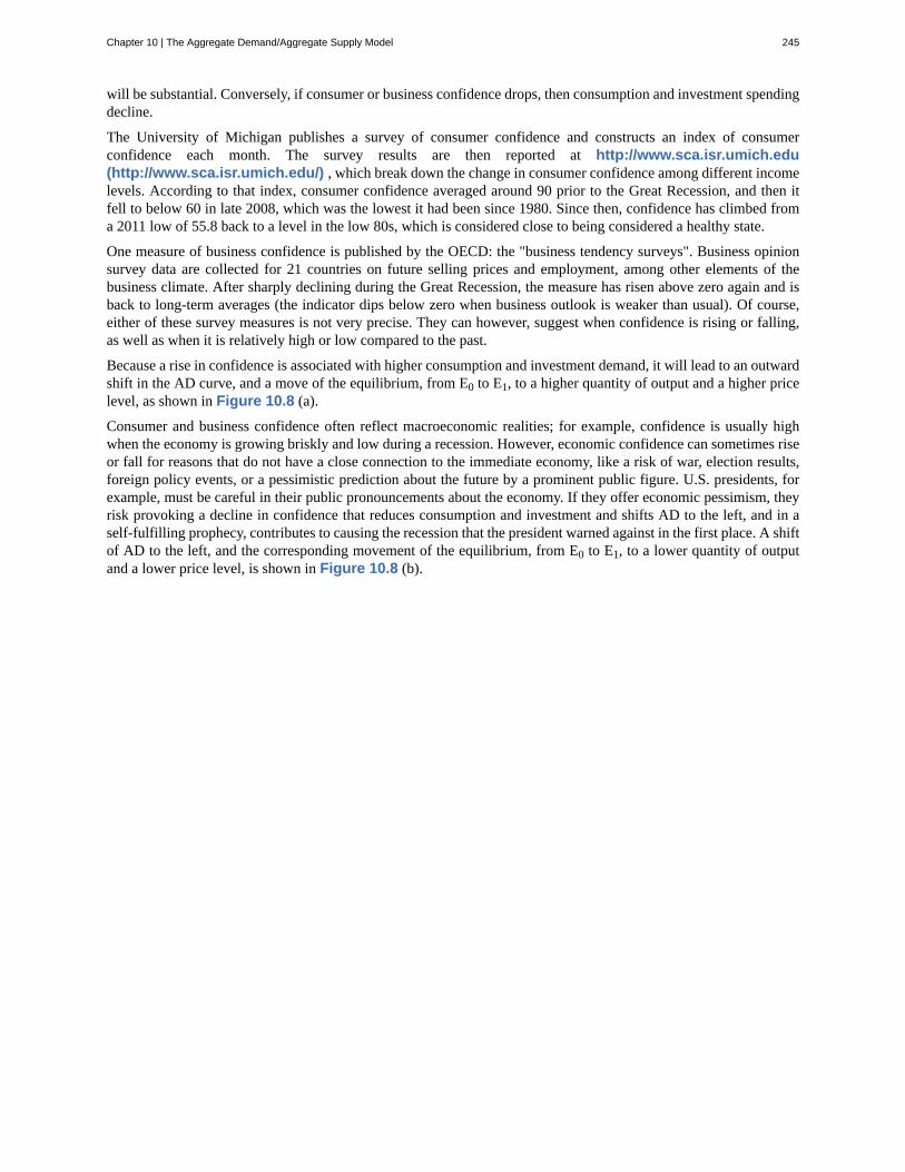
will be substantial. Conversely, if consumer or business confidence drops, then consumption and investment spendingdecline.
The University of Michigan publishes a survey of consumer confidence and constructs an index of consumerconfidence each month. The survey results are then reported at http://www.sca.isr.umich.edu(http://www.sca.isr.umich.edu/) , which break down the change in consumer confidence among different incomelevels. According to that index, consumer confidence averaged around 90 prior to the Great Recession, and then itfell to below 60 in late 2008, which was the lowest it had been since 1980. Since then, confidence has climbed froma 2011 low of 55.8 back to a level in the low 80s, which is considered close to being considered a healthy state.
One measure of business confidence is published by the OECD: the "business tendency surveys". Business opinionsurvey data are collected for 21 countries on future selling prices and employment, among other elements of thebusiness climate. After sharply declining during the Great Recession, the measure has risen above zero again and isback to long-term averages (the indicator dips below zero when business outlook is weaker than usual). Of course,either of these survey measures is not very precise. They can however, suggest when confidence is rising or falling,as well as when it is relatively high or low compared to the past.
Because a rise in confidence is associated with higher consumption and investment demand, it will lead to an outwardshift in the AD curve, and a move of the equilibrium, from E0 to E1, to a higher quantity of output and a higher pricelevel, as shown in Figure 10.8 (a).
Consumer and business confidence often reflect macroeconomic realities; for example, confidence is usually highwhen the economy is growing briskly and low during a recession. However, economic confidence can sometimes riseor fall for reasons that do not have a close connection to the immediate economy, like a risk of war, election results,foreign policy events, or a pessimistic prediction about the future by a prominent public figure. U.S. presidents, forexample, must be careful in their public pronouncements about the economy. If they offer economic pessimism, theyrisk provoking a decline in confidence that reduces consumption and investment and shifts AD to the left, and in aself-fulfilling prophecy, contributes to causing the recession that the president warned against in the first place. A shiftof AD to the left, and the corresponding movement of the equilibrium, from E0 to E1, to a lower quantity of outputand a lower price level, is shown in Figure 10.8 (b).
Chapter 10 | The Aggregate Demand/Aggregate Supply Model 245
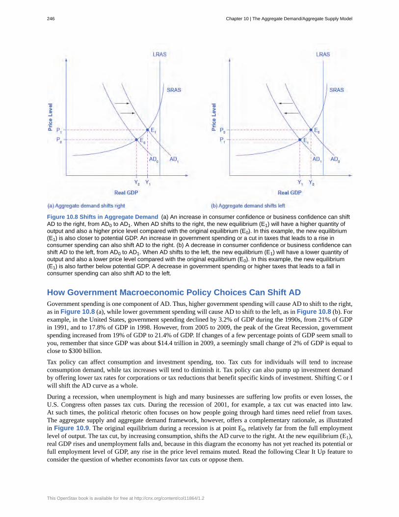
Figure 10.8 Shifts in Aggregate Demand (a) An increase in consumer confidence or business confidence can shiftAD to the right, from AD0 to AD1. When AD shifts to the right, the new equilibrium (E1) will have a higher quantity ofoutput and also a higher price level compared with the original equilibrium (E0). In this example, the new equilibrium(E1) is also closer to potential GDP. An increase in government spending or a cut in taxes that leads to a rise inconsumer spending can also shift AD to the right. (b) A decrease in consumer confidence or business confidence canshift AD to the left, from AD0 to AD1. When AD shifts to the left, the new equilibrium (E1) will have a lower quantity ofoutput and also a lower price level compared with the original equilibrium (E0). In this example, the new equilibrium(E1) is also farther below potential GDP. A decrease in government spending or higher taxes that leads to a fall inconsumer spending can also shift AD to the left.
How Government Macroeconomic Policy Choices Can Shift ADGovernment spending is one component of AD. Thus, higher government spending will cause AD to shift to the right,as in Figure 10.8 (a), while lower government spending will cause AD to shift to the left, as in Figure 10.8 (b). Forexample, in the United States, government spending declined by 3.2% of GDP during the 1990s, from 21% of GDPin 1991, and to 17.8% of GDP in 1998. However, from 2005 to 2009, the peak of the Great Recession, governmentspending increased from 19% of GDP to 21.4% of GDP. If changes of a few percentage points of GDP seem small toyou, remember that since GDP was about $14.4 trillion in 2009, a seemingly small change of 2% of GDP is equal toclose to $300 billion.
Tax policy can affect consumption and investment spending, too. Tax cuts for individuals will tend to increaseconsumption demand, while tax increases will tend to diminish it. Tax policy can also pump up investment demandby offering lower tax rates for corporations or tax reductions that benefit specific kinds of investment. Shifting C or Iwill shift the AD curve as a whole.
During a recession, when unemployment is high and many businesses are suffering low profits or even losses, theU.S. Congress often passes tax cuts. During the recession of 2001, for example, a tax cut was enacted into law.At such times, the political rhetoric often focuses on how people going through hard times need relief from taxes.The aggregate supply and aggregate demand framework, however, offers a complementary rationale, as illustratedin Figure 10.9. The original equilibrium during a recession is at point E0, relatively far from the full employmentlevel of output. The tax cut, by increasing consumption, shifts the AD curve to the right. At the new equilibrium (E1),real GDP rises and unemployment falls and, because in this diagram the economy has not yet reached its potential orfull employment level of GDP, any rise in the price level remains muted. Read the following Clear It Up feature toconsider the question of whether economists favor tax cuts or oppose them.
246 Chapter 10 | The Aggregate Demand/Aggregate Supply Model
This OpenStax book is available for free at http://cnx.org/content/col11864/1.2
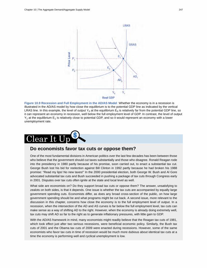
Figure 10.9 Recession and Full Employment in the AD/AS Model Whether the economy is in a recession isillustrated in the AD/AS model by how close the equilibrium is to the potential GDP line as indicated by the verticalLRAS line. In this example, the level of output Y0 at the equilibrium E0 is relatively far from the potential GDP line, soit can represent an economy in recession, well below the full employment level of GDP. In contrast, the level of outputY1 at the equilibrium E1 is relatively close to potential GDP, and so it would represent an economy with a lowerunemployment rate.
Do economists favor tax cuts or oppose them?One of the most fundamental divisions in American politics over the last few decades has been between thosewho believe that the government should cut taxes substantially and those who disagree. Ronald Reagan rodeinto the presidency in 1980 partly because of his promise, soon carried out, to enact a substantial tax cut.George Bush lost his bid for reelection against Bill Clinton in 1992 partly because he had broken his 1988promise: “Read my lips! No new taxes!” In the 2000 presidential election, both George W. Bush and Al Goreadvocated substantial tax cuts and Bush succeeded in pushing a package of tax cuts through Congress earlyin 2001. Disputes over tax cuts often ignite at the state and local level as well.
What side are economists on? Do they support broad tax cuts or oppose them? The answer, unsatisfying tozealots on both sides, is that it depends. One issue is whether the tax cuts are accompanied by equally largegovernment spending cuts. Economists differ, as does any broad cross-section of the public, on how largegovernment spending should be and what programs might be cut back. A second issue, more relevant to thediscussion in this chapter, concerns how close the economy is to the full employment level of output. In arecession, when the intersection of the AD and AS curves is far below the full employment level, tax cuts canmake sense as a way of shifting AD to the right. However, when the economy is already doing extremely well,tax cuts may shift AD so far to the right as to generate inflationary pressures, with little gain to GDP.
With the AD/AS framework in mind, many economists might readily believe that the Reagan tax cuts of 1981,which took effect just after two serious recessions, were beneficial economic policy. Similarly, the Bush taxcuts of 2001 and the Obama tax cuts of 2009 were enacted during recessions. However, some of the sameeconomists who favor tax cuts in time of recession would be much more dubious about identical tax cuts at atime the economy is performing well and cyclical unemployment is low.
Chapter 10 | The Aggregate Demand/Aggregate Supply Model 247

The use of government spending and tax cuts can be a useful tool to affect aggregate demand and it will be discussedin greater detail in the Government Budgets and Fiscal Policy chapter and The Impacts of GovernmentBorrowing. Other policy tools can shift the aggregate demand curve as well. For example, as discussed in theMonetary policy and Bank Regulation chapter, the Federal Reserve can affect interest rates and the availabilityof credit. Higher interest rates tend to discourage borrowing and thus reduce both household spending on big-ticketitems like houses and cars and investment spending by business. Conversely, lower interest rates will stimulateconsumption and investment demand. Interest rates can also affect exchange rates, which in turn will have effects onthe export and import components of aggregate demand.
Spelling out the details of these alternative policies and how they affect the components of aggregate demand can waitfor The Keynesian Perspective chapter. Here, the key lesson is that a shift of the aggregate demand curve to theright leads to a greater real GDP and to upward pressure on the price level. Conversely, a shift of aggregate demandto the left leads to a lower real GDP and a lower price level. Whether these changes in output and price level arerelatively large or relatively small, and how the change in equilibrium relates to potential GDP, depends on whetherthe shift in the AD curve is happening in the relatively flat or relatively steep portion of the AS curve.
10.5 | How the AD/AS Model Incorporates Growth,Unemployment, and InflationBy the end of this section, you will be able to:
• Identify periods of economic growth and recession using the aggregate demand/aggregate supplymodel
• Explain how unemployment and inflation impact the aggregate demand/aggregate supply model• Evaluate the importance of the aggregate demand/aggregate supply model
The AD/AS model can convey a number of interlocking relationships between the four macroeconomic goals ofgrowth, unemployment, inflation, and a sustainable balance of trade. Moreover, the AD/AS framework is flexibleenough to accommodate both the Keynes’ law approach that focuses on aggregate demand and the short run, whilealso including the Say’s law approach that focuses on aggregate supply and the long run. These advantages areconsiderable. Every model is a simplified version of the deeper reality and, in the context of the AD/AS model, thethree macroeconomic goals arise in ways that are sometimes indirect or incomplete. In this module, we considerhow the AD/AS model illustrates the three macroeconomic goals of economic growth, low unemployment, and lowinflation.
Growth and Recession in the AD/AS DiagramIn the AD/AS diagram, long-run economic growth due to productivity increases over time will be represented by agradual shift to the right of aggregate supply. The vertical line representing potential GDP (or the “full employmentlevel of GDP”) will gradually shift to the right over time as well. A pattern of economic growth over three years, withthe AS curve shifting slightly out to the right each year, was shown earlier in Figure 10.7 (a). However, the factorsthat determine the speed of this long-term economic growth rate—like investment in physical and human capital,technology, and whether an economy can take advantage of catch-up growth—do not appear directly in the AD/ASdiagram.
In the short run, GDP falls and rises in every economy, as the economy dips into recession or expands out of recession.Recessions are illustrated in the AD/AS diagram when the equilibrium level of real GDP is substantially belowpotential GDP, as occurred at the equilibrium point E0 in Figure 10.9. On the other hand, in years of resurgenteconomic growth the equilibrium will typically be close to potential GDP, as shown at equilibrium point E1 in thatearlier figure.
Unemployment in the AD/AS DiagramTwo types of unemployment were described in the Unemployment chapter. Cyclical unemployment bounces upand down according to the short-run movements of GDP. Over the long run, in the United States, the unemploymentrate typically hovers around 5% (give or take one percentage point or so), when the economy is healthy. In many ofthe national economies across Europe, the rate of unemployment in recent decades has only dropped to about 10%
248 Chapter 10 | The Aggregate Demand/Aggregate Supply Model
This OpenStax book is available for free at http://cnx.org/content/col11864/1.2
or a bit lower, even in good economic years. This baseline level of unemployment that occurs year-in and year-outis called the natural rate of unemployment and is determined by how well the structures of market and governmentinstitutions in the economy lead to a matching of workers and employers in the labor market. Potential GDP canimply different unemployment rates in different economies, depending on the natural rate of unemployment for thateconomy.
Visit this website (http://openstaxcollege.org/l/consumerconfid) for data on consumer confidence.
In the AD/AS diagram, cyclical unemployment is shown by how close the economy is to the potential or fullemployment level of GDP. Returning to Figure 10.9, relatively low cyclical unemployment for an economy occurswhen the level of output is close to potential GDP, as in the equilibrium point E1. Conversely, high cyclicalunemployment arises when the output is substantially to the left of potential GDP on the AD/AS diagram, as at theequilibrium point E0. The factors that determine the natural rate of unemployment are not shown separately in the AD/AS model, although they are implicitly part of what determines potential GDP or full employment GDP in a giveneconomy.
Inflationary Pressures in the AD/AS DiagramInflation fluctuates in the short run. Higher inflation rates have typically occurred either during or just after economicbooms: for example, the biggest spurts of inflation in the U.S. economy during the twentieth century followedthe wartime booms of World War I and World War II. Conversely, rates of inflation generally decline duringrecessions. As an extreme example, inflation actually became negative—a situation called “deflation”—during theGreat Depression. Even during the relatively short recession of 1991–1992, the rate of inflation declined from 5.4%in 1990 to 3.0% in 1992. During the relatively short recession of 2001, the rate of inflation declined from 3.4% in2000 to 1.6% in 2002. During the deep recession of 2007–2009, the rate of inflation declined from 3.8% in 2008 to–0.4% in 2009. Some countries have experienced bouts of high inflation that lasted for years. In the U.S. economysince the mid–1980s, inflation does not seem to have had any long-term trend to be substantially higher or lower;instead, it has stayed in the range of 1–5% annually.
Visit this website (http://openstaxcollege.org/l/businessconfid) for data on business confidence.
Chapter 10 | The Aggregate Demand/Aggregate Supply Model 249
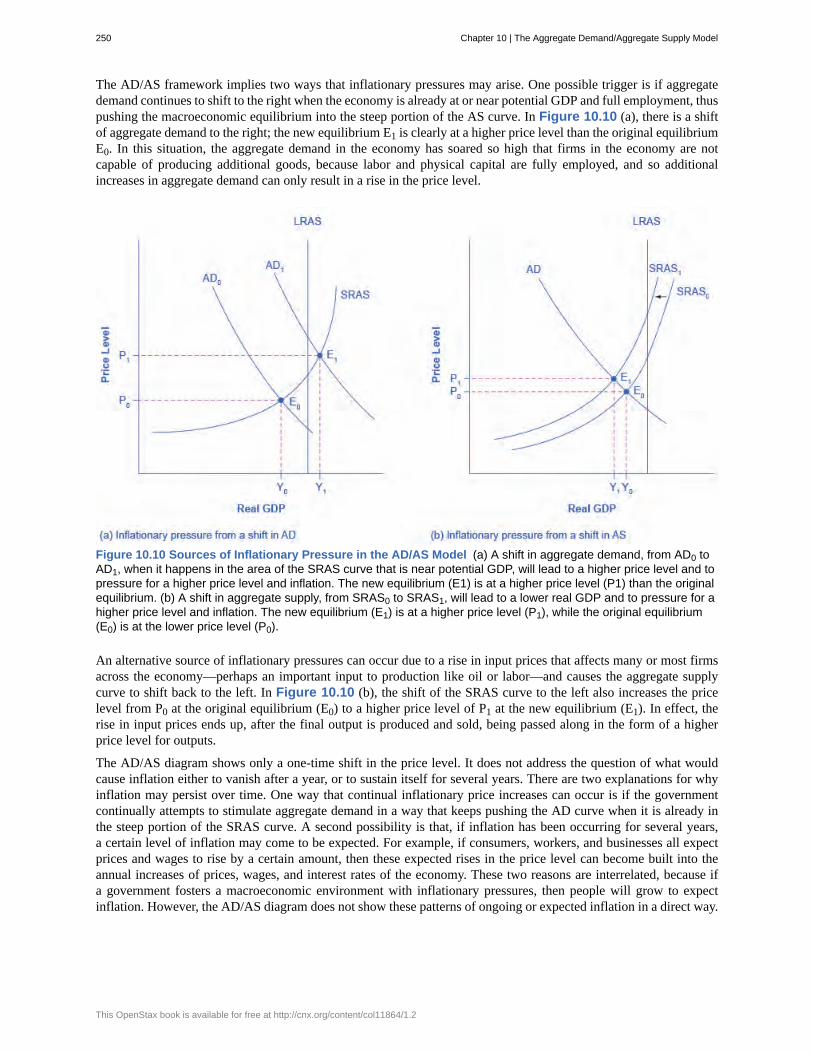
The AD/AS framework implies two ways that inflationary pressures may arise. One possible trigger is if aggregatedemand continues to shift to the right when the economy is already at or near potential GDP and full employment, thuspushing the macroeconomic equilibrium into the steep portion of the AS curve. In Figure 10.10 (a), there is a shiftof aggregate demand to the right; the new equilibrium E1 is clearly at a higher price level than the original equilibriumE0. In this situation, the aggregate demand in the economy has soared so high that firms in the economy are notcapable of producing additional goods, because labor and physical capital are fully employed, and so additionalincreases in aggregate demand can only result in a rise in the price level.
Figure 10.10 Sources of Inflationary Pressure in the AD/AS Model (a) A shift in aggregate demand, from AD0 toAD1, when it happens in the area of the SRAS curve that is near potential GDP, will lead to a higher price level and topressure for a higher price level and inflation. The new equilibrium (E1) is at a higher price level (P1) than the originalequilibrium. (b) A shift in aggregate supply, from SRAS0 to SRAS1, will lead to a lower real GDP and to pressure for ahigher price level and inflation. The new equilibrium (E1) is at a higher price level (P1), while the original equilibrium(E0) is at the lower price level (P0).
An alternative source of inflationary pressures can occur due to a rise in input prices that affects many or most firmsacross the economy—perhaps an important input to production like oil or labor—and causes the aggregate supplycurve to shift back to the left. In Figure 10.10 (b), the shift of the SRAS curve to the left also increases the pricelevel from P0 at the original equilibrium (E0) to a higher price level of P1 at the new equilibrium (E1). In effect, therise in input prices ends up, after the final output is produced and sold, being passed along in the form of a higherprice level for outputs.
The AD/AS diagram shows only a one-time shift in the price level. It does not address the question of what wouldcause inflation either to vanish after a year, or to sustain itself for several years. There are two explanations for whyinflation may persist over time. One way that continual inflationary price increases can occur is if the governmentcontinually attempts to stimulate aggregate demand in a way that keeps pushing the AD curve when it is already inthe steep portion of the SRAS curve. A second possibility is that, if inflation has been occurring for several years,a certain level of inflation may come to be expected. For example, if consumers, workers, and businesses all expectprices and wages to rise by a certain amount, then these expected rises in the price level can become built into theannual increases of prices, wages, and interest rates of the economy. These two reasons are interrelated, because ifa government fosters a macroeconomic environment with inflationary pressures, then people will grow to expectinflation. However, the AD/AS diagram does not show these patterns of ongoing or expected inflation in a direct way.
250 Chapter 10 | The Aggregate Demand/Aggregate Supply Model
This OpenStax book is available for free at http://cnx.org/content/col11864/1.2
Importance of the Aggregate Demand/Aggregate Supply ModelMacroeconomics takes an overall view of the economy, which means that it needs to juggle many different concepts.For example, start with the three macroeconomic goals of growth, low inflation, and low unemployment. Aggregatedemand has four elements: consumption, investment, government spending, and exports less imports. Aggregatesupply reveals how businesses throughout the economy will react to a higher price level for outputs. Finally, awide array of economic events and policy decisions can affect aggregate demand and aggregate supply, includinggovernment tax and spending decisions; consumer and business confidence; changes in prices of key inputs like oil;and technology that brings higher levels of productivity.
The aggregate demand/aggregate supply model is one of the fundamental diagrams in this course (like the budgetconstraint diagram introduced in the Choice in a World of Scarcity chapter and the supply and demand diagramintroduced in the Demand and Supply chapter) because it provides an overall framework for bringing these factorstogether in one diagram. Indeed, some version of the AD/AS model will appear in every chapter in the rest of thisbook.
10.6 | Keynes’ Law and Say’s Law in the AD/AS ModelBy the end of this section, you will be able to:
• Identify the neoclassical zone, the intermediate zone, and the Keynesian zone in the aggregatedemand/aggregate supply model
• Use an aggregate demand/aggregate supply model as a diagnostic test to understand the current stateof the economy
The AD/AS model can be used to illustrate both Say’s law that supply creates its own demand and Keynes’ lawthat demand creates its own supply. Consider the three zones of the SRAS curve as identified in Figure 10.11: theKeynesian zone, the neoclassical zone, and the intermediate zone.
Chapter 10 | The Aggregate Demand/Aggregate Supply Model 251
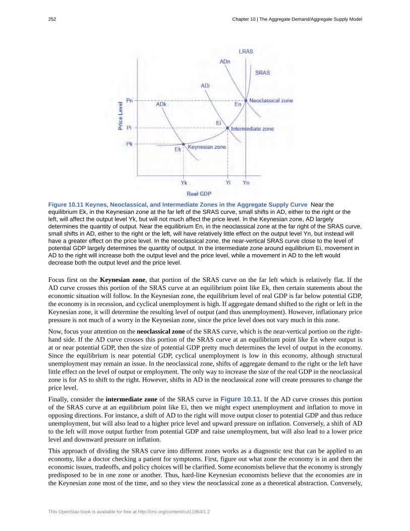
Figure 10.11 Keynes, Neoclassical, and Intermediate Zones in the Aggregate Supply Curve Near theequilibrium Ek, in the Keynesian zone at the far left of the SRAS curve, small shifts in AD, either to the right or theleft, will affect the output level Yk, but will not much affect the price level. In the Keynesian zone, AD largelydetermines the quantity of output. Near the equilibrium En, in the neoclassical zone at the far right of the SRAS curve,small shifts in AD, either to the right or the left, will have relatively little effect on the output level Yn, but instead willhave a greater effect on the price level. In the neoclassical zone, the near-vertical SRAS curve close to the level ofpotential GDP largely determines the quantity of output. In the intermediate zone around equilibrium Ei, movement inAD to the right will increase both the output level and the price level, while a movement in AD to the left woulddecrease both the output level and the price level.
Focus first on the Keynesian zone, that portion of the SRAS curve on the far left which is relatively flat. If theAD curve crosses this portion of the SRAS curve at an equilibrium point like Ek, then certain statements about theeconomic situation will follow. In the Keynesian zone, the equilibrium level of real GDP is far below potential GDP,the economy is in recession, and cyclical unemployment is high. If aggregate demand shifted to the right or left in theKeynesian zone, it will determine the resulting level of output (and thus unemployment). However, inflationary pricepressure is not much of a worry in the Keynesian zone, since the price level does not vary much in this zone.
Now, focus your attention on the neoclassical zone of the SRAS curve, which is the near-vertical portion on the right-hand side. If the AD curve crosses this portion of the SRAS curve at an equilibrium point like En where output isat or near potential GDP, then the size of potential GDP pretty much determines the level of output in the economy.Since the equilibrium is near potential GDP, cyclical unemployment is low in this economy, although structuralunemployment may remain an issue. In the neoclassical zone, shifts of aggregate demand to the right or the left havelittle effect on the level of output or employment. The only way to increase the size of the real GDP in the neoclassicalzone is for AS to shift to the right. However, shifts in AD in the neoclassical zone will create pressures to change theprice level.
Finally, consider the intermediate zone of the SRAS curve in Figure 10.11. If the AD curve crosses this portionof the SRAS curve at an equilibrium point like Ei, then we might expect unemployment and inflation to move inopposing directions. For instance, a shift of AD to the right will move output closer to potential GDP and thus reduceunemployment, but will also lead to a higher price level and upward pressure on inflation. Conversely, a shift of ADto the left will move output further from potential GDP and raise unemployment, but will also lead to a lower pricelevel and downward pressure on inflation.
This approach of dividing the SRAS curve into different zones works as a diagnostic test that can be applied to aneconomy, like a doctor checking a patient for symptoms. First, figure out what zone the economy is in and then theeconomic issues, tradeoffs, and policy choices will be clarified. Some economists believe that the economy is stronglypredisposed to be in one zone or another. Thus, hard-line Keynesian economists believe that the economies are inthe Keynesian zone most of the time, and so they view the neoclassical zone as a theoretical abstraction. Conversely,
252 Chapter 10 | The Aggregate Demand/Aggregate Supply Model
This OpenStax book is available for free at http://cnx.org/content/col11864/1.2
hard-line neoclassical economists argue that economies are in the neoclassical zone most of the time and that theKeynesian zone is a distraction. The Keynesian Perspective and The Neoclassical Perspective should helpto clarify the underpinnings and consequences of these contrasting views of the macroeconomy.
From Housing Bubble to Housing BustEconomic fluctuations, whether those experienced during the Great Depression of the 1930s, the stagflationof the 1970s, or the Great Recession of 2008–2009, can be explained using the AD/AS diagram. Short-runfluctuations in output occur due to shifts of the SRAS curve, the AD curve, or both. In the case of the housingbubble, rising home values caused the AD curve to shift to the right as more people felt that rising homevalues increased their overall wealth. Many homeowners took on mortgages that exceeded their ability topay because, as home values continued to go up, the increased value would pay off any debt outstanding.Increased wealth due to rising home values lead to increased home equity loans and increased spending.All these activities pushed AD to the right, contributing to low unemployment rates and economic growth inthe United States. When the housing bubble burst, overall wealth dropped dramatically, wiping out the recentgains. This drop in the value of homes was a demand shock to the U.S. economy because of its impact directlyon the wealth of the household sector, and its contagion into the financial that essentially locked up new credit.The AD curve shifted to the left as evidenced by the rising unemployment of the Great Recession.
Understanding the source of these macroeconomic fluctuations provided monetary and fiscal policy makerswith insight about what policy actions to take to mitigate the impact of the housing crisis. From a monetarypolicy perspective, the Federal Reserve lowered short-term interest rates to between 0% and 0.25 %, toloosen up credit throughout the financial system. Discretionary fiscal policy measures included the passageof the Emergency Economic Stabilization Act of 2008 that allowed for the purchase of troubled assets, suchas mortgages, from financial institutions and the American Recovery and Reinvestment Act of 2009 thatincreased government spending on infrastructure, provided for tax cuts, and increased transfer payments. Incombination, both monetary and fiscal policy measures were designed to help stimulate aggregate demand inthe U.S. economy, pushing the AD curve to the right.
While most economists agree on the usefulness of the AD/AS diagram in analyzing the sources of thesefluctuations, there is still some disagreement about the effectiveness of policy decisions that are useful instabilizing these fluctuations. We discuss the possible policy actions and the differences among economistsabout their effectiveness in more detail in The Keynesian Perspective, Monetary Policy and BankRegulation, and Government Budgets and Fiscal Policy.
Chapter 10 | The Aggregate Demand/Aggregate Supply Model 253
aggregate demand (AD)
aggregate demand (AD) curve
aggregate demand/aggregate supply model
aggregate supply (AS)
aggregate supply (AS) curve
full-employment GDP
intermediate zone
Keynesian zone
Keynes’ law
long run aggregate supply (LRAS) curve
neoclassical economists
neoclassical zone
potential GDP
Say’s law
short run aggregate supply (SRAS) curve
stagflation
KEY TERMS
the amount of total spending on domestic goods and services in an economy
the total spending on domestic goods and services at each price level
a model that shows what determines total supply or total demand forthe economy, and how total demand and total supply interact at the macroeconomic level
the total quantity of output (i.e. real GDP) firms will produce and sell
the total quantity of output (i.e. real GDP) that firms will produce and sell at each pricelevel
another name for potential GDP, when the economy is producing at its potential andunemployment is at the natural rate of unemployment
portion of the SRAS curve where GDP is below potential but not so far below as in the Keynesianzone; the SRAS curve is upward-sloping, but not vertical in the intermediate zone
portion of the SRAS curve where GDP is far below potential and the SRAS curve is flat
“demand creates its own supply”
vertical line at potential GDP showing no relationship between the pricelevel for output and real GDP in the long run
economists who generally emphasize the importance of aggregate supply in determining thesize of the macroeconomy over the long run
portion of the SRAS curve where GDP is at or near potential output where the SRAS curve is steep
the maximum quantity that an economy can produce given full employment of its existing levels oflabor, physical capital, technology, and institutions
“supply creates its own demand”
positive short run relationship between the price level for output andreal GDP, holding the prices of inputs fixed
an economy experiences stagnant growth and high inflation at the same time
KEY CONCEPTS AND SUMMARY
10.1 Macroeconomic Perspectives on Demand and SupplyNeoclassical economists emphasize Say’s law, which holds that supply creates its own demand. Keynesianeconomists emphasize Keynes’ law, which holds that demand creates its own supply. Many mainstream economiststake a Keynesian perspective, emphasizing the importance of aggregate demand, for the short run, and a neoclassicalperspective, emphasizing the importance of aggregate supply, for the long run.
10.2 Building a Model of Aggregate Demand and Aggregate SupplyThe upward-sloping short run aggregate supply (SRAS) curve shows the positive relationship between the pricelevel and the level of real GDP in the short run. Aggregate supply slopes up because when the price level foroutputs increases, while the price level of inputs remains fixed, the opportunity for additional profits encourages moreproduction. The aggregate supply curve is near-horizontal on the left and near-vertical on the right. In the long run,
254 Chapter 10 | The Aggregate Demand/Aggregate Supply Model
This OpenStax book is available for free at http://cnx.org/content/col11864/1.2
aggregate supply is shown by a vertical line at the level of potential output, which is the maximum level of output theeconomy can produce with its existing levels of workers, physical capital, technology, and economic institutions.
The downward-sloping aggregate demand (AD) curve shows the relationship between the price level for outputs andthe quantity of total spending in the economy. It slopes down because of: (a) the wealth effect, which means thata higher price level leads to lower real wealth, which reduces the level of consumption; (b) the interest rate effect,which holds that a higher price level will mean a greater demand for money, which will tend to drive up interest ratesand reduce investment spending; and (c) the foreign price effect, which holds that a rise in the price level will makedomestic goods relatively more expensive, discouraging exports and encouraging imports.
10.3 Shifts in Aggregate SupplyThe aggregate demand/aggregate supply (AD/AS) diagram shows how AD and AS interact. The intersection of theAD and AS curves shows the equilibrium output and price level in the economy. Movements of either AS or ADwill result in a different equilibrium output and price level. The aggregate supply curve will shift out to the rightas productivity increases. It will shift back to the left as the price of key inputs rises, and will shift out to the rightif the price of key inputs falls. If the AS curve shifts back to the left, the combination of lower output, higherunemployment, and higher inflation, called stagflation, occurs. If AS shifts out to the right, a combination of lowerinflation, higher output, and lower unemployment is possible.
10.4 Shifts in Aggregate DemandThe AD curve will shift out as the components of aggregate demand—C, I, G, and X–M—rise. It will shift back tothe left as these components fall. These factors can change because of different personal choices, like those resultingfrom consumer or business confidence, or from policy choices like changes in government spending and taxes. If theAD curve shifts to the right, then the equilibrium quantity of output and the price level will rise. If the AD curve shiftsto the left, then the equilibrium quantity of output and the price level will fall. Whether equilibrium output changesrelatively more than the price level or whether the price level changes relatively more than output is determined bywhere the AD curve intersects with the AS curve.
The AD/AS diagram superficially resembles the microeconomic supply and demand diagram on the surface, butin reality, what is on the horizontal and vertical axes and the underlying economic reasons for the shapes of thecurves are very different. Long-term economic growth is illustrated in the AD/AS framework by a gradual shift ofthe aggregate supply curve to the right. A recession is illustrated when the intersection of AD and AS is substantiallybelow potential GDP, while an expanding economy is illustrated when the intersection of AS and AD is near potentialGDP.
10.5 How the AD/AS Model Incorporates Growth, Unemployment, and InflationCyclical unemployment is relatively large in the AD/AS framework when the equilibrium is substantially belowpotential GDP. Cyclical unemployment is small in the AD/AS framework when the equilibrium is near potential GDP.The natural rate of unemployment, as determined by the labor market institutions of the economy, is built into whatis meant by potential GDP, but does not otherwise appear in an AD/AS diagram. Pressures for inflation to rise or fallare shown in the AD/AS framework when the movement from one equilibrium to another causes the price level torise or to fall. The balance of trade does not appear directly in the AD/AS diagram, but it appears indirectly in severalways. Increases in exports or declines in imports can cause shifts in AD. Changes in the price of key imported inputsto production, like oil, can cause shifts in AS. The AD/AS model is the key model used in this book to understandmacroeconomic issues.
10.6 Keynes’ Law and Say’s Law in the AD/AS ModelThe SRAS curve can be divided into three zones. Keynes’ law says demand creates its own supply, so that changesin aggregate demand cause changes in real GDP and employment. Keynes’ law can be shown on the horizontalKeynesian zone of the aggregate supply curve. The Keynesian zone occurs at the left of the SRAS curve where itis fairly flat, so movements in AD will affect output, but have little effect on the price level. Say’s law says supplycreates its own demand. Changes in aggregate demand have no effect on real GDP and employment, only on the pricelevel. Say’s law can be shown on the vertical neoclassical zone of the aggregate supply curve. The neoclassical zoneoccurs at the right of the SRAS curve where it is fairly vertical, and so movements in AD will affect the price level,but have little impact on output. The intermediate zone in the middle of the SRAS curve is upward-sloping, so a risein AD will cause higher output and price level, while a fall in AD will lead to a lower output and price level.
Chapter 10 | The Aggregate Demand/Aggregate Supply Model 255
SELF-CHECK QUESTIONS1. Describe the mechanism by which supply creates its own demand.
2. Describe the mechanism by which demand creates its own supply.
3. The short run aggregate supply curve was constructed assuming that as the price of outputs increases, the price ofinputs stays the same. How would an increase in the prices of important inputs, like energy, affect aggregate supply?
4. In the AD/AS model, what prevents the economy from achieving equilibrium at potential output?
5. Suppose the U.S. Congress passes significant immigration reform that makes it easier for foreigners to come tothe United States to work. Use the AD/AS model to explain how this would affect the equilibrium level of GDP andthe price level.
6. Suppose concerns about the size of the federal budget deficit lead the U.S. Congress to cut all funding for researchand development for ten years. Assuming this has an impact on technology growth, what does the AD/AS modelpredict would be the likely effect on equilibrium GDP and the price level?
7. How would a dramatic increase in the value of the stock market shift the AD curve? What effect would the shifthave on the equilibrium level of GDP and the price level?
8. Suppose Mexico, one of our largest trading partners and purchaser of a large quantity of our exports, goes into arecession. Use the AD/AS model to determine the likely impact on our equilibrium GDP and price level.
9. A policymaker claims that tax cuts led the economy out of a recession. Can we use the AD/AS diagram to showthis?
10. Many financial analysts and economists eagerly await the press releases for the reports on the home price indexand consumer confidence index. What would be the effects of a negative report on both of these? What about apositive report?
11. What impact would a decrease in the size of the labor force have on GDP and the price level according to theAD/AS model?
12. Suppose, after five years of sluggish growth, the economy of the European Union picks up speed. What wouldbe the likely impact on the U.S. trade balance, GDP, and employment?
13. Suppose the Federal Reserve begins to increase the supply of money at an increasing rate. What impact wouldthat have on GDP, unemployment, and inflation?
14. If the economy is operating in the neoclassical zone of the SRAS curve and aggregate demand falls, what islikely to happen to real GDP?
15. If the economy is operating in the Keynesian zone of the SRAS curve and aggregate demand falls, what is likelyto happen to real GDP?
REVIEW QUESTIONS
16. What is Say’s law?
17. What is Keynes’ law?
18. Do neoclassical economists believe in Keynes’ lawor Say’s law?
19. Does Say’s law apply more accurately in the longrun or the short run? What about Keynes’ law?
20. What is on the horizontal axis of the AD/ASdiagram? What is on the vertical axis?
21. What is the economic reason why the SRAS curveslopes up?
22. What are the components of the aggregate demand(AD) curve?
256 Chapter 10 | The Aggregate Demand/Aggregate Supply Model
This OpenStax book is available for free at http://cnx.org/content/col11864/1.2
23. What are the economic reasons why the AD curveslopes down?
24. Briefly explain the reason for the near-horizontalshape of the SRAS curve on its far left.
25. Briefly explain the reason for the near-verticalshape of the SRAS curve on its far right.
26. What is potential GDP?
27. Name some factors that could cause the SRAScurve to shift, and say whether they would shift SRASto the right or to the left.
28. Will the shift of SRAS to the right tend to makethe equilibrium quantity and price level higher or lower?What about a shift of SRAS to the left?
29. What is stagflation?
30. Name some factors that could cause AD to shift,and say whether they would shift AD to the right or tothe left.
31. Would a shift of AD to the right tend to make theequilibrium quantity and price level higher or lower?What about a shift of AD to the left?
32. How is long-term growth illustrated in an AD/ASmodel?
33. How is recession illustrated in an AD/AS model?
34. How is cyclical unemployment illustrated in anAD/AS model?
35. How is the natural rate of unemployment illustratedin an AD/AS model?
36. How is pressure for inflationary price increasesshown in an AD/AS model?
37. What are some of the ways in which exports andimports can affect the AD/AS model?
38. What is the Keynesian zone of the SRAS curve?How much is the price level likely to change in theKeynesian zone?
39. What is the neoclassical zone of the SRAS curve?How much is the output level likely to change in theneoclassical zone?
40. What is the intermediate zone of the SRAS curve?Will a rise in output be accompanied by a rise or a fall inthe price level in this zone?
CRITICAL THINKING QUESTIONS
41. Why would an economist choose either theneoclassical perspective or the Keynesian perspective,but not both?
42. On a microeconomic demand curve, a decrease inprice causes an increase in quantity demanded becausethe product in question is now relatively less expensivethan substitute products. Explain why aggregate demanddoes not increase for the same reason in response to adecrease in the aggregate price level. In other words,what causes total spending to increase if it is not becausegoods are now cheaper?
43. Economists expect that as the labor marketcontinues to tighten going into the latter part of 2015that workers should begin to expect wage increases in2015 and 2016. Assuming this occurs and it was theonly development in the labor market that year, howwould this affect the AS curve? What if it was alsoaccompanied by an increase in worker productivity?
44. If new government regulations require firms touse a cleaner technology that is also less efficient thanwhat was previously used, what would the effect be on
output, the price level, and employment using the AD/AS diagram?
45. During the spring of 2016 the Midwestern UnitedStates, which has a large agricultural base, experiencesabove-average rainfall. Using the AD/AS diagram, whatis the effect on output, the price level, and employment?
46. Hydraulic fracturing (fracking) has the potentialto significantly increase the amount of natural gasproduced in the United States. If a large percentage offactories and utility companies use natural gas, what willhappen to output, the price level, and employment asfracking becomes more widely used?
47. Some politicians have suggested tying theminimum wage to the consumer price index (CPI).Using the AD/AS diagram, what effects would thispolicy most likely have on output, the price level, andemployment?
48. If households decide to save a larger portion oftheir income, what effect would this have on the output,employment, and price level in the short run? Whatabout the long run?
Chapter 10 | The Aggregate Demand/Aggregate Supply Model 257
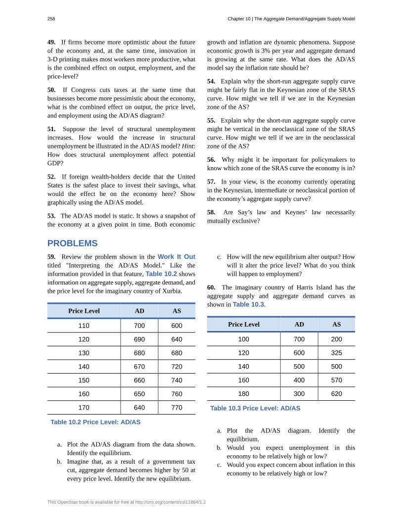
49. If firms become more optimistic about the futureof the economy and, at the same time, innovation in3-D printing makes most workers more productive, whatis the combined effect on output, employment, and theprice-level?
50. If Congress cuts taxes at the same time thatbusinesses become more pessimistic about the economy,what is the combined effect on output, the price level,and employment using the AD/AS diagram?
51. Suppose the level of structural unemploymentincreases. How would the increase in structuralunemployment be illustrated in the AD/AS model? Hint:How does structural unemployment affect potentialGDP?
52. If foreign wealth-holders decide that the UnitedStates is the safest place to invest their savings, whatwould the effect be on the economy here? Showgraphically using the AD/AS model.
53. The AD/AS model is static. It shows a snapshot ofthe economy at a given point in time. Both economic
growth and inflation are dynamic phenomena. Supposeeconomic growth is 3% per year and aggregate demandis growing at the same rate. What does the AD/ASmodel say the inflation rate should be?
54. Explain why the short-run aggregate supply curvemight be fairly flat in the Keynesian zone of the SRAScurve. How might we tell if we are in the Keynesianzone of the AS?
55. Explain why the short-run aggregate supply curvemight be vertical in the neoclassical zone of the SRAScurve. How might we tell if we are in the neoclassicalzone of the AS?
56. Why might it be important for policymakers toknow which zone of the SRAS curve the economy is in?
57. In your view, is the economy currently operatingin the Keynesian, intermediate or neoclassical portion ofthe economy’s aggregate supply curve?
58. Are Say’s law and Keynes’ law necessarilymutually exclusive?
PROBLEMS59. Review the problem shown in the Work It Outtitled "Interpreting the AD/AS Model." Like theinformation provided in that feature, Table 10.2 showsinformation on aggregate supply, aggregate demand, andthe price level for the imaginary country of Xurbia.
Price Level AD AS
110 700 600
120 690 640
130 680 680
140 670 720
150 660 740
160 650 760
170 640 770
Table 10.2 Price Level: AD/AS
a. Plot the AD/AS diagram from the data shown.Identify the equilibrium.
b. Imagine that, as a result of a government taxcut, aggregate demand becomes higher by 50 atevery price level. Identify the new equilibrium.
c. How will the new equilibrium alter output? Howwill it alter the price level? What do you thinkwill happen to employment?
60. The imaginary country of Harris Island has theaggregate supply and aggregate demand curves asshown in Table 10.3.
Price Level AD AS
100 700 200
120 600 325
140 500 500
160 400 570
180 300 620
Table 10.3 Price Level: AD/AS
a. Plot the AD/AS diagram. Identify theequilibrium.
b. Would you expect unemployment in thiseconomy to be relatively high or low?
c. Would you expect concern about inflation in thiseconomy to be relatively high or low?
258 Chapter 10 | The Aggregate Demand/Aggregate Supply Model
This OpenStax book is available for free at http://cnx.org/content/col11864/1.2
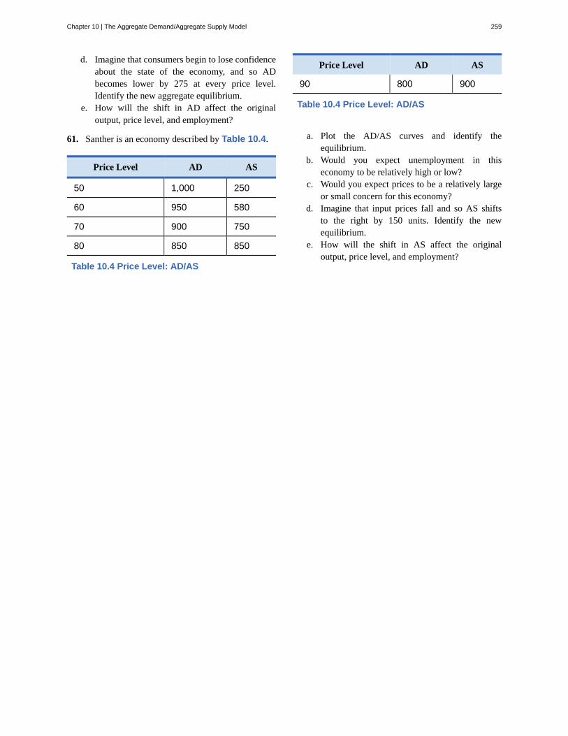
d. Imagine that consumers begin to lose confidenceabout the state of the economy, and so ADbecomes lower by 275 at every price level.Identify the new aggregate equilibrium.
e. How will the shift in AD affect the originaloutput, price level, and employment?
61. Santher is an economy described by Table 10.4.
Price Level AD AS
50 1,000 250
60 950 580
70 900 750
80 850 850
Table 10.4 Price Level: AD/AS
Price Level AD AS
90 800 900
Table 10.4 Price Level: AD/AS
a. Plot the AD/AS curves and identify theequilibrium.
b. Would you expect unemployment in thiseconomy to be relatively high or low?
c. Would you expect prices to be a relatively largeor small concern for this economy?
d. Imagine that input prices fall and so AS shiftsto the right by 150 units. Identify the newequilibrium.
e. How will the shift in AS affect the originaloutput, price level, and employment?
Chapter 10 | The Aggregate Demand/Aggregate Supply Model 259

260 Chapter 10 | The Aggregate Demand/Aggregate Supply Model
This OpenStax book is available for free at http://cnx.org/content/col11864/1.2
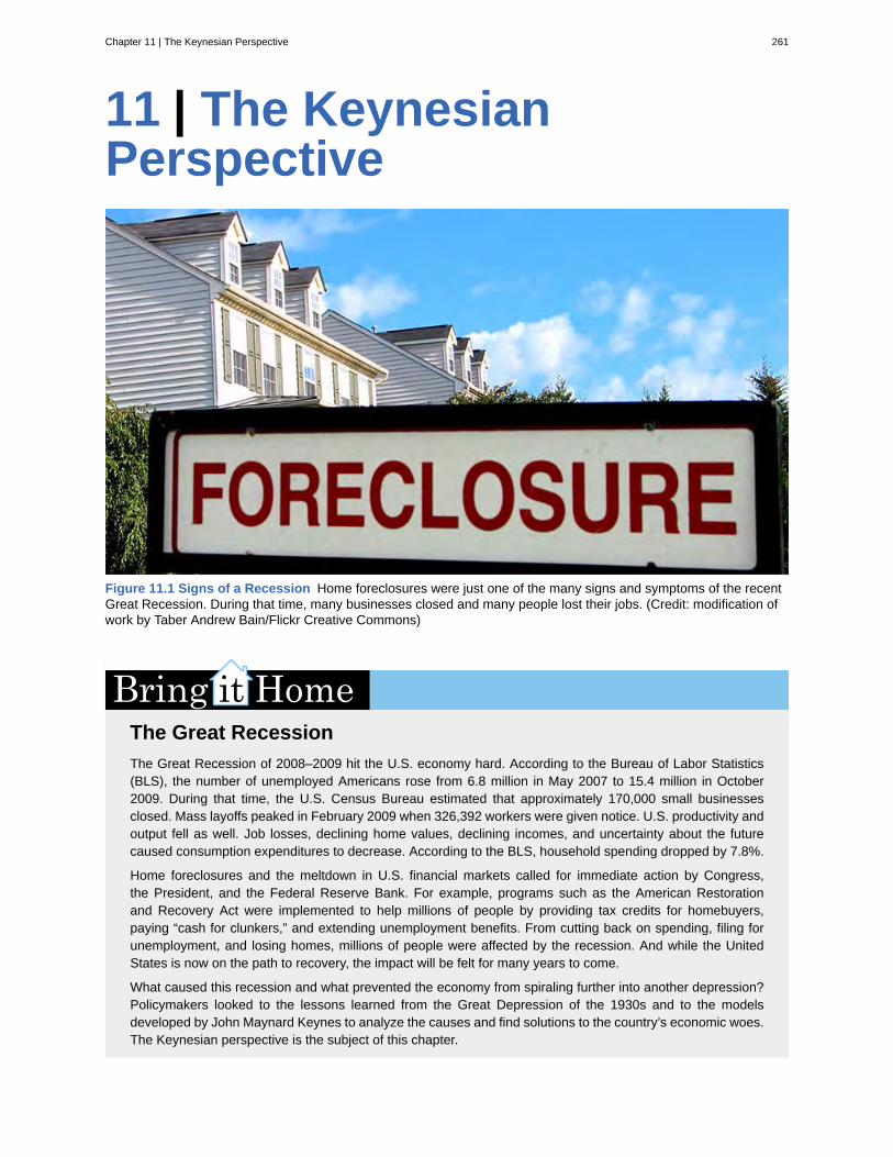
11 | The KeynesianPerspective
Figure 11.1 Signs of a Recession Home foreclosures were just one of the many signs and symptoms of the recentGreat Recession. During that time, many businesses closed and many people lost their jobs. (Credit: modification ofwork by Taber Andrew Bain/Flickr Creative Commons)
The Great RecessionThe Great Recession of 2008–2009 hit the U.S. economy hard. According to the Bureau of Labor Statistics(BLS), the number of unemployed Americans rose from 6.8 million in May 2007 to 15.4 million in October2009. During that time, the U.S. Census Bureau estimated that approximately 170,000 small businessesclosed. Mass layoffs peaked in February 2009 when 326,392 workers were given notice. U.S. productivity andoutput fell as well. Job losses, declining home values, declining incomes, and uncertainty about the futurecaused consumption expenditures to decrease. According to the BLS, household spending dropped by 7.8%.
Home foreclosures and the meltdown in U.S. financial markets called for immediate action by Congress,the President, and the Federal Reserve Bank. For example, programs such as the American Restorationand Recovery Act were implemented to help millions of people by providing tax credits for homebuyers,paying “cash for clunkers,” and extending unemployment benefits. From cutting back on spending, filing forunemployment, and losing homes, millions of people were affected by the recession. And while the UnitedStates is now on the path to recovery, the impact will be felt for many years to come.
What caused this recession and what prevented the economy from spiraling further into another depression?Policymakers looked to the lessons learned from the Great Depression of the 1930s and to the modelsdeveloped by John Maynard Keynes to analyze the causes and find solutions to the country’s economic woes.The Keynesian perspective is the subject of this chapter.
Chapter 11 | The Keynesian Perspective 261
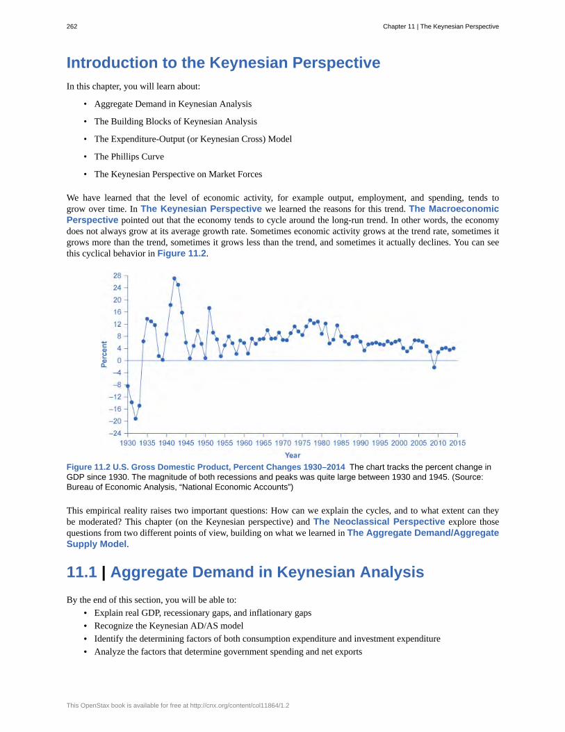
Introduction to the Keynesian PerspectiveIn this chapter, you will learn about:
• Aggregate Demand in Keynesian Analysis
• The Building Blocks of Keynesian Analysis
• The Expenditure-Output (or Keynesian Cross) Model
• The Phillips Curve
• The Keynesian Perspective on Market Forces
We have learned that the level of economic activity, for example output, employment, and spending, tends togrow over time. In The Keynesian Perspective we learned the reasons for this trend. The MacroeconomicPerspective pointed out that the economy tends to cycle around the long-run trend. In other words, the economydoes not always grow at its average growth rate. Sometimes economic activity grows at the trend rate, sometimes itgrows more than the trend, sometimes it grows less than the trend, and sometimes it actually declines. You can seethis cyclical behavior in Figure 11.2.
Figure 11.2 U.S. Gross Domestic Product, Percent Changes 1930–2014 The chart tracks the percent change inGDP since 1930. The magnitude of both recessions and peaks was quite large between 1930 and 1945. (Source:Bureau of Economic Analysis, “National Economic Accounts”)
This empirical reality raises two important questions: How can we explain the cycles, and to what extent can theybe moderated? This chapter (on the Keynesian perspective) and The Neoclassical Perspective explore thosequestions from two different points of view, building on what we learned in The Aggregate Demand/AggregateSupply Model.
11.1 | Aggregate Demand in Keynesian AnalysisBy the end of this section, you will be able to:
• Explain real GDP, recessionary gaps, and inflationary gaps• Recognize the Keynesian AD/AS model• Identify the determining factors of both consumption expenditure and investment expenditure• Analyze the factors that determine government spending and net exports
262 Chapter 11 | The Keynesian Perspective
This OpenStax book is available for free at http://cnx.org/content/col11864/1.2
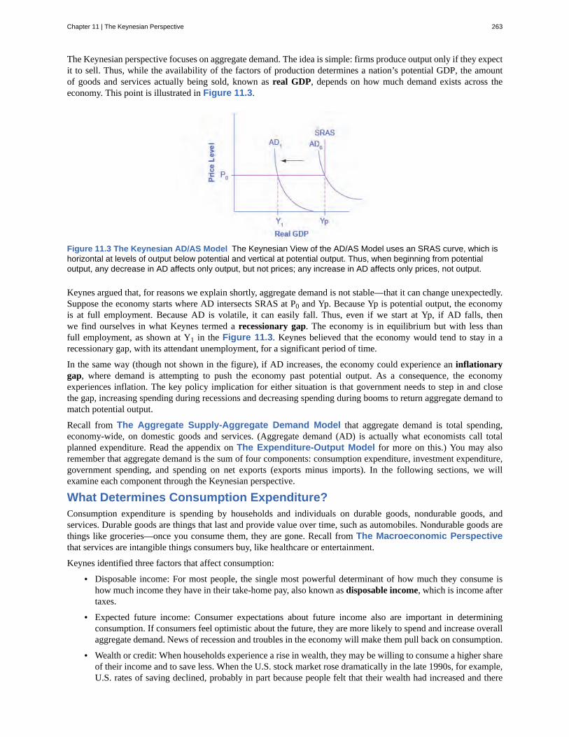
The Keynesian perspective focuses on aggregate demand. The idea is simple: firms produce output only if they expectit to sell. Thus, while the availability of the factors of production determines a nation’s potential GDP, the amountof goods and services actually being sold, known as real GDP, depends on how much demand exists across theeconomy. This point is illustrated in Figure 11.3.
Figure 11.3 The Keynesian AD/AS Model The Keynesian View of the AD/AS Model uses an SRAS curve, which ishorizontal at levels of output below potential and vertical at potential output. Thus, when beginning from potentialoutput, any decrease in AD affects only output, but not prices; any increase in AD affects only prices, not output.
Keynes argued that, for reasons we explain shortly, aggregate demand is not stable—that it can change unexpectedly.Suppose the economy starts where AD intersects SRAS at P0 and Yp. Because Yp is potential output, the economyis at full employment. Because AD is volatile, it can easily fall. Thus, even if we start at Yp, if AD falls, thenwe find ourselves in what Keynes termed a recessionary gap. The economy is in equilibrium but with less thanfull employment, as shown at Y1 in the Figure 11.3. Keynes believed that the economy would tend to stay in arecessionary gap, with its attendant unemployment, for a significant period of time.
In the same way (though not shown in the figure), if AD increases, the economy could experience an inflationarygap, where demand is attempting to push the economy past potential output. As a consequence, the economyexperiences inflation. The key policy implication for either situation is that government needs to step in and closethe gap, increasing spending during recessions and decreasing spending during booms to return aggregate demand tomatch potential output.
Recall from The Aggregate Supply-Aggregate Demand Model that aggregate demand is total spending,economy-wide, on domestic goods and services. (Aggregate demand (AD) is actually what economists call totalplanned expenditure. Read the appendix on The Expenditure-Output Model for more on this.) You may alsoremember that aggregate demand is the sum of four components: consumption expenditure, investment expenditure,government spending, and spending on net exports (exports minus imports). In the following sections, we willexamine each component through the Keynesian perspective.
What Determines Consumption Expenditure?Consumption expenditure is spending by households and individuals on durable goods, nondurable goods, andservices. Durable goods are things that last and provide value over time, such as automobiles. Nondurable goods arethings like groceries—once you consume them, they are gone. Recall from The Macroeconomic Perspectivethat services are intangible things consumers buy, like healthcare or entertainment.
Keynes identified three factors that affect consumption:
• Disposable income: For most people, the single most powerful determinant of how much they consume ishow much income they have in their take-home pay, also known as disposable income, which is income aftertaxes.
• Expected future income: Consumer expectations about future income also are important in determiningconsumption. If consumers feel optimistic about the future, they are more likely to spend and increase overallaggregate demand. News of recession and troubles in the economy will make them pull back on consumption.
• Wealth or credit: When households experience a rise in wealth, they may be willing to consume a higher shareof their income and to save less. When the U.S. stock market rose dramatically in the late 1990s, for example,U.S. rates of saving declined, probably in part because people felt that their wealth had increased and there
Chapter 11 | The Keynesian Perspective 263
was less need to save. How do people spend beyond their income, when they perceive their wealth increasing?The answer is borrowing. On the other side, when the U.S. stock market declined about 40% from March 2008to March 2009, people felt far greater uncertainty about their economic future, so rates of saving increasedwhile consumption declined.
Finally, Keynes noted that a variety of other factors combine to determine how much people save and spend. Ifhousehold preferences about saving shift in a way that encourages consumption rather than saving, then AD will shiftout to the right.
Visit this website (http://openstaxcollege.org/l/Diane_Rehm) for more information about how the recessionaffected various groups of people.
What Determines Investment Expenditure?Spending on new capital goods is called investment expenditure. Investment falls into four categories: producer’sdurable equipment and software, new nonresidential structures (such as factories, offices, and retail locations),changes in inventories, and residential structures (such as single-family homes, townhouses, and apartmentbuildings). The first three types of investment are conducted by businesses, while the last is conducted by households.
Keynes’s treatment of investment focuses on the key role of expectations about the future in influencing businessdecisions. When a business decides to make an investment in physical assets, like plants or equipment, or in intangibleassets, like skills or a research and development project, that firm considers both the expected benefits of theinvestment (expectations of future profits) and the costs of the investment (interest rates).
• Expectations of future profits: The clearest driver of the benefits of an investment is expectations for futureprofits. When an economy is expected to grow, businesses perceive a growing market for their products. Theirhigher degree of business confidence will encourage new investment. For example, in the second half of the1990s, U.S. investment levels surged from 18% of GDP in 1994 to 21% in 2000. However, when a recessionstarted in 2001, U.S. investment levels quickly sank back to 18% of GDP by 2002.
• Interest rates also play a significant role in determining how much investment a firm will make. Just asindividuals need to borrow money to purchase homes, so businesses need financing when they purchase bigticket items. The cost of investment thus includes the interest rate. Even if the firm has the funds, the interestrate measures the opportunity cost of purchasing business capital. Lower interest rates stimulate investmentspending and higher interest rates reduce it.
Many factors can affect the expected profitability on investment. For example, if the price of energy declines, theninvestments that use energy as an input will yield higher profits. If government offers special incentives for investment(for example, through the tax code), then investment will look more attractive; conversely, if government removesspecial investment incentives from the tax code, or increases other business taxes, then investment will look lessattractive. As Keynes noted, business investment is the most variable of all the components of aggregate demand.
What Determines Government Spending?The third component of aggregate demand is spending by federal, state, and local governments. Although the UnitedStates is usually thought of as a market economy, government still plays a significant role in the economy. Aswe discuss in Environmental Protection and Negative Externalities (http://cnx.org/content/m57254/
264 Chapter 11 | The Keynesian Perspective
This OpenStax book is available for free at http://cnx.org/content/col11864/1.2
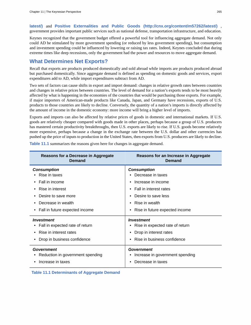
latest/) and Positive Externalities and Public Goods (http://cnx.org/content/m57262/latest/) ,government provides important public services such as national defense, transportation infrastructure, and education.
Keynes recognized that the government budget offered a powerful tool for influencing aggregate demand. Not onlycould AD be stimulated by more government spending (or reduced by less government spending), but consumptionand investment spending could be influenced by lowering or raising tax rates. Indeed, Keynes concluded that duringextreme times like deep recessions, only the government had the power and resources to move aggregate demand.
What Determines Net Exports?Recall that exports are products produced domestically and sold abroad while imports are products produced abroadbut purchased domestically. Since aggregate demand is defined as spending on domestic goods and services, exportexpenditures add to AD, while import expenditures subtract from AD.
Two sets of factors can cause shifts in export and import demand: changes in relative growth rates between countriesand changes in relative prices between countries. The level of demand for a nation’s exports tends to be most heavilyaffected by what is happening in the economies of the countries that would be purchasing those exports. For example,if major importers of American-made products like Canada, Japan, and Germany have recessions, exports of U.S.products to those countries are likely to decline. Conversely, the quantity of a nation’s imports is directly affected bythe amount of income in the domestic economy: more income will bring a higher level of imports.
Exports and imports can also be affected by relative prices of goods in domestic and international markets. If U.S.goods are relatively cheaper compared with goods made in other places, perhaps because a group of U.S. producershas mastered certain productivity breakthroughs, then U.S. exports are likely to rise. If U.S. goods become relativelymore expensive, perhaps because a change in the exchange rate between the U.S. dollar and other currencies haspushed up the price of inputs to production in the United States, then exports from U.S. producers are likely to decline.
Table 11.1 summarizes the reasons given here for changes in aggregate demand.
Reasons for a Decrease in AggregateDemand
Reasons for an Increase in AggregateDemand
Consumption• Rise in taxes
• Fall in income
• Rise in interest
• Desire to save more
• Decrease in wealth
• Fall in future expected income
Consumption• Decrease in taxes
• Increase in income
• Fall in interest rates
• Desire to save less
• Rise in wealth
• Rise in future expected income
Investment• Fall in expected rate of return
• Rise in interest rates
• Drop in business confidence
Investment• Rise in expected rate of return
• Drop in interest rates
• Rise in business confidence
Government• Reduction in government spending
• Increase in taxes
Government• Increase in government spending
• Decrease in taxes
Table 11.1 Determinants of Aggregate Demand
Chapter 11 | The Keynesian Perspective 265
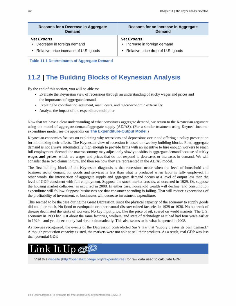
Reasons for a Decrease in AggregateDemand
Reasons for an Increase in AggregateDemand
Net Exports• Decrease in foreign demand
• Relative price increase of U.S. goods
Net Exports• Increase in foreign demand
• Relative price drop of U.S. goods
Table 11.1 Determinants of Aggregate Demand
11.2 | The Building Blocks of Keynesian AnalysisBy the end of this section, you will be able to:
• Evaluate the Keynesian view of recessions through an understanding of sticky wages and prices andthe importance of aggregate demand
• Explain the coordination argument, menu costs, and macroeconomic externality• Analyze the impact of the expenditure multiplier
Now that we have a clear understanding of what constitutes aggregate demand, we return to the Keynesian argumentusing the model of aggregate demand/aggregate supply (AD/AS). (For a similar treatment using Keynes’ income-expenditure model, see the appendix on The Expenditure-Output Model.)
Keynesian economics focuses on explaining why recessions and depressions occur and offering a policy prescriptionfor minimizing their effects. The Keynesian view of recession is based on two key building blocks. First, aggregatedemand is not always automatically high enough to provide firms with an incentive to hire enough workers to reachfull employment. Second, the macroeconomy may adjust only slowly to shifts in aggregate demand because of stickywages and prices, which are wages and prices that do not respond to decreases or increases in demand. We willconsider these two claims in turn, and then see how they are represented in the AD/AS model.
The first building block of the Keynesian diagnosis is that recessions occur when the level of household andbusiness sector demand for goods and services is less than what is produced when labor is fully employed. Inother words, the intersection of aggregate supply and aggregate demand occurs at a level of output less than thelevel of GDP consistent with full employment. Suppose the stock market crashes, as occurred in 1929. Or, supposethe housing market collapses, as occurred in 2008. In either case, household wealth will decline, and consumptionexpenditure will follow. Suppose businesses see that consumer spending is falling. That will reduce expectations ofthe profitability of investment, so businesses will decrease investment expenditure.
This seemed to be the case during the Great Depression, since the physical capacity of the economy to supply goodsdid not alter much. No flood or earthquake or other natural disaster ruined factories in 1929 or 1930. No outbreak ofdisease decimated the ranks of workers. No key input price, like the price of oil, soared on world markets. The U.S.economy in 1933 had just about the same factories, workers, and state of technology as it had had four years earlierin 1929—and yet the economy had shrunk dramatically. This also seems to be what happened in 2008.
As Keynes recognized, the events of the Depression contradicted Say’s law that “supply creates its own demand.”Although production capacity existed, the markets were not able to sell their products. As a result, real GDP was lessthan potential GDP.
Visit this website (http://openstaxcollege.org/l/expenditures) for raw data used to calculate GDP.
266 Chapter 11 | The Keynesian Perspective
This OpenStax book is available for free at http://cnx.org/content/col11864/1.2
Wage and Price StickinessKeynes also pointed out that although AD fluctuated, prices and wages did not immediately respond as economistsoften expected. Instead, prices and wages are “sticky,” making it difficult to restore the economy to full employmentand potential GDP. Keynes emphasized one particular reason why wages were sticky: the coordination argument.This argument points out that, even if most people would be willing—at least hypothetically—to see a decline intheir own wages in bad economic times as long as everyone else also experienced such a decline, a market-orientedeconomy has no obvious way to implement a plan of coordinated wage reductions. Unemployment proposed anumber of reasons why wages might be sticky downward, most of which center on the argument that businesses avoidwage cuts because they may in one way or another depress morale and hurt the productivity of the existing workers.
Some modern economists have argued in a Keynesian spirit that, along with wages, other prices may be sticky, too.Many firms do not change their prices every day or even every month. When a firm considers changing prices, it mustconsider two sets of costs. First, changing prices uses company resources: managers must analyze the competition andmarket demand and decide what the new prices will be, sales materials must be updated, billing records will change,and product labels and price labels must be redone. Second, frequent price changes may leave customers confused orangry—especially if they find out that a product now costs more than expected. These costs of changing prices arecalled menu costs—like the costs of printing up a new set of menus with different prices in a restaurant. Prices dorespond to forces of supply and demand, but from a macroeconomic perspective, the process of changing all pricesthroughout the economy takes time.
To understand the effect of sticky wages and prices in the economy, consider Figure 11.4 (a) illustrating the overalllabor market, while Figure 11.4 (b) illustrates a market for a specific good or service. The original equilibrium (E0)in each market occurs at the intersection of the demand curve (D0) and supply curve (S0). When aggregate demanddeclines, the demand for labor shifts to the left (to D1) in Figure 11.4 (a) and the demand for goods shifts to the left(to D1) in Figure 11.4 (b). However, because of sticky wages and prices, the wage remains at its original level (W0)for a period of time and the price remains at its original level (P0).
As a result, a situation of excess supply—where the quantity supplied exceeds the quantity demanded at the existingwage or price—exists in markets for both labor and goods, and Q1 is less than Q0 in both Figure 11.4 (a) and Figure11.4 (b). When many labor markets and many goods markets all across the economy find themselves in this position,the economy is in a recession; that is, firms cannot sell what they wish to produce at the existing market price anddo not wish to hire all who are willing to work at the existing market wage. The Clear It Up feature discusses thisproblem in more detail.
Chapter 11 | The Keynesian Perspective 267
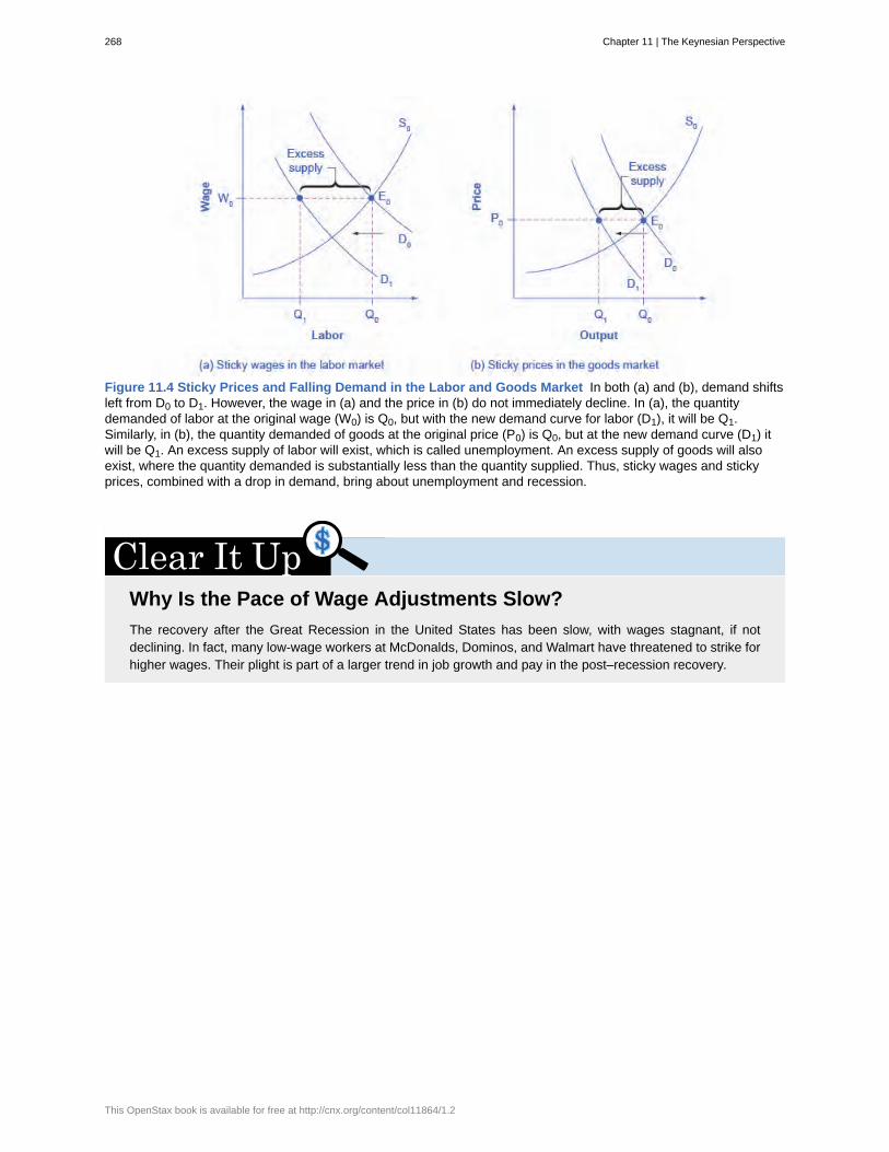
Figure 11.4 Sticky Prices and Falling Demand in the Labor and Goods Market In both (a) and (b), demand shiftsleft from D0 to D1. However, the wage in (a) and the price in (b) do not immediately decline. In (a), the quantitydemanded of labor at the original wage (W0) is Q0, but with the new demand curve for labor (D1), it will be Q1.Similarly, in (b), the quantity demanded of goods at the original price (P0) is Q0, but at the new demand curve (D1) itwill be Q1. An excess supply of labor will exist, which is called unemployment. An excess supply of goods will alsoexist, where the quantity demanded is substantially less than the quantity supplied. Thus, sticky wages and stickyprices, combined with a drop in demand, bring about unemployment and recession.
Why Is the Pace of Wage Adjustments Slow?The recovery after the Great Recession in the United States has been slow, with wages stagnant, if notdeclining. In fact, many low-wage workers at McDonalds, Dominos, and Walmart have threatened to strike forhigher wages. Their plight is part of a larger trend in job growth and pay in the post–recession recovery.
268 Chapter 11 | The Keynesian Perspective
This OpenStax book is available for free at http://cnx.org/content/col11864/1.2
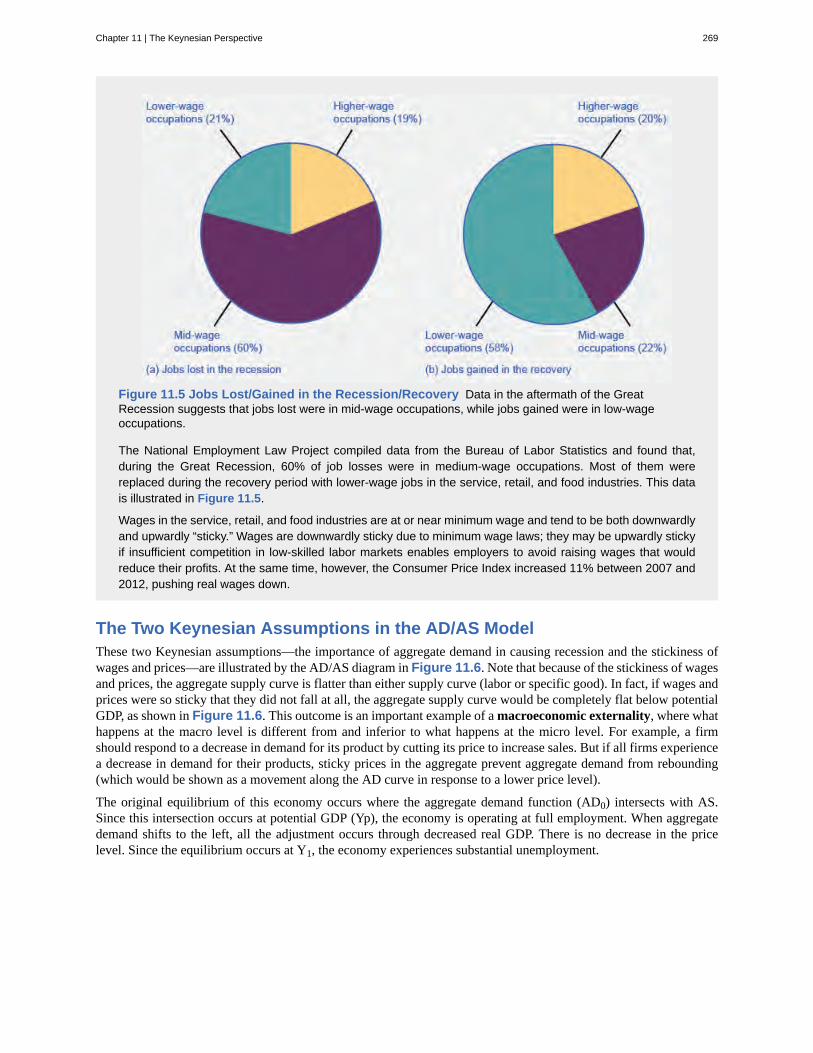
Figure 11.5 Jobs Lost/Gained in the Recession/Recovery Data in the aftermath of the GreatRecession suggests that jobs lost were in mid-wage occupations, while jobs gained were in low-wageoccupations.
The National Employment Law Project compiled data from the Bureau of Labor Statistics and found that,during the Great Recession, 60% of job losses were in medium-wage occupations. Most of them werereplaced during the recovery period with lower-wage jobs in the service, retail, and food industries. This datais illustrated in Figure 11.5.
Wages in the service, retail, and food industries are at or near minimum wage and tend to be both downwardlyand upwardly “sticky.” Wages are downwardly sticky due to minimum wage laws; they may be upwardly stickyif insufficient competition in low-skilled labor markets enables employers to avoid raising wages that wouldreduce their profits. At the same time, however, the Consumer Price Index increased 11% between 2007 and2012, pushing real wages down.
The Two Keynesian Assumptions in the AD/AS ModelThese two Keynesian assumptions—the importance of aggregate demand in causing recession and the stickiness ofwages and prices—are illustrated by the AD/AS diagram in Figure 11.6. Note that because of the stickiness of wagesand prices, the aggregate supply curve is flatter than either supply curve (labor or specific good). In fact, if wages andprices were so sticky that they did not fall at all, the aggregate supply curve would be completely flat below potentialGDP, as shown in Figure 11.6. This outcome is an important example of a macroeconomic externality, where whathappens at the macro level is different from and inferior to what happens at the micro level. For example, a firmshould respond to a decrease in demand for its product by cutting its price to increase sales. But if all firms experiencea decrease in demand for their products, sticky prices in the aggregate prevent aggregate demand from rebounding(which would be shown as a movement along the AD curve in response to a lower price level).
The original equilibrium of this economy occurs where the aggregate demand function (AD0) intersects with AS.Since this intersection occurs at potential GDP (Yp), the economy is operating at full employment. When aggregatedemand shifts to the left, all the adjustment occurs through decreased real GDP. There is no decrease in the pricelevel. Since the equilibrium occurs at Y1, the economy experiences substantial unemployment.
Chapter 11 | The Keynesian Perspective 269
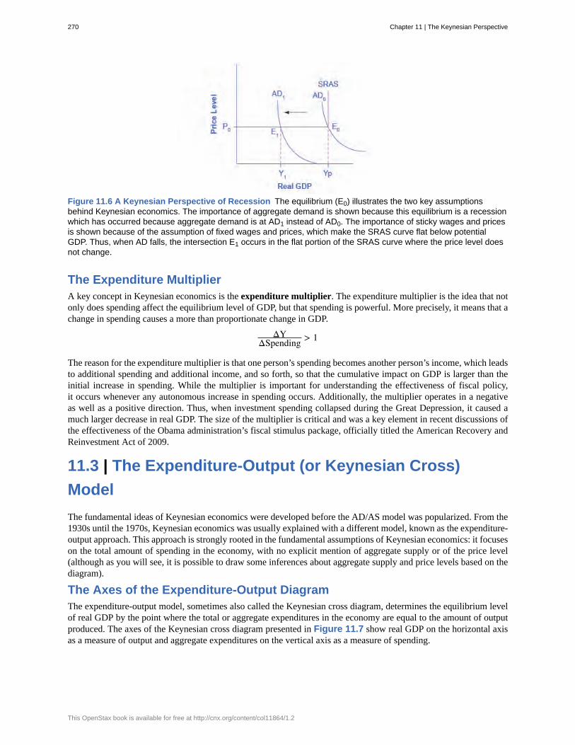
Figure 11.6 A Keynesian Perspective of Recession The equilibrium (E0) illustrates the two key assumptionsbehind Keynesian economics. The importance of aggregate demand is shown because this equilibrium is a recessionwhich has occurred because aggregate demand is at AD1 instead of AD0. The importance of sticky wages and pricesis shown because of the assumption of fixed wages and prices, which make the SRAS curve flat below potentialGDP. Thus, when AD falls, the intersection E1 occurs in the flat portion of the SRAS curve where the price level doesnot change.
The Expenditure MultiplierA key concept in Keynesian economics is the expenditure multiplier. The expenditure multiplier is the idea that notonly does spending affect the equilibrium level of GDP, but that spending is powerful. More precisely, it means that achange in spending causes a more than proportionate change in GDP.
ΔYΔSpending > 1
The reason for the expenditure multiplier is that one person’s spending becomes another person’s income, which leadsto additional spending and additional income, and so forth, so that the cumulative impact on GDP is larger than theinitial increase in spending. While the multiplier is important for understanding the effectiveness of fiscal policy,it occurs whenever any autonomous increase in spending occurs. Additionally, the multiplier operates in a negativeas well as a positive direction. Thus, when investment spending collapsed during the Great Depression, it caused amuch larger decrease in real GDP. The size of the multiplier is critical and was a key element in recent discussions ofthe effectiveness of the Obama administration’s fiscal stimulus package, officially titled the American Recovery andReinvestment Act of 2009.
11.3 | The Expenditure-Output (or Keynesian Cross)ModelThe fundamental ideas of Keynesian economics were developed before the AD/AS model was popularized. From the1930s until the 1970s, Keynesian economics was usually explained with a different model, known as the expenditure-output approach. This approach is strongly rooted in the fundamental assumptions of Keynesian economics: it focuseson the total amount of spending in the economy, with no explicit mention of aggregate supply or of the price level(although as you will see, it is possible to draw some inferences about aggregate supply and price levels based on thediagram).
The Axes of the Expenditure-Output DiagramThe expenditure-output model, sometimes also called the Keynesian cross diagram, determines the equilibrium levelof real GDP by the point where the total or aggregate expenditures in the economy are equal to the amount of outputproduced. The axes of the Keynesian cross diagram presented in Figure 11.7 show real GDP on the horizontal axisas a measure of output and aggregate expenditures on the vertical axis as a measure of spending.
270 Chapter 11 | The Keynesian Perspective
This OpenStax book is available for free at http://cnx.org/content/col11864/1.2
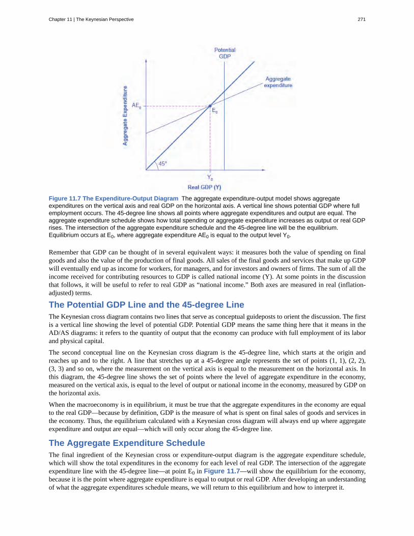
Figure 11.7 The Expenditure-Output Diagram The aggregate expenditure-output model shows aggregateexpenditures on the vertical axis and real GDP on the horizontal axis. A vertical line shows potential GDP where fullemployment occurs. The 45-degree line shows all points where aggregate expenditures and output are equal. Theaggregate expenditure schedule shows how total spending or aggregate expenditure increases as output or real GDPrises. The intersection of the aggregate expenditure schedule and the 45-degree line will be the equilibrium.Equilibrium occurs at E0, where aggregate expenditure AE0 is equal to the output level Y0.
Remember that GDP can be thought of in several equivalent ways: it measures both the value of spending on finalgoods and also the value of the production of final goods. All sales of the final goods and services that make up GDPwill eventually end up as income for workers, for managers, and for investors and owners of firms. The sum of all theincome received for contributing resources to GDP is called national income (Y). At some points in the discussionthat follows, it will be useful to refer to real GDP as “national income.” Both axes are measured in real (inflation-adjusted) terms.
The Potential GDP Line and the 45-degree LineThe Keynesian cross diagram contains two lines that serve as conceptual guideposts to orient the discussion. The firstis a vertical line showing the level of potential GDP. Potential GDP means the same thing here that it means in theAD/AS diagrams: it refers to the quantity of output that the economy can produce with full employment of its laborand physical capital.
The second conceptual line on the Keynesian cross diagram is the 45-degree line, which starts at the origin andreaches up and to the right. A line that stretches up at a 45-degree angle represents the set of points (1, 1), (2, 2),(3, 3) and so on, where the measurement on the vertical axis is equal to the measurement on the horizontal axis. Inthis diagram, the 45-degree line shows the set of points where the level of aggregate expenditure in the economy,measured on the vertical axis, is equal to the level of output or national income in the economy, measured by GDP onthe horizontal axis.
When the macroeconomy is in equilibrium, it must be true that the aggregate expenditures in the economy are equalto the real GDP—because by definition, GDP is the measure of what is spent on final sales of goods and services inthe economy. Thus, the equilibrium calculated with a Keynesian cross diagram will always end up where aggregateexpenditure and output are equal—which will only occur along the 45-degree line.
The Aggregate Expenditure ScheduleThe final ingredient of the Keynesian cross or expenditure-output diagram is the aggregate expenditure schedule,which will show the total expenditures in the economy for each level of real GDP. The intersection of the aggregateexpenditure line with the 45-degree line—at point E0 in Figure 11.7—will show the equilibrium for the economy,because it is the point where aggregate expenditure is equal to output or real GDP. After developing an understandingof what the aggregate expenditures schedule means, we will return to this equilibrium and how to interpret it.
Chapter 11 | The Keynesian Perspective 271
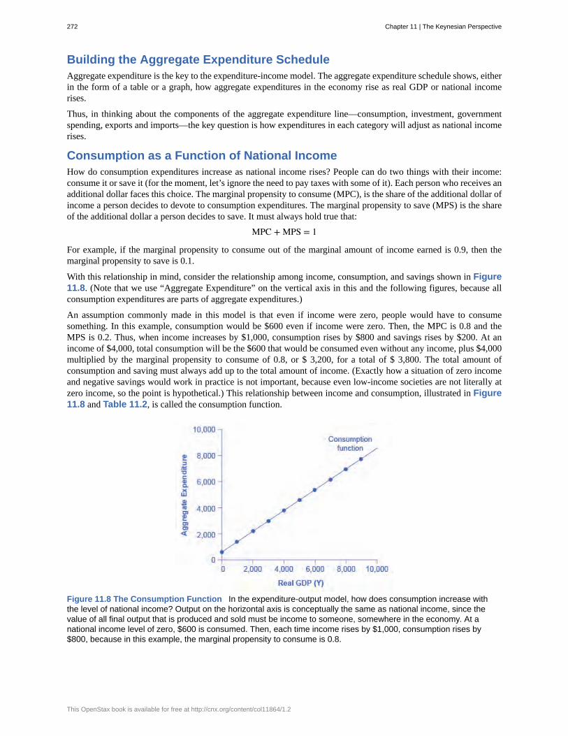
Building the Aggregate Expenditure ScheduleAggregate expenditure is the key to the expenditure-income model. The aggregate expenditure schedule shows, eitherin the form of a table or a graph, how aggregate expenditures in the economy rise as real GDP or national incomerises.
Thus, in thinking about the components of the aggregate expenditure line—consumption, investment, governmentspending, exports and imports—the key question is how expenditures in each category will adjust as national incomerises.
Consumption as a Function of National IncomeHow do consumption expenditures increase as national income rises? People can do two things with their income:consume it or save it (for the moment, let’s ignore the need to pay taxes with some of it). Each person who receives anadditional dollar faces this choice. The marginal propensity to consume (MPC), is the share of the additional dollar ofincome a person decides to devote to consumption expenditures. The marginal propensity to save (MPS) is the shareof the additional dollar a person decides to save. It must always hold true that:
MPC + MPS = 1
For example, if the marginal propensity to consume out of the marginal amount of income earned is 0.9, then themarginal propensity to save is 0.1.
With this relationship in mind, consider the relationship among income, consumption, and savings shown in Figure11.8. (Note that we use “Aggregate Expenditure” on the vertical axis in this and the following figures, because allconsumption expenditures are parts of aggregate expenditures.)
An assumption commonly made in this model is that even if income were zero, people would have to consumesomething. In this example, consumption would be $600 even if income were zero. Then, the MPC is 0.8 and theMPS is 0.2. Thus, when income increases by $1,000, consumption rises by $800 and savings rises by $200. At anincome of $4,000, total consumption will be the $600 that would be consumed even without any income, plus $4,000multiplied by the marginal propensity to consume of 0.8, or $ 3,200, for a total of $ 3,800. The total amount ofconsumption and saving must always add up to the total amount of income. (Exactly how a situation of zero incomeand negative savings would work in practice is not important, because even low-income societies are not literally atzero income, so the point is hypothetical.) This relationship between income and consumption, illustrated in Figure11.8 and Table 11.2, is called the consumption function.
Figure 11.8 The Consumption Function In the expenditure-output model, how does consumption increase withthe level of national income? Output on the horizontal axis is conceptually the same as national income, since thevalue of all final output that is produced and sold must be income to someone, somewhere in the economy. At anational income level of zero, $600 is consumed. Then, each time income rises by $1,000, consumption rises by$800, because in this example, the marginal propensity to consume is 0.8.
272 Chapter 11 | The Keynesian Perspective
This OpenStax book is available for free at http://cnx.org/content/col11864/1.2
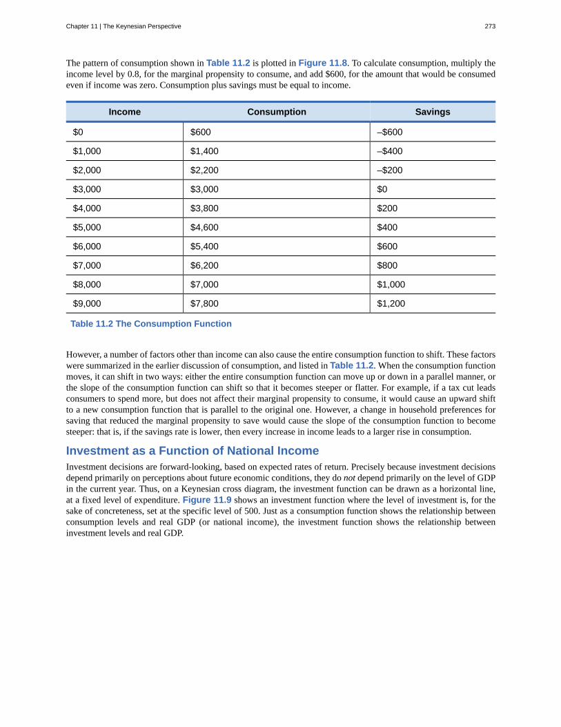
The pattern of consumption shown in Table 11.2 is plotted in Figure 11.8. To calculate consumption, multiply theincome level by 0.8, for the marginal propensity to consume, and add $600, for the amount that would be consumedeven if income was zero. Consumption plus savings must be equal to income.
Income Consumption Savings
$0 $600 –$600
$1,000 $1,400 –$400
$2,000 $2,200 –$200
$3,000 $3,000 $0
$4,000 $3,800 $200
$5,000 $4,600 $400
$6,000 $5,400 $600
$7,000 $6,200 $800
$8,000 $7,000 $1,000
$9,000 $7,800 $1,200
Table 11.2 The Consumption Function
However, a number of factors other than income can also cause the entire consumption function to shift. These factorswere summarized in the earlier discussion of consumption, and listed in Table 11.2. When the consumption functionmoves, it can shift in two ways: either the entire consumption function can move up or down in a parallel manner, orthe slope of the consumption function can shift so that it becomes steeper or flatter. For example, if a tax cut leadsconsumers to spend more, but does not affect their marginal propensity to consume, it would cause an upward shiftto a new consumption function that is parallel to the original one. However, a change in household preferences forsaving that reduced the marginal propensity to save would cause the slope of the consumption function to becomesteeper: that is, if the savings rate is lower, then every increase in income leads to a larger rise in consumption.
Investment as a Function of National IncomeInvestment decisions are forward-looking, based on expected rates of return. Precisely because investment decisionsdepend primarily on perceptions about future economic conditions, they do not depend primarily on the level of GDPin the current year. Thus, on a Keynesian cross diagram, the investment function can be drawn as a horizontal line,at a fixed level of expenditure. Figure 11.9 shows an investment function where the level of investment is, for thesake of concreteness, set at the specific level of 500. Just as a consumption function shows the relationship betweenconsumption levels and real GDP (or national income), the investment function shows the relationship betweeninvestment levels and real GDP.
Chapter 11 | The Keynesian Perspective 273
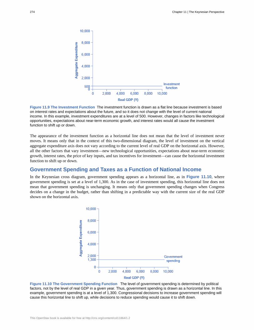
Figure 11.9 The Investment Function The investment function is drawn as a flat line because investment is basedon interest rates and expectations about the future, and so it does not change with the level of current nationalincome. In this example, investment expenditures are at a level of 500. However, changes in factors like technologicalopportunities, expectations about near-term economic growth, and interest rates would all cause the investmentfunction to shift up or down.
The appearance of the investment function as a horizontal line does not mean that the level of investment nevermoves. It means only that in the context of this two-dimensional diagram, the level of investment on the verticalaggregate expenditure axis does not vary according to the current level of real GDP on the horizontal axis. However,all the other factors that vary investment—new technological opportunities, expectations about near-term economicgrowth, interest rates, the price of key inputs, and tax incentives for investment—can cause the horizontal investmentfunction to shift up or down.
Government Spending and Taxes as a Function of National IncomeIn the Keynesian cross diagram, government spending appears as a horizontal line, as in Figure 11.10, wheregovernment spending is set at a level of 1,300. As in the case of investment spending, this horizontal line does notmean that government spending is unchanging. It means only that government spending changes when Congressdecides on a change in the budget, rather than shifting in a predictable way with the current size of the real GDPshown on the horizontal axis.
Figure 11.10 The Government Spending Function The level of government spending is determined by politicalfactors, not by the level of real GDP in a given year. Thus, government spending is drawn as a horizontal line. In thisexample, government spending is at a level of 1,300. Congressional decisions to increase government spending willcause this horizontal line to shift up, while decisions to reduce spending would cause it to shift down.
274 Chapter 11 | The Keynesian Perspective
This OpenStax book is available for free at http://cnx.org/content/col11864/1.2
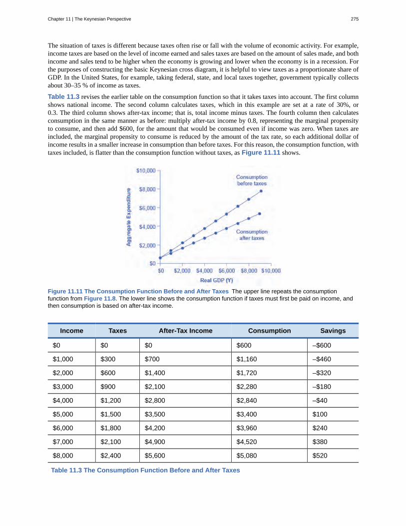
The situation of taxes is different because taxes often rise or fall with the volume of economic activity. For example,income taxes are based on the level of income earned and sales taxes are based on the amount of sales made, and bothincome and sales tend to be higher when the economy is growing and lower when the economy is in a recession. Forthe purposes of constructing the basic Keynesian cross diagram, it is helpful to view taxes as a proportionate share ofGDP. In the United States, for example, taking federal, state, and local taxes together, government typically collectsabout 30–35 % of income as taxes.
Table 11.3 revises the earlier table on the consumption function so that it takes taxes into account. The first columnshows national income. The second column calculates taxes, which in this example are set at a rate of 30%, or0.3. The third column shows after-tax income; that is, total income minus taxes. The fourth column then calculatesconsumption in the same manner as before: multiply after-tax income by 0.8, representing the marginal propensityto consume, and then add $600, for the amount that would be consumed even if income was zero. When taxes areincluded, the marginal propensity to consume is reduced by the amount of the tax rate, so each additional dollar ofincome results in a smaller increase in consumption than before taxes. For this reason, the consumption function, withtaxes included, is flatter than the consumption function without taxes, as Figure 11.11 shows.
Figure 11.11 The Consumption Function Before and After Taxes The upper line repeats the consumptionfunction from Figure 11.8. The lower line shows the consumption function if taxes must first be paid on income, andthen consumption is based on after-tax income.
Income Taxes After-Tax Income Consumption Savings
$0 $0 $0 $600 –$600
$1,000 $300 $700 $1,160 –$460
$2,000 $600 $1,400 $1,720 –$320
$3,000 $900 $2,100 $2,280 –$180
$4,000 $1,200 $2,800 $2,840 –$40
$5,000 $1,500 $3,500 $3,400 $100
$6,000 $1,800 $4,200 $3,960 $240
$7,000 $2,100 $4,900 $4,520 $380
$8,000 $2,400 $5,600 $5,080 $520
Table 11.3 The Consumption Function Before and After Taxes
Chapter 11 | The Keynesian Perspective 275
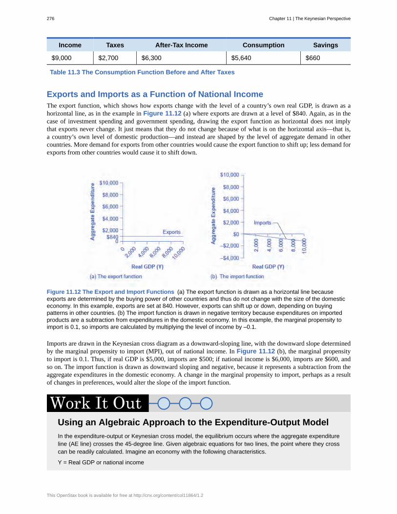
Income Taxes After-Tax Income Consumption Savings
$9,000 $2,700 $6,300 $5,640 $660
Table 11.3 The Consumption Function Before and After Taxes
Exports and Imports as a Function of National IncomeThe export function, which shows how exports change with the level of a country’s own real GDP, is drawn as ahorizontal line, as in the example in Figure 11.12 (a) where exports are drawn at a level of $840. Again, as in thecase of investment spending and government spending, drawing the export function as horizontal does not implythat exports never change. It just means that they do not change because of what is on the horizontal axis—that is,a country’s own level of domestic production—and instead are shaped by the level of aggregate demand in othercountries. More demand for exports from other countries would cause the export function to shift up; less demand forexports from other countries would cause it to shift down.
Figure 11.12 The Export and Import Functions (a) The export function is drawn as a horizontal line becauseexports are determined by the buying power of other countries and thus do not change with the size of the domesticeconomy. In this example, exports are set at 840. However, exports can shift up or down, depending on buyingpatterns in other countries. (b) The import function is drawn in negative territory because expenditures on importedproducts are a subtraction from expenditures in the domestic economy. In this example, the marginal propensity toimport is 0.1, so imports are calculated by multiplying the level of income by –0.1.
Imports are drawn in the Keynesian cross diagram as a downward-sloping line, with the downward slope determinedby the marginal propensity to import (MPI), out of national income. In Figure 11.12 (b), the marginal propensityto import is 0.1. Thus, if real GDP is $5,000, imports are $500; if national income is $6,000, imports are $600, andso on. The import function is drawn as downward sloping and negative, because it represents a subtraction from theaggregate expenditures in the domestic economy. A change in the marginal propensity to import, perhaps as a resultof changes in preferences, would alter the slope of the import function.
Using an Algebraic Approach to the Expenditure-Output ModelIn the expenditure-output or Keynesian cross model, the equilibrium occurs where the aggregate expenditureline (AE line) crosses the 45-degree line. Given algebraic equations for two lines, the point where they crosscan be readily calculated. Imagine an economy with the following characteristics.
Y = Real GDP or national income
276 Chapter 11 | The Keynesian Perspective
This OpenStax book is available for free at http://cnx.org/content/col11864/1.2
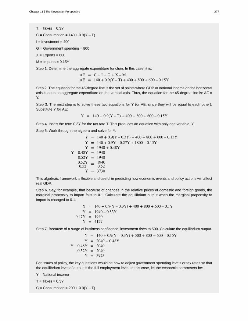
T = Taxes = 0.3Y
C = Consumption = 140 + 0.9(Y – T)
I = Investment = 400
G = Government spending = 800
X = Exports = 600
M = Imports = 0.15Y
Step 1. Determine the aggregate expenditure function. In this case, it is:
AE = C + I + G + X – MAE = 140 + 0.9(Y – T) + 400 + 800 + 600 – 0.15Y
Step 2. The equation for the 45-degree line is the set of points where GDP or national income on the horizontalaxis is equal to aggregate expenditure on the vertical axis. Thus, the equation for the 45-degree line is: AE =Y.
Step 3. The next step is to solve these two equations for Y (or AE, since they will be equal to each other).Substitute Y for AE:
Y = 140 + 0.9(Y – T) + 400 + 800 + 600 – 0.15Y
Step 4. Insert the term 0.3Y for the tax rate T. This produces an equation with only one variable, Y.
Step 5. Work through the algebra and solve for Y.
Y = 140 + 0.9(Y – 0.3Y) + 400 + 800 + 600 – 0.15YY = 140 + 0.9Y – 0.27Y + 1800 – 0.15YY = 1940 + 0.48Y
Y – 0.48Y = 19400.52Y = 19400.52Y0.52 = 1940
0.52Y = 3730
This algebraic framework is flexible and useful in predicting how economic events and policy actions will affectreal GDP.
Step 6. Say, for example, that because of changes in the relative prices of domestic and foreign goods, themarginal propensity to import falls to 0.1. Calculate the equilibrium output when the marginal propensity toimport is changed to 0.1.
Y = 140 + 0.9(Y – 0.3Y) + 400 + 800 + 600 – 0.1YY = 1940 – 0.53Y
0.47Y = 1940Y = 4127
Step 7. Because of a surge of business confidence, investment rises to 500. Calculate the equilibrium output.
Y = 140 + 0.9(Y – 0.3Y) + 500 + 800 + 600 – 0.15Y Y = 2040 + 0.48Y
Y – 0.48Y = 20400.52Y = 2040
Y = 3923
For issues of policy, the key questions would be how to adjust government spending levels or tax rates so thatthe equilibrium level of output is the full employment level. In this case, let the economic parameters be:
Y = National income
T = Taxes = 0.3Y
C = Consumption = 200 + 0.9(Y – T)
Chapter 11 | The Keynesian Perspective 277
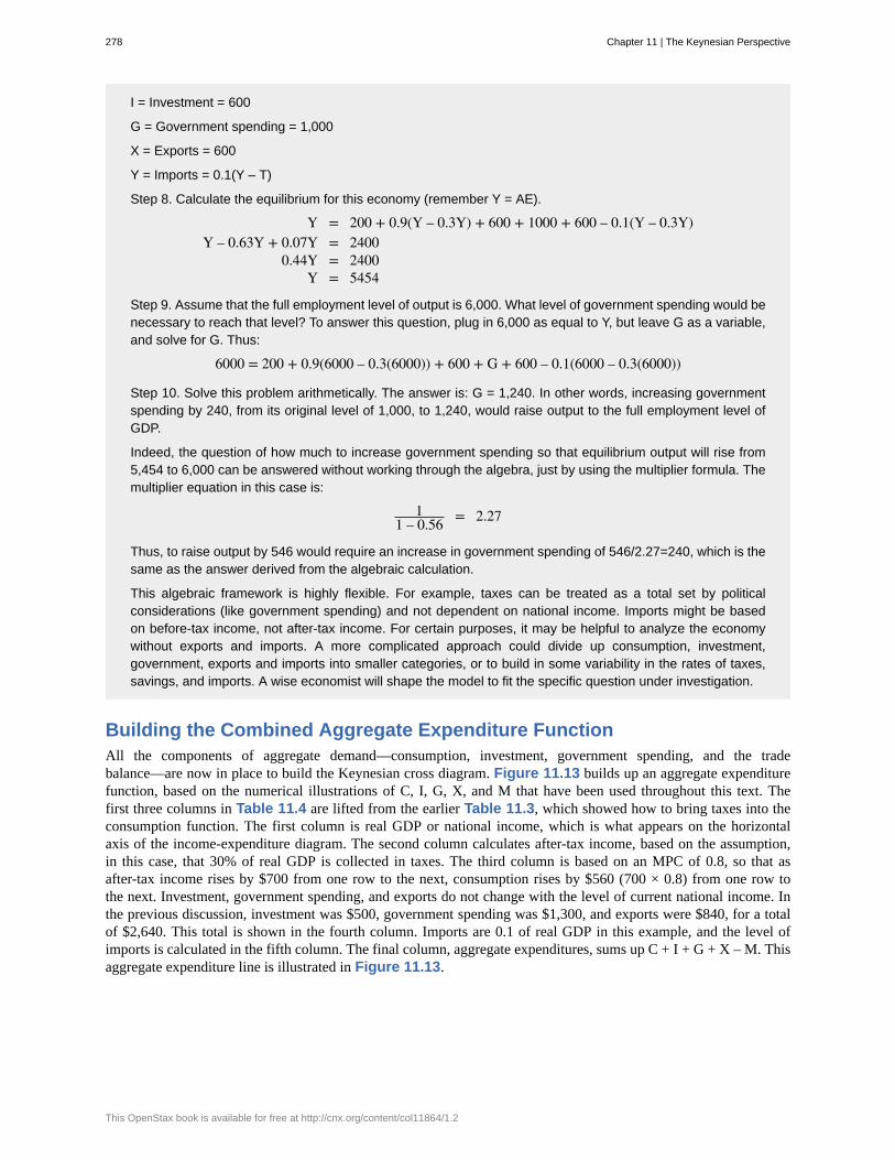
I = Investment = 600
G = Government spending = 1,000
X = Exports = 600
Y = Imports = 0.1(Y – T)
Step 8. Calculate the equilibrium for this economy (remember Y = AE).
Y = 200 + 0.9(Y – 0.3Y) + 600 + 1000 + 600 – 0.1(Y – 0.3Y)Y – 0.63Y + 0.07Y = 2400
0.44Y = 2400Y = 5454
Step 9. Assume that the full employment level of output is 6,000. What level of government spending would benecessary to reach that level? To answer this question, plug in 6,000 as equal to Y, but leave G as a variable,and solve for G. Thus:
6000 = 200 + 0.9(6000 – 0.3(6000)) + 600 + G + 600 – 0.1(6000 – 0.3(6000))
Step 10. Solve this problem arithmetically. The answer is: G = 1,240. In other words, increasing governmentspending by 240, from its original level of 1,000, to 1,240, would raise output to the full employment level ofGDP.
Indeed, the question of how much to increase government spending so that equilibrium output will rise from5,454 to 6,000 can be answered without working through the algebra, just by using the multiplier formula. Themultiplier equation in this case is:
11 – 0.56 = 2.27
Thus, to raise output by 546 would require an increase in government spending of 546/2.27=240, which is thesame as the answer derived from the algebraic calculation.
This algebraic framework is highly flexible. For example, taxes can be treated as a total set by politicalconsiderations (like government spending) and not dependent on national income. Imports might be basedon before-tax income, not after-tax income. For certain purposes, it may be helpful to analyze the economywithout exports and imports. A more complicated approach could divide up consumption, investment,government, exports and imports into smaller categories, or to build in some variability in the rates of taxes,savings, and imports. A wise economist will shape the model to fit the specific question under investigation.
Building the Combined Aggregate Expenditure FunctionAll the components of aggregate demand—consumption, investment, government spending, and the tradebalance—are now in place to build the Keynesian cross diagram. Figure 11.13 builds up an aggregate expenditurefunction, based on the numerical illustrations of C, I, G, X, and M that have been used throughout this text. Thefirst three columns in Table 11.4 are lifted from the earlier Table 11.3, which showed how to bring taxes into theconsumption function. The first column is real GDP or national income, which is what appears on the horizontalaxis of the income-expenditure diagram. The second column calculates after-tax income, based on the assumption,in this case, that 30% of real GDP is collected in taxes. The third column is based on an MPC of 0.8, so that asafter-tax income rises by $700 from one row to the next, consumption rises by $560 (700 × 0.8) from one row tothe next. Investment, government spending, and exports do not change with the level of current national income. Inthe previous discussion, investment was $500, government spending was $1,300, and exports were $840, for a totalof $2,640. This total is shown in the fourth column. Imports are 0.1 of real GDP in this example, and the level ofimports is calculated in the fifth column. The final column, aggregate expenditures, sums up C + I + G + X – M. Thisaggregate expenditure line is illustrated in Figure 11.13.
278 Chapter 11 | The Keynesian Perspective
This OpenStax book is available for free at http://cnx.org/content/col11864/1.2
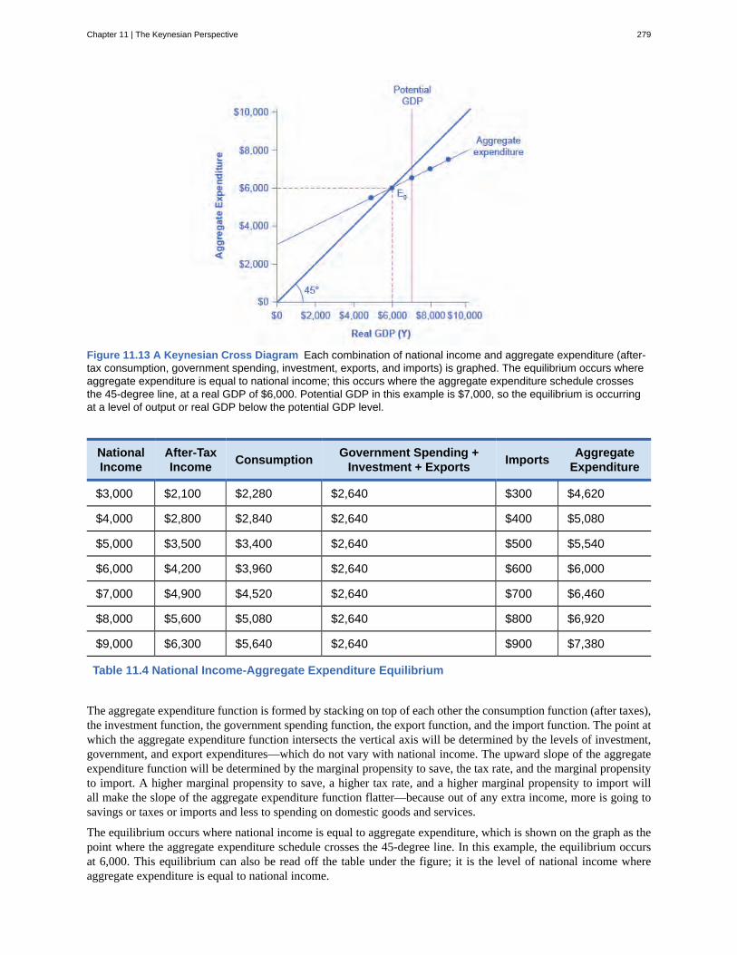
Figure 11.13 A Keynesian Cross Diagram Each combination of national income and aggregate expenditure (after-tax consumption, government spending, investment, exports, and imports) is graphed. The equilibrium occurs whereaggregate expenditure is equal to national income; this occurs where the aggregate expenditure schedule crossesthe 45-degree line, at a real GDP of $6,000. Potential GDP in this example is $7,000, so the equilibrium is occurringat a level of output or real GDP below the potential GDP level.
NationalIncome
After-TaxIncome Consumption Government Spending +
Investment + Exports Imports AggregateExpenditure
$3,000 $2,100 $2,280 $2,640 $300 $4,620
$4,000 $2,800 $2,840 $2,640 $400 $5,080
$5,000 $3,500 $3,400 $2,640 $500 $5,540
$6,000 $4,200 $3,960 $2,640 $600 $6,000
$7,000 $4,900 $4,520 $2,640 $700 $6,460
$8,000 $5,600 $5,080 $2,640 $800 $6,920
$9,000 $6,300 $5,640 $2,640 $900 $7,380
Table 11.4 National Income-Aggregate Expenditure Equilibrium
The aggregate expenditure function is formed by stacking on top of each other the consumption function (after taxes),the investment function, the government spending function, the export function, and the import function. The point atwhich the aggregate expenditure function intersects the vertical axis will be determined by the levels of investment,government, and export expenditures—which do not vary with national income. The upward slope of the aggregateexpenditure function will be determined by the marginal propensity to save, the tax rate, and the marginal propensityto import. A higher marginal propensity to save, a higher tax rate, and a higher marginal propensity to import willall make the slope of the aggregate expenditure function flatter—because out of any extra income, more is going tosavings or taxes or imports and less to spending on domestic goods and services.
The equilibrium occurs where national income is equal to aggregate expenditure, which is shown on the graph as thepoint where the aggregate expenditure schedule crosses the 45-degree line. In this example, the equilibrium occursat 6,000. This equilibrium can also be read off the table under the figure; it is the level of national income whereaggregate expenditure is equal to national income.
Chapter 11 | The Keynesian Perspective 279
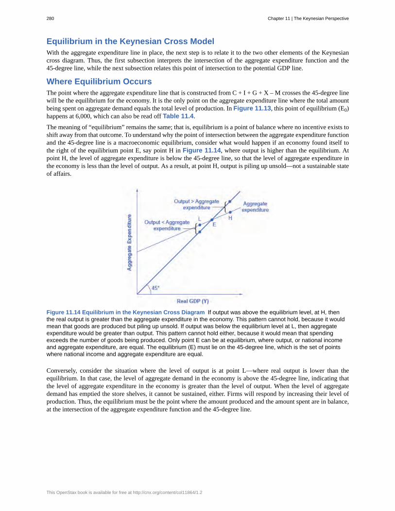
Equilibrium in the Keynesian Cross ModelWith the aggregate expenditure line in place, the next step is to relate it to the two other elements of the Keynesiancross diagram. Thus, the first subsection interprets the intersection of the aggregate expenditure function and the45-degree line, while the next subsection relates this point of intersection to the potential GDP line.
Where Equilibrium OccursThe point where the aggregate expenditure line that is constructed from C + I + G + X – M crosses the 45-degree linewill be the equilibrium for the economy. It is the only point on the aggregate expenditure line where the total amountbeing spent on aggregate demand equals the total level of production. In Figure 11.13, this point of equilibrium (E0)happens at 6,000, which can also be read off Table 11.4.
The meaning of “equilibrium” remains the same; that is, equilibrium is a point of balance where no incentive exists toshift away from that outcome. To understand why the point of intersection between the aggregate expenditure functionand the 45-degree line is a macroeconomic equilibrium, consider what would happen if an economy found itself tothe right of the equilibrium point E, say point H in Figure 11.14, where output is higher than the equilibrium. Atpoint H, the level of aggregate expenditure is below the 45-degree line, so that the level of aggregate expenditure inthe economy is less than the level of output. As a result, at point H, output is piling up unsold—not a sustainable stateof affairs.
Figure 11.14 Equilibrium in the Keynesian Cross Diagram If output was above the equilibrium level, at H, thenthe real output is greater than the aggregate expenditure in the economy. This pattern cannot hold, because it wouldmean that goods are produced but piling up unsold. If output was below the equilibrium level at L, then aggregateexpenditure would be greater than output. This pattern cannot hold either, because it would mean that spendingexceeds the number of goods being produced. Only point E can be at equilibrium, where output, or national incomeand aggregate expenditure, are equal. The equilibrium (E) must lie on the 45-degree line, which is the set of pointswhere national income and aggregate expenditure are equal.
Conversely, consider the situation where the level of output is at point L—where real output is lower than theequilibrium. In that case, the level of aggregate demand in the economy is above the 45-degree line, indicating thatthe level of aggregate expenditure in the economy is greater than the level of output. When the level of aggregatedemand has emptied the store shelves, it cannot be sustained, either. Firms will respond by increasing their level ofproduction. Thus, the equilibrium must be the point where the amount produced and the amount spent are in balance,at the intersection of the aggregate expenditure function and the 45-degree line.
280 Chapter 11 | The Keynesian Perspective
This OpenStax book is available for free at http://cnx.org/content/col11864/1.2
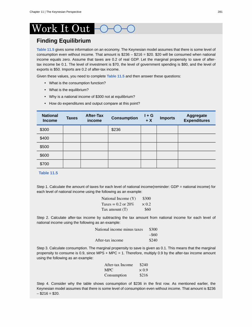
Finding EquilibriumTable 11.5 gives some information on an economy. The Keynesian model assumes that there is some level ofconsumption even without income. That amount is $236 – $216 = $20. $20 will be consumed when nationalincome equals zero. Assume that taxes are 0.2 of real GDP. Let the marginal propensity to save of after-tax income be 0.1. The level of investment is $70, the level of government spending is $80, and the level ofexports is $50. Imports are 0.2 of after-tax income.
Given these values, you need to complete Table 11.5 and then answer these questions:
• What is the consumption function?
• What is the equilibrium?
• Why is a national income of $300 not at equilibrium?
• How do expenditures and output compare at this point?
NationalIncome Taxes After-Tax
income Consumption I + G+ X Imports Aggregate
Expenditures
$300 $236
$400
$500
$600
$700
Table 11.5
Step 1. Calculate the amount of taxes for each level of national income(reminder: GDP = national income) foreach level of national income using the following as an example:
National Income (Y) $300Taxes = 0.2 or 20% × 0.2Tax amount (T) $60
Step 2. Calculate after-tax income by subtracting the tax amount from national income for each level ofnational income using the following as an example:
National income minus taxes $300–$60
After-tax income $240
Step 3. Calculate consumption. The marginal propensity to save is given as 0.1. This means that the marginalpropensity to consume is 0.9, since MPS + MPC = 1. Therefore, multiply 0.9 by the after-tax income amountusing the following as an example:
After-tax Income $240MPC × 0.9Consumption $216
Step 4. Consider why the table shows consumption of $236 in the first row. As mentioned earlier, theKeynesian model assumes that there is some level of consumption even without income. That amount is $236– $216 = $20.
Chapter 11 | The Keynesian Perspective 281
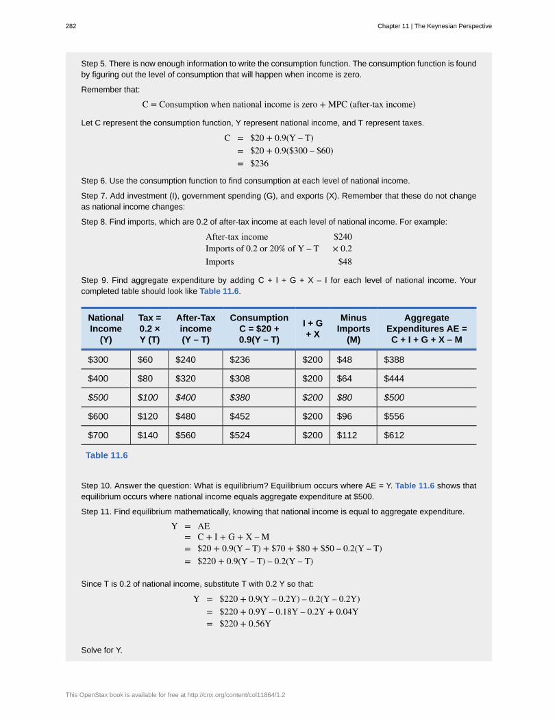
Step 5. There is now enough information to write the consumption function. The consumption function is foundby figuring out the level of consumption that will happen when income is zero.
Remember that:
C = Consumption when national income is zero + MPC (after-tax income)
Let C represent the consumption function, Y represent national income, and T represent taxes.
C = $20 + 0.9(Y – T) = $20 + 0.9($300 – $60) = $236
Step 6. Use the consumption function to find consumption at each level of national income.
Step 7. Add investment (I), government spending (G), and exports (X). Remember that these do not changeas national income changes:
Step 8. Find imports, which are 0.2 of after-tax income at each level of national income. For example:
After-tax income $240Imports of 0.2 or 20% of Y – T × 0.2Imports $48
Step 9. Find aggregate expenditure by adding C + I + G + X – I for each level of national income. Yourcompleted table should look like Table 11.6.
NationalIncome
(Y)
Tax =0.2 ×Y (T)
After-Taxincome(Y – T)
ConsumptionC = $20 +0.9(Y – T)
I + G+ X
MinusImports
(M)
AggregateExpenditures AE =C + I + G + X – M
$300 $60 $240 $236 $200 $48 $388
$400 $80 $320 $308 $200 $64 $444
$500 $100 $400 $380 $200 $80 $500
$600 $120 $480 $452 $200 $96 $556
$700 $140 $560 $524 $200 $112 $612
Table 11.6
Step 10. Answer the question: What is equilibrium? Equilibrium occurs where AE = Y. Table 11.6 shows thatequilibrium occurs where national income equals aggregate expenditure at $500.
Step 11. Find equilibrium mathematically, knowing that national income is equal to aggregate expenditure.
Y = AE = C + I + G + X – M = $20 + 0.9(Y – T) + $70 + $80 + $50 – 0.2(Y – T) = $220 + 0.9(Y – T) – 0.2(Y – T)
Since T is 0.2 of national income, substitute T with 0.2 Y so that:
Y = $220 + 0.9(Y – 0.2Y) – 0.2(Y – 0.2Y) = $220 + 0.9Y – 0.18Y – 0.2Y + 0.04Y = $220 + 0.56Y
Solve for Y.
282 Chapter 11 | The Keynesian Perspective
This OpenStax book is available for free at http://cnx.org/content/col11864/1.2
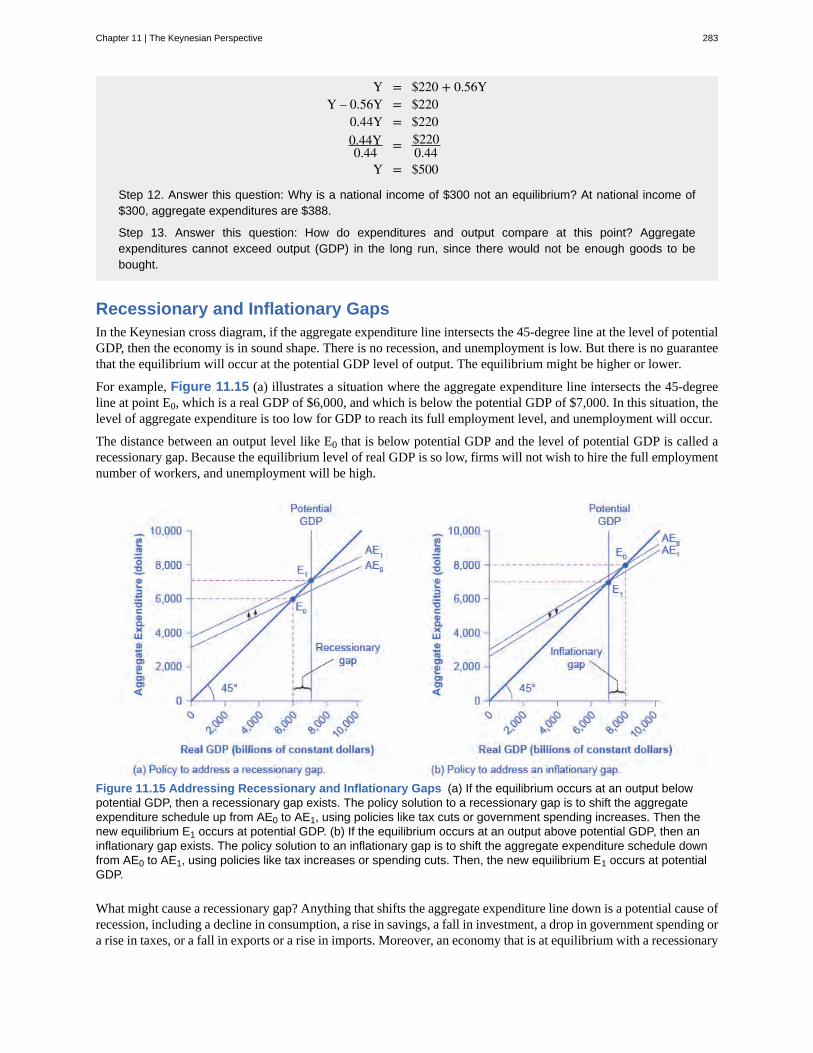
Y = $220 + 0.56YY – 0.56Y = $220
0.44Y = $2200.44Y0.44 = $220
0.44Y = $500
Step 12. Answer this question: Why is a national income of $300 not an equilibrium? At national income of$300, aggregate expenditures are $388.
Step 13. Answer this question: How do expenditures and output compare at this point? Aggregateexpenditures cannot exceed output (GDP) in the long run, since there would not be enough goods to bebought.
Recessionary and Inflationary GapsIn the Keynesian cross diagram, if the aggregate expenditure line intersects the 45-degree line at the level of potentialGDP, then the economy is in sound shape. There is no recession, and unemployment is low. But there is no guaranteethat the equilibrium will occur at the potential GDP level of output. The equilibrium might be higher or lower.
For example, Figure 11.15 (a) illustrates a situation where the aggregate expenditure line intersects the 45-degreeline at point E0, which is a real GDP of $6,000, and which is below the potential GDP of $7,000. In this situation, thelevel of aggregate expenditure is too low for GDP to reach its full employment level, and unemployment will occur.
The distance between an output level like E0 that is below potential GDP and the level of potential GDP is called arecessionary gap. Because the equilibrium level of real GDP is so low, firms will not wish to hire the full employmentnumber of workers, and unemployment will be high.
Figure 11.15 Addressing Recessionary and Inflationary Gaps (a) If the equilibrium occurs at an output belowpotential GDP, then a recessionary gap exists. The policy solution to a recessionary gap is to shift the aggregateexpenditure schedule up from AE0 to AE1, using policies like tax cuts or government spending increases. Then thenew equilibrium E1 occurs at potential GDP. (b) If the equilibrium occurs at an output above potential GDP, then aninflationary gap exists. The policy solution to an inflationary gap is to shift the aggregate expenditure schedule downfrom AE0 to AE1, using policies like tax increases or spending cuts. Then, the new equilibrium E1 occurs at potentialGDP.
What might cause a recessionary gap? Anything that shifts the aggregate expenditure line down is a potential cause ofrecession, including a decline in consumption, a rise in savings, a fall in investment, a drop in government spending ora rise in taxes, or a fall in exports or a rise in imports. Moreover, an economy that is at equilibrium with a recessionary
Chapter 11 | The Keynesian Perspective 283
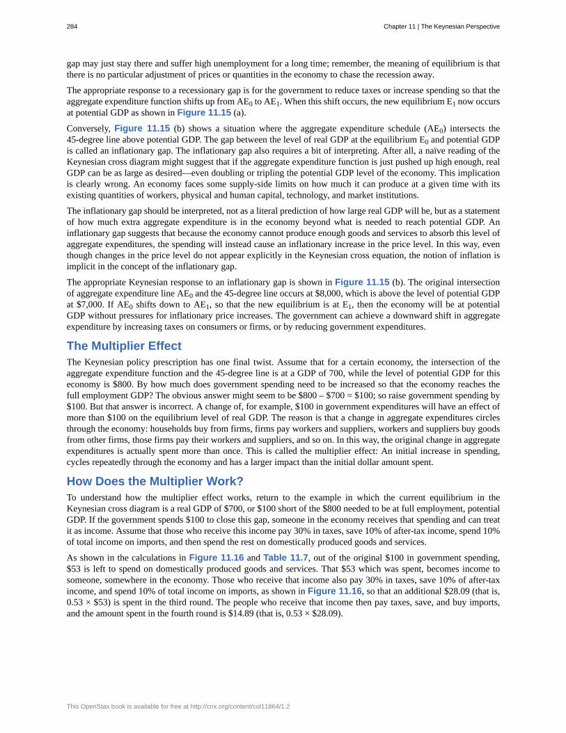
gap may just stay there and suffer high unemployment for a long time; remember, the meaning of equilibrium is thatthere is no particular adjustment of prices or quantities in the economy to chase the recession away.
The appropriate response to a recessionary gap is for the government to reduce taxes or increase spending so that theaggregate expenditure function shifts up from AE0 to AE1. When this shift occurs, the new equilibrium E1 now occursat potential GDP as shown in Figure 11.15 (a).
Conversely, Figure 11.15 (b) shows a situation where the aggregate expenditure schedule (AE0) intersects the45-degree line above potential GDP. The gap between the level of real GDP at the equilibrium E0 and potential GDPis called an inflationary gap. The inflationary gap also requires a bit of interpreting. After all, a naïve reading of theKeynesian cross diagram might suggest that if the aggregate expenditure function is just pushed up high enough, realGDP can be as large as desired—even doubling or tripling the potential GDP level of the economy. This implicationis clearly wrong. An economy faces some supply-side limits on how much it can produce at a given time with itsexisting quantities of workers, physical and human capital, technology, and market institutions.
The inflationary gap should be interpreted, not as a literal prediction of how large real GDP will be, but as a statementof how much extra aggregate expenditure is in the economy beyond what is needed to reach potential GDP. Aninflationary gap suggests that because the economy cannot produce enough goods and services to absorb this level ofaggregate expenditures, the spending will instead cause an inflationary increase in the price level. In this way, eventhough changes in the price level do not appear explicitly in the Keynesian cross equation, the notion of inflation isimplicit in the concept of the inflationary gap.
The appropriate Keynesian response to an inflationary gap is shown in Figure 11.15 (b). The original intersectionof aggregate expenditure line AE0 and the 45-degree line occurs at $8,000, which is above the level of potential GDPat $7,000. If AE0 shifts down to AE1, so that the new equilibrium is at E1, then the economy will be at potentialGDP without pressures for inflationary price increases. The government can achieve a downward shift in aggregateexpenditure by increasing taxes on consumers or firms, or by reducing government expenditures.
The Multiplier EffectThe Keynesian policy prescription has one final twist. Assume that for a certain economy, the intersection of theaggregate expenditure function and the 45-degree line is at a GDP of 700, while the level of potential GDP for thiseconomy is $800. By how much does government spending need to be increased so that the economy reaches thefull employment GDP? The obvious answer might seem to be $800 – $700 = $100; so raise government spending by$100. But that answer is incorrect. A change of, for example, $100 in government expenditures will have an effect ofmore than $100 on the equilibrium level of real GDP. The reason is that a change in aggregate expenditures circlesthrough the economy: households buy from firms, firms pay workers and suppliers, workers and suppliers buy goodsfrom other firms, those firms pay their workers and suppliers, and so on. In this way, the original change in aggregateexpenditures is actually spent more than once. This is called the multiplier effect: An initial increase in spending,cycles repeatedly through the economy and has a larger impact than the initial dollar amount spent.
How Does the Multiplier Work?To understand how the multiplier effect works, return to the example in which the current equilibrium in theKeynesian cross diagram is a real GDP of $700, or $100 short of the $800 needed to be at full employment, potentialGDP. If the government spends $100 to close this gap, someone in the economy receives that spending and can treatit as income. Assume that those who receive this income pay 30% in taxes, save 10% of after-tax income, spend 10%of total income on imports, and then spend the rest on domestically produced goods and services.
As shown in the calculations in Figure 11.16 and Table 11.7, out of the original $100 in government spending,$53 is left to spend on domestically produced goods and services. That $53 which was spent, becomes income tosomeone, somewhere in the economy. Those who receive that income also pay 30% in taxes, save 10% of after-taxincome, and spend 10% of total income on imports, as shown in Figure 11.16, so that an additional $28.09 (that is,0.53 × $53) is spent in the third round. The people who receive that income then pay taxes, save, and buy imports,and the amount spent in the fourth round is $14.89 (that is, 0.53 × $28.09).
284 Chapter 11 | The Keynesian Perspective
This OpenStax book is available for free at http://cnx.org/content/col11864/1.2
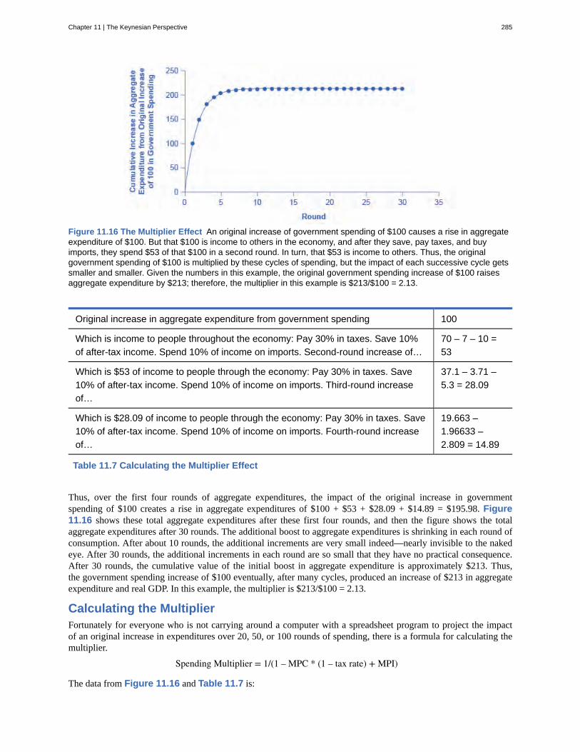
Figure 11.16 The Multiplier Effect An original increase of government spending of $100 causes a rise in aggregateexpenditure of $100. But that $100 is income to others in the economy, and after they save, pay taxes, and buyimports, they spend $53 of that $100 in a second round. In turn, that $53 is income to others. Thus, the originalgovernment spending of $100 is multiplied by these cycles of spending, but the impact of each successive cycle getssmaller and smaller. Given the numbers in this example, the original government spending increase of $100 raisesaggregate expenditure by $213; therefore, the multiplier in this example is $213/$100 = 2.13.
Original increase in aggregate expenditure from government spending 100
Which is income to people throughout the economy: Pay 30% in taxes. Save 10%of after-tax income. Spend 10% of income on imports. Second-round increase of…
70 – 7 – 10 =53
Which is $53 of income to people through the economy: Pay 30% in taxes. Save10% of after-tax income. Spend 10% of income on imports. Third-round increaseof…
37.1 – 3.71 –5.3 = 28.09
Which is $28.09 of income to people through the economy: Pay 30% in taxes. Save10% of after-tax income. Spend 10% of income on imports. Fourth-round increaseof…
19.663 –1.96633 –2.809 = 14.89
Table 11.7 Calculating the Multiplier Effect
Thus, over the first four rounds of aggregate expenditures, the impact of the original increase in governmentspending of $100 creates a rise in aggregate expenditures of $100 + $53 + $28.09 + $14.89 = $195.98. Figure11.16 shows these total aggregate expenditures after these first four rounds, and then the figure shows the totalaggregate expenditures after 30 rounds. The additional boost to aggregate expenditures is shrinking in each round ofconsumption. After about 10 rounds, the additional increments are very small indeed—nearly invisible to the nakedeye. After 30 rounds, the additional increments in each round are so small that they have no practical consequence.After 30 rounds, the cumulative value of the initial boost in aggregate expenditure is approximately $213. Thus,the government spending increase of $100 eventually, after many cycles, produced an increase of $213 in aggregateexpenditure and real GDP. In this example, the multiplier is $213/$100 = 2.13.
Calculating the MultiplierFortunately for everyone who is not carrying around a computer with a spreadsheet program to project the impactof an original increase in expenditures over 20, 50, or 100 rounds of spending, there is a formula for calculating themultiplier.
Spending Multiplier = 1/(1 – MPC * (1 – tax rate) + MPI)
The data from Figure 11.16 and Table 11.7 is:
Chapter 11 | The Keynesian Perspective 285
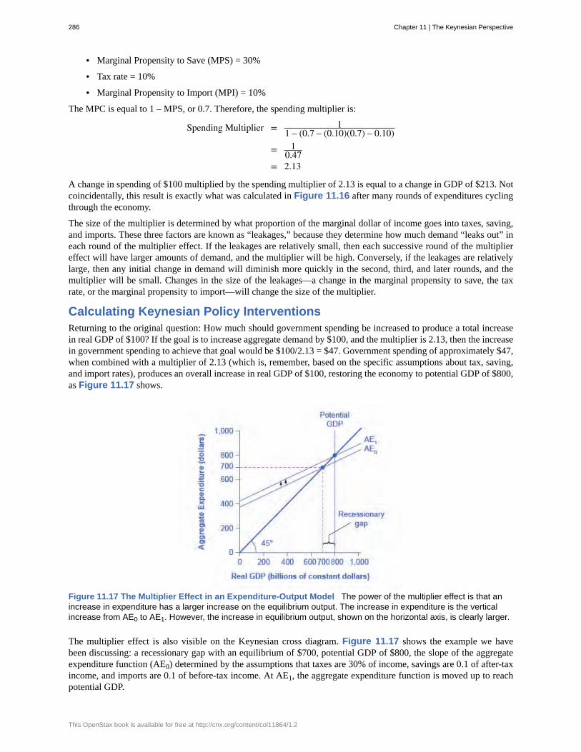
• Marginal Propensity to Save (MPS) = 30%
• Tax rate = 10%
• Marginal Propensity to Import (MPI) = 10%
The MPC is equal to 1 – MPS, or 0.7. Therefore, the spending multiplier is:
Spending Multiplier = 11 – (0.7 – (0.10)(0.7) – 0.10)
= 10.47
= 2.13
A change in spending of $100 multiplied by the spending multiplier of 2.13 is equal to a change in GDP of $213. Notcoincidentally, this result is exactly what was calculated in Figure 11.16 after many rounds of expenditures cyclingthrough the economy.
The size of the multiplier is determined by what proportion of the marginal dollar of income goes into taxes, saving,and imports. These three factors are known as “leakages,” because they determine how much demand “leaks out” ineach round of the multiplier effect. If the leakages are relatively small, then each successive round of the multipliereffect will have larger amounts of demand, and the multiplier will be high. Conversely, if the leakages are relativelylarge, then any initial change in demand will diminish more quickly in the second, third, and later rounds, and themultiplier will be small. Changes in the size of the leakages—a change in the marginal propensity to save, the taxrate, or the marginal propensity to import—will change the size of the multiplier.
Calculating Keynesian Policy InterventionsReturning to the original question: How much should government spending be increased to produce a total increasein real GDP of $100? If the goal is to increase aggregate demand by $100, and the multiplier is 2.13, then the increasein government spending to achieve that goal would be $100/2.13 = $47. Government spending of approximately $47,when combined with a multiplier of 2.13 (which is, remember, based on the specific assumptions about tax, saving,and import rates), produces an overall increase in real GDP of $100, restoring the economy to potential GDP of $800,as Figure 11.17 shows.
Figure 11.17 The Multiplier Effect in an Expenditure-Output Model The power of the multiplier effect is that anincrease in expenditure has a larger increase on the equilibrium output. The increase in expenditure is the verticalincrease from AE0 to AE1. However, the increase in equilibrium output, shown on the horizontal axis, is clearly larger.
The multiplier effect is also visible on the Keynesian cross diagram. Figure 11.17 shows the example we havebeen discussing: a recessionary gap with an equilibrium of $700, potential GDP of $800, the slope of the aggregateexpenditure function (AE0) determined by the assumptions that taxes are 30% of income, savings are 0.1 of after-taxincome, and imports are 0.1 of before-tax income. At AE1, the aggregate expenditure function is moved up to reachpotential GDP.
286 Chapter 11 | The Keynesian Perspective
This OpenStax book is available for free at http://cnx.org/content/col11864/1.2
Now, compare the vertical shift upward in the aggregate expenditure function, which is $47, with the horizontal shiftoutward in real GDP, which is $100 (as these numbers were calculated earlier). The rise in real GDP is more thandouble the rise in the aggregate expenditure function. (Similarly, if you look back at Figure 11.15, you will see thatthe vertical movements in the aggregate expenditure functions are smaller than the change in equilibrium output thatis produced on the horizontal axis. Again, this is the multiplier effect at work.) In this way, the power of the multiplieris apparent in the income–expenditure graph, as well as in the arithmetic calculation.
The multiplier does not just affect government spending, but applies to any change in the economy. Say that businessconfidence declines and investment falls off, or that the economy of a leading trading partner slows down so thatexport sales decline. These changes will reduce aggregate expenditures, and then will have an even larger effect onreal GDP because of the multiplier effect. Read the following Clear It Up feature to learn how the multiplier effectcan be applied to analyze the economic impact of professional sports.
How can the multiplier be used to analyze the economic impact ofprofessional sports?Attracting professional sports teams and building sports stadiums to create jobs and stimulate businessgrowth is an economic development strategy adopted by many communities throughout the United States. Inhis recent article, “Public Financing of Private Sports Stadiums,” James Joyner of Outside the Beltway lookedat public financing for NFL teams. Joyner’s findings confirm the earlier work of John Siegfried of VanderbiltUniversity and Andrew Zimbalist of Smith College.
Siegfried and Zimbalist used the multiplier to analyze this issue. They considered the amount of taxes paidand dollars spent locally to see if there was a positive multiplier effect. Since most professional athletes andowners of sports teams are rich enough to owe a lot of taxes, let’s say that 40% of any marginal income theyearn is paid in taxes. Because athletes are often high earners with short careers, let’s assume that they saveone-third of their after-tax income.
However, many professional athletes do not live year-round in the city in which they play, so let’s say thatone-half of the money that they do spend is spent outside the local area. One can think of spending outside alocal economy, in this example, as the equivalent of imported goods for the national economy.
Now, consider the impact of money spent at local entertainment venues other than professional sports. Whilethe owners of these other businesses may be comfortably middle-income, few of them are in the economicstratosphere of professional athletes. Because their incomes are lower, so are their taxes; say that they payonly 35% of their marginal income in taxes. They do not have the same ability, or need, to save as much asprofessional athletes, so let’s assume their MPC is just 0.8. Finally, because more of them live locally, they willspend a higher proportion of their income on local goods—say, 65%.
If these general assumptions hold true, then money spent on professional sports will have less local economicimpact than money spent on other forms of entertainment. For professional athletes, out of a dollar earned,40 cents goes to taxes, leaving 60 cents. Of that 60 cents, one-third is saved, leaving 40 cents, and half isspent outside the area, leaving 20 cents. Only 20 cents of each dollar is cycled into the local economy in thefirst round. For locally-owned entertainment, out of a dollar earned, 35 cents goes to taxes, leaving 65 cents.Of the rest, 20% is saved, leaving 52 cents, and of that amount, 65% is spent in the local area, so that 33.8cents of each dollar of income is recycled into the local economy.
Siegfried and Zimbalist make the plausible argument that, within their household budgets, people have a fixedamount to spend on entertainment. If this assumption holds true, then money spent attending professionalsports events is money that was not spent on other entertainment options in a given metropolitan area.Since the multiplier is lower for professional sports than for other local entertainment options, the arrival ofprofessional sports to a city would reallocate entertainment spending in a way that causes the local economyto shrink, rather than to grow. Thus, their findings seem to confirm what Joyner reports and what newspapersacross the country are reporting. A quick Internet search for “economic impact of sports” will yield numerousreports questioning this economic development strategy.
Chapter 11 | The Keynesian Perspective 287
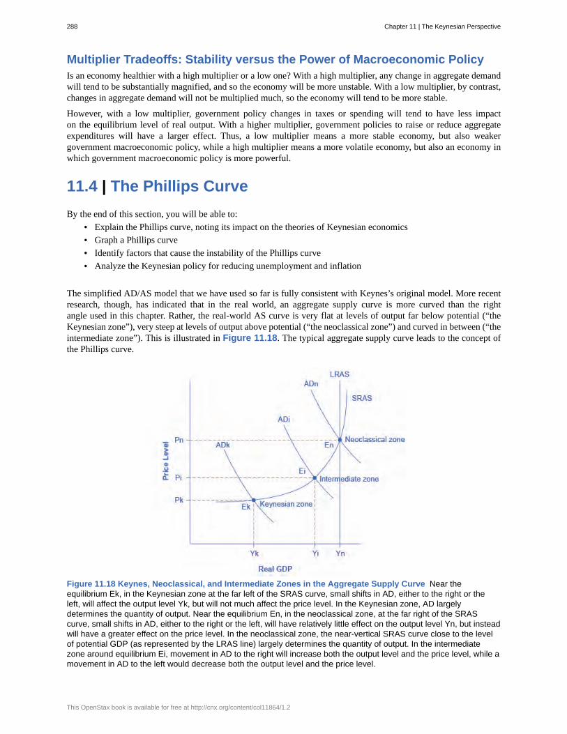
Multiplier Tradeoffs: Stability versus the Power of Macroeconomic PolicyIs an economy healthier with a high multiplier or a low one? With a high multiplier, any change in aggregate demandwill tend to be substantially magnified, and so the economy will be more unstable. With a low multiplier, by contrast,changes in aggregate demand will not be multiplied much, so the economy will tend to be more stable.
However, with a low multiplier, government policy changes in taxes or spending will tend to have less impacton the equilibrium level of real output. With a higher multiplier, government policies to raise or reduce aggregateexpenditures will have a larger effect. Thus, a low multiplier means a more stable economy, but also weakergovernment macroeconomic policy, while a high multiplier means a more volatile economy, but also an economy inwhich government macroeconomic policy is more powerful.
11.4 | The Phillips CurveBy the end of this section, you will be able to:
• Explain the Phillips curve, noting its impact on the theories of Keynesian economics• Graph a Phillips curve• Identify factors that cause the instability of the Phillips curve• Analyze the Keynesian policy for reducing unemployment and inflation
The simplified AD/AS model that we have used so far is fully consistent with Keynes’s original model. More recentresearch, though, has indicated that in the real world, an aggregate supply curve is more curved than the rightangle used in this chapter. Rather, the real-world AS curve is very flat at levels of output far below potential (“theKeynesian zone”), very steep at levels of output above potential (“the neoclassical zone”) and curved in between (“theintermediate zone”). This is illustrated in Figure 11.18. The typical aggregate supply curve leads to the concept ofthe Phillips curve.
Figure 11.18 Keynes, Neoclassical, and Intermediate Zones in the Aggregate Supply Curve Near theequilibrium Ek, in the Keynesian zone at the far left of the SRAS curve, small shifts in AD, either to the right or theleft, will affect the output level Yk, but will not much affect the price level. In the Keynesian zone, AD largelydetermines the quantity of output. Near the equilibrium En, in the neoclassical zone, at the far right of the SRAScurve, small shifts in AD, either to the right or the left, will have relatively little effect on the output level Yn, but insteadwill have a greater effect on the price level. In the neoclassical zone, the near-vertical SRAS curve close to the levelof potential GDP (as represented by the LRAS line) largely determines the quantity of output. In the intermediatezone around equilibrium Ei, movement in AD to the right will increase both the output level and the price level, while amovement in AD to the left would decrease both the output level and the price level.
288 Chapter 11 | The Keynesian Perspective
This OpenStax book is available for free at http://cnx.org/content/col11864/1.2
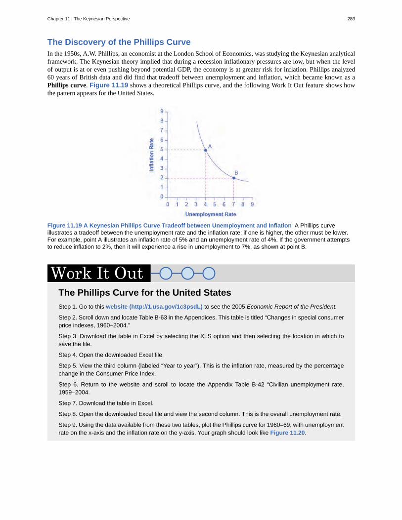
The Discovery of the Phillips CurveIn the 1950s, A.W. Phillips, an economist at the London School of Economics, was studying the Keynesian analyticalframework. The Keynesian theory implied that during a recession inflationary pressures are low, but when the levelof output is at or even pushing beyond potential GDP, the economy is at greater risk for inflation. Phillips analyzed60 years of British data and did find that tradeoff between unemployment and inflation, which became known as aPhillips curve. Figure 11.19 shows a theoretical Phillips curve, and the following Work It Out feature shows howthe pattern appears for the United States.
Figure 11.19 A Keynesian Phillips Curve Tradeoff between Unemployment and Inflation A Phillips curveillustrates a tradeoff between the unemployment rate and the inflation rate; if one is higher, the other must be lower.For example, point A illustrates an inflation rate of 5% and an unemployment rate of 4%. If the government attemptsto reduce inflation to 2%, then it will experience a rise in unemployment to 7%, as shown at point B.
The Phillips Curve for the United StatesStep 1. Go to this website (http://1.usa.gov/1c3psdL) to see the 2005 Economic Report of the President.
Step 2. Scroll down and locate Table B-63 in the Appendices. This table is titled “Changes in special consumerprice indexes, 1960–2004.”
Step 3. Download the table in Excel by selecting the XLS option and then selecting the location in which tosave the file.
Step 4. Open the downloaded Excel file.
Step 5. View the third column (labeled “Year to year”). This is the inflation rate, measured by the percentagechange in the Consumer Price Index.
Step 6. Return to the website and scroll to locate the Appendix Table B-42 “Civilian unemployment rate,1959–2004.
Step 7. Download the table in Excel.
Step 8. Open the downloaded Excel file and view the second column. This is the overall unemployment rate.
Step 9. Using the data available from these two tables, plot the Phillips curve for 1960–69, with unemploymentrate on the x-axis and the inflation rate on the y-axis. Your graph should look like Figure 11.20.
Chapter 11 | The Keynesian Perspective 289
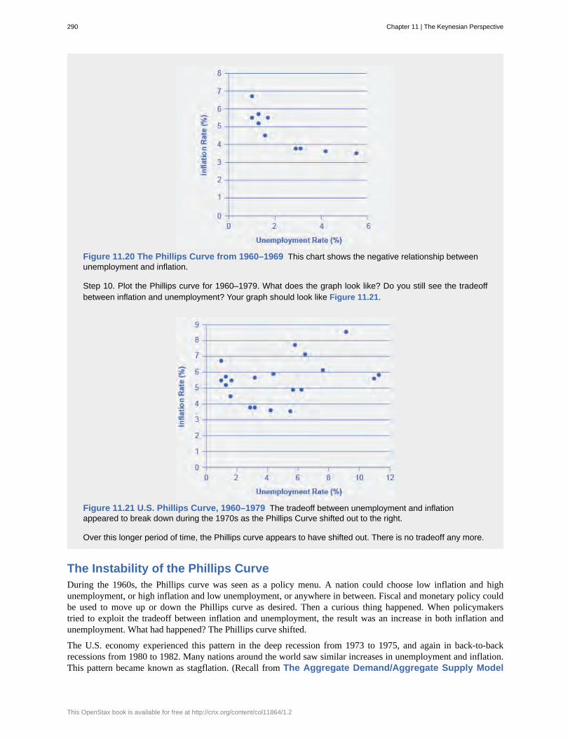
Figure 11.20 The Phillips Curve from 1960–1969 This chart shows the negative relationship betweenunemployment and inflation.
Step 10. Plot the Phillips curve for 1960–1979. What does the graph look like? Do you still see the tradeoffbetween inflation and unemployment? Your graph should look like Figure 11.21.
Figure 11.21 U.S. Phillips Curve, 1960–1979 The tradeoff between unemployment and inflationappeared to break down during the 1970s as the Phillips Curve shifted out to the right.
Over this longer period of time, the Phillips curve appears to have shifted out. There is no tradeoff any more.
The Instability of the Phillips CurveDuring the 1960s, the Phillips curve was seen as a policy menu. A nation could choose low inflation and highunemployment, or high inflation and low unemployment, or anywhere in between. Fiscal and monetary policy couldbe used to move up or down the Phillips curve as desired. Then a curious thing happened. When policymakerstried to exploit the tradeoff between inflation and unemployment, the result was an increase in both inflation andunemployment. What had happened? The Phillips curve shifted.
The U.S. economy experienced this pattern in the deep recession from 1973 to 1975, and again in back-to-backrecessions from 1980 to 1982. Many nations around the world saw similar increases in unemployment and inflation.This pattern became known as stagflation. (Recall from The Aggregate Demand/Aggregate Supply Model
290 Chapter 11 | The Keynesian Perspective
This OpenStax book is available for free at http://cnx.org/content/col11864/1.2
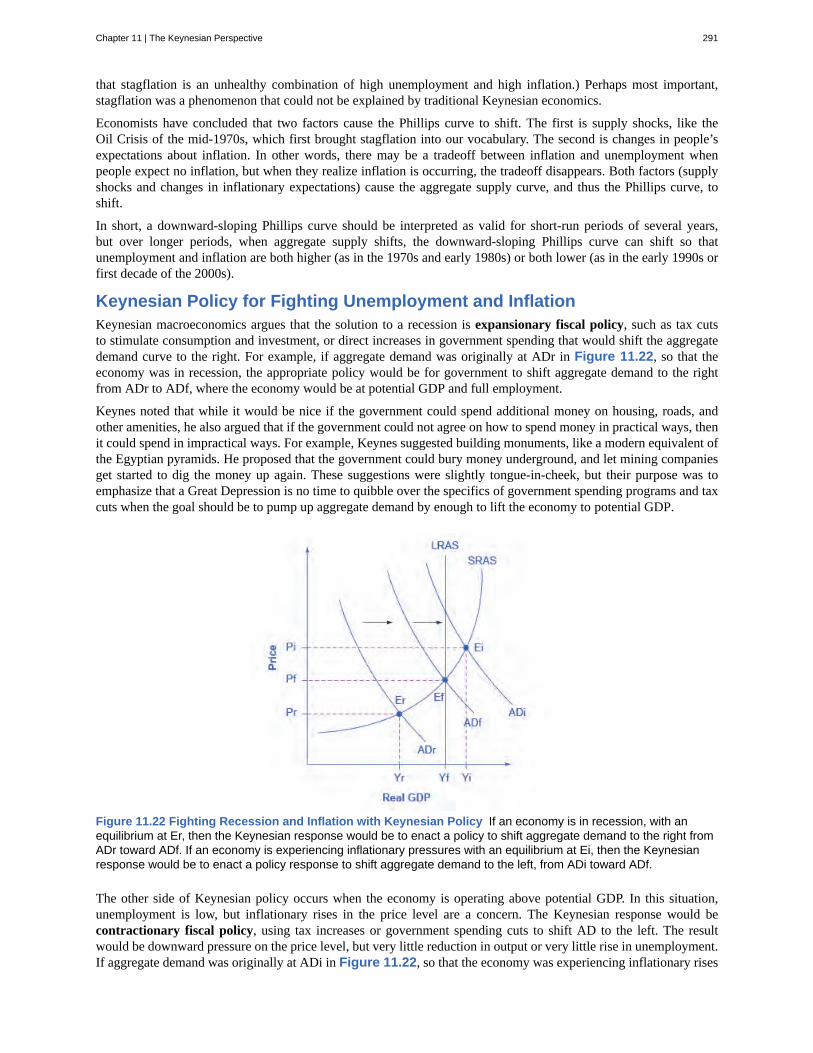
that stagflation is an unhealthy combination of high unemployment and high inflation.) Perhaps most important,stagflation was a phenomenon that could not be explained by traditional Keynesian economics.
Economists have concluded that two factors cause the Phillips curve to shift. The first is supply shocks, like theOil Crisis of the mid-1970s, which first brought stagflation into our vocabulary. The second is changes in people’sexpectations about inflation. In other words, there may be a tradeoff between inflation and unemployment whenpeople expect no inflation, but when they realize inflation is occurring, the tradeoff disappears. Both factors (supplyshocks and changes in inflationary expectations) cause the aggregate supply curve, and thus the Phillips curve, toshift.
In short, a downward-sloping Phillips curve should be interpreted as valid for short-run periods of several years,but over longer periods, when aggregate supply shifts, the downward-sloping Phillips curve can shift so thatunemployment and inflation are both higher (as in the 1970s and early 1980s) or both lower (as in the early 1990s orfirst decade of the 2000s).
Keynesian Policy for Fighting Unemployment and InflationKeynesian macroeconomics argues that the solution to a recession is expansionary fiscal policy, such as tax cutsto stimulate consumption and investment, or direct increases in government spending that would shift the aggregatedemand curve to the right. For example, if aggregate demand was originally at ADr in Figure 11.22, so that theeconomy was in recession, the appropriate policy would be for government to shift aggregate demand to the rightfrom ADr to ADf, where the economy would be at potential GDP and full employment.
Keynes noted that while it would be nice if the government could spend additional money on housing, roads, andother amenities, he also argued that if the government could not agree on how to spend money in practical ways, thenit could spend in impractical ways. For example, Keynes suggested building monuments, like a modern equivalent ofthe Egyptian pyramids. He proposed that the government could bury money underground, and let mining companiesget started to dig the money up again. These suggestions were slightly tongue-in-cheek, but their purpose was toemphasize that a Great Depression is no time to quibble over the specifics of government spending programs and taxcuts when the goal should be to pump up aggregate demand by enough to lift the economy to potential GDP.
Figure 11.22 Fighting Recession and Inflation with Keynesian Policy If an economy is in recession, with anequilibrium at Er, then the Keynesian response would be to enact a policy to shift aggregate demand to the right fromADr toward ADf. If an economy is experiencing inflationary pressures with an equilibrium at Ei, then the Keynesianresponse would be to enact a policy response to shift aggregate demand to the left, from ADi toward ADf.
The other side of Keynesian policy occurs when the economy is operating above potential GDP. In this situation,unemployment is low, but inflationary rises in the price level are a concern. The Keynesian response would becontractionary fiscal policy, using tax increases or government spending cuts to shift AD to the left. The resultwould be downward pressure on the price level, but very little reduction in output or very little rise in unemployment.If aggregate demand was originally at ADi in Figure 11.22, so that the economy was experiencing inflationary rises
Chapter 11 | The Keynesian Perspective 291
in the price level, the appropriate policy would be for government to shift aggregate demand to the left, from ADitoward ADf, which reduces the pressure for a higher price level while the economy remains at full employment.
In the Keynesian economic model, too little aggregate demand brings unemployment and too much brings inflation.Thus, you can think of Keynesian economics as pursuing a “Goldilocks” level of aggregate demand: not too much,not too little, but looking for what is just right.
11.5 | The Keynesian Perspective on Market ForcesBy the end of this section, you will be able to:
• Explain the Keynesian perspective on market forces• Analyze the role of government policy in economic management
Ever since the birth of Keynesian economics in the 1930s, controversy has simmered over the extent to whichgovernment should play an active role in managing the economy. In the aftermath of the human devastation andmisery of the Great Depression, many people—including many economists—became more aware of vulnerabilitieswithin the market-oriented economic system. Some supporters of Keynesian economics advocated a high degree ofgovernment planning in all parts of the economy.
However, Keynes himself was careful to separate the issue of aggregate demand from the issue of how well individualmarkets worked. He argued that individual markets for goods and services were appropriate and useful, but thatsometimes that level of aggregate demand was just too low. When 10 million people are willing and able to work, butone million of them are unemployed, he argued, individual markets may be doing a perfectly good job of allocatingthe efforts of the nine million workers—the problem is that insufficient aggregate demand exists to support jobs forall 10 million. Thus, he believed that, while government should ensure that overall level of aggregate demand issufficient for an economy to reach full employment, this task did not imply that the government should attempt toset prices and wages throughout the economy, nor to take over and manage large corporations or entire industriesdirectly.
Even if one accepts the Keynesian economic theory, a number of practical questions remain. In the real world,can government economists identify potential GDP accurately? Is a desired increase in aggregate demand betteraccomplished by a tax cut or by an increase in government spending? Given the inevitable delays and uncertaintiesas policies are enacted into law, is it reasonable to expect that the government can implement Keynesian economics?Can fixing a recession really be just as simple as pumping up aggregate demand? Government Budgets andFiscal Policy will probe these issues. The Keynesian approach, with its focus on aggregate demand and stickyprices, has proved useful in understanding how the economy fluctuates in the short run and why recessions andcyclical unemployment occur. In The Neoclassical Perspective, we will consider some of the shortcomings ofthe Keynesian approach and why it is not especially well-suited for long-run macroeconomic analysis.
The Great RecessionThe lessons learned during the Great Depression of the 1930s and the aggregate expenditure modelproposed by John Maynard Keynes gave the modern economists and policymakers of today the tools toeffectively navigate the treacherous economy in the latter half of the 2000s. In “How the Great Recession WasBrought to an End,” Alan S. Blinder and Mark Zandi wrote that the actions taken by today’s policymakers standin sharp contrast to those of the early years of the Great Depression. Today’s economists and policymakerswere not content to let the markets recover from recession without taking proactive measures to supportconsumption and investment. The Federal Reserve actively lowered short-term interest rates and developedinnovative ways to pump money into the economy so that credit and investment would not dry up. BothPresidents Bush and Obama and Congress implemented a variety of programs ranging from tax rebates to“Cash for Clunkers” to the Troubled Asset Relief Program to stimulate and stabilize household consumption
292 Chapter 11 | The Keynesian Perspective
This OpenStax book is available for free at http://cnx.org/content/col11864/1.2

and encourage investment. Although these policies came under harsh criticism from the public and manypoliticians, they lessened the impact of the economic downturn and may have saved the country from asecond Great Depression.
Chapter 11 | The Keynesian Perspective 293
contractionary fiscal policy
coordination argument
disposable income
expansionary fiscal policy
expenditure multiplier
inflationary gap
macroeconomic externality
menu costs
Phillips curve
real GDP
recessionary gap
sticky wages and prices
KEY TERMS
tax increases or cuts in government spending designed to decrease aggregate demandand reduce inflationary pressures
downward wage and price flexibility requires perfect information about the level of lowercompensation acceptable to other laborers and market participants
income after taxes
tax cuts or increases in government spending designed to stimulate aggregate demand andmove the economy out of recession
Keynesian concept that asserts that a change in autonomous spending causes a more thanproportionate change in real GDP
equilibrium at a level of output above potential GDP
occurs when what happens at the macro level is different from and inferior to whathappens at the micro level; an example would be where upward sloping supply curves for firms become a flataggregate supply curve, illustrating that the price level cannot fall to stimulate aggregate demand
costs firms face in changing prices
the tradeoff between unemployment and inflation
the amount of goods and services actually being sold in a nation
equilibrium at a level of output below potential GDP
a situation where wages and prices do not fall in response to a decrease in demand, or do notrise in response to an increase in demand
KEY CONCEPTS AND SUMMARY
11.1 Aggregate Demand in Keynesian AnalysisAggregate demand is the sum of four components: consumption, investment, government spending, and net exports.Consumption will change for a number of reasons, including movements in income, taxes, expectations about futureincome, and changes in wealth levels. Investment will change in response to its expected profitability, which in turnis shaped by expectations about future economic growth, the creation of new technologies, the price of key inputs,and tax incentives for investment. Investment will also change when interest rates rise or fall. Government spendingand taxes are determined by political considerations. Exports and imports change according to relative growth ratesand prices between two economies.
11.2 The Building Blocks of Keynesian AnalysisKeynesian economics is based on two main ideas: (1) aggregate demand is more likely than aggregate supply tobe the primary cause of a short-run economic event like a recession; (2) wages and prices can be sticky, and so, inan economic downturn, unemployment can result. The latter is an example of a macroeconomic externality. Whilesurpluses cause prices to fall at the micro level, they do not necessarily at the macro level; instead the adjustmentto a decrease in demand occurs only through decreased quantities. One reason why prices may be sticky is menucosts, the costs of changing prices. These include internal costs a business faces in changing prices in terms oflabeling, recordkeeping, and accounting, and also the costs of communicating the price change to (possibly unhappy)customers. Keynesians also believe in the existence of the expenditure multiplier—the notion that a change inautonomous expenditure causes a more than proportionate change in GDP.
294 Chapter 11 | The Keynesian Perspective
This OpenStax book is available for free at http://cnx.org/content/col11864/1.2
11.3 The Expenditure-Output (or Keynesian Cross) ModelThe expenditure-output model or Keynesian cross diagram shows how the level of aggregate expenditure (on thevertical axis) varies with the level of economic output (shown on the horizontal axis). Since the value of allmacroeconomic output also represents income to someone somewhere else in the economy, the horizontal axis canalso be interpreted as national income. The equilibrium in the diagram will occur where the aggregate expenditure linecrosses the 45-degree line, which represents the set of points where aggregate expenditure in the economy is equalto output (or national income). Equilibrium in a Keynesian cross diagram can happen at potential GDP, or below orabove that level.
The consumption function shows the upward-sloping relationship between national income and consumption. Themarginal propensity to consume (MPC) is the amount consumed out of an additional dollar of income. A highermarginal propensity to consume means a steeper consumption function; a lower marginal propensity to consumemeans a flatter consumption function. The marginal propensity to save (MPS) is the amount saved out of an additionaldollar of income. It is necessarily true that MPC + MPS = 1. The investment function is drawn as a flat line, showingthat investment in the current year does not change with regard to the current level of national income. However,the investment function will move up and down based on the expected rate of return in the future. Governmentspending is drawn as a horizontal line in the Keynesian cross diagram, because its level is determined by politicalconsiderations, not by the current level of income in the economy. Taxes in the basic Keynesian cross diagram aretaken into account by adjusting the consumption function. The export function is drawn as a horizontal line in theKeynesian cross diagram, because exports do not change as a result of changes in domestic income, but they moveas a result of changes in foreign income, as well as changes in exchange rates. The import function is drawn asa downward-sloping line, because imports rise with national income, but imports are a subtraction from aggregatedemand. Thus, a higher level of imports means a lower level of expenditure on domestic goods.
In a Keynesian cross diagram, the equilibrium may be at a level below potential GDP, which is called a recessionarygap, or at a level above potential GDP, which is called an inflationary gap.
The multiplier effect describes how an initial change in aggregate demand generated several times as much ascumulative GDP. The size of the spending multiplier is determined by three leakages: spending on savings, taxes, andimports. The formula for the multiplier is:
Multiplier = 11 – (MPC × (1 – tax rate) + MPI)
An economy with a lower multiplier is more stable—it is less affected either by economic events or by governmentpolicy than an economy with a higher multiplier.
11.4 The Phillips CurveA Phillips curve shows the tradeoff between unemployment and inflation in an economy. From a Keynesianviewpoint, the Phillips curve should slope down so that higher unemployment means lower inflation, and vice versa.However, a downward-sloping Phillips curve is a short-term relationship that may shift after a few years.
Keynesian macroeconomics argues that the solution to a recession is expansionary fiscal policy, such as tax cuts tostimulate consumption and investment, or direct increases in government spending that would shift the aggregatedemand curve to the right. The other side of Keynesian policy occurs when the economy is operating above potentialGDP. In this situation, unemployment is low, but inflationary rises in the price level are a concern. The Keynesianresponse would be contractionary fiscal policy, using tax increases or government spending cuts to shift AD to theleft.
11.5 The Keynesian Perspective on Market ForcesThe Keynesian prescription for stabilizing the economy implies government intervention at the macroeconomiclevel—increasing aggregate demand when private demand falls and decreasing aggregate demand when privatedemand rises. This does not imply that the government should be passing laws or regulations that set prices andquantities in microeconomic markets.
SELF-CHECK QUESTIONS
Chapter 11 | The Keynesian Perspective 295
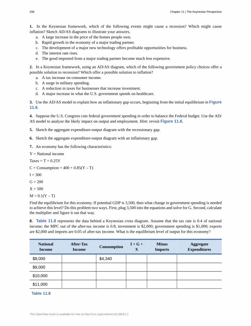
1. In the Keynesian framework, which of the following events might cause a recession? Which might causeinflation? Sketch AD/AS diagrams to illustrate your answers.
a. A large increase in the price of the homes people own.b. Rapid growth in the economy of a major trading partner.c. The development of a major new technology offers profitable opportunities for business.d. The interest rate rises.e. The good imported from a major trading partner become much less expensive.
2. In a Keynesian framework, using an AD/AS diagram, which of the following government policy choices offer apossible solution to recession? Which offer a possible solution to inflation?
a. A tax increase on consumer income.b. A surge in military spending.c. A reduction in taxes for businesses that increase investment.d. A major increase in what the U.S. government spends on healthcare.
3. Use the AD/AS model to explain how an inflationary gap occurs, beginning from the initial equilibrium in Figure11.6.
4. Suppose the U.S. Congress cuts federal government spending in order to balance the Federal budget. Use the AD/AS model to analyze the likely impact on output and employment. Hint: revisit Figure 11.6.
5. Sketch the aggregate expenditure-output diagram with the recessionary gap.
6. Sketch the aggregate expenditure-output diagram with an inflationary gap.
7. An economy has the following characteristics:
Y = National income
Taxes = T = 0.25Y
C = Consumption = 400 + 0.85(Y – T)
I = 300
G = 200
X = 500
M = 0.1(Y – T)
Find the equilibrium for this economy. If potential GDP is 3,500, then what change in government spending is neededto achieve this level? Do this problem two ways. First, plug 3,500 into the equations and solve for G. Second, calculatethe multiplier and figure it out that way.
8. Table 11.8 represents the data behind a Keynesian cross diagram. Assume that the tax rate is 0.4 of nationalincome; the MPC out of the after-tax income is 0.8; investment is $2,000; government spending is $1,000; exportsare $2,000 and imports are 0.05 of after-tax income. What is the equilibrium level of output for this economy?
NationalIncome
After-TaxIncome Consumption I + G +
XMinus
ImportsAggregate
Expenditures
$8,000 $4,340
$9,000
$10,000
$11,000
Table 11.8
296 Chapter 11 | The Keynesian Perspective
This OpenStax book is available for free at http://cnx.org/content/col11864/1.2
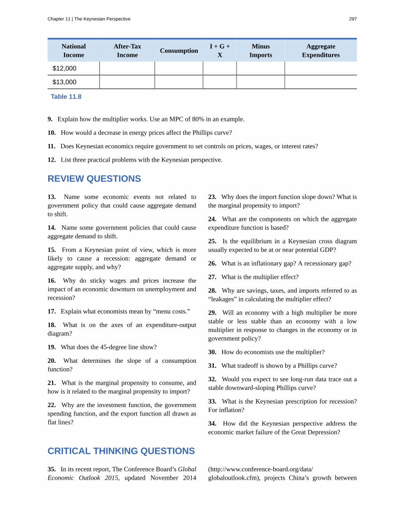
NationalIncome
After-TaxIncome Consumption I + G +
XMinus
ImportsAggregate
Expenditures
$12,000
$13,000
Table 11.8
9. Explain how the multiplier works. Use an MPC of 80% in an example.
10. How would a decrease in energy prices affect the Phillips curve?
11. Does Keynesian economics require government to set controls on prices, wages, or interest rates?
12. List three practical problems with the Keynesian perspective.
REVIEW QUESTIONS
13. Name some economic events not related togovernment policy that could cause aggregate demandto shift.
14. Name some government policies that could causeaggregate demand to shift.
15. From a Keynesian point of view, which is morelikely to cause a recession: aggregate demand oraggregate supply, and why?
16. Why do sticky wages and prices increase theimpact of an economic downturn on unemployment andrecession?
17. Explain what economists mean by “menu costs.”
18. What is on the axes of an expenditure-outputdiagram?
19. What does the 45-degree line show?
20. What determines the slope of a consumptionfunction?
21. What is the marginal propensity to consume, andhow is it related to the marginal propensity to import?
22. Why are the investment function, the governmentspending function, and the export function all drawn asflat lines?
23. Why does the import function slope down? What isthe marginal propensity to import?
24. What are the components on which the aggregateexpenditure function is based?
25. Is the equilibrium in a Keynesian cross diagramusually expected to be at or near potential GDP?
26. What is an inflationary gap? A recessionary gap?
27. What is the multiplier effect?
28. Why are savings, taxes, and imports referred to as“leakages” in calculating the multiplier effect?
29. Will an economy with a high multiplier be morestable or less stable than an economy with a lowmultiplier in response to changes in the economy or ingovernment policy?
30. How do economists use the multiplier?
31. What tradeoff is shown by a Phillips curve?
32. Would you expect to see long-run data trace out astable downward-sloping Phillips curve?
33. What is the Keynesian prescription for recession?For inflation?
34. How did the Keynesian perspective address theeconomic market failure of the Great Depression?
CRITICAL THINKING QUESTIONS
35. In its recent report, The Conference Board’s GlobalEconomic Outlook 2015, updated November 2014
(http://www.conference-board.org/data/globaloutlook.cfm), projects China’s growth between
Chapter 11 | The Keynesian Perspective 297
2015 and 2019 to be about 5.5%. International BusinessTimes (http://www.ibtimes.com/us-exports-china-have-grown-294-over-past-decade-1338693) reports thatChina is the United States’ third largest export market,with exports to China growing 294% over the last tenyears. Explain what impact China has on the U.S.economy.
36. What may happen if growth in China continues orcontracts?
37. Does it make sense that wages would be stickydownwards but not upwards? Why or why not?
38. Suppose the economy is operating at potential GDPwhen it experiences an increase in export demand. Howmight the economy increase production of exports tomeet this demand, given that the economy is already atfull employment?
39. What does it mean when the aggregate expenditureline crosses the 45-degree line? In other words, howwould you explain the intersection in words?
40. Which model, the AD/AS or the AE model betterexplains the relationship between rising price levels andGDP? Why?
41. What are some reasons that the economy might bein a recession, and what is the appropriate governmentaction to alleviate the recession?
42. What should the government do to relieveinflationary pressures if the aggregate expenditure isgreater than potential GDP?
43. Two countries are in a recession. Country A hasan MPC of 0.8 and Country B has an MPC of 0.6.In which country will government spending have thegreatest impact?
44. Compare two policies: a tax cut on income or anincrease in government spending on roads and bridges.What are both the short-term and long-term impacts ofsuch policies on the economy?
45. What role does government play in stabilizing theeconomy and what are the tradeoffs that must beconsidered?
46. If there is a recessionary gap of $100 billion, shouldthe government increase spending by $100 billion toclose the gap? Why? Why not?
47. What other changes in the economy can beevaluated by using the multiplier?
48. Do you think the Phillips curve is a useful tool foranalyzing the economy today? Why or why not?
49. Return to the table from the Economic Report of thePresident in the earlier The Phillips Curve for theUnited States feature titled “The Phillips Curve forthe United States.” How would you expect governmentspending to have changed over the last six years?
50. Explain what types of policies the federalgovernment may have implemented to restore aggregatedemand and the potential obstacles policymakers mayhave encountered.
298 Chapter 11 | The Keynesian Perspective
This OpenStax book is available for free at http://cnx.org/content/col11864/1.2

12 | The NeoclassicalPerspective
Figure 12.1 Impact of the Great Recession The impact of the Great Recession can be seen in many areas of theeconomy that impact our daily lives. One of the most visible signs can be seen in the housing market where manyhomes and other buildings are abandoned, including ones that midway through construction. (Credit: modification ofwork by A McLin/Flickr Creative Commons)
Navigating Unchartered WatersThe Great Recession ended in June 2009 after 18 months, according to the National Bureau of EconomicResearch (NBER). The NBER examines a variety of measures of economic activity to gauge the overall healthof the economy. These measures include real income, wholesale and retail sales, employment, and industrialproduction. In the years since the official end of this historic economic downturn, it has become clear thatthe Great Recession was two-pronged, hitting the U.S. economy with the collapse of the housing market andthe failure of the financial system's credit institutions, further contaminating global economies. While the stockmarket rapidly lost trillions of dollars of value, consumer spending dried up, and companies began cuttingjobs, economic policymakers were struggling with how to best combat and prevent a national, and even globaleconomic collapse. In the end, policymakers used a number of controversial monetary and fiscal policies tosupport the housing market and domestic industries as well as to stabilize the financial sector. Some of theseinitiatives included:
• Federal Reserve Bank purchase of both traditional and nontraditional assets off banks' balancesheets. By doing this, the Fed injected money into the banking system and increased the amounts offunds available to lend to the business sector and consumers. This also dropped short-term interestrates to as low as zero percent and had the effect of devaluing U.S. dollars in the global market andboosting exports.
Chapter 12 | The Neoclassical Perspective 299
• The Congress and the President also passed several pieces of legislation that would stabilize thefinancial market. The Troubled Asset Relief Program (TARP), passed in late 2008, allowed thegovernment to inject cash into troubled banks and other financial institutions and help support GeneralMotors and Chrysler as they faced bankruptcy and threatened job losses throughout their supplychain. The American Recovery and Reinvestment Act in early 2009 provided tax rebates to low- andmiddle-income households to encourage consumer spending.
Four years after the end of the Great Recession, the economy has yet to return to its pre-recession levelsof productivity and growth. Annual productivity increased only 1.9% between 2009 and 2012 compared toits 2.7% annual growth rate between 2000 and 2007, unemployment remains above the natural rate, andreal GDP continues to lag behind potential growth. The actions taken to stabilize the economy are still underscrutiny and debate about their effectiveness continues. In this chapter, we will discuss the neoclassicalperspective on economics and compare it to the Keynesian perspective. At the end of the chapter, we will usethe neoclassical perspective to analyze the actions taken in the Great Recession.
Introduction to the Neoclassical PerspectiveIn this chapter, you will learn about:
• The Building Blocks of Neoclassical Analysis
• The Policy Implications of the Neoclassical Perspective
• Balancing Keynesian and Neoclassical Models
In Chicago, Illinois, the highest recorded temperature was 105° in July 1995, while the lowest recorded temperaturewas 27° below zero in January 1958. Understanding why these extreme weather patterns occurred would beinteresting. However, if you wanted to understand the typical weather pattern in Chicago, instead of focusing on one-time extremes, you would need to look at the entire pattern of data over time.
A similar lesson applies to the study of macroeconomics. It is interesting to study extreme situations, like the GreatDepression of the 1930s or what many have called the Great Recession of 2008–2009. If you want to understandthe whole picture, however, you need to look at the long term. Consider the unemployment rate. The unemploymentrate has fluctuated from as low as 3.5% in 1969 to as high as 9.7% in 1982 and 9.6% in 2009. Even as theU.S. unemployment rate rose during recessions and declined during expansions, it kept returning to the generalneighborhood of 5.0–5.5%. When the nonpartisan Congressional Budget Office carried out its long-range economicforecasts in 2010, it assumed that from 2015 to 2020, after the recession has passed, the unemployment rate would be5.0%. From a long-run perspective, the economy seems to keep adjusting back to this rate of unemployment.
As the name “neoclassical” implies, this perspective of how the macroeconomy works is a “new” view of the “old”classical model of the economy. The classical view, the predominant economic philosophy until the Great Depression,was that short-term fluctuations in economic activity would rather quickly, with flexible prices, adjust back to fullemployment. This view of the economy implied a vertical aggregate supply curve at full employment GDP, andprescribed a “hands off” policy approach. For example, if the economy were to slip into recession (a leftward shift ofthe aggregate demand curve), it would temporarily exhibit a surplus of goods. This surplus would be eliminated withfalling prices, and the economy would return to full employment level of GDP; no active fiscal or monetary policywas needed. In fact, the classical view was that expansionary fiscal or monetary policy would only cause inflation,rather than increase GDP. The deep and lasting impact of the Great Depression changed this thinking and Keynesianeconomics, which prescribed active fiscal policy to alleviate weak aggregate demand, became the more mainstreamperspective.
300 Chapter 12 | The Neoclassical Perspective
This OpenStax book is available for free at http://cnx.org/content/col11864/1.2
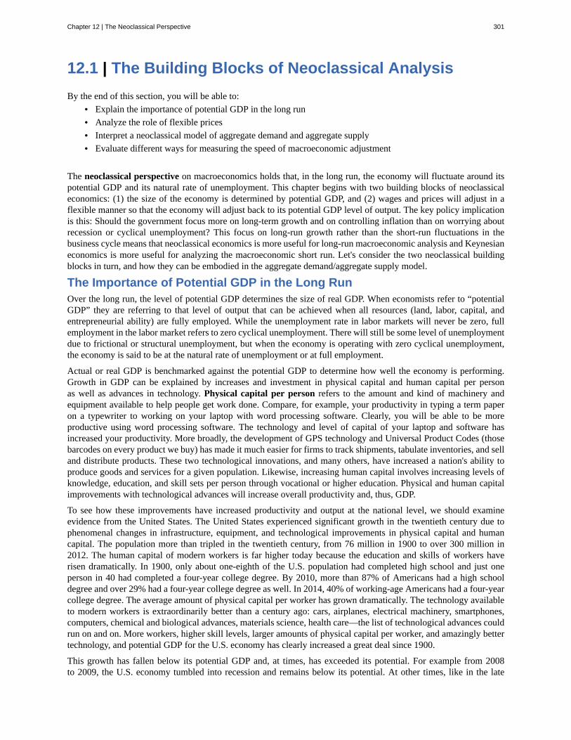
12.1 | The Building Blocks of Neoclassical AnalysisBy the end of this section, you will be able to:
• Explain the importance of potential GDP in the long run• Analyze the role of flexible prices• Interpret a neoclassical model of aggregate demand and aggregate supply• Evaluate different ways for measuring the speed of macroeconomic adjustment
The neoclassical perspective on macroeconomics holds that, in the long run, the economy will fluctuate around itspotential GDP and its natural rate of unemployment. This chapter begins with two building blocks of neoclassicaleconomics: (1) the size of the economy is determined by potential GDP, and (2) wages and prices will adjust in aflexible manner so that the economy will adjust back to its potential GDP level of output. The key policy implicationis this: Should the government focus more on long-term growth and on controlling inflation than on worrying aboutrecession or cyclical unemployment? This focus on long-run growth rather than the short-run fluctuations in thebusiness cycle means that neoclassical economics is more useful for long-run macroeconomic analysis and Keynesianeconomics is more useful for analyzing the macroeconomic short run. Let's consider the two neoclassical buildingblocks in turn, and how they can be embodied in the aggregate demand/aggregate supply model.
The Importance of Potential GDP in the Long RunOver the long run, the level of potential GDP determines the size of real GDP. When economists refer to “potentialGDP” they are referring to that level of output that can be achieved when all resources (land, labor, capital, andentrepreneurial ability) are fully employed. While the unemployment rate in labor markets will never be zero, fullemployment in the labor market refers to zero cyclical unemployment. There will still be some level of unemploymentdue to frictional or structural unemployment, but when the economy is operating with zero cyclical unemployment,the economy is said to be at the natural rate of unemployment or at full employment.
Actual or real GDP is benchmarked against the potential GDP to determine how well the economy is performing.Growth in GDP can be explained by increases and investment in physical capital and human capital per personas well as advances in technology. Physical capital per person refers to the amount and kind of machinery andequipment available to help people get work done. Compare, for example, your productivity in typing a term paperon a typewriter to working on your laptop with word processing software. Clearly, you will be able to be moreproductive using word processing software. The technology and level of capital of your laptop and software hasincreased your productivity. More broadly, the development of GPS technology and Universal Product Codes (thosebarcodes on every product we buy) has made it much easier for firms to track shipments, tabulate inventories, and selland distribute products. These two technological innovations, and many others, have increased a nation's ability toproduce goods and services for a given population. Likewise, increasing human capital involves increasing levels ofknowledge, education, and skill sets per person through vocational or higher education. Physical and human capitalimprovements with technological advances will increase overall productivity and, thus, GDP.
To see how these improvements have increased productivity and output at the national level, we should examineevidence from the United States. The United States experienced significant growth in the twentieth century due tophenomenal changes in infrastructure, equipment, and technological improvements in physical capital and humancapital. The population more than tripled in the twentieth century, from 76 million in 1900 to over 300 million in2012. The human capital of modern workers is far higher today because the education and skills of workers haverisen dramatically. In 1900, only about one-eighth of the U.S. population had completed high school and just oneperson in 40 had completed a four-year college degree. By 2010, more than 87% of Americans had a high schooldegree and over 29% had a four-year college degree as well. In 2014, 40% of working-age Americans had a four-yearcollege degree. The average amount of physical capital per worker has grown dramatically. The technology availableto modern workers is extraordinarily better than a century ago: cars, airplanes, electrical machinery, smartphones,computers, chemical and biological advances, materials science, health care—the list of technological advances couldrun on and on. More workers, higher skill levels, larger amounts of physical capital per worker, and amazingly bettertechnology, and potential GDP for the U.S. economy has clearly increased a great deal since 1900.
This growth has fallen below its potential GDP and, at times, has exceeded its potential. For example from 2008to 2009, the U.S. economy tumbled into recession and remains below its potential. At other times, like in the late
Chapter 12 | The Neoclassical Perspective 301
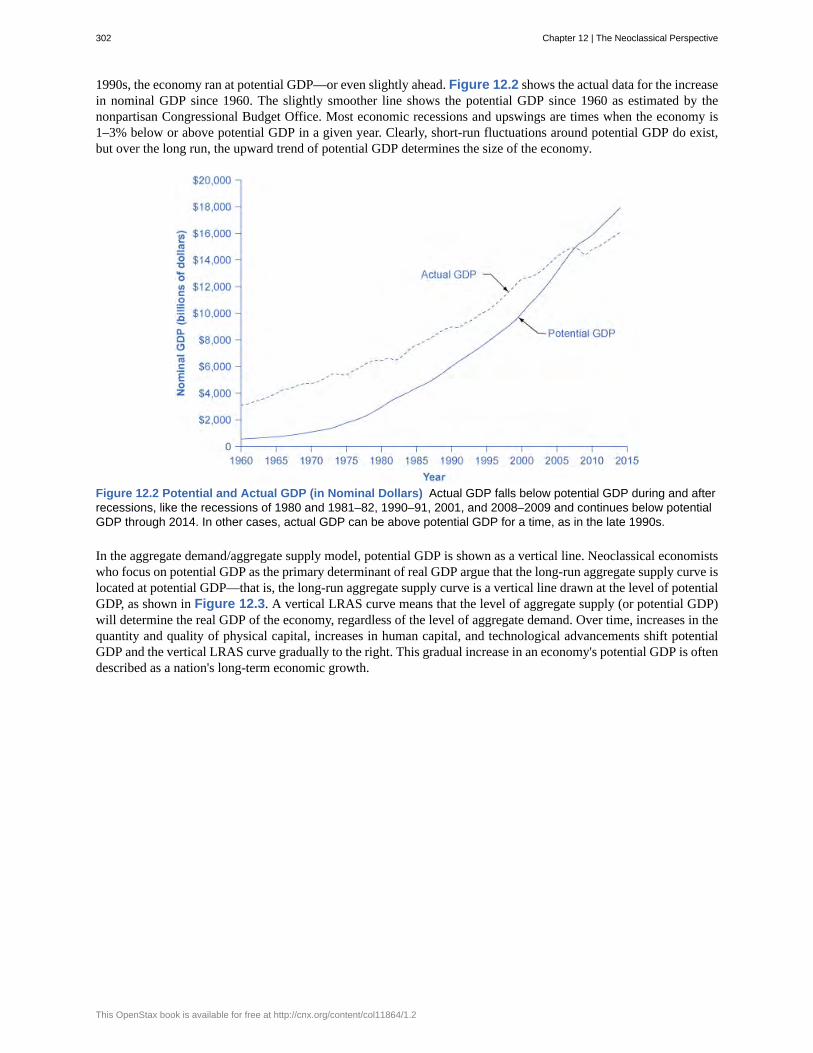
1990s, the economy ran at potential GDP—or even slightly ahead. Figure 12.2 shows the actual data for the increasein nominal GDP since 1960. The slightly smoother line shows the potential GDP since 1960 as estimated by thenonpartisan Congressional Budget Office. Most economic recessions and upswings are times when the economy is1–3% below or above potential GDP in a given year. Clearly, short-run fluctuations around potential GDP do exist,but over the long run, the upward trend of potential GDP determines the size of the economy.
Figure 12.2 Potential and Actual GDP (in Nominal Dollars) Actual GDP falls below potential GDP during and afterrecessions, like the recessions of 1980 and 1981–82, 1990–91, 2001, and 2008–2009 and continues below potentialGDP through 2014. In other cases, actual GDP can be above potential GDP for a time, as in the late 1990s.
In the aggregate demand/aggregate supply model, potential GDP is shown as a vertical line. Neoclassical economistswho focus on potential GDP as the primary determinant of real GDP argue that the long-run aggregate supply curve islocated at potential GDP—that is, the long-run aggregate supply curve is a vertical line drawn at the level of potentialGDP, as shown in Figure 12.3. A vertical LRAS curve means that the level of aggregate supply (or potential GDP)will determine the real GDP of the economy, regardless of the level of aggregate demand. Over time, increases in thequantity and quality of physical capital, increases in human capital, and technological advancements shift potentialGDP and the vertical LRAS curve gradually to the right. This gradual increase in an economy's potential GDP is oftendescribed as a nation's long-term economic growth.
302 Chapter 12 | The Neoclassical Perspective
This OpenStax book is available for free at http://cnx.org/content/col11864/1.2
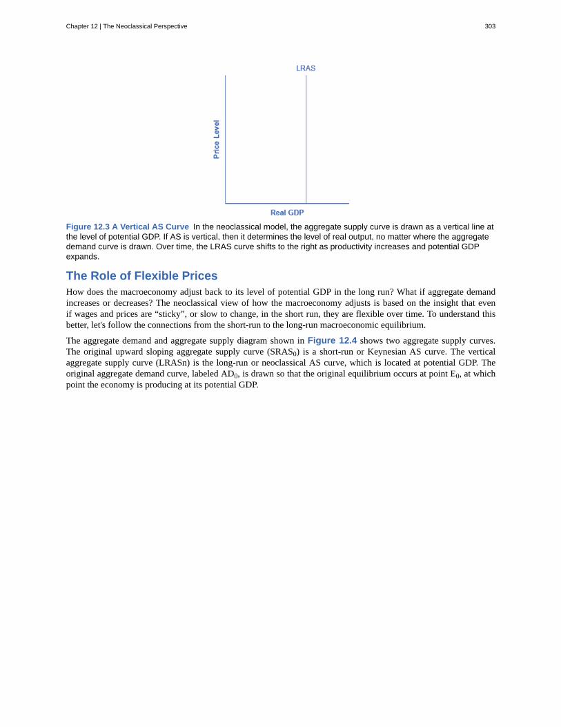
Figure 12.3 A Vertical AS Curve In the neoclassical model, the aggregate supply curve is drawn as a vertical line atthe level of potential GDP. If AS is vertical, then it determines the level of real output, no matter where the aggregatedemand curve is drawn. Over time, the LRAS curve shifts to the right as productivity increases and potential GDPexpands.
The Role of Flexible PricesHow does the macroeconomy adjust back to its level of potential GDP in the long run? What if aggregate demandincreases or decreases? The neoclassical view of how the macroeconomy adjusts is based on the insight that evenif wages and prices are “sticky”, or slow to change, in the short run, they are flexible over time. To understand thisbetter, let's follow the connections from the short-run to the long-run macroeconomic equilibrium.
The aggregate demand and aggregate supply diagram shown in Figure 12.4 shows two aggregate supply curves.The original upward sloping aggregate supply curve (SRAS0) is a short-run or Keynesian AS curve. The verticalaggregate supply curve (LRASn) is the long-run or neoclassical AS curve, which is located at potential GDP. Theoriginal aggregate demand curve, labeled AD0, is drawn so that the original equilibrium occurs at point E0, at whichpoint the economy is producing at its potential GDP.
Chapter 12 | The Neoclassical Perspective 303
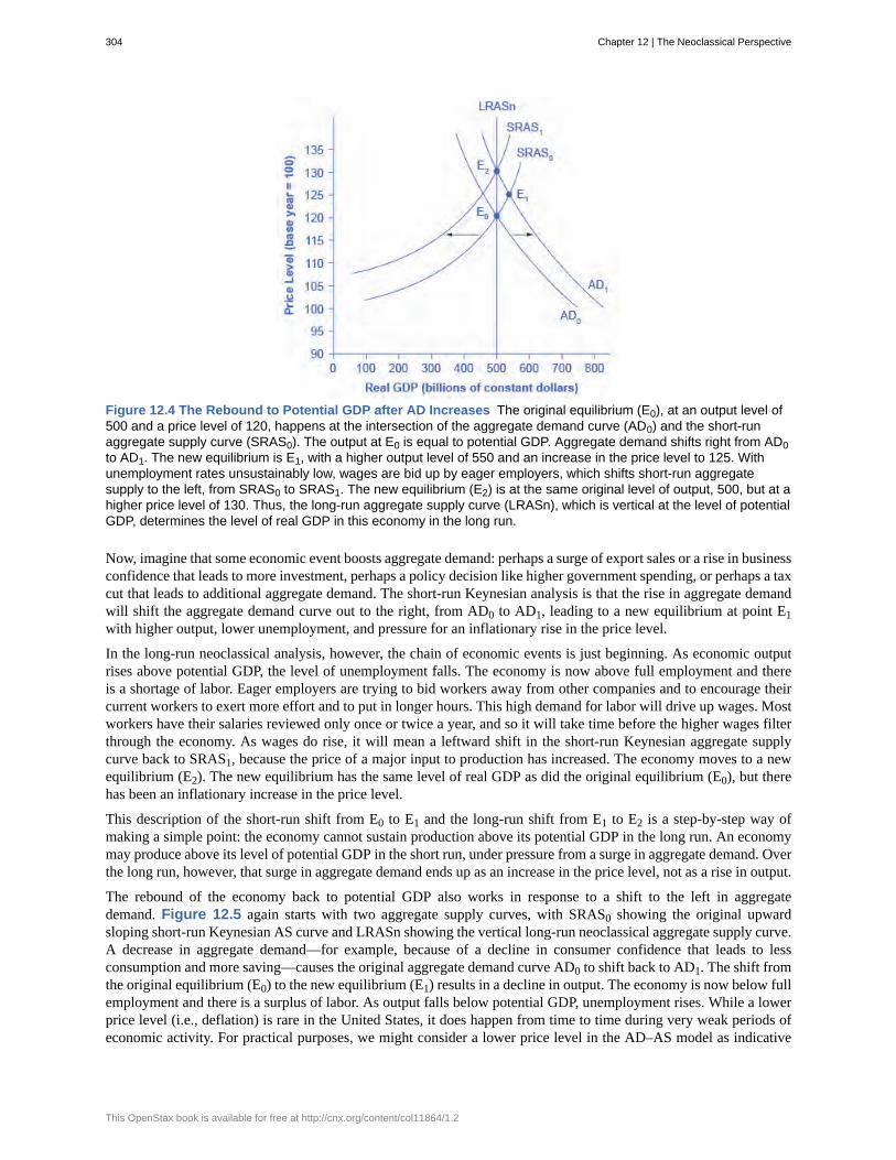
Figure 12.4 The Rebound to Potential GDP after AD Increases The original equilibrium (E0), at an output level of500 and a price level of 120, happens at the intersection of the aggregate demand curve (AD0) and the short-runaggregate supply curve (SRAS0). The output at E0 is equal to potential GDP. Aggregate demand shifts right from AD0to AD1. The new equilibrium is E1, with a higher output level of 550 and an increase in the price level to 125. Withunemployment rates unsustainably low, wages are bid up by eager employers, which shifts short-run aggregatesupply to the left, from SRAS0 to SRAS1. The new equilibrium (E2) is at the same original level of output, 500, but at ahigher price level of 130. Thus, the long-run aggregate supply curve (LRASn), which is vertical at the level of potentialGDP, determines the level of real GDP in this economy in the long run.
Now, imagine that some economic event boosts aggregate demand: perhaps a surge of export sales or a rise in businessconfidence that leads to more investment, perhaps a policy decision like higher government spending, or perhaps a taxcut that leads to additional aggregate demand. The short-run Keynesian analysis is that the rise in aggregate demandwill shift the aggregate demand curve out to the right, from AD0 to AD1, leading to a new equilibrium at point E1with higher output, lower unemployment, and pressure for an inflationary rise in the price level.
In the long-run neoclassical analysis, however, the chain of economic events is just beginning. As economic outputrises above potential GDP, the level of unemployment falls. The economy is now above full employment and thereis a shortage of labor. Eager employers are trying to bid workers away from other companies and to encourage theircurrent workers to exert more effort and to put in longer hours. This high demand for labor will drive up wages. Mostworkers have their salaries reviewed only once or twice a year, and so it will take time before the higher wages filterthrough the economy. As wages do rise, it will mean a leftward shift in the short-run Keynesian aggregate supplycurve back to SRAS1, because the price of a major input to production has increased. The economy moves to a newequilibrium (E2). The new equilibrium has the same level of real GDP as did the original equilibrium (E0), but therehas been an inflationary increase in the price level.
This description of the short-run shift from E0 to E1 and the long-run shift from E1 to E2 is a step-by-step way ofmaking a simple point: the economy cannot sustain production above its potential GDP in the long run. An economymay produce above its level of potential GDP in the short run, under pressure from a surge in aggregate demand. Overthe long run, however, that surge in aggregate demand ends up as an increase in the price level, not as a rise in output.
The rebound of the economy back to potential GDP also works in response to a shift to the left in aggregatedemand. Figure 12.5 again starts with two aggregate supply curves, with SRAS0 showing the original upwardsloping short-run Keynesian AS curve and LRASn showing the vertical long-run neoclassical aggregate supply curve.A decrease in aggregate demand—for example, because of a decline in consumer confidence that leads to lessconsumption and more saving—causes the original aggregate demand curve AD0 to shift back to AD1. The shift fromthe original equilibrium (E0) to the new equilibrium (E1) results in a decline in output. The economy is now below fullemployment and there is a surplus of labor. As output falls below potential GDP, unemployment rises. While a lowerprice level (i.e., deflation) is rare in the United States, it does happen from time to time during very weak periods ofeconomic activity. For practical purposes, we might consider a lower price level in the AD–AS model as indicative
304 Chapter 12 | The Neoclassical Perspective
This OpenStax book is available for free at http://cnx.org/content/col11864/1.2
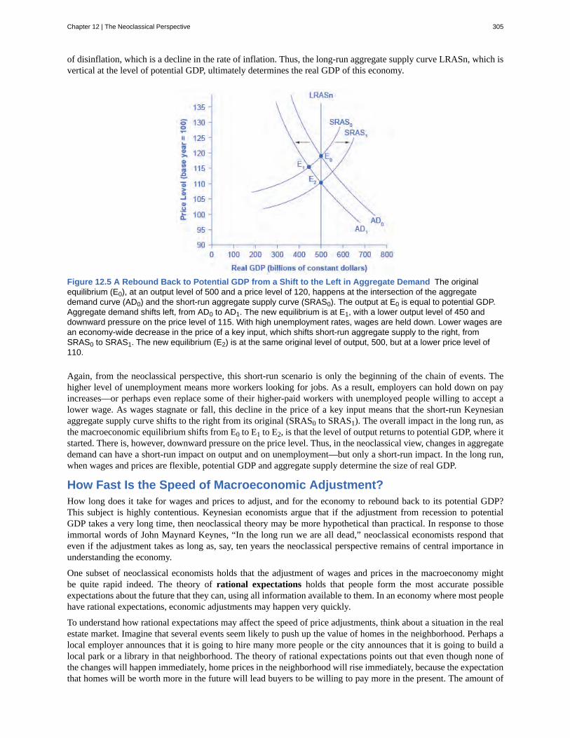
of disinflation, which is a decline in the rate of inflation. Thus, the long-run aggregate supply curve LRASn, which isvertical at the level of potential GDP, ultimately determines the real GDP of this economy.
Figure 12.5 A Rebound Back to Potential GDP from a Shift to the Left in Aggregate Demand The originalequilibrium (E0), at an output level of 500 and a price level of 120, happens at the intersection of the aggregatedemand curve (AD0) and the short-run aggregate supply curve (SRAS0). The output at E0 is equal to potential GDP.Aggregate demand shifts left, from AD0 to AD1. The new equilibrium is at E1, with a lower output level of 450 anddownward pressure on the price level of 115. With high unemployment rates, wages are held down. Lower wages arean economy-wide decrease in the price of a key input, which shifts short-run aggregate supply to the right, fromSRAS0 to SRAS1. The new equilibrium (E2) is at the same original level of output, 500, but at a lower price level of110.
Again, from the neoclassical perspective, this short-run scenario is only the beginning of the chain of events. Thehigher level of unemployment means more workers looking for jobs. As a result, employers can hold down on payincreases—or perhaps even replace some of their higher-paid workers with unemployed people willing to accept alower wage. As wages stagnate or fall, this decline in the price of a key input means that the short-run Keynesianaggregate supply curve shifts to the right from its original (SRAS0 to SRAS1). The overall impact in the long run, asthe macroeconomic equilibrium shifts from E0 to E1 to E2, is that the level of output returns to potential GDP, where itstarted. There is, however, downward pressure on the price level. Thus, in the neoclassical view, changes in aggregatedemand can have a short-run impact on output and on unemployment—but only a short-run impact. In the long run,when wages and prices are flexible, potential GDP and aggregate supply determine the size of real GDP.
How Fast Is the Speed of Macroeconomic Adjustment?How long does it take for wages and prices to adjust, and for the economy to rebound back to its potential GDP?This subject is highly contentious. Keynesian economists argue that if the adjustment from recession to potentialGDP takes a very long time, then neoclassical theory may be more hypothetical than practical. In response to thoseimmortal words of John Maynard Keynes, “In the long run we are all dead,” neoclassical economists respond thateven if the adjustment takes as long as, say, ten years the neoclassical perspective remains of central importance inunderstanding the economy.
One subset of neoclassical economists holds that the adjustment of wages and prices in the macroeconomy mightbe quite rapid indeed. The theory of rational expectations holds that people form the most accurate possibleexpectations about the future that they can, using all information available to them. In an economy where most peoplehave rational expectations, economic adjustments may happen very quickly.
To understand how rational expectations may affect the speed of price adjustments, think about a situation in the realestate market. Imagine that several events seem likely to push up the value of homes in the neighborhood. Perhaps alocal employer announces that it is going to hire many more people or the city announces that it is going to build alocal park or a library in that neighborhood. The theory of rational expectations points out that even though none ofthe changes will happen immediately, home prices in the neighborhood will rise immediately, because the expectationthat homes will be worth more in the future will lead buyers to be willing to pay more in the present. The amount of
Chapter 12 | The Neoclassical Perspective 305

the immediate increase in home prices will depend on how likely it seems that the announcements about the futurewill actually happen and on how distant the local jobs and neighborhood improvements are in the future. The keypoint is that, because of rational expectations, prices do not wait on events, but adjust immediately.
At a macroeconomic level, the theory of rational expectations points out that if the aggregate supply curve is verticalover time, then people should rationally expect this pattern. When a shift in aggregate demand occurs, people andbusinesses with rational expectations will know that its impact on output and employment will be temporary, while itsimpact on the price level will be permanent. If firms and workers perceive the outcome of the process in advance, andif all firms and workers know that everyone else is perceiving the process in the same way, then they have no incentiveto go through an extended series of short-run scenarios, like a firm first hiring more people when aggregate demandshifts out and then firing those same people when aggregate supply shifts back. Instead, everyone will recognizewhere this process is heading—toward a change in the price level—and then will act on that expectation. In thisscenario, the expected long-run change in the price level may happen very quickly, without a drawn-out zigzag ofoutput and employment first moving one way and then the other.
The theory that people and firms have rational expectations can be a useful simplification, but as a statement abouthow people and businesses actually behave, the assumption seems too strong. After all, many people and firms arenot especially well informed, either about what is happening in the economy or about how the economy works.An alternate assumption is that people and firms act with adaptive expectations: they look at past experience andgradually adapt their beliefs and behavior as circumstances change, but are not perfect synthesizers of information andaccurate predictors of the future in the sense of rational expectations theory. If most people and businesses have someform of adaptive expectations, then the adjustment from the short run and long run will be traced out in incrementalsteps that occur over time.
The empirical evidence on the speed of macroeconomic adjustment of prices and wages is not clear-cut. Indeed, thespeed of macroeconomic adjustment probably varies among different countries and time periods. A reasonable guessis that the initial short-run effect of a shift in aggregate demand might last two to five years, before the adjustmentsin wages and prices cause the economy to adjust back to potential GDP. Thus, one might think of the short run forapplying Keynesian analysis as time periods less than two to five years, and the long run for applying neoclassicalanalysis as longer than five years. For practical purposes, this guideline is frustratingly imprecise, but when analyzinga complex social mechanism like an economy as it evolves over time, some imprecision seems unavoidable.
12.2 | The Policy Implications of the NeoclassicalPerspectiveBy the end of this section, you will be able to:
• Discuss why and how inflation expectations are measured• Analyze the impacts of fiscal policy and monetary policy on aggregate supply and aggregate demand• Explain the neoclassical Phillips curve, noting its tradeoff between inflation and unemployment• Identify clear distinctions between neoclassical economics and Keynesian economics
To understand the policy recommendations of the neoclassical economists, it helps to start with the Keynesianperspective. Suppose a decrease in aggregate demand causes the economy to go into recession with highunemployment. The Keynesian response would be to use government policy to stimulate aggregate demand andeliminate the recessionary gap. The neoclassical economists believe that the Keynesian response, while perhaps wellintentioned, will not have a good outcome for reasons we will discuss shortly. Since the neoclassical economistsbelieve that the economy will correct itself over time, the only advantage of a Keynesian stabilization policy wouldbe to speed up the process and minimize the time that the unemployed are out of work. Is that the likely outcome?
Keynesian macroeconomic policy requires some optimism about the ability of the government to recognize a situationof too little or too much aggregate demand, and to adjust aggregate demand accordingly with the right level ofchanges in taxes or spending, all enacted in a timely fashion. After all, neoclassical economists argue, it takesgovernment statisticians months to produce even preliminary estimates of GDP so that politicians know whether arecession is occurring—and those preliminary estimates may be revised substantially later. Moreover, there is thequestion of timely action. The political process can take more months to enact a tax cut or a spending increase; the
306 Chapter 12 | The Neoclassical Perspective
This OpenStax book is available for free at http://cnx.org/content/col11864/1.2
amount of those tax or spending changes may be determined as much by political considerations as economic ones;and then the economy will take still more months to put changes in aggregate demand into effect through spendingand production. When all of these time lags and political realities are considered, active fiscal policy may fail toaddress the current problem, and could even make the future economy worse. The average U.S. post-World War IIrecession has lasted only about a year. By the time government policy kicks in, the recession will likely be over. As aconsequence, the only result of government fine-tuning will be to stimulate the economy when it is already recovering(or to contract the economy when it is already falling). In other words, an active macroeconomic policy is likelyto exacerbate the cycles rather than dampen them. Indeed, some neoclassical economists believe a large part of thebusiness cycles we observe are due to flawed government policy. To learn about this issue further, read the followingClear It Up feature.
Why and how are inflation expectations measured?People take expectations about inflation into consideration every time they make a major purchase, suchas a house or a car. As inflation fluctuates, so too does the nominal interest rate on loans to buy thesegoods. The nominal interest rate is comprised of the real rate, plus an expected inflation factor. Expectedinflation also tells economists about how the public views the direction of the economy. Suppose the publicexpects inflation to increase. This could be the result of positive demand shock due to an expanding economyand increasing aggregate demand. It could also be the result of a negative supply shock, perhaps fromrising energy prices, and decreasing aggregate supply. In either case, the public may expect the centralbank to engage in contractionary monetary policy to reduce inflation, and this policy results in higher interestrates. If, on the other hand, inflation is expected to decrease, the public may anticipate a recession. In turn,the public may expect expansionary monetary policy, and the lowering of interest rates, in the short run.By monitoring expected inflation, economists garner information about the effectiveness of macroeconomicpolicies. Additionally, monitoring expected inflation allows for projecting the direction of real interest ratesthat isolate for the effect of inflation. This information is necessary for making decisions about financinginvestments.
Expectations about inflation may seem like a highly theoretical concept, but, in fact, inflation expectationsare measured by the Federal Reserve Bank based upon early research conducted by Joseph Livingston,a financial journalist for the Philadelphia Inquirer. In 1946, he started a twice-a-year survey of economistsabout their expectations of inflation. After Livingston's death in 1969, the survey was continued by the FederalReserve Bank and other economic research agencies such as the Survey Research Center at the Universityof Michigan, the American Statistical Association, and the National Bureau of Economic Research.
Current research by the Federal Reserve compares these expectations to actual inflation that has occurred,and the results, so far, are mixed. Economists' forecasts, however, have become notably more accurate inthe last few decades. Economists are actively researching how expectations of inflation and other economicvariables are formed and changed.
Visit this website (http://openstaxcollege.org/l/Haubrich) to read “The Federal Reserve Bank of Cleveland’sEconomic Commentary: A New Approach to Gauging Inflation Expectations” by Joseph G. Haubrich for moreinformation about how expected inflation is forecast.
Chapter 12 | The Neoclassical Perspective 307
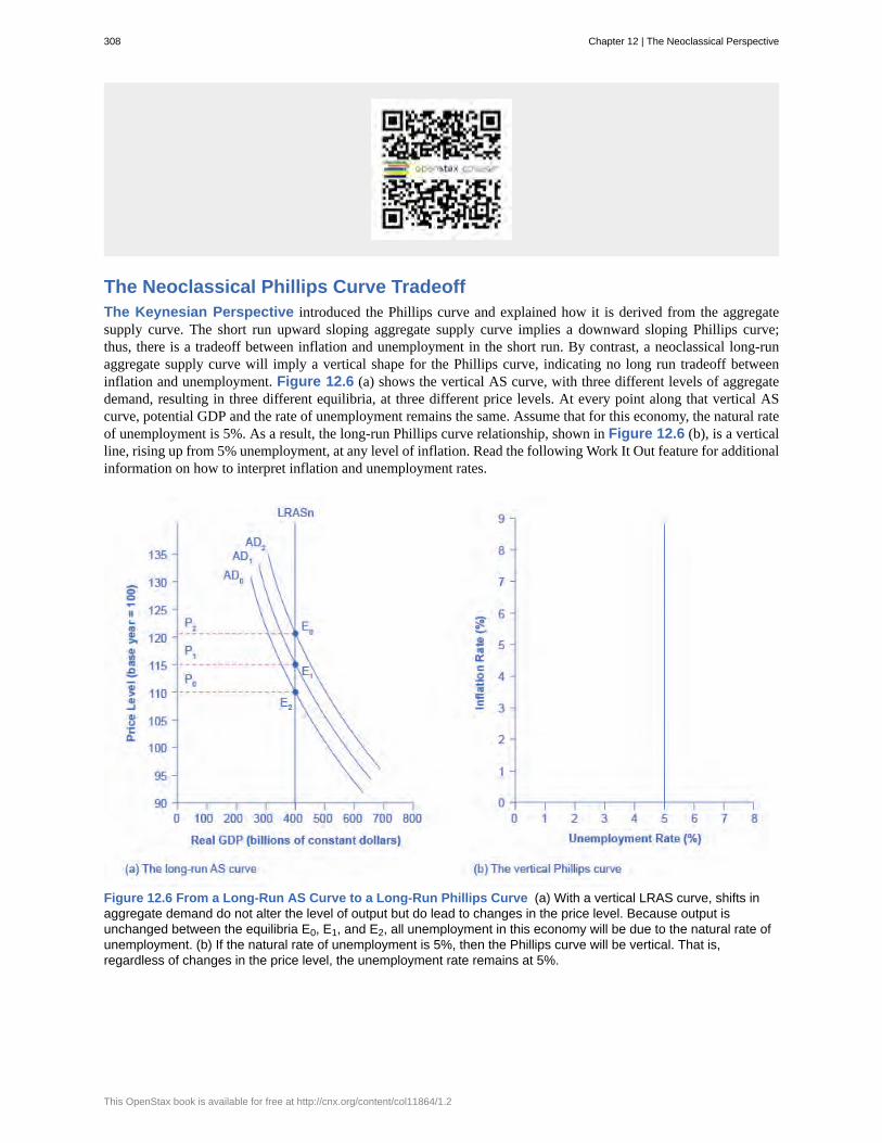
The Neoclassical Phillips Curve TradeoffThe Keynesian Perspective introduced the Phillips curve and explained how it is derived from the aggregatesupply curve. The short run upward sloping aggregate supply curve implies a downward sloping Phillips curve;thus, there is a tradeoff between inflation and unemployment in the short run. By contrast, a neoclassical long-runaggregate supply curve will imply a vertical shape for the Phillips curve, indicating no long run tradeoff betweeninflation and unemployment. Figure 12.6 (a) shows the vertical AS curve, with three different levels of aggregatedemand, resulting in three different equilibria, at three different price levels. At every point along that vertical AScurve, potential GDP and the rate of unemployment remains the same. Assume that for this economy, the natural rateof unemployment is 5%. As a result, the long-run Phillips curve relationship, shown in Figure 12.6 (b), is a verticalline, rising up from 5% unemployment, at any level of inflation. Read the following Work It Out feature for additionalinformation on how to interpret inflation and unemployment rates.
Figure 12.6 From a Long-Run AS Curve to a Long-Run Phillips Curve (a) With a vertical LRAS curve, shifts inaggregate demand do not alter the level of output but do lead to changes in the price level. Because output isunchanged between the equilibria E0, E1, and E2, all unemployment in this economy will be due to the natural rate ofunemployment. (b) If the natural rate of unemployment is 5%, then the Phillips curve will be vertical. That is,regardless of changes in the price level, the unemployment rate remains at 5%.
308 Chapter 12 | The Neoclassical Perspective
This OpenStax book is available for free at http://cnx.org/content/col11864/1.2
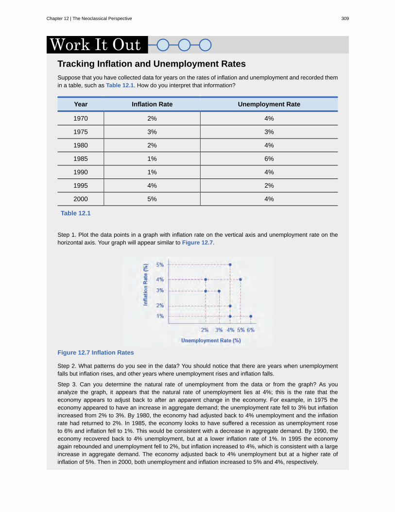
Tracking Inflation and Unemployment RatesSuppose that you have collected data for years on the rates of inflation and unemployment and recorded themin a table, such as Table 12.1. How do you interpret that information?
Year Inflation Rate Unemployment Rate
1970 2% 4%
1975 3% 3%
1980 2% 4%
1985 1% 6%
1990 1% 4%
1995 4% 2%
2000 5% 4%
Table 12.1
Step 1. Plot the data points in a graph with inflation rate on the vertical axis and unemployment rate on thehorizontal axis. Your graph will appear similar to Figure 12.7.
Figure 12.7 Inflation Rates
Step 2. What patterns do you see in the data? You should notice that there are years when unemploymentfalls but inflation rises, and other years where unemployment rises and inflation falls.
Step 3. Can you determine the natural rate of unemployment from the data or from the graph? As youanalyze the graph, it appears that the natural rate of unemployment lies at 4%; this is the rate that theeconomy appears to adjust back to after an apparent change in the economy. For example, in 1975 theeconomy appeared to have an increase in aggregate demand; the unemployment rate fell to 3% but inflationincreased from 2% to 3%. By 1980, the economy had adjusted back to 4% unemployment and the inflationrate had returned to 2%. In 1985, the economy looks to have suffered a recession as unemployment roseto 6% and inflation fell to 1%. This would be consistent with a decrease in aggregate demand. By 1990, theeconomy recovered back to 4% unemployment, but at a lower inflation rate of 1%. In 1995 the economyagain rebounded and unemployment fell to 2%, but inflation increased to 4%, which is consistent with a largeincrease in aggregate demand. The economy adjusted back to 4% unemployment but at a higher rate ofinflation of 5%. Then in 2000, both unemployment and inflation increased to 5% and 4%, respectively.
Chapter 12 | The Neoclassical Perspective 309
Step 4. Do you see the Phillips curve(s) in the data? If we trace the downward sloping trend of data points,we could see a short-run Phillips curve that exhibits the inverse tradeoff between higher unemployment andlower inflation rates. If we trace the vertical line of data points, we could see a long-run Phillips curve at the4% natural rate of unemployment.
The unemployment rate on the long-run Phillips curve will be the natural rate of unemployment. A small inflationaryincrease in the price level from AD0 to AD1 will have the same natural rate of unemployment as a larger inflationaryincrease in the price level from AD0 to AD2. The macroeconomic equilibrium along the vertical aggregate supplycurve can occur at a variety of different price levels, and the natural rate of unemployment can be consistent with alldifferent rates of inflation. The great economist Milton Friedman (1912–2006) summed up the neoclassical view ofthe long-term Phillips curve tradeoff in a 1967 speech: “[T]here is always a temporary trade-off between inflation andunemployment; there is no permanent trade-off.”
In the Keynesian perspective, the primary focus is on getting the level of aggregate demand right in relationshipto an upward-sloping aggregate supply curve. That is, AD should be adjusted so that the economy produces at itspotential GDP, not so low that cyclical unemployment results and not so high that inflation results. In the neoclassicalperspective, aggregate supply will determine output at potential GDP, unemployment is determined by the naturalrate of unemployment churned out by the forces of supply and demand in the labor market, and shifts in aggregatedemand are the primary determinant of changes in the price level.
Visit this website (http://openstaxcollege.org/l/modeledbehavior) to read about the effects of economicintervention.
Fighting Unemployment or Inflation?As explained in Unemployment, unemployment can be divided into two categories: cyclical unemployment and thenatural rate of unemployment, which is the sum of frictional and structural unemployment. Cyclical unemploymentresults from fluctuations in the business cycle and is created when the economy is producing below potentialGDP—giving potential employers less incentive to hire. When the economy is producing at potential GDP, cyclicalunemployment will be zero. Because of the dynamics of the labor market, in which people are always entering orexiting the labor force, the unemployment rate never falls to 0%, not even when the economy is producing at oreven slightly above potential GDP. Probably the best we can hope for is for the number of job vacancies to equal thenumber of job seekers. We know that it takes time for job seekers and employers to find each other, and this time isthe cause of frictional unemployment. Most economists do not consider frictional unemployment to be a “bad” thing.After all, there will always be workers who are unemployed while looking for a job that is a better match for theirskills. There will always be employers that have an open position, while looking for a worker that is a better match forthe job. Ideally, these matches happen quickly, but even when the economy is very strong there will be some naturalunemployment and this is what is measured by the natural rate of unemployment.
The neoclassical view of unemployment tends to focus attention away from the problem of cyclicalunemployment—that is, unemployment caused by recession—while putting more attention on the issue of the ratesof unemployment that prevail even when the economy is operating at potential GDP. To put it another way, theneoclassical view of unemployment tends to focus on how public policy can be adjusted to reduce the natural rate
310 Chapter 12 | The Neoclassical Perspective
This OpenStax book is available for free at http://cnx.org/content/col11864/1.2
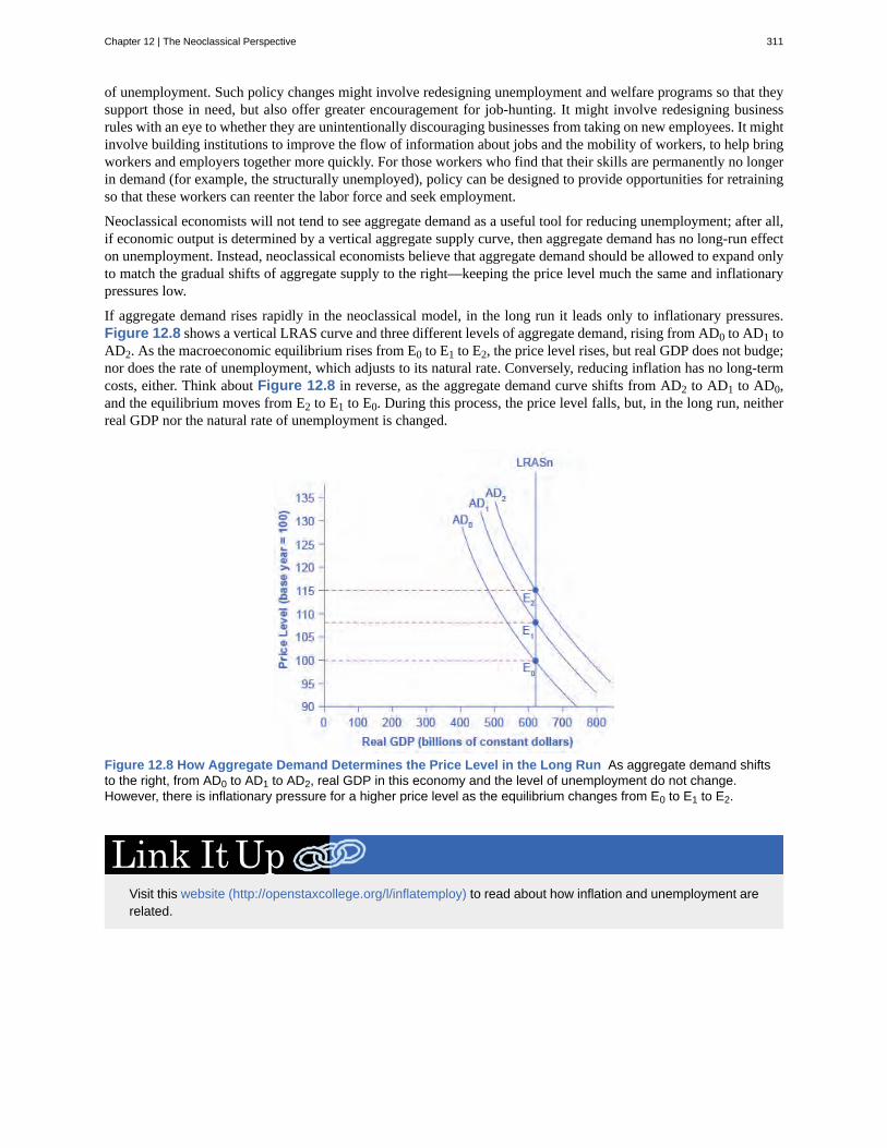
of unemployment. Such policy changes might involve redesigning unemployment and welfare programs so that theysupport those in need, but also offer greater encouragement for job-hunting. It might involve redesigning businessrules with an eye to whether they are unintentionally discouraging businesses from taking on new employees. It mightinvolve building institutions to improve the flow of information about jobs and the mobility of workers, to help bringworkers and employers together more quickly. For those workers who find that their skills are permanently no longerin demand (for example, the structurally unemployed), policy can be designed to provide opportunities for retrainingso that these workers can reenter the labor force and seek employment.
Neoclassical economists will not tend to see aggregate demand as a useful tool for reducing unemployment; after all,if economic output is determined by a vertical aggregate supply curve, then aggregate demand has no long-run effecton unemployment. Instead, neoclassical economists believe that aggregate demand should be allowed to expand onlyto match the gradual shifts of aggregate supply to the right—keeping the price level much the same and inflationarypressures low.
If aggregate demand rises rapidly in the neoclassical model, in the long run it leads only to inflationary pressures.Figure 12.8 shows a vertical LRAS curve and three different levels of aggregate demand, rising from AD0 to AD1 toAD2. As the macroeconomic equilibrium rises from E0 to E1 to E2, the price level rises, but real GDP does not budge;nor does the rate of unemployment, which adjusts to its natural rate. Conversely, reducing inflation has no long-termcosts, either. Think about Figure 12.8 in reverse, as the aggregate demand curve shifts from AD2 to AD1 to AD0,and the equilibrium moves from E2 to E1 to E0. During this process, the price level falls, but, in the long run, neitherreal GDP nor the natural rate of unemployment is changed.
Figure 12.8 How Aggregate Demand Determines the Price Level in the Long Run As aggregate demand shiftsto the right, from AD0 to AD1 to AD2, real GDP in this economy and the level of unemployment do not change.However, there is inflationary pressure for a higher price level as the equilibrium changes from E0 to E1 to E2.
Visit this website (http://openstaxcollege.org/l/inflatemploy) to read about how inflation and unemployment arerelated.
Chapter 12 | The Neoclassical Perspective 311
Fighting Recession or Encouraging Long-Term Growth?Neoclassical economists believe that the economy will rebound out of a recession or eventually contract duringan expansion because prices and wage rates are flexible and will adjust either upward or downward to restore theeconomy to its potential GDP. Thus, the key policy question for neoclassicals is how to promote growth of potentialGDP. We know that economic growth ultimately depends on the growth rate of long-term productivity. Productivitymeasures how effective inputs are at producing outputs. We know that U.S. productivity has grown on average about2% per year. That means that the same amount of inputs produce 2% more output than the year before. We also knowthat productivity growth varies a great deal in the short term due to cyclical factors. It also varies somewhat in thelong term. From 1953–1972, U.S. labor productivity (as measured by output per hour in the business sector) grew at3.2% per year. From 1973–1992, productivity growth declined significantly to 1.8% per year. Then, from 1993–2014,productivity growth increased slightly to 2% per year. The neoclassical economists believe the underpinnings of long-run productivity growth to be an economy’s investments in human capital, physical capital, and technology, operatingtogether in a market-oriented environment that rewards innovation. Promotion of these factors is what governmentpolicy should focus on.
Summary of Neoclassical Macroeconomic Policy RecommendationsLet’s summarize what neoclassical economists recommend for macroeconomic policy. Neoclassical economists donot believe in “fine-tuning” the economy. They believe that economic growth is fostered by a stable economicenvironment with a low rate of inflation. Similarly, tax rates should be low and unchanging. In this environment,private economic agents can make the best possible investment decisions, which will lead to optimal investment inphysical and human capital as well as research and development to promote improvements in technology.
Summary of Neoclassical Economics versus Keynesian EconomicsTable 12.2 summarizes the key differences between the two schools of thought.
Summary Neoclassical Economics Keynesian Economics
Focus: long-term or short term Long-term Short-term
Prices and wages: sticky orflexible?
Flexible Sticky
Economic output: Primarilydetermined by aggregate demandor aggregate supply?
Aggregate supply Aggregate demand
Aggregate supply: vertical orupward-sloping?
Vertical Upward-sloping
Phillips curve vertical ordownward-sloping
Vertical Downward sloping
Table 12.2 Neoclassical versus Keynesian Economics
312 Chapter 12 | The Neoclassical Perspective
This OpenStax book is available for free at http://cnx.org/content/col11864/1.2
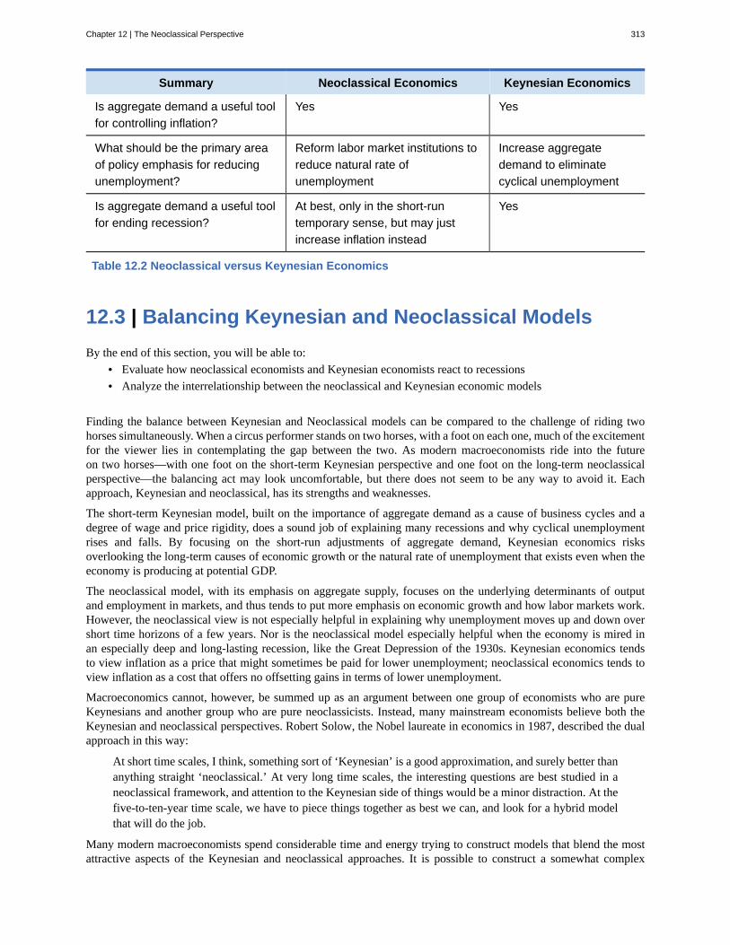
Summary Neoclassical Economics Keynesian Economics
Is aggregate demand a useful toolfor controlling inflation?
Yes Yes
What should be the primary areaof policy emphasis for reducingunemployment?
Reform labor market institutions toreduce natural rate ofunemployment
Increase aggregatedemand to eliminatecyclical unemployment
Is aggregate demand a useful toolfor ending recession?
At best, only in the short-runtemporary sense, but may justincrease inflation instead
Yes
Table 12.2 Neoclassical versus Keynesian Economics
12.3 | Balancing Keynesian and Neoclassical ModelsBy the end of this section, you will be able to:
• Evaluate how neoclassical economists and Keynesian economists react to recessions• Analyze the interrelationship between the neoclassical and Keynesian economic models
Finding the balance between Keynesian and Neoclassical models can be compared to the challenge of riding twohorses simultaneously. When a circus performer stands on two horses, with a foot on each one, much of the excitementfor the viewer lies in contemplating the gap between the two. As modern macroeconomists ride into the futureon two horses—with one foot on the short-term Keynesian perspective and one foot on the long-term neoclassicalperspective—the balancing act may look uncomfortable, but there does not seem to be any way to avoid it. Eachapproach, Keynesian and neoclassical, has its strengths and weaknesses.
The short-term Keynesian model, built on the importance of aggregate demand as a cause of business cycles and adegree of wage and price rigidity, does a sound job of explaining many recessions and why cyclical unemploymentrises and falls. By focusing on the short-run adjustments of aggregate demand, Keynesian economics risksoverlooking the long-term causes of economic growth or the natural rate of unemployment that exists even when theeconomy is producing at potential GDP.
The neoclassical model, with its emphasis on aggregate supply, focuses on the underlying determinants of outputand employment in markets, and thus tends to put more emphasis on economic growth and how labor markets work.However, the neoclassical view is not especially helpful in explaining why unemployment moves up and down overshort time horizons of a few years. Nor is the neoclassical model especially helpful when the economy is mired inan especially deep and long-lasting recession, like the Great Depression of the 1930s. Keynesian economics tendsto view inflation as a price that might sometimes be paid for lower unemployment; neoclassical economics tends toview inflation as a cost that offers no offsetting gains in terms of lower unemployment.
Macroeconomics cannot, however, be summed up as an argument between one group of economists who are pureKeynesians and another group who are pure neoclassicists. Instead, many mainstream economists believe both theKeynesian and neoclassical perspectives. Robert Solow, the Nobel laureate in economics in 1987, described the dualapproach in this way:
At short time scales, I think, something sort of ‘Keynesian’ is a good approximation, and surely better thananything straight ‘neoclassical.’ At very long time scales, the interesting questions are best studied in aneoclassical framework, and attention to the Keynesian side of things would be a minor distraction. At thefive-to-ten-year time scale, we have to piece things together as best we can, and look for a hybrid modelthat will do the job.
Many modern macroeconomists spend considerable time and energy trying to construct models that blend the mostattractive aspects of the Keynesian and neoclassical approaches. It is possible to construct a somewhat complex
Chapter 12 | The Neoclassical Perspective 313
mathematical model where aggregate demand and sticky wages and prices matter in the short run, but wages, prices,and aggregate supply adjust in the long run. However, creating an overall model that encompasses both short-termKeynesian and long-term neoclassical models is not easy.
Navigating Unchartered WatersWere the policies implemented to stabilize the economy and financial markets during the Great Recessioneffective? Many economists from both the Keynesian and neoclassical schools have found that they were,although to varying degrees. Alan Blinder of Princeton University and Mark Zandi for Moody’s Analytics foundthat, without fiscal policy, GDP decline would have been significantly more than its 3.3% in 2008 followedby its 0.1% decline in 2009. They also estimated that there would have been 8.5 million more job losseshad the government not intervened in the market with the TARP to support the financial industry and keyautomakers General Motors and Chrysler. Federal Reserve Bank economists Carlos Carvalho, Stefano Eusip,and Christian Grisse found in their study, Policy Initiatives in the Global Recession: What Did ForecastersExpect? that once policies were implemented, forecasters adapted their expectations to these policies. Theywere more likely to anticipate increases in investment due to lower interest rates brought on by monetarypolicy and increased economic growth resulting from fiscal policy.
The difficulty with evaluating the effectiveness of the stabilization policies that were taken in response to theGreat Recession is that we will never know what would have happened had those policies not have beenimplemented. Surely some of the programs were more effective at creating and saving jobs, while otherprograms were less so. The final conclusion on the effectiveness of macroeconomic policies is still up fordebate, and further study will no doubt consider the impact of these policies on the U.S. budget and deficit, aswell as the value of the U.S. dollar in the financial market.
314 Chapter 12 | The Neoclassical Perspective
This OpenStax book is available for free at http://cnx.org/content/col11864/1.2
adaptive expectations
expected inflation
neoclassical perspective
physical capital per person
rational expectations
KEY TERMS
the theory that people look at past experience and gradually adapt their beliefs and behavior ascircumstances change
a future rate of inflation that consumers and firms build into current decision making
the philosophy that, in the long run, the business cycle will fluctuate around the potential,or full-employment, level of output
the amount and kind of machinery and equipment available to help a person produce agood or service
the theory that people form the most accurate possible expectations about the future that theycan, using all information available to them
KEY CONCEPTS AND SUMMARY
12.1 The Building Blocks of Neoclassical AnalysisNeoclassical perspective argues that, in the long run, the economy will adjust back to its potential GDP level of outputthrough flexible price levels. Thus, the neoclassical perspective views the long-run AS curve as vertical. A rationalexpectations perspective argues that people have excellent information about economic events and how the economyworks and that, as a result, price and other economic adjustments will happen very quickly. In adaptive expectationstheory, people have limited information about economic information and how the economy works, and so price andother economic adjustments can be slow.
12.2 The Policy Implications of the Neoclassical PerspectiveNeoclassical economists tend to put relatively more emphasis on long-term growth than on fighting recession,because they believe that recessions will fade in a few years and long-term growth will ultimately determine thestandard of living. They tend to focus more on reducing the natural rate of unemployment caused by economicinstitutions and government policies than the cyclical unemployment caused by recession.
Neoclassical economists also see no social benefit to inflation. With an upward-sloping Keynesian AS curve, inflationcan arise because an economy is approaching full employment. With a vertical long-run neoclassical AS curve,inflation does not accompany any rise in output. If aggregate supply is vertical, then aggregate demand does not affectthe quantity of output. Instead, aggregate demand can only cause inflationary changes in the price level. A verticalaggregate supply curve, where the quantity of output is consistent with many different price levels, also implies avertical Phillips curve.
12.3 Balancing Keynesian and Neoclassical ModelsThe Keynesian perspective considers changes to aggregate demand to be the cause of business cycle fluctuations.Keynesians are likely to advocate that policy makers actively attempt to reverse recessionary and inflationary periodsbecause they are not convinced that the self-correcting economy can easily return to full employment.
The neoclassical perspective places more emphasis on aggregate supply. The level of potential GDP is determinedby long term productivity growth and that the economy typically will return to full employment after a change inaggregate demand. Skeptical of the effectiveness and timeliness of Keynesian policy, neoclassical economists aremore likely to advocate a hands-off, or fairly limited, role for active stabilization policy.
While Keynesians would tend to advocate an acceptable tradeoff between inflation and unemployment whencounteracting a recession, neoclassical economists argue that no such tradeoff exists; any short-term gains in lowerunemployment will eventually vanish and the result of active policy will only be inflation.
SELF-CHECK QUESTIONS
Chapter 12 | The Neoclassical Perspective 315
1. Do rational expectations tend to look back at past experience while adaptive expectations look ahead to the future?Explain your answer.
2. Legislation proposes that the government should use macroeconomic policy to achieve an unemployment rate ofzero percent, by increasing aggregate demand for as much and as long as necessary to accomplish this goal. From aneoclassical perspective, how will this policy affect output and the price level in the short run and in the long run?Sketch an aggregate demand/aggregate supply diagram to illustrate your answer. Hint: revisit Figure 12.4.
3. Would it make sense to argue that rational expectations economics is an extreme version of neoclassicaleconomics? Explain.
4. Summarize the Keynesian and Neoclassical models.
REVIEW QUESTIONS
5. Does neoclassical economics focus on the long termor the short term? Explain your answer.
6. Does neoclassical economics view prices and wagesas sticky or flexible? Why?
7. What shape is the long-run aggregate supply curve?Why does it have this shape?
8. What is the difference between rational expectationsand adaptive expectations?
9. A neoclassical economist and a Keynesianeconomist are studying the economy of Vineland. Itappears that Vineland is beginning to experience a mildrecession with a decrease in aggregate demand. Whichof these two economists would likely advocate that thegovernment of Vineland take active measures to reversethis decline in aggregate demand? Why?
10. Do neoclassical economists tend to focus more onlong term economic growth or on recessions? Explainbriefly.
11. Do neoclassical economists tend to focus more oncyclical unemployment or on inflation? Explain briefly.
12. Do neoclassical economists see a value in toleratinga little more inflation if it brings additional economicoutput? Explain your answer.
13. If aggregate supply is vertical, what role doesaggregate demand play in determining output? Indetermining the price level?
14. What is the shape of the neoclassical long-runPhillips curve? What assumptions are made that lead tothis shape?
15. When the economy is experiencing a recession,why would a neoclassical economist be unlikely to arguefor aggressive policy to stimulate aggregate demand andreturn the economy to full employment? Explain youranswer.
16. If the economy is suffering through a rampantinflationary period, would a Keynesian economistadvocate for stabilization policy that involves highertaxes and higher interest rates? Explain your answer.
CRITICAL THINKING QUESTIONS
17. If most people have rational expectations, how longwill recessions last?
18. Explain why the neoclassical economists believethat nothing much needs to be done aboutunemployment. Do you agree or disagree? Explain.
19. The American Recovery and Reinvestment Act wascriticized by economists from all theoretical
persuasions. The “Stimulus Package” was arguably aKeynesian measure so why would a Keynesianeconomist be critical of it? Why would neoclassicaleconomists be critical?
20. Is it a logical contradiction to be a neoclassicalKeynesian? Explain.
PROBLEMS
316 Chapter 12 | The Neoclassical Perspective
This OpenStax book is available for free at http://cnx.org/content/col11864/1.2
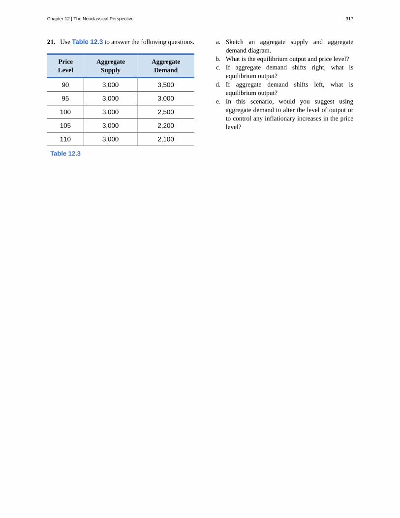
21. Use Table 12.3 to answer the following questions.
PriceLevel
AggregateSupply
AggregateDemand
90 3,000 3,500
95 3,000 3,000
100 3,000 2,500
105 3,000 2,200
110 3,000 2,100
Table 12.3
a. Sketch an aggregate supply and aggregatedemand diagram.
b. What is the equilibrium output and price level?c. If aggregate demand shifts right, what is
equilibrium output?d. If aggregate demand shifts left, what is
equilibrium output?e. In this scenario, would you suggest using
aggregate demand to alter the level of output orto control any inflationary increases in the pricelevel?
Chapter 12 | The Neoclassical Perspective 317
318 Chapter 12 | The Neoclassical Perspective
This OpenStax book is available for free at http://cnx.org/content/col11864/1.2
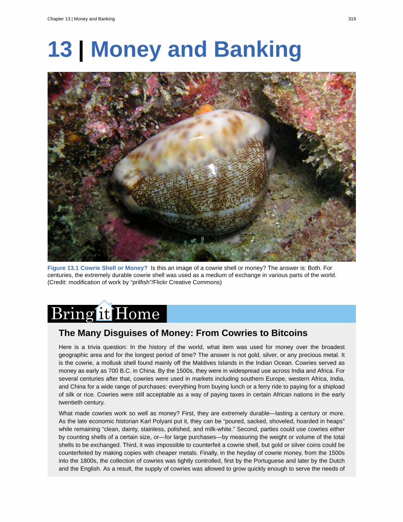
13 | Money and Banking
Figure 13.1 Cowrie Shell or Money? Is this an image of a cowrie shell or money? The answer is: Both. Forcenturies, the extremely durable cowrie shell was used as a medium of exchange in various parts of the world.(Credit: modification of work by “prilfish”/Flickr Creative Commons)
The Many Disguises of Money: From Cowries to BitcoinsHere is a trivia question: In the history of the world, what item was used for money over the broadestgeographic area and for the longest period of time? The answer is not gold, silver, or any precious metal. Itis the cowrie, a mollusk shell found mainly off the Maldives Islands in the Indian Ocean. Cowries served asmoney as early as 700 B.C. in China. By the 1500s, they were in widespread use across India and Africa. Forseveral centuries after that, cowries were used in markets including southern Europe, western Africa, India,and China for a wide range of purchases: everything from buying lunch or a ferry ride to paying for a shiploadof silk or rice. Cowries were still acceptable as a way of paying taxes in certain African nations in the earlytwentieth century.
What made cowries work so well as money? First, they are extremely durable—lasting a century or more.As the late economic historian Karl Polyani put it, they can be “poured, sacked, shoveled, hoarded in heaps”while remaining “clean, dainty, stainless, polished, and milk-white.” Second, parties could use cowries eitherby counting shells of a certain size, or—for large purchases—by measuring the weight or volume of the totalshells to be exchanged. Third, it was impossible to counterfeit a cowrie shell, but gold or silver coins could becounterfeited by making copies with cheaper metals. Finally, in the heyday of cowrie money, from the 1500sinto the 1800s, the collection of cowries was tightly controlled, first by the Portuguese and later by the Dutchand the English. As a result, the supply of cowries was allowed to grow quickly enough to serve the needs of
Chapter 13 | Money and Banking 319
commerce, but not so quickly that they were no longer scarce. Money throughout the ages has taken manydifferent forms and continues to evolve even today. What do you think money is?
Introduction to Money and BankingIn this chapter, you will learn about:
• Defining Money by Its Functions
• Measuring Money: Currency, M1, and M2
• The Role of Banks
• How Banks Create Money
The discussion of money and banking is a central component in the study of macroeconomics. At this point,you should have firmly in mind the main goals of macroeconomics from Welcome to Economics!: economicgrowth, low unemployment, and low inflation. We have yet to discuss money and its role in helping to achieve ourmacroeconomic goals.
You should also understand Keynesian and neoclassical frameworks for macroeconomic analysis and how theseframeworks can be embodied in the aggregate demand/aggregate supply (AD/AS) model. With the goals andframeworks for macroeconomic analysis in mind, the final step is to discuss the two main categories ofmacroeconomic policy: monetary policy, which focuses on money, banking and interest rates; and fiscal policy, whichfocuses on government spending, taxes, and borrowing. This chapter discusses what economists mean by money, andhow money is closely interrelated with the banking system. Monetary Policy and Bank Regulation furthers thisdiscussion.
13.1 | Defining Money by Its FunctionsBy the end of this section, you will be able to:
• Explain the various functions of money• Contrast commodity money and fiat money
Money for the sake of money is not an end in itself. You cannot eat dollar bills or wear your bank account. Ultimately,the usefulness of money rests in exchanging it for goods or services. As the American writer and humorist AmbroseBierce (1842–1914) wrote in 1911, money is a “blessing that is of no advantage to us excepting when we part with it.”Money is what people regularly use when purchasing or selling goods and services, and thus money must be widelyaccepted by both buyers and sellers. This concept of money is intentionally flexible, because money has taken a widevariety of forms in different cultures.
Barter and the Double Coincidence of WantsTo understand the usefulness of money, we must consider what the world would be like without money. Howwould people exchange goods and services? Economies without money typically engage in the barter system.Barter—literally trading one good or service for another—is highly inefficient for trying to coordinate the trades in amodern advanced economy. In an economy without money, an exchange between two people would involve a doublecoincidence of wants, a situation in which two people each want some good or service that the other person canprovide. For example, if an accountant wants a pair of shoes, this accountant must find someone who has a pair ofshoes in the correct size and who is willing to exchange the shoes for some hours of accounting services. Such a tradeis likely to be difficult to arrange. Think about the complexity of such trades in a modern economy, with its extensivedivision of labor that involves thousands upon thousands of different jobs and goods.
Another problem with the barter system is that it does not allow us to easily enter into future contracts for the purchaseof many goods and services. For example, if the goods are perishable it may be difficult to exchange them for othergoods in the future. Imagine a farmer wanting to buy a tractor in six months using a fresh crop of strawberries.
320 Chapter 13 | Money and Banking
This OpenStax book is available for free at http://cnx.org/content/col11864/1.2
Additionally, while the barter system might work adequately in small economies, it will keep these economies fromgrowing. The time that individuals would otherwise spend producing goods and services and enjoying leisure time isspent bartering.
Functions for MoneyMoney solves the problems created by the barter system. (We will get to its definition soon.) First, money serves as amedium of exchange, which means that money acts as an intermediary between the buyer and the seller. Instead ofexchanging accounting services for shoes, the accountant now exchanges accounting services for money. This moneyis then used to buy shoes. To serve as a medium of exchange, money must be very widely accepted as a method ofpayment in the markets for goods, labor, and financial capital.
Second, money must serve as a store of value. In a barter system, we saw the example of the shoemaker trading shoesfor accounting services. But she risks having her shoes go out of style, especially if she keeps them in a warehousefor future use—their value will decrease with each season. Shoes are not a good store of value. Holding money is amuch easier way of storing value. You know that you do not need to spend it immediately because it will still hold itsvalue the next day, or the next year. This function of money does not require that money is a perfect store of value. Inan economy with inflation, money loses some buying power each year, but it remains money.
Third, money serves as a unit of account, which means that it is the ruler by which other values are measured. Forexample, an accountant may charge $100 to file your tax return. That $100 can purchase two pair of shoes at $50 apair. Money acts as a common denominator, an accounting method that simplifies thinking about trade-offs.
Finally, another function of money is that money must serve as a standard of deferred payment. This means that ifmoney is usable today to make purchases, it must also be acceptable to make purchases today that will be paid in thefuture. Loans and future agreements are stated in monetary terms and the standard of deferred payment is what allowsus to buy goods and services today and pay in the future. So money serves all of these functions— it is a medium ofexchange, store of value, unit of account, and standard of deferred payment.
Commodity versus Fiat MoneyMoney has taken a wide variety of forms in different cultures. Gold, silver, cowrie shells, cigarettes, and even cocoabeans have been used as money. Although these items are used as commodity money, they also have a value fromuse as something other than money. Gold, for example, has been used throughout the ages as money although todayit is not used as money but rather is valued for its other attributes. Gold is a good conductor of electricity and is usedin the electronics and aerospace industry. Gold is also used in the manufacturing of energy efficient reflective glassfor skyscrapers and is used in the medical industry as well. Of course, gold also has value because of its beauty andmalleability in the creation of jewelry.
As commodity money, gold has historically served its purpose as a medium of exchange, a store of value, and as aunit of account. Commodity-backed currencies are dollar bills or other currencies with values backed up by goldor other commodity held at a bank. During much of its history, the money supply in the United States was backed bygold and silver. Interestingly, antique dollars dated as late as 1957, have “Silver Certificate” printed over the portraitof George Washington, as shown in Figure 13.2. This meant that the holder could take the bill to the appropriatebank and exchange it for a dollar’s worth of silver.
Chapter 13 | Money and Banking 321

Figure 13.2 A Silver Certificate and a Modern U.S. Bill Until 1958, silver certificates were commodity-backedmoney—backed by silver, as indicated by the words “Silver Certificate” printed on the bill. Today, U.S. bills are backedby the Federal Reserve, but as fiat money. (Credit: “The.Comedian”/Flickr Creative Commons)
As economies grew and became more global in nature, the use of commodity monies became more cumbersome.Countries moved towards the use of fiat money. Fiat money has no intrinsic value, but is declared by a governmentto be the legal tender of a country. The United States’ paper money, for example, carries the statement: “THIS NOTEIS LEGAL TENDER FOR ALL DEBTS, PUBLIC AND PRIVATE.” In other words, by government decree, if youowe a debt, then legally speaking, you can pay that debt with the U.S. currency, even though it is not backed by acommodity. The only backing of our money is universal faith and trust that the currency has value, and nothing more.
Watch this video (http://openstaxcollege.org/l/moneyhistory) on the “History of Money.”
13.2 | Measuring Money: Currency, M1, and M2By the end of this section, you will be able to:
• Contrast M1 money supply and M2 money supply• Classify monies as M1 money supply or M2 money supply
Cash in your pocket certainly serves as money. But what about checks or credit cards? Are they money, too? Ratherthan trying to state a single way of measuring money, economists offer broader definitions of money based onliquidity. Liquidity refers to how quickly a financial asset can be used to buy a good or service. For example, cash isvery liquid. Your $10 bill can be easily used to buy a hamburger at lunchtime. However, $10 that you have in your
322 Chapter 13 | Money and Banking
This OpenStax book is available for free at http://cnx.org/content/col11864/1.2
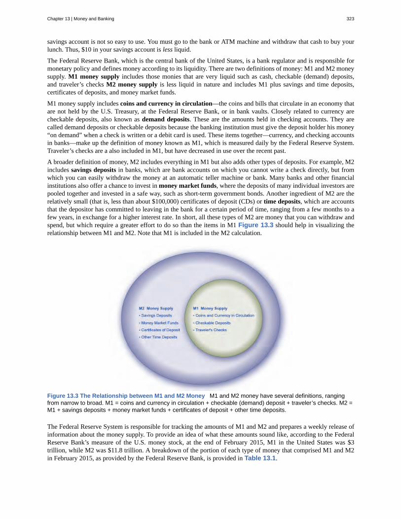
savings account is not so easy to use. You must go to the bank or ATM machine and withdraw that cash to buy yourlunch. Thus, $10 in your savings account is less liquid.
The Federal Reserve Bank, which is the central bank of the United States, is a bank regulator and is responsible formonetary policy and defines money according to its liquidity. There are two definitions of money: M1 and M2 moneysupply. M1 money supply includes those monies that are very liquid such as cash, checkable (demand) deposits,and traveler’s checks M2 money supply is less liquid in nature and includes M1 plus savings and time deposits,certificates of deposits, and money market funds.
M1 money supply includes coins and currency in circulation—the coins and bills that circulate in an economy thatare not held by the U.S. Treasury, at the Federal Reserve Bank, or in bank vaults. Closely related to currency arecheckable deposits, also known as demand deposits. These are the amounts held in checking accounts. They arecalled demand deposits or checkable deposits because the banking institution must give the deposit holder his money“on demand” when a check is written or a debit card is used. These items together—currency, and checking accountsin banks—make up the definition of money known as M1, which is measured daily by the Federal Reserve System.Traveler’s checks are a also included in M1, but have decreased in use over the recent past.
A broader definition of money, M2 includes everything in M1 but also adds other types of deposits. For example, M2includes savings deposits in banks, which are bank accounts on which you cannot write a check directly, but fromwhich you can easily withdraw the money at an automatic teller machine or bank. Many banks and other financialinstitutions also offer a chance to invest in money market funds, where the deposits of many individual investors arepooled together and invested in a safe way, such as short-term government bonds. Another ingredient of M2 are therelatively small (that is, less than about $100,000) certificates of deposit (CDs) or time deposits, which are accountsthat the depositor has committed to leaving in the bank for a certain period of time, ranging from a few months to afew years, in exchange for a higher interest rate. In short, all these types of M2 are money that you can withdraw andspend, but which require a greater effort to do so than the items in M1 Figure 13.3 should help in visualizing therelationship between M1 and M2. Note that M1 is included in the M2 calculation.
Figure 13.3 The Relationship between M1 and M2 Money M1 and M2 money have several definitions, rangingfrom narrow to broad. M1 = coins and currency in circulation + checkable (demand) deposit + traveler’s checks. M2 =M1 + savings deposits + money market funds + certificates of deposit + other time deposits.
The Federal Reserve System is responsible for tracking the amounts of M1 and M2 and prepares a weekly release ofinformation about the money supply. To provide an idea of what these amounts sound like, according to the FederalReserve Bank’s measure of the U.S. money stock, at the end of February 2015, M1 in the United States was $3trillion, while M2 was $11.8 trillion. A breakdown of the portion of each type of money that comprised M1 and M2in February 2015, as provided by the Federal Reserve Bank, is provided in Table 13.1.
Chapter 13 | Money and Banking 323
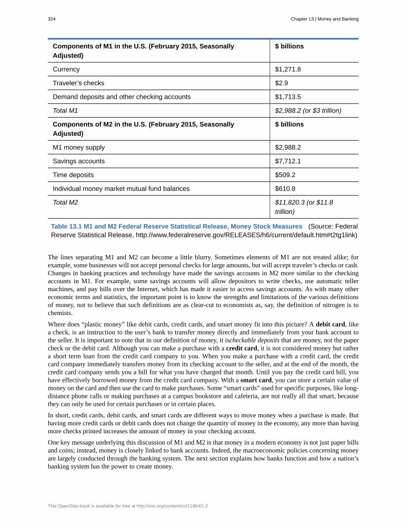
Components of M1 in the U.S. (February 2015, SeasonallyAdjusted)
$ billions
Currency $1,271.8
Traveler’s checks $2.9
Demand deposits and other checking accounts $1,713.5
Total M1 $2,988.2 (or $3 trillion)
Components of M2 in the U.S. (February 2015, SeasonallyAdjusted)
$ billions
M1 money supply $2,988.2
Savings accounts $7,712.1
Time deposits $509.2
Individual money market mutual fund balances $610.8
Total M2 $11,820.3 (or $11.8trillion)
Table 13.1 M1 and M2 Federal Reserve Statistical Release, Money Stock Measures (Source: FederalReserve Statistical Release, http://www.federalreserve.gov/RELEASES/h6/current/default.htm#t2tg1link)
The lines separating M1 and M2 can become a little blurry. Sometimes elements of M1 are not treated alike; forexample, some businesses will not accept personal checks for large amounts, but will accept traveler’s checks or cash.Changes in banking practices and technology have made the savings accounts in M2 more similar to the checkingaccounts in M1. For example, some savings accounts will allow depositors to write checks, use automatic tellermachines, and pay bills over the Internet, which has made it easier to access savings accounts. As with many othereconomic terms and statistics, the important point is to know the strengths and limitations of the various definitionsof money, not to believe that such definitions are as clear-cut to economists as, say, the definition of nitrogen is tochemists.
Where does “plastic money” like debit cards, credit cards, and smart money fit into this picture? A debit card, likea check, is an instruction to the user’s bank to transfer money directly and immediately from your bank account tothe seller. It is important to note that in our definition of money, it ischeckable deposits that are money, not the papercheck or the debit card. Although you can make a purchase with a credit card, it is not considered money but rathera short term loan from the credit card company to you. When you make a purchase with a credit card, the creditcard company immediately transfers money from its checking account to the seller, and at the end of the month, thecredit card company sends you a bill for what you have charged that month. Until you pay the credit card bill, youhave effectively borrowed money from the credit card company. With a smart card, you can store a certain value ofmoney on the card and then use the card to make purchases. Some “smart cards” used for specific purposes, like long-distance phone calls or making purchases at a campus bookstore and cafeteria, are not really all that smart, becausethey can only be used for certain purchases or in certain places.
In short, credit cards, debit cards, and smart cards are different ways to move money when a purchase is made. Buthaving more credit cards or debit cards does not change the quantity of money in the economy, any more than havingmore checks printed increases the amount of money in your checking account.
One key message underlying this discussion of M1 and M2 is that money in a modern economy is not just paper billsand coins; instead, money is closely linked to bank accounts. Indeed, the macroeconomic policies concerning moneyare largely conducted through the banking system. The next section explains how banks function and how a nation’sbanking system has the power to create money.
324 Chapter 13 | Money and Banking
This OpenStax book is available for free at http://cnx.org/content/col11864/1.2

Read a brief article (http://openstaxcollege.org/l/Sweden) on the current monetary challenges in Sweden.
13.3 | The Role of BanksBy the end of this section, you will be able to:
• Explain how banks act as intermediaries between savers and borrowers• Evaluate the relationship between banks, savings and loans, and credit unions• Analyze the causes of bankruptcy and recessions
The late bank robber named Willie Sutton was once asked why he robbed banks. He answered: “That’s where themoney is.” While this may have been true at one time, from the perspective of modern economists, Sutton is bothright and wrong. He is wrong because the overwhelming majority of money in the economy is not in the form ofcurrency sitting in vaults or drawers at banks, waiting for a robber to appear. Most money is in the form of bankaccounts, which exist only as electronic records on computers. From a broader perspective, however, the bank robberwas more right than he may have known. Banking is intimately interconnected with money and consequently, withthe broader economy.
Banks make it far easier for a complex economy to carry out the extraordinary range of transactions that occur ingoods, labor, and financial capital markets. Imagine for a moment what the economy would be like if all paymentshad to be made in cash. When shopping for a large purchase or going on vacation you might need to carry hundredsof dollars in a pocket or purse. Even small businesses would need stockpiles of cash to pay workers and to purchasesupplies. A bank allows people and businesses to store this money in either a checking account or savings account, forexample, and then withdraw this money as needed through the use of a direct withdrawal, writing a check, or using adebit card.
Banks are a critical intermediary in what is called the payment system, which helps an economy exchange goods andservices for money or other financial assets. Also, those with extra money that they would like to save can store theirmoney in a bank rather than look for an individual that is willing to borrow it from them and then repay them at alater date. Those who want to borrow money can go directly to a bank rather than trying to find someone to lend themcash Transaction costs are the costs associated with finding a lender or a borrower for this money. Thus, banks lowertransactions costs and act as financial intermediaries—they bring savers and borrowers together. Along with makingtransactions much safer and easier, banks also play a key role in the creation of money.
Banks as Financial IntermediariesAn “intermediary” is one who stands between two other parties. Banks are a financial intermediary—that is, aninstitution that operates between a saver who deposits money in a bank and a borrower who receives a loan fromthat bank. Financial intermediaries include other institutions in the financial market such as insurance companiesand pension funds, but they will not be included in this discussion because they are not considered to be depositoryinstitutions, which are institutions that accept money deposits and then use these to make loans. All the fundsdeposited are mingled in one big pool, which is then loaned out. Figure 13.4 illustrates the position of banks asfinancial intermediaries, with deposits flowing into a bank and loans flowing out. Of course, when banks make loans
Chapter 13 | Money and Banking 325
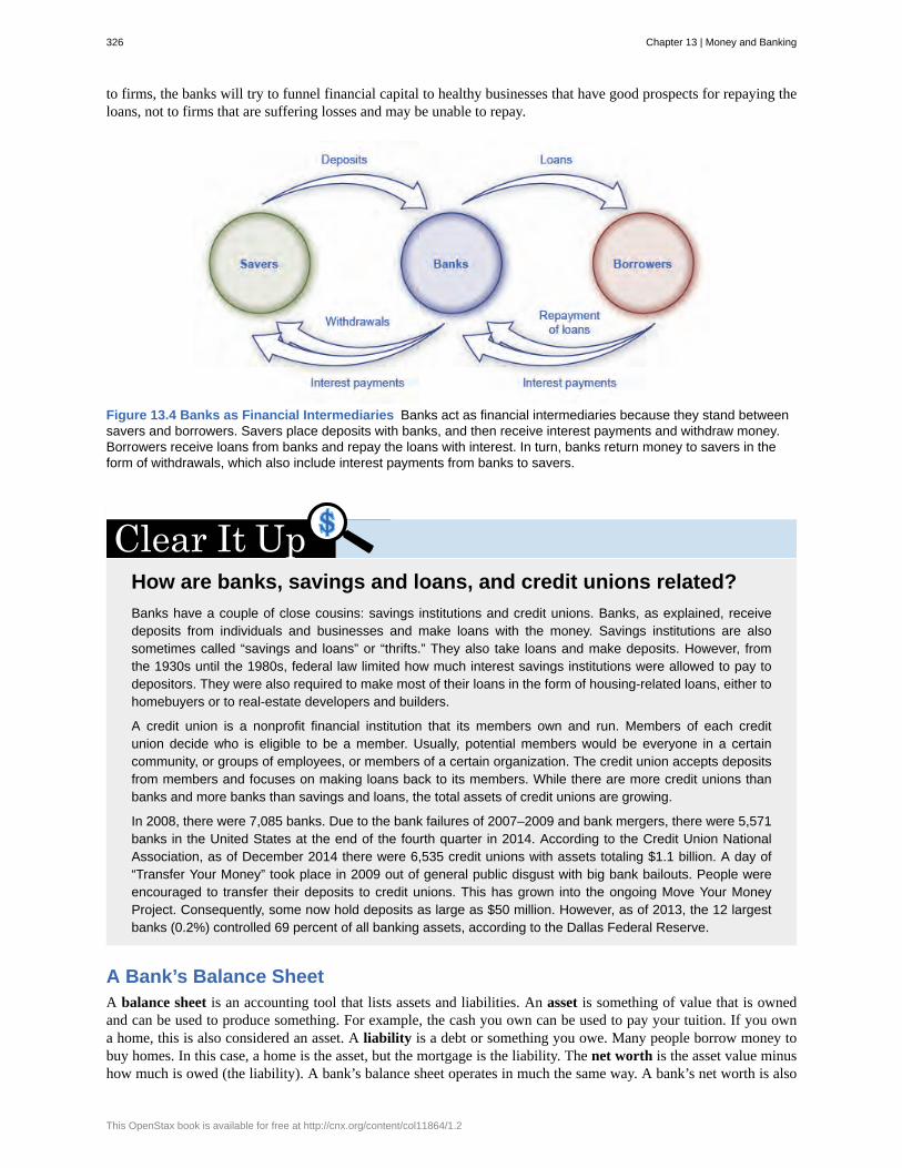
to firms, the banks will try to funnel financial capital to healthy businesses that have good prospects for repaying theloans, not to firms that are suffering losses and may be unable to repay.
Figure 13.4 Banks as Financial Intermediaries Banks act as financial intermediaries because they stand betweensavers and borrowers. Savers place deposits with banks, and then receive interest payments and withdraw money.Borrowers receive loans from banks and repay the loans with interest. In turn, banks return money to savers in theform of withdrawals, which also include interest payments from banks to savers.
How are banks, savings and loans, and credit unions related?Banks have a couple of close cousins: savings institutions and credit unions. Banks, as explained, receivedeposits from individuals and businesses and make loans with the money. Savings institutions are alsosometimes called “savings and loans” or “thrifts.” They also take loans and make deposits. However, fromthe 1930s until the 1980s, federal law limited how much interest savings institutions were allowed to pay todepositors. They were also required to make most of their loans in the form of housing-related loans, either tohomebuyers or to real-estate developers and builders.
A credit union is a nonprofit financial institution that its members own and run. Members of each creditunion decide who is eligible to be a member. Usually, potential members would be everyone in a certaincommunity, or groups of employees, or members of a certain organization. The credit union accepts depositsfrom members and focuses on making loans back to its members. While there are more credit unions thanbanks and more banks than savings and loans, the total assets of credit unions are growing.
In 2008, there were 7,085 banks. Due to the bank failures of 2007–2009 and bank mergers, there were 5,571banks in the United States at the end of the fourth quarter in 2014. According to the Credit Union NationalAssociation, as of December 2014 there were 6,535 credit unions with assets totaling $1.1 billion. A day of“Transfer Your Money” took place in 2009 out of general public disgust with big bank bailouts. People wereencouraged to transfer their deposits to credit unions. This has grown into the ongoing Move Your MoneyProject. Consequently, some now hold deposits as large as $50 million. However, as of 2013, the 12 largestbanks (0.2%) controlled 69 percent of all banking assets, according to the Dallas Federal Reserve.
A Bank’s Balance SheetA balance sheet is an accounting tool that lists assets and liabilities. An asset is something of value that is ownedand can be used to produce something. For example, the cash you own can be used to pay your tuition. If you owna home, this is also considered an asset. A liability is a debt or something you owe. Many people borrow money tobuy homes. In this case, a home is the asset, but the mortgage is the liability. The net worth is the asset value minushow much is owed (the liability). A bank’s balance sheet operates in much the same way. A bank’s net worth is also
326 Chapter 13 | Money and Banking
This OpenStax book is available for free at http://cnx.org/content/col11864/1.2
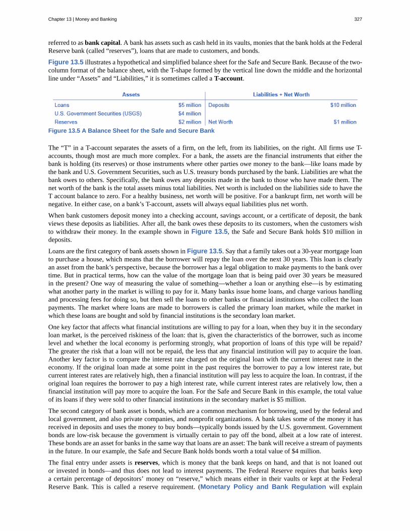
referred to as bank capital. A bank has assets such as cash held in its vaults, monies that the bank holds at the FederalReserve bank (called “reserves”), loans that are made to customers, and bonds.
Figure 13.5 illustrates a hypothetical and simplified balance sheet for the Safe and Secure Bank. Because of the two-column format of the balance sheet, with the T-shape formed by the vertical line down the middle and the horizontalline under “Assets” and “Liabilities,” it is sometimes called a T-account.
Figure 13.5 A Balance Sheet for the Safe and Secure Bank
The “T” in a T-account separates the assets of a firm, on the left, from its liabilities, on the right. All firms use T-accounts, though most are much more complex. For a bank, the assets are the financial instruments that either thebank is holding (its reserves) or those instruments where other parties owe money to the bank—like loans made bythe bank and U.S. Government Securities, such as U.S. treasury bonds purchased by the bank. Liabilities are what thebank owes to others. Specifically, the bank owes any deposits made in the bank to those who have made them. Thenet worth of the bank is the total assets minus total liabilities. Net worth is included on the liabilities side to have theT account balance to zero. For a healthy business, net worth will be positive. For a bankrupt firm, net worth will benegative. In either case, on a bank’s T-account, assets will always equal liabilities plus net worth.
When bank customers deposit money into a checking account, savings account, or a certificate of deposit, the bankviews these deposits as liabilities. After all, the bank owes these deposits to its customers, when the customers wishto withdraw their money. In the example shown in Figure 13.5, the Safe and Secure Bank holds $10 million indeposits.
Loans are the first category of bank assets shown in Figure 13.5. Say that a family takes out a 30-year mortgage loanto purchase a house, which means that the borrower will repay the loan over the next 30 years. This loan is clearlyan asset from the bank’s perspective, because the borrower has a legal obligation to make payments to the bank overtime. But in practical terms, how can the value of the mortgage loan that is being paid over 30 years be measuredin the present? One way of measuring the value of something—whether a loan or anything else—is by estimatingwhat another party in the market is willing to pay for it. Many banks issue home loans, and charge various handlingand processing fees for doing so, but then sell the loans to other banks or financial institutions who collect the loanpayments. The market where loans are made to borrowers is called the primary loan market, while the market inwhich these loans are bought and sold by financial institutions is the secondary loan market.
One key factor that affects what financial institutions are willing to pay for a loan, when they buy it in the secondaryloan market, is the perceived riskiness of the loan: that is, given the characteristics of the borrower, such as incomelevel and whether the local economy is performing strongly, what proportion of loans of this type will be repaid?The greater the risk that a loan will not be repaid, the less that any financial institution will pay to acquire the loan.Another key factor is to compare the interest rate charged on the original loan with the current interest rate in theeconomy. If the original loan made at some point in the past requires the borrower to pay a low interest rate, butcurrent interest rates are relatively high, then a financial institution will pay less to acquire the loan. In contrast, if theoriginal loan requires the borrower to pay a high interest rate, while current interest rates are relatively low, then afinancial institution will pay more to acquire the loan. For the Safe and Secure Bank in this example, the total valueof its loans if they were sold to other financial institutions in the secondary market is $5 million.
The second category of bank asset is bonds, which are a common mechanism for borrowing, used by the federal andlocal government, and also private companies, and nonprofit organizations. A bank takes some of the money it hasreceived in deposits and uses the money to buy bonds—typically bonds issued by the U.S. government. Governmentbonds are low-risk because the government is virtually certain to pay off the bond, albeit at a low rate of interest.These bonds are an asset for banks in the same way that loans are an asset: The bank will receive a stream of paymentsin the future. In our example, the Safe and Secure Bank holds bonds worth a total value of $4 million.
The final entry under assets is reserves, which is money that the bank keeps on hand, and that is not loaned outor invested in bonds—and thus does not lead to interest payments. The Federal Reserve requires that banks keepa certain percentage of depositors’ money on “reserve,” which means either in their vaults or kept at the FederalReserve Bank. This is called a reserve requirement. (Monetary Policy and Bank Regulation will explain
Chapter 13 | Money and Banking 327
how the level of these required reserves are one policy tool that governments have to influence bank behavior.)Additionally, banks may also want to keep a certain amount of reserves on hand in excess of what is required. TheSafe and Secure Bank is holding $2 million in reserves.
The net worth of a bank is defined as its total assets minus its total liabilities. For the Safe and Secure Bank shownin Figure 13.5, net worth is equal to $1 million; that is, $11 million in assets minus $10 million in liabilities. Fora financially healthy bank, the net worth will be positive. If a bank has negative net worth and depositors tried towithdraw their money, the bank would not be able to give all depositors their money.
For some concrete examples of what banks do, watch this video (http://openstaxcollege.org/l/makingsense)from Paul Solman’s “Making Sense of Financial News.”
How Banks Go BankruptA bank that is bankrupt will have a negative net worth, meaning its assets will be worth less than its liabilities. Howcan this happen? Again, looking at the balance sheet helps to explain.
A well-run bank will assume that a small percentage of borrowers will not repay their loans on time, or at all, andfactor these missing payments into its planning. Remember, the calculations of the expenses of banks every yearincludes a factor for loans that are not repaid, and the value of a bank’s loans on its balance sheet assumes a certainlevel of riskiness because some loans will not be repaid. Even if a bank expects a certain number of loan defaults,it will suffer if the number of loan defaults is much greater than expected, as can happen during a recession. Forexample, if the Safe and Secure Bank in Figure 13.5 experienced a wave of unexpected defaults, so that its loansdeclined in value from $5 million to $3 million, then the assets of the Safe and Secure Bank would decline so that thebank had negative net worth.
What led to the financial crisis of 2008–2009?Many banks make mortgage loans so that people can buy a home, but then do not keep the loans on theirbooks as an asset. Instead, the bank sells the loan. These loans are “securitized,” which means that theyare bundled together into a financial security that is sold to investors. Investors in these mortgage-backedsecurities receive a rate of return based on the level of payments that people make on all the mortgages thatstand behind the security.
Securitization offers certain advantages. If a bank makes most of its loans in a local area, then the bankmay be financially vulnerable if the local economy declines, so that many people are unable to make theirpayments. But if a bank sells its local loans, and then buys a mortgage-backed security based on home loansin many parts of the country, it can avoid being exposed to local financial risks. (In the simple example in thetext, banks just own “bonds.” In reality, banks can own a number of financial instruments, as long as thesefinancial investments are safe enough to satisfy the government bank regulators.) From the standpoint of alocal homebuyer, securitization offers the benefit that a local bank does not need to have lots of extra funds
328 Chapter 13 | Money and Banking
This OpenStax book is available for free at http://cnx.org/content/col11864/1.2
to make a loan, because the bank is only planning to hold that loan for a short time, before selling the loan sothat it can be pooled into a financial security.
But securitization also offers one potentially large disadvantage. If a bank is going to hold a mortgage loanas an asset, the bank has an incentive to scrutinize the borrower carefully to ensure that the loan is likely tobe repaid. However, a bank that is going to sell the loan may be less careful in making the loan in the firstplace. The bank will be more willing to make what are called “subprime loans,” which are loans that havecharacteristics like low or zero down-payment, little scrutiny of whether the borrower has a reliable income,and sometimes low payments for the first year or two that will be followed by much higher payments after that.Some subprime loans made in the mid-2000s were later dubbed NINJA loans: loans made even though theborrower had demonstrated No Income, No Job, or Assets.
These subprime loans were typically sold and turned into financial securities—but with a twist. The idea wasthat if losses occurred on these mortgage-backed securities, certain investors would agree to take the first,say, 5% of such losses. Other investors would agree to take, say, the next 5% of losses. By this approach, stillother investors would not need to take any losses unless these mortgage-backed financial securities lost 25%or 30% or more of their total value. These complex securities, along with other economic factors, encourageda large expansion of subprime loans in the mid-2000s.
The economic stage was now set for a banking crisis. Banks thought they were buying only ultra-safesecurities, because even though the securities were ultimately backed by risky subprime mortgages, thebanks only invested in the part of those securities where they were protected from small or moderate levels oflosses. But as housing prices fell after 2007, and the deepening recession made it harder for many people tomake their mortgage payments, many banks found that their mortgage-backed financial assets could end upbeing worth much less than they had expected—and so the banks were staring bankruptcy in the face. In the2008–2011 period, 318 banks failed in the United States.
The risk of an unexpectedly high level of loan defaults can be especially difficult for banks because a bank’s liabilities,namely the deposits of its customers, can be withdrawn quickly, but many of the bank’s assets like loans and bondswill only be repaid over years or even decades.This asset-liability time mismatch—a bank’s liabilities can bewithdrawn in the short term while its assets are repaid in the long term—can cause severe problems for a bank. Forexample, imagine a bank that has loaned a substantial amount of money at a certain interest rate, but then sees interestrates rise substantially. The bank can find itself in a precarious situation. If it does not raise the interest rate it paysto depositors, then deposits will flow to other institutions that offer the higher interest rates that are now prevailing.However, if the bank raises the interest rates that it pays to depositors, it may end up in a situation where it is payinga higher interest rate to depositors than it is collecting from those past loans that were made at lower interest rates.Clearly, the bank cannot survive in the long term if it is paying out more in interest to depositors than it is receivingfrom borrowers.
How can banks protect themselves against an unexpectedly high rate of loan defaults and against the risk of anasset-liability time mismatch? One strategy is for a bank to diversify its loans, which means lending to a variety ofcustomers. For example, suppose a bank specialized in lending to a niche market—say, making a high proportion ofits loans to construction companies that build offices in one downtown area. If that one area suffers an unexpectedeconomic downturn, the bank will suffer large losses. However, if a bank loans both to consumers who are buyinghomes and cars and also to a wide range of firms in many industries and geographic areas, the bank is less exposedto risk. When a bank diversifies its loans, those categories of borrowers who have an unexpectedly large number ofdefaults will tend to be balanced out, according to random chance, by other borrowers who have an unexpectedlylow number of defaults. Thus, diversification of loans can help banks to keep a positive net worth. However, if awidespread recession occurs that touches many industries and geographic areas, diversification will not help.
Along with diversifying their loans, banks have several other strategies to reduce the risk of an unexpectedly largenumber of loan defaults. For example, banks can sell some of the loans they make in the secondary loan market, asdescribed earlier, and instead hold a greater share of assets in the form of government bonds or reserves. Nevertheless,in a lengthy recession, most banks will see their net worth decline because a higher share of loans will not be repaidin tough economic times.
Chapter 13 | Money and Banking 329
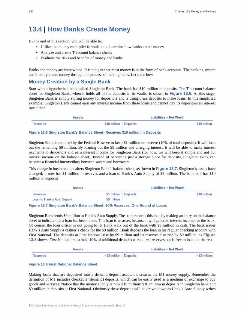
13.4 | How Banks Create MoneyBy the end of this section, you will be able to:
• Utilize the money multiplier formulate to determine how banks create money• Analyze and create T-account balance sheets• Evaluate the risks and benefits of money and banks
Banks and money are intertwined. It is not just that most money is in the form of bank accounts. The banking systemcan literally create money through the process of making loans. Let’s see how.
Money Creation by a Single BankStart with a hypothetical bank called Singleton Bank. The bank has $10 million in deposits. The T-account balancesheet for Singleton Bank, when it holds all of the deposits in its vaults, is shown in Figure 13.6. At this stage,Singleton Bank is simply storing money for depositors and is using these deposits to make loans. In this simplifiedexample, Singleton Bank cannot earn any interest income from these loans and cannot pay its depositors an interestrate either.
Figure 13.6 Singleton Bank’s Balance Sheet: Receives $10 million in Deposits
Singleton Bank is required by the Federal Reserve to keep $1 million on reserve (10% of total deposits). It will loanout the remaining $9 million. By loaning out the $9 million and charging interest, it will be able to make interestpayments to depositors and earn interest income for Singleton Bank (for now, we will keep it simple and not putinterest income on the balance sheet). Instead of becoming just a storage place for deposits, Singleton Bank canbecome a financial intermediary between savers and borrowers.
This change in business plan alters Singleton Bank’s balance sheet, as shown in Figure 13.7. Singleton’s assets havechanged; it now has $1 million in reserves and a loan to Hank’s Auto Supply of $9 million. The bank still has $10million in deposits.
Figure 13.7 Singleton Bank’s Balance Sheet: 10% Reserves, One Round of Loans
Singleton Bank lends $9 million to Hank’s Auto Supply. The bank records this loan by making an entry on the balancesheet to indicate that a loan has been made. This loan is an asset, because it will generate interest income for the bank.Of course, the loan officer is not going to let Hank walk out of the bank with $9 million in cash. The bank issuesHank’s Auto Supply a cashier’s check for the $9 million. Hank deposits the loan in his regular checking account withFirst National. The deposits at First National rise by $9 million and its reserves also rise by $9 million, as Figure13.8 shows. First National must hold 10% of additional deposits as required reserves but is free to loan out the rest
Figure 13.8 First National Balance Sheet
Making loans that are deposited into a demand deposit account increases the M1 money supply. Remember thedefinition of M1 includes checkable (demand) deposits, which can be easily used as a medium of exchange to buygoods and services. Notice that the money supply is now $19 million: $10 million in deposits in Singleton bank and$9 million in deposits at First National. Obviously these deposits will be drawn down as Hank’s Auto Supply writes
330 Chapter 13 | Money and Banking
This OpenStax book is available for free at http://cnx.org/content/col11864/1.2

checks to pay its bills. But the bigger picture is that a bank must hold enough money in reserves to meet its liabilities;the rest the bank loans out. In this example so far, bank lending has expanded the money supply by $9 million.
Now, First National must hold only 10% as required reserves ($900,000) but can lend out the other 90% ($8.1 million)in a loan to Jack’s Chevy Dealership as shown in Figure 13.9.
Figure 13.9 First National Balance Sheet
If Jack’s deposits the loan in its checking account at Second National, the money supply just increased by anadditional $8.1 million, as Figure 13.10 shows.
Figure 13.10 Second National Bank’s Balance Sheet
How is this money creation possible? It is possible because there are multiple banks in the financial system, they arerequired to hold only a fraction of their deposits, and loans end up deposited in other banks, which increases depositsand, in essence, the money supply.
Watch this video (http://openstaxcollege.org/l/createmoney) to learn more about how banks create money.
The Money Multiplier and a Multi-Bank SystemIn a system with multiple banks, the initial excess reserve amount that Singleton Bank decided to lend to Hank’s AutoSupply was deposited into Frist National Bank, which is free to loan out $8.1 million. If all banks loan out their excessreserves, the money supply will expand. In a multi-bank system, the amount of money that the system can create isfound by using the money multiplier. The money multiplier tells us by how many times a loan will be “multiplied” asit is spent in the economy and then re-deposited in other banks.
Fortunately, a formula exists for calculating the total of these many rounds of lending in a banking system. The moneymultiplier formula is:
1Reserve Requirement
The money multiplier is then multiplied by the change in excess reserves to determine the total amount of M1 moneysupply created in the banking system. See the Work it Out feature to walk through the multiplier calculation.
Chapter 13 | Money and Banking 331
Using the Money Multiplier FormulaUsing the money multiplier for the example in this text:
Step 1. In the case of Singleton Bank, for whom the reserve requirement is 10% (or 0.10), the money multiplieris 1 divided by .10, which is equal to 10.
Step 2. We have identified that the excess reserves are $9 million, so, using the formula we can determinethe total change in the M1 money supply:
Total Change in the M1 Money Supply = 1Reserve Requirement × Excess Requirement
= 10.10 × $9 million
= 10 × $9 million= $90 million
Step 3. Thus, we can say that, in this example, the total quantity of money generated in this economy after allrounds of lending are completed will be $90 million.
Cautions about the Money MultiplierThe money multiplier will depend on the proportion of reserves that banks are required to hold by the Federal ReserveBank. Additionally, a bank can also choose to hold extra reserves. Banks may decide to vary how much they hold inreserves for two reasons: macroeconomic conditions and government rules. When an economy is in recession, banksare likely to hold a higher proportion of reserves because they fear that loans are less likely to be repaid when theeconomy is slow. The Federal Reserve may also raise or lower the required reserves held by banks as a policy moveto affect the quantity of money in an economy, as Monetary Policy and Bank Regulation will discuss.
The process of how banks create money shows how the quantity of money in an economy is closely linked to thequantity of lending or credit in the economy. Indeed, all of the money in the economy, except for the original reserves,is a result of bank loans that are re-deposited and loaned out, again, and again.
Finally, the money multiplier depends on people re-depositing the money that they receive in the banking system.If people instead store their cash in safe-deposit boxes or in shoeboxes hidden in their closets, then banks cannotrecirculate the money in the form of loans. Indeed, central banks have an incentive to assure that bank deposits aresafe because if people worry that they may lose their bank deposits, they may start holding more money in cash,instead of depositing it in banks, and the quantity of loans in an economy will decline. Low-income countries havewhat economists sometimes refer to as “mattress savings,” or money that people are hiding in their homes becausethey do not trust banks. When mattress savings in an economy are substantial, banks cannot lend out those funds andthe money multiplier cannot operate as effectively. The overall quantity of money and loans in such an economy willdecline.
Watch a video (http://openstaxcollege.org/l/moneymyth) of Jem Bendell discussing “The Money Myth.”
332 Chapter 13 | Money and Banking
This OpenStax book is available for free at http://cnx.org/content/col11864/1.2
Money and Banks—Benefits and DangersMoney and banks are marvelous social inventions that help a modern economy to function. Compared with thealternative of barter, money makes market exchanges vastly easier in goods, labor, and financial markets. Bankingmakes money still more effective in facilitating exchanges in goods and labor markets. Moreover, the process of banksmaking loans in financial capital markets is intimately tied to the creation of money.
But the extraordinary economic gains that are possible through money and banking also suggest some possiblecorresponding dangers. If banks are not working well, it sets off a decline in convenience and safety of transactionsthroughout the economy. If the banks are under financial stress, because of a widespread decline in the value of theirassets, loans may become far less available, which can deal a crushing blow to sectors of the economy that dependon borrowed money like business investment, home construction, and car manufacturing. The Great Recession of2008–2009 illustrated this pattern.
The Many Disguises of Money: From Cowries to Bit CoinsThe global economy has come a long way since it started using cowrie shells as currency. We have movedaway from commodity and commodity-backed paper money to fiat currency. As technology and globalintegration increases, the need for paper currency is diminishing, too. Every day, we witness the increaseduse of debit and credit cards.
The latest creation and perhaps one of the purest forms of fiat money is the Bitcoin. Bitcoins are a digitalcurrency that allows users to buy goods and services online. Products and services such as videos andbooks may be purchased using Bitcoins. It is not backed by any commodity nor has it been decreed by anygovernment as legal tender, yet it used as a medium of exchange and its value (online at least) can be stored.It is also unregulated by any central bank, but is created online through people solving very complicatedmathematics problems and getting paid afterward. Bitcoin.org is an information source if you are curious.Bitcoins are a relatively new type of money. At present, because it is not sanctioned as a legal currency by anycountry nor regulated by any central bank, it lends itself for use in illegal trading activities as well as legal ones.As technology increases and the need to reduce transactions costs associated with using traditional forms ofmoney increases, Bitcoins or some sort of digital currency may replace our dollar bill, just as the cowrie shellwas replaced.
Chapter 13 | Money and Banking 333
asset
asset–liability time mismatch
balance sheet
bank capital
barter
coins and currency in circulation
commodity money
commodity-backed currencies
credit card
debit card
demand deposit
depository institution
diversify
double coincidence of wants
fiat money
financial intermediary
liability
M1 money supply
M2 money supply
medium of exchange
money
money market fund
KEY TERMS
item of value owned by a firm or an individual
a bank’s liabilities can be withdrawn in the short term while its assets are repaid in thelong term
an accounting tool that lists assets and liabilities
a bank’s net worth
literally, trading one good or service for another, without using money
the coins and bills that circulate in an economy that are not held by the U.STreasury, at the Federal Reserve Bank, or in bank vaults
an item that is used as money, but which also has value from its use as something other than money
are dollar bills or other currencies with values backed up by gold or anothercommodity
immediately transfers money from the credit card company’s checking account to the seller, and at the endof the month the user owes the money to the credit card company; a credit card is a short-term loan
like a check, is an instruction to the user’s bank to transfer money directly and immediately from your bankaccount to the seller
checkable deposit in banks that is available by making a cash withdrawal or writing a check
institution that accepts money deposits and then uses these to make loans
making loans or investments with a variety of firms, to reduce the risk of being adversely affected by events atone or a few firms
a situation in which two people each want some good or service that the other personcan provide
has no intrinsic value, but is declared by a government to be the legal tender of a country
an institution that operates between a saver with financial assets to invest and an entity whowill borrow those assets and pay a rate of return
any amount or debt owed by a firm or an individual
a narrow definition of the money supply that includes currency and checking accounts in banks, andto a lesser degree, traveler’s checks.
a definition of the money supply that includes everything in M1, but also adds savings deposits,money market funds, and certificates of deposit
whatever is widely accepted as a method of payment
whatever serves society in four functions: as a medium of exchange, a store of value, a unit of account, and astandard of deferred payment.
the deposits of many investors are pooled together and invested in a safe way like short-termgovernment bonds
334 Chapter 13 | Money and Banking
This OpenStax book is available for free at http://cnx.org/content/col11864/1.2
money multiplier formula
net worth
payment system
reserves
savings deposit
smart card
standard of deferred payment
store of value
T-account
time deposit
transaction costs
unit of account
total money in the economy divided by the original quantity of money, or change in thetotal money in the economy divided by a change in the original quantity of money
the excess of the asset value over and above the amount of the liability; total assets minus total liabilities
helps an economy exchange goods and services for money or other financial assets
funds that a bank keeps on hand and that are not loaned out or invested in bonds
bank account where you cannot withdraw money by writing a check, but can withdraw the money at abank—or can transfer it easily to a checking account
stores a certain value of money on a card and then the card can be used to make purchases
money must also be acceptable to make purchases today that will be paid in the future
something that serves as a way of preserving economic value that can be spent or consumed in the future
a balance sheet with a two-column format, with the T-shape formed by the vertical line down the middle andthe horizontal line under the column headings for “Assets” and “Liabilities”
account that the depositor has committed to leaving in the bank for a certain period of time, in exchangefor a higher rate of interest; also called certificate of deposit
the costs associated with finding a lender or a borrower for money
the common way in which market values are measured in an economy
KEY CONCEPTS AND SUMMARY
13.1 Defining Money by Its FunctionsMoney is what people in a society regularly use when purchasing or selling goods and services. If money were notavailable, people would need to barter with each other, meaning that each person would need to identify others withwhom they have a double coincidence of wants—that is, each party has a specific good or service that the otherdesires. Money serves several functions: a medium of exchange, a unit of account, a store of value, and a standard ofdeferred payment. There are two types of money: commodity money, which is an item used as money, but which alsohas value from its use as something other than money; and fiat money, which has no intrinsic value, but is declaredby a government to be the legal tender of a country.
13.2 Measuring Money: Currency, M1, and M2Money is measured with several definitions: M1 includes currency and money in checking accounts (demanddeposits). Traveler’s checks are also a component of M1, but are declining in use. M2 includes all of M1, plus savingsdeposits, time deposits like certificates of deposit, and money market funds.
13.3 The Role of BanksBanks facilitate the use of money for transactions in the economy because people and firms can use bank accountswhen selling or buying goods and services, when paying a worker or being paid, and when saving money or receivinga loan. In the financial capital market, banks are financial intermediaries; that is, they operate between savers whosupply financial capital and borrowers who demand loans. A balance sheet (sometimes called a T-account) is anaccounting tool which lists assets in one column and liabilities in another column. The liabilities of a bank are itsdeposits. The assets of a bank include its loans, its ownership of bonds, and its reserves (which are not loaned out).The net worth of a bank is calculated by subtracting the bank’s liabilities from its assets. Banks run a risk of negativenet worth if the value of their assets declines. The value of assets can decline because of an unexpectedly high numberof defaults on loans, or if interest rates rise and the bank suffers an asset-liability time mismatch in which the bankis receiving a low rate of interest on its long-term loans but must pay the currently higher market rate of interest to
Chapter 13 | Money and Banking 335
attract depositors. Banks can protect themselves against these risks by choosing to diversify their loans or to hold agreater proportion of their assets in bonds and reserves. If banks hold only a fraction of their deposits as reserves, thenthe process of banks’ lending money, those loans being re-deposited in banks, and the banks making additional loanswill create money in the economy.
13.4 How Banks Create MoneyThe money multiplier is defined as the quantity of money that the banking system can generate from each $1 of bankreserves. The formula for calculating the multiplier is 1/reserve ratio, where the reserve ratio is the fraction of depositsthat the bank wishes to hold as reserves. The quantity of money in an economy and the quantity of credit for loans areinextricably intertwined. Much of the money in an economy is created by the network of banks making loans, peoplemaking deposits, and banks making more loans.
Given the macroeconomic dangers of a malfunctioning banking system, Monetary Policy and Bank Regulationwill discuss government policies for controlling the money supply and for keeping the banking system safe.
SELF-CHECK QUESTIONS1. In many casinos, a person buys chips to use for gambling. Within the walls of the casino, these chips can often beused to buy food and drink or even a hotel room. Do chips in a gambling casino serve all three functions of money?
2. Can you name some item that is a store of value, but does not serve the other functions of money?
3. If you are out shopping for clothes and books, what is easiest and most convenient for you to spend: M1 or M2?Explain your answer.
4. For the following list of items, indicate if they are in M1, M2, or neither:a. Your $5,000 line of credit on your Bank of America cardb. $50 dollars’ worth of traveler’s checks you have not used yetc. $1 in quarters in your pocketd. $1200 in your checking accounte. $2000 you have in a money market account
5. Explain why the money listed under assets on a bank balance sheet may not actually be in the bank?
6. Imagine that you are in the position of buying loans in the secondary market (that is, buying the right to collectthe payments on loans made by banks) for a bank or other financial services company. Explain why you would bewilling to pay more or less for a given loan if:
a. The borrower has been late on a number of loan paymentsb. Interest rates in the economy as a whole have risen since the loan was madec. The borrower is a firm that has just declared a high level of profitsd. Interest rates in the economy as a whole have fallen since the loan was made
REVIEW QUESTIONS
7. What are the four functions served by money?
8. How does the existence of money simplify theprocess of buying and selling?
9. What is the double-coincidence of wants?
10. What components of money are counted as part ofM1?
11. What components of money are counted in M2?
12. Why is a bank called a financial intermediary?
13. What does a balance sheet show?
14. What are the assets of a bank? What are itsliabilities?
15. How do you calculate the net worth of a bank?
16. How can a bank end up with negative net worth?
336 Chapter 13 | Money and Banking
This OpenStax book is available for free at http://cnx.org/content/col11864/1.2
17. What is the asset-liability time mismatch that allbanks face?
18. What is the risk if a bank does not diversify itsloans?
19. How do banks create money?
20. What is the formula for the money multiplier?
CRITICAL THINKING QUESTIONS
21. The Bring it Home Feature discusses the use ofcowrie shells as money. Although cowrie shells are nolonger used as money, do you think other forms ofcommodity monies are possible? What role mighttechnology play in our definition of money?
22. Imagine that you are a barber in a world withoutmoney. Explain why it would be tricky to obtaingroceries, clothing, and a place to live.
23. Explain why you think the Federal Reserve Banktracks M1 and M2.
24. The total amount of U.S. currency in circulationdivided by the U.S. population comes out to about$3,500 per person. That is more than most of us carry.Where is all the cash?
25. Explain the difference between how you wouldcharacterize bank deposits and loans as assets andliabilities on your own personal balance sheet and how abank would characterize deposits and loans as assets andliabilities on its balance sheet.
26. Should banks have to hold 100% of their deposits?Why or why not?
27. Explain what will happen to the money multiplierprocess if there is an increase in the reserverequirement?
28. What do you think the Federal Reserve Bank didto the reserve requirement during the Great Recession of2008–2009?
PROBLEMS29. If you take $100 out of your piggy bank and depositit in your checking account, how did M1 change? DidM2 change?
30. A bank has deposits of $400. It holds reserves of$50. It has purchased government bonds worth $70. Ithas made loans of $500. Set up a T-account balancesheet for the bank, with assets and liabilities, andcalculate the bank’s net worth.
31. Humongous Bank is the only bank in the economy.The people in this economy have $20 million in money,and they deposit all their money in Humongous Bank.
a. Humongous Bank decides on a policy of holding100% reserves. Draw a T-account for the bank.
b. Humongous Bank is required to hold 5% of itsexisting $20 million as reserves, and to loan outthe rest. Draw a T-account for the bank after thisfirst round of loans has been made.
c. Assume that Humongous bank is part of amultibank system. How much will money supplyincrease with that original loan of $19 million?
Chapter 13 | Money and Banking 337
338 Chapter 13 | Money and Banking
This OpenStax book is available for free at http://cnx.org/content/col11864/1.2
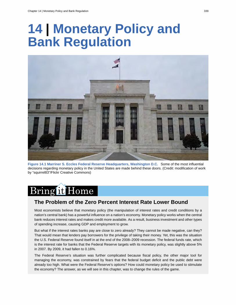
14 | Monetary Policy andBank Regulation
Figure 14.1 Marriner S. Eccles Federal Reserve Headquarters, Washington D.C. Some of the most influentialdecisions regarding monetary policy in the United States are made behind these doors. (Credit: modification of workby “squirrel83”/Flickr Creative Commons)
The Problem of the Zero Percent Interest Rate Lower BoundMost economists believe that monetary policy (the manipulation of interest rates and credit conditions by anation’s central bank) has a powerful influence on a nation’s economy. Monetary policy works when the centralbank reduces interest rates and makes credit more available. As a result, business investment and other typesof spending increase, causing GDP and employment to grow.
But what if the interest rates banks pay are close to zero already? They cannot be made negative, can they?That would mean that lenders pay borrowers for the privilege of taking their money. Yet, this was the situationthe U.S. Federal Reserve found itself in at the end of the 2008–2009 recession. The federal funds rate, whichis the interest rate for banks that the Federal Reserve targets with its monetary policy, was slightly above 5%in 2007. By 2009, it had fallen to 0.16%.
The Federal Reserve’s situation was further complicated because fiscal policy, the other major tool formanaging the economy, was constrained by fears that the federal budget deficit and the public debt werealready too high. What were the Federal Reserve’s options? How could monetary policy be used to stimulatethe economy? The answer, as we will see in this chapter, was to change the rules of the game.
Chapter 14 | Monetary Policy and Bank Regulation 339
Introduction to Monetary Policy and Bank RegulationIn this chapter, you will learn about:
• The Federal Reserve Banking System and Central Banks
• Bank Regulation
• How a Central Bank Executes Monetary Policy
• Monetary Policy and Economic Outcomes
• Pitfalls for Monetary Policy
Money, loans, and banks are all tied together. Money is deposited in bank accounts, which is then loaned tobusinesses, individuals, and other banks. When the interlocking system of money, loans, and banks works well,economic transactions are made smoothly in goods and labor markets and savers are connected with borrowers. If themoney and banking system does not operate smoothly, the economy can either fall into recession or suffer prolongedinflation.
The government of every country has public policies that support the system of money, loans, and banking. But thesepolicies do not always work perfectly. This chapter discusses how monetary policy works and what may prevent itfrom working perfectly.
14.1 | The Federal Reserve Banking System and CentralBanksBy the end of this section, you will be able to:
• Explain the structure and organization of the U.S. Federal Reserve• Discuss how central banks impact monetary policy, promote financial stability, and provide banking
services
In making decisions about the money supply, a central bank decides whether to raise or lower interest rates and, inthis way, to influence macroeconomic policy, whose goal is low unemployment and low inflation. The central bankis also responsible for regulating all or part of the nation’s banking system to protect bank depositors and insure thehealth of the bank’s balance sheet.
The organization responsible for conducting monetary policy and ensuring that a nation’s financial system operatessmoothly is called the central bank. Most nations have central banks or currency boards. Some prominent centralbanks around the world include the European Central Bank, the Bank of Japan, and the Bank of England. In the UnitedStates, the central bank is called the Federal Reserve—often abbreviated as just “the Fed.” This section explains theorganization of the U.S. Federal Reserve and identifies the major responsibilities of a central bank.
Structure/Organization of the Federal ReserveUnlike most central banks, the Federal Reserve is semi-decentralized, mixing government appointees withrepresentation from private-sector banks. At the national level, it is run by a Board of Governors, consisting of sevenmembers appointed by the President of the United States and confirmed by the Senate. Appointments are for 14-yearterms and they are arranged so that one term expires January 31 of every even-numbered year. The purpose of thelong and staggered terms is to insulate the Board of Governors as much as possible from political pressure so thatpolicy decisions can be made based only on their economic merits. Additionally, except when filling an unfinishedterm, each member only serves one term, further insulating decision-making from politics. Policy decisions of the Feddo not require congressional approval, and the President cannot ask for the resignation of a Federal Reserve Governoras the President can with cabinet positions.
340 Chapter 14 | Monetary Policy and Bank Regulation
This OpenStax book is available for free at http://cnx.org/content/col11864/1.2
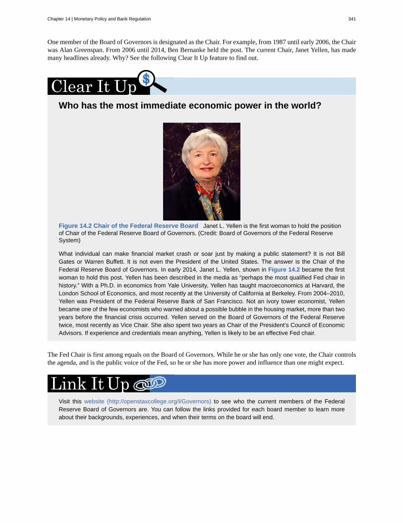
One member of the Board of Governors is designated as the Chair. For example, from 1987 until early 2006, the Chairwas Alan Greenspan. From 2006 until 2014, Ben Bernanke held the post. The current Chair, Janet Yellen, has mademany headlines already. Why? See the following Clear It Up feature to find out.
Who has the most immediate economic power in the world?
Figure 14.2 Chair of the Federal Reserve Board Janet L. Yellen is the first woman to hold the positionof Chair of the Federal Reserve Board of Governors. (Credit: Board of Governors of the Federal ReserveSystem)
What individual can make financial market crash or soar just by making a public statement? It is not BillGates or Warren Buffett. It is not even the President of the United States. The answer is the Chair of theFederal Reserve Board of Governors. In early 2014, Janet L. Yellen, shown in Figure 14.2 became the firstwoman to hold this post. Yellen has been described in the media as “perhaps the most qualified Fed chair inhistory.” With a Ph.D. in economics from Yale University, Yellen has taught macroeconomics at Harvard, theLondon School of Economics, and most recently at the University of California at Berkeley. From 2004–2010,Yellen was President of the Federal Reserve Bank of San Francisco. Not an ivory tower economist, Yellenbecame one of the few economists who warned about a possible bubble in the housing market, more than twoyears before the financial crisis occurred. Yellen served on the Board of Governors of the Federal Reservetwice, most recently as Vice Chair. She also spent two years as Chair of the President’s Council of EconomicAdvisors. If experience and credentials mean anything, Yellen is likely to be an effective Fed chair.
The Fed Chair is first among equals on the Board of Governors. While he or she has only one vote, the Chair controlsthe agenda, and is the public voice of the Fed, so he or she has more power and influence than one might expect.
Visit this website (http://openstaxcollege.org/l/Governors) to see who the current members of the FederalReserve Board of Governors are. You can follow the links provided for each board member to learn moreabout their backgrounds, experiences, and when their terms on the board will end.
Chapter 14 | Monetary Policy and Bank Regulation 341
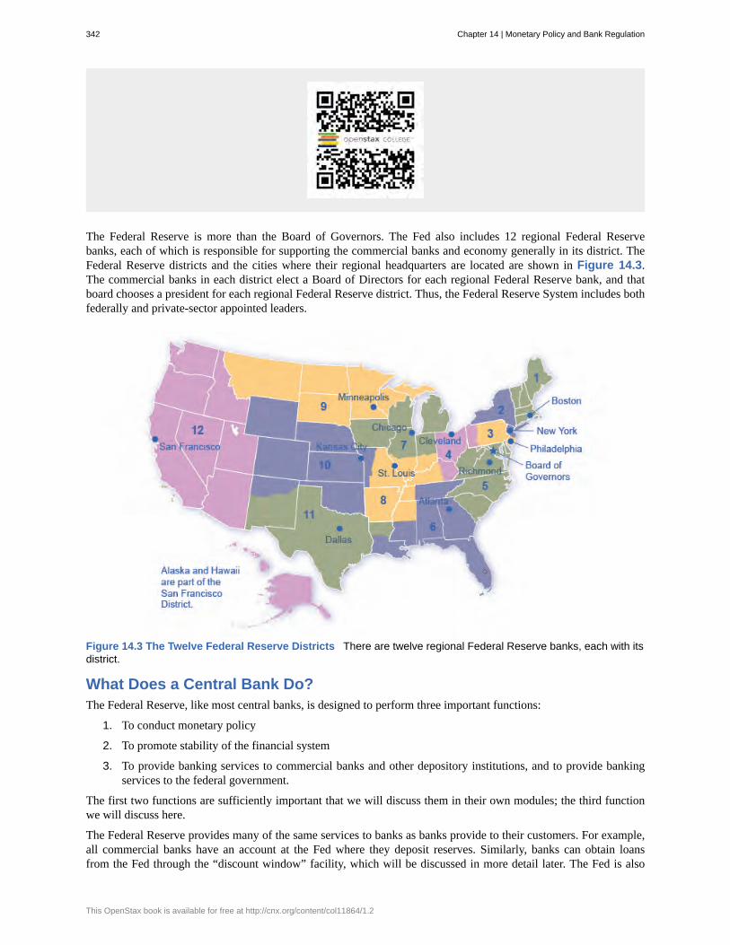
The Federal Reserve is more than the Board of Governors. The Fed also includes 12 regional Federal Reservebanks, each of which is responsible for supporting the commercial banks and economy generally in its district. TheFederal Reserve districts and the cities where their regional headquarters are located are shown in Figure 14.3.The commercial banks in each district elect a Board of Directors for each regional Federal Reserve bank, and thatboard chooses a president for each regional Federal Reserve district. Thus, the Federal Reserve System includes bothfederally and private-sector appointed leaders.
Figure 14.3 The Twelve Federal Reserve Districts There are twelve regional Federal Reserve banks, each with itsdistrict.
What Does a Central Bank Do?The Federal Reserve, like most central banks, is designed to perform three important functions:
1. To conduct monetary policy
2. To promote stability of the financial system
3. To provide banking services to commercial banks and other depository institutions, and to provide bankingservices to the federal government.
The first two functions are sufficiently important that we will discuss them in their own modules; the third functionwe will discuss here.
The Federal Reserve provides many of the same services to banks as banks provide to their customers. For example,all commercial banks have an account at the Fed where they deposit reserves. Similarly, banks can obtain loansfrom the Fed through the “discount window” facility, which will be discussed in more detail later. The Fed is also
342 Chapter 14 | Monetary Policy and Bank Regulation
This OpenStax book is available for free at http://cnx.org/content/col11864/1.2

responsible for check processing. When you write a check, for example, to buy groceries, the grocery store depositsthe check in its bank account. Then, the physical check (or an image of that actual check) is returned to your bank,after which funds are transferred from your bank account to the account of the grocery store. The Fed is responsiblefor each of these actions.
On a more mundane level, the Federal Reserve ensures that enough currency and coins are circulating through thefinancial system to meet public demands. For example, each year the Fed increases the amount of currency availablein banks around the Christmas shopping season and reduces it again in January.
Finally, the Fed is responsible for assuring that banks are in compliance with a wide variety of consumer protectionlaws. For example, banks are forbidden from discriminating on the basis of age, race, sex, or marital status. Banks arealso required to disclose publicly information about the loans they make for buying houses and how those loans aredistributed geographically, as well as by sex and race of the loan applicants.
14.2 | Bank RegulationBy the end of this section, you will be able to:
• Discuss the relationship between bank regulation and monetary policy• Explain bank supervision• Explain how deposit insurance and lender of last resort are two strategies to protect against bank runs
A safe and stable national financial system is a critical concern of the Federal Reserve. The goal is not only to protectindividuals’ savings, but to protect the integrity of the financial system itself. This esoteric task is usually behind thescenes, but came into view during the 2008–2009 financial crisis, when for a brief period of time, critical parts ofthe financial system failed and firms became unable to obtain financing for ordinary parts of their business. Imagineif suddenly you were unable to access the money in your bank accounts because your checks were not accepted forpayment and your debit cards were declined. This gives an idea of what a failure of the payments/financial system islike.
Bank regulation is intended to maintain the solvency of banks by avoiding excessive risk. Regulation falls intoa number of categories, including reserve requirements, capital requirements, and restrictions on the types ofinvestments banks may make. In Money and Banking, we learned that banks are required to hold a minimumpercentage of their deposits on hand as reserves. “On hand” is a bit of a misnomer because, while a portion of bankreserves are held as cash in the bank, the majority are held in the bank’s account at the Federal Reserve, and theirpurpose is to cover desired withdrawals by depositors. Another part of bank regulation is restrictions on the types ofinvestments banks are allowed to make. Banks are allowed to make loans to businesses, individuals, and other banks.They are allowed to purchase U.S. Treasury securities but, to protect depositors, they are not permitted to invest inthe stock market or other assets that are perceived as too risky.
Bank capital is the difference between a bank’s assets and its liabilities. In other words, it is a bank’s net worth. Abank must have positive net worth; otherwise it is insolvent or bankrupt, meaning it would not have enough assets topay back its liabilities. Regulation requires that banks maintain a minimum net worth, usually expressed as a percentof their assets, to protect their depositors and other creditors.
Visit this website (http://openstaxcollege.org/l/bankregulation) to read the brief article, “Stop ConfusingMonetary Policy and Bank Regulation.”
Chapter 14 | Monetary Policy and Bank Regulation 343
Bank SupervisionSeveral government agencies monitor the balance sheets of banks to make sure they have positive net worth and arenot taking too high a level of risk. Within the U.S. Department of the Treasury, the Office of the Comptroller of theCurrency has a national staff of bank examiners who conduct on-site reviews of the 1,500 or so of the largest nationalbanks. The bank examiners also review any foreign banks that have branches in the United States. The Office of theComptroller of the Currency also monitors and regulates about 800 savings and loan institutions.
The National Credit Union Administration (NCUA) supervises credit unions, which are nonprofit banks owned andrun by their members. There are over 6,000 credit unions in the U.S. economy, though the typical credit union is smallcompared to most banks.
The Federal Reserve also has some responsibility for supervising financial institutions. For example, conglomeratefirms that own banks and other businesses are called “bank holding companies.” While other regulators like the Officeof the Comptroller of the Currency supervises the banks, the Federal Reserve supervises the holding companies.
When the supervision of banks (and bank-like institutions such as savings and loans and credit unions) works well,most banks will remain financially healthy most of the time. If the bank supervisors find that a bank has low ornegative net worth, or is making too high a proportion of risky loans, they can require that the bank change itsbehavior—or, in extreme cases, even force the bank to be closed or sold to a financially healthy bank.
Bank supervision can run into both practical and political questions. The practical question is that measuring the valueof a bank’s assets is not always straightforward. As discussed in Money and Banking, a bank’s assets are its loans,and the value of these assets depends on estimates about the risk that these loans will not be repaid. These issues canbecome even more complex when a bank makes loans to banks or firms in other countries, or arranges financial dealsthat are much more complex than a basic loan.
The political question arises because the decision by a bank supervisor to require a bank to close or to change itsfinancial investments is often controversial, and the bank supervisor often comes under political pressure from theowners of the bank and the local politicians to keep quiet and back off.
For example, many observers have pointed out that Japan’s banks were in deep financial trouble through most of the1990s; however, nothing substantial had been done about it by the early 2000s. A similar unwillingness to confrontproblems with struggling banks is visible across the rest of the world, in East Asia, Latin America, Eastern Europe,Russia, and elsewhere.
In the United States, laws were passed in the 1990s requiring that bank supervisors make their findings open andpublic, and that they act as soon as a problem is identified. However, as many U.S. banks were staggered by therecession of 2008–2009, critics of the bank regulators asked pointed questions about why the regulators had notforeseen the financial shakiness of the banks earlier, before such large losses had a chance to accumulate.
Bank RunsBack in the nineteenth century and during the first few decades of the twentieth century (around and during the GreatDepression), putting your money in a bank could be nerve-wracking. Imagine that the net worth of your bank becamenegative, so that the bank’s assets were not enough to cover its liabilities. In this situation, whoever withdrew theirdeposits first received all of their money, and those who did not rush to the bank quickly enough, lost their money.Depositors racing to the bank to withdraw their deposits, as shown in Figure 14.4 is called a bank run. In the movieIt’s a Wonderful Life, the bank manager, played by Jimmy Stewart, faces a mob of worried bank depositors who want
344 Chapter 14 | Monetary Policy and Bank Regulation
This OpenStax book is available for free at http://cnx.org/content/col11864/1.2
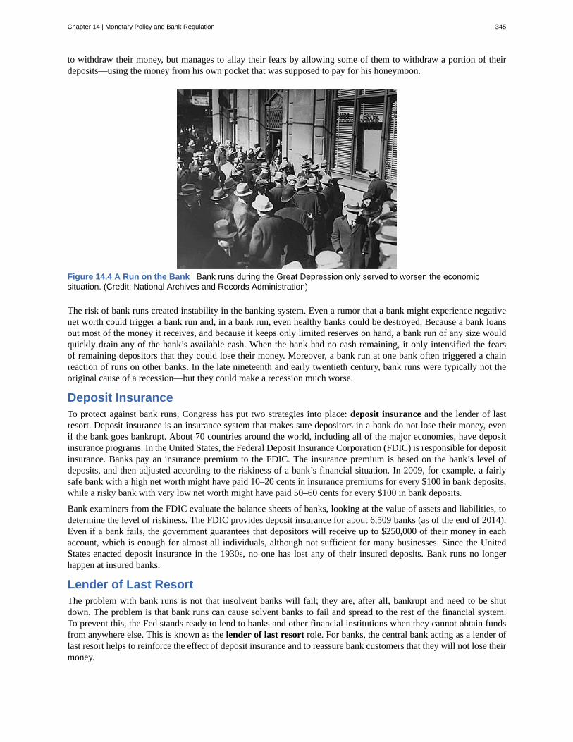
to withdraw their money, but manages to allay their fears by allowing some of them to withdraw a portion of theirdeposits—using the money from his own pocket that was supposed to pay for his honeymoon.
Figure 14.4 A Run on the Bank Bank runs during the Great Depression only served to worsen the economicsituation. (Credit: National Archives and Records Administration)
The risk of bank runs created instability in the banking system. Even a rumor that a bank might experience negativenet worth could trigger a bank run and, in a bank run, even healthy banks could be destroyed. Because a bank loansout most of the money it receives, and because it keeps only limited reserves on hand, a bank run of any size wouldquickly drain any of the bank’s available cash. When the bank had no cash remaining, it only intensified the fearsof remaining depositors that they could lose their money. Moreover, a bank run at one bank often triggered a chainreaction of runs on other banks. In the late nineteenth and early twentieth century, bank runs were typically not theoriginal cause of a recession—but they could make a recession much worse.
Deposit InsuranceTo protect against bank runs, Congress has put two strategies into place: deposit insurance and the lender of lastresort. Deposit insurance is an insurance system that makes sure depositors in a bank do not lose their money, evenif the bank goes bankrupt. About 70 countries around the world, including all of the major economies, have depositinsurance programs. In the United States, the Federal Deposit Insurance Corporation (FDIC) is responsible for depositinsurance. Banks pay an insurance premium to the FDIC. The insurance premium is based on the bank’s level ofdeposits, and then adjusted according to the riskiness of a bank’s financial situation. In 2009, for example, a fairlysafe bank with a high net worth might have paid 10–20 cents in insurance premiums for every $100 in bank deposits,while a risky bank with very low net worth might have paid 50–60 cents for every $100 in bank deposits.
Bank examiners from the FDIC evaluate the balance sheets of banks, looking at the value of assets and liabilities, todetermine the level of riskiness. The FDIC provides deposit insurance for about 6,509 banks (as of the end of 2014).Even if a bank fails, the government guarantees that depositors will receive up to $250,000 of their money in eachaccount, which is enough for almost all individuals, although not sufficient for many businesses. Since the UnitedStates enacted deposit insurance in the 1930s, no one has lost any of their insured deposits. Bank runs no longerhappen at insured banks.
Lender of Last ResortThe problem with bank runs is not that insolvent banks will fail; they are, after all, bankrupt and need to be shutdown. The problem is that bank runs can cause solvent banks to fail and spread to the rest of the financial system.To prevent this, the Fed stands ready to lend to banks and other financial institutions when they cannot obtain fundsfrom anywhere else. This is known as the lender of last resort role. For banks, the central bank acting as a lender oflast resort helps to reinforce the effect of deposit insurance and to reassure bank customers that they will not lose theirmoney.
Chapter 14 | Monetary Policy and Bank Regulation 345
The lender of last resort task can come up in other financial crises, as well. During the panic of the stock market crashin 1987, when the value of U.S. stocks fell by 25% in a single day, the Federal Reserve made a number of short-term emergency loans so that the financial system could keep functioning. During the recession of 2008–2009, the“quantitative easing” policies (discussed below) of the Federal Reserve can be interpreted as a willingness to makeshort-term credit available as needed in a time when the banking and financial system was under stress.
14.3 | How a Central Bank Executes Monetary PolicyBy the end of this section, you will be able to:
• Explain the reason for open market operations• Evaluate reserve requirements and discount rates• Interpret and show bank activity through balance sheets
The most important function of the Federal Reserve is to conduct the nation’s monetary policy. Article I, Section 8of the U.S. Constitution gives Congress the power “to coin money” and “to regulate the value thereof.” As part ofthe 1913 legislation that created the Federal Reserve, Congress delegated these powers to the Fed. Monetary policyinvolves managing interest rates and credit conditions, which influences the level of economic activity, as describedin more detail below.
A central bank has three traditional tools to implement monetary policy in the economy:
• Open market operations
• Changing reserve requirements
• Changing the discount rate
In discussing how these three tools work, it is useful to think of the central bank as a “bank for banks”—that is, eachprivate-sector bank has its own account at the central bank. We will discuss each of these monetary policy tools in thesections below.
Open Market OperationsThe most commonly used tool of monetary policy in the U.S. is open market operations. Open market operationstake place when the central bank sells or buys U.S. Treasury bonds in order to influence the quantity of bank reservesand the level of interest rates. The specific interest rate targeted in open market operations is the federal funds rate.The name is a bit of a misnomer since the federal funds rate is the interest rate charged by commercial banks makingovernight loans to other banks. As such, it is a very short term interest rate, but one that reflects credit conditions infinancial markets very well.
The Federal Open Market Committee (FOMC) makes the decisions regarding these open market operations. TheFOMC is made up of the seven members of the Federal Reserve’s Board of Governors. It also includes five votingmembers who are drawn, on a rotating basis, from the regional Federal Reserve Banks. The New York districtpresident is a permanent voting member of the FOMC and the other four spots are filled on a rotating, annual basis,from the other 11 districts. The FOMC typically meets every six weeks, but it can meet more frequently if necessary.The FOMC tries to act by consensus; however, the chairman of the Federal Reserve has traditionally played a verypowerful role in defining and shaping that consensus. For the Federal Reserve, and for most central banks, openmarket operations have, over the last few decades, been the most commonly used tool of monetary policy.
Visit this website (http://openstaxcollege.org/l/monetarypolicy) for the Federal Reserve to learn more aboutcurrent monetary policy.
346 Chapter 14 | Monetary Policy and Bank Regulation
This OpenStax book is available for free at http://cnx.org/content/col11864/1.2
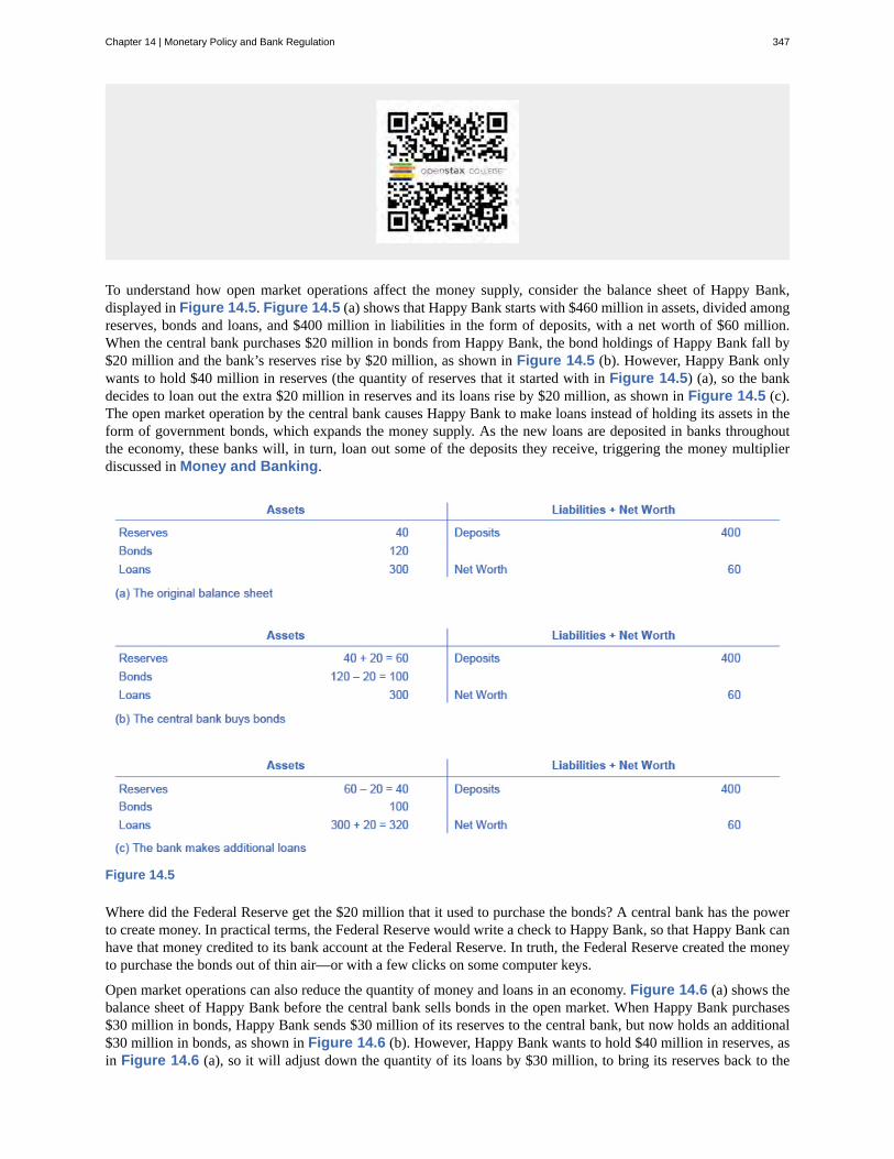
To understand how open market operations affect the money supply, consider the balance sheet of Happy Bank,displayed in Figure 14.5. Figure 14.5 (a) shows that Happy Bank starts with $460 million in assets, divided amongreserves, bonds and loans, and $400 million in liabilities in the form of deposits, with a net worth of $60 million.When the central bank purchases $20 million in bonds from Happy Bank, the bond holdings of Happy Bank fall by$20 million and the bank’s reserves rise by $20 million, as shown in Figure 14.5 (b). However, Happy Bank onlywants to hold $40 million in reserves (the quantity of reserves that it started with in Figure 14.5) (a), so the bankdecides to loan out the extra $20 million in reserves and its loans rise by $20 million, as shown in Figure 14.5 (c).The open market operation by the central bank causes Happy Bank to make loans instead of holding its assets in theform of government bonds, which expands the money supply. As the new loans are deposited in banks throughoutthe economy, these banks will, in turn, loan out some of the deposits they receive, triggering the money multiplierdiscussed in Money and Banking.
Figure 14.5
Where did the Federal Reserve get the $20 million that it used to purchase the bonds? A central bank has the powerto create money. In practical terms, the Federal Reserve would write a check to Happy Bank, so that Happy Bank canhave that money credited to its bank account at the Federal Reserve. In truth, the Federal Reserve created the moneyto purchase the bonds out of thin air—or with a few clicks on some computer keys.
Open market operations can also reduce the quantity of money and loans in an economy. Figure 14.6 (a) shows thebalance sheet of Happy Bank before the central bank sells bonds in the open market. When Happy Bank purchases$30 million in bonds, Happy Bank sends $30 million of its reserves to the central bank, but now holds an additional$30 million in bonds, as shown in Figure 14.6 (b). However, Happy Bank wants to hold $40 million in reserves, asin Figure 14.6 (a), so it will adjust down the quantity of its loans by $30 million, to bring its reserves back to the
Chapter 14 | Monetary Policy and Bank Regulation 347
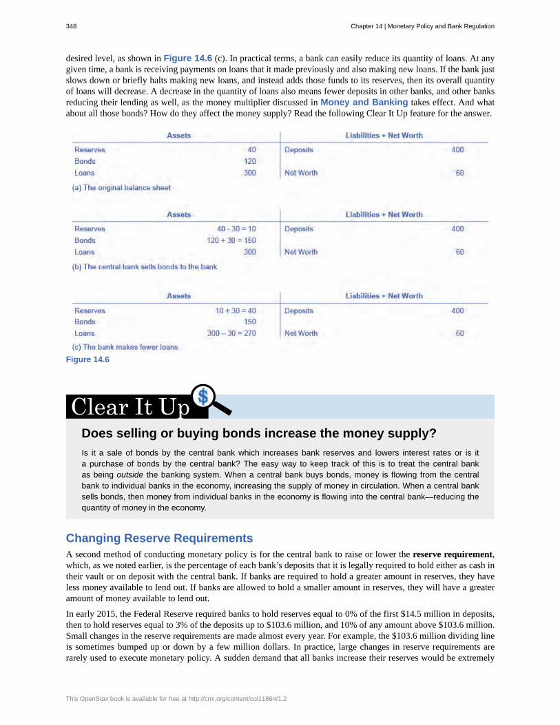
desired level, as shown in Figure 14.6 (c). In practical terms, a bank can easily reduce its quantity of loans. At anygiven time, a bank is receiving payments on loans that it made previously and also making new loans. If the bank justslows down or briefly halts making new loans, and instead adds those funds to its reserves, then its overall quantityof loans will decrease. A decrease in the quantity of loans also means fewer deposits in other banks, and other banksreducing their lending as well, as the money multiplier discussed in Money and Banking takes effect. And whatabout all those bonds? How do they affect the money supply? Read the following Clear It Up feature for the answer.
Figure 14.6
Does selling or buying bonds increase the money supply?Is it a sale of bonds by the central bank which increases bank reserves and lowers interest rates or is ita purchase of bonds by the central bank? The easy way to keep track of this is to treat the central bankas being outside the banking system. When a central bank buys bonds, money is flowing from the centralbank to individual banks in the economy, increasing the supply of money in circulation. When a central banksells bonds, then money from individual banks in the economy is flowing into the central bank—reducing thequantity of money in the economy.
Changing Reserve RequirementsA second method of conducting monetary policy is for the central bank to raise or lower the reserve requirement,which, as we noted earlier, is the percentage of each bank’s deposits that it is legally required to hold either as cash intheir vault or on deposit with the central bank. If banks are required to hold a greater amount in reserves, they haveless money available to lend out. If banks are allowed to hold a smaller amount in reserves, they will have a greateramount of money available to lend out.
In early 2015, the Federal Reserve required banks to hold reserves equal to 0% of the first $14.5 million in deposits,then to hold reserves equal to 3% of the deposits up to $103.6 million, and 10% of any amount above $103.6 million.Small changes in the reserve requirements are made almost every year. For example, the $103.6 million dividing lineis sometimes bumped up or down by a few million dollars. In practice, large changes in reserve requirements arerarely used to execute monetary policy. A sudden demand that all banks increase their reserves would be extremely
348 Chapter 14 | Monetary Policy and Bank Regulation
This OpenStax book is available for free at http://cnx.org/content/col11864/1.2
disruptive and difficult to comply with, while loosening requirements too much would create a danger of banks beingunable to meet the demand for withdrawals.
Changing the Discount RateThe Federal Reserve was founded in the aftermath of the Financial Panic of 1907 when many banks failed as a resultof bank runs. As mentioned earlier, since banks make profits by lending out their deposits, no bank, even those thatare not bankrupt, can withstand a bank run. As a result of the Panic, the Federal Reserve was founded to be the“lender of last resort.” In the event of a bank run, sound banks, (banks that were not bankrupt) could borrow as muchcash as they needed from the Fed’s discount “window” to quell the bank run. The interest rate banks pay for suchloans is called the discount rate. (They are so named because loans are made against the bank’s outstanding loans“at a discount” of their face value.) Once depositors became convinced that the bank would be able to honor theirwithdrawals, they no longer had a reason to make a run on the bank. In short, the Federal Reserve was originallyintended to provide credit passively, but in the years since its founding, the Fed has taken on a more active role withmonetary policy.
So, the third traditional method for conducting monetary policy is to raise or lower the discount rate. If the centralbank raises the discount rate, then commercial banks will reduce their borrowing of reserves from the Fed, and insteadcall in loans to replace those reserves. Since fewer loans are available, the money supply falls and market interestrates rise. If the central bank lowers the discount rate it charges to banks, the process works in reverse.
In recent decades, the Federal Reserve has made relatively few discount loans. Before a bank borrows from theFederal Reserve to fill out its required reserves, the bank is expected to first borrow from other available sources, likeother banks. This is encouraged by Fed’s charging a higher discount rate, than the federal funds rate. Given that mostbanks borrow little at the discount rate, changing the discount rate up or down has little impact on their behavior.More importantly, the Fed has found from experience that open market operations are a more precise and powerfulmeans of executing any desired monetary policy.
In the Federal Reserve Act, the phrase “...to afford means of rediscounting commercial paper” is contained in its longtitle. This tool was seen as the main tool for monetary policy when the Fed was initially created. This illustrates howmonetary policy has evolved and how it continues to do so.
14.4 | Monetary Policy and Economic OutcomesBy the end of this section, you will be able to:
• Contrast expansionary monetary policy and contractionary monetary policy• Explain how monetary policy impacts interest rates and aggregate demand• Evaluate Federal Reserve decisions over the last forty years• Explain the significance of quantitative easing (QE)
A monetary policy that lowers interest rates and stimulates borrowing is known as an expansionary monetarypolicy or loose monetary policy. Conversely, a monetary policy that raises interest rates and reduces borrowingin the economy is a contractionary monetary policy or tight monetary policy. This module will discuss howexpansionary and contractionary monetary policies affect interest rates and aggregate demand, and how such policieswill affect macroeconomic goals like unemployment and inflation. We will conclude with a look at the Fed’s monetarypolicy practice in recent decades.
The Effect of Monetary Policy on Interest RatesConsider the market for loanable bank funds, shown in Figure 14.7. The original equilibrium (E0) occurs at aninterest rate of 8% and a quantity of funds loaned and borrowed of $10 billion. An expansionary monetary policywill shift the supply of loanable funds to the right from the original supply curve (S0) to S1, leading to an equilibrium(E1) with a lower interest rate of 6% and a quantity of funds loaned of $14 billion. Conversely, a contractionarymonetary policy will shift the supply of loanable funds to the left from the original supply curve (S0) to S2, leading toan equilibrium (E2) with a higher interest rate of 10% and a quantity of funds loaned of $8 billion.
Chapter 14 | Monetary Policy and Bank Regulation 349
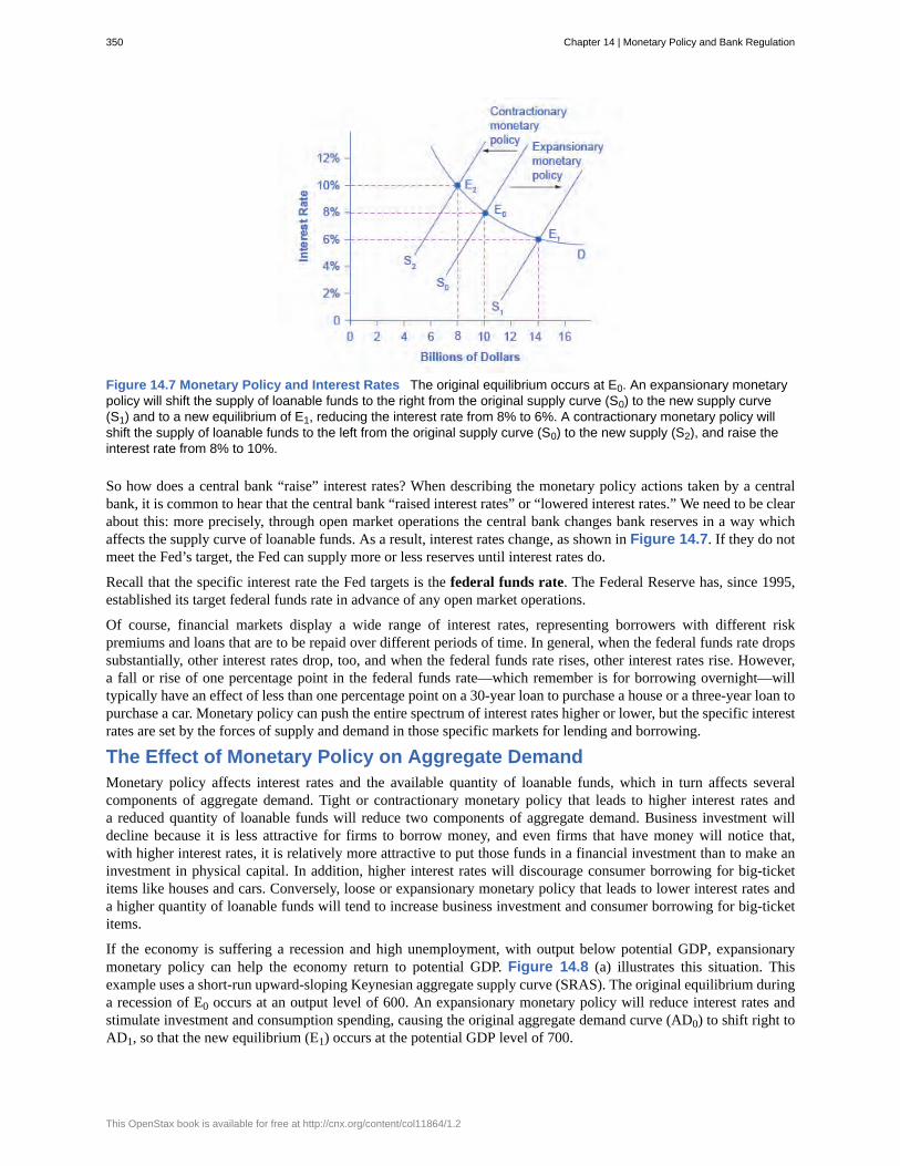
Figure 14.7 Monetary Policy and Interest Rates The original equilibrium occurs at E0. An expansionary monetarypolicy will shift the supply of loanable funds to the right from the original supply curve (S0) to the new supply curve(S1) and to a new equilibrium of E1, reducing the interest rate from 8% to 6%. A contractionary monetary policy willshift the supply of loanable funds to the left from the original supply curve (S0) to the new supply (S2), and raise theinterest rate from 8% to 10%.
So how does a central bank “raise” interest rates? When describing the monetary policy actions taken by a centralbank, it is common to hear that the central bank “raised interest rates” or “lowered interest rates.” We need to be clearabout this: more precisely, through open market operations the central bank changes bank reserves in a way whichaffects the supply curve of loanable funds. As a result, interest rates change, as shown in Figure 14.7. If they do notmeet the Fed’s target, the Fed can supply more or less reserves until interest rates do.
Recall that the specific interest rate the Fed targets is the federal funds rate. The Federal Reserve has, since 1995,established its target federal funds rate in advance of any open market operations.
Of course, financial markets display a wide range of interest rates, representing borrowers with different riskpremiums and loans that are to be repaid over different periods of time. In general, when the federal funds rate dropssubstantially, other interest rates drop, too, and when the federal funds rate rises, other interest rates rise. However,a fall or rise of one percentage point in the federal funds rate—which remember is for borrowing overnight—willtypically have an effect of less than one percentage point on a 30-year loan to purchase a house or a three-year loan topurchase a car. Monetary policy can push the entire spectrum of interest rates higher or lower, but the specific interestrates are set by the forces of supply and demand in those specific markets for lending and borrowing.
The Effect of Monetary Policy on Aggregate DemandMonetary policy affects interest rates and the available quantity of loanable funds, which in turn affects severalcomponents of aggregate demand. Tight or contractionary monetary policy that leads to higher interest rates anda reduced quantity of loanable funds will reduce two components of aggregate demand. Business investment willdecline because it is less attractive for firms to borrow money, and even firms that have money will notice that,with higher interest rates, it is relatively more attractive to put those funds in a financial investment than to make aninvestment in physical capital. In addition, higher interest rates will discourage consumer borrowing for big-ticketitems like houses and cars. Conversely, loose or expansionary monetary policy that leads to lower interest rates anda higher quantity of loanable funds will tend to increase business investment and consumer borrowing for big-ticketitems.
If the economy is suffering a recession and high unemployment, with output below potential GDP, expansionarymonetary policy can help the economy return to potential GDP. Figure 14.8 (a) illustrates this situation. Thisexample uses a short-run upward-sloping Keynesian aggregate supply curve (SRAS). The original equilibrium duringa recession of E0 occurs at an output level of 600. An expansionary monetary policy will reduce interest rates andstimulate investment and consumption spending, causing the original aggregate demand curve (AD0) to shift right toAD1, so that the new equilibrium (E1) occurs at the potential GDP level of 700.
350 Chapter 14 | Monetary Policy and Bank Regulation
This OpenStax book is available for free at http://cnx.org/content/col11864/1.2
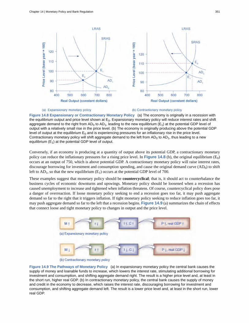
Figure 14.8 Expansionary or Contractionary Monetary Policy (a) The economy is originally in a recession withthe equilibrium output and price level shown at E0. Expansionary monetary policy will reduce interest rates and shiftaggregate demand to the right from AD0 to AD1, leading to the new equilibrium (E1) at the potential GDP level ofoutput with a relatively small rise in the price level. (b) The economy is originally producing above the potential GDPlevel of output at the equilibrium E0 and is experiencing pressures for an inflationary rise in the price level.Contractionary monetary policy will shift aggregate demand to the left from AD0 to AD1, thus leading to a newequilibrium (E1) at the potential GDP level of output.
Conversely, if an economy is producing at a quantity of output above its potential GDP, a contractionary monetarypolicy can reduce the inflationary pressures for a rising price level. In Figure 14.8 (b), the original equilibrium (E0)occurs at an output of 750, which is above potential GDP. A contractionary monetary policy will raise interest rates,discourage borrowing for investment and consumption spending, and cause the original demand curve (AD0) to shiftleft to AD1, so that the new equilibrium (E1) occurs at the potential GDP level of 700.
These examples suggest that monetary policy should be countercyclical; that is, it should act to counterbalance thebusiness cycles of economic downturns and upswings. Monetary policy should be loosened when a recession hascaused unemployment to increase and tightened when inflation threatens. Of course, countercyclical policy does posea danger of overreaction. If loose monetary policy seeking to end a recession goes too far, it may push aggregatedemand so far to the right that it triggers inflation. If tight monetary policy seeking to reduce inflation goes too far, itmay push aggregate demand so far to the left that a recession begins. Figure 14.9 (a) summarizes the chain of effectsthat connect loose and tight monetary policy to changes in output and the price level.
Figure 14.9 The Pathways of Monetary Policy (a) In expansionary monetary policy the central bank causes thesupply of money and loanable funds to increase, which lowers the interest rate, stimulating additional borrowing forinvestment and consumption, and shifting aggregate demand right. The result is a higher price level and, at least inthe short run, higher real GDP. (b) In contractionary monetary policy, the central bank causes the supply of moneyand credit in the economy to decrease, which raises the interest rate, discouraging borrowing for investment andconsumption, and shifting aggregate demand left. The result is a lower price level and, at least in the short run, lowerreal GDP.
Chapter 14 | Monetary Policy and Bank Regulation 351
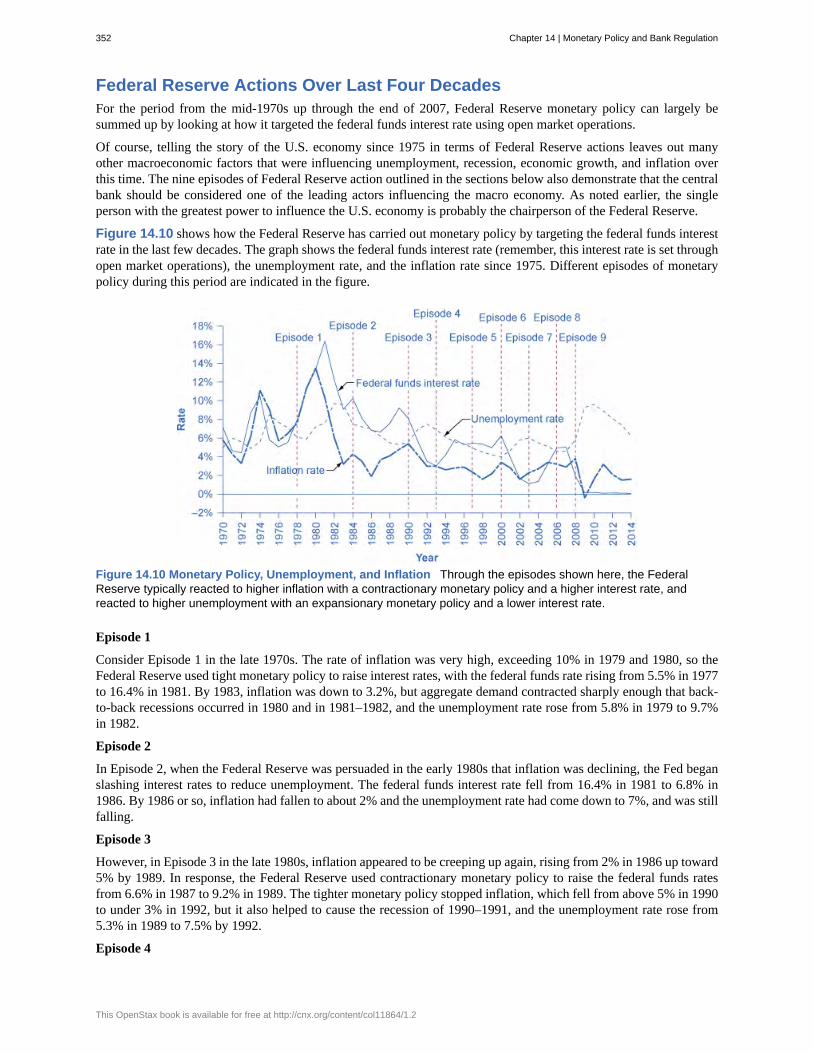
Federal Reserve Actions Over Last Four DecadesFor the period from the mid-1970s up through the end of 2007, Federal Reserve monetary policy can largely besummed up by looking at how it targeted the federal funds interest rate using open market operations.
Of course, telling the story of the U.S. economy since 1975 in terms of Federal Reserve actions leaves out manyother macroeconomic factors that were influencing unemployment, recession, economic growth, and inflation overthis time. The nine episodes of Federal Reserve action outlined in the sections below also demonstrate that the centralbank should be considered one of the leading actors influencing the macro economy. As noted earlier, the singleperson with the greatest power to influence the U.S. economy is probably the chairperson of the Federal Reserve.
Figure 14.10 shows how the Federal Reserve has carried out monetary policy by targeting the federal funds interestrate in the last few decades. The graph shows the federal funds interest rate (remember, this interest rate is set throughopen market operations), the unemployment rate, and the inflation rate since 1975. Different episodes of monetarypolicy during this period are indicated in the figure.
Figure 14.10 Monetary Policy, Unemployment, and Inflation Through the episodes shown here, the FederalReserve typically reacted to higher inflation with a contractionary monetary policy and a higher interest rate, andreacted to higher unemployment with an expansionary monetary policy and a lower interest rate.
Episode 1
Consider Episode 1 in the late 1970s. The rate of inflation was very high, exceeding 10% in 1979 and 1980, so theFederal Reserve used tight monetary policy to raise interest rates, with the federal funds rate rising from 5.5% in 1977to 16.4% in 1981. By 1983, inflation was down to 3.2%, but aggregate demand contracted sharply enough that back-to-back recessions occurred in 1980 and in 1981–1982, and the unemployment rate rose from 5.8% in 1979 to 9.7%in 1982.
Episode 2
In Episode 2, when the Federal Reserve was persuaded in the early 1980s that inflation was declining, the Fed beganslashing interest rates to reduce unemployment. The federal funds interest rate fell from 16.4% in 1981 to 6.8% in1986. By 1986 or so, inflation had fallen to about 2% and the unemployment rate had come down to 7%, and was stillfalling.
Episode 3
However, in Episode 3 in the late 1980s, inflation appeared to be creeping up again, rising from 2% in 1986 up toward5% by 1989. In response, the Federal Reserve used contractionary monetary policy to raise the federal funds ratesfrom 6.6% in 1987 to 9.2% in 1989. The tighter monetary policy stopped inflation, which fell from above 5% in 1990to under 3% in 1992, but it also helped to cause the recession of 1990–1991, and the unemployment rate rose from5.3% in 1989 to 7.5% by 1992.
Episode 4
352 Chapter 14 | Monetary Policy and Bank Regulation
This OpenStax book is available for free at http://cnx.org/content/col11864/1.2
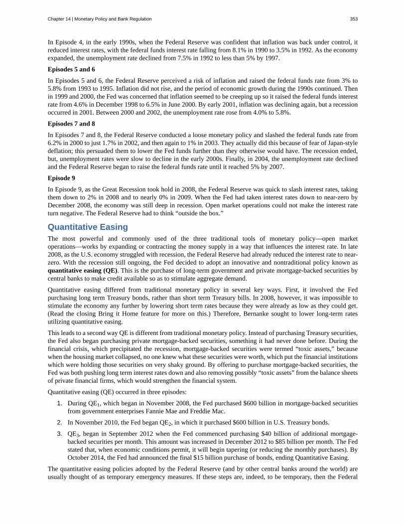
In Episode 4, in the early 1990s, when the Federal Reserve was confident that inflation was back under control, itreduced interest rates, with the federal funds interest rate falling from 8.1% in 1990 to 3.5% in 1992. As the economyexpanded, the unemployment rate declined from 7.5% in 1992 to less than 5% by 1997.
Episodes 5 and 6
In Episodes 5 and 6, the Federal Reserve perceived a risk of inflation and raised the federal funds rate from 3% to5.8% from 1993 to 1995. Inflation did not rise, and the period of economic growth during the 1990s continued. Thenin 1999 and 2000, the Fed was concerned that inflation seemed to be creeping up so it raised the federal funds interestrate from 4.6% in December 1998 to 6.5% in June 2000. By early 2001, inflation was declining again, but a recessionoccurred in 2001. Between 2000 and 2002, the unemployment rate rose from 4.0% to 5.8%.
Episodes 7 and 8
In Episodes 7 and 8, the Federal Reserve conducted a loose monetary policy and slashed the federal funds rate from6.2% in 2000 to just 1.7% in 2002, and then again to 1% in 2003. They actually did this because of fear of Japan-styledeflation; this persuaded them to lower the Fed funds further than they otherwise would have. The recession ended,but, unemployment rates were slow to decline in the early 2000s. Finally, in 2004, the unemployment rate declinedand the Federal Reserve began to raise the federal funds rate until it reached 5% by 2007.
Episode 9
In Episode 9, as the Great Recession took hold in 2008, the Federal Reserve was quick to slash interest rates, takingthem down to 2% in 2008 and to nearly 0% in 2009. When the Fed had taken interest rates down to near-zero byDecember 2008, the economy was still deep in recession. Open market operations could not make the interest rateturn negative. The Federal Reserve had to think “outside the box.”
Quantitative EasingThe most powerful and commonly used of the three traditional tools of monetary policy—open marketoperations—works by expanding or contracting the money supply in a way that influences the interest rate. In late2008, as the U.S. economy struggled with recession, the Federal Reserve had already reduced the interest rate to near-zero. With the recession still ongoing, the Fed decided to adopt an innovative and nontraditional policy known asquantitative easing (QE). This is the purchase of long-term government and private mortgage-backed securities bycentral banks to make credit available so as to stimulate aggregate demand.
Quantitative easing differed from traditional monetary policy in several key ways. First, it involved the Fedpurchasing long term Treasury bonds, rather than short term Treasury bills. In 2008, however, it was impossible tostimulate the economy any further by lowering short term rates because they were already as low as they could get.(Read the closing Bring it Home feature for more on this.) Therefore, Bernanke sought to lower long-term ratesutilizing quantitative easing.
This leads to a second way QE is different from traditional monetary policy. Instead of purchasing Treasury securities,the Fed also began purchasing private mortgage-backed securities, something it had never done before. During thefinancial crisis, which precipitated the recession, mortgage-backed securities were termed “toxic assets,” becausewhen the housing market collapsed, no one knew what these securities were worth, which put the financial institutionswhich were holding those securities on very shaky ground. By offering to purchase mortgage-backed securities, theFed was both pushing long term interest rates down and also removing possibly “toxic assets” from the balance sheetsof private financial firms, which would strengthen the financial system.
Quantitative easing (QE) occurred in three episodes:
1. During QE1, which began in November 2008, the Fed purchased $600 billion in mortgage-backed securitiesfrom government enterprises Fannie Mae and Freddie Mac.
2. In November 2010, the Fed began QE2, in which it purchased $600 billion in U.S. Treasury bonds.
3. QE3, began in September 2012 when the Fed commenced purchasing $40 billion of additional mortgage-backed securities per month. This amount was increased in December 2012 to $85 billion per month. The Fedstated that, when economic conditions permit, it will begin tapering (or reducing the monthly purchases). ByOctober 2014, the Fed had announced the final $15 billion purchase of bonds, ending Quantitative Easing.
The quantitative easing policies adopted by the Federal Reserve (and by other central banks around the world) areusually thought of as temporary emergency measures. If these steps are, indeed, to be temporary, then the Federal
Chapter 14 | Monetary Policy and Bank Regulation 353
Reserve will need to stop making these additional loans and sell off the financial securities it has accumulated.The concern is that the process of quantitative easing may prove more difficult to reverse than it was to enact. Theevidence suggests that QE1 was somewhat successful, but that QE2 and QE3 have been less so.
14.5 | Pitfalls for Monetary PolicyBy the end of this section, you will be able to:
• Analyze whether monetary policy decisions should be made more democratically• Calculate the velocity of money• Evaluate the central bank’s influence on inflation, unemployment, asset bubbles, and leverage cycles• Calculate the effects of monetary stimulus
In the real world, effective monetary policy faces a number of significant hurdles. Monetary policy affects theeconomy only after a time lag that is typically long and of variable length. Remember, monetary policy involvesa chain of events: the central bank must perceive a situation in the economy, hold a meeting, and make a decisionto react by tightening or loosening monetary policy. The change in monetary policy must percolate through thebanking system, changing the quantity of loans and affecting interest rates. When interest rates change, businessesmust change their investment levels and consumers must change their borrowing patterns when purchasing homes orcars. Then it takes time for these changes to filter through the rest of the economy.
As a result of this chain of events, monetary policy has little effect in the immediate future; instead, its primary effectsare felt perhaps one to three years in the future. The reality of long and variable time lags does not mean that a centralbank should refuse to make decisions. It does mean that central banks should be humble about taking action, becauseof the risk that their actions can create as much or more economic instability as they resolve.
Excess ReservesBanks are legally required to hold a minimum level of reserves, but no rule prohibits them from holding additionalexcess reserves above the legally mandated limit. For example, during a recession banks may be hesitant to lend,because they fear that when the economy is contracting, a high proportion of loan applicants become less likely torepay their loans.
When many banks are choosing to hold excess reserves, expansionary monetary policy may not work well. This mayoccur because the banks are concerned about a deteriorating economy, while the central bank is trying to expandthe money supply. If the banks prefer to hold excess reserves above the legally required level, the central bankcannot force individual banks to make loans. Similarly, sensible businesses and consumers may be reluctant to borrowsubstantial amounts of money in a recession, because they recognize that firms’ sales and employees’ jobs are moreinsecure in a recession, and they do not want to face the need to make interest payments. The result is that during anespecially deep recession, an expansionary monetary policy may have little effect on either the price level or the realGDP.
Japan experienced this situation in the 1990s and early 2000s. Japan’s economy entered a period of very slow growth,dipping in and out of recession, in the early 1990s. By February 1999, the Bank of Japan had lowered the equivalentof its federal funds rate to 0%. It kept it there most of the time through 2003. Moreover, in the two years from March2001 to March 2003, the Bank of Japan also expanded the money supply of the country by about 50%—an enormousincrease. Even this highly expansionary monetary policy, however, had no substantial effect on stimulating aggregatedemand. Japan’s economy continued to experience extremely slow growth into the mid-2000s.
354 Chapter 14 | Monetary Policy and Bank Regulation
This OpenStax book is available for free at http://cnx.org/content/col11864/1.2
Should monetary policy decisions be made more democratically?Should monetary policy be conducted by a nation’s Congress or legislature comprised of electedrepresentatives? Or should it be conducted by a politically appointed central bank that is more independent ofvoters? Here are some of the arguments made by each side.
The Case for Greater Democratic Control of Monetary Policy
Elected representatives conduct fiscal policy by passing tax and spending bills. They could handle monetarypolicy in the same way. Sure, they will sometimes make mistakes, but in a democracy, it is better to havemistakes made by elected officials accountable to voters than by political appointees. After all, the peopleappointed to the top governing positions at the Federal Reserve—and to most central banks around theworld—are typically bankers and economists. They are not representatives of borrowers like small businessesor farmers nor are they representatives of labor unions. Central banks might not be so quick to raise interestrates if they had to pay more attention to firms and people in the real economy.
The Case for an Independent Central Bank
Because the central bank has some insulation from day-to-day politics, its members can take a nonpartisanlook at specific economic situations and make tough, immediate decisions when necessary. The idea of givinga legislature the ability to create money and hand out loans is likely to end up badly, sooner or later. It is simplytoo tempting for lawmakers to expand the money supply to fund their projects. The long term result will berampant inflation. Also, a central bank, acting according to the laws passed by elected officials, can respondfar more quickly than a legislature. For example, the U.S. budget takes months to debate, pass, and be signedinto law, but monetary policy decisions can be made much more rapidly. Day-to-day democratic control ofmonetary policy is impractical and seems likely to lead to an overly expansionary monetary policy and higherinflation.
The problem of excess reserves does not affect contractionary policy. Central bankers have an old saying thatmonetary policy can be like pulling and pushing on a string: when the central bank pulls on the string and usescontractionary monetary policy, it can definitely raise interest rates and reduce aggregate demand. However, when thecentral bank tries to push on the string of expansionary monetary policy, the string may sometimes just fold up limpand have little effect, because banks decide not to loan out their excess reserves. This analogy should not be taken tooliterally—expansionary monetary policy usually does have real effects, after that inconveniently long and variablelag. There are also times, like Japan’s economy in the late 1990s and early 2000s, when expansionary monetary policyhas been insufficient to lift a recession-prone economy.
Unpredictable Movements of VelocityVelocity is a term that economists use to describe how quickly money circulates through the economy. The velocityof money in a year is defined as:
Velocity = nominal GDPmoney supply
Specific measurements of velocity depend on the definition of the money supply being used. Consider the velocityof M1, the total amount of currency in circulation and checking account balances. In 2009, for example, M1 was$1.7 trillion and nominal GDP was $14.3 trillion, so the velocity of M1 was 8.4 ($14.3 trillion/$1.7 trillion). A highervelocity of money means that the average dollar circulates more times in a year; a lower velocity means that theaverage dollar circulates fewer times in a year.
Perhaps you heard the “d” word mentioned during our recent economic downturn. See the following Clear It Upfeature for a discussion of how deflation could affect monetary policy.
Chapter 14 | Monetary Policy and Bank Regulation 355
What happens during episodes of deflation?Deflation occurs when the rate of inflation is negative; that is, instead of money having less purchasing powerover time, as occurs with inflation, money is worth more. Deflation can make it very difficult for monetary policyto address a recession.
Remember that the real interest rate is the nominal interest rate minus the rate of inflation. If the nominalinterest rate is 7% and the rate of inflation is 3%, then the borrower is effectively paying a 4% real interest rate.If the nominal interest rate is 7% and there is deflation of 2%, then the real interest rate is actually 9%. In thisway, an unexpected deflation raises the real interest payments for borrowers. It can lead to a situation wherean unexpectedly high number of loans are not repaid, and banks find that their net worth is decreasing ornegative. When banks are suffering losses, they become less able and eager to make new loans. Aggregatedemand declines, which can lead to recession.
Then the double-whammy: After causing a recession, deflation can make it difficult for monetary policy towork. Say that the central bank uses expansionary monetary policy to reduce the nominal interest rate allthe way to zero—but the economy has 5% deflation. As a result, the real interest rate is 5%, and becausea central bank cannot make the nominal interest rate negative, expansionary policy cannot reduce the realinterest rate further.
In the U.S. economy during the early 1930s, deflation was 6.7% per year from 1930–1933, which causedmany borrowers to default on their loans and many banks to end up bankrupt, which in turn contributedsubstantially to the Great Depression. Not all episodes of deflation, however, end in economic depression.Japan, for example, experienced deflation of slightly less than 1% per year from 1999–2002, which hurt theJapanese economy, but it still grew by about 0.9% per year over this period. Indeed, there is at least onehistorical example of deflation coexisting with rapid growth. The U.S. economy experienced deflation of about1.1% per year over the quarter-century from 1876–1900, but real GDP also expanded at a rapid clip of 4% peryear over this time, despite some occasional severe recessions.
The central bank should be on guard against deflation and, if necessary, use expansionary monetary policyto prevent any long-lasting or extreme deflation from occurring. Except in severe cases like the GreatDepression, deflation does not guarantee economic disaster.
Changes in velocity can cause problems for monetary policy. To understand why, rewrite the definition of velocity sothat the money supply is on the left-hand side of the equation. That is:
Money supply × velocity = Nominal GDP
Recall from The Macroeconomic Perspective that
Nominal GDP = Price Level (or GDP Deflator) x Real GDP.
Therefore,
Money Supply x velocity = Nominal GDP = Price Level x Real GDP.
This equation is sometimes called the basic quantity equation of money but, as you can see, it is just the definitionof velocity written in a different form. This equation must hold true, by definition.
If velocity is constant over time, then a certain percentage rise in the money supply on the left-hand side of the basicquantity equation of money will inevitably lead to the same percentage rise in nominal GDP—although this changecould happen through an increase in inflation, or an increase in real GDP, or some combination of the two. If velocityis changing over time but in a constant and predictable way, then changes in the money supply will continue to have apredictable effect on nominal GDP. If velocity changes unpredictably over time, however, then the effect of changesin the money supply on nominal GDP becomes unpredictable.
The actual velocity of money in the U.S. economy as measured by using M1, the most common definition of themoney supply, is illustrated in Figure 14.11. From 1960 up to about 1980, velocity appears fairly predictable; that
356 Chapter 14 | Monetary Policy and Bank Regulation
This OpenStax book is available for free at http://cnx.org/content/col11864/1.2
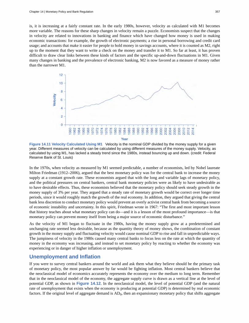
is, it is increasing at a fairly constant rate. In the early 1980s, however, velocity as calculated with M1 becomesmore variable. The reasons for these sharp changes in velocity remain a puzzle. Economists suspect that the changesin velocity are related to innovations in banking and finance which have changed how money is used in makingeconomic transactions: for example, the growth of electronic payments; a rise in personal borrowing and credit cardusage; and accounts that make it easier for people to hold money in savings accounts, where it is counted as M2, rightup to the moment that they want to write a check on the money and transfer it to M1. So far at least, it has provendifficult to draw clear links between these kinds of factors and the specific up-and-down fluctuations in M1. Givenmany changes in banking and the prevalence of electronic banking, M2 is now favored as a measure of money ratherthan the narrower M1.
Figure 14.11 Velocity Calculated Using M1 Velocity is the nominal GDP divided by the money supply for a givenyear. Different measures of velocity can be calculated by using different measures of the money supply. Velocity, ascalculated by using M1, has lacked a steady trend since the 1980s, instead bouncing up and down. (credit: FederalReserve Bank of St. Louis)
In the 1970s, when velocity as measured by M1 seemed predictable, a number of economists, led by Nobel laureateMilton Friedman (1912–2006), argued that the best monetary policy was for the central bank to increase the moneysupply at a constant growth rate. These economists argued that with the long and variable lags of monetary policy,and the political pressures on central bankers, central bank monetary policies were as likely to have undesirable asto have desirable effects. Thus, these economists believed that the monetary policy should seek steady growth in themoney supply of 3% per year. They argued that a steady rate of monetary growth would be correct over longer timeperiods, since it would roughly match the growth of the real economy. In addition, they argued that giving the centralbank less discretion to conduct monetary policy would prevent an overly activist central bank from becoming a sourceof economic instability and uncertainty. In this spirit, Friedman wrote in 1967: “The first and most important lessonthat history teaches about what monetary policy can do—and it is a lesson of the most profound importance—is thatmonetary policy can prevent money itself from being a major source of economic disturbance.”
As the velocity of M1 began to fluctuate in the 1980s, having the money supply grow at a predetermined andunchanging rate seemed less desirable, because as the quantity theory of money shows, the combination of constantgrowth in the money supply and fluctuating velocity would cause nominal GDP to rise and fall in unpredictable ways.The jumpiness of velocity in the 1980s caused many central banks to focus less on the rate at which the quantity ofmoney in the economy was increasing, and instead to set monetary policy by reacting to whether the economy wasexperiencing or in danger of higher inflation or unemployment.
Unemployment and InflationIf you were to survey central bankers around the world and ask them what they believe should be the primary taskof monetary policy, the most popular answer by far would be fighting inflation. Most central bankers believe thatthe neoclassical model of economics accurately represents the economy over the medium to long term. Rememberthat in the neoclassical model of the economy, the aggregate supply curve is drawn as a vertical line at the level ofpotential GDP, as shown in Figure 14.12. In the neoclassical model, the level of potential GDP (and the naturalrate of unemployment that exists when the economy is producing at potential GDP) is determined by real economicfactors. If the original level of aggregate demand is AD0, then an expansionary monetary policy that shifts aggregate
Chapter 14 | Monetary Policy and Bank Regulation 357

demand to AD1 only creates an inflationary increase in the price level, but it does not alter GDP or unemployment.From this perspective, all that monetary policy can do is to lead to low inflation or high inflation—and low inflationprovides a better climate for a healthy and growing economy. After all, low inflation means that businesses makinginvestments can focus on real economic issues, not on figuring out ways to protect themselves from the costs andrisks of inflation. In this way, a consistent pattern of low inflation can contribute to long-term growth.
Figure 14.12 Monetary Policy in a Neoclassical Model In a neoclassical view, monetary policy affects only theprice level, not the level of output in the economy. For example, an expansionary monetary policy causes aggregatedemand to shift from the original AD0 to AD1. However, the adjustment of the economy from the original equilibrium(E0) to the new equilibrium (E1) represents an inflationary increase in the price level from P0 to P1, but has no effect inthe long run on output or the unemployment rate. In fact, no shift in AD will affect the equilibrium quantity of output inthis model.
This vision of focusing monetary policy on a low rate of inflation is so attractive that many countries have rewrittentheir central banking laws since in the 1990s to have their bank practice inflation targeting, which means that thecentral bank is legally required to focus primarily on keeping inflation low. By 2014, central banks in 28 countries,including Austria, Brazil, Canada, Israel, Korea, Mexico, New Zealand, Spain, Sweden, Thailand, and the UnitedKingdom faced a legal requirement to target the inflation rate. A notable exception is the Federal Reserve in theUnited States, which does not practice inflation-targeting. Instead, the law governing the Federal Reserve requires itto take both unemployment and inflation into account.
Economists have no final consensus on whether a central bank should be required to focus only on inflation or shouldhave greater discretion. For those who subscribe to the inflation targeting philosophy, the fear is that politicians whoare worried about slow economic growth and unemployment will constantly pressure the central bank to conduct aloose monetary policy—even if the economy is already producing at potential GDP. In some countries, the centralbank may lack the political power to resist such pressures, with the result of higher inflation, but no long-termreduction in unemployment. The U.S. Federal Reserve has a tradition of independence, but central banks in othercountries may be under greater political pressure. For all of these reasons—long and variable lags, excess reserves,unstable velocity, and controversy over economic goals—monetary policy in the real world is often difficult. Thebasic message remains, however, that central banks can affect aggregate demand through the conduct of monetarypolicy and in that way influence macroeconomic outcomes.
Asset Bubbles and Leverage CyclesOne long-standing concern about having the central bank focus on inflation and unemployment is that it may beoverlooking certain other economic problems that are coming in the future. For example, from 1994 to 2000 duringwhat was known as the “dot-com” boom, the U.S. stock market, which is measured by the Dow Jones IndustrialIndex (which includes 30 very large companies from across the U.S. economy), nearly tripled in value. The Nasdaqindex, which includes many smaller technology companies, increased in value by a multiple of five from 1994 to2000. These rates of increase were clearly not sustainable. Indeed, stock values as measured by the Dow Jones werealmost 20% lower in 2009 than they had been in 2000. Stock values in the Nasdaq index were 50% lower in 2009than they had been in 2000. The drop-off in stock market values contributed to the recession of 2001 and the higherunemployment that followed.
358 Chapter 14 | Monetary Policy and Bank Regulation
This OpenStax book is available for free at http://cnx.org/content/col11864/1.2
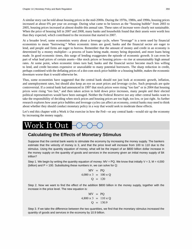
A similar story can be told about housing prices in the mid-2000s. During the 1970s, 1980s, and 1990s, housing pricesincreased at about 6% per year on average. During what came to be known as the “housing bubble” from 2003 to2005, housing prices increased at almost double this annual rate. These rates of increase were clearly not sustainable.When the price of housing fell in 2007 and 2008, many banks and households found that their assets were worth lessthan they expected, which contributed to the recession that started in 2007.
At a broader level, some economists worry about a leverage cycle, where “leverage” is a term used by financialeconomists to mean “borrowing.” When economic times are good, banks and the financial sector are eager tolend, and people and firms are eager to borrow. Remember that the amount of money and credit in an economy isdetermined by a money multiplier—a process of loans being made, money being deposited, and more loans beingmade. In good economic times, this surge of lending exaggerates the episode of economic growth. It can even bepart of what lead prices of certain assets—like stock prices or housing prices—to rise at unsustainably high annualrates. At some point, when economic times turn bad, banks and the financial sector become much less willingto lend, and credit becomes expensive or unavailable to many potential borrowers. The sharp reduction in credit,perhaps combined with the deflating prices of a dot-com stock price bubble or a housing bubble, makes the economicdownturn worse than it would otherwise be.
Thus, some economists have suggested that the central bank should not just look at economic growth, inflation,and unemployment rates, but should also keep an eye on asset prices and leverage cycles. Such proposals are quitecontroversial. If a central bank had announced in 1997 that stock prices were rising “too fast” or in 2004 that housingprices were rising “too fast,” and then taken action to hold down price increases, many people and their electedpolitical representatives would have been outraged. Neither the Federal Reserve nor any other central banks want totake the responsibility of deciding when stock prices and housing prices are too high, too low, or just right. As furtherresearch explores how asset price bubbles and leverage cycles can affect an economy, central banks may need to thinkabout whether they should conduct monetary policy in a way that would seek to moderate these effects.
Let’s end this chapter with a Work it Out exercise in how the Fed—or any central bank—would stir up the economyby increasing the money supply.
Calculating the Effects of Monetary StimulusSuppose that the central bank wants to stimulate the economy by increasing the money supply. The bankersestimate that the velocity of money is 3, and that the price level will increase from 100 to 110 due to thestimulus. Using the quantity equation of money, what will be the impact of an $800 billion dollar increase inthe money supply on the quantity of goods and services in the economy given an initial money supply of $4trillion?
Step 1. We begin by writing the quantity equation of money: MV = PQ. We know that initially V = 3, M = 4,000(billion) and P = 100. Substituting these numbers in, we can solve for Q:
MV = PQ4,000 × 3 = 100 × Q
Q = 120
Step 2. Now we want to find the effect of the addition $800 billion in the money supply, together with theincrease in the price level. The new equation is:
MV = PQ4,800 × 3 = 110 × Q
Q = 130.9
Step 3. If we take the difference between the two quantities, we find that the monetary stimulus increased thequantity of goods and services in the economy by 10.9 billion.
Chapter 14 | Monetary Policy and Bank Regulation 359
The discussion in this chapter has focused on domestic monetary policy; that is, the view of monetary policy within aneconomy. Exchange Rates and International Capital Flows explores the international dimension of monetarypolicy, and how monetary policy becomes involved with exchange rates and international flows of financial capital.
The Problem of the Zero Percent Interest Rate Lower BoundIn 2008, the U.S. Federal Reserve found itself in a difficult position. The federal funds rate was on itsway to near zero, which meant that traditional open market operations, by which the Fed purchases U.S.Treasury Bills to lower short term interest rates, was no longer viable. This so called “zero bound problem,”prompted the Fed, under then Chair Ben Bernanke, to attempt some unconventional policies, collectivelycalled quantitative easing. By early 2014, quantitative easing nearly quintupled the amount of bank reserves.This likely contributed to the U.S. economy’s recovery, but the impact was muted, probably due to some of thehurdles mentioned in the last section of this module. The unprecedented increase in bank reserves also led tofears of inflation. As of early 2015, however, there have been no serious signs of a boom, with core inflationaround a stable 1.7%.
360 Chapter 14 | Monetary Policy and Bank Regulation
This OpenStax book is available for free at http://cnx.org/content/col11864/1.2
bank run
basic quantity equation of money
central bank
contractionary monetary policy
countercyclical
deposit insurance
discount rate
excess reserves
expansionary monetary policy
federal funds rate
inflation targeting
lender of last resort
loose monetary policy
open market operations
quantitative easing (QE)
reserve requirement
tight monetary policy
velocity
KEY TERMS
when depositors race to the bank to withdraw their deposits for fear that otherwise they would be lost
money supply × velocity = nominal GDP
institution which conducts a nation’s monetary policy and regulates its banking system
a monetary policy that reduces the supply of money and loans
moving in the opposite direction of the business cycle of economic downturns and upswings
an insurance system that makes sure depositors in a bank do not lose their money, even if the bankgoes bankrupt
the interest rate charged by the central bank on the loans that it gives to other commercial banks
reserves banks hold that exceed the legally mandated limit
a monetary policy that increases the supply of money and the quantity of loans
the interest rate at which one bank lends funds to another bank overnight
a rule that the central bank is required to focus only on keeping inflation low
an institution that provides short-term emergency loans in conditions of financial crisis
see expansionary monetary policy
the central bank selling or buying Treasury bonds to influence the quantity of money and thelevel of interest rates
the purchase of long term government and private mortgage-backed securities by centralbanks to make credit available in hopes of stimulating aggregate demand
the percentage amount of its total deposits that a bank is legally obligated to to either hold ascash in their vault or deposit with the central bank
see contractionary monetary policy
the speed with which money circulates through the economy; calculated as the nominal GDP divided by themoney supply
KEY CONCEPTS AND SUMMARY
14.1 The Federal Reserve Banking System and Central BanksThe most prominent task of a central bank is to conduct monetary policy, which involves changes to interest ratesand credit conditions, affecting the amount of borrowing and spending in an economy. Some prominent central banksaround the world include the U.S. Federal Reserve, the European Central Bank, the Bank of Japan, and the Bank ofEngland.
14.2 Bank RegulationA bank run occurs when there are rumors (possibly true, possibly false) that a bank is at financial risk of havingnegative net worth. As a result, depositors rush to the bank to withdraw their money and put it someplace safer. Evenfalse rumors, if they cause a bank run, can force a healthy bank to lose its deposits and be forced to close. Depositinsurance guarantees bank depositors that, even if the bank has negative net worth, their deposits will be protected. In
Chapter 14 | Monetary Policy and Bank Regulation 361
the United States, the Federal Deposit Insurance Corporation (FDIC) collects deposit insurance premiums from banksand guarantees bank deposits up to $250,000. Bank supervision involves inspecting the balance sheets of banks tomake sure that they have positive net worth and that their assets are not too risky. In the United States, the Office ofthe Comptroller of the Currency (OCC) is responsible for supervising banks and inspecting savings and loans and theNational Credit Union Administration (NCUA) is responsible for inspecting credit unions. The FDIC and the FederalReserve also play a role in bank supervision.
When a central bank acts as a lender of last resort, it makes short-term loans available in situations of severe financialpanic or stress. The failure of a single bank can be treated like any other business failure. Yet if many banks fail, itcan reduce aggregate demand in a way that can bring on or deepen a recession. The combination of deposit insurance,bank supervision, and lender of last resort policies help to prevent weaknesses in the banking system from causingrecessions.
14.3 How a Central Bank Executes Monetary PolicyA central bank has three traditional tools to conduct monetary policy: open market operations, which involves buyingand selling government bonds with banks; reserve requirements, which determine what level of reserves a bank islegally required to hold; and discount rates, which is the interest rate charged by the central bank on the loans that itgives to other commercial banks. The most commonly used tool is open market operations.
14.4 Monetary Policy and Economic OutcomesAn expansionary (or loose) monetary policy raises the quantity of money and credit above what it otherwise wouldhave been and reduces interest rates, boosting aggregate demand, and thus countering recession. A contractionarymonetary policy, also called a tight monetary policy, reduces the quantity of money and credit below what it otherwisewould have been and raises interest rates, seeking to hold down inflation. During the 2008–2009 recession, centralbanks around the world also used quantitative easing to expand the supply of credit.
14.5 Pitfalls for Monetary PolicyMonetary policy is inevitably imprecise, for a number of reasons: (a) the effects occur only after long and variablelags; (b) if banks decide to hold excess reserves, monetary policy cannot force them to lend; and (c) velocity mayshift in unpredictable ways. The basic quantity equation of money is MV = PQ, where M is the money supply, Vis the velocity of money, P is the price level, and Q is the real output of the economy. Some central banks, like theEuropean Central Bank, practice inflation targeting, which means that the only goal of the central bank is to keepinflation within a low target range. Other central banks, such as the U.S. Federal Reserve, are free to focus on eitherreducing inflation or stimulating an economy that is in recession, whichever goal seems most important at the time.
SELF-CHECK QUESTIONS1. Why is it important for the members of the Board of Governors of the Federal Reserve to have longer terms inoffice than elected officials, like the President?
2. Given the danger of bank runs, why do banks not keep the majority of deposits on hand to meet the demands ofdepositors?
3. Bank runs are often described as “self-fulfilling prophecies.” Why is this phrase appropriate to bank runs?
4. If the central bank sells $500 in bonds to a bank that has issued $10,000 in loans and is exactly meeting the reserverequirement of 10%, what will happen to the amount of loans and to the money supply in general?
5. What would be the effect of increasing the reserve requirements of banks on the money supply?
6. Why does contractionary monetary policy cause interest rates to rise?
7. Why does expansionary monetary policy causes interest rates to drop?
8. Why might banks want to hold excess reserves in time of recession?
9. Why might the velocity of money change unexpectedly?
362 Chapter 14 | Monetary Policy and Bank Regulation
This OpenStax book is available for free at http://cnx.org/content/col11864/1.2
REVIEW QUESTIONS
10. How is a central bank different from a typicalcommercial bank?
11. List the three traditional tools that a central bankhas for controlling the money supply.
12. How is bank regulation linked to the conduct ofmonetary policy?
13. What is a bank run?
14. In a program of deposit insurance as it is operatedin the United States, what is being insured and who paysthe insurance premiums?
15. In government programs of bank supervision, whatis being supervised?
16. What is the lender of last resort?
17. Name and briefly describe the responsibilities ofeach of the following agencies: FDIC, NCUA, andOCC.
18. Explain how to use an open market operation toexpand the money supply.
19. Explain how to use the reserve requirement toexpand the money supply.
20. Explain how to use the discount rate to expand themoney supply.
21. How do the expansionary and contractionarymonetary policy affect the quantity of money?
22. How do tight and loose monetary policy affectinterest rates?
23. How do expansionary, tight, contractionary, andloose monetary policy affect aggregate demand?
24. Which kind of monetary policy would you expectin response to high inflation: expansionary orcontractionary? Why?
25. Explain how to use quantitative easing to stimulateaggregate demand.
26. Which kind of monetary policy would you expectin response to recession: expansionary orcontractionary? Why?
27. How might each of the following factorscomplicate the implementation of monetary policy: longand variable lags, excess reserves, and movements invelocity?
28. Define the velocity of the money supply.
29. What is the basic quantity equation of money?
30. How does a monetary policy of inflation targetingwork?
CRITICAL THINKING QUESTIONS
31. Why do presidents typically reappoint Chairs of theFederal Reserve Board even when they were originallyappointed by a president of a different political party?
32. In what ways might monetary policy be superior tofiscal policy? In what ways might it be inferior?
33. The term “moral hazard” describes increases inrisky behavior resulting from efforts to make thatbehavior safer. How does the concept of moral hazardapply to deposit insurance and other bank regulations?
34. Explain what would happen if banks were notifiedthey had to increase their required reserves by onepercentage point from, say, 9% to10% of deposits. Whatwould their options be to come up with the cash?
35. A well-known economic model called the PhillipsCurve (discussed in The Keynesian Perspectivechapter) describes the short run tradeoff typicallyobserved between inflation and unemployment. Basedon the discussion of expansionary and contractionarymonetary policy, explain why one of these variablesusually falls when the other rises.
36. How does rule-based monetary policy differ fromdiscretionary monetary policy (that is, monetary policynot based on a rule)? What are some of the argumentsfor each?
37. Is it preferable for central banks to primarily targetinflation or unemployment? Why?
PROBLEMS
Chapter 14 | Monetary Policy and Bank Regulation 363
38. Suppose the Fed conducts an open market purchaseby buying $10 million in Treasury bonds from AcmeBank. Sketch out the balance sheet changes that willoccur as Acme converts the bond sale proceeds to newloans. The initial Acme bank balance sheet contains thefollowing information: Assets – reserves 30, bonds 50,and loans 50; Liabilities – deposits 300 and equity 30.
39. Suppose the Fed conducts an open market sale byselling $10 million in Treasury bonds to Acme Bank.Sketch out the balance sheet changes that will occur asAcme restores its required reserves (10% of deposits) byreducing its loans. The initial balance sheet for AcmeBank contains the following information: Assets –reserves 30, bonds 50, and loans 250; Liabilities –deposits 300 and equity 30.
40. All other things being equal, by how much willnominal GDP expand if the central bank increases the
money supply by $100 billion, and the velocity ofmoney is 3? (Use this information as necessary toanswer the following 4 questions.)
41. Suppose now that economists expect the velocity ofmoney to increase by 50% as a result of the monetarystimulus. What will be the total increase in nominalGDP?
42. If GDP is 1,500 and the money supply is 400, whatis velocity?
43. If GDP now rises to 1,600, but the money supplydoes not change, how has velocity changed?
44. If GDP now falls back to 1,500 and the moneysupply falls to 350, what is velocity?
364 Chapter 14 | Monetary Policy and Bank Regulation
This OpenStax book is available for free at http://cnx.org/content/col11864/1.2
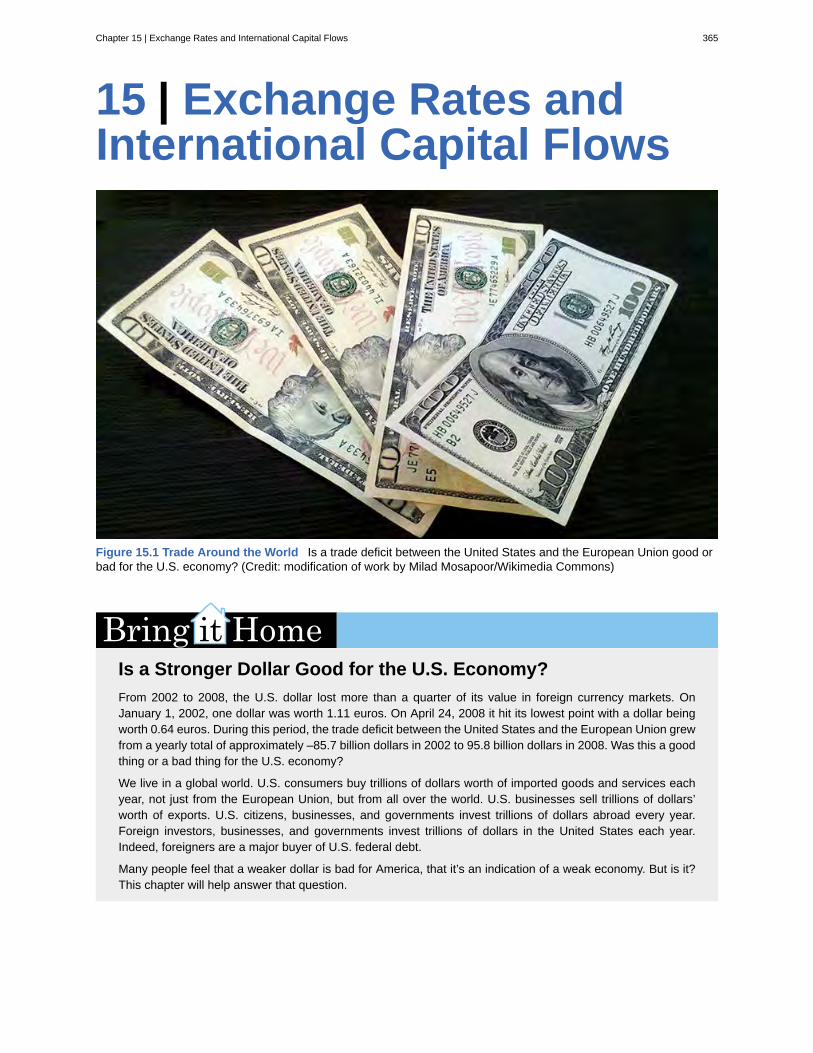
15 | Exchange Rates andInternational Capital Flows
Figure 15.1 Trade Around the World Is a trade deficit between the United States and the European Union good orbad for the U.S. economy? (Credit: modification of work by Milad Mosapoor/Wikimedia Commons)
Is a Stronger Dollar Good for the U.S. Economy?From 2002 to 2008, the U.S. dollar lost more than a quarter of its value in foreign currency markets. OnJanuary 1, 2002, one dollar was worth 1.11 euros. On April 24, 2008 it hit its lowest point with a dollar beingworth 0.64 euros. During this period, the trade deficit between the United States and the European Union grewfrom a yearly total of approximately –85.7 billion dollars in 2002 to 95.8 billion dollars in 2008. Was this a goodthing or a bad thing for the U.S. economy?
We live in a global world. U.S. consumers buy trillions of dollars worth of imported goods and services eachyear, not just from the European Union, but from all over the world. U.S. businesses sell trillions of dollars’worth of exports. U.S. citizens, businesses, and governments invest trillions of dollars abroad every year.Foreign investors, businesses, and governments invest trillions of dollars in the United States each year.Indeed, foreigners are a major buyer of U.S. federal debt.
Many people feel that a weaker dollar is bad for America, that it’s an indication of a weak economy. But is it?This chapter will help answer that question.
Chapter 15 | Exchange Rates and International Capital Flows 365
Introduction to Exchange Rates and International CapitalFlowsIn this chapter, you will learn about:
• How the Foreign Exchange Market Works
• Demand and Supply Shifts in Foreign Exchange Markets
• Macroeconomic Effects of Exchange Rates
• Exchange Rate Policies
The world has over 150 different currencies, from the Afghanistan afghani and the Albanian lek all the way throughthe alphabet to the Zambian kwacha and the Zimbabwean dollar. For international economic transactions, householdsor firms will wish to exchange one currency for another. Perhaps the need for exchanging currencies will come froma German firm that exports products to Russia, but then wishes to exchange the Russian rubles it has earned for euros,so that the firm can pay its workers and suppliers in Germany. Perhaps it will be a South African firm that wishesto purchase a mining operation in Angola, but to make the purchase it must convert South African rand to Angolankwanza. Perhaps it will be an American tourist visiting China, who wishes to convert U.S. dollars to Chinese yuan topay the hotel bill.
Exchange rates can sometimes change very swiftly. For example, in the United Kingdom the pound was worth $2in U.S. currency in spring 2008, but was worth only $1.40 in U.S. currency six months later. For firms engaged ininternational buying, selling, lending, and borrowing, these swings in exchange rates can have an enormous effect onprofits.
This chapter discusses the international dimension of money, which involves conversions from one currency toanother at an exchange rate. An exchange rate is nothing more than a price—that is, the price of one currency interms of another currency—and so they can be analyzed with the tools of supply and demand. The first module of thischapter begins with an overview of foreign exchange markets: their size, their main participants, and the vocabularyfor discussing movements of exchange rates. The following module uses demand and supply graphs to analyze someof the main factors that cause shifts in exchange rates. A final module then brings the central bank and monetarypolicy back into the picture. Each country must decide whether to allow its exchange rate to be determined in themarket, or have the central bank intervene in the exchange rate market. All the choices for exchange rate policyinvolve distinctive tradeoffs and risks.
15.1 | How the Foreign Exchange Market WorksBy the end of this section, you will be able to:
• Define "foreign exchange market"• Describe different types of investments like foreign direct investments (FDI), portfolio investments,
and hedging• Explain how the appreciating or depreciating of currency affects exchange rates• Identify who benefits from a stronger currency and benefits from a weaker currency
Most countries have different currencies, but not all. Sometimes small economies use the currency of an economicallylarger neighbor. For example, Ecuador, El Salvador, and Panama have decided to dollarize—that is, to use the U.S.dollar as their currency. Sometimes nations share a common currency. A large-scale example of a common currency isthe decision by 17 European nations—including some very large economies such as France, Germany, and Italy—toreplace their former currencies with the euro. With these exceptions duly noted, most of the international economytakes place in a situation of multiple national currencies in which both people and firms need to convert from onecurrency to another when selling, buying, hiring, borrowing, traveling, or investing across national borders. Themarket in which people or firms use one currency to purchase another currency is called the foreign exchangemarket.
366 Chapter 15 | Exchange Rates and International Capital Flows
This OpenStax book is available for free at http://cnx.org/content/col11864/1.2
You have encountered the basic concept of exchange rates in earlier chapters. In The International Tradeand Capital Flows (http://cnx.org/content/m57383/latest/) , for example, we discussed how exchange ratesare used to compare GDP statistics from countries where GDP is measured in different currencies. These earlierexamples, however, took the actual exchange rate as given, as if it were a fact of nature. In reality, the exchange rate isa price—the price of one currency expressed in terms of units of another currency. The key framework for analyzingprices, whether in this course, any other economics course, in public policy, or business examples, is the operation ofsupply and demand in markets.
Visit this website (http://openstaxcollege.org/l/exratecalc) for an exchange rate calculator.
The Extraordinary Size of the Foreign Exchange MarketsThe quantities traded in foreign exchange markets are breathtaking. A survey done in April, 2013 by the Bank ofInternational Settlements, an international organization for banks and the financial industry, found that $5.3 trillionper day was traded on foreign exchange markets, which makes the foreign exchange market the largest market in theworld economy. In contrast, 2013 U.S. real GDP was $15.8 trillion per year.
Table 15.1 shows the currencies most commonly traded on foreign exchange markets. The foreign exchange marketis dominated by the U.S. dollar, the currencies used by nations in Western Europe (the euro, the British pound, andthe Australian dollar), and the Japanese yen.
Currency % Daily Share
U.S. dollar 87.0%
Euro 33.4%
Japanese yen 23.0%
British pound 11.8%
Australian dollar 8.6%
Swiss franc 5.2%
Canadian dollar 4.6%
Mexican peso 2.5%
Chinese yuan 2.2%
Table 15.1 Currencies Traded Most on Foreign Exchange Markets as of April, 2013 (Source:http://www.bis.org/publ/rpfx13fx.pdf)
Chapter 15 | Exchange Rates and International Capital Flows 367
Demanders and Suppliers of Currency in Foreign Exchange MarketsIn foreign exchange markets, demand and supply become closely interrelated, because a person or firm who demandsone currency must at the same time supply another currency—and vice versa. To get a sense of this, it is useful toconsider four groups of people or firms who participate in the market: (1) firms that are involved in internationaltrade of goods and services; (2) tourists visiting other countries; (3) international investors buying ownership (or part-ownership) of a foreign firm; (4) international investors making financial investments that do not involve ownership.Let’s consider these categories in turn.
Firms that buy and sell on international markets find that their costs for workers, suppliers, and investors are measuredin the currency of the nation where their production occurs, but their revenues from sales are measured in thecurrency of the different nation where their sales happened. So, a Chinese firm exporting abroad will earn some othercurrency—say, U.S. dollars—but will need Chinese yuan to pay the workers, suppliers, and investors who are basedin China. In the foreign exchange markets, this firm will be a supplier of U.S. dollars and a demander of Chineseyuan.
International tourists will supply their home currency to receive the currency of the country they are visiting. Forexample, an American tourist who is visiting China will supply U.S. dollars into the foreign exchange market anddemand Chinese yuan.
Financial investments that cross international boundaries, and require exchanging currency, are often divided into twocategories. Foreign direct investment (FDI) refers to purchasing a firm (at least ten percent) in another country orstarting up a new enterprise in a foreign country For example, in 2008 the Belgian beer-brewing company InBevbought the U.S. beer-maker Anheuser-Busch for $52 billion. To make this purchase of a U.S. firm, InBev would haveto supply euros (the currency of Belgium) to the foreign exchange market and demand U.S. dollars.
The other kind of international financial investment, portfolio investment, involves a purely financial investment thatdoes not entail any management responsibility. An example would be a U.S. financial investor who purchased bondsissued by the government of the United Kingdom, or deposited money in a British bank. To make such investments,the American investor would supply U.S. dollars in the foreign exchange market and demand British pounds.
Portfolio investment is often linked to expectations about how exchange rates will shift. Look at a U.S. financialinvestor who is considering purchasing bonds issued in the United Kingdom. For simplicity, ignore any interest paidby the bond (which will be small in the short run anyway) and focus on exchange rates. Say that a British poundis currently worth $1.50 in U.S. currency. However, the investor believes that in a month, the British pound will beworth $1.60 in U.S. currency. Thus, as Figure 15.2 (a) shows, this investor would change $24,000 for 16,000 Britishpounds. In a month, if the pound is indeed worth $1.60, then the portfolio investor can trade back to U.S. dollars atthe new exchange rate, and have $25,600—a nice profit. A portfolio investor who believes that the foreign exchangerate for the pound will work in the opposite direction can also invest accordingly. Say that an investor expects thatthe pound, now worth $1.50 in U.S. currency, will decline to $1.40. Then, as shown in Figure 15.2 (b), that investorcould start off with £20,000 in British currency (borrowing the money if necessary), convert it to $30,000 in U.S.currency, wait a month, and then convert back to approximately £21,429 in British currency—again making a niceprofit. Of course, this kind of investing comes without guarantees, and an investor will suffer losses if the exchangerates do not move as predicted.
368 Chapter 15 | Exchange Rates and International Capital Flows
This OpenStax book is available for free at http://cnx.org/content/col11864/1.2
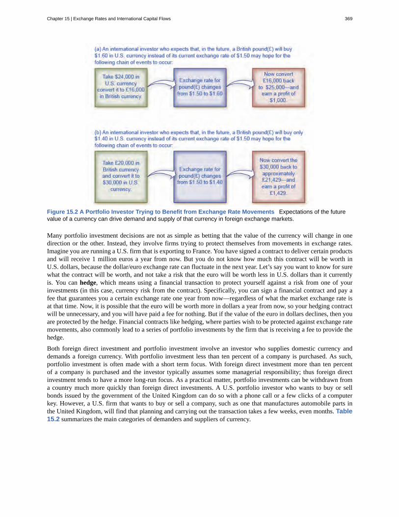
Figure 15.2 A Portfolio Investor Trying to Benefit from Exchange Rate Movements Expectations of the futurevalue of a currency can drive demand and supply of that currency in foreign exchange markets.
Many portfolio investment decisions are not as simple as betting that the value of the currency will change in onedirection or the other. Instead, they involve firms trying to protect themselves from movements in exchange rates.Imagine you are running a U.S. firm that is exporting to France. You have signed a contract to deliver certain productsand will receive 1 million euros a year from now. But you do not know how much this contract will be worth inU.S. dollars, because the dollar/euro exchange rate can fluctuate in the next year. Let’s say you want to know for surewhat the contract will be worth, and not take a risk that the euro will be worth less in U.S. dollars than it currentlyis. You can hedge, which means using a financial transaction to protect yourself against a risk from one of yourinvestments (in this case, currency risk from the contract). Specifically, you can sign a financial contract and pay afee that guarantees you a certain exchange rate one year from now—regardless of what the market exchange rate isat that time. Now, it is possible that the euro will be worth more in dollars a year from now, so your hedging contractwill be unnecessary, and you will have paid a fee for nothing. But if the value of the euro in dollars declines, then youare protected by the hedge. Financial contracts like hedging, where parties wish to be protected against exchange ratemovements, also commonly lead to a series of portfolio investments by the firm that is receiving a fee to provide thehedge.
Both foreign direct investment and portfolio investment involve an investor who supplies domestic currency anddemands a foreign currency. With portfolio investment less than ten percent of a company is purchased. As such,portfolio investment is often made with a short term focus. With foreign direct investment more than ten percentof a company is purchased and the investor typically assumes some managerial responsibility; thus foreign directinvestment tends to have a more long-run focus. As a practical matter, portfolio investments can be withdrawn froma country much more quickly than foreign direct investments. A U.S. portfolio investor who wants to buy or sellbonds issued by the government of the United Kingdom can do so with a phone call or a few clicks of a computerkey. However, a U.S. firm that wants to buy or sell a company, such as one that manufactures automobile parts inthe United Kingdom, will find that planning and carrying out the transaction takes a few weeks, even months. Table15.2 summarizes the main categories of demanders and suppliers of currency.
Chapter 15 | Exchange Rates and International Capital Flows 369
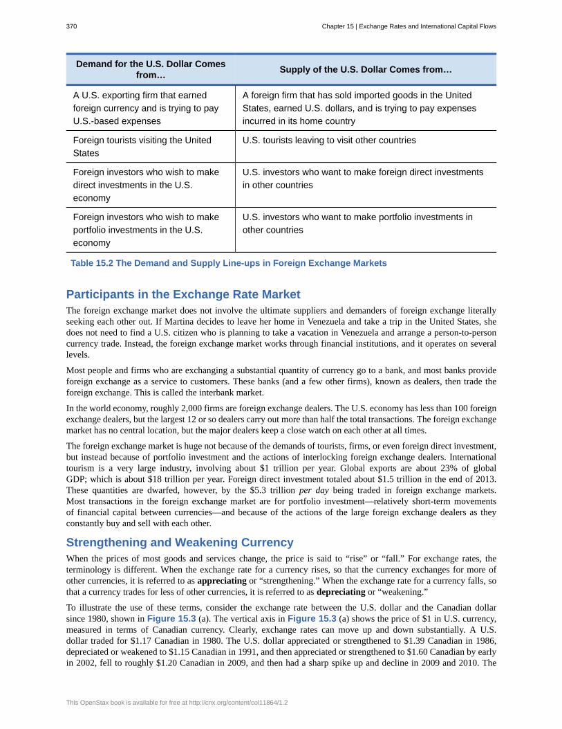
Demand for the U.S. Dollar Comesfrom… Supply of the U.S. Dollar Comes from…
A U.S. exporting firm that earnedforeign currency and is trying to payU.S.-based expenses
A foreign firm that has sold imported goods in the UnitedStates, earned U.S. dollars, and is trying to pay expensesincurred in its home country
Foreign tourists visiting the UnitedStates
U.S. tourists leaving to visit other countries
Foreign investors who wish to makedirect investments in the U.S.economy
U.S. investors who want to make foreign direct investmentsin other countries
Foreign investors who wish to makeportfolio investments in the U.S.economy
U.S. investors who want to make portfolio investments inother countries
Table 15.2 The Demand and Supply Line-ups in Foreign Exchange Markets
Participants in the Exchange Rate MarketThe foreign exchange market does not involve the ultimate suppliers and demanders of foreign exchange literallyseeking each other out. If Martina decides to leave her home in Venezuela and take a trip in the United States, shedoes not need to find a U.S. citizen who is planning to take a vacation in Venezuela and arrange a person-to-personcurrency trade. Instead, the foreign exchange market works through financial institutions, and it operates on severallevels.
Most people and firms who are exchanging a substantial quantity of currency go to a bank, and most banks provideforeign exchange as a service to customers. These banks (and a few other firms), known as dealers, then trade theforeign exchange. This is called the interbank market.
In the world economy, roughly 2,000 firms are foreign exchange dealers. The U.S. economy has less than 100 foreignexchange dealers, but the largest 12 or so dealers carry out more than half the total transactions. The foreign exchangemarket has no central location, but the major dealers keep a close watch on each other at all times.
The foreign exchange market is huge not because of the demands of tourists, firms, or even foreign direct investment,but instead because of portfolio investment and the actions of interlocking foreign exchange dealers. Internationaltourism is a very large industry, involving about $1 trillion per year. Global exports are about 23% of globalGDP; which is about $18 trillion per year. Foreign direct investment totaled about $1.5 trillion in the end of 2013.These quantities are dwarfed, however, by the $5.3 trillion per day being traded in foreign exchange markets.Most transactions in the foreign exchange market are for portfolio investment—relatively short-term movementsof financial capital between currencies—and because of the actions of the large foreign exchange dealers as theyconstantly buy and sell with each other.
Strengthening and Weakening CurrencyWhen the prices of most goods and services change, the price is said to “rise” or “fall.” For exchange rates, theterminology is different. When the exchange rate for a currency rises, so that the currency exchanges for more ofother currencies, it is referred to as appreciating or “strengthening.” When the exchange rate for a currency falls, sothat a currency trades for less of other currencies, it is referred to as depreciating or “weakening.”
To illustrate the use of these terms, consider the exchange rate between the U.S. dollar and the Canadian dollarsince 1980, shown in Figure 15.3 (a). The vertical axis in Figure 15.3 (a) shows the price of $1 in U.S. currency,measured in terms of Canadian currency. Clearly, exchange rates can move up and down substantially. A U.S.dollar traded for $1.17 Canadian in 1980. The U.S. dollar appreciated or strengthened to $1.39 Canadian in 1986,depreciated or weakened to $1.15 Canadian in 1991, and then appreciated or strengthened to $1.60 Canadian by earlyin 2002, fell to roughly $1.20 Canadian in 2009, and then had a sharp spike up and decline in 2009 and 2010. The
370 Chapter 15 | Exchange Rates and International Capital Flows
This OpenStax book is available for free at http://cnx.org/content/col11864/1.2
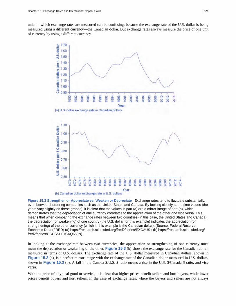
units in which exchange rates are measured can be confusing, because the exchange rate of the U.S. dollar is beingmeasured using a different currency—the Canadian dollar. But exchange rates always measure the price of one unitof currency by using a different currency.
Figure 15.3 Strengthen or Appreciate vs. Weaken or Depreciate Exchange rates tend to fluctuate substantially,even between bordering companies such as the United States and Canada. By looking closely at the time values (theyears vary slightly on these graphs), it is clear that the values in part (a) are a mirror image of part (b), whichdemonstrates that the depreciation of one currency correlates to the appreciation of the other and vice versa. Thismeans that when comparing the exchange rates between two countries (in this case, the United States and Canada),the depreciation (or weakening) of one country (the U.S. dollar for this example) indicates the appreciation (orstrengthening) of the other currency (which in this example is the Canadian dollar). (Source: Federal ReserveEconomic Data (FRED) (a) https://research.stlouisfed.org/fred2/series/EXCAUS ; (b) https://research.stlouisfed.org/fred2/series/CCUSSP01CAQ650N)
In looking at the exchange rate between two currencies, the appreciation or strengthening of one currency mustmean the depreciation or weakening of the other. Figure 15.3 (b) shows the exchange rate for the Canadian dollar,measured in terms of U.S. dollars. The exchange rate of the U.S. dollar measured in Canadian dollars, shown inFigure 15.3 (a), is a perfect mirror image with the exchange rate of the Canadian dollar measured in U.S. dollars,shown in Figure 15.3 (b). A fall in the Canada $/U.S. $ ratio means a rise in the U.S. $/Canada $ ratio, and viceversa.
With the price of a typical good or service, it is clear that higher prices benefit sellers and hurt buyers, while lowerprices benefit buyers and hurt sellers. In the case of exchange rates, where the buyers and sellers are not always
Chapter 15 | Exchange Rates and International Capital Flows 371
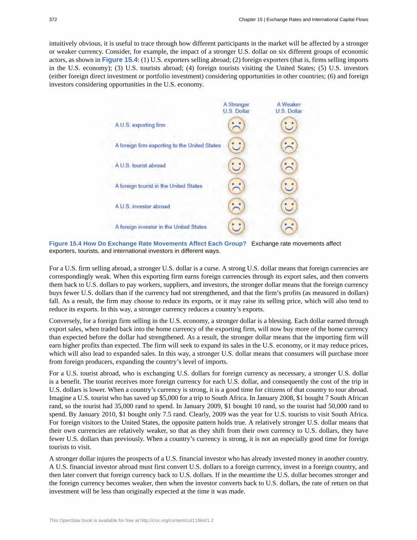
intuitively obvious, it is useful to trace through how different participants in the market will be affected by a strongeror weaker currency. Consider, for example, the impact of a stronger U.S. dollar on six different groups of economicactors, as shown in Figure 15.4: (1) U.S. exporters selling abroad; (2) foreign exporters (that is, firms selling importsin the U.S. economy); (3) U.S. tourists abroad; (4) foreign tourists visiting the United States; (5) U.S. investors(either foreign direct investment or portfolio investment) considering opportunities in other countries; (6) and foreigninvestors considering opportunities in the U.S. economy.
Figure 15.4 How Do Exchange Rate Movements Affect Each Group? Exchange rate movements affectexporters, tourists, and international investors in different ways.
For a U.S. firm selling abroad, a stronger U.S. dollar is a curse. A strong U.S. dollar means that foreign currencies arecorrespondingly weak. When this exporting firm earns foreign currencies through its export sales, and then convertsthem back to U.S. dollars to pay workers, suppliers, and investors, the stronger dollar means that the foreign currencybuys fewer U.S. dollars than if the currency had not strengthened, and that the firm’s profits (as measured in dollars)fall. As a result, the firm may choose to reduce its exports, or it may raise its selling price, which will also tend toreduce its exports. In this way, a stronger currency reduces a country’s exports.
Conversely, for a foreign firm selling in the U.S. economy, a stronger dollar is a blessing. Each dollar earned throughexport sales, when traded back into the home currency of the exporting firm, will now buy more of the home currencythan expected before the dollar had strengthened. As a result, the stronger dollar means that the importing firm willearn higher profits than expected. The firm will seek to expand its sales in the U.S. economy, or it may reduce prices,which will also lead to expanded sales. In this way, a stronger U.S. dollar means that consumers will purchase morefrom foreign producers, expanding the country’s level of imports.
For a U.S. tourist abroad, who is exchanging U.S. dollars for foreign currency as necessary, a stronger U.S. dollaris a benefit. The tourist receives more foreign currency for each U.S. dollar, and consequently the cost of the trip inU.S. dollars is lower. When a country’s currency is strong, it is a good time for citizens of that country to tour abroad.Imagine a U.S. tourist who has saved up $5,000 for a trip to South Africa. In January 2008, $1 bought 7 South Africanrand, so the tourist had 35,000 rand to spend. In January 2009, $1 bought 10 rand, so the tourist had 50,000 rand tospend. By January 2010, $1 bought only 7.5 rand. Clearly, 2009 was the year for U.S. tourists to visit South Africa.For foreign visitors to the United States, the opposite pattern holds true. A relatively stronger U.S. dollar means thattheir own currencies are relatively weaker, so that as they shift from their own currency to U.S. dollars, they havefewer U.S. dollars than previously. When a country’s currency is strong, it is not an especially good time for foreigntourists to visit.
A stronger dollar injures the prospects of a U.S. financial investor who has already invested money in another country.A U.S. financial investor abroad must first convert U.S. dollars to a foreign currency, invest in a foreign country, andthen later convert that foreign currency back to U.S. dollars. If in the meantime the U.S. dollar becomes stronger andthe foreign currency becomes weaker, then when the investor converts back to U.S. dollars, the rate of return on thatinvestment will be less than originally expected at the time it was made.
372 Chapter 15 | Exchange Rates and International Capital Flows
This OpenStax book is available for free at http://cnx.org/content/col11864/1.2
However, a stronger U.S. dollar boosts the returns of a foreign investor putting money into a U.S. investment. Thatforeign investor converts from the home currency to U.S. dollars and seeks a U.S. investment, while later planning toswitch back to the home currency. If, in the meantime, the dollar grows stronger, then when the time comes to convertfrom U.S. dollars back to the foreign currency, the investor will receive more foreign currency than expected at thetime the original investment was made.
The preceding paragraphs all focus on the case where the U.S. dollar becomes stronger. The corresponding happy orunhappy economic reactions are illustrated in the first column of Figure 15.4. The following Work It Out featurecenters the analysis on the opposite: a weaker dollar.
Effects of a Weaker DollarLet’s work through the effects of a weaker dollar on a U.S. exporter, a foreign exporter into the United States,a U.S. tourist going abroad, a foreign tourist coming to the United States, a U.S. investor abroad, and a foreigninvestor in the United States.
Step 1. Note that the demand for U.S. exports is a function of the price of those exports, which depends onthe dollar price of those goods and the exchange rate of the dollar in terms of foreign currency. For example,a Ford pickup truck costs $25,000 in the United States. When it is sold in the United Kingdom, the priceis $25,000 / $1.50 per British pound, or £16,667. The dollar affects the price faced by foreigners who maypurchase U.S. exports.
Step 2. Consider that, if the dollar weakens, the pound rises in value. If the pound rises to $2.00 per pound,then the price of a Ford pickup is now $25,000 / $2.00 = £12,500. A weaker dollar means the foreign currencybuys more dollars, which means that U.S. exports appear less expensive.
Step 3. Summarize that a weaker U.S. dollar leads to an increase in U.S. exports. For a foreign exporter, theoutcome is just the opposite.
Step 4. Suppose a brewery in England is interested in selling its Bass Ale to a grocery store in the UnitedStates. If the price of a six pack of Bass Ale is £6.00 and the exchange rate is $1.50 per British pound, theprice for the grocery store is 6.00 × $1.50 = $9.00 per six pack. If the dollar weakens to $2.00 per pound, theprice of Bass Ale is now 6.00 × $2.00 = $12.
Step 5. Summarize that, from the perspective of U.S. purchasers, a weaker dollar means that foreign currencyis more expensive, which means that foreign goods are more expensive also. This leads to a decrease in U.S.imports, which is bad for the foreign exporter.
Step 6. Consider U.S. tourists going abroad. They face the same situation as a U.S. importer—they arepurchasing a foreign trip. A weaker dollar means that their trip will cost more, since a given expenditure offoreign currency (e.g., hotel bill) will take more dollars. The result is that the tourist may not stay as longabroad, and some may choose not to travel at all.
Step 7. Consider that, for the foreign tourist to the United States, a weaker dollar is a boon. It means theircurrency goes further, so the cost of a trip to the United States will be less. Foreigners may choose to takelonger trips to the United States, and more foreign tourists may decide to take U.S. trips.
Step 8. Note that a U.S. investor abroad faces the same situation as a U.S. importer—they are purchasing aforeign asset. A U.S. investor will see a weaker dollar as an increase in the “price” of investment, since thesame number of dollars will buy less foreign currency and thus less foreign assets. This should decrease theamount of U.S. investment abroad.
Step 9. Note also that foreign investors in the Unites States will have the opposite experience. Since foreigncurrency buys more dollars, they will likely invest in more U.S. assets.
At this point, you should have a good sense of the major players in the foreign exchange market: firms involved ininternational trade, tourists, international financial investors, banks, and foreign exchange dealers. The next module
Chapter 15 | Exchange Rates and International Capital Flows 373
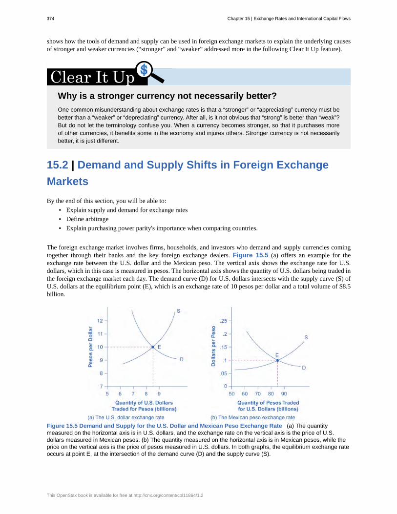
shows how the tools of demand and supply can be used in foreign exchange markets to explain the underlying causesof stronger and weaker currencies (“stronger” and “weaker” addressed more in the following Clear It Up feature).
Why is a stronger currency not necessarily better?One common misunderstanding about exchange rates is that a “stronger” or “appreciating” currency must bebetter than a “weaker” or “depreciating” currency. After all, is it not obvious that “strong” is better than “weak”?But do not let the terminology confuse you. When a currency becomes stronger, so that it purchases moreof other currencies, it benefits some in the economy and injures others. Stronger currency is not necessarilybetter, it is just different.
15.2 | Demand and Supply Shifts in Foreign ExchangeMarketsBy the end of this section, you will be able to:
• Explain supply and demand for exchange rates• Define arbitrage• Explain purchasing power parity's importance when comparing countries.
The foreign exchange market involves firms, households, and investors who demand and supply currencies comingtogether through their banks and the key foreign exchange dealers. Figure 15.5 (a) offers an example for theexchange rate between the U.S. dollar and the Mexican peso. The vertical axis shows the exchange rate for U.S.dollars, which in this case is measured in pesos. The horizontal axis shows the quantity of U.S. dollars being traded inthe foreign exchange market each day. The demand curve (D) for U.S. dollars intersects with the supply curve (S) ofU.S. dollars at the equilibrium point (E), which is an exchange rate of 10 pesos per dollar and a total volume of $8.5billion.
Figure 15.5 Demand and Supply for the U.S. Dollar and Mexican Peso Exchange Rate (a) The quantitymeasured on the horizontal axis is in U.S. dollars, and the exchange rate on the vertical axis is the price of U.S.dollars measured in Mexican pesos. (b) The quantity measured on the horizontal axis is in Mexican pesos, while theprice on the vertical axis is the price of pesos measured in U.S. dollars. In both graphs, the equilibrium exchange rateoccurs at point E, at the intersection of the demand curve (D) and the supply curve (S).
374 Chapter 15 | Exchange Rates and International Capital Flows
This OpenStax book is available for free at http://cnx.org/content/col11864/1.2
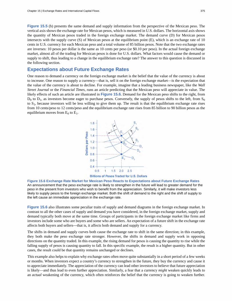
Figure 15.5 (b) presents the same demand and supply information from the perspective of the Mexican peso. Thevertical axis shows the exchange rate for Mexican pesos, which is measured in U.S. dollars. The horizontal axis showsthe quantity of Mexican pesos traded in the foreign exchange market. The demand curve (D) for Mexican pesosintersects with the supply curve (S) of Mexican pesos at the equilibrium point (E), which is an exchange rate of 10cents in U.S. currency for each Mexican peso and a total volume of 85 billion pesos. Note that the two exchange ratesare inverses: 10 pesos per dollar is the same as 10 cents per peso (or $0.10 per peso). In the actual foreign exchangemarket, almost all of the trading for Mexican pesos is done for U.S. dollars. What factors would cause the demand orsupply to shift, thus leading to a change in the equilibrium exchange rate? The answer to this question is discussed inthe following section.
Expectations about Future Exchange RatesOne reason to demand a currency on the foreign exchange market is the belief that the value of the currency is aboutto increase. One reason to supply a currency—that is, sell it on the foreign exchange market—is the expectation thatthe value of the currency is about to decline. For example, imagine that a leading business newspaper, like the WallStreet Journal or the Financial Times, runs an article predicting that the Mexican peso will appreciate in value. Thelikely effects of such an article are illustrated in Figure 15.6. Demand for the Mexican peso shifts to the right, fromD0 to D1, as investors become eager to purchase pesos. Conversely, the supply of pesos shifts to the left, from S0to S1, because investors will be less willing to give them up. The result is that the equilibrium exchange rate risesfrom 10 cents/peso to 12 cents/peso and the equilibrium exchange rate rises from 85 billion to 90 billion pesos as theequilibrium moves from E0 to E1.
Figure 15.6 Exchange Rate Market for Mexican Peso Reacts to Expectations about Future Exchange RatesAn announcement that the peso exchange rate is likely to strengthen in the future will lead to greater demand for thepeso in the present from investors who wish to benefit from the appreciation. Similarly, it will make investors lesslikely to supply pesos to the foreign exchange market. Both the shift of demand to the right and the shift of supply tothe left cause an immediate appreciation in the exchange rate.
Figure 15.6 also illustrates some peculiar traits of supply and demand diagrams in the foreign exchange market. Incontrast to all the other cases of supply and demand you have considered, in the foreign exchange market, supply anddemand typically both move at the same time. Groups of participants in the foreign exchange market like firms andinvestors include some who are buyers and some who are sellers. An expectation of a future shift in the exchange rateaffects both buyers and sellers—that is, it affects both demand and supply for a currency.
The shifts in demand and supply curves both cause the exchange rate to shift in the same direction; in this example,they both make the peso exchange rate stronger. However, the shifts in demand and supply work in opposingdirections on the quantity traded. In this example, the rising demand for pesos is causing the quantity to rise while thefalling supply of pesos is causing quantity to fall. In this specific example, the result is a higher quantity. But in othercases, the result could be that quantity remains unchanged or declines.
This example also helps to explain why exchange rates often move quite substantially in a short period of a few weeksor months. When investors expect a country’s currency to strengthen in the future, they buy the currency and cause itto appreciate immediately. The appreciation of the currency can lead other investors to believe that future appreciationis likely—and thus lead to even further appreciation. Similarly, a fear that a currency might weaken quickly leads toan actual weakening of the currency, which often reinforces the belief that the currency is going to weaken further.
Chapter 15 | Exchange Rates and International Capital Flows 375
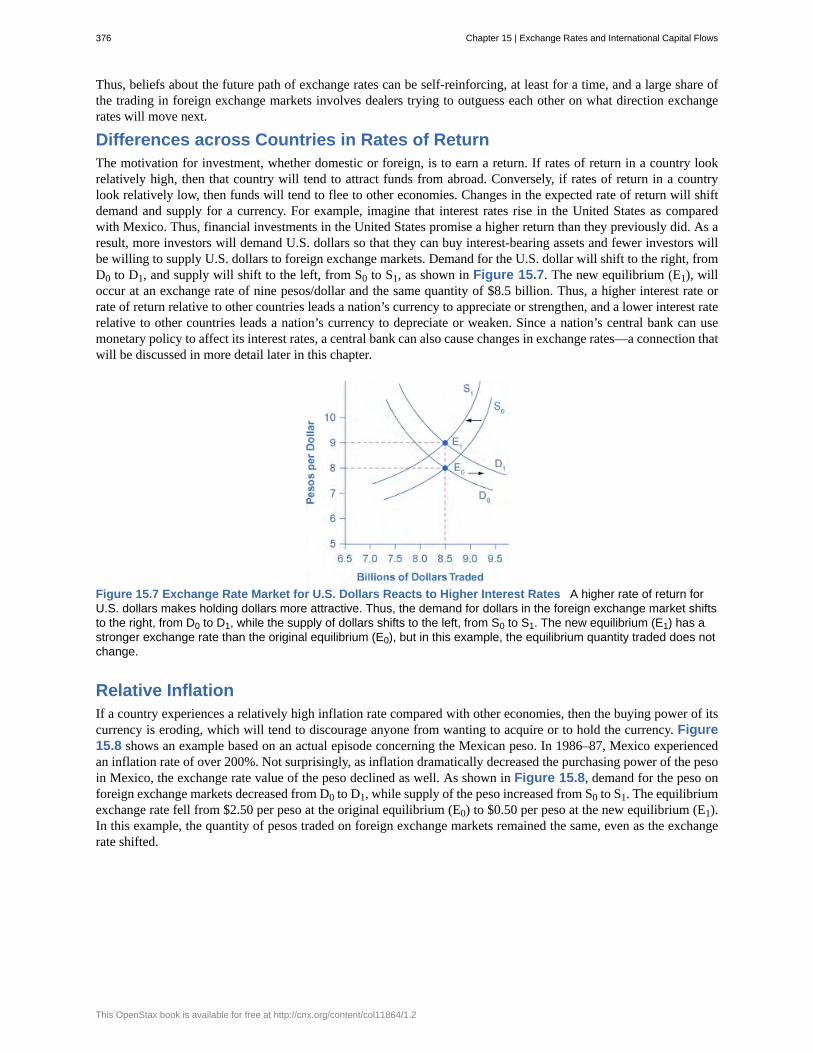
Thus, beliefs about the future path of exchange rates can be self-reinforcing, at least for a time, and a large share ofthe trading in foreign exchange markets involves dealers trying to outguess each other on what direction exchangerates will move next.
Differences across Countries in Rates of ReturnThe motivation for investment, whether domestic or foreign, is to earn a return. If rates of return in a country lookrelatively high, then that country will tend to attract funds from abroad. Conversely, if rates of return in a countrylook relatively low, then funds will tend to flee to other economies. Changes in the expected rate of return will shiftdemand and supply for a currency. For example, imagine that interest rates rise in the United States as comparedwith Mexico. Thus, financial investments in the United States promise a higher return than they previously did. As aresult, more investors will demand U.S. dollars so that they can buy interest-bearing assets and fewer investors willbe willing to supply U.S. dollars to foreign exchange markets. Demand for the U.S. dollar will shift to the right, fromD0 to D1, and supply will shift to the left, from S0 to S1, as shown in Figure 15.7. The new equilibrium (E1), willoccur at an exchange rate of nine pesos/dollar and the same quantity of $8.5 billion. Thus, a higher interest rate orrate of return relative to other countries leads a nation’s currency to appreciate or strengthen, and a lower interest raterelative to other countries leads a nation’s currency to depreciate or weaken. Since a nation’s central bank can usemonetary policy to affect its interest rates, a central bank can also cause changes in exchange rates—a connection thatwill be discussed in more detail later in this chapter.
Figure 15.7 Exchange Rate Market for U.S. Dollars Reacts to Higher Interest Rates A higher rate of return forU.S. dollars makes holding dollars more attractive. Thus, the demand for dollars in the foreign exchange market shiftsto the right, from D0 to D1, while the supply of dollars shifts to the left, from S0 to S1. The new equilibrium (E1) has astronger exchange rate than the original equilibrium (E0), but in this example, the equilibrium quantity traded does notchange.
Relative InflationIf a country experiences a relatively high inflation rate compared with other economies, then the buying power of itscurrency is eroding, which will tend to discourage anyone from wanting to acquire or to hold the currency. Figure15.8 shows an example based on an actual episode concerning the Mexican peso. In 1986–87, Mexico experiencedan inflation rate of over 200%. Not surprisingly, as inflation dramatically decreased the purchasing power of the pesoin Mexico, the exchange rate value of the peso declined as well. As shown in Figure 15.8, demand for the peso onforeign exchange markets decreased from D0 to D1, while supply of the peso increased from S0 to S1. The equilibriumexchange rate fell from $2.50 per peso at the original equilibrium (E0) to $0.50 per peso at the new equilibrium (E1).In this example, the quantity of pesos traded on foreign exchange markets remained the same, even as the exchangerate shifted.
376 Chapter 15 | Exchange Rates and International Capital Flows
This OpenStax book is available for free at http://cnx.org/content/col11864/1.2
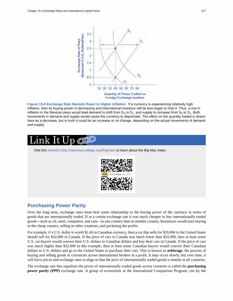
Figure 15.8 Exchange Rate Markets React to Higher Inflation If a currency is experiencing relatively highinflation, then its buying power is decreasing and international investors will be less eager to hold it. Thus, a rise ininflation in the Mexican peso would lead demand to shift from D0 to D1, and supply to increase from S0 to S1. Bothmovements in demand and supply would cause the currency to depreciate. The effect on the quantity traded is drawnhere as a decrease, but in truth it could be an increase or no change, depending on the actual movements of demandand supply.
Visit this website (http://openstaxcollege.org/l/bigmac) to learn about the Big Mac index.
Purchasing Power ParityOver the long term, exchange rates must bear some relationship to the buying power of the currency in terms ofgoods that are internationally traded. If at a certain exchange rate it was much cheaper to buy internationally tradedgoods—such as oil, steel, computers, and cars—in one country than in another country, businesses would start buyingin the cheap country, selling in other countries, and pocketing the profits.
For example, if a U.S. dollar is worth $1.60 in Canadian currency, then a car that sells for $20,000 in the United Statesshould sell for $32,000 in Canada. If the price of cars in Canada was much lower than $32,000, then at least someU.S. car-buyers would convert their U.S. dollars to Canadian dollars and buy their cars in Canada. If the price of carswas much higher than $32,000 in this example, then at least some Canadian buyers would convert their Canadiandollars to U.S. dollars and go to the United States to purchase their cars. This is known as arbitrage, the process ofbuying and selling goods or currencies across international borders at a profit. It may occur slowly, but over time, itwill force prices and exchange rates to align so that the price of internationally traded goods is similar in all countries.
The exchange rate that equalizes the prices of internationally traded goods across countries is called the purchasingpower parity (PPP) exchange rate. A group of economists at the International Comparison Program, run by the
Chapter 15 | Exchange Rates and International Capital Flows 377
World Bank, have calculated the PPP exchange rate for all countries, based on detailed studies of the prices andquantities of internationally tradable goods.
The purchasing power parity exchange rate has two functions. First, PPP exchange rates are often used forinternational comparison of GDP and other economic statistics. Imagine that you are preparing a table showing thesize of GDP in many countries in several recent years, and for ease of comparison, you are converting all the valuesinto U.S. dollars. When you insert the value for Japan, you need to use a yen/dollar exchange rate. But should youuse the market exchange rate or the PPP exchange rate? Market exchange rates bounce around. In summer 2008, theexchange rate was 108 yen/dollar, but in late 2009 the U.S. dollar exchange rate versus the yen was 90 yen/dollar. Forsimplicity, say that Japan’s GDP was ¥500 trillion in both 2008 and 2009. If you use the market exchange rates, thenJapan’s GDP will be $4.6 trillion in 2008 (that is, ¥500 trillion /(¥108/dollar)) and $5.5 trillion in 2009 (that is, ¥500trillion /(¥90/dollar)).
Of course, it is not true that Japan’s economy increased enormously in 2009—in fact, Japan had a recession like muchof the rest of the world. The misleading appearance of a booming Japanese economy occurs only because we used themarket exchange rate, which often has short-run rises and falls. However, PPP exchange rates stay fairly constant andchange only modestly, if at all, from year to year.
The second function of PPP is that exchanges rates will often get closer and closer to it as time passes. It is true that inthe short run and medium run, as exchange rates adjust to relative inflation rates, rates of return, and to expectationsabout how interest rates and inflation will shift, the exchange rates will often move away from the PPP exchange ratefor a time. But, knowing the PPP will allow you to track and predict exchange rate relationships.
15.3 | Macroeconomic Effects of Exchange RatesBy the end of this section you will be able to:
• Explain how exchange rate shifting influences aggregate demand and supply• Explain how loans and banks can also be influenced by shifting exchange rates
A central bank will be concerned about the exchange rate for multiple reasons: (1) Movements in the exchange ratewill affect the quantity of aggregate demand in an economy; (2) frequent substantial fluctuations in the exchangerate can disrupt international trade and cause problems in a nation’s banking system–this may contribute to anunsustainable balance of trade and large inflows of international financial capital, which can set the economy up for adeep recession if international investors decide to move their money to another country. Let’s discuss these scenariosin turn.
Exchange Rates, Aggregate Demand, and Aggregate SupplyForeign trade in goods and services typically involves incurring the costs of production in one currency whilereceiving revenues from sales in another currency. As a result, movements in exchange rates can have a powerfuleffect on incentives to export and import, and thus on aggregate demand in the economy as a whole.
For example, in 1999, when the euro first became a currency, its value measured in U.S. currency was $1.06/euro. Bythe end of 2013, the euro had risen (and the U.S. dollar had correspondingly weakened) to $1.37/euro. Consider thesituation of a French firm that each year incurs €10 million in costs, and sells its products in the United States for $10million. In 1999, when this firm converted $10 million back to euros at the exchange rate of $1.06/euro (that is, $10million × [€1/$1.06]), it received €9.4 million, and suffered a loss. In 2013, when this same firm converted $10 millionback to euros at the exchange rate of $1.37/euro (that is, $10 million × [€1 euro/$1.37]), it received approximately€7.3 million and an even larger loss. This example shows how a stronger euro discourages exports by the Frenchfirm, because it makes the costs of production in the domestic currency higher relative to the sales revenues earnedin another country. From the point of view of the U.S. economy, the example also shows how a weaker U.S. dollarencourages exports.
Since an increase in exports results in more dollars flowing into the economy, and an increase in imports meansmore dollars are flowing out, it is easy to conclude that exports are “good” for the economy and imports are “bad,”but this overlooks the role of exchange rates. If an American consumer buys a Japanese car for $20,000 instead ofan American car for $30,000, it may be tempting to argue that the American economy has lost out. However, theJapanese company will have to convert those dollars to yen to pay its workers and operate its factories. Whoever buys
378 Chapter 15 | Exchange Rates and International Capital Flows
This OpenStax book is available for free at http://cnx.org/content/col11864/1.2
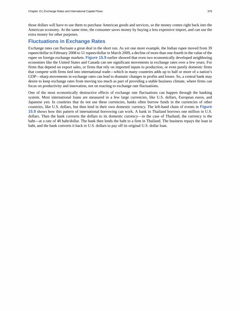
those dollars will have to use them to purchase American goods and services, so the money comes right back into theAmerican economy. At the same time, the consumer saves money by buying a less expensive import, and can use theextra money for other purposes.
Fluctuations in Exchange RatesExchange rates can fluctuate a great deal in the short run. As yet one more example, the Indian rupee moved from 39rupees/dollar in February 2008 to 51 rupees/dollar in March 2009, a decline of more than one-fourth in the value of therupee on foreign exchange markets. Figure 15.9 earlier showed that even two economically developed neighboringeconomies like the United States and Canada can see significant movements in exchange rates over a few years. Forfirms that depend on export sales, or firms that rely on imported inputs to production, or even purely domestic firmsthat compete with firms tied into international trade—which in many countries adds up to half or more of a nation’sGDP—sharp movements in exchange rates can lead to dramatic changes in profits and losses. So, a central bank maydesire to keep exchange rates from moving too much as part of providing a stable business climate, where firms canfocus on productivity and innovation, not on reacting to exchange rate fluctuations.
One of the most economically destructive effects of exchange rate fluctuations can happen through the bankingsystem. Most international loans are measured in a few large currencies, like U.S. dollars, European euros, andJapanese yen. In countries that do not use these currencies, banks often borrow funds in the currencies of othercountries, like U.S. dollars, but then lend in their own domestic currency. The left-hand chain of events in Figure15.9 shows how this pattern of international borrowing can work. A bank in Thailand borrows one million in U.S.dollars. Then the bank converts the dollars to its domestic currency—in the case of Thailand, the currency is thebaht—at a rate of 40 baht/dollar. The bank then lends the baht to a firm in Thailand. The business repays the loan inbaht, and the bank converts it back to U.S. dollars to pay off its original U.S. dollar loan.
Chapter 15 | Exchange Rates and International Capital Flows 379
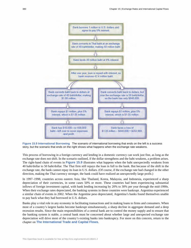
Figure 15.9 International Borrowing The scenario of international borrowing that ends on the left is a successstory, but the scenario that ends on the right shows what happens when the exchange rate weakens.
This process of borrowing in a foreign currency and lending in a domestic currency can work just fine, as long as theexchange rate does not shift. In the scenario outlined, if the dollar strengthens and the baht weakens, a problem arises.The right-hand chain of events in Figure 15.9 illustrates what happens when the baht unexpectedly weakens from40 baht/dollar to 50 baht/dollar. The Thai firm still repays the loan in full to the bank. But because of the shift in theexchange rate, the bank cannot repay its loan in U.S. dollars. (Of course, if the exchange rate had changed in the otherdirection, making the Thai currency stronger, the bank could have realized an unexpectedly large profit.)
In 1997–1998, countries across eastern Asia, like Thailand, Korea, Malaysia, and Indonesia, experienced a sharpdepreciation of their currencies, in some cases 50% or more. These countries had been experiencing substantialinflows of foreign investment capital, with bank lending increasing by 20% to 30% per year through the mid-1990s.When their exchange rates depreciated, the banking systems in these countries were bankrupt. Argentina experienceda similar chain of events in 2002. When the Argentine peso depreciated, Argentina’s banks found themselves unableto pay back what they had borrowed in U.S. dollars.
Banks play a vital role in any economy in facilitating transactions and in making loans to firms and consumers. Whenmost of a country’s largest banks become bankrupt simultaneously, a sharp decline in aggregate demand and a deeprecession results. Since the main responsibilities of a central bank are to control the money supply and to ensure thatthe banking system is stable, a central bank must be concerned about whether large and unexpected exchange ratedepreciation will drive most of the country’s existing banks into bankruptcy. For more on this concern, return to thechapter on The International Trade and Capital Flows.
380 Chapter 15 | Exchange Rates and International Capital Flows
This OpenStax book is available for free at http://cnx.org/content/col11864/1.2
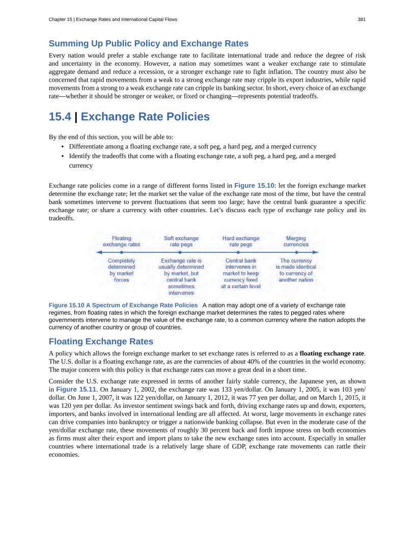
Summing Up Public Policy and Exchange RatesEvery nation would prefer a stable exchange rate to facilitate international trade and reduce the degree of riskand uncertainty in the economy. However, a nation may sometimes want a weaker exchange rate to stimulateaggregate demand and reduce a recession, or a stronger exchange rate to fight inflation. The country must also beconcerned that rapid movements from a weak to a strong exchange rate may cripple its export industries, while rapidmovements from a strong to a weak exchange rate can cripple its banking sector. In short, every choice of an exchangerate—whether it should be stronger or weaker, or fixed or changing—represents potential tradeoffs.
15.4 | Exchange Rate PoliciesBy the end of this section, you will be able to:
• Differentiate among a floating exchange rate, a soft peg, a hard peg, and a merged currency• Identify the tradeoffs that come with a floating exchange rate, a soft peg, a hard peg, and a merged
currency
Exchange rate policies come in a range of different forms listed in Figure 15.10: let the foreign exchange marketdetermine the exchange rate; let the market set the value of the exchange rate most of the time, but have the centralbank sometimes intervene to prevent fluctuations that seem too large; have the central bank guarantee a specificexchange rate; or share a currency with other countries. Let’s discuss each type of exchange rate policy and itstradeoffs.
Figure 15.10 A Spectrum of Exchange Rate Policies A nation may adopt one of a variety of exchange rateregimes, from floating rates in which the foreign exchange market determines the rates to pegged rates wheregovernments intervene to manage the value of the exchange rate, to a common currency where the nation adopts thecurrency of another country or group of countries.
Floating Exchange RatesA policy which allows the foreign exchange market to set exchange rates is referred to as a floating exchange rate.The U.S. dollar is a floating exchange rate, as are the currencies of about 40% of the countries in the world economy.The major concern with this policy is that exchange rates can move a great deal in a short time.
Consider the U.S. exchange rate expressed in terms of another fairly stable currency, the Japanese yen, as shownin Figure 15.11. On January 1, 2002, the exchange rate was 133 yen/dollar. On January 1, 2005, it was 103 yen/dollar. On June 1, 2007, it was 122 yen/dollar, on January 1, 2012, it was 77 yen per dollar, and on March 1, 2015, itwas 120 yen per dollar. As investor sentiment swings back and forth, driving exchange rates up and down, exporters,importers, and banks involved in international lending are all affected. At worst, large movements in exchange ratescan drive companies into bankruptcy or trigger a nationwide banking collapse. But even in the moderate case of theyen/dollar exchange rate, these movements of roughly 30 percent back and forth impose stress on both economiesas firms must alter their export and import plans to take the new exchange rates into account. Especially in smallercountries where international trade is a relatively large share of GDP, exchange rate movements can rattle theireconomies.
Chapter 15 | Exchange Rates and International Capital Flows 381
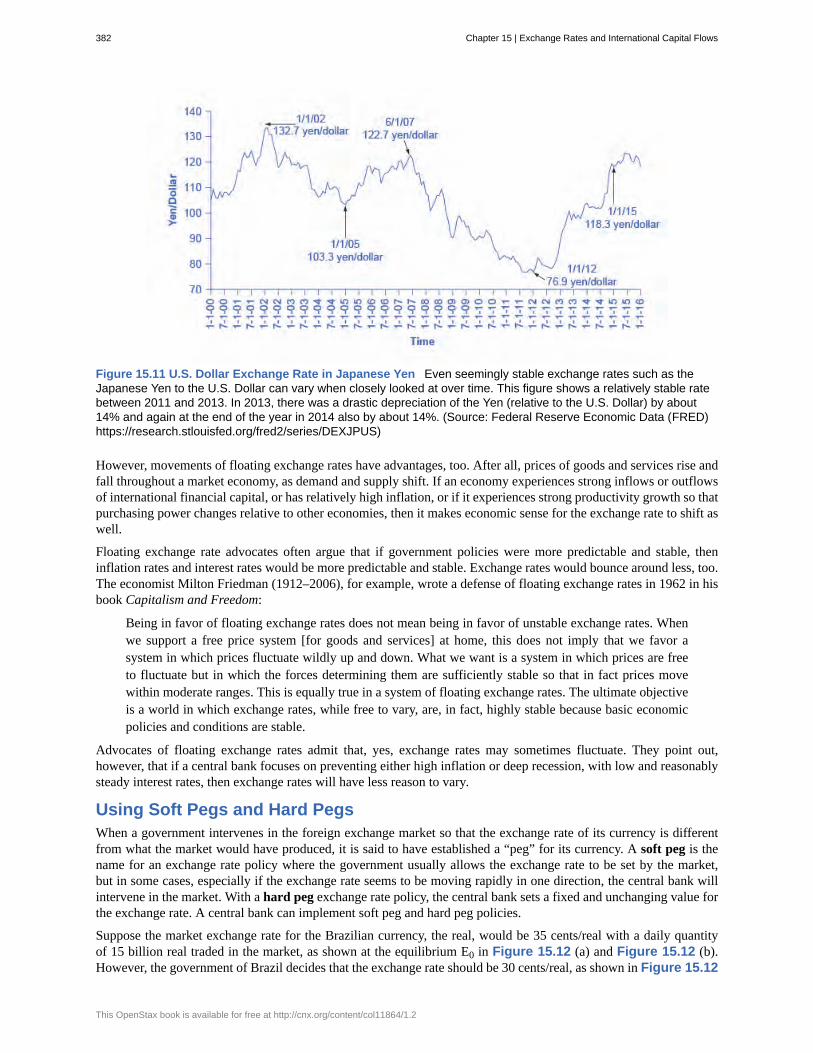
Figure 15.11 U.S. Dollar Exchange Rate in Japanese Yen Even seemingly stable exchange rates such as theJapanese Yen to the U.S. Dollar can vary when closely looked at over time. This figure shows a relatively stable ratebetween 2011 and 2013. In 2013, there was a drastic depreciation of the Yen (relative to the U.S. Dollar) by about14% and again at the end of the year in 2014 also by about 14%. (Source: Federal Reserve Economic Data (FRED)https://research.stlouisfed.org/fred2/series/DEXJPUS)
However, movements of floating exchange rates have advantages, too. After all, prices of goods and services rise andfall throughout a market economy, as demand and supply shift. If an economy experiences strong inflows or outflowsof international financial capital, or has relatively high inflation, or if it experiences strong productivity growth so thatpurchasing power changes relative to other economies, then it makes economic sense for the exchange rate to shift aswell.
Floating exchange rate advocates often argue that if government policies were more predictable and stable, theninflation rates and interest rates would be more predictable and stable. Exchange rates would bounce around less, too.The economist Milton Friedman (1912–2006), for example, wrote a defense of floating exchange rates in 1962 in hisbook Capitalism and Freedom:
Being in favor of floating exchange rates does not mean being in favor of unstable exchange rates. Whenwe support a free price system [for goods and services] at home, this does not imply that we favor asystem in which prices fluctuate wildly up and down. What we want is a system in which prices are freeto fluctuate but in which the forces determining them are sufficiently stable so that in fact prices movewithin moderate ranges. This is equally true in a system of floating exchange rates. The ultimate objectiveis a world in which exchange rates, while free to vary, are, in fact, highly stable because basic economicpolicies and conditions are stable.
Advocates of floating exchange rates admit that, yes, exchange rates may sometimes fluctuate. They point out,however, that if a central bank focuses on preventing either high inflation or deep recession, with low and reasonablysteady interest rates, then exchange rates will have less reason to vary.
Using Soft Pegs and Hard PegsWhen a government intervenes in the foreign exchange market so that the exchange rate of its currency is differentfrom what the market would have produced, it is said to have established a “peg” for its currency. A soft peg is thename for an exchange rate policy where the government usually allows the exchange rate to be set by the market,but in some cases, especially if the exchange rate seems to be moving rapidly in one direction, the central bank willintervene in the market. With a hard peg exchange rate policy, the central bank sets a fixed and unchanging value forthe exchange rate. A central bank can implement soft peg and hard peg policies.
Suppose the market exchange rate for the Brazilian currency, the real, would be 35 cents/real with a daily quantityof 15 billion real traded in the market, as shown at the equilibrium E0 in Figure 15.12 (a) and Figure 15.12 (b).However, the government of Brazil decides that the exchange rate should be 30 cents/real, as shown in Figure 15.12
382 Chapter 15 | Exchange Rates and International Capital Flows
This OpenStax book is available for free at http://cnx.org/content/col11864/1.2
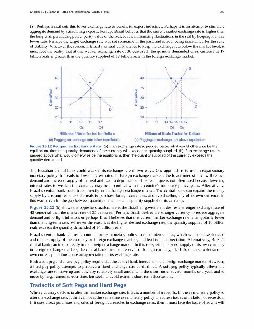
(a). Perhaps Brazil sets this lower exchange rate to benefit its export industries. Perhaps it is an attempt to stimulateaggregate demand by stimulating exports. Perhaps Brazil believes that the current market exchange rate is higher thanthe long-term purchasing power parity value of the real, so it is minimizing fluctuations in the real by keeping it at thislower rate. Perhaps the target exchange rate was set sometime in the past, and is now being maintained for the sakeof stability. Whatever the reason, if Brazil’s central bank wishes to keep the exchange rate below the market level, itmust face the reality that at this weaker exchange rate of 30 cents/real, the quantity demanded of its currency at 17billion reals is greater than the quantity supplied of 13 billion reals in the foreign exchange market.
Figure 15.12 Pegging an Exchange Rate (a) If an exchange rate is pegged below what would otherwise be theequilibrium, then the quantity demanded of the currency will exceed the quantity supplied. (b) If an exchange rate ispegged above what would otherwise be the equilibrium, then the quantity supplied of the currency exceeds thequantity demanded.
The Brazilian central bank could weaken its exchange rate in two ways. One approach is to use an expansionarymonetary policy that leads to lower interest rates. In foreign exchange markets, the lower interest rates will reducedemand and increase supply of the real and lead to depreciation. This technique is not often used because loweringinterest rates to weaken the currency may be in conflict with the country’s monetary policy goals. Alternatively,Brazil’s central bank could trade directly in the foreign exchange market. The central bank can expand the moneysupply by creating reals, use the reals to purchase foreign currencies, and avoid selling any of its own currency. Inthis way, it can fill the gap between quantity demanded and quantity supplied of its currency.
Figure 15.12 (b) shows the opposite situation. Here, the Brazilian government desires a stronger exchange rate of40 cents/real than the market rate of 35 cents/real. Perhaps Brazil desires the stronger currency to reduce aggregatedemand and to fight inflation, or perhaps Brazil believes that that current market exchange rate is temporarily lowerthan the long-term rate. Whatever the reason, at the higher desired exchange rate, the quantity supplied of 16 billionreals exceeds the quantity demanded of 14 billion reals.
Brazil’s central bank can use a contractionary monetary policy to raise interest rates, which will increase demandand reduce supply of the currency on foreign exchange markets, and lead to an appreciation. Alternatively, Brazil’scentral bank can trade directly in the foreign exchange market. In this case, with an excess supply of its own currencyin foreign exchange markets, the central bank must use reserves of foreign currency, like U.S. dollars, to demand itsown currency and thus cause an appreciation of its exchange rate.
Both a soft peg and a hard peg policy require that the central bank intervene in the foreign exchange market. However,a hard peg policy attempts to preserve a fixed exchange rate at all times. A soft peg policy typically allows theexchange rate to move up and down by relatively small amounts in the short run of several months or a year, and tomove by larger amounts over time, but seeks to avoid extreme short-term fluctuations.
Tradeoffs of Soft Pegs and Hard PegsWhen a country decides to alter the market exchange rate, it faces a number of tradeoffs. If it uses monetary policy toalter the exchange rate, it then cannot at the same time use monetary policy to address issues of inflation or recession.If it uses direct purchases and sales of foreign currencies in exchange rates, then it must face the issue of how it will
Chapter 15 | Exchange Rates and International Capital Flows 383
handle its reserves of foreign currency. Finally, a pegged exchange rate can even create additional movements of theexchange rate; for example, even the possibility of government intervention in exchange rate markets will lead torumors about whether and when the government will intervene, and dealers in the foreign exchange market will reactto those rumors. Let’s consider these issues in turn.
One concern with pegged exchange rate policies is that they imply a country’s monetary policy is no longer focusedon controlling inflation or shortening recessions, but now must also take the exchange rate into account. For example,when a country pegs its exchange rate, it will sometimes face economic situations where it would like to havean expansionary monetary policy to fight recession—but it cannot do so because that policy would depreciate itsexchange rate and break its hard peg. With a soft peg exchange rate policy, the central bank can sometimes ignore theexchange rate and focus on domestic inflation or recession—but in other cases the central bank may ignore inflationor recession and instead focus on its soft peg exchange rate. With a hard peg policy, domestic monetary policy iseffectively no longer determined by domestic inflation or unemployment, but only by what monetary policy is neededto keep the exchange rate at the hard peg.
Another issue arises when a central bank intervenes directly in the exchange rate market. If a central bank ends upin a situation where it is perpetually creating and selling its own currency on foreign exchange markets, it will bebuying the currency of other countries, like U.S. dollars or euros, to hold as reserves. Holding large reserves of othercurrencies has an opportunity cost, and central banks will not wish to boost such reserves without limit.
In addition, a central bank that causes a large increase in the supply of money is also risking an inflationary surge inaggregate demand. Conversely, when a central bank wishes to buy its own currency, it can do so by using its reservesof international currency like the U.S. dollar or the euro. But if the central bank runs out of such reserves, it can nolonger use this method to strengthen its currency. Thus, buying foreign currencies in exchange rate markets can beexpensive and inflationary, while selling foreign currencies can work only until a central bank runs out of reserves.
Yet another issue is that when a government pegs its exchange rate, it may unintentionally create another reasonfor additional fluctuation. With a soft peg policy, foreign exchange dealers and international investors react to everyrumor about how or when the central bank is likely to intervene to influence the exchange rate, and as they reactto rumors the exchange rate will shift up and down. Thus, even though the goal of a soft peg policy is to reduceshort-term fluctuations of the exchange rate, the existence of the policy—when anticipated in the foreign exchangemarket—may sometimes increase short-term fluctuations as international investors try to anticipate how and when thecentral bank will act. The following Clear It Up feature discusses the effects of international capital flows—capitalthat flows across national boundaries as either portfolio investment or direct investment.
How do Tobin taxes control the flow of capital?Some countries like Chile and Malaysia have sought to reduce movements in exchange rates by limitinginflows and outflows of international financial capital. This policy can be enacted either through targeted taxesor by regulations.
Taxes on international capital flows are sometimes known as Tobin taxes, named after James Tobin, the 1981Nobel laureate in economics who proposed such a tax in a 1972 lecture. For example, a government might taxall foreign exchange transactions, or attempt to tax short-term portfolio investment while exempting long-termforeign direct investment. Countries can also use regulation to forbid certain kinds of foreign investment in thefirst place or to make it difficult for international financial investors to withdraw their funds from a country.
The goal of such policies is to reduce international capital flows, especially short-term portfolio flows, inthe hope that doing so will reduce the chance of large movements in exchange rates that can bringmacroeconomic disaster.
But proposals to limit international financial flows have severe practical difficulties. Taxes are imposed bynational governments, not international ones. If one government imposes a Tobin tax on exchange ratetransactions carried out within its territory, the exchange rate market might easily be operated by a firmbased someplace like the Grand Caymans, an island nation in the Caribbean well-known for allowing somefinancial wheeling and dealing. In an interconnected global economy, if goods and services are allowed to
384 Chapter 15 | Exchange Rates and International Capital Flows
This OpenStax book is available for free at http://cnx.org/content/col11864/1.2
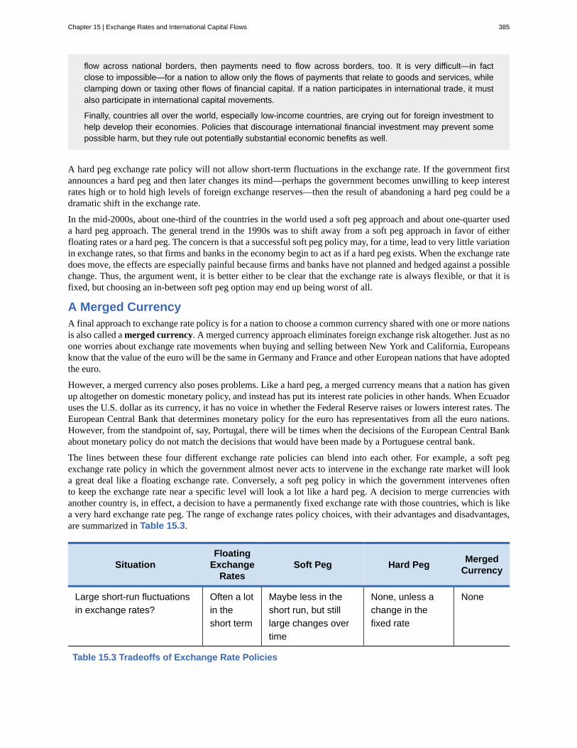
flow across national borders, then payments need to flow across borders, too. It is very difficult—in factclose to impossible—for a nation to allow only the flows of payments that relate to goods and services, whileclamping down or taxing other flows of financial capital. If a nation participates in international trade, it mustalso participate in international capital movements.
Finally, countries all over the world, especially low-income countries, are crying out for foreign investment tohelp develop their economies. Policies that discourage international financial investment may prevent somepossible harm, but they rule out potentially substantial economic benefits as well.
A hard peg exchange rate policy will not allow short-term fluctuations in the exchange rate. If the government firstannounces a hard peg and then later changes its mind—perhaps the government becomes unwilling to keep interestrates high or to hold high levels of foreign exchange reserves—then the result of abandoning a hard peg could be adramatic shift in the exchange rate.
In the mid-2000s, about one-third of the countries in the world used a soft peg approach and about one-quarter useda hard peg approach. The general trend in the 1990s was to shift away from a soft peg approach in favor of eitherfloating rates or a hard peg. The concern is that a successful soft peg policy may, for a time, lead to very little variationin exchange rates, so that firms and banks in the economy begin to act as if a hard peg exists. When the exchange ratedoes move, the effects are especially painful because firms and banks have not planned and hedged against a possiblechange. Thus, the argument went, it is better either to be clear that the exchange rate is always flexible, or that it isfixed, but choosing an in-between soft peg option may end up being worst of all.
A Merged CurrencyA final approach to exchange rate policy is for a nation to choose a common currency shared with one or more nationsis also called a merged currency. A merged currency approach eliminates foreign exchange risk altogether. Just as noone worries about exchange rate movements when buying and selling between New York and California, Europeansknow that the value of the euro will be the same in Germany and France and other European nations that have adoptedthe euro.
However, a merged currency also poses problems. Like a hard peg, a merged currency means that a nation has givenup altogether on domestic monetary policy, and instead has put its interest rate policies in other hands. When Ecuadoruses the U.S. dollar as its currency, it has no voice in whether the Federal Reserve raises or lowers interest rates. TheEuropean Central Bank that determines monetary policy for the euro has representatives from all the euro nations.However, from the standpoint of, say, Portugal, there will be times when the decisions of the European Central Bankabout monetary policy do not match the decisions that would have been made by a Portuguese central bank.
The lines between these four different exchange rate policies can blend into each other. For example, a soft pegexchange rate policy in which the government almost never acts to intervene in the exchange rate market will looka great deal like a floating exchange rate. Conversely, a soft peg policy in which the government intervenes oftento keep the exchange rate near a specific level will look a lot like a hard peg. A decision to merge currencies withanother country is, in effect, a decision to have a permanently fixed exchange rate with those countries, which is likea very hard exchange rate peg. The range of exchange rates policy choices, with their advantages and disadvantages,are summarized in Table 15.3.
SituationFloating
ExchangeRates
Soft Peg Hard Peg MergedCurrency
Large short-run fluctuationsin exchange rates?
Often a lotin theshort term
Maybe less in theshort run, but stilllarge changes overtime
None, unless achange in thefixed rate
None
Table 15.3 Tradeoffs of Exchange Rate Policies
Chapter 15 | Exchange Rates and International Capital Flows 385
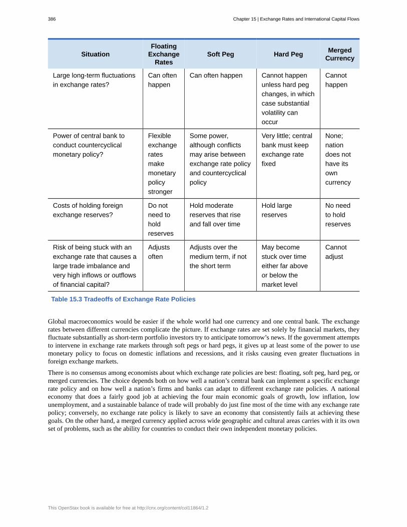
SituationFloating
ExchangeRates
Soft Peg Hard Peg MergedCurrency
Large long-term fluctuationsin exchange rates?
Can oftenhappen
Can often happen Cannot happenunless hard pegchanges, in whichcase substantialvolatility canoccur
Cannothappen
Power of central bank toconduct countercyclicalmonetary policy?
Flexibleexchangeratesmakemonetarypolicystronger
Some power,although conflictsmay arise betweenexchange rate policyand countercyclicalpolicy
Very little; centralbank must keepexchange ratefixed
None;nationdoes nothave itsowncurrency
Costs of holding foreignexchange reserves?
Do notneed toholdreserves
Hold moderatereserves that riseand fall over time
Hold largereserves
No needto holdreserves
Risk of being stuck with anexchange rate that causes alarge trade imbalance andvery high inflows or outflowsof financial capital?
Adjustsoften
Adjusts over themedium term, if notthe short term
May becomestuck over timeeither far aboveor below themarket level
Cannotadjust
Table 15.3 Tradeoffs of Exchange Rate Policies
Global macroeconomics would be easier if the whole world had one currency and one central bank. The exchangerates between different currencies complicate the picture. If exchange rates are set solely by financial markets, theyfluctuate substantially as short-term portfolio investors try to anticipate tomorrow’s news. If the government attemptsto intervene in exchange rate markets through soft pegs or hard pegs, it gives up at least some of the power to usemonetary policy to focus on domestic inflations and recessions, and it risks causing even greater fluctuations inforeign exchange markets.
There is no consensus among economists about which exchange rate policies are best: floating, soft peg, hard peg, ormerged currencies. The choice depends both on how well a nation’s central bank can implement a specific exchangerate policy and on how well a nation’s firms and banks can adapt to different exchange rate policies. A nationaleconomy that does a fairly good job at achieving the four main economic goals of growth, low inflation, lowunemployment, and a sustainable balance of trade will probably do just fine most of the time with any exchange ratepolicy; conversely, no exchange rate policy is likely to save an economy that consistently fails at achieving thesegoals. On the other hand, a merged currency applied across wide geographic and cultural areas carries with it its ownset of problems, such as the ability for countries to conduct their own independent monetary policies.
386 Chapter 15 | Exchange Rates and International Capital Flows
This OpenStax book is available for free at http://cnx.org/content/col11864/1.2
Is a Stronger Dollar Good for the U.S. Economy?The foreign exchange value of the dollar is a price and whether a higher price is good or bad depends onwhere you are standing: sellers benefit from higher prices and buyers are harmed. A stronger dollar is goodfor U.S. imports (and people working for U.S. importers) and U.S. investment abroad. It is also good for U.S.tourists going to other countries, since their dollar goes further. But a stronger dollar is bad for U.S. exports(and people working in U.S. export industries); it is bad for foreign investment in the United States (leading,for example, to higher U.S. interest rates); and it is bad for foreign tourists (as well as U.S hotels, restaurants,and others in the tourist industry). In short, whether the U.S. dollar is good or bad is a more complex questionthan you may have thought. The economic answer is “it depends.”
Chapter 15 | Exchange Rates and International Capital Flows 387
appreciating
arbitrage
depreciating
dollarize
floating exchange rate
foreign direct investment (FDI)
foreign exchange market
hard peg
hedge
international capital flows
merged currency
portfolio investment
purchasing power parity (PPP)
soft peg
Tobin taxes
KEY TERMS
when a currency is worth more in terms of other currencies; also called “strengthening”
the process of buying a good and selling goods across borders to take advantage of international pricedifferences
when a currency is worth less in terms of other currencies; also called “weakening”
a country that is not the United States uses the U.S. dollar as its currency
a country lets the value of its currency be determined in the exchange rate market
purchasing more than ten percent of a firm or starting a new enterprise in anothercountry
the market in which people use one currency to buy another currency
an exchange rate policy in which the central bank sets a fixed and unchanging value for the exchange rate
using a financial transaction as protection against risk
flow of financial capital across national boundaries either as portfolio investment or directinvestment
when a nation chooses to use the currency of another nation
an investment in another country that is purely financial and does not involve any managementresponsibility
the exchange rate that equalizes the prices of internationally traded goods acrosscountries
an exchange rate policy in which the government usually allows the exchange rate to be set by the market, butin some cases, especially if the exchange rate seems to be moving rapidly in one direction, the central bank willintervene
see international capital flows
KEY CONCEPTS AND SUMMARY
15.1 How the Foreign Exchange Market WorksIn the foreign exchange market, people and firms exchange one currency to purchase another currency. The demandfor dollars comes from those U.S. export firms seeking to convert their earnings in foreign currency back into U.S.dollars; foreign tourists converting their earnings in a foreign currency back into U.S. dollars; and foreign investorsseeking to make financial investments in the U.S. economy. On the supply side of the foreign exchange market for thetrading of U.S. dollars are foreign firms that have sold imports in the U.S. economy and are seeking to convert theirearnings back to their home currency; U.S. tourists abroad; and U.S. investors seeking to make financial investmentsin foreign economies. When currency A can buy more of currency B, then currency A has strengthened or appreciatedrelative to B. When currency A can buy less of currency B, then currency A has weakened or depreciated relativeto B. If currency A strengthens or appreciates relative to currency B, then currency B must necessarily weaken ordepreciate with regard to currency A. A stronger currency benefits those who are buying with that currency andinjures those who are selling. A weaker currency injures those, like importers, who are buying with that currency andbenefits those who are selling with it, like exporters.
388 Chapter 15 | Exchange Rates and International Capital Flows
This OpenStax book is available for free at http://cnx.org/content/col11864/1.2
15.2 Demand and Supply Shifts in Foreign Exchange MarketsIn the extreme short run, ranging from a few minutes to a few weeks, exchange rates are influenced by speculatorswho are trying to invest in currencies that will grow stronger, and to sell currencies that will grow weaker. Suchspeculation can create a self-fulfilling prophecy, at least for a time, where an expected appreciation leads to a strongercurrency and vice versa. In the relatively short run, exchange rate markets are influenced by differences in rates ofreturn. Countries with relatively high real rates of return (for example, high interest rates) will tend to experiencestronger currencies as they attract money from abroad, while countries with relatively low rates of return will tend toexperience weaker exchange rates as investors convert to other currencies.
In the medium run of a few months or a few years, exchange rate markets are influenced by inflation rates. Countrieswith relatively high inflation will tend to experience less demand for their currency than countries with lowerinflation, and thus currency depreciation. Over long periods of many years, exchange rates tend to adjust toward thepurchasing power parity (PPP) rate, which is the exchange rate such that the prices of internationally tradable goodsin different countries, when converted at the PPP exchange rate to a common currency, are similar in all economies.
15.3 Macroeconomic Effects of Exchange RatesA central bank will be concerned about the exchange rate for several reasons. Exchange rates will affect imports andexports, and thus affect aggregate demand in the economy. Fluctuations in exchange rates may cause difficulties formany firms, but especially banks. The exchange rate may accompany unsustainable flows of international financialcapital.
15.4 Exchange Rate PoliciesIn a floating exchange rate policy, a country’s exchange rate is determined in the foreign exchange market. In a softpeg exchange rate policy, a country’s exchange rate is usually determined in the foreign exchange market, but thegovernment sometimes intervenes to strengthen or weaken the exchange rate. In a hard peg exchange rate policy, thegovernment chooses an exchange rate. A central bank can intervene in exchange markets in two ways. It can raiseor lower interest rates to make the currency stronger or weaker. Or it can directly purchase or sell its currency inforeign exchange markets. All exchange rates policies face tradeoffs. A hard peg exchange rate policy will reduceexchange rate fluctuations, but means that a country must focus its monetary policy on the exchange rate, not onfighting recession or controlling inflation. When a nation merges its currency with another nation, it gives up onnationally oriented monetary policy altogether.
A soft peg exchange rate may create additional volatility as exchange rate markets try to anticipate when and howthe government will intervene. A flexible exchange rate policy allows monetary policy to focus on inflation andunemployment, and allows the exchange rate to change with inflation and rates of return, but also raises a risk thatexchange rates may sometimes make large and abrupt movements. The spectrum of exchange rate policies includes:(a) a floating exchange rate, (b) a pegged exchange rate, soft or hard, and (c) a merged currency. Monetary policy canfocus on a variety of goals: (a) inflation; (b) inflation or unemployment, depending on which is the most dangerousobstacle; and (c) a long-term rule based policy designed to keep the money supply stable and predictable.
SELF-CHECK QUESTIONS1. How will a stronger euro affect the following economic agents?
a. A British exporter to Germany.b. A Dutch tourist visiting Chile.c. A Greek bank investing in a Canadian government bond.d. A French exporter to Germany.
2. Suppose that political unrest in Egypt leads financial markets to anticipate a depreciation in the Egyptian pound.How will that affect the demand for pounds, supply of pounds, and exchange rate for pounds compared to, say, U.S.dollars?
3. Suppose U.S. interest rates decline compared to the rest of the world. What would be the likely impact on thedemand for dollars, supply of dollars, and exchange rate for dollars compared to, say, euros?
Chapter 15 | Exchange Rates and International Capital Flows 389
4. Suppose Argentina gets inflation under control and the Argentine inflation rate decreases substantially. Whatwould likely happen to the demand for Argentine pesos, the supply of Argentine pesos, and the peso/U.S. dollarexchange rate?
5. This chapter has explained that “one of the most economically destructive effects of exchange rate fluctuationscan happen through the banking system,” if banks borrow from abroad to lend domestically. Why is this less likely tobe a problem for the U.S. banking system?
6. A booming economy can attract financial capital inflows, which promote further growth. But capital can just aseasily flow out of the country, leading to economic recession. Is a country whose economy is booming because itdecided to stimulate consumer spending more or less likely to experience capital flight than an economy whose boomis caused by economic investment expenditure?
7. How would a contractionary monetary policy affect the exchange rate, net exports, aggregate demand, andaggregate supply?
8. A central bank can allow its currency to fall indefinitely, but it cannot allow its currency to rise indefinitely. Whynot?
9. Is a country for which imports and exports make up a large fraction of the GDP more likely to adopt a flexibleexchange rate or a fixed (hard peg) exchange rate?
REVIEW QUESTIONS
10. What is the foreign exchange market?
11. Describe some buyers and some sellers in themarket for U.S. dollars.
12. What is the difference between foreign directinvestment and portfolio investment?
13. What does it mean to hedge a financial transaction?
14. What does it mean to say that a currencyappreciates? Depreciates? Becomes stronger? Becomesweaker?
15. Does an expectation of a stronger exchange rate inthe future affect the exchange rate in the present? If so,how?
16. Does a higher rate of return in a nation’s economy,all other things being equal, affect the exchange rate ofits currency? If so, how?
17. Does a higher inflation rate in an economy, otherthings being equal, affect the exchange rate of itscurrency? If so, how?
18. What is the purchasing power parity exchangerate?
19. What are some of the reasons a central bank islikely to care, at least to some extent, about the exchangerate?
20. How can an unexpected fall in exchange ratesinjure the financial health of a nation’s banks?
21. What is the difference between a floating exchangerate, a soft peg, a hard peg, and dollarization?
22. List some advantages and disadvantages of thedifferent exchange rate policies.
CRITICAL THINKING QUESTIONS
23. Why would a nation “dollarize”—that is, adoptanother country’s currency instead of having its own?
24. Can you think of any major disadvantages todollarization? How would a central bank work in acountry that has dollarized?
25. If a country’s currency is expected to appreciatein value, what would you think will be the impact ofexpected exchange rates on yields (e.g., the interest ratepaid on government bonds) in that country? Hint: Thinkabout how expected exchange rate changes and interestrates affect demand and supply for a currency.
390 Chapter 15 | Exchange Rates and International Capital Flows
This OpenStax book is available for free at http://cnx.org/content/col11864/1.2
26. Do you think that a country experiencinghyperinflation is more or less likely to have an exchangerate equal to its purchasing power parity value whencompared to a country with a low inflation rate?
27. Suppose a country has an overall balance of tradeso that exports of goods and services equal imports ofgoods and services. Does that imply that the country hasbalanced trade with each of its trading partners?
28. We learned that monetary policy is amplified bychanges in exchange rates and the correspondingchanges in the balance of trade. From the perspectiveof a nation’s central bank, is this a good thing or a badthing?
29. If a developing country needs foreign capitalinflows, management expertise, and technology, howcan it encourage foreign investors while at the same timeprotect itself against capital flight and banking systemcollapse, as happened during the Asian financial crisis?
30. Many developing countries, like Mexico, havemoderate to high rates of inflation. At the same time,international trade plays an important role in theireconomies. What type of exchange rate regime wouldbe best for such a country’s currency vis à vis the U.S.dollar?
31. What would make a country decide to change froma common currency, like the euro, back to its owncurrency?
PROBLEMS32. A British pound cost $1.56 in U.S. dollars in 1996,but $1.66 in U.S. dollars in 1998. Was the pound weakeror stronger against the dollar? Did the dollar appreciateor depreciate versus the pound?
33. In Exercise 15.32 calculate the cost of a U.S.dollar in terms of British pounds in 1996 and 1998.
Chapter 15 | Exchange Rates and International Capital Flows 391
392 Chapter 15 | Exchange Rates and International Capital Flows
This OpenStax book is available for free at http://cnx.org/content/col11864/1.2

16 | Government Budgetsand Fiscal Policy
Figure 16.1 Shut Downs and Parks Yellowstone National Park is one of the many national parks forced to closedown during the government shut down in October 2013. (Credit: modification of work by “daveynin”/flickr CreativeCommons)
No Yellowstone Park?So you had trekked all the way to see Yellowstone National Park in the beautiful month of October 2013, onlyto find it… closed. Closed! Why?
For two weeks in October 2013, the U.S. federal government shut down. Many federal services, like thenational parks, closed and 800,000 federal employees were furloughed. Tourists were shocked and so wasthe rest of the world: Congress and the President could not agree on a budget. Inside the Capitol, Republicansand Democrats argued about spending priorities and whether to increase the national debt limit. Each year'sbudget, which is over $3 trillion of spending, must be approved by Congress and signed by the President.Two thirds of the budget is entitlements and other mandatory spending which occur without congressionalor presidential action once the programs are set up. Tied to the budget debate was the issue of increasingthe debt ceiling—how high the national debt of the U.S. government can be. The House of Representativesrefused to sign on to the bills to fund the government unless they included provisions to stop or change theAffordable Health Care Act (more colloquially known as Obamacare). As the days ticked by, the United Statescame very close to defaulting on its debt.
Why does the federal budget create such intense debates? What would happen if the United States actuallydefaulted on its debt? In this chapter, we will examine the federal budget, taxation, and fiscal policy. We willalso look at the annual federal budget deficits and the national debt.
Chapter 16 | Government Budgets and Fiscal Policy 393
Introduction to Government Budgets and Fiscal PolicyIn this chapter, you will learn about:
• Government Spending
• Taxation
• Federal Deficits and the National Debt
• Using Fiscal Policy to Fight Recessions, Unemployment, and Inflation
• Automatic Stabilizers
• Practical Problems with Discretionary Fiscal Policy
• The Question of a Balanced Budget
All levels of government—federal, state, and local—have budgets that show how much revenue the governmentexpects to receive in taxes and other income and how the government plans to spend it. Budgets, however, can shiftdramatically within a few years, as policy decisions and unexpected events shake up earlier tax and spending plans.
In this chapter, we revisit fiscal policy, which was first covered in Welcome to Economics! Fiscal policy is oneof two policy tools for fine tuning the economy (the other is monetary policy). While monetary policy is made bypolicymakers at the Federal Reserve, fiscal policy is made by Congress and the President.
The discussion of fiscal policy focuses on how federal government taxing and spending affects aggregate demand.All government spending and taxes affect the economy, but fiscal policy focuses strictly on the policies of the federalgovernment. We begin with an overview of U.S. government spending and taxes. We then discuss fiscal policy froma short-run perspective; that is, how government uses tax and spending policies to address recession, unemployment,and inflation; how periods of recession and growth affect government budgets; and the merits of balanced budgetproposals.
16.1 | Government SpendingBy the end of this section, you will be able to:
• Identify U.S. budget deficit and surplus trends over the past five decades• Explain the differences between the U.S. federal budget, and state and local budgets
Government spending covers a range of services provided by the federal, state, and local governments. When thefederal government spends more money than it receives in taxes in a given year, it runs a budget deficit. Conversely,when the government receives more money in taxes than it spends in a year, it runs a budget surplus. If governmentspending and taxes are equal, it is said to have a balanced budget. For example, in 2009, the U.S. governmentexperienced its largest budget deficit ever, as the federal government spent $1.4 trillion more than it collected in taxes.This deficit was about 10% of the size of the U.S. GDP in 2009, making it by far the largest budget deficit relative toGDP since the mammoth borrowing used to finance World War II.
This section presents an overview of government spending in the United States.
Total U.S. Government SpendingFederal spending in nominal dollars (that is, dollars not adjusted for inflation) has grown by a multiple of more than38 over the last four decades, from $93.4 billion in 1960 to $3.9 trillion in 2014. Comparing spending over time innominal dollars is misleading because it does not take into account inflation or growth in population and the realeconomy. A more useful method of comparison is to examine government spending as a percent of GDP over time.
The top line in Figure 16.2 shows the level of federal spending since 1960, expressed as a share of GDP. Despitea widespread sense among many Americans that the federal government has been growing steadily larger, the graphshows that federal spending has hovered in a range from 18% to 22% of GDP most of the time since 1960. Theother lines in Figure 16.2 show the major federal spending categories: national defense, Social Security, health
394 Chapter 16 | Government Budgets and Fiscal Policy
This OpenStax book is available for free at http://cnx.org/content/col11864/1.2

programs, and interest payments. From the graph, we see that national defense spending as a share of GDP hasgenerally declined since the 1960s, although there were some upward bumps in the 1980s buildup under PresidentRonald Reagan and in the aftermath of the terrorist attacks on September 11, 2001. In contrast, Social Securityand healthcare have grown steadily as a percent of GDP. Healthcare expenditures include both payments for seniorcitizens (Medicare), and payments for low-income Americans (Medicaid). Medicaid is also partially funded by stategovernments. Interest payments are the final main category of government spending shown in the figure.
Figure 16.2 Federal Spending, 1960–2014 Since 1960, total federal spending has ranged from about 18% to 22%of GDP, although it climbed above that level in 2009, but quickly dropped back down to that level by 2013. The sharespent on national defense has generally declined, while the share spent on Social Security and on healthcareexpenses (mainly Medicare and Medicaid) has increased. (Source: Economic Report of the President, Tables B-2and B-22, http://www.gpo.gov/fdsys/pkg/ERP-2014/content-detail.html)
Each year, the government borrows funds from U.S. citizens and foreigners to cover its budget deficits. It does thisby selling securities (Treasury bonds, notes, and bills)—in essence borrowing from the public and promising to repaywith interest in the future. From 1961 to 1997, the U.S. government has run budget deficits, and thus borrowed funds,in almost every year. It had budget surpluses from 1998 to 2001, and then returned to deficits.
The interest payments on past federal government borrowing were typically 1–2% of GDP in the 1960s and 1970sbut then climbed above 3% of GDP in the 1980s and stayed there until the late 1990s. The government was able torepay some of its past borrowing by running surpluses from 1998 to 2001 and, with help from low interest rates, theinterest payments on past federal government borrowing had fallen back to 1.4% of GDP by 2012.
We investigate the patterns of government borrowing and debt in more detail later in this chapter, but first we needto clarify the difference between the deficit and the debt. The deficit is not the debt. The difference between thedeficit and the debt lies in the time frame. The government deficit (or surplus) refers to what happens with the federalgovernment budget each year. The government debt is accumulated over time; it is the sum of all past deficits andsurpluses. If you borrow $10,000 per year for each of the four years of college, you might say that your annual deficitwas $10,000, but your accumulated debt over the four years is $40,000.
These four categories—national defense, Social Security, healthcare, and interest payments—account for roughly73% of all federal spending, as Figure 16.3 shows. The remaining 27% wedge of the pie chart covers all othercategories of federal government spending: international affairs; science and technology; natural resources and theenvironment; transportation; housing; education; income support for the poor; community and regional development;law enforcement and the judicial system; and the administrative costs of running the government.
Chapter 16 | Government Budgets and Fiscal Policy 395
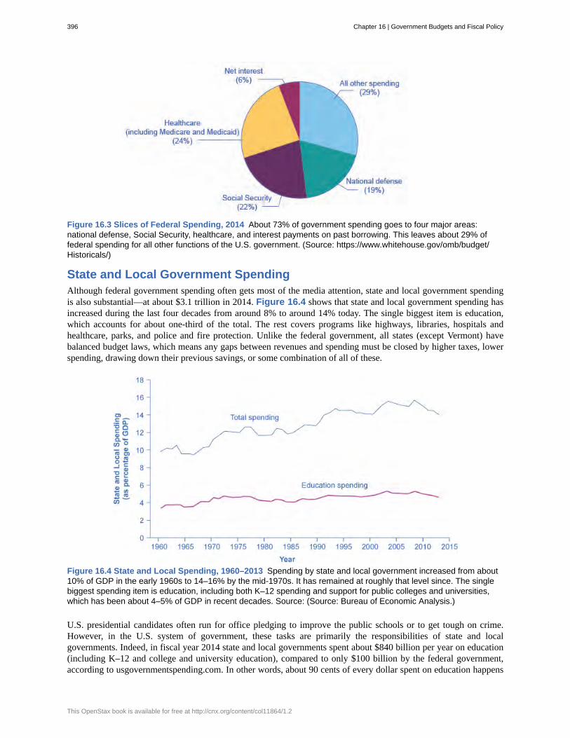
Figure 16.3 Slices of Federal Spending, 2014 About 73% of government spending goes to four major areas:national defense, Social Security, healthcare, and interest payments on past borrowing. This leaves about 29% offederal spending for all other functions of the U.S. government. (Source: https://www.whitehouse.gov/omb/budget/Historicals/)
State and Local Government SpendingAlthough federal government spending often gets most of the media attention, state and local government spendingis also substantial—at about $3.1 trillion in 2014. Figure 16.4 shows that state and local government spending hasincreased during the last four decades from around 8% to around 14% today. The single biggest item is education,which accounts for about one-third of the total. The rest covers programs like highways, libraries, hospitals andhealthcare, parks, and police and fire protection. Unlike the federal government, all states (except Vermont) havebalanced budget laws, which means any gaps between revenues and spending must be closed by higher taxes, lowerspending, drawing down their previous savings, or some combination of all of these.
Figure 16.4 State and Local Spending, 1960–2013 Spending by state and local government increased from about10% of GDP in the early 1960s to 14–16% by the mid-1970s. It has remained at roughly that level since. The singlebiggest spending item is education, including both K–12 spending and support for public colleges and universities,which has been about 4–5% of GDP in recent decades. Source: (Source: Bureau of Economic Analysis.)
U.S. presidential candidates often run for office pledging to improve the public schools or to get tough on crime.However, in the U.S. system of government, these tasks are primarily the responsibilities of state and localgovernments. Indeed, in fiscal year 2014 state and local governments spent about $840 billion per year on education(including K–12 and college and university education), compared to only $100 billion by the federal government,according to usgovernmentspending.com. In other words, about 90 cents of every dollar spent on education happens
396 Chapter 16 | Government Budgets and Fiscal Policy
This OpenStax book is available for free at http://cnx.org/content/col11864/1.2
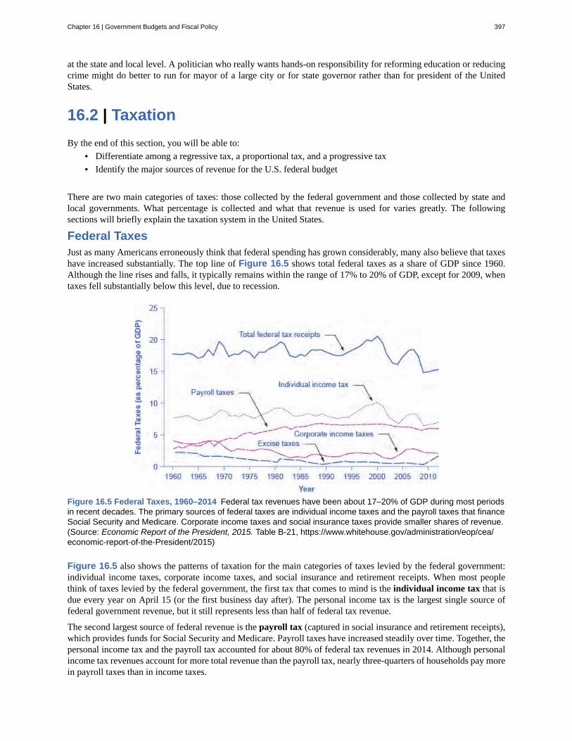
at the state and local level. A politician who really wants hands-on responsibility for reforming education or reducingcrime might do better to run for mayor of a large city or for state governor rather than for president of the UnitedStates.
16.2 | TaxationBy the end of this section, you will be able to:
• Differentiate among a regressive tax, a proportional tax, and a progressive tax• Identify the major sources of revenue for the U.S. federal budget
There are two main categories of taxes: those collected by the federal government and those collected by state andlocal governments. What percentage is collected and what that revenue is used for varies greatly. The followingsections will briefly explain the taxation system in the United States.
Federal TaxesJust as many Americans erroneously think that federal spending has grown considerably, many also believe that taxeshave increased substantially. The top line of Figure 16.5 shows total federal taxes as a share of GDP since 1960.Although the line rises and falls, it typically remains within the range of 17% to 20% of GDP, except for 2009, whentaxes fell substantially below this level, due to recession.
Figure 16.5 Federal Taxes, 1960–2014 Federal tax revenues have been about 17–20% of GDP during most periodsin recent decades. The primary sources of federal taxes are individual income taxes and the payroll taxes that financeSocial Security and Medicare. Corporate income taxes and social insurance taxes provide smaller shares of revenue.(Source: Economic Report of the President, 2015. Table B-21, https://www.whitehouse.gov/administration/eop/cea/economic-report-of-the-President/2015)
Figure 16.5 also shows the patterns of taxation for the main categories of taxes levied by the federal government:individual income taxes, corporate income taxes, and social insurance and retirement receipts. When most peoplethink of taxes levied by the federal government, the first tax that comes to mind is the individual income tax that isdue every year on April 15 (or the first business day after). The personal income tax is the largest single source offederal government revenue, but it still represents less than half of federal tax revenue.
The second largest source of federal revenue is the payroll tax (captured in social insurance and retirement receipts),which provides funds for Social Security and Medicare. Payroll taxes have increased steadily over time. Together, thepersonal income tax and the payroll tax accounted for about 80% of federal tax revenues in 2014. Although personalincome tax revenues account for more total revenue than the payroll tax, nearly three-quarters of households pay morein payroll taxes than in income taxes.
Chapter 16 | Government Budgets and Fiscal Policy 397
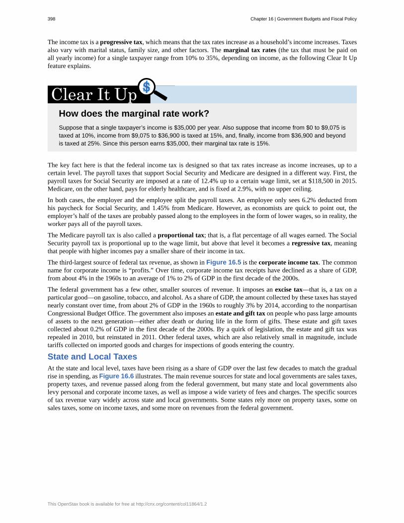
The income tax is a progressive tax, which means that the tax rates increase as a household’s income increases. Taxesalso vary with marital status, family size, and other factors. The marginal tax rates (the tax that must be paid onall yearly income) for a single taxpayer range from 10% to 35%, depending on income, as the following Clear It Upfeature explains.
How does the marginal rate work?Suppose that a single taxpayer’s income is $35,000 per year. Also suppose that income from $0 to $9,075 istaxed at 10%, income from $9,075 to $36,900 is taxed at 15%, and, finally, income from $36,900 and beyondis taxed at 25%. Since this person earns $35,000, their marginal tax rate is 15%.
The key fact here is that the federal income tax is designed so that tax rates increase as income increases, up to acertain level. The payroll taxes that support Social Security and Medicare are designed in a different way. First, thepayroll taxes for Social Security are imposed at a rate of 12.4% up to a certain wage limit, set at $118,500 in 2015.Medicare, on the other hand, pays for elderly healthcare, and is fixed at 2.9%, with no upper ceiling.
In both cases, the employer and the employee split the payroll taxes. An employee only sees 6.2% deducted fromhis paycheck for Social Security, and 1.45% from Medicare. However, as economists are quick to point out, theemployer’s half of the taxes are probably passed along to the employees in the form of lower wages, so in reality, theworker pays all of the payroll taxes.
The Medicare payroll tax is also called a proportional tax; that is, a flat percentage of all wages earned. The SocialSecurity payroll tax is proportional up to the wage limit, but above that level it becomes a regressive tax, meaningthat people with higher incomes pay a smaller share of their income in tax.
The third-largest source of federal tax revenue, as shown in Figure 16.5 is the corporate income tax. The commonname for corporate income is “profits.” Over time, corporate income tax receipts have declined as a share of GDP,from about 4% in the 1960s to an average of 1% to 2% of GDP in the first decade of the 2000s.
The federal government has a few other, smaller sources of revenue. It imposes an excise tax—that is, a tax on aparticular good—on gasoline, tobacco, and alcohol. As a share of GDP, the amount collected by these taxes has stayednearly constant over time, from about 2% of GDP in the 1960s to roughly 3% by 2014, according to the nonpartisanCongressional Budget Office. The government also imposes an estate and gift tax on people who pass large amountsof assets to the next generation—either after death or during life in the form of gifts. These estate and gift taxescollected about 0.2% of GDP in the first decade of the 2000s. By a quirk of legislation, the estate and gift tax wasrepealed in 2010, but reinstated in 2011. Other federal taxes, which are also relatively small in magnitude, includetariffs collected on imported goods and charges for inspections of goods entering the country.
State and Local TaxesAt the state and local level, taxes have been rising as a share of GDP over the last few decades to match the gradualrise in spending, as Figure 16.6 illustrates. The main revenue sources for state and local governments are sales taxes,property taxes, and revenue passed along from the federal government, but many state and local governments alsolevy personal and corporate income taxes, as well as impose a wide variety of fees and charges. The specific sourcesof tax revenue vary widely across state and local governments. Some states rely more on property taxes, some onsales taxes, some on income taxes, and some more on revenues from the federal government.
398 Chapter 16 | Government Budgets and Fiscal Policy
This OpenStax book is available for free at http://cnx.org/content/col11864/1.2
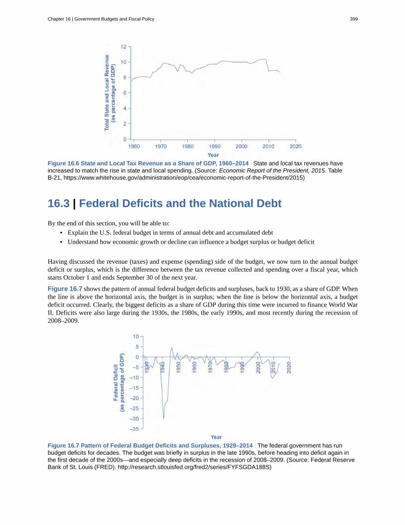
Figure 16.6 State and Local Tax Revenue as a Share of GDP, 1960–2014 State and local tax revenues haveincreased to match the rise in state and local spending. (Source: Economic Report of the President, 2015. TableB-21, https://www.whitehouse.gov/administration/eop/cea/economic-report-of-the-President/2015)
16.3 | Federal Deficits and the National DebtBy the end of this section, you will be able to:
• Explain the U.S. federal budget in terms of annual debt and accumulated debt• Understand how economic growth or decline can influence a budget surplus or budget deficit
Having discussed the revenue (taxes) and expense (spending) side of the budget, we now turn to the annual budgetdeficit or surplus, which is the difference between the tax revenue collected and spending over a fiscal year, whichstarts October 1 and ends September 30 of the next year.
Figure 16.7 shows the pattern of annual federal budget deficits and surpluses, back to 1930, as a share of GDP. Whenthe line is above the horizontal axis, the budget is in surplus; when the line is below the horizontal axis, a budgetdeficit occurred. Clearly, the biggest deficits as a share of GDP during this time were incurred to finance World WarII. Deficits were also large during the 1930s, the 1980s, the early 1990s, and most recently during the recession of2008–2009.
Figure 16.7 Pattern of Federal Budget Deficits and Surpluses, 1929–2014 The federal government has runbudget deficits for decades. The budget was briefly in surplus in the late 1990s, before heading into deficit again inthe first decade of the 2000s—and especially deep deficits in the recession of 2008–2009. (Source: Federal ReserveBank of St. Louis (FRED). http://research.stlouisfed.org/fred2/series/FYFSGDA188S)
Chapter 16 | Government Budgets and Fiscal Policy 399
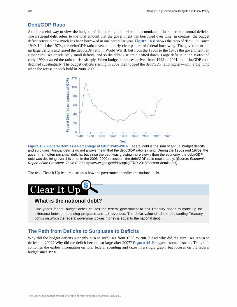
Debt/GDP RatioAnother useful way to view the budget deficit is through the prism of accumulated debt rather than annual deficits.The national debt refers to the total amount that the government has borrowed over time; in contrast, the budgetdeficit refers to how much has been borrowed in one particular year. Figure 16.8 shows the ratio of debt/GDP since1940. Until the 1970s, the debt/GDP ratio revealed a fairly clear pattern of federal borrowing. The government ranup large deficits and raised the debt/GDP ratio in World War II, but from the 1950s to the 1970s the government raneither surpluses or relatively small deficits, and so the debt/GDP ratio drifted down. Large deficits in the 1980s andearly 1990s caused the ratio to rise sharply. When budget surpluses arrived from 1998 to 2001, the debt/GDP ratiodeclined substantially. The budget deficits starting in 2002 then tugged the debt/GDP ratio higher—with a big jumpwhen the recession took hold in 2008–2009.
Figure 16.8 Federal Debt as a Percentage of GDP, 1942–2014 Federal debt is the sum of annual budget deficitsand surpluses. Annual deficits do not always mean that the debt/GDP ratio is rising. During the 1960s and 1970s, thegovernment often ran small deficits, but since the debt was growing more slowly than the economy, the debt/GDPratio was declining over this time. In the 2008–2009 recession, the debt/GDP ratio rose sharply. (Source: EconomicReport of the President, Table B-20, http://www.gpo.gov/fdsys/pkg/ERP-2015/content-detail.html)
The next Clear it Up feature discusses how the government handles the national debt.
What is the national debt?One year’s federal budget deficit causes the federal government to sell Treasury bonds to make up thedifference between spending programs and tax revenues. The dollar value of all the outstanding Treasurybonds on which the federal government owes money is equal to the national debt.
The Path from Deficits to Surpluses to DeficitsWhy did the budget deficits suddenly turn to surpluses from 1998 to 2001? And why did the surpluses return todeficits in 2002? Why did the deficit become so large after 2007? Figure 16.9 suggests some answers. The graphcombines the earlier information on total federal spending and taxes in a single graph, but focuses on the federalbudget since 1990.
400 Chapter 16 | Government Budgets and Fiscal Policy
This OpenStax book is available for free at http://cnx.org/content/col11864/1.2
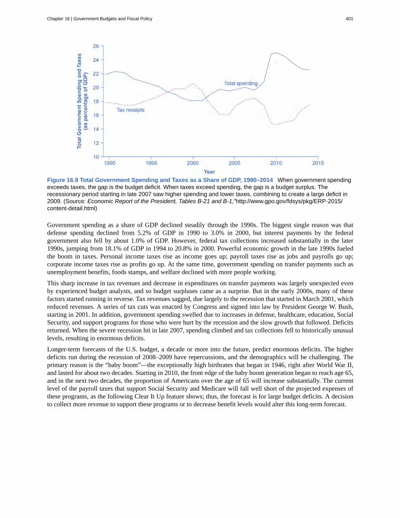
Figure 16.9 Total Government Spending and Taxes as a Share of GDP, 1990–2014 When government spendingexceeds taxes, the gap is the budget deficit. When taxes exceed spending, the gap is a budget surplus. Therecessionary period starting in late 2007 saw higher spending and lower taxes, combining to create a large deficit in2009. (Source: Economic Report of the President, Tables B-21 and B-1,"http://www.gpo.gov/fdsys/pkg/ERP-2015/content-detail.html)
Government spending as a share of GDP declined steadily through the 1990s. The biggest single reason was thatdefense spending declined from 5.2% of GDP in 1990 to 3.0% in 2000, but interest payments by the federalgovernment also fell by about 1.0% of GDP. However, federal tax collections increased substantially in the later1990s, jumping from 18.1% of GDP in 1994 to 20.8% in 2000. Powerful economic growth in the late 1990s fueledthe boom in taxes. Personal income taxes rise as income goes up; payroll taxes rise as jobs and payrolls go up;corporate income taxes rise as profits go up. At the same time, government spending on transfer payments such asunemployment benefits, foods stamps, and welfare declined with more people working.
This sharp increase in tax revenues and decrease in expenditures on transfer payments was largely unexpected evenby experienced budget analysts, and so budget surpluses came as a surprise. But in the early 2000s, many of thesefactors started running in reverse. Tax revenues sagged, due largely to the recession that started in March 2001, whichreduced revenues. A series of tax cuts was enacted by Congress and signed into law by President George W. Bush,starting in 2001. In addition, government spending swelled due to increases in defense, healthcare, education, SocialSecurity, and support programs for those who were hurt by the recession and the slow growth that followed. Deficitsreturned. When the severe recession hit in late 2007, spending climbed and tax collections fell to historically unusuallevels, resulting in enormous deficits.
Longer-term forecasts of the U.S. budget, a decade or more into the future, predict enormous deficits. The higherdeficits run during the recession of 2008–2009 have repercussions, and the demographics will be challenging. Theprimary reason is the “baby boom”—the exceptionally high birthrates that began in 1946, right after World War II,and lasted for about two decades. Starting in 2010, the front edge of the baby boom generation began to reach age 65,and in the next two decades, the proportion of Americans over the age of 65 will increase substantially. The currentlevel of the payroll taxes that support Social Security and Medicare will fall well short of the projected expenses ofthese programs, as the following Clear It Up feature shows; thus, the forecast is for large budget deficits. A decisionto collect more revenue to support these programs or to decrease benefit levels would alter this long-term forecast.
Chapter 16 | Government Budgets and Fiscal Policy 401
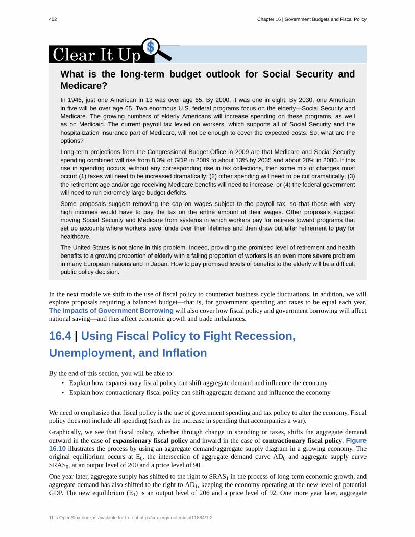
What is the long-term budget outlook for Social Security andMedicare?In 1946, just one American in 13 was over age 65. By 2000, it was one in eight. By 2030, one Americanin five will be over age 65. Two enormous U.S. federal programs focus on the elderly—Social Security andMedicare. The growing numbers of elderly Americans will increase spending on these programs, as wellas on Medicaid. The current payroll tax levied on workers, which supports all of Social Security and thehospitalization insurance part of Medicare, will not be enough to cover the expected costs. So, what are theoptions?
Long-term projections from the Congressional Budget Office in 2009 are that Medicare and Social Securityspending combined will rise from 8.3% of GDP in 2009 to about 13% by 2035 and about 20% in 2080. If thisrise in spending occurs, without any corresponding rise in tax collections, then some mix of changes mustoccur: (1) taxes will need to be increased dramatically; (2) other spending will need to be cut dramatically; (3)the retirement age and/or age receiving Medicare benefits will need to increase, or (4) the federal governmentwill need to run extremely large budget deficits.
Some proposals suggest removing the cap on wages subject to the payroll tax, so that those with veryhigh incomes would have to pay the tax on the entire amount of their wages. Other proposals suggestmoving Social Security and Medicare from systems in which workers pay for retirees toward programs thatset up accounts where workers save funds over their lifetimes and then draw out after retirement to pay forhealthcare.
The United States is not alone in this problem. Indeed, providing the promised level of retirement and healthbenefits to a growing proportion of elderly with a falling proportion of workers is an even more severe problemin many European nations and in Japan. How to pay promised levels of benefits to the elderly will be a difficultpublic policy decision.
In the next module we shift to the use of fiscal policy to counteract business cycle fluctuations. In addition, we willexplore proposals requiring a balanced budget—that is, for government spending and taxes to be equal each year.The Impacts of Government Borrowing will also cover how fiscal policy and government borrowing will affectnational saving—and thus affect economic growth and trade imbalances.
16.4 | Using Fiscal Policy to Fight Recession,Unemployment, and InflationBy the end of this section, you will be able to:
• Explain how expansionary fiscal policy can shift aggregate demand and influence the economy• Explain how contractionary fiscal policy can shift aggregate demand and influence the economy
We need to emphasize that fiscal policy is the use of government spending and tax policy to alter the economy. Fiscalpolicy does not include all spending (such as the increase in spending that accompanies a war).
Graphically, we see that fiscal policy, whether through change in spending or taxes, shifts the aggregate demandoutward in the case of expansionary fiscal policy and inward in the case of contractionary fiscal policy. Figure16.10 illustrates the process by using an aggregate demand/aggregate supply diagram in a growing economy. Theoriginal equilibrium occurs at E0, the intersection of aggregate demand curve AD0 and aggregate supply curveSRAS0, at an output level of 200 and a price level of 90.
One year later, aggregate supply has shifted to the right to SRAS1 in the process of long-term economic growth, andaggregate demand has also shifted to the right to AD1, keeping the economy operating at the new level of potentialGDP. The new equilibrium (E1) is an output level of 206 and a price level of 92. One more year later, aggregate
402 Chapter 16 | Government Budgets and Fiscal Policy
This OpenStax book is available for free at http://cnx.org/content/col11864/1.2
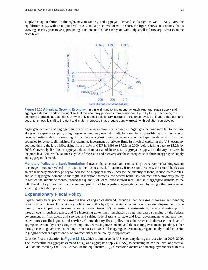
supply has again shifted to the right, now to SRAS2, and aggregate demand shifts right as well to AD2. Now theequilibrium is E2, with an output level of 212 and a price level of 94. In short, the figure shows an economy that isgrowing steadily year to year, producing at its potential GDP each year, with only small inflationary increases in theprice level.
Figure 16.10 A Healthy, Growing Economy In this well-functioning economy, each year aggregate supply andaggregate demand shift to the right so that the economy proceeds from equilibrium E0 to E1 to E2. Each year, theeconomy produces at potential GDP with only a small inflationary increase in the price level. But if aggregate demanddoes not smoothly shift to the right and match increases in aggregate supply, growth with deflation can develop.
Aggregate demand and aggregate supply do not always move neatly together. Aggregate demand may fail to increasealong with aggregate supply, or aggregate demand may even shift left, for a number of possible reasons: householdsbecome hesitant about consuming; firms decide against investing as much; or perhaps the demand from othercountries for exports diminishes. For example, investment by private firms in physical capital in the U.S. economyboomed during the late 1990s, rising from 14.1% of GDP in 1993 to 17.2% in 2000, before falling back to 15.2% by2002. Conversely, if shifts in aggregate demand run ahead of increases in aggregate supply, inflationary increases inthe price level will result. Business cycles of recession and recovery are the consequence of shifts in aggregate supplyand aggregate demand.
Monetary Policy and Bank Regulation shows us that a central bank can use its powers over the banking systemto engage in countercyclical—or “against the business cycle”—actions. If recession threatens, the central bank usesan expansionary monetary policy to increase the supply of money, increase the quantity of loans, reduce interest rates,and shift aggregate demand to the right. If inflation threatens, the central bank uses contractionary monetary policyto reduce the supply of money, reduce the quantity of loans, raise interest rates, and shift aggregate demand to theleft. Fiscal policy is another macroeconomic policy tool for adjusting aggregate demand by using either governmentspending or taxation policy.
Expansionary Fiscal PolicyExpansionary fiscal policy increases the level of aggregate demand, through either increases in government spendingor reductions in taxes. Expansionary policy can do this by (1) increasing consumption by raising disposable incomethrough cuts in personal income taxes or payroll taxes; (2) increasing investments by raising after-tax profitsthrough cuts in business taxes; and (3) increasing government purchases through increased spending by the federalgovernment on final goods and services and raising federal grants to state and local governments to increase theirexpenditures on final goods and services. Contractionary fiscal policy does the reverse: it decreases the level ofaggregate demand by decreasing consumption, decreasing investments, and decreasing government spending, eitherthrough cuts in government spending or increases in taxes. The aggregate demand/aggregate supply model is usefulin judging whether expansionary or contractionary fiscal policy is appropriate.
Consider first the situation in Figure 16.11, which is similar to the U.S. economy during the recession in 2008–2009.The intersection of aggregate demand (AD0) and aggregate supply (SRAS0) is occurring below the level of potentialGDP as indicated by the LRAS curve. At the equilibrium (E0), a recession occurs and unemployment rises. In this
Chapter 16 | Government Budgets and Fiscal Policy 403
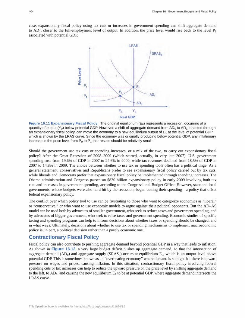
case, expansionary fiscal policy using tax cuts or increases in government spending can shift aggregate demandto AD1, closer to the full-employment level of output. In addition, the price level would rise back to the level P1associated with potential GDP.
Figure 16.11 Expansionary Fiscal Policy The original equilibrium (E0) represents a recession, occurring at aquantity of output (Y0) below potential GDP. However, a shift of aggregate demand from AD0 to AD1, enacted throughan expansionary fiscal policy, can move the economy to a new equilibrium output of E1 at the level of potential GDPwhich is shown by the LRAS curve. Since the economy was originally producing below potential GDP, any inflationaryincrease in the price level from P0 to P1 that results should be relatively small.
Should the government use tax cuts or spending increases, or a mix of the two, to carry out expansionary fiscalpolicy? After the Great Recession of 2008–2009 (which started, actually, in very late 2007), U.S. governmentspending rose from 19.6% of GDP in 2007 to 24.6% in 2009, while tax revenues declined from 18.5% of GDP in2007 to 14.8% in 2009. The choice between whether to use tax or spending tools often has a political tinge. As ageneral statement, conservatives and Republicans prefer to see expansionary fiscal policy carried out by tax cuts,while liberals and Democrats prefer that expansionary fiscal policy be implemented through spending increases. TheObama administration and Congress passed an $830 billion expansionary policy in early 2009 involving both taxcuts and increases in government spending, according to the Congressional Budget Office. However, state and localgovernments, whose budgets were also hard hit by the recession, began cutting their spending—a policy that offsetfederal expansionary policy.
The conflict over which policy tool to use can be frustrating to those who want to categorize economics as “liberal”or “conservative,” or who want to use economic models to argue against their political opponents. But the AD–ASmodel can be used both by advocates of smaller government, who seek to reduce taxes and government spending, andby advocates of bigger government, who seek to raise taxes and government spending. Economic studies of specifictaxing and spending programs can help to inform decisions about whether taxes or spending should be changed, andin what ways. Ultimately, decisions about whether to use tax or spending mechanisms to implement macroeconomicpolicy is, in part, a political decision rather than a purely economic one.
Contractionary Fiscal PolicyFiscal policy can also contribute to pushing aggregate demand beyond potential GDP in a way that leads to inflation.As shown in Figure 16.12, a very large budget deficit pushes up aggregate demand, so that the intersection ofaggregate demand (AD0) and aggregate supply (SRAS0) occurs at equilibrium E0, which is an output level abovepotential GDP. This is sometimes known as an “overheating economy” where demand is so high that there is upwardpressure on wages and prices, causing inflation. In this situation, contractionary fiscal policy involving federalspending cuts or tax increases can help to reduce the upward pressure on the price level by shifting aggregate demandto the left, to AD1, and causing the new equilibrium E1 to be at potential GDP, where aggregate demand intersects theLRAS curve.
404 Chapter 16 | Government Budgets and Fiscal Policy
This OpenStax book is available for free at http://cnx.org/content/col11864/1.2
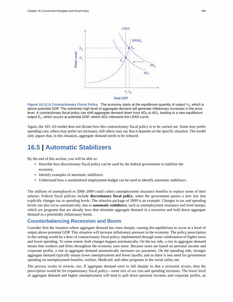
Figure 16.12 A Contractionary Fiscal Policy The economy starts at the equilibrium quantity of output Y0, which isabove potential GDP. The extremely high level of aggregate demand will generate inflationary increases in the pricelevel. A contractionary fiscal policy can shift aggregate demand down from AD0 to AD1, leading to a new equilibriumoutput E1, which occurs at potential GDP, where AD1 intersects the LRAS curve.
Again, the AD–AS model does not dictate how this contractionary fiscal policy is to be carried out. Some may preferspending cuts; others may prefer tax increases; still others may say that it depends on the specific situation. The modelonly argues that, in this situation, aggregate demand needs to be reduced.
16.5 | Automatic StabilizersBy the end of this section, you will be able to:
• Describe how discretionary fiscal policy can be used by the federal government to stabilize theeconomy.
• Identify examples of automatic stabilizers.• Understand how a standardized employment budget can be used to identify automatic stabilizers.
The millions of unemployed in 2008–2009 could collect unemployment insurance benefits to replace some of theirsalaries. Federal fiscal policies include discretionary fiscal policy, when the government passes a new law thatexplicitly changes tax or spending levels. The stimulus package of 2009 is an example. Changes in tax and spendinglevels can also occur automatically, due to automatic stabilizers, such as unemployment insurance and food stamps,which are programs that are already laws that stimulate aggregate demand in a recession and hold down aggregatedemand in a potentially inflationary boom.
Counterbalancing Recession and BoomConsider first the situation where aggregate demand has risen sharply, causing the equilibrium to occur at a level ofoutput above potential GDP. This situation will increase inflationary pressure in the economy. The policy prescriptionin this setting would be a dose of contractionary fiscal policy, implemented through some combination of higher taxesand lower spending. To some extent, both changes happen automatically. On the tax side, a rise in aggregate demandmeans that workers and firms throughout the economy earn more. Because taxes are based on personal income andcorporate profits, a rise in aggregate demand automatically increases tax payments. On the spending side, strongeraggregate demand typically means lower unemployment and fewer layoffs, and so there is less need for governmentspending on unemployment benefits, welfare, Medicaid, and other programs in the social safety net.
The process works in reverse, too. If aggregate demand were to fall sharply so that a recession occurs, then theprescription would be for expansionary fiscal policy—some mix of tax cuts and spending increases. The lower levelof aggregate demand and higher unemployment will tend to pull down personal incomes and corporate profits, an
Chapter 16 | Government Budgets and Fiscal Policy 405
effect that will reduce the amount of taxes owed automatically. Higher unemployment and a weaker economy shouldlead to increased government spending on unemployment benefits, welfare, and other similar domestic programs. In2009, the stimulus package included an extension in the time allowed to collect unemployment insurance. In addition,the automatic stabilizers react to a weakening of aggregate demand with expansionary fiscal policy and react to astrengthening of aggregate demand with contractionary fiscal policy, just as the AD/AS analysis suggests.
The very large budget deficit of 2009 was produced by a combination of automatic stabilizers and discretionary fiscalpolicy. The Great Recession, starting in late 2007, meant less tax-generating economic activity, which triggered theautomatic stabilizers that reduce taxes. Most economists, even those who are concerned about a possible pattern ofpersistently large budget deficits, are much less concerned or even quite supportive of larger budget deficits in theshort run of a few years during and immediately after a severe recession.
A glance back at economic history provides a second illustration of the power of automatic stabilizers. Remember thatthe length of economic upswings between recessions has become longer in the U.S. economy in recent decades (asdiscussed in Unemployment). The three longest economic booms of the twentieth century happened in the 1960s,the 1980s, and the 1991–2001 time period. One reason why the economy has tipped into recession less frequentlyin recent decades is that the size of government spending and taxes has increased in the second half of the twentiethcentury. Thus, the automatic stabilizing effects from spending and taxes are now larger than they were in the first halfof the twentieth century. Around 1900, for example, federal spending was only about 2% of GDP. In 1929, just beforethe Great Depression hit, government spending was still just 4% of GDP. In those earlier times, the smaller size ofgovernment made automatic stabilizers far less powerful than in the last few decades, when government spendingoften hovers at 20% of GDP or more.
The Standardized Employment Deficit or SurplusEach year, the nonpartisan Congressional Budget Office (CBO) calculates the standardized employmentbudget—that is, what the budget deficit or surplus would be if the economy were producing at potential GDP, wherepeople who look for work were finding jobs in a reasonable period of time and businesses were making normalprofits, with the result that both workers and businesses would be earning more and paying more taxes. In effect,the standardized employment deficit eliminates the impact of the automatic stabilizers. Figure 16.13 compares theactual budget deficits of recent decades with the CBO’s standardized deficit.
Visit this website (http://openstaxcollege.org/l/CBO) to learn more from the Congressional Budget Office.
406 Chapter 16 | Government Budgets and Fiscal Policy
This OpenStax book is available for free at http://cnx.org/content/col11864/1.2
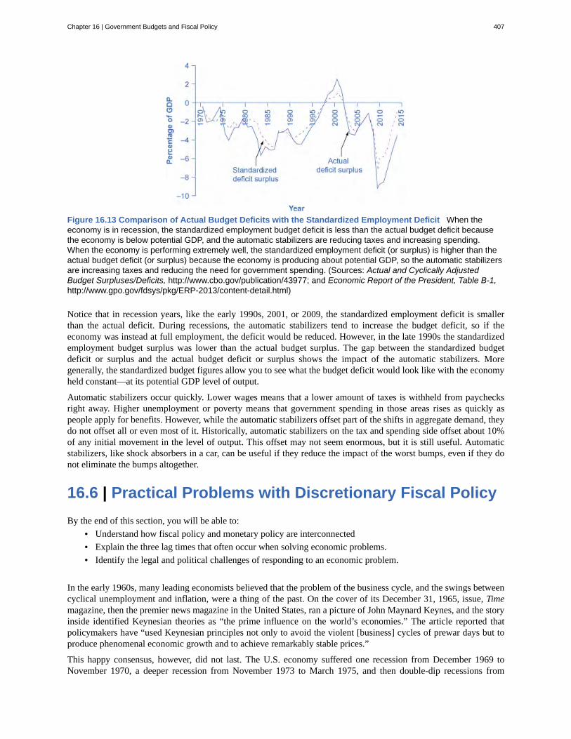
Figure 16.13 Comparison of Actual Budget Deficits with the Standardized Employment Deficit When theeconomy is in recession, the standardized employment budget deficit is less than the actual budget deficit becausethe economy is below potential GDP, and the automatic stabilizers are reducing taxes and increasing spending.When the economy is performing extremely well, the standardized employment deficit (or surplus) is higher than theactual budget deficit (or surplus) because the economy is producing about potential GDP, so the automatic stabilizersare increasing taxes and reducing the need for government spending. (Sources: Actual and Cyclically AdjustedBudget Surpluses/Deficits, http://www.cbo.gov/publication/43977; and Economic Report of the President, Table B-1,http://www.gpo.gov/fdsys/pkg/ERP-2013/content-detail.html)
Notice that in recession years, like the early 1990s, 2001, or 2009, the standardized employment deficit is smallerthan the actual deficit. During recessions, the automatic stabilizers tend to increase the budget deficit, so if theeconomy was instead at full employment, the deficit would be reduced. However, in the late 1990s the standardizedemployment budget surplus was lower than the actual budget surplus. The gap between the standardized budgetdeficit or surplus and the actual budget deficit or surplus shows the impact of the automatic stabilizers. Moregenerally, the standardized budget figures allow you to see what the budget deficit would look like with the economyheld constant—at its potential GDP level of output.
Automatic stabilizers occur quickly. Lower wages means that a lower amount of taxes is withheld from paychecksright away. Higher unemployment or poverty means that government spending in those areas rises as quickly aspeople apply for benefits. However, while the automatic stabilizers offset part of the shifts in aggregate demand, theydo not offset all or even most of it. Historically, automatic stabilizers on the tax and spending side offset about 10%of any initial movement in the level of output. This offset may not seem enormous, but it is still useful. Automaticstabilizers, like shock absorbers in a car, can be useful if they reduce the impact of the worst bumps, even if they donot eliminate the bumps altogether.
16.6 | Practical Problems with Discretionary Fiscal PolicyBy the end of this section, you will be able to:
• Understand how fiscal policy and monetary policy are interconnected• Explain the three lag times that often occur when solving economic problems.• Identify the legal and political challenges of responding to an economic problem.
In the early 1960s, many leading economists believed that the problem of the business cycle, and the swings betweencyclical unemployment and inflation, were a thing of the past. On the cover of its December 31, 1965, issue, Timemagazine, then the premier news magazine in the United States, ran a picture of John Maynard Keynes, and the storyinside identified Keynesian theories as “the prime influence on the world’s economies.” The article reported thatpolicymakers have “used Keynesian principles not only to avoid the violent [business] cycles of prewar days but toproduce phenomenal economic growth and to achieve remarkably stable prices.”
This happy consensus, however, did not last. The U.S. economy suffered one recession from December 1969 toNovember 1970, a deeper recession from November 1973 to March 1975, and then double-dip recessions from
Chapter 16 | Government Budgets and Fiscal Policy 407
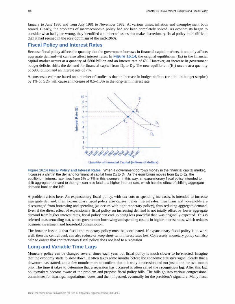
January to June 1980 and from July 1981 to November 1982. At various times, inflation and unemployment bothsoared. Clearly, the problems of macroeconomic policy had not been completely solved. As economists began toconsider what had gone wrong, they identified a number of issues that make discretionary fiscal policy more difficultthan it had seemed in the rosy optimism of the mid-1960s.
Fiscal Policy and Interest RatesBecause fiscal policy affects the quantity that the government borrows in financial capital markets, it not only affectsaggregate demand—it can also affect interest rates. In Figure 16.14, the original equilibrium (E0) in the financialcapital market occurs at a quantity of $800 billion and an interest rate of 6%. However, an increase in governmentbudget deficits shifts the demand for financial capital from D0 to D1. The new equilibrium (E1) occurs at a quantityof $900 billion and an interest rate of 7%.
A consensus estimate based on a number of studies is that an increase in budget deficits (or a fall in budget surplus)by 1% of GDP will cause an increase of 0.5–1.0% in the long-term interest rate.
Figure 16.14 Fiscal Policy and Interest Rates When a government borrows money in the financial capital market,it causes a shift in the demand for financial capital from D0 to D1. As the equilibrium moves from E0 to E1, theequilibrium interest rate rises from 6% to 7% in this example. In this way, an expansionary fiscal policy intended toshift aggregate demand to the right can also lead to a higher interest rate, which has the effect of shifting aggregatedemand back to the left.
A problem arises here. An expansionary fiscal policy, with tax cuts or spending increases, is intended to increaseaggregate demand. If an expansionary fiscal policy also causes higher interest rates, then firms and households arediscouraged from borrowing and spending (as occurs with tight monetary policy), thus reducing aggregate demand.Even if the direct effect of expansionary fiscal policy on increasing demand is not totally offset by lower aggregatedemand from higher interest rates, fiscal policy can end up being less powerful than was originally expected. This isreferred to as crowding out, where government borrowing and spending results in higher interest rates, which reducesbusiness investment and household consumption.
The broader lesson is that fiscal and monetary policy must be coordinated. If expansionary fiscal policy is to workwell, then the central bank can also reduce or keep short-term interest rates low. Conversely, monetary policy can alsohelp to ensure that contractionary fiscal policy does not lead to a recession.
Long and Variable Time LagsMonetary policy can be changed several times each year, but fiscal policy is much slower to be enacted. Imaginethat the economy starts to slow down. It often takes some months before the economic statistics signal clearly that adownturn has started, and a few months more to confirm that it is truly a recession and not just a one- or two-monthblip. The time it takes to determine that a recession has occurred is often called the recognition lag. After this lag,policymakers become aware of the problem and propose fiscal policy bills. The bills go into various congressionalcommittees for hearings, negotiations, votes, and then, if passed, eventually for the president’s signature. Many fiscal
408 Chapter 16 | Government Budgets and Fiscal Policy
This OpenStax book is available for free at http://cnx.org/content/col11864/1.2
policy bills about spending or taxes propose changes that would start in the next budget year or would be phased ingradually over time. The time to get a bill passed is often referred to as the legislative lag. Finally, once the bill ispassed it takes some time for the funds to be dispersed to the appropriate agencies to implement the programs. Thetime to get the projects started is often called the implementation lag.
Moreover, the exact level of fiscal policy to be implemented is never completely clear. Should the budget deficit beincreased by 0.5% of GDP? By 1% of GDP? By 2% of GDP? In an AD/AS diagram, it is straightforward to sketch anaggregate demand curve shifting to the potential GDP level of output. In the real world, the actual level of potentialoutput is known only roughly, not precisely, and exactly how a spending cut or tax increase will affect aggregatedemand is always somewhat controversial. Also unknown is the state of the economy at any point in time. Duringthe early days of the Obama administration, for example, no one knew how deep in the hole the economy really was.During the financial crisis of 2008-09, the rapid collapse of the banking system and automotive sector made it difficultto assess how quickly the economy was collapsing.
Thus, it can take many months or even more than a year to begin an expansionary fiscal policy after a recession hasstarted—and even then, uncertainty will remain over exactly how much to expand or contract taxes and spending.When politicians attempt to use countercyclical fiscal policy to fight recession or inflation, they run the risk ofresponding to the macroeconomic situation of two or three years ago, in a way that may be exactly wrong for theeconomy at that time. George P. Schultz, a professor of economics, former Secretary of the Treasury, and Director ofthe Office of Management and Budget, once wrote: “While the economist is accustomed to the concept of lags, thepolitician likes instant results. The tension comes because, as I have seen on many occasions, the economist’s lag isthe politician’s nightmare.”
Temporary and Permanent Fiscal PolicyA temporary tax cut or spending increase will explicitly last only for a year or two, and then revert back to its originallevel. A permanent tax cut or spending increase is expected to stay in place for the foreseeable future. The effect oftemporary and permanent fiscal policies on aggregate demand can be very different. Consider how you would reactif the government announced a tax cut that would last one year and then be repealed, in comparison with how youwould react if the government announced a permanent tax cut. Most people and firms will react more strongly to apermanent policy change than a temporary one.
This fact creates an unavoidable difficulty for countercyclical fiscal policy. The appropriate policy may be to have anexpansionary fiscal policy with large budget deficits during a recession, and then a contractionary fiscal policy withbudget surpluses when the economy is growing well. But if both policies are explicitly temporary ones, they will havea less powerful effect than a permanent policy.
Structural Economic Change Takes TimeWhen an economy recovers from a recession, it does not usually revert back to its exact earlier shape. Instead, theinternal structure of the economy evolves and changes and this process can take time. For example, much of theeconomic growth of the mid-2000s was in the sectors of construction (especially of housing) and finance. However,when housing prices started falling in 2007 and the resulting financial crunch led into recession (as discussed inMonetary Policy and Bank Regulation), both sectors contracted. The manufacturing sector of the U.S. economyhas been losing jobs in recent years as well, under pressure from technological change and foreign competition. Manyof the people thrown out of work from these sectors in the Great Recession of 2008–2009 will never return to the samejobs in the same sectors of the economy; instead, the economy will need to grow in new and different directions, as thefollowing Clear It Up feature shows. Fiscal policy can increase overall demand, but the process of structural economicchange—the expansion of a new set of industries and the movement of workers to those industries—inevitably takestime.
Why do jobs vanish?People can lose jobs for a variety of reasons: because of a recession, but also because of longer-run changesin the economy, such as new technology. Productivity improvements in auto manufacturing, for example, can
Chapter 16 | Government Budgets and Fiscal Policy 409
reduce the number of workers needed, and eliminate these jobs in the long run. The Internet has created jobsbut also caused the loss of jobs as well, from travel agents to book store clerks. Many of these jobs may nevercome back. Short-run fiscal policy to reduce unemployment can create jobs, but it cannot replace jobs that willnever return.
The Limitations of Fiscal PolicyFiscal policy can help an economy that is producing below its potential GDP to expand aggregate demand so that itproduces closer to potential GDP, thus lowering unemployment. But fiscal policy cannot help an economy produceat an output level above potential GDP without causing inflation At this point, unemployment becomes so low thatworkers become scarce and wages rise rapidly.
Visit this website (http://openstaxcollege.org/l/fiscalpolicy) to read about how the recovery is being affected byfiscal policies.
Political Realties and Discretionary Fiscal PolicyA final problem for discretionary fiscal policy arises out of the difficulties of explaining to politicians howcountercyclical fiscal policy that runs against the tide of the business cycle should work. Politicians often have agut-level belief that when the economy and tax revenues slow down, it is time to hunker down, pinch pennies, andtrim expenses. Countercyclical policy, however, says that when the economy has slowed down, it is time for thegovernment to go on a spree, raising spending, and cutting taxes. This offsets the drop in the economy in the othersectors. Conversely, when economic times are good and tax revenues are rolling in, politicians often feel that it is timefor tax cuts and new spending. But countercyclical policy says that this economic boom should be an appropriate timefor keeping taxes high and restraining spending.
Politicians tend to prefer expansionary fiscal policy over contractionary policy. There is rarely a shortage of proposalsfor tax cuts and spending increases, especially during recessions. However, politicians are less willing to hear themessage that in good economic times, they should propose tax increases and spending limits. In the economicupswing of the late 1990s and early 2000s, for example, the U.S. GDP grew rapidly. Estimates from respectedgovernment economic forecasters like the nonpartisan Congressional Budget Office and the Office of Managementand Budget stated that the GDP was above potential GDP, and that unemployment rates were unsustainably low.However, no mainstream politician took the lead in saying that the booming economic times might be an appropriatetime for spending cuts or tax increases.
Discretionary Fiscal Policy: Summing UpExpansionary fiscal policy can help to end recessions and contractionary fiscal policy can help to reduce inflation.Given the uncertainties over interest rate effects, time lags, temporary and permanent policies, and unpredictablepolitical behavior, many economists and knowledgeable policymakers had concluded by the mid-1990s thatdiscretionary fiscal policy was a blunt instrument, more like a club than a scalpel. It might still make sense to useit in extreme economic situations, like an especially deep or long recession. For less extreme situations, it was oftenpreferable to let fiscal policy work through the automatic stabilizers and focus on monetary policy to steer short-termcountercyclical efforts.
410 Chapter 16 | Government Budgets and Fiscal Policy
This OpenStax book is available for free at http://cnx.org/content/col11864/1.2
16.7 | The Question of a Balanced BudgetBy the end of this section, you will be able to:
• Understand the arguments for and against requiring the U.S. federal budget to be balanced• Consider the long-run and short-run effects of a federal budget deficit
For many decades, going back to the 1930s, proposals have been put forward to require that the U.S. governmentbalance its budget every year. In 1995, a proposed constitutional amendment that would require a balanced budgetpassed the U.S. House of Representatives by a wide margin, and failed in the U.S. Senate by only a single vote. (Forthe balanced budget to have become an amendment to the Constitution would have required a two-thirds vote byCongress and passage by three-quarters of the state legislatures.)
Most economists view the proposals for a perpetually balanced budget with bemusement. After all, in the shortterm, economists would expect the budget deficits and surpluses to fluctuate up and down with the economy andthe automatic stabilizers. Economic recessions should automatically lead to larger budget deficits or smaller budgetsurpluses, while economic booms lead to smaller deficits or larger surpluses. A requirement that the budget bebalanced each and every year would prevent these automatic stabilizers from working and would worsen the severityof economic fluctuations.
Some supporters of the balanced budget amendment like to argue that, since households must balance their ownbudgets, the government should too. But this analogy between household and government behavior is severelyflawed. Most households do not balance their budgets every year. Some years households borrow to buy houses orcars or to pay for medical expenses or college tuition. Other years they repay loans and save funds in retirementaccounts. After retirement, they withdraw and spend those savings. Also, the government is not a household formany reasons, one of which is that the government has macroeconomic responsibilities. The argument of Keynesianmacroeconomic policy is that the government needs to lean against the wind, spending when times are hard andsaving when times are good, for the sake of the overall economy.
There is also no particular reason to expect a government budget to be balanced in the medium term of a fewyears. For example, a government may decide that by running large budget deficits, it can make crucial long-terminvestments in human capital and physical infrastructure that will build the long-term productivity of a country. Thesedecisions may work out well or poorly, but they are not always irrational. Such policies of ongoing government budgetdeficits may persist for decades. As the U.S. experience from the end of World War II up to about 1980 shows, it isperfectly possible to run budget deficits almost every year for decades, but as long as the percentage increases in debtare smaller than the percentage growth of GDP, the debt/GDP ratio will decline at the same time.
Nothing in this argument should be taken as a claim that budget deficits are always a wise policy. In the short run, agovernment that runs a very large budget deficit can shift aggregate demand to the right and trigger severe inflation.Additionally, governments may borrow for foolish or impractical reasons. The Macroeconomics Impacts ofGovernment Borrowing will discuss how large budget deficits, by reducing national saving, can in certain casesreduce economic growth and even contribute to international financial crises. A requirement that the budget bebalanced in each calendar year, however, is a misguided overreaction to the fear that in some cases, budget deficitscan become too large.
No Yellowstone Park?The federal budget shutdown of 2013 illustrated the many sides to fiscal policy and the federal budget. In2013, Republicans and Democrats could not agree on which spending policies to fund and how large thegovernment debt should be. Due to the severity of the recession in 2008–2009, the fiscal stimulus, andprevious policies, the federal budget deficit and debt was historically high. One way to try to cut federalspending and borrowing was to refuse to raise the legal federal debt limit, or tie on conditions to appropriationbills to stop the Affordable Health Care Act. This disagreement led to a two-week shutdown of the federal
Chapter 16 | Government Budgets and Fiscal Policy 411
government and got close to the deadline where the federal government would default on its Treasury bonds.Finally, however, a compromise emerged and default was avoided. This shows clearly how closely fiscalpolicies are tied to politics.
412 Chapter 16 | Government Budgets and Fiscal Policy
This OpenStax book is available for free at http://cnx.org/content/col11864/1.2
automatic stabilizers
balanced budget
budget deficit
budget surplus
contractionary fiscal policy
corporate income tax
crowding out
discretionary fiscal policy
estate and gift tax
excise tax
expansionary fiscal policy
implementation lag
individual income tax
legislative lag
marginal tax rates
national debt
payroll tax
progressive tax
proportional tax
recognition lag
regressive tax
standardized employment budget
KEY TERMS
tax and spending rules that have the effect of slowing down the rate of decrease in aggregatedemand when the economy slows down and restraining aggregate demand when the economy speeds up, withoutany additional change in legislation
when government spending and taxes are equal
when the federal government spends more money than it receives in taxes in a given year
when the government receives more money in taxes than it spends in a year
fiscal policy that decreases the level of aggregate demand, either through cuts ingovernment spending or increases in taxes
a tax imposed on corporate profits
federal spending and borrowing causes interest rates to rise and business investment to fall
the government passes a new law that explicitly changes overall tax or spending levelswith the intent of influencing the level or overall economic activity
a tax on people who pass assets to the next generation—either after death or during life in the formof gifts
a tax on a specific good—on gasoline, tobacco, and alcohol
fiscal policy that increases the level of aggregate demand, either through increases ingovernment spending or cuts in taxes
the time it takes for the funds relating to fiscal policy to be dispersed to the appropriate agencies toimplement the programs
a tax based on the income, of all forms, received by individuals
the time it takes to get a fiscal policy bill passed
or the tax that must be paid on all yearly income
the total accumulated amount the government has borrowed, over time, and not yet paid back
a tax based on the pay received from employers; the taxes provide funds for Social Security and Medicare
a tax that collects a greater share of income from those with high incomes than from those with lowerincomes
a tax that is a flat percentage of income earned, regardless of level of income
the time it takes to determine that a recession has occurred
a tax in which people with higher incomes pay a smaller share of their income in tax
the budget deficit or surplus in any given year adjusted for what it would havebeen if the economy were producing at potential GDP
Chapter 16 | Government Budgets and Fiscal Policy 413
KEY CONCEPTS AND SUMMARY
16.1 Government SpendingFiscal policy is the set of policies that relate to federal government spending, taxation, and borrowing. In recentdecades, the level of federal government spending and taxes, expressed as a share of GDP, has not changed much,typically fluctuating between about 18% to 22% of GDP. However, the level of state spending and taxes, as a share ofGDP, has risen from about 12–13% to about 20% of GDP over the last four decades. The four main areas of federalspending are national defense, Social Security, healthcare, and interest payments, which together account for about70% of all federal spending. When a government spends more than it collects in taxes, it is said to have a budgetdeficit. When a government collects more in taxes than it spends, it is said to have a budget surplus. If governmentspending and taxes are equal, it is said to have a balanced budget. The sum of all past deficits and surpluses make upthe government debt.
16.2 TaxationThe two main federal taxes are individual income taxes and payroll taxes that provide funds for Social Securityand Medicare; these taxes together account for more than 80% of federal revenues. Other federal taxes include thecorporate income tax, excise taxes on alcohol, gasoline and tobacco, and the estate and gift tax. A progressive tax isone, like the federal income tax, where those with higher incomes pay a higher share of taxes out of their income thanthose with lower incomes. A proportional tax is one, like the payroll tax for Medicare, where everyone pays the sameshare of taxes regardless of income level. A regressive tax is one, like the payroll tax (above a certain threshold) thatsupports Social Security, where those with high income pay a lower share of income in taxes than those with lowerincomes.
16.3 Federal Deficits and the National DebtFor most of the twentieth century, the U.S. government took on debt during wartime and then paid down that debtslowly in peacetime. However, it took on quite substantial debts in peacetime in the 1980s and early 1990s, before abrief period of budget surpluses from 1998 to 2001, followed by a return to annual budget deficits since 2002, withvery large deficits in the recession of 2008 and 2009. A budget deficit or budget surplus is measured annually. Totalgovernment debt or national debt is the sum of budget deficits and budget surpluses over time.
16.4 Using Fiscal Policy to Fight Recession, Unemployment, and InflationExpansionary fiscal policy increases the level of aggregate demand, either through increases in government spendingor through reductions in taxes. Expansionary fiscal policy is most appropriate when an economy is in recessionand producing below its potential GDP. Contractionary fiscal policy decreases the level of aggregate demand, eitherthrough cuts in government spending or increases in taxes. Contractionary fiscal policy is most appropriate when aneconomy is producing above its potential GDP.
16.5 Automatic StabilizersFiscal policy is conducted both through discretionary fiscal policy, which occurs when the government enactstaxation or spending changes in response to economic events, or through automatic stabilizers, which are taxing andspending mechanisms that, by their design, shift in response to economic events without any further legislation. Thestandardized employment budget is the calculation of what the budget deficit or budget surplus would have been ina given year if the economy had been producing at its potential GDP in that year. Many economists and politicianscriticize the use of fiscal policy for a variety of reasons, including concerns over time lags, the impact on interestrates, and the inherently political nature of fiscal policy. We cover the critique of fiscal policy in the next module.
16.6 Practical Problems with Discretionary Fiscal PolicyBecause fiscal policy affects the quantity of money that the government borrows in financial capital markets, it notonly affects aggregate demand—it can also affect interest rates. If an expansionary fiscal policy also causes higherinterest rates, then firms and households are discouraged from borrowing and spending, reducing aggregate demandin a situation called crowding out. Given the uncertainties over interest rate effects, time lags (implementation lag,legislative lag, and recognition lag), temporary and permanent policies, and unpredictable political behavior, manyeconomists and knowledgeable policymakers have concluded that discretionary fiscal policy is a blunt instrument andbetter used only in extreme situations.
414 Chapter 16 | Government Budgets and Fiscal Policy
This OpenStax book is available for free at http://cnx.org/content/col11864/1.2
16.7 The Question of a Balanced BudgetBalanced budget amendments are a popular political idea, but the economic merits behind such proposals arequestionable. Most economists accept that fiscal policy needs to be flexible enough to accommodate unforeseenexpenditures, such as wars or recessions. While persistent, large budget deficits can indeed be a problem, a balancedbudget amendment prevents even small, temporary deficits that might, in some cases, be necessary.
SELF-CHECK QUESTIONS1. When governments run budget deficits, how do they make up the differences between tax revenue and spending?
2. When governments run budget surpluses, what is done with the extra funds?
3. Is it possible for a nation to run budget deficits and still have its debt/GDP ratio fall? Explain your answer. Is itpossible for a nation to run budget surpluses and still have its debt/GDP ratio rise? Explain your answer.
4. Suppose that gifts were taxed at a rate of 10% for amounts up to $100,000 and 20% for anything over that amount.Would this tax be regressive or progressive?
5. If an individual owns a corporation for which he is the only employee, which different types of federal tax will hehave to pay?
6. What taxes would an individual pay if he were self-employed and the business is not incorporated?
7. The social security tax is 6.2% on employees’ income earned below $113,000. Is this tax progressive, regressiveor proportional?
8. Debt has a certain self-reinforcing quality to it. There is one category of government spending that automaticallyincreases along with the federal debt. What is it?
9. True or False:a. Federal spending has grown substantially in recent decades.b. By world standards, the U.S. government controls a relatively large share of the U.S. economy.c. A majority of the federal government’s revenue is collected through personal income taxes.d. Education spending is slightly larger at the federal level than at the state and local level.e. State and local government spending has not risen much in recent decades.f. Defense spending is higher now than ever.g. The share of the economy going to federal taxes has increased substantially over time.h. Foreign aid is a large portion, although less than half, of federal spending.i. Federal deficits have been very large for the last two decades.j. The accumulated federal debt as a share of GDP is near an all-time high.
10. What is the main reason for employing contractionary fiscal policy in a time of strong economic growth?
11. What is the main reason for employing expansionary fiscal policy during a recession?
12. In a recession, does the actual budget surplus or deficit fall above or below the standardized employmentbudget?
13. What is the main advantage of automatic stabilizers over discretionary fiscal policy?
14. Explain how automatic stabilizers work, both on the taxation side and on the spending side, first in a situationwhere the economy is producing less than potential GDP and then in a situation where the economy is producingmore than potential GDP.
15. What would happen if expansionary fiscal policy was implemented in a recession but, due to lag, did not actuallytake effect until after the economy was back to potential GDP?
Chapter 16 | Government Budgets and Fiscal Policy 415
16. What would happen if contractionary fiscal policy were implemented during an economic boom but, due to lag,it did not take effect until the economy slipped into recession?
17. Do you think the typical time lag for fiscal policy is likely to be longer or shorter than the time lag for monetarypolicy? Explain your answer?
18. How would a balanced budget amendment affect a decision by Congress to grant a tax cut during a recession?
19. How would a balanced budget amendment change the effect of automatic stabilizer programs?
REVIEW QUESTIONS
20. Give some examples of changes in federal spendingand taxes by the government that would be fiscal policyand some that would not.
21. Have the spending and taxes of the U.S. federalgovernment generally had an upward or a downwardtrend in the last few decades?
22. What are the main categories of U.S. federalgovernment spending?
23. What is the difference between a budget deficit, abalanced budget, and a budget surplus?
24. Have spending and taxes by state and localgovernments in the United States had a generallyupward or downward trend in the last few decades?
25. What are the main categories of U.S. federalgovernment taxes?
26. What is the difference between a progressive tax, aproportional tax, and a regressive tax?
27. What has been the general pattern of U.S. budgetdeficits in recent decades?
28. What is the difference between a budget deficit andthe national debt?
29. What is the difference between expansionary fiscalpolicy and contractionary fiscal policy?
30. Under what general macroeconomic circumstancesmight a government use expansionary fiscal policy?When might it use contractionary fiscal policy?
31. What is the difference between discretionary fiscalpolicy and automatic stabilizers?
32. Why do automatic stabilizers function“automatically?”
33. What is the standardized employment budget?
34. What are some practical weaknesses ofdiscretionary fiscal policy?
35. What are some of the arguments for and againsta requirement that the federal government budget bebalanced every year?
CRITICAL THINKING QUESTIONS
36. Why is government spending typically measured asa percentage of GDP rather than in nominal dollars?
37. Why are expenditures such as crime preventionand education typically done at the state and local levelrather than at the federal level?
38. Why is spending by the U.S. government onscientific research at NASA fiscal policy while spendingby the University of Illinois is not fiscal policy? Why isa cut in the payroll tax fiscal policy whereas a cut in astate income tax is not fiscal policy?
39. Excise taxes on tobacco and alcohol and state salestaxes are often criticized for being regressive. Although
everyone pays the same rate regardless of income, whymight this be so?
40. What is the benefit of having state and local taxeson income instead of collecting all such taxes at thefederal level?
41. In a booming economy, is the federal governmentmore likely to run surpluses or deficits? What are thevarious factors at play?
42. Economist Arthur Laffer famously pointed out that,in some cases, income tax revenue can actually go upwhen tax rates go down. Why might this be the case?
416 Chapter 16 | Government Budgets and Fiscal Policy
This OpenStax book is available for free at http://cnx.org/content/col11864/1.2
43. Is it possible for a nation to run budget deficits andstill have its debt/GDP ratio fall? Explain your answer.Is it possible for a nation to run budget surpluses and stillhave its debt/GDP ratio rise? Explain your answer.
44. How will cuts in state budget spending affectfederal expansionary policy?
45. Is expansionary fiscal policy more attractive topoliticians who believe in larger government or topoliticians who believe in smaller government? Explainyour answer.
46. Is Medicaid (federal government aid to low-incomefamilies and individuals) an automatic stabilizer?
47. What is a potential problem with a temporary taxincrease designed to increase aggregate demand ifpeople know that it is temporary?
48. If the government gives a $300 tax cut to everyonein the country, explain the mechanism by which this willcause interest rates to rise.
49. Do you agree or disagree with this statement: “It isin the best interest of our economy for Congress and thePresident to run a balanced budget each year.” Explainyour answer.
50. During the Great Recession of 2008–2009, whatactions would have been required of Congress and thePresident had a balanced budget amendment to theConstitution been ratified? What impact would that havehad on the unemployment rate?
PROBLEMS51. A government starts off with a total debt of $3.5billion. In year one, the government runs a deficit of$400 million. In year two, the government runs a deficitof $1 billion. In year three, the government runs asurplus of $200 million. What is the total debt of thegovernment at the end of year three?
52. If a government runs a budget deficit of $10 billiondollars each year for ten years, then a surplus of $1billion for five years, and then a balanced budget foranother ten years, what is the government debt?
53. Specify whether expansionary or contractionaryfiscal policy would seem to be most appropriate inresponse to each of the situations below and sketch adiagram using aggregate demand and aggregate supplycurves to illustrate your answer:
a. A recession.b. A stock market collapse that hurts consumer and
business confidence.c. Extremely rapid growth of exports.d. Rising inflation.e. A rise in the natural rate of unemployment.f. A rise in oil prices.
Chapter 16 | Government Budgets and Fiscal Policy 417
418 Chapter 16 | Government Budgets and Fiscal Policy
This OpenStax book is available for free at http://cnx.org/content/col11864/1.2

17 | The Impacts ofGovernment Borrowing
Figure 17.1 President Lyndon B. Johnson President Lyndon Johnson played a pivotal role in financing highereducation. (Credit: modification of image by LBJ Museum & Library)
Financing Higher EducationOn November 8, 1965, President Lyndon B. Johnson signed The Higher Education Act of 1965 into law. Witha stroke of the pen, he implemented what we know as the financial aid, work study, and student loan programsto help Americans pay for a college education. In his remarks, the President said:
Here the seeds were planted from which grew my firm conviction that for the individual, educationis the path to achievement and fulfillment; for the Nation, it is a path to a society that is not onlyfree but civilized; and for the world, it is the path to peace—for it is education that places reasonover force.
This Act, he said, "is responsible for funding higher education for millions of Americans. It is the embodiment ofthe United States’ investment in ‘human capital’." Since the Act was first signed into law, it has been renewedseveral times.
The purpose of The Higher Education Act of 1965 was to build the country’s human capital by creatingeducational opportunity for millions of Americans. The three criteria used to judge eligibility are income,full-time or part-time attendance, and the cost of the institution. According to the 2011–2012 NationalPostsecondary Student Aid Study (NPSAS:12), in the 2011–2012 school year, over 70% of all full-time collegestudents received some form of federal financial aid; 47% received grants; and another 55% received federalgovernment student loans. The budget to support financial aid has increased not only because of increasedenrollment, but also because of increased tuition and fees for higher education. These increases are currently
Chapter 17 | The Impacts of Government Borrowing 419
being questioned. The President and Congress are charged with balancing fiscal responsibility and importantgovernment-financed expenditures like investing in human capital.
Introduction to the Impacts of Government BorrowingIn this chapter, you will learn about:
• How Government Borrowing Affects Investment and the Trade Balance
• Fiscal Policy, Investment, and Economic Growth
• How Government Borrowing Affects Private Saving
• Fiscal Policy and the Trade Balance
Governments have many competing demands for financial support. Any spending should be tempered by fiscalresponsibility and by looking carefully at the spending’s impact. When a government spends more than it collects intaxes, it runs a budget deficit. It then needs to borrow. When government borrowing becomes especially large andsustained, it can substantially reduce the financial capital available to private sector firms, as well as lead to tradeimbalances and even financial crises.
The Government Budgets and Fiscal Policy chapter introduced the concepts of deficits and debt, as well ashow a government could use fiscal policy to address recession or inflation. This chapter begins by building on thenational savings and investment identity, first introduced in The International Trade and Capital Flows chapter,to show how government borrowing affects firms’ physical capital investment levels and trade balances. A prolongedperiod of budget deficits may lead to lower economic growth, in part because the funds borrowed by the governmentto fund its budget deficits are typically no longer available for private investment. Moreover, a sustained pattern oflarge budget deficits can lead to disruptive economic patterns of high inflation, substantial inflows of financial capitalfrom abroad, plummeting exchange rates, and heavy strains on a country’s banking and financial system.
17.1 | How Government Borrowing Affects Investmentand the Trade BalanceBy the end of this section, you will be able to:
• Explain the national saving and investment identity in terms of demand and supply• Evaluate the role of budget surpluses and trade surpluses in national saving and investment identity
When governments are borrowers in financial markets, there are three possible sources for the funds from amacroeconomic point of view: (1) households might save more; (2) private firms might borrow less; and (3) theadditional funds for government borrowing might come from outside the country, from foreign financial investors.Let’s begin with a review of why one of these three options must occur, and then explore how interest rates andexchange rates adjust to these connections.
The National Saving and Investment IdentityThe national saving and investment identity, first introduced in The International Trade and Capital Flowschapter, provides a framework for showing the relationships between the sources of demand and supply in financialcapital markets. The identity begins with a statement that must always hold true: the quantity of financial capitalsupplied in the market must equal the quantity of financial capital demanded.
The U.S. economy has two main sources for financial capital: private savings from inside the U.S. economy andpublic savings.
Total savings = Private savings (S) + Public savings (T – G)
420 Chapter 17 | The Impacts of Government Borrowing
This OpenStax book is available for free at http://cnx.org/content/col11864/1.2
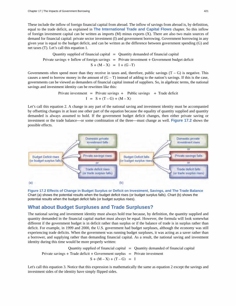
These include the inflow of foreign financial capital from abroad. The inflow of savings from abroad is, by definition,equal to the trade deficit, as explained in The International Trade and Capital Flows chapter. So this inflowof foreign investment capital can be written as imports (M) minus exports (X). There are also two main sources ofdemand for financial capital: private sector investment (I) and government borrowing. Government borrowing in anygiven year is equal to the budget deficit, and can be written as the difference between government spending (G) andnet taxes (T). Let’s call this equation 1.
Quantity supplied of financial capital = Quantity demanded of financial capitalPrivate savings + Inflow of foreign savings = Private investment + Government budget deficit
S + (M – X) = I + (G –T)
Governments often spend more than they receive in taxes and, therefore, public savings (T – G) is negative. Thiscauses a need to borrow money in the amount of (G – T) instead of adding to the nation’s savings. If this is the case,governments can be viewed as demanders of financial capital instead of suppliers. So, in algebraic terms, the nationalsavings and investment identity can be rewritten like this:
Private investment = Private savings + Public savings + Trade deficitI = S + (T – G) + (M – X)
Let’s call this equation 2. A change in any part of the national saving and investment identity must be accompaniedby offsetting changes in at least one other part of the equation because the equality of quantity supplied and quantitydemanded is always assumed to hold. If the government budget deficit changes, then either private saving orinvestment or the trade balance—or some combination of the three—must change as well. Figure 17.2 shows thepossible effects.
Figure 17.2 Effects of Change in Budget Surplus or Deficit on Investment, Savings, and The Trade BalanceChart (a) shows the potential results when the budget deficit rises (or budget surplus falls). Chart (b) shows thepotential results when the budget deficit falls (or budget surplus rises).
What about Budget Surpluses and Trade Surpluses?The national saving and investment identity must always hold true because, by definition, the quantity supplied andquantity demanded in the financial capital market must always be equal. However, the formula will look somewhatdifferent if the government budget is in deficit rather than surplus or if the balance of trade is in surplus rather thandeficit. For example, in 1999 and 2000, the U.S. government had budget surpluses, although the economy was stillexperiencing trade deficits. When the government was running budget surpluses, it was acting as a saver rather thana borrower, and supplying rather than demanding financial capital. As a result, the national saving and investmentidentity during this time would be more properly written:
Quantity supplied of financial capital = Quantity demanded of financial capitalPrivate savings + Trade deficit + Government surplus = Private investment
S + (M – X) + (T – G) = I
Let's call this equation 3. Notice that this expression is mathematically the same as equation 2 except the savings andinvestment sides of the identity have simply flipped sides.
Chapter 17 | The Impacts of Government Borrowing 421
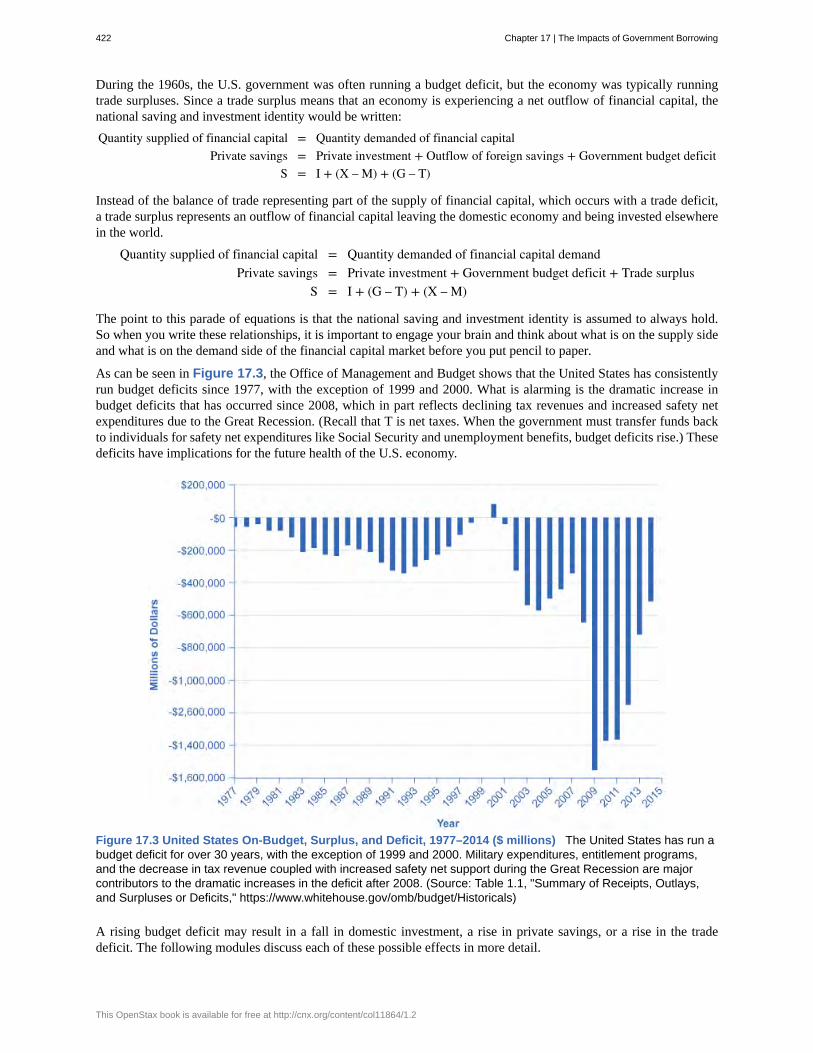
During the 1960s, the U.S. government was often running a budget deficit, but the economy was typically runningtrade surpluses. Since a trade surplus means that an economy is experiencing a net outflow of financial capital, thenational saving and investment identity would be written:
Quantity supplied of financial capital = Quantity demanded of financial capitalPrivate savings = Private investment + Outflow of foreign savings + Government budget deficit
S = I + (X – M) + (G – T)
Instead of the balance of trade representing part of the supply of financial capital, which occurs with a trade deficit,a trade surplus represents an outflow of financial capital leaving the domestic economy and being invested elsewherein the world.
Quantity supplied of financial capital = Quantity demanded of financial capital demandPrivate savings = Private investment + Government budget deficit + Trade surplus
S = I + (G – T) + (X – M)
The point to this parade of equations is that the national saving and investment identity is assumed to always hold.So when you write these relationships, it is important to engage your brain and think about what is on the supply sideand what is on the demand side of the financial capital market before you put pencil to paper.
As can be seen in Figure 17.3, the Office of Management and Budget shows that the United States has consistentlyrun budget deficits since 1977, with the exception of 1999 and 2000. What is alarming is the dramatic increase inbudget deficits that has occurred since 2008, which in part reflects declining tax revenues and increased safety netexpenditures due to the Great Recession. (Recall that T is net taxes. When the government must transfer funds backto individuals for safety net expenditures like Social Security and unemployment benefits, budget deficits rise.) Thesedeficits have implications for the future health of the U.S. economy.
Figure 17.3 United States On-Budget, Surplus, and Deficit, 1977–2014 ($ millions) The United States has run abudget deficit for over 30 years, with the exception of 1999 and 2000. Military expenditures, entitlement programs,and the decrease in tax revenue coupled with increased safety net support during the Great Recession are majorcontributors to the dramatic increases in the deficit after 2008. (Source: Table 1.1, "Summary of Receipts, Outlays,and Surpluses or Deficits," https://www.whitehouse.gov/omb/budget/Historicals)
A rising budget deficit may result in a fall in domestic investment, a rise in private savings, or a rise in the tradedeficit. The following modules discuss each of these possible effects in more detail.
422 Chapter 17 | The Impacts of Government Borrowing
This OpenStax book is available for free at http://cnx.org/content/col11864/1.2
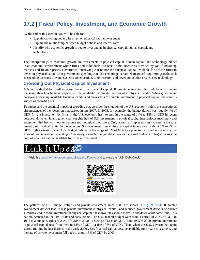
17.2 | Fiscal Policy, Investment, and Economic GrowthBy the end of this section, you will be able to:
• Explain crowding out and its effect on physical capital investment• Explain the relationship between budget deficits and interest rates• Identify why economic growth is tied to investments in physical capital, human capital, and
technology
The underpinnings of economic growth are investments in physical capital, human capital, and technology, all setin an economic environment where firms and individuals can react to the incentives provided by well-functioningmarkets and flexible prices. Government borrowing can reduce the financial capital available for private firms toinvest in physical capital. But government spending can also encourage certain elements of long-term growth, suchas spending on roads or water systems, on education, or on research and development that creates new technology.
Crowding Out Physical Capital InvestmentA larger budget deficit will increase demand for financial capital. If private saving and the trade balance remainthe same, then less financial capital will be available for private investment in physical capital. When governmentborrowing soaks up available financial capital and leaves less for private investment in physical capital, the result isknown as crowding out.
To understand the potential impact of crowding out, consider the situation of the U.S. economy before the exceptionalcircumstances of the recession that started in late 2007. In 2005, for example, the budget deficit was roughly 4% ofGDP. Private investment by firms in the U.S. economy has hovered in the range of 14% to 18% of GDP in recentdecades. However, in any given year, roughly half of U.S. investment in physical capital just replaces machinery andequipment that has worn out or become technologically obsolete. Only about half represents an increase in the totalquantity of physical capital in the economy. So investment in new physical capital in any year is about 7% to 9% ofGDP. In this situation, even U.S. budget deficits in the range of 4% of GDP can potentially crowd out a substantialshare of new investment spending. Conversely, a smaller budget deficit (or an increased budget surplus) increases thepool of financial capital available for private investment.
Visit this website (http://openstaxcollege.org/l/debtclock) to view the “U.S. Debt Clock.”
The patterns of U.S. budget deficits and private investment since 1980 are shown in Figure 17.4. If greatergovernment deficits lead to less private investment in physical capital, and reduced government deficits or budgetsurpluses lead to more investment in physical capital, these two lines should move up and down at the same time. Thispattern occurred in the late 1990s and early 2000s. The U.S. federal budget went from a deficit of 2.2% of GDP in1995 to a budget surplus of 2.4% of GDP in 2000—a swing of 4.6% of GDP. From 1995 to 2000, private investmentin physical capital rose from 15% to 18% of GDP—a rise of 3% of GDP. Then, when the U.S. government againstarted running budget deficits in the early 2000s, less financial capital became available for private investment, andthe rate of private investment fell back to about 15% of GDP by 2003.
Chapter 17 | The Impacts of Government Borrowing 423
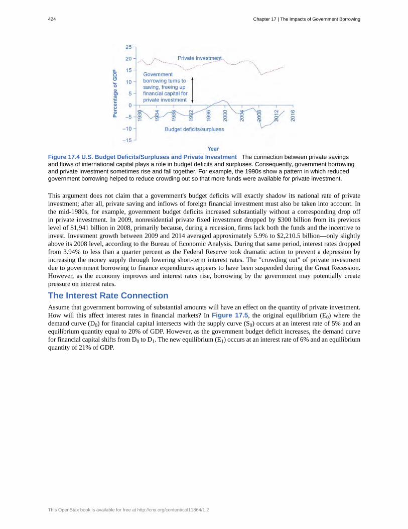
Figure 17.4 U.S. Budget Deficits/Surpluses and Private Investment The connection between private savingsand flows of international capital plays a role in budget deficits and surpluses. Consequently, government borrowingand private investment sometimes rise and fall together. For example, the 1990s show a pattern in which reducedgovernment borrowing helped to reduce crowding out so that more funds were available for private investment.
This argument does not claim that a government's budget deficits will exactly shadow its national rate of privateinvestment; after all, private saving and inflows of foreign financial investment must also be taken into account. Inthe mid-1980s, for example, government budget deficits increased substantially without a corresponding drop offin private investment. In 2009, nonresidential private fixed investment dropped by $300 billion from its previouslevel of $1,941 billion in 2008, primarily because, during a recession, firms lack both the funds and the incentive toinvest. Investment growth between 2009 and 2014 averaged approximately 5.9% to $2,210.5 billion—only slightlyabove its 2008 level, according to the Bureau of Economic Analysis. During that same period, interest rates droppedfrom 3.94% to less than a quarter percent as the Federal Reserve took dramatic action to prevent a depression byincreasing the money supply through lowering short-term interest rates. The "crowding out" of private investmentdue to government borrowing to finance expenditures appears to have been suspended during the Great Recession.However, as the economy improves and interest rates rise, borrowing by the government may potentially createpressure on interest rates.
The Interest Rate ConnectionAssume that government borrowing of substantial amounts will have an effect on the quantity of private investment.How will this affect interest rates in financial markets? In Figure 17.5, the original equilibrium (E0) where thedemand curve (D0) for financial capital intersects with the supply curve (S0) occurs at an interest rate of 5% and anequilibrium quantity equal to 20% of GDP. However, as the government budget deficit increases, the demand curvefor financial capital shifts from D0 to D1. The new equilibrium (E1) occurs at an interest rate of 6% and an equilibriumquantity of 21% of GDP.
424 Chapter 17 | The Impacts of Government Borrowing
This OpenStax book is available for free at http://cnx.org/content/col11864/1.2
Figure 17.5 Budget Deficits and Interest Rates In the financial market, an increase in government borrowing canshift the demand curve for financial capital to the right from D0 to D1. As the equilibrium interest rate shifts from E0 toE1, the interest rate rises from 5% to 6% in this example. The higher interest rate is one economic mechanism bywhich government borrowing can crowd out private investment.
A survey of economic studies on the connection between government borrowing and interest rates in the U.S.economy suggests that an increase of 1% in the budget deficit will lead to a rise in interest rates of between 0.5and 1.0%, other factors held equal. In turn, a higher interest rate tends to discourage firms from making physicalcapital investments. One reason government budget deficits crowd out private investment, therefore, is the increasein interest rates. There are, however, economic studies that show a limited connection between the two (at least in theUnited States), but as the budget deficit grows, the dangers of rising interest rates become more real.
At this point, you may wonder about the Federal Reserve. After all, can the Federal Reserve not use expansionarymonetary policy to reduce interest rates, or in this case, to prevent interest rates from rising? This useful questionemphasizes the importance of considering how fiscal and monetary policies work in relation to each other. Imaginea central bank faced with a government that is running large budget deficits, causing a rise in interest rates andcrowding out private investment. If the budget deficits are increasing aggregate demand when the economy is alreadyproducing near potential GDP, threatening an inflationary increase in price levels, the central bank may react with acontractionary monetary policy. In this situation, the higher interest rates from the government borrowing would bemade even higher by contractionary monetary policy, and the government borrowing might crowd out a great deal ofprivate investment.
On the other hand, if the budget deficits are increasing aggregate demand when the economy is producingsubstantially less than potential GDP, an inflationary increase in the price level is not much of a danger and thecentral bank might react with expansionary monetary policy. In this situation, higher interest rates from governmentborrowing would be largely offset by lower interest rates from expansionary monetary policy, and there would belittle crowding out of private investment.
However, even a central bank cannot erase the overall message of the national savings and investment identity. Ifgovernment borrowing rises, then private investment must fall, or private saving must rise, or the trade deficit mustfall. By reacting with contractionary or expansionary monetary policy, the central bank can only help to determinewhich of these outcomes is likely.
Public Investment in Physical CapitalGovernment can invest in physical capital directly: roads and bridges; water supply and sewers; seaports and airports;schools and hospitals; plants that generate electricity, like hydroelectric dams or windmills; telecommunicationsfacilities; and weapons used by the military. In 2014, the U.S. federal government budget for Fiscal Year 2014 showsthat the United States spent about $92 billion on transportation, including highways, mass transit, and airports. Table17.1 shows the total outlay for 2014 for major public physical capital investment by the federal government in theUnited States. Physical capital related to the military or to residences where people live is omitted from this table,because the focus here is on public investments that have a direct effect on raising output in the private sector.
Chapter 17 | The Impacts of Government Borrowing 425
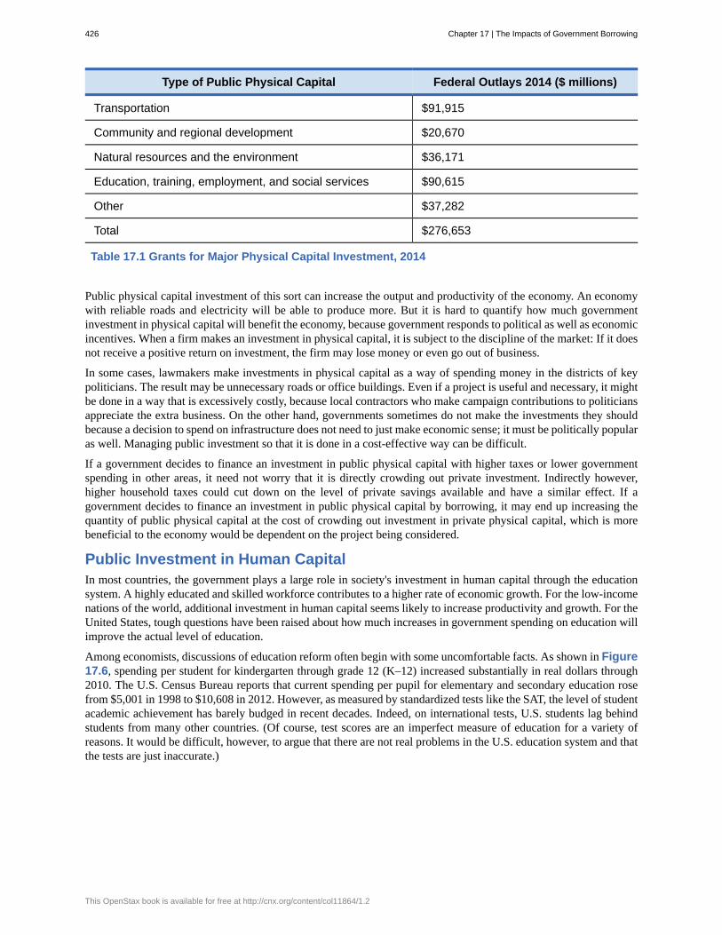
Type of Public Physical Capital Federal Outlays 2014 ($ millions)
Transportation $91,915
Community and regional development $20,670
Natural resources and the environment $36,171
Education, training, employment, and social services $90,615
Other $37,282
Total $276,653
Table 17.1 Grants for Major Physical Capital Investment, 2014
Public physical capital investment of this sort can increase the output and productivity of the economy. An economywith reliable roads and electricity will be able to produce more. But it is hard to quantify how much governmentinvestment in physical capital will benefit the economy, because government responds to political as well as economicincentives. When a firm makes an investment in physical capital, it is subject to the discipline of the market: If it doesnot receive a positive return on investment, the firm may lose money or even go out of business.
In some cases, lawmakers make investments in physical capital as a way of spending money in the districts of keypoliticians. The result may be unnecessary roads or office buildings. Even if a project is useful and necessary, it mightbe done in a way that is excessively costly, because local contractors who make campaign contributions to politiciansappreciate the extra business. On the other hand, governments sometimes do not make the investments they shouldbecause a decision to spend on infrastructure does not need to just make economic sense; it must be politically popularas well. Managing public investment so that it is done in a cost-effective way can be difficult.
If a government decides to finance an investment in public physical capital with higher taxes or lower governmentspending in other areas, it need not worry that it is directly crowding out private investment. Indirectly however,higher household taxes could cut down on the level of private savings available and have a similar effect. If agovernment decides to finance an investment in public physical capital by borrowing, it may end up increasing thequantity of public physical capital at the cost of crowding out investment in private physical capital, which is morebeneficial to the economy would be dependent on the project being considered.
Public Investment in Human CapitalIn most countries, the government plays a large role in society's investment in human capital through the educationsystem. A highly educated and skilled workforce contributes to a higher rate of economic growth. For the low-incomenations of the world, additional investment in human capital seems likely to increase productivity and growth. For theUnited States, tough questions have been raised about how much increases in government spending on education willimprove the actual level of education.
Among economists, discussions of education reform often begin with some uncomfortable facts. As shown in Figure17.6, spending per student for kindergarten through grade 12 (K–12) increased substantially in real dollars through2010. The U.S. Census Bureau reports that current spending per pupil for elementary and secondary education rosefrom $5,001 in 1998 to $10,608 in 2012. However, as measured by standardized tests like the SAT, the level of studentacademic achievement has barely budged in recent decades. Indeed, on international tests, U.S. students lag behindstudents from many other countries. (Of course, test scores are an imperfect measure of education for a variety ofreasons. It would be difficult, however, to argue that there are not real problems in the U.S. education system and thatthe tests are just inaccurate.)
426 Chapter 17 | The Impacts of Government Borrowing
This OpenStax book is available for free at http://cnx.org/content/col11864/1.2
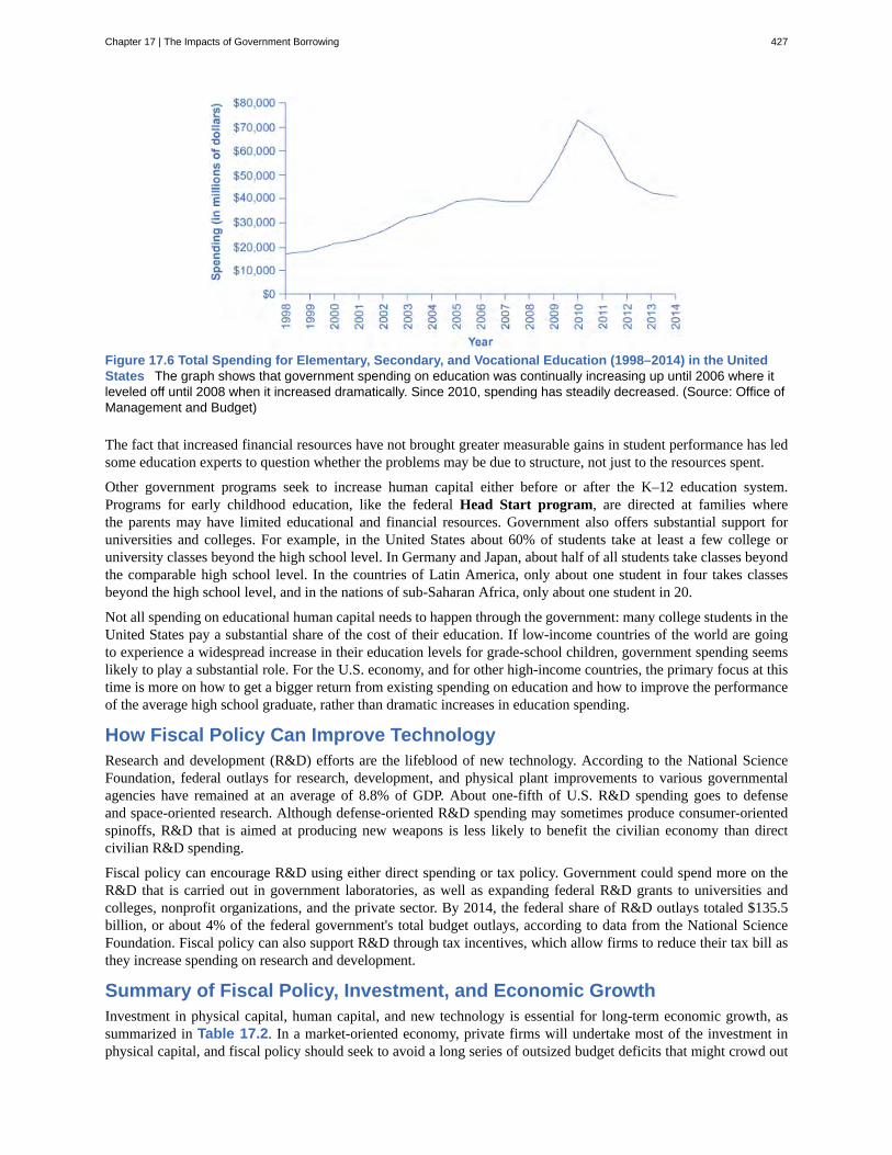
Figure 17.6 Total Spending for Elementary, Secondary, and Vocational Education (1998–2014) in the UnitedStates The graph shows that government spending on education was continually increasing up until 2006 where itleveled off until 2008 when it increased dramatically. Since 2010, spending has steadily decreased. (Source: Office ofManagement and Budget)
The fact that increased financial resources have not brought greater measurable gains in student performance has ledsome education experts to question whether the problems may be due to structure, not just to the resources spent.
Other government programs seek to increase human capital either before or after the K–12 education system.Programs for early childhood education, like the federal Head Start program, are directed at families wherethe parents may have limited educational and financial resources. Government also offers substantial support foruniversities and colleges. For example, in the United States about 60% of students take at least a few college oruniversity classes beyond the high school level. In Germany and Japan, about half of all students take classes beyondthe comparable high school level. In the countries of Latin America, only about one student in four takes classesbeyond the high school level, and in the nations of sub-Saharan Africa, only about one student in 20.
Not all spending on educational human capital needs to happen through the government: many college students in theUnited States pay a substantial share of the cost of their education. If low-income countries of the world are goingto experience a widespread increase in their education levels for grade-school children, government spending seemslikely to play a substantial role. For the U.S. economy, and for other high-income countries, the primary focus at thistime is more on how to get a bigger return from existing spending on education and how to improve the performanceof the average high school graduate, rather than dramatic increases in education spending.
How Fiscal Policy Can Improve TechnologyResearch and development (R&D) efforts are the lifeblood of new technology. According to the National ScienceFoundation, federal outlays for research, development, and physical plant improvements to various governmentalagencies have remained at an average of 8.8% of GDP. About one-fifth of U.S. R&D spending goes to defenseand space-oriented research. Although defense-oriented R&D spending may sometimes produce consumer-orientedspinoffs, R&D that is aimed at producing new weapons is less likely to benefit the civilian economy than directcivilian R&D spending.
Fiscal policy can encourage R&D using either direct spending or tax policy. Government could spend more on theR&D that is carried out in government laboratories, as well as expanding federal R&D grants to universities andcolleges, nonprofit organizations, and the private sector. By 2014, the federal share of R&D outlays totaled $135.5billion, or about 4% of the federal government's total budget outlays, according to data from the National ScienceFoundation. Fiscal policy can also support R&D through tax incentives, which allow firms to reduce their tax bill asthey increase spending on research and development.
Summary of Fiscal Policy, Investment, and Economic GrowthInvestment in physical capital, human capital, and new technology is essential for long-term economic growth, assummarized in Table 17.2. In a market-oriented economy, private firms will undertake most of the investment inphysical capital, and fiscal policy should seek to avoid a long series of outsized budget deficits that might crowd out
Chapter 17 | The Impacts of Government Borrowing 427
such investment. The effects of many growth-oriented policies will be seen very gradually over time, as students arebetter educated, physical capital investments are made, and new technologies are invented and implemented.
Physical Capital HumanCapital New Technology
PrivateSector
New investment inproperty andequipment
On-the-jobtraining
Research and development
PublicSector
Public infrastructure PubliceducationJob training
Research and development encouraged throughprivate sector incentives and direct spending.
Table 17.2 Investment Role of Public and Private Sector in a Market Economy
17.3 | How Government Borrowing Affects Private SavingBy the end of this section, you will be able to:
• Apply Ricardian equivalence to evaluate how government borrowing affects private saving• Interpret a graphic representation of Ricardian equivalence
A change in government budgets may impact private saving. Imagine that people watch government budgets andadjust their savings accordingly. For example, whenever the government runs a budget deficit, people might reason:“Well, a higher budget deficit means that I’m just going to owe more taxes in the future to pay off all that governmentborrowing, so I’ll start saving now.” If the government runs budget surpluses, people might reason: “With thesebudget surpluses (or lower budget deficits), interest rates are falling, so that saving is less attractive. Moreover, witha budget surplus the country will be able to afford a tax cut sometime in the future. I won’t bother saving as muchnow.”
The theory that rational private households might shift their saving to offset government saving or borrowing isknown as Ricardian equivalence because the idea has intellectual roots in the writings of the early nineteenth-century economist David Ricardo (1772–1823). If Ricardian equivalence holds completely true, then in the nationalsaving and investment identity, any change in budget deficits or budget surpluses would be completely offset by acorresponding change in private saving. As a result, changes in government borrowing would have no effect at all oneither physical capital investment or trade balances.
In practice, the private sector only sometimes and partially adjusts its savings behavior to offset government budgetdeficits and surpluses. Figure 17.7 shows the patterns of U.S. government budget deficits and surpluses and the rateof private saving—which includes saving by both households and firms—since 1980. The connection between thetwo is not at all obvious. In the mid-1980s, for example, government budget deficits were quite large, but there isno corresponding surge of private saving. However, when budget deficits turn to surpluses in the late 1990s, there isa simultaneous decline in private saving. When budget deficits get very large in 2008 and 2009, on the other hand,there is some sign of a rise in saving. A variety of statistical studies based on the U.S. experience suggests that whengovernment borrowing increases by $1, private saving rises by about 30 cents. A World Bank study done in the late1990s, looking at government budgets and private saving behavior in countries around the world, found a similarresult.
428 Chapter 17 | The Impacts of Government Borrowing
This OpenStax book is available for free at http://cnx.org/content/col11864/1.2
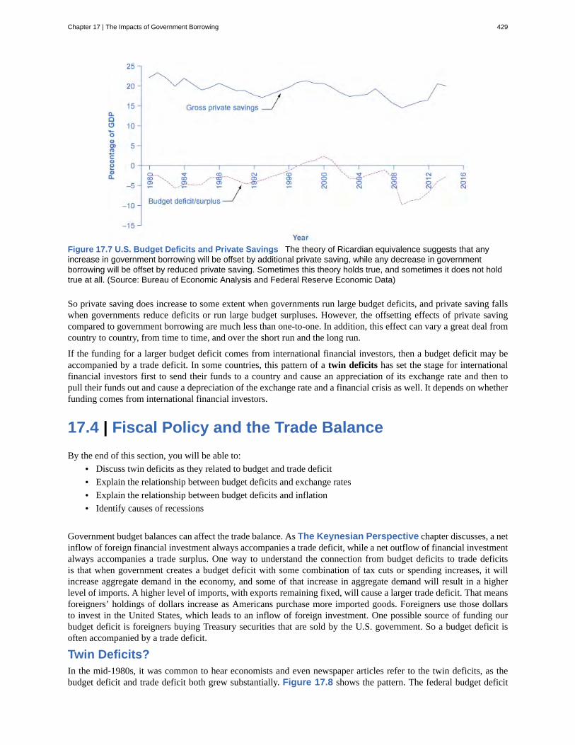
Figure 17.7 U.S. Budget Deficits and Private Savings The theory of Ricardian equivalence suggests that anyincrease in government borrowing will be offset by additional private saving, while any decrease in governmentborrowing will be offset by reduced private saving. Sometimes this theory holds true, and sometimes it does not holdtrue at all. (Source: Bureau of Economic Analysis and Federal Reserve Economic Data)
So private saving does increase to some extent when governments run large budget deficits, and private saving fallswhen governments reduce deficits or run large budget surpluses. However, the offsetting effects of private savingcompared to government borrowing are much less than one-to-one. In addition, this effect can vary a great deal fromcountry to country, from time to time, and over the short run and the long run.
If the funding for a larger budget deficit comes from international financial investors, then a budget deficit may beaccompanied by a trade deficit. In some countries, this pattern of a twin deficits has set the stage for internationalfinancial investors first to send their funds to a country and cause an appreciation of its exchange rate and then topull their funds out and cause a depreciation of the exchange rate and a financial crisis as well. It depends on whetherfunding comes from international financial investors.
17.4 | Fiscal Policy and the Trade BalanceBy the end of this section, you will be able to:
• Discuss twin deficits as they related to budget and trade deficit• Explain the relationship between budget deficits and exchange rates• Explain the relationship between budget deficits and inflation• Identify causes of recessions
Government budget balances can affect the trade balance. As The Keynesian Perspective chapter discusses, a netinflow of foreign financial investment always accompanies a trade deficit, while a net outflow of financial investmentalways accompanies a trade surplus. One way to understand the connection from budget deficits to trade deficitsis that when government creates a budget deficit with some combination of tax cuts or spending increases, it willincrease aggregate demand in the economy, and some of that increase in aggregate demand will result in a higherlevel of imports. A higher level of imports, with exports remaining fixed, will cause a larger trade deficit. That meansforeigners’ holdings of dollars increase as Americans purchase more imported goods. Foreigners use those dollarsto invest in the United States, which leads to an inflow of foreign investment. One possible source of funding ourbudget deficit is foreigners buying Treasury securities that are sold by the U.S. government. So a budget deficit isoften accompanied by a trade deficit.
Twin Deficits?In the mid-1980s, it was common to hear economists and even newspaper articles refer to the twin deficits, as thebudget deficit and trade deficit both grew substantially. Figure 17.8 shows the pattern. The federal budget deficit
Chapter 17 | The Impacts of Government Borrowing 429
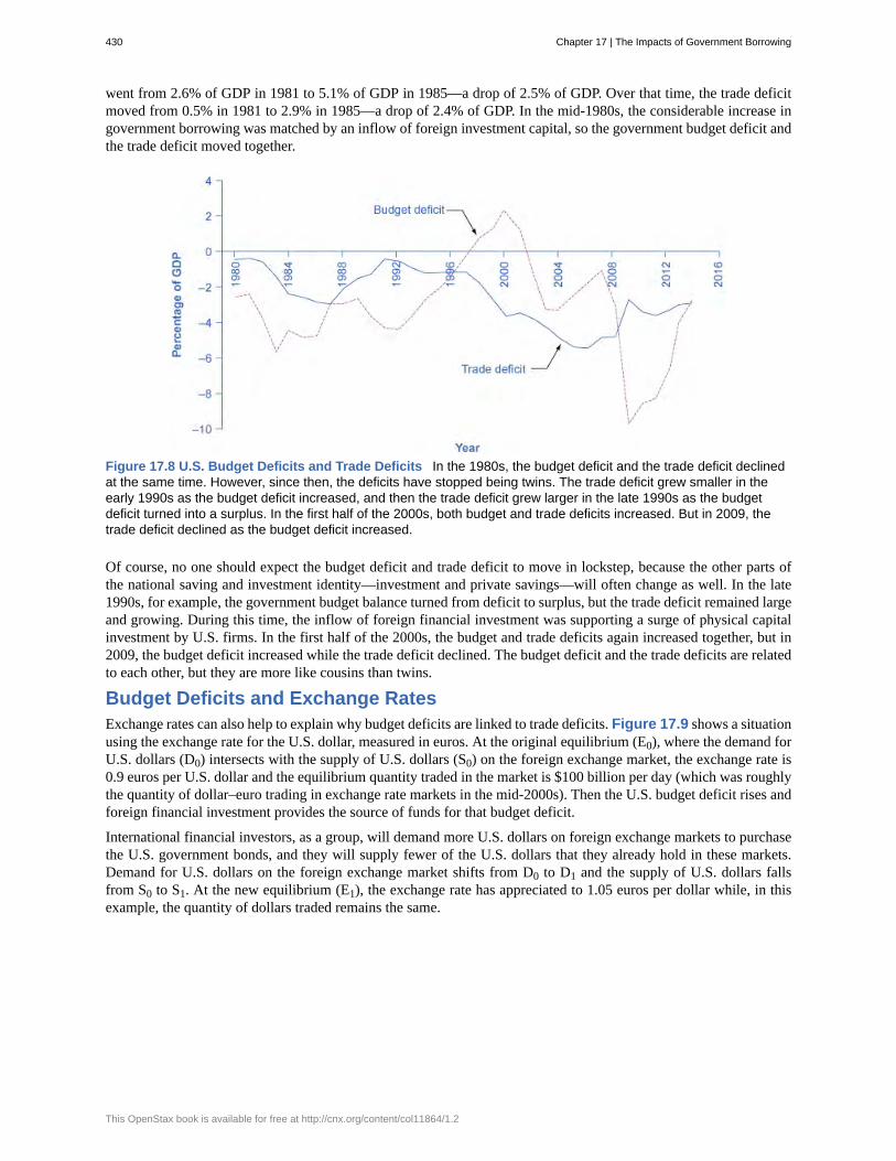
went from 2.6% of GDP in 1981 to 5.1% of GDP in 1985—a drop of 2.5% of GDP. Over that time, the trade deficitmoved from 0.5% in 1981 to 2.9% in 1985—a drop of 2.4% of GDP. In the mid-1980s, the considerable increase ingovernment borrowing was matched by an inflow of foreign investment capital, so the government budget deficit andthe trade deficit moved together.
Figure 17.8 U.S. Budget Deficits and Trade Deficits In the 1980s, the budget deficit and the trade deficit declinedat the same time. However, since then, the deficits have stopped being twins. The trade deficit grew smaller in theearly 1990s as the budget deficit increased, and then the trade deficit grew larger in the late 1990s as the budgetdeficit turned into a surplus. In the first half of the 2000s, both budget and trade deficits increased. But in 2009, thetrade deficit declined as the budget deficit increased.
Of course, no one should expect the budget deficit and trade deficit to move in lockstep, because the other parts ofthe national saving and investment identity—investment and private savings—will often change as well. In the late1990s, for example, the government budget balance turned from deficit to surplus, but the trade deficit remained largeand growing. During this time, the inflow of foreign financial investment was supporting a surge of physical capitalinvestment by U.S. firms. In the first half of the 2000s, the budget and trade deficits again increased together, but in2009, the budget deficit increased while the trade deficit declined. The budget deficit and the trade deficits are relatedto each other, but they are more like cousins than twins.
Budget Deficits and Exchange RatesExchange rates can also help to explain why budget deficits are linked to trade deficits. Figure 17.9 shows a situationusing the exchange rate for the U.S. dollar, measured in euros. At the original equilibrium (E0), where the demand forU.S. dollars (D0) intersects with the supply of U.S. dollars (S0) on the foreign exchange market, the exchange rate is0.9 euros per U.S. dollar and the equilibrium quantity traded in the market is $100 billion per day (which was roughlythe quantity of dollar–euro trading in exchange rate markets in the mid-2000s). Then the U.S. budget deficit rises andforeign financial investment provides the source of funds for that budget deficit.
International financial investors, as a group, will demand more U.S. dollars on foreign exchange markets to purchasethe U.S. government bonds, and they will supply fewer of the U.S. dollars that they already hold in these markets.Demand for U.S. dollars on the foreign exchange market shifts from D0 to D1 and the supply of U.S. dollars fallsfrom S0 to S1. At the new equilibrium (E1), the exchange rate has appreciated to 1.05 euros per dollar while, in thisexample, the quantity of dollars traded remains the same.
430 Chapter 17 | The Impacts of Government Borrowing
This OpenStax book is available for free at http://cnx.org/content/col11864/1.2
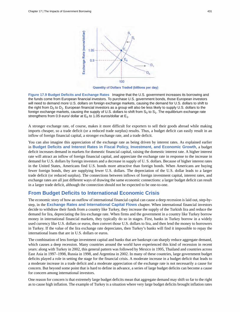
Figure 17.9 Budget Deficits and Exchange Rates Imagine that the U.S. government increases its borrowing andthe funds come from European financial investors. To purchase U.S. government bonds, those European investorswill need to demand more U.S. dollars on foreign exchange markets, causing the demand for U.S. dollars to shift tothe right from D0 to D1. European financial investors as a group will also be less likely to supply U.S. dollars to theforeign exchange markets, causing the supply of U.S. dollars to shift from S0 to S1. The equilibrium exchange ratestrengthens from 0.9 euro/ dollar at E0 to 1.05 euros/dollar at E1.
A stronger exchange rate, of course, makes it more difficult for exporters to sell their goods abroad while makingimports cheaper, so a trade deficit (or a reduced trade surplus) results. Thus, a budget deficit can easily result in aninflow of foreign financial capital, a stronger exchange rate, and a trade deficit.
You can also imagine this appreciation of the exchange rate as being driven by interest rates. As explained earlierin Budget Deficits and Interest Rates in Fiscal Policy, Investment, and Economic Growth, a budgetdeficit increases demand in markets for domestic financial capital, raising the domestic interest rate. A higher interestrate will attract an inflow of foreign financial capital, and appreciate the exchange rate in response to the increase indemand for U.S. dollars by foreign investors and a decrease in supply of U. S. dollars. Because of higher interest ratesin the United States, Americans find U.S. bonds more attractive than foreign bonds. When Americans are buyingfewer foreign bonds, they are supplying fewer U.S. dollars. The depreciation of the U.S. dollar leads to a largertrade deficit (or reduced surplus). The connections between inflows of foreign investment capital, interest rates, andexchange rates are all just different ways of drawing the same economic connections: a larger budget deficit can resultin a larger trade deficit, although the connection should not be expected to be one-to-one.
From Budget Deficits to International Economic CrisisThe economic story of how an outflow of international financial capital can cause a deep recession is laid out, step-by-step, in the Exchange Rates and International Capital Flows chapter. When international financial investorsdecide to withdraw their funds from a country like Turkey, they increase the supply of the Turkish lira and reduce thedemand for lira, depreciating the lira exchange rate. When firms and the government in a country like Turkey borrowmoney in international financial markets, they typically do so in stages. First, banks in Turkey borrow in a widelyused currency like U.S. dollars or euros, then convert those U.S. dollars to lira, and then lend the money to borrowersin Turkey. If the value of the lira exchange rate depreciates, then Turkey’s banks will find it impossible to repay theinternational loans that are in U.S. dollars or euros.
The combination of less foreign investment capital and banks that are bankrupt can sharply reduce aggregate demand,which causes a deep recession. Many countries around the world have experienced this kind of recession in recentyears: along with Turkey in 2002, this general pattern was followed by Mexico in 1995, Thailand and countries acrossEast Asia in 1997–1998, Russia in 1998, and Argentina in 2002. In many of these countries, large government budgetdeficits played a role in setting the stage for the financial crisis. A moderate increase in a budget deficit that leads toa moderate increase in a trade deficit and a moderate appreciation of the exchange rate is not necessarily a cause forconcern. But beyond some point that is hard to define in advance, a series of large budget deficits can become a causefor concern among international investors.
One reason for concern is that extremely large budget deficits mean that aggregate demand may shift so far to the rightas to cause high inflation. The example of Turkey is a situation where very large budget deficits brought inflation rates
Chapter 17 | The Impacts of Government Borrowing 431
well into double digits. In addition, very large budget deficits at some point begin to raise a fear that the borrowingwill not be repaid. In the last 175 years, the government of Turkey has been unable to pay its debts and defaultedon its loans six times. Brazil’s government has been unable to pay its debts and defaulted on its loans seven times;Venezuela, nine times; and Argentina, five times. The risk of high inflation or a default on repaying internationalloans will worry international investors, since both factors imply that the rate of return on their investments in thatcountry may end up lower than expected. If international investors start withdrawing the funds from a country rapidly,the scenario of less investment, a depreciated exchange rate, widespread bank failure, and deep recession can occur.The following Clear It Up feature explains other impacts of large deficits.
What are the risks of chronic large deficits in the United States?If a government runs large budget deficits for a sustained period of time, what can go wrong? According toa recent report by the Brookings Institution, a key risk of a large budget deficit is that government debt maygrow too high compared to the country’s GDP growth. As debt grows, the national savings rate will decline,leaving less available in financial capital for private investment. The impact of chronically large budget deficitsis as follows:
• As the population ages, there will be an increasing demand for government services that may causehigher government deficits. Government borrowing and its interest payments will pull resources awayfrom domestic investment in human capital and physical capital that is essential to economic growth.
• Interest rates may start to rise so that the cost of financing government debt will rise as well, creatingpressure on the government to reduce its budget deficits through spending cuts and tax increases.These steps will be politically painful, and they will also have a contractionary effect on aggregatedemand in the economy.
• Rising percentage of debt to GDP will create uncertainty in the financial and global markets that mightcause a country to resort to inflationary tactics to reduce the real value of the debt outstanding. Thiswill decrease real wealth and damage confidence in the country’s ability to manage its spending. Afterall, if the government has borrowed at a fixed interest rate of, say, 5%, and it lets inflation rise abovethat 5%, then it will effectively be able to repay its debt at a negative real interest rate.
The conventional reasoning suggests that the relationship between sustained deficits that lead to high levelsof government debt and long-term growth is negative. How significant this relationship is, how big an issue itis compared to other macroeconomic issues, and the direction of causality, is less clear.
What remains important to acknowledge is that the relationship between debt and growth is negative and thatfor some countries, the relationship may be stronger than in others. It is also important to acknowledge thedirection of causality: does high debt cause slow growth, slow growth cause high debt, or are both high debtand slow growth the result of third factors? In our analysis, we have argued simply that high debt causes slowgrowth. There may be more to this debate than we have space to discuss here.
Using Fiscal Policy to Address Trade ImbalancesIf a nation is experiencing the inflow of foreign investment capital associated with a trade deficit because foreigninvestors are making long-term direct investments in firms, there may be no substantial reason for concern. After all,many low-income nations around the world would welcome direct investment by multinational firms that ties themmore closely into the global networks of production and distribution of goods and services. In this case, the inflowsof foreign investment capital and the trade deficit are attracted by the opportunities for a good rate of return on privatesector investment in an economy.
However, governments should beware of a sustained pattern of high budget deficits and high trade deficits. Thedanger arises in particular when the inflow of foreign investment capital is not funding long-term physical capitalinvestment by firms, but instead is short-term portfolio investment in government bonds. When inflows of foreignfinancial investment reach high levels, foreign financial investors will be on the alert for any reason to fear that thecountry’s exchange rate may decline or the government may be unable to repay what it has borrowed on time. Just
432 Chapter 17 | The Impacts of Government Borrowing
This OpenStax book is available for free at http://cnx.org/content/col11864/1.2
as a few falling rocks can trigger an avalanche; a relatively small piece of bad news about an economy can trigger anenormous outflow of short-term financial capital.
Reducing a nation’s budget deficit will not always be a successful method of reducing its trade deficit, because otherelements of the national saving and investment identity, like private saving or investment, may change instead. Inthose cases when the budget deficit is the main cause of the trade deficit, governments should take steps to reducetheir budget deficits, lest they make their economy vulnerable to a rapid outflow of international financial capital thatcould bring a deep recession.
Financing Higher EducationOver the period between 1982 and 2012, the increases in the cost of a college education had far outpacedthat of the income of the typical American family. According to the research done by the President Obama’sstaff, the cost of education at a four-year public college increased by 257% compared to an increase infamily incomes of only 16% over the prior 30 years. The ongoing debate over a balanced budget andproposed cutbacks accentuated the need to increase investment in human capital to grow the economyversus deepening the already significant debt levels of the U.S. government. In the summer of 2013, PresidentObama presented a plan to make college more affordable that included increasing Pell Grant awards and thenumber of recipients, caps on interest rates for student loans, and providing education tax credits. In addition,the plan includes an accountability method for institutions of higher education that focuses on completion ratesand creates a College Scorecard. Whether or not all these initiatives come to fruition remains to be seen, butthey are indicative of creative approaches that government can take to meet its obligation from both a publicand fiscal policy perspective.
Chapter 17 | The Impacts of Government Borrowing 433
Head Start program
Ricardian equivalence
twin deficits
KEY TERMS
a program for early childhood education directed at families with limited educational andfinancial resources.
the theory that rational private households might shift their saving to offset government savingor borrowing
deficits that occur when a country is running both a trade and a budget deficit
KEY CONCEPTS AND SUMMARY
17.1 How Government Borrowing Affects Investment and the Trade BalanceA change in any part of the national saving and investment identity suggests that if the government budgetdeficit changes, then either private savings, private investment in physical capital, or the trade balance—or somecombination of the three—must change as well.
17.2 Fiscal Policy, Investment, and Economic GrowthEconomic growth comes from a combination of investment in physical capital, human capital, and technology.Government borrowing can crowd out private sector investment in physical capital, but fiscal policy can alsoincrease investment in publicly owned physical capital, human capital (education), and research and development.Possible methods for improving education and society’s investment in human capital include spending more moneyon teachers and other educational resources, and reorganizing the education system to provide greater incentivesfor success. Methods for increasing research and development spending to generate new technology include directgovernment spending on R&D and tax incentives for businesses to conduct additional R&D.
17.3 How Government Borrowing Affects Private SavingThe theory of Ricardian equivalence holds that changes in government borrowing or saving will be offset by changesin private saving. Thus, higher budget deficits will be offset by greater private saving, while larger budget surpluseswill be offset by greater private borrowing. If the theory holds true, then changes in government borrowing or savingwould have no effect on private investment in physical capital or on the trade balance. However, empirical evidencesuggests that the theory holds true only partially.
17.4 Fiscal Policy and the Trade BalanceThe government need not balance its budget every year. However, a sustained pattern of large budget deficits overtime risks causing several negative macroeconomic outcomes: a shift to the right in aggregate demand that causes aninflationary increase in the price level; crowding out private investment in physical capital in a way that slows downeconomic growth; and creating a dependence on inflows of international portfolio investment which can sometimesturn into outflows of foreign financial investment that can be injurious to a macroeconomy.
SELF-CHECK QUESTIONS1. In a country, private savings equals 600, the government budget surplus equals 200, and the trade surplus equals100. What is the level of private investment in this economy?
2. Assume an economy has a budget surplus of 1,000, private savings of 4,000, and investment of 5,000.a. Write out a national saving and investment identity for this economy.b. What will be the balance of trade in this economy?c. If the budget surplus changes to a budget deficit of 1000, with private saving and investment unchanged, what
is the new balance of trade in this economy?
434 Chapter 17 | The Impacts of Government Borrowing
This OpenStax book is available for free at http://cnx.org/content/col11864/1.2
3. Why have many education experts recently placed an emphasis on altering the incentives faced by U.S. schoolsrather than on increasing their budgets? Without endorsing any of these proposals as especially good or bad, list someof the ways in which incentives for schools might be altered.
4. What are some steps the government can take to encourage research and development?
5. Imagine an economy in which Ricardian equivalence holds. This economy has a budget deficit of 50, a tradedeficit of 20, private savings of 130, and investment of 100. If the budget deficit rises to 70, how are the other termsin the national saving and investment identity affected?
6. In the late 1990s, the U.S. government moved from a budget deficit to a budget surplus and the trade deficit inthe U.S. economy grew substantially. Using the national saving and investment identity, what can you say about thedirection in which saving and/or investment must have changed in this economy?
REVIEW QUESTIONS
7. Based on the national saving and investment identity,what are the three ways the macroeconomy might reactto greater government budget deficits?
8. How would you expect larger budget deficits toaffect private sector investment in physical capital?Why?
9. What are some of the ways fiscal policy mightencourage economic growth?
10. What are some fiscal policies for improving asociety’s human capital?
11. What are some fiscal policies for improving thetechnologies that the economy will have to draw upon inthe future?
12. Explain how cuts in funding for programs suchas Head Start might affect the development of humancapital in the United States.
13. What is the theory of Ricardian equivalence?
14. What does the concept of rationality have to dowith Ricardian equivalence?
15. Under what conditions will a larger budget deficitcause a trade deficit?
CRITICAL THINKING QUESTIONS
16. Assume there is no discretionary increase ingovernment spending. Explain how an improvingeconomy will affect the budget balance and, in turn,investment and the trade balance.
17. Explain how decreased domestic investments thatoccur due to a budget deficit will affect future economicgrowth.
18. The U.S. government has shut down a numberof times in recent history. Explain how a governmentshutdown will affect the variables in the nationalinvestment and savings identity. Could the shutdownaffect the government budget deficit?
19. Explain why the government might prefer toprovide incentives to private firms to do investment orresearch and development, rather than simply doing thespending itself?
20. Under what condition would crowding out notinhibit long-run economic growth? Under what
condition would crowding out impede long-runeconomic growth?
21. What must take place for the government to rundeficits without any crowding out?
22. Explain whether or not you agree with the premiseof the Ricardian equivalence theory that rational peoplemight reason: “Well, a higher budget deficit (surplus)means that I’m just going to owe more (less) taxes in thefuture to pay off all that government borrowing, so I’llstart saving (spending) now.” Why or why not?
23. Explain how a shift from a government budgetdeficit to a budget surplus might affect the exchangerate.
24. Describe how a plan for reducing the governmentdeficit might affect a college student, a youngprofessional, and a middle-income family.
Chapter 17 | The Impacts of Government Borrowing 435
PROBLEMS25. During the most recent recession, some economistsargued that the change in the interest rates that comesabout due to deficit spending implied in the demand andsupply of financial capital graph would not occur. Asimple reason was that the government was stepping into invest when private firms were not. Using a graph,explain how the deficit demand is offset by the use bygovernment in investment.
26. Illustrate the concept of Ricardian equivalenceusing the demand and supply of financial capital graph.
27. Sketch a diagram of how a budget deficit causesa trade deficit. (Hint: Begin with what will happen tothe exchange rate when foreigners demand more U.S.government debt.)
28. Sketch a diagram of how sustained budget deficitscause low economic growth.
29. Assume that you are employed by the governmentof Tanzania in 1964, a new nation recently independentfrom Britain. The Tanzanian parliament has decided thatit will spend 10 million shillings on schools, roads, andhealthcare for the year. You estimate that the net taxesfor the year are eight million shillings. The differencewill be financed by selling 10-year government bonds at12% interest per year. The interest on outstanding bondsmust be added to government expenditure each year.Assume that additional taxes are added to finance thisincrease in government expenditure so the gap betweengovernment spending is always two million. If theschool, road, and healthcare budget are unchanged,compute the value of the accumulated debt in 10 years.
436 Chapter 17 | The Impacts of Government Borrowing
This OpenStax book is available for free at http://cnx.org/content/col11864/1.2
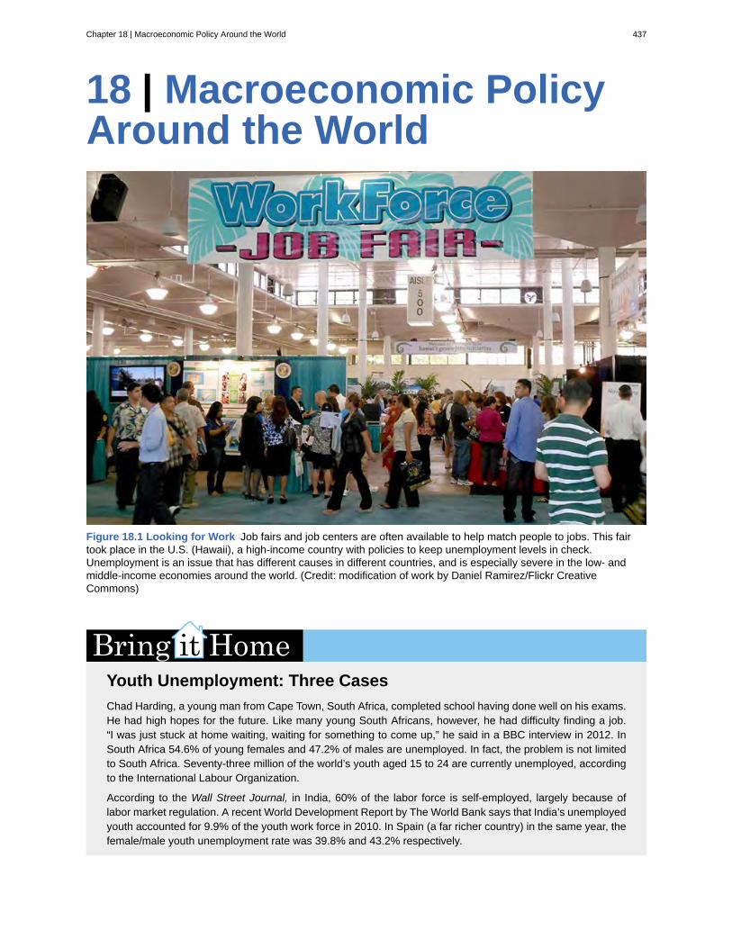
18 | Macroeconomic PolicyAround the World
Figure 18.1 Looking for Work Job fairs and job centers are often available to help match people to jobs. This fairtook place in the U.S. (Hawaii), a high-income country with policies to keep unemployment levels in check.Unemployment is an issue that has different causes in different countries, and is especially severe in the low- andmiddle-income economies around the world. (Credit: modification of work by Daniel Ramirez/Flickr CreativeCommons)
Youth Unemployment: Three CasesChad Harding, a young man from Cape Town, South Africa, completed school having done well on his exams.He had high hopes for the future. Like many young South Africans, however, he had difficulty finding a job.“I was just stuck at home waiting, waiting for something to come up,” he said in a BBC interview in 2012. InSouth Africa 54.6% of young females and 47.2% of males are unemployed. In fact, the problem is not limitedto South Africa. Seventy-three million of the world’s youth aged 15 to 24 are currently unemployed, accordingto the International Labour Organization.
According to the Wall Street Journal, in India, 60% of the labor force is self-employed, largely because oflabor market regulation. A recent World Development Report by The World Bank says that India’s unemployedyouth accounted for 9.9% of the youth work force in 2010. In Spain (a far richer country) in the same year, thefemale/male youth unemployment rate was 39.8% and 43.2% respectively.
Chapter 18 | Macroeconomic Policy Around the World 437
Youth unemployment is a significant issue in many parts of the world. However, despite the apparentsimilarities in rates between South Africa, Spain, and India, macroeconomic policy solutions to decreaseyouth unemployment in these three countries are different. This chapter will look at macroeconomic policiesaround the world, specifically those related to reducing unemployment, promoting economic growth, andstable inflation and exchange rates. Then we will look again at the three cases of South Africa, Spain, andIndia.
Introduction to Macroeconomic Policy around the WorldIn this chapter, you will learn about:
• The Diversity of Countries and Economies across the World
• Improving Countries’ Standards of Living
• Causes of Unemployment around the World
• Causes of Inflation in Various Countries and Regions
• Balance of Trade Concerns
There are extraordinary differences in the composition and performance of economies across the world. Whatexplains these differences? Are countries motivated by similar goals when it comes to macroeconomic policy? Can weapply the same macroeconomic framework developed in this text to understand the performance of these countries?Let’s take each of these questions in turn.
Explaining differences: Recall from Unemployment that we explained the difference in composition andperformance of economies by appealing to an aggregate production function. We argued that the diversity of averageincomes across the world was explained by differences in productivity, which in turn were affected by inputs such ascapital deepening, human capital, and “technology.” Every economy has its own distinctive economic characteristics,institutions, history, and political realities, which imply that access to these “ingredients” will vary by country and sowill economic performance.
For example, South Korea invested heavily in education and technology to increase agricultural productivity in theearly 1950s. Some of this investment came from its historical relationship with the United States. As a result of theseand many other institutions, its economy has managed to converge to the levels of income in leading economies likeJapan and the United States.
Similar goals and frameworks: Many economies that have performed well in terms of per capita income have—forbetter or worse—been motivated by a similar goal: to maintain the quality of life of their citizens. Quality of lifeis a broad term, but as you can imagine it includes but is not limited to such things as low level of unemployment,price stability (low levels of inflation), and the ability to trade. These seem to be universal macroeconomic goals asdiscussed in The Macroeconomic Perspective. No country would argue against them. To study macroeconomicpolicy around the world, we begin by comparing standards of living. In keeping with these goals, we also look atindicators such as unemployment, inflation, and the balance of trade policies across countries. Remember that everycountry has had a diverse set of experiences; therefore although our goals may be similar, each country may wellrequire macroeconomic policies tailored to its circumstances.
For more reading on the topic of youth unemployment, visit this website (http://openstaxcollege.org/l/genjobless) to read “Generation Jobless” in the Economist.
438 Chapter 18 | Macroeconomic Policy Around the World
This OpenStax book is available for free at http://cnx.org/content/col11864/1.2
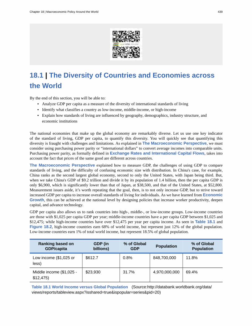
18.1 | The Diversity of Countries and Economies acrossthe WorldBy the end of this section, you will be able to:
• Analyze GDP per capita as a measure of the diversity of international standards of living• Identify what classifies a country as low-income, middle-income, or high-income• Explain how standards of living are influenced by geography, demographics, industry structure, and
economic institutions
The national economies that make up the global economy are remarkably diverse. Let us use one key indicatorof the standard of living, GDP per capita, to quantify this diversity. You will quickly see that quantifying thisdiversity is fraught with challenges and limitations. As explained in The Macroeconomic Perspective, we mustconsider using purchasing power parity or “international dollars” to convert average incomes into comparable units.Purchasing power parity, as formally defined in Exchange Rates and International Capital Flows, takes intoaccount the fact that prices of the same good are different across countries.
The Macroeconomic Perspective explained how to measure GDP, the challenges of using GDP to comparestandards of living, and the difficulty of confusing economic size with distribution. In China's case, for example,China ranks as the second largest global economy, second to only the United States, with Japan being third. But,when we take China's GDP of $9.2 trillion and divide it by its population of 1.4 billion, then the per capita GDP isonly $6,900, which is significantly lower than that of Japan, at $38,500, and that of the United States, at $52,800.Measurement issues aside, it’s worth repeating that the goal, then, is to not only increase GDP, but to strive towardincreased GDP per capita to increase overall standards of living for individuals. As we have learned from EconomicGrowth, this can be achieved at the national level by designing policies that increase worker productivity, deepencapital, and advance technology.
GDP per capita also allows us to rank countries into high-, middle-, or low-income groups. Low-income countriesare those with $1,025 per capita GDP per year; middle-income countries have a per capita GDP between $1,025 and$12,475; while high-income countries have over $12,475 per year per capita income. As seen in Table 18.1 andFigure 18.2, high-income countries earn 68% of world income, but represent just 12% of the global population.Low-income countries earn 1% of total world income, but represent 18.5% of global population.
Ranking based onGDP/capita
GDP (inbillions)
% of GlobalGDP Population % of Global
Population
Low income ($1,025 orless)
$612.7 0.8% 848,700,000 11.8%
Middle income ($1,025 -$12,475)
$23,930 31.7% 4,970,000,000 69.4%
Table 18.1 World Income versus Global Population (Source:http://databank.worldbank.org/data/views/reports/tableview.aspx?isshared=true&ispopular=series&pid=20)
Chapter 18 | Macroeconomic Policy Around the World 439
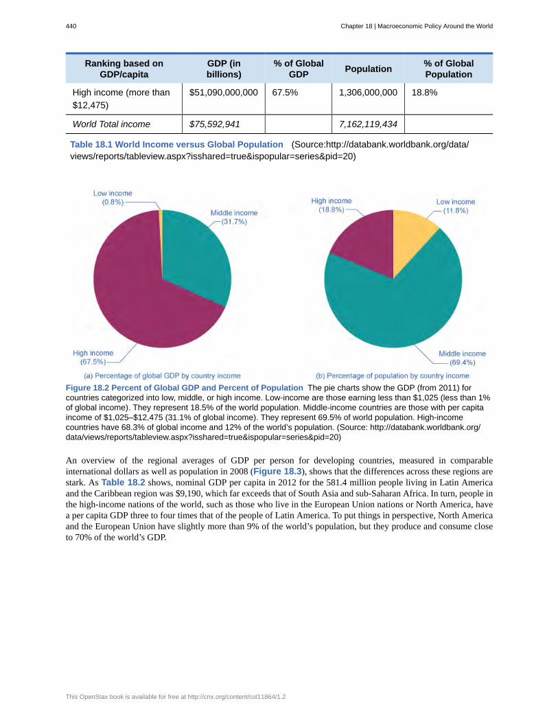
Ranking based onGDP/capita
GDP (inbillions)
% of GlobalGDP Population % of Global
Population
High income (more than$12,475)
$51,090,000,000 67.5% 1,306,000,000 18.8%
World Total income $75,592,941 7,162,119,434
Table 18.1 World Income versus Global Population (Source:http://databank.worldbank.org/data/views/reports/tableview.aspx?isshared=true&ispopular=series&pid=20)
Figure 18.2 Percent of Global GDP and Percent of Population The pie charts show the GDP (from 2011) forcountries categorized into low, middle, or high income. Low-income are those earning less than $1,025 (less than 1%of global income). They represent 18.5% of the world population. Middle-income countries are those with per capitaincome of $1,025–$12,475 (31.1% of global income). They represent 69.5% of world population. High-incomecountries have 68.3% of global income and 12% of the world’s population. (Source: http://databank.worldbank.org/data/views/reports/tableview.aspx?isshared=true&ispopular=series&pid=20)
An overview of the regional averages of GDP per person for developing countries, measured in comparableinternational dollars as well as population in 2008 (Figure 18.3), shows that the differences across these regions arestark. As Table 18.2 shows, nominal GDP per capita in 2012 for the 581.4 million people living in Latin Americaand the Caribbean region was $9,190, which far exceeds that of South Asia and sub-Saharan Africa. In turn, people inthe high-income nations of the world, such as those who live in the European Union nations or North America, havea per capita GDP three to four times that of the people of Latin America. To put things in perspective, North Americaand the European Union have slightly more than 9% of the world’s population, but they produce and consume closeto 70% of the world’s GDP.
440 Chapter 18 | Macroeconomic Policy Around the World
This OpenStax book is available for free at http://cnx.org/content/col11864/1.2
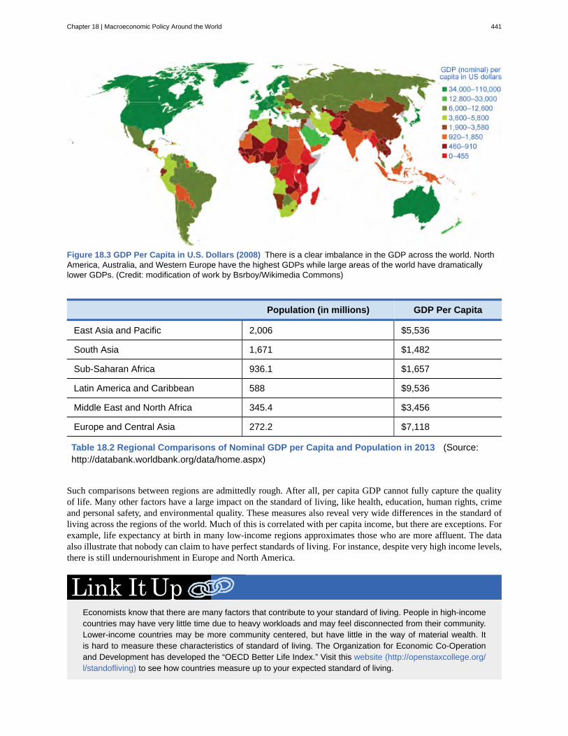
Figure 18.3 GDP Per Capita in U.S. Dollars (2008) There is a clear imbalance in the GDP across the world. NorthAmerica, Australia, and Western Europe have the highest GDPs while large areas of the world have dramaticallylower GDPs. (Credit: modification of work by Bsrboy/Wikimedia Commons)
Population (in millions) GDP Per Capita
East Asia and Pacific 2,006 $5,536
South Asia 1,671 $1,482
Sub-Saharan Africa 936.1 $1,657
Latin America and Caribbean 588 $9,536
Middle East and North Africa 345.4 $3,456
Europe and Central Asia 272.2 $7,118
Table 18.2 Regional Comparisons of Nominal GDP per Capita and Population in 2013 (Source:http://databank.worldbank.org/data/home.aspx)
Such comparisons between regions are admittedly rough. After all, per capita GDP cannot fully capture the qualityof life. Many other factors have a large impact on the standard of living, like health, education, human rights, crimeand personal safety, and environmental quality. These measures also reveal very wide differences in the standard ofliving across the regions of the world. Much of this is correlated with per capita income, but there are exceptions. Forexample, life expectancy at birth in many low-income regions approximates those who are more affluent. The dataalso illustrate that nobody can claim to have perfect standards of living. For instance, despite very high income levels,there is still undernourishment in Europe and North America.
Economists know that there are many factors that contribute to your standard of living. People in high-incomecountries may have very little time due to heavy workloads and may feel disconnected from their community.Lower-income countries may be more community centered, but have little in the way of material wealth. Itis hard to measure these characteristics of standard of living. The Organization for Economic Co-Operationand Development has developed the “OECD Better Life Index.” Visit this website (http://openstaxcollege.org/l/standofliving) to see how countries measure up to your expected standard of living.
Chapter 18 | Macroeconomic Policy Around the World 441

The differences in economic statistics and other measures of well-being, substantial though they are, do not fullycapture the reasons for the enormous differences between countries. Aside from the neoclassical determinants ofgrowth, four additional determinants are significant in a wide range of statistical studies and are worth mentioning:geography, demography, industrial structure, and institutions.
Geographic and Demographic Differences
Countries have geographic differences: some have extensive coastlines, some are landlocked. Some have large riversthat have been a path of commerce for centuries, or mountains that have been a barrier to trade. Some have deserts,some have rain forests. These differences create different positive and negative opportunities for commerce, health,and the environment.
Countries also have considerable differences in the age distribution of the population. Many high-income nations areapproaching a situation by 2020 or so in which the elderly will form a much larger share of the population. Most low-income countries still have a higher proportion of youth and young adults, but by about 2050, the elderly populationsin these low-income countries are expected to boom as well. These demographic changes will have considerableimpact on the standard of living of the young and the old.
Differences in Industry Structure and Economic Institutions
Countries have differences in industry structure. In the high-income economies of the world, only about 2% of GDPcomes from agriculture; the average for the rest of the world is 12%. Countries have strong differences in degree ofurbanization.
Countries also have strong differences in economic institutions: some nations have economies that are extremelymarket-oriented, while other nations have command economies. Some nations are open to international trade, whileothers use tariffs and import quotas to limit the impact of trade. Some nations are torn by long-standing armedconflicts; other nations are largely at peace. There are differences in political, religious, and social institutions as well.
No nation intentionally aims for a low standard of living, high rates of unemployment and inflation, or anunsustainable trade imbalance. However, nations will differ in their priorities and in the situations in which theyfind themselves, and so their policy choices can reasonably vary, too. The next modules will discuss how nationsaround the world, from high income to low income, approach the four macroeconomic goals of economic growth,low unemployment, low inflation, and a sustainable balance of trade.
18.2 | Improving Countries’ Standards of LivingBy the end of this section, you will be able to:
• Analyze the growth policies of low-income countries seeking to improve standards of living• Analyze the growth policies of middle-income countries, particularly the East Asian Tigers with their
focus on technology and market-oriented incentives• Analyze the struggles facing economically-challenged countries wishing to enact growth policies• Evaluate the success of sending aid to low-income countries
Jobs are created in economies that grow. Where does economic growth come from? According to most economistswho believe in the growth consensus, economic growth (as discussed in Economic Growth) is built on a
442 Chapter 18 | Macroeconomic Policy Around the World
This OpenStax book is available for free at http://cnx.org/content/col11864/1.2
foundation of productivity improvements. In turn, productivity increases are the result of greater human and physicalcapital and technology, all interacting in a market-driven economy. In the pursuit of economic growth, however, somecountries and regions start from different levels, as illustrated by the differences in per capita GDP presented earlierin Table 18.2.
Growth Policies for the High-Income CountriesFor the high-income countries, the challenge of economic growth is to push continually for a more educatedworkforce that can create, invest in, and apply new technologies. In effect, the goal of their growth-oriented publicpolicy is to shift their aggregate supply curves to the right (refer to The Aggregate Demand/Aggregate SupplyModel). The main public policies targeted at achieving this goal are fiscal policies focused on investment, includinginvestment in human capital, in technology, and in physical plant and equipment. These countries also recognize thateconomic growth works best in a stable and market-oriented economic climate. For this reason, they use monetarypolicy to keep inflation low and stable, and to minimize the risk of exchange rate fluctuations, while also encouragingdomestic and international competition.
However, early in the second decade of the 2000s, many high-income countries found themselves more focused onthe short term than on the long term. The United States, Western Europe, and Japan all experienced a combinationof financial crisis and deep recession, and the after-effects of the recession—like high unemployment rates—seemedlikely to linger for several years. Most of these governments took aggressive, and in some cases controversial, steps tojump-start their economies by running very large budget deficits as part of expansionary fiscal policy. These countriesmust adopt a course that combines lower government spending and higher taxes.
Similarly, many central banks ran highly expansionary monetary policies, with both near-zero interest rates andunconventional loans and investments. For example, in 2012, Shinzo Abe (see Figure 18.4), then newly-electedPrime Minister of Japan, unveiled a plan to get his country out of its two-decade-long slump in economic growth.It included both fiscal stimulus and an increase in the money supply. The plan was quite successful in the short run.However, according to the Economist, with public debt “expected to approach 240% of GDP,” (as of 2012 it was226% of GDP) printing money and public-works spending were only short-term solutions.
Figure 18.4 Japan’s Prime Minister, Shinzo Abe Japan’s Prime Minister used fiscal and monetary policies tostimulate his country’s economy, which has worked in only the short run. (Credit: modification of work by ChathamHouse/Flickr Creative Commons)
As other chapters discuss, macroeconomics needs to have both a short-run and a long-run focus. The challenge formany of the developed countries in the next few years will be to exit from the short-term policies that were used tocorrect the 2008–2009 recession. Since the return to growth has been sluggish, it has been politically challenging forthese governments to refocus their efforts on new technology, education, and physical capital investment.
Growth Policies for the Middle-Income EconomiesThe world’s great economic success stories in the last few decades began in the 1970s with that group of nationssometimes known as the East Asian Tigers: South Korea, Thailand, Malaysia, Indonesia, and Singapore. The listsometimes includes Hong Kong and Taiwan, although these are often treated under international law as part of China,rather than as separate countries. The economic growth of the Tigers has been phenomenal, typically averaging 5.5%real per capita growth for several decades. In the 1980s, other countries began to show signs of convergence. Chinabegan growing rapidly, often at annual rates of 8% to 10% per year. India began growing rapidly, first at rates of about5% per year in the 1990s, but then higher still in the first decade of the 2000s.
The underlying causes of these rapid growth rates are known:
Chapter 18 | Macroeconomic Policy Around the World 443
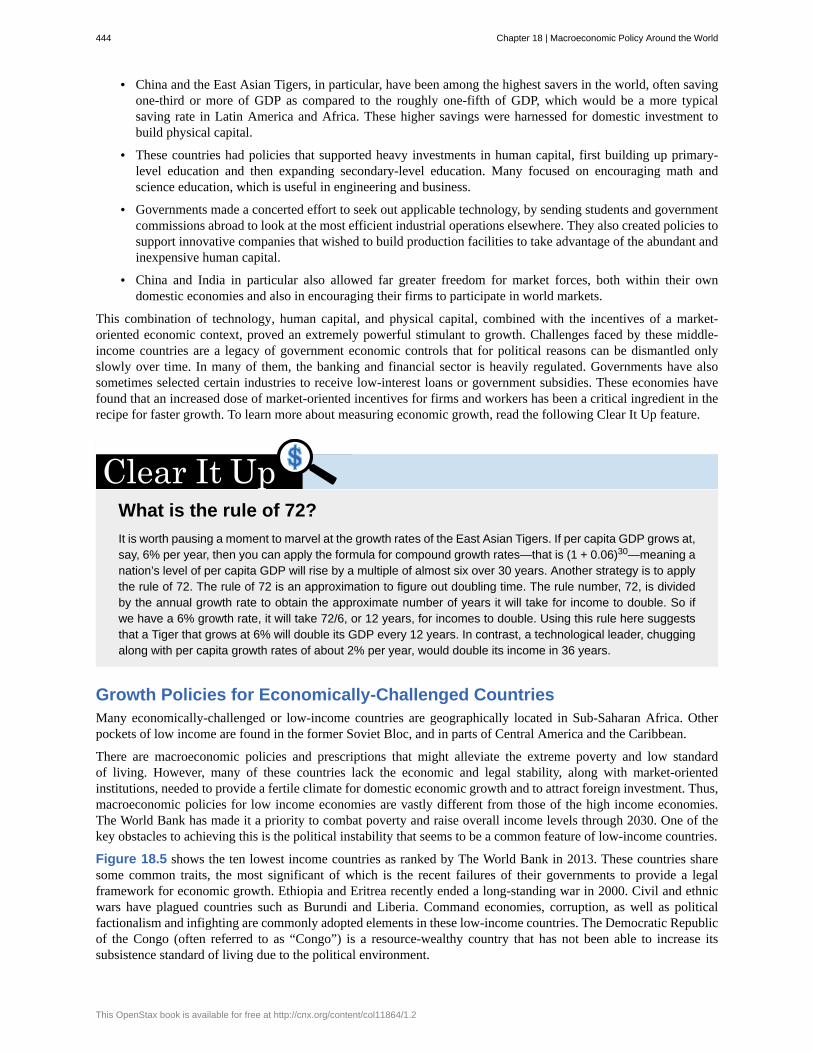
• China and the East Asian Tigers, in particular, have been among the highest savers in the world, often savingone-third or more of GDP as compared to the roughly one-fifth of GDP, which would be a more typicalsaving rate in Latin America and Africa. These higher savings were harnessed for domestic investment tobuild physical capital.
• These countries had policies that supported heavy investments in human capital, first building up primary-level education and then expanding secondary-level education. Many focused on encouraging math andscience education, which is useful in engineering and business.
• Governments made a concerted effort to seek out applicable technology, by sending students and governmentcommissions abroad to look at the most efficient industrial operations elsewhere. They also created policies tosupport innovative companies that wished to build production facilities to take advantage of the abundant andinexpensive human capital.
• China and India in particular also allowed far greater freedom for market forces, both within their owndomestic economies and also in encouraging their firms to participate in world markets.
This combination of technology, human capital, and physical capital, combined with the incentives of a market-oriented economic context, proved an extremely powerful stimulant to growth. Challenges faced by these middle-income countries are a legacy of government economic controls that for political reasons can be dismantled onlyslowly over time. In many of them, the banking and financial sector is heavily regulated. Governments have alsosometimes selected certain industries to receive low-interest loans or government subsidies. These economies havefound that an increased dose of market-oriented incentives for firms and workers has been a critical ingredient in therecipe for faster growth. To learn more about measuring economic growth, read the following Clear It Up feature.
What is the rule of 72?It is worth pausing a moment to marvel at the growth rates of the East Asian Tigers. If per capita GDP grows at,say, 6% per year, then you can apply the formula for compound growth rates—that is (1 + 0.06)30—meaning anation’s level of per capita GDP will rise by a multiple of almost six over 30 years. Another strategy is to applythe rule of 72. The rule of 72 is an approximation to figure out doubling time. The rule number, 72, is dividedby the annual growth rate to obtain the approximate number of years it will take for income to double. So ifwe have a 6% growth rate, it will take 72/6, or 12 years, for incomes to double. Using this rule here suggeststhat a Tiger that grows at 6% will double its GDP every 12 years. In contrast, a technological leader, chuggingalong with per capita growth rates of about 2% per year, would double its income in 36 years.
Growth Policies for Economically-Challenged CountriesMany economically-challenged or low-income countries are geographically located in Sub-Saharan Africa. Otherpockets of low income are found in the former Soviet Bloc, and in parts of Central America and the Caribbean.
There are macroeconomic policies and prescriptions that might alleviate the extreme poverty and low standardof living. However, many of these countries lack the economic and legal stability, along with market-orientedinstitutions, needed to provide a fertile climate for domestic economic growth and to attract foreign investment. Thus,macroeconomic policies for low income economies are vastly different from those of the high income economies.The World Bank has made it a priority to combat poverty and raise overall income levels through 2030. One of thekey obstacles to achieving this is the political instability that seems to be a common feature of low-income countries.
Figure 18.5 shows the ten lowest income countries as ranked by The World Bank in 2013. These countries sharesome common traits, the most significant of which is the recent failures of their governments to provide a legalframework for economic growth. Ethiopia and Eritrea recently ended a long-standing war in 2000. Civil and ethnicwars have plagued countries such as Burundi and Liberia. Command economies, corruption, as well as politicalfactionalism and infighting are commonly adopted elements in these low-income countries. The Democratic Republicof the Congo (often referred to as “Congo”) is a resource-wealthy country that has not been able to increase itssubsistence standard of living due to the political environment.
444 Chapter 18 | Macroeconomic Policy Around the World
This OpenStax book is available for free at http://cnx.org/content/col11864/1.2
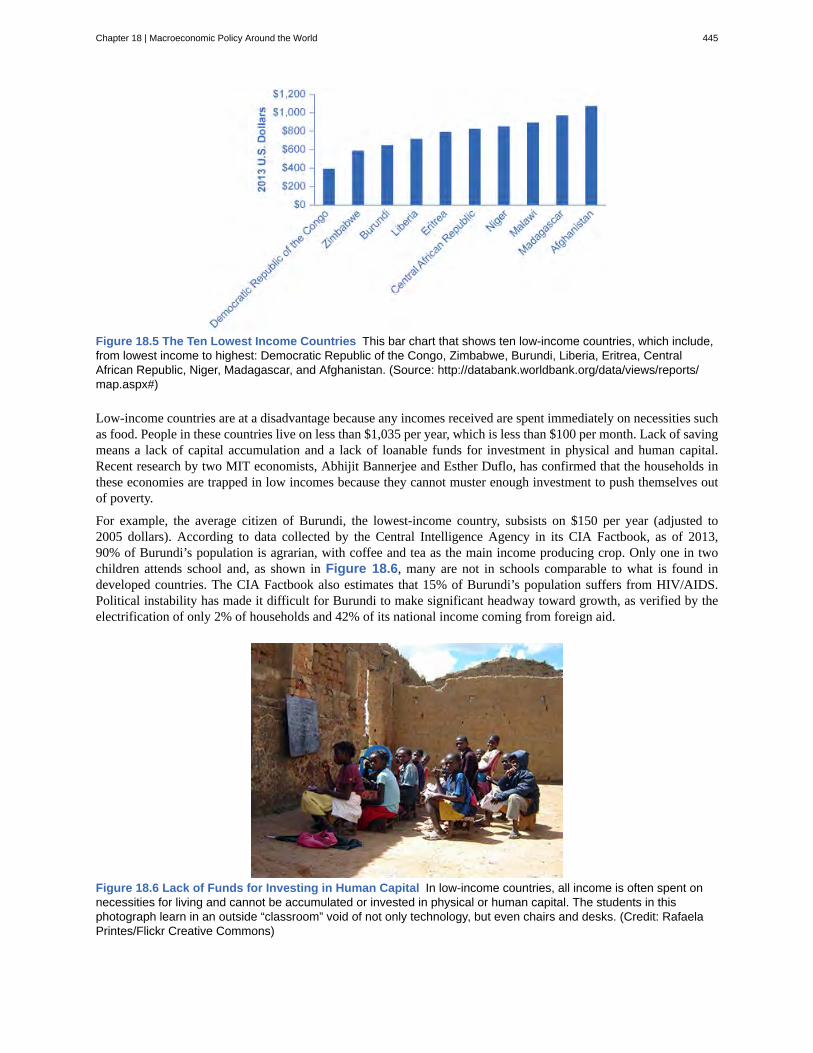
Figure 18.5 The Ten Lowest Income Countries This bar chart that shows ten low-income countries, which include,from lowest income to highest: Democratic Republic of the Congo, Zimbabwe, Burundi, Liberia, Eritrea, CentralAfrican Republic, Niger, Madagascar, and Afghanistan. (Source: http://databank.worldbank.org/data/views/reports/map.aspx#)
Low-income countries are at a disadvantage because any incomes received are spent immediately on necessities suchas food. People in these countries live on less than $1,035 per year, which is less than $100 per month. Lack of savingmeans a lack of capital accumulation and a lack of loanable funds for investment in physical and human capital.Recent research by two MIT economists, Abhijit Bannerjee and Esther Duflo, has confirmed that the households inthese economies are trapped in low incomes because they cannot muster enough investment to push themselves outof poverty.
For example, the average citizen of Burundi, the lowest-income country, subsists on $150 per year (adjusted to2005 dollars). According to data collected by the Central Intelligence Agency in its CIA Factbook, as of 2013,90% of Burundi’s population is agrarian, with coffee and tea as the main income producing crop. Only one in twochildren attends school and, as shown in Figure 18.6, many are not in schools comparable to what is found indeveloped countries. The CIA Factbook also estimates that 15% of Burundi’s population suffers from HIV/AIDS.Political instability has made it difficult for Burundi to make significant headway toward growth, as verified by theelectrification of only 2% of households and 42% of its national income coming from foreign aid.
Figure 18.6 Lack of Funds for Investing in Human Capital In low-income countries, all income is often spent onnecessities for living and cannot be accumulated or invested in physical or human capital. The students in thisphotograph learn in an outside “classroom” void of not only technology, but even chairs and desks. (Credit: RafaelaPrintes/Flickr Creative Commons)
Chapter 18 | Macroeconomic Policy Around the World 445
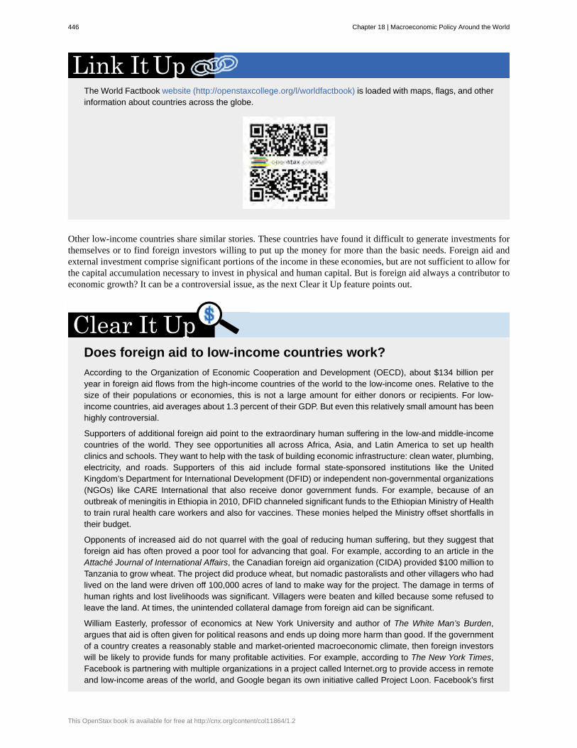
The World Factbook website (http://openstaxcollege.org/l/worldfactbook) is loaded with maps, flags, and otherinformation about countries across the globe.
Other low-income countries share similar stories. These countries have found it difficult to generate investments forthemselves or to find foreign investors willing to put up the money for more than the basic needs. Foreign aid andexternal investment comprise significant portions of the income in these economies, but are not sufficient to allow forthe capital accumulation necessary to invest in physical and human capital. But is foreign aid always a contributor toeconomic growth? It can be a controversial issue, as the next Clear it Up feature points out.
Does foreign aid to low-income countries work?According to the Organization of Economic Cooperation and Development (OECD), about $134 billion peryear in foreign aid flows from the high-income countries of the world to the low-income ones. Relative to thesize of their populations or economies, this is not a large amount for either donors or recipients. For low-income countries, aid averages about 1.3 percent of their GDP. But even this relatively small amount has beenhighly controversial.
Supporters of additional foreign aid point to the extraordinary human suffering in the low-and middle-incomecountries of the world. They see opportunities all across Africa, Asia, and Latin America to set up healthclinics and schools. They want to help with the task of building economic infrastructure: clean water, plumbing,electricity, and roads. Supporters of this aid include formal state-sponsored institutions like the UnitedKingdom’s Department for International Development (DFID) or independent non-governmental organizations(NGOs) like CARE International that also receive donor government funds. For example, because of anoutbreak of meningitis in Ethiopia in 2010, DFID channeled significant funds to the Ethiopian Ministry of Healthto train rural health care workers and also for vaccines. These monies helped the Ministry offset shortfalls intheir budget.
Opponents of increased aid do not quarrel with the goal of reducing human suffering, but they suggest thatforeign aid has often proved a poor tool for advancing that goal. For example, according to an article in theAttaché Journal of International Affairs, the Canadian foreign aid organization (CIDA) provided $100 million toTanzania to grow wheat. The project did produce wheat, but nomadic pastoralists and other villagers who hadlived on the land were driven off 100,000 acres of land to make way for the project. The damage in terms ofhuman rights and lost livelihoods was significant. Villagers were beaten and killed because some refused toleave the land. At times, the unintended collateral damage from foreign aid can be significant.
William Easterly, professor of economics at New York University and author of The White Man’s Burden,argues that aid is often given for political reasons and ends up doing more harm than good. If the governmentof a country creates a reasonably stable and market-oriented macroeconomic climate, then foreign investorswill be likely to provide funds for many profitable activities. For example, according to The New York Times,Facebook is partnering with multiple organizations in a project called Internet.org to provide access in remoteand low-income areas of the world, and Google began its own initiative called Project Loon. Facebook’s first
446 Chapter 18 | Macroeconomic Policy Around the World
This OpenStax book is available for free at http://cnx.org/content/col11864/1.2
forays into providing Internet access via mobile phones began in stable, market-oriented countries like India,Brazil, Indonesia, Turkey, and the Philippines.
Policymakers are now wiser about the limitations of foreign aid than they were a few decades ago. In targetedand specific cases, especially if foreign aid is channeled to long-term investment projects, foreign aid canhave a modest role to play in reducing the extreme levels of deprivation experienced by hundreds of millionsof people around the world.
Watch this video (http://openstaxcollege.org/l/foodafrica) on the complexities of providing economic aid inAfrica.
18.3 | Causes of Unemployment around the WorldBy the end of this section, you will be able to:
• Explain the nature and causes of unemployment• Analyze the natural rate of unemployment and the factors that affect it• Identify how undeveloped labor markets can result in the same hardships as unemployment
The causes of unemployment in high-income countries of the world can be categorized in two ways: either cyclicalunemployment caused by the economy being in a recession, or the natural rate of unemployment caused by factors inlabor markets, such as government regulations regarding hiring and starting businesses.
Unemployment from a RecessionFor unemployment caused by a recession, the Keynesian economic model points out that both monetary and fiscalpolicy tools are available. The monetary policy prescription for dealing with recession is straightforward: run anexpansionary monetary policy to increase the quantity of money and loans, drive down interest rates, and increaseaggregate demand. In a recession, there is usually relatively little danger of inflation taking off, and so even a centralbank, with fighting inflation as its top priority, can usually justify some reduction in interest rates.
With regard to fiscal policy, the automatic stabilizers discussed in Government Budget and Fiscal Policyshould be allowed to work, even if this means larger budget deficits in times of recession. There is less agreementover whether, in addition to automatic stabilizers, governments in a recession should try to adopt discretionary fiscalpolicy of additional tax cuts or spending increases. In the case of the Great Recession, the case for this kind of extra-aggressive expansionary fiscal policy is stronger, but for a smaller recession, given the time lags of implementingfiscal policy, discretionary fiscal policy should be used with caution.
However, the aftermath of the Recession emphasizes that expansionary fiscal and monetary policies do not turn offa recession like flipping a switch turns off a lamp. Even after a recession is officially over, and positive growth hasreturned, it can take some months—or even a couple of years—before private-sector firms believe the economicclimate is healthy enough that they can expand their workforce.
Chapter 18 | Macroeconomic Policy Around the World 447
The Natural Rate of UnemploymentUnemployment rates in the nations of Europe have typically been higher than in the United States. In 2006, before thestart of the Great Recession, the U.S. unemployment rate was 4.6%, compared with 9% in France, 10.4% in Germany,and 7.1% in Sweden. The pattern of generally higher unemployment rates in Europe, which dates back to the 1970s,is typically attributed to the fact that European economies have a higher natural rate of unemployment because theyhave a greater number of rules and restrictions that discourage firms from hiring and unemployed workers from takingjobs.
Addressing the natural rate of unemployment is straightforward in theory but difficult in practice. Government canplay a useful role in providing unemployment and welfare payments, passing rules about where and when businessescan operate, assuring that the workplace is safe, and so on. But these well-intentioned laws can, in some cases, becomeso intrusive that businesses decide to place limits on their hiring.
For example, a law that imposes large costs on a business that tries to fire or lay off workers will mean that businessestry to avoid hiring in the first place, as is the case in France. According to Business Week, “France has 2.4 times asmany companies with 49 employees as with 50 ... according to the French labor code, once a company has at least50 employees inside France, management must create three worker councils, introduce profit sharing, and submitrestructuring plans to the councils if the company decides to fire workers for economic reasons.” This labor lawessentially limits employment (or raises the natural rate of unemployment).
Undeveloped Labor MarketsLow-income and middle-income countries face employment issues that go beyond unemployment as it is understoodin the high-income economies. A substantial number of workers in these economies provide many of their own needsby farming, fishing, or hunting. They barter and trade with others and may take a succession of short-term or one-dayjobs, sometimes being paid with food or shelter, sometimes with money. They are not “unemployed” in the sense thatthe term is used in the United States and Europe, but neither are they employed in a regular wage-paying job.
The starting point of economic activity, as discussed in Welcome to Economics!, is the division of labor, in whichworkers specialize in certain tasks and trade the fruits of their labor with others. Workers who are not connected to alabor market are often unable to specialize very much. Because these workers are not “officially” employed, they areoften not eligible for social benefits like unemployment insurance or old-age payments—if such payments are evenavailable in their country. Helping these workers to become more connected to the labor market and the economy isan important policy goal. Indeed, recent research by development economists suggests that one of the key factors inraising people in low-income countries out of the worst kind of poverty is whether they can make a connection to asomewhat regular wage-paying job.
18.4 | Causes of Inflation in Various Countries andRegionsBy the end of this section, you will be able to:
• Identify the causes and effects of inflation in various economic markets• Explain the significance of a converging economy
Policymakers of the high-income economies appear to have learned some lessons about fighting inflation. First,whatever happens with aggregate supply and aggregate demand in the short run, monetary policy can be used toprevent inflation from becoming entrenched in the economy in the medium and long term. Second, there is no long-run gain to letting inflation become established. In fact, allowing inflation to become lasting and persistent posesundesirable risks and tradeoffs. When inflation is high, businesses and individuals need to spend time and effortworrying about protecting themselves against inflation, rather than seeking out better ways to serve customers. Inshort, the high-income economies appear to have both a political consensus to hold inflation low and the economictools to do so.
In a number of middle- and low-income economies around the world, inflation is far from a solved problem. In theearly 2000s, Turkey experienced inflation of more than 50% per year for several years. Belarus had inflation of about100% per year from 2000 to 2001. From 2008 to 2010, Venezuela and Myanmar had inflation rates of 20% to 30%
448 Chapter 18 | Macroeconomic Policy Around the World
This OpenStax book is available for free at http://cnx.org/content/col11864/1.2

per year. Indonesia, Iran, Nigeria, the Russian Federation, and Ukraine all had double-digit inflation for most of theyears from 2000 to 2010. Zimbabwe had hyperinflation, with inflation rates that went from more than 100% per yearin the mid-2000s to a rate of several million percent in 2008.
In these countries, the problem of very high inflation generally arises from huge budget deficits, which are financedby the government printing its domestic currency. This is a case of “too much money chasing too few goods.” In thecase of Zimbabwe, the government covered its widening deficits by printing ever higher currency notes, includinga $100 trillion bill. By late 2008, the money was nearly worthless, which led Zimbabwe to adopt the U.S. dollar,immediately halting their hyperinflation. In some countries, the central bank makes loans to politically favored firms,essentially printing money to do so, and this too leads to higher inflation.
A number of countries have managed to sustain solid levels of economic growth for sustained periods of time withlevels of inflation that would sound high by recent U.S. standards, like 10% to 30% per year. In such economies, mostcontracts, wage levels, and interest rates are indexed to inflation. Indexing wage contracts and interest rates means thatthey will increase when inflation increases to retain purchasing power. When wages do not rise as price levels rise,this leads to a decline in the real wage rate and a decrease in the standard of living. Likewise, interest rates that are notindexed mean that the lenders of money will be paid back in devalued currency and will also lose purchasing poweron monies that were lent. It is clearly possible—and perhaps sometimes necessary—for a converging economy (theeconomy of a country that demonstrates the ability to catch up to the technology leaders) to live with a degree ofuncertainty over inflation that would be politically unacceptable in the high-income economies.
18.5 | Balance of Trade ConcernsBy the end of this section, you will be able to:
• Explain the meaning of trade balance and its implications for the foreign exchange market• Analyze concerns over international trade in goods and services and international flows of capital• Identify and evaluate market-oriented economic reforms
In the 1950s and 1960s, and even into the 1970s, openness to global flows of goods, services, and financial capitalwas often viewed in a negative light by low- and middle-income countries. These countries feared that foreign tradewould mean both economic losses as their economy was “exploited” by high-income trading partners and a loss ofdomestic political control to powerful business interests and multinational corporations.
These negative feelings about international trade have evolved. After all, the great economic success stories of recentyears like Japan, the East Asian Tiger economies, China, and India, all took advantage of opportunities to sell in globalmarkets. The economies of Europe thrive with high levels of trade. In the North American Free Trade Agreement(NAFTA), the United States, Canada, and Mexico pledged themselves to reduce trade barriers. Many countries haveclearly learned that reducing barriers to trade is at least potentially beneficial to the economy. Indeed, many smallereconomies of the world have learned an even tougher lesson: if they do not participate actively in world trade, theyare unlikely to join the success stories among the converging economies. There are no examples in world history ofsmall economies that remained apart from the global economy but still attained a high standard of living.
Although almost every country now claims that its goal is to participate in global trade, the possible negativeconsequences have remained highly controversial. It is useful to divide up these possible negative consequencesinto issues involving trade of goods and services and issues involving flows of international capital. These issuesare related, but not the same. An economy may have a high level of trade in goods and services relative to GDP,but if exports and imports are balanced, the net flow of foreign investment in and out of the economy will be zero.Conversely, an economy may have only a moderate level of trade relative to GDP, but find that it has a substantialcurrent account trade imbalance. Thus, it is useful to consider the concerns over international trade of goods andservices and international flows of financial capital separately.
Concerns over International Trade in Goods and ServicesThere is a long list of worries about foreign trade in goods and services: fear of job loss, environmental dangers,unfair labor practices, and many other concerns. These arguments are discussed at some length in The InternationalTrade and Capital Flows.
Chapter 18 | Macroeconomic Policy Around the World 449
Of all of the arguments for limitations on trade, perhaps the most controversial one among economists is theinfant industry argument; that is, subsidizing or protecting new industries for a time until they become established.(Globalization and Protectionism (http://cnx.org/content/m57388/latest/) explains this concept in moredetail.) Such policies have been used with some success at certain points in time, but in the world as a whole, supportfor key industries is far more often directed at long-established industries with substantial political power that aresuffering losses and laying off workers, rather than potentially vibrant new industries that have yet to be established.If government is going to favor certain industries, it needs to do so in a way that is temporary and that orients themtoward a future of market competition, rather than a future of unending government subsidies and trade protection.
Concerns over International Flows of CapitalRecall from The Macroeconomic Perspective that a trade deficit exists when a nation’s imports exceed itsexports. In order for a trade deficit to take place, foreign countries must provide loans or investments, which theyare willing to do because they expect they will be repaid eventually (that the deficit will become a surplus). A tradesurplus, you may remember, exists when a nation’s exports exceed its imports. So, in order for a trade deficit to switchto a trade surplus, a nation’s exports must rise and its imports must fall. Sometimes this happens when the currencydecreases in value. For example, if the U.S. had a trade deficit and the dollar depreciated, imports would becomemore expensive. This would, in turn, benefit the foreign countries who provided the loans or investments.
The expected pattern of trade imbalances in the world economy has been that high-income economies will run tradesurpluses, which means they will experience a net outflow of capital to foreign destinations or export more than theyimport, while low- and middle-income economies will run trade deficits, which means that they will experience a netinflow of foreign capital.
This pattern of international investing can benefit all sides. Investors in the high-income countries benefit becausethey can receive high returns on their investments, and also because they can diversify their investments so that theyare at less risk of a downturn in their own domestic economy. The low-income economies that receive an inflow ofcapital presumably have potential for rapid catch-up economic growth, and they can use the inflow of internationalfinancial capital to help spur their physical capital investment. In addition, inflows of financial capital often comewith management abilities, technological expertise, and training.
However, for the last couple of decades, this cheerful scenario has faced two “dark clouds.” The first cloud is the verylarge trade or current account deficits in the U.S. economy. (See The International Trade and Capital Flows.)Instead of offering net financial investment abroad, the U.S. economy is soaking up savings from all over the world.These substantial U.S. trade deficits may not be sustainable according to Sebastian Edwards writing for the NationalBureau of Economic Research. While trade deficits on their own are not bad, the question is whether they will bereduced gradually or hastily. In the gradual scenario, U.S. exports could grow more rapidly than imports over a periodof years, aided by a depreciation of the U.S. dollar. An unintended consequence of the slow growth since the GreatRecession has been a decline in the size of the U.S. current account deficit from 6% pre-recession to 3% most recently.
The other option is that the U.S. trade deficit could be reduced in a rush. Here is one scenario: if foreign investorsbecame less willing to hold U.S. dollar assets, the dollar exchange rate could weaken. As speculators see this processhappening, they might rush to unload their dollar assets, which would drive the dollar down still further.
A lower U.S. dollar would stimulate aggregate demand by making exports cheaper and imports more expensive. Itwould mean higher prices for imported inputs throughout the economy, shifting the short-term aggregate supply curveto the left. The result could be a burst of inflation and, if the Federal Reserve were to run a tight monetary policy toreduce the inflation, it could also lead to recession. People sometimes talk as if the U.S. economy, with its great size,is invulnerable to this sort of pressure from international markets. While it is tough to rock, it is not impossible forthe $17 trillion U.S. economy to face these international pressures.
The second “dark cloud” is how the smaller economies of the world should deal with the possibility of sudden inflowsand outflows of foreign financial capital. Perhaps the most vivid recent example of the potentially destructive forcesof international capital movements occurred in the economies of the East Asian Tigers in 1997–1998. Thanks to theirexcellent growth performance over the previous few decades, these economies had attracted considerable interestfrom foreign investors. In the mid-1990s, however, foreign investment into these countries surged even further. Muchof this money was funneled through banks that borrowed in U.S. dollars and loaned in their national currencies.Bank lending surged at rates of 20% per year or more. This inflow of foreign capital meant that investment in theseeconomies exceeded the level of domestic savings, so that current account deficits in these countries jumped into therange of 5–10% of GDP.
450 Chapter 18 | Macroeconomic Policy Around the World
This OpenStax book is available for free at http://cnx.org/content/col11864/1.2
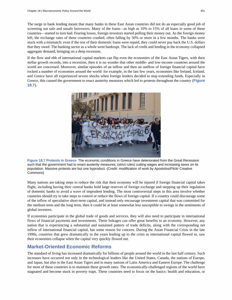
The surge in bank lending meant that many banks in these East Asian countries did not do an especially good job ofscreening out safe and unsafe borrowers. Many of the loans—as high as 10% to 15% of all loans in some of thesecountries—started to turn bad. Fearing losses, foreign investors started pulling their money out. As the foreign moneyleft, the exchange rates of these countries crashed, often falling by 50% or more in a few months. The banks werestuck with a mismatch: even if the rest of their domestic loans were repaid, they could never pay back the U.S. dollarsthat they owed. The banking sector as a whole went bankrupt. The lack of credit and lending in the economy collapsedaggregate demand, bringing on a deep recession.
If the flow and ebb of international capital markets can flip even the economies of the East Asian Tigers, with theirstellar growth records, into a recession, then it is no wonder that other middle- and low-income countries around theworld are concerned. Moreover, similar episodes of an inflow and then an outflow of foreign financial capital haverocked a number of economies around the world: for example, in the last few years, economies like Ireland, Iceland,and Greece have all experienced severe shocks when foreign lenders decided to stop extending funds. Especially inGreece, this caused the government to enact austerity measures which led to protests throughout the country (Figure18.7).
Figure 18.7 Protests in Greece The economic conditions in Greece have deteriorated from the Great Recessionsuch that the government had to enact austerity measures, (strict rules) cutting wages and increasing taxes on itspopulation. Massive protests are but one byproduct. (Credit: modification of work by Apostolos/Flickr CreativeCommons)
Many nations are taking steps to reduce the risk that their economy will be injured if foreign financial capital takesflight, including having their central banks hold large reserves of foreign exchange and stepping up their regulationof domestic banks to avoid a wave of imprudent lending. The most controversial steps in this area involve whethercountries should try to take steps to control or reduce the flows of foreign capital. If a country could discourage someof the inflow of speculative short-term capital, and instead only encourage investment capital that was committed forthe medium term and the long term, then it could be at least somewhat less susceptible to swings in the sentiments ofglobal investors.
If economies participate in the global trade of goods and services, they will also need to participate in internationalflows of financial payments and investments. These linkages can offer great benefits to an economy. However, anynation that is experiencing a substantial and sustained pattern of trade deficits, along with the corresponding netinflow of international financial capital, has some reason for concern. During the Asian Financial Crisis in the late1990s, countries that grew dramatically in the years leading up to the crisis as international capital flowed in, sawtheir economies collapse when the capital very quickly flowed out.
Market-Oriented Economic ReformsThe standard of living has increased dramatically for billions of people around the world in the last half century. Suchincreases have occurred not only in the technological leaders like the United States, Canada, the nations of Europe,and Japan, but also in the East Asian Tigers and in many nations of Latin America and Eastern Europe. The challengefor most of these countries is to maintain these growth rates. The economically-challenged regions of the world havestagnated and become stuck in poverty traps. These countries need to focus on the basics: health and education, or
Chapter 18 | Macroeconomic Policy Around the World 451
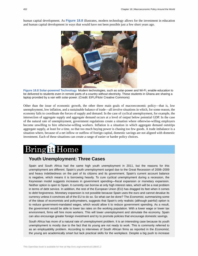
human capital development. As Figure 18.8 illustrates, modern technology allows for the investment in educationand human capital development in ways that would have not been possible just a few short years ago.
Figure 18.8 Solar-powered Technology Modern technologies, such as solar-power and Wi-Fi, enable education tobe delivered to students even in remote parts of a country without electricity. These students in Ghana are sharing alaptop provided by a van with solar-power. (Credit: EIFL/Flickr Creative Commons)
Other than the issue of economic growth, the other three main goals of macroeconomic policy—that is, lowunemployment, low inflation, and a sustainable balance of trade—all involve situations in which, for some reason, theeconomy fails to coordinate the forces of supply and demand. In the case of cyclical unemployment, for example, theintersection of aggregate supply and aggregate demand occurs at a level of output below potential GDP. In the caseof the natural rate of unemployment, government regulations create a situation where otherwise-willing employersbecome unwilling to hire otherwise-willing workers. Inflation is a situation in which aggregate demand outstripsaggregate supply, at least for a time, so that too much buying power is chasing too few goods. A trade imbalance is asituation where, because of a net inflow or outflow of foreign capital, domestic savings are not aligned with domesticinvestment. Each of these situations can create a range of easier or harder policy choices.
Youth Unemployment: Three CasesSpain and South Africa had the same high youth unemployment in 2011, but the reasons for thisunemployment are different. Spain’s youth unemployment surged due to the Great Recession of 2008–2009and heavy indebtedness on the part of its citizens and its government. Spain’s current account balanceis negative, which means it is borrowing heavily. To cure cyclical unemployment during a recession, theKeynesian model suggests increases in government spending—fiscal expansion or monetary expansion.Neither option is open to Spain. It currently can borrow at only high interest rates, which will be a real problemin terms of debt service. In addition, the rest of the European Union (EU) has dragged its feet when it comesto debt forgiveness. Monetary expansion is not possible because Spain uses the euro and cannot devalue itscurrency unless it convinces all of the EU to do so. So what can be done? The Economist, summarizing someof the ideas of economists and policymakers, suggests that Spain’s only realistic (although painful) option isto reduce government-mandated wages, which would allow it to reduce government spending. As a result,the government would be able to lower tax rates on the working population. With a lower wage or lower taxenvironment, firms will hire more workers. This will lower unemployment and stimulate the economy. Spaincan also encourage greater foreign investment and try to promote policies that encourage domestic savings.
South Africa has more of a natural rate of unemployment problem. It is an interesting case because its youthunemployment is mostly due to the fact that its young are not ready to work. This is commonly referred toas an employability problem. According to interviews of South African firms as reported in the Economist,the young are academically smart but lack practical skills for the workplace. Despite a big push to increase
452 Chapter 18 | Macroeconomic Policy Around the World
This OpenStax book is available for free at http://cnx.org/content/col11864/1.2

investment in human capital, the results have not yet borne fruit. Recently the government unveiled a plan topay unemployed youth while they were “trained-up” or apprenticed in South African firms. The governmenthas room to increase fiscal expenditure, encourage domestic savings, and continue to fund investment ineducation, vocational training, and apprentice programs. South Africa can also improve the climate for foreigninvestment from technology leaders, which would encourage economic growth.
India has a smaller youth employment problem in terms of percentages. However, bear in mind that since thisis a populous country, it turns out to be a significant problem in raw numbers. According to Kaushik Basu,writing for the BBC, “there are 45 national laws governing the hiring and firing decisions of firms and closeto four times that amount at the state level”. These laws make it difficult for companies to fire workers. Tostay nimble and responsive to markets, Indian companies respond to these laws by hiring fewer workers. TheIndian government can do much to solve this problem by adjusting its labor laws. Essentially, the governmenthas to remove itself from firms’ hiring and firing decisions, so that growing Indian firms can freely employ moreworkers. Indian workers, like those in South Africa, do not have workforce skills. Again, the government canincrease its spending on education, vocational training, and workforce readiness programs.
Finally, India has a significant current account deficit. This deficit is mainly a result of short- and long-termcapital flows. To solve this deficit, India has experimented by lifting the limitation on domestic savers frominvesting abroad. This is a step in the right direction that may dampen the growth in the current accountdeficit. A final policy possibility is to improve domestic capital markets so many self-employed Indians can getaccess to capital to realize their business ideas. If more Indians can get access to capital to start businesses,employment might increase.
Chapter 18 | Macroeconomic Policy Around the World 453
converging economy
East Asian Tigers
growth consensus
high-income country
low-income country
middle-income country
KEY TERMS
economy of a country that has demonstrated the ability to catch up to the technology leaders byinvesting in both physical and human capital
the economies of Taiwan, Singapore, Hong Kong, and South Korea, which maintained high growthrates and rapid export-led industrialization between the early 1960s and 1990 allowing them to converge with thetechnological leaders in high-income countries
a series of studies that show, statistically, that 70% of the differences in income per person acrossthe world is explained by differences in physical capital (savings/investment)
nation with a per capita income of $12,475 or more; typically has high levels of human andphysical capital
a nation that has a per capita income of less than $1,025; a third of the world’s population
a nation with per capita income between $1,025 and $12, 475 and that has shown someability, even if not always sustained, to catch up to the technology leaders in high-income countries
KEY CONCEPTS AND SUMMARY
18.1 The Diversity of Countries and Economies across the WorldMacroeconomic policy goals for most countries strive toward low levels of unemployment and inflation, as wellas stable trade balances. Countries are analyzed based on their GDP per person and ranked as low-, middle-, and high-income countries. Low-income are those earning less than $1,025 (less than 1%) of global income.They currently have 18.5% of the world population. Middle-income countries are those with per capital income of$1,025–$12,475 (31.1% of global income). They have 69.5% of world population. High-income countries are thosewith per capita income greater than $12,475 (68.3% of global income). They have 12% of the world’s population.Regional comparisons tend to be inaccurate because even countries within those regions tend to differ from eachother.
18.2 Improving Countries’ Standards of LivingThe fundamentals of growth are the same in every country: improvements in human capital, physical capital, andtechnology interacting in a market-oriented economy. Countries that are high-income tend to focus on developingand using new technology. Countries that are middle-income focus on increasing human capital and becomingmore connected to technology and global markets. They have charted unconventional paths by relying more onstate-led support rather than relying solely on markets. Low-income, economically-challenged countries have manyhealth and human development needs, but they are also challenged by the lack of investment and foreign aid todevelop infrastructure like roads. There are some bright spots when it comes to financial development and mobilecommunications, which suggest that low-income countries can become technology leaders in their own right, but itis too early to claim victory. These countries must do more to connect to the rest of the global economy and find thetechnologies that work best for them.
18.3 Causes of Unemployment around the WorldCyclical unemployment can be addressed by expansionary fiscal and monetary policy. The natural rate ofunemployment can be harder to deal with, because it involves thinking carefully about the tradeoffs involved in lawsthat affect employment and hiring. Unemployment is understood differently in high-income countries compared tolow- and middle-income countries. People in these countries are not “unemployed” in the sense that term is used inthe United States and Europe, but neither are they employed in a regular wage-paying job. While some may haveregular wage-paying jobs, others are part of a barter economy.
454 Chapter 18 | Macroeconomic Policy Around the World
This OpenStax book is available for free at http://cnx.org/content/col11864/1.2
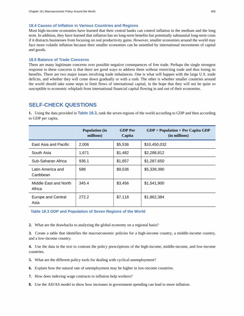
18.4 Causes of Inflation in Various Countries and RegionsMost high-income economies have learned that their central banks can control inflation in the medium and the longterm. In addition, they have learned that inflation has no long-term benefits but potentially substantial long-term costsif it distracts businesses from focusing on real productivity gains. However, smaller economies around the world mayface more volatile inflation because their smaller economies can be unsettled by international movements of capitaland goods.
18.5 Balance of Trade ConcernsThere are many legitimate concerns over possible negative consequences of free trade. Perhaps the single strongestresponse to these concerns is that there are good ways to address them without restricting trade and thus losing itsbenefits. There are two major issues involving trade imbalances. One is what will happen with the large U.S. tradedeficits, and whether they will come down gradually or with a rush. The other is whether smaller countries aroundthe world should take some steps to limit flows of international capital, in the hope that they will not be quite sosusceptible to economic whiplash from international financial capital flowing in and out of their economies.
SELF-CHECK QUESTIONS1. Using the data provided in Table 18.3, rank the seven regions of the world according to GDP and then accordingto GDP per capita.
Population (inmillions)
GDP PerCapita
GDP = Population × Per Capita GDP(in millions)
East Asia and Pacific 2,006 $5,536 $10,450,032
South Asia 1,671 $1,482 $2,288,812
Sub-Saharan Africa 936.1 $1,657 $1,287,650
Latin America andCaribbean
588 $9,536 $5,339,390
Middle East and NorthAfrica
345.4 $3,456 $1,541,900
Europe and CentralAsia
272.2 $7,118 $1,862,384
Table 18.3 GDP and Population of Seven Regions of the World
2. What are the drawbacks to analyzing the global economy on a regional basis?
3. Create a table that identifies the macroeconomic policies for a high-income country, a middle-income country,and a low-income country.
4. Use the data in the text to contrast the policy prescriptions of the high-income, middle-income, and low-incomecountries.
5. What are the different policy tools for dealing with cyclical unemployment?
6. Explain how the natural rate of unemployment may be higher in low-income countries.
7. How does indexing wage contracts to inflation help workers?
8. Use the AD/AS model to show how increases in government spending can lead to more inflation.
Chapter 18 | Macroeconomic Policy Around the World 455
9. Show, using the AD/AS model, how monetary policy can be used to decrease the price level.
10. What do international flows of capital have to do with trade imbalances?
11. Use the demand-and-supply of foreign currency graph to determine what would happen to a small, openeconomy that experienced capital outflows.
REVIEW QUESTIONS
12. What is the primary way in which economistsmeasure standards of living?
13. What are some of the other ways of comparing thestandard of living in countries around the world?
14. What are the four other factors that determine theeconomic standard of living around the world?
15. What other factors, aside from labor productivity,capital investment, and technology, impact the economicgrowth of a country? How?
16. What strategies were employed by the East AsianTigers to stimulate economic growth?
17. What are the two types of unemploymentproblems?
18. In low-income countries, does it make sense toargue that most of the people without long-term jobs areunemployed?
19. Is inflation likely to be a severe problem for at leastsome high-income economies in the near future?
20. Is inflation likely to be a problem for at least somelow- and middle-income economies in the near future?
21. What are the major issues with regard to tradeimbalances for the U.S. economy?
22. What are the major issues with regard to tradeimbalances for low- and middle-income countries?
CRITICAL THINKING QUESTIONS
23. Demography can have important economic effects.The United States has an aging population. Explain oneeconomic benefit and one economic cost of an agingpopulation as well as of a population that is very young.
24. Explain why is it difficult to set aside funds forinvestment when you are in poverty.
25. Why do you think it is difficult for high-incomecountries to achieve high growth rates?
26. Is it possible to protect workers from being firedwithout distorting the labor market?
27. Explain what will happen in a nation that triesto solve a structural unemployment problem using
expansionary monetary and fiscal policy. Draw one AD/AS diagram, based on the Keynesian model, for whatthe nation hopes will happen. Then draw a second AD/AS diagram, based on the neoclassical model, for whatis more likely to happen.
28. Why are inflationary dangers lower in the high-income economies than in low-income and middle-income economies?
29. Explain why converging economies may present astrong argument for limiting flows of capital but not forlimiting trade.
PROBLEMS30. Retrieve the following data from The World Bankdatabase (http://databank.worldbank.org/data/home.aspx) for India, Spain, and South Africa for themost recent year available:
• GDP in constant international dollars or PPP• Population• GDP per person in constant international dollars
• Mortality rate, infant (per 1,000 live births)• Health expenditure per capita (current U.S.
dollars)• Life expectancy at birth, total (years)
31. Prepare a chart that compares India, Spain, andSouth Africa based on the data you find. Describe the
456 Chapter 18 | Macroeconomic Policy Around the World
This OpenStax book is available for free at http://cnx.org/content/col11864/1.2
key differences between the countries. Rank these ashigh-, medium-, and low-income countries, explain whatis surprising or expected about this data.
32. Use the Rule of 72 to estimate how long it willtake for India, Spain, and South Africa to double theirstandards of living.
33. Using the research skills you have acquired,retrieve the following data from The World Bankdatabase (http://databank.worldbank.org/data/home.aspx) for India, Spain, and South Africa for2008–2013, if available:
• Telephone lines• Mobile cellular subscriptions• Secure Internet servers (per one million people)• Electricity production (kWh)
Prepare a chart that compares these three countries.Describe the key differences between the countries.
34. Retrieve the unemployment data from The WorldBank database (http://databank.worldbank.org/data/home.aspx) for India, Spain, and South Africa for2008–2012. Prepare a chart that compares India, Spain,and South Africa based on the data. Describe the keydifferences between the countries. Rank these countriesas high-, medium-, and low-income countries. Explainwhat is surprising or expected about this data. How werethese countries impacted by the Great Recession?
35. Retrieve inflation data from The World Bank database (http://databank.worldbank.org/data/home.aspx)for India, Spain, and South Africa for 2008–2013.Prepare a chart that compares India, Spain, and SouthAfrica based on the data. Describe the key differencesbetween the countries. Rank these countries as high-,medium-, and low-income. Explain what is surprising orexpected about the data.
Chapter 18 | Macroeconomic Policy Around the World 457
458 Chapter 18 | Macroeconomic Policy Around the World
This OpenStax book is available for free at http://cnx.org/content/col11864/1.2

Appendix A(This appendix should be consulted after first reading Welcome to Eonomics!) Economics is not math. There isno important concept in this course that cannot be explained without mathematics. That said, math is a tool that can beused to illustrate economic concepts. Remember the saying a picture is worth a thousand words? Instead of a picture,think of a graph. It is the same thing. Economists use models as the primary tool to derive insights about economicissues and problems. Math is one way of working with (or manipulating) economic models.
There are other ways of representing models, such as text or narrative. But why would you use your fist to bang anail, if you had a hammer? Math has certain advantages over text. It disciplines your thinking by making you specifyexactly what you mean. You can get away with fuzzy thinking in your head, but you cannot when you reduce a modelto algebraic equations. At the same time, math also has disadvantages. Mathematical models are necessarily based onsimplifying assumptions, so they are not likely to be perfectly realistic. Mathematical models also lack the nuanceswhich can be found in narrative models. The point is that math is one tool, but it is not the only tool or even always thebest tool economists can use. So what math will you need for this book? The answer is: little more than high schoolalgebra and graphs. You will need to know:
• What a function is
• How to interpret the equation of a line (i.e., slope and intercept)
• How to manipulate a line (i.e., changing the slope or the intercept)
• How to compute and interpret a growth rate (i.e., percentage change)
• How to read and manipulate a graph
In this text, we will use the easiest math possible, and we will introduce it in this appendix. So if you find some mathin the book that you cannot follow, come back to this appendix to review. Like most things, math has diminishingreturns. A little math ability goes a long way; the more advanced math you bring in, the less additional knowledgethat will get you. That said, if you are going to major in economics, you should consider learning a little calculus. Itwill be worth your while in terms of helping you learn advanced economics more quickly.
Algebraic ModelsOften economic models (or parts of models) are expressed in terms of mathematical functions. What is a function?A function describes a relationship. Sometimes the relationship is a definition. For example (using words), yourprofessor is Adam Smith. This could be expressed as Professor = Adam Smith. Or Friends = Bob + Shawn +Margaret.
Often in economics, functions describe cause and effect. The variable on the left-hand side is what is being explained(“the effect”). On the right-hand side is what is doing the explaining (“the causes”). For example, suppose your GPAwas determined as follows:
GPA = 0.25 × combined_SAT + 0.25 × class_attendance + 0.50 × hours_spent_studying
This equation states that your GPA depends on three things: your combined SAT score, your class attendance, and thenumber of hours you spend studying. It also says that study time is twice as important (0.50) as either combined_SATscore (0.25) or class_attendance (0.25). If this relationship is true, how could you raise your GPA? By not skippingclass and studying more. Note that you cannot do anything about your SAT score, since if you are in college, youhave (presumably) already taken the SATs.
Of course, economic models express relationships using economic variables, like Budget =money_spent_on_econ_books + money_spent_on_music, assuming that the only things you buy are economics booksand music.
Most of the relationships we use in this course are expressed as linear equations of the form:
y = b + mx
Expressing Equations Graphically
Appendix A 459
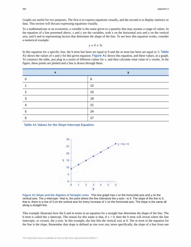
Graphs are useful for two purposes. The first is to express equations visually, and the second is to display statistics ordata. This section will discuss expressing equations visually.
To a mathematician or an economist, a variable is the name given to a quantity that may assume a range of values. Inthe equation of a line presented above, x and y are the variables, with x on the horizontal axis and y on the verticalaxis, and b and m representing factors that determine the shape of the line. To see how this equation works, considera numerical example:
y = 9 + 3x
In this equation for a specific line, the b term has been set equal to 9 and the m term has been set equal to 3. TableA1 shows the values of x and y for this given equation. Figure A1 shows this equation, and these values, in a graph.To construct the table, just plug in a series of different values for x, and then calculate what value of y results. In thefigure, these points are plotted and a line is drawn through them.
x y
0 9
1 12
2 15
3 18
4 21
5 24
6 27
Table A1 Values for the Slope Intercept Equation
Figure A1 Slope and the Algebra of Straight Lines This line graph has x on the horizontal axis and y on thevertical axis. The y-intercept—that is, the point where the line intersects the y-axis—is 9. The slope of the line is 3;that is, there is a rise of 3 on the vertical axis for every increase of 1 on the horizontal axis. The slope is the same allalong a straight line.
This example illustrates how the b and m terms in an equation for a straight line determine the shape of the line. Theb term is called the y-intercept. The reason for this name is that, if x = 0, then the b term will reveal where the lineintercepts, or crosses, the y-axis. In this example, the line hits the vertical axis at 9. The m term in the equation forthe line is the slope. Remember that slope is defined as rise over run; more specifically, the slope of a line from one
460 Appendix A
This OpenStax book is available for free at http://cnx.org/content/col11864/1.2
point to another is the change in the vertical axis divided by the change in the horizontal axis. In this example, eachtime the x term increases by one (the run), the y term rises by three. Thus, the slope of this line is three. Specifying ay-intercept and a slope—that is, specifying b and m in the equation for a line—will identify a specific line. Althoughit is rare for real-world data points to arrange themselves as an exact straight line, it often turns out that a straight linecan offer a reasonable approximation of actual data.
Interpreting the Slope
The concept of slope is very useful in economics, because it measures the relationship between two variables. Apositive slope means that two variables are positively related; that is, when x increases, so does y, or when x decreases,y decreases also. Graphically, a positive slope means that as a line on the line graph moves from left to right, the linerises. The length-weight relationship, shown in Figure A3 later in this Appendix, has a positive slope. We will learnin other chapters that price and quantity supplied have a positive relationship; that is, firms will supply more whenthe price is higher.
A negative slope means that two variables are negatively related; that is, when x increases, y decreases, or when xdecreases, y increases. Graphically, a negative slope means that, as the line on the line graph moves from left to right,the line falls. The altitude-air density relationship, shown in Figure A4 later in this appendix, has a negative slope.We will learn that price and quantity demanded have a negative relationship; that is, consumers will purchase lesswhen the price is higher.
A slope of zero means that there is no relationship between x and y. Graphically, the line is flat; that is, zero rise overthe run. Figure A5 of the unemployment rate, shown later in this appendix, illustrates a common pattern of manyline graphs: some segments where the slope is positive, other segments where the slope is negative, and still othersegments where the slope is close to zero.
The slope of a straight line between two points can be calculated in numerical terms. To calculate slope, begin bydesignating one point as the “starting point” and the other point as the “end point” and then calculating the riseover run between these two points. As an example, consider the slope of the air density graph between the pointsrepresenting an altitude of 4,000 meters and an altitude of 6,000 meters:
Rise: Change in variable on vertical axis (end point minus original point)
= 0.100 – 0.307 = –0.207
Run: Change in variable on horizontal axis (end point minus original point)
= 6,000 – 4,000= 2,000
Thus, the slope of a straight line between these two points would be that from the altitude of 4,000 meters up to 6,000meters, the density of the air decreases by approximately 0.1 kilograms/cubic meter for each of the next 1,000 meters
Suppose the slope of a line were to increase. Graphically, that means it would get steeper. Suppose the slope of a linewere to decrease. Then it would get flatter. These conditions are true whether or not the slope was positive or negativeto begin with. A higher positive slope means a steeper upward tilt to the line, while a smaller positive slope means aflatter upward tilt to the line. A negative slope that is larger in absolute value (that is, more negative) means a steeperdownward tilt to the line. A slope of zero is a horizontal flat line. A vertical line has an infinite slope.
Suppose a line has a larger intercept. Graphically, that means it would shift out (or up) from the old origin, parallel tothe old line. If a line has a smaller intercept, it would shift in (or down), parallel to the old line.
Solving Models with Algebra
Economists often use models to answer a specific question, like: What will the unemployment rate be if the economygrows at 3% per year? Answering specific questions requires solving the “system” of equations that represent themodel.
Suppose the demand for personal pizzas is given by the following equation:
Qd = 16 – 2P
where Qd is the amount of personal pizzas consumers want to buy (i.e., quantity demanded), and P is the price ofpizzas. Suppose the supply of personal pizzas is:
Appendix A 461
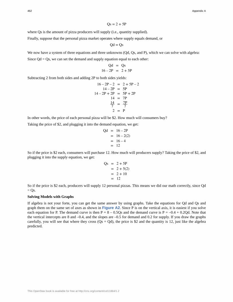
Qs = 2 + 5P
where Qs is the amount of pizza producers will supply (i.e., quantity supplied).
Finally, suppose that the personal pizza market operates where supply equals demand, or
Qd = Qs
We now have a system of three equations and three unknowns (Qd, Qs, and P), which we can solve with algebra:
Since Qd = Qs, we can set the demand and supply equation equal to each other:
Qd = Qs16 – 2P = 2 + 5P
Subtracting 2 from both sides and adding 2P to both sides yields:
16 – 2P – 2 = 2 + 5P – 214 – 2P = 5P
14 – 2P + 2P = 5P + 2P14 = 7P147 = 7P
72 = P
In other words, the price of each personal pizza will be $2. How much will consumers buy?
Taking the price of $2, and plugging it into the demand equation, we get:
Qd = 16 – 2P = 16 – 2(2) = 16 – 4 = 12
So if the price is $2 each, consumers will purchase 12. How much will producers supply? Taking the price of $2, andplugging it into the supply equation, we get:
Qs = 2 + 5P = 2 + 5(2) = 2 + 10 = 12
So if the price is $2 each, producers will supply 12 personal pizzas. This means we did our math correctly, since Qd= Qs.
Solving Models with Graphs
If algebra is not your forte, you can get the same answer by using graphs. Take the equations for Qd and Qs andgraph them on the same set of axes as shown in Figure A2. Since P is on the vertical axis, it is easiest if you solveeach equation for P. The demand curve is then P = 8 – 0.5Qs and the demand curve is P = –0.4 + 0.2Qd. Note thatthe vertical intercepts are 8 and –0.4, and the slopes are –0.5 for demand and 0.2 for supply. If you draw the graphscarefully, you will see that where they cross (Qs = Qd), the price is $2 and the quantity is 12, just like the algebrapredicted.
462 Appendix A
This OpenStax book is available for free at http://cnx.org/content/col11864/1.2
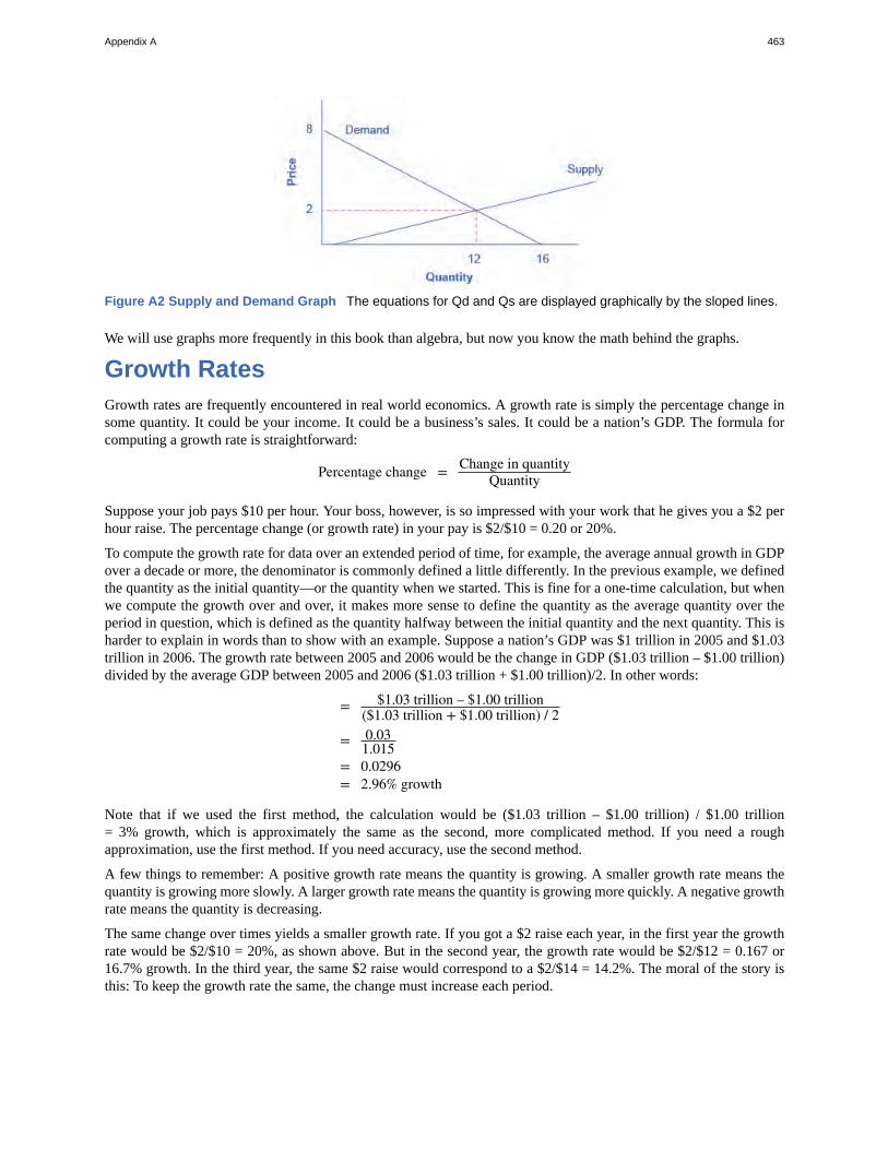
Figure A2 Supply and Demand Graph The equations for Qd and Qs are displayed graphically by the sloped lines.
We will use graphs more frequently in this book than algebra, but now you know the math behind the graphs.
Growth RatesGrowth rates are frequently encountered in real world economics. A growth rate is simply the percentage change insome quantity. It could be your income. It could be a business’s sales. It could be a nation’s GDP. The formula forcomputing a growth rate is straightforward:
Percentage change = Change in quantityQuantity
Suppose your job pays $10 per hour. Your boss, however, is so impressed with your work that he gives you a $2 perhour raise. The percentage change (or growth rate) in your pay is $2/$10 = 0.20 or 20%.
To compute the growth rate for data over an extended period of time, for example, the average annual growth in GDPover a decade or more, the denominator is commonly defined a little differently. In the previous example, we definedthe quantity as the initial quantity—or the quantity when we started. This is fine for a one-time calculation, but whenwe compute the growth over and over, it makes more sense to define the quantity as the average quantity over theperiod in question, which is defined as the quantity halfway between the initial quantity and the next quantity. This isharder to explain in words than to show with an example. Suppose a nation’s GDP was $1 trillion in 2005 and $1.03trillion in 2006. The growth rate between 2005 and 2006 would be the change in GDP ($1.03 trillion – $1.00 trillion)divided by the average GDP between 2005 and 2006 ($1.03 trillion + $1.00 trillion)/2. In other words:
= $1.03 trillion – $1.00 trillion($1.03 trillion + $1.00 trillion) / 2
= 0.031.015
= 0.0296 = 2.96% growth
Note that if we used the first method, the calculation would be ($1.03 trillion – $1.00 trillion) / $1.00 trillion= 3% growth, which is approximately the same as the second, more complicated method. If you need a roughapproximation, use the first method. If you need accuracy, use the second method.
A few things to remember: A positive growth rate means the quantity is growing. A smaller growth rate means thequantity is growing more slowly. A larger growth rate means the quantity is growing more quickly. A negative growthrate means the quantity is decreasing.
The same change over times yields a smaller growth rate. If you got a $2 raise each year, in the first year the growthrate would be $2/$10 = 20%, as shown above. But in the second year, the growth rate would be $2/$12 = 0.167 or16.7% growth. In the third year, the same $2 raise would correspond to a $2/$14 = 14.2%. The moral of the story isthis: To keep the growth rate the same, the change must increase each period.
Appendix A 463
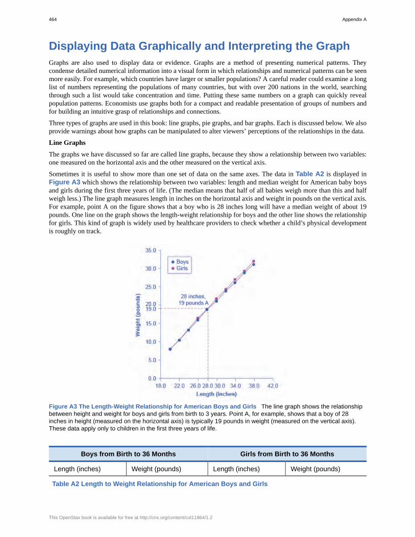
Displaying Data Graphically and Interpreting the GraphGraphs are also used to display data or evidence. Graphs are a method of presenting numerical patterns. Theycondense detailed numerical information into a visual form in which relationships and numerical patterns can be seenmore easily. For example, which countries have larger or smaller populations? A careful reader could examine a longlist of numbers representing the populations of many countries, but with over 200 nations in the world, searchingthrough such a list would take concentration and time. Putting these same numbers on a graph can quickly revealpopulation patterns. Economists use graphs both for a compact and readable presentation of groups of numbers andfor building an intuitive grasp of relationships and connections.
Three types of graphs are used in this book: line graphs, pie graphs, and bar graphs. Each is discussed below. We alsoprovide warnings about how graphs can be manipulated to alter viewers’ perceptions of the relationships in the data.
Line Graphs
The graphs we have discussed so far are called line graphs, because they show a relationship between two variables:one measured on the horizontal axis and the other measured on the vertical axis.
Sometimes it is useful to show more than one set of data on the same axes. The data in Table A2 is displayed inFigure A3 which shows the relationship between two variables: length and median weight for American baby boysand girls during the first three years of life. (The median means that half of all babies weigh more than this and halfweigh less.) The line graph measures length in inches on the horizontal axis and weight in pounds on the vertical axis.For example, point A on the figure shows that a boy who is 28 inches long will have a median weight of about 19pounds. One line on the graph shows the length-weight relationship for boys and the other line shows the relationshipfor girls. This kind of graph is widely used by healthcare providers to check whether a child’s physical developmentis roughly on track.
Figure A3 The Length-Weight Relationship for American Boys and Girls The line graph shows the relationshipbetween height and weight for boys and girls from birth to 3 years. Point A, for example, shows that a boy of 28inches in height (measured on the horizontal axis) is typically 19 pounds in weight (measured on the vertical axis).These data apply only to children in the first three years of life.
Boys from Birth to 36 Months Girls from Birth to 36 Months
Length (inches) Weight (pounds) Length (inches) Weight (pounds)
Table A2 Length to Weight Relationship for American Boys and Girls
464 Appendix A
This OpenStax book is available for free at http://cnx.org/content/col11864/1.2
Boys from Birth to 36 Months Girls from Birth to 36 Months
20.0 8.0 20.0 7.9
22.0 10.5 22.0 10.5
24.0 13.5 24.0 13.2
26.0 16.4 26.0 16.0
28.0 19.0 28.0 18.8
30.0 21.8 30.0 21.2
32.0 24.3 32.0 24.0
34.0 27.0 34.0 26.2
36.0 29.3 36.0 28.9
38.0 32.0 38.0 31.3
Table A2 Length to Weight Relationship for American Boys and Girls
Not all relationships in economics are linear. Sometimes they are curves. Figure A4 presents another example of aline graph, representing the data from Table A3. In this case, the line graph shows how thin the air becomes whenyou climb a mountain. The horizontal axis of the figure shows altitude, measured in meters above sea level. Thevertical axis measures the density of the air at each altitude. Air density is measured by the weight of the air in a cubicmeter of space (that is, a box measuring one meter in height, width, and depth). As the graph shows, air pressure isheaviest at ground level and becomes lighter as you climb. Figure A4 shows that a cubic meter of air at an altitudeof 500 meters weighs approximately one kilogram (about 2.2 pounds). However, as the altitude increases, air densitydecreases. A cubic meter of air at the top of Mount Everest, at about 8,828 meters, would weigh only 0.023 kilograms.The thin air at high altitudes explains why many mountain climbers need to use oxygen tanks as they reach the top ofa mountain.
Appendix A 465
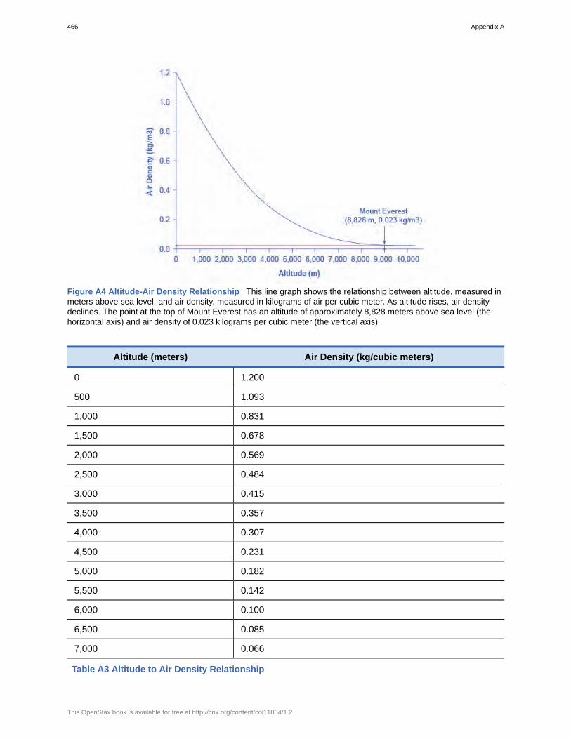
Figure A4 Altitude-Air Density Relationship This line graph shows the relationship between altitude, measured inmeters above sea level, and air density, measured in kilograms of air per cubic meter. As altitude rises, air densitydeclines. The point at the top of Mount Everest has an altitude of approximately 8,828 meters above sea level (thehorizontal axis) and air density of 0.023 kilograms per cubic meter (the vertical axis).
Altitude (meters) Air Density (kg/cubic meters)
0 1.200
500 1.093
1,000 0.831
1,500 0.678
2,000 0.569
2,500 0.484
3,000 0.415
3,500 0.357
4,000 0.307
4,500 0.231
5,000 0.182
5,500 0.142
6,000 0.100
6,500 0.085
7,000 0.066
Table A3 Altitude to Air Density Relationship
466 Appendix A
This OpenStax book is available for free at http://cnx.org/content/col11864/1.2
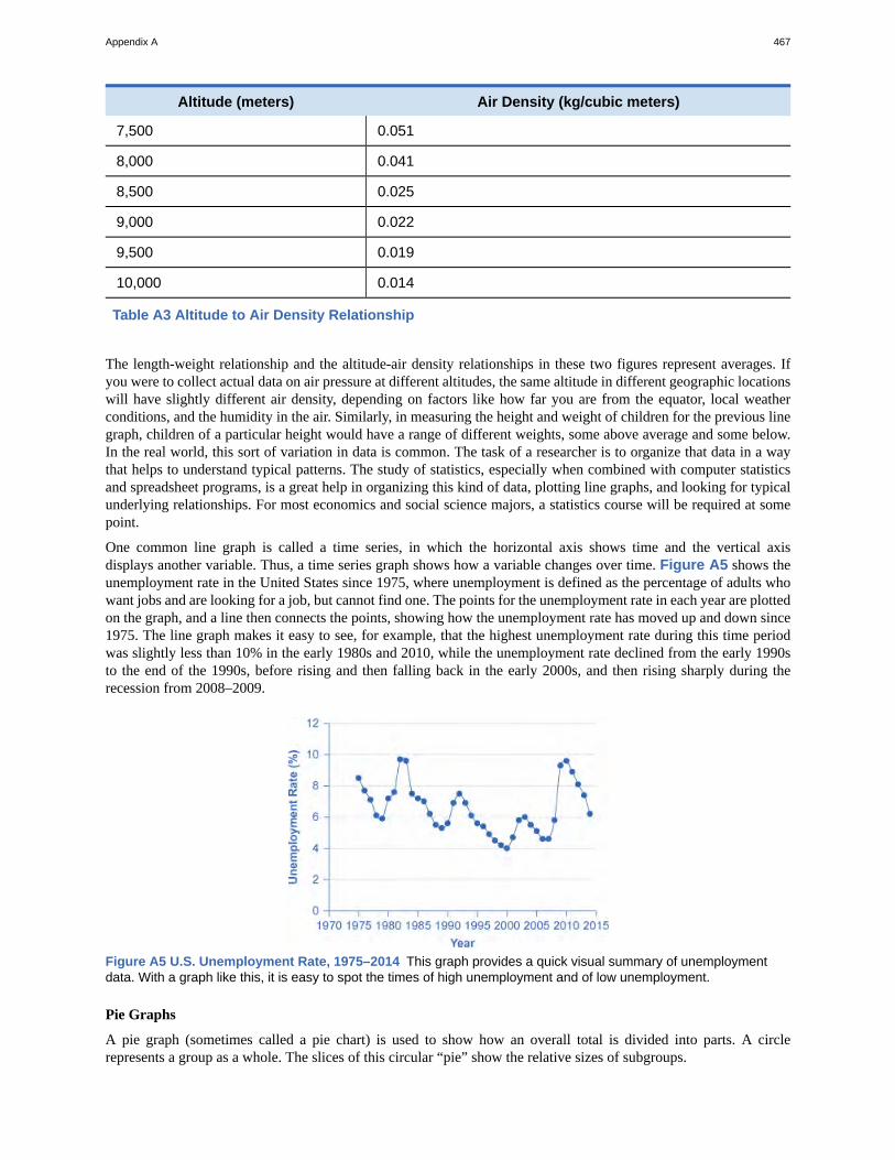
Altitude (meters) Air Density (kg/cubic meters)
7,500 0.051
8,000 0.041
8,500 0.025
9,000 0.022
9,500 0.019
10,000 0.014
Table A3 Altitude to Air Density Relationship
The length-weight relationship and the altitude-air density relationships in these two figures represent averages. Ifyou were to collect actual data on air pressure at different altitudes, the same altitude in different geographic locationswill have slightly different air density, depending on factors like how far you are from the equator, local weatherconditions, and the humidity in the air. Similarly, in measuring the height and weight of children for the previous linegraph, children of a particular height would have a range of different weights, some above average and some below.In the real world, this sort of variation in data is common. The task of a researcher is to organize that data in a waythat helps to understand typical patterns. The study of statistics, especially when combined with computer statisticsand spreadsheet programs, is a great help in organizing this kind of data, plotting line graphs, and looking for typicalunderlying relationships. For most economics and social science majors, a statistics course will be required at somepoint.
One common line graph is called a time series, in which the horizontal axis shows time and the vertical axisdisplays another variable. Thus, a time series graph shows how a variable changes over time. Figure A5 shows theunemployment rate in the United States since 1975, where unemployment is defined as the percentage of adults whowant jobs and are looking for a job, but cannot find one. The points for the unemployment rate in each year are plottedon the graph, and a line then connects the points, showing how the unemployment rate has moved up and down since1975. The line graph makes it easy to see, for example, that the highest unemployment rate during this time periodwas slightly less than 10% in the early 1980s and 2010, while the unemployment rate declined from the early 1990sto the end of the 1990s, before rising and then falling back in the early 2000s, and then rising sharply during therecession from 2008–2009.
Figure A5 U.S. Unemployment Rate, 1975–2014 This graph provides a quick visual summary of unemploymentdata. With a graph like this, it is easy to spot the times of high unemployment and of low unemployment.
Pie Graphs
A pie graph (sometimes called a pie chart) is used to show how an overall total is divided into parts. A circlerepresents a group as a whole. The slices of this circular “pie” show the relative sizes of subgroups.
Appendix A 467
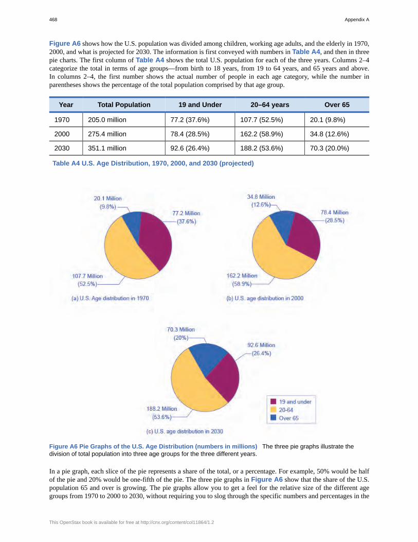
Figure A6 shows how the U.S. population was divided among children, working age adults, and the elderly in 1970,2000, and what is projected for 2030. The information is first conveyed with numbers in Table A4, and then in threepie charts. The first column of Table A4 shows the total U.S. population for each of the three years. Columns 2–4categorize the total in terms of age groups—from birth to 18 years, from 19 to 64 years, and 65 years and above.In columns 2–4, the first number shows the actual number of people in each age category, while the number inparentheses shows the percentage of the total population comprised by that age group.
Year Total Population 19 and Under 20–64 years Over 65
1970 205.0 million 77.2 (37.6%) 107.7 (52.5%) 20.1 (9.8%)
2000 275.4 million 78.4 (28.5%) 162.2 (58.9%) 34.8 (12.6%)
2030 351.1 million 92.6 (26.4%) 188.2 (53.6%) 70.3 (20.0%)
Table A4 U.S. Age Distribution, 1970, 2000, and 2030 (projected)
Figure A6 Pie Graphs of the U.S. Age Distribution (numbers in millions) The three pie graphs illustrate thedivision of total population into three age groups for the three different years.
In a pie graph, each slice of the pie represents a share of the total, or a percentage. For example, 50% would be halfof the pie and 20% would be one-fifth of the pie. The three pie graphs in Figure A6 show that the share of the U.S.population 65 and over is growing. The pie graphs allow you to get a feel for the relative size of the different agegroups from 1970 to 2000 to 2030, without requiring you to slog through the specific numbers and percentages in the
468 Appendix A
This OpenStax book is available for free at http://cnx.org/content/col11864/1.2
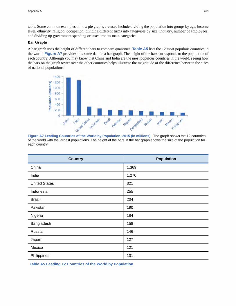
table. Some common examples of how pie graphs are used include dividing the population into groups by age, incomelevel, ethnicity, religion, occupation; dividing different firms into categories by size, industry, number of employees;and dividing up government spending or taxes into its main categories.
Bar Graphs
A bar graph uses the height of different bars to compare quantities. Table A5 lists the 12 most populous countries inthe world. Figure A7 provides this same data in a bar graph. The height of the bars corresponds to the population ofeach country. Although you may know that China and India are the most populous countries in the world, seeing howthe bars on the graph tower over the other countries helps illustrate the magnitude of the difference between the sizesof national populations.
Figure A7 Leading Countries of the World by Population, 2015 (in millions) The graph shows the 12 countriesof the world with the largest populations. The height of the bars in the bar graph shows the size of the population foreach country.
Country Population
China 1,369
India 1,270
United States 321
Indonesia 255
Brazil 204
Pakistan 190
Nigeria 184
Bangladesh 158
Russia 146
Japan 127
Mexico 121
Philippines 101
Table A5 Leading 12 Countries of the World by Population
Appendix A 469
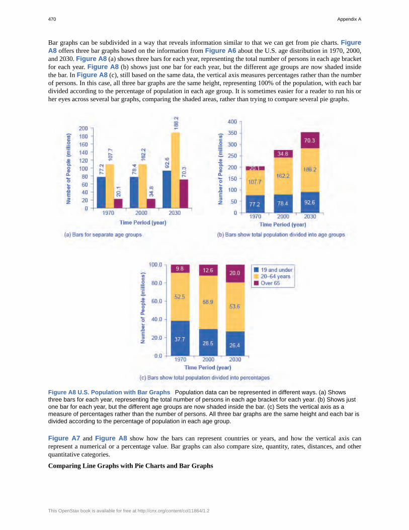
Bar graphs can be subdivided in a way that reveals information similar to that we can get from pie charts. FigureA8 offers three bar graphs based on the information from Figure A6 about the U.S. age distribution in 1970, 2000,and 2030. Figure A8 (a) shows three bars for each year, representing the total number of persons in each age bracketfor each year. Figure A8 (b) shows just one bar for each year, but the different age groups are now shaded insidethe bar. In Figure A8 (c), still based on the same data, the vertical axis measures percentages rather than the numberof persons. In this case, all three bar graphs are the same height, representing 100% of the population, with each bardivided according to the percentage of population in each age group. It is sometimes easier for a reader to run his orher eyes across several bar graphs, comparing the shaded areas, rather than trying to compare several pie graphs.
Figure A8 U.S. Population with Bar Graphs Population data can be represented in different ways. (a) Showsthree bars for each year, representing the total number of persons in each age bracket for each year. (b) Shows justone bar for each year, but the different age groups are now shaded inside the bar. (c) Sets the vertical axis as ameasure of percentages rather than the number of persons. All three bar graphs are the same height and each bar isdivided according to the percentage of population in each age group.
Figure A7 and Figure A8 show how the bars can represent countries or years, and how the vertical axis canrepresent a numerical or a percentage value. Bar graphs can also compare size, quantity, rates, distances, and otherquantitative categories.
Comparing Line Graphs with Pie Charts and Bar Graphs
470 Appendix A
This OpenStax book is available for free at http://cnx.org/content/col11864/1.2
Now that you are familiar with pie graphs, bar graphs, and line graphs, how do you know which graph to use for yourdata? Pie graphs are often better than line graphs at showing how an overall group is divided. However, if a pie graphhas too many slices, it can become difficult to interpret.
Bar graphs are especially useful when comparing quantities. For example, if you are studying the populations ofdifferent countries, as in Figure A7, bar graphs can show the relationships between the population sizes of multiplecountries. Not only can it show these relationships, but it can also show breakdowns of different groups within thepopulation.
A line graph is often the most effective format for illustrating a relationship between two variables that are bothchanging. For example, time series graphs can show patterns as time changes, like the unemployment rate over time.Line graphs are widely used in economics to present continuous data about prices, wages, quantities bought and sold,the size of the economy.
How Graphs Can Be Misleading
Graphs not only reveal patterns; they can also alter how patterns are perceived. To see some of the ways this canbe done, consider the line graphs of Figure A9, Figure A10, and Figure A11. These graphs all illustrate theunemployment rate—but from different perspectives.
Appendix A 471
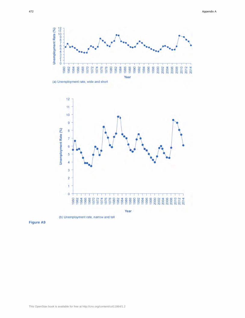
Figure A9
472 Appendix A
This OpenStax book is available for free at http://cnx.org/content/col11864/1.2
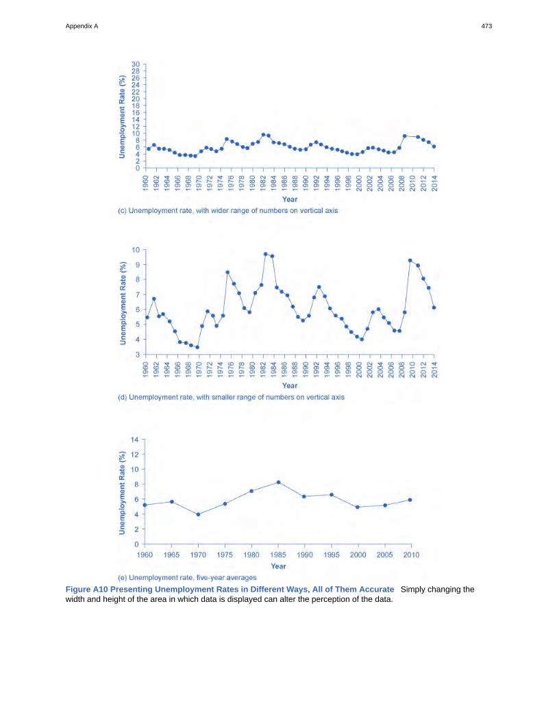
Figure A10 Presenting Unemployment Rates in Different Ways, All of Them Accurate Simply changing thewidth and height of the area in which data is displayed can alter the perception of the data.
Appendix A 473

Figure A11 Presenting Unemployment Rates in Different Ways, All of Them Accurate Simply changing thewidth and height of the area in which data is displayed can alter the perception of the data.
Suppose you wanted a graph which gives the impression that the rise in unemployment in 2009 was not all thatlarge, or all that extraordinary by historical standards. You might choose to present your data as in Figure A9 (a).Figure A9 (a) includes much of the same data presented earlier in Figure A5, but stretches the horizontal axisout longer relative to the vertical axis. By spreading the graph wide and flat, the visual appearance is that the risein unemployment is not so large, and is similar to some past rises in unemployment. Now imagine you wantedto emphasize how unemployment spiked substantially higher in 2009. In this case, using the same data, you canstretch the vertical axis out relative to the horizontal axis, as in Figure A9 (b), which makes all rises and falls inunemployment appear larger.
A similar effect can be accomplished without changing the length of the axes, but by changing the scale on the verticalaxis. In Figure A10 (c), the scale on the vertical axis runs from 0% to 30%, while in Figure A10 (d), the verticalaxis runs from 3% to 10%. Compared to Figure A5, where the vertical scale runs from 0% to 12%, Figure A10 (c)makes the fluctuation in unemployment look smaller, while Figure A10 (d) makes it look larger.
Another way to alter the perception of the graph is to reduce the amount of variation by changing the number of pointsplotted on the graph. Figure A10 (e) shows the unemployment rate according to five-year averages. By averagingout some of the year- to-year changes, the line appears smoother and with fewer highs and lows. In reality, theunemployment rate is reported monthly, and Figure A11 (f) shows the monthly figures since 1960, which fluctuatemore than the five-year average. Figure A11 (f) is also a vivid illustration of how graphs can compress lots ofdata. The graph includes monthly data since 1960, which over almost 50 years, works out to nearly 600 data points.
474 Appendix A
This OpenStax book is available for free at http://cnx.org/content/col11864/1.2
Reading that list of 600 data points in numerical form would be hypnotic. You can, however, get a good intuitivesense of these 600 data points very quickly from the graph.
A final trick in manipulating the perception of graphical information is that, by choosing the starting and endingpoints carefully, you can influence the perception of whether the variable is rising or falling. The original data showa general pattern with unemployment low in the 1960s, but spiking up in the mid-1970s, early 1980s, early 1990s,early 2000s, and late 2000s. Figure A11 (g), however, shows a graph that goes back only to 1975, which gives animpression that unemployment was more-or-less gradually falling over time until the 2009 recession pushed it backup to its “original” level—which is a plausible interpretation if one starts at the high point around 1975.
These kinds of tricks—or shall we just call them “presentation choices”— are not limited to line graphs. In a pie chartwith many small slices and one large slice, someone must decided what categories should be used to produce theseslices in the first place, thus making some slices appear bigger than others. If you are making a bar graph, you canmake the vertical axis either taller or shorter, which will tend to make variations in the height of the bars appear moreor less.
Being able to read graphs is an essential skill, both in economics and in life. A graph is just one perspective or pointof view, shaped by choices such as those discussed in this section. Do not always believe the first quick impressionfrom a graph. View with caution.
Key Concepts and SummaryMath is a tool for understanding economics and economic relationships can be expressed mathematically usingalgebra or graphs. The algebraic equation for a line is y = b + mx, where x is the variable on the horizontal axis andy is the variable on the vertical axis, the b term is the y-intercept and the m term is the slope. The slope of a line isthe same at any point on the line and it indicates the relationship (positive, negative, or zero) between two economicvariables.
Economic models can be solved algebraically or graphically. Graphs allow you to illustrate data visually. Theycan illustrate patterns, comparisons, trends, and apportionment by condensing the numerical data and providing anintuitive sense of relationships in the data. A line graph shows the relationship between two variables: one is shownon the horizontal axis and one on the vertical axis. A pie graph shows how something is allotted, such as a sum ofmoney or a group of people. The size of each slice of the pie is drawn to represent the corresponding percentage ofthe whole. A bar graph uses the height of bars to show a relationship, where each bar represents a certain entity, likea country or a group of people. The bars on a bar graph can also be divided into segments to show subgroups.
Any graph is a single visual perspective on a subject. The impression it leaves will be based on many choices, suchas what data or time frame is included, how data or groups are divided up, the relative size of vertical and horizontalaxes, whether the scale used on a vertical starts at zero. Thus, any graph should be regarded somewhat skeptically,remembering that the underlying relationship can be open to different interpretations.
Review QuestionsExercise A1
Name three kinds of graphs and briefly state when is most appropriate to use each type of graph.
Exercise A2
What is slope on a line graph?
Exercise A3
What do the slices of a pie chart represent?
Exercise A4
Why is a bar chart the best way to illustrate comparisons?
Exercise A5
How does the appearance of positive slope differ from negative slope and from zero slope?
Appendix A 475

476 Appendix A
This OpenStax book is available for free at http://cnx.org/content/col11864/1.2
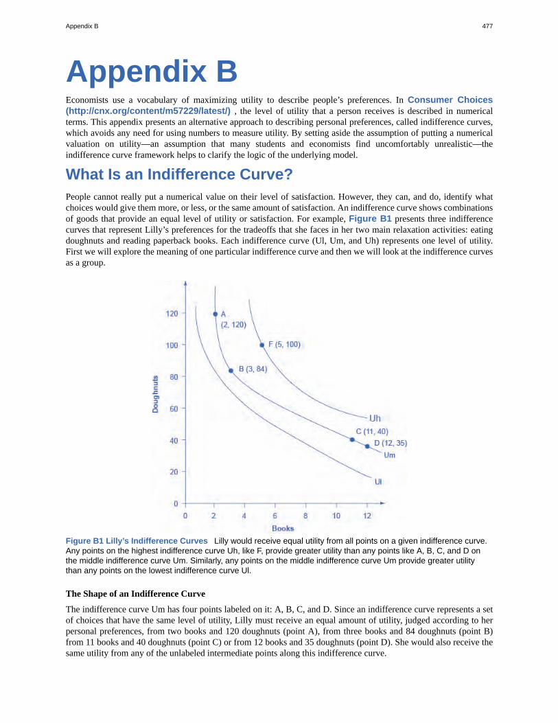
Appendix BEconomists use a vocabulary of maximizing utility to describe people’s preferences. In Consumer Choices(http://cnx.org/content/m57229/latest/) , the level of utility that a person receives is described in numericalterms. This appendix presents an alternative approach to describing personal preferences, called indifference curves,which avoids any need for using numbers to measure utility. By setting aside the assumption of putting a numericalvaluation on utility—an assumption that many students and economists find uncomfortably unrealistic—theindifference curve framework helps to clarify the logic of the underlying model.
What Is an Indifference Curve?People cannot really put a numerical value on their level of satisfaction. However, they can, and do, identify whatchoices would give them more, or less, or the same amount of satisfaction. An indifference curve shows combinationsof goods that provide an equal level of utility or satisfaction. For example, Figure B1 presents three indifferencecurves that represent Lilly’s preferences for the tradeoffs that she faces in her two main relaxation activities: eatingdoughnuts and reading paperback books. Each indifference curve (Ul, Um, and Uh) represents one level of utility.First we will explore the meaning of one particular indifference curve and then we will look at the indifference curvesas a group.
Figure B1 Lilly’s Indifference Curves Lilly would receive equal utility from all points on a given indifference curve.Any points on the highest indifference curve Uh, like F, provide greater utility than any points like A, B, C, and D onthe middle indifference curve Um. Similarly, any points on the middle indifference curve Um provide greater utilitythan any points on the lowest indifference curve Ul.
The Shape of an Indifference Curve
The indifference curve Um has four points labeled on it: A, B, C, and D. Since an indifference curve represents a setof choices that have the same level of utility, Lilly must receive an equal amount of utility, judged according to herpersonal preferences, from two books and 120 doughnuts (point A), from three books and 84 doughnuts (point B)from 11 books and 40 doughnuts (point C) or from 12 books and 35 doughnuts (point D). She would also receive thesame utility from any of the unlabeled intermediate points along this indifference curve.
Appendix B 477
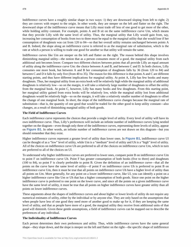
Indifference curves have a roughly similar shape in two ways: 1) they are downward sloping from left to right; 2)they are convex with respect to the origin. In other words, they are steeper on the left and flatter on the right. Thedownward slope of the indifference curve means that Lilly must trade off less of one good to get more of the other,while holding utility constant. For example, points A and B sit on the same indifference curve Um, which meansthat they provide Lilly with the same level of utility. Thus, the marginal utility that Lilly would gain from, say,increasing her consumption of books from two to three must be equal to the marginal utility that she would lose if herconsumption of doughnuts was cut from 120 to 84—so that her overall utility remains unchanged between points Aand B. Indeed, the slope along an indifference curve is referred to as the marginal rate of substitution, which is therate at which a person is willing to trade one good for another so that utility will remain the same.
Indifference curves like Um are steeper on the left and flatter on the right. The reason behind this shape involvesdiminishing marginal utility—the notion that as a person consumes more of a good, the marginal utility from eachadditional unit becomes lower. Compare two different choices between points that all provide Lilly an equal amountof utility along the indifference curve Um: the choice between A and B, and between C and D. In both choices, Lillyconsumes one more book, but between A and B her consumption of doughnuts falls by 36 (from 120 to 84) andbetween C and D it falls by only five (from 40 to 35). The reason for this difference is that points A and C are differentstarting points, and thus have different implications for marginal utility. At point A, Lilly has few books and manydoughnuts. Thus, her marginal utility from an extra book will be relatively high while the marginal utility of additionaldoughnuts is relatively low—so on the margin, it will take a relatively large number of doughnuts to offset the utilityfrom the marginal book. At point C, however, Lilly has many books and few doughnuts. From this starting point,her marginal utility gained from extra books will be relatively low, while the marginal utility lost from additionaldoughnuts would be relatively high—so on the margin, it will take a relatively smaller number of doughnuts to offsetthe change of one marginal book. In short, the slope of the indifference curve changes because the marginal rate ofsubstitution—that is, the quantity of one good that would be traded for the other good to keep utility constant—alsochanges, as a result of diminishing marginal utility of both goods.
The Field of Indifference Curves
Each indifference curve represents the choices that provide a single level of utility. Every level of utility will have itsown indifference curve. Thus, Lilly’s preferences will include an infinite number of indifference curves lying nestledtogether on the diagram—even though only three of the indifference curves, representing three levels of utility, appearon Figure B1. In other words, an infinite number of indifference curves are not drawn on this diagram—but youshould remember that they exist.
Higher indifference curves represent a greater level of utility than lower ones. In Figure B1, indifference curve Ulcan be thought of as a “low” level of utility, while Um is a “medium” level of utility and Uh is a “high” level of utility.All of the choices on indifference curve Uh are preferred to all of the choices on indifference curve Um, which in turnare preferred to all of the choices on Ul.
To understand why higher indifference curves are preferred to lower ones, compare point B on indifference curve Umto point F on indifference curve Uh. Point F has greater consumption of both books (five to three) and doughnuts(100 to 84), so point F is clearly preferable to point B. Given the definition of an indifference curve—that all thepoints on the curve have the same level of utility—if point F on indifference curve Uh is preferred to point B onindifference curve Um, then it must be true that all points on indifference curve Uh have a higher level of utility thanall points on Um. More generally, for any point on a lower indifference curve, like Ul, you can identify a point on ahigher indifference curve like Um or Uh that has a higher consumption of both goods. Since one point on the higherindifference curve is preferred to one point on the lower curve, and since all the points on a given indifference curvehave the same level of utility, it must be true that all points on higher indifference curves have greater utility than allpoints on lower indifference curves.
These arguments about the shapes of indifference curves and about higher or lower levels of utility do not require anynumerical estimates of utility, either by the individual or by anyone else. They are only based on the assumptions thatwhen people have less of one good they need more of another good to make up for it, if they are keeping the samelevel of utility, and that as people have more of a good, the marginal utility they receive from additional units of thatgood will diminish. Given these gentle assumptions, a field of indifference curves can be mapped out to describe thepreferences of any individual.
The Individuality of Indifference Curves
Each person determines their own preferences and utility. Thus, while indifference curves have the same generalshape—they slope down, and the slope is steeper on the left and flatter on the right—the specific shape of indifference
478 Appendix B
This OpenStax book is available for free at http://cnx.org/content/col11864/1.2
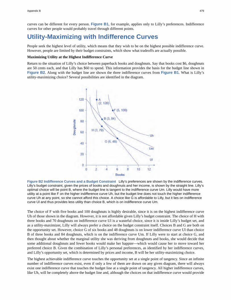
curves can be different for every person. Figure B1, for example, applies only to Lilly’s preferences. Indifferencecurves for other people would probably travel through different points.
Utility-Maximizing with Indifference CurvesPeople seek the highest level of utility, which means that they wish to be on the highest possible indifference curve.However, people are limited by their budget constraints, which show what tradeoffs are actually possible.
Maximizing Utility at the Highest Indifference Curve
Return to the situation of Lilly’s choice between paperback books and doughnuts. Say that books cost $6, doughnutsare 50 cents each, and that Lilly has $60 to spend. This information provides the basis for the budget line shown inFigure B2. Along with the budget line are shown the three indifference curves from Figure B1. What is Lilly’sutility-maximizing choice? Several possibilities are identified in the diagram.
Figure B2 Indifference Curves and a Budget Constraint Lilly’s preferences are shown by the indifference curves.Lilly’s budget constraint, given the prices of books and doughnuts and her income, is shown by the straight line. Lilly’soptimal choice will be point B, where the budget line is tangent to the indifference curve Um. Lilly would have moreutility at a point like F on the higher indifference curve Uh, but the budget line does not touch the higher indifferencecurve Uh at any point, so she cannot afford this choice. A choice like G is affordable to Lilly, but it lies on indifferencecurve Ul and thus provides less utility than choice B, which is on indifference curve Um.
The choice of F with five books and 100 doughnuts is highly desirable, since it is on the highest indifference curveUh of those shown in the diagram. However, it is not affordable given Lilly’s budget constraint. The choice of H withthree books and 70 doughnuts on indifference curve Ul is a wasteful choice, since it is inside Lilly’s budget set, andas a utility-maximizer, Lilly will always prefer a choice on the budget constraint itself. Choices B and G are both onthe opportunity set. However, choice G of six books and 48 doughnuts is on lower indifference curve Ul than choiceB of three books and 84 doughnuts, which is on the indifference curve Um. If Lilly were to start at choice G, andthen thought about whether the marginal utility she was deriving from doughnuts and books, she would decide thatsome additional doughnuts and fewer books would make her happier—which would cause her to move toward herpreferred choice B. Given the combination of Lilly’s personal preferences, as identified by her indifference curves,and Lilly’s opportunity set, which is determined by prices and income, B will be her utility-maximizing choice.
The highest achievable indifference curve touches the opportunity set at a single point of tangency. Since an infinitenumber of indifference curves exist, even if only a few of them are drawn on any given diagram, there will alwaysexist one indifference curve that touches the budget line at a single point of tangency. All higher indifference curves,like Uh, will be completely above the budget line and, although the choices on that indifference curve would provide
Appendix B 479
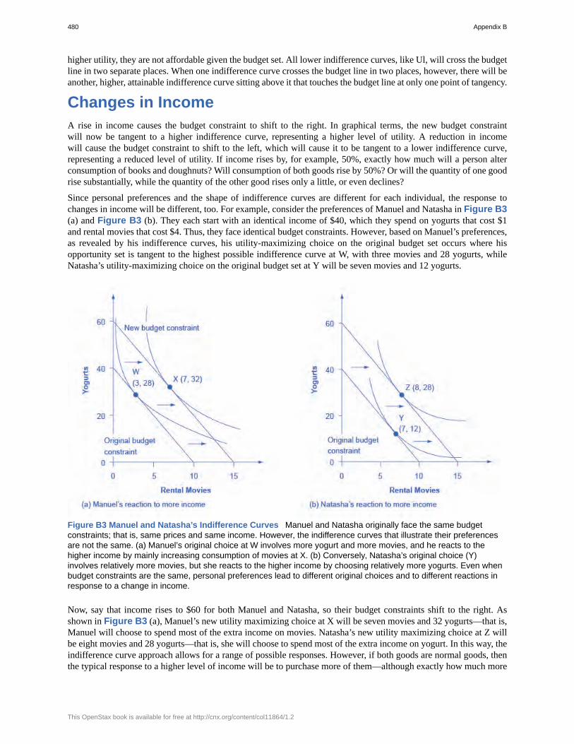
higher utility, they are not affordable given the budget set. All lower indifference curves, like Ul, will cross the budgetline in two separate places. When one indifference curve crosses the budget line in two places, however, there will beanother, higher, attainable indifference curve sitting above it that touches the budget line at only one point of tangency.
Changes in IncomeA rise in income causes the budget constraint to shift to the right. In graphical terms, the new budget constraintwill now be tangent to a higher indifference curve, representing a higher level of utility. A reduction in incomewill cause the budget constraint to shift to the left, which will cause it to be tangent to a lower indifference curve,representing a reduced level of utility. If income rises by, for example, 50%, exactly how much will a person alterconsumption of books and doughnuts? Will consumption of both goods rise by 50%? Or will the quantity of one goodrise substantially, while the quantity of the other good rises only a little, or even declines?
Since personal preferences and the shape of indifference curves are different for each individual, the response tochanges in income will be different, too. For example, consider the preferences of Manuel and Natasha in Figure B3(a) and Figure B3 (b). They each start with an identical income of $40, which they spend on yogurts that cost $1and rental movies that cost $4. Thus, they face identical budget constraints. However, based on Manuel’s preferences,as revealed by his indifference curves, his utility-maximizing choice on the original budget set occurs where hisopportunity set is tangent to the highest possible indifference curve at W, with three movies and 28 yogurts, whileNatasha’s utility-maximizing choice on the original budget set at Y will be seven movies and 12 yogurts.
Figure B3 Manuel and Natasha’s Indifference Curves Manuel and Natasha originally face the same budgetconstraints; that is, same prices and same income. However, the indifference curves that illustrate their preferencesare not the same. (a) Manuel’s original choice at W involves more yogurt and more movies, and he reacts to thehigher income by mainly increasing consumption of movies at X. (b) Conversely, Natasha’s original choice (Y)involves relatively more movies, but she reacts to the higher income by choosing relatively more yogurts. Even whenbudget constraints are the same, personal preferences lead to different original choices and to different reactions inresponse to a change in income.
Now, say that income rises to $60 for both Manuel and Natasha, so their budget constraints shift to the right. Asshown in Figure B3 (a), Manuel’s new utility maximizing choice at X will be seven movies and 32 yogurts—that is,Manuel will choose to spend most of the extra income on movies. Natasha’s new utility maximizing choice at Z willbe eight movies and 28 yogurts—that is, she will choose to spend most of the extra income on yogurt. In this way, theindifference curve approach allows for a range of possible responses. However, if both goods are normal goods, thenthe typical response to a higher level of income will be to purchase more of them—although exactly how much more
480 Appendix B
This OpenStax book is available for free at http://cnx.org/content/col11864/1.2
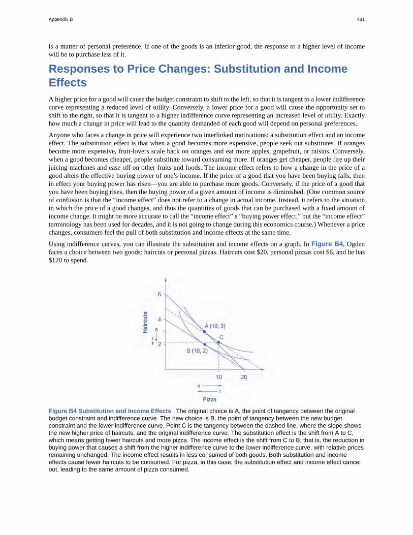
is a matter of personal preference. If one of the goods is an inferior good, the response to a higher level of incomewill be to purchase less of it.
Responses to Price Changes: Substitution and IncomeEffectsA higher price for a good will cause the budget constraint to shift to the left, so that it is tangent to a lower indifferencecurve representing a reduced level of utility. Conversely, a lower price for a good will cause the opportunity set toshift to the right, so that it is tangent to a higher indifference curve representing an increased level of utility. Exactlyhow much a change in price will lead to the quantity demanded of each good will depend on personal preferences.
Anyone who faces a change in price will experience two interlinked motivations: a substitution effect and an incomeeffect. The substitution effect is that when a good becomes more expensive, people seek out substitutes. If orangesbecome more expensive, fruit-lovers scale back on oranges and eat more apples, grapefruit, or raisins. Conversely,when a good becomes cheaper, people substitute toward consuming more. If oranges get cheaper, people fire up theirjuicing machines and ease off on other fruits and foods. The income effect refers to how a change in the price of agood alters the effective buying power of one’s income. If the price of a good that you have been buying falls, thenin effect your buying power has risen—you are able to purchase more goods. Conversely, if the price of a good thatyou have been buying rises, then the buying power of a given amount of income is diminished. (One common sourceof confusion is that the “income effect” does not refer to a change in actual income. Instead, it refers to the situationin which the price of a good changes, and thus the quantities of goods that can be purchased with a fixed amount ofincome change. It might be more accurate to call the “income effect” a “buying power effect,” but the “income effect”terminology has been used for decades, and it is not going to change during this economics course.) Whenever a pricechanges, consumers feel the pull of both substitution and income effects at the same time.
Using indifference curves, you can illustrate the substitution and income effects on a graph. In Figure B4, Ogdenfaces a choice between two goods: haircuts or personal pizzas. Haircuts cost $20, personal pizzas cost $6, and he has$120 to spend.
Figure B4 Substitution and Income Effects The original choice is A, the point of tangency between the originalbudget constraint and indifference curve. The new choice is B, the point of tangency between the new budgetconstraint and the lower indifference curve. Point C is the tangency between the dashed line, where the slope showsthe new higher price of haircuts, and the original indifference curve. The substitution effect is the shift from A to C,which means getting fewer haircuts and more pizza. The income effect is the shift from C to B; that is, the reduction inbuying power that causes a shift from the higher indifference curve to the lower indifference curve, with relative pricesremaining unchanged. The income effect results in less consumed of both goods. Both substitution and incomeeffects cause fewer haircuts to be consumed. For pizza, in this case, the substitution effect and income effect cancelout, leading to the same amount of pizza consumed.
Appendix B 481
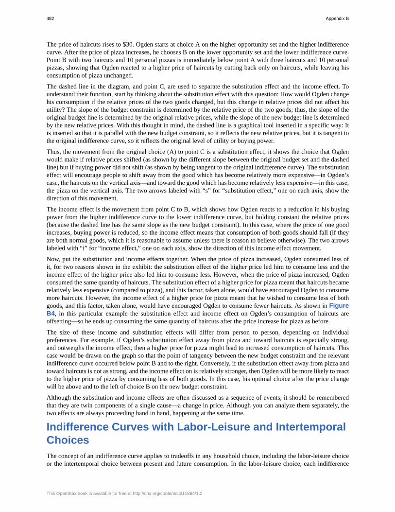
The price of haircuts rises to $30. Ogden starts at choice A on the higher opportunity set and the higher indifferencecurve. After the price of pizza increases, he chooses B on the lower opportunity set and the lower indifference curve.Point B with two haircuts and 10 personal pizzas is immediately below point A with three haircuts and 10 personalpizzas, showing that Ogden reacted to a higher price of haircuts by cutting back only on haircuts, while leaving hisconsumption of pizza unchanged.
The dashed line in the diagram, and point C, are used to separate the substitution effect and the income effect. Tounderstand their function, start by thinking about the substitution effect with this question: How would Ogden changehis consumption if the relative prices of the two goods changed, but this change in relative prices did not affect hisutility? The slope of the budget constraint is determined by the relative price of the two goods; thus, the slope of theoriginal budget line is determined by the original relative prices, while the slope of the new budget line is determinedby the new relative prices. With this thought in mind, the dashed line is a graphical tool inserted in a specific way: Itis inserted so that it is parallel with the new budget constraint, so it reflects the new relative prices, but it is tangent tothe original indifference curve, so it reflects the original level of utility or buying power.
Thus, the movement from the original choice (A) to point C is a substitution effect; it shows the choice that Ogdenwould make if relative prices shifted (as shown by the different slope between the original budget set and the dashedline) but if buying power did not shift (as shown by being tangent to the original indifference curve). The substitutioneffect will encourage people to shift away from the good which has become relatively more expensive—in Ogden’scase, the haircuts on the vertical axis—and toward the good which has become relatively less expensive—in this case,the pizza on the vertical axis. The two arrows labeled with “s” for “substitution effect,” one on each axis, show thedirection of this movement.
The income effect is the movement from point C to B, which shows how Ogden reacts to a reduction in his buyingpower from the higher indifference curve to the lower indifference curve, but holding constant the relative prices(because the dashed line has the same slope as the new budget constraint). In this case, where the price of one goodincreases, buying power is reduced, so the income effect means that consumption of both goods should fall (if theyare both normal goods, which it is reasonable to assume unless there is reason to believe otherwise). The two arrowslabeled with “i” for “income effect,” one on each axis, show the direction of this income effect movement.
Now, put the substitution and income effects together. When the price of pizza increased, Ogden consumed less ofit, for two reasons shown in the exhibit: the substitution effect of the higher price led him to consume less and theincome effect of the higher price also led him to consume less. However, when the price of pizza increased, Ogdenconsumed the same quantity of haircuts. The substitution effect of a higher price for pizza meant that haircuts becamerelatively less expensive (compared to pizza), and this factor, taken alone, would have encouraged Ogden to consumemore haircuts. However, the income effect of a higher price for pizza meant that he wished to consume less of bothgoods, and this factor, taken alone, would have encouraged Ogden to consume fewer haircuts. As shown in FigureB4, in this particular example the substitution effect and income effect on Ogden’s consumption of haircuts areoffsetting—so he ends up consuming the same quantity of haircuts after the price increase for pizza as before.
The size of these income and substitution effects will differ from person to person, depending on individualpreferences. For example, if Ogden’s substitution effect away from pizza and toward haircuts is especially strong,and outweighs the income effect, then a higher price for pizza might lead to increased consumption of haircuts. Thiscase would be drawn on the graph so that the point of tangency between the new budget constraint and the relevantindifference curve occurred below point B and to the right. Conversely, if the substitution effect away from pizza andtoward haircuts is not as strong, and the income effect on is relatively stronger, then Ogden will be more likely to reactto the higher price of pizza by consuming less of both goods. In this case, his optimal choice after the price changewill be above and to the left of choice B on the new budget constraint.
Although the substitution and income effects are often discussed as a sequence of events, it should be rememberedthat they are twin components of a single cause—a change in price. Although you can analyze them separately, thetwo effects are always proceeding hand in hand, happening at the same time.
Indifference Curves with Labor-Leisure and IntertemporalChoicesThe concept of an indifference curve applies to tradeoffs in any household choice, including the labor-leisure choiceor the intertemporal choice between present and future consumption. In the labor-leisure choice, each indifference
482 Appendix B
This OpenStax book is available for free at http://cnx.org/content/col11864/1.2
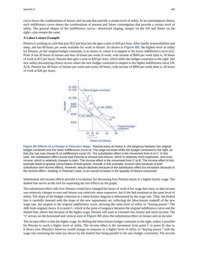
curve shows the combinations of leisure and income that provide a certain level of utility. In an intertemporal choice,each indifference curve shows the combinations of present and future consumption that provide a certain level ofutility. The general shapes of the indifference curves—downward sloping, steeper on the left and flatter on theright—also remain the same.
A Labor-Leisure Example
Petunia is working at a job that pays $12 per hour but she gets a raise to $20 per hour. After family responsibilities andsleep, she has 80 hours per week available for work or leisure. As shown in Figure B5, the highest level of utilityfor Petunia, on her original budget constraint, is at choice A, where it is tangent to the lower indifference curve (Ul).Point A has 30 hours of leisure and thus 50 hours per week of work, with income of $600 per week (that is, 50 hoursof work at $12 per hour). Petunia then gets a raise to $20 per hour, which shifts her budget constraint to the right. Hernew utility-maximizing choice occurs where the new budget constraint is tangent to the higher indifference curve Uh.At B, Petunia has 40 hours of leisure per week and works 40 hours, with income of $800 per week (that is, 40 hoursof work at $20 per hour).
Figure B5 Effects of a Change in Petunia’s Wage Petunia starts at choice A, the tangency between her originalbudget constraint and the lower indifference curve Ul. The wage increase shifts her budget constraint to the right, sothat she can now choose B on indifference curve Uh. The substitution effect is the movement from A to C. In thiscase, the substitution effect would lead Petunia to choose less leisure, which is relatively more expensive, and moreincome, which is relatively cheaper to earn. The income effect is the movement from C to B. The income effect in thisexample leads to greater consumption of both goods. Overall, in this example, income rises because of bothsubstitution and income effects. However, leisure declines because of the substitution effect but increases because ofthe income effect—leading, in Petunia’s case, to an overall increase in the quantity of leisure consumed.
Substitution and income effects provide a vocabulary for discussing how Petunia reacts to a higher hourly wage. Thedashed line serves as the tool for separating the two effects on the graph.
The substitution effect tells how Petunia would have changed her hours of work if her wage had risen, so that incomewas relatively cheaper to earn and leisure was relatively more expensive, but if she had remained at the same level ofutility. The slope of the budget constraint in a labor-leisure diagram is determined by the wage rate. Thus, the dashedline is carefully inserted with the slope of the new opportunity set, reflecting the labor-leisure tradeoff of the newwage rate, but tangent to the original indifference curve, showing the same level of utility or “buying power.” Theshift from original choice A to point C, which is the point of tangency between the original indifference curve and thedashed line, shows that because of the higher wage, Petunia will want to consume less leisure and more income. The“s” arrows on the horizontal and vertical axes of Figure B5 show the substitution effect on leisure and on income.
The income effect is that the higher wage, by shifting the labor-leisure budget constraint to the right, makes it possiblefor Petunia to reach a higher level of utility. The income effect is the movement from point C to point B; that is,it shows how Petunia’s behavior would change in response to a higher level of utility or “buying power,” with thewage rate remaining the same (as shown by the dashed line being parallel to the new budget constraint). The income
Appendix B 483
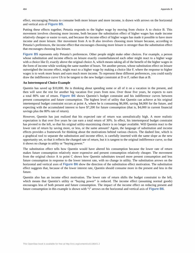
effect, encouraging Petunia to consume both more leisure and more income, is drawn with arrows on the horizontaland vertical axis of Figure B5.
Putting these effects together, Petunia responds to the higher wage by moving from choice A to choice B. Thismovement involves choosing more income, both because the substitution effect of higher wages has made incomerelatively cheaper or easier to earn, and because the income effect of higher wages has made it possible to have moreincome and more leisure. Her movement from A to B also involves choosing more leisure because, according toPetunia’s preferences, the income effect that encourages choosing more leisure is stronger than the substitution effectthat encourages choosing less leisure.
Figure B5 represents only Petunia’s preferences. Other people might make other choices. For example, a personwhose substitution and income effects on leisure exactly counterbalanced each other might react to a higher wagewith a choice like D, exactly above the original choice A, which means taking all of the benefit of the higher wages inthe form of income while working the same number of hours. Yet another person, whose substitution effect on leisureoutweighed the income effect, might react to a higher wage by making a choice like F, where the response to higherwages is to work more hours and earn much more income. To represent these different preferences, you could easilydraw the indifference curve Uh to be tangent to the new budget constraint at D or F, rather than at B.
An Intertemporal Choice Example
Quentin has saved up $10,000. He is thinking about spending some or all of it on a vacation in the present, andthen will save the rest for another big vacation five years from now. Over those five years, he expects to earna total 80% rate of return. Figure B6 shows Quentin’s budget constraint and his indifference curves betweenpresent consumption and future consumption. The highest level of utility that Quentin can achieve at his originalintertemporal budget constraint occurs at point A, where he is consuming $6,000, saving $4,000 for the future, andexpecting with the accumulated interest to have $7,200 for future consumption (that is, $4,000 in current financialsavings plus the 80% rate of return).
However, Quentin has just realized that his expected rate of return was unrealistically high. A more realisticexpectation is that over five years he can earn a total return of 30%. In effect, his intertemporal budget constrainthas pivoted to the left, so that his original utility-maximizing choice is no longer available. Will Quentin react to thelower rate of return by saving more, or less, or the same amount? Again, the language of substitution and incomeeffects provides a framework for thinking about the motivations behind various choices. The dashed line, which isa graphical tool to separate the substitution and income effect, is carefully inserted with the same slope as the newopportunity set, so that it reflects the changed rate of return, but it is tangent to the original indifference curve, so thatit shows no change in utility or “buying power.”
The substitution effect tells how Quentin would have altered his consumption because the lower rate of returnmakes future consumption relatively more expensive and present consumption relatively cheaper. The movementfrom the original choice A to point C shows how Quentin substitutes toward more present consumption and lessfuture consumption in response to the lower interest rate, with no change in utility. The substitution arrows on thehorizontal and vertical axes of Figure B6 show the direction of the substitution effect motivation. The substitutioneffect suggests that, because of the lower interest rate, Quentin should consume more in the present and less in thefuture.
Quentin also has an income effect motivation. The lower rate of return shifts the budget constraint to the left,which means that Quentin’s utility or “buying power” is reduced. The income effect (assuming normal goods)encourages less of both present and future consumption. The impact of the income effect on reducing present andfuture consumption in this example is shown with “i” arrows on the horizontal and vertical axis of Figure B6.
484 Appendix B
This OpenStax book is available for free at http://cnx.org/content/col11864/1.2
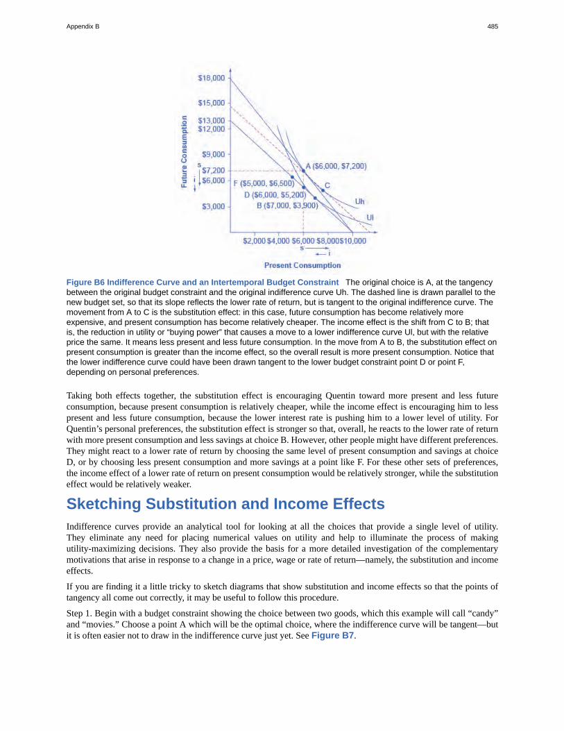
Figure B6 Indifference Curve and an Intertemporal Budget Constraint The original choice is A, at the tangencybetween the original budget constraint and the original indifference curve Uh. The dashed line is drawn parallel to thenew budget set, so that its slope reflects the lower rate of return, but is tangent to the original indifference curve. Themovement from A to C is the substitution effect: in this case, future consumption has become relatively moreexpensive, and present consumption has become relatively cheaper. The income effect is the shift from C to B; thatis, the reduction in utility or “buying power” that causes a move to a lower indifference curve Ul, but with the relativeprice the same. It means less present and less future consumption. In the move from A to B, the substitution effect onpresent consumption is greater than the income effect, so the overall result is more present consumption. Notice thatthe lower indifference curve could have been drawn tangent to the lower budget constraint point D or point F,depending on personal preferences.
Taking both effects together, the substitution effect is encouraging Quentin toward more present and less futureconsumption, because present consumption is relatively cheaper, while the income effect is encouraging him to lesspresent and less future consumption, because the lower interest rate is pushing him to a lower level of utility. ForQuentin’s personal preferences, the substitution effect is stronger so that, overall, he reacts to the lower rate of returnwith more present consumption and less savings at choice B. However, other people might have different preferences.They might react to a lower rate of return by choosing the same level of present consumption and savings at choiceD, or by choosing less present consumption and more savings at a point like F. For these other sets of preferences,the income effect of a lower rate of return on present consumption would be relatively stronger, while the substitutioneffect would be relatively weaker.
Sketching Substitution and Income EffectsIndifference curves provide an analytical tool for looking at all the choices that provide a single level of utility.They eliminate any need for placing numerical values on utility and help to illuminate the process of makingutility-maximizing decisions. They also provide the basis for a more detailed investigation of the complementarymotivations that arise in response to a change in a price, wage or rate of return—namely, the substitution and incomeeffects.
If you are finding it a little tricky to sketch diagrams that show substitution and income effects so that the points oftangency all come out correctly, it may be useful to follow this procedure.
Step 1. Begin with a budget constraint showing the choice between two goods, which this example will call “candy”and “movies.” Choose a point A which will be the optimal choice, where the indifference curve will be tangent—butit is often easier not to draw in the indifference curve just yet. See Figure B7.
Appendix B 485
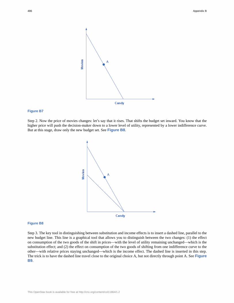
Figure B7
Step 2. Now the price of movies changes: let’s say that it rises. That shifts the budget set inward. You know that thehigher price will push the decision-maker down to a lower level of utility, represented by a lower indifference curve.But at this stage, draw only the new budget set. See Figure B8.
Figure B8
Step 3. The key tool in distinguishing between substitution and income effects is to insert a dashed line, parallel to thenew budget line. This line is a graphical tool that allows you to distinguish between the two changes: (1) the effecton consumption of the two goods of the shift in prices—with the level of utility remaining unchanged—which is thesubstitution effect; and (2) the effect on consumption of the two goods of shifting from one indifference curve to theother—with relative prices staying unchanged—which is the income effect. The dashed line is inserted in this step.The trick is to have the dashed line travel close to the original choice A, but not directly through point A. See FigureB9.
486 Appendix B
This OpenStax book is available for free at http://cnx.org/content/col11864/1.2
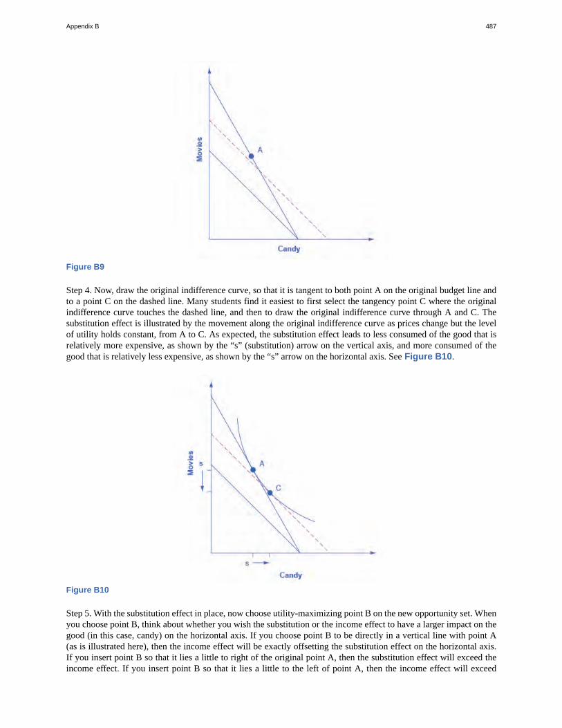
Figure B9
Step 4. Now, draw the original indifference curve, so that it is tangent to both point A on the original budget line andto a point C on the dashed line. Many students find it easiest to first select the tangency point C where the originalindifference curve touches the dashed line, and then to draw the original indifference curve through A and C. Thesubstitution effect is illustrated by the movement along the original indifference curve as prices change but the levelof utility holds constant, from A to C. As expected, the substitution effect leads to less consumed of the good that isrelatively more expensive, as shown by the “s” (substitution) arrow on the vertical axis, and more consumed of thegood that is relatively less expensive, as shown by the “s” arrow on the horizontal axis. See Figure B10.
Figure B10
Step 5. With the substitution effect in place, now choose utility-maximizing point B on the new opportunity set. Whenyou choose point B, think about whether you wish the substitution or the income effect to have a larger impact on thegood (in this case, candy) on the horizontal axis. If you choose point B to be directly in a vertical line with point A(as is illustrated here), then the income effect will be exactly offsetting the substitution effect on the horizontal axis.If you insert point B so that it lies a little to right of the original point A, then the substitution effect will exceed theincome effect. If you insert point B so that it lies a little to the left of point A, then the income effect will exceed
Appendix B 487
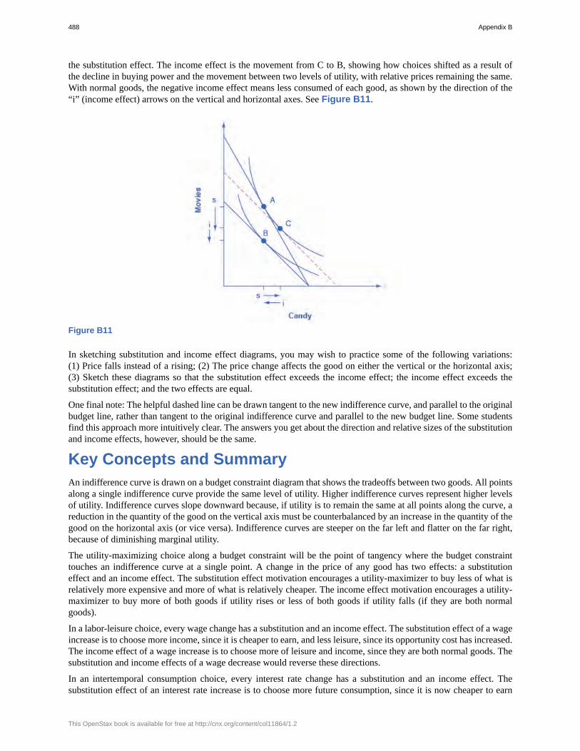
the substitution effect. The income effect is the movement from C to B, showing how choices shifted as a result ofthe decline in buying power and the movement between two levels of utility, with relative prices remaining the same.With normal goods, the negative income effect means less consumed of each good, as shown by the direction of the“i” (income effect) arrows on the vertical and horizontal axes. See Figure B11.
Figure B11
In sketching substitution and income effect diagrams, you may wish to practice some of the following variations:(1) Price falls instead of a rising; (2) The price change affects the good on either the vertical or the horizontal axis;(3) Sketch these diagrams so that the substitution effect exceeds the income effect; the income effect exceeds thesubstitution effect; and the two effects are equal.
One final note: The helpful dashed line can be drawn tangent to the new indifference curve, and parallel to the originalbudget line, rather than tangent to the original indifference curve and parallel to the new budget line. Some studentsfind this approach more intuitively clear. The answers you get about the direction and relative sizes of the substitutionand income effects, however, should be the same.
Key Concepts and SummaryAn indifference curve is drawn on a budget constraint diagram that shows the tradeoffs between two goods. All pointsalong a single indifference curve provide the same level of utility. Higher indifference curves represent higher levelsof utility. Indifference curves slope downward because, if utility is to remain the same at all points along the curve, areduction in the quantity of the good on the vertical axis must be counterbalanced by an increase in the quantity of thegood on the horizontal axis (or vice versa). Indifference curves are steeper on the far left and flatter on the far right,because of diminishing marginal utility.
The utility-maximizing choice along a budget constraint will be the point of tangency where the budget constrainttouches an indifference curve at a single point. A change in the price of any good has two effects: a substitutioneffect and an income effect. The substitution effect motivation encourages a utility-maximizer to buy less of what isrelatively more expensive and more of what is relatively cheaper. The income effect motivation encourages a utility-maximizer to buy more of both goods if utility rises or less of both goods if utility falls (if they are both normalgoods).
In a labor-leisure choice, every wage change has a substitution and an income effect. The substitution effect of a wageincrease is to choose more income, since it is cheaper to earn, and less leisure, since its opportunity cost has increased.The income effect of a wage increase is to choose more of leisure and income, since they are both normal goods. Thesubstitution and income effects of a wage decrease would reverse these directions.
In an intertemporal consumption choice, every interest rate change has a substitution and an income effect. Thesubstitution effect of an interest rate increase is to choose more future consumption, since it is now cheaper to earn
488 Appendix B
This OpenStax book is available for free at http://cnx.org/content/col11864/1.2
future consumption and less present consumption (more savings), since the opportunity cost of present consumptionin terms of what is being given up in the future has increased. The income effect of an interest rate increase is tochoose more of both present and future consumption, since they are both normal goods. The substitution and incomeeffects of an interest rate decrease would reverse these directions.
Review QuestionsExercise B1
What point is preferred along an indifference curve?
Exercise B2
Why do indifference curves slope down?
Exercise B3
Why are indifference curves steep on the left and flatter on the right?
Exercise B4
How many indifference curves does a person have?
Exercise B5
How can you tell which indifference curves represent higher or lower levels of utility?
Exercise B6
What is a substitution effect?
Exercise B7
What is an income effect?
Exercise B8
Does the “income effect” involve a change in income? Explain.
Exercise B9
Does a change in price have both an income effect and a substitution effect? Does a change in income have both anincome effect and a substitution effect?
Exercise B10
Would you expect, in some cases, to see only an income effect or only a substitution effect? Explain.
Exercise B11
Which is larger, the income effect or the substitution effect?
Appendix B 489

490 Appendix B
This OpenStax book is available for free at http://cnx.org/content/col11864/1.2
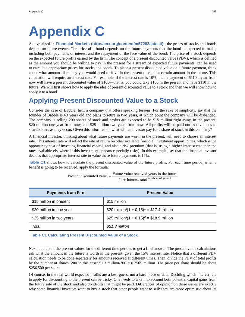
Appendix CAs explained in Financial Markets (http://cnx.org/content/m57283/latest/) , the prices of stocks and bondsdepend on future events. The price of a bond depends on the future payments that the bond is expected to make,including both payments of interest and the repayment of the face value of the bond. The price of a stock dependson the expected future profits earned by the firm. The concept of a present discounted value (PDV), which is definedas the amount you should be willing to pay in the present for a stream of expected future payments, can be usedto calculate appropriate prices for stocks and bonds. To place a present discounted value on a future payment, thinkabout what amount of money you would need to have in the present to equal a certain amount in the future. Thiscalculation will require an interest rate. For example, if the interest rate is 10%, then a payment of $110 a year fromnow will have a present discounted value of $100—that is, you could take $100 in the present and have $110 in thefuture. We will first shows how to apply the idea of present discounted value to a stock and then we will show how toapply it to a bond.
Applying Present Discounted Value to a StockConsider the case of Babble, Inc., a company that offers speaking lessons. For the sake of simplicity, say that thefounder of Babble is 63 years old and plans to retire in two years, at which point the company will be disbanded.The company is selling 200 shares of stock and profits are expected to be $15 million right away, in the present,$20 million one year from now, and $25 million two years from now. All profits will be paid out as dividends toshareholders as they occur. Given this information, what will an investor pay for a share of stock in this company?
A financial investor, thinking about what future payments are worth in the present, will need to choose an interestrate. This interest rate will reflect the rate of return on other available financial investment opportunities, which is theopportunity cost of investing financial capital, and also a risk premium (that is, using a higher interest rate than therates available elsewhere if this investment appears especially risky). In this example, say that the financial investordecides that appropriate interest rate to value these future payments is 15%.
Table C1 shows how to calculate the present discounted value of the future profits. For each time period, when abenefit is going to be received, apply the formula:
Present discounted value = Future value received years in the future(1 + Interest rate)numbers of years t
Payments from Firm Present Value
$15 million in present $15 million
$20 million in one year $20 million/(1 + 0.15)1 = $17.4 million
$25 million in two years $25 million/(1 + 0.15)2 = $18.9 million
Total $51.3 million
Table C1 Calculating Present Discounted Value of a Stock
Next, add up all the present values for the different time periods to get a final answer. The present value calculationsask what the amount in the future is worth in the present, given the 15% interest rate. Notice that a different PDVcalculation needs to be done separately for amounts received at different times. Then, divide the PDV of total profitsby the number of shares, 200 in this case: 51.3 million/200 = 0.2565 million. The price per share should be about$256,500 per share.
Of course, in the real world expected profits are a best guess, not a hard piece of data. Deciding which interest rateto apply for discounting to the present can be tricky. One needs to take into account both potential capital gains fromthe future sale of the stock and also dividends that might be paid. Differences of opinion on these issues are exactlywhy some financial investors want to buy a stock that other people want to sell: they are more optimistic about its
Appendix C 491
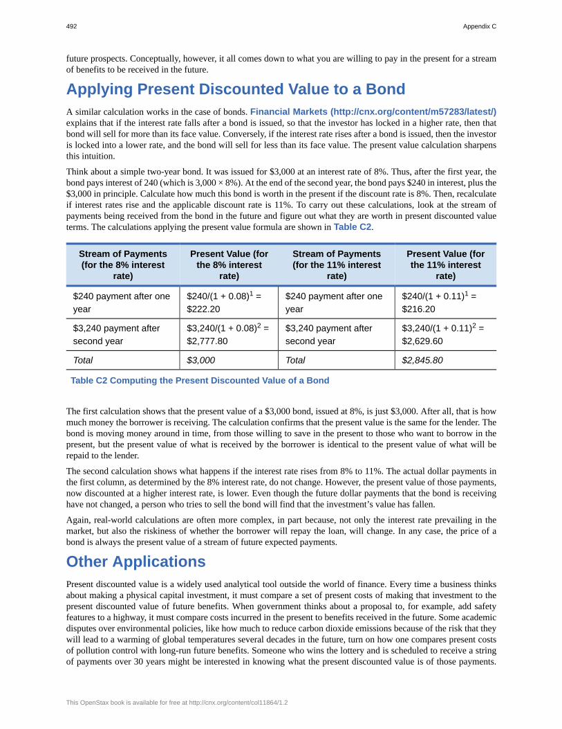
future prospects. Conceptually, however, it all comes down to what you are willing to pay in the present for a streamof benefits to be received in the future.
Applying Present Discounted Value to a BondA similar calculation works in the case of bonds. Financial Markets (http://cnx.org/content/m57283/latest/)explains that if the interest rate falls after a bond is issued, so that the investor has locked in a higher rate, then thatbond will sell for more than its face value. Conversely, if the interest rate rises after a bond is issued, then the investoris locked into a lower rate, and the bond will sell for less than its face value. The present value calculation sharpensthis intuition.
Think about a simple two-year bond. It was issued for $3,000 at an interest rate of 8%. Thus, after the first year, thebond pays interest of 240 (which is 3,000 × 8%). At the end of the second year, the bond pays $240 in interest, plus the$3,000 in principle. Calculate how much this bond is worth in the present if the discount rate is 8%. Then, recalculateif interest rates rise and the applicable discount rate is 11%. To carry out these calculations, look at the stream ofpayments being received from the bond in the future and figure out what they are worth in present discounted valueterms. The calculations applying the present value formula are shown in Table C2.
Stream of Payments(for the 8% interest
rate)
Present Value (forthe 8% interest
rate)
Stream of Payments(for the 11% interest
rate)
Present Value (forthe 11% interest
rate)
$240 payment after oneyear
$240/(1 + 0.08)1 =$222.20
$240 payment after oneyear
$240/(1 + 0.11)1 =$216.20
$3,240 payment aftersecond year
$3,240/(1 + 0.08)2 =$2,777.80
$3,240 payment aftersecond year
$3,240/(1 + 0.11)2 =$2,629.60
Total $3,000 Total $2,845.80
Table C2 Computing the Present Discounted Value of a Bond
The first calculation shows that the present value of a $3,000 bond, issued at 8%, is just $3,000. After all, that is howmuch money the borrower is receiving. The calculation confirms that the present value is the same for the lender. Thebond is moving money around in time, from those willing to save in the present to those who want to borrow in thepresent, but the present value of what is received by the borrower is identical to the present value of what will berepaid to the lender.
The second calculation shows what happens if the interest rate rises from 8% to 11%. The actual dollar payments inthe first column, as determined by the 8% interest rate, do not change. However, the present value of those payments,now discounted at a higher interest rate, is lower. Even though the future dollar payments that the bond is receivinghave not changed, a person who tries to sell the bond will find that the investment’s value has fallen.
Again, real-world calculations are often more complex, in part because, not only the interest rate prevailing in themarket, but also the riskiness of whether the borrower will repay the loan, will change. In any case, the price of abond is always the present value of a stream of future expected payments.
Other ApplicationsPresent discounted value is a widely used analytical tool outside the world of finance. Every time a business thinksabout making a physical capital investment, it must compare a set of present costs of making that investment to thepresent discounted value of future benefits. When government thinks about a proposal to, for example, add safetyfeatures to a highway, it must compare costs incurred in the present to benefits received in the future. Some academicdisputes over environmental policies, like how much to reduce carbon dioxide emissions because of the risk that theywill lead to a warming of global temperatures several decades in the future, turn on how one compares present costsof pollution control with long-run future benefits. Someone who wins the lottery and is scheduled to receive a stringof payments over 30 years might be interested in knowing what the present discounted value is of those payments.
492 Appendix C
This OpenStax book is available for free at http://cnx.org/content/col11864/1.2

Whenever a string of costs and benefits stretches from the present into different times in the future, present discountedvalue becomes an indispensable tool of analysis.
Appendix C 493

494 Appendix C
This OpenStax book is available for free at http://cnx.org/content/col11864/1.2
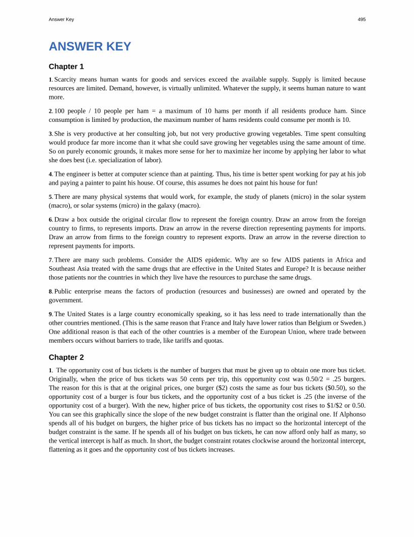
ANSWER KEYChapter 11. Scarcity means human wants for goods and services exceed the available supply. Supply is limited becauseresources are limited. Demand, however, is virtually unlimited. Whatever the supply, it seems human nature to wantmore.
2. 100 people / 10 people per ham = a maximum of 10 hams per month if all residents produce ham. Sinceconsumption is limited by production, the maximum number of hams residents could consume per month is 10.
3. She is very productive at her consulting job, but not very productive growing vegetables. Time spent consultingwould produce far more income than it what she could save growing her vegetables using the same amount of time.So on purely economic grounds, it makes more sense for her to maximize her income by applying her labor to whatshe does best (i.e. specialization of labor).
4. The engineer is better at computer science than at painting. Thus, his time is better spent working for pay at his joband paying a painter to paint his house. Of course, this assumes he does not paint his house for fun!
5. There are many physical systems that would work, for example, the study of planets (micro) in the solar system(macro), or solar systems (micro) in the galaxy (macro).
6. Draw a box outside the original circular flow to represent the foreign country. Draw an arrow from the foreigncountry to firms, to represents imports. Draw an arrow in the reverse direction representing payments for imports.Draw an arrow from firms to the foreign country to represent exports. Draw an arrow in the reverse direction torepresent payments for imports.
7. There are many such problems. Consider the AIDS epidemic. Why are so few AIDS patients in Africa andSoutheast Asia treated with the same drugs that are effective in the United States and Europe? It is because neitherthose patients nor the countries in which they live have the resources to purchase the same drugs.
8. Public enterprise means the factors of production (resources and businesses) are owned and operated by thegovernment.
9. The United States is a large country economically speaking, so it has less need to trade internationally than theother countries mentioned. (This is the same reason that France and Italy have lower ratios than Belgium or Sweden.)One additional reason is that each of the other countries is a member of the European Union, where trade betweenmembers occurs without barriers to trade, like tariffs and quotas.
Chapter 21. The opportunity cost of bus tickets is the number of burgers that must be given up to obtain one more bus ticket.Originally, when the price of bus tickets was 50 cents per trip, this opportunity cost was 0.50/2 = .25 burgers.The reason for this is that at the original prices, one burger ($2) costs the same as four bus tickets ($0.50), so theopportunity cost of a burger is four bus tickets, and the opportunity cost of a bus ticket is .25 (the inverse of theopportunity cost of a burger). With the new, higher price of bus tickets, the opportunity cost rises to $1/$2 or 0.50.You can see this graphically since the slope of the new budget constraint is flatter than the original one. If Alphonsospends all of his budget on burgers, the higher price of bus tickets has no impact so the horizontal intercept of thebudget constraint is the same. If he spends all of his budget on bus tickets, he can now afford only half as many, sothe vertical intercept is half as much. In short, the budget constraint rotates clockwise around the horizontal intercept,flattening as it goes and the opportunity cost of bus tickets increases.
Answer Key 495
2. Because of the improvement in technology, the vertical intercept of the PPF would be at a higher level of healthcare.In other words, the PPF would rotate clockwise around the horizontal intercept. This would make the PPF steeper,corresponding to an increase in the opportunity cost of education, since resources devoted to education would nowmean forgoing a greater quantity of healthcare.
3. No. Allocative efficiency requires productive efficiency, because it pertains to choices along the productionpossibilities frontier.
4. Both the budget constraint and the PPF show the constraint that each operates under. Both show a tradeoff betweenhaving more of one good but less of the other. Both show the opportunity cost graphically as the slope of the constraint(budget or PPF).
5. When individuals compare cost per unit in the grocery store, or characteristics of one product versus another, theyare behaving approximately like the model describes.
6. Since an op-ed makes a case for what should be, it is considered normative.
7. Assuming that the study is not taking an explicit position about whether soft drink consumption is good or bad, butjust reporting the science, it would be considered positive.
Chapter 31. Since $1.60 per gallon is above the equilibrium price, the quantity demanded would be lower at 550 gallons andthe quantity supplied would be higher at 640 gallons. (These results are due to the laws of demand and supply,respectively.) The outcome of lower Qd and higher Qs would be a surplus in the gasoline market of 640 – 550 = 90gallons.
2. To make it easier to analyze complex problems. Ceteris paribus allows you to look at the effect of one factor at atime on what it is you are trying to analyze. When you have analyzed all the factors individually, you add the resultstogether to get the final answer.
3.a. An improvement in technology that reduces the cost of production will cause an increase in supply.
Alternatively, you can think of this as a reduction in price necessary for firms to supply any quantity. Eitherway, this can be shown as a rightward (or downward) shift in the supply curve.
b. An improvement in product quality is treated as an increase in tastes or preferences, meaning consumersdemand more paint at any price level, so demand increases or shifts to the right. If this seems counterintuitive,note that demand in the future for the longer-lasting paint will fall, since consumers are essentially shiftingdemand from the future to the present.
c. An increase in need causes an increase in demand or a rightward shift in the demand curve.d. Factory damage means that firms are unable to supply as much in the present. Technically, this is an increase
in the cost of production. Either way you look at it, the supply curve shifts to the left.
4.
496 Answer Key
This OpenStax book is available for free at http://cnx.org/content/col11864/1.2
a. More fuel-efficient cars means there is less need for gasoline. This causes a leftward shift in the demand forgasoline and thus oil. Since the demand curve is shifting down the supply curve, the equilibrium price andquantity both fall.
b. Cold weather increases the need for heating oil. This causes a rightward shift in the demand for heating oiland thus oil. Since the demand curve is shifting up the supply curve, the equilibrium price and quantity bothrise.
c. A discovery of new oil will make oil more abundant. This can be shown as a rightward shift in the supplycurve, which will cause a decrease in the equilibrium price along with an increase in the equilibrium quantity.(The supply curve shifts down the demand curve so price and quantity follow the law of demand. If price goesdown, then the quantity goes up.)
d. When an economy slows down, it produces less output and demands less input, including energy, which isused in the production of virtually everything. A decrease in demand for energy will be reflected as a decreasein the demand for oil, or a leftward shift in demand for oil. Since the demand curve is shifting down the supplycurve, both the equilibrium price and quantity of oil will fall.
e. Disruption of oil pumping will reduce the supply of oil. This leftward shift in the supply curve will show amovement up the demand curve, resulting in an increase in the equilibrium price of oil and a decrease in theequilibrium quantity.
f. Increased insulation will decrease the demand for heating. This leftward shift in the demand for oil causes amovement down the supply curve, resulting in a decrease in the equilibrium price and quantity of oil.
g. Solar energy is a substitute for oil-based energy. So if solar energy becomes cheaper, the demand for oil willdecrease as consumers switch from oil to solar. The decrease in demand for oil will be shown as a leftwardshift in the demand curve. As the demand curve shifts down the supply curve, both equilibrium price andquantity for oil will fall.
h. A new, popular kind of plastic will increase the demand for oil. The increase in demand will be shown as arightward shift in demand, raising the equilibrium price and quantity of oil.
5. Step 1. Draw the graph with the initial supply and demand curves. Label the initial equilibrium price and quantity.Step 2. Did the economic event affect supply or demand? Jet fuel is a cost of producing air travel, so an increase injet fuel price affects supply. Step 3. An increase in the price of jet fuel caused a decrease in the cost of air travel. Weshow this as a downward or rightward shift in supply. Step 4. A rightward shift in supply causes a movement downthe demand curve, lowering the equilibrium price of air travel and increasing the equilibrium quantity.
6. Step 1. Draw the graph with the initial supply and demand curves. Label the initial equilibrium price and quantity.Step 2. Did the economic event affect supply or demand? A tariff is treated like a cost of production, so this affectssupply. Step 3. A tariff reduction is equivalent to a decrease in the cost of production, which we can show as arightward (or downward) shift in supply. Step 4. A rightward shift in supply causes a movement down the demandcurve, lowering the equilibrium price and raising the equilibrium quantity.
7. A price ceiling (which is below the equilibrium price) will cause the quantity demanded to rise and the quantitysupplied to fall. This is why a price ceiling creates a shortage.
8. A price ceiling is just a legal restriction. Equilibrium is an economic condition. People may or may not obey theprice ceiling, so the actual price may be at or above the price ceiling, but the price ceiling does not change theequilibrium price.
9. A price ceiling is a legal maximum price, but a price floor is a legal minimum price and, consequently, it wouldleave room for the price to rise to its equilibrium level. In other words, a price floor below equilibrium will not bebinding and will have no effect.
Chapter 41. Changes in the wage rate (the price of labor) cause a movement along the demand curve. A change in anything elsethat affects demand for labor (e.g., changes in output, changes in the production process that use more or less labor,government regulation) causes a shift in the demand curve.
Answer Key 497
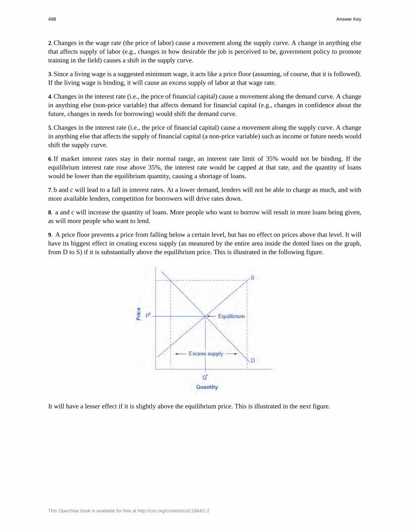
2. Changes in the wage rate (the price of labor) cause a movement along the supply curve. A change in anything elsethat affects supply of labor (e.g., changes in how desirable the job is perceived to be, government policy to promotetraining in the field) causes a shift in the supply curve.
3. Since a living wage is a suggested minimum wage, it acts like a price floor (assuming, of course, that it is followed).If the living wage is binding, it will cause an excess supply of labor at that wage rate.
4. Changes in the interest rate (i.e., the price of financial capital) cause a movement along the demand curve. A changein anything else (non-price variable) that affects demand for financial capital (e.g., changes in confidence about thefuture, changes in needs for borrowing) would shift the demand curve.
5. Changes in the interest rate (i.e., the price of financial capital) cause a movement along the supply curve. A changein anything else that affects the supply of financial capital (a non-price variable) such as income or future needs wouldshift the supply curve.
6. If market interest rates stay in their normal range, an interest rate limit of 35% would not be binding. If theequilibrium interest rate rose above 35%, the interest rate would be capped at that rate, and the quantity of loanswould be lower than the equilibrium quantity, causing a shortage of loans.
7. b and c will lead to a fall in interest rates. At a lower demand, lenders will not be able to charge as much, and withmore available lenders, competition for borrowers will drive rates down.
8. a and c will increase the quantity of loans. More people who want to borrow will result in more loans being given,as will more people who want to lend.
9. A price floor prevents a price from falling below a certain level, but has no effect on prices above that level. It willhave its biggest effect in creating excess supply (as measured by the entire area inside the dotted lines on the graph,from D to S) if it is substantially above the equilibrium price. This is illustrated in the following figure.
It will have a lesser effect if it is slightly above the equilibrium price. This is illustrated in the next figure.
498 Answer Key
This OpenStax book is available for free at http://cnx.org/content/col11864/1.2
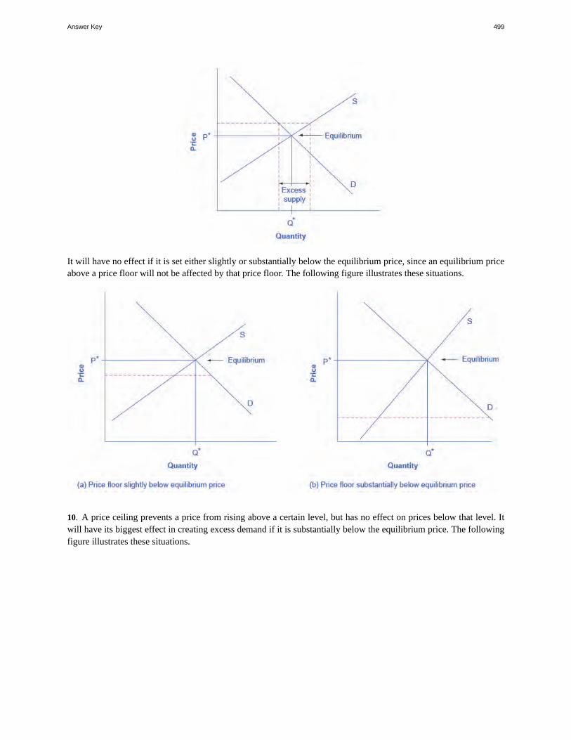
It will have no effect if it is set either slightly or substantially below the equilibrium price, since an equilibrium priceabove a price floor will not be affected by that price floor. The following figure illustrates these situations.
10. A price ceiling prevents a price from rising above a certain level, but has no effect on prices below that level. Itwill have its biggest effect in creating excess demand if it is substantially below the equilibrium price. The followingfigure illustrates these situations.
Answer Key 499
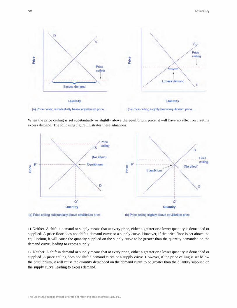
When the price ceiling is set substantially or slightly above the equilibrium price, it will have no effect on creatingexcess demand. The following figure illustrates these situations.
11. Neither. A shift in demand or supply means that at every price, either a greater or a lower quantity is demanded orsupplied. A price floor does not shift a demand curve or a supply curve. However, if the price floor is set above theequilibrium, it will cause the quantity supplied on the supply curve to be greater than the quantity demanded on thedemand curve, leading to excess supply.
12. Neither. A shift in demand or supply means that at every price, either a greater or a lower quantity is demanded orsupplied. A price ceiling does not shift a demand curve or a supply curve. However, if the price ceiling is set belowthe equilibrium, it will cause the quantity demanded on the demand curve to be greater than the quantity supplied onthe supply curve, leading to excess demand.
500 Answer Key
This OpenStax book is available for free at http://cnx.org/content/col11864/1.2
Chapter 51. GDP is C + I + G + (X – M). GDP = $2,000 billion + $50 billion + $1,000 billion + ($20 billion – $40 billion) =$3,030
2.a. Hospital stays are part of GDP.b. Changes in life expectancy are not market transactions and not part of GDP.c. Child care that is paid for is part of GDP.d. If Grandma gets paid and reports this as income, it is part of GDP, otherwise not.e. A used car is not produced this year, so it is not part of GDP.f. A new car is part of GDP.g. Variety does not count in GDP, where the cheese could all be cheddar.h. The iron is not counted because it is an intermediate good.
3. From 1980 to 1990, real GDP grew by (8,225.0 – 5,926.5) / (5,926.5) = 39%. Over the same period, prices increasedby (72.7 – 48.3) / (48.3/100) = 51%. So about 57% of the growth 51 / (51 + 39) was inflation, and the remainder: 39/ (51 + 39) = 43% was growth in real GDP.
4. Two other major recessions are visible in the figure as slight dips: those of 1973–1975, and 1981–1982. Two otherrecessions appear in the figure as a flattening of the path of real GDP. These were in 1990–1991 and 2001.
5. 11 recessions in approximately 70 years averages about one recession every six years.
6. The table lists the “Months of Contraction” for each recession. Averaging these figures for the post-WWIIrecessions gives an average duration of 11 months, or slightly less than a year.
7. The table lists the “Months of Expansion.” Averaging these figures for the post-WWII expansions gives an averageexpansion of 60.5 months, or more than five years.
8. Yes. The answer to both questions depends on whether GDP is growing faster or slower than population. Ifpopulation grows faster than GDP, GDP increases, while GDP per capita decreases. If GDP falls, but population fallsfaster, then GDP decreases, while GDP per capita increases.
9. Start with Central African Republic’s GDP measured in francs. Divide it by the exchange rate to convert to U.S.dollars, and then divide by population to obtain the per capita figure. That is, 1,107,689 million francs / 284.681francs per dollar / 4.862 million people = $800.28 GDP per capita.
10.a. A dirtier environment would reduce the broad standard of living, but not be counted in GDP, so a rise in GDP
would overstate the standard of living.b. A lower crime rate would raise the broad standard of living, but not be counted directly in GDP, and so a rise
in GDP would understate the standard of living.c. A greater variety of goods would raise the broad standard of living, but not be counted directly in GDP, and
so a rise in GDP would understate the rise in the standard of living.d. A decline in infant mortality would raise the broad standard of living, but not be counted directly in GDP, and
so a rise in GDP would understate the rise in the standard of living.
Chapter 61. The Industrial Revolution refers to the widespread use of power-driven machinery and the economic and socialchanges that resulted in the first half of the 1800s. Ingenious machines—the steam engine, the power loom, and thesteam locomotive—performed tasks that would have taken vast numbers of workers to do. The Industrial Revolutionbegan in Great Britain, and soon spread to the United States, Germany, and other countries.
Answer Key 501
2. Property rights are the rights of individuals and firms to own property and use it as they see fit. Contractual rightsare based on property rights and they allow individuals to enter into agreements with others regarding the use of theirproperty providing recourse through the legal system in the event of noncompliance. Economic growth occurs whenthe standard of living increases in an economy, which occurs when output is increasing and incomes are rising. Forthis to happen, societies must create a legal environment that gives individuals the ability to use their property to theirfullest and highest use, including the right to trade or sell that property. Without a legal system that enforces contracts,people would not be likely to enter into contracts for current or future services because of the risk of non-payment.This would make it difficult to transact business and would slow economic growth.
3. Yes. Since productivity is output per unit of input, we can measure productivity using GDP (output) per worker(input).
4. In 20 years the United States will have an income of 10,000 × (1 + 0.01)20 = $12,201.90, and South Korea will havean income of 10,000 × (1 + 0.04)20 = $21,911.23. South Korea has grown by a multiple of 2.1 and the United Statesby a multiple of 1.2.
5. Capital deepening and technology are important. What seems to be more important is how they are combined.
6. Government can contribute to economic growth by investing in human capital through the education system,building a strong physical infrastructure for transportation and commerce, increasing investment by lowering capitalgains taxes, creating special economic zones that allow for reduced tariffs, and investing in research anddevelopment.
7. Public education, low investment taxes, funding for infrastructure projects, special economic zones
8. A good way to think about this is how a runner who has fallen behind in a race feels psychologically and physicallyas he catches up. Playing catch-up can be more taxing than maintaining one’s position at the head of the pack.
9.a. No. Capital deepening refers to an increase in the amount of capital per person in an economy. A decrease in
investment by firms will actually cause the opposite of capital deepening (since the population will grow overtime).
b. There is no direct connection between and increase in international trade and capital deepening. One couldimagine particular scenarios where trade could lead to capital deepening (for example, if international capitalinflows which are the counterpart to increasing the trade deficit) lead to an increase in physical capitalinvestment), but in general, no.
c. Yes. Capital deepening refers to an increase in either physical capital or human capital per person. Continuingeducation or any time of lifelong learning adds to human capital and thus creates capital deepening.
10. The advantages of backwardness include faster growth rates because of the process of convergence, as well as theability to adopt new technologies that were developed first in the “leader” countries. While being “backward” is notinherently a good thing, Gerschenkron stressed that there are certain advantages which aid countries trying to “catchup.”
11. Capital deepening, by definition, should lead to diminished returns because you're investing more and more butusing the same methods of production, leading to the marginal productivity declining. This is shown on a productionfunction as a movement along the curve. Improvements in technology should not lead to diminished returns becauseyou are finding new and more efficient ways of using the same amount of capital. This can be illustrated as a shiftupward of the production function curve.
12. Productivity growth from new advances in technology will not slow because the new methods of production willbe adopted relatively quickly and easily, at very low marginal cost. Also, countries that are seeing technology growthusually have a vast and powerful set of institutions for training workers and building better machines, which allowsthe maximum amount of people to benefit from the new technology. These factors have the added effect of makingadditional technological advances even easier for these countries.
502 Answer Key
This OpenStax book is available for free at http://cnx.org/content/col11864/1.2
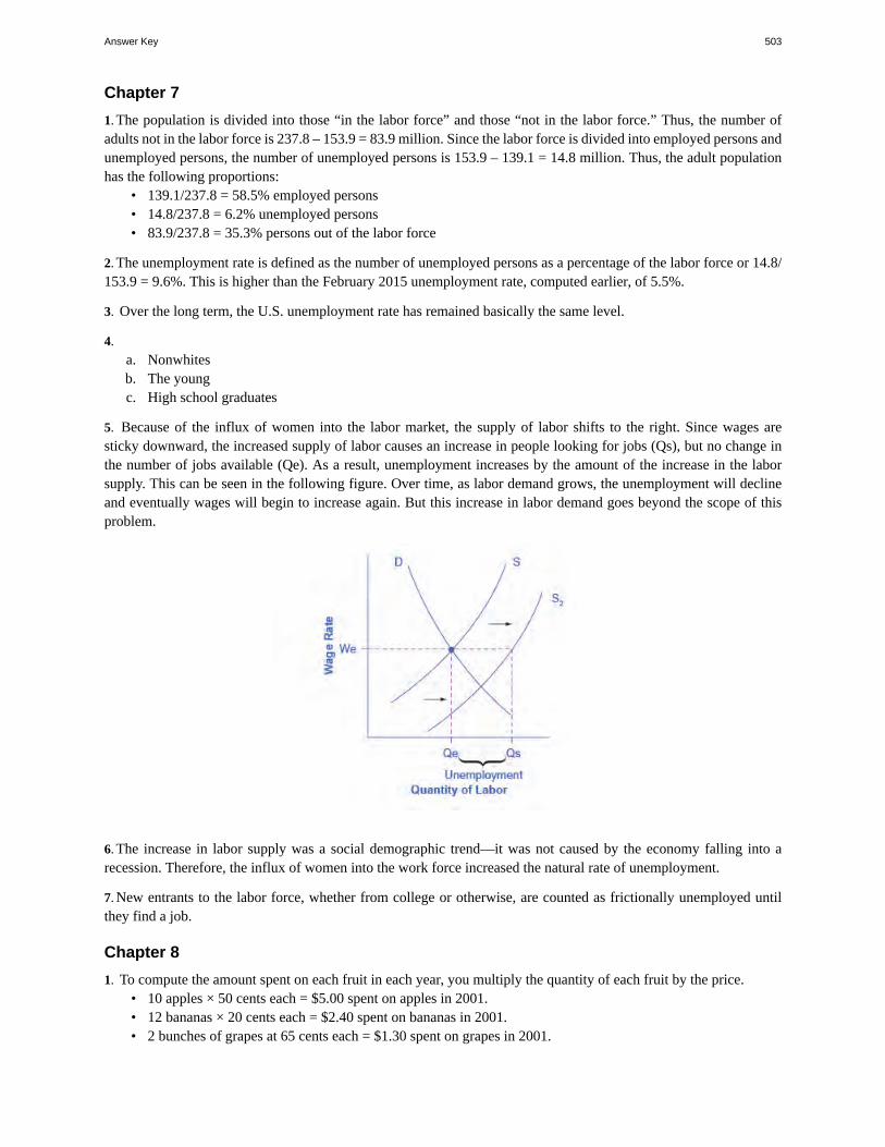
Chapter 71. The population is divided into those “in the labor force” and those “not in the labor force.” Thus, the number ofadults not in the labor force is 237.8 – 153.9 = 83.9 million. Since the labor force is divided into employed persons andunemployed persons, the number of unemployed persons is 153.9 – 139.1 = 14.8 million. Thus, the adult populationhas the following proportions:
• 139.1/237.8 = 58.5% employed persons• 14.8/237.8 = 6.2% unemployed persons• 83.9/237.8 = 35.3% persons out of the labor force
2. The unemployment rate is defined as the number of unemployed persons as a percentage of the labor force or 14.8/153.9 = 9.6%. This is higher than the February 2015 unemployment rate, computed earlier, of 5.5%.
3. Over the long term, the U.S. unemployment rate has remained basically the same level.
4.a. Nonwhitesb. The youngc. High school graduates
5. Because of the influx of women into the labor market, the supply of labor shifts to the right. Since wages aresticky downward, the increased supply of labor causes an increase in people looking for jobs (Qs), but no change inthe number of jobs available (Qe). As a result, unemployment increases by the amount of the increase in the laborsupply. This can be seen in the following figure. Over time, as labor demand grows, the unemployment will declineand eventually wages will begin to increase again. But this increase in labor demand goes beyond the scope of thisproblem.
6. The increase in labor supply was a social demographic trend—it was not caused by the economy falling into arecession. Therefore, the influx of women into the work force increased the natural rate of unemployment.
7. New entrants to the labor force, whether from college or otherwise, are counted as frictionally unemployed untilthey find a job.
Chapter 81. To compute the amount spent on each fruit in each year, you multiply the quantity of each fruit by the price.
• 10 apples × 50 cents each = $5.00 spent on apples in 2001.• 12 bananas × 20 cents each = $2.40 spent on bananas in 2001.• 2 bunches of grapes at 65 cents each = $1.30 spent on grapes in 2001.
Answer Key 503
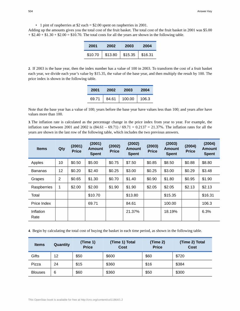
• 1 pint of raspberries at $2 each = $2.00 spent on raspberries in 2001.Adding up the amounts gives you the total cost of the fruit basket. The total cost of the fruit basket in 2001 was $5.00+ $2.40 + $1.30 + $2.00 = $10.70. The total costs for all the years are shown in the following table.
2001 2002 2003 2004
$10.70 $13.80 $15.35 $16.31
2. If 2003 is the base year, then the index number has a value of 100 in 2003. To transform the cost of a fruit basketeach year, we divide each year’s value by $15.35, the value of the base year, and then multiply the result by 100. Theprice index is shown in the following table.
2001 2002 2003 2004
69.71 84.61 100.00 106.3
Note that the base year has a value of 100; years before the base year have values less than 100; and years after havevalues more than 100.
3. The inflation rate is calculated as the percentage change in the price index from year to year. For example, theinflation rate between 2001 and 2002 is (84.61 – 69.71) / 69.71 = 0.2137 = 21.37%. The inflation rates for all theyears are shown in the last row of the following table, which includes the two previous answers.
Items Qty (2001)Price
(2001)AmountSpent
(2002)Price
(2002)AmountSpent
(2003)Price
(2003)AmountSpent
(2004)Price
(2004)AmountSpent
Apples 10 $0.50 $5.00 $0.75 $7.50 $0.85 $8.50 $0.88 $8.80
Bananas 12 $0.20 $2.40 $0.25 $3.00 $0.25 $3.00 $0.29 $3.48
Grapes 2 $0.65 $1.30 $0.70 $1.40 $0.90 $1.80 $0.95 $1.90
Raspberries 1 $2.00 $2.00 $1.90 $1.90 $2.05 $2.05 $2.13 $2.13
Total $10.70 $13.80 $15.35 $16.31
Price Index 69.71 84.61 100.00 106.3
InflationRate
21.37% 18.19% 6.3%
4. Begin by calculating the total cost of buying the basket in each time period, as shown in the following table.
Items Quantity (Time 1)Price
(Time 1) TotalCost
(Time 2)Price
(Time 2) TotalCost
Gifts 12 $50 $600 $60 $720
Pizza 24 $15 $360 $16 $384
Blouses 6 $60 $360 $50 $300
504 Answer Key
This OpenStax book is available for free at http://cnx.org/content/col11864/1.2
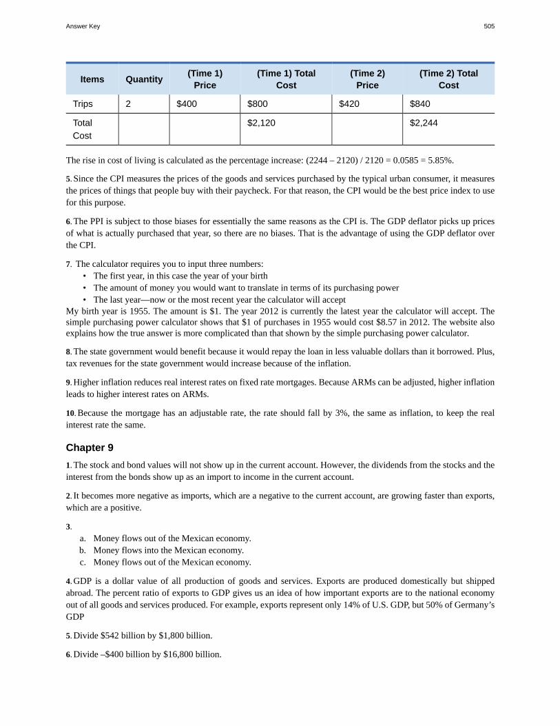
Items Quantity (Time 1)Price
(Time 1) TotalCost
(Time 2)Price
(Time 2) TotalCost
Trips 2 $400 $800 $420 $840
TotalCost
$2,120 $2,244
The rise in cost of living is calculated as the percentage increase: (2244 – 2120) / 2120 = 0.0585 = 5.85%.
5. Since the CPI measures the prices of the goods and services purchased by the typical urban consumer, it measuresthe prices of things that people buy with their paycheck. For that reason, the CPI would be the best price index to usefor this purpose.
6. The PPI is subject to those biases for essentially the same reasons as the CPI is. The GDP deflator picks up pricesof what is actually purchased that year, so there are no biases. That is the advantage of using the GDP deflator overthe CPI.
7. The calculator requires you to input three numbers:• The first year, in this case the year of your birth• The amount of money you would want to translate in terms of its purchasing power• The last year—now or the most recent year the calculator will accept
My birth year is 1955. The amount is $1. The year 2012 is currently the latest year the calculator will accept. Thesimple purchasing power calculator shows that $1 of purchases in 1955 would cost $8.57 in 2012. The website alsoexplains how the true answer is more complicated than that shown by the simple purchasing power calculator.
8. The state government would benefit because it would repay the loan in less valuable dollars than it borrowed. Plus,tax revenues for the state government would increase because of the inflation.
9. Higher inflation reduces real interest rates on fixed rate mortgages. Because ARMs can be adjusted, higher inflationleads to higher interest rates on ARMs.
10. Because the mortgage has an adjustable rate, the rate should fall by 3%, the same as inflation, to keep the realinterest rate the same.
Chapter 91. The stock and bond values will not show up in the current account. However, the dividends from the stocks and theinterest from the bonds show up as an import to income in the current account.
2. It becomes more negative as imports, which are a negative to the current account, are growing faster than exports,which are a positive.
3.a. Money flows out of the Mexican economy.b. Money flows into the Mexican economy.c. Money flows out of the Mexican economy.
4. GDP is a dollar value of all production of goods and services. Exports are produced domestically but shippedabroad. The percent ratio of exports to GDP gives us an idea of how important exports are to the national economyout of all goods and services produced. For example, exports represent only 14% of U.S. GDP, but 50% of Germany’sGDP
5. Divide $542 billion by $1,800 billion.
6. Divide –$400 billion by $16,800 billion.
Answer Key 505
7. The trade balance is the difference between exports and imports. The current account balance includes this number(whether it is a trade balance or a trade surplus), but also includes international flows of money from globalinvestments.
8.a. An export sale to Germany involves a financial flow from Germany to the U.S. economy.b. The issue here is not U.S. investments in Brazil, but the return paid on those investments, which involves a
financial flow from the Brazilian economy to the U.S. economy.c. Foreign aid from the United States to Egypt is a financial flow from the United States to Egypt.d. Importing oil from the Russian Federation means a flow of financial payments from the U.S. economy to the
Russian Federation.e. Japanese investors buying U.S. real estate is a financial flow from Japan to the U.S. economy.
9. The top portion tracks the flow of exports and imports and the payments for those. The bottom portion is looking atinternational financial investments and the outflow and inflow of monies from those investments. These investmentscan include investments in stocks and bonds or real estate abroad, as well as international borrowing and lending.
10. If more monies are flowing out of the country (for example, to pay for imports) it will make the current accountmore negative or less positive, and if more monies are flowing into the country, it will make the current account lessnegative or more positive.
11. Write out the national savings and investment identity for the situation of the economy implied by this question:Supply of capital = Demand for capital
S + (M – X) + (T – G) = I Savings + (trade deficit) + (government budget surplus) = Investment
If domestic savings increases and
nothing else changes, then the trade deficit will fall. In effect, the economy would be relying more on domestic capitaland less on foreign capital. If the government starts borrowing instead of saving, then the trade deficit must rise. Ineffect, the government is no longer providing savings and so, if nothing else is to change, more investment funds mustarrive from abroad. If the rate of domestic investment surges, then, ceteris paribus, the trade deficit must also rise, toprovide the extra capital. The ceteris paribus—or “other things being equal”—assumption is important here. In all ofthese situations, there is no reason to expect in the real world that the original change will affect only, or primarily,the trade deficit. The identity only says that something will adjust—it does not specify what.
12. The government is saving rather than borrowing. The supply of savings, whether private or public, is on the leftside of the identity.
13. A trade deficit is determined by a country’s level of private and public savings and the amount of domesticinvestment.
14. The trade deficit must increase. To put it another way, this increase in investment must be financed by an inflowof financial capital from abroad.
15. Incomes fall during a recession, and consumers buy fewer good, including imports.
16. A booming economy will increase the demand for goods in general, so import sales will increase. If our tradingpartners’ economies are doing well, they will buy more of our products and so U.S. exports will increase.
17.a. Increased federal spending on Medicare may not increase productivity, so a budget deficit is not justified.b. Increased spending on education will increase productivity and foster greater economic growth, so a budget
deficit is justified.c. Increased spending on the space program may not increase productivity, so a budget deficit is not justified.d. Increased spending on airports and air traffic control will increase productivity and foster greater economic
growth, so a budget deficit is justified.
506 Answer Key
This OpenStax book is available for free at http://cnx.org/content/col11864/1.2
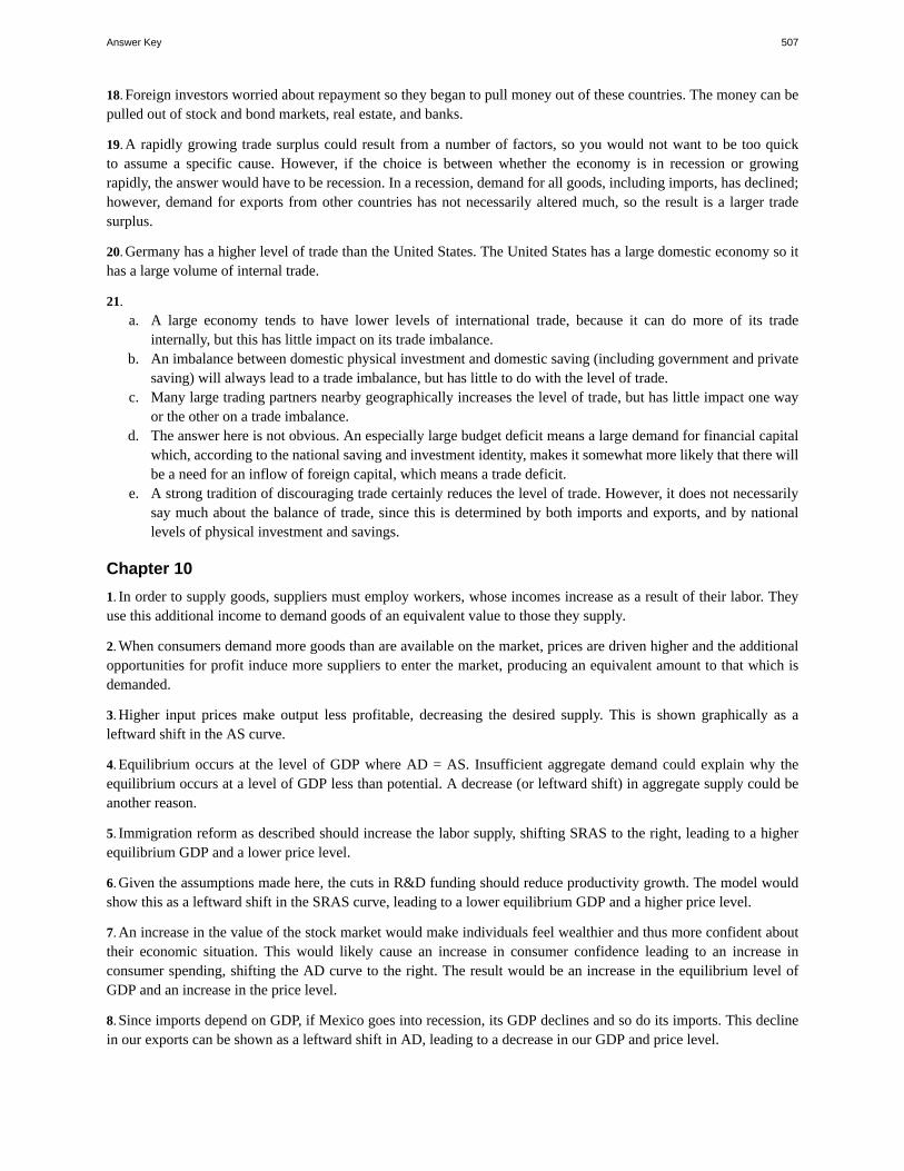
18. Foreign investors worried about repayment so they began to pull money out of these countries. The money can bepulled out of stock and bond markets, real estate, and banks.
19. A rapidly growing trade surplus could result from a number of factors, so you would not want to be too quickto assume a specific cause. However, if the choice is between whether the economy is in recession or growingrapidly, the answer would have to be recession. In a recession, demand for all goods, including imports, has declined;however, demand for exports from other countries has not necessarily altered much, so the result is a larger tradesurplus.
20. Germany has a higher level of trade than the United States. The United States has a large domestic economy so ithas a large volume of internal trade.
21.a. A large economy tends to have lower levels of international trade, because it can do more of its trade
internally, but this has little impact on its trade imbalance.b. An imbalance between domestic physical investment and domestic saving (including government and private
saving) will always lead to a trade imbalance, but has little to do with the level of trade.c. Many large trading partners nearby geographically increases the level of trade, but has little impact one way
or the other on a trade imbalance.d. The answer here is not obvious. An especially large budget deficit means a large demand for financial capital
which, according to the national saving and investment identity, makes it somewhat more likely that there willbe a need for an inflow of foreign capital, which means a trade deficit.
e. A strong tradition of discouraging trade certainly reduces the level of trade. However, it does not necessarilysay much about the balance of trade, since this is determined by both imports and exports, and by nationallevels of physical investment and savings.
Chapter 101. In order to supply goods, suppliers must employ workers, whose incomes increase as a result of their labor. Theyuse this additional income to demand goods of an equivalent value to those they supply.
2. When consumers demand more goods than are available on the market, prices are driven higher and the additionalopportunities for profit induce more suppliers to enter the market, producing an equivalent amount to that which isdemanded.
3. Higher input prices make output less profitable, decreasing the desired supply. This is shown graphically as aleftward shift in the AS curve.
4. Equilibrium occurs at the level of GDP where AD = AS. Insufficient aggregate demand could explain why theequilibrium occurs at a level of GDP less than potential. A decrease (or leftward shift) in aggregate supply could beanother reason.
5. Immigration reform as described should increase the labor supply, shifting SRAS to the right, leading to a higherequilibrium GDP and a lower price level.
6. Given the assumptions made here, the cuts in R&D funding should reduce productivity growth. The model wouldshow this as a leftward shift in the SRAS curve, leading to a lower equilibrium GDP and a higher price level.
7. An increase in the value of the stock market would make individuals feel wealthier and thus more confident abouttheir economic situation. This would likely cause an increase in consumer confidence leading to an increase inconsumer spending, shifting the AD curve to the right. The result would be an increase in the equilibrium level ofGDP and an increase in the price level.
8. Since imports depend on GDP, if Mexico goes into recession, its GDP declines and so do its imports. This declinein our exports can be shown as a leftward shift in AD, leading to a decrease in our GDP and price level.
Answer Key 507
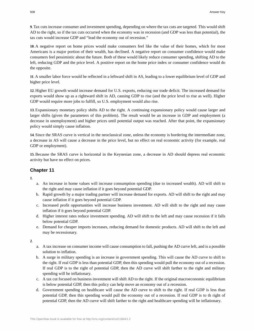
9. Tax cuts increase consumer and investment spending, depending on where the tax cuts are targeted. This would shiftAD to the right, so if the tax cuts occurred when the economy was in recession (and GDP was less than potential), thetax cuts would increase GDP and “lead the economy out of recession.”
10. A negative report on home prices would make consumers feel like the value of their homes, which for mostAmericans is a major portion of their wealth, has declined. A negative report on consumer confidence would makeconsumers feel pessimistic about the future. Both of these would likely reduce consumer spending, shifting AD to theleft, reducing GDP and the price level. A positive report on the home price index or consumer confidence would dothe opposite.
11. A smaller labor force would be reflected in a leftward shift in AS, leading to a lower equilibrium level of GDP andhigher price level.
12. Higher EU growth would increase demand for U.S. exports, reducing our trade deficit. The increased demand forexports would show up as a rightward shift in AD, causing GDP to rise (and the price level to rise as well). HigherGDP would require more jobs to fulfill, so U.S. employment would also rise.
13. Expansionary monetary policy shifts AD to the right. A continuing expansionary policy would cause larger andlarger shifts (given the parameters of this problem). The result would be an increase in GDP and employment (adecrease in unemployment) and higher prices until potential output was reached. After that point, the expansionarypolicy would simply cause inflation.
14. Since the SRAS curve is vertical in the neoclassical zone, unless the economy is bordering the intermediate zone,a decrease in AS will cause a decrease in the price level, but no effect on real economic activity (for example, realGDP or employment).
15. Because the SRAS curve is horizontal in the Keynesian zone, a decrease in AD should depress real economicactivity but have no effect on prices.
Chapter 111.
a. An increase in home values will increase consumption spending (due to increased wealth). AD will shift tothe right and may cause inflation if it goes beyond potential GDP.
b. Rapid growth by a major trading partner will increase demand for exports. AD will shift to the right and maycause inflation if it goes beyond potential GDP.
c. Increased profit opportunities will increase business investment. AD will shift to the right and may causeinflation if it goes beyond potential GDP.
d. Higher interest rates reduce investment spending. AD will shift to the left and may cause recession if it fallsbelow potential GDP.
e. Demand for cheaper imports increases, reducing demand for domestic products. AD will shift to the left andmay be recessionary.
2.a. A tax increase on consumer income will cause consumption to fall, pushing the AD curve left, and is a possible
solution to inflation.b. A surge in military spending is an increase in government spending. This will cause the AD curve to shift to
the right. If real GDP is less than potential GDP, then this spending would pull the economy out of a recession.If real GDP is to the right of potential GDP, then the AD curve will shift farther to the right and militaryspending will be inflationary.
c. A tax cut focused on business investment will shift AD to the right. If the original macroeconomic equilibriumis below potential GDP, then this policy can help move an economy out of a recession.
d. Government spending on healthcare will cause the AD curve to shift to the right. If real GDP is less thanpotential GDP, then this spending would pull the economy out of a recession. If real GDP is to th right ofpotential GDP, then the AD curve will shift farther to the right and healthcare spending will be inflationary.
508 Answer Key
This OpenStax book is available for free at http://cnx.org/content/col11864/1.2
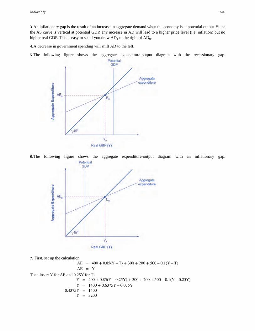
3. An inflationary gap is the result of an increase in aggregate demand when the economy is at potential output. Sincethe AS curve is vertical at potential GDP, any increase in AD will lead to a higher price level (i.e. inflation) but nohigher real GDP. This is easy to see if you draw AD1 to the right of AD0.
4. A decrease in government spending will shift AD to the left.
5. The following figure shows the aggregate expenditure-output diagram with the recessionary gap.
6. The following figure shows the aggregate expenditure-output diagram with an inflationary gap.
7. First, set up the calculation.AE = 400 + 0.85(Y – T) + 300 + 200 + 500 – 0.1(Y – T)AE = Y
Then insert Y for AE and 0.25Y for T.Y = 400 + 0.85(Y – 0.25Y) + 300 + 200 + 500 – 0.1(Y – 0.25Y)Y = 1400 + 0.6375Y – 0.075Y
0.4375Y = 1400Y = 3200
Answer Key 509
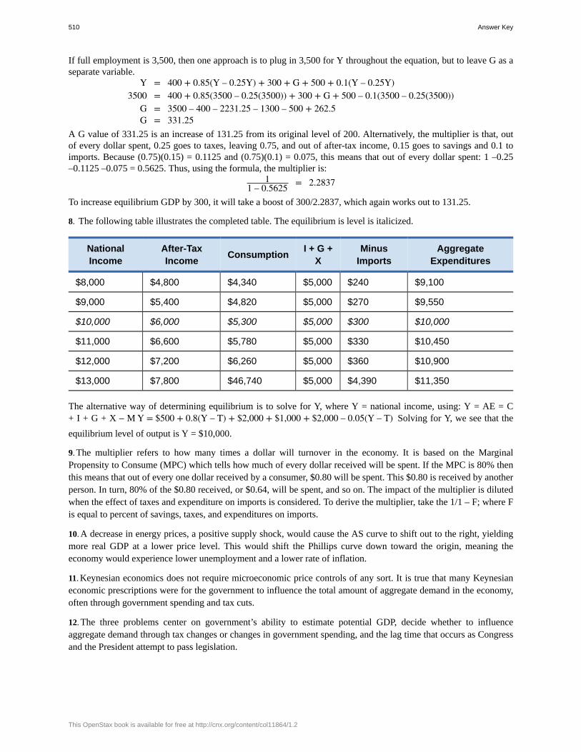
If full employment is 3,500, then one approach is to plug in 3,500 for Y throughout the equation, but to leave G as aseparate variable.
Y = 400 + 0.85(Y – 0.25Y) + 300 + G + 500 + 0.1(Y – 0.25Y)3500 = 400 + 0.85(3500 – 0.25(3500)) + 300 + G + 500 – 0.1(3500 – 0.25(3500))
G = 3500 – 400 – 2231.25 – 1300 – 500 + 262.5G = 331.25
A G value of 331.25 is an increase of 131.25 from its original level of 200. Alternatively, the multiplier is that, outof every dollar spent, 0.25 goes to taxes, leaving 0.75, and out of after-tax income, 0.15 goes to savings and 0.1 toimports. Because (0.75)(0.15) = 0.1125 and (0.75)(0.1) = 0.075, this means that out of every dollar spent: 1 –0.25–0.1125 –0.075 = 0.5625. Thus, using the formula, the multiplier is:
11 – 0.5625 = 2.2837
To increase equilibrium GDP by 300, it will take a boost of 300/2.2837, which again works out to 131.25.
8. The following table illustrates the completed table. The equilibrium is level is italicized.
NationalIncome
After-TaxIncome Consumption I + G +
XMinus
ImportsAggregate
Expenditures
$8,000 $4,800 $4,340 $5,000 $240 $9,100
$9,000 $5,400 $4,820 $5,000 $270 $9,550
$10,000 $6,000 $5,300 $5,000 $300 $10,000
$11,000 $6,600 $5,780 $5,000 $330 $10,450
$12,000 $7,200 $6,260 $5,000 $360 $10,900
$13,000 $7,800 $46,740 $5,000 $4,390 $11,350
The alternative way of determining equilibrium is to solve for Y, where Y = national income, using: Y = AE = C+ I + G + X – M Y = $500 + 0.8(Y – T) + $2,000 + $1,000 + $2,000 – 0.05(Y – T) Solving for Y, we see that the
equilibrium level of output is Y = $10,000.
9. The multiplier refers to how many times a dollar will turnover in the economy. It is based on the MarginalPropensity to Consume (MPC) which tells how much of every dollar received will be spent. If the MPC is 80% thenthis means that out of every one dollar received by a consumer, $0.80 will be spent. This $0.80 is received by anotherperson. In turn, 80% of the $0.80 received, or $0.64, will be spent, and so on. The impact of the multiplier is dilutedwhen the effect of taxes and expenditure on imports is considered. To derive the multiplier, take the 1/1 – F; where Fis equal to percent of savings, taxes, and expenditures on imports.
10. A decrease in energy prices, a positive supply shock, would cause the AS curve to shift out to the right, yieldingmore real GDP at a lower price level. This would shift the Phillips curve down toward the origin, meaning theeconomy would experience lower unemployment and a lower rate of inflation.
11. Keynesian economics does not require microeconomic price controls of any sort. It is true that many Keynesianeconomic prescriptions were for the government to influence the total amount of aggregate demand in the economy,often through government spending and tax cuts.
12. The three problems center on government’s ability to estimate potential GDP, decide whether to influenceaggregate demand through tax changes or changes in government spending, and the lag time that occurs as Congressand the President attempt to pass legislation.
510 Answer Key
This OpenStax book is available for free at http://cnx.org/content/col11864/1.2
Chapter 121. No, this statement is false. It would be more accurate to say that rational expectations seek to predict the future asaccurately as possible, using all of past experience as a guide. Adaptive expectations are largely backward looking;that is, they adapt as experience accumulates, but without attempting to look forward.
2. An unemployment rate of zero percent is presumably well below the rate that is consistent with potential GDPand with the natural rate of unemployment. As a result, this policy would be attempting to push AD out to the right.In the short run, it is possible to have unemployment slightly below the natural rate for a time, at a price of higherinflation, as shown by the movement from E0 to E1 along the short-run AS curve. However, over time the extremelylow unemployment rates will tend to cause wages to be bid up, and shift the short-run AS curve back to the left. Theresult would be a higher price level, but an economy still at potential GDP and the natural rate of unemployment, asdetermined by the long-run AS curve. If the government continues this policy, it will continually be pushing the pricelevel higher and higher, but it will not be able to achieve its goal of zero percent unemployment, because that goal isinconsistent with market forces.
3. The statement is accurate. Rational expectations can be thought of as a version of neoclassical economics becauseit argues that potential GDP and the rate of unemployment are shaped by market forces as wages and prices adjust.However, it is an “extreme” version because it argues that this adjustment takes place very quickly. Other theories,like adaptive expectations, suggest that adjustment to the neoclassical outcome takes a few years.
4. The short-term Keynesian model is built on the importance of aggregate demand as a cause of business cyclesand a degree of wage and price rigidity, and thus does a sound job of explaining many recessions and why cyclicalunemployment rises and falls. The neoclassical model emphasizes aggregate supply by focusing on the underlyingdeterminants of output and employment in markets, and thus tends to put more emphasis on economic growth andhow labor markets work.
Chapter 131. As long as you remain within the walls of the casino, chips fit the definition of money; that is, they serve as amedium of exchange, a unit of account, and a store of value. Chips do not work very well as money once you leavethe casino, but many kinds of money do not work well in other areas. For example, it is hard to spend money fromTurkey or Brazil at your local supermarket or at the movie theater.
2. Many physical items that a person buys at one time but may sell at another time can serve as an answer to thisquestion. Examples include a house, land, art, rare coins or stamps, and so on.
3. The currency and checks in M1 are easiest to spend. It is harder to spend M2 directly, although if there is anautomatic teller machine in the shopping mall, you can turn M2 from your savings account into an M1 of currencyquite quickly. If your answer is about “credit cards,” then you are really talking about spending M1—although it isM1 from the account of the credit card company, which you will repay later when you credit card bill comes due.
4.a. Neither in M1 or M2b. That is part of M1, and because M2 includes M1 it is also part of M2c. Currency out in the public hands is part of M1 and M2d. Checking deposits are in M1 and M2e. Money market accounts are in M2
5. A bank’s assets include cash held in their vaults, but assets also include monies that the bank holds at the FederalReserve Bank (called “reserves”), loans that are made to customers, and bonds.
6.a. A borrower who has been late on a number of loan payments looks perhaps less likely to repay the loan, or to
repay it on time, and so you would want to pay less for that loan.
Answer Key 511
b. If interest rates generally have risen, then this loan made at a time of relatively lower interest rates looks lessattractive, and you would pay less for it.
c. If the borrower is a firm with a record of high profits, then it is likely to be able to repay the loan, and youwould be willing to pay more for the loan.
d. If interest rates in the economy have fallen, then the loan is worth more.
Chapter 141. Longer terms insulate the Board from political forces. Since the presidency can potentially change every four years,the Federal Reserve’s independence prevents drastic swings in monetary policy with every new administration andallows policy decisions to be made only on economic grounds.
2. Banks make their money from issuing loans and charging interest. The more money that is stored in the bank’svault, the less is available for lending and the less money the bank stands to make.
3. The fear and uncertainty created by the suggestion that a bank might fail can lead depositors to withdraw theirmoney. If many depositors do this at the same time, the bank may not be able to meet their demands and will, indeed,fail.
4. The bank has to hold $1,000 in reserves, so when it buys the $500 in bonds, it will have to reduce its loans by $500to make up the difference. The money supply decreases by the same amount.
5. An increase in reserve requirements would reduce the supply of money, since more money would be held in banksrather than circulating in the economy.
6. Contractionary policy reduces the amount of loanable funds in the economy. As with all goods, greater scarcityleads a greater price, so the interest rate, or the price of borrowing money, rises.
7. An increase in the amount of available loanable funds means that there are more people who want to lend. They,therefore, bid the price of borrowing (the interest rate) down.
8. In times of economic uncertainty, banks may worry that borrowers will lose the ability to repay their loans. Theymay also fear that a panic is more likely and they will need the excess reserves to meet their obligations.
9. If consumer optimism changes, spending can speed up or slow down. This could also happen in a case whereconsumers need to buy a large number of items quickly, such as in a situation of national emergency.
Chapter 151.
a. The British use the pound sterling, while Germans use the euro, so a British exporter will receive euros fromexport sales, which will need to be exchanged for pounds. A stronger euro will mean more pounds per euro,so the exporter will be better off. In addition, the lower price for German imports will stimulate demand forBritish exports. For both these reasons, a stronger euro benefits the British exporter.
b. The Dutch use euros while the Chileans use pesos, so the Dutch tourist needs to turn euros into Chilean pesos.An increase in the euro means that the tourist will get more pesos per euro. As a consequence, the Dutchtourist will have a less expensive vacation than he planned, so the tourist will be better off.
c. The Greek use euros while the Canadians use dollars. An increase in the euro means it will buy more Canadiandollars. As a result, the Greek bank will see a decrease in the cost of the Canadian bonds, so it may purchasemore bonds. Either way, the Greek bank benefits.
d. Since both the French and Germans use the euro, an increase in the euro, in terms of other currencies, shouldhave no impact on the French exporter.
2. Expected depreciation in a currency will lead people to divest themselves of the currency. We should expect to seean increase in the supply of pounds and a decrease in demand for pounds. The result should be a decrease in the valueof the pound vis à vis the dollar.
512 Answer Key
This OpenStax book is available for free at http://cnx.org/content/col11864/1.2
3. Lower U.S. interest rates make U.S. assets less desirable compared to assets in the European Union. We shouldexpect to see a decrease in demand for dollars and an increase in supply of dollars in foreign currency markets. As aresult, we should expect to see the dollar depreciate compared to the euro.
4. A decrease in Argentine inflation relative to other countries should cause an increase in demand for pesos, adecrease in supply of pesos, and an appreciation of the peso in foreign currency markets.
5. The problem occurs when banks borrow foreign currency but lend in domestic currency. Since banks’ assets (loansthey made) are in domestic currency, while their debts (money they borrowed) are in foreign currency, when thedomestic currency declines, their debts grow larger. If the domestic currency falls substantially in value, as happenedduring the Asian financial crisis, then the banking system could fail. This problem is unlikely to occur for U.S. banksbecause, even when they borrow from abroad, they tend to borrow dollars. Remember, there are trillions of dollars incirculation in the global economy. Since both assets and debts are in dollars, a change in the value of the dollar doesnot cause banking system failure the way it can when banks borrow in foreign currency.
6. While capital flight is possible in either case, if a country borrows to invest in real capital it is more likely to beable to generate the income to pay back its debts than a country that borrows to finance consumption. As a result, aninvestment-stimulated economy is less likely to provoke capital flight and economic recession.
7. A contractionary monetary policy, by driving up domestic interest rates, would cause the currency to appreciate.The higher value of the currency in foreign exchange markets would reduce exports, since from the perspective offoreign buyers, they are now more expensive. The higher value of the currency would similarly stimulate imports,since they would now be cheaper from the perspective of domestic buyers. Lower exports and higher importscause net exports (EX – IM) to fall, which causes aggregate demand to fall. The result would be a decrease inGDP working through the exchange rate mechanism reinforcing the effect contractionary monetary policy has ondomestic investment expenditure. However, cheaper imports would stimulate aggregate supply, bringing GDP backto potential, though at a lower price level.
8. For a currency to fall, a central bank need only supply more of its currency in foreign exchange markets. It canprint as much domestic currency as it likes. For a currency to rise, a central bank needs to buy its currency in foreignexchange markets, paying with foreign currency. Since no central bank has an infinite amount of foreign currencyreserves, it cannot buy its currency indefinitely.
9. Variations in exchange rates, because they change import and export prices, disturb international trade flows. Whentrade is a large part of a nation’s economic activity, government will find it more advantageous to fix exchange ratesto minimize disruptions of trade flows.
Chapter 161. The government borrows funds by selling Treasury bonds, notes, and bills.
2. The funds can be used to pay down the national debt or else be refunded to the taxpayers.
3. Yes, a nation can run budget deficits and see its debt/GDP ratio fall. In fact, this is not uncommon. If the deficit issmall in a given year, than the addition to debt in the numerator of the debt/GDP ratio will be relatively small, whilethe growth in GDP is larger, and so the debt/GDP ratio declines. This was the experience of the U.S. economy for theperiod from the end of World War II to about 1980. It is also theoretically possible, although not likely, for a nationto have a budget surplus and see its debt/GDP ratio rise. Imagine the case of a nation with a small surplus, but in arecession year when the economy shrinks. It is possible that the decline in the nation’s debt, in the numerator of thedebt/GDP ratio, would be proportionally less than the fall in the size of GDP, so the debt/GDP ratio would rise.
4. Progressive. People who give larger gifts subject to the higher tax rate would typically have larger incomes as well.
5. Corporate income tax on his profits, individual income tax on his salary, and payroll tax taken out of the wages hepays himself.
Answer Key 513
6. individual income taxes
7. The tax is regressive because wealthy income earners are not taxed at all on income above $113,000. As a percentof total income, the social security tax hits lower income earners harder than wealthier individuals.
8. As debt increases, interest payments also rise, so that the deficit grows even if we keep other government spendingconstant.
9.a. As a share of GDP, this is false. In nominal dollars, it is true.b. False.c. False.d. False. Education spending is much higher at the state level.e. False. As a share of GDP, it is up about 50.f. As a share of GDP, this is false, and in real dollars, it is also false.g. False.h. False; it’s about 1%.i. False. Although budget deficits were large in 2003 and 2004, and continued into the later 2000s, the federal
government ran budget surpluses from 1998–2001.j. False.
10. To keep prices from rising too much or too rapidly.
11. To increase employment.
12. It falls below because less tax revenue than expected is collected.
13. Automatic stabilizers take effect very quickly, whereas discretionary policy can take a long time to implement.
14. In a recession, because of the decline in economic output, less income is earned, and so less in taxes isautomatically collected. Many welfare and unemployment programs are designed so that those who fall into certaincategories, like “unemployed” or “low income,” are eligible for benefits. During a recession, more people fallinto these categories and become eligible for benefits automatically. The combination of reduced taxes and higherspending is just what is needed for an economy in recession producing below potential GDP. With an economic boom,average income levels rise in the economy, so more in taxes is automatically collected. Fewer people meet the criteriafor receiving government assistance to the unemployed or the needy, so government spending on unemploymentassistance and welfare falls automatically. This combination of higher taxes and lower spending is just what is neededif an economy is producing above its potential GDP.
15. Prices would be pushed up as a result of too much spending.
16. Employment would suffer as a result of too little spending.
17. Monetary policy probably has shorter time lags than fiscal policy. Imagine that the data becomes fairly clear that aneconomy is in or near a recession. Expansionary monetary policy can be carried out through open market operations,which can be done fairly quickly, since the Federal Reserve’s Open Market Committee meets six times a year. Also,monetary policy takes effect through interest rates, which can change fairly quickly. However, fiscal policy is carriedout through acts of Congress that need to be signed into law by the president. Negotiating such laws often takesmonths, and even after the laws are negotiated, it takes more months for spending programs or tax cuts to have aneffect on the macroeconomy.
18. The government would have to make up the revenue either by raising taxes in a different area or cutting spending.
19. Programs where the amount of spending is not fixed, but rather determined by macroeconomic conditions, such asfood stamps, would lose a great deal of flexibility if spending increases had to be met by corresponding tax increasesor spending cuts.
514 Answer Key
This OpenStax book is available for free at http://cnx.org/content/col11864/1.2
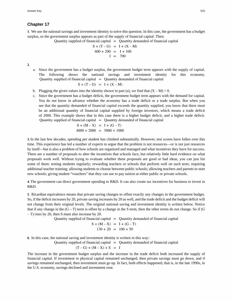
Chapter 171. We use the national savings and investment identity to solve this question. In this case, the government has a budgetsurplus, so the government surplus appears as part of the supply of financial capital. Then:
Quantity supplied of financial capital = Quantity demanded of financial capitalS + (T – G) = I + (X – M)
600 + 200 = I + 100I = 700
2.a. Since the government has a budget surplus, the government budget term appears with the supply of capital.
The following shows the national savings and investment identity for this economy.Quantity supplied of financial capital = Quantity demanded of financial capital
S + (T – G) = I + (X – M)
b. Plugging the given values into the identity shown in part (a), we find that (X – M) = 0.c. Since the government has a budget deficit, the government budget term appears with the demand for capital.
You do not know in advance whether the economy has a trade deficit or a trade surplus. But when yousee that the quantity demanded of financial capital exceeds the quantity supplied, you know that there mustbe an additional quantity of financial capital supplied by foreign investors, which means a trade deficitof 2000. This example shows that in this case there is a higher budget deficit, and a higher trade deficit.Quantity supplied of financial capital = Quantity demanded of financial capital
S + (M – X) = I + (G – T)4000 + 2000 = 5000 + 1000
3. In the last few decades, spending per student has climbed substantially. However, test scores have fallen over thistime. This experience has led a number of experts to argue that the problem is not resources—or is not just resourcesby itself—but is also a problem of how schools are organized and managed and what incentives they have for success.There are a number of proposals to alter the incentives that schools face, but relatively little hard evidence on whatproposals work well. Without trying to evaluate whether these proposals are good or bad ideas, you can just listsome of them: testing students regularly; rewarding teachers or schools that perform well on such tests; requiringadditional teacher training; allowing students to choose between public schools; allowing teachers and parents to startnew schools; giving student “vouchers” that they can use to pay tuition at either public or private schools.
4. The government can direct government spending to R&D. It can also create tax incentives for business to invest inR&D.
5. Ricardian equivalence means that private saving changes to offset exactly any changes in the government budget.So, if the deficit increases by 20, private saving increases by 20 as well, and the trade deficit and the budget deficit willnot change from their original levels. The original national saving and investment identity is written below. Noticethat if any change in the (G – T) term is offset by a change in the S term, then the other terms do not change. So if (G– T) rises by 20, then S must also increase by 20.
Quantity supplied of financial capital = Quantity demanded of financial capitalS + (M – X) = I + (G – T)
130 + 20 = 100 + 50
6. In this case, the national saving and investment identity is written in this way:Quantity supplied of financial capital = Quantity demanded of financial capital
(T – G) + (M – X) + S = IThe increase in the government budget surplus and the increase in the trade deficit both increased the supply offinancial capital. If investment in physical capital remained unchanged, then private savings must go down, and ifsavings remained unchanged, then investment must go up. In fact, both effects happened; that is, in the late 1990s, inthe U.S. economy, savings declined and investment rose.
Answer Key 515
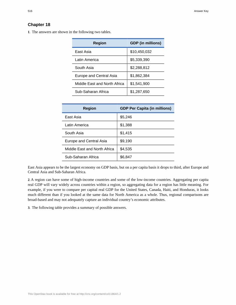
Chapter 181. The answers are shown in the following two tables.
Region GDP (in millions)
East Asia $10,450,032
Latin America $5,339,390
South Asia $2,288,812
Europe and Central Asia $1,862,384
Middle East and North Africa $1,541,900
Sub-Saharan Africa $1,287,650
Region GDP Per Capita (in millions)
East Asia $5,246
Latin America $1,388
South Asia $1,415
Europe and Central Asia $9,190
Middle East and North Africa $4,535
Sub-Saharan Africa $6,847
East Asia appears to be the largest economy on GDP basis, but on a per capita basis it drops to third, after Europe andCentral Asia and Sub-Saharan Africa.
2. A region can have some of high-income countries and some of the low-income countries. Aggregating per capitareal GDP will vary widely across countries within a region, so aggregating data for a region has little meaning. Forexample, if you were to compare per capital real GDP for the United States, Canada, Haiti, and Honduras, it looksmuch different than if you looked at the same data for North America as a whole. Thus, regional comparisons arebroad-based and may not adequately capture an individual country’s economic attributes.
3. The following table provides a summary of possible answers.
516 Answer Key
This OpenStax book is available for free at http://cnx.org/content/col11864/1.2
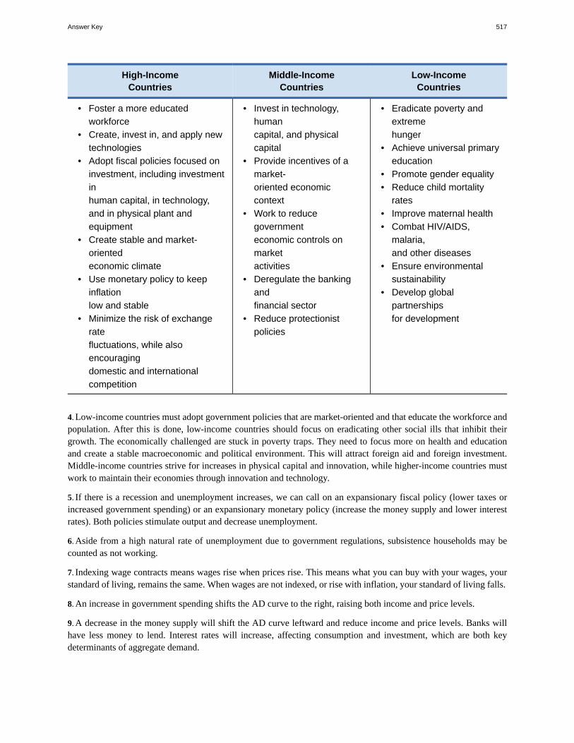
High-IncomeCountries
Middle-IncomeCountries
Low-IncomeCountries
• Foster a more educatedworkforce
• Create, invest in, and apply newtechnologies
• Adopt fiscal policies focused oninvestment, including investmentinhuman capital, in technology,and in physical plant andequipment
• Create stable and market-orientedeconomic climate
• Use monetary policy to keepinflationlow and stable
• Minimize the risk of exchangeratefluctuations, while alsoencouragingdomestic and internationalcompetition
• Invest in technology,humancapital, and physicalcapital
• Provide incentives of amarket-oriented economiccontext
• Work to reducegovernmenteconomic controls onmarketactivities
• Deregulate the bankingandfinancial sector
• Reduce protectionistpolicies
• Eradicate poverty andextremehunger
• Achieve universal primaryeducation
• Promote gender equality• Reduce child mortality
rates• Improve maternal health• Combat HIV/AIDS,
malaria,and other diseases
• Ensure environmentalsustainability
• Develop globalpartnershipsfor development
4. Low-income countries must adopt government policies that are market-oriented and that educate the workforce andpopulation. After this is done, low-income countries should focus on eradicating other social ills that inhibit theirgrowth. The economically challenged are stuck in poverty traps. They need to focus more on health and educationand create a stable macroeconomic and political environment. This will attract foreign aid and foreign investment.Middle-income countries strive for increases in physical capital and innovation, while higher-income countries mustwork to maintain their economies through innovation and technology.
5. If there is a recession and unemployment increases, we can call on an expansionary fiscal policy (lower taxes orincreased government spending) or an expansionary monetary policy (increase the money supply and lower interestrates). Both policies stimulate output and decrease unemployment.
6. Aside from a high natural rate of unemployment due to government regulations, subsistence households may becounted as not working.
7. Indexing wage contracts means wages rise when prices rise. This means what you can buy with your wages, yourstandard of living, remains the same. When wages are not indexed, or rise with inflation, your standard of living falls.
8. An increase in government spending shifts the AD curve to the right, raising both income and price levels.
9. A decrease in the money supply will shift the AD curve leftward and reduce income and price levels. Banks willhave less money to lend. Interest rates will increase, affecting consumption and investment, which are both keydeterminants of aggregate demand.
Answer Key 517
10. Given the high level of activity in international financial markets, it is typically believed that financial flows acrossborders are the real reason for trade imbalances. For example, the United States had an enormous trade deficit inthe late 1990s and early 2000s because it was attracting vast inflows of foreign capital. Smaller countries that haveattracted such inflows of international capital worry that if the inflows suddenly turn to outflows, the resulting declinein their currency could collapse their banking system and bring on a deep recession.
11. The demand for the country’s currency would decrease, lowering the exchange rate.
518 Answer Key
This OpenStax book is available for free at http://cnx.org/content/col11864/1.2
REFERENCESWelcome to Economics!Bureau of Labor Statistics, U.S. Department of Labor. 2015. "The Employment Situation—February 2015." Accessed
March 27, 2015. http://www.bls.gov/news.release/pdf/empsit.pdf.
Williamson, Lisa. “US Labor Market in 2012.” Bureau of Labor Statistics. Accessed December 1, 2013.http://www.bls.gov/opub/mlr/2013/03/art1full.pdf.
The Heritage Foundation. 2015. "2015 Index of Economic Freedom." Accessed March 11, 2015.http://www.heritage.org/index/ranking.
Garling, Caleb. “S.F. plane crash: Reporting, emotions on social media,” The San Francisco Chronicle. July 7, 2013.http://www.sfgate.com/news/article/S-F-plane-crash-Reporting-emotions-on-social-4651639.php.
Irvine, Jessica. “Social Networking Sites are Factories of Modern Ideas.” The Sydney Morning Herald. November25, 2011.http://www.smh.com.au/federal-politics/society-and-culture/social-networking-sites-are-factories-of-modern-ideas-20111124-1nwy3.html#ixzz2YZhPYeME.
Pew Research Center. 2015. "Social Networking Fact Sheet." Accessed March 11, 2015. http://www.pewinternet.org/fact-sheets/social-networking-fact-sheet/.
The World Bank Group. 2015. "World Data Bank." Accessed March 30, 2014. http://databank.worldbank.org/data/.
Choice in a World of ScarcityBureau of Labor Statistics, U.S. Department of Labor. 2015. “Median Weekly Earnings by Educational Attainment
in 2014.” Accessed March 27, 2015. http://www.bls.gov/opub/ted/2015/median-weekly-earnings-by-education-gender-race-and-ethnicity-in-2014.htm.
Robbins, Lionel. An Essay on the Nature and Significance of Economic Science. London: Macmillan. 1932.
United States Department of Transportation. “Total Passengers on U.S Airlines and Foreign Airlines U.S. FlightsIncreased 1.3% in 2012 from 2011.” Accessed October 2013. http://www.rita.dot.gov/bts/press_releases/bts016_13
Smith, Adam. “Of Restraints upon the Importation from Foreign Countries.” In The Wealth of Nations. London:Methuen & Co., 1904, first pub 1776), I.V. 2.9.
Smith, Adam. “Of the Propriety of Action.” In The Theory of Moral Sentiments. London: A. Millar, 1759, 1.
Demand and SupplyCostanza, Robert, and Lisa Wainger. “No Accounting For Nature: How Conventional Economics Distorts the Value
of Things.” The Washington Post. September 2, 1990.
European Commission: Agriculture and Rural Development. 2013. "Overview of the CAP Reform: 2014-2024."Accessed April 13, 205. http://ec.europa.eu/agriculture/cap-post-2013/.
Radford, R. A. “The Economic Organisation of a P.O.W. Camp.” Economica. no. 48 (1945): 189-201.http://www.jstor.org/stable/2550133.
Landsburg, Steven E. The Armchair Economist: Economics and Everyday Life. New York: The Free Press. 2012.specifically Section IV: How Markets Work.
National Chicken Council. 2015. "Per Capita Consumption of Poultry and Livestock, 1965 to Estimated 2015,in Pounds." Accessed April 13, 2015. http://www.nationalchickencouncil.org/about-the-industry/statistics/per-capita-consumption-of-poultry-and-livestock-1965-to-estimated-2012-in-pounds/.
Wessel, David. “Saudi Arabia Fears $40-a-Barrel Oil, Too.” The Wall Street Journal. May 27, 2004, p. 42.http://online.wsj.com/news/articles/SB108561000087822300.
Pew Research Center. “Pew Research: Center for the People & the Press.” http://www.people-press.org/.
Labor and Financial Markets
References 519
American Community Survey. 2012. "School Enrollment and Work Status: 2011." Accessed April 13, 2015.http://www.census.gov/prod/2013pubs/acsbr11-14.pdf.
National Center for Educational Statistics. “Digest of Education Statistics.” (2008 and 2010). Accessed December 11,2013. nces.ed.gov.
CreditCards.com. 2013. http://www.creditcards.com/credit-card-news/credit-card-industry-facts-personal-debt-statistics-1276.php.
The Macroeconomic PerspectiveU.S. Department of Commerce: Bureau of Economic Analysis. “National data: National Income and Product
Accounts Tables.” http://bea.gov/iTable/iTable.cfm?ReqID=9&step=1.
U.S. Department of Commerce: United States Census Bureau. “Census of Governments: 2012 Census ofGovernments.” http://www.census.gov/govs/cog/.
United States Department of Transportation. “About DOT.” Last modified March 2, 2012. http://www.dot.gov/about.
U.S. Department of Energy. “Energy.gov.” http://energy.gov/.
U.S. Department of Health & Human Services. “Agency for Healthcare Research and Quality.” http://www.ahrq.gov/.
United States Department of Agriculture. “USDA.” http://www.usda.gov/wps/portal/usda/usdahome.
Schneider, Friedrich. Department of Economics. “Size and Development of the Shadow Economy of 31 Europeanand 5 other OECD Countries from 2003 to 2013: A Further Decline.” Johannes Kepler University. Lastmodified April 5, 2013. http://www.econ.jku.at/members/Schneider/files/publications/2013/ShadEcEurope31_Jan2013.pdf.
The National Bureau of Economic Research. “Information on Recessions and Recoveries, the NBER Business CycleDating Committee, and related topics.” http://www.nber.org/cycles/main.html.
Economic GrowthBolt, Jutta, and Jan Luiten van Zanden. “The Maddison Project: The First Update of the Maddison Project Re-
Estimating Growth Before 1820 (Maddison-Project Working Paper WP-4).” University of Groningen:Groningen Growth and Development Centre. Last modified January 2013. http://www.ggdc.net/maddison/publications/pdf/wp4.pdf.
Central Intelligence Agency. “The World Factbook: Country Comparison GDP (Purchasing Power Parity).”https://www.cia.gov/library/publications/the-world-factbook/rankorder/2001rank.html.
DeLong, Brad. “Lighting the Rocket of Growth and Lightening the Toil of Work: Another Outtake from My‘Slouching Towards Utopia’ MS....” This is Brad DeLong's Grasping Reality (blog). September 3, 2013.http://delong.typepad.com/sdj/2013/09/lighting-the-rocket-of-growth-and-lightening-the-toil-of-work-another-outtake-from-my-slouching-towards-utopia-ms.html.
Easterlin, Richard A. “The Worldwide Standard of Living since 1800.” The Journal of Economic Perspectives. no. 1(2000): 7–26. http://pubs.aeaweb.org/doi/pdfplus/10.1257/jep.14.1.7.
Maddison, Angus. Contours of the World Economy 1-2030 AD: Essays in Macro-Economic History. Oxford: OxfordUniversity Press, 2007.
British Library. “Treasures in Full: Magna Carta.” http://www.bl.uk/treasures/magnacarta/.
Rothbard, Murray N. Ludwig von Mises Institute. “Property Rights and the Theory of Contracts.” The Ethics ofLiberty. Last modified June 22, 2007. http://mises.org/daily/2580.
Salois, Matthew J., J. Richard Tiffin, and Kelvin George Balcombe. IDEAS: Research Division of the FederalReserve Bank of St. Louis. “Impact of Income on Calorie and Nutrient Intakes: A Cross-Country Analysis.”Presention at the annual meeting of the Agricultural and Applied Economics Association, Pittsburg, PA, July24–26, 2011. http://ideas.repec.org/p/ags/aaea11/103647.html.
van Zanden, Jan Luiten. The Long Road to the Industrial Revolution: The European Economy in a GlobalPerspective, 1000–1800 (Global Economic History Series). Boston: Brill, 2009.
520 References
This OpenStax book is available for free at http://cnx.org/content/col11864/1.2
The World Bank. “CPIA Property Rights and Rule-based Governance Rating (1=low to 6=high).”http://data.worldbank.org/indicator/IQ.CPA.PROP.XQ.
Rex A. Hudson, ed. Brazil: A Country Study. “Spectacular Growth, 1968–73.” Washington: GPO for the Library ofCongress, 1997. http://countrystudies.us/brazil/64.htm.
“Women and the World Economy: A Guide to Womenomics.” The Economist, April 12, 2006.http://www.economist.com/node/6802551.
Farole, Thomas, and Gokhan Akinci, eds. Special Economic Zones: Progress, Emerging Challenges, and FutureDirections. Washington: The World Bank, 2011. http://publications.worldbank.org/index.php?main_page=product_info&products_id=24138.
Garcia, Abraham, and Pierre Mohnen. United Nations University, Maastricht Economic and Social Research andTraining Centre on Innovation and Technology: UNU-MERIT. “Impact of Government Support on R&Dand Innovation (Working Paper Series #2010-034).” http://www.merit.unu.edu/publications/wppdf/2010/wp2010-034.pdf.
Heston, Alan, Robert Summers, and Bettina Aten. “Penn World Table Version 7.1.” Center for InternationalComparisons of Production, Income and Prices at the University of Pennsylvania. Last modified July 2012.https://pwt.sas.upenn.edu/php_site/pwt71/pwt71_form.php.
United States Department of Labor: Bureau of Labor Statistics. “Women at Work: A Visual Essay.” Monthly LaborReview, October 2003, 45–50. http://www.bls.gov/opub/mlr/2003/10/ressum3.pdf.
Central Intelligence Agency. “The World Factbook: Country Comparison: GDP–Real Growth Rate.”https://www.cia.gov/library/publications/the-world-factbook/rankorder/2003rank.html.
Sen, Amartya. “Hunger in the Contemporary World (Discussion Paper DEDPS/8).” The Suntory Centre: LondonSchool of Economics and Political Science. Last modified November 1997. http://sticerd.lse.ac.uk/dps/de/dedps8.pdf.
UnemploymentBureau of Labor Statistics. Labor Force Statistics from the Current Population Survey. Accessed March 6, 2015
http://data.bls.gov/timeseries/LNS14000000.
Cappelli, P. (20 June 2012). “Why Good People Can’t Get Jobs: Chasing After the Purple Squirrel.”http://knowledge.wharton.upenn.edu/article.cfm?articleid=3027.
InflationSources for Table 8.1:
http://www.eia.gov/dnav/pet/pet_pri_gnd_a_epmr_pte_dpgal_w.htmhttp://data.bls.gov/cgi-bin/surveymost?aphttp://www.bls.gov/ro3/apmw.htmhttp://www.autoblog.com/2014/03/12/who-can-afford-the-average-car-price-only-folks-in-washington/https://www.census.gov/construction/nrs/pdf/uspricemon.pdfhttp://www.bls.gov/news.release/empsit.t24.htmhttp://variety.com/2015/film/news/movie-ticket-prices-increased-in-2014-1201409670/
US Inflation Calculator. "Historical Inflation Rates: 1914-2013." Accessed March 4, 2015.http://www.usinflationcalculator.com/inflation/historical-inflation-rates/.
Bernhard, Kent. “Pump Prices Jump Across U.S. after Katrina.” NBC News, September 1, 2005.http://www.nbcnews.com/id/9146363/ns/business-local_business/t/pump-prices-jump-across-us-after-katrina/#.U00kRfk7um4.
Wynne, Mark A. “Core Inflation, A Review of Some Conceptual Issues.” Federal Reserve Bank of St. Louis. p. 209.Accessed April 14, 2014. http://research.stlouisfed.org/publications/review/08/05/part2/Wynne.pdf
Shiller, Robert. “Why Do People Dislike Inflation?” NBER Working Paper Series, National Bureau of EconomicResearch, p. 52. 1996.
Wines, Michael. “How Bad is Inflation in Zimbabwe?” The New York Times, May 2, 2006. http://www.nytimes.com/2006/05/02/world/africa/02zimbabwe.html?pagewanted=all&_r=0.
References 521
Hanke, Steve H. “R.I.P. Zimbabwe Dollar.” CATO Institute. Accessed December 31, 2013. http://www.cato.org/zimbabwe.
Massachusetts Institute of Technology. 2015. "Billion Prices Project." Accessed March 4, 2015. http://bpp.mit.edu/usa/.
The International Trade and Capital FlowsCentral Intelligence Agency. “The World Factbook.” Last modified October 31, 2013. https://www.cia.gov/library/
publications/the-world-factbook/geos/gm.html.
U.S. Department of Commerce. “Bureau of Economic Analysis.” Last modified December 1, 2013.http://www.bea.gov/.
U.S. Department of Commerce. “United States Census Bureau.” http://www.census.gov/.
Tabuchi, Hiroko. “Japan Reports a $78 Billion Trade Deficit for 2012.” The New York Times, January 23, 2013.http://www.nytimes.com/2013/01/24/business/global/japan-reports-a-78-billion-trade-deficit-for-2012.html?_r=0.
World Bank. 2014. "Exports of Goods and Services (% of GDP)." Accesed April 13, 2015. http://data.worldbank.org/indicator/NE.EXP.GNFS.ZS/countries.
The Aggregate Demand/Aggregate Supply ModelKeynes, John Maynard. The General Theory of Employment, Interest and Money. London: Palgrave Macmillan, 1936.
U.S. Department of Commerce: United States Census Bureau. “New Residential Sales: Historical Data.”http://www.census.gov/construction/nrs/historical_data/.
Library of Economics and Liberty. “The Concise Encyclopedia of Economics: Jean-Baptiste Say.”http://www.econlib.org/library/Enc/bios/Say.html.
Library of Economics and Liberty. “The Concise Encyclopedia of Economics: John Maynard Keynes.”http://www.econlib.org/library/Enc/bios/Keynes.html.
Organization for Economic Cooperation and Development. 2015. "Business Tendency Surveys: Construction."Accessed March 4, 2015. http://stats.oecd.org/mei/default.asp?lang=e&subject=6.
University of Michigan. 2015. "Surveys of Consumers." Accessed March 4, 2015. http://www.sca.isr.umich.edu/tables.html.
The Keynesian PerspectiveMahapatra, Lisa. “US Exports To China Have Grown 294% Over The Past Decade.” International Business Times.
Last modified July 09, 2013. http://www.ibtimes.com/us-exports-china-have-grown-294-over-past-decade-1338693.
The Conference Board, Inc. “Global Economic Outlook 2014, November 2013.” http://www.conference-board.org/data/globaloutlook.cfm.
Thomas, G. Scott. “Recession claimed 170,000 small businesses in two years.” The Business Journals. Last modifiedJuly 24, 2012. http://www.bizjournals.com/bizjournals/on-numbers/scott-thomas/2012/07/recession-claimed-170000-small.html.
United States Department of Labor: Bureau of Labor Statistics. “Top Picks.” http://data.bls.gov/cgi-bin/surveymost?bls.
Joyner, James. Outside the Beltway. “Public Financing of Private Sports Stadiums.” Last modified May 23, 2012.http://www.outsidethebeltway.com/public-financing-of-private-sports-stadiums/.
Siegfried, John J., and Andrew Zimbalist. “The Economics of Sports Facilities and Their Communities.” Journal ofEconomic Perspectives. no. 3 (2000): 95-114. http://pubs.aeaweb.org/doi/pdfplus/10.1257/jep.14.3.95.
Harford, Tim. “What Price Supply and Demand?” http://timharford.com/2014/01/what-price-supply-and-demand/?utm_source=dlvr.it&utm_medium=twitter.
522 References
This OpenStax book is available for free at http://cnx.org/content/col11864/1.2

National Employment Law Project. “Job Creation and Economic Recovery.” http://www.nelp.org/index.php/content/content_issues/category/job_creation_and_economic_recovery/.
Hoover, Kevin. “Phillips Curve.” The Concise Encyclopedia of Economics. http://www.econlib.org/library/Enc/PhillipsCurve.html.
U.S. Government Printing Office. “Economic Report of the President.” http://1.usa.gov/1c3psdL.
Blinder, Alan S., and Mark Zandi. “How the Great Recession Was Brought to an End.” Last modified July 27, 2010.http://www.princeton.edu/~blinder/End-of-Great-Recession.pdf.
The Neoclassical PerspectiveLumina Foundation. 2014. "A Stronger Nation Through Higher Education." Accessed March 4, 2015.
http://www.luminafoundation.org/publications/A_stronger_nation_through_higher_education-2014.pdf.
The National Bureau of Economic Research. http://www.nber.org/.
U.S. Department of Commerce: United States Census Bureau. “The 2012 Statistical Abstract.”http://www.census.gov/compendia/statab/cats/education.html.
U.S. Department of the Treasury. “TARP Programs.” Last modified December 12, 2013. http://www.treasury.gov/initiatives/financial-stability/TARP-Programs/Pages/default.aspx.
United States Government. “Recovery.gov: Track the Money.” Last modified October 30, 2013.http://www.recovery.gov/Pages/default.aspx.
American Statistical Association. “ASA Headlines.” http://www.amstat.org/.
Haubrich, Joseph G., George Pennacchi, and Peter Ritchken. “Working Paper 11-07: Inflation Expectations, RealRates, and Risk Premia: Evidence from Inflation Swaps.” Federal Reserve Bank of Cleveland. Last modifiedMarch 2011. http://www.clevelandfed.org/research/workpaper/2011/wp1107.pdf.
University of Michigan: Institute for Social Research. “Survey Research Center.” http://www.src.isr.umich.edu/.
Carvalho, Carlos, Stefano Eusepi, and Christian Grisse. “Policy Initiatives in the Global Recession: What DidForecasters Expect?” Federal Reserve Bank of New York: Current Issues in Economics and Finance, 18, no. 2(2012). http://www.newyorkfed.org/research/current_issues/ci18-2.pdf.
Money and BankingHogendorn, Jan and Marion Johnson. The Shell Money of the Slave Trade. Cambridge University Press, 2003. 6.
Federal Reserve Statistical Release. November 23, 2013. http://www.federalreserve.gov/RELEASES/h6/current/default.htm#t2tg1link.
Credit Union National Association. 2014. "Monthly Credit Union Estimates." Last accessed March 4, 2015.http://www.cuna.org/Research-And-Strategy/Credit-Union-Data-And-Statistics/.
Dallas Federal Reserve. 2013. "Ending `Too Big To Fail': A Proposal for Reform Before It's Too Late". AccessedMarch 4, 2015. http://www.dallasfed.org/news/speeches/fisher/2013/fs130116.cfm.
Richard W. Fisher. “Ending 'Too Big to Fail': A Proposal for Reform Before It's Too Late (With Reference to PatrickHenry, Complexity and Reality) Remarks before the Committee for the Republic, Washington, D.C. DallasFederal Reserve. January 16, 2013.
“Commercial Banks in the U.S.” Federal Reserve Bank of St. Louis. Accessed November 2013.http://research.stlouisfed.org/fred2/series/USNUM.
Bitcoin. 2013. www.bitcoin.org.
National Public Radio. Lawmakers and Regulators Take Closer Look at Bitcoin. November 19, 2013.http://thedianerehmshow.org/shows/2013-11-19/lawmakers-and-regulators-take-closer-look-bitcoin.
Monetary Policy and Bank RegulationMatthews, Dylan. “Nine amazing facts about Janet Yellen, our next Fed chair.” Wonkblog. The Washington Post.
Posted October 09, 2013. http://www.washingtonpost.com/blogs/wonkblog/wp/2013/10/09/nine-amazing-facts-about-janet-yellen-our-next-fed-chair/.
References 523
Appelbaum, Binyamin. “Divining the Regulatory Goals of Fed Rivals.” The New York Times. Posted August14, 2013. http://www.nytimes.com/2013/08/14/business/economy/careers-of-2-fed-contenders-reveal-little-on-regulatory-approach.html?pagewanted=3.
U.S. Department of the Treasury. “Office of the Comptroller of the Currency.” Accessed November 2013.http://www.occ.gov/.
National Credit Union Administration. “About NCUA.” Accessed November 2013. http://www.ncua.gov/about/Pages/default.aspx.
Board of Governors of the Federal Reserve System. “Federal Open Market Committee.” Accessed September 3, 2013.http://www.federalreserve.gov/monetarypolicy/fomc.htm.
Board of Governors of the Federal Reserve System. “Reserve Requirements.” Accessed November 5, 2013.http://www.federalreserve.gov/monetarypolicy/reservereq.htm.
Cox, Jeff. 2014. "Fed Completes the Taper." Accessed March 31, 2015. http://www.cnbc.com/id/102132961.
Jahan, Sarwat. n.d. "Inflation Targeting: Holding the Line." International Monetary Fund. Accessed March 31, 2015.http://www.imf.org/external/pubs/ft/fandd/basics/target.htm.
Tobin, James. “The Concise Encyclopedia of Economics: Monetary Policy.” Library of Economics and Liberty.Accessed November 2013. http://www.econlib.org/library/Enc/MonetaryPolicy.html.
Federal Reserve Bank of New York. “The Founding of the Fed.” Accessed November 2013.http://www.newyorkfed.org/aboutthefed/history_article.html.
Exchange Rates and International Capital FlowsFriedman, Milton. Capitalism and Freedom. Chicago: University of Chicago Press, 1962.
Government Budgets and Fiscal PolicyKramer, Mattea, et. al. A People's Guide to the Federal Budget. National Priorities Project. Northampton: Interlink
Books, 2012.
Kurtzleben, Danielle. “10 States With The Largest Budget Shortfalls.” U.S. News & World Report. Januray 14, 2011.http://www.usnews.com/news/articles/2011/01/14/10-states-with-the-largest-budget-shortfalls.
Miller, Rich, and William Selway. “U.S. Cities and States Start Spending Again.” BloombergBusinessweek, January10, 2013. http://www.businessweek.com/articles/2013-01-10/u-dot-s-dot-cities-and-states-start-spending-again.
Weisman, Jonathan. “After Year of Working Around Federal Cuts, Agencies Face Fewer Options.” The New YorkTimes, October 26, 2013. http://www.nytimes.com/2013/10/27/us/politics/after-year-of-working-around-federal-cuts-agencies-face-fewer-options.html?_r=0.
Chantrill, Christopher. USGovernmentSpending.com. “Government Spending Details: United States Federal Stateand Local Government Spending, Fiscal Year 2013.” http://www.usgovernmentspending.com/year_spending_2013USbn_15bs2n_20.
Burman, Leonard E., and Joel Selmrod. Taxes in America: What Everyone Needs to Know. New York: OxfordUniversity Press, 2012.
Hall, Robert E., and Alvin Rabushka. The Flat Tax (Hoover Classics). Stanford: Hoover Institution Press, 2007.
Kliff, Sarah. “How Congress Paid for Obamacare (in Two Charts).” The Washington Post: WonkBlog (blog), August30, 2012. http://www.washingtonpost.com/blogs/wonkblog/wp/2012/08/30/how-congress-paid-for-obamacare-in-two-charts/.
Matthews, Dylan. “America’s Taxes are the Most Progressive in the World. Its Government is Among the Least.” TheWashington Post: WonkBlog (blog). April 5, 2013. http://www.washingtonpost.com/blogs/wonkblog/wp/2013/04/05/americas-taxes-are-the-most-progressive-in-the-world-its-government-is-among-the-least/.
Eisner, Robert. The Great Deficit Scares: The Federal Budget, Trade, and Social Security. New York: Priority PressPublications, 1997.
Weisman, Jonathan, and Ashley Parker. “Republicans Back Down, Ending Crisis Over Shutdown and Debt Limit.”The New York Times, October 16, 2013. http://www.nytimes.com/2013/10/17/us/congress-budget-debate.html.
524 References
This OpenStax book is available for free at http://cnx.org/content/col11864/1.2
Wessel, David. Red Ink: Inside the High-Stakes Politics of Federal Budget. New York: Crown Publishing Group,2013.
Alesina, Alberto, and Francesco Giavazzi. Fiscal Policy after the Financial Crisis (National Bureau of EconomicResearch Conference Report). Chicago: University Of Chicago Press, 2013.
Martin, Fernando M. “Fiscal Policy in the Great Recession and Lessons from the Past.” Federal Reserve Bank of St.Louis: Economic Synopses. no. 1 (2012). http://research.stlouisfed.org/publications/es/12/ES_2012-01-06.pdf.
Bivens, Josh, Andrew Fieldhouse, and Heidi Shierholz. “From Free-fall to Stagnation: Five Years After the Start ofthe Great Recession, Extraordinary Policy Measures Are Still Needed, But Are Not Forthcoming.” EconomicPolicy Institute. Last modified February 14, 2013. http://www.epi.org/publication/bp355-five-years-after-start-of-great-recession/.
Lucking, Brian, and Dan Wilson. Federal Reserve Bank of San Francisco, “FRBSF Economic Letter—U.S. FiscalPolicy: Headwind or Tailwind?” Last modified July 2, 2012. http://www.frbsf.org/economic-research/publications/economic-letter/2012/july/us-fiscal-policy/.
Greenstone, Michael, and Adam Looney. Brookings. “The Role of Fiscal Stimulus in the Ongoing Recovery.” Lastmodified July 6, 2012. http://www.brookings.edu/blogs/jobs/posts/2012/07/06-jobs-greenstone-looney.
Leduc, Sylvain, and Daniel Wilson. Federal Reserve Bank of San Francisco: Working Paper Series. “Are StateGovernments Roadblocks to Federal Stimulus? Evidence from Highway Grants in the 2009 Recovery Act.(Working Paper 2013-16).” Last modified July 2013. http://www.frbsf.org/economic-research/files/wp2013-16.pdf.
Lucking, Brian, and Daniel Wilson. “FRBSF Economic Letter-Fiscal Headwinds: Is the Other Shoe About to Drop?”Federal Reserve Bank of San Francisco. Last modified June 3, 2013. http://www.frbsf.org/economic-research/publications/economic-letter/2013/june/fiscal-headwinds-federal-budget-policy/.
Recovery.gov. “Track the Money.” http://www.recovery.gov/Pages/default.aspx.
Bastagli, Francesca, David Coady, and Sanjeev Gupta. International Monetary Fund. “IMF Staff Discussion Note:Income Inequality and Fiscal Policy.” Last modified June 28, 2012. http://www.imf.org/external/pubs/ft/sdn/2012/sdn1208.pdf.
The Impacts of Government BorrowingU.S. Department of Commerce: Bureau of Economic Analysis. “National Data: National Income and Product
Accounts Tables.” Accessed December 1, 2013. http://www.bea.gov/iTable/iTable.cfm?ReqID=9&step=1#reqid=9&step=3&isuri=1&910=X&911=0&903=146&904=2008&905=2013&906=A.
Board of Governors of the Federal Reserve System, “Selected Interest Rates (Daily) – H.15.” Accessed December10, 2013. http://www.federalreserve.gov/releases/h15/data.htm.
The White House. “Fiscal Year 2013 Historical Tables: Budget of the U.S. Government.” Accessed December 12,2013. http://www.whitehouse.gov/sites/default/files/omb/budget/fy2013/assets/hist.pdf.
The National Science Foundation. Accessed December 19, 2013. http://www.nsf.gov/.
The White House. “This is why it's time to make college more affordable.” Last modified August 20, 2013.http://www.whitehouse.gov/share/college-affordability.
Rubin, Robert E., Peter R. Orszag, and Allen Sinai. “Sustained Budget Deficits: Longer-Run U.S. EconomicPerformance and the Risk of Financial and Fiscal Disarray.” Last modified January 4, 2004.http://www.brookings.edu/~/media/research/files/papers/2004/1/05budgetdeficit%20orszag/20040105.pdf.
Macroeconomic Policy Around the WorldInternational Labour Organization. “Global Employment Trends for Youth 2013.” http://www.ilo.org/global/research/
global-reports/global-employment-trends/youth/2013/lang--en/index.htm
International Monetary Fund. “World Economic and Financial Surveys: World Economic Outlook—Transitions andTensions.” Last modified October 2013. http://www.imf.org/external/pubs/ft/weo/2013/02/pdf/text.pdf.
Nobelprize.org. “The Prize in Economics 1987 - Press Release.” Nobel Media AB 2013. Last modified October 21,1987. http://www.nobelprize.org/nobel_prizes/economic-sciences/laureates/1987/press.html.
References 525
Redvers, Louise. BBC News Business. “Youth unemployment: The big question and South Africa.” Last modifiedOctober 31, 2012. http://www.bbc.co.uk/news/business-20125053.
The World Bank. “The Complete World Development Report Online.” http://www.wdronline.worldbank.org/.
The World Bank. “World DataBank.” http://databank.worldbank.org/data/home.aspx.
Todaro, Michael P., and Stephen C Smith. Economic Development (11thEdition). Boston, MA: Addison-Wesley:Pearson, 2011, chap. 1–2.
“Shinzo Abe’s Government Looks Likely to Disappoint on Fiscal Consolidation.” The Economist, May 4, 2013.http://www.economist.com/news/finance-and-economics/21577080-shinzo-abes-government-looks-likely-disappoint-fiscal-consolidation-dont.
Banerjee, Abhijit V., and Esther Duflo. Poor Economics. “About the Book: Overview.” http://pooreconomics.com/about-book.
CARE International. “About Us.” Accessed January 14, 2014. http://www.care-international.org/about-us.aspx.
Central Intelligence Agency. “The World Factbook: Africa, Burundi.” Last modified November 12, 2013.https://www.cia.gov/library/publications/the-world-factbook/geos/by.html.
Central Intelligence Agency. “The World Factbook: Africa, Democratic Republic of the Congo.” Last modifiedNovember 12, 2013. https://www.cia.gov/library/publications/the-world-factbook/geos/cg.html.
Easterly, William. The White Man’s Burden: Why the West’s Efforts to Aid the Rest Have Done So Much Ill and SoLittle Good. Penguin Group (USA), 2006.
Goel, Vindu. “Facebook Leads an Effort to Lower Barriers to Internet Access,” The New York Times. Last modifiedAugust 20, 2013.
Google. “Project Loon.” http://www.google.com/loon/.
GOV.UK. “Department for International Development.” https://www.gov.uk/government/organisations/department-for-international-development.
The World Bank. “Millennium Development Goals.” http://www.worldbank.org/mdgs/.
Todaro, Michael P., and Stephen C Smith. Economic Development (11th Edition). Boston, MA: Addison-Wesley:Pearson, 2011, chap. 3.
Vercillo, Siera. “The Failures of Canadian Foreign Aid: Tied, Mismanaged and Uncoordinated.” The Attaché Journalof International Affairs. (2010). http://theattachejia.files.wordpress.com/2013/10/the-attache-2010-issue.pdf.
Viscusi, Gregory, and Mark Deen. “Why France Has So Many 49-Employee Companies.” Business Week. Lastmodified May 3, 2012. http://www.businessweek.com/articles/2012-05-03/why-france-has-so-many-49-employee-companies.
Edwards, S. (n.d.). “America’s Unsustainable Current Account Deficit.” National Bureau of Economic ResearchDigest. http://www.nber.org/digest/mar06/w11541.html. http://www.ustr.gov/trade-agreements/free-trade-agreements/north-american-free-trade-agreement-nafta.
New Country Classifications | Data. (n.d.). Accessed January 14, 2014. http://data.worldbank.org/news/new-country-classifications.
Office of the United States Trade Representative: Executive Office of the President. “North American Free TradeAgreement (NAFTA).”
Why India’s Labour Laws are a Problem. (2006, May 18). BBC. May 18, 2006. http://news.bbc.co.uk/2/hi/south_asia/4984256.stm.
526 References
This OpenStax book is available for free at http://cnx.org/content/col11864/1.2
INDEX
Symbols401(k), 197
AA.W. Phillips, 289Abhijit Bannerjee, 445Abraham García, 145Adam Smith, 10, 37, 235adaptive expectations, 306, 315adjustable-rate mortgage(ARM), 200, 203adverse selection of wage cutsargument, 167, 177aggregate demand, 235, 263,302, 306, 311, 353, 357, 378,402, 447aggregate demand (AD), 105,254Aggregate demand (AD), 238aggregate demand (AD) curve,238, 254aggregate demand/aggregatesupply (AD/AS), 320aggregate demand/aggregatesupply model, 236, 254, 301aggregate production function,136, 141, 150, 151aggregate supply, 235, 302, 402aggregate supply (AS), 105, 254Aggregate supply (AS), 236aggregate supply (AS) curve,237, 254aggregate supply curve, 311Alexander Gerschenkron, 147Allocative efficiency, 34allocative efficiency, 40American Recovery andReinvestment Act of 2009, 270appreciating, 370, 388arbitrage, 377, 388Asian Financial Crisis, 451asset, 326, 334asset-liability time mismatch,329assets, 344asset–liability time mismatch,334automatic stabilizers, 405, 413,447
Bbalance of payments, 218balance of trade, 210, 226, 386balance of trade (tradebalance), 228balance sheet, 326, 334balanced budget, 394, 411, 413bank capital, 327, 334Bank capital, 343Bank regulation, 343bank run, 344, 361banking system, 324bankrupt, 380bar graph, 469Barter, 320barter, 334base year, 185, 203basic quantity equation ofmoney, 356, 361basket of goods and services,183, 203bonds, 201, 327, 347, 491budget constraint, 26, 40, 480budget deficit, 394, 413budget line, 479budget surplus, 394, 413Bureau of Economic Analysis(BEA), 211Bureau of Labor Statistics, 124business confidence, 244business cycle, 119, 126
Ccapital deepening, 141, 151central bank, 340, 354, 361,378, 384certificates of deposit (CDs),323ceteris paribus, 50, 62, 71, 82circular flow diagram, 14, 21coins and currency incirculation, 323, 334command economy, 16, 21commodity money, 321, 334Commodity-backed currencies,321commodity-backed currencies,334comparative advantage, 11, 35,40, 217complements, 52, 71
compound growth rate, 140, 151consumer confidence, 245Consumer Price Index (CPI),186, 203consumer surplus, 68consumption budget constraint,33consumption demand, 107contractionary fiscal policy, 291,294, 402, 413contractionary monetary policy,349, 361, 383, 425contractual rights, 134, 151convergence, 145, 151converging economy, 449, 454coordination argument, 267, 294core competency, 11core inflation index, 189, 203corporate income tax, 398, 413cost, 33cost of living, 187cost-of-living adjustments(COLAs), 200, 203countercyclical, 351, 361credit card, 324, 334credit union, 326crowding out, 408, 413, 423current account balance, 211,228cyclical unemployment, 166,177, 310Cyclical unemployment, 248
Ddeadweight loss, 69dealers, 370debit card, 324, 334deficit, 421deflation, 191, 203Deflation, 356demand, 45, 71, 105, 235, 366demand and supply diagram, 68demand and supply models, 94demand curve, 45, 50, 71, 375,424demand deposit, 334demand deposits, 323demand schedule, 45, 71deposit insurance, 345, 361depository institution, 334depository institutions, 325depreciating, 370, 388
Index 527
depreciation, 112, 126depression, 119, 126, 161diminishing marginal utility, 478direct investment, 384discount rate, 349, 361Discouraged workers, 159discouraged workers, 177discretionary fiscal policy, 405,413, 447disposable income, 263, 294diversify, 329, 334division of labor, 10, 21dollarize, 366, 388double coincidence of wants,320, 334double counting, 110, 126Dow Jones, 358durable good, 126durable goods, 109
EEast Asian Tigers, 443, 454economic efficiency, 38economic growth, 320economic surplus, 69Economics, 8economics, 21economies of scale, 11, 21efficiency, 68Efficiency wage theory, 167efficiency wage theory, 177Employment Cost Index, 190,203equilibrium, 48, 68, 71, 82equilibrium exchange rate, 375equilibrium price, 48, 71equilibrium quantity, 48, 64, 71estate and gift tax, 398, 413Esther Duflo, 445European Union (EU), 67excess demand, 49, 71excess reserves, 354, 361excess supply, 49, 71exchange rate, 120, 126, 366,430exchange rates, 360excise tax, 398, 413expansionary fiscal policy, 291,294, 402, 413expansionary monetary policy,349, 361, 383, 425, 447expected inflation, 307, 315expenditure multiplier, 270, 294Exports, 18exports, 21, 211, 239, 265, 378
exports of goods and servicesas a percentage of GDP, 215,228
Ffactors of production, 54, 71Federal Deposit InsuranceCorporation (FDIC), 345federal funds rate, 350, 361Federal Open MarketCommittee (FOMC), 346Federal Reserve, 340, 343, 358,425, 450Federal Reserve Bank, 323Federal Reserve EconomicData (FRED), 161, 371fiat money, 322, 334final good and service, 126final goods and services, 111financial capital, 89, 216, 220,228, 360, 420financial capital market, 219financial capital markets, 408,420financial intermediary, 325, 334firm, 35, 56firms, 368Fiscal policy, 13fiscal policy, 21, 394, 447floating exchange rate, 381, 388Foreign direct investment (FDI),368foreign direct investment (FDI),388foreign exchange market, 366,375, 388foreign financial capital, 223foreign investment capital, 380FRED, 382frictional unemployment, 170,177full-employment GDP, 238, 254function, 459
GGDP, 367, 378GDP deflator, 114, 190, 203GDP per capita, 122, 124, 126,141, 242, 439globalization, 18, 21good, 46goods and services market, 14,21Great Depression, 119, 236,300, 313
Great Recession, 109, 119, 192,300, 448gross domestic product (GDP),18, 21, 105, 126gross national product (GNP),112, 126growth consensus, 442, 454growth rate, 463
Hhard peg, 382, 388Head Start program, 427, 434hedge, 369, 388hidden unemployment, 159high-income country, 454Human capital, 135human capital, 151, 301, 411,427, 444hyperinflation, 193, 203
Iimplementation lag, 409, 413implicit contract, 167, 177Imports, 18imports, 21, 211, 239, 265income effect, 481income payments, 212index number, 185, 203indexed, 200, 203indifference curve, 477individual income tax, 397, 413Industrial Revolution, 132, 151infant industry argument, 450inferior good, 52, 71Inflation, 182inflation, 203, 234, 248, 291,320, 340, 448inflation rate, 352inflation targeting, 358, 361inflationary gap, 263, 294infrastructure, 141, 151, 411innovation, 135, 151inputs, 54, 71insider-outsider model, 167, 177interbank market, 370interest rate, 90, 99, 264, 491interest rates, 340, 350intermediate good, 126Intermediate goods, 111intermediate zone, 252, 254international capital flows, 384,388international financial flows, 384International Price Index, 190,203international trade, 381
528 Index
This OpenStax book is available for free at http://cnx.org/content/col11864/1.2
intertemporal choices, 39intertemporal decision making,91invention, 135, 151inventories, 109inventory, 126Investment demand, 107Investment expenditure, 107investment expenditure, 264investment income, 218invisible hand, 38, 40involuntary unemployment, 166
JJames Tobin, 384Jan Luiten van Zanden, 132Janet L. Yellen, 341Jean-Baptiste Say, 235John Maynard Keynes, 13, 236,305, 407
KKeynesian aggregate supplycurve, 350Keynesian economic model,447Keynesian economics, 301, 313Keynesian macroeconomicpolicy, 411Keynesian zone, 252, 254Keynes’ law, 235, 251, 254
Llabor force participation rate,159, 177labor market, 14, 21, 82, 166labor markets, 200Labor productivity, 135labor productivity, 151labor-leisure diagram, 483law of demand, 45, 71, 91law of diminishing marginalutility, 30, 40law of diminishing returns, 33,40, 147law of supply, 46, 71legislative lag, 409, 413lender of last resort, 345, 361level of trade, 225leverage cycle, 359liability, 326, 334line graphs, 464Liquidity, 322living wage, 87loan market, 327
long run aggregate supply(LRAS) curve, 242, 254loose monetary policy, 349, 361low-income countries, 165low-income country, 454
MM1, 355M1 money supply, 323, 334M2, 357M2 money supply, 323, 334macro economy, 165macroeconomic externality, 269,294Macroeconomics, 12macroeconomics, 21marginal analysis, 30, 40marginal rate of substitution,478marginal tax rates, 398, 413marginal utility, 478market, 16, 21market economy, 16, 21, 35,170, 198median, 464medium of exchange, 321, 334menu costs, 267, 294merchandise trade balance,211, 228merged currency, 385, 388Microeconomics, 12microeconomics, 21middle-income country, 454Milton Friedman, 310, 357, 382minimum wage, 87, 99, 166,196model, 14, 21modern economic growth, 132,151Monetary policy, 13monetary policy, 21, 340, 346,383, 394money, 321, 334money market fund, 334money market funds, 323money multiplier, 359money multiplier formula, 331,335
NNasdaq, 358National Bureau of EconomicResearch, 450National Bureau of EconomicResearch (NBER), 120
National Credit UnionAdministration (NCUA), 344national debt, 400, 413national income, 112, 126national saving and investmentidentity, 219national savings and investmentidentity, 228natural rate of unemployment,169, 177, 249, 310negative slope, 461neoclassical determinants ofgrowth, 442neoclassical economists, 235,254neoclassical model, 357neoclassical perspective, 301,315neoclassical zone, 252, 254Net national product (NNP), 112net national product (NNP), 126net worth, 326, 335, 343nominal GDP, 117, 356nominal interest rate, 196, 356nominal value, 113, 126nondurable good, 126nondurable goods, 109normal good, 52, 71normative statement, 40normative statements, 37North American Free TradeAgreement (NAFTA), 449
Oopen market operations, 346,361opportunity cost, 27, 40, 156,384opportunity set, 26, 40, 482out of the labor force, 157, 177
Ppayment system, 325, 335payroll tax, 397, 413peak, 119, 126pensions, 197per capita GDP, 183, 224percentage change, 184Pew Research Center forPeople and the Press, 61Phillips curve, 289, 294, 308physical capital, 141, 151, 423,444Physical capital per person, 301physical capital per person, 315
Index 529
pie chart, 467pie graph, 467Pierre Mohnen, 145portfolio investment, 368, 384,388positive slope, 461positive statement, 40positive statements, 37potential GDP, 237, 254, 263,291, 301, 350, 358present discounted value (PDV),491price, 29, 45, 49, 71price ceiling, 65, 70, 71price control, 69, 71Price controls, 65price controls, 96price floor, 65, 70, 71price level, 183private enterprise, 16, 21private markets, 200Producer Price Index (PPI), 190,203producer surplus, 69production function, 136, 151production possibilities frontier(PPF), 31, 40Productive efficiency, 34productive efficiency, 40Productivity growth, 138productivity growth, 242progressive tax, 398, 413property rights, 134proportional tax, 398, 413purchasing power parity, 439purchasing power parity (PPP),120, 377, 388
Qquality/new goods bias, 188,203quantitative easing (QE), 353,361quantity demanded, 45, 71, 383quantity supplied, 46, 71, 383
Rrational expectations, 305, 315real GDP, 117, 210, 225, 263,294, 301, 354, 356real interest rate, 196real value, 113, 126recession, 119, 126, 161, 235,246, 266, 354, 431, 447recessionary gap, 263, 294
recognition lag, 408, 413redistributions, 195, 199regressive tax, 398, 413relative wage coordinationargument, 167, 177reserve requirement, 348, 361reserves, 327, 335, 343, 348,384revenue, 399Ricardian equivalence, 428, 434Richard Easterlin, 134Robert Shiller, 195Robert Solow, 313rule of law, 134, 151
Ssalary, 80savings deposit, 335savings deposits, 323Say’s law, 235, 251, 254Scarcity, 8scarcity, 21, 37Sebastian Edwards, 450Securitization, 328service, 46, 126services, 109, 263shift in demand, 53, 72shift in supply, 54, 72short run aggregate supply(SRAS) curve, 242, 254shortage, 49, 72shortages, 198slope, 32, 460smart card, 324, 335Social Security Indexing Act of1972, 200social surplus, 69soft peg, 382, 388special economic zone (SEZ),151special economic zones (SEZ),145specialization, 11, 21stagflation, 243, 254, 290standard of deferred payment,321, 335standard of living, 123, 126standardized employmentbudget, 406, 413standards of living, 441sticky, 167sticky wages and prices, 266,294stocks, 491store of value, 321, 335
structural unemployment, 170,177structure, 126structures, 109subprime loans, 329substitute, 52, 72substitution bias, 187, 203substitution effect, 481sunk costs, 30, 40supply, 46, 72, 235, 366supply curve, 47, 50, 72, 375,424supply schedule, 47, 72surplus, 49, 72, 212, 421surpluses, 198
TT-account, 327, 335tax, 246Technological change, 135technological change, 151technology, 141, 151, 444The Land of Funny Money, 195theory, 14, 21tight monetary policy, 349, 361time deposit, 335time deposits, 323time series, 467Tobin taxes, 384, 388total surplus, 72trade balance, 108, 126trade deficit, 108, 126, 210, 450trade surplus, 108, 126, 210,450tradeoffs, 37traditional economy, 15, 21Transaction costs, 325transaction costs, 335Treasury bills, 353Treasury bonds, 353trough, 119, 126twin deficits, 429, 434
UU.S. Census Bureau, 52U.S. Department of Commerce,211U.S. Patent and TrademarkOffice, 143underemployed, 159, 177underground economies, 18underground economy, 22unemployment, 234, 248, 291,320, 340, 447
530 Index
This OpenStax book is available for free at http://cnx.org/content/col11864/1.2
unemployment rate, 157, 177,352unilateral transfers, 212, 228unit of account, 321, 335usury laws, 94, 99utility, 30, 40, 477
Vvariable, 460velocity, 355, 361
Wwage, 80Wages, 171wages, 183, 195
Index 531