Stock rationing under service level constraints in a vertically integrated distribution system1 Roberto Pinto CELS – University of Bergamo – Dept. of Management, Information and Production Engineering Italy

Abstract:

This paper addresses a rationing problem in a two-level, vertically integrated distribution

system composed of one manufacturer and several retail points. The motivating case,

developed in the vending machine sector and modeled as a newsvendor-like problem, is

representative of many real settings where short-term changes in demand can be substantial

while capacity modification is not a viable option. The paper provides an analytical

discussion of the problem from two different standpoints: a pure profit-maximization

perspective and a minimum service-level perspective, both subject to a product availability

constraint that affects the service level the company can provide, and the related expected

profit. By analyzing the Lagrangean formulation of the problem, we devise efficient

computational procedures based on dichotomy search to find the optimal allotments to

retailers, maximizing the expected profit and ensuring a minimum service level. Then, we

extend the analysis to the evaluation of the highest service level that can be provided, under a

product availability constraint. We identify conditions such that the proposed search

procedures succeed in finding the optimal solutions, as well as bounds for the search

domains. The proposed approach is legitimated under several demand distribution functions

subject to a few commonly adopted restrictions that encompass many of the usually adopted

continuous distributions. Finally, the paper presents a three-step decision-making framework

using the proposed procedures, summarizing the decision paths the manufacturer might

follow in order to optimize the allocation decision.

Keywords: Rationing, Stock allocation, Service constraint, Distribution system

1 Cite as: Pinto, R. (2012). Stock rationing under service level constraints in a vertically integrated distribution system, International Journal of Production Economics, 136(1):231–240 - DOI: 10.1016/j.ijpe.2011.11.023

1 Introduction

In many business scenarios where companies face uncertain demand and building extra

capacity does not represent a viable option, the available production capacity or amount of

stock might not be sufficient to fulfill every possible demand realization. Though investments

in capacity expansion might be recommended when long-term demand structurally exceeds

capacity, from a short-term perspective the investment option could be precluded. As a result,

in many supply chains the answer to shortage situations is to put the customer “on

allocation,” rationing capacity and stock through quantity limits, and devising proper rules to

distribute the availability (Cachon & Lariviere, 1999a); uncovered demand is thus

backlogged or lost, depending upon the specific sector or product.

Allocation and rationing problems2 arise in many industrial settings, and in relation to

different aspects: for example, while in a make-to-stock environment a company needs to

ration the actual product inventory on hand, in a make-to-order setting it needs to ration

manufacturing capacity (Hung & Lee, 2010). While the former is generally well quantified,

the latter needs to be estimated in advance considering the product mix that might be

requested and disruptive events that might reduce its availability once an allocation decision

has already been taken.

In addition, allocation problems arise when a supplier maintains a common pool of inventory

or production capacity in order to satisfy different customers, or in cases where each

customer has specific contract delivery performance requirements: this exerts pressure on the

supplier to differentiate stock allocation priorities (de Véricourt et al., 2002).

The objective of a company forced to manage a limited amount of a resource (capacity or

stock) is to achieve the best possible result under the resource-availability constraint. A

2 Although rationing may be viewed as a special case of the so-called allocation problem (where the former allocates all available material while the latter might allocate only a portion) (Lagodimos and Koukoumialos, 2008), we will use both terms equivalently, always assuming the need for a complete allocation.

decision support tool is therefore needed in these cases, since a wrong allocation of a scarce

resource may jeopardize performance. The aim is usually at balancing supply risk (the cost of

having insufficient resources) and inventory risk (the cost of unsold resources).

In this paper, we address a rationing problem arising in a vertically integrated distribution

system (or supply chain), where a company (referred to as a manufacturer or supplier) has to

allocate its product availability to many retailers, which in turn sell the product to the final

customers. The objective of the company is to maximize the expected profit resulting from

the rationing decision.

The integration between the members of the system is realized through an organizational

setting (i.e. the retail shops belong to the manufacturer), though contractual settings (i.e.

return contracts) can also be considered. In both cases, the vertical integration implies that the

final profit of the manufacturer is tightly linked to the performance of the retailers, which in

turn depends on demand from the final customers. Thus, the rationing decision involves risk

to some extent, arising from the stochastic behavior of the demand in time. A proper

allocation in this context aims at avoiding situations where some retailer shops are out of

stock while others are sitting on excess stock, while optimizing a profit measure.

1.1 Motivating case

The real case that motivated this research concerns a company operating in the vending

machine sector; the company regularly replenishes automatic vending machines,

geographically distributed on a wide area, with fresh products that have short shelf lives

(salads, fruit salads, yogurt and so on). The frequency of replenishment is strongly affected

by parameters such as product shelf life, magnitude of demand, location and number of

installed machines, and the number of resources (agents and vans) available for

replenishment. Therefore, replenishment frequency might differ quite substantially from

company to company and from case to case. In the analyzed case, the product could have a

very short commercial shelf life (two or three days), and the number of installed machines

and available resources allows for an average rate of replenishment of once every two days.

Clearly, some high-demand locations are served more frequently, while low-demand

locations may receive a visit from the agents once every three or four days. For tractability

purposes, we assume that all machines are visited with the same frequency.

The demand at the machines largely depends on the place where they are installed (i.e.

hospitals, offices, schools, train stations, etc.) and prices can be slightly different from place

to place, depending on the agreement with the contractor (the owner or the manager of the

building where the machines are installed).

The company periodically faces availability problems for some products, due to suppliers’

constraints and structural or contingent situations. Once the machines are replenished, the

products cannot be moved from one place to another, and unmet demand is lost. Due to the

short product shelf life and to the replenishment frequency, when the company’s agent visits

a machine either it is empty or the remaining shelf life of unsold products is too short to leave

them for sale. Such unsold products are considered expired and machines can be considered

empty at each agent visit.

Expired products are collected and sold at less than cost price to companies producing cattle

feed or natural fertilizer, or simply disposed of. Thus, the total profit of the company depends

on the selling performance of the vending machines. With regard to the vertically integrated

distribution system described above, the company acts as the manufacturer, while the vending

machines represent the retail shops that belongs to the manufacturer.

Such characteristics of the problem lead to the typical structure of the well-known single-

period newsvendor (or newsboy) model: each vending machine represents a newsvendor

whose optimal stock for each product until the next period (i.e. the next visit from the agent)

may be determined considering product cost, selling price, salvage value and demand

probability distribution, balancing the trade-off between lost sales and excessive stock.

The newsvendor setting presented in this paper can be easily generalized to many domains,

typically seasonal products, products with long lead times, dairy or perishable products and

style goods, i.e., merchandise such as fashion apparel, Christmas toys, etc., with highly

uncertain demands and short selling seasons. Furthermore, the newsvendor model is

distinctive of all those situations where the decision taken at the beginning of the period

cannot be modified afterward, and no inventory can be carried over from one planning period

to the next one.

In summary, the described problem is paradigmatic of an industry in which (1) capacity

investment is sufficiently expensive that available product quantity may be less than total

orders, (2) short-term changes in demand can be substantial, but short-term modifications of

capacity are infeasible, (3) spot markets are not available or impose prohibitively high

transaction costs, and (4) the profit of the manufacturer is tightly interconnected with the

performance of the retailers (Cachon & Lariviere, 1999a).

1.2 Goal and structure of the paper

Considering the contour of the general problem depicted so far, the goal of this paper is to

address three specific questions about the allocation of available quantity in a vertically

integrated distribution system:

1. How should a company allocate the available quantity in order to maximize the

expected profit under a stochastic demand?

2. How does such allocation change if a service-level constraint is imposed at the

retail level?

3. What is the highest service level that could be met at each retail shop, and what is

the consequent allocation?

We provide an analytical treatment of the problem as well as answers to these questions in

the form of efficient calculation methods. Furthermore, we show how these methods can be

used in a decision workflow to address the rationing problem at hand.

The paper is structured as follows: Section 2 provides an overview of literature on different

aspects of rationing problems. Section 3 develops the profit model that will be used in

subsequent sections. Then the paper addresses the research questions; section 4 is devoted to

the maximization of the expected profit problem under availability constraints, while Section

5 extends the analysis to include inventory service-level constraints. Section 6 provides more

insights into the problem of determining the highest service level that could be met at each

retailer given a fixed available inventory. Section 7 sums up the different procedures

proposing a use case scenario with the conjoint use of the results presented, and Section 8

draws some conclusions and delineates possible future research directions.

2 Literature review

There are many literature contributions on capacity and stock rationing. A very concise and

illustrative classification can be found in Teunter and Haneveld (2008), so we only provide

an abridged review of some exemplary works (including later contributions, where available)

representing different aspects and classes of models and how they relate to this work.

A general and essential assumption is that it is possible to categorize the demands into classes

having a different impact on the company’s performance. Distinguishing between different

priority classes of demand arises quite often in practice: examples can be found in airline

reservations, presales of season tickets, different customers yielding different profits per unit

sold for the same product, and so forth (Moon & Kang, 1998). Other situations that illustrate

the importance of demand segmentation are, for example, equipment criticality (a spare part

may be critical in one plant and non-critical in another) and multiple order types (a part can

be ordered for regular restocking or because there is a shortage) (Teunter & Haneveld, 2008).

Perhaps the first structured contribution on the topic, dating back to the late 1960s, is the

work by Topkis (1968). In his seminal contribution, the author considered a single-period

problem associated with an inventory system in which stochastic demands can be categorized

in classes of varying importance. The task of the decision maker is to decide whether to

satisfy an incoming request or to reject it, conserving stock for possible later demands from a

more important class and thereby incurring in a small penalty in the hope of avoiding a higher

one in the future. The problem was tackled by formulating and solving a dynamic problem.

Another fundamental contribution on the same subject—though very similar to the work of

Topkis—is from Kaplan3 (1969), who provided an algorithm to periodically calculate

optimum reserve levels—that is, the stock levels at which to stop issuing to lower-priority

demands. As evidence of the current relevance of the decision task here discussed, recently

Chen-Ritzo et al. (2011) addressed the problem of rationing common components among

multiple products in a configure-to-order setting, where a manufacturer may choose to reject

lower-revenue orders, even if all required components are available, in anticipation of the

arrival of higher-revenue orders that may require the same components.

The reserve level approach (also referred to as critical level approach) is further developed by

Nahmias and Demmy (1981), where it is called support level in the context of the operation

of a spare parts pool in a military depot. The paper reports analytical results about the

expected backorder rates when rationing is accomplished by maintaining a support level.

The model presented by Nahmias and Demmy is taken after and further developed by Moon

and Kang (1998). The authors extended the original model, with only two demand classes, to

a multiple-demand-class model with multiple support levels. Critical level approach has been

3 Although Topkis (1968) references an earlier work by Kaplan (dating back to 1966, but with no further information) in the bibliography, the published version referenced here is dated 1969.

recently addressed by Fadıloğlu and Bulut (2010a), who describe a Markov chain approach to

stock rationing and a related recursive procedure to approximate the steady-state distribution

of the inventory.

Regarding single-period environments without possibility of backlog, the contributions of

Cachon and Lariviere are among the most notable. Cachon and Lariviere (1999a) performed

a comparison of different allocation mechanisms, namely linear, proportional and uniform

allocation, showing the implications on equilibrium conditions of the order inflation effect,

also discussed in Lee et al. (1997).

In the same vein, Cachon and Lariviere (1999b) analyzed the case of a simple supply chain

in which a single supplier with limited capacity sells to several downstream retailers. The

supplier allocates inventory using a publicly known allocation mechanism, a mapping from

retailer orders to capacity assignments. They show that a broad class of allocation

mechanisms is prone to manipulation and order inflation.

Although similar to each other, capacity rationing reveals some peculiarities when compared

to inventory rationing, since it refers to an asset that cannot be stocked for future use.

Balakrishnan et al. (1996) argued that the objective in capacity rationing problems in make-

to-order manufacturing firms is rather similar to the objective in perishable asset revenue

management (PARM) problems, typical of the service operations management field. Besides

a few key features that clearly separate the two classes, such as time-sensitive prices and

stationary demand distribution, both problems seek to allocate a known quantity of an asset

that loses its value at the end of the planning horizon to different demand classes in order to

maximize the overall profit.

Glasserman (1996) considered the problem of allocating production capacity among multiple

items, assuming that a fixed proportion of overall capacity can be dedicated exclusively to the

production of each item. The author reported procedures for choosing base-stock levels and

capacity allocations that are asymptotically optimal as backorder penalties become very large

or target service levels become very high. De Kok (2000) introduced the outsourcing option

in place of demand postponement when requests exceed capacity, while more recently Xu et

al. (2010) discussed optimal joint production and rationing policies in a make-to-stock

system, showing that the optimal policy is characterized by multiple rationing levels.

In some situations, price decisions can be combined with rationing decisions; Feng and Xiao

(2006) provided a single-period comprehensive model to integrate these two decisions for

perishable products, aimed at supporting decision makers in defining which customer classes

should be served and at what price. Nonetheless, as argued in the paper, while competition

often hinders suppliers from using pricing strategy liberally, capacity allocation is solely

under suppliers control and thus can usually be used.

Although not addressed in this paper, it is worth mentioning the contribution by Cattani and

Souza (2002) that elaborated on multi-period problems, analyzing rationing policies between

two customer classes for a single product in a case with continuous-review inventory

management. The authors compared first-come-first-served policy against a rationing policy

where the firm ships only orders for the higher margin customers when inventory drops

below a certain level. They reported the performance of these two policies under various

scenarios for customer response to unavailable inventory, namely lost sales, backlogging and

a combination of lost sales and backlogging, providing conditions under which the rationing

policies are beneficial.

Regarding time aspects, Haynsworth and Price (1989) described a periodic review model that

permits a manager to establish a discrete time-rationing policy during lead time, while

Teunter and Haneveld (2008) and Fadıloğlu and Bulut (2010b) analyzed dynamic rationing

strategies: in the former, the number of items reserved for critical demand depends on the

remaining time until the next order arrives, applying a time-continuous approach, while the

latter leverages the information on the status of outstanding replenishment orders to improve

general static (time invariant) rationing policies.

Depending on time, dynamic policies are subject to demand uncertainty. Thus, decisions rely

on effective estimation of the future demand. Tan et al. (2009) discussed the incorporation of

imperfect advance demand information in inventory replenishment and rationing decisions.

Another focus of literature contributions is on multi-echelon systems. Axsäter et al. (2004)

considered a multi-echelon inventory system where demand occurs not only at the end-stage

stock points (i.e. at retailers) but also at higher stages (i.e. at centralized warehouses and

factories). Thus, a warehouse manager faces different demands—from retailers and from

final customers—that should be properly categorized depending on their importance. The

authors introduced and discussed an inventory model that allows setting different service

levels for retailers and direct customer demand at the warehouse. In the same vein of

research, Lagodimos and Koukoumialos (2008) revisited a very simple two-echelon chain,

where one central stock point feeds several end stock points, aiming at developing closed

form service performance models under a linear rationing policy, and van der Heijden et al.

(1997) analyzed stock allocation policies in general N-echelon distribution systems, where it

is allowed to hold stock at all levels in the network. Combining a two-stage supply chain

configuration and a periodic review model, Paul and Rajendran (2011) developed a

mathematical programming model aimed at evaluating the optimum total supply chain cost

determining the base-stock levels, the review periods and the inventory rationing quantities.

To tackle the computational complexity involved in optimally solving problems over a large

finite time horizon, the authors proposed a genetic algorithm-based heuristic.

Finally, a further class of contributions dealt with queuing-based systems to model explicitly

the limited production capacity and the associated randomness. In Ha (1997a) and Ha

(1997b), the author considered the stock rationing problem of a single item in a make-to-

stock production system with two or more demand classes, backlog and lost sales. Besides

the rationing problem, the author also addressed the problem of when to start and stop

production to reduce the risk of incurring lost sales costs due to stock out and limiting, at the

same time, holding costs. To this end the article formulated the rationing problem as a

queuing control problem that allows us to consider production capacity explicitly in the

analysis by modeling the system as a single-product M/M/1 make-to-stock queue. This model

was further refined by Ha (2000), considering processing time that follows an Erlang

distribution, and in de Véricourt et al. (2002), considering different backlog costs for

customer classes.

With regard to the outlined body of research, the contribution presented in this paper is a

single-period, static inventory allocation model developed in a two-echelon distribution

system, where the stock are allowed only at the end-stage of the system (i.e. at retailers). For

each retailer a demand distribution can be estimated; thus, the model virtually considers n

different classes of demand (one for each retailer) where the importance is given by the

expected profit at the retailer. Shortages at retailer level are treated as lost demand (according

to the single-period approach, which does not allow contemplating customers’ waiting

queues). Another distinguishing feature of the case at hand is that no real orders are issued by

retailers (the vending machines in our case), but the potential demand is represented by a

known statistical distribution that the manufacturer can use to make decisions.

One of the main emerging disadvantages that many of the above-mentioned contributions

have in common is the complexity of their formulations and the time-consuming optimization

approach (as noted in Teunter and Haneveld, 2008). Our approach is meant to be as simple as

possible, aiming at providing a user-friendly tool. To this end, we provide not only an

analytical discussion, but also a workflow supporting the decision-making process.

3 The model

In this section, we first describe the problem, generalizing the motivating case introduced in

Section 1.1 and substantiating the underlying assumptions. Then, we formulate the

representative model and the related solution approaches.

3.1 Description of the general problem

A company (for the sake of generality, also referred to as the manufacturer M in the

remainder) distributes a single product to the final market through a commercial channel

composed by n proprietary retailers (��). The available product quantity, denoted by �, is

assumed to be less than the sum of the quantities ��∗ the manufacturer might want to stock at

each retailer site. Hence, we expect to allocate the whole quantity � to the retailers.

Each retailer sells the product to the final customers at fixed, exogenous prices �� known in

advance (at least, just before the selling period). We assume no interaction between the n

retailers belonging to the company, and due to geographical dispersion, we assume no

possibility of lateral transshipment.

Some of the reasons that generally legitimate exogenous and different prices at different retail

shops and no interaction between retailers of the same company (valid in the analyzed case as

well as in the general case) are summarized in Table 1.

The product has a limited shelf life because of either product obsolescence or physical decay.

According to the general notation of the classical newsvendor model, the production cost for

the manufacturer is � per unit, and at the end of the season it is possible to recover unsold

quantities at a salvage value of � < � per unit (or, dually, it is necessary to dispose of the

unsold quantity at a cost of � per unit; in our analysis, this case implies � < 0). We do not

explicitly consider holding cost for simplicity, which could be adjusted by subtracting the

holding cost from the salvage value as suggested by Parlar (1998). Nonetheless, considering

products with a short life cycle, the stock holding cost can be assumed negligible.

Assumptions Motivations

Exogenous fixed prices

• Competitive market: the retailer has no power to control the prices.

• Exogenous decision: the prices are fixed a priori by a decision maker in an “optimal way” that will not be changed in the near future.

• Catalog-style goods: items are advertised at a particular price in a catalog that is distributed to customers and that cannot be changed frequently due to cost of distribution (Emmons & Gilbert, 2008).

Different prices at different locations

• Local monopoly: retailers that enjoy local monopolies and are not in direct competition with other retailers could have higher prices, while others that compete with retailers from other companies should leverage on price to attract more demand.

• Multiple locations: in geographically extended multi-retailer systems, items might be differentiated due to multiple locations, hence having different prices.

No interaction between retailers

• Geographical dispersion: retailers are far apart from each other, and is not convenient for the customers to search for the lowest price; in this case we assume that customers choose the closest retail shop, and the sale is lost if he/she cannot find the product on the first attempt.

• Cost or time constraints: due to geographical dispersion, it is either too expensive or takes too much time to move products from one retailer to another. Hence lateral transshipment is forbidden.

Table 1 – Motivations of price and interaction assumptions

The demand faced at each retailer shop is represented by a random variable �� with known

density �� and cumulative distribution �. We also require that ��0� = 0, to exclude negative

demand, and that ����0� has a unique value. We limit the scope of our contribution to these

assumptions; nevertheless, a discussion on how to handle cases where ����0� is

indeterminate can be found in Lau and Lau (1996). The assumption of a known distribution at

each retail site is rather strong in the general case. Nevertheless, in the case at hand we

assumed that the system is vertically integrated, so it is possible for the manufacturer to

gather and analyze selling data and draw an empirical distribution. However, such

assumptions can be relaxed to include the case of independent retailers at the cost of

implementing a reliable information-sharing mechanism (see for example Zhao et al. (2002)).

Even so, this option is out of the scope of the present work.

We assume that demands are independent, since retailers enjoy local monopolies and are not

in direct competition. This assumption reflects the case of the vending machine sector in a

specific market, where vending concessionaires sign a sole-distributor agreement with the

managers of a given area or building.

These characteristics lead to a single-period framework, in which the manufacturer has only

one chance to allocate the quantity � among the retailers, with the aim of maximizing profits.

Formally, we define an allocation decision among n retailers as a vector,

�� = ���, … , ��� 1

where �� represents the quantity allotted to the i-th retailer.

Beyond profit maximization, however, it may also be important for the company, from a

strategic point of view, to preserve a certain minimum service level at each retail shop to

avoid lost sales and discontent customers. Thus, in the following development of the model

we focus on the maximization of the expected profit in different circumstances, namely (1)

under an availability constraint and (2) under availability and service-level constraints.

In the next subsection, we develop the model of the company’s profit that will be used for the

definition of the optimal allocation decision.

3.2 The model of the company’s profit

The profit �� of the overall system is given by:

�����, … , ��� = ��� ∙ min���, ������� + � ∙�max�0, �� − ����

��� − � ∙����

��� 2

Thus, the profit depends on the allocation decision ���, … , ��� and upon the distributions of

random variables ��. Due to the presence of random variables, to optimize equation (2) we

have to resort to the expected value of the profit #$�����, … , ���%. To this end, since max �0, �� − ��� = �� −min ���, ���, we can conveniently rewrite (2)

as:

�����, … , ��� = ���� − �� ∙ min���, ������� + �� − �� ∙���

����

3

and subsequently define

&���� = #$�����, … , ���% = �#'�()����*���� + �� − �� ∙���

����

4

where �()���� is the profit obtained by retailer �� allotted with a quantity ��: �()���� = ��� − �� ∙ min���, ��� = ∀- 5

Using the model of the expected profit represented by equation (4), we develop the

optimization procedures illustrated in the next sections.

4 Maximization of the expected profit under availability constraint

The maximization of the expected profit is probably one of the most common and perhaps

intuitive optimization objectives adopted, as it involves costs minimization (see for example

Besanko and Braeutigam, 2011, pg. 384) that represents a necessary but not sufficient

condition for profit maximization. In this problem, while trying to optimize a given objective

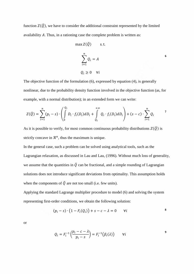
function &����, we have to consider the additional constraint represented by the limited

availability �. Thus, in a rationing case the complete problem is written as:

max&����s. t. ����

��� = �

�� ≥ 0∀- 6

The objective function of the formulation (6), expressed by equation (4), is generally

nonlinear, due to the probability density function involved in the objective function (as, for

example, with a normal distribution); in an extended form we can write:

&���� = ���� − �� ∙ 23 �� ∙ ������4��5)

6+ 3 �� ∙ ������4��

785)

9 +����

�� − �� ∙����

��� 7

As it is possible to verify, for most common continuous probability distributions &���� is

strictly concave in ℛ�, thus the maximum is unique.

In the general case, such a problem can be solved using analytical tools, such as the

Lagrangian relaxation, as discussed in Lau and Lau, (1996). Without much loss of generality,

we assume that the quantities in �� can be fractional, and a simple rounding of Lagrangian

solutions does not introduce significant deviations from optimality. This assumption holds

when the components of �� are not too small (i.e. few units).

Applying the standard Lagrange multiplier procedure to model (6) and solving the system

representing first-order conditions, we obtain the following solution:

��� − �� ∙ ;1 − �����= + � − � − > = 0∀- 8

or

�� = ��� ?�� − � − >�� − � @ = ���;A��>�=∀- 9

The constraint qualification is met in the whole domain of the profit function; so if there

exists a global optimum B∗, then there also exists a value of > such that �B∗, >� is a critical

point of the Lagrangian function (Sundaram, 1996). The structure of equation (9) is analogue

to the structure of the solution of the well-known newsvendor problem, where the numerator

of the fractile ratio A� has been modified, incorporating the > term to reduce the optimal

quantity to meet the availability constraint.

Thus, the allocation decision only depends on the distributions of the demands at different

retailers and prices, all other parameters being the same.

The value of > has to be determined in such a way that the constraint � − ∑ ������ = 0 holds;

thus> is determined by solving the following single-variable (nonlinear) equation:

� −� ��� ?�� − � − >�� − � @���� = 0

10

Still, the structure of equations (9) and (10) lead to the following observations and

implications:

• When > = 0 equation (9) reverts to the classical fractile formula, that represents the

maximum quantity ��∗ the manufacturer might want to stock at each retailer. Thus,

equation (10) reveals that, in cases of rationing and without any further constraint,

each retailer will receive less than the optimum quantity ��∗; therefore

#$�����, … , ���% ≤ #$�����∗, … , ��∗�%. In other words, when capacity is binding,

from a profit-maximization perspective it is optimal to “penalize” all the retailers

instead of just some of them.

• In contrast with the uncapacitated case where capacity is not binding, the quantity

allotted to each retailer is dependent on the prices and demand distributions of other

retailers. Since prices are fixed, the only possibility for the retailer to increase his/her

next allotment is to act on the demand distribution (i.e. advertisement, promotions not

based on discount and so forth).

• From the classical newsvendor problem, we know that A� corresponds to the Type I

service level we expect if we allocate �� units to retailer i (Brandimarte & Zotteri,

2007, pg. 253). Thus, in our case, a positive > can be interpreted as the loss of Type I

service level due to the limited availability �. It is noteworthy to observe that for

extremely low values of �, the service level at some retailers might fall below zero. In

such cases, retailers with zero service level will not receive any quantity. In the

following, we will use this observation to reduce the search space of the solving

procedure.

• If we assume a unique price such that �� = �, then it is optimal to have the same Type

I service level at all retailers. This result reflects the fair share rules (Clark & Scarf,

1960; Eppen & Schrage, 1981) in equalizing the stock-out probability of the retailers.

Nonetheless, the allotted quantities might not be the same, depending on the demand

distribution.

For simple distributions (like the uniform continuous distribution), equation (10) is linear and

the problem can be solved analytically. In other cases, and especially when integrals are

involved, applying nonlinear programming might result as impractical and not immediately

understandable by practitioners. Thus, we decided to keep the solution approach as simple as

possible, resorting to easily implementable numerical methods, avoiding the burden of

complex algorithms and sophisticated software.

4.1 Outline of the search procedure

A simple numerical procedure for solving equation (10) operates by trying different values of

>. Since we have one constraint (and, thus, one multiplier), a straightforward approach is

based on an efficient dichotomy search algorithm that reduces the domain of >

systematically.

To provide the starting bounds of the search procedures we can leverage on some properties

that equation (9) and (10) must preserve.

Observation 1 (bounds for E): the value of > must belong to the interval

0 ≤ > ≤ min� F��� − �� − ��0� ∙ ��� − ��G = min� ��� − �� = H 11

The proof of Observation 1 descends directly from the conditions 0 ≤ A��>� = I)�J�KI)�L ≤ A� and ���;A��>�= ≥ 0, and the right-hand equality descends from the assumption that ��0� =0.

Given condition (11), the dichotomy search on > in the interval (11) can be easily and

efficiently implemented. The procedure stops when the constraint is satisfied with a tolerance

ε given by the user, or after a specified number of iterations N.

We further observe that in some cases, condition (11) leads the procedure to fail in satisfying

the constraint on inventory with the given tolerance. This happens when the value of � is too

low, pushing > to increase in equation (10) beyond the limit imposed by (11). In cases where

����0� has a unique value, the meaning of too low is clarified by the following:

Observation 2 (lower bound for M): There exists a value MNOP such that for M < MNOP the

dichotomy search procedure fails. Such a lower threshold is given by

�Q�� = � ���;A��H�=����

12

where H = min���� − ��. In fact, � < �Q�� implies > > H, but this is prevented by condition

(11).

Nonetheless, despite Observation 2, it is still possible to use the proposed procedure in the

following, iterative way:

SEARCH PROCEDURE 1

1) Calculate H with equation (11) and �Q�� with equation (12). If � ≥ �Q��, then run

the dichotomy search on > and exit; otherwise, if� < �Q��, then for > = H the

availability constraint is not met with the tolerance S; at this point, there will be one or

more retailers with service level equal to zero.

2) Remove all retailers with service level equal to zero. Evaluate H and �Q��with the

remaining retailers.

3) If still � < �Q��, go to step 2; otherwise go to step 4.

4) Allot a null quantity to retailers removed so far, and run the dichotomy search with

the remaining retailers.

The procedure iteratively removes retailers with service level equal to zero until the

minimum quantity �Q�� required by the remaining ones falls below the actually available

quantity �. It is worth noticing that in case the condition �� ≠ �U for each couple of retailers - and V (such that - ≠ V) holds, the procedure realizes a step-wise removal of retailers with null

service level; differently, in case two or more retailers have the same price, they are all

removed simultaneously rather than one at a time.

This different behavior is dictated by the conditions expressed by observations 1 and 2. At

step 2 of the procedure we have to remove all retailers with null service level in order to let H

and �Q�� change. In fact, when at any iteration of the procedure � < �Q�� and two or more

retailers have simultaneously a null service level, they also have the same value of the

difference �� − �. Therefore, to let H (and consequently �Q��) change, we need to remove all

retailers with the same �� − � value. Finally, in case one iteration leads to a situation where

retailers have all the same difference �� − �, �Q�� = 0 and the problem is solvable. All these

considerations also apply in the general case when the cost � depends upon the retailers.

4.2 Numerical examples

To illustrate the procedure, we present two examples. With the aim at illustrating the search

procedure step by step, the first example addresses a simple case with three retailers where all

selling prices are different. The second example illustrates a case with five retailers where

some selling prices are the same, in order to show the effectiveness of the search procedure.

Consider an instance of the problem with n = 3 retailers characterized by the parameters of

price and demand shown in Table 2. We assume that demands are truncated normal

distributed in $0, +∞�, and the current availability is � = 4,800 units, greater than �Z-[ =2,217.

^_ ^` ^a

Selling price (bO) 18 16 14

Demand

parameter

Mean 1300 1500 1500

Standard

deviation 200 450 600

Production cost per unit (c) 5

Salvage cost per unit (d) 3

Table 2 – Parameters of the numerical example

Solving the unconstrained case we immediately verify that we are indeed subject to an

availability constraint; in fact, the unconstrained optima requires an availability � = 5,529.

Applying the search procedure with a tolerance S = 10�g, the optimal allocation in the

constrained case is found after 18 steps and reported in Table 3. Suppose now that due to an

unforeseen event, the availability drops to � = 2,000. In this case, the allotments previously

defined are no longer valid. Since now for > = H = 9, � < �Z-[ = 2,217, the availability

constraint is not satisfied as expected, and the service level of retailer 3 is zero. Removing

retailer 3 and recalculating the values we obtain H = 11 and, consequently, �Z-[ = 1,078 <�. Then, excluding retailer 3, it is now possible to allocate the quantity � between retailers 1

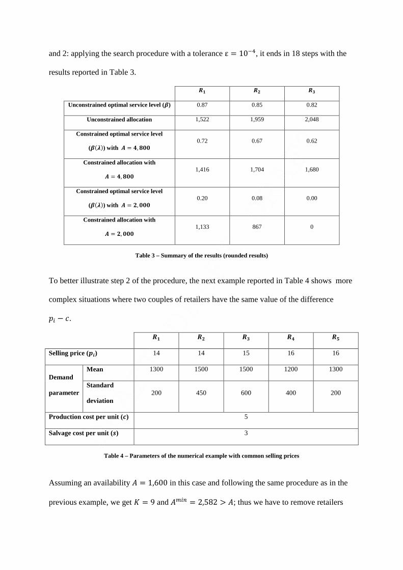
and 2: applying the search procedure with a tolerance ε = 10�g, it ends in 18 steps with the

results reported in Table 3.

^_ ^` ^a

Unconstrained optimal service level (i) 0.87 0.85 0.82

Unconstrained allocation 1,522 1,959 2,048

Constrained optimal service level

(i�E�) with M = j, kll 0.72 0.67 0.62

Constrained allocation with

M = j, kll 1,416 1,704 1,680

Constrained optimal service level

(i�E�) with M = `, lll 0.20 0.08 0.00

Constrained allocation with

M = `, lll 1,133 867 0

Table 3 – Summary of the results (rounded results)

To better illustrate step 2 of the procedure, the next example reported in Table 4 shows more

complex situations where two couples of retailers have the same value of the difference

�� − �.

^_ ^` ^a ^j ^m

Selling price (bO) 14 14 15 16 16

Demand

parameter

Mean 1300 1500 1500 1200 1300

Standard

deviation 200 450 600 400 200

Production cost per unit (c) 5

Salvage cost per unit (d) 3

Table 4 – Parameters of the numerical example with common selling prices

Assuming an availability � = 1,600 in this case and following the same procedure as in the

previous example, we get H = 9 and �Q�� = 2,582 > �; thus we have to remove retailers

with null service level, which are retailers 1 and 2. Notice at this point that by removing only

one of them H does not change, and consequently �Q�� does not change. To allow Hand

�Q�� to change we remove both retailers, leading to a new value of H = 10 and�Q�� =1,647 > �.

We proceed removing the next retailer among the remaining ones with null service level,

which is retailer 3. This leads to H = 11 and �Q�� = 0 < �; in fact, the last two retailers sell

at the same price. Therefore the problem can be solved running the dichotomy search on >

leading to a �g = 601, �o = 999, �� = �p = �q = 0 allocation decision.

As illustrated, when availability is too low, the Search Procedure 1 will eventually provide a

result where one or more retailers have a zero service level. Though this is correct from a

pure profit-maximization viewpoint, a managerial perspective might suggest avoiding these

cases. To this end, we have to sacrifice a part of the expected profit in order to ensure a

minimum service level to all retailers, as discussed in the next section.

5 Profit maximization under availability and service-level

constraints

The maximization of the profit might disregard some important managerial aspects. In some

cases, as the examples reported at the end of previous section, the maximization of expected

profit under availability constraints could lead to unbalanced allocation that in turn results in

remarkable differences in service level at different retailers.

Thus, it might be a better policy to change the profit-optimal allocation in order to increase

the service level at some retailers, foregoing some profits at others (where the service level

will be inevitably reduced, due to limited availability). At least, the company might want to

avoid drastic cases where the service level at some retailers is below an acceptable threshold.

To do this, the allocation decision has to be modified in such a way that in the worst case,

Type I service level is above a given threshold r. Formally, we want to assure the following

condition:

min� A� ≥ r 13

or equivalently, expressed in terms of allocation decision:

�� = ����A�� ≥ ����r� = ��s∀- 14

Including condition (14) in the original model (6) results in a program with many inequality

constraints; due to this, an approach based on Lagrangian multipliers is usually impractical

and very ineffective, especially when we have to consider more than just a few retailers.

Nevertheless, we can exploit constraints (14) to devise a suitable procedure. In fact, we know

that to assure a minimum service level r to all retailers, we have to allot to each at least a

quantity��s = ����r�. Any quantity below ��s will provide a Type I service level lower than

r. Hence, the total quantity allotted to each retailer becomes �� = ��s + ∆��. As a first result, if ∑ ��s� > �, then it is not possible to assure a service level r to all

retailers, and it should be reduced. Otherwise, we still have to allocate the difference �( =� −∑ ��s� .

By allocating the quantity ��s to each retailer, we are satisfying by definition the service-level

constraint, which can be removed from the problem, leaving again a problem with one single

equality constraint:

� −����s + ∆������� = 0

15

Applying the Lagrange procedure, we obtain the following rather intuitive result:

∆�� = ��� ?�� − � − >�� − � @ − ��s 16

Clearly, we want ∆�� ≥ 0, since otherwise the retailer is allotted a quantity that does not

allow meeting the requested service level r. Hence, condition (16) leads to the following:

Observation 3 (bounds for E under a service level constraint): the value of > must belong

to the interval

0 ≤ > ≤ min� F��� − �� − ����s� ∙ ��� − ��G = u 17

It is now possible to apply again the dichotomy search to find a value of > in the interval (17)

such that the constraint (15) holds. Nonetheless, as described in the previous case, if �( is too

small, such a value of > does not exist. In fact, if

�( < � ���;A��u�=����

18

where u = min�F��� − �� − ����s� ∙ ��� − ��G, then it is implied that > > u, but this is

prevented by condition (17). We can further notice that for > > u there exists at least a

negative ∆��. This means that at the optimum, the i-th retailer receives less than ��s and that

no further allotment will be guaranteed to such retailer. Thus, we can safely exclude the i-th

retailer from the allocation of �(.

Summarizing, we can still approach and solve the problem using an iterative procedure very

similar to the Search Procedure 1:

SEARCH PROCEDURE 2

1) Given r, calculate ��s for each retailer. If ∑ ��s� > �, then the thresholdr is too

high and should be reduced. Otherwise, proceed to step 2.

2) Calculate the bound u using equation (17) and the residual quantity �( = � −∑ ��s� .

3) Calculate ∆�� with > = u using equation (16). If ∑ ∆��� > �(, then remove

retailers with ∆�� = 0 and repeat step 3 considering the remaining retailers.

Otherwise, go to step 4.

4) Allot a null extra quantity to retailers removed so far, and run the dichotomy

search with the remaining retailers.

Eventually, all retailers have a guaranteed service level of r, and higher service levels are

guaranteed to those retailers that maximize the expected profit. We would underline that

these results hold also if r is specific to each retailer, that is there exists a value r� for each

retailer such that equation (13) becomes

A� ≥ r� 19

Nonetheless, in such a case, if ∑ ��s� > � it would not be immediate to decide which r� should be modified.

5.1 Numerical example

Consider the first example discussed in the previous section and described in Table 1 and

Table 2. When the availability is � = 4,800, the service levels are remarkably different. In

particular, suppose that the service level at retailer 3 is judged as too low by the management,

who would esteem as acceptable a value no lower than 0.68.

Nevertheless, calculating ��s with r = 0.68 results in a required quantity of � = 4,888 units,

indicating the impossibility to ensure such a minimum service level with the current

availability of 4,800 units. Testing a value r = 0.64 results in a required quantity of 4,752

units, below the actual availability. Thus, the management wants to allocate the remaining

�( = 48 units, aiming at maximizing the expected profit. Following the Search Procedure 2,

the bound is u = 1.96 that leads to ∑ ∆��� = 123 > �( with ∆�q = 0. This means that

retailer 3 does not contribute to the maximization of the profit and, thus, no extra quantity is

allotted. Removing retailer 3, we have u = 2.68 and ∑ ∆��� = 26 < �(. Hence we can

apply the dichotomy search to retailers 1 and 2, obtaining the extra allocations ∆�� = 33 and

∆�p = 15. As it is possible to verify, the expected service level at each retailer is above or

equal to the threshold 0.64 (A� = 0.70, Ap = 0.65 and Aq = 0.64, respectively).

5.2 Discussion

The two cases discussed above are reflective of two different approaches to the management

of availability constraints: one is oriented toward the maximization of the expected profit,

disregarding the differences in service levels provided at different retailer shops, while the

other focuses on ensuring minimum service levels, potentially foregoing some profits. Which

one is to be preferred depends on a variety of factors, even though the service-level

perspective has gained a lot of attention in recent past over a pure profit-oriented perspective.

We underline the following aspects that emerge from the analysis of the models.

• According to the newsvendor-like model presented, the unconstrained case where

each retailer receives an optimal allotment ��∗ provides the highest expected profit

possible, whereas any deviation from the optimal solution leads to a lower value.

Therefore, if an availability constraint is binding (that is, ∑ ��∗� > �), it always

reduces the expected profit since it determines a deviation from the optimal,

unconstrained allocation ��∗. Thus, under an availability constraint #$������% ≤#$�����∗�%. Furthermore, since the expected profit is strictly concave for commonly

used continuous probability distributions, the maximum is unique; thus the equality

holds only for �� = ��∗, that is when the availability constraint is not binding.

• By imposing a further constraint related to the minimum service level at the retailers’

level, we may further modify the optimum profit, since by adding the service-level

constraint we may further reduce the solution space cutting out the optimal solution

under the sole availability constraint. Therefore, if we represent the allocation

decision under availability and service-level constraints with �s + ∆������������, we can write

#$����s + ∆�������������% ≤ #$������%. As it is possible to verify, the equality holds only for

�s + ∆������������ = ��, thus for r = min� � ����.

From a managerial standpoint, the mathematical results reflect the fact that by reducing the

quantity stocked at the retailer shops, the availability constraint negatively affects the profit

and the service level they can provide, sometimes pushing down to very low values the

performance of some retailers compared to others. Even though this is optimal from a profit-

maximization standpoint, such an approach may backfire in the medium-to-long run since the

company may be recognized as low performing in some areas, therefore losing market share

and visibility. Imposing a service constraint implies a commercial policy that strives to

guarantee a minimum acceptable service level at the cost of some profit. This could also have

positive influence on the long term, as the company being seen positively by the customers

might increase the average demand.

The Search Procedure 2 leaves one thing uncovered, and that is how to set r in such a way

that it would not result too high. This is discussed in the next section.

6 Maximum service level under availability constraints

When faced with the necessity of setting a threshold for the service level, management can

use a trial and error approach. Nevertheless, it might be important to know which is the

highest limit of the service level that is possible to require, given an availability �.

Formally, we want to solve the following program:

max rs. t. ����

��� = �

����� ≥ r∀- �� ≥ 0∀-

20

Depending on the distribution functions �, it could be possible to apply a standard

optimization approach (i.e. with uniform continuous distribution). Otherwise, we should

resort again to a numerical approach.

To this end, we can restate the problem in a different way; in fact, from equation (14) we

know that the quantity we need to ensure a service level of r at each retailer is ∑ ����r����� .

Hence, setting different values of r and examining how far the sum is from the actual

availability � we can find the maximum r satisfying (20). Again, this problem can be

efficiently solved via dichotomy search.

In fact, we know by definition that in a rationing problem, 0 ≤ r < min� A�. We also know

that in order to provide a service level r at retailer i, we should allot a quantity ��s = ����r�. Therefore, a too-high value of r would lead to ∑ ��s���� > �, evidently violating the

availability constraint. On the other hand, a too-low value would violate the constraint in the

other direction. Then we can apply a dichotomy search procedure where the search proceeds

as follows:

SEARCH PROCEDURE 3

1. Define r according to company’s strategy.

2. If ∑ ��s���� > �, then reduce r. Otherwise, increase r.

3. Repeat step 2 until ∑ |��s − �|���� < S.

At the end of the procedure, r is the highest service level that can be provided at each retail

shop.

7 Use case workflow

Although discussed separately, the results and the solution procedures presented are meant to

be operated conjointly in a coordinated model, aimed at supporting decision makers facing

rationing problems. Using the presented procedures as building blocks, we propose the use

case workflow depicted in Figure 1. Such a workflow is meant to summarize the decision

paths the manufacturer’s management might follow in order to optimize the allocation

decision.

The decision workflow operates as follows:

1. Facing a rationing problem, the first objective of the company is to evaluate how far

the constrained solution is from the unconstrained optima. By solving the problem of

maximizing the expected profit under availability constraint, it is possible to measure

the gap of the actual solution from the theoretical optima. Such a gap can be

measured either in terms of lower expected profit or in terms of lower service levels.

Notice that though we preemptively excluded the possibility to expand capacity, in

case it is possible to increase the availability in the short term (for example, resorting

to an outsourcer), this analysis will support the investment decision allowing a

comparison between the cost of the investment and the increase in the expected

profit.

2. In the second stage of the decision process, the focus shifts to service level. If service

levels of the constrained solution are not satisfactory, the decision maker wants to

assess the maximum service threshold r he/she can set.

3. Once the maximum threshold r is set, the decision maker can try out a few other

values in order to find the right mix of service levels, and allocate the available

quantity accordingly.

Figure 1 – Use case workflow

8 Conclusions

This paper originated from a real world problem in the vending machine sector. Indeed, the

characteristics of the case, modeled as a newsvendor problem, are general enough to be

representative of many other industrial settings, where capacity investment is not a viable

option, short term changes in demand can be substantial, spot markets are not available and

the profit of the manufacturer is tightly interconnected with the performance of the sellers

(i.e. the vending machine in the original case, the retailers in the general case).

In these contexts, the quest for an optimal inventory and/or capacity allocation arises often, as

the availability of resources shrinks down, or due to commercial or operational decisions.

We presented formulations and solution procedures for the general rationing problem, along

with a variant contemplating inventory service levels. The solution approach has been

designed to handle the problems in the most efficient way, leveraging on two well-proven

methods—Lagrange multipliers and dichotomy search. Finally, the different components of

the solution procedure have been structured in a decision workflow contemplating

availability and service constraints.

The proposed approach is legitimated under several demand distribution functions subject to

a few commonly adopted restrictions. Nevertheless, many of the usually adopted continuous

distributions automatically fall within such restrictions.

One of the major limitations is that we only considered a Type I service level measure,

suggested by the structure of the problem. However, we see as a possible development an

analysis of the model to extend it to other service indicators.

References

Axsäter, S., Kleijn, M., de Kok, T.G., 2004. Stock Rationing in a Continuous Review Two-Echelon

Inventory Model. Annals of Operations Research 126 (1-4), 177-194.

Balakrishnan, N., Patterson, J.W., Sridharan, V., 1996. Rationing Capacity Between Two Product

Classes. Decision Sciences 27 (2), 185-214.

Besanko, D., Braeutigam, R.R., 2011, Microeconomics (4th Edition). John Wiley & Sons, Hoboken,

NJ.

Brandimarte, P., Zotteri, G., 2007, Introduction to Distribution Logistics. John Wiley & Sons,

Hoboken, NJ.

Cachon, G.P., Lariviere, M.A., 1999a. Capacity Choice and Allocation: Strategic Behavior and

Supply Chain Performance. Management Science 45 (8), 1091-1108.

Cachon, G.P., Lariviere, M.A., 1999b. An equilibrium analysis of linear, proportional and uniform

allocation of scarce capacity. IIE Transactions 31 (9), 835-849.

Chen-Ritzo, C.-H., Ervolina, T., Harrison, T.P., Gupta, B., 2011. Component rationing for available-

to-promise scheduling in configure-to-order systems. European Journal of Operational Research,

211(1), 57-65.

Cattani, K.D., Souza, G.C., 2002. Inventory rationing and shipment flexibility alternatives for direct

market firms. Production and Operations Management 11 (4), 441-458.

Clark, A.J., Scarf, H., 1960. Optimal Policies for a Multi-Echelon Inventory Problem. Management

Science, 6(4), 475-490.

de Kok, T.G., 2000. Capacity allocation and outsourcing in a process industry. International Journal

of Production Economics 68 (3), 229-239.

de Véricourt, F., Karaesmen, F., Dallery, Y., 2002. Optimal Stock Allocation for a Capacitated

Supply System. Management Science 48 (11), 1486-1501.

Emmons, H., Gilbert, S.M., 2008. The Role of Returns Policies in Pricing and Inventory Decisions for

Catalogue Goods. Management Science 44 (2), 276-283.

Eppen, G., Schrage, L., 1981. Centralized ordering policies in a multi-warehouse system with lead

times and random demand. In L. B. Schwarz (Ed.), Multi-Level Production/Inventory Control

Systems: Theory and Practice (pp. 51-68). North-Holland, Amsterdam.

Fadıloğlu, M. M., Bulut, Ö., 2010a. An embedded Markov chain approach to stock rationing.

Operations Research Letters, 38(6), 510-515.

Fadıloğlu, M.M., Bulut, Ö., 2010b. A dynamic rationing policy for continuous-review inventory

systems. European Journal of Operational Research 202 (3), 675-685.

Feng, Y., Xiao, B., 2006. Integration of pricing and capacity allocation for perishable products.

European Journal of Operational Research 168 (1), 17-34.

Glasserman, P., 1996. Allocating Production Capacity among Multiple Products. Operations Research

44 (5), 724-734.

Ha, A.Y., 1997a. Stock-Rationing Policy for a Make-to-Stock Production System with Two Priority

Classes and Backordering. Naval Research Logistics 44 (5), 457-472.

Ha, A.Y., 1997b. Inventory Rationing in a Make-to-Stock Production System with Several Demand

Classes and Lost Sales. Management Science 43 (8), 1093-1103.

Ha, A.Y., 2000. Rationing in an M / Ek / 1 Queue. Management Science 46 (1), 77-87.

Haynsworth, H.C., Price, B.A., 1989. A Model for Use in the Rationing of Inventory during Lead

Time. Naval Research Logistics 36 (4), 491-506.

Hung, Y.-F., Lee, T.-Y., 2010. Capacity rationing decision procedures with order profit as a

continuous random variable. International Journal of Production Economics 125 (1), 125-136.

Kaplan, A., 1969. Stock Rationing. Management Science 15 (5), 260-267.

Lagodimos, A.G., Koukoumialos, S., 2008. Service performance of two-echelon supply chains under

linear rationing. International Journal of Production Economics 112 (2), 869-884.

Lau, H.-S., Lau, A.H.-L., 1996. The newsstand problem: A capacitated multiple-product single-period

inventory problem. European Journal of Operational Research 94 (1), 29-42.

Lee, H., Padmanabhan, V., Whang, S., 1997. Information distortion in a supply chain: The bullwhip

effect. Management Science 43 (4), 546-558.

Moon, I., Kang, S., 1998. Rationing policies for some inventory systems. The Journal of the

Operational Research Society 49 (5), 509- 518.

Nahmias, S., Demmy, W.S., 1981. Operating Characteristics of an Inventory System with Rationing.

Management Science 27 (11), 1236-1245.

Parlar, M., 1988. Game theoretic analysis of the substitutable product inventory problem with random

demands. Naval Research Logistics 35 (3), 397-409.

Paul, B., Rajendran, C., 2011. Rationing mechanisms and inventory control-policy parameters for a

divergent supply chain operating with lost sales and costs of review. Computers & Operations

Research, 38(8), 1117-1130.

Sundaram, R.K., 1996. A first course in optimization theory. Cambridge University Press, Cambridge,

UK.

Tan, T., Güllu, R., Erkip, N., 2009. Using imperfect advance demand information in ordering and

rationing decisions. International Journal of Production Economics 121(2), 665-677.

Teunter, R.H., Haneveld, W.K.K., 2008. Dynamic inventory rationing strategies for inventory systems

with two demand classes, Poisson demand and backordering. European Journal of Operational

Research 190 (1), 156-178.

Topkis, D.M., 1968. Optimal Ordering and Rationing Policies in a Nonstationary Dynamic Inventory

Model with n Demand Classes. Management Science 15 (3), 160-176.

van Der Heijden, M.C., Diks, E.B., de Kok, A.G., 1997. Stock allocation in general multi-echelon

distribution systems with (R , S) order-up-to-policies. International Journal of Production

Economics 49 (2), 157-174.

Xu, J., Chen, S., Lin, B., Bhatnagar, R., 2010. Optimal production and rationing policies of a make-to-

stock production system with batch demand and backordering. Operations Research Letters,

38(3), 231-235.

Zhao, X., Xie, J., Zhang, W.J., 2002. The impact of information sharing and ordering co-ordination on

supply chain performance. Supply Chain Management: an International Journal 7 (1), 24-40.