J Intell Inf SystDOI 10.1007/s10844-013-0281-4

Soft constraints for pattern mining

Willy Ugarte · Patrice Boizumault · Samir Loudni ·Bruno Crémilleux · Alban Lepailleur

Received: 22 February 2013 / Revised: 16 September 2013 / Accepted: 4 October 2013© Springer Science+Business Media New York 2013

Abstract Constraint-based pattern discovery is at the core of numerous data miningtasks. Patterns are extracted with respect to a given set of constraints (frequency,closedness, size, etc). In practice, many constraints require threshold values whosechoice is often arbitrary. This difficulty is even harder when several thresholds arerequired and have to be combined. Moreover, patterns barely missing a threshold willnot be extracted even if they may be relevant. The paper advocates the introductionof softness into the pattern discovery process. By using Constraint Programming,we propose efficient methods to relax threshold constraints as well as constraintsinvolved in patterns such as the top-k patterns and the skypatterns. We show the rel-evance and the efficiency of our approach through a case study in chemoinformaticsfor discovering toxicophores.

Keywords Constraint-based pattern mining · Soft constraints · Soft skypatterns ·Constraint Programming · Disjonctive relaxation · Chemoinformatics

W. Ugarte (B) · P. Boizumault · S. Loudni · B. CrémilleuxGREYC (CNRS UMR 6072), University of Caen, Campus II Côte de Nacre,14000 Caen, Francee-mail: willy.ugarte@unicaen.fr

P. Boizumaulte-mail: patrice.boizumault@unicaen.fr

S. Loudnie-mail: samir.loudni@unicaen.fr

B. Crémilleuxe-mail: bruno.cremilleux@unicaen.fr

A. LepailleurCERMN (UPRES EA 4258 - FR CNRS 3038 INC3M), University of Caen,Boulevard Becquerel, 14032 Caen Cedex, Francee-mail: alban.lepailleur@unicaen.fr

J Intell Inf Syst

1 Introduction

Extracting knowledge from large amounts of data is at the core of the KnowledgeDiscovery in Databases. This involves different challenges, such as designing efficienttools to tackle data and the discovery of patterns of a potential user’s interest.Mannila and Toivonen (1997), Ng et al. (1998) have promoted the use of constraintsto represent background knowledge and to focus on the most promising knowledgeby reducing the number of extracted patterns to those of a potential interest given bythe final user. The most popular example with local patterns is the minimal frequencyconstraint based on the frequency measure: it addresses all patterns having a numberof occurrences in the database exceeding a given minimal threshold.

In practice, data mining tasks require to deal both with pattern characteristics(e.g., frequency, size, contrast (Novak et al. 2009)) and background knowledge (e.g.,price in the traditional example of supermarket databases, chemical features suchas aromaticity in chemoinformatics). Then several measures have to be handled andcombined leading to entail choosing several threshold values.

This notion of thresholding has serious drawbacks. Firstly, unless specific domainknowledge is available, the choice is often arbitrary and relevant patterns aremissed or lost within a lot of spurious patterns. This drawback is obviously evendeeper when several measures have to be combined and thus several thresholds areneeded. A second drawback is the stringent aspect of the classical constraint-basedmining framework: a pattern satisfies or does not satisfy the set of constraints. But,what about patterns that respect only some thresholds, especially if only very fewconstraints are slightly violated? There are very few works such as Bistarelli andBonchi (2007), Ugarte et al. (2012) which propose to introduce a softness criterioninto the mining process as we will see in Section 5. This thresholding issue is alsopresent in pattern set mining (De Raedt and Zimmermann 2007) where the goal isto mine for a set of patterns with constraints combining several local patterns. Acouple of examples of pattern sets are the top-k patterns (i.e., the k best patternsaccording to a score function) and the skypatterns (i.e. the best patterns accordingto a dominance relation based on a set of user-preferences). In the following ofthe paper, we propose methods to introduce softness in these problems and theimprovements brought by the softness.

The key contribution of this paper is to propose a soft constraint based patternmining framework. Our proposition benefits from the recent progress on cross-fertilization between data mining and Constraint Programming (CP) (Guns et al.2011; Khiari et al. 2010; De Raedt et al. 2008). The common point of all thesemethods is to model in a declarative way pattern mining as Constraint SatisfactionProblems (CSP), whose resolution provides the complete set of solutions satisfyingall the constraints.

Our contributions address both handling soft threshold constraints, including thetop-k patterns, and the skypatterns. The key idea of the first contribution is totransform each soft threshold constraint into an equivalent hard constraint that canbe directly managed by a CSP solver. For that purpose, each soft threshold constraintis associated to a violation measure to determine the distance between a patternand a threshold. Then, we show how soft threshold constraints can be exploited forextracting the top-k patterns according to an interestingness measure. The techniquefully benefits from the handling of the soft threshold constraints: contrary to the

J Intell Inf Syst

data mining methods, the top-k patterns can include patterns violating constraints onthe measures given by the user. Our method offers a natural way to simultaneouslycombine in a same framework usual data mining measures with measures comingfrom the background knowledge. The second contribution is an efficient approachto mine skypatterns as well as soft ones thanks to the CP framework. We show howthe (soft-)skypattern problem can be modeled and solved with CP techniques. Amajor advantage of the method is to improve the mining step during the processthanks to constraints dynamically posted and stemming from the current set ofcandidate skypatterns. Moreover, the declarative side of the CP framework easilyenables us to manage constraints providing several kinds of softness and leadsto a unified framework handling softness in the skypattern problem. Finally, therelevance and the effectiveness of our approach is highlighted through a case studyin chemoinformatics for discovering toxicophores.

This paper is organized as follows. Section 2 presents the context. Section 3describes our framework to model and solve soft threshold constraints and the top-kpatterns. Section 4 presents our method to deal with (soft-)skypatterns. We reviewsome related work in Section 5, and Section 6 reports in depth a case study from thechemoinformatics domain on the discovery of toxicophores.

2 Context and definitions

Let I be a set of distinct literals called items. An itemset (or pattern) is a non-nullsubset of I . The language of itemsets corresponds to LI = 2I\∅. A transactionaldataset is a multiset of patterns of LI . Each pattern (or transaction) is a databaseentry. Table 1 (left side) presents a transactional dataset T where each transactionti gathers articles described by items denoted A,. . . ,F. The traditional example is asupermarket database in which each transaction corresponds to a customer and everyitem in the transaction to a product bought by the customer. A price is associated toeach product (cf. Table 1, right side).

Constraint-based pattern mining aims at extracting all patterns of LI satisfyinga query q (conjunction of constraints) which is usually called theory (Mannilaand Toivonen 1997): Th(q) = {Xi ∈ LI | q(Xi) is true}. A common example is thefrequency measure leading to the minimal frequency constraint. The latter providespatterns Xi having a number of occurrences in the database exceeding a givenminimal threshold min fr: freq(Xi) ≥ min fr. Another usual measures are the sizeof a pattern (i.e. the number of items that a pattern contains), the average price

Table 1 Transactional dataset TTrans. Items

t1 B E Ft2 B C Dt3 A E Ft4 A B C D Et5 B C D Et6 B C D E Ft7 A B C D E F

Items A B C D E F

Price 30 40 10 40 70 55

J Intell Inf Syst

avgPrice(Xi) (i.e., the average of the prices associated to the items of Xi), and thearea of Xi with area(Xi) = f req(Xi) × size(Xi). In many applications, it appearshighly appropriate to look for contrasts between subsets of transactions, such as toxicand non toxic molecules in chemoinformatics. The growth rate is a well-used contrastmeasure (Novak et al. 2009). Let T be a database partitioned into two subsets D1

and D2:

Definition 2.1 (Growth rate) The growth rate of a pattern Xi from D2 to D1 is:

mgr(Xi) = |D2| × f req(Xi,D1)

|D1| × f req(Xi,D2)

Emerging Patterns and Jumping Emerging Patterns stem from this measure. Theyare at the core of a useful knowledge in many applications involving classificationfeatures such as the discovery of structural alerts in chemoinformatics (see Section 6).

Definition 2.2 (Emerging Pattern) Given a threshold mingr > 1, a pattern Xi is saidto be an Emerging Pattern (EP) from D2 and D1 if mgr(Xi) ≥ mingr .

Definition 2.3 (Jumping Emerging Pattern) A pattern Xi which does not occur inD2(mgr(Xi) = +∞) is called a Jumping Emerging Pattern (JEP).

Moreover, the user is often interested in discovering richer patterns satis-fying properties involving several local patterns. These patterns define patternsets (De Raedt and Zimmermann 2007) or n-ary patterns (Khiari et al. 2010). Theapproach that we present in this paper is able to deal with pattern sets such as thetop-k patterns and the skypatterns.

3 Modeling and solving soft threshold constraints

In this section, we first give a motivating example. Then, we show how soft thresholdconstraints can be transformed into equivalent hard constraints that can be directlyhandled by a CSP solver. This transformation uses the disjunctive relaxation frame-work in CP (Petit et al. 2000).

3.1 Motivating example

Example 3.1 Let us consider the following query q(X). It addresses all frequentpatterns (min fr = 4), having a size greater than or equal to 3, and an average price(avgPrice) greater than 45:

q(X) ≡ freq(X) ≥ 4 ∧ size(X) ≥ 3 ∧ avgPrice(X) ≥ 45

Thereafter, we use the notation Xi < v1,v2,v3 >, where Xi is a solution to the queryq(X), and v1, v2, v3 denote its value for the three measures freq, size and avgPrice.With the running example in Table 1, we get 17 solutions by considering only thefrequency constraint. With the conjunction of the three constraints, there is only one

J Intell Inf Syst

solution: BDE < 4,3,50 >. Let us consider the following four patterns which aremissed by the mining process:

– BEF < 3, 3, 55 >

– CDE < 4, 3, 40 >

– BCE < 4, 3, 40 >

– BCDE < 4, 4, 40 >

The pattern BEF slightly violates the frequency threshold and satisfies the twoother constraints. However, this pattern is clearly interesting because its value on theaverage price measure is largely higher than the value of BDE which satisfies thequery. By slightly relaxing the frequency threshold (freq(X) ≥ 3), BEF would beextracted.

Similarly, relaxing the average price threshold (from 45 to 40) would enableto discover three new patterns: CDE, BCE and BCDE. Due to the uncertaintyinherent to the determination of the thresholds, it is difficult to say that thesepatterns are less interesting than BDE which is produced. So, the stringent aspectof the classical constraint-based mining framework means that interesting patternsare lost as soon as at least one threshold is slightly violated. Moreover, in real lifeapplications, all threshold constraints are not considered to be equally important, andthis characteristic should be taken into account in the mining process. Overcomingthese drawbacks is the motivation of our proposal.

3.2 Violation measures for soft constraints

When relaxing constraints, we have to quantify the violation. This task is performedby a violation measure. Violation measures associate costs to constraints, a cost valuequantifies the violation. A global objective related to the whole set of costs is usuallydefined (for example to minimize the total sum of costs).

Definition 3.1 (Violation measure) μc is a violation measure for the constraintc(X1, ..., Xp) if f μc is a function from D1 × D2 × ... × Dp to �+ where Di is thefinite domain of variable Xi s.t. ∀A ∈ D1 × D2 × ... × Dp, μc(A) = 0 if f A satisfiesc(X1, ..., Xp).

For a given constraint, several violation measures can be defined. We take as anintroductory example the frequency measure, then we consider any measure.

For the frequency measure Let X be a pattern, α a minimal threshold and theconstraint freq(X) ≥ α. A first violation measure can be defined as the absolutedistance from threshold α. However, to combine violations of several thresholdconstraints, it is more appropriate to consider relative distances. A second violationmeasure μ can be defined as the relative distance from α:

μ(X) =⎧⎨

⎩

0 if freq(X) ≥ αα − freq(X)

αotherwise

J Intell Inf Syst

For any measure m Let I be a set of distinct items and T a set of transactions.Let maxm be the maximum value1 for measure m. Violation measures are defined asfollows:

For ci ≡ m(X) ≥ α μi(X) =⎧⎨

⎩

0 if m(X) ≥ αα − m(X)

αotherwise

For ci ≡ m(X) ≤ α μi(X) =⎧⎨

⎩

0 if m(X) ≤ αm(X) − α

maxm − αotherwise

Violation measures are normalized in order to combine violations of severalthreshold constraints occurring in a same query. So, violation values will be realnumbers ranging from 0.0 to 1.0.

3.3 Soft threshold constraint based pattern mining: key ideas

We introduce our soft threshold constraint based pattern mining framework, whereconstraints can be violated according to a violation measure.

Definition 3.2 (Soft threshold constraint based pattern mining) Let q be a soft query(conjunction of n soft threshold constraints ci) and λ be the maximal amount ofviolation that is allowed. Let μi be the violation measure associated to ci. Theviolation measure for a query q is defined as μq(X) = ∑n

i=1 μi(X). The soft-patternmining problem for a query q consists in extracting all patterns whose violation doesnot exceed λ, i.e.: Sof t(λ, q) = {Xi ∈ LI | μq(Xi) ≤ λ}.

The main steps of our approach are the following:

1. each soft threshold constraint ci is associated to a violation measure μi and a costvariable zi.

2. use the disjunctive relaxation of ci to transform it into an equivalent hardconstraint c′

i.3. add a constraint to control the amount of violation:

∑zi ≤ λ.

4. solve the equivalent hard query using a pattern set extractor based on CP.2

The following sections describe how to concretely apply a CP approach for thismining problem. In particular, we will show how to transform the soft problem intoan equivalent hard problem using the disjunctive relaxation.

3.3.1 Disjunctive relaxation

Constraint relaxation enables to deal with over-constrained problems, i.e., problemswith no solution satisfying all the constraints. Over-constrained problems are gen-erally modeled as Constraint Optimization Problems (COP). Our method uses the

1For the frequency measure, maxm =| T |; for the size measure, maxm =| I |.2More information on the implementation of the above constraint-based pattern mining task usingConstraint Programming techniques are in Guns et al. (2011), Khiari et al. (2010).

J Intell Inf Syst

disjunctive relaxation (Petit et al. 2000). Recalling that at each soft constraint ci isassociated a violation measure μi and a cost variable zi that measures the violationof ci. So the COP is transformed into a CSP where all constraints are hard and theglobal cost variable z = ∑n

i=1 zi ≤ λ, where λ is the maximum amount of violationthat is allowed (λ ∈ [0.0 , 1.0]). If the domain of a cost variable is reduced during thesearch, propagation will be performed on domains of other cost variables. Each softconstraint is modeled as a disjunction: either the constraint is satisfied and the cost isnull, or the constraint is not satisfied and the cost is specified.

Definition 3.3 (Disjunctive relaxation of a constraint) Let ci be a constraint, c̄i itsnegation and zi the associated cost variable. The disjunctive relaxation of ci isc′

i ≡ [ci ∧ (zi = 0)] ∨ [c̄i ∧ (zi > 0)].

3.3.2 From soft constraints to equivalent hard constraints

This section shows how to transform any soft threshold constraint into an equivalenthard constraint.

Transformation for the frequency measure Let X be a pattern, α a minimal thresh-old and the constraint ci ≡ freq(X) ≥ α. Let zi be its associated cost variable and μi

its violation measure. The disjunctive relaxation of ci for μi is:

[(freq(X) ≥ α) ∧ zi = 0] ∨ [(freq(X) < α) ∧ zi = α − freq(X)

α]

This disjunction can be reformulated in an equivalent way by the following (hard)constraint:

zi = μi(X) = max(0,α − freq(X)

α)

Transformation for any measure m By applying the previous transformation, softthreshold constraints associated to a measure m can be transformed into equivalenthard constraints:

– The relaxation of ci ≡ (m(X) ≥ α) is c′i ≡ [zi = μi(X) = max(0, α−m(X)

α)]

– The relaxation of ci ≡ (m(X) ≤ α) is c′i ≡ [zi = μi(X) = max(0, m(X)−α

maxm−α)]

Consider again the query q(X) of our running Example 3.1. Applying the abovetransformations on q(X), we get the following equivalent hard query:

q′(X) ≡

⎧⎪⎪⎪⎪⎪⎪⎨

⎪⎪⎪⎪⎪⎪⎩

z1 = max(0,4 − f req(X)

4) ∧

z2 = max(0,3 − size(X)

3) ∧

z3 = max(0,45 − avgPrice(X)

45) ∧

z = z1 + z2 + z3 ≤ λ

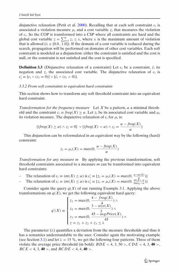
The parameter (λ) quantifies a deviation from the measure thresholds and thus ithas a semantics understandable to the user. Consider again the motivating example(see Section 3.1) and let λ = 15 %, we get the following four patterns. Three of themviolate the average price threshold (in bold): BDE < 4, 3, 50 >, CDE < 4, 3, 40 >,BCE < 4, 3, 40 >, and BCDE < 4, 4, 40 >.

J Intell Inf Syst

Therefore, computing all the soft patterns satisfying a conjunction of soft thresh-old constraints, can be performed by solving the corresponding hard query whereall the soft constraints are transformed into equivalent hard ones. The followingproposition states this important result.

Proposition 3.1 (Equivalence between the queries) Let q(X) = ∧ni=1 ci(X) be a

conjunction of soft threshold constraints ci. Let λ be the maximal amount of violation.Let zi be the cost variable associated to ci and μi its violation measure.

Let q′(X) = ∧ni=1(zi = μi(X)) ∧ (

∑ni=1 zi ≤ λ). It holds that: Sof t(λ, q) = Th(q′).

The proof is immediate as, each soft constraint ci(X) is equivalent to the hardconstraint (zi = μi(X)), and the violation measure for a query q is defined asμq(X) = ∑n

i=1 μi(X). (see Definition 3.2).

3.3.3 A f lexible framework for handling softness

Our approach can be extended in several ways, leading to a more flexible frame-work. First, for every constraint ci, several violation measures can be defined: gap,relative distance, etc. Moreover, cost variables (zi) enable a fine control of theviolation:

– to limit the violation of a particular soft threshold constraint: zi ≤ �.– to balance the total amount of violation: (i) for any couple of cost variables, their

difference must be lower than a threshold; (ii) or by sharing equally the violationfor the set of constraints.

i)∧

1≤i< j≤n

| zi − z j | ≤ ε ii)∧

1≤i≤n

zi ≤ 1

n×

n∑

i=1

zi

3.4 Mining top-k patterns with an interestingness measure

Ranking the patterns according to interest measures is an attractive data miningtask which is very helpful for the user. The top-k pattern methods associate eachpattern with a rank score and compute an ordered list of the k patterns withthe highest score (Ke et al. 2009; Wang et al. 2005). Rank scores are determinedby interestingness measures provided by the user. In this section, we define aninterestingness measure enabling us to exploit our method on pattern mining withsoft threshold constraints. As an example, with the constraint freq(X) ≥ α, a patternXi having a frequency much larger than the threshold α, will be considered as moreinteresting than a pattern X j whose frequency is slightly higher than α. The approachfully benefits from the handling of the soft threshold constraints: the top-k patternscan include patterns violating constraints on the measures given by the user. Up tonow, data mining methods are not able to take into account softness in top-k mining.

3.4.1 Interestingness of a pattern for a threshold constraint

An interestingness measure of a pattern for a threshold constraint c may be eitherpositive (when c is satisfied) or negative (when c is not satisfied). As for a violationmeasure (see Section 3.2), an interestingness measure is also normalized in order to

J Intell Inf Syst

combine interests of several threshold constraints occurring in a same query. Let mbe a measure, and maxm its maximal value.

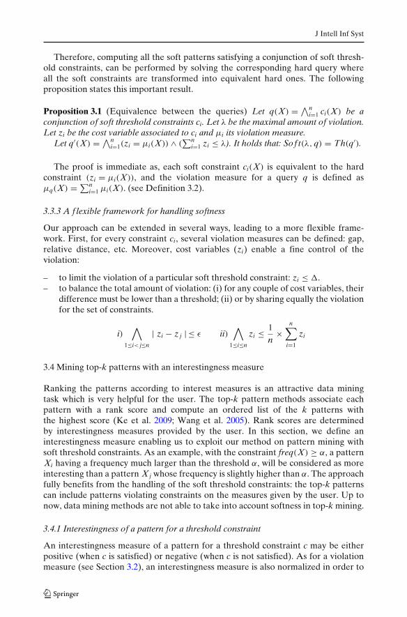
We define the interestingness measure θi :: LI → [−1.0 , 1.0] by:

For ci ≡ m(X) ≥ α θi(X) =

⎧⎪⎪⎨

⎪⎪⎩

m(X) − α

maxm − αif m(X) ≥ α

−μ(X) otherwise

For ci ≡ m(X) ≤ α θi(X) =

⎧⎪⎨

⎪⎩

α − m(X)

αif m(X) ≤ α

−μ(X) otherwise

3.4.2 Interestingness of a pattern for a query

Le q be a soft query, i.e. a conjunction of n soft threshold constraints on measures(cf. Definition 3.2). We define the interestingness of a pattern X for q as the sum ofthe interests of X for the threshold constraints of q.

θq(X) =∑

1≤i≤n

γi × θi(X)

where γi is a coefficient reflecting the importance of the constraint ci.

3.4.3 Computing top-k

Let q(X) be a query involving soft threshold constraints and λ the maximal amountof violation that is allowed. Let q′(X) be the hard query associated to both q(X)

and λ (see Section 3.3.2). Computing the top-k patterns, for the query q′(X)

according to the interestingness measure θ , is performed as follows. The first ksolutions (X1, X2, ..., Xk) for the query q′(X) are computed and ordered accordingto the interestingness measure θ . Then, as soon as a new solution X(k+1) withθ(X(k+1)) > θ(Xk) is obtained, then X(k+1) is inserted in the top-k solutions and Xk isremoved. Furthermore, the constraint (θ(X) > θ(Xk)) is dynamically posted in orderto improve the pruning of the search tree.

4 Modeling and solving (soft-)skypatterns

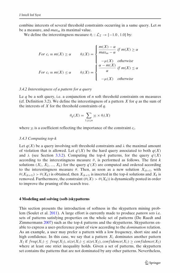
This section presents the introduction of softness in the skypattern mining prob-lem (Soulet et al. 2011). A large effort is currently made to produce pattern sets i.e.sets of patterns satisfying properties on the whole set of patterns (De Raedt andZimmermann 2007) such as the top-k patterns and the skypatterns. Skypatterns en-able to express a user-preference point of view according to the domination relation.As an example, a user may prefer a pattern with a low frequency, short size and ahigh confidence. In this case, we say that a pattern X1 dominates another patternX2 if freq(X1) ≤ f req(X2), size(X1) ≤ size(X2), conf idence(X1) ≥ conf idence(X2)

where at least one strict inequality holds. Given a set of patterns, the skypatternset contains the patterns that are not dominated by any other patterns. Nevertheless,

J Intell Inf Syst

similarly to the threshold constraints, the skypatterns suffer from the stringent aspectof the constraint-based framework.

This section starts with a motivating example on skylines (Börzönyi et al. 2001).This problem comes from the database community and gives rise of skypatternproblem. We show the interest of introducing softness in this context. Then we definethe skypattern mining problem and we introduce two kinds of soft skypatterns: theedge-skypatterns that belongs to the edge of the dominance area (see Section 4.3)and the δ-skypatterns that are close to this edge (see Section 4.4). The key idea isto soften the dominance relation in order to capture skypatterns occurring in theforbidden area.

4.1 Motivating example

Consider a coach of a football team who looks for players for the next season (seeFig. 1). Every player is depicted according to the number of goals he scored and thenumber of assistances he performed during the last season. A point (here, a player)Pi dominates another point Pj if Pi is better (i.e., more preferred) than Pj in at leastone dimension, and Pi is not worse than Pj on every other dimension. A skyline pointis a point which is not dominated by any other point. The skyline set (or skyline forshort) consists of players p1, p2, p3, p4 and p5. Indeed, players p6, p7, p8, p9 and p10

are dominated by at least one other player, thus they cannot be part of the skyline.Nevertheless, the coach could be interested in non-skyline players if he looks for:

– players in a forward position: the coach will give the priority to the number ofscored goals. The players p1 (skyline), p2 (skyline) are still interesting and p6

(non-skyline) and p9 (non-skyline) become interesting.

Fig. 1 Skyline example

J Intell Inf Syst

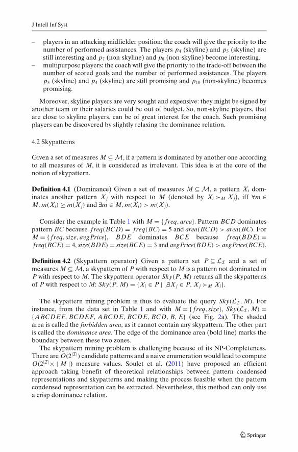
– players in an attacking midfielder position: the coach will give the priority to thenumber of performed assistances. The players p4 (skyline) and p5 (skyline) arestill interesting and p7 (non-skyline) and p8 (non-skyline) become interesting.

– multipurpose players: the coach will give the priority to the trade-off between thenumber of scored goals and the number of performed assistances. The playersp3 (skyline) and p4 (skyline) are still promising and p10 (non-skyline) becomespromising.

Moreover, skyline players are very sought and expensive: they might be signed byanother team or their salaries could be out of budget. So, non-skyline players, thatare close to skyline players, can be of great interest for the coach. Such promisingplayers can be discovered by slightly relaxing the dominance relation.

4.2 Skypatterns

Given a set of measures M ⊆ M, if a pattern is dominated by another one accordingto all measures of M, it is considered as irrelevant. This idea is at the core of thenotion of skypattern.

Definition 4.1 (Dominance) Given a set of measures M ⊆ M, a pattern Xi dom-inates another pattern X j with respect to M (denoted by Xi �M X j), iff ∀m ∈M, m(Xi) ≥ m(X j) and ∃m ∈ M, m(Xi) > m(X j).

Consider the example in Table 1 with M = { f req, area}. Pattern BCD dominatespattern BC because f req(BCD) = f req(BC) = 5 and area(BCD) > area(BC). ForM = { f req, size, avgPrice}, BDE dominates BCE because f req(BDE) =freq(BCE) = 4, size(BDE) = size(BCE) = 3 and avgPrice(BDE) > avgPrice(BCE).

Definition 4.2 (Skypattern operator) Given a pattern set P ⊆ LI and a set ofmeasures M ⊆ M, a skypattern of P with respect to M is a pattern not dominated inP with respect to M. The skypattern operator Sky(P, M) returns all the skypatternsof P with respect to M: Sky(P, M) = {Xi ∈ P | � ∃X j ∈ P, X j �M Xi}.

The skypattern mining problem is thus to evaluate the query Sky(LI, M). Forinstance, from the data set in Table 1 and with M = { f req, size}, Sky(LI, M) ={ABCDEF, BCDEF, ABCDE, BCDE, BCD, B, E} (see Fig. 2a). The shadedarea is called the forbidden area, as it cannot contain any skypattern. The other partis called the dominance area. The edge of the dominance area (bold line) marks theboundary between these two zones.

The skypattern mining problem is challenging because of its NP-Completeness.There are O(2|I|) candidate patterns and a naive enumeration would lead to computeO(2|I|× | M |) measure values. Soulet et al. (2011) have proposed an efficientapproach taking benefit of theoretical relationships between pattern condensedrepresentations and skypatterns and making the process feasible when the patterncondensed representation can be extracted. Nevertheless, this method can only usea crisp dominance relation.

J Intell Inf Syst

(a) (b)

Fig. 2 Soft-skypatterns extracted from the example in Table 1

4.3 Edge-skypatterns

Similarly to skypatterns, edge-skypatterns are defined according to a dominancerelation and a Sky operator. These two notions are reformulated as follows:

Definition 4.3 (Strict dominance) Given a set of measures M ⊆ M, a pattern Xi

strictly dominates a pattern X j with respect to M (denoted by Xi �M X j), iff∀m ∈ M, m(Xi) > m(X j).

Definition 4.4 (Edge-skypattern operator) Given a pattern set P ⊆ LI and a setof measures M ⊆ M, an edge-skypattern of P, with respect to M, is a patternnot strictly dominated in P, with respect to M. The edge-skypattern operatorEdge-Sky(P, M) returns all the edge-skypatterns of P with respect to M: Edge-Sky(P, M) = {Xi ∈ P | � ∃X j ∈ P, X j �M Xi}.

It is obvious that for two patterns Xi and X j, (Xi �M X j =⇒ Xi �M X j).Moreover, as (soft-)skypatterns are patterns that are not dominated, we can deducethat: Edge-Sky(P, M) ⊇ Sky(P, M). Given a set of measures M ⊆ M, the edge-skypattern mining problem is thus to evaluate the query Edge-Sky(P, M). Figure 2adepicts the 28 = 7 + (4 + 8 + 3 + 4 + 2) edge-skypatterns extracted from the exam-ple in Table 1 for M = { f req, size}. Obviously, all edge-skypatterns belong to theedge of the dominance area, and seven of them are (hard) skypatterns.

4.4 δ-skypatterns

In many cases the user may be interested in skypatterns expressing a trade-offbetween measures. The δ-skypatterns address this issue.

Definition 4.5 (δ-Dominance) Given a set of measures M ⊆ M, a pattern Xi

δ-dominates another pattern X j (with 0 ≤ δ ≤ 1) with respect to M (denoted byXi �δ

M X j), iff ∀m ∈ M, (1 − δ) × m(Xi) > m(X j).

Definition 4.6 (δ-Skypattern operator) Given a pattern set P ⊆ LI and a set ofmeasures M ⊆ M, a δ-skypattern of P with respect to M is a pattern not δ-dominated

J Intell Inf Syst

in P with respect to M. The δ-skypattern operator δ-Sky(P, M) returns all the δ-skypatterns of P with respect to M: δ-Sky(P, M) = {Xi ∈ P | � ∃X j ∈ P : X j �δ

M Xi}.

It is obvious that for two patterns Xi and X j, (Xi �δM X j =⇒ Xi �M X j). More-

over, as (soft-)skypatterns are patterns that are not strictly dominated, we can deducethat: δ-Sky(P, M) ⊇ Edge-Sky(P, M). The δ-skypattern mining problem is thus toevaluate the query δ-Sky(P, M). There are 38 (28 + 10) δ-skypatterns extracted fromthe example in Table 1 for M = { f req, size} and δ = 0.25. Figure 2b only depicts the10 δ-skypatterns that are not edge-skypatterns. Intuitively, the δ-skypatterns are closeto the edge of the dominance relation, the value of δ expressing the maximal relativedistance between a skypattern and this border.

4.5 Mining (soft-)skypatterns using CP

This section describes our CP approach for mining both skypatterns and soft-skypatterns. As for computing the top-k patterns (see Section 3.4), constraints on thedominance relation are dynamically posted during the mining process and softnessis easily introduced using such constraints. The implementation of our approach hasbeen carried out in Gecode3 extending the (CP based) pattern extractor developedby Khiari et al. (2010). Consider the following queries recursively defined by:

– q1(X) = closedM(X)

– qi+1(X) = qi(X) ∧ φR(Xi, X) where Xi is a solution to query qi(X)

First, the constraint closedM(X), which states that X must be a closed patternw.r.t all the measures of M, allows to reduce the number of redundant patterns.4

Then, the constraint φR(Xi, X) states that the pattern X, we are looking for, will notbe dominated by Xi w.r.t. to a dominance relation R. Each kind of (soft-)skypatternswill have its proper constraint φR(Xi, X) according to its dominance relation R (seebelow). Finally, by using an induction proof, we can argue that query qi+1(X) looksfor a pattern X that will not be dominated by any of the patterns X1,X2,. . .,Xi.

Each time a solution Xi is found for query qi(X), we dynamically post a newconstraint φR(Xi, X), based on the values of the measures for Xi, leading to reducethe search space. This process stops when we cannot enlarge the forbidden area (i.e.there exits n s.t. query qn+1(X) has no solution). The constraint φR(Xi, X) states that¬(Xi R X).

For skypatterns, φ�M(Xi, X) ≡ ¬(Xi �M X) that is encoded by the followingformulae (see Definition 4.1):

φ�M(Xi, X) ≡ (∨

m∈M

m(Xi) < m(X)) ∨ (∧

m∈M

m(X) = m(Xi))

For edge-skypatterns, φ�M(Xi, X) ≡ ¬(Xi �M X) (see Definition 4.3):

φ�M(Xi, X) ≡∨

m∈M

m(Xi) ≤ m(X)

3http://www.gecode.org/4The closed constraint is used to reduce pattern redundancy. Indeed, closed skypatterns make up anexact condensed representation of the whole set of skypatterns (Soulet et al. 2011).

J Intell Inf Syst

For δ-skypatterns, φ�δM(Xi, X) ≡ ¬(Xi �δ

M X) (see Definition 4.5):

φ�δM(Xi, X) ≡

∨

m∈M

(1 − δ) × m(Xi) < m(X)

But, the n extracted patterns X1, . . ., Xn are not necessarily all (soft-)sky patterns.Some of them can only be “intermediate” patterns simply used to enlarge theforbidden area. A post processing step must be achieved to filter all patterns Xi forwhich there exists X j (1 ≤ i < j ≤ n) s.t. X j dominates Xi. While this number n couldbe very large (this mining problem is NP-complete), it remains reasonably-sized inpractice for the experiments we conducted (see Table 6).

5 Related work

5.1 Soft threshold constraints

There are very few works in data mining to cope with the stringent aspect of theusual constraint-based mining framework. Relaxation has been studied to providesoft constraints with specific properties in order to be able to manage them by usingusual constraint mining algorithms. In Garofalakis et al. (1999), regular expressionconstraints have been relaxed into anti-monotonic constraints for mining significantsequences.

In the context of local patterns, Bistarelli and Bonchi (2007) have proposeda generic framework using semirings to express preferences between solutions.Each constraint has its own measure of interest and the interest of a query is theaggregation of the interests of all constraints composing the query. Given a queryand a threshold value, the goal is to find all local patterns whose interest satisfies thisthreshold value. However, this approach relies on the following strong hypothesis:the interest of a given query satisfies the threshold, if and only if, the interest ofeach constraint satisfies the same threshold (Bistarelli and Bonchi 2007). If theaggregation operator is performed using the min operator (fuzzy semiring), theequivalence holds. However, for the sum operator (weighted semiring) and the ×operator (probabilistic semiring), it is no longer the case. That is why the authorsneed to perform a post-processing step to filter the set of effective solutions.

So, unlike Bistarelli and Bonchi (2007), our approach preserves the equivalencewithout requiring a post-processing step (see Proposition 3.1). Moreover, it can beapplied on pattern sets and therefore to local patterns.

5.2 (Soft-)skypatterns

The notion of dominance introduced in Section 4.2 is at the core of the skylineprocessing. Interesting data points are the ones that are not dominated by any otherpoint, and can be considered as optimal with respect to a given set of criteria.

Computing skylines is a derivation from the maximal vector problem in compu-tational geometry (Matousek 1991), the Pareto set (Kung et al. 1975) and multi-objective optimization (Steuer 1992). Since its rediscovery within the databasecommunity by Börzönyi et al. (2001), several methods have been developed for

J Intell Inf Syst

answering skyline queries (Börzönyi et al. 2001; Papadias et al. 2005, 2008; Tan et al.2001). These methods assume that tuples are stored in efficient data structures, suchas B-Tree or R-Tree. Gavanelli (2002) proposed a method based on CP to determinethe Pareto frontier. This proposal is similar to our approach, but only deals with(hard) skylines. Alternative approaches have also been proposed towards helpingthe user in selecting most significant skylines. For example, Lin et al. (2007) measurethis significance by means of the number of points dominated by a skyline. Jin et al.(2004) have proposed thick skylines to extend the concept of skyline. A thick skylineis either a skyline point P, or a point P′ dominated by a skyline point P and suchthat P′ is close to P (their distance is less than a threshold ε). Thick skylines are aparticular case of δ-skypatterns that we introduced in Section 4.4.

Computing skypatterns is different from computing skylines. Skyline queries focusin extracting tuples of the dataset, while for skypatterns the mining task consists inextracting patterns. The search space for skypatterns is larger: O(2|I|) instead ofO(| T |) for skylines. Moreover skylines have been intensively studied and benefitfrom efficient data structures, while only one work is devoted to skypatterns. Souletet al. (2011) have proposed an efficient approach taking benefit of theoretical rela-tionships between pattern condensed representations and skypatterns and makingthe process feasible when the pattern condensed representation can be extracted.Nevertheless, this method can only use a crisp dominance relation.

Fuzzy techniques is a way to introduce softness but in data mining this approachis rather used to manage quantitative data and avoid certain undesirable thresholdeffects (Hüllermeier 2005). In pattern mining, fuzzy techniques are used by fuzzifingthe original dataset and applying pattern mining techniques to obtain a fuzzy output.In our approach, softness is introduced directly into the output through constraints.

6 Experimentations

Toxicology is a scientific discipline involving the study of the toxic effects of chemi-cals on living organisms. A major issue in chemoinformatics is to establish relation-ships between chemicals and a given activity (e.g., CL505 in ecotoxicity). Chemicalfragments6 which cause toxicity are called toxicophores and their discovery is at thecore of prediction models in (eco)toxicity (Bajorath and Auer 2006; Poezevara et al.2011). The aim of this present study, which is part of a larger research collaborationwith the CERMN Lab, a laboratory of medicinal chemistry, is to investigate theuse of softness (i.e. soft threshold constraints and soft-skypatterns) for discoveringtoxicophores.

5Lethal concentration of a substance required to kill half the members of a tested population after aspecified test duration.6A fragment denominates a connected part of a chemical structure containing at least one chemicalbond.

J Intell Inf Syst

6.1 Settings

The dataset is collected from the ECB web site.7 For each chemical, the chemistsassociate it with hazard statement codes (HSC) in 3 categories: H400 (very toxic,CL50 ≤ 1 mg/L), H401 (toxic, 1 mg/L < CL50 ≤ 10 mg/L), and H402 (harmful, 10mg/L < CL50 ≤ 100 mg/L). We focus on the H400 and H402 classes. The dataset Tconsists of 567 chemicals, 372 from the H400 class and 195 from the H402 class. Thechemicals are encoded using 1450 frequent closed subgraphs previously extractedfrom T 8 with a 1 % relative frequency threshold.

In order to discover patterns as candidate toxicophores, we use both measurestypically used in contrast mining (Novak et al. 2009) such as the growth rate sincetoxicophores are linked to a classification problem with respect to the HSC andmeasures expressing the background knowledge such as the aromaticity or rigiditybecause chemists consider that this information may yield promising candidatetoxicophores. Our method offers a natural way to simultaneously combine in a sameframework these measures coming from various origins. We briefly sketch thesemeasures and the associated threshold constraints.

Growth rate When a pattern has a frequency which significantly increases from theH402 class to the H400 class, then it stands a potential structural alert related to thetoxicity. In other words, if a chemical has, in its structure, fragments that are relatedto a toxic effect, then it is more likely to be toxic. Emerging patterns embody thisnatural idea by using the growth-rate measure (cf. Definition 2.1).

Frequency Real-world datasets are often noisy and patterns with low frequencymay be artefacts. The minimal frequency constraint ensures that a pattern is rep-resentative enough (i.e., the higher the frequency, the better it is).

Aromaticity Chemists know that the aromaticity is a chemical property that favorstoxicity since their metabolites can lead to very reactive species which can interactwith biomacromolecules in a harmful way. We compute the aromaticity of a patternas the mean of the aromaticity of its chemical fragments. We denote by ma thearomaticity measure of a pattern.

Rigidity In addition, chemists consider that the rigidity of chemicals may yield aninterest for candidate toxicophores. A common hypothesis is that the higher thechemical rigidity, the more hazardous its environmental behavior. The rigidity ofa pattern is given by the mean of rigidity of its subgraphs.9 We denote by md therigidity measure of a pattern.

7European Chemicals Bureau http://ecb.jrc.ec.europa.eu/documentation/ now http://echa.europa.eu/.8A chemical Ch contains an item A if Ch supports A, and A is a frequent subgraph of T .9The rigidity of a subgraph is equal to 2e/v(v − 1), where e (resp. v) is the number of its edges (resp.vertices).

J Intell Inf Syst

6.2 Experimental protocol

In order to asses the concrete effects of using soft threshold constraints and soft-skypatterns for discovering toxicophores, we considered the following queries :

– query q1(X) modeling the extraction of soft-patterns:q1(X) ≡ mgr(X) ≥ mingr ∧ freq(X) ≥ min fr ∧ ma(X) ≥ mina ∧ md(X) ≥ minr

where mingr, min fr, mina, and minr are the minimal thresholds on growth rate,frequency, aromaticity, and rigidity measures respectively.

– query q2(X) modeling the extraction of the top-k patterns satisfying the queryq1(X).

– query q3(X) (resp. its soft version) modeling the extraction of skypatterns (resp.soft-skypatterns) (see Section 4).

The thresholds on aromaticity and rigidity measures were set to 2/3 of themaximal values of these measures on the dataset (mina = 60 and minr = 60). Indeed,high thresholds suggest an interest for candidate toxicophores. The minimal growthrate and the minimal frequency thresholds were fixed to 1/4 of the maximal values ofthese measures (mingr = 5 and min fr = 90) in order to keep only the most frequentemerging patterns (EPs) with the highest growth rates. Setting these thresholds mightbe subtle and it illustrates the interest of the soft constraints because the choice of theuser is then downplayed. We consider three different values for λ : {0, 20 %, 40 %}.We set γgr, γ f r and γd to 1 et γa to 2. Indeed, aromaticity is the most importantchemical knowledge.

For the query q3(X), M = {mgr, ma, freq}. Chemists consider that adding therigidity measure does not bring new chemical knowledge for the (soft-)skypatternmining problem. We performed several combinations of the three measures. For theparameter δ, we considered two values: 10 % and 20 %.

The extracted (soft-)EPs and (soft-)skypatterns are made of molecular fragmentsand to evaluate the presence of toxicophores in their description, an expert analysisled to the identification of well-known environmental toxicophores, namely thebenzene, the phenol ring, the chloro-substituted aromatic ring (e.g. chlorobenzene),the organophosphorus moiety, the aromatic amines (e.g. aniline), the pyrrole, andthe polycyclic aromatic hydrocarbons (e.g. naphthalene).

Experiments were conducted on a computer running Linux operating system witha core i3 processor at 2,13 GHz and a RAM of 4 GB. The implementation of ourapproach was carried out in Gecode by extending the n-ary patterns extractor based-CSP (Khiari et al. 2010).

6.3 Extracting the Soft Emerging Patterns

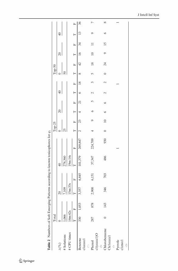
Table 2 provides results for the query q1. It depicts the numbers of (soft-)EPscontaining at least one complete toxicophore compound (columns marked T) or sub-fragments of a toxicophore (columns marked F) among the six fragments previouslyidentified in the database according to the three values of λ. Col. 2–7 provide thetotal number of solutions, Col. 8–13 over the top25 and Col. 14–19 over the top50. Asthe two categories T and F are not disjoint, the accumulated number of (soft-)EPsin the two categories may exceed #(Solutions). The CPU time for extracting the set

J Intell Inf Syst

Tab

le2

Num

bers

ofSo

ftE

mer

ging

Pat

tern

sac

cord

ing

tokn

own

toxi

coph

ores

for

q 1

Tot

alT

op-2

5T

op-5

0

λ(%

)0

2040

020

400

2040

#So

luti

ons

1,06

67,

109

278,

360

2550

#C

PU

tim

es14

m:4

2s15

m:3

3s19

m:1

4s

TF

TF

TF

TF

TF

TF

TF

TF

TF

Ben

zene

330

1,05

33,

357

6,84

510

1,37

926

9,84

72

234

216

188

4216

3413

36c1

cccc

c1

Phe

nol

287

878

2,90

06,

151

37,3

4722

4,70

94

96

52

35

1810

119

7c1

(ccc

cc1)

O

Chl

orob

enze

ne0

143

346

703

486

930

010

66

22

024

915

68

Clc

1ccc

cc1

Pyr

role

11

1c1

cncc

1

J Intell Inf Syst

of all solutions is about 14 min. for (λ = 0), 15 min. for (λ = 20 %) and 19 min. for(λ = 40 %).

As shown in Table 2, 47 %10 (resp. 36.4 %) of soft-EPs with λ = 20 % (resp.40 %) contain a benzene (fragment of category T), against of about 31 % forλ = 0. Thus, soft thresholds allow to better discover this toxicophore (average gainof about 11 %). Regarding the category F, the proportion of soft-EPs containing sub-fragments of benzene (Smiles code11): {cc, ccc, cccc, ccccc}) is almost the samein the hard and soft cases (about 97 %). This trend is also confirmed for phenol ring,where 40 % of extracted solutions with λ = 20 % include such a fragment, against26.9 % for λ = 0 %. For λ = 40 %, the ratio of extracted soft-EPs with a phenolring is 13.4 %. Once again, soft thresholds enable to better meet this toxicophore,particularly with λ = 20 % (gain of about 13 %).

For the chlorobenzene (with λ = 0 %), only patterns containing fragments ofcategory F are extracted: {Clc(c)cc, Clc(c)ccc, Clc(c)cccc, Clc(cc)ccc,Clccc . . . }. The soft thresholds enable to find on average 2.5 % of toxicophorescontaining the chlorobenzene (i.e., fragment of category T). Moreover, for N-containing aromatic compounds, new patterns with a novel chemical characteristic(containing the subfragment nc) are discovered. Indeed, this derivative, not detectedwith (λ = 0), is rather difficult to extract as it is associated to a chemical fragmentwith a low value of frequency.

(soft-)EPs containing the aniline aromatic ring are not detected because of theirlow rigidity (33). Indeed, with λ = 40 %, the minimal value allowed is 60 × 0.60 = 36.Increasing very slightly λ (λ = 45 %), would permit the extraction of those EPs.

Finally, the organophosphorus fragment has the highest growth rate (+∞) andthus is a JEP (cf. Definition 2.2). The chemists have a strong interest for suchpatterns. They are not listed in Table 2 and we will come back on these patternsin Section 6.4.2.

6.4 Mining the top-k soft patterns

6.4.1 Extracting the top-k Soft Emerging Patterns

Results from Table 2 show that among the top25 (resp. top50) (hard) EPs minedwith λ = 0, only 2 (resp. 4) patterns contain the benzene (resp. phenol) ring. Theremaining topk EPs are constituted solely of subfragments of chlorobenzene.

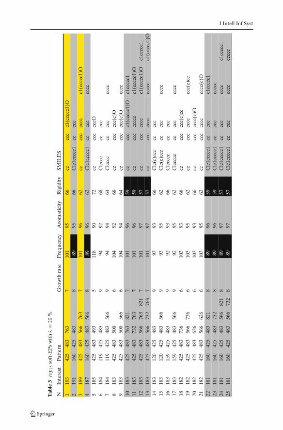
Table 3 addresses the query q2 and gives the top25 soft-EPs extracted with λ =20 %. Yellow lines correspond to patterns obtained with λ = 0 and having at leastone complete phenol ring, while gray lines correspond to the new patterns minedwith soft thresholds constraints (the violated constraints are highlighted in black).

The soft thresholds enable us to find 4 new soft-EPs containing the phenol ringamong the top25 patterns (lines 10–13), that represents a ratio of 1.5 (λ = 20 %detects 1.5 times more useful EPs compared to λ = 0). Let us note that two of thesepatterns also contain an aromatic ring (e.g. benzene) (lines 10 and 12). Moreover,these patterns, which violate slightly the rigidity constraint, are highly aromatic

10Ratio of the number of solutions containing a toxicophore by the total number of solutions.11Smiles code is a line notation for describing the structure of chemical molecules: http://www.daylight.com/dayhtml/doc/theory/theory.smiles.html.

J Intell Inf Syst

Tab

le3

top 2

5so

ft-E

Ps

wit

hλ

=20

%

J Intell Inf Syst

and from a biodegradability point of view, aromatic compounds are among themost recalcitrant of the pollutants. These patterns have a high growth rate andthis result strengthens our hypothesis that the growth rate measure captures toxicbehavior. Furthermore, λ = 20 % led to the extraction of 6 new soft-EPs containingthe chlorobenzene. Let us note that two of these patterns (lines 2 and 4) violateslightly the frequency constraint, while the four other ones (lines 22–25) violate bothfrequency and rigidity constraints. These patterns are of a great interest and theyreinforce our previous hypothesis of toxicophore.

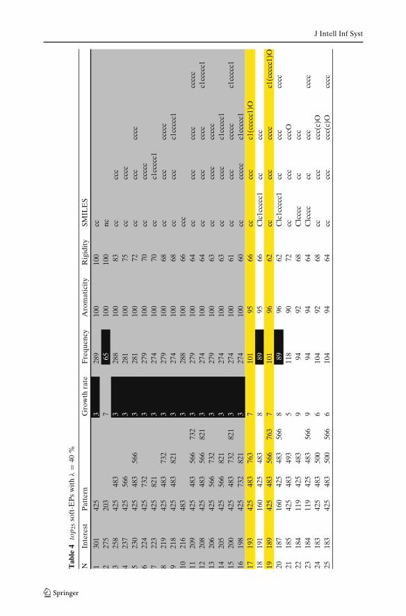
Table 4 depicts the top25 soft-EPs with λ = 40 %. As before, soft thresholds allowto discover 6 new soft-EPs containing benzene (cf. lines 7, 9, 12, 14, 15 and 16).These patterns, which slightly violate the growth rate constraint, are highly aromaticand relatively dense and thus reinforce the hypothesis that the higher the chemicalrigidity is, the more hazardous its environmental behavior. A new EP of particularinterest to chemists is obtained: {nc}. This pattern is environmentally hazardous sinceit corresponds to N-aromatic compound which are often toxic to aquatic species.

For the top50 soft-EPs, soft thresholds with λ = 20 % (resp. 40 %) allow todetect 2 (resp. 1.8) times more solutions containing the phenol ring. Furthermore,λ = 40 % enables to extract 13 (resp. 6) new soft-EPs containing benzene (resp. thechlorobenzene).

All these results confirm the benefit of using soft thresholds in order to obtainnovel chemical knowledge of a great interest.

6.4.2 Extracting the top-k soft jumping emerging patterns

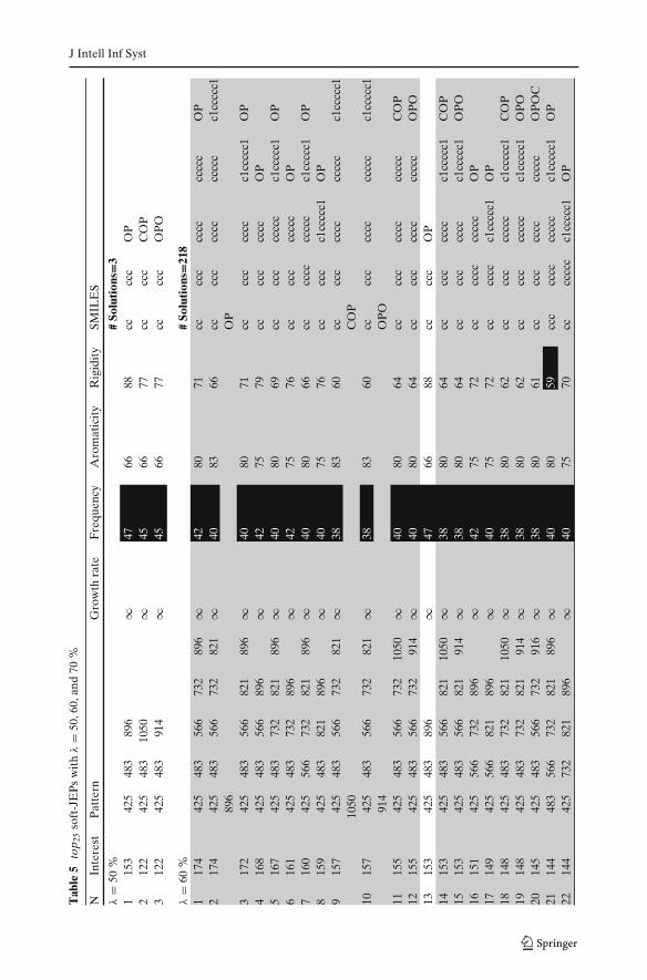
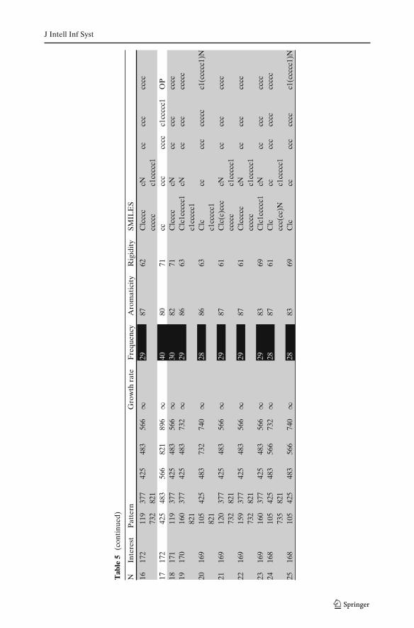
Our third experiment evaluates the character of toxicity carried by the chemicalfragments which occur only in chemicals classified H400 (i.e. high toxicity), the so-called Jumping Emerging Patterns (JEPs) (cf. Definition 2.2). Table 5 shows the top25

(soft-)JEPs according to different values of λ.One can draw the following remarks: (i) Without soft threshold constraints, JEPs

are not detected; (ii) With λ = 50 % (resp. 60 % and 70 %), we get 3 (resp. 218and 421, 504) soft-JEPs. Indeed, this kind of patterns are less frequent, thus it isnecessary to have a relatively high threshold violation; (iii) All patterns containingorganophosphorus fragments have a growth rate equal to +∞. It appears thatthe organophosphorus fragment is a generalization of several Jumping EmergingFragments (JEFs) and can be seen as a kind of maximum common structure ofthese fragments; (iv) Among the top25 soft-JEPs extracted with λ = 60 %, the mostinteresting patterns are those including a benzene ring ({c1ccccc1}). With λ =50 %, the extracted soft-JEPs contain subfragments of benzene without completerings. Thus, these JEPS are less relevant from a chemical point of view comparedto those mined with λ = 60 %; (v) Increasing the value of λ to 70 % led to thedetection of new several promissing soft-JEPs. These JEPs, which include the aminefunction (e.g. aniline {c1(ccccc1)N}), are very toxic to aquatic organisms. Again,these results demonstrate the effectiveness and the contribution of soft thresholdconstraints to highlight relevant chemical structures, such as benzene rings comparedto its subfragments.

J Intell Inf Syst

Tab

le4

top 2

5so

ft-E

Ps

wit

hλ

=40

%

J Intell Inf Syst

Tab

le5

top 2

5so

ft-J

EP

sw

ith

λ=

50,60

,and

70%

J Intell Inf Syst

Tab

le5

(con

tinu

ed)

J Intell Inf Syst

Tab

le5

(con

tinu

ed)

J Intell Inf Syst

6.5 Mining the (soft-)skypatterns

In our last series of experiments, we evaluate the interest of using soft-skypatterns fordiscovering toxicophores. Table 6 compares the performance of the three skypatternoperators in terms of number of (soft-)skypatterns extracted before (n) and after(# of sol.) the post processing step (see Section 4.5) as well as computational times,for different combinations of measures.

Regarding the cardinality of mined soft-skypatterns, increasing the number ofmeasures leads to a higher number of soft-skypatterns. The explanation is that apattern rarely dominates all other patterns on the whole set of measures. Nev-ertheless, in our experiments, the number of soft-skypatterns remains reasonablysmall. At most, there is a maximum of 1,055 δ-skypatterns. Moreover, regardingthe computational time, our approach is very effective (less than 1 hour), even withthe increase of the number of measures (except for δ = 20 %, where the number ofδ-skypatterns and run time increase). From these results, the following remarks canbe drawn.

First, using the growth rate and frequency measures, only 8 skypatterns havebeen found, and 3 well-known toxicophores were emphasized. Two of them arearomatic compounds, namely the chlorobenzene ({Clc}) and the phenol rings({c1(ccccc1)O}). The contamination of water and soil by organic aromatic chemi-cals is widespread as a result of industrial applications ranging from their use as pes-ticides, solvents to explosives and dyestuffs. Many of them may bioaccumulate in thefood chain and have the potential to be harmful to living systems including humans,animals, and plants. The third one, the organophosphorus moiety ({OP, OP=S}) is acomponent occurring in numerous pesticides. Concerning the soft-skypatterns, noadditional information were extracted in this case. However, the chloro-substitutedaromatic rings (e.g. {Clc(ccc)c, Clcccc}), and the organophosphorus moietypattern (e.g. {OP(=S)O), COP(=S)O}) are efficiently detected by the edge- andδ-skypatterns respectively.

Second, by considering the growth rate and aromaticity measures, or the fre-quency and aromaticity measures, the results are quite similar. Although the ob-tained skypatterns are less informative in comparison with the previous ones (growthrate and frequency measures), the extraction of the soft skypatterns led to the iden-

Table 6 Performance analysis of (soft)-skypattern mining

M Skypattern Edge-skypattern δ-skypattern

n # of sol. n # of sol. δ(%)

10 20

n # of sol. n # of sol.

{growth rate, frequency} 120 8 2,259 24 19,468 25 21,710 8023m:01s 28m:42s 32m:22s 44m:50s

{growth rate, aromaticity} 122 5 6,522 76 16,235 181 18,543 1,02724m:52s 25m:59s 38m:02s 2h:23m:04s

{frequency, aromaticity} 2 2 10,954 72 27,836 181 30,583 1,01123m:42s 26m:33s 35m:59s 2h:30m:32s

{growth rate, frequency, 246 21 23,887 144 32,322 223 33,744 1,055aromaticity} 35m:04s 40m:30s 1h:4m:27s 4h:35m:27s

J Intell Inf Syst

tification of several different aromatic rings. In fact, the nature of these chemicals canvary in function of i) the presence/absence of heteroatoms (e.g. N, S), ii) the numberof rings, and iii) the presence/absence of substituents. Regarding the two kinds ofsoft-skypatterns, the edge-skypatterns led to the extraction of nitrogen aromaticcompounds (e.g. indole {ncc, c1cccccc1}, benzoimidazole {ncnc, c1ccccc1}),S-containing aromatic compounds (e.g benzothiophene {scc, c1ccccc1}), aromaticoxygen compounds (e.g. benzofurane {coc, c1ccccc1}) and polycyclic aromatichydrocarbons (e.g. naphthalene {c1ccc2ccccc2c1}). The δ-skypatterns completethe list of the aromatic rings which were not enumerated during the extraction of theskypatterns (e.g. biphenyl {c1ccccc1c2ccccc2}). It is also important to note thatin this case, δ-skypatterns detect another type of toxicophore very harmful to aquaticorganisms, namely aromatic amines (e.g. aniline {c1(ccccc1)N}).

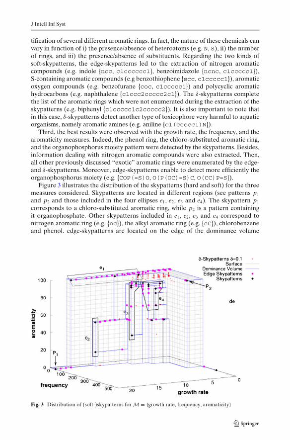
Third, the best results were observed with the growth rate, the frequency, and thearomaticity measures. Indeed, the phenol ring, the chloro-substituted aromatic ring,and the organophosphorus moiety pattern were detected by the skypatterns. Besides,information dealing with nitrogen aromatic compounds were also extracted. Then,all other previously discussed “exotic” aromatic rings were enumerated by the edge-and δ-skypatterns. Moreover, edge-skypatterns enable to detect more efficiently theorganophosphorus moiety (e.g. {COP(=S)O, O(P(OC)=S)C, O(CC)P=S}).

Figure 3 illustrates the distribution of the skypatterns (hard and soft) for the threemeasures considered. Skypatterns are located in different regions (see patterns p1

and p2 and those included in the four ellipses e1, e2, e3 and e4). The skypattern p1

corresponds to a chloro-substituted aromatic ring, while p2 is a pattern containingit organophosphate. Other skypatterns included in e1, e2, e3 and e4 correspond tonitrogen aromatic ring (e.g. {nc}), the alkyl aromatic ring (e.g. {cC}), chlorobenzeneand phenol. edge-skypatterns are located on the edge of the dominance volume

Fig. 3 Distribution of (soft-)skypatterns for M = {growth rate, frequency, aromaticity}

J Intell Inf Syst

Table 7 Ratio analysis of (soft)-skypattern mining

M Skypatterns Soft-Skypatterns

Edge-skypatterns δ-Skypatterns

δ(%)

10 20

{growth rate, frequency} 78 = 0.875 30

32 = 0.938 5558 = 0.948 115

119 = 0.966

{growth rate, aromaticity} 55 = 1.000 79

81 = 0.975 421426 = 0.988 1749

1751 = 0.999

{frequency, aromaticity} 12 = 0.500 70

74 = 0.946 421426 = 0.988 1722

1728 = 0.997

{growth rate, frequency, aromaticity} 2021 = 0.952 161

165 = 0.976 545550 = 0.991 1883

1889 = 0.997

corresponding to the patterns in e1. These patterns complete the list of aromaticrings which were not found during the extraction of the skypattern mining such thatS-containing aromatic ring (e.g. {cs}) and biphenyl. Finally, for δ-skypatterns, themost informative are those located around the patterns belonging to e1 (e.g. naph-thalene and aniline).

The Table 7 shows the values of the ratio (# patterns containing toxicophoresdivided by # of patterns) for all the queries for the (soft)-skypattern mining problem,and clearly the results are better in the soft case than the hard case (increasing itsvalue w.r.t to δ).

7 Conclusion

This paper highlights usefulness of the softness into the pattern discovery process.It shows how softness allows to discover interesting patterns that would be missedotherwise. Our methods address both soft threshold constraints and the skypatterns.By defining an interestingness measure on patterns, we have shown how softthreshold constraints can be exploited for extracting the top-k patterns. Our methodoffers a natural way to simultaneously combine in a same framework usual datamining measures with measures coming from the background knowledge. We havedesigned an efficient method to mine skypatterns as well as soft ones thanks to the CPframework. Thanks to constraints dynamically posted during the process, the miningstep becomes more and more efficient. The declarative side of the CP frameworkeasily enables us to manage constraints providing several kinds of softness. Therelevance and the efficiency of our approach is highlighted through a case study inchemoinformatics for discovering toxicophores. Experimental results demonstratethe benefit of using soft threshold constraints as well as soft-skypatterns in orderto obtain promising novel chemical knowledge. In the future, we want to study theintroduction of softness on new tasks such as clustering, the contribution of soft-skypatterns for recommendation and extend our approach to skycubes.

References

Bajorath, J., & Auer, J. (2006). Emerging chemical patterns: a new methodology for molecularclassification and compound selection. Journal of Chemical Information and Modeling, 46, 2502–2514.

J Intell Inf Syst

Bistarelli, S., & Bonchi, F. (2007). Soft constraint based pattern mining. Data and Knowledge Engi-neering, 62(1), 118–137.

Börzönyi, S., Kossmann, D., Stocker, K. (2001). The skyline operator. In Proceedings of the 17thInternational Conference on Data Engineering (ICDE’01) (pp. 421–430). Springer: IEEEComputer Science.

De Raedt, L., Guns, T., Nijssen, S. (2008). Constraint programming for itemset mining. In KDD’08(pp. 204–212). ACM.

De Raedt, L., & Zimmermann, A. (2007). Constraint-based pattern set mining. In Proceedings of the7th SIAM international conference on data mining. Minneapolis, MN: SIAM.

Garofalakis, M.N., Rastogi, R., Shim, K. (1999). SPIRIT: Sequential pattern mining with regularexpression constraints. In Proceedings of 25th international conference on very large data bases(pp. 223–234).

Gavanelli, M. (2002). An algorithm for multi-criteria optimization in csps. In F. van Harmelen (Ed.),ECAI (pp. 136–140). IOS Press.

Guns, T., Nijssen, S., De Raedt, L. (2011). Itemset mining: a constraint programming perspective.Artif icial Intelligence, 175(12–13), 1951–1983.

Hüllermeier, E. (2005). Fuzzy methods in machine learning and data mining: status and prospects.Fuzzy Sets and Systems, 156(3), 387–406.

Jin, W., Han, J., Ester, M. (2004). Mining thick skylines over large databases. In PKDD’04 (pp. 255–266).

Ke, Y., Cheng, J., Yu, J.X. (2009). Top-k correlative graph mining. In SDM (pp. 1038–1049).Khiari, M., Boizumault, P., Crémilleux, B. (2010). Constraint programming for mining n-ary patterns.

In CP’10. LNCS (Vol. 6308, pp. 552–567). Springer.Kung, H.T., Luccio, F., Preparata, F.P. (1975). On finding the maxima of a set of vectors. Journal of

the ACM, 22(4), 469–476. doi:10.1145/321906.321910.Lin, X., Yuan, Y., Zhang, Q., Zhang, Y. (2007). Selecting stars: The k most representative skyline

operator. In ICDE 2007 (pp. 86–95). IEEE Computer Society Press.Mannila, H., & Toivonen, H. (1997). Levelwise search and borders of theories in knowledge discov-

ery. Data Mining and Knowledge Discovery, 1(3), 241–258.Matousek, J. (1991). Computing dominances in e. Information Processing Letter, 38(5), 277–278.Ng, R.T., Lakshmanan, V.S., Han, J., Pang, A. (1998). Exploratory mining and pruning optimizations

of constrained associations rules. In Proceedings of ACM SIGMOD’98 (pp. 13–24). ACM Press.Novak, P.K., Lavrac, N., Webb, G.I. (2009). Supervised descriptive rule discovery: a unifying survey

of contrast set, emerging pattern and subgroup mining. Journal of Machine Learning Research,10, 377–403.

Papadias, D., Tao, Y., Fu, G., Seeger, B. (2005). Progressive skyline computation in database systems.ACM Transactions on Database Systems, 30(1), 41–82.

Papadias, D., Yiu, M.L., Mamoulis, N., Tao, Y. (2008). Nearest neighbor queries in network data-bases. In Encyclopedia of GIS (pp. 772–776).

Petit, T., Régin, J., Bessière, C., Puget, J. (2000). An original constraint based approach for solvingover constrained problems. In CP’2000. LNCS (Vol. 1894, pp. 543–548). Springer.

Poezevara, G., Cuissart, B., Crémilleux, B. (2011). Extracting and summarizing the frequent emerg-ing graph patterns from a dataset of graphs. Journal of Intelligent Information System, 37(3),333–353.

Soulet, A., Raïssi, C., Plantevit, M., Crémilleux, B. (2011). Mining dominant patterns in the sky. In11th IEEE Int. Conf. on Data Mining series (ICDM 2011) (pp. 655–664).

Steuer, R.E. (1992). Multiple criteria optimization: Theory, computation and application. Radio eSvyaz, Moscow (504 pp) (in Russian)

Tan, K.L., Eng, P.K., Ooi, B.C. (2001). Efficient progressive skyline computation. In VLDB (pp. 301–310).

Ugarte, W., Boizumault, P., Loudni, S., Crémilleux, B. (2012). Soft threshold constraints for patternmining. In J.G. Ganascia, P. Lenca, J.M. Petit (Eds.), Discovery science. Lecture notes in com-puter science (Vol. 7569, pp. 313–327). Springer.

Wang, J., Han, J., Lu, Y., Tzvetkov, P. (2005). Tfp: an efficient algorithm for mining top-k frequentclosed itemsets. IEEE Transactions on Knowledge and Data Engineering, 17(5), 652–664.