Artificial Intelligence 139 (2002) 175–211

www.elsevier.com/locate/artint

Abstracting soft constraints:Framework, properties, examples

Stefano Bistarelli a, Philippe Codognet b, Francesca Rossi c,∗

a C.N.R., Istituto per le Applicazioni Telematiche Area della Ricerca di Pisa, Via G. Moruzzi 1, Pisa, Italyb University of Paris 6, LIP6, case 169, 4, Place Jussieu, 75 252 Paris cedex 05, France

c Università di Padova, Dipartimento di Matematica Pura ed Applicata, Via G. B. Belzoni 7, 35131 Padova, Italy

Received 13 June 2001

Abstract

Soft constraints are very flexible and expressive. However, they are also very complex to handle.For this reason, it may be reasonable in several cases to pass to an abstract version of a given softconstraint problem, and then to bring some useful information from the abstract problem to theconcrete one. This will hopefully make the search for a solution, or for an optimal solution, of theconcrete problem, faster.

In this paper we propose an abstraction scheme for soft constraint problems and we study its mainproperties. We show that processing the abstracted version of a soft constraint problem can help us infinding good approximations of the optimal solutions, or also in obtaining information that can makethe subsequent search for the best solution easier.

We also show how the abstraction scheme can be used to devise new hybrid algorithms forsolving soft constraint problems, and also to import constraint propagation algorithms from theabstract scenario to the concrete one. This may be useful when we don’t have any (or any efficient)propagation algorithm in the concrete setting. 2002 Elsevier Science B.V. All rights reserved.

Keywords:Abstraction; Constraint solving; Soft constraints; Fuzzy reasoning; Constraint propagation

1. Introduction

Classical constraint satisfaction problems (CSPs) [26] are a very convenient and ex-pressive formalism for many real-life problems, like scheduling, resource allocation, vehi-

* Corresponding author.E-mail addresses:Stefano.Bistarelli@iat.cnr.it (S. Bistarelli), Philippe.Codognet@lip6.fr (P. Codognet),

frossi@math.unipd.it (F. Rossi).

0004-3702/02/$ – see front matter 2002 Elsevier Science B.V. All rights reserved.PII: S0004-3702(02) 00 20 8- 4

176 S. Bistarelli et al. / Artificial Intelligence 139 (2002) 175–211

cle routing, timetabling, and many others [33]. However, many of these problems are oftenmore faithfully represented as soft constraint satisfaction problems(SCSPs), which are justlike classical CSPs except that each assignment of values to variables in the constraints isassociated to an element taken from a partially ordered set. These elements can then beinterpreted as levels of preference, or costs, or levels of certainty, or many other criteria.

There are many formalizations of soft constraint problems. In this paper we considerthe one based on semirings [2,6,7], where the semiring specifies the partially ordered setand the appropriate operation to use to combine constraints together.

Although it is obvious that SCSPs are much more expressive than classical CSPs, theyare also more difficult to process and to solve. Therefore, sometimes it may be too costly tofind all, or even only one, optimal solution. Also, although classical propagation techniqueslike arc-consistency [25,32] can be extended to SCSPs [7], even such techniques can be toocostly to be used, depending on the size and structure of the partial order associated to theSCSP.

For these reasons, it may be reasonable to work on a simplified version of the givenproblem, trying however to not loose too much information. We propose to define thissimplified version by means of the notion of abstraction, which takes an SCSP and returnsa new one which is simpler to solve. Here, as in many other works on abstraction [20,21],“simpler” may mean many things, like the fact that a certain solution algorithm finds asolution, or an optimal solution, in a fewer number of steps, or also that the abstractedproblem can be processed by a machinery which is not available in the concrete context.

There are many formal proposals to describe the process of abstracting a notion, be it aformula, or a problem [21], or even a classical [14] or a soft CSP [22]. Among these, wechose to use one based on Galois insertions [9], mainly to refer to a well-know theory, withmany results and properties that can be useful for our purposes. This made our approachcompatible with the general theory of abstraction in [21]. Then, we adapted it to workon soft constraints: given an SCSP (the concreteone), we get an abstract SCSP by justchanging the associated semiring, and relating the two structures (the concrete and theabstract one) via a Galois insertion. Note that this way of abstracting constraint problemsdoes not change the structure of the problem (the set of variables remains the same, as wellas the set of constraints), but just the semiring values to be associated to the tuples of valuesfor the variables in each constraint.

Once we get the abstracted version of a given problem, we propose to

(1) process the abstracted version: this may mean either solving it completely, or alsoapplying some incomplete solver which may derive some useful information on theabstract problem;

(2) bring back to the original problem some (or possibly all) of the information derived inthe abstract context;

(3) continue the solution process on the transformed problem, which is a concrete problemequivalent to the given one.

All this process has the main aim of finding an optimal solution, or an approximation of it,for the original SCSP, within the resource bounds we have. The hope is that, by followingthe above three steps, we get to the final goal faster than just solving the original problem.

S. Bistarelli et al. / Artificial Intelligence 139 (2002) 175–211 177

A deep study of the relationship between the concrete SCSP and the correspondingabstract one allows us to prove some results which can help in deriving useful informationon the abstract problem and then take some of the derived information back to the concreteproblem. In particular, we can prove the following:

• If the abstraction satisfies a certain property, all optimal solutions of the concrete SCSPare also optimal in the corresponding abstract SCSP (see Theorem 27). Thus, in orderto find an optimal solution of the concrete problem, we could find all the optimalsolutions of the abstract problem, and then just check their optimality on the concreteSCSP.• Given any optimal solution of the abstract problem, we can find upper and lower

bounds for an optimal solution for the concrete problem (see Theorem 29). If weare satisfied with these bounds, we could just take the optimal solution of theabstract problem as a reasonable approximation of an optimal solution for the concreteproblem.• It is possible to define iterative hybrid algorithms which can approximate an optimal

solution of a soft constraint problem by solving a series of problems which abstract, indifferent ways, the original problem. These are anytime algorithms since they can bestopped at any phase, giving better and better approximations of an optimal solution.• If we apply some constraint propagation technique over the abstract problem, say P ,

obtaining a new abstract problem, say P ′, some of the information in P ′ can be insertedinto P , obtaining a new concrete problem which is closer to its solution and thus easierto solve (see Theorems 34 and 37).This however can be done only if the semiring operation which describes how tocombine constraints on the concrete side is idempotent (see Theorem 34).• If instead this operation is not idempotent, still we can bring back some information

from the abstract side. In particular, we can bring back the inconsistencies (that is,tuples with associated the worst element of the semiring), since we are sure that thesesame tuples are inconsistent also in the concrete SCSP (see Theorem 37).

In both the last two cases, the new concrete problem is easier to solve, in the sense, forexample, that a branch-and-bound algorithm would explore a smaller (or equal) search treebefore finding an optimal solution.

We also show how to use our abstraction framework, and its properties, to importconstraint propagation algorithms from the abstract scenario to the concrete one. Moreprecisely, we show how to construct propagation rules for the concrete problem frompropagation rules for the abstract problem. This may be useful when we don’t have any(or any efficient) propagation algorithm in the concrete setting.

The paper is organized as follows. First, in Section 2 we give the necessary backgroundnotions about soft constraints and abstraction. Then, in Section 3 we define our notionof abstraction for soft constraints, and in Section 4 we prove some properties that relateabstract and concrete soft constraint problems. In Section 5 we show how abstraction canhelp in providing approximations of optimal solutions, and in Section 6 we define a schemefor iterative hybrid algorithms for solving soft constraints, which is base on successiveabstractions of a given problem. In Section 7 we prove several other properties of our

178 S. Bistarelli et al. / Artificial Intelligence 139 (2002) 175–211

abstraction scheme and discuss some of their consequences. Then, in Section 8 we discussin detail a specific example of a soft constraint problem and the use of the results of thispaper to solve it in a faster way. In Section 9 we show how to use our abstraction scheme toimport constraint propagation algorithms from the abstract domain, and in Section 10 wepresent and discuss several examples of abstraction mappings. Finally, in Section 11 wediscuss the relationship between our proposal and existing related work, and in Section 12we summarize our work and give hints about future directions.

This paper is an extended and improved version of [3] and [4]. In particular, Section 6and 8 are completely new, while most of the others have been updated and extended.

2. Background

In this section we recall the main notions about soft constraints[7] and abstractinterpretation[9], that will be useful for the developments and results of this paper.

2.1. Soft constraints

In the literature there are many formalizations of the concept of soft constraints[11,13,16,30]. Here we refer to the one described in [2,6,7], which however can be shownto generalize and express many of the others [5,7]. In a few words, a soft constraint isjust a classical constraint where each instantiation of its variables has an associated valuefrom a partially ordered set. Combining constraints will then have to take into accountsuch additional values, and thus the formalism has also to provide suitable operations forcombination (×) and comparison (+) of tuples of values and constraints. This is why thisformalization is based on the concept of semiring, which is just a set plus two operations.

Definition 1 (semirings and c-semirings). A semiring is a tuple 〈A,+,×,0,1〉 such that:

• A is a set and 0,1 ∈A;• + is commutative, associative and 0 is its unit element;• × is associative, distributes over+, 1 is its unit element and 0 is its absorbing element.

A c-semiring is a semiring 〈A,+,×,0,1〉 such that: + is idempotent with 1 as itsabsorbing element and × is commutative.

Let us consider the relation �S overA such that a �S b iff a+b= b. Then it is possibleto prove that (see [7]):

• �S is a partial order;• + and × are monotone on �S ;• 0 is its minimum and 1 its maximum;• 〈A,�S〉 is a complete lattice and, for all a, b ∈A, a + b= lub(a, b).

S. Bistarelli et al. / Artificial Intelligence 139 (2002) 175–211 179

Moreover, if × is idempotent, then 〈A,�S〉 is a complete distributive lattice and × is itsglb. Informally, the relation �S gives us a way to compare (some of the) tuples of valuesand constraints. In fact, when we have a �S b, we will say that b is better than a.

Definition 2 (constraints). Given a c-semiring S = 〈A,+,×,0,1〉, a finite set D (thedomain of the variables), and an ordered set of variables V , a constraint is a pair 〈def,con〉where con⊆ V and def :D|con| →A.

Therefore, a constraint specifies a set of variables (the ones in con), and assigns to eachtuple of values of D of these variables an element of the semiring set A. This element canthen be interpreted in several ways: as a level of preference, or as a cost, or as a probability,etc. The correct way to interpret such elements depends on the choice of the semiringoperations.

Constraints can be compared by looking at the semiring values associated to thesame tuples. In fact, consider two constraints c1 = 〈def1,con〉 and c2 = 〈def2,con〉, with|con| = k. Then c1 S c2 if for all k-tuples t , def1(t) �S def2(t). The relation S is apartial order. In the following we will also use the obvious extension of this relation tosets of constraints, and also to problems (seen as sets of constraints). Therefore, giventwo SCSPs P1 and P2 with the same graph topology, we will write P1 S P2 if, for eachconstraint c1 in P and the corresponding constraint c2 in P2, we have that c1 S c2.

Definition 3 (soft constraint problem). A soft constraint satisfaction problem (SCSP) is apair 〈C,con〉 where con⊆ V and C is a set of constraints.

Note that a classical CSP is a SCSP where the chosen c-semiring is:

SCSP=⟨{false, true},∨,∧, false, true

⟩.

Fuzzy CSPs [11,28,29] can instead be modeled in the SCSP framework by choosing thec-semiring:

SFCSP=⟨[0,1],max,min,0,1

⟩.

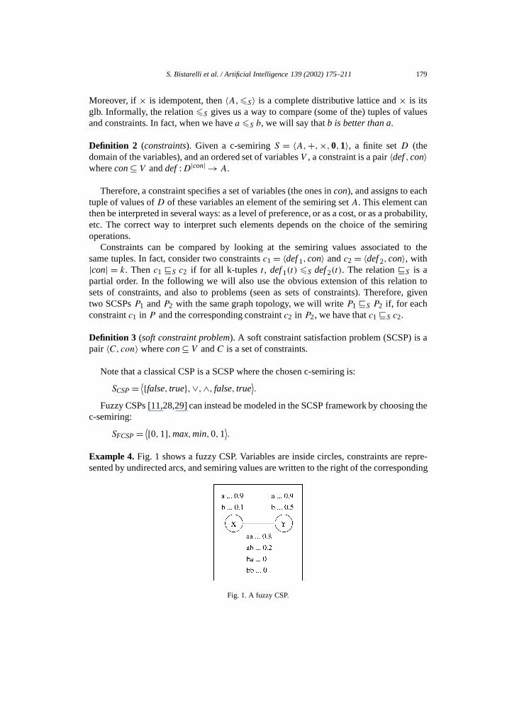
Example 4. Fig. 1 shows a fuzzy CSP. Variables are inside circles, constraints are repre-sented by undirected arcs, and semiring values are written to the right of the corresponding

Fig. 1. A fuzzy CSP.

180 S. Bistarelli et al. / Artificial Intelligence 139 (2002) 175–211

tuples. Here we assume that the domain D of the variables contains only elements aand b.

Definition 5 (combination). Given two constraints c1 = 〈def1, con1〉 and c2 = 〈def2,con2〉, their combinationc1 ⊗ c2 is the constraint 〈def,con〉 defined by con= con1 ∪con2 and def(t) = def1(t ↓con

con1) × def2(t ↓con

con2)1. The combination operator ⊗ can be

straightforward extended also to sets of constraints: when applied to a set of constraints C,we will write

⊗C.

In words, combining two constraints means building a new constraint involving all thevariables of the original ones, and which associates to each tuple of domain values for suchvariables a semiring element which is obtained by multiplying the elements associated bythe original constraints to the appropriate subtuples.

Using the properties of × and +, it is easy to prove that:

• ⊗ is associative, commutative, and monotone over S ;• if × is idempotent,⊗ is idempotent as well.

Definition 6 (projection). Given a constraint c = 〈def,con〉 and a subset I of V , theprojectionof c over I , written c ⇓I , is the constraint 〈def′,con′〉 where con′ = con∩ Iand def′(t ′)=∑

t/t↓conI∩con=t ′ def(t).

Informally, projecting means eliminating some variables. This is done by associatingto each tuple over the remaining variables a semiring element which is the sum of theelements associated by the original constraint to all the extensions of this tuple over theeliminated variables.

Definition 7 (solution). The solutionof a SCSP problem P = 〈C,con〉 is the constraintSol(P )= (⊗C)⇓con.

That is, to obtain the solution of an SCSP, we combine all constraints, and then projectover the variables in con. In this way we get the constraint over conwhich is “induced” bythe entire SCSP.

Example 8. For example, each solution of the fuzzy CSP of Fig. 1 consists of a pair ofdomain values (that is, a domain value for each of the two variables) and an associatedsemiring element (here we assume that con contains all variables). Such an element isobtained by looking at the smallest value for all the subtuples (as many as the constraints)forming the pair. For example, for tuple 〈a, a〉 (that is, x = y = a), we have to computethe minimum between 0.9 (which is the value for x = a), 0.8 (which is the value for〈x = a, y = a〉) and 0.9 (which is the value for y = a). Hence, the resulting value for thistuple is 0.8.

1 By t ↓XY

we mean the projection of tuple t , which is defined over the set of variables X, over the set ofvariables Y ⊆X.

S. Bistarelli et al. / Artificial Intelligence 139 (2002) 175–211 181

Fig. 2. A fuzzy CSP, its solutions, and its best solutions.

Definition 9 (optimal solution). Given an SCSP problem P , consider Sol(P )= 〈def,con〉.An optimal solution of P is a pair 〈t, v〉 such that def(t) = v, and there is no t ′ such thatv <S def(t ′).

Therefore optimal solutions are solutions which have the best semiring element amongthose associated to solutions. The set of optimal solutions of an SCSP P will be written asOpt(P ).

Example 10. Fig. 2 shows an example of a fuzzy CSP, its solutions, and its best solutions.

Definition 11 (problem ordering and equivalence). Consider two problems P1 and P2.Then P1 P P2 if Sol(P1) S Sol(P2). If P1 P P2 and P2 P P1, then they have thesame solution, thus we say that they are equivalent and we write P1 ≡ P2.

The relation P is a preorder. Moreover, P1 S P2 implies P1 P P2. Also, ≡ is anequivalence relation.

SCSP problems can be solved by extending and adapting the technique usually usedfor classical CSPs. For example, to find the best solution we could employ a branch-and-bound search algorithm (instead of the classical backtracking), and also the successfullyused propagation techniques, like arc-consistency [25,32], can be generalized to be usedfor SCSPs.

The detailed formal definition of propagationalgorithms (sometimes called also localconsistencyalgorithms) for SCSPs can be found in [7]. For the purpose of this paper,what is important to say is that a propagation ruleis a function which, taken an SCSP,solves a subproblem of it. It is possible to show that propagation rules are idempotent,monotone, and intensive functions (over the partial order of problems) which do not changethe solution set. Given a set of propagation rules, a local consistency algorithm consists ofapplying them in any order until stability. It is possible to prove that local consistencyalgorithms defined in this way have the following properties if the multiplicative operationof the semiring is idempotent: equivalence, termination, and uniqueness of the result.

Thus we can notice that the generalization of local consistency from classical CSPsto SCSPs concerns the fact that, instead of deleting values or tuples, obtaining localconsistency in SCSPs means changing the semiring values associated to some tuples ordomain elements. The change always brings these values towards the worst value of

182 S. Bistarelli et al. / Artificial Intelligence 139 (2002) 175–211

the semiring, that is, the 0. Thus, it is obvious that, given an SCSP problem P and theproblem P ′ obtained by applying some local consistency algorithm to P , we must haveP ′ S P .

2.2. Abstraction

Abstract interpretation[1,9,10] is a theory developed to reason about the relationbetween two different semantics (the concreteand the abstract semantics). The ideaof approximating program properties by evaluating a program on a simpler domain ofdescriptions of “concrete” program states goes back to the early 70’s. The inspiration wasthat of approximating properties from the exact (concrete) semantics into an approximate(abstract) semantics, that explicitly exhibits a structure (e.g., ordering) which is somehowpresent in the richer concrete structure associated to program execution.

The guiding idea is to relate the concrete and the abstract interpretation of the calculusby a pair of functions, the abstractionfunction α and the concretizationfunction γ , whichform a Galois connection.

Let (C, ) (concrete domain) be the domain of the concrete semantics, while (A,�)(abstract domain) be the domain of the abstract semantics. The partial order relationsreflect an approximation relation. Since in approximation theory a partial order specifiesthe precision degree of any element in a poset, it is obvious to assume that if α is amapping associating an abstract object in (A,�) for any concrete element in (C, ), thenthe following holds: if α(x) � y , then y is also a correct, although less precise, abstractapproximation of x . The same argument holds if x γ (y). Then y is also a correctapproximation of x , although x provides more accurate information than γ (y). This givesrise to the following formal definition.

Definition 12 (Galois insertion). Let (C, ) and (A,�) be two posets (the concrete andthe abstract domain). A Galois connection 〈α,γ 〉 : (C, ) � (A,�) is a pair of mapsα :C→A and γ :A→ C such that:

(1) α and γ are monotonic,(2) for each x ∈ C, x γ (α(x)), and(3) for each y ∈A, α(γ (y))� y.

Moreover, a Galois insertion (of A in C) 〈α,γ 〉 : (C, )� (A,�) is a Galois connectionwhere α · γ = IdA.

Property (2) is called extensivityof γ · α. The map α (γ ) is called the lower (upper)adjointor abstraction(concretization) in the context of abstract interpretation.

The following basic properties are satisfied by any Galois insertion:

(1) γ is injective and α is surjective.(2) α · γ is an upper closure operator in (C, ).(3) α is additive and γ is co-additive.

S. Bistarelli et al. / Artificial Intelligence 139 (2002) 175–211 183

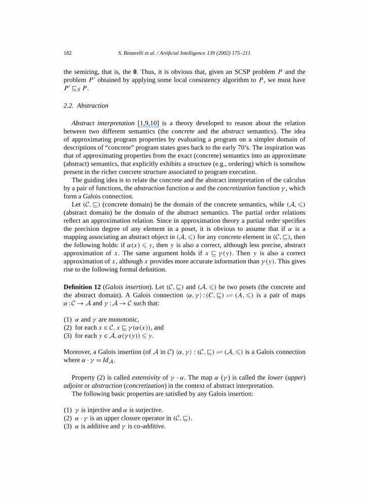
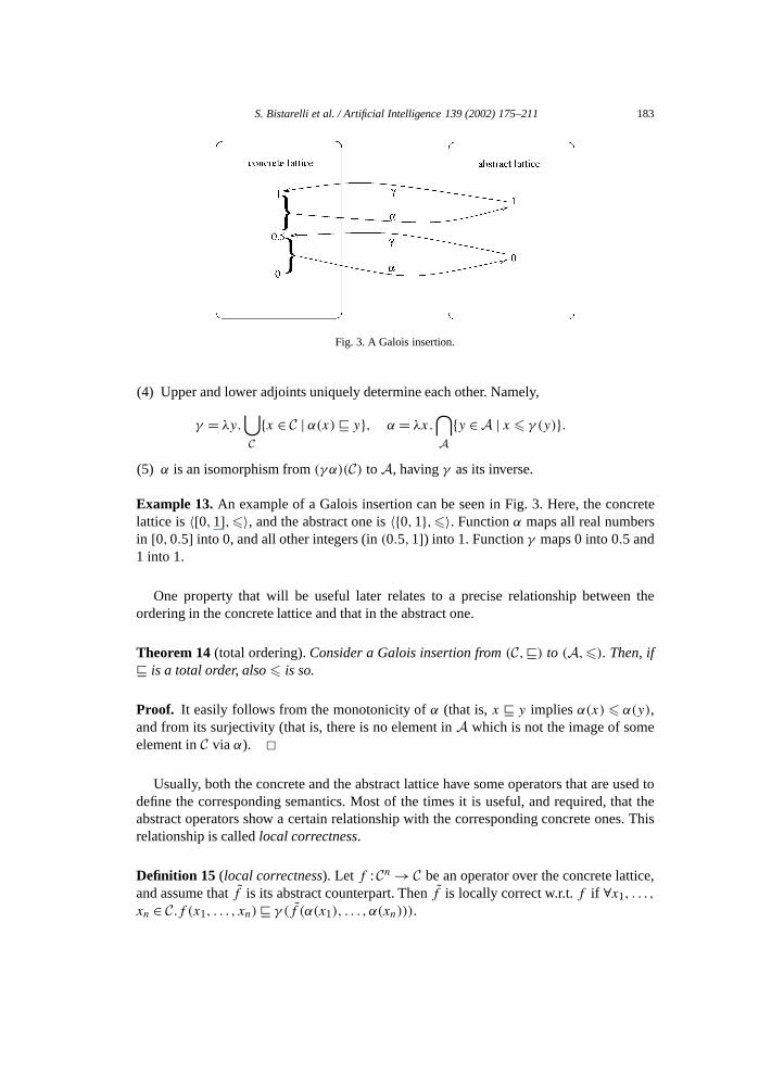
Fig. 3. A Galois insertion.

(4) Upper and lower adjoints uniquely determine each other. Namely,

γ = λy.⋃C{x ∈ C | α(x) y}, α = λx.

⋂A{y ∈A | x � γ (y)}.

(5) α is an isomorphism from (γ α)(C) to A, having γ as its inverse.

Example 13. An example of a Galois insertion can be seen in Fig. 3. Here, the concretelattice is 〈[0,1],�〉, and the abstract one is 〈{0,1},�〉. Function α maps all real numbersin [0,0.5] into 0, and all other integers (in (0.5,1]) into 1. Function γ maps 0 into 0.5 and1 into 1.

One property that will be useful later relates to a precise relationship between theordering in the concrete lattice and that in the abstract one.

Theorem 14 (total ordering). Consider a Galois insertion from(C, ) to (A,�). Then, if is a total order, also� is so.

Proof. It easily follows from the monotonicity of α (that is, x y implies α(x) � α(y),and from its surjectivity (that is, there is no element in A which is not the image of someelement in C via α). ✷

Usually, both the concrete and the abstract lattice have some operators that are used todefine the corresponding semantics. Most of the times it is useful, and required, that theabstract operators show a certain relationship with the corresponding concrete ones. Thisrelationship is called local correctness.

Definition 15 (local correctness). Let f :Cn→ C be an operator over the concrete lattice,and assume that f is its abstract counterpart. Then f is locally correct w.r.t. f if ∀x1, . . . ,

xn ∈ C.f (x1, . . . , xn) γ (f (α(x1), . . . , α(xn))).

184 S. Bistarelli et al. / Artificial Intelligence 139 (2002) 175–211

3. Abstracting soft CSPs

Given the notions of soft constraints and abstraction, recalled in the previous sections,we now want to show how to abstract soft constraint problems. The main idea is verysimple: we just want to pass, via the abstraction, from an SCSP P over a certain semiringS to another SCSP P over the semiring S, where the lattices associated to S and S arerelated by a Galois insertion as shown above.

Definition 16 (abstracting SCSPs). Consider the concreteSCSP problem P = 〈C,con〉over semiring S, where

• S = 〈A,+,×,0,1〉 and• C = {c0, . . . , cn} with ci = 〈coni ,defi〉 and defi :D|coni | →A;

we define the abstractSCSP problem P = 〈C,con〉 over the semiring S, where

• S = 〈A, +, ×, 0, 1〉;• C = {c0, . . . , cn} with ci = 〈coni, defi〉 and defi :D|coni | → A;

• if L= 〈A,�〉 is the lattice associated to S and L= 〈A, �〉 the lattice associated to S,then there is a Galois insertion 〈α,γ 〉 such that α :L→ L;• × is locally correct with respect to ×.

Notice that the kind of abstraction we consider in this paper does not change thestructure of the SCSP problem. That is, C and C have the same number of constraints,and ci and ci involve the same variables. The only thing that is changed by abstractingan SCSP is the semiring. Thus P and P have the same graph topology (variables andconstraints), but different constraint definitions, since if a certain tuple of domain valuesin a constraint of P has semiring value a, then the same tuple in the same constraint of Phas semiring value α(a). Notice also that α and γ can be defined in several different ways,but all of them have to satisfy the properties of the Galois insertion, from which it derives,among others, that α(0)= 0 and α(1)= 1.

Example 17. As an example, consider any SCSP over the semiring for optimization

SWCSP=⟨R− ∪ {−∞},max,+,−∞,0⟩

(where costs are represented by negative reals) and suppose we want to abstract it onto thesemiring for fuzzy reasoning

SFCSP=⟨[0,1],max,min,0,1

⟩.

In other words, instead of computing the maximum of the sum of all costs, we just wantto compute the maximum of the minimum of all costs, and we want to normalize the costsover [0..1]. Notice that the abstract problem is in the FCSP class and it has an idempotent× operator (which is the min). This means that in the abstract framework we can performlocal consistency over the problem in order to find inconsistencies. As noted above, the

S. Bistarelli et al. / Artificial Intelligence 139 (2002) 175–211 185

mapping α : 〈R−,�WCSP〉 → 〈[0,1],�FCSP〉 can be defined in different ways. For exam-ple one can decide to map all the reals below some fixed real x onto 0 and then to map thereals in [x,0] into the reals in [0,1] by using a normalization function, for example f (r)=(x − r)/x .

Example 18. Another example is the abstraction from the fuzzy semiring to the classicalone:

SCSP=⟨{0,1},∨,∧,0,1⟩

.

Here function α maps each element of [0,1] into either 0 or 1. For example, one couldmap all the elements in [0, x] onto 0, and all those in (x,1] onto 1, for some fixed x . Fig. 3represents this example with x = 0.5.

We have defined Galois insertions between two lattices 〈L,�S 〉 and 〈L, �S〉 of semiringvalues. However, for convenience, in the following we will often use Galois insertionsbetween lattices of problems 〈PL, S〉 and 〈PL, S〉 where PL contains problems over theconcrete semiring and PL over the abstract semiring. This does not change the meaningof our abstraction, we are just upgrading the Galois insertion from semiring values toproblems. Thus, when we will say that P = α(P ), it will mean that P is obtained by P viathe application of α to all the semiring values appearing in P .

An important property of our notion of abstraction is that the composition of twoabstractions is still an abstraction. This allows to build a complex abstraction by definingseveral simpler abstractions to be composed.

Theorem 19 (abstraction composition). Consider an abstraction from the lattice corre-sponding to a semiringS1 to that corresponding to a semiringS2, denoted by the pair〈α1, γ1〉. Consider now another abstraction from the lattice corresponding to the semiringS2 to that corresponding to a semiringS3, denoted by the pair〈α2, γ2〉. Then the pair〈α1 · α2, γ2 · γ1〉 is an abstraction as well.

Proof. We first have to prove that 〈α,γ 〉 = 〈α1 · α2, γ2 · γ1〉 satisfies the four properties ofa Galois insertion:

• since the composition of monotone functions is again a monotone function, we havethat both α and γ are monotone functions;• given a value x ∈ S1, from the first abstraction we have that x 1 γ1(α1(x)). Moreover,

for any element y ∈ S2, we have that y 2 γ2(α2(y)). This holds also for y = α1(x),thus by monotonicity of γ1 we have x 1 γ1(γ2(α2(α1(x)))).• a similar proof can be used for the third property;• the composition of two identities is still an identity.

To prove that×3 is locally correct w.r.t.×1, it is enough to consider the local correctnessof ×2 w.r.t. ×1 and of ×3 w.r.t. ×2, and the monotonicity of γ1. ✷

186 S. Bistarelli et al. / Artificial Intelligence 139 (2002) 175–211

4. Relating a soft constraint problem and its abstract version

In this section we will define and prove several properties that hold on abstractions ofsoft constraint problems. The main goal here is to point out some of the advantages thatone can have in passing through the abstracted version of a soft constraint problem insteadof solving directly the concrete version.

Let us consider the scheme depicted in Fig. 4. Here and in the following pictures, theleft box contains the lattice of concrete problems, and the right one the lattice of abstractproblems. The partial order in each of these lattices is shown via dashed lines. Connectionsbetween the two lattices, via the abstraction and concretization functions, is shown viadirected arrows. In the following, we will call S = 〈A,+,×,0,1〉 the concrete semiringand S = 〈A, +, ×, 0, 1〉 the abstract one. Thus we will always consider a Galois insertion〈α,γ 〉 : 〈A,�S〉� 〈A,�S〉.

In Fig. 4, P is the starting SCSP problem. Then with the mapping α we get P = α(P ),which is an abstraction of P . By applying the mapping γ to P , we get the problemγ (α(P )). Let us first notice that these two problems (P and γ (α(P ))) are related by aprecise property, as stated by the following theorem.

Theorem 20. Given an SCSP problemP overS, we have thatP S γ (α(P )).

Proof. Immediately follows from the properties of a Galois insertion, in particular fromthe fact that x �S γ (α(x)) for any x in the concrete lattice. In fact, P S γ (α(P )) meansthat, for each tuple in each constraint of P , the semiring value associated to such a tuplein P is smaller (w.r.t. �S) than the corresponding value associated to the same tuple inγ (α(P )). ✷

Notice that this implies that, if a tuple in γ (α(P )) has semiring value 0, then it musthave value 0 also in P . This holds also for the solutions, whose semiring value is obtainedby combining the semiring values of several tuples.

Corollary 21. Given an SCSP problemP overS, we have that Sol(P ) S Sol(γ (α(P )).

Proof. We recall that Sol(P ) is just a constraint, which is obtained as⊗(C) ⇓con. Thus

the statement of this corollary comes from the monotonicity of × and +. ✷

Fig. 4. The concrete and the abstract problem.

S. Bistarelli et al. / Artificial Intelligence 139 (2002) 175–211 187

Fig. 5. An example of the abstraction fuzzy-classical.

Therefore, by passing from P to γ (α(P )), no new inconsistencies are introduced: if asolution of γ (α(P )) has value 0, then this was true also in P . However, it is possible thatsome inconsistencies are forgotten (that is, they appear to be consistent after the abstractionprocess).

Example 22. Consider the abstraction from the fuzzy to the classical semiring, as describedin Fig. 3. Then, if we call P the fuzzy problem in Fig. 2, Fig. 5 shows the concreteproblem P , the abstract problem α(P ), and its concretization γ (α(P )). It is easy too seethat, for each tuple in each constraint, the associated semiring value in P is lower than orequal to that in γ (α(P )).

If the abstraction preserves the semiring ordering (that is, applying the abstractionfunction and then combining gives elements which are in the same ordering as the elementsobtained by combining only), then there is also an interesting relationship between the setof optimal solutions of P and that of α(P ). In fact, if a certain tuple is optimal in P ,then this same tuple is also optimal in α(P ). Let us first investigate the meaning of theorder-preservingproperty.

Definition 23 (order-preserving abstraction). Consider two sets I1 and I2 of concreteelements. Then an abstraction is said to be order-preserving if

∏x∈I1

α(x)�S

∏x∈I2

α(x)⇒∏x∈I1

x �S

∏x∈I2

x,

where the products refer to the multiplicative operations of the concrete (∏

) and theabstract (

∏) semirings.

188 S. Bistarelli et al. / Artificial Intelligence 139 (2002) 175–211

Fig. 6. An abstraction which is not order-preserving.

In words, this notion of order-preservation means that if we first abstract and thencombine, or we combine only, we get the same ordering (but on different semirings) amongthe resulting elements.

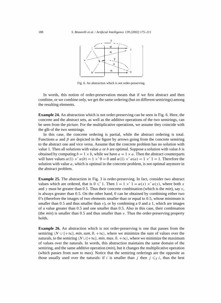
Example 24. An abstraction which is not order-preserving can be seen in Fig. 6. Here, theconcrete and the abstract sets, as well as the additive operations of the two semirings, canbe seen from the picture. For the multiplicative operations, we assume they coincide withthe glb of the two semirings.

In this case, the concrete ordering is partial, while the abstract ordering is total.Functions α and β are depicted in the figure by arrows going from the concrete semiringto the abstract one and vice versa. Assume that the concrete problem has no solution withvalue 1. Then all solutions with value a or b are optimal. Suppose a solution with value b isobtained by computing b= 1×b, while we have a = 1×a. Then the abstract counterpartswill have values α(1)×′ α(b)= 1×′ 0= 0 and α(1)×′ α(a)= 1×′ 1= 1. Therefore thesolution with value a, which is optimal in the concrete problem, is not optimal anymore inthe abstract problem.

Example 25. The abstraction in Fig. 3 is order-preserving. In fact, consider two abstractvalues which are ordered, that is 0 �′ 1. Then 1 = 1×′ 1 = α(x) ×′ α(y), where both xand y must be greater than 0.5. Thus their concrete combination (which is the min), say v,is always greater than 0.5. On the other hand, 0 can be obtained by combining either two0’s (therefore the images of two elements smaller than or equal to 0.5, whose minimum issmaller than 0.5 and thus smaller than v), or by combining a 0 and a 1, which are imagesof a value greater than 0.5 and one smaller than 0.5. Also in this case, their combination(the min) is smaller than 0.5 and thus smaller than v. Thus the order-preserving propertyholds.

Example 26. An abstraction which is not order-preserving is one that passes from thesemiring 〈N ∪ {+∞},min,sum,0,+∞〉, where we minimize the sum of values over thenaturals, to the semiring 〈N ∪{+∞},min,max,0,+∞〉, where we minimize the maximumof values over the naturals. In words, this abstraction maintains the same domain of thesemiring, and the same additive operation (min), but it changes the multiplicative operation(which passes from sumto max). Notice that the semiring orderings are the opposite asthose usually used over the naturals: if i is smaller than j then j �S i , thus the best

S. Bistarelli et al. / Artificial Intelligence 139 (2002) 175–211 189

element is 0 and the worst is +∞. The abstraction function α is just the identity, andalso the concretization function γ .

In this case, consider in the abstract semiring two values and the way they are obtainedby combining other two values of the abstract semiring: for example, 8 =max(7,8) and9=max(1,9). In the abstract ordering, 8 is higher than 9. Then, let us see how the imagesof the combined values (the same values, since α is the identity) relate to each other: wehave sum(7,8)= 15 and sum(1,9)= 10, and 15 is lower than 10 in the concrete ordering.Thus the order-preserving property does not hold.

Notice that, if we reduce the sets I1 and I2 to singletons, say x and y , then the order-preserving property says that α(x) �S α(y) implies that x �S y . This means that if twoabstract objects are ordered, then their concrete counterparts have to be ordered as well,and in the same way. Of course they could never be ordered in the opposite sense, otherwiseα would not be monotonic; but they could be incomparable. Therefore, if we choosean abstraction where incomparable objects are mapped by α onto ordered objects, thenwe don’t have the order-preserving property. A consequence of this is that if the abstractsemiring is totally ordered, and we want an order-preserving abstraction, then the concretesemiring must be totally ordered as well.

On the other hand, if two abstract objects are not ordered, then the correspondingconcrete objects can be ordered in any sense, or they can also be not comparable. Noticethat this restriction of the order-preserving property to singleton sets always holds whenthe concrete ordering is total. In fact, in this case, if two abstract elements are ordered in acertain way, then it is impossible that the corresponding concrete elements are ordered inthe opposite way, because, as we said above, of the monotonicity of the α function.

Theorem 27. Consider an abstraction which is order-preserving. Given an SCSP problemP overS, we have that Opt(P )⊆Opt(α(P )).

Proof. Let us take a tuple t which is optimal in the concrete semiring S, with value v. Thenv has been obtained by multiplying the values of some subtuples. Suppose, without lossof generality, that the number of such subtuples is two (that is, we have two constraints):v = v1 × v2. Let us then take the value of this tuple in the abstract problem, that is, theabstract combination of the abstractions of v1 and v2: this is v′ = α(v1)×′ α(v2). We haveto show that if v is optimal, then also v′ is optimal.

Suppose then that v′ is not optimal, that is, there exists another tuple t ′′ with value v′′such that v′ �S ′ v′′. Assume v′′ = v′′1 ×′ v′′2 . Now let us see the value of tuple t ′′ in P . Ifwe set v′′i = α(vi ), then we have that this value is v = v1 × v2. Let us now compare v withv. Since v′ �S v

′′, by order-preservation we get that v �S v. But this means that v is notoptimal, which was our initial assumption. Therefore v′ has to be optimal. ✷

Therefore, in case of order-preservation, the set of optimal solutions of the abstractproblem contains all the optimal solutions of the concrete problem. In other words, itis not allowed that an optimal solution in the concrete domain becomes non-optimal

190 S. Bistarelli et al. / Artificial Intelligence 139 (2002) 175–211

in the abstract domain. However, some non-optimal solutions could become optimal bybecoming incomparable with the optimal solutions.

Example 28. Consider again the example in Fig. 5. The optimal solutions in P are thetuples 〈a, b, a〉 and 〈a, b, b〉. It is easy to see that these tuples are also optimal in α(P ). Infact, this is a classical constraint problem where the solutions are tuples 〈a, b, a〉, 〈a, b, b〉,〈b, b, a〉, and 〈b, b, b〉.

Thus, if we want to find an optimal solution of the concrete problem, we could find allthe optimal solutions of the abstract problem, and then use them on the concrete side tofind an optimal solution for the concrete problem. Assuming that working on the abstractside is easier than on the concrete side, this method could help us find an optimal solutionof the concrete problem by looking at just a subset of tuples in the concrete problem.

5. From abstract optimal solutions to bounds of concrete optimal solutions

Another important property, which holds for any abstraction, concerns computingbounds that approximate an optimal solution of a concrete problem. In fact, any optimalsolution, say t , of the abstract problem, say with value v, can be used to obtain both anupper and a lower bound of an optimum in P . In fact, we can prove that there is an optimalsolution in P with value between γ (v) and the value of t in P . Thus, if we think thatapproximating the optimal value with a value within these two bounds is satisfactory, wecan take t as an approximation of an optimal solution of P .

Theorem 29. Given an SCSP problemP over S, consider an optimal solution ofα(P ),sayt , with semiring valuev in α(P ) andv in P . Then there exists an optimal solutiont ofP , say with valuev, such thatv � v � γ (v).

Proof. By local correctness of the multiplicative operation of the abstract semiring, wehave that v �S γ (v). Since v is the value of t in P , either t itself is optimal in P , or thereis another tuple which has value better than v, say v. We will now show that v cannot begreater than γ (v).

In fact, assume by absurd that γ (v) �S v. Then, by local correctness of themultiplicative operation of the abstract semiring, we have that α(v) is smaller than thevalue of t in α(P ). Also, by monotonicity of α, by γ (v) �S v we get that v �S α(v).Therefore by transitivity we obtain that v is smaller than the value of t in α(P ), which isnot possible because we assumed that v was optimal.

Therefore there must be an optimal value between v and γ (v). ✷Notice that this theorem does not need the order-preserving property in the abstraction,

thus any abstraction can exploit its result.Let us first consider a very simple use of this theorem in order to find an approximation

of an optimal concrete solution by going through the abstract domain. Consider a tuple t

S. Bistarelli et al. / Artificial Intelligence 139 (2002) 175–211 191

with optimal value v in the abstract problem. Instead of spending time to compute an exactoptimum of P , we can do the following:

• Compute γ (v), thus obtaining an upper bound of an optimum of P ;• Compute the value of t in P , which is a lower bound of the same optimum of P ;• If we think that such bounds are close enough, we can take t as a reasonable

approximation (to be precise, a lower bound) of an optimum of P .

Example 30. Consider again the example in Fig. 5. Now take any optimal solution ofα(P ), for example tuple 〈b, b, b〉. Then the above result states that there exists an optimalsolution of P with semiring value v between the value of this tuple in P , which is 0.7, andγ (1)= 1. In fact, there are optimal solutions with value 1 in P .

However, a better lower bound can be computed in the special case of an abstractionwhere the semirings are totally ordered and have idempotent multiplicative operations. Inthis case, any abstraction is order-preserving.

Theorem 31. Consider an abstraction between totally ordered semirings with idempotentmultiplicative operations. Given an SCSP problemP overS, consider an optimal solutionof α(P ), sayt , with semiring valuev in α(P ). Consider also the setV = {vi | α(vi )= v}.Then there exists an optimal solutiont of P , say with valuev, such that min(V ) � v �max(V ).

Proof. From Theorem 29, we know that v � γ (v). We recall that γ (v) is the highestelement in V , because of the properties of any Galois insertion (in particular, that x �S

γ (α(x))). Therefore, either v is in V , or it is lower than min(V ).We will now prove that v ∈ V , that is, α(v)= v.If v is in V , then the theorem holds. Otherwise, let us assume that v is lower than

min(V ).Now, v is obtained as the multiplication of several elements in the concrete semirings,

say v =⊗{x1, . . . , xn}. Because of the idempotence, there exists xk , with k ∈ {1, . . . , n},such that xk =min({x1, . . . , xn})= v.

Consider now the value v∗ of t in the abstract semiring. This is the multiplicationof all the α(xi). Thus v∗ = α(xk) = α(v) by monotonicity of α and idempotence of themultiplication operator.

Now, v∗ = v, since v∗ is an optimal solution by Theorem 27. Thus α(v)= v, thereforev ∈ V . ✷

6. Soft constraint solving through iterated abstractions

The results of the previous section can be the basis for a very interesting constraintsolving method, or more precisely a family of methods, where abstraction will be usedto indeed approximate the solution of the concrete problem. Let us first consider twoexamples of concrete algorithms and then present the general algorithm.

192 S. Bistarelli et al. / Artificial Intelligence 139 (2002) 175–211

An interesting method to solve a fuzzy CSP is to reduce the fuzzy problem to a sequenceof classical (boolean) CSPs to be solved by a classical solver. This method has been forinstance recently implemented in the JFSolver [23]. Indeed, according to the well-knownprinciple of of resolution identity in fuzzy set theory, a fuzzy CSP can be considered asa collection of crisp constraints at different levels of satisfaction [11] and one can thusconsider the so-called α-cuts (or level sets) containing, for each constraint, only the tupleswhose fuzzy value is above a certain value α. In this method, one derives from an originalproblem P a (classical) CSP problem P containing only the constraint tuples (α-cuts)above some value α, e.g., 0.5, and then solve P with a classical CSP solver. If P has asolution, this means that P has a corresponding solution with fuzzy value above α. Onecan then iterate this process with another value α′ (above α or below it) to further refinethe fuzzy value of the best solution. The main interest of this iterative technique is that itcan reuse an existing classical CSP solver in order to solve fuzzy CSP problems.

Let us formalize this algorithm within our abstraction framework. We want to abstracta fuzzy CSP P = 〈C,con〉 into the boolean semiring. Let us consider the abstraction αwhich maps the values in [0,0.5] to 0 and the values in ]0.5,1] to 1, which is depicted inFig. 3. Let us now consider the abstract problem P = α(P ) = 〈C, con〉. There are twopossibilities, depending whether α(P ) has a solution or not.

(1) If α(P ) has a solution, then (by the previous theorem) P has an optimal solution t withvalue v, such that 0.5< v � 1. We can now further cut this interval in two parts, e.g.,]0.5,0.75] and ]0.75,1], and consider now the abstraction α′ which maps the values in[0,0.75] to 0 and the values in ]0.75,1] to 1, which is depicted in Fig. 7. If α′(P ) has asolution, then P has a corresponding optimal solution with fuzzy value between 0.75and 1, otherwise the optimal solution has fuzzy value between 0.5 and 0.75, becausewe know from the previous iteration that the solution is above 0.5. If tighter boundsare needed, one could further iterate this process until the desired precision is reached.

(2) If α(P ) has no solution, then (by the previous theorem) P has an optimal solutiont with value v, such that 0 � v � 0.5. We can now further cut this interval in twoparts, e.g., [0,0.25] and ]0.25,0.5], and consider now the abstraction α′′ which mapsthe values in [0,0.25] to 0 and the values in ]0.25,1] to 1, which is depicted in Fig. 8.If α′′(P ) has a solution, then P has a corresponding optimal solution with fuzzy valuebetween 0.25 and 0.5, otherwise the optimal solution has fuzzy value between 0 and0.25. And so on and so forth.

Fig. 7. An abstraction from the fuzzy semiring to the boolean one.

S. Bistarelli et al. / Artificial Intelligence 139 (2002) 175–211 193

Fig. 8. An abstraction from the fuzzy semiring to the boolean one.

Observe that the dichotomy method used in this example is not the only one that canbe used: we can cut each interval not necessarily in the middle but at any point at will(e.g., if some heuristic method allows us to guess in which part of the semiring the optimalsolution is). The method will work as well, although the convergence rate, and thus theperformance, could be different.

Let us now consider an extension of the above method. Consider a SCSP solver ableto solve any problem on semirings defined on finite domains, such as the clp(FD,S)systems designed in [17].2 This system solves fuzzy CSP problems by considering asemiring with discrete values and implements a general semiring-based solver achievinglocal consistency and partial local consistency. Consider a simple abstraction α whichmaps [0,0.1] to 0.1, ]0.1,0.2] to 0.2, . . . , ]0.9,1] to 1. We thus have a 10-valued domainfor semiring values. Considering for any fuzzy CSP problem P the abstract problem α(P ),and solving it with clp(FD,S), will give us the value v of an optimal solution of theabstract problem. This, by the above theorem, will tell us in which interval I the valueof a corresponding optimal solution of the original problem P is located, thus giving usa 1-digit precision over an optimal solution of the concrete problem. If tighter bounds areneeded, one could then divide I in 10 sub-intervals and apply a similar abstraction α′ to geta second abstract problem α′(P ), and solve it again with clp(FD,S). We would thus getthe value of an optimal solution with a 2-digit precision. And so on and so forth. Comparingto the previous technique that uses a classical CSP solver, the method using clp(FD,S)should be able to converge faster towards the solution with the desired precision, as wehave more values in the abstract semiring and thus are able, at each iteration, to cut theoriginal (fuzzy) semiring into smaller intervals through the abstraction process.

In this two examples, we have seen that we need severalabstraction functions from theconcrete domain to the abstract one, which are working on different subsets of the originalsemiring S and are decomposing them into two or more abstract values. Indeed, as weare working with totally ordered sets, we are interested only in intervals and not on anysubset. Formally, an interval of a semiring S = 〈A,+,×,0,1〉, is a subset I ⊆ A suchthat min(I)� x � max(I)⇒ x ∈ I . As we are working on totally ordered semirings withidempotent× operation, it is obvious that for any such c-semiring S = 〈A,+,×,0,1〉, and

2 This system is available on the Web at the URL: http://contraintes.inria.fr/~georget/software/clp_fds/clp_fds.html.

194 S. Bistarelli et al. / Artificial Intelligence 139 (2002) 175–211

any interval I ⊆ A, SI = 〈I,+,×,0,1〉 is also a totally ordered semiring with idempotent× operation. Thus, if we have an abstraction function αI from SI to some other semiringS′, it can be trivially extended to an abstraction α from S to S′, called the S-extensionof αI ,as follows:

• if x � min(I), then α(x)= 0;• if x � max(I), then α(x)= 1;• if x ∈ I , then α(x)= αI (x).

Observe that the necessary properties of an abstraction function ensure that αI (min(I))= 0and αI (max(I))= 1.

Let us now define the general constraint solving method of which the two previousexamples are simple but computationally effective instances.

Algorithm for soft constraint solving through iterated abstractionsInput:

• a SCSP problem P over a totally ordered semiring S = 〈A,+,×,0,1〉 withidempotent× operation,• another totally ordered semiring S′ with idempotent× operation,• a set DecS of disjoint intervals of S covering A,• a family of abstraction functions αI from I to S′, for each I ∈DecS .

Let I =ARepeatlet α be the S-extension of αIsolve α(P ), and let t be an optimal solution with value vlet I = {vi ∈ S / α(vi)= v}until I /∈DecSoutput t

Output: a tuple t , whose semiring value approximates the value of an optimal solution ofP with the desired precision.

The idea of this algorithms is that one defines the decomposition DecS of S and theabstraction functions αI down to the desired level of precision, and the algorithm stopswhen it has reached the desired bounds for the value of an optimal solution.

7. Working on the abstract problem

Consider now what we can do on the abstract problem, α(P ). One possibility is toapply an abstract function f , which can be, for example, a local consistency algorithm oralso a solution algorithm. In the following, we will consider functions f which are alwaysintensive, that is, which bring the given problem closer to the bottom of the lattice. In

S. Bistarelli et al. / Artificial Intelligence 139 (2002) 175–211 195

fact, our goal is to solve an SCSP, thus going higher in the lattice does not help in thistask, since solving means combining constraints and thus getting lower in the lattice. Also,functions f will always be locally correct with respect to any function fsol which solvesthe concrete problem. We will call such a property solution-correctness. More precisely,given a problem P with constraint set C, fsol(P ) is a new problem P ′ with the sametopology as P whose tuples have semiring values possibly lower. Let us call C′ the set ofconstraints of P ′. Then, for any constraint c′ ∈ C′, c′ = (⊗C)⇓var(c′). In other words, fsol

combines all constraints of P and then projects the resulting global constraint over each ofthe original constraints.

Definition 32. Given an SCSP problem P over S, consider a function f on α(P ). Then fis solution-correct if, given any fsol which solves P , f is locally correct w.r.t. fsol.

We will also need the notion of safeness of a function, which just means that it maintainsall the solutions.

Definition 33. Given an SCSP problem P and a function f : PL→ PL, f is safe ifSol(P )= Sol(f (P )).

It is easy to see that any local consistency algorithm, as defined in [7], can be seen as asafe, intensive, and solution-correct function.

From f (α(P )), applying the concretization function γ , we get γ (f (α(P ))), whichtherefore is again over the concrete semiring (the same as P ). The following property saysthat, under certain conditions, P and P ⊗γ (f (α(P ))) are equivalent. Fig. 9 describes sucha situation. In this figure, we can see that several partial order lines have been drawn:

• on the abstract side, function f takes any element closer to the bottom, because of itsintensiveness;

Fig. 9. The general abstraction scheme, with × idempotent.

196 S. Bistarelli et al. / Artificial Intelligence 139 (2002) 175–211

• on the concrete side, we have that– P ⊗ γ (f (α(P ))) is smaller than both P and γ (f (α(P ))) because of the properties

of ⊗;– γ (f (α(P ))) is smaller than γ (α(P )) because of the monotonicity of γ ;– γ (f (α(P ))) is higher than fsol(P ) because of the solution-correctness of f ;– fsol(P ) is smaller than P because of the way fsol(P ) is constructed;– if× is idempotent, then it coincides with the glb, thus we have that P ⊗γ (f (α(P )))

is higher than fsol(P ), because by definition the glb is the highest among all thelower bounds of P and γ (f (α(P ))).

Theorem 34. Given an SCSP problemP over S, consider a functionf on α(P ) whichis safe, solution-correct, and intensive. Then, if× is idempotent, Sol(P ) = Sol(P ⊗γ (f (α(P )))).

Proof. Take any tuple t with value v in P , which is obtained by combining the valuesof some subtuples, say two: v = v1 × v2. Let us now consider the abstract versions of v1

and v2: α(v1) and α(v2). Function f changes these values by lowering them, thus we getf (α(v1))= v′1 and f (α(v2))= v′2.

Since f is safe, we have that v′1 ×′ v′2 = α(v1)×′ α(v2)= v′. Moreover, f is solution-correct, thus v �S γ (v

′). By monotonicity of γ , we have that γ (v′)�S γ (v′i ) for i = 1,2.

This implies that γ (v′)�S (γ (v′1)×γ (v′2)), since× is idempotent by assumption and thus

it coincides with the glb. Thus we have that v �S (γ (v′1)× γ (v′2)).

To prove that P and P ⊗ γ (f (α(P ))) give the same value to each tuple, we now haveto prove that v = (v1 × γ (v′1))× (v2 × γ (v′2)). By commutativity of ×, we can write thisas (v1× v2)× (γ (v′1)× γ (v′2)). Now, v1× v2 = v by assumption, and we have shown thatv �S γ (v

′1)× γ (v′2). Therefore v × (γ (v′1)× γ (v′2))= v. ✷

This theorem does not say anything about the power of f , which could makemany modifications to α(P ), or it could also not modify anything. In this last case,γ (f (α(P )))= γ (α(P ))" P (see Fig. 10), so P ⊗γ (f (α(P )))= P , which means that wehave not gained anything in abstracting P . However, we can always use the relationship

Fig. 10. The scheme when f does not modify anything.

S. Bistarelli et al. / Artificial Intelligence 139 (2002) 175–211 197

between P and α(P ) (see Theorem 27 and 29) to find an approximation of the optimalsolutions and of the inconsistencies of P .

Example 35. Fig. 11 uses the abstraction in Fig. 3 and shows a concrete problem and theresult of the construction of Fig. 9 over it.

If instead f modifies all semiring elements in α(P ), then if the order of the concretesemiring is total, we have that P ⊗ γ (f (α(P )))= γ (f (α(P ))) (see Fig. 12), and thus wecan work on γ (f (α(P ))) to find the solutions of P . In fact, γ (f (α(P ))) is lower than Pand thus closer to the solution.

Fig. 11. An example with × idempotent.

Fig. 12. The scheme when the concrete semiring has a total order.

198 S. Bistarelli et al. / Artificial Intelligence 139 (2002) 175–211

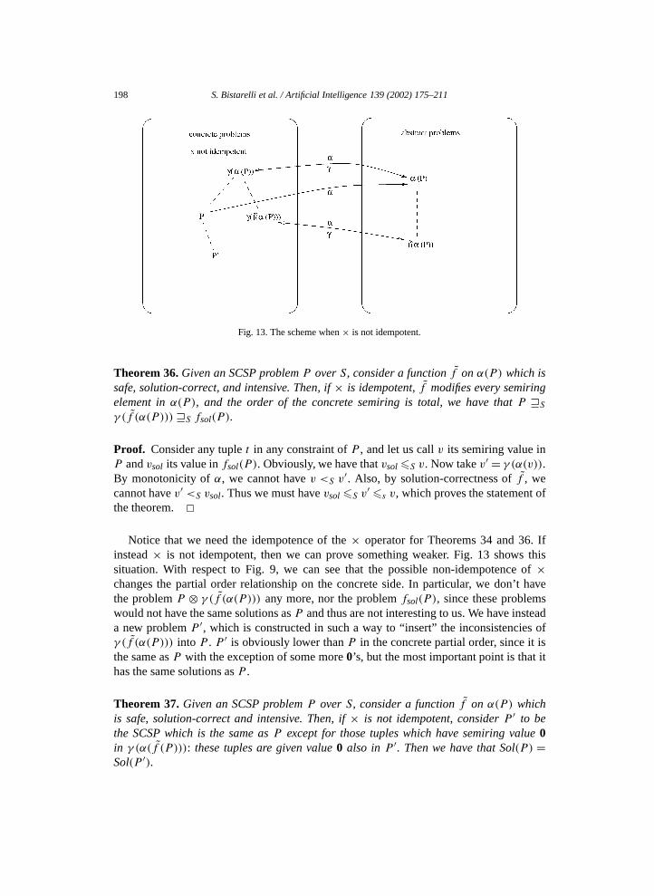
Fig. 13. The scheme when × is not idempotent.

Theorem 36. Given an SCSP problemP overS, consider a functionf onα(P ) which issafe, solution-correct, and intensive. Then, if× is idempotent,f modifies every semiringelement inα(P ), and the order of the concrete semiring is total, we have thatP "Sγ (f (α(P )))"S fsol(P ).

Proof. Consider any tuple t in any constraint of P , and let us call v its semiring value inP and vsol its value in fsol(P ). Obviously, we have that vsol �S v. Now take v′ = γ (α(v)).By monotonicity of α, we cannot have v <S v′. Also, by solution-correctness of f , wecannot have v′ <S vsol. Thus we must have vsol �S v

′ �s v, which proves the statement ofthe theorem. ✷

Notice that we need the idempotence of the × operator for Theorems 34 and 36. Ifinstead × is not idempotent, then we can prove something weaker. Fig. 13 shows thissituation. With respect to Fig. 9, we can see that the possible non-idempotence of ×changes the partial order relationship on the concrete side. In particular, we don’t havethe problem P ⊗ γ (f (α(P ))) any more, nor the problem fsol(P ), since these problemswould not have the same solutions as P and thus are not interesting to us. We have insteada new problem P ′, which is constructed in such a way to “insert” the inconsistencies ofγ (f (α(P ))) into P . P ′ is obviously lower than P in the concrete partial order, since it isthe same as P with the exception of some more 0’s, but the most important point is that ithas the same solutions as P .

Theorem 37. Given an SCSP problemP over S, consider a functionf on α(P ) whichis safe, solution-correct and intensive. Then, if× is not idempotent, considerP ′ to bethe SCSP which is the same asP except for those tuples which have semiring value0in γ (α(f (P ))): these tuples are given value0 also inP ′. Then we have that Sol(P ) =Sol(P ′).

S. Bistarelli et al. / Artificial Intelligence 139 (2002) 175–211 199

Fig. 14. An example with × is not idempotent.

Proof. Take any tuple t with value v in P , which is obtained by combining the valuesof some subtuples, say two: v = v1 × v2. Let us now consider the abstract versions of v1and v2: α(v1) and α(v2). Function f changes these values by lowering them, thus we getf (α(v1))= v′1 and f (α(v2))= v′2.

Since f is safe, we have that v′1 ×′ v′2 = α(v1)×′ α(v2)= v′. Moreover, f is solution-correct, thus v �S γ (v

′). By monotonicity of γ , we have that γ (v′)�S γ (v′i ) for i = 1,2.

Thus we have that v �S γ (v′i ) for i = 1,2.

Now suppose that γ (v′1)= 0. This implies that also v = 0. Therefore, if we set v1 = 0,again the combination of v1 and v2 will result in v, which is 0. ✷Example 38. Consider the abstraction from the semiring S = 〈Z− ∪ {−∞},max,+,−∞,0〉 to the semiring S′ = 〈Z− ∪ {−∞},max,min,−∞,0〉, where α and γ arethe identity. This means that we perform the abstraction just to change the multiplicativeoperation, which is min instead of +. Then Fig. 14 shows a concrete problem over S, andthe construction shown in Fig. 13 over it.

Summarizing, the above theorems can give us several hints on how to use the abstractionscheme to make the solution of P easier: If × is idempotent, then we can replace Pwith P ⊗ γ (α(f (P ))), and get the same solutions (by Theorem 34). If instead × is notidempotent, we can replace P with P ′ (by Theorem 37). In any case, the point in passingfrom P to P ⊗ γ (α(f (P ))) (or P ′) is that the new problem should be easier to solvethan P , since the semiring values of its tuples are more explicit, that is, closer to the valuesof these tuples in a completely solved problem.

More precisely, consider a branch-and-boundalgorithm to find an optimal solution of P .Then, once a solution is found, its value will be used to cut away some branches, where thesemiring value is worse than the value of the solution already found. Now, if the values of

200 S. Bistarelli et al. / Artificial Intelligence 139 (2002) 175–211

the tuples are worse in the new problem than in P , each branch will have a worse value andthus we might cut away more branches. For example, consider the fuzzy semiring (that is,we want to maximize the minimum of the values of the subtuples): if the solution alreadyfound has value 0.6, then each partial solution of P with value smaller than or equal to0.6 can be discarded (together with all its corresponding subtree in the search tree), but allpartial solutions with value greater than 0.6 must be considered; if instead we work in thenew problem, the same partial solution with value greater than 0.6 may now have a smallervalue, possibly also smaller than 0.6, and thus can be disregarded. Therefore, the searchtree of the new problem is smaller than that of P .

Another point to notice is that, if using a greedy algorithm to find the initial solution(to use later as a lower bound), this initial phase in the new problem will lead to a betterestimate, since the values of the tuples are worse in the new problem and thus close to theoptimum. In the extreme case in which the change from P to the new problem brings thesemiring values of the tuples to coincide with the value of their combination, it is possibleto see that the initial solution is already the optimal one.

Notice also that, if × is not idempotent, a tuple of P ′ has either the same value as in P ,or 0. Thus the initial estimate in P ′ is the same as that of P (since the initial solution mustbe a solution), but the search tree of P ′ is again smaller than that of P , since there may bepartial solutions which in P have value different from 0 and in P ′ have value 0, and thusthe global inconsistency may be recognized earlier.

The same reasoning used for Theorem 27 on α(P ) can also be applied to f (α(P )). Infact, since f is safe, the solutions of f (α(P )) have the same values as those of α(P ). Thusalso the optimal solution sets coincide. Therefore we have that Opt(f (α(P ))) contains allthe optimal solutions of P if the abstraction is order-preserving. This means that, in orderto find an optimal solution of P , we can find all optimal solutions of f (α(P )) and then usesuch a set to prune the search for an optimal solution of P .

Theorem 39. Given an SCSP problemP overS, consider a functionf onP which is safe,solution-correct and intensive, and let us assume the abstraction is order-preserving. Thenwe have that Opt(P )⊆Opt(f (α(P ))).

Proof. Easy follows from Theorem 27 and from the safeness of f . ✷Theorem 29 can be adapted to f (α(P )) as well, thus allowing us to use an optimal

solution of f (α(P )) to find both a lower and an upper bound of an optimal solution of P .

8. An example

In this section we will consider an example of a problem which can be described by aset of soft constraints, and we will show how in this example the abstraction scenarios thatwe have described in the previous sections work.

The example we will consider is taken from the class of crossword puzzles creationproblems. A crossword puzzle creation problem is a problem where there is a bi-dimen-sional board where some cells have been blackened. In the other cells, we have to put

S. Bistarelli et al. / Artificial Intelligence 139 (2002) 175–211 201

a letter in each cell, in such a way that the maximal sequences of adjacent cells, verticallyand horizontally, form a word from a certain set of allowed words.

Crossword puzzles are frequently used as examples of constraint satisfaction problems,and the behavior of search algorithms over such problems is considered to be meaningfulto evaluate such algorithms. In fact, it has been shown that search can be used to greateffect in crossword puzzle creation problems [19].

First we need to say how to represent a crossword puzzle as a constraint problem,that is, we need to say which are the variables, the variable domains, and the constraints.A possible constraint-based formulation of these problems is as follows: there is a variablefor each cell that can hold a letter, the domain of each variable is the set of alphabet letters,and the constraints are the possible words. That is, each constraint connects a certainnumber of variables and it is satisfied when these variables have values that form oneof the allowed words.

Consider for example the crossword puzzle in Fig. 15, for which the available wordsare: HOSES, LASER, SHEET, SNAIL, STEER, HIKE, ARON, KEET, EARN, SAME,RUN, SUN, LET, YES, EAT, TEN, NO, BE, US, IT. For this crossword puzzle problem,we have 13 variables, x1, . . . , x13, and the constraints (described by sets of allowed words)are as follows, where each constraint has an index which is a list of integers, denoting thevariables it connects. For example, constraint Ci,j,k connects variables xi , xj , and xk .

C1,2,3,4,5 ={(H,O,S,E,S), (L,A,S,E,R), (S,H,E,E,T), (S,N,A, I,L),

(S,T,E,E,R)},

C3,6,9,12 ={(H, I,K,E), (A,R,O,N), (K,E,E,T), (E,A,R,N),

(S,A,M,E)},

C5,7,11 ={(R,U,N), (S,U,N), (L,E,T), (Y,E,S), (E,A,T), (T,E,N)

},

C8,9,10,11 = C3,6,9,12,

C10,13 ={(N,O), (B,E), (U,S), (I,T)

},

C12,13 = C10,13.

For now we have described a set of hard constraints. We will now add some softness tothe problem. This can be done in many ways, by choosing any semiring to work on. In ourexample, we decided to associate a cost with each letter of the alphabet, and by lookingfor the solutions with the minimum sum of the costs over all the variables. That is, our

Fig. 15. A crossword puzzle problem.

202 S. Bistarelli et al. / Artificial Intelligence 139 (2002) 175–211

Fig. 16. The abstraction/concretization functions.

problem is over the semiring of weighted CSPs: 〈N,+,min,+∞,0〉, where the costs areall the natural numbers plus +∞, costs are combined via the sum operator, and smallercosts are preferred. In this semiring, +∞ is the worst cost, and 0 is the best one. For thesoft version of our problem, to each letter of the alphabet, say x , we associate a uniquelyidentified cost cx , taken from the natural numbers. This means that it is not possible thattwo domains associate two different costs to the same letter. Notice also that we introducesoftness just in the variable domains, while the constraints representing the words remainhard: for our semiring, this means that tuples of letters that are allowed in the list above aregiven cost 0, while the others (not appearing in the lists above) are given cost +∞.

In the terminology of this paper, this is our concrete problem. We will now consider anabstract version of it. Again, this can be done in many ways, by just choosing a differentsemiring for the abstract problem and a suitable abstraction function. In our case, we usethe semiring of classical constraints: 〈{true, false},and,or, false, true〉. Thus, the abstractversion of our problem will be a set of hard constraints.

We now need to define the abstraction function α which allows us to pass from theconcrete problem to the abstract one. We will use is a very simple abstraction function, theone which maps every natural number to 1 and +∞ to 0. Given this abstraction function,the concretization function γ is then mapping 1 to 0 and 0 to +∞. Fig. 16 shows these twofunctions.

The intuitive meaning of this abstraction function is that, if a letter does not contributewith a +∞ cost, then in the abstract problem is allowed. Thus the abstract version of ourproblem is exactly the hard problem we started with, which has the hard constraints listedabove and the variable domains allowing any letter of the alphabet.

It is easy to see that this abstraction is order-preserving (see Section 4 for its definition).This means (see Theorem 27) that the set of optimal solutions of the concrete problem isa subset of (or is equal to) the set of optimal solutions of the abstract problem. This result,however, cannot help us, unless we discover something on the set of optimal solutions (thatis, solutions, in this case) of the abstract problem.

Thus, although our goal is to find an optimal solution of the concrete problem, let uswork on the abstract problem. The hope is that working in the abstract problem, and using

S. Bistarelli et al. / Artificial Intelligence 139 (2002) 175–211 203

the results of this paper, will help us in our goal more than working directly on the concreteproblem.

For example, following the scenario of Fig. 9, we can apply some sort of localconsistency algorithm to the abstract problem, then concretize the problem, and combineit with the original concrete problem.

Let us then apply arc-consistency [25,32] to the abstract problem. Notice that wecan indeed apply it, since the semiring has an idempotent multiplicative operation(which is logical and), while we could not apply any local consistency algorithm to theconcrete problem, because the chosen semiring has a multiplicative operation which is notidempotent.

By applying arc-consistency, we discover that only some variable values remain in thevariable domains. In fact, arc consistency eliminates all those domain values which arenot consistent with some constraints involving that variable. For example, the domain ofvariable v1 will be left with just letters H , L, and S, since all other letters are incompatiblewith constraint C1,2,3,4,5. This new smaller domain for v1 can in turn be used to see thatsome constraint tuples which seem allowed are in reality not possible, and thus otherdomain elements from other variable domains can be eliminated by arc-consistency. Arc-consistency is achieved when no more domain elements can be removed. At that point,it is easy to see that in our example all variable domains have become empty. Thus arc-consistency, which has the role of function f in Fig. 9, has brought us to a problem whereall domain elements have semiring value 0.

By concretizing such a problem, we get a concrete problem where all domain elementshave semiring value+∞. By combining this problem with the original one, we get exactlythis problem (since it is lower in the lattice of problems). It is now immediate to see that thisproblem has all no solutions, that is, all its complete variable assignments have semiringvalue +∞.

Notice that, to discover this, we just needed to pass to the abstract side, apply arc-consistency, which is a low polynomial algorithm (quadratic in the size of the problem),and get back to the concrete side. Discovering this same information without going to theabstract side would have been much more expensive, since a complete visit of the searchtree (although with possibly some pruning) would have been necessary.

9. Abstraction vs. local consistency

It is now interesting to consider the relationship between our abstraction framework andthe concept of local consistency.

In fact, it is possible to show that, given an abstraction 〈α,γ 〉 between semirings Sand S and any propagation rule r in S, the function γ (r(α(P )))⊗ P is a propagation rulefor problem P over S. This can be convenient when S does not have any, or any efficient,propagation algorithms. In fact, in such cases, we can resort to the propagation algorithmsof S to perform propagation also over S.

Notice however that, when S has a non-idempotent multiplicative operator, functionγ (r(α(P ))) ⊗ P could change the solution of P . To avoid this problem, we just have tofollow the same reasoning as in the previous section, that is, to replace such a function with

204 S. Bistarelli et al. / Artificial Intelligence 139 (2002) 175–211

a function with just inserts into P the inconsistencies of γ (r(α(P )). We will denote sucha function by using a different combination operator: ⊗0. Thus the function to be usedin these cases is γ (r(α(P ))⊗0 P . Notice that ⊗0 is a non-commutative operator, since itinserts into the right operand the zeros of the left operand.

These results however hold only when the abstraction is order-preserving. We recallthat this means that applying the abstraction function and then combining gives elementswhich are in the same ordering as the elements obtained by combining only. In particular,if two abstract elements α(x) and α(y) are ordered, then also x and y are ordered as well,and in the same direction.

Theorem 40. Given an order-preserving abstraction〈α,γ 〉 between semiringS and S,assume thatS has an idempotent multiplicative operation and consider any propagationrule r in S and any problemP overS. Then the functionf (P ) = γ (r(α(P ))) ⊗ P is apropagation rule forP .

Proof. By definition, a propagation rule is an intensive, monotone, and idempotentfunction which takes a problem and returns an equivalent problem over the same semiring.Since ⊗ is intensive, also f is so. Moreover, by monotonicity of γ , r , α, and ⊗, also f ismonotone.

For proving idempotence of f , we need the order-preserving property of the abstraction.In fact, consider what happens when applying function f to P : some tuple values inα(P ), say v = α(v), will not be changed by r , while others will receive a lower value,say v′ = r(v). By order-preservation, the new tuples values in the concrete semiring (thatis, γ (r(α(v)))×v), are equal or lower than the original values. Let us now apply function fagain. Function α will bring these new concrete values to either v (if we start from v) or v′(if we start from γ (r(α(v)))). In any case, r will bring such values to v′, for Lemma 41(see below). Thus f is idempotent. Finally, f returns an equivalent problem by the theoremdepicted in Fig. 9. ✷Lemma 41. Consider any SCSPP over S and any propagation ruler for P , withr(P )= P ′. Then, taken any SCSPP ′′ such thatP ′ �S P

′′ �S P , we haver(P ′′)= P ′.

Proof. Any rule r solves a subproblem 〈C,con〉 and changes the values of the tuplesconnecting the variables in con. Thus the result of applying r is a new constraint overcon: (C ⊗ Ccon) ⇓con, where Ccon is the original constraint connecting the variablesin con. This can also be written as Ccon⊗ C ⇓con. Let us now take any C′′con such that(Ccon⊗ C ⇓con) �S C

′′con �S Ccon. We can now multiply all these three constraints by

C ⇓con, obtaining: (Ccon⊗ C ⇓con⊗C ⇓con) �S (C′′con⊗ C ⇓con) �S (Ccon⊗ C ⇓con).

By idempotence of ⊗, we get: (Ccon⊗ C ⇓con)�S (C′′con⊗C ⇓con)�S (Ccon⊗C ⇓con).

Thus we have that (Ccon⊗C ⇓con)= (C′′con⊗C ⇓con). ✷We can now prove a similar result for the case of a non-idempotent multiplicative oper-

ation in the concrete semiring. However, as noted above, we cannot combine the new prob-lem with the old one, but we can just insert the zeroes of the new problem into the old one.

S. Bistarelli et al. / Artificial Intelligence 139 (2002) 175–211 205

Theorem 42. Given an order-preserving abstraction〈α,γ 〉 between semiringS andS, assume thatS has a non-idempotent multiplicative operation and consider anypropagation rule r in S and any problemP over S. Then the functionf (P ) =γ (r(α(P ))) ⊗0 P is a propagation rule forP , where⊗0 inserts the zeroes of its leftoperand into the right one.

The proof of this theorem is similar to the previous one, and for the equivalence it refersalso to the theorem depicted in Fig. 13.

By taking several propagation rules in the abstract semiring, we can thus obtain an equalnumber of propagation rules over the concrete semiring. This set of rules can then be usedto perform constraint propagation over a concrete problem. Notice however that, while anidempotent multiplicative operation in the concrete semiring allows us to use such rulesuntil stability, with all the desired properties (equivalence, uniqueness, and termination),in the case of a non-idempotent multiplicative operation we can just apply the variouspropagation rules once each to insert several zeroes into the original problem (with thesame properties as above).

10. Some abstraction mappings

In this section we will list some semirings and several abstractions between them,in order to provide the reader with a scenario of possible abstractions that he/she canuse, starting from one of the semirings considered here. Some of these semirings and/orabstractions have been already described in the previous sections of the paper, howeverhere we will re-define them to make this section self-contained. Of course many othersemirings could be defined, but here we focus on the ones for which either it has beendefined, or it is easy to imagine, a system of constraint solving. The semirings we willconsider are the following ones:

• the classical one, which describes classical CSPs via the use of logical and and logicalor:

SCSP=⟨{T ,F },∨,∧,F,T ⟩;

• the fuzzy semiring, where the goal is to maximize the minimum of some values over[0,1]:

Sfuzzy=⟨[0,1], max, min,0,1

⟩;• the extension of the fuzzy semiring over the naturals, where the goal is to maximize

the minimum of some values of the naturals:

SfuzzyN=⟨N ∪ {+∞}, max, min,0,+∞⟩;

• the extension of the fuzzy semiring over the positive reals:

SfuzzyR=⟨R+ ∪ {+∞}, max, min,0,+∞⟩;

206 S. Bistarelli et al. / Artificial Intelligence 139 (2002) 175–211

• the optimization semiring over the naturals, where we want to maximize the sum ofcosts (which are negative integers):

SoptN=⟨Z− ∪ {−∞},max,+,−∞,0⟩;

• the optimization semiring over the negative reals:

SoptR=⟨R− ∪ {−∞},max,+,−∞,0⟩;

• the probabilistic semiring, where we want to maximize a certain probability whichis obtained by multiplying several individual probabilities. The idea here is thateach tuple in each constraint has associated the probability of being allowed in thereal problems we are modeling, and different tuples in different constraints haveindependent probabilities (so that their combined probability is just the multiplicationof their individual probabilities) [13]. The semiring is:

Sprob=⟨[0,1], max,×,0,1⟩;

• the subset semiring, where the elements are all the subsets of a certain set A, theoperations are set intersection and set union, the smallest element is the empty set, andthe largest element is the whole given set:

Ssub=⟨2A,

⋃,⋂,∅,A

⟩.

We will now define several abstractions between pairs of these semirings. The resultis drawn in Fig. 17, where the dashed lines denote the abstractions that have not beendefined but can be obtained by abstraction composition. In reality, each line in the figurerepresents a whole family of abstractions, since each 〈α,γ 〉 pair makes a specific choicewhich identifies a member of the family. Moreover, by defining one of this families ofabstractions we do not want to say that there do not exist other abstractions between thetwo semirings.

It is easy to see that some abstractions focus on the domain, by passing to a givendomain to a smaller one, others change the semiring operations, and others change both:

(1) From fuzzy to classical CSPs: this abstraction changes both the domain and theoperations. The abstraction function is defined by choosing a threshold within theinterval [0,1], say x , and mapping all elements in [0, x] to F and all elements in(x,1] to T . Consequently, the concretization function maps T to 1 and F to x . SeeFig. 3 as an example of such an abstraction. We recall that all the abstractions in thisfamily are order-preserving, so Theorem 27 can be used.

(2) From fuzzy over the positive reals to fuzzy CSPs: this abstraction changes only thedomain, by mapping the whole set of positive reals into the [0,1] interval. This meansthat the abstraction function has to set a threshold, say x , and map all reals above xinto 1, and any other real, say r , into r/x . Then, the concretization function will map1 into +∞, and each element of [0,1), say y , into y× x . It is easy to prove that all themembers of this family of abstractions are order-preserving.

(3) From probabilistic to fuzzy CSPs: this abstraction changes only the multiplicativeoperation of the semiring, that is, the way constraints are combined. In fact, instead

S. Bistarelli et al. / Artificial Intelligence 139 (2002) 175–211 207

Fig. 17. Several semiring and abstractions between them.

of multiplying a set of semiring elements, in the abstracted version we choose theminimum value among them. Since the domain remains the same, both the abstractionand the concretization functions are the identity (otherwise they would not have theproperties required by a Galois insertion, like monotonicity). Thus this family ofabstractions contains just one member.It is easy to see that this abstraction is not order-preserving. In fact, considerfor example the elements 0.6 and 0.5, obtained in the abstract domain by 0.6 =min(0.7,0.6) and 0.5 = min(0.9,0.5). These same combinations in the concretedomain would be 0.7×0.6= 0.42 and 0.9×0.5= 0.45, thus resulting in two elementswhich are in the opposite order with respect to 0.5 and 0.6.

(4) From optimization-N to fuzzy-N CSPs: here the domain remains the same (thenegative integers) and only the multiplicative operation is modified. Instead ofsumming the values, we want to take their minimum. As noted in a previous example,these abstractions are not order-preserving.

(5) From optimization-R to fuzzy-R CSPs: similar to the previous one but on the negativereals.

(6) From optimization-R to optimization-N CSPs: here we have to map the negative realsinto the negative integers. The operations remain the same. A possible example ofabstraction is the one where α(x)= %x& and γ (x)= x . It is not order-preserving.

(7) From fuzzy-R to fuzzy-N CSPs: again, we have to map the positive reals into thenaturals, while maintaining the same operations. The abstraction could be the sameas before, but in this case it is order-preserving (because of the use of min instead ofsum).

(8) From fuzzy-N to classical CSPs: this is similar to the abstraction from fuzzy CSPs toclassical ones. The abstraction function has to set a threshold, say x , and map each

208 S. Bistarelli et al. / Artificial Intelligence 139 (2002) 175–211

natural in [0, x] into F , and each natural above x into T . The concretization functionmaps T into +∞ and F into x . All such abstractions are order-preserving.

(9) From subset CSPs to any of the other semirings: if we want to abstract to a semiringwith domain A, we start from the semiring with domain 2A. The abstraction mappingtakes a set of elements of A and has to choose one of them by using a given function,for example min or max. The concretization function will then map an element of Ainto the union of all the corresponding sets in 2A. For reasons similar to those used inExample 3, some abstractions of this family may be not order-preserving.

11. Related work

We will compare here our work to other abstraction proposals, more or less related tothe concepts of constraints.

11.1. Abstracting valued CSPs

The only other abstraction scheme for soft constraint problems we are aware of is theone in [22], where valued CSPs[30] are abstracted in order to produce good lower boundsfor the optimal solutions. The concept of valued CSPs is similar to our notion of SCSPs. Infact, in valued CSPs, the goal is to minimize the value associated to a complete assignment.In valued CSPs, each constraint has one associated element, not one for each tuple ofdomain values of its variables. However, our notion of soft CSPs and that in valued CSPsare just different formalizations of the same idea, since one can pass from one formalizationto the other one without changing the solutions, provided that the partial order is total [5].However, our abstraction scheme is different from the one in [22]. In fact, we are not onlyinterested in finding good lower bounds for the optimum, but also in finding the exactoptimal solutions in a shorter time. Moreover, we don’t define ad hocabstraction functionsbut we follow the classical abstraction scheme devised in [9], with Galois insertions torelate the concrete and the abstract domain, and locally correct functions on the abstractside. We think that this is important in that it allows to inherit many properties whichhave already been proven for the classical case. It is also worth noticing that our notionof an order-preserving abstraction is related to their concept of aggregation compatibility,although generalized to deal with partial orders.

11.2. Abstracting classical CSPs

Other work related to abstracting constraint problems proposed the abstraction of thedomains [8,14,15,31], or of the graph topology (for example to model a subgraph as asingle variable or constraint) [12], or both [24,27]. We did not focus on these kinds ofabstractions for SCSPs in this paper, but we believe that they could be embedded into ourabstraction framework: we just need to define the abstraction function in such a way thatnot only we can change the semiring but also any other feature of the concrete problem. Theonly difference will be that we cannot define the concrete and abstract lattices of problemsby simply extending the lattices of the two semirings.

S. Bistarelli et al. / Artificial Intelligence 139 (2002) 175–211 209

11.3. A general theory of abstraction

A general theory of abstraction has been proposed in [21]. The purpose of this work isto define a notion of abstraction that can be applied to many domains: from planning toproblem solving, from theorem proving to decision procedures. Then, several propertiesof this notion are considered and studied. The abstraction notion proposed consists ofjust two formal systems Σ1 and Σ2 with languages L1 and L2 and an effective totalfunction f :L1→ L2, and it is written as f :Σ1⇒Σ2. Much emphasis is placed in [21]onto the study of the properties that are preserved by passing from the concrete to theabstract system. In particular, one property that appears to be very desirable, and presentin most abstraction frameworks, is that what is a theorem in the concrete domain, remainsa theorem in the abstract domain(called the TI property, for Theorem Increasing).

It is easy to see that our definition of abstraction is an instance of this general notion.Then, to see whether our concept of abstraction has this property, we first must say whatis a theorem in our context. A natural and simple notion of a theorem could be an SCSPwhich has at least one solution with a semiring value different from the 0 of the semiring.However, we can be more general that this, and say that a theorem for us is an SCSP whichhas a solution with value greater than or equal tok, wherek � 0. Then we can prove ourversion of the TI property:

Theorem 43 (our TI property). Given an SCSPP which has a solution with valuev � k,then the SCSPα(P ) has a solution with valuev′ � α(k).

Proof. Take any tuple t in P with value v > k. Assume that v = v1 × v2. By abstracting,we have v′ = α(v1)×′ α(v2). By solution correctness of ×′, we have that v �S γ (v

′). Bymonotonicity of α, we have that α(v) �S ′ α(γ (v′))= v′ again by monotonicity of α, wehave α(k)�S ′ α(v), thus by transitivity α(k)�S v

′. ✷Notice that, if we consider the boolean semiring (where a solution has either value true

or false), this statement reduces to saying that if we have a solution in the concrete prob-lem, then we also have a solution in the abstract problem, which is exactly what the TIproperty says in [21]. Thus our notion of abstraction, as defined in the previous sections,on one side can be cast within the general theory proposed in [21], while on the otherside it generalizes it to concrete and abstract domains which are more complex than justthe boolean semiring. This is predictable, because, while in [21] formulas can be eithertrue (thus theorems) or false, here they may have any level of satisfaction which can bedescribed by the given semiring.

Notice also that, in our definition of abstraction of an SCSP, we have chosen to havea Galois insertion between the two lattices 〈A,�〉 (which corresponds to the concretesemiring S) and 〈A, �〉 (which corresponds to the abstract semiring S). This means thatthe ordering in the two lattices coincide with those of the semirings. We could have chosendifferently: for example, that the ordering of the lattices in the abstraction be the opposite ofthose of those in the semirings. In that case, we would not have had property TI. However,we would have the dual property (called TD in [21]), which states that abstract theoremsremain theorems in the concrete domain. It has been shown that such a property can beuseful in some application domains, such as databases.

210 S. Bistarelli et al. / Artificial Intelligence 139 (2002) 175–211

12. Conclusions and future work

We have proposed an abstraction scheme for abstracting soft constraint problems, withthe goal of finding an optimal solution, or a good approximation of it, in shorter time. Themain idea is to work on the abstract version of the problem and then bring back some usefulinformation to the concrete problem, to make it easier to solve.

This paper is just a first step towards the use of abstraction for helping to find thesolution of a soft constraint problem in a shorter time. More properties can probably beinvestigated and proved, and also an experimental phase is necessary to check the realpractical value of our proposal. We plan to perform such a phase within the clp(fd,S)system developed at INRIA [18], which can already solve soft constraints in the classicalway (branch-and-bound plus propagation via partial arc-consistency).

Another line for future research concerns the generalization of our approach to includealso domain and topological abstractions, as already considered for classical CSPs.

We also plan to investigate the relationship of our notion of abstraction with severalother existing notions currently used in constraint solving. For example, it seems tous that many versions of intelligent backtracking search could be easily modeled viasoft constraints, by associating to each constraint some information about the variablesresponsible for the failure. Then, it should be possible to define suitable abstractionsbetween the more complex of these frameworks and the simpler ones.

Acknowledgements

This work has been partially supported by Italian MURST project TOSCA.

References

[1] G. Birkhoff, S. MacLane, A Survey of Modern Algebra, MacMillan, New York, 1965.[2] S. Bistarelli, Soft constraint solving programming: A general framework. Ph.D. Thesis, Dipartimento di

Informatica, Università di Pisa, Italy, TD-2/01, 2001.[3] S. Bistarelli, P. Codognet, Y. Georget, F. Rossi, Abstracting soft constraints, in: K. Apt, E. Monfroy, T.

Kakas, F. Rossi (Eds.), New Trends in Constraints, Joint ERCIM/Compulog Net Workshop on Constraints,Paphos, Greece, 1999, Lecture Notes in Artficial Intelligence, Vol. 1865, Springer, Berlin, 2000, pp. 108–133.

[4] S. Bistarelli, P. Codognet, F. Rossi, An abstraction framework for soft constraints, and its relationship withconstraint propagation, in: B.Y. Chouery, T. Walsh (Eds.), Proc. SARA 2000 (Symposium on Abstraction,Reformulation, and Approximation), Lecture Notes in Artficial Intelligence, Vol. 1864, Springer, Berlin,2000, pp. 71–86.

[5] S. Bistarelli, H. Fargier, U. Montanari, F. Rossi, T. Schiex, G. Verfaillie, Semiring-based CSPs and valuedCSPs: Basic properties and comparison, in: Over-Constrained Systems, Lecture Notes in Computer Science,Vol. 1106, Springer, Berlin, 1996, pp. 111–150.

[6] S. Bistarelli, U. Montanari, F. Rossi, Constraint solving over semirings, in: Proc. IJCAI-95, Montreal,Quebec, Morgan Kaufmann, San Mateo, CA, 1995, pp. 624–630.

[7] S. Bistarelli, U. Montanari, F. Rossi, Semiring-based constraint solving and optimization, J. ACM 44 (2)(1997) 201–236.

[8] Y. Caseau, Abstract interpretation of constraints on order-sorted domains, in: Proc. ISLP-91, San Diego, CA,MIT Press, Cambridge, MA, 1991, pp. 435–452.

S. Bistarelli et al. / Artificial Intelligence 139 (2002) 175–211 211

[9] P. Cousot, R. Cousot, Abstract interpretation: A unified lattice model for static analysis of programsby construction or approximation of fixpoints, in: Fourth ACM Symposium Principles of ProgrammingLanguages, 1977, pp. 238–252.

[10] P. Cousot, R. Cousot, Systematic design of program analysis, in: Proc. Sixth ACM Symposium Principlesof Programming Languages, 1979, pp. 269–282.

[11] D. Dubois, H. Fargier, H. Prade, The calculus of fuzzy restrictions as a basis for flexible constraintsatisfaction, in: Proc. IEEE International Conference on Fuzzy Systems, IEEE, 1993, pp. 1131–1136.

[12] T. Ellman, Synthesis of abstraction hierarchies for constraint satisfaction by clustering approximatelyequivalent objects, in: Proc. International Conference on Machine Learning, Amherst, MA, 1993, pp. 104–111.

[13] H. Fargier, J. Lang, Uncertainty in constraint satisfaction problems: A probabilistic approach, in: Proc.European Conference on Symbolic and Qualitative Approaches to Reasoning and Uncertainty (ECSQARU),Lecture Notes in Computer Science, Vol. 747, Springer, Berlin, 1993, pp. 97–104.

[14] E.C. Freuder, Eliminating interchangeable values in constraint satisfaction subproblems, in: Proc. AAAI-91,Anaheim, CA, 1991, pp. 227–233.

[15] E.C. Freuder, D. Sabin, Interchangeability supports abstraction and reformulation for constraint sat-isfaction, in: Proc. Symposium on Abstraction, Reformulation and Approximation (SARA-95), 1995,http://www.cs.unh.edu/csprojects/csp/csp.html.

[16] E.C. Freuder, R.J. Wallace, Partial constraint satisfaction, Artificial Intelligence 58 (1992) 21–70.[17] Y. Georget, Reactive extensios of constraint logic programming, Ph.D. Thesis, Ecole Polytechnique, France,

September 1999 (in French).[18] Y. Georget, P. Codognet, Compiling semiring-based constraints with clp(FD,S), in: M. Maher, J.-F. Puget

(Eds.), Proc. CP-98, Pisa, Italy, Lecture Notes in Computer Science, Vol. 1520, Springer, Berlin, 1998,pp. 205–219.

[19] M.L. Ginsberg, M. Frank, M.P. Halpin, M.C. Torrance, Search lessons learned from crossword puzzles, in:Proc. AAAI-90, Boston, MA, 1990, pp. 210–215.

[20] F. Giunchiglia, A. Villafiorita, T. Walsh, Theories of abstraction, AI Comm. 10 (3–4) (1997) 167–176.[21] F. Giunchiglia, T. Walsh, A theory of abstraction, Artificial Intelligence 56 (2–3) (1992) 323–390.[22] S. de Givry, G. Verfaillie, T. Schiex, Bounding the optimum of constraint optimization problems, in:

G. Smolka (Ed.), Proc. CP-97, Lecture Notes in Computer Science, Vol. 1330, Springer, Berlin, 1997,pp. 405–419.

[23] R. Kowalczyk, Van Anh Bui, JFSolver: A tool for solving fuzzy constraint satisfaction, in: H. Yan (Ed.),Proc. FUZZ-IEEE 2001 (10th IEEE International Conference on Fuzzy Systems), Melbourne, Australia,IEEE Press, Piscataway, NJ, 2001.

[24] C. Lecoutre, S. Merchez, F. Boussemart, E. Gregoire, A CSP abstraction framework, in: B.Y. Chouery,T. Walsh (Eds.), Proc. SARA 2000 (Symposium on Abstraction, Reformulation, and Approximation),Lecture Notes in Artficial Intelligence, Vol. 1864, Springer, Berlin, 2000, pp. 164–184.

[25] A.K. Mackworth, Consistency in networks of relations, Artificial Intelligence 8 (1) (1977) 99–118.[26] A.K. Mackworth, Constraint satisfaction, in: S.C. Shapiro (Ed.), Encyclopedia of AI, Vol. 1, 2nd edition,

Wiley, New York, 1992, pp. 285–293.[27] S. Merchez, C. Lecoutre, F. Boussemart, AbsCon: A prototype to solve CSPs with abstraction, in: Proc.

CP-2001, Lecture Notes in Computer Science, Vol. 2239, Springer, Berlin, 2001, pp. 730–744.[28] Zs. Ruttkay, Fuzzy constraint satisfaction, in: Proc. 3rd IEEE International Conference on Fuzzy Systems,

1994, pp. 1263–1268.[29] T. Schiex, Possibilistic constraint satisfaction problems, or “how to handle soft constraints?”, in: Proc. 8th

Conference of Uncertainty in AI, 1992, pp. 269–275.[30] T. Schiex, H. Fargier, G. Verfaille, Valued constraint satisfaction problems: Hard and easy problems, in:

Proc. IJCAI-95, Montreal, Quebec, Morgan Kaufmann, San Mateo, CA, 1995, pp. 631–637.[31] R. Schrag, D. Miranker, An evaluation of domain reduction: Abstraction for unstructured CSPs,

in: Proc. Symposium on Abstraction, Reformulation, and Approximation, 1992, pp. 126–133,http://www.cs.utexas.edu/users/schrag/SARA.ps.

[32] E.P.K. Tsang, Foundations of Constraint Satisfaction, Academic Press, New York, 1993.[33] M. Wallace, Practical applications of constraint programming, Constraints 1 (1996) 139–168.