arX

iv:c

ond-

mat

/971

2267

v2 [

cond

-mat

.sta

t-m

ech]

21

Aug

199

8

Random Tilings:

Concepts and Examples

Christoph Richard, Moritz Hoffe,Joachim Hermisson and Michael Baake

Institut fur Theoretische Physik, Universitat Tubingen,

Auf der Morgenstelle 14, D-72076 Tubingen, Germany

February 1, 2008

Abstract

We introduce a concept for random tilings which, comprising the conventionalone, is also applicable to tiling ensembles without height representation. In particu-lar, we focus on the random tiling entropy as a function of the tile densities. In thiscontext, and under rather mild assumptions, we prove a generalization of the firstrandom tiling hypothesis which connects the maximum of the entropy with the sym-metry of the ensemble. Explicit examples are obtained through the re-interpretationof several exactly solvable models. This also leads to a counterexample to the ana-logue of the second random tiling hypothesis about the form of the entropy functionnear its maximum.

1 Introduction

Perfect quasiperiodic tilings provide useful tools for the description of certain thermody-namically stable quasicrystals [26, 32, 49], at least for their averaged structure. However,it is widely accepted that the perfect structure is an idealization, and that a systematictreatment of defectiveness is necessary for all but a few quasicrystals [12, 18, 30]. Inparticular, starting from the perfect structure, the inclusion of local defects [12] is helpfulto overcome a number of pertinent problems, ranging from the observed degree of im-perfections [15] to the impossibility of strictly local growth rules for perfect quasiperiodicpatterns [50].

An alternative approach relies on a stochastic picture and adds an entropic side to thestabilization mechanism. Its most prominent representatives are usually formulated interms of so-called random tilings [18, 29, 30]. It has long been argued that such stochastic

1

tilings should provide a more realistic description both of the structures with their intrinsicimperfections and of their stabilization, which is then mainly entropic in nature.

Recently, improved methods have been suggested [34] to test this hypothesis in prac-tice, and the results support the claim that such models are realistic and relevant [35].Further impetus is given by the very recent progress to grow (almost) equilibrium randomtilings on the computer [33] in suitable grand-canonical ensembles.

The concept of entropic stabilization applies to a wide class of – not necessarily qua-sicrystalline – tiling ensembles (defined through a set of proto-tiles and packing rules).However, within the original approach to random tilings (see [30] for a review), only a(while interesting) rather special subset of these can be described. This is because twoconcepts are mixed here that, in principle, have nothing to do with each other: the mech-anism of entropic stabilization and the concept of the phason strain, the latter being usedfor the description of quasicrystalline order for those tilings that allow a so-called heightrepresentation. Hereby, the phasonic language is used throughout, restricting the rangeof applicability.

In this paper, we propose a more elementary and, at the same time, more rigorous pointof view which directly employs the densities of the tiles to describe the phase diagram.While allowing for adequate generality, the new picture conforms to the other one, if thisexists – at least, if the relation between the tile densities and the strain parameters islocally linear.

This reformulation is, however, not done for mere aesthetic reasons, but has a numberof advantages and leads to consequences of direct interest. In particular, the generalityof the approach now makes classes of exactly solvable models accessible – e. g. examplescompatible with crystallographic symmetries – which already show a variety of interestingand typical phenomena.

For an explicit result, let us mention the two so-called random tiling hypotheses. Thevalidity of these hypotheses is the usual set-up for an elastic theory in order to show theexistence of a diffraction pattern with Bragg peaks for three-dimensional tilings, see [30]and, for a recent discussion of experimental results, [17]. The first hypothesis assumesthat the point of maximum entropy in the phase space is one of maximal symmetry. Wewill show below how it can be derived from more basic assumptions as a consequence,and need not be stated as hypothesis. The second hypothesis uses the phasonic picture ofquasicrystals to establish a kind of elastic theory. The hypothesis would now state thatthe entropy is locally a quadratic function of the densities near its maximal value, and theHessian can be interpreted as an entropic elasticity tensor. However, this picture shouldto be taken with a pinch of salt: we shall show a counterexample where the maximum isunique, but coincides with a second order phase transition and is thus not of quadraticnature.

In the conventional setup much information, such as elastic constants and diffractionproperties, are extracted from the correlations of the height variables. The fundamentalvariable analogous to the height correlations in our picture turns out to be the covariance

2

matrix of the tile numbers.Let us sketch how the paper is organized. The following section is devoted to the

introduction of our concept and the thermodynamic formalism used. After a brief discus-sion of the class of (generalized) polyomino tilings [23], which comprises all our examples,we will illustrate our concepts by simple examples in one dimension. In the section onsymmetry versus entropy, we present an argument on how to derive the first random tilinghypothesis from elementary assumptions. This is then substantiated by various planarexamples, where our focus is on the re-interpretation of exactly solvable models whichthereby gain a slightly different interpretation and, eventually, even another application.Our examples are taken from dimer models, but also the three-colouring model on thesquare lattice and hard hexagons are discussed.

2 Setup and preliminaries

In this section, we describe the way how we deal with random tilings. Since we do notwant to use the special and somewhat restrictive phasonic picture for our fundamentaldefinitions, these will differ from those given elsewhere [30].

As a (random) tiling we define a face-to-face space filling with tiles from a finite setof prototiles, without any gaps or overlaps. There might be a number of additionallocal packing rules specifying the allowed tilings. The number of allowed patches shouldincrease exponentially with the volume of the patch (and hence with the number of tiles),resulting in a positive entropy density for the tiling ensemble, which we then call randomtiling ensemble. For the tiling ensemble being homogeneous, prototile shapes and packingrules should admit tilings containing all sorts of tiles (with positive density), otherwise theensemble splits into different subensembles that have to be taken into account separately.

With this setting, random tilings in the sense of [30] are included as a proper subset.In order to give the thermodynamic limit a precise meaning, we formalize the definitionas follows.

For a random tiling of the space Rd, its prototiles Ti are compact, connected subsetsof Rd of positive volume li, homeomorphic to balls. Let Λ ⊂ Rd be given as connected,compact set of positive volume V (Λ). We now have to explain our notion of a patch. IfPΛ is a collection of translated prototiles, we call PΛ a Λ-patch iff PΛ is a covering of Λ(without gaps) such that each element of PΛ has a nonempty intersection with Λ, andevery two elements have empty common interior. We call two Λ-patches equivalent iffthey are translates of each other. For fixed prototile numbers n1, . . . , nM (with corre-sponding densities ρi = lini/V (Λ)), let us denote the number of non-equivalent Λ-patchesby gΛ(n1, . . . , nM).

It should be stressed here that, in principle, we can impose any type of boundaryconditions for our definitions. However, free boundary conditions are the natural ones tochoose from a physical point of view – a different choice may indeed lead to deviatingresults; fixed boundary conditions in particular seem to be too restrictive in most cases

3

[54, 19, 43]. On the other hand, most of the exact results have been obtained by use ofperiodic boundary conditions, and it has to be shown, for each example, that the resultsalso apply to the case of free boundary conditions.

We will use a grand-canonical formulation in the following, in difference to the (usual)canonical treatment of tiling ensembles [30, 44], as we believe that an ensemble with fluc-tuating tile numbers is the adequate setup to cover processes such as local rearrangementsor tiling growth. Moreover, this formulation will prove advantageous for our argumentsand practical calculations.

As we are interested in configurational entropy only, we will assign equal (zero) energyto every prototile. In this situation, the chemical potentials of the prototiles are the onlyparameters remaining. As variables conjugated to the densities, we introduce chemicalpotentials µi as well as activities zi = eµi for every prototile, 1 (i = 1, . . . , M), and definethe grand-canonical partition function to be the configuration generating function

ZΛ(µ1, . . . , µM) =∑

n1,···,nM

gΛ(n1, . . . , nM)zℓ1n

1

1 · · · zℓM

nM

M . (1)

Since we are interested in the entropic behaviour of large systems, we define the grand-canonical potential 2 per unit volume to be the limit

φ(µ1, . . . , µM) = limΛ→∞

1

V (Λ)logZΛ(µ1, . . . , µM). (2)

Here, {Λ} is any collection of connected, compact subsets of Rd of positive volume V (Λ)such that lim V (Λ) = ∞ and lim B(Λ)/V (Λ) = 0, where B(Λ) denotes (the maximum)over the volume of the boundary tiles of any Λ-patch, in the same spirit as the van Hovelimit taken for ensembles in statistical mechanics [55]. For models of physical relevancethe thermodynamic limit defined that way should exist for all physical quantities and beindependent of the special choice of the limit sequence {Λ}.

The mean (volume) densities of the different prototiles in this ensemble can be com-puted as

ρi(µ1, . . . , µM) = limΛ→∞

1

V (Λ)〈lini〉Λ =

∂φ(µ1, . . . , µM)

∂µi

(i = 1, . . . , M), (3)

where 〈 〉Λ denotes the finite-size ensemble average for given chemical potentials µ1, . . . , µM .Note that all physical quantities defined here are ensemble averages. In cases where

these quantities differ from corresponding values of a typical representative of the ensem-ble, one has to reflect whether the grand-canonical setup fits the experimental situation,or if a canonical ensemble is the correct choice. Bear in mind, however, that the van Hove

1 We suppress extra prefactors β in all definitions below.2 If Boltzmann-factors are taken instead of activities, this corresponds to the (canonical) free energy

in statistical mechanics.

4

limit is not properly defined for single tilings that are not self-averaging. Thus eithercanonical and grand-canonical thermodynamics coincide, or the the canonical picture islikely not to be well defined at all.

So far, the chemical potentials and also the conjugated (mean) densities do not forman independent set of macroscopical parameters to describe the ensemble. We always have∑M

i=1 ρi = 1 as normalization constraint, and in general, the tile geometries and packingrules may eventually impose further constraints on the densities.

In order to make the notion of macroscopical independence precise, let v =∑

vjnj 6= 0be an arbitrary linear combination of some prototile numbers nj, with real coefficients vj .We call the accompanying set of tile densities {ρj} independent in the thermodynamiclimit, iff the variance per unit volume of v is strictly positive for any choice of the vj :

〈〈v〉〉 := limΛ→∞

1

V (Λ)〈(v − 〈v〉Λ)2〉Λ > 0. (4)

The degrees of freedom of the tiling ensemble are given by a maximal set of independentdensities. One checks that, with this definition, normalization reduces the independentdensities by one, and there is no additional freedom due to surface effects or subclassesof the ensemble that do not contribute entropically.

In general, since the average taken in (4) depends on the chemical potentials, thevariance of some v may vanish only for a special choice of the potentials leading to areduction of independent densities at isolated points of the phase space. However, nosuch thing will happen in any of the examples we discuss in this sequel and, for simplicityof the presentation, we exclude this possibility in the following.

Let us mention a consequence of this definition for the covariance matrix of the tilenumbers (which corresponds to the isothermal compressibility in the thermodynamic sit-uation), in the thermodynamic limit:

κij = limΛ→∞

1

V (Λ)

(

〈liniljnj〉Λ − 〈lini〉Λ〈ljnj〉Λ)

=∂ρi

∂µj

(i, j = 1, . . . , M). (5)

This matrix describes tile fluctuations around the mean density and correlations amongdifferent tiles. A straightforward calculation shows that (5) is indeed strictly positive iffit is restricted to the subspace of density parameters that had been chosen independentlyaccording to the above definition.

In general, a linear constraint on the tile numbers of the form

M∑

j=1

vj(ljnj) = cV (Λ) + O(V α(Λ)) (α < 1, c ∈ R) (6)

leads to linear variation of the grand-canonical potential in certain coordinate directions:

φ(µ1 + v1t, . . . , µM + vM t) = φ(µ1, . . . , µM) + ct (t ∈ R). (7)

5

For each constraint of this form, we can shift a single chemical potential to zero in thegrand-canonical potential by a suitable choice of t.

Let us choose an independent subset of macroscopic parameters, ρ1, . . . , ρk say, whichwe abbreviate as {ρ}, and write the random tiling entropy as a function of these indepen-dent densities. According to the considerations above, this can be done as follows. Weset µk+1 = · · · = µM = 0 in (1), i.e. we normalize the grand-canonical potential by an ap-propriate choice of the origin of the energy scale. We call the normalized grand-canonicalpotential φ again. From (7) and (3) it is readily verified that the normalization of φ leavesthe independent densities invariant.

The (grand-canonical) entropy per unit volume as a function of the independent(mean) tile densities is obtained as Legendre transform of the (normalized) grand-canonicalpotential 3 with respect to the conjugated chemical potentials,

s(ρ1, . . . , ρk) = φ(µ1({ρ}), . . . , µk({ρ})) −k∑

i=1

ρiµi({ρ}). (8)

Note that the Legendre transform is well defined owing to the non-singularity of thematrix

∂2φ(µ1, . . . , µk)

∂µi∂µj

= κij (i, j = 1, . . . , k). (9)

Let us locate the maximum of the entropy curve as a function of the independentdensities ρ1, . . . , ρk. We have by definition

∂s({ρ})∂ρj

= −µj({ρ}) (j = 1, . . . , k). (10)

It follows that the entropy is extremal, smax = φ, at µ1 = · · · = µk = 0. (For the grand-canonical potential (2) this point occurs at µ1 = · · · = µM = 0.) This is the situation ofthe maximal random ensemble where each configuration is weighted equally. Let us takea closer look at the Hessian, the matrix of the second derivative

∂2s({ρ})∂ρi∂ρj

= −∂µj({ρ})∂ρi

= −(

κ−1)

ij(i, j = 1, . . . , k). (11)

If s is locally C3, we conclude that the entropy is a concave function everywhere. Onthe other hand, also in the vector space of the independent densities, the variance of vand hence the covariance matrix (5) may diverge in the thermodynamic limit for certainvalues of the chemical potentials. This generally occurs at phase transitions. In this casethe Hessian of the entropy has 0 as an eigenvalue in the large system limit; we will givean example below where this happens at the point of maximum entropy. For all other

3 Under the above assumption, this definition coincides with the micro-canonical one [51]; for a numberof examples in the sequel this can be shown explicitly.

6

situations, the shape of the entropy curve near its maximum is completely determined bythe Hessian.

We interpret the negative of the Hessian, at the point of maximum entropy, as tensor ofentropic elasticity. Without any further symmetry, we refer to its eigenvalues as the elasticconstants of the random tiling ensemble. We will define a symmetry-adapted version inthe section on symmetry.

3 Polyomino tiling ensembles

A class of (crystallographic) tilings that allow a re-interpretation of many exactly solvedmodels are the (generalized) polyomino tilings, see [23, 43] for definitions and backgroundmaterial. Their prototiles are taken from one or combinations of several elementary cells ofa given periodic graph. There may be as well certain packing rules, resulting in restrictedrandom tiling ensembles. We will give a number of examples of tilings consisting ofmonominoes and dominoes.

The simplest class of random tilings are tilings of (coloured) monominoes withoutfurther restrictions. For lattices of any dimension, this results in Bernoulli ensembles [53].A natural way to impose packing rules for these models is to exclude the occurrence ofclusters with moniminoes of the same colour. For nearest-neighbour exclusion on lattices,the restriction is hierarchical: the tiling can be regarded as being built from consecutivelayers of “hypertilings” with additional constraints along the layer direction. In this case,the entropy is bounded by the entropy of the corresponding hypertiling ensemble. Severaltwo-dimensional examples are discussed below.

We should mention the one-to-one correspondence between polyomino tilings on aperiodic graph Λ and polymer arrangements on the dual cell complex Λ∗ (the so-calledDelone complex). This is illustrated in figure 1 for a simple case, the monomer-dimersystem on the square lattice.

Figure 1: Each polyomino tiling is a polymer configuration on the dual cell complex.

Owing to this connection, the (pure) domino problem can be solved in a number ofcases in two dimensions, as the dual fully packed dimer problem allows the exact solution

7

on planar graphs by means of Pfaffians 4. This has been shown by Kasteleyn in [38, 39],where he computed the entropy of dimers on the square lattice. It is even possible tocompute densities of finite patches explicitely, which has recently been shown by Kenyon[40]. We will treat two examples representing the different types of critical behaviour ofthe solvable domino systems [48]: systems of Onsager type (with logarithmic singularityof the covariance matrix) and systems of Kasteleyn type (with square-root singularity ofthe covariance matrix).

Let us consider monomino-domino tilings without restriction next. The one-dimensionalsystem will be discussed below. In two dimensions, there are various connections withother models, e. g. for the triangle-rhombus tiling on the triangular lattice [59], but,to our knowledge, no explicit exact solutions. On the other hand, as follows from thetheory of monomer-dimer systems [28], phase transitions can only occur for tilings withvanishing monomino density, regardless of the dimensionality of the system – these phasesare the (pure) domino tilings mentioned above. There is at least one monomino-dominotiling with constraints that allows for exact solution in two dimensions: the tiling on thehexagonal lattice together with exclusion of neighbouring dominoes on different sublat-tices. This tiling ensemble is equivalent to the ensemble of hard hexagons [9, 11], see alsobelow.

4 Unrestricted and one-dimensional examples

The simplest class of random tilings, built from M coloured monominoes on an arbitrarylattice, can be described purely combinatorially. There are no local constraints or packingrules, and thus no global constraints for the densities besides normalization. One applica-tion of this model is the description of unrestricted chemical disorder in multicomponentalloys [6].

The thermodynamic limit may be taken by counting the number of monomino config-urations on consecutive lines of length N . In this simple case, the densities ρi

5 can begiven as explicit expressions of the activities:

ρi =zi

z1 + . . . + zM

(i = 1, . . . , M). (12)

In order to eliminate the normalization constraint, we choose ρ1, . . . , ρM−1 as independentdensities and normalize the grand-canonical potential via

φ(µ1, . . . , µM−1) := φ(µ1, . . . , µM−1, 0). (13)

Both functions are related via (7),

φ (µ1 − µM , . . . , µM−1 − µM) = φ(µ1, . . . , µM) − µM . (14)4 For an introduction into the Pfaffian method, we refer to Appendix E of [57].5 We suppress the overbar and write ρi instead of ρi from now on.

8

We obtain the entropy as Legendre transform of the normalized grand-canonical potential,

s(ρ1, . . . , ρM−1) = −M∑

j=1

ρj log ρj , (15)

where ρM = 1−∑M−1j=1 ρj . This coincides with the entropy of a Bernoulli system [53] with

fixed frequencies pi = ρi. The entropy function is strictly concave and takes its (unique)maximum at the point ρ1 = · · · = ρM = 1

M, with value

smax = −M∑

j=1

1

Mlog

1

M= log M. (16)

Near its maximum, the entropy curve is a quadratic function of the independent orderparameters. Its shape near this point is completely determined by the Hessian

∂2s

∂ρi∂ρj

∣

∣

∣

∣

∣

s=smax

= − (ρ−1M + ρ−1

i δij)∣

∣

∣

s=smax

= −M(1 + δij) (i, j = 1, . . . , M − 1). (17)

The negative Hessian is the elastic tensor. In particular, for M = 2, we obtain

s(ρ) = log 2 − 2(

ρ − 1

2

)2

+ O(

(

ρ − 1

2

)4)

(18)

which (with E = 2ρ − 1) conforms to the phasonic expression given in [30].Owing to the lack of geometric or other constraints, this class of examples is fully

controlled by the strong law of large numbers [7]: With probability one, for a givenmember of the ensemble, the probability to occupy a position with a tile of type j is itsfrequency, pj. This even connects the growth with the equilibrium properties, as alsoobserved recently for other, more complicated ensembles [33].

A first natural step to examine the effect of different tile geometries as well as ofcertain packing rules is to allow these in one coordinate direction. Introducing differenttile sizes, one of the simplest models is the 1D monomino-domino model [28].

Similar to the previous example, the only constraint of this model is due to densitynormalization. We eliminate this constraint in the same way, i.e. we write

ZN(µ) =N∑

k=0

gN(k)zk (19)

where gN(k) is the number of connected patches with N occupied sites, k of which beingmonominoes. So, µ = log z is the chemical potential of a monomino. Obviously, ZN(µ)fulfils the Fibonacci-type recursion formula

ZN (µ) = zZN−1(µ) + ZN−2(µ) (20)

9

Z0 := 1 Z1(µ) = z.

The quotient ZN(µ)/ZN−1(µ) is a rational function whose limit, for N → ∞, exists andcan easily be calculated from (20) to be

limN→∞

ZN (µ)

ZN−1(µ)=

z

2+

√

1 +(

z

2

)2

. (21)

The grand-canonical potential per site is defined through φ(µ) = limN→∞1N

logZN(µ),but can directly be calculated from the quotient (21) as

φ(µ) = limN→∞

logZN (µ)

ZN−1(µ)= arsinh

z

2. (22)

We denote the monomino density by ρ1, the domino density by ρ2 (ρ1 + ρ2 = 1). Letus now write the entropy curve as a function of the monomino density ρ1. The entropycurve can be computed from the grand-canonical potential as

s(ρ1) = φ(z(ρ1)) − ρ1 log z(ρ1) (23)

= (ρ1 +ρ2

2) log(ρ1 +

ρ2

2) − ρ1 log ρ1 −

ρ2

2log

ρ2

2,

where

ρ1(µ) =∂φ(µ)

∂µ= tanhφ(µ) =

z2

√

1 +(

z2

)2.

The entropy function is a strictly concave function with a quadratic maximum

smax = log τ ≈ 0.4812 (24)

at 2ρ1

ρ2

= τ ≈ 1.6180, where τ = 1+√

52

denotes the golden number 6. We obtain an elastic

constant λ = 54

√5 ≈ 2.7951.

It is possible to derive a closed expression for the grand-canonical partition sum [28].Defining PN(x) = i−NZN(2ix) transforms the recursion (20) into that of the Chebyshevpolynomials of the second kind [1] which are

PN(cos θ) =sin(N + 1)θ

sin θ(25)

wherefrom one gets

ZN (µ) =1

√

1 +(

z2

)2

{

coshsinh

}

(

(N + 1) arsinhz

2

)

, for N

{

evenodd

}

. (26)

6 The silver number λ = 1 +√

2 appears in the monomino-domino model of monominoes with twodifferent colours.

10

Packing rules and supertiles

So far, no further constraint or packing rule has been imposed on the ensembles. Anatural way to do this in one dimension is to exclude certain strings of consecuting tiles.In many cases, these ensembles can be directly dealt with by recursive methods as shownabove (e.g. the M-colouring problem in 1D), or the constraints can be eliminated bya reformulation of the problem in terms of ‘supertiles’. Let us illustrate this for theensemble of chains in two monominoes a, b with the exclusion of r consecuting a’s and sconsecuting b’s. A moments reflection shows that any allowed chain can (up to boundarytiles) uniquely be written in supertiles Ai,j, 1 ≤ i < r, 1 ≤ j < s, forming strings of iconsecuting a’s, followed by j b’s. Vice versa, any sequence in the supertiles translates toan allowed one in a, b.

Similarly, the ensemble of monomino chains with tiles a, b and exclusion of bb is equiv-alent to the monomino-domino model mentioned above. We give the entropy for thisensemble via its ‘supertile’ formulation with polyominoes A = a and B = ab, startingfrom a Bernoulli ensemble rather than taking different tile geometries of the supertilesinto account. The frequencies of the two models are related according to

pa =pA + pB

pA + 2pB

, pb =pB

pA + 2pB

, (27)

pA = 1 − pb

pa

, pB =pb

pa

.

It is obvious from here that the possible values of pa, pb are restricted to

1

2≤ pa, 0 ≤ pb ≤ pa ≤ 1. (28)

As the entropy per supertile is given by

s(pA, pB) = −pA log pA − pB log pB, (29)

the entropy per (small) monomino follows as

s(pa, pb) =

(

1 +pb

pa

)−1

s(pA(pa, pb), pB(pa, pb))

= pa log pa − pb log pb − (pa − pb) log(pa − pb). (30)

Taking x = 2pa − 1 as parameter, 0 ≤ x ≤ 1, the entropy curve is exactly the curve ofthe monomino-domino model. The maximum occurs at pa = 2+τ

5≈ 0.7326. We obtain

an elastic constant λ = 5√

5 ≈ 11.1803.However, already in 1D, more complex examples may be considered. An interesting

family is provided by the ensemble of square-free words in n letters, n ≥ 3, which is knownto display positive entropy. In fact, the value

s(n) = arcosh(

n − 1

2

)

(31)

11

gives (for n ≥ 4) a reasonable lower bound of it, which is asymptotically exact, but thedetermination of the exact value is still an open problem [2].

5 Entropy and symmetry

In this section we consider effects of the symmetries of a tiling ensemble on its entropyfunction. It should be stressed again that the results below are derived using the grand-canonical formalism. All physical quantities are averages over the whole tiling ensemble.In most situations of physical relevance, however, the ensemble averages coincide with thecorresponding quantities of a typical single tiling, and all results translate to the canonicalensemble as well. This will be the case for all examples discussed in this article.

As a symmetry of a random tiling ensemble, we define every linear bijection Sρ on thedensity parameters that leaves the entropy function invariant. We write

Sρ : ρi 7→ ρi =M∑

j=1

Sijρj (i = 1, . . . , M). (32)

Owing to the normalization constraint, the restriction of Sρ to the subspace of independentdensity parameters where the entropy function is defined leads in general to an affinebijection.

Examples are obtained from bijections on the tiling ensemble which transform den-sities like (32). They are symmetries of the random tiling ensemble if they respect thethermodynamic limit, i.e. if they induce a bijection on the set of Λ-patches, for each Λof a suitably chosen limit sequence {Λ}. The simplest examples are colour symmetries,which permute equal prototiles of different colour. Moreover, rotations and reflectionson the tiling ensemble, together with a limit sequence of circular sets, lead to geometricsymmetries. Let us denote every symmetry which is not of the former type as hiddensymmetry. We will discuss a random tiling with a hidden symmetry below.

In general, every linear bijection on the densities can as well be represented in thevector space of all chemical potentials; as can be verified from (3), a transformation Sρ

induces the adjoint mapping

Sµ : µi 7→ µi =M∑

j=1

(S∗)ij µj (i = 1, . . . , M), (33)

where S∗ = (S−1)t means the matrix inverse and transpose of S. In particular, the invari-ance of the grand-canonical potential under symmetry operations (33) imposes symmetriesof the (mean) density vector field in the space of chemical potentials,

ρ(µ) = ρ(µ). (34)

We conclude immediately that symmetry related tiles having equal chemical potentialoccur with the same (mean) density. Note that the point of maximum entropy (µ = 0) is

12

a fixed point under any given symmetry which means that symmetries constrain possibledensity parameters at the entropy maximum. This is precisely the statement of the so-called first random tiling hypothesis:

• The point of maximum entropy is a point of maximum symmetry.

For random tilings with a height representation, maximum symmetry implies zero phasonstrain, E ≡ 0 [30], so this is contained. In our setting, the conlusion above implies:

• At the point of maximum entropy, symmetry related tiles occur with equal (mean)density.

We can further conclude, as can be read off from (34), the density vector ρ, at the pointof maximum entropy, has only components in direction of the trivial one-dimensionalrepresentations of the symmetry group. Thus, the symmetry determines the entropymaximum completely, if the representation of the symmetry group on the vector space ofindependent density parameters is irreducible (and nontrivial). We will give examples ofthat kind later on.

Let us now focus on the transformation behaviour of the entropy function (8). Thisis done most easily within a symmetry-adapted parametrization. By an affine coordinatetransformation, it is always possible to introduce new independent density parameterssuch that the new origin is the point of maximum entropy, and the symmetries are repre-sented by linear, orthogonal transformations. In many cases, the new density parametershave a geometric interpretation in form of densities of supertiles. Let us call these newparameters r and assume that we are in such a frame.

The entropy is invariant under symmetry transformations,

s(r) = s(r). (35)

At its maximum, the entropy expansion can be written in terms of invariants of thegiven symmetry group 7. The form of the second order terms is determined by theHessian H of the entropy (the matrix of its second derivatives). The symmetries inducea transformation behaviour of the form

H|r = (Sr)t H|r Sr. (36)

Since Sr is an orthogonal transformation, it commutes with H at the point of maximumentropy,

H|o Sr = Sr H|o . (37)

According to Schur’s lemma [27], H|o acts trivially on the irreducible subspaces of thesymmetry group and can thus be written as a linear combination of projectors P (i) ontothe irreducible components,

H|o = −∑

λiP(i). (38)

7 For the quasicrystal entropy as a function of perp strain, this kind of arguing was used in [47].

13

We refer to the λi as elastic constants of the given random tiling. This is more appropriatethan the use of the eigenvalues since they are no longer independent in the presence ofsymmetries. The quadratic term of the entropy expansion is then of the form

s2(r, r) = −1

2

∑

λiI(i)(r, r), (39)

where the I(i)(r, r) are the quadratic invariants defined by

I(i)(r, r) = < r, P (i)r >, (40)

and < ·, · > denotes the scalar product. We will give examples later on.Now, the discussion on the relation of entropy and symmetry can be extended even

further. Above, we have always taken a set of tiles as basic elements to construct thetiling. This is, however, not the only possibility. Instead, tilings can also be seen asbuilt from bonds, vertex configurations, patches of a given volume or number of tiles, orthe like. Adopting this point of view, we can assign chemical potentials and densities topatches or bonds rather than to the prototiles. While the number of basic elements andpacking rules may increase quite rapidly this way, the above arguments can neverthelessbe repeated without change, and we conclude that ensemble densities of symmetry relatedpatches of any size are equal at the point of maximum entropy. If the density parametersof a typical tiling of the ensemble coincide with their ensemble averages, then:

• Entropically stabilized random tilings are (with probability one) locally indistin-guishable8 from their images under symmetry transformations.

This is the main result of this section. Note that, also for tilings with a height represen-tation, this is a much stronger statement than the demand E ≡ 0 on the phason strain,since different densities of symmetry related patches may be compatible with the samevalue for the phason strain.

6 Examples in two dimensions

6.1 The rhombus tiling – a domino tiling of Kasteleyn type with height

representation

The rhombus random tiling [19, 14] is the ensemble of all coverings of the plane with 60◦-rhombi. It is also called a lozenge tiling. It is a domino tiling on the triangular lattice,equivalent to the fully packed dimer model on the hexagonal lattice [39, 58]. We discuss ithere since it is the prototype of a random tiling possessing a height representation, whichallows us to demonstrate the equivalence of our approach to the conventional one, forthis model. In the following, we focus on the symmetries of the tiling and give a simple

8An introduction to equivalence concepts of tilings is given in [5].

14

derivation of the entropy. In the appendix, we relate the elastic constant given by Henley[29, 30] to our result.

The symmetry of the random tiling ensemble which transforms rhombus tilings intoother allowed ones is D6 = D3 × C2. For undecorated tiles, however, the inversion sym-metry of the prototiles already enforces C2 as (minimal) symmetry for any element ofthe tiling ensemble, thus S3 ≃ D3 remains as relevant geometric symmetry in the spaceof density parameters. There are no hidden symmetries in this case. Since all pro-totiles are related by rotation, for the point of maximal entropy we immediately concludeρ1 = ρ2 = ρ3 = 1

3.

The filling constraint ρ1 + ρ2 + ρ3 = 1 reduces the number of independent variables totwo. As the symmetry acts irreducibly on the remaining two-dimensional subspace, thesymmetry of the entropy function must belong to a two-dimensional irreducible represen-tation of D3. It is most convenient to represent the phase space as the set of points insidean equilateral triangle, see figure 2, this way obtaining a handy parametrization whichwe call its phase diagram. We choose its center as the origin and the vectors pointing

r2

3

r1

r

Figure 2: The phase space of the rhombus tiling is an equilateral triangle.

to the corners of the triangle as unit vectors of the different tile densities. The centercorresponds to the point of maximal entropy, and each point r = (r1, r2, r3) correspondsto an ensemble with densities ρi = ri + 1

3. The symmetries of the entropy function are

then reflected in the symmetries of the triangle. The point of maximum entropy is theonly one with D3 symmetry. Along lines with equal density of two different tiles there isreflection symmetry.

The grand-canonical potential per rhombus as a function of the different tile potentialsµi = log zi (with i = 1, 2, 3) reads [58]

φ(µ1, µ2, µ3) =1

8π2

2π∫

0

2π∫

0

log det λ(ϕ1, ϕ2)dϕ1dϕ2, (41)

=1

4π

2π∫

0

log(

max{

z21 , z

22 + z2

3 − 2z2z3 cos ϕ})

dϕ,

15

where the determinant is given by

det λ(ϕ1, ϕ2) = z21 + z2

2 + z23 + 2z1z2 cos ϕ1 + 2z2z3 cos ϕ2 + 2z3z1 cos(ϕ1 − ϕ2).

This result was obtained by taking rhombohedral patches of increasing size, togetherwith periodic boundary conditions. The result applies nevertheless to the correspondinglimit with free boundary conditions, as can be seen as follows. The rhombus tiling canbe regarded as a limiting case of the dart-rhombus tiling described below, where somechemical potentials are set to −∞. This operation commutes with the free thermodynamiclimit [46], yielding the same result as in (41).

We introduce the normalization constraint by setting

φ(µ1, µ2) := φ(µ1, µ2, 0). (42)

The relation between φ and φ is given by

φ (µ1 − µ3, µ2 − µ3) = φ(µ1, µ2, µ3) − µ3, (43)

ρ1 (µ1 − µ3, µ2 − µ3) = ρ1(µ1, µ2, µ3), ρ2 (µ1 − µ3, µ2 − µ3) = ρ2(µ1, µ2, µ3).

Let us determine the entropy curve as a function of the independent densities ρ1 = ρ1

and ρ2 = ρ2. From the normalized grand-canonical potential φ we obtain

z1(ρ1, ρ2) =sin πρ1

sin π(ρ1 + ρ2), z2(ρ1, ρ2) =

sin πρ2

sin π(ρ1 + ρ2). (44)

The expression for the entropy follows as

s(ρ1, ρ2) = −∫ ρ1

0log z1(ρ, ρ2)dρ = −

∫ ρ1

0log

sin πρ

sin π(ρ + ρ2)dρ. (45)

At the point of maximum entropy we find

smax =1

π

∞∑

k=1

sin π3k

k2≈ 0.3230, (46)

which is considerably smaller than the value 1π

∑∞k=0

(−1)k

(2k+1)2≈ 0.583 of the square lattice

domino problem [38].As the irreducible representation of the symmetry group is two-dimensional, we expect

to have a single elastic constant. In fact, for the quadratic term in the entropy expansionwe find

s2(r, r) = −1

2· π√

3· 2(r2

1 + r1r2 + r22). (47)

16

On the other hand, the entropy function is defined on the subspace complementary to thevector (1, 1, 1)t. This yields

I(r, r) = 2(r21 + r1r2 + r2

2). (48)

Thus we find an elastic constant of λ = π√3. In the appendix we relate this constant to

the constant given by Henley [29, 30] which was defined from the height representationof this model.

Note that there is a phase transition at points where two densities approach zero. Inthe above parametrization, this corresponds to the corners of the triangle. At these points,the covariance matrix shows a square-root singularity [14], indicating a phase transitionof Kasteleyn type [48].

We give an expression of the entropy along a line of reflection symmetry: in the regimeρ1 = ρ2, we have

s(ρ1) =2

π

∫ πρ1

0log 2 cosxdx. (49)

This function is plotted in figure 3. The elastic constant is λ = π√3.

0 0.1 0.2 0.3 0.4 0.5

ρ1=ρ2

0

0.05

0.1

0.15

0.2

0.25

0.3

s

Figure 3: Entropy of the rhombus random tiling in the regime ρ1 = ρ2.

6.2 The dart-rhombus tiling – a domino tiling of Onsager type with hidden

symmetry

We now present another random tiling of the domino class, but this time with two differenttypes of prototiles [4]. It is therefore slightly more interesting than the model discussedabove. The prototiles of the dart-rhombus random tiling are 60◦-rhombi and darts madefrom two rhombus halfs, see figure 4. In addition to the usual face-to-face condition,

17

we impose an alternation condition on the rhombi, such that neighbouring rhombi ofequal orientation are excluded. Finally, to avoid pathologic lines of alternating darts, wedemand that two neighbouring darts must not share a short edge. These tiling rules forcethe darts to arrange in closed lines, see figures 10 and 11. We thus deal with a dilute loopmodel of dart loops in a background of rhombi. For more on this picture, which we willnot expand here, see [56]. The dense loop phase has the minimal total rhombus densityρ = 1

3, see also figure 8.

This random tiling corresponds to the fully packed dimer system on one of the so-called Archimedian tilings (where all faces are regular polygons) [25]. Lattices and tilingsof this type have already been described in detail by Kepler [41], but have since beenrediscovered many times. In the context of statistical mechanics the graph of our modelhas also been called a Fisher lattice [57], its dual graph is named a Kagome lattice. The

z

5

z

z

z

z

z 1

y y

y

26

3

1

3

2

4

Figure 4: Prototiles of the dart-rhombus tiling and fundamental cell of the

Fisher lattice.

first solution of the Fisher lattice dimer model was given by Fan and Wu [20] by realizingthe correspondence to a soluble subcase of the the eight-vertex model [11], the so-calledfree-fermion case. A one-to-one mapping between the free-fermion case of the eight-vertexmodel 9 and the dart-rhombus tiling is obtained by a reformulation of the latter in termsof ‘supertiles’, see figure 5. Closed dart loops in the tiling correspond to closed edgeloops on the square lattice.

Another interpretation exists as a model with domain walls where different walls canmeet and annihilate [13], in generalization of the dimer system on the hexagonal lattice,which can also be interpreted as a domain-wall model. In our model, the domain wallscorrespond to the dart loops.

Let us denote the densities of rhombi by ρi (i = 1, 2, 3) and the densities of darts byσi (i = 1, . . . , 6). We have several constraints on these macroscopic variables: in additionto the filling condition, the loop condition means that densities of opposite darts have to

9 We follow the Baxter’s convention here [11].

18

8 1 2 3w = y y y z12 3 3w = y y z z6 56

w = y z z w = y z zw = y z z1 1 1 4 w = y y y2 1 2 3 3 3 3 6 4 2 2 5

7 1 2 3 4w = y y y z2 3 2w = y y z z5

Figure 5: A mapping between the eight-vertex model and the dart-rhombus tiling via “super-

tiles”.

be the same,σ1 = σ4, σ2 = σ5, σ3 = σ6. (50)

Moreover, as each dart is accompanied by a rhombus of equal type, the remaining rhombioccur with equal frequency of each type due to the alternation condition,

ρ1 − σ1 = ρ2 − σ2 = ρ3 − σ3. (51)

These constraints reduce the number of independent parameters to three.The group of geometric symmetries of the tiling is D3. But these are not the only

symmetries of the model: there is a hidden symmetry which exchanges darts and rhombi.It is most easily described in the vertex model formulation where it corresponds to theexchange of free and occupied edges (spin reversal symmetry).

The full symmetry group of the dart-rhombus tiling turns out to be the tetrahedralgroup Td. As the group action respects the density constraints and acts irreducible onthe remaining subspace of independent density parameters, we can characterize the phasespace of the dart-rhombus random tiling according to the three-dimensional irreduciblerepresentation of the tetrahedral group Td. Each phase of the dart-rhombus tiling cor-responds to a point inside the tetrahedron: we fix the tetrahedron center as the originand choose an orthonormal basis of unit vectors pointing to edges along twofold axes, asis indicated in figure 6. In this way we obtain a parametrization in terms of reducedrhombi densities

ri = ρi −1

6(i = 1, 2, 3). (52)

The vectors pointing to the four corners of the tetrahedron are unit vectors for the reduceddart densities si and for the reduced total rhombi density r,

si = 2σi − 16

(i = 1, 2, 3), (53)

r = r1 + r2 + r3.

19

r1 r2

r3

r1=r2=r3

Figure 6: The phase space of the dart-rhombus tiling is a tetrahedron.

In this geometry, the dense loop phase is found on the triangle surface with minimalrhombus density r = −1

6. The other triangle surfaces which are obtained by the exchange

symmetry are diluted phases where the darts arrange along directed lines due to exclusionof one dart orientation. On the other hand, the dense loop phase is an obvious decorationof the rhombus tiling, suggested by figure 8. We conclude that the surface phases are ofKasteleyn type with phase transitions at the corners of the tetrahedron.

The point of maximum entropy (the tetrahedron’s centre) is fixed by symmetry toρi = 1

6, σi = 1

12where the darts and the rhombi occupy half of the tiling area each. The

value at the entropy at its maximum

smax =1

3log 2 ≈ 0.231 (54)

follows from a geometrical consideration: in the supertile formulation, building a rhombicpatch by starting from a prescribed configuration on the left and on the upper boundaryof a π

3sector, there are in general two different possibilities to add a new tile. This results

in an entropy of log 2 per supertile because the choice of the boundary does not affectthe entropy value. Observing that each supertile consists of 3 ordinary tiles by area, oneobtains (54).

In general, phase transitions occur in regions where we have infinite dart lines whichtend to minimize the enclosed area as in percolation, see figures 10 and 11. For a moreconcrete description, we introduce rhombus activities y1, y2, y3, dart activities z1, . . . , z6,and compute the grand-canonical potential per tile via Pfaffians, yielding [57]

φ =1

24π2

2π∫

0

2π∫

0

log det λ(ϕ1, ϕ2)dϕ1dϕ2, (55)

20

where the determinant is given by

det λ(ϕ1, ϕ2) = y21z

21z

24 + y2

2z22z

25 + y2

3z23z

26 + y2

1y22y

23

+2y1y2(z1z2z4z5 − y23z3z6) cos ϕ1

+2y2y3(z2z3z5z6 − y21z1z4) cos(ϕ1 − ϕ2)

+2y3y1(z1z3z4z6 − y22z2z5) cos ϕ2.

This result was obtained by using periodic boundary conditions. It applies, however,in the case of nonzero activities, to the free case as well, since this has been shown byRuelle [55] for the more general eight-vertex model. (Note that the Kasteleyn subclasshas already been discussed above.)

Let us now proceed with the discussion of the critical behaviour as a function of the tiledensities. It is of Onsager type in the generic case [20]. At points fulfilling the criticalitycondition

w1 + w2 + w3 + w4 = 2 max{w1, w2, w3, w4} (56)

the grand-canonical potential is nonanalytic, resulting in a logarithmic divergence in thecovariance matrix. The wi (i = 1, . . . , 8) are the Boltzmann factors of the eight-vertexmodel whose relation to the tile activities is given in figure 5.

The entropy as a function of the rhombi densities indeed leads to a Hessian whichis proportional to the identity. In the four-dimensional vector space of the reduced dartdensities and the reduced total rhombus density, the entropy is defined on the hyperplanecomplementary to the vector (1, 1, 1, 1)t. This leads to

I(r, r) = 2(r21 + r2

2 + r23), λ = 6. (57)

Let us focus on the behaviour of the random tiling in the sixfold symmetric phasewhere each orientation of darts, respectively rhombi, occurs with the same frequency.The only free parameters are the total density ρ of the rhombi or the total density σof the darts, each being equally distributed over the different orientations. The entropycurve as a function of the rhombus density ρ is plotted in figure 7. The maximumis already discussed above; the elastic constant in the sixfold phase is λ = 6. A phasetransition of Onsager type occurs at ρ = 5

6with the usual logarithmic singularity in the

isothermal compressibility. A phase transition of Kasteleyn type occurs at ρ = 1. Thepoint ρ = 1

3is the point of maximal symmetry of the previously mentioned rhombus tiling

(its maximum scaled by a factor of 3).Below are four characteristic snapshots of tilings in the sixfold symmetric phase to-

gether with their diffraction patterns, taken at different rhombi densities [31]. The tilingsare periodic in the vertical direction and periodic up to a cyclical shift in the horizontaldirection. To obtain diffraction patterns, delta-scatterers were positioned in the middleof every prototile. Figures 8-11 show contour lines of the absolute value of the scatterer’sFourier transform, computed in arbitrary units.

21

0.4 0.5 0.6 0.7 0.8 0.9 1

ρ

0

0.05

0.1

0.15

0.2

s

Figure 7: Entropy of the dart-rhombus random tiling in the sixfold symmetric phase as a

function of the rhombus density ρ.

The phase transition (at rhombi density ρc = 56) is directly visible in the tiling. Above

the phase transition (ρ > ρc) we have just some small dart islands (figure 11) whereasbelow the phase transition (ρ < ρc) they form infinite lines as in percolation (figure 10).The phase transition is also visible in the diffraction pictures. Above the phase transitionpoint, we have a small separated, sixfold symmetric background which gets connectedbelow the phase transition.

At the entropy maximum (figure 9), the diffuse background has maximal intensity andis least structured whereas at minimal rhombus density (figure 8) it is still connected butlaced up.

We mention that the height of the diffraction spots scales with the system size, asfollows from our numerical analysis. The diffraction pattern in the thermodynamic limitconsists of a point part (Bragg peaks) and an absolutely continous background [3]. Al-though this is not the generic result one expects for 2D random tilings, it is inevitable forthis kind of crystallographic random tiling that lives on a lattice background.

6.3 Three-colourings of the square lattice – a monomino tiling violating the

second random tiling hypothesis

The three-colouring model is the ensemble of tilings with three types of monominoes suchthat no two tiles of the same type are adjacent. Since the packing rule is of nearest-neighbour type, the restriction is hierarchical, and it is instructive to look at the one-dimensional model first. In one dimension, using the recursion method demonstratedabove, the grand-canonical potential can be shown to be the logarithm of the positive

22

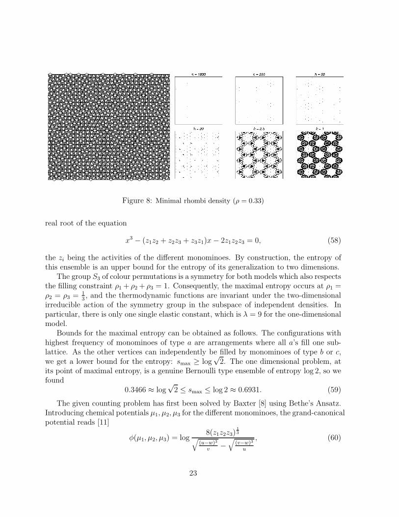
Figure 8: Minimal rhombi density (ρ = 0.33)

real root of the equation

x3 − (z1z2 + z2z3 + z3z1)x − 2z1z2z3 = 0, (58)

the zi being the activities of the different monominoes. By construction, the entropy ofthis ensemble is an upper bound for the entropy of its generalization to two dimensions.

The group S3 of colour permutations is a symmetry for both models which also respectsthe filling constraint ρ1 + ρ2 + ρ3 = 1. Consequently, the maximal entropy occurs at ρ1 =ρ2 = ρ3 = 1

3, and the thermodynamic functions are invariant under the two-dimensional

irreducible action of the symmetry group in the subspace of independent densities. Inparticular, there is only one single elastic constant, which is λ = 9 for the one-dimensionalmodel.

Bounds for the maximal entropy can be obtained as follows. The configurations withhighest frequency of monominoes of type a are arrangements where all a’s fill one sub-lattice. As the other vertices can independently be filled by monominoes of type b or c,we get a lower bound for the entropy: smax ≥ log

√2. The one dimensional problem, at

its point of maximal entropy, is a genuine Bernoulli type ensemble of entropy log 2, so wefound

0.3466 ≈ log√

2 ≤ smax ≤ log 2 ≈ 0.6931. (59)

The given counting problem has first been solved by Baxter [8] using Bethe’s Ansatz.Introducing chemical potentials µ1, µ2, µ3 for the different monominoes, the grand-canonicalpotential reads [11]

φ(µ1, µ2, µ3) = log8(z1z2z3)

1

3

√

(u−w)3

v−√

(v−w)3

u

, (60)

23

Figure 9: The entropy maximum (ρ = 0.50)

where u, v, w are the positive real solutions of

x(3B − x)2 = 4, u > v ≥ w, (61)

where B is given by

B =z1z2 + z2z3 + z1z3

3(z1z2z3)1

3

. (62)

It has to be stressed again that this solution was obtained by making use of periodicboundary conditions. The result agrees, on the other hand, with the corresponding freelimit, as can be shown [56] by generalizing an argument of G. Kuperberg [42].

The value at the maximum entropy is

smax =3

2log

4

3≈ 0.4315, (63)

which was already obtained before as the residual entropy of square ice [45].It is instructive to analyse the entropy function along a line of reflection symmetry,

see figure 12. Note that the entropy at its maximum is flat, indicating a vanishingsecond derivative, hence a phase transition at s = smax. The phase transition is of fluid-solid type: below the phase transition, monominoes arrange on the lattice homogeneously,whereas above the phase transition one sublattice is preferred in occupation [52]. Thephase transition causes a square-root singularity in the covariance matrix [8].

In fact, explicit expressions for the entropy can be given in the two phases [56]. Itturns out that both functions are analytic on the whole interval 0 ≤ ρ < 1

2and intersect

smoothly at ρ1 = 13. They can therefore be polynomially approximated at the entropy

maximum. The absolute values of the coefficients coincide up to fourth order; with

24

Figure 10: Below the phase transition (ρ = 0.77)

r = ρ − 13, we find

s(r) =3

2log

4

3− 1

3!

92

2|r|3 − 1

4!

93

2r4 + O(r5). (64)

We conclude that the square lattice three-colouring model violates the second randomtiling hypothesis! This means that the usual reasoning about elastic theory [30] is notapplicable here.

It would be interesting to compare this result with an expansion of the entropy interms of variables taken from the height representation of this model [16].

6.4 Hard hexagons – a monomino tiling with unexpected entropy

Our last example belongs to a tiling class with two kinds of monominoes which we callparticles and holes together with nearest neighbour exclusion for the particles. Its one-dimensional version has already been discussed above. The two-dimensional generaliza-tions to the square lattice and to the hexagonal lattice correspond to the ensembles ofhard squares [10, 21] and hard hexagons [9, 11]. Both models show a kind of fluid-solidphase transition: the low density phase is homogeneous, each sublattice has the sameparticle density, whereas at high density one sublattice is preferred in occupation. Thereis no obvious symmetry in these models, and therefore no preferred point in the phasespace where the entropy maximum should be located.

It is interesting to mention that the three-colouring model discussed above was in-terpreted as an ‘approximating’ hard squares model, with two types of holes [8, 52]. Asthe hard squares model itself has escaped exact solution so far, we concentrate on thehard hexagon model in the following. The solution of this model was given by Baxter

25

Figure 11: Above the phase transition (ρ = 0.90)

[9, 11]. This result is again obtained from periodic boundary conditions. It is easy to see,however, that it coincides with the result for the corresponding free boundary conditions,as each free rectangular patch can be transformed into a periodic one by adding a row ofholes.

A phase transition occurs at ρc = 1τ√

5≈ 0.2764 (the maximal density being normalized

to 13) with a critical exponent α = 1

3in the covariance matrix. The entropy is a concave

function with a quadratic maximum

smax ≈ 0.333243 at ρ ≈ 0.162433. (65)

Note that the maximum occurs nearly at the point where the hexagons occupy half of thelattice area. The small deviation of the entropy from 1

3lead to an incorrect prediction 10

in 1978. The elastic constant turns out to be λ ≈ 24.0807.Joyce [36] used the theory of modular functions to write the particle activity z as an

algebraic function of the mean density ρ. Applying Joyce’s results, one can in fact findclosed expressions for smax, ρ and λ. As these are quite complicated, we omit them here[56].

7 Concluding remarks

We have shown, both conceptually and by a number of examples, that the densities of tilesin random tiling ensembles provide natural parameters to investigate the phase diagramof such models. This is then independent of the existence of a height representation, butfully consistent with it if it happens to exist.

10 For a short history of the model, see chapter 14.1 of Baxter’s book [11].

26

0 0.1 0.2 0.3 0.4 0.5

ρ1

0

0.1

0.2

0.3

0.4

0.5

0.6

s

Figure 12: Entropy of the three-colouring model along a line of reflection symmetry (ρ2 = ρ3) as

a function of ρ1 (heavy curve). The dotted curve represents the system with exclusion restricted

to one dimension.

Whereas the re-interpretation of exactly solvable models directly leads to a number ofrandom tilings with analytic expressions for the entropy function, it is much more difficultto extract information about diffraction properties via Fourier transforms because this alsorequires the knowledge of the autocorrelation. For simple models such as the domino tilingand the rhombus tiling, it is possible [3] to compute the diffraction Bragg part explicitlyand also the behaviour of the diffuse background in the thermodynamic limit.

The next step in the analysis of random tilings is certainly the application of the con-cept developed so far to quasicrystalline random tilings. Although there are recent exactresults on rectangle-triangle tilings [22, 37], the interpretation of some of the results, forexample the shape of the entropy curve in the solvable regime, is subject to controversialdiscussion. It may turn out that the framework of statistical mechanics proposed heregains additional insight into the phase space of the tilings.

Acknowledgements

It is our pleasure to thank Paul Pearce for several useful hints and some help with thebody of known results and Elliott Lieb for a number of clarifying discussions. We thankChris Henley for numerous valuable comments on the manuscript. Financial support fromthe German Science Foundation (DFG) is gratefully acknowledged.

27

Appendix: Height representation of the rhombus tiling

Here, we briefly describe the connection between our description of the rhombus tiling tothe description by Henley [29, 30]. In particular, we show the connection between theelastic constants defined by both approaches.

As was first pointed out in [14], each configuration of the rhombus tiling can beobtained by projecting a roof-type surface in the cubic lattice to the diagonal hyperplane.In this way, the rhombus tiling possesses a natural height representation. As the averageslope of this surface determines the average densities of the different tiles and vice versa,we can parametrize the ensemble alternatively by some slope variables.

Let us describe this more formally. Our vector space is R3 with the standard scalarproduct < ·, · >. The diagonal hyperplane in R3 can be described by its normal vectore⊥ = 1√

3(1, 1, 1)t. We call the space spanned by e⊥ perp(endicular) space V ⊥ and the

complementary hyperplane physical space V ‖. Let us denote the projections of vectorsx ∈ R3 to these subspaces by x⊥ resp. x‖. The perp strain tensor E is a linear map

E : V ‖ → V ⊥. (66)

E defines a hyperplane in R3. By definition, E ≡ 0 corresponds to V ‖. We define matrixelements E1, E2 of E:

E1e⊥1 = Ee

‖1, E2e

⊥2 = Ee

‖2. (67)

A normal vector to this hyperplane is given by (1 − E1, 1 − E2, 1 + E1 + E2)t.

We can easily relate the average slope of a surface parametrized by E = (E1, E2) tothe mean densities of the projected tiles:

ρ1 =1

3(1 − E1), ρ2 =

1

3(1 − E2). (68)

The quadratic form (47) can (with r = ρ − 13) be rewritten in the form

s2(E, E) = −1

2· 2√

3· π

9· (E2

1 + E1E2 + E22). (69)

This is the expression given by Henley [29, 30] up to a constant of 2√3

which arises fromdifferent normalizations of unit vectors in physical and perp space in his setup.

References

[1] M. Abramowitz and I. Stegun, Handbook of mathematical functions, Dover publica-tions, New York (1972).

[2] M. Baake, V. Elser and U. Grimm, On the entropy of square-free words, Mathl. Com-put. Modelling 26 (1997) 13-26.

28

[3] M. Baake and M. Hoffe, Comments on the diffraction of random tilings (in prepara-tion).

[4] M. Baake, J. Hermisson, M. Hoffe and C. Richard, Random tilings and dimer models,Proc. Int. Conf. Quasicrystals 6 (Tokyo), ed S. Takeuchi and T. Fujiwara, WorldScientific, Singapore (1998) p. 128-131.

[5] M. Baake and M. Schlottmann, Geometric aspects of tilings and equivalence concepts,Proc. Int. Conf. Quasicrystals 5 (Avignon), editors C.Janot and R. Mosseri, WorldScientific, Singapore (1995) p. 15-21.

[6] R. Balian, From microphysics to macrophysics, vol. 1, Springer, Berlin (1991).

[7] H. Bauer, Wahrscheinlichkeitstheorie, de Gruyter, Berlin (1991).

[8] R.J. Baxter, Three-colourings of the square lattice: a hard squares model,J. Math. Phys. 11 (1970) 3116-3124.

[9] R.J. Baxter, Hard hexagons: exact solution, J. Phys. A 13 (1980) L61-L70.

[10] R.J. Baxter, I. G. Enting and S. K. Tsang, Hard-square lattice gas, J. Stat. Phys. 22

(1980) 465-489.

[11] R.J. Baxter, Exactly Solved Models in Statistical Mechanics, Academic Press, London(1982).

[12] S.I. Ben-Abraham, Defective vertex configurations in quasicrystalline structures,Int. Journ. Mod. Phys. B7 (1993) 1415-1425.

[13] S. M. Bhattacharjee, Crossover in an exactly solvable dimer model of domain wallswith dislocations, Phys. Rev. Lett. 53 (1984) 1161-1163.

[14] H.W.J. Blote and H.J. Hilhorst, Roughening transitions and the zero-temperaturetriangular Ising antiferromagnet J. Phys. A15 (1982) L631-L637.

[15] M. de Boissieu, P. Stephens, M. Boudard, C. Janot, D.L. Chapman and M. Au-dier, Evidence for random disorder in the perfect icosahedral phase of AlPdMn,Proc. Int. Conf. Aper. Cryst. (1994), World Scientific, Singapore, p. 535-540.

[16] J. K. Burton and C. L. Henley Simulations of a constrained antiferromagnetic Pottsmodel J. Phys. A 30 (1997) 8385-8413.

[17] G. Coddens, Models for assisted phason hopping and phason elasticity in icosahedralquasicrystals, Int. Journ. Mod. Phys. B 11 (1997) 1679-1716.

29

[18] V. Elser, Comments on “Quasicrystals: a new class of ordered structures”,Phys. Rev. Lett. 54 (1985) 1730-1730,Indexing problems in quasicrystals diffraction, Phys. Rev. B32 (1985) 4892-4898.

[19] V. Elser, Solution of the dimer problem on a hexagonal lattice with boundary,J. Phys. A 17 (1984) 1509-1513.

[20] C. Fan and F.Y. Wu, General model of phase transitions, Phys. Rev. B2 (1970)723-733.

[21] D.S. Gaunt and M.E. Fisher, Hard-sphere lattice gases. I. Plane-square lattice gas,J. Chem. Phys. 43 (1965) 2840-2489.

[22] L. de Gier and B. Nienhuis, Exact solution of an octagonal tiling model,Phys. Rev. Lett. 76 (1996) 2918-2921,

J. de Gier and B. Nienhuis, The exact solution of an octagonal rectangle-trianglerandom tiling, J. Stat. Phys. 87 (1997) 415-437,

J. de Gier and B. Nienhuis, Bethe Ansatz solution of a decagonal rectangle trianglerandom tiling, J. Phys. A 31 (1998) 2141-2154.

[23] S.W. Golomb, Polyominoes: puzzles, patterns, problems, and packings, 2nd. edition,Princeton University Press, Princeton, New Jersey (1994).

[24] D. Grensing and G. Grensing, Boundary effects in the dimer problem on a non-Bravais lattice, J. Math. Phys. 24 (1983) 620-630,

D. Grensing, I. Carlsen and H.Chr. Zapp, Some exact results for the dimer problemon plane lattices with non-standard boundaries, Phil. Mag. A 41 (1980) 777-781.

[25] B. Grunbaum and G. C. Shephard, Tilings and patterns, W. H. Freeman and Com-pany, New York (1987).

[26] P. Guyot, P. Kramer and M. de Boissieu, Quasicrystals, Rep. Prog. Phys. 54 (1991)1373-1425.

[27] M. Hamermesh, Group theory and its application to physical problems, Dover publi-cations, New York (1962).

[28] O.J. Heilmann and E.H. Lieb, Monomers and dimers, Phys. Rev. Lett. 24 (1970)1412-1414,

O.J. Heilmann and E.H. Lieb, Theory of monomer-dimer systems,Comm. Math. Phys. 25 (1972) 190-232.

30

[29] C.L. Henley, Random tilings with quasicrystal order: transfer-matrix approach,J. Phys. A 21 (1988) 1649-1677.

[30] C.L. Henley, Random Tiling Models, in Quasicrystals: The State of the Art (1991),ed. D.P. DiVincenzo and P. Steinhardt, 429-524.

[31] M. Hoffe, Zufallsparkettierungen und Dimermodelle, Diplomarbeit, UniversitatTubingen (1997).

[32] C. Janot, Quasicrystals – a primer, 2nd. ed., Clarendon Press, Oxford (1994).

[33] D. Joseph and V. Elser, A model of quasicrystal growth, Phys. Rev. Lett. 79 (1997)1066-1069.

[34] D. Joseph and M. Baake, Boundary conditions, entropy and the signature of randomtilings, J. Phys. A 29 (1996) 6709-6716.

[35] D. Joseph, S. Ritsch and C. Beeli, Distinguishing quasiperiodic from random orderin high-resolution TEM images, Phys. Rev. B 55 (1997) 8175-8183.

[36] G.S. Joyce, On the hard-hexagon model and the theory of modular functions,Phil. Trans. R. Soc. Lond. A 325 (1988) 643-702.

[37] P.A. Kalugin, The square-triangle random tiling model in the thermodynamic limit,J. Phys. A 27 (1994) 3599-3614,

P.A. Kalugin, Low-lying excitations in the square-triangle random tiling model,J. Phys. A 30 (1997) 7077-7087.

[38] P.W. Kasteleyn, The statistics of dimers on a lattice, Physica 27 (1961) 1209-1225.

[39] P.W. Kasteleyn, Dimer statistics and phase transitions, J. Math. Phys. 4 (1963)287-293.

[40] R. Kenyon, Local statistics of lattice dimers, Ann. Inst. H. Poincare, Probabilites, 33

(1997) 591-618.

[41] I. Keppler [J. Kepler] Harmonice Mundi, Lincii (1619).

[42] G. Kuperberg, private communication.

[43] J.C. Lagarias and D.S. Romano, A polyomino tiling problem of Thurston and itsconfigurational entropy, J. Comb. Theory A 63 (1993) 338-358.

[44] W. Li, H. Park and M. Widom, Phase diagram of a random tiling quasicrystal,J. Stat. Phys. 66 (1992) 1-69.

31

[45] E.H. Lieb, Residual entropy of square ice, Phys. Rev. 162 (1967) 162-172.

[46] E.H. Lieb and F.Y. Wu, Two-dimensional ferroelectric models, in Phase Transitionsand Critical Phenomena, Vol. 1, (ed. C.Domb and J.L.Lebowitz), Academic Press,London (1972), p.331-490.

[47] T.C. Lubensky, in Aperiodic Crystals I: Introduction to quasicrystals, ed. M. V. Jaric,Academic Press (1988).

[48] J.F. Nagle, Dimer Models on Anisotropic Lattices, in Phase Transitions and Criti-cal Phenomena, Vol. 13, (ed. C.Domb and J.L.Lebowitz), Academic Press, London(1989), p.236-297.

[49] H.-U. Nissen and C. Beeli, Electron microscopy of quasicrystals and the validity ofthe tiling approach, Int. J. Mod. Phys. B7 (1993) 1387-1413.

[50] G. van Ophuysen, M. Weber and L. Danzer, Strictly local growth of Penrose patterns,J. Phys. A 28 (1995) 281-290.

[51] R.K. Pathria, Statistical mechanics, Pergamon press, Oxford (1977).

[52] P. A. Pearce and K. A. Seaton, Exact solution of cyclic solid–on–solid lattice models,Ann. Phys. 193 (1989) 326-366.

[53] K. Petersen, Ergodic theory, Cambridge University Press, Cambridge (1983).

[54] J. Propp, Boundary-dependent local behaviour for 2-D dimer models,Int. J. Mod. Phys. B 11 (1997) 183-187.

[55] D. Ruelle, Statistical Mechanics: Rigorous results, W.A. Benjamin, London (1969).

[56] C. Richard, Entropie in periodischen und nichtperiodischen Festkorpern, Dissertation,Universitat Tubingen, in preparation.

[57] C.J. Thompson, Mathematical Statistical Mechanics, Princeton University Press,Princeton, New Jersey (1972).

[58] F.Y. Wu, Remarks on the modified Potassium Dihydrogen Phosphate Model of aFerroelectric, Phys. Rev. 168 (1968) 539-543.

[59] F.Y. Wu, Eight-vertex model on the honeycomb lattice, J. Math. Phys. 15 (1974)678-681.

32