J Heuristics (2006) 12: 347–373

DOI 10.1007/s10732-006-6550-4

On global warming: Flow-based soft global constraints

Willem-Jan van Hoeve · Gilles Pesant ·Louis-Martin Rousseau

C© Springer Science + Business Media, LLC 2006

Abstract In case a CSP is over-constrained, it is natural to allow some constraints, called softconstraints, to be violated. We propose a generic method to soften global constraints that can

be represented by a flow in a graph. Such constraints are softened by adding violation arcs to

the graph and then computing a minimum-weight flow in the extended graph to measure the

violation. We present efficient propagation algorithms, based on different violation measures,

achieving domain consistency for the alldifferent constraint, the global cardinality constraint,

the regular constraint and the same constraint.

Keywords Soft constraints . Global constraints . Network flows

1. Introduction

Many real-life problems are over-constrained. In personnel rostering problems for example,

people often have conflicting preferences. To such problems there does not exist a feasible

solution that respects all preferences. However, we still want to find some solution, preferably

one that keeps conflicts to a minimum. In the case of the personnel rostering example, we

may want to construct a roster in which the number of respected preferences is spread equally

among the employees.

∗This work was for a large part carried out while the author was at the Centrum voor Wiskunde enInformatica, Amsterdam, The Netherlands

W.-J. van HoeveCornell University, Department of Computer Science, 4130 Upson Hall, Ithaca, NY 14853, USAe-mail: vanhoeve@cs.cornell.edu

G. Pesant (�) . L.-M. Rousseau

Ecole Polytechnique de Montreal, Montreal, CanadaCentre for Research on Transportation (CRT), Universite de Montreal, C.P. 6128, succ. Centre-ville,Montreal, H3C 3J7, Canadae-mail: {pesant,louism}@crt.umontreal.ca

Springer

348 J Heuristics (2006) 12: 347–373

In constraint programming, we seek an (optimal) feasible solution to a given problem.

Hence, we cannot apply constraint programming directly to over-constrained problems be-

cause it finds no solution. As a remedy several methods have been proposed. Most of these

methods introduce so-called soft constraints that are allowed to be violated. Constraints that

are not allowed to be violated are called hard constraints. Most methods then try to find a so-

lution that minimizes the number of violated constraints, or some other measure of constraint

violation.

Global constraints are often key elements in successfully modeling and solving real-

life applications with constraint programming. For many soft global constraints, however, no

efficient propagation algorithm was available, up to very recently. In this paper we distinguish

two main objectives with respect to soft global constraints: useful violation measures and

efficient propagation algorithms.

In many cases we can represent a solution to a global constraint as a property in some graph

representation of the constraint. For example, a solution to the alldifferent constraint

corresponds to a matching in a particular graph; see (Regin, 1994). There exists a large class

of such global constraints, see for example (Beldiceanu, 2000) for a collection. In this paper,

we focus on global constraints for which a solution can be represented by a flow in a graph.

Our method adds violation arcs to the graph representation of a global constraint. To these

arcs we assign a cost, corresponding to some violation measure of the constraint. Each tuple

in the constraint has an associated cost of violation. If the tuple satisfies the constraint, the

corresponding flow does not use any violation arc, and the cost is 0. If the tuple does not

satisfy the constraint, the corresponding flow must use violation arcs, whose costs sum up to

the violation cost of this tuple.

This approach allows us to define and implement useful violation measures for soft global

constraints. Moreover, we present an efficient generic propagation algorithm for soft global

constraints, making use of flow theory. We apply our method to several global constraints

that are well-known to the constraint programming community: the alldifferent, the

gcc, the regular, and the same constraints, which will be recalled in turn. To each of

these global constraints we apply several violation measures, some of which are new.

This paper is organized as follows. In Section 2 we give an overview of related literature.

Section 3 provides some background on constraint programming and flow theory. Then our

method to soften global constraints is presented in Section 4. We first discuss the general

concepts of constraint softening and violation measures. Then we describe the addition

of violation arcs to the graph representation and present the generic domain consistency

propagation algorithm. The next four sections apply our method to the four global constraints

mentioned above. For each constraint we present new or existing violation measures and

the corresponding graph representations. We also analyze the corresponding propagation

algorithms to achieve domain consistency. Finally, in Section 9 a conclusion is given.

2. Related literature

The best-known framework to handle soft constraints is the Partial-CSP framework (Freuder

and Wallace, 1992). This framework includes the Max-CSP framework that tries to maximize

the number of satisfied constraints. Since in this framework all constraints are either violated

or satisfied, the objective is equivalent to minimizing the number of violated constraints.

It has been extended to the Weighted-CSP framework in Larrosa, (2002) and (Larrosa and

Schiex, 2003), associating a degree of violation (not just a boolean value) to each constraint

and minimizing the sum of all weighted violations. The Possibilistic-CSP framework in

Springer

J Heuristics (2006) 12: 347–373 349

(Schiex, 1992) associates a preference to each constraint (a real value between 0 and 1)

representing its importance. The objective of the framework is the hierarchical satisfaction

of the most important constraints, i.e. the minimization of the highest preference level for a

violated constraint. The Fuzzy-CSP framework in Dubois et al. (1993), (Fargier et al., 1993),

and (Ruttkay, 1994) is somewhat similar to the Possibilistic-CSP but here a preference is

associated to each tuple of each constraint. A preference value of 0 means the constraint

is highly violated and 1 stands for satisfaction. The objective is the maximization of the

smallest preference value induced by a variable assignment. The last two frameworks are

different from the previous ones since the aggregation operator is a min/max function instead

of addition. With valued-CSPs (Schiex et al., 1995) and semi-rings (Bistarelli et al., 1997) it

is possible to encode Max-CSP, weighted CSPs, Fuzzy CSPs, and Possibilistic CSPs.

Another approach to model and solve over-constrained problems was proposed in Regin

et al. (2000) and refined in Beldiceanu and Petit (2004). The idea is to identify with each soft

constraint S a “cost” variable z, and replace the constraint S by the disjunction

(S ∧ (z = 0)) ∨ (S ∧ (z > 0))

where S is a constraint of the type z = μ(S) for some violation measure μ(S) depending on

S. The newly defined problem is not over-constrained anymore. If we ask to minimize the

(weighted) sum of violation costs, we can solve the problem with a traditional constraint pro-

gramming solver. A similar approach, specifically designed for over-constrained scheduling

problems, was introduced by (Baptiste et al., 1998).

This approach also allows us to design specialized filtering algorithms for soft global

constraints. Namely, if we treat the soft constraints as “optimization constraints” (see for

example (Focacci et al., 2002), (Regin, 2002), (Sellmann, 2003)), we can apply cost-based

propagation algorithms. Constraint propagation algorithms for soft constraints based on this

method were given in Petit et al. (2001) and (van Hoeve, 2004). We follow the same method

in this paper. Note that in this way we don’t need to introduce new theory as we interpret

certain optimization constraints as being soft constraints.

3. Background

3.1. Constraint programming

We first introduce basic constraint programming concepts. For more information on constraint

programming we refer to (Apt, 2003) and (Dechter, 2003).

Let x be a variable. The domain of x is a set of values that can be assigned to x . In this

paper we only consider variables with finite domains.

Let X = x1, x2, . . . , xk be a sequence of variables with respective domains

D1, D2, . . . , Dk . We denote DX = ⋃1≤i≤n Di . A constraint C on X is defined as a subset of

the Cartesian product of the domains of the variables in X , i.e. C ⊆ D1 × D2 × · · · × Dk .

A tuple (d1, . . . , dk) ∈ C is called a solution to C . We also say that the tuple satisfies C . A

value d ∈ Di for some i = 1, . . . , k is inconsistent with respect to C if it does not belong

to a tuple of C , otherwise it is consistent. C is inconsistent if it does not contain a solution.

Otherwise, C is called consistent. A constraint is called a binary constraint if it is defined on

two variables. If it is defined on more than two variables, we call C a global constraint.

Springer

350 J Heuristics (2006) 12: 347–373

Sometimes a constraint C is defined on variables X together with a certain set of parameters

p, for example a set of cost values. In such cases, we denote the constraint as C(X, p) for

syntactical convenience.

A constraint satisfaction problem, or a CSP, is defined by a finite sequence of variables

X = x1, x2, . . . , xn with respective domains D = D1, D2, . . . , Dn , together with a finite set

of constraints C, each on a subsequence of X . This is written as P = (X ,D, C). The goal

is to find an assignment xi = di with di ∈ Di for i = 1, . . . , n, such that all constraints are

satisfied. This assignment is called a solution to the CSP. A constraint optimization problemproblem is a CSP together with an objective function on X that has to be optimized.

The solution process of constraint programming interleaves constraint propagation, or

propagation in short, and search. The search process essentially consists of enumerating

all possible variable-value combinations, until we find a solution or prove that none exists.

We say that this process constructs a search tree. To reduce the exponential number of

combinations, constraint propagation is applied to each node of the search tree: Given the

current domains and a constraint C , remove domain values that do not belong to a solution

to C . This is repeated for all constraints until no more domain value can be removed.

In order to be effective, constraint propagation algorithms should be efficient, because

they are applied many times during the solution process. Further, they should remove as

many inconsistent values as possible. If a constraint propagation algorithm for a constraint

C removes all inconsistent values from the domains with respect to C , we say that it makes

C domain consistent. More formally:

Definition 1 (Domain consistency, (Mohr and Masini, 1988)). A constraint C on the vari-

ables x1, . . . , xk with respective domains D1, . . . , Dk is called domain consistent if for each

variable xi and each value di ∈ Di (i = 1, . . . , k), there exist a value d j ∈ D j for all j = isuch that (d1, . . . , dk) ∈ C .

In the literature, domain consistency is also referred to as hyper-arc consistency or

generalized-arc consistency.

In this paper our goal is to find efficient propagation algorithms for soft global constraints

with useful violation measures, that achieve domain consistency.

3.2. Flow theory

We present some concepts of flow theory that are necessary to understand this paper. For more

information on flow theory we refer to (Ahuja et al., 1993) and ((Schrijver, 2003) Chapters

6–15).

Let G = (V, A) be a directed graph, or digraph, with vertex set V and arc set A. We

denote m = |A|. Let s, t ∈ V . A function f : A → R is called a flow from s to t , or an s − tflow, if (i) f (a) ≥ 0 for each a ∈ A, and (i i) f (δout(v)) = f (δin(v)) for each v ∈ V \ {s, t},where δin(v) and δout(v) denote the multiset of arcs entering and leaving v, respectively. Here

f (S) = ∑a∈S f (a) for all S ⊆ A. Property (i i) ensures flow conservation, i.e. for a vertex

v = s, t , the amount of flow entering v is equal to the amount of flow leaving v. The value of

an s − t flow f is defined as value ( f ) = f (δout(s)) − f (δin(s)). In other words, the value of

a flow is the net amount of flow leaving s. This is equal to the net amount of flow entering t .

Springer

J Heuristics (2006) 12: 347–373 351

Let d : A → R+ and c : A → R+ be a “demand” function and a “capacity” function,

respectively1. We say that a flow f is feasible if d(a) ≤ f (a) ≤ c(a) for each a ∈ A. Let

w : A → R be a “weight” function. We often also refer to such function as a “cost” function.

For a directed path P in G we define w(P) = ∑a∈P w(a). Similarly for a directed circuit. The

weight of any function f : A → R is defined as weight ( f ) = ∑a∈A w(a) f (a). A feasible

flow is called a minimum-weight flow if it has minimum weight among all feasible flows

with the same value. Given a graph G = (V, A) with s, t ∈ V and a number φ ∈ R+, the

minimum-weight flow problem is: find a minimum-weight s − t flow with value φ.

A feasible s − t flow in G with value φ and minimum weight can be found using the

successive shortest path algorithm ((Schrijver, 2003), p. 175, 176). It can be proved that for

integer demand and capacity functions it finds an integer s − t flow with minimum weight.

The time complexity of the algorithm is O(φ · SP), where SP is the time to compute a

shortest directed path in G. Although faster algorithms exist for general minimum-weight

flow problems, this algorithm suffices when applied to our problems. This is because in our

case the value of any flow is bounded above by the number of variables in the constraint.

Given a minimum-weight s − t flow, we want to compute the additional weight when an

unused arc is forced to be used. In order to do so we need the following notation. Let f be an

s − t flow in G. The residual graph of f (with respect to d and c) is defined as G f = (V, A f )

where A f = {a | a ∈ A, f (a) < c(a)} ∪ {a−1 | a ∈ A, f (a) > d(a)}. Here a−1 = (v, u) if

a = (u, v). We extend w to A−1 = {a−1 | a ∈ A} by defining w(a−1) = −w(a) for each

a ∈ A. Any directed circuit C in G f gives an undirected circuit in G = (V, A). We define

χC ∈ RA by

χC (a) =⎧⎨⎩

1 if C traverses a,

−1 if C traverses a−1,

0 if C traverses neither a nor a−1,

for a ∈ A. We have the following result.

Theorem 1. Let f be a minimum-weight s − t flow of value φ in G = (V, A) with f (a) = 0

for some a ∈ A. Let C be a directed circuit in G f with a ∈ C, minimizing w(C). Thenf ′ = f + εχC , where ε is subject to d ≤ f + εχC ≤ c, has minimum weight among alls − t flows g in G with value(g) = φ and g(a) = ε. If C does not exist, f ′ does not exist.Otherwise, weight( f ′) = weight( f ) + ε · w(C).

The proof of Theorem 1 relies on the fact that for a minimum-weight flow f in G, the residual

graph G f does not contain directed circuits with negative weight; see also ((Ahuja et al.,

1993), p. 337–339).

Finally a digraph G = (V, E) is strongly connected if for any two vertices u, v ∈ V there

is a directed path from u to v. A maximally strongly connected non-empty subgraph of a

digraph G is called a strongly connected component of G.

1 Here R+ denotes {x ∈ R | x ≥ 0}. Similarly for Q+.

Springer

352 J Heuristics (2006) 12: 347–373

4. Outline of method

In this section we first define how we soften global constraints, and define some general

violation measures. Then we present a generic constraint propagation algorithm for a class

of soft global constraints: those that can be represented by a flow in a graph.

4.1. Constraint softening and violation measures

As stated before, the idea of the scheme in Regin et al. (2000) is as follows. To each soft

constraint are associated a violation measure and a cost variable that measures this violation.

Then the CSP (or COP) is transformed into a COP where all constraints are hard, and the

(weighted) sum of cost variables is minimized.

Let X = x1, . . . , xn be variables with respective finite domains D1, . . . , Dn .

Definition 2 (Violation measure). A violation measure of a constraint C(x1, . . . , xn) is a

function μ : D1 × · · · × Dn → Q+ defined over the possible tuples of C with the property

that μ(d1, . . . , dn) = 0 if and only if (d1, . . . , dn) ∈ C .

Definition 3 (Constraint softening). Let z be a variable with finite domain Dz and

C(x1, . . . , xn) a constraint with a violation measure μ. Then

soft C(x1, . . . , xn, z, μ) ={(d1, . . . , dn, d) | di ∈ Di , d ∈ Dz, μ(d1, . . . , dn) ≤ d}

is the soft version of C with respect to μ.

Thus z is a “cost” variable that represents the measure of violation of C — max Dz and

min Dz respectively represent the maximum and minimum value of violation that is allowed,

given the current state of the solution process.2 It should be noted that z does not equal the

measure of violation, because we only consider its bounds. The reason for this is that the

current definition allows us to establish domain consistency on soft constraints efficiently. If

we would define μ(d1, . . . , dn) = d instead, it would make that task NP-complete.

There may be several natural ways to evaluate the degree to which a global constraint is

violated and these are usually not equivalent. Two general measures are the variable-basedviolation measure and the decomposition-based violation measure.

Definition 4 (Variable-based violation measure, (Petit et al., 2001)). Let C be a constraint

on the variables x1, . . . , xn and let d1, . . . , dn be an instantiation of variables such that

di ∈ Di for i = 1, . . . , n. The variable-based violation measure μvar of C is the minimum

number of variables that need to change their value in order to satisfy C .

For the decomposition-based violation measure we make use of the binary decomposition

of a constraint.

Definition 5 (Binary decomposition, (Dechter, 1990)). Let C be a constraint on the vari-

ables x1, . . . , xn . A binary decomposition of C is a minimal set of binary constraints

2 We assume that cost variable z is being minimized.

Springer

J Heuristics (2006) 12: 347–373 353

Cdec = {C1, . . . , Ck} (for integer k > 0) on the variables x1, . . . , xn such that the solution

set of C equals the solution set of⋂k

i=1 Ci .

Note that we can extend the definition of binary decomposition by defining the constraints

in Cdec on arbitrary variables, such that the solution set of∧k

i=1 Ci is mapped to the solution

set of C and vice versa, as proposed in Rossi et al. (1990). In this paper this extension is not

necessary, however.

Definition 6 (Decomposition-based violation measure, (Petit et al., 2001)). Let C be a con-

straint on the variables x1, . . . , xn for which a binary decomposition Cdec exists and

let d1, . . . , dn be an instantiation of variables such that di ∈ Di for i = 1, . . . , n. The

decomposition-based violation measure μdec of C is the number of violated constraints

in Cdec.

In Petit et al. (2001), the decomposition-based violation measure is referred to as primalgraph based violation cost.

Alternative measures exist for specific constraints. For the soft gcc and the soft

regular constraint, we introduce new violation measures that are likely to be more ef-

fective in practical applications.

After we have assigned a violation measure to each soft constraint, we can recast our

problem. Consider a CSP (or COP) of the form P = (X, D, Chard ∪ Csoft), where Chard and

Csoft denote the set of hard and soft constraints of P , respectively. We soften each constraint

Ci ∈ Csoft using the violation measure it has been assigned and a cost variable zi with domain

Dzi (i = 1, . . . , |Csoft|) that represents this measure. Then we transform P into the COP

P = (X , D, C) where X = X ∪ {z1, . . . , z|Csoft|}, D contains their corresponding domains,

and C contains Chard and the soft version of each constraint in Csoft.

4.2. Propagation of soft constraints

We assume from now on that constraint C(x1, . . . , xn) can be represented by a directed graph

G = (V, A) with capacity function c : A → N that has the following properties:

– a pair (xi , d) is represented by at least one arc a ∈ A for i = 1, . . . , n and all d ∈ Di , and

c(a) = 1,

– a tuple (d1, . . . , dn) ∈ C is represented by a feasible flow f of value φ ∈ R+ in G such

that f (a) = 1 for an arc a representing the pair (xi , di ) for i = 1, . . . , n, and f (a) = 0 for

all arcs a representing the pair (xi , d) with d = di for i = 1, . . . , n.

In case the constraint C is violated, it is impossible to find a flow with the above mentioned

properties in the corresponding digraph G. We propose to extend G with certain arcs, such

that it becomes possible to find a feasible flow corresponding to a solution. We call these arcs

violation arcs, and they are denoted by A. Violation arcs may appear anywhere in the graph.

The only restriction we impose on them is that after their addition, there exists a feasible flow

in G = (V, A ∪ A) that represents a solution to C .

There is no set recipe for the way violation arcs should be added, as their introduction

greatly varies from one constraint to another and even between violation measures of the

same constraint. The intuition is to consider all the properties imposed by a given graph and

decide which ones should be relaxed and which ones should still be enforced. Then, violation

arcs are added so that solutions exhibiting a relaxed property now constitute feasible flows.

Springer

354 J Heuristics (2006) 12: 347–373

The next step is to make a connection with the violation measures for a constraint. This is

done by applying a “cost” function w : A ∪ A → Q to G in the following way. For all arcs

a ∈ A we define w(a) = 0, while w(a) ≥ 0 for all arcs a ∈ A. Then each flow f in G has

an associated cost ∑a∈A∪ A

w(a) f (a) =∑a∈ A

w(a) f (a).

After the addition of violation arcs, a solution to C corresponds to a feasible flow in G with

an associated cost. If the flow does not use any violation arcs, this cost is 0. Otherwise, the

cost of the flow depends on the costs we impose on the violation arcs. Hence we can define

a violation measure as follows. For each solution to C we define its cost of violation as

the minimum-weight flow in G that represents this solution. Conversely, for many existing

violation measures it is possible to choose a particular set of violation arcs and associated

costs, such that a minimum-weight flow in G representing a solution is exactly the cost of

violation of that solution. In the following sections we provide several examples for different

constraints and different violation measures. We often denote the extended digraph G as Gμ

to indicate its dependence on some violation measure μ.

In other words, if C is represented by the digraph G = (V, A) and we can find violation

arcs A and a cost function w : A ∪ A → Q+ that represent violation measure μ, then the soft

version of C with respect to μ, i.e. soft C(x1, . . . , xn, z, μ), is represented by the digraph

Gμ = (V, A ∪ A) with cost function w. By construction, we have the following result:

Theorem 2. The constraint soft C(x1, . . . , xn, z, μ) is domain consistent if and only if

i) for all i ∈ {1, . . . , n} and all d ∈ Di there is an arc a ∈ A representing (xi , d) such thatthere exists a feasible flow f in Gμ representing a solution to soft C with f (a) = 1 andcost( f ) ≤ maxDz,ii) the minimum cost of all such flows f is not larger than min Dz.

Theorem 2 gives rise to the following propagation algorithm, presented as Algorithm 1.

For a sequence of variables X = x1, . . . , xn , and a constraint soft C(X, z, μ) the algorithm

first builds the digraph Gμ that represents the constraint. Then, for all variable-value pairs

(xi , d) we check whether the pair belongs to a solution, i.e. whether there exists a flow in Gμ

that represents a solution containing xi = d , with cost at most max Dz . If this is not the case,

we can remove d from Di . Finally, we update min Dz , if necessary.

Springer

J Heuristics (2006) 12: 347–373 355

The time complexity of this algorithm is O(nd K ) where d is the maximum domain size

and K is the time complexity to compute a flow in Gμ corresponding to a solution tosoft C .

However, we can improve the efficiency by applying Theorem 1.

The resulting, more efficient, algorithm is as follows. We first compute an initial minimum-

weight flow f in Gμ representing a solution. Then for all arcs a = (u, v) representing (xi , d)

with f (a) = 0, we compute a minimum-weight directed path P from v to u in the residual

graph (Gμ) f . Together with a, P forms a directed circuit. Provided that c(b) ≥ 1 for all

arcs b ∈ P , we reroute the flow over the circuit and obtain a flow f ′. Then cost( f ′) =cost( f ) + cost(P), because w(a) = 0 for all a ∈ A. If cost( f ′) > max Dz we remove d from

the domain of xi .

This reduces the time complexity of the algorithm to O(K + nd · SP) where SP denotes

the time complexity to compute a minimum-weight directed path in Gμ. It should be noted

that a similar algorithm was first applied in Regin (1999, 2002) to make the “cost-gcc”

domain consistent.

5. Soft alldifferent constraint

5.1. Definitions

Thealldifferent constraint on a sequence of variables specifies that all variables should

be pairwise different. To thealldifferent constraint we apply two measures of violation:

the variable-based violation measure μvar and the decomposition-based violation measure

μdec.

Let X = x1, . . . , xn be a sequence of variables with respective finite domains D1, . . . , Dn .

For alldifferent(x1, . . . , xn) we have

μvar(x1, . . . , xn) =∑

d∈DX

max (|{i | xi = d}| − 1, 0),

μdec(x1, . . . , xn) = ∣∣{(i, j) | xi = x j , for i < j}∣∣

Example 1. Consider the following over-constrained CSP:

x1 ∈ {a, b}, x2 ∈ {a, b}, x3 ∈ {a, b}, x4 ∈ {b, c},alldifferent(x1, x2, x3, x4).

We have μvar(b, b, b, b) = 3 and μdec(b, b, b, b) = 6. �

If we apply Definition 3 to the alldifferent constraint using the measures μvar

and μdec, we obtain soft alldifferent(x1, . . . , xn, z, μvar) and soft alldiffe-rent(x1, . . . , xn, z, μdec). Each of the violation measures μvar and μdec gives rise to a dif-

ferent domain consistency propagation algorithm. Before we present them, we introduce the

graph representation of the alldifferent constraint in terms of flows.

5.2. Graph representation

A solution to the alldifferent constraint corresponds to a flow in a particular graph:

Springer

356 J Heuristics (2006) 12: 347–373

x2

1x

x3

x4

ts

a

b

c

Fig. 1 Graph representation forthe alldifferent constraint.For all arcs the capacity is 1

Theorem 3. (Regin, 1994) A solution to alldifferent(x1, . . . , xn) corresponds to aninteger feasible s − t flow of value n in the digraph A = (V, A) with vertex set

V = X ∪ DX ∪ {s, t}and arc set A = As ∪ AX ∪ At ,

where

As = {(s, xi ) | i ∈ {1, . . . , n}},AX = {(xi , d) | d ∈ Di , i ∈ {1, . . . , n}},

At = {(d, t) | d ∈ DX },

with capacity function c(a) = 1 for all a ∈ A.

Proof: With an integer feasible s − t flow f of value n in A we associate the assignment

xi = d for all arcs a = (xi , d) ∈ AX with f (a) = 1. Because c(a) = 1 for all a ∈ As ∪ At ,

this is indeed a solution to the alldifferent constraint. As value( f ) = n, all variables

have been assigned a value. Similarly, each solution to the alldifferent gives rise to a

corresponding appropriate flow in A. �

Figure 1 gives the corresponding graph representation for the CSP of Example 1.

5.3. Variable-based violation measure

The results in this section are originally due to (Petit et al., 2001). We state their result in

terms of our method, by adding violation arcs to the graph representing the alldifferentconstraint.

To graph A of Theorem 3 we add the violation arcs At = {(d, t) | d ∈ DX }} (in fact, At

is a copy of At ), with capacity c(a) = ∣∣δin(d)∣∣ − 1 for all arcs a = (d, t) ∈ At . Further, we

apply a cost function w as described in Section 4.2, with a uniform cost of 1 for violation arcs.

Let the resulting digraph be denoted by Avar (see Figure 2 for an illustration on Example 1).

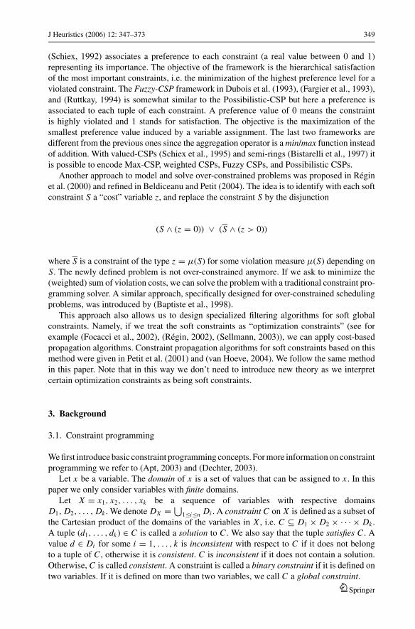
The intuition is to add violation arcs that capture the fact that more than one variable can

be assigned to the same value. For example, in Figure 2(b) four variables are assigned to

the same value b. To make this possible, there are three units of flow on the corresponding

violation arc, while one unit of flow can use the arc without violation cost. Indeed, we should

change the value of at least three variables in order to satisfy thealldifferent constraint.

Corollary 1. The constraint soft alldifferent(x1, . . . , xn, z, μvar) is domain consis-tent if and only if

Springer

J Heuristics (2006) 12: 347–373 357

3=3, =1w

c =2,=1

w

c =1,=0

w

x4

ts

a

b

c

x3

x2

1x

c=1,

=0w

c =1, =0w

(a)

x4

ts

a

b

c

x3

x2

1x

(b)

1

1

1

1

1

1

1

1

1

c

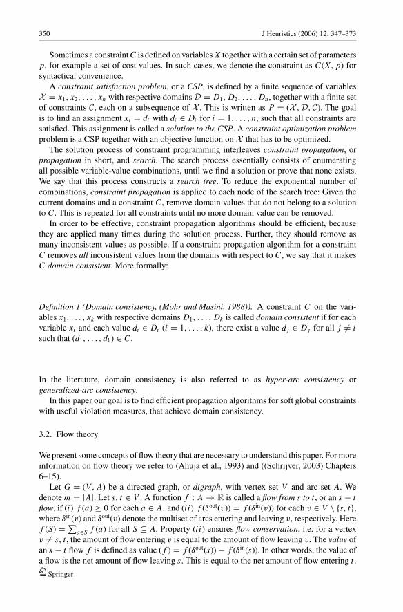
Fig. 2 (a) Graph representation for the variable-based soft alldifferent constraint. For all arcs thecapacity c = 1, unless specified otherwise. Dashed arcs indicate the inserted weighted arcs with weight w = 1.(b) Example: arcs and associated flows used in solution x1 = x2 = x3 = x4 = b of weight 3

i) for every arc a ∈ AX there exists an integer feasible s − t flow f of value n in Avar withf (a) = 1 and weight( f ) ≤ maxDz, and

ii) minDz ≥ weight( f ) for a feasible minimum-weight s − t flow f of value n in Avar.

Proof: The weights on the arcs in At are chosen such that the weight of a minimum-

weight flow of value n is exactly μvar for the corresponding solution. The result follows from

Theorem 2. �

The constraint soft alldifferent(x1, . . . , xn, z, μvar) can now be made domain

consistent in the following way. First we compute a minimum-weight flow f in Avar in

O(m√

n) time, using the algorithm in Hopcroft and Karp (1973). If weight( f ) > max Dz or

min Dz > weight( f ) the constraint is inconsistent. Otherwise, we distinguish two situations:

either weight( f ) < max Dz or weight( f ) = max Dz .

Forcing a flow to use an unused arc in AX can only increase weight( f ) by 1. Hence, if

min Dz ≤ weight( f ) < max Dz , all arcs in AX are consistent.

If min Dz ≤ weight( f ) = max Dz , an unused arc a = (xi , d) in AX is consistent if and

only if there exists a d − xi path in (Avar) f with weight 0. We can find these paths in O(m)

time by breadth-first-search. Finally, we update min Dz = n − |M | if min Dz < n − |M |.Then, by Corollary 1, the soft alldifferent(x1, . . . , xn, z, μvar) is domain consistent.

5.4. Decomposition-based violation measure

The results in this section are originally presented in van Hoeve (2004). For the

decomposition-based soft alldifferent constraint, we add the following violation

arcs to the graph representing the alldifferent constraint.

In the graph A of Theorem 3 we replace the arc set At by At = {(d, t) | d ∈ Di , i =1, . . . , n}, with capacity c(a) = 1 for all arcs a ∈ At . Note that At contains parallel arcs if

two or more variables share a domain value. If there are k parallel arcs (d, t) between some

d ∈ DX and t , we distinguish them by numbering the arcs as (d, t)0, (d, t)1, . . . , (d, t)k−1 in

a fixed but arbitrary way. One can view the arcs (d, t)0 to be the original arc set At .

We apply a cost function w : A ∪ At → N as follows. If a ∈ At , so a = (d, t)i for some

d ∈ DX and integer i , the value of w(a) = i . Otherwise w(a) = 0. Let the resulting digraph

be denoted by Adec (see Figure 3 for an illustration on Example 1).

Springer

358 J Heuristics (2006) 12: 347–373

c

x2

1x

x3

x2

1x

x3

=0w

=1w

=2w=3w

=1w

=0w

=2w

=0w

x4

ts

a

b

c

1

1

1

1

1

1

1

1

1

1

1

1

(a) (b)

x4

ts

a

b

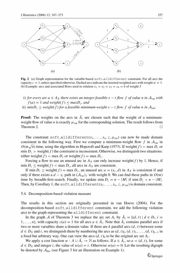
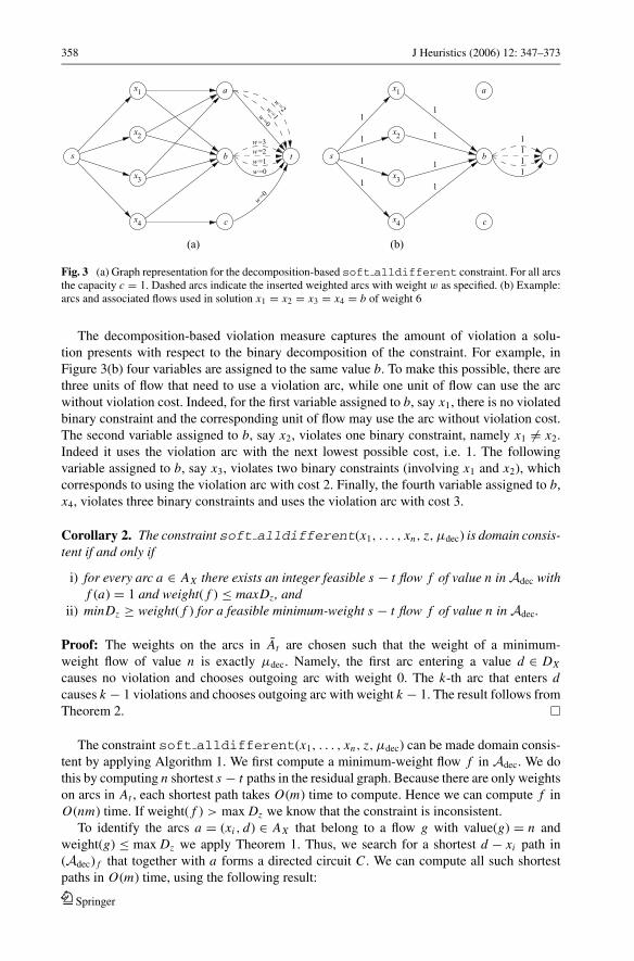
Fig. 3 (a) Graph representation for the decomposition-based soft alldifferent constraint. For all arcsthe capacity c = 1. Dashed arcs indicate the inserted weighted arcs with weight w as specified. (b) Example:arcs and associated flows used in solution x1 = x2 = x3 = x4 = b of weight 6

The decomposition-based violation measure captures the amount of violation a solu-

tion presents with respect to the binary decomposition of the constraint. For example, in

Figure 3(b) four variables are assigned to the same value b. To make this possible, there are

three units of flow that need to use a violation arc, while one unit of flow can use the arc

without violation cost. Indeed, for the first variable assigned to b, say x1, there is no violated

binary constraint and the corresponding unit of flow may use the arc without violation cost.

The second variable assigned to b, say x2, violates one binary constraint, namely x1 = x2.

Indeed it uses the violation arc with the next lowest possible cost, i.e. 1. The following

variable assigned to b, say x3, violates two binary constraints (involving x1 and x2), which

corresponds to using the violation arc with cost 2. Finally, the fourth variable assigned to b,

x4, violates three binary constraints and uses the violation arc with cost 3.

Corollary 2. The constraint soft alldifferent(x1, . . . , xn, z, μdec) is domain consis-tent if and only if

i) for every arc a ∈ AX there exists an integer feasible s − t flow f of value n in Adec withf (a) = 1 and weight( f ) ≤ maxDz, and

ii) minDz ≥ weight( f ) for a feasible minimum-weight s − t flow f of value n in Adec.

Proof: The weights on the arcs in At are chosen such that the weight of a minimum-

weight flow of value n is exactly μdec. Namely, the first arc entering a value d ∈ DX

causes no violation and chooses outgoing arc with weight 0. The k-th arc that enters dcauses k − 1 violations and chooses outgoing arc with weight k − 1. The result follows from

Theorem 2. �

The constraint soft alldifferent(x1, . . . , xn, z, μdec) can be made domain consis-

tent by applying Algorithm 1. We first compute a minimum-weight flow f in Adec. We do

this by computing n shortest s − t paths in the residual graph. Because there are only weights

on arcs in At , each shortest path takes O(m) time to compute. Hence we can compute f in

O(nm) time. If weight( f ) > max Dz we know that the constraint is inconsistent.

To identify the arcs a = (xi , d) ∈ AX that belong to a flow g with value(g) = n and

weight(g) ≤ max Dz we apply Theorem 1. Thus, we search for a shortest d − xi path in

(Adec) f that together with a forms a directed circuit C . We can compute all such shortest

paths in O(m) time, using the following result:

Springer

J Heuristics (2006) 12: 347–373 359

Theorem 4. (van Hoeve, 2004) Let soft alldifferent(x1, . . . , xn, z, μdec) be con-sistent and let f be an integer feasible minimum-weight flow in Adec of value n. Thensoft alldifferent(x1, . . . , xn, z, μdec) can be made domain consistent in O(m) time.

Proof: The complexity of the filtering algorithm depends on the computation of the

minimum-weight d − xi paths in (Adec) f for arcs (xi , d) ∈ AX . We make use of the fact

that only arcs a ∈ At contribute to the cost of such path.

Consider the strongly connected components of the graph (Adec) f which is a copy of

(Adec) f where s and t and all their incident arcs are removed. Let P be a minimum-weight

d − xi path P in A f . If P is equal to d, xi then f (xi , d) = 1 and cost(P) = 0. Otherwise,

either xi and d are in the same strongly connected component of (Adec) f , or not. In case they

are in the same strongly connected component, P can avoid t in A f , and cost(P) = 0. In

case xi and d are in different strongly connected components, P must visit t , and we do the

following.

Split t into two vertices t in and tout such that δin(t in) = δin(t), δout(t in) = ∅, and δin(tout) =∅, δout(tout) = δout(t). For every vertex v ∈ X ∪ DX we can compute the minimum-weight

path from v to t in and from tout to v in total O(m) time.

The strongly connected components of (Adec) f can be computed in O(n + m) time, fol-

lowing (Tarjan, 1972). Hence the total time complexity of achieving domain consistency is

O(m), as n < m. �

Hence, we update Di = Di \ {d} if weight( f ) + weight(C) > max Dz . Finally, we update

min Dz = weight( f ) if min Dz < weight( f ). Then, by Corollary 2, the soft alldiffe-rent(x1, . . . , xn, z, μdec) is domain consistent.

6. Soft global cardinality constraint

6.1. Definitions

A global cardinality constraint (gcc) on a sequence of variables specifies for each value

in the union of their domains an upper and lower bound to the number of variables that

are assigned to this value. A domain consistency propagation algorithm for the gcc was

developed in Regin (1996), making use of network flows.

Let ld , ud ∈ N with ld ≤ ud for all d ∈ DX .

Definition 7 (Global cardinality constraint, (Regin, 1996)).

gcc(X, l, u) = {(d1, . . . , dn) | di ∈ Di , ld ≤ |{di | di = d}| ≤ ud ∀ d ∈ DX }

Note that the gcc is a generalization of the alldifferent constraint. If we set ld = 0

and ud = 1 for all d ∈ DX , the gcc is equal to the alldifferent constraint.

In order to define measures of violation for the gcc, it is convenient to introduce for each

domain value a “shortage” function s : D1 × · · · × Dn × DX → N and an “excess” function

e : D1 × · · · × Dn × DX → N as follows:

s(X, d) ={

ld − |{xi | xi = d}| if |{xi | xi = d}| ≤ ld ,

0 otherwise.

Springer

360 J Heuristics (2006) 12: 347–373

e(X, d) ={ |{xi | xi = d}| − ud if |{xi | xi = d}| ≥ ud ,

0 otherwise,

To the gcc we apply two measures of violation: the variable-based violation measure

μvar and the value-based violation measure μval that we will define in this section. The next

lemma expresses μvar in terms of the shortage and excess functions.

Lemma 1. For gcc(X, l, u) we have

μvar(X ) = max

( ∑d∈DX

s(X, d),∑

d∈DX

e(X, d)

)

provided that ∑d∈DX

ld ≤ |X | ≤∑

d∈DX

ud . (1)

Proof: Note that if (1) does not hold, there is no variable assignment that satisfies the gcc,

and μvar cannot be applied.

Applying μvar corresponds to the minimal number of re-assignments of variables until

both∑

d∈DXs(X, d) = 0 and

∑d∈DX

e(X, d) = 0.

Assume∑

d∈DXs(X, d) ≥ ∑

d∈DXe(X, d). Variables assigned to values d ′ ∈ DX with

s(X, d ′) > 0 can be assigned to values d ′′ ∈ DX with e(X, d ′′) > 0, until∑

d∈DXe(X, d) =

0. In order to achieve∑

d∈DXs(X, d) = 0, we still need to re-assign the other variables

assigned to values d ′ ∈ DX with s(X, d ′) > 0. Hence, in total we need to re-assign exactly∑d∈DX

s(X, d) variables.

Similarly when we assume∑

d∈DXs(X, d) ≤ ∑

d∈DXe(X, d). Then we need to re-assign

exactly∑

d∈DXe(X, d) variables. �

We introduce the following violation measure for the gcc, which can also be applied

when assumption (1) does not hold.

Definition 8 (Value-based violation measure). For gcc(X, l, u) the value-based violation

measure is

μval(X ) =∑

d∈DX

(s(X, d) + e(X, d)) .

6.2. Graph representation

The gcc has the following graph representation:

Springer

J Heuristics (2006) 12: 347–373 361

x2

1x

x3

x4

s

2

1

t

(1,1

)

(1,1)

(1,1)

(1,1)

(0,1)

(0,1)

(0,1)

(0,1)

(0,1

)

(0,1)

(1,2)

(3,5)

Fig. 4 Graph representation forthe gcc. Demand and capacityare indicated between parenthesesfor each arc a as (d(a), c(a))

Theorem 5. (Regin, 1996) A solution to gcc(X, l, u) corresponds to an integer feasibles − t flow of value n in the digraph G = (V, A) with vertex set

V = X ∪ DX ∪ {s, t}and arc set A = As ∪ AX ∪ At ,

whereAs = {(s, xi ) | i ∈ {1, . . . , n}},AX = {(xi , d) | d ∈ Di , i ∈ {1, . . . , n}},At = {(d, t) | d ∈ DX },

with demand function d(a) =⎧⎨⎩

1 if a ∈ As,

0 if a ∈ AX ,

ld if a = (d, t) ∈ At ,

and capacity function c(a) =⎧⎨⎩

1 if a ∈ As,

1 if a ∈ AX ,

ud if a = (d, t) ∈ At .

Example 2. Consider the following CSP:

x1 ∈ {1, 2}, x2 ∈ {1}, x3 ∈ {1, 2}, x4 ∈ {1},gcc(x1, x2, x3, x4, [1, 3], [2, 5]).

In Figure 4 the corresponding graph representation of the gcc is presented. �

6.3. Variable-based violation measure

For the variable-based violation measure, we adapt the graph G of Theorem 5 in the following

way. We add the violation arcs

A = {(di , d j ) | di , d j ∈ DX , i = j},

with demand d(a) = 0, capacity c(a) = n and weight w(a) = 1 for all arcs a ∈ A. Let the

resulting digraph be denoted by Gvar (see Figure 5 for an illustration on Example 2). The

objective of the variable-based violation measure is to count the variables which need to

change value in order for a solution to be feasible with respect to the original gcc. Here the

Springer

362 J Heuristics (2006) 12: 347–373

x2

1x

x3

x2

1x

x3

=1

w

x4

s

2

1

t

(a) (b)

1

1

1

1

1

3

x4

s

2

1

t

(1,1

)

(1,1)

(1,1)

(1,1)

(0,1)

(0,1)

(0,1)

(0,1

)

(0,1)

(1,2)

(3,5)

(0,4

)

(0,1) 2

1

1

1

1

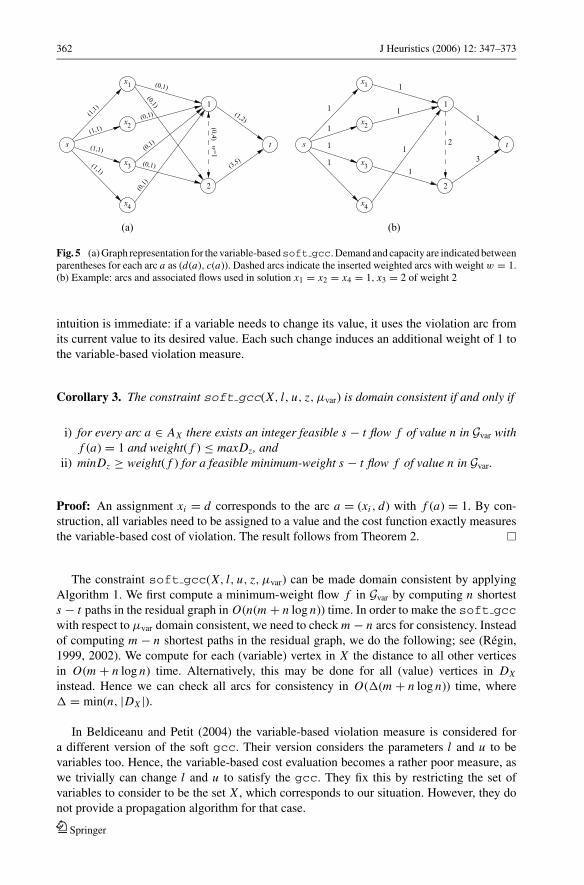
Fig. 5 (a) Graph representation for the variable-basedsoft gcc. Demand and capacity are indicated betweenparentheses for each arc a as (d(a), c(a)). Dashed arcs indicate the inserted weighted arcs with weight w = 1.(b) Example: arcs and associated flows used in solution x1 = x2 = x4 = 1, x3 = 2 of weight 2

intuition is immediate: if a variable needs to change its value, it uses the violation arc from

its current value to its desired value. Each such change induces an additional weight of 1 to

the variable-based violation measure.

Corollary 3. The constraint soft gcc(X, l, u, z, μvar) is domain consistent if and only if

i) for every arc a ∈ AX there exists an integer feasible s − t flow f of value n in Gvar withf (a) = 1 and weight( f ) ≤ maxDz, and

ii) minDz ≥ weight( f ) for a feasible minimum-weight s − t flow f of value n in Gvar.

Proof: An assignment xi = d corresponds to the arc a = (xi , d) with f (a) = 1. By con-

struction, all variables need to be assigned to a value and the cost function exactly measures

the variable-based cost of violation. The result follows from Theorem 2. �

The constraint soft gcc(X, l, u, z, μvar) can be made domain consistent by applying

Algorithm 1. We first compute a minimum-weight flow f in Gvar by computing n shortest

s − t paths in the residual graph in O(n(m + n log n)) time. In order to make the soft gccwith respect to μvar domain consistent, we need to check m − n arcs for consistency. Instead

of computing m − n shortest paths in the residual graph, we do the following; see (Regin,

1999, 2002). We compute for each (variable) vertex in X the distance to all other vertices

in O(m + n log n) time. Alternatively, this may be done for all (value) vertices in DX

instead. Hence we can check all arcs for consistency in O(�(m + n log n)) time, where

� = min(n, |DX |).

In Beldiceanu and Petit (2004) the variable-based violation measure is considered for

a different version of the soft gcc. Their version considers the parameters l and u to be

variables too. Hence, the variable-based cost evaluation becomes a rather poor measure, as

we trivially can change l and u to satisfy the gcc. They fix this by restricting the set of

variables to consider to be the set X , which corresponds to our situation. However, they do

not provide a propagation algorithm for that case.

Springer

J Heuristics (2006) 12: 347–373 363

x2

1x

x3

=1w

=1w

=1w

=1w

x4

s

2

1

t

(1,1

)

(1,1)

(1,1)

(1,1)

(0,1)

(0,1)

(0,inf)

(0,1)

(0,in

f)

(0,1)

(0,1)

(0,1)

(0,1

)

(1,2)

(3,5)

(0,3)

x2

1x

x3

x4

s

2

1

t

1

1

1

1

1

1

1

1

3

3

2

2

(a) (b)

Fig. 6 (a) Graph representation for the value-based soft gcc. Demand and capacity are indicated betweenparentheses for each arc a as (d(a), c(a)). Dashed arcs indicate the inserted weighted arcs with weight w = 1.(b) Example: arcs and associated flows used in solution x1 = x2 = x3 = x4 = 1 of weight 5

6.4. Value-based violation measure

For the value-based violation measure, we adapt the graph G of Theorem 5 in the following

way. We add the violation arcs

Ashortage = {(s, d) | d ∈ DX } and Aexcess = {(d, t) | d ∈ DX },

with demand d(a) = 0 for all a ∈ Ashortage ∪ Aexcess and capacity

c(a) ={

ld if a = (s, d) ∈ Ashortage,

∞ if a ∈ Aexcess.

We again apply a cost function w assigning unit cost to violation arcs. Let the resulting

digraph be denoted by Gval (see Figure 6 for an illustration on Example 2).

This value-based violation measure is not concerned with variables but rather tries to

evaluate the amount of flow missing or exceeding the requirement of the original gcc. As

we are only interested with the demands and capacities stated on values, we allow the flow

to completely bypass the layer of nodes corresponding to the variables.

Corollary 4. The constraint soft gcc(X, l, u, z, μval) is domain consistent if and only if

i) for every arc a ∈ AX there exists an integer feasible s − t flow f of value n in Gval withf (a) = 1 and weight( f ) ≤ max Dz, and

ii) minDz ≥ weight( f ) for a feasible minimum-weight s − t flow f of value n in Gval.

Proof: Similar to the proof of Theorem 3. �

We design an efficient propagation algorithm for the value-based soft gcc, by applying

again Algorithm 1 and Theorem 1. First, we compute a minimum-weight feasible flow in

Gval. For this we first need to compute n shortest paths to satisfy the demand of the arcs in As .

In order to meet the demand of the arcs in At , we need to compute at most another k shortest

paths, where k = |DX |. Hence the total time complexity is O((n + k)(m + n log n)).

Springer

364 J Heuristics (2006) 12: 347–373

In order to make the soft gcc with respect to μval domain consistent, we need to check

m − n arcs for consistency. Similar to the variable-based soft gcc, this can be done in

O(�(m + n log n)) time, where � = min(n, |DX |).When ld = 0 for all d ∈ DX , the arc set Ashortage is empty. In that case, Gval has a particular

structure, i.e. the costs only appear on arcs from DX to t . Then, similar to the reasoning for the

soft alldifferent constraint with respect to μdec, we can compute a minimum-weight

flow of value n in Gval in O(mn) time and achieve domain consistency in O(m) time.

7. Soft regular constraint

7.1. Definitions

The regular constraint was introduced in Pesant (2004). It is defined on a fixed-length se-

quence of finite-domain variables and it states that the corresponding sequence of values taken

by these variables belongs to a given regular language. A domain consistency propagation al-

gorithm for this constraint was also provided in Pesant (2004). Particular instances of there-gular constraint can for example be applied in rostering problems or sequencing problems.

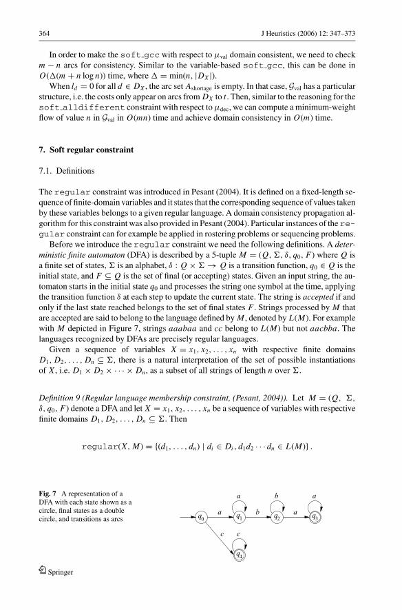
Before we introduce the regular constraint we need the following definitions. A deter-ministic finite automaton (DFA) is described by a 5-tuple M = (Q, �, δ, q0, F) where Q is

a finite set of states, � is an alphabet, δ : Q × � → Q is a transition function, q0 ∈ Q is the

initial state, and F ⊆ Q is the set of final (or accepting) states. Given an input string, the au-

tomaton starts in the initial state q0 and processes the string one symbol at the time, applying

the transition function δ at each step to update the current state. The string is accepted if and

only if the last state reached belongs to the set of final states F . Strings processed by M that

are accepted are said to belong to the language defined by M , denoted by L(M). For example

with M depicted in Figure 7, strings aaabaa and cc belong to L(M) but not aacbba. The

languages recognized by DFAs are precisely regular languages.

Given a sequence of variables X = x1, x2, . . . , xn with respective finite domains

D1, D2, . . . , Dn ⊆ �, there is a natural interpretation of the set of possible instantiations

of X , i.e. D1 × D2 × · · · × Dn , as a subset of all strings of length n over �.

Definition 9 (Regular language membership constraint, (Pesant, 2004)). Let M = (Q, �,

δ, q0, F) denote a DFA and let X = x1, x2, . . . , xn be a sequence of variables with respective

finite domains D1, D2, . . . , Dn ⊆ �. Then

regular(X, M) = {(d1, . . . , dn) | di ∈ Di , d1d2 · · · dn ∈ L(M)} .

q0

q2

q3

q4

q1

a b a

c

a b a

c

Fig. 7 A representation of aDFA with each state shown as acircle, final states as a doublecircle, and transitions as arcs

Springer

J Heuristics (2006) 12: 347–373 365

To the regular constraint we apply two measures of violation: the variable-based vi-

olation measure μvar and the edit-based violation measure μedit that we will define in this

section.

Let s1 and s2 be two strings of the same length. The Hamming distance H (s1, s2) is the

number of positions in which they differ. Associating with a tuple (d1, d2, . . . , dn) the string

d1d2 · · · dn , the variable-based violation measure can be expressed in terms of the Hamming

distance:

μvar(X ) = min{H (D, X ) | D = d1 · · · dn ∈ L(M)}.

Another distance function that is often used for two strings is the following. Let s1 and

s2 be two strings of the same length. The edit distance E(s1, s2) is the smallest number of

insertions, deletions, and substitutions required to change one string into another. It captures

the fact that two strings that are identical except for one extra or missing symbol should be

considered close to one another. Edit distance is probably a better way to measure violations

of a regular constraint. Consider for example a regular language in which strings alternate

between pairs of a’s and b’s: the Hamming distance of string “abbaabbaab” is 5 (that is,

n/2) since changing either the first a to a b or the first b to an a has a domino effect; the

edit distance of the same string is 2 since we can insert an a at the beginning and remove a

b at the end. In this case, the edit distance reflects the number of incomplete pairs whereas

the Hamming distance is proportional to the length of the string rather than to the amount of

violation.

Definition 10 (Edit-based violation measure). For regular(X, M) the edit-based viola-

tion measure is

μedit(X ) = min{E(D, X ) | D = d1 · · · dn ∈ L(M)}.

Example 3. Consider the CSP

x1 ∈ {a, b, c}, x2 ∈ {a, b, c}, x3 ∈ {a, b, c}, x4 ∈ {a, b, c},regular(x1, x2, x3, x4, M)

with M as in Figure 7. We have μvar(c, a, a, b) = 3, because we have to change at least 3

variables. A corresponding valid string with Hamming distance 3 is for example aaba. On

the other hand, we have μedit(c, a, a, b) = 2, because we can delete the value c at the front

and add the value a at the end, thus obtaining the valid string aaba. �

7.2. Graph representation

A graph representation for the regular constraint was presented in (Pesant, 2004). Recall

that M = (Q, �, δ, q0, F).

Theorem 6. (Pesant, 2004) A solution to regular(X, M) corresponds to an integer fea-sible s − t flow of value 1 in the digraph R = (V, A) with vertex set

V = V1 ∪ V2 ∪ . . . ∪ Vn+1 ∪ {s, t}Springer

366 J Heuristics (2006) 12: 347–373

q2

q0

q3

q4

q1

q2

q0

q3

q4

q1

q2

q0

q3

q4

q1

q2

q0

q3

q4

q1

q2

q0

q3

q4

s

t

q1

x1

x2

x3

x4

V1

a

c

c c c

a

b b

b

a a

a

V5

V4

V3

V2

Fig. 8 Graph representation for the regular constraint. For all arcs the capacity is 1

and arc set A = As ∪ A1 ∪ A2 ∪ . . . ∪ An ∪ At ,

where Vi = {qik | qk ∈ Q} for i = 1, . . . , n + 1,

and

As = {(s, q10 },

Ai = {(qi

k, qi+1l

) | δ(qk, d) = ql for d ∈ Di}

for i = 1, . . . , n,

At = {(qn+1

k , t) | qk ∈ F

},

with capacity function c(a) = 1 for all a ∈ A.

Proof: Each arc in Ai corresponds to a variable-value pair: there is an arc from qik to qi+1

l if

and only if there exists some d ∈ Di such that δ(qk, d) = ql . If an arc belongs to an integer

s − t flow of value 1, it belongs to a path from q10 to a member of F in the last Vn+1. Hence

the assignment xi = d belongs to a solution to the regular constraint. �

Figure 8 gives the corresponding graph representation of the regular constraint from

Example 3.

7.3. Variable-based violation measure

For the variable-based soft regular constraint, we add the following violation arcs to

the graph representing the regular constraint.

To the graph R of Theorem 6 we add violation arcs

Asub = {(qi

k, qi+1l

) | δ(qk, d) = ql for some d ∈ �, i = 1, . . . , n},

with capacity c(a) = 1 for all arcs a ∈ Asub. We apply the usual cost function w with unit cost.

Let the resulting digraph be denoted by Rvar (see Figure 9 for an illustration on Example 3).

The input automaton of this constraint specifies the allowed transitions from state to

state according to different values. The objective here, in counting the minimum number of

substitutions, is to make these transitions value independent. To do so, we add a violation

arc between to states (qik, qi+1

l ) if there already exists at least one valid arc between them.

Springer

J Heuristics (2006) 12: 347–373 367

3

q4

q1

q2

q0

q3

q4

q1

q2

q0

q3

q4

q1

q2

q0

q3

q4

q1

q2

q0

q3

q4

s

t

q2

x1

V1

(a) (b)

x2

x3

x4

V2

V3

V4

V5

c

11

1

1

1

q

1

1

q0

q3

q4

q1

q2

q0

q3

q4

q1

q2

q0

q3

q4

q1

q2

q0

q3

q4

q1

q2

q0

q3

q4

s

t

q2

x1

V1

c c c

a

a

b

b

a a

a

b

x2

x3

x4

V2

V3

V4

V5

c

q1

q0

q

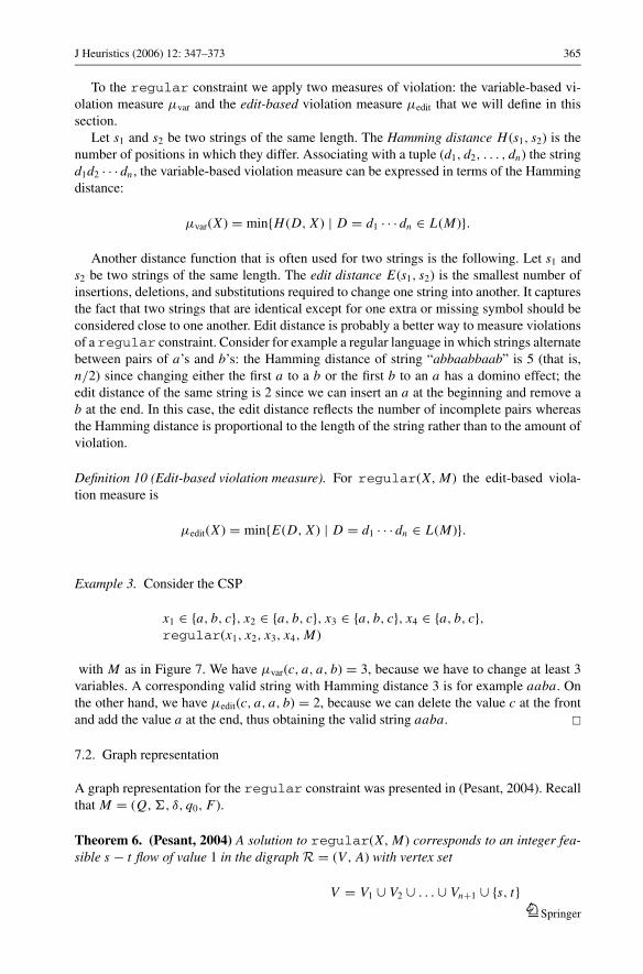
Fig. 9 Graph representation for the variable-based soft regular constraint. For all arcs the capacity is1. Dashed arcs indicate the inserted weighted arcs with weight 1. b) Example: arcs and associated flows usedin solution x1 = c, x2 = a, x3 = a, x4 = b of weight 3, corresponding to three substitutions from valid stringaaba

This means that a flow using a violation arc is in fact a solution where a variable takes a

value outside of its domain. The number of such variables thus constitutes a minimum on the

number of variables which need to change value.

Corollary 5. The constraint soft regular(X, M, z, μvar) is domain consistent if andonly if

i) for every arc a ∈ A1 ∪ · · · ∪ An there exists an integer feasible s − t flow f of value 1

in Rvar with f (a) = 1 and weight( f ) ≤ max Dz, andii) minDz ≥ weight( f ) for a minimum-weight s − t flow f of value 1 in Rvar.

Proof: The weight function measures exactly μvar. The result follows from Theorem 2. �

Note that a minimum-weight s − t flow of value 1 is in fact a shortest s − t path with respect

to w. The constraint propagation algorithm thus must ensure that all arcs corresponding to

a variable-value assignment are on an s − t path with cost smaller than max Dz . Computing

shortest paths from the initial state in the first layer to every other node and from every node to

a final state in the last layer can be done in O(n |δ|) time through topological sorts because of

the special structure of the graph, as observed in Pesant (2004). Here |δ| denotes the number

of transitions in the corresponding DFA. Hence, the algorithm runs in O(m) time, where m is

the number of arcs in the graph. The computation can also be made incremental in the same

way as in Pesant (2004). Note that this result has been obtained independently in Beldiceanu

et al. (2004).

7.4. Edit-based violation measure

For the edit-based soft regular constraint, we add the following violation arcs to the

graph R representing the regular constraint. As in the previous section, we add Asub to

allow the substitution of a value. To allow deletions and insertions, we add violation arcs

Adel = {(qik, qi+1

k ) | i = 1, . . . , n}} \ A

Springer

368 J Heuristics (2006) 12: 347–373

q0

q3

q4

q2

q0

q3

q4

q1

q2

q0

q3

q4

q0

q3

q4

s

q2

x1

V1

q2

t

q1

q1

q1

q2

q0

q3

q4

V5

q1

q1

q0

q3

q4

q2

q0

q3

q4

q1

q2

q0

q3

q4

q0

q3

q4

s

q2

x1

V1

q1

q2

q0

q3

q4

V5

q1

q2

t

q1

x2

x3

x4

V2

V3

V4

x2

x3

x4

V2

V3

V4

a a a a

b b

a a a

b

a

c c c

c cc

a a

a

b b

c

c

bb b

aa

aaa

1 1

1

1

1

1

(a) (b)

1

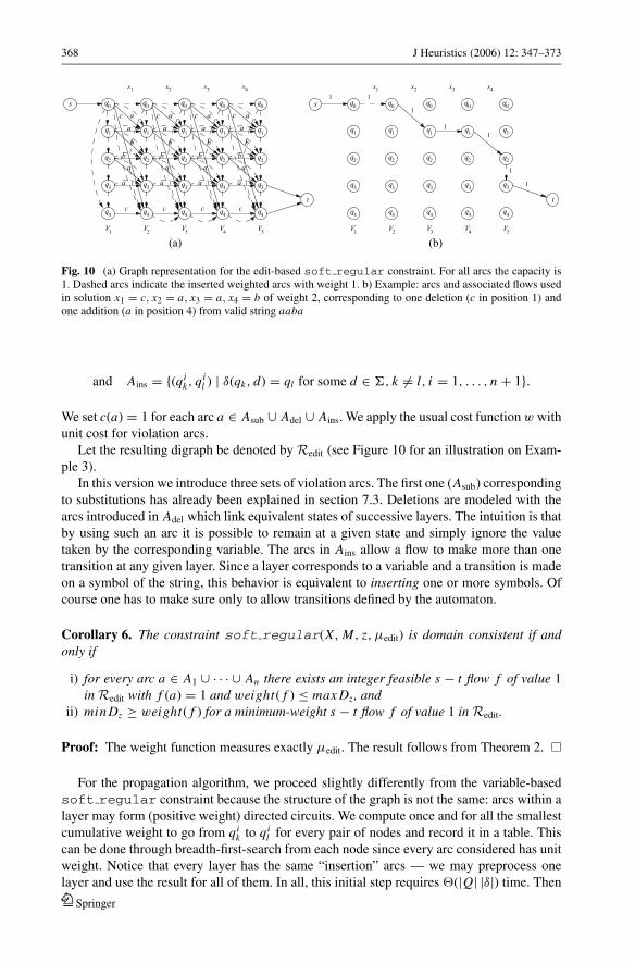
Fig. 10 (a) Graph representation for the edit-based soft regular constraint. For all arcs the capacity is1. Dashed arcs indicate the inserted weighted arcs with weight 1. b) Example: arcs and associated flows usedin solution x1 = c, x2 = a, x3 = a, x4 = b of weight 2, corresponding to one deletion (c in position 1) andone addition (a in position 4) from valid string aaba

and Ains = {(qik, qi

l ) | δ(qk, d) = ql for some d ∈ �, k = l, i = 1, . . . , n + 1}.

We set c(a) = 1 for each arc a ∈ Asub ∪ Adel ∪ Ains. We apply the usual cost function w with

unit cost for violation arcs.

Let the resulting digraph be denoted by Redit (see Figure 10 for an illustration on Exam-

ple 3).

In this version we introduce three sets of violation arcs. The first one (Asub) corresponding

to substitutions has already been explained in section 7.3. Deletions are modeled with the

arcs introduced in Adel which link equivalent states of successive layers. The intuition is that

by using such an arc it is possible to remain at a given state and simply ignore the value

taken by the corresponding variable. The arcs in Ains allow a flow to make more than one

transition at any given layer. Since a layer corresponds to a variable and a transition is made

on a symbol of the string, this behavior is equivalent to inserting one or more symbols. Of

course one has to make sure only to allow transitions defined by the automaton.

Corollary 6. The constraint soft regular(X, M, z, μedit) is domain consistent if andonly if

i) for every arc a ∈ A1 ∪ · · · ∪ An there exists an integer feasible s − t flow f of value 1

in Redit with f (a) = 1 and weight( f ) ≤ max Dz, andii) minDz ≥ weight( f ) for a minimum-weight s − t flow f of value 1 in Redit.

Proof: The weight function measures exactly μedit. The result follows from Theorem 2. �

For the propagation algorithm, we proceed slightly differently from the variable-based

soft regular constraint because the structure of the graph is not the same: arcs within a

layer may form (positive weight) directed circuits. We compute once and for all the smallest

cumulative weight to go from qik to qi

l for every pair of nodes and record it in a table. This

can be done through breadth-first-search from each node since every arc considered has unit

weight. Notice that every layer has the same “insertion” arcs — we may preprocess one

layer and use the result for all of them. In all, this initial step requires �(|Q| |δ|) time. Then

Springer

J Heuristics (2006) 12: 347–373 369

we can proceed as before through topological sort with table lookups, in O(n |δ|) time. The

overall time complexity is therefore O((n + |Q|) |δ|) = O(m), where m is the number of

arcs in the graph. The last step follows from |Q| ≤ n, because otherwise some states would

be unreachable.

8. Soft same constraint

8.1. Definitions

The same constraint is defined on two sequences of variables and states that the variables in

one sequence use the same values as the variables in the other sequence. The constraint was

introduced in Beldiceanu (2000). One can also view the same constraint as demanding that

one sequence is a permutation of the other. A domain consistency algorithm for the sameconstraint was presented in Beldiceanu et al. (2004), making use of flow theory.

Definition 11 (Same constraint, Beldiceanu (2000)). Let X = x1, . . . , xn and Y = y1, . . . ,

yn be sequences of variables with respective finite domains D1, . . . , Dn and D′1, . . . , D′

n .

Then

same(X, Y ) ={(

d1, . . . , dn, d ′1, . . . , d ′

n

)∣∣di ∈ Di , d ′i ∈ D′

i ,

n⋃i=1

{di } =n⋃

i=1

{d ′

i

}}.

Note that in the above definition⋃n

i=1{di } and⋃n

i=1{d ′i } are multisets, in which elements

may occur more than once.

To the same constraint we apply the variable-based violation measure μvar. Denote the

symmetric difference of two multisets S and T by S�T , i.e. S�T = (S \ T ) ∪ (T \ S). For

same(X, Y ) we have

μvar(X, Y ) =∣∣∣∣∣(

n⋃i=1

{xi })

�

(n⋃

i=1

{yi })∣∣∣∣∣

/2.

Example 4. Consider the following over-constrained CSP:

x1 ∈ {a, b, c}, x2 ∈ {c, d, e}, x3 ∈ {c, d, e},y1 ∈ {a, b}, y2 ∈ {a, b}, y3 ∈ {c, d},same(x1, x2, x3, y1, y2, y3).

We have μvar(a, c, c, a, b, c) = 1 because {a, c, c}�{a, b, c} = {b, c}. This gives|{b, c}| /2 = 1. �

8.2. Graph representation

The same constraint has the following graph representation:

Springer

370 J Heuristics (2006) 12: 347–373

x2

1x

x3

s t

a

b

e

d

c

1y

y2

y3

Fig. 11 Graph representation forthe same constraint. For all arcsthe capacity is 1

Theorem 7. (Beldiceanu et al., 2004) A solution to same(X, Y ) corresponds to an integerfeasible s − t flow of value n in the digraph S = (V, A) with vertex set

V = X ∪ (DX ∩ D′

Y

) ∪ Y ∪ {s, t}and arc set A = As ∪ AX ∪ AY ∪ At ,

where As = {(s, xi ) | i ∈ {1, . . . , n}},AX = {(xi , d) | d ∈ Di ∩ DY , i ∈ {1, . . . , n}},AY = {(d, yi ) | d ∈ D′

i ∩ DX , i ∈ {1, . . . , n}},At = {(yi , t) | i ∈ {1, . . . , n}},

with capacity function c(a) = 1 for all a ∈ A.

Figure 11 gives the corresponding graph representation of the same constraint from

Example 4.

8.3. Variable-based violation measure

To the graph S of Theorem 7 we add the arc sets

A = {(di , d j ) | di , d j ∈ DX ∪ DY , i = j},

with capacity c(a) = n and weight w(a) = 1 for all arcs a ∈ A. Let the resulting digraph be

denoted by Svar (see Figure 12 for an illustration on Example 4). The inserted violation arcs

are similar to the violation arcs of the variable-based soft gcc. Again, if a variable needs

to change its value, it uses the violation arc from its current value to its desired value. The

total induced weight corresponds exactly to the variable-based violation measure.

Corollary 7. The constraint soft same(X, Y, z, μvar) is domain consistent if and only if

i) for every arc a ∈ AX ∪ AY there exists a feasible s − t flow f of value n in Svar withf (a) = 1 and weight( f ) ≤ max Dz, and

ii) minDz ≥ weight( f ) for a minimum-weight s − t flow f of value n in Svar.

Proof: An assignment xi = d corresponds to the arc a = (xi , d) with f (a) = 1. By con-

struction, all variables need to be assigned to a value and the cost function exactly measures

the variable-based cost of violation. The result follows from Theorem 2. �Springer

J Heuristics (2006) 12: 347–373 371

x2

1x

x3

s tx2

1x

x3

s t

=1w

a

b

e

d

c

1y

y2

y3

(a) (b)

a

b

e

d

c

1y

y2

y3

1

1

1

1

1

11

1

11

1

1

1

Fig. 12 (a) Graph representation for the variable-based soft same constraint. For all arcs the capacity is 1.Dashed arcs indicate the inserted weighted arcs with weight 1. (b) Example: arcs and associated flows used insolution x1 = a, x2 = c, x3 = c, y1 = a, y2 = b, y3 = c of weight 1

The constraint soft same(X, Y, z, μvar) can be made domain consistent by applying

Algorithm 1 and Theorem 1. Consistency can again be checked by computing an initial

flow in O(n(m + n log n)) time and, similar to the soft gcc, domain consistency can be

achieved in O(�(m + n log n)) time, where � = min(n, |DX |).

9. Conclusion

Many real-life problems are over-constrained; constraint programming deals with the issue

by softening constraints. In this paper we have proposed a generic constraint propagation

algorithm for soft versions of an important class of global constraints; those that can be

represented by a flow in a graph. To allow solutions that were originally infeasible, we have

added violation arcs to the graph, with an associated cost. Hence, a flow that represents an

originally infeasible solution induces a cost. This cost corresponds to a violation measure of

the soft global constraint. We have applied our method to soften the alldifferent, the

gcc, the regular, and the same constraints, and described efficient domain consistency

algorithms for each of them. The results are summarized in Table 1.

Table 1 Time complexity for soft global constraints on n variables with maximum domain size d, and variousviolation measures. Here “consistency check” denotes the time complexity to check that the constraint isconsistent, while “domain consistency” denotes the additional time complexity to make the constraint domainconsistent, given at least one solution. Each algorithm is based on a graph G with m arcs. K denotes the timecomplexity to compute a minimum-weight flow in G, while SP denotes the time to compute a minimum-weight path in G. Finally, k = |DX | and � = min(n, k)

constraint violation measure consistency check domain consistency

general case O(K ) O(nd · SP)

soft alldifferent variable-based O(m√

n) O(m) (Petit et al., 2001)

soft alldifferent decomposition-based O(mn) O(m) (van Hoeve, 2004)

soft gcc variable-based O(n(m + n log n)) O(�(m + n log n))

soft gcc value-based O((n + k)(m + n log n)) O(�(m + n log n))

soft regular variable-based O(m) O(m)

soft regular edit-based O(m) O(m)

soft same variable-based O(n(m + n log n)) O(�(m + n log n))

Springer

372 J Heuristics (2006) 12: 347–373

We have used existing violation measures, but also introduced new measures for the

soft gcc and the soft regular constraint. For many of those violation measures we

applied in this paper, the cost function assigned unit penalties. The framework makes it

possible to use more varied costs, though. Namely, we may even assign any convex cost

function to the arcs without changing the complexity of the algorithms; see ((Ahuja et al.,

1993), p. 543–565). In fact, the cost function applied to the decomposition-basedsoft all-different constraint can be regarded as a convex cost function on the aggregation of the

parallel arcs. Such cost functions could also be advantageous in other cases, for example to

distinguish between insertions and deletions in the soft regular constraint. This could

also be particularly useful in application to personnel rostering problems, where one could

penalize differently (using soft gcc) the over-usage of values associated to night shifts or

day shifts for instance.

The approach to soft constraints which we favored in this paper allows us to restrict the

amount of violation of individual (global) constraints and to use that restriction to perform

domain filtering in the spirit of cost-based filtering for optimization constraints. Our results

hopefully provide helpful ingredients for modeling and solving real-life over-constrained

problems efficiently with constraint programming.

References

Ahuja, R.K., T.L. Magnanti, and J.B. Orlin. (1993). Network Flows. Prentice Hall.Apt, K.R. (2003). Principles of Constraint Programming. Cambridge University Press.Baptiste, P., C. Le Pape, and L. Peridy. (1998). “Global Constraints for Partial CSPs: A Case-Study of Resource

and Due Date Constraints.” In M.J. Maher and J.-F. Puget, (eds.), Proceedings of the Fourth InternationalConference on Principles and Practice of Constraint Programming (CP98), volume 1520 of LNCS,Springer, pp. 87–101.

Beldiceanu, N., M. Carlsson, and T. Petit. (2004). “Deriving Filtering Algorithms from Constraint Checkers.” InProceedings of the Tenth International Conference on Principles and Practice of Constraint Programming(CP 2004), volume 3258 of LNCS, Springer.

Beldiceanu, N., I. Katriel, and S. Thiel. (2004). Filtering Algorithms for the Same Constraint. In J.-C. Reginand M. Rueher, editors, Proceedings of the First International Conference on the Integration of AI andOR Techniques in Constraint Programming for Combinatorial Optimization Problems (CPAIOR 2004),volume 3011 of LNCS, Springer, pp. 65–79.

Beldiceanu, N. and T. Petit. (2004). Cost Evaluation of Soft Global Constraints. In J.-C. Regin and M. Rueher,editors, Proceedings of the First International Conference on the Integration of AI and OR Techniquesin Constraint Programming for Combinatorial Optimization Problems (CPAIOR 2004), volume 3011 ofLNCS, Springer, pp. 80–95.

Beldiceanu, N. (2000). “Global Constraints as Graph Properties on Structured Network of Elementary Con-straints of the Same Type.” Technical Report T2000/01, SICS.

Bistarelli, S., U. Montanari, and F. Rossi. (1997). “Semiring-based Constraint Satisfaction and Optimization.”Journal of the ACM 44(2), 201–236.

Dechter, R. (1990). “On the Expressiveness of Networks with Hidden Variables.” In Proceedings of the 8thNational Conference on Artificial Intelligence (AAAI), AAAI Press/The MIT Press, pp. 555–562.

Dechter, R. (2003). Constraint Processing. Morgan Kaufmann.Dubois, D., H. Fargier, and H. Prade. (1993). “The Calculus of Fuzzy Restrictions as a Basis for Flexible

Constraint Satisfaction.” In Proceedings of the Second IEEE International Conference on Fuzzy Systems,volume 2, pp. 1131–1136.

Fargier, H., J. Lang, and T. Schiex. (1993). “Selecting Preferred Solutions in Fuzzy Constraint SatisfactionProblems.” In Proceedings of the first European Congress on Fuzzy and Intelligent Technologies.

Focacci, F., A. Lodi, and M. Milano. (2002). Optimization-Oriented Global Constraints. Constraints 7(3–4),351–365.

Freuder, E.C. and R.J. Wallace. (1992). “Partial Constraint Satisfaction.” Artificial Intelligence 58(1–3), 21–70.van Hoeve, W.J. (2004). “A Hyper-Arc Consistency Algorithm for the Soft Alldifferent Constraint.” In M.

Wallace, (ed.), Proceedings of the Tenth International Conference on Principles and Practice of ConstraintProgramming (CP 2004), volume 3258 of LNCS, Springer, pp. 679–689.

Springer

J Heuristics (2006) 12: 347–373 373

Hopcroft, J.E. and R.M. Karp. (1973). “An n5/2 Algorithm for Maximum Matchings in Bipartite Graphs.”SIAM Journal on Computing 2(4), 225–231.

Larrosa, J. and T. Schiex. (2003). “In the Quest of the Best form of Local Consistency for Weighted CSP.” In Pro-ceedings of the Eighteenth International Joint Conference on Artificial Intelligence, Morgan Kaufmann,pp. 239–244.

Larrosa, J. (2002). “Node and Arc Consistency in Weighted CSP.” In Proceedings of the Eighteenth NationalConference on Artificial Intelligence, AAAI Press, pp. 48–53.

Mohr, R. and G. Masini. (1988). “Good Old Discrete Relaxation.” In European Conference on ArtificialIntelligence (ECAI), pp. 651–656.

Pesant, G. (2004). “A Regular Language Membership Constraint for Finite Sequences of Variables.” In Pro-ceedings of the Tenth International Conference on Principles and Practice of Constraint Programming(CP 2004), volume 3258 of LNCS, Springer.

Petit, T., J.-C. Regin, and C. Bessiere. (2001). “Specific Filtering Algorithms for Over-Constrained Problems.”In T. Walsh, editor, Proceedings of the Seventh International Conference on Principles and Practice ofConstraint Programming (CP 2001), volume 2239 of LNCS, Springer, pp. 451–463.

Regin, J.-C., T. Petit, C. Bessiere, and J.-F. Puget. (2000). “An Original Constraint Based Approach for Solvingover Constrained Problems.” In R. Dechter, (eds.), Proceedings of the Sixth International Conference onPrinciples and Practice of Constraint Programming (CP 2000), volume 1894 of LNCS, Springer, pp.543–548.

Regin, J.-C. (1994). “A Filtering Algorithm for Constraints of Difference in CSPs.” In Proceedings of theTwelfth National Conference on Artificial Intelligence (AAAI), volume 1, AAAI Press, pp. 362–367.

Regin, J.-C. (1996). “Generalized Arc Consistency for Global Cardinality Constraint.” In Proceedings ofAAAI/IAAI, volume 1, AAAI Press/The MIT Press, pp. 209–215.

Regin, J.-C. (1999). “Arc Consistency for Global Cardinality Constraints with Costs.” In J. Jaffar, (ed.),Proceedings of the Fifth International Conference on Principles and Practice of Constraint Programming(CP’99), volume 1713 of LNCS, Springer, pp. 390–404.

Regin, J.-C. (2002). “Cost-Based Arc Consistency for Global Cardinality Constraints.” Constraints 7, 387–405.Rossi, F., C. Petrie, and V. Dhar. (1990). “On the Equivalence of Constraint Satisfaction Problems.” In Pro-

ceedings of the 9th European Conference on Artificial Intelligence (ECAI), pp. 550-556.Ruttkay, Z. (1994). “Fuzzy Constraint Satisfaction.” In Proceedings of the First IEEE Conference on Evolu-

tionary Computing, pp. 542–547.Schiex, T., H. Fargier, and G. Verfaillie. (1995). “Valued Constraint Satisfaction Problems: Hard and Easy

Problems.” In Proceedings of the Fourteenth International Joint Conference on Artificial Intelligence,Morgan Kaufmann, pp. 631–639.

Schiex, T. (1992). Possibilistic Constraint Satisfaction Problems or “How to handle soft constraints ?”. InProceedings of the 8th Annual Conference on Uncertainty in Artificial Intelligence, Morgan Kaufmann,pp. 268–275.

Schrijver, A. (2003). Combinatorial Optimization-Polyhedra and Efficiency. Springer.Sellmann, M. (2003). “Cost-Based Filtering for Shorter Path Constraints.” In F. Rossi, (ed.), Proceedings of

the Ninth International Conference on Principles and Practice of Constraint Programming (CP 2003),volume 2833 of LNCS, Springer, pp. 694–708.

Tarjan, R. (1972). “Depth-First Search and Linear Graph Algorithms”. SIAM Journal on Computing 1,146–160.

Springer